____________________________________________ AUSTRALIAN VANADIUM PROJECT HYDROGEOLOGICAL ASSESSMENT Prepared for AUSTRALIAN VANADIUM LIMITED March 2021 ____________________________________________ AQ2 Pty Ltd Level 4, 56 William Street Perth 6000 T: 08 9322 9733 www.aq2.com.au

Welcome message from author
This document is posted to help you gain knowledge. Please leave a comment to let me know what you think about it! Share it to your friends and learn new things together.
Transcript
____________________________________________
AUSTRALIAN VANADIUM PROJECT
HYDROGEOLOGICAL ASSESSMENT
Prepared for
AUSTRALIAN VANADIUM LIMITED
March 2021
____________________________________________
AQ2 Pty Ltd Level 4, 56 William Street Perth 6000 T: 08 9322 9733 www.aq2.com.au
F:\183\3.C&R\048d.docx
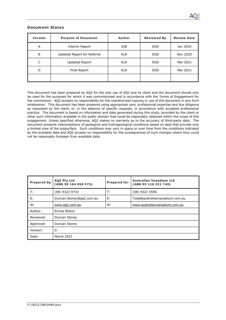
Document Status
Version Purpose of Document Author Reviewed By Review Date
A Interim Report EJB DGS Jan 2020
B Updated Report for Referral KLR DGS Nov 2020
C Updated Report KLR DGS Mar 2021
D Final Report KLR DGS Mar 2021
This document has been prepared by AQ2 for the sole use of AQ2 and its client and the document should only be used for the purposes for which it was commissioned and in accordance with the Terms of Engagement for the commission. AQ2 accepts no responsibility for the unauthorised copying or use of this document in any form whatsoever. This document has been prepared using appropriate care, professional expertise and due diligence as requested by the client, or, in the absence of specific requests, in accordance with accepted professional practice. The document is based on information and data generated during this study, provided by the client or other such information available in the public domain that could be reasonably obtained within the scope of this engagement. Unless specified otherwise, AQ2 makes no warranty as to the accuracy of third-party data. The document presents interpretations of geological and hydrogeological conditions based on data that provide only a limited view of the subsurface. Such conditions may vary in space or over time from the conditions indicated by the available data and AQ2 accepts no responsibility for the consequences of such changes where they could not be reasonably foreseen from available data.
Prepared by: AQ2 Pty Ltd (ABN 38 164 858 075) Prepared for: Australian Vanadium Ltd
(ABN 90 116 221 740)
T: (08) 9322 9733 T: (08) 9321 5594
E: [email protected] E: [email protected]
W: www.aq2.com.au W: www.australianvanadium.com.au
Author: Emma Bolton
Reviewed: Duncan Storey
Approved: Duncan Storey
Version: D
Date: March 2021

F:\183\3.C&R\048d.docx Page i
TABLE OF CONTENTS
1 INTRODUCTION ......................................................................................................... 1
1.1 Background ...................................................................................................... 1 1.2 Objectives and Limitations .................................................................................. 1 1.3 Topography and Hydrology .................................................................................. 2 1.4 Climate ............................................................................................................ 2 1.5 Geology ............................................................................................................ 2
2 HYDROGEOLOGICAL FIELD INVESTIGATIONS ........................................................... 4
2.1 Geophysical Survey ............................................................................................ 4 2.2 Drilling and Bore Construction ............................................................................. 4 2.3 Hydraulic Testing ............................................................................................... 6
3 HYDROGEOLOGY ...................................................................................................... 10
3.1 Hydrogeological Units ........................................................................................ 10 3.2 Aquifer Parameters ........................................................................................... 11 3.3 Groundwater Levels .......................................................................................... 14 3.4 Groundwater Quality ......................................................................................... 14 3.5 Conceptual Hydrogeological Model and Implications for Mining................................. 15
4 WATER MANAGEMENT ............................................................................................. 18
4.1 Dewatering ...................................................................................................... 18 4.1.1 Project Mine Plan ................................................................................... 18 4.1.2 Dewatering Assessment Methodology ........................................................ 18 4.1.3 Pit Dewatering Requirements ................................................................... 20 4.1.4 Open Pit Dewatering Method .................................................................... 21
4.2 Water Balance .................................................................................................. 22 4.2.1 Water Demand ...................................................................................... 22
4.3 Water Supply ................................................................................................... 22 4.4 Excess Water Management ................................................................................. 23
5 IMPACT ASSESSMENT .............................................................................................. 24
5.1 Regional Drawdown Impact - End of Mining .......................................................... 24 5.2 Mine Closure .................................................................................................... 24
6 CONCLUSIONS & RECOMMENDATIONS .................................................................... 25
6.1 Conclusions...................................................................................................... 25 6.2 Recommendations ............................................................................................ 27
7 REFERENCES ............................................................................................................ 28
Tables
Table 1: Details of the Monitoring and Production Bores ........................................................ 8 Table 2: Hydraulic Test Details ........................................................................................... 9 Table 3: Test Pumping Details ........................................................................................... 9 Table 4: Analysis of Micro-test Data ................................................................................... 12 Table 5: Summary of Estimated Aquifer Permeability ........................................................... 13 Table 6: Groundwater Chemistry Analyses .......................................................................... 17 Table 7: Adopted Mining Schedule for Dewatering Predictions ................................................ 18 Table 8: Calibrated Aquifer Parameters .............................................................................. 19 Table 9: Predicted Dewatering By Pit ................................................................................. 21 Table 10: Predicted Dewatering and Surplus (in kL/d) .......................................................... 23
Figures
Figure 1 Location Map Showing Project Tenements Figure 2 Bore Location Map Figure 3 Geology Map Showing Water Level Contours Figure 4 Expanded Durov Diagram Figure 5 Predicted Dewatering Inflows Figure 6 Modelled Drawdown at End of Mining Figure 7 Modelled Drawdown at Closure

F:\183\3.C&R\048d.docx Page ii
Appendices
Appendix A: TEM Survey Results Appendix B: Borelogs Appendix C: Hydraulic Testing Plots Appendix D: Water Quality Analyses Appendix E: Numerical Groundwater Modelling

F:\183\3.C&R\048d.docx Page 1
1 INTRODUCTION
1.1 Background
Australian Vanadium Ltd (AVL) are currently undertaking a Feasibility Study for the Australian
Vanadium Project in the Murchison region of Western Australia.
The Australian Vanadium Project (Project) is located approximately 610 km northeast of Perth and
45 km southeast of Meekatharra, adjacent to the Meekatharra-Sandstone Road. The project extends
along the strike of the orebody and is covered by a series of Exploration Licences; four pits are
proposed (refer Figure 1).
The project will involve open-cut mining to a depth of approximately 240 metres below ground level
(mbgl). Static water levels across the orebody are in the order of 10 mbgl and dewatering of at least
230 m will be required for the deepest pits.
Water will be required for mining and dust suppression purposes. Additionally, the project will involve
crushing and processing of ore and a process water supply will be required. The process water supply
must be low salinity water.
AVL have engaged AQ2 to assist with water management issues relating to dewatering and water
supply for the project. Preliminary assessments were conducted as part of the Pre-Feasibility Study
(AQ2, 2018), before any specific hydrogeological drilling was completed. This report documents the
field investigations, dewatering assessment and impact assessment that have been completed to
date, as part of the Feasibility Study and in support of the Environmental Protection Authority (EPA)
Referral document.
1.2 Objectives and Limitations
The scope of work for this study included:
Determination of dewatering requirements and associated impacts for the life of mine.
Assessment of the water supply potential in the proximity of the project.
Installation of a groundwater monitoring network to allow the collection of baseline data sets
such that the potential impacts of future mining operations can be identified.
Prediction of the impacts of dewatering and mine closure.
The integrated mine water management strategy is pending finalisation of the mine design and
development strategy. Key elements of the strategy will include:
Mining below the water table will require dewatering (the dewatering product is expected to
be brackish to saline).
Where possible, dewatering water will be used for dust suppression and mining operations.
Any surplus dewatering production will be evaporated with the use of water cannons onto
waste dumps.
Freshwater will be obtained from pumping from WestGold mining operations in the area.
This study has focused on characterization of the regional groundwater system, investigation of
dewatering requirements and confirmation of local water supply potential. The study was conducted
F:\183\3.C&R\048d.docx Page 2
based on available site specific data and regional publicly available data including details on
registered water supply bores, geophysical surveys and regional geological mapping. The field
investigation programme was completed in early to mid 2019, and involved installation of
groundwater monitoring bores and hydraulic testing in the potential water supply and orebody areas.
Field investigations in the orebody area were focused in the area of the northern most pit (Pit 3) and
did not include assessment of the additional three pits (Pits 1, 2 and 4) as they were not part of the
original mine design. Results from the hydrogeological investigations in the area of Pit 3 have been
extrapolated to cover the additional pits, located along strike. No timeseries data was collected from
the bore network prior to completing the groundwater modelling.
Obtaining process water supplies from WestGold Mining operations primarily relates to logistics and
agreements between AVL and WestGold and these arrangements are not covered in this technical
report.
1.3 Topography and Hydrology
The project is located in an area of relatively flat topography, with isolated hills. Surface water drains
in a southwesterly direction across the deposit, off the hills to the north, into a main drainage line
which feeds into Lake Annean, approximately 30 km to the north west.
1.4 Climate
The climate is characterised as arid with dry, hot summers and mild winters. The long-term annual
average rainfall for Meekatharra between 1944 and 2019 is 235 mm, with rainfall predominantly
occurring during the summer months. According to the Bureau of Meteorology (BOM) weather station
at Meekatharra Airport (Site 007045), the mean maximum daily temperatures range between 19°C
in July to 38°C in January. High evaporation rates of over 200 mm/month result in a large
environmental water deficit within the area.
1.5 Geology
The orebody is located toward the northern margins of the Archean Yilgarn Craton and the geology
comprises greenstone juxtaposed with granite. Regionally to the north lies the metasedimentary
sequence associated with the Capricorn orogen while to the west lies greenstone/granites of the
Murchison Domain. Basement rocks in the area are characterised by a deep oxidation profile of over
50 m in places. Basement rocks have been peneplaned and over much of the area are covered with
a thin veneer of eluvial sediments.
During the Tertiary, a well-developed drainage system was incised into the basement geology, the
relicts of which are preserved in a series of regional paleochannels. Sedimentary cover can be 50 m
or more where the basement is overlain by paleochannel sediments. Calcrete outcrops can be
associated with these paleochannels and are evident to the south of the orebody area, along the
current drainage line which feeds into Lake Annean (refer Section 3.1). Larger streams associated
with the modern ephemeral drainage pattern also tend to follow the alignment of the paleovalley
system. An airborne time-domain electro- magnetic survey (TEM) completed by DWER and CSIRO
(Bell et al, 2012; Davis & Macaulay et al, 2016) suggests a northwest-southeast trending
paleochannel exists to the south of the deposit, in alignment with the current-day drainage line that
flows to Lake Annean.

F:\183\3.C&R\048d.docx Page 3
The orebody is hosted in mafic, ultramafic and volcanic rocks of the Gabanintha Formation. The
mineralisation is closely associated with a series of massive to disseminated V-Ti-Fe beds, ranging
from a few metres up to 20 to 30 m thick. The orebody is some 20 km in strike length and dips to
the west at an average of 55 - 60 degrees. The orebody is disrupted by a number of cross cutting
structures including dolerite dykes, faults and quartz porphyries.
Over the deposit area, the bedrock is oxidized to various depths:
Complete oxidation and the development of saprolite clay occurs to between around 0 m
and 30 m below ground level. Partial oxidation, forming saprock, occurs below this at depths of between 30 and 70 m
below ground level (mbgl).
Oxidation within individual structures (faults, fractures and veins where dissolution has
occurred) is inferred in drill core to depths of up to 100 m. However, the frequency of such
zones is low.
F:\183\3.C&R\048d.docx Page 4
2 HYDROGEOLOGICAL FIELD INVESTIGATIONS
A preliminary site visit was conducted between 31st July and 2nd August 2018 during which water
levels were measured in mineral drill holes across the orebody area and hydraulic testing (micro-
test pumping) and groundwater sampling was conducted at selected drill holes to provide preliminary
estimates of aquifer properties.
Field investigations were conducted as part of the Feasibility Study between 9th of April and 20th July
2019 and were focused on the assessment of both water supply and dewatering. Dewatering
investigations focused on the area of Pit 3 (the only area included in the proposed development at
that time). Fieldwork comprised the following:
A ground-based geophysical survey to identify drilling targets in the mapped paleochannel
to the south of the orebody.
Exploration drilling and installation of five monitoring bores (two deep and three shallow) to
investigate the water supply potential of the deep and shallow paleochannel sediments to
the southeast of the orebody and to allow baseline and on-going monitoring of the
groundwater system and potential stygofauna in this area.
Exploration drilling and installation of six monitoring bores in the Pit 3 orebody area to
identify aquifers, provide a baseline monitoring network and in some locations, to allow on-
going monitoring of the potential impacts of mining.
Installation and test pumping of one deep production bore in the Pit 3 orebody and one
shallow production bore in the paleochannel area to determine aquifer parameters and
sustainable bore yields.
Hydraulic testing (micro-testing and falling head tests) of newly installed monitoring bores
to provide additional estimates of hydraulic parameters for both the dewatering and water
supply assessments.
Collection of representative water samples from all newly constructed monitoring and
production bores for chemical analysis.
2.1 Geophysical Survey
A ground-based TEM survey was conducted between 5th and 10th March 2019 by Southern
Geoscience Consultants Pty Ltd (SGC), under direct contract to AVL.
Six transects were completed across the mapped paleochannel, over a strike length of approximately
14 km. The locations of the geophysical survey lines are shown in Figure 2, with profile plots of the
TEM data and cross-sections of the conductivity depth inversion (CDI) models presented in
Appendix A.
A channel feature is evident on each of the TEM transects, such that drill sites could be selected to
target the deepest part of each profile (i.e. the paleochannel thalweg). The inferred paleochannel is
also shown on Figure 2.
2.2 Drilling and Bore Construction
The installation of monitoring and production bores was undertaken by Ausdrill Northwest under
direct contract to AVL and supervised by an AQ2 hydrogeologist. Drilling started on 9th April 2019
and was completed on 15th July 2019, with a hiatus of approximately 2 weeks towards the end of

F:\183\3.C&R\048d.docx Page 5
April, due to flooding of access tracks. A combination of dual-rotary (DR) and conventional air-
hammer / down-the-hole hammer (DTH) drilling was used for the entire programme. The type of
ground determined the type of drilling method, with DR generally being used for the Tertiary,
unconsolidated overburden and weathered / fractured bedrock, and DTH being used for competent
bedrock.
For the monitoring bore sites, where the DR method was used, a 241 mm diameter hole was drilled,
whilst DTH drilling was conducted at 191 mm diameter (i.e. 95/8” ND drill-casing with an 8” ND drill
bit). Drill cuttings were collected at 2 m intervals and the holes were logged by the site hydrogeologist.
Whist drilling with air, water returns were measured using a timed-bucket method to determine the
yields from zones of groundwater inflow (i.e. permeable horizons).
Following the drilling, 50 mm ND Class 18 PVC casing was installed to the final depth of the monitoring
hole, with machine-slotted casing installed against the areas where higher yields were intersected
during drilling (i.e. more permeable zones). 1 mm slotted casing was used for the deep monitoring
bores in the paleochannel area and 3 mm slots were used for the shallow monitoring bores, to allow
for stygofauna monitoring. In order to use the remaining 3 mm slotted casing on site, a combination
of 1 mm and 3 mm slots were used to complete the monitoring bores in the orebody area.
Gravel pack was then installed down the bore annulus, progressively retrieving the DR conductor
casing in the process. 1.6 to 3.2 mm graded gravel pack was used where 1 mm slotted casing had
been installed, and 3.2 to 6.4 mm gravel was installed adjacent to the 3 mm slotted casing. A
significant volume of gravel pack was required at Bore 19AVWM02d to fill a cavity at a depth of
114 mbgl. The cavity had formed during drilling due to an interval of pressurised sand being
intersected at this depth; with the removal of the pressurised sand (which rose up inside the DR
casing string), creating an extensive cavity.
A bentonite seal was installed in the bore annulus a few meters above the targeted aquifer, with
gravel also used for backfilling the annulus, above the seal, to the surface. All DR conductor casing
was removed from the drilled holes, with the exception of Bore 19AVWM01 where 125 m of casing
remains in place, due to the failure of the casing during retrieval.
Each bore was completed with headworks, including a concrete surface plinth with a heavy-duty steel
standpipe and locking cap. Once completed, each monitoring bore was developed (airlifted) until the
site hydrogeologist was satisfied the discharge water was free of sediment. The development time
ranged from 1 hour to 6 hours with water samples taken for lab analysis at the end of the airlift
development. During the development of Bore 19AVWM112, gravel pack was found in the airlift
returns and inside the PVC casing string. It is assumed that settlement of the gravel in the bore
annulus has resulted in the 1.6 to 3.2 mm gravel pack being adjacent to, and passing through, the
3 mm slots.
Two production bores were drilled, one shallow bore targeting the shallow Tertiary sediments in the
paleochannel area, and one deep bore targeting the fractured bedrock in the orebody. At the shallow
production bore site only the DR drilling method was used, with a drill diameter of 346 mm (i.e.
13½” ND). At the deep production bore site, a combination of DR and DTH was used to drill to total
depth, with drill diameters being 346 mm and 298 mm respectively (i.e. 13½” ND drill casing with a
12” ND drill bit). 200 mm ND Class 18 PVC casing was installed following the drilling. 1 mm slotted
casing was installed in both the shallow and deep production bores against the zones of high yields
F:\183\3.C&R\048d.docx Page 6
experienced during drilling, with 1.6 - 3.2 mm gravel pack installed in the annulus. A bentonite seal
was installed a few meters above the targeted aquifer, with gravel used to backfill the remaining
annulus to surface. Both bores were completed with headworks, including a concrete surface plinth
with a heavy-duty steel standpipe and locking cap.
Once completed, each production bore was developed (airlifted) until the discharged water was free
from sediment. The development time ranged from 6 hours to 8 hours.
The locations of the installed bores are shown in Figure 2. Bore logs are presented in Appendix B
with bore details summarised in Table 1.
2.3 Hydraulic Testing
Hydraulic testing has been conducted in both the paleochannel and orebody areas, comprising:
micro-pumping tests at selected mineral / geotechnical drill holes (during the preliminary
site visit);
airlift tests and / or falling head tests at the installed monitoring bores; and
test pumping of the two production bores.
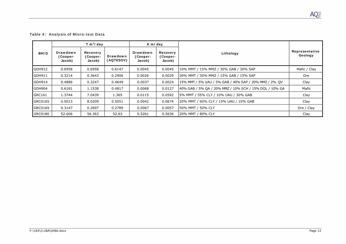
Micro-pumping tests were undertaken in 4 geotechnical (diamond) drill holes (GDH904, 911, 912
and 914) and 4 mineral exploration (RC) holes (GRC0161, 165, 169 and 180). The tests were
conducted using a low-discharge pump and pressure transducer to provide high frequency accurate
water level measurements. Both drawdown and recovery measurements were taken during the
micro-testing and the results were analysed using standard curve-fitting analysis methods.
Airlift aquifer tests were undertaken at 19AVWM02s, 02d, 03, 104 and 114 as part of the Ausdrill
Northwest drilling programme. The bores were airlifted for 30 minutes using a poly pipe and
compressor, with an installed pressure transducer / logger recording the water level drawdown and
subsequent recovery.
Falling head tests were undertaken at 19AVWM01, 108 and 113 using a pressure transducer to
measure the rise and fall in water level as water was introduced into the bore. Approximately 60 L
of water was added to each bore to raise water levels as quickly as possible. The water level peak
was obtained from the pressure transducer data and the decline in water levels from this peak was
analysed. Analysis was undertaken using the Bower-Rice method.
The test pumping of the two production bores (19AVWP001 and 19AVWP002) was conducted
between the 3rd of August 2019 and the 12th of August 2019 by Resource Water Group (RWG), in
partnership with Kgalya Services, under direct contact to AVL.
At each bore, a step test (comprising four thirty minute-steps for 19AVWP001 and four sixty-minute
steps for 19AVWP002) and a ~2-day constant rate test were conducted, each followed by monitored
recovery periods. Water levels were recorded manually at the production bore and adjacent
monitoring bore as well as with pressure transducers. All discharge water was transferred via lay-
flat to turkey’s nest dams located between 50 and 250 m from the tested production bores. The
constant rate test at 19AVWP001 (in the paleochannel area) was terminated after 30 hours when
the dam was full. Whilst at 19AVWP001 (targeting the fractured rock aquifer in the orebody area),
as a steady state was reached when pumping at 5 L/s, the abstraction rate was increased to 8 L/s

F:\183\3.C&R\048d.docx Page 7
at the end of the constant rate test for an additional half hour of pumping to determine if the bore
was capable of higher yields.
Details of the conducted hydraulic tests are presented in Tables 2 and 3 with the data plots presented
in Appendix C.

F:\183\3.C&R\048d.docx Page 8
Table 1: Details of the Monitoring and Production Bores
Hole ID Area / Purpose
Easting (GDA94_Z50)
Northing (GDA94_Z50)
Ground Elevation
(mRL)
Top of Casing
Elevation (mRL)
Stick- up (m)
Drilling Method
Drill Depth (m)
Drill Diam (mm)
Cased Depth
Casing ND
(mm)
Screened Depth (m)
SWL (mbTOC) - vertical
depth
SWL (mRL)
Date of SWL
Max Drilling Airlift Yield (L/s)
Completion Airlift Yield
(L/s)
19AVWM01 Paleochannel 666070 7011649 468.00 468.75 0.75 DR 134 241 134 50 98-134 14.14 455 17/06/2019 6.5 0.07
19AVWM02d 661573 7012645 463.00 463.86 0.86 DR 138 241 138 50 114-138 11.65 452 17/06/2019 ~10 5 Area
19AVWM02s Water Supply – 661591 7012641 463.00 463.88 0.88 DR 28 241 28 50* 10-28 7.76 456 17/06/2019 6 1.7
19AVWM03 654653 7014407 458.00 458.83 0.83 DR 28 241 28 50* 4-28 4.00 455 17/06/2019 10 - Regional
Monitoring 19AVWM04 663545 7011754 464.00 464.77 0.77 DR 28 241 28 50* 22-28 8.43 456 17/06/2019 ~10 2
19AVWM104 663778 7015448 469.50 470.34 0.84 DR 0-60
241/191 175 50 7-19, 31-175 13.96 456 17/06/2019 ~10 2.0 DTH 60-175
19AVWM105 663421 7016066 469.00 469.82 0.82 DR 0-84
241/191 178 50 10-16, 28-178 12.49 457 17/06/2019 12 - DTH 84-178
19AVWM108 Orebody Area 663916 7015608 470.00 470.76 0.76 DR DTH
0-34 34-100 241/191 100 50 28-100 12.30 458 17/06/2019 2 0.7
19AVWM112 Dewatering -
664733 7014236 468.00 468.82 0.82 DR 0-88
241/191 151 50 6-54, 60-150 8.32 461 17/06/2019 20 - Monitoring DTH 88-151
19AVWM113 662879 7017174 472.00 472.87 0.87 DR 0-52
241/191 142 50 10-94, 94-142 11.80 461 17/06/2019 2-3 - DTH 52-142
19AVWM114 663427 7015416 467.00 467.92 0.92 DR 0-106
241/191 148 50 10-46, 52-82, 82-
10.32 458 14/07/2019 9 - DTH 106-148 148
19AVWP001
Orebody Area Dewatering –
Test Production Bore
663418 7016082 469.00 469.58 0.58 DR DTH
0-94 94-184 346/298 184 200 94 - 184 15.64 454 15/07/2019 15 10
19AVWP002
Paleochannel Area
Water Supply - Test Production
Bore
663541 7011751 464.00 464.41 0.41 DR 0-28 346 28 200 16-28 8.15 456 15/07/2019 20 -
Co-ordinates from handheld GPS; Elevation from SRTM data EC= electrical conductivity; SWL= static water level. mbTOC = metres below top of casing

F:\183\3.C&R\048d.docx Page 9
Table 2: Hydraulic Test Details
BHID Easting MGA_Z50
Northing MGA_Z50
TOC Elevation
(mRL) Dip Type
SWL at Start of Test Test Type Test Date
mbRP mRL
19AVWM01 666070 7011649 468.75 -90 Mon Bore 14.14 454.61 Falling Head 15/07/19
19AVWM02d 661573 7012645 463.86 -90 Mon Bore 11.66 452.2 Airlift 14/07/19
19AVWM02s 661591 7012641 463.88 -90 Mon Bore 7.80 456.08 Airlift 14/07/19
19AVWM03 654653 7014407 458.83 -90 Mon Bore 4.02 454.81 Airlift 14/07/19
19AVWM104 663778 7015448 470.34 -90 Mon Bore 14.03 456.31 Airlift 14/07/19
19AVWM108 663916 7015608 470.76 -90 Mon Bore 12.30 458.46 Falling Head 15/07/19
19AVWM113 662879 7017174 472.87 -90 Mon Bore 12.65 460.22 Falling Head 15/07/19
19AVWM114 663427 7015416 467.92 -90 Mon Bore 10.32 457.6 Airlift 14/07/19
GDH912 663448 7015976 467.6 -61 DDH, open 12.69 454.95 Micro-pump 1/08/2018
GDH911 663388 7016120 466.3 -60 DDH, open 10.78 455.56 Micro-pump 2/08/2018
GDH914 663732 7015411 467.0 -61 DDH, open 12.44 454.52 Micro-pump 2/08/2018
GDH904 666566 7011966 466.3 -59 DDH, open 11.24 455.04 Micro-pump 31/07/2018
GRC161 663754 7015431 467.8 -60 RC, open 12.66 455.15 Micro-pump 1/08/2018
GRC0165 663724 7015539 470.3 -60 RC, open 13.44 456.82 Micro-pump 1/08/2018
GRC0169 663686 7015747 470.3 -60 RC, open 14.72 455.58 Micro-pump 2/08/2018
GRC0180 663630 7015909 467.7 -60 RC, open 11.86 455.86 Micro-pump 1/08/2018 Bores 19AVWM04 and 19AVWM105 were not tested as aquifer parameters at these sites were derived from the test pumping of the adjacent production bores. Bore 19AVWM112 was not tested due to the compromised status of the bore.
Table 3: Test Pumping Details
Bore SWL (mbRP)
Step Test Constant Rate Test
Test Date
Step Duration (mins)
Step Discharge Rates (L/s) Test Date Duration
(hrs) Rates (L/s)
Total Drawdown
(m)
Monitoring Bore
Distance from PB
Total Drawdown
(m)
19AVWP001 19.33 9/8/19 30 2, 4, 6, 8 10/8/19 48 5 40.09 19AVWM105 16.2 5.67
19AVWP002 10.12 3/8/19 60 10, 15, 20, 25 4/8/19 30 10 2.25 19AVWM04 4.9 0.59
mbRP = metres below reference point
F:\183\3.C&R\048d.docx Page 10
3 HYDROGEOLOGY
The results of the field investigations described above have been combined with AVL’s drilling data
and all other publicly available hydrogeological reporting for the area, to form a hydrogeological
understanding of the project area. The results from hydrogeological field investigations at Pit 3 have
been extrapolated to cover Pits 1, 2 and 4 where no investigations have been completed to date (i.e.
aquifer parameters and permeable structural features such as the footwall fault have been
extrapolated to the other pits).
3.1 Hydrogeological Units
A 1 to 2 km-wide, paleochannel has been identified from the ground-based TEM, to the south of the
orebody, trending in a northwest-southeast direction. The inferred location of the paleochannel is
shown in Figure 2, together with the locations of the installed monitoring bores and the proposed pits.
A shallow Mixed Aquifer has been encountered over all of the project area comprising calcrete,
silcrete and ironstone gravel with varying clay and sand content. In places (i.e. at 19AVWM04),
intervals of consolidated calcrete exist within this unit. This gravel and calcrete aquifer unit has been
found to be extensive across the paleochannel area to depths of 28 m, intersected by all drill holes
in the area (19AVWM01 to 19AVWM04), with airlift yields ranging between 4 and 12 L/s. This
shallow Tertiary aquifer unit also extends beyond the paleochannel, both to the south, where
outcropping calcrete is evident along the current-day drainage line, and to the north, where recent
drilling has intersected the unit overlying the orebody. In the orebody area, however, the gravel and
calcrete unit is much more variable in thickness, lithology and permeability (indicated by drilling
yields); it is generally thinner (i.e., 0 to 10 m) with yields, if present, of less than 1 L/s (i.e., at Bores
19AVWM104, 105, 108 and 113), although thicknesses of 38 m and 80 m have been recorded at
19AVWM112 and 19AVWM114 (respectively) with yields of 18 L/s and 10 L/s (respectively).
The shallow mixed aquifer includes alluvial sediments and a shallow “paleochannel” associated with
a north-east to south-west tributary drainage flowing towards the main paleochannel. This tributary
drainage crosses Pit 4. This tributary drainage is inferred from both present drainage patterns and
the available TEM survey; there are no drilling data to confirm its nature.
From the recent drilling, underlying the shallow mixed aquifer, the channel infill comprises the
following units:
Clay Aquitard – An upper, 70 m thick, unit of clay with minor sand / gravel horizons.
Although this unit is predominantly comprised of stiff, puggy clay, Bore 19AVWM01
intersected grey-white calcareous clay (i.e. weathered calcrete) between 75 and 98 mbgl.
Basal Sand and Gravel Aquifer – Comprising medium to coarse-grained, angular to sub-
rounded sand and gravel with clasts ranging between 7 and 50 mm in size. Particles are
predominantly composed of quartz, although black shale and lignite clasts are also present.
This unit has been intersected at both 19AVWM01 and 19AVWM02d, at depths of 100 and
105 mbgl respectively, with a thickness of approximately 20 m and airlift yields ranging
between 6.5 and 10 L/s.
F:\183\3.C&R\048d.docx Page 11
From the recent drilling in the area of the orebody (i.e. outside of the limits of the paleochannel
sediments), three main hydrogeological units have been identified, underlying the shallow mixed
aquifer (where present). These comprise:
Fractured Rock Aquifer – As evident from the yields at depth (ranging between 4 and
10 L/s) at Bores 19AVWM104, 105, 112 and 114 and 19AVWP001, increased (secondary)
permeability occurs as a result of fracturing and faulting between depths of 100 and
180 mbgl. From the structural mapping for the orebody area, numerous small faults cross-
cut the deposit and may be responsible for zones of increased permeability. However, it is
anticipated that the above-listed bores may all intercept a larger northwest-southeast
trending fault (i.e. coincident with the strike of the deposit), possibly associated with the
footwall of the orebody. The aquifer associated with the fault zone is assumed to extend
along the strike of the orebody into all pits. There is a cross cutting fault between Pits 1 and
4 which is assumed to result in some dislocation of the aquifer / orebody.
Unfractured Ore / Bedrock – Where there is no (or minimal) fracturing / faulting the
permeability of the bedrock in the project area (including the orebody) is anticipated to be
low. This is evident from many of the micro-tested RC and diamond drill holes as well as
Bores 19AVWM108 and 113.
A Saprock / Transition zone – This weathered basement unit is evident from the recent
hydrogeological drilling and has been mapped (as indicated by the base of oxidation) by AVL
across the orebody area. This saprock / transition zone has an increased permeability by
comparison to the underlying fresh bedrock, although hydraulic properties may vary laterally
due to changes in bedrock composition and oxidation characteristics.
3.2 Aquifer Parameters
A summary of the aquifer parameters derived from the 2018 and 2019 hydraulic testing are
presented in Tables 4 and 5, respectively. The permeability estimates for the shallow Tertiary aquifer
range from 0.2 to 38 m/d, with higher permeabilities evident in the paleochannel area, rather than
the orebody area. The basal sand and gravel of the paleochannel is estimated to have a permeability
ranging between 0.7 and ~3 m/d.
Although no bores were specifically completed in the either the unfractured bedrock or the saprock /
transition zone, the hydraulic testing of the lower yielding bores (i.e. Bores 19AVWM108 and 113, as
well as the majority of the tested RC and diamond holes) allow aquifer parameters for these combined
units to be derived. As such, the estimated permeabilities for the unfractured bedrock and the
saprock / transition zone ranges between 0.001 and 0.035 m/d. The more permeable, faulted /
fractured rock aquifer in the orebody has a derived permeability ranging between 0.2 and 3.3 m/d.
F:\183\3.C&R\048d.docx Page 12
Table 4: Analysis of Micro-test Data
BHID
T m2/day K m/day
Lithology Representative Geology
Drawdown (Cooper‐
Jacob)
Recovery (Cooper‐
Jacob) Drawdown (AQTESOV)
Drawdown (Cooper‐
Jacob)
Recovery (Cooper‐
Jacob)
GDH912 0.6958 0.6958 0.6147 0.0045 0.0045 10% MMT / 15% MMZ / 30% GAB / 30% SAP Mafic / Clay
GDH911 0.3214 0.3643 0.2906 0.0026 0.0029 30% MMT / 30% MMZ / 15% GAB / 15% SAP Ore
GDH914 0.4886 0.3247 0.4649 0.0037 0.0024 15% MMT / 5% UAU / 5% GAB / 40% SAP / 20% MMZ / 2% QV Clay
GDH904 0.6181 1.1538 0.4817 0.0068 0.0127 40% GAB / 5% QA / 20% MMZ / 10% SCH / 15% DOL / 10% GA Mafic
GRC161 1.3744 7.0439 1.365 0.0115 0.0592 5% MMT / 55% CLY / 10% UAU / 30% GAB Clay
GRC0165 0.5013 8.0209 0.5051 0.0042 0.0674 20% MMT / 60% CLY / 15% UAU / 10% GAB Clay
GRC0169 0.3147 0.2697 0.2789 0.0067 0.0057 50% MMT / 50% CLY Ore / Clay
GRC0180 52.606 56.363 52.63 0.5261 0.5636 20% MMT / 80% CLY Clay

F:\183\3.C&R\048d.docx Page 13
Table 5: Summary of Estimated Aquifer Permeability
Test Bore Screened Aquifer
Aquifer Thickness (m) Test Analytical Method Monitoring Bore Transmissivity
(m2/d)
Hydraulic Conductivity
(m/d) Comments
19AVWM108 Orebody No Aquifer
156 Falling Head Bower‐Rice
4.368 0.028 Early Time 0.156 0.001 Late Time
19AVWM113 132 4.62 0.035 Early Time 0.264 0.002 Late Time
19AVWM114 Orebody Shallow Aquifer 12 Airlift Cooper‐Jacob
3.84 0.32 Early Time
2.52 0.21 Late Time
19AVWM104
Orebody Deep Aquifer
24 Airlift Cooper‐Jacob 19.2 0.8 Early Time 4.8 0.2 Late Time
19AVWP001 24
SRT Logan 19AVWP001
13.2 0.55 12.48 0.52 11.76 0.49 11.76 0.49
CRT
Theis 19AVWP001 14.64 0.61 Early Time 19AVWM105 79.2 3.3 Early Time
Theis Recovery 19AVWP001 16.8 0.7 Late Time 19AVWM105 40.8 1.7 Early Time
Cooper‐Jacob 19AVWP001 12 0.5 Early Time 19AVWM105 38.4 1.6 Late Time
Fractured Rock 19AVWP001 14.16 0.59 Early Time 19AVWM105 57.6 2.4 Early Time
19AVWPM02s
Shallow Aquifer 12
Airlift Cooper‐Jacob
9.6 0.8 Early Time
52.8 4.4 Late Time
19AVWM03 34.8 2.9 Early Time 84.12 7.01 Late Time
19AVWP002 SRT Logan 19AVWP002
504 42 438 36.5
392.4 32.7 355.2 29.6
CRT Hantush for leaky Aquifer 19AVWM04 456 38 Early Time
19AVWM02d
Paleochannel Aquifer
22 Airlift Cooper‐Jacob 63.36 2.88 Early Time
15.84 0.72 Late Time
19AVWM01 3 (Steel casing stuck In Ground
Blocking aquifer) Falling Head Bower‐Rice
1.005 0.335 Early Time
0.024 0.008 Late Time
F:\183\3.C&R\048d.docx Page 14
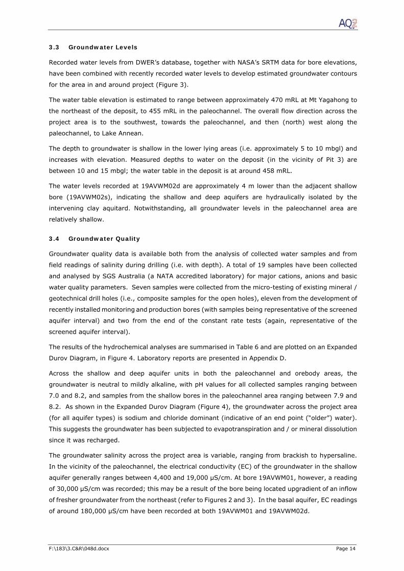
3.3 Groundwater Levels
Recorded water levels from DWER’s database, together with NASA’s SRTM data for bore elevations,
have been combined with recently recorded water levels to develop estimated groundwater contours
for the area in and around project (Figure 3).
The water table elevation is estimated to range between approximately 470 mRL at Mt Yagahong to
the northeast of the deposit, to 455 mRL in the paleochannel. The overall flow direction across the
project area is to the southwest, towards the paleochannel, and then (north) west along the
paleochannel, to Lake Annean.
The depth to groundwater is shallow in the lower lying areas (i.e. approximately 5 to 10 mbgl) and
increases with elevation. Measured depths to water on the deposit (in the vicinity of Pit 3) are
between 10 and 15 mbgl; the water table in the deposit is at around 458 mRL.
The water levels recorded at 19AVWM02d are approximately 4 m lower than the adjacent shallow
bore (19AVWM02s), indicating the shallow and deep aquifers are hydraulically isolated by the
intervening clay aquitard. Notwithstanding, all groundwater levels in the paleochannel area are
relatively shallow.
3.4 Groundwater Quality
Groundwater quality data is available both from the analysis of collected water samples and from
field readings of salinity during drilling (i.e. with depth). A total of 19 samples have been collected
and analysed by SGS Australia (a NATA accredited laboratory) for major cations, anions and basic
water quality parameters. Seven samples were collected from the micro-testing of existing mineral /
geotechnical drill holes (i.e., composite samples for the open holes), eleven from the development of
recently installed monitoring and production bores (with samples being representative of the screened
aquifer interval) and two from the end of the constant rate tests (again, representative of the
screened aquifer interval).
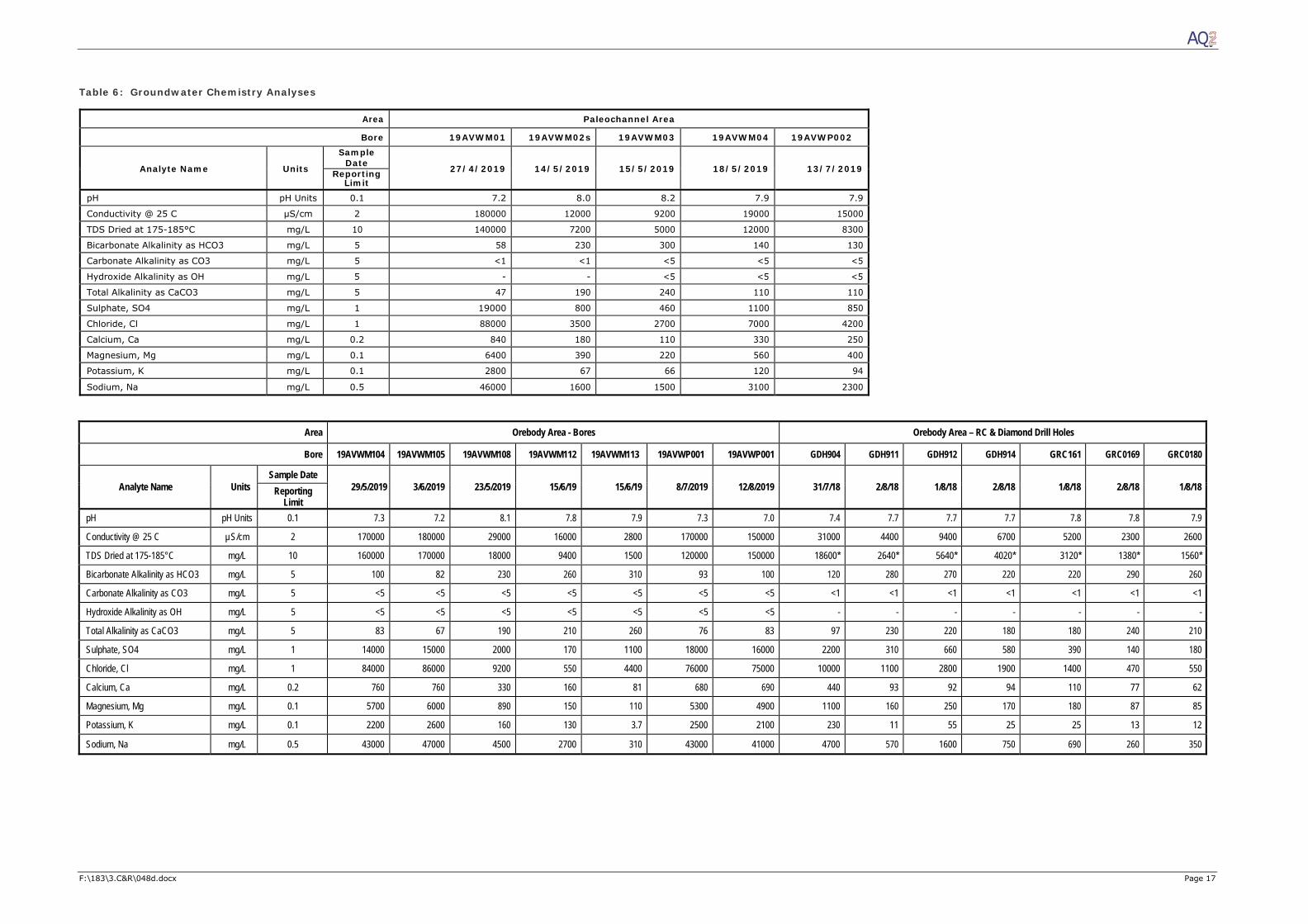
The results of the hydrochemical analyses are summarised in Table 6 and are plotted on an Expanded
Durov Diagram, in Figure 4. Laboratory reports are presented in Appendix D.
Across the shallow and deep aquifer units in both the paleochannel and orebody areas, the
groundwater is neutral to mildly alkaline, with pH values for all collected samples ranging between
7.0 and 8.2, and samples from the shallow bores in the paleochannel area ranging between 7.9 and
8.2. As shown in the Expanded Durov Diagram (Figure 4), the groundwater across the project area
(for all aquifer types) is sodium and chloride dominant (indicative of an end point (“older”) water).
This suggests the groundwater has been subjected to evapotranspiration and / or mineral dissolution
since it was recharged.
The groundwater salinity across the project area is variable, ranging from brackish to hypersaline.
In the vicinity of the paleochannel, the electrical conductivity (EC) of the groundwater in the shallow
aquifer generally ranges between 4,400 and 19,000 µS/cm. At bore 19AVWM01, however, a reading
of 30,000 µS/cm was recorded; this may be a result of the bore being located upgradient of an inflow
of fresher groundwater from the northeast (refer to Figures 2 and 3). In the basal aquifer, EC readings
of around 180,000 µS/cm have been recorded at both 19AVWM01 and 19AVWM02d.
F:\183\3.C&R\048d.docx Page 15
In the orebody area, the shallow groundwater is slightly fresher, with EC readings ranging between
2,500 and 5,200 µS/cm. However, in Bores 19AVWM104, 105, 112, 114 and 19AVWP001, at depths
of approximately 100 m (where zones of increased permeability have been intersected), salinities of
~250,000 µS/cm have been recorded. In the lower yielding bores of the orebody area (i.e.
19AVWM113 and 108) the groundwater at depth is brackish, as opposed to hypersaline; with EC
readings of 3,300 and ~29,000 µS/cm respectively). At Bore 19AVWM113, the lower salinity is most
likely due to its location adjacent to an ephemeral creek which may provide recharge to the aquifer
locally. Whilst at 19AVWM108, this may be indicative of the “background” groundwater salinity of
the area, with the higher salinity readings in the higher yielding bores, being evident of hypersaline
groundwater associated with the fault zones.
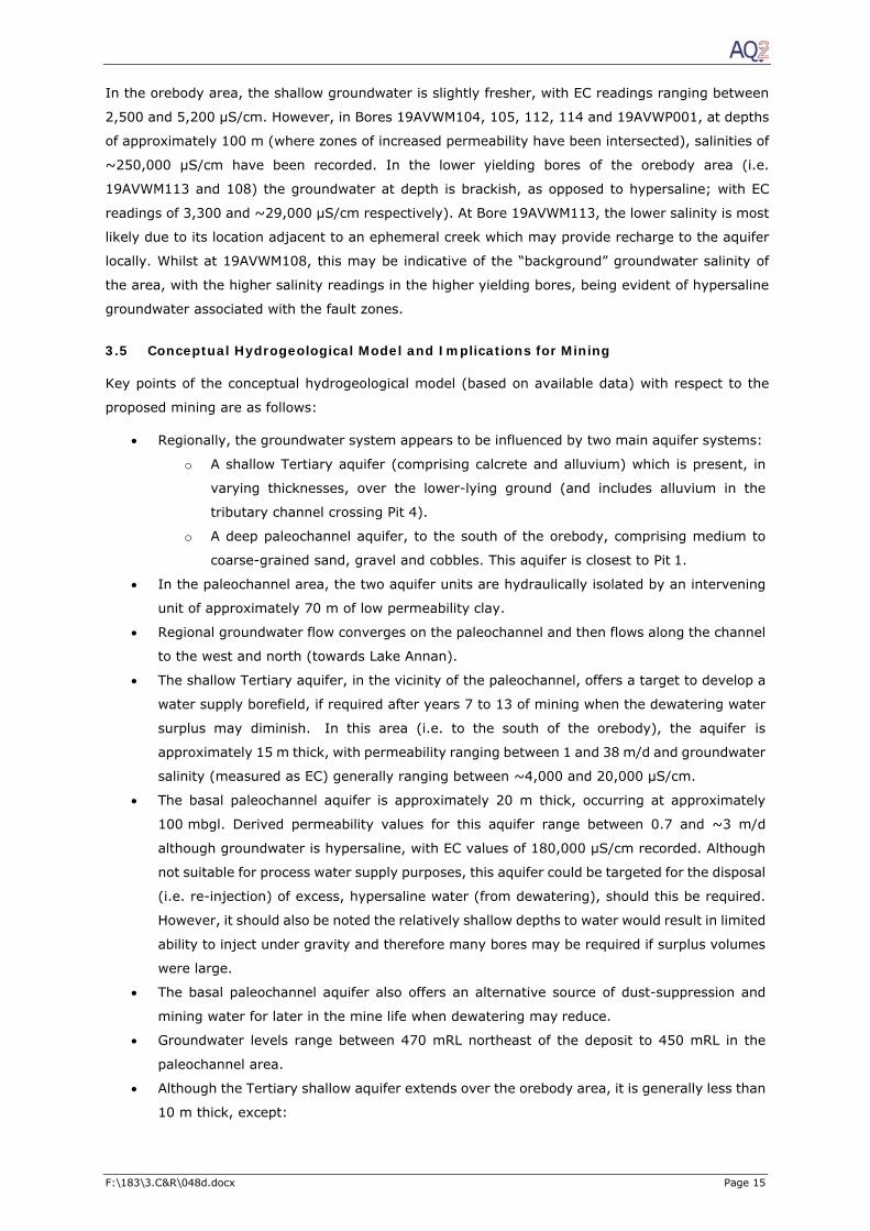
3.5 Conceptual Hydrogeological Model and Implications for Mining
Key points of the conceptual hydrogeological model (based on available data) with respect to the
proposed mining are as follows:
Regionally, the groundwater system appears to be influenced by two main aquifer systems:
o A shallow Tertiary aquifer (comprising calcrete and alluvium) which is present, in
varying thicknesses, over the lower-lying ground (and includes alluvium in the
tributary channel crossing Pit 4).
o A deep paleochannel aquifer, to the south of the orebody, comprising medium to
coarse-grained sand, gravel and cobbles. This aquifer is closest to Pit 1.
In the paleochannel area, the two aquifer units are hydraulically isolated by an intervening
unit of approximately 70 m of low permeability clay.
Regional groundwater flow converges on the paleochannel and then flows along the channel
to the west and north (towards Lake Annan).
The shallow Tertiary aquifer, in the vicinity of the paleochannel, offers a target to develop a
water supply borefield, if required after years 7 to 13 of mining when the dewatering water
surplus may diminish. In this area (i.e. to the south of the orebody), the aquifer is
approximately 15 m thick, with permeability ranging between 1 and 38 m/d and groundwater
salinity (measured as EC) generally ranging between ~4,000 and 20,000 µS/cm.
The basal paleochannel aquifer is approximately 20 m thick, occurring at approximately
100 mbgl. Derived permeability values for this aquifer range between 0.7 and ~3 m/d
although groundwater is hypersaline, with EC values of 180,000 µS/cm recorded. Although
not suitable for process water supply purposes, this aquifer could be targeted for the disposal
(i.e. re-injection) of excess, hypersaline water (from dewatering), should this be required.
However, it should also be noted the relatively shallow depths to water would result in limited
ability to inject under gravity and therefore many bores may be required if surplus volumes
were large.
The basal paleochannel aquifer also offers an alternative source of dust-suppression and
mining water for later in the mine life when dewatering may reduce.
Groundwater levels range between 470 mRL northeast of the deposit to 450 mRL in the
paleochannel area.
Although the Tertiary shallow aquifer extends over the orebody area, it is generally less than
10 m thick, except:
F:\183\3.C&R\048d.docx Page 16
o in the southwest (i.e., at 19AVWM0112 and 114) where thicknesses of up to 80 m
have been intersected;
o over the tributary channel that crosses Pit 4, where an alluvial thickness of up to
50 m is inferred.
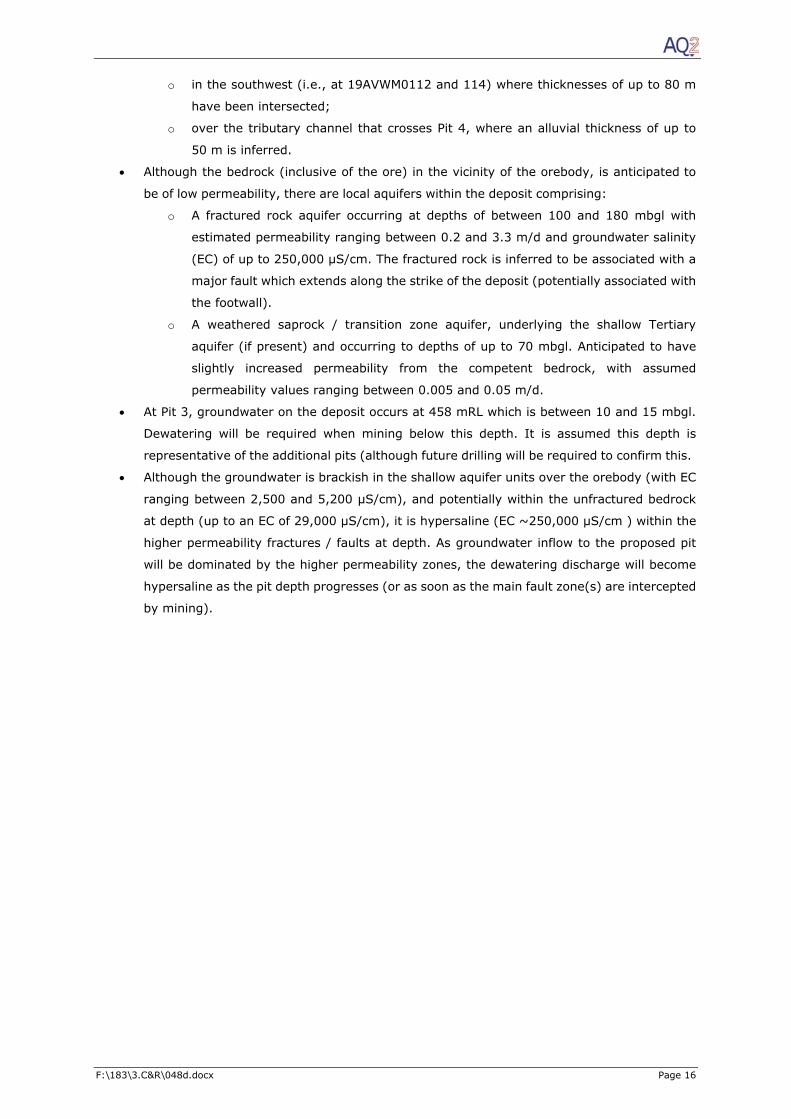
Although the bedrock (inclusive of the ore) in the vicinity of the orebody, is anticipated to
be of low permeability, there are local aquifers within the deposit comprising:
o A fractured rock aquifer occurring at depths of between 100 and 180 mbgl with
estimated permeability ranging between 0.2 and 3.3 m/d and groundwater salinity
(EC) of up to 250,000 µS/cm. The fractured rock is inferred to be associated with a
major fault which extends along the strike of the deposit (potentially associated with
the footwall).
o A weathered saprock / transition zone aquifer, underlying the shallow Tertiary
aquifer (if present) and occurring to depths of up to 70 mbgl. Anticipated to have
slightly increased permeability from the competent bedrock, with assumed
permeability values ranging between 0.005 and 0.05 m/d.
At Pit 3, groundwater on the deposit occurs at 458 mRL which is between 10 and 15 mbgl.
Dewatering will be required when mining below this depth. It is assumed this depth is
representative of the additional pits (although future drilling will be required to confirm this.
Although the groundwater is brackish in the shallow aquifer units over the orebody (with EC
ranging between 2,500 and 5,200 µS/cm), and potentially within the unfractured bedrock
at depth (up to an EC of 29,000 µS/cm), it is hypersaline (EC ~250,000 µS/cm ) within the
higher permeability fractures / faults at depth. As groundwater inflow to the proposed pit
will be dominated by the higher permeability zones, the dewatering discharge will become
hypersaline as the pit depth progresses (or as soon as the main fault zone(s) are intercepted
by mining).
F:\183\3.C&R\048d.docx Page 17
Table 6: Groundwater Chemistry Analyses
Area Orebody Area - Bores Orebody Area – RC & Diamond Drill Holes
Bore 19AVWM104 19AVWM105 19AVWM108 19AVWM112 19AVWM113 19AVWP001 19AVWP001 GDH904 GDH911 GDH912 GDH914 GRC161 GRC0169 GRC0180
Analyte Name
Units
Sample Date 29/5/2019
3/6/2019
23/5/2019
15/6/19
15/6/19
8/7/2019
12/8/2019
31/7/18
2/8/18
1/8/18
2/8/18
1/8/18
2/8/18
1/8/18 Reporting
Limit pH pH Units 0.1 7.3 7.2 8.1 7.8 7.9 7.3 7.0 7.4 7.7 7.7 7.7 7.8 7.8 7.9
Conductivity @ 25 C µS/cm 2 170000 180000 29000 16000 2800 170000 150000 31000 4400 9400 6700 5200 2300 2600
TDS Dried at 175-185°C mg/L 10 160000 170000 18000 9400 1500 120000 150000 18600* 2640* 5640* 4020* 3120* 1380* 1560*
Bicarbonate Alkalinity as HCO3 mg/L 5 100 82 230 260 310 93 100 120 280 270 220 220 290 260
Carbonate Alkalinity as CO3 mg/L 5 <5 <5 <5 <5 <5 <5 <5 <1 <1 <1 <1 <1 <1 <1
Hydroxide Alkalinity as OH mg/L 5 <5 <5 <5 <5 <5 <5 <5 - - - - - - -
Total Alkalinity as CaCO3 mg/L 5 83 67 190 210 260 76 83 97 230 220 180 180 240 210
Sulphate, SO4 mg/L 1 14000 15000 2000 170 1100 18000 16000 2200 310 660 580 390 140 180
Chloride, Cl mg/L 1 84000 86000 9200 550 4400 76000 75000 10000 1100 2800 1900 1400 470 550
Calcium, Ca mg/L 0.2 760 760 330 160 81 680 690 440 93 92 94 110 77 62
Magnesium, Mg mg/L 0.1 5700 6000 890 150 110 5300 4900 1100 160 250 170 180 87 85
Potassium, K mg/L 0.1 2200 2600 160 130 3.7 2500 2100 230 11 55 25 25 13 12
Sodium, Na mg/L 0.5 43000 47000 4500 2700 310 43000 41000 4700 570 1600 750 690 260 350
Area Paleochannel Area
Bore 19AVWM01 19AVWM02s 19AVWM03 19AVWM04 19AVWP002
Analyte Name
Units
Sample Date
27/4/2019
14/5/2019
15/5/2019
18/5/2019
13/7/2019Reporting Limit
pH pH Units 0.1 7.2 8.0 8.2 7.9 7.9
Conductivity @ 25 C µS/cm 2 180000 12000 9200 19000 15000
TDS Dried at 175-185°C mg/L 10 140000 7200 5000 12000 8300
Bicarbonate Alkalinity as HCO3 mg/L 5 58 230 300 140 130
Carbonate Alkalinity as CO3 mg/L 5 <1 <1 <5 <5 <5
Hydroxide Alkalinity as OH mg/L 5 - - <5 <5 <5
Total Alkalinity as CaCO3 mg/L 5 47 190 240 110 110
Sulphate, SO4 mg/L 1 19000 800 460 1100 850
Chloride, Cl mg/L 1 88000 3500 2700 7000 4200
Calcium, Ca mg/L 0.2 840 180 110 330 250
Magnesium, Mg mg/L 0.1 6400 390 220 560 400
Potassium, K mg/L 0.1 2800 67 66 120 94
Sodium, Na mg/L 0.5 46000 1600 1500 3100 2300
F:\183\3.C&R\048d.docx Page 18
4 WATER MANAGEMENT
4.1 Dewatering
4.1.1 Project Mine Plan
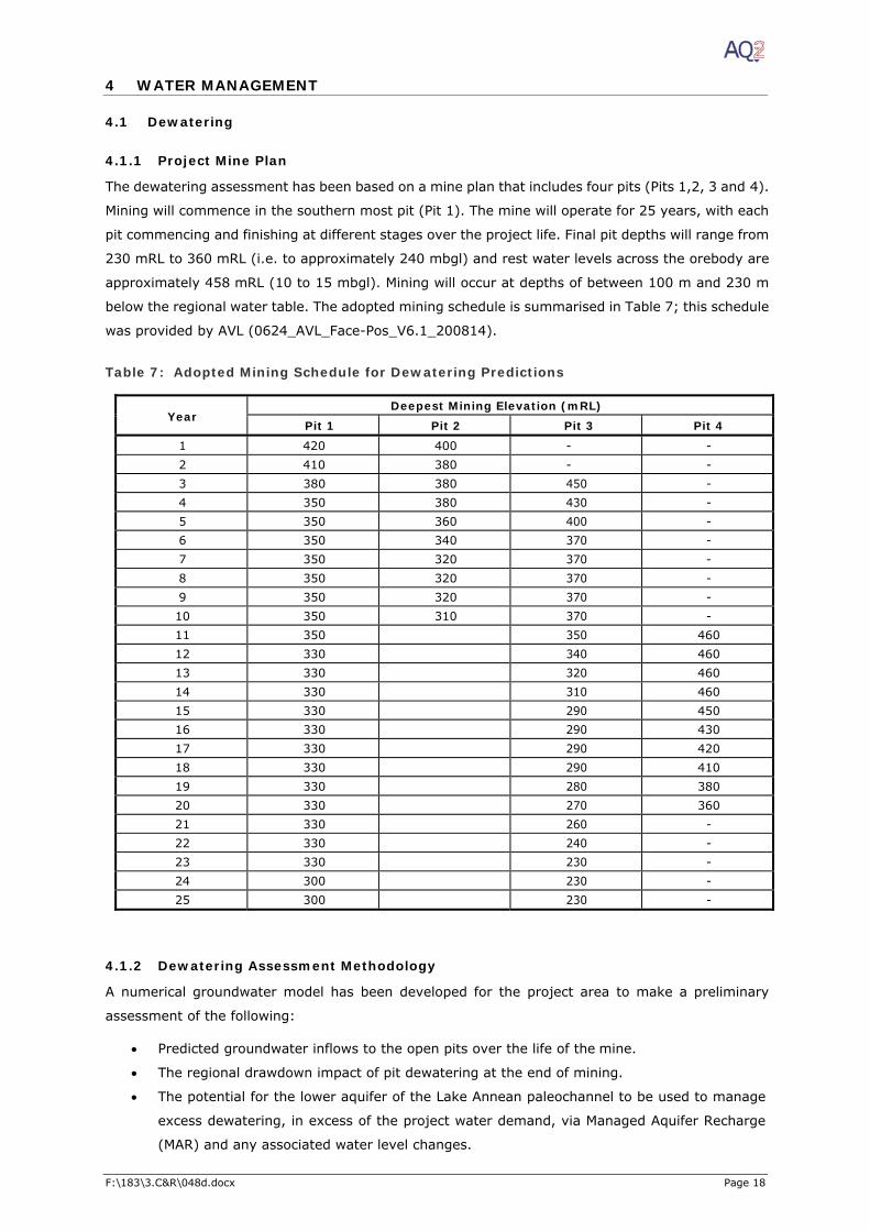
The dewatering assessment has been based on a mine plan that includes four pits (Pits 1,2, 3 and 4).
Mining will commence in the southern most pit (Pit 1). The mine will operate for 25 years, with each
pit commencing and finishing at different stages over the project life. Final pit depths will range from
230 mRL to 360 mRL (i.e. to approximately 240 mbgl) and rest water levels across the orebody are
approximately 458 mRL (10 to 15 mbgl). Mining will occur at depths of between 100 m and 230 m
below the regional water table. The adopted mining schedule is summarised in Table 7; this schedule
was provided by AVL (0624_AVL_Face-Pos_V6.1_200814).
Table 7: Adopted Mining Schedule for Dewatering Predictions
Year Deepest Mining Elevation (mRL)
Pit 1 Pit 2 Pit 3 Pit 4 1 420 400 - - 2 410 380 - - 3 380 380 450 - 4 350 380 430 - 5 350 360 400 - 6 350 340 370 - 7 350 320 370 - 8 350 320 370 - 9 350 320 370 - 10 350 310 370 - 11 350 350 460 12 330 340 460 13 330 320 460 14 330 310 460 15 330 290 450 16 330 290 430 17 330 290 420 18 330 290 410 19 330 280 380 20 330 270 360 21 330 260 - 22 330 240 - 23 330 230 - 24 300 230 - 25 300 230 -
4.1.2 Dewatering Assessment Methodology
A numerical groundwater model has been developed for the project area to make a preliminary
assessment of the following:
Predicted groundwater inflows to the open pits over the life of the mine.
The regional drawdown impact of pit dewatering at the end of mining.
The potential for the lower aquifer of the Lake Annean paleochannel to be used to manage
excess dewatering, in excess of the project water demand, via Managed Aquifer Recharge
(MAR) and any associated water level changes.
F:\183\3.C&R\048d.docx Page 19
The long term behaviour of the final pit voids once mining is complete, including the time
taken for recovery to post mining or equilibrium levels and regional drawdown associated
with the final mine voids.
Details of the model set up are presented in Appendix E; key points of note are as follows:
The model extent includes the mine area and the Lake Annean paleochannel and tributaries.
Seven model layers are used to represent the mine area and the lower aquifer, clay aquitard
and upper aquifer of the Lake Annean paleochannel and tributaries.
Regional groundwater flows are simulated, with inflow included from the upstream (i.e., from
the northeast, southwest and southeast) and groundwater outflow to the northwest (i.e.,
along the main paleochannel towards Lake Annean).
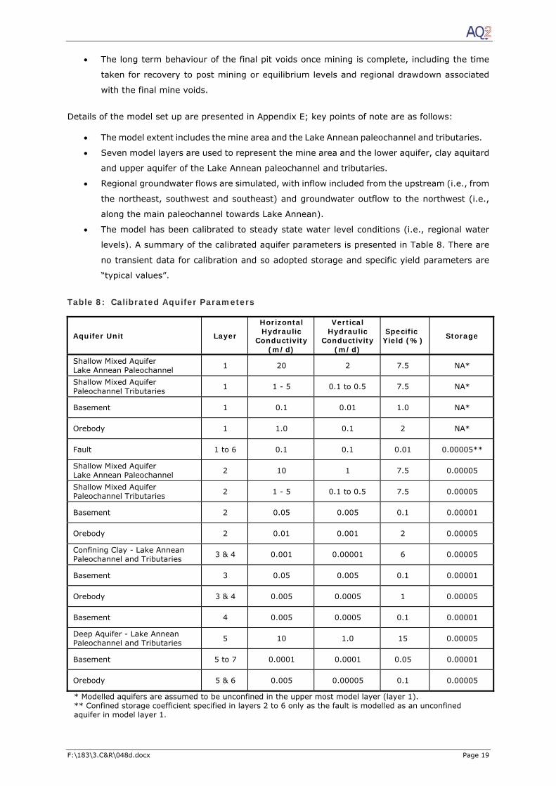
The model has been calibrated to steady state water level conditions (i.e., regional water
levels). A summary of the calibrated aquifer parameters is presented in Table 8. There are
no transient data for calibration and so adopted storage and specific yield parameters are
“typical values”.
Table 8: Calibrated Aquifer Parameters
Aquifer Unit Layer
Horizontal Hydraulic
Conductivity (m/d)
Vertical Hydraulic
Conductivity (m/d)
Specific Yield (%) Storage
Shallow Mixed Aquifer Lake Annean Paleochannel 1 20 2 7.5 NA*
Shallow Mixed Aquifer Paleochannel Tributaries 1 1 - 5 0.1 to 0.5 7.5 NA*
Basement 1 0.1 0.01 1.0 NA*
Orebody 1 1.0 0.1 2 NA*
Fault 1 to 6 0.1 0.1 0.01 0.00005**
Shallow Mixed Aquifer Lake Annean Paleochannel 2 10 1 7.5 0.00005
Shallow Mixed Aquifer Paleochannel Tributaries 2 1 - 5 0.1 to 0.5 7.5 0.00005
Basement 2 0.05 0.005 0.1 0.00001
Orebody 2 0.01 0.001 2 0.00005
Confining Clay - Lake Annean Paleochannel and Tributaries 3 & 4 0.001 0.00001 6 0.00005
Basement 3 0.05 0.005 0.1 0.00001
Orebody 3 & 4 0.005 0.0005 1 0.00005
Basement 4 0.005 0.0005 0.1 0.00001
Deep Aquifer - Lake Annean Paleochannel and Tributaries 5 10 1.0 15 0.00005
Basement 5 to 7 0.0001 0.0001 0.05 0.00001
Orebody 5 & 6 0.005 0.00005 0.1 0.00005
* Modelled aquifers are assumed to be unconfined in the upper most model layer (layer 1). ** Confined storage coefficient specified in layers 2 to 6 only as the fault is modelled as an unconfined aquifer in model layer 1.

F:\183\3.C&R\048d.docx Page 20
4.1.3 Pit Dewatering Requirements
The predicted inflow rates over the 25-year mine life are presented in Figure 5 and summarised by
pit in Table 9. The results of the dewatering assessment can be summarised as follows:
Predicted mine dewatering is initially high as paleochannel sediments are intersected in Pit 2
but decrease as each pit goes into lower permeability bedrock.
o Dewatering for the first year is approximately 8,000 kL/d (92 L/s).
o Dewatering of between 4,000 kL/d (45 L/s) to 5,000 kL/d (60 L/s) between years 2 and 6.
o Dewatering volumes continue to decrease from 3,000 kL/d (35 L/s) at year 7 to 1,500 kL/d (18 L/s) by year 25.
The distribution of permeability within the fractured rock aquifer may be quite variable. In
practice, this means increases in dewatering are likely to be concentrated over permeable
horizons and this level of discretization cannot be included in the model.
The dewatering estimates take no account of the impact of cross-cutting dolerite and gabbro
dykes which may be of lower permeability and compartmentalise the orebody.
In low permeability rocks, the area affected by dewatering does not extend far from the
dewatering stress (i.e. far from pit wall into the aquifer) and the hydrostatic pressure behind
the pit walls is expected to be high. This may affect wall stability, particularly where the high
pressure corresponds with geomechanical failure surfaces. Subject to geotechnical analysis,
depressurisation of the pit walls may be required, at least in susceptible areas.
It is anticipated that dewatering discharge may initially be brackish; potentially for the first
two years of mining. However, as the mining depth progresses and / or once the higher
permeability fault zones are intersected, the dewatering production may become saline (or
hyper saline), with the fault zones anticipated to comprise 25 to 40% of groundwater inflow
to the pit.

F:\183\3.C&R\048d.docx Page 21
Table 9: Predicted Dewatering By Pit
Year Pit 1
Dewatering (kL/d)
Pit 2 Dewatering
(kL/d)
Pit 3 Dewatering
(kL/d)
Pit 4 Dewatering
(kL/d)
Total Dewatering
(kL/d) 1 3849 4149 0 0 7998
2 1966 1936 0 0 3902
3 1905 1467 1894 0 5266
4 1706 1256 1273 0 4236 5 1369 1257 1880 0 4505
6 1262 1220 1387 0 3868
7 1180 977 710 0 2866
8 1113 904 618 0 2635
9 1058 847 559 0 2464
10 1014 823 517 0 2354
11 976 0 1002 0 1978 12 1154 0 693 0 1848
13 1023 0 723 0 1746
14 1029 0 598 0 1627
15 1021 0 617 0 1638
16 929 0 555 1310 2794
17 883 0 545 701 2129
18 830 0 531 623 1985 19 783 0 550 728 2061
20 764 0 557 649 1970
21 764 0 537 0 1301
22 804 0 535 0 1338
23 792 0 519 0 1310
24 949 0 500 0 1448
25 832 0 489 0 1321
4.1.4 Open Pit Dewatering Method
Based on the initially high dewatering estimates for the first year of mining and variability of
groundwater inflows to each pit, dewatering of the open pits would be best achieved through a
combination of:
Dewatering bores which can be used to dewater the higher permeability shallow aquifer
sediments associated with the large groundwater inflow volumes at the initiation of mining.
Dewatering bores should also target the permeable structure that is inferred to run along
the footwall of the pit. Bores should be located on the pit crest at either end of the pit with
additional bores along strike and within the pit (if they can be accommodated from mining
logistics).
In-pit sump pumping to remove groundwater inflows from lower permeability units. The
mine plan should therefore allow for the presence of sumps within the pit and temporary
drains across the pit floor to direct groundwater to the sumps.
Sump pumping will not allow any dewatering freeboard which means mining will be affected by:
Rises in groundwater levels following rainfall events that may contribute to inundation of the
lower-benches; and
Wet blasting will be required on lower active benches.
F:\183\3.C&R\048d.docx Page 22
Following the dewatering of the shallow aquifer, sump pumping may continue to be effective for the
life of mine. Although dewatering bores similar to, and including, 19AVWP01 could also be used to
target and dewater the higher permeability fault zone(s). This would offer the advantage of advanced
dewatering and increased dewatered free-board.
Based on test pumping of 19AVWP01, a recommended pumping rate of 8 L/s has been derived (refer
Appendix C). However, it should be noted that the sustainability of pumping from a fractured rock
aquifer and its effectiveness for dewatering is uncertain as it depends on the connectivity and extent
of the fractures / faults. If the orientation of the permeable fault(s) becomes well understood, these
bores could potentially be sited outside the pit areas to avoid the logistical difficulties of in-pit bores
(i.e. mining through and recovering them).
Dewatering infrastructure should be designed to accommodate the likely inflow estimate (presented
in Table 9), with additional capacity for surface water runoff.
4.2 Water Balance
4.2.1 Water Demand
The mining and dust suppression (i.e. low-quality) water demand has been estimated by AVL, at
between 0.83 and 0.98 GL/a (2,300 to 2,700 kL/d) with the breakdown of water use as below:
Roads (dust suppression) 0.67 GL/annum (~ 1,835 kL/d)
Mining, wet season 0.16 GL/annum (~440 kL/d)
Mining, dry season 0.31 GL/annum (~850 kL/d)
4.3 Water Supply
Although initial inflows into the pit may be brackish, it is assumed that all mine dewatering is saline
or hypersaline. As such, dewatering will be used to meet mine and dust-suppression water
requirements only.
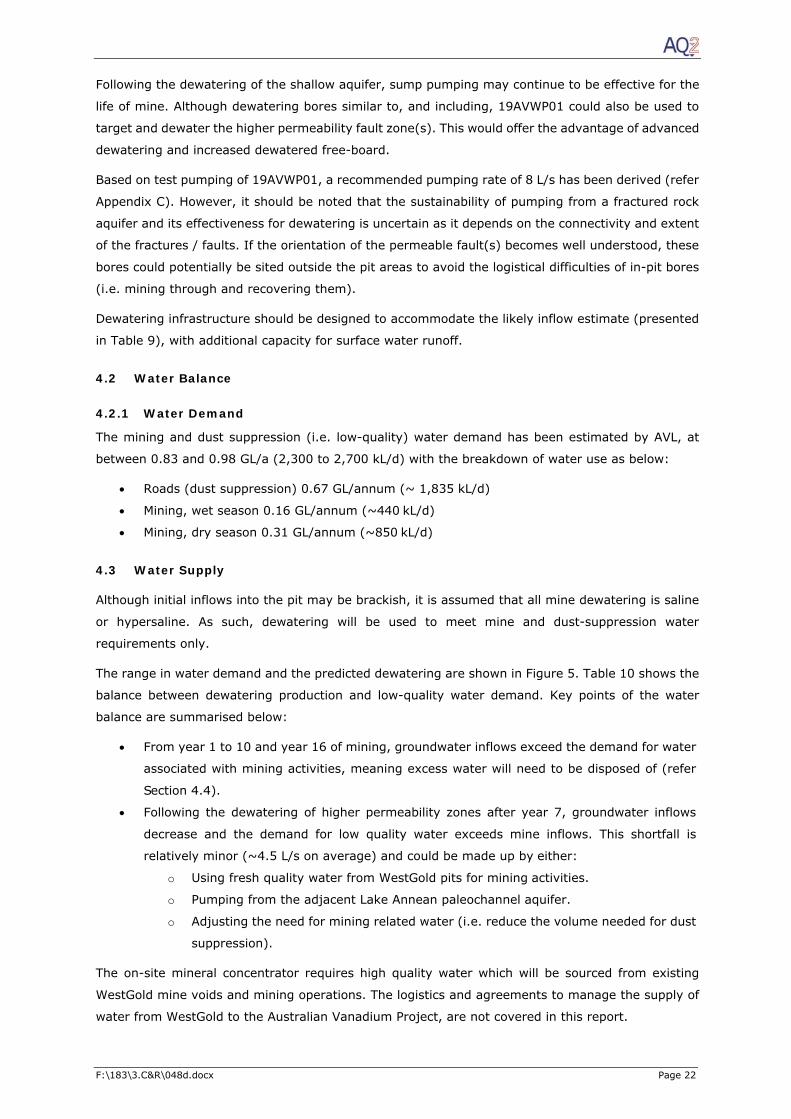
The range in water demand and the predicted dewatering are shown in Figure 5. Table 10 shows the
balance between dewatering production and low-quality water demand. Key points of the water
balance are summarised below:
From year 1 to 10 and year 16 of mining, groundwater inflows exceed the demand for water
associated with mining activities, meaning excess water will need to be disposed of (refer
Section 4.4).
Following the dewatering of higher permeability zones after year 7, groundwater inflows
decrease and the demand for low quality water exceeds mine inflows. This shortfall is
relatively minor (~4.5 L/s on average) and could be made up by either:
o Using fresh quality water from WestGold pits for mining activities.
o Pumping from the adjacent Lake Annean paleochannel aquifer.
o Adjusting the need for mining related water (i.e. reduce the volume needed for dust
suppression).
The on-site mineral concentrator requires high quality water which will be sourced from existing
WestGold mine voids and mining operations. The logistics and agreements to manage the supply of
water from WestGold to the Australian Vanadium Project, are not covered in this report.
F:\183\3.C&R\048d.docx Page 23
Table 10: Predicted Dewatering and Surplus (in kL/d)
Year Predicted
Dewatering (kL/d)
Water Demand (kL/d) Surplus (kL/d)
Minimum Maximum Minimum Maximum 1 7998 2274 2685 5313 5724 2 3902 2274 2685 1217 1628 3 5266 2274 2685 2581 2992 4 4236 2274 2685 1551 1962 5 4505 2274 2685 1820 2231 6 3868 2274 2685 1183 1594 7 2866 2274 2685 181 592 8 2635 2274 2685 0 361 9 2464 2274 2685 0 190 10 2354 2274 2685 0 80 11 1978 2274 2685 0 0 12 1848 2274 2685 0 0 13 1746 2274 2685 0 0 14 1627 2274 2685 0 0 15 1638 2274 2685 0 0 16 2794 2274 2685 109 520 17 2129 2274 2685 0 0 18 1985 2274 2685 0 0 19 2061 2274 2685 0 0 20 1970 2274 2685 0 0 21 1301 2274 2685 0 0 22 1338 2274 2685 0 0 23 1310 2274 2685 0 0 24 1448 2274 2685 0 0 25 1321 2274 2685 0 0
4.4 Excess Water Management
Excess groundwater over the mine life is displayed in Figure 5 and Table 10. Groundwater inflows
exceed low quality water demand for Year 1 to 10 and year 16 of mining. Excess water volumes
decrease from an initial volume of 5,500 kL/d (64 L/s) in year 1 to 520 kL/d (46 L/s) by year 16.
Managed Aquifer Recharge (MAR) into the hypersaline paleochannel aquifer has been evaluated. The
numerical model was used to simulate the gravity injection of excess groundwater to the deep
paleochannel aquifer (refer Appendix E, Section E7.1). Several injection borefield layouts were
simulated, adjusting both the individual injection rates and the bore spacing. However, the shallow
depth to water (with limited injection head) means many bores will be required to operate over a
very wide area, at low individual injection rates. MAR is unlikely to be cost-effective and no further
optimisation of MAR was considered.
Options for excess water management/reduction include:
Utilising spray canons over the waste dumps to facilitate evaporation.
Commence pumping from the dewatering bores early to spread the ‘peak’ over a longer
period of time.
F:\183\3.C&R\048d.docx Page 24
5 IMPACT ASSESSMENT
The numerical groundwater flow model described in Appendix E was also used to predict the
drawdown impact of mining and the long term behaviour of the mined out voids. Details of the model
predictions are described in Appendix E.
5.1 Regional Drawdown Impact - End of Mining
Contours of predicted drawdown after 25 years of mining are shown in Figure 6. The predicted
drawdown is the difference between pre-mining water levels and the water levels predicted at the
end of mining (Year 25 of mine life). The following observations are made regarding the predicted
drawdown:
Maximum drawdown is predicted in Pit 1 (228 m).
Drawdown of 1 m is predicted a maximum distance of 8 km from the south eastern and
north western ends of the mining area (or 10 km from Pit 2 / the centre of the mining area).
This drawdown extends along the paleochannel south of the mine areas.
5.2 Mine Closure
Water levels in the mining areas are not predicted to recover due to the large evaporative area at
the base of each empty pit. The pits are predicted to develop into local sinks and pit lakes are
predicted to develop in the base of open pits and are discussed below:
Water levels in Pits 1, 3 and 4 remain close to dewatered levels of 300 mRL, 230 mRL and
360 mRL respectively or approximately 240 m, 170 m and 110 m below the pre-mining
ground surface respectively (or 230 m, 160 and 100 m below the pre-mining water table
respectively, refer Figure E14 and E15). These shallow pit void lakes may not persist
throughout the year as they respond to episodic rainfall / run off.
Water levels in Pit 2 are predicted to recover to 332 mRL or approximately 140 m below the
pre-mining ground level (~130 m below the pre-mining water table), 35 years after the
cessation of dewatering. The south eastern end of Pit 2 is located on the northern side of a
shallow tributary of the Lake Annean paleochannel. The Pit 2 void lake is predicted to be
approximately 20 m deep and is predicted to persist throughout the year. There may be
small fluctuations in pit lake elevation in response to episodic rainfall / run off.
Pit 4 is located within the shallow tributary of the Lake Annean paleochannel. As Pit 2 and
Pit 1 (located to the south of the tributary) are both deeper than Pit 4, groundwater flow is
towards Pits 1 and 2. As a result a pit lake is not predicted to develop in Pit 4.
The pits will function as long term groundwater sinks with sustained groundwater flow
towards the mined out voids and discharge through evaporation. This means there will be no
long term outflow of saline groundwater from the pits into the regional system.
Contours of predicted water level drawdown 100 years after the end of mining are shown in Figure 7.
The following observations are made regarding the predicted drawdown after mine closure:
Drawdown of 1 m is predicted to extend a maximum distance of 13 km to the north and
14 km to the south of the mine area (from the centre of Pit 2). Drawdown of 1 m is also
predicted to extend through the paleochannel aquifers a maximum distance of 15 km to the
south east of the centre of the mining area, and 18 km to the west.
In the mine areas, where pit lakes are expected to develop, water levels are between 100 m
to 230 m below pre-mining water levels.

F:\183\3.C&R\048d.docx Page 25
6 CONCLUSIONS & RECOMMENDATIONS
6.1 Conclusions
Australian Vanadium Ltd (AVL) are undertaking a feasibility study of the Australian Vanadium Project
in the Murchison region of Western Australia. The project will involve open-cut mining to a depth of
approximately 240 mbgl.
Groundwater levels in the project area range between 470 mRL, to the northeast of the deposit, to
450 mRL, in the paleochannel area. Groundwater on the deposit occurs at 458 mRL which is between
10 and 15 mbgl. Dewatering will be required when mining below this depth.
The main regional aquifers in the project area comprise a deep paleochannel aquifer, to the south of
the orebody, and a laterally extensive shallow Tertiary aquifer.
The deep paleochannel aquifer comprises approximately 20 m of medium to coarse-grained sand,
gravel and cobbles, occurring at depths of approximately 100 mbgl, with a permeability of between
0.7 and ~3 m/d. Groundwater within this aquifer unit is hypersaline, with EC values of
180,000 µS/cm recorded.
In the paleochannel, overlying the basal aquifer is a 70 m thick unit of low permeability clay over
which lies the shallow Tertiary aquifer. Outside of the paleochannel, the shallow aquifer directly
overlies basement.
The shallow aquifer comprises calcrete and alluvial gravels and extends beyond the paleochannel,
forming a cover over the low-lying ground of the project area. The thickness of the unit is uniform
(~30 m) across the paleochannel area, but variable (0 to 80 m) across the orebody. Permeability
estimates for this unit range between 1 and 38 m/d and groundwater salinity (measured as EC)
generally ranges between ~4,000 and 20,000 µS/cm.
Although the ore and competent bedrock in the deposit area are generally of low permeability, local
aquifers comprise a saprock / transition zone and a fractured rock aquifer. The saprock / transition
zone aquifer occurs at depths ranging between 30 and 70 mbgl and is anticipated to have a variable
permeability due to changes in bedrock composition and oxidation characteristics. The fractured
basement tends to occur at depths between 100 and 180 mbgl, with derived permeability values
ranging between 0.2 and 3.3 m/d. Although the fracturing may be associated with the mapped faults
that cross-cut the orebody, it is anticipated that the higher yielding bores drilled to date intercept a
northwest-southeast trending fault (i.e. coincident with the strike of the deposit), possibly associated
with the footwall of the orebody.
A numerical model has been developed for the mine area and surrounding catchment and used to
simulate mine dewatering and associated impacts. The results of model predictions are summarised
below:
Dewatering requirements over the life of the mine, that includes four pits (Pits 1 to 4), peaks
during Year 1 of mining when dewatering rates of 8,000 kL/d are predicted, decreasing to
less than 1,500 kL/d by Year 25 of mining.
Site water demand, seasonally varying between 2,300 and 2,700 kL/d will result in an excess
of water of up to 5,700 kL/d. The model was also used to assess the potential for MAR into
the deep paleochannel aquifer to be used to manage excess water. The injection rates
required, the limited aquifer extent and the shallow depth to water predicted that injection
F:\183\3.C&R\048d.docx Page 26
under gravity was not feasible. Groundwater levels in the lower aquifer were predicted to
increase to at or above ground level along the Lake Annean paleochannel and the tributaries
within a year of commencement of re-injection.
After 25 years of mining, drawdown of 1 m is predicted a maximum distance of 8 km from
the south eastern and north western ends of the mining area (or 10 km from Pit 2 / the
centre of the mining area). This drawdown extends along the paleochannel south of the
mine areas.
Water levels in the mining areas are not predicted to recover due to the large evaporative
area at the base of each empty pit. The pits are predicted to develop into local sinks and pit
lakes are predicted to develop in the base of open pits. Very shallow pit lakes (less than 1 m
in depth) are predicted to develop in Pits 1, 3 and 4 approximately 160 m, 230 m and 100 m
below the pre-mining water table, respectively. Water levels in Pit 2 are predicted to recover
to 332 mRL, or approximately 140 m below the pre-mining ground level, resulting in a pit
lake approximately 20 m deep. The south eastern end of Pit 2 is located on the northern
side of a shallow tributary of the Lake Annean paleochannel and higher inflows to this pit
are possible once mining in complete compared to the other pits.
Pit 4 is located within the shallow tributary of the Lake Annean paleochannel. As Pit 2 and
Pit 1 (located to the south of the tributary) are both deeper than Pit 4, groundwater flow is
towards Pits 1 and 2. As a result a pit lake is not predicted to develop in Pit 4.
As the pits are predicted to develop into groundwater sinks in the long term, predicted
drawdown is predicted to continue after the end of mining. Drawdown of 1 m is predicted to
extend a maximum distance of 13 km to north and 14 km to the south of the mine area
(from the centre of Pit 2). Drawdown of 1 m is also predicted to extend through the
paleochannel aquifers a maximum distance of 15 km to the south east of the centre of the
mining area, and 18 km to the west.
Although the groundwater is brackish in the shallow aquifer units over the orebody (with EC ranging
between 2,500 and 5,200 µS/cm), and potentially within the unfractured bedrock at depth (up to an
EC of 29,000 µS/cm), the groundwater is hypersaline (EC ~250,000 µS/cm ) within the higher
permeability fractures / faults at depths below ~100 mbgl. As groundwater inflow to the proposed
pit will be dominated by the higher permeability zones, the dewatering discharge will become
hypersaline as the pit depth progresses (or as soon as the main fault zone(s) are intercepted by
mining).
Based on the initially high dewatering estimates for the first year of mining and variability of
groundwater inflows to each pit, dewatering of the open pits would be best achieved through a
combination of:
Dewatering bores which can be used to dewater the higher permeability shallow aquifer
sediments associated with the large groundwater inflow volumes at the initiation of mining.
Dewatering bores should also target the permeable structure that is inferred to run along
the footwall of the pit. Bores should be located on the pit crest at either of the pit with
additional bores along strike and within the pit (if they can be accommodated from mining
logistics).
F:\183\3.C&R\048d.docx Page 27
In-pit sump pumping to remove groundwater inflows from lower permeability units. The
mine plan should therefore allow for the presence of sumps within the pit and temporary
drains across the pit floor to direct groundwater to the sumps.
6.2 Recommendations
Hydrogeological field investigations should be extended over Pits 1, 2 and 4 to:
Confirm that the hydrogeological conditions remain consistent with those encountered at
Pit 1.
Install additional groundwater monitoring bores to extend the determination of baseline
conditions.
The dewatering assessment (modelling and data analysis) should be updated when the results from
field investigations over Pits 1, 2 and 4 are available.
As the project evolves, modelling should be undertaken to refine / optimize progression of dewatering
with a view to minimizing periods of water surplus. For example, this may involve opportunities to
commence dewatering sooner but at lower rates (i.e. to achieve advanced dewatering). Any
dewatering optimisation should wait until the results from field investigations over Pits 1, 2 and 4 are
available.
F:\183\3.C&R\048d.docx Page 28
7 REFERENCES
Bell, J.G., Kilgour, P.L., English, P.M., Woodgate, M.F., Lewis, S.J. and Wischusen, J.D.H. (compilers),
2012. WASANT Paleovalley Map – Distribution of Paleovalleys in Arid and Semi-arid WA-SA-NT (First
Edition), scale: 1:4 500 000, Geoscience Australia Thematic Map (Geocat № 73980) – hard-copy and
digital data publication: http://www.ga.gov.au/cedda/maps/96.
Cashman, P. and M Preene, 2013. Groundwater Lowering in Construction: A Practical Guide to
Dewatering.
Davis, A., S. Macaulay, T. Munday, C. Sorensen, J. Shudra and T. Ibrahimi, 2016, Uncovering the
groundwater resource potential of Murchison Region in Western Australia through targeted
application of airborne electromagnetics: 25th International Geophysical Conference and Exhibition,
ASEG-PESA-AIG, 459–464.
Marinelli F, Niccoli, WL, 2000, Simple Analytical Equations for estimating Groundwater Inflow to a
Mine Pit, Groundwater, Vol 38 no.2, pp311 – 314.

FIGURES

< No Content >
LOCATION MAP
FIGURE 1PROJECT AREA
Location: F:\183\4.GIS\Workspaces\Figures\Report Figures
KEY
NOTES & DATA SOURCES:AUTHOR: LDS REPORT NO: 048
DRAWN: LDS REVISION: a
DATE: 02/12/19 JOB NO: 183
PERTH
ProjectKALGOORLIE
PROJECT
Proposed Pit Outline
Tenement Boundary
Paleochannel Thalweg
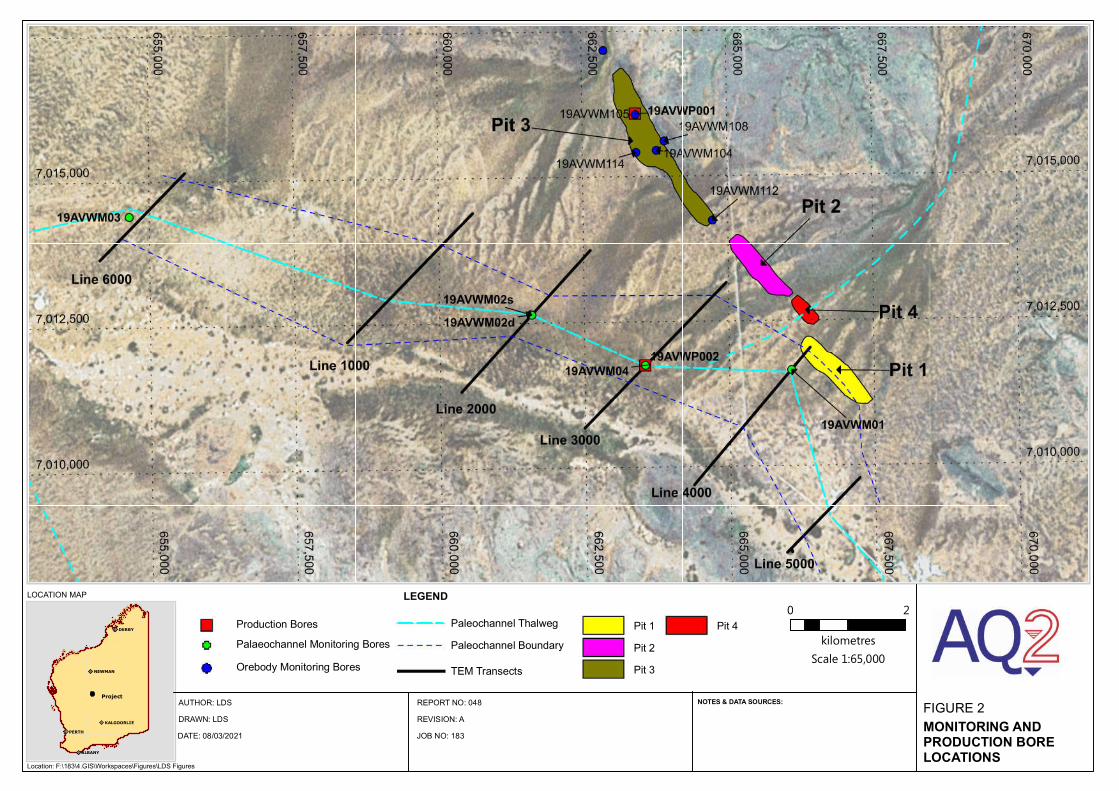
PERTH
Project
KALGOORLIE
Project
PERTH
ALBANY
KALGOORLIE
NEWMAN
DERBY
LOCATION MAP
MONITORING AND PRODUCTION BORE LOCATIONS
Location: F:\183\4.GIS\Workspaces\Figures\LDS Figures
LEGEND
NOTES & DATA SOURCES:AUTHOR: LDS REPORT NO: 048
DRAWN: LDS REVISION: A
DATE: 08/03/2021 JOB NO: 183
Production Bores
Palaeochannel Monitoring Bores
Orebody Monitoring Bores
FIGURE 2
TEM Transects
Paleochannel Thalweg0 2
kilometres
Scale 1:65,000Paleochannel Boundary
Pit 1
Pit 2
Pit 3
Pit 4
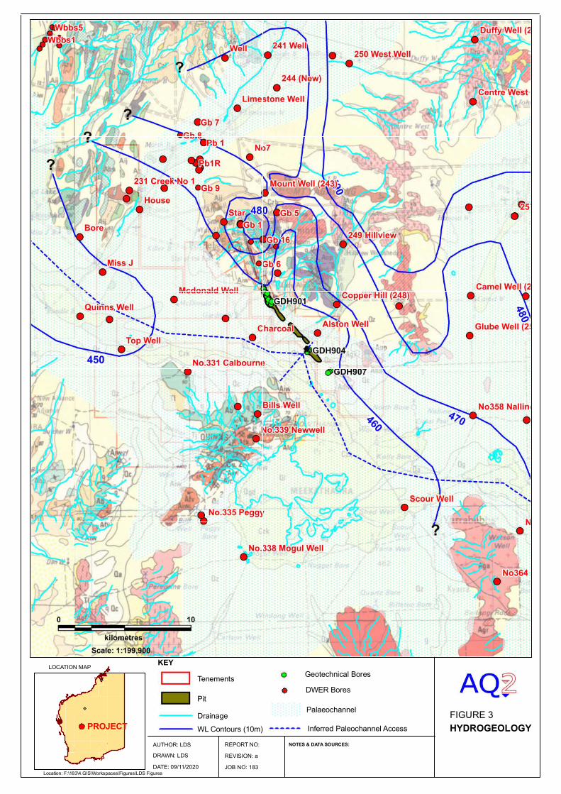
LOCATION MAP
FIGURE 3
HYDROGEOLOGY
Location: F:\183\4.GIS\Workspaces\Figures\LDS Figures
KEY
NOTES & DATA SOURCES:AUTHOR: LDS REPORT NO:
DRAWN: LDS REVISION: a
DATE: 09/11/2020 JOB NO: 183
PERTH
Project
KALGOORLIE
PROJECT
Geotechnical Bores
DWER Bores
Drainage
Tenements
Pit
WL Contours (10m)
Palaeochannel
Inferred Paleochannel Access
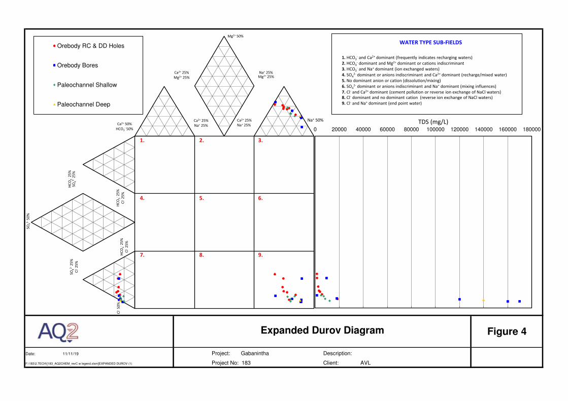
Date: 11/11/19 Description:
F:\183\2.TECH\[183_AQ2CHEM_revC w legend.xlsm]EXPANDED DUROV (1) Client: AVL
Figure 4Expanded Durov Diagram
Project: Gabanintha
Project No: 183
Orebody RC & DD Holes
Orebody Bores
Paleochannel Shallow
Paleochannel Deep
Na+ 25%Mg2+ 25%
Mg2+ 50%
Ca2+ 25%
Na+ 25%
Ca2+ 25%
Na+ 25%
Ca2+ 25%
Mg2+ 25%
Ca2+ 50%
HCO3- 50%
HC
O3
-2
5%
SO
42
-2
5%
HC
O3
-2
5%
Cl-
25
%
1.
8.
2.
9.7.
6.5.4.
3.
Na+ 50%
SO
42
-2
5%
Cl-
25
%
HC
O3
-2
5%
Cl-
25
%
SO
42
-5
0%
Cl-
50
%
0 20000 40000 60000 80000 100000 120000 140000 160000 180000
TDS (mg/L)
1. HCO3- and Ca2+ dominant (frequently indicates recharging waters)
2. HCO3- dominant and Mg2+ dominant or cations indiscriminant
3. HCO3- and Na+ dominant (ion exchanged waters)
4. SO42- dominant or anions indiscriminant and Ca2+ dominant (recharge/mixed water)
5. No dominant anion or cation (dissolution/mixing)
6. SO42- dominant or anions indiscriminant and Na+ dominant (mixing influences)
7. Cl- and Ca2+ dominant (cement pollution or reverse ion exchange of NaCl waters)
8. Cl- dominant and no dominant cation (reverse ion exchange of NaCl waters)
9. Cl- and Na+ dominant (end point water)
WATER TYPE SUB-FIELDS

Dewatering Volumes and Disposal Requirements FIGURE 5F:\183\3.C&R\048 Figs & App\Appendix E_Modelling\[Figure E10 - Dewatering Volumes.xlsx]Figure 5
0
1000
2000
3000
4000
5000
6000
7000
8000
9000
0 5 10 15 20 25
Rat
e (
kL/d
ay)
Years
Dewatering Rate (kL/day) Upper Disposal Limit (kL/d) Lower Disposal Limit (kL/d)


APPENDIX A
TEM SURVEY RESULTS

Datum: GDA 94Grid: MGA Zone 50
Southern Geoscience Consultants Pty LtdACN 067 552 461
Drawn: G.Maude
Scale: 1:15,000
Date: Mar-2019
Figure:
GABANINTHA PROJECTCoincident Loop EM SurveyTEM PROFILESCDI SECTIONLine 1000
GABANINTHA PROJECTCoincident Loop EM Survey
TEM PROFILESCDI SECTION
Line 1000
-100 0 100 200 300 400 500
Scale 1:15000
WINDOW TIMES (ms): Centre From the end of the turn off (160.3 ms)1 : 0.09952 : 0.12453 : 0.15404 : 0.19105 : 0.23756 : 0.29507 : 0.36608 : 0.45459 : 0.564510 : 0.700511 : 0.869512 : 1.08013 : 1.34114 : 1.66415 : 2.06616 : 2.56517 : 3.184
18 : 3.95319 : 4.90820 : 6.09321 : 7.56422 : 9.39023 : 11.6624 : 14.4725 : 17.9726 : 22.3127 : 27.6928 : 34.3829 : 42.6830 : 52.9931 : 65.7932 : 81.6733 : 101.434 : 125.9
SURVEY PARAMETERS
Configuration : Coincident LoopStation Spacing : 100 m
RECEIVER
Receiver : SMARTem24Frequency : 1.5625Component : ZRx Coil : Loop WireRx Area : 10000 turn-m
TRANSMITTER
Transmitter : Zonge NT-20Tx Loop Side : 100 mTx Current : 8.4-8.6 ATurn Off : 0.3 ms
Z Component Log Scale - Channels 1 to 34
EM R
espo
nse
(uV/
A)
-1-1
0
11
10
100
1000
10000
100000
Station (metres)
200 400 600 800 1000 1200 1400 1600 1800 2000 2200 2400 2600 2800 3000 3200
0.09950.12450.1540.1910.23750.2950.3660.45450.56450.70050.86951.081.34051.6642.0662.56453.1843.9534.90756.09257.56359.390511.65814.47317.96822.307
27.6935
34.380542.68352.9965.785581.671101.393125.8765
Channels 1-34
Z Component Linear Scale - Channels 25 to 34
EM R
espo
nse
(uV/
A)
-0-0
6
12
18
24
30
Station (metres)
200 400 600 800 1000 1200 1400 1600 1800 2000 2200 2400 2600 2800 3000 3200
17.968
22.30727.693534.380542.68352.9965.785581.671101.393125.8765
Channels 25-34
200200
300
400
500
600
700
800
900mS/mEMAX CDI Section
Pseu
dode
pth
-250-250
-200
-150
-100
-50
0
Station (metres)
200 400 600 800 1000 1200 1400 1600 1800 2000 2200 2400 2600 2800 3000 3200
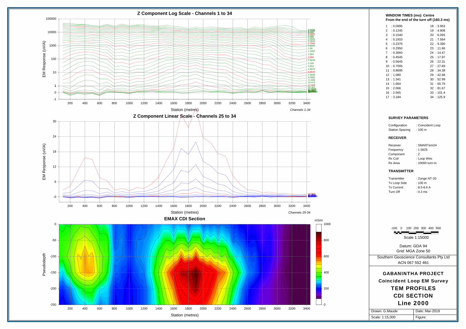
Datum: GDA 94Grid: MGA Zone 50
Southern Geoscience Consultants Pty LtdACN 067 552 461
Drawn: G.Maude
Scale: 1:15,000
Date: Mar-2019
Figure:
GABANINTHA PROJECTCoincident Loop EM SurveyTEM PROFILESCDI SECTIONLine 2000
GABANINTHA PROJECTCoincident Loop EM Survey
TEM PROFILESCDI SECTION
Line 2000
-100 0 100 200 300 400 500
Scale 1:15000
WINDOW TIMES (ms): Centre From the end of the turn off (160.3 ms)1 : 0.09952 : 0.12453 : 0.15404 : 0.19105 : 0.23756 : 0.29507 : 0.36608 : 0.45459 : 0.564510 : 0.700511 : 0.869512 : 1.08013 : 1.34114 : 1.66415 : 2.06616 : 2.56517 : 3.184
18 : 3.95319 : 4.90820 : 6.09321 : 7.56422 : 9.39023 : 11.6624 : 14.4725 : 17.9726 : 22.3127 : 27.6928 : 34.3829 : 42.6830 : 52.9931 : 65.7932 : 81.6733 : 101.434 : 125.9
SURVEY PARAMETERS
Configuration : Coincident LoopStation Spacing : 100 m
RECEIVER
Receiver : SMARTem24Frequency : 1.5625Component : ZRx Coil : Loop WireRx Area : 10000 turn-m
TRANSMITTER
Transmitter : Zonge NT-20Tx Loop Side : 100 mTx Current : 8.5-8.6 ATurn Off : 0.3 ms
Z Component Log Scale - Channels 1 to 34
EM R
espo
nse
(uV/
A)
-1-1
0
11
10
100
1000
10000
100000
Station (metres)
200 400 600 800 1000 1200 1400 1600 1800 2000 2200 2400 2600 2800 3000 3200 3400
0.09950.12450.1540.1910.23750.2950.3660.45450.56450.70050.86951.081.34051.6642.0662.56453.1843.9534.90756.09257.56359.390511.65814.47317.96822.30727.693534.380542.68352.9965.785581.671101.393125.8765
Channels 1-34
Z Component Linear Scale - Channels 25 to 34
EM R
espo
nse
(uV/
A)
-0-0
6
12
18
24
30
Station (metres)
200 400 600 800 1000 1200 1400 1600 1800 2000 2200 2400 2600 2800 3000 3200 3400
17.96822.30727.693534.380542.68352.9965.785581.671101.393125.8765
Channels 25-34
00
200
400
600
800
1000mS/mEMAX CDI Section
Pseu
dode
pth
-250-250
-200
-150
-100
-50
0
Station (metres)
200 400 600 800 1000 1200 1400 1600 1800 2000 2200 2400 2600 2800 3000 3200 3400

Datum: GDA 94Grid: MGA Zone 50
Southern Geoscience Consultants Pty LtdACN 067 552 461
Drawn: G.Maude
Scale: 1:15,000
Date: Mar-2019
Figure:
GABANINTHA PROJECTCoincident Loop EM SurveyTEM PROFILESCDI SECTIONLine 3000
GABANINTHA PROJECTCoincident Loop EM Survey
TEM PROFILESCDI SECTION
Line 3000
-100 0 100 200 300 400 500
Scale 1:15000
WINDOW TIMES (ms): Centre From the end of the turn off (160.3 ms)1 : 0.09952 : 0.12453 : 0.15404 : 0.19105 : 0.23756 : 0.29507 : 0.36608 : 0.45459 : 0.564510 : 0.700511 : 0.869512 : 1.08013 : 1.34114 : 1.66415 : 2.06616 : 2.56517 : 3.184
18 : 3.95319 : 4.90820 : 6.09321 : 7.56422 : 9.39023 : 11.6624 : 14.4725 : 17.9726 : 22.3127 : 27.6928 : 34.3829 : 42.6830 : 52.9931 : 65.7932 : 81.6733 : 101.434 : 125.9
SURVEY PARAMETERS
Configuration : Coincident LoopStation Spacing : 100 m
RECEIVER
Receiver : SMARTem24Frequency : 1.5625Component : ZRx Coil : Loop WireRx Area : 10000 turn-m
TRANSMITTER
Transmitter : Zonge NT-20Tx Loop Side : 100 mTx Current : 8.4-8.5 ATurn Off : 0.3 ms
Z Component Log Scale - Channels 1 to 34
EM R
espo
nse
(uV/
A)
-1-1
0
11
10
100
1000
10000
100000
Station (metres)
200 400 600 800 1000 1200 1400 1600 1800 2000 2200 2400 2600 2800 3000 3200 3400 3600
0.09950.12450.1540.1910.23750.2950.3660.45450.56450.70050.86951.081.34051.6642.0662.56453.1843.9534.90756.0925
7.5635
9.3905
11.658
14.473
17.96822.30727.693534.380542.68352.9965.785581.671101.393125.8765
Channels 1-34
Z Component Linear Scale - Channels 25 to 34
EM R
espo
nse
(uV/
A)
-0-0
6
12
18
24
30
Station (metres)
200 400 600 800 1000 1200 1400 1600 1800 2000 2200 2400 2600 2800 3000 3200 3400 3600
17.96822.30727.693534.380542.68352.9965.785581.671101.393125.8765
Channels 25-34
100100
200
300
400
500
600
700
800mS/mEMAX CDI Section
Pseu
dode
pth
-250-250
-200
-150
-100
-50
0
Station (metres)
200 400 600 800 1000 1200 1400 1600 1800 2000 2200 2400 2600 2800 3000 3200 3400 3600

Datum: GDA 94Grid: MGA Zone 50
Southern Geoscience Consultants Pty LtdACN 067 552 461
Drawn: G.Maude
Scale: 1:15,000
Date: Mar-2019
Figure:
GABANINTHA PROJECTCoincident Loop EM SurveyTEM PROFILESCDI SECTIONLine 4000
GABANINTHA PROJECTCoincident Loop EM Survey
TEM PROFILESCDI SECTION
Line 4000
-100 0 100 200 300 400 500
Scale 1:15000
WINDOW TIMES (ms): Centre From the end of the turn off (160.3 ms)1 : 0.09952 : 0.12453 : 0.15404 : 0.19105 : 0.23756 : 0.29507 : 0.36608 : 0.45459 : 0.564510 : 0.700511 : 0.869512 : 1.08013 : 1.34114 : 1.66415 : 2.06616 : 2.56517 : 3.184
18 : 3.95319 : 4.90820 : 6.09321 : 7.56422 : 9.39023 : 11.6624 : 14.4725 : 17.9726 : 22.3127 : 27.6928 : 34.3829 : 42.6830 : 52.9931 : 65.7932 : 81.6733 : 101.434 : 125.9
SURVEY PARAMETERS
Configuration : Coincident LoopStation Spacing : 100 m
RECEIVER
Receiver : SMARTem24Frequency : 1.5625Component : ZRx Coil : Loop WireRx Area : 10000 turn-m
TRANSMITTER
Transmitter : Zonge NT-20Tx Loop Side : 100 mTx Current : 8.2-8.5 ATurn Off : 0.3 ms
Z Component Log Scale - Channels 1 to 34
EM R
espo
nse
(uV/
A)
-1-1
0
11
10
100
1000
10000
100000
Station (metres)
200 400 600 800 1000 1200 1400 1600 1800 2000 2200 2400 2600 2800 3000 3200
0.09950.12450.1540.1910.23750.2950.3660.45450.56450.70050.86951.081.34051.6642.0662.56453.1843.9534.90756.09257.5635
9.3905
11.658
14.473
17.968
22.30727.693534.380542.68352.9965.785581.671101.393125.8765
Channels 1-34
Z Component Linear Scale - Channels 25 to 34
EM R
espo
nse
(uV/
A)
-0-0
6
12
18
24
30
Station (metres)
200 400 600 800 1000 1200 1400 1600 1800 2000 2200 2400 2600 2800 3000 3200
17.96822.30727.693534.380542.68352.9965.785581.671101.393125.8765
Channels 25-34
00
200
400
600
800
1000
1200mS/mEMAX CDI Section
Pseu
dode
pth
-250-250
-200
-150
-100
-50
0
Station (metres)
200 400 600 800 1000 1200 1400 1600 1800 2000 2200 2400 2600 2800 3000 3200

Datum: GDA 94Grid: MGA Zone 50
Southern Geoscience Consultants Pty LtdACN 067 552 461
Drawn: G.Maude
Scale: 1:15,000
Date: Mar-2019
Figure:
GABANINTHA PROJECTCoincident Loop EM SurveyTEM PROFILESCDI SECTIONLine 5000
GABANINTHA PROJECTCoincident Loop EM Survey
TEM PROFILESCDI SECTION
Line 5000
-100 0 100 200 300 400 500
Scale 1:15000
WINDOW TIMES (ms): Centre From the end of the turn off (160.3 ms)1 : 0.09952 : 0.12453 : 0.15404 : 0.19105 : 0.23756 : 0.29507 : 0.36608 : 0.45459 : 0.564510 : 0.700511 : 0.869512 : 1.08013 : 1.34114 : 1.66415 : 2.06616 : 2.56517 : 3.18418 : 3.953
19 : 4.90820 : 6.09321 : 7.56422 : 9.39023 : 11.6624 : 14.4725 : 17.9726 : 22.3127 : 27.6928 : 34.3829 : 42.6830 : 52.9931 : 65.7932 : 81.6733 : 101.434 : 125.935 : 156.336 : 194.0
SURVEY PARAMETERS
Configuration : Coincident LoopStation Spacing : 100 m
RECEIVER
Receiver : SMARTem24Frequency : 1.5625Component : ZRx Coil : Loop WireRx Area : 10000 turn-m
TRANSMITTER
Transmitter : Zonge NT-20Tx Loop Side : 100 mTx Current : 8.1-8.3 ATurn Off : 0.3 ms
Z Component Log Scale - Channels 1 to 34
EM R
espo
nse
(uV/
A)-1-1
0
11
10
100
1000
10000
100000
Station (metres)
0 200 400 600 800 1000 1200 1400 1600 1800 2000
0.09950.12450.1540.1910.23750.2950.3660.45450.56450.70050.86951.081.34051.6642.0662.56453.1843.9534.90756.09257.56359.390511.65814.473
17.968
22.307
27.6935
34.3805
42.68352.9965.785581.671101.393125.8765
Channels 1-36
Z Component Linear Scale - Channels 25 to 34
EM R
espo
nse
(uV/
A)
-0-0
8
16
24
32
40
Station (metres)
0 200 400 600 800 1000 1200 1400 1600 1800 2000
17.968
22.307
27.693534.380542.68352.9965.785581.671101.393125.8765
Channels 25-35
200200
400
600
800
1000
1200mS/mEMAX CDI Section
Pseu
dode
pth
-250-250
-200
-150
-100
-50
0
Station (metres)
0 200 400 600 800 1000 1200 1400 1600 1800 2000
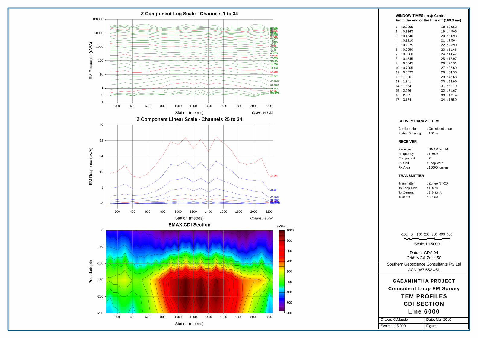
Datum: GDA 94Grid: MGA Zone 50
Southern Geoscience Consultants Pty LtdACN 067 552 461
Drawn: G.Maude
Scale: 1:15,000
Date: Mar-2019
Figure:
GABANINTHA PROJECTCoincident Loop EM SurveyTEM PROFILESCDI SECTIONLine 6000
GABANINTHA PROJECTCoincident Loop EM Survey
TEM PROFILESCDI SECTION
Line 6000
-100 0 100 200 300 400 500
Scale 1:15000
WINDOW TIMES (ms): Centre From the end of the turn off (160.3 ms)1 : 0.09952 : 0.12453 : 0.15404 : 0.19105 : 0.23756 : 0.29507 : 0.36608 : 0.45459 : 0.564510 : 0.700511 : 0.869512 : 1.08013 : 1.34114 : 1.66415 : 2.06616 : 2.56517 : 3.184
18 : 3.95319 : 4.90820 : 6.09321 : 7.56422 : 9.39023 : 11.6624 : 14.4725 : 17.9726 : 22.3127 : 27.6928 : 34.3829 : 42.6830 : 52.9931 : 65.7932 : 81.6733 : 101.434 : 125.9
SURVEY PARAMETERS
Configuration : Coincident LoopStation Spacing : 100 m
RECEIVER
Receiver : SMARTem24Frequency : 1.5625Component : ZRx Coil : Loop WireRx Area : 10000 turn-m
TRANSMITTER
Transmitter : Zonge NT-20Tx Loop Side : 100 mTx Current : 8.5-8.6 ATurn Off : 0.3 ms
Z Component Log Scale - Channels 1 to 34
EM R
espo
nse
(uV/
A)
-1-1
0
11
10
100
1000
10000
100000
Station (metres)
200 400 600 800 1000 1200 1400 1600 1800 2000 2200
0.09950.12450.1540.1910.23750.2950.3660.45450.56450.70050.86951.081.34051.6642.0662.56453.1843.9534.90756.09257.56359.390511.65814.473
17.968
22.307
27.6935
34.380542.68352.9965.785581.671101.393125.8765
Channels 1-34
Z Component Linear Scale - Channels 25 to 34
EM R
espo
nse
(uV/
A)
-0-0
8
16
24
32
40
Station (metres)
200 400 600 800 1000 1200 1400 1600 1800 2000 2200
17.968
22.307
27.693534.380542.68352.9965.785581.671101.393125.8765
Channels 25-34
200200
300
400
500
600
700
800
900
1000mS/mEMAX CDI Section
Pseu
dode
pth
-250-250
-200
-150
-100
-50
0
Station (metres)
200 400 600 800 1000 1200 1400 1600 1800 2000 2200

APPENDIX B
BORELOGS
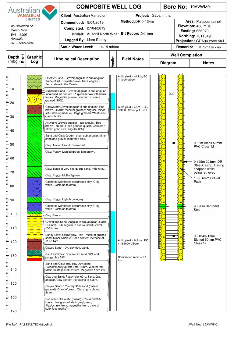
Project:Client:
Logged By:
COMPOSITE WELL LOG
Drilled:
Commenced:S
trat Well Completion
Field NotesDepth GraphicLog(mbgl)
Lithological DescriptionNotesDiagram
Easting:
Northing:
Bore No:
Static Water Level:
Elevation:
Remarks:
Area:
Projection:Australia
Method:
Completed:
WA 6005
Aq
uif
er
+61 8 93215594
West Perth
85 Havelock St
Bit Record:
File Ref: Well No:
0
10
20
30
40
50
60
70
80
90
100
110
120
130
140
150
160
170
Australian Vanadium Gabanintha
9/04/2019
27/04/2019
Ausdrill North West
Liam Storey
14.14 mbtoc
468 mRL
666070
7011649
0.75m Stick up
Palaeochannel
GDA94 zone 50J
19AVWM01
DR 0-134m
241mm
F:\183\2.TECH\LogPlot 19AVWM01
Airlift yield = <1 L/s, EC= 1000 uS/cm
Airlift yield = 4 L/s, EC =30000 uS/cm, pH = 7.3
Airlift yield = 6.5 L/s, EC= 182000 uS/cm
Completion Airlift = 0.1L/s
Laterite: Sand - Gravel; angular to sub angular.Trace of silt. Purplish-brown; trace of grey.Ferricrete with the Quartz.
Duricrust: Sand - Gravel; angular to sub angular.Increased silt content. Purplish-brown with blacktraces. Magnetite present; medium - coarsegrained (10%).
Colluvium: Gravel; angular to sub angular. Red-brown. Quartz; medium grained; angular. Minorsilt. Silcrete; medium - large grained. Weatheredclasts; brittle.
Alluvium: Gravel; angular - sub angular. Red -brown - cream. Fined grained quartz. Calcrete 1-10mm grain size, angular (2%).
Sand and Clay: Green - grey, sub angular. Minorsand and gravel. Indurated clay.
Clay: Trace of sand. Brown-red.
Clay: Puggy. Mottled green-light brown.
Clay: Trace of very fine quartz sand. Pale Grey.
Clay: Puggy. Mottled green.
Calcrete: Weathered calcareous clay. Grey-white. Clasts up to 3mm.
Clay: Puggy. Light brown-grey.
Calcrete: Weathered calcareous clay. Grey-white. Clasts up to 3mm.
Clay: Sandy.
Gravel and Sand: Angular to sub angular Quartz(1-4mm). Sub angular to sub rounded Gravel(2-15mm).
Sandy Clay: Yellow/grey. Fine - medium grainedsand. Minor calcrete. Sand content increase at112-114m.
Clayey Sand: 10% clay 90% sand.
Sand and Clay: Coarse Qtz sand 50% andpuggy clay 50%.
Sand and Clay: 10% clay 90% sand.Predominantly quartz upto 15mm. WeatheredMafic clasts (basalt) 20mm. Magnetite 1mm 2%.
Clay and Sand: Puggy clay 60%. Sand, Qtz,angular. Clay content increasing at 128m.
Clayey Sand: 10% clay 90% sand (coarsegrained). Orange/brown. Qtz, ang - sub ang 1-5mm.
Bedrock: Ultra mafic (basalt) 70% sand 30%.Basalt: fine grained, dark grey/green,Plagioclase 1mm, magnetite 1mm, trace ofsulphides (pyrite?).
0-98m Blank 50mmPVC Class 12
0-125m 203mm DRSteel Casing. Casingsnapped whilebeing retrieved
1.2-3.6mm GravelPack
93-96m BentoniteSeal
98-134m 1mmSlotted 50mm PVCClass 12
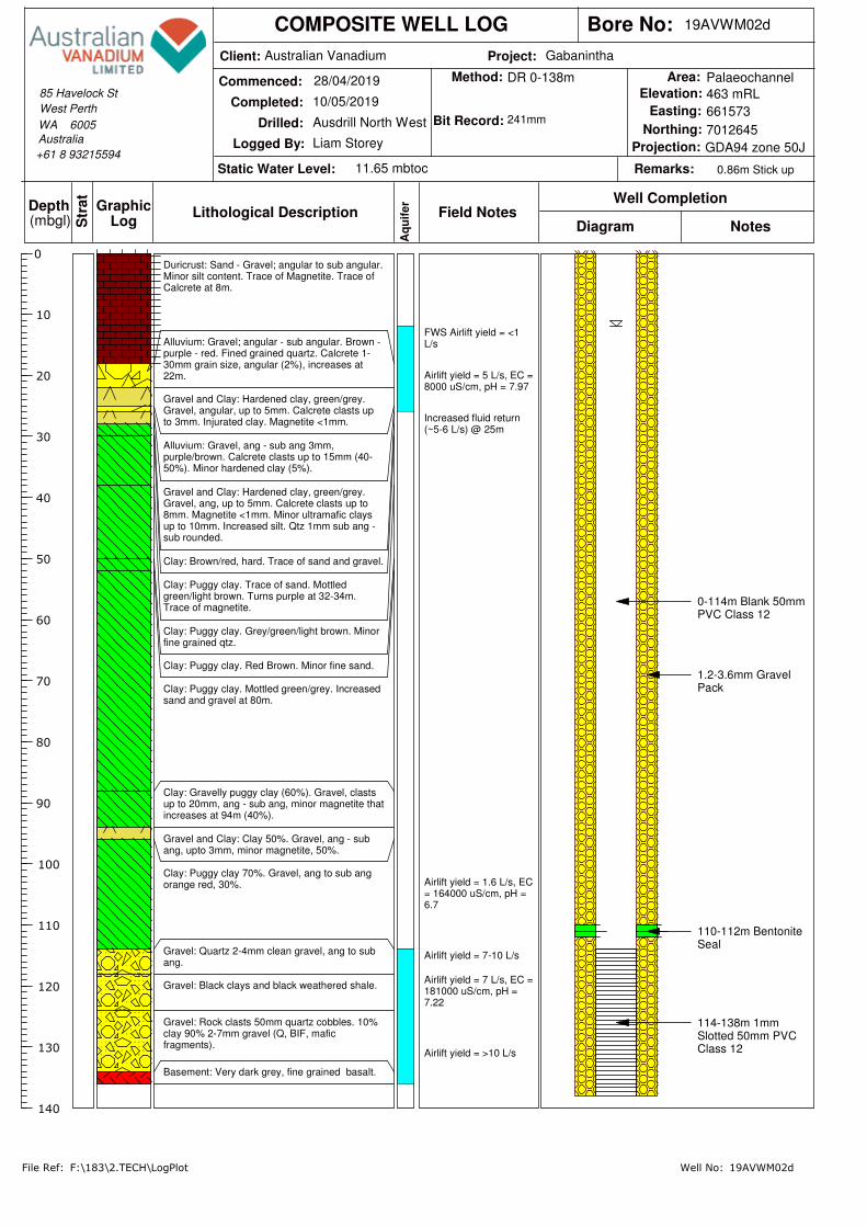
Project:Client:
Logged By:
COMPOSITE WELL LOG
Drilled:
Commenced:S
trat Well Completion
Field NotesDepth GraphicLog(mbgl)
Lithological DescriptionNotesDiagram
Easting:
Northing:
Bore No:
Static Water Level:
Elevation:
Remarks:
Area:
Projection:Australia
Completed:
WA 6005
Aq
uif
er
+61 8 93215594
West Perth
85 Havelock St
Method:
Bit Record:
File Ref: Well No:
0
10
20
30
40
50
60
70
80
90
100
110
120
130
140
Australian Vanadium Gabanintha
28/04/2019
10/05/2019
Ausdrill North West
Liam Storey
11.65 mbtoc
463 mRL
661573
7012645
0.86m Stick up
Palaeochannel
GDA94 zone 50J
19AVWM02d
DR 0-138m
241mm
F:\183\2.TECH\LogPlot 19AVWM02d
FWS Airlift yield = <1L/s
Airlift yield = 5 L/s, EC =8000 uS/cm, pH = 7.97
Increased fluid return(~5-6 L/s) @ 25m
Airlift yield = 1.6 L/s, EC= 164000 uS/cm, pH =6.7
Airlift yield = 7-10 L/s
Airlift yield = 7 L/s, EC =181000 uS/cm, pH =7.22
Airlift yield = >10 L/s
Duricrust: Sand - Gravel; angular to sub angular.Minor silt content. Trace of Magnetite. Trace ofCalcrete at 8m.
Alluvium: Gravel; angular - sub angular. Brown -purple - red. Fined grained quartz. Calcrete 1-30mm grain size, angular (2%), increases at22m.
Gravel and Clay: Hardened clay, green/grey.Gravel, angular, up to 5mm. Calcrete clasts upto 3mm. Injurated clay. Magnetite <1mm.
Alluvium: Gravel, ang - sub ang 3mm,purple/brown. Calcrete clasts up to 15mm (40-50%). Minor hardened clay (5%).
Gravel and Clay: Hardened clay, green/grey.Gravel, ang, up to 5mm. Calcrete clasts up to8mm. Magnetite <1mm. Minor ultramafic claysup to 10mm. Increased silt. Qtz 1mm sub ang -sub rounded.
Clay: Brown/red, hard. Trace of sand and gravel.
Clay: Puggy clay. Trace of sand. Mottledgreen/light brown. Turns purple at 32-34m.Trace of magnetite.
Clay: Puggy clay. Grey/green/light brown. Minorfine grained qtz.
Clay: Puggy clay. Red Brown. Minor fine sand.
Clay: Puggy clay. Mottled green/grey. Increasedsand and gravel at 80m.
Clay: Gravelly puggy clay (60%). Gravel, clastsup to 20mm, ang - sub ang, minor magnetite thatincreases at 94m (40%).
Gravel and Clay: Clay 50%. Gravel, ang - subang, upto 3mm, minor magnetite, 50%.
Clay: Puggy clay 70%. Gravel, ang to sub angorange red, 30%.
Gravel: Quartz 2-4mm clean gravel, ang to subang.
Gravel: Black clays and black weathered shale.
Gravel: Rock clasts 50mm quartz cobbles. 10%clay 90% 2-7mm gravel (Q, BIF, maficfragments).
Basement: Very dark grey, fine grained basalt.
0-114m Blank 50mmPVC Class 12
1.2-3.6mm GravelPack
110-112m BentoniteSeal
114-138m 1mmSlotted 50mm PVCClass 12
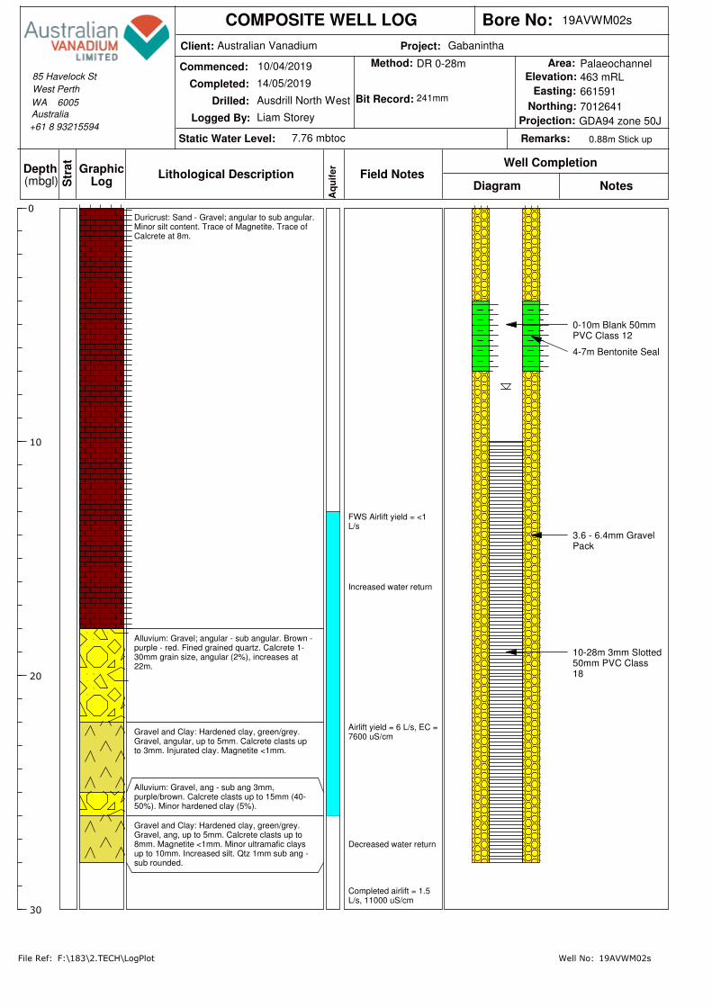
Project:Client:
Logged By:
COMPOSITE WELL LOG
Drilled:
Commenced:S
trat Well Completion
Field NotesDepth GraphicLog(mbgl)
Lithological DescriptionNotesDiagram
Easting:
Northing:
Bore No:
Static Water Level:
Elevation:
Remarks:
Area:
Projection:Australia
Completed:
WA 6005
Aq
uif
er
+61 8 93215594
West Perth
85 Havelock St
Method:
Bit Record:
File Ref: Well No:
0
10
20
30
Australian Vanadium Gabanintha
10/04/2019
14/05/2019
Ausdrill North West
Liam Storey
7.76 mbtoc
463 mRL
661591
7012641
0.88m Stick up
Palaeochannel
GDA94 zone 50J
19AVWM02s
DR 0-28m
241mm
F:\183\2.TECH\LogPlot 19AVWM02s
FWS Airlift yield = <1L/s
Increased water return
Airlift yield = 6 L/s, EC =7600 uS/cm
Decreased water return
Completed airlift = 1.5L/s, 11000 uS/cm
Duricrust: Sand - Gravel; angular to sub angular.Minor silt content. Trace of Magnetite. Trace ofCalcrete at 8m.
Alluvium: Gravel; angular - sub angular. Brown -purple - red. Fined grained quartz. Calcrete 1-30mm grain size, angular (2%), increases at22m.
Gravel and Clay: Hardened clay, green/grey.Gravel, angular, up to 5mm. Calcrete clasts upto 3mm. Injurated clay. Magnetite <1mm.
Alluvium: Gravel, ang - sub ang 3mm,purple/brown. Calcrete clasts up to 15mm (40-50%). Minor hardened clay (5%).
Gravel and Clay: Hardened clay, green/grey.Gravel, ang, up to 5mm. Calcrete clasts up to8mm. Magnetite <1mm. Minor ultramafic claysup to 10mm. Increased silt. Qtz 1mm sub ang -sub rounded.
0-10m Blank 50mmPVC Class 12
4-7m Bentonite Seal
3.6 - 6.4mm GravelPack
10-28m 3mm Slotted50mm PVC Class18
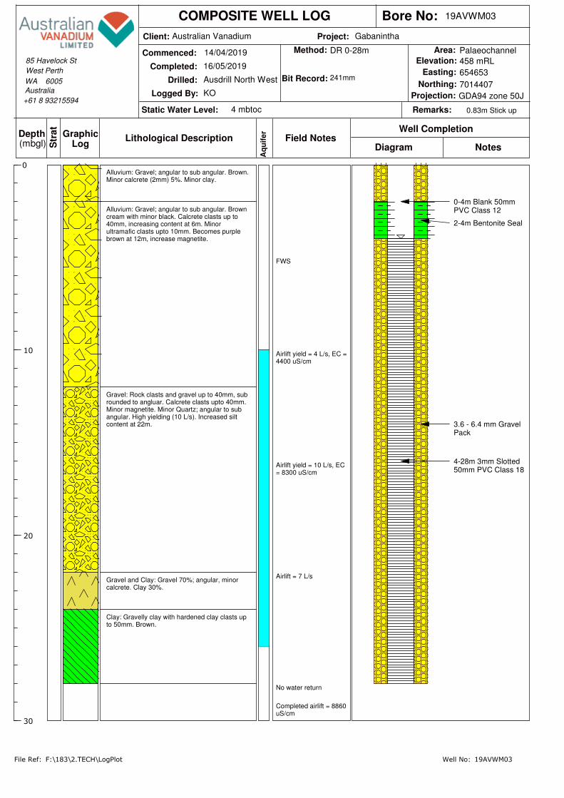
Project:Client:
Logged By:
COMPOSITE WELL LOG
Drilled:
Commenced:S
trat Well Completion
Field NotesDepth GraphicLog(mbgl)
Lithological DescriptionNotesDiagram
Easting:
Northing:
Bore No:
Static Water Level:
Elevation:
Remarks:
Area:
Projection:Australia
Completed:
WA 6005
Aq
uif
er
+61 8 93215594
West Perth
85 Havelock St
Method:
Bit Record:
File Ref: Well No:
0
10
20
30
Australian Vanadium Gabanintha
14/04/2019
16/05/2019
Ausdrill North West
KO
4 mbtoc
458 mRL
654653
7014407
0.83m Stick up
Palaeochannel
GDA94 zone 50J
19AVWM03
DR 0-28m
241mm
F:\183\2.TECH\LogPlot 19AVWM03
FWS
Airlift yield = 4 L/s, EC =4400 uS/cm
Airlift yield = 10 L/s, EC= 8300 uS/cm
Airlift = 7 L/s
No water return
Completed airlift = 8860uS/cm
Alluvium: Gravel; angular to sub angular. Brown.Minor calcrete (2mm) 5%. Minor clay.
Alluvium: Gravel; angular to sub angular. Browncream with minor black. Calcrete clasts up to40mm, increasing content at 6m. Minorultramafic clasts upto 10mm. Becomes purplebrown at 12m, increase magnetite.
Gravel: Rock clasts and gravel up to 40mm, subrounded to angluar. Calcrete clasts upto 40mm.Minor magnetite. Minor Quartz; angular to subangular. High yielding (10 L/s). Increased siltcontent at 22m.
Gravel and Clay: Gravel 70%; angular, minorcalcrete. Clay 30%.
Clay: Gravelly clay with hardened clay clasts upto 50mm. Brown.
0-4m Blank 50mmPVC Class 12
2-4m Bentonite Seal
3.6 - 6.4 mm GravelPack
4-28m 3mm Slotted50mm PVC Class 18

Project:Client:
Logged By:
COMPOSITE WELL LOG
Drilled:
Commenced:S
trat Well Completion
Field NotesDepth GraphicLog(mbgl)
Lithological DescriptionNotesDiagram
Easting:
Northing:
Bore No:
Static Water Level:
Elevation:
Remarks:
Area:
Projection:Australia
Completed:
WA 6005
Aq
uif
er
+61 8 93215594
West Perth
85 Havelock St
Method:
Bit Record:
File Ref: Well No:
0
10
20
30
Australian Vanadium Gabanintha
16/05/2019
18/05/2019
Ausdrill North West
KO
8.43 mbtoc
464 mRL
663545
7011754
0.77m Stick up
Palaeochannel
GDA94 zone 50J
19AVWM04
DR 0-28m
241mm
F:\183\2.TECH\LogPlot 19AVWM04
Airlift = 0.5 L/s
Airlift = 5 L/s
Airlift = 10 L/s, EC =13370 uS/cm
Airlift = 10-12 L/s, EC =13650 uS/cm
Completion Airlift = 2L/sEC = 17630 uS/cmpH = 7.62
Soil: Surficial soil with rock fragments. Redbrown, angluar caprock and silty soils.
Gravel: Sandy. Tan/khaki clay, silt and rockfragments 10-40mm.
Calcrete: Ivory calcrete with brown coarse sandand gravel 1-8mm. CaCO3 80%.
Gravel and Sand: Brown sandy gravel and clay(30%). Rock fragments 10-25mm.
Clay: Red brown clay with sandy gravel. Clay80%.
2-4m Bentonite Seal
0-22m Blank 50mmND PVC Class 18
3.6-6.4mm GravelPack
22-28m 3mm Slotted50mm ND PVCClass 18

Project:Client:
Logged By:
COMPOSITE WELL LOG
Drilled:
Commenced:S
trat Well Completion
Field NotesDepth GraphicLog(mbgl)
Lithological DescriptionNotesDiagram
Easting:
Northing:
Bore No:
Static Water Level:
Elevation:
Remarks:
Area:
Projection:Australia
Completed:
WA 6005
Aq
uif
er
+61 8 93215594
West Perth
85 Havelock St
Method:
Bit Record:
File Ref: Well No:
0
10
20
30
40
50
60
70
80
90
100
110
120
130
140
150
160
170
180
Australian Vanadium Gabanintha
23/05/2019
29/05/2019
Ausdrill North West
KO
13.96 mbtoc
469.50 mRL
663778
7015448
0.84m Stick up
Orebody
GDA94 zone 50J
19AVWM104
DR 0-60m
DDH 60-175m
241mm(0-60m)/191mm(60-175m)
F:\183\2.TECH\LogPlot 19AVWM104
FWS
Airlft yield = <1 L/s
Airlift yield = 1.2 L/s, EC= 15000 uS/cm
Airlfit yield = <1 L/s
Airlift yield = <1 L/s
Airlift yield = 1 L/s
Airlift yield = 2.5 L/s, EC= 60000 uS/cm
Airlift yield = 3.5 L/s, EC= 121000 uS/cm
Airlift yield = 3 L/s, EC =156000 uS/cm
Airlift yield = 5 L/s, EC =176000 uS/cm
Airlift yield = 10 L/s, EC> 240000 uS/cm
Airlift yield = 6 L/s, EC >240000 uS/cm
Airlift yield = 5 L/s, EC =190000 uS/cm
Airlift yield = 5.0 L/s
Airlift yield = 5.0 L/s
Airlift yield = 10 L/s, EC= 226000 uS/cm
Duricrust: Red - brown, silty. Gravel; anguar tosub angular, clasts upto 20mm. Trace ofmagnetite. Trace of Calcrete.
Calcrete: Weathered calcrete, purple - cream,clasts upto 20mm. Gravel; angular to subangular. High silt content. Minor clay.
Saprock: Weathered igneous rock sub roundedto angular. Clasts of ultra mafic upto 20mm. 50%clay; purple brown.
Saprock: Gravelly. Grey - brown, puggy clay(weathered bedrock). Minor gravel.
Saprock: Clayey (weathered bedrock). Red -brown - purple. Gravel; angular to sub angular.Clay 30%, decreasing with depth. Gravelbecoming fine grained at 38m.
Mafic: Weathered igneous rock (dolerite?) withminor gravels. 20% clay. Highly magnetic.
Mafic: Fresh igneous rock, highly magnetic,minor gravels. 30% clay. Quartz up to 2mm.
Mafic: Purple weathered igneous rock. Highlymagnetic, fine grained.
Ore: Dark green - black- metallic. Highlymagnetic. Minor gravel. Ore content increasingat 92m. Fine grained with clasts up to 15mm.
Ore: Green fractured mafic igneous rock.Plagioclase & Pyroxene present. Highlymagnetic. Minor Sulphides.
Basement: Competent rock dark green - purple,fractured igneous rock. Minor ore/magnetite.Large quartz; angular to sub angluar up to20mm, weathered. High sulphide content.
2-4m Bentonite Seal
0-7m Blank 50mmPVC Class 12
7-19m 1mm Slotted50mm PVC Class 12
19-31m Blank 50mmPVC Class 12
1.2-3.6mm GravelPack
31-175m 3mmSlotted 50mm PVCClass 12
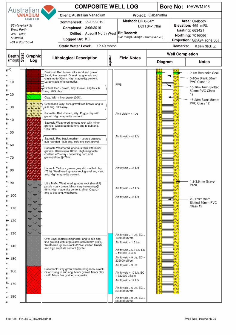
Project:Client:
Logged By:
COMPOSITE WELL LOG
Drilled:
Commenced:S
trat Well Completion
Field NotesDepth GraphicLog(mbgl)
Lithological DescriptionNotesDiagram
Easting:
Northing:
Bore No:
Static Water Level:
Elevation:
Remarks:
Area:
Projection:Australia
Completed:
WA 6005
Aq
uif
er
+61 8 93215594
West Perth
85 Havelock St
Method:
Bit Record:
File Ref: Well No:
0
10
20
30
40
50
60
70
80
90
100
110
120
130
140
150
160
170
180
Australian Vanadium Gabanintha
29/05/2019
2/06/2019
Ausdrill North West
KO
12.49 mbtoc
469 mRL
663421
7016066
0.82m Stick up
Orebody
GDA94 zone 50J
19AVWM105
DR 0-84m
DDH 84-178m
241mm(0-84m)/191mm(84-178)
F:\183\2.TECH\LogPlot 19AVWM105
FWS
Airlft yield = <1 L/s
Airlfit yield = <1 L/s
Airlfit yield = <1 L/s
Airlift yield = <1 L/s
Airlift yield = <1 L/s
Airlift yield = 1 L/s, EC =135000 uS/cm
Airlift yield = 1.5 L/s
Airlift yield = 5.5 L/s, EC= 193000 uS/cm
Airlift yield = 9 L/s, EC =225000 uS/cm
Airlift yield = 9 L/s
Airlift yield = 10 L/s, EC= 322000 uS/cm
Airlift yield = 12 L/s
Airlift yield = 6 L/s, EC =232000 uS/cm
Airlift yield = 9 L/s, EC =280000 uS/cm
Duricrust: Red brown, silty sand and gravel.Sand; fine grained. Gravek; ang to sub angclasts up to 30mm. High magnetite content.Large clasts of ultra mafics.
Gravel: Red - brown, silty. Gravel; ang to subang. 20% clay.
Clay: With minor gravel (20%).
Gravel and Clay: 50% gravel; red brown, ang tosub ang. 50% clay.
Saprolite: Red - brown, silty. Puggy clay withgravel. High magnetite content.
Saprock: Weathered igneous rock with minorgravels. Clasts up to 50mm; ang to sub ang.Clay 30%.
Saprock: Red black medium - coarse grained;sub rounded - sub ang. 50% ore 50% gravel.
Saprock: Weathered ignenous rock with minorgravels. Clasts upto 10mm. High magnetitecontent. 40% clay - becoming hard andgreen/yellow @ 70m.
Saprock: Yellow - green- grey stiff mottled clay(70%). Weathered igneous rock/gravel ang - subang. High magnetite content.
Ultra Mafic: Weathered igneous rock (basalt?)purple - dark green. Minor clay increasing @96m. High magentite content. Minor Quartz -ang to sub ang, weathered.
Ore: Black metallic magnetite; ang to sub angfine grained with large clasts upto 30mm (80%).Weathered igneous rock (20%).Limitted Quartzand high sulphide content (pyrite).
Basement: Grey grren weathered ignenous rock.Quartz; ang to sub ang. Minor gravel. Minor clay- stiff. Minor fine grained magnetite.
2-4m Bentonite Seal
0-10m Blank 50mmPVC Class 12
10-16m 1mm Slotted50mm PVC Class12
16-28m Blank 50mmPVC Class 12
1.2-3.6mm GravelPack
28-178m 3mmSlotted 50mm PVCClass 12

Project:Client:
Logged By:
COMPOSITE WELL LOG
Drilled:
Commenced:S
trat Well Completion
Field NotesDepth GraphicLog(mbgl)
Lithological DescriptionNotesDiagram
Easting:
Northing:
Bore No:
Static Water Level:
Elevation:
Remarks:
Area:
Projection:Australia
Completed:
WA 6005
Aq
uif
er
+61 8 93215594
West Perth
85 Havelock St
Method:
Bit Record:
File Ref: Well No:
0
10
20
30
40
50
60
70
80
90
100
110
Australian Vanadium Gabanintha
19/05/2019
23/05/2019
Ausdrill North West
KO
12.30 mbtoc
470.00 mRL
663916
7015608
0.8m Stick up
Orebody
GDA94 zone 50J
19AVWM108
DR 0-34m
DDH 34-100m
241mm(0-34m)/191mm(34-100m)
F:\183\2.TECH\LogPlot 19AVWM108
FWS
Seepage only
Airlfit yield = 2 L/sEC = 12520 uS/cmpH = 7.72
Airlfit yield = 3 L/s
Completed Airlift = 0.6 -0.7 L/sEC = 28800 uS/cm
Duricrust: Red brown silty coarse sand andangular to sub angular gravel rock fragments 2-10 mm
Calcrete: Pinkish brown weathered calcrete andsilty gravels comprised of rock fragments 4-8mmdiameter.
Calcrete: Purplish ivory calcrete with weatheredrock fragments and pebbles.
Ore: Purple brown highly weathered ore bodybasalt, ~50% remnant clay.
Ore: Purple weathered ore body basalt, clay~30%, highly fractured.
Ore: Green grey highly weathered ore body hostrock, friable cuttings in fracture zone.
Ore: Whitish grey fractured and weathered hostcountry rock, highly weathered
Mafic: Grey green competent host country rock,minor fracturing
0-28m Blank 50mmPVC Class 12
23-25m BentoniteSeal
1.2-3.6mm GravelPack
28-100m 1mmSlotted 50mm PVCClass 12

Project:Client:
Logged By:
COMPOSITE WELL LOG
Drilled:
Commenced:S
trat Well Completion
Field NotesDepth GraphicLog(mbgl)
Lithological DescriptionNotesDiagram
Easting:
Northing:
Bore No:
Static Water Level:
Elevation:
Remarks:
Area:
Projection:Australia
Completed:
WA 6005
Aq
uif
er
+61 8 93215594
West Perth
85 Havelock St
Method:
Bit Record:
File Ref: Well No:
0
10
20
30
40
50
60
70
80
90
100
110
120
130
140
150
160
Australian Vanadium Gabanintha
3/06/2019
9/06/2019
Ausdrill North West
KO
8.32 mbtoc
468 mRL
664733
7014236
0.8m Stick up
Orebody
GDA94 zone 50J
19AVWM112
DR 0-88m
DDH 88-151m
241mm(0-88m)/191(88-151m)
F:\183\2.TECH\LogPlot 19AVWM112
FWS
Airlft yield = <1 L/s, EC= 4300 uS/cm
Airlfit yield = 9 L/s, EC =3420 uS/cm
Airlfit yield = 18 L/s, EC= 2950 uS/cm
Airlift yield = 12 L/s, EC= 2990 uS/cm
No fluid return
Airlift yield = 10 L/s
Airlift yield = 15 L/s, EC= 2810 uS/cm
Airlift yield = 15 L/s, EC= 2560 uS/cm
Airlift yield = 20 L/s
Airlift yield = 4 L/s, EC =250000 uS/cm
Airlift yield = 4 L/s, EC =250000 uS/cm
Airlift yield = 4 L/s, EC =250000 uS/cm
Airlift yield = 4 L/s, EC =255000 uS/cm
Airlift yield = 4 L/s, EC =255000 uS/cm
Duricrust: Red brown silty angular to sub-angular gravels, with minor calcrete clasts up to10mm.
Calcrete: Red brown and cream weathered andfresh calcrete (50%),silty weathered caprockclasts up to 20mm.
Clay: Brownish cream silty clay with finecalcareous sand.
Calcrete: Pale white fine- grained chalky sandwith clasts up to 40mm
Saprock: Red brown and cream medium tocoarse angular to sub- angular silty gravel withlarge clasts of weathered caprock.
Saprock: Red brown to Black angular to sub-angular fine- coarse grained gravels with minormagnetite. Large clasts of weathered caprock.
Saprock: Dark green to purple weatheredigneous; clastsup to 10cm, sub- rounded toangular with 50% angular to sub- angulargravels and minor magnetite.
Saprock: GRAVELLY CLAY Grey brown clay50%, angular to sub- angular gravel with largecaprock clasts and magnetite
Mudstone: Red to dark brown medium to coarsegrained angular to sub- angular gravel; largeclasts of mudstone, silty with high magnetite %,minor angular quartz at 55m.
Ultra Mafic: Grey green weathered basalticigneous rock with calcareous band 70- 72m.Friable above with weathering degreedecreasing with depth.
Ore: Dark grey green competent crystalline orebody, mafic basaltic with iron pyrite at base 136-140m.
Ultra Mafic: Pale grey basalt with quartz richfracture zone 142- 151m.
2-4m Bentonite Seal
0-6m Blank 50mmPVC Class 12
1.2-3.6mm GravelPack
6-54m 1mm Slotted50mm PVC Class 12
54-60m Blank 50mmPVC Class 12
3.6 - 6.4mm GravelPack
60-151m 3mmSlotted 50mm PVCClass 12
Gravel pack insidecasing duringairlifting- blockedbore

Project:Client:
Logged By:
COMPOSITE WELL LOG
Drilled:
Commenced:S
trat Well Completion
Field NotesDepth GraphicLog(mbgl)
Lithological DescriptionNotesDiagram
Easting:
Northing:
Bore No:
Static Water Level:
Elevation:
Remarks:
Area:
Projection:Australia
Completed:
WA 6005
Aq
uif
er
+61 8 93215594
West Perth
85 Havelock St
Method:
Bit Record:
File Ref: Well No:
0
10
20
30
40
50
60
70
80
90
100
110
120
130
140
150
Australian Vanadium Gabanintha
10/06/2019
15/06/2019
Ausdrill North West
KO
11.80 mbtoc
472 mRL
662879
7017174
0.8m Stick up
Orebody
GDA94 zone 50J
19AVWM113
DR 0-52m
DDH 52-142m
241mm(0-52m)/191(52-142m)
F:\183\2.TECH\LogPlot 19AVWM113
Seepage only
Seepage only
FWS
Airlfit yield = 2-3 L/s
Airlift yield = <1 L/s, EC= 1800 uS/cm
Airlift yield = <1 L/s, EC= 2330 uS/cm
Airlift yield = <1 L/s, EC= 2180 uS/cm
Airlift yield = <1 L/s, EC= 2450 uS/cm
Airlift yield = <1 L/s, EC= 2700 uS/cm
Airlift yield = <1 L/s, EC= 3330 uS/cm
Duricrust: Red brown angular clasts, gravel andsand up to 12mm.
Gravel: Red brown gravel and sand, minor clay.10% calcrete. Coarse sand; angular.
Gravel: Pink purple orange gravels, sub roundedto angular. Minor clay and magnetite (roundedpebbles and gravels up to 3mm). Calcretenodules up to 2mm.
Gravel: Khaki grey/tan weathered basalt gravels,angular magnetite coarse sand, clay 40-50%,silty.
Basalt: Grey green, angular to sub angularbasalt. Becoming fine grained at 78m. High siltcontent at 56-68m. Magntite/ore; sub angular.
2-4m Bentonite Seal
0-6m Blank 50mmPVC Class 12
10-94m 1mm Slotted50mm PVC Class12
1.2-3.6mm GravelPack
94-142m 3mmSlotted 50mm PVCClass 12

Project:Client:
Logged By:
COMPOSITE WELL LOG
Drilled:
Commenced:S
trat Well Completion
Field NotesDepth GraphicLog(mbgl)
Lithological DescriptionNotesDiagram
Easting:
Northing:
Bore No:
Static Water Level:
Elevation:
Remarks:
Area:
Projection:Australia
Completed:
WA 6005
Aq
uif
er
+61 8 93215594
West Perth
85 Havelock St
Method:
Bit Record:
File Ref: Well No:
0
10
20
30
40
50
60
70
80
90
100
110
120
130
140
150
160
Australian Vanadium Gabanintha
19/06/2019
27/06/2019
Ausdrill North West
LS
10.32 mbtoc
467 mRL
663427
7015416
0.8m Stick up
Orebody
GDA94 zone 50J
19AVWM114
DR 0-106m
DDH 106-148m
241mm(0-106m)/191(106-148m)
F:\183\2.TECH\LogPlot 19AVWM114
FWS
Airlift yield = 2 L/s, EC =4140 uS/cm
Airlift yield = 5 L/s, EC =4000 uS/cm
Airlfit yield = 3-4 L/s, EC= 3940 uS/cm
Airlift yield = 8-10 L/s,EC = 3780 uS/cm
Airlift yield = 8-10 L/s,EC = 3690 uS/cm
Airlift yield = <1 L/s, EC= 4300 uS/cm
Airlift yield = 7-9 L/s, EC= 5210 uS/cm
Airlift yield = 1.5 L/s, EC= 29000 uS/cm
Airlift yield = 4 L/s
Airlift yield = 2 L/s
Airlift yield = 4 L/s, EC =95200 uS/cm
Airlift yield = 4 L/s
Airlift yield = 4-5 L/s
Airlift yield = 6-7 L/s
Airlift yield = 5-6 L/s, EC= 197000 uS/cm
Airlift yield = 5-6 L/s
Airlift yield = 4-5 L/s
Airlift yield = 5 L/s, EC =254000 uS/cm
Duricrust: Red brown gravel and sand; angular -sub angular, clasts upto 12mm.
Gravel: Red brown gravel (1-4mm) and sand,minor clay. Highly magnetic; angular.
Gravel: Red brown large gravel clasts upto30mm; angular - sub rounded. Highly magnetic.Minor clay at 28m.
Gravel and Clay: Red brown gravel (1-4mm);angular. Clay 60%.
Calcrete: Weathered, White red clay, mix of softand stiff. Minor gravel and magnetite. Large hardcalcrete clasts upto 60mm.
Calcrete: Red white soft weathered calcrete(60%) with large calcrete clasts upto 50mm;angular - sub angular. Gravel; medium - coarsegrained 1-5mm gravel ang-sub angular.
Gravel and Clay: Soft clay (40%). Gravel 1-3mm; angular - sub angular. Minor calcreteclasts upto 3mm. Silty.
Gravel: Red brown gravel; angular - sub angular.Trace of calcrete; sub angular. Minor clays.Large gravel clasts upto 40mm @ 54m.
Gravel: Red brown black fine - medium grainedgravel; angular - sub angular. Minor calcrete.Minor magnetite.
Gravel: Khaki grey/red brown gravel with clastsupto 30mm; angular - sub angular. Minor quartzupto 20mm. Minor calcrete and magnetite.
Gravel: Brown red grey gravel with angular rockclasts upto 40mm. Minor calcrete clasts upto20mm. Minor clay.
Saprock: Khaki grey green gravel; angular - subangula. Rock clasts upto 20mm. Clay (50%).
Saprock: Khaki green gravel; angular - subangular. Weathered rock clasts upto 80mm; subangular.
Ultra Mafic: Green blue weathered igneousangular-subangular, clasts upto 40mm. Minorgravels at 92-96m
Ore: Dark blue weathered basalt angular-subangular. Minor gravels. High ore content. Minorquartz; angular - sub angular.
2-4m Bentonite Seal
0-10m Blank 50mmPVC Class 12
1.2-3.6mm GravelPack
10-46m 1mm Slotted50mm PVC Class12
46-52m Blank 50mmPVC Class 12
52-82m 1mm Slotted50mm PVC Class12
3.6-6.4mm GravelPack
82-148m 3mmSlotted 50mm PVCClass 12

Project:Client:
Logged By:
COMPOSITE WELL LOG
Drilled:
Commenced:S
trat Well Completion
Field NotesDepth GraphicLog(mbgl)
Lithological DescriptionNotesDiagram
Easting:
Northing:
Bore No:
Static Water Level:
Elevation:
Remarks:
Area:
Projection:Australia
Completed:
WA 6005
Aq
uif
er
+61 8 93215594
West Perth
85 Havelock St
Method:
Bit Record:
File Ref: Well No:
0
10
20
30
40
50
60
70
80
90
100
110
120
130
140
150
160
170
180
190
Australian Vanadium Gabanintha
29/06/2019
8/07/2019
Ausdrill North West
LC
15.64 mbtoc
469 mRL
663418
7016082
0.82m Stick up
Orebody
GDA94 zone 50J
19AVWP001
DR 0-94m
DDH 94-184m
346mm(0-94m)/298mm(94-184m)
F:\183\2.TECH\LogPlot 19AVWP001
FWS
Airlft yield = <1 L/s
Airlfit yield = <1 L/s
Airlfit yield = <1 L/s
Airlift yield = <1 L/s
Airlift yield = <1 L/s
Airlift yield = 1 L/s, EC =135000 mS/cm
Airlift yield = 1.5 L/s
Airlift yield = 5.5 L/s, EC= 193000 mS/cm
Airlift yield = 9 L/s, EC =225000 mS/cm
Airlift yield = 9 L/s
Airlift yield = 10 L/s, EC= 322000 mS/cm
Airlift yield = 12 L/s
Airlift yield = 6 L/s, EC =232000 mS/cm
Airlift yield = 9 L/s, EC =280000 mS/cm
Duricrust: Red brown, silty sand and gravel.Sand; fine grained. Gravek; ang to sub angclasts up to 30mm. High magnetite content.Large clasts of ultra mafics.
Gravel: Red - brown, silty. Gravel; ang to subang. 20% clay.
Clay: With minor gravel (20%).
Gravel and Clay: 50% gravel; red brown, ang tosub ang. 50% clay.
Saprolite: Red - brown, silty. Puggy clay withgravel. High magnetite content.
Saprock: Weathered igneous rock with minorgravels. Clasts up to 50mm; ang to sub ang.Clay 30%.
Saprock: Red black medium - coarse grained;sub rounded - sub ang. 50% ore 50% gravel.
Saprock: Weathered ignenous rock with minorgravels. Clasts upto 10mm. High magnetitecontent. 40% clay - becoming hard andgreen/yellow @ 70m.
Saprock: Yellow - green- grey stiff mottled clay(70%). Weathered igneous rock/gravel ang - subang. High magnetite content.
Ultra Mafic: Weathered igneous rock (basalt?)purple - dark green. Minor clay increasing @96m. High magentite content. Minor Quartz -ang to sub ang, weathered.
Ore: Black metallic magnetite; ang to sub angfine grained with large clasts upto 30mm (80%).Weathered igneous rock (20%).Limitted Quartzand high sulphide content (pyrite).
Basement: Grey green weathered ignenousrock. Quartz; ang to sub ang. Minor gravel.Minor clay - stiff. Minor fine grained magnetite.
2-4m Bentonite Seal
0-94m Blank 200mmPVC Class 12
1.2-3.6mm GravelPack
94-184m 1mmSlotted 200mm PVCClass 12
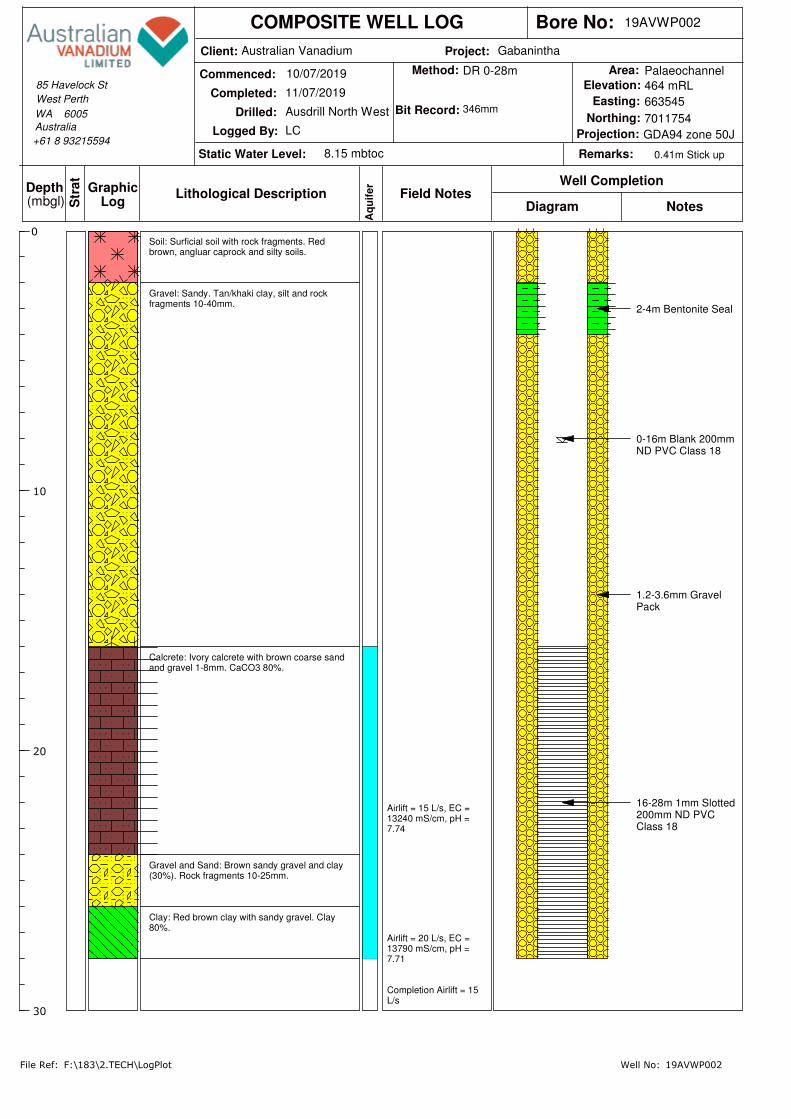
Project:Client:
Logged By:
COMPOSITE WELL LOG
Drilled:
Commenced:S
trat Well Completion
Field NotesDepth GraphicLog(mbgl)
Lithological DescriptionNotesDiagram
Easting:
Northing:
Bore No:
Static Water Level:
Elevation:
Remarks:
Area:
Projection:Australia
Completed:
WA 6005
Aq
uif
er
+61 8 93215594
West Perth
85 Havelock St
Method:
Bit Record:
File Ref: Well No:
0
10
20
30
Australian Vanadium Gabanintha
10/07/2019
11/07/2019
Ausdrill North West
LC
8.15 mbtoc
464 mRL
663545
7011754
0.41m Stick up
Palaeochannel
GDA94 zone 50J
19AVWP002
DR 0-28m
346mm
F:\183\2.TECH\LogPlot 19AVWP002
Airlift = 15 L/s, EC =13240 mS/cm, pH =7.74
Airlift = 20 L/s, EC =13790 mS/cm, pH =7.71
Completion Airlift = 15L/s
Soil: Surficial soil with rock fragments. Redbrown, angluar caprock and silty soils.
Gravel: Sandy. Tan/khaki clay, silt and rockfragments 10-40mm.
Calcrete: Ivory calcrete with brown coarse sandand gravel 1-8mm. CaCO3 80%.
Gravel and Sand: Brown sandy gravel and clay(30%). Rock fragments 10-25mm.
Clay: Red brown clay with sandy gravel. Clay80%.
2-4m Bentonite Seal
0-16m Blank 200mmND PVC Class 18
1.2-3.6mm GravelPack
16-28m 1mm Slotted200mm ND PVCClass 18

APPENDIX C
HYDRAULIC TESTING PLOTS

FALLING HEAD TEST
Bore No: 19AVWM01 Test No: 1 Job No: 183 Date: 10-Aug-19 Logged by: EE/ZA
Depth to top of test section (m): 98 Length of test section, L (m): 3
Depth of static water level, Hw (m): 14.14 Radius of borehole, r (m): 0.1
Excess head, he (m): 13.04 Radius of standpipe or casing, rc (m): 0.025
Calculations:
h1 1.000 1.000
t1 0.00 0.000
h2 0.200 0.800
t2 5.00 30.00
S 1.4E-01 3.2E-03
k 3.87E-06 8.95E-08
m/d 3.35E-01 7.73E-03
Permeability, k = 0.133 x S x (rc2/L), (m/sec)
Notes:
where S = (log (h1/h2)/(t2 - t1),
(ie slope of plot, t in mins)
Head - time graph (slope of graph is S)
0.100
1.000
0 5 10 15 20 25 30 35
ht/h
e
Time (min)
F:\183\2.TECH\Aquifer Testing\Analysis\19AVWM01_slug_analysis

Airlift Hydraulic TestF:\183\3.C&R\048 Figs & App\App C_Hydraulic Testing Plots\[Airlift Tests.xlsx]19AVWM02s&d
0
0.2
0.4
0.6
0.8
1
1.2
1.4
1.6
1.8
2
1 10 100 1000 10000
Dra
wd
ow
n (
m)
Time (secs)
19AVWM02s
0
1
2
3
4
5
6
7
8
1 10 100 1000 10000
Dra
wd
ow
n (
m)
Time (secs)
19AVWM02d
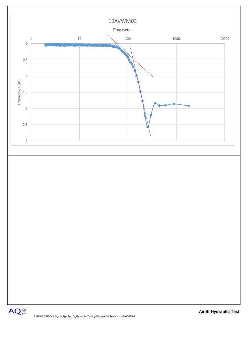
Airlift Hydraulic TestF:\183\3.C&R\048 Figs & App\App C_Hydraulic Testing Plots\[Airlift Tests.xlsx]19AVWM03
0
0.5
1
1.5
2
2.5
3
1 10 100 1000 10000
Dra
wd
ow
n (
m)
Time (secs)
19AVWM03
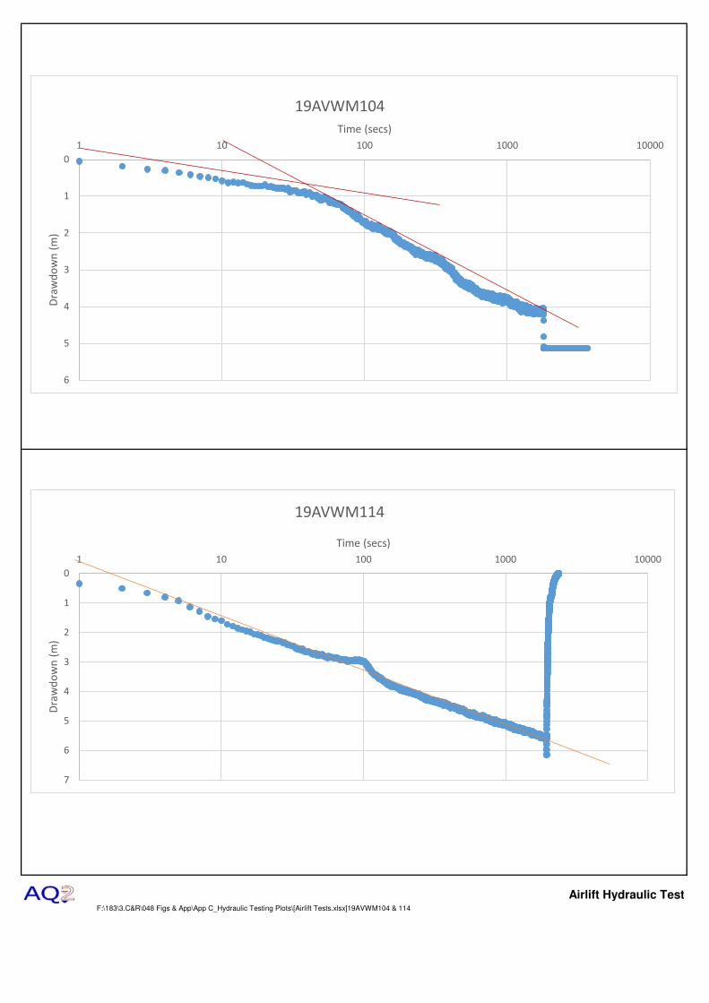
Airlift Hydraulic TestF:\183\3.C&R\048 Figs & App\App C_Hydraulic Testing Plots\[Airlift Tests.xlsx]19AVWM104 & 114
0
1
2
3
4
5
6
1 10 100 1000 10000
Dra
wd
ow
n (
m)
Time (secs)
19AVWM104
0
1
2
3
4
5
6
7
1 10 100 1000 10000
Dra
wd
ow
n (
m)
Time (secs)
19AVWM114
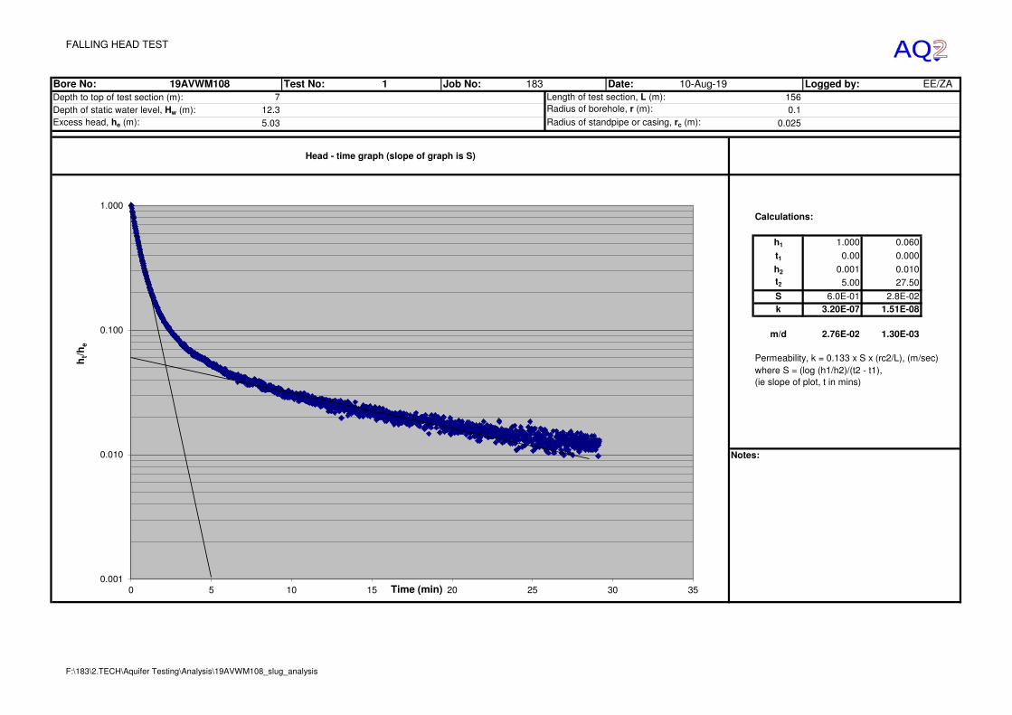
FALLING HEAD TEST
Bore No: 19AVWM108 Test No: 1 Job No: 183 Date: 10-Aug-19 Logged by: EE/ZA
Depth to top of test section (m): 7 Length of test section, L (m): 156
Depth of static water level, Hw (m): 12.3 Radius of borehole, r (m): 0.1
Excess head, he (m): 5.03 Radius of standpipe or casing, rc (m): 0.025
Calculations:
h1 1.000 0.060
t1 0.00 0.000
h2 0.001 0.010
t2 5.00 27.50
S 6.0E-01 2.8E-02
k 3.20E-07 1.51E-08
m/d 2.76E-02 1.30E-03
Permeability, k = 0.133 x S x (rc2/L), (m/sec)
Notes:
where S = (log (h1/h2)/(t2 - t1),
(ie slope of plot, t in mins)
Head - time graph (slope of graph is S)
0.001
0.010
0.100
1.000
0 5 10 15 20 25 30 35
ht/h
e
Time (min)
F:\183\2.TECH\Aquifer Testing\Analysis\19AVWM108_slug_analysis

FALLING HEAD TEST
Bore No: 19AVWM113 Test No: 1 Job No: 183 Date: 10-Aug-19 Logged by: EE/ZA
Depth to top of test section (m): 10 Length of test section, L (m): 132
Depth of static water level, Hw (m): 12.65 Radius of borehole, r (m): 0.1
Excess head, he (m): 2.21 Radius of standpipe or casing, rc (m): 0.025
Calculations:
h1 1.000 0.697
t1 0.00 1.000
h2 0.862 0.308
t2 0.10 10.07
S 6.5E-01 3.9E-02
k 4.07E-07 2.46E-08
m/d 3.52E-02 2.12E-03
Permeability, k = 0.133 x S x (rc2/L), (m/sec)
Notes:
where S = (log (h1/h2)/(t2 - t1),
(ie slope of plot, t in mins)
Head - time graph (slope of graph is S)
0.010
0.100
1.000
0 5 10 15 20 25 30 35
ht/h
e
Time (min)
F:\183\2.TECH\Aquifer Testing\Analysis\19AVWM113_slug_analysis_RevB

0.00
10.00
20.00
30.00
40.00
50.00
60.00
70.00
80.00
0.1 1.0 10.0 100.0 1,000.0 10,000.0
Dra
wd
ow
n (
me
ters
)
Duration (minutes)
19AVWP001 Constant Rate Test Chart
19AVWP001
19AVWM105
Increased Rate
Replotted
Test Start: 10/8/19
Rate: 5L/s for 48 hrs
Increased Rate to
8L/s after 48 hrs
(2880 mins)

Discharge Short Term Long Term Interference Total Pumping
(kL/d) Drawdown
(m)
Drawdown
(m)
Effects
(m)
Drawdown
(m) Water Level
(mbgl)
0 0 0 0 0 15.60
346 33.77 20.56 0.00 54.33 69.93
518 52.61 30.78 0.00 83.39 98.99
691 72.93 41.05 0.00 113.98 129.58
864 94.63 51.33 0.00 145.96 161.56
0.00
20.00
40.00
60.00
80.00
100.00
120.00
140.00
160.00
180.00
0 100 200 300 400 500 600 700 800 900 1000
Wa
ter
Le
ve
l (m
bg
l)
Discharge (kL/d)
19AVWP001: Bore Performance and Deployable Yield
Predicted Pumping WL Max Pumping WL Avg SWL

sw(n) = BQn + CQnP (Rorabaugh's equation)
Where: B = Intercept with y axis (coefficient of aquifer loss or laminar flow)
C = Gradient (coefficient of turbulent flow loss or apparent well loss)
s = Drawdown in the borehole
P = Value determined using Rorabaugh's method of superposition
Components of Jacob's (1947) equation BQ and CQ2 are termed the aquifer loss and apparent well loss respectively.
They give an indication of the proportion of total drawdown caused by laminar and turbulent flow.
Please note: 1. In thin or fissured aquifers large components of well loss are due to high flow velocities in the aquifer
rather than inefficient bore design. Therefore, the term "apparent well loss" is better than well loss.
2. In aquifers where the flow horizons are vertically anisotropic, changes in bore performance often
relate to changes in the rest water level with respect to the primary aquifer horizons.
Ew = (BQ/(BQ + CQP) x 100
Ew or Well Efficiency represents the proportion of drawdown caused by laminar flow
From plot of s/Q v Q (trend line equation): Intercept (B) 8.965E-02
Gradient (C) 2.300E-05
ANALYSIS TABLE
Measured
Step Discharge Discharge (Q) Incremental Corrected Predicted Apparent
(60 minute (l/s) (m3/d) Drawdown Drawdown Drawdown s/Q Efficiency (Ew)
duration) (metres) (metres) (metres) %
1 2.0 173 16.00 16.00 16.18 9.26E-02 95.8
2 4.0 346 18.00 34.00 33.73 9.84E-02 91.9
3 6.0 518 19.45 53.45 52.65 1.03E-01 88.3
4 8.0 691 18.62 72.07 72.95 1.04E-01 84.9
Calculation of well efficiency and comparison of observed and predicted drawdowns
0
10
20
30
40
50
60
70
800.1 1 10 100 1000
Dra
wd
ow
n (
m)
Time (minutes)
19AVWP001: Step Discharge Pumping Test
y = 2.300E-05x + 8.965E-02
0.0E+00
2.0E-02
4.0E-02
6.0E-02
8.0E-02
1.0E-01
1.2E-01
0 100 200 300 400 500 600 700 800
s (
m)
/ Q
(m
3/d
ay)
Q (m3/day)
Analytical Plot of s/Q v Q
B = y intercept (coefficient of aquifer loss)
C = Gradient (coefficient of well loss)
s = BQ +CQ2

0.00
1.00
2.00
3.00
1.0 10.0 100.0 1,000.0 10,000.0
Dra
wd
ow
n (
me
ters
)
Duration (minutes)
19AVWP002 Constant Rate Test Chart
19AVWP002
19AVWM104
Test Start: 4/8/19
Rate: 10L/s
Duration: 30 hrs
(1800 mins)

Discharge Short Term Long Term Interference Total Pumping
(kL/d) Drawdown
(m)
Drawdown
(m)
Effects
(m)
Drawdown
(m) Water Level
(mbgl)
0 0 0 0 0 8.15
864 2.10 1.47 0.00 3.57 11.72
1296 3.59 2.21 0.00 5.80 13.95
1728 5.36 2.94 0.00 8.31 16.46
2160 7.43 3.68 0.00 11.11 19.26
0.00
2.00
4.00
6.00
8.00
10.00
12.00
14.00
16.00
18.00
20.00
0 500 1000 1500 2000 2500
Wa
ter
Le
ve
l (m
bg
l)
Discharge (kL/d)
19AVWP002: Bore Performance and Deployable Yield
Predicted Pumping WL Max Pumping WL Avg SWL
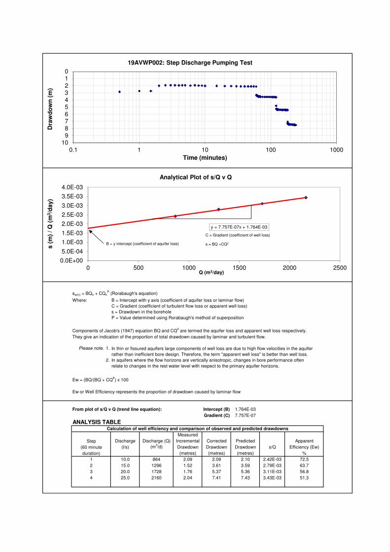
sw(n) = BQn + CQnP (Rorabaugh's equation)
Where: B = Intercept with y axis (coefficient of aquifer loss or laminar flow)
C = Gradient (coefficient of turbulent flow loss or apparent well loss)
s = Drawdown in the borehole
P = Value determined using Rorabaugh's method of superposition
Components of Jacob's (1947) equation BQ and CQ2 are termed the aquifer loss and apparent well loss respectively.
They give an indication of the proportion of total drawdown caused by laminar and turbulent flow.
Please note: 1. In thin or fissured aquifers large components of well loss are due to high flow velocities in the aquifer
rather than inefficient bore design. Therefore, the term "apparent well loss" is better than well loss.
2. In aquifers where the flow horizons are vertically anisotropic, changes in bore performance often
relate to changes in the rest water level with respect to the primary aquifer horizons.
Ew = (BQ/(BQ + CQP) x 100
Ew or Well Efficiency represents the proportion of drawdown caused by laminar flow
From plot of s/Q v Q (trend line equation): Intercept (B) 1.764E-03
Gradient (C) 7.757E-07
ANALYSIS TABLE
Measured
Step Discharge Discharge (Q) Incremental Corrected Predicted Apparent
(60 minute (l/s) (m3/d) Drawdown Drawdown Drawdown s/Q Efficiency (Ew)
duration) (metres) (metres) (metres) %
1 10.0 864 2.09 2.09 2.10 2.42E-03 72.5
2 15.0 1296 1.52 3.61 3.59 2.79E-03 63.7
3 20.0 1728 1.76 5.37 5.36 3.11E-03 56.8
4 25.0 2160 2.04 7.41 7.43 3.43E-03 51.3
Calculation of well efficiency and comparison of observed and predicted drawdowns
0123456789
100.1 1 10 100 1000
Dra
wd
ow
n (
m)
Time (minutes)
19AVWP002: Step Discharge Pumping Test
y = 7.757E-07x + 1.764E-03
0.0E+00
5.0E-04
1.0E-03
1.5E-03
2.0E-03
2.5E-03
3.0E-03
3.5E-03
4.0E-03
0 500 1000 1500 2000 2500
s (
m)
/ Q
(m
3/d
ay)
Q (m3/day)
Analytical Plot of s/Q v Q
B = y intercept (coefficient of aquifer loss)
C = Gradient (coefficient of well loss)
s = BQ +CQ2

1. 10. 100. 1000. 1.0E+40.
0.8
1.6
2.4
3.2
4.
Adjusted Time (sec)
Corr
ecte
d D
ispla
cem
ent (m
)
WELL TEST ANALYSIS
Data Set: F:\183\2.TECH\Field Data\AQTESOLV\GHD912.aqtDate: 08/13/18 Time: 14:14:39
PROJECT INFORMATION
Company: AQ2Client: AVLProject: 183Location: GabaninthaTest Well: GDH912
AQUIFER DATA
Saturated Thickness: 156.1 m Anisotropy Ratio (Kz/Kr): 0.1
WELL DATA
Pumping WellsWell Name X (m) Y (m)GDH912 0 0
Observation WellsWell Name X (m) Y (m)
GDH912 0 0
SOLUTION
Aquifer Model: Unconfined Solution Method: Cooper-Jacob
T = 0.6417 m2/day S = 0.3366
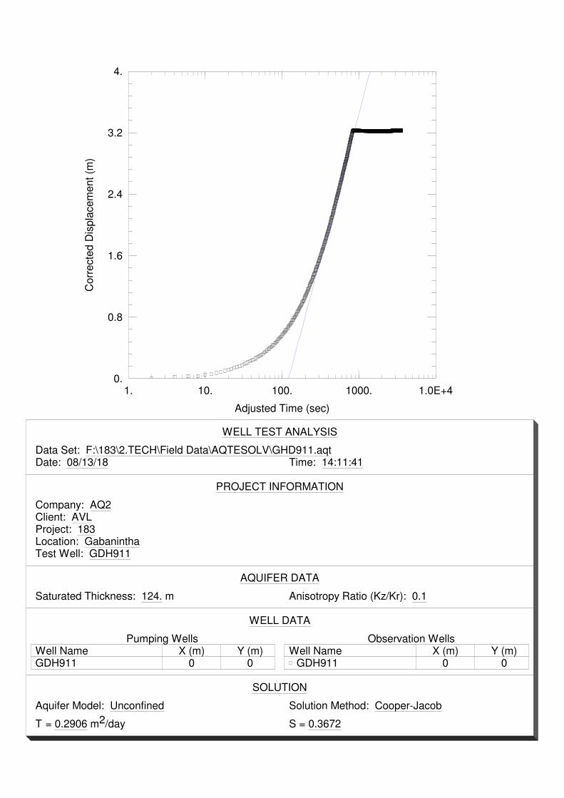
1. 10. 100. 1000. 1.0E+40.
0.8
1.6
2.4
3.2
4.
Adjusted Time (sec)
Corr
ecte
d D
ispla
cem
ent (m
)
WELL TEST ANALYSIS
Data Set: F:\183\2.TECH\Field Data\AQTESOLV\GHD911.aqtDate: 08/13/18 Time: 14:11:41
PROJECT INFORMATION
Company: AQ2Client: AVLProject: 183Location: GabaninthaTest Well: GDH911
AQUIFER DATA
Saturated Thickness: 124. m Anisotropy Ratio (Kz/Kr): 0.1
WELL DATA
Pumping WellsWell Name X (m) Y (m)GDH911 0 0
Observation WellsWell Name X (m) Y (m)
GDH911 0 0
SOLUTION
Aquifer Model: Unconfined Solution Method: Cooper-Jacob
T = 0.2906 m2/day S = 0.3672
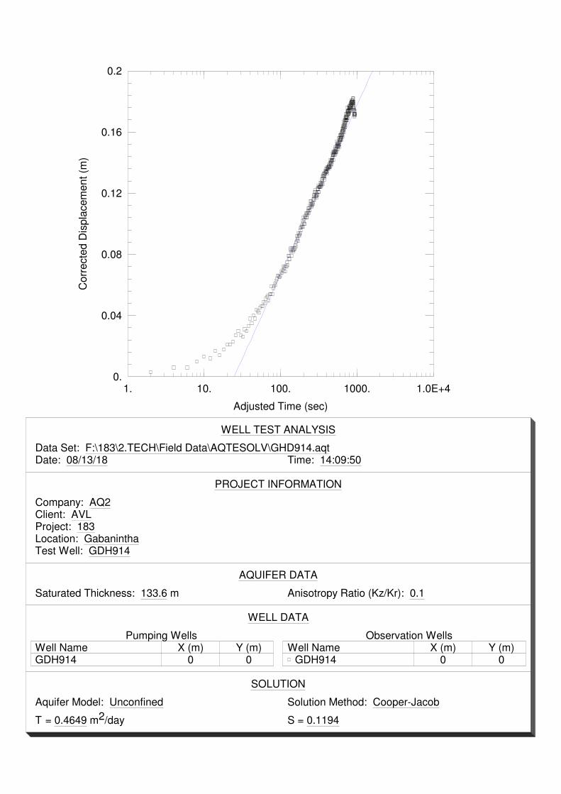
1. 10. 100. 1000. 1.0E+40.
0.04
0.08
0.12
0.16
0.2
Adjusted Time (sec)
Corr
ecte
d D
ispla
cem
ent (m
)
WELL TEST ANALYSIS
Data Set: F:\183\2.TECH\Field Data\AQTESOLV\GHD914.aqtDate: 08/13/18 Time: 14:09:50
PROJECT INFORMATION
Company: AQ2Client: AVLProject: 183Location: GabaninthaTest Well: GDH914
AQUIFER DATA
Saturated Thickness: 133.6 m Anisotropy Ratio (Kz/Kr): 0.1
WELL DATA
Pumping WellsWell Name X (m) Y (m)GDH914 0 0
Observation WellsWell Name X (m) Y (m)
GDH914 0 0
SOLUTION
Aquifer Model: Unconfined Solution Method: Cooper-Jacob
T = 0.4649 m2/day S = 0.1194

1. 10. 100. 1000. 1.0E+40.
0.4
0.8
1.2
1.6
2.
Adjusted Time (sec)
Corr
ecte
d D
ispla
cem
ent (m
)
WELL TEST ANALYSIS
Data Set: F:\183\2.TECH\Field Data\AQTESOLV\GHD904.aqtDate: 08/13/18 Time: 14:07:51
PROJECT INFORMATION
Company: AQ2Client: AVLProject: 183Location: GabaninthaTest Well: GDH904
AQUIFER DATA
Saturated Thickness: 90.5 m Anisotropy Ratio (Kz/Kr): 0.1
WELL DATA
Pumping WellsWell Name X (m) Y (m)GDH904 0 0
Observation WellsWell Name X (m) Y (m)
GDH904 0 0
SOLUTION
Aquifer Model: Unconfined Solution Method: Cooper-Jacob
T = 0.4817 m2/day S = 0.1966
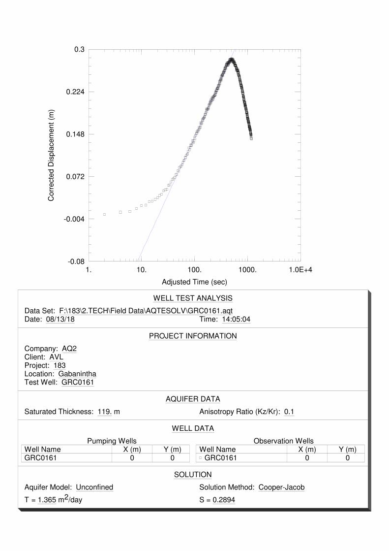
1. 10. 100. 1000. 1.0E+4-0.08
-0.004
0.072
0.148
0.224
0.3
Adjusted Time (sec)
Corr
ecte
d D
ispla
cem
ent (m
)
WELL TEST ANALYSIS
Data Set: F:\183\2.TECH\Field Data\AQTESOLV\GRC0161.aqtDate: 08/13/18 Time: 14:05:04
PROJECT INFORMATION
Company: AQ2Client: AVLProject: 183Location: GabaninthaTest Well: GRC0161
AQUIFER DATA
Saturated Thickness: 119. m Anisotropy Ratio (Kz/Kr): 0.1
WELL DATA
Pumping WellsWell Name X (m) Y (m)GRC0161 0 0
Observation WellsWell Name X (m) Y (m)
GRC0161 0 0
SOLUTION
Aquifer Model: Unconfined Solution Method: Cooper-Jacob
T = 1.365 m2/day S = 0.2894

1. 10. 100. 1000. 1.0E+40.
0.6
1.2
1.8
2.4
3.
Adjusted Time (sec)
Corr
ecte
d D
ispla
cem
ent (m
)
WELL TEST ANALYSIS
Data Set: F:\183\2.TECH\Field Data\AQTESOLV\GRC0165.aqtDate: 08/13/18 Time: 14:02:49
PROJECT INFORMATION
Company: AQ2Client: AVLProject: 183Location: GabaninthaTest Well: GRC0165
AQUIFER DATA
Saturated Thickness: 119. m Anisotropy Ratio (Kz/Kr): 0.1
WELL DATA
Pumping WellsWell Name X (m) Y (m)GRC0165 0 0
Observation WellsWell Name X (m) Y (m)
GRC0165 0 0
SOLUTION
Aquifer Model: Unconfined Solution Method: Cooper-Jacob
T = 0.5051 m2/day S = 0.4928

1. 10. 100. 1000. 1.0E+40.001
0.01
0.1
1.
10.
Time (sec)
Corr
ecte
d D
ispla
cem
ent (m
)
WELL TEST ANALYSIS
Data Set: F:\183\2.TECH\Field Data\AQTESOLV\GRC0169.aqtDate: 08/13/18 Time: 14:00:33
PROJECT INFORMATION
Company: AQ2Client: AVLProject: 183Location: GabaninthaTest Well: GRC0169
WELL DATA
Pumping WellsWell Name X (m) Y (m)GRC0169 0 0
Observation WellsWell Name X (m) Y (m)
GRC0169 0 0
SOLUTION
Aquifer Model: Unconfined Solution Method: Theis
T = 0.2789 m2/day S = 0.3761Kz/Kr = 0.1 b = 47. m
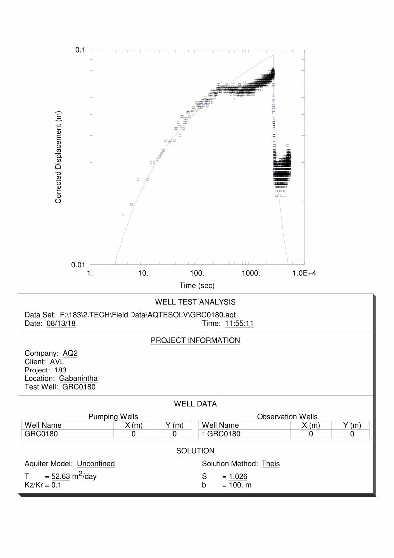
1. 10. 100. 1000. 1.0E+40.01
0.1
Time (sec)
Corr
ecte
d D
ispla
cem
ent (m
)
WELL TEST ANALYSIS
Data Set: F:\183\2.TECH\Field Data\AQTESOLV\GRC0180.aqtDate: 08/13/18 Time: 11:55:11
PROJECT INFORMATION
Company: AQ2Client: AVLProject: 183Location: GabaninthaTest Well: GRC0180
WELL DATA
Pumping WellsWell Name X (m) Y (m)GRC0180 0 0
Observation WellsWell Name X (m) Y (m)
GRC0180 0 0
SOLUTION
Aquifer Model: Unconfined Solution Method: Theis
T = 52.63 m2/day S = 1.026Kz/Kr = 0.1 b = 100. m
APPENDIX D
WATER QUALITY ANALYSES
Accreditation No. 2562
Date Reported
Contact
SGS Perth Environmental
28 Reid Rd
Perth Airport WA 6105
Ros Ma
(08) 9373 3500
(08) 9373 3556
7
SGS Reference
Facsimile
Telephone
Address
Manager
Laboratory
183 Gabanintha
183 Gabanintha
(Not specified)
0417 183224
PO BOX 976
SOUTH PERTH WA 6951
AQ2
Alex Storey
Samples
Order Number
Project
Facsimile
Telephone
Address
Client
CLIENT DETAILS LABORATORY DETAILS
10 Aug 2018
ANALYTICAL REPORT
PE127757 R0
06 Aug 2018Date Received
Accredited for compliance with ISO/IEC 17025 - Testing. NATA accredited laboratory 2562(898/20210).
For determination of soluble metals, filtered sample was not received so samples were laboratory filtered on receipt. This may give soluble metals
results that do not represent the concentrations present at the time of sampling.
Metals: Dissolved Na: Spike recovery failed acceptance criteria due to the presence of significant concentration of analyte (i.e. the concentration
of analyte exceeds the spike level).
Ionic Balance: #4 is outside acceptance criteria due sample heterogeneity.
COMMENTS
Hue Thanh Ly
Metals Team Leader
Mary Ann Ola-A
Inorganics Team Leader
SIGNATORIES
SGS Australia Pty Ltd
ABN 44 000 964 278
Environment, Health and Safety 28 Reid Rd
PO Box 32
Perth Airport WA 6105
Welshpool WA 6983
Australia
Australia
t +61 8 9373 3500
f +61 8 9373 3556
www.sgs.com.au
Member of the SGS Group
Page 1 of 710-August-2018
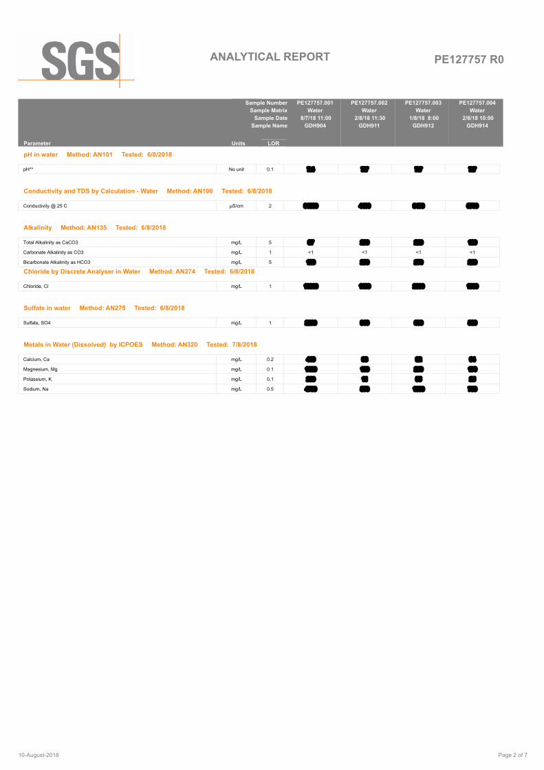
PE127757 R0ANALYTICAL REPORT
PE127757.001
Water
8/7/18 11:00
GDH904
PE127757.002
Water
2/8/18 11:30
GDH911
PE127757.003
Water
1/8/18 8:00
GDH912
PE127757.004
Water
2/8/18 10:00
GDH914
Parameter LORUnits
Sample Number
Sample Matrix
Sample Date
Sample Name
pH in water Method: AN101 Tested: 6/8/2018
pH** No unit 0.1 7.4 7.7 7.7 7.7
Conductivity and TDS by Calculation - Water Method: AN106 Tested: 6/8/2018
Conductivity @ 25 C µS/cm 2 31000 4400 9400 6700
Alkalinity Method: AN135 Tested: 6/8/2018
Total Alkalinity as CaCO3 mg/L 5 97 230 220 180
Carbonate Alkalinity as CO3 mg/L 1 <1 <1 <1 <1
Bicarbonate Alkalinity as HCO3 mg/L 5 120 280 270 220
Chloride by Discrete Analyser in Water Method: AN274 Tested: 6/8/2018
Chloride, Cl mg/L 1 10000 1100 2800 1900
Sulfate in water Method: AN275 Tested: 6/8/2018
Sulfate, SO4 mg/L 1 2200 310 660 580
Metals in Water (Dissolved) by ICPOES Method: AN320 Tested: 7/8/2018
Calcium, Ca mg/L 0.2 440 93 92 94
Magnesium, Mg mg/L 0.1 1100 160 250 170
Potassium, K mg/L 0.1 230 11 55 25
Sodium, Na mg/L 0.5 4700 570 1600 750
Page 2 of 710-August-2018
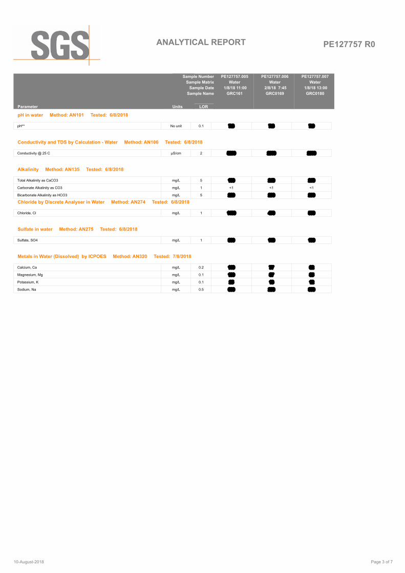
PE127757 R0ANALYTICAL REPORT
PE127757.005
Water
1/8/18 11:00
GRC161
PE127757.006
Water
2/8/18 7:45
GRC0169
PE127757.007
Water
1/8/18 13:00
GRC0180
Parameter LORUnits
Sample Number
Sample Matrix
Sample Date
Sample Name
pH in water Method: AN101 Tested: 6/8/2018
pH** No unit 0.1 7.8 7.8 7.9
Conductivity and TDS by Calculation - Water Method: AN106 Tested: 6/8/2018
Conductivity @ 25 C µS/cm 2 5200 2300 2600
Alkalinity Method: AN135 Tested: 6/8/2018
Total Alkalinity as CaCO3 mg/L 5 180 240 210
Carbonate Alkalinity as CO3 mg/L 1 <1 <1 <1
Bicarbonate Alkalinity as HCO3 mg/L 5 220 290 260
Chloride by Discrete Analyser in Water Method: AN274 Tested: 6/8/2018
Chloride, Cl mg/L 1 1400 470 550
Sulfate in water Method: AN275 Tested: 6/8/2018
Sulfate, SO4 mg/L 1 390 140 180
Metals in Water (Dissolved) by ICPOES Method: AN320 Tested: 7/8/2018
Calcium, Ca mg/L 0.2 110 77 62
Magnesium, Mg mg/L 0.1 180 87 85
Potassium, K mg/L 0.1 25 13 12
Sodium, Na mg/L 0.5 690 260 350
Page 3 of 710-August-2018

PE127757 R0QC SUMMARY
MB blank results are compared to the Limit of Reporting
LCS and MS spike recoveries are measured as the percentage of analyte recovered from the sample compared the the amount of analyte spiked into the sample.
DUP and MSD relative percent differences are measured against their original counterpart samples according to the formula : the absolute difference of the two results divided
by the average of the two results as a percentage. Where the DUP RPD is 'NA' , the results are less than the LOR and thus the RPD is not applicable.
Alkalinity Method: ME-(AU)-[ENV]AN135
MB DUP %RPD LCS
%Recovery
Total Alkalinity as CaCO3 LB149123 mg/L 5 <5 1 - 5% 99%
Carbonate Alkalinity as CO3 LB149123 mg/L 1 <1
Bicarbonate Alkalinity as HCO3 LB149123 mg/L 5 <5
LORUnits Parameter QC
Reference
Chloride by Discrete Analyser in Water Method: ME-(AU)-[ENV]AN274
MB DUP %RPD LCS
%Recovery
MS
%Recovery
Chloride, Cl LB149034 mg/L 1 <1 0 - 1% 105% 86 - 100%
LORUnits Parameter QC
Reference
Conductivity and TDS by Calculation - Water Method: ME-(AU)-[ENV]AN106
MB DUP %RPD LCS
%Recovery
Conductivity @ 25 C LB149130 µS/cm 2 <2 0 - 1% 99 - 100%
LB149131 µS/cm 2 <2 0 - 1% 99%
LORUnits Parameter QC
Reference
Metals in Water (Dissolved) by ICPOES Method: ME-(AU)-[ENV]AN320
MB DUP %RPD LCS
%Recovery
MS
%Recovery
Calcium, Ca LB149048 mg/L 0.2 <0.2 0% 101% 102%
Magnesium, Mg LB149048 mg/L 0.1 <0.1 0 - 1% 100% 107%
Potassium, K LB149048 mg/L 0.1 <0.1 1% 101% 104%
Sodium, Na LB149048 mg/L 0.5 <0.5 1% 99% 166%
LORUnits Parameter QC
Reference
pH in water Method: ME-(AU)-[ENV]AN101
MB DUP %RPD LCS
%Recovery
pH** LB149130 No unit 0.1 5.7 - 6.6 0 - 1% 100%
LB149131 No unit 0.1 5.9 0% 100%
LORUnits Parameter QC
Reference
Page 4 of 710-August-2018

PE127757 R0QC SUMMARY
MB blank results are compared to the Limit of Reporting
LCS and MS spike recoveries are measured as the percentage of analyte recovered from the sample compared the the amount of analyte spiked into the sample.
DUP and MSD relative percent differences are measured against their original counterpart samples according to the formula : the absolute difference of the two results divided
by the average of the two results as a percentage. Where the DUP RPD is 'NA' , the results are less than the LOR and thus the RPD is not applicable.
Sulfate in water Method: ME-(AU)-[ENV]AN275
MB DUP %RPD LCS
%Recovery
MS
%Recovery
Sulfate, SO4 LB149034 mg/L 1 <1 0% 99% 95 - 96%
LORUnits Parameter QC
Reference
Page 5 of 710-August-2018

PE127757 R0
METHOD METHODOLOGY SUMMARY
METHOD SUMMARY
pH in Soil Sludge Sediment and Water: pH is measured electrometrically using a combination electrode (glass plus
reference electrode) and is calibrated against 3 buffers purchased commercially. For soils, an extract with water is
made at a ratio of 1:5 and the pH determined and reported on the extract. Reference APHA 4500-H+.
AN101
Conductivity and TDS by Calculation: Conductivity is measured by meter with temperature compensation and is
calibrated against a standard solution of potassium chloride. Conductivity is generally reported as µmhos/cm or
µS/cm @ 25°C. For soils, an extract with water is made at a ratio of 1:5 and the EC determined and reported on
the extract, or calculated back to the as-received sample. Total Dissolved Salts can be estimated from conductivity
using a conversion factor, which for natural waters, is in the range 0.55 to 0.75. SGS use 0.6. Reference APHA
2510 B.
AN106
Salinity may be calculated in terms of NaCl from the sample conductivity. This assumes all soluble salts present,
measured by the conductivity, are present as NaCl.
AN106
This method is used to calculation the balance of major Anions and Cations in water samples and converts major
ion concentration to milliequivalents and then summed. Anions sum and Cation sum is calculated as a difference
and expressed as a percentage.
AN121
The sum of cations and anions in mg/L may also be reported. This sums Na, K, Ca, Mg, NH3, Fe, Cl, Total
Alkalinity, SO4 and NO3.
AN121
Alkalinity (and forms of) by Titration: The sample is titrated with standard acid to pH 8.3 (P titre) and pH 4.5 (T titre)
and permanent and/or total alkalinity calculated. The results are expressed as equivalents of calcium carbonate or
recalculated as bicarbonate, carbonate and hydroxide. Reference APHA 2320. Internal Reference AN135
AN135
Chloride by Aquakem DA: Chloride reacts with mercuric thiocyanate forming a mercuric chloride complex. In the
presence of ferric iron, highly coloured ferric thiocyanate is formed which is proportional to the chloride
concentration. Reference APHA 4500Cl-
AN274
sulfate by Aquakem DA: sulfate is precipitated in an acidic medium with barium chloride. The resulting turbidity is
measured photometrically at 405nm and compared with standard calibration solutions to determine the sulfate
concentration in the sample. Reference APHA 4500-SO42-. Internal reference AN275.
AN275
Metals by ICP-OES: Samples are preserved with 10% nitric acid for a wide range of metals and some non-metals.
This solution is measured by Inductively Coupled Plasma. Solutions are aspirated into an argon plasma at
8000-10000K and emit characteristic energy or light as a result of electron transitions through unique energy
levels. The emitted light is focused onto a diffraction grating where it is separated into components .
AN320
Photomultipliers or CCDs are used to measure the light intensity at specific wavelengths. This intensity is directly
proportional to concentration. Corrections are required to compensate for spectral overlap between elements.
Reference APHA 3120 B.
AN320
Free and Total Carbon Dioxide may be calculated using alkalinity forms only when the samples TDS is <500mg/L.
If TDS is >500mg/L free or total carbon dioxide cannot be reported . APHA4500CO2 D.
Calculation
Page 6 of 710-August-2018
PE127757 R0
Samples analysed as received.
Solid samples expressed on a dry weight basis.
Where "Total" analyte groups are reported (for example, Total PAHs, Total OC Pesticides) the total will be calculated as the sum of the individual
analytes, with those analytes that are reported as <LOR being assumed to be zero. The summed (Total) limit of reporting is calcuated by summing
the individual analyte LORs and dividing by two. For example, where 16 individual analytes are being summed and each has an LOR of 0.1 mg/kg,
the "Totals" LOR will be 1.6 / 2 (0.8 mg/kg). Where only 2 analytes are being summed, the " Total" LOR will be the sum of those two LORs.
Some totals may not appear to add up because the total is rounded after adding up the raw values.
If reported, measurement uncertainty follow the ± sign after the analytical result and is expressed as the expanded uncertainty calculated using a
coverage factor of 2, providing a level of confidence of approximately 95%, unless stated otherwise in the comments section of this report.
Results reported for samples tested under test methods with codes starting with ARS -SOP, radionuclide or gross radioactivity concentrations are
expressed in becquerel (Bq) per unit of mass or volume or per wipe as stated on the report. Becquerel is the SI unit for activity and equals one
nuclear transformation per second.
Note that in terms of units of radioactivity:
a. 1 Bq is equivalent to 27 pCi
b. 37 MBq is equivalent to 1 mCi
For results reported for samples tested under test methods with codes starting with ARS -SOP, less than (<) values indicate the detection limit for
each radionuclide or parameter for the measurement system used. The respective detection limits have been calculated in accordance with ISO
11929.
The QC criteria are subject to internal review according to the SGS QAQC plan and may be provided on request or alternatively can be found here :
http://www.sgs.com.au/~/media/Local/Australia/Documents/Technical%20Documents/MP-AU-ENV-QU-022%20QA%20QC%20Plan.pdf
This document is issued by the Company under its General Conditions of Service accessible at www.sgs.com/en/Terms-and-Conditions.aspx.
Attention is drawn to the limitation of liability, indemnification and jurisdiction issues defined therein.
Any holder of this document is advised that information contained hereon reflects the Company 's findings at the time of its intervention only and
within the limits of Client's instructions, if any. The Company's sole responsibility is to its Client only. Any unauthorized alteration, forgery or
falsification of the content or appearance of this document is unlawful and offenders may be prosecuted to the fullest extent of the law .
This report must not be reproduced, except in full.
IS
LNR
*
**
Insufficient sample for analysis.
Sample listed, but not received.
NATA accreditation does not cover the
performance of this service.
Indicative data, theoretical holding time exceeded.
FOOTNOTES
LOR
↑↓
QFH
QFL
-
NVL
Limit of Reporting
Raised or Lowered Limit of Reporting
QC result is above the upper tolerance
QC result is below the lower tolerance
The sample was not analysed for this analyte
Not Validated
Page 7 of 710-August-2018

Accreditation No. 2562
Date Reported
Contact
SGS Perth Environmental
28 Reid Rd
Perth Airport WA 6105
Marjana Siljanoska
(08) 9373 3500
(08) 9373 3556
1
SGS Reference
Facsimile
Telephone
Address
Manager
Laboratory
183C C2
183C C2
(Not specified)
0417 183224
PO BOX 976
SOUTH PERTH WA 6951
AQ2
Duncan Storey
Samples
Order Number
Project
Facsimile
Telephone
Address
Client
CLIENT DETAILS LABORATORY DETAILS
17 May 2019
ANALYTICAL REPORT
PE134594 R0
02 May 2019Date Received
Accredited for compliance with ISO/IEC 17025 - Testing. NATA accredited laboratory 2562(898/20210).
For determination of soluble metals, filtered sample was not received so samples were laboratory subsampled and filtered on receipt. This may
give soluble metals results that do not represent the concentrations present at the time of sampling.
Metals: LORs raised due to high conductivity.
The upper limit for Conductivity in Water is 100,000 uS/cm. Any result above this is an estimate. This will also cause the TDS on EC ratio to bias
high.
COMMENTS
Hue Thanh Ly
Metals Team Leader
Louise Hope
Laboratory Technician
SIGNATORIES
SGS Australia Pty Ltd
ABN 44 000 964 278
Environment, Health and Safety 28 Reid Rd
PO Box 32
Perth Airport WA 6105
Welshpool WA 6983
Australia
Australia
t +61 8 9373 3500
f +61 8 9373 3556
www.sgs.com.au
Member of the SGS Group
Page 1 of 717-May-2019
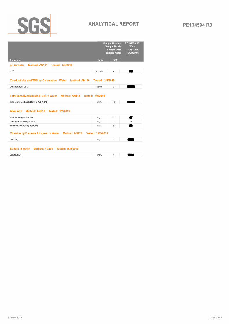
PE134594 R0ANALYTICAL REPORT
PE134594.001
Water
27 Apr 2019
19AVWM01
Parameter LORUnits
Sample Number
Sample Matrix
Sample Date
Sample Name
pH in water Method: AN101 Tested: 2/5/2019
pH** pH Units - 7.2
Conductivity and TDS by Calculation - Water Method: AN106 Tested: 2/5/2019
Conductivity @ 25 C µS/cm 2 180000
Total Dissolved Solids (TDS) in water Method: AN113 Tested: 7/5/2019
Total Dissolved Solids Dried at 175-185°C mg/L 10 140000
Alkalinity Method: AN135 Tested: 2/5/2019
Total Alkalinity as CaCO3 mg/L 5 47
Carbonate Alkalinity as CO3 mg/L 1 <1
Bicarbonate Alkalinity as HCO3 mg/L 5 58
Chloride by Discrete Analyser in Water Method: AN274 Tested: 14/5/2019
Chloride, Cl mg/L 1 88000
Sulfate in water Method: AN275 Tested: 16/5/2019
Sulfate, SO4 mg/L 1 19000
Page 2 of 717-May-2019

PE134594 R0ANALYTICAL REPORT
PE134594.001
Water
27 Apr 2019
19AVWM01
Parameter LORUnits
Sample Number
Sample Matrix
Sample Date
Sample Name
Metals in Water (Dissolved) by ICPOES Method: AN320 Tested: 3/5/2019
Calcium, Ca mg/L 0.2 840
Magnesium, Mg mg/L 0.1 6400
Potassium, K mg/L 0.1 2800
Sodium, Na mg/L 0.5 46000
Page 3 of 717-May-2019
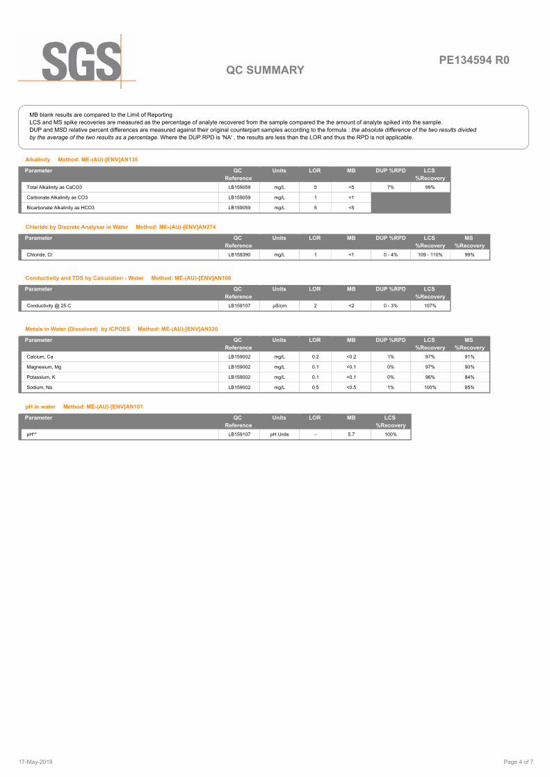
PE134594 R0QC SUMMARY
MB blank results are compared to the Limit of Reporting
LCS and MS spike recoveries are measured as the percentage of analyte recovered from the sample compared the the amount of analyte spiked into the sample.
DUP and MSD relative percent differences are measured against their original counterpart samples according to the formula : the absolute difference of the two results divided
by the average of the two results as a percentage. Where the DUP RPD is 'NA' , the results are less than the LOR and thus the RPD is not applicable.
Alkalinity Method: ME-(AU)-[ENV]AN135
MB DUP %RPD LCS
%Recovery
Total Alkalinity as CaCO3 LB159059 mg/L 5 <5 7% 99%
Carbonate Alkalinity as CO3 LB159059 mg/L 1 <1
Bicarbonate Alkalinity as HCO3 LB159059 mg/L 5 <5
LORUnits Parameter QC
Reference
Chloride by Discrete Analyser in Water Method: ME-(AU)-[ENV]AN274
MB DUP %RPD LCS
%Recovery
MS
%Recovery
Chloride, Cl LB159390 mg/L 1 <1 0 - 4% 109 - 110% 99%
LORUnits Parameter QC
Reference
Conductivity and TDS by Calculation - Water Method: ME-(AU)-[ENV]AN106
MB DUP %RPD LCS
%Recovery
Conductivity @ 25 C LB159107 µS/cm 2 <2 0 - 3% 107%
LORUnits Parameter QC
Reference
Metals in Water (Dissolved) by ICPOES Method: ME-(AU)-[ENV]AN320
MB DUP %RPD LCS
%Recovery
MS
%Recovery
Calcium, Ca LB159002 mg/L 0.2 <0.2 1% 97% 91%
Magnesium, Mg LB159002 mg/L 0.1 <0.1 0% 97% 90%
Potassium, K LB159002 mg/L 0.1 <0.1 0% 96% 84%
Sodium, Na LB159002 mg/L 0.5 <0.5 1% 100% 85%
LORUnits Parameter QC
Reference
pH in water Method: ME-(AU)-[ENV]AN101
MB LCS
%Recovery
pH** LB159107 pH Units - 5.7 100%
LORUnits Parameter QC
Reference
Page 4 of 717-May-2019

PE134594 R0QC SUMMARY
MB blank results are compared to the Limit of Reporting
LCS and MS spike recoveries are measured as the percentage of analyte recovered from the sample compared the the amount of analyte spiked into the sample.
DUP and MSD relative percent differences are measured against their original counterpart samples according to the formula : the absolute difference of the two results divided
by the average of the two results as a percentage. Where the DUP RPD is 'NA' , the results are less than the LOR and thus the RPD is not applicable.
Sulfate in water Method: ME-(AU)-[ENV]AN275
MB DUP %RPD LCS
%Recovery
MS
%Recovery
Sulfate, SO4 LB159497 mg/L 1 <1 0 - 2% 107 - 108% 86 - 95%
LORUnits Parameter QC
Reference
Total Dissolved Solids (TDS) in water Method: ME-(AU)-[ENV]AN113
MB DUP %RPD LCS
%Recovery
MS
%Recovery
MSD %RPD
Total Dissolved Solids Dried at 175-185°C LB159173 mg/L 10 <10 1% 96% 99% 1%
LORUnits Parameter QC
Reference
Page 5 of 717-May-2019

PE134594 R0
METHOD METHODOLOGY SUMMARY
METHOD SUMMARY
pH in Soil Sludge Sediment and Water: pH is measured electrometrically using a combination electrode (glass plus
reference electrode) and is calibrated against 3 buffers purchased commercially. For soils, an extract with water is
made at a ratio of 1:5 and the pH determined and reported on the extract. Reference APHA 4500-H+.
AN101
Conductivity and TDS by Calculation: Conductivity is measured by meter with temperature compensation and is
calibrated against a standard solution of potassium chloride. Conductivity is generally reported as µmhos/cm or
µS/cm @ 25°C. For soils, an extract with water is made at a ratio of 1:5 and the EC determined and reported on
the extract, or calculated back to the as-received sample. Total Dissolved Salts can be estimated from conductivity
using a conversion factor, which for natural waters, is in the range 0.55 to 0.75. SGS use 0.6. Reference APHA
2510 B.
AN106
Salinity may be calculated in terms of NaCl from the sample conductivity. This assumes all soluble salts present,
measured by the conductivity, are present as NaCl.
AN106
Total Dissolved Solids: A well-mixed filtered sample of known volume is evaporated to dryness at 180°C and the
residue weighed. Approximate methods for correlating chemical analysis with dissolved solids are available.
Reference APHA 2540 C.
AN113
The Total Dissolved Solids residue may also be ignited at 550 C and volatile TDS (Organic TDS) and non-volatile
TDS (Inorganic) can be determined.
AN113
Alkalinity (and forms of) by Titration: The sample is titrated with standard acid to pH 8.3 (P titre) and pH 4.5 (T titre)
and permanent and/or total alkalinity calculated. The results are expressed as equivalents of calcium carbonate or
recalculated as bicarbonate, carbonate and hydroxide. Reference APHA 2320. Internal Reference AN135
AN135
Chloride by Aquakem DA: Chloride reacts with mercuric thiocyanate forming a mercuric chloride complex. In the
presence of ferric iron, highly coloured ferric thiocyanate is formed which is proportional to the chloride
concentration. Reference APHA 4500Cl-
AN274
sulfate by Aquakem DA: sulfate is precipitated in an acidic medium with barium chloride. The resulting turbidity is
measured photometrically at 405nm and compared with standard calibration solutions to determine the sulfate
concentration in the sample. Reference APHA 4500-SO42-. Internal reference AN275.
AN275
Metals by ICP-OES: Samples are preserved with 10% nitric acid for a wide range of metals and some non-metals.
This solution is measured by Inductively Coupled Plasma. Solutions are aspirated into an argon plasma at
8000-10000K and emit characteristic energy or light as a result of electron transitions through unique energy
levels. The emitted light is focused onto a diffraction grating where it is separated into components .
AN320
Photomultipliers or CCDs are used to measure the light intensity at specific wavelengths. This intensity is directly
proportional to concentration. Corrections are required to compensate for spectral overlap between elements.
Reference APHA 3120 B.
AN320
Free and Total Carbon Dioxide may be calculated using alkalinity forms only when the samples TDS is <500mg/L.
If TDS is >500mg/L free or total carbon dioxide cannot be reported . APHA4500CO2 D.
Calculation
Page 6 of 717-May-2019

PE134594 R0
Unless it is reported that sampling has been perfomed by SGS, the samples have been analysed as received.
Solid samples expressed on a dry weight basis.
Where "Total" analyte groups are reported (for example, Total PAHs, Total OC Pesticides) the total will be calculated as the sum of the individual
analytes, with those analytes that are reported as <LOR being assumed to be zero. The summed (Total) limit of reporting is calcuated by summing
the individual analyte LORs and dividing by two. For example, where 16 individual analytes are being summed and each has an LOR of 0.1 mg/kg,
the "Totals" LOR will be 1.6 / 2 (0.8 mg/kg). Where only 2 analytes are being summed, the " Total" LOR will be the sum of those two LORs.
Some totals may not appear to add up because the total is rounded after adding up the raw values.
If reported, measurement uncertainty follow the ± sign after the analytical result and is expressed as the expanded uncertainty calculated using a
coverage factor of 2, providing a level of confidence of approximately 95%, unless stated otherwise in the comments section of this report.
Results reported for samples tested under test methods with codes starting with ARS -SOP, radionuclide or gross radioactivity concentrations are
expressed in becquerel (Bq) per unit of mass or volume or per wipe as stated on the report. Becquerel is the SI unit for activity and equals one
nuclear transformation per second.
Note that in terms of units of radioactivity:
a. 1 Bq is equivalent to 27 pCi
b. 37 MBq is equivalent to 1 mCi
For results reported for samples tested under test methods with codes starting with ARS -SOP, less than (<) values indicate the detection limit for
each radionuclide or parameter for the measurement system used. The respective detection limits have been calculated in accordance with ISO
11929.
The QC and MU criteria are subject to internal review according to the SGS QAQC plan and may be provided on request or alternatively can be
found here: www.sgs.com.au.pv.sgsvr/en-gb/environment.
This document is issued by the Company under its General Conditions of Service accessible at www.sgs.com/en/Terms-and-Conditions.aspx.
Attention is drawn to the limitation of liability, indemnification and jurisdiction issues defined therein.
Any holder of this document is advised that information contained hereon reflects the Company 's findings at the time of its intervention only and
within the limits of Client's instructions, if any. The Company's sole responsibility is to its Client only. Any unauthorized alteration, forgery or
falsification of the content or appearance of this document is unlawful and offenders may be prosecuted to the fullest extent of the law .
This report must not be reproduced, except in full.
IS
LNR
*
**
Insufficient sample for analysis.
Sample listed, but not received.
NATA accreditation does not cover the
performance of this service.
Indicative data, theoretical holding time exceeded.
FOOTNOTES
LOR
↑↓
QFH
QFL
-
NVL
Limit of Reporting
Raised or Lowered Limit of Reporting
QC result is above the upper tolerance
QC result is below the lower tolerance
The sample was not analysed for this analyte
Not Validated
Page 7 of 717-May-2019
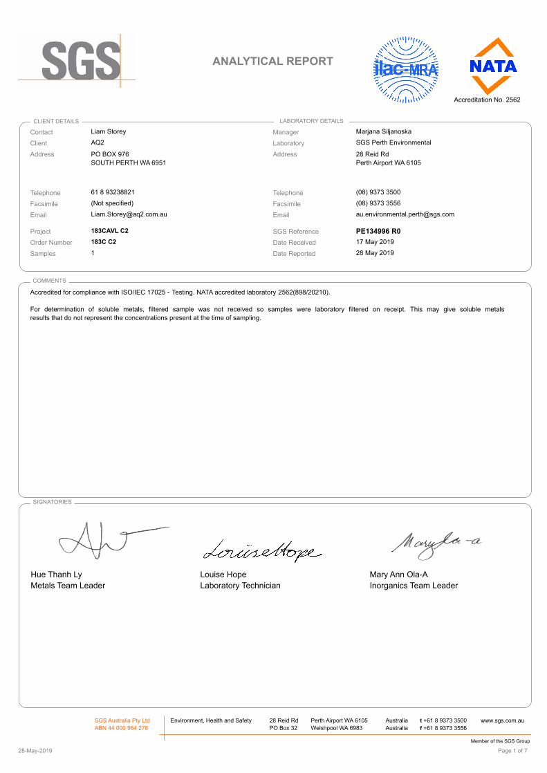
Accreditation No. 2562
Date Reported
Contact
SGS Perth Environmental
28 Reid Rd
Perth Airport WA 6105
Marjana Siljanoska
(08) 9373 3500
(08) 9373 3556
1
SGS Reference
Facsimile
Telephone
Address
Manager
Laboratory
183C C2
183CAVL C2
(Not specified)
61 8 93238821
PO BOX 976
SOUTH PERTH WA 6951
AQ2
Liam Storey
Samples
Order Number
Project
Facsimile
Telephone
Address
Client
CLIENT DETAILS LABORATORY DETAILS
28 May 2019
ANALYTICAL REPORT
PE134996 R0
17 May 2019Date Received
Accredited for compliance with ISO/IEC 17025 - Testing. NATA accredited laboratory 2562(898/20210).
For determination of soluble metals, filtered sample was not received so samples were laboratory filtered on receipt. This may give soluble metals
results that do not represent the concentrations present at the time of sampling.
COMMENTS
Hue Thanh Ly
Metals Team Leader
Louise Hope
Laboratory Technician
Mary Ann Ola-A
Inorganics Team Leader
SIGNATORIES
SGS Australia Pty Ltd
ABN 44 000 964 278
Environment, Health and Safety 28 Reid Rd
PO Box 32
Perth Airport WA 6105
Welshpool WA 6983
Australia
Australia
t +61 8 9373 3500
f +61 8 9373 3556
www.sgs.com.au
Member of the SGS Group
Page 1 of 728-May-2019

PE134996 R0ANALYTICAL REPORT
PE134996.001
Water
14/5/19 12:15
19AVWM02S
Parameter LORUnits
Sample Number
Sample Matrix
Sample Date
Sample Name
pH in water Method: AN101 Tested: 17/5/2019
pH** No unit 0.1 8.0
Conductivity and TDS by Calculation - Water Method: AN106 Tested: 17/5/2019
Conductivity @ 25 C µS/cm 2 12000
Total Dissolved Solids (TDS) in water Method: AN113 Tested: 17/5/2019
Total Dissolved Solids Dried at 175-185°C mg/L 10 7200
Alkalinity Method: AN135 Tested: 17/5/2019
Total Alkalinity as CaCO3 mg/L 5 190
Carbonate Alkalinity as CO3 mg/L 1 <1
Bicarbonate Alkalinity as HCO3 mg/L 5 230
Chloride by Discrete Analyser in Water Method: AN274 Tested: 24/5/2019
Chloride, Cl mg/L 1 3500
Sulfate in water Method: AN275 Tested: 24/5/2019
Sulfate, SO4 mg/L 1 800
Page 2 of 728-May-2019

PE134996 R0ANALYTICAL REPORT
PE134996.001
Water
14/5/19 12:15
19AVWM02S
Parameter LORUnits
Sample Number
Sample Matrix
Sample Date
Sample Name
Metals in Water (Dissolved) by ICPOES Method: AN320 Tested: 20/5/2019
Calcium, Ca mg/L 0.2 180
Magnesium, Mg mg/L 0.1 390
Potassium, K mg/L 0.1 67
Sodium, Na mg/L 0.5 1600
Page 3 of 728-May-2019
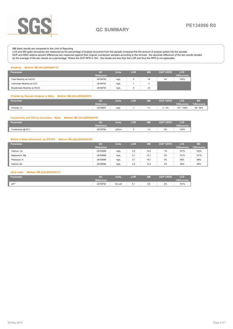
PE134996 R0QC SUMMARY
MB blank results are compared to the Limit of Reporting
LCS and MS spike recoveries are measured as the percentage of analyte recovered from the sample compared the the amount of analyte spiked into the sample.
DUP and MSD relative percent differences are measured against their original counterpart samples according to the formula : the absolute difference of the two results divided
by the average of the two results as a percentage. Where the DUP RPD is 'NA' , the results are less than the LOR and thus the RPD is not applicable.
Alkalinity Method: ME-(AU)-[ENV]AN135
MB DUP %RPD LCS
%Recovery
Total Alkalinity as CaCO3 LB159793 mg/L 5 <5 0% 102%
Carbonate Alkalinity as CO3 LB159793 mg/L 1 <1
Bicarbonate Alkalinity as HCO3 LB159793 mg/L 5 <5
LORUnits Parameter QC
Reference
Chloride by Discrete Analyser in Water Method: ME-(AU)-[ENV]AN274
MB DUP %RPD LCS
%Recovery
MS
%Recovery
Chloride, Cl LB159837 mg/L 1 <1 0 - 3% 107 - 108% 90 - 98%
LORUnits Parameter QC
Reference
Conductivity and TDS by Calculation - Water Method: ME-(AU)-[ENV]AN106
MB DUP %RPD LCS
%Recovery
Conductivity @ 25 C LB159762 µS/cm 2 <2 0% 104%
LORUnits Parameter QC
Reference
Metals in Water (Dissolved) by ICPOES Method: ME-(AU)-[ENV]AN320
MB DUP %RPD LCS
%Recovery
MS
%Recovery
Calcium, Ca LB159589 mg/L 0.2 <0.2 1% 101% 102%
Magnesium, Mg LB159589 mg/L 0.1 <0.1 0% 101% 101%
Potassium, K LB159589 mg/L 0.1 <0.1 3% 96% 98%
Sodium, Na LB159589 mg/L 0.5 <0.5 2% 98% 98%
LORUnits Parameter QC
Reference
pH in water Method: ME-(AU)-[ENV]AN101
MB DUP %RPD LCS
%Recovery
pH** LB159762 No unit 0.1 5.6 2% 101%
LORUnits Parameter QC
Reference
Page 4 of 728-May-2019

PE134996 R0QC SUMMARY
MB blank results are compared to the Limit of Reporting
LCS and MS spike recoveries are measured as the percentage of analyte recovered from the sample compared the the amount of analyte spiked into the sample.
DUP and MSD relative percent differences are measured against their original counterpart samples according to the formula : the absolute difference of the two results divided
by the average of the two results as a percentage. Where the DUP RPD is 'NA' , the results are less than the LOR and thus the RPD is not applicable.
Sulfate in water Method: ME-(AU)-[ENV]AN275
MB DUP %RPD LCS
%Recovery
MS
%Recovery
Sulfate, SO4 LB159837 mg/L 1 <1 0 - 2% 106 - 108% 90 - 91%
LORUnits Parameter QC
Reference
Total Dissolved Solids (TDS) in water Method: ME-(AU)-[ENV]AN113
MB DUP %RPD LCS
%Recovery
MS
%Recovery
MSD %RPD
Total Dissolved Solids Dried at 175-185°C LB159575 mg/L 10 <10 1 - 8% 98% 101% 3%
LORUnits Parameter QC
Reference
Page 5 of 728-May-2019

PE134996 R0
METHOD METHODOLOGY SUMMARY
METHOD SUMMARY
pH in Soil Sludge Sediment and Water: pH is measured electrometrically using a combination electrode (glass plus
reference electrode) and is calibrated against 3 buffers purchased commercially. For soils, an extract with water is
made at a ratio of 1:5 and the pH determined and reported on the extract. Reference APHA 4500-H+.
AN101
Conductivity and TDS by Calculation: Conductivity is measured by meter with temperature compensation and is
calibrated against a standard solution of potassium chloride. Conductivity is generally reported as µmhos/cm or
µS/cm @ 25°C. For soils, an extract with water is made at a ratio of 1:5 and the EC determined and reported on
the extract, or calculated back to the as-received sample. Total Dissolved Salts can be estimated from conductivity
using a conversion factor, which for natural waters, is in the range 0.55 to 0.75. SGS use 0.6. Reference APHA
2510 B.
AN106
Salinity may be calculated in terms of NaCl from the sample conductivity. This assumes all soluble salts present,
measured by the conductivity, are present as NaCl.
AN106
Total Dissolved Solids: A well-mixed filtered sample of known volume is evaporated to dryness at 180°C and the
residue weighed. Approximate methods for correlating chemical analysis with dissolved solids are available.
Reference APHA 2540 C.
AN113
The Total Dissolved Solids residue may also be ignited at 550 C and volatile TDS (Organic TDS) and non-volatile
TDS (Inorganic) can be determined.
AN113
Alkalinity (and forms of) by Titration: The sample is titrated with standard acid to pH 8.3 (P titre) and pH 4.5 (T titre)
and permanent and/or total alkalinity calculated. The results are expressed as equivalents of calcium carbonate or
recalculated as bicarbonate, carbonate and hydroxide. Reference APHA 2320. Internal Reference AN135
AN135
Chloride by Aquakem DA: Chloride reacts with mercuric thiocyanate forming a mercuric chloride complex. In the
presence of ferric iron, highly coloured ferric thiocyanate is formed which is proportional to the chloride
concentration. Reference APHA 4500Cl-
AN274
sulfate by Aquakem DA: sulfate is precipitated in an acidic medium with barium chloride. The resulting turbidity is
measured photometrically at 405nm and compared with standard calibration solutions to determine the sulfate
concentration in the sample. Reference APHA 4500-SO42-. Internal reference AN275.
AN275
Metals by ICP-OES: Samples are preserved with 10% nitric acid for a wide range of metals and some non-metals.
This solution is measured by Inductively Coupled Plasma. Solutions are aspirated into an argon plasma at
8000-10000K and emit characteristic energy or light as a result of electron transitions through unique energy
levels. The emitted light is focused onto a diffraction grating where it is separated into components .
AN320
Photomultipliers or CCDs are used to measure the light intensity at specific wavelengths. This intensity is directly
proportional to concentration. Corrections are required to compensate for spectral overlap between elements.
Reference APHA 3120 B.
AN320
Free and Total Carbon Dioxide may be calculated using alkalinity forms only when the samples TDS is <500mg/L.
If TDS is >500mg/L free or total carbon dioxide cannot be reported . APHA4500CO2 D.
Calculation
Page 6 of 728-May-2019

PE134996 R0
Unless it is reported that sampling has been perfomed by SGS, the samples have been analysed as received.
Solid samples expressed on a dry weight basis.
Where "Total" analyte groups are reported (for example, Total PAHs, Total OC Pesticides) the total will be calculated as the sum of the individual
analytes, with those analytes that are reported as <LOR being assumed to be zero. The summed (Total) limit of reporting is calcuated by summing
the individual analyte LORs and dividing by two. For example, where 16 individual analytes are being summed and each has an LOR of 0.1 mg/kg,
the "Totals" LOR will be 1.6 / 2 (0.8 mg/kg). Where only 2 analytes are being summed, the " Total" LOR will be the sum of those two LORs.
Some totals may not appear to add up because the total is rounded after adding up the raw values.
If reported, measurement uncertainty follow the ± sign after the analytical result and is expressed as the expanded uncertainty calculated using a
coverage factor of 2, providing a level of confidence of approximately 95%, unless stated otherwise in the comments section of this report.
Results reported for samples tested under test methods with codes starting with ARS -SOP, radionuclide or gross radioactivity concentrations are
expressed in becquerel (Bq) per unit of mass or volume or per wipe as stated on the report. Becquerel is the SI unit for activity and equals one
nuclear transformation per second.
Note that in terms of units of radioactivity:
a. 1 Bq is equivalent to 27 pCi
b. 37 MBq is equivalent to 1 mCi
For results reported for samples tested under test methods with codes starting with ARS -SOP, less than (<) values indicate the detection limit for
each radionuclide or parameter for the measurement system used. The respective detection limits have been calculated in accordance with ISO
11929.
The QC and MU criteria are subject to internal review according to the SGS QAQC plan and may be provided on request or alternatively can be
found here: www.sgs.com.au.pv.sgsvr/en-gb/environment.
This document is issued by the Company under its General Conditions of Service accessible at www.sgs.com/en/Terms-and-Conditions.aspx.
Attention is drawn to the limitation of liability, indemnification and jurisdiction issues defined therein.
Any holder of this document is advised that information contained hereon reflects the Company 's findings at the time of its intervention only and
within the limits of Client's instructions, if any. The Company's sole responsibility is to its Client only. Any unauthorized alteration, forgery or
falsification of the content or appearance of this document is unlawful and offenders may be prosecuted to the fullest extent of the law .
This report must not be reproduced, except in full.
IS
LNR
*
**
Insufficient sample for analysis.
Sample listed, but not received.
NATA accreditation does not cover the
performance of this service.
Indicative data, theoretical holding time exceeded.
FOOTNOTES
LOR
↑↓
QFH
QFL
-
NVL
Limit of Reporting
Raised or Lowered Limit of Reporting
QC result is above the upper tolerance
QC result is below the lower tolerance
The sample was not analysed for this analyte
Not Validated
Page 7 of 728-May-2019

Accreditation No. 2562
Date Reported
Contact
SGS Perth Environmental
28 Reid Rd
Perth Airport WA 6105
Marjana Siljanoska
(08) 9373 3500
(08) 9373 3556
5
SGS Reference
Facsimile
Telephone
Address
Manager
Laboratory
183C C2
183C AVL C2
(Not specified)
61 8 93238821
PO BOX 976
SOUTH PERTH WA 6951
AQ2
Liam Storey
Samples
Order Number
Project
Facsimile
Telephone
Address
Client
CLIENT DETAILS LABORATORY DETAILS
13 Jun 2019
ANALYTICAL REPORT
PE135457 R0
06 Jun 2019Date Received
Accredited for compliance with ISO/IEC 17025 - Testing. NATA accredited laboratory 2562(898/20210).
Metals bottles not received for samples 3 4 5. Subsampled from unpreserved
For determination of soluble metals, filtered sample was not received so samples were laboratory filtered on receipt. This may give soluble metals
results that do not represent the concentrations present at the time of sampling.
Metals: LORs raised due to high conductivity.
The upper limit for Conductivity in Water is 100,000 uS/cm. Any result above this is an estimate. This will also cause the TDS on EC ratio to bias
high.
COMMENTS
Louise Hope
Laboratory Technician
Mary Ann Ola-A
Inorganics Team Leader
Sanaa Hussain
Chemist
SIGNATORIES
SGS Australia Pty Ltd
ABN 44 000 964 278
Environment, Health and Safety 28 Reid Rd
PO Box 32
Perth Airport WA 6105
Welshpool WA 6983
Australia
Australia
t +61 8 9373 3500
f +61 8 9373 3556
www.sgs.com.au
Member of the SGS Group
Page 1 of 913-June-2019
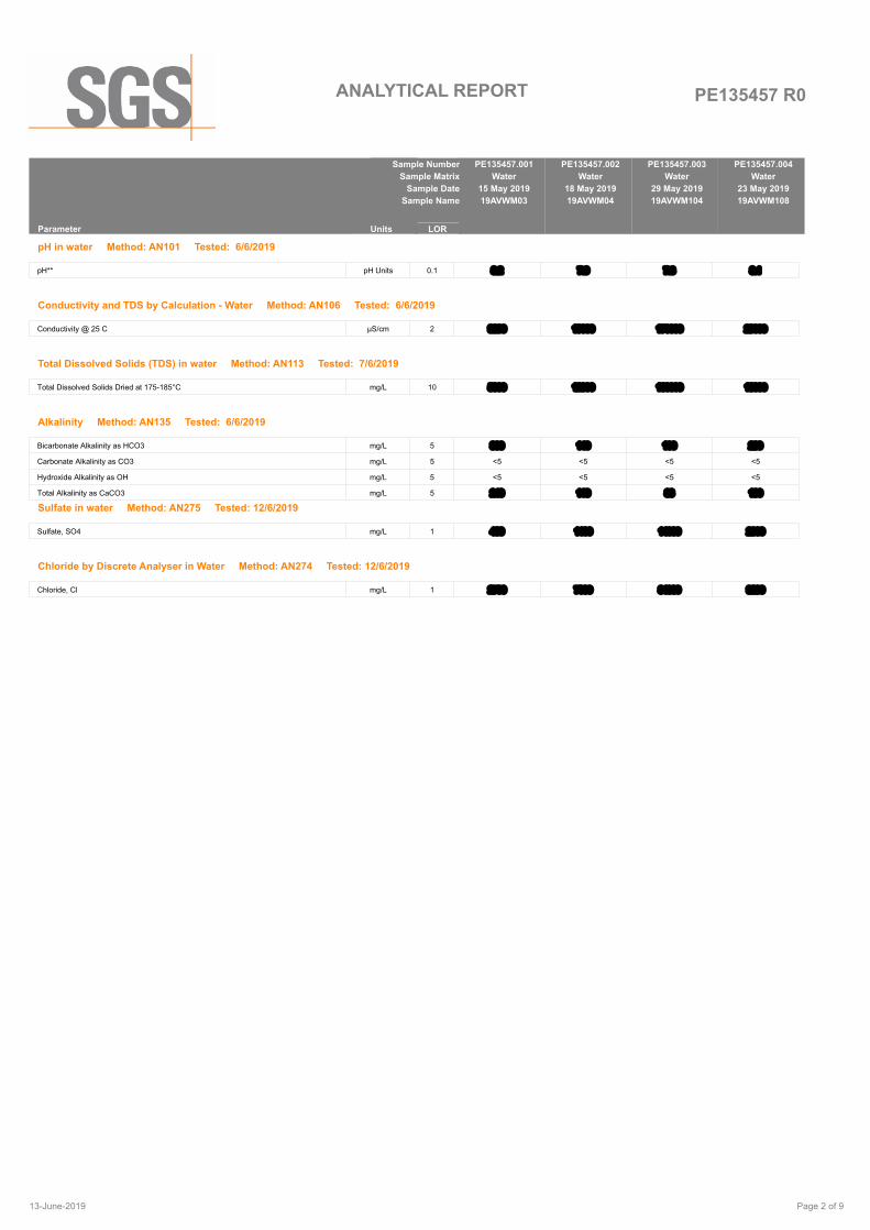
PE135457 R0ANALYTICAL REPORT
PE135457.001
Water
15 May 2019
19AVWM03
PE135457.002
Water
18 May 2019
19AVWM04
PE135457.003
Water
29 May 2019
19AVWM104
PE135457.004
Water
23 May 2019
19AVWM108
Parameter LORUnits
Sample Number
Sample Matrix
Sample Date
Sample Name
pH in water Method: AN101 Tested: 6/6/2019
pH** pH Units 0.1 8.2 7.9 7.3 8.1
Conductivity and TDS by Calculation - Water Method: AN106 Tested: 6/6/2019
Conductivity @ 25 C µS/cm 2 9200 19000 170000 29000
Total Dissolved Solids (TDS) in water Method: AN113 Tested: 7/6/2019
Total Dissolved Solids Dried at 175-185°C mg/L 10 5000 12000 160000 18000
Alkalinity Method: AN135 Tested: 6/6/2019
Bicarbonate Alkalinity as HCO3 mg/L 5 300 140 100 230
Carbonate Alkalinity as CO3 mg/L 5 <5 <5 <5 <5
Hydroxide Alkalinity as OH mg/L 5 <5 <5 <5 <5
Total Alkalinity as CaCO3 mg/L 5 240 110 83 190
Sulfate in water Method: AN275 Tested: 12/6/2019
Sulfate, SO4 mg/L 1 460 1100 14000 2000
Chloride by Discrete Analyser in Water Method: AN274 Tested: 12/6/2019
Chloride, Cl mg/L 1 2700 7000 84000 9200
Page 2 of 913-June-2019

PE135457 R0ANALYTICAL REPORT
PE135457.001
Water
15 May 2019
19AVWM03
PE135457.002
Water
18 May 2019
19AVWM04
PE135457.003
Water
29 May 2019
19AVWM104
PE135457.004
Water
23 May 2019
19AVWM108
Parameter LORUnits
Sample Number
Sample Matrix
Sample Date
Sample Name
Metals in Water (Dissolved) by ICPOES Method: AN320 Tested: 10/6/2019
Calcium, Ca mg/L 0.2 110 330 760 330
Magnesium, Mg mg/L 0.1 220 560 5700 890
Potassium, K mg/L 0.1 66 120 2200 160
Sodium, Na mg/L 0.5 1500 3100 43000 4500
Page 3 of 913-June-2019
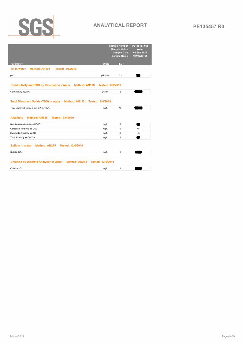
PE135457 R0ANALYTICAL REPORT
PE135457.005
Water
03 Jun 2019
19AVWM105
Parameter LORUnits
Sample Number
Sample Matrix
Sample Date
Sample Name
pH in water Method: AN101 Tested: 6/6/2019
pH** pH Units 0.1 7.2
Conductivity and TDS by Calculation - Water Method: AN106 Tested: 6/6/2019
Conductivity @ 25 C µS/cm 2 180000
Total Dissolved Solids (TDS) in water Method: AN113 Tested: 7/6/2019
Total Dissolved Solids Dried at 175-185°C mg/L 10 170000
Alkalinity Method: AN135 Tested: 6/6/2019
Bicarbonate Alkalinity as HCO3 mg/L 5 82
Carbonate Alkalinity as CO3 mg/L 5 <5
Hydroxide Alkalinity as OH mg/L 5 <5
Total Alkalinity as CaCO3 mg/L 5 67
Sulfate in water Method: AN275 Tested: 12/6/2019
Sulfate, SO4 mg/L 1 15000
Chloride by Discrete Analyser in Water Method: AN274 Tested: 12/6/2019
Chloride, Cl mg/L 1 86000
Page 4 of 913-June-2019

PE135457 R0ANALYTICAL REPORT
PE135457.005
Water
03 Jun 2019
19AVWM105
Parameter LORUnits
Sample Number
Sample Matrix
Sample Date
Sample Name
Metals in Water (Dissolved) by ICPOES Method: AN320 Tested: 10/6/2019
Calcium, Ca mg/L 0.2 760
Magnesium, Mg mg/L 0.1 6000
Potassium, K mg/L 0.1 2600
Sodium, Na mg/L 0.5 47000
Page 5 of 913-June-2019
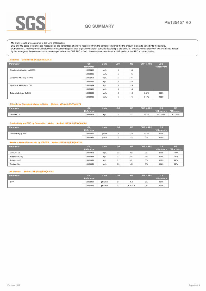
PE135457 R0QC SUMMARY
MB blank results are compared to the Limit of Reporting
LCS and MS spike recoveries are measured as the percentage of analyte recovered from the sample compared the the amount of analyte spiked into the sample.
DUP and MSD relative percent differences are measured against their original counterpart samples according to the formula : the absolute difference of the two results divided
by the average of the two results as a percentage. Where the DUP RPD is 'NA' , the results are less than the LOR and thus the RPD is not applicable.
Alkalinity Method: ME-(AU)-[ENV]AN135
MB DUP %RPD LCS
%Recovery
Bicarbonate Alkalinity as HCO3 LB160459 mg/L 5 <5
LB160460 mg/L 5 <5
Carbonate Alkalinity as CO3 LB160459 mg/L 5 <5
LB160460 mg/L 5 <5
Hydroxide Alkalinity as OH LB160459 mg/L 5 <5
LB160460 mg/L 5 <5
Total Alkalinity as CaCO3 LB160459 mg/L 5 <5 1 - 2% 104%
LB160460 mg/L 5 <5 0 - 1% 102%
LORUnits Parameter QC
Reference
Chloride by Discrete Analyser in Water Method: ME-(AU)-[ENV]AN274
MB DUP %RPD LCS
%Recovery
MS
%Recovery
Chloride, Cl LB160514 mg/L 1 <1 0 - 1% 99 - 100% 81 - 99%
LORUnits Parameter QC
Reference
Conductivity and TDS by Calculation - Water Method: ME-(AU)-[ENV]AN106
MB DUP %RPD LCS
%Recovery
Conductivity @ 25 C LB160451 µS/cm 2 <2 0 - 1% 100%
LB160452 µS/cm 2 <2 0% 102%
LORUnits Parameter QC
Reference
Metals in Water (Dissolved) by ICPOES Method: ME-(AU)-[ENV]AN320
MB DUP %RPD LCS
%Recovery
MS
%Recovery
Calcium, Ca LB160353 mg/L 0.2 <0.2 0% 106% 103%
Magnesium, Mg LB160353 mg/L 0.1 <0.1 1% 106% 104%
Potassium, K LB160353 mg/L 0.1 <0.1 0% 105% 99%
Sodium, Na LB160353 mg/L 0.5 <0.5 0% 104% 92%
LORUnits Parameter QC
Reference
pH in water Method: ME-(AU)-[ENV]AN101
MB DUP %RPD LCS
%Recovery
pH** LB160451 pH Units 0.1 5.5 0% 101%
LB160452 pH Units 0.1 5.6 - 5.7 0% 100%
LORUnits Parameter QC
Reference
Page 6 of 913-June-2019
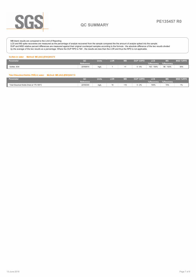
PE135457 R0QC SUMMARY
MB blank results are compared to the Limit of Reporting
LCS and MS spike recoveries are measured as the percentage of analyte recovered from the sample compared the the amount of analyte spiked into the sample.
DUP and MSD relative percent differences are measured against their original counterpart samples according to the formula : the absolute difference of the two results divided
by the average of the two results as a percentage. Where the DUP RPD is 'NA' , the results are less than the LOR and thus the RPD is not applicable.
Sulfate in water Method: ME-(AU)-[ENV]AN275
MB DUP %RPD LCS
%Recovery
MS
%Recovery
MSD %RPD
Sulfate, SO4 LB160514 mg/L 1 <1 0 - 4% 102 - 104% 96 - 102% 30%
LORUnits Parameter QC
Reference
Total Dissolved Solids (TDS) in water Method: ME-(AU)-[ENV]AN113
MB DUP %RPD LCS
%Recovery
MS
%Recovery
MSD %RPD
Total Dissolved Solids Dried at 175-185°C LB160344 mg/L 10 <10 0 - 2% 100% 72% 1%
LORUnits Parameter QC
Reference
Page 7 of 913-June-2019

PE135457 R0
METHOD METHODOLOGY SUMMARY
METHOD SUMMARY
pH in Soil Sludge Sediment and Water: pH is measured electrometrically using a combination electrode (glass plus
reference electrode) and is calibrated against 3 buffers purchased commercially. For soils, an extract with water is
made at a ratio of 1:5 and the pH determined and reported on the extract. Reference APHA 4500-H+.
AN101
Conductivity and TDS by Calculation: Conductivity is measured by meter with temperature compensation and is
calibrated against a standard solution of potassium chloride. Conductivity is generally reported as µmhos/cm or
µS/cm @ 25°C. For soils, an extract with water is made at a ratio of 1:5 and the EC determined and reported on
the extract, or calculated back to the as-received sample. Total Dissolved Salts can be estimated from conductivity
using a conversion factor, which for natural waters, is in the range 0.55 to 0.75. SGS use 0.6. Reference APHA
2510 B.
AN106
Salinity may be calculated in terms of NaCl from the sample conductivity. This assumes all soluble salts present,
measured by the conductivity, are present as NaCl.
AN106
Total Dissolved Solids: A well-mixed filtered sample of known volume is evaporated to dryness at 180°C and the
residue weighed. Approximate methods for correlating chemical analysis with dissolved solids are available.
Reference APHA 2540 C.
AN113
The Total Dissolved Solids residue may also be ignited at 550 C and volatile TDS (Organic TDS) and non-volatile
TDS (Inorganic) can be determined.
AN113
Alkalinity (and forms of) by Titration: The sample is titrated with standard acid to pH 8.3 (P titre) and pH 4.5 (T titre)
and permanent and/or total alkalinity calculated. The results are expressed as equivalents of calcium carbonate or
recalculated as bicarbonate, carbonate and hydroxide. Reference APHA 2320. Internal Reference AN135
AN135
Chloride by Aquakem DA: Chloride reacts with mercuric thiocyanate forming a mercuric chloride complex. In the
presence of ferric iron, highly coloured ferric thiocyanate is formed which is proportional to the chloride
concentration. Reference APHA 4500Cl-
AN274
sulfate by Aquakem DA: sulfate is precipitated in an acidic medium with barium chloride. The resulting turbidity is
measured photometrically at 405nm and compared with standard calibration solutions to determine the sulfate
concentration in the sample. Reference APHA 4500-SO42-. Internal reference AN275.
AN275
Metals by ICP-OES: Samples are preserved with 10% nitric acid for a wide range of metals and some non-metals.
This solution is measured by Inductively Coupled Plasma. Solutions are aspirated into an argon plasma at
8000-10000K and emit characteristic energy or light as a result of electron transitions through unique energy
levels. The emitted light is focused onto a diffraction grating where it is separated into components .
AN320
Photomultipliers or CCDs are used to measure the light intensity at specific wavelengths. This intensity is directly
proportional to concentration. Corrections are required to compensate for spectral overlap between elements.
Reference APHA 3120 B.
AN320
Free and Total Carbon Dioxide may be calculated using alkalinity forms only when the samples TDS is <500mg/L.
If TDS is >500mg/L free or total carbon dioxide cannot be reported . APHA4500CO2 D.
Calculation
Page 8 of 913-June-2019

PE135457 R0
Unless it is reported that sampling has been perfomed by SGS, the samples have been analysed as received.
Solid samples expressed on a dry weight basis.
Where "Total" analyte groups are reported (for example, Total PAHs, Total OC Pesticides) the total will be calculated as the sum of the individual
analytes, with those analytes that are reported as <LOR being assumed to be zero. The summed (Total) limit of reporting is calcuated by summing
the individual analyte LORs and dividing by two. For example, where 16 individual analytes are being summed and each has an LOR of 0.1 mg/kg,
the "Totals" LOR will be 1.6 / 2 (0.8 mg/kg). Where only 2 analytes are being summed, the " Total" LOR will be the sum of those two LORs.
Some totals may not appear to add up because the total is rounded after adding up the raw values.
If reported, measurement uncertainty follow the ± sign after the analytical result and is expressed as the expanded uncertainty calculated using a
coverage factor of 2, providing a level of confidence of approximately 95%, unless stated otherwise in the comments section of this report.
Results reported for samples tested under test methods with codes starting with ARS -SOP, radionuclide or gross radioactivity concentrations are
expressed in becquerel (Bq) per unit of mass or volume or per wipe as stated on the report. Becquerel is the SI unit for activity and equals one
nuclear transformation per second.
Note that in terms of units of radioactivity:
a. 1 Bq is equivalent to 27 pCi
b. 37 MBq is equivalent to 1 mCi
For results reported for samples tested under test methods with codes starting with ARS -SOP, less than (<) values indicate the detection limit for
each radionuclide or parameter for the measurement system used. The respective detection limits have been calculated in accordance with ISO
11929.
The QC and MU criteria are subject to internal review according to the SGS QAQC plan and may be provided on request or alternatively can be
found here: www.sgs.com.au.pv.sgsvr/en-gb/environment.
This document is issued by the Company under its General Conditions of Service accessible at www.sgs.com/en/Terms-and-Conditions.aspx.
Attention is drawn to the limitation of liability, indemnification and jurisdiction issues defined therein.
Any holder of this document is advised that information contained hereon reflects the Company 's findings at the time of its intervention only and
within the limits of Client's instructions, if any. The Company's sole responsibility is to its Client only. Any unauthorized alteration, forgery or
falsification of the content or appearance of this document is unlawful and offenders may be prosecuted to the fullest extent of the law .
This report must not be reproduced, except in full.
IS
LNR
*
**
Insufficient sample for analysis.
Sample listed, but not received.
NATA accreditation does not cover the
performance of this service.
Indicative data, theoretical holding time exceeded.
FOOTNOTES
LOR
↑↓
QFH
QFL
-
NVL
Limit of Reporting
Raised or Lowered Limit of Reporting
QC result is above the upper tolerance
QC result is below the lower tolerance
The sample was not analysed for this analyte
Not Validated
Page 9 of 913-June-2019
Accreditation No. 2562
Date Reported
Contact
SGS Perth Environmental
28 Reid Rd
Perth Airport WA 6105
Marjana Siljanoska
(08) 9373 3500
(08) 9373 3556
2
SGS Reference
Facsimile
Telephone
Address
Manager
Laboratory
183C C2
183C AVL C2
(Not specified)
61 8 93238821
PO BOX 976
SOUTH PERTH WA 6951
AQ2
Liam Storey
Samples
Order Number
Project
Facsimile
Telephone
Address
Client
CLIENT DETAILS LABORATORY DETAILS
08 Jul 2019
ANALYTICAL REPORT
PE136072 R0
02 Jul 2019Date Received
Accredited for compliance with ISO/IEC 17025 - Testing. NATA accredited laboratory 2562(898/20210).
COMMENTS
Louise Hope
Laboratory Technician
Mary Ann Ola-A
Inorganics Team Leader
Sanaa Hussain
Chemist
SIGNATORIES
SGS Australia Pty Ltd
ABN 44 000 964 278
Environment, Health and Safety 28 Reid Rd
PO Box 32
Perth Airport WA 6105
Welshpool WA 6983
Australia
Australia
t +61 8 9373 3500
f +61 8 9373 3556
www.sgs.com.au
Member of the SGS Group
Page 1 of 708-July-2019

PE136072 R0ANALYTICAL REPORT
PE136072.001
Water
15 Jun 2019
DEB01R
PE136072.002
Water
15 Jun 2019
DEB10
Parameter LORUnits
Sample Number
Sample Matrix
Sample Date
Sample Name
pH in water Method: AN101 Tested: 2/7/2019
pH** pH Units 0.1 7.8 7.9
Conductivity and TDS by Calculation - Water Method: AN106 Tested: 2/7/2019
Conductivity @ 25 C µS/cm 2 16000 2800
Total Dissolved Solids (TDS) in water Method: AN113 Tested: 3/7/2019
Total Dissolved Solids Dried at 175-185°C mg/L 10 9400 1500
Alkalinity Method: AN135 Tested: 2/7/2019
Bicarbonate Alkalinity as HCO3 mg/L 5 260 310
Carbonate Alkalinity as CO3 mg/L 5 <5 <5
Hydroxide Alkalinity as OH mg/L 5 <5 <5
Total Alkalinity as CaCO3 mg/L 5 210 260
Sulfate in water Method: AN275 Tested: 3/7/2019
Sulfate, SO4 mg/L 1 170 1100
Chloride by Discrete Analyser in Water Method: AN274 Tested: 3/7/2019
Chloride, Cl mg/L 1 550 4400
Page 2 of 708-July-2019

PE136072 R0ANALYTICAL REPORT
PE136072.001
Water
15 Jun 2019
DEB01R
PE136072.002
Water
15 Jun 2019
DEB10
Parameter LORUnits
Sample Number
Sample Matrix
Sample Date
Sample Name
Metals in Water (Dissolved) by ICPOES Method: AN320 Tested: 3/7/2019
Calcium, Ca mg/L 0.2 160 81
Magnesium, Mg mg/L 0.1 450 110
Potassium, K mg/L 0.1 130 3.7
Sodium, Na mg/L 0.5 2700 310
Page 3 of 708-July-2019
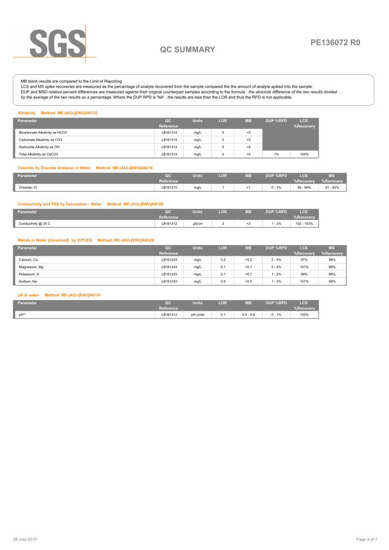
PE136072 R0QC SUMMARY
MB blank results are compared to the Limit of Reporting
LCS and MS spike recoveries are measured as the percentage of analyte recovered from the sample compared the the amount of analyte spiked into the sample.
DUP and MSD relative percent differences are measured against their original counterpart samples according to the formula : the absolute difference of the two results divided
by the average of the two results as a percentage. Where the DUP RPD is 'NA' , the results are less than the LOR and thus the RPD is not applicable.
Alkalinity Method: ME-(AU)-[ENV]AN135
MB DUP %RPD LCS
%Recovery
Bicarbonate Alkalinity as HCO3 LB161314 mg/L 5 <5
Carbonate Alkalinity as CO3 LB161314 mg/L 5 <5
Hydroxide Alkalinity as OH LB161314 mg/L 5 <5
Total Alkalinity as CaCO3 LB161314 mg/L 5 <5 1% 104%
LORUnits Parameter QC
Reference
Chloride by Discrete Analyser in Water Method: ME-(AU)-[ENV]AN274
MB DUP %RPD LCS
%Recovery
MS
%Recovery
Chloride, Cl LB161270 mg/L 1 <1 0 - 1% 98 - 99% 91 - 92%
LORUnits Parameter QC
Reference
Conductivity and TDS by Calculation - Water Method: ME-(AU)-[ENV]AN106
MB DUP %RPD LCS
%Recovery
Conductivity @ 25 C LB161312 µS/cm 2 <2 1 - 2% 102 - 103%
LORUnits Parameter QC
Reference
Metals in Water (Dissolved) by ICPOES Method: ME-(AU)-[ENV]AN320
MB DUP %RPD LCS
%Recovery
MS
%Recovery
Calcium, Ca LB161243 mg/L 0.2 <0.2 2 - 4% 97% 98%
Magnesium, Mg LB161243 mg/L 0.1 <0.1 2 - 4% 101% 98%
Potassium, K LB161243 mg/L 0.1 <0.1 1 - 2% 99% 98%
Sodium, Na LB161243 mg/L 0.5 <0.5 1 - 3% 101% 99%
LORUnits Parameter QC
Reference
pH in water Method: ME-(AU)-[ENV]AN101
MB DUP %RPD LCS
%Recovery
pH** LB161312 pH Units 0.1 5.5 - 5.6 0 - 1% 100%
LORUnits Parameter QC
Reference
Page 4 of 708-July-2019

PE136072 R0QC SUMMARY
MB blank results are compared to the Limit of Reporting
LCS and MS spike recoveries are measured as the percentage of analyte recovered from the sample compared the the amount of analyte spiked into the sample.
DUP and MSD relative percent differences are measured against their original counterpart samples according to the formula : the absolute difference of the two results divided
by the average of the two results as a percentage. Where the DUP RPD is 'NA' , the results are less than the LOR and thus the RPD is not applicable.
Sulfate in water Method: ME-(AU)-[ENV]AN275
MB DUP %RPD LCS
%Recovery
MS
%Recovery
Sulfate, SO4 LB161270 mg/L 1 <1 0 - 4% 99% 96 - 99%
LORUnits Parameter QC
Reference
Total Dissolved Solids (TDS) in water Method: ME-(AU)-[ENV]AN113
MB DUP %RPD LCS
%Recovery
MS
%Recovery
MSD %RPD
Total Dissolved Solids Dried at 175-185°C LB161274 mg/L 10 <10 0 - 3% 95% 104% 3%
LORUnits Parameter QC
Reference
Page 5 of 708-July-2019
PE136072 R0
METHOD METHODOLOGY SUMMARY
METHOD SUMMARY
pH in Soil Sludge Sediment and Water: pH is measured electrometrically using a combination electrode (glass plus
reference electrode) and is calibrated against 3 buffers purchased commercially. For soils, an extract with water is
made at a ratio of 1:5 and the pH determined and reported on the extract. Reference APHA 4500-H+.
AN101
Conductivity and TDS by Calculation: Conductivity is measured by meter with temperature compensation and is
calibrated against a standard solution of potassium chloride. Conductivity is generally reported as µmhos/cm or
µS/cm @ 25°C. For soils, an extract with water is made at a ratio of 1:5 and the EC determined and reported on
the extract, or calculated back to the as-received sample. Total Dissolved Salts can be estimated from conductivity
using a conversion factor, which for natural waters, is in the range 0.55 to 0.75. SGS use 0.6. Reference APHA
2510 B.
AN106
Salinity may be calculated in terms of NaCl from the sample conductivity. This assumes all soluble salts present,
measured by the conductivity, are present as NaCl.
AN106
Total Dissolved Solids: A well-mixed filtered sample of known volume is evaporated to dryness at 180°C and the
residue weighed. Approximate methods for correlating chemical analysis with dissolved solids are available.
Reference APHA 2540 C.
AN113
The Total Dissolved Solids residue may also be ignited at 550 C and volatile TDS (Organic TDS) and non-volatile
TDS (Inorganic) can be determined.
AN113
Alkalinity (and forms of) by Titration: The sample is titrated with standard acid to pH 8.3 (P titre) and pH 4.5 (T titre)
and permanent and/or total alkalinity calculated. The results are expressed as equivalents of calcium carbonate or
recalculated as bicarbonate, carbonate and hydroxide. Reference APHA 2320. Internal Reference AN135
AN135
Chloride by Aquakem DA: Chloride reacts with mercuric thiocyanate forming a mercuric chloride complex. In the
presence of ferric iron, highly coloured ferric thiocyanate is formed which is proportional to the chloride
concentration. Reference APHA 4500Cl-
AN274
sulfate by Aquakem DA: sulfate is precipitated in an acidic medium with barium chloride. The resulting turbidity is
measured photometrically at 405nm and compared with standard calibration solutions to determine the sulfate
concentration in the sample. Reference APHA 4500-SO42-. Internal reference AN275.
AN275
Metals by ICP-OES: Samples are preserved with 10% nitric acid for a wide range of metals and some non-metals.
This solution is measured by Inductively Coupled Plasma. Solutions are aspirated into an argon plasma at
8000-10000K and emit characteristic energy or light as a result of electron transitions through unique energy
levels. The emitted light is focused onto a diffraction grating where it is separated into components .
AN320
Photomultipliers or CCDs are used to measure the light intensity at specific wavelengths. This intensity is directly
proportional to concentration. Corrections are required to compensate for spectral overlap between elements.
Reference APHA 3120 B.
AN320
Free and Total Carbon Dioxide may be calculated using alkalinity forms only when the samples TDS is <500mg/L.
If TDS is >500mg/L free or total carbon dioxide cannot be reported . APHA4500CO2 D.
Calculation
Page 6 of 708-July-2019

PE136072 R0
Unless it is reported that sampling has been performed by SGS, the samples have been analysed as received.
Solid samples expressed on a dry weight basis.
Where "Total" analyte groups are reported (for example, Total PAHs, Total OC Pesticides) the total will be calculated as the sum of the individual
analytes, with those analytes that are reported as <LOR being assumed to be zero. The summed (Total) limit of reporting is calcuated by summing
the individual analyte LORs and dividing by two. For example, where 16 individual analytes are being summed and each has an LOR of 0.1 mg/kg,
the "Totals" LOR will be 1.6 / 2 (0.8 mg/kg). Where only 2 analytes are being summed, the " Total" LOR will be the sum of those two LORs.
Some totals may not appear to add up because the total is rounded after adding up the raw values.
If reported, measurement uncertainty follow the ± sign after the analytical result and is expressed as the expanded uncertainty calculated using a
coverage factor of 2, providing a level of confidence of approximately 95%, unless stated otherwise in the comments section of this report.
Results reported for samples tested under test methods with codes starting with ARS -SOP, radionuclide or gross radioactivity concentrations are
expressed in becquerel (Bq) per unit of mass or volume or per wipe as stated on the report. Becquerel is the SI unit for activity and equals one
nuclear transformation per second.
Note that in terms of units of radioactivity:
a. 1 Bq is equivalent to 27 pCi
b. 37 MBq is equivalent to 1 mCi
For results reported for samples tested under test methods with codes starting with ARS -SOP, less than (<) values indicate the detection limit for
each radionuclide or parameter for the measurement system used. The respective detection limits have been calculated in accordance with ISO
11929.
The QC and MU criteria are subject to internal review according to the SGS QAQC plan and may be provided on request or alternatively can be
found here: www.sgs.com.au.pv.sgsvr/en-gb/environment.
This document is issued by the Company under its General Conditions of Service accessible at www.sgs.com/en/Terms-and-Conditions.aspx.
Attention is drawn to the limitation of liability, indemnification and jurisdiction issues defined therein.
Any holder of this document is advised that information contained hereon reflects the Company 's findings at the time of its intervention only and
within the limits of Client's instructions, if any. The Company's sole responsibility is to its Client only. Any unauthorized alteration, forgery or
falsification of the content or appearance of this document is unlawful and offenders may be prosecuted to the fullest extent of the law .
This report must not be reproduced, except in full.
IS
LNR
*
**
Insufficient sample for analysis.
Sample listed, but not received.
NATA accreditation does not cover the
performance of this service.
Indicative data, theoretical holding time exceeded.
FOOTNOTES
LOR
↑↓
QFH
QFL
-
NVL
Limit of Reporting
Raised or Lowered Limit of Reporting
QC result is above the upper tolerance
QC result is below the lower tolerance
The sample was not analysed for this analyte
Not Validated
Page 7 of 708-July-2019
Accreditation No. 2562
Date Reported
Contact
SGS Perth Environmental
28 Reid Rd
Perth Airport WA 6105
Marjana Siljanoska
(08) 9373 3500
(08) 9373 3556
2
SGS Reference
Facsimile
Telephone
Address
Manager
Laboratory
183C C2
183C AVL C2
(Not specified)
61 8 93238821
PO BOX 976
SOUTH PERTH WA 6951
AQ2
Emma Bolton
Samples
Order Number
Project
Facsimile
Telephone
Address
Client
CLIENT DETAILS LABORATORY DETAILS
29 Jul 2019
ANALYTICAL REPORT
PE136531 R0
19 Jul 2019Date Received
Accredited for compliance with ISO/IEC 17025 - Testing. NATA accredited laboratory 2562(898/20210).
For determination of soluble metals, filtered sample was not received so samples were laboratory filtered on receipt. This may give soluble metals
results that do not represent the concentrations present at the time of sampling.
Metals: LORs raised due to high conductivity.
The upper limit for Conductivity in Water is 100,000 uS/cm. Any result above this is an estimate. This will also cause the TDS on EC ratio to bias
high.
COMMENTS
Louise Hope
Laboratory Technician
Mary Ann Ola-A
Inorganics Team Leader
Sanaa Hussain
Chemist
SIGNATORIES
SGS Australia Pty Ltd
ABN 44 000 964 278
Environment, Health and Safety 28 Reid Rd
PO Box 32
Perth Airport WA 6105
Welshpool WA 6983
Australia
Australia
t +61 8 9373 3500
f +61 8 9373 3556
www.sgs.com.au
Member of the SGS Group
Page 1 of 729-July-2019
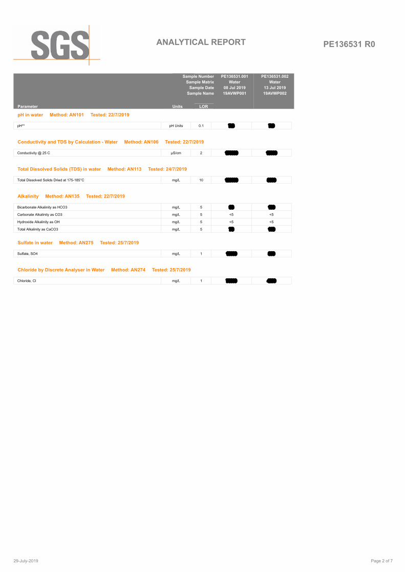
PE136531 R0ANALYTICAL REPORT
PE136531.001
Water
08 Jul 2019
19AVWP001
PE136531.002
Water
13 Jul 2019
19AVWP002
Parameter LORUnits
Sample Number
Sample Matrix
Sample Date
Sample Name
pH in water Method: AN101 Tested: 22/7/2019
pH** pH Units 0.1 7.3 7.9
Conductivity and TDS by Calculation - Water Method: AN106 Tested: 22/7/2019
Conductivity @ 25 C µS/cm 2 170000 15000
Total Dissolved Solids (TDS) in water Method: AN113 Tested: 24/7/2019
Total Dissolved Solids Dried at 175-185°C mg/L 10 120000 8300
Alkalinity Method: AN135 Tested: 22/7/2019
Bicarbonate Alkalinity as HCO3 mg/L 5 93 130
Carbonate Alkalinity as CO3 mg/L 5 <5 <5
Hydroxide Alkalinity as OH mg/L 5 <5 <5
Total Alkalinity as CaCO3 mg/L 5 76 110
Sulfate in water Method: AN275 Tested: 25/7/2019
Sulfate, SO4 mg/L 1 18000 850
Chloride by Discrete Analyser in Water Method: AN274 Tested: 25/7/2019
Chloride, Cl mg/L 1 76000 4200
Page 2 of 729-July-2019

PE136531 R0ANALYTICAL REPORT
PE136531.001
Water
08 Jul 2019
19AVWP001
PE136531.002
Water
13 Jul 2019
19AVWP002
Parameter LORUnits
Sample Number
Sample Matrix
Sample Date
Sample Name
Metals in Water (Dissolved) by ICPOES Method: AN320 Tested: 23/7/2019
Calcium, Ca mg/L 0.2 680 250
Magnesium, Mg mg/L 0.1 5300 400
Potassium, K mg/L 0.1 2500 94
Sodium, Na mg/L 0.5 43000 2300
Page 3 of 729-July-2019
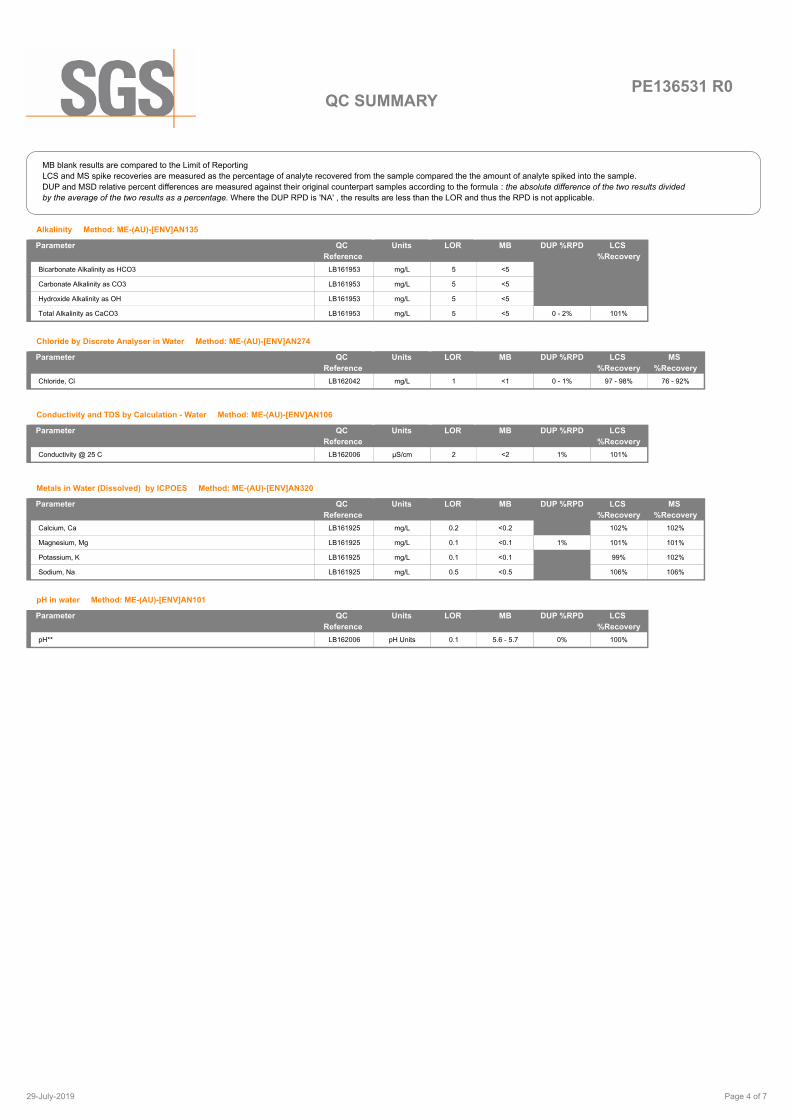
PE136531 R0QC SUMMARY
MB blank results are compared to the Limit of Reporting
LCS and MS spike recoveries are measured as the percentage of analyte recovered from the sample compared the the amount of analyte spiked into the sample.
DUP and MSD relative percent differences are measured against their original counterpart samples according to the formula : the absolute difference of the two results divided
by the average of the two results as a percentage. Where the DUP RPD is 'NA' , the results are less than the LOR and thus the RPD is not applicable.
Alkalinity Method: ME-(AU)-[ENV]AN135
MB DUP %RPD LCS
%Recovery
Bicarbonate Alkalinity as HCO3 LB161953 mg/L 5 <5
Carbonate Alkalinity as CO3 LB161953 mg/L 5 <5
Hydroxide Alkalinity as OH LB161953 mg/L 5 <5
Total Alkalinity as CaCO3 LB161953 mg/L 5 <5 0 - 2% 101%
LORUnits Parameter QC
Reference
Chloride by Discrete Analyser in Water Method: ME-(AU)-[ENV]AN274
MB DUP %RPD LCS
%Recovery
MS
%Recovery
Chloride, Cl LB162042 mg/L 1 <1 0 - 1% 97 - 98% 76 - 92%
LORUnits Parameter QC
Reference
Conductivity and TDS by Calculation - Water Method: ME-(AU)-[ENV]AN106
MB DUP %RPD LCS
%Recovery
Conductivity @ 25 C LB162006 µS/cm 2 <2 1% 101%
LORUnits Parameter QC
Reference
Metals in Water (Dissolved) by ICPOES Method: ME-(AU)-[ENV]AN320
MB DUP %RPD LCS
%Recovery
MS
%Recovery
Calcium, Ca LB161925 mg/L 0.2 <0.2 102% 102%
Magnesium, Mg LB161925 mg/L 0.1 <0.1 1% 101% 101%
Potassium, K LB161925 mg/L 0.1 <0.1 99% 102%
Sodium, Na LB161925 mg/L 0.5 <0.5 106% 106%
LORUnits Parameter QC
Reference
pH in water Method: ME-(AU)-[ENV]AN101
MB DUP %RPD LCS
%Recovery
pH** LB162006 pH Units 0.1 5.6 - 5.7 0% 100%
LORUnits Parameter QC
Reference
Page 4 of 729-July-2019
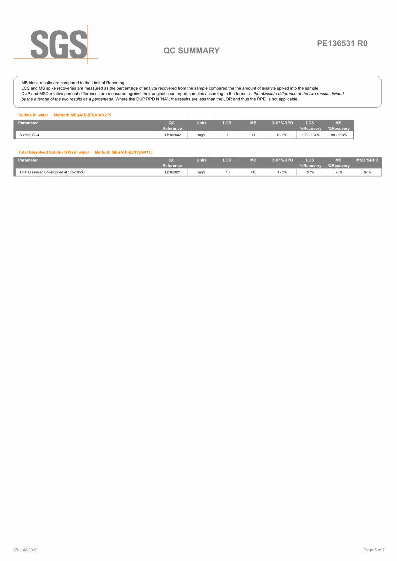
PE136531 R0QC SUMMARY
MB blank results are compared to the Limit of Reporting
LCS and MS spike recoveries are measured as the percentage of analyte recovered from the sample compared the the amount of analyte spiked into the sample.
DUP and MSD relative percent differences are measured against their original counterpart samples according to the formula : the absolute difference of the two results divided
by the average of the two results as a percentage. Where the DUP RPD is 'NA' , the results are less than the LOR and thus the RPD is not applicable.
Sulfate in water Method: ME-(AU)-[ENV]AN275
MB DUP %RPD LCS
%Recovery
MS
%Recovery
Sulfate, SO4 LB162042 mg/L 1 <1 0 - 2% 103 - 104% 98 - 113%
LORUnits Parameter QC
Reference
Total Dissolved Solids (TDS) in water Method: ME-(AU)-[ENV]AN113
MB DUP %RPD LCS
%Recovery
MS
%Recovery
MSD %RPD
Total Dissolved Solids Dried at 175-185°C LB162021 mg/L 10 <10 1 - 3% 97% 76% 87%
LORUnits Parameter QC
Reference
Page 5 of 729-July-2019

PE136531 R0
METHOD METHODOLOGY SUMMARY
METHOD SUMMARY
pH in Soil Sludge Sediment and Water: pH is measured electrometrically using a combination electrode (glass plus
reference electrode) and is calibrated against 3 buffers purchased commercially. For soils, an extract with water is
made at a ratio of 1:5 and the pH determined and reported on the extract. Reference APHA 4500-H+.
AN101
Conductivity and TDS by Calculation: Conductivity is measured by meter with temperature compensation and is
calibrated against a standard solution of potassium chloride. Conductivity is generally reported as µmhos/cm or
µS/cm @ 25°C. For soils, an extract with water is made at a ratio of 1:5 and the EC determined and reported on
the extract, or calculated back to the as-received sample. Total Dissolved Salts can be estimated from conductivity
using a conversion factor, which for natural waters, is in the range 0.55 to 0.75. SGS use 0.6. Reference APHA
2510 B.
AN106
Salinity may be calculated in terms of NaCl from the sample conductivity. This assumes all soluble salts present,
measured by the conductivity, are present as NaCl.
AN106
Total Dissolved Solids: A well-mixed filtered sample of known volume is evaporated to dryness at 180°C and the
residue weighed. Approximate methods for correlating chemical analysis with dissolved solids are available.
Reference APHA 2540 C.
AN113
The Total Dissolved Solids residue may also be ignited at 550 C and volatile TDS (Organic TDS) and non-volatile
TDS (Inorganic) can be determined.
AN113
Alkalinity (and forms of) by Titration: The sample is titrated with standard acid to pH 8.3 (P titre) and pH 4.5 (T titre)
and permanent and/or total alkalinity calculated. The results are expressed as equivalents of calcium carbonate or
recalculated as bicarbonate, carbonate and hydroxide. Reference APHA 2320. Internal Reference AN135
AN135
Chloride by Aquakem DA: Chloride reacts with mercuric thiocyanate forming a mercuric chloride complex. In the
presence of ferric iron, highly coloured ferric thiocyanate is formed which is proportional to the chloride
concentration. Reference APHA 4500Cl-
AN274
sulfate by Aquakem DA: sulfate is precipitated in an acidic medium with barium chloride. The resulting turbidity is
measured photometrically at 405nm and compared with standard calibration solutions to determine the sulfate
concentration in the sample. Reference APHA 4500-SO42-. Internal reference AN275.
AN275
Metals by ICP-OES: Samples are preserved with 10% nitric acid for a wide range of metals and some non-metals.
This solution is measured by Inductively Coupled Plasma. Solutions are aspirated into an argon plasma at
8000-10000K and emit characteristic energy or light as a result of electron transitions through unique energy
levels. The emitted light is focused onto a diffraction grating where it is separated into components .
AN320
Photomultipliers or CCDs are used to measure the light intensity at specific wavelengths. This intensity is directly
proportional to concentration. Corrections are required to compensate for spectral overlap between elements.
Reference APHA 3120 B.
AN320
Free and Total Carbon Dioxide may be calculated using alkalinity forms only when the samples TDS is <500mg/L.
If TDS is >500mg/L free or total carbon dioxide cannot be reported . APHA4500CO2 D.
Calculation
Page 6 of 729-July-2019

PE136531 R0
Unless it is reported that sampling has been performed by SGS, the samples have been analysed as received.
Solid samples expressed on a dry weight basis.
Where "Total" analyte groups are reported (for example, Total PAHs, Total OC Pesticides) the total will be calculated as the sum of the individual
analytes, with those analytes that are reported as <LOR being assumed to be zero. The summed (Total) limit of reporting is calcuated by summing
the individual analyte LORs and dividing by two. For example, where 16 individual analytes are being summed and each has an LOR of 0.1 mg/kg,
the "Totals" LOR will be 1.6 / 2 (0.8 mg/kg). Where only 2 analytes are being summed, the " Total" LOR will be the sum of those two LORs.
Some totals may not appear to add up because the total is rounded after adding up the raw values.
If reported, measurement uncertainty follow the ± sign after the analytical result and is expressed as the expanded uncertainty calculated using a
coverage factor of 2, providing a level of confidence of approximately 95%, unless stated otherwise in the comments section of this report.
Results reported for samples tested under test methods with codes starting with ARS -SOP, radionuclide or gross radioactivity concentrations are
expressed in becquerel (Bq) per unit of mass or volume or per wipe as stated on the report. Becquerel is the SI unit for activity and equals one
nuclear transformation per second.
Note that in terms of units of radioactivity:
a. 1 Bq is equivalent to 27 pCi
b. 37 MBq is equivalent to 1 mCi
For results reported for samples tested under test methods with codes starting with ARS -SOP, less than (<) values indicate the detection limit for
each radionuclide or parameter for the measurement system used. The respective detection limits have been calculated in accordance with ISO
11929.
The QC and MU criteria are subject to internal review according to the SGS QAQC plan and may be provided on request or alternatively can be
found here: www.sgs.com.au.pv.sgsvr/en-gb/environment.
This document is issued by the Company under its General Conditions of Service accessible at www.sgs.com/en/Terms-and-Conditions.aspx.
Attention is drawn to the limitation of liability, indemnification and jurisdiction issues defined therein.
Any holder of this document is advised that information contained hereon reflects the Company 's findings at the time of its intervention only and
within the limits of Client's instructions, if any. The Company's sole responsibility is to its Client only. Any unauthorized alteration, forgery or
falsification of the content or appearance of this document is unlawful and offenders may be prosecuted to the fullest extent of the law .
This report must not be reproduced, except in full.
IS
LNR
*
**
Insufficient sample for analysis.
Sample listed, but not received.
NATA accreditation does not cover the
performance of this service.
Indicative data, theoretical holding time exceeded.
FOOTNOTES
LOR
↑↓
QFH
QFL
-
NVL
Limit of Reporting
Raised or Lowered Limit of Reporting
QC result is above the upper tolerance
QC result is below the lower tolerance
The sample was not analysed for this analyte
Not Validated
Page 7 of 729-July-2019

Accreditation No. 2562
Date Reported
Contact
SGS Perth Environmental
28 Reid Rd
Perth Airport WA 6105
Marjana Siljanoska
(08) 9373 3500
(08) 9373 3556
2
SGS Reference
Facsimile
Telephone
Address
Manager
Laboratory
183C C2
183C AVL C2
(Not specified)
61 8 93238821
PO BOX 976
SOUTH PERTH WA 6951
AQ2
Emma Bolton
Samples
Order Number
Project
Facsimile
Telephone
Address
Client
CLIENT DETAILS LABORATORY DETAILS
23 Aug 2019
ANALYTICAL REPORT
PE137221 R0
16 Aug 2019Date Received
Accredited for compliance with ISO/IEC 17025 - Testing. NATA accredited laboratory 2562(898/20210).
For determination of soluble metals, filtered sample was not received so samples were laboratory filtered on receipt. This may give soluble metals
results that do not represent the concentrations present at the time of sampling.
The upper limit for Conductivity in Water is 100,000 uS/cm. Any result above this is an estimate. This will also cause the TDS on EC ratio to bias
high.
Metals: LORs raised due to high conductivity.
COMMENTS
Louise Hope
Laboratory Technician
Mary Ann Ola-A
Inorganics Team Leader
Sanaa Hussain
Chemist
SIGNATORIES
SGS Australia Pty Ltd
ABN 44 000 964 278
Environment, Health and Safety 28 Reid Rd
PO Box 32
Perth Airport WA 6105
Welshpool WA 6983
Australia
Australia
t +61 8 9373 3500
f +61 8 9373 3556
www.sgs.com.au
Member of the SGS Group
Page 1 of 723-August-2019
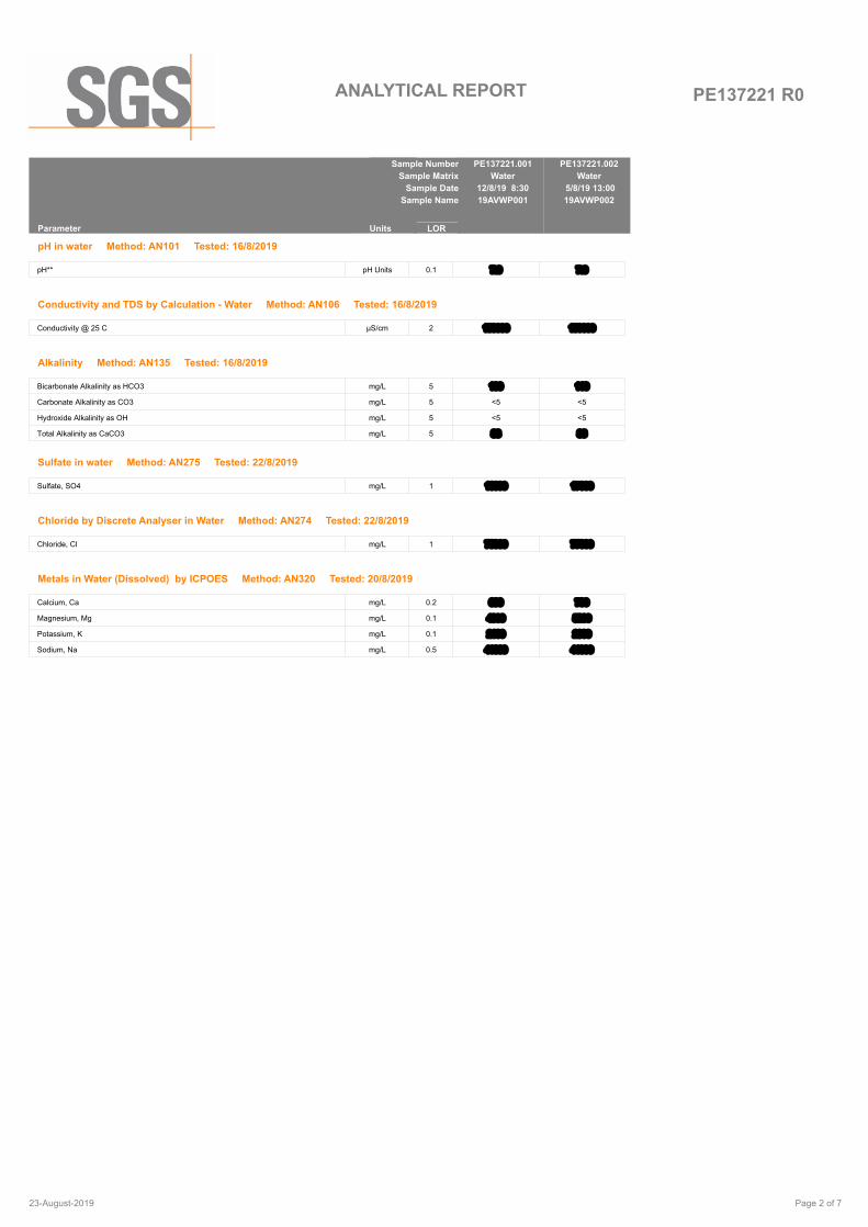
PE137221 R0ANALYTICAL REPORT
PE137221.001
Water
12/8/19 8:30
19AVWP001
PE137221.002
Water
5/8/19 13:00
19AVWP002
Parameter LORUnits
Sample Number
Sample Matrix
Sample Date
Sample Name
pH in water Method: AN101 Tested: 16/8/2019
pH** pH Units 0.1 7.0 7.0
Conductivity and TDS by Calculation - Water Method: AN106 Tested: 16/8/2019
Conductivity @ 25 C µS/cm 2 150000 150000
Alkalinity Method: AN135 Tested: 16/8/2019
Bicarbonate Alkalinity as HCO3 mg/L 5 100 110
Carbonate Alkalinity as CO3 mg/L 5 <5 <5
Hydroxide Alkalinity as OH mg/L 5 <5 <5
Total Alkalinity as CaCO3 mg/L 5 83 86
Sulfate in water Method: AN275 Tested: 22/8/2019
Sulfate, SO4 mg/L 1 16000 17000
Chloride by Discrete Analyser in Water Method: AN274 Tested: 22/8/2019
Chloride, Cl mg/L 1 75000 77000
Metals in Water (Dissolved) by ICPOES Method: AN320 Tested: 20/8/2019
Calcium, Ca mg/L 0.2 690 730
Magnesium, Mg mg/L 0.1 4900 5200
Potassium, K mg/L 0.1 2100 2300
Sodium, Na mg/L 0.5 41000 41000
Page 2 of 723-August-2019

PE137221 R0ANALYTICAL REPORT
PE137221.001
Water
12/8/19 8:30
19AVWP001
PE137221.002
Water
5/8/19 13:00
19AVWP002
Parameter LORUnits
Sample Number
Sample Matrix
Sample Date
Sample Name
Total Dissolved Solids (TDS) in water Method: AN113 Tested: 20/8/2019
Total Dissolved Solids Dried at 175-185°C mg/L 10 150000 150000
Page 3 of 723-August-2019

PE137221 R0QC SUMMARY
MB blank results are compared to the Limit of Reporting
LCS and MS spike recoveries are measured as the percentage of analyte recovered from the sample compared the the amount of analyte spiked into the sample.
DUP and MSD relative percent differences are measured against their original counterpart samples according to the formula : the absolute difference of the two results divided
by the average of the two results as a percentage. Where the DUP RPD is 'NA' , the results are less than the LOR and thus the RPD is not applicable.
Alkalinity Method: ME-(AU)-[ENV]AN135
MB DUP %RPD LCS
%Recovery
Bicarbonate Alkalinity as HCO3 LB162929 mg/L 5 <5
Carbonate Alkalinity as CO3 LB162929 mg/L 5 <5
Hydroxide Alkalinity as OH LB162929 mg/L 5 <5
Total Alkalinity as CaCO3 LB162929 mg/L 5 <5 1 - 2% 99 - 101%
LORUnits Parameter QC
Reference
Chloride by Discrete Analyser in Water Method: ME-(AU)-[ENV]AN274
MB DUP %RPD LCS
%Recovery
MS
%Recovery
Chloride, Cl LB163084 mg/L 1 <1 0 - 1% 105 - 106% 100 - 101%
LORUnits Parameter QC
Reference
Conductivity and TDS by Calculation - Water Method: ME-(AU)-[ENV]AN106
MB DUP %RPD LCS
%Recovery
Conductivity @ 25 C LB162934 µS/cm 2 <2 0% 101%
LORUnits Parameter QC
Reference
Metals in Water (Dissolved) by ICPOES Method: ME-(AU)-[ENV]AN320
MB DUP %RPD LCS
%Recovery
MS
%Recovery
Calcium, Ca LB162965 mg/L 0.2 <0.2 0 - 1% 95% 88%
Magnesium, Mg LB162965 mg/L 0.1 <0.1 1% 93% 90%
Potassium, K LB162965 mg/L 0.1 <0.1 1% 94% 87%
Sodium, Na LB162965 mg/L 0.5 <0.5 1% 97% 95%
LORUnits Parameter QC
Reference
pH in water Method: ME-(AU)-[ENV]AN101
MB DUP %RPD LCS
%Recovery
pH** LB162934 pH Units 0.1 5.7 0% 101%
LORUnits Parameter QC
Reference
Page 4 of 723-August-2019

PE137221 R0QC SUMMARY
MB blank results are compared to the Limit of Reporting
LCS and MS spike recoveries are measured as the percentage of analyte recovered from the sample compared the the amount of analyte spiked into the sample.
DUP and MSD relative percent differences are measured against their original counterpart samples according to the formula : the absolute difference of the two results divided
by the average of the two results as a percentage. Where the DUP RPD is 'NA' , the results are less than the LOR and thus the RPD is not applicable.
Sulfate in water Method: ME-(AU)-[ENV]AN275
MB DUP %RPD LCS
%Recovery
MS
%Recovery
Sulfate, SO4 LB163084 mg/L 1 <1 0 - 7% 102 - 103% 100 - 102%
LORUnits Parameter QC
Reference
Total Dissolved Solids (TDS) in water Method: ME-(AU)-[ENV]AN113
MB DUP %RPD LCS
%Recovery
MS
%Recovery
MSD %RPD
Total Dissolved Solids Dried at 175-185°C LB163002 mg/L 10 <10 1 - 2% 97% 98% 5%
LORUnits Parameter QC
Reference
Page 5 of 723-August-2019

PE137221 R0
METHOD METHODOLOGY SUMMARY
METHOD SUMMARY
pH in Soil Sludge Sediment and Water: pH is measured electrometrically using a combination electrode (glass plus
reference electrode) and is calibrated against 3 buffers purchased commercially. For soils, an extract with water is
made at a ratio of 1:5 and the pH determined and reported on the extract. Reference APHA 4500-H+.
AN101
Conductivity and TDS by Calculation: Conductivity is measured by meter with temperature compensation and is
calibrated against a standard solution of potassium chloride. Conductivity is generally reported as µmhos/cm or
µS/cm @ 25°C. For soils, an extract with water is made at a ratio of 1:5 and the EC determined and reported on
the extract, or calculated back to the as-received sample. Total Dissolved Salts can be estimated from conductivity
using a conversion factor, which for natural waters, is in the range 0.55 to 0.75. SGS use 0.6. Reference APHA
2510 B.
AN106
Salinity may be calculated in terms of NaCl from the sample conductivity. This assumes all soluble salts present,
measured by the conductivity, are present as NaCl.
AN106
Total Dissolved Solids: A well-mixed filtered sample of known volume is evaporated to dryness at 180°C and the
residue weighed. Approximate methods for correlating chemical analysis with dissolved solids are available.
Reference APHA 2540 C.
AN113
The Total Dissolved Solids residue may also be ignited at 550 C and volatile TDS (Organic TDS) and non-volatile
TDS (Inorganic) can be determined.
AN113
Alkalinity (and forms of) by Titration: The sample is titrated with standard acid to pH 8.3 (P titre) and pH 4.5 (T titre)
and permanent and/or total alkalinity calculated. The results are expressed as equivalents of calcium carbonate or
recalculated as bicarbonate, carbonate and hydroxide. Reference APHA 2320. Internal Reference AN135
AN135
Chloride by Aquakem DA: Chloride reacts with mercuric thiocyanate forming a mercuric chloride complex. In the
presence of ferric iron, highly coloured ferric thiocyanate is formed which is proportional to the chloride
concentration. Reference APHA 4500Cl-
AN274
sulfate by Aquakem DA: sulfate is precipitated in an acidic medium with barium chloride. The resulting turbidity is
measured photometrically at 405nm and compared with standard calibration solutions to determine the sulfate
concentration in the sample. Reference APHA 4500-SO42-. Internal reference AN275.
AN275
Metals by ICP-OES: Samples are preserved with 10% nitric acid for a wide range of metals and some non-metals.
This solution is measured by Inductively Coupled Plasma. Solutions are aspirated into an argon plasma at
8000-10000K and emit characteristic energy or light as a result of electron transitions through unique energy
levels. The emitted light is focused onto a diffraction grating where it is separated into components .
AN320
Photomultipliers or CCDs are used to measure the light intensity at specific wavelengths. This intensity is directly
proportional to concentration. Corrections are required to compensate for spectral overlap between elements.
Reference APHA 3120 B.
AN320
Free and Total Carbon Dioxide may be calculated using alkalinity forms only when the samples TDS is <500mg/L.
If TDS is >500mg/L free or total carbon dioxide cannot be reported . APHA4500CO2 D.
Calculation
Page 6 of 723-August-2019
PE137221 R0
Unless it is reported that sampling has been performed by SGS, the samples have been analysed as received.
Solid samples expressed on a dry weight basis.
Where "Total" analyte groups are reported (for example, Total PAHs, Total OC Pesticides) the total will be calculated as the sum of the individual
analytes, with those analytes that are reported as <LOR being assumed to be zero. The summed (Total) limit of reporting is calcuated by summing
the individual analyte LORs and dividing by two. For example, where 16 individual analytes are being summed and each has an LOR of 0.1 mg/kg,
the "Totals" LOR will be 1.6 / 2 (0.8 mg/kg). Where only 2 analytes are being summed, the " Total" LOR will be the sum of those two LORs.
Some totals may not appear to add up because the total is rounded after adding up the raw values.
If reported, measurement uncertainty follow the ± sign after the analytical result and is expressed as the expanded uncertainty calculated using a
coverage factor of 2, providing a level of confidence of approximately 95%, unless stated otherwise in the comments section of this report.
Results reported for samples tested under test methods with codes starting with ARS -SOP, radionuclide or gross radioactivity concentrations are
expressed in becquerel (Bq) per unit of mass or volume or per wipe as stated on the report. Becquerel is the SI unit for activity and equals one
nuclear transformation per second.
Note that in terms of units of radioactivity:
a. 1 Bq is equivalent to 27 pCi
b. 37 MBq is equivalent to 1 mCi
For results reported for samples tested under test methods with codes starting with ARS -SOP, less than (<) values indicate the detection limit for
each radionuclide or parameter for the measurement system used. The respective detection limits have been calculated in accordance with ISO
11929.
The QC and MU criteria are subject to internal review according to the SGS QAQC plan and may be provided on request or alternatively can be
found here: www.sgs.com.au.pv.sgsvr/en-gb/environment.
This document is issued by the Company under its General Conditions of Service accessible at www.sgs.com/en/Terms-and-Conditions.aspx.
Attention is drawn to the limitation of liability, indemnification and jurisdiction issues defined therein.
Any holder of this document is advised that information contained hereon reflects the Company 's findings at the time of its intervention only and
within the limits of Client's instructions, if any. The Company's sole responsibility is to its Client only. Any unauthorized alteration, forgery or
falsification of the content or appearance of this document is unlawful and offenders may be prosecuted to the fullest extent of the law .
This report must not be reproduced, except in full.
IS
LNR
*
**
Insufficient sample for analysis.
Sample listed, but not received.
NATA accreditation does not cover the
performance of this service.
Indicative data, theoretical holding time exceeded.
FOOTNOTES
LOR
↑↓
QFH
QFL
-
NVL
Limit of Reporting
Raised or Lowered Limit of Reporting
QC result is above the upper tolerance
QC result is below the lower tolerance
The sample was not analysed for this analyte
Not Validated
Page 7 of 723-August-2019
APPENDIX E
NUMERICAL GROUNDWATER MODELLING

Appendix E Page 1
APPENDIX E - GROUNDWATER MODELLING
E1 Introduction
The objective of the groundwater modelling was to predict:
Groundwater inflows associated with the development of four open pits,
The potential for Managed Aquifer Recharge (MAR) to be used to dispose of water in excess
of the project water demand. Water requirements for the project have been estimated as:
o 0.67 GL per annum for roads (~1,835 kL/d),
o 0.16 GL per annum for mining during the wet season (~440 kL/d),
o 0.31 GL per annum for mining during the dry season (850 kL/d),
o Total water demand is estimated to vary between ~2,300 and 2,700 kL/d.
The regional water level change associated with dewatering,
The long term behaviour of the mined out pit voids.
The model was calibrated to available data and used to predict:
Groundwater inflows to the four proposed open pits over the life of the mine.
The regional drawdown and catchment water balance impact of pit dewatering over the life
of the mine.
The potential for the lower aquifer of the Lake Annean paleochannel, located south of the
open pits, to be used to manage dewatering abstraction, in excess of the project water
demand, via MAR, and any associated water level changes.
The long term behaviour of the final pit voids once mining is complete, including the time
taken for recovery to post mining or equilibrium level and the time taken for recovery.
Key features of the groundwater model are described in detail in the following sections and
summarised below. The model includes:
The upper (shallow mixed aquifer) and lower (deep) paleochannel aquifers of the Lake
Annean paleochannel, separated by a confining clay.
A similar sequence of aquifers and aquitards in tributaries of the Lake Annean paleochannel.
The mine area, including the orebody aquifer and adjacent fault.
Rainfall recharge to the aquifer system.
Groundwater inflow from upstream, from the northwest, southwest and southeast.
Groundwater outflow to the northwest.
E2 Model Set Up and Extent
The model was developed using the Modflow SURFACT groundwater modelling code (Hydrogeologic,
1996) operating under the Groundwater Vistas graphical user interface. The model was calibrated to
steady state conditions, with transient simulations used to predict dewatering of open pits and mine
closure impacts.
The extent of the model domain and the location of model boundaries are shown in Figure E1 and
summarised in Table E1. The model and all associated data are specified using the GDA 94 (Zone 50)
coordinate system. The model grid is rotated 30 degrees to align it with the inferred groundwater
flow direction. The model domain covers an area of 39 km north west to south east and 41 km
northeast to southwest.

Appendix E Page 2
Table E1: Extent of Model Domain
Easting (m)* Northing (m)*
Northwest 660,385 7,042,975
Northeast 694,080 7,023,530
Southwest 638,500 7,005,025
Southeast 672,260 6,985,520
A minimum model cell size of 50 m is assigned in the mine area (refer Figure E1) to accommodate
the geometry of the pits and the paleochannel aquifers. A maximum cell size of 650 m is assigned
elsewhere away from the mine and paleochannel areas. The model includes 408 rows and 413
columns over seven model layers resulting in a total of 1,179,528 model cells and 1,157,233 active
model cells.
E3 Model Geometry
Seven model layers are used to represent the mine area and the lower aquifer, clay aquitard and
upper aquifer of the Lake Annean paleochannel and tributaries. Low hydraulic conductivity basement
is represented by model layer seven, as well as the areas outside the paleochannel aquifer. Model
layers are generally assigned a uniform thickness with model geometry summarised in Table E2.
Aquifer property zones for model layers 1 to 6 are shown in Figures E2, E3 and E4 (model layer 7 is
included as basement only). The orebody is simulated over a length of 14 km and assigned a width
of 0.3 km. In the Lake Annean paleochannels the upper aquifer, aquitard and lower aquifer are
assigned widths of 1 to 2 km, 0.7 to 1.8 km and 0.5 to 1.2 km respectively.
A schematic model section is shown in Figure E5.
Table E2: Summary of Model Geometry
Layer Aquifer Units Layer Geometry
1 Basement, orebody and fault and shallow (upper) mixed aquifer
Top of layer represents ground surface (from SRTM). Base of layer set to simulate a minimum saturated thickness of 10 m in the paleochannel area (15 m total thickness). In areas of higher elevation, layer thickness increases to a maximum of 130 m. In areas of lower elevation, thickness reduces to a minimum of 15 m.
2 Basement, orebody and fault and paleochannel shallow (upper) mixed aquifer
Layer thickness of 10 m across model domain.
3 Basement, orebody and fault and paleochannel clay aquitard Layer thickness of 40 m across model domain.
4 Basement, orebody and fault and paleochannel confining clay aquitard
Layer thickness of 40 m across model domain.
5 Basement, lower orebody and fault and paleochannel deep (lower) aquifer
Layer thickness of 27 m across model domain.
6 Basement, lower orebody and fault
Layer thickness of 80 m to 140 m across model domain, consistent with a base of layer elevation of 230 mRL.
7 Basement Layer thickness of 10 m across model domain.
Appendix E Page 3
E4 Groundwater Inflow and Outflow
E4.1 Groundwater Throughflow
The locations of all model boundaries are shown in Figure E1. The general direction of groundwater
flow in the model domain is as follows:
From areas of higher topographic elevation toward drainage lines and the Lake Annean
paleochannel, including from northeast to southwest, along tributaries to the Lake Annean
paleochannel.
From southeast to northwest along the Lake Annean paleochannel.
Groundwater inflow to the modelled catchment from upstream is simulated by using fixed head inflow
boundaries (shown in Figure E1). The north eastern upstream boundary is set at an elevation of
490 mRL and is aligned with the estimated 490 mRL groundwater elevation. The southwestern
boundary, to the south of the Lake Annean paleochannel is set at an elevation of 465 mRL (also
aligned with the estimated 465 mRL groundwater elevation). This boundary was chosen to allow
simulation of the impacts of dewatering and MAR in the palaoechannel aquifer and the basement
immediately south of paleochannel. The upstream and downstream ends of the Lake Annean
paleochannel are set at elevations of 466 mRL and 440 mRL respectively to simulate groundwater
inflow from upstream and outflow to downstream. In each model layer, the extents of the fixed head
boundaries associated with the Lake Annean paleochannel are limited to the extent of aquifer where
it crosses the boundary (i.e., consistent with the aquifer distributions discussed in Section E3 and
shown in Figures E2 to E4). Fixed head boundaries are assigned in all six model layers.
All other model boundaries are aligned perpendicular to the inferred groundwater flow direction and
are set as no flow boundaries, as shown in Figure E1. These boundaries are set far enough away to
have minimal impact on model predictions.
E4.2 Recharge
In addition to groundwater inflows from upstream, the groundwater system is also recharged by
incident rainfall. In this arid environment, where evaporation exceeds long term rainfall by a factor
of almost 10, rainfall recharge to groundwater is expected to be low. Recharge to groundwater is
assumed to be along aquifers and drainage lines with recharge also assigned to the basement.
E4.3 Dewatering
Groundwater inflows into the open pits were simulated using the Drain (DRN) package in Modflow
SURFACT. The DRN package uses a head dependent relationship to predict the groundwater flow
that would result in a reduction in water level to a specified elevation. Drain cell elevations can
change in time and extent over the duration of a model prediction. Dewatering was simulated during
model predictions only.
E5 Model Calibration
Model calibration is the process by which the parameters of a numerical model are adjusted, within
realistic limits to provide the best match to measured data. This process involves testing and refining
the aquifer properties and the boundary conditions of the model to improve the match between
observed data and simulated values. The current model calibration used a manual or trial and error
approach. The amount of available data, in particular water level monitoring across the modelled
catchment and the applicability to a long term or steady state water level calibration means that
Appendix E Page 4
using automated techniques to calibrate the model will not increase the reliability of model
predictions.
An initial steady state model was completed to generate a set of initial or pre-development
groundwater levels that reflect groundwater conditions period to the start of pumping. The
groundwater level data available for model calibration was provided from the following sources:
Groundwater monitoring from the Department of Water and Environmental Regulation
(DWER) data base.
Monitoring from 13 bores installed during the recent hydrogeological investigations, located
on the orebody and in the paleochannel aquifer.
Ideally all water level data used for steady state model calibration would be contemporaneous or
taken over the duration an investigation programme. The investigations to date were focused on
the orebody area and the paleochannel aquifers. The regional DWER monitoring was added to the
water levels from the hydrogeological investigations to allow water levels to be estimated across the
modelled catchment and allow assignment of appropriate boundary conditions. This data has been
used as part of the calibration, however, there are uncertainties associated with this data (bore
construction details, water levels impacted by pumping / discharge etc.).
No historical or long term groundwater monitoring data from across the modelled catchment is
available to calibrate the model to time varying or transient conditions.
E5.1 Steady State Calibration
The locations of bores used for calibration of the steady state model are shown in Figure E6. Measured
groundwater levels and contours of predicted groundwater levels (steady state conditions) are shown
in Figure E7. The contours of predicted water levels show the general direction of groundwater flow
across the model domain.
Measured and modelled water levels are presented in Figure E8 and summarised in Table E3. In
general, measured groundwater levels at investigation bores are well matched with the difference
between measured and modelled water levels between 1 and 2 m. The maximum difference between
measured and modelled water levels in recently installed bores is 4.8 m. This difference is at bore
19AVWP001, which is located in the mine area. This bore is also close to bore 19AVWM105, where
the difference between measured and modelled water levels is 1.4 m.

Appendix E Page 5
Table E3: Measured and Modelled Water Levels
Bore Name Hydrogeological Unit Measured Water Level
Modelled Water Level
Difference (m)*
19AVWM01 Paleochannel (deep) 454.61 454.75 ‐0.14
19AVWM02d Paleochannel (deep) 452.21 452.82 ‐0.61 19AVWM02s Paleochannel (shallow) 456.12 455.83 0.29
19AVWM03 Paleochannel (shallow) 454.83 450.99 3.84
19AVWM04 Paleochannel (shallow) 456.34 457.58 ‐1.24
19AVWP002 Paleochannel (shallow) 456.26 457.5822 ‐1.32 19AVWM108 Orebody 458.46 458.81 ‐0.35
19AVWM104 Orebody 456.38 458.64 ‐2.26
19AVWM105 Orebody 457.33 458.75 ‐1.42
19AVWM112 Orebody 460.50 458.61 1.89
19AVWM113 Orebody 461.07 459.14 1.93
19AVWM114 Orebody 457.60 458.50 ‐0.90
19AVWP001 Orebody 453.94 458.77 ‐4.83
Camel unknown 483.03 476.14 6.88
Fig unknown 490.57 486.40 4.17
Hopout unknown 486.92 482.45 4.47
Sunday unknown 480.84 480.01 0.83
Bullock unknown 491.32 483.97 7.35
Centre unknown 484.86 487.93 ‐3.08
Well unknown 479.68 473.25 6.43
No358NallineWell unknown 470.01 465.28 4.74
No360ReidWell unknown 472.69 467.07 5.61
No339Newwell unknown 473.96 459.40 14.56
ScourWell unknown 462.51 463.90 ‐1.39
No333Well unknown 462.88 462.12 0.77
No335Peggy unknown 462.45 462.52 ‐0.06
No338MogulWell unknown 463.02 464.05 ‐1.04
2576FootPaddock unknown 474.25 484.92 ‐10.67
267HorseWell unknown 477.91 484.88 ‐6.97
241Well unknown 472.22 476.40 ‐4.18
244New unknown 472.12 474.52 ‐2.40
250WestWell unknown 486.29 485.07 1.22
‘* Positive number denotes under prediction of water levels. Negative number denotes under
prediction of water level.
At DWER data base bores, there are greater differences between measured and modelled water
levels. These water levels were not recorded contemporaneously, and it is unknown if they are
impacted by pumping from these locations. At these locations, measured and modelled water level
are generally consistent however, greater differences between measured and modelled water levels
are predicted when compared to the hydrogeological investigation bores.
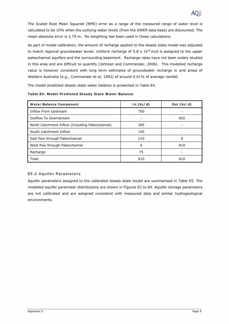
Appendix E Page 6
The Scaled Root Mean Squared (RMS) error as a range of the measured range of water level is
calculated to be 10% when the outlying water levels (from the DWER data base) are discounted. The
mean absolute error is 2.75 m. No weighting has been used in these calculations.
As part of model calibration, the amount of recharge applied to the steady state model was adjusted
to match regional groundwater levels. Uniform recharge of 5.8 x 10⁻⁸ m/d is assigned to the upper
paleochannel aquifers and the surrounding basement. Recharge rates have not been widely studied
in this area and are difficult to quantify (Johnson and Commander, 2006). This modelled recharge
value is however consistent with long term estimates of groundwater recharge in arid areas of
Western Australia (e.g., Commander et al, 1992) of around 0.01% of average rainfall.
The model predicted steady state water balance is presented in Table E4.
Table E4: Model Predicted Steady State Water Balance
Water Balance Component In (kL/d) Out (kL/d)
Inflow From Upstream 750 -
Outflow To Downstream - 820
North Catchment Inflow (Including Paleochannel) 385 -
South Catchment Inflow 140 -
East flow through Paleochannel 210 0
West flow through Paleochannel 0 810
Recharge 75 -
Total 810 810
E5.2 Aquifer Parameters
Aquifer parameters assigned to the calibrated steady state model are summarised in Table E5. The
modelled aquifer parameter distributions are shown in Figures E2 to E4. Aquifer storage parameters
are not calibrated and are assigned consistent with measured data and similar hydrogeological
environments.
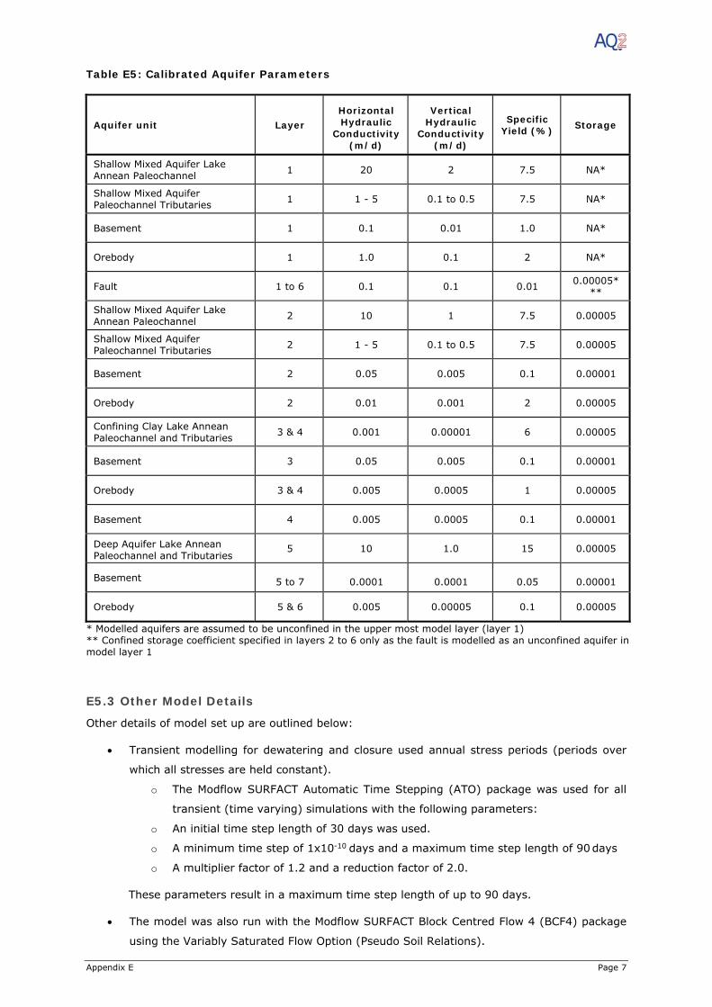
Appendix E Page 7
Table E5: Calibrated Aquifer Parameters
Aquifer unit Layer Horizontal Hydraulic
Conductivity (m/d)
Vertical Hydraulic
Conductivity (m/d)
Specific Yield (%) Storage
Shallow Mixed Aquifer Lake Annean Paleochannel 1 20 2 7.5 NA*
Shallow Mixed Aquifer Paleochannel Tributaries 1 1 - 5 0.1 to 0.5 7.5 NA*
Basement 1 0.1 0.01 1.0 NA*
Orebody 1 1.0 0.1 2 NA*
Fault 1 to 6 0.1 0.1 0.01 0.00005***
Shallow Mixed Aquifer Lake Annean Paleochannel 2 10 1 7.5 0.00005
Shallow Mixed Aquifer Paleochannel Tributaries 2 1 - 5 0.1 to 0.5 7.5 0.00005
Basement 2 0.05 0.005 0.1 0.00001
Orebody 2 0.01 0.001 2 0.00005
Confining Clay Lake Annean Paleochannel and Tributaries 3 & 4 0.001 0.00001 6 0.00005
Basement 3 0.05 0.005 0.1 0.00001
Orebody 3 & 4 0.005 0.0005 1 0.00005
Basement 4 0.005 0.0005 0.1 0.00001
Deep Aquifer Lake Annean Paleochannel and Tributaries
5 10 1.0 15 0.00005
Basement 5 to 7 0.0001 0.0001 0.05 0.00001
Orebody 5 & 6 0.005 0.00005 0.1 0.00005
* Modelled aquifers are assumed to be unconfined in the upper most model layer (layer 1) ** Confined storage coefficient specified in layers 2 to 6 only as the fault is modelled as an unconfined aquifer in model layer 1
E5.3 Other Model Details
Other details of model set up are outlined below:
Transient modelling for dewatering and closure used annual stress periods (periods over
which all stresses are held constant).
o The Modflow SURFACT Automatic Time Stepping (ATO) package was used for all
transient (time varying) simulations with the following parameters:
o An initial time step length of 30 days was used.
o A minimum time step of 1x10⁻¹⁰ days and a maximum time step length of 90 days
o A multiplier factor of 1.2 and a reduction factor of 2.0.
These parameters result in a maximum time step length of up to 90 days.
The model was also run with the Modflow SURFACT Block Centred Flow 4 (BCF4) package
using the Variably Saturated Flow Option (Pseudo Soil Relations).
Appendix E Page 8
The model was run with the Pre-Conjugated 5 (PCG5) solver along with the following
parameters:
o Number of outer iterations - 100
o Number of inner iterations - 20
o Maximum orthoganalisations - 10
o Head change criteria = 0.01 m
o Relative convergence criterion = 0.1
o Newton Raphson Linearisation (Back tracking Factor) = 0.9
o Newton Raphson Linearisation (Residual Reduction Factor) = 1
E6 Model Predictions
The calibrated model was used to:
Predict groundwater inflows to the open pits to allow calculation of water disposal
requirements in excess of the project water demand which has been estimated at between
2,300 kL/d and 2,700 kL/d (for the wet and dry seasons respectively).
Predict the water level (drawdown) impact of open pit dewatering at the end of mine life.
Predict the potential for MAR to the lower paleochannel aquifer to be used to dispose of
dewatering in excess of the project demand.
Predict the recovery of water levels in mine out pits once mine in complete, assuming that
pits are left empty, including final equilibrium levels and the time taken for recovery to final
levels.
These predictions were completed assuming transient conditions.
E6.1 Prediction Set up
For single open pit developments, in low permeability basement rock environments with limited
hydrogeological data, groundwater inflows to open pits and the long term behaviour of final mine
voids can be estimated using analytical methods. This analytical approach can be just as reliable as
numerical approaches in some environments (single pits developed in low permeability
environments). The current plan for the project includes four open pits, with basement rocks to the
north and a paleochannel to the south. To simulate the groundwater interactions between the
adjacent pits / pit voids, and the variable aquifer conditions close to the pits, a numerical approach
is required.
Prediction of groundwater inflow to the open pits was completed for the mine plan provided, in dxf
format. The plan included 40 pit progressions for four pits for a period of 25 years. Mine plans were
provided in quarterly increments for Year 1 to 5 in 0624_avl_v6_1_y1_q1_surf_mga.dxf to
0624_avl_v6_1_y5_q4_surf_mga.dxf and annual increments for Years 6 to 25 in
0624_avl_v6_1_y6_surf_mga.dxf to 0624_avl_v6_1_y25_surf_mga.dxf. Mining will progress to a
depth of between 110 m and 240 m below ground surface and will cover a total mined area of up to
260 ha. The extent of the mining area with Pit Locations is shown in Figure E8.
Other details of model predictions are outlined below:
Operational (mining) model predictions were completed for the period Year 1 to Year 25,
using an annual time increment or stress period, with initial water level conditions for model
predictions taken from the steady state model calibration.
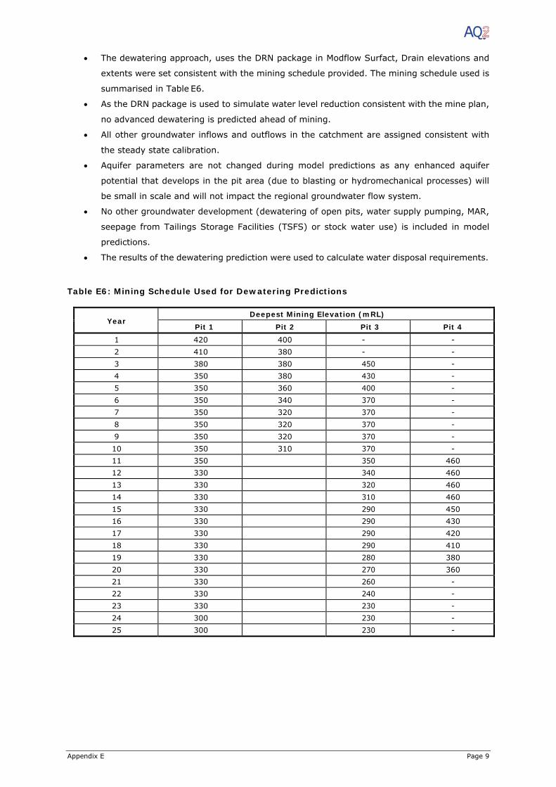
Appendix E Page 9
The dewatering approach, uses the DRN package in Modflow Surfact, Drain elevations and
extents were set consistent with the mining schedule provided. The mining schedule used is
summarised in Table E6.
As the DRN package is used to simulate water level reduction consistent with the mine plan,
no advanced dewatering is predicted ahead of mining.
All other groundwater inflows and outflows in the catchment are assigned consistent with
the steady state calibration.
Aquifer parameters are not changed during model predictions as any enhanced aquifer
potential that develops in the pit area (due to blasting or hydromechanical processes) will
be small in scale and will not impact the regional groundwater flow system.
No other groundwater development (dewatering of open pits, water supply pumping, MAR,
seepage from Tailings Storage Facilities (TSFS) or stock water use) is included in model
predictions.
The results of the dewatering prediction were used to calculate water disposal requirements.
Table E6: Mining Schedule Used for Dewatering Predictions
Year Deepest Mining Elevation (mRL)
Pit 1 Pit 2 Pit 3 Pit 4 1 420 400 - - 2 410 380 - - 3 380 380 450 - 4 350 380 430 - 5 350 360 400 - 6 350 340 370 - 7 350 320 370 - 8 350 320 370 - 9 350 320 370 - 10 350 310 370 - 11 350 350 460 12 330 340 460 13 330 320 460 14 330 310 460 15 330 290 450 16 330 290 430 17 330 290 420 18 330 290 410 19 330 280 380 20 330 270 360 21 330 260 - 22 330 240 - 23 330 230 - 24 300 230 - 25 300 230 -
Appendix E Page 10
E6.2 Mine Closure
Closure predictions have been completed assuming the mine voids will be left empty after closure.
Post mining (closure) predictions were completed for a period of 100 years to simulate the balance
between rainfall recharge, groundwater inflows and evaporation from the pit void lake surfaces and
the impact on regional water levels as depleted storage is replenished by rainfall recharge and
groundwater inflows. Analytical estimates of groundwater recovery suggest that a significant pit lake
will not develop in the final pit void and water will only be present intermittently in the lower benches
of the pit void. This is because the evaporation from the empty pits is estimated to be higher than
the long-term inflows (groundwater inflows and recharge).
Closure predictions have been completed for a Base Case that includes the conditions outlined below
and a Recharge Case, which also includes recharge the from surface water flows in creeks located to
the south of the mine and between Pits 2 and 4. Recharge of 5 mm is included biennially over a
period of a month. Other details of the closure predictions are summarised below:
Initial water level conditions for the closure predictions were taken from the end of the
dewatering prediction.
The open pits are left empty after the end of mining (i.e. no backfilling).
The final mine areas are bunded so that the final pit catchment is similar to the final pit crest
areas.
Groundwater recovery in the open pit is assumed to commence immediately after the end
of mining (i.e. after 25 years of mining).
The geometry of the mined-out pit is included in the model by assigning pit void cells a high
hydraulic conductivity value (99 m/d) and specific yield value (99%). This approach
simulates the mined-out pit as a lake surrounded by undisturbed material.
Once a pit void lake is predicted to develop, it is subject to evaporation equivalent to 75%
of average annual pan evaporation of 1,950 mm/year. This is based on annual average pan
evaporation for Meekatharra of 2,600 mm per year (Luke, 1987).
Recharge to the mine voids is assigned as follows:
o Recharge to the pit lake is assigned at 100% of long term average annual rainfall
(238 mm/year).
o Runoff from the area between the pit void lake and the pit crest also recharges the
pit void lake. This runoff is included at a rate of 20% of annual average rainfall that
falls on the area between the pit void lake and the pit crest.
E7 Prediction Results
E7.1 Dewatering Predictions
Predicted groundwater inflows for each year of mining are shown in Figure E10. The maximum
predicted dewatering rate is 8,000 kL/day in the first year of mining, decreasing to 1,300 kL/day by
Year 25. The average groundwater inflow over the life of mine is 2,660 kL/day.
Predicted water levels for selected locations in the mining areas (Pits 1 to 4) are shown in Figures
E11 and E12. Contours of predicted water level drawdown after 25 years of dewatering are shown in
Figure E13. The predicted drawdown is the difference between pre-mining water levels and the water
levels predicted at the end of mining (Year 25 of mine life). The following observations are made
regarding the predicted drawdown:
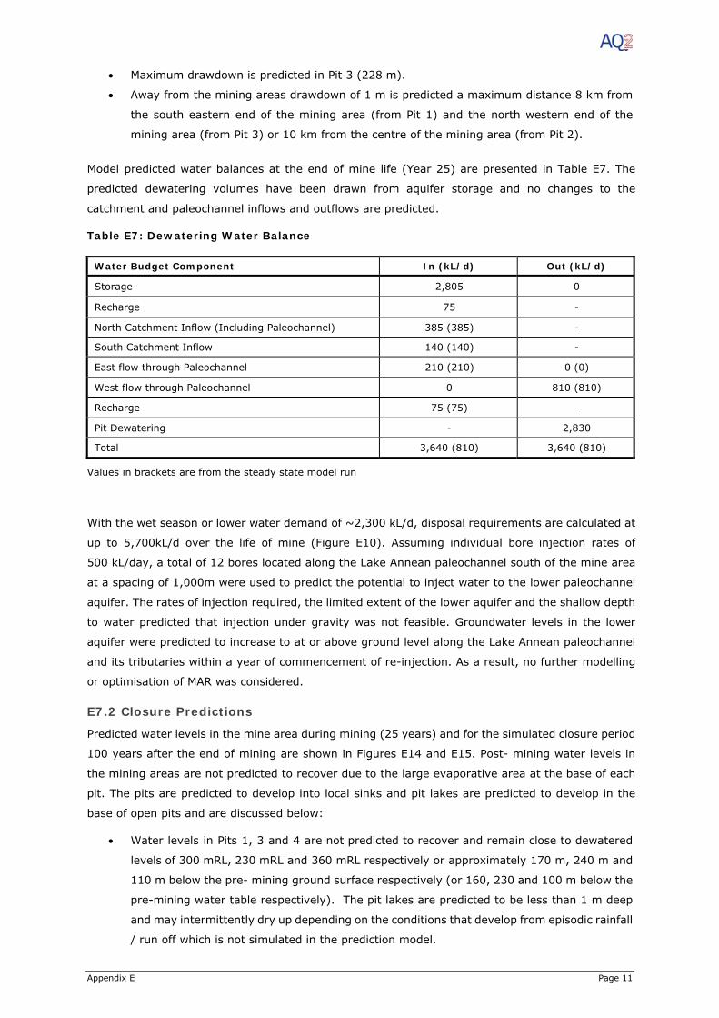
Appendix E Page 11
Maximum drawdown is predicted in Pit 3 (228 m).
Away from the mining areas drawdown of 1 m is predicted a maximum distance 8 km from
the south eastern end of the mining area (from Pit 1) and the north western end of the
mining area (from Pit 3) or 10 km from the centre of the mining area (from Pit 2).
Model predicted water balances at the end of mine life (Year 25) are presented in Table E7. The
predicted dewatering volumes have been drawn from aquifer storage and no changes to the
catchment and paleochannel inflows and outflows are predicted.
Table E7: Dewatering Water Balance
Water Budget Component In (kL/d) Out (kL/d)
Storage 2,805 0
Recharge 75 -
North Catchment Inflow (Including Paleochannel) 385 (385) -
South Catchment Inflow 140 (140) -
East flow through Paleochannel 210 (210) 0 (0)
West flow through Paleochannel 0 810 (810)
Recharge 75 (75) -
Pit Dewatering - 2,830
Total 3,640 (810) 3,640 (810)
Values in brackets are from the steady state model run
With the wet season or lower water demand of ~2,300 kL/d, disposal requirements are calculated at
up to 5,700kL/d over the life of mine (Figure E10). Assuming individual bore injection rates of
500 kL/day, a total of 12 bores located along the Lake Annean paleochannel south of the mine area
at a spacing of 1,000m were used to predict the potential to inject water to the lower paleochannel
aquifer. The rates of injection required, the limited extent of the lower aquifer and the shallow depth
to water predicted that injection under gravity was not feasible. Groundwater levels in the lower
aquifer were predicted to increase to at or above ground level along the Lake Annean paleochannel
and its tributaries within a year of commencement of re-injection. As a result, no further modelling
or optimisation of MAR was considered.
E7.2 Closure Predictions
Predicted water levels in the mine area during mining (25 years) and for the simulated closure period
100 years after the end of mining are shown in Figures E14 and E15. Post- mining water levels in
the mining areas are not predicted to recover due to the large evaporative area at the base of each
pit. The pits are predicted to develop into local sinks and pit lakes are predicted to develop in the
base of open pits and are discussed below:
Water levels in Pits 1, 3 and 4 are not predicted to recover and remain close to dewatered
levels of 300 mRL, 230 mRL and 360 mRL respectively or approximately 170 m, 240 m and
110 m below the pre- mining ground surface respectively (or 160, 230 and 100 m below the
pre-mining water table respectively). The pit lakes are predicted to be less than 1 m deep
and may intermittently dry up depending on the conditions that develop from episodic rainfall
/ run off which is not simulated in the prediction model.

Appendix E Page 12
Water levels in Pit 2 are predicted to recover to 332 mRL or approximately 140 m below the
pre-mining ground level (130 m below the pre-mining water table) 35 years after the
cessation of dewatering. The southern eastern edge of Pit 2 is located on the northern side
of a shallow tributary of the Lake Annean paleochannel and higher inflows to this pit are
possible once mining in complete compared to the other pits. The Pit 2 void lake is predicted
to be approximately 22 m deep. This pit void lake is predicted to persist during the year
with small fluctuations in response to episodic rainfall / run off.
Pit 4 is located within the shallow tributary of the Lake Annean paleochannel. As Pit 2 and
Pit 1 (located to the south of the tributary) are both deeper than Pit 4, groundwater flow is
towards Pits 1 and 2. As a result a pit lake is not predicted to develop in Pit 4.
Similar pit void lake responses are predicted for both closure simulations (Base Case and
Recharge Case).
Contours of predicted water level drawdown 100 years after the end of mining are shown in Figure
E16 for the Base Case and Figure E17 for the Recharge Case. The following observations are made
regarding the predicted drawdown after mine closure:
For both cases in the mine area, where pit lakes are predicted to develop, water levels are
between 100 m to 230 m below pre-mining water levels. Similar drawdown is predicted for
both cases.
For the Base Case drawdown of 1 m is predicted to extend a maximum distance of 13 km to
the north and 14 km to the south of the mine area (from the centre of Pit 2). Drawdown of 1 m is
also predicted to extend through the paleochannel aquifers a maximum distance of 15 km to the
south east of the centre of the mining area, and 18 km west.
For the Recharge Case, drawdown of 1 m is predicted to extend a similar distance to the
north as the Base Case (~13 km). Drawdown to the west along the paleochannel is
predicted to be reduced in extent compared to the Base Case (~3 km reduction). Similar
drawdown is predicted to the east and to the south. Closer to the mine area, there is also
some reduction in predicted drawdown along the paleochannel. These results suggest that
significant recharge from the creek systems would be required to mitigate the long term
drawdown that would result from long term groundwater discharge from pit void lakes.
The model predicted water balance 100 years after mine closure is shown in Table E8 for the Base
Case and in Table E9 for the Recharge Case. The water balance is shown for the January of the last
year of the simulation (i.e., when enhanced recharge is included in the Recharge Case model). The
groundwater sinks that are predicted to develop in the pit voids will continue to remove water from
the catchment into the future. As a result, groundwater inflows, from the north east and south, to
the catchment are predicted to increase as the impact of the pit voids extends to the model
boundaries. Correspondingly, groundwater outflow to the west is also predicted to decrease. The
difference in the model predicted water balances for the Base Case and the Recharge Case are small
and suggest that the recharge rates adopted have a minimal impact on the modelled catchment
water balances.
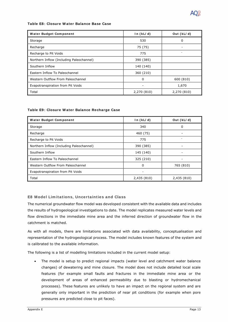
Appendix E Page 13
Table E8: Closure Water Balance Base Case
Water Budget Component In (kL/d) Out (kL/d)
Storage 530 0
Recharge 75 (75) -
Recharge to Pit Voids 775 -
Northern Inflow (Including Paleochannel) 390 (385)
Southern Inflow 140 (140)
Eastern Inflow To Paleochannel 360 (210)
Western Outflow From Paleochannel 0 600 (810)
Evapotranspiration from Pit Voids - 1,670
Total 2,270 (810) 2,270 (810)
Table E9: Closure Water Balance Recharge Case
Water Budget Component In (kL/d) Out (kL/d)
Storage 340 0
Recharge 460 (75) -
Recharge to Pit Voids 775 -
Northern Inflow (Including Paleochannel) 390 (385) -
Southern Inflow 145 (140) -
Eastern Inflow To Paleochannel 325 (210) -
Western Outflow From Paleochannel 0 765 (810)
Evapotranspiration from Pit Voids -
Total 2,435 (810) 2,435 (810)
E8 Model Limitations, Uncertainties and Class
The numerical groundwater flow model was developed consistent with the available data and includes
the results of hydrogeological investigations to date. The model replicates measured water levels and
flow directions in the immediate mine area and the inferred direction of groundwater flow in the
catchment is matched.
As with all models, there are limitations associated with data availability, conceptualisation and
representation of the hydrogeological process. The model includes known features of the system and
is calibrated to the available information.
The following is a list of modelling limitations included in the current model setup:
The model is setup to predict regional impacts (water level and catchment water balance
changes) of dewatering and mine closure. The model does not include detailed local scale
features (for example small faults and fractures in the immediate mine area or the
development of areas of enhanced permeability due to blasting or hydromechanical
processes). These features are unlikely to have an impact on the regional system and are
generally only important in the prediction of near pit conditions (for example when pore
pressures are predicted close to pit faces).
Appendix E Page 14
The model was calibrated to limited data in the pit area, the alluvial aquifer and regionally.
No long-term transient data exists for the immediate mine area or the paleochannel for both
natural and aquifer stress conditions. As a result, the assigned aquifer storage parameters
are not calibrated and are assigned consistent with similar hydrogeological environments.
A number of assumptions have been included in the model as outlined below:
Recharge to the final pit void will vary depending on the final pit catchments and run off
characteristics of the pit void and walls. The current closure scenario includes runoff from a
final pit catchment that extends 50 m from the pit crest to simulate the runoff that would
occur after mine closure from inside the limits of an abandonment bund at the completion
of mining.
Evaporation from the pit void lake is assigned at a rate of 75% of average annual
evaporation. This value may be more, or less, depending on in-pit conditions however, it is
likely that the pits will develop into long term sinks over a wide range of assigned evaporation
rates due the water deficit of the area.
Long term predictions do not account for potential climate change and the subsequent impact
on evaporation and rainfall conditions of the future.
The groundwater model developed for the mining and surrounding groundwater catchment was
completed consistent with the Australian Groundwater Modelling Guidelines (Barnett et al, 2012).
Based on the Australian Groundwater modelling guidelines (2012), specifically Table 2:1 (Model
confidence level classification – characteristics and indicators), the model satisfies the requirements
of a Class 1 confidence level (the lowest level) as:
The model is not calibrated to long term data and the model is not calibrated to aquifer
storage.
The duration of model predictions (25 year of dewatering and 100 year of recovery) is not
replicated by the model calibration.
Aquifer stresses from dewatering, injection and closure are also not replicated in the model
calibration.
Table 2.1 of the modelling guidelines suggests that the model is suitable to predict the impacts of
the proposed development, which is low risk, in a low value aquifer (hypersaline environment with
no other significant groundwater users). The guidelines also suggest that the model is suitable for
the prediction of dewatering rates at this level of study.
E9 References
Barnett et al, 2012, Australian groundwater modelling guidelines, Waterlines report, National Water
Commission, Canberra.
Commander, D. P., Kern, R. M. and Smith, R. A. 1992, Hydrogeology of the Tertiary Palaeochannels
in the Kalgoorlie Region (Roe Palaeodrainage), Geological Survey of Western Australia, Record
1991/10.
Environmental Solutions, Inc. 1996-2011. Groundwater Vistas Version 8.06 Build 18.
Hydrogeologic Inc (1996). MODHMS / MODFLOW-SURFACT. A Comprehensive MODFLOW-Based
Hydrologic Modelling System.

Appendix E Page 15
Johnson, S.L., and Commander, D.P., 2006. Mid West Regional Minerals Study – Groundwater
Resource Appraisal, Department of Water, Hydrogeological Record Series HG 17.
Luke, G J, Burke, K L, and O'Brien, T M. (1987), Evaporation data for Western Australia. Department
of Agriculture and Food, Western Australia, Perth. Report 65.
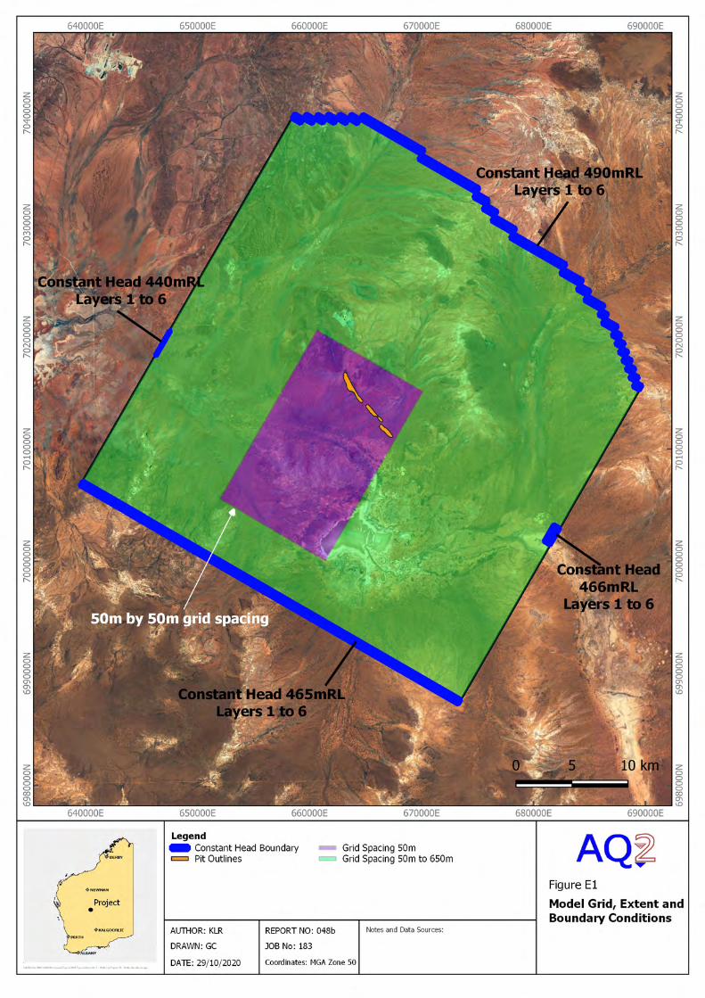
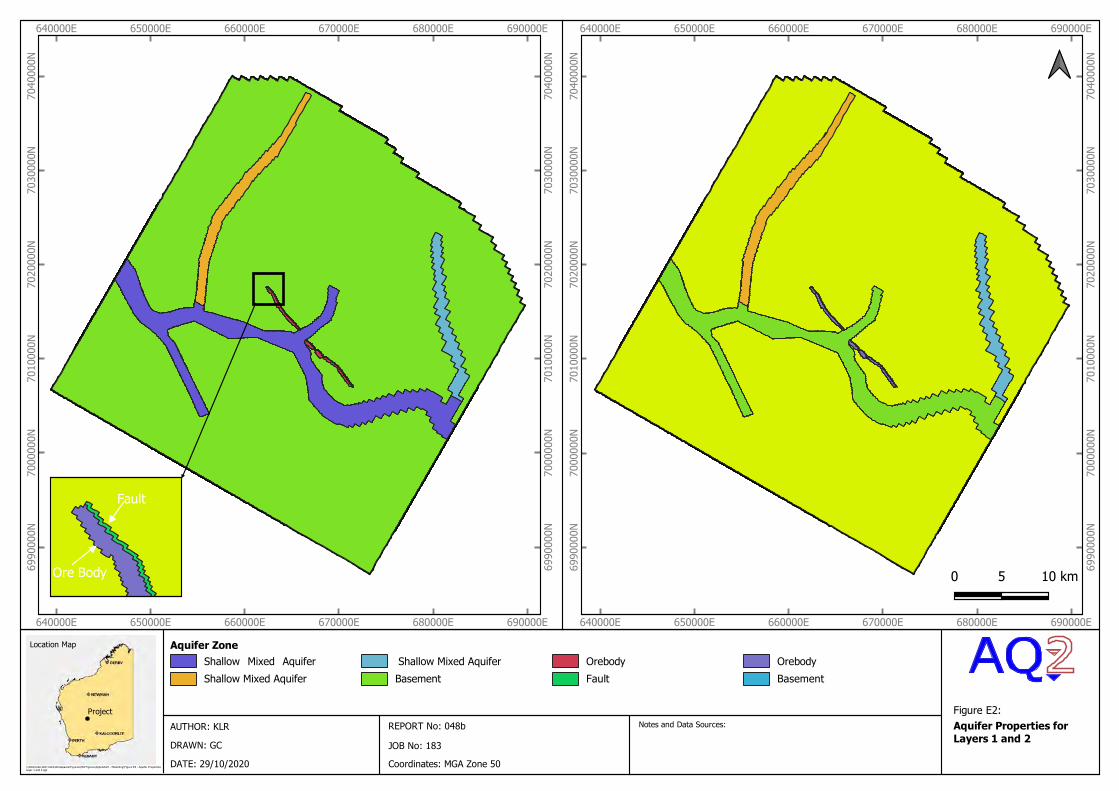
\\dc02\Jobs\183\4.GIS\Workspaces\Figures\048 Figures\Appendix E - Modelling\Figure E2 - Aquifer PropertiesLayer 1 and 2.qgz
Project
Location Map
Notes and Data Sources:
Coordinates: MGA Zone 50
JOB No: 183
REPORT No: 048b
DATE: 29/10/2020
DRAWN: GC
AUTHOR: KLR Aquifer Properties forLayers 1 and 2
Figure E2:
Shallow Mixed Aquifer
Shallow Mixed Aquifer
Shallow Mixed Aquifer
Basement
Orebody
Fault
Orebody
Basement
Paleochannel Upper Aquifer
Aquifer Zone
Fault
Ore Body
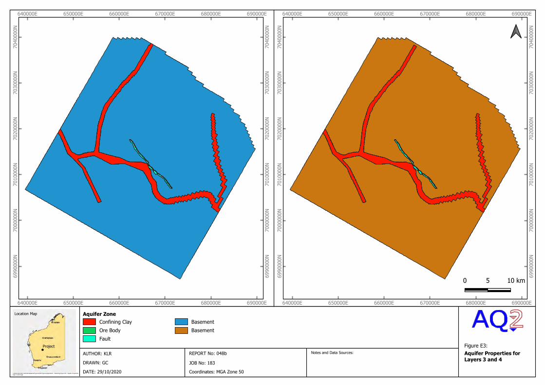
\\dc02\Jobs\183\4.GIS\Workspaces\Figures\048 Figures\Appendix E - Modelling\Figure E3 - Aquifer PropertiesLayer 3 and 4.qgz
Project
Location Map
Notes and Data Sources:
Coordinates: MGA Zone 50
JOB No: 183
REPORT No: 048b
DATE: 29/10/2020
DRAWN: GC
AUTHOR: KLR Aquifer Properties forLayers 3 and 4
Figure E3:
Confining Clay
Ore Body
Fault
Basement
Basement
Aquifer Zone
Fault
Ore Body
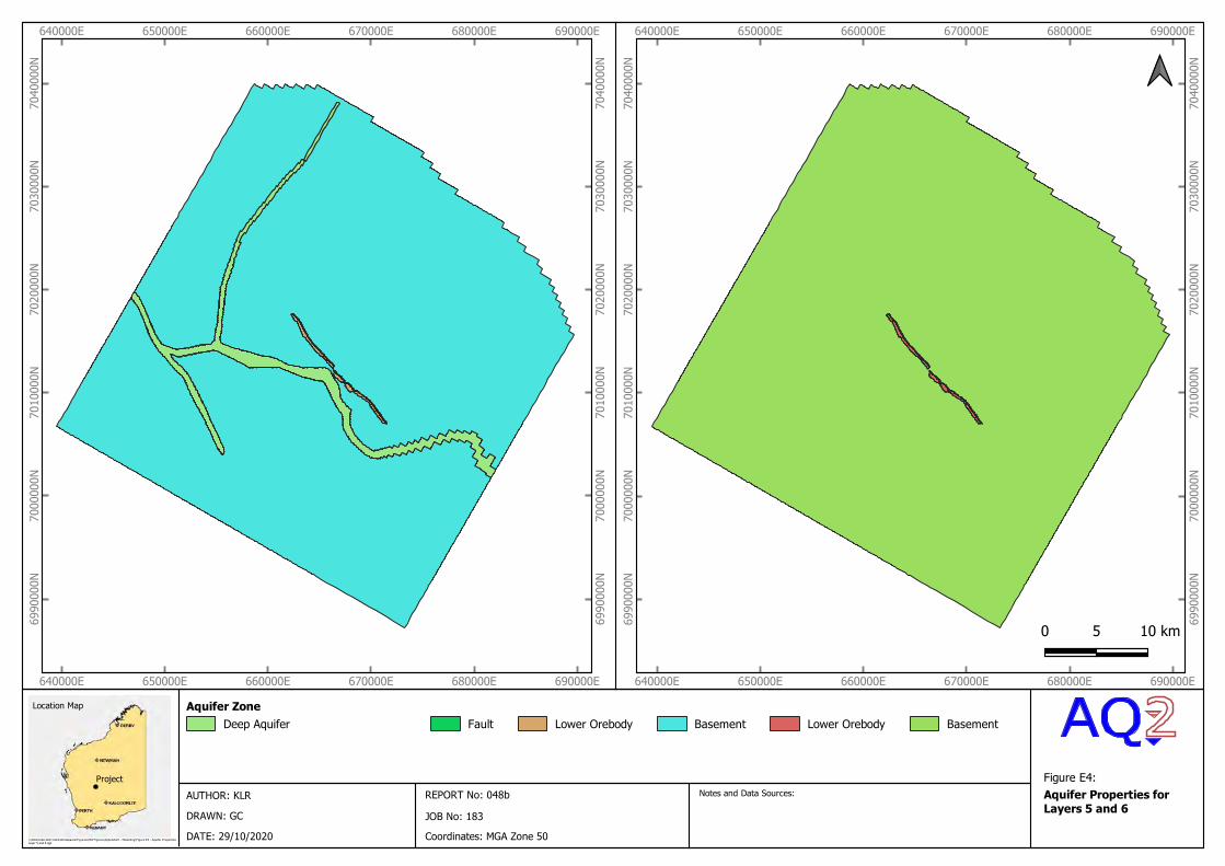
\\dc02\Jobs\183\4.GIS\Workspaces\Figures\048 Figures\Appendix E - Modelling\Figure E3 - Aquifer PropertiesLayer 5 and 6.qgz
Project
Location Map
Notes and Data Sources:
Coordinates: MGA Zone 50
JOB No: 183
REPORT No: 048b
DATE: 29/10/2020
DRAWN: GC
AUTHOR: KLR Aquifer Properties forLayers 5 and 6
Figure E4:
Deep Aquifer Fault Lower Orebody Basement Lower Orebody Basement
Aquifer Zone
Fault
Ore Body
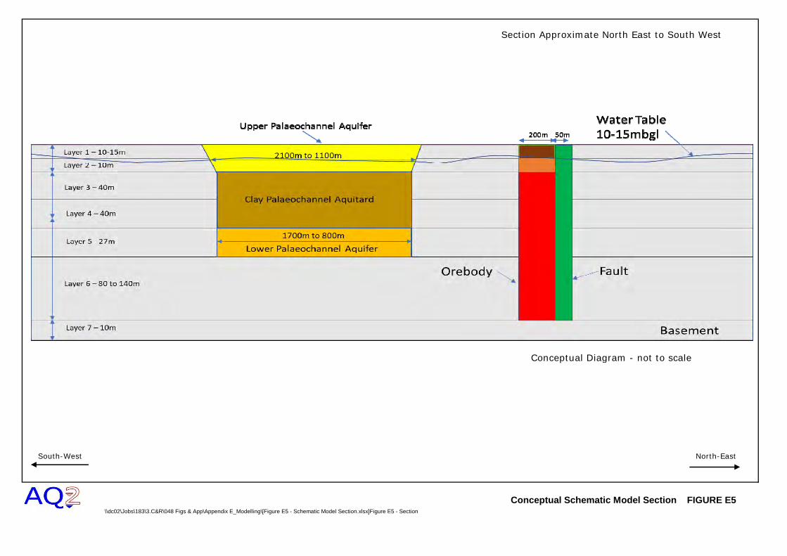
South-West
Conceptual Schematic Model Section FIGURE E5\\dc02\Jobs\183\3.C&R\048 Figs & App\Appendix E_Modelling\[Figure E5 - Schematic Model Section.xlsx]Figure E5 - Section
Conceptual Diagram - not to scale
Section Approximate North East to South West
North-East

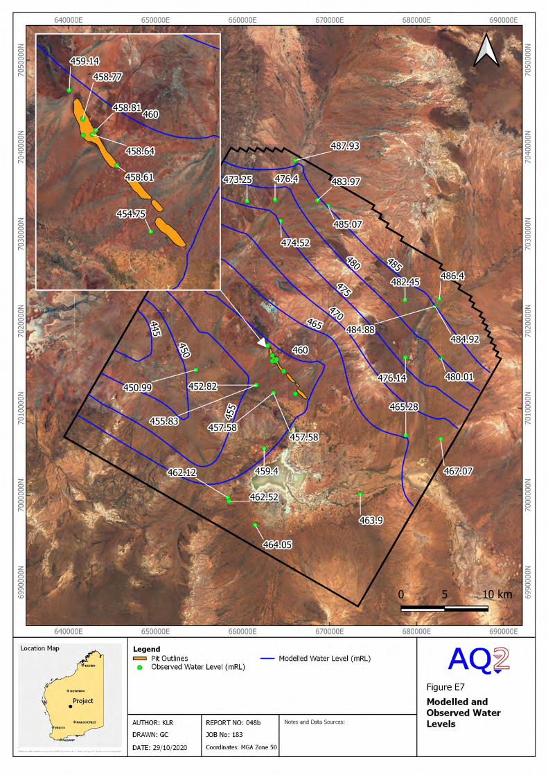

Measured and Modelled water levels FIGURE E8\\dc02\Jobs\183\3.C&R\048 Figs & App\Appendix E_Modelling\[Figure E8 - RMS plot.xlsx]Figure E7
19AVWM01
19AVWM02d
19AVWM02s19AVWM03
19AVWM04
19AVWM108
19AVWM104
19AVWM105
19AVWM112
19AVWM113
19AVWM114
19AVWP001
19AVWP002
Camel
Fig
Hopout
Sunday
Bullock
Centre
Well
No358NallineWell
No360ReidWell
No339Newwell
ScourWell
No333Well
No335Peggy
No338MogulWell
2576FootPaddock 267HorseWell
241Well
244New
250WestWell
450
455
460
465
470
475
480
485
490
495
450 455 460 465 470 475 480 485 490 495
Mo
del
led
(m
RL)
Measured (mRL)
Water Level Measurements Measured = Modelled 5m error
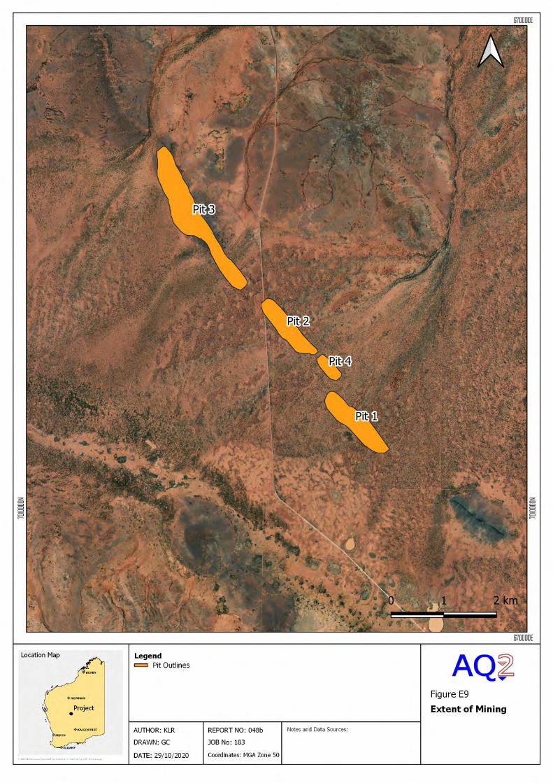
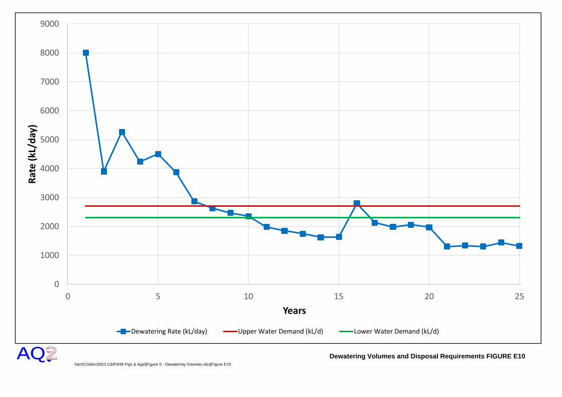
Dewatering Volumes and Disposal Requirements FIGURE E10\\dc02\Jobs\183\3.C&R\048 Figs & App\[Figure 5 - Dewatering Volumes.xlsx]Figure E10
0
1000
2000
3000
4000
5000
6000
7000
8000
9000
0 5 10 15 20 25
Rate
(kL/
day)
Years
Dewatering Rate (kL/day) Upper Water Demand (kL/d) Lower Water Demand (kL/d)

Modelled Water Levels for Pits 1 and 2 FIGURE E11F:\183\3.C&R\048 Figs & App\Appendix E_Modelling\[Figure E11 and 12 - Predicted Water Levels.xlsx]Figure E11
220
240
260
280
300
320
340
360
380
400
420
0 5 10 15 20 25
Elev
atio
n (
mR
L)
YearPit 2 Mining Schedule Pit 2 Modelled Water Level
220
270
320
370
420
470
0 5 10 15 20 25
Ele
vati
on
(m
RL)
YearPit 1 Modelled Water Level Pit 1 Mining Schedule
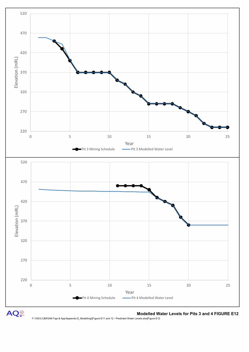
Modelled Water Levels for Pits 3 and 4 FIGURE E12F:\183\3.C&R\048 Figs & App\Appendix E_Modelling\[Figure E11 and 12 - Predicted Water Levels.xlsx]Figure E12
220
270
320
370
420
470
520
0 5 10 15 20 25
Elev
atio
n (
mR
L)
YearPit 4 Mining Schedule Pit 4 Modelled Water Level
220
270
320
370
420
470
520
0 5 10 15 20 25
Ele
vati
on
(m
RL)
YearPit 3 Mining Schedule Pit 3 Modelled Water Level
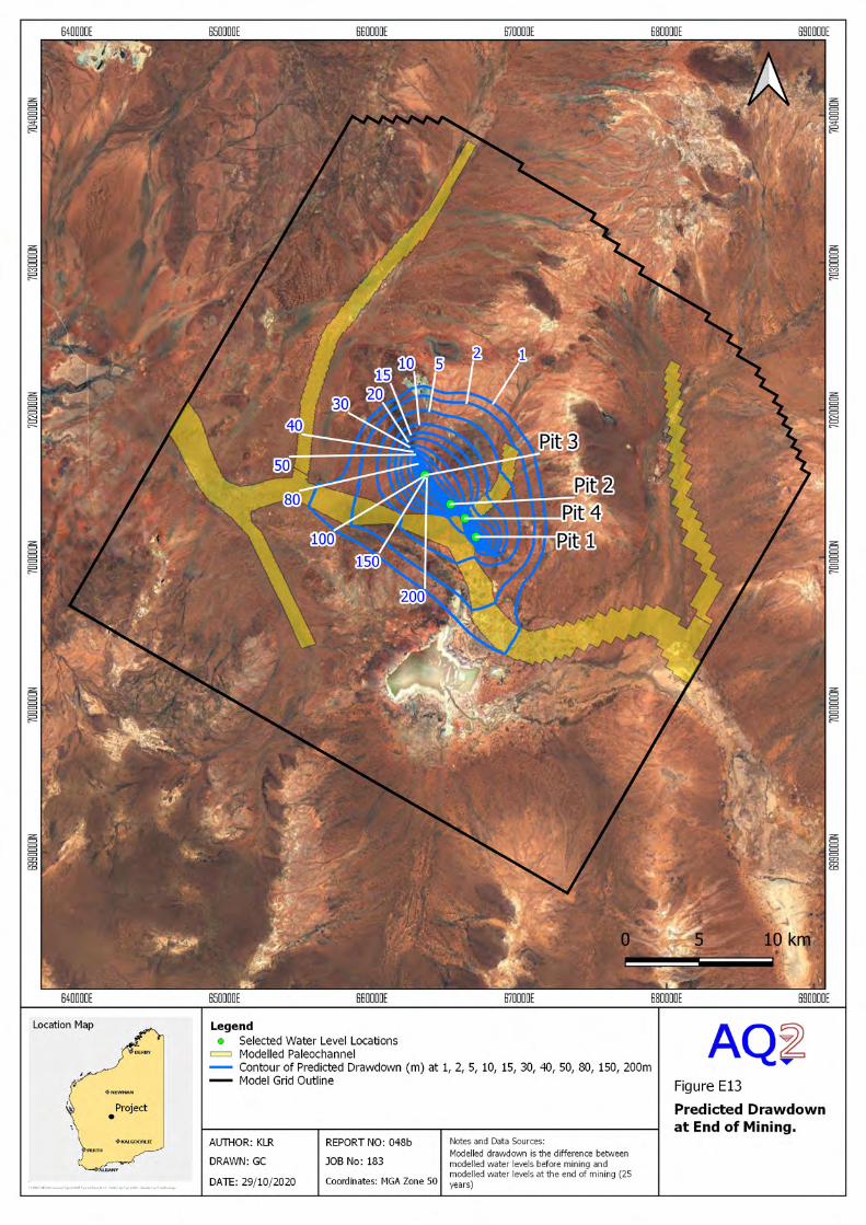
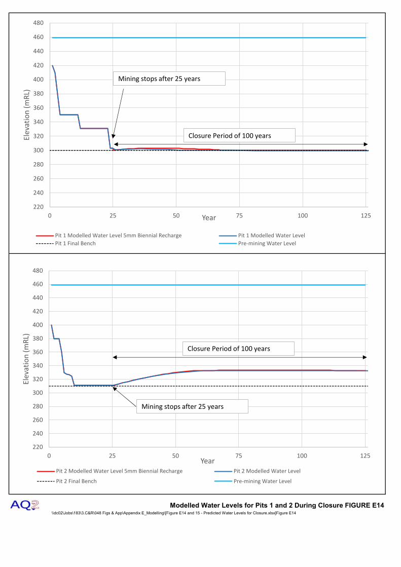
Modelled Water Levels for Pits 1 and 2 During Closure FIGURE E14\\dc02\Jobs\183\3.C&R\048 Figs & App\Appendix E_Modelling\[Figure E14 and 15 - Predicted Water Levels for Closure.xlsx]Figure E14
220
240
260
280
300
320
340
360
380
400
420
440
460
480
0 25 50 75 100 125
Ele
vati
on
(m
RL)
Year
Pit 1 Modelled Water Level 5mm Biennial Recharge Pit 1 Modelled Water Level
Pit 1 Final Bench Pre-mining Water Level
220
240
260
280
300
320
340
360
380
400
420
440
460
480
0 25 50 75 100 125
Elev
atio
n (
mR
L)
YearPit 2 Modelled Water Level 5mm Biennial Recharge Pit 2 Modelled Water Level
Pit 2 Final Bench Pre-mining Water Level
Mining stops after 25 years
Mining stops after 25 years
Closure Period of 100 years
Closure Period of 100 years

Modelled Water Levels for Pits 3 and 4 During Closure FIGURE E15\\dc02\Jobs\183\3.C&R\048 Figs & App\Appendix E_Modelling\[Figure E14 and 15 - Predicted Water Levels for Closure.xlsx]Figure E15
220
240
260
280
300
320
340
360
380
400
420
440
460
480
0 25 50 75 100 125
Ele
vati
on
(m
RL)
Year
Pit 3 Modelled Water Level with 5mm Biennial Recharge Pit 3 Modelled Water Level Pit 3 Final Bench Pre-mining Water Level
220
240
260
280
300
320
340
360
380
400
420
440
460
480
0 25 50 75 100 125
Elev
atio
n (
mR
L)
Year
Pit 4 Modelled Water Level 5mm Biennial Recharge Pit 4 Modelled Water Level
Pit 4 Final Bench Pre-mining Water Level
Mining stops after 25 years
Mining stops after 25 years
Closure Period of 100 years
Closure Period of 100 years

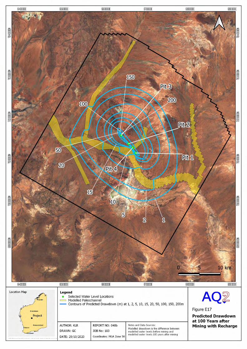
Related Documents