Circumstellar Disk Structure and Evolution
through Resolved Submillimeter Observations
A dissertation presented
by
Alanna Meredith Hughes
to
The Department of Astronomy
in partial fulfillment of the requirements
for the degree of
Doctor of Philosophy
in the subject of
Astronomy
Harvard University
Cambridge, Massachusetts
May 2010

©c 2010 — Alanna Meredith Hughes
All rights reserved.

iii
Thesis Advisor: David J. Wilner Alanna Meredith Hughes
Circumstellar Disk Structure and Evolution
through Resolved Submillimeter Observations
Abstract
Circumstellar disks provide the reservoirs of raw material and determine conditions
for the formation of nascent planetary systems. This thesis presents observations
from millimeter-wavelength interferometers, particularly the Submillimeter Array,
that address the following outstanding problems in the study of protoplanetary
disks: (1) constraining the physical mechanisms driving the viscous transport of
material through the disk, and (2) carrying out detailed studies of “transitional”
objects between the gas-rich protoplanetary and tenuous, dusty debris disk
phases to better understand how gas and dust are cleared from the system. We
study accretion processes in three complementary ways: using spatially resolved
observations of molecular gas lines at high spectral resolution to determine the
magnitude and spatial distribution of turbulence in the disk; using polarimetry to
constrain the magnetic properties of the outer disk in order to evaluate whether
the MRI is a plausible origin for this turbulence; and investigating the gas and
dust distribution at the outer disk edge in the context of self-similar models
of accretion disk structure and evolution. The studies of transition disks use
spatially resolved observations to study the detailed structure of the gas and
dust in systems that are currently in the process of clearing material. We obtain
snapshots of the inside-out clearing of gas and dust in several systems, and
compare our observations with the theoretical predictions generated for different
disk clearing mechanisms. Our observations are generally consistent with the
characteristics predicted for viscous transport driven by the magnetorotational
instability and disk clearing accomplished through the dual action of giant planet
formation and photoevaporation by energetic radiation from the star.

iv
Contents
Abstract . . . . . . . . . . . . . . . . . . . . . . . . . . . . . . . . . . . . iii
Acknowledgments . . . . . . . . . . . . . . . . . . . . . . . . . . . . . . . x
1 Introduction 1
1.1 Why Millimeter Interferometry? . . . . . . . . . . . . . . . . . . . . 2
1.2 Protoplanetary Disks as Accretion Disks . . . . . . . . . . . . . . . 4
1.3 Disk Dissipation . . . . . . . . . . . . . . . . . . . . . . . . . . . . . 6
2 An Inner Hole in the Disk around TW Hydrae Resolved in 7 mil-
limeter Dust Emission 9
2.1 Introduction . . . . . . . . . . . . . . . . . . . . . . . . . . . . . . . 9
2.2 Observations . . . . . . . . . . . . . . . . . . . . . . . . . . . . . . . 11
2.3 Results . . . . . . . . . . . . . . . . . . . . . . . . . . . . . . . . . . 12
2.3.1 7 mm Image . . . . . . . . . . . . . . . . . . . . . . . . . . . 12
2.3.2 Radially Averaged 7 mm Visibilities . . . . . . . . . . . . . . 13
2.4 Discussion . . . . . . . . . . . . . . . . . . . . . . . . . . . . . . . . 14
2.4.1 Comparison with Disk Models . . . . . . . . . . . . . . . . . 16
2.4.2 Disk Clearing . . . . . . . . . . . . . . . . . . . . . . . . . . 18
2.5 Conclusions . . . . . . . . . . . . . . . . . . . . . . . . . . . . . . . 19
3 A Spatially Resolved Inner Hole in the Disk around GM Aurigae 21
3.1 Introduction . . . . . . . . . . . . . . . . . . . . . . . . . . . . . . . 22
v

vi CONTENTS
3.2 Observations and Data Reduction . . . . . . . . . . . . . . . . . . . 24
3.3 Results . . . . . . . . . . . . . . . . . . . . . . . . . . . . . . . . . . 26
3.3.1 Millimeter Continuum Emission . . . . . . . . . . . . . . . . 26
3.3.2 CO Channel and Moment Maps . . . . . . . . . . . . . . . . 29
3.4 Disk Structure Models . . . . . . . . . . . . . . . . . . . . . . . . . 30
3.4.1 Updated SED Model . . . . . . . . . . . . . . . . . . . . . . 30
3.4.2 Comparison with CO Observations . . . . . . . . . . . . . . 35
3.5 Discussion . . . . . . . . . . . . . . . . . . . . . . . . . . . . . . . . 38
3.5.1 Inner Disk Clearing . . . . . . . . . . . . . . . . . . . . . . . 38
3.5.2 Evidence for a Warp? . . . . . . . . . . . . . . . . . . . . . . 43
3.6 Conclusions . . . . . . . . . . . . . . . . . . . . . . . . . . . . . . . 44
4 A Resolved Molecular Gas Disk around the Nearby A Star 49
Ceti 47
4.1 Introduction . . . . . . . . . . . . . . . . . . . . . . . . . . . . . . . 48
4.2 Observations . . . . . . . . . . . . . . . . . . . . . . . . . . . . . . . 50
4.3 Results and Analysis . . . . . . . . . . . . . . . . . . . . . . . . . . 51
4.4 Disk Modeling . . . . . . . . . . . . . . . . . . . . . . . . . . . . . . 53
4.4.1 Grid of Disk Models . . . . . . . . . . . . . . . . . . . . . . 58
4.4.2 Spectral Energy Distribution . . . . . . . . . . . . . . . . . . 63
4.4.3 Best-Fit Disk Model . . . . . . . . . . . . . . . . . . . . . . 65
4.5 Discussion . . . . . . . . . . . . . . . . . . . . . . . . . . . . . . . . 66
4.6 Conclusions . . . . . . . . . . . . . . . . . . . . . . . . . . . . . . . 70
5 Structure and Composition of Two Transitional Circumstellar
Disks in Corona Australis 71
5.1 Introduction . . . . . . . . . . . . . . . . . . . . . . . . . . . . . . . 72
5.2 Observations and Data Reduction . . . . . . . . . . . . . . . . . . . 74
CONTENTS vii
5.2.1 SMA Observations . . . . . . . . . . . . . . . . . . . . . . . 74
5.2.2 ASTE Observations . . . . . . . . . . . . . . . . . . . . . . . 75
5.3 Results . . . . . . . . . . . . . . . . . . . . . . . . . . . . . . . . . . 76
5.3.1 Millimeter Continuum . . . . . . . . . . . . . . . . . . . . . 76
5.3.2 CO(2-1) and CO(3-2) Line Observations . . . . . . . . . . . 77
5.4 Analysis . . . . . . . . . . . . . . . . . . . . . . . . . . . . . . . . . 78
5.4.1 Modeling the SED and Millimeter Visibilities . . . . . . . . 78
5.4.2 Representative Models . . . . . . . . . . . . . . . . . . . . . 81
5.4.3 Constraints on Molecular Gas Content . . . . . . . . . . . . 83
5.5 Discussion and Conclusions . . . . . . . . . . . . . . . . . . . . . . 86
6 Gas and Dust Emission at the Outer Edges of Protoplanetary
Disks 91
6.1 Introduction . . . . . . . . . . . . . . . . . . . . . . . . . . . . . . . 92
6.2 Dust Continuum and CO J=3-2 Data . . . . . . . . . . . . . . . . . 94
6.3 Disk Models . . . . . . . . . . . . . . . . . . . . . . . . . . . . . . . 94
6.3.1 Truncated Power Law . . . . . . . . . . . . . . . . . . . . . 94
6.3.2 Similarity Solution from Accretion Disk Evolution . . . . . . 96
6.3.3 Model Comparison . . . . . . . . . . . . . . . . . . . . . . . 97
6.3.4 Model Fitting . . . . . . . . . . . . . . . . . . . . . . . . . . 98
6.4 Results and Discussion . . . . . . . . . . . . . . . . . . . . . . . . . 100
6.5 Summary and Conclusions . . . . . . . . . . . . . . . . . . . . . . . 106
7 Stringent Limits on the Polarized Submillimeter Emission from
Protoplanetary Disks 109
7.1 Introduction . . . . . . . . . . . . . . . . . . . . . . . . . . . . . . . 110
7.2 Observations and Data Reduction . . . . . . . . . . . . . . . . . . . 114
7.3 Results . . . . . . . . . . . . . . . . . . . . . . . . . . . . . . . . . . 116
viii CONTENTS
7.4 Analysis and Discussion . . . . . . . . . . . . . . . . . . . . . . . . 119
7.4.1 Initial Models . . . . . . . . . . . . . . . . . . . . . . . . . . 122
7.4.2 Parameter Exploration . . . . . . . . . . . . . . . . . . . . . 124
7.4.3 Other Effects . . . . . . . . . . . . . . . . . . . . . . . . . . 134
7.5 Summary and Conclusions . . . . . . . . . . . . . . . . . . . . . . . 137
8 Empirical Constraints on Turbulence in Protoplanetary Accre-
tion Disks 139
8.1 Introduction . . . . . . . . . . . . . . . . . . . . . . . . . . . . . . . 140
8.2 Observations . . . . . . . . . . . . . . . . . . . . . . . . . . . . . . . 142
8.3 Results . . . . . . . . . . . . . . . . . . . . . . . . . . . . . . . . . . 143
8.4 Analysis . . . . . . . . . . . . . . . . . . . . . . . . . . . . . . . . . 145
8.4.1 Description of Models . . . . . . . . . . . . . . . . . . . . . 147
8.4.2 Modeling Procedure . . . . . . . . . . . . . . . . . . . . . . 149
8.4.3 Best-fit Models . . . . . . . . . . . . . . . . . . . . . . . . . 151
8.4.4 Parameter Degeneracies . . . . . . . . . . . . . . . . . . . . 152
8.5 Discussion . . . . . . . . . . . . . . . . . . . . . . . . . . . . . . . . 158
8.5.1 Comparison with Theory . . . . . . . . . . . . . . . . . . . . 158
8.5.2 Implications for Planet Formation . . . . . . . . . . . . . . . 162
8.5.3 Future Directions . . . . . . . . . . . . . . . . . . . . . . . . 163
8.6 Summary and Conclusions . . . . . . . . . . . . . . . . . . . . . . . 163
9 Conclusions and Future Directions 165
9.1 Disk Dissipation . . . . . . . . . . . . . . . . . . . . . . . . . . . . . 165
9.2 Protoplanetary Disks as Accretion Disks . . . . . . . . . . . . . . . 167
9.3 Future Directions . . . . . . . . . . . . . . . . . . . . . . . . . . . . 169
A Protoplanetary Disk Visibility Functions 173
CONTENTS ix
A.1 Power-Law Disk with a Central Hole . . . . . . . . . . . . . . . . . 173
A.1.1 Position of the Null . . . . . . . . . . . . . . . . . . . . . . . 175
A.2 Thin Wall . . . . . . . . . . . . . . . . . . . . . . . . . . . . . . . . 176
A.3 Application to TW Hya . . . . . . . . . . . . . . . . . . . . . . . . 176
B Supplementary Disk Polarimetry 179
B.1 Observations . . . . . . . . . . . . . . . . . . . . . . . . . . . . . . . 179
B.2 Results and Analysis . . . . . . . . . . . . . . . . . . . . . . . . . . 180
B.3 Discussion and Conclusions . . . . . . . . . . . . . . . . . . . . . . 182
C High Spectral Resolution Channel Maps 187
References 193

Acknowledgments
I can’t possibly say enough to thank David Wilner for the guidance and
support that have made this thesis possible. I have never wanted for data,
resources, opportunities, feedback, or attention as his student. I am grateful for
his responsiveness in part because it has meant that my only limitations have
been my own, which seems to be a rare and valuable experience in grad school.
I am also thankful that fate and the Hubble fellowship brought Sean Andrews
to the CfA two years after I arrived. He has made my experience here better in
every way, as a valuable resource and a shining example to (try to) live up to, and
by always being willing to talk about whatever’s on my mind. I am also grateful
for Charlie Qi’s quiet support in helping me work with RATRAN and dealing
with the weirder SMA issues we’ve encountered over the years.
The contributions of many wonderful collaborators are represented in this
thesis. I’m particularly grateful to Inga Kamp, Jungyeon Cho, and Michiel
Hogerheijde for letting me mess with their wondrously complex codes, as well as
Antonio Hales, Simon Casassus, and Michael Meyer for providing opportunities
to work with new kinds of data. Dan Marrone and Ram Rao kindly taught
me to use the SMA polarimeter and have helped me deal with its quirks. At
the CfA, I’ve enjoyed rare but beneficial conversations with Ruth Murray-Clay,
Alyssa Goodman, and Ramesh Narayan, and I thank Jim Moran for providing
me with a thorough grounding in the fundamentals of radio astronomy. The
mostly invisible work of the SMA staff also forms the backbone of this thesis, and
I am particularly grateful to the schedulers, the operators, the TAC, and Taco
for helping me to get such great data out of the telescope. Long nights at the
summit were shortened by Shelbi’s wacky movies and Erin’s guitar.
Life at the CfA has been immeasurably enriched by my fellow grad students.
I’m not sure what I’d have done without the opportunity to talk through ideas
and presentations, rant, or go for afternoon cookie or frisbee walks with Stephanie
Bush, Joey Munoz, and Ryan O’Leary. I also don’t think I could have worked
back-to-back for five years with anyone other than Gurtina Besla. I’m grateful for
the advice and encouragement of Antonella Fruscione, and to Jean Collins, Peg
Herlihy, and Jennifer Barnett for cheerfully practicing their administrative magic.
The observatory night bunch and the Friday afternoon EHI crew at the Museum
of Science have provided a friendly atmosphere in which to play with science
and remember how exciting it is. I thank Christine Pulliam and David Aguilar
for opportunities to share my enthusiasm for my work with non-astronomers,
particularly short and noisy ones.
x

CONTENTS xi
I am, as always, grateful to my family for their love and support, and for their
excitement and pride in what I’m doing even when they’re not quite sure what
it is. I thank my grandfather for introducing me to my first computer program
and for showing me that logic puzzles were fun long before I found out they were
uncool. I am grateful to my mother for everything and more. I absolutely could
not have done this without her.

xii CONTENTS
Chapter 1
Introduction
Circumstellar disks provide the reservoirs of raw material and initial physical
conditions for the formation of nascent planetary systems. Studies of their
structure and evolution therefore hold the potential to reveal much about
the planet formation process in all of its most important stages: the growth
of submicron-sized, primordial interstellar grains into larger particles; the
agglomeration of these particles into planetesimals; and the growth and orbital
evolution of these planetary embryos into the mature systems observed around
our own star and dozens of others. The variety of extrasolar planetary properties
and system architectures observed over the past 15 years is staggering (e.g.,
Butler et al. 2006) and largely unexplained. Attention is increasingly focused
on unraveling the origins of these planetary systems and the role of the disk
in shaping their properties. This thesis uses spatially resolved observations at
millimeter wavelengths to study circumstellar disks in their planet-forming stages,
with the aim of constraining the basic physical processes that determine their
structure and evolution.
Circumstellar disks pass through several discernible stages on their way to
becoming planetary systems. While the terminology describing these disks is
a matter of some discussion1, we use the following terms to refer to the major
stages of evolution of circumstellar disks:
• protoplanetary disks retain a substantial and largely primordial reservoir
of gas and dust, massive enough to imply planet-forming potential
• transition disks have properties intermediate between protoplanetary and
1See the Diskionary at http://arxiv.org/abs/0901.1691
1

2 CHAPTER 1. INTRODUCTION
debris disks, exhibiting substantial clearing of gas and/or dust from the
system
• debris disks have little or no gas, tenuous dust disks, and dust lifetimes
shorter than the age of the system, indicating that the disk is second-
generation rather than primordial
This thesis focuses on the first two stages of evolution, which necessarily include
the epoch of planetesimal growth and giant planet formation as large planets
must form before gas is dissipated from the disk.
The time-dependent structure of a protoplanetary disk tells us where, when,
and how much material is available for planet formation. We measure the gas
and dust distribution in protoplanetary and transition disks in order to (1)
characterize their planet-forming potential, (2) determine the conditions under
which planets may form, and (3) constrain the physical processes that drive disk
evolution and dispersal. The major questions in the study of disk evolution are
how and why the radial distribution of gas and dust changes with time, and when
and how gas and dust are cleared from the system. The former question is laid
out in more detail in Section 1.2, and the latter in Section 1.3.
1.1 Why Millimeter Interferometry?
Current millimeter interferometers provide spatial resolution from several
arcseconds to a few tenths of an arcsecond. With the nearest star-forming regions
at distances of order ∼100 pc, this resolution corresponds to radial scales of tens
to hundreds of astronomical units, just outside the orbit of Saturn in our own
solar system. This is sufficient to substantially resolve circumstellar disks, which
typically span several hundreds of AU in radius (e.g. Dutrey et al. 1996; Kitamura
et al. 2002; Andrews & Williams 2007).
The millimeter region of the spectrum provides access to important
diagnostics of gas and dust content. The millimeter-wavelength dust continuum
emission is generally optically thin, even for protoplanetary disks. It therefore
traces the mass distribution rather than surface features, and is weighted towards
the dense midplane where most of the mass is located. Furthermore, the stellar
photosphere is very faint at long wavelengths compared to the dust emission,
which has low surface brightness but subtends a large solid angle, so that the
contrast between star and disk is quite low. The primary challenge associated

1.1. WHY MILLIMETER INTERFEROMETRY? 3
with interpreting millimeter-wavelength continuum observations is the unknown
opacity of the dust grains. Various ad hoc estimates of mass opacity are used
(the most common being Beckwith et al. 1990), but they depend sensitively
on the currently unknown size distribution of grains in each system. Most of
the mass is in gas, and much of the mass in solids could be locked up in larger
particles, implying that measurements of disk mass from millimeter continuum
observations may represent lower limits. Since the millimeter flux is the product
of temperature, surface density, and opacity, it can be particularly difficult to
disentangle these properties without complementary constraints on one or more
of the parameters, for example gas tracers, resolved observations at multiple radio
frequencies, or broadband photometry across the spectrum.
This millimeter-wavelength spectral region is also rich with rotational
transitions of small molecules that provide access to dynamical and chemical
information about the gas disk. The dominant mass constituent of protoplanetary
disks is thought to be H2, due to the high elemental abundance of hydrogen and
its resistance to depletion onto dust grains. Its lack of a dipole moment makes
it all but unobservable, with the exception of some measurements of infrared
and fluorescent ultraviolet H2 lines originating in the warm inner disk (e.g.,
Beckwith et al. 1978; Brown et al. 1981; Carr 1990). Other small molecules are
readily observable at millimeter wavelengths, however, including CO, which is
the next most abundant molecule after H2 (with a nominal abundance of 10−4).
The primary complications associated with deriving information about the gas
content from millimeter-wavelength observations are the high optical depth of
abundant molecules, which makes the line flux largely insensitive to density, and
the chemistry, which affects the relative abundances of different molecules (as a
function of radius, scale height, or even azimuth), and can also include freeze-out
of molecules from gaseous to solid phase onto grain surfaces in low-temperature
regions of the disk.
Despite the complications, the combination of spatial resolution and
sensitivity provided by millimeter-wavelength interferometers makes an important
contribution to the study of protoplanetary disks. The constraints provided at
millimeter wavelengths, including dust grain sizes, the surface density of solids,
gas content, and temperatures from gas lines, complement diagnostics from
observations across the spectrum. The integration of spectral energy distribution
(SED) modeling with spatially resolved observations at millimeter wavelengths
has provided important constraints on the temperature and surface density
structure of circumstellar disks (e.g. Calvet et al. 2002; Andrews & Williams
2007; Andrews et al. 2009). While measurements of the sizes of inner holes in

4 CHAPTER 1. INTRODUCTION
transition disks are best accomplished using millimeter-wavelength (or longer)
observations to trace the location of large dust grains (see discussion in Hughes
et al. 2007), critical information about the properties of gas and dust in the inner
disks of these systems is provided by gas and dust tracers at shorter wavelengths
and higher spatial resolution (see e.g. Ratzka et al. 2007; Salyk et al. 2007, 2009;
Eisner et al. 2006; Pontoppidan et al. 2008). Multiwavelength constraints are
crucial for understanding the structure and evolution of circumstellar disks, and
millimeter wavelengths play an important role in that process.
1.2 Protoplanetary Disks as Accretion Disks
Since the seminal work by Lynden-Bell & Pringle (1974), the photospheric excess
and optical and UV variability exhibited by many pre-main sequence stars has
been attributed to emission from an accreting disk. Steady accretion from the
disk to the star requires some form of viscous angular momentum transport
through the disk. The molecular viscosity in a protoplanetary disk implies a disk
evolution timescale much too long to account for the observed evolution of disks:
an additional source of viscosity is therefore required. As conjectured by Shakura
& Syunyaev (1973), turbulence can provide an “anomalous” viscosity large
enough to account for accretion and disk evolution on the appropriate time scales.
However, while turbulence is commonly invoked as the source of viscosity in disks,
its physical origin, magnitude, and spatial distribution are largely unconstrained.
The mechanism most commonly invoked as the source of turbulence providing
viscous transport in circumstellar disks is the magnetorotational instability (MRI),
in which magnetic interactions between fluid elements in the disk combine with
an outwardly decreasing velocity field to produce torques that transfer angular
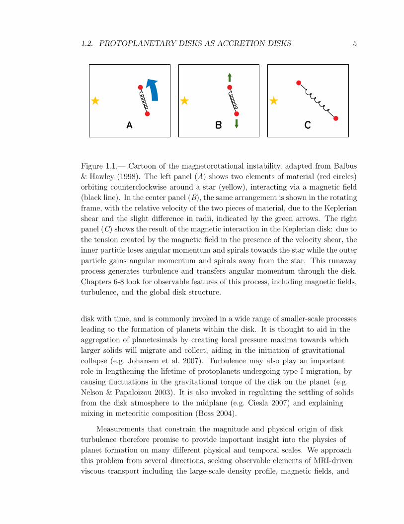
momentum from the inner disk outwards (Balbus & Hawley 1991, 1998). A
cartoon of the elements of this instability, adapted from Balbus & Hawley (1998),
is included in Figure 1.1. The conditions for the instability are satisfied over
much of the extent of a typical primordial circumstellar disk: there must be a
subthermal magnetic field (B2/8πρ < c2s); the ionization fraction must be high
enough for the elements to interact via the magnetic field; and the velocity
field must decrease outwards, a condition easily satisfied in any Keplerian disk
(Gammie & Johnson 2005, and references therein). Where these conditions are
satisfied, the instability will operate and the disk will become turbulent.
The importance of MRI turbulence to circumstellar disks is manifold. It
drives the viscous evolution that determines the global structure of the accretion
1.2. PROTOPLANETARY DISKS AS ACCRETION DISKS 5
Figure 1.1.— Cartoon of the magnetorotational instability, adapted from Balbus
& Hawley (1998). The left panel (A) shows two elements of material (red circles)
orbiting counterclockwise around a star (yellow), interacting via a magnetic field
(black line). In the center panel (B), the same arrangement is shown in the rotating
frame, with the relative velocity of the two pieces of material, due to the Keplerian
shear and the slight difference in radii, indicated by the green arrows. The right
panel (C) shows the result of the magnetic interaction in the Keplerian disk: due to
the tension created by the magnetic field in the presence of the velocity shear, the
inner particle loses angular momentum and spirals towards the star while the outer
particle gains angular momentum and spirals away from the star. This runaway
process generates turbulence and transfers angular momentum through the disk.
Chapters 6-8 look for observable features of this process, including magnetic fields,
turbulence, and the global disk structure.
disk with time, and is commonly invoked in a wide range of smaller-scale processes
leading to the formation of planets within the disk. It is thought to aid in the
aggregation of planetesimals by creating local pressure maxima towards which
larger solids will migrate and collect, aiding in the initiation of gravitational
collapse (e.g. Johansen et al. 2007). Turbulence may also play an important
role in lengthening the lifetime of protoplanets undergoing type I migration, by
causing fluctuations in the gravitational torque of the disk on the planet (e.g.
Nelson & Papaloizou 2003). It is also invoked in regulating the settling of solids
from the disk atmosphere to the midplane (e.g. Ciesla 2007) and explaining
mixing in meteoritic composition (Boss 2004).
Measurements that constrain the magnitude and physical origin of disk
turbulence therefore promise to provide important insight into the physics of
planet formation on many different physical and temporal scales. We approach
this problem from several directions, seeking observable elements of MRI-driven
viscous transport including the large-scale density profile, magnetic fields, and
6 CHAPTER 1. INTRODUCTION
turbulence. In Chapter 6, we investigate how the global structure of gas and
dust, particularly at the disk outer edge, can reflect viscous accretion processes
operating on small scales. In Chapter 7 we use polarimetry to seek evidence
of large-scale magnetic fields in the outer disk, with the aim of providing
observational support for the magnetic origin of disk turbulence. In Chapter 8,
we use high spectral resolution observations to measure the nonthermal widths of
molecular lines in order to the turbulent linewidth in the outer disk.
1.3 Disk Dissipation
The dissipation of material from low- and intermediate-mass systems seems to
occur by ages of around 10Myr (e.g. Mamajek 2009), and the correlation between
dust tracers at many different wavelengths implies that the process occurs nearly
simultaneously across the radial extent of the disk (Skrutskie et al. 1990; Wolk &
Walter 1996; Andrews & Williams 2005). Similarly, the low fraction of systems
observed in the transitional stage in any given star-forming region implies that
this stage is either rapid or rare (e.g. Cieza et al. 2007; Uzpen et al. 2008).
Because transition disks are rare and difficult to identify, they have only recently
begun to be studied in detail.
Transition disks were first classified more than 20 years ago (Strom et al.
1989), and are generally identified observationally by a deficit of mid-infrared
flux in their SED relative to stars of comparable ages. Figure 1.2 illustrates the
basics of how SED modeling is used to derive spatial information from unresolved
spectra: because wavelength is associated with temperature, and temperature
decreases monotonically with distance from the star, wavelength can serve as
a proxy for distance from the star. SED modeling has undergone numerous
advances over the past few decades, increasing in sophistication as the quality and
quantity of data have increased, particularly with the advent of the Spitzer Space
Telescope. Some highlights include the addition of a flared disk geometry (Adams
et al. 1987; Kenyon & Hartmann 1987), the introduction of hydrostatics and
distinct surface and interior layers (Chiang & Goldreich 1997; Chiang et al. 2001),
and the inclusion of a self-consistent temperature structure, heating by accretion,
two-dimensional radiative transfer, realistic dust composition and opacities, and
shadowing by an inner rim (D’Alessio et al. 1999, 2001, 2006; Dullemond et al.
2001, 2002). The interpretation of a mid-IR deficit as an inner hole is not unique,
however. Boss & Yorke (1996) showed that the signature of an inner hole could
alternatively be attributed to variations of opacity and geometry in the unresolved

1.3. DISK DISSIPATION 7
Figure 1.2.— Cartoon illustrating SED modeling and the association between mid-
IR deficits and inner holes in transition disks. The black solid line shows a model
of a T Tauri star surrounded by a disk that (left) extends in to the dust destruction
radius or (right) is truncated at 1AU from the star. The dashed line marks the
SED contribution from the stellar photosphere. The colored lines are blackbody
curves showing the contribution of dust at different temperatures to the excess over
the photosphere: curves with peaks at shorter wavelengths originate from hotter
dust. The mid-IR deficit in the figure on the right corresponds to missing emission
from the hottest dust. The illustration below each plot shows how the temperature
of the dust is related to distance from the star, and highlights the idea that missing
short-wavelength emission from the SED corresponds to missing dust close to the
star. Chapters 2-5 include detailed studies of individual transition disks and seek
clues to the physical processes underlying the clearing of gas and dust from the
disk.
system, and healthy skepticism about the inner hole interpretation was also
expressed by other authors, including Chiang & Goldreich (1999). These studies
highlight the necessity of using spatially resolved observations to test the inferred
characteristics of disk structure from models of spatially unresolved SEDs.
The processes determining the amount and distribution of gas and dust
in transition disks are the same processes that shape the features of emergent
planetary systems around young stars. Many basic questions about transition
disks remain unaddressed: when in the lifetime of the star does the disk clear?
Does the dust clear before the gas, or vice versa? Does the disk clear from the
inside out or in a radially invariant manner? These questions address the larger
problem of when and how in the lifetime of a star planets are formed. Detailed
8 CHAPTER 1. INTRODUCTION
studies of transitional objects can also help to distinguish the physical mechanisms
responsible for the clearing of gas and dust from the system. Several different
mechanisms have been proposed to drive the dispersal of gas and dust from
protoplanetary disks, including decreasing dust opacity due to grain growth (e.g.
Strom et al. 1989), photophoretic effects of gas on dust grains (Krauss & Wurm
2005), photoevaporation of material by x-ray or UV photons from the central star
(e.g., Clarke et al. 2001; Owen et al. 2010), or the dynamical influence of a giant
planet forming within the disk (e.g., Lin & Papaloizou 1986; Bryden et al. 1999).
Each makes distinct predictions for the observable disk features, although more
than one mechanism may come into play over the lifetime of the disk.
We use millimeter-wavelength interferometry to study several transitional
objects in order to characterize their structure and constrain the physical
mechanisms responsible for the dissipation of the gas and dust disk. Chapters 2
and 3 describe observations of the disks around the prototypical transitional
systems TW Hya and GM Aur, designed to test the paradigm that mid-IR
SED deficits are associated with the clearing of dust from the inner disk. These
chapters also explore the multiwavelength constraints on the properties of these
systems and how they compare to proposed theoretical mechanisms for disk
clearing. Chapter 4 provides spatially resolved observations of the disk around 49
Ceti, which represents a rare example of a system in which the dust distribution
resembles a debris disk but with a substantial reservoir of molecular gas remaining.
Chapter 5 combines SED modeling with millimeter-wavelength constraints on gas
and dust content to model the structure and composition of two old transitional
systems in Corona Australis.

Chapter 2
An Inner Hole in the Disk around
TW Hydrae Resolved in
7 millimeter Dust Emission
A. M. Hughes, D. J. Wilner, N. Calvet, P. D’Alessio, M. J. Claussen, & M. R.
Hogerheijde 2007, The Astrophysical Journal, Vol. 664, pp. 536-542
Abstract
We present Very Large Array observations at 7 millimeters wavelength that
resolve the dust emission structure in the disk around the young star TW Hydrae
at the scale of the ∼4 AU (∼0.′′16) radius inner hole inferred from spectral energy
distribution modeling. These high resolution data confirm directly the presence of
an inner hole in the dust disk and reveal a high brightness ring that we associate
with the directly illuminated inner edge of the disk. The clearing of the inner disk
plausibly results from the dynamical effects of a giant planet in formation. In an
appendix, we develop an analytical framework for the interpretation of visibility
curves from power-law disk models with inner holes.
2.1 Introduction
The TW Hya system is thought to be a close analog of the early Solar nebula.
At a distance of 51±4 pc (Mamajek 2005), it is the closest known classical
9

10 CHAPTER 2. TW HYA INNER HOLE
T Tauri star, and a suite of observational studies have shown that TW Hya
harbors a massive disk of gas and dust. Scattered light observations at optical
and near-infrared wavelengths reveal a surface brightness profile consistent with
a nearly face-on, optically thick, flared disk extending to ∼200 AU in radius
(Roberge et al. 2005; Weinberger et al. 2002; Krist et al. 2000; Trilling et al. 2001).
Observations at millimeter wavelengths have detected thermal dust emission and
a variety of molecular species, including 13CO, 12CO, CN, HCN, HCO+, and
DCO+ (Weintraub et al. 1989; Zuckerman et al. 1995; Kastner et al. 1997; van
Dishoeck et al. 2003; Wilner et al. 2003; Qi et al. 2004). The dust also displays
signatures of grain growth up to centimeter scales (Wilner et al. 2005), and
perhaps substantially larger sizes.
Detailed models of the TW Hya spectral energy distribution (SED) provide
constraints on many aspects of the disk structure (Calvet et al. 2002), including
the radial dependence of outer disk surface density and temperature, and
a clearing of the inner disk within ∼4 AU radius. Resolved interferometric
observations of millimeter and submillimeter dust emission are in good agreement
with the structure inferred from the irradiated accretion disks models that match
the SED (Qi et al. 2004; Wilner et al. 2000), though the resolution and sensitivity
at these wavelengths have not been sufficient to address the presence of the inner
hole.
The inner hole is indicated by two features of the SED (Calvet et al. 2002):
(1) a flux deficit from ∼2-20µm, indicative of low (dust) surface density in the
inner disk, and (2) a flux excess at ∼20-60 µm, thought to originate from the
truncated inner edge of the disk, directly illuminated by the star. Similar spectral
features have been recognized in other T Tauri star SEDs (e.g. GM Aurigae and
DM Tauri; see Calvet et al. 2005) and may signify an important phase in the
evolution of circumstellar disks. One exciting possibility is that a discontinuity in
the inner disk is a consequence of the perturbative gravity field of a giant planet.
Theories of planet-disk interaction predict the opening of gaps in a disk as a
result of the formation of massive planets (e.g. Lin & Papaloizou 1986; Bryden
et al. 1999). However, Boss & Yorke (1993, 1996) show that the interpretation
of infrared flux deficits as central clearings is not unique and reproduce SEDs of
accreting disks around low-mass, pre-main sequence stars with a combination
of opacity and geometry effects in the unresolved system. Spatially resolved
observations of disk structure are required to confirm the inference from spectral
deficits of inner disk clearing.
To probe the disk morphology on size scales commensurate with the 4 AU

2.2. OBSERVATIONS 11
transitional radius of Calvet et al. (2002), we have used the Very Large Array1 to
observe thermal dust emission from TW Hya at a wavelength of 7 millimeters.
These observations show clearly a deficit of dust emission in the inner disk
consistent with the predicted hole.
2.2 Observations
We used the Very Large Array to observe TW Hya at 7 millimeters in the most
extended (A) configuration. The observations used 23 VLA antennas (several
were unavailable due to eVLA upgrades) that gave baseline lengths from 130
to 5200 kλ. The observations were conducted for four hours per night on 10,
11 February 2006 and 7 March 2006, from 7 and 11 UT (0 to 4 MST), during
the late night when atmospheric phases on long baselines are most likely to be
stable. Both circular polarizations and two 50 MHz wide bands were used to
obtain maximum continuum sensitivity. The calibrator J1037-295 was used to
calibrate the complex gains, using an 80-second fast switching cycle with TW
Hya. The calibrator J1103-328, closer to TW Hya in the sky, was also included in
a few minutes of fast switching each hour to test of the effectiveness of the phase
transfer from J1037-295. The phase stability was good during the observations of
11 February, worse on 10 February, and much worse on 7 March. Using the AIPS
task SNFLG, we pruned the data with phase jumps of more than 70 between
phase calibrator scans. This procedure passed about 80% of the data from the
night of 11 February but substantially less from the other nights. Therefore, in
the subsequent analysis we have used data only from 11 February, the most stable
night. The calibrator 3C286 was used to set the absolute flux scale (adopting 1.45
Jy, from the AIPS routine SETJY), and we derived 1.95 Jy for J1037-295. The
uncertainty in the flux scale should be less than 10%.
1The National Radio Astronomy Observatory is a facility of the National Science Foundation
operated under cooperative agreement by Associated Universities, Inc.
12 CHAPTER 2. TW HYA INNER HOLE
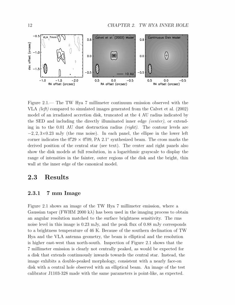
Figure 2.1.— The TW Hya 7 millimeter continuum emission observed with the
VLA (left) compared to simulated images generated from the Calvet et al. (2002)
model of an irradiated accretion disk, truncated at the 4 AU radius indicated by
the SED and including the directly illuminated inner edge (center), or extend-
ing in to the 0.01 AU dust destruction radius (right). The contour levels are
−2, 2, 3×0.23 mJy (the rms noise). In each panel, the ellipse in the lower left
corner indicates the 0.′′29 × 0.′′09, PA 2.1 synthesized beam. The cross marks the
derived position of the central star (see text). The center and right panels also
show the disk models at full resolution, in a logarithmic grayscale to display the
range of intensities in the fainter, outer regions of the disk and the bright, thin
wall at the inner edge of the canonical model.
2.3 Results
2.3.1 7 mm Image
Figure 2.1 shows an image of the TW Hya 7 millimeter emission, where a
Gaussian taper (FWHM 2000 kλ) has been used in the imaging process to obtain
an angular resolution matched to the surface brightness sensitivity. The rms
noise level in this image is 0.23 mJy, and the peak flux of 0.88 mJy corresponds
to a brightness temperature of 46 K. Because of the southern declination of TW
Hya and the VLA antenna geometry, the beam is elliptical and the resolution
is higher east-west than north-south. Inspection of Figure 2.1 shows that the
7 millimeter emission is clearly not centrally peaked, as would be expected for
a disk that extends continuously inwards towards the central star. Instead, the
image exhibits a double-peaked morphology, consistent with a nearly face-on
disk with a central hole observed with an elliptical beam. An image of the test
calibrator J1103-328 made with the same parameters is point-like, as expected.
2.3. RESULTS 13
2.3.2 Radially Averaged 7 mm Visibilities
The central hole in the TW Hya emission may be identified even more clearly
in the visibility domain, free from the effects of the Fourier transform process
and non-linear deconvolution. To better show the brightness distribution, we
averaged the visibility data in concentric annuli of deprojected (u,v) distance,
Ruv, as described in Lay et al. (1997). We use the TW Hya disk position angle
and inclination found by Qi et al. (2004) from CO line imaging of the outer disk
(-45 and 7, respectively). These values may not be valid in the inner disk, if
e.g. the disk warps in the interior. However, as long as the disk remains close to
face-on at all radii, the deprojection correction is small and therefore insensitive
to the exact values of these parameters.
For each visibility, the coordinates were redefined in terms of R =√u2 + v2,
the distance from the origin of the (u,v) plane, and φ = arctan(
vu− PA
)
, the
polar angle from the major axis of the disk (defined by the position angle, PA,
measured east of north). Assuming circular symmetry and taking into account
the disk inclination i, the deprojected (u,v) distances parallel to the major and
minor axes of the disk, are da = R sinφ, db = R cosφ cos i, respectively, and the
deprojected (u,v) distance is Ruv =√
d2a + d2
b .
An important parameter in the averaging process is the position of the star,
or the center of the disk. To examine the radial distribution of flux at the smallest
scales permitted by the data, particularly in the east-west direction of highest
resolution, we must know the phase center to within a fraction of the radius
set by the resolution, i.e., the position of the star must be specified to within a
few hundredths of an arcsecond, which is better than the absolute astrometric
accuracy of the data (typical positional accuracies in the A array are ∼0.′′1 due to
baseline uncertainties and uncorrected tropospheric phase fluctuations; see, e.g.
the 2004 VLA Observational Status Summary). To the extent that the disk is
symmetric, the process of deprojecting and averaging at the correct star position
will minimize the scatter within each deprojected radial bin and bring the average
of the imaginary parts of the visibilities (the average phase) to zero. Therefore,
we chose the star position to be that which minimized the absolute value of the
mean of the imaginary visibility bins. This position is indicated by the cross in
the left panel of Figure 2.1.
Figure 2.2 shows the annularly averaged visibility amplitude as a function
of Ruv. The width of each bin is 430 kλ, chosen to be narrow enough to sample
the shape of the visibility function and also wide enough to have sufficient
signal-to-noise ratio. Although the visibility data are still noisy when divided up

14 CHAPTER 2. TW HYA INNER HOLE
in this way, it is evident that the visibility function passes through a null near
Ruv of ∼1000 kλ, indicative of a sharp edge in the emission.
2.4 Discussion
The most striking feature of the new 7 millimeter observations is the central
depression in the image, which is also indicated by the presence of the null in
the deprojected visibility function. We identify this feature with a clearing of the
inner dust disk. A continuous disk that extends inward to the dust destruction
radius at ∼0.01 AU would show sharply centrally peaked emission and would not
show a null at the observed baselines. Figure 2.1 compares the 7 millimeter image
(left panel) with an image generated for a model with a continuous disk (right
panel). Figure 2.2 also shows the visibility function of continuous disk (dashed
line); this is clearly not compatible with the 7 mm observations (or the infrared
SED ).
Independent of detailed modeling, the size scale of this inner hole can be
estimated simply from the separation of the peaks in the image. These peaks are
sensitive primarily to inner edge of the disk, where the 7 millimeter brightness
is highest. The separation of the peaks is ∼0.′′14, or ∼ 7 AU. This separation is
slightly smaller than the diameter of the inner hole, since the bright emission
from the inner edge to the north and to the south of the star, combined with
the lower angular resolution in the north-south direction, tend to draw the image
peaks together. This effect is evident in the right panel of Figure 2.1, in which the
contoured peaks can be seen to lie interior to the inner edge of the disk. The null
in the visibility function provides a corroborating estimate of the size of the inner
hole in the disk. In appendix A, we show how the angular scale of the null in the
visibility function of a power law disk depends on the density and temperature
power law indices and the radius of the inner hole. If we assume that the outer
disk emission contributes little on these long baselines, and that the total emission
is dominated by a bright, thin ring associated with the inner edge of the disk, as
discussed in §2.4.1 below, then we can estimate the radius of the inner hole hole
with equation A.11. A linear fit to the binned visibilities gives a null position
of 930±60 kλ and implies an inner hole radius 4.3±0.3 AU. Thus the resolved
dust emission shows an inner hole in the disk at a size scale very similar to that
inferred from SED modeling.

2.4. DISCUSSION 15
Figure 2.2.— TW Hya real and imaginary 7 millimeter visibilities, in 430-kλ bins
of deprojected u-v distance from the center of the disk. Error bars represent the
standard error of the mean in each bin. Note that bins represented by open and
filled circles are not independent: the bins are overlapping, i.e., the domain of
each open circle extends to the neighboring filled circles. The calculated visibility
functions for the best fit irradiated accretion disk model is indicated by the heavy
solid line and is composed of contributions from an outer disk (solid line) with an
inner hole of radius 4.5 AU and a bright, thin wall (dotted line). For comparison,
the visibility function for a disk model that extends in to the dust destruction
radius at ∼0.01 AU is also shown (dashed line). To the extent that the disk is
radially symmetric, the imaginary part of the visibility (the average phase) should
be zero for all models.
16 CHAPTER 2. TW HYA INNER HOLE
2.4.1 Comparison with Disk Models
Power Law Disk Models
The dust emission from the outer disk of TW Hya has been shown to be a good
match to the structure of an irradiated accretion disk model, approximated by
power laws in temperature and surface density with indices q ∼ 0.5 and p ∼ 1.0,
respectively, over a wide range of radii. However, an extrapolation of this very
simple power law model to an inner disk truncated at ∼ 4 AU radius is not
compatible with the new long-baseline 7 millimeter data. For these power laws,
the null in the visibility function of the 4 AU hole should appear at ∼ 500 kλ,
which is a factor of two smaller than observed (equation A.9). In order for a
4 AU hole to be consistent with a ∼1000 kλ null, the power law model requires
a much steeper emission gradient, with the sum of the radial power law indices
p + q approaching 5. Such steep power laws are inconsistent with observations of
the outer disk. In addition, this power law model fails to reproduce the flux in
the image peaks by nearly an order of magnitude. Another possibility is that the
radius of the hole is smaller than that predicted by the SED. A power law disk
with p + q = 1.5 and radius 2 AU does reproduce the 1000 kλ null and observed
peak separation; however, this model still fails to reproduce the observed peak
flux by more than a factor of five. These discrepancies indicate that a more
complex model of the disk is needed. In general, reproducing the observed peak
flux in the new high resolution observations requires a greater concentration of
material at the inner edge of the disk than that of power-law disk models.
A natural modification to the power law disk model with an inner hole is
the addition of a bright, thin, inner edge, or “wall” component. This “wall”
component corresponds to the frontally illuminated inner edge of the disk in the
calculations of Calvet et al. (2002), who show that a small range of temperatures
is required to reproduce the narrow spectral width of the mid-infrared excess. The
presence of this additional compact component to the model shifts the angular
scale of the null in the visibility function to larger Ruv and raises the flux at
long baselines. In this composite model, for a given power law description, the
angular scale of the null in the composite “disk+wall” visibility function depends
on (1) the radius of the inner hole, and (2) the relative brightness of the disk and
wall. The effect of the second dependency is to move the angular scale of the null
between the limiting positions from the “disk” alone and from the “wall” alone.
In fact, the position of the null in the 7 millimeter data is close to that expected
from an infinitesimally thin ring of ∼4 AU radius (equation A.11). A bright, thin
ring also reproduces the ∼0.′′14 separation of the image peaks. Thus it appears

2.4. DISCUSSION 17
that the high resolution observations show primarily the directly illuminated wall
at the inner edge of the disk. At these long baselines, the extended emission from
the outer disk that dominates at larger size scales is weak and effectively not
detected.
Irradiated Accretion Disk Model
The irradiated accretion disk model of Calvet et al. (2002) provides a more
realistic description of disk structure than a simple power-law model. To compare
the data to this more sophisticated disk model, we simulate numerically the
expected emission at 7 millimeters, including the detailed visibility sampling of
the Very Large Array observations.
For the frontally illuminated component of the inner edge of the disk, we
follow the prescription of Calvet et al. (2002), adopting a shape given by
zs = z0 exp [(R −R0)/∆R] (2.1)
and temperature
Tphot(R) ≈ T∗
(
R∗
R
)1/2(µ0
2
)1/4
(2.2)
where R is the radius from the star, zs is the height of the wall, subscript 0
refers to the boundary between the wall and the outer disk, µ0 = cos θ0 and
θ0 = π/2 − tan−1(dzs/dR), and we assume that at 7 millimeters the radial
brightness tracks the temperature. To set the absolute flux of this component, we
normalized the intensity distribution to match the peak flux of the image and the
total flux of the disk determined from previous, lower resolution imaging (Wilner
et al. 2000). Since ∆R is not well constrained by our data, except that the wall
must be narrow compared to the size of the hole (∆R ≪ R) and the resolution of
the data (∆R ≪ 0.′′09, or 4.6 AU at 51 pc), we use the value ∆R = 0.5 AU which
Calvet et al. (2002) find to be consistent with the shape of the mid-IR SED. We
choose R0 to be 4.5 AU so that the peak of the wall emission occurs near 4.0 AU,
causing the null of the model to match the position indicated by the data. For
the dust mass opacity, we use the power law form κ = κ0(νν0
)β where κ0 = 1.8,
ν0 = 1.0 × 10¹², and β = 0.8 (D’Alessio et al. 2001).
We used the Monte Carlo radiative transfer code RATRAN (Hogerheijde &
van der Tak 2000) to calculate a sky-projected image from the model continuum
emission, with frequency and bandwidth appropriate for the observations, and the
miriad task uvmodel to simulate the observations, using the appropriate antenna

18 CHAPTER 2. TW HYA INNER HOLE
positions and visibility weights. Figure 2.2 shows the visibility function from
this model (heavy solid line), which matches well the observations. The light
solid line shows the contribution from the outer disk, which accounts for only a
small fraction of the flux observed at long baselines, and the dotted curve shows
contribution from the thin wall component, which dominates the outer disk at
Ruv beyond ∼ 100 kλ. The long baseline data are sensitive to the total flux
and thin width of the wall, and are compatible with the assumptions of the wall
structure used in the previous SED modeling. In the image domain, we have
compared the 7 millimeter data to the Calvet et al. (2002) model using RATRAN
to generate images of a disk with an inner hole of radius 4.5 AU and a bright wall
of width 0.5 AU and total flux 1.7 mJy (Figure 2.1, center panel), which Calvet
et al. (2002) find to be consistent with the mid-infrared SED. For comparison,
we also generate an image of a continuous disk extending inward to the dust
destruction radius at 0.01 AU (Figure 2.1, right panel). The data are inconsistent
with this continuous disk model, while the SED-based model of Calvet et al.
(2002) with an inner hole and bright wall matches the observed structure well.
In short, the 7 millimeter data suggest an outer dust disk extending inward
to ∼ 4.5 AU, where there is wall of radial extent ∼0.5 AU that is much brighter
than the surrounding disk on account of direct illumination by the star. Interior
to the wall, a sharp transition occurs to a region of lower dust surface density and
correspondingly weak or absent 7 millimeter emission.
2.4.2 Disk Clearing
The resolved observations bolster the inference from SED models that the TW
Hya disk has an inner hole of much reduced dust column density of radius
∼ 4 AU. Theories of disk-planet interaction have long predicted the opening of
gaps in circumstellar disks as a consequence of the formation of giant planets (e.g.
Lin & Papaloizou 1986; Bryden et al. 1999), and numerical simulations of such
interactions produce these gaps in a consistent way across differing architectures
and computational algorithms (de Val-Borro et al. 2006). Recent work by Varniere
et al. (2006) has shown that in turbulent disks with α-viscosity, inner holes are
in fact more likely than gaps as a consequence of the formation of Jupiter-mass
planets around solar mass stars, as the process of outward angular momentum
transfer mediated by spiral density waves can cause clearing of the inner disk on
time scales an order of magnitude shorter than the viscous timescale.
While the inner disk is largely cleared, it is not entirely devoid of gas and
dust. Optical emission lines indicate gas accretion (Muzerolle et al. 2000), albeit
2.5. CONCLUSIONS 19
at the low rate of 4 × 10⁻¹⁰ M⊙ yr−1. Rettig et al. (2004) detect ∼ 6 × 10²¹ g of
warm CO at distances of 0.5-1 AU from the star, and Herczeg et al. (2004) infer
the presence of warm H2 within 2 AU of the star by modeling the HST and FUSE
H2 emission spectrum. The 10 µm silicate feature (Sitko et al. 2000; Uchida et al.
2004) indicates that there must be at least a few tenths of a lunar mass of dust
grains present in the otherwise largely cleared inner disk (Calvet et al. 2002).
The region within ∼0.3 AU has been spatially resolved by Eisner et al. (2006)
at 2 µm using the Keck interferometer, detecting emission from optically thin,
submicron-sized dust populating the inner regions. This small amount of material
may be the result of a restricted flow through the transition region at ∼ 4 AU
from the massive reservoir of the outer disk. A population of micron-sized grains
in the inner disk is consistent with the predictions of Alexander & Armitage
(2007), who show that planet-induced gaps tend to filter out and confine large
grains at the gap edge while allowing small grains to migrate across the gap with
accreting gas and populate the inner disk. Our data are consistent with an inner
region devoid of 7mm dust emission; however, the degree of clearing is difficult
to constrain due to both the low signal-to-noise ratio at long baselines and the
dependence on the wall model adopted.
The dynamical effect of a planet is not the only possible explanation for
the observed central flux deficit at millimeter wavelengths. Photoevaporation of
gas by ultraviolet radiation has also been invoked to explain inner disk clearing
(Clarke et al. 2001), if the evaporation rate at the gravitational radius dominates
the accretion rate. As discussed by Alexander et al. (2006), TW Hya is at best
marginally consistent with a photoevaporation scenario, since the outer disk mass
is larger than predicted for photoevaporation, and the observed accretion should
occur only for the brief period while the inner disk is draining onto the star. In
contrast with the case of a planet-induced gap, photoevaporation should also clear
the inner disk of all but the largest grains, as noted by Alexander & Armitage
(2007). Other mechanisms, such as photophoretic effects (Krauss & Wurm 2005),
could also aid in clearing the inner disk region, if gas densities are high enough.
2.5 Conclusions
We present new, spatially resolved observations of the TW Hya disk at
7 millimeters that provide direct evidence for a sharp transition in dust surface
density at ∼ 4 AU radius, a feature consistent with the inner hole inferred from
SED modeling by Calvet et al. (2002). The interpretation of the mid-infrared flux
20 CHAPTER 2. TW HYA INNER HOLE
deficit as a central clearing of material is robust. The TW Hya system is ideally
suited to future observations that will be able to distinguish between the various
scenarios invoked to explain central clearing in the disks around young stars.
Signatures diagnostic of planets in formation, in particular spiral density waves
in the disk and thermal emission from circumplanetary dust, should be within
the detection capabilities of the Atacama Large Millimeter Array operating at
the shortest submillimeter wavelengths (300 µm) and at the longest baselines
(> 10 km) to achieve the necessary angular resolution (Wolf & D’Angelo 2005).
Such observations will benefit from the close proximity of TW Hya, the nearly
face-on viewing geometry, and the size scale of the inner hole now confirmed by
direct observation at millimeter wavelengths.
Chapter 3
A Spatially Resolved Inner Hole
in the Disk around GM Aurigae
A. M. Hughes, S. M. Andrews, C. C. Espaillat, D. J. Wilner, N. Calvet, P.
D’Alessio, C. Qi, J. P. Williams, & M. R. Hogerheijde 2009, The Astrophysical
Journal, Vol. 698, pp. 131-142
Abstract
We present 0.′′3 resolution observations of the disk around GM Aurigae with the
Submillimeter Array (SMA) at a wavelength of 860µm and with the Plateau de
Bure Interferometer at a wavelength of 1.3mm. These observations probe the
distribution of disk material on spatial scales commensurate with the size of the
inner hole predicted by models of the spectral energy distribution. The data
clearly indicate a sharp decrease in millimeter optical depth at the disk center,
consistent with a deficit of material at distances less than ∼20AU from the star.
We refine the accretion disk model of Calvet et al. (2005) based on the unresolved
spectral energy distribution (SED) and demonstrate that it reproduces well
the spatially resolved millimeter continuum data at both available wavelengths.
We also present complementary SMA observations of CO J=3−2 and J=2−1
emission from the disk at 2′′ resolution. The observed CO morphology is
consistent with the continuum model prediction, with two significant deviations:
(1) the emission displays a larger CO J=3−2/J=2−1 line ratio than predicted,
which may indicate additional heating of gas in the upper disk layers; and (2)
the position angle of the kinematic rotation pattern differs by 11 ± 2 from that
21

22 CHAPTER 3. GM AUR INNER HOLE
measured at smaller scales from the dust continuum, which may indicate the
presence of a warp. We note that photoevaporation, grain growth, and binarity
are unlikely mechanisms for inducing the observed sharp decrease in opacity or
surface density at the disk center. The inner hole plausibly results from the
dynamical influence of a planet on the disk material. Warping induced by a
planet could also potentially explain the difference in position angle between the
continuum and CO data sets.
3.1 Introduction
Understanding of the planet formation process is intimately tied to knowledge of
the structure and evolution of protoplanetary disks. Of particular importance is
how and when in the lifetime of the disk its constituent material is cleared, which
provides clues to how and when planets may be assembled. While observations
suggest that the inner and outer dust disk disperse nearly simultaneously (e.g.
Skrutskie et al. 1990; Wolk & Walter 1996; Andrews & Williams 2005), it is
not clear which physical mechanism(s) drives this process, or the details of how
it progresses. Possible dispersal mechanisms, of which several may come into
play over the lifetime of a disk, include a drop in dust opacity due to grain
growth (e.g. Strom et al. 1989; Dullemond & Dominik 2005), photoevaporation
of material by energetic stellar radiation (e.g. Clarke et al. 2001), photophoretic
effects of gas on dust grains (Krauss & Wurm 2005), inside-out evacuation via the
magnetorotational instability (Chiang & Murray-Clay 2007), and the dynamical
interaction of giant planets with natal disk material (e.g. Lin & Papaloizou 1986;
Bryden et al. 1999). Observing the distribution of gas and dust in disks allows us
to evaluate the roles of these disk clearing mechanisms.
One particular class of systems, those with “transitional” disks (e.g. Strom
et al. 1989; Skrutskie et al. 1990), have become central to our understanding
of disk clearing. These disks exhibit a spectral energy distribution (SED)
morphology with a deficit in the near- to mid-infrared excess over the photosphere
consistent with a depletion of warm dust near the star. The advent of the Spitzer
Space Telescope has allowed detailed measurement of mid-infrared spectra with
unprecedented quality and quantity. Combined with simultaneous advances in
disk modeling that can now reproduce in detail the SED features (e.g. D’Alessio
et al. 1999, 2001; Dullemond et al. 2002; D’Alessio et al. 2006), these observations
have revolutionized the study of disk structure. However, such studies rely
entirely on SED deficits whose interpretations are not unique, since effects of

3.1. INTRODUCTION 23
geometry and opacity can mimic the signature of disk clearing (Boss & Yorke
1996; Chiang & Goldreich 1999).
Spatially resolved observations are crucial for confirming the structures
inferred from disk SEDs. High resolution imaging at millimeter wavelengths is
especially important because dust opacities are low, and the disk mass distribution
can be determined in a straightforward way for an assumed opacity. Millimeter
observations also avoid many of the complications present at shorter wavelengths,
including large optical depths, spectral features, and contrast with the central
star. Several recent millimeter studies have resolved inner emission cavities for
disks with infrared SED deficits through direct imaging observations, e.g. TW
Hya (Calvet et al. 2002; Hughes et al. 2007), LkHα 330 (Brown et al. 2007,
2008), and LkCa 15 (Pietu et al. 2007; Espaillat et al. 2008). These observations
unambiguously associate infrared SED deficits with a sharp drop in millimeter
optical depth in the disk center. More information is needed to determine whether
the low optical depth is a result of decreased surface density or opacity.
GM Aurigae is a prototypical example of a star host to a “transitional” disk.
The ∼1-5 Myr old T Tauri star (Simon & Prato 1995; Gullbring et al. 1998) of
spectral type K5 is located at a distance of 140 pc in the Taurus-Auriga molecular
complex (Bertout & Genova 2006), and its brightness and relative isolation
from intervening cloud material have enabled a suite of observational studies of
its disk properties. The presence of circumstellar dust emitting at millimeter
wavelengths was first inferred by Weintraub et al. (1989), and the disk structure
was subsequently resolved in the 13CO J=2–1 transition by Koerner et al. (1993).
Their arcsecond-resolution mapping of the gas disk revealed gaseous material in
rotation about the central star. Assuming a Keplerian rotation pattern allowed
a determination of the dynamical mass for the central star of 0.8 M⊙. Further
modeling of the structure and dynamics of the disk was carried out by Dutrey
et al. (1998), using higher-resolution 12CO J=2–1 observations. Scattered light
images revealed a dust disk inclined by 50-56 extending to radii ∼ 300AU from
the star (Stapelfeldt & The WFPC2 Science Team 1997; Schneider et al. 2003).
Efforts to model the SED of GM Aurigae have long indicated the presence of
an inner hole, and estimates of its size have grown over the years as the quality
of data and models have improved. In the early 1990s, the low 12µm flux led to
∼ 0.5AU estimates of the inner disk radius (Marsh & Mahoney 1992; Koerner
et al. 1993). That value was later increased to 4.8AU by Chiang & Goldreich
(1999) in the context of hydrostatic radiative equilibrium models, and a putative
planet at a distance of 2.5AU from the star was shown to be capable of clearing
an inner hole of this extent using simulations of the relevant hydrodynamics
24 CHAPTER 3. GM AUR INNER HOLE
(Rice et al. 2003). With the aid of a ground-based mid-IR spectrum, Bergin
et al. (2004) increased the gap size estimate to 6.5AU, and subsequently Calvet
et al. (2005) inferred an inner hole radius of 24AU using a Spitzer IRS spectrum
in combination with sophisticated disk structure models. Recently, Dutrey
et al. (2008) have argued for a 19±4AU inner hole in the gas distribution,
using combined observations of several different molecular line tracers. Like the
SED-based measurements, their method is indirect: they use a model of the disk
in Keplerian rotation to associate a lack of high-velocity molecular gas with a
deficit of material in the inner disk.
We present interferometric observations at 860µm from the Submillimeter
Array1 and 1.3mm from the Plateau de Bure Interferometer2 that probe disk
material on scales commensurate with the 24AU inner disk radius inferred from
the SED. These data allow us to directly resolve the inner hole in the GM Aur
disk for the first time. We describe the observations in §3.2 and present the
dual-wavelength continuum data in §3.3.1. We also present observations of the
molecular gas disk in the CO J=3–2 and J=2–1 lines that allow us to study
disk kinematics in §3.3.2. We use these data to investigate disk structure in
the context of the SED-based models of Calvet et al. (2005), described in §3.4.
Implications for the disk structure and evolutionary status are discussed in §3.5.
3.2 Observations and Data Reduction
The GM Aur disk was observed with the 8-element (each with a 6m diameter)
Submillimeter Array (SMA; Ho et al. 2004) in the very extended (68-509m
baselines) and compact (16-70m baselines) configurations on 2005 November 5
and 26, respectively. Observing conditions on both nights were excellent, with
∼1mm of precipitable water vapor and good phase stability. Double sideband
receivers were tuned to a central frequency of 349.935GHz (857µm), with each
2GHz-wide sideband centered ±5GHz from that value. The SMA correlator
was configured to observe the CO J=3−2 (345.796GHz) and HCN J=4−3
(354.505GHz) transitions with a velocity resolution of 0.18 km s−1. No HCN
1The Submillimeter Array is a joint project between the Smithsonian Astrophysical Obser-
vatory and the Academica Sinica Institute of Astronomy and Astrophysics and is funded by the
Smithsonian Institution and the Academica Sinica.
2Based on observations carried out with the IRAM Plateau de Bure Interferometer. IRAM is
supported by INSU/CNRS (France), MPG (Germany) and IGN (Spain).

3.2. OBSERVATIONS AND DATA REDUCTION 25
was detected, with a 3σ upper limit of 0.9 Jy beam−1 in the 2.′′2×1.′′9 synthesized
beam. The observing sequence alternated between GM Aur and the two gain
calibrators 3C 84 and 3C 111. The data were edited and calibrated using the MIR
software package.3 The passband response was calibrated using observations of
Saturn (compact configuration) or the bright quasars 3C 273 and 3C 454.3 (very
extended configuration). The amplitude scale was determined by bootstrapping
observations of Uranus and these bright quasars, and is expected to be accurate
at the ∼10% level. Antenna-based gain calibration was conducted using 3C 111,
while the 3C 84 observations were used to check on the quality of the phase
transfer. We infer that the “seeing” induced on the very extended observations
by phase noise and small baseline errors is small, .0.′′1. Wideband continuum
channels from both sidebands and configurations were combined. The derived
870µm flux of GM Aur is 640 ± 60mJy.
Additional SMA observations in the extended (28-226m) and sub-compact
(6-69m baselines) configurations were conducted on 2006 December 10 and 2007
September 14, respectively, with a central frequency of 224.702GHz (1335µm).
While the sub-compact observations were conducted in typical weather conditions
for this band (2.5mm of water vapor), the extended data were obtained in better
conditions similar to those for the higher frequency observations described above.
The correlator was configured to simultaneously cover the J=2−1 transitions of
CO (230.538GHz), 13CO (220.399GHz), and C18O (219.560GHz) with a velocity
resolution of ∼0.28 km s−1. The calibrations were performed as above.
GM Aurigae was also observed with the 6-element (each with a 15m
diameter) Plateau de Bure Interferometer (PdBI) in the A configuration (up to
750m baselines) on 2006 January 15. Observing conditions were excellent, with
atmospheric phase noise generating a seeing disk of .0.2′′. The PdBI dual-receiver
system was set to observe the 110.201GHz (2.7mm) and 230.538GHz (1.3mm)
continuum simultaneously. As with the SMA data, observations alternated
between GM Aur and two gain calibrators, 3C 111 and J0528+134. The data
were edited and calibrated using the GILDAS package (Pety 2005). The passband
responses and amplitude scales were calibrated with observations of 3C 454.3
and MWC 349, respectively. The derived 1.3 and 2.7mm fluxes of GM Aur are
180 ± 20 and 21 ± 2mJy.
The standard tasks of Fourier inverting the visibilities, deconvolution with
the CLEAN algorithm, and restoration with a synthesized beam were conducted
with the MIRIAD software package. A high spatial resolution image of the
3See http://cfa-www.harvard.edu/∼cqi/mircook.html.
26 CHAPTER 3. GM AUR INNER HOLE
860µm continuum emission from the SMA data was created with a Briggs robust
= 1.0 weighting scheme for the visibilities, excluding projected baselines ≤ 70 kλ,
resulting in a synthesized beam FWHM of 0.′′30 × 0.′′24 at a position angle of
34. A similar image of the 1.3mm continuum emission with a synthesized beam
FWHM of 0.′′43 × 0.′′30 at a position angle of 35 was generated from the PdBI
data using natural weighting (robust = 2.0). Table 3.1 summarizes the line and
continuum observational parameters.
3.3 Results
3.3.1 Millimeter Continuum Emission
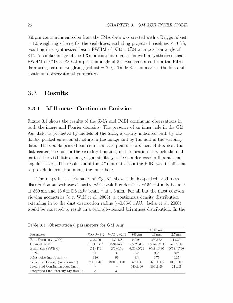
Figure 3.1 shows the results of the SMA and PdBI continuum observations in
both the image and Fourier domains. The presence of an inner hole in the GM
Aur disk, as predicted by models of the SED, is clearly indicated both by the
double-peaked emission structure in the image and by the null in the visibility
data. The double-peaked emission structure points to a deficit of flux near the
disk center; the null in the visibility function, or the location at which the real
part of the visibilities change sign, similarly reflects a decrease in flux at small
angular scales. The resolution of the 2.7mm data from the PdBI was insufficient
to provide information about the inner hole.
The maps in the left panel of Fig. 3.1 show a double-peaked brightness
distribution at both wavelengths, with peak flux densities of 59 ± 4 mJy beam−1
at 860µm and 16.6 ± 0.3 mJy beam−1 at 1.3mm. For all but the most edge-on
viewing geometries (e.g. Wolf et al. 2008), a continuous density distribution
extending in to the dust destruction radius (∼0.05-0.1AU; Isella et al. 2006)
would be expected to result in a centrally-peaked brightness distribution. In the
Table 3.1: Observational parameters for GM AurContinuum
Parameter 12CO J=3–2 12CO J=2–1 860µm 1.3mm 2.7mm
Rest Frequency (GHz) 345.796 230.538 349.935 230.538 110.201
Channel Width 0.18 km s−1 0.28 km s−1 2 × 2GHz 2 × 548MHz 548MHz
Beam Size (FWHM) 2.′′2×1.′′9 2.′′1×1.′′4 0.′′30×0.′′24 0.′′43×0.′′30 0.′′93×0.′′60
PA 14 56 34 35 31
RMS noise (mJybeam−1) 310 90 3.5 0.75 0.25
Peak Flux Density (mJybeam−1) 6700 ± 300 2400 ± 100 59 ± 4 16.6 ± 0.8 10.3 ± 0.3
Integrated Continuum Flux (mJy) – – 640 ± 60 180 ± 20 21 ± 2
Integrated Line Intensity (Jy km s−1) 29 37 – – –

3.3. RESULTS 27
Figure 3.1.— Continuum emission from the disk around GM Aur at wavelengths
of 860µm observed with the SMA (top) and 1.3mm observed with PdBI (bottom).
The data are displayed in both the image (a) and Fourier (b) domains. In the
image domain (a), the observed brightness distribution at each wavelength (left)
is compared with the model prediction (center; see §3.4.1 for model details), and
the residuals are also shown (right). In the data and model frames, the contours
are [3, 6, 9, ...]× the rms noise (3.5mJybeam−1 at 860µm and 0.75mJybeam−1 at
1.3mm). In the residual frame, the contours start at 2σ and are never greater than
3σ. The synthesized beam sizes and orientations for the two maps are, respectively,
0.′′30×0.′′24 at a position angle of 34 and 0.′′43×0.′′30 at a position angle of 35. Two
sets of axes are shown: the dotted line indicates the position angle of the double-
peaked continuum emission, while the solid line indicates the best-fit position angle
of the CO emission (see §3.3.2 for details). In the Fourier domain (b), the visibilities
are averaged in bins of deprojected u-v distance from the disk center, and compared
with the model prediction (red line). The inner hole in the GM Aur disk is clearly
observed at both wavelengths, as a double-peaked emission structure in the image
domain or as a null in the visibility function in the Fourier domain.

28 CHAPTER 3. GM AUR INNER HOLE
case of GM Aurigae, the double-peaked emission structure is a geometric effect
due to the truncation of disk material at a much larger radius, viewed at an
intermediate inclination of 50-56 (Dutrey et al. 1998, 2008): the region of highest
density is near the inner disk edge, with a large column density of optically thin
material in this ring effectively generating limb brightening at the inner edge of
the outer disk, at two points along the disk major axis.
The size of the inner hole can be roughly estimated by the separation of the
emission peaks, although the peak separation will also depend on the brightness
of the directly-illuminated inner edge of the outer disk relative to the extended
disk component (Hughes et al. 2007). The separation of the peaks in the 860 µm
image is 0.′′38 ± 0.′′03, corresponding to a physical diameter of 53 ± 4 AU (radius
27 ± 2 AU) at a distance of 140 pc. A position angle of 66 is estimated by the
orientation of a line that bisects the two peaks, although a more robust value of
64 ± 2 is derived in §3.4.1 below. Since the peaks are not distinctly separated in
the 1.3mm image, the same estimate cannot be made, but the position angle is
clearly consistent with that derived from the 860µm visibilities and indicated by
the perpendicular dashed lines in Fig. 3.1.
The presence of an inner hole is also evident from the visibilities displayed
in the right panel of Fig. 3.1. The real part of the complex visibilities have been
averaged in concentric annuli of deprojected (u, v) distance from the disk center.
For details of the deprojection process, see Lay et al. (1997). As discussed in
the appendix of Hughes et al. (2007), the presence of a null in the visibility
function indicates a sharp decrease in flux at a radius corresponding roughly to
the angular scale of the null position. The precise position of the null depends
primarily on the angular size of the inner hole, but also on the radial gradients of
the surface density and temperature distribution and the relative brightness of
the directly illuminated wall at the inner edge of the outer disk. In a standard
power-law parameterization, the disk temperature T and surface density Σ vary
inversely with radius as Σ ∝ R−p and T ∝ R−q. Neglecting the emission from
the wall and assuming standard values of p = 1.0 and q = 0.5, expected for a
typical viscous disk with constant α (Hartmann et al. 1998) and consistent with
previous studies of the GM Aur disk (Dutrey et al. 1998; Andrews & Williams
2007; Hughes et al. 2008b), we may obtain a rough estimate of the size of the
inner hole using the observed null position and Eq. A9 from Hughes et al. (2007):
Rnull(kλ) = (1 AU/Rhole)(Dsource/100 pc)[2618 + 1059(p + q)]. A polynomial
curve fit to the visibilities yields a null position of 190 kλ at 860µm and 224 kλ
at 1.3mm, which correspond to inner hole radii of 31 and 26 AU, respectively.
However, these estimates are uncertain to within ∼30%, as the data are consistent

3.3. RESULTS 29
with a broad range of null positions. We therefore turn to a more sophisticated
modeling procedure described in §3.4.1 below.
3.3.2 CO Channel and Moment Maps
Figures 3.2–3.4 display the new SMA observations of CO emission from the GM
Aur disk. Figures 3.2 and 3.3 show channel maps with contours starting at twice
the rms noise level and increasing by factors of√
2, while Figure 3.4 displays the
zeroth (contours) and first (color) moments of the data: these are the velocity-
integrated intensity and intensity-weighted velocities, respectively. The peak flux
density is 6.7 ± 0.3 Jybeam−1 in the CO J=3–2 line and 2.4 ± 0.1 Jybeam−1 in
the CO J=2–1 line, with integrated fluxes of 9.4 Jy km s−1 and 21.2 Jy km s−1,
respectively (although emission from extended ambient cloud material is likely
to increase the CO J=2–1 integrated flux over that originating from the disk
alone). The channel and moment maps are broadly consistent with the expected
kinematic pattern for material in Keplerian rotation about the central star,
substantially inclined to our line of sight (as in Dutrey et al. 1998; Simon et al.
2000).
The short-baseline spatial frequencies in the (u, v) plane provided by the
subcompact configuration of the SMA during our observations of the J=2−1
transition are sensitive to emission on the largest spatial scales. These short
antenna spacings reveal the severity of the cloud contamination to an extent not
possible with previous data. The contamination is evident as an extended halo
around the disk emission in the central channels of the J=2−1 channel maps
near LSR velocities of 5-6 km s−1 (Fig. 3.3). It is also evident in the moment map
(Fig. 3.4) as an elongation of emission near the systemic velocity (green-yellow)
to the northwest along the disk minor axis. This contamination indicates that
caution must be exercised when deriving kinematic information from the CO
lines, particularly the central channels. Spatial filtering by the interferometer does
not ameliorate cloud contamination in an abundant, easily-excited, high-optical
depth tracer like COJ=2–1. The J=3−2 line appears less contaminated than
J=2−1 (Figs. 3.2 and 3.4), although similarly short antenna spacings (8-43m)
are not present in this data set. Nevertheless, we expect less cloud contamination
in the J=3−2 transition, since the temperature of the cloud will be lower than
that of the disk and will therefore populate the upper rotational levels of the
CO molecule less efficiently. The cloud contamination prevents detection of
self-absorption in the central channels of the CO J=2–1 channel maps along the
near (northwest) edge of the disk (as determined by scattered light observations;
30 CHAPTER 3. GM AUR INNER HOLE
see Schneider et al. 2003). Dutrey et al. (1998) report self-absorption along the
southeast edge, but our observations suggest that this brightness asymmetry may
be due to cloud contamination. It is also possible that the contamination is due to
a residual envelope, although we are unable to determine the large-scale structure
of the extended line emission with our interferometric data.
In all figures, the disk orientation based on the position angle of 64 derived
from the continuum emission (Fig. 3.1 and §3.4.1) is plotted over the CO
emission as a set of crossed dashed lines, with the relative extent of the major
and minor axes (based on the inclination angle of 55) indicated by the length
of the perpendicular lines. The position angle of 51 derived by Dutrey et al.
(1998) from fitting the CO J=2−1 emission, consistent with our own J=3−2
and J=2−1 observations, is illustrated by the solid line. Note that the position
angle of the CO emission differs slightly from the position angle of the continuum
emission, by 11 ± 2 (see §3.4.1). The trend is clear for both transitions, but
more obvious in the less-contaminated J=3−2 transition. Note that the position
angle for the CO emission is derived entirely from the rotation pattern (evident
in the isovelocity contours) and not from the geometry of the integrated CO
emission: the integrated emission appears to match the position angle from the
continuum emission reasonably well. We do not observe the isophote twisting in
integrated CO emission seen by Dutrey et al. (1998). The cloud contamination
and differences in antenna spacings may play a role.
3.4 Disk Structure Models
3.4.1 Updated SED Model
Here we revisit the broadband SED modeling of GM Aur presented by Calvet
et al. (2005). Taking into consideration new observational constraints at
sub-millimeter and millimeter wavelengths, we use the irradiated accretion disk
models of D’Alessio et al. (2005, 2006) to re-derive the properties of the outer disk
of GM Aur and its inner, truncated edge or “wall.” Our grain-size distribution
follows a power-law of a−3.5, where a is the grain radius. We assume ISM-sized
grains in the upper layers of the disk and accordingly adopt amin=0.005µm and
amax=0.25µm (Draine & Lee 1984). Closer to the disk midplane grains have a
maximum size of 1mm. Input parameters for the outer disk include the stellar
properties, the mass accretion rate, the viscosity parameter (α), and the settling
parameter (ǫ) which measures the dust-to-gas mass ratio in the upper layers of

3.4. DISK STRUCTURE MODELS 31
Figure 3.2.— Channel maps of CO J=3−2 emission from the GM Aur disk. Con-
tour levels start at 0.61 Jy (2 times the rms noise) and increase by factors of√
2.
LSR velocity is indicated by color and quoted in the upper right of each panel. The
synthesized beam (2.′′2×1.′′9 at a PA of 14) and physical scale are indicated in the
lower left panel. Two sets of axes are shown: the dotted line indicates the position
angle of the double-peaked continuum emission, while the solid line indicates the
best-fit position angle of the CO emission.
Figure 3.3.— Channel maps of CO J=2−1 emission from the GM Aur disk. Con-
tour levels start at 0.17 Jy (2 times the rms noise) and increase by factors of√
2.
LSR velocity is indicated by color and quoted in the upper right of each panel. The
synthesized beam (2.′′1×1.′′4 at a PA of 56) and physical scale are indicated in the
lower left panel. Two sets of axes are shown: the dotted line indicates the position
angle of the double-peaked continuum emission, while the solid line indicates the
best-fit position angle of the CO emission. Cloud contamination is evident in at
least the central four channels.

32 CHAPTER 3. GM AUR INNER HOLE
Figure 3.4.— Zeroeth (contours) and first (colors) moment map of the CO J=3−2
(top) and J=2−1 (bottom) data in Figs. 3.2 and 3.3. The dotted line indicates the
position angle of the double-peaked continuum emission, while the solid line indi-
cates the best-fit position angle of the CO emission. The zeroth moment contours
are well aligned with the latter, while the isovelocity contours of the first moment
map are more consistent with the former. Cloud contamination is evident in the
CO J=2−1 map in the northwest region along the disk minor axis.
the disk relative to the standard dust-to-gas mass ratio. Following Calvet et al.
(2005), we adopt the same extinction, distance, inclination, dust grain opacities,
and stellar properties (i.e. luminosity, radius, and temperature; see Table 3.2).
We use a mass accretion rate of 7.2×10⁻⁹ M⊙ yr−1 which was derived using HST
STIS spectra by Ingleby & Calvet (2009), in contrast to the value of 10−8 M⊙ yr−1
derived from veiling measurements in Calvet et al. (2005). We assume an outer
disk radius of 300AU, which matches the observed extent of scattered light from
the dust disk (Schneider et al. 2003) and previous fits to the continuum emission
(Hughes et al. 2008b), as well as the short-baseline data presented here.
In order to reproduce the outer disk component of the SED, we vary ǫ and
α (Figure 3.5). As described in (Calvet et al. 2005), α effectively determines
3.4. DISK STRUCTURE MODELS 33
the mass surface density distribution and therefore the disk mass, which is best
reflected by the longest-wavelength SED points. The value of ǫ has the greatest
effect on the slope of the SED beyond 100µm. With the new millimeter data
we find ǫ=0.5, indicating less settling than reported previously. We also find
α=0.002 and a more massive outer disk of 0.16M⊙. This mass is significantly
larger than an estimate based on the 860µm and 1.3mm flux measurements
using opacities from Beckwith et al. (1990), which yields ∼0.04M⊙, and is only
marginally Toomre stable at 300AU (Q∼1.1). The outer disk model uses an
opacity of ∼0.1 cm2 g−1 at 1mm (D’Alessio et al. 2001) which is about four times
lower than that derived from the Beckwith et al. (1990) opacities, accounting for
the discrepancy in mass. Within the inner disk hole, there are 1.1×10⁻¹¹ M⊙ of
optically thin small dust grains, which account for the 10 µm emission and the
near-IR excess. The mass in solids could be much larger than this mass if pebbles,
rocks, or even planetesimals have grown in the inner disk, since they would have
a negligible opacity in the near-IR. We note that Calvet et al. (2005) reports
the mass of the dust as 7×10⁻¹⁰ M⊙; this is actually the mass of the gas within
the hole, assuming the standard dust to gas mass ratio. The gas mass could be
significantly larger, depending on the total amount of solids and the actual ratio,
but these are poorly constrained by existing data.
We vary the temperature of the wall to best reproduce the data. The radius
of the wall is set by the temperature and dust composition, and the wall’s height
is set by the disk scale height. We assume that the wall is axisymmetric and
composed of relatively small grains, as well as vertically flat in order to reproduce
the rapid rise of the mid-IR excess at wavelengths beyond 10µm. We adopt the
dust composition used in D’Alessio et al. (2005) and Calvet et al. (2005). The
maximum grain size is adjusted from ISM sizes to reproduce the shape of the IRS
spectrum as necessary. At short wavelengths, larger grains have smaller opacities
than ISM-sized grains. Therefore, at a given temperature large grains will be at
smaller radii than ISM-sized grains as per Eqn. 12 of D’Alessio et al. (2005). The
derived size of the inner hole varies somewhat depending on whether the SED
or the resolved millimeter visibilities are included. Fitting only the broadband
SED and neglecting the resolved millimeter-wavelength data, the wall is located
at 26AU and has a temperature of 130K and a height of ∼2AU with maximum
grain size amax=0.25µm (Fig. 3.5, left panel). The radius of the wall differs by
∼2 AU from Calvet et al. (2005), since here we take Lacc ∼ GMM/R assuming
magnetospheric accretion while Calvet et al. (2005) uses Lacc ∼ GMM/2R as per
the boundary layer model. We also adopt a different mass accretion rate.
In order to compare the SED model with the resolved continuum data, it is
34 CHAPTER 3. GM AUR INNER HOLE
necessary to fix the disk geometry. As listed in Table 3.2, we adopt an inclination
of 55, in order to maintain consistency with Calvet et al. (2005). However,
the position angle is poorly reproduced by the value of 53.4 ± 0.9 that is the
weighted average of fits to the CO emission (Dutrey et al. 1998, 2008, see Fig. 3.1).
To derive a more appropriate position angle, we generate a sky-projected image
from the disk model and use the MIRIAD task uvmodel to sample the image at
the same spatial frequencies as the data. We compare these model visibilities with
the observed 860µm visibilities (which have the finest resolution). We repeat this
process for a range of position angles and calculate a χ2 value comparing each set
of model visibilities with the data. Using this method, we fit a position angle of
64 ± 2, which differs by 11 ± 2 from the position angle of the CO disk derived
by Dutrey et al. (1998, 2008).
When considering the resolved millimeter-wavelength visibilities, a disk with
a 20AU hole reproduces the emission much better (Fig. 3.5, right panel, and
Fig. 3.1, center panels). Using the same χ2 comparison of visibilities as described
in the previous paragraph, the 20AU model represents a 3σ improvement over the
26AU model, which significantly underpredicts the amount of flux produced close
to the star. This 20AU hole has a wall with a temperature of 120K, a height of
1.4AU, and maximum grain size amax=5µm. For neither the 20AU nor the 26AU
model does the wall contribute significant continuum emission at the wavelengths
and spatial scales probed by our data. The main discrepancy between the fits to
the SED and the millimeter visibilities occurs between wavelengths of ∼20–40µm
where the 20AU hole model overpredicts the flux. However, the SED morphology
in this region is likely sensitive to the properties of the wall at the inner disk edge,
which are not well known and are not constrained by our data. It is also possible
that the composition of the grains, particularly whether the silicate and graphite
form composite grains or are separated, can affect the temperature and therefore
the mid-IR morphology of the wall component of the SED (D’Alessio 2009).
Since our focus is on the interferometric millimeter-wavelength data, we adopt
the model with a 20AU inner hole for the remainder of the analysis. Figure 3.1
compares this model with the data in the image plane (center panel) and in the
visibility domain (red line in the right panel). The agreement is excellent, and the
residuals are less than 3σ within the 2′′ box shown.
The flux density of the eastern peak of the 860µm image is 50mJybeam−1,
while that of the western peak is 59mJybeam−1. The corresponding peaks in
the model images are 49 and 50mJybeam−1, respectively. Given the rms noise
of 3.5mJybeam−1, these values are consistent with no flux difference and hence
axially symmetric emission from the inner disk edge. The positional accuracy of
3.4. DISK STRUCTURE MODELS 35
the data and knowledge of the stellar proper motion are insufficient to determine
whether or not the emission peaks are equally offset from the star. This result
may be contrasted with the strong asymmetries observed by Brown et al. (2008)
in their observations of the inner hole in LkHα 330, although these data are
missing short antenna spacings present in the GM Aur data that may dilute
asymmetries. However, as in the case of LkHα 330, we find that the GM Aur
continuum presents a sharp contrast in brightness between the inner and outer
disk, reflected by the null in the visibility function and the strong agreement
between the data and the model containing an inner hole. The 1.1 × 10⁻¹¹ M⊙ of
dust within the central hole in the model implies a reduction in the mass surface
density of small grains of at least 6 orders of magnitude at 1AU relative to a
continuous model of the dust disk, indicating that the data are consistent with an
inner disk region that is essentially completely evacuated of small grains.
3.4.2 Comparison with CO Observations
In order to compare the gas and dust properties of the GM Aur disk, we used
the SED-based model described above to generate predicted CO J=3−2 and
J=2−1 emission. We assume that gas and dust are well mixed, with a uniform
gas-to-dust mass ratio of 100 (neglecting the complication of dust settling) and
a constant CO abundance relative to H2 of 10−6, which is required to reproduce
the peak CO J=2−1 flux. We also add microturbulence with a FWHM of
0.17 km s−1 throughout the outer disk, as derived by Dutrey et al. (1998).
This is comparable to the 0.18 km s−1 spectral resolution of the data and does
not affect our determination of the disk geometry. Due to the position angle
differences evident between the continuum emission in Fig. 3.1 and the central
channels in Fig. 3.2, we also adjust the position angle to 51 (as in Dutrey et al.
1998). Finally, we note that with an outer radius of 300AU, the continuum
model severely underpredicts the CO emission at large radii, as expected for a
model with a sharp cutoff at its outer edge (Hughes et al. 2008b). We therefore
extrapolate the model to 525AU to match the spatial extent of the CO emission
(Dutrey et al. 1998). While this larger CO model no longer matches perfectly the
continuum emission for the shortest baselines, based on the prediction assuming
a constant gas-to-dust mass ratio, it retains the kinematic and thermal structure
of the small-scale continuum model. In order to consistently solve for the level
populations and generate sky-projected images in the CO lines, we use the Monte
Carlo radiative transfer code RATRAN (Hogerheijde & van der Tak 2000). We
then use the MIRIAD task uvmodel to sample the model image at identical

36 CHAPTER 3. GM AUR INNER HOLE
Figure 3.5.— Model of the SED of GM Aur using the method of D’Alessio et al.
(2005, 2006). Final model of SED alone has an inner disk hole of 26 AU (left),
while the model that best reproduces the resolved millimeter visibilities has a
hole of radius 20AU (right). See §3.4 for model details. We show optical (open
circles; Kenyon & Hartmann 1995), 2MASS (closed circles), IRAC (open squares;
Hartmann et al. 2005), and IRAS (closed squares; Weaver & Jones 1992) data and
a Spitzer IRS spectrum (Calvet et al. 2005). Open pentagons represent millimeter
observations (Andrews & Williams 2005; Beckwith & Sargent 1991; Dutrey et al.
1998; Kitamura et al. 2002; Koerner et al. 1993; Looney et al. 2000; Rodmann et al.
2006; Weintraub et al. 1989). Closed pentagons are from this work. The final model
(solid line) includes the following components: stellar photosphere (dotted line),
optically thin dust region (long-dashed line), disk wall (short-long dashed line),
outer disk (dot-dashed line). The peak at ∼1µm from the wall emission is due
to scattered light. While the 20AU model does not fit the IRS spectrum as well
between ∼20–40 µm as the 26AU model, it reproduces the millimeter continuum
emission very well at both 860µm and 1.3mm (Fig. 3.1).

3.4. DISK STRUCTURE MODELS 37
Table 3.2: Stellar and Model Properties
Property Value
L∗ (L⊙) 1.1
R∗ (R⊙) 1.5
T∗ (K) 4730
M (M⊙yr−1) 7.9 × 10⁻⁹
Distance (pc) 140
AV 1.2
Inclination () 55
Rwall (AU) 20 (26)
amin (µm)1 0.005
amax (µm)3 5 (0.25)
Twall (K)3 120 (130)
zwall (AU)3,4 1.4 (2)
Rd,out (AU)1.................. 300
ǫ3.......................... 0.5
α3................... 0.002
Md (M⊙)................ 0.16
1These values are adopted. Refer to text for references.2Values in parenthesis refer to parameters in the case that the hole is 26 AU.3These are free parameters that are constrained by the SED.4zwall is the height of the wall above the midplane
spatial frequencies to those present in our interferometric CO data set.
Figure 3.6 compares the predicted CO emission from the extended SED
model (right) with the observed emission from the GM Aur disk (left) for the
J=2−1 (top) and J=3−2 transitions. It is clear that the velocity pattern in
the disk is consistent with Keplerian rotation (as previously noted by Koerner
et al. 1993; Dutrey et al. 1998), and that the SED-based model is capable of
reproducing the basic morphology of the CO emission.
The primary difference between data and model is the CO J=3–2/J=2–1
line ratio: the disk structure model that reproduces the peak flux density of the
J=2−1 transition underpredicts the peak J=3−2 flux by 30%. This difference
may be attributed to a ∼10K difference in temperature between the gas and
dust in the upper layers of the GM Aur disk that are probed by these optically

38 CHAPTER 3. GM AUR INNER HOLE
thick CO lines. While the vertical temperature gradient of the dust in the model
is fixed by the SED, a relative increase in gas temperature would populate the
upper rotational transition of the molecule more efficiently and produce more
J=3−2 emission relative to J=2−1. The temperature and the CO abundance are
also somewhat interdependent, since the CO abundance sets the vertical location,
and therefore the temperature, of the τ=1 surface from which most of the line
emission originates. An increase in temperature would therefore also vary the
anomalously low CO/H2 ratio necessary to reproduce the J=2−1 flux. Such line
ratio differences have been previously observed in the disk around TW Hya (Qi
et al. 2004, 2006), and may be due to additional heating of gas in the upper disk
by such processes as x-ray and UV irradiation, dissociative or mechanical heating
(e.g. Glassgold et al. 2004; Kamp & Dullemond 2004; Nomura et al. 2007)
Nevertheless, while the flux levels vary between the data and model
prediction, the similarity in morphology makes it clear that the overall disk
structure is consistent between the molecular gas traced by CO and the model
based on dust traced by continuum emission and the SED. The only other
significant difference between the two is in the position angle of the emission,
which differs by ∼11. The implications of this result are discussed in §3.5.2
below.
3.5 Discussion
3.5.1 Inner Disk Clearing
The resolved millimeter continuum observations of the GM Aur system are
consistent with the prediction from the SED model. Models of the observed
860µm and 1.3mm maps in conjunction with the SED and Spitzer IRS spectrum,
give a value of ∼20 AU for the extent of this inner cleared region. The inference
of an inner hole of this size from the SED and resolved millimeter visibilities is
consistent with recent millimeter-wave observations of rotational transitions of
CO isotopologues from the GM Aur disk that provide spectroscopic evidence for a
diminished density of cold CO within 20 AU (Dutrey et al. 2008). However, other
observations indicate that this region cannot be entirely devoid of gas. Salyk et al.
(2007) detect CO rovibrational emission originating from hot gas at radii near
∼ 0.5AU, from which they infer a total gas mass in the inner disk of ∼ 0.3 M⊕.
Measurements of the Hα linewidth imply an accretion rate of ∼ 10−8 M⊙ yr−1
(White & Ghez 2001; Ingleby & Calvet 2009); accretion at this rate requires a

3.5. DISCUSSION 39
Figure 3.6.— Position-velocity diagram comparing the molecular line observations
(left) with the predicted (right) CO J=2–1 (top) and CO J=3–2 (bottom) emission
from the GM Aur disk, assuming a standard gas-to-dust mass ratio of 100. The
plots show the brightness as a function of distance along the disk major axis,
assuming a position angle of 51. Contours are [2,4,6,...] times the rms flux density
in each map (0.17 and 0.61 Jy beam−1, respectively). The dotted line shows
the expected Keplerian rotation curve for a star of mass 0.84M⊙. The outer
radius of the model has been extended to 525AU to reproduce the extent of the
molecular gas emission (see §3.4.2 for details). The CO morphology is consistent
with the SED-based model, with the exception of the line ratio: the model that
best reproduces the peak flux of the CO J=2–1 line underpredicts the CO J=3–2
brightness by 30%.
40 CHAPTER 3. GM AUR INNER HOLE
steady supply of gas from the inner disk. The SED model also requires 3 × 10⁻⁴
lunar masses of dust in the inner disk, to account for the 10µm silicate feature
and slight near- to mid-IR excess (Calvet et al. 2005).
A wide variety of mechanisms has been invoked to explain the low optical
depth of the central regions of transition disks (see e.g. Najita et al. 2007, and
references therein), each with different implications for planet formation and the
process of evolution between the primordial and debris disk stages. The available
measurements of properties of the inner hole in the GM Aur disk allow us to
evaluate the plausibility of each mechanism as the driver of disk clearing in this
system.
Grain Growth – The agglomeration of dust into larger particles should
proceed faster in central regions where relative velocities of particles are faster and
surface densities are higher. This would produce a drop in opacities associated
only with the inefficiency of emission of large grains at the observed wavelengths
(e.g. Strom et al. 1989; Dullemond & Dominik 2005). However, this process is
inconsistent with the clearing of CO from the central region observed by Dutrey
et al. (2008), as grain growth should proceed without diminishing the gas density.
Grain growth is also somewhat inconsistent with the steep submillimeter slope
observed by Rodmann et al. (2006) for the GM Aur system. The value inferred for
the millimeter wavelength slope α of 3.2 is the steepest in their sample of ten T
Tauri stars, and is typical of a grain population that has undergone little growth,
with grain size amax ≤ 1mm. Furthermore, the original SED model and the
submillimeter visibilities both independently indicate a sharp decrease in surface
density or opacity near 24AU, while grain growth and dust settling are predicted
to be a continuous process and so should display a more gradual transition
between the inner and outer disk (Weidenschilling et al. 1997; Dullemond &
Dominik 2005).
Photoevaporation – Another proposed process to generate inside-out clearing
of protoplanetary disks is photoevaporation via the “UV switch” mechanism
(Clarke et al. 2001). In this scenario, high-energy photons from the star heat the
upper disk layers, allowing material to escape the system at a rate that gradually
diminishes the disk mass, while most of the disk mass drains onto the star via
viscous accretion (e.g. Hartmann et al. 1998). Once the photoevaporation rate
matches the accretion rate near 1 AU and prevents resupply of material from the
outer disk, the inner disk will decouple and drain onto the star within a viscous
timescale, leaving an evacuated central region surrounded by a low-mass outer
disk that will then rapidly disperse. As noted by Alexander & Armitage (2007),
the properties of the GM Aur system are inconsistent with a photoevaporative

3.5. DISCUSSION 41
scenario because the large mass of the outer disk should still be sufficient
to provide a substantial accretion rate to counteract the photoevaporative
wind. Furthermore, the measured accretion rate is high enough that within
the framework of the photoevaporation scenario, it would only be observed
during the brief period of time when the inner disk was draining onto the star.
Photoevaporation may yet play a role in clearing the outer disk of its remaining
gas and dust, but it cannot explain the current lack of inner disk material.
Inside-Out MRI Clearing – The magnetorotational instability operating on
the inner disk edge may also drive accretion and central clearing, although it
should be noted that this is purely an evacuation mechanism: it can only take
hold after the generation of a gap by some other means. Nevertheless, given the
creation of a gap, MRI clearing is predicted to operate in systems like GM Aur
whose outer disks are still too massive for photoevaporation to dominate (Chiang
& Murray-Clay 2007). The observed depletion of CO interior to 20 AU radius
(Dutrey et al. 2008) is consistent with this theory, which predicts a total gas mass
depletion of order 1000× interior to the rim radius relative to the extrapolated
value from the outer disk power law fit, normalizing to the total disk mass of
0.16M⊙. This theory is consistent with the substantial accretion rate of the GM
Aur system, yielding a value of α of 0.005, only slightly greater than the derived
value of 0.002 from the model. Salyk et al. (2007) estimate a gas-to-dust ratio of
∼ 1000 in the inner disk, roughly 10 times greater than that of the outer disk,
which is consistent with the prediction of the inside-out MRI evaporation scenario
that flux from the star should promote blowout of small dust grains by radiation
pressure, substantially clearing the inner disk of dust even as the gas continues to
accrete onto the star. However, it is difficult to reconcile this with the substantial
population of µm-size grains that must be present in the inner disk to account for
the 10µm silicate feature in the IRS spectrum. It is also important to consider
the source of the requisite initial gap in the disk.
Binarity – The dynamical influence of an unseen stellar or substellar
companion would also cause clearing of the inner disk. A notable example is
the recent result by Ireland & Kraus (2008) demonstrating that the inner hole
in the transition disk around CoKu Tau/4 is caused by a previously unobserved
companion. There are relatively few constraints on the multiplicity of GM Aur at
the < 20AU separations relevant for the inner hole. Radial velocity studies with
km s−1 precision do not note variability (Bouvier et al. 1986; Hartmann et al.
1986), ruling out a close massive companion. As Dutrey et al. (2008) discuss, the
stellar temperature and dynamical mass from the disk rotation combined with
the H-band flux place an upper limit of ∼0.3 M⊙ on the mass of a companion.

42 CHAPTER 3. GM AUR INNER HOLE
Interferometric aperture-masking observations with NIRC2 that take advantage
of adaptive optics on the Keck II telescope place an upper limit of ∼40 times the
mass of Jupiter on companions with separations between 1.5 and 35AU from the
primary (A. Kraus and M. Ireland, private communication). The presence of hot
CO in the central 1AU of the system (Salyk et al. 2007) and the high accretion
rate, undiminished relative to the Taurus median, also argue against the presence
of a massive close companion. A stellar companion is therefore an unlikely origin
for the central clearing in the GM Aur system.
Planet-Disk Interaction – Perhaps the most compelling mechanism for
producing a transition disk is the dynamic clearing of material by a giant planet
a few times the mass of Jupiter. The opening of gaps and holes in circumstellar
disks has long been predicted as a consequence of giant planet formation (e.g.
Lin & Papaloizou 1986; Bryden et al. 1999). Some simulations have shown
that inner holes may in fact be a more common outcome than gaps as angular
momentum transfer mediated by spiral density waves can clear the inner disk
faster than the viscous timescale (Varniere et al. 2006; Lubow & D’Angelo
2006). The planet-induced clearing scenario was considered in detail for GM
Aur by Rice et al. (2003) and found to be globally consistent with the observed
properties of the system (although their estimate of the inner hole radius is
based on pre-Spitzer SED information). This mechanism naturally explains
the diminished but persistent accretion rates and presence of small dust grains
through two predictions of models of planet-disk interaction: (1) filtration of
dust grains according to size is expected at the inner disk edge, leading to a
dominant population of small grains in the inner disk (Rice et al. 2006); and (2)
a sustained reduction in accretion rate to ∼ 10% of that through the outer disk
is predicted as the giant planet begins to intercept most of the accreting material
(Lubow & D’Angelo 2006). These effects combined may also explain the enhanced
gas-to-dust ratio in the inner disk. A planet-induced gap could also serve as a
catalyst for inside-out MRI clearing Chiang & Murray-Clay (2007).
Given the observed 20AU inner disk radius and the scenario of clearing via
dynamical interaction with a giant planet, it is possible to make a simple estimate
of the distance of the planet from the star. The width of a gap opened by a planet
is approximately 2√
3 Roche radii (Artymowicz 1987), and simulations show that
the minimum mass necessary to open a gap is of order 1 Jupiter mass (e.g. Lin &
Papaloizou 1993; Edgar et al. 2007). If the outer edge of the planet-induced gap
coincides with the 20AU inner disk radius (with the portion of the disk interior
to the planet cleared via spiral density waves or the MRI), then a companion
between 1 and 40 times the mass of Jupiter would be located between 11 and

3.5. DISCUSSION 43
16AU from the star. The influence of a planet carving out an inner cavity in
the dust distribution is therefore a plausible scenario, bolstered by recent results
demonstrating that a planet is responsible for dynamical sculpting of dust in the
much older Fomalhaut system (Kalas et al. 2008).
3.5.2 Evidence for a Warp?
While the model comparison in §3.4 above shows that CO emission from the disk
is globally consistent with Keplerian rotation, the 11 difference in position angle
between the continuum data and the two CO data sets is significant at the ∼ 5σ
level, and may indicate some kinematic deviation from pure Keplerian rotation
in a single plane. Changes in position angle with physical scale are commonly
interpreted as warps in the context of studies of galaxy dynamics (e.g. Rogstad
et al. 1974); it may be that the change in position angle in the GM Aur disk
indicates a kinematic warp.
The possibility of a warp or other deviation from Keplerian rotation was
discussed by Dutrey et al. (1998), although their discussion was based on possible
isophote twisting observed in integrated CO J=2−1 contours. We observe no
such isophote twisting in the integrated CO J=2–1 or J=3–2 emission presented
here (Fig. 3.4), although this determination may be influenced by the differing
baseline lengths and beam shapes in the respective interferometric data sets.
Instead, we observe deviations from the expected position angle only in the
rotation pattern of the resolved CO emission, which is reflected in the isovelocity
contours of Fig. 3.4. This position angle change does not appear to be related to
the cloud contamination, as it is more clear in the less-contaminated CO J=3−2
data set. In order to test whether the position angle of the true brightness
distribution might have been altered by incomplete sampling of the data in the
Fourier domain, we generated a model of the disk at a position angle of 64,
consistent with that measured independently for the two continuum data sets.
We then fit the position angle by χ2 minimization as in §3.4.1 above. With this
method, after sampling with the response at the spatial frequencies in the CO
J=3–2 data set, we recover the position angle to within less than a degree of
the input model. This is to be expected, since the χ2 fitting procedure takes
into account the interferometer response when fitting for the position angle. The
position angle change is therefore robust independent of beam convolution effects.
In order to cause a change in position angle on physical scales between those
probed by the continuum (∼ 30AU) and the CO (∼ 200AU), a warp would
have to occur at a size scale of order 100AU. The most natural explanations

44 CHAPTER 3. GM AUR INNER HOLE
for the presence of a warp in a gas-rich circumstellar disk include flybys and
perturbations by a planet or substellar companion. A simple estimate of the
timescale of flyby interactions is τ = 1/(Nπb2σ), where N is the number density
of stars, b is the approach distance, and σ is the velocity dispersion. Assuming
typical values for Taurus, including a stellar density of ∼10 pc−3 (e.g. Gomez
et al. 1993) and velocity dispersion of 0.2 km s−1 (Kraus & Hillenbrand 2008), the
timescale for interactions at distances of ∼1000 AU, sufficient to cause significant
perturbations at Oort Cloud radii (Scholl et al. 1982), is of order 1Gyr. Since
the results of a one-time perturbation would likely damp in a few orbital periods
(103 yr at a distance of 100AU), such an interaction is statistically unlikely.
However, it should be noted that a recent interaction might have been capable of
producing an extended feature like the “blue ribbon” observed in scattered light
by Schneider et al. (2003).
The influence of a massive planet or substellar companion has been
investigated as the origin of warps observed in gas-depleted debris disks, including
β Pic (Mouillet et al. 1997) and HD 100546 (Quillen 2006). However, there
is a dearth of theoretical investigation into the plausibility of warps caused by
planetary systems in gas-rich disks more closely analogous to the GM Aur system.
Since the warp in the GM Aur disk must occur between the Hill sphere of the
putative planet and the ∼200AU resolution of the CO line observations, it is
plausible that the warp could be due to the gravitational influence of the same
body responsible for evacuating the inner disk. A theoretical inquiry into this
possibility would be useful, but is beyond the scope of this paper.
3.6 Conclusions
Spatially resolved observations in millimeter continuum emission, obtained using
the SMA at 860µm and PdBI at 1.3mm, reveal a sharp decrease in optical depth
near the center of the GM Aur disk. Simple estimates of the extent of this region,
based on the separation of peaks in the continuum images and the position of the
null in the visibility functions in Fig. 3.1, are consistent with the inner hole radius
of 24AU derived by Calvet et al. (2005) using disk structure models to fit the
SED. No significant azimuthal asymmetry is detected in the continuum emission.
Refined versions of the SED-based model of Calvet et al. (2005) show that the
data are very well reproduced by a disk model with an inner hole of radius 20AU.
This model overpredicts the broadband SED flux in the 20–40µm wavelength
regime, but this region of the spectrum likely depends on the properties of the

3.6. CONCLUSIONS 45
wall at the inner disk edge, which are poorly constrained by available data.
CO emission in the J=3−2 and J=2−1 transitions confirms the presence of
a disk with kinematics consistent with Keplerian rotation about the central star,
but at a position angle offset from the continuum by ∼11. The morphology of
the CO emission is broadly consistent with the SED model, but with a larger
CO J=3–2/J=2–1 line ratio than predicted for the SED model. This is a likely
indication of additional gas heating relative to dust in the upper disk atmosphere.
Given the observed properties of the GM Aur system, photoevaporation,
grain growth, and binarity are unlikely physical mechanisms for inducing a sharp
decrease in opacity or surface density at the disk center. The inner hole plausibly
results from the dynamical influence of a planet on the disk material, with the
inner disk possibly cleared by spiral density waves or the MRI. While a recent
flyby is statistically unlikely, warping induced by a planet could also explain the
difference in position angle between the continuum and CO data sets.

46 CHAPTER 3. GM AUR INNER HOLE

Chapter 4
A Resolved Molecular Gas Disk
around the Nearby A Star 49 Ceti
A. M. Hughes, D. J. Wilner, I. Kamp, & M. R. Hogerheijde 2008, The
Astrophysical Journal, Vol. 681, pp. 626-635
Abstract
The A star 49 Ceti, at a distance of 61 pc, is unusual in retaining a substantial
quantity of molecular gas while exhibiting dust properties similar to those of a
debris disk. We present resolved observations of the disk around 49 Ceti from the
Submillimeter Array in the J=2-1 rotational transition of CO with a resolution
of 1.0×1.2 arcsec. The observed emission reveals an extended rotating structure
viewed approximately edge-on and clear of detectable CO emission out to a
distance of ∼ 90 AU from the star. No 1.3 millimeter continuum emission is
detected at a 3σ sensitivity of 2.1 mJy/beam. Models of disk structure and
chemistry indicate that the inner disk is devoid of molecular gas, while the outer
gas disk between 40 and 200 AU from the star is dominated by photochemistry
from stellar and interstellar radiation. We determine parameters for a model
that reproduces the basic features of the spatially resolved CO J=2-1 emission,
the spectral energy distribution, and the unresolved CO J=3-2 spectrum. We
investigate variations in disk chemistry and observable properties for a range of
structural parameters. 49 Ceti appears to be a rare example of a system in a late
stage of transition between a gas-rich protoplanetary disk and a tenuous, virtually
gas-free debris disk.
47
48 CHAPTER 4. 49 CET MOLECULAR GAS DISK
4.1 Introduction
A key to understanding the formation of planetary systems lies in characterizing
the transitional phase between the gas-rich primordial disks found around young
T Tauri stars and the tenuous, virtually gas-free debris disks around their
main-sequence counterparts. Unfortunately, disks in this transitional phase are
rare and difficult to identify. Dust disks around young stars are commonly
identified through the “Vega-excess” phenomenon (first observed using the
Infrared Astronomical Satellite by Aumann et al. 1984; see review by Zuckerman
2001), in which an infared excess over the stellar photosphere is attributed to
reprocessing of optical and ultraviolet starlight by thermally emitting circumstellar
dust grains. 49 Ceti was first identified in this way by Sadakane & Nishida (1986).
The quantity τ = LIR/Lbol is often used as an indicator of the “optical depth” of
the dust disk, as it provides a rough estimate of the quantity of optical/ultraviolet
light intercepted and reemitted by the dust. Jura et al. (1993) correlated the
IRAS Point Source Catalog with the Yale Bright Star Catalog (Hoffleit & Jaschek
1991) and identified three A stars with τ > 10−3, indicative of tenuous, optically
thin circumstellar dust. Two were the stars β Pic and HR4796, which are now
known to host debris disks. The third was 49 Ceti, which unlike the other two
defies classification as a debris disk because it retains a substantial quantity
of molecular gas, first observed in the CO J=2-1 line (Zuckerman et al. 1995)
and later confirmed in J=3-2 (Dent et al. 2005). At a distance of only 61 pc
(Hipparcos), it is one of the closest known gas-rich circumstellar disks, farther
only than TW Hydrae (51pc; Mamajek 2005). Its outward similarity to a debris
disk, combined with the substantial quantity of molecular gas still present in the
system, suggest that the disk may be in an unusual transitional evolutionary
phase.
All three high-τ A stars are young: HR 4796A has an age of 8 ± 2 Myr
(Stauffer et al. 1995) and β Pic has been placed at ∼ 20 Myr by Thi et al.
(2001b), consistent with the age determination of 20 ± 10 Myr by Barrado y
Navascues et al. (1999). The age of 49 Ceti is uncertain due to its isolation; unlike
β Pic or HR 4796A there are no known associated low-mass stars to provide
a corroborating age estimate. Jura et al. (1998) demonstrate that on an HR
diagram, all three stars exhibit a low luminosity for their color, which is likely
attributable to their young ages (∼ 10 Myr). Using the evolutionary tracks of
Siess et al. (2000), Thi et al. (2001b) assign an age of 7.8 Myr to 49 Ceti based
on its position on the HR diagram.
Few conclusive measurements have been made of the dust properties in the

4.1. INTRODUCTION 49
49 Ceti system. HST/NICMOS coronographic observations of 49 Ceti failed to
detect any scattered light in the near infrared at r > 1.′′6 (Weinberger et al.
1999). Recent subarcsecond-scale imaging at mid-infrared wavelengths with Keck
(Wahhaj et al. 2007) revealed dust emission at 12.5 and 17.9 µm, extended along
a NW-SE axis and apparently inclined at an angle of 60. Simple models of the
dust emission suggest a radial size segregation of dust grains, with a population
of very small grains (a ∼ 0.1µm) confined between 30 and 60 AU from the
star, and a population of larger grains (a ∼ 15µm) from 60 to 900 AU from the
star. However, the outer radius of this latter component is uncertain due to its
dependence on the millimeter flux, which is not well determined. There are two
contradictory single dish measurements of the millimeter dust emission, both with
modest signal-to-noise. Bockelee-Morvan et al. (1994) report a IRAM 1.2 mm
flux of 12.7 ± 2.3 mJy, while Song et al. (2004) report a JCMT/SCUBA 850 µm
flux of 8.2 ± 1.9 mJy. These measurements are mutually inconsistent for either
a thermal spectrum (Fλ ∝ λ−2) or a typical optically thin circumstellar disk
spectrum (Fλ ∝ λ−3) in this wavelength regime.
If we accept the lower value of the 850 µm flux and make standard
assumptions about the dust opacity (e.g. Beckwith & Sargent 1991), then the
total mass of the 49 Ceti dust disk is 0.1 M⊕. If we compare this to other nearby
dusty disks at potentially similar stages of evolution, we find that 49 Ceti, with
an 850 µm flux of 8.2 mJy at a distance of 61 pc, has a dust mass (∝ F850µmd2)
approximately 80% that of β Pic (104.3 mJy, 19.3 pc; Holland et al. 1998) but
only 0.3% that of the typical Herbig Ae star HD 169142 (554 mJy, 145 pc;
Sylvester et al. 1996). Thus the 49 Ceti disk appears to have a tenuous dust disk
more akin to that of the debris disk around β Pic than a gas-rich protoplanetary
disk.
Studies of the distribution of gas in the 49 Ceti system have been similarly
inconclusive, particularly since it is not obvious that a substantial reservoir of
molecular gas should persist in the strong UV field of an A star at this apparently
advanced stage. Attempts to detect pure rotational transitions of the H2 molecule
have resulted in contradictory reports, with Thi et al. (2001a) reporting a
marginal detection using SWS/ISO, which Chen et al. (2006) did not confirm with
Spitzer/IRS observations; nor did Carmona et al. (2007) detect H2 emission with
VLT/CRIRES observations. Models of the double-peaked JCMT CO J=3-2 line
profile observed by Dent et al. (2005) indicated that the gas is likely distributed
in either a very compact disk with ∼ 16 inclination or a more inclined ring of
radius ∼ 50 AU and inclination ∼ 35. The latter was deemed more consistent
with the dust distribution seen in the mid-infrared, although it fails to reproduce

50 CHAPTER 4. 49 CET MOLECULAR GAS DISK
the high-velocity wings that may be present in the CO J=3-2 line profile.
In order to obtain spatially resolved information on the distribution of
material in the system, we observed 49 Ceti with the Submillimeter Array in the
J=2-1 transition of CO and associated continuum. We detect a rotating structure
of much greater extent than predicted from the single-dish measurements, with
a large central region devoid of molecular gas emission. We also model the disk
emission using COSTAR (Kamp & Bertoldi 2000; Kamp & van Zadelhoff 2001),
a code that combines thin hydrostatic equilibrium models of disks with a rich
chemistry network and a detailed heating and cooling balance to determine gas
properties. The models provide some insight into basic properties of the disk,
including the region of photodissociation of CO in the inner disk and the spatial
extent of the emission.
The observations are described in §4.2, and results presented in §4.3. In §4.4
we discuss the process undertaken to model the data, including the basic model
structure, the initial conditions for the chemistry, and the initial model adopted
from the dust emission analysis of Wahhaj et al. (2007), as well as adjustments to
that fiducial model necessitated by the new observations. The parameter space is
explored in §4.4.1, including an investigation of the varying influence of chemistry
across the model grid, and §4.4.2 discusses the dust properties in the context
of the spectral energy distribution predicted from the gas model. The best-fit
model is discussed in §4.4.3, including an a posteriori comparison of the model
prediction with the observed CO J=3-2 spectrum; inadequacies of the model are
also noted. The results are discussed in the broader context of disk evolution in
§4.5, and a summary is presented in §4.6.
4.2 Observations
We observed 49 Ceti with the SMA at 230 GHz during an 11-hour track on the
night of October 13, 2006. Atmospheric phase was extremely stable, with typical
phase changes of < 15 between calibrator scans (every 25 minutes). Seven
antennas were used in the “extended” configuration, with projected baselines
between 15 and 130 meters. The primary flux calibrator was Uranus, and the
passband calibrators were the quasars 3C454.3 and J0530+135. Gain calibration
was carried out using the quasar J0132-169, located just 1.3 from 49 Ceti; the
flux derived for this quasar was 0.93 Jy. The nearby quasar J0006-063 was also
included to test the quality of the phase transfer from J0132-169.

4.3. RESULTS AND ANALYSIS 51
Figure 4.1.— A renzogram of SMA observations of 49 Ceti in the CO J=2-1 line.
The beam size is 1.′′0×1.′′2, and the position angle is −79. Contours are -3, 3, and
5 × 37 mJy/beam (the rms noise). The position of 49 Ceti is marked with a star
symbol, while the green line indicates the position angle derived by Wahhaj et al.
(2007) from mid-IR imaging. The contour colors indicate heliocentric line-of-sight
velocity; the four distinct velocities shown are 9.0, 11.1, 13.2, and 15.3 km/s, in the
order of bluest to reddest channel. No emission was detected outside this velocity
range.
Two 2-GHz sidebands separated by 10 GHz were used, yielding a continuum
sensitivity of 0.7 mJy (1σ). Spectral resolution in the line was 0.26 km/s,
subsequently binned to 2.1 km/s, with rms sensitivity 0.030 Jy in a single 2.1
km/s channel. The LSR velocities were converted to heliocentric using an offset
of -9.14 km/s. The synthesized naturally weighted beam in the CO J=2-1 line
was 1.′′0×1.′′2, at a position angle of -78.6. Imaging was carried out using the
MIRIAD software package.
4.3 Results and Analysis
Figure 4.1 shows the observed line emission from the region around 49 Ceti.
Four velocity channels are shown, with the velocity indicated by the color of the
contour lines. The observations are centered on the J2000 coordinates of 49 Ceti;
the star symbol indicates the position corrected for the proper motion measured
by Hipparcos. The maximum signal-to-noise ratio in the line is 8. The CO

52 CHAPTER 4. 49 CET MOLECULAR GAS DISK
J=2-1 emission appears to be in an extended rotating structure of > 2” radius,
apparently viewed close to edge-on. The symmetric distribution of the emission
in the four velocity channels implies a heliocentric velocity near 12.2 km/s,
consistent with previous determinations of the systemic velocity (10.5 and 9.9
km/s for the disk and the star, respectively; see Dent et al. 2005, and references
therein). No emission is detected outside the range of velocities shown. The wide
separation of the emission peaks, combined with a lack of compact, high-velocity
emission, suggests that the central regions are clear of CO J=2-1 emission out to
∼90 AU radius (∼1.′′5), twice that of the larger ring predicted from the CO J=3-2
single dish data. Table 4.1 lists the observed parameters of the system.
Assuming optically thin lines and LTE, the total mass in CO probed by the
J=2-1 transition is given by
M =4π
hν21
F21md2
A21x2
(4.1)
where the subscript 21 refers to the CO(2-1) transition, F is the integrated flux in
the line, d is the distance to the source (61 pc; Hipparcos), m is the mass of the
CO molecule, ν is the rest frequency of the transition, h is Planck’s constant, and
x2 ≡ N2
Ntotwhere N2 is the population in the J=2 rotational level while Ntot is the
total CO population. The CO mass calculated using this method is 2.2 × 10⁻⁴
M⊕. Using the canonical CO/H2 ratio of 10−4 this yields a molecular hydrogen
mass of 2.2 M⊕, consistent with the value of 6.3×10⁻³ MJup = 2.0 M⊕ calculated
by Zuckerman et al. (1995).
No continuum emission was detected at this combination of resolution
and sensitivity. This indicates one of two things: either the continuum flux is
concentrated at the center of the disk but the total flux is too low to be detected,
or the total flux may be larger but spread over many beams, so that the brightness
within each beam is below our detection threshold. These observations were
sensitive enough to detect the higher continuum flux reported by Bockelee-Morvan
et al. (1994) if it were concentrated within a few synthesized beams. However,
an extrapolation of the Song et al. (2004) value for a typical circumstellar dust
spectrum predicts a lower flux by a factor of 6, which is just below the detection
threshold. The lack of an SMA continuum detection at 230GHz is therefore
inconclusive: if the Song et al. (2004) value is correct, we would not expect to
detect even centrally concentrated emission, and so we cannot constrain the
spatial extent of dust emission through the nondetection at 230GHz.

4.4. DISK MODELING 53
4.4 Disk Modeling
In order to gain insight into the physical processes at work in the 49 Ceti system,
we carried out modeling of the disk with COSTAR (Kamp & Bertoldi 2000;
Kamp & van Zadelhoff 2001), a code which solves the chemical equilibrium
simultaneously with a detailed heating and cooling balance to determine gas
properties of circumstellar disks. In the following, the salient features of these
models are summarized. The chemistry is modeled using a network of 48 different
species covering the elements H, He, C, O, S, Mg, Si, and Fe. The elemental
abundances and key parameters of these models, including the stellar mass,
radius, effective temperature, surface gravity, and ultraviolet flux, are summarized
in Table 4.2. The 48 species are connected through 281 reactions, including cosmic
ray chemistry, photochemistry and the chemistry of excited H2. We compute
equilibrium chemistry using a modified Newton-Raphson algorithm. The solution
then only depends on the element abundances and not on initial conditions.
We use the results of dust modeling by Wahhaj et al. (2007) and assume
large 30 µm black body grains with radiative efficiencies of Qλ = 2πa/λ for
λ > 2πa and Qλ = 1 otherwise. These grains are efficient absorbers and inefficient
emitters, thus achieving dust radiative equilibrium temperatures of
Tdust = 324
(
L∗
L⊙
)0.2
(aµm)−0.2(rAU)−0.4 K . (4.2)
Here, L∗ and L⊙ are the stellar and solar luminosity respectively, aµm is the grain
size in micron and rAU the distance from the star in astronomical units. The gas
temperature is derived from a detailed energy balance including the most relevant
heating and cooling processes (Kamp & van Zadelhoff 2001).
The radiation field consists of both stellar and interstellar components.
The stellar properties are determined by a Kurucz model fit to photometric
points collected from the literature (Wahhaj et al. 2007; Sylvester et al. 1996;
Bockelee-Morvan et al. 1994; Song et al. 2004); using Teff=10000 K and log g
= 4.5, consistent with the values quoted by Chen et al. (2006), the derived
stellar luminosity is L∗ = 26.1L⊙ and the radius is 1.7 R⊙. The spectral energy
distribution and Kurucz model are plotted in Figure 4.2, including dereddening
according to extinction derived by Sylvester et al. (1996) and using a Cardelli
et al. (1989) extinction law. The solid line in the figure denotes the fit to the
photometry of a Kurucz stellar atmosphere model at the Hipparcos distance of 61
pc. The dashed line shows the spectral energy distribution of the best-fit model
of the outer disk as described in §4.4.3. The interstellar radiation field in the
ultraviolet is assumed to be 1.2 × 107 cm−2 s−1 (Habing 1968).

54 CHAPTER 4. 49 CET MOLECULAR GAS DISK
Table 4.1: Observational parameters for 49 CetiParameter 12CO(3-2)a 12CO(2-1) 13CO(2-1) continuum
Rest frequency (GHz) 345.796 230.538 220.399 230.5 (USBb)
Channel width 0.27 km s−1 2.1 km s−1 8.4 km s−1 2×2 GHz
Beam size (FWHM) 14” 1.′′0×1.′′2 1.′′0×1.′′2 1.′′0×1.′′2
PA – -78.6 -78.6 -78.6
rms noise (Jy beam−1) 0.22 0.030 0.017 7.0 × 10⁻⁴
Dust flux (mJy) – – – < 2.1
Peak brightness temperature (K) 0.076±0.008 3.5±0.5 < 0.8 –
Integrated intensity (Jy km s−1) 9.5±1.9 2.0±0.3 < 0.5 –
a Dent et al. (2005)b Upper sideband frequency; lower sideband is centered at 220.5 GHz. Both sidebands have 2
GHz width.
Table 4.2: Element abundances and parameters used in the disk models
Parametera Value
AHe 7.5 × 10⁻²
AC 1.3 × 10⁻⁴
AO 2.9 × 10⁻⁴
AMg 4.2 × 10⁻⁶
ASi 8.0 × 10⁻⁶
AS 1.9 × 10⁻⁶
AFe 4.3 × 10⁻⁶
Teff 10 000 K
log g 4.5
R∗ 1.7 R⊙
M∗ 2.3 M⊙
σUV 4.68 10−24 cm−2 H − atom−1
aGas-phase abundances (A) are relative to hydrogen.

4.4. DISK MODELING 55
A basic model of the dust disk was constructed according to the Bayesian
analysis of mid-infrared emission carried out by Wahhaj et al. (2007). Their
model consists of an inner disk extending from 30 to 60 AU, composed primarily
of small grains (a ∼ 0.1 µm) with a surface density of 5 × 10⁻⁸ g/cm2, and
an outer disk extending from 60 to 900 AU composed of larger grains (a ∼ 15
µm) with a surface density of 3 × 10⁻⁶ g/cm2. They derive a surface density
distribution for the outer disk that is constant with radius, yielding a total disk
mass of 0.35 M⊕. From the mid-IR images, they also determine a position angle
of 125± 10 (indicated in Figure 4.1) and an inclination of 60± 15. We use this
model as a starting point for the disk structure, since it reflects the best available
information on the dust density distribution. However, since the molecular gas
emission provides better constraints on some aspects of disk structure, including
the vertical density distribution and the surface density structure of the outer
disk, we introduce refinements to this initial model where justified, as described
in §4.4 and §4.4.1 below. For the large grain population, our model uses 30 µm
grains instead of 15 µm grains, although the grain size used in this simple model
is highly degenerate with other disk properties, as discussed in §4.4.2.
To predict gas properties from this dust model, we make two primary
assumptions: (1) gas and dust are well-mixed, (2) the gas:dust mass ratio is
constant. We initially assume a constant scale height H=2AU, since there
is no information on disk scale height from the dust model of Wahhaj et al.
(2007); we also begin by retaining the inner and outer radii and radially constant
surface density structure from the Wahhaj et al. (2007) model, although these
assumptions are modified in §4.4 below. Throughout the modeling process, we use
the canonical gas:dust mass ratio of 100 and assume that the disk is embedded
in interstellar material of density 10 cm−3 to avoid model densities dropping to
unrealistically low values near the boundaries of the numerical grid.
To compare our models with the SMA data, we use the radiative transfer
code RATRAN (Hogerheijde & van der Tak 2000) to generate a sky-projected
image of the CO J=2-1 emission predicted for the physical model. We then use
the MIRIAD task uvmodel to sample the image with the combination of spatial
frequencies and visibility weights appropriate for our SMA data. We allow the
inclination and position angle of the system to vary in order to best match the
data.

56 CHAPTER 4. 49 CET MOLECULAR GAS DISK
Figure 4.2.— Spectral energy distribution (de-reddened according to extinction
derived by Sylvester et al. 1996 and Cardelli et al. 1989 extinction law) for 49
Ceti using available optical, infrared, and submillimeter photometry. The solid
line denotes a Kurucz stellar atmosphere model fitted to the photometry using the
Hipparcos distance of 61 pc. The dot-dashed line shows the SED for the best-fit
model of the outer disk see text of §4.4.2 for details.
Inner Disk
In the inner disk, inside 60 AU, composed primarily of small grains, the stellar
radiation field raises the dust temperature to 1000-2000 K and dissociates most
of the molecular gas. In this region, the dominant form of carbon is C+, and even
hydrogen is predominantly atomic. We therefore ignore the inner disk component
in subsequent modeling and focus on reproducing the observed CO emission with
only the outer disk component.
This lack of molecular gas in the inner disk is consistent with the non-
detection of warm H2 by Chen et al. (2006) and Carmona et al. (2007), and with
the lack of high-velocity CO emission in Figure 4.1. The lack of CO emission more
than 4.3 km/s from the stellar velocity is consistent with an absence of CO within
a radius of ∼ 90 AU, for gas in Keplerian rotation around a star of 2.3 M⊙.
4.4. DISK MODELING 57
Outer Disk
There are three primary features of the observed CO emission from the outer
disk that we attempted to reproduce with this modeling effort: (1) the separation
of the emission peaks in the outer channels (∼ 3”), (2) the spatial extent of the
CO emission in all channels, and (3) the strength of the emission. Reproducing
these features of the observed CO emission requires several modifications to the
best-fit Wahhaj et al. (2007) model of the outer dust disk, including adjustments
to the inner and outer radii and a departure from the constant surface density
prescription.
At first glance, the inner radius of 60 AU derived by Wahhaj et al. (2007)
might seem consistent with the lack of emission within 90 AU derived from the
missing high-velocity wings in our data; however, there is a large region at the
inner edge of the outer disk subject to photodissociation by stellar radiation
which therefore contributes little to the CO emission. In order to reproduce
the separation of the emission peaks, material is required interior to this 60 AU
radius. We therefore take the uncertainties in the Wahhaj et al. (2007) dust
distribution into account and allow the inner disk radius to vary. However,
moving the inner radius closer than ∼ 40 AU to the star results in high-velocity
emission that we do not observe in the data, while still producing emission peaks
wider than observed. We therefore set the disk inner radius at 40 AU, and then
adjust the gas densities to further reduce the separation of the emission peaks.
Increasing the total gas mass leads to an elongated morphology with an
aspect ratio larger than the observations, as the optical depth rises throughout
the disk. To meet the three criteria of (1) enough gas-phase CO near the inner
disk edge to reproduce the observed peak separation, (2) low enough optical
depth in the outer parts of the disk to keep the emission from becoming more
elongated than the data (through photodissociation by interstellar UV photons),
and (3) maintaining an inner radius large enough to avoid generating high-velocity
emission that is not present in the data, we must “pile up” material at the inner
disk edge to enhance shielding and concentrate emission. We therefore modify
the initial assumption of constant surface density as derived from the infrared
analysis, instead adopting an r−ǫ density profile. We simultaneously relax the
constant scale height assumption, introducing a scale height H that increases
linearly with radius r, with proportionality constant h = H/r. The full 2-D
density structure then becomes n(r, z) = r−ǫ exp (−z2/2H2), where the exponent
ǫ and scale height constant h are varied to obtain the best fit to the CO data.
The power-law surface density profile results in a much better match between

58 CHAPTER 4. 49 CET MOLECULAR GAS DISK
the model and the observed emission peak separation. It also curbs the elongation
of the emission to some extent, as the vertical column density of the outer disk
drops and the material far from the star becomes subject to dissociation by
interstellar radiation. However, even steep power law indices for the surface
density profile do not result in a completely photoevaporated outer disk and
consequently produce emission that is much more elongated than observed. In a
next step, we therefore reduce the outer radius from 900 to 200 AU. While this is
at the lower end of the range allowed by Wahhaj et al. (2007), their derived outer
radius was based largely on the uncertain millimeter flux measurement, and the
gas geometry is likely a better probe of the disk extent.
4.4.1 Grid of Disk Models
After these initial studies of the outer disk, it became clear that several model
parameters were ill-constrained by previously existing data. Specifically, the disk
mass is constrained only by the weakly-detected and contradictory millimeter flux
measurements; similarly, the density power law index ǫ is ill-determined by the
infrared observations, which are primarily sensitive to inner disk emission. The
scale height h is also completely unconstrained by the continuum or single-dish
measurements, neither of which is sensitive to disk structure in the vertical
direction. The disk geometry (PA and inclination) quoted by Wahhaj et al.
(2007) is also subject to large uncertainties, due to the irregular shape of the
emission observed in the infrared. We therefore attempt to better constrain
these disk parameters by using our resolved CO gas line observations. Gas lines
are generally more sensitive than dust emission to temperature and density
gradients, and can thus provide means to break model degeneracies. We ran grids
of models for the three structural parameters (disk mass, density index, scale
height) and two geometrical parameters (PA, inclination), finding the best-fit
values by calculating and minimizing a χ2 value comparing the model to the
observed emission from the disk. Due to the computational intensity of the
calculations necessary to determine the chemistry and radiative transfer solutions
for each model, we ran only a sparsely sampled grid of models. In order to ensure
that the final model reflects all available observational constraints, we centered
the grid on the fiducial model of §4.4 and adjusted the parameters only as
necessary to better reproduce the new CO(2-1) observations, moving from coarse
to fine grids to ensure adequate exploration of the parameter space. We use the
modeling primarily as a demonstration that the basic features of the observed
CO emission can be reproduced by a simple azimuthally symmetric model of disk
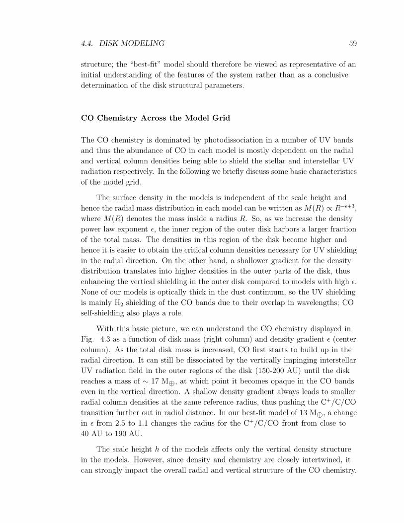
4.4. DISK MODELING 59
structure; the “best-fit” model should therefore be viewed as representative of an
initial understanding of the features of the system rather than as a conclusive
determination of the disk structural parameters.
CO Chemistry Across the Model Grid
The CO chemistry is dominated by photodissociation in a number of UV bands
and thus the abundance of CO in each model is mostly dependent on the radial
and vertical column densities being able to shield the stellar and interstellar UV
radiation respectively. In the following we briefly discuss some basic characteristics
of the model grid.
The surface density in the models is independent of the scale height and
hence the radial mass distribution in each model can be written as M(R) ∝ R−ǫ+3,
where M(R) denotes the mass inside a radius R. So, as we increase the density
power law exponent ǫ, the inner region of the outer disk harbors a larger fraction
of the total mass. The densities in this region of the disk become higher and
hence it is easier to obtain the critical column densities necessary for UV shielding
in the radial direction. On the other hand, a shallower gradient for the density
distribution translates into higher densities in the outer parts of the disk, thus
enhancing the vertical shielding in the outer disk compared to models with high ǫ.
None of our models is optically thick in the dust continuum, so the UV shielding
is mainly H2 shielding of the CO bands due to their overlap in wavelengths; CO
self-shielding also plays a role.
With this basic picture, we can understand the CO chemistry displayed in
Fig. 4.3 as a function of disk mass (right column) and density gradient ǫ (center
column). As the total disk mass is increased, CO first starts to build up in the
radial direction. It can still be dissociated by the vertically impinging interstellar
UV radiation field in the outer regions of the disk (150-200 AU) until the disk
reaches a mass of ∼ 17 M⊕, at which point it becomes opaque in the CO bands
even in the vertical direction. A shallow density gradient always leads to smaller
radial column densities at the same reference radius, thus pushing the C+/C/CO
transition further out in radial distance. In our best-fit model of 13 M⊕, a change
in ǫ from 2.5 to 1.1 changes the radius for the C+/C/CO front from close to
40 AU to 190 AU.
The scale height h of the models affects only the vertical density structure
in the models. However, since density and chemistry are closely intertwined, it
can strongly impact the overall radial and vertical structure of the CO chemistry.

60 CHAPTER 4. 49 CET MOLECULAR GAS DISK
M=13 M_E eps=2.5 h=0.02
h=0.01
h=0.03
50 100 150 200r [AU]
0
2
4
6
8
10
z [A
U]
50 100 150 200r [AU]
0
2
4
6
8
10
z [A
U]
-10
-8
-6
-4
-2
0
log
ε CO
50 100 150 200r [AU]
0
2
4
6
8
z [A
U]
50 100 150 200r [AU]
0
2
4
6
8
z [A
U]
-10
-8
-6
-4
-2
0
log
ε CO
50 100 150 200r [AU]
0
2
4
6
8
z [A
U]
50 100 150 200r [AU]
0
2
4
6
8
z [A
U]
-10
-8
-6
-4
-2
0
log
ε CO
50 100 150 200r [AU]
0
2
4
6
8
z [A
U]
50 100 150 200r [AU]
0
2
4
6
8
z [A
U]
-10
-8
-6
-4
-2
0
log
ε CO
50 100 150 200r [AU]
0
2
4
6
8
z [A
U]
50 100 150 200r [AU]
0
2
4
6
8
z [A
U]
-10
-8
-6
-4
-2
0
log
ε CO
eps=3.5
eps=1.1 M=9 M_E
50 100 150 200r [AU]
0
2
4
6
8
z [A
U]
50 100 150 200r [AU]
0
2
4
6
8
z [A
U]
-10
-8
-6
-4
-2
0
log
ε CO
50 100 150 200r [AU]
0
2
4
6
8
z [A
U]
50 100 150 200r [AU]
0
2
4
6
8
z [A
U]
-10
-8
-6
-4
-2
0
log
ε CO
M=17 M_E
Figure 4.3.— Two-dimensional CO abundances in a subset of disk models. The
center panel shows the best-fit model (M = 13M⊕, ǫ = 2.5, h = 0.02), while the
rows of models above and below show the effects of incrementing and decrementing,
respectively, each of the three structural parameters that were allowed to vary
during the fitting process: h (left column), ǫ (center column), and Mdisk (right
column). The values of the parameters shown are h = 0.01, 0.03; ǫ = 1.1, 3.5; and
M = 9, 17 M⊕.
From a comparison of the center panel with the bottom left panel in Figure
4.3, we see that a factor 2 lower scale height with respect to the best fit model
(h = 0.02), enhances the CO abundance in the disk significantly, leading to radial
and vertical column densities that are more than a factor 10 higher with respect
to the best fit model. The total CO mass increases by a factor of 10 as well, with
the integrated emission undergoing a corresponding dramatic increase.
Table 4.3 displays some key results from a subset of grid models such as
characteristic radial and vertical CO column densities, CO masses and total CO
J=2-1 line emission. For all models in the table, the inner radius is fixed at 40 AU
and the outer radius at 200 AU.
From Chemistry to Observables
The predicted CO J=2-1 emission for the models in Figure 4.3 is displayed in
Figure 4.4; a comparison of these figures illustrates the ways in which differences
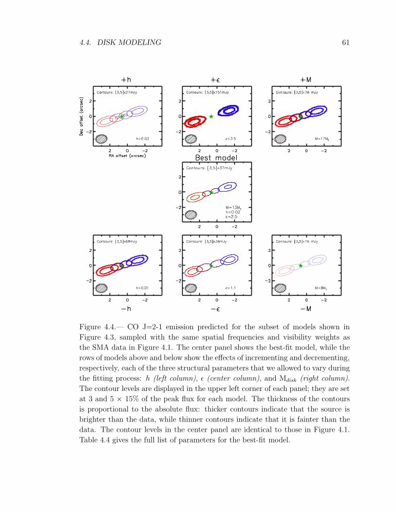
4.4. DISK MODELING 61
Figure 4.4.— CO J=2-1 emission predicted for the subset of models shown in
Figure 4.3, sampled with the same spatial frequencies and visibility weights as
the SMA data in Figure 4.1. The center panel shows the best-fit model, while the
rows of models above and below show the effects of incrementing and decrementing,
respectively, each of the three structural parameters that we allowed to vary during
the fitting process: h (left column), ǫ (center column), and Mdisk (right column).
The contour levels are displayed in the upper left corner of each panel; they are set
at 3 and 5 × 15% of the peak flux for each model. The thickness of the contours
is proportional to the absolute flux: thicker contours indicate that the source is
brighter than the data, while thinner contours indicate that it is fainter than the
data. The contour levels in the center panel are identical to those in Figure 4.1.
Table 4.4 gives the full list of parameters for the best-fit model.

62 CHAPTER 4. 49 CET MOLECULAR GAS DISK
Table 4.3: Derived quantities from a subset of the 49 Ceti disk models
Madisk ǫ h N(CO)bradial N(CO)100AU,c
vertical MdCO ICO(J=2-1)e
(M⊕) (1018 cm−2) (1015 cm−2) (10−4 M⊕) (Jy km s−1)
13 2.5 0.020 2.76 4.23 9.66 2.6
9 2.5 0.020 0.32 1.82 2.46 1.2
17 2.5 0.020 13.5 9.06 37.2 6.9
13 3.5 0.020 15.1 4.47 98.0 11.7
13 1.1 0.020 0.13 0.91 3.74 2.3
13 2.5 0.010 42.8 78.4 96.6 14.5
13 2.5 0.030 0.12 2.20 2.97 1.5
aTotal disk gas massbTotal radial CO column density through the midplanecCO vertical column density at 100 AUdTotal CO mass in the diskeIntegrated CO(J=2-1) line emission
in chemical structure are manifested in the observable properties of the CO
emission. The CO emission is sampled with the same spatial frequencies and
visibility weights as the SMA data and displayed in renzogram form with the same
velocity structure as in Figure 4.1. In order to emphasize the relative structural
differences between models, the contour levels are 15% of the peak flux for each
model, with the absolute flux indicated by the thickness of the contours, and also
printed explicitly at the top of each panel.
The decreased shielding in the inner disk caused by reducing the density
gradient ǫ is visible as a lengthening of the emission in the central channels and
a widening of the emission peaks in the outer channels in the low-epsilon model
(bottom center panel). Increasing ǫ (top center panel) leads to enhanced shielding
at the disk inner edge, causing much higher CO fluxes in the outer part of the
disk and extremely high contrast between the inner and outer velocity channels.
The primary observable consequence of adjusting the mass (right panels, top
and bottom) is that the increased or decreased shielding from extra gas leads to a
corresponding increase or decrease in the total CO flux; changes to the shape of
the emission are minimal, and the primary difference between models of different

4.4. DISK MODELING 63
mass over the mass range under consideration is simply in the relative brightness
of the emission.
Differences in the scale height of the disk similarly manifest as differences in
the flux scale; however, decreasing the scale height (bottom left panel) also causes
greater shielding at the inner disk edge, leading to greater elongation of the outer
velocity channels and causing the inner velocity channels to draw together and
overlap as the CO flux rises throughout the inner areas of the disk. An increase
in scale height (top left panel) leads to a greater area in the front and back of
the disk, projected along our line of sight, which increases the flux in the central
channels and leads to a lower contrast between the inner and outer channels of
the disk.
Table 4.4: Parameters for Best-Fit Disk Model
h 0.020+0.015−0.005
ǫ 2.5+0.5−1.0
Mgas 13 ± 3 M⊕Mdust 0.02 ± 0.01 M⊕i 90 ± 5
PA −70 ± 10
Rin 40 AUa
Rout 200 AUa
aFor a description of the constraints on the inner and outer radii, see §4.4
4.4.2 Spectral Energy Distribution
After converging initially on a model that was able to reproduce the observed CO
J=2-1 emission, we used that model to predict the spectral energy distribution.
This serves as an a posteriori test of the consistency between the gas and dust
properties in the models and the available observables.
We integrate over the disk volume to obtain the flux as a function of
wavelength
Fλ = (πa2/d2)
∫ ∫
2πr Bλ(Tdust(r, z))ndust(r, z)Q(λ) dz dr , (4.3)
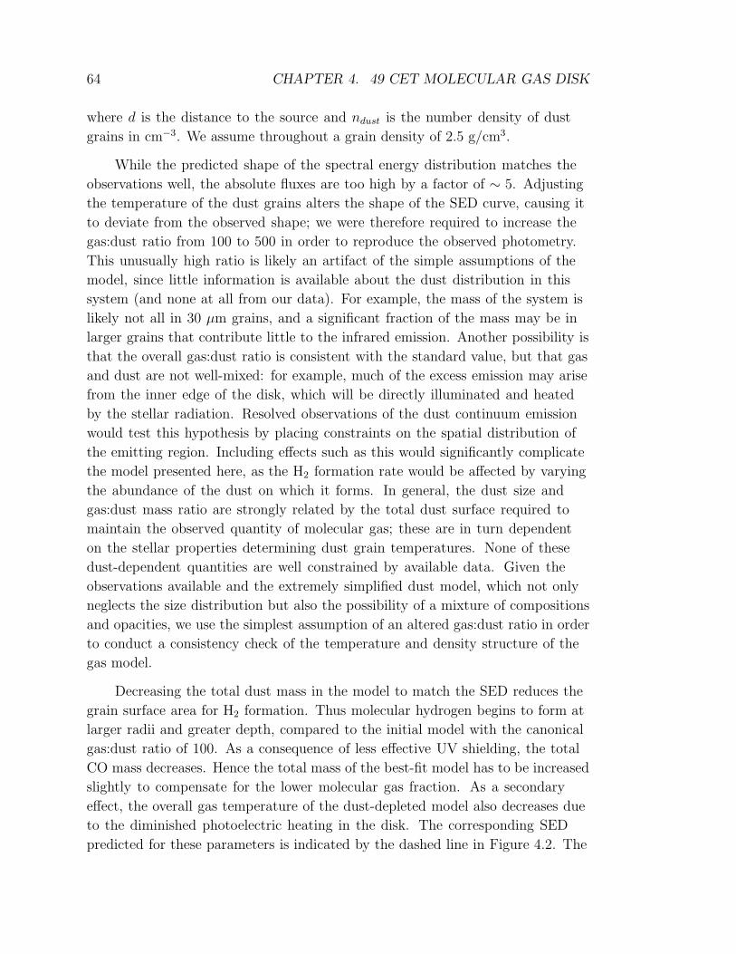
64 CHAPTER 4. 49 CET MOLECULAR GAS DISK
where d is the distance to the source and ndust is the number density of dust
grains in cm−3. We assume throughout a grain density of 2.5 g/cm3.
While the predicted shape of the spectral energy distribution matches the
observations well, the absolute fluxes are too high by a factor of ∼ 5. Adjusting
the temperature of the dust grains alters the shape of the SED curve, causing it
to deviate from the observed shape; we were therefore required to increase the
gas:dust ratio from 100 to 500 in order to reproduce the observed photometry.
This unusually high ratio is likely an artifact of the simple assumptions of the
model, since little information is available about the dust distribution in this
system (and none at all from our data). For example, the mass of the system is
likely not all in 30 µm grains, and a significant fraction of the mass may be in
larger grains that contribute little to the infrared emission. Another possibility is
that the overall gas:dust ratio is consistent with the standard value, but that gas
and dust are not well-mixed: for example, much of the excess emission may arise
from the inner edge of the disk, which will be directly illuminated and heated
by the stellar radiation. Resolved observations of the dust continuum emission
would test this hypothesis by placing constraints on the spatial distribution of
the emitting region. Including effects such as this would significantly complicate
the model presented here, as the H2 formation rate would be affected by varying
the abundance of the dust on which it forms. In general, the dust size and
gas:dust mass ratio are strongly related by the total dust surface required to
maintain the observed quantity of molecular gas; these are in turn dependent
on the stellar properties determining dust grain temperatures. None of these
dust-dependent quantities are well constrained by available data. Given the
observations available and the extremely simplified dust model, which not only
neglects the size distribution but also the possibility of a mixture of compositions
and opacities, we use the simplest assumption of an altered gas:dust ratio in order
to conduct a consistency check of the temperature and density structure of the
gas model.
Decreasing the total dust mass in the model to match the SED reduces the
grain surface area for H2 formation. Thus molecular hydrogen begins to form at
larger radii and greater depth, compared to the initial model with the canonical
gas:dust ratio of 100. As a consequence of less effective UV shielding, the total
CO mass decreases. Hence the total mass of the best-fit model has to be increased
slightly to compensate for the lower molecular gas fraction. As a secondary
effect, the overall gas temperature of the dust-depleted model also decreases due
to the diminished photoelectric heating in the disk. The corresponding SED
predicted for these parameters is indicated by the dashed line in Figure 4.2. The
4.4. DISK MODELING 65
mid-infrared flux points are underestimated by this model because we do not
include the inner disk component of Wahhaj et al. (2007); as our data provide
no constraints on the properties of the inner disk, we ignore this component and
concentrate on the fit to the outer disk. The flux predicted by the model SED is
consistent with our own continuum upper limit reported in Table 4.1.
4.4.3 Best-Fit Disk Model
The center panel of Figure 4.4 shows the best-fit model from the grid, with the
minor modifications introduced by reproducing simultaneously the spectral energy
distribution. The structural and geometric parameters for this model are listed
in Table 4.4. The errors given in the table are the approximate 1-σ uncertainty
range interpolated from the χ2 grid.
This model reproduces the basic features of the CO J=2-1 emission well,
including the strength of the emission, the separation of the emission peaks, and
the spatial extent of the emission. There are still several important differences
between the model and the data, however, including (1) an inability to reproduce
the changes in position angle with radius evident in the data (the “wings” of
emission extending to the southeast and northwest of the position angle axis),
and (2) the separation of the innermost, low-velocity channels. Both of these may
be indicative of departures from azimuthal symmetry in the disk structure, the
former possibly indicating a warp in the disk and the latter apparently pointing
to a deficit of emission along the minor axis of the disk. In none of our models
were we able to reproduce the wide separation between the inner channels; while
the signal-to-noise ratio in these channels is low, the observed CO morphology is
difficult to reproduce in detail with a simple, azimuthally symmetric disk model.
The CO emission for this best-fit model is optically thin in both the J=2-1 and
J=3-2 transitions, even for the edge-on disk orientation, and therefore traces the
full column density of disk material.
The densities in the disk are too low for efficient gas-dust coupling and
thus the gas finds its own equilibrium temperature determined mainly by
photoelectric heating and line cooling. The most important cooling lines from
surface to midplane are [C ii], [O i], and H2. CO abundances are only high in
a region between 45 and 70 AU (Fig. 4.3). Outside that region, CO cooling is
less important for the energy balance. Fig. 4.5 summarizes the most important
heating and cooling processes and also shows the resulting gas temperature
structure. The disk surface stays well below 100 K due to efficient fine structure
line cooling. The molecular cooling is however less efficient in competing with the

66 CHAPTER 4. 49 CET MOLECULAR GAS DISK
photoelectric heating from the large silicate grains (Kamp & van Zadelhoff 2001),
leading to temperatures of a few 100 K in the disk interior.
In order to test the robustness of the best-fit model to the gas properties, we
used this model to predict the CO J=3-2 spectrum. It compares favorably with
the spectrum observed by Dent et al. (2005), reproduced in Figure 4.6. The heavy
solid line shows the J=3-2 spectrum predicted from the best-fit disk model, while
the light solid line shows the observed JCMT spectrum. Although the observed
spectrum is noisy and likely subject to an absolute calibration uncertainty, the
overall agreement is within ∼ 30%, which is very good given that the CO J=3-2
spectrum was not used a priori to determine these model parameters.
4.5 Discussion
The processes determining the amount and distribution of gas and dust in
transition disks like that around 49 Ceti are the same processes that shape the
features of emergent planetary systems around these young stars. Resolved
observations of individual disks in this phase are desirable to address such basic
questions as when in the lifetime of a star its disk disperses, whether the gas
clears before the dust, and whether the disk clears from the center or in a radially
invariant manner.
In the 49 Ceti system, the infrared dust properties appear similar to those of
a debris disk (Wahhaj et al. 2007). Yet observations presented here indicate that
a substantial quantity of molecular gas persists in the outer disk, between radii
of 40 and 200 AU, where photochemistry from stellar and interstellar radiation
dominates. The lack of molecular gas emission interior to this radius as indicated
by our observations, combined with the lack of dust emission within a radius of
30 AU inferred by Wahhaj et al. (2007), implies that the 49 Ceti system appears
to be clearing its gas and dust from the center out. The mechanism responsible
for this central clearing is not indicated; in general, the best-developed theories to
explain this transitional morphology are (1) central clearing through the influence
of a massive planet and (2) photoevaporation by radiation from the central star.
The clearing of gaps and inner holes has long been predicted as a consequence
of the formation of massive planets in circumstellar disks (e.g. Lin & Papaloizou
1986; Bryden et al. 1999). In the case of 49 Ceti, the formation of a Jupiter-mass
planet would be required at a distance of ∼ 40 AU from the star, roughly the
inner radius of the observed hole in the gas distribution. Such a scenario could
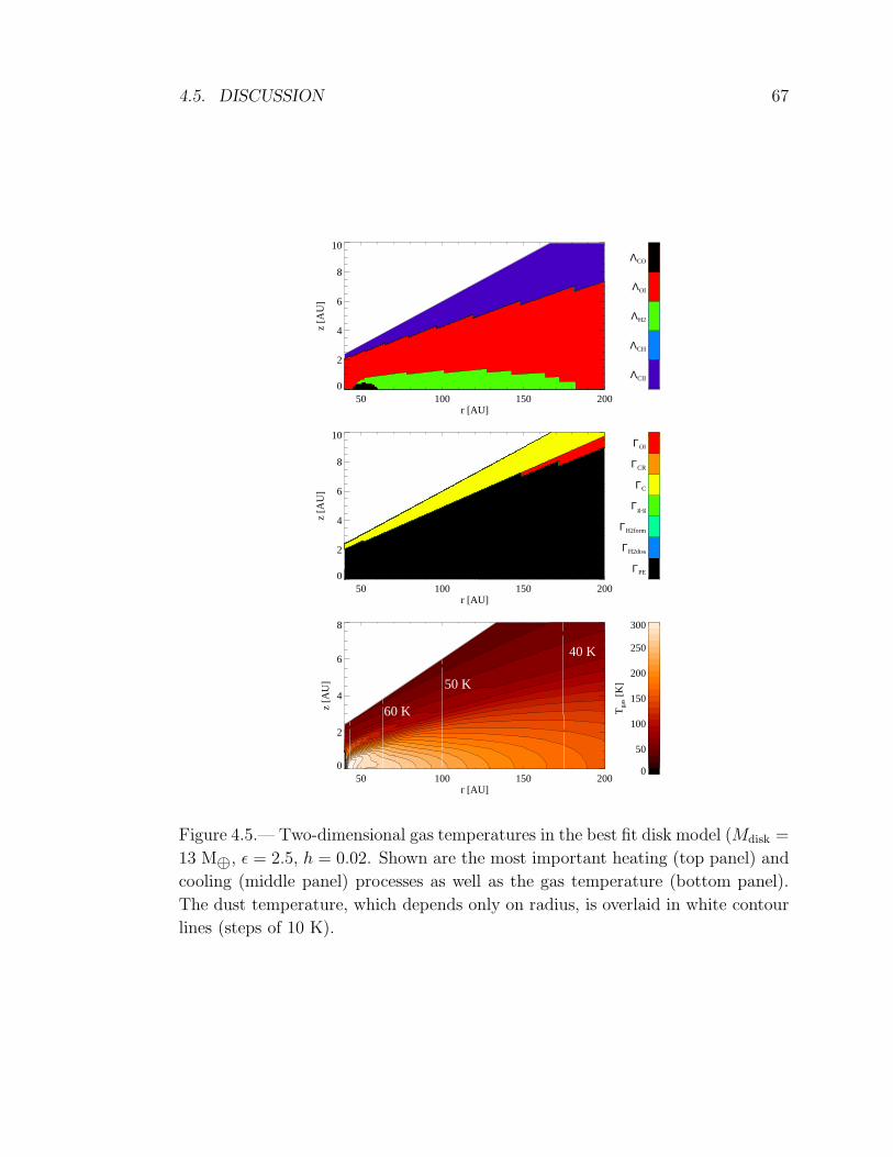
4.5. DISCUSSION 67
50 100 150 200r [AU]
0
2
4
6
8
10
z [A
U]
ΓPE
ΓH2diss
ΓH2form
Γg-g
ΓC
ΓCR
ΓOI
50 100 150 200r [AU]
0
2
4
6
8
z [A
U]
0
50
100
150
200
250
300T
gas [
K]
50 100 150 200r [AU]
0
2
4
6
8
10
z [A
U]
ΛCII
ΛCH
ΛH2
ΛOI
ΛCO
60 K
50 K
40 K
Figure 4.5.— Two-dimensional gas temperatures in the best fit disk model (Mdisk =
13 M⊕, ǫ = 2.5, h = 0.02. Shown are the most important heating (top panel) and
cooling (middle panel) processes as well as the gas temperature (bottom panel).
The dust temperature, which depends only on radius, is overlaid in white contour
lines (steps of 10 K).

68 CHAPTER 4. 49 CET MOLECULAR GAS DISK
Figure 4.6.— CO J=3-2 spectrum predicted for the model that provides the best
fit to the resolved J=2-1 emission (heavy solid line), compared with the Dent et al.
(2005) JCMT CO J=3-2 spectrum (light solid line). The x-axis shows heliocentric
velocity while the y-axis gives the JCMT main beam brightness temperature.
also help to explain the size segregation of dust grains observed by Wahhaj et al.
(2007); a predicted consequence of inner disk clearing by gravitational influence
of a massive planet is a filtration of dust grains by size, with only those below a
certain threshold (typically 1-10 µm) accreted across the gap along with a reduced
amount of gas (Rice et al. 2006). However, this scenario ultimately requires
the accretion of substantial amounts of gas into the inner disk, and searches for
molecular gas in the inner disk of 49 Ceti (Chen et al. 2006; Carmona et al.
2007) have not detected such a population. Another indication that an inner
hole is likely caused by a massive planet in formation would be non-axisymmetric
features resulting from its gravitational influence, such as spiral waves. While the
CO emission from 49 Ceti does not appear asymmetric within the limits of the
SMA observations, more sensitive spatially resolved observations could address
this hypothesis.
The absence of gas in the inner disk is, however, consistent with a
photoevaporation scenario: as the photoevaporative wind produced by stellar
radiation becomes comparable to the accretion rate in the disk, material within
the gravitational radius Rg = GM⋆/c2s will quickly drain onto the star, leaving an
evacuated inner hole free of gas and dust (e.g. Hollenbach et al. 1994; Alexander
et al. 2006). The gravitational radius for 49 Ceti is roughly 20 AU, which is
comparable to the inferred inner radius of 40 AU for the outer disk. The larger
4.5. DISCUSSION 69
outer radius may in fact be consistent with the later stages of photoevaporation,
after the inner disk has become optically thin to ultraviolet radiation and the
inner disk radius slowly increases under the influence of the photoevaporative
wind (Alexander et al. 2006). Alexander & Armitage (2007) propose a method
of discriminating between inner holes caused by photoevaporation and those
caused by the formation of a giant planet, involving a simple comparison between
two observables: the disk mass and the accretion rate. As there is no measured
accretion rate for 49 Ceti, we cannot apply the criteria presented by these authors;
however, we note that the low disk mass does indeed fall within the parameter
space consistent with a photoevaporative scenario. Further observations are
necessary to determine the origin of the inner hole; in particular, stringent limits
on the accretion rate could suggest a photoevaporative mechanism.
There are few disks which appear to be in a similar evolutionary stage to
that of 49 Ceti; a rare example is the disk around the A star HD 141569. Like
49 Ceti, it hosts a disk composed primarily of subµm-size grains with infrared
properties approaching those of a debris disk (Wahhaj et al. 2007; Marsh et al.
2002), while still retaining a substantial quantity of molecular gas with central
region clear of gas emission, in this case out to a radius of ∼ 11 AU (Goto et al.
2006; Brittain et al. 2007). It exhibits a transitional SED (Merın et al. 2004),
and observations of the rovibrational CO spectrum reveal gas with disparate
rotational and vibrational temperatures (200 K and 5000 K respectively; Brittain
et al. 2007), indicative of UV fluorescence on the outer edges of an inner disk
region cleared of gas and dust. An analysis of the chemistry and gas properties
of the system similar to the one presented here for 49 Ceti was conducted by
Jonkheid et al. (2006). While the presence and extent of the inner hole are
clearly indicated, the physical origin of this clearing is less obvious. The Brγ
profile is indicative of substantial accretion, and Brittain et al. (2007) deem a
photoevaporative clearing mechanism unlikely due to the large column density
outside the cleared region and the lack of evidence for a photoevaporative wind in
the FUV (Martin-Zaıdi et al. 2005). However, Merın et al. (2004) place a much
lower limit of 10−11 M⊙/yr on the accretion rate, based on the assumed gas:dust
ratio of 100 and the low optical depth of the inner disk, which would be much
more consistent with a photoevaporation scenario. Goto et al. (2006) note that
the rough coincidence of the inner rim of the disk with the gravitational radius
suggests that photoevaporation in concert with viscous accretion is a likely cause
for the inner disk clearing.
Whatever the origin of their morphology, the observed gas and dust properties
indicate that the disks surrounding both 49 Ceti and HD 141569 appear to be in

70 CHAPTER 4. 49 CET MOLECULAR GAS DISK
a transitional state of evolution during which the dust properties are beginning
to appear more like those of a debris disk, while the gas is in the process of being
cleared from the disk from the center out.
4.6 Conclusions
The SMA CO J=2-1 observations presented here provide the first spatially
resolved observations of molecular gas in the 49 Ceti system. The data reveal a
surprisingly extended and complex molecular gas distribution in rotation about
the central star, viewed approximately edge on and clear of molecular gas emission
in the central region of the disk. Modeling the disk structure and chemistry in
this system indicates that the inner disk is entirely devoid of molecular gas due to
irradiation by the central star, while a ring of molecular gas persists between 40
and 200 AU, subject to photodissociation at the inner edge by stellar radiation.
The disk model presented here reproduces well the observed properties of the
system, including the resolved CO J=2-1 emission, the CO J=3-2 spectrum, and
the spectral energy distribution. With dust properties similar to those of a debris
disk and a substantial reservoir of gas maintained in the outer disk, 49 Ceti
appears to be a rare example of a system in a late stage of transition between a
gas-rich protoplanetary disk and a tenuous, gas-free debris disk.

Chapter 5
Structure and Composition of
Two Transitional Circumstellar
Disks in Corona Australis
A. M. Hughes, S. M. Andrews, D. J. Wilner, M. R. Meyer, J. M. Carpenter, C.
Qi, A. S. Hales, S. Casassus, M. R. Hogerheijde, E. E. Mamajek, S. Wolf, T.
Henning, & M. D. Silverstone The Astronomical Journal, submitted
Abstract
We consider basic structural models for the transition disks around two
∼10Myr-old members of the nearby RCrA association, RX J1842.9-3532 and
RX J1852.3-3700. We present new arcsecond-resolution maps of their 230GHz
continuum emission from the Submillimeter Array and unresolved CO(3-2) spectra
from the Atacama Submillimeter Telescope Experiment. By combining these
data with broadband fluxes from the literature and infrared fluxes and spectra
from the catalog of the Formation and Evolution of Planetary Systems (FEPS)
Legacy program on the Spitzer Space Telescope, we assemble a multiwavelength
data set probing the gas and dust disks. Using the Monte Carlo radiative transfer
code RADMC to model simultaneously the SED and resolved millimeter continuum
visibilities, we derive basic dust disk properties and identify an inner cavity of
radius 16AU in the disk around RX J1852.3-3700. We also identify an optically
thin 5AU cavity in the disk around RX J1842.9-3532, with a small amount of
optically thick material close to the star. The molecular line observations confirm
71
72 CHAPTER 5. CRA TRANSITION DISKS
the intermediate disk inclination in RX J1842.9-3532. In combination with the
dust models, the molecular data allow us to derive a lower CO content than
expected for standard assumptions, suggesting that the process of gas clearing is
likely underway in both systems. With their advanced age, reduced CO content,
and substantial outer dust disks, these transitional systems present interesting
opportunities for follow-up with next-generation instruments like the Atacama
Large Millimeter Array.
5.1 Introduction
One of the key problems in planet formation is understanding how the reservoir of
planet-forming material – the disk of gas and dust around a young star – evolves
with time. Perhaps the most compelling stage in the evolution of protoplanetary
disks is the “transitional” stage during which gas and dust are cleared from the
system (e.g. Strom et al. 1989; Skrutskie et al. 1990). This stage appears to be
either rapid or rare, since fewer than 10% of low- to intermediate-mass stars in
young star-forming regions are typically observed to be transitional systems (e.g.
Cieza et al. 2007; Uzpen et al. 2008). Transition disks are traditionally identified
empirically by a deficit of mid-infrared dust excess over the stellar photosphere
relative to other systems at comparable ages. This deficit is associated with a
lack of hot dust close to the star. The advent of the Spitzer Space Telescope
has revolutionized the quality and quantity of available data on the dust content
of young stellar systems, particularly transitional objects (see e.g. Najita et al.
2007). One of its many contributions has been to reveal a new class of gapped
or “pre-transitional” disks, in which an anomalously faint mid-infrared spectrum
is bracketed by substantial near- and far-infrared excesses (Espaillat et al. 2007,
2008). Follow-up of Spitzer-identified transitional systems with high spatial
resolution observations of continuum emission at millimeter wavelengths has led
to the confirmation that mid-IR spectral deficits are associated with a lack of
long-wavelength emission from the disk center (Calvet et al. 2002, 2005; Hughes
et al. 2007, 2009a; Brown et al. 2007, 2008, 2009; Pietu et al. 2007; Espaillat et al.
2008). The properties of systems with gaps and holes are beginning to provide
valuable insight into the physical mechanisms responsible for the dispersal of the
circumstellar disk, many of which may come into play over the lifetime of the
star. Gas dynamics, the presence of unknown binary companions, grain growth,
dynamical interactions with giant planets in formation, and photoevaporation
have all been suggested as clearing mechanisms; there is some indication that
different processes may dominate at different ages (see, e.g., Sicilia-Aguilar et al.

5.1. INTRODUCTION 73
2010).
The Formation and Evolution of Planetary Systems (FEPS) Legacy program
on the Spitzer Space Telescope (Meyer et al. 2006; Carpenter et al. 2008) is a
spectrophotometric survey of nearby young Solar analogues, with masses from 0.7
to 1.3 M⊙ and ages between 3 Myr and 3 Gyr. These ages bracket the period of
time when gas and dust were cleared from the primordial Solar nebula, and the
epoch when the Solar system achieved its present configuration. For 328 objects
in the FEPS sample, the survey includes IRAC 3.6-8.0µm photometry to probe
for hot, dusty analogues to the asteroid belt in the Solar system, MIPS 24 and
70µm photometry to probe dust in the Kuiper Belt regions, and IRS 5-40µm
spectra to search for mineralogical features. The excellent coverage of the infrared
spectral energy distribution (SED) permits modeling of the temperature, size,
composition, and an initial estimate of the spatial distribution of dust grains
(see, e.g., Kim et al. 2005; Bouwman et al. 2008; Cortes et al. 2009). The IRS
spectra are particularly useful for identifying systems with inner cavities or gaps
in their dust distribution. However, there are many degeneracies inherent in the
derivation of spatial information from unresolved spectra, and the SED provides
little information about the large grains that comprise most of the dust mass in
the system. It is therefore desirable to combine the information from the SED
with spatially resolved observations at millimeter wavelengths. Since the emission
is dominated by dust grains comparable in size to the wavelength of observation,
resolved millimeter observations primarily trace the spatial mass distribution of
large (millimeter-size) particles in the disk. Spectral line observations of low-level
rotational emission from the CO molecule can provide a complementary probe of
the total mass, which is dominated by molecular gas, and can yield important
clues to the gas evolution of transitional objects.
In this paper, we analyze the SEDs and resolved millimeter continuum
emission of two sources from the FEPS sample, RX J1842.9-3532 and RX J1852.3-
3700. These sources were detected in the ROSAT All-Sky Survey and identified
as young stars by Neuhauser et al. (2000). They have spectral type K2 and K3,
respectively (Carpenter et al. 2008), and have been classified as classical T Tauri
stars (cTTSs) based on the presence of strong Hα emission lines. Neither was
identified as a multiple-star system in the speckle-interferometric observations
of Kohler et al. (2008). They are located within a few degrees of the CrA
molecular cloud (distance 130 pc; Neuhauser et al. 2000), and have kinematics
and secular parallaxes consistent with the RCrA association (E. Mamajek, private
communication). The estimated stellar ages are ∼10Myr, among the oldest in
the 1-10Myr range for T Tauri objects in CrA measured by Neuhauser et al.

74 CHAPTER 5. CRA TRANSITION DISKS
(2000). These sources were selected for study on the basis of their age, their
brightness in the 1.2mm continuum (Carpenter et al. 2005), and their accessibility
to the Submillimeter Array (SMA), so that the spectral information from the
FEPS survey could be combined with resolved submillimeter observations. They
were also chosen for their proximity on the sky, which increases the efficiency
of submillimeter observations by allowing them to share calibrators. The
high-quality Spitzer IRS spectra provide constraints on the dust composition and
temperature structure on the two systems, and both exhibit a flux deficit in the
mid-IR photospheric excess that points to the presence of an inner hole or gap.
Sections 5.2 and 5.3 describe the collection of new data from the SMA and
the Atacama Submillimeter Telescope Experiment (ASTE) that complement
the spectra and broadband fluxes from the FEPS survey and the literature. In
Section 5.4.1 we present the tools and techniques that we use to model the SED
and resolved millimeter-wavelength data, and we present the models of the dust
disk structures in Section 5.4.2. In Section 5.4.3, we explore the dust disk model
in the context of the constraints on the gas content of the two systems. We
summarize our results and discuss their implications in Section 5.5.
5.2 Observations and Data Reduction
5.2.1 SMA Observations
The SMA observations of the two sources took place on 2005 May 14 during
a full six-hour track with six of the 6-meter diameter antennas operating in
the compact-north configuration, yielding baseline lengths between 10 and 180
meters (8 and 140 kλ). The phase stability was adequate for most of the track,
with phase differences of 20-30 degrees between calibrator scans, but the phases
lost coherence during the last hour of the night. The weather was fair, with
the 225GHz atmospheric opacity increasing from 0.10 to 0.14 throughout the
night. Observations of the two FEPS sources were alternated with observations
of the quasar J1924-292 at 15-minute intervals to calibrate the atmospheric
and instrumental variations of phase and amplitude gain. Callisto was used as
the flux calibrator, with a calculated brightness of 6.59 Jy; the derived flux of
J1924-292 was 5.4 Jy, with an estimated uncertainty of . 20%. The correlator
was configured to provide a spectral resolution of 512 channels over the 104
MHzbandwidth in the chunk containing the CO(2-1) line, corresponding to a
velocity resolution of 0.26 km s−1. Two other 104MHz chunks were observed

5.2. OBSERVATIONS AND DATA REDUCTION 75
at high resolution at frequencies corresponding to the 13CO(2-1) and C18O(2-1)
lines. The remainder of bandwidth in each 2GHz-wide sideband was devoted to
measuring the 230GHz continuum, observed at a spectral resolution of 4.2 km s−1.
The data were calibrated using the MIR software package and imaging was carried
out with the MIRIAD software package.
5.2.2 ASTE Observations
Observations of both FEPS sources took place on 2008 June 28 and 29 using
the CATS345 receiver on the 10.4-meter ASTE dish. RX J1842.9-3532 was
observed on both nights, while RX J1852.3-3700 was observed only on the second
night. The receiver was tuned to place the CO(3-2) rotational transition in the
lower sideband with the HCO+(4-3) transition in the upper sideband. The high
resolution spectrometer mode was used to partition the 128MHz bandwidth into
1024 channels, yielding a spectral resolution of 0.11 km/s. Position switching was
used to subtract the instrumental and sky background. In order to ensure that
the detected CO emission originated at the position of the star, we used an offset
position 1.5 arcmin to the east on the night of June 28 and 1.5 arcmin to the
west on June 29 and averaged the baseline-subtracted spectra to create the final
spectrum. The double-peaked CO(3-2) line from RX J1842.9-3532 is detected
independently on both nights using the different offset positions, which allows us
to localize the emission to within 1.5 arcmin of the star (∼4 beam widths).
The CO(3-2) and HCO+(4-3) tuning of the receiver resulted in a spurious
1.11MHz sinusoidal ripple of variable amplitude and phase across the bandpass,
which was subtracted individually from each 10-second integration in the following
manner. The amplitude and frequency of the ripple were estimated by finding
the peak in a fast fourier transform of the spectrum, and then a least squares fit
was performed to determine the precise amplitude, phase, and frequency of the
sinusoidal ripple, plus the slope and intercept of a linear component to remove
the worst of the baseline features. During this process, the region of the spectrum
containing the line was not included in the fit so as to avoid inadvertently
subtracting it. Integrations with an abnormally large ripple amplitude or highly
irregular baseline shape across the bandpass were discarded (roughly 10% of each
data set). After subtracting the sinusoid and linear fit, a third-order polynomial
was subtracted from each integration using the CLASS software package1, fitting
the 20 km s−1 to each side of the region that appeared to contain the line. The
1http://www.iram.fr/IRAMFR/GILDAS

76 CHAPTER 5. CRA TRANSITION DISKS
10-second integrations were then averaged together to produce a spectrum for
each night; the spectra for each night were averaged and weighted according
to their total integration time to produce the final spectrum. Due to differing
exposure times and poorer weather on the night of June 29, the rms noise in
the spectrum of RX J1842.9-3532 is 24mK, while the rms noise in the spectrum
of RX J1852.3-3700 is 39mK. To derive the absolute flux scale, we calculated
the main beam efficiency using observations of the calibrator M17SW taken
throughout the night. Assuming a peak main beam temperature in the CO(3-2)
line of 85.3K, derived on the CSO 10.4m telescope by Wang et al. (1994), we
derive main beam efficiencies that varied between 0.55 and 0.63 over the course
of the two nights.
5.3 Results
5.3.1 Millimeter Continuum
With the SMA observations, we detect 230GHz continuum emission from the
disks around both target stars. The contour maps in Figure 5.1 show the
strong detection of emission centered on the star position at the middle of the
field. In order to estimate the integrated flux and approximate disk geometry,
a Gaussian fit to the visibilities was performed using the MIRIAD task uvfit.
For RX J1842.9-3532, the fit yields an integrated flux of 49±8mJy and indicates
that the disk is only marginally resolved: the major and minor axes lengths
of 0.′′74±0.′′32 and 0.′′44±0.′′32 suggest that the disk is probably not viewed
face-on, but do not place strong constraints on the inclination. We estimate an
inclination angle of 54 based on these measurements, which is consistent with the
morphology of the ASTE CO(3-2) spectrum described in Section 5.3.2 below. The
fit to the RX J1852.3-3700 visibilities yields a flux of 60±8mJy and major and
minor axes of length 0.′′76±0.′′21 and 0.′′73±0.′′21, consistent with a nearly face-on
geometry; we estimate an inclination of 16. The inclination estimates are highly
uncertain, but the intermediate geometry of RX J1842.9-3532 is supported by the
line profile in Section 5.3.2 and the more face-on geometry of RX J1852.3-3700
is supported by the Hα line profile modeling of Pascucci et al. (2007). While
observations at higher resolution would be advantageous for constraining the
detailed mass distribution, even the rudimentary estimates of disk geometry
provided by these observations are useful for constraining the disk properties when
combined with constraints from the broadband SED. Simultaneous modeling of
the SED and millimeter-wavelength visibilities is described in Section 5.4.1 below.
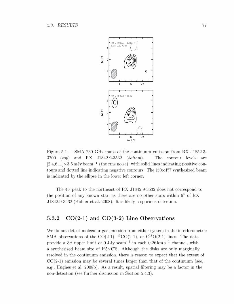
5.3. RESULTS 77
Figure 5.1.— SMA 230 GHz maps of the continuum emission from RX J1852.3-
3700 (top) and RX J1842.9-3532 (bottom). The contour levels are
[2,4,6,...]×3.5mJybeam−1 (the rms noise), with solid lines indicating positive con-
tours and dotted line indicating negative contours. The 1.′′0×1.′′7 synthesized beam
is indicated by the ellipse in the lower left corner.
The 4σ peak to the northeast of RX J1842.9-3532 does not correspond to
the position of any known star, as there are no other stars within 6” of RX
J1842.9-3532 (Kohler et al. 2008). It is likely a spurious detection.
5.3.2 CO(2-1) and CO(3-2) Line Observations
We do not detect molecular gas emission from either system in the interferometric
SMA observations of the CO(2-1), 13CO(2-1), or C18O(2-1) lines. The data
provide a 3σ upper limit of 0.4 Jy beam−1 in each 0.26 km s−1 channel, with
a synthesized beam size of 1.′′5×0.′′8. Although the disks are only marginally
resolved in the continuum emission, there is reason to expect that the extent of
CO(2-1) emission may be several times larger than that of the continuum (see,
e.g., Hughes et al. 2008b). As a result, spatial filtering may be a factor in the
non-detection (see further discussion in Section 5.4.3).
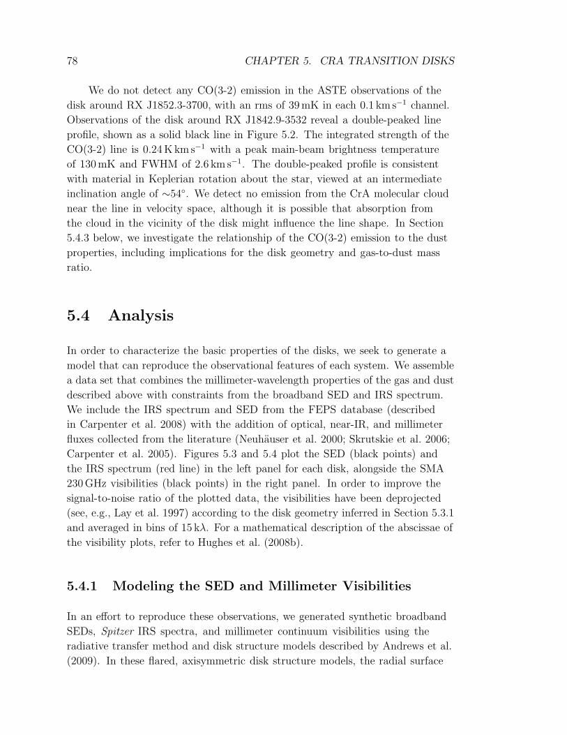
78 CHAPTER 5. CRA TRANSITION DISKS
We do not detect any CO(3-2) emission in the ASTE observations of the
disk around RX J1852.3-3700, with an rms of 39mK in each 0.1 kms−1 channel.
Observations of the disk around RX J1842.9-3532 reveal a double-peaked line
profile, shown as a solid black line in Figure 5.2. The integrated strength of the
CO(3-2) line is 0.24Kkms−1 with a peak main-beam brightness temperature
of 130mK and FWHM of 2.6 km s−1. The double-peaked profile is consistent
with material in Keplerian rotation about the star, viewed at an intermediate
inclination angle of ∼54. We detect no emission from the CrA molecular cloud
near the line in velocity space, although it is possible that absorption from
the cloud in the vicinity of the disk might influence the line shape. In Section
5.4.3 below, we investigate the relationship of the CO(3-2) emission to the dust
properties, including implications for the disk geometry and gas-to-dust mass
ratio.
5.4 Analysis
In order to characterize the basic properties of the disks, we seek to generate a
model that can reproduce the observational features of each system. We assemble
a data set that combines the millimeter-wavelength properties of the gas and dust
described above with constraints from the broadband SED and IRS spectrum.
We include the IRS spectrum and SED from the FEPS database (described
in Carpenter et al. 2008) with the addition of optical, near-IR, and millimeter
fluxes collected from the literature (Neuhauser et al. 2000; Skrutskie et al. 2006;
Carpenter et al. 2005). Figures 5.3 and 5.4 plot the SED (black points) and
the IRS spectrum (red line) in the left panel for each disk, alongside the SMA
230GHz visibilities (black points) in the right panel. In order to improve the
signal-to-noise ratio of the plotted data, the visibilities have been deprojected
(see, e.g., Lay et al. 1997) according to the disk geometry inferred in Section 5.3.1
and averaged in bins of 15 kλ. For a mathematical description of the abscissae of
the visibility plots, refer to Hughes et al. (2008b).
5.4.1 Modeling the SED and Millimeter Visibilities
In an effort to reproduce these observations, we generated synthetic broadband
SEDs, Spitzer IRS spectra, and millimeter continuum visibilities using the
radiative transfer method and disk structure models described by Andrews et al.
(2009). In these flared, axisymmetric disk structure models, the radial surface

5.4. ANALYSIS 79
Figure 5.2.— ASTE CO(3-2) spectra of the disks around RX J1852.3-3700 (upper)
and RX J1842.9-3532 (lower). No emission is detected from the RX J1852.3-3700
system. The RX J1842.9-3532 emission (solid line) displays the double-peaked
profile characteristic of an inclined structure in Keplerian rotation about the central
star. The line profile predicted by the SED- and visibility-based model of the dust
disk structure (dotted line) compares favorably with the observations.

80 CHAPTER 5. CRA TRANSITION DISKS
Figure 5.3.— Spectral energy distribution (left) and the real and imaginary com-
ponents of the deprojected SMA 230GHz visibilities (right) for RX J1842.9-3532.
The broad-band SED (black points) and IRS spectrum (red line) are well repro-
duced by the best-fit RADMC disk structure model (green line). The model stellar
photosphere (dashed blue line) is plotted for comparison. The units of the ordinate
are defined so that Lν = 4πd2νFν in units of L⊙. For a mathematical definition
of the abscissa, refer to Hughes et al. (2008b); the deprojection is carried out as in
Lay et al. (1997).
density profile is characterized by a similarity solution for viscous accretion
disks, Σ ∝ (Rc/R)γ exp−(R/Rc)2−γ , where Rc is a characteristic radius and
the normalization is proportional to the disk mass (for simplicity, the radial
index has been fixed to γ = 1; Lynden-Bell & Pringle 1974; Hartmann et al.
1998). Vertically, the densities are distributed as a Gaussian with a scale height
that varies as a power-law with radius, H ∝ R1+ψ. This parametric definition
of the vertical dust distribution is maintained to mimic the sedimentation of
dust grains below the disk atmosphere (e.g., Dullemond & Dominik 2004b); no
attempt is made to iterate on the density structure to force the dust into vertical
hydrostatic equilibrium. To model the cleared inner disks for these transitional
sources, we scale down the surface densities by a factor δΣ inside a radius Rcav
(Σcav = δΣΣ; Andrews et al. 2009). Moreover, in an effort to better reproduce
the detailed shape and solid state features in the IRS spectra, we permit a small
(multiplicative) increase in the scale-height at the cavity edge (δH) and adjust the
dust grain properties in the inner disk (for details, see Andrews et al. 2010).
For a given parametric disk structure, fixed input stellar information
(Carpenter et al. 2008), and opacities (see Andrews et al. 2009), we use the
5.4. ANALYSIS 81
Figure 5.4.— Same as Fig. 5.3 above, but for RX J1852.3-3700.
two-dimensional Monte Carlo radiative transfer code RADMC (Dullemond &
Dominik 2004a) to calculate an internally-consistent temperature structure and
generate synthetic data products that can be compared to the observations.
However, the parameter degeneracies introduced by the additional inner disk
parameters and the high quality of the IRS spectra make the minimization
method described by Andrews et al. (2009) prohibitive. Instead, we aimed to
produce a representative model that can reproduce all of the basic features of
the data set by focusing on varying parameters like the cavity size (Rcav) and
surface density reduction (δΣ). These models serve as initial estimates of the
disk structures that can be substantially improved when future observations are
available (e.g., high angular resolution millimeter data).
5.4.2 Representative Models
Table 5.1 presents the parameters of representative disk structure models capable
of reproducing the observational data for both systems, and indicates those
parameters that were fixed by particular observational constraints. The 130 pc
distance to the RCrA association is from Neuhauser et al. (2000) and the visual
extinction is drawn from the FEPS database (Carpenter et al. 2008), while
the inclination and position angle are estimated from the data as described in
Sections 5.3.1 and 5.3.2 above. The other parameters are defined in Section 5.4.1;
Andrews et al. (2009, 2010) include extensive discussion of the degeneracies
between parameters and the ways in which the observational features are linked to
the components of the disk structure model. Here we include comments on several

82 CHAPTER 5. CRA TRANSITION DISKS
parameters that are particularly relevant for reproducing the data described in
this paper.
Inner disk structure (Rcav and δcav) — These parameters are tied primarily to
the wavelength and magnitude of the rise in the far-IR flux longward of the 10µm
silicate feature. It should be noted that while the density reduction δcav is greater
for RX J1842.9-3532 than for RX J1852.3-3700, the initial difference in surface
density must be taken into account: because RX J1842.9-3532 is almost a factor
of four more compact than RX J1852.3-3700, the surface density throughout most
of the disk, including within the cavity, is larger. As a result, the inner disk of
RX J1852.3-3700 is entirely optically thin, while that of RX J1842.9-3532 includes
both optically thick and optically thin regimes. The surface density profile of the
two models is plotted in Figure 5.5. As indicated in Section 5.5 below, the details
of the inner disk structure are not well constrained by these models, although the
presence of an inner cavity of greatly reduced surface density is firmly indicated.
Puffing at inner edge of outer disk (δH) — The parameter δH describes
the extent to which the scale height at the edge of the cavity is puffed up,
which is tied primarily to the shape of the far-IR SED. While a small δH can
help to account for the very steep mid- to far-IR jump in flux observed in the
RX J1852.3-3700 IRS spectrum, no shadowing is required to reproduce the
spectrum of RX J1842.9-3532. This parameter is somewhat degenerate with the
other vertical structure parameters (ψ and H100).
Inner disk dust properties — The 10µm silicate feature and steep rise in
flux near 20µm from the disk around RX J1852.3-3700 are reproduced well by
an inner disk and cavity edge populated entirely by small (∼0.1µm) amorphous
silicate grains. For the disk around RX J1842.9-3532, the strength and position in
wavelength of the silicate feature are well reproduced by a mixture of small and
large ISM-composition grains (∼80%) and crystalline and amorphous silicates
(∼20%). This combination of grain compositions is by no means a unique solution
to the problem of fitting the mid-IR spectrum, but merely demonstrates that
a mixture of different grain properties is helpful in accounting for the observed
spectral features. A more detailed mineralogical analysis of these systems can be
found in Bouwman et al. (2008).
The model SED and millimeter visibilities for the structural parameters in
Table 5.1 are shown by the green lines in Figures 5.3 and 5.4. They reproduce the
basic features of all of the available dust disk diagnostics, including the broadband
SED, the IRS spectrum, and the millimeter-wavelength visibilities. In the
discussion below, we focus on the most robustly-constrained model parameters,

5.4. ANALYSIS 83
including the extent and surface density reduction of the inner cavity and the size
and dust mass of the outer disk.
Table 5.1: Estimated Disk Parameters
Parameter RX J1842.9-3532 RX J1852.3-3700
Distance (pc)a 130 130
AV (magnitudes)a 1.06 0.97
i ()a 54 16
P.A. ()a 32 -56
γa 1.0 1.0
RC (AU) 50 180
MD (M⊙)b 0.010 0.016
ψ 0.2 0.2
H100 (AU) 4.8 6.3
Rcav (AU) 5 15
δcav 9 × 10⁻⁶ 3 × 10⁻⁶
δH 1 1.4
aFixedbTotal mass in gas and dust, assuming a gas-to-dust mass ratio of 100
5.4.3 Constraints on Molecular Gas Content
Here we compare the predictions of the dust disk model with the constraints
on the CO emission described in Section 5.3.2. For simplicity, we assume that
gas and dust are well-mixed, and “paint” CO on top of the dust disk structure
using the standard assumptions of a gas-to-dust mass ratio of 100:1 and a CO
abundance of 10−4 relative to H2. As in Andrews et al. (2009), we then use the
Monte Carlo molecular line radiative transfer code RATRAN (Hogerheijde & van
der Tak 2000) to calculate the level populations and predict the sky-projected
intensity of CO arising from each system, given the underlying structure of the
representative models derived in Section 5.4.2. We use the MIRIAD task convol
to convolve the resulting intensity distributions with the 21.′′1 beam of the 10.4m
ASTE telescope, since the ASTE spectra provide the most stringent limits on the
CO emission from the systems.

84 CHAPTER 5. CRA TRANSITION DISKS
Figure 5.5.— Surface density profiles for the representative model parameters in
Table 5.1. The line colors indicate the dust grain composition at each position
within the disk; the dust grain composition is described in Section 5.4.2. The
surface density incorporates the total mass in gas and dust, assuming a gas-to-
dust mass ratio of 100.
Because the scale height of the dust in our models is affected by settling, the
thickness of the dust disk would generally be expected to be lower than that of
the gas disk if it is in vertical hydrostatic equilibrium. As a result the gas in our
model, which is not required to obey the conditions for hydrostatic equilibrium,
would be expected to be at somewhat lower temperatures than it might be in
a thicker disk. We therefore expect to somewhat underpredict the CO emission
from these systems; any constraints on the CO abundance or gas-to-dust ratio
may therefore be taken as upper limits since they may be artificially inflated by
this effect.
However, with the standard assumptions of gas-to-dust and CO-to-H2 ratios,
the model projection of CO(3-2) line flux strongly overpredicts both the upper
limit for the disk around RX J1852.3-3700 and the detection of CO(3-2) emission
from the disk around RX J1842.9-3532. In order for the model to successfully
reproduce the weak emission from RX J1842.9-3532, the number density of CO
must be decreased to 8±3% of its initial value. A model spectrum for this case
is given by the dotted line in Figure 5.2, and compares well with the strength
and width of the observed CO spectrum. While the line peaks appear narrower
than the model, the noise in the line is too large to merit modeling the profile
in detail; it is also possible that contamination from remnant molecular cloud
material could contribute to the narrowing of the peaks.

5.4. ANALYSIS 85
In the absence of measurements of the H2 content of the outer disk, it is not
possible to determine whether the lower CO content results from a reduction in
gas-to-dust mass ratio or abundance of CO relative to H2, but in either case it
marks a significant departure from standard assumptions. Because the rms in
the ASTE spectrum of RX J1852.3-3700 is larger than that of RX J1842.9-3532,
the upper limit on the CO content of the disk is similarly ∼8% of the initial
value, assuming a standard gas-to-dust ratio and CO abundance. The model
with reduced CO content relative to standard assumptions is also consistent with
the limits on CO(2-1) emission from the SMA. We use RATRAN to generate
a sky-projected CO(2-1) emission map, which is then sampled with the fourier
components of the SMA data using the MIRIAD task uvmodel to account for
spatial filtering effects. The model with standard CO abundance should be
detected by the SMA observations, whereas the model with 8% CO content is
consistent with the upper limits on the CO(2-1) emission from both systems.
If the gas disk were truncated relative to the dust disk, this could contribute
to the low CO content; however, it is unlikely that both systems would undergo
truncation, especially given the dearth of companions within 6” (Kohler et al.
2008), and the truncation would have to be severe in order to account for an
order of magnitude reduction in CO content. It should also be noted that the
conclusion of reduced CO content is largely independent of the model parameters
describing the inner disk and the transitional region between inner and outer disk.
The CO(3-2) emission arises only from the cold outer disk, and the gas-to-dust
ratio is derived only for this region. The extent of the outer disk and its total
dust mass are derived from two observational parameters: the millimeter flux and
size scale indicated by the resolved visibilities. While the vertical structure and
inner disk properties can affect the temperature of the outer disk and therefore
the magnitude of the CO(3-2) emission, these effects are secondary to the basic
midplane temperature structure determined by the radial scale of the dust disk.
The reduced CO content is therefore robust to variations in the details of the inner
disk structure, since variations in inner disk properties will have only second-order
effects on the gross outer disk properties from which this conclusion is derived.
Both systems therefore appear to have undergone a reduction in molecular
gas content relative to the standard assumptions for primordial disks. Given
their age and transitional SEDs, this may indicate that gas dispersal is underway
simultaneously with dust clearing from the inner disk.

86 CHAPTER 5. CRA TRANSITION DISKS
5.5 Discussion and Conclusions
We have generated models that can reproduce simultaneously the basic
observational diagnostics of the gas and dust disks around RX J1842.9-3532
and RX J1852.3-3700, including their broadband SEDs, IRS spectra, resolved
millimeter-wavelength visibilities, and CO(3-2) spectra. As indicated by the
mid-IR flux deficit, both systems are transitional, with an inner cavity of
significantly decreased dust optical depth.
The disk around RX J1842.9-3532 also exhibits a substantial near-IR excess
over the stellar photosphere. It shares this feature with the sample of objects
labeled gapped, or “pre-transitional” by Espaillat et al. (2007). They model such
systems with an optically thin inner disk bracketed by an optically thick ring
close to the star and the optically thick outer disk at large radii. Similar models
for the LkCa 15 system, refined with the addition of radiative transfer through
the inner disk, are described in Mulders et al. (2010). Isella et al. (2009) modeled
the near-IR excess and mid-IR deficit in the LkCa 15 system using a density
distribution that increases with distance from the star, but includes a puffed-up
inner rim at the dust disk edge. In our study, the inner disk model retains the
continuous surface density profile of the outer disk (decreasing with distance
from the star), suppressed by the factor δcav (see Figure 5.5), with no change in
scale height at the inner edge of the inner disk. Due to the relatively small scale
heights in the inner disk, we can approximate the optical depth to starlight as
the product of surface density and 1µm opacity, ΣRκ1µm. In this approximation,
the cavity is optically thick between 0.01 and ∼0.2AU but optically thin between
∼0.2 and 5AU, comparable to the models described in Espaillat et al. (2007).
These results suggest that transition disks with near-IR excess are not necessarily
“gapped” in terms of their surface density or discontinuous in terms of their scale
height, since we demonstrate that the inner disk can be modeled using a single,
continuous surface density function for the disk cavity that contains just enough
mass to have both optically thick and optically thin regimes. Effectively, this
indicates that we can place no constraint on the contrast in surface density or
scale height between the “gap” and the optically thick ring near the star based on
the morphology of the IRS spectrum. This is reflected by the success of several
very different models of inner disk structure (Espaillat et al. 2007; Isella et al.
2009; Mulders et al. 2010, this work) in reproducing the characteristic mid-IR
deficit surrounded by near- and far-IR excesses.
The global properties of the two disks modeled in this paper are similar to
those of the the nine disks in Ophiuchus that were modeled using this method

5.5. DISCUSSION AND CONCLUSIONS 87
by Andrews et al. (2009). This is perhaps unsurprising, since these targets were
similarly selected on the basis of their large submillimeter fluxes. RX J1842.9-3532
and RX J1852.3-3700 have slightly lower masses due to missing material in the
otherwise dense disk center, as for the transitional systems in the high-resolution
Ophiuchus sample; yet as with the other transition disks in Andrews et al. (2009)
they are still on the more massive end of the distribution of masses of Taurus and
Ophiuchus disks in the sample of Andrews & Williams (2007).
While relatively little is known about the gas evolution of circumstellar
disks, it is somewhat surprising that such massive dusty disks should have
such low CO content. While relatively little information is available about
the gas and dust conditions within the inner disk, the indications of low CO
abundance in the outer disk from the ASTE spectra provide some clues. One
popularly invoked mechanism for clearing central cavities in transition disks is
gravitational interaction with a giant planet in formation (e.g., Lin & Papaloizou
1986; Bryden et al. 1999); this should not affect the CO content of the outer
disk. Photoevaporation, on the other hand, is predicted to take hold at disk
masses very close to those inferred for these systems (see, e.g., Clarke et al. 2001;
Alexander et al. 2006; Alexander & Armitage 2007). It should be noted that the
masses in Table 5.1 may be misleading, since they represent the total mass in
gas and dust of the RADMC model assuming a standard gas-to-dust mass ratio of
100, without taking into account the evidence for low CO content described in
Section 5.4.3; if the low CO content is a result of reduced gas-to-dust mass ratio,
the disk masses may be reduced by an order of magnitude or more, placing them
squarely within the region of parameter space preferred by photoevaporative
clearing models. This may be true of other systems as well; to date no studies
have been done of the consistency between models of millimeter dust emission and
their predicted flux in cold molecular gas lines. However, if standard assumptions
are true for non-transitional systems at similar ages, this would provide support
for photoevaporation as the dominant clearing mechanism in the systems studied
here.
One complicating factor, however, is the measured accretion rate of material
onto the stars based on modeling of the Hα profiles by Pascucci et al. (2007).
They calculate an accretion rate of 1 × 10⁻⁹ M⊙ yr−1 for RX J1842.9-3532
and 5 × 10⁻¹⁰ M⊙ yr−1 for RX J1852.3-3700. These are roughly an order of
magnitude below the average for 1Myr-old stars in Taurus (Gullbring et al.
1998; Calvet et al. 2004), which is consistent with the trend for transitional
systems in Taurus noted by Najita et al. (2007). While this relatively low but
measurable accretion rate is inconsistent with the original predictions of some
88 CHAPTER 5. CRA TRANSITION DISKS
photoevaporation models (see, e.g., Alexander & Armitage 2007), recent work
by Owen et al. (2010) indicates that accretion rates of this magnitude are in
fact consistent with more recent predictions of radiation-hydrodynamic models
that incorporate both x-ray and EUV photoevaporation. The pre-transitional
source RX J1842.9-3532 in particular shares many characteristics with their
predictions for an intermediate phase with a gapped disk and a low but still
detectable accretion rate. Furthermore, Pascucci et al. (2007) report a blueshifted
absorption feature in the Hα line profile indicative of significant mass loss, which
may be associated with photoevaporative processes. The larger, emptier cavity
and still-substantial accretion rate in the RX J1852.3-3700 system are somewhat
more compatible with clearing by a giant planet than photoevaporation, although
this does not explain the reduced CO content of the outer disk.
At least two other well-studied systems at ages of ∼10Myr have been
identified as candidate transition disks undergoing photoevaporation: HD 100453
(Collins et al. 2009) and 49 Ceti (Hughes et al. 2008a). The former exhibits a
strong IR excess indicative of an optically thick outer disk, but with no evidence
of accretion and a maximum gas-to-dust ratio of 4:1 in the outer disk. The latter
exhibits dust properties similar to a debris disk, yet retains an extended optically
thin molecular gas disk with an inner hole. The differences between these systems
and the CrA transition disks in this paper are striking, and are perhaps indicative
of the range of evolutionary paths over which the transition from protoplanetary
to debris disk may occur.
The transitional systems in CrA observed in this paper therefore mark
interesting test cases for distinguishing between proposed mechanisms for gas
and dust clearing at late ages. Follow-up of these objects with instruments at
various wavelengths can help to fill in our picture of the properties of the inner
and outer disks. For example, the far superior spatial resolution of the Atacama
Large Millimeter Array (ALMA) will permit vastly improved modeling of the
structure of the extended gas and dust disk, as well as providing direct access to
the conditions within the cavity, removing ambiguity about surface densities and
scale heights in the inner disk. The sensitivity to spectral line emission provided
by ALMA and Herschel will yield insight into the gas mass and chemistry and
therefore the origin of the reduced CO content of the outer disk. In the meantime,
observations of rovibrational lines can aid in determining the gas content of the
warm inner disk, which will aid in distinguishing between proposed clearing
mechanisms. Scattered light images would also be useful for constraining the
vertical structure of the disks and reducing degeneracies in these initial models.
The suite of instruments currently coming online is poised to revolutionize our

5.5. DISCUSSION AND CONCLUSIONS 89
ability to characterize the physics of individual disks in the compelling transitional
stage of evolution.

90 CHAPTER 5. CRA TRANSITION DISKS

Chapter 6
Gas and Dust Emission at the
Outer Edges of Protoplanetary
Disks
A. M. Hughes, D. J. Wilner, C. Qi, & M. R. Hogerheijde 2008, The Astrophysical
Journal, Vol. 678, pp. 1119-1126
Abstract
We investigate the apparent discrepancy between gas and dust outer radii derived
from millimeter observations of protoplanetary disks. Using 230 and 345 GHz
continuum and CO J=3-2 data from the Submillimeter Array for four nearby disk
systems (HD 163296, TW Hydrae, GM Aurigae, and MWC 480), we examine
models of circumstellar disk structure and the effects of their treatment of the
outer disk edge. We show that for these disks, models described by power laws
in surface density and temperature that are truncated at an outer radius are
incapable of reproducing both the gas and dust emission simultaneously: the outer
radius derived from the dust continuum emission is always significantly smaller
than the extent of the molecular gas disk traced by CO emission. However, a
simple model motivated by similarity solutions of the time evolution of accretion
disks that includes a tapered exponential edge in the surface density distribution
(and the same number of free parameters) does much better at reproducing both
the gas and dust emission. While this analysis does not rule out the disparate
radii implied by the truncated power-law models, a realistic alternative disk
91

92 CHAPTER 6. DISK OUTER EDGES
model, grounded in the physics of accretion, provides a consistent picture for the
extent of both the gas and dust.
6.1 Introduction
Characterizing the gas and dust distribution in the disks around young stars is
important for understanding the planet formation process, as these disks provide
the reservoirs of raw material for nascent planetary systems. A common method
of modeling circumstellar disk structure is to use models described by power
laws in surface density and temperature that are truncated at a particular outer
radius. This prescription has its historical roots in calculations of the minimum
mass solar nebula, which indicated a surface density profile of Σ ∝ r−3/2 (e.g.
Weidenschilling 1977), as well as theoretical predictions of a radial power-law
dependence of temperature for accreting disks around young stars (Adams & Shu
1986; Adams et al. 1987). Observationally, the parameterization of temperature
and surface density as power-law functions of radius began with early spatially
unresolved studies of continuum emission from disks (Beckwith et al. 1990;
Beckwith & Sargent 1991). These models have since been refined and applied to
spatially resolved observations of many disks with success (e.g. Mundy et al. 1993;
Dutrey et al. 1994; Lay et al. 1994; Dutrey et al. 1998), and they have proven
useful for understanding the basic global properties of disk structure. Recently,
however, with the advent of high signal-to-noise, multi-frequency observations
of gas and dust in protoplanetary disks, these models have begun to encounter
difficulties, particularly in the treatment of the outer disk edge.
The extent of the gas and dust distribution in circumstellar disks has
implications for our understanding of the planet formation process in our own
solar system. There is some evidence for a sharp decrease in the surface density
of Kuiper Belt objects beyond a distance of 50 AU from the Sun (Jewitt et al.
1998; Trujillo & Brown 2001; Petit et al. 2006). However, the origin of this
edge is unclear. Adams et al. (2004) note that the observed distance is far
interior to the radius at which truncation by photoevaporation would be expected
to occur, while Youdin & Shu (2002) find that the presence of such an edge
in planetesimal density could be explained by drift-induced enhancement. A
compelling possibility is that the Sun formed in a cluster environment, and the
early solar disk was truncated by a close encounter with a passing star (see
Reipurth 2005, and references therein). A more complete understanding of the
outer regions of protoplanetary disks may provide insight into the processes that
6.1. INTRODUCTION 93
shape the outer solar system.
Pietu et al. (2005) present multiwavelength millimeter continuum and CO
isotopologue observations of the disk around the Herbig Ae star AB Aurigae and
found from fitting models of disk structure described by truncated power laws
that the outer radius of the dust derived from continuum emission (350± 30 AU)
was much smaller than that of the gas derived from 12CO J=2-1 emission
(1050 ± 10 AU). They suggest that a change in dust grain properties resulting in
a drop in opacity could be responsible for the difference, and note the possible
association with a ring feature in the disk at 200 AU. A similar result was
obtained by Isella et al. (2007) from observations of the disk around the Herbig
Ae star HD 163296: they found a significant discrepancy between the outer radius
derived for the dust continuum emission (200± 15 AU) and that derived from CO
emission (540 ± 40 AU). These data appeared to require a sharp drop in surface
density, opacity, or dust-to-gas ratio beyond 200 AU; however, as they discuss,
there is no obvious physical basis for such a discontinuity. As Isella et al. (2007)
demonstrate, the discrepancy in outer radii derived from the dust and gas is not
simply an issue of sensitivity; the observations were sufficiently sensitive to detect
emission from the power-law dust disk if it did extend to the radius indicated by
the CO emission. The underlying issue is that the truncated power law model
does not simultaneously reproduce the extent of both the continuum and CO
emission for these disks.
Using data from the Submillimeter Array we show that the same apparent
discrepancy in gas and dust outer radius applies to the circumstellar disks
around several more young stars. In an attempt to understand the origin of this
discrepancy, we investigate an alternative surface density profile based on work
by Hartmann et al. (1998), which is similar to a power law profile in the inner
disk but includes a tapered outer edge. We show that this model, which has a
physical basis in similarity solutions of disk evolution with time, is capable of
simultaneously reproducing both continuum and CO emission from these disks.
The primary difference between this model and the truncated power-law disk is
that instead of a sharp outer edge the surface density falls off gradually, with
sufficient column density at large radii that CO emission extends beyond the
point at which dust continuum emission becomes negligible.

94 CHAPTER 6. DISK OUTER EDGES
6.2 Dust Continuum and CO J=3-2 Data
The analysis was conducted on extant SMA data of the disks around of HD
163296, TW Hydrae, GM Aurigae, and MWC 480. The dates, frequencies,
antenna configurations, number of antennas, and original publications associated
with the data sets are listed in Table 6.1. The four disk systems chosen for this
analysis are all nearby, bright, isolated, and have been well studied at a wide
range of wavelengths. The velocity fields of these disks all appear to be well
described by Keplerian rotation (Isella et al. 2007; Qi et al. 2004; Dutrey et al.
1998; Pietu et al. 2007). The relevant properties of these systems (spectral type,
distance, stellar mass, age, and disk inclination and position angle) are listed in
Table 6.2.
6.3 Disk Models
Using the SMA data available for the four disk systems, we compared two classes
of disk models: the first model is described by power laws in surface density and
temperature and is truncated at an outer radius Rout (details in §6.3.1), and the
second model is described by a power law in temperature and a surface density
profile similar to a power law in the inner disk but tapered with an exponential
edge in the outer disk (details in §6.3.2). This latter model is not intended to
be a definitive description of these disks, but rather illustrative of the broader
category of models without a sharp outer edge. The model fitting process involved
deriving a minimum χ2 solution for those parameters of each class of model that
best fit the continuum emission, and then using standard assumptions to predict
CO emission (described in §6.3.4). The CO emission was not used to determine
the model fits, due to the computational intensity of solving the excitation and
radiative transfer for the molecular line for a large grid of models.
6.3.1 Truncated Power Law
For the truncated power law models, we used the prescription of Dutrey et al.
(1994). In this framework, the disk structure is described by power laws in
temperature and surface density, with the scale height specified through the
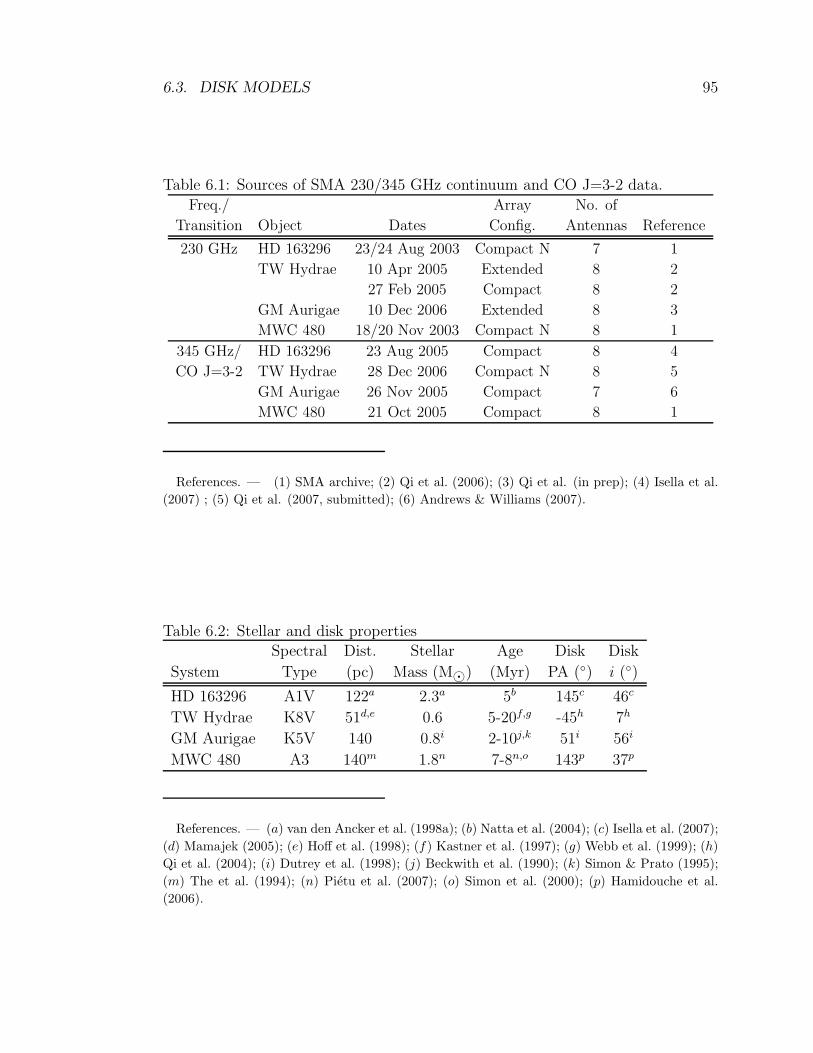
6.3. DISK MODELS 95
Table 6.1: Sources of SMA 230/345 GHz continuum and CO J=3-2 data.
Freq./ Array No. of
Transition Object Dates Config. Antennas Reference
230 GHz HD 163296 23/24 Aug 2003 Compact N 7 1
TW Hydrae 10 Apr 2005 Extended 8 2
27 Feb 2005 Compact 8 2
GM Aurigae 10 Dec 2006 Extended 8 3
MWC 480 18/20 Nov 2003 Compact N 8 1
345 GHz/ HD 163296 23 Aug 2005 Compact 8 4
CO J=3-2 TW Hydrae 28 Dec 2006 Compact N 8 5
GM Aurigae 26 Nov 2005 Compact 7 6
MWC 480 21 Oct 2005 Compact 8 1
References. — (1) SMA archive; (2) Qi et al. (2006); (3) Qi et al. (in prep); (4) Isella et al.
(2007) ; (5) Qi et al. (2007, submitted); (6) Andrews & Williams (2007).
Table 6.2: Stellar and disk propertiesSpectral Dist. Stellar Age Disk Disk
System Type (pc) Mass (M⊙) (Myr) PA () i ()
HD 163296 A1V 122a 2.3a 5b 145c 46c
TW Hydrae K8V 51d,e 0.6 5-20f,g -45h 7h
GM Aurigae K5V 140 0.8i 2-10j,k 51i 56i
MWC 480 A3 140m 1.8n 7-8n,o 143p 37p
References. — (a) van den Ancker et al. (1998a); (b) Natta et al. (2004); (c) Isella et al. (2007);
(d) Mamajek (2005); (e) Hoff et al. (1998); (f) Kastner et al. (1997); (g) Webb et al. (1999); (h)
Qi et al. (2004); (i) Dutrey et al. (1998); (j) Beckwith et al. (1990); (k) Simon & Prato (1995);
(m) The et al. (1994); (n) Pietu et al. (2007); (o) Simon et al. (2000); (p) Hamidouche et al.
(2006).
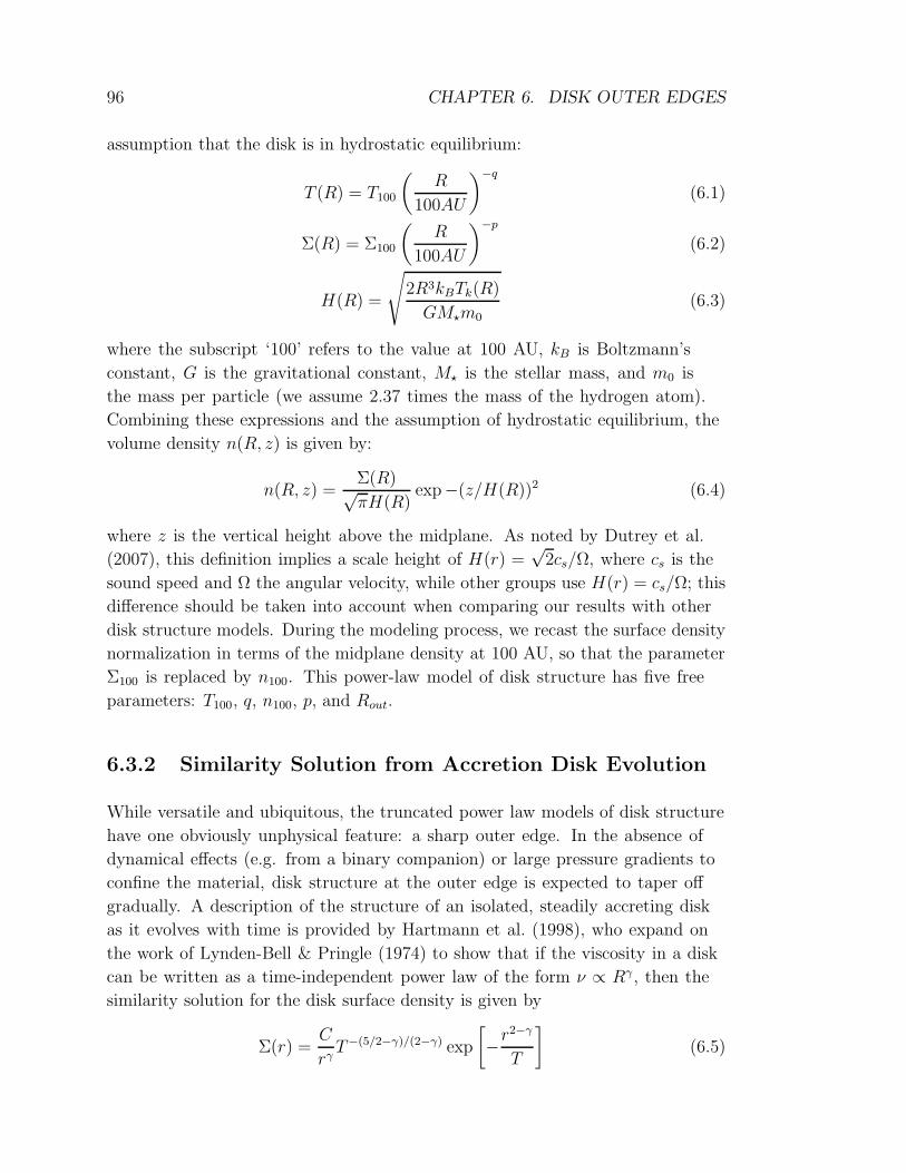
96 CHAPTER 6. DISK OUTER EDGES
assumption that the disk is in hydrostatic equilibrium:
T (R) = T100
(
R
100AU
)−q
(6.1)
Σ(R) = Σ100
(
R
100AU
)−p
(6.2)
H(R) =
√
2R3kBTk(R)
GM⋆m0(6.3)
where the subscript ‘100’ refers to the value at 100 AU, kB is Boltzmann’s
constant, G is the gravitational constant, M⋆ is the stellar mass, and m0 is
the mass per particle (we assume 2.37 times the mass of the hydrogen atom).
Combining these expressions and the assumption of hydrostatic equilibrium, the
volume density n(R, z) is given by:
n(R, z) =Σ(R)√πH(R)
exp−(z/H(R))2 (6.4)
where z is the vertical height above the midplane. As noted by Dutrey et al.
(2007), this definition implies a scale height of H(r) =√
2cs/Ω, where cs is the
sound speed and Ω the angular velocity, while other groups use H(r) = cs/Ω; this
difference should be taken into account when comparing our results with other
disk structure models. During the modeling process, we recast the surface density
normalization in terms of the midplane density at 100 AU, so that the parameter
Σ100 is replaced by n100. This power-law model of disk structure has five free
parameters: T100, q, n100, p, and Rout.
6.3.2 Similarity Solution from Accretion Disk Evolution
While versatile and ubiquitous, the truncated power law models of disk structure
have one obviously unphysical feature: a sharp outer edge. In the absence of
dynamical effects (e.g. from a binary companion) or large pressure gradients to
confine the material, disk structure at the outer edge is expected to taper off
gradually. A description of the structure of an isolated, steadily accreting disk
as it evolves with time is provided by Hartmann et al. (1998), who expand on
the work of Lynden-Bell & Pringle (1974) to show that if the viscosity in a disk
can be written as a time-independent power law of the form ν ∝ Rγ , then the
similarity solution for the disk surface density is given by
Σ(r) =C
rγT−(5/2−γ)/(2−γ) exp
[
−r2−γ
T
]
(6.5)

6.3. DISK MODELS 97
where C is a constant, r is the disk radius in units of the radial scale factor R1
such that r = R/R1, and T is the nondimensional time T = t/ts + 1 where ts is
the viscous scaling time (eq. 20 in Hartmann et al. 1998). For simplicity, when
applying these models to our data we used physical units and absorbed several of
the parameters into two constants so that the surface density is of the form
Σ(R) =c1Rγ
exp
[
−(
R
c2
)2−γ]
, (6.6)
where R is the disk radius in AU and c1, c2, and γ are constants that we allowed
to vary during the fitting process.
The temperature profile for the similarity solution disk model is identical to
that of the truncated power-law disk, except that its spatial extent is infinite.
We do not allow it to drop below 10 K, but this low temperature limit is not
problematic for any of the disks considered here. This model therefore includes
five free parameters: T100, q, c1, γ, and c2. The constant c1 describes the
normalization of the surface density, similar to n100 in the power-law model, while
the constant c2 is analogous to the outer radius, since it describes the radial scale
length over which the exponential taper acts to cause the surface density to drop
towards zero.
6.3.3 Model Comparison
The surface density description for the similarity solution is similar to the
truncated power law except at the outer edge of the disk. In the inner
regions of the disk for which R ≪ c2, we may expand the exponential so that
exp [−(R/c2)2−γ ] → 1 − ( R
c2)2−γ + · · · , and the surface density becomes
Σ(R) =c1Rγ
(1 −(
R
c2
)2−γ
) =c1Rγ
− c1
c2−γ2
R2(1−γ) (6.7)
In the α-viscosity context (Shakura & Syunyaev 1973), for a vertically isothermal
disk with the typical temperature index q = 0.5, we would expect that γ = 1.
This implies that for standard assumptions, the inner disk surface density will
be described by a power law in R with index γ, modified by a constant ( c1c2
) due
to the influence of the exponential. If γ deviates from 1, an additional shallow
dependence on R would be expected.
It is illuminating to consider the behavior of these models in the Fourier
domain, the natural space for interferometer observations. To do so we define the

98 CHAPTER 6. DISK OUTER EDGES
coordinate Ruv, the distance from the phase center of the disk in the (u, v) plane,
as it would be observed if the disk were viewed directly face-on. To perform
the deprojection from the inclined and rotated sky coordinates, we calculate the
position of each point in the (u, v) plane as a projected distance from the major
and minor axes of the disk, respectively: da = R sinφ and db = R cosφ cos i,
where i is the disk inclination, R = (u2 + v2)1/2, φ is the polar angle from the
major axis of the disk, φ = arctan(v/u − PA), and PA is the position angle
measured east of north; then Ruv = (d2a + d2
b)1/2 (Lay et al. 1997; Hughes et al.
2007).
In the Fourier domain, the truncated disk models show “ringing” and the
visibilities will drop rapidly to zero in the vicinity of Ruv = 1/Rout. Under the
simplifying assumption of γ = 1, the Fourier transform of the similarity solution
becomes a convolution of two functions: (1) 1/R, which is just the Fourier
transform of the 1/R dependence of a power law extending from zero to infinity,
and (2) c2/(1 + R2c2)3/2, where c is a scaling constant for the term that describes
the exponential taper. Since these two functions both decrease monotonically and
are always positive, the visibilities drop smoothly to zero without any ringing.
6.3.4 Model Fitting
For both disk models, we fit for the five parameters describing the disk
temperature and surface density structure using the continuum data for each
disk with the widest range of available baseline lengths. The position angle and
inclination were fixed and adopted from previous studies (see Table 6.2). For
opacity, we assume the standard millimeter value adopted by Beckwith & Sargent
(1991) (κν = κ0(ν/ν0)β, where κ0 = 10.0 cm2/gdust, ν0=1 THz, and β = 1),
although we allow β to vary in order to obtain the proper normalization when
extrapolating from one frequency to another. Due to the ∼ 100 AU spatial
resolution, these data are not sensitive to the inner radius of the disk. For both
sets of models, therefore, we simply fix the inner radius at a value of 4 AU for
TW Hya (Calvet et al. 2002; Hughes et al. 2007), 24 AU for GM Aur (Calvet
et al. 2005), and 3 AU for the other two systems, for which reliable inner radius
information is not available; this is sufficiently small that changes in the inner
radius do not affect the derived model parameters. To compare the models to the
data, we use the Monte-Carlo radiative transfer code RATRAN (Hogerheijde &
van der Tak 2000) to calculate sky-projected images of the dust continuum and
CO emission, with frequency and bandwidth appropriate for the observations, and
assuming Keplerian rotation. We then use the MIRIAD task uvmodel to simulate
6.3. DISK MODELS 99
the SMA observations, with the same antenna positions and visibility weights.
For each set of parameters, we directly compare the model visibilities to
the continuum data and calculate a χ2 value, using the minimum χ2 value to
determine the best-fit parameters. The resulting best-fit models are shown along
with continuum data for both frequencies in the left panels of Figure 6.1. The
abscissa gives the deprojected radial distance in the (u, v) plane, and the ordinate
shows the real and imaginary components of the visibility. For a disk with
circular symmetry, the imaginary components should average to zero. The 230
GHz continuum data are depicted as open circles, while the 345 GHz data are
filled circles. The best-fit power-law model is shown in blue and the similarity
solution in orange. Dotted and dashed lines distinguish between the 230 and 345
GHz model predictions; the fit was determined at that frequency with the largest
baseline coverage and extrapolated to the other frequency, by varying β. The
uncertainties quoted for β reflect an assumed 10% calibration uncertainty. Note
that varying β has no effect on the modeled CO emission.
We measure values of β that are consistent with 1, which is in agreement
with the typical values measured for disks in the Taurus-Auriga association (e.g.
Dutrey et al. 1996; Rodmann et al. 2006). These shallow millimeter spectral
slopes indicate that some grain growth has occurred from ISM grain sizes, which
typically exhibit a steeper spectral slope (β ∼ 2). In particular, the value of 1.2
measured for GM Aur matches well the value of 1.2 reported by Andrews &
Williams (2007), and the value of 0.7 measured for TW Hydrae matches well the
value of 0.7 reported by Calvet et al. (2002) and Natta et al. (2004).
After fitting the continuum, we then assumed a gas/dust mass ratio of 100
and a standard interstellar CO/H2 mass ratio of 10−4 to predict the expected
strength and spatial extent of CO emission from the disks, based on the best-fit
continuum model. We assume throughout that the gas and dust are well-mixed,
and that CO traces molecular hydrogen. We do not take into account the
complexities of disk chemistry, such as the depletion of CO molecules in the cold,
dense midplane (Aikawa 2007; Semenov et al. 2006). However, deviations from
these simple assumptions should have no appreciable effect on our conclusions
concerning the radial extent of CO emission.
Since we neglect the vertical temperature gradient in the disk, we might
expect to underpredict the strength of optically thick CO line emission, which
likely originates in the upper layers of the disk that are subject to heating by
stellar irradiation. The continuum emission, by contrast, is likely weighted toward
the cold midplane of the disk. For this reason, after obtaining an initial fit from
100 CHAPTER 6. DISK OUTER EDGES
the continuum, we allowed the temperature scale (T100) to vary to best reproduce
the flux levels of the observed CO emission, and then iteratively fit for the other
structural parameters (q, n100, c2/Rout, and γ/p).
Deriving the temperature from the CO emission in this way may
underestimate the midplane density in some cases, due to the degeneracy between
T100 and n100: the temperature derived from CO emission is typically greater than
or equal to that of the shielded midplane, depending in detail on the dust opacity
and molecular dissociation due to ultraviolet radiation in the upper disk layers
(for a discussion of the processes involved, see Jonkheid et al. 2007; Isella et al.
2007). For the disks considered, the temperature derived for the dust continuum
emission was within ∼ 40% of that derived to match the CO line strength.
6.4 Results and Discussion
The parameters for the best-fit model solutions to the continuum data for each
source and for each of the two model types are listed in Table 6.3. This table
lists only the set of parameters with the minimum χ2 value; formal errors are not
quoted as these are not intended to be definitive structural models but simply
illustrative of the differences between the model classes in their treatment of the
outer edge. The midplane surface density profiles for these models are plotted
in Figure 6.2. The solid lines depict the profile for the power-law solution, while
the dashed lines are for the similarity solution. The parameters of the two model
solutions are very similar, particularly for HD 163296 and MWC 480. For all four
disks, the two model solutions are particularly similar just within the outer edge
of the disk, around the range of radii well-matched to the resolution of the data
(∼ 200 AU for HD 163296, ∼ 90 AU for TW Hydrae, ∼ 200 AU for GM Aurigae,
and ∼ 300 AU for MWC 480). The outer radius for the power-law solution
typically falls at roughly twice the scale length (c2) of the similarity solution. The
analogous parameters γ and p, which describe how quickly the midplane density
drops with radius, are also very similar between the two models.

6.4. RESULTS AND DISCUSSION 101
Figure 6.1.— Comparison between the data and the two types of models (similarity
solution and power law) for the four disks in our sample: (a) HD 163296, (b) TW
Hydrae, (c) GM Aurigae, and (d) MWC 480. For each source, the left panel shows
the real and imaginary visibilities as a function of deprojected (u, v) distance from
the phase center. Symbols are SMA data; open circles are 230 GHz and filled circles
are 345 GHz continuum. The lines represent the best fit to the 345 GHz continuum
for the power law (orange) and similarity (blue) models. Dashed lines show the
model at 345 GHz while solid lines are 230 GHz. The right panel shows position-
velocity diagrams of the J=3-2 rotational transition of CO along the major axis of
the disk. The left plot (black contours) shows the SMA data. The middle plot (blue
contours) displays the emission predicted by the similarity solution parameters that
provide the best fit to the continuum emission, and the right plot (orange contours)
displays the emission predicted for the best-fit power-law model. The horizontal
dashed line across the right panel represents the extent of the outer radius (Rout)
derived for each source through fitting of the continuum emission in the context
of the power-law model. The contour levels, beam, and velocity resolution for
each source are as follows: (a) [2,4,6,8,10,12]×1.1 Jy/beam, 3.0×2.1 arcsec at a
position angle of 14.3, and 0.35 km/s; (b) [2,4,6,8]×2.0 Jy/beam, 4.0×1.8 arcsec
at a position angle of 3.2, and 0.18 km/s; (c) [2,4,8,12,16]×0.5 Jy/beam, 2.3×2.1
arcsec at a position angle of 12.9, and 0.35 km/s; (d) [2,4,6,8,10]×0.5 Jy/beam,
2.5×2.3 arcsec at a position angle of 45.3, and 0.35 km/s.
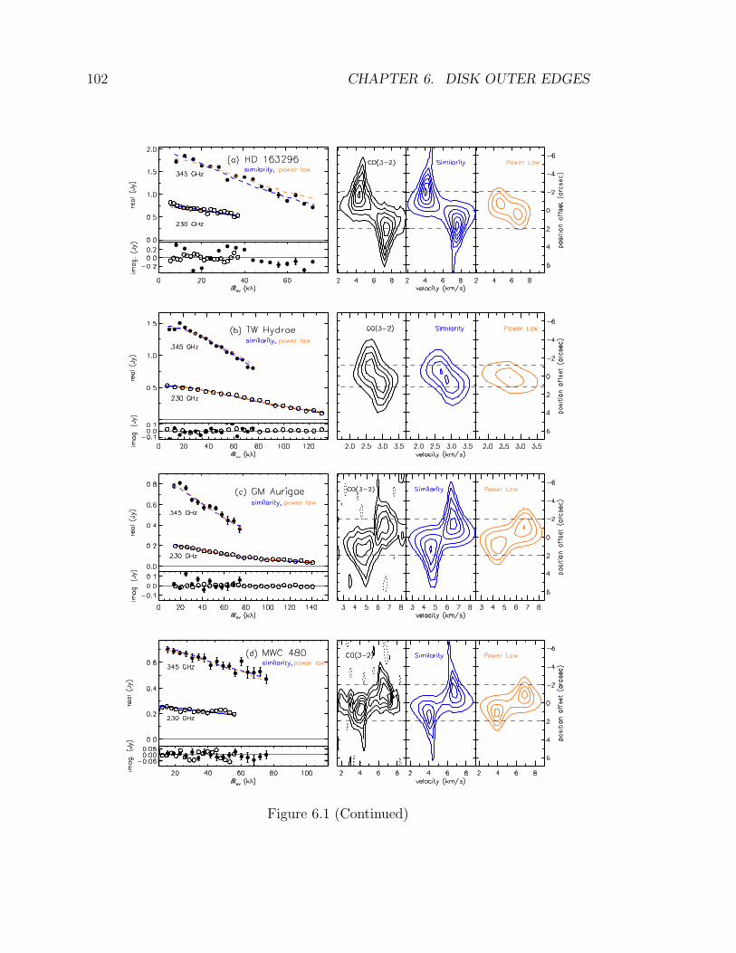
102 CHAPTER 6. DISK OUTER EDGES
Figure 6.1 (Continued)
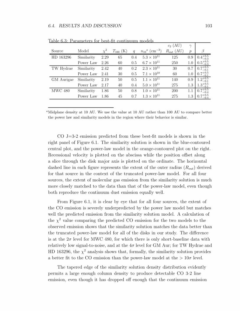
6.4. RESULTS AND DISCUSSION 103
Table 6.3: Parameters for best-fit continuum modelsc2 (AU) γ
Source Model χ2 T100 (K) q n10a (cm−3) Rout (AU) p β
HD 163296 Similarity 2.29 65 0.4 5.3 × 10¹¹ 125 0.9 0.4+0.5−0.3
Power Law 2.26 60 0.5 6.7 × 10¹¹ 250 1.0 0.5+0.5−0.3
TW Hydrae Similarity 2.42 40 0.2 2.3 × 10¹¹ 30 0.7 0.7+0.5−0.1
Power Law 2.41 30 0.5 7.1 × 10¹⁰ 60 1.0 0.7+0.5−0.1
GM Aurigae Similarity 2.19 50 0.5 1.1 × 10¹¹ 140 0.9 1.2+0.5−0.1
Power Law 2.17 40 0.4 5.0 × 10¹¹ 275 1.3 1.3+0.5−0.1
MWC 480 Similarity 1.86 50 0.8 1.0 × 10¹¹ 200 1.1 0.7+0.5−0.4
Power Law 1.86 45 0.7 1.3 × 10¹¹ 275 1.3 0.7+0.5−0.4
aMidplane density at 10 AU. We use the value at 10 AU rather than 100 AU to compare better
the power law and similarity models in the region where their behavior is similar.
CO J=3-2 emission predicted from these best-fit models is shown in the
right panel of Figure 6.1. The similarity solution is shown in the blue-contoured
central plot, and the power-law model in the orange-contoured plot on the right.
Recessional velocity is plotted on the abscissa while the position offset along
a slice through the disk major axis is plotted on the ordinate. The horizontal
dashed line in each figure represents the extent of the outer radius (Rout) derived
for that source in the context of the truncated power-law model. For all four
sources, the extent of molecular gas emission from the similarity solution is much
more closely matched to the data than that of the power-law model, even though
both reproduce the continuum dust emission equally well.
From Figure 6.1, it is clear by eye that for all four sources, the extent of
the CO emission is severely underpredicted by the power law model but matches
well the predicted emission from the similarity solution model. A calculation of
the χ2 value comparing the predicted CO emission for the two models to the
observed emission shows that the similarity solution matches the data better than
the truncated power-law model for all of the disks in our study. The difference
is at the 2σ level for MWC 480, for which there is only short-baseline data with
relatively low signal-to-noise, and at the 4σ level for GM Aur; for TW Hydrae and
HD 163296, the χ2 analysis shows that, formally, the similarity solution provides
a better fit to the CO emission than the power-law model at the > 10σ level.
The tapered edge of the similarity solution density distribution evidently
permits a large enough column density to produce detectable CO 3-2 line
emission, even though it has dropped off enough that the continuum emission

104 CHAPTER 6. DISK OUTER EDGES
Figure 6.2.— Midplane density structure of the models that provide the best fit
to the continuum data. Solid lines show truncated power-law models while dashed
lines show similarity solution models.

6.4. RESULTS AND DISCUSSION 105
is negligible. The power-law model, by contrast, is strictly limited in the extent
of its CO emission by the sharp outer radius. In particular, for the case of HD
163296, the CO emission predicted by the power law model (orange contours in
the right panel of Figure 6.1a) falls to 4.4 Jy/beam at a distance of 1.8 arcsec
(220 AU) from the source center, while the similarity solution (blue contours)
maintains this brightness out to a distance of 4.7 arcsec (570 AU). This latter size
is well matched to the data (black contours) which extends at this brightness to
a distance of 5.0 arcsec (600 AU). These distances likely overestimate the true
physical extent of the disk due to convolution with the 2.1 × 3.0 arcsec beam,
though they are very comparable to the values observed by Isella et al. (2007).
While the similarity solution does not provide a perfect fit to the data, nor do we
intend it to do so, it illustrates that the outer radius discrepancy is peculiar to
the truncated power-law model; other disk structure models with a tapered outer
edge may be able to reproduce the gas and dust emission as well as, or better
than, the similarity solution adopted here.
Analysis of the CO excitation in the similarity solution model shows that
the extent of the CO J=3-2 emission in these disks coincides roughly with the
radius at which the line excitation becomes subthermal, determined primarily by
where the mid-plane density drops below the critical density (∼ 4.4 × 104 cm−3
at 20 K, though effectively lowered when photon trapping plays a role). In the
similarity solution model, the surface density distribution steepens dramatically
at large radii, but without the sharp truncation of the power-law model. This
suggests that caution should be exercised not only when comparing outer radius
measurements based on dust continuum and molecular gas emission, but also
when comparing measurements based on emission from different transitions of
CO or from isotopologues of the CO molecule that have differing abundances and
optical depths. Pietu et al. (2007) fit truncated power law models to the disks
around DM Tau, LkCa 15, and MWC 480 in several different isotopologues and
rotational transitions of CO. For the two cases in which multiple transitions of the13CO molecule were observed, the derived outer radius is marginally smaller for
the J=2-1 transition than the J=1-0 transition. This result is consistent with the
expected trend that lower-J transitions will exhibit larger outer radii due to their
lower critical density: a lower critical density will be reached at a greater distance
as the surface density tapers off near the outer edge of the disk. In all cases the
Pietu et al. (2007) analysis also yielded a smaller outer radius in 13CO than in12CO, as well as a flatter surface density power law index for 13CO than for 12CO.
These differences may be related to selective photodissociation, or other chemical
processes. However, the trends of smaller outer radius and shallower surface
density index in 13CO are also consistent with surface density falling off rapidly

106 CHAPTER 6. DISK OUTER EDGES
at large radii, as expected for a disk with a tapered outer edge. In the similarity
solution model, the less abundant 13CO isotopologue will become undetectable
at smaller radii than 12CO, which is more sensitive to the exponential drop in
surface density in the outer disk.
It is noteworthy that studies of six largest “proplyds” with the most distinct
silhouettes in the Orion Nebula Cluster reveal radial profiles in extinction that
are well-described by an exponential taper at the outer edge (McCaughrean &
O’Dell 1996). These isolated disks may be analogous to the systems considered
here with a tapered outer edge.
Models with tapered outer edges also aid in addressing discrepancies between
the size of the dust disk observed in the millimeter and the extent of scattered
light observed in the optical and near-infrared. For example, coronographic
observations of TW Hydrae detect scattered light to a distance of ∼ 200 AU from
the star (Krist et al. 2000; Trilling et al. 2001; Weinberger et al. 2002), while the
truncated power-law model places the outer edge of the dust disk closer to 60 AU.
Similarly, observations of HD 163296 by Grady et al. (2000) detect scattered light
out to ∼ 400 AU from the star, much larger than the 250 AU radius of the dust
disk implied by the truncated power-law model. While the exponential taper
causes the density of the similarity solution to drop rapidly with radius, these
models retain a substantial vertical column density for several exponential scale
lengths. It is therefore plausible that scattered light can remain visible at this
distance, in contrast to the case of the smaller truncated power-law disk.
Although we intend for the similarity solution applied here to be an
illustrative rather than definitive description of the disk structure, it is important
to note that the particular form applied here has potential implications for the
study of the evolutionary status of these disks. The form of the similarity solution
developed by Lynden-Bell & Pringle (1974) and Hartmann et al. (1998) relates
the observed structure to the disk age, viscosity, and initial radius. Although all
three of these variables are poorly constrained by current observations, a large
and homogeneous sample of objects studied in this way might reveal evolutionary
trends in the disk structure.
6.5 Summary and Conclusions
With the advent of high signal-to-noise interferometer observations that resolve
the outer regions of nearby protoplanetary disks, an apparent discrepancy has

6.5. SUMMARY AND CONCLUSIONS 107
emerged between the extent of the dust continuum and molecular gas emission
(Pietu et al. 2005; Isella et al. 2007). Using multi-frequency interferometric data
from the Submillimeter Array, we have investigated this disparity for four disk
systems (HD 163296, TW Hydrae, GM Aurigae, and MWC 480) in the context
of two distinct classes of disk structure models: (1) a truncated power law, and
(2) a similarity solution for the time evolution of an accretion disk. The primary
difference between these models is in their treatment of the disk outer edge: the
abruptly truncated outer edge of the power-law disk causes the visibilities to drop
rapidly to zero, leading to an inferred outer radius that is small in comparison
with the observed molecular gas emission. The similarity solution, by contrast,
tapers off smoothly, creating a broader visibility function and allowing molecular
gas emission to persist at radii well beyond the region in the disk where continuum
falls below the detection threshold. The outer radius discrepancy appears to exist
only in the context of the power-law models.
In light of this result, it appears that an abrupt change in dust properties
for these disks is unlikely, as there is no physical mechanism to explain such a
discontinuity. This may imply that a sharp change in dust properties in the early
solar nebula is similarly an unlikely explanation for the Kuiper belt edge observed
by Jewitt et al. (1998), and that a dynamical mechanism such as truncation by
a close encounter with a cluster member (Reipurth 2005, and references therein)
may provide a more plausible origin. In this case, we would expect to observe
disks with sharp outer edges only in clustered environments, and a model with a
tapered edge would be a more realistic prescription for investigating the structure
of a typical isolated disk. The tapered disk models provide a natural explanation
for the disparate outer radii observed using different probes of the disk extent,
including comparison of continuum and molecular gas observations (Pietu
et al. 2005; Isella et al. 2007), and also comparison of different isotopologues
and rotational transitions of a particular molecule (Pietu et al. 2007). When
predicting CO emission, this simple model does neglect potential variance in the
CO abundance due to depletion in the midplane and photodissociation at the
disk surface; however, the results presented are intended simply to illustrate the
global differences between gas and dust emission from the two model classes,
independent of detailed CO chemistry.
While we cannot rule out disparate gas and dust radii in these disks, we show
that an alternative disk structure model, grounded in the physics of accretion,
resolves the apparent size discrepancy without the need to invoke dramatic
changes in dust opacity, dust density, or dust-to-gas ratio in the outer disk.

108 CHAPTER 6. DISK OUTER EDGES
Chapter 7
Stringent Limits on the Polarized
Submillimeter Emission from
Protoplanetary Disks
A. M. Hughes, D. J. Wilner, J. Cho, D. P. Marrone, A. Lazarian, S. M. Andrews,
& R. Rao 2009, The Astrophysical Journal, Vol. 704, pp. 1204-1217
Abstract
We present arcsecond-resolution Submillimeter Array (SMA) polarimetric
observations of the 880µm continuum emission from the protoplanetary disks
around two nearby stars, HD 163296 and TW Hydrae. Although previous
observations and theoretical work have suggested that a 2-3% polarization
fraction should be common for the millimeter continuum emission from such
disks, we detect no polarized continuum emission above a 3σ upper limit of 7mJy
in each arcsecond-scale beam, or < 1% in integrated continuum emission. We
compare the SMA upper limits with the predictions from the exploratory Cho
& Lazarian (2007) model of polarized emission from T Tauri disks threaded by
toroidal magnetic fields, and rule out their fiducial model at the ∼ 10σ level. We
explore some potential causes for this discrepancy, focusing on model parameters
that describe the shape, magnetic field alignment, and size distribution of grains
in the disk. We also investigate related effects like the magnetic field strength
and geometry, scattering off of large grains, and the efficiency of grain alignment,
including recent advances in grain alignment theory, which are not considered
109

110 CHAPTER 7. POLARIZED SUBMM DISK LIMITS
in the fiducial model. We discuss the impact each parameter would have on the
data and determine that the suppression of polarized emission plausibly arises
from rounding of large grains, reduced efficiency of grain alignment with the
magnetic field, and/or some degree of magnetic field tangling (perhaps due to
turbulence). A poloidal magnetic field geometry could also reduce the polarization
signal, particularly for a face-on viewing geometry like the TW Hya disk. The
data provided here offer the most stringent limits to date on the polarized
millimeter-wavelength emission from disks around young stars.
7.1 Introduction
The magnetic properties of circumstellar disks are central to a wide range
of physical processes relevant for planet formation. Dust and gas transport
and mixing (e.g. Ciesla 2007), meteoritic composition (e.g. Boss 2004), disk
chemistry (e.g. Semenov et al. 2006), and the migration of planetary embryos
through the disk (e.g. Chambers 2006) are all thought to be influenced by
magnetohydrodynamic (MHD) turbulence. But perhaps the greatest impact of
a magnetized disk is that MHD turbulence can provide the source of viscosity
that drives disk evolution. Since the seminal work by Lynden-Bell & Pringle
(1974), the photospheric excess and variability exhibited by pre-main sequence
stars have been attributed to an accretion disk. The viscous transport mechanism
that supports the accretion process can also explain many aspects of the time
evolution of circumstellar disks (Hartmann et al. 1998), and by extension can help
to constrain the physical conditions and timescales relevant for planet formation.
However, there are remarkably few observational constraints on the magnitude
and physical origin of viscosity in circumstellar disks.
As conjectured by Shakura & Syunyaev (1973), turbulence can provide
large enough viscosities to account for accretion and disk evolution on the
appropriate timescales. The mechanism most commonly invoked as the source
of this turbulence is the magnetorotational instability (MRI), in which magnetic
interactions between fluid elements in the disk combine with an outwardly
decreasing velocity field to produce torques that transfer angular momentum
from the inner disk outwards (Balbus & Hawley 1991, 1998; see also Velikhov
1959 and Chandrasekhar 1960). Indeed, it is unlikely that turbulence in an
unmagnetized, azimuthally symmetric Keplerian disk can sufficiently redistribute
angular momentum: magnetic fields must be invoked to enable Shakura-Sunyaev
viscosity (e.g. Balbus et al. 1996). The ionization fraction is likely high enough

7.1. INTRODUCTION 111
for magnetic coupling of material over much of the outer disk (see e.g. Sano et al.
2000; Turner et al. 2007), and the observed Keplerian rotation of protoplanetary
disks provides the requisite velocity shear. However, the magnetic field properties
(strength and geometry) far from the central star remain unconstrained.
Resolved observations of polarized submillimeter continuum emission are
uniquely suited to constrain the magnetic field geometry – independent of disk
structure – via the orientation of polarization vectors produced by dust grains
aligned with the magnetic field (Aitken et al. 2002). In the presence of an
anisotropic radiation field, irregularly shaped grains with different cross sections
to left and right circular polarizations of light can be spun up to high speeds by
radiative torques (e.g. Dolginov 1972; Dolginov & Mitrofanov 1976; Draine &
Weingartner 1996)1. These spinning grains precess around magnetic field lines,
and ultimately align with their long axes perpendicular to the local magnetic
field direction. Polarized emission or absorption by these aligned grains can thus
trace magnetic field structure in dusty interstellar media (see Lazarian 2007, and
references therein).
The first models of polarized emission from disks incorporating the radiative
torque alignment mechanism have recently been calculated by Cho & Lazarian
(2007). Using a two-layer Chiang et al. (2001) disk structure model threaded
by a toroidal magnetic field (with circular field lines in the plane of the disk,
centered on the star), they calculated the polarization emitted as a function
of wavelength and position in the disk, incorporating emission and selective
absorption mechanisms, but not scattering. They predict a 2-3% polarization
fraction at 850µm, and note that grain alignment is particularly efficient in the
low-density outer disk regions. At millimeter wavelengths, dust grain opacities
are low and optically thin thermal continuum emission primarily originates in
the midplane where most of the mass is located. Polarimetric observations of
millimeter-wavelength dust continuum emission therefore trace magnetic field
geometry near the midplane in the outer disk, in regions where the magnetic field
is strong enough for grains to become aligned and the density is low enough that
grain spin-up is not impeded by gas drag.
The first attempt to observe polarized millimeter-wavelength emission from
1More recent research in Lazarian & Hoang (2007) shows that in many cases rather than
being spun up paramagnetic grains get slowed down by radiative torques, which means that the
grains aligned by radiative torques do not necessarily rotate suprathermally. Nevertheless, the
maximal rotational rate provides a useful parameterization of the effect of the radiative torques
as discussed in detail in Hoang & Lazarian (2008).

112 CHAPTER 7. POLARIZED SUBMM DISK LIMITS
protoplanetary disks was made by Tamura et al. (1995, 1999). They used the
James Clerk Maxwell Telescope (JCMT) to observe several young systems in the
Taurus-Auriga molecular cloud complex – HL Tau, GG Tau, DG Tau and GM
Aur – and reported tentative (∼ 3σ) detections of polarized millimeter-wavelength
continuum emission from three of the four systems. The exception was GG Tau,
for which they report a 2σ upper limit of 3%. While the disks are unresolved
in the 14” JCMT beam, the approximate alignment of the GM Aur and DG
Tau polarization vectors with the known orientation of the disk minor axis is
suggestive of a globally toroidal magnetic field structure. However, finer resolution
is required to confirm the magnetic field structure in the disks, and differentiate
it from any potential contamination from an envelope or cloud material. DG
Tau was followed up at a wavelength of 350µm using the Caltech Submillimeter
Observatory by Krejny et al. (2009), and no polarization was detected with an
upper limit of ∼ 1%. They suggest that the decrease of polarization percentage
relative to the tentative 850µm detection and the corresponding Cho & Lazarian
(2007) prediction at 350µm may be due to some combination of polarization
self-suppression – effectively an absorption optical depth effect (see e.g. Hildebrand
et al. 2000) – or increased scattering at shorter wavelengths, which would produce
a signal orthogonal to that expected for a toroidal magnetic field. In summary,
while the Cho & Lazarian (2007) predictions are consistent with the magnitude of
the tentative JCMT detections, as discussed by Krejny et al. (2009), the predicted
polarization spectrum is inconsistent with the 350 and 850µm observations of DG
Tau.
In the absence of spatially resolved observations, the origin of the polarized
emission in these systems remains unclear. While the position angle of the
polarized emission observed in the three systems in the Taurus-Auriga complex
suggests association with the circumstellar disk, at least two of these sources
(DG Tau and HL Tau) are flat-spectrum sources host to jets and likely retain
envelope material that could aid in generating a polarization signal (Kitamura
et al. 1996; D’Alessio et al. 1997, e.g.). Tamura et al. (1995) suggest that the
emission from HL Tau may arise from an interface region between the disk and
a small envelope, and that the upper limit for GG Tau may be due to the lack
of an envelope combined with weak, compact emission from the circumbinary
ring. Observations of the GM Aur system using the NICMOS instrument on
the Hubble Space Telescope indicate that it too may host a tenuous remnant
outflow and envelope (Schneider et al. 2003). Nevertheless, with both theoretical
predictions and observational evidence pointing to a 2-3% polarization fraction at
850µm in several T Tauri disks, resolved observations revealing the magnetic field
geometry should be possible with current millimeter interferometers for bright

7.1. INTRODUCTION 113
disks. At ∼ 1” resolution, such data would be well matched to the size scales at
which the polarization fraction is expected to be the largest in the context of the
Cho & Lazarian (2007) models.
In order to test the Cho & Lazarian (2007) model predictions and constrain
magnetic field strengths and geometries, we observed two nearby systems,
HD 163296 and TW Hya, with the Submillimeter Array (SMA) polarimeter.
These targets were selected primarily for their large millimeter-wave fluxes to
maximize the expected polarization signal. Unlike the previously-observed Taurus
targets, they are isolated from molecular cloud material. HD 163296 has a
total flux of 1.92 Jy at 850µm (Mannings 1994), while TW Hya has a flux of
1.45 Jy at 800µm (Weintraub et al. 1989), predicting a total polarized flux of
∼40mJy in each system. Polarization of this magnitude should be observable
with the SMA even if resolved across a few beams. HD 163296 is a Herbig Ae
star with a mass of 2.3M⊙ located at a distance of 122 pc (van den Ancker et al.
1998b). It is surrounded by a flared disk viewed at an intermediate inclination
of ∼ 45, observed to extend to at least 500AU in molecular gas and scattered
light (Isella et al. 2007; Grady et al. 2000), which has been extensively observed
and modeled at millimeter wavelengths (Mannings & Sargent 1997; Natta et al.
2004; Isella et al. 2007). TW Hya is a K star located at a distance of only 51 pc
(Mamajek 2005; Hoff et al. 1998). It hosts a massive circumstellar disk viewed
nearly face-on at an inclination of 7 and extending to a radius of ∼200AU in
molecular gas and scattered light (Qi et al. 2004; Roberge et al. 2005). It is also a
prototypical example of the class of disks with infrared deficits in their spectral
energy distribution, known as “transition” disks. It has been shown to have a
central deficit of dust emission extending out to 4AU (Calvet et al. 2002; Hughes
et al. 2007), with a low mass accretion rate (Muzerolle et al. 2000) that may
indicate clearing by a giant planet in formation (Alexander & Armitage 2007).
We describe our observations of these systems in Section 7.2 and present the
upper limits in Section 7.3. In Section 7.4.1 we describe the initial predictions
generated by the Cho & Lazarian (2007) models and compare these predictions
to the SMA observations. We then use these initial models as a starting point for
an exploration of parameter space that seeks to describe how the different factors
affect the predicted polarization properties (Section 7.4.2). We expand on these
results by discussing the potential effects of physical mechanisms not included in
the models (Section 7.4.3). In Section 7.5, we evaluate which physical conditions
are most likely to contribute to the suppression of polarization relative to the
fiducial model and summarize our results. Appendix B presents supplementary
polarimetric observations of two more circumstellar disks, GM Aur and MWC 480.

114 CHAPTER 7. POLARIZED SUBMM DISK LIMITS
7.2 Observations and Data Reduction
Observations were conducted using the SMA polarimeter, described in detail in
Marrone & Rao (2008). The polarimeter uses a set of quarter-wave plates to
convert the normally linear SMA feeds to circular polarization. By rotating the
wave plate between two orientations separated by 90, a single linear feed can
be converted into either of the circular bases (left and right, or L and R). Since
only one polarization (L or R) can be sampled on any antenna at any given
time, full sampling of all four polarization states (LL, RR, RL, and LR) for all
baselines (numbering N(N − 1)/2, where N is the number of antennas) must be
accomplished by rotating the waveplates through a series of orientation patterns
conveniently described by the two-state Walsh functions (see Marrone 2006).
A full set of polarization states can be obtained for all baselines in ∼5minutes
using a series of short (10-second) integrations with the waveplates rotated
through patterns described by Walsh functions for the appropriate number of
antennas. These 5-minute intervals of data are combined into quasi-simultaneous
Stokes parameters for each baseline (I = (RR + LL)/2, Q = (RL + LR)/2,
U = i(LR − RL)/2, V = (RR − LL)/2), where I measures the total intensity,
V measures the intensity of circular polarization, and√
Q2 + U2 gives the total
linearly polarized intensity, which can also be used to calculate the local fractional
(or percent) linear polarization√
Q2 + U2/I. Note that the aligned states (RR
and LL) separate the total intensity from the circularly polarized intensity, while
the crossed states (LR and RL) provide information about the linearly polarized
intensity. Of course, this represents an idealization. Two relevant non-ideal effects
are (1) if the R and L gains are not perfectly matched, then some of the bright
Stokes I flux can leak into Stokes V when the difference is taken between LL and
RR, and (2) instrumental “leakage” of left circularly polarized light through a
nominally right circularly polarized waveplate (and vice versa) can transfer Stokes
I to the linear states Q and U .
Polarimetric SMA observations of the HD 163296 disk at 880µm wavelength
were carried out in the compact configuration on 29 May 2008, and in the
extended configuration on 12 July 2008. The weather was excellent, with the
225GHz opacity below 0.05 both nights, reaching as low as 0.03 on the night of
12 July. The phases were also extremely stable on both nights. The projected
baseline lengths spanned a range of 9 to 260 kλ, providing a synthesized beam size
of 1.′′1×0.′′89 for the combined data set, using natural weighting (see Table 7.1 for
details). The quasar 3c454.3 was observed for 2.5 hours through more than 90
of parallactic angle during its transit, in order to calibrate the complex leakages

7.2. OBSERVATIONS AND DATA REDUCTION 115
of the quarter-wave plates. The quasar J1733-130 was used to calibrate the
atmospheric and instrumental gain, and the quasar J1924-292 was observed at
45-minute intervals throughout the night to test the quality of the phase transfer
from J1733-130 as well as the calibration of the quarter-wave plate leakage.
Uranus was used as the flux calibrator, yielding a flux for J1733-130 of 1.62 Jy on
the night of May 29 and 2.01 Jy on the night of July 12. Uranus, Callisto, 3c273,
and 3c279 were included as passband calibrators.
Observations of the disk around TW Hya were conducted in the subcompact
and extended configurations of the SMA during the nights of 25 January and
15 February 2009, respectively. Due to the far southern declination of TW Hya
in combination with the stringent elevation limits imposed to avoid antenna
collisions in the subcompact configuration, the source was only observable for
three hours on the night of 25 January, while a full six hours of observations
were obtained on 15 February. The weather was again excellent, particularly for
the extended configuration, during which the 225GHz opacity remained stable
between 0.03 and 0.04 for most of the night. The projected baseline lengths in
the final data set varied from 6 to 250 kλ, providing a synthesized beam size of
1.′′2×0.′′9 in the final data set (see Table 7.1). The instrumental polarization was
calibrated by observing 3c273 over 90 degrees of parallactic angle for three hours
across its transit. The quasar J1037-295 was used as the gain calibrator, and
3c279 was observed once per hour to test both the quality of the phase transfer
and the instrumental polarization calibration. The primary flux calibrator was
Titan, yielding a flux for J1037-295 of 0.64 Jy on the night of 25 Jan and 0.53 Jy
on the night of 15 Feb. 3c279, 3c273, and J1037-295 were included as passband
calibrators.
The double sideband receivers were tuned to a central frequency of
340.75GHz (880 µm) for the HD 163296 observations and 341.44GHz (877µm)
for the TW Hya observations, with each 2GHz-wide sideband centered ±5GHz
from that value. The correlator was configured to observe the CO(3-2) transition
(rest frequency 345.796GHz) with a velocity resolution of 0.70 km s−1. The data
were edited and calibrated using the MIR software package, while the standard
tasks of Fourier transforming the visibilities, deconvolution with the CLEAN
algorithm, and restoration were carried out using the MIRIAD software package.
For a summary of the observational parameters, including the 3σ upper limits
in Stokes Q and U for the individual tracks and the combined data sets, refer
to Table 7.1. The test quasars for all tracks were point-like and unresolved. We
detect polarized emission from the test quasars independently in each data set
with a polarization fraction of between 8 and 12% and a direction consistent

116 CHAPTER 7. POLARIZED SUBMM DISK LIMITS
Table 7.1: Observational ParametersHD 163296 TW Hya
Compact Extended C+E Compact Extended C+E
Parameter 29 May 2008 12 July 2008 25 Jan 2009 15 Feb 2009
340GHz Continuum
Beam Size (FWHM) 2.′′2×1.′′3 0.′′9×0.′′7 1.′′0×0.′′9 4.′′7×2.′′0 1.′′1×0.′′8 1.′′2×0.′′8
P.A. 50 -8 7 -1 6 6
RMS Noise (mJybeam−1)
Stokes I 11 7.8 5.7 35 6.8 5.5
Stokes Q & U 3.8 2.7 2.4 6.3 2.4 2.3
Peak Flux Density (mJybeam−1)
Stokes I 996 639 739 990 450 474
Stokes Q & U (3σ upper limit) <11 <8.1 <7.2 <19 <7.2 <6.9
Integrated Flux (Stokes I; Jy) 1.65 1.79 1.64 1.24 1.33 1.26
CO(3-2) Line
Beam Size (FWHM) 2.′′2×1.′′4 0.′′9×0.′′7 1.′′1×1.′′0 5.′′0×1.′′2 1.′′1×0.′′7 1.′′2×0.′′7
P.A. 50 -8 17 -1 9 9
RMS Noise (mJybeam−1) 25 19 15 55 14 13
Peak Flux Density (mJybeam−1)
Stokes I 6500 2650 3730 1520 1800 3090
Stokes Q & U (3σ upper limit) <75 <57 <45 <170 <42 <39
Integrated Flux (Stokes I; Jy km s−1) 110 56 95 47 13 27
aAll quoted values assume natural weighting.bThe rms in Stokes I is limited by dynamic range rather than sensitivity.cThe integrated continuum flux is calculated using the MIRIAD task uvfit, assuming an elliptical
Gaussian brightness profile.dThe rms for the line is calculated using a channel width of 0.7 km s−1.eThe integrated line flux is calculated by integrating the zeroth moment map inside the 3σ bright-
ness contours.
between lower and upper sidebands, as expected for linearly polarized emission
from quasars at these wavelengths (see Marrone 2006).
7.3 Results
Figure 7.1 shows the Stokes I (unpolarized) visibilities as a function of distance
from the phase center in the (u,v) plane, corrected for the projection effects due to
the disk inclination as in Lay et al. (1997) (for the mathematical definition of the
abscissa, see Section 3.3 of Hughes et al. 2008b). This is effectively the Fourier
transform of the radial brightness distribution of the disk. Both the HD 163296
and TW Hya disks are well resolved with high signal-to-noise ratios.
We detect no polarized emission, in the CO(3-2) line or 880µm continuum,
from the HD 163296 or TW Hya disks. The rms values achieved in Stokes Q and

7.3. RESULTS 117
U for the combined (compact+extended) continuum data are 2.4mJybeam−1
and 2.3mJybeam−1, respectively, yielding a 3σ upper limit in both data sets
of 7mJybeam−1. Given the integrated Stokes I fluxes of 1.65 Jy and 1.25 Jy
for HD 163296 and TW Hya (see Table 7.1), the Cho & Lazarian (2007) result
predictions of 2-3% polarization at these wavelengths imply ∼30-50mJy of
polarized flux. Even if the spatial distribution of polarized flux in the source
differs from that of the unpolarized emission, we should be able to detect it
given that we recover most of the Stokes I flux. Figures 7.2 and 7.3 compare the
data with the fiducial model predictions (described in Section 7.4.1 below). The
upper right panel of each figure displays the amount and direction of observed
polarized flux for each source, while the bottom row presents contour maps for
each of the individual Stokes parameters. The emission in Stokes Q and U (linear
polarization), as well as in Stokes V (circular polarization), is consistent with
noise. As noted in Section 7.2, since Stokes V is calculated as the difference
between the measured right and left (RR and LL) circular polarization, the
difficulty of calibrating the gains precisely enough to remove the influence of the
bright Stokes I emission raises the rms value in this Stokes parameter relative
to Stokes Q and U , which are calculated instead from the crossed (RL and LR)
polarization states.
We can rule out calibration errors as the reason for the lack of polarized
emission for three reasons: (1) The point-like test quasars and the similarity of
the visibility profiles in Figure 7.1 with previous observations of these sources
(see e.g. Isella et al. 2007; Hughes et al. 2008b) illustrate both the success of the
atmospheric and instrumental gain calibration and the high sensitivity of the
data set. (2) The detection of polarized emission from the test quasars in each
of the data sets, with direction consistent between sidebands, demonstrates the
success of the instrumental leakage calibration. Furthermore, (3) several of the
nights were shared with other SMA polarization projects and our solutions for the
instrumental leakage between Stokes parameters for the eight quarter-wave plates
were effectively identical to those derived by other observers, who successfully
detect polarization in their targets.
It is worthwhile to compare the rms noise achieved here with the limiting
precision of the current SMA polarimeter. Errors in alignment of the quarter-wave
plates introduce instrumental “leakage” between Stokes parameters, allowing
some of the flux from Stokes I to bleed into the linear Stokes parameters. The
instrumental leakage correction is quite small (. 3%) and can to a large extent
be calibrated by observing a bright point source as it rotates through 90 of
parallactic angle. Nevertheless, the uncertainty of this correction under typical

118 CHAPTER 7. POLARIZED SUBMM DISK LIMITS
observing conditions is ∼0.2%, although this can be reduced to . 0.1% with
parallactic angle rotation, provided the source polarization does not vary with
time (Marrone 2006). Given the 2mJybeam−1 rms noise from our observations
compared with the peak Stokes I fluxes of 740 and 470mJybeam−1 (∼0.3%), our
constraints on the polarized flux are approaching the limit of what is achievable
with the SMA polarimeter.
It is difficult to directly compare the observations presented here with the
Cho & Lazarian (2007) model predictions and the Tamura et al. (1999) JCMT
result. The 2-3% polarization factor reported by both sources refers to the
integrated emission over the entire spatial extent of the disk. Since the SMA
spatially resolves the emission from the disk, the limit on the percent polarization
varies with position across the disk. The emission structure is predicted to be
quite complicated (Cho & Lazarian 2007), with the percent polarization increasing
as a function of distance from the star, so there is no straightforward way to quote
a single value for the percent polarization that can be easily compared with the
data. By tapering the SMA visibilities with a Gaussian whose FWHM is equal to
the diameter of the disk as measured by a truncated power law model (Hughes
et al. 2008b), we can simulate an unresolved observation, similar to the JCMT
result from Tamura et al. (1999). Using this method, we place a 3σ upper limit
of 1% on the total polarized flux from both disks. However, such an extreme
taper severely down-weights the visibilities on the longest baselines, which still
have very high signal-to-noise ratios (see Figure 7.1). This effectively neglects
the majority of the data: when all of the spatially resolved data are taken into
account, the limits are much more stringent, but they must be compared with the
more complicated predictions from the spatially resolved model. Furthermore,
decreasing the resolution may be additionally detrimental in the case of more
face-on disks like TW Hya: if the magnetic field is perfectly toroidal, then the
resulting radial polarization signal will cancel to zero in a large beam, no matter
how strong the emission. To give a rough estimate, the ∼ 40mJy of integrated
polarized flux predicted for a 2-3% polarization fraction resolved into a few beams
might predict a peak flux density of ∼ 20mJybeam−1, which is about 10σ above
the ∼ 2mJybeam−1 noise in the data. However, a detailed comparison with the
spatially resolved model predictions for each disk can give a more robust result.
The highest signal-to-noise ratio in an image is achieved using natural
weighting, which assigns each visibility a weight inversely proportional to its
variance. In the case of observations with the SMA polarimeter, the bandwidth
and integration time are the same for each integration, so the visibilities are
primarily weighted by system temperature. For this reason, we use natural
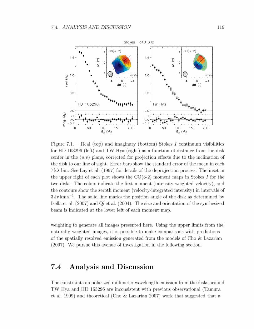
7.4. ANALYSIS AND DISCUSSION 119
Figure 7.1.— Real (top) and imaginary (bottom) Stokes I continuum visibilities
for HD 163296 (left) and TW Hya (right) as a function of distance from the disk
center in the (u,v) plane, corrected for projection effects due to the inclination of
the disk to our line of sight. Error bars show the standard error of the mean in each
7 kλ bin. See Lay et al. (1997) for details of the deprojection process. The inset in
the upper right of each plot shows the CO(3-2) moment maps in Stokes I for the
two disks. The colors indicate the first moment (intensity-weighted velocity), and
the contours show the zeroth moment (velocity-integrated intensity) in intervals of
3 Jy km s−1. The solid line marks the position angle of the disk as determined by
Isella et al. (2007) and Qi et al. (2004). The size and orientation of the synthesized
beam is indicated at the lower left of each moment map.
weighting to generate all images presented here. Using the upper limits from the
naturally weighted images, it is possible to make comparisons with predictions
of the spatially resolved emission generated from the models of Cho & Lazarian
(2007). We pursue this avenue of investigation in the following section.
7.4 Analysis and Discussion
The constraints on polarized millimeter wavelength emission from the disks around
TW Hya and HD 163296 are inconsistent with previous observational (Tamura
et al. 1999) and theoretical (Cho & Lazarian 2007) work that suggested that a
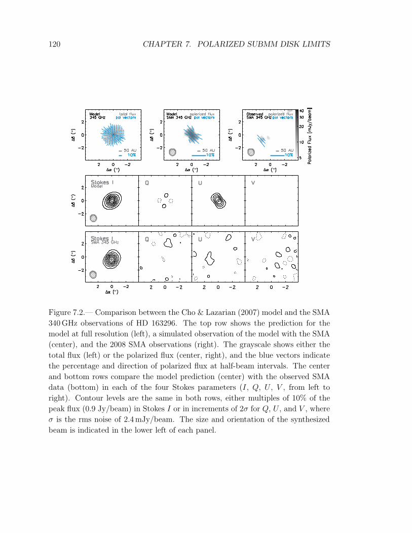
120 CHAPTER 7. POLARIZED SUBMM DISK LIMITS
Figure 7.2.— Comparison between the Cho & Lazarian (2007) model and the SMA
340GHz observations of HD 163296. The top row shows the prediction for the
model at full resolution (left), a simulated observation of the model with the SMA
(center), and the 2008 SMA observations (right). The grayscale shows either the
total flux (left) or the polarized flux (center, right), and the blue vectors indicate
the percentage and direction of polarized flux at half-beam intervals. The center
and bottom rows compare the model prediction (center) with the observed SMA
data (bottom) in each of the four Stokes parameters (I, Q, U , V , from left to
right). Contour levels are the same in both rows, either multiples of 10% of the
peak flux (0.9 Jy/beam) in Stokes I or in increments of 2σ for Q, U , and V , where
σ is the rms noise of 2.4mJy/beam. The size and orientation of the synthesized
beam is indicated in the lower left of each panel.
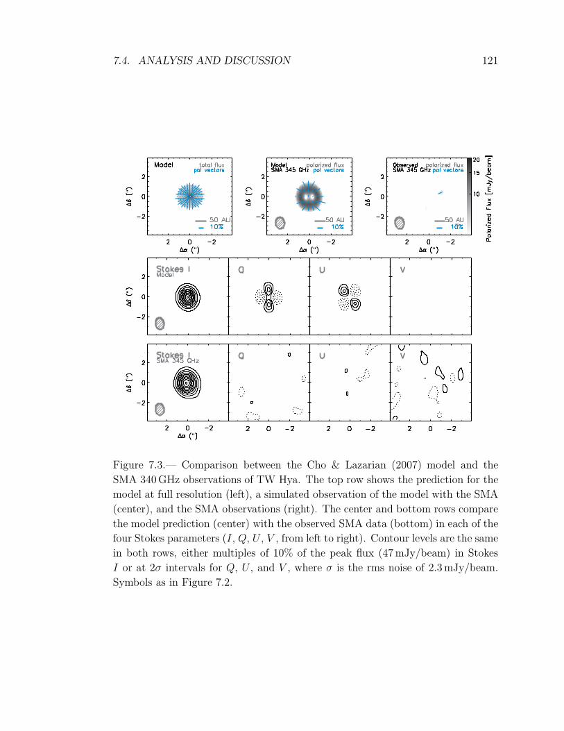
7.4. ANALYSIS AND DISCUSSION 121
Figure 7.3.— Comparison between the Cho & Lazarian (2007) model and the
SMA 340GHz observations of TW Hya. The top row shows the prediction for the
model at full resolution (left), a simulated observation of the model with the SMA
(center), and the SMA observations (right). The center and bottom rows compare
the model prediction (center) with the observed SMA data (bottom) in each of the
four Stokes parameters (I, Q, U , V , from left to right). Contour levels are the same
in both rows, either multiples of 10% of the peak flux (47mJy/beam) in Stokes
I or at 2σ intervals for Q, U , and V , where σ is the rms noise of 2.3mJy/beam.
Symbols as in Figure 7.2.
122 CHAPTER 7. POLARIZED SUBMM DISK LIMITS
polarization fraction of 2-3% should be common among protoplanetary disks. The
stringent limit on the polarization fraction, when investigated within the context
of the Cho & Lazarian (2007) model, can provide clues to the physical conditions
within the disk that may be responsible for the suppression of polarized emission
relative to the fiducial model prediction. We therefore use the code described
in Cho & Lazarian (2007) to generate models of the emission predicted for the
TW Hya and HD 163296 disks, using available observational constraints on the
disk properties as inputs, and compare these predictions to the upper limits from
the SMA observations (Section 7.4.1). We then identify parameters that are not
well constrained by existing observations, and which have the greatest effect on
the polarized emission rather than unpolarized Stokes I emission. We vary these
parameters and investigate their effects on the predicted polarized submillimeter
emission. We infer the range of values over which the predictions are consistent
with the observations as well as the interactions between parameters in the
context of the models (Section 7.4.2). Finally, we investigate other effects not
implemented in these models that may contribute to the suppression of polarized
disk emission, and estimate the magnitude of their contribution (Section 7.4.3).
7.4.1 Initial Models
The Cho & Lazarian (2007) predictions employ a two-layered Chiang et al.
(2001) model of the density and temperature structure of a protoplanetary disk,
including a surface layer with hot, small dust grains and an interior with cooler,
larger grains. Within this model, the elongated dust grains are allowed to align
via the radiative torque mechanism with a perfectly toroidal magnetic field
threading the disk. The dust grains are assigned a size distribution described by a
power law dN ∝ r−qgraindr where N is the number of grains of size r, and qgrain is
initially taken to be 3.5 (Mathis et al. 1977). The grains are also assigned a degree
of elongation given by the ratio of long-to-short axis cross sections, C⊥/C‖, where
C⊥ and C‖ are the polarization cross sections for the electric field perpendicular
and parallel to the grain symmetry axis, respectively. The grain size is defined
as r, such that C⊥ = (1 + α)πr2 and C‖ = (1 − α)πr2, where α parameterizes
the degree of elongation. The ratio of the major and minor axes of the grain are
then given by a/b =√
(1 + α)/(1 − α). The grain shape is assumed to be oblate
as in Cho & Lazarian (2007), consistent with observational evidence described in
Hildebrand & Dragovan (1995). The initial 2-3% polarization estimates are based
on the parameters for the “typical” T Tauri disk investigated in Chiang et al.
(2001).

7.4. ANALYSIS AND DISCUSSION 123
In order to generate a model prediction that can be compared with the
upper limits from the SMA observations, we adjust these parameters to reflect
the best available information about the grain properties and density structures
in the disks around HD 163296 and TW Hya. The initial model inputs, with
references, are summarized in Table 7.2. We use temperature and surface density
power law indices and outer radii derived from previous SMA 345GHz continuum
observations (Hughes et al. 2008b). The temperatures are calculated from the
stellar temperature and gas and dust densities and opacities as in Chiang et al.
(2001), while the surface density is adjusted to best reproduce the observed
880µm continuum flux. The temperatures and surface densities calculated
here are consistent with previously determined values (e.g. Isella et al. 2007;
Hughes et al. 2008b) to within a factor of two. Variations can be attributed to
differences in the vertical temperature structure and dust grain opacities assumed
in the models. While these disk structure models do not precisely reproduce the
observed brightness profile, they represent a reasonable approximation within
which the parameters determining the polarization properties of interest can be
investigated.
We use the model routines to generate 400×600 pixel sky-projected images
(i.e. with 6- and 8-milliarcsecond pixels for TW Hya and HD 163296, respectively,
significantly more finely spatially sampled than the data) giving the total
continuum flux, percent polarization, and orientation of polarized emission at
each position across the disk. The full-resolution model is shown in the upper left
panel of Figures 7.2 and 7.3, although the lines indicating orientation have been
vector-averaged in bins of several pixels for clarity of display. We then use the
MIRIAD task uvmodel to sample the image with the same spatial frequencies
as the SMA data. We invert the visibilities and image with natural weighting
to create a simulated SMA observation of the disk model, shown in the top
center panel of Figures 7.2 and 7.3. We also create simulated images in each of
the four Stokes parameters (center row), since the Stokes parameter images are
most directly comparable to the upper limits set by the observations. The model
images show the distinctive quadrupolar pattern in Stokes Q and U predicted by
the model for a toroidal magnetic field geometry, due to the radial orientation of
the polarization vectors. The intermediate inclination of HD 163296 creates an
hourglass-shaped bright region along the disk minor axis, where the synthesized
beam picks up emission from the highly polarized regions along the front and back
of the outer disk, concentrated towards the disk center by the viewing geometry.
This predicted morphology echoes the alignment of polarization vectors with the
minor axes of the disk observed by Tamura et al. (1999). With predicted peak
Stokes Q and U fluxes of 23 and 16 mJybeam−1, these initial models of polarized

124 CHAPTER 7. POLARIZED SUBMM DISK LIMITS
Table 7.2: Initial Model Parameters
HD 163296 TW Hya
Parametera Value Ref. Value Ref.
T∗ (K) 9330 1 4000 2
R∗ (R⊙) 2.1 1 1.0 2
M∗ (M⊙) 2.3 1 0.6 2
p 0.8 3 1.0 3
ainner (AU) 0.45 4 4.0 5,6
a0 (AU) 200 3 60 3
rmax,i (µm) 103 4 104 7
i 46 4 7 8
d (pc) 122 1 51 9,10
Σ0 (g cm−2) 130 – 170 –
aSymbols as in Chiang et al. (2001): T∗, R∗, and M∗ are stellar temperature, radius, and mass,
respectively; p and Σ0 describe the surface density profile Σ(R) = Σ0(R/1AU)−p; a0 is the outer
disk radius; and rmax,i is the maximum dust grain size in the disk interior. Additionally, we
define ainner (disk inner radius), i (inclination), and d (distance). All parameters not listed here
are equal to the fiducial input parameters from Chiang et al. (2001).
References. — (1) van den Ancker et al. (1998b); (2) Webb et al. (1999); (3) Hughes et al.
(2008b); (4) Isella et al. (2007); (5) Calvet et al. (2002); (6) Hughes et al. (2007); (7) Wilner
et al. (2005); (8) Qi et al. (2004); (9) Mamajek (2005); (10) Hoff et al. (1998)
emission are ruled out at the 10σ and 7σ level for HD 163296 and TW Hya,
respectively, by the SMA upper limits.
7.4.2 Parameter Exploration
With the fiducial model prediction ruled out at high confidence, we turn to
an exploration of the input parameter space to provide information about the
conditions in the disk that might be responsible for the suppression of polarized
emission. We first identify several parameters that most strongly affect the
polarization properties of the disk, without significant impact on the Stokes I
emission. In the Cho & Lazarian (2007) model, the radiative torque mechanism
that spins up elongated dust grains along magnetic field lines is impeded primarily
by gas drag in regions of high density. Since we normalize the surface density to

7.4. ANALYSIS AND DISCUSSION 125
reproduce the 880µm flux (for the assumed opacities and derived temperatures),
we cannot vary this quantity. However, the degree of elongation of the dust
grains, the threshold set within the model for grain alignment, and the dust grain
size distribution are all important factors that affect the polarization properties
of the disk rather than the Stokes I emission. These parameters are discussed in
greater detail in the following sections.
Grain Elongation
The elongation of the dust grains is important both for the radiative torque and
because the differing cross-sections parallel and perpendicular to the magnetic field
allow the grain to emit polarized continuum emission at millimeter wavelengths.
The fiducial model assumes a long-to-short axis cross-section ratio C⊥/C‖ = 2.1,
corresponding to an axial ratio of 1.5:1 for oblate dust grains (for the relationship
between cross section and axial ratios for different grain geometries, see e.g.
Padoan et al. 2001). Varying this ratio determines the radial extent of the disk
over which the dust grains are aligned with the magnetic field, as well as how
much polarized light is emitted from the disk: it effectively changes the efficiency
of grain alignment and the emission cross-section of the grains.
In order to obtain a quantitative description of the effect of grain elongation
on the predicted intensity of polarized emission from the disk, we generate a
series of models with different cross section ratios as described in Cho & Lazarian
(2007) with initial parameters listed in Table 7.2. We then sample the model
images with the SMA spatial frequencies, as described in Section 7.4.1 above, and
compare the peak flux in Stokes Q and U with the 3σ upper limit from the SMA
observations. Figure 7.4 plots the peak flux in the Stokes Q and U model images
as a function of the dust grain cross section ratio. For comparison, the shaded
area marks the region of parameter space consistent with the 3σ upper limits
from the SMA observations. The series of panels across the top of the plot show
the model images in Stokes Q and U , sampled with the SMA spatial frequencies,
for three representative values of the dust grain cross section ratio. From these
maps, it is clear that the dust grain elongation acts primarily as a scaling factor
for observations at this resolution: the emission morphology does not change,
but simply becomes stronger or weaker as the dust grains become more or less
elongated. From the HD 163296 plot on the left and the TW Hya plot on the
right, we can see that if the dust grain elongation were the only factor suppressing
polarized emission from the disk, the grains would have to be quite round, with
C⊥/C‖ . 1.2 − 1.3.
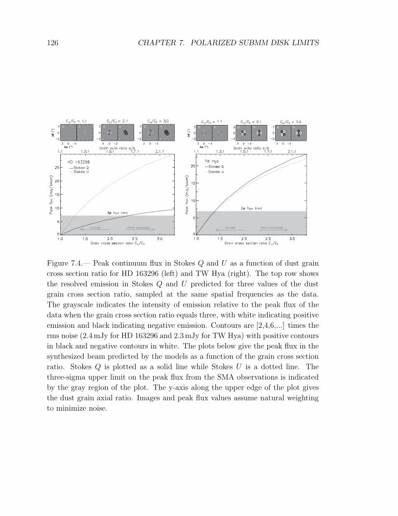
126 CHAPTER 7. POLARIZED SUBMM DISK LIMITS
Figure 7.4.— Peak continuum flux in Stokes Q and U as a function of dust grain
cross section ratio for HD 163296 (left) and TW Hya (right). The top row shows
the resolved emission in Stokes Q and U predicted for three values of the dust
grain cross section ratio, sampled at the same spatial frequencies as the data.
The grayscale indicates the intensity of emission relative to the peak flux of the
data when the grain cross section ratio equals three, with white indicating positive
emission and black indicating negative emission. Contours are [2,4,6,...] times the
rms noise (2.4mJy for HD 163296 and 2.3mJy for TW Hya) with positive contours
in black and negative contours in white. The plots below give the peak flux in the
synthesized beam predicted by the models as a function of the grain cross section
ratio. Stokes Q is plotted as a solid line while Stokes U is a dotted line. The
three-sigma upper limit on the peak flux from the SMA observations is indicated
by the gray region of the plot. The y-axis along the upper edge of the plot gives
the dust grain axial ratio. Images and peak flux values assume natural weighting
to minimize noise.

7.4. ANALYSIS AND DISCUSSION 127
Grain Alignment Criterion
Another model input that is important for the polarization properties of the disk
is the value at which the threshold for grain alignment via the radiative torque is
set. In order to determine whether or not the dust grains are aligned with the
magnetic field in a particular region of the disk, a comparison is made between
the rotational kinetic energy imparted by the radiative torque and that imparted
by random collisions with gas particles in the disk. A useful parameterization
is (ωrad/ωth)2, where ωrad and ωth are the angular velocities of the grains due to
radiative torques and thermal collisions, respectively. The radiative torques act to
align grains with the magnetic field, while gas drag inhibits alignment and causes
grains to point in random directions: the ratio (ωrad/ωth)2 therefore serves as a
measurement of the effectiveness of the radiative torque in aligning the grains
with the magnetic field. This ratio will generally be highest, and the grains most
aligned, in the outer disk where the gas density is low. We therefore expect grains
to be aligned in the outer disk, and oriented randomly in the inner disk. Since the
value of (ωrad/ωth)2 varies with radial distance from the star, the chosen threshold
value for alignment effectively varies the radius at which grains become aligned
with the disk magnetic field. The threshold is initially set so that grains are
assumed to be aligned in regions of the disk where the kinetic energy imparted by
the radiative torque is 103 times greater than that imparted by thermal collisions.
We vary this threshold in order to study its effects on the polarization properties
of the disk.
Figure 7.5 shows the peak flux predicted for Stokes Q and U as a function
of the grain alignment threshold (ωrad/ωth)2, compared with the 3σ upper limit
from the SMA observations for HD 163296 (left) and TW Hya (right). It is clear
that for both disks, the threshold would have to be set many orders of magnitude
higher than the conservative initial value in order for the alignment to be weak
enough to account for the lack of a polarization signal. Indeed, in order for this to
be the primary mechanism suppressing the disk polarization, the threshold would
need to be raised until alignment is permitted to occur only when the rotational
kinetic energy imparted by the radiative torque is at least 5-7 orders of magnitude
greater than that of gas grain collisions. This is most likely an unrealistically
stringent constraint.
It should be noted here that the approach to alignment in Cho & Lazarian
(2007) requires revisions to account for recent advances in the quantitative
theory of grain alignment. First of all, in the calculations of the ratio (ωrad/ωth),
the simplifying assumption is made that the radiation seen by each grain is
128 CHAPTER 7. POLARIZED SUBMM DISK LIMITS
coming from a point source. In fact, the bulk of the radiation field originates
as reprocessed starlight from neighboring regions of the disk, so although there
should be an overall radial gradient, it is better approximated by multipoles
rather than a purely unidirectional signal. When the effects of this radiation
structure are accounted for, the ratio (ωrad/ωth) can decrease by up to a factor
of 10 (Hoang & Lazarian 2009, Figure 17). An additional decrease by another
factor of ∼10 may come from the fact that the overall direction of anisotropy
is perpendicular to the assumed toroidal magnetic field in the disk (Hoang &
Lazarian 2009, Figure 17). This effect may be mitigated somewhat in a clumpy
disk, where local anisotropies will not necessarily be radially oriented and may
even be aligned with the magnetic field. Taking both effects into account and
squaring the ratio demonstrates that the kinetic energy of the grains in their
maximal state of rotation may be up to 4 orders of magnitude less than is
assumed using ad hoc assumptions in the spirit of the old understanding of
radiative torque alignment. An additional decrease comes from the fact that an
appreciable portion of grains may be aligned in the so-called “zero-J” alignment
point (Lazarian & Hoang 2007). Grains in this point are not perfectly aligned as
assumed in Cho & Lazarian (2007), but instead will wobble, reducing the degree
of alignment to only ∼20% (see Hoang & Lazarian 2008). In addition, while
interstellar grains are always aligned with long axes perpendicular to magnetic
field, larger grains in circumstellar disks may not have efficient internal relaxation
and can be occasionally aligned with long axes parallel to magnetic field (Hoang
& Lazarian 2009). These factors can significantly decrease the observed degree
of polarization expected from the circumstellar disks compared to the Cho &
Lazarian (2007) estimate, making the predictions roughly comparable (to within
an order of magnitude or so) to the SMA upper limits.
Grain Size Distribution
Cho & Lazarian (2007) emphasize the importance of the grain size distribution in
determining the observed polarization properties of circumstellar disks. We fix the
minimum grain size at rmin = 0.01µm as in Cho & Lazarian (2007) and Chiang
et al. (2001). Although growth to larger sizes may have occurred, the minimum
grain size affects the millimeter-wavelength polarization properties in the context
of the model only through the normalization of the total mass: increasing the
minimum grain size to 1µm (required to reproduce the 10µm silicate feature
from the inner disk; see e.g. Calvet et al. 2002) changes the predicted polarization
by less than 0.1%, since it does not bring the density above the threshold value
necessary to suppress grain alignment in the outer disk. Two aspects of the grain

7.4. ANALYSIS AND DISCUSSION 129
Figure 7.5.— Peak continuum flux in Stokes Q and U as a function of the threshold
for grain alignment (see Section 7.4.2 in the text) for HD 163296 (left) and TW Hya
(right). The top row shows the resolved emission in Stokes Q and U predicted for
three values of the alignment threshold, sampled at the same spatial frequencies
as the data. The grayscale indicates the intensity of emission relative to the peak
flux of the data when the alignment threshold equals 103, with white indicating
positive emission and black indicating negative emission. Contours are [2,4,6,...]
times the rms noise (2.4mJy for HD 163296 and 2.3mJy for TW Hya) with positive
contours in black and negative contours in white. The plots below give the peak
flux in the synthesized beam predicted by the models as a function of the alignment
threshold. Stokes Q is plotted as a solid line while Stokes U is a dotted line. The
three-sigma upper limit on the peak flux from the SMA observations is indicated
by the gray region of the plot. The y-axis along the upper edge of the plot gives
the dust grain axial ratio. Images and peak flux values assume natural weighting
to minimize noise.

130 CHAPTER 7. POLARIZED SUBMM DISK LIMITS
size distribution that can be varied in the context of the model are the maximum
grain size rmax and the power law index qgrain, where the grain size number density
goes as dN ∝ r−qgrainda.
Observational evidence points to grain growth up to at least 1mm in the
HD 163296 disk (Isella et al. 2007) and 1 cm in the TW Hya disk (Wilner et al.
2005), without ruling out the possibility that grains have grown to even larger
sizes (perhaps even planetary dimensions in the case of TW Hya; see Calvet
et al. 2002; Hughes et al. 2007). Since the surface density is chosen to maintain
consistency with the observed 880µm flux in Stokes I, the number density
of particles with sizes near 880µm, which dominate the 880µm flux, remains
roughly constant regardless of the maximum grain size in the distribution. Thus
the effect of raising the maximum grain size in the distribution is primarily to
introduce “invisible” grains at sizes larger than 1mm or 1 cm, which has no effect
on the observable polarization properties (cf. Figure 7 in Cho & Lazarian 2007).
However, adding mass at the large-grain end of the size distribution while keeping
constant the mass in small grains has the effect of raising the total surface density
of the disk. This is unrealistic for all but a small increase in maximum grain
size, as the disk quickly becomes Toomre unstable and gravitational collapse or
deviations from Keplerian rotation should rapidly become observable. While this
is most likely an artifact of the assumed grain size distribution, it suggests that
within the context of the model, grain growth is unlikely to be the mechanism
suppressing the emission of polarized radiation.
The power law index qgrain controlling the relative population of large and
small grains in the disk is somewhat more promising. In general, the polarized
emission observed at a particular wavelength will tend to originate primarily
from dust grains smaller than the wavelength, while the unpolarized emission
will be dominated by grains of roughly the same size as the wavelength. Because
dust grains of size ∼880µm are within the geometric optics regime (2πr/λ > 1,
where λ is the wavelength of observation, 880µm), they do not contribute to
the polarized emission predicted by the models. Most of the Stokes Q and U
emission at these wavelengths originates from dust grains with sizes less than
λ/2π ≈ 100µm (Cho & Lazarian 2007), while most of the Stokes I emission
originates from grains with sizes similar to the wavelength of observation. The
relative number of 100 and 880µm grains in the disk, determined by qgrain,
therefore plays a role in determining the amount of polarized emission observed.
However, since the differences in grain sizes is not large, the power law index
must change substantially before the effect on the polarization properties becomes
appreciable. Varying qgrain from 3.5 to 2 changes the peak linearly polarized flux

7.4. ANALYSIS AND DISCUSSION 131
in the model by only 20%. Therefore, when comparing the SMA limits with the
model predictions, the dust grain size distribution has relatively little impact on
the predicted polarization properties of the disks.
Interactions Between the Parameters
The analysis so far has explored individual model parameters as though they were
fully independent, determining the range of values permitted by the SMA upper
limit for each parameter separately. However, it is useful to understand how the
parameters relate to one another in determining the polarization properties of the
disk. Here we investigate relationships between pairs of the parameters considered
above.
We first study the relationship between dust grain elongation and the grain
alignment threshold. As discussed in §2.3 of Cho & Lazarian (2007), the rotation
rate of dust grains due to the radiative torque is a function of the peak wavelength
of the radiation field and the dust grain size, with no explicit dependence on
grain axial ratio. As described in Dolginov & Mitrofanov (1976), spin-up by the
radiative torque mechanism is caused by the irregular shape of the grain, which
gives it differing cross sections to left and right circular polarization; elongation
does not necessarily favor either polarization basis. This is reflected in the table
of timescales relevant for grain alignment in Lazarian (2007): neither the radiative
precession time nor the gas damping time depends on the grain axial ratio. The
primary effect of the grain elongation in alignment is to decrease the Larmor
precession time, which causes the spinning grains to align their major axes more
quickly with the magnetic field lines (or, alternatively, decreases the critical
magnetic field strength in a given region of the disk; see Section 7.4.3 below).
We therefore do not expect much, if any, dependence between these variables. In
order to test this expectation, we vary the dust grain cross section ratio and the
grain alignment threshold for the HD 163296 disk. The model prediction of peak
flux in Stokes U (which provides the most stringent limits when compared to the
SMA data) are shown in Figure 7.6. The shaded gray region of the plot represents
the parameter space within which the model prediction is less than the 3σ upper
limit given by the SMA data, i.e., combinations of parameters consistent with the
observational results. The contours show the predicted peak flux of the model
in Stokes U for each combination of parameters: model predictions with greater
polarized intensity are more strongly inconsistent with the observational limits.
Because of the assumption in the models that grains meeting the alignment
criterion will become aligned with 100% efficiency, grain alignment and elongation
132 CHAPTER 7. POLARIZED SUBMM DISK LIMITS
are evidently only weakly coupled.
Another potentially important relationship is that between the grain size
distribution and grain elongation. Little is known about the relationship between
these variables, since both are notoriously difficult to constrain observationally.
Nevertheless, if grains grow simply by accumulating material evenly over their
surface then they may naturally become more spherical as they become larger.
Spherical grains emit less strongly polarized radiation than more elongated
grains, so it might be expected that grain growth can suppress the emission of
polarized light, even in cases where the alignment mechanisms are quite efficient
(as expected for large grains, e.g. Cho & Lazarian 2005). Indeed, a corresponding
inverse relationship between grain size and polarization fraction has been observed
in molecular clouds (e.g. Vrba et al. 1993). Given the observed growth to
millimeter and even centimeter sizes within the disks around HD 163296 and
TW Hya (Isella et al. 2007; Wilner et al. 2005), and the large (∼100µm) sizes of
the grains responsible for emitting most of the polarized radiation (see Section
7.4.2), it is perhaps plausible that the grains in these disks should have cross
section ratios consistent with the values of 1.2-1.3 constrained in Section 7.4.2
above. We know that this cannot be true everywhere in the interstellar medium
(ISM): polarization at 850µm is observed in star-forming regions at much earlier
stages (e.g. Girart et al. 2006), and far-infrared polarimetry indicates that grains
with axial ratios a/b between 1.1-3 are common at sizes of tens of microns in
molecular clouds (Hildebrand & Dragovan 1995). However, a tendency towards
spherical grains in T Tauri disks, even just at the low end of the distribution
inferred by Hildebrand & Dragovan (1995), should be able to suppress the
emission of polarized radiation from the disk enough to bring the models within
range of the observational constraints.
We can test the plausibility of this degree of elongation by modifying the
discussion of grain growth based on turbulent coagulation in Vrba et al. (1993).
If we assume that the grains in T Tauri disks originate exclusively from small,
highly elongated grains in the ISM, e.g. with initial major axis ai = 0.1µm and
axial ratio ai/bi = 2 (Aannestad & Purcell 1973; Hildebrand & Dragovan 1995),
then we can estimate how the axial ratio changes with grain size. Neglecting
asymmetric effects like collisional destruction, grain size might be expected to
grow roughly evenly in all directions with the number of grain-grain collisions,
N , in such a way that the final grain size is simply af = aiN1/3. The change in
any dimension of the grain, δ, is then given by δ = aiN1/3 − ai, yielding a final
minor axis size of bf = bi + δ, or af/bf = af/(af − ai + bi). If ai = 0.1µm and af= 100µm, then af/bf = 1.001, significantly more round than the upper limit set

7.4. ANALYSIS AND DISCUSSION 133
Figure 7.6.— Detectability of Stokes U continuum emission from the HD 163296
disk as a function of the dust grain cross section ratio (Section 7.4.2) and the
threshold for dust grain alignment (Section 7.4.2). The gray regions of the plot
represent portions of the parameter space that would be undetectable given the 3σ
upper limit from the SMA observations, while contours show the peak flux of the
model for each set of parameters, beginning at the 3σ level (7.2mJy) and increasing
by intervals of 2σ (4.8mJy). The two parameters are only weakly degenerate.
by the SMA data. The timescale needed for grain growth to these (up to meter)
sizes is of order 105 years at a distance of 50AU from the central star (see e.g.
Weidenschilling 1988; Dullemond & Dominik 2005). This calculation is highly
simplified and neglects complications like the evolution of conditions within the
disk, shaping by grain-grain collisions (e.g. Dullemond & Dominik 2005), and
the complexity of the grain size distribution. Yet the extremely spherical grains
produced on relatively short timescales in this oversimplified scenario represent
a lower limit to the grain elongation that perhaps suggests a scenario by which
grains might have grown into shapes that are nearly spherical enough (with
axial ratios of 1.2 rather than 1.001) to plausibly account for the suppression of
polarized emission.

134 CHAPTER 7. POLARIZED SUBMM DISK LIMITS
7.4.3 Other Effects
In the previous section, we investigated the effects of those parameters considered
in the Cho & Lazarian (2007) model. However, there are additional effects that
may also play a role in suppressing polarized emission from the disk relative to
the fiducial 2-3% prediction. Among these are the magnetic field strength, the
geometric regularity of the magnetic field, and polarization due to scattering.
Magnetic Field Strength
The magnetic field strength plays a role in determining whether or not grains
can become aligned via the radiative torque. If the magnetic field is above some
critical strength, grains will become aligned provided that the radiative torque can
generate more rotational kinetic energy than thermal collisions. At low magnetic
field strengths, grains are not expected to align with the magnetic field at all. The
critical magnetic field strength for alignment may be estimated by comparing the
Larmor precession time tL with the gas damping time tgas. Following Lazarian
(2007) and using fiducial values for the magnetic susceptibility and dust grain
density, alignment is possible when tL < tgas, or:
B > 4.1 × 10⁻⁵ rnTdT1/2g
s2(7.1)
where B is the magnetic field strength in units of µG, r is the grain size in cm,
n is the gas density in units of cm−3, Td is the dust temperature in K, Tg is the
gas temperature in units of K, and s is the ratio of minor to major dust grain
axes. Using the power law models of density and temperature derived in Hughes
et al. (2008b), it is possible to estimate these quantities for the regions of the
outer disk probed by the SMA data. Taking the values at disk radii equivalent
to the spatial resolution of the data (∼1.′′0, or 50 and 120AU for TW Hya and
HD 163296, respectively), and assuming equivalent gas and dust temperatures, we
derive densities of several times 108 cm−3 and temperatures of ∼ 40 − 50K. For
the 10-100µm grains contributing most of the polarized emission in the models,
the critical magnetic field strength is of order 10-100mG.
This strength matches reasonably well with theoretical expectations. Shu
et al. (2007) developed a model of steady-state magnetized accretion disks that
predict magnetic field strengths of order 10-100mG on the spatial scales probed
by the data. Wardle (2007) pointed out that Zeeman splitting of OH in molecular
cloud cores and masers in star forming regions place a lower limit of ∼10mG on
the magnetic field strength, which will likely be amplified by compression and

7.4. ANALYSIS AND DISCUSSION 135
shear during the process of collapse that forms the central star and disk. It should
also be noted that the value quoted above should be taken as a lower limit, since
superparamagnetic inclusions would significantly decrease the required magnetic
field strength for alignment (Lazarian & Hoang 2008). The critical magnetic field
strength required to align grains within the conditions of the model is therefore
reasonable compared to theoretical expectations. We do not expect that the lack
of polarized emission is due to extremely low magnetic field strengths.
Geometric Regularity of the Magnetic Field
The assumption that the field is toroidal arises from the supposition that the
rotational motion of the disk has affected the magnetic field geometry. Yet for
this to occur, the ionization fraction must be large enough that disk material and
magnetic fields can interact. However, this also implies that turbulent motions
within the disk (perhaps even of magnetic origin) may tangle the magnetic fields
locally, adding a random component to the ordered toroidal magnetic field.
It is extremely difficult to estimate the magnitude of such an effect without
knowing both the ionization fraction and the magnitude of turbulence as a
function of position in the disk. Lee & Draine (1985) discuss the effect of a
random magnetic field component on the strength of the observed polarization
signature, and note that the strength of polarized emission will be reduced by a
factor F = 3/2(〈cos2 θ〉 − 1/3), where θ is the angle between the local magnetic
field and the direction of the ordered global magnetic field. This quantity varies
from one (perfectly ordered field; 〈cos2 θ〉 = 1) to zero (perfectly random field;
〈cos2 θ〉 = 1/3), but the exact value depends on the details of the local magnetic
field geometry. If magnetic field tangling were the sole factor responsible for the
difference between the fiducial modeling prediction and the SMA upper limits,
we would constrain F to be less than ∼ 0.1 for the case of HD 163296, implying
〈cos2 θ〉 < 0.4, which indicates an almost completely random magnetic field
structure.
It should also be noted that grain alignment efficiency would play a similar
role, quantified in exactly the same way as F above, with θ indicating the angle
between the long axis of the grain rather than the angle between the local and
global magnetic fields (Greenberg 1968; Lee & Draine 1985). The Cho & Lazarian
(2007) code assumes 100% efficient alignment in regions that meet the grain
alignment criterion (Section 7.4.2). In order to account fully for the suppression
of polarized emission relative to the fiducial model, the alignment efficiency would
have to be quite low, less than 10% in the case of HD 163296.

136 CHAPTER 7. POLARIZED SUBMM DISK LIMITS
The tentative single-dish detections appear to indicate a toroidal magnetic
field geometry for the disks around DG Tau and GM Aur, consistent with
observations indicating a dominant toroidal component to the magnetic field in
the flattened structures around YSOs at earlier evolutionary stages (see Wright
2007, and references therein). However, it is also possible that the field could be
poloidal: as discussed e.g. in Shu et al. (2007), a magnetic field gathered from the
interstellar medium that threads vertically through the disk might be expected to
remain poloidal in geometry as it interacts with disk material. While the SMA
limits are unable to constrain the magnetic field geometry, a poloidal geometry
might be expected to reduce the expected polarization signature particularly for
the case of a face-on viewing geometry as in the case of the TW Hya disk. The
effects of a poloidal geometry for a disk viewed at intermediate inclination, like
HD 163296, are less clear and are not investigated in the context of the Cho &
Lazarian (2007) models, although it is plausible that the strength of polarized
emission from a toroidal or poloidal field would be comparable.
Scattering
Cho & Lazarian (2007) argue that scattering contributes significantly less than
thermal emission to the polarized flux at millimeter wavelengths in the disk. In
order to estimate the relative contribution of scattering and emission at a range
of radii throughout the disk, they compare the product Jλκscatt, where Jλ is the
mean radiation field and κscatt is the mass scattering coefficient, to the product
Bλκabs, where Bλ is the intensity of blackbody radiation in the region of interest
and κabs is the mass absorption coefficient. They show that in the outer disk,
where R & 10AU, the ratio of these products falls below one (and ultimately
below 0.5), indicating that emission is dominant over scattering in the outer disk.
It is of interest, however, that pure scattering of light from a central
source off of large grains in the outer disk should produce a polarization signal
precisely orthogonal to that expected for elongated grains aligned with a toroidal
magnetic field. While the radiation field at 850µm is dominated by the local
conditions rather than a central source, as discussed in Section 7.4.2 there will
be an overall radially anisotropic component of the radiation field that might be
expected to produce a weaker, but still orthogonal on average, scattering signal.
The contribution from scattering would therefore generally act to cancel the
expected polarization signal from emission. An estimate of the magnitude of the
scattered light signal compared with the predicted strength of polarized emission
is beyond the scope of this paper, but we note that for scattering to be the

7.5. SUMMARY AND CONCLUSIONS 137
dominant mechanism suppressing the expected polarization signal, the intensity of
polarized emission arising from scattering and emission would have to be precisely
equivalent, to within 10-15%, in both disks. Furthermore, since the scattering
and emission have different wavelength dependences, the coincidental canceling
of the emission signal would only occur at the wavelength of observation. In the
absence of any expectation that these quantities should be related, this seems an
unlikely coincidence.
7.5 Summary and Conclusions
Despite the expectation of a 2-3% polarization fraction in circumstellar disks
based on previous observational and theoretical work (Tamura et al. 1999; Cho
& Lazarian 2007), the SMA polarimeter observations presented here show no
polarization from the disks around two nearby stars. With these observations
we place a 3σ upper limit on the integrated polarization fraction of less than
1% and rule out the fiducial Cho & Lazarian (2007) models at the ∼10σ
level. These represent the most stringent limits to date on the magnitude of
submillimeter polarized emission from circumstellar disks. We are therefore left
with the question of which model assumptions are unrealistic enough to account
for an approximately order-of-magnitude (at minimum) overprediction of the
polarization signal from these disks.
Among the model parameters and additional effects considered in Section 7.4,
several seem unlikely as the source of the suppression of polarized emission.
The critical magnetic field strength expected for alignment seems reasonable
relative to theoretical expectations and observations. An almost completely
random magnetic field with no dominant toroidal (or poloidal) component would
also be surprising, although a poloidal field geometry would be expected to
significantly weaken the polarized emission arising from a face-on disk like TW
Hya. Scattering is expected to be weak, but it should produce a polarization
signature perpendicular to that expected for emission from aligned grains.
However, scattering and emission signals would have to cancel nearly perfectly in
order to account entirely for the low observed polarization fraction. Nevertheless,
there are promising candidates to describe how the suppression of polarized
emission might have occurred. Cho & Lazarian (2007) assume 100% efficient
alignment of grains with the magnetic field in regions of the disk where the
alignment criterion is met, which is overly optimistic and now known to be
unrealistic (see discussion in Section 7.4.2). In light of the recent work on

138 CHAPTER 7. POLARIZED SUBMM DISK LIMITS
the quantitative theory of grain alignment (Lazarian & Hoang 2007; Hoang &
Lazarian 2008, 2009), the Cho & Lazarian (2007) result may be considered an
upper limit to the theoretical expectation for the polarization properties of disks.
A reduction to 10% efficiency, which is within the expectations based on recent
developments in grain alignment theory, could alone explain the low polarization
fraction observed. Another possibility is that the grains contributing most of the
polarized emission in the model are well (or not so well) aligned, but rounder
than the cross section ratio assumed in the initial model and therefore inefficient
emitters of polarized radiation. This is also reasonable based on a rough estimate
of the timescales and shapes expected for collisional growth of elongated ISM
grains.
While each of these factors would have to be substantially different from what
is expected in the initial model to alone account for the low polarization fraction,
it is of course entirely possible that several effects are playing a combined role.
For example, grains with a cross section ratio of 1.5 instead of 2.1 could combine
with a 50% alignment efficiency to account entirely for the difference between
observations and models. A small degree of field tangling (expected because of
turbulence in the disk) could further reduce the expected polarization signature.
While we cannot constrain precisely which factors are contributing in which
proportions to the suppression of polarization in the disks observed with the SMA,
we identify these three factors (grain elongation, alignment efficiency, and field
tangling) as the most plausible sources of the suppression of polarized emission.
They produce the greatest change in polarization properties within a reasonable
range of parameter values, and there exists a theoretical justification for why they
should exist, even if the magnitude of the effect is not well constrained.
Future observations with higher sensitivity may be able to disentangle these
effects to some extent, particularly the degree of field tangling. It would also be
useful to obtain high spatial resolution observations of the disks with tentative
detections of a 2-3% polarization fractions to confirm the strength and origin
of the emission on small spatial scales, and to expand the sample size in order
to determine whether the low polarization fraction constrained by the SMA is
universal for disks around young stars. These latter points are addressed in
Appendix B, in which we present observations of the disks around GM Aur, which
has a previously reported 2.5σ detection of polarized emission, and MWC 480.
The non-detection of polarized millimeter-wavelength emission from additional
systems strengthens the conclusions of this study.

Chapter 8
Empirical Constraints on
Turbulence in Protoplanetary
Accretion Disks
A. M. Hughes, D. J. Wilner, S. M. Andrews, C. Qi, & M. R. Hogerheijde 2010
Abstract
We present arcsecond-scale Submillimeter Array observations of the CO(3-2) line
emission from the disks around the young stars HD 163296 and TW Hya at a
spectral resolution of 44m s−1. These observations probe below the ∼100m s−1
turbulent linewidth inferred from lower-resolution observations, and allow us
to place constraints on the turbulent linewidth in the disk atmospheres. We
reproduce the observed CO(3-2) emission using two physical models of disk
structure: (1) a power-law temperature distribution with a tapered density
distribution following a simple functional form for an evolving accretion disk,
and (2) the radiative transfer models developed by D’Alessio et al. (1998) that
can reproduce the dust emission probed by the spectral energy distribution.
Both types of models yield a low upper limit on the turbulent linewidth in the
TW Hya system (.40m s−1), and a tentative (3σ) detection of a ∼300m s−1
turbulent linewidth in the upper layers of the HD 163296 disk. These correspond
to roughly ≤10% and 40% of the sound speed at size scales commensurate with
the resolution of the data. The derived linewidths imply a turbulent viscosity
coefficient, α, of order 10−2 and provide observational support for theoretical
139
140 CHAPTER 8. CIRCUMSTELLAR DISK TURBULENCE
predictions of subsonic turbulence in protoplanetary accretion disks.
8.1 Introduction
The circumstellar accretion disks around young stars provide the raw material
and physical conditions for the planet formation process. The viscous transport of
angular momentum drives the evolution of the protoplanetary disks around young
stars (Lynden-Bell & Pringle 1974; Hartmann et al. 1998), determining when,
where, and how much material is available for planet formation. Understanding
the physical mechanisms behind the viscous transport process is therefore central
to constraining planet formation theory. The source of viscosity is uncertain, since
molecular viscosity implies a disk evolution timescale far longer than the observed
1-10Myr. The classic result from Shakura & Syunyaev (1973) demonstrates that
turbulence can provide viscosities large enough to account for disk evolution
on the appropriate timescales. However, while turbulence is commonly invoked
as the source of viscosity in disks, its physical origin, magnitude, and spatial
distribution are not well constrained.
The mechanism most commonly invoked as the source of this turbulence in
disks around young stars is the magnetorotational instability (MRI), in which
magnetic interactions between fluid elements in the disk couple with an outwardly
decreasing velocity field to produce torques that transfer angular momentum from
the inner disk outward (Balbus & Hawley 1991, 1998). Models of disk structure
indicate that the conditions for the MRI are likely satisfied over much of the
extent of a typical circumstellar disk, with the possible exception of an annular
dead zone (Gammie & Johnson 2005, and references therein). MRI turbulence has
also been invoked to address a wide array of problems in planet formation theory.
For example, it has been proposed to regulate the settling of dust particles (e.g.,
Ciesla 2007), to explain mixing in meteoritic composition (e.g., Boss 2004), to
form planetesimals (e.g., Johansen et al. 2007), and to slow planet migration (e.g.,
Nelson & Papaloizou 2003). Measurements that constrain the magnitude and
physical origin of disk turbulence therefore promise to provide important insight
into the physics of planet formation on a variety of physical and temporal scales.
The only directly observable manifestation of turbulence is the non-thermal
broadening of spectral lines. To date, no lines have been detected in disks that
would allow an independent determination of temperature and non-thermal
broadening, similar to NH3 in molecular cloud cores. Previous interferometric
observations of molecular line emission from several disks show gas in Keplerian

8.1. INTRODUCTION 141
rotation around the star with inferred subsonic turbulent velocity widths, close
to the scale of the spectral resolution of ∼200m s−1 (e.g. Pietu et al. 2007).
Spectroscopic observations of infrared CO overtone bandhead emission originating
from smaller disk radii indicate larger, approximately transonic, local line
broadening that may be associated with turbulence (Carr et al. 2004), although
as for CO(3-2) these observations of optically thick lines can only probe far
above the midplane. In combination with the millimeter data, this may indicate
variations of turbulent velocity with radius. However, this interpretation is
uncertain: it is important to exercise caution when deriving information about
velocity fluctuations on scales smaller than the spectral resolution of the data (as
noted by, e.g., Pietu et al. 2007). The advent of a high spectral resolution mode
of the Submillimeter Array (SMA) correlator, capable of resolving well below the
∼200m s−1 linewidths in the low-J transitions of CO derived from lower-resolution
observations, permits access to turbulent linewidth measurements in the cold,
outer regions of molecular gas disks around young stars.
In this paper, we conduct high spectral resolution (44m s−1) observations of
the CO(3-2) emission from the disks around two nearby young stars, HD 163296
and TW Hya. These systems were selected on the basis of their bright
CO(3-2) line emission (e.g. Dent et al. 2005), to ensure adequate sensitivity
for high-resolution spectroscopy. They are also particularly well-studied using
spatially-resolved observations at millimeter wavelengths, so that excellent models
of the temperature and density structure of the gas and dust disks are already
available (Calvet et al. 2002; Isella et al. 2007, 2009; Hughes et al. 2008b; Qi et al.
2004, 2006, 2008, 2010 in prep). Both exhibit CO(3-2) emission that is consistent
with Keplerian rotation about the central star, and neither suffers from significant
cloud contamination. TW Hya is a K7 star with an age of ∼10Myr (Webb et al.
1999), located at a distance of only 51 ± 4 pc (Mamajek 2005). It hosts a nearly
face-on “transition” disk, with an optically thin inner cavity of radius ∼4AU
indicated by the SED (Calvet et al. 2002) and interferometrically resolved at
wavelengths of 7mm (Hughes et al. 2007) and 10µm (Ratzka et al. 2007). The
low spectral resolution CO(3-2) line emission from the disk around TW Hya was
modeled with a 50m s−1 turbulent linewidth by (Qi et al. 2004). HD 163296 is a
Herbig Ae star with a mass of 2.3M⊙, located at a distance of 122 pc (van den
Ancker et al. 1998b). Its massive, gas-rich disk extends to at least 500AU (Grady
et al. 2000) and is viewed at an intermediate inclination angle of 45 (Isella et al.
2007).
We describe the high spectral resolution SMA observations of the CO(3-2)
line emission from TW Hya and HD 163296 in Section 8.2 and present the results

142 CHAPTER 8. CIRCUMSTELLAR DISK TURBULENCE
in Section 8.3 (with full channel maps provided in Appendix C). In Section 8.4 we
outline the widely-used procedures that we use to model the temperature, density,
and velocity structure of the disk, including the fixed parameters and assumptions
about how the turbulent linewidth is spatially distributed. Section 8.4.3 presents
the best-fit models, and a discussion of the degeneracies between parameters is
provided in Section 8.4.4. We compare our results to theoretical predictions of
the magnitude and spatial distribution of turbulence in Section 8.5, and describe
the implications for planet formation. A summary is provided in Section 8.6.
8.2 Observations
The SMA observations of TW Hya took place on 2008 March 2 in the compact
configuration, with baseline lengths of 16-77m, and on 2008 February 20 during
the move from compact to extended configuration, with baseline lengths of
16-182m. The weather was good both nights, with stable atmospheric phases.
Precipitable water vapor levels were extremely low on February 20, with 225GHz
atmospheric opacities less than 0.05 throughout the night, while the March 2
levels were somewhat higher, rising smoothly from 0.08 to 0.11. In order to
calibrate the atmospheric and instrumental gain variations, observations of TW
Hya were interleaved with the nearby quasar J1037-295. To test the efficacy of
phase transfer, observations of 3c279 were also included in the observing loop.
Flux calibration was carried out using observations of Callisto; the derived fluxes
of 3c111 were 0.76 and 0.78 Jy on February 20 and March 2, respectively.
The observations of HD 163296 were carried out in the compact-north
configuration on 2009 May 6, with baseline lengths of 16 to 139m, and in the
extended configuration on 2009 August 23, with baseline lengths of 44 to 226m.
Atmospheric phases were stable on both nights, and the 225GHz opacities were
0.05 on May 6 and 0.10 on August 23. The observing loop included 1733-130 for
gain calibration and 1924-292 for testing the phase transfer. Callisto again served
as the flux calibrator, yielding derived fluxes of 1.17 and 1.30 Jy for 1733-130 on
May 6 and August 23, respectively.
For all observations, the correlator was configured to divide a single 104MHz-
wide chunk of the correlator into 2048 channels. This high-resolution chunk was
centered on the 345.796GHz frequency of the CO(3-2) line, yielding a spectral
resolution of 44.1m s−1 across the line. Because this used up a large portion of
the available correlator capacity, only 1.3GHz of the 2GHz bandwidth in each
sideband was available for continuum observations. The bandpass response was

8.3. RESULTS 143
calibrated using extended observations of 3c273, 3c279, and Saturn for the TW
Hya tracks and 3c454.3, Callisto, and 1924-292 for the HD 163296 tracks. Since
the sidebands are separated by 10GHz and the CO(3-2) line was located in the
upper sideband for the HD 163296 observations and in the lower sideband for the
TW Hya observations, the continuum observations are at frequencies of 340GHz
for HD 163296 and 350GHz for TW Hya.
Routine calibration tasks were carried out using the MIR software
package1, and imaging and deconvolution were accomplished with MIRIAD. The
observational parameters, including the rms noise for both the line and continuum
data, are given in Table 8.1. Note that due to weather the compact observations
of HD 163296 were substantially more sensitive than the extended data and so
the combined data set is dominated by the compact data; the reverse is true for
TW Hya.
8.3 Results
We detect CO(3-2) emission at 44m s−1 resolution from both TW Hya and
HD 163296 in the compact and extended configurations. Figures 8.1 and 8.2
present the line emission from HD 163296 and TW Hya, respectively. The upper
left panel shows the full line profile summed within a 6” square box (neglecting
emission within the range ±2σ), with emission detected across ∼50 channels for
TW Hya and ∼200 for HD 163296. Beneath the line profiles are the spatially
resolved channel maps for a subset of the data, indicated by the gray box around
the line peak. In the upper right are the zeroth (contours) and first (colors)
moment maps: these are the velocity-integrated intensity and intensity-weighted
velocity of the emission, respectively. The line emission is regular, symmetric, and
consistent with material in Keplerian rotation around the central star viewed at
an inclination to our line of sight.
The peak and integrated fluxes for each of the four tracks and the combined
data sets are listed in Table 8.1. Appendix C presents the full channel maps of
the combined (compact and extended configuration) data set for each source.
Along with the high spectral resolution molecular line data, we obtained 340
and 350GHz continuum observations of HD 163296 and TW Hya, respectively.
The continuum data are of excellent quality, and the visibility profiles and images
1See http://cfa-www.harvard.edu/∼cqi/mircook.html.
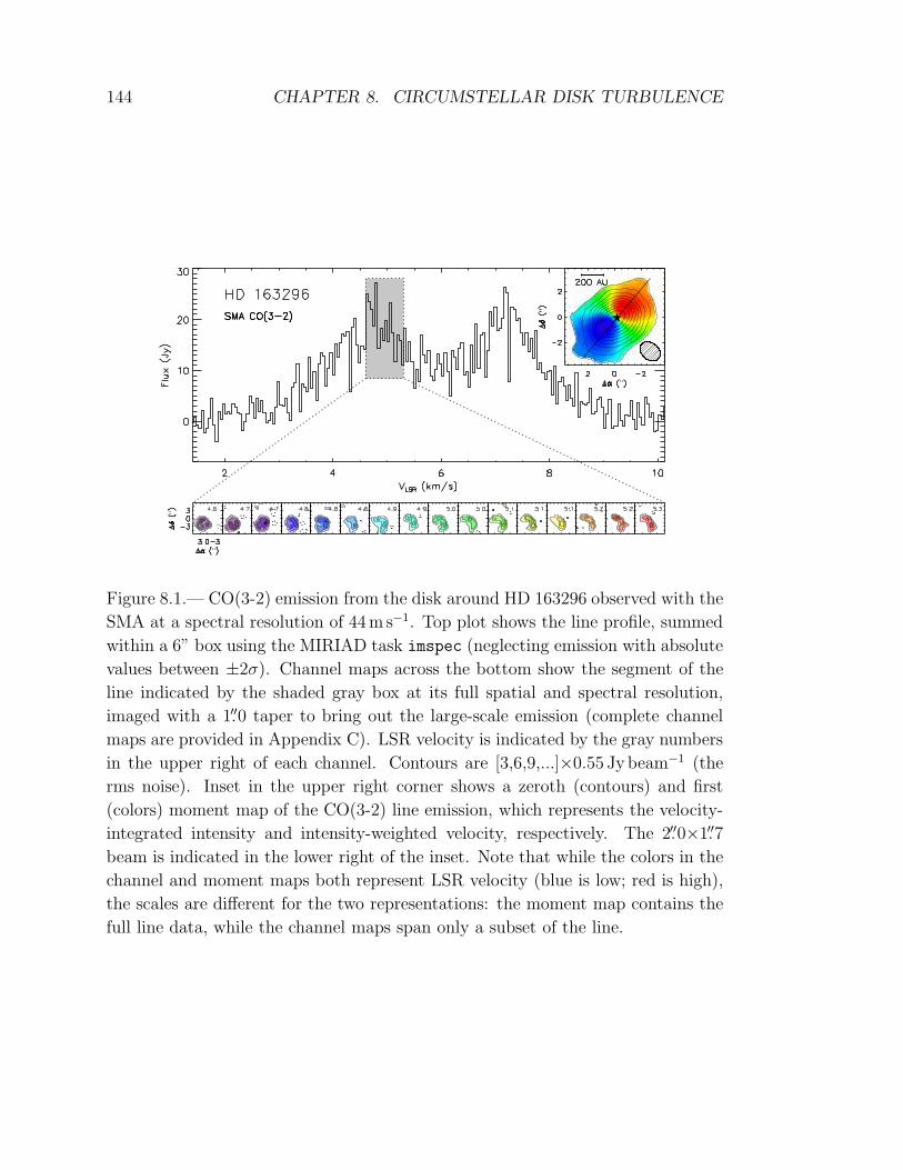
144 CHAPTER 8. CIRCUMSTELLAR DISK TURBULENCE
Figure 8.1.— CO(3-2) emission from the disk around HD 163296 observed with the
SMA at a spectral resolution of 44m s−1. Top plot shows the line profile, summed
within a 6” box using the MIRIAD task imspec (neglecting emission with absolute
values between ±2σ). Channel maps across the bottom show the segment of the
line indicated by the shaded gray box at its full spatial and spectral resolution,
imaged with a 1.′′0 taper to bring out the large-scale emission (complete channel
maps are provided in Appendix C). LSR velocity is indicated by the gray numbers
in the upper right of each channel. Contours are [3,6,9,...]×0.55 Jybeam−1 (the
rms noise). Inset in the upper right corner shows a zeroth (contours) and first
(colors) moment map of the CO(3-2) line emission, which represents the velocity-
integrated intensity and intensity-weighted velocity, respectively. The 2.′′0×1.′′7
beam is indicated in the lower right of the inset. Note that while the colors in the
channel and moment maps both represent LSR velocity (blue is low; red is high),
the scales are different for the two representations: the moment map contains the
full line data, while the channel maps span only a subset of the line.
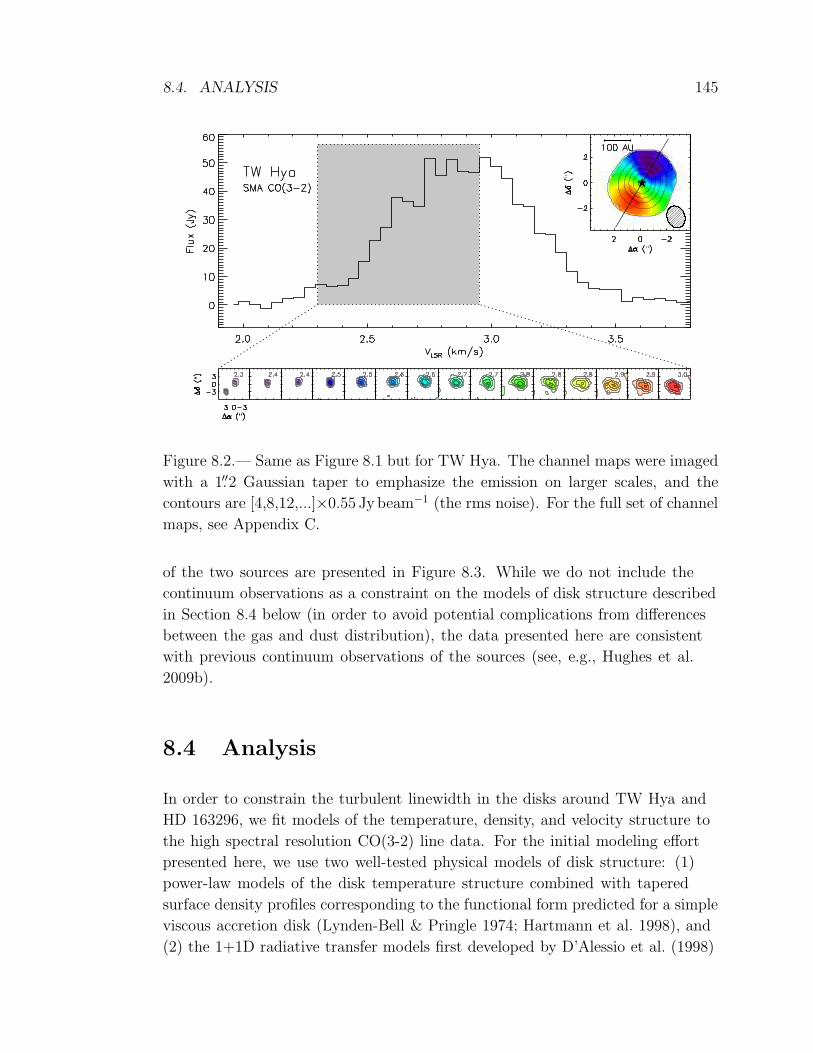
8.4. ANALYSIS 145
Figure 8.2.— Same as Figure 8.1 but for TW Hya. The channel maps were imaged
with a 1.′′2 Gaussian taper to emphasize the emission on larger scales, and the
contours are [4,8,12,...]×0.55 Jybeam−1 (the rms noise). For the full set of channel
maps, see Appendix C.
of the two sources are presented in Figure 8.3. While we do not include the
continuum observations as a constraint on the models of disk structure described
in Section 8.4 below (in order to avoid potential complications from differences
between the gas and dust distribution), the data presented here are consistent
with previous continuum observations of the sources (see, e.g., Hughes et al.
2009b).
8.4 Analysis
In order to constrain the turbulent linewidth in the disks around TW Hya and
HD 163296, we fit models of the temperature, density, and velocity structure to
the high spectral resolution CO(3-2) line data. For the initial modeling effort
presented here, we use two well-tested physical models of disk structure: (1)
power-law models of the disk temperature structure combined with tapered
surface density profiles corresponding to the functional form predicted for a simple
viscous accretion disk (Lynden-Bell & Pringle 1974; Hartmann et al. 1998), and
(2) the 1+1D radiative transfer models first developed by D’Alessio et al. (1998)
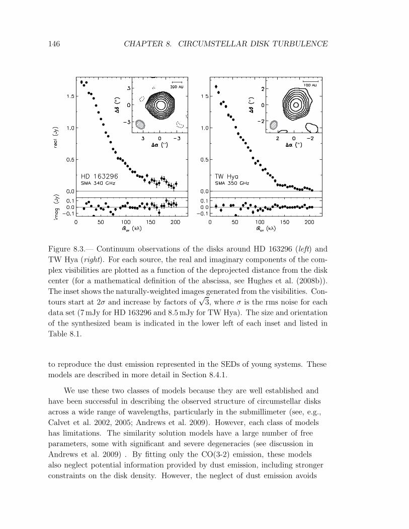
146 CHAPTER 8. CIRCUMSTELLAR DISK TURBULENCE
Figure 8.3.— Continuum observations of the disks around HD 163296 (left) and
TW Hya (right). For each source, the real and imaginary components of the com-
plex visibilities are plotted as a function of the deprojected distance from the disk
center (for a mathematical definition of the abscissa, see Hughes et al. (2008b)).
The inset shows the naturally-weighted images generated from the visibilities. Con-
tours start at 2σ and increase by factors of√
3, where σ is the rms noise for each
data set (7mJy for HD 163296 and 8.5mJy for TW Hya). The size and orientation
of the synthesized beam is indicated in the lower left of each inset and listed in
Table 8.1.
to reproduce the dust emission represented in the SEDs of young systems. These
models are described in more detail in Section 8.4.1.
We use these two classes of models because they are well established and
have been successful in describing the observed structure of circumstellar disks
across a wide range of wavelengths, particularly in the submillimeter (see, e.g.,
Calvet et al. 2002, 2005; Andrews et al. 2009). However, each class of models
has limitations. The similarity solution models have a large number of free
parameters, some with significant and severe degeneracies (see discussion in
Andrews et al. 2009) . By fitting only the CO(3-2) emission, these models
also neglect potential information provided by dust emission, including stronger
constraints on the disk density. However, the neglect of dust emission avoids

8.4. ANALYSIS 147
complications due to heating processes and chemistry that affect gas differently
than dust. The D’Alessio et al. (1998) models of dust emission include only
stellar irradiation and viscous dissipation as heating sources, and do not take into
account the additional heating processes that may affect molecular line strengths
in the upper layers of circumstellar disks (Qi et al. 2006). While the constraints
from the dust continuum reduce the number of free parameters in this class of
models, they also have the disadvantage of an unrealistic treatment of the density
structure at the disk outer edge: since they are simply truncated at a particular
outer radius, they are not capable of simultaneously reproducing the extent of gas
and dust emission in these systems (Hughes et al. 2008b).
The primary reason for using the two types of models, however, is that they
differ substantially in their treatment of the disk temperature structures. For the
D’Alessio et al. (1998) models, the temperature structure is fixed by the dust
continuum. The similarity solution models, by contrast, allow the temperature
to vary to best match the data. There are a few independent constraints on
temperature: it should increase with height above the midplane, due to surface
heating by the star and low viscous heating in the midplane, and the dust will
generally not be colder than the gas, since the gas is subject to additional heating
processes beyond the stellar irradiation that determines dust temperature. Both
classes of models adhere to these constraints. The temperature structure in the
disk is the single factor most closely tied to the derived value of the turbulent
linewidth (see discussion in Section 8.4.4), which will be model-dependent.
We therefore fit both classes of models to the data, in order to compare the
model-dependent conclusions about turbulent linewidth for two distinct classes of
models with very different treatments of gas temperature. The spatial dynamic
range of the data is insufficient to investigate radial variations in turbulent
linewidth. We therefore assume a global value, ξ, that will apply to size scales
commensurate with the spatial resolution of the data.
8.4.1 Description of Models
D’Alessio et al. (1998) Model
While we refer to these as D’Alessio et al. (1998) models for convenience, it should
be noted that they have been developed and improved upon since the original
paper in a series of related work; see also D’Alessio et al. (1999, 2001, 2006). Here
we provide a general outline of the model properties and discuss the particular
models used in this paper.

148 CHAPTER 8. CIRCUMSTELLAR DISK TURBULENCE
The D’Alessio et al. (1998) models were developed to reproduce the
unresolved SEDs arising from warm dust orbiting young stars, although they
have also been demonstrated to be successful at reproducing spatially resolved
dust continuum emission at millimeter wavelengths (see, e.g., Calvet et al. 2002;
Hughes et al. 2007, 2009a) as well as spatially-resolved molecular line emission
(see, e.g., Qi et al. 2004, 2006). The models include heating from the central
star and viscous dissipation within the disk, although they tend to be dominated
by stellar irradiation. The structure is solved iteratively to provide consistency
between the irradiation heating and the vertical structure. The mass accretion
rate is assumed to be constant throughout the disk. The assumed dust properties
are described by Calvet et al. (2002), and the model includes provisions for
changing dust properties, dust growth, and settling. We allow the outer radius of
the model to vary to best reproduce the extent of the molecular line observations.
We use the structure model for TW Hya that was developed by Calvet et al.
(2002) and successfully compared to molecular line emission by Qi et al. (2004,
2006). For HD 163296, we use a comparable model that reproduces the spatially
unresolved SED and is designed to reproduce the integrated line strengths of
several CO transitions as well as other molecules (Qi et al., in prep).
Since the D’Alessio et al. (1998) models were developed primarily to
reproduce the dust emission from the SED, we are required to fit several
parameters to match the observed CO(3-2) emission using the SED-based models.
We fit the structural parameters RD, XCO (the disk outer radius and CO
abundance, respectively), the geometrical parameters i, PA (the disk inclination
and position angle), and the turbulent linewidth, ξ.
Viscous Disk Similarity Solution Models
We also fit the observations using a power-law temperature distribution and
surface density profile that follows the class of similarity solutions for evolving
viscous accretion disks described by Lynden-Bell & Pringle (1974) and Hartmann
et al. (1998). This particular method of parameterizing circumstellar disk
structure has a long history of success in reproducing observational diagnostics,
although with limitations. Theoretical predictions of the power-law dependence of
temperature for accretion disks around young stars were first made by Adams &
Shu (1986), and power-law parameterizations of temperature and surface density
have been used by many studies since then (e.g. Beckwith et al. 1990; Beckwith
& Sargent 1991; Mundy et al. 1993; Dutrey et al. 1994; Lay et al. 1994; Andrews
& Williams 2007). The similarity solutions are equivalent to a power-law surface
8.4. ANALYSIS 149
density description in the inner disk, but with an exponentially tapered outer
edge, which was shown by Hughes et al. (2008b) to better reproduce the extent
of gas and dust emission than traditional power-law descriptions with abruptly
truncated outer edges. Recent high spatial resolution studies have used this
class of models to reproduce successfully the extent of gas and dust emission in
circumstellar disks from several nearby star-forming regions (e.g. Andrews et al.
2009; Isella et al. 2009).
The temperatures and surface densities of these models are parameterized as
follows:
T (R) = T100
(
R
100AU
)−q
(8.1)
Σ(R) =c1Rγ
exp
[
−(
R
c2
)2−γ]
(8.2)
where R is the radial distance from the star in AU, T100 is the temperature
indicated by the CO(3-2) line at 100AU from the star, q describes how the
temperature decreases with distance from the star, c1 is a constant describing the
surface density normalization, c2 is a constant related to the radial scale on which
the exponential taper decreases the disk density, and γ describes how surface
density falls with radius in the inner disk regions (comparable to the parameter p
in typical power-law descriptions of surface density; see e.g. Dutrey et al. 1994, for
a description of the power-law model parameters). Because the high optical depth
of the CO(3-2) line is a poor tracer of the radial dependence of Σ, we fix γ at a
value of 1 for both systems, which is consistent with theoretical predictions for a
constant-α accretion disk (Hartmann et al. 1998), as well as observations of young
disks in Ophiuchus (Andrews et al. 2009) and previous studies of the continuum
emission from these systems (Hughes et al. 2008b). We therefore fit the high
spectral resolution CO(3-2) observations using four structural parameters, T100,
q, c1, c2, two geometric parameters, i, PA, and the turbulent linewidth, ξ.
8.4.2 Modeling Procedure
We assume that the disks have a Keplerian velocity field, using stellar masses
and distances from the literature to model the rotation pattern (0.6M⊙ at 51 pc
for TW Hya and 2.3M⊙ at 122 pc for HD 163296; see Calvet et al. 2002; Webb
et al. 1999; Mamajek 2005; van den Ancker et al. 1998b). Gas and dust are
assumed to be well-mixed in both models; the gas-to-dust mass ratio is fixed at
100 while the CO abundance is allowed to vary in the D’Alessio et al. (1998)

150 CHAPTER 8. CIRCUMSTELLAR DISK TURBULENCE
models in order to reproduce the CO emission while maintaining consistency with
the dust continuum emission from which the model was derived. Since we don’t
include continuum emission in the fits, we fix the CO abundance at 10−4 for the
similarity solution models because there is no constraint on the relative content of
gas and dust. In regions of the disk where the temperature drops below 20K, the
CO abundance is reduced by a factor of 10−4 to simulate the effects of freeze-out
onto dust grains. We assume a global, spatially uniform value of the turbulent
linewidth, which is implemented as an addition to the thermal linewidth.
In order to compare the models with the data, the systemic velocity, or
central velocity of the line, must be determined. We calculated the visibility
phases for the spatially integrated CO(3-2) emission and fit a line to the central
few channels (45 for HD 163296; 12 for TW Hya) to determine the systemic
velocity. The visibility phases encode information about the spatial symmetry of
the line emission in each channel: for a Keplerian disk, it is most symmetric, and
therefore the phase is zero, at line center. The channel maps are most asymmetric
about disk center near the line peaks, with opposite spatial offsets at the two line
peaks. The phase therefore reverses sign between one peak and the other, with
an approximately linear relationship near the line center. The linear fit therefore
uses the integrated emission from the central few channels to pinpoint the precise
location where the phase is zero and the line is most symmetric, i.e., at the
systemic velocity (it should be noted that if there were large-scale asymmetries in
the CO data this method would not produce a reliable systemic velocity, but we
see no evidence of such asymmetries in the data). We derive a systemic velocity
of 5.79 km s−1 for HD 163296 and 2.86 km s−1 for TW Hya. In order to generate
model emission with the appropriate velocity offset, we generate a model image
at higher spectral resolution than the data, and then re-bin it at the appropriate
velocity sampling using the MIRIAD task regrid.
Each disk model specifies a particular density, temperature, and velocity
structure. We use the Monte-Carlo radiative transfer code RATRAN (Hogerheijde
& van der Tak 2000) to calculate equilibrium populations for each rotational
level of the CO molecule and generate a sky-projected image of the CO(3-2) line
emission at a given viewing geometry i,PA for each model. We compare these
simulated models directly to the data in the Fourier domain. In order to sample
the model images at the appropriate spatial frequencies for comparison with the
SMA data, we use the MIRIAD task uvmodel. We then compute the χ2 statistic
for each model compared with the data using the real and imaginary simulated
visibilities. Due to the high computational intensity of the molecular line radiative
transfer, it is prohibitively time-intensive to generate very large and well-sampled
8.4. ANALYSIS 151
grids of models for the χ2 comparison. Instead, we move from coarsely-sampled
grids that cover large regions of parameter space to progressively more refined
(but still small) grids to avoid landing at a local minimum. However, this has the
result that the degeneracies of the parameter space are poorly characterized. A
discussion of these degeneracies is included in Section 8.4.4 below.
8.4.3 Best-fit Models
The best-fit parameters for both types of models are presented in Table 8.2.
Their temperature and density structures are plotted in Figure 8.6. Note that the
midplane temperatures for the similarity solution models are likely much lower
than indicated; the power-law temperature representation parameterizes only
the radial dependence of temperature in the upper disk layers from which the
optically thick CO(3-2) emission arises.
The χ2 values for the similarity solutions are lower than for the D’Alessio
et al. (1998) models; this may be due to gradients between gas and dust properties
that influence the D’Alessio et al. (1998) model fit but not the similarity solution
models. A sample of channel maps comparing the data with the two classes of
models are presented in Figures 8.4 and 8.5. From the residuals in the D’Alessio
et al. (1998) model of TW Hya, there is evidence of a mismatch in the temperature
gradient between the model and the data: the residuals are systematically more
positive near the disk center and negative farther from the star. For HD 163296,
the difference is more subtle: the residuals are small and apparently spatially
random (with the exception of some positive emission seen near a velocity of
4.7m s−1 but not near the corresponding position in the mirror half of the line). It
should be noted that the CO abundance derived for this source is extremely low,
nearly three orders of magnitude below the standard value of 10−4. The reason
for this is most likely an overestimate of the temperature in the upper disk layers.
In the absence of better information, this SED model was created with a very low
turbulent linewidth (∼50m s−1) and correspondingly little stirring of large dust
grains above the midplane. The addition of a turbulent linewidth comparable to
the best-fit value for the CO lines would substantially reduce settling and lower
the temperature of the upper disk layers as more of the mass is placed in large
dust grains. Such a model is under development by Qi et al. (in prep), and can
also aid in explaining the spatial distribution of the DCO+ emission from this
disk.
One important outcome of the modeling process is the consistency in the
measurement of turbulent linewidth in each source for the two types of models,

152 CHAPTER 8. CIRCUMSTELLAR DISK TURBULENCE
despite the differences in their treatment of temperature. In both types of models
for HD 163296, the best-fit model with turbulence fits the data better than a
comparable model without turbulence at the ∼ 3σ level. If the turbulent linewidth
is fixed at 0m s−1 in the similarity solution and the temperature allowed to vary
to compensate, the parameter T100 must increase to 77K; even then, the χ2 for a
model with higher temperature and no turbulence is a poorer fit than the best-fit
model with turbulence at the ∼ 3σ level. The TW Hya data are consistent with
no turbulent linewidth whatsoever.
8.4.4 Parameter Degeneracies
In order to better characterize our ability to measure turbulent linewidth,
it is important to understand its relationship to the other parameters. The
interdependence between parameters other than the turbulent linewidth has been
explored at length in previous papers (see, e.g., discussion of similarity solution
parameters in Andrews et al. 2009), so here we focus on the relationships and
degeneracies specific to the turbulent linewidth. There are four main categories
of line broadening in circumstellar disks that are relevant to our investigation:
rotational, thermal, turbulent, and optical depth. These types of line broadening
are all incorporated in detail into the ray-tracing portion of the RATRAN
radiative transfer code, and will be handled appropriately for a given disk
structure. The goal is to understand how to distinguish the distinct contributions
of each of these different sources of line broadening and their relationships to the
parameters of our disk structure models.
As discussed above, a detailed characterization of the multi-dimensional
parameter space is prohibitively computationally expensive. We therefore
investigate parameter relationships in two complementary ways: (1) by generating
two-dimensional χ2 plots for pairs of variables with the other parameters fixed
at their best-fit values in order to identify strongly dependent parameters, and
(2) using a toy model of an optically thick spectral line profile to highlight the
distinct contribution of each related parameter to the observable properties.
The χ2 plots show that for the similarity solution models, the parameters
that are most strongly degenerate with the turbulent linewidth are the
temperature (T100 and q) and inclination (i). This is unsurprising, given
the obvious relationship between temperature and thermal broadening and
between inclination and rotational broadening. The optically thick CO(3-2) line
responds only weakly to variations in density, and the outer radius and position
angle of emission should intuitively be unrelated to line broadening, hence the
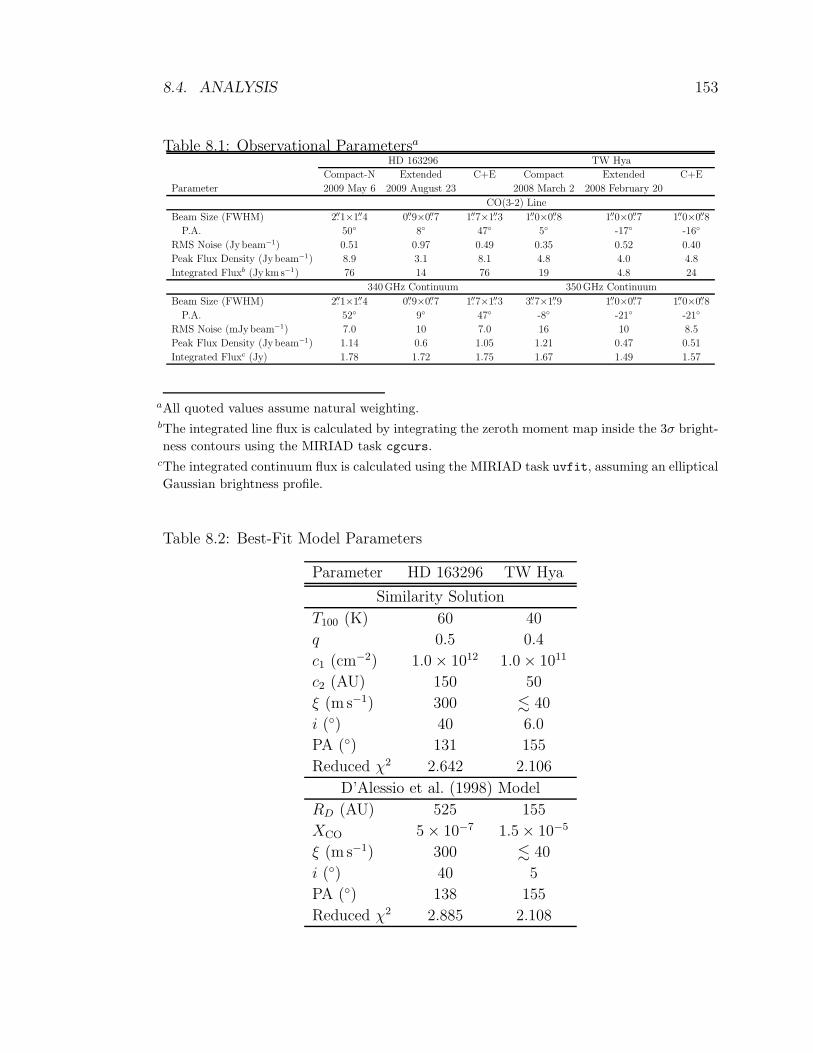
8.4. ANALYSIS 153
Table 8.1: Observational ParametersaHD 163296 TW Hya
Compact-N Extended C+E Compact Extended C+E
Parameter 2009 May 6 2009 August 23 2008 March 2 2008 February 20
CO(3-2) Line
Beam Size (FWHM) 2.′′1×1.′′4 0.′′9×0.′′7 1.′′7×1.′′3 1.′′0×0.′′8 1.′′0×0.′′7 1.′′0×0.′′8
P.A. 50 8 47 5 -17 -16
RMS Noise (Jy beam−1) 0.51 0.97 0.49 0.35 0.52 0.40
Peak Flux Density (Jy beam−1) 8.9 3.1 8.1 4.8 4.0 4.8
Integrated Fluxb (Jy km s−1) 76 14 76 19 4.8 24
340GHz Continuum 350GHz Continuum
Beam Size (FWHM) 2.′′1×1.′′4 0.′′9×0.′′7 1.′′7×1.′′3 3.′′7×1.′′9 1.′′0×0.′′7 1.′′0×0.′′8
P.A. 52 9 47 -8 -21 -21
RMS Noise (mJybeam−1) 7.0 10 7.0 16 10 8.5
Peak Flux Density (Jy beam−1) 1.14 0.6 1.05 1.21 0.47 0.51
Integrated Fluxc (Jy) 1.78 1.72 1.75 1.67 1.49 1.57
aAll quoted values assume natural weighting.bThe integrated line flux is calculated by integrating the zeroth moment map inside the 3σ bright-
ness contours using the MIRIAD task cgcurs.cThe integrated continuum flux is calculated using the MIRIAD task uvfit, assuming an elliptical
Gaussian brightness profile.
Table 8.2: Best-Fit Model Parameters
Parameter HD 163296 TW Hya
Similarity Solution
T100 (K) 60 40
q 0.5 0.4
c1 (cm−2) 1.0 × 10¹² 1.0 × 10¹¹
c2 (AU) 150 50
ξ (m s−1) 300 . 40
i () 40 6.0
PA () 131 155
Reduced χ2 2.642 2.106
D’Alessio et al. (1998) Model
RD (AU) 525 155
XCO 5 × 10⁻⁷ 1.5 × 10⁻⁵
ξ (m s−1) 300 . 40
i () 40 5
PA () 138 155
Reduced χ2 2.885 2.108
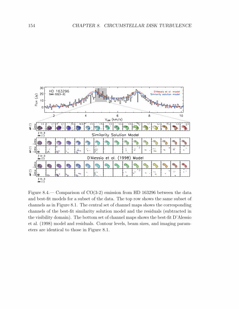
154 CHAPTER 8. CIRCUMSTELLAR DISK TURBULENCE
Figure 8.4.— Comparison of CO(3-2) emission from HD 163296 between the data
and best-fit models for a subset of the data. The top row shows the same subset of
channels as in Figure 8.1. The central set of channel maps shows the corresponding
channels of the best-fit similarity solution model and the residuals (subtracted in
the visibility domain). The bottom set of channel maps shows the best-fit D’Alessio
et al. (1998) model and residuals. Contour levels, beam sizes, and imaging param-
eters are identical to those in Figure 8.1.
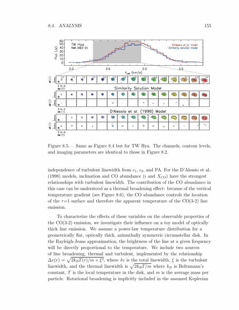
8.4. ANALYSIS 155
Figure 8.5.— Same as Figure 8.4 but for TW Hya. The channels, contour levels,
and imaging parameters are identical to those in Figure 8.2.
independence of turbulent linewidth from c1, c2, and PA. For the D’Alessio et al.
(1998) models, inclination and CO abundance (i and XCO) have the strongest
relationships with turbulent linewidth. The contribution of the CO abundance in
this case can be understood as a thermal broadening effect: because of the vertical
temperature gradient (see Figure 8.6), the CO abundance controls the location
of the τ=1 surface and therefore the apparent temperature of the CO(3-2) line
emission.
To characterize the effects of these variables on the observable properties of
the CO(3-2) emission, we investigate their influence on a toy model of optically
thick line emission. We assume a power-law temperature distribution for a
geometrically flat, optically thick, azimuthally symmetric circumstellar disk. In
the Rayleigh-Jeans approximation, the brightness of the line at a given frequency
will be directly proportional to the temperature. We include two sources
of line broadening, thermal and turbulent, implemented by the relationship
∆v(r) =√
2kBT (r)/m+ ξ2, where δv is the total linewidth, ξ is the turbulent
linewidth, and the thermal linewidth is√
2kBT/m where kB is Boltzmann’s
constant, T is the local temperature in the disk, and m is the average mass per
particle. Rotational broadening is implicitly included in the assumed Keplerian

156 CHAPTER 8. CIRCUMSTELLAR DISK TURBULENCE
Figure 8.6.— Comparison between the temperature and density structures of the
similarity solution and D’Alessio et al. (1998) models for HD 163296 (left) and
TW Hya (right). The bar across the top shows the temperature scale represented
by the colors, while the white contours represent density, marked with the base
10 logarithm of the total (gas+dust) mass density in units of g cm−3. Note that
while the D’Alessio et al. (1998) model of HD 163296 appears to be two orders of
magnitude more dense than the similarity solution model, the CO abundance is
more than two orders of magnitude lower, making the CO mass densities compa-
rable. The CO abundance of the TW Hya model is one order of magnitude lower
than for the similarity solution. The abscissae of the plots are scaled to match the
radial extent of the power-law disk model (excising the central 10AU, which are
not accessible with the data), although the similarity solution models will extend
farther.

8.4. ANALYSIS 157
rotation pattern of the material, so that in polar coordinates, the central frequency
of the line as a function of position is given by ν(r, θ) = ν0/c√
GM∗/r sin i cos θ,
where ν0 is the line frequency and M∗ is the stellar mass. The line profile at any
point in the disk is then given by
φ(ν, r) ∝ T (r)
∆v(r)ν0/cexp
[ −(ν − ν0)2
(∆v(r)ν0/c)2
]
(8.3)
where ν0 is the frequency of the line center and c is the speed of light. To project the
disk onto the sky, we define a radial coordinate reff =√
(r cos θ)2 + (r sin θ/ cos i)2,
with θ used as a polar coordinate so that the isophotes are elliptical, and substitute
this expression for r in the line profile. We then integrate over the r and θ
coordinates across the extent of the elliptical disk to calculate the line profile as
a function of frequency. We investigate the contribution of the different sources
of broadening by varying ξ, T (r), and i to correspond to the turbulent, thermal,
and rotational broadening effects. Here we discuss the ways in which turbulent
broadening can be distinguished from the other two effects in the context of our
toy model.
Temperature — The left panel of Figure 8.7 shows model line profiles that
illustrate the relationship between broadening due to temperature and broadening
due to a global turbulent linewidth. The solid line is the model line profile
calculated using values from the best-fit similarity solution: T100=60K, q=0.5,
and ξ=300ms−1. The dotted line represents the profile for a model with the same
parameters but no turbulent linewidth. To create the dashed line profile, the
temperature was varied until the peak line flux of the model without turbulence
matched the peak flux of the original model with turbulence. This sequence of line
profiles illustrates how thermal and turbulent broadening produce distinct effects
on the observable properties of the data, rather than being fully interchangeable.
Since increases in temperature increase the line flux throughout the disk while
turbulence simply redistributes the flux in frequency space, turbulence tends
to shift flux from the line peaks to the center, changing the shape of the line.
As a result, the peak-to-center line flux ratios will be different for line profiles
with comparable widths and peak fluxes, depending on the relative contributions
of turbulence and temperature to line broadening. The difference between the
best-fit 300m s−1 turbulent linewidth in HD 163296 and a comparable model
without turbulence corresponds to a 30% change in peak-to-center line flux in
the context of this toy model, which should be easily distinguishable given the
uncertainty of our data.
Inclination — The right panel of Figure 8.7 shows model line profiles
that illustrate the relationship between turbulent broadening and rotational

158 CHAPTER 8. CIRCUMSTELLAR DISK TURBULENCE
broadening due to inclination. As in the left panel, we first generate a model
with no turbulent broadening (dotted line), and then adjust the inclination
until the peak flux matches the original line model (dashed line). In this case,
the absence of turbulence once again alters the peak-to-center line ratio. But
another obvious difference between the turbulent model and the more inclined
model without turbulence is that rotational broadening through inclination alters
the separation between the line peaks in velocity space. The sequence of toy
models shows that the contribution of the 300m s−1 turbulent linewidth in the
HD 163296 model corresponds to a 6 change in inclination, in addition to the
large depression of flux at the line center. Since spatially resolved spectra of the
Keplerian rotation patterns in molecular lines allow for very precise determination
of circumstellar disk inclination (to within a degree or less; see discussion in Qi
et al. 2004), turbulent line broadening at the level detected in HD 163296 should
be distinguishable from rotational broadening.
8.5 Discussion
8.5.1 Comparison with Theory
The problem of accurately modeling and predicting the magnitude of velocity
fluctuations arising from magnetohydrodynamic (MHD) turbulence is historically
fraught, but a few general features seem to be agreed upon. The difficulty hinges
largely on derived values of α and how they relate to the expected magnitude
of the turbulent linewidth. The dimensionless parameter α was defined by
Shakura & Syunyaev (1973) to describe the effective viscosity in terms of a
proportionality constant multiplied by the largest velocity and length scales on
which turbulence may act: the scale height and the sound speed. In mathematical
terms, νeff = αcsH , where νeff is the effective viscosity, cs is the sound speed, H
is the local scale height, and α is then an efficiency factor with a value ≤1. The
magnitude of turbulent velocity fluctuations depends both on the value of α and
on how this efficiency factor is apportioned between the sound speed and the
scale height. If, for example, the majority of the power in turbulent fluctuations
occurs at the length of the scale height, the velocity fluctuations can be as small
as αcs (perhaps augmented by a geometric factor of a few). On the other hand,
if the proportionality factor α applies evenly to the length and velocity scales in
the problem, the turbulent fluctuations could be as large as√αcs (again possibly
modified by a geometric factor). Since there is no evidence of shocks that would
point to sonic or supersonic turbulence in circumstellar disks, it is unlikely that
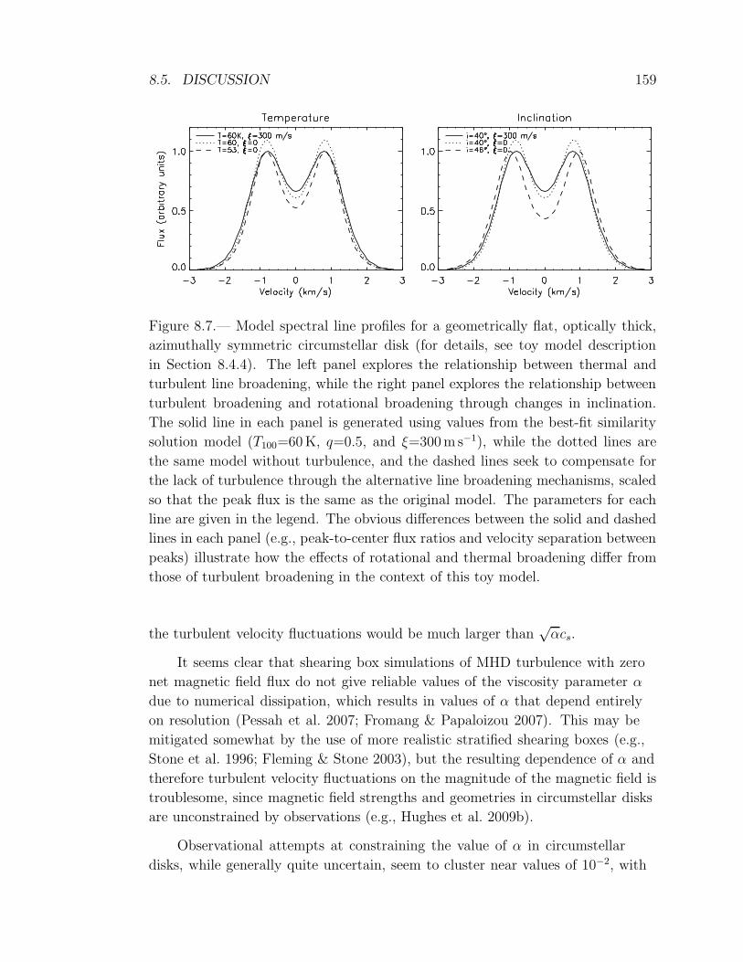
8.5. DISCUSSION 159
Figure 8.7.— Model spectral line profiles for a geometrically flat, optically thick,
azimuthally symmetric circumstellar disk (for details, see toy model description
in Section 8.4.4). The left panel explores the relationship between thermal and
turbulent line broadening, while the right panel explores the relationship between
turbulent broadening and rotational broadening through changes in inclination.
The solid line in each panel is generated using values from the best-fit similarity
solution model (T100=60K, q=0.5, and ξ=300ms−1), while the dotted lines are
the same model without turbulence, and the dashed lines seek to compensate for
the lack of turbulence through the alternative line broadening mechanisms, scaled
so that the peak flux is the same as the original model. The parameters for each
line are given in the legend. The obvious differences between the solid and dashed
lines in each panel (e.g., peak-to-center flux ratios and velocity separation between
peaks) illustrate how the effects of rotational and thermal broadening differ from
those of turbulent broadening in the context of this toy model.
the turbulent velocity fluctuations would be much larger than√αcs.
It seems clear that shearing box simulations of MHD turbulence with zero
net magnetic field flux do not give reliable values of the viscosity parameter α
due to numerical dissipation, which results in values of α that depend entirely
on resolution (Pessah et al. 2007; Fromang & Papaloizou 2007). This may be
mitigated somewhat by the use of more realistic stratified shearing boxes (e.g.,
Stone et al. 1996; Fleming & Stone 2003), but the resulting dependence of α and
therefore turbulent velocity fluctuations on the magnitude of the magnetic field is
troublesome, since magnetic field strengths and geometries in circumstellar disks
are unconstrained by observations (e.g., Hughes et al. 2009b).
Observational attempts at constraining the value of α in circumstellar
disks, while generally quite uncertain, seem to cluster near values of 10−2, with

160 CHAPTER 8. CIRCUMSTELLAR DISK TURBULENCE
large scatter (e.g., Hartmann et al. 1998; Andrews et al. 2009). If the velocity
fluctuations are estimated as√αcs, this result would imply velocity fluctuations
up to 10% of the sound speed near the midplane, although this global value is
likely to vary widely depending on local conditions that affect the ionization
fraction and the coupling of ions and neutrals. A theoretical comparison between
circumstellar disks and the Taylor-Couette flow by Hersant et al. (2005) finds that
the 100m s−1 turbulent linewidth (of order .30% of the sound speed) derived
from low spectral resolution observations of DM Tau by Guilloteau & Dutrey
(1998) are on par with expectations from laboratory measurements by Dubrulle
et al. (2005). There is some evidence, both from the study of FU Ori objects
(Hartmann et al. 2004) and global MHD simulations of stratified disks (e.g.
Fromang & Nelson 2006), that the turbulent linewidth may be larger at several
scale heights above the midplane of the disk, perhaps up to 40% of the sound
speed.
In this context, HD 163296 seems to fit in fairly seamlessly, with a turbulent
linewidth of 300m s−1 corresponding to about 40% of the sound speed at the size
scales probed by our data (if 1.′′5 corresponds to ∼180AU at a distance of 122 pc).
The lower turbulent linewidth in TW Hya, .10% of the turbulent linewidth at
the scale of our observations (80AU at 51 pc), could be associated with a lower
global value of α, although the reason for such a difference is unclear. Following
Andrews et al. (2009), the best-fit similarity solution model parameters imply
α = 0.03 for TW Hya and 0.009 for HD 163296, although these numbers are
quite uncertain given the reliance on the optically thick CO(3-2) tracer for the
determination of density. The D’Alessio et al. (1998) models use α = 0.0018 for
TW Hya and 0.003 for HD 163296. Perhaps the only conclusion that should be
drawn from this estimate is that our observations are consistent with estimates
that place α in the range of 10−2-10−3. With a sample of only two sources and
with a wide range of theoretical results and approaches to the study of turbulence,
it can be difficult to compare our results to theoretical predictions in a detailed
way. Nevertheless, the detection of a turbulent linewidth in the HD 163296
system and the upper limit on turbulence in the TW Hya system are suggestive.
There are several potential explanations for this difference rooted in theoretical
studies of protoplanetary disk turbulence.
Inclination and Vertical Structure — In general, the CO(3-2) line emission
from these systems is expected to be optically thick, and therefore will arise from
the tenuous upper disk layers several scale heights above the midplane. However,
this simple picture can be complicated by geometry and velocity: the combination
of inclination and rotational line broadening in HD 163296 will permit the escape

8.5. DISCUSSION 161
of radiation from deeper layers of the disk. As a result, a different vertical height
may be probed in the HD 163296 system than in TW Hya. Naively, it would be
expected that the turbulent linewidth in TW Hya should be larger as a result,
since turbulence is predicted to become stronger farther from the midplane. But it
is also possible that poor coupling of ions to neutrals in the low-density uppermost
disk layers could inhibit the detection of turbulence even if it is present. This
may also depend on the relative amounts of small dust grains in the upper layers
of the two disks, since small grains are more adept at absorbing free electrons.
Stellar Mass and Ionizing Flux — One of the factors determining the extent
of turbulent regions in circumstellar disks is the magnitude of ionizing X-ray flux
from the star (e.g., Gammie 1996; Igea & Glassgold 1999). With stellar masses
differing by a factor of 4, the radiation (and therefore ionization) properties of
TW Hya and HD 163296 are likely to be quite different. Despite the tendency for
X-ray flux to be lower for intermediate-mass than low-mass stars of comparable
ages, HD 163296 has the largest X-ray flux of the sample of 13 Herbig Ae stars
studied by Hubrig et al. (2009), comparable to that of lower-mass T Tauri stars.
Nevertheless, its measured X-ray luminosity of 4.0× 1029 erg s−1 is still lower than
that of TW Hya, which is estimated as 2.0× 1030 erg s−1 by Kastner et al. (1999).
Given the comparable disk densities, by X-ray luminosity alone, TW Hya should
be the more active disk. However, since we are observing these disks on relatively
large spatial scales (∼80AU for TW Hya and ∼180AU for HD 163296, with 1.′′5
resolution viewed from their respective 51 and 122 pc distances), the ionization
at these distances may instead be dominated by cosmic rays. It is extremely
difficult to determine how the cosmic ray environment of these two sources might
compare; if HD 163296 were located in a region of greater cosmic ray activity,
that could account for the greater turbulent linewidth observed for this system.
Evolutionary State — One of the most obvious differences between TW Hya
and HD 163296 is their respective evolutionary states. TW Hya is a 10Myr-old
transition disk with an inner cavity of ∼4AU radius, while HD 163296 is a
primordial disk with an inner radius consistent with the expected ∼0.4AU extent
of the dust destruction zone (see, e.g., Isella et al. 2007). It is possible that X-ray
ionization and the MRI might operate differently at different stages of evolution;
one example is the inside-out MRI clearing proposed by Chiang & Murray-Clay
(2007) to explain the cavities in transition disks. In their scenario, the mass
accretion rate onto the star can be explained entirely by the MRI operating on
the disk inner rim, and requires no resupply from the outer disk; they therefore
require little to no turbulent viscosity in the outer disk to explain the observed
accretion rates in transitional systems. However, they note that their theory

162 CHAPTER 8. CIRCUMSTELLAR DISK TURBULENCE
cannot be readily applied to primordial systems, leaving the viscous transport
mechanism responsible for large accretion rates at earlier stages unexplained.
There is no reason to expect MRI turbulence in the outer disk to “shut off” when
a gap is opened, so while our observation of a small turbulent linewidth in the
TW Hya system is consistent with the Chiang & Murray-Clay (2007) hypothesis,
it is still surprising that the turbulent linewidth in HD 163296 should be so much
larger.
8.5.2 Implications for Planet Formation
The presence of subsonic turbulence in protoplanetary accretion disks – likely
strongly subsonic in the midplane – is consistent with the observations presented
in this study. Subsonic turbulence has important implications for the formation
and evolution of young planetary systems. One series of papers (Papaloizou &
Nelson 2003; Papaloizou et al. 2004; Nelson & Papaloizou 2003, 2004) explores
in detail the effects of turbulence on planet-forming disks. Their cylindrical
models of turbulent disks have an average α in the range of 10−2-10−3, but they
demonstrate that the realistic implementation of turbulence results in different
effects than are seen in laminar disk simulations with comparable values of
α incorporated as an anomalous Navier-Stokes viscosity. They show that for
massive planets, turbulence can widen and deepen the gap opened by massive
protoplanets, and may reduce the accretion rate onto the protoplanet. For the
case of migrating low-mass planet cores, the presence of turbulence in the disk
can slow or even reverse the migration rate, converting the monotonic inward
motion of the planet into a random walk. The presence of dead zones in the radial
direction may also act to halt migration and encourage the survival and growth
of protoplanets (e.g. Matsumura et al. 2009). Another important proposed effect
of subsonic turbulence is to aid in concentrating planetesimals to allow them
to collapse gravitationally (Johansen et al. 2007). MHD turbulence on these
scales can also reduce the strength of the gravitational instability and reduce disk
fragmentation (Fromang 2005). There is also substantial literature on the effects
of turbulence on dust settling and grain growth (e.g. Johansen & Klahr 2005;
Carballido et al. 2006; Ciesla 2007; Balsara et al. 2009; Fromang & Nelson 2009).
Although it is difficult to compare the properties of the simulations directly
with our observations, the generic features of these models (α=10−2-10−3,
subsonic turbulence even in the upper disk layers) are globally consistent with the
derived properties of turbulence in the disks around HD 163296 and TW Hya,
indicating that these effects are likely to play a role in planet formation.

8.6. SUMMARY AND CONCLUSIONS 163
8.5.3 Future Directions
The most obvious improvement to our method would be to include additional
spectral lines from different transitions or isotopologues of the CO molecule in
order to provide independent constraints on the gas temperature. While this
would necessarily introduce additional parameters into the model (i.e., to describe
the vertical distribution of temperature and turbulence, as well as a consistent
density distribution to properly account for the line opacity), the addition of
several lines that are resolved in the spectral and spatial domains would more
firmly constrain the models. It might also provide direct measurements of the
vertical profile of the turbulent velocity structure. Dartois et al. (2003) and Panic
et al. (2008) provide examples of studies that use multiple molecular lines to study
the vertical structure of density and temperature in circumstellar disks; these
techniques could be extended to constrain the turbulent linewidths in similar
systems.
Another possibility is to observe ions rather than neutral species. This would
eliminate complications introduced by the interaction between ions and neutrals,
and would more directly probe the turbulent motions of the charged gas.
Even with the current set of observations, greater sensitivity would be
extremely valuable in constraining the turbulent linewidth, since the distinctions
between turbulent and thermal broadening are subtle (see Section 8.4.4). The
vast improvements in sensitivity provided by the Atacama Large Millimeter Array
will permit significantly better modeling of the velocity structure of young disks.
In addition, higher sensitivity combined with a greater spatial dynamic range will
allow for the investigation of radial variations in the turbulent linewidth.
8.6 Summary and Conclusions
We have obtained the first spatially resolved observations of molecular line
emission from two nearby circumstellar disks with spectral resolution finer
than the expected turbulent linewidth. We fit these high spectral resolution
observations of the CO(3-2) line emission using two well-tested models of
circumstellar disk structure, and derive a turbulent linewidth of ∼300m s−1 for
the disk around HD 163296 and .40m s−1 for the disk around TW Hya. The
results are consistent for the two model classes despite their different treatments
of the temperature structure of the disk, which is significant since thermal
broadening is closely related to turbulent broadening. The magnitude of turbulent
164 CHAPTER 8. CIRCUMSTELLAR DISK TURBULENCE
velocity fluctuations implied by these results – up to tens of percent of the sound
speed – is broadly consistent with theoretical predictions for MRI turbulence in
the upper layers of circumstellar disks, although it is unclear why the linewidth
should be lower for TW Hya than for HD 163296.
These results demonstrate the potential of this method for constraining
theories of the magnitude and spatial distribution of turbulence. Future
observations with greater sensitivity, perhaps incorporating different molecular
line species and isotopologues of the same molecule, have the potential to vastly
improve our ability to characterize turbulence in these systems.

Chapter 9
Conclusions and Future
Directions
We have used spatially resolved observations at millimeter wavelengths to
characterize the structure and evolution of circumstellar disks during their critical
planet-forming stages. Sections 9.1 and 9.2 summarize the results of the work
presented in this thesis, organized according to the themes laid out in Chapter 1.
In Section 9.3 we discuss likely future directions that the work will take.
9.1 Disk Dissipation
Chapters 2-5 study the structure and composition of individual disks apparently
in the process of clearing their natal gas and dust. Most of the sources – with the
exception of 49 Ceti – fall under the original definition of a transition disk, with a
pronounced mid-IR deficit in the SED.
Chapters 2 and 3 test the paradigm that mid-IR deficits are associated
with inner cavities in the dust distribution. We use millimeter-wavelength
interferometry to spatially resolve the distribution of large dust grains in
the system, and find that the SED-based models predict well the resolved
observations. The inherent degeneracy between surface density and opacity
at long wavelengths does not allow us to uniquely identify the absence of
millimeter-wavelength emission with missing mass at the disk center. However,
combining these observations with constraints on the inner hole properties from
other wavelengths strongly suggests that the dust surface density is lower within
the cavity, and that dynamical interactions with giant planets in formation are
165

166 CHAPTER 9. CONCLUSIONS AND FUTURE DIRECTIONS
the dominant dust clearing mechanism in these systems. The measured inner
hole sizes are comparable to but slightly different from those predicted from
SED modeling. Because inferred cavity sizes depend on poorly-constrained dust
grain properties, which affect the inferred temperature structure of the inner
disk, spatially resolved observations at long wavelengths are the more accurate
diagnostic of inner hole size.
We also generate basic models of the structure and composition of two
newly-identified transition disks in Corona Australis. Chapter 5 presents these
models, including constraints from marginally-resolved SMA observations of
the outer disks, and examines the implications of the models for the molecular
gas content of the outer disk. In both cases, we find evidence for CO content
significantly below that predicted using standard assumptions. This echoes the
low CO abundance derived for GM Aur in Chapter 3 and for TW Hya in Qi et al.
(2004). While it is unclear whether the low CO content results from a reduced
gas-to-dust mass ratio or CO abundance relative to H2, this result is suggestive
of significant chemical or dynamical evolution of the gas disk in parallel with the
dust disk clearing. It is unclear whether protoplanetary disks share this property;
very few protoplanetary disks in the literature exhibit bright, uncontaminated
CO emission with which to compare the results for these transition disks. Further
study is required to understand the implications of the low CO content of the
transitional systems. One of the systems studied, RX J1842.9-3532, now adds
to the growing number of recently-identified “pre-transitional” objects that
exhibit evidence for a band of optically thick material within their inner cavities
(Espaillat et al. 2007). Given the ∼10Myr ages, the inferred disk properties, and
the far southern declination of Corona Australis, the systems studied in Chapter 5
will be interesting targets for follow-up with next-generation interferometers like
ALMA.
49 Ceti, discussed in Chapter 4, differs markedly from the other transitional
objects studied in this thesis. In fact, according to some definitions (including
the original) it should not be classified as a transition disk at all. It nevertheless
appears to represent a unique stage of disk evolution, with characteristics
intermediate between the protoplanetary and debris disk phases. Despite dust
properties consistent with those of a debris disk, it retains a substantial reservoir
of molecular gas, apparently in rotation about the star. The gas-to-dust mass
ratio in this system is also much lower than predicted for typical assumptions,
approximately of order unity; even the CO(2-1) line is apparently optically thin
throughout the disk. There is evidence for a deficit of CO emission within a
distance of 40AU from the star. The low gas mass and inner cavity in the

9.2. PROTOPLANETARY DISKS AS ACCRETION DISKS 167
gas disk are strongly consistent with a photoevaporative clearing scenario. 49
Ceti therefore represents an interesting case study that argues caution in the
identification and interpretation of transition disks: it is likely that several
different clearing mechanisms play a role in disk dissipation, whether different
mechanisms are relevant for different systems or different mechanisms come into
play at different times in the life of a star. While systems like 49 Ceti appear
even more rare and difficult to identify than systems with inner dust cavities in
otherwise massive gas-rich disks, they evidently represent an important missing
piece in the puzzle of disk dissipation.
Overall, our results are consistent with the following: (1) SED-based models
of mid-IR deficits accurately predict a deficit of long-wavelength flux from the
disk center, at roughly the correct size scales. (2) Molecular gas disks can persist
to ages as late as ∼10Myr, and several transitional systems show evidence of
lower CO content than expected based on typical assumptions of gas-to-dust
mass ratio and CO abundance for primordial disks. (3) Several distinct physical
mechanisms likely contribute to the dissipation of gas and dust disks, and there
is good evidence based on the observable properties of individual systems for
photoevaporation by energetic stellar radiation and dynamical interactions with
giant planets.
9.2 Protoplanetary Disks as Accretion Disks
Chapters 6-8 look for observational signatures of the viscous transport processes
that drive accretion in protoplanetary disks. In particular, a sample of the
brightest, largest, and best-studied nearby disks is examined for evidence of
turbulence, magnetic fields, and large-scale structure reflective of ongoing viscous
evolution. We focus on observable features of the most popular theoretical
mechanism proposed for generating turbulent viscosity in accretion disks, the
magnetorotational instability.
In Chapter 6 we use archival continuum and molecular line observations from
the SMA to study the large-scale structure of four nearby objects: TW Hya,
GM Aur, MWC 480, and HD 163296. We model the systems with two distinct
parameterizations of surface density structure, including the widely used
power-law descriptions with truncated outer edges and the theoretically motivated
similarity solutions for viscous accretion disks with exponentially tapered outer
edges. We show that the tapered edge of the similarity solution model resolves
an apparent discrepancy between the spatial extent of gas and dust disks arising

168 CHAPTER 9. CONCLUSIONS AND FUTURE DIRECTIONS
as a result of the truncated outer edge in the ubiquitous power-law models.
While we are not able to constrain independently the shape of the outer edge,
the similarity solution models have the dual advantages of being grounded in
the physics of accretion and providing a consistent description of both the gas
and dust distribution, despite having the same number of free parameters as the
power-law models. This result provides indirect evidence for the viscous evolution
of circumstellar disks, and suggests that the present-day properties of disks may
reflect their accretion history.
The more directly observable features of the MRI are the presence of
large-scale magnetic fields and turbulence. Chapter 7 uses the SMA polarimeter
to search for evidence of large-scale magnetic fields through polarized thermal
emission from aligned dust grains in TW Hya and HD 163296. We place upper
limits on the polarization fraction approximately an order of magnitude below
the 2-3% level expected based on previous observational and theoretical studies.
Appendix B adds the other objects from the Chapter 6 sample, including GM Aur,
which had a tentative detection of polarization at the 2% level from Tamura et al.
(1999). However, it is difficult to relate polarization fraction directly to magnetic
field strength. Instead of weak magnetic fields, the low polarization fraction
likely reflects the inefficient alignment of large dust grains with the magnetic
field, perhaps in combination with other sources of inefficiency like magnetic field
tangling or rounding of large grains.
We use the high spectral resolution capabilities of the SMA correlator
to search directly for turbulence in the CO(3-2) line emission from the disks
around HD 163296 and TW Hya. Chapter 8 describes the observations and the
modeling procedure used to tease the turbulent linewidth from other sources
of broadening. We place an upper limit on the turbulent linewidth in the disk
around TW Hya and report a 3σ detection of turbulence at the 300m s−1 level in
the disk around HD 163296, corresponding to .10% and ∼30% of the turbulent
linewidth at the spatial scales probed, respectively. While it is not clear why the
linewidths should be so different for these two systems (which themselves differ in
age, mass, evolutionary state, and environment), both results appear consistent
with the broad range of values predicted from simulations of MRI turbulence
in protoplanetary disks. This first step in characterizing observationally the
properties of protoplanetary disk turbulence has many obvious extensions,
including broadening the sample to search for trends by system property, using
molecular line tracers of differing optical depths to trace the properties in the
vertical directions, studying lines of ions that may be more sensitive to magnetic
turbulence, and improving the resolution to characterize radial variations in
9.3. FUTURE DIRECTIONS 169
turbulent linewidth, including seeking observational evidence for the presence of
the dead zones that are expected to extend throughout the inner disk.
On the whole, the observations described in these chapters are generally in
agreement with the predicted properties of circumstellar disks undergoing viscous
evolution as a result of the operation of the MRI.
9.3 Future Directions
It is impossible to contemplate the future of the types of observations presented
in this thesis without considering the transformative role that ALMA and the
EVLA will play, beginning only months from now. With improvements in
both sensitivity and spatial resolution of an order of magnitude or more over
current instruments, ALMA in particular is poised to initiate a revolution in
millimeter-wavelength studies of circumstellar disks (and everything else). While
it is impossible to predict the new research directions that will inevitably unfold
with such extreme advances in instrumentation, we discuss here some of the ways
in which the new capabilities will contribute to our understanding of circumstellar
disk structure and evolution, particularly for the types of objects and questions
that have been central to this thesis work.
Inside Transition Disk Cavities — ALMA’s combination of sensitivity and
spatial resolution will for the first time provide direct access to the gas and dust
content of the inner disk. In addition to providing the first look at the amount
and location of planet-forming material on the spatial scale of the inner Solar
system, this will have profound implications in particular for the study of the disk
clearing processes operating in transition disks. As in the Dutrey et al. (2008)
result that provided spectroscopic evidence for a deficit of cold CO within the
central cavity in the GM Aur disk, knowledge of the cold molecular gas content
in inner disk cavities will provide a strong discriminator between theoretical
clearing mechanisms for a large sample of transitional objects. This will aid in
distinguishing between clearing mechanisms in transition disks, similar to the
work described in Chapters 2-5. The forest of molecular lines observable with
the sensitive ALMA receivers, including low optical depth tracers, will allow for
chemical modeling of the gas within the cavity, and has the potential to constrain
the total gas mass throughout the disk. Multiwavelength continuum observations
of the inner disk with ALMA and the EVLA will constrain the dust grain size
distribution within the cavity, another important discriminator between clearing
mechanisms.
170 CHAPTER 9. CONCLUSIONS AND FUTURE DIRECTIONS
Planet-Disk Interactions — High-resolution continuum observations with
next-generation instruments should provide direct evidence for planet formation
through dynamical interactions, as well as constraints on the masses of young
planets. SED modeling is insensitive to small radial gaps (rather than large inner
holes) as well as azimuthal asymmetries in the dust distribution, both of which
should be accessible to the combination of sensitivity and resolution available
with ALMA. If giant planets are indeed responsible for clearing the inner cavities
in transition disks, their dynamical signatures may be imprinted in particular on
the wall at the inner edge of the outer disk. One particularly exciting prediction
is that the accretion luminosity of the planet itself may be observable for the
closest and most favorably oriented systems, by pushing ALMA to its limits in
sensitivity and resolution (Wolf & D’Angelo 2005).
Molecular Lines — Some of the unexpected questions raised by this thesis
are: what is the molecular gas content of protoplanetary and transition disks, and
why does it appear to differ from standard expectations? Are protoplanetary disks
different from transition disks in this way? Why is it that (nearly) all of the bright
molecular gas disks seem to be transition disks? Next-generation instruments
will provide the capability to carry out detailed studies of the chemistry and
kinematics of disks using molecular line observations, including rare tracers that
will be less sensitive to cloud contamination and will permit the study of the gas
properties of embedded disks. In general, a more sophisticated understanding
of disk chemistry will permit improved characterization of the gas content of
circumstellar disks. One exciting possibility in the study of disk dynamics is
that the type of high spectral resolution observations described in Chapter 8
can be extended to few-AU-scale linear resolution, potentially revealing the
signature of a dead zone. This could provide some of the best evidence yet for the
dominant role of the MRI in protoplanetary disks. Combining sensitive spectral
line surveys with high spatial resolution can also yield detailed information about
the temperature, density, and kinematics as a function of height above the disk
midplane (extending the work of Dartois et al. 2003; Panic et al. 2008, as well
as that described in Chapter 8).
Polarimetry — While it is unclear how much more sensitive the new
instruments will be to polarized emission at millimeter wavelengths, it will
be valuable to survey large samples spanning evolutionary stages, stellar and
disk masses, and environments, to determine whether and how the polarization
fraction differs between objects. The increase in resolution will also be important,
as turbulent motions are expected to take place on scales no larger than the scale
height; resolving below this linear scale is therefore desirable and should help

9.3. FUTURE DIRECTIONS 171
to answer the question of how much of the low polarization fraction is due to
field tangling. The sensitivity to molecular line polarization provided by ALMA
will also provide access to tracers of various optical depth through the disks,
which could have profound effects on the diagnostic value of line observations for
unraveling magnetic field structure (e.g., Goldreich & Kylafis 1981, 1982).
The capabilities of next-generation instruments promise to open exciting
new research directions in all of the lines of study discussed in this thesis.
The observations and analysis described here are beginning to pave the way
towards answering some of the fundamental questions in planet formation: the
physics driving the evolution and dissipation of gas and dust disks, the role that
planet-disk interactions play in shaping systems, and the bridge between the
properties of natal disks and the architectures of planetary systems.

172 CHAPTER 9. CONCLUSIONS AND FUTURE DIRECTIONS

Appendix A
Protoplanetary Disk Visibility
Functions
We analyze a simplified disk model parameterized by power law distributions in
surface density and temperature and including a central hole, to illustrate how the
model parameters affect the shape of the visibility function. We also discuss the
visibility function of a model consisting of a thin ring. For both cases, we provide
analytical expressions for calculating the position of the null in the (deprojected)
visibility function, which is an easily observed feature.
A.1 Power-Law Disk with a Central Hole
For a flat, optically thin disk described by power-law distributions in temperature
and surface density, assumed to be radiating in the Rayleigh-Jeans limit and
viewed face-on, the intensity of radiation as a function of radial angular scale θ
from the center of the disk is
Iν(θ) =2ν2kBκν
c2T0
(
θ
θ0
)−q
Σ0
(
θ
θ0
)−p
(A.1)
The visibility as a function of (u,v) distance, R, is given by the Fourier transform
of the intensity:
V (R) =4πν2kBκνT0Σ0θ
p+q0
c2
∫ θb
θa
θ1−(p+q)J0(2πθR)dθ (A.2)
173
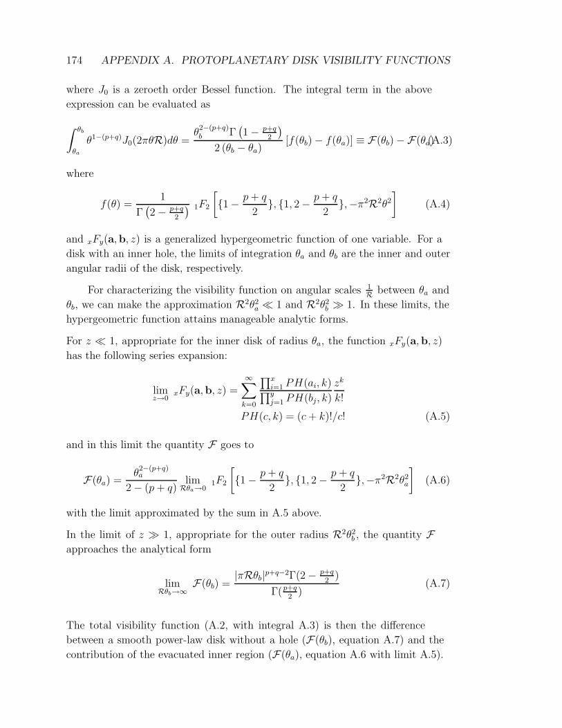
174 APPENDIX A. PROTOPLANETARY DISK VISIBILITY FUNCTIONS
where J0 is a zeroeth order Bessel function. The integral term in the above
expression can be evaluated as
∫ θb
θa
θ1−(p+q)J0(2πθR)dθ =θ
2−(p+q)b Γ
(
1 − p+q2
)
2 (θb − θa)[f(θb) − f(θa)] ≡ F(θb) − F(θa)(A.3)
where
f(θ) =1
Γ(
2 − p+q2
) 1F2
[
1 − p+ q
2, 1, 2 − p+ q
2,−π2R2θ2
]
(A.4)
and xFy(a,b, z) is a generalized hypergeometric function of one variable. For a
disk with an inner hole, the limits of integration θa and θb are the inner and outer
angular radii of the disk, respectively.
For characterizing the visibility function on angular scales 1R
between θa and
θb, we can make the approximation R2θ2a ≪ 1 and R2θ2
b ≫ 1. In these limits, the
hypergeometric function attains manageable analytic forms.
For z ≪ 1, appropriate for the inner disk of radius θa, the function xFy(a,b, z)
has the following series expansion:
limz→0
xFy(a,b, z) =∞
∑
k=0
∏xi=1 PH(ai, k)
∏yj=1 PH(bj, k)
zk
k!
PH(c, k) = (c+ k)!/c! (A.5)
and in this limit the quantity F goes to
F(θa) =θ
2−(p+q)a
2 − (p+ q)lim
Rθa→01F2
[
1 − p+ q
2, 1, 2 − p + q
2,−π2R2θ2
a
]
(A.6)
with the limit approximated by the sum in A.5 above.
In the limit of z ≫ 1, appropriate for the outer radius R2θ2b , the quantity F
approaches the analytical form
limRθb→∞
F(θb) =|πRθb|p+q−2Γ(2 − p+q
2)
Γ(p+q2
)(A.7)
The total visibility function (A.2, with integral A.3) is then the difference
between a smooth power-law disk without a hole (F(θb), equation A.7) and the
contribution of the evacuated inner region (F(θa), equation A.6 with limit A.5).
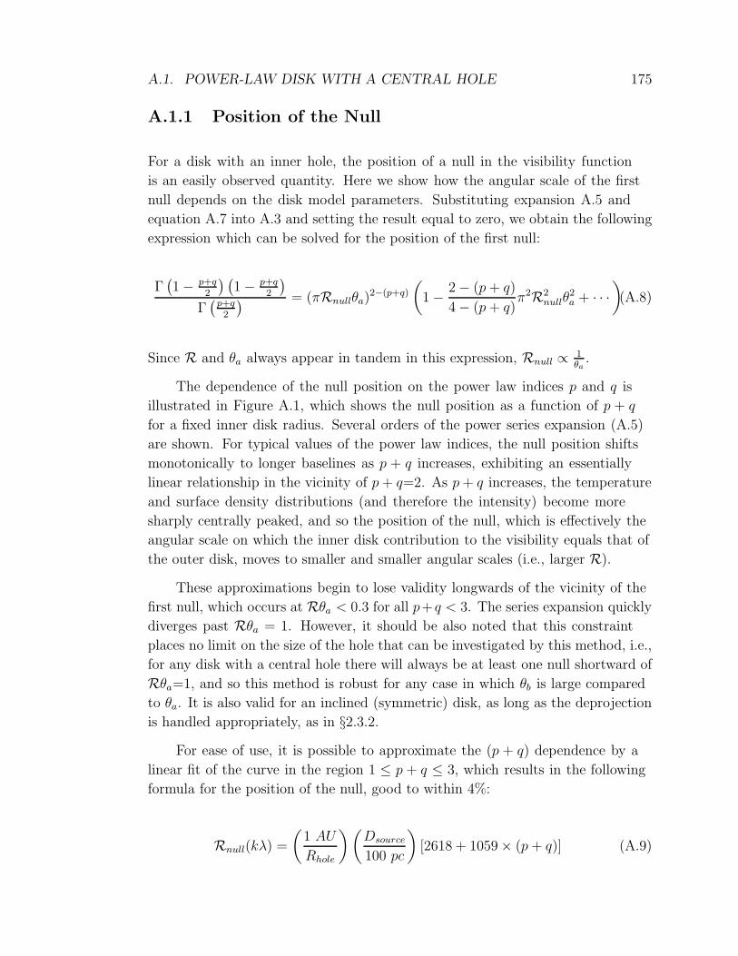
A.1. POWER-LAW DISK WITH A CENTRAL HOLE 175
A.1.1 Position of the Null
For a disk with an inner hole, the position of a null in the visibility function
is an easily observed quantity. Here we show how the angular scale of the first
null depends on the disk model parameters. Substituting expansion A.5 and
equation A.7 into A.3 and setting the result equal to zero, we obtain the following
expression which can be solved for the position of the first null:
Γ(
1 − p+q2
) (
1 − p+q2
)
Γ(
p+q2
) = (πRnullθa)2−(p+q)
(
1 − 2 − (p+ q)
4 − (p+ q)π2R2
nullθ2a + · · ·
)
(A.8)
Since R and θa always appear in tandem in this expression, Rnull ∝ 1θa
.
The dependence of the null position on the power law indices p and q is
illustrated in Figure A.1, which shows the null position as a function of p + q
for a fixed inner disk radius. Several orders of the power series expansion (A.5)
are shown. For typical values of the power law indices, the null position shifts
monotonically to longer baselines as p + q increases, exhibiting an essentially
linear relationship in the vicinity of p+ q=2. As p+ q increases, the temperature
and surface density distributions (and therefore the intensity) become more
sharply centrally peaked, and so the position of the null, which is effectively the
angular scale on which the inner disk contribution to the visibility equals that of
the outer disk, moves to smaller and smaller angular scales (i.e., larger R).
These approximations begin to lose validity longwards of the vicinity of the
first null, which occurs at Rθa < 0.3 for all p+ q < 3. The series expansion quickly
diverges past Rθa = 1. However, it should be also noted that this constraint
places no limit on the size of the hole that can be investigated by this method, i.e.,
for any disk with a central hole there will always be at least one null shortward of
Rθa=1, and so this method is robust for any case in which θb is large compared
to θa. It is also valid for an inclined (symmetric) disk, as long as the deprojection
is handled appropriately, as in §2.3.2.
For ease of use, it is possible to approximate the (p + q) dependence by a
linear fit of the curve in the region 1 ≤ p + q ≤ 3, which results in the following
formula for the position of the null, good to within 4%:
Rnull(kλ) =
(
1 AU
Rhole
) (
Dsource
100 pc
)
[2618 + 1059 × (p+ q)] (A.9)

176 APPENDIX A. PROTOPLANETARY DISK VISIBILITY FUNCTIONS
Figure A.1.— The dependence of R on disk temperature and surface density power
law indices (p+ q), source distance (Dsource), and inner hole size (Rhole).
A.2 Thin Wall
A thin wall (∆R ≪ R) can be described by a ring of constant brightness at a
distance Rhole from the star, with a visibility function which is a zeroeth order
Bessel function:
V (R) = 2π
∫ ∞
0
Iν(θ)J0(2πθR)θdθ
= 2πθholeIwallJ0(2πθholeR) (A.10)
where θhole is the angular radius of the hole and Iwall is the intensity of emission
from the wall. The position of the null in the visibility function of a thin wall will
then be
Rnull(kλ) =77916
π2
(
Dsource
100 pc
) (
1 AU
Rhole
)
(A.11)
A.3 Application to TW Hya
The TW Hya disk has an outer radius of 196 AU (CO emission, Qi et al. (2004))
and an inner hole with radius 4 AU (SED models, Calvet et al. (2002); imaging,
this paper). These size scales correspond to (u,v) distances of 54 kλ ≤ R ≤ 2600
kλ, a range well matched to the coverage of the Very Large Array 7 millimeter
observations, and we may apply the method of §A.1 to generate the visibility
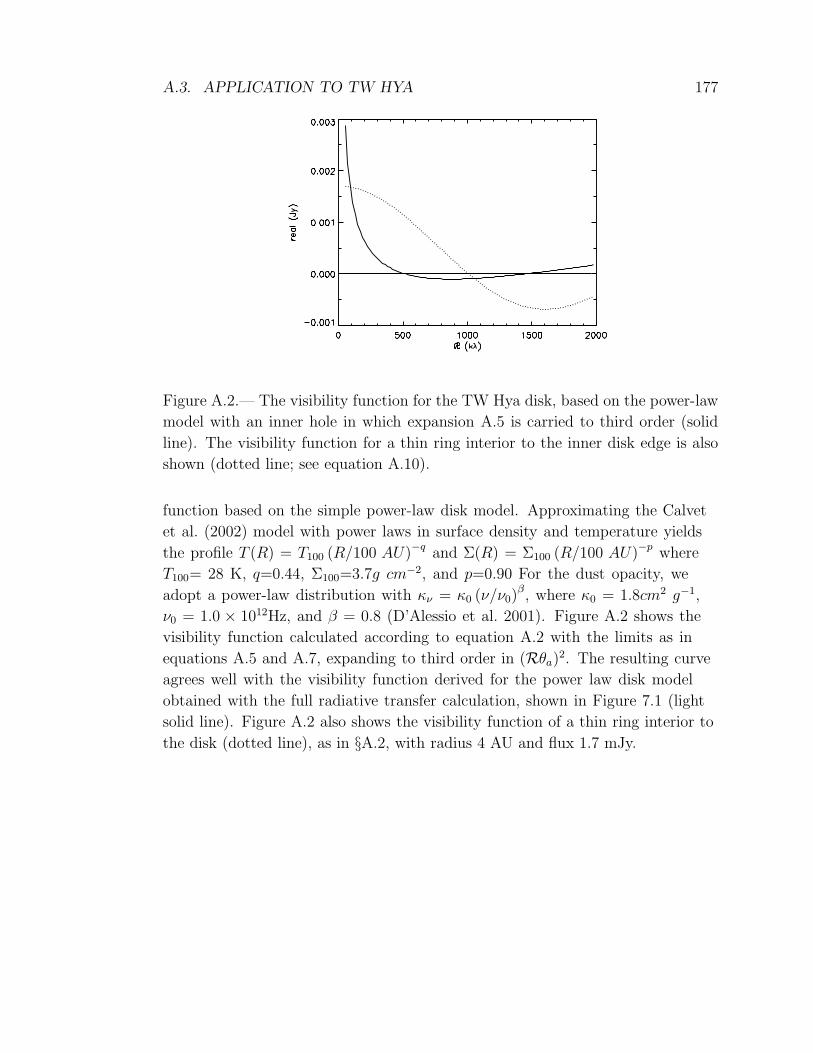
A.3. APPLICATION TO TW HYA 177
Figure A.2.— The visibility function for the TW Hya disk, based on the power-law
model with an inner hole in which expansion A.5 is carried to third order (solid
line). The visibility function for a thin ring interior to the inner disk edge is also
shown (dotted line; see equation A.10).
function based on the simple power-law disk model. Approximating the Calvet
et al. (2002) model with power laws in surface density and temperature yields
the profile T (R) = T100 (R/100 AU)−q and Σ(R) = Σ100 (R/100 AU)−p where
T100= 28 K, q=0.44, Σ100=3.7g cm−2, and p=0.90 For the dust opacity, we
adopt a power-law distribution with κν = κ0 (ν/ν0)β, where κ0 = 1.8cm2 g−1,
ν0 = 1.0 × 10¹²Hz, and β = 0.8 (D’Alessio et al. 2001). Figure A.2 shows the
visibility function calculated according to equation A.2 with the limits as in
equations A.5 and A.7, expanding to third order in (Rθa)2. The resulting curve
agrees well with the visibility function derived for the power law disk model
obtained with the full radiative transfer calculation, shown in Figure 7.1 (light
solid line). Figure A.2 also shows the visibility function of a thin ring interior to
the disk (dotted line), as in §A.2, with radius 4 AU and flux 1.7 mJy.

178 APPENDIX A. PROTOPLANETARY DISK VISIBILITY FUNCTIONS

Appendix B
Supplementary Disk Polarimetry
We present polarimetric observations of two additional systems not discussed
in Chapter 7: GM Aurigae and MWC 480. These systems were selected on
the basis of their 880µm brightness and also, in the case of GM Aur, because
of the tentative detection of polarized 850µm emission reported by Tamura
et al. (1999). Here we report on the arcsecond-scale SMA observations of these
systems, which yield upper limits on the polarization fraction comparable to those
reported for HD 163296 and TW Hya in Chapter 7. By doubling the sample
size of circumstellar disks observed with the SMA polarimeter, we strengthen our
conclusion that the polarization fraction of disks is substantially lower than the
2-3% expected based on the results of Tamura et al. (1999) and Cho & Lazarian
(2007).
B.1 Observations
We conducted observations of GM Aur with the SMA polarimeter on the night
of 2009 November 6. The array was in the compact-north configuration, with
baseline lengths between 16 and 123m and the longest baselines along the
north-south direction. The weather was good, with the 225GHz opacity at
around 0.07 and the atmospheric phase remaining steady over the course of the
night. MWC 480 was observed on the night of 2009 December 11 in similarly
good weather with stable phase and 225GHz opacity of 0.06. The array was in
the compact configuration for the MWC 480 observations, with baseline lengths
between 16 and 77m.
The data were collected with the receivers tuned to a frequency of 341GHz.
179

180 APPENDIX B. SUPPLEMENTARY DISK POLARIMETRY
These observations differ from those described in Chapter 7 in that a new double-
bandwidth observing mode was introduced on the SMA in the intervening period.
Effectively, this doubles the bandwidth of each sideband from 2GHz to 4GHz,
increasing the sensitivity of the continuum observations by a factor of slightly
less than√
2 (due to lower sensitivity in the upper 2GHz of each sideband). We
use a uniform correlator configuration that divides each 104MHz-wide correlator
chunk into 128 channels to achieve maximum continuum sensitivity at the highest
possible uniform spectral resolution (0.7 km s−1).
For both sources, the quasar 3c111 served as the atmospheric and instrumental
gain calibrator, while J0510+180 was included in the observing loop to test the
quality of the phase transfer. Callisto was observed near the beginning of each
track to determine the absolute flux scale, and Titan was also included at the end
of the MWC 480 track; we derive fluxes of 1.09 and 1.52 Jy for 3c111 on the nights
of November 6 and December 11, respectively. The instrumental polarization
calibration was carried out as described in Chapter 7, by observing 3c273 and
3c279 in the hours before and after transit. We derive consistent instrumental
leakage solutions for both sources, and adopt the solutions from the brighter
3c273. 3c111, J0510+180, Callisto, 3c273, and 3c279 were used as passband
calibrators. The passband, gain, and instrumental polarization calibrations were
carried out independently for each 2GHz segment of each sideband.
The data were edited and calibrated with the MIR software package, and the
standard tasks of inversion and beam deconvolution were carried out using the
MIRIAD software package.
B.2 Results and Analysis
We detect no polarized CO(3-2) line or continuum emission from the disks around
GM Aur and MWC 480. The measured Stokes I fluxes and Stokes Q & U upper
limits are listed in Table B.1. The same table notes apply as in Table 7.1.
As in Chapter 7, we generate initial models of the disk temperature and
surface density structure that allow us to reproduce the Stokes I continuum
data. We then use these models as inputs to the Cho & Lazarian (2007) code to
predict the magnitude of polarized flux that should be observed in Stokes Q and
U . Table B.2 gives the model parameters with references. Figures B.1 and B.2
show a comparison between the data and the polarization properties predicted by
the Cho & Lazarian (2007) code for GM Aur and MWC 480, respectively. The

B.2. RESULTS AND ANALYSIS 181
Table B.1: Observational Parameters
GM Aur MWC 480
Com-N Compact
341GHz Continuum
Beam Size (FWHM) 2.′′0×1.′′3 2.′′6×2.′′1
P.A. 56 12
RMS Noise (mJybeam−1)
Stokes I 12 13
Stokes Q & U 2.8 3.1
Peak Flux Density (mJybeam−1)
Stokes I 360 880
Stokes Q & U (3σ upper limit) ≤8 ≤9
Integrated Flux (Stokes I; Jy) 0.53 0.95
CO(3-2) Line
Beam Size (FWHM) 2.′′1×1.′′3 2.′′5×2.′′2
P.A. 75 35
RMS Noise (Jy beam−1)
Stokes I 0.17 0.28
Stokes Q & U 0.17 0.23
Peak Flux Density (Jy beam−1)
Stokes I 4.6 5.4
Stokes Q & U (3σ upper limit) ≤0.5 ≤0.7
Integrated Flux (Stokes I; Jy km s−1) 49 23
182 APPENDIX B. SUPPLEMENTARY DISK POLARIMETRY
Table B.2: Model Parameters
GM Aur MWC 480
Parameter Value Ref. Value Ref.
T∗ (K) 4000 1 8460 2
R∗ (R⊙) 1.7 1 1.6 2
M∗ (M⊙) 0.84 3 1.65 4
p 1.1 5 1.0 6
ainner (AU) 20 5 0.1a –
a0 (AU) 300 5 275 6
rmax,i (µm) 103 5 103 6
i 56 3 37 7
d (pc) 140 8 140 8
Σ0 (g cm−2) 175 – 275 –
aEstimated dust destruction radius
References. — (1) Beckwith et al. (1990); (2) Kenyon & Hartmann (1995); (3) Dutrey
et al. (1998); (4) Simon et al. (2000); (5) Hughes et al. (2009a); (6) Hughes et al. (2008b); (7)
Hamidouche et al. (2006); (8) Elias (1978)
symbols are as in Figure 7.2. Just as for the HD 163296 and TW Hya systems,
the theory substantially overpredicts the upper limit on the polarized flux. While
we would expect to detect polarized emission at the 7 and 5σ levels for GM Aur
and MWC 480, respectively, we detect no polarized 880µm emission from either
system.
B.3 Discussion and Conclusions
The non-detection of polarized continuum emission from the disks around
GM Aurigae and MWC 480 supports the conclusions reached in Chapter 7. The
upper limits for these systems are less significant than those for HD 163296 and
TW Hya, largely due to the fainter Stokes I continuum emission from GM Aur
and MWC 480, which means that observations comparably sensitive in flux
are less sensitive in percentage of unpolarized light. Nevertheless, the 2-3%
polarization fraction indicated by the work of Cho & Lazarian (2007) and Tamura
et al. (1999) is ruled out at the 5 and 7σ level by these observations, strengthening

B.3. DISCUSSION AND CONCLUSIONS 183
Figure B.1.— Comparison between the Cho & Lazarian (2007) model and the
SMA 341GHz observations of GM Aur. The top row shows the prediction for the
model at full resolution (left), a simulated observation of the model with the SMA
(center), and the SMA observations (right). The grayscale shows either the total
flux (left) or the polarized flux (center, right), and the blue vectors indicate the
percentage and direction of polarized flux at half-beam intervals. The center and
bottom rows compare the model prediction (center) with the observed SMA data
(bottom) in each of the four Stokes parameters (I, Q, U , V , from left to right).
Contour levels are the same in both rows, either multiples of 20% of the peak flux
(0.34 Jy/beam) in Stokes I or in increments of 2σ for Q, U , and V , where σ is the
rms noise of 2.8mJy/beam. The size and orientation of the synthesized beam is
indicated in the lower left of each panel.
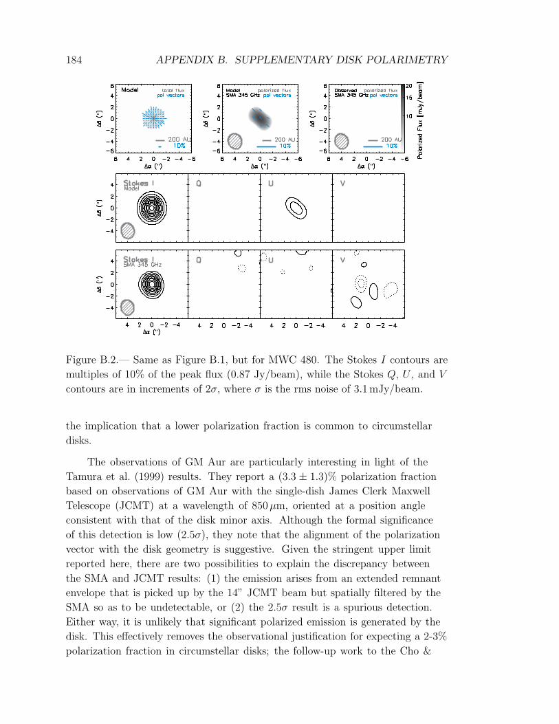
184 APPENDIX B. SUPPLEMENTARY DISK POLARIMETRY
Figure B.2.— Same as Figure B.1, but for MWC 480. The Stokes I contours are
multiples of 10% of the peak flux (0.87 Jy/beam), while the Stokes Q, U , and V
contours are in increments of 2σ, where σ is the rms noise of 3.1mJy/beam.
the implication that a lower polarization fraction is common to circumstellar
disks.
The observations of GM Aur are particularly interesting in light of the
Tamura et al. (1999) results. They report a (3.3 ± 1.3)% polarization fraction
based on observations of GM Aur with the single-dish James Clerk Maxwell
Telescope (JCMT) at a wavelength of 850µm, oriented at a position angle
consistent with that of the disk minor axis. Although the formal significance
of this detection is low (2.5σ), they note that the alignment of the polarization
vector with the disk geometry is suggestive. Given the stringent upper limit
reported here, there are two possibilities to explain the discrepancy between
the SMA and JCMT results: (1) the emission arises from an extended remnant
envelope that is picked up by the 14” JCMT beam but spatially filtered by the
SMA so as to be undetectable, or (2) the 2.5σ result is a spurious detection.
Either way, it is unlikely that significant polarized emission is generated by the
disk. This effectively removes the observational justification for expecting a 2-3%
polarization fraction in circumstellar disks; the follow-up work to the Cho &
B.3. DISCUSSION AND CONCLUSIONS 185
Lazarian (2007) result (Lazarian & Hoang 2007; Hoang & Lazarian 2009) weakens
the theoretical justification by predicting a smaller alignment efficiency for large
grains than that assumed in the original analysis (see Section 7.4.2).
Based on the increased sample size of disks exhibiting low 880µm polarization
fractions, as well as the non-detection of polarized emission at predicted levels
from GM Aur, we conclude that a low polarization fraction (.0.5%) is likely
common to circumstellar disks.

186 APPENDIX B. SUPPLEMENTARY DISK POLARIMETRY
Appendix C
High Spectral Resolution Channel
Maps
Figures C.1 and C.2 show the full channel maps for the high spectral resolution
observations of the CO(3-2) emission from the disks around TW Hya and HD
163296. The line overlaid on the emission indicates the disk major axis. The TW
Hya and HD 163296 maps have been imaged with Gaussian tapers of 1.′′2 and 1.′′0,
respectively, to bring out the large-scale emission.
187

188 APPENDIX C. HIGH SPECTRAL RESOLUTION CHANNEL MAPS
Figure C.1.— Channel maps of the CO(3-2) line emission from the disk around
HD 163296. The LSR velocity is indicated in the upper right of each channel, while
the synthesized beam size and orientation (2.′′0×1.′′7 at a position angle of 41) is
indicated in the lower left panel. The contour levels start at 2σ and increase
by factors of√
2, where σ is the rms noise of 0.6 Jy beam−1. The star symbol
indicates the disk center while the dark solid line indicates the disk position angle
as determined by CO fitting in Section 8.4.

189
Figure C.1 (Continued)

190 APPENDIX C. HIGH SPECTRAL RESOLUTION CHANNEL MAPS
Figure C.1 (Continued)

191
Figure C.1 (Continued)

192 APPENDIX C. HIGH SPECTRAL RESOLUTION CHANNEL MAPS
Figure C.2.— Same as Figure C.1 above, but for TW Hya. The beam size is
1.′′9×1.′′4 at a position angle of 21 and the contour levels are the same as in Fig-
ure C.1.
References
Aannestad, P. A. & Purcell, E. M. 1973, ARA&A, 11, 309
Adams, F. C., Hollenbach, D., Laughlin, G., & Gorti, U. 2004, ApJ, 611,
360
Adams, F. C., Lada, C. J., & Shu, F. H. 1987, ApJ, 312, 788
Adams, F. C. & Shu, F. H. 1986, ApJ, 308, 836
Aikawa, Y. 2007, ApJ, 656, L93
Aitken, D. K., Efstathiou, A., McCall, A., & Hough, J. H. 2002, MNRAS,
329, 647
Alexander, R. D. & Armitage, P. J. 2007, MNRAS, 375, 500
Alexander, R. D., Clarke, C. J., & Pringle, J. E. 2006, MNRAS, 369, 229
Andrews, S. M., Czekala, I., Wilner, D. J., Espaillat, C., Dullemond, C. P.,
& Hughes, A. M. 2010, ApJ, 710, 462
Andrews, S. M. & Williams, J. P. 2005, ApJ, 631, 1134
—. 2007, ApJ, 659, 705
Andrews, S. M., Wilner, D. J., Hughes, A. M., Qi, C., & Dullemond, C. P.
2009, ApJ, 700, 1502
Artymowicz, P. 1987, Icarus, 70, 303
Aumann, H. H., Beichman, C. A., Gillett, F. C., de Jong, T., Houck, J. R.,
Low, F. J., Neugebauer, G., Walker, R. G., & Wesselius, P. R. 1984, ApJ,
278, L23
Balbus, S. A. & Hawley, J. F. 1991, ApJ, 376, 214
193

194 REFERENCES
—. 1998, Reviews of Modern Physics, 70, 1
Balbus, S. A., Hawley, J. F., & Stone, J. M. 1996, ApJ, 467, 76
Balsara, D. S., Tilley, D. A., Rettig, T., & Brittain, S. D. 2009, MNRAS,
397, 24
Barrado y Navascues, D., Stauffer, J. R., Song, I., & Caillault, J.-P. 1999,
ApJ, 520, L123
Beckwith, S., Gatley, I., Matthews, K., & Neugebauer, G. 1978, ApJ, 223,
L41
Beckwith, S. V. W. & Sargent, A. I. 1991, ApJ, 381, 250
Beckwith, S. V. W., Sargent, A. I., Chini, R. S., & Guesten, R. 1990, AJ,
99, 924
Bergin, E., Calvet, N., Sitko, M. L., Abgrall, H., D’Alessio, P., Herczeg,
G. J., Roueff, E., Qi, C., Lynch, D. K., Russell, R. W., Brafford, S. M., &
Perry, R. B. 2004, ApJ, 614, L133
Bertout, C. & Genova, F. 2006, A&A, 460, 499
Bockelee-Morvan, D., Andre, P., Colom, P., Colas, F., Crovisier, J., Despois,
D., & Jorda, L. 1994, in Circumstellar Dust Disks and Planet Formation,
ed. R. Ferlet & A. Vidal-Madjar, 341–+
Boss, A. P. 2004, ApJ, 616, 1265
Boss, A. P. & Yorke, H. W. 1993, ApJ, 411, L99
—. 1996, ApJ, 469, 366
Bouvier, J., Bertout, C., Benz, W., & Mayor, M. 1986, A&A, 165, 110
Bouwman, J., Henning, T., Hillenbrand, L. A., Meyer, M. R., Pascucci, I.,
Carpenter, J., Hines, D., Kim, J. S., Silverstone, M. D., Hollenbach, D., &
Wolf, S. 2008, ApJ, 683, 479
Brittain, S. D., Simon, T., Najita, J. R., & Rettig, T. W. 2007, ApJ, 659,
685
Brown, A., Jordan, C., Millar, T. J., Gondhalekar, P., & Wilson, R. 1981,
Nature, 290, 34

REFERENCES 195
Brown, J. M., Blake, G. A., Dullemond, C. P., Merın, B., Augereau, J. C.,
Boogert, A. C. A., Evans, II, N. J., Geers, V. C., Lahuis, F., Kessler-Silacci,
J. E., Pontoppidan, K. M., & van Dishoeck, E. F. 2007, ApJ, 664, L107
Brown, J. M., Blake, G. A., Qi, C., Dullemond, C. P., & Wilner, D. J. 2008,
ApJ, 675, L109
Brown, J. M., Blake, G. A., Qi, C., Dullemond, C. P., Wilner, D. J., &
Williams, J. P. 2009, ApJ, 704, 496
Bryden, G., Chen, X., Lin, D. N. C., Nelson, R. P., & Papaloizou, J. C. B.
1999, ApJ, 514, 344
Butler, R. P., Wright, J. T., Marcy, G. W., Fischer, D. A., Vogt, S. S.,
Tinney, C. G., Jones, H. R. A., Carter, B. D., Johnson, J. A., McCarthy,
C., & Penny, A. J. 2006, ApJ, 646, 505
Calvet, N., D’Alessio, P., Hartmann, L., Wilner, D., Walsh, A., & Sitko, M.
2002, ApJ, 568, 1008
Calvet, N., D’Alessio, P., Watson, D. M., Franco-Hernandez, R., Furlan,
E., Green, J., Sutter, P. M., Forrest, W. J., Hartmann, L., Uchida, K. I.,
Keller, L. D., Sargent, B., Najita, J., Herter, T. L., Barry, D. J., & Hall, P.
2005, ApJ, 630, L185
Calvet, N., Muzerolle, J., Briceno, C., Hernandez, J., Hartmann, L.,
Saucedo, J. L., & Gordon, K. D. 2004, AJ, 128, 1294
Carballido, A., Fromang, S., & Papaloizou, J. 2006, MNRAS, 373, 1633
Cardelli, J. A., Clayton, G. C., & Mathis, J. S. 1989, ApJ, 345, 245
Carmona, A., van den Ancker, M. E., Henning, T., Goto, M., Fedele, D., &
Stecklum, B. 2007, ArXiv e-prints, 710
Carpenter, J. M., Bouwman, J., Silverstone, M. D., Kim, J. S., Stauffer, J.,
Cohen, M., Hines, D. C., Meyer, M. R., & Crockett, N. 2008, ApJS, 179,
423
Carpenter, J. M., Wolf, S., Schreyer, K., Launhardt, R., & Henning, T.
2005, AJ, 129, 1049
Carr, J. S. 1990, AJ, 100, 1244
Carr, J. S., Tokunaga, A. T., & Najita, J. 2004, ApJ, 603, 213

196 REFERENCES
Chambers, J. E. 2006, ApJ, 652, L133
Chandrasekhar, S. 1960, Proceedings of the National Academy of Science,
46, 253
Chen, C. H., Sargent, B. A., Bohac, C., Kim, K. H., Leibensperger, E.,
Jura, M., Najita, J., Forrest, W. J., Watson, D. M., Sloan, G. C., & Keller,
L. D. 2006, ApJS, 166, 351
Chiang, E. & Murray-Clay, R. 2007, Nature Physics, 3, 604
Chiang, E. I. & Goldreich, P. 1997, ApJ, 490, 368
—. 1999, ApJ, 519, 279
Chiang, E. I., Joung, M. K., Creech-Eakman, M. J., Qi, C., Kessler, J. E.,
Blake, G. A., & van Dishoeck, E. F. 2001, ApJ, 547, 1077
Cho, J. & Lazarian, A. 2005, ApJ, 631, 361
—. 2007, ApJ, 669, 1085
Ciesla, F. J. 2007, Science, 318, 613
Cieza, L., Padgett, D. L., Stapelfeldt, K. R., Augereau, J., Harvey, P.,
Evans, II, N. J., Merın, B., Koerner, D., Sargent, A., van Dishoeck, E. F.,
Allen, L., Blake, G., Brooke, T., Chapman, N., Huard, T., Lai, S., Mundy,
L., Myers, P. C., Spiesman, W., & Wahhaj, Z. 2007, ApJ, 667, 308
Clarke, C. J., Gendrin, A., & Sotomayor, M. 2001, MNRAS, 328, 485
Collins, K. A., Grady, C. A., Hamaguchi, K., Wisniewski, J. P., Brittain,
S., Sitko, M., Carpenter, W. J., Williams, J. P., Mathews, G. S., Williger,
G. M., van Boekel, R., Carmona, A., Henning, T., van den Ancker, M. E.,
Meeus, G., Chen, X. P., Petre, R., & Woodgate, B. E. 2009, ApJ, 697, 557
Cortes, S. R., Meyer, M. R., Carpenter, J. M., Pascucci, I., Schneider, G.,
Wong, T., & Hines, D. C. 2009, ApJ, 697, 1305
D’Alessio, P. 2009, in Revista Mexicana de Astronomia y Astrofisica
Conference Series, Vol. 35, Revista Mexicana de Astronomia y Astrofisica
Conference Series, 33–38
D’Alessio, P., Calvet, N., & Hartmann, L. 1997, ApJ, 474, 397
—. 2001, ApJ, 553, 321
REFERENCES 197
D’Alessio, P., Calvet, N., Hartmann, L., Franco-Hernandez, R., & Servın,
H. 2006, ApJ, 638, 314
D’Alessio, P., Calvet, N., Hartmann, L., Lizano, S., & Canto, J. 1999, ApJ,
527, 893
D’Alessio, P., Canto, J., Calvet, N., & Lizano, S. 1998, ApJ, 500, 411
D’Alessio, P., Hartmann, L., Calvet, N., Franco-Hernandez, R., Forrest,
W. J., Sargent, B., Furlan, E., Uchida, K., Green, J. D., Watson, D. M.,
Chen, C. H., Kemper, F., Sloan, G. C., & Najita, J. 2005, ApJ, 621, 461
Dartois, E., Dutrey, A., & Guilloteau, S. 2003, A&A, 399, 773
de Val-Borro, M., Edgar, R. G., Artymowicz, P., Ciecielag, P., Cresswell,
P., D’Angelo, G., Delgado-Donate, E. J., Dirksen, G., Fromang, S.,
Gawryszczak, A., Klahr, H., Kley, W., Lyra, W., Masset, F., Mellema, G.,
Nelson, R. P., Paardekooper, S., Peplinski, A., Pierens, A., Plewa, T., Rice,
K., Schafer, C., & Speith, R. 2006, MNRAS, 370, 529
Dent, W. R. F., Greaves, J. S., & Coulson, I. M. 2005, MNRAS, 359, 663
Dolginov, A. Z. 1972, Ap&SS, 18, 337
Dolginov, A. Z. & Mitrofanov, I. G. 1976, Ap&SS, 43, 291
Draine, B. T. & Lee, H. M. 1984, ApJ, 285, 89
Draine, B. T. & Weingartner, J. C. 1996, ApJ, 470, 551
Dubrulle, B., Dauchot, O., Daviaud, F., Longaretti, P., Richard, D., &
Zahn, J. 2005, Physics of Fluids, 17, 095103
Dullemond, C. P. & Dominik, C. 2004a, A&A, 417, 159
—. 2004b, A&A, 421, 1075
—. 2005, A&A, 434, 971
Dullemond, C. P., Dominik, C., & Natta, A. 2001, ApJ, 560, 957
Dullemond, C. P., van Zadelhoff, G. J., & Natta, A. 2002, A&A, 389, 464
Dutrey, A., Guilloteau, S., Duvert, G., Prato, L., Simon, M., Schuster, K.,
& Menard, F. 1996, A&A, 309, 493

198 REFERENCES
Dutrey, A., Guilloteau, S., & Ho, P. 2007, in Protostars and Planets V, ed.
B. Reipurth, D. Jewitt, & K. Keil, 495–506
Dutrey, A., Guilloteau, S., Pietu, V., Chapillon, E., Gueth, F., Henning,
T., Launhardt, R., Pavlyuchenkov, Y., Schreyer, K., & Semenov, D. 2008,
A&A, 490, L15
Dutrey, A., Guilloteau, S., Prato, L., Simon, M., Duvert, G., Schuster, K.,
& Menard, F. 1998, A&A, 338, L63
Dutrey, A., Guilloteau, S., & Simon, M. 1994, A&A, 286, 149
Edgar, R. G., Quillen, A. C., & Park, J. 2007, MNRAS, 381, 1280
Eisner, J. A., Chiang, E. I., & Hillenbrand, L. A. 2006, ApJ, 637, L133
Elias, J. H. 1978, ApJ, 224, 857
Espaillat, C., Calvet, N., D’Alessio, P., Hernandez, J., Qi, C., Hartmann,
L., Furlan, E., & Watson, D. M. 2007, ApJ, 670, L135
Espaillat, C., Calvet, N., Luhman, K. L., Muzerolle, J., & D’Alessio, P.
2008, ApJ, 682, L125
Fleming, T. & Stone, J. M. 2003, ApJ, 585, 908
Fromang, S. 2005, A&A, 441, 1
Fromang, S. & Nelson, R. P. 2006, A&A, 457, 343
—. 2009, A&A, 496, 597
Fromang, S. & Papaloizou, J. 2007, A&A, 476, 1113
Gammie, C. F. 1996, ApJ, 457, 355
Gammie, C. F. & Johnson, B. M. 2005, in Astronomical Society of the
Pacific Conference Series, Vol. 341, Chondrites and the Protoplanetary
Disk, ed. A. N. Krot, E. R. D. Scott, & B. Reipurth, 145–+
Girart, J. M., Rao, R., & Marrone, D. P. 2006, Science, 313, 812
Glassgold, A. E., Najita, J., & Igea, J. 2004, ApJ, 615, 972
Goldreich, P. & Kylafis, N. D. 1981, ApJ, 243, L75
—. 1982, ApJ, 253, 606
REFERENCES 199
Gomez, M., Hartmann, L., Kenyon, S. J., & Hewett, R. 1993, AJ, 105, 1927
Goto, M., Usuda, T., Dullemond, C. P., Henning, T., Linz, H., Stecklum,
B., & Suto, H. 2006, ApJ, 652, 758
Grady, C. A., Devine, D., Woodgate, B., Kimble, R., Bruhweiler, F. C.,
Boggess, A., Linsky, J. L., Plait, P., Clampin, M., & Kalas, P. 2000, ApJ,
544, 895
Greenberg, J. M. Interstellar Grains, ed. B. M. Middlehurst & L. H. Aller
(the University of Chicago Press), 221–+
Guilloteau, S. & Dutrey, A. 1998, A&A, 339, 467
Gullbring, E., Hartmann, L., Briceno, C., & Calvet, N. 1998, ApJ, 492, 323
Habing, H. J. 1968, Bull. Astron. Inst. Netherlands, 19, 421
Hamidouche, M., Looney, L. W., & Mundy, L. G. 2006, ApJ, 651, 321
Hartmann, L., Calvet, N., Gullbring, E., & D’Alessio, P. 1998, ApJ, 495,
385
Hartmann, L., Hewett, R., Stahler, S., & Mathieu, R. D. 1986, ApJ, 309,
275
Hartmann, L., Hinkle, K., & Calvet, N. 2004, ApJ, 609, 906
Hartmann, L., Megeath, S. T., Allen, L., Luhman, K., Calvet, N., D’Alessio,
P., Franco-Hernandez, R., & Fazio, G. 2005, ApJ, 629, 881
Herczeg, G. J., Wood, B. E., Linsky, J. L., Valenti, J. A., & Johns-Krull,
C. M. 2004, ApJ, 607, 369
Hersant, F., Dubrulle, B., & Hure, J. 2005, A&A, 429, 531
Hildebrand, R. H., Davidson, J. A., Dotson, J. L., Dowell, C. D., Novak,
G., & Vaillancourt, J. E. 2000, PASP, 112, 1215
Hildebrand, R. H. & Dragovan, M. 1995, ApJ, 450, 663
Ho, P. T. P., Moran, J. M., & Lo, K. Y. 2004, ApJ, 616, L1
Hoang, T. & Lazarian, A. 2008, MNRAS, 388, 117
—. 2009, ApJ, 697, 1316

200 REFERENCES
Hoff, W., Henning, T., & Pfau, W. 1998, A&A, 336, 242
Hoffleit, D. & Jaschek, C. . 1991, The Bright star catalogue (New Haven,
Conn.: Yale University Observatory, —c1991, 5th rev.ed., edited by Hoffleit,
Dorrit; Jaschek, Carlos —v(coll.))
Hogerheijde, M. R. & van der Tak, F. F. S. 2000, A&A, 362, 697
Holland, W. S., Greaves, J. S., Zuckerman, B., Webb, R. A., McCarthy, C.,
Coulson, I. M., Walther, D. M., Dent, W. R. F., Gear, W. K., & Robson, I.
1998, Nature, 392, 788
Hollenbach, D., Johnstone, D., Lizano, S., & Shu, F. 1994, ApJ, 428, 654
Hubrig, S., Stelzer, B., Scholler, M., Grady, C., Schutz, O., Pogodin, M. A.,
Cure, M., Hamaguchi, K., & Yudin, R. V. 2009, A&A, 502, 283
Hughes, A. M., Andrews, S. M., Espaillat, C., Wilner, D. J., Calvet, N.,
D’Alessio, P., Qi, C., Williams, J. P., & Hogerheijde, M. R. 2009a, ApJ,
698, 131
Hughes, A. M., Wilner, D. J., Calvet, N., D’Alessio, P., Claussen, M. J., &
Hogerheijde, M. R. 2007, ApJ, 664, 536
Hughes, A. M., Wilner, D. J., Cho, J., Marrone, D. P., Lazarian, A.,
Andrews, S. M., & Rao, R. 2009b, ApJ, 704, 1204
Hughes, A. M., Wilner, D. J., Kamp, I., & Hogerheijde, M. R. 2008a, ApJ,
681, 626
Hughes, A. M., Wilner, D. J., Qi, C., & Hogerheijde, M. R. 2008b, ApJ,
678, 1119
Igea, J. & Glassgold, A. E. 1999, ApJ, 518, 848
Ingleby, L. & Calvet, N. 2009, ApJ, submitted
Ireland, M. J. & Kraus, A. L. 2008, ApJ, 678, L59
Isella, A., Carpenter, J. M., & Sargent, A. I. 2009, ApJ, 701, 260
Isella, A., Testi, L., & Natta, A. 2006, A&A, 451, 951
Isella, A., Testi, L., Natta, A., Neri, R., Wilner, D., & Qi, C. 2007, A&A,
469, 213

REFERENCES 201
Jewitt, D., Luu, J., & Trujillo, C. 1998, AJ, 115, 2125
Johansen, A. & Klahr, H. 2005, ApJ, 634, 1353
Johansen, A., Oishi, J. S., Low, M.-M. M., Klahr, H., Henning, T., &
Youdin, A. 2007, Nature, 448, 1022
Jonkheid, B., Dullemond, C. P., Hogerheijde, M. R., & van Dishoeck, E. F.
2007, A&A, 463, 203
Jonkheid, B., Kamp, I., Augereau, J.-C., & van Dishoeck, E. F. 2006, A&A,
453, 163
Jura, M., Malkan, M., White, R., Telesco, C., Pina, R., & Fisher, R. S.
1998, ApJ, 505, 897
Jura, M., Zuckerman, B., Becklin, E. E., & Smith, R. C. 1993, ApJ, 418,
L37+
Kalas, P., Graham, J. R., Chiang, E., Fitzgerald, M. P., Clampin, M., Kite,
E. S., Stapelfeldt, K., Marois, C., & Krist, J. 2008, ArXiv e-prints
Kamp, I. & Bertoldi, F. 2000, A&A, 353, 276
Kamp, I. & Dullemond, C. P. 2004, ApJ, 615, 991
Kamp, I. & van Zadelhoff, G.-J. 2001, A&A, 373, 641
Kastner, J. H., Huenemoerder, D. P., Schulz, N. S., & Weintraub, D. A.
1999, ApJ, 525, 837
Kastner, J. H., Zuckerman, B., Weintraub, D. A., & Forveille, T. 1997,
Science, 277, 67
Kenyon, S. J. & Hartmann, L. 1987, ApJ, 323, 714
—. 1995, ApJS, 101, 117
Kim, J. S., Hines, D. C., Backman, D. E., Hillenbrand, L. A., Meyer,
M. R., Rodmann, J., Moro-Martın, A., Carpenter, J. M., Silverstone, M. D.,
Bouwman, J., Mamajek, E. E., Wolf, S., Malhotra, R., Pascucci, I., Najita,
J., Padgett, D. L., Henning, T., Brooke, T. Y., Cohen, M., Strom, S. E.,
Stobie, E. B., Engelbracht, C. W., Gordon, K. D., Misselt, K., Morrison,
J. E., Muzerolle, J., & Su, K. Y. L. 2005, ApJ, 632, 659
Kitamura, Y., Kawabe, R., & Saito, M. 1996, ApJ, 457, 277

202 REFERENCES
Kitamura, Y., Momose, M., Yokogawa, S., Kawabe, R., Tamura, M., & Ida,
S. 2002, ApJ, 581, 357
Koerner, D. W., Sargent, A. I., & Beckwith, S. V. W. 1993, Icarus, 106, 2
Kohler, R., Neuhauser, R., Kramer, S., Leinert, C., Ott, T., & Eckart, A.
2008, A&A, 488, 997
Kraus, A. L. & Hillenbrand, L. A. 2008, ApJ, 686, L111
Krauss, O. & Wurm, G. 2005, ApJ, 630, 1088
Krejny, M., Matthews, T., Novak, G., Cho, J., Li, H., Shinnaga, H., &
Vaillancourt, J. E. 2009, ArXiv e-prints
Krist, J. E., Stapelfeldt, K. R., Menard, F., Padgett, D. L., & Burrows,
C. J. 2000, ApJ, 538, 793
Lay, O. P., Carlstrom, J. E., & Hills, R. E. 1997, ApJ, 489, 917
Lay, O. P., Carlstrom, J. E., Hills, R. E., & Phillips, T. G. 1994, ApJ, 434,
L75
Lazarian, A. 2007, Journal of Quantitative Spectroscopy and Radiative
Transfer, 106, 225
Lazarian, A. & Hoang, T. 2007, ApJ, 669, L77
—. 2008, ApJ, 676, L25
Lee, H. M. & Draine, B. T. 1985, ApJ, 290, 211
Lin, D. N. C. & Papaloizou, J. 1986, ApJ, 309, 846
Lin, D. N. C. & Papaloizou, J. C. B. 1993, in Protostars and Planets III,
ed. E. H. Levy & J. I. Lunine, 749–835
Looney, L. W., Mundy, L. G., & Welch, W. J. 2000, ApJ, 529, 477
Lubow, S. H. & D’Angelo, G. 2006, ApJ, 641, 526
Lynden-Bell, D. & Pringle, J. E. 1974, MNRAS, 168, 603
Mamajek, E. E. 2005, ApJ, 634, 1385

REFERENCES 203
Mamajek, E. E. 2009, in American Institute of Physics Conference Series,
Vol. 1158, American Institute of Physics Conference Series, ed. T. Usuda,
M. Tamura, & M. Ishii, 3–10
Mannings, V. 1994, MNRAS, 271, 587
Mannings, V. & Sargent, A. I. 1997, ApJ, 490, 792
Marrone, D. P. 2006, PhD thesis, Harvard University
Marrone, D. P. & Rao, R. 2008, in Society of Photo-Optical Instrumentation
Engineers (SPIE) Conference Series, Vol. 7020, Society of Photo-Optical
Instrumentation Engineers (SPIE) Conference Series
Marsh, K. A. & Mahoney, M. J. 1992, ApJ, 395, L115
Marsh, K. A., Silverstone, M. D., Becklin, E. E., Koerner, D. W., Werner,
M. W., Weinberger, A. J., & Ressler, M. E. 2002, ApJ, 573, 425
Martin-Zaıdi, C., Deleuil, M., Simon, T., Bouret, J.-C., Roberge, A.,
Feldman, P. D., Lecavelier Des Etangs, A., & Vidal-Madjar, A. 2005, A&A,
440, 921
Mathis, J. S., Rumpl, W., & Nordsieck, K. H. 1977, ApJ, 217, 425
Matsumura, S., Pudritz, R. E., & Thommes, E. W. 2009, ApJ, 691, 1764
McCaughrean, M. J. & O’Dell, C. R. 1996, AJ, 111, 1977
Merın, B., Montesinos, B., Eiroa, C., Solano, E., Mora, A., D’Alessio, P.,
Calvet, N., Oudmaijer, R. D., de Winter, D., Davies, J. K., Harris, A. W.,
Cameron, A., Deeg, H. J., Ferlet, R., Garzon, F., Grady, C. A., Horne,
K., Miranda, L. F., Palacios, J., Penny, A., Quirrenbach, A., Rauer, H.,
Schneider, J., & Wesselius, P. R. 2004, A&A, 419, 301
Meyer, M. R., Hillenbrand, L. A., Backman, D., Beckwith, S., Bouwman,
J., Brooke, T., Carpenter, J., Cohen, M., Cortes, S., Crockett, N., Gorti, U.,
Henning, T., Hines, D., Hollenbach, D., Kim, J. S., Lunine, J., Malhotra, R.,
Mamajek, E., Metchev, S., Moro-Martin, A., Morris, P., Najita, J., Padgett,
D., Pascucci, I., Rodmann, J., Schlingman, W., Silverstone, M., Soderblom,
D., Stauffer, J., Stobie, E., Strom, S., Watson, D., Weidenschilling, S., Wolf,
S., & Young, E. 2006, PASP, 118, 1690
Mouillet, D., Larwood, J. D., Papaloizou, J. C. B., & Lagrange, A. M. 1997,
MNRAS, 292, 896

204 REFERENCES
Mulders, G. D., Dominik, C., & Min, M. 2010, ArXiv e-prints
Mundy, L. G., McMullin, J. P., Grossman, A. W., & Sandell, G. 1993,
Icarus, 106, 11
Muzerolle, J., Briceno, C., Calvet, N., Hartmann, L., Hillenbrand, L., &
Gullbring, E. 2000, ApJ, 545, L141
Najita, J. R., Strom, S. E., & Muzerolle, J. 2007, MNRAS, 378, 369
Natta, A., Testi, L., Neri, R., Shepherd, D. S., & Wilner, D. J. 2004, A&A,
416, 179
Nelson, R. P. & Papaloizou, J. C. B. 2003, MNRAS, 339, 993
—. 2004, MNRAS, 350, 849
Neuhauser, R., Walter, F. M., Covino, E., Alcala, J. M., Wolk, S. J., Frink,
S., Guillout, P., Sterzik, M. F., & Comeron, F. 2000, A&AS, 146, 323
Nomura, H., Aikawa, Y., Tsujimoto, M., Nakagawa, Y., & Millar, T. J.
2007, ApJ, 661, 334
Owen, J. E., Ercolano, B., Clarke, C. J., & Alexander, R. D. 2010, MNRAS,
401, 1415
Padoan, P., Goodman, A., Draine, B. T., Juvela, M., Nordlund, A., &
Rognvaldsson, O. E. 2001, ApJ, 559, 1005
Panic, O., Hogerheijde, M. R., Wilner, D., & Qi, C. 2008, A&A, 491, 219
Papaloizou, J. C. B. & Nelson, R. P. 2003, MNRAS, 339, 983
Papaloizou, J. C. B., Nelson, R. P., & Snellgrove, M. D. 2004, MNRAS,
350, 829
Pascucci, I., Hollenbach, D., Najita, J., Muzerolle, J., Gorti, U., Herczeg,
G. J., Hillenbrand, L. A., Kim, J. S., Carpenter, J. M., Meyer, M. R.,
Mamajek, E. E., & Bouwman, J. 2007, ApJ, 663, 383
Pessah, M. E., Chan, C., & Psaltis, D. 2007, ApJ, 668, L51
Petit, J.-M., Holman, M. J., Gladman, B. J., Kavelaars, J. J., Scholl, H., &
Loredo, T. J. 2006, MNRAS, 365, 429

REFERENCES 205
Pety, J. 2005, in SF2A-2005: Semaine de l’Astrophysique Francaise, ed.
F. Casoli, T. Contini, J. M. Hameury, & L. Pagani, 721–+
Pietu, V., Dutrey, A., & Guilloteau, S. 2007, A&A, 467, 163
Pietu, V., Guilloteau, S., & Dutrey, A. 2005, A&A, 443, 945
Pontoppidan, K. M., Blake, G. A., van Dishoeck, E. F., Smette, A., Ireland,
M. J., & Brown, J. 2008, ApJ, 684, 1323
Qi, C., Ho, P. T. P., Wilner, D. J., Takakuwa, S., Hirano, N., Ohashi, N.,
Bourke, T. L., Zhang, Q., Blake, G. A., Hogerheijde, M., Saito, M., Choi,
M., & Yang, J. 2004, ApJ, 616, L11
Qi, C., Wilner, D. J., Aikawa, Y., Blake, G. A., & Hogerheijde, M. R. 2008,
ApJ, 681, 1396
Qi, C., Wilner, D. J., Calvet, N., Bourke, T. L., Blake, G. A., Hogerheijde,
M. R., Ho, P. T. P., & Bergin, E. 2006, ApJ, 636, L157
Quillen, A. C. 2006, ApJ, 640, 1078
Ratzka, T., Leinert, C., Henning, T., Bouwman, J., Dullemond, C. P., &
Jaffe, W. 2007, A&A, 471, 173
Reipurth, B. 2005, in Astronomical Society of the Pacific Conference Series,
Vol. 341, Chondrites and the Protoplanetary Disk, ed. A. N. Krot, E. R. D.
Scott, & B. Reipurth, 54–+
Rettig, T. W., Haywood, J., Simon, T., Brittain, S. D., & Gibb, E. 2004,
ApJ, 616, L163
Rice, W. K. M., Armitage, P. J., Wood, K., & Lodato, G. 2006, MNRAS,
373, 1619
Rice, W. K. M., Wood, K., Armitage, P. J., Whitney, B. A., & Bjorkman,
J. E. 2003, MNRAS, 342, 79
Roberge, A., Weinberger, A. J., & Malumuth, E. M. 2005, ApJ, 622, 1171
Rodmann, J., Henning, T., Chandler, C. J., Mundy, L. G., & Wilner, D. J.
2006, A&A, 446, 211
Rogstad, D. H., Lockhart, I. A., & Wright, M. C. H. 1974, ApJ, 193, 309
Sadakane, K. & Nishida, M. 1986, PASP, 98, 685

206 REFERENCES
Salyk, C., Blake, G. A., Boogert, A. C. A., & Brown, J. M. 2007, ApJ, 655,
L105
—. 2009, ApJ, 699, 330
Sano, T., Miyama, S. M., Umebayashi, T., & Nakano, T. 2000, ApJ, 543,
486
Schneider, G., Wood, K., Silverstone, M. D., Hines, D. C., Koerner, D. W.,
Whitney, B. A., Bjorkman, J. E., & Lowrance, P. J. 2003, AJ, 125, 1467
Scholl, H., Cazenave, A., & Brahic, A. 1982, A&A, 112, 157
Semenov, D., Wiebe, D., & Henning, T. 2006, ApJ, 647, L57
Shakura, N. I. & Syunyaev, R. A. 1973, A&A, 24, 337
Shu, F. H., Galli, D., Lizano, S., Glassgold, A. E., & Diamond, P. H. 2007,
ApJ, 665, 535
Sicilia-Aguilar, A., Henning, T., & Hartmann, L. W. 2010, ApJ, 710, 597
Siess, L., Dufour, E., & Forestini, M. 2000, A&A, 358, 593
Simon, M., Dutrey, A., & Guilloteau, S. 2000, ApJ, 545, 1034
Simon, M. & Prato, L. 1995, ApJ, 450, 824
Sitko, M. L., Lynch, D. K., & Russell, R. W. 2000, AJ, 120, 2609
Skrutskie, M. F., Cutri, R. M., Stiening, R., Weinberg, M. D., Schneider, S.,
Carpenter, J. M., Beichman, C., Capps, R., Chester, T., Elias, J., Huchra,
J., Liebert, J., Lonsdale, C., Monet, D. G., Price, S., Seitzer, P., Jarrett, T.,
Kirkpatrick, J. D., Gizis, J. E., Howard, E., Evans, T., Fowler, J., Fullmer,
L., Hurt, R., Light, R., Kopan, E. L., Marsh, K. A., McCallon, H. L., Tam,
R., Van Dyk, S., & Wheelock, S. 2006, AJ, 131, 1163
Skrutskie, M. F., Dutkevitch, D., Strom, S. E., Edwards, S., Strom, K. M.,
& Shure, M. A. 1990, AJ, 99, 1187
Song, I., Sandell, G., & Friberg, P. 2004, in ASP Conf. Ser. 324: Debris
Disks and the Formation of Planets, ed. L. Caroff, L. J. Moon, D. Backman,
& E. Praton, 250–+
Stapelfeldt, K. & The WFPC2 Science Team. 1997, in Science with the
VLT Interferometer, ed. F. Paresce, 395–+

REFERENCES 207
Stauffer, J. R., Hartmann, L. W., & Barrado y Navascues, D. 1995, ApJ,
454, 910
Stone, J. M., Hawley, J. F., Gammie, C. F., & Balbus, S. A. 1996, ApJ,
463, 656
Strom, K. M., Strom, S. E., Edwards, S., Cabrit, S., & Skrutskie, M. F.
1989, AJ, 97, 1451
Sylvester, R. J., Skinner, C. J., Barlow, M. J., & Mannings, V. 1996,
MNRAS, 279, 915
Tamura, M., Hough, J. H., Greaves, J. S., Morino, J.-I., Chrysostomou, A.,
Holland, W. S., & Momose, M. 1999, ApJ, 525, 832
Tamura, M., Hough, J. H., & Hayashi, S. S. 1995, ApJ, 448, 346
The, P. S., de Winter, D., & Perez, M. R. 1994, A&AS, 104, 315
Thi, W. F., Blake, G. A., van Dishoeck, E. F., van Zadelhoff, G. J., Horn,
J. M. M., Becklin, E. E., Mannings, V., Sargent, A. I., van den Ancker,
M. E., & Natta, A. 2001a, Nature, 409, 60
Thi, W. F., van Dishoeck, E. F., Blake, G. A., van Zadelhoff, G. J., Horn,
J., Becklin, E. E., Mannings, V., Sargent, A. I., van den Ancker, M. E.,
Natta, A., & Kessler, J. 2001b, ApJ, 561, 1074
Trilling, D. E., Koerner, D. W., Barnes, J. W., Ftaclas, C., & Brown, R. H.
2001, ApJ, 552, L151
Trujillo, C. A. & Brown, M. E. 2001, ApJ, 554, L95
Turner, N. J., Sano, T., & Dziourkevitch, N. 2007, ApJ, 659, 729
Uchida, K. I., Calvet, N., Hartmann, L., Kemper, F., Forrest, W. J.,
Watson, D. M., D’Alessio, P., Chen, C. H., Furlan, E., Sargent, B., Brandl,
B. R., Herter, T. L., Morris, P., Myers, P. C., Najita, J., Sloan, G. C.,
Barry, D. J., Green, J., Keller, L. D., & Hall, P. 2004, ApJS, 154, 439
Uzpen, B., Kobulnicky, H. A., Semler, D. R., Bensby, T., & Thom, C. 2008,
ApJ, 685, 1157
van den Ancker, M. E., de Winter, D., & Tjin A Djie, H. R. E. 1998a, A&A,
330, 145

208 REFERENCES
—. 1998b, A&A, 330, 145
van Dishoeck, E. F., Thi, W., & van Zadelhoff, G. 2003, A&A, 400, L1
Varniere, P., Blackman, E. G., Frank, A., & Quillen, A. C. 2006, ApJ, 640,
1110
Velikhov, E. P. 1959, Soviet Phys. JETP, 36, 1398
Vrba, F. J., Coyne, G. V., & Tapia, S. 1993, AJ, 105, 1010
Wahhaj, Z., Koerner, D. W., & Sargent, A. I. 2007, ArXiv Astrophysics
e-prints
Wang, Y., Jaffe, D. T., Graf, U. U., & Evans, II, N. J. 1994, ApJS, 95, 503
Wardle, M. 2007, Ap&SS, 311, 35
Weaver, W. B. & Jones, G. 1992, ApJS, 78, 239
Webb, R. A., Zuckerman, B., Platais, I., Patience, J., White, R. J.,
Schwartz, M. J., & McCarthy, C. 1999, ApJ, 512, L63
Weidenschilling, S. J. 1977, Ap&SS, 51, 153
—. Formation processes and time scales for meteorite parent bodies, ed.
J. F. Kerridge & M. S. Matthews, 348–371
Weidenschilling, S. J., Spaute, D., Davis, D. R., Marzari, F., & Ohtsuki, K.
1997, Icarus, 128, 429
Weinberger, A. J., Becklin, E. E., Schneider, G., Chiang, E. I., Lowrance,
P. J., Silverstone, M., Zuckerman, B., Hines, D. C., & Smith, B. A. 2002,
ApJ, 566, 409
Weinberger, A. J., Becklin, E. E., Schneider, G., Smith, B. A., Lowrance,
P. J., Silverstone, M. D., Zuckerman, B., & Terrile, R. J. 1999, ApJ, 525,
L53
Weintraub, D. A., Sandell, G., & Duncan, W. D. 1989, ApJ, 340, L69
White, R. J. & Ghez, A. M. 2001, ApJ, 556, 265
Wilner, D. J., Bourke, T. L., Wright, C. M., Jørgensen, J. K., van Dishoeck,
E. F., & Wong, T. 2003, ApJ, 596, 597

REFERENCES 209
Wilner, D. J., D’Alessio, P., Calvet, N., Claussen, M. J., & Hartmann, L.
2005, ApJ, 626, L109
Wilner, D. J., Ho, P. T. P., Kastner, J. H., & Rodrıguez, L. F. 2000, ApJ,
534, L101
Wolf, S. & D’Angelo, G. 2005, ApJ, 619, 1114
Wolf, S., Schegerer, A., Beuther, H., Padgett, D. L., & Stapelfeldt, K. R.
2008, ApJ, 674, L101
Wolk, S. J. & Walter, F. M. 1996, AJ, 111, 2066
Wright, C. M. 2007, Ap&SS, 311, 47
Youdin, A. N. & Shu, F. H. 2002, ApJ, 580, 494
Zuckerman, B. 2001, ARA&A, 39, 549
Zuckerman, B., Forveille, T., & Kastner, J. H. 1995, Nature, 373, 494


![Dean C. Hines [Deputy Principle Investigator] Exoplanetary Circumstellar Environments and Disk Explorer (EXCEDE): A new space telescope proposed for NASA’s.](https://static.cupdf.com/doc/110x72/56649e915503460f94b96a9f/dean-c-hines-deputy-principle-investigator-exoplanetary-circumstellar-environments.jpg)