1
Chap.7 Filter Design Techniques
~ Filters are a class of LTI systems whose primary function is to modify certain frequency components relative to others.
~ The design of filters involves the following stages:1. the specification of the desired properties (bandwidth,
stopband level, etc.) of the system 2. the approximation of the specifications using a causal
discrete LTI system 3. the realization of the system
This chapter focuses on the 2nd stage
2
7.1 Filter Specifications
1 2
~A general set of filter specifications includes :
passband tolerance range ( ), stopband tolerance range ( )
passband cutoff frequency ( ), stopband cutoff frequency ( )
Remark: transitio
p s
δ δω ω
n band: the freq. band between passband & stopband cutoff frequencies
~ General desired properties:
1.passband as flat as possible
2.stopband level as low as possible
3. transition band as narrow as possible
Tω = Ω

3
7.2 Design of Discrete-Time IIR Filters From Continuous-Time Filters
Due to the superiorities and advancement of continuous-time (C-T) IIR filter technique, discrete-time (D-T) IIR filters are typically designed indirectly via the procedure:1. specification of the D-T filter 2. conversion of D-T specifications into C-T specifications 3. design of the prototype C-T filter meeting the C-T
specifications 4. transformation of the prototype C-T filter into a D-T filter
We will focus on filter design based on two transformations: impulse invariance and bilinear.
4
Major types of C-T IIR filters:
Butterworth filter, Chebyshev filter-type I, Chebyshev filter-type II ,
and elliptic filter
1.Butterworth filter:
where cutoff freq.
order of filter
2
2
1( )
(1 ( / ))c Nc
H jΩ =+ Ω Ω
3c dBΩ = −
:N
Monotonic in the passband and in the stopband

5
2.Chebyshev filter:
2
2
12 2
1( ) (type I)
1 ( / )
1 (type II)
1 ( / )
cN c
N s
H jV
V
ε
ε−
Ω =+ Ω Ω
+ Ω Ω 1where ( ) cos( cos ) :
th order Chebyshev polynomial NV x N x
N
−=
Type I Chebyshev filter: equiripple in the passband and
varies monotonically in the stopband
Type II Chebyshev filter: monotonic in the passband and
equiripple in the stopband
Type-I
Type-II
2gain=
1
εε+
6
3. Elliptic filter :
where Jacobian elliptic function
equiripple in both the passband and the stopband
2
2 2
1( )
1 ( / )cN p
H jUε
Ω =+ Ω Ω
( )NU x =

7
7.2.1 Filter design by impulse invariance
~ Impulse invariance can be used as a means of obtaining a D-T LTI system from a C-T LTI system through the relationship
where is a constant and needs not to be the same as the sampling period T. In frequency domain, we have
2( ) ( )j
ck d d
H e H j j kT T
ω ω π∞
=−∞
= +
[ ] ( )cd dh n T h nT=
dT
Remark: Td is of no consequence in the design procedure. The design problem begins with specification on the D-T filter. When these specifications are mapped C-T specifications and the C-T filter is then mapped back to a D-T filter, the effect of Td
cancels.
8
If is bandlimited, so that ( )cH jΩ
( ) 0, | | /c dH j TπΩ = Ω ≥then
( ) ( ),
In this case , the C-T freq. response is transformed into D-T freq. response
perfectly by a linear scaling of the freq. axis, i.e., for | |
Howeve
jc
d
d
H e H jT
T
ω ω ω π
ω ω π
= ≤
= Ω <r, practical C-T filters cannot be bandlimited, and aliasing
always occurs.
In practice, to compensate for aliasing that might occur in the transformation, the continuous-time filter may be somewhat overdesigned, particularly in the stopband

9
1
1
( ) (assuming distinct poles)
( ) ( ) (assuming causality)k
Nk
ck k
Ns t
c kk
AH s
s s
h t A e u t
=
=
=−
=
~ Transformation on the system functionConsider a C-T IIR system having the rational transfer function in partial fraction expansion :
By impulse invariance, we get
1
11
[ ] ( ) ( ) [ ]
( ) (7.12) 1
k d
k d
Ns T n
d c d d kk
Nd ks T
k
h n T h nT T A e u n
T AH z
e z
=
−=
= =
=−
Note: A pole at of is transformed into a pole at of causal stable maps into causal stable
s ks= ( )cH s = k ds Tz e( ) H z ( )cH s ( )H z
10
Ex. 7.2 Suppose that we want to design a lowpass D-T filter with
1 2
0.89125 ( ) 1 0 0.2
( ) 0.17783 0.3
0.10875, 0.17783, 0.2 , 0.3
j
j
p s
H e
H e
ω
ω
ω π
π ω π
δ δ ω π ω π
≤ ≤ ≤ ≤
≤ ≤ ≤
= = = =
0.89125 ( ) 1 0 0.2
( ) 0.17783 0.3
c
c
H j
H j
ππ π
≤ Ω ≤ ≤ Ω ≤
Ω ≤ ≤ Ω ≤
Suppose that the C-T filter is of Butterworth type with the magnituderesponse
2
2
1( )
1 ( / )c Nc
H jΩ =+ Ω Ω
We choose for convenience ( does not affect the result) . Inthis case, the prototype C-T filter must satisfy the constraints
1dT =dT

11
Since Butterworth filter magnitude response is monotonically decreasing ,the constraints will be satisfied if
2
22
2
22
2
1 0.2 (0.89125) , 0.25893
1 (0.2 / )
1 0.3 (0.17783) , 30.62204
1 (0.3 / )
0.3 118.26378 5.8858
0.2
N
Nc c
N
Nc c
N
N
ππ
ππ
ππ
≥ ≤ + Ω Ω
≤ ≥ + Ω Ω
≥ ≥
120.2
0.25893 0.7032cc
π = Ω = Ω
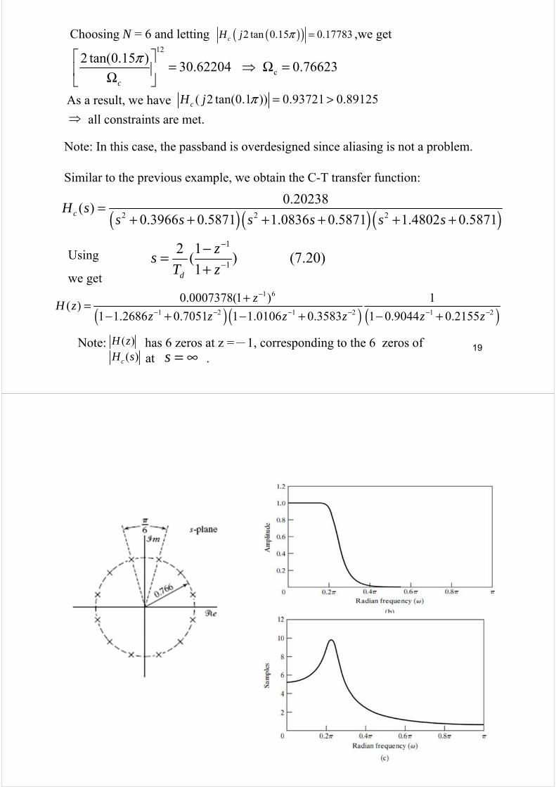
Choosing N=6 and letting = 0.89125 , we get( 0.2 )cH j π
As a result, we have =0.1700 < 0.17783 all constraints are met.Note : Criteria are : (1) choose N as small as possible to reduce complexity
(2) choose to overdesign in stopband to reduce aliasing.
( 0.3 )cH j π
cΩ
12
Find ( ) from and c cH s N Ω2
2/
1( ) ( ) ( )
1 ( / )c c c Ns j
c
H s H s H js jΩ=
− = Ω =+ Ω
2N=12 poles at:1 2
2 2 2 [(1 2 ) ] 2 2( ) ( ) ( ) , , 0 ~ 11k N
jN N N j k N N Nc c k cs j e s e k
ππ+ +
+ += − Ω = Ω = Ω =
2 2 2
1 1
1 2
Choose the 6 poles in the left-half plane
0.12093( )
( 0.3640 0.4945)( 0.9945 0.4945)( 1.3585 0.4945)
by Eq. (7.12)
0.2871 0.4466 2.1428 1.1455( )
1 1.2971 0.6949 1 1.0691
cH ss s s s s s
z zH z
z z z
− −
− − −
=+ + + + + +
− − −= +− + − 1 2
1
1 2
0.3699
1.8557 0.6303
1 0.9972 0.2570
z
z
z z
−
−
− −
+−+
− +
Consider real filter
Remark : Impulse invariance is suitable only for lowpass or bandpass filters with low stopband levels, due to aliasing problem.

13
Group delay
Log magnitude
magnitude
Poles of Hc(s)Hc(-s)
14
7.2.2 Bilinear transformation
Note that the aliasing problem can be avoided if the entire Ω-axis is mapped into the interval . This can be accomplished by the following transformation
π ω π− ≤ ≤
1
1
2 1( ) (7.20)1d
zs
T z
−
−
−=+
for the variables in , respectively. That is, and s z ( ) and ( )cH s H z
1
1
2 1( )1
( ) ( )d
zc ST z
H z H s −
−−=+
=
where is a parameter. Eq. (7.20) is called the bilinear transformation and isderived by approximating integration with trapezoidal rule.
dT

15
From Eq. (7.20)
1/ 22 2
2 2
1 ( / 2) (7.22)
1 ( / 2)
(1 / 2) ( / 2) ( )
(1 / 2) ( / 2)
0 maps into 1 and 0 maps into 1
d
d
d d
d d
T sz
T s
T Tz s j
T T
z z
σ σσ
σ σ
+=−
+ + Ω = = + Ω − + Ω < < = =
16
Note: A pole of in the left-half s-plane maps into a pole of inside the unit circle causal stable C-T filters map into causal stable D-T filters.
~ Relationship between variables The -axis in s-plane is mapped into according to
jΩ/ 2
/ 2
1
2 1 2 2 ( sin / 2) 2[ ] tan( )
1 2 (cos / 2) 2
2tan( ) or 2 tan
2 2
j j
j jd d d
d
d
e e j jj
T e T e T
T
T
ω ω
ω ωω ω
ωω ω
− −
− −
−
−Ω = = = + Ω Ω = =
( )cH s ( )H z
jz e ω=and ωΩ

17
Note: The entire -axis is mapped into , resulting no aliasing .However, high freq. portions suffer nonlinear distortion called freq warping .
Ω π ω π− ≤ ≤
18
Ex. 7.3. We now repeat Ex. 7.2 using bilinear transformation. Again,since does not affect the result, we set =1. This leads to the followingconstraints for
dT( ) :CH jΩ
( )( )
0.89125 ( ) 1 0 2 tan 0.1
( ) 0.17783 2 tan 0.15
C
C
H j
H j
ππ
≤ Ω ≤ ≤ Ω ≤
Ω ≤ ≤ Ω < ∞
With Butterworth prototype C-T filter, we have
2
2
2
2 tan(0.1 ) 0.25893
2 tan(0.15 ) 30.62204
2 tan(0.15 )118.26378 5.30466
2 tan(0.1 )
N
c
N
c
N
N
π
π
ππ
≤ Ω
≥ Ω
≥ ≥
dT
19
Choosing N = 6 and letting ,we get( )( )2 tan 0.15 0.17783cH j π =12
c
2 tan(0.15 )30.62204 0.76623
c
π = Ω = Ω
As a result, we have ( 2 tan(0.1 )) 0.93721 0.89125cH j π = >all constraints are met.
Note: In this case, the passband is overdesigned since aliasing is not a problem.
Similar to the previous example, we obtain the C-T transfer function:
( )( )( )2 2 2
0.20238( )
0.3966 0.5871 1.0836 0.5871 1.4802 0.5871cH s
s s s s s s=
+ + + + + +
Using
we get
1
1
2 1( ) (7.20)1d
zs
T z
−
−
−=+
( )( ) ( )1 6
1 2 1 2 1 2
0.0007378(1 ) 1( )
1 1.2686 0.7051 1 1.0106 0.3583 1 0.9044 0.2155
zH z
z z z z z z
−
− − − − − −
+=− + − + − +
Note: has 6 zeros at z =-1, corresponding to the 6 zeros ofat .
( )H z( )cH s s = ∞
20

21
Design Comparisons
The following examples describe the design of D-T lowpass filters with
1 20.01, 0.001, 0.4 & 0.6p sδ δ ω π ω π= = = = using 4 C-T prototypes.
Bilinear transform is applied.
7.3 Discrete-Time Butterworth, Chebyshev and Elliptic Filters
22
Ex. 7.4. Butterworth approximationN=14

23
Ex 7.5. Chebyshev-Type I approximation N=8
24
Chebyshev- TypeⅡ approximationN=8

25
Ex. 7.6 Elliptic approximationN=6
26
Remarks:1. Bilinear transformation of analog filters designed by Butterworth,
Chebyshev, or elliptic approximation methods is a standard method of design of IIR discrete-time filters.
2. All the approximation methods yield digital filters with nonconstant group delay or, equivalently, nonlinear phase.
3. (1) Butterworth is maximally flat in the passband, (2) type II Chebyshev yields the smallest delay in the passband and the
widest region of the passband over which the group delay is approximately constant
(3) Elliptic yields the lowest order system function (least computation cost)

27
Matlab functions:
~ Order estimationThe m-files for estimations of the order of the IIR filter to be designedButterworth filter: buttord type-1 Chebyshev filter: cheb1ordtype-2 Chebyshev filter: cheb2ordElliptic filter: ellipord
[N, wp] = ellipord(wp, ws, rp,rs)
rp: passband ripple in dB rs: Minimum stopband attenuation in dB wp and ws are the passband and stopband edge frequencies, normalized from 0 to 1 (where 1 corresponds to π radians/sample).
order N: the lowest order digital elliptic filter wp: passband edge frequency.
28
~ Discrete IIR filter design
The m-files for IIR filter design based on the bilinear transformationButterworth filter: buttertype-1 Chebyshev filter: cheby1type-2 Chebyshev filter: cheby2Elliptic filter: ellip
[b, a] = ellip(N,rp,rs,wp);
returns the filter coefficients in length N+1 vectors b (numerator) and a (denominator).
~ Frequency response m-file: freqz(b,a,ns);ns: returns the ns-point complex frequency response vector, default: 512

29
% Program 7_1% Elliptic IIR Lowpass Filter Design%wp = input('Normalized passband edge = ');ws = input('Normalized stopband edge = ');rp = input('Passband ripple in dB = ');rs = input('Minimum stopband attenuation in dB = ');[N,wp] = ellipord(wp,ws,rp,rs)[b,a] = ellip(N,rp,rs,wp);[h,omega] = freqz(b,a,256);plot (omega/pi,20*log10(abs(h)));grid;xlabel('\omega/\pi'); ylabel('Gain, dB');title('IIR Elliptic Lowpass Filter');
Wp=0.3, ws=0.4, rp=5, rs=40
30
HW:
[ ] sin(0.1 ) 0.3sin(0.8 )x n n nπ π= +
0 10 20 30 40 50 60 70 80 90 100-1.5
-1
-0.5
0
0.5
1
1.5
Design a lowpass filter to filter out the high frequency component

31
7.5 Design of FIR Filters by Windowing
~ Design of D-T IIR filters are based on C-T IIR systems ~ Design of D-T FIR filters are almost entirely restricted to D-T implementations.~ Generally speaking, the problem is to determine an impulse response of a
linear phase FIR filter whose freq. response satisfies a set of specifications.
~ The simplest method of FIR filter design is the window method. It generally begins with an ideal desired freq. response
( ) [ ] , [ ] : impulse response
1 [ ] ( )
2
~ Ideal lowpass filter:
1, | | sin ( ) [ ] ,
0,
[ ] is n
j j nd d d
n
j j nd d
cj clp lp
c
lp
H e h n e h n
h n H e e d
nH e h n n
n
h n
ω ω
π ω ω
π
ω
ωπ
ω ω ωω ω π π
∞−
=−∞
−
=
=
<= ⇔ = −∞ < < ∞ < ≤
oncausal and is infinitely long impractical
[ ]h n
32
~ One simple solution: truncate the desired impulse response into a causaland finite duration (FIR) sequence.
~ The truncation can be done via windowing
[ ] [ ] [ ]dh n h n w n=
: finite duration “window” defined over [0 , M][ ]w n
window
0 M
truncatedtruncated
1, 0e.g., rectangular window [ ]
0, otherwise
n Mw n
≤ ≤=
…………

33
As a result , will be a “ smeared ” version of ( )jH e ω ( )jdH e ω
( 1)/2
0
( )
1 sin[ ( 1) / 2] ~ ( )
1 sin( / 2)
note: ( ) has a generalized linear phase
~From modulation, or windowing, theorem, we have
1( ) ( ) ( )
2
j MMj j n j M
jn
j
j j jd
e MW e e e
e
W e
H e H e W e d
ωω ω ω
ω
ω
πω θ ω θ
π
ωω
θπ
− +− −
−=
−
−
− += = =−
=
(7.45)
θ ω
34
( )( )jW e ω θ
ω π
−
=
( )( )j
c
W e ω θ
ω ω π
−
< <
( )( )j
c
W e ω θ
ω ω
−
=
( )( )
0
j
c
W e ω θ
ω ω
−
< <
θ
θ
θ
θ
35
~ ideal ( but impractical):
[ ]=1 for all , ( ) 2 ( 2 ) ( ) ( )
~ Considerations in choosing a window
1. For ( ) to faithfully reproduce ( ), ( ) should approximate
j j jd
r
j j jd
w n n W e r H e H e
H e H e W e
ω ω ω
ω ω ω
πδ ω π∞
=−∞
= + =
an
impulse, i.e., ( ) is highly concentrated in frequency
2. [ ] is as short as as possible in duration, so as to minimize computation
~ These are two conflicting requirements, e.g., for a
jW e
w n
ω
rectangular
36
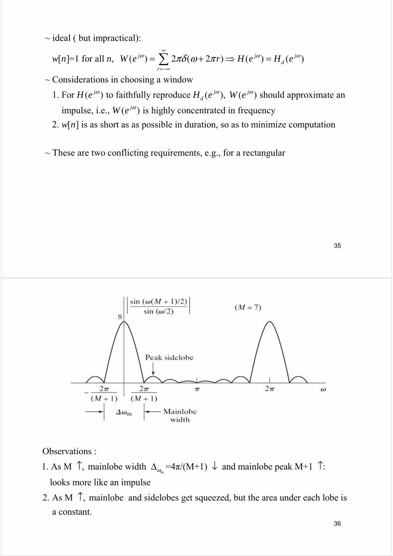
m
Observations :
1. As M , mainlobe width =4π/(M+1) and mainlobe peak M+1 :
looks more like an impulse
2. As M , mainlobe and sidelobes get squeezed, but the area under each lobe is
a cons
ω↑ Δ ↓ ↑
↑tant.

37
3. As slides by a discontinuity of in Eq. (7.45) , willoscillate as each sidelobe of moves past the discontinuity.From Observation 2, the oscillations occur more rapidly but do not change in amplitude as M increases. This is called the Gibbs phenomenon.
Solution: To alleviate the Gibbs phenomenon, we need to use windows tapered smoothly to zero at each end so as to produce lower sidelobes.
( )jdH e θ ( )jH e ω
( )( )jW e ω θ−
( )( )jW e ω θ−
38
7.5.1 Properties of commonly used windows
Some commonly used windows are listed below :
1. Rectangular :
2. Bartlett (triangular):
3. Hanning :
4. Hamming :
5. Blackman :
1 0[ ]
0
n MW n
otherwise
≤ ≤=
2 / 0 / 2
[ ] 2 2 / / 2
0
n M n M
W n n M M n M
otherwise
≤ ≤= − < ≤
0.5 0.5cos(2 / ) 0[ ]
0
n M n MW n
otherwise
π− ≤ ≤=
0.54 0.46cos(2 / ) 0[ ]
0
n M n MW n
otherwise
π− ≤ ≤=
0.42 0.5cos(2 / ) 0.08cos(4 / ) 0[ ]
0
n M n M n MW n
otherwise
π π− + ≤ ≤=

39
Remarks: 1. Except for rectangular, all windows decrease toward zero.2. All windows are symmetric about the point M/2
40
M=50
Rectangular
Bartlett
Hanning
Hamming
Blackman

41
Observations :1. Fourier transform of Bartlett window can be expressed as a product of
Fourier transform of rectangular windows.2. Fourier transforms of Hanning , Hamming & Blackman windows can be
expressed as sums of freq. shifted Fourier transforms of rectangularwindows.
3. Rectangular window has the narrowest mainlobe (sharpest transitions of H ata discontinuity of Hd), but the highest sidelobes (-13dB for 1st sidelobes ) (oscillations of considerable size around discontinuities of Hd)
4. Blackman window has the lowest sidelobes, but the widest mainlobe.
42
7.5.2 Incorporation of generalized linear phase
/2
~All windows have the property that
[ ], 0[ ] , symmetric about / 2
0, otherwise
~Their Fourier transforms are of the form
( ) ( )
( ) : a real, ev
j j j Me
je
w M n n Mw n M
W e W e e
W e
ω ω ω
ω
−
− ≤ ≤=
=
en function of
~ If the desired impulse response [ ] is also symmetric about / 2
[ ] [ ]
[ ] [ ] [ ] is also symmetric about /2
( )
d
d d
d
je
h n M
h M n h n
h n h n w n M
H e Aω
ω
− = =
= /2( ) (generalized linear phase)
( ) : a real and even function of
~ Similarly, if the desired impulse response [ ] is antisymmetric about / 2
j j M
je
d
e e
A e
h n M
ω ω
ω ω
−
/2
[ ] [ ]
[ ] [ ] [ ] is also antisymmetric about /2
( ) ( ) (generalized linear phase)
( ) : a real and odd function of
d d
d
j j j Me
je
h M n h n
h n h n w n M
H e jA e e
A e
ω ω ω
ω ω
−
− = − =
=

43
Ex. 7.7 Linear-phase lowpass filter
[ ]
/2
/2
, ( ) ( )
0,
1 sin[ ( / 2)][ ] , [ ] [ ]
2 ( / 2)
sin[ ( / 2)][ ] [ ] [ ], [ ]: ymmetric window
( / 2)
( ) has a li
c
c
j Mcj j
d lp
c
j M j n cd d d
cd
j
eH e H e
n Mh n e e d h M n h n
n M
n Mh n h n w n w n w n s
n M
H e
ωω ω
ω ω ω
ω
ω
ω ωω ω
ωωπ π
ωπ
−
−
−
<= = <
−= = − =−
−= =−
/2 ( ) ( ) /2
( ) /2
/2
near phase
~Frequency domain:
( ) ( ) ( )
1 = ( )
21
= ( )2
( ) (generali
c
c
c
c
j j jd
j M j j Me
j j Me
j j Me
H e H e W e
e W e e d
W e d e
A e e
ω ω ω
ω θ ω θ ω θ
ω
ω ω θ ω
ω
ω ω
θπ
θπ
− − − −
−
− −
−
−
= ∗
⋅
=
( )
zed linear phase)
1( ) ( )
2
c
c
j je eA e W e d
ωω ω θ
ωθ
π−
− =
44
Passband overshoot peaks at
Stopband undershoot peaks at
2m
c
ωω Δ−
2m
c
ωω Δ+
Peaks approximation error maximumδ =overshoot or undershoot.
Approximation tends to be
symmetric about cω
Amplitude response
Trying different windows with different M by trial and error is not a very satisfactory way to design filters
pω
sω

45
7.5.3 The Kaiser window filter design method
~ A window which is maximally concentrated around ω=0 is desired. ~ Optimum solutions which lead to maximally concentrated windows are difficult to
compute. ~ As an alternative, Kaiser found a near-optimal window by using zeroth-order
modified Bessel function of the first kind( )oI ⋅
( )1/ 22
~ Kaiser window
[ 1 [ / ] ], 0 [ ] ( )
0, otherwise
/ 2
~ Remark: Modified Bessel functions are solutions of modifi
o
o
I nn Mw n I
M
β α αβ
α
− − ≤ ≤=
=
2 2 2
2
20
ed Bessel's
differential equations
( ) 0, : the order of the Bessel function
( ) ( !) 4
k
ok
k
x y xy x a y a
xI x
k
∞
=
′′ ′+ − + =
=
46
M=20
M=10,20,40

47
Observations:1. For a larger (smaller) , the window is tapered more (less)
sidelobes are lower (higher) but mainlobe is wider (narrower).2. For a larger (smaller) M, mainlobe is narrower (wider) but sidelobe
levels are not affected. (this is true for all windows)Hence, trade-off can be made between mainlobe width and sidelobe levels by
choosing proper M and .
β
β
~ Empirical rule for choosing M and β:Given , define =highest freq. such that and = lowest
freq. such that . Also, define and
Kaiser determined empirically that for a specified value of and ,
δ pω ( ) 1jH e ω δ≥ − sω( )jH e ω δ≥ s pω ω ωΔ = −
1020 logA δ= −
ωΔ
0.4
0.1102( 8.7), 50
0.5842( 21) 0.07886( 21), 21 50
0, 21
8
2.285
A A
A A A
A
AM
β
ω
− >= − + − ≤ ≤ <
−=Δ
A
48
1 2
1 2
Design a lowpass filter with 0.4 , 0.6 , 0.01, 0.001
Solution: filters designed by the window method inherently have =
0.001
p sω π ω π δ δ
δ δδ
= = = =
=
Ex. Kaiser window design of a lowpass filter
( )
10
1/22
1 ( ) 0.5 ,
2 0.2 , 20log 60
5.653, 37, / 2 8.5
[ 1 [ / ] ]sin ( ), 0 [ ] [ ] [ ] ( ) ( )
0,
c p s
s p
oc
d o
A
M M
I nnn Mh n h n w n n I
ω ω ω π
ω ω ω π δβ α
β α αω απ α β
≈ + =
Δ = − = = − =
= = = =
− −− ⋅ ≤ ≤ = = − otherwise
=37 is an odd number, the resulting linear-phase would be of type II (See 5.7.3)
Increasing to 38 results in a type I filter for which 0.0008
M
M δ
=
7.6 Examples of FIR Filter Design by the Kaiser Window Method7.6.1 Lowpass filter

49
50
Remarks: 1. The phase is precisely linear and the group delay is M/2=18.5 samples. 2. The Kaiser window represents a class of windows with a wide range of
mainlobe and sidelobe levels. As shown in Table 7.1, each window has an equivalent Kaiser window counterpart under a specific criterion (e.g. for the same value).δ

51
Matlab functions:
Order estimation: kaiserordKaiser window design: kaiserFIR filter design: fir1
Example: F = input('Type in the bandedges = ');A = input('Type in the desired magnitude values = ');DEV = input('Type in the ripples in each band = ');Fs=input(‘Type in the sampling frequency=‘);[N,Wn,BTA,FILTYPE] = kaiserord(F,A,DEV,Fs)B = FIR1(N, Wn, FILTYPE, kaiser( N+1,BTA ), 'noscale' )[h,omega] = freqz(B,1,256);plot(omega/pi,20*log10(abs(h)));grid;xlabel('\omega/\pi'); ylabel('Gain, dB');
%w = kaiser(N+1,beta);
e.g., Design a lowpass filter with a passband edge of 1500Hz, a stopband edge of 2000Hz, passband ripple of 0.01, stopband ripple of 0.1, and a sampling frequency of 8000Hz:
[n,Wn,bta,filtype] = kaiserord( [1500 2000], [1 0], [0.01 0.1], 8000 );
52
7.7 Optimum Approximations of FIR Filters
1. Design of FIR filters by windowing is straightforward and is quite general.
2. We want to design a filter that is the "best" that can be achieved for
7.7.1 Optim
a given val
al Type I Lo
ue of
wpass
M
/2
1 2 p
~ [ ]=0 for 0 (causal) and (finite length), and
[ ] [ ] (linear phase)
frequency response
Filt
( ) ( )
~ Given constraints , , ,
e s
r
j j j Me
h n n n M
h n h M n
H e A e eω ω ω
δ δ ω
−
< >= −
=
sand , optimal parameters [ ], 0 can be found using the
Parks-McClellan algorithm
h n n Lω ≤ ≤
53
~ The Parks-McClellan (PM) algorithm is based on reformulating the filter design
problem as one of polynomial approximation. This is done by expressing the
terms cos( nω
Parks - McClellan algorithm :
1
) in Eq. (5.140a)
( ) ( [ ] 2 [ ]cos( )) ( ), / 2 : integer --- (5.140a)
as a sum of powers of cos( ) in the form
cos( ) (cos
Lj j L j L j
ek
k
H e e h L h L k k e A e L M
k
k T
ω ω ω ωω
ωω ω
− −
=
= + − = =
=
1
1 2 0 1
), th-order Chebyshev polynomial
where ( ) cos( cos ),
( ) 2 ( ) ( ) ( ) 1, ( )
~ Rewrite Eq. (5.140a) as an th-order polynomial in cos( )
k
k k k
k
T x k x
T x xT x T x T x T x x
L ω
−
− −
== − = = =
cos0
0
( ) (cos ) ( ) |
where
( )
~ Objective, find
Lj k
e k xk
Lk
kk
A e a P x
P x a x
ωωω =
=
=
= =
=
Optimization problem formulation
0 [ ] min ( ( ))
where ( ) is a nonnegative function.
h n Lf E
f
ω≤ ≤
⋅
54
2
Examples:
1. Mean square error function: ( ( )) ( )
2. Minimax function: ( ( )) max ( ) (Chebyshev, used here)
Remarks: It can be shown that the mean square error function with =[0, ]
F
F
f E E d
f E E
Fω
ω ω ω
ω ω
π∈
=
=
leads to
rectangular windowing approximation and minimax function leads to
equiripple approximation
~ ( ) ( )[ ( ) ( )]
( ) : weighting function, ( ) : desi
j jd e
jd
E W H e A e
W H e
ω ω
ω
ω ωω
= −
red frequency response
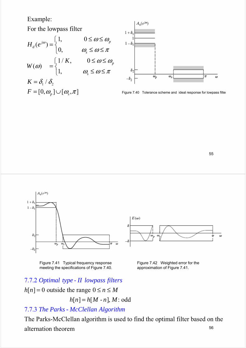
55
1 2
Example:
For the lowpass filter
1, 0( )
0,
1 / , 0( )
1,
/
[0, ] [ , ]
pjd
s
p
s
p s
H e
KW
K
F
ω ω ωω ω π
ω ωω
ω ω πδ δ
ω ω π
≤ ≤= ≤ ≤
≤ ≤= ≤ ≤
== ∪ Figure 7.40 Tolerance scheme and ideal response for lowpass filter
56
Figure 7.41 Typical frequency response meeting the specifications of Figure 7.40.
Figure 7.42 Weighted error for the approximation of Figure 7.41.
[ ] 0 outside the range 0
[ ] [ - ], : odd
The Parks-McClellan algorithm is used to f
7.
in
7.2 -
7
d t
.7.3
h
e o
h n n M
h n h M
Optimal type II lowpass filters
The Parks - McClellan Algorit
n
hm
M
= ≤ ≤=
ptimal filter based on the
alternation theorem
57
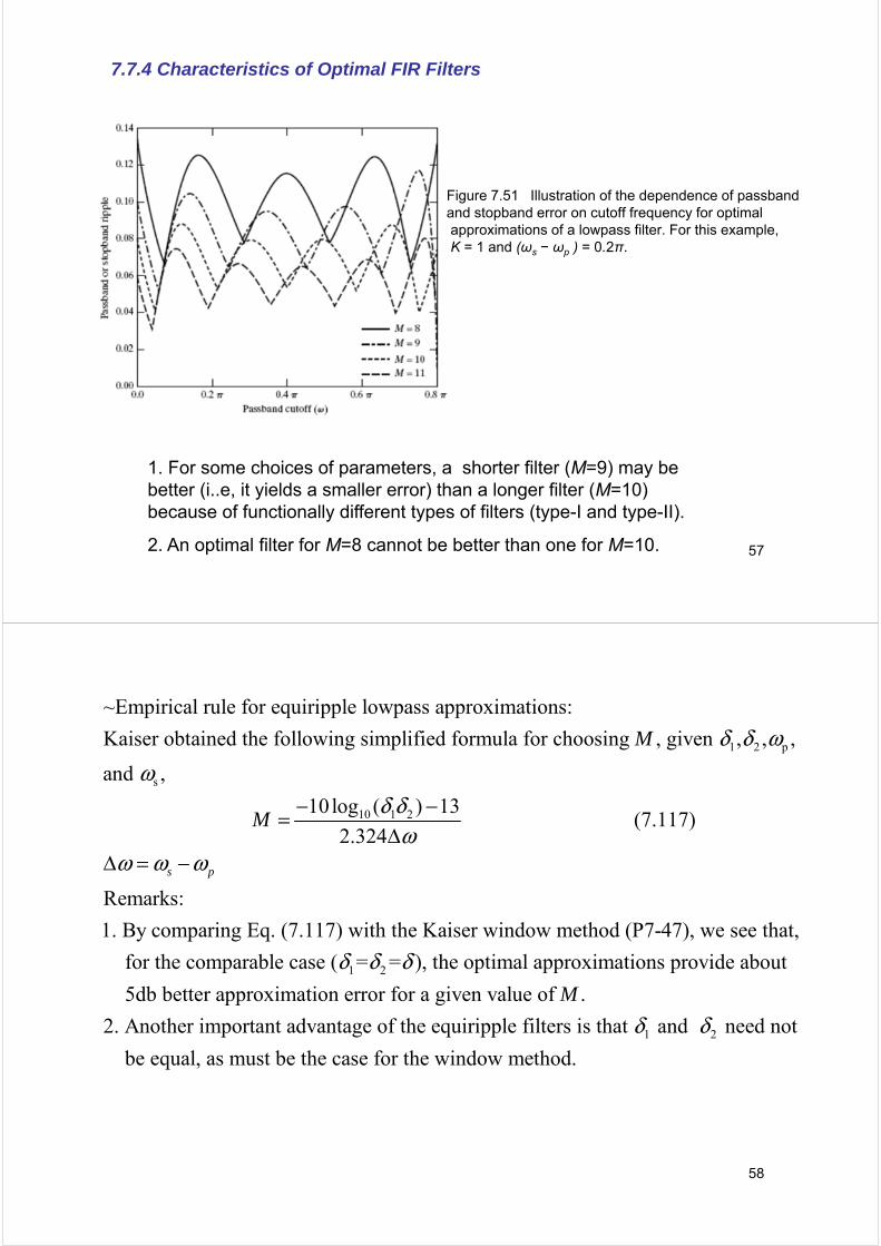
7.7.4 Characteristics of Optimal FIR Filters
1. For some choices of parameters, a shorter filter (M=9) may be better (i..e, it yields a smaller error) than a longer filter (M=10) because of functionally different types of filters (type-I and type-II).
2. An optimal filter for M=8 cannot be better than one for M=10.
Figure 7.51 Illustration of the dependence of passbandand stopband error on cutoff frequency for optimalapproximations of a lowpass filter. For this example,K = 1 and (ωs − ωp ) = 0.2π.
58
1 2 p
s
10 1 2
~Empirical rule for equiripple lowpass approximations:
Kaiser obtained the following simplified formula for choosing , given , , ,
and ,
10 log ( ) 13
2.324
M
M
δ δ ωω
δ δω
− −=Δ
1 2
(7.117)
Remarks:
1. By comparing Eq. (7.117) with the Kaiser window method (P7-47), we see that,
for the comparable case ( = = ), the optimal approximations pro
s pω ω ω
δ δ δ
Δ = −
1 2
vide about
5db better approximation error for a given value of .
2. Another important advantage of the equiripple filters is that and need not
be equal, as must be the case for the wind
M
δ δow method.

59
7.8 Examples of FIR Equiripple Approximation
From Eq. (7.117)
60

61
Matlab functions:
Order estimation: remezord
Filter design: remez
(The iterative Remez exchange algorithm is used in the Parks-McClellan algorithm)
% Design of Equiripple Linear-Phase FIR Filters%format longfedge = input('Band edges in Hz = ');mval = input('Desired magnitude values in each band = ');dev = input('Desired ripple in each band =');FT = input('Sampling frequency in Hz = ');[N,fpts,mag,wt] = remezord(fedge,mval,dev,FT);b = remez(N,fpts,mag,wt);disp('FIR Filter Coefficients'); disp(b)[h,w] = freqz(b,1,256);plot(w/pi,20*log10(abs(h)));grid;xlabel('\omega/\pi'); ylabel('Gain, dB');
62
Comparisons between IIR and FIR filters:
~IIR filters:
1. Closed form procedures are available for designing a variety of frequency selective filters (lowpass, highpass, bandpass and bandstop).
2. Phase response is typically poorer.
3. Economics in implementation: If we put aside phase considerations, it is generally true that a given magnitude response specification can be met most efficiently with an IIR filter.
~FIR filters:
1. Closed form procedures do not exist. Though the window method is straightforward to apply, some iterations may be necessary to meet a prescribed specification.
2. Offers more flexibilities in approximating arbitrary frequency-response characteristics
3. Linear phase is easy to be achieved.
7.9 Comments on IIR and FIR Discrete-Time Filters