Calculation of optical properties of light-absorbing carbon withweakly absorbing coating: A model with tunable transition fromfilm-coating to spherical-shell coating
Downloaded from: https://research.chalmers.se, 2022-02-04 03:41 UTC
Citation for the original published paper (version of record):Kanngiesser, F., Kahnert, M. (2018)Calculation of optical properties of light-absorbing carbon with weakly absorbing coating: Amodel with tunable transition from film-coating to spherical-shell coatingJournal of Quantitative Spectroscopy and Radiative Transfer, 216: 17-36http://dx.doi.org/10.1016/j.jqsrt.2018.05.014
N.B. When citing this work, cite the original published paper.
research.chalmers.se offers the possibility of retrieving research publications produced at Chalmers University of Technology.It covers all kind of research output: articles, dissertations, conference papers, reports etc. since 2004.research.chalmers.se is administrated and maintained by Chalmers Library
(article starts on next page)

Calculation of optical properties of light-absorbingcarbon with weakly absorbing coating: a model withtunable transition from film-coating to spherical-shell
coating
Franz Kanngießera, Michael Kahnerta,b
aDepartment of Space, Earth and Environment, Chalmers University of Technology, SE-41296 Gothenburg, Sweden
bResearch Department, Swedish Meteorological and Hydrological Institute, Folkborgsvagen17, SE-601 76 Norrkoping, Sweden
Abstract
Optical properties of particles consisting of light-absorbing carbon (or soot) and
a weakly absorbing coating material are computed at a wavelength of 355 nm
and 532 nm. A morphological particle models is used, in which small amounts of
coating are applied as a thin film to the surface of the aggregate, while heavily
coated aggregates are enclosed in a spherical shell. As the amount of coating
material is increased, a gradual transition from film-coating to spherical-shell
coating is accounted for. The speed of this transition can be varied by specifying
a single parameter. Two different choices of this parameter, corresponding to a
slow and a rapid transition from film-coating to spherical-shell coating, respec-
tively, are investigated. For low soot volume fractions the impact of this tran-
sition on the linear depolarisation ratio δl is most pronounced. The model that
describes a rapid transition to a spherical coating yields results for δl that are
more consistent with existing lidar field measurements than the slow-transition
model. At 532 nm the relative uncertainty in modelled δl for a rapid transition
values due to uncertainties in the aggregate’s geometry and chemical composi-
tion are estimated to range from 109 to 243%, depending on the soot volume
Email addresses: [email protected] (Franz Kanngießer),[email protected] (Michael Kahnert)
Preprint submitted to J. Quant. Spectrosc. Radiat. Transfer May 3, 2018

fraction. At 355 nm the relative uncertainties were estimated to range from 90.9
to 200%.
Keywords: Scattering, Aerosol, Soot, Depolarization ratio
2010 MSC: 00-01, 99-00
1. Introduction
Particles consisting of light-absorbing carbon or soot are among the atmo-
spheric aerosol particles with the largest impact on the Earth’s climate. They
can influence the climate system through their role in cloud formation processes,
by reducing the albedo of snow and ice in polar and mountainous regions, or by5
direct absorption of solar radiation [1, 2]. Also, soot particles have an adverse
impact on air quality and human health [3]. Observations of soot particles by re-
mote sensing techniques play an important role in monitoring sources, transport
pathways, and deposition of soot particles in the atmosphere. These observa-
tions are also essential for constraining and improving aerosol transport and air10
quality forecasting models. The interpretation of remote sensing observations
as well as predictions of the climate impact of soot particles relies on a thorough
understanding of the particles’ optical properties.
Soot particles themselves consist of highly absorbing carbonaceous material.
Aged atmospheric soot particles are commonly coated by weakly absorbing ma-15
terial, which can complicate the modelling of optical properties of soot particles
[4]. Both images of atmospheric soot particles and chemical analyses often in-
dicate a thick coating and hence a low soot volume fraction [5, 6, 7, 8]. In [8]
50% of freshly emitted soot particles were reported to be heavily coated, thus
indicating a fast coating process in the atmosphere. As shown in [7] the coating20
itself may consist of different materials.
Various models have been employed to investigate the impact of the par-
ticles’ morphological features on radiative and optical properties. The extent
to which morphological features of coated soot particles need to be resolved in
models depends on the intended application. To account for the coating different25
2

particle models have been used. The climate relevant impact on the broadband
solar radiative flux can be investigated by assuming a spherical core-shell or the
recently introduced core grey shell model [9]. Using morphologically more com-
plex particle models requires more computational efforts. The impact of the use
of simplified particle models in climate models can be quantified by comparing30
the results obtained for simplified models to those obtained for more complex
models (e.g. [10]).
Prior work on the uncertainty introduced into climate models by assuming
strongly simplified shapes of soot particles focused on radiative properties, such
as the mass absorption cross section (e.g. [11]) or the scattering and absorption35
cross sections [12, 13], as well as on the single scattering albedo and asymmetry
parameter. The closed cell or concentric core-shell monomer model employed
by [14, 15, 13] uses aggregates where each individual monomer is coated by
a spherical shell. Other approaches apply the coating onto the aggregate of
contacting soot monomers. Two other approaches in which the coating follows40
the shape of the aggregate were used in [13]. The first approach defines a fixed
coating thickness. A coating layer with this thickness is then added to the
aggregate. The other approach adds small coating volumes at the edges of the
soot aggregate or the coating until a prescribed volume fraction is reached. In
another study coating was added by first filling voids in branches with more45
densely packed monomers; then the coating is continued in descending order of
the density of monomer packing [12]. Partial soot inclusions in spherical coating
shells were investigated in [12, 16]. Both the model which filled voids in branches
and the partial soot inclusion model discussed in [12] served as a references for
comparison with simpler core-shell and homogeneous sphere models. However50
there were differences between the two morphologically more complex models.
The scattering cross section is larger if the surface of coated soot increases.
In [16] the impact of monomer surfaces intersecting with the coating surface
was investigated. The difference between the two models was less than 5% for
optical cross sections, asymmetry factor and single scattering albedo; therefore,55
this morphological feature may be ignored.
3
A numerical investigation presented in [17] was carried out to evaluate the
possibility of determining the primary particle size of bare soot aggregates
by measuring the depolarisation of light. In that numerical investigation it
was found that refractive index, the aggregate shape and connections of the60
monomers making up the aggregate have a strong impact on the depolarisation.
Compared to climate models, remote sensing applications may require mor-
phologically more complex models. One quantity frequently used in lidar remote
sensing is the linear depolarisation ratio, δl. This quantity is a key element
in classifying aerosol species using lidar techniques. The aerosol classification65
schemes of the Cloud-Aerosol Lidar and Infrared Pathfinder Satellite Observa-
tions (CALIPSO) [18] and for the planned Earth Clouds, Aerosols and Radiation
Explorer (EarthCARE) [19, 20] rely on measurements of δl. Depolarisation is
highly sensitive to morphology, and even to particle inhomogeneity [21]. It is
therefore expected that a correct description of depolarisation requires signif-70
icantly more realistic model particles than radiative forcing computations in
climate models.
Images of coated soot particles presented by [6, 22] suggest that the coating
in case of low soot volume fraction tends to form a spherical or almost spher-
ical shape, which encapsulates parts of the soot aggregate, while parts of the75
aggregate are sticking out of the coating. A corresponding model has been con-
sidered in, e.g., [9, 16]. However, this model is not expected to be very realistic
for high soot volume fractions (i.e., thin coatings). For those the coating forms
a thin film that closely follows the shape of the aggregate, similar to the model
in [13]. It is plausible to assume that there should be a smooth transition from80
the nonspherical to the spherical coating, which would take place at intermedi-
ate soot volume fractions. Also, as soot particles age in the atmosphere, their
fractal dimension tends to increase, resulting in a collapse and compaction of
the aggregate structure [4, 23, 24, 25]. In [8] the particles with the lowest soot
volume fraction were reported to have the highest fractal dimension, i.e. being85
the most compact particles. Particles with higher soot volume fractions were
reported to have lower fractal dimension.
4

Thus, most coating models considered earlier can be expected to be realistic
either for low or for high soot volume fractions. A recent study presented a
first attempt to cover the entire range of volume fractions by devising a coated90
aggregate model that accounts for the transition from thinly coating films to
spherical coatings [26]. However, the fractal dimension has been assumed to be
constant, i.e., the transition from lacy to more compact soot aggregates during
the coating process has been neglected. The computational results were com-
pared to those obtained with the closed cell model. The cross sections of both95
models were in relatively good agreement for high soot volume fractions (i.e.,
thin coatings). However, the depolarisation ratios were found to differ between
the two models. The depolarisation ratios of soot particles obtained with the
coated aggregate model were more consistent with field observations than those
obtained in the closed cell model. However, there seems to be a certain risk that100
the coated aggregate model overestimates depolarisation at low volume fractions
and for large particle sizes. This suggests that the model particles proposed in
[26] might be too nonspherical for low soot volume fractions.
To lower the depolarisation by soot particles one could make the transition
from thinly-coating films to spherical coatings more rapid, because this will105
make particles with low soot volume fractions more spherical. This can be
achieved by (i) reducing the radius of the critical sphere defined in [26] that
marks the transition from film-coating to spherical coating; and (ii) assuming
that the fractal dimension of the aggregate increases with decreasing soot volume
fraction (i.e., increased coating thickness).110
We hypothesize that the speed of transition from film-coating to spherically
encapsulated soot aggregates is an essential morphological parameter to which
the linear depolarisation ratio is highly sensitive. By a high speed of transition,
we mean that the coating becomes spherical at relatively small amounts of coat-
ing material (i.e, at relatively high soot volume fractions); while a low speed of115
transition requires higher amounts of coating material before the shell becomes
spherical.
We will test our hypothesis by formulating a particle model in which the
5

speed of transition can be continuously adjusted by tuning a single parameter.
We will then compare two choices of this parameter, which simulate a slow and120
a rapid transition, respectively, from film-coating to spherical coating as more
liquid-phase material is added to the soot aggregate. The computational results
for the linear depolarisation ratio are gauged against published observations
from field measurements.
A more detailed description of the particle model, as well as a description of125
the computational methods are given in Sec. 2. The results are presented and
discussed in Secs. 3 and 4, respectively. Concluding remarks are given in Sec.
5.
2. Methods
2.1. Particle models130
Atmospheric soot aerosol particles can be approximated as aggregates con-
sisting of spherical monomers following the scaling relation [27]:
N = k0
(Rg
a
)Df
(1)
In Eq. (1) N denotes the number of monomers, a the monomer radius, k0 is
the fractal prefactor and Df the fractal dimension. The fractal dimension takes
values between 1 (linear aligned monomers) and 3 (spheres). The radius of
gyration Rg is given by
Rg =
√√√√ 1
N
N∑i=1
|~ri − ~rc|2 (2)
Here ~ri is the position vector of the centre of the ith monomer and ~rc the position
vector of the aggregate’s centre of mass.
In this study aggregates following the scaling relation in Eq. (1) have
been created using the cluster-cluster aggregation algorithm presented in [28].
This method mimics aggregate formation processes in nature more closely than135
6

diffusion-limited aggregation algorithms. The cluster-cluster algorithm com-
bines smaller aggregates, each fulfilling the scaling relation, to larger aggregates,
while a diffusion limited algorithm adds one monomer at a time.
We generated aggregates consisting of 8, 64, 216 and 512 monomers. For all
particles a prefactor of k0 = 0.7 was assumed following the measured median140
reported in [29]. For each size, five different stochastic realisations of aggregates
with prescribed fractal parameters have been generated. These will be used
to estimate the variation of optical properties with changes in the aggregate
geometry.
Based on the conclusions in [26], we hypothesise that a crucial morphological145
feature of coated soot particles is the transition from a coating film of liquid
material that closely follows the shape of the aggregate to a spherical coating
that encapsulates the aggregate. More specifically, we hypothesise that the
linear depolarisation ratio is highly sensitive to the speed of this transition, i.e.,
to whether the onset of sphericity occurs at relatively low or high amounts of150
coating.
To test this hypothesis, we devise a model in which the coating is added to
the aggregate layer by layer, where the layer thickness d is equal to the volume
cell size (or dipole spacing) that we employ in the discrete dipole approximation
(DDA, see section 2.3). More specifically, we proceed as follows. For each155
aggregate the maximum dimension D is determined. Based on this maximum
dimension we define a critical sphere of Diameter Dc centred at the aggregate’s
centre of mass. Inside the critical sphere the coating is applied layer by layer
following the shape of the aggregate, while being constrained not to be applied
outside the critical sphere. These successive coating layers are represented by the160
grey lines in Fig. 1. Once the critical sphere is completely filled, successive layers
of coating are applied radially onto the sphere (see dash-dotted grey sphere in
Fig. 1). The whole process is terminated once the desired soot volume fraction
is reached.
The critical diameter Dc is a tunable parameter of the model. We consider165
two choices of this parameter. In the first one (the ”slow” transition model),
7

we use Dc,slow = D + 2d. Thus, the critical sphere completely encapsulates the
aggregate; its diameter is larger by 2d than that of the smallest circumscribing
sphere (see solid blue sphere in Fig. 1). In the second one (the ”rapid” transition
model), we use Dc,rapid = 0.6(D + 2d). Thus, the critical sphere does not170
completely encapsulate the aggregate (see dashed blue sphere in Fig. 1).1
Thus the rapid-transition model simulates a coating process where the tran-
sition from film-coating to spherical coating occurs rather rapidly as more coat-
ing material is added. In the slow-transition model, the onset of sphericity is
reached at a much later stage at lower soot volume fractions, i.e., when a larger175
amount of coating has been added to the aggregate. In the slow-transition
model, sphericity is not reached before the aggregate is completely encapsu-
lated. In the rapid-transition model, the coating becomes spherical at higher
soot volume fractions, where part of the aggregate is allowed to stick out of the
coating. This is consistent with images of coated soot aggregates (e.g. [30]).180
The rapid-transition model is further motivated by recent laboratory mea-
surements reported in [31], where the morphological changes of soot particles
during the process of condensation of coating material are investigated. They
observed that a gradual increase of the amount of coating material first had a
negligible effect on the particles’ mobility diameter, followed by a sudden sharp185
increase in diameter. This behaviour is explained as follows. At first, inner voids
of the aggregates are filled with the coating material. Once the open voids are
filled, the particles grow radially in diameter. The mechanism of soot particle
growth due to condensation of matter presented in [31] qualitatively supports
our assumption of a transition from a coating film to growth of an encapsulating190
sphere.
As stated in section 1 restructuring of the aggregate with decreasing soot
volume fraction was assumed for both the slow and the rapid transition model
1We emphasize that the terms slow and rapid transition models are employed for the sake
of brevity. However, both are, in fact, based on one a single model with two different choices
of the free parameter in the model.
8

based on [4, 23, 8, 25, 24]. The process of restructuring of the soot aggregate
during the process of coating is rather complex and depends on the coating ma-195
terial. For sulphuric acid a proportional increase in compactness with increasing
coating mass was reported in [4]. However for oleic acid a rapid compaction was
reported for small amounts of coating material added to the aggregate. After
that rapid collapse of the aggregate further condensation of coating material
onto the aggregate led to further compaction, but at a smaller rate [23, 24].200
The condensation of aromatic hydrocarbons leads to a restructuring of the ag-
gregate after a certain threshold of condensated mass is passed. After reaching
that threshold the compactness increases with increasing amount of coating
material [25]. The compactness increases with condensation of coating material
until the maximum compactness of the aggregate is reached [23, 24, 25]. Ad-205
ditionally [8] reported that atmospheric soot particles with the thickest coating
had the highest fractal dimension (i.e. compactness).
To reflect the restructuring an increase in the fractal dimension Df from
2.0 to 2.6 was included in our model. The assumed relation between soot vol-
ume fraction fvol and fractal dimension Df for this study is given in Tab. 1.210
As a simplification, changes in fractal dimension were not adapted for different
coating materials. The values of Df were based on [29]. In that study they
measured the fractal dimension using three-dimensional scans, which system-
atically yield higher results than methods inferring the fractal dimension from
two-dimensional images.215
To illustrate the effect of the fractal dimension on the compactness of aggre-
gates two examples of aggregates with the same number of aggregates (N = 64)
and fractal prefactor (k0 = 0.7) are depicted in Fig. 2. Figure 2a shows an
aggregate with a fractal dimension of Df = 2.0, while Fig. 2b shows an aggre-
gate with a fractal dimension of Df = 2.6. The latter is more compact than the220
former.
Several examples of soot particles used for the calculations with N = 64
are shown in Fig. 3. The aggregates are plotted in grey, while the coating is
plotted in yellow. The top row (a–c) shows model particles based on the slow-
9

fvol(%) Df
100 2.0
75 2.0
50 2.2
25 2.4
10 2.6
Table 1: Assumed relation between the soot volume fraction fvol and the fractal dimension
Df
transition mdoel, while the bottom row (d–f) shows corresponding particles225
based on the rapid-transition model. The three columns show examples of
model particles with volume fractions and fractal dimensions of fvol = 50% and
Df = 2.2 (left, panels a and d), fvol = 25% and Df = 2.4 (centre, panels b
and e), and fvol = 10% and Df = 2.6 (right, panels c and f). This example
illustrates the increasing sphericity of the coated aggregates with decreasing230
soot volume fraction, as well as the differences between the slow- and rapid-
transistion models.
The calculations were carried out for two wavelengths, λ = 355 nm and
532 nm. These are the third and second harmonics of the neodymium-doped
yttrium aluminium garnet (Nd:YAG) laser, which is commonly employed in235
lidar instruments (e.g. [32, 33, 34, 35, 20, 36, 37, 38, 39]; see also references in
[26]). At those two wavelengths the slow-transition and rapid-transition models
are compared to each other assuming point-contacting monomers.
The refractive index m = n+ik for soot at 355 nm was determined with Eqs.
(3) and (4) [40] with λ being the wavelength in µm. The expression has been
obtained by fitting measurements on soot aggregates in the wavelength range
between 0.4 ≤ λ ≤ 30µm. Therefore, the values for the real and imaginary part
10

of the refractive index at 0.355µm had to be obtained by extrapolation.2
n = 1.811 + 0.1263 lnλ+ 0.027 ln2 λ+ 0.0417 ln3 λ (3)
k = 0.5821 + 0.1213 lnλ+ 0.2309 ln2 λ− 0.01 ln3 λ (4)
This resulted in a refractive index of msoot = 1.66284 + i0.71528 for λ =
0.355µm. For the refractive index at 532 nm we use msoot = 1.76 + i0.63 in240
accordance with the void-fraction-curve discussed in [1]. The coating material
is assumed to be sulphate, which has a refractive index of mSO4= 1.43 + i10−8
for 532 nm and mSO4= 1.45 + i10−8 for 355 nm. The refractive indices for
sulphate were taken from the OPAC (optical properties of aerosols and clouds)
software package (Version 4.0b). [41].245
2.2. Approach to estimate uncertainties
We estimate the model uncertainties by considering seven sources of error,
namely, uncertainties in aggregate geometry, uncertainties in fractal prefactor,
fractal dimension, monomer radius, overlapping of spheres, uncertainties in the
refractive index of soot, and uncertainties in the refractive index of the coating250
material.
• As mentioned earlier, we perform computations for different stochastic re-
alisations of aggregates with prescribed fractal parameters. This allows us
to assess errors introduced by representing a large ensemble of aggregates
by a small selection of (more or less) representative geometries.255
• Based on [29] we assumed a fractal prefactor of k0 = 0.7 in our reference
calculation. The fractal prefactors of the samples analysed in [29] ranged
from k0 = 0.25 to k0 = 1.6. We performed additional calculations with
these values but assumed a constant fractal dimension of the aggregates.
2It turns out that the polynomials in (3) and (4) do not vary very rapidly in the range from
355 to 400 nm. However, we did perform estimates of the error introduced by the extrapolation
assumption. The approach to the error analysis is described in the the next section.
11
• To estimate the uncertainty of the model imposed by variations in fractal260
dimensions additional calculations were carried out assuming variations
in fractal dimension of ∆Df = ±0.2 compared to the value tabulated in
Tab. 1.
• Different values of the monomer radius have been reported ranging from
a = 10 nm [1] to a = 28 nm [8]. In our reference calculations we assumed265
a monomer radius of a = 25 nm. The influence of changes in monomer
radius were investigated in two different ways: a) assuming unchanged
number of monomers and thus a change in the overall aggregate size and
b) adapting the number of monomers to the changed monomer radius and
thus having a constant overall aggregate size.270
• In the reference computations point-contacting monomers are assumed.
This is an idealised shape. Soot aggregates observed in nature typically
consist of overlapping monomers [29, 42, 43]. The effect of adding over-
lapping in the model is investigated. To parametrize the overlap between
monomers the overlapping factor Cov defined in Eq. (5) was used. Let
dp = 2a be the diameter of the monomer and let us denote by dij the
distance between the centres of the two neighbouring monomers i and j.
Then the overlapping factor Cov is defined by [44]
Cov =dp − dijdp
(5)
We have Cov = 0 if two neighbouring monomers are in point-contact, and
Cov = 1 if the the monomers completely overlap. Thus the overlapping
factor describes the fraction by which the radius of a monomer intersects
with its neighbouring monomers. As a simplification it was assumed, that
the overlapping factor within an aggregate does not change. To apply275
the overlapping on the previously created aggregates the coordinates of
each monomer’s centre where multiplied by (1 − Cov) following the ap-
proach described in [43]. As the volume equivalent radius of the aggre-
gate, which is used as an input parameter for the scattering calculations,
12
is fixed this results in an increase of the monomers’ radii. Figure 4 shows280
two aggregates composed of N = 8 monomers, one aggregate consisting of
point-contacting monomers (Fig. 4a) and the other aggregate consisting
of overlapping monomers with an overlapping factor of Cov = 0.15 (Fig.
4b).
• Soot consists of amorphous carbonaceous material with microphysical and285
dielectric properties that can depend on the combustion conditions under
which the soot is being produced. The electronic structure of soot has
been described as a mixture of sp2 and sp3 orbitals. Further, soot can
contain a variable amount of void fractions. Accordingly, measurements
can constrain the refractive index of soot only to a certain range (see290
the review in [1]). This is a potentially important source of uncertainty
in model calculations. Here, we quantify the range of uncertainty by
performing computations for two values of the refractive index of soot.
The first one is our reference value at 532 nm of msoot,1 = 1.76 + i0.63,
which lies close to the lowest end of the void-fraction curve discussed in295
[1]. The second one is msoot,2 = 1.95 + i0.79, which lies at the upper end
of the void-fraction curve. Following the review in [1], we assume that
these two values brace the range of refractive indices that are likely to be
encountered in the majority of atmospheric soot aerosols. Analogously we
chose two different refractive indices of soot for 355 nm. The first one is300
our reference value for 355 nm: msoot,3 = 1.66284 + i0.71528, obtained by
extrapolating Eqs. 3 and 4 and msoot,4 = 1.68586 + i0.67251 which was
obtained by using the results of Eqs. 3 and 4 for 400 nm and assuming no
spectral dependence of the refractive index of soot for UV wavelengths.
• The coating material can be a mixture of different compounds, such as305
sulphate and organic substances. The chemical composition determines
the refractive index; hence the refractive index of the coating material
can be another source of uncertainty. For our reference computations,
we assumed that the coating consists of pure sulphate with a refractive
13

index at 532 nm of mSO4 = 1.43 + i10−8. In addition, we performed310
computations for a coating consisting of organic material with a refractive
index of morganic = 1.53 + i0.0055 [45]. As for 532 nm we assumed for
our reference calculations for 355 nm a coating material consisting of pure
sulphate with a refractive index of mSO4 = 1.45 + i10−8. Additional
computations were performed for pure toluene coating with a refractive315
index for 355 nm of mtoluene = 1.632+ i0.047 [46]. These refractive indices
of pure non-absorbing sulphate and pure mildly absorbing organic coating
act as estimates for the lower and upper bounds of the refractive index of
the coating material.
To keep computation times within reasonable limits the calculations for dif-320
ferent fractal dimension, different refractive indices and different monomer radii
with changing number of monomers were performed for a single particle geome-
try per aggregate size and soot volume fraction. The uncertainty estimates have
been performed for the rapid transition model at both wavelengths of 532 nm
and 355 nm.325
2.3. Discrete dipole approximation
Single scattering properties of the soot particles were calculated using the
DDA. This method is based on solving the volume-integral equation of electro-
magnetic scattering. The volume integral is discretised by dividing the scatterer
into n polarisable volume cells (or dipoles) much smaller than the wavelength.330
This leads to a system of linear equations that can be solved by standard nu-
merical techniques. The DDA allows for scatterers to have arbitrary shapes.
Here the publicly available DDA code ADDA (Version 1.2) has been used [47].
A brief introduction into the theoretical foundation of the DDA can be found
in [48]. A more detailed account of the method can be found in [49, 50].335
The accuracy of the DDA for computing optical properties of soot aggregates
has been investigated earlier [51] by comparison with the superposition T-matrix
method, and by using the reciprocity condition [52]. Here we used a dipole
14

spacing d such that | m | kd ≤ 0.358, where m is the refractive index of soot,
and where k denotes the wavenumber of light in vacuum.340
In our case, the number of dipoles n = nsoot + ncoating can be partitioned
into nsoot volume cells of soot and ncoating volume cells of coating. Then the
soot volume fraction is given by fvol = nsoot/(nsoot + ncoating).
To control the target size the volume-equivalent radius reff is used in ADDA.
For bare aggregates consisting of N point-contacting monomers of radius a the
volume equivalent radius reff,agg is calculated using:
reff,agg = aN13 (6)
The volume equivalent radius reff for the coated aggregate is then calculated by
reff =reff,agg
f13
vol
(7)
ADDA gives the complete scattering matrix as well as the extinction and
absorption cross sections and the corresponding efficiencies for the scatterers.
From the scattering matrix we can compute other optical parameters of interest,
such as the linear backscattering depolarisation ratio [53]
δl =S11 − S22
S11 + S22
∣∣∣∣ϑ=180◦
(8)
S11 and S22 are the 11 and 22 element of the scattering matrix in the backscat-
tering direction (ϑ = 180◦). For particles with spherical symmetry the backscat-345
tering depolarisation ratio is zero. Thus the depolarisation ratio is sensitive to
changes in particle shape [53, 54].
Within ADDA the orientation averaging of the targets is performed numer-
ically over discrete orientations [47]. For each scatterer 1024 orientations were
used.350
3. Results
3.1. Visible light
Figure 5 shows the scattering and the absorption cross section for the slow-
transition and the rapid-transition model as well as the ratio of the optical cross
15

sections computed with both models using msoot,1 = 1.76 + i0.63 as refractive355
index for the soot and mSO4= 1.43 + i10−8 as refractive index of the coating
material.
The differences between the calculated scattering and absorption cross sec-
tions are relatively small. In case of fvol = 100% the results are identical, as
they should. The ratio of the optical cross sections of the rapid-transition to360
the slow-transition model is close to unity, indicating that both coating models
yield similar optical cross sections. In Fig. 5, as for all following figures, the
size of the coated aggregates is expressed by the volume equivalent radius aeff
of a spherical particle having the same volume as the aggregate.
In either coating model the optical cross sections increase with decreasing365
soot volume fraction. Decreasing the soot volume fraction and thereby adding
coating material results in particle growth. An increase in particle size enlarges
the geometric cross section, which generally increases the optical cross sections.
The enhancement due to coating can be quantified by calculating the ratio
Cabs(fvol < 100%)/Cabs(fvol = 100%). The values for each number of monomers370
per aggregate and for each soot volume fraction are given in Tab. 2. Consistent
with Fig. 5 the values in Tab. 2 indicate an increased absorption with increased
amount of coating material.
fvol(%) N = 8 N = 64 N = 216 N = 512
75 1.04 1.04 1.03 1.03
50 1.13 1.12 1.08 1.05
25 1.24 1.33 1.26 1.19
10 1.53 1.74 1.62 1.5
Table 2: Ratio of Cabs(fvol < 100%) to Cabs(fvol = 100%) at λ = 0.532µm
Figure 6 shows the calculated depolarisation ratios for different soot volume
fractions at λ = 0.532µm (left column) and λ = 0.355µm (right column).375
The solid lines in the figure show the arithmetic mean over the ensemble of
five geometries, while the shaded regions show the maximum variation within
16

the ensemble. The results obtained for the slow-transition model are shown
in blue, those obtained for the rapid-transition model are shown in red. The
depolarisation ratio is considerably more sensitive to particle morphology than380
the optical cross sections. This becomes apparent when we compare Figs. 5 and
6. In Fig. 5 the shaded regions cannot be discerned. By contrast, the linear
depolarisation ratios in Fig. 6 vary significantly within the ensemble of different
geometries.
Figure 6 shows for λ = 0.532µm (left column) that the differences between385
the two coating models are relatively small for high soot volume fractions. For
volume fractions larger than fvol = 25 % (rows 1–4) the differences in the mean
values are smaller than the range of uncertainty. However for small soot volume
fractions (i.e. fvol = 10%, bottom panel) there are significant differences in the
calculated depolarisation ratios; the difference in the mean values exceeds the390
range of geometry-related uncertainty.
Another presentation of linear depolarisation ratios is given in Fig. 7, in
which δl is plotted as a function of the soot volume fraction. The rows pertain
to different numbers of monomers, while the columns display the results for the
two wavelengths used as in Fig. 6. The colours are analogous to Fig.6. For all395
numbers of monomers the depolarisation ratios calculated with both models are
in good agreement for larger soot volume fractions. For small volume fractions
(i.e. fvol = 10%) the resulting depolarisation ratios clearly differ. The low
values of δl < 0.25% for N = 8 and N = 64 in case of λ = 0.532µm at
fvol = 10% can be attributed to the (nearly) spherical particle shape (see Fig.400
3f for comparison).
The arithmetic mean depolarisation ratios obtained with the rapid-transition
model range from 0.05% to 6.2%. The corresponding values obtained with
the slow-transition model range from 0.3% to 35.0%. The small values at the
lower end of the range obtained by the rapid-transition model correspond to405
small aggregates (N = 8, N = 64) with low soot volume fraction (fvol = 10%)
that are completely encapsulated in a spherical coating. The slow-transition
coating model does not produce spherical particles for the range of soot fractions
17

covered, which explains the high depolarisation ratios at the upper end of the
range of computed values.410
3.2. Ultraviolet light
To quantify the enhancement in absorption due to coating at λ = 0.355µm
the ratio of Cabs(fvol < 100%) to Cabs(fvol = 100%) was calculated. The results
are shown in Tab. 3. The ratios of Cabs(fvol < 100%) to Cabs(fvol = 100%)
differ between λ = 0.532µm and λ = 0.355µm. For soot volume fractions of415
fvol = 75% the ratios do not differ much between the wavelengths. In case of
soot volume fractions with fvol < 75% the ratios at λ = 0.355µm are higher for
aggregates with N = 8 than the ratios at λ = 0.532µm. For the larger particles
the ratio is lower at λ = 0.355µm. In case of aggregates with N = 512 and
fvol = 50% the absorption cross section Cabs is lower than the absorption cross420
section for the bare aggregate. For N = 512 and fvol = 25% the absorption
cross section is only a little larger than for the bare aggregate. Except for one
case there is an absorption enhancement at λ = 0.355µm which is for aggregates
consisting of aggregates with N ≥ 64 monomers lower than the enhancement at
λ = 0.532µm.425
fvol(%) N = 8 N = 64 N = 216 N = 512
75 1.05 1.04 1.02 1.03
50 1.13 1.09 1.04 0.99
25 1.31 1.23 1.1 1.01
10 1.71 1.56 1.36 1.19
Table 3: Ratio of Cabs(fvol < 100%) to Cabs(fvol = 100%) at λ = 0.355µm
The general trends we observe in the ultraviolet are analogous (see Figs.
6 and 7, right column) to those we obtained for visible light in Fig. 6 (left
column). For higher soot volume fractions both particle models predict rather
similar depolarisation ratios, while for a volume fraction of 10 % the two models
differ substantially. The slow-transition model yields mean linear depolarisation430
18

ratios ranging from 1.4% to 52.5%, while the rapid-transition model yields cor-
responding values from 0.2% to 17.5%.
The resulting linear depolarisation ratios for coated soot particles display a
strong dependency on the wavelength. Comparison of equal sizes and volume
fractions in Figs. 6 and 7 reveals that δl is generally higher at 355 nm than at435
532 nm.
3.3. Estimates of relative uncertainty
The effect of a variation in geometry among aggregates with prescribed frac-
tal parameters has been presented and discussed in the previous section. Here
we consider the effect of the other sources of uncertainty listed in Sect. 2.2.440
3.3.1. Effect of changes in fractal prefactor
The fractal prefactor describes how densely the monomers are packed within
each branch of the aggregate. Fig. 8 shows the depolarisation ratios obtained
with the rapid transition model for two different fractal prefactors. Depolari-
sation ratios for aggregates with k0 = 0.25 are shown in red, aggregates with445
k0 = 1.6 in blue. The lines, shadings, panels and columns are as in Fig. 6.
For bare aggregates (fvol = 100%) and thinly coated aggregates (fvol = 75%)
consisting of at least 64 monomers the effect of changes in the fractal prefactor
is smaller than the uncertainties due to different geometric realisations. The
uncertainty caused by changes in the fractal prefactor increases with decreasing450
soot volume fraction and for aggregates with fvol ≤ 25% exceeds the uncer-
tainty due different geometric realisations. For certain configurations of number
of monomers, wavelength and soot volume fraction however, the uncertainties
due to changes in fractal prefactor are outweighed by the uncertainties due to
different stochastic realisations of the aggregate (e.g. for N = 216, fvol = 10%455
and λ = 0.355µm).
The impact of changes in the fractal prefactor for the two models is illus-
trated in Fig. 9. Blue lines indicate the arithmetic mean of depolarisation ratios
from five different stochastic realisations using the slow transition model. Red
19

lines refer to the fast transition model. As in Fig. 8 two values were used for460
the fractal prefactor: k0 = 0.25 (solid lines) and k0 = 1.6 (dotted lines).
For higher soot volume fractions (fvol > 10%) the change in fractal prefactor
can be considered as having stronger impact on the depolarisation ratio than
the choice of the coating model. For soot volume fractions with fvol ≥ 50%
the depolarisation ratios for small aggregates (N = 8 and less pronounced for465
N = 64) seem to be especially sensitive to the choice of fractal prefactor.
For low soot volume fractions (i.e., fvol = 10%) the impact of the choice
of the coating model is more pronounced. Using the slow-transition model and
aggregates with a fractal prefactor of k0 = 1.6 (blue dotted line) results in depo-
larisation ratios for larger aggregates (N = 216, N = 512) which clearly exceed470
the range of depolarisation ratios obtained from lidar field observations. The
rapid-transition model gives depolarisation ratios which are within the range of
observed depolarisation ratios. We therefore conclude that the uncertainties in
the linear depolarisation ratio due to changes in the fractal prefactor are reduced
in the rapid-transition model.475
3.3.2. Effect of uncertainties in fractal dimension
The impact of uncertainties in the fractal dimension and therefore in the
compactness of the aggregate for both the rapid-transition and the slow-transition
model is shown in Fig. 10 for λ = 0.532µm (left column) and for λ = 0.355µm
(right column). The depolarisation ratios obtained with the rapid transition480
model are shown in red while blue indicates depolarisation ratios obtained with
the slow transition model. The solid lines refer to aggregates with the fractal
dimension as given in Tab. 1 also referred to as Df,ref . The depolarisation
ratios for more compact aggregates with Df,ref + 0.2 are indicated by dashed
lines. The dotted lines denote the lacier aggregates with Df,ref −0.2. To reduce485
the amount of required computation time only one realisation of the aggregate
geometry for each case was considered, rather than computing a mean over five
20

realisations.3
As for the results of the reference calculations (see subsections 3.1 and 3.2)
the differences for the different coating models and the changes in fractal di-490
mension are most pronounced for fvol = 10% For the rapid-transition model
increasing the fractal dimension and thus the compactness of the aggregate re-
sults in a lower depolarisation ratio, as assumed in our hypothesis. For the
slow-transition model the reverse holds: With growing fractal dimension the
depolarisation ratio increases. This behaviour can be seen at both wavelengths.495
In case of λ = 355 nm for the aggregate with N = 216 monomers and Df = 2.4
(Df,ref−0.2) the depolarisation ratio calculated with the rapid-transition model
is actually higher then that calculated with the slow-transition model. However,
apart from this isolated case the rapid-transition model yields lower values of
the depolarisation ratio than the slow transition model. For λ = 355 nm and500
fvol = 10% the calculated depolarisation ratios using the slow-transition model
are unusually high in comparison to typical field observations. Especially for
λ = 532 nm the rapid-transition model reduces the uncertainty for fvol = 10%
caused by changes in fractal dimension.
3.3.3. Effect of changes in monomer radius505
As indicated in section 2.2 monomer radii ranging from a = 10 nm [1] to
a = 28 nm [8] were reported. Two possible implications for a changed monomer
radius were considered: a) changing the monomer radius and keeping the num-
ber of monomers constant thus changing the particle size and b) adjusting the
number of monomers to keep the particle size fixed while changing the monomer510
radius.
Keeping the number of monomers constant results in an increasing volume-
equivalent radius (i.e. increasing aggregate size) with increasing monomer ra-
3This does carry a risk of observing statistical artefacts. For instance, the higher depolar-
isation ratio for Df = 2.8 (Df,ref + 0.2) compared to Df = 2.6 (Df,ref ) for fvol = 10% and
λ = 532 nm is likely to be caused by the comparison using only a single aggregate.
21
dius. Fig. 11 shows the linear depolarisation ratios for a = 15 nm (red),
a = 25 nm (green) and a = 30 nm (blue) and the panels are as in Fig. 6.515
For the same soot volume fraction and the same number of monomers the de-
polarisation ratio generally increases with increasing monomer radius. At both
wavelengths the depolarisation ratios for a = 25 nm and a = 30 nm for a soot
volume fraction fvol = 10% stronlgy overlap. The depolarisation ratios for a
monomer radius of a = 10 nm is at both wavelengths below the values obtained520
by lidar field measurements as indicated by the gray dash-dotted lines. However,
this does not invalidate the results, as the range of field observations reported
in literature is based on relatively few measurements (see section 4).
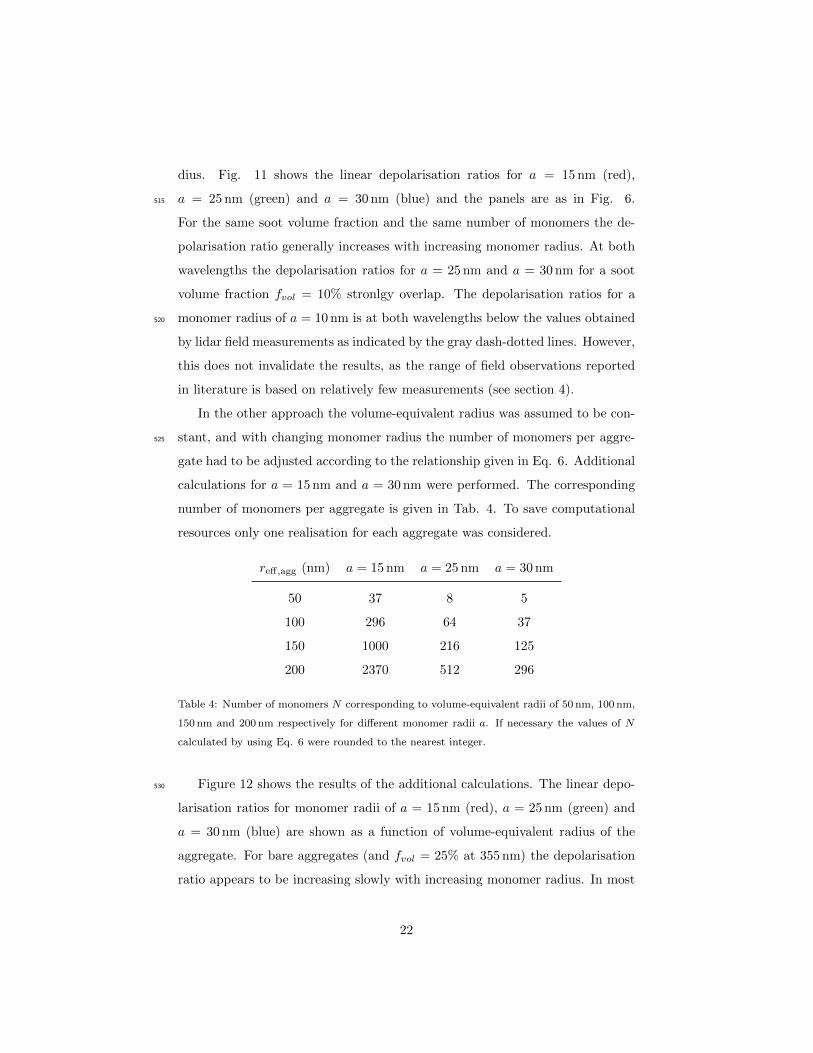
In the other approach the volume-equivalent radius was assumed to be con-
stant, and with changing monomer radius the number of monomers per aggre-525
gate had to be adjusted according to the relationship given in Eq. 6. Additional
calculations for a = 15 nm and a = 30 nm were performed. The corresponding
number of monomers per aggregate is given in Tab. 4. To save computational
resources only one realisation for each aggregate was considered.
reff,agg (nm) a = 15 nm a = 25 nm a = 30 nm
50 37 8 5
100 296 64 37
150 1000 216 125
200 2370 512 296
Table 4: Number of monomers N corresponding to volume-equivalent radii of 50 nm, 100 nm,
150 nm and 200 nm respectively for different monomer radii a. If necessary the values of N
calculated by using Eq. 6 were rounded to the nearest integer.
Figure 12 shows the results of the additional calculations. The linear depo-530
larisation ratios for monomer radii of a = 15 nm (red), a = 25 nm (green) and
a = 30 nm (blue) are shown as a function of volume-equivalent radius of the
aggregate. For bare aggregates (and fvol = 25% at 355 nm) the depolarisation
ratio appears to be increasing slowly with increasing monomer radius. In most
22
other cases it is difficult to discern any clear trends. However, in many cases the535
depolarisation ratios for a = 30 nm tend to be higher than those for a = 15 nm,
with exception of the aggregates with reff,agg = 200 nm at 532 nm.
3.3.4. Effect of uncertainties in the refractive index
The depolarisation ratios computed for different refractive indices of soot and
of the coating material at λ = 0.532µm are depicted in the left column of Fig.540
13. The panels and particle-size ranges are similar to Fig. 6. The computations
have been performed using only one aggregate realisation. The left column
of the figure shows soot-1 (msoot,1 = 1.76 + i0.63) with organic (morganic =
1.53 + i0.0055) (dark red) and sulphate coating (mSO4 = 1.43 + i10−8) (blue),
and soot-2 (msoot,2 = 1.95 + i0.79) with organic (orange) and sulphate coating545
(green).
A change in the refractive index of the coating material has the largest effect
for low soot volume fractions. By contrast, a change in the refractive index
of soot can impact the depolarsation ratio both at low and at high volume
fractions. In general, changes in the refractive index have a stronger effect550
on the depolarisation ratio than the differences we observe when varying the
geometry of the aggregates (compare to the shaded regions in Fig. 6).
The depolarisation ratios for different refractive indices at λ = 0.355µm (see
right column of Fig. 13) have to be compared with caution to the values for
λ = 0.532µm as the chosen refractive indices do not refer to the same type555
of soot and mildly absorbing coating, respectively, as pointed out in section
2.2. The right column of Fig. 13 shows soot-3 (msoot,3 = 1.66284 + i0.71528)
with toluene (mtoluene = 1.632 + i0.047) (red) and sulphate coating (mSO4=
1.45 + i10−8) (blue), and soot-4 (msoot,4 = 1.68586 + i0.67251) with toluene
(orange) and sulphate coating (green). The relatively small differences between560
the two different soot types, which is in every considered case smaller than the
difference between the coating types, is most likely due to the relatively small
change in refractive index. For soot volume fractions of fvol = 75%, fvol = 50%
and fvol = 25% the aggregates coated with weakly absorbing toluene have a
23
higher depolarisation ratio than the aggregates coated with non-absorbing sul-565
phate. However, for fvol = 10% the depolarisation ratios of the toluene coated
aggregates is smaller than that of the aggregates coated with sulphate. For ex-
ample the depolarisation ratios of the toluene coated aggregates with N = 216
are δl = 1.2% and δl = 1.3% respectively. The depolarisation ratios for the
sulphate coated aggregates with N = 216 are δl = 14.9% and δl = 16.6%, re-570
spectively, which is a difference of about an order of magnitude. A similar but
less pronounced effect can be seen for the depolarisation ratios at λ = 0.532µm.
A likely explanation is that non-absorbing sulphate allows the electromagnetic
field to penetrate into the coating and interact with the nonspherical soot ag-
gregate. By contrast, absorbing organic material, especially toluene, allows less575
electromagnetic energy to penetrate to the encapsulated soot aggregate. As a
result, for organic materials the depolarisation of heavily coated soot is dom-
inated by the spherical shell. By contrast, for sulphate the nonspherical soot
core makes a stronger contribution, thus giving rise to stronger depolarisation.
3.3.5. Effect of overlapping monomers580
Fig. 14 shows the scattering and absorption cross sections for aggregates
with overlapping and non-overlapping monomers as well as ratios of the optical
cross sections for Cov = 0.0 and Cov = 0.15. For larger soot volume fractions
(fvol ≥ 50%) the calculated scattering cross sections are higher after introducing
overlapping. For smaller soot volume fraction the effect appears to be suppressed585
by the thicker coating. The absorption cross section is almost not effected by
introducing overlapping monomers. This is also reflected by the ratios of the
absorption cross section, which are closer to unity than for the ratios of the
scattering cross section.
The depolarisation ratio is affected in a similar way, as can be seen in Fig. 15.590
This figure shows analogous to Fig. 6 the linear depolarisation ratios for different
soot volume fractions (rows) and wavelengths (columns) calculated using the
rapid transition model in conjunction with different overlap factors. The results
for aggregates with point-contacting monomers (Cov = 0.0) are shown in red,
24

those for overalpping monomers (Cov = 0.15) are shown in blue. Introducing595
overlapping monomers increases the linear depolarisation. Irrespective of the
soot volume fraction the mean linear depolarisation ratio at λ = 0.532µm (see
left column) is higher for aggregates with Cov = 0.15 than for aggregates wit
Cov = 0.0. However, with decreasing soot volume fraction the differences in δl
between overlapping and non-overlapping monomers become much smaller than600
those among different aggregate geometries. Thus the effect of overlapping is
weakened by the coating.
For a wavelength of λ = 355 nm the effect of introducing overlapping monomers
on the mean linear depolarisation ratio is depending on the soot volume frac-
tion, as can be seen in the right column of Fig. 15. While for larger aggregates605
(N > 8) with soot volume fractions of fvol ≥ 25% the introduction of overlap-
ping increases δl, the reverse happens for all aggregates for fvol = 10%, as well
as for aggregates with N = 8 and fvol ≤ 50%.
3.3.6. Summary of relative uncertainties
We calculated the (maximum) relative uncertainty4 for each aggregate size
and soot volume fraction. It was found that changes in the soot volume frac-
tion had a larger impact on the relative uncertainty than the particle size. For
each volume fraction, we take the maximum relative uncertainty over all par-
ticle sizes (not considering the spherically coated aggregates for N = 8 with
fvol = 25%, fvol = 10%). The different relative uncertainties ∆δl for λ = 532 nm
are shown in Tab. 5. The subscripts refer to the different sources of uncertainty,
namely, aggregate geometry (geo), fractal prefactor (k0), fractal dimension (Df ),
monomer radius (rad), overlapping monomers (ov), refractive index of aggregate
(agg) and coating (coat). In case of the uncertainty due to changes in monomer
radius only the effects of aggregates with constant volume-equivalent aggregate
4The relative uncertainty is defined as ∆δl = 100%× | δl,ref − δl,x | /δl,ref, where δl,ref
denotes a reference or mean value, and δl,x represents the maximum deviation from the ref-
erence.
25

radius were considered. The total relative uncertainty was calculated by assum-
ing that the different sources of error are statistically independent of each other,
so that
∆totδl =√
∆geoδ2l + ∆k0
δ2l + ∆Df
δ2l + ∆radδ2
l + ∆ovδ2l + ∆aggδ2
l + ∆coatδ2l .
(9)
More detailed measurements can provide us with better knowledge of the610
fractal parameters (k0, Df and monomer radius), of the overlapping factor and
of the refractive indices of the aggregate and the coating material. This can
decrease the corresponding uncertainties in the computed optical properties.
As both the collapse of the aggregate due to coating, especially at intermedi-
ate soot volume fractions, and the refractive index of the coating depend of615
the type of the coating material itself, more detailed measurements might help
to provide better understanding of potential correlations between the various
types of uncertainty and thus leading to a lower total uncertainty. However the
uncertainty related to the different stochastic geometries is nearly impossible to
reduce, since it is practically not feasible to account for each and every particle620
geometry encountered in an ensemble of aerosols. Thus the geometry-related
uncertainty can be seen as a lower bound of the overall uncertainty.
fvol(%) ∆geoδl ∆k0δl ∆Df
δl ∆radδl ∆ovδl ∆aggδl ∆coatδl ∆totδl
100 25.2 79.6 32.5 54.5 41.0 20.4 — 114.4
75 27.4 74.1 39.5 61.6 40.1 18.8 6.1 116.6
50 44.2 80.2 32.8 62.6 30.1 18.3 10.5 121.4
25 49.6 59.1 59.7 33.7 32.0 10.9 11.9 109.3
10 41.0 93.5 204.0 46.7 21.3 32.5 56.2 242.7
Table 5: Maximum relative uncertainties and total relative uncertainty in % for different fvol
at λ = 532 nm
In case of the fractal prefactor there is additionally a dependence of uncer-
tainty on the number of monomers, as can be inferred from Fig. 8. To address
the size dependence of the uncertainty due to changes in fractal prefactors we625
26

fvol(%) ∆k0,smallδl(%) ∆k0,largeδl
100 79.6 4.9
75 74.1 14.5
50 80.2 14.0
25 59.1 38.5
10 93.2 18.4
Table 6: Uncertainty due to changes in fractal prefactor for different soot volume fraction fvol
at λ = 0.532µm compared for ”small” aggregates (N = 8, N = 64) and ”large” aggregates
(N = 216, N = 512)
decided to refer to aggregate consisting either of N = 8 or N = 64 monomers
as ”small” and to aggregate consisting of N = 216 and N = 512 monomers as
”large”. The corresponding maximum uncertainties at λ = 0.532µm for both
small and large aggregates for each of the considered soot volume fraction are
given in Tab. 6. As can be seen the uncertainty is substantially lower for large630
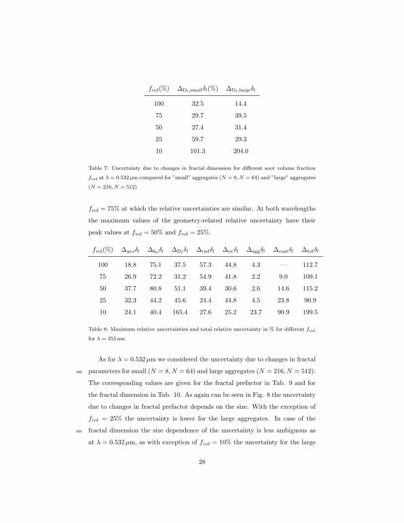
aggregates. For the fractal dimension the dependence is rather ambiguous (see
Tab. 7): For fvol = 100% and f25% the uncertainty decreases for the large
aggregates. For fvol = 75% and f50% the calculated uncertainties are higher
for the large aggregates, but the increase is smaller than the decrease in the
other two cases. However, in case of fvol = 10% the highest uncertainties due635
to changes in the fractal dimensions are for larger aggregates. If knowledge
about the aggregate size exists and in case of the fractal dimension additional
knowledge of the coating thickness, the total uncertainty due to changes in frac-
tal prefactor can be reduced. A likely explanation for the high sensitivity of δl
to changes in fractal parameters for small aggregates is that for the latter the640
fractal structure, hence the fractal parameters, are poorly defined, due to the
small number of monomers. Thus the observed sensitivity of δl to changes in
the fractal parameters may simply be a statistical artifact.
The uncertainties at λ = 355 nm are shown in Tab. 8. In general, the
relative uncertainties ∆geoδl are smaller at 355 nm than at 532 nm, except for645
27
fvol(%) ∆Df ,smallδl(%) ∆Df ,largeδl
100 32.5 14.4
75 29.7 39.5
50 27.4 31.4
25 59.7 29.3
10 101.3 204.0
Table 7: Uncertainty due to changes in fractal dimension for different soot volume fraction
fvol at λ = 0.532µm compared for ”small” aggregates (N = 8, N = 64) and ”large” aggregates
(N = 216, N = 512)
fvol = 75% at which the relative uncertainties are similar. At both wavelengths
the maximum values of the geometry-related relative uncertainty have their
peak values at fvol = 50% and fvol = 25%.
fvol(%) ∆geoδl ∆k0δl ∆Df
δl ∆radδl ∆ovδl ∆aggδl ∆coatδl ∆totδl
100 18.8 75.1 37.5 57.3 44.8 4.3 — 112.7
75 26.9 72.2 31.2 54.9 41.8 2.2 9.0 109.1
50 37.7 80.8 51.1 39.4 30.6 2.6 14.6 115.2
25 32.3 44.2 45.6 24.4 44.8 4.5 23.8 90.9
10 24.1 40.4 165.4 27.6 25.2 23.7 90.9 199.5
Table 8: Maximum relative uncertainties and total relative uncertainty in % for different fvol
for λ = 355 nm
As for λ = 0.532µm we considered the uncertainty due to changes in fractal
parameters for small (N = 8, N = 64) and large aggregates (N = 216, N = 512).650
The corresponding values are given for the fractal prefactor in Tab. 9 and for
the fractal dimension in Tab. 10. As again can be seen in Fig. 8 the uncertainty
due to changes in fractal prefactor depends on the size. With the exception of
fvol = 25% the uncertainty is lower for the large aggregates. In case of the
fractal dimension the size dependence of the uncertainty is less ambiguous as655
at λ = 0.532µm, as with exception of fvol = 10% the uncertainty for the large
28

fvol(%) ∆k0,smallδl(%) ∆k0,largeδl
100 75.1 3.5
75 72.2 2.6
50 80.8 13.9
25 16.2 44.2
10 40.4 19.7
Table 9: Uncertainty due to changes in fractal prefactor for different soot volume fraction fvol
at λ = 0.355µm compared for ”small” aggregates (N = 8, N = 64) and ”large” aggregates
(N = 216, N = 512)
fvol(%) ∆Df ,smallδl(%) ∆Df ,largeδl
100 37.5 21.9
75 31.2 26.9
50 51.1 25.0
25 45.6 18.6
10 58.7 165.4
Table 10: Uncertainty due to changes in fractal dimension for different soot volume fraction
fvol at λ = 0.355µm compared for ”small” aggregates (N = 8, N = 64) and ”large” aggregates
(N = 216, N = 512)
aggregates is smaller than the uncertainty for the small aggregates.
4. Discussion
Field measurements of the linear backscattering depolarisation ratio at λ=532 nm
of aged smoke lie in the range of 1.5 to 23% (see Tab. 11) with most re-660
ported values in the range of 1.5 to 11%. In our calculations based on the
rapid-transition model we obtained, depending on the soot volume fraction and
number of monomers, mean linear depolarisation ratios in the range of 0.055 -
6.2% for the reference calculations for aggregates consisting of point-contacting
monomers and coated with sulphate.665
29

δl(%) location type reference
6-11 Lindenberg, Germany aged BBA [55]
5-8 Tokyo, Japan aged smoke [56]
1.5-3 Leipzig, Germany smoke [57]
<3 Fairbanks, USA fresh smoke [58]
5 Fairbanks, USA aged smoke [58]
15-17 Praia, Cape Verde BBA [34]
15-23 Praia, Cape Verde probably BBA [34]
3-7 Praia, Cape Verde smoke [59]
<2-5 North America (various flight campaigns) fresh smoke [60]
3-8 North America (various flight campaigns) aged smoke [60]
<3 Manaus, Brazil aged smoke [35]
6-8 North-East Germany aged smoke [61]
5.8-7.8 US East Coast smoke [36]
7.8-10.8 Denver, USA smoke [36]
<5 Western Mediterranean Sea BBA [38]
Table 11: δl at 532 nm obtained from various field campaigns. The given type always refers
the the classification given in the cited reference. We assume that smoke and biomass burning
aerosol (BBA) refer to (coated) soot aerosol particles.
30

fvol(%) age location reference
7− 24 (median: 15) < 12h Mexico City, Mexico [5]
6, 13 (not reported) Lindenberg, Germany [6]
7± 8 < 1 day Mexico City, Mexico [7]
(not quantitatively reported) ∼ 1− 2h Los Alamos, USA [8]
Table 12: Examples of soot volume fractions fvol of sampled atmospheric soot particles re-
ported in the literature
Aged soot particles in the atmosphere often have low soot volume fractions
[5, 6, 7, 8]. Some reported values of soot volume fraction are shown in Tab. 12.
In [8] 1026 soot particles from forest fire smoke were analysed, while the soot
volume fraction was not quantitatively reported, it is worth noting, that 50% of
the particles were described as being heavily coated, 34% as partly coated and670
4% as uncoated or very thinly coated. The remaining 12% were described as soot
partly embedded in coating material. This particle count might be biased low,
as very thick coating might lead to the soot monomers being indistinguishable
and therefore this particles might be wrongly classified as not soot containing
[8]. The reported soot particle age in [5, 8] indicates fast coating processes in675
the atmosphere. The range of reported soot volume fractions for atmospheric
soot particles (fvol < 24%), as given in Tab. 12, indicate that our simulation
results for soot volume fractions of fvol = 10% and fvol = 25% (see rows 4
and 5 in Figs. 6, 15) are most relevant for comparing or modelling results to
lidar field measurements. The higher soot volume fractions, on the other hand,680
are more relevant for comparison with laboratory measurements than with field
measurements.
As a reference case we assumed aggregates consisting of monomers with a
radius of a = 25 nm. For fvol = 10% this corresponds to an aggregate with a vol-
ume equivalent radius of aeff = 320 nm (N = 216) and aeff = 430nm (N = 512)685
respectively (see Eqs. 6, 7). Reported median and mean volume equivalent
radii of aeff,median = 145 nm [5] and aeff,mean = 206 nm [7] suggest that most
31

atmospheric soot aerosol particles are smaller then the largest particles mod-
elled in this study. However scattering by particles increases with particle size.
Therefore relatively few large particles can still have a considerable impact on690
bulk scattering properties [62].
According to table 5, the uncertainty in our model estimates for such parti-
cles is close to ∆totδl≈245% (λ = 0.532µm) and ∆totδl≈200% (λ = 0.355µm).
For certain configurations of input parameters the modell may still give results
not consistent with lidar field measurements.695
By contrast, the slow-transition model yields depolarisation ratios of δl =
35.0% for fvol = 10% and N = 512 assuming point-contacting monomers and
sulphate coating, which is higher than the depolarisation ratio of δl = 5.7%
resulting from the rapid-transition model. These values obtained with the slow
transition model lie outside the range of observed field measurements. Also,700
the slow-transition model used here yields results for δl that are higher than
values of δl = 16% as reported in [26]. The main difference is that the slow-
transition model in the present study does account for the compaction of the
aggregate with decreasing soot volume fraction, while the model in [26] does
not. Thus an increase of the compactness of the aggregate with decreasing soot705
volume fraction without changing the critical coating diameter for the onset
of sphericity results in an increase of the depolarisation ratio. By contrast,
in the rapid-transition aggregate model the combined effect of reducing the
critical coating diameter and of increasing the aggregate’s compactness resulted
in depolarisation ratios consistent with the existing lidar field measurements.710
To check the consistency of the calculated depolarisation ratios at 355 nm
they were gauged against results of lidar field measurements reported in the
literature, which we summarise in Tab. 13.
These field measurements report depolarisation ratios at 355 nm ranging
from 2−25%. Most notable are the relatively large values reported in [20, 34, 36],715
which pertain to non-dust containing aerosols. The calculations for an aggregate
of point-contacting monomers with sulphate coating using the rapid-transition
model cover a range of δl from 1.7 to 20.3%, which largely lies within the range
32

δl(%) location type reference
4-5 Manaus, Brazil aged biomass burning [33]
15-19 Praia, Cape Verde BBA [34]
21-25 Praia, Cape Verde probably BBA [34]
< 3 Manaus, Brazil aged smoke [35]
7-13 Leipzig, Germany aged biomass burning [20]
16-24 Denver, USA pure smoke [36]
2-6 Kazan, Russia pure BBA [37]
2-5 Elandsfontein, South Africa BBA [39]
Table 13: δl at 355 nm obtained from various field campaigns. The given type always refers
the the classification given in the cited reference. We assume that smoke and biomass burning
aerosol (BBA) refer to (coated) soot aerosol particles.
of reported values obtained from lidar field measurements. The slow-transition
model yields values of δl up to 55% for fvol = 10%; this is clearly inconsistent720
with the values obtained in lidar field measurements.
The values calculated for the linear depolarisation ratio at 355 nm for fvol =
10% have the same order of magnitude (∼20%) as results presented in [63].
Those values were obtained in order to reproduce the measurements by [36]
using different particle models, all having relatively small fvol, namely a closed725
cell model with 0.4% < fvol < 0.5%, a model of two contacting spheres each
encapsulating an aggregate with 2.0% < fvol < 8.0% and concentric core-mantle
spheroids for different combinations of axis ratio and soot volume fraction with
2.0% < fvol < 12.5%.
The depolarisation ratios obtained with the rapid-transition model are more730
consistent with the reported field measurements than those obtained with either
the slow-transition model or the model used in [26]. This is remarkable, since
the morphological differences among these three models are rather subtle. These
results illustrate the high sensitivity of the depolarisation ratio to the particles’
geometry.735
33

However, comparisons of model results with field observations provide us
with little more than a consistency check; they cannot be interpreted as reliable
quantitative evidence. This is due to a number of unknowns in the experimental
data. The field measurements do not provide us with information on the aggre-
gates’ geometry (e.g. fractal parameters) and the soot volume fraction. Nor is it740
always trivial to determine whether or not the observed plumes were composed
of pure soot aerosols or of mixtures contaminated with other compounds, such
as dust.
Our main hypothesis was that the depolarisation ratio of the model particles
can be controlled by the the mode of transition from film-coating to spherical745
coating. As more coating material is added to the soot aggregate, a faster
transition to spherically coated aggregates was expected to result in lower de-
polarisation ratios as compared to a slow-transition model. This hypothesis was
largely confirmed by our results, although with some rather interesting reserva-
tions.750
It was hypothesised that a fast transition to spherical coating can be achieved
by (i) choosing a relatively small value of the critical radius that marks to onset
of spherical growth; and (ii) allowing the aggregate to become more compact as
more coating material is added. The choice of the critical radius had, indeed,
a profound impact on the depolarisation ratio, as hypothesised. However, an755
increase in fractal dimension may give rise to two competing effects.
• A more compact aggregate is more readily encapsulated by a spherical
shell with no parts of the aggregate sticking out of the shell. This is ex-
pected to result in a low depolarisation ratio, especially for heavily coated
aggregates.760
• A more compact aggregate would give rise to more electromagnetic in-
teraction among the monomers, so the optical properties should be less
similar to independently scattering monomers than in a lacy aggregate.
This may increase the depolarisation ratio, especially in thinly coated ag-
gregates.765
34

The latter effect explains why the depolarisation ratios computed in [26] were
lower than those computed with the slow transition model. Both models use
the same critical radius that defines the onset of spherical growth. However,
the model in [26] neglects compaction of the aggregates with increasing coating
thickness, which results in less electromagnetic interaction among the monomers.770
It is also possible that overlapping of monomers enhances electromagnetic
interaction. This could explain why in Fig. 15 the depolarisation ratios for
overlapping monomers are generally higher than those for monomers in point-
contact. This is most pronounced for bare aggregates and for soot volume
fractions fvol ≥ 25%. For fvol = 10% there is little difference for small size pa-775
rameters. For large size parameters (large numbers of monomers in the UV) the
overlapping monomers yield slightly lower depolarisation than those in point-
contact.
Deviations from point-contacting monomers are only parametrized as over-
lapping monomers. The effect of “necking” between two monomers is not con-780
sidered here. According to the results presented in [43], necking can have a sig-
nificant impact on scattering and absorption, especially at smaller wavelengths.
The influence of necking on the linear depolarisation ratio should be addressed
in future studies.
5. Summary and Conclusions785
A main goal in fundamental aerosol optics research is to understand the
relation between morphological and optical properties. In particular, we want
to identify those morphological features that have a dominant impact on the
optical properties. This is often much easier for integral optical properties,
such as the total scattering and absorption cross sections, than for differential790
scattering properties. It is particularly challenging for quantities, such as δl,
that are exceedingly sensitive to even small variations in particle morphology.
The findings of this study have allowed us to make some encouraging progress
in this regard. The results indicate that one of the essential morphological
35

features of soot aerosols is the speed of transition from the nonspherical to795
the spherical coating regime as more coating material is added. In the present
study we parameterised the onset of the spherical-coating regime by defining a
critical diameter, which was based on an educated guess. However, we expect
that this critical diameter should be dependent on the hygroscopicity of the
soot aggregate and/or the surface tension of the coating material. Suitable800
refinements of our model will have to depend on more guidance from laboratory
studies, such as the ones reported in [31].
In choosing the critical radius we can get some rough guidance from field
measurements with lidar instruments. However, we know from earlier modelling
studies (e.g. [36, 26]) that it is challenging to reproduce lidar field observations805
of the linear backscattering depolarisation ratio δl of soot aerosols with models.
There may be a certain risk that the model in [26] overestimates δl for large,
heavily coated soot particles, which may indicate that those model particles are
not sufficiently spherical. This observation lead us to hypothesise that one of
the essential morphological properties in soot-particles is the mode of transition810
from a thin film-coating to a spherical shell; we proposed to account for a
relatively rapid transition from nonspherical to spherical shape as more coating
material is added to the soot aggregate. This can be achieved by (i) reducing the
critical diameter which defines the onset of sphericity in the coated aggregate
model; and (ii) taking the compaction of soot into account as more coating815
material is added. Our main hypothesis was that the depolarisation ratio is
highly sensitive to this speed of transition. This hypothesis is supported by
our results. However, the compaction of soot can also enhance electromagnetic
interaction among the monomers, which can increase the depolarisation. This
phenomenon seems to somewhat diminish the depolarisation-reducing effect of820
the rapid transition to a spherical coating, at least for soot volume fractions
higher than 25 %.
Here we extended the computations in [26], which were limited to a visible
wavelength of 532 nm, to include a UV wavelength of 355 nm. For both wave-
lengths we found that our rapid-transition coated aggregate model produced δl825
36

values that were largely consistent with lidar field observations of soot plumes.
A long-term goal of this study is to develop a model particle that can be
employed in retrieval algorithms and in chemical data assimilation. For such
purposes it is essential to have not only a reliable aerosol optics model, but
also a realistic estimate of the model uncertainties. Using the rapid-transition830
model, different sources of uncertainty of the model results were examined at
532 nm and 355 nm. Depending on the soot volume fraction the total relative
uncertainty in δl at 532 nm ranges between 109 and 243%. At 355 nm the total
relative uncertainty in δl ranges from 90.9 to 200%. Model errors caused by a
limited knowledge of the extent of overlapping between neighbouring monomers835
or the refractive index of both aggregate and coating material could be reduced
as more reliable measurements become available. However, the uncertainty
related to our lack of precise knowledge of the aggregate geometry cannot be
reduced. The values for this type of uncertainty range from 25 to 50% at 532 nm
and 19 to 38% at 355 nm depending on the soot volume fraction. This can be840
considered a lower bound for the modelling uncertainty in δl.
Acknowledgements
We are grateful to Dan Mackowski for providing us with his cluster-cluster
aggregation program. Maxim Yurkin and Alfons G. Hoekstra are acknowledged
for making their ADDA code publicly available. F. Kanngießer and M. Kahnert845
acknowledge funding by the Swedish Research Council (Vetenskapsradet ; dnr
2016-03499); M. Kahnert acknowledges funding by the Swedish National Space
Board (Rymdstyrelsen; dnr 100/16).
References
[1] T. C. Bond, R. W. Bergstrom, Light absorption by carbonaceous parti-850
cles: An investigative review, Aerosol Sci. Technol. 40 (1). doi:10.1080/
02786820500421521.
37

[2] P. Chylek, G. B. Lesins, G. Videen, J. G. D. Wong, R. G. Pinnick, D. Ngo,
J. D. Klett, Black carbon and absorption of solar radiation by clouds, J.
Geophys. Res. 101 (D18) (1996) 23365–23371. doi:10.1029/96JD01901.855
[3] S. C. Anenberg, K. Talgo, S. Arunachalam, P. Dolwick, C. Jang, J. J. West,
Impacts of global, regional, and sectoral black carbon emission reductions
on surface air quality and human mortality, Atmos. Chem. Phys. 11 (14)
(2011) 7253–7267. doi:10.5194/acp-11-7253-2011.
[4] R. Zhang, A. F. Khalizov, J. Pagels, D. Zhang, H. Xue, P. H. McMurry,860
Variability in morphology, hygroscopicity, and optical properties of soot
aerosols during atmospheric processing, Proc Natl Acad Sci U S A 105 (30)
(2008) 10291–10296. doi:10.1073/pnas.0804860105.
[5] K. Adachi, P. R. Buseck, Internally mixed soot, sulfates, and organic matter
in aerosol particles from mexico city, Atmos. Chem. Phys. 8 (21) (2008)865
6469–6481. doi:10.5194/acp-8-6469-2008.
[6] A. Worringen, M. Ebert, T. Trautmann, S. Weinbruch, G. Helas, Optical
properties of internally mixed ammonium sulfate and soot particles–a study
of individual aerosol particles and ambient aerosol populations, Appl. Opt.
47 (21) (2008) 3835–3845. doi:10.1364/AO.47.003835.870
[7] K. Adachi, S. H. Chung, P. R. Buseck, Shapes of soot aerosol particles and
implications for their effects on climate, J. Geophys. Res. 115 (D15) (2010)
n/a–n/a. doi:10.1029/2009JD012868.
[8] S. China, C. Mazzoleni, K. Gorkowski, A. C. Aiken, M. K. Dubey, Morphol-
ogy and mixing state of individual freshly emitted wildfire carbonaceous875
particles, Nat. Commun. 4 (2122). doi:10.1038/ncomms3122.
[9] M. Kahnert, T. Nousiainen, H. Lindqvist, Models for integrated and differ-
ential scattering optical properties of encapsulated light absorbing carbon
aggregates, Opt. Express 21 (7) (2013) 7974–7993. doi:10.1364/OE.21.
007974.880
38

[10] M. Kahnert, T. Nousiainen, H. Lindqvist, Review: Model particles in at-
mospheric optics, J. Quant. Spectrosc. Radiat. Transfer 146 (Supplement
C) (2014) 41 – 58, electromagnetic and Light Scattering by Nonspherical
Particles XIV. doi:https://doi.org/10.1016/j.jqsrt.2014.02.014.
[11] F. Liu, J. Yon, A. Bescond, On the radiative properties of soot aggregates885
part 2: Effects of coating, J. Quant. Spectrosc. Radiat. Transfer 172 (Sup-
plement C) (2016) 134–145. doi:10.1016/j.jqsrt.2015.08.005.
[12] J. Dong, J. Zhao, L. Liu, Morphological effects on the radiative properties
of soot aerosols in different internally mixing states with sulfate, J. Quant.
Spectrosc. Radiat. Transfer 165 (Supplement C) (2015) 43–55. doi:10.890
1016/j.jqsrt.2015.06.025.
[13] Y. Wu, T. Cheng, L. Zheng, H. Chen, Models for the optical simulations of
fractal aggregated soot particles thinly coated with non-absorbing aerosols,
J. Quant. Spectrosc. Radiat. Transfer 182 (Supplement C) (2016) 1–11.
doi:10.1016/j.jqsrt.2016.05.011.895
[14] Y. Wu, T. Cheng, X. Gu, L. Zheng, H. Chen, H. Xu, The single scattering
properties of soot aggregates with concentric coreshell spherical monomers,
J. Quant. Spectrosc. Radiat. Transfer 135 (Supplement C) (2014) 9 – 19.
doi:https://doi.org/10.1016/j.jqsrt.2013.11.009.
[15] K. Liou, Y. Takano, P. Yang, Light absorption and scattering by aggregates:900
Application to black carbon and snow grains, J. Quant. Spectrosc. Radiat.
Transfer 112 (10) (2011) 1581 – 1594. doi:https://doi.org/10.1016/j.
jqsrt.2011.03.007.
[16] Y. Wu, T. Cheng, L. Zheng, H. Chen, H. Xu, Single scattering properties
of semi-embedded soot morphologies with intersecting and non-intersecting905
surfaces of absorbing spheres and non-absorbing host, J. Quant. Spectrosc.
Radiat. Transfer 157 (Supplement C) (2015) 1 – 13. doi:https://doi.
org/10.1016/j.jqsrt.2015.02.006.
39

[17] A. Bescond, J. Yon, T. Girasole, C. Jouen, C. Roz, A. Coppalle, Numerical
investigation of the possibility to determine the primary particle size of910
fractal aggregates by measuring light depolarization, J. Quant. Spectrosc.
Radiat. Transfer 126 (Supplement C) (2013) 130 – 139. doi:https://doi.
org/10.1016/j.jqsrt.2012.10.011.
[18] A. H. Omar, D. M. Winker, M. A. Vaughan, Y. Hu, C. R. Trepte, R. A.
Ferrare, K.-P. Lee, C. A. Hostetler, C. Kittaka, R. R. Rogers, R. E. Kuehn,915
Z. Liu, The calipso automated aerosol classification and lidar ratio selection
algorithm, J. Atmos. Oceanic Technol. 26 (10) (2009) 1994–2014. doi:
10.1175/2009JTECHA1231.1.
[19] S. Groß, V. Freudenthaler, M. Wirth, B. Weinzierl, Towards an aerosol
classification scheme for future earthcare lidar observations and implica-920
tions for research needs, Atmos. Sci. Lett. 16 (1) (2015) 77–82. doi:
10.1002/asl2.524.
[20] A. J. Illingworth, H. W. Barker, A. Beljaars, M. Ceccaldi, H. Chepfer,
N. Clerbaux, J. Cole, J. Delano, C. Domenech, D. P. Donovan, S. Fukuda,
M. Hirakata, R. J. Hogan, A. Huenerbein, P. Kollias, T. Kubota, T. Naka-925
jima, T. Y. Nakajima, T. Nishizawa, Y. Ohno, H. Okamoto, R. Oki,
K. Sato, M. Satoh, M. W. Shephard, A. Velzquez-Blzquez, U. Wandinger,
T. Wehr, G.-J. van Zadelhoff, The earthcare satellite: The next step for-
ward in global measurements of clouds, aerosols, precipitation, and radi-
ation, Bull. Amer. Meteor. Soc. 96 (8) (2015) 1311–1332. doi:10.1175/930
BAMS-D-12-00227.1.
[21] M. Kahnert, Modelling radiometric properties of inhomogeneous mineral
dust particles: Applicability and limitations of effective medium theories,
J. Quant. Spectrosc. Radiat. Transfer 152 (2015) 16–27. doi:10.1016/j.
jqsrt.2014.10.025.935
[22] Y. Wu, T. Cheng, L. Zheng, H. Chen, Optical properties of the semi-
external mixture composed of sulfate particle and different quantities of
40

soot aggregates, J. Quant. Spectrosc. Radiat. Transfer 179 (Supplement C)
(2016) 139 – 148. doi:https://doi.org/10.1016/j.jqsrt.2016.03.012.
[23] R. P. Bambha, M. A. Dansson, P. E. Schrader, H. A. Michelsen, Effects940
of volatile coatings and coating removal mechanisms on the morphology of
graphitic soot, Carbon 61 (2013) 80 – 96. doi:10.1016/j.carbon.2013.
04.070.
[24] R. Ghazi, J. S. Olfert, Coating mass dependence of soot aggregate re-
structuring due to coatings of oleic acid and dioctyl sebacate, Aerosol Sci.945
Technol. 47 (2) (2013) 192–200. doi:10.1080/02786826.2012.741273.
[25] E. G. Schnitzler, A. Dutt, A. M. Charbonneau, J. S. Olfert, W. Jger,
Soot aggregate restructuring due to coatings of secondary organic aerosol
derived from aromatic precursors, Environ. Sci. Technol. 48 (24) (2014)
14309–14316, pMID: 25390075. doi:10.1021/es503699b.950
[26] M. Kahnert, Optical properties of black carbon aerosols encapsulated in a
shell of sulfate: comparison of the closed cell model with a coated aggregate
model, Opt. Express 25 (20) (2017) 24579–24593. doi:10.1364/OE.25.
024579.
[27] C. M. Sorensen, Light scattering by fractal aggregates: A review, Aerosol955
Sci. Technol. 35 (2001) 648–687. doi:10.1080/02786820117868.
[28] D. W. Mackowski, A simplified model to predict the effects of aggregation
on the absorption properties of soot particles, J. Quant. Spectrosc. Radiat.
Transfer 100 (1) (2006) 237–249, vIII Conference on Electromagnetic and
Light Scattering by Nonspherical Particles. doi:10.1016/j.jqsrt.2005.960
11.041.
[29] K. Adachi, S. H. Chung, H. Friedrich, P. R. Buseck, Fractal parameters of
individual soot particles determined using electron tomography: Implica-
tions for optical properties, J. Geophys. Res. 112 (D14) (2007) n/a–n/a.
doi:10.1029/2006JD008296.965
41

[30] M. Kahnert, T. Nousiainen, H. Lindqvist, M. Ebert, Optical properties
of light absorbing carbon aggregates mixed with sulfate: assessment of
different model geometries for climate forcing calculations, Opt. Express
20 (9) (2012) 10042–10058. doi:10.1364/OE.20.010042.
[31] X. Pei, M. Hallquist, A. C. Eriksson, J. H. Pagels, N. M. Donahue,970
T. Mentel, B. Svenningsson, W. Brune, R. K. Pathak, Morphological trans-
formation of soot: investigation of microphysical processes during the con-
densation of sulfuric acid and limonene ozonolysis product vapors, Atmos.
Chem. Phys. Discuss. 2017 (2017) 1–30. doi:10.5194/acp-2017-769.
[32] U. Wandinger, Lidar - Range-resolved optical remote sensing of the atmo-975
sphere, Springer New York, 2005, Ch. Introduction to lidar, pp. 1–18.
[33] A. Ansmann, H. Baars, M. Tesche, D. Muller, D. Althausen, R. En-
gelmann, T. Pauliquevis, P. Artaxo, Dust and smoke transport from
africa to south america: Lidar profiling over cape verde and the ama-
zon rainforest, Geophys. Res. Lett. 36 (11) (2009) n/a–n/a, l11802. doi:980
10.1029/2009GL037923.
[34] S. Groß, M. Tesche, V. Freudenthaler, C. Toledano, M. Wiegner, A. Ans-
mann, D. Althausen, M. Seefeldner, Characterization of saharan dust, ma-
rine aerosols and mixtures of biomass-burning aerosols and dust by means
of multi-wavelength depolarization and raman lidar measurements during985
samum 2, Tellus B: Chemical and Physical Meteorology 63 (4) (2011) 706–
724. doi:10.1111/j.1600-0889.2011.00556.x.
[35] H. Baars, A. Ansmann, D. Althausen, R. Engelmann, B. Heese, D. Muller,
P. Artaxo, M. Paixao, T. Pauliquevis, R. Souza, Aerosol profiling with
lidar in the amazon basin during the wet and dry season, J. Geophys. Res.990
117 (D21) (2012) n/a–n/a. doi:10.1029/2012JD018338.
[36] S. P. Burton, J. W. Hair, M. Kahnert, R. A. Ferrare, C. A. Hostetler,
A. L. Cook, D. B. Harper, T. A. Berkoff, S. T. Seaman, J. E. Collins,
42

M. A. Fenn, R. R. Rogers, Observations of the spectral dependence of
linear particle depolarization ratio of aerosols using nasa langley airborne995
high spectral resolution lidar, Atmos. Chem. Phys. 15 (23) (2015) 13453–
13473. doi:10.5194/acp-15-13453-2015.
[37] E. Dieudonne, P. Chazette, F. Marnas, J. Totems, X. Shang, Lidar profiling
of aerosol optical properties from paris to lake baikal (siberia), Atmos.
Chem. Phys. 15 (9) (2015) 5007–5026. doi:10.5194/acp-15-5007-2015.1000
[38] G. Ancellet, J. Pelon, J. Totems, P. Chazette, A. Bazureau, M. Sicard,
T. Di Iorio, F. Dulac, M. Mallet, Long-range transport and mixing of
aerosol sources during the 2013 north american biomass burning episode:
analysis of multiple lidar observations in the western mediterranean
basin, Atmos. Chem. Phys. 16 (7) (2016) 4725–4742. doi:10.5194/1005
acp-16-4725-2016.
[39] E. Giannakaki, P. G. van Zyl, D. Muller, D. Balis, M. Komppula, Opti-
cal and microphysical characterization of aerosol layers over south africa
by means of multi-wavelength depolarization and raman lidar measure-
ments, Atmos. Chem. Phys. 16 (13) (2016) 8109–8123. doi:10.5194/1010
acp-16-8109-2016.
[40] H. Chang, T. T. Charalampopoulos, Determination of the wavelength de-
pendence of refractive indices of flame soot, Proc. R. Soc. Lond. 430 (1880)
(1990) 577–591. doi:10.1098/rspa.1990.0107.
[41] M. Hess, P. Koepke, I. Schult, Optical properties of aerosols and clouds:1015
The software package opac, Bull. Amer. Meteor. Soc. 79 (5). doi:10.1175/
1520-0477(1998)079<0831:OPOAAC>2.0.CO;2.
[42] B. V. Scarnato, S. Vahidinia, D. T. Richard, T. W. Kirchstetter, Effects
of internal mixing and aggregate morphology on optical properties of black
carbon using a discrete dipole approximation model, Atmos. Chem. Phys.1020
13 (10). doi:10.5194/acp-13-5089-2013.
43

[43] J. Yon, A. Bescond, F. Liu, On the radiative properties of soot aggregates
part 1: Necking and overlapping, J. Quant. Spectrosc. Radiat. Transfer
162 (Supplement C). doi:10.1016/j.jqsrt.2015.03.027.
[44] A. Brasil, T. Farias, M. Carvalho, A recipe for image characterization of1025
fractal-like aggregates, J. Aerosol Sci. 30 (10) (1999) 1379–1389. doi:
10.1016/S0021-8502(99)00026-9.
[45] R. K. Chakrabarty, H. Moosmuller, L.-W. A. Chen, K. Lewis, W. P. Arnott,
C. Mazzoleni, M. K. Dubey, C. E. Wold, W. M. Hao, S. M. Kreidenweis,
Brown carbon in tar balls from smoldering biomass combustion, Atmos.1030
Chem. Phys. 10 (2010) 6363–6370. doi:10.5194/acp-10-6363-2010.
[46] T. Nakayama, Y. Matsumi, K. Sato, T. Imamura, A. Yamazaki,
A. Uchiyama, Laboratory studies on optical properties of secondary or-
ganic aerosols generated during the photooxidation of toluene and the
ozonolysis of -pinene, J. Geophys. Res. 115 (D24) (2010) n/a–n/a, d24204.1035
doi:10.1029/2010JD014387.
[47] M. A. Yurkin, A. G. Hoekstra, The discrete-dipole-approximation code
adda: Capabilities and known limitations, J. Quant. Spectrosc. Radiat.
Transfer 112 (13). doi:10.1016/j.jqsrt.2011.01.031.
[48] M. Kahnert, Numerical solutions of the macroscopic Maxwell equations for1040
scattering by non-spherical particles: A tutorial review, J. Quant. Spec-
trosc. Radiat. Transfer 178 (Supplement C) (2016) 22 – 37, electromagnetic
and light scattering by nonspherical particles XV: Celebrating 150 years of
Maxwell’s electromagnetics. doi:10.1016/j.jqsrt.2015.10.029.
[49] A. Lakhtakia, G. W. Mulholland, On two numerical techniques for light1045
scattering by dielectric agglomerated structures, J. Res. Natl. Inst. Stand.
Technol. 98 (1993) 699–716. doi:10.6028/jres.098.046.
[50] M. Yurkin, A. Hoekstra, The discrete dipole approximation: An overview
and recent developments, J. Quant. Spectrosc. Radiat. Transfer 106 (1)
44

(2007) 558–589, iX Conference on Electromagnetic and Light Scattering1050
by Non-Spherical Particles. doi:10.1016/j.jqsrt.2007.01.034.
[51] M. Kahnert, T. Nousiainen, H. Lindqvist, M. Ebert, Optical properties
of light absorbing carbon aggregates mixed with sulfate: assessment of
different model geometries for climate forcing calculations, Opt. Express
20 (2012) 10042–10058. doi:10.1364/OE.20.010042.1055
[52] K. Schmidt, M. Yurkin, M. Kahnert, A case study on the reciprocity in
light scattering computations, Opt. Express 20 (2012) 23253–23274. doi:
10.1364/OE.20.023253.
[53] M. I. Mishchenko, J. W. Hovenier, Depolarization of light backscattered by
randomly oriented nonspherical particles, Opt. Lett. 20 (12) (1995) 1356–1060
1358. doi:10.1364/OL.20.001356.
[54] M. I. Mishchenko, K. Sassen, Depolarization of lidar returns by small ice
crystals: An application to contrails, Geophys. Res. Lett. 25 (3) (1998)
309–312. doi:10.1029/97GL03764.
[55] M. Fiebig, A. Petzold, U. Wandinger, M. Wendisch, C. Kiemle, A. Stifter,1065
M. Ebert, T. Rother, U. Leiterer, Optical closure for an aerosol column:
Method, accuracy, and inferable properties applied to a biomass-burning
aerosol and its radiative forcing, J. Geophys. Res. 107 (D21) (2002) LAC
12–1–LAC 12–15, 8130. doi:10.1029/2000JD000192.
[56] T. Murayama, D. Muller, K. Wada, A. Shimizu, M. Sekiguchi,1070
T. Tsukamoto, Characterization of asian dust and siberian smoke with
multi-wavelength raman lidar over tokyo, japan in spring 2003, Geophys.
Res. Lett. 31 (23) (2004) n/a–n/a, l23103. doi:10.1029/2004GL021105.
URL 10.1029/2004GL021105
[57] D. Muller, I. Mattis, U. Wandinger, A. Ansmann, D. Althausen, A. Stohl,1075
Raman lidar observations of aged siberian and canadian forest fire smoke
in the free troposphere over germany in 2003: Microphysical particle
45

characterization, J. Geophys. Res. 110 (D17) (2005) n/a–n/a, d17201.
doi:10.1029/2004JD005756.
[58] K. Sassen, V. I. Khvorostyanov, Cloud effects from boreal forest fire1080
smoke: evidence for ice nucleation from polarization lidar data and cloud
model simulations, Environ. Res. Lett. 3 (2) (2008) 025006. doi:10.1088/
1748-9326/3/2/025006.
[59] M. Tesche, S. Gross, A. Ansmann, D. Muller, D. Althausen, V. Freuden-
thaler, M. Esselborn, Profiling of saharan dust and biomass-burning smoke1085
with multiwavelength polarization raman lidar at cape verde, Tellus B
63 (4) (2011) 649–676. doi:10.1111/j.1600-0889.2011.00548.x.
[60] S. P. Burton, R. A. Ferrare, C. A. Hostetler, J. W. Hair, R. R. Rogers, M. D.
Obland, C. F. Butler, A. L. Cook, D. B. Harper, K. D. Froyd, Aerosol
classification using airborne high spectral resolution lidar measurements1090
methodology and examples, Atmos. Meas. Tech. 5 (1) (2012) 73–98. doi:
10.5194/amt-5-73-2012.
[61] F. Dahlkotter, M. Gysel, D. Sauer, A. Minikin, R. Baumann, P. Seifert,
A. Ansmann, M. Fromm, C. Voigt, B. Weinzierl, The pagami creek smoke
plume after long-range transport to the upper troposphere over europe1095
- aerosol properties and black carbon mixing state, Atmos. Chem. Phys.
14 (12) (2014) 6111–6137. doi:10.5194/acp-14-6111-2014.
[62] M. Kahnert, Modelling the optical and radiative properties of freshly
emitted light absorbing carbon within an atmospheric chemical trans-
port model, Atmos. Chem. Phys. 10 (3) (2010) 1403–1416. doi:10.5194/1100
acp-10-1403-2010.
[63] M. I. Mishchenko, J. M. Dlugach, L. Liu, Linear depolarization of lidar
returns by aged smoke particles, Appl. Opt. 55 (35). doi:10.1364/AO.55.
009968.
46
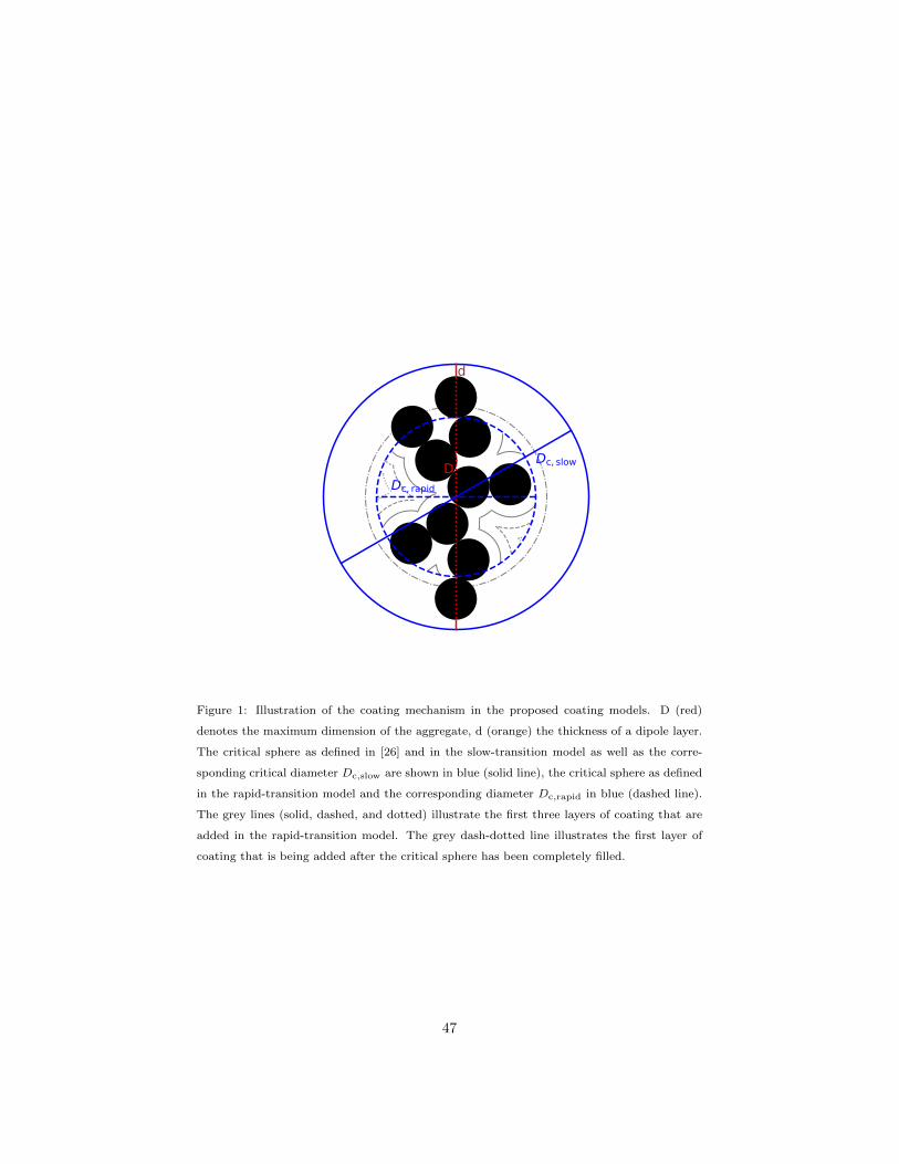
d
DDc, rapid
Dc, slow
Figure 1: Illustration of the coating mechanism in the proposed coating models. D (red)
denotes the maximum dimension of the aggregate, d (orange) the thickness of a dipole layer.
The critical sphere as defined in [26] and in the slow-transition model as well as the corre-
sponding critical diameter Dc,slow are shown in blue (solid line), the critical sphere as defined
in the rapid-transition model and the corresponding diameter Dc,rapid in blue (dashed line).
The grey lines (solid, dashed, and dotted) illustrate the first three layers of coating that are
added in the rapid-transition model. The grey dash-dotted line illustrates the first layer of
coating that is being added after the critical sphere has been completely filled.
47

(a) Df = 2.0 (b) Df = 2.6
Figure 2: Example of two bare aggregates with N = 64 and k0 = 0.7. a) aggregate with a
fractal dimension of Df = 2.0 b) aggregate with a fractal dimension of (Df = 2.6)
(a) fvol = 50% (b) fvol = 25% (c) fvol = 10%
(d) fvol = 50% (e) fvol = 25% (f) fvol = 10%
Figure 3: Examples of six coated aggregates with N = 64 and k0 = 0.7. The aggregate is
shown in grey and the coating is shown in yellow. The top row (a-c) shows aggregates coated
using the slow-transition model. In the bottom row (d-f) coated aggregates obtained with the
rapid-transition model are shown. a, d) aggregate with fvol = 50% (Df = 2.2) b, e) aggregate
with fvol = 25% (Df = 2.4) c, f) aggregate with fvol = 10% (Df = 2.6)
48

(a) Cov = 0.0 (b) Cov = 0.15
Figure 4: Example of two bare aggregates with N = 8 and Df = 2.0. a) aggregate with point-
contacting monomers (Cov = 0.0) b) aggregate with overlapping monomers (Cov = 0.15)
0.00
0.05
0.10
f vol=
100%
Csca ( m2)rapid-transitionslow-transition
0.0
0.2
Cabs ( m2)
0.95
1.00
1.05Csca
0.95
1.00
1.05Cabs
0.0
0.1
f vol=
75%
0.0
0.21.050
1.075
1.100
0.995
1.000
1.005
0.0
0.2
f vol=
50%
0.0
0.21.04
1.05
0.990
0.995
1.000
0.0
0.5
f vol=
25%
0.0
0.2
0.4
1.10
1.15
0.96
0.98
8 64 216 512number of monomers N
0
1
f vol=
10%
8 64 216 512number of monomers N
0.0
0.2
0.4
8 64 216 512number of monomers N
1.02
1.04
8 64 216 512number of monomers N
0.97
0.98
Figure 5: Comparison of optical cross sections for both coating models at λ = 532 nm. The
first column shows the scattering cross sections and the second column shows the absorption
cross section for the rapid-transition model (red line) and the slow-transition model (blue
line). The third column shows the ratio of the scattering cross section calculated for the
rapid-transition and slow-transition model, and the fourth column shows the corresponding
ratio for the absorption cross section. The rows correspond, from top to bottom, to soot
volume fractions of 100%, 75%, 50%, 25%, and 10%, respectively.
49

2
4
lin (%
)f vo
l=10
0%
= 532 nmrapid-transitionslow-transition
= 355 nm
2
4
lin (%
)f vo
l=75
%
2.5
5.0
7.5
lin (%
)f vo
l=50
%
0
5
10
lin (%
)f vo
l=25
%
8 64 216 512number of monomers N
0
25
50
lin (%
)f vo
l=10
%
8 64 216 512number of monomers N
Figure 6: Linear backscattering depolarisation ratio at λ = 0.532µm (left colum) and at
λ = 0.355µm (right column) for soot volume fractions fvol = 100% (first row), 75% (second
row), 50% (third row), 25% (fourth row) and 10% (fifth row) computed for the rapid-transition
(red) and the slow-transition model (blue). The dark lines correspond to the arithmetic
mean of an ensemble of five different stochastic realisations of the aggregate geometry. The
shaded area indicates the maximum variation within the ensemble. The grey dash-dotted lines
indicate lower and upper bound of reported lidar field observations. Most reported values at
λ = 0.532µm are below 11% (indicated by the grey dotted line).
50
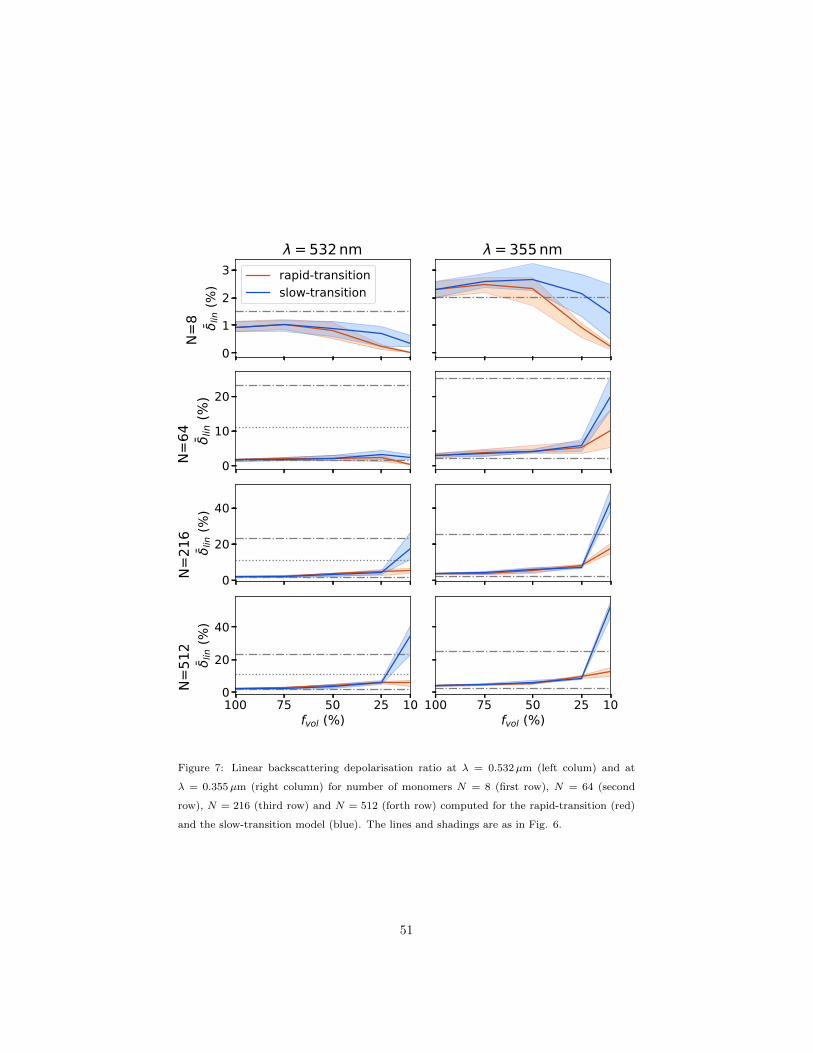
0
1
2
3
lin (%
)N=
8
= 532 nmrapid-transitionslow-transition
= 355 nm
0
10
20
lin (%
)N=
64
0
20
40
lin (%
)N=
216
100 75 50 25 10fvol (%)
0
20
40
lin (%
)N=
512
100 75 50 25 10fvol (%)
Figure 7: Linear backscattering depolarisation ratio at λ = 0.532µm (left colum) and at
λ = 0.355µm (right column) for number of monomers N = 8 (first row), N = 64 (second
row), N = 216 (third row) and N = 512 (forth row) computed for the rapid-transition (red)
and the slow-transition model (blue). The lines and shadings are as in Fig. 6.
51

0
2
4
lin (%
)f vo
l=10
0%
= 532 nmk0 = 0.25k0 = 1.6
= 355 nm
0.0
2.5
5.0
lin (%
)f vo
l=75
%
0
5
lin (%
)f vo
l=50
%
0
10
20
lin (%
)f vo
l=25
%
8 64 216 512number of monomers N
0
10
20
lin (%
)f vo
l=10
%
8 64 216 512number of monomers N
Figure 8: As Fig. 6, but for different fractal prefactors. The linear depolarisation ratios were
calculated using the rapid transition model for two fractal prefactors k0 = 0.25 (red) and
k0 = 1.6 (blue), which corresponds to the range reported in [29].
52

0
2
4
lin (%
)f vo
l=10
0%
= 532 nm = 355 nm
rapid-transition, k0 = 0.25rapid-transition, k0 = 1.6slow-transition, k0 = 0.25slow-transition, k0 = 1.6
0
2
4
lin (%
)f vo
l=75
%
0
5
lin (%
)f vo
l=50
%
0
10
20
lin (%
)f vo
l=25
%
8 64 216 512number of monomers N
0
25
50
lin (%
)f vo
l=10
%
8 64 216 512number of monomers N
Figure 9: Linear backscattering depolarisation ratio at λ = 0.532µm (left colum) and at
λ = 0.355µm (right column) for soot volume fractions fvol = 100% (first row), 75% (second
row), 50% (third row), 25% (fourth row) and 10% (fifth row) computed for the rapid-transition
(red) and the slow-transition model (blue) and for the two different fractal prefactors in 8.
The solid lines indicate a fractal prefactor of k0 = 0.25 and the dashed lines indicate a fractal
prefactor of k0 = 1.6. The grey lines are as in 6.
53

0
5
10
lin (%
)f vo
l=10
0%
= 532 nmrapid-transition, Df, ref + 0.2rapid-transition, Df, ref
rapid-transition, Df, ref 0.2
= 355 nmslow-transition, Df, ref + 0.2slow-transition, Df, ref
slow-transition, Df, ref 0.2
2
4
lin (%
)f vo
l=75
%
2.5
5.0
lin (%
)f vo
l=50
%
0
5
10
lin (%
)f vo
l=25
%
8 64 216 512number of monomers N
0
25
50
lin (%
)f vo
l=10
%
8 64 216 512number of monomers N
Figure 10: As Fig. 9, but for changes in fractal dimension. Df,ref (indicated by solid lines)
refers to the values in Tab. 1. More compact aggregates (Df,ref + 0.2) are indicated by
dashed lines. The dotted lines indicate lacier aggregates (Df,ref − 0.2).
54

0
5
lin (%
)f vo
l=10
0%
= 532 nmamon = 10 nmamon = 25 nmamon = 30 nm
= 355 nm
0.0
2.5
5.0
lin (%
)f vo
l=75
%
0
5
lin (%
)f vo
l=50
%
0
5
10
lin (%
)f vo
l=25
%
8 64 216 512number of monomers N
0
10
20
lin (%
)f vo
l=10
%
8 64 216 512number of monomers N
Figure 11: Linear backscattering depolarisation ratio for different monomer radii: a =
0.015µm (red), a = 0.025µm (green) and a = 0.03µm (blue) using the rapid-transition
model and assuming a constant number of monomers. The panels are as in Fig. 6.
55

0
5
10
lin (%
)f vo
l=10
0%
= 532 nmamon = 0.015 mamon = 0.025 mamon = 0.03 m
= 355 nm
2.5
5.0
lin (%
)f vo
l=75
%
0
5
lin (%
)f vo
l=50
%
0
5
10
lin (%
)f vo
l=25
%
0.05 0.1 0.15 0.2volume-equivalent aggregate radius
reff, agg[ m]
0
10
20
lin (%
)f vo
l=10
%
0.05 0.1 0.15 0.2volume-equivalent aggregate radius
reff, agg[ m]
Figure 12: Linear backscattering depolarisation ratio for different monomer radii: a =
0.015µm (red), a = 0.025µm (green) and a = 0.03µm (blue) using the rapid-transition
model. The depolarisation ratios are shown as function of the volume-equivalent aggregate
radius, which was kept constant for the different monomer radii. The panels are as in Fig. 6.
56

0
5
lin (%
)f vo
l=10
0%
msoot, 1, morganic
msoot, 1, mSO4
msoot, 2, morganic
msoot, 2, mSO4
msoot, 3, mtoluene
msoot, 3, mSO4
msoot, 4, mtoluene
msoot, 4, mSO4
2
4
lin (%
)f vo
l=75
%
2.5
5.0
7.5
lin (%
)f vo
l=50
%
0
5
10
lin (%
)f vo
l=25
%
8 64 216 512number of monomers N
0
10
lin (%
)f vo
l=10
%
8 64 216 512number of monomers N
Figure 13: Linear backscattering depolarisation ratio as in Fig. 6, but showing results obtained
with the rapid-transition model for a single geometry per aggregate size, and by using different
combinations of the complex refractive index m for the soot aggregate and the coating. The
colours refer to the different combinations of refractive indices depending on the wavelength.
For λ = 0.532µm (left column): msoot,1 = 1.76 + i0.63, morganic = 1.53 + i0.0055 (dark
red), msoot,1, mSO4 = 1.43 + i10−8 (blue), msoot,2 = 1.95 + i0.79, morganic (orange) and
msoot,2, mSO4(green). For λ = 0.355µm: msoot,3 = 1.66284 + i0.71528 and mtoluene =
1.632 + i0.047 (dark red), msoot,4 = 1.68586 + i0.67251 and mtoluene (orange), msoot,3 and
mSO4= 1.45 + i10−8 (blue) and msoot,4 and mSO4
(green).
57

0.00
0.05
0.10
f vol=
100%
Csca ( m2)Cov = 0.0Cov = 0.15
0.0
0.2
Cabs ( m2)
0.825
0.850
0.875Csca
0.96
0.98
1.00Cabs
0.0
0.1
f vol=
75%
0.0
0.20.850
0.875
0.900
0.96
0.98
1.00
0.0
0.2
f vol=
50%
0.0
0.2
0.85
0.90
0.98
1.00
0.0
0.5
f vol=
25%
0.0
0.2
0.4
0.95
1.00
0.975
1.000
8 64 216 512number of monomers N
0
1
f vol=
10%
8 64 216 512number of monomers N
0.0
0.2
0.4
8 64 216 512number of monomers N
1.000
1.025
1.050
8 64 216 512number of monomers N
0.98
1.00
1.02
Figure 14: Comparison of optical cross sections for non-overlapping (Cov = 0.0, red lines) and
overlapping (Cov = 0.15, blue lines) monomers at λ = 532 nm using the rapid-transition coat-
ing model. The rows are as in Fig. 5. The third column shows the ratio Csca(0.0)/Csca(0.15)
of the scattering cross sections, the fourth column shows the corresponding ratio for the ab-
sorption cross section.
58

2
4
lin (%
)f vo
l=10
0%
= 532 nmCov = 0.0Cov = 0.15
= 355 nm
2
4
6
lin (%
)f vo
l=75
%
2.5
5.0
7.5
lin (%
)f vo
l=50
%
0
10
lin (%
)f vo
l=25
%
8 64 216 512number of monomers N
0
10
20
lin (%
)f vo
l=10
%
8 64 216 512number of monomers N
Figure 15: As Fig. 6, but comparing computations with the rapid-transition model in con-
junction with an overlap factor of Cov = 0.0 (red) and Cov = 0.15 (blue).
59