Background Facts on
Economic Statistics
2004:13 – Revised
Testing for Normality and ARCH
An Empirical Study of Swedish GDP Revisions 1980–1999
Department of Economic Statistics

The series Background facts presents background material for statistics produced by the Department of Economic Statistics at Statistics Sweden. Product descriptions, methodology reports and various statistic compilations are exampels of background material that give an overview and facilitate the use of statistics. Publications in the series Background facts on Economic Statistics 2001:1 Offentlig och privat verksamhet – statistik om anordnare av välfärdstjänster 1995, 1997 och 1999
2002:1 Forskar kvinnor mer än män? Resultat från en arbetstidsundersökning riktad till forskande och undervisande personal vid universitet och högskolor år 2000
2002:2 Forskning och utveckling (FoU) i företag med färre än 50 anställda år 2000
2002:3 Företagsenheten i den ekonomiska statistiken
2002:4 Statistik om privatiseringen av välfärdstjänster 1995–2001. En sammanställning från SCB:s statistikkällor
2003:1 Effekter av minskad detaljeringsgrad i varunomenklaturen i Intrastat – från KN8 till KN6
2003:2 Consequences of reduced grade in detail in the nomenclature in Intrastat – from CN8 to CN6
2003:3 SAMU. The system for co-ordination of frame populations and samples from the Business Register at Statistics Sweden
2003:4 Projekt med anknytning till projektet “Statistik om den nya ekonomin”. En kart- läggning av utvecklingsprojekt och uppdrag
2003:5 Development of Alternative Methods to Produce Early Estimates of the Swedish Foreign Trade Statistics
2003:6 Övergång från SNI 92 till SNI 2002: Underlag för att bedöma effekter av tids- seriebrott
2003:7 Sveriges industriproduktionsindex 1913–2002 – Tidsserieanalys The Swedish Industrial Production Index 1913–2002 – Time Series Analysis
2003:8 Cross-country comparison of prices for durable consumer goods: Pilot study – washing machines
2003:9 Monthly leading indicators using the leading information in the monthly Business Tendency Survey
2003:10 Privat drift av offentligt finansierade välfärdstjänster. En sammanställning av statistik
2003:11 Säsongrensning av Nationalräkenskaperna – Översikt
2003:12 En tillämpning av TRAMO/SEATS: Den svenska utrikeshandeln 1914–2003
2003:13 A note on improving imputations using time series forecasts
2003:14 Definitions of goods and services in external trade statistics
Continued on inside of the back cover! These publications and others can be ordered from: Statistics Sweden, Publication Services, SE 701 89 ÖREBRO, Sweden phone +46 19 17 68 00 or fax +46 19 17 64 44. You can also purchase our publications at our Statistics Shop: Karlavägen 100, Stockholm, Sweden
2004:13 – Revised
Testing for Normality and ARCH
An Empirical Study of Swedish GDP Revisions 1980–1999
Statistics Sweden 2004

2
Producer Statistics Sweden Department for Economic Statistics Inquiries Lars-Erik Öller, Statistics Sweden and Department of Statistics, Stockholm University e-mail: [email protected] Undergraduate Thesis, 10 points, Spring 2004 Authors Robert Boström Frida Tomberg Supervisor Lars-Erik Öller © 2004 Statistics Sweden ISSN 1650-9447 Printed in Sweden
SCB-Tryck, Örebro 2004.09 MILJÖMÄRKT Trycksak 341590
3
Contents 1 Introduction............................................................................................................... 6
2 Method and theory.................................................................................................... 8 2.1 Normality .................................................................................................................... 8 2.1.1 Statistical Concepts..................................................................................................... 8 2.1.2 Skewness..................................................................................................................... 9 2.1.3 Kurtosis ..................................................................................................................... 10 2.2 Normality tests .......................................................................................................... 11 2.2.1 Anderson-Darling Normality Test ............................................................................ 11 2.2.2 Jarque-Bera Test of Normality.................................................................................. 12 2.2.3 Kolmogorov-Smirnov Test ....................................................................................... 12 2.2.4 Ryan-Joiner Test ....................................................................................................... 13 2.3 Testing for ARCH...................................................................................................... 14 2.3.1 Engle’s LM test for ARCH ....................................................................................... 14 2.3.2 The Squared Ljung-Box Test.................................................................................... 15
3 Data .......................................................................................................................... 16
4 Results and analysis ................................................................................................ 17 4.1 Skewness and kurtosis tests....................................................................................... 17 4.2 The normality tests.................................................................................................... 18 4.3 The ARCH test........................................................................................................... 19
5 Conclusions.............................................................................................................. 21
6 References................................................................................................................ 22
Appendices............................................................................................................................ 23
Appendix I – Glossary ......................................................................................................... 23
Appendix II – ARCH models .............................................................................................. 25
Appendix III – GARCH models ......................................................................................... 26
Appendix IV – LJUNG-BOX test ....................................................................................... 27

4
Abstract A revision is defined as a difference between a final and a preliminary figure. In this thesis we investigate Swedish revisions of all the expenditure components of Gross Domestic Product (GDP). We use quarterly data for the years 1980-1999 to check GDP revisions for normality, skewness, kurtosis and ARCH behavior. Four tests for normality are used: Anderson-Darling, Jarque-Bera, Kolmogorov-Smirnov and Ryan-Joiner. The results are that many of the revisions are non-normal. We also find that the revisions are skewed and thick-tailed but they do not contain any ARCH effects.
Keywords: Normality Tests, ARCH, GDP Revisions, Skewness, Kurtosis

5
Acknowledgement During the course of this study, we have had the pleasure of talking to many people whose knowledge and patience have made this paper possible. We would therefore like to express our sincere gratitude to the following people and organizations.
International Mr Jorge Mina, Head of Quantitative Research, RiskMetrics Group, New York, USA.
Mr Thomas Ta, Quantitative Research, RiskMetrics Group, London, UK.
Ms Katrin Boström, Quantitative Research, RiskMetrics Group, London, UK.
National Mr Jörgen Säve-Söderbergh, Doctoral Student, Department of Statistics, Stockholm University, for fruitful discussions.
Mr Alfred Kanis, Senior Lecturer, Department of Economics, Stockholm University, for valuable ideas and advice.
Ms Petra Jansson, Statistics Sweden, who taught us TRAMO/SEATS.
Mr Håkan Slättman, Computer Assistant, Department of Statistics, Stockholm University, who helped us get access to the computers and programs.
Special Thanks The librarians at the Royal Institute of Technology Library, Stockholm University Library, Stockholm School of Economics Library and Statistics Sweden Library.
Ms Jenny Axelsson and Mr David Ringkvist for constructive opinions at the opposition seminar.
Our Supervisor, Adjunct Professor Lars-Erik Öller, Statistics Sweden and Depart-ment of Statistics, Stockholm University.
Stockholm Spring 2004
Robert Boström Frida Tomberg
6
1 Introduction In this Section we are presenting the background of the Gross Domestic Product (GDP) revisions, followed by the purpose and finally the outline of this study.
The need for reliable forecasts of the macroeconomic development has increased with time and the need for data likewise. Statistics Sweden (SCB) assembles data from all areas of the Swedish economy and compiles them into the National Accounts. The sum of it all is the Gross Domestic Product (GDP).
The National Accounts have become a very important source for those who work with macroeconomic analysis. The data that are used in forecasting need to be cor-rect and published early for the forecast to be useful and interesting. More reliable but old figures may have lost their relevance when a decision has to be made. In order to achieve punctuality, early statistical figures are published as preliminary information that is eventually revised when more information becomes available. The revisions are measured as the difference between final and preliminary growth figures. It has to be kept in mind that one can never be sure that a revised figure really is more relevant and accurate than the preliminary one because all published figures of GDP are estimates.
Revisions can also be a moral matter. Just because the revisions are small it is not sure that the preliminary figures were that accurate. The statistician who made the revisions may not have been careful enough. Another statistician goes to great lengths to find errors and this results in a big revision.
Preliminary figures are often based on sample estimates that are revised later when more figures become available. A lot of different types of error will appear in the revisions, for many of them we cannot easily construct numerical measures of re-liability. One type of error is model assumption errors. An ordinary model assump-tion is that the distribution is normal, but the normal distribution only exists in theory and the real distributions are only approximately normal and sometimes they are not even that.
Öller and Hansson (2002) have checked Swedish revisions of the components of GDP between the years 1980 to 1998 to see if they contain bias. One of their aims was to expose the shortcomings of the statistical production process so that it would be possible to see if improvements could be made. They found that the revisions are generally positively biased which means that the preliminary figures are lower then the revised figures in general. They also came to the conclusions that the frequency distributions of revisions are thick-tailed and skewed, but they never tested their revision distributions. That is what we intend to do in this essay.
Nilsson and Rosander (2003) picked up where Öller and Hansson (2002) left. They checked for another type of systematic errors, autocorrelation in the revision time series. They came to the conclusion that the revisions for some variables were auto-correlated and they first thought that it would be possible to estimate models that can make the preliminary figures better. Models could be specified and estimated, but they could not be used to improve preliminary figures, due to lack of final figures for year t-1.
We are going to check the revisions in Öller and Hansson (2002) for normality. A convenient way to do this is to look at a histogram, or a frequency distribution. A histogram says much about location, spread, non-normality and outliers. But to get more detailed information some testing must be done.
Harvey and Newbold (2002) investigated the distributional properties of individual and consensus time series macroeconomic forecast errors, using data from Survey of Professional Forecasters. The degree of autocorrelation and the presence of ARCH in the consensus errors were also tested. They found strong evidence of leptokurtic (see Section 2.1.3) forecast errors as well as evidence of skewness (see Section 2.1.2),

7
suggesting that an assumption of forecast error normality was inappropriate. Many of the forecasts error series were found to have non-zero mean. They also found widespread evidence of consensus error ARCH.
We are going to test for skewness and kurtosis with the same measures as the ones Harvey and Newbold (2002) used. Furthermore we are going to check for ARCH behavior in the GDP revisions.
In Section 2 we discuss methodology and the theoretical framework. The theory for the statistical measures normality, skewness and kurtosis are discussed followed by the normality tests. After that the theory for the ARCH test is presented. The data are described in Section 3. In Section 4 the empirical results and their analysis are presented and Section 5 gives an overall summary of the study.

8
2 Method and theory In this Section the procedures of the study are presented. The statistical measures: normality, skewnes and kurtosis are presented and the theory of the normality tests is discussed. After that follows the theory of the ARCH test.
A revision is defined as the difference between a final and a preliminary growth figure. Preliminary figures of the quarterly National Accounts are published 65-80 days after the quarter has expired. Since preliminary figures are revised several times one must decide which to choose as the final figures. It is important to remem-ber that both the preliminary and the final figures are estimates because one can never find the exact figures for the variables. Even though the final figures are estimates we expect them to be more “true” than the preliminary ones, although this is not always the case.
We are going to study the revisions of all expenditure components of GDP sepa-rately. The revisions are: Private Consumption, Government Consumption, Central Government Consumption, Local Government Consumption, Investments, Change in Inventories, Exports, Exports of Goods, Exports of Services, Imports, Imports of Goods, Imports of Services and GDP.
We will test for skewness and kurtosis using Excel to calculate the figures. It is interesting to know if it is skewness or kurtosis, or both that make the distributions non-normal.
The program package in Minitab contains critical values for three tests: Anderson-Darling, Kolmogorov-Smirnov and Ryan-Joiner. We also did a Jarque-Bera test of normality using the formula in Section 2.2.2 to calculate the JB statistic. Excel was used to calculate the JB statistic using the skewness and kurtosis formulas from Harvey and Newbold (2002). We thought a priori that the results of all our tests would state that many of the revisions of the components of the GDP are not normally distributed.
Finally the revisions were tested for heteroskedasticity. Two tests were used, Lagrange multiplier (LM) test for Autoregressive Conditional Heteroskedasticity (ARCH) and the squared Ljung-Box test statistic. To decide which model we should use when testing for ARCH in the revisions we used the program package TRAMO/ SEATS, which is an Autoregressive Integrated Moving Average-model (ARIMA) based method. A common assumption in many time series techniques is that the data are stationary. This is a necessary condition for the time series to be considered as an adequate ARIMA model. A stationary process has the property that the mean, variance and autocorrelation structure do not change over time. Another assump-tion is the concept white noise, which means that the revision term is independent and normally distributed1.
2.1 Normality
2.1.1 Statistical Concepts The normal distribution, or the Gaussian distribution, is paramount in statistics. It is a family of distributions of the same general form, differing only in their location and scale parameters, that is the mean and the standard deviation. Many measure-ments have approximate normal distributions. The reason why the normal distribu-tion is used so often is that it has several good mathematical features.
1 For further reading about these conditions the reader is referred to Bowerman and O’Connel (1993).
9
The standard normal distribution has mean zero and standard deviation one. For all normal distributions, the density function is symmetric about its mean value.
A statistic probability distribution can be described by its different moments. If a discrete random variable is defined by X and the summation index is denoted by k, the px(k) is equal to the probability that X assumes the value k, which leads to that the different moments can be written as follow
The first moment is the popoulation mean and is defined as
∑ ==k
x kkpXE µ)()( (1)
The second moment is written as
∑ +==k
x XEXVarkpkXE 222 ))(()()()( (2)
Moments of higher order can be written by the general formula
∑ ==k
xrr rkpkXE 1,2,3,... )()( (3)
In this thesis we are interested in the third and fourth moments of the distribution, that is the skewness and kurtosis respectively which will be discussed in next Sections [Kleinbaum et al. (1998)].
As noted above, a probability distribution can be summarized in terms of the mo-ments of its distribution. Several popular tests for normality focus on measuring skewness and kurtosis, which are higher moments of the probability distribution. We will use the same measures that Harvey and Newbold (2002) used in their study, which are bias corrected.
2.1.2 Skewness The term skewness in this report refers to the third moment. Skewness is a measure of the degree of asymmetry of the probability distribution and is defined by
Skewness = ( ) ( )3
1
2 1 ∑
=
−
−−
n
t r
t
s
rr
nn
n (4)
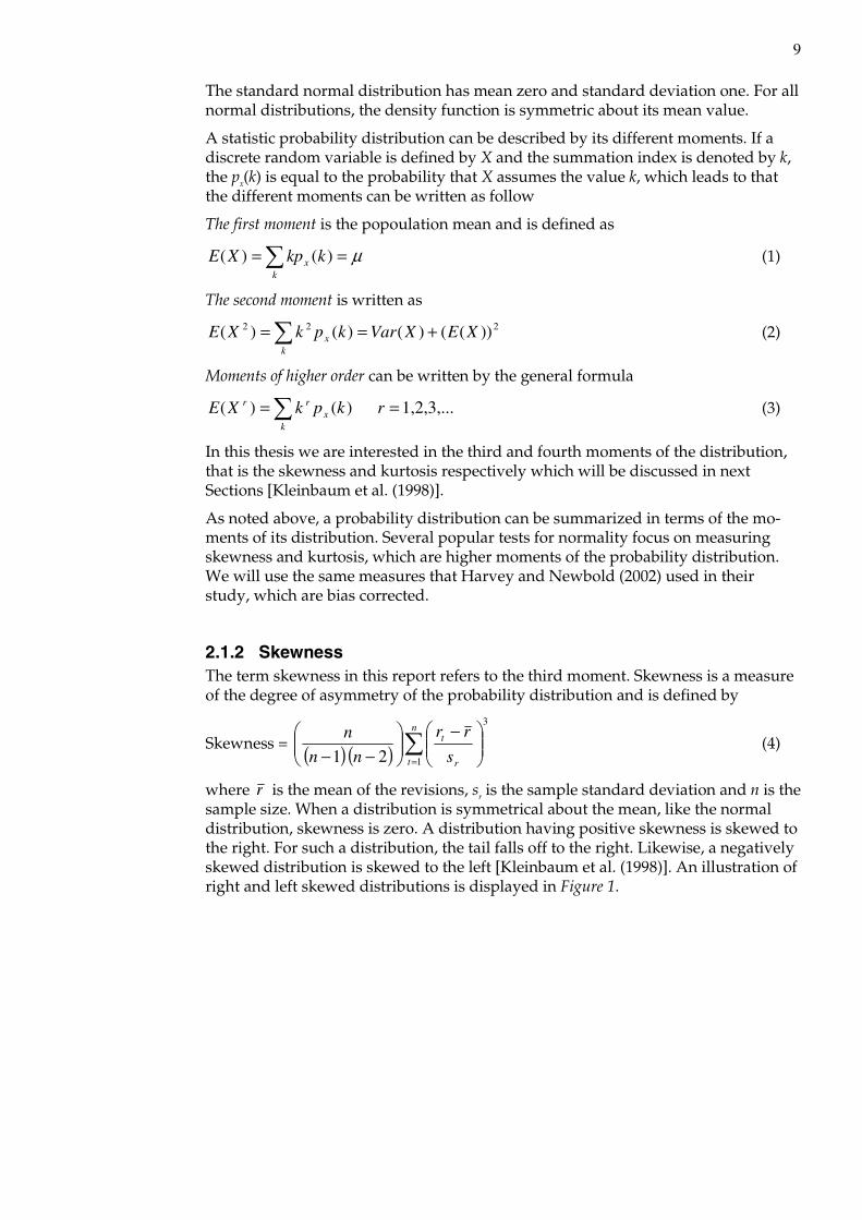
where r is the mean of the revisions, sr is the sample standard deviation and n is the sample size. When a distribution is symmetrical about the mean, like the normal distribution, skewness is zero. A distribution having positive skewness is skewed to the right. For such a distribution, the tail falls off to the right. Likewise, a negatively skewed distribution is skewed to the left [Kleinbaum et al. (1998)]. An illustration of right and left skewed distributions is displayed in Figure 1.
10
Figure 1 Right skewed, left skewed and symmetrical distributions
Source: Gujarati (2002).
2.1.3 Kurtosis The term kurtosis in this thesis refers to the fourth moment. Kurtosis measures the peakness or fat-tailedness versus flatness or short-tailedness of the probability distribution and may be computed as
Kurtosis = ( )
( ) ( ) ( )( )
( ) ( )3 2
13
3 2 1
1 24
1 −−−−
−−−−
+ ∑= nn
n
s
rr
nnn
nn n
t r
t +3 (5)
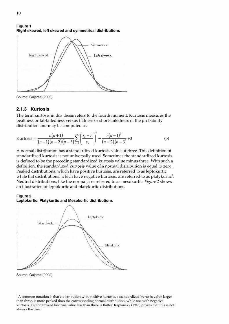
A normal distribution has a standardized kurtosis value of three. This definition of standardized kurtosis is not universally used. Sometimes the standardized kurtosis is defined to be the preceding standardized kurtosis value minus three. With such a definition, the standardized kurtosis value of a normal distribution is equal to zero. Peaked distributions, which have positive kurtosis, are referred to as leptokurtic while flat distributions, which have negative kurtosis, are referred to as platykurtic2. Neutral distributions, like the normal, are referred to as mesokurtic. Figure 2 shows an illustration of leptokurtic and platykurtic distributions.
Figure 2 Leptokurtic, Platykurtic and Mesokurtic distributions
Source: Gujarati (2002).
2 A common notation is that a distribution with positive kurtosis, a standardized kurtosis value larger than three, is more peaked than the corresponding normal distribution, while one with negative kurtosis, a standardized kurtosis value less than three is flatter. Kaplansky (1945) proves that this is not always the case.
11
Finally, the reader should bear in mind that skewness and kurtosis statistics are highly variable in small samples and hence are often difficult to interpret. However, since we have eighty observations in our study, these measures should be reason-ably stable [Hogg and Tanis (2001)].
2.2 Normality Tests
2.2.1 Anderson-Darling Normality Test The Anderson-Darling statistic A2 measures how well the data follow a particular distribution. The better the distribution fits the data, the smaller this statistic will be. It is a modification of the Kolmogorov-Smirnov test (see Section 2.2.3) and gives more weight to the tails than the Kolmogorov-Smirnov test. The Anderson-Darling test makes use of a specific distribution in calculating critical values. This has the advantage of allowing a more sensitive test and the disadvantage that critical values must be calculated for each distribution [Stephens (1974)].
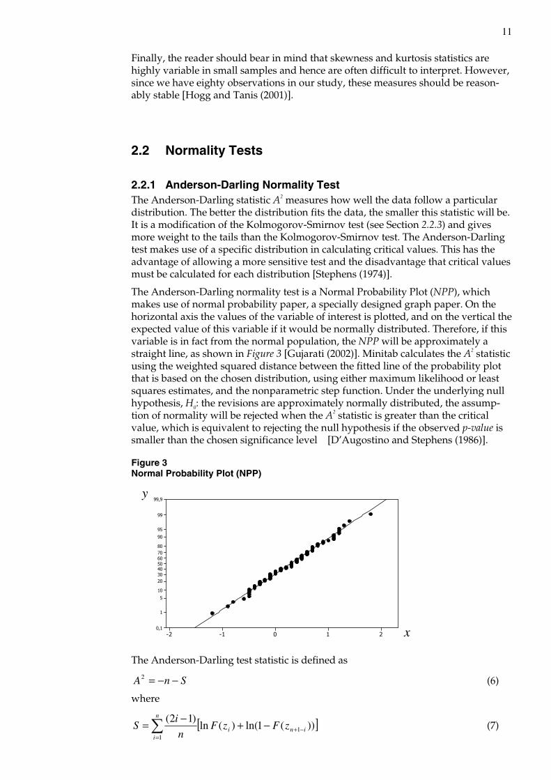
The Anderson-Darling normality test is a Normal Probability Plot (NPP), which makes use of normal probability paper, a specially designed graph paper. On the horizontal axis the values of the variable of interest is plotted, and on the vertical the expected value of this variable if it would be normally distributed. Therefore, if this variable is in fact from the normal population, the NPP will be approximately a straight line, as shown in Figure 3 [Gujarati (2002)]. Minitab calculates the A2 statistic using the weighted squared distance between the fitted line of the probability plot that is based on the chosen distribution, using either maximum likelihood or least squares estimates, and the nonparametric step function. Under the underlying null hypothesis, H0: the revisions are approximately normally distributed, the assump-tion of normality will be rejected when the A2 statistic is greater than the critical value, which is equivalent to rejecting the null hypothesis if the observed p-value is smaller than the chosen significance level [D’Augostino and Stephens (1986)].
Figure 3 Normal Probability Plot (NPP)
x
y
210-1-2
99,9
99
95
90
80706050403020
10
5
1
0,1
The Anderson-Darling test statistic is defined as
SnA −−=2 (6)
where
[ ]))(1ln()(ln)12(
11
ini
n
i
zFzFn
iS −+
=
−+−=∑ (7)
12
F is the assumed normal distribution with the assumed or sample estimated para-meters )ˆ,ˆ( σµ , zi is the ith sorted, standardized, sample value, n is the sample size, ln is the natural logarithm and subscript i runs from i to n.
Among the tests based on the empirical distribution function, Anderson-Darling tends to be more effective in detecting departures in the tails of the distribution. In practice, if departures from normality at the tails were the major concern, many statisticians would use Anderson-Darling as their first choice. However, you need big samples to be able to say something about the tails.
2.2.2 Jarque-Bera Test of Normality The JB test, originally suggested by Jarque and Bera (1987), is probably the most commonly used test of normality. They developed a Lagrange Multiplier (LM) test of the null hypothesis against the two-sided alternative hypothesis, which is equiva-lent to testing the null hypothesis of normality.
The LM test, or the JB test, uses the following test statistic
( )
−+=24
3
6
22 KSnJB (8)
where n is the sample size, S is the skewness value from (4), and K is the kurtosis value from (5). For a normally distributed variable, S is equal to zero and K is equal to three. Therefore, the JB test of normality is a test of the joint hypothesis that S and K are zero and three, respectively. In that case the value of the JB statistic is expected to be zero. Under the null hypothesis that the revisions are normally distributed, Jarque and Bera showed that asymptotically the JB statistic given in (8) follows the chi-square distribution with two degrees of freedom, [ ]
22χ . If the computed p-value of
the JB statistic is sufficiently low, which will happen if the value of the statistic is different from zero, one can reject the hypothesis that the revisions are normally distributed [Gujarati (2002)]. Note that skewness and kurtosis can be tested separa-tely using chi-square distribution with one degree of freedom, each. This test needs a big sample size to give appropriate results, which is not a problem in our case.
2.2.3 Kolmogorov-Smirnov Test This test considers the goodness of fit between a hypothesized distribution function and an empirical distribution function. The empirical distribution function is given here in terms of the order statistics. Let y1 < y2 < ... < yn be the observed values of the order statistics of a random sample x1, x2, ..., xn of size n. When no two observations are equal, the empirical distribution function is defined by
1,...,2,1 ,
,1
,/
,0
)( 1
1
−=
≥<≤
<= + nk
yx
yxynk
yx
xF
n
kkn (9)
The empirical distribution function has a jump of magnitude 1/n occurring at each observation. Fn(x) is the fraction of sample observations that are less than or equal to x.
Because of the convergence of the empirical distribution function to the theoretical distribution function, it makes sense to construct a goodness of fit test based on the closeness of the empirical function and a hypothesized distribution function, say Fn(x) and F0(x). The Kolmogorov-Smirnov statistic Dn is defined by
[ ])()(sup 0 xFxFD nxn −= (10)
13
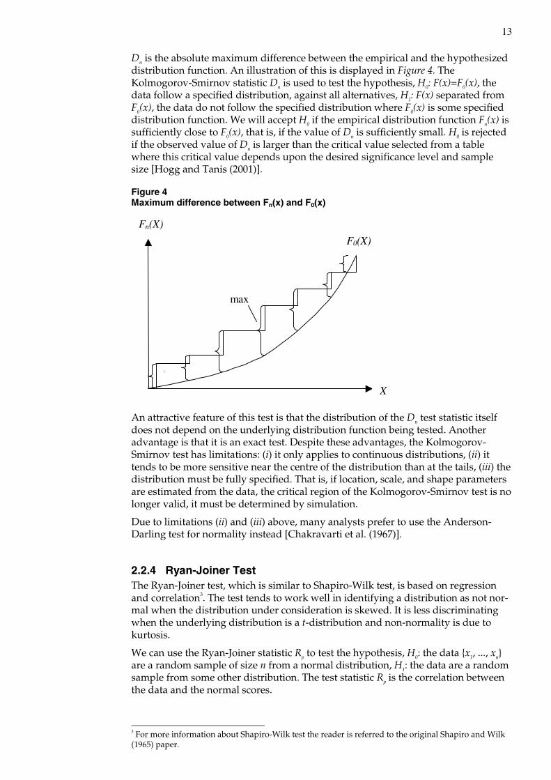
Dn is the absolute maximum difference between the empirical and the hypothesized distribution function. An illustration of this is displayed in Figure 4. The Kolmogorov-Smirnov statistic Dn is used to test the hypothesis, H0: F(x)=F0(x), the data follow a specified distribution, against all alternatives, H1: F(x) separated from F0(x), the data do not follow the specified distribution where F0(x) is some specified distribution function. We will accept H0 if the empirical distribution function Fn(x) is sufficiently close to F0(x), that is, if the value of Dn is sufficiently small. H0 is rejected if the observed value of Dn is larger than the critical value selected from a table where this critical value depends upon the desired significance level and sample size [Hogg and Tanis (2001)].
Figure 4 Maximum difference between Fn(x) and F0(x)
X
Fn(X)
F0(X)
max
An attractive feature of this test is that the distribution of the Dn test statistic itself does not depend on the underlying distribution function being tested. Another advantage is that it is an exact test. Despite these advantages, the Kolmogorov-Smirnov test has limitations: (i) it only applies to continuous distributions, (ii) it tends to be more sensitive near the centre of the distribution than at the tails, (iii) the distribution must be fully specified. That is, if location, scale, and shape parameters are estimated from the data, the critical region of the Kolmogorov-Smirnov test is no longer valid, it must be determined by simulation.
Due to limitations (ii) and (iii) above, many analysts prefer to use the Anderson-Darling test for normality instead [Chakravarti et al. (1967)].
2.2.4 Ryan-Joiner Test The Ryan-Joiner test, which is similar to Shapiro-Wilk test, is based on regression and correlation3. The test tends to work well in identifying a distribution as not nor-mal when the distribution under consideration is skewed. It is less discriminating when the underlying distribution is a t-distribution and non-normality is due to kurtosis.
We can use the Ryan-Joiner statistic Rp to test the hypothesis, H0: the data {x1, ..., xn} are a random sample of size n from a normal distribution, H1: the data are a random sample from some other distribution. The test statistic Rp is the correlation between the data and the normal scores.
3 For more information about Shapiro-Wilk test the reader is referred to the original Shapiro and Wilk (1965) paper.
14
If the data are a sample from a normal distribution then the NPP, plot of normal scores against the data, will be close to a straight line. The correlation Rp will be close to one and if the data are sampled from a non-normal distribution then the plot will exhibit some degree of curvature, resulting in a smaller correlation Rp. Small values of Rp are therefore regarded as strong evidence against H0.
The Ryan-Joiner test is given by the formula for the correlation coefficient, namely
∑ ∑∑
−−
−−=
22 )()(
))((
bbYY
bbYYR
ii
iip (11)
Since 0=b , Rp can be simplified to
∑ ∑∑
−
−=
22)(
)(
ii
iip
bYY
bYYR (12)
Yi is the ordered observations in a sample of size n and bi is the pth percentage point of the standard normal distribution, that is, )(1
ii pb −Φ= .
The statistic Rp can be used to provide an indication of how non-normal the revi-sions are. This will be particularly true with larger samples. The test has the de-sirable feature of linking together a graphical display of the data with a simple, objective test statistic. Some may object to the use of the term correlation coefficient since the bi are not random variables. However, given any set of points in the plane, one can use the correlation coefficient associated with those points as a descriptive measure of how close they are to a straight line. In this sense, Rp can be thought of as a correlation coefficient. Since Rp does not arise from sampling a bivariate distri-bution, it is not the same as the usual correlation coefficient [Ryan et al. (1976)].
Ryan et al. (1976) have compared the power of Rp and the Shapiro-Wilk statistic W. The tests show that overall there is little difference between the powers of the two tests for most of the alternatives. The only appreciable difference is that for extreme-ly short-tailed distributions like the uniform and triangular, W has more power than Rp, while for heavy-tailed distributions like the Cauchy and contaminated normal, Rp does slightly better.
2.3 Testing for ARCH To test if the revisions are heteroskedastic we used two different tests, Engle’s LM test for ARCH and the squared Ljung-Box test.
2.3.1 Engle’s LM test for ARCH The original Lagrange multiplier (LM) test for ARCH proposed by Engle (1982) is very simple to compute, and relatively easy to derive. Under the null hypothesis it is assumed that the model is a standard dynamic regression model, which can be written as
ttt xy εβ += (13)
where tx is a set of weakly exogenous and lagged dependent variables and tε is a
Gaussian white noise process
1−Ψttε ~ ( )2,0 σN (14)
15
where 1−Ψt denotes the available information set. Because the null hypothesis, H0: there are no ARCH errors, is easily estimated, the LM test is a natural choice. The alternative hypothesis, H1: is that the conditional error variance is given by an ARCH (q) process1 [Bollerslev et al. (1994)].
We examine two serial dependence properties of interest, the extent to which the revisions are autocorrelated and whether they exhibit ARCH-type behavior. The order of autocorrelation present in a given revision time series is found by TRAMO/SEATS.
Testing for ARCH in the revisions is performed using the standard Engle (1982) test. First the regression of the preferred ARIMA-model is estimated for observations
Tqqt ,...,2,1 +−+−= and the sample residuals tε̂ are saved. Next step is to regress
the squared residuals 2tε on a constant and q lagged values of the squared residuals,
221 ,..., qtt −− εε
tqtqttt v+++++= −−−22
222
112 ˆ...ˆˆˆˆ εαεαεαωε (15)
for t = 1, 2,…,T. The sample size T times the squared coefficient of determination 2R from the regression of (15) then converges to a chi-square distribution, [ ]
2qχ with q
degrees of freedom. There is evidence to reject the null hypothesis if the test statistic exceeds a critical value, which means that the revisions are actually heteroskedastic [Hamilton (1994)].
2.3.2 The Squared Ljung-Box Test If no significant autocorrelation can be found by the Ljung-Box test the conclusion is that there is no linear structure in the revisions5. A dependence can however exist according to underlying non-linear structure. Mcleod and Li (1983) showed that the Ljung-Box test statistic has the same distribution as the squared Ljung-Box statistic, which can be used as an indication of non-linearity, that is, heteroskedasticity. This can also be an indication that the specified model suffers from ARCH-effects.
A slow decline of the autocorrelation function (ACF) of the squared residuals suggests that a GARCH (1,1) process may be suitable for describing the revisions6. That is, a low order ARCH process may not fully capture the time-varying volatility in the data.
The problem is that in fact, the LM test for GARCH (1,1) is just the same as the LM test for ARCH (1), which proposes a locally most powerful test for ARCH and GARCH. Since it is found that the GARCH (1,1) is often a superior model and is surely more parsimoniously parameterised7, one would like a test, which is more powerful for this alternative8.
We suggest that when quarterly data are being used, a fourth order process may be appropriate. However, instead of a general fourth order process, we suggest that only the residuals in corresponding quarters of each year should be correlated, that is 4, 8, 12 and so on.
1 See Appendix II for an overview of this process. 5 See Appendix IV for more details about this test. 6 See Appendix III for more details. 7 Parsimoniously means that it is desirable with as few parameters as possible in the model, because that gives more stable and safe estimated forecasts. 8 See Bollerslev et al. (1994).

16
3 Data We use quarterly data of GDP revisions for the years 1980-1999 from Öller and Hansson (2002). The preliminary and revised figures are given in percentage change from the same quarter last year and are given in constant prices. The data are neither seasonally nor working day adjusted.
The revised, also called “final”, quarterly figures are published in December t+2, this is the time when the first revised annual accounts are published. The same choice was made as Öller and Hansson (2002) who argued that: “By choosing t+2 we try to avoid, as much as possible, revisions that are due to changes in definitions or methods”. We are going to use data from 1980 to 1999 for the revisions Private Consumption and GDP. For the other eleven revisions we are going to use data for the period 1984 quarter two to 1999 quarter four. These revisions have a lot of missing values in the beginning and we prefer unbroken series. The revision In-ventories has one missing value in year 1990 quarter one for which we have substituted the mean.
17
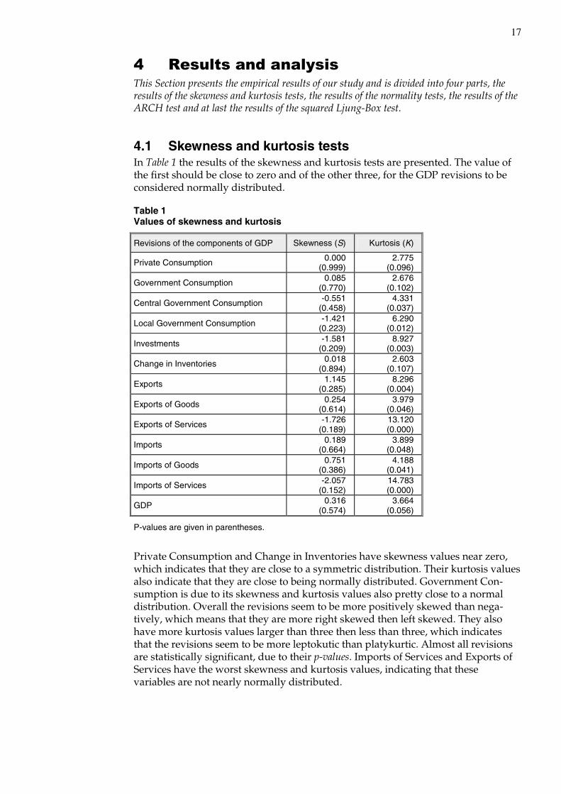
4 Results and analysis This Section presents the empirical results of our study and is divided into four parts, the results of the skewness and kurtosis tests, the results of the normality tests, the results of the ARCH test and at last the results of the squared Ljung-Box test.
4.1 Skewness and kurtosis tests In Table 1 the results of the skewness and kurtosis tests are presented. The value of the first should be close to zero and of the other three, for the GDP revisions to be considered normally distributed.
Table 1 Values of skewness and kurtosis
Revisions of the components of GDP Skewness (S) Kurtosis (K)
Private Consumption 0.000 (0.999)
2.775 (0.096)
Government Consumption 0.085 (0.770)
2.676 (0.102)
Central Government Consumption -0.551 (0.458)
4.331 (0.037)
Local Government Consumption -1.421 (0.223)
6.290 (0.012)
Investments -1.581 (0.209)
8.927 (0.003)
Change in Inventories 0.018 (0.894)
2.603 (0.107)
Exports 1.145 (0.285)
8.296 (0.004)
Exports of Goods 0.254 (0.614)
3.979 (0.046)
Exports of Services -1.726 (0.189)
13.120 (0.000)
Imports 0.189 (0.664)
3.899 (0.048)
Imports of Goods 0.751 (0.386)
4.188 (0.041)
Imports of Services -2.057 (0.152)
14.783 (0.000)
GDP 0.316 (0.574)
3.664 (0.056)
P-values are given in parentheses.
Private Consumption and Change in Inventories have skewness values near zero, which indicates that they are close to a symmetric distribution. Their kurtosis values also indicate that they are close to being normally distributed. Government Con-sumption is due to its skewness and kurtosis values also pretty close to a normal distribution. Overall the revisions seem to be more positively skewed than nega-tively, which means that they are more right skewed then left skewed. They also have more kurtosis values larger than three then less than three, which indicates that the revisions seem to be more leptokutic than platykurtic. Almost all revisions are statistically significant, due to their p-values. Imports of Services and Exports of Services have the worst skewness and kurtosis values, indicating that these variables are not nearly normally distributed.
18
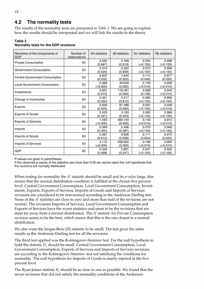
4.2 The normality tests The results of the normality tests are presented in Table 2. We are going to explain how the results should be interpreted and we will link the results to the theory.
Table 2 Normality tests for the GDP revisions
Revisions of the components of GDP
Number of observations
A2 statistics JB statistics Dn statistics Rp statistics
Private Consumption 80 0.265 (0.687)
0.169 (0.919)
0.034 (>0.150)
0.998 (>0.100)
Government Consumption 63 0.318 (0.529)
0.352 (0.839)
0.073 (>0.150)
0.996 (>0.100)
Central Government Consumption 63 0.822 (0.032)
7.840 (0.020)
0.112 (0.048)
0.977 (0.035)
Local Government Consumption 63 2.068 (<0.005)
49.629 (0.000)
0.159 (<0.010)
0.936 (<0.010)
Investments 63 0.951 (0.015)
118.461 (0.000)
0.098 (0.138)
0.943 (<0.010)
Change in Inventories 63 0.461 (0.252)
0.417 (0.812)
0.085 (>0.150)
0.995 (>0.100)
Exports 63 0.839 (0.029)
87.388 (0.000)
0.091 (>0.150)
0.948 (<0.010)
Exports of Goods 63 0.429 (0.301)
3.193 (0.203)
0.065 (>0.150)
0.989 (>0.100)
Exports of Services 63 1.593 (<0.005)
300.144 (0.000)
0.140 (<0.010)
0.910 (<0.010)
Imports 63 0.399 (0.355)
2.496 (0.287)
0.070 (>0.150)
0.989 (>0.100)
Imports of Goods 63 0.987 (0.012)
9.626 (0.008)
0.111 (0.054)
0.975 (0.025)
Imports of Services 63 3.172 (<0.005)
408.852 (0.000)
0.196 (<0.010)
0.883 (<0.010)
GDP 80 0.348 (0.468)
2.801 (0.247)
0.047 (>0.150)
0.992 (>0.100)
P-values are given in parentheses. If the observed p-values of the statistics are more than 0.05 we cannot reject the null hypothesis that the revisions are normally distributed.
When testing for normality the A2 statistic should be small and its p-value large, this means that the normal distribution condition is fulfilled at the chosen five percent level. Central Government Consumption, Local Government Consumption, Invest-ments, Exports, Exports of Services, Imports of Goods and Imports of Services revisions are considered to be non-normal according to the Anderson-Darling test. None of the A2 statistics are close to zero and more than half of the revisions are not normal. The revisions Imports of Services, Local Government Consumption and Exports of Services have the worst statistics and seem to be the revisions that are most far away from a normal distribution. The A2 statistic for Private Consumption revision seems to be the best, which means that this is the one closest to a normal distribution.
We also want the Jarque-Bera (JB) statistic to be small. The test gives the same results as the Anderson-Darling test for all the revisions.
The third test applied was the Kolmogorov-Smirnov test. For the null hypothesis to hold the statistic Dn should be small. Central Government Consumption, Local Government Consumption, Exports of Services and Imports of Services revisions are according to the Kolmogorov-Smirnov test not satisfying the conditions for normality. The null hypothesis for Imports of Goods is nearly rejected at the five percent level.
The Ryan Joiner statistic Rp should be as close to one as possible. We found that the seven revisions that did not satisfy the normality conditions of the Anderson-

19
Darling and the Jarque-Bera tests are also non-normal according to the Ryan Joiner test.
We found that barely half of the revisions are not normal according to the four tests above. We can also see that all four tests choose the same best and worst revisions, which means that the tests are very concordant.
The test that produces slightly different results is the Kolmogorov-Smirnov test. This test seems to be less sensible to non-normality than the others. The statistics for the revisions of Investments, Exports and Imports of Goods do not reject the null hypothesis at the five percent level, which the other tests do. This can be explained by the fact that the Kolmogorov-Smirnov test tends to be more sensitive near the centre of the distribution than at the tails. This means that the test does not detect all the non-normal behaviour in the tails.
Revisions of Imports are close to be normal. But its two components, Imports of Goods and Imports of Services, have revisions that are not even close to be normal. The explanations can be that the deviations from normality in the two revisions partly cancel.
4.3 The ARCH Test Results of the autocorrelation specification and tests for relatively low order ARCH (q=1,2) are given in Table 3.
Table 3 Autocorrelation specification and ARCH tests for GDP revisions
Revisions of the components of GDP
Autocorrealtionspecification*
ARCH (1) statistics1 ARCH (2) statistics2
Private Consumption (0,0,1) 0.216 (0.642)
0.220 (0.896)
Government Consumption (0,0,1) 0.427 (0.513)
0.540 (0.763)
Central Government Consumption (0,0,1) 0.000 (0.999)
0.290 (0.865)
Local Government Consumption (0,0,1) 0.000 (0.999)
1.680 (0.432)
Investments (1,0,0)s 2.806 (0.094)
2.880 (0.237)
Exports (1,0,0) 0.180 (0.671)
0.177 (0.915)
Exports of Services (1,0,0) (1,0,0) 0.912 (0.340)
4.256 (0.119)
Imports (1,0,0) 0.220 (0.639)
1.188 (0.552)
Imports of Goods (1,0,0) 0.486 (0.486)
0.795 (0.672)
Imports of Services (0,0,1) 0.122 (0.727)
0.300 (0.861)
P-values are given in parentheses. 1 If the ARCH statistics are larger than 3.884 we will reject the null hypothesis, setting α equal to 0.05. 2 If the ARCH statistics are larger than 5.991 we will reject the null hypothesis, setting α equal to 0.05. * s stands for seasonal AR(1).
If the ARCH (1) statistics are larger than 3.884 and the ARCH (2) statistics are larger than 5.991 we will reject the null hypothesis that there are no ARCH effect. Looking at our results we can see that there is no evidence of ARCH for any of the revisions considered, even if the null hypothesis for the revisions of Investments [ARCH (1)]
20
and Exports of Services [ARCH (2)] are close to being rejected at the five percent level.
The revisions Change in Inventories, Exports of Goods and GDP shows no autocorrelation and therefore we cannot create adequate models with ARIMA for them. The test statistics for these revisions are instead given by the squared Ljung-Box to investigate if they have ARCH behaviour. An indication of ARCH is that the residuals will be uncorrelated but the squared residuals will show autocorrelation. In Table 4 the results of the squared Ljung-Box test is shown.
Table 4 The squared Ljung-Box test for the GDP revisions
Revisions of the components of GDP
QK2(4)
statistics1 QK
2(8) statistics2
QK2(12)
statistics3
Change in Inventories 2.497 (0.476)
10.259 (0.174)
15.670 (0.154)
Exports of Goods 3.913 (0.271)
6.031 (0.536)
13.202 (0.280)
GDP 4.625 (0.201)
8.109 (0.323)
10.240 (0.509)
P-values are given in parentheses. 1 If the QK
2 statistics are larger than 7.815 we will reject the null hypothesis, setting α equal to 0.05. 2 If the QK
2 statistics are larger than 14.067 we will reject the null hypothesis, setting α equal to 0.05. 3 If the QK
2 statistics are larger than 19.675 we will reject the null hypothesis, setting α equal to 0.05.
The QK
2 statistics should be smaller than the critical values 7.815, 14.067 and 19.675, respectively, for the null hypothesis to hold on the five percent level. The QK
2 sta-tistics does not reject the null hypothesis of homoscedasticity for any of the revi-sions. That means that the revisions Change in Inventories, Exports of Goods and GDP don’t have any ARCH effects. Hence all revisions in this study can be regarded as homoscedastic.
21
5 Conclusions There are several tests available when one wants to test data for normality. We chose four of them to use on the GDP revisions that we were interested in. We have also checked for skewness and kurtosis. We have found that revisions of Private Consumption and Change in Inventories have skewness values near zero, indicating that they are close to a symmetric distribution. Their kurtosis also indicates that they are close to being normal. Revisions of Government Consumption are pretty close to a normal distribution. Imports of Services and Exports of Services have the worst skewness and kurtosis values indicating that these revisions are not even nearly normally distributed. This is concordant with the results in Öller and Hansson (2002), which contains histograms over the revision distributions. We also found that the revisions were more positively skewed than negatively which also is concordant with the results from Öller and Hansson (2002).
We can draw the conclusion that more than half of the revisions are not normal according to the four tests that we have used: Anderson-Darling, Jarque-Bera, Kolmogorov-Smirnov and Ryan-Joiner. We can also see that all four tests chose the same best (Private Consumption) and worst (Local Government Consumption, Exports of Services and Imports of Services) revisions, which means that the tests are very concordant. The test that produces slightly different results is the Kolmogorov-Smirnov test. It seems to be less sensitive to non-normality than the others.
When we checked for the presence of ARCH effects in the GDP revisions we used two tests, the Lagrange Multiplier (LM) test and the squared Ljung-Box test. In TRAMO/SEATS we could identify adequate models that we used for the LM test for ARCH. We found that the revisions Change in Inventories, Exports of Goods and GDP did not contain any autocorrelation. Therefore we used the squared Ljung-Box test for these revisions to investigate if they had ARCH behavior. None of the revisions contained any ARCH effect, but the null hypotheses of homoscedasticity for the revisions of Investments and Exports of Services were close to be rejected at the five percent level.
The Swedish GDP revisions for the years 1980-1999 are skewed and thick-tailed and our figures show that the revisions cannot be described by a normal distribution. We also found that none of the revisions contained any ARCH effects.

22
6 References Bollerslev, T. (1986). Generalized Autoregressive Conditional Heteroskedasticity. Journal of Econometrics, 31, 307-327.
Bollerslev, T., Engle, R. F. and Nelson, D. F. (1994). ARCH Models. I: R. F. Engle and D. L. McFadden (eds.), Handbook of Econometrics, Vol. 4. Amsterdam: Elsevier Science, 2959-3038.
Bowerman, B. L. and O’Connel, R. T. (1993). Forecasting and Time Series an Applied Approach, 3rd ed. Belmont: Duxbury Press.
Chakravarti, I. M., Laha, R. G. and Roy, J. (1967). Techniques of Computation Descriptive Method and Statistical Inference. I: Handbook of Methods of Applied Statistics, Vol. 1. New York: Wiley.
D’Augostino, R. B. and M. A. Stephens. (1986). Goodness-of-Fit Techniques. New York: Marcel Dekker.
Engle, R. F. (1982). Autoregressive Conditional Heteroskedasticity with Estimates of the Variance of United Kingdom Inflation. Econometrica, 50, 987-1008.
Gujarati, D. N. (2002). Basic Econometrics, 4th ed. Boston: McGrawHill.
Hamilton, J. D. (1994). Time Series Analysis. Princeton: Princeton University Press.
Harvey, D. I. and Newbold, P. (2002). The Non-Normality of some Macroeconomic Forecasts. International Journal of Forecasting, 19, 635-653.
Hogg, R. V. and Tanis, E. A. (2001). Probability and Statistical Inference, 6th ed. Upper Saddle River: Prentice Hall.
Jarque, C. M. and Bera, A. K. (1987). A Tests for Normality of Observations and Regression Residuals. International Statistical Review, 55, 163-172.
Kaplansky, I. (1945). A Common Error Concerning Kurtosis. Journal of the American Statistical Association, 40, 259-263.
Kleinbaum, D. G., Kupper, L. L., Muller, K. E. and Nizzan, A. (1998). Applied Regression Analysis and Other Multivariate Methods, 3rd ed. Pacific Grove: Duxbury Press.
Ljung, G. M. and Box, G. E. P. (1978). On a Measure of a Lack of Fit in Time series Models. Biometrika, 65, 297-303.
Mcleod, A. I. and Li, W. K. (1983). Diagnostic Checking ARIMA Time Series Models Using Squared-Residual Autocorrelation. Journal of Time Series Analysis, 4, 269-273.
Nilsson, J. and Rosander, O. (2003). Tidsserieanalys av svenska BNP-revideringar 1980-1999 Kan BNP-revideringarna prognostiseras med en ARIMA-modell?. Stockholm: Stockholm University.
Öller, L.-E. and Hansson, K.-G. (2002). Revisions of Swedish National Accounts 1980-1998 and an International Comparision. I: SOU 2002:118. Stockholm: Fritzes förlag.
Ryan, A. T. Jr., Joiner, B. L. and Ryan, B. F. (1976). Minitab : Student Handbook. North Scituate: Duxbury Press.
Shapiro, S. S. and Wilk, M. B. (1965). An Analysis of Variance Test for Normality. Biometrika, 52, 591-611.
Stephens, M. A. (1974). EDF Statistics for Goodness of Fit and Some Comparisons. Journal of the American Statistical Association, 69, 730-737.

23
Appendices
Appendix I – Glossary > bigger than
< smaller than
≥ bigger or equal to
≤ smaller or equal to
^ an estimator (usually maximum likelihood) or forecast value
α regression coefficient alpha and significance level
β regression coefficient beta
( )Lα polynomial in the lag operator L
( )Lβ polynomial in the lag operator L
[ ]2qχ chi-square distribution with q degrees of freedom
tε stochastic error term, usually called white noise
µ the mean
tv unpredictable, or innovation, error
σ standard deviation 2σ variance 2tσ variance at time t
∑ summation over implicit range
∑=
n
t 1
summation over range shown
1−Ψt the information set
ω constant term in ARCH specification
{ } ⋅ stochastic process or sequence
⋅ absolute value
∼ is distributed as 2A Anderson-Darling statistic
bi the pth percentage point of the standard normal distribution, that is, )(1
ii pb −Φ=
b mean of the slope coefficient
d the degree of differencing
nD Kolmogorov-Smirnov statistic
{ } ⋅⋅E conditional expectation of a variable given an other
E ( )⋅ expected value of

24
F the cumulative distribution function of the specified distribution in the Anderson-Darling test
( )xFn the empirical function in the Kolmogorov-Smirnov test
( )xF0 the hypothesized distribution function in the Kolmogorov-Smirnov test
0H null hypothesis
1H alternative hypothesis
JB Jarque-Bera statistic
K kurtosis
K the degrees of freedom in the Ljung-Box test
l lag l
L the lag operator
ln natural logarithm
n sample size
np the number of parameters
NPP Normal Probability Plot
( )2 ,0 σN normal density function with zero mean and variance 2σ
p-value probability, or test-rejection probability
p the order of an autoregressive process
px(k) the probability that X assumes the value k in a moment generating function
QK the Ljung-Box test statistic
QK
2 the squared Ljung-Box statistic
q the order of a moving average process
r the mean of the revisions
( )arl ˆ2 the squared sample autocorrelation of the residuals at lag l in a Ljung- Box test
rt the revisions at time t 2R the squared coefficient of determination
Rp Ryan-Joiner statistic
sr the estimated standard deviation or standard error of the revisions
S skewness
Supx stands for supremum, and is the maximum vertical distance between the graphs of Fn(x) and F0(x) over the range of possible x values
t time
T number of observations in a time series
W Shapiro-Wilk statistic
Yi the ordered observations in a sample size n from a Ryan-Joiner test
X a random variable or a stochastic variable
zi the ith sorted, standardized, sample value in the Anderson-Darling test
25
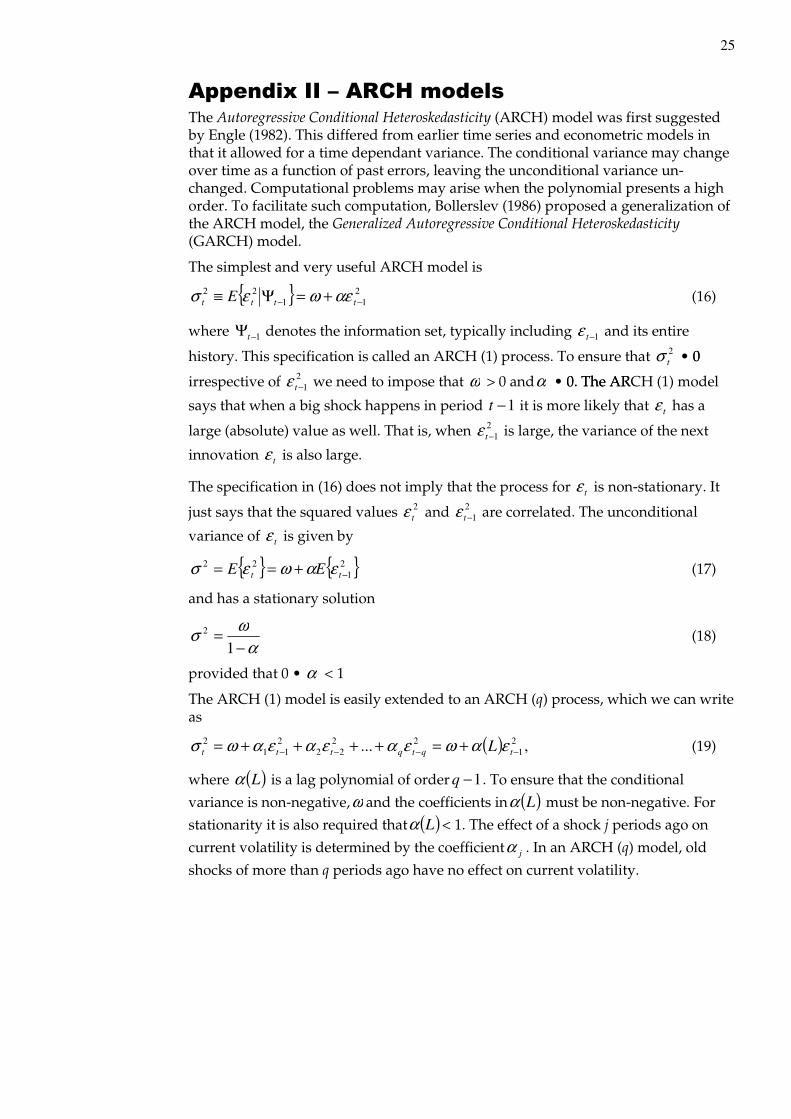
Appendix II – ARCH models The Autoregressive Conditional Heteroskedasticity (ARCH) model was first suggested by Engle (1982). This differed from earlier time series and econometric models in that it allowed for a time dependant variance. The conditional variance may change over time as a function of past errors, leaving the unconditional variance un-changed. Computational problems may arise when the polynomial presents a high order. To facilitate such computation, Bollerslev (1986) proposed a generalization of the ARCH model, the Generalized Autoregressive Conditional Heteroskedasticity (GARCH) model.
The simplest and very useful ARCH model is
{ } 211
22−− +=Ψ≡ tttt E αεωεσ (16)
where 1−Ψt denotes the information set, typically including 1−tε and its entire
history. This specification is called an ARCH (1) process. To ensure that 2tσ • 0 0
irrespective of 21−tε we need to impose that ω > 0 andα • 0. The AR 0. The ARCH (1) model
says that when a big shock happens in period 1−t it is more likely that tε has a
large (absolute) value as well. That is, when 21−tε is large, the variance of the next
innovation tε is also large.
The specification in (16) does not imply that the process for tε is non-stationary. It
just says that the squared values 2tε and 2
1−tε are correlated. The unconditional
variance of tε is given by
{ } { }21
22−+== tt EE εαωεσ (17)
and has a stationary solution
αωσ−
=1
2 (18)
provided that 0 • α < 1
The ARCH (1) model is easily extended to an ARCH (q) process, which we can write as
( ) ,... 21
2222
211
2−−−− +=++++= tqtqttt L εαωεαεαεαωσ (19)
where ( )Lα is a lag polynomial of order 1−q . To ensure that the conditional
variance is non-negative,ω and the coefficients in ( )Lα must be non-negative. For
stationarity it is also required that ( )Lα < 1. The effect of a shock j periods ago on
current volatility is determined by the coefficient jα . In an ARCH (q) model, old
shocks of more than q periods ago have no effect on current volatility.
26
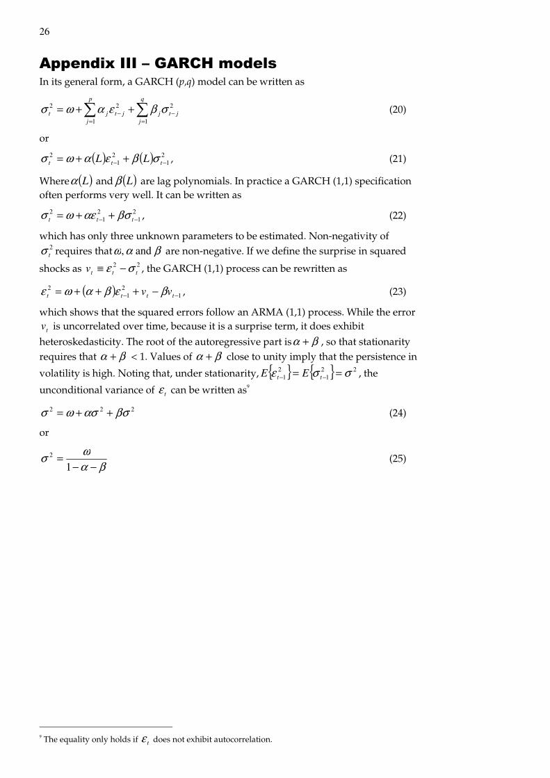
Appendix III – GARCH models In its general form, a GARCH (p,q) model can be written as
2
1
2
1
2jt
q
jjjt
p
jjt −
=−
=∑∑ ++= σβεαωσ (20)
or
( ) ( ) 21
21
2−− ++= ttt LL σβεαωσ , (21)
Where ( )Lα and ( )Lβ are lag polynomials. In practice a GARCH (1,1) specification often performs very well. It can be written as
21
21
2−− ++= ttt βσαεωσ , (22)
which has only three unknown parameters to be estimated. Non-negativity of 2tσ requires that βαω and , are non-negative. If we define the surprise in squared
shocks as 22tttv σε −≡ , the GARCH (1,1) process can be rewritten as
( ) 12
12
−− −+++= tttt vv βεβαωε , (23)
which shows that the squared errors follow an ARMA (1,1) process. While the error
tv is uncorrelated over time, because it is a surprise term, it does exhibit
heteroskedasticity. The root of the autoregressive part is βα + , so that stationarity requires that βα + < 1. Values of βα + close to unity imply that the persistence in
volatility is high. Noting that, under stationarity, { } { } 221
21 σσε == −− tt EE , the
unconditional variance of tε can be written as9
222 βσασωσ ++= (24)
or
βαωσ
−−=
12 (25)
9 The equality only holds if tε does not exhibit autocorrelation.
27
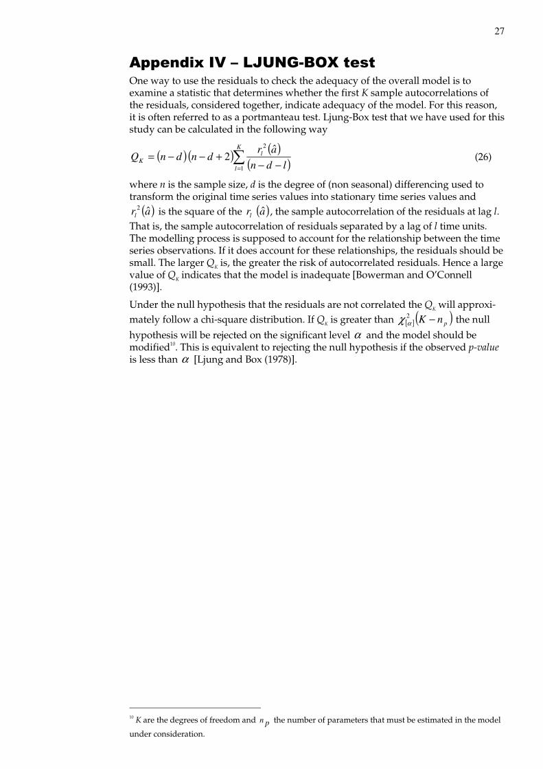
Appendix IV – LJUNG-BOX test One way to use the residuals to check the adequacy of the overall model is to examine a statistic that determines whether the first K sample autocorrelations of the residuals, considered together, indicate adequacy of the model. For this reason, it is often referred to as a portmanteau test. Ljung-Box test that we have used for this study can be calculated in the following way
( ) ( ) ( )( )∑
= −−+−−=
K
l
lK ldn
ardndnQ
1
2 ˆ2 (26)
where n is the sample size, d is the degree of (non seasonal) differencing used to transform the original time series values into stationary time series values and
( )arl ˆ2 is the square of the ( )arl ˆ , the sample autocorrelation of the residuals at lag l. That is, the sample autocorrelation of residuals separated by a lag of l time units. The modelling process is supposed to account for the relationship between the time series observations. If it does account for these relationships, the residuals should be small. The larger QK is, the greater the risk of autocorrelated residuals. Hence a large value of QK indicates that the model is inadequate [Bowerman and O’Connell (1993)].
Under the null hypothesis that the residuals are not correlated the QK will approxi-mately follow a chi-square distribution. If QK is greater than [ ] ( )pnK −2
αχ the null
hypothesis will be rejected on the significant level α and the model should be modified10. This is equivalent to rejecting the null hypothesis if the observed p-value is less than α [Ljung and Box (1978)].
10 K are the degrees of freedom and pn the number of parameters that must be estimated in the model
under consideration.
2004:01 Hjälpverksamhet. Avrapportering av projektet Systematisk hantering av hjälpverksamhet 2004:02 Report from the Swedish Task Force on Time Series Analysis 2004:03 Minskad detaljeringsgrad i Sveriges officiella utrikeshandelsstatistik 2004:04 Finansiellt sparande i den svenska ekonomin. Utredning av skillnaderna i finansiellt sparande Nationalräkenskaper, NR – Finansräkenskaper, FiR Bakgrund – jämförelser – analys 2004:05 Designutredning för KPI: Effektiv allokering av urvalet för prismätningarna i butiker och tjänsteställen. Examensarbete inom Matematisk statistik utfört på Statistiska centralbyrån i Stockholm 2004:06 Tidsserieanalys av svenska BNP-revideringar 1980–1999 2004:07 Labor Quality and Productivity: Does Talent Make Capital Dance? 2004:08 Slutrapport från projektet Uppsnabbning av den ekonomiska korttidsstatistiken 2004:09 Bilagor till slutrapporten från projektet Uppsnabbning av den ekonomiska kort- tidsstatistiken 2004:10 Förbättring av bortfallsprocessen i Intrastat 2004:11 PLÖS. Samordning av produktion, löner och sysselsättning 2004:12 Net lending in the Swedish economy. Analysis of differences in net lending National accounts (NA) – Financial accounts (FA). Background – comparisons - analysis

ISSN 1650-9447 Statistical publications can be ordered from Statistics Sweden, Publication Services, SE-701 89 ÖREBRO, Sweden (phone: +46 19 17 68 00, fax: +46 19 17 64 44, e-mail: [email protected]). If you do not find the data you need in the publications, please contact Statistics Sweden, Library and Information, Box 24300, SE-104 51 STOCKHOLM, Sweden (e-mail: [email protected], phone: +46 8 506 948 01, fax: +46 8 506 948 99).
www.scb.se