APPLICATION OF SATELLITE-DERIVED WIND PROFILES TO JOINT
PRECISION AIRDROP SYSTEM (JPADS) OPERATIONS
THESIS
David C. Meier, Major, USAF
AFIT/GAP/ENP/10-M10
DEPARTMENT OF THE AIR FORCE AIR UNIVERSITY
AIR FORCE INSTITUTE OF TECHNOLOGY
Wright-Patterson Air Force Base, Ohio
APPROVED FOR PUBLIC RELEASE; DISTRIBUTION UNLIMITED

Sample . Cover, Dual-Author Thesis
The views expressed in this thesis are those of the author and do not reflect the official
policy or position of the United States Air Force, the Department of Defense, or the
United States Government.

AFIT/GAP/ENP/10-M10
APPLICATION OF SATELLITE-DERIVED WIND PROFILES TO JOINT
PRECISION AIRDROP SYSTEM (JPADS) OPERATIONS
THESIS
Presented to the Faculty
Department of Engineering Physics
Graduate School of Engineering and Management
Air Force Institute of Technology
Air University
Air Education and Training Command
In Partial Fulfillment of the Requirements for the
Degree of Master of Science in Applied Physics
David C. Meier, BS
Major, USAF
March 2010
APPROVED FOR PUBLIC RELEASE; DISTRIBUTION UNLIMITED
Sample 4. Thesis Title Page, Single Author

iv
AFIT/GAP/ENP/10-M10
Abstract
The Joint Precision Airdrop System has revolutionized military airdrop capability,
allowing accurate delivery of equipment and supplies to smaller drop zones, from higher
altitudes than was previously possible. This capability depends on accurate wind data
which is currently provided by a combination of high-resolution forecast models and GPS
dropsondes released in the vicinity of the dropzone shortly before the airdrop. This
research develops a windprofiling algorithm to derive the needed wind data from passive
IR satellite soundings, eliminating the requirement for a hazardous dropsonde pass near
the drop zone, or allowing the dropsonde to be dropped farther from the dropzone.
Atmospheric temperature measurements made by the Atmospheric Infrared Sounder
(AIRS) onboard the polar-orbiting Aqua satellite are gridded to create a three-
dimensional temperature field surrounding a notional airdrop objective area. From these
temperatures, pressure surfaces are calculated and geostrophic and thermal wind direction
and magnitude are predicted for 25 altitudes between the surface and 500 mb level.
These wind profiles are compared to rawinsonde measurements from balloon releases
near the notional airdrop location and time of the satellite sounding. The validity of the
satellite-derived wind profile is demonstrated at higher altitudes, but this method does not
consistently predict wind velocity within the boundary layer. Future research which
better accounts for surface friction may improve these results and lead to the single-pass
airdrop capability desired by Air Mobility Command.

v
Acknowledgments
I would first like to express my sincere appreciation to my faculty advisor Dr.
Steven Fiorino, for his guidance during this research effort. His expertise and
enthusiastic approach toward the subject made the project enlightening and enjoyable. I
would also like to thank committee members Dr. Kevin Gross and Mr. John Polander for
insights and recommendations that were vital to the completion of this thesis
I am especially grateful to my wife for her patience and support throughout this
project.
David C. Meier
vi
Table of Contents
Page
Abstract ........................................................................................................................ iv
Acknowledgements ........................................................................................................v
List of Figures ............................................................................................................ viii
List of Tables .................................................................................................................x
I. Introduction ...............................................................................................................1
Background .............................................................................................................1
Motivation ...............................................................................................................2
Problem Statement ..................................................................................................3
Theory .....................................................................................................................5
Research Approach .................................................................................................6
Document Structure ................................................................................................7
II. Literature Review .....................................................................................................9
JPADS Program History ........................................................................................9
JPADS Operations .................................................................................................9
Current Sources of Winds for JPADS Operations ...............................................14
Temperature Retrieval from Satellite Sounding and Wind Derivation ...............16
GOES and AMSU Programs ...............................................................................20
UW-CIMSS Satellite-Derived Algorithm ............................................................23
Geostrophic Wind ................................................................................................24
Thermal Wind ......................................................................................................26
Accuracy of Satellite-Derived Winds ..................................................................27
METEOSAT and MetOp Satellite Systems .........................................................28
Atmospheric Infrared Sounder .............................................................................30
Global Forecast System .......................................................................................32
Radiosonde Sounding System .............................................................................32
III. Methodology ..........................................................................................................34
Data Sources ........................................................................................................35
Satellite Data ........................................................................................................37
Data Filtering and Processing ..............................................................................40
Derivation of Vertical Wind Profile ....................................................................44
Sample 12. Table of Contents
vii
Page
IV. Results and Analysis .............................................................................................46
Validation of Satellite-Measured Temperature Data ...........................................46
Lookup of Terrain Elevation for Each Sounding Location .................................47
Assignment of Heights to Pressure Level ............................................................49
Incorporation of Global Forecast System Data ....................................................51
Calculation of Isobaric Surfaces ..........................................................................54
Determination of Temperature Gradients in Each Pressure Level ......................58
Derivation of the Vertical Wind Profile ...............................................................59
Ekman Spiral Boundary Layer Wind Profile .......................................................62
Comparison to GPS Dropsonde Performance......................................................63
V. Discussion ..............................................................................................................65
Conclusions ..........................................................................................................65
Summary of Advantages of this Method .............................................................65
Recommendations for Future Research ...............................................................66
Appendix A. List of Acronyms ...................................................................................68
Appendix B. MATLAB Code .....................................................................................70
Appendix C. Additional RAOB Comparisons ............................................................77
Bibliography ................................................................................................................82
viii
List of Figures
Figure Page
1. Depiction of JPADS Airdrop Sequence ................................................................12
2. High Altitude Airdrop Terminology .....................................................................12
3. JPADS Components..............................................................................................13
4. Microwave Weighting Functions for AMSU Sounding Channels .......................19
5a. Example Weighting Functions for AIRS Sounding Channels ............................19
5b. Weighting Functions for AIRS Sounding Channels near 4.3 μm .......................20
6. NOAA GOES Sounder Components ....................................................................21
7. Emission Spectra and GOES Spectral Bands .......................................................21
8. Flowchart of GOES Sounder Data Processing .....................................................22
9. Depiction of Geostrophic Wind Relationship .......................................................25
10. Thermal Wind Relationship ................................................................................27
11. Comparison of Satellite-Derived and Aircraft Measured Wind Strengths .........28
12. IASI Derived Temperature Profile......................................................................29
13. AIRS Instrument Layout .....................................................................................31
14. Scan Geometry for AIRS Instrument ..................................................................31
15. Flowchart of Data Sources and Wind Derivation Sequence ...............................34
16. AFWA Nested Contingency Window Illustration ..............................................36
17. AFWA 1-D JPADS Vertical Forecast Profile Format ........................................37
18. NASA Graphic - Sequential Polar Orbit Passes .................................................39
19. Overlapping Swath Width for Consecutive Descending Polar Orbit Passes ......39
20. File Format Available through NASA’s Satellite Overpass Prediction Tool .....41
21. Depiction of Sounding Boresight Coordinates for a 6-Minute Data File ...........43
22. Illustration of Temperature Measurement Error for Single Pressure Layer .......44
23. Comparison of RAOB and AIRS Measured Temperatures - Stuttgart, GE .......46
24. Zonum Solutions Software Interface – USGS Elevation Query .........................47
25a. Plotted USGS Elevation Values for Anchorage, AK Area ...............................48
25b. Anchorage Area Topographic Map ..................................................................49
ix
Figure Page
26. Determination of Thickness of Each Atmospheric Layer ...................................50
27. Calculated Heights Compared to Rawinsonde Observed (RAOB) Heights .......51
28. Global Forecast System 500 mb Geopotential Heights ......................................52
29. Gridded GFS 500 mb Geopotential Heights .......................................................53
30. Sounding Location Cross-Sections .....................................................................55
31a. Cross-Section Satellite Measured Temperatures ..............................................55
31b. Depiction of Temperature Data Smoothing Technique ....................................56
32. Isobaric Surfaces Calculated from Satellite-Derived Layer Thicknesses ...........57
33. Geopotential Height Contours by Latitude and Longitude .................................58
34. Temperature Distribution within Isobaric Surfaces ............................................59
35. Comparison of Derived Geostrophic Wind with RAOB ....................................61
36. Comparison of Derived Thermal Wind with RAOB ..........................................61
37. Depiction of Ekman Spiral Wind Profile in the Boundary Layer .......................62
38. Thermal Winds with Ekman Spiral Speeds Below 800 mb ................................63
x
List of Tables
Table Page
3.1. Comparison of Resolutions for GFS and AFWA JPADS 4-D Forecasts ..........35
4.1. Excerpts from JPL AIRS Sounder Data File Description File ..........................42
4.2. Example Pressure and Temperature Gradients by Pressure Level ....................60
1
APPLICATION OF SATELLITE-DERIVED WIND PROFILES TO JOINT
PRECISION AIRDROP SYSTEM (JPADS) OPERATIONS
I. Introduction
Background
The Joint Precision Airdrop System was developed to provide airdrop capable
aircraft the ability to carry out high altitude cargo airdrop with accuracy previously
unattainable. The evolving system relies heavily on advancements in GPS guidance
systems and parachute decelerators, but it was also made possible by an advanced
computer based mission planning tool and rapid assimilation of weather data.
The JPADS system uses a high-resolution 4-D wind forecast provided by
atmospheric models. This wind field is used for preflight mission planning, but alone it
is not reliable enough for consistent, accurate high altitude airdrop. Aircrews need the
ability to update the winds during flight prior to an airdrop to correct errors in the forecast
model. As currently employed, this update is obtained by dropping a GPS dropsonde in
the vicinity of the dropzone and receiving wind data by radio. The JPADS Mission
Planner (JPADS-MP) incorporates the new wind profile and recalculates a computed air
release point (CARP).
The updated CARP, displayed on the mission planner laptop, is verified by the
aircrew and is manually entered into the aircraft’s navigation system. Depending on the
type of aircraft performing the mission, this task is accomplished by the navigator or by
an additional crewmember referred to as the Precision Airdrop System (PADS) operator.
2
The crew is then prepared to return to the dropzone, configure the aircraft for airdrop, and
navigate to the release point for the drop.
Dropsonde use for the wind update has proven effective, but is not the only
possible method of obtaining a wind profile to update the JPADS-MP. Existing wind
profile data computed from US GOES satellite soundings could be applied to high
altitude JPADS operations in North America. Satellite sounding takes advantage of
remote sensing techniques to measure the temperature of the atmosphere at multiple
altitudes. From the temperature gradient, wind strength and direction at each level are
derived. This wind profile could be used to update the JPADS-MP, eliminating the
requirement for release of a dropsonde. A major drawback preventing operational use of
this technique is the fact that the GOES satellite system only covers North America.
While the European METEOSAT system does not currently compute gradient
winds from satellite sounding data, the available raw data can be processed to generate
wind profiles for locations in Southwest Asia, enhancing the effectiveness and accuracy
of operational airdrops in the current CENTCOM Area of Responsibility. This method
will provide the capability for low cost, single-pass airdrop operations sought by Air
Mobility Command.
Motivation
The Joint Precision Airdrop System was developed to utilize near real-time wind
data for altitudes between the surface and drop altitude, and specialized, portable
hardware components on an aircraft to compute a High Altitude Release Point (HARP).
From this computed release point, GPS guided cargo systems are able to make glide path
corrections to land very close to their intended point of impact on the ground.
3
Due to their high cost, the difficulty in returning the reusable components from
the field, and the current requirement for frequent high-altitude combat airdrops; guided
cargo systems are not available in sufficient quantities to meet demand. As these systems
began to prove themselves, it was realized that the accurate wind profile received from a
GPS dropsonde and the new JPADS mission planning software could allow a vast
improvement in the accuracy of non-guided Container Delivery System (CDS) airdrops
from medium altitudes (5,000-10,000 feet AGL). The process of dropping these non-
guided ballistic parachute cargo systems from a JPADS-MP computed release point is
referred to as Improved Container Delivery System (ICDS).
Air Mobility Command has embraced the ICDS method as the standard for CDS
airdrops. In the combat environment, the risk to an aircraft is greatly increased if the
mission requires flight over the same objective area twice, as is the case when a
dropsonde is used to measure wind over the dropzone. To prevent the increased exposure
of the aircraft in the threat environment and increased chance of compromising the
location of friendly forces on the ground, AMC is pursuing alternatives to the dropsonde
for wind measurement. The single pass airdrop is an important future capability which
will be required for continued combat JPADS operations (Staine-Pyne, 2009).
Problem Statement
The current procedure for both guided JPADS and ICDS airdrops, according to
the AMC Concept of Employment (CONEMP), requires airdrop of a GPS dropsonde
within 25 nautical miles of the drop zone, a minimum of 20 minutes prior to the airdrop
of cargo. This two-pass approach is effective, but is not optimal in a combat environment
where accurate determination of ground threat locations is difficult. AMC is pursuing
4
multiple technologies that have the potential to eliminate the need for the first pass over
the drop zone to release the dropsonde.
Options being considered fall into three categories, each with advantages and
limitations. The ground-based solutions are to release a balloon, launch a rocket, or fly
small unmanned aerial vehicle (UAV) from an area near the drop zone to determine the
winds prior to the drop. These methods would be inexpensive, and could be implemented
in the near future, but would require prepositioned equipment and training for the forces
on the ground. Another challenge is that these ground-based solutions would rely on
close coordination for mission changes that would affect the drop time.
The next category of proposed solutions does not eliminate the first pass, but
allows it to be flown by a different aircraft from the cargo delivery aircraft. The aircraft
delivering the dropsonde to the target location could be another aircraft from the same
unit conducting the airdrop or could be a UAV, such as the Predator. The disadvantages
of this solution are that it still requires two passes over the objective area, and requires
the scheduling of a second aircraft for each airdrop.
The final category of solutions considered is platform-based wind sensing
systems. High-resolution radar, LIDAR, or other optical systems could potentially
measure wind ahead of and below the aircraft in real time providing data to compute and
dynamically update a release point throughout the run-in to the airdrop, allowing for
accurate cargo placement on the first pass. These are not near term solutions because it
would be difficult to develop these to be portable, roll-on roll-off systems, and any
needed aircraft modifications greatly increases the cost and time required. In addition, if
the system computing the CARP is not directly tied into the aircraft’s navigation system

5
presenting the release point to the pilots ―under the glass‖, the ability to react to last
minute wind changes is lost. The current requirement for a navigator or PADS operator
to manually verify and enter the release point coordinates in the aircraft’s computer after
the JPADS-MP calculates it is the main reason the JPADS CONEMP requires 20 minutes
from dropsonde release and cargo airdrop. Radar based methods have the problem of
being less covert than other solutions. The emitted radar energy is detectable at a large
distance, making aircraft detection in a combat environment easy for enemy forces. A
disadvantage of the LIDAR and optical solutions is the inability to measure winds
through significant clouds or rain.
An alternative approach, and the one investigated in this research, is to use
satellite sounding data to compute a wind profile that can be used by the JPADS-MP to
compute a CARP. This method only depends on passive satellite sounding, and has the
potential to eliminate the need for the first aircraft pass over the drop zone. The wind
profile computed could also be used in conjunction with any of the alternative wind
measurement methods to validate their result or improve the CARP solution.
Theory
The process of computing a wind profile using satellite data begins with remote
sensing brightness temperature at multiple locations and altitudes in the atmosphere.
Passive vertical sounding measures the brightness temperature of the atmosphere,
detecting the upwelling thermal radiation both from the surface and from the atmosphere
itself. By selecting multiple channels in the vicinity of a strong absorption line of an
atmospheric constituent gas, multiple values are measured--each corresponding to the
temperature of a different layer of the atmosphere. Results are best if the absorption line

6
is for a gas which is well mixed throughout the troposphere and stratosphere, meaning its
mass ratio is well known at all altitudes. Common gases used are oxygen and carbon
dioxide (Petty, 2006).
The process of assigning temperature values to the measured radiances is an
iterative process which finds the likely temperature profile and trace gas concentration
that would have produced the observed set of measurements. The process begins with a
guess at what the temperature profile might be and calculates the resulting weighting
functions and radiances. These values are then compared with the observed values and
the process repeated with a new initial temperature profile until convergence with the
observation is achieved (Kidder and Vonder Haar, 1995).
This physical retrieval process and an algorithm to derive a wind profile from a
satellite measured temperature field are described in detail in Chapter 2 of this document.
Wind direction and velocity are not directly measured by this method, but are derived by
applying physical principles to the temperature and pressure gradients. For this reason,
there are more potential sources for error in this method than in the alternate method of
computing winds from satellite observations, tracking cloud movement from subsequent
images taken by geostationary satellites. Tracking clouds restricts useful wind
calculation to altitudes where clouds are present. Clear air sounding, however, has the
ability to derive winds simultaneously at multiple altitudes, providing the vertical profile
needed to update the JPADS Mission Planner.
Research Approach
The first portion of this research analyzes the process currently in use to derive
wind profiles from GOES satellite data, and develops a proof of concept algorithm to
7
compute similar wind fields using polar-orbiting satellite sounder data. The data
available from the polar-orbiting satellites is compared to GOES and METEOSAT data,
and the expected accuracy of wind data derived from the polar-orbiter data is evaluated.
Another goal of this research is to determine the applicability of these derived
wind profiles for JPADS operations. Comparisons between satellite-derived winds and
wind profiles obtained from GPS dropsondes will be made. Expected error in computed
winds is analyzed in terms of the effect the error would have on CARP location and the
ability to meet AMC requirements for JPADS airdrops.
The final phase of this research is recommendations for future research of
possible strategies for combining satellite-derived winds with wind profiles from other
sources (forecast model, GPS dropsonde, weather balloon, etc), and assess the advantage
provided. The two specific approaches considered are how much improvement in
accuracy can be obtained by incorporating satellite winds into wind profiles measured at
the drop zone, and also how satellite-derived winds could be used in conjunction with a
forecast model and winds measured 25-50 nautical miles away from the drop zone. This
second use of the satellite data facilitates a single-pass airdrop, by calibrating the
dropzone wind field generated by the forecast model. This potential application also
depends on the terrain surrounding the drop zone—significant terrain between the
objective area and location of wind measurement could lead to an unpredictable wind
difference between the two.
Document Structure
Chapter 2 of this document is an overview of the JPADS program and a survey of
existing research to summarize the current satellite remote temperature sensing

8
technology and wind field derivation, as well as how wind data is currently being used
for JPADS operations. Chapter 3 outlines the methodology for each phase of this
research. Chapter 4 details and analyzes the results obtained during each phase of
research. The raw data currently available from satellite soundings is described, and an
effective algorithm for processing this data to create usable wind profiles is defined. The
final chapter, Chapter 5, summarizes the conclusions that can be drawn from this project.
Recommendations are made for both appropriate use of satellite-derived winds, and areas
for future research to improve their operational impact.
9
II. Literature Review
JPADS Program History
Development of the Joint Precision Airdrop System began in 1998 as a product of
a partnership between AFRL, AMC and the US Army Soldier Systems Center. Initial
efforts focused on leveraging technology to increase high altitude airdrop accuracy.
Army Soldier Systems Center projects explored guided payload delivery vehicles. The
USAF researched the technology needed to acquire near-real-time winds over the drop
zone. The third area of research needed to lay the foundation of the USAF PADS
program was capturing more accurate parachute ballistic characteristics to compute better
release points and enable aerial delivery to smaller drop zones (AMC Single Pass Airdrop
Workshop, 2009).
Over the following years, the Army advanced the guided payload delivery
vehicles while the Air Force developed PADS software and the Mission Planner
equipment. As these systems were reaching their first successful tests, the rapidly
changing combat environments in Afghanistan and Iraq led CENTCOM to endorse
Urgent Need Statements in both 2004 and 2006 requesting accelerated fielding the 2,000
pound JPADS payload delivery systems. In August 2006, ten prototype systems were
delivered and by April 2007 over 60 systems were in place in the CENTCOM AOR
(AMC Single Pass Airdrop Workshop, 2009).
JPADS Operations
The capabilities of the Joint Precision Airdrop System allow resupply of smaller
tactical drop zones than previously possible from high altitude, providing critical
flexibility to rapidly moving ground forces by the reducing the required DZ size. More
10
potential locations for dropzones are available, and the forces needed to secure the DZ
are reduced. The increased accuracy minimizes the distance friendly ground forces need
to travel in a combat environment to recover the cargo, and reduces the possibility that
enemy forces intercept the cargo. Because the slow speed, straight and level flight profile
required to execute a successful airdrop makes an aircraft especially vulnerable to attack
from the ground, the ability to carry out these missions from higher altitudes, above many
ground threat envelopes, reduces the risk to aircraft.
Richard Benney, JPADS Technical Manager at the US Army RD&E Command
gives the following description of the current threat environment and its impact on the
JPADS program. The proliferation of Man Portable Air Defense Systems (MANPADs)
and other non-traditional threats presents a serious risk for airmen and soldiers
conducting resupply operations. Supply line security is never guaranteed and insurgent
forces are able to continually interdict the ground convoys that utilize them. There are
significant risks and shortfalls associated with conducting conventional airdrop
operations. For example, US and Allied Nation aircraft cannot meet desired accuracy
standards once drop altitudes exceed 2000 feet above ground level (AGL). While drops
below this altitude are more accurate, they are subject to small arms, Anti-Aircraft
Artillery (AAA) and MANPAD threats. In addition, the time associated with deploying
multiple payloads out of an aircraft necessitates a drop zone of substantial length for low
altitude drops. Strategic, operational, and tactical employment of forces in the
contemporary operating environment requires a change in the way US and Allied Nations
sustain their forces. The time and place of the next battle is unknown and military
planners are not able to define the next area of operations with certainty and thus can no
11
longer carefully prepare by strategic forward positioning of forces, equipment, and
stocks. Current adversaries have developed tactics, techniques, and procedures that result
in significant disruption of operations. Helicopters are downed by rocket-propelled
grenades; vulnerable lines of communications are disrupted by improvised explosive
devices (IEDs). Current and emerging US guidance directs that forces must be able to
rapidly deploy, immediately employ upon arrival in the theater, and be continuously
sustained throughout the operation. These forces can operate cohesively and maintain
situational awareness even while separated by great distances. However, these operations
outpace the ability of the logistics tail to keep up, so new methods of maneuver must be
matched by new methods of agile sustainment. NATO commanders also require
sustainment capabilities that can support forces that will be rapidly deployed,
immediately employed upon arrival in theater, and conduct widely dispersed operations
with lightning agility. JPADS delivers just such a capability (Benney, 2005).
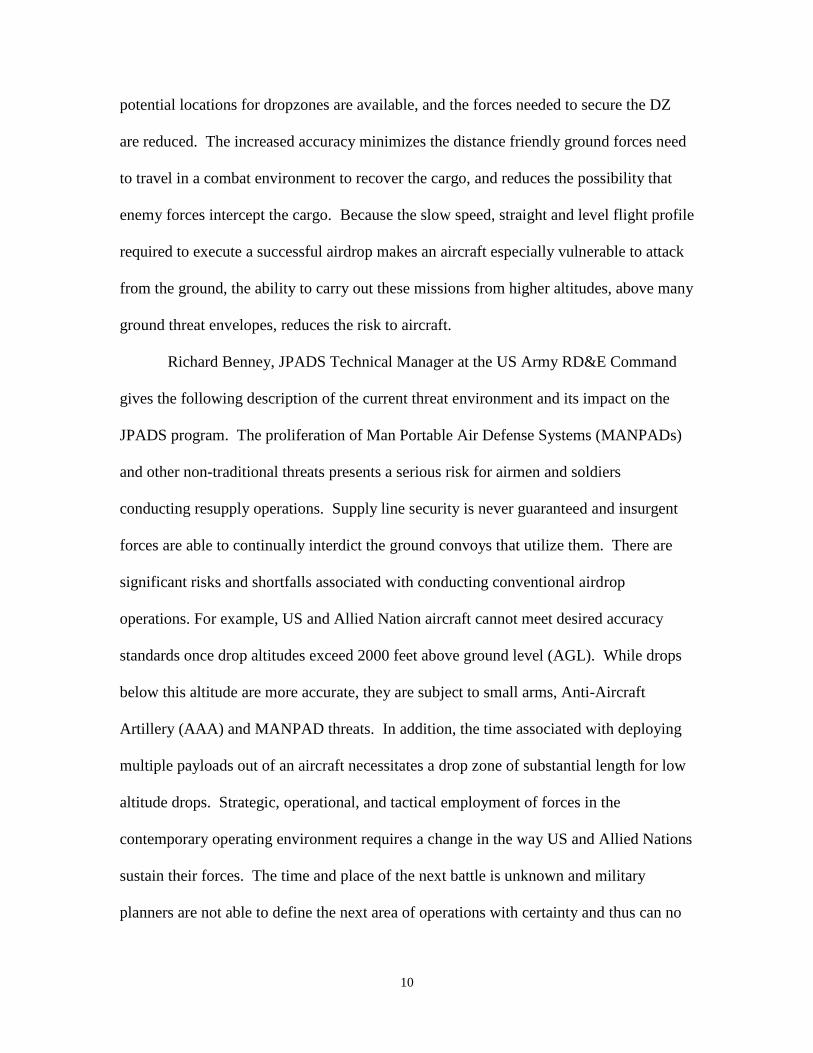
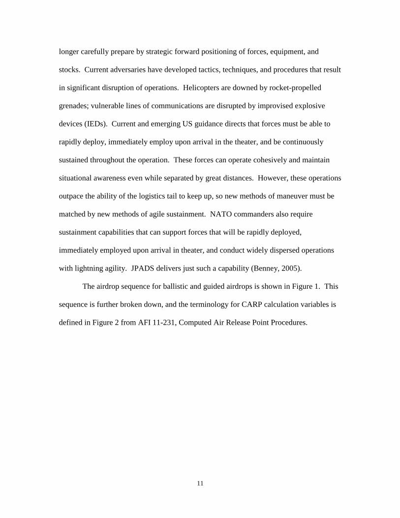
The airdrop sequence for ballistic and guided airdrops is shown in Figure 1. This
sequence is further broken down, and the terminology for CARP calculation variables is
defined in Figure 2 from AFI 11-231, Computed Air Release Point Procedures.
12
Figure 1. Depiction of Airdrop Sequence (Hattis, et al., 2006)
Figure 2. High Altitude Airdrop Terminology (AFI 11-231, 2005)
DESCENT TRAJECTORY
Fall Trajectory Model
+ 3D Atmospheric
Wind/Density Field
Complex 3D
Atmospheric Flow
over/through
Mountainous Terrain
Ballistic System or
Guided System(Corrects to Predicted Descent Trajectory)
CARP
Green Light
Roll-Out
Canopy-
Opening
STAND-OFF Depending on Altitude & Wind Field
13
According to AFI 11-231, the minimum required wind data prior to a high altitude
airdrop are a ballistic wind and a deployed wind. The ballistic wind is a vectorial average
of the winds between the drop altitude and the actuation altitude (or ground level for
single stage airdrops). A deployed wind is the vectorial average between the actuation
altitude and the surface. These winds can be provided by a weather forecaster, but more
commonly are computed by the aircrew from forecast winds at 1,000 foot intervals (AFI
11-231, 2005).
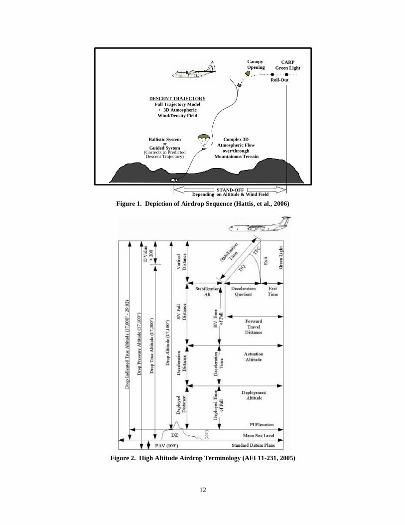
The JPADS-MP system operates in the cockpit on a high altitude compatible
laptop computer that is connected to Combat Track II (CTII) secure satellite
communication system (Benney, 2005). The roll-on/roll-off capability of the equipment,
shown in Figure 3, does not require permanent modification of each aircraft, and allows
multiple aircraft to share the limited number of JPADS hardware systems in operation.
There is no direct interface to the aircraft systems, so once a revised CARP is calculated
and displayed on the laptop, the aircrew manually enters it into the aircraft navigation
system.
Figure 3. JPADS Components (QinetiQ- North America, 2008)
14
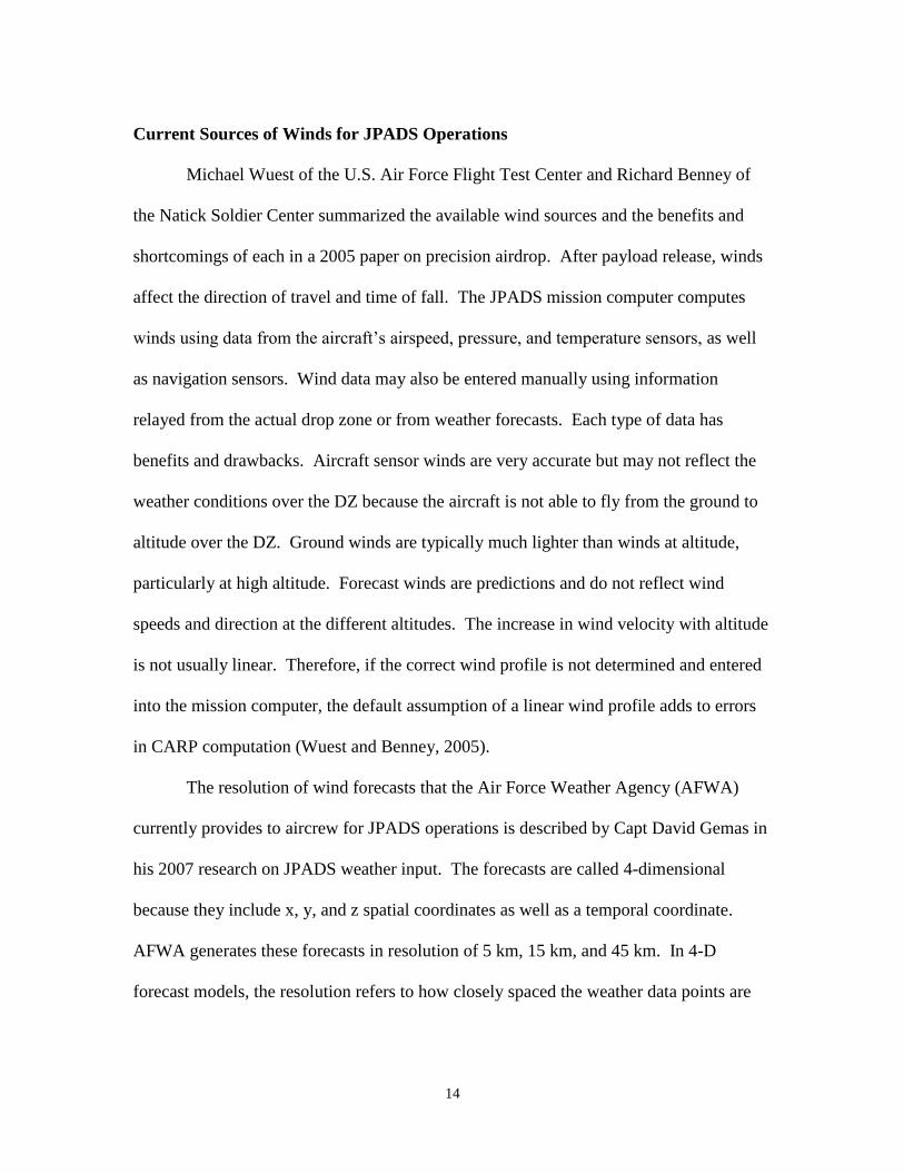
Current Sources of Winds for JPADS Operations
Michael Wuest of the U.S. Air Force Flight Test Center and Richard Benney of
the Natick Soldier Center summarized the available wind sources and the benefits and
shortcomings of each in a 2005 paper on precision airdrop. After payload release, winds
affect the direction of travel and time of fall. The JPADS mission computer computes
winds using data from the aircraft’s airspeed, pressure, and temperature sensors, as well
as navigation sensors. Wind data may also be entered manually using information
relayed from the actual drop zone or from weather forecasts. Each type of data has
benefits and drawbacks. Aircraft sensor winds are very accurate but may not reflect the
weather conditions over the DZ because the aircraft is not able to fly from the ground to
altitude over the DZ. Ground winds are typically much lighter than winds at altitude,
particularly at high altitude. Forecast winds are predictions and do not reflect wind
speeds and direction at the different altitudes. The increase in wind velocity with altitude
is not usually linear. Therefore, if the correct wind profile is not determined and entered
into the mission computer, the default assumption of a linear wind profile adds to errors
in CARP computation (Wuest and Benney, 2005).
The resolution of wind forecasts that the Air Force Weather Agency (AFWA)
currently provides to aircrew for JPADS operations is described by Capt David Gemas in
his 2007 research on JPADS weather input. The forecasts are called 4-dimensional
because they include x, y, and z spatial coordinates as well as a temporal coordinate.
AFWA generates these forecasts in resolution of 5 km, 15 km, and 45 km. In 4-D
forecast models, the resolution refers to how closely spaced the weather data points are
15
on the horizontal grid plane. Higher resolution means more data available, but also
means a larger data file, with greater bandwidth and longer time required for
transmission. The 5 and 15 km models are run every 12 hours and the 45 km model is
run every 6 hours with each model run predicting 24 hours of weather (Gemas, 2007).
These winds are updated in flight through the release of a dropsonde near the drop
zone just prior to the airdrop. The GPS dropsonde is a hand-launched probe that
measures atmospheric data near the drop zone while falling at 70-90 feet per second. The
dropsonde radio is programmed by the crew in 0.5 MHz increments between 400.5 and
405.5 MHz (HQ AMC JPADS CONEMP, 2009). It transmits its position during descent
to an onboard dropsonde receiver connected the aircraft’s lower UHF antenna. The
dropsonde receiver then feeds the GPS position data to the MPS laptop to derive the wind
profile. This initial wind profile is combined with the pre-flight forecast winds, and the
resulting wind profile is used to generate either a release point for a ballistic payload, or
in some instances, a Launch Acceptability Region (LAR) for guided payload delivery
(AMC Single Pass Airdrop Workshop, 2009).
The GPS dropsonde is the most proven current source of wind updates for JPADS
operations. Because variations in time and location of data collection can influence wind
estimation, especially at lower altitudes, operators should consider the use of dropsondes
to measure winds in the objective area as close to drop time as possible. The dropsonde
does not need to be dropped by the aircraft performing the cargo airdrop, but could be
deployed from another aircraft, or from a jet fighter, before the cargo plane arrives
(Wuest and Benney, 2005).

16
Temperature Retrieval from Satellite Sounding and Wind Derivation
Molecular absorption by atmospheric gases provides an excellent tool for
measuring temperatures from satellites. By knowing the concentration of a gas in the
atmosphere and its mass absorption coefficient for a given wavelength, we can determine
an optical depth. When a particular wavelength is measured from the atmosphere from
above, the altitude that the radiation is coming from can be determined.
If the atmosphere strongly absorbs the wavelength being measured, any emissions
from the surface or lower atmosphere will not make it to space. Instead, the strongest
emissions received will be from an altitude corresponding with the peak in the weighting
function for that wavelength. The usefulness of an individual measurement is limited,
but when measurements are combined from a series of sensors, each receiving a slightly
different wavelength near a strong molecular absorption line, a temperature profile can be
constructed.
Since the gas will have a different optical depth for each wavelength, each sensor
will ―see‖ down to a different altitude in the atmosphere. A sensor at the center of an
absorption line will measure the temperature near the top of the atmosphere, while farther
from the absorption peak a sensor may receive surface temperature. Matching these
individual measurements to a model of the atmosphere through an iterative process can
yield a full temperature profile.
The most commonly used gases in temperature sounding are CO2, water vapor,
oxygen and ozone (CO2 and oxygen having the advantage that they are well mixed
throughout the atmosphere making their density easy to determine). For good results
from ozone or water vapor sounding, local concentrations would need to be determined
17
through another process or model. Without knowing concentration, the altitude for water
vapor returns is difficult to determine, but returns can still be useful for imagery.
Common wavelengths used by geostationary satellites are in the vicinity of 15 microns
(CO2), 9.6 microns (ozone), and 5-8 microns (water vapor).
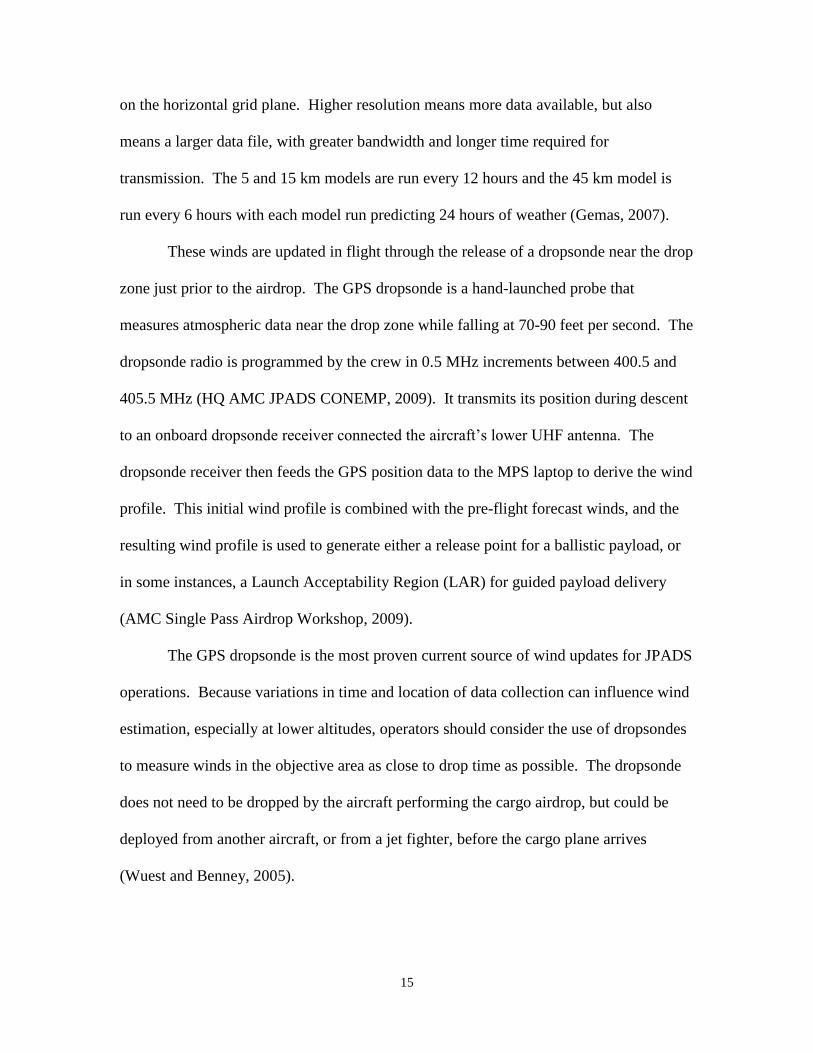
The determination of temperature by passive atmospheric sounding relies on
Schwarzchild’s equation. Vertical sounding theory begins with the integrated form of
this equation:
(1)
From the optical depth δ, height in the atmosphere can be determined. Schwarzchild’s
equation is manipulated to yield a weighting function for an individual wavelength. The
peak in this weighting function is used to assign an altitude to the measured radiance
(Kidder and Vonder Haar, 1995)
(2)
The problem of retrieving temperature from brightness temperature measurements
is complicated. A series of observed radiances is measured and matched with the
corresponding weighting function for the wavelength of the measurement channel. The
process for solving the inverse problem, determining what temperature and trace gas
concentration profiles could have produced that set of observed radiances, is laid out by
Stanley Kidder and Thomas Vonder Haar in their text Satellite Meteorology. Because the
forward problem of determining the radiance from a known temperature and trace gas
concentration profile is easy, the scheme to solve the inverse problem is to make a series

18
of profile guesses until convergence is achieved. Kidder and Vonder Haar’s iterative
process is:
1. A first-guess temperature profile is chosen
2. The weighting functions are calculated
3. The forward problem is solved to yield estimates of the radiance in each
channel of the radiometer.
4. If the computed radiances match the observed radiances within the noise level
of the radiometer, the current profile is accepted as the solution.
5. If convergence has not been achieved, the current profile is adjusted.
6. Steps 3 through 5 (or 2 through 5) are repeated until a solution is found.
(Kidder and Vonder Haar, 1995)
Polar orbits are much lower than geostationary orbits, and do not need short
wavelengths to have useful resolution. For this reason, these satellites can take advantage
of microwave absorption features like oxygen’s strong line at 60 GHz (5 mm). The
Advanced Microwave Sounding Unit is a polar orbiting satellite that uses 11 channels on
the edge of this oxygen line.
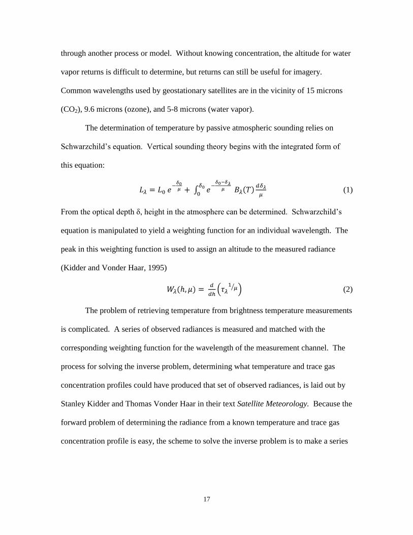
The weighting functions for these channels plotted against pressure in millibars
(mb), as depicted in Grant Petty’s text A First Course in Atmospheric Radiation is shown
in Figure 4. For each wavelength, approximate altitude can be determined using the
pressure for the point where the corresponding channel’s weighting function reaches a
maximum.
19
Figure 4. Microwave Weighting Functions for AMSU Sounding Channels (Petty, 2006)
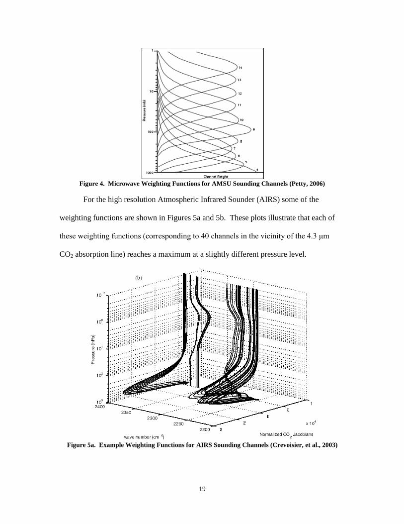
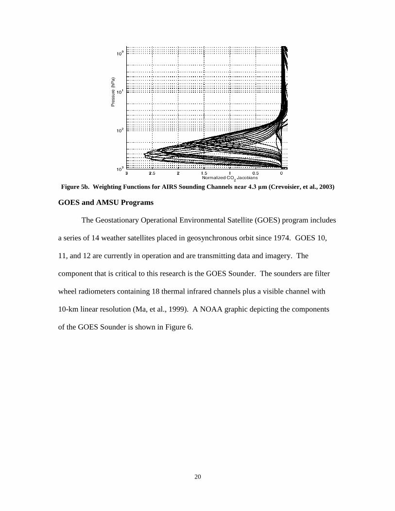
For the high resolution Atmospheric Infrared Sounder (AIRS) some of the
weighting functions are shown in Figures 5a and 5b. These plots illustrate that each of
these weighting functions (corresponding to 40 channels in the vicinity of the 4.3 μm
CO2 absorption line) reaches a maximum at a slightly different pressure level.
Figure 5a. Example Weighting Functions for AIRS Sounding Channels (Crevoisier, et al., 2003)
20
Figure 5b. Weighting Functions for AIRS Sounding Channels near 4.3 μm (Crevoisier, et al., 2003)
GOES and AMSU Programs
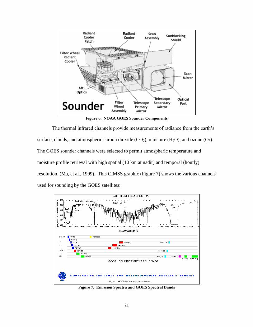
The Geostationary Operational Environmental Satellite (GOES) program includes
a series of 14 weather satellites placed in geosynchronous orbit since 1974. GOES 10,
11, and 12 are currently in operation and are transmitting data and imagery. The
component that is critical to this research is the GOES Sounder. The sounders are filter
wheel radiometers containing 18 thermal infrared channels plus a visible channel with
10-km linear resolution (Ma, et al., 1999). A NOAA graphic depicting the components
of the GOES Sounder is shown in Figure 6.
21
Figure 6. NOAA GOES Sounder Components
The thermal infrared channels provide measurements of radiance from the earth’s
surface, clouds, and atmospheric carbon dioxide (CO2), moisture (H2O), and ozone (O3).
The GOES sounder channels were selected to permit atmospheric temperature and
moisture profile retrieval with high spatial (10 km at nadir) and temporal (hourly)
resolution. (Ma, et al., 1999). This CIMSS graphic (Figure 7) shows the various channels
used for sounding by the GOES satellites:
Figure 7. Emission Spectra and GOES Spectral Bands
22
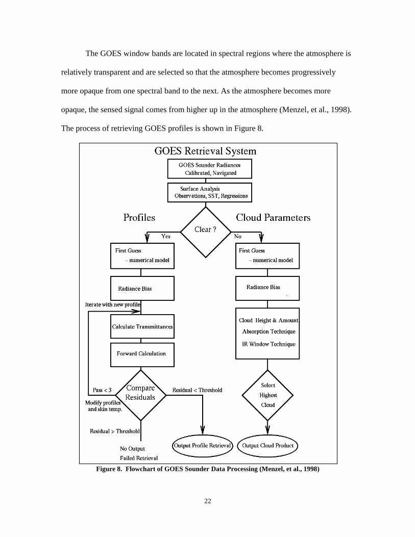
The GOES window bands are located in spectral regions where the atmosphere is
relatively transparent and are selected so that the atmosphere becomes progressively
more opaque from one spectral band to the next. As the atmosphere becomes more
opaque, the sensed signal comes from higher up in the atmosphere (Menzel, et al., 1998).
The process of retrieving GOES profiles is shown in Figure 8.
Figure 8. Flowchart of GOES Sounder Data Processing (Menzel, et al., 1998)

23
In a paper detailing the application of GOES soundings to weather forecasting, W.
Paul Menzel et al. describe the progress made in computing thermal winds. In mid
latitudes, using the assumption of a balanced atmosphere, thermal wind profiles have
been used successfully to estimate atmospheric motions in clear sky situations. The
thermal wind profiles are derived from a field of soundings, using horizontal temperature
gradients to infer vertical motion gradients. Modelers often prefer this form of the
sounding product over the geopotential height fields. In combination with features
tracked in sequences of sounder water vapor images, these sounder thermal winds have
proven to be valuable in depicting near mid-tropospheric motions. Such information,
especially in the northwest sector of the near hurricane environment, has proven to be
very useful. Improvements in the total suite of GOES wind field estimations have
reduced the average 72 hour forecast error for a given storm feature of 360 nautical miles
(670 km) by about 20% in a variety of research and operational models (Menzel et al.,
1998).
UW-CIMSS Satellite-Derived Wind Algorithm
The University of Wisconsin’s Cooperative Institute for Meteorological Satellite
Studies has done extensive research into wind determination from satellite observations.
Early successes came from automating the process of deriving wind direction and
velocity by observing cloud movement in subsequent frames of visible and IR satellite
images. An alternate method, which does not rely on cloud presence at each altitude for
which wind is derived is their CO2-Infrared Window Ratio Method, or the CO2 Slicing
method. Due to the fact that the emissivities of ice clouds and the cloud fractions for the
Infrared Window and CO2 Channels are roughly the same, this method is effective where
24
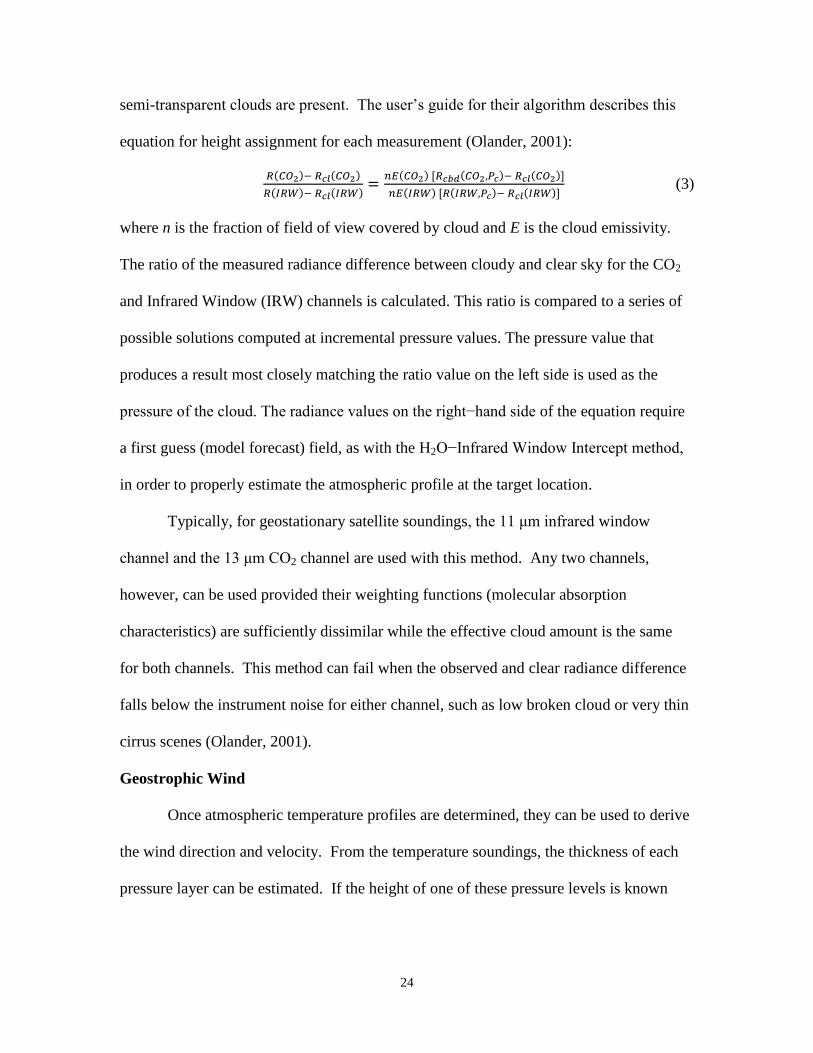
semi-transparent clouds are present. The user’s guide for their algorithm describes this
equation for height assignment for each measurement (Olander, 2001):
(3)
where n is the fraction of field of view covered by cloud and E is the cloud emissivity.
The ratio of the measured radiance difference between cloudy and clear sky for the CO2
and Infrared Window (IRW) channels is calculated. This ratio is compared to a series of
possible solutions computed at incremental pressure values. The pressure value that
produces a result most closely matching the ratio value on the left side is used as the
pressure of the cloud. The radiance values on the right−hand side of the equation require
a first guess (model forecast) field, as with the H2O−Infrared Window Intercept method,
in order to properly estimate the atmospheric profile at the target location.
Typically, for geostationary satellite soundings, the 11 μm infrared window
channel and the 13 μm CO2 channel are used with this method. Any two channels,
however, can be used provided their weighting functions (molecular absorption
characteristics) are sufficiently dissimilar while the effective cloud amount is the same
for both channels. This method can fail when the observed and clear radiance difference
falls below the instrument noise for either channel, such as low broken cloud or very thin
cirrus scenes (Olander, 2001).
Geostrophic Wind
Once atmospheric temperature profiles are determined, they can be used to derive
the wind direction and velocity. From the temperature soundings, the thickness of each
pressure layer can be estimated. If the height of one of these pressure levels is known
25
from either a surface or upper atmosphere observation or forecast, the heights of all other
pressure levels can be calculated. By combining heights from a series of sounding
locations, isobaric pressure surfaces can be constructed, and from these pressure surfaces,
several relationships can be used to determine winds. One of these is the geostrophic
wind, which is related to the gradient of the geopotential heights:
(4)
where Φ is the geopotential (gz), f is the Coriolis parameter, and is a vertical unit vector
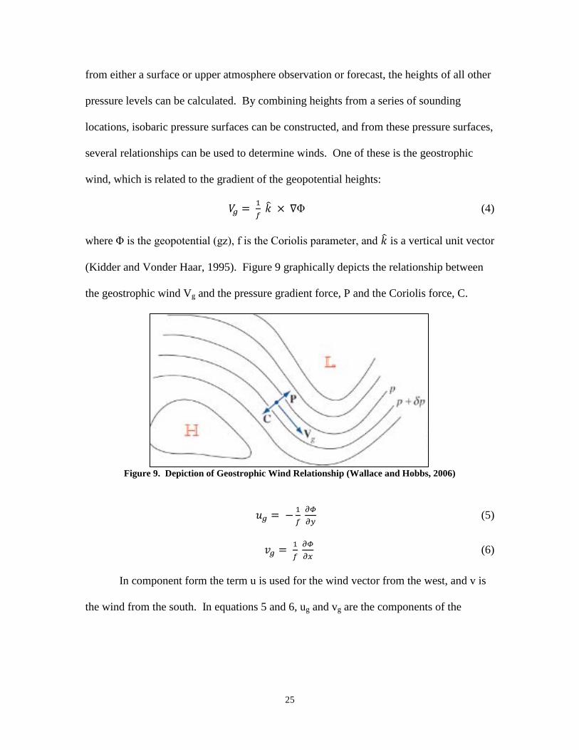
(Kidder and Vonder Haar, 1995). Figure 9 graphically depicts the relationship between
the geostrophic wind Vg and the pressure gradient force, P and the Coriolis force, C.
Figure 9. Depiction of Geostrophic Wind Relationship (Wallace and Hobbs, 2006)
(5)
(6)
In component form the term u is used for the wind vector from the west, and v is
the wind from the south. In equations 5 and 6, ug and vg are the components of the
26
geostrophic wind. Another relationship determines the magnitude of the gradient wind
by:
(7)
where RT is the radius of curvature of the trajectory of an air parcel. Comparisons made
in 1982 showed the gradient wind to most closely match rawinsonde data. The
agreement for winds aloft (compared at 300 hPa) was good with a correlation coefficient
of 0.87, but for lower altitude 850 hPa winds, the accuracy was much lower. For one of
the days of the experiment, satellite-derived and rawinsonde measured 850 hPa winds
were essentially uncorrelated (Kidder and Vonder Haar, 1995).
Thermal Wind
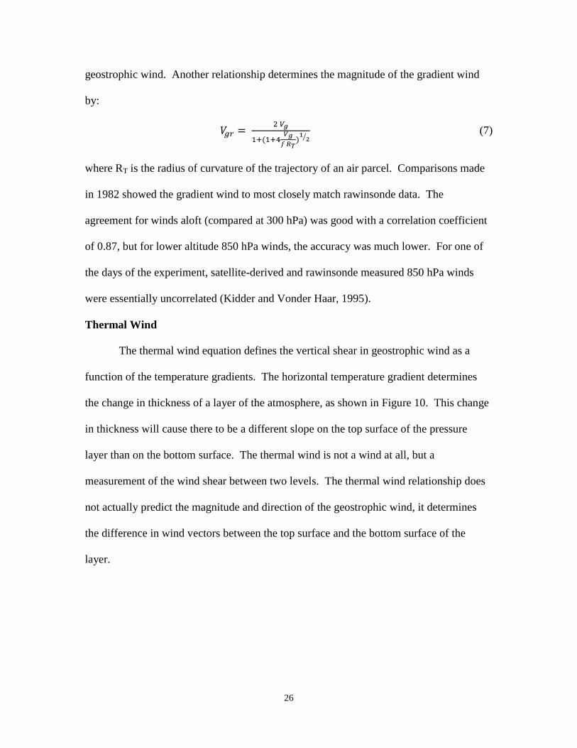
The thermal wind equation defines the vertical shear in geostrophic wind as a
function of the temperature gradients. The horizontal temperature gradient determines
the change in thickness of a layer of the atmosphere, as shown in Figure 10. This change
in thickness will cause there to be a different slope on the top surface of the pressure
layer than on the bottom surface. The thermal wind is not a wind at all, but a
measurement of the wind shear between two levels. The thermal wind relationship does
not actually predict the magnitude and direction of the geostrophic wind, it determines
the difference in wind vectors between the top surface and the bottom surface of the
layer.
27
Figure 10. Thermal Wind Relationship (Wallace and Hobbs, 2006)
In component form, the thermal wind equations are described by Wallace and
Hobbs as:
(8)
(9)
Accuracy of Satellite-Derived Winds
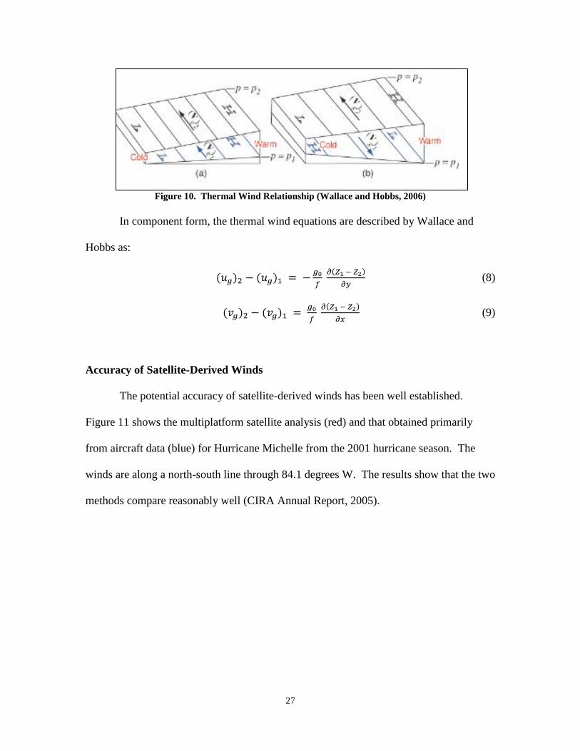
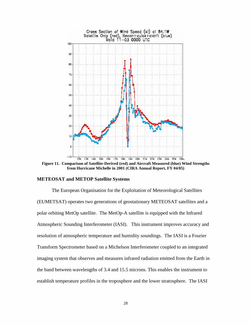
The potential accuracy of satellite-derived winds has been well established.
Figure 11 shows the multiplatform satellite analysis (red) and that obtained primarily
from aircraft data (blue) for Hurricane Michelle from the 2001 hurricane season. The
winds are along a north-south line through 84.1 degrees W. The results show that the two
methods compare reasonably well (CIRA Annual Report, 2005).
28
. Figure 11. Comparison of Satellite-Derived (red) and Aircraft Measured (blue) Wind Strengths
from Hurricane Michelle in 2001 (CIRA Annual Report, FY 04/05)
METEOSAT and METOP Satellite Systems
The European Organisation for the Exploitation of Meteorological Satellites
(EUMETSAT) operates two generations of geostationary METEOSAT satellites and a
polar orbiting MetOp satellite. The MetOp-A satellite is equipped with the Infrared
Atmospheric Sounding Interferometer (IASI). This instrument improves accuracy and
resolution of atmospheric temperature and humidity soundings. The IASI is a Fourier
Transform Spectrometer based on a Michelson Interferometer coupled to an integrated
imaging system that observes and measures infrared radiation emitted from the Earth in
the band between wavelengths of 3.4 and 15.5 microns. This enables the instrument to
establish temperature profiles in the troposphere and the lower stratosphere. The IASI
29
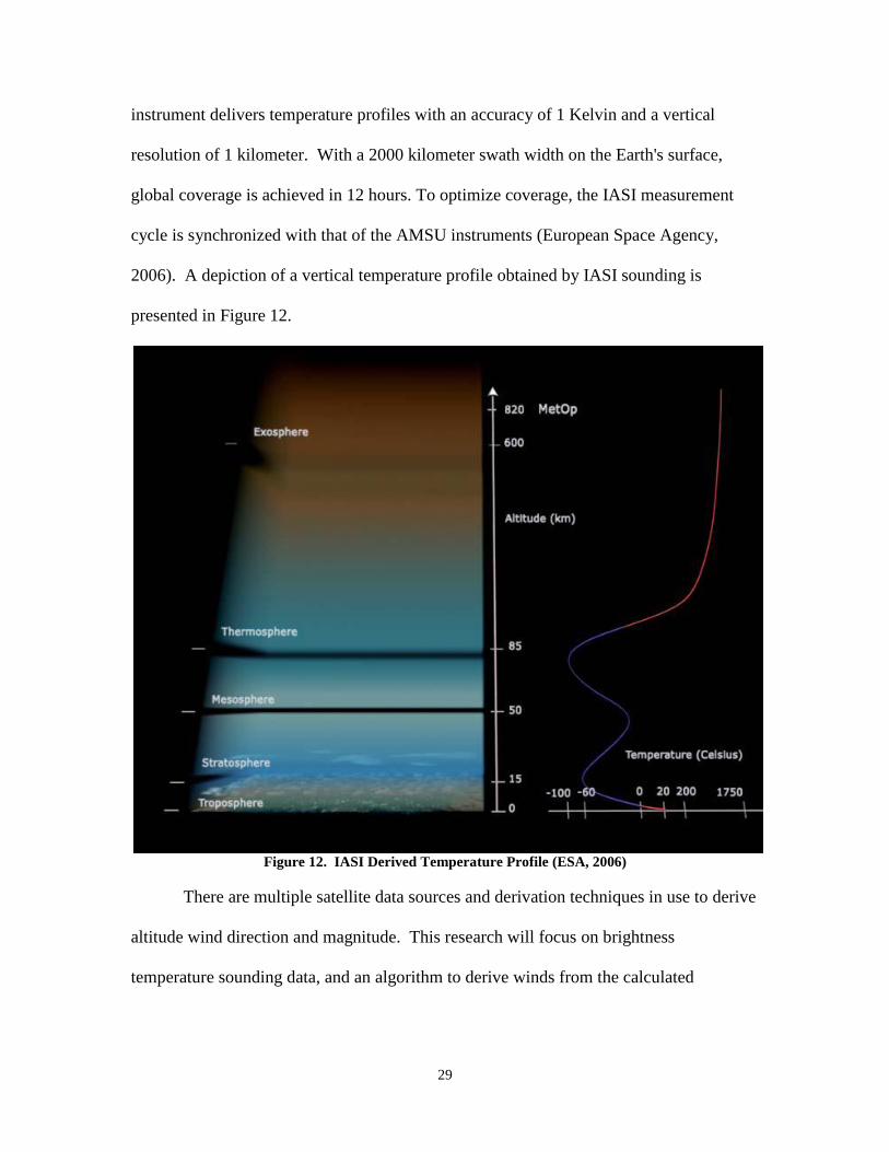
instrument delivers temperature profiles with an accuracy of 1 Kelvin and a vertical
resolution of 1 kilometer. With a 2000 kilometer swath width on the Earth's surface,
global coverage is achieved in 12 hours. To optimize coverage, the IASI measurement
cycle is synchronized with that of the AMSU instruments (European Space Agency,
2006). A depiction of a vertical temperature profile obtained by IASI sounding is
presented in Figure 12.
Figure 12. IASI Derived Temperature Profile (ESA, 2006)
There are multiple satellite data sources and derivation techniques in use to derive
altitude wind direction and magnitude. This research will focus on brightness
temperature sounding data, and an algorithm to derive winds from the calculated
30
temperature and pressure gradients. A significant advantage of this method is that the
results do not require the presence of clouds as needed for the feature tracking wind
determination methods. A limitation is the inability to derive winds below heavy cloud
cover. The best, and most operationally useful, solution would be to combine the IR
sounding technique investigated in this research, with wind data derived from microwave
soundings and cloud feature tracking. This would increase the availability of wind
profiles in areas with cloud cover.
Atmospheric Infrared Sounder (AIRS)
According to BAE Systems, NASA’s Aqua spacecraft is collecting data on earth
systems and weather features in a scope and detail not seen before. Aqua, launched on
May 4, 2002, as part of the Earth Observing System, collects data related to global water
cycles with the goal of improving weather prediction and scientists’ understanding of
climate change.
Hyperspectral sensing from space is a technique that delivers weather-balloon-
quality measurements on a global scale. Using infrared hyperspectral sensing, AIRS
passively measures temperature and humidity. The infrared region consists of a range of
wavelengths that correlate with altitude. Measuring the brightness of infrared
wavelengths that correspond to temperature, AIRS creates full and accurate mapping of
temperature from the surface to more than 30 km in altitude.
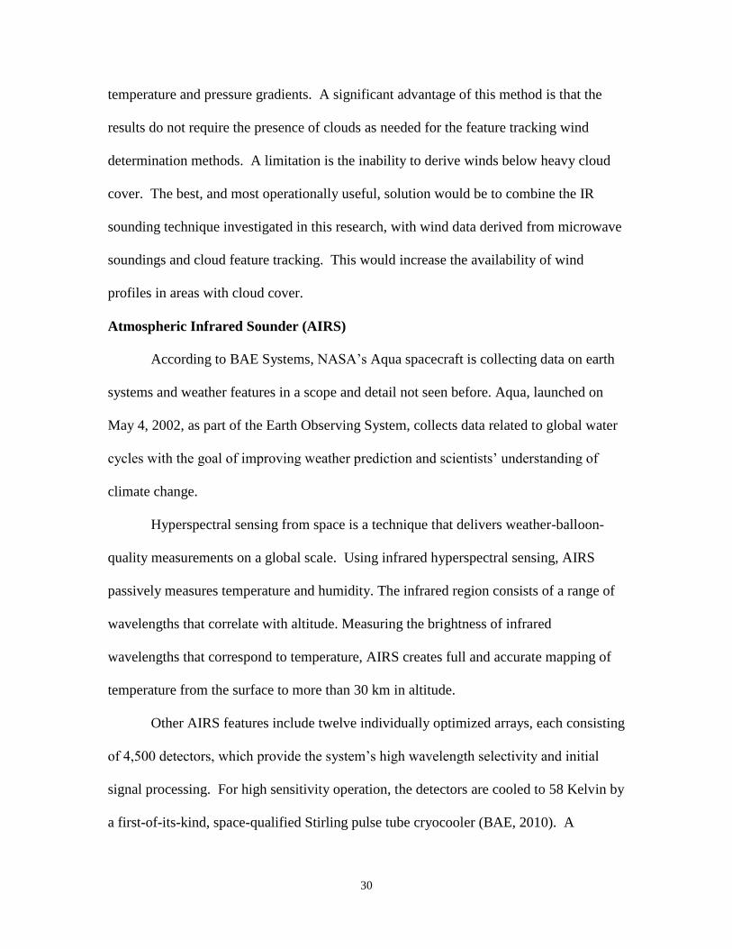
Other AIRS features include twelve individually optimized arrays, each consisting
of 4,500 detectors, which provide the system’s high wavelength selectivity and initial
signal processing. For high sensitivity operation, the detectors are cooled to 58 Kelvin by
a first-of-its-kind, space-qualified Stirling pulse tube cryocooler (BAE, 2010). A
31
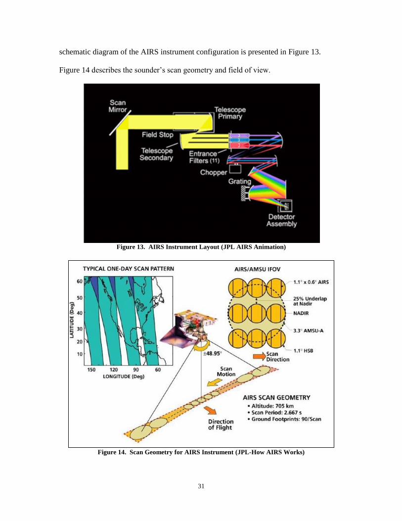
schematic diagram of the AIRS instrument configuration is presented in Figure 13.
Figure 14 describes the sounder’s scan geometry and field of view.
Figure 13. AIRS Instrument Layout (JPL AIRS Animation)
Figure 14. Scan Geometry for AIRS Instrument (JPL-How AIRS Works)

32
Global Forecast System (GFS)
The GFS is run four times per day (00 UTC, 06 UTC, 12 UTC, and 18 UTC) out
to 384 hours. The initial forecast resolution was changed on May 31, 2005 to T382
(equivalent to about 40-km grid-point resolution) with 64 levels out to 7.5 days (180
hours). At later forecast times, the GFS has a resolution of T190 (equivalent to about 80-
km resolution) and 64 levels between 24 and 384 hours. All GFS runs get their initial
conditions from the Gridpoint Statistical Interpolation (GSI) global data assimilation
system (GDAS) as of 1 May 2007, which is updated continuously throughout the day
(MetEd, 2007).
Radiosonde Sounding System
A global network of sites release weather balloons with attached rawinsondes, or
radiosondes daily, usually 00Z and 12Z. The accuracy of the atmospheric measurements
made by these radiosondes has been well established, so radiosonde data provides
temperature and wind profiles for validation of satellite-derived data. The
Meteorological Resource Center’s website, WebMET.com, describes the radiosonde
technology and process: Radiosonde sounding systems use sensors carried aloft by a
small, balloon-borne instrument package (the radiosonde, or simply ―sonde‖) to measure
vertical profiles of atmospheric pressure, temperature, and moisture (relative humidity or
wet bulb temperature) as the balloon ascends. In the United States, helium is typically
used to inflate weather balloons, but some locations use hydrogen. The altitude of the
balloon is typically determined using thermodynamic variables or by satellite-based
Global Positioning Systems (GPS). Pressure is measured by a capacitance aneroid
33
barometer or similar sensor. Temperature is typically measured by a small rod or bead
thermistor. Most commercial radiosonde sounding systems use a carbon hygristor or a
capacitance sensor to measure relative humidity directly, although a wet-bulb sensor is
used by some systems.
A radiosonde includes electronic subsystems that sample each sensor at regular
intervals (usually every 2 to 5 seconds), and transmit the data to a ground-based receiver
and data acquisition system. Most commercial radiosonde systems operate at either 404
MHZ or 1680 MHZ. Once the data are received at the ground station, they are converted
to engineering units based on calibrations supplied by the manufacturer. The data
acquisition system reduces the data in near-real time, calculates the altitude of the
balloon, and computes wind speed and direction aloft based on information obtained by
the data systems on the position of the balloon as it is borne along by the wind. The
radiosondes are typically smaller than a shoebox and weigh only a few hundred grams.
Upper-air winds (horizontal wind speed and direction) are determined during
radiosonde ascents by measuring the position of the radiosonde relative to the earth's
surface as the balloon ascends. By measuring the position of the balloon with respect to
time and altitude, wind vectors can be calculated that represent the layer-averaged
horizontal wind speed and wind direction for each successive layer. The position of the
radiosonde was originally tracked using radio direction finding techniques (RDF) or by
radio navigation network, but the use of satellite-based GPS has become more common
(WebMET.com, 2002).
34
III. Methodology
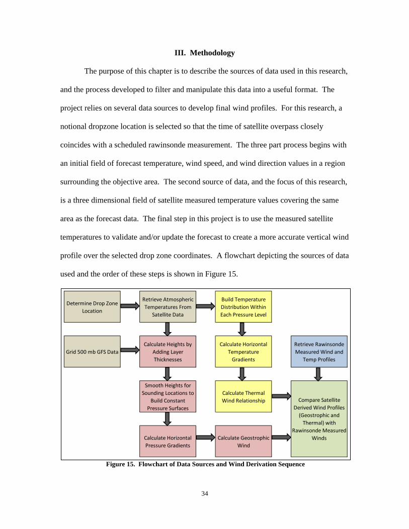
The purpose of this chapter is to describe the sources of data used in this research,
and the process developed to filter and manipulate this data into a useful format. The
project relies on several data sources to develop final wind profiles. For this research, a
notional dropzone location is selected so that the time of satellite overpass closely
coincides with a scheduled rawinsonde measurement. The three part process begins with
an initial field of forecast temperature, wind speed, and wind direction values in a region
surrounding the objective area. The second source of data, and the focus of this research,
is a three dimensional field of satellite measured temperature values covering the same
area as the forecast data. The final step in this project is to use the measured satellite
temperatures to validate and/or update the forecast to create a more accurate vertical wind
profile over the selected drop zone coordinates. A flowchart depicting the sources of data
used and the order of these steps is shown in Figure 15.
Figure 15. Flowchart of Data Sources and Wind Derivation Sequence
Determine Drop Zone
Location
Retrieve Atmospheric
Temperatures From
Satellite Data
Build Temperature
Distribution Within
Each Pressure Level
Grid 500 mb GFS Data
Calculate Heights by
Adding Layer
Thicknesses
Calculate Horizontal
Temperature
Gradients
Retrieve Rawinsonde
Measured Wind and
Temp Profiles
Smooth Heights for
Sounding Locations to
Build Constant
Pressure Surfaces
Calculate Thermal
Wind Relationship
Calculate Horizontal
Pressure Gradients
Calculate Geostrophic
Wind
Compare Satellite
Derived Wind Profiles
(Geostrophic and
Thermal) with
Rawinsonde Measured
Winds
35
Data Sources
The two sources of gridded forecast data evaluated are 6 hour Global Forecast
System (GFS) data and a 4 dimensional weather product specifically generated by the Air
Force Weather Agency (AFWA) for use in JPADS operations. Both of these products
provide the needed temperature and wind values, with the most significant differences
being the resolution of the available data. These differences are shown in Table 3.1:
(MetEd, 2007 and Air Force Weather Agency)
Table 3.1 Comparison of Resolutions for GFS and AFWA JPADS 4-D Forecasts
Horizontal Vertical Temporal
Global Forecast System (GFS)
AFWA JPADS 4-D Forecast
0.9°/40 km
5 km (in contingency
windows)
64 Layers
56 Layers
6 Hours
3 Hours
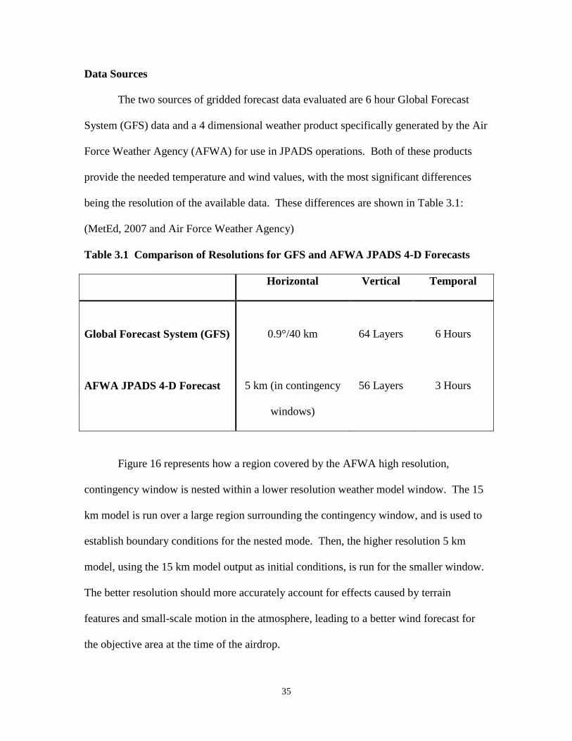
Figure 16 represents how a region covered by the AFWA high resolution,
contingency window is nested within a lower resolution weather model window. The 15
km model is run over a large region surrounding the contingency window, and is used to
establish boundary conditions for the nested mode. Then, the higher resolution 5 km
model, using the 15 km model output as initial conditions, is run for the smaller window.
The better resolution should more accurately account for effects caused by terrain
features and small-scale motion in the atmosphere, leading to a better wind forecast for
the objective area at the time of the airdrop.
36
Figure 16. Nested Contingency Window Illustration (QinetiQ-North America, 2008)
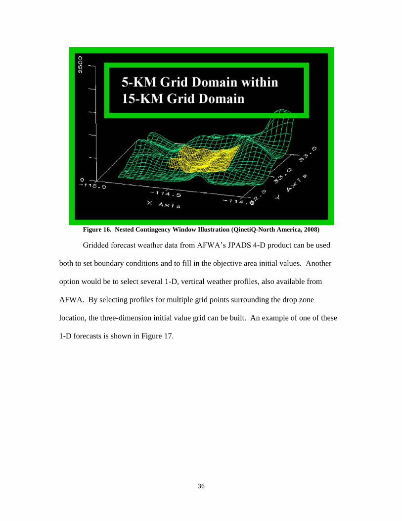
Gridded forecast weather data from AFWA’s JPADS 4-D product can be used
both to set boundary conditions and to fill in the objective area initial values. Another
option would be to select several 1-D, vertical weather profiles, also available from
AFWA. By selecting profiles for multiple grid points surrounding the drop zone
location, the three-dimension initial value grid can be built. An example of one of these
1-D forecasts is shown in Figure 17.
37
Figure 17. AFWA 1-D JPADS Vertical Forecast Profile Format
Satellite Data
The first decision made in the selection of the most appropriate source of satellite
data is whether to use data from geostationary or polar orbiting satellites. The primary
advantage of a geostationary platform is that it is continually present over its assigned
area. This leads to the availability of more frequent sounding data (usually hourly), and
38
makes feature tracking wind calculation possible. In addition to deriving wind direction
from brightness temperature data, wind speed and direction can be calculated by
automated algorithms which track the position of visible or IR cloud features in
subsequent satellite images. Once an altitude is assigned to these features, additional
wind speed and direction data is available to augment brightness temperature wind data.
The limitations of geostationary satellite sounding data are primarily caused by
the sounder resolution. Due to the high orbital altitude of 35,800 km, the horizontal
resolution of an instrument on a geostationary satellite is more than 40 times larger than it
would be for the same instrument mounted on a satellite in a low altitude (700-1000 km)
polar orbit. Vertical resolution, or the number of altitude layers that can be accurately
resolved, is a function of the number of sounder channels measured. Current
geostationary satellites only measure brightness on 15-20 channels.
Instruments in use on polar orbiting satellites are able to measure brightness
temperatures on many more spectral channels. The Atmospheric Infrared Sounder
(AIRS) on the Aqua satellite uses 2378 channels and the Infrared Atmospheric Sounding
Interferometer on the European MetOp satellite uses 8461 channels. A weighting
function is calculated for each of these channels, and the density of the data allows for the
determination of atmospheric temperature at each of 100 or more layers to an accuracy of
1.0 ºC. The quality of data from this latest generation of infrared sounders is ―expected
to exceed temperature and humidity measurements of operational radiosondes‖.
(EUMETSAT, 2007)
For this research, AIRS data from the polar orbiting Aqua satellite was used to
determine the applicability of the technique. During each 90 to 100 minute orbit of the
39
satellite, the Earth rotates about 25 degrees, so each day, most locations on earth are
covered by both an ascending and descending satellite pass. Near the equator, the
coverage is not complete and the surface area missed is filled in by the next day’s flight
path. At latitudes greater than about 30 degrees however, each swath overlaps the
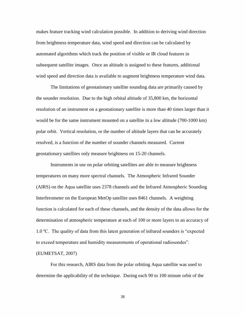
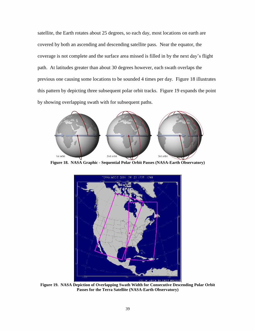
previous one causing some locations to be sounded 4 times per day. Figure 18 illustrates
this pattern by depicting three subsequent polar orbit tracks. Figure 19 expands the point
by showing overlapping swath with for subsequent paths.
Figure 18. NASA Graphic - Sequential Polar Orbit Passes (NASA-Earth Observatory)
Figure 19. NASA Depiction of Overlapping Swath Width for Consecutive Descending Polar Orbit
Passes for the Terra Satellite (NASA-Earth Observatory)
40
Once proven for AIRS data, the same technique could be used with data from
other polar orbiting satellites with similar infrared sounders, NOAA 18, NOAA 10,
MetOp A, and DMSP F16. Using all five platforms would reduce the mean time between
overflight for a mid-latitude drop zone to 2.4 hours. For this source of wind data to be
operationally valuable, it would need to be available close to the time of a planned
airdrop. With multiple polar orbiting sounders to choose from, there would be many
opportunities each day to schedule a JPADS airdrop for which sounder data (from one of
these multiple platforms) is available from a satellite pass 1-2 hours prior to the drop.
Data Filtering and Processing
AIRS and AMSU sounder data files are available over the internet from the Jet
Propulsion Laboratory (JPL). Individual data files cover six minutes of flight time,
during which the platform travels approximately 1500 km and the AIRS-suite scan covers
a swath roughly 1500 km wide. Level 2 data has been geolocated and processed to
calibrate and correct brightness temperatures for sun position and instrument errors. The
file format, Hierarchical Data Format-Earth Observing System (HDF-EOS), is a
specialized form of HDF selected by NASA to standardize the format of the terabyte of
data delivered daily by each of the EOS satellites.
Files on JPL’s server are selected by defining a geographic area as well as start
and stop times. A list of all applicable data files is presented and individual six minute
files can be downloaded. In order to have radiosonde wind profiles available to compare
to the profiles derived from satellite soundings, locations for this project were selected
from radiosonde sites that the Aqua satellite passed over near scheduled release times
(00Z and 12Z). NASA’s Earth Observatory website provides a Satellite Overpass
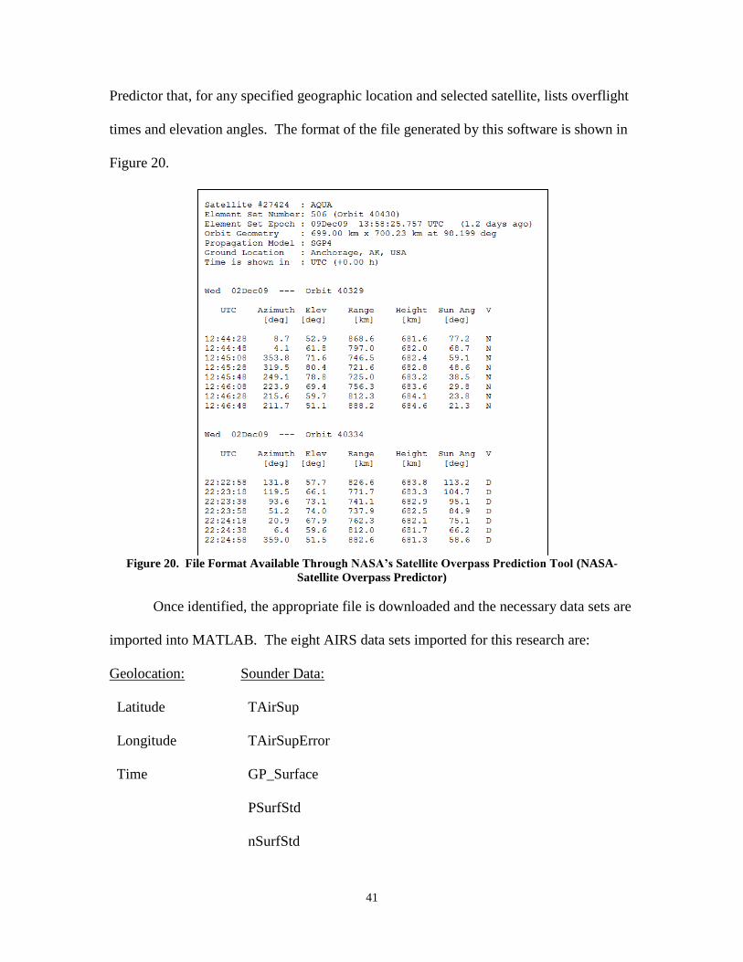
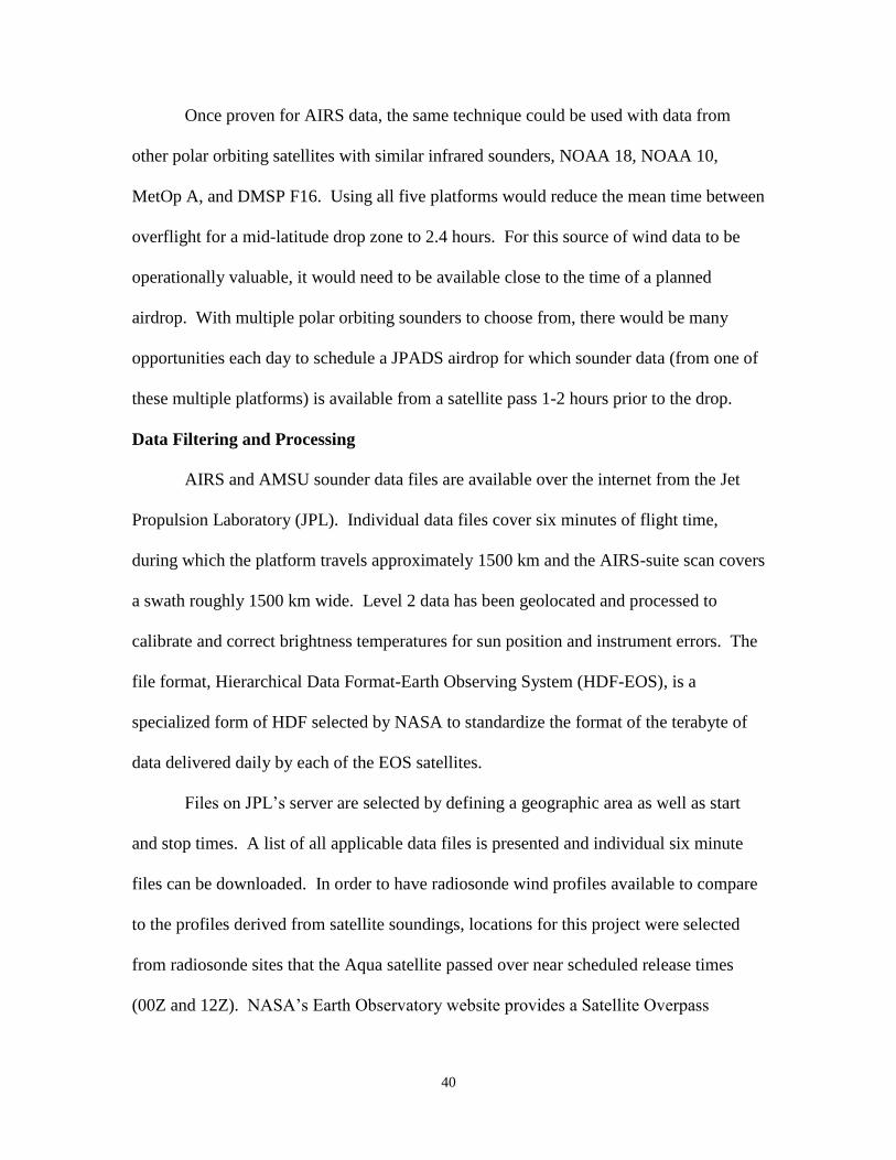
41
Predictor that, for any specified geographic location and selected satellite, lists overflight
times and elevation angles. The format of the file generated by this software is shown in
Figure 20.
Figure 20. File Format Available Through NASA’s Satellite Overpass Prediction Tool (NASA-
Satellite Overpass Predictor)
Once identified, the appropriate file is downloaded and the necessary data sets are
imported into MATLAB. The eight AIRS data sets imported for this research are:
Geolocation: Sounder Data:
Latitude TAirSup
Longitude TAirSupError
Time GP_Surface
PSurfStd
nSurfStd
42
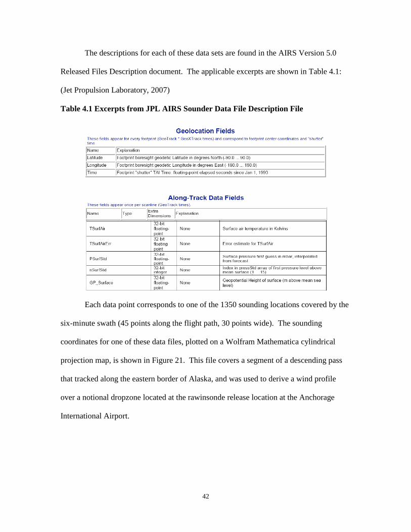
The descriptions for each of these data sets are found in the AIRS Version 5.0
Released Files Description document. The applicable excerpts are shown in Table 4.1:
(Jet Propulsion Laboratory, 2007)
Table 4.1 Excerpts from JPL AIRS Sounder Data File Description File
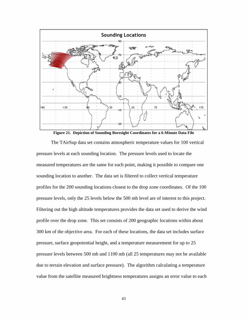
Each data point corresponds to one of the 1350 sounding locations covered by the
six-minute swath (45 points along the flight path, 30 points wide). The sounding
coordinates for one of these data files, plotted on a Wolfram Mathematica cylindrical
projection map, is shown in Figure 21. This file covers a segment of a descending pass
that tracked along the eastern border of Alaska, and was used to derive a wind profile
over a notional dropzone located at the rawinsonde release location at the Anchorage
International Airport.
43
Figure 21. Depiction of Sounding Boresight Coordinates for a 6-Minute Data File
The TAirSup data set contains atmospheric temperature values for 100 vertical
pressure levels at each sounding location. The pressure levels used to locate the
measured temperatures are the same for each point, making it possible to compare one
sounding location to another. The data set is filtered to collect vertical temperature
profiles for the 200 sounding locations closest to the drop zone coordinates. Of the 100
pressure levels, only the 25 levels below the 500 mb level are of interest to this project.
Filtering out the high altitude temperatures provides the data set used to derive the wind
profile over the drop zone. This set consists of 200 geographic locations within about
300 km of the objective area. For each of these locations, the data set includes surface
pressure, surface geopotential height, and a temperature measurement for up to 25
pressure levels between 500 mb and 1100 mb (all 25 temperatures may not be available
due to terrain elevation and surface pressure). The algorithm calculating a temperature
value from the satellite measured brightness temperatures assigns an error value to each
-90
-70
-50
-30
-10
10
30
50
70
90
-180 -130 -80 -30 20 70 120 170
Sounding Locations
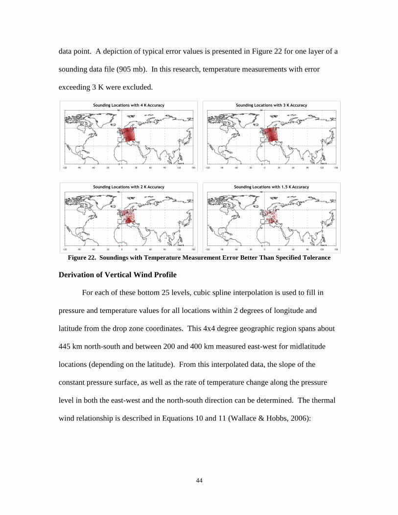
44
data point. A depiction of typical error values is presented in Figure 22 for one layer of a
sounding data file (905 mb). In this research, temperature measurements with error
exceeding 3 K were excluded.
Figure 22. Soundings with Temperature Measurement Error Better Than Specified Tolerance
Derivation of Vertical Wind Profile
For each of these bottom 25 levels, cubic spline interpolation is used to fill in
pressure and temperature values for all locations within 2 degrees of longitude and
latitude from the drop zone coordinates. This 4x4 degree geographic region spans about
445 km north-south and between 200 and 400 km measured east-west for midlatitude
locations (depending on the latitude). From this interpolated data, the slope of the
constant pressure surface, as well as the rate of temperature change along the pressure
level in both the east-west and the north-south direction can be determined. The thermal
wind relationship is described in Equations 10 and 11 (Wallace & Hobbs, 2006):
0
30
60
90
-120 -90 -60 -30 0 30 60 90 120 150
Sounding Locations with 4 K Accuracy
0
30
60
90
-120 -90 -60 -30 0 30 60 90 120 150
Sounding Locations with 3 K Accuracy
0
30
60
90
-120 -90 -60 -30 0 30 60 90 120 150
Sounding Locations with 2 K Accuracy
0
30
60
90
-120 -90 -60 -30 0 30 60 90 120 150
Sounding Locations with 1.5 K Accuracy
45
(10)
(11)
The thickness of each layer ( is linearly proportional to the temperature,
as described by the hypsometric equation:
(12)
Rd is the dry gas constant and go is the acceleration due to gravity at the surface.
The variable f is the Coriolis parameter, which depends on the latitude of the objective
area. Combining these two equations provides a method of determining the vertical
change in u and v components of the geostrophic wind through each layer. The change
wind between the top and bottom of a pressure layer is only a function of the vertical
change in pressure through the layer, and the horizontal temperature gradient.
(13)
(14)
This form of the thermal wind relationship from the Wallace and Hobbs text
neglects the dependence on vertical temperature gradient, which also contributes to the
wind gradient. Howard Bluestein, in Synoptic-Dynamic Meteorology in Midlatitudes,
provides the more complete equations for the wind gradients by u and v components
(Bluestein, 1992):
(15)
(16)
46
IV. Results and Analysis
Validation of Satellite-Measured Temperatures
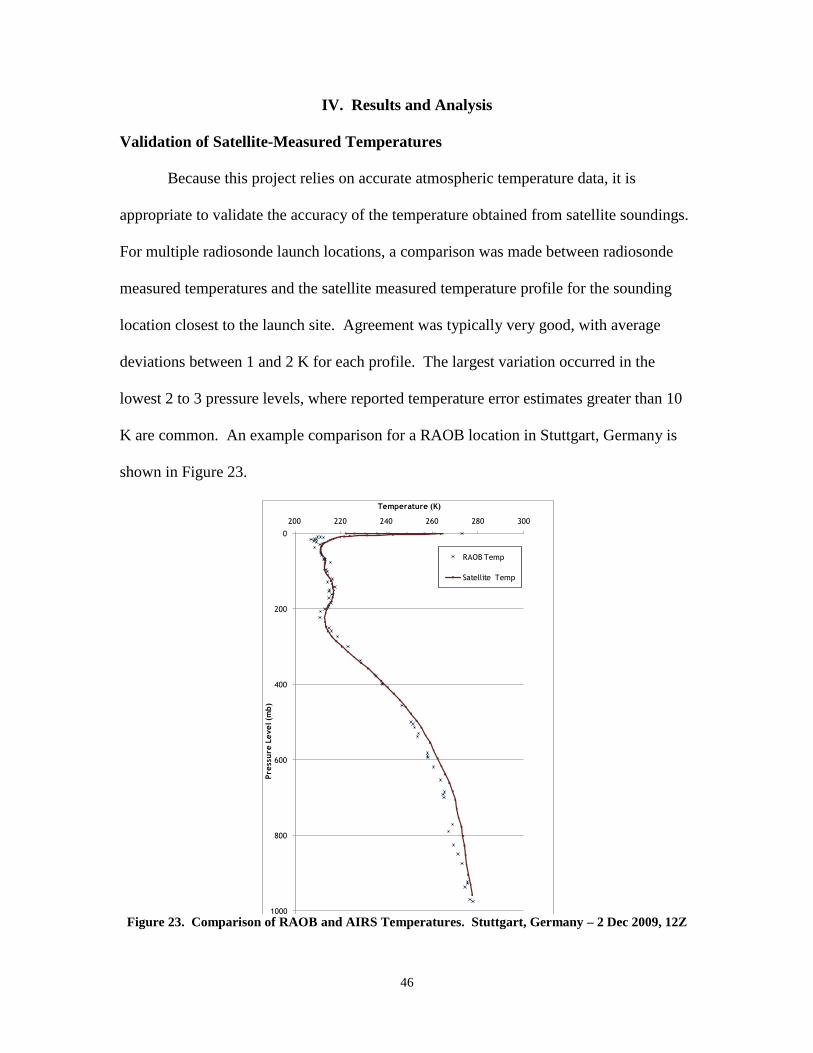
Because this project relies on accurate atmospheric temperature data, it is
appropriate to validate the accuracy of the temperature obtained from satellite soundings.
For multiple radiosonde launch locations, a comparison was made between radiosonde
measured temperatures and the satellite measured temperature profile for the sounding
location closest to the launch site. Agreement was typically very good, with average
deviations between 1 and 2 K for each profile. The largest variation occurred in the
lowest 2 to 3 pressure levels, where reported temperature error estimates greater than 10
K are common. An example comparison for a RAOB location in Stuttgart, Germany is
shown in Figure 23.
Figure 23. Comparison of RAOB and AIRS Temperatures. Stuttgart, Germany – 2 Dec 2009, 12Z
0
200
400
600
800
1000
200 220 240 260 280 300
Pre
ssu
re L
eve
l (m
b)
Temperature (K)
RAOB Temp
Satellite Temp
47
Lookup of Terrain Elevation for Each Sounding Location
The Level 2 data available from the Aqua satellite sounders provides the
atmospheric pressure at the surface (by interpolation from forecast data) and the
geopotential height of the surface in meters. The surface terrain elevation for each of
these sounding locations is a potential starting point for assigning heights to each
subsequent pressure level. The coarse elevation data required is available from many
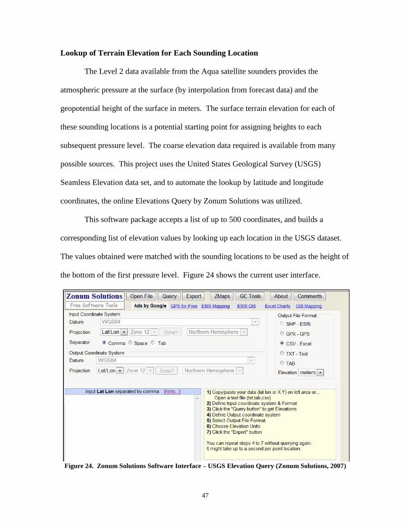
possible sources. This project uses the United States Geological Survey (USGS)
Seamless Elevation data set, and to automate the lookup by latitude and longitude
coordinates, the online Elevations Query by Zonum Solutions was utilized.
This software package accepts a list of up to 500 coordinates, and builds a
corresponding list of elevation values by looking up each location in the USGS dataset.
The values obtained were matched with the sounding locations to be used as the height of
the bottom of the first pressure level. Figure 24 shows the current user interface.
Figure 24. Zonum Solutions Software Interface – USGS Elevation Query (Zonum Solutions, 2007)
48
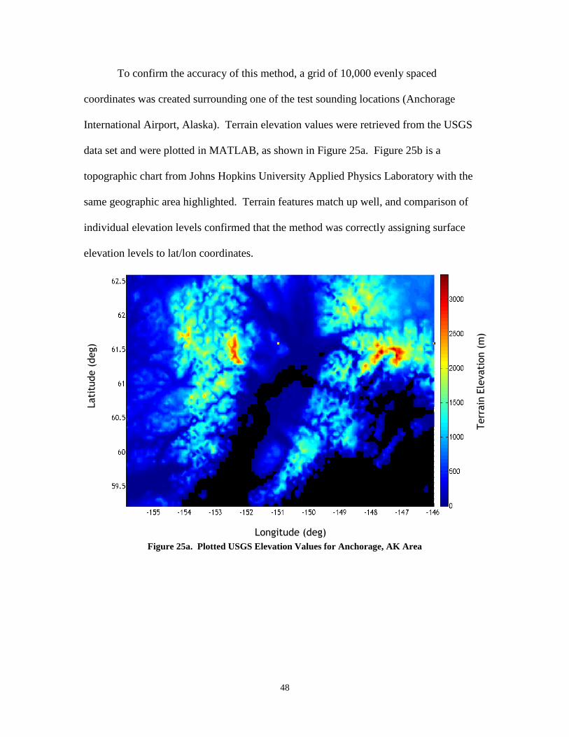
To confirm the accuracy of this method, a grid of 10,000 evenly spaced
coordinates was created surrounding one of the test sounding locations (Anchorage
International Airport, Alaska). Terrain elevation values were retrieved from the USGS
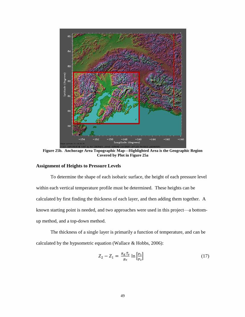
data set and were plotted in MATLAB, as shown in Figure 25a. Figure 25b is a
topographic chart from Johns Hopkins University Applied Physics Laboratory with the
same geographic area highlighted. Terrain features match up well, and comparison of
individual elevation levels confirmed that the method was correctly assigning surface
elevation levels to lat/lon coordinates.
Figure 25a. Plotted USGS Elevation Values for Anchorage, AK Area
Longitude (deg)
Lati
tude (
deg)
Terr
ain
Ele
vati
on (
m)
49
Figure 25b. Anchorage Area Topographic Map—Highlighted Area is the Geographic Region
Covered by Plot in Figure 25a
Assignment of Heights to Pressure Levels
To determine the shape of each isobaric surface, the height of each pressure level
within each vertical temperature profile must be determined. These heights can be
calculated by first finding the thickness of each layer, and then adding them together. A
known starting point is needed, and two approaches were used in this project—a bottom-
up method, and a top-down method.
The thickness of a single layer is primarily a function of temperature, and can be
calculated by the hypsometric equation (Wallace & Hobbs, 2006):
(17)
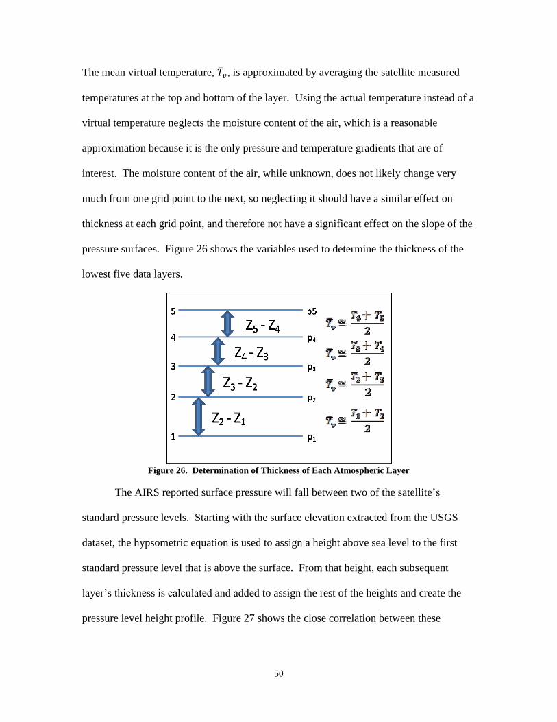
50
The mean virtual temperature, , is approximated by averaging the satellite measured
temperatures at the top and bottom of the layer. Using the actual temperature instead of a
virtual temperature neglects the moisture content of the air, which is a reasonable
approximation because it is the only pressure and temperature gradients that are of
interest. The moisture content of the air, while unknown, does not likely change very
much from one grid point to the next, so neglecting it should have a similar effect on
thickness at each grid point, and therefore not have a significant effect on the slope of the
pressure surfaces. Figure 26 shows the variables used to determine the thickness of the
lowest five data layers.
Figure 26. Determination of Thickness of Each Atmospheric Layer
The AIRS reported surface pressure will fall between two of the satellite’s
standard pressure levels. Starting with the surface elevation extracted from the USGS
dataset, the hypsometric equation is used to assign a height above sea level to the first
standard pressure level that is above the surface. From that height, each subsequent
layer’s thickness is calculated and added to assign the rest of the heights and create the
pressure level height profile. Figure 27 shows the close correlation between these
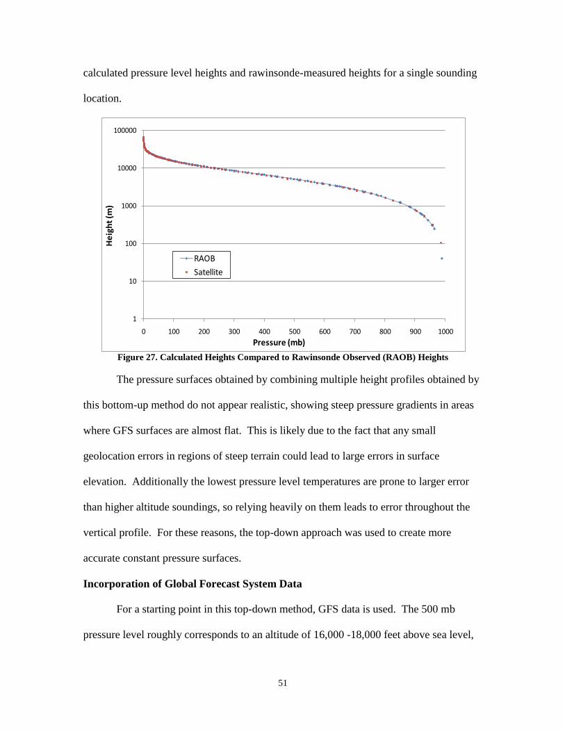
51
calculated pressure level heights and rawinsonde-measured heights for a single sounding
location.
Figure 27. Calculated Heights Compared to Rawinsonde Observed (RAOB) Heights
The pressure surfaces obtained by combining multiple height profiles obtained by
this bottom-up method do not appear realistic, showing steep pressure gradients in areas
where GFS surfaces are almost flat. This is likely due to the fact that any small
geolocation errors in regions of steep terrain could lead to large errors in surface
elevation. Additionally the lowest pressure level temperatures are prone to larger error
than higher altitude soundings, so relying heavily on them leads to error throughout the
vertical profile. For these reasons, the top-down approach was used to create more
accurate constant pressure surfaces.
Incorporation of Global Forecast System Data
For a starting point in this top-down method, GFS data is used. The 500 mb
pressure level roughly corresponds to an altitude of 16,000 -18,000 feet above sea level,
1
10
100
1000
10000
100000
0 100 200 300 400 500 600 700 800 900 1000
He
igh
t (m
)
Pressure (mb)
RAOB
Satellite
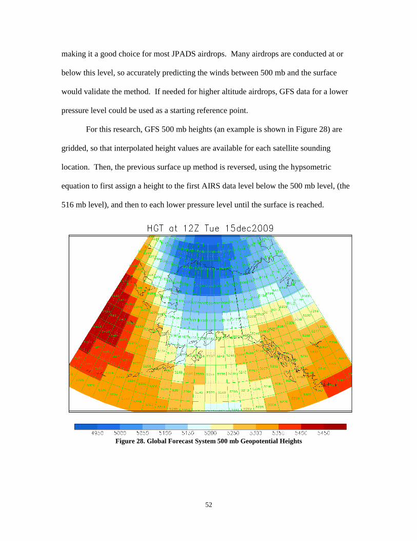
52
making it a good choice for most JPADS airdrops. Many airdrops are conducted at or
below this level, so accurately predicting the winds between 500 mb and the surface
would validate the method. If needed for higher altitude airdrops, GFS data for a lower
pressure level could be used as a starting reference point.
For this research, GFS 500 mb heights (an example is shown in Figure 28) are
gridded, so that interpolated height values are available for each satellite sounding
location. Then, the previous surface up method is reversed, using the hypsometric
equation to first assign a height to the first AIRS data level below the 500 mb level, (the
516 mb level), and then to each lower pressure level until the surface is reached.
Figure 28. Global Forecast System 500 mb Geopotential Heights
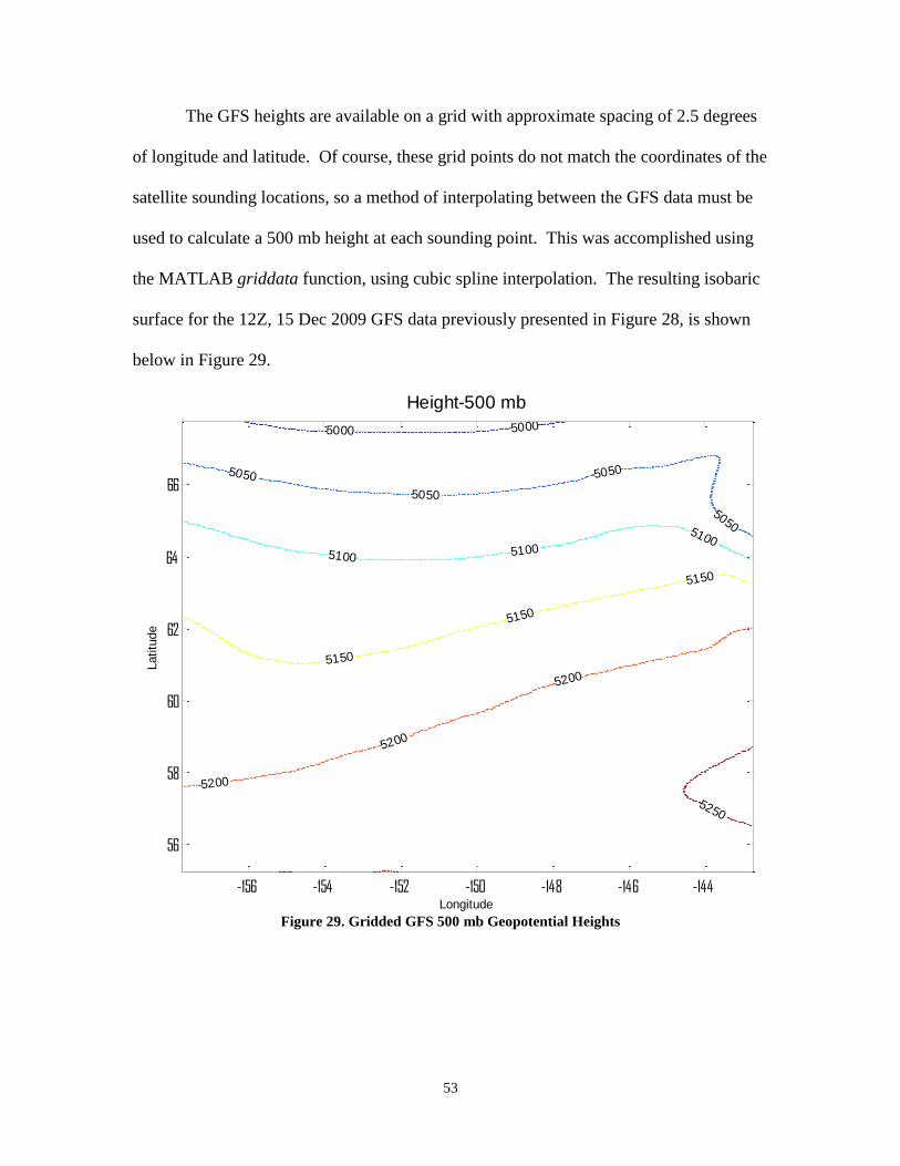
53
The GFS heights are available on a grid with approximate spacing of 2.5 degrees
of longitude and latitude. Of course, these grid points do not match the coordinates of the
satellite sounding locations, so a method of interpolating between the GFS data must be
used to calculate a 500 mb height at each sounding point. This was accomplished using
the MATLAB griddata function, using cubic spline interpolation. The resulting isobaric
surface for the 12Z, 15 Dec 2009 GFS data previously presented in Figure 28, is shown
below in Figure 29.
Figure 29. Gridded GFS 500 mb Geopotential Heights
5000 5000
5050
5050
5050
5050
5100 5100
5100
5150
5150
5150
5200
5200
5200
5250
Height-500 mb
Longitude
Latitu
de
-156 -154 -152 -150 -148 -146 -144
56
58
60
62
64
66
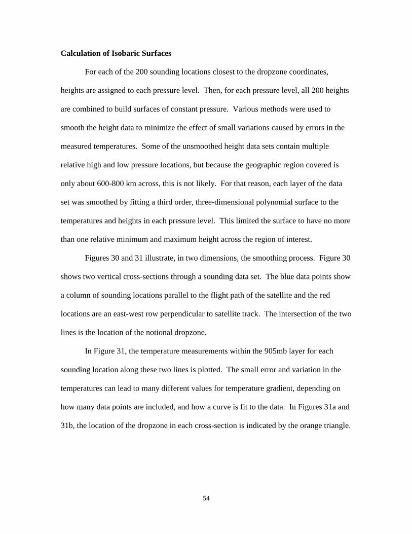
54
Calculation of Isobaric Surfaces
For each of the 200 sounding locations closest to the dropzone coordinates,
heights are assigned to each pressure level. Then, for each pressure level, all 200 heights
are combined to build surfaces of constant pressure. Various methods were used to
smooth the height data to minimize the effect of small variations caused by errors in the
measured temperatures. Some of the unsmoothed height data sets contain multiple
relative high and low pressure locations, but because the geographic region covered is
only about 600-800 km across, this is not likely. For that reason, each layer of the data
set was smoothed by fitting a third order, three-dimensional polynomial surface to the
temperatures and heights in each pressure level. This limited the surface to have no more
than one relative minimum and maximum height across the region of interest.
Figures 30 and 31 illustrate, in two dimensions, the smoothing process. Figure 30
shows two vertical cross-sections through a sounding data set. The blue data points show
a column of sounding locations parallel to the flight path of the satellite and the red
locations are an east-west row perpendicular to satellite track. The intersection of the two
lines is the location of the notional dropzone.
In Figure 31, the temperature measurements within the 905mb layer for each
sounding location along these two lines is plotted. The small error and variation in the
temperatures can lead to many different values for temperature gradient, depending on
how many data points are included, and how a curve is fit to the data. In Figures 31a and
31b, the location of the dropzone in each cross-section is indicated by the orange triangle.
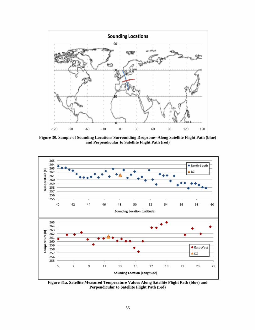
55
Figure 30. Sample of Sounding Locations Surrounding Dropzone--Along Satellite Flight Path (blue)
and Perpendicular to Satellite Flight Path (red)
Figure 31a. Satellite Measured Temperature Values Along Satellite Flight Path (blue) and
Perpendicular to Satellite Flight Path (red)
0
30
60
90
-120 -90 -60 -30 0 30 60 90 120 150
Sounding Locations
255256257258259260261262263264265
40 42 44 46 48 50 52 54 56 58 60
Tem
pe
ratu
re (K
)
Sounding Location (Latitude)
North-South
DZ
255256257258259260261262263264265
5 7 9 11 13 15 17 19 21 23 25
Tem
pe
ratu
re (K
)
Sounding Location (Longitude)
East-West
DZ
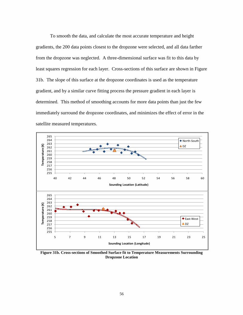
56
To smooth the data, and calculate the most accurate temperature and height
gradients, the 200 data points closest to the dropzone were selected, and all data farther
from the dropzone was neglected. A three-dimensional surface was fit to this data by
least squares regression for each layer. Cross-sections of this surface are shown in Figure
31b. The slope of this surface at the dropzone coordinates is used as the temperature
gradient, and by a similar curve fitting process the pressure gradient in each layer is
determined. This method of smoothing accounts for more data points than just the few
immediately surround the dropzone coordinates, and minimizes the effect of error in the
satellite measured temperatures.
Figure 31b. Cross-sections of Smoothed Surface fit to Temperature Measurements Surrounding
Dropzone Location
255256257258259260261262263264265
40 42 44 46 48 50 52 54 56 58 60
Tem
pe
ratu
re (K
)
Sounding Location (Latitude)
North-South
DZ
255256257258259260261262263264265
5 7 9 11 13 15 17 19 21 23 25
Tem
pe
ratu
re (K
)
Sounding Location (Longitude)
East-West
DZ
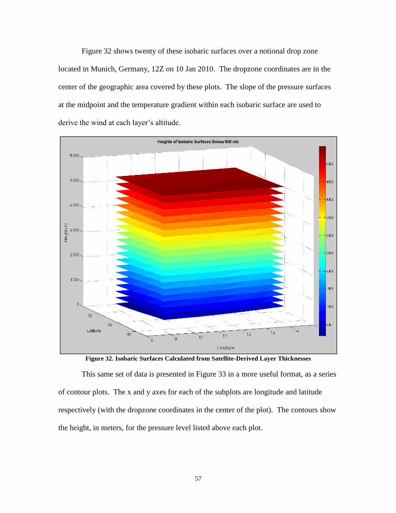
57
Figure 32 shows twenty of these isobaric surfaces over a notional drop zone
located in Munich, Germany, 12Z on 10 Jan 2010. The dropzone coordinates are in the
center of the geographic area covered by these plots. The slope of the pressure surfaces
at the midpoint and the temperature gradient within each isobaric surface are used to
derive the wind at each layer’s altitude.
Figure 32. Isobaric Surfaces Calculated from Satellite-Derived Layer Thicknesses
This same set of data is presented in Figure 33 in a more useful format, as a series
of contour plots. The x and y axes for each of the subplots are longitude and latitude
respectively (with the dropzone coordinates in the center of the plot). The contours show
the height, in meters, for the pressure level listed above each plot.
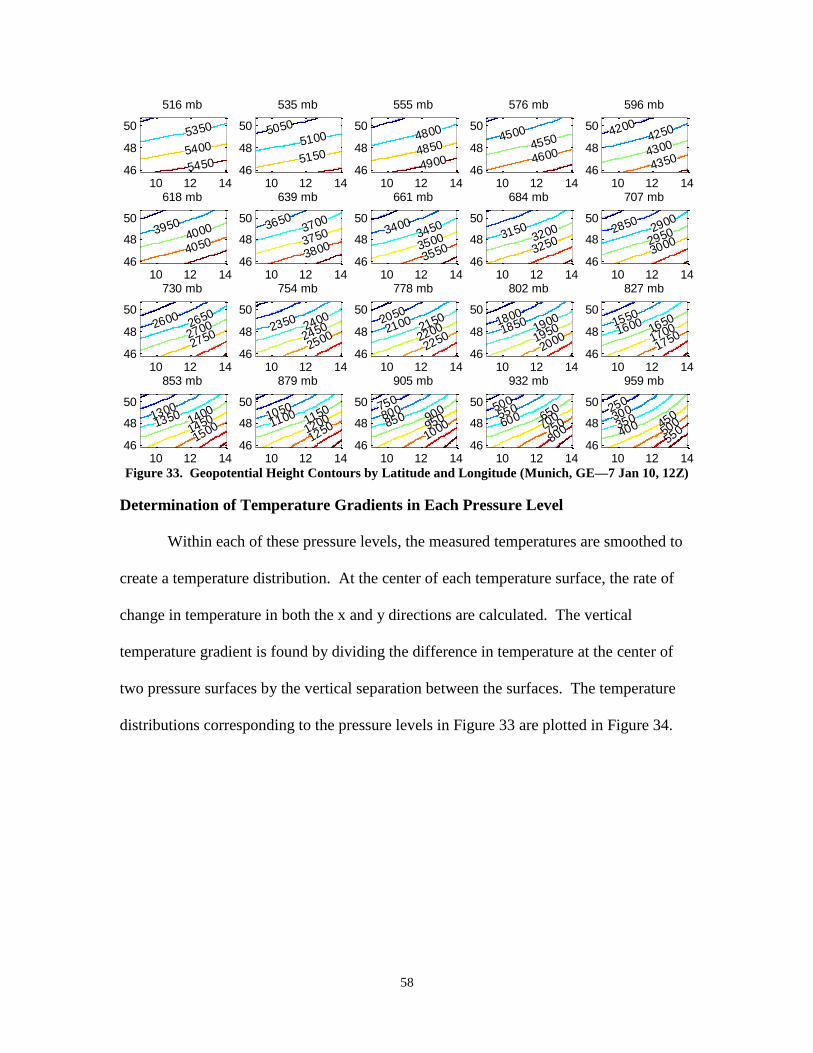
58
Figure 33. Geopotential Height Contours by Latitude and Longitude (Munich, GE—7 Jan 10, 12Z)
Determination of Temperature Gradients in Each Pressure Level
Within each of these pressure levels, the measured temperatures are smoothed to
create a temperature distribution. At the center of each temperature surface, the rate of
change in temperature in both the x and y directions are calculated. The vertical
temperature gradient is found by dividing the difference in temperature at the center of
two pressure surfaces by the vertical separation between the surfaces. The temperature
distributions corresponding to the pressure levels in Figure 33 are plotted in Figure 34.
5350
5400
5450
516 mb
10 12 1446
48
50 5050
5100
5150
535 mb
10 12 1446
48
504800
4850
4900
555 mb
10 12 1446
48
504500
4550
4600
576 mb
10 12 1446
48
50 42004250
4300
4350
596 mb
10 12 1446
48
50
39504000
4050
618 mb
10 12 1446
48
503650
3700
3750
3800
639 mb
10 12 1446
48
503400
3450
3500
3550
661 mb
10 12 1446
48
50
31503200
3250
684 mb
10 12 1446
48
502850
2900
2950
3000
707 mb
10 12 1446
48
50
26002650
2700
2750
730 mb
10 12 1446
48
50
23502400
2450
2500
754 mb
10 12 1446
48
502050
2100 2150
2200
2250
778 mb
10 12 1446
48
501800
1850 1900
1950
2000
802 mb
10 12 1446
48
501550
1600 1650
1700
1750
827 mb
10 12 1446
48
50
1300
1350 1400
1450
1500
853 mb
10 12 1446
48
501050
1100 1150
1200
1250
879 mb
10 12 1446
48
50 750
800850 900
950
1000
905 mb
10 12 1446
48
50 500550600 650
700750
800
932 mb
10 12 1446
48
50250
300
350400 450
500
550
959 mb
10 12 1446
48
50
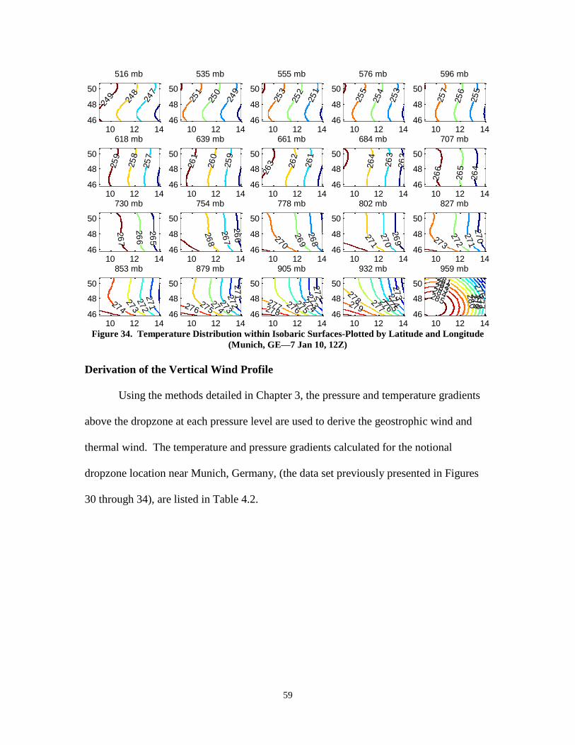
59
Figure 34. Temperature Distribution within Isobaric Surfaces-Plotted by Latitude and Longitude
(Munich, GE—7 Jan 10, 12Z)
Derivation of the Vertical Wind Profile
Using the methods detailed in Chapter 3, the pressure and temperature gradients
above the dropzone at each pressure level are used to derive the geostrophic wind and
thermal wind. The temperature and pressure gradients calculated for the notional
dropzone location near Munich, Germany, (the data set previously presented in Figures
30 through 34), are listed in Table 4.2.
247
248
249
516 mb
10 12 1446
48
50
249
250
251
535 mb
10 12 1446
48
50
251
252
253
555 mb
10 12 1446
48
50
25
3
25
4
255
576 mb
10 12 1446
48
50
25
5
25
6
25
7
596 mb
10 12 1446
48
50
25
7
25
8
25
9
618 mb
10 12 1446
48
50
25
9
26
0
26
1
639 mb
10 12 1446
48
50
26
1
26
2
263
661 mb
10 12 1446
48
50
26
2
26
3
26
4
684 mb
10 12 1446
48
50
26
4
26
5
26
6
707 mb
10 12 1446
48
50
26
5
26
6
26
7
730 mb
10 12 1446
48
50
26
6
26
7
26
8
754 mb
10 12 1446
48
50
26
8
269
270
778 mb
10 12 1446
48
50
26
9
27
0
271
802 mb
10 12 1446
48
50
27
0
27
1
272273
827 mb
10 12 1446
48
50
27
1
272
273
274
853 mb
10 12 1446
48
50 27
127
2273
274275276
879 mb
10 12 1446
48
50 27
2273274
275276
277278
905 mb
10 12 1446
48
50 27
3274275
276
277
278279
932 mb
10 12 1446
48
50 2762
77
27
827
928
0
281282283284285
959 mb
10 12 1446
48
50
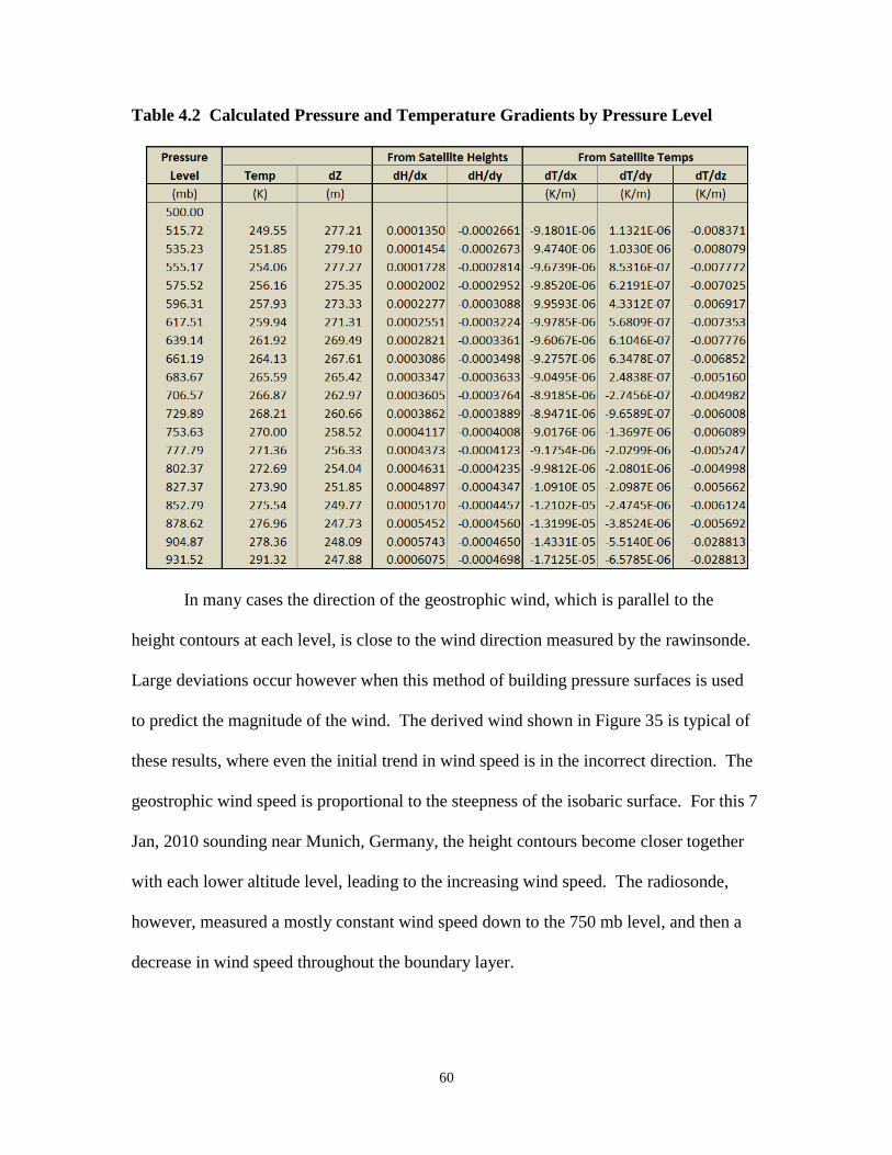
60
Table 4.2 Calculated Pressure and Temperature Gradients by Pressure Level
In many cases the direction of the geostrophic wind, which is parallel to the
height contours at each level, is close to the wind direction measured by the rawinsonde.
Large deviations occur however when this method of building pressure surfaces is used
to predict the magnitude of the wind. The derived wind shown in Figure 35 is typical of
these results, where even the initial trend in wind speed is in the incorrect direction. The
geostrophic wind speed is proportional to the steepness of the isobaric surface. For this 7
Jan, 2010 sounding near Munich, Germany, the height contours become closer together
with each lower altitude level, leading to the increasing wind speed. The radiosonde,
however, measured a mostly constant wind speed down to the 750 mb level, and then a
decrease in wind speed throughout the boundary layer.
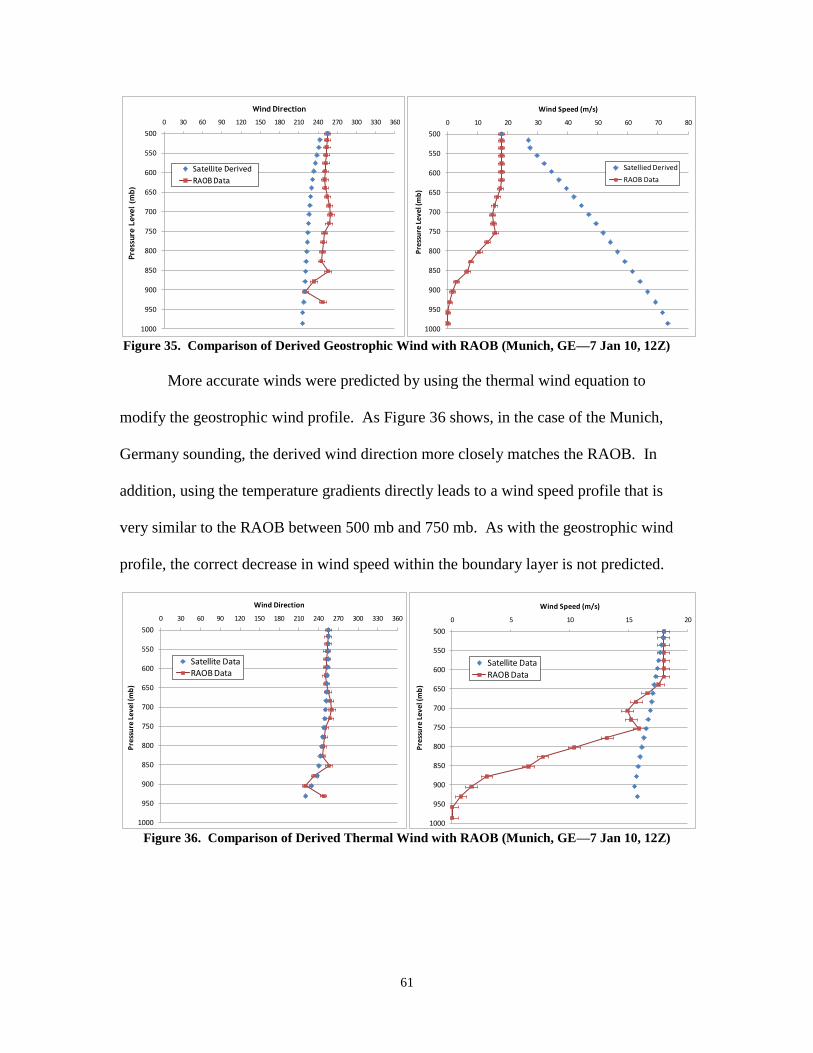
61
Figure 35. Comparison of Derived Geostrophic Wind with RAOB (Munich, GE—7 Jan 10, 12Z)
More accurate winds were predicted by using the thermal wind equation to
modify the geostrophic wind profile. As Figure 36 shows, in the case of the Munich,
Germany sounding, the derived wind direction more closely matches the RAOB. In
addition, using the temperature gradients directly leads to a wind speed profile that is
very similar to the RAOB between 500 mb and 750 mb. As with the geostrophic wind
profile, the correct decrease in wind speed within the boundary layer is not predicted.
Figure 36. Comparison of Derived Thermal Wind with RAOB (Munich, GE—7 Jan 10, 12Z)
500
550
600
650
700
750
800
850
900
950
1000
0 30 60 90 120 150 180 210 240 270 300 330 360
Pre
ssure
Level
(mb)
Wind Direction
Satellite Derived
RAOB Data
500
550
600
650
700
750
800
850
900
950
1000
0 10 20 30 40 50 60 70 80
Pre
ssu
re L
evel
(mb
)
Wind Speed (m/s)
Satellied Derived
RAOB Data
500
550
600
650
700
750
800
850
900
950
1000
0 30 60 90 120 150 180 210 240 270 300 330 360
Pre
ssu
re L
eve
l (m
b)
Wind Direction
Satellite DataRAOB Data
500
550
600
650
700
750
800
850
900
950
1000
0 5 10 15 20
Pre
ssu
re L
eve
l (m
b)
Wind Speed (m/s)
Satellite Data
RAOB Data
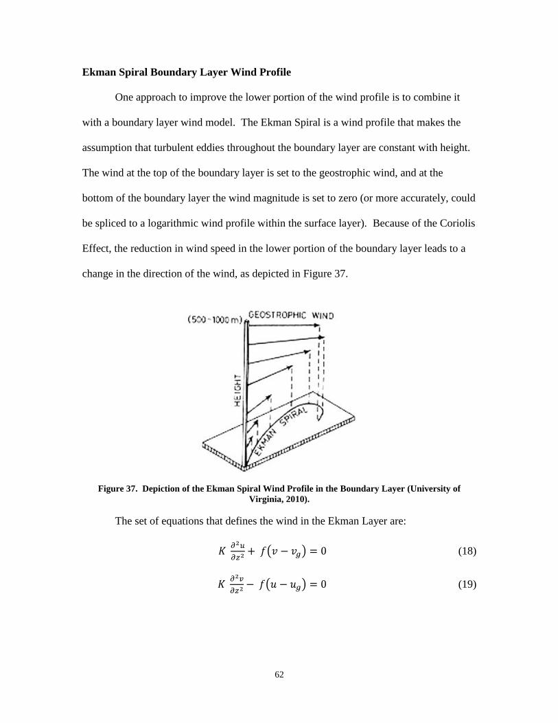
62
Ekman Spiral Boundary Layer Wind Profile
One approach to improve the lower portion of the wind profile is to combine it
with a boundary layer wind model. The Ekman Spiral is a wind profile that makes the
assumption that turbulent eddies throughout the boundary layer are constant with height.
The wind at the top of the boundary layer is set to the geostrophic wind, and at the
bottom of the boundary layer the wind magnitude is set to zero (or more accurately, could
be spliced to a logarithmic wind profile within the surface layer). Because of the Coriolis
Effect, the reduction in wind speed in the lower portion of the boundary layer leads to a
change in the direction of the wind, as depicted in Figure 37.
Figure 37. Depiction of the Ekman Spiral Wind Profile in the Boundary Layer (University of
Virginia, 2010).
The set of equations that defines the wind in the Ekman Layer are:
(18)
(19)
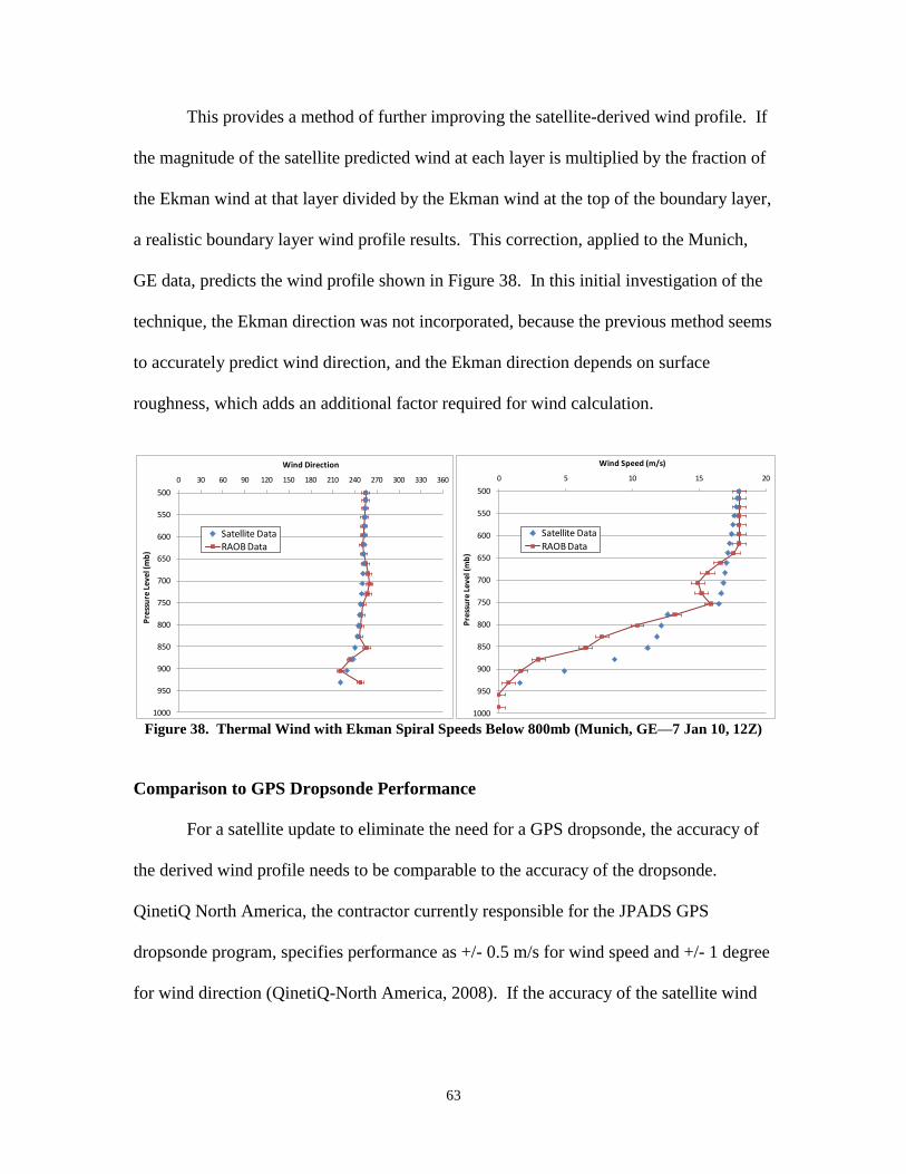
63
This provides a method of further improving the satellite-derived wind profile. If
the magnitude of the satellite predicted wind at each layer is multiplied by the fraction of
the Ekman wind at that layer divided by the Ekman wind at the top of the boundary layer,
a realistic boundary layer wind profile results. This correction, applied to the Munich,
GE data, predicts the wind profile shown in Figure 38. In this initial investigation of the
technique, the Ekman direction was not incorporated, because the previous method seems
to accurately predict wind direction, and the Ekman direction depends on surface
roughness, which adds an additional factor required for wind calculation.
Figure 38. Thermal Wind with Ekman Spiral Speeds Below 800mb (Munich, GE—7 Jan 10, 12Z)
Comparison to GPS Dropsonde Performance
For a satellite update to eliminate the need for a GPS dropsonde, the accuracy of
the derived wind profile needs to be comparable to the accuracy of the dropsonde.
QinetiQ North America, the contractor currently responsible for the JPADS GPS
dropsonde program, specifies performance as +/- 0.5 m/s for wind speed and +/- 1 degree
for wind direction (QinetiQ-North America, 2008). If the accuracy of the satellite wind
500
550
600
650
700
750
800
850
900
950
1000
0 30 60 90 120 150 180 210 240 270 300 330 360
Pre
ssu
re L
evel
(mb
)
Wind Direction
Satellite DataRAOB Data
500
550
600
650
700
750
800
850
900
950
1000
0 5 10 15 20
Pre
ssu
re L
evel
(mb
)Wind Speed (m/s)
Satellite Data
RAOB Data

64
profile is comparable, it could replace the dropsonde in all situations where reception of
the satellite data is available. The actual wind profile accuracy required for a specific
mission depends on the type of airdrop load, the size of the planned drop zone, and the
drop altitude required by the threat environment.
65
V. Discussion
Conclusions
This project illustrates the potential for satellite-derived wind profiles to be used
to make combat JPADS airdrops safer, while retaining the accuracy necessary to allow
resupply to small dropzones. The method of combining calculated geostrophic wind and
thermal wind profiles does a reasonable job determining the wind vector above the
boundary layer. With some improvements to the low altitude wind profile modeling and
expansion to use IR sounder data from additional polar-orbit satellites, this technique
could be used in the near future to expand high altitude airdrop capabilities in the
CENTCOM AOR.
Because wind speed generally increases with height, it is the higher altitude, free
atmosphere winds that have the greatest effect on airdrop load drift. The strength of the
method derived in this research is that it most reliably predicts the winds at the altitudes
where knowing them is most important. As an example, for an airdrop from an altitude
of 16,000 ft AGL, the portion of the atmosphere that the airdrop load will fall through
that is above the boundary layer may only be about 70%, but the winds in that portion of
the atmosphere could account for 85% or more of the drift effect on the airdrop load.
Satellite-Derived Wind Profile Advantages
The most important reasons to pursue this solution are the advantages it has over
alternative wind update solutions. If the method can be improved to the point that the
satellite-derived wind profile is as good as the dropsonde measured wind, the need for the
potentially hazardous dropsonde pass through the objective area can be eliminated. The
single pass solution saves the cost of the dropsonde, shortens the airdrop mission flight
66
time by 20-30 minutes, and prevents the aircraft from having to fly over the same terrain
twice in a combat environment.
Other key advantages of the satellite wind solution include the fact that sensing
the winds from space is completely passive. There are no emissions to be detected, or
other indications that would identify the intended objective area prior to the airdrop. If
existing communications methods are used to relay updated wind profiles to aircrew,
using satellite-derived winds does not require any additional equipment to be installed on
the aircraft conducting the airdrop. In addition, this method would not require a
significant change in aircrew procedures nor require any additional training or equipment
for ground forces.
One last advantage of satellite-derived winds versus dropsondes is that there is no
dependence on GPS availability. Interference or jamming which interrupts the GPS
signal during the time of fall of the dropsonde would prevent the dropsonde from
accurately measuring the wind. At that point, crew options would be to release another
dropsonde, abort the mission, or accept the greater potential for error and drop based only
on the preflight forecast.
Recommendations for Future Research
Follow-on research in several areas could enhance the operational utility of this
method. The first of these would be to expand the model to more accurately predict the
wind within the boundary layer. Splicing the satellite-derived wind at the top of the
boundary layer to an Ekman spiral wind profile, possible tied to the reported surface wind
speed, will improve the overall accuracy of most profiles, and would lead to an integrated
drift effect that is closer to reality. These approaches would account for the effect of
67
surface friction, and would create profiles with lighter winds in the boundary layer. An
additional challenge with these techniques would be to accurately determine the height of
the top of the boundary for each location because the thickness of the boundary layer
varies greatly with location, time of day and time of year. It may also be possible to use
satellite measured boundary level temperature in a more sophisticated weather model to
even more accurately account for surface friction and come up with a better wind profile.
Also, as additional IR sounders are placed in orbit, the increased coverage and
improvements in resolution will further enhance the availability and accuracy of derived
wind profiles. Different satellites and sounders often provide data in different formats, so
research should be conducted to adapt this wind derivation method to these new sources
of atmospheric temperature.
This research demonstrates a method to predict wind profiles in areas with thin
clouds, or no cloud cover. Microwave sounders on polar orbiting satellites provide data
that could be used in a similar way to derive winds in cloud covered regions, with the
disadvantage of less resolution than the infrared data. A third source of winds is winds
determined by cloud feature tracking, using geostationary satellite images. By combining
these three methods, winds profiles could be derived for more locations, with various
levels of cloud cover. This would lead to a more flexible, operationally useful product,
enabling in most situations, the single-pass airdrop.

68
Appendix A: List of Acronyms
AAA Anti-Aircraft Artillery
AIRS Atmospheric Infrared Sounder
AGU Airborne Guidance Unit
AFIT Air Force Institute of Technology
AFRL Air Force Research Lab
AFWA Air Force Weather Agency
AGAS Affordable Guided Parachute System
AGL Above Ground Level
AMC Air Mobility Command
AMSU Advanced Microwave Sounding Unit
AOR Area of Responsibility
CARP Computed Air Release Point
CDS Container Delivery System
CENTCOM Central Command
CONEMP Concept of Employment
CTII Combat Track II
DMSP Defense Meteorological Satellite Program
EOS Earth Observing System
EUMETSAT Organisation for the Exploitation of Meteorological Satellites
GDAS Global Data Assimilation System
GOES Geostationary Operational Environmental Satellite
GFS Global Forecast System
GPS Global Positioning System
GRIB Gridded Binary

69
GSI Gridpoint Statistical Interpolation
HARP High Altitude Release Point
HDF Hierarchical Data Format
HVCDS High Velocity Container Delivery System
IASI Infrared Atmospheric Sounding Interferometer
I-CDS Improved Container Delivery System
IED Improvised Explosive Device
JPADS Joint Precision Air Drop System
JPADS-MP Joint Precision Air Drop System-Mission Planner
JPL Jet Propulsion Laboratory, California Institute of Technology
LAR Launch Acceptability Region
LIDAR Light Direction and Ranging
MAF Mobility Air Forces
MANPAD Man Portable Air Defense System
METEOSAT Meteorological Satellite
MetOp Meteorological Operational
MSL Mean Sea Level
NOAA National Oceanic and Atmospheric Administration
PADS Precision Air Drop System
RAOB Rawinsonde Observation
RDF Radio Direction Finding
RPG Rocket Propelled Grenade
UAV Unmanned Aerial Vehicle
USGS United States Geological Survey
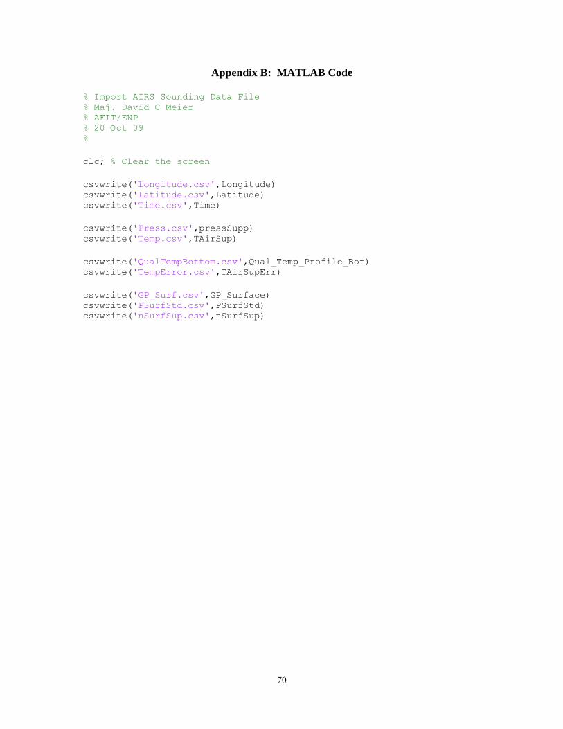
70
Appendix B: MATLAB Code
% Import AIRS Sounding Data File % Maj. David C Meier % AFIT/ENP % 20 Oct 09 %
clc; % Clear the screen
csvwrite('Longitude.csv',Longitude) csvwrite('Latitude.csv',Latitude) csvwrite('Time.csv',Time)
csvwrite('Press.csv',pressSupp) csvwrite('Temp.csv',TAirSup)
csvwrite('QualTempBottom.csv',Qual_Temp_Profile_Bot) csvwrite('TempError.csv',TAirSupErr)
csvwrite('GP_Surf.csv',GP_Surface) csvwrite('PSurfStd.csv',PSurfStd) csvwrite('nSurfSup.csv',nSurfSup)
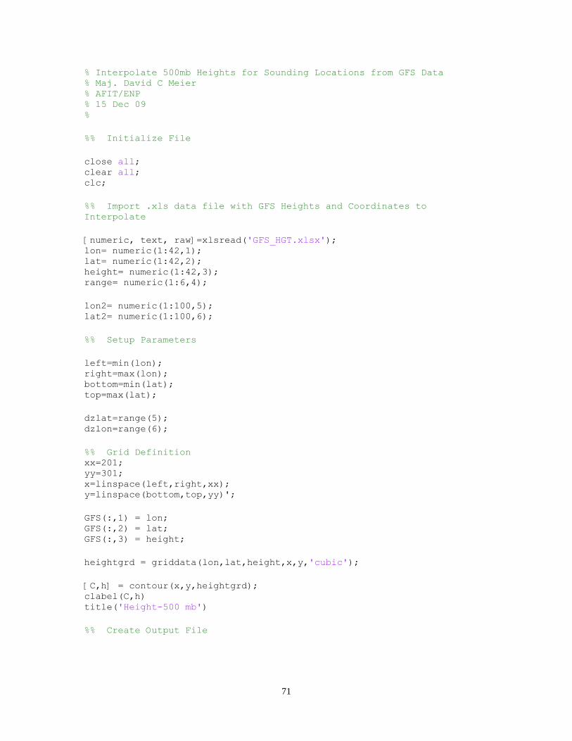
71
% Interpolate 500mb Heights for Sounding Locations from GFS Data % Maj. David C Meier % AFIT/ENP % 15 Dec 09 %
%% Initialize File
close all; clear all; clc;
%% Import .xls data file with GFS Heights and Coordinates to
Interpolate
[numeric, text, raw]=xlsread('GFS_HGT.xlsx'); lon= numeric(1:42,1); lat= numeric(1:42,2); height= numeric(1:42,3); range= numeric(1:6,4);
lon2= numeric(1:100,5); lat2= numeric(1:100,6);
%% Setup Parameters
left=min(lon); right=max(lon); bottom=min(lat); top=max(lat);
dzlat=range(5); dzlon=range(6);
%% Grid Definition xx=201; yy=301; x=linspace(left,right,xx); y=linspace(bottom,top,yy)';
GFS(:,1) = lon; GFS(:,2) = lat; GFS(:,3) = height;
heightgrd = griddata(lon,lat,height,x,y,'cubic');
[C,h] = contour(x,y,heightgrd); clabel(C,h) title('Height-500 mb')
%% Create Output File
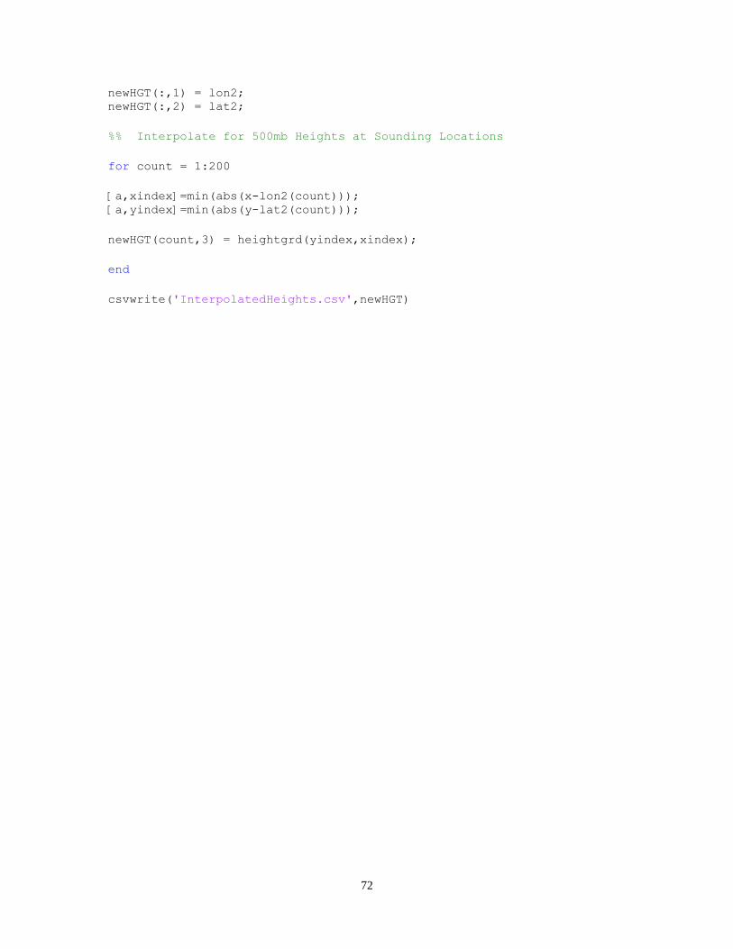
72
newHGT(:,1) = lon2; newHGT(:,2) = lat2;
%% Interpolate for 500mb Heights at Sounding Locations
for count = 1:200
[a,xindex]=min(abs(x-lon2(count))); [a,yindex]=min(abs(y-lat2(count)));
newHGT(count,3) = heightgrd(yindex,xindex);
end
csvwrite('InterpolatedHeights.csv',newHGT)
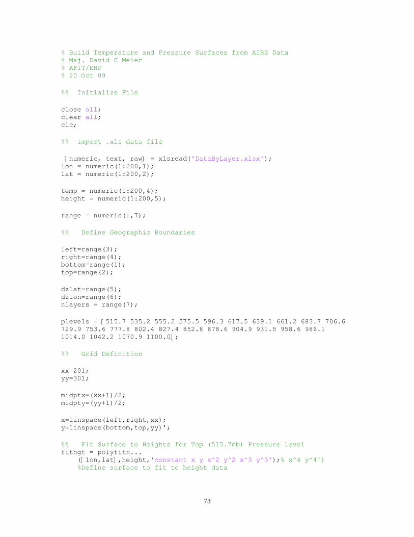
73
% Build Temperature and Pressure Surfaces from AIRS Data % Maj. David C Meier % AFIT/ENP % 20 Oct 09
%% Initialize File
close all; clear all; clc;
%% Import .xls data file
[numeric, text, raw] = xlsread('DataByLayer.xlsx'); lon = numeric(1:200,1); lat = numeric(1:200,2);
temp = numeric(1:200,4); height = numeric(1:200,5);
range = numeric(:,7);
%% Define Geographic Boundaries
left=range(3); right=range(4); bottom=range(1); top=range(2);
dzlat=range(5); dzlon=range(6); nlayers = range(7);
plevels = [515.7 535.2 555.2 575.5 596.3 617.5 639.1 661.2 683.7 706.6
729.9 753.6 777.8 802.4 827.4 852.8 878.6 904.9 931.5 958.6 986.1
1014.0 1042.2 1070.9 1100.0];
%% Grid Definition
xx=201; yy=301;
midptx=(xx+1)/2; midpty=(yy+1)/2;
x=linspace(left,right,xx); y=linspace(bottom,top,yy)';
%% Fit Surface to Heights for Top (515.7mb) Pressure Level fithgt = polyfitn...
([lon,lat],height,'constant x y x^2 y^2 x^3 y^3');% x^4 y^4')
%Define surface to fit to height data
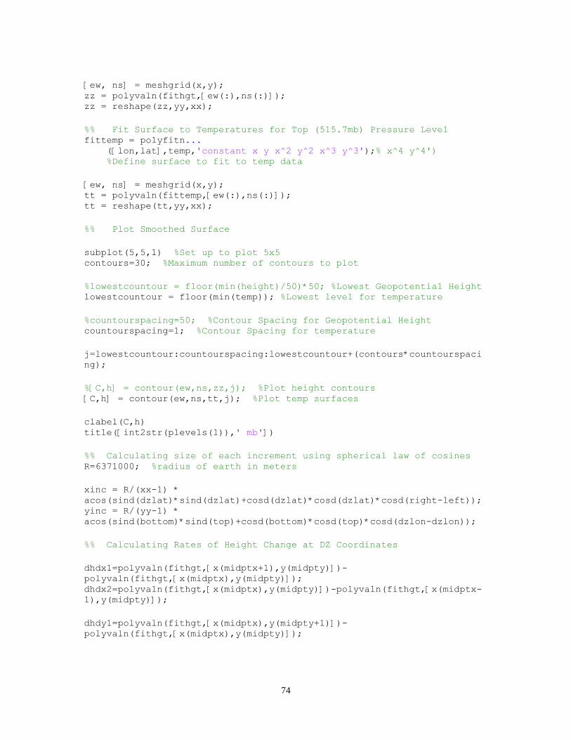
74
[ew, ns] = meshgrid(x,y); zz = polyvaln(fithgt,[ew(:),ns(:)]); zz = reshape(zz,yy,xx);
%% Fit Surface to Temperatures for Top (515.7mb) Pressure Level fittemp = polyfitn...
([lon,lat],temp,'constant x y x^2 y^2 x^3 y^3');% x^4 y^4')
%Define surface to fit to temp data
[ew, ns] = meshgrid(x,y); tt = polyvaln(fittemp,[ew(:),ns(:)]); tt = reshape(tt,yy,xx);
%% Plot Smoothed Surface
subplot(5,5,1) %Set up to plot 5x5 contours=30; %Maximum number of contours to plot
%lowestcountour = floor(min(height)/50)*50; %Lowest Geopotential Height lowestcountour = floor(min(temp)); %Lowest level for temperature
%countourspacing=50; %Contour Spacing for Geopotential Height countourspacing=1; %Contour Spacing for temperature
j=lowestcountour:countourspacing:lowestcountour+(contours*countourspaci
ng);
%[C,h] = contour(ew,ns,zz,j); %Plot height contours [C,h] = contour(ew,ns,tt,j); %Plot temp surfaces
clabel(C,h) title([int2str(plevels(1)),' mb'])
%% Calculating size of each increment using spherical law of cosines R=6371000; %radius of earth in meters
xinc = R/(xx-1) *
acos(sind(dzlat)*sind(dzlat)+cosd(dzlat)*cosd(dzlat)*cosd(right-left)); yinc = R/(yy-1) *
acos(sind(bottom)*sind(top)+cosd(bottom)*cosd(top)*cosd(dzlon-dzlon));
%% Calculating Rates of Height Change at DZ Coordinates
dhdx1=polyvaln(fithgt,[x(midptx+1),y(midpty)])-
polyvaln(fithgt,[x(midptx),y(midpty)]); dhdx2=polyvaln(fithgt,[x(midptx),y(midpty)])-polyvaln(fithgt,[x(midptx-
1),y(midpty)]);
dhdy1=polyvaln(fithgt,[x(midptx),y(midpty+1)])-
polyvaln(fithgt,[x(midptx),y(midpty)]);
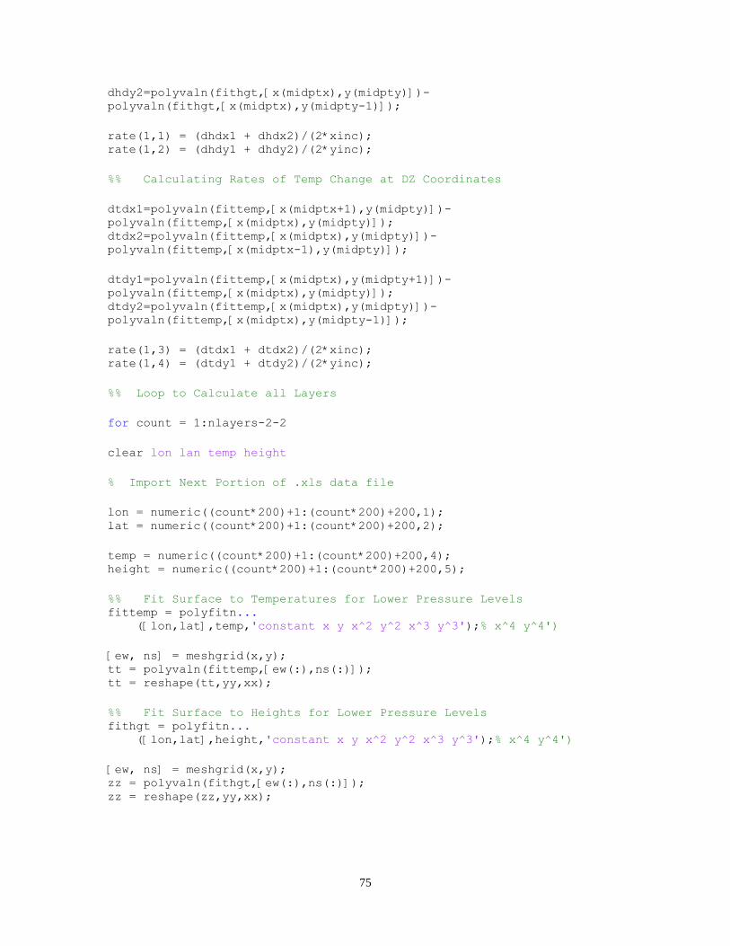
75
dhdy2=polyvaln(fithgt,[x(midptx),y(midpty)])-
polyvaln(fithgt,[x(midptx),y(midpty-1)]);
rate(1,1) = (dhdx1 + dhdx2)/(2*xinc); rate(1,2) = (dhdy1 + dhdy2)/(2*yinc);
%% Calculating Rates of Temp Change at DZ Coordinates
dtdx1=polyvaln(fittemp,[x(midptx+1),y(midpty)])-
polyvaln(fittemp,[x(midptx),y(midpty)]); dtdx2=polyvaln(fittemp,[x(midptx),y(midpty)])-
polyvaln(fittemp,[x(midptx-1),y(midpty)]);
dtdy1=polyvaln(fittemp,[x(midptx),y(midpty+1)])-
polyvaln(fittemp,[x(midptx),y(midpty)]); dtdy2=polyvaln(fittemp,[x(midptx),y(midpty)])-
polyvaln(fittemp,[x(midptx),y(midpty-1)]);
rate(1,3) = (dtdx1 + dtdx2)/(2*xinc); rate(1,4) = (dtdy1 + dtdy2)/(2*yinc);
%% Loop to Calculate all Layers
for count = 1:nlayers-2-2
clear lon lan temp height
% Import Next Portion of .xls data file
lon = numeric((count*200)+1:(count*200)+200,1); lat = numeric((count*200)+1:(count*200)+200,2);
temp = numeric((count*200)+1:(count*200)+200,4); height = numeric((count*200)+1:(count*200)+200,5);
%% Fit Surface to Temperatures for Lower Pressure Levels fittemp = polyfitn... ([lon,lat],temp,'constant x y x^2 y^2 x^3 y^3');% x^4 y^4')
[ew, ns] = meshgrid(x,y); tt = polyvaln(fittemp,[ew(:),ns(:)]); tt = reshape(tt,yy,xx);
%% Fit Surface to Heights for Lower Pressure Levels fithgt = polyfitn... ([lon,lat],height,'constant x y x^2 y^2 x^3 y^3');% x^4 y^4')
[ew, ns] = meshgrid(x,y); zz = polyvaln(fithgt,[ew(:),ns(:)]); zz = reshape(zz,yy,xx);
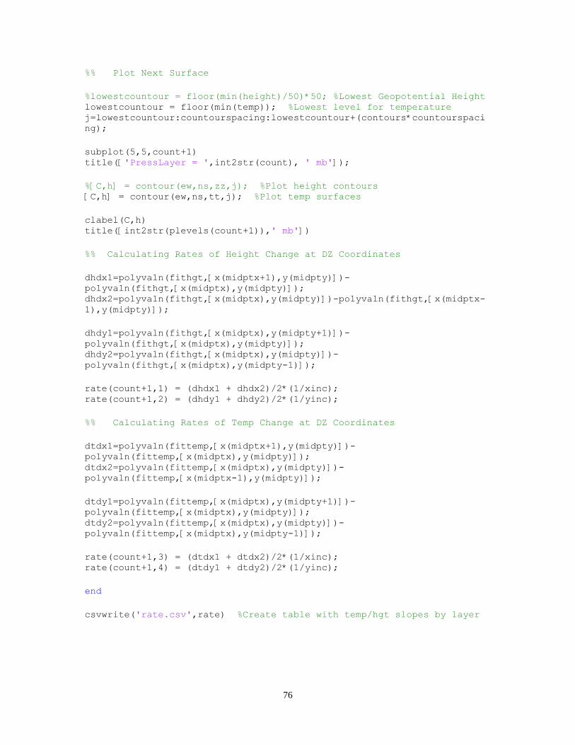
76
%% Plot Next Surface
%lowestcountour = floor(min(height)/50)*50; %Lowest Geopotential Height lowestcountour = floor(min(temp)); %Lowest level for temperature j=lowestcountour:countourspacing:lowestcountour+(contours*countourspaci
ng);
subplot(5,5,count+1) title(['PressLayer = ',int2str(count), ' mb']);
%[C,h] = contour(ew,ns,zz,j); %Plot height contours [C,h] = contour(ew,ns,tt,j); %Plot temp surfaces
clabel(C,h) title([int2str(plevels(count+1)),' mb'])
%% Calculating Rates of Height Change at DZ Coordinates
dhdx1=polyvaln(fithgt,[x(midptx+1),y(midpty)])-
polyvaln(fithgt,[x(midptx),y(midpty)]); dhdx2=polyvaln(fithgt,[x(midptx),y(midpty)])-polyvaln(fithgt,[x(midptx-
1),y(midpty)]);
dhdy1=polyvaln(fithgt,[x(midptx),y(midpty+1)])-
polyvaln(fithgt,[x(midptx),y(midpty)]); dhdy2=polyvaln(fithgt,[x(midptx),y(midpty)])-
polyvaln(fithgt,[x(midptx),y(midpty-1)]);
rate(count+1,1) = (dhdx1 + dhdx2)/2*(1/xinc); rate(count+1,2) = (dhdy1 + dhdy2)/2*(1/yinc);
%% Calculating Rates of Temp Change at DZ Coordinates
dtdx1=polyvaln(fittemp,[x(midptx+1),y(midpty)])-
polyvaln(fittemp,[x(midptx),y(midpty)]); dtdx2=polyvaln(fittemp,[x(midptx),y(midpty)])-
polyvaln(fittemp,[x(midptx-1),y(midpty)]);
dtdy1=polyvaln(fittemp,[x(midptx),y(midpty+1)])-
polyvaln(fittemp,[x(midptx),y(midpty)]); dtdy2=polyvaln(fittemp,[x(midptx),y(midpty)])-
polyvaln(fittemp,[x(midptx),y(midpty-1)]);
rate(count+1,3) = (dtdx1 + dtdx2)/2*(1/xinc); rate(count+1,4) = (dtdy1 + dtdy2)/2*(1/yinc);
end
csvwrite('rate.csv',rate) %Create table with temp/hgt slopes by layer
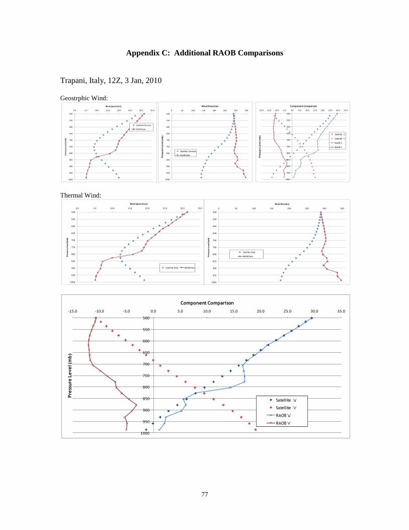
77
Appendix C: Additional RAOB Comparisons
Trapani, Italy, 12Z, 3 Jan, 2010
Geostrphic Wind:
Thermal Wind:
500
550
600
650
700
750
800
850
900
950
1000
0 50 100 150 200 250 300 350
Pre
ssure
Level (
mb)
Wind Direction
Satellite Derived
RAOB Data
500
550
600
650
700
750
800
850
900
950
1000
0.0 5.0 10.0 15.0 20.0 25.0 30.0 35.0
Pre
ssu
re L
eve
l (m
b)
Wind Speed (m/s)
Satellied Derived
RAOB Data
500
550
600
650
700
750
800
850
900
950
1000
-20.0 -15.0 -10.0 -5.0 0.0 5.0 10.0 15.0 20.0 25.0 30.0 35.0
Pre
ssure
Level (
mb)
Component Comparison
Satellite 'u'
Satellite 'v'
RAOB 'u'
RAOB 'v'
500
550
600
650
700
750
800
850
900
950
1000
0 50 100 150 200 250 300 350P
ress
ure
Le
vel (
mb
)
Wind Direction
Satellite Data
RAOB Data
500
550
600
650
700
750
800
850
900
950
1000
0.0 5.0 10.0 15.0 20.0 25.0 30.0 35.0
Pre
ssu
re L
eve
l (m
b)
Wind Speed (m/s)
Satellite Data RAOB Data
500
550
600
650
700
750
800
850
900
950
1000
-15.0 -10.0 -5.0 0.0 5.0 10.0 15.0 20.0 25.0 30.0 35.0
Pre
ssure
Level (
mb)
Component Comparison
Satellite 'u'
Satellite 'v'
RAOB 'u'
RAOB 'v'
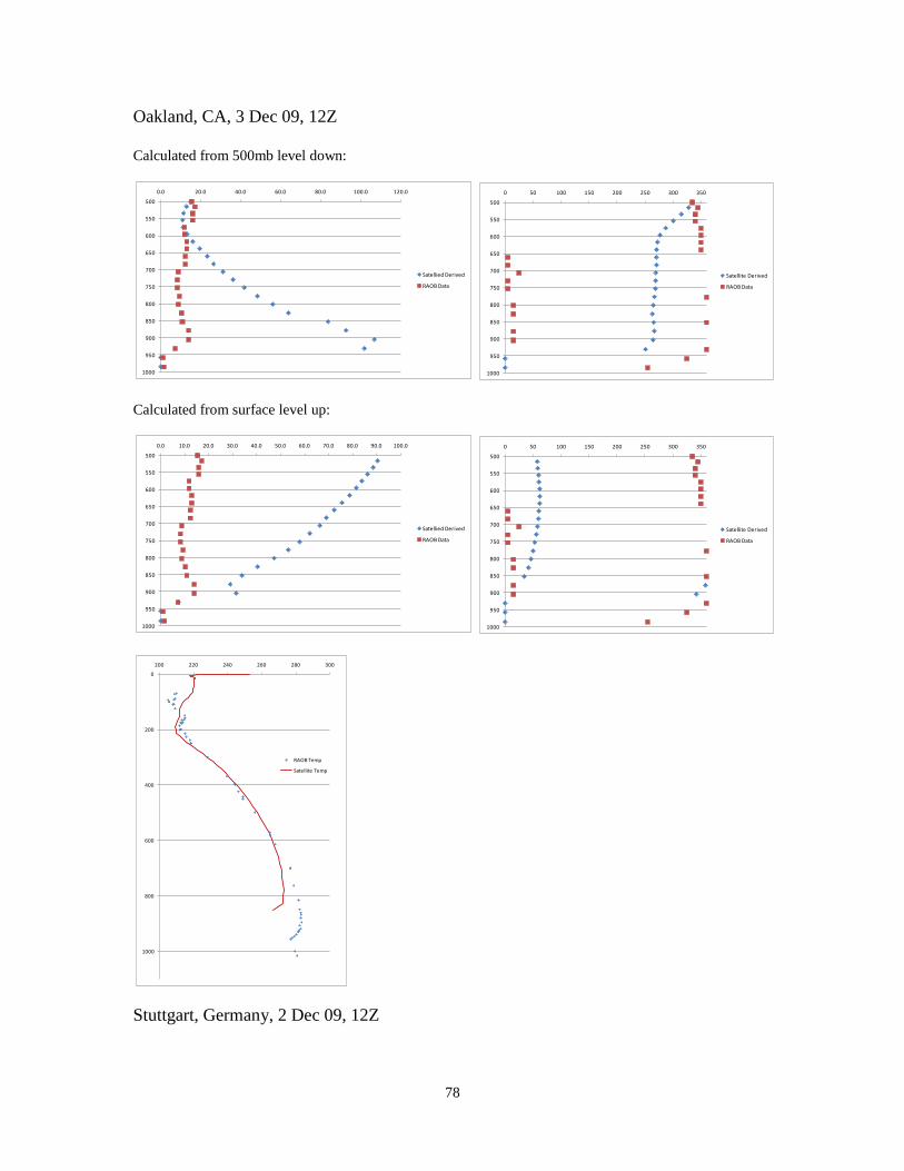
78
Oakland, CA, 3 Dec 09, 12Z
Calculated from 500mb level down:
Calculated from surface level up:
Stuttgart, Germany, 2 Dec 09, 12Z
500
550
600
650
700
750
800
850
900
950
1000
0 50 100 150 200 250 300 350
Satellite Derived
RAOB Data
500
550
600
650
700
750
800
850
900
950
1000
0.0 20.0 40.0 60.0 80.0 100.0 120.0
Satellied Derived
RAOB Data
500
550
600
650
700
750
800
850
900
950
1000
0 50 100 150 200 250 300 350
Satellite Derived
RAOB Data
500
550
600
650
700
750
800
850
900
950
1000
0.0 10.0 20.0 30.0 40.0 50.0 60.0 70.0 80.0 90.0 100.0
Satellied Derived
RAOB Data
0
200
400
600
800
1000
200 220 240 260 280 300
RAOB Temp
Satellite Temp
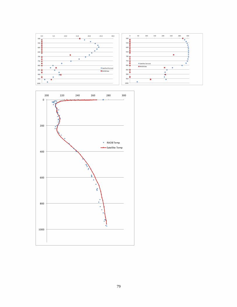
79
500
550
600
650
700
750
800
850
900
950
1000
0 50 100 150 200 250 300 350
Satellite Derived
RAOB Data
500
550
600
650
700
750
800
850
900
950
1000
0.0 5.0 10.0 15.0 20.0 25.0 30.0
Satellied Derived
RAOB Data
0
200
400
600
800
1000
200 220 240 260 280 300
RAOB Temp
Satellite Temp
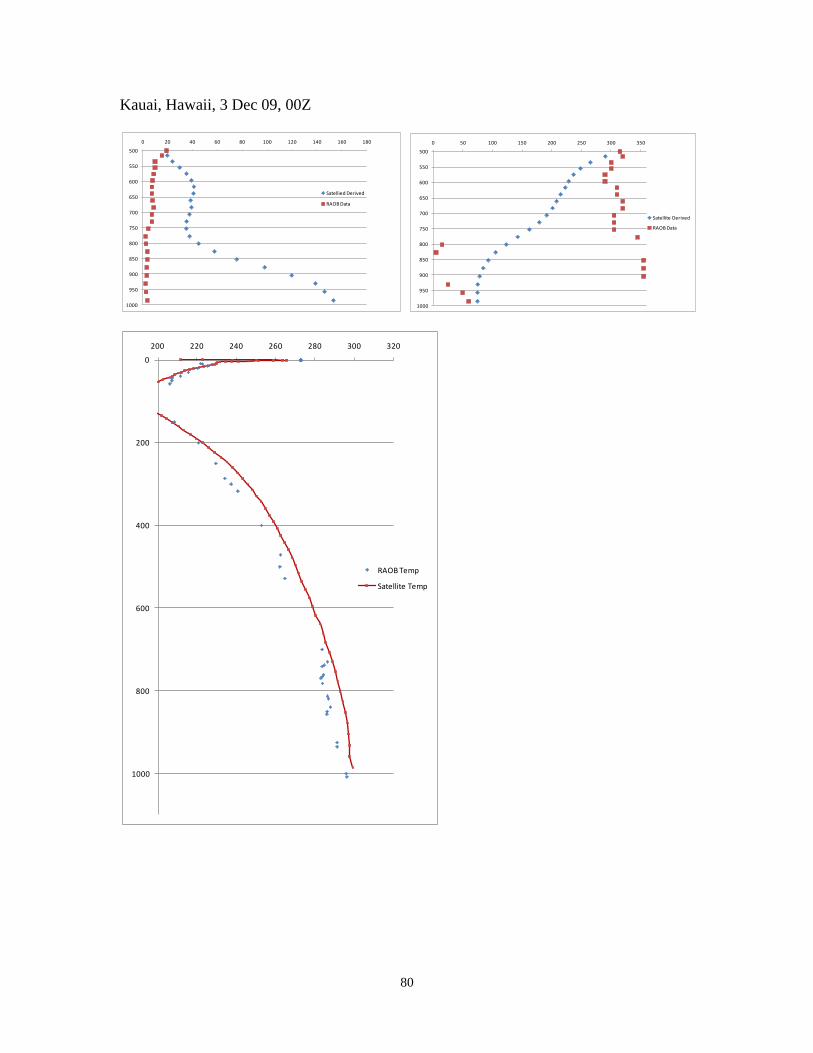
80
Kauai, Hawaii, 3 Dec 09, 00Z
500
550
600
650
700
750
800
850
900
950
1000
0 50 100 150 200 250 300 350
Satellite Derived
RAOB Data
500
550
600
650
700
750
800
850
900
950
1000
0 20 40 60 80 100 120 140 160 180
Satellied Derived
RAOB Data
0
200
400
600
800
1000
200 220 240 260 280 300 320
RAOB Temp
Satellite Temp
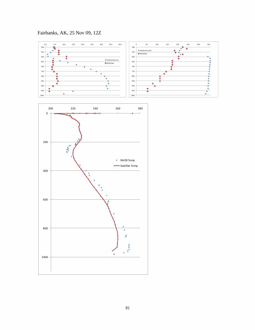
81
Fairbanks, AK, 25 Nov 09, 12Z
500
550
600
650
700
750
800
850
900
950
1000
0 50 100 150 200 250 300 350
Satellite Derived
RAOB Data
500
550
600
650
700
750
800
850
900
950
1000
0.0 5.0 10.0 15.0 20.0 25.0 30.0 35.0 40.0
Satellied Derived
RAOB Data
0
200
400
600
800
1000
200 220 240 260 280
RAOB Temp
Satellite Temp

82
Bibliography
Air Force Weather Agency. Joint Air Force & Army Weather Information Network (JAAWIN).
[On Line] Available: https://weather.afwa.af.mil/jaawin/specialsupport/specialsupport.jsp
AMC Single Pass Airdrop Workshop, JPADS Background Paper. HQ AMC. June 2009.
BAE Systems, Atmospheric Infrared Sounder (AIRS). [On Line] 2010. [Cited: October 25,
2009.] http://www.baesystems.com/ProductsServices/bae_prod_s2_airs.html
Benney, Richard J, The New Military Applications of Precision Airdrop Systems. American
Institute of Aeronautics and Astronautics (AIAA) 2005-7069, 2005.
Bluestein, Howard B, Synoptic-Dynamic Meteorology in Midlatitudes, volume 1.New York:
Oxford University Press, 1992.
Capewell, Precision Air Drop System. Company Brochure. Capewell Life Support/Aerial
Delivery Systems. http://www.capewell.com/products_aerial_Airdrop.php
Cooperative Institute for Research in the Atmosphere, CIRA Annual Report 2004-2005.
Colorado State University, 2005.
Crevoisier, Cyril, Alain Chedin, and Noelle A. Scott. AIRS channel selection for CO2 and
other trace-gas retrievals. Q. J. R. Meteorol. Soc. (2003), 129. pp.2719-2740.
Department of the Air Force. Flying Operations, Computed Air Release Point Procedures. AFI
11-231, 31 July 2005. [On Line]. Available: http://afpubs.hq.af.mil
Department of the Air Force. Flying Operations, C-17 Operations Procedures. AFI 11-2C-117
Volume 3, 15 December 2005. [On Line]. Available: http://afpubs.hq.af.mil
Department of the Air Force. Flying Operations, C-130 Aircrew Training. AFI 11-2C-130
Volume 1, 19 July 2006. [On Line]. Available: http://afpubs.hq.af.mil
Department of the Air Force. Flying Operations, C-130 Operations Procedures. AFI 11-2C-130
Volume 3, 14 March 2006. [On Line]. Available: http://afpubs.hq.af.mil
EUMETSAT. Monitoring Weather and Climate from Space-Press Release. May 31, 2007 [On
Line] Available:
http://www.eumetsat.int/Home/Main/News/Press_Releases/029837?l=en
European Space Agency. Monitoring the Weather from Polar Orbit. BR-261 Brochure. EAS
Publications Division, Noordwijk, The Netherlands. May 2006
Fujiwara, M, M. Ondras, H. Vomel, J. Wang, J. Nash, D. Seidel, and P. Thorne.
Specifications for a Reference Radiosonde for the GCOS Reference Upper-Air Network
(GRAUN). Working Group on Atmospheric Reference Observations. July-October
2008.

83
Gemas, David L. A Systems Engineering Approach to Analyzing Weather Input Sensitivites of
the Joint Precision Air Drop System. Wright-Patterson AFB: Air Force Institute of
Technology., March 2007.
Hattis, Philip, Kai Angemueller, Thomas Fill, Robert Wright, Richard Benney, and David
LeMoine. An In-flight Precision Airdrop System. Draper Laboratory, Cambridge, MA.,
2006.
Headquarters Air Mobility Command, MAF JPADS CONEMP. HQ AMC/A3D, 18 June
2009.
Holton, James R. An Introduction to Dynamic Meteorology. Academic Press, San Diego, CA,
1979.
Jet Propulsion Laboratory, AIRS Version 5.0 Released Files Description. California Institute
of Technology, July 2007.
Jet Propulsion Laboratory, AIRS Animation. [On Line]. Available:
http://photojournal.jpl.nasa.gov/animation/PIA11170 .
Jet Propulsion Laboratory, How AIRS Works, Detailed Desctiption. [On Line] Available:
http://airs.jpl.nasa.gov/technology/how_AIRS_works/how_AIRS_works_detail/
JPADS Mission Planner. Version 5.1.0, Computer Software, Planning Systems, Inc.C.S. Draper
Laboratory, 2006.
Kidder, Stanley Q. and Vonder Haar, Thomas H., Satellite Meteorology. San Diego:
Academic Press, Inc, 1995.
Ma, Xia L., Timothy J. Schmit and William L. Smith, 1999: A Nonlinear Physical Retrieval
Algorithm. American Meteorological Society, 38, 500-513.
Menzel, W. Paul, Frances C. Holt, Timothy, J. Schmit, Robert M. Aune, Anthony J.
Schreiner, Gary S. Wade and Donald G. Gray. Application of GOES-8/9 Soundings to
Weather Forecasting and Nowcasting, 1998.
MetEd-The COMET Program. Numerical Weather Prediction-GFS Introduction. [On Line]
May 2007. Available: http://www.meted.ucar.edu/nwp/pcu2/avintro.htm
NASA, Earth Observatory-Three Classes of Orbit. [On Line] Available:
http://earthobservatory.nasa.gov/Features/OrbitsCatalog/page2.php
NASA, Satellite Overpass Predictor. [On Line] Available:
http://earthobservatory.nasa.gov/MissionControl/overpass.php
Olander, Timothy L., UW-CIMSS Satellite-Derived Wind Algorithm User’s Guide. Cooperative
Institute for Meteorological Satellite Studies - Space Science and Engineering Center,
University of Wisconsin—Madison, 2001.

84
Petty, Grant W., A First Course in Atmospheric Radiation (2nd Edition). - Madison : Sundog
Publishing, 2006.
QinetiQ-North America, PADS-Precision AirDrop System. [On Line] 2008. Available:
http://www.planningsystemsinc.com/downloads/DS08_083_PADS%20w_generic
_c.pdf
Sela, J., 1980: Spectral modeling at the National Meteorological Center. Mon. Wea. Rev.,
108, 1279-1292
Staine-Pyne, Erin, Major, USAF. AMC Industry Days Briefing. Headquarters Air Mobility
Command, 28 April 2009.
Sterner, Ray, Southcentral Alaska Topographic Map. Johns Hopkins University Physics
Laboratory, 1997. [On Line] Available: http://fermi.jhuapl.edu/states/maps1/ak_sc.gif
University of Virginia, Department of Environmental Sciences. Atmosphere and Weather
course materials. 2010. [OnLine] Available:
http://www.evsc.virginia.edu/~evscta/EVSC350/overheadsIII/9.jpg
Wallace, John M. and Hobbs, Peter V. Atmospheric Science, An Introductory Survey (2nd
Edition). Amsterdam: Academic Press, 2006.
WebMET.com. Radiosonde Sounding System. [On Line]. 2002. Available:
http://www.webmet.com/met_monitoring/912.html
Wuest, Michael R. and Richard J. Benney., Precision Airdrop. NASA Center for AeroSpace
Information (CASI). 2005
Zonum Solutions. Free Software Tools-E-Query Elevation Extraction. [ On Line] 2007.
Available: http://www.zonums.com/online/equery.html
Zou, C.Z., and M.L. Van Woert, 2002: Atmospheric Wind Retrievals from Satellite Soundings
over the Middle- and High-Latitude Oceans. Mon. Wea. Rev., 130, 1771–1791.

85
REPORT DOCUMENTATION PAGE Form Approved OMB No. 074-0188
The public reporting burden for this collection of information is estimated to average 1 hour per response, including the time for reviewing instructions, searching existing data sources, gathering and maintaining the data needed, and completing and reviewing the collection of information. Send comments regarding this burden estimate or any other aspect of the collection of information, including suggestions for reducing this burden to Department of Defense, Washington Headquarters Services, Directorate for Information Operations and Reports (0704-0188), 1215 Jefferson Davis Highway, Suite 1204, Arlington, VA 22202-4302. Respondents should be aware that notwithstanding any other provision of law, no person shall be subject to an penalty for failing to comply with a collection of information if it does not display a currently valid OMB control number.
PLEASE DO NOT RETURN YOUR FORM TO THE ABOVE ADDRESS.
1. REPORT DATE (DD-MM-YYYY) 25 -03-2010
2. REPORT TYPE Master’s Thesis
3. DATES COVERED (From – To) Jan 2009 - Mar 2010
4. TITLE AND SUBTITLE
Application of Satellite-Derived Wind Profiles to Joint Precision Airdrop System
(JPADS) Operations
5a. CONTRACT NUMBER
5b. GRANT NUMBER
5c. PROGRAM ELEMENT NUMBER
6. AUTHOR(S)
Meier, David C., Maj, USAF
5d. PROJECT NUMBER
5e. TASK NUMBER
5f. WORK UNIT NUMBER
7. PERFORMING ORGANIZATION NAMES(S) AND ADDRESS(S) Air Force Institute of Technology Graduate School of Engineering and Management (AFIT/EN)
2950 Hobson Way
WPAFB OH 45433-7765
8. PERFORMING ORGANIZATION REPORT NUMBER
AFIT/GAP/ENP/10-M10
9. SPONSORING/MONITORING AGENCY NAME(S) AND ADDRESS(ES) Detachment 3, 16 WS 516
th AESW/XR
2049 Monahan Way, Area B, Bldg 91 2590 Loop Rd West, Area B, Bldg 558 Wright-Patterson AFB, OH 45433 Wright-Patterson AFB, OH 45433
10. SPONSOR/MONITOR’S ACRONYM(S) Det3 16WS, 516 AESW/XR
11. SPONSOR/MONITOR’S REPORT NUMBER(S)
12. DISTRIBUTION/AVAILABILITY STATEMENT APPROVED FOR PUBLIC RELEASE; DISTRIBUTION UNLIMITED.
13. SUPPLEMENTARY NOTES
This material is declared a work of the U.S. Government and is not subject to copyright protection in the United States. 14. ABSTRACT
The Joint Precision Airdrop System has revolutionized military airdrop capability, allowing accurate delivery of equipment and supplies to smaller drop zones, from higher altitudes than was previously possible. This capability depends on accurate wind data which is currently provided by a combination of high-resolution forecast models and GPS dropsondes released in the vicinity of the dropzone shortly before the airdrop. This research develops a windprofiling algorithm to derive the needed wind data from passive IR satellite soundings, eliminating the requirement for a hazardous dropsonde pass near the drop zone, or allowing the dropsonde to be dropped farther from the dropzone. Atmospheric temperature measurements made by the Atmospheric Infrared Sounder (AIRS) onboard the polar-orbiting Aqua satellite are gridded and filtered to create a three-dimensional temperature field surrounding a notional airdrop objective area. From these temperatures, pressure surfaces are calculated and geostrophic and thermal wind direction and magnitude are predicted for 25 altitudes between the surface and 500 mb level. These wind profiles are compared to rawinsonde measurements from balloon releases near the notional airdrop location and time of the satellite sounding. The validity of the satellite-derived wind profile is demonstrated at higher altitudes, but this method does not consistently predict wind velocity within the boundary layer. Future research which better accounts for surface friction may improve these results and lead to the single-pass airdrop capability desired by Air Mobility Command. 15. SUBJECT TERMS
16. SECURITY CLASSIFICATION OF:
17. LIMITATION OF ABSTRACT UU
18. NUMBER OF PAGES 96
19a. NAME OF RESPONSIBLE PERSON Dr. Steven T. Fiorino, (ENP)
REPORT
U ABSTRACT
U c. THIS PAGE
U 19b. TELEPHONE NUMBER (Include area code) (937) 255-6565, x4506 [email protected]
Standard Form 298 (Rev: 8-98) Prescribed by ANSI Std. Z39-18


![DOD JPADS Programs Overview and Nato Activitiesfaculty.nps.edu/oayakime/ADSC/PATCAD - Benney - DOD JPADS Progr… · 2) JPADS Mission Planning System The JPADS-MP (Figure 4)[3][4][5][6]](https://static.cupdf.com/doc/110x72/5a7a98907f8b9a0a668b5b36/dod-jpads-programs-overview-and-nato-benney-dod-jpads-progr2-jpads-mission.jpg)