


�����������������
Citation: Chen, G.; You, H.; Huang,
Z.; Fei, J.; Wang, Y.; Liu, C. An
Efficient Sampling-Based Path
Planning for the Lunar Rover with
Autonomous Target Seeking.
Aerospace 2022, 9, 148. https://
doi.org/10.3390/aerospace9030148
Academic Editor: Jekanthan
Thangavelautham
Received: 20 December 2021
Accepted: 6 March 2022
Published: 8 March 2022
Publisher’s Note: MDPI stays neutral
with regard to jurisdictional claims in
published maps and institutional affil-
iations.
Copyright: © 2022 by the authors.
Licensee MDPI, Basel, Switzerland.
This article is an open access article
distributed under the terms and
conditions of the Creative Commons
Attribution (CC BY) license (https://
creativecommons.org/licenses/by/
4.0/).
aerospace
Article
An Efficient Sampling-Based Path Planning for the Lunar Roverwith Autonomous Target SeekingGang Chen 1, Hong You 1 , Zeyuan Huang 1,* , Junting Fei 1, Yifan Wang 2 and Chuankai Liu 3,4
1 School of Automation, Beijing University of Posts and Telecommunications, Beijing 100876, China;[email protected] (G.C.); [email protected] (H.Y.); [email protected] (J.F.)
2 School of Artificial Intelligence, Beijing University of Posts and Telecommunications, Beijing 100876, China;[email protected]
3 Beijing Aerospace Control Centre, Beijing 100094, China; [email protected] Key Laboratory of Science and Technology on Aerospace Flight Dynamics, Beijing 100094, China* Correspondence: [email protected]; Tel.: +86-135-2183-2124
Abstract: This paper presents an efficient path planning method for the lunar rover to improve theautonomy and exploration ability in the complex and unstructured lunar surface environment. Firstly,the safe zone for the rover’s motion is defined, based on which a detecting point selection strategyis proposed to choose target positions that meet the rover’s constraints. Secondly, an improvedsampling-based path planning method is proposed to get a safe path for the rover efficiently. Thirdly,a map extension strategy for the unstructured and continually varying environment is includedto update the roadmap, which takes advantage of the historical planning information. Finally, theproposed method is tested in a complex lunar surface environment. Numerical results show thatthe appropriate detecting positions can be selected autonomously, while a safe path to the selecteddetecting position can be obtained with high efficiency and quality compared with the ProbabilisticRoadmap (PRM) and A* search algorithm.
Keywords: lunar rover; selection of detecting point; path planning; map extension
1. Introduction
The Moon is rich in minerals and energy resources and has been one of the mostattractive destinations for space exploration [1]. As a specialized mobile robot on thelunar surface, the lunar rover can adapt to the harsh environment, cross obstacles, andbear large loads [2]. Therefore, it plays a prominent role in lunar exploration and hasbeen widely used in plenty of lunar missions. The former Soviet Union’s lunar probes“Luna 11” and “Lunar 21” carried lunar rovers, which completed tasks including lunarreconnaissance, topographic photography, and mineral composition analysis with variousscientific instruments [3]. The “Apollo 15” and “Apollo 16” of the United States carriedmanned lunar rovers [4]. Recently, China launched two lunar rovers the “Yutu” and “Yutu-2”, to detect the lunar surface [5]. In the near future, more missions including lunar rovershave been proposed, for instance, the USA’s Artemis and China’s lunar program IV, formore thorough exploitation and utilization of the lunar resources [6].
Generally, the lunar surface exploration is carried out based on the information of thelunar environment after a safe landing. Common exploration tasks include a geologicalsurvey of the lunar surface, soil sampling, rock mineral analysis, etc., and the process ofthem is mainly divided into four steps:
• Perception of the lunar environment. It mostly relies on satellites and the vehicularcameras to gather information about the lunar environment, from which a digital eleva-tion model (DEM) is generated that includes details like rocks, craters, slopes, etc. [7].
• Selection of the detecting point. A suitable target detecting point is usually selectedbased on the information of the lunar environment and the structure of the lunar rover.
Aerospace 2022, 9, 148. https://doi.org/10.3390/aerospace9030148 https://www.mdpi.com/journal/aerospace

Aerospace 2022, 9, 148 2 of 27
• Path planning. The path of the rover is planned in the safe area to ensure the arrival atthe detecting point, in which the key is the avoidance of obstacles.
• Execution of the detecting task. After the arrival of the target point, sampling andother scientific missions are carried out by using the sampling manipulator and otherscientific instruments.
Normally, the first three steps are performed by the rover, while the fourth step isexecuted by the manipulator, which is beyond the scope of this study. In recent years, theperception technology of the surface environment has made great progress, and can beconducted with high precision [8]. However, the selection of the detecting point and pathplanning for the lunar rover still mainly rely on manual control from ground personnel,which makes it inefficient to transmit large amounts of surrounding information and pathplanning data between the lunar rover and the ground console. Moreover, due to thetime delay of transmission between the Moon and the Earth, the manual command of theongoing task may violate the feasibility in the unstructured lunar surface environment, andeven threaten the lunar rover’s security [9]. In recent years, plenty of research has beencarried out on these two abovementioned topics.
For the selection of the detecting point, to ensure it is appropriate and reachable,the safe zone for the rover’s motion should be determined first. For this purpose, Li [10]analyzed the safe zone by extracting the topographic slope of the lunar surface. Garrido [11]solved the safe zone by calculating the maximum and minimum slope based on the tensorialway at any point on the lunar surface. Zhou [12] generated the goodness raster map basedon the slope cost function to solve the safe zone. These studies analyzed the safe zone forrover’s motion only based on slope, while small obstacles, which cannot be expressed bythe slope, are eliminated macroscopically. Moreover, the energy consumption of those smallobstacles is ignored for the selection of a detecting point within the obtained safe zone.Kose [13] chose it according to the illumination requirements of the Raman spectrometer,while Hewitt [14] selected it by analyzing the topographic features of each grid in the rastermap, such as point variance, average height, etc. The abovementioned studies consider theequipment requirements or terrain features separately, which are not feasible for the actualtask because the real lunar environments are complex.
Once the detecting point is selected, a safe path from the current position to thedetecting point should be searched within the safe zone. Orger [15] planned the path oflunar rovers based on the A* algorithm, without taking into consideration the physical sizeof the lunar rover. The “Yutu” adopted the A* algorithm to find the optimal path in theDEM of the lunar surface [16]. Wang [17] applied the A* algorithm for the path planningand optimization of the lunar rover to improve the path quality. However, the efficiency ofthe A* algorithm is limited in a large-scale environment, since additional manual correctionis required for practical engineering applications. Seo [18] realized the path planning of thelunar rover from the actual landing position to the expected landing position based on theD* algorithm, which is limited in practicability since the shape of the obstacles is assumedto be ideal. Saito [19] proposed a new path planning method based on the physical size ofthe lunar rover and the DEM of the real environment, but the efficiency is limited due toits slow convergence speed. The limitations of the above methods make it difficult to beapplied in lunar rover exploration with limited computing resources.
Compared with the above methods, the PRM is more efficient and practical becauseit converts the path planning in higher dimensional space into the topological space byconstructing a roadmap. However, PRM is weak in the quality of the paths in the denseobstacle region, which is called the “narrow channel problem”. Amato [20] proposed theObstacle-Based PRM method to improve the sampling density in the narrow channels bysampling near the obstacle. David [21] proposed a bridge test method by testing whetherthe sample points are in the narrow channel, which improves the sampling density inthe narrow channel. The above methods can only solve the insufficiency of samplingpoints in the narrow channel, yet the unreasonable distribution of sampling points remainsunimproved. Raouf [22] proposed the Sequential Linear Paths (SLP) approach that divided

Aerospace 2022, 9, 148 3 of 27
the working area into obstacle areas and open areas. In obstacle areas, a basic path planningalgorithm such as PRM is used, while in open areas, the path is planned as a line segmentto avoid wasting too many computing resources. However, the obstacle area cannotenwrap the obstacle appropriately; in practice there are still some open areas within theobstacle area.
In addition, the lunar environment always varies during the lunar rover explorationdue to the unstructured features, which cannot be represented in the original planninginformation (such as the safe zone and roadmap, etc.). Repeatedly solving the safe zoneand constructing a roadmap for the varying environment would reduce the efficiency. Tosolve this problem, Speyerer [23] developed a probe task planning tool called R-Traverse,which realized the optimal energy consumption during task execution. Gao [9] proposed anautomated activity planning method based on intelligent planning technology. While theabove research improves the planning efficiency to some extent, the original planning infor-mation is not utilized sufficiently for new exploration tasks. To solve the abovementionedproblems, this study will mainly focus on improving the autonomy and the efficiency ofthe detecting point selection and path planning for the lunar rover, especially in the un-structured and complex lunar environment. A detecting point autonomy selection strategyis proposed taking into consideration various influencing factors, such as topographicfeatures, working requirements of detecting instruments, etc. Then, a sampling-based pathplanning method combined with linear guidance is proposed to minimize the consumedtime. Finally, taking full advantage of the original planning information and eliminatingthe redundant content from newly supplemented information, a map extension strategy isdesigned to tackle the environmental changes.
This paper contains three main innovations:
• Construct the selection strategy for mission-oriented detecting points. The detectingpoint of the rover is solved by weighing the effect of slope and obstacles synthetically,and the requirements of detecting instruments are taken into consideration;
• Construct the sampling-based path planning method under linear guidance. Onlythe local roadmap near the obstacle is constructed, and the linear guidance is appliedin the path planning; therefore, the efficiency and quality of path planning can begreatly improved;
• Design the map extension strategy to meet the requirements of extending and updatingthe roadmap brought by environmental uncertainty and multitasking.
The rest of this paper is organized as follows: Section 2 constructs the detecting pointselection strategy for lunar rover missions. Section 3 describes the sampling-based pathplanning method under linear guidance, and the map extension method by using the localcharacteristics of the path planning in detail. Section 4 carries out a simulation to verify thecorrectness and effectiveness of the proposed strategy. Finally, conclusions are summarized.
2. Autonomous Selection of Detecting Points within the Safe Zone
High autonomy is essential for the exploration tasks like soil sampling, rock-mineralanalysis, etc., so that the rover is capable of selecting the mission-oriented detecting pointindependently. In this paper, a strategy for selecting detecting points is proposed, whichincludes three steps: Firstly, determine the lunar rover’s safe zone by considering thesafety requirements. Then, establish an optimal indicator according to the characteristics ofthe detecting instruments, which is used to evaluate candidate detecting points. Lastly, asuitable point is selected autonomously within the safe zone by an optimization algorithm.
To simplify the description, a general model of the lunar rover is designed by referenceto the structure of lunar rovers, the United States “Chariot”, and the Chinese “Yutu”. It is3l meters long, 3l meters wide, 2l meters high, and M kilograms in weight (see Figure 1). Inaddition, the key symbols and abbreviations involved in this chapter are listed in Table 1:

Aerospace 2022, 9, 148 4 of 27
Aerospace 2022, 9, x FOR PEER REVIEW 4 of 29
independently. In this paper, a strategy for selecting detecting points is proposed, which
includes three steps: Firstly, determine the lunar rover’s safe zone by considering the
safety requirements. Then, establish an optimal indicator according to the characteristics
of the detecting instruments, which is used to evaluate candidate detecting points. Lastly,
a suitable point is selected autonomously within the safe zone by an optimization algo‐
rithm.
To simplify the description, a general model of the lunar rover is designed by refer‐
ence to the structure of lunar rovers, the United States “Chariot”, and the Chinese “Yutu”.
It is 3l meters long, 3l meters wide, 2l meters high, and M kilograms in weight (see Figure
1). In addition, the key symbols and abbreviations involved in this chapter are listed in Ta‐
ble 1:
2l
3l
(1)
(2)
(3)
(4)
3ll
(a) (b)
Figure 1. Structure model of the lunar rover. It carries (1) the front camera, (2) the vehicle‐mounted
manipulator, (3) the signal receiver, (4) the system controller. (a) The left view. (b) The main
view.
Table 1. Key symbols and abbreviations in Section 2.
Symbol or Acronym Paraphrase
safe zone An area where the lunar rover can safely travel.
datS The datum plane in generating the DEM which describes the real topography of the
lunar surface.
curR The current region where the rover is located.
fitS The reference plane which is fitted according to the digital elevation in curR .
detS The reference plane which is fitted according to the digital elevation in the detecting
region.
clif The slope‐climbing cost function of the lunar rover, which is used to evaluate the
traversability of a grid.
obsf The obstacle‐crossing cost function of the lunar rover, which is used to evaluate the
energy consumption for crossing over obstacles.
FEI Flatness Evaluation Index, which indicates the flatness of a region around the de‐
tecting point. Generally, this region is smaller than a grid.
2.1. Solution of the Safe Zone
When the rover travels on the lunar surface, the slope and obstacles (i.e., rocks and
soil pits) would cause more energy consumption or even rollovers. To ensure the rover’s
driving safety as well as avoid consuming excessive energy, we determine its safe zone
by integrating the slope‐climbing cost and the obstacle‐crossing cost.
Figure 1. Structure model of the lunar rover. It carries (1) the front camera, (2) the vehicle-mountedmanipulator, (3) the signal receiver, (4) the system controller. (a) The left view. (b) The main view.
Table 1. Key symbols and abbreviations in Section 2.
Symbol or Acronym Paraphrase
safe zone An area where the lunar rover can safely travel.
SdatThe datum plane in generating the DEM which describes the realtopography of the lunar surface.
Rcur The current region where the rover is located.
SfitThe reference plane which is fitted according to the digital elevationin Rcur.
SdetThe reference plane which is fitted according to the digital elevationin the detecting region.
fcliThe slope-climbing cost function of the lunar rover, which is used toevaluate the traversability of a grid.
fobsThe obstacle-crossing cost function of the lunar rover, which is usedto evaluate the energy consumption for crossing over obstacles.
FEIFlatness Evaluation Index, which indicates the flatness of a regionaround the detecting point. Generally, this region is smaller thana grid.
2.1. Solution of the Safe Zone
When the rover travels on the lunar surface, the slope and obstacles (i.e., rocks andsoil pits) would cause more energy consumption or even rollovers. To ensure the rover’sdriving safety as well as avoid consuming excessive energy, we determine its safe zone byintegrating the slope-climbing cost and the obstacle-crossing cost.
2.1.1. The Slope-Climbing Cost Function
Generally, the DEM of the lunar surface is provided by the satellites and the cameraon the rover. It is represented by N elevation points containing 3D position information,and can be expressed as a 3D array:
Pele_total = {Pele_i} = {xi, yi, zi}, i = 1, 2, . . . , N (1)
where Pele_i is the position vector of the i-th elevation point, N is the total number ofelevation points, and N relates to the modeling accuracy of the DEM.
We mesh the DEM into grids, where the size of each grid is l × l. Thus, according tothe rover’s physical structure (see Figure 2), the region Rcur is 3l × 3l.

Aerospace 2022, 9, 148 5 of 27
Aerospace 2022, 9, x FOR PEER REVIEW 5 of 29
2.1.1. The Slope‐Climbing Cost Function
Generally, the DEM of the lunar surface is provided by the satellites and the camera
on the rover. It is represented by N elevation points containing 3D position information,
and can be expressed as a 3D array:
ele_total ele_= = = 1,2,...,P P i i i ix ,y ,z , i N (1)
where ele_P i is the position vector of the ‐ thi elevation point, N is the total number
of elevation points, and N relates to the modeling accuracy of the DEM.
We mesh the DEM into grids, where the size of each grid is l l . Thus, according to
the rover’s physical structure (see Figure 2), the region curR is 3l 3l .
e
Ne
Se
ENe
ESe
We
Ee
WNe
WSe
Figure 2. Schematic of the lunar rover’s current region Rcur .
Then we apply the least square method [24] to fit the plane fitS , using all elevation
point ele_3 3 cur= =1,2,...,P
j j jx , y , z , j N in region curR (where cur
N is the total number of
elevation points in curR ). That is to minimize F in the following plane equation:
2
Cj j j
F Ax By z (2)
where, A, B, C are undetermined coefficients which can be obtained by solving Equation
(3).
2
2
0
0 so,
0
j j j j j j
j j j j j j
j j j
F
A A x B y x C x z xF
A x y B y C y z yB
A x B y Cn zF
C
(3)
The spatial position of fitS related to the datum plane datS is shown in Figure 3.
fitS
(a)
zl
X
eP
SeP
prol
Y
Z
OfitS
datS
(b)
Figure 2. Schematic of the lunar rover’s current region Rcur.
Then we apply the least square method [24] to fit the plane Sfit, using all elevationpoint Pele_3×3 =
{xj, yj, zj
}, j= 1, 2, . . . , Ncur in region Rcur (where Ncur is the total number
of elevation points in Rcur). That is to minimize F in the following plane equation:
F = ∑(
Axj + Byj + C− zj)2 (2)
where, A, B, C are undetermined coefficients which can be obtained by solving Equation (3).∂F∂A = 0∂F∂B = 0∂F∂C = 0
so,
A∑ x2
j + B∑ yjxj + C∑ xj = ∑ zjxj
A∑ xjyj + B∑ y2j + C∑ yj = ∑ zjyj
A∑ xj + B∑ yj + Cn = ∑ zj
(3)
The spatial position of Sfit related to the datum plane Sdat is shown in Figure 3.
Aerospace 2022, 9, x FOR PEER REVIEW 5 of 29
2.1.1. The Slope‐Climbing Cost Function
Generally, the DEM of the lunar surface is provided by the satellites and the camera
on the rover. It is represented by N elevation points containing 3D position information,
and can be expressed as a 3D array:
ele_total ele_= = = 1,2,...,P P i i i ix ,y ,z , i N (1)
where ele_P i is the position vector of the ‐ thi elevation point, N is the total number
of elevation points, and N relates to the modeling accuracy of the DEM.
We mesh the DEM into grids, where the size of each grid is l l . Thus, according to
the rover’s physical structure (see Figure 2), the region curR is 3l 3l .
e
Ne
Se
ENe
ESe
We
Ee
WNe
WSe
Figure 2. Schematic of the lunar rover’s current region Rcur .
Then we apply the least square method [24] to fit the plane fitS , using all elevation
point ele_3 3 cur= =1,2,...,P
j j jx , y , z , j N in region curR (where cur
N is the total number of
elevation points in curR ). That is to minimize F in the following plane equation:
2
Cj j j
F Ax By z (2)
where, A, B, C are undetermined coefficients which can be obtained by solving Equation
(3).
2
2
0
0 so,
0
j j j j j j
j j j j j j
j j j
F
A A x B y x C x z xF
A x y B y C y z yB
A x B y Cn zF
C
(3)
The spatial position of fitS related to the datum plane datS is shown in Figure 3.
fitS
(a)
zl
X
eP
SeP
prol
Y
Z
OfitS
datS
(b)
Figure 3. (a) Schematic of the elevation points relative to Sfit. (b) Schematic of the relative position ofSfit with respect to Sdat.
In Figure 3, θ ∈ [0◦, 90◦] is the included angle between Sfit and Sdat; Pe and PeS have thecoordinates (xe, ye, ze) and (xeS , yeS , zeS), respectively; lz is the height difference between Peand PeS ; lpro is the distance between Pe and PeS projected to Sdat; lz and lpro can be expressedas follows: {
lz = |ze − zeS |lpro =
[(xe − xeS)
2 + (ye − yeS)2]1/2 (4)
Thus, the angle θ measuring the slope of grid e can be obtained by:
θ = arctan(lz
lpro) (5)
The structure of the lunar rover determines that it is difficult to grip the lunar surfacewell. When the slope angle θ of the grid e is too large, the rover may overturn. Therefore,the range of θ should be constrained to guarantee the rover’s safety, which is set as [0, θmax].
Aerospace 2022, 9, 148 6 of 27
Since the energy consumption can affect the sustainable operation (i.e., service life)of the lunar rover, we use it to evaluate the traversability of a grid. According to therequirement of sustainable operation, the slope-climbing cost function of the lunar rover isdefined as
fcli =
{Mglunlsinθ = Mglunlz (0 ≤ θ ≤ θmax)
+∞ (θ > θmax)(6)
where glun is the gravitational acceleration on the lunar surface. Using Equation (6), theenergy consumption for overcoming gravity can be evaluated when the rover passes a grid.
2.1.2. Obstacle-Crossing Cost Function
In the process of fitting plane Sfit macroscopically, some small obstacles are eliminated,such as small rocks, small soil pits, etc. The energy cost to cross them cannot be ignored inreal missions, but is not included in fdi. Therefore, an obstacle-crossing cost function needsto be considered in the mission analysis.
In this section, we construct the obstacle-crossing cost function based on the energyconsumption to cross the maximum obstacle, which is characterized by the extreme heightof each elevation point relative to Sfit in the grid e.
The distance lele_j of any elevation point Pele_3×3_j = (xj, yj, zj) in Pele_3×3 movingalong the normal direction to the plane Sfit can be obtained by
lele_j =(Axj + Byj − zj + C)√
A2 + B2 + 1(7)
By combining the distances lele_j, j = 1, 2, . . . , Ncur corresponding to all elevationpoints, a set lele is obtained. The maximum height lobs of the obstacles in the plane can begiven by
lobs = max{lele} −min{lele} ≥ 0 (8)
where max{lele} and min{lele} are the maximal and the minimal in set lele, respectively.The highest obstacle that can be crossed is defined as lmax, which is related to the
rover’s structure. If the obstacle’s height lobs is greater than the maximum surmountableobstacle height lmax, the lunar rover cannot pass through grid e. A safe pass can only occurwhen lobs ≤ lmax. The obstacle-crossing cost function of the lunar rover can be expressed as:
fobs =
{Mglunlobs (lobs ≤ lmax)
+∞ (lobs > lmax)(9)
2.1.3. Solution of the Safe Zone
Based on the slope-climbing cost function and the obstacle-crossing cost function, anevaluation function fgri can be constructed, which represents the cost of crossing a grid,given by
fgri =
{fcli + fobs (θmin ≤ θ ≤ θmax and lobs ≤ lmax)
+∞ (else)(10)
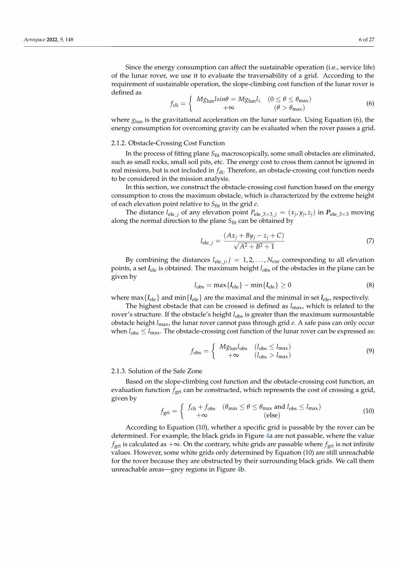
According to Equation (10), whether a specific grid is passable by the rover can bedetermined. For example, the black grids in Figure 4a are not passable, where the valuefgri is calculated as +∞. On the contrary, white grids are passable where fgri is not infinitevalues. However, some white grids only determined by Equation (10) are still unreachablefor the rover because they are obstructed by their surrounding black grids. We call themunreachable areas—grey regions in Figure 4b.
Aerospace 2022, 9, 148 7 of 27
Aerospace 2022, 9, x FOR PEER REVIEW 7 of 29
where elemax l
and elemin l
are the maximal and the minimal in set elel , respec‐
tively.
The highest obstacle that can be crossed is defined as maxl , which is related to the
rover’s structure. If the obstacle’s height obsl is greater than the maximum surmountable
obstacle height maxl , the lunar rover cannot pass through grid e. A safe pass can only occur
when obs maxl l . The obstacle‐crossing cost function of the lunar rover can be expressed as:
lun obs obs max
obs
obs max
( )=
+ ( > )
Mg l l lf
l l
(9)
2.1.3. Solution of the Safe Zone
Based on the slope‐climbing cost function and the obstacle‐crossing cost function, an
evaluation function grif can be constructed, which represents the cost of crossing a grid,
given by
( )
( )
cli obs min max obs max
gri
and
else
f f l lf
(10)
According to Equation (10), whether a specific grid is passable by the rover can be
determined. For example, the black grids in Figure 4a are not passable, where the value
grif is calculated as + . On the contrary, white grids are passable where grif is not in‐
finite values. However, some white grids only determined by Equation (10) are still un‐
reachable for the rover because they are obstructed by their surrounding black grids. We
call them unreachable areas—grey regions in Figure 4b.
To obtain the safe zone, we introduce the seed‐filling method to exclude the un‐
reachable area from all the white grids calculated by Equation (10). Specifically, the loca‐
tion of the lunar rover is chosen as the seed; then, we apply the breadth‐first search al‐
gorithm [25], one of the common methods to find the largest connected domain, to search
the grids adjacent to the seed. Grids with the same property are merged into one set, and
the safe zone can be determined. Note that, due to the structural constraints of the lunar
rover, the passing cost of the outermost region (see Figure 4b) cannot be calculated since
it is not considered a safe zone.
At this point, the autonomous solution of the safe zone has been obtained.
Figure 4. Schematic of the fitS of the lunar rover. (a) The passable region by white grids. (b) The
constituted actual safe zone.
2.2. The Selection Strategy of the Detecting Point
In this section, we propose an automatic strategy to select the mission‐oriented de‐
tecting point for the rover. In general, a flat detecting region is beneficial to the detecting
Figure 4. Schematic of the Sfit of the lunar rover. (a) The passable region by white grids. (b) Theconstituted actual safe zone.
To obtain the safe zone, we introduce the seed-filling method to exclude the unreach-able area from all the white grids calculated by Equation (10). Specifically, the location ofthe lunar rover is chosen as the seed; then, we apply the breadth-first search algorithm [25],one of the common methods to find the largest connected domain, to search the gridsadjacent to the seed. Grids with the same property are merged into one set, and the safezone can be determined. Note that, due to the structural constraints of the lunar rover,the passing cost of the outermost region (see Figure 4b) cannot be calculated since it is notconsidered a safe zone.
At this point, the autonomous solution of the safe zone has been obtained.
2.2. The Selection Strategy of the Detecting Point
In this section, we propose an automatic strategy to select the mission-oriented de-tecting point for the rover. In general, a flat detecting region is beneficial to the detectinginstruments. Therefore, we introduce the FEI to evaluate the flatness of a detecting region,and then we use the particle swarm optimization (PSO) algorithm to search for a flat regionas the candidate detecting point.
2.2.1. The FEI
For missions like lunar soil sampling and rock mineral analysis, the X-ray massspectrometer is the main equipment, and two necessary conditions should be met for thenormal operation [26]:
• Detecting orientation. When the X-ray mass spectrometer analyzes soil on the Moonsurface, it needs to receive the reflected light of the X-ray emitted by itself. Therefore,its axis should coincide with the normal to the fitted plane corresponding to thedetecting point.
• Detecting distance. The distance between the mirror surface of the X-ray mass spec-trometer and the detecting point should be smaller than the maximum explorationrange. However, some features of the detecting region, such as convex and concave,may lead to volatility in distance. To meet the distance requirement, the detectingpoint should have high flatness.
The required detecting orientation can be achieved by adjusting the pose of the vehicle-mounted end effector, on which the X-ray mass spectrometer is installed. Therefore, thispaper merely focuses on the detecting distance requirement.
The flatness of a region can be measured based on the DEM because it includes detailedtopographic information. The standard deviation is a measure of the fluctuation in heightof elevation points, and that of a flat region is usually small. Thus, the standard deviationis taken as the FEI to estimate the flatness.
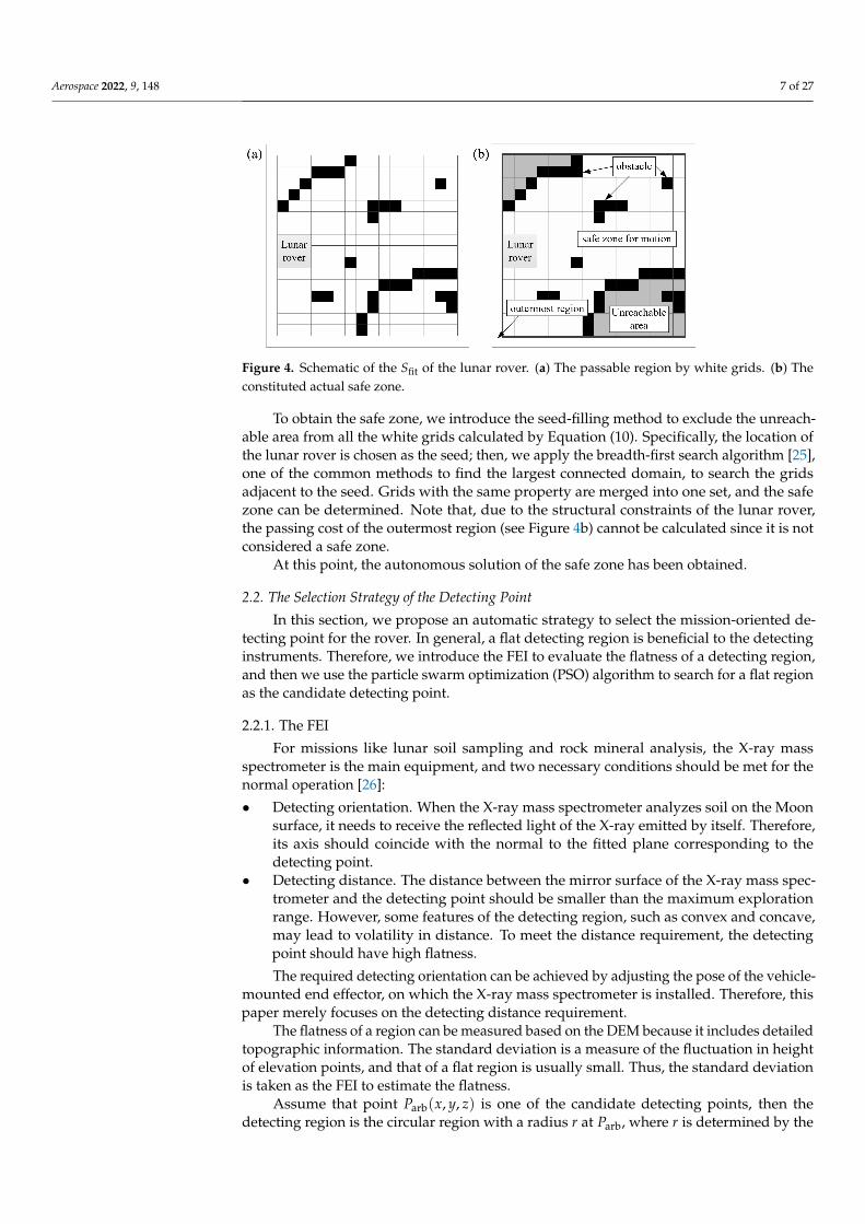
Assume that point Parb(x, y, z) is one of the candidate detecting points, then thedetecting region is the circular region with a radius r at Parb, where r is determined by the
Aerospace 2022, 9, 148 8 of 27
mirror radius of the X-ray mass spectrometer. This region contains Narb elevation points,which make up the set Pele_Xray = {xk, yk, zk}, (k = 1, 2, . . . , Narb) (see Figure 5).
Aerospace 2022, 9, x FOR PEER REVIEW 8 of 29
instruments. Therefore, we introduce the FEI to evaluate the flatness of a detecting re‐
gion, and then we use the particle swarm optimization (PSO) algorithm to search for a
flat region as the candidate detecting point.
2.2.1. The FEI
For missions like lunar soil sampling and rock mineral analysis, the X‐ray mass
spectrometer is the main equipment, and two necessary conditions should be met for the
normal operation [26]:
Detecting orientation. When the X‐ray mass spectrometer analyzes soil on the Moon
surface, it needs to receive the reflected light of the X‐ray emitted by itself. There‐
fore, its axis should coincide with the normal to the fitted plane corresponding to the
detecting point.
Detecting distance. The distance between the mirror surface of the X‐ray mass spec‐
trometer and the detecting point should be smaller than the maximum exploration
range. However, some features of the detecting region, such as convex and concave,
may lead to volatility in distance. To meet the distance requirement, the detecting
point should have high flatness.
The required detecting orientation can be achieved by adjusting the pose of the ve‐
hicle‐mounted end effector, on which the X‐ray mass spectrometer is installed. Therefore,
this paper merely focuses on the detecting distance requirement.
The flatness of a region can be measured based on the DEM because it includes de‐
tailed topographic information. The standard deviation is a measure of the fluctuation in
height of elevation points, and that of a flat region is usually small. Thus, the standard
deviation is taken as the FEI to estimate the flatness.
Assume that point arbP (x,y,z) is one of the candidate detecting points, then the de‐
tecting region is the circular region with a radius r at arbP , where r is determined by
the mirror radius of the X‐ray mass spectrometer. This region contains arbN elevation
points, which make up the set 1,2,...,ele_Xray arb=P ,k k kx ,y ,z k N (see Figure 5).
Figure 5. The planform of the elevation points near point arbP in a grid.
The arbN elevation points are used to fit the plane detS as stated in Section 2.1.1,
and the distance kl from the points 1,2,...,ele_Xray_k arb,k k kP (x ,y ,z ) k N in the set
ele_XrayP to detS is calculated by Equation (7). The FEI is defined by the standard de‐viation of 1,2,..., arbkl k N
2
1
1 arb
arb
N
k kk=
(l ‐ l )N
(11)
where, kl is the mean of all the distances 1,2,..., arbkl k N .
Figure 5. The planform of the elevation points near point Parb in a grid.
The Narb elevation points are used to fit the plane Sdet as stated in Section 2.1.1, andthe distance lk from the points Pele_Xray_k(xk, yk, zk), (k = 1, 2, . . . , Narb) in the set Pele_Xrayto Sdet is calculated by Equation (7). The FEI σ is defined by the standard deviation oflk (k = 1, 2, . . . , Narb)
σ =
√√√√ 1Narb
Narb
∑k=1
(lk − lk)2
(11)
where, lk is the mean of all the distances lk (k = 1, 2, . . . , Narb).
2.2.2. Selection of the Detecting Point
A suitable detecting point should be selected in the region which meets the conditionof detecting distance in the safe zone. For a large scale of the lunar environment, in whichthe safe zone is usually in several thousand square meters, it requires a heavy lift in time andresources for manual work. To overcome those shortcomings, the PSO is applied to selectthe detecting point autonomously in this paper, which stands out with fast convergenceand high precision [27].
Randomly select Npar elevation points in the safe zone, denoted as Pele_par = {xn, yn, zn},(n = 1, 2, . . . , Npar
). Npar can be determined according to the size of the safe zone. The
first two dimensions Pn = (xn, yn),(n = 1, 2, . . . , Npar
)of the set Pele_par are extracted
to initialize the particle swarm. The fitness function f (Pn) of the particle is constructedaccording to the FEI which is shown as Equation (12):
f (Pn) =1
k·σ(Pele_par) + 1(12)
where the value range of f (Pn) is (0, 1]; k is an amplification factor. The high value of f (Pn)means that the area where the elevation points of particles are located is relatively flat.
According to the requirements of the flatness of the detecting point, the fitness thresh-old of the particle Gbest can be set, and the fitness of the final optimum particle needs to begreater than or equal to Gbest. The upper limit of the iteration Kmax is set according to therequirement of calculation efficiency.
So far, the best mission-oriented detecting point can be selected. The entire process ofthe detecting point selection strategy is shown in Figure 6.

Aerospace 2022, 9, 148 9 of 27Aerospace 2022, 9, x FOR PEER REVIEW 10 of 29
Figure 6. The flow of detecting point selection of lunar rover.
3. The Sampling‐Based Path Planning Method under Linear Guidance (The Integrated
Sampling‐Based and Linear‐Guided Path Planning Method)
Sampling‐based global path planning algorithms such as PRM and visibility graph
method are efficient in path planning in a static working environment [28]. These algo‐
rithms firstly construct roadmaps, then search the path quickly with the roadmaps to
obtain feasible paths. However, many sampling points and connecting paths fall in open
areas far from obstacles. These points have no obvious effect on improving the connec‐
tivity of the roadmap.
In this section, a sampling‐based path planning under the linear guidance method is
proposed, taking advantage of the higher efficiency of the linear path planning in open
areas. It includes three steps: First, divide the safe zone into open areas and dense ob‐
stacle areas, and the dense obstacle areas are sampled to construct local roadmaps. Sec‐
Figure 6. The flow of detecting point selection of lunar rover.
3. The Sampling-Based Path Planning Method under Linear Guidance (The IntegratedSampling-Based and Linear-Guided Path Planning Method)
Sampling-based global path planning algorithms such as PRM and visibility graphmethod are efficient in path planning in a static working environment [28]. These algorithmsfirstly construct roadmaps, then search the path quickly with the roadmaps to obtainfeasible paths. However, many sampling points and connecting paths fall in open areasfar from obstacles. These points have no obvious effect on improving the connectivity ofthe roadmap.
In this section, a sampling-based path planning under the linear guidance method isproposed, taking advantage of the higher efficiency of the linear path planning in openareas. It includes three steps: First, divide the safe zone into open areas and dense obstacleareas, and the dense obstacle areas are sampled to construct local roadmaps. Second,

Aerospace 2022, 9, 148 10 of 27
the initial path is constructed based on the linear path planning, which is then modifiedand simplified to avoid colliding with obstacles according to the sampled local roadmaps.Finally, the original map and several supplemented maps for new tasks are combined bythe map extension strategy, which fully utilizes the local roadmap to improve the efficiencyof roadmap reconstruction.
3.1. Sampling in Areas with Dense Obstacles3.1.1. Division of the Safe Zone
To divide the safe zone clearly, the area within ε (ε is determined by the grid size)around the obstacle is defined as the dense obstacle area. The detailed division process ofthe open area and the dense obstacle area is introduced as follows:
In a workplace Cwork containing obstacles, the center of grid (i, j) is denoted asA(
xi,j, yi,j). Take A as the center (see Figure 7) and search for the nearest obstacle grid
as follows:
Aerospace 2022, 9, x FOR PEER REVIEW 11 of 29
ond, the initial path is constructed based on the linear path planning, which is then
modified and simplified to avoid colliding with obstacles according to the sampled local
roadmaps. Finally, the original map and several supplemented maps for new tasks are
combined by the map extension strategy, which fully utilizes the local roadmap to im‐
prove the efficiency of roadmap reconstruction.
3.1. Sampling in Areas with Dense Obstacles
3.1.1. Division of the Safe Zone
To divide the safe zone clearly, the area within ( is determined by the grid size)
around the obstacle is defined as the dense obstacle area. The detailed division process of
the open area and the dense obstacle area is introduced as follows:
In a workplace workC containing obstacles, the center of grid
i, j is denoted as
i, j i, jA x ,y. Take A as the center (see Figure 7) and search for the nearest obstacle grid
as follows:
4a
1a 3aA
Bd
2a
Figure 7. Schematic of the searching order of grids within one layer.
1. First, search all grids in the 1 2 3th ‐ n = , , ,...Nn layer that encloses A . The
maximum number of the layer / N l ( indicates an upward rounding).
2. During the search of grids in each layer, the four grids in the horizontal and vertical
directions are searched preferentially, and are shown as 1 2 3 4, , ,a a a a in Figure 7. If
neither of the searched grids is the obstacle grid, the upward and downward adja‐
cent grids of 1a and 3a are searched, respectively. Similarly, the left and right adja‐
cent grids of 2a and 4a are searched, respectively.
The first obstacle grid detected is the nearest obstacle grid, for example, the dark red
grid centred at point B in Figure 7. The distance ( )d A,B can be calculated between the
nearest obstacle grid’s center obs obsB x ,y
and i, j i, jA x ,y:
2 2( ) i, j obs i, j obsd A,B x x y y
(13)
If no obstacle grid is detected by the end of the search, the grid does not belong to
the dense obstacle area, and then ( )d A, B is set as .
According to the value of ( )d A, B , the dense obstacle area and the open area can be
expressed as a set, given by
( ) denseD A d A,B
(14)
( ) openD A d A,B
(15)
Figure 7. Schematic of the searching order of grids within one layer.
1. First, search all grids in the n-th (n = 1, 2, 3, . . . N) layer that encloses A. The maxi-mum number of the layer N = dε/le (d·e indicates an upward rounding).
2. During the search of grids in each layer, the four grids in the horizontal and verticaldirections are searched preferentially, and are shown as a1, a2, a3, a4 in Figure 7. Ifneither of the searched grids is the obstacle grid, the upward and downward adjacentgrids of a1 and a3 are searched, respectively. Similarly, the left and right adjacent gridsof a2 and a4 are searched, respectively.
The first obstacle grid detected is the nearest obstacle grid, for example, the dark redgrid centred at point B in Figure 7. The distance d(A, B) can be calculated between thenearest obstacle grid’s center B(xobs, yobs) and A
(xi,j, yi,j
):
d(A, B) =√(
xi,j − xobs)2
+(yi,j − yobs
)2 (13)
If no obstacle grid is detected by the end of the search, the grid does not belong to thedense obstacle area, and then d(A, B) is set as ∞.
According to the value of d(A, B), the dense obstacle area and the open area can beexpressed as a set, given by
Ddense = {A|d(A, B) ≤ ε} (14)
Dopen = {A|d(A, B) = ∞} (15)
3.1.2. Sampling Points in the Areas with Dense Obstacles
The number and distribution of the sampling points directly affect the efficiency of pathplanning and the connectivity of the roadmap. A large number and a worse distributioncan increase not only the complexity of the search problem, but also the computation time.However, fewer sampling points, although costing less computational time, might fail

Aerospace 2022, 9, 148 11 of 27
concerning a feasible path. If each sampling point includes rich information of obstacles,the total number of sampling points can be reduced. In this paper, the shape points and thedistance points are used to characterize the contour features of the obstacles.
For the obstacles with the same size, the complexity of the shape determines thenumber of shape points. Prominent parts of the obstacle depict the effective contour ofthe obstacle and contain rich connectivity information. As shown in Figure 8a, partssurrounded by dashed lines can improve the connectivity of the roadmap. Consideringthe geometric feature, we sample points in the prominent part of obstacles, which can berepresented by partial grids (see the orange grids in Figure 8b).
Aerospace 2022, 9, x FOR PEER REVIEW 12 of 29
3.1.2. Sampling Points in the Areas with Dense Obstacles
The number and distribution of the sampling points directly affect the efficiency of
path planning and the connectivity of the roadmap. A large number and a worse distri‐
bution can increase not only the complexity of the search problem, but also the compu‐
tation time. However, fewer sampling points, although costing less computational time,
might fail concerning a feasible path. If each sampling point includes rich information of
obstacles, the total number of sampling points can be reduced. In this paper, the shape
points and the distance points are used to characterize the contour features of the obsta‐
cles.
For the obstacles with the same size, the complexity of the shape determines the
number of shape points. Prominent parts of the obstacle depict the effective contour of
the obstacle and contain rich connectivity information. As shown in Figure 8a, parts
surrounded by dashed lines can improve the connectivity of the roadmap. Considering
the geometric feature, we sample points in the prominent part of obstacles, which can be
represented by partial grids (see the orange grids in Figure 8b).
2Nl
B
t
a b
Figure 8. (a) The prominent part of the obstacle. (b) Sampling of shape points.
According to Section 3.1.1, a grid t denseD in the dense obstacle area can be en‐
sured, whose center locates on the diagonal of the nearest obstacle grid B. The distance
between the center of t and that of B satisfies the following relationship
( ) 2 / d t,B Nl,N l
(16)
The center of the grid t is chosen as the shape point because it can represent the bulged part of the obstacle to some extent. The above process corresponds to the line
03~08 in Algorithm 1. We define the set of shape points as follows:
1 ( , ) 2 , denseT t d t B Nl t D
(17)
The number and distribution of shape points are the same for obstacles with similar
shapes but different areas. As the area increases, the distance between shape points in‐
creases, and the connected paths in the roadmap are lengthened, as shown in Figure 9a.
a b
Figure 9. Schematic of connected paths and sampling points. (a) The connected paths in the
roadmap are constructed only with shape points. (b) The connected paths in the roadmap are con‐
structed with shape points and distance points.
Figure 8. (a) The prominent part of the obstacle. (b) Sampling of shape points.
According to Section 3.1.1, a grid t ∈ Ddense in the dense obstacle area can be ensured,whose center locates on the diagonal of the nearest obstacle grid B. The distance betweenthe center of t and that of B satisfies the following relationship
d(t, B) =√
2Nl, N = dε/le (16)
The center of the grid t is chosen as the shape point because it can represent the bulgedpart of the obstacle to some extent. The above process corresponds to the line 03~08 inAlgorithm 1. We define the set of shape points as follows:
T1 ={
t∣∣∣d(t, B) =
√2Nl, t ∈ Ddense
}(17)
The number and distribution of shape points are the same for obstacles with similarshapes but different areas. As the area increases, the distance between shape pointsincreases, and the connected paths in the roadmap are lengthened, as shown in Figure 9a.
Aerospace 2022, 9, x FOR PEER REVIEW 12 of 29
3.1.2. Sampling Points in the Areas with Dense Obstacles
The number and distribution of the sampling points directly affect the efficiency of
path planning and the connectivity of the roadmap. A large number and a worse distri‐
bution can increase not only the complexity of the search problem, but also the compu‐
tation time. However, fewer sampling points, although costing less computational time,
might fail concerning a feasible path. If each sampling point includes rich information of
obstacles, the total number of sampling points can be reduced. In this paper, the shape
points and the distance points are used to characterize the contour features of the obsta‐
cles.
For the obstacles with the same size, the complexity of the shape determines the
number of shape points. Prominent parts of the obstacle depict the effective contour of
the obstacle and contain rich connectivity information. As shown in Figure 8a, parts
surrounded by dashed lines can improve the connectivity of the roadmap. Considering
the geometric feature, we sample points in the prominent part of obstacles, which can be
represented by partial grids (see the orange grids in Figure 8b).
2Nl
B
t
a b
Figure 8. (a) The prominent part of the obstacle. (b) Sampling of shape points.
According to Section 3.1.1, a grid t denseD in the dense obstacle area can be en‐
sured, whose center locates on the diagonal of the nearest obstacle grid B. The distance
between the center of t and that of B satisfies the following relationship
( ) 2 / d t,B Nl,N l
(16)
The center of the grid t is chosen as the shape point because it can represent the bulged part of the obstacle to some extent. The above process corresponds to the line
03~08 in Algorithm 1. We define the set of shape points as follows:
1 ( , ) 2 , denseT t d t B Nl t D
(17)
The number and distribution of shape points are the same for obstacles with similar
shapes but different areas. As the area increases, the distance between shape points in‐
creases, and the connected paths in the roadmap are lengthened, as shown in Figure 9a.
a b
Figure 9. Schematic of connected paths and sampling points. (a) The connected paths in the
roadmap are constructed only with shape points. (b) The connected paths in the roadmap are con‐
structed with shape points and distance points.
Figure 9. Schematic of connected paths and sampling points. (a) The connected paths in the roadmapare constructed only with shape points. (b) The connected paths in the roadmap are constructed withshape points and distance points.
However, in the long narrow channels, the shape points do not enhance the connec-tivity of the roadmap significantly. To solve this problem, distance points are introducedin the paper; see the red points in Figure 9b. The set composed of the distance points t2 isdenoted as T2, on which the following constraints are imposed:
• t2 ∈ {Ddense\T1};

Aerospace 2022, 9, 148 12 of 27
• d(t2, t1) > ε for ∀t1 ∈ T1;• d(t2, t′2) > ε for ∀t′2 ∈ T2 and t2 6= t′2.
To meet the above three conditions simultaneously, the distance points are selected bytraversing all the elements in T1 as follows (the lines 09~15 in Algorithm 1):
(1) Determine the annular area with radius ε ∼ 2ε and center tx ∈ T1 (see Figure 10).(2) Search the center of grid zi /∈ T1 ∪ T2 in the overlap between the annular area and the
dense obstacle area. If no center point is detected within the overlap, turn to (1).(3) Calculate the Euclidean distance d(tx, zi) between zi and tx. Notice that zi may not be
unique, in which corresponding to the minimum distance min d(tx, zi) is taken as adistance point ty as follows
ty = argmin{ε ≤ d(tx, zi) ≤ 2ε} (18)
Then, put the point ty into the set T2.(4) Take ty as the center of the annular area with radius ε ∼ 2ε; turn to (2).
Aerospace 2022, 9, x FOR PEER REVIEW 13 of 29
However, in the long narrow channels, the shape points do not enhance the con‐
nectivity of the roadmap significantly. To solve this problem, distance points are intro‐
duced in the paper; see the red points in Figure 9b. The set composed of the distance
points 2t is denoted as 2T , on which the following constraints are imposed:
2 1\ denset D T ;
2 1 d t ,t for 1 1 t T ;
2 2 d t ,t for 2 2 t T and 2 2t t .
To meet the above three conditions simultaneously, the distance points are selected
by traversing all the elements in 1T as follows (the lines 09~15 in Algorithm 1):
(1) Determine the annular area with radius ~ 2 and center 1xt T (see Figure 10).
(2) Search the center of grid 1 2iz T T in the overlap between the annular area and
the dense obstacle area. If no center point is detected within the overlap, turn to (1).
(3) Calculate the Euclidean distance x id t ,z
between iz and xt . Notice that iz
may not be unique, in which corresponding to the minimum distance min x id t ,z
is taken as a distance point yt as follows
2 argminy x it d t ,z
(18)
Then, put the point yt into the set 2T .
(4) Take yt as the center of the annular area with radius ~ 2 ; turn to (2).
xt yt
1yt
2
Figure 10. Schematic of sampling of the distance points.
Algorithm 1: Sampling Points
01 Require: Initialize denseD , 1 0, 0t , 2 0, 0t , l is the side length of grid, is the threshold of the area with dense obstacles.
02 if denseD do
03 for each the center of the grid denseA D
04 find out the nearest obstacle B grid to A
05 if ( , ) 2 , / d A B Nl N l
06 1T A
07 end
08 end
09 for each 1 1t T
Figure 10. Schematic of sampling of the distance points.
Algorithm 1: Sampling Points
01Require: Initialize Ddense, t1 = (0, 0), t2 = (0, 0), l is the side length of grid, ε is thethreshold of the area with dense obstacles.
02 if Ddense 6= φ do03 for each the center of the grid A ∈ Ddense04 find out the nearest obstacle B grid to A05 if d(A, B) =
√2Nl, N = dε/le
06 T1 ← A07 end08 end09 for each t1 ∈ T110 for each t2 ∈ Ddense\T1 ∩ Ddense\T211 if ε < d(t1, t2) < 2ε do12 T2 ← t213 end14 end15 end16 end
Based on the obtained sampling points, the local roadmap can be constructed. Allthe sampling points in a circle with centre ti and radius r (r can be determined accordingto the connecting requirements of the roadmap for path planning) are connected to thepoint ti(ti ⊂ T1 ∪ T2) to get Nr edges. The edges which do not collide with obstacles arestored to the set E. The roadmap G is made up of the set of sampling points T1 ∪ T2 and theset of collision-free edges E. By constructing a roadmap, the path planning in continuous
Aerospace 2022, 9, 148 13 of 27
space can be solved in the topological space; thus, the search complexity of path planningis reduced.
3.2. Path Planning under Linear Guidance
There is no connecting path in the open area since all the sampling points are locatedin the dense obstacle area, and the connecting paths of the roadmap are distributed aroundthe obstacle. This section adopts a linear path in the open area as the path guidance.
3.2.1. Planning the Linear Path
Considering the generality, we assume that there are some arbitrary obstacles in themap and specify the rover’s current location and detecting point. It starts by establishing alinear path between the two points:
y =ycurrent − ydetecting
xcurrent − xdetecting(x− xcurrent) + ycurrent (19)
where, (xcurrent, ycurrent) is the coordinates of the current location and(
xdetecting, ydetecting
)is the coordinates of the detecting point.
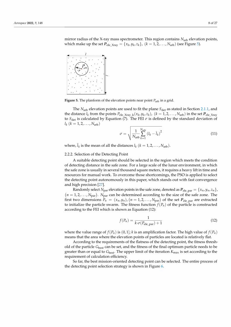
If no obstacle intersects with the linear path, this linear path is the final path, as A1B1 inFigure 11. Otherwise, it is necessary to find out the feasible paths that can bypass obstacles.The intersecting points with the edge of obstacles are denoted as (a1, b1, a2, b2, . . . , an, bn)(see Figure 11).
Aerospace 2022, 9, x FOR PEER REVIEW 14 of 29
10 for each 2 1 2\ \dense denset D T D T
11 if 1 2, 2d t t do
12 2 2T t
13 end 14 end
15 end
16 end
Based on the obtained sampling points, the local roadmap can be constructed. All
the sampling points in a circle with centre it and radius r (r can be determined accord‐
ing to the connecting requirements of the roadmap for path planning) are connected to
the point it ( 1 2it T T ) to get rN edges. The edges which do not collide with obstacles
are stored to the set E. The roadmap G is made up of the set of sampling points 1 2T T
and the set of collision‐free edges E. By constructing a roadmap, the path planning in
continuous space can be solved in the topological space; thus, the search complexity of
path planning is reduced.
3.2. Path Planning under Linear Guidance
There is no connecting path in the open area since all the sampling points are located
in the dense obstacle area, and the connecting paths of the roadmap are distributed
around the obstacle. This section adopts a linear path in the open area as the path guid‐
ance.
3.2.1. Planning the Linear Path
Considering the generality, we assume that there are some arbitrary obstacles in the
map and specify the rover’s current location and detecting point. It starts by establishing
a linear path between the two points:
current detecting
current current
current detecting
y yy = x x +yx x
--
-
(19)
where, current current,x y
is the coordinates of the current location and detecting detectingx ,y
is the coordinates of the detecting point.
If no obstacle intersects with the linear path, this linear path is the final path, as
1 1A B in Figure 11. Otherwise, it is necessary to find out the feasible paths that can bypass
obstacles. The intersecting points with the edge of obstacles are denoted as
1 1 2 2 n na ,b ,a ,b ,...,a ,b (see Figure 11).
1A
1B
2A1a
1b
2a2b
1B
Figure 11. Schematic of a linear path. Figure 11. Schematic of a linear path.
3.2.2. Searching for Local Feasible Paths in the Roadmap of Dense Obstacle Areas
If the linear path intersects with obstacles, the A* heuristic search algorithm is adoptedto search the local feasible path in the roadmap G constructed in Section 3.1. The localfeasible path can help to bypass the obstacle. The sampling points nearest to a1 and b1are used as the starting and the ending point to search the path. The maximum distancebetween each sampling point and the obstacle is strictly required to be ε in Section 3.1; theremust be one or two sampling points t that meet d(t, a1) < 2ε. Therefore, the search rangefor the nearest sampling point of a1, which is denoted as Ca_i, is the circle with center a1and radius 2ε. The nearest sampling point searched as a′1 is recorded, and so is b′1. The localfeasible path is a′1− > x1− > x2− > b′1 (see Figure 12), and this process corresponds toline 07~22 in Algorithm 2.

Aerospace 2022, 9, 148 14 of 27
Aerospace 2022, 9, x FOR PEER REVIEW 15 of 29
3.2.2. Searching for Local Feasible Paths in the Roadmap of Dense Obstacle Areas
If the linear path intersects with obstacles, the A* heuristic search algorithm is adopted
to search the local feasible path in the roadmap G constructed in Section 3.1. The local
feasible path can help to bypass the obstacle. The sampling points nearest to 1a and 1b are used as the starting and the ending point to search the path. The maximum distance
between each sampling point and the obstacle is strictly required to be in Section 3.1;
there must be one or two sampling points t that meet 1 2d t,a
. Therefore, the search
range for the nearest sampling point of 1a , which is denoted as a_iC , is the circle with center
1a and radius 2 . The nearest sampling point searched as 1a is recorded, and so is 1b .
The local feasible path is 1 1 2 1a x x b (see Figure 12), and this process corresponds
to line 07~22 in Algorithm 2.
1A
1B
2A
2B
1a
1b
2a2b
1a
1x 2x1b
2b2a
_a iC
_b iC
Figure 12. Schematic of the local feasible path in areas with dense obstacles.
3.2.3. Solution of the Best Feasible Path
An obstacle‐free path can be obtained by modifying the linear path with local feasi‐
ble paths. However, it is rather tortuous. In the paper, a forward trial method is used to
enhance the obstacle‐free path by linearizing it.
Take 2 2A B for example to explain this method.
Step1: Take 2A as the starting point; connect with the next node 1a. Try to connect
2A with 1x ; if 2 1A x does not intersect with any obstacle, 1a is discarded, and so on.
Get the first furthest point 1x and the first valid shortcut 2 1A x .
Step2: Take 1x as the new starting point; then repeat Step 1. Get the second furthest
key point 2a and the second valid shortcut 1 2xa .
Step3: Take 2a as the new starting point; then repeat Step 1. Get the third valid shortcut 2 2a B .
So far, the final feasible path 2 2 2 2A x a B has fewer turn points and is the
best possible shortcut obtained (see Figure 13), and this process corresponds to line 24~34
in Algorithm 2.
Figure 12. Schematic of the local feasible path in areas with dense obstacles.
3.2.3. Solution of the Best Feasible Path
An obstacle-free path can be obtained by modifying the linear path with local feasiblepaths. However, it is rather tortuous. In the paper, a forward trial method is used toenhance the obstacle-free path by linearizing it.
Take A2B2 for example to explain this method.Step1: Take A2 as the starting point; connect with the next node a′1. Try to connect A2
with x1; if A2x1 does not intersect with any obstacle, a′1 is discarded, and so on. Get the firstfurthest point x1 and the first valid shortcut A2x1.
Step2: Take x1 as the new starting point; then repeat Step 1. Get the second furthestkey point a′2 and the second valid shortcut x1a′2.
Step3: Take a′2 as the new starting point; then repeat Step 1. Get the third valid shortcuta′2B2.
So far, the final feasible path A2− > x2− > a′2− > B2 has fewer turn points and is thebest possible shortcut obtained (see Figure 13), and this process corresponds to line 24~34in Algorithm 2.
Aerospace 2022, 9, x FOR PEER REVIEW 16 of 29
1A
1B
2A
2B
2a2b
1a
1x 2x1b
2b2a
Figure 13. Schematic of the final feasible path.
Algorithm 2: Path Planning Strategy under Linear Guidance
01 Require: Specify the current location of the rover current current,x y and the detecting point detecting detecting,x y .
02 Initialize the roadmap G , the obstacle areas O , the area with dense obstacles S , the set of the key points T .
03 Initialize the finite set of the points of local path []P and the set final_path [] .
04 Plan a linear path from current current,x y to detecting detecting,x y .
05 Find intersection points of the straight line and the O :
06 1 1 2 2, , , , ..., ,its n nP a b a b a b
07 if itsP is not NULL do
08 for 1i to n
09 Take all elements of T in the search range _a iC as the set _a iT .
10 for each element it of _a iT
11 Calculate the distance ,i id t a between it and ia .
12 end
13 if it correspond to the minimum of ,i id t a
14 i ja t
15 end
16 Take all elements of T in the search range _b iC as the set _b iT , and
the same process as _a iT .
17 Search the path ip from ia to ib in G by using A* algorithm.
18 for each node node node,x y of the ip
19 node node,P x y
20 end
21 end
22 end
23 current currentfinal_path ,x y
24 for 2j to length P
Figure 13. Schematic of the final feasible path.
3.3. Map Extension
With the deeper exploration of the lunar rover, the explorable area continues to expand.The detection of a new area or the change of a local area can render the existing roadmapunusable, so that the roadmap needs to be updated. Reconstructing a large-scale andcomplete roadmap of the lunar environment would take a long time, which would lead toa sharp decrease in planning efficiency. To improve the efficiency, map extension is carriedout combined with the roadmap’s local feature.

Aerospace 2022, 9, 148 15 of 27
Algorithm 2: Path Planning Strategy under Linear Guidance
01Require: Specify the current location of the rover (xcurrent, ycurrent) and the detecting
point(
xdetecting, ydetecting
).
02Initialize the roadmap G, the obstacle areas O, the area with dense obstacles S, theset of the key points T.
03 Initialize the finite set of the points of local path P = [] and the set final_path = [].
04 Plan a linear path from (xcurrent, ycurrent) to(
xdetecting, ydetecting
).
05 Find intersection points of the straight line and the O:06 Pits = (a1, b1, a2, b2, . . . , an, bn)07 if Pits is not NULL do08 for i = 1 to n09 Take all elements of T in the search range Ca_i as the set Ta_i.10 for each element ti of Ta_i11 Calculate the distance d(ti, ai) between ti and ai.12 end13 if ti correspond to the minimum of d(ti, ai)14 a′i = tj15 end
16Take all elements of T in the search range Cb_i as the set Tb_i, andthe same process as Ta_i.
17 Search the path pi from a′i to b′i in G by using A* algorithm.18 for each node (xnode, ynode) of the pi19 P← (xnode, ynode)20 end21 end22 end23 final_path← (xcurrent, ycurrent)24 for j = 2 to length [P]25 for i = j length [P]26 xj = P[j]27 xi = P[i]28 if the straight path xjxi intersects with obstacle do29 final_path← xi−130 j = i− 131 end32 end33 end34 final_path←
(xdetecting, ydetecting
)3.3.1. Data Processing of Map Extension
The following process needs to be done to execute the map extension:
• Map preprocessing. The whole map Z is the same as the initial map at the beginning.• Roadmap construction. According to Equation (10), the initial safe zone for motion is
determined. The set of sampling points T0 is got and the roadmap G0 is constructedby Section 3.1.
• Set collections Tset and Gset, the sampling points set T and the roadmap G of the initialmap or the individual map, respectively.
The part that needs to be updated is treated as an individual map, and the safe zoneSnew, the sampling points set Tnew, and the roadmap Gnew of it are obtained accordingto Sections 2.1 and 3.1. According to the relative position R between the individual mapcoordinate origin and the whole map origin, the coordinates of each point are updated. Forexample, if the position of the key point in the individual map is RT , then its position R′T inthe whole map can be updated as follows:
R′T = R + RT (20)
Aerospace 2022, 9, 148 16 of 27
Store the updated sampling points set Tnew, the roadmap Gnew in Tset and Gset, re-spectively.
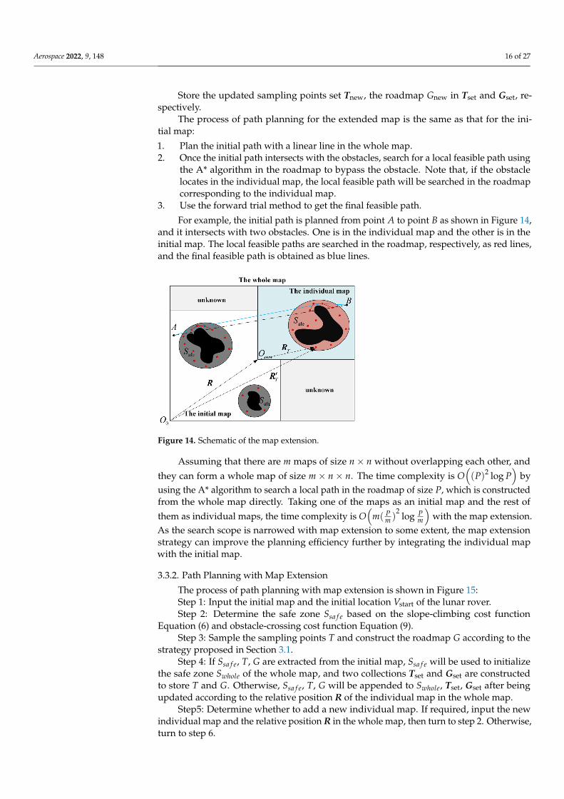
The process of path planning for the extended map is the same as that for the ini-tial map:
1. Plan the initial path with a linear line in the whole map.2. Once the initial path intersects with the obstacles, search for a local feasible path using
the A* algorithm in the roadmap to bypass the obstacle. Note that, if the obstaclelocates in the individual map, the local feasible path will be searched in the roadmapcorresponding to the individual map.
3. Use the forward trial method to get the final feasible path.
For example, the initial path is planned from point A to point B as shown in Figure 14,and it intersects with two obstacles. One is in the individual map and the other is in theinitial map. The local feasible paths are searched in the roadmap, respectively, as red lines,and the final feasible path is obtained as blue lines.
Aerospace 2022, 9, x FOR PEER REVIEW 18 of 29
is in the initial map. The local feasible paths are searched in the roadmap, respectively, as
red lines, and the final feasible path is obtained as blue lines.
Figure 14. Schematic of the map extension.
Assuming that there are m maps of size n n without overlapping each other,
and they can form a whole map of size m n n . The time complexity is 2( ) logO P P
by using the A* algorithm to search a local path in the roadmap of size P , which is
constructed from the whole map directly. Taking one of the maps as an initial map and
the rest of them as individual maps, the time complexity is
2( ) logP P
O mm m
with the
map extension. As the search scope is narrowed with map extension to some extent, the
map extension strategy can improve the planning efficiency further by integrating the
individual map with the initial map.
3.3.2. Path Planning with Map Extension
The process of path planning with map extension is shown in Figure 15:
Step 1: Input the initial map and the initial location startV of the lunar rover.
Step 2: Determine the safe zone Ssafe based on the slope‐climbing cost function
Equation (6) and obstacle‐crossing cost function Equation (9).
Step 3: Sample the sampling points T and construct the roadmap G according to
the strategy proposed in Section 3.1.
Step 4: If Ssafe
, T , G are extracted from the initial map, Ssafe
will be used to ini‐
tialize the safe zone Swhole of the whole map, and two collections setT and setG are con‐
structed to store T and G . Otherwise, Ssafe
, T , G will be appended to Swhole
, setT ,
setG after being updated according to the relative position R of the individual map in
the whole map.
Step5: Determine whether to add a new individual map. If required, input the new
individual map and the relative position R in the whole map, then turn to step 2. Oth‐
erwise, turn to step 6.
Step 6: Select the detecting point goalV in the safe zone Swhole of the whole map based
on the strategy of the selection of detecting point proposed in Section 2.2.
Step 7: Obtain the final feasible path using the sampling‐based path planning
method under linear guidance.
Step 8: Output the path planning result, and wait for the command of the next ex‐
ploration mission. If the command is received, turn to Step 5.
Based on the above process, a path planning method with map extension can be
executed.
Figure 14. Schematic of the map extension.
Assuming that there are m maps of size n× n without overlapping each other, andthey can form a whole map of size m× n× n. The time complexity is O
((P)2 log P
)by
using the A* algorithm to search a local path in the roadmap of size P, which is constructedfrom the whole map directly. Taking one of the maps as an initial map and the rest ofthem as individual maps, the time complexity is O
(m( P
m )2
log Pm
)with the map extension.
As the search scope is narrowed with map extension to some extent, the map extensionstrategy can improve the planning efficiency further by integrating the individual mapwith the initial map.
3.3.2. Path Planning with Map Extension
The process of path planning with map extension is shown in Figure 15:Step 1: Input the initial map and the initial location Vstart of the lunar rover.Step 2: Determine the safe zone Ssa f e based on the slope-climbing cost function
Equation (6) and obstacle-crossing cost function Equation (9).Step 3: Sample the sampling points T and construct the roadmap G according to the
strategy proposed in Section 3.1.Step 4: If Ssa f e, T, G are extracted from the initial map, Ssa f e will be used to initialize
the safe zone Swhole of the whole map, and two collections Tset and Gset are constructedto store T and G. Otherwise, Ssa f e, T, G will be appended to Swhole, Tset, Gset after beingupdated according to the relative position R of the individual map in the whole map.
Step5: Determine whether to add a new individual map. If required, input the newindividual map and the relative position R in the whole map, then turn to step 2. Otherwise,turn to step 6.

Aerospace 2022, 9, 148 17 of 27
Step 6: Select the detecting point Vgoal in the safe zone Swhole of the whole map basedon the strategy of the selection of detecting point proposed in Section 2.2.
Step 7: Obtain the final feasible path using the sampling-based path planning methodunder linear guidance.
Step 8: Output the path planning result, and wait for the command of the nextexploration mission. If the command is received, turn to Step 5.
Based on the above process, a path planning method with map extension can be executed.Aerospace 2022, 9, x FOR PEER REVIEW 19 of 29
Figure 15. The flow of path planning with map extension.
4. Simulation
Simulations were executed based on the DEM of the lunar surface environment with
16 m length and 14.5 m width (see Figure 16). This DEM totally contains 687,969 elevation
points to describe detailed features of the lunar environment.
Figure 16. The 3D model of lunar surface environment.
Figure 15. The flow of path planning with map extension.
4. Simulation
Simulations were executed based on the DEM of the lunar surface environment with16 m length and 14.5 m width (see Figure 16). This DEM totally contains 687,969 elevationpoints to describe detailed features of the lunar environment.
Aerospace 2022, 9, 148 18 of 27
Aerospace 2022, 9, x FOR PEER REVIEW 19 of 29
Figure 15. The flow of path planning with map extension.
4. Simulation
Simulations were executed based on the DEM of the lunar surface environment with
16 m length and 14.5 m width (see Figure 16). This DEM totally contains 687,969 elevation
points to describe detailed features of the lunar environment.
Figure 16. The 3D model of lunar surface environment. Figure 16. The 3D model of lunar surface environment.
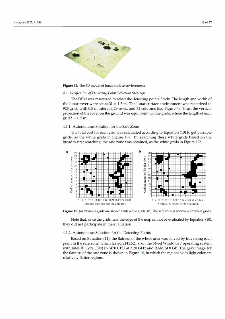
4.1. Verification of Detecting Point Selection Strategy
The DEM was rasterized to select the detecting points firstly. The length and width ofthe lunar rover were set as 3l = 1.5 m. The lunar surface environment was rasterized to928 grids with 0.5 m interval, 29 rows, and 32 columns (see Figure 7). Thus, the verticalprojection of the rover on the ground was equivalent to nine grids, where the length of eachgrid l = 0.5 m.
4.1.1. Autonomous Solution for the Safe Zone
The total cost for each grid was calculated according to Equation (10) to get passablegrids, as the white grids in Figure 17a. By searching these white grids based on thebreadth-first searching, the safe zone was obtained, as the white grids in Figure 17b.
Aerospace 2022, 9, x FOR PEER REVIEW 20 of 29
4.1. Verification of Detecting Point Selection Strategy
The DEM was rasterized to select the detecting points firstly. The length and width
of the lunar rover were set as 3 1.5 ml . The lunar surface environment was rasterized
to 928 grids with 0.5 m interval, 29 rows, and 32 columns (see Figure 7). Thus, the vertical
projection of the rover on the ground was equivalent to nine grids, where the length of
each grid 0.5 ml .
4.1.1. Autonomous Solution for the Safe Zone
The total cost for each grid was calculated according to Equation (10) to get passable
grids, as the white grids in Figure 17a. By searching these white grids based on the
breadth‐first searching, the safe zone was obtained, as the white grids in Figure 17b.
Figure 17. (a) Passable grids are shown with white grids. (b) The safe zone is shown with white
grids.
Note that, since the grids near the edge of the map cannot be evaluated by Equation
(10), they did not participate in the evaluation.
4.1.2. Autonomous Selection for the Detecting Points
Based on Equation (11), the flatness of the whole area was solved by traversing each
point in the safe zone, which lasted 2141.521 s, on the 64‐bit Windows 7 operating system
with Intel(R) Core (TM) i5‐3470 CPU at 3.20 GHz and RAM of 8 GB. The gray image for
the flatness of the safe zone is shown in Figure 18, in which the regions with light color
are relatively flatter regions.
Figure 18. The gray level map for the flatness of the safe zone.
Twenty elevation points were randomly selected in the safe zone, and their x and y
coordinate values were encoded to get the initial particle swarm. According to task re‐
Figure 17. (a) Passable grids are shown with white grids. (b) The safe zone is shown with white grids.
Note that, since the grids near the edge of the map cannot be evaluated by Equation (10),they did not participate in the evaluation.
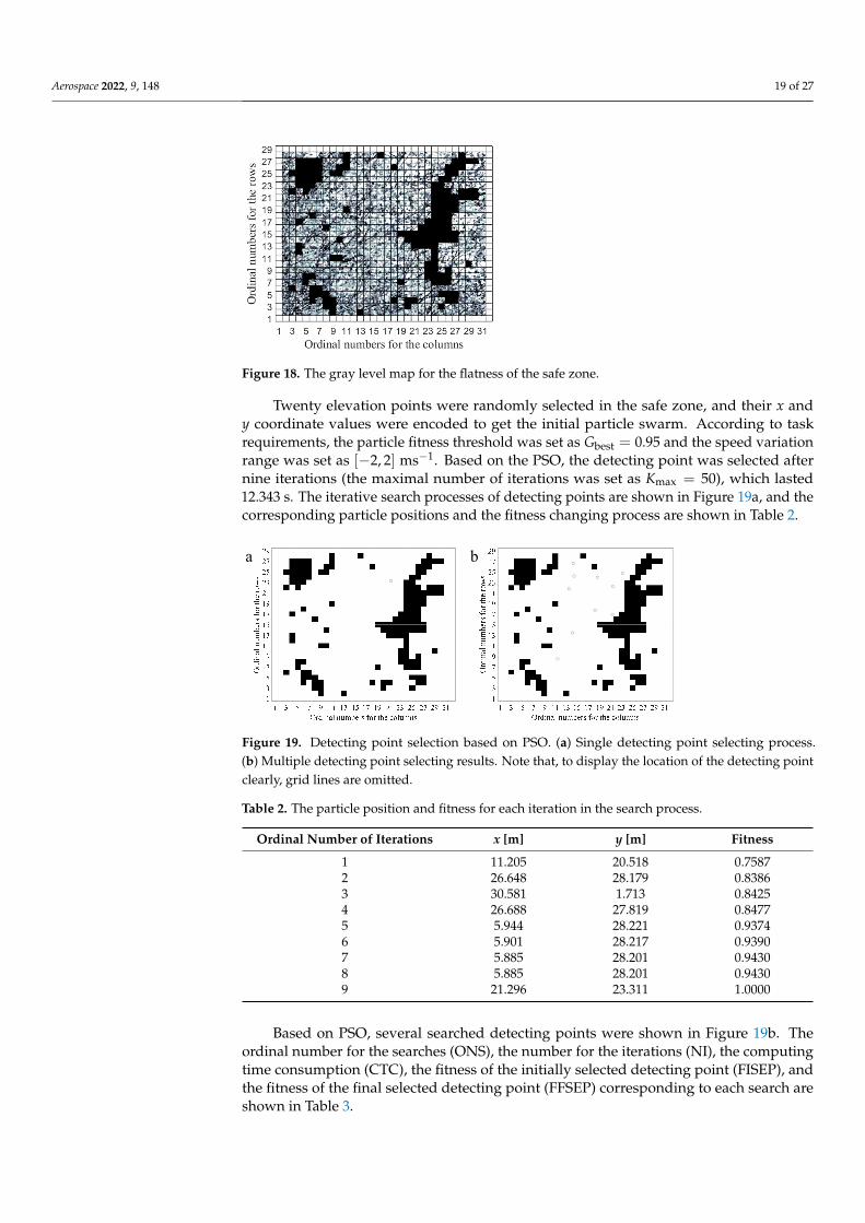
4.1.2. Autonomous Selection for the Detecting Points
Based on Equation (11), the flatness of the whole area was solved by traversing eachpoint in the safe zone, which lasted 2141.521 s, on the 64-bit Windows 7 operating systemwith Intel(R) Core (TM) i5-3470 CPU at 3.20 GHz and RAM of 8 GB. The gray image forthe flatness of the safe zone is shown in Figure 18, in which the regions with light color arerelatively flatter regions.
Aerospace 2022, 9, 148 19 of 27
Aerospace 2022, 9, x FOR PEER REVIEW 20 of 29
4.1. Verification of Detecting Point Selection Strategy
The DEM was rasterized to select the detecting points firstly. The length and width
of the lunar rover were set as 3 1.5 ml . The lunar surface environment was rasterized
to 928 grids with 0.5 m interval, 29 rows, and 32 columns (see Figure 7). Thus, the vertical
projection of the rover on the ground was equivalent to nine grids, where the length of
each grid 0.5 ml .
4.1.1. Autonomous Solution for the Safe Zone
The total cost for each grid was calculated according to Equation (10) to get passable
grids, as the white grids in Figure 17a. By searching these white grids based on the
breadth‐first searching, the safe zone was obtained, as the white grids in Figure 17b.
Figure 17. (a) Passable grids are shown with white grids. (b) The safe zone is shown with white
grids.
Note that, since the grids near the edge of the map cannot be evaluated by Equation
(10), they did not participate in the evaluation.
4.1.2. Autonomous Selection for the Detecting Points
Based on Equation (11), the flatness of the whole area was solved by traversing each
point in the safe zone, which lasted 2141.521 s, on the 64‐bit Windows 7 operating system
with Intel(R) Core (TM) i5‐3470 CPU at 3.20 GHz and RAM of 8 GB. The gray image for
the flatness of the safe zone is shown in Figure 18, in which the regions with light color
are relatively flatter regions.
Figure 18. The gray level map for the flatness of the safe zone.
Twenty elevation points were randomly selected in the safe zone, and their x and y
coordinate values were encoded to get the initial particle swarm. According to task re‐
Figure 18. The gray level map for the flatness of the safe zone.
Twenty elevation points were randomly selected in the safe zone, and their x andy coordinate values were encoded to get the initial particle swarm. According to taskrequirements, the particle fitness threshold was set as Gbest = 0.95 and the speed variationrange was set as [−2, 2] ms−1. Based on the PSO, the detecting point was selected afternine iterations (the maximal number of iterations was set as Kmax = 50), which lasted12.343 s. The iterative search processes of detecting points are shown in Figure 19a, and thecorresponding particle positions and the fitness changing process are shown in Table 2.
Aerospace 2022, 9, x FOR PEER REVIEW 21 of 29
quirements, the particle fitness threshold was set as best 0.95G and the speed variation
range was set as 2,2 1ms . Based on the PSO, the detecting point was selected after
nine iterations (the maximal number of iterations was set as max 50K ), which lasted
12.343 s. The iterative search processes of detecting points are shown in Figure 19a, and
the corresponding particle positions and the fitness changing process are shown in Table
2.
a b
Figure 19. Detecting point selection based on PSO. (a) Single detecting point selecting process. (b)
Multiple detecting point selecting results. Note that, to display the location of the detecting point
clearly, grid lines are omitted.
Table 2. The particle position and fitness for each iteration in the search process.
Ordinal Number of
Iterations x [m] y [m] Fitness
1 11.205 20.518 0.7587
2 26.648 28.179 0.8386
3 30.581 1.713 0.8425
4 26.688 27.819 0.8477
5 5.944 28.221 0.9374
6 5.901 28.217 0.9390
7 5.885 28.201 0.9430
8 5.885 28.201 0.9430
9 21.296 23.311 1.0000
Based on PSO, several searched detecting points were shown in Figure 19b. The or‐
dinal number for the searches (ONS), the number for the iterations (NI), the computing
time consumption (CTC), the fitness of the initially selected detecting point (FISEP), and
the fitness of the final selected detecting point (FFSEP) corresponding to each search are
shown in Table 3.
Table 3. Search information of detecting points for 10 random searches based on particle swarm
optimization.
ONS NI CTC/(s) FISEP FFSEP
1 6 7.153 0.7877 0.9798
2 6 6.617 0.7766 0.9611
3 14 11.332 0.7729 1.0000
4 17 13.039 0.7671 1.0000
5 46 29.827 0.7989 0.9711
6 5 6.229 0.8167 0.9771
7 11 10.310 0.7977 1.0000
8 26 20.434 0.8300 1.0000
9 23 17.916 0.7947 0.9883
Figure 19. Detecting point selection based on PSO. (a) Single detecting point selecting process.(b) Multiple detecting point selecting results. Note that, to display the location of the detecting pointclearly, grid lines are omitted.
Table 2. The particle position and fitness for each iteration in the search process.
Ordinal Number of Iterations x [m] y [m] Fitness
1 11.205 20.518 0.75872 26.648 28.179 0.83863 30.581 1.713 0.84254 26.688 27.819 0.84775 5.944 28.221 0.93746 5.901 28.217 0.93907 5.885 28.201 0.94308 5.885 28.201 0.94309 21.296 23.311 1.0000
Based on PSO, several searched detecting points were shown in Figure 19b. Theordinal number for the searches (ONS), the number for the iterations (NI), the computingtime consumption (CTC), the fitness of the initially selected detecting point (FISEP), andthe fitness of the final selected detecting point (FFSEP) corresponding to each search areshown in Table 3.

Aerospace 2022, 9, 148 20 of 27
Table 3. Search information of detecting points for 10 random searches based on particle swarmoptimization.
ONS NI CTC/(s) FISEP FFSEP
1 6 7.153 0.7877 0.97982 6 6.617 0.7766 0.96113 14 11.332 0.7729 1.00004 17 13.039 0.7671 1.00005 46 29.827 0.7989 0.97116 5 6.229 0.8167 0.97717 11 10.310 0.7977 1.00008 26 20.434 0.8300 1.00009 23 17.916 0.7947 0.988310 5 6.509 0.4505 1.0000
From Table 3, we can see that FFSEPs from the above 10 random searches are all greaterthan Gbest. This means all the final searched detecting points locate in flatter areas than theinitial position, and meet the requirements of the detecting instrument. Besides, the averagevalue of time consumption for the above 10 random searches is 12.937 s. This is two ordersof magnitude lower than the time consumption with traversal solution 2141.521 s. We alsonotice a loose linear relationship between NI and CTC; that is, the increment of CTC isgradually less than the linear increment of NI. This shows that, compared with the lineartime consumption traversal search, our strategy, which introduces the particle guidancemechanism from PSO, effectively speeds up the search for detecting points.
4.2. Verification of the Sampling-Based Path Planning Method under Linear Guidance4.2.1. The Sampling Method of Points in the Dense Obstacle Region
The 23 obstacles in the environment were numbered (see Figure 20).
Aerospace 2022, 9, x FOR PEER REVIEW 22 of 29
10 5 6.509 0.4505 1.0000
From Table 3, we can see that FFSEPs from the above 10 random searches are all
greater than bestG . This means all the final searched detecting points locate in flatter ar‐
eas than the initial position, and meet the requirements of the detecting instrument. Be‐
sides, the average value of time consumption for the above 10 random searches is 12.937
s. This is two orders of magnitude lower than the time consumption with traversal solu‐
tion 2141.521 s. We also notice a loose linear relationship between NI and CTC; that is, the
increment of CTC is gradually less than the linear increment of NI. This shows that,
compared with the linear time consumption traversal search, our strategy, which intro‐
duces the particle guidance mechanism from PSO, effectively speeds up the search for
detecting points.
4.2. Verification of the Sampling‐Based Path Planning Method under Linear Guidance
4.2.1. The Sampling Method of Points in the Dense Obstacle Region
The 23 obstacles in the environment were numbered (see Figure 20).
Figure 20. The map with numbered obstacles.
The obstacles No. 1–23 were sequentially added to the map, and the number of
sampling points with the increase of the obstacle was obtained (see Figure 21).
Figure 21. The number of sampling point changes with the increase of obstacle.
It can be seen that obstacles with large area or irregular shape will lead to a signifi‐
cant increase in the number of sampling points, especially obstacle No. 2, 15, and 23.
When all obstacles were added to the map, a total of 133 sampling points were obtained
(see Figure 22).
0 5 10 15 20Number of obstacles
0
20
40
60
80
100
120
140
Figure 20. The map with numbered obstacles.
The obstacles No. 1–23 were sequentially added to the map, and the number ofsampling points with the increase of the obstacle was obtained (see Figure 21).
Aerospace 2022, 9, x FOR PEER REVIEW 22 of 29
10 5 6.509 0.4505 1.0000
From Table 3, we can see that FFSEPs from the above 10 random searches are all
greater than bestG . This means all the final searched detecting points locate in flatter ar‐
eas than the initial position, and meet the requirements of the detecting instrument. Be‐
sides, the average value of time consumption for the above 10 random searches is 12.937
s. This is two orders of magnitude lower than the time consumption with traversal solu‐
tion 2141.521 s. We also notice a loose linear relationship between NI and CTC; that is, the
increment of CTC is gradually less than the linear increment of NI. This shows that,
compared with the linear time consumption traversal search, our strategy, which intro‐
duces the particle guidance mechanism from PSO, effectively speeds up the search for
detecting points.
4.2. Verification of the Sampling‐Based Path Planning Method under Linear Guidance
4.2.1. The Sampling Method of Points in the Dense Obstacle Region
The 23 obstacles in the environment were numbered (see Figure 20).
Figure 20. The map with numbered obstacles.
The obstacles No. 1–23 were sequentially added to the map, and the number of
sampling points with the increase of the obstacle was obtained (see Figure 21).
Figure 21. The number of sampling point changes with the increase of obstacle.
It can be seen that obstacles with large area or irregular shape will lead to a signifi‐
cant increase in the number of sampling points, especially obstacle No. 2, 15, and 23.
When all obstacles were added to the map, a total of 133 sampling points were obtained
(see Figure 22).
0 5 10 15 20Number of obstacles
0
20
40
60
80
100
120
140
Figure 21. The number of sampling point changes with the increase of obstacle.

Aerospace 2022, 9, 148 21 of 27
It can be seen that obstacles with large area or irregular shape will lead to a significantincrease in the number of sampling points, especially obstacle No. 2, 15, and 23. Whenall obstacles were added to the map, a total of 133 sampling points were obtained (seeFigure 22).
Aerospace 2022, 9, x FOR PEER REVIEW 23 of 29
Figure 22. Distribution of key sampling points.
Shape points (blue dots in Figure 22) are distributed in the protruding part of the
obstacle, while distance points (red dots in Figure 22) are distributed at the long edge or
in the concave part of the obstacle. Both of these types of sampling points constitute the
key feature of the obstacles in the whole map. More importantly, some points locate in
narrow channels (between obstacle No. 2 and 3, 21 and 23, etc.), which helps to form
connected paths for the roadmap. There are no sampling points in the open area, so that
the redundancy of the roadmap is reduced.
4.2.2. Roadmap Construction and Path Planning
In this section, the A* searching algorithm and the standard PRM are applied to
verify the proposed method. The A* searching algorithm is the latest baseline method
for the path planning of the lunar rover, which is applied in “Yutu‐2”, the lunar rover in
China’s Chang’e 4 mission to the Moon. In addition, the process of constructing a
roadmap in our method is similar to that of PRM, the efficient and popular method in
robotic path planning. Thus, we chose these two methods to compare with our method,
and verify the advantages of our method in time consuming and path quality.
After 133 sampling points were selected within the safe zone (Figure 22), the
roadmap was constructed, shown as red lines in Figure 23a. For comparison, we also
randomly sampled 133 points in the safe zone to construct the roadmap of PRM, shown
as red lines in Figure 23b. We can see that the connected paths of PRM cannot completely
cover the safe zone. For example, there are numerous unconnected areas on the top left of
obstacle No. 2, above No. 15, and on the right of No. 23. It is difficult to plan a feasible
path to reach these areas because the planning result of PRM only consists of connected
paths. In contrast, the roadmap constructed by our method forms a good envelope
around obstacles, resulting in good connectivity. Furthermore, our method allows the
planning result to be out of the roadmap in open areas, avoiding unnecessary turns
caused by inappropriate sampling points.
a b c
Figure 23. One of the path planning results. (a) The green line is the planned path using the sam‐
pling‐based path planning method under linear guidance. (b) The black line is the planned path
using the standard PRM method. (c) The blue line is the planned path using A* search algorithm.
0 5 10 15 20 25 30Ordinal numbers for the columns
0
5
10
15
20
25O
rdin
al n
umbe
rs f
or th
e ro
ws
Figure 22. Distribution of key sampling points.
Shape points (blue dots in Figure 22) are distributed in the protruding part of theobstacle, while distance points (red dots in Figure 22) are distributed at the long edgeor in the concave part of the obstacle. Both of these types of sampling points constitutethe key feature of the obstacles in the whole map. More importantly, some points locatein narrow channels (between obstacle No. 2 and 3, 21 and 23, etc.), which helps to formconnected paths for the roadmap. There are no sampling points in the open area, so thatthe redundancy of the roadmap is reduced.
4.2.2. Roadmap Construction and Path Planning
In this section, the A* searching algorithm and the standard PRM are applied to verifythe proposed method. The A* searching algorithm is the latest baseline method for thepath planning of the lunar rover, which is applied in “Yutu-2”, the lunar rover in China’sChang’e 4 mission to the Moon. In addition, the process of constructing a roadmap in ourmethod is similar to that of PRM, the efficient and popular method in robotic path planning.Thus, we chose these two methods to compare with our method, and verify the advantagesof our method in time consuming and path quality.
After 133 sampling points were selected within the safe zone (Figure 22), the roadmapwas constructed, shown as red lines in Figure 23a. For comparison, we also randomlysampled 133 points in the safe zone to construct the roadmap of PRM, shown as red linesin Figure 23b. We can see that the connected paths of PRM cannot completely cover thesafe zone. For example, there are numerous unconnected areas on the top left of obstacleNo. 2, above No. 15, and on the right of No. 23. It is difficult to plan a feasible path toreach these areas because the planning result of PRM only consists of connected paths. Incontrast, the roadmap constructed by our method forms a good envelope around obstacles,resulting in good connectivity. Furthermore, our method allows the planning result to beout of the roadmap in open areas, avoiding unnecessary turns caused by inappropriatesampling points.
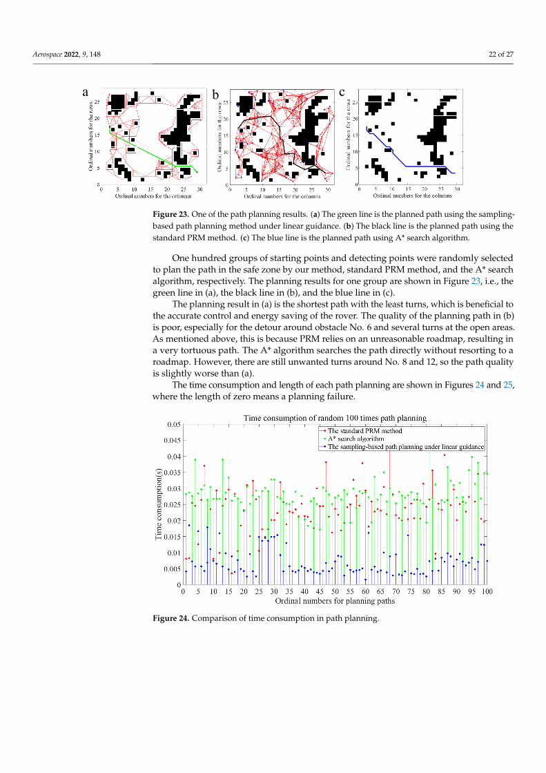
Aerospace 2022, 9, 148 22 of 27
Aerospace 2022, 9, x FOR PEER REVIEW 23 of 29
Figure 22. Distribution of key sampling points.
Shape points (blue dots in Figure 22) are distributed in the protruding part of the
obstacle, while distance points (red dots in Figure 22) are distributed at the long edge or
in the concave part of the obstacle. Both of these types of sampling points constitute the
key feature of the obstacles in the whole map. More importantly, some points locate in
narrow channels (between obstacle No. 2 and 3, 21 and 23, etc.), which helps to form
connected paths for the roadmap. There are no sampling points in the open area, so that
the redundancy of the roadmap is reduced.
4.2.2. Roadmap Construction and Path Planning
In this section, the A* searching algorithm and the standard PRM are applied to
verify the proposed method. The A* searching algorithm is the latest baseline method
for the path planning of the lunar rover, which is applied in “Yutu‐2”, the lunar rover in
China’s Chang’e 4 mission to the Moon. In addition, the process of constructing a
roadmap in our method is similar to that of PRM, the efficient and popular method in
robotic path planning. Thus, we chose these two methods to compare with our method,
and verify the advantages of our method in time consuming and path quality.
After 133 sampling points were selected within the safe zone (Figure 22), the
roadmap was constructed, shown as red lines in Figure 23a. For comparison, we also
randomly sampled 133 points in the safe zone to construct the roadmap of PRM, shown
as red lines in Figure 23b. We can see that the connected paths of PRM cannot completely
cover the safe zone. For example, there are numerous unconnected areas on the top left of
obstacle No. 2, above No. 15, and on the right of No. 23. It is difficult to plan a feasible
path to reach these areas because the planning result of PRM only consists of connected
paths. In contrast, the roadmap constructed by our method forms a good envelope
around obstacles, resulting in good connectivity. Furthermore, our method allows the
planning result to be out of the roadmap in open areas, avoiding unnecessary turns
caused by inappropriate sampling points.
a b c
Figure 23. One of the path planning results. (a) The green line is the planned path using the sam‐
pling‐based path planning method under linear guidance. (b) The black line is the planned path
using the standard PRM method. (c) The blue line is the planned path using A* search algorithm.
0 5 10 15 20 25 30Ordinal numbers for the columns
0
5
10
15
20
25
Ord
inal
num
bers
for
the
row
s
Figure 23. One of the path planning results. (a) The green line is the planned path using the sampling-based path planning method under linear guidance. (b) The black line is the planned path using thestandard PRM method. (c) The blue line is the planned path using A* search algorithm.
One hundred groups of starting points and detecting points were randomly selectedto plan the path in the safe zone by our method, standard PRM method, and the A* searchalgorithm, respectively. The planning results for one group are shown in Figure 23, i.e., thegreen line in (a), the black line in (b), and the blue line in (c).
The planning result in (a) is the shortest path with the least turns, which is beneficial tothe accurate control and energy saving of the rover. The quality of the planning path in (b)is poor, especially for the detour around obstacle No. 6 and several turns at the open areas.As mentioned above, this is because PRM relies on an unreasonable roadmap, resulting ina very tortuous path. The A* algorithm searches the path directly without resorting to aroadmap. However, there are still unwanted turns around No. 8 and 12, so the path qualityis slightly worse than (a).
The time consumption and length of each path planning are shown in Figures 24 and 25,where the length of zero means a planning failure.
Aerospace 2022, 9, x FOR PEER REVIEW 24 of 29
One hundred groups of starting points and detecting points were randomly select‐
ed to plan the path in the safe zone by our method, standard PRM method, and the A*
search algorithm, respectively. The planning results for one group are shown in Figure
23, i.e., the green line in (a), the black line in (b), and the blue line in (c).
The planning result in (a) is the shortest path with the least turns, which is benefi‐
cial to the accurate control and energy saving of the rover. The quality of the planning
path in (b) is poor, especially for the detour around obstacle No. 6 and several turns at
the open areas. As mentioned above, this is because PRM relies on an unreasonable
roadmap, resulting in a very tortuous path. The A* algorithm searches the path directly
without resorting to a roadmap. However, there are still unwanted turns around No. 8
and 12, so the path quality is slightly worse than (a).
The time consumption and length of each path planning are shown in Figures 24
and 25, where the length of zero means a planning failure.
Figure 24. Comparison of time consumption in path planning.
Figure 25. Comparison of the length of the path.
Figure 24. Comparison of time consumption in path planning.

Aerospace 2022, 9, 148 23 of 27
Aerospace 2022, 9, x FOR PEER REVIEW 24 of 29
One hundred groups of starting points and detecting points were randomly select‐
ed to plan the path in the safe zone by our method, standard PRM method, and the A*
search algorithm, respectively. The planning results for one group are shown in Figure
23, i.e., the green line in (a), the black line in (b), and the blue line in (c).
The planning result in (a) is the shortest path with the least turns, which is benefi‐
cial to the accurate control and energy saving of the rover. The quality of the planning
path in (b) is poor, especially for the detour around obstacle No. 6 and several turns at
the open areas. As mentioned above, this is because PRM relies on an unreasonable
roadmap, resulting in a very tortuous path. The A* algorithm searches the path directly
without resorting to a roadmap. However, there are still unwanted turns around No. 8
and 12, so the path quality is slightly worse than (a).
The time consumption and length of each path planning are shown in Figures 24
and 25, where the length of zero means a planning failure.
Figure 24. Comparison of time consumption in path planning.
Figure 25. Comparison of the length of the path. Figure 25. Comparison of the length of the path.
Figure 24 shows that, compared with the other two methods, our method has greatadvantage in time because local paths to bypass obstacles are searched in parallel in theroadmap. Figure 25 shows that our method can get slightly better results in length. Table 4lists the detailed comparison of these three methods. It can be seen that our method has ahigher success rate compared with the standard PRM method. The average path-planningtime consumptions of our method reduce 69.25% and 74.71% compared with PRM and A*search algorithm, respectively. The average length shortens 19.89% compared with PRMand is nearly equal with the A* search algorithm, which always finds the shortest path.
Table 4. Comparison of algorithm performance.
MethodThe Construction Time
of Roadmap [s]
100 Times Path Planning
The AveragePath-Planning Time [s]
The Average Length ofthe Planned Path [m] Success Rate
The standard PRM method 0.034 0.023 31.18 82%A* search algorithm - 0.028 25.79 >99%
Our method 0.031 0.007 24.98 >99%
4.2.3. Verification of Map Extension
In this section, we verified the efficiency of our proposed map extension strategy forthe continual addition of environmental information. Assuming that Figure 16 is the initialmap, we gradually added three new sub-maps to the initial map, where the red, blue,and yellow boxes represent the first, second, and third updates, respectively, as shown inFigure 26a. We conducted 50 groups of planning experiments, each of which carried outfull-map reconstruction planning and our map-extension planning for three map updates,respectively. Here, full-map reconstruction means that the added submap and the initialmap are regarded as a new whole map for roadmap reconstruction. The roadmaps foreach map update, as well as a group of planning results, are shown sequentially fromFigure 26b–d.
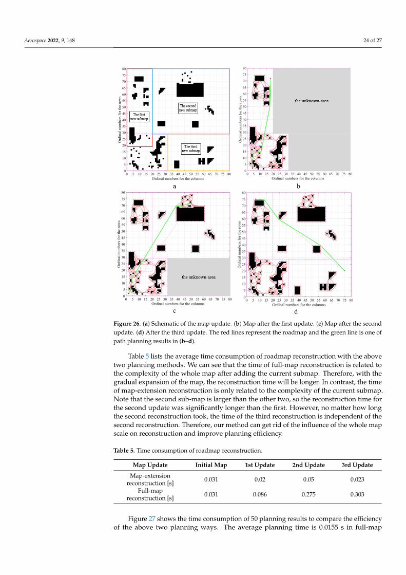
Aerospace 2022, 9, 148 24 of 27Aerospace 2022, 9, x FOR PEER REVIEW 26 of 29
Figure 26. (a) Schematic of the map update. (b) Map after the first update. (c) Map after the second
update. (d) After the third update. The red lines represent the roadmap and the green line is one of
path planning results in (b)–(d).
Table 5 lists the average time consumption of roadmap reconstruction with the
above two planning methods. We can see that the time of full‐map reconstruction is re‐
lated to the complexity of the whole map after adding the current submap. Therefore,
with the gradual expansion of the map, the reconstruction time will be longer. In con‐
trast, the time of map‐extension reconstruction is only related to the complexity of the
current submap. Note that the second sub‐map is larger than the other two, so the re‐
construction time for the second update was significantly longer than the first. However,
no matter how long the second reconstruction took, the time of the third reconstruction is
independent of the second reconstruction. Therefore, our method can get rid of the in‐
fluence of the whole map scale on reconstruction and improve planning efficiency.
Table 5. Time consumption of roadmap reconstruction.
Map Update Initial Map 1st Update 2nd Update 3rd Update
Map‐extension
reconstruction [s] 0.031 0.02 0.05 0.023
Full‐map
reconstruction [s] 0.031 0.086 0.275 0.303
Figure 27 shows the time consumption of 50 planning results to compare the effi‐
ciency of the above two planning ways. The average planning time is 0.0155 s in
Figure 26. (a) Schematic of the map update. (b) Map after the first update. (c) Map after the secondupdate. (d) After the third update. The red lines represent the roadmap and the green line is one ofpath planning results in (b–d).
Table 5 lists the average time consumption of roadmap reconstruction with the abovetwo planning methods. We can see that the time of full-map reconstruction is related tothe complexity of the whole map after adding the current submap. Therefore, with thegradual expansion of the map, the reconstruction time will be longer. In contrast, the timeof map-extension reconstruction is only related to the complexity of the current submap.Note that the second sub-map is larger than the other two, so the reconstruction time forthe second update was significantly longer than the first. However, no matter how longthe second reconstruction took, the time of the third reconstruction is independent of thesecond reconstruction. Therefore, our method can get rid of the influence of the whole mapscale on reconstruction and improve planning efficiency.
Table 5. Time consumption of roadmap reconstruction.
Map Update Initial Map 1st Update 2nd Update 3rd Update
Map-extensionreconstruction [s] 0.031 0.02 0.05 0.023
Full-mapreconstruction [s] 0.031 0.086 0.275 0.303
Figure 27 shows the time consumption of 50 planning results to compare the efficiencyof the above two planning ways. The average planning time is 0.0155 s in full-map
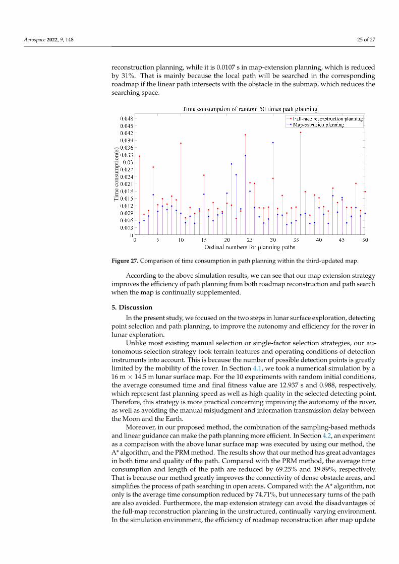
Aerospace 2022, 9, 148 25 of 27
reconstruction planning, while it is 0.0107 s in map-extension planning, which is reducedby 31%. That is mainly because the local path will be searched in the correspondingroadmap if the linear path intersects with the obstacle in the submap, which reduces thesearching space.
Aerospace 2022, 9, x FOR PEER REVIEW 27 of 29
full‐map reconstruction planning, while it is 0.0107 s in map‐extension planning, which
is reduced by 31%. That is mainly because the local path will be searched in the corre‐
sponding roadmap if the linear path intersects with the obstacle in the submap, which
reduces the searching space.
Figure 27. Comparison of time consumption in path planning within the third‐updated map.
According to the above simulation results, we can see that our map extension
strategy improves the efficiency of path planning from both roadmap reconstruction and
path search when the map is continually supplemented.
5. Discussion
In the present study, we focused on the two steps in lunar surface exploration, de‐
tecting point selection and path planning, to improve the autonomy and efficiency for the
rover in lunar exploration.
Unlike most existing manual selection or single‐factor selection strategies, our au‐
tonomous selection strategy took terrain features and operating conditions of detection
instruments into account. This is because the number of possible detection points is
greatly limited by the mobility of the rover. In Section 4.1, we took a numerical simula‐
tion by a 16 m × 14.5 m lunar surface map. For the 10 experiments with random initial
conditions, the average consumed time and final fitness value are 12.937 s and 0.988, re‐
spectively, which represent fast planning speed as well as high quality in the selected
detecting point. Therefore, this strategy is more practical concerning improving the au‐
tonomy of the rover, as well as avoiding the manual misjudgment and information
transmission delay between the Moon and the Earth.
Moreover, in our proposed method, the combination of the sampling‐based meth‐
ods and linear guidance can make the path planning more efficient. In Section 4.2, an
experiment as a comparison with the above lunar surface map was executed by using our
method, the A* algorithm, and the PRM method. The results show that our method has
great advantages in both time and quality of the path. Compared with the PRM method,
the average time consumption and length of the path are reduced by 69.25% and 19.89%,
respectively. That is because our method greatly improves the connectivity of dense ob‐
stacle areas, and simplifies the process of path searching in open areas. Compared with
the A* algorithm, not only is the average time consumption reduced by 74.71%, but un‐
necessary turns of the path are also avoided. Furthermore, the map extension strategy
can avoid the disadvantages of the full‐map reconstruction planning in the unstructured,
Tim
e co
nsum
ptio
n(s)
Figure 27. Comparison of time consumption in path planning within the third-updated map.
According to the above simulation results, we can see that our map extension strategyimproves the efficiency of path planning from both roadmap reconstruction and path searchwhen the map is continually supplemented.
5. Discussion
In the present study, we focused on the two steps in lunar surface exploration, detectingpoint selection and path planning, to improve the autonomy and efficiency for the rover inlunar exploration.
Unlike most existing manual selection or single-factor selection strategies, our au-tonomous selection strategy took terrain features and operating conditions of detectioninstruments into account. This is because the number of possible detection points is greatlylimited by the mobility of the rover. In Section 4.1, we took a numerical simulation by a16 m × 14.5 m lunar surface map. For the 10 experiments with random initial conditions,the average consumed time and final fitness value are 12.937 s and 0.988, respectively,which represent fast planning speed as well as high quality in the selected detecting point.Therefore, this strategy is more practical concerning improving the autonomy of the rover,as well as avoiding the manual misjudgment and information transmission delay betweenthe Moon and the Earth.
Moreover, in our proposed method, the combination of the sampling-based methodsand linear guidance can make the path planning more efficient. In Section 4.2, an experimentas a comparison with the above lunar surface map was executed by using our method, theA* algorithm, and the PRM method. The results show that our method has great advantagesin both time and quality of the path. Compared with the PRM method, the average timeconsumption and length of the path are reduced by 69.25% and 19.89%, respectively.That is because our method greatly improves the connectivity of dense obstacle areas, andsimplifies the process of path searching in open areas. Compared with the A* algorithm, notonly is the average time consumption reduced by 74.71%, but unnecessary turns of the pathare also avoided. Furthermore, the map extension strategy can avoid the disadvantages ofthe full-map reconstruction planning in the unstructured, continually varying environment.In the simulation environment, the efficiency of roadmap reconstruction after map update

Aerospace 2022, 9, 148 26 of 27
has been improved by orders of magnitude, while the time for full-map reconstruction stilldepends on the accumulation of each reconstruction from the initial map to the currentupdate. In addition, the time for map extension-based planning is also reduced by 31%compared with the full-map planning. This improvement is mainly due to the use of theroadmap’s local characteristics in path searching, which avoids invalid searches in the otheradded submaps.
Despite the great improvement in the autonomy and planning efficiency, there arestill some limitations in our method. Firstly, for the map extension strategy, the specialcase where a common part exists between the initial map and the submap has not beenconsidered. In this case, the submap needs to be divided to ensure that the added submapis completely new concerning the initial map. Secondly, our method is applied in a two-dimensional environment, and we hope to extend it to a three-dimensional case withappropriate improvements. These two topics will be our future concerns.
6. Conclusions
In this paper, we proposed an autonomous task planning method for the lunar roverin a complex environment. Considering the equipment requirements and terrain features,a strategy for autonomous selection of detecting points is designed, where the safe zone forthe rover’s motion is defined, and within it the detecting points can be selected. Accordingto the characteristics and distribution of obstacles in the environment, the safe zone isdivided into two kinds of area, the open area and the dense obstacle area. Then the pointsare sampled in the dense obstacle area to construct the local roadmap. A feasible path fromthe current position to the detecting point can be planned by combining the linear pathwith local paths searched within the roadmap. In addition, taking into consideration thechange of the unstructured lunar environment and the enlargement of the detecting area,a map extension strategy is proposed to further improve our path planning method in areal environment. The contributions of this paper mainly include: (1) The autonomousdetecting points selection strategy is proposed, with terrain and instrument requirementstaken into consideration. (2) The sampling-based path planning method under linearguidance can reduce the time for roadmap construction and the planning process, and sothe planning efficiency can be greatly improved with high connectivity and high planningsuccess rate. (3) The map extension strategy can deal with the expansions and changes ofthe map, further improving the planning capacity and efficiency. The insights from thisstudy may contribute to the task planning of surface rovers for extraterrestrial objects.
Author Contributions: Conceptualization, G.C. and H.Y.; methodology, Z.H.; software, H.Y.; vali-dation, Z.H., J.F. and Y.W.; formal analysis, J.F.; investigation, H.Y.; resources, G.C.; data curation,Z.H.; writing—original draft preparation, H.Y.; writing—review and editing, G.C.; visualization,Z.H.; supervision, Y.W.; project administration, H.Y.; funding acquisition, C.L. All authors have readand agreed to the published version of the manuscript.
Funding: This study was co-supported by the Research Fund of the Manned Space Engineering(No. 18051030101), the National Natural Science Foundation of China (No. 62173044), State Admin-istration of Science Technology and Industry for National Defense (No. HTKJ2019KL502012), theScience and Technology Foundation of State Key Laboratory (No. 19NY1208), and BUPT ExcellentPh.D. Students Foundation (CX2021119).
Institutional Review Board Statement: Not applicable.
Informed Consent Statement: Not applicable.
Data Availability Statement: Not applicable.
Acknowledgments: The authors would like to thank the reviewer for their valuable comments andsuggestions that greatly improve our paper. Special thanks to Yu Cheng for the careful revision inthe writing.
Conflicts of Interest: The authors declare no conflict of interest.

Aerospace 2022, 9, 148 27 of 27
References1. Wang, M.C.; Song, Z.M.; Dai, G.M.; Peng, L.; Zheng, C. Asteroids Exploration Trajectory Optimal Design with Differential
Evolution Based on Mixed Coding. Int. J. Distrib. Sens. Netw. 2015, 2015, 1–8. [CrossRef]2. Tom, E.; Pierre, L.; Yin, H.R. Dynamic Anchoring in Soft Regolith: Testing and Prediction. J. Aerosp. Eng. 2018, 31, 04017087.3. Burns, J.O.; Benjamin, M.; Matthew, S. Science on the lunar surface facilitated by low latency telerobotics from a Lunar Orbital
Platform-Gateway. Acta Astronaut. 2019, 154, 195–203. [CrossRef]4. Xing, Y.; Teng, B.Y.; Liu, X. Guidance, Navigation and Control Technology for Lunar Surface Exploration. Chin. J. Space Sci. 2016,
36, 196–201.5. Zhao, N.; Zhu, P.M.; Yuan, Y.F. The shallow subsurface structures of Chang’E-3 landing site based on the wavefield characteristics
of LPR Channel-2B data. Adv. Space Res. 2018, 62, 884–889. [CrossRef]6. Wang, L.W.; Guo, D.W.; Zhang, Z.; Lyu, Z.H.; Zhao, M.; Liu, Y. Introduction to NASA’s Artemis Lunar Exploration Program.
Spacecr. Recovery Remote Sens. 2020, 41, 12.7. Dai, Z.P. Small-Scale Complex Environment Perception and Terrain Modeling for Patrol and Exploration Missions; Hubei University of
Technology: Wuhan, China, 2020.8. Di, K.C.; Wang, J.; Xing, Y.; Liu, Z.; Wan, W.; Peng, M.; Wang, Y.; Liu, B.; Yu, T.; Li, L.; et al. Progresses and prospects of
environment perception and navigation for deep space exploration rovers. Acta Geod. Cartogr. Sin. 2021, 50, 12.9. Gao, W.; Cai, D.B.; Zhou, J.P.; Gao, Y.; Yin, M. Activity planning method for Chang’ E-3 “Jade Rabbit” rover. J. Beijing Univ.
Aeronaut. Astronaut. 2017, 43, 277–284.10. Li, L.H.; Lian, J.; Huang, H.Y. Traversability based obstacle avoidance path-planning and path-following control for lunar rover. J.
Intell. Fuzzy Syst. Appl. Eng. Technol. 2015, 28, 547–559. [CrossRef]11. Garrido, S.; Martin, F.; Alvarez, D.; Moreno, L. Towards an Anisotropic Fast Marching Method applied to the Path Planning Task
for Mars Rovers. In Proceedings of the 6th International Conference on Space Mission Challenges for Information Technology(SMC-IT), Madrid, Spain, 27–29 September 2017; pp. 13–19.
12. Zhou, L.F.; Yang, L.N.; Tang, H.W. Research on Path Planning Algorithm and Its Application Based on Terrain Slope for SlippingPrediction in Complex Terrain Environment. In Proceedings of the 2017 International Conference on Security, Pattern Analysis,and Cybernetics (SPAC), Shenzhen, China, 15–17 December 2017; pp. 224–227.
13. Kosek, F.; Culka, A.; Drahota, P. Applying portable Raman spectrometers for field discrimination of sulfates: Training forsuccessful extraterrestrial detection. J. Raman Spectrosc. 2017, 48, 1085–1093. [CrossRef]
14. Hewitt, R.A.; Ellery, A.; Ruiter, D.A. Training a terrain traversability classifier for a planetary rover through simulation. Int. J. Adv.Robot. Syst. 2017, 14, 1–14. [CrossRef]
15. Orger, N.C.; Yin, Y.; Chen, Z. Dynamic analysis for peg-in-hole assembly with contact deformation. Int. J. Adv. Manuf. Technol.2006, 30, 118–128.
16. Wu, W.R.; Zhou, J.L. Key Technologies in Teleoperation of the “Yutu” lunar rover. Sci. Sin. Inf. 2014, 44, 425–440.17. Wang, K.W.; Peng, S. Study on Path Planning of Lunar Rover Based on A* Algorithm Optimization. Spacecr. Eng. 2019, 28, 19–26.18. Seo, M.G.; Hong, S.M.; Tahk, M.J. Lunar Lander Landing Site Decision in Low-Fuel Case. MATEC Web Conf. 2016, 54, 9003.
[CrossRef]19. Saito, M.; Nonaka, K.; Sekiguchi, K. Optimal Path Planning utilizing Dissipation Function based on Terrain Elevation Map of
lunar rovers. In Proceedings of the 2017 11th Asian Control Conference (ASCC), Gold Coast, Australia, 17–20 December 2017;pp. 394–399.
20. Amato, N.M.; Bayazit, O.B.; Dale, L.K. OBPRM: An Obstacle-Based PRM for 3D Workspaces. In Proceedings of the 3rd Workshopon the Algorithmic Foundations of Robotics on Robotics, Houston, TX, USA, 5–7 March 1998; pp. 155–168.
21. David, H.; Jiang, T.T.; John, R. The bridge test for sampling narrow passages with probabilistic roadmap planners. In Proceedingsof the 2003 IEEE International Conference on Robotics and Automation (Cat. No. 03CH37422), Taipei, China, 14–19 September2003; Volume 3, pp. 4420–4426.
22. Fareh, R.; Baziyad, M.; Rabie, T. Enhancing Path Quality of Real-Time Path Planning Algorithms for Mobile Robots: A SequentialLinear Paths Approach. IEEE Access 2020, 8, 167090–167104. [CrossRef]
23. Speyerer, E.J.; Lawrence, J.D.; Stopar, J.D. Optimized traverse planning for future polar prospectors based on lunar topography.Icarus 2017, 273, 337–345. [CrossRef]
24. Li, Q.H.; Pan, F.; Zhao, Z.G. Process Modeling and Monitoring with Incomplete Data Based on Robust Probabilistic Partial LeastSquare Method. IEEE Access 2018, 6, 10160–10168. [CrossRef]
25. Ryu, H.; Chung, W.K. Local map-based exploration using a breadth-first search algorithm for mobile robots. Int. J. Precis. Eng.Manuf. 2015, 16, 2073–2080. [CrossRef]
26. Zhang, T.; Xu, H.X. Path Planning for Lunar Rover Parking in Place to Probe. Comput. Simul. 2017, 34, 110–114.27. Zhang, J.T.; Yang, F.X.; Weng, X. An Evolutionary Scatter Search Particle Swarm Optimization Algorithm for the Vehicle Routing
Problem with Time Windows. IEEE Access 2018, 6, 63468–63485. [CrossRef]28. Lozano-Perez, T.; Wesley, M.A. An Algorithm for Planning Collision-Free Paths Among Polyhedral Obstacles. Commun. ACM
1979, 22, 560–570. [CrossRef]


![Practical Product Path Guiding Using Linearly Transformed ...€¦ · our data structures to effectively guide such sampling decisions, without storing the complete path [RHJD18].](https://static.cupdf.com/doc/110x72/5f57497a81f37b5d6f4189d8/practical-product-path-guiding-using-linearly-transformed-our-data-structures.jpg)
