A GENERALIZED FLUIDIZED BED REACTOR MODEL ACROSS THE FLOW REGIMES
by
IBRAHIM A. ABBA
B.Eng., Ahmadu Bello University, Nigeria, 1991 M.Sc, University of Petroleum & Minerals, Saudi Arabia, 1995
A THESIS SUBMITTED IN PARTIAL FULFILMENT O F
T H E REQUIREMENTS FOR T H E D E G R E E OF
D O C T O R O F PHILOSOPHY
in
T H E FACULTY OF G R A D U A T E STUDIES
Department of Chemical and Biological Engineering
We accept this thesis as conforming to the required standard
T H E UNIVERSITY OF BRITISH COLUMBIA
July, 2001
© Ibrahim Abba, 2001
In presenting this thesis in partial fulfilment of the requirements for an advanced
degree at the University of British Columbia, I agree that the Library shall make it
freely available for reference and study. I further agree that permission for extensive
copying of this thesis for scholarly purposes may be granted by the head of my
department or by his or her representatives. It is understood that copying or
publication of this thesis for financial gain shall not be allowed without my written
permission.
Department of
The University of British Columbia Vancouver, Canada
Date
DE-6 (2/88)

A b s t r a c t
A large number of industrial catalytic and non-catalytic processes employ
fluidized beds, and newer and more challenging applications are emerging. Driven by the
growth in applications and the challenges they bring, reliable reactor models for fluidized
beds are vital for the design, scale-up and optimal operation of these processes.
Traditionally, models are often developed with a particular process in mind based on
consideration of the operating conditions and flow regime of fluidization, with the range
of applicability limited to the cases tested. The complexity is compounded by the
existence of distinctly different flow regimes. Considerable uncertainty exists in flow
regime transition criteria, and most existing models predict discontinuities at the
boundaries, contrary to experimental evidence. In addition, most practically important
fluid bed reactors involve complex reactions, sometimes accompanied by significant
volume change, with selectivity critical. However, there are few attempts to evaluate
reactor model performance using commercial-scale data with selectivity as a criterion.
In this research, sponsored by the Mitsubishi Chemical Corporation in Japan, a new
generic fluid bed reactor (GFBR) model is developed applicable across the flow regimes
most commonly encountered in industrial scale fluid bed reactors: bubbling, turbulent
and fast fluidization. The model interpolates between three regime-specific models - the
generalized two-phase bubbling bed model, dispersed plug flow, and the generalized
core-annulus model - by probabilistic averaging of hydrodynamic and dispersion
variables based on the uncertainty in the flow regime transitions. Predictions of
hydrodynamic variables across the three fluidization flow regimes are realistic, while
conversion predictions are in good agreement with available experimental data. The
probabilistic approach leads to improved predictions of reactor performance compared
with any of the three separate models for individual flow regimes, while overcoming the
difficulties in predicting the transition boundaries among these flow regimes and
avoiding discontinuities at these boundaries.
Model predictions of selectivities, yields and conversions for two industrial-scale
processes (oxidation of naphthalene to phthalic anhydride and oxy-chlorination of
ethylene) are reasonable and compare favourably with available plant data. Ability of the
model to aid in simulation experimentation over a wide range of conditions is
ii
demonstrated. Model predictions are strongly influenced by the reaction kinetics, gas
dispersion, superficial gas velocity and reactor temperature. Their accuracy strongly
depends on utilizing reliable estimates of the model parameters. Accounting for the
volume change due to reaction, caused by a change in the number of moles as well as
variations in temperature and pressure along the reactor, improves the performance of the
model relative to industrial data. Multiple flow regimes can exist in the same reactor due
to changing volumetric flow. The probabilistic modeling approach is shown to effectively
track such changes.
Application of the GFBR model to gas-solid reactions is demonstrated by coupling a
single-particle model with the generic fluid bed reactor model. Predictions from the
combined model for the zinc sulfide roasting process are reasonable. However, in order
to fully realize the potential of the combined model, some extensions are required.
Gas mixing experiments were conducted using both steady state and step change
tracer injection in a 4.4 m high and 0.286 m ID column to provide better understanding of
the effects of dispersion in each phase, as well as interphase mass transfer, with
increasing gas velocities. Data interpretation using a one-dimensional single-phase model
and a generalized two-phase model confirmed the expected trends of increasing
dispersion in both the low- and high-density phases as the superficial gas velocity is
increased. Beyond the transition velocity, Uc, however, the dispersion coefficients
decreased in some cases.
The GFBR model provides a means of predicting hydrodynamics states and quantities
in reactors. For given particle properties, operating conditions and reactor geometry, it is
possible to predict the flow regime(s) and key hydrodynamic and thermal properties. The
model is a useful tool for the design and simulation of fluid bed processes. Further pursuit
of the probabilistic modeling approach is well warranted.
i i i
T a b l e o f C o n t e n t s
Abstract "
Table of Contents iv
List of Tables viii
List of Figures x
Acknowledgements xvii
1. Introduction 1
1.1 Hydrodynamic Flow Regimes and Transition Velocities 2
1.2 Fluidized Bed Reactor Models 4 1.2.1 Bubbling bed 4 1.2.2 Turbulent bed 6
1.2.3 Fast Fluidization 7
1.3 Outstanding Issues 8
1.4 Research Objectives 10
1.5 Thesis Layout 11
2. Integrated Approach to FBR Modeling 13
2.1 Introduction 13
2.2. Generic Descriptors: L- and H-phases 14
2.3. Generic Fluid Bed Reactor (GFBR) Model 14 2.3.1 Modeling across Operating Regimes 16
2.3.1.1 Regime-Specific Approach 16 2.3.1.2 Synergistic (Probabilistic) Approach 16
2.3.2 Probabilistic Paradigm 21 2.3.2.1 Introduction and Scope of Application 21 2.3.2.2 Steps in Probabilistic Approach to GFBR modeling 22
2.3.3 Generalized Model Equations 23 2.3.3.1 Mole Balance for the Two-Phases/Regions 23 2.3.3.2 Energy Balance 25 2.3.3.3 Pressure Balance 25
2.3.4 Freeboard Region 25 2.3.4.1 Distribution of Solids Concentration 26 2.3.4.2 Modeling the Freeboard as Dispersed Flow 27
2.3.5 Bed and Phase Balances 28 2.3.6 Representing and Quantifying the Uncertainty in Regime Boundaries 31 2.3.7 Flow Regime Transition Equations 33
iv
2.4 Current Limits of G F B R Model 36
2.5 Numerical Solution Approach 38 2.5.1 general PROcess Modeling System (gPROMS) 38 2.5.2 Implementing the GFBR Model in gPROMS 40
2.6 Remarks on the Application of G F B R Model 43
2.7 Conclusion 44
3. Gas Mixing in Bubbling-Turbulent Fluidized Bed 45
3.1 Introduction 45
3.2 Experimental Studies 45 3.2.1 Experimental Apparatus and Instrumentation 45 3.2.2 Gas Mixing Experiments 47
3.2.2.1 Calibration of Thermal Conductivity Detectors 47 3.2.2.2 Steady State Measurements 50 3.2.2.3 Unsteady State Measurements 50
3.3. Interpretation of Gas Mix ing Data 58 3.3.1 Steady State Measurements 58
3.3.1.1 Single-Phase One-Dimensional Dispersion Model 58 3.3.1.2 One-Dimensional Two-Phase Model with Dispersion 64
3.3.2. Unsteady State Measurements 70 3.3.2.1 Single-Phase Dispersion Model 70 3.3.2.2 Two-Phase Model with Dispersion 75
3.4. Comments on Correlations for Pe z 77
3.5. Conclusions and Recommendations 77
4. Validation of GFBR Model with Ozone Decomposition Data 79
4.1 Introduction 79
4.2 Case study: Ozone Decomposition Reaction 79 4.2.1 Reaction Kinetics and Model Parameters 79 4.2.2 Other Considerations in Applying the GFBR Model to Sun's Data 80 4.2.3 Results and Discussion 82
4.2.3.1 Hydrodynamics 82 4.2.3.2 Reactor Performance 87
(a) Influence of Freeboard on Ozone Conversion 87 (b) Comparison of Predictions from Regime-Specific and Probabilistic Models
91
4.3 Conclusions 91
5. Application of GFBR Model to Industrial-Scale Processes 96
5.1 Phthalic Anhydride Process 96 5.1.1 Model Parameters and Reaction Kinetics 98 5.1.2 Simulation and Comparison with Plant Data 100

5.1.3 Sensitivity Analysis 103 5.1.3.1 Influence of Freeboard 103 5.1.3.2 Effect of Interphase Mass Transfer 106 5.1.3.3 Effect of Gas Dispersion 109 5.1.3.4 Influence of Reaction Rate Constants I l l 5.1.3.5 Influence of Gas Flow 115
5.1.4 Conclusions 117
5.2 Oxy-Chlorination Process 118 5.2.1 Model Parameters and Reaction Kinetics 118 5.2.2 Simulation and comparison with commercial data 121 5.2.3 Sensitivity analysis 123
5.2.3.1 Influence of Freeboard 123 5.2.3.2 Effect of Temperature 127 5.2.3.3 Influence of Gas Flow 127 5.2.3.4 Effect of Interphase Mass Transfer and Gas Dispersion 130 5.2.3.5 Influence of Reaction Rate Constants 130
5.2.4 Conclusions 134
5.3 Gas-Solid Reactions 136 5.3.1. Introduction 136
A. Low velocity flow regimes 136 B. High velocity flow regimes 136
5.3.2. Single Particle Model 137 5.3.2.1 Introduction 137 5.3.2.2 Model Equations 137
5.3.3 Coupling the Reactor and Particle Models 141 5.3.3.1 Overall Conversion of Solids Leaving the Bed 141 5.3.3.2 Accounting for Solids Interchange between the L - and H-Phases 142 5.3.3.3 Overall Material Balance 143
5.3.4 Case Study: Zinc Sulfide Roasting 143 5.3.4.1 Assumptions, Model Parameters and Reaction Kinetics 143 5.3.4.2 Results and Discussion 145
5.3.3 Concluding Remarks 151
6. Implementation of Volume Change with Reaction 152
6.1 Introduction 152
6.2 Modeling Approach 153
6.3 Case Study: Oxy-Chlorination Process 155
6.4 Results and Discussion 157 6.4.1 Effect of volume change on the hydrodynamic variables 157
6.4.1.1 Gas velocity 157 6.4.1.2 Gas flow distribution and phase volume fractions 157 6.4.1.3 Regime probabilities 161
6.4.2 Effect of volume change on the reactor performance 165 6.4.3 Effect of bulk transfer of gas between phases 167
vi
6.5 Conclusions 172
7. Overall Conclusions and Recommendations 173
7.1 Conclusions 173
7.2 Recommendations for Future Work 175
Nomenclature 177
References 184
Appendix A Bed Properties Evaluation Scheme 193
Appendix B. Thermophysical Properties Evaluation Scheme 195
v i i

L i s t o f T a b l e s
Table 2.1. Summary of bed and phase balances 30
Table 2.2. Summary of correlations for regime transition velocities 33
Table 2.3. Summary of regime bounds and transition equations 37
Table 3.1. Fitted values of interphase mass transfer and L- and H-phase axial dispersion coefficients 70
Table 3.2. Initial and boundary conditions for eqs. (3.21) and (3.22) 75
Table 4.1. Operating conditions, hydrodynamic properties and reactor geometry (Details are given by Sun, 1991) 81
Table 5.1 Operating conditions and hydrodynamic properties for the phthalic anhydride process 99
Table 5.2. Reaction kinetics for the naphthalene-based phthalic anhydride process 99
Table 5.3 Comparison of model exit predictions with plant data 103
Table 5.4 Comparison with plant data of exit predictions from GFBR model for cases when the freeboard is included and excluded 106
Table 5.5. Reaction rate constants and the range of variation for the sensitivity analysis I l l
Table 5.6 Sensitivity of the GFBR model predictions to variations in kinetic rate constants. (Results shown are exit values.) 115
Table 5.7. Typical operating conditions, hydrodynamic properties and reactor geometry for the air-based oxy-chlorination process. (All quantities are shown in normalized form; pg and // are based on inlet temperature and pressure.) 120
Table 5.8. Per pass exit model predictions for all cases including the base case (normalized by corresponding plant exit data) 123
viii
Table 5.9 Comparison of per pass exit predictions from the GFBR model for the cases when the freeboard is included and when it is ignored (normalized by exit plant data) 127
Table 5.10 Sensitivity of the model predictions to variations in kinetic rate constants. (Results shown are the exit values normalized by exit plant data.) 134
Table 5.11 Summary of operating conditions and hydrodynamic properties for the zinc sulfide roasting process corresponding to the base case (from Avedesian, 1974; Grace, 1986) 144
Table 5.12. Summary of pertinent variables at reaction completion for 60 um particles. Other properties as in Table 5.11 150
Table 6.1. Four different cases considered for simulating the effects of changes in the number of moles, temperature and pressure on reactor performance.
156
Table 6.2. Comparison of per pass exit model predictions (normalized by exit plant data) for the four cases 165
ix
L i s t o f F i g u r e s
Figure 1.1. Flow patterns in gas-solids fluidized beds (adapted from Grace, 1986): (a) fixed bed; (b) bubbling bed; (c) slug flow; (d) turbulent fluidization; (e) fast fluidization; (f) pneumatic conveying 3
Figure 1.2. Flow regime map for gas-solids fluidization. Heavy lines indicate transition velocities, while shaded regions designate typical operating range of bubbling fluidized beds (Bi and Grace, 1995a) 5
Figure 2.1. Schematic of generalized one-dimensional, two-phase/region model with freeboard (inset shows axial notations for the two regions) 15
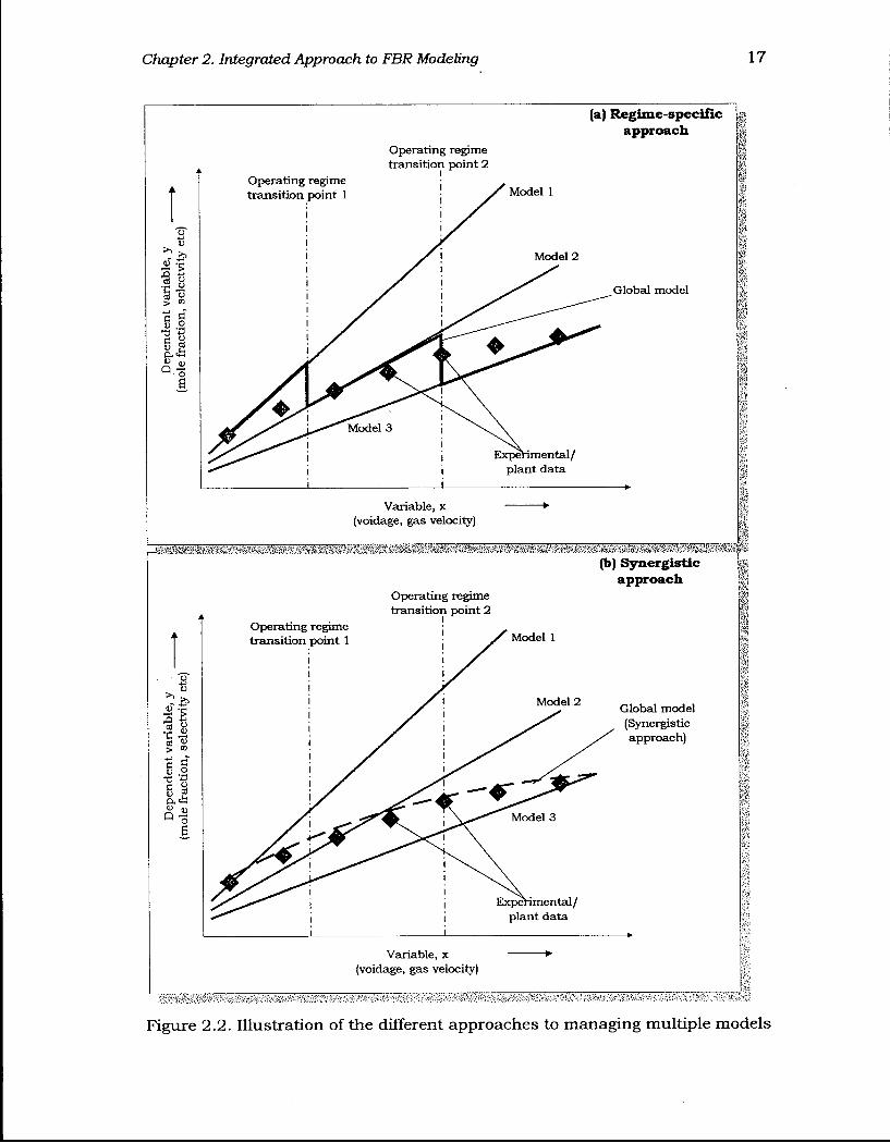
Figure 2.2. Illustration of the different approaches to managing multiple models 17
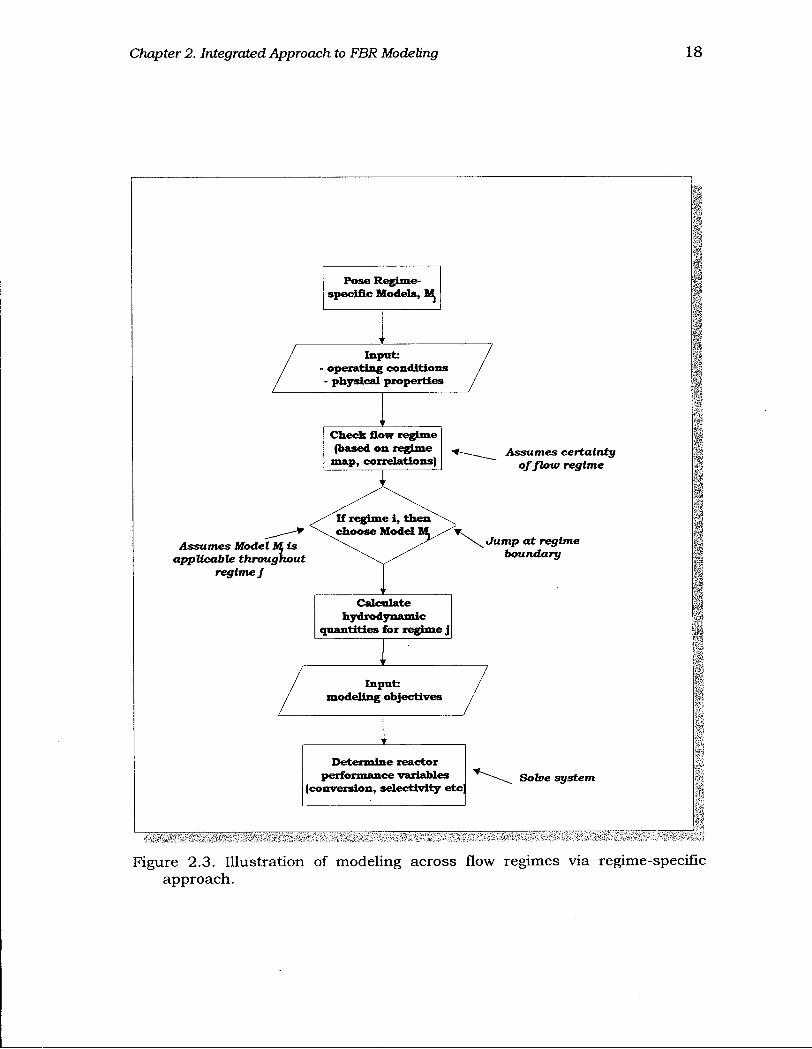
Figure 2.3. Illustration of modeling across flow regimes via regime-specific approach 18
Figure 2.4. Illustration of modeling across flow regimes via probabilistic approach 20
Figure 2.5. Schematic of generalized two-phase/region model with freeboard..29
Figure 2.6. Regime diagram boundaries and regions of uncertainty. Correlations used, from Table 2.2, are: U"c = Re c/ Ar1/3 = 0.74Ar 0 0 9 3 and Ke = R e s e / A r 1 / 3 = 1 .68Ar 0 1 3 6 34
Figure 2.7 (a) Uncertainties in flow regime boundary correlations; b) Probability of being in each regime as a function of dimensionless superficial gas velocity 35
Figure 2.8 Hierarchical structure of modeling languages (adapted from Park, 1998) 39
Figure 2.9 Components of the equation-based modeling language "gPROMS"..41
Figure 2.10 Typical EXCEL screen illustrating the foreign-process-interfacing feature of gPROMS 42
Figure 3.1. Schematic diagram of the pilot scale cold model unit. All dimensions in m (not to scale) 46
Figure 3.2. Schematic of TCD calibration set-up 48
Figure 3.3. Plot of detected signals as a function of volume percent He injected for a) TCD#1, and b) TCD#2. [Signal amplification ratio = 100; Current = 95 mA; TCD sample flow rate = 1.67x10⁻⁶ m3/s.] 49
Figure 3.4. Schematic diagram of steady state tracer injection/detection set-up. 51
Figure 3.5. Radial concentration profiles for tracer: (a) downstream, (b) upstream of injection point. [L0 = 1.0 m, U = 0.2 m/s, tracer injection level 0.654 m above distributor.] 52
Figure 3.6. Radial concentration profiles for tracer: (a) downstream, (b) upstream of injection point. [L0 = 1.0 m, U = 0.3 m/s, tracer injection level 0.654 m above distributor.] 53
Figure 3.7. Radial concentration profiles for tracer: (a) downstream, (b) upstream of injection point. [L0 = 1.0 m, U = 0.4 m/s, tracer injection level 0.654 m above distributor.] 54
Figure 3.8. Radial concentration profiles for tracer: (a) downstream, (b) upstream of injection point. [Lo = 1.0 m, U = 0.5 m/s, tracer injection level 0.654 m above distributor.] 55
Figure 3.9. Contours for the dimensionless He concentration as functions of bed height and radius: (a) downstream, (b) upstream of injection point. [L0 = 1.0 m, U = 0.5 m/s, tracer injection level 0.654 m above distributor.] 56
Figure 3.10. Schematic of unsteady state tracer injection/detection set-up 57
Figure 3.11. Experimental F curves for downstream (detection) measurements for different superficial gas velocities. [Lo= 1.5 m.] 59
Figure 3.12. F and E curves for a) windbox measurements (near entrance to column), b) downstream measurements (near bed surface). [L0= 1.5 m, U = 0.6 m/s; tracer injection is just upstream of 90° elbow (1 m from the distributor) of 6" (150 mm) air line leading to windbox.] 60
Figure 3.13. Plot of log of dimensionless concentration vs. superficial gas velocity for a commercial catalyst with boundary condition at z = 0: (a) included, (b) excluded. [U = 0.4 m/s, L 0 = 1.0 m.] 62
x i
Figure 3.14. Backmixing coefficient as function of superficial gas velocity for a commercial catalyst: analytical solution obtained using Excel with boundary condition at z = 0: (a) included, (b) excluded. [Lo=1.0 m.] 63
Figure 3.15. Backmixing coefficient as function of superficial gas velocity for a commercial catalyst: Solution from gPROMS parameter estimation function [Lo=1.0 m.] 65
Figure 3.16. Two-phase dispersion model predictions of dimensionless concentration vs. experimental data for different superficial gas velocities. [L0= 1.0 m.] 68
Figure 3.17. Axial dispersion and interphase mass transfer coefficients as functions of superficial gas velocity: Solution through gPROMS parameter estimation function [L0 = 1.0 m, 17 = 664 mm.] 69
Figure 3.18. Mean residence time and variance of tracer gas as function of superficial gas velocity [L0=1.5 m.] 71
Figure 3.19 1-D dispersion model predictions of transient dimensionless concentration (F curves) compared with experimental data for different superficial gas velocities. [L0 =1.5 m.] 73
Figure 3.20. Axial dispersion coefficient obtained from gPROMS parameter estimation function as a function of superficial gas velocity for a commercial catalyst. [L0=1.5 m.] 74
Figure 3.21. L- and H-phase axial dispersion coefficients and interphase mass transfer coefficient as functions of superficial gas velocity: Solution via gPROMS parameter estimation [L0=1.5 m.] 76
Figure 4.1. Axial profiles of solids hold-up in column at different superficial gas velocities. Conditions are listed in Table 4.1 83
Figure 4.2. Predicted gas velocities in low- and high-density phases and bed average with increasing superficial gas velocity in the dense bed. Conditions are listed in Table 4.1 84
Figure 4.3. Predicted suspension densities in low- and high-density phases and bed average with increasing superficial gas velocity in the dense bed. Conditions are listed in Table 4.1 85
Figure 4.4. Predicted L-phase fractional gas flow allocation with increasing superficial gas velocity in the dense bed. Conditions are given in Table 4.1.
86
xii

Figure 4.5. Comparison of computed expanded bed heights for the cases when freeboard is included and excluded in the GFBR model 88
Figure 4.6. Predicted axial ozone conversions for the cases when freeboard is included and excluded in the GFBR model at different superficial gas velocities. (kr = 8.95 s1) : 89
Figure 4.7. Comparison of predicted ozone conversions with experimental data for different catalyst activities for cases when freeboard is included and excluded in the GFBR model 90
Figure 4.8. Comparison of predicted conversion trends from individual regime-specific models which switch sharply at regime boundaries with experimental data for kr = 8.95 s-1. Other conditions are given in Table 4.1.
92
Figure 4.9 Comparison of predicted conversions (solid line) using GFBR model with experimental results (points) for kr = 8.95 s1. Other conditions are given in Table 4.1.Regime probabilities (dots) are also indicated 93
Figure 4.10 Predicted and experimental conversion trends: i) individual regime-specific models which switch sharply at regime boundaries; ii) GFBR model. kr = 8.95 s-1. Other conditions are given in Table 4.1 94
Figure 5.1. Reaction pathway for naphthalene oxidation to phthalic anhydride proposed by De Maria et al. (1961) 98
Figure 5.2 Axial concentration profiles of naphthalene (NA), naphthaquinone (NQ), phthalic anhydride (PA) and oxidation products (OP) predicted by the GFBR model. Conditions are given in Tables 5.1 and 5.2 101
Figure 5.3 Predictions of axial profiles of (a) NA conversion and (b) selectivity to PA from the three models: GFBRM, 2PBBM and DPFM for conditions given in Tables 5.1 and 5.2 102
Figure 5.4. Comparison of computed expanded bed heights for cases when freeboard is included and excluded in the GFBR model. [Operating velocity, U = 0.43 m/s; Total reactor height, Lt = 13.7 m.] 104
Figure 5.5. Predicted axial profiles of naphthalene and phthalic anhydride concentrations for cases when freeboard is included in the GFBR model and when it is ignored at different superficial gas velocities. Conditions are given in Tables 5.1 and 5.2 105
xiii
Figure 5.6. Axial profiles of PA concentrations predicted by (a) GFBR model (b) 2PBBM at different values of the dimensionless interphase mass transfer coefficient for conditions given in Tables 5.1 and 5.2 107
Figure 5.7. Predictions of exit PA concentrations from the GFBRM, 2PBBM and DPFM as function of dimensionless interphase mass transfer coefficient for the conditions given in Tables 5.1 and 5.2 108
Figure 5.8. Axial profiles of PA concentration predicted by the GFBR model at different values of the axial Peclet number for conditions given in Tables 5.1 and 5.2 110
Figure 5.9. Axial profiles of PA and NA concentrations for different values of the reaction rate constants varied one at a time: (a) reaction 1, k r i ; (b) reaction 2, krs. Base case conditions are given in Tables 5.1 and 5.2 112
Figure 5.10. (a) Axial profiles of PA and NA concentrations at different values of the reaction rate constant, k r 3; (b) NA conversion, OP yield and selectivities to PA and NQ as a function of k r 3. Base case conditions are given in Tables 5.1 and 5.2 113
Figure 5.11. (a) Axial profiles of PA and NA concentrations at different values of the reaction rate constant, k r4; (b) NA conversion, OP yield and selectivities to PA and NQ as a function of k r4. Base case conditions are given in Tables 5.1 and 5.2 114
Figure 5.12. Predictions of NA conversion and selectivities to PA, NQ and OP from the GFBR model as a function of superficial gas velocity for conditions given in Tables 5.1 and 5.2 116
Figure 5.13. Schematics of the oxy-chlorination processes: (a) air-feed, (b) O2-feed operation 119
Figure 5.14. Reaction pathways for oxy-chlorination reactions 121
Figure 5.15. Axial bed temperature profile normalized by bed-average plant data, Tave, based on conditions in Table 5.7 124
Figure 5.16. Axial conversion profiles of ETY and HC1 normalized by exit plant data for conditions given in Table 5.7 124
Figure 5.17. Axial profiles normalized by exit plant data: (a) selectivities of ETY to EDC, COx and IMP, (b) yields of EDC, COx and IMP for conditions in Table 5.7 125
xiv
Figure 5.18. Normalized model predictions for the six cases in Table 5.8: (a) ETY and HQ conversions, (b) yields of EDC, COx and IMP. Case 0 is the base case in Table 5.8 126
Figure 5.19. Effect of temperature on reactor performance: (a) Normalized conversion of ETY and HC1, (b) Normalized yields of EDC, COx and IMP. (Base case conditions are given in Table 5.7.) 128
Figure 5.20. Predicted ETY conversion and EDC, IMP and COx yields as a function of superficial gas velocity for base case conditions in Table 5.7.129
Figure 5.21. Effect of interphase mass transfer on reactor performance for base case conditions given in Table 5.7: (a) Normalized conversion of ETY and HC1, (b) Normalized yields of EDC, COx and IMP 131
Figure 5.22. Effect of gas dispersion on reactor performance for base case conditions given in Table 5.7: (a) Normalized conversion of ETY and HC1, (b) Normalized yields of EDC, COx and IMP 132
Figure 5.23. Normalized conversion and yields as a function of reaction rate constant, k r 2 , for base case conditions given in Table 5.7 133
Figure 5.23. (a) Schematic of bed, particle and grain (three different scales of space), (b) Schematic of reaction progression for the GPM 138
Figure 5.24. Complete visualization of gas-solid contact in the bed 140
Figure 5.25. Local conversion of grain, x, as function of dimensionless radius and reaction time for: (a) 60 / /m; (b) 200 /jm particles. Other conditions as in Table 5.11 146
Figure 5.26. Dimensionless radial concentration profile of O2 as a function of time for particle of dp=60 fitn;. Other conditions as in Table 5.11 147
Figure 5.27. Comparison of particle conversion with time for two particles sizes for the conditions given in Table 5.11 148
Figure 5.28. Time for complete conversion of individual particles and overall conversion of solids leaving the bed as a function of particle size. Other conditions as in Table 5.11 149
Figure 6.1. Predicted bed-average axial gas velocity profiles [Case 1: u.j=Uj0; Case 2: UJ=UJOXFTJ/FT0; Case 3: UJ=UJOXFTJ/'FTOXT/T0; Case 4: urUjoxFTj/FToxT/ ToxPo/P; j = L&H\ 158
X V
Figure 6.2. Predicted axial gas velocity profiles for case 4 158
Figure 6.3. Predicted axial profiles of gas flow distribution in L-phase for conditions in Table 5.8 and cases in Table 6.1 159
Figure 6.4. Predicted axial profiles of gas flow through both phases for case 4 in Table 7.1 and conditions given in Table 5.8 159
Figure 6.5. Predicted axial profiles for phase volume fractions, y/, for case 4 .160
Figure 6.6. Axial profiles of probability of turbulent fluidization 162
Figure 6.7. Axial profiles of bed temperature 163
Figure 6.8. (a) Axial profiles of regime probabilities for case 4; (b) probability regime diagram based on dimensionless gas velocity 164
Figure 6.9. Axial profiles of ethylene conversion normalized by plant exit conversion for the four cases identified in Table 6.1 166
Figure 6.10. Axial profiles of COx yield normalized by plant exit value for the same cases as in Fig. 6.9 166
Figure 6.11. Schematic of generalized one-dimensional, two-phase/region model 168
Figure 6.12. Axial profiles of the total gas flow Q for the L- and H-phases: (a) case 2, (b) case 4 [ : bulk transfer between phases ignored; : bulk transfer between phases considered] 170
Figure 6.13. Axial profiles normalized by plant exit data for cases 2 and 4: (a) COx yield, (b) ETY conversion[ : bulk transfer between phases ignored; -
: bulk transfer between phases considered] 171
xvi
A c k n o w l e d g e m e n t s
I am deeply indebted to Prof. John R. Grace and Dr. Xiaotao Bi for their excellent all-
around supervision. I also sincerely appreciate the invaluable inputs of Dr. Michael
Thompson on many aspects of this research.
The design and construction of the fluidized bed column used for the gas mixing
experiments in Chapter 3 was a team effort. To Hiroshi Morikawa, for the joint
construction of the column, and to Naoko Ellis, for both the joint construction of the
column and the joint performance of the gas mixing experiments, I say a special thank-
you.
This work was made possible by the financial support from Mitsubishi Chemical
Corporation of Japan, a scholarship awarded by the King Faisal Foundation, Saudi Arabia
and a graduate fellowship awarded by the University, of British Columbia. I sincerely
thank each of these, with gratitude.
A special thanks is also due to the members of the fluidization research group (past
and present), staff in the Chemical Engineering office, workshop and stores, and the
faculty and fellow students in the department for all their support.
Finally, I would like to dedicate this work to my family, both here and away, for
their unconditional support.
xvii

Chapter 1
I n t r o d u c t i o n
Fluidized bed reactors constitute an integral part of the chemical process industries. Over
the years, newer and more challenging applications have been sought, from biochemical
and petrochemical to applications in microelectronics. As applications grow, so do the
challenges and the need for gaining further insight. Reactor models for fluidized beds are
therefore indispensable in the design, scale-up and optimal operation of chemical
processes. Efforts are being made continually to develop new and efficient models and to
refine existing ones. Fluidized bed reactor models range from those based on the simple
"two-phase theory" of Toomey and Johnston (1952) to complex ones based entirely on
solving continuity, momentum and energy equations using fast computers (e.g. Ding and
Gidaspow, 1990).
Despite the voluminous literature in this area (e.g., see Geldart, 1986; Kunii and
Levenspiel, 1991; Geldart and Rhodes, 1992; Grace et al., 1997), a number of reactor
modeling issues remain to be addressed. Traditionally, reactor models have been
constructed and applied to specific processes based on consideration of the operating
conditions and regime of fluidization. However, although criteria for transition to
different flow regimes have been the subject of many studies, they have not yet been
established with certainty, as highlighted in a recent review (Bi et al., 2000). Hence, a
number of questions arise as flow conditions in the fluidized bed change across the flow
regime spectrum as shown in Fig. 1.1: For example, is the concept of bubbles applicable
to flow regimes beyond bubbling? What is the degree of certainty that the bed operates
within a prescribed flow regime for a given set of operating conditions and particle
properties? What mathematical formulation best describes a particular flow regime,
assuming certainty of being in that regime? How are the multiple flow regimes within the
same bed addressed for systems accompanied by changing volumetric flow? How are the
fluidization regimes best identified for different classes of particles?
To address these and other questions, a broad-based reactor model capable of
reliably predicting changes within the bed over a wide range of operating conditions is
1
Chapter 1. Introduction 2
needed. Such a model should be applicable over the fluidization flow regimes of interest
and provide a means of predicting the transition boundaries among these flow regimes,
while giving improved predictions of particle and gas dynamics and of reactor
performance. This is the goal of this project, sponsored by the Mitsubishi Chemical
Corporation (MCC) in the interest of achieving better understanding of the behavior of
gas-phase fluidized bed reactors. An improved model should provide more reliable scale-
up (e.g., for the propane-based acrylonitrile process), rigorous simulation
experimentation of existing processes for performance enhancement and exploration of
alternatives for other processes (e.g., air-based to oxygen-based oxy-chlorination).
We begin with an overview of the pertinent hydrodynamics flow regimes and
transition velocities to set the stage for the model development in Chapter 2. Second,
fluidized bed reactor models constructed for the different flow regimes are briefly
reviewed, from which key outstanding issues are identified. The specific objectives of
this study are then outlined.
1.1 Hydrodynamic Flow Regimes and Transition Velocities
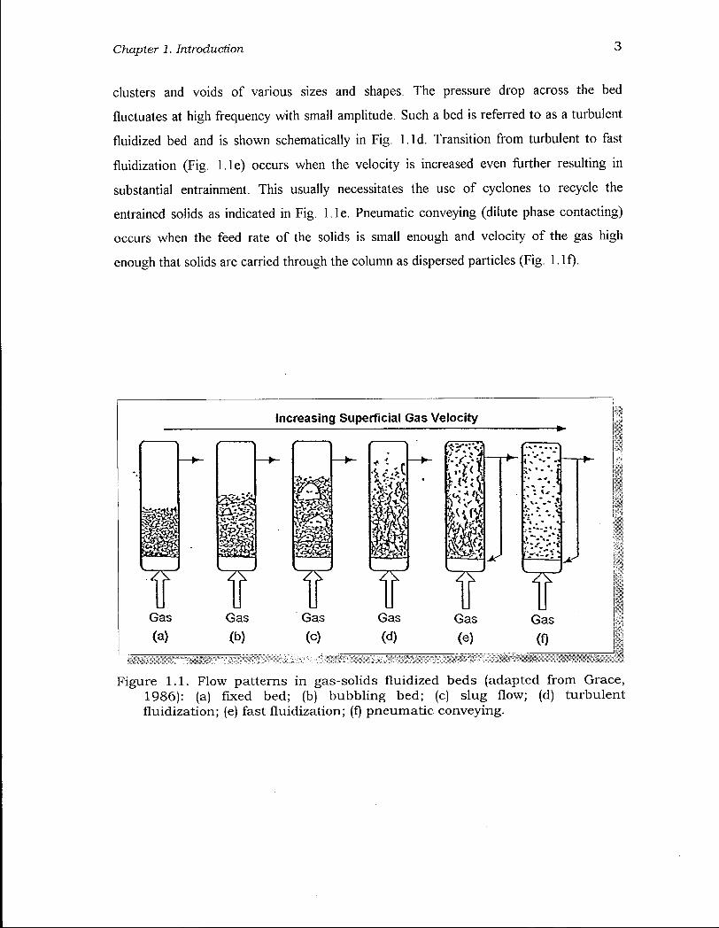
In gas fluidization, a suspension of fine solid particles behaves like a liquid due to upflow
of a gas. If sufficient gas passes upward through the particles, the bed begins to fluidize.
At low velocity, when the gas merely percolates through the interstices in the bed of
stagnant particles, the bed is in a fixed state (Fig. 1.1a). As the velocity is increased, the
bed undergoes transition from a fixed bed to an expanded bed in which the particles
move apart and vibrate in restricted regions and where the particles are just suspended by
the upflowing gas; the bed is then referred to as incipiently fluidized. At higher flows,
bubbles coalesce and grow as they rise to the top of the bed. Because of large bubbles
leaving the column in an irregular manner, the pressure drop across the bed fluctuates
with high amplitude and frequency. Such a bed is called a bubbling fluidized bed as
shown in Fig. 1.1b. The gas bubbles coalesce and grow as they rise and may eventually
become big enough to fill the column cross-section. These large bubbles are called slugs,
and the flow regime is called slugging (see Fig. 1.1c). At sufficiently high velocity, the
upper surface of the bed disappears, and entrainment becomes appreciable. Rapid
coalescence and splitting of bubbles are observed leading to turbulent motion of solid
Chapter 1. Introduction 3
clusters and voids of various sizes and shapes. The pressure drop across the bed
fluctuates at high frequency with small amplitude. Such a bed is referred to as a turbulent
fluidized bed and is shown schematically in Fig. l . ld. Transition from turbulent to fast
fluidization (Fig. l.le) occurs when the velocity is increased even further resulting in
substantial entrainment. This usually necessitates the use of cyclones to recycle the
entrained solids as indicated in Fig. l i e . Pneumatic conveying (dilute phase contacting)
occurs when the feed rate of the solids is small enough and velocity of the gas high
enough that solids are carried through the column as dispersed particles (Fig. I.If).
Figure 1.1. Flow patterns in gas-solids fluidized beds (adapted from Grace, 1986): (a) fixed bed; (b) bubbling bed; (c) slug flow; (d) turbulent fluidization; (e) fast fluidization; (f) pneumatic conveying.
Chapter 1. Introduction 4
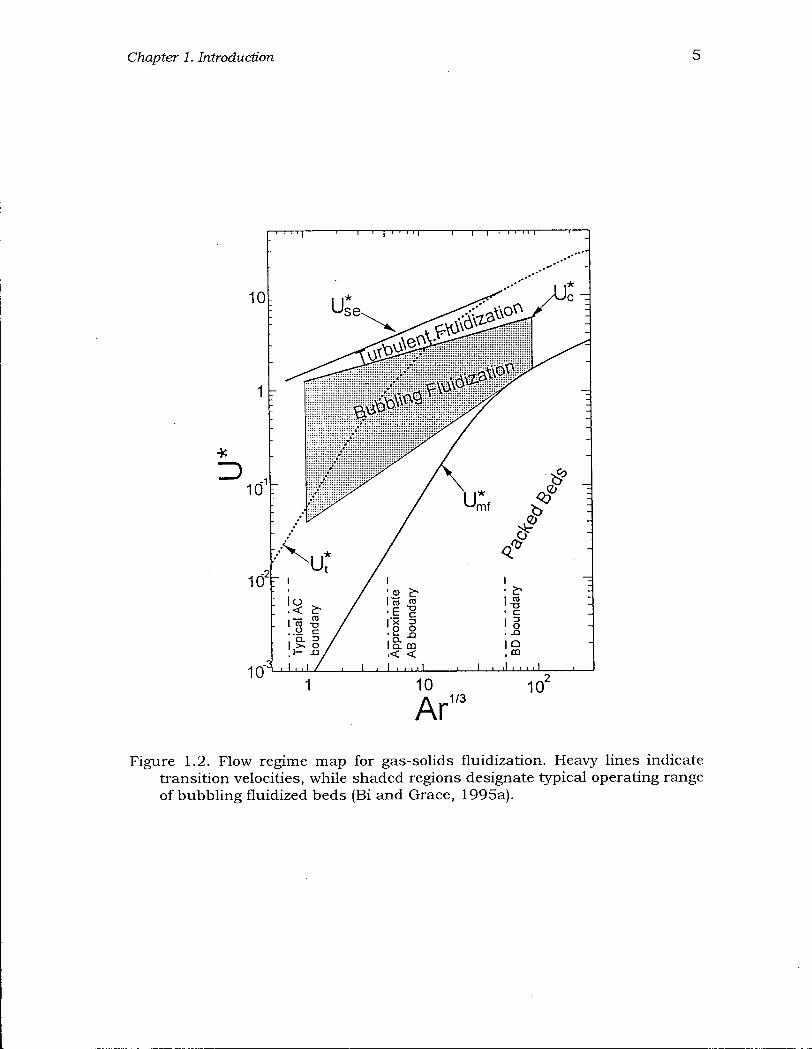
Bi and Grace (1995a) proposed a flow regime diagram capturing all the regimes
as shown in Fig. 1.2. The scope of this thesis is limited to the three principal fluidization
flow regimes: bubbling, turbulent and fast fluidization, as they are by far the most widely
applied by industry. There have been many attempts to establish criteria for regime
transitions (see Yerushalmi and Cankurt, 1979; Bi and Grace, 1995a; Bi et al., 2000). The
following mark the onset of the three regimes of interest in this work:
• Velocity at which bubbles first appear, minimum bubbling velocity, Umb
(Abrahamsen and Geldart, 1980).
• Velocity Uc at which the standard deviation of absolute pressure fluctuations reaches
a maximum (Yerushalmi and Cankurt, 1979; Bi and Grace, 1995b), often used to
demarcate the onset of the turbulent fluidization regime.
• Velocity Use at which significant entrainment of particles occurs (Bi et al., 1995),
thought to denote the onset of the fast fluidization flow regime.
Correlations for determining the Uc and Use transition velocities are presented in Chapter
2, while that for Umb is given in Appendix A. The uncertainty in these correlations is
discussed in Chapter 2.
1.2 Fluidized Bed Reactor Models
Reactor models attempt to obviate the need for experiments by capturing the
physicochemical state of the system through appropriate mathematical representations.
Models can be categorized as either mechanistic or empirical. Mechanistic models
incorporate continuity and energy balances, and are derived mainly on the basis of
detailed understanding of the underlying mechanisms of the process in question.
Empirical models are derived from specific observed behavior of the system with little or
no attention to physical mechanisms. Our focus throughout this thesis is on the former.
1.2.1 Bubbling bed
The bubbling fluidization regime has been extensively studied. The two-phase
theory of fluidization considers the fluid bed as a two-phase system consisting of a
discontinuous phase made up of bubbles and a continuous phase made of a dense mixture
of solid particles and gas, with mass transfer occurring between the two phases (Toomey
Chapter 1. Introduction 5
Figure 1.2. Flow regime map for gas-solids fluidization. Heavy lines indicate transition velocities, while shaded regions designate typical operating range of bubbling fluidized beds (Bi and Grace, 1995a).
Chapter 1. Introduction 6
and Johnston, 1952). Most bubbling bed models are based on this concept, while others
(e.g., Kunii and Levenspiel, 1969) consider clouds around the bubbles as a third phase.
These models can be classified into two-phase models and bubbling bed models. The
bubbling bed models consider the dilute phase as consisting of well-defined bubbles
whose diameters are key parameters, while two-phase models consider the dilute phase as
a continuous system. They incorporate solid fractions, mixing parameters and interchange
coefficients and can be used for modeling and scale-up purposes. Such models include
the Grace (1984) two-phase model, the Kunii and Levenspiel (1969) three-phase model,
the Kato and Wen (1969) bubble assemblage model and the Partridge and Rowe (1966)
cloud model. A modified form of the Kato and Wen model was successful in simulating
the partial oxidation of methane to synthesis gas in a bubbling fluidized bed (Mleczko et
al., 1996; Wurzel and Mleczko, 1998). Because of the extensive literature on this subject,
details of these models are not covered here. They have either been derived or
comprehensively summarized by Grace (1971, 1984, 1986), Kunii and Levenspiel (1991)
and more recently by Marmo et al. (1999).
1.2.2 T u r b u l e n t bed
Because of the advantages of the turbulent regime such as enhanced gas-solids
contacting, reduced gas backmixing and favourable bed-to-surface heat transfer (e.g. see
Massimilla, 1973; Avidan, 1997; Chaouki et al., 1999; Sotudeh-Gharebaagh et al., 1999;
Bi et al., 2000), many commercial fluid bed processes operate in the turbulent fluidization
regime. In addition, the bottom section of fast-fluidized beds is also often considered to
operate in the turbulent fluidization flow regime. Relatively little has been reported on the
reactor performance and modeling for turbulent bed reactors compared to the abundance
of information on bubbling and fast-fluidized bed reactors. Turbulent fluidized bed
reactor models have assumed single phase one-dimensional plug flow (van Swaaij, 1978;
Fane & Wen, 1982), a continuous stirred tank reactor (e.g. Wen, 1984; Hashimoto et al.,
1989), axially dispersed plug flow (Avidan, 1982; Wen, 1984; Edwards & Avidan, 1986;
Li and Wu, 1991; Foka et al., 1994) or two-phase behaviour with interchange of gas
between dilute and dense phases/regions (Krambeck et al., 1987; Foka et al., 1996; Ege et
al., 1996; Venderbosch, 1998; Thompson et al., 1999).
Chapter 1. Introduction 7
For example, Foka et al. (1994) reported satisfactory prediction of conversion in a
catalytic turbulent fluidized bed methane combustor with a single-phase axially dispersed
plug flow model. They showed that the idealized limiting case of perfect mixing (CSTR)
consistently under-predicted the conversion, while the plug flow model over-predicted it,
consistent with experimental evidence on the behaviour of turbulent beds showing that
there is appreciable backmixing of gas, intermediate between these two idealized cases.
The two-phase model with axial dispersion has also been shown to give satisfactory
prediction of methane conversion (Foka et al., 1996) and carbon monoxide conversion
(Venderbosch, 1998) in the turbulent regime. Werther and Wein (1994) considered a
combination of a bubbling bed model to represent the lower dense part of the reactor and
a fast fluidization model for the freeboard. The core-annulus model and its variants have
also been reported to have had some success in accounting for the solids hold-up and the
radial variations in flow structure experimentally observed in turbulent fluidized beds
(e.g. Abed, 1984; Ege et al., 1996; Kunii and Levenspiel, 1997).
Bi et al. (2000) summarized models developed for turbulent fluidized bed
reactors, accounting for interchange of gas between low- and high-density phases, axial
dispersion, gas convection and reaction.
1.2.3 Fast Fluidization
Yerushalmi et al. (1976) coined the term fast fluidization to indicate the flow regime
between turbulent fluidization and pneumatic transport. Since then, circulating fluidized
beds (CFBs), operating in the fast fluidization regime, have developed very quickly.
Hundreds are now in operation for combustion and other chemical reactions. For
example, CFB has been used for direct oxidation of butane to maleic anhydride
(Contractor et al., 1994), pyrolysis (Berg, 1989) and combustion of fuels (Itoh et al.,
1991).
Not surprisingly, many CFB reactor models have been proposed. Models can be
broadly classified into single-region one-dimensional models and distinctly two-region
models with and without allowance for hydrodynamic axial gradients. Some single-
region models completely ignore radial and axial gradients, assuming plug flow of gas
(e.g., Ouyang et al., 1995), while others allow for axial gradient (e.g., Arena et al., 1995).
Chapter 1. Introduction 8
Single region models have generally not been very successful as they do not give good
description of actual behavior in CFB reactors. Two-region models are more realistic as
there is ample evidence that there exist distinct dilute core and dense annular regions,
especially for fully developed conditions (Ouyang et al., 1995; Schoenfelder et al., 1996).
Models in this category include those that ignore axial hydrodynamic gradients (Brereton,
et al., 1988, Kagawa et al., 1991) and those that consider axial gradients (Pugsley, et al.,
1992, Puchyr et al., 1997; Kunii and Levenspiel, 2000).
In addition, a number of other so-called "two-fluid models" CFD have been
established based on fundamental continuity, momentum and energy equations (Ding and
Gidaspow, 1990; Sinclair, 1997). Although rapid advances are being made,
computational limitations have limited the viability of the two-fluid models. However,
given the recent advances in computing power, practical contributions are anticipated.
Berruti et al. (1995) and Grace and Lim (1997) have given excellent reviews of the
different categories of CFB models.
It is clear from the above that regardless of the model adopted for the bubbling,
turbulent and fast-fluidized bed reactors, one must account appropriately for interchange
of gas between the low and high-density structures, and dispersion due to chaotic motion.
Generalized forms of the representative models (two-phase model (Grace, 1984),
dispersed plug flow model (Edwards and Avidan, 1986) and core-annulus model
(Brereton et al., 1988)) for the three flow regimes provide the framework for the generic
model development in this work, presented in detail in Chapter 2. These regime-specific
models are chosen because they are realistic and have had some success in describing the
physical phenomena in the individual flow regimes. In addition, after the generalizations
(explained in Chapter 2), they become fully compatible with each other so that a single
model formulation for each of two phases can describe the phenomena across all three
flow regimes.
1.3 Outstanding Issues
Models are often developed with a particular process in mind, and the range of
applicability is then limited to the cases tested. The complexity is compounded by the
existence of distinctly different flow regimes in fluidized beds that call for different
Chapter 1. Introduction 9
models, often requiring fundamentally different approaches and assumptions. Grace et al.
(1999) outlined some limitations of existing models. The many models call into question
the need for newer ones; however, a closer look reveals a number of critical issues that
have yet to be addressed. For example:
(i) A practical model that adequately captures and describes the physicochemical fluid
bed phenomena on a general scale applicable over multiple operating flow regimes is
lacking. The closest attempt was by Grace (1986) who presented a framework for a
general two-phase, one-dimensional model. In the analysis that followed, the general
scheme was reduced to limiting cases through a series of assumptions.
(ii) In addition to the considerable uncertainty in the regime transition correlations and
diagrams, the flow regime transitions are, in reality, diffuse rather than sharp as the
transition criteria might suggest. As a result, predictions from most models result in
discontinuities at the boundaries, whereas smooth transitions are observed in practice
as the gas velocity is increased. Only recently has this aspect received attention
(Thompson, et al., 1999; Grace et al., 1999).
(iii) A sound model should be capable of closely approximating the phenomena within the
bed as well as be useful in providing guidelines for enhancing reactor performance,
e.g. through optimization. Most practically important fluid bed reactors involve
complex reactions where selectivity is critical. However, the number of such
reactions handled and reported in performance analysis of models is normally small.
It is, therefore, not surprising that there has been little comparison of models using
selectivity as a criterion. There is a need to address this issue as most commercially
important reactions follow complex paths with the desired product being an
intermediate.
(iv) Models need to be validated using commercial-scale data. Most models are either
never tested against large-scale data or, when this is done, compared only to the data
for which the model was developed.
(v) A number of industrial gas phase reactions are accompanied by significant volume
change due to reaction. The volume change can cause significant change in the bed
hydrodynamics and reactor performance. Most existing models have been limited to
single reactions with simple first order kinetics or single reactions with non-linear

Chapter 1. Introduction 10
kinetics; they have also been mostly limited to the bubbling flow regime of
fluidization and to isothermal, isobaric conditions. No attempts have been reported to
assess the impact of volume changes on the performance of a commercial-scale
reactor. Efforts to address this issue are strongly warranted.
(vi)At present, no model in the open literature combines a single-particle model with a
generalized fluid bed reactor model. Although complex, this task is important given
the number of industrial fluidized bed processes involving gas-solid reactions.
1.4 Research Objectives
The purpose of this study is to address some of the issues outlined above. The principal
objectives are to:
(a) . Develop a generic fluidized bed reactor model applicable over the most commonly
encountered fluidization regimes: bubbling, turbulent and fast fluidization, by
capturing features of the limiting models and quantifying the uncertainty in regime
boundaries.
(b) . Overcome the difficulties in predicting the transition boundaries among these flow
regimes and eliminate discontinuities at the boundaries, while giving improved
predictions of particle and gas dynamics and of reactor performance.
(c) . Conduct experimental investigation of gas mixing in bubbling-turbulent fluidized
bed to provide better understanding of the effects of dispersion in each phase as well
as interphase mass transfer, over a range of gas velocities spanning regime
boundaries.
(d) . Compare model predictions with experimental results and plant data for a number of
pilot and commercial-scale systems with established reaction schemes, and compare
various models using selectivity as the criterion.
(e) . Establish a tool for making inferences about hydrodynamic quantities and states such
as voidage, gas velocity, solids densities and flow regimes, and for aiding in design
and scale-up; and also to offer means for reliable screening of options before
committing major capital outlays to new projects or upgrading existing ones.

Chapter 1. Introduction 11
1.5 Thesis Layout
The remainder of the thesis is laid out in the following fashion.
Chapter 2 presents the complete development of the generic fluidized bed reactor
(GFBR) model, a model which provides a seamless way of covering the complete range
of gas velocities and flow conditions from minimum bubbling right up to fully fast
fluidization conditions. It provides an overview of the different approaches to modeling
across multiple operating regimes; in particular, it treats regime-specific and probabilistic
approaches. The probabilistic approach adopted is then presented in detail. The numerical
technique employed is also briefly explained. The chapter ends by describing how the
generalized model is applied to specific cases in the subsequent chapters.
Chapter 3 presents gas-mixing experiments conducted using both steady state and
step change tracer injection. Data are interpreted to determine the dispersion coefficients
in both phases and the interphase mass transfer coefficient using a one-dimensional
single-phase model and a generalized two-phase model.
In Chapter 4, the GFBR model is validated using experimental ozone
decomposition data of Sun (1991), covering a wide range of superficial gas velocities and
catalyst activities. The capability of the model in eliminating discontinuities at the
boundaries, while giving improved predictions of particle and gas dynamics and of
reactor performance is demonstrated. The regime-specific modeling approach is
compared with the probabilistic approach.
Chapter 5 examines the application of the model to both catalytic and non-
catalytic gas-solid industrial processes - oxy-chlorination of ethylene, oxidation of
naphthalene to phthalic anhydride and zinc sulfide roasting - for which plant
measurements are available, accompanied by sufficient details of reactor configuration
and operating conditions. The model's ability to aid in "simulation experimentation" over
a wide range of conditions is illustrated. For the non-catalytic process, a framework is
presented for coupling the GFBR model with a single-particle gas-solid reaction model;
the application of the combined model is demonstrated using zinc sulfide roasting as a
case study.
In Chapter 6, the GFBR model is extended to variable-density gas-phase systems,
accounting for changes in both temperature and pressure, as well as variations in total
Chapter 1. Introduction 12
molar flowrate along the reactor height. Multiple reactions with non-linear kinetics for
the oxy-chlorination process treated in Chapter 5 are considered to assess the impact of
volume change on the hydrodynamics and reactor performance. The influence of bulk
transfer of gas between the low and high-density phases is also considered. This chapter
effectively implements the full capability of the GFBR model as applied to catalytic gas-
phase reactions.
The thesis concludes in Chapter 7 by summarizing key results and observations.
Recommendations for further work are also outlined.
Chapter 2
Integrated Approach to FBR Modeling
2.1 Introduction
Until recently, each of the fluidization flow regimes described in Chapter 1 was treated
quite separately with a distinct reactor model. An implicit assumption has been that the
flow regime is known with certainty for given operating conditions and particle
properties. This results in substantial discontinuities at the boundaries between the flow
regimes, notwithstanding the fact that the transitions tend to be diffuse and gradual in
nature, with a continuous variation in reactor performance as one passes from one flow
regime to another (e.g. see Sun, 1991). Most catalytic fluid bed processes of commercial
importance (e.g. acrylonitrile, phthalic anhydride, oxy-chlorination etc.) operate between
the bubbling and turbulent or between the turbulent and fast fluidization flow regimes
(Bolthrunis, 1989; Rhodes, 1996). The turbulent fluidized bed possesses aspects of both
bubbling beds, where the mass transfer resistance between the bubble and dense phases
affects conversion and selectivity, and fast-fluidized beds, where there is relatively rapid
interchange between the dilute core and the dense annular region containing most of the
particles. There is considerable uncertainty regarding flow regime transition correlations.
In earlier U B C / M C C work (Thompson et al., 1999; Grace et al., 1999), a
"Generalized Bubbling Turbulent" (GBT) model was introduced based on the
probabilistic averaging approach. This model provides a smooth transition between the
bubbling and turbulent flow regimes and gives good agreement with available data for
low and intermediate gas velocities. This approach is extended in this thesis so that the
new model, which we call the Generic Fluidized Bed Reactor (GFBR) model provides a
seamless way of covering the complete range of gas velocities and flow conditions from
minimum bubbling right up to fully fast fluidization conditions. As noted in Chapter 1,
the goals are to overcome the difficulties in predicting the transition boundaries among
the three flow regimes and to eliminate discontinuities at the boundaries, while giving
improved predictions of particle and gas dynamics and reactor performance.
13
Chapter 2. Integrated Approach to FBR Modeling 14
2.2. Generic Descriptors: L- and H-phases
There are many ways in which the different phases and regions observed in fluidized
beds have been described in the fluidization literature. The dense phase/region has been
described as "dense, emulsion, more dense, annulus, clusters" etc. while the dilute
phase/region has been variously referred to as "bubble, dilute, lean, void, core, less
dense" etc. As a result of this array of confusing labels, it has not only been difficult to
unify these descriptors into a coherent and standard form, but misleading descriptors have
often been used in the literature (e.g. reference to the distorted and transitory voids in the
turbulent flow regime as bubbles). Therefore, we introduce generic descriptors that
realistically represent the different phases/regions encountered in all the fluidization flow
regimes. As in Thompson et al. (1999), we use for the dilute phase/region the descriptor
"low-density"(L) phase and for the dense phase/region the term "high-density" (H) phase.
Thus, for the three flow regimes under consideration, the L-phase represents the bubble
phase at low U, voids at intermediate U and core region at high U, while the H-phase
represents dense/emulsion phase at low U, dense phase at intermediate U and annular
region at high U.
2.3. Generic Fluid Bed Reactor (GFBR) Model
Our approach involves formulation of model equations that describe phenomena within
each of the three flow regimes while providing smooth transitions between them without
ever achieving complete certainty of being in any regime. This enables prediction of
reactor performance variables for the three regimes through weighted averaging of the
three regime-specific models themselves (not of their predictions). A schematic
representation of the generalized model is shown in Fig. 2.1. The remainder of section 2.3
introduces formally the probabilistic approach and explains in detail all the steps involved
in the probabilistic modeling approach.
But first, section 2.3.1 presents an overview of the different approaches to handling
multiple models when operating across multiple regimes. Here, the pitfalls in the regime-
specific approach within different contexts are highlighted. An attempt is made to
distinguish the different approaches and to explain the basis for choosing the path taken.

Chapter 2. Integrated Approach to FBR Modeling 15
Convection Dispersion Reaction
c,
Convection Dispersion Reaction
L-phase (Low-density phase/region)
XfL>PL><l>L>UL>DZg,L
t
Freeboard D.
Interphase
transfer
K
,C H
H-phase (High-density phase/region)
Convection Dispersion Reaction
LO
Q 0
Figure 2 .1. Schematic of generalized one-dimensional, two-phase/region model with freeboard (inset shows axial notations for the two regions)

Chapter 2. Integrated Approach to FBR Modeling 16
2.3.1 M o d e l i n g across O p e r a t i n g Reg imes
Figure 2.2 qualitatively presents two approaches (modular and synergistic) to managing
multiple models. For illustration purpose, three candidate local models (1, 2 and 3) are
applied across three operating flow regimes over a range of values of a hydrodynamic
variable such as superficial gas velocity or gas hold-up. The distinguishing features of
these approaches and their methodologies are described below.
2.3.1.1 Regime-Specific Approach
As illustrated in Fig. 2.2a, a broad-based fluid bed reactor model across the fluidization
flow regimes can be developed via formulation of separate models, each unique and
specific to a particular fluidization regime. In this way, the particular model employed
during simulation depends on the fluidization conditions and regime determination
criteria. We label this approach the "Regime-specific" approach. There are a number of
drawbacks of this approach, namely: (i) Regime-specific models do not fully capture the
physical phenomena in the bed, especially near the operating regime boundaries, (ii)
There is an implicit assumption of complete certainty in determining the regime
boundaries, (iii) The approach does not provide means of predicting hydrodynamic states
and quantities, (iv) This approach results in discontinuities at regime boundaries, (v) The
regime-specific models tend to ignore hydrodynamic regime changes within the same bed
for given operating conditions (e.g. caused by a change in the molar flowrate or variation
in cross-sectional area due to baffles).
Figure 2.3. outlines the steps involved in this approach. Although this approach is the
traditional and easiest approach to modeling, because of the above inadequacies, it is not
considered any further in this thesis, except in Chapter 4 where predictions from this
approach are compared with predictions from the probabilistic approach and with
experimental data.
2.3.1.2 Synergistic (Probabilistic) Approach
This approach is based on formulation of generalized model equations that can
adequately describe phenomena within each flow regime. The approach does not assume
complete certainty of being in any particular fluidization regime for any operating
conditions; instead it interpolates between the various models. It creates synergy by
Chapter 2. Integrated Approach to FBR Modeling 17
(a) Regime-specific approach
Operating regime
Global model
Variable, x • (voidage, gas velocity)
. - - -(b) Synergistic
approach Operating regime i
Variable, x • (voidage, gas velocity)
Figure 2 .2 . Illustration of the different approaches to managing multiple models
Chapter 2. Integrated Approach to FBR Modeling 18
Pose Regime-specific Models, Mj
Assumes Model NL is applicable throughout
regime j
Input > operating conditions - physical properties
^ Check flow regime (based on regime
map, correlations)
Calculate hydrodynamic
quantities for regime j
Assumes certainty of flow regime
Jump at regime boundary
Input: modeling objectives
Determine reactor performance variables
(conversion, selectivity etcl Solve system
Figure 2 .3 . Illustration of modeling across flow regimes via regime-specific approach.
Chapter 2. Integrated Approach to FBR Modeling 19
capturing salient features of the limiting models at any given operating point, and is
labeled the "Probabilistic" approach. Probability theory dictates that, when dealing with
multiple models, the net minimum risk prediction from the combination of all models at a
given point in an operating regime, i.e., the point prediction with minimum variance in
prediction errors, is their probabilistic average (see Lainiotis, 1971; Thompson, 1996;
Murray-Smith and Johansen, 1997). The continuous prediction from the global model
(shown as a broken line in Fig. 2.2b) results from interpolating between the three
hypothetical models (models 1, 2 and 3) using the probabilities of the models being
applicable as the weighting factors. There are two broadly possible approaches to
combining the multiple regime-specific models probabilistically into a global one as
outlined in Fig. 2.4.
(i) In the first case (approach a), this is achieved as follows: at each point along the
variable path x, estimate the probability that each of the regime-specific models is
applicable either by comparing available experimental / plant data with the model
prediction or by quantifying the uncertainties in regime transitions along the variable
path. The overall model prediction at that point is then simply the weighted average of
the point predictions of the regime-specific models with the probability of the models
being applicable at these points as weighting factors. Symbolically:
N " regime
m= zZy/x)xP(Mj\x>H)
where the global point prediction of the performance variable y (mole fraction,
conversion etc) is the average of the point predictions from the individual models
J/Jweighted by the probability P(Mj\x,H) that model Mj is applicable at that point
given the state variable x, conditioned on the hypothesis H, where the hypothesis
embodies information about the assumptions inherent in the model structure,
correlations etc. The limitation of this approach is that, because kinetics are typically
non-linear, the global point prediction at a given point may not fall between those
predicted by the individual models and thus, it cannot be assured that all model
equations are satisfied at all points.
(ii) In the second approach (approach b), one interpolates at a finer level, i.e. by
continuously averaging the parameters of the local models and using them in a
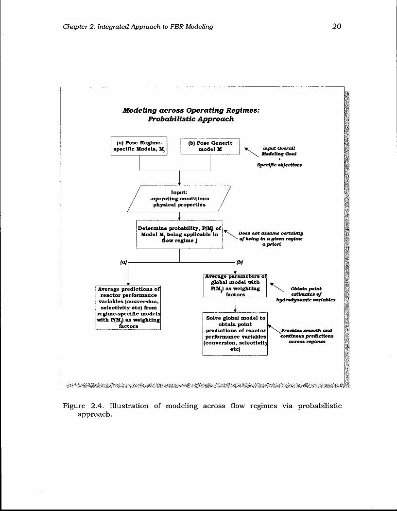
Chapter 2. Integrated Approach to FBR Modeling 20
Modeling across Operating Regimes: Probabilistic Approach
(a) Pose Regime-specific Models, Mj
(b) Pose Generic model M input Overall
\ Modeling Goal +
Specific objectives
Input: -operating conditions
physical properties
Determine probability, PJB J of Model M. being applicable in
flow regime j
(a)
Average predictions of reactor performance
variables (conversion, selectivity etc) from
regime-specific models' with P(M.) as weighting
factors
Does not assume certainty *• of being in a given regime
a priori
(b)
Average parameters of global model with PJMj) as weighting
factors
Solve global model to obtain point
predictions of reactor performance variables
(conversion, selectivity etc)
\ ^ Obtain point estimates of
hydrodynamic variables
^Provides smooth and contlnous predictions
across regimes
Figure 2.4. Illustration of modeling across flow regimes via probabilistic approach.
Chapter 2. Integrated Approach to FBR Modeling 21
globally constructed generic model. Note that this global model reduces to the
regime-specific models at any operating point at which any local model is 100%
probable. Since this approach, rather than averaging point predictions of the regime-
specific models, interpolates at the model parameter level, it can be ensured that the
model equations are satisfied at all points regardless of the type of reaction kinetics.
Symbolically N 'regime
j=i
where the global point estimate of the hydrodynamic parameter 6 (e.g. interphase
mass transfer) is the average of the values of 6 in regime j , 0j, weighted by the
respective probabilities P(Mj\x,H).
Because of the robust interpolation at the finest possible resolution (parameter level), the
latter approach is adopted in this work. In so doing, we are faced with the problem of
accurately determining the probabilities of the regime-specific models being applicable in
the various operating regimes. Probability theory provides a means of addressing this
issue. The following section briefly overviews the probabilistic concepts and outlines the
steps in the GFBR model development.
2.3.2 Probabilistic Paradigm
2.3.2.1 Introduction and Scope of Application
We noted in the probabilistic approach above the need to accurately estimate the
weighting factors to carry out the model averaging. Because of the uncertainties in the
flow regime transition boundaries and the correlations to estimate them, we are faced
with the problem of making decisions/inferences under uncertainty. Probability density
functions (pdfs) capture and represent the inherent uncertainties in correlations, model
structure, assumptions etc. Combining this knowledge base represented in the pdfs and
available data, probability theory provides means of making rational inferences under
uncertainty.
The Bayesian probabilistic approach has been successful in synthesizing robust
models for chemical processes (Thompson, 1996), interpolating between linear models
for process control (Murray-Smith and Johansen, 1997; Banerjee et al., 1997),
Chapter 2. Integrated Approach to FBR Modeling 22
uncertainty analyses of fuel biodegradation (McNab and Dooher, 1998), etc. The main
idea lies in Baye's theorem (see Bernardo and Smith, 1994), which is essentially a
mechanism for updating a prior probability of A, P(A \H) to a posterior probability
P(A\B,H), when additional information B under hypothesis H, P(B\A,H) becomes
available. Symbolically
y 1 ; P(B\H)
Considerable literature exists describing this concept from both theoretical and applied
perspectives (e.g. Berger, 1985; Loredo, 1990; Bernardo and Smith, 1994; Johansen,
1995; Thompson, 1996; Banerjee et al., 1997; Hoeting et al., 1998). However, because of
the complexity of implementing the complete Bayesian analysis, we limit the scope of the
probabilistic application to probabilistic averaging of hydrodynamic variables. This
means that we are implicitly assuming certainty in the operating conditions,
hydrodynamic correlations (except the regime boundary correlations), kinetic parameters
etc. used in the model equations. As a result, our implementation does not take advantage
of updating our prior knowledge to the posterior. In other words, Baye's theorem is not
applied in this work. The simplified approach adopted here is as follows: Given a regime
boundary correlation and the uncertainty associated with it, the probabilities of the flow
regime being above or below the boundary is computed by imposing an appropriate pdf.
These probabilities are then used as proxies for the probabilities that the regime-specific
models are applicable in the respective regimes. The steps are outlined below.
2.3.2.2 Steps in Probabilistic Approach to GFBR modeling
A complete algorithm is as follows.
(i) Formulate generalized model equations applicable over the fluidization
regimes of interest (sections 2.3.3 to 2.3.5 below)
(ii) Represent the uncertain regime boundaries as probability density functions
(pdfs) using appropriate distributions.
(iii) Determine the probability of being in regime j given the operating
conditions and model parameters (i.e., P(H = Hj\x)).
Chapter 2. Integrated Approach to FBR Modeling 23
(iv) Establish bounds " df in the hydrodynamic parameters (transition variables)
central to the flow regime transitions for each flow regime j (e.g. uL = uL,turb
= U, when the flow regime is turbulent).
(v) Average the transition parameters probabilistically at the bounds
established in step (iv), and obtain point estimates as:
0 = j]djxP(H = Hj\x). i
(vi) Finally, utilize these estimates in model equations posed in step (i) and
solve together with the phase/bed balances, energy and pressure equations
to obtain performance variables "y".
The remainder of this chapter presents in detail the steps outlined above.
2.3.3 Generalized Model Equations
From the various reactor models written specifically for the three fluidization flow
regimes (reviewed in Chapter 1), three regime-specific models are chosen to represent the
limiting behavior of the GFBR model at the fully bubbling, turbulent and fast fluidization
conditions: (i) generalized version of Grace (1984) two-phase bubbling bed model
(expanded to include dispersion in both phases) at low gas velocities, (ii) dispersed
(axially and radially) flow model for turbulent beds at intermediate velocities, and (iii) a
generalized version of the Brereton et al. (1988) core-annulus model (expanded to
include reaction terms as well as dispersion terms in both the core and annulus regions) at
higher velocities. After these generalizations, the three regime-specific models are then
fully compatible with each other, and therefore a single model formulation each for the L
and H-phase can describe the phenomena in all three flow regimes.
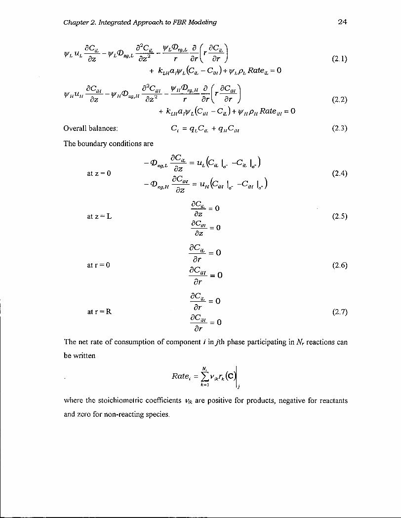
2.3.3.1 Mole Balance for the Two-Phases/Regions
Steady state two-phase/region mole balances represent the two-phase bubbling bed model
in the low velocity limit, dispersed flow model at intermediate gas velocities where the
turbulent fluidization regime is predominant, and the core-annulus model in the high
velocity limit:
Chapter 2. Integrated Approach to FBR Modeling 24
dz2 r dry dr .
dC d2CiH ¥H^rg,H 0 dz ' n~ **-n dz2 dr
dC m dr
+ ^ H a / ^ ( C i H - Cu) + ¥HPH R a t e m = 0
Overall balances: C, = g^C^ + qHCiH
The boundary conditions are
dC^ = uL(ciL\0--CiL\o.)
= u„(c„[r -c„ | J atz = 0
<D
<D
^ dz dC iH
zg.H dz
at z = L dz dC,
= 0
iH
dz
SC., iL
atr = 0 dr
dC iH
dr
dC iL
atr = R dr dC iH
dr
= 0
= 0
= 0
= 0
0
(2.1)
(2.2)
(2.3)
(2.4)
(2.5)
(2.6)
(2.7)
The net rate of consumption of component / in yth phase participating in Nr reactions can
be written
^ • = & / k ( c ) fc=l
where the stoichiometric coefficients vtk are positive for products, negative for reactants
and zero for non-reacting species.
Chapter 2. Integrated Approach to FBR Modeling 25
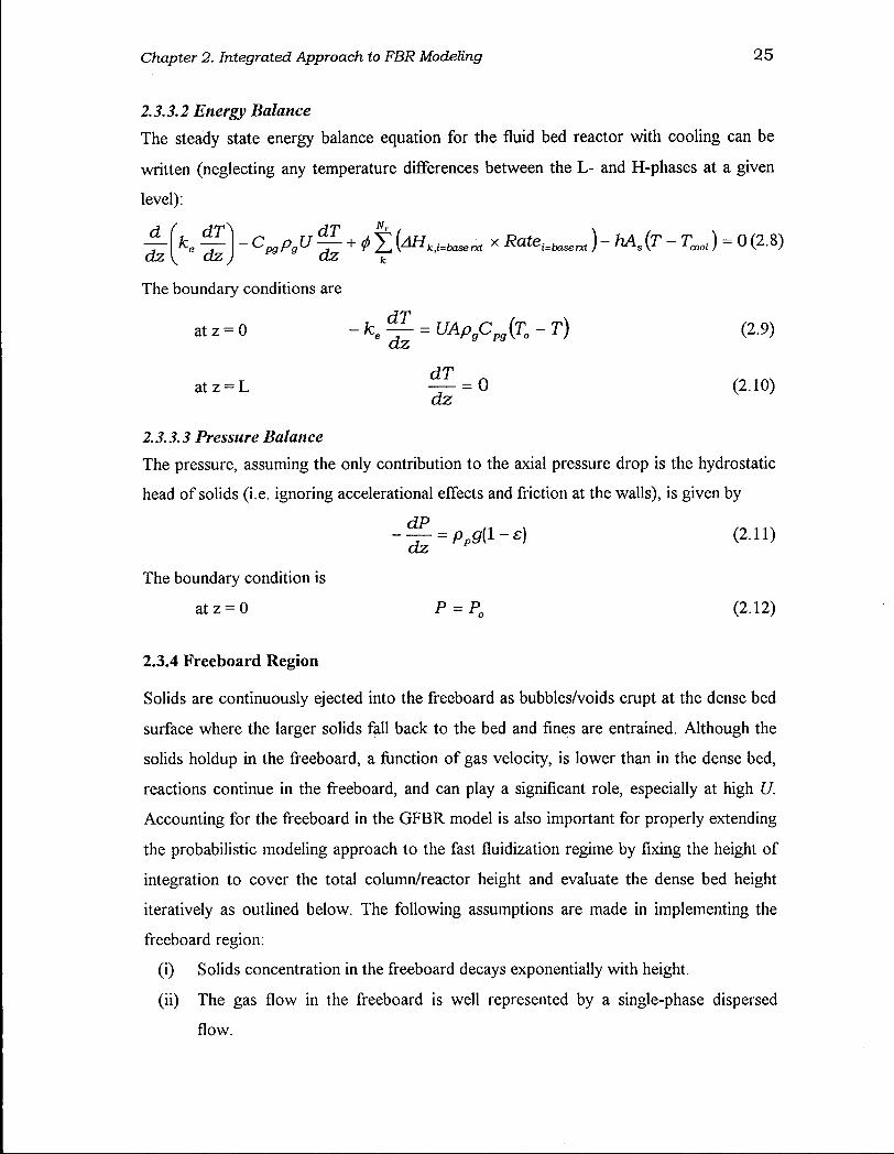
2.3.3.2 Energy Balance
The steady state energy balance equation for the fluid bed reactor with cooling can be
written (neglecting any temperature differences between the L - and H-phases at a given
level):
- f [ke ^ ] - C p g P g U ^ + ^{AHkJ=basend x Ratei=baserxt)-hAs(T- ) = 0(2.8) dz \ cLz J dz k
The boundary conditions are
at z = 0 ~ K ' % = U A P , C K , ( T ° ~ T) <2 9>
^ = 0 (2,0) dz
2.3.3.3 Pressure Balance
The pressure, assuming the only contribution to the axial pressure drop is the hydrostatic
head of solids (i.e. ignoring accelerational effects and friction at the walls), is given by
- ^ - = pg(l-e) (2.11) dz
The boundary condition is
atz = 0 P = P Q (2.12)
2.3.4 Freeboard Region
Solids are continuously ejected into the freeboard as bubbles/voids erupt at the dense bed
surface where the larger solids fall back to the bed and fines are entrained. Although the
solids holdup in the freeboard, a function of gas velocity, is lower than in the dense bed,
reactions continue in the freeboard, and can play a significant role, especially at high U.
Accounting for the freeboard in the GFBR model is also important for properly extending
the probabilistic modeling approach to the fast fluidization regime by fixing the height of
integration to cover the total column/reactor height and evaluate the dense bed height
iteratively as outlined below. The following assumptions are made in implementing the
freeboard region:
(i) Solids concentration in the freeboard decays exponentially with height.
(ii) The gas flow in the freeboard is well represented by a single-phase dispersed
flow.
Chapter 2. Integrated Approach to FBR Modeling 26
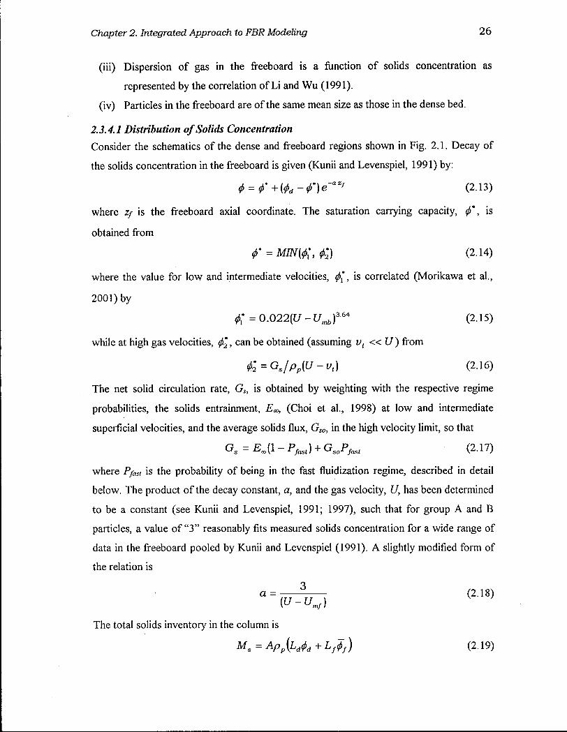
(iii) Dispersion of gas in the freeboard is a function of solids concentration as
represented by the correlation of Li and Wu (1991).
(iv) Particles in the freeboard are of the same mean size as those in the dense bed.
2.3.4.1 Distribution of Solids Concentration
Consider the schematics of the dense and freeboard regions shown in Fig. 2.1. Decay of
the solids concentration in the freeboard is given (Kunii and Levenspiel, 1991) by:
<t> = f+{<f>d-f)eaz> (2.13)
where z/ is the freeboard axial coordinate. The saturation carrying capacity, <f>*, is
obtained from
f=MIN{fx,f2) (2.14)
where the value for low and intermediate velocities, (j>[, is correlated (Morikawa et al.,
2001)by
tf= 0.022(1/-17.J 3 - 6 4 (2.15)
while at high gas velocities, > c a n D e obtained (assuming vt «U) from
fe=Gs/pp(U-vt) (2.16)
The net solid circulation rate, G s , is obtained by weighting with the respective regime
probabilities, the solids entrainment, Eco, (Choi et al., 1998) at low and intermediate
superficial velocities, and the average solids flux, G s o , in the high velocity limit, so that
Gs =Eo0(l-Pfast) + GsoPfast (2.17)
where Pfast is the probability of being in the fast fluidization regime, described in detail
below. The product of the decay constant, a, and the gas velocity, U, has been determined
to be a constant (see Kunii and Levenspiel, 1991; 1997), such that for group A and B
particles, a value of "3" reasonably fits measured solids concentration for a wide range of
data in the freeboard pooled by Kunii and Levenspiel (1991). A slightly modified form of
the relation is
3 a = (2.18)
(u-umf)
The total solids inventory in the column is
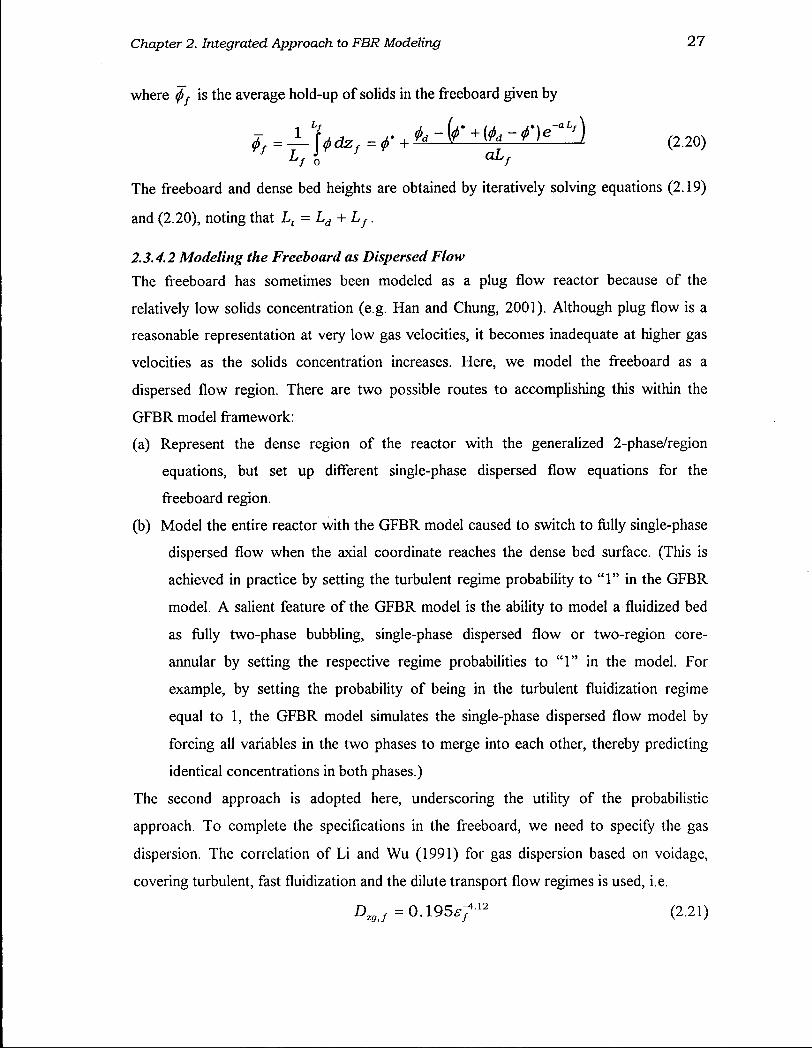
Ms=App(LJd+Lfff) (2.19)
Chapter 2. Integrated Approach to FBR Modeling 27
where <j>f is the average hold-up of solids in the freeboard given by
(2.20)
The freeboard and dense bed heights are obtained by iteratively solving equations (2.19)
and (2.20), noting that Lt = Ld+Lf.
2.3.4.2 Modeling the Freeboard as Dispersed Flow
The freeboard has sometimes been modeled as a plug flow reactor because of the
relatively low solids concentration (e.g. Han and Chung, 2001). Although plug flow is a
reasonable representation at very low gas velocities, it becomes inadequate at higher gas
velocities as the solids concentration increases. Here, we model the freeboard as a
dispersed flow region. There are two possible routes to accomplishing this within the
GFBR model framework:
(a) Represent the dense region of the reactor with the generalized 2-phase/region
equations, but set up different single-phase dispersed flow equations for the
freeboard region.
(b) Model the entire reactor with the GFBR model caused to switch to fully single-phase
dispersed flow when the axial coordinate reaches the dense bed surface. (This is
achieved in practice by setting the turbulent regime probability to "1" in the GFBR
model. A salient feature of the GFBR model is the ability to model a fluidized bed
as fully two-phase bubbling, single-phase dispersed flow or two-region core-
annular by setting the respective regime probabilities to "1" in the model. For
example, by setting the probability of being in the turbulent fluidization regime
equal to 1, the GFBR model simulates the single-phase dispersed flow model by
forcing all variables in the two phases to merge into each other, thereby predicting
identical concentrations in both phases.)
The second approach is adopted here, underscoring the utility of the probabilistic
approach. To complete the specifications in the freeboard, we need to specify the gas
dispersion. The correlation of Li and Wu (1991) for gas dispersion based on voidage,
covering turbulent, fast fluidization and the dilute transport flow regimes is used, i.e.
D ^ O . 1 9 5 ^ 4 1 2 (2.21)
Chapter 2. Integrated Approach to FBR Modeling 28
2.3.5 Bed and Phase Balances
Consider the schematic of the fluidized bed showing both dense and freeboard regions
given in Fig. 2.5. The phase balances relate only to the dense region where there are two
distinct phases, while the bed material balances apply to the entire column. The dense bed
volume fractions in the L and H phases must add up to 1, i.e:
VL + ¥H = 1 ( 2 - 2 2 )
where
VL=\\ VH=^- (2.23)
The gas flows through the phases add up to the total gas flow through bed, i.e.
Q = QL + QH (2-24)
Fractional gas flow through the phases add up to 1, i.e:
qL+qH=l (2.25)
where
L Q U ' Q U { ]
Combining eqs. (2.25) and (2.26), the gas flow balance can be written in terms of gas
velocities as
U = VLUL+VHUH (2-27)
The sum of the solids hold-up in the two phases equals the bed average.
\-e = y/L{l-eL)+y/H{\-eH) (2.28)
so that
£ = VL£L+YH£H (2-29)
Solids densities in the two phases add up to the bed average, i.e.
P = VLPL + VHPH (2.30)
Gas and solids volume fractions in each phase as well as the column add up to one, i.e:
L-phase: eL+0L=l (231)
H-phase: eH + <j)H = 1 (2.32)
Column average: e + <j> = 1 (2.33)
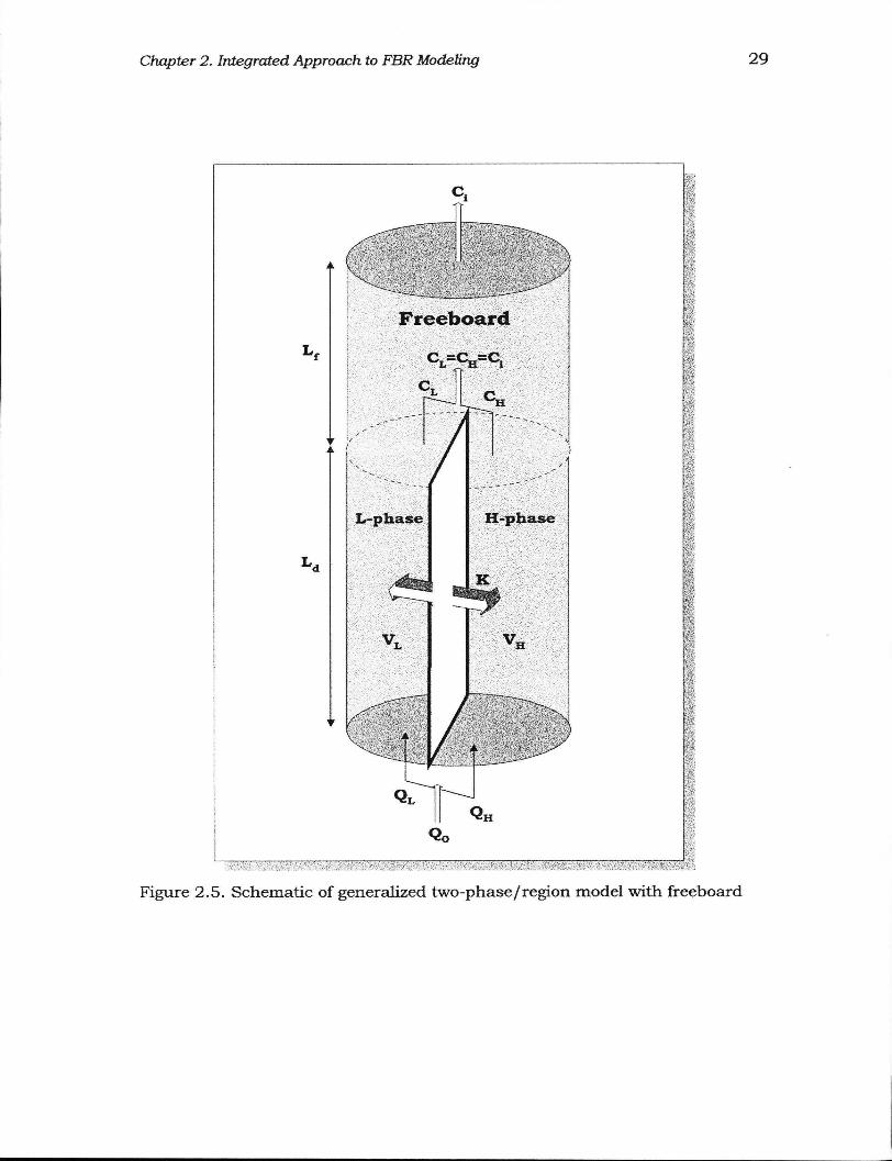
Chapter 2. Integrated Approach to FBR Modeling
Figure 2.5. Schematic of generalized two-phase/region model with freeboard
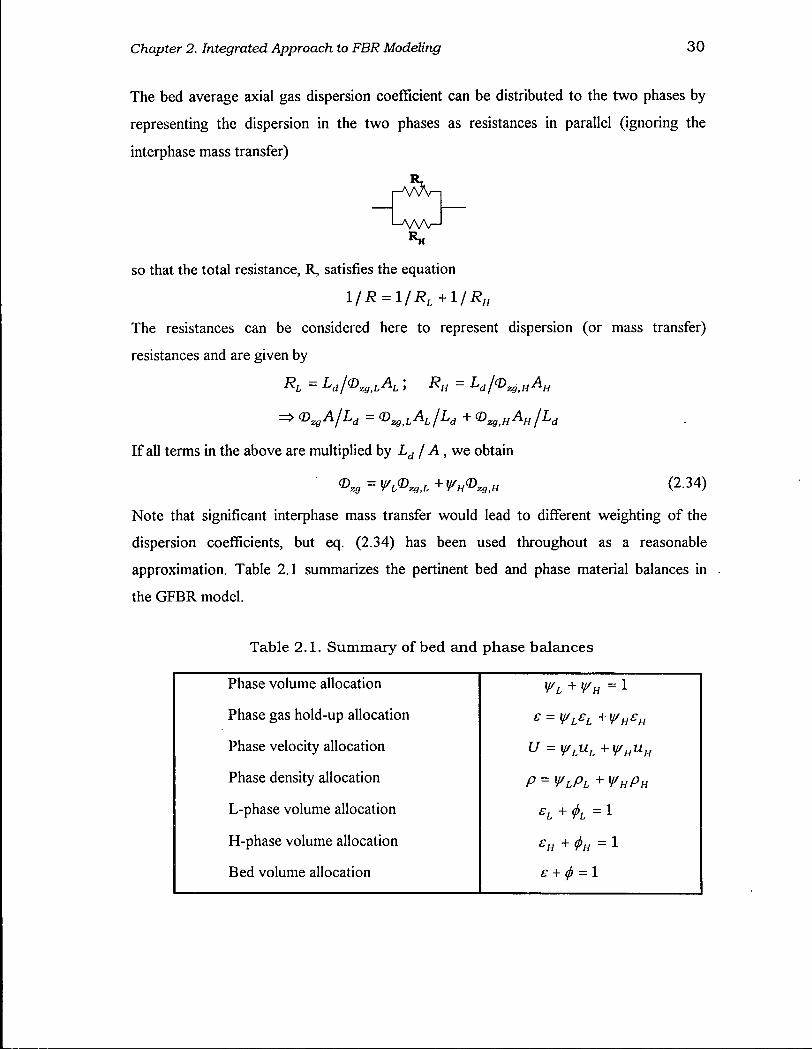
Chapter 2. Integrated Approach to FBR Modeling 30
The bed average axial gas dispersion coefficient can be distributed to the two phases by
representing the dispersion in the two phases as resistances in parallel (ignoring the
interphase mass transfer)
so that the total resistance, R, satisfies the equation
l/R = l/RL+l/RH
The resistances can be considered here to represent dispersion (or mass transfer)
resistances and are given by
RL = V®*».*A ; RH = La/<l>zg.HAH
=> VzgA/LD = <D^LAL /LD + (D^AH jhd
If all terms in the above are multiplied by LD / A, we obtain
© « 9 = ^ © 2 9 > t + i / H ( D 2 B > „ (2.34)
Note that significant interphase mass transfer would lead to different weighting of the
dispersion coefficients, but eq. (2.34) has been used throughout as a reasonable
approximation. Table 2.1 summarizes the pertinent bed and phase material balances in
the GFBR model.
Table 2.1. Summary of bed and phase balances
Phase volume allocation WL + ¥H = 1
Phase gas hold-up allocation e = YL
EL +VH£H
Phase velocity allocation U = yLuL + \j/HuH
Phase density allocation P = YLPL + WHPH
L-phase volume allocation * L + & = 1
H-phase volume allocation E H + = 1
Bed volume allocation e + <f> - 1
Chapter 2. Integrated Approach to FBR Modeling 31
2.3.6 Representing and Quantifying the Uncertainty in Regime Boundaries
The probabilities of being above or below the boundaries are computed by imposing
appropriate probability density functions, using the Uc and Use regime boundary
correlations and the uncertainty associated with them. These probabilities are then used
as proxies for the probabilities of the applicability of the regime-specific models in the
different flow regimes. The following notations are defined. Let:
• pi(C7]Ar) = pdf representing the uncertainty in regime correlation for U given the
gas and particle properties embodied by the Archimedes number, Ar. (Subscript
"i" is used to denote either "c" or "se".)
• Pbubb, Pturb, Pfast = probabilities of being in the bubbling, turbulent and fast
fluidization flow regimes respectively, with the sum always equal to 1.
The gamma probability density function has been determined to be the most appropriate
pdf satisfying all the constraints: uncertainty/error "e" in correlations normally
distributed with mean "0" and variances erf and USe> Uc > 0 (Thompson, 1996;
Thompson et al., 1999). If the transition velocity, U\, is far enough from zero, the pdfs
can also be assumed to be normally distributed with the same means and variances. For
example, the uncertainty in regime correlation for Use represented by the Gaussian pdf is:
Pse(U | Ar) = — i = e x p f - ( t 7 ~ ^ ' (2.35)
For ease of computation, sigmoid-shaped logistic regression functions (LRFs) were fitted
to the cumulative distributions evaluated from the Gaussian function:
Pfast = P(U > UJ = (l + e^Y =- ]pJU \Ar)dU (2.36)
u
where
[U-U ) vse=- — (2.37)
It was found that B = 1.7 fitted both the Gaussian and gamma distributions within a 1%
tolerance. Complete assignment of all the probabilities is specified below.

Chapter 2. Integrated Approach to FBR Modeling 32
In constructing the regime probability diagram for our probabilistic approach, we
need to specify some minimum U = Umin below which there is zero probability of
turbulent fluidization. The rationale for this is briefly examined. The probability of
bubbling fluidization must be "1" at the onset of bubbling and should reach zero
asymptotically with increasing gas velocity. To achieve this, Uc must be sufficiently far
from zero, which may not be satisfied always. To ensure that turbulent fluidization does
not co-exist with bubbling at the onset of bubbling, we impose the following constraint:
for U just above Umb (Umb < U < Umin), Pbubb must be 1 and Pturb = Pfast = 0. Umi„ is
assigned as a reasonable multiple of Umb. Here, we assigned Umi„ = 2Umb or UJ10,
whichever is lower. The same problem could arise with respect to some minimum
velocity below which the bed has 0 probability of being in the fast fluidization regime.
This could be to avoid the coexistence of bubbling and fast fluidization conditions.
However, given that the mean of the Use distribution is well above zero, we do not
impose such a constraint. Overall, the set of constraints Use> Uc > Umin > Umb > 0 are
satisfied for all cases.
Central to the probability predictions in the GFBR model is a reliable estimate of
the standard deviation of the error, o\. In earlier work (Thompson et al., 1999), a
reasonable value of 0.2 m/s was adopted for o c and the need to estimate this parameter
from actual hydrodynamic data was noted. Here, with the aid of the raw data used to
determine the flow regime transition correlations for Uc and Use (Bi et al., 1995) and
additional data from Bi (1994), improved correlations with a reduced level of dispersion
have been developed. Estimates of the normalized standard deviations, o?*, at the regime
boundary correlations are summarized in Table 2.2. Note that <J* is assumed to be
invariant to operating conditions and particle properties. This assists generic model
development, obviating the need for determining case-specific oj 's. With these controls
and by invoking the axioms of probability theory, the probabilities of being in each of the
three flow regimes are expressed as
Pbubb = 1 - P(W > K) = 1 - [1 + epv' }l (2.38)
Pfast = P{U* > Ul) = [1 + e"'"-]-1 (2.39)
and from the summation rule
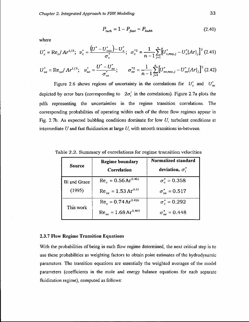
Chapter 2. Integrated Approach to FBR Modeling 3 3
Pturb = 1 " Pfast ~ P b u b b (2-40)
where
u:=Rec/Ar^; y ; = f c l z i % l z ^ I ; a ? = I f f r ' ^ . u : { A r ) j f ( 2 . 4 1 )
t/s*e = R e s e / A r 1 ' 3 ; vse = = J _ - L ^ A r ) , ] 2 (2.42)
Figure 2.6 shows regions of uncertainty in the correlations for U'c and U'^
depicted by error bars (corresponding to 2cr," in the correlations). Figure 2.7a plots the
pdfs representing the uncertainties in the regime transition correlations. The
corresponding probabilities of operating within each of the three flow regimes appear in
Fig. 2.7b. As expected bubbling conditions dominate for low U, turbulent conditions at
intermediate U and fast fluidization at large U, with smooth transitions in-between.
Table 2.2. Summary of correlations for regime transition velocities
Source Regime boundary
Correlation
Normalized standard
deviation, cr*
Bi and Grace
(1995)
Re c = 0.56 A r ° 4 6 1
R e s e = 1 . 5 3 A r 0 5 1
a'c = 0.358
< e =0.517
This work Re c = 0 . 7 4 A r 0 4 2 6
R e s e = 1.68 A r ° 4 6 9
cr* = 0.292
< e = 0-448
2.3.7 Flow Regime Transition Equations
With the probabilities of being in each flow regime determined, the next critical step is to
use these probabilities as weighting factors to obtain point estimates of the hydrodynamic
parameters. The transition equations are essentially the weighted averages of the model
parameters (coefficients in the mole and energy balance equations for each separate
fluidization regime), computed as follows:
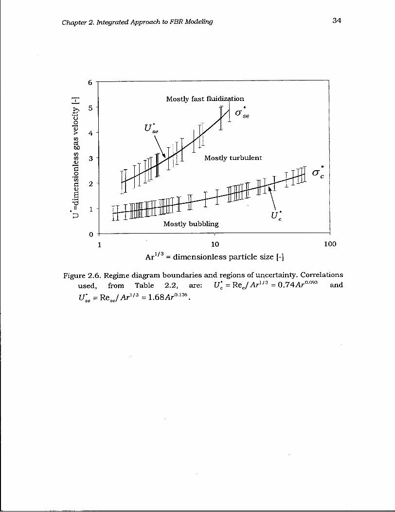
Chapter 2. Integrated Approach to FBR Modeling 34
51.
4 1
1 1
0
Mostly fast fluidization
0 \
Mostly bubbling
10 100
A r 1 / 3 = d i m e n s i o n l e s s p a r t i c l e s i z e [-]
Figure 2.6. Regime diagram boundaries and regions of uncertainty. Correlations used, from Table 2.2, are: U*c = ReJAr1'3 = 0.74Ar 0.093 and u: ReJAr1'3 = 1.68 Ar 0.136
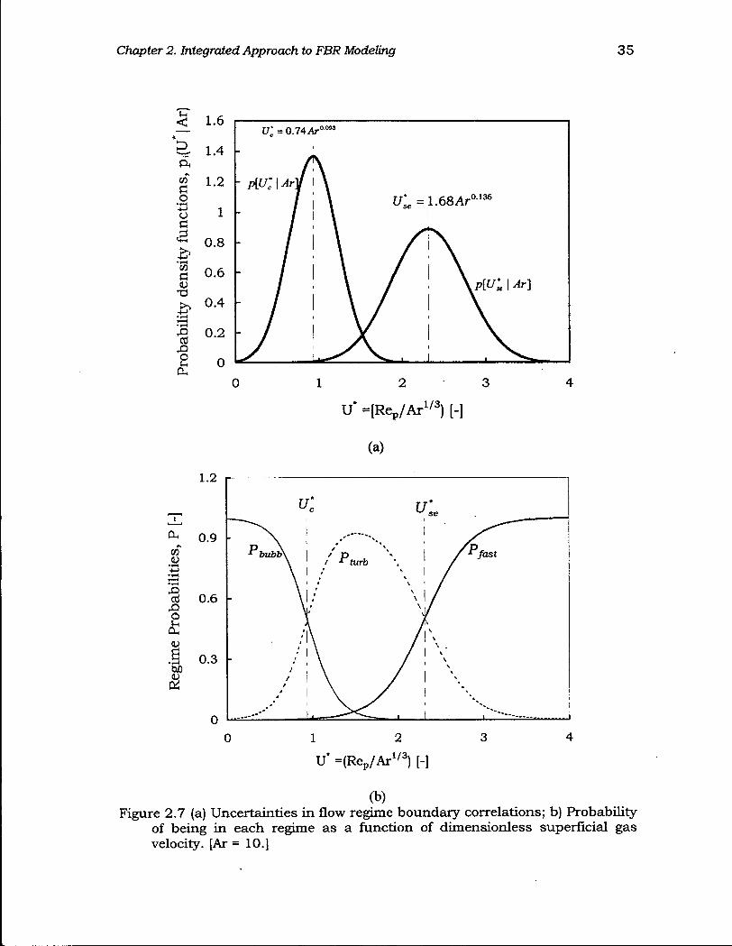
Chapter 2. Integrated Approach to FBR Modeling 3 5
< D
CO fi o 4-1 o a a •rH CO
c T 3
r Q O
CU
1.6
1.4
1.2
1
0.8
0.6
0.4
0.2
0
U'C = 0.74 A r 0 0 9 3
" PiU;\Arl/ 1 \ I I
/ ' \ Ul =1.68Ar0136
I
# \ / yctc i
y |3 1.2
0.9
.5 0.3
0
U =[Re p /Ar 1 / 3 ) [-]
(a)
V r
\
Pbubb\ \
\
1 >^ / n '» 1 /Pfast
i ^turb /
\ i /
/
\ A \ /1 * \ / ' -
\ / 1 /
*
U =(Rep/Ar1/3) [-]
(b) Figure 2.7 (a) Uncertainties in flow regime boundary correlations; b) Probability
of being in each regime as a function of dimensionless superficial gas velocity. [Ar = 10.]
Chapter 2. Integrated Approach to FBR Modeling 36
0 = j^0jPj (2.43)
where 0jis the value of 0 in regime j and P, is the probability of being in regime j . The
values of j represent: 1 = bubbling fluidization, 2 = turbulent fluidization and 3 = fast
fluidization. For example, consider the bed average voidage 6. The point estimate e from
the expected values of 8 in each regime is obtained as
£ ~ £bubbPbubb + £hLrb^turb + £ fast^fast (2-44)
where e^^, and efast are the voidages in the bubbling, turbulent and fast
fluidization flow regimes given in Table 2.3; the table also lists all the averaged variables
and the equations used to evaluate them in the three flow regimes. Correlations for other
hydrodynamic parameters for each of the three regimes such as uor, d0, rc etc. appearing
in Table 2.3 are summarized in Appendix A, while Appendix B presents the schemes
used to evaluate thermophysical properties such as gas mixture diffusivity, thermal
conductivity etc. Note that it should be straightforward to replace correlations currently
listed with better ones as these become available through future work.
2.4 Current Limits of GFBR Model
The GFBR model is explicitly developed for the three principal fluidization flow
regimes: bubbling, turbulent and fast fluidization. While it would be possible to extend
this model to other flow regimes, at present its applicability is limited to those three
regimes. Therefore, we note the following limits of the model:
(a) U > U^, i.e. the gas velocity is at least sufficient enough to initiate
bubbling;
(b) A large or shallow enough column that slug flow conditions are avoided over
the entire range of flow conditions;
(c) U < UCA or Gs > GsCA (Grace and Bi, 1997) in the high gas velocity limit
to avoid the dilute-phase transport flow regime;
(d) C/<[ / D S U =0.0113Gi 1 9 V s
1 064[^(/'p-^)r0064 to ensure that the
system is not operating in the dense suspension upflow regime (Grace et al.,
1999).
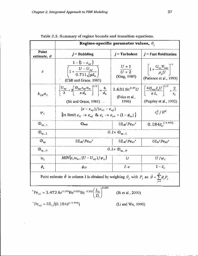
Chapter 2. Integrated Approach to FBR Modeling 37
Table 2.3. Summary of regime bounds and transition equations.
Regime-specific parameter values, 9}
Point estimate, 9
j = Bubbling j = Turbulent j = Fast fluidization
1 + U - U,
mf
0 . 7 1 1 ^ ,
(Clift and Grace, 1985)
LT + 1
U + 2 (King, 1989)
G Y , ^ so slip . p p u .
(Patience et al., 1993)
kLHa[
U mf + 2 C^mix£mfUbr
ndh
1/2 1
(Sit and Grace, 1981)
1.631 Sc° 3 7 U
(Foka et al. 1996)
1/2
?rLt
(Pugsley et al., 1992)
(in limit * H -> & * L -> = (1 - ^ ) j
zg^L (Drab ULd/Pezl*
rg _L O.lx OD zg_L
ULa/Pezi' ULd/Pezi* ULt/Pez2
+
zg_H
MIN{sLubr,{U-Umf)/¥Lj UR U
<t>L 4 'LO 1-s l - S r
Point estimate 6 in column 1 is obtained by weighting 0i with Pj as: 6 = X#,P,
*Pe2l = 3.472 A r 0 1 4 9 R e 0 0 2 3 S c - a 2 3 2
^ 0.285 LA
Pe z 2 = C/L(/(0.184^(-4-445))
(Bi et al., 2000)
(Li and Wu, 1990)
Chapter 2. Integrated Approach to FBR Modeling 38
2.5 Numerical Solution Approach
The differential equations resulting from the mole, energy and pressure balances, coupled
with the set of algebraic and integral equations in the model, render the problem an
integro-differential algebraic equation system (IDAEs). For such systems, the dispersed
boundary conditions introduce a complexity that requires careful choice of solution
approach. Most existing IDAEs solvers (Mathlab, Mathmatica, Mathcad etc) do not fully
handle boundary value problems. Where such solvers do exist, the extent of flexibility is
severely limited by the built-in bounds within the solvers leading to convergence
problems (e.g. in the Microsoft Fortran Developer Studio with IMSL).
As a result of the above limitations, solution to complex boundary value problems
are sought either through in-house development of coding with "Programming
Languages" (e.g. Fortran, C+ + etc.) employing one of a variety of finite difference
/element techniques, or by using advanced modeling languages such as MODEL.LA
(Stephanopoulos, et al, 1990), gPROMS (Pantelides and Barton, 1993), or LCR (Han et
al., 1995). These modeling languages are called "Equation-based* and
"Phenomenological Languages", the latter being a variant of the former, differing only in
some implementation aspects. Their development has made possible a shift from
traditional programming languages such as Fortran. Equation-based languages are easier
to use while sacrificing some flexibility, as illustrated in Fig. 2.8
2.5.1 general PROcess Modeling System (gPROMS)
The modeling language employed in this study is gPROMS from Process Systems
Enterprise Limited, London, UK. Detailed description of the gPROMS language, its
features and capabilities are given in the gPROMS Users Guide, readily accessible at
www, psenterprise, com. It is possible using gPROMS to switch among a variety of
solution techniques (e.g. finite difference discretization schemes of different order,
orthogonal collocation, robust algebraic solvers etc.) to solve the set of equations.
Modeling languages, with gPROMS at the forefront, are considered as the emerging
programming paradigm for the 21st century (Stephanopoulos and Han, 1996).
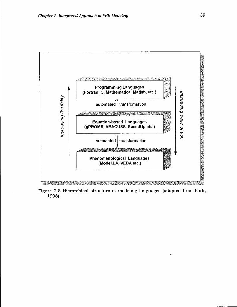
Chapter 2. Integrated Approach to FBR Modeling 39
•o I «: O) c: <o
8
P r o g r a m m i n g L a n g u a g e s (Fortran, C , Mathematica, Matlab, etc.)
automated transformation
Equa t ion -based L a n g u a g e s ( g P R O M S , A B A C U S S , S p e e d U p etc.)
automated transformation
P h e n o m e n o l o g i c a l L a n g u a g e s (Model .LA, V E D A etc.)
3 co
<Q <D Q) O)
c:
mm Figure 2.8 Hierarchical structure of modeling languages (adapted from
1998) Park,
Chapter 2. Integrated Approach to FBR Modeling 4 0
2.5.2 Implementing the G F B R Model in gPROMS
Equation-based modeling languages generally have several segmented components as
shown in Fig. 2.9. Each such component must be defined separately. Solution is attained
through compilation of the model and process sections followed by execution. The
versatility of the language lies in its ability to handle several process sections using only
one main model section as a backbone, while allowing a foreign process/object (e.g.
Fortran code, Excel worksheet) to be incorporated by interfacing. As a result, a variety of
different processes can be modeled using a single model section containing the
fundamental equations.
Within the context of the GFBR model, the main equations in the "model section" of
gPROMS are: mole, energy and pressure balance equations, phase and bed balance
equations, hydrodynamic regime transition equations, probability equations, reactor
performance equations (performance variables, kinetics etc.), hydrodynamics
equations/correlations and physical properties evaluation equations/correlations. In other
words, the complete sets of IDAEs are contained in this section. The "process section"
allows a so-called "simulation experiment" to be performed, so that the model section is
used to study the behaviour of the system under different circumstances. For our system,
this is the section where process-specific information such as kinetic parameters, physical
properties not computed within the model section (e.g. particle density, mean particle
size), operating conditions (e.g. inlet temperature and pressure) etc. are specified.
An important feature of gPROMS is the dynamic interfacing with foreign
programs such as C++, Fortran and E X C E L . Taking advantage of this feature, we
constructed a template in E X C E L containing most of the input information required
under the process section. Figure 2.10 presents a typical E X C E L screen showing the
different worksheets for the reactor data, physical properties etc. The reactor schematic
within the Figure is constructed in E X C E L using a combination of graphing and drawing
tools such that real time changes in bed properties, such as expanded bed height, regime
probabilities, etc. can be directly monitored from the user interface created in E X C E L as
the simulation proceeds.
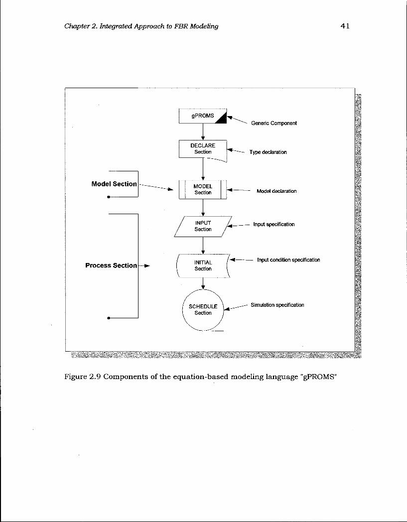
Chapter 2. Integrated Approach to FBR Modeling 41
Model Sect ion
Process Sect ion
gPROMS
DECLARE Section
MODEL Section
INPUT Section
Generic Component
Type declaration
Model declaration
Input specification
Input condition specification
Simulation specification
Figure 2.9 Components of the equation-based modeling language "gPROMS"
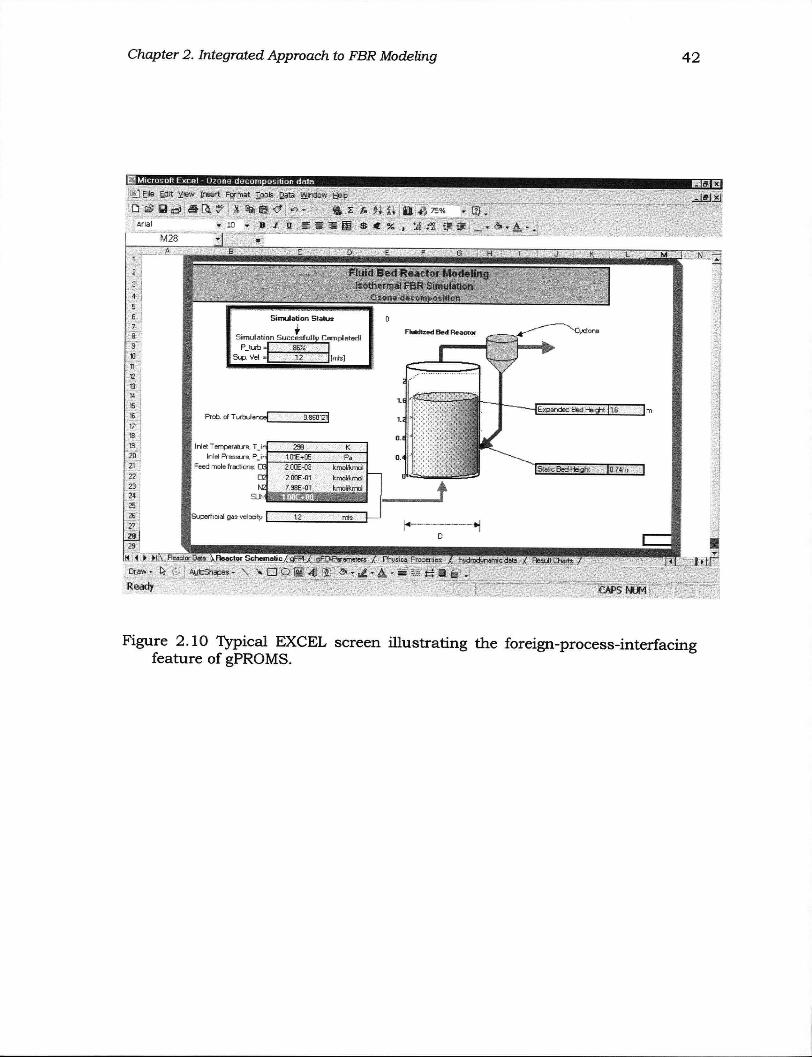
Chapter 2. Integrated Approach to FBR Modeling 42
a] File Edit View Insert Format Tools p_ata Window Help
D S H e * a a ? s%s<? * x f.'n u a*>,75% ~ g .
M28 >|
1 J 3
4
6 7
8 Q
10 11
13 I w
15 16
B
[H i • H \
Draw - tj
Ready
Fluid Bed Reactor Modeling i s o t h e r m a l FBR Simulation
Simulation Status 0
S imu la t ion S u c c e s f u l l y Completer!! P j u r b - 86%
Sup. Vel - 12
Fluidized B e d Reactor
Prob. of TurbulenceTJ 3 860i;i[
296 [Inlet Temperature. T J n Inlet Pressure. P_ir 1.P1E»05
I Feed mole fractions: 03 2.00E-03 CP 2 00E.01 N2| 7.98E-01
Pa kmolfkmol kmold r.-i l
kmolikmul
•Superficial gas velocity f"
Cyclone
Reactor Data \Reoclor Schematic/gFPI / gFO-Parameters / Physical Properties / hydrodynamic dato / f lesuBiart^/
AutoShapes- \ > O O B 4 W * ' i - i - = § S I | . •.tr
CAPS NUM
Figure 2.10 Typical EXCEL screen illustrating the foreign-process-interfacing feature of gPROMS.
Chapter 2. Integrated Approach to FBR Modeling 43
Typical gPROMS simulation involving eight gaseous species and three reactions
for the oxy-chlorination process, for example, takes about eight minutes to complete
using a second order central finite difference discretization scheme.
2.6 Remarks on the Application of GFBR Model
A number of aspects have been considered in the GFBR model, namely: probabilistic
averaging of hydrodynamic variables; inclusion of the freeboard region; energy and
pressure variations along the reactor. In most commercial processes operated at high
enough gas velocities, it is important to apply the complete model outlined above.
However, in certain cases, some of these aspects can be ignored in order reduce computer
processing time when their inclusion will not significantly change the model predictions
or the overall model utility. (For example, when the reactor is operated at superficial gas
velocities of a few multiples of Umb for group A catalysts, it is safe to ignore the
contribution from the freeboard region.)
Additional complexities are considered in subsequent chapters; specifically: (i)
extension to simulate gas-solid reactions by coupling the GFBR model with a single
particle model (Chapter 5 c); (ii) implementation of volume change with reaction for
systems accompanied by a change in molar flowrate (Chapter 6). The application of the
GFBR model in this thesis is therefore structured as follows:
1 Isothermal and isobaric cold model version (without the reaction terms) is applied in
the interpretation of gas mixing experiments in Chapter 3.
2 Isothermal, isobaric version of the model is applied to case studies for ozone
decomposition (Chapter 4), phthalic anhydride process (Chapter 5a), and zinc sulfide
roasting (Chapter 5c).
3 Chapter 6 implements the full capability of the GFBR model, accounting for volume
change with reaction, energy and pressure variations along the reactor, and the
influence of the freeboard region. The oxy-chlorination process is used to illustrate
and validate the approach.
Chapter 2. Integrated Approach to FBR Modeling 44
2.7 Conclusion
A new generic fluid bed reactor model is presented, applicable across the fluidization
flow regimes most commonly encountered in industrial scale fluid bed reactors: bubbling,
turbulent and fast fluidization. The model interpolates between three regime-specific
models - the generalized two-phase bubbling bed model, dispersed plug flow model and
the generalized core-annulus model - by means of probabilistic averaging of
hydrodynamic and dispersion variables based on the uncertainty in the flow regime
transitions. It is shown that the probabilistic approach captures salient features of the
limiting models at any given operating point across the operating regimes and adequately
describes phenomena within each flow regime. Applications of this model using
gPROMS ® software is demonstrated in the following chapters.

C h a p t e r 3
G a s M i x i n g i n B u b b l i n g - T u r b u l e n t F l u i d i z e d B e d
3.1 Introduction
Gas mixing in fluidized beds is strongly affected by the gas-solid interaction between the
low- and high-density phases. Knowledge of the extent of mixing is important not only to
provide a description of the gas flow pattern, but also to evaluate reactor performance.
While results of several lab-scale investigations, usually carried out in columns of ID
-100 mm, have been reported in the literature, data for gas mixing in the turbulent and
transition flow regimes are scarce (Bi et al, 2000). Existing correlations for the axial and
radial dispersion coefficients mostly developed for the bubbling and slugging flow
regimes, can provide only gross estimates at best for the turbulent flow regime.
This study was therefore undertaken to further study gas mixing using a commercial
catalyst to help characterize the gas flow pattern in the bed for the operating conditions
considered and to estimate dispersion and interphase mass transfer coefficients from the
experimental data. Results from this study are intended to provide better understanding of
the effects of dispersion in each phase with increasing velocities and at regime
boundaries.
3.2 Experimental Studies
3.2.1 E x p e r i m e n t a l A p p a r a t u s a n d Ins t rumenta t ion
The Plexiglas column used in this study, shown schematically in Fig. 3.1, is 4.4 m high
and 0.286 m in inside diameter with a distributor plate composed of two perforated
aluminum plates supporting the catalyst. There are 98 holes in each perforated plate, each
4.4 mm in diameter with a 30 mm pitch giving a fractional open area of 1.7 %. Two
external cyclones in series with return leg diameters of 51 mm are used to capture
entrained particles, while a baghouse filter removes fine particles not captured by the
cyclones. A Roots blower supplies air as the fluidizing gas, with its flowrate
45
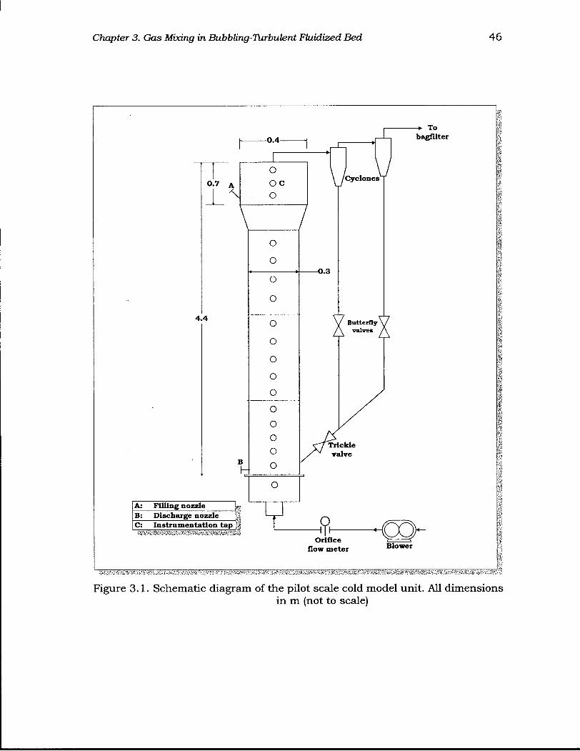
Chapter 3. Gas Mixing in Bubbting-Turbulent Fluidized Bed 46
Figure 3.1. Schematic diagram of the pilot scale cold model unit. All dimensions in m (not to scale)
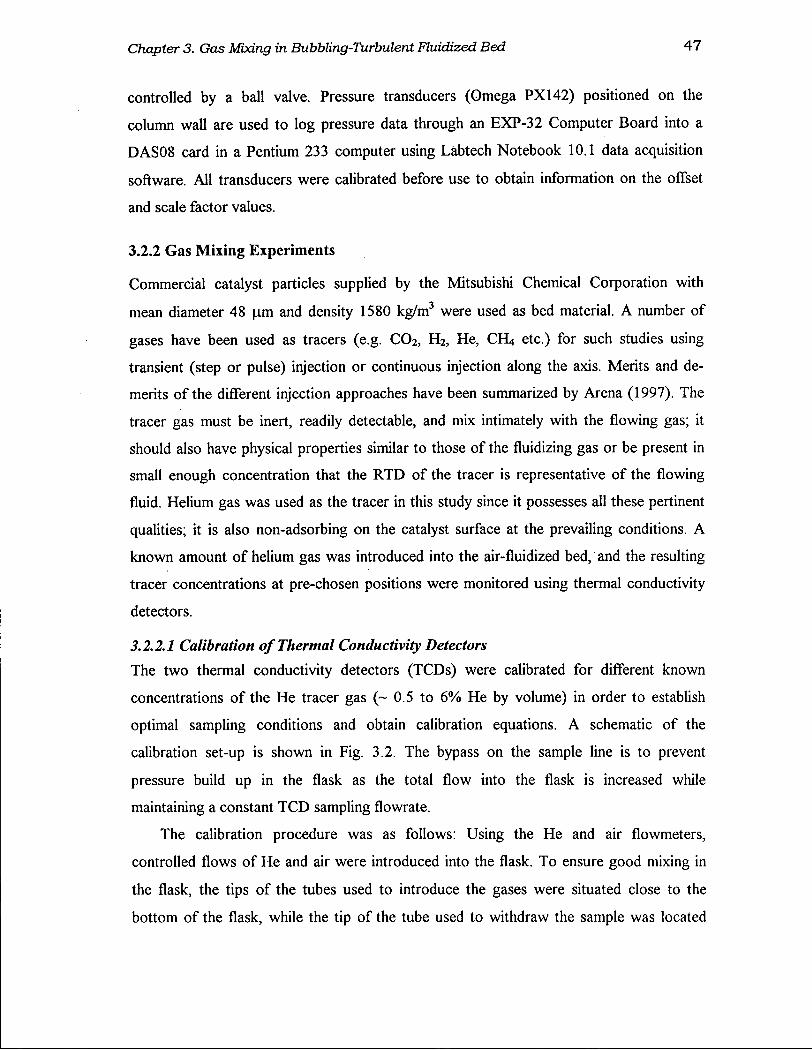
Chapter 3. Gas Mixing in Bubbling-Turbulent Fluidized Bed 47
controlled by a ball valve. Pressure transducers (Omega PX142) positioned on the
column wall are used to log pressure data through an EXP-32 Computer Board into a
DAS08 card in a Pentium 233 computer using Labtech Notebook 10.1 data acquisition
software. All transducers were calibrated before use to obtain information on the offset
and scale factor values.
3.2.2 Gas Mixing Experiments
Commercial catalyst particles supplied by the Mitsubishi Chemical Corporation with
mean diameter 48 urn and density 1580 kg/m3 were used as bed material. A number of
gases have been used as tracers (e.g. CO2, H 2 , He, CH4 etc.) for such studies using
transient (step or pulse) injection or continuous injection along the axis. Merits and de
merits of the different injection approaches have been summarized by Arena (1997). The
tracer gas must be inert, readily detectable, and mix intimately with the flowing gas; it
should also have physical properties similar to those of the fluidizing gas or be present in
small enough concentration that the RTD of the tracer is representative of the flowing
fluid. Helium gas was used as the tracer in this study since it possesses all these pertinent
qualities; it is also non-adsorbing on the catalyst surface at the prevailing conditions. A
known amount of helium gas was introduced into the air-fluidized bed, and the resulting
tracer concentrations at pre-chosen positions were monitored using thermal conductivity
detectors.
3.2.2.1 Calibration of Thermal Conductivity Detectors
The two thermal conductivity detectors (TCDs) were calibrated for different known
concentrations of the He tracer gas (~ 0.5 to 6% He by volume) in order to establish
optimal sampling conditions and obtain calibration equations. A schematic of the
calibration set-up is shown in Fig. 3.2. The bypass on the sample line is to prevent
pressure build up in the flask as the total flow into the flask is increased while
maintaining a constant TCD sampling flowrate.
The calibration procedure was as follows: Using the He and air flowmeters,
controlled flows of He and air were introduced into the flask. To ensure good mixing in
the flask, the tips of the tubes used to introduce the gases were situated close to the
bottom of the flask, while the tip of the tube used to withdraw the sample was located
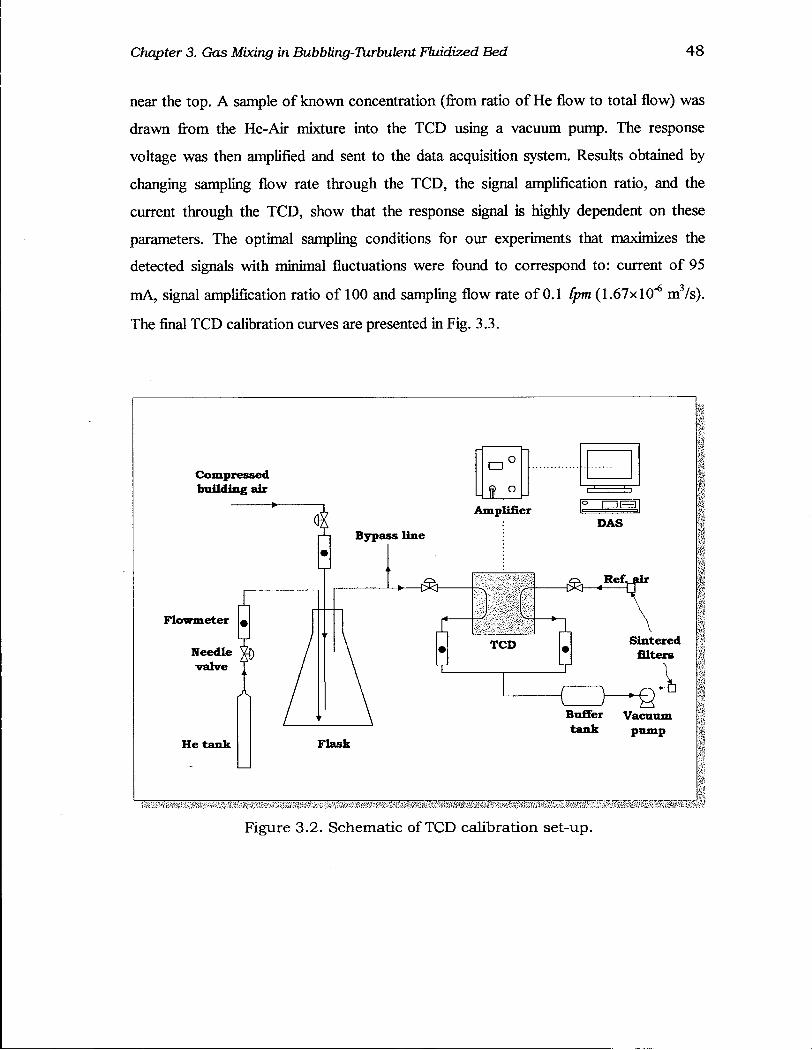
Chapter 3. Gas Mixing in Bubbttng-Turbulent Fluidized Bed 48
near the top. A sample of known concentration (from ratio of He flow to total flow) was
drawn from the He-Air mixture into the TCD using a vacuum pump. The response
voltage was then amplified and sent to the data acquisition system. Results obtained by
changing sampling flow rate through the TCD, the signal amplification ratio, and the
current through the TCD, show that the response signal is highly dependent on these
parameters. The optimal sampling conditions for our experiments that maximizes the
detected signals with rrunirnal fluctuations were found to correspond to: current of 95
mA, signal amplification ratio of 100 and sampling flow rate of 0.1 Cpm (1.67X10"6 m3/s).
The final TCD calibration curves are presented in Fig. 3.3.
Compressed building air
Flowmeter
Needle valve
He tank
Bypass line
Flask
-fcSCr-
Amplifier DAS
Ref.
T C D Sintered filters
•CD—S Buffer Vacuum tank pump
Figure 3.2. Schematic of TCD calibration set-up.
Chapter 3. Gas Mixing in Bubbling-Turbulent Fluidized Bed 49
3.5
0 4 0 1 2 3 4 5 6
Volumetric He conc'n (vol He/(vol Air+He)), %
(b) Figure 3.3. Plot of detected signals as a function of volume percent He injected
for a) TCD#1, and b) TCD#2. [Signal amplification ratio = 100; Current = 95 mA; TCD sample flow rate = 1.67x10⁻⁶ m3/s.]
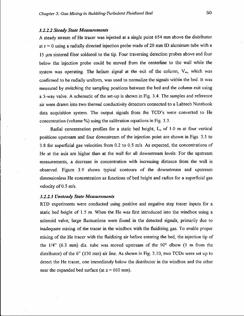
Chapter 3. Gas Mixing in Bubbling-Turbulent Fluidized Bed 50
3.2.2.2 Steady State Measurements
A steady stream of He tracer was injected at a single point 654 mm above the distributor
at r = 0 using a radially directed injection probe made of 20 mm ID aluminum tube with a
15 urn sintered filter soldered to the tip. Four traversing detection probes above and four
below the injection probe could be moved from the centerline to the wall while the
system was operating. The helium signal at the exit of the column, V w , which was
confirmed to be radially uniform, was used to normalize the signals within the bed. It was
measured by switching the sampling positions between the bed and the column exit using
a 3-way valve. A schematic of the set-up is shown in Fig. 3.4. The samples and reference
air were drawn into two thermal conductivity detectors connected to a Labtech Notebook
data acquisition system. The output signals from the TCD's were converted to He
concentration (volume %) using the calibration equations in Fig. 3.3.
Radial concentration profiles for a static bed height, L 0 of 1.0 m at four vertical
positions upstream and four downstream of the injection point are shown in Figs. 3.5 to
3.8 for superficial gas velocities from 0.2 to 0.5 m/s. As expected, the concentrations of
He at the axis are higher than at the wall for all downstream levels. For the upstream
measurements, a decrease in concentration with increasing distance from the wall is
observed. Figure 3.9 shows typical contours of the downstream and upstream
dimensionless He concentration as functions of bed height and radius for a superficial gas
velocity of 0.5 m/s.
3.2.2.3 Unsteady State Measurements
RTD experiments were conducted using positive and negative step tracer inputs for a
static bed height of 1.5 m. When the He was first introduced into the windbox using a
solenoid valve, large fluctuations were found in the detected signals, primarily due to
inadequate mixing of the tracer in the windbox with the fluidizing gas. To enable proper
mixing of the He tracer with the fluidizing air before entering the bed, the injection tip of
the 1/4" (6.3 mm) dia. tube was moved upstream of the 90° elbow (1 m from the
distributor) of the 6" (150 mm) air line. As shown in Fig. 3.10, two TCDs were set up to
detect the He tracer, one immediately below the distributor in the windbox and the other
near the expanded bed surface (at z = 660 mm).

Chapter 3. Gas Mixing in Bubbting-Turbulent Fluidized Bed 51
Amplifier
Ref. air
Flowmeter!* TCD #2
^—cz> Vacuum Buffer
pump ••mifc
To cyclone
Windbox
CD O
t o Amplifier
Pressors transduce rm
T valve -tSr- Ref. air
TCD *1 Flowmeter
-CD—g Bu£fer Vacuum tank pump
Needle valve
He Inlet
Air (from blower)
Figure 3.4. Schematic diagram of steady state tracer injection/detection set-up.

Chapter 3. Gas Mixing in Babbling-Turbulent Fluidized Bed 52
Sampling level below injection pt
(mm)
-•-127 -B-191 - ± - 2 5 4 - © - 4 4 5
0 0.25 0.5 0.75 1 Radial position, r/R [-]
(b)
Figure 3.5. Radial concentration profiles for tracer: (a) downstream, (b) upstream of injection point. [Lo= 1.0 m, U = 0.2 m/s, tracer injection level 0.654 m above distributor.]
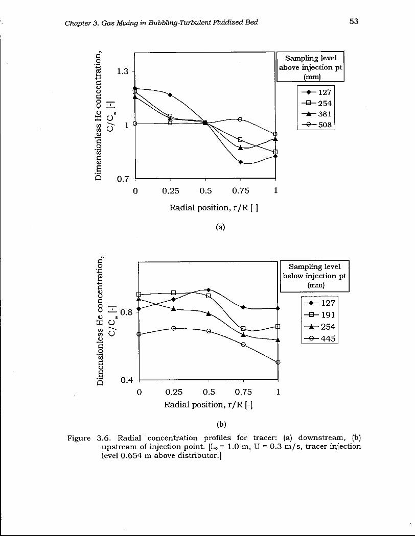
Chapter 3. Gas Mixing in Bubbling-Turbulent Fluidized Bed 53
Figure 3.6. Radial concentration profiles for tracer: (a) downstream, (b) upstream of injection point. [LQ = 1.0 m, U = 0.3 m/s, tracer injection level 0.654 m above distributor.]
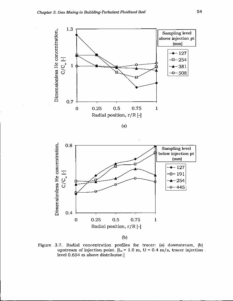
Chapter 3. Gas Mixing in Bubbling-Turbulent Fluidized Bed 54
fi o
• t—I
td u 4-1 fi <u o fi o o
CO CO <D fi o
• r H CO
fi <L)
0 • f - H
Q
1.3
O O
0.7
Sampling level above injection pt
(mm)
— - 1 2 7 —B-- 2 5 4
- 3 8 1 - O - - 5 0 8
0 0 .25 0 .5 0 .75
Radial p o s i t i o n , r/R [-]
(a)
fi o
• r H
ts u fi o fi
8 zn <D 8
co U
fi o CO fi
0 .8 Sampling level
below injection pt (mm)
127
- o - 191
• ^ 2 5 4
- e - 4 4 5
Q 0.4
0 0 .25 0 .5 0 .75 1
Radial p o s i t i o n , r/R [-]
(b)
Figure 3 .7 . Radial concentration profiles for tracer: (a) downstream, (b) upstream of injection point. [LQ = 1.0 m, U = 0.4 m/s, tracer injection level 0 .654 m above distributor.]
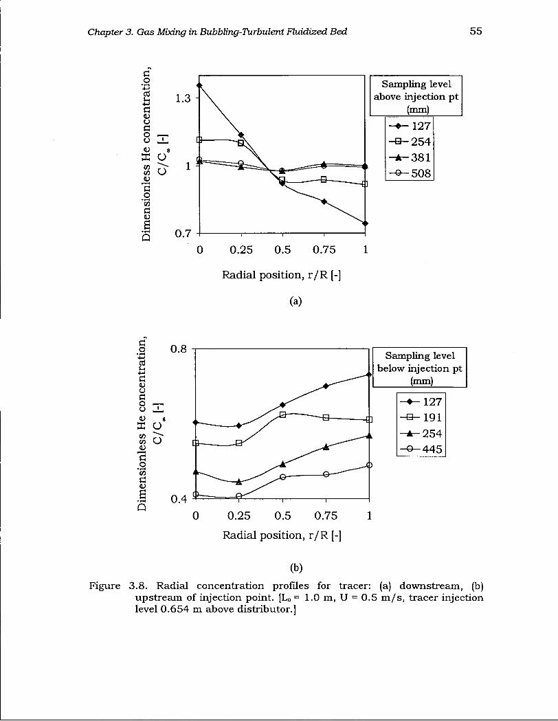
Chapter 3. Gas Mixing in Bubbling-Turbulent Fluidized Bed 55
(b)
Figure 3.8. Radial concentration profiles for tracer: (a) downstream, (b) upstream of injection point. [L0 = 1.0 m, U = 0.5 m/s, tracer injection level 0.654 m above distributor.]
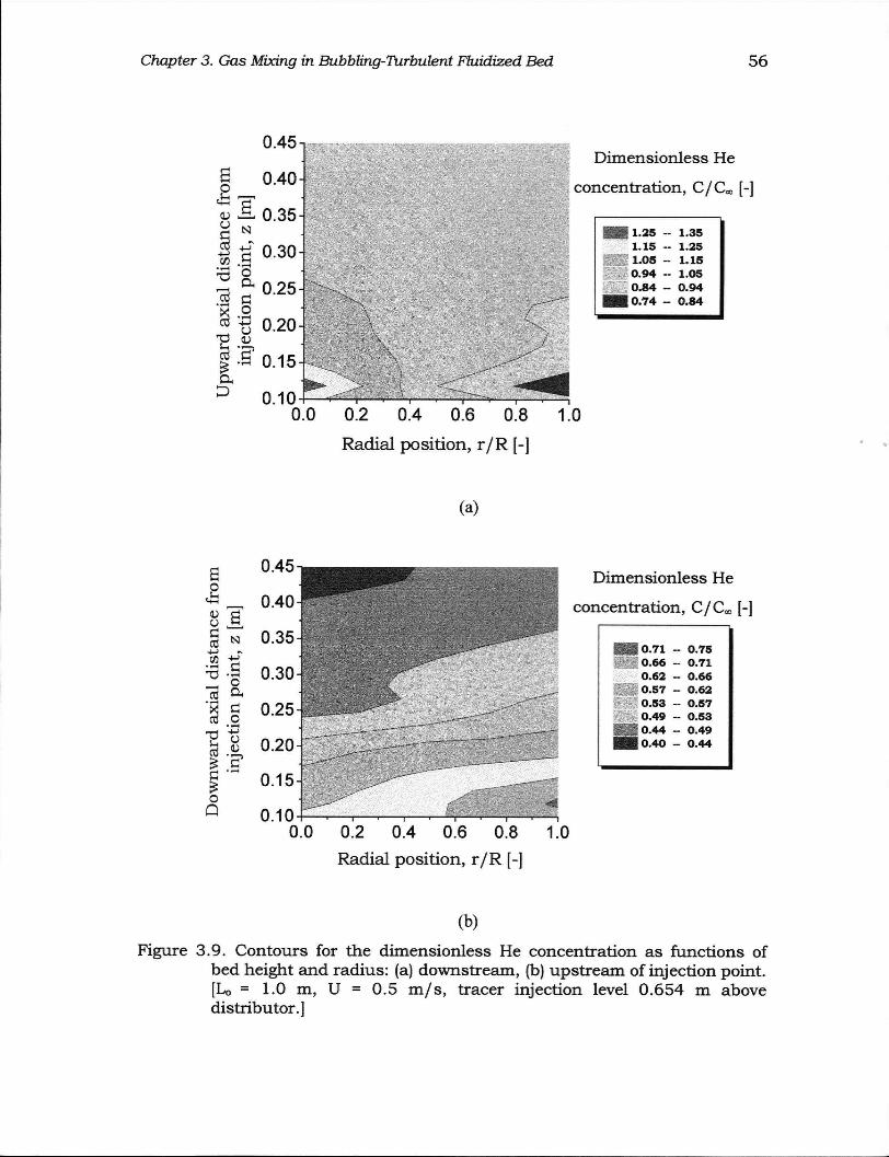
Chapter 3. Gas Mixing in BubbUng-Turbulent Fluidized Bed 56
(a)
Radial position, r/R [-]
(b)
Figure 3.9. Contours for the dimensionless He concentration as functions of bed height and radius: (a) downstream, (b) upstream of injection point. [Lo = 1.0 m, U = 0.5 m/s, tracer injection level 0.654 m above distributor.]
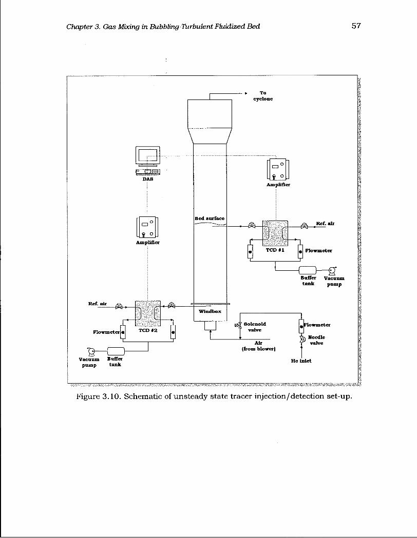
Chapter 3. Gas Mixing in Bubbling-Turbulent Fluidized Bed 57
Ref. air
Flowmeter
Vacnum Buffer pump tank
DAS
Amplifier
TCD #2
Bed surface
Windbox
To cyclone
Ampiifier
TCD #1
Solenoid valve
Air (from blower)
-iSr-Ref. air
Flowmeter
- a — g Buffer Vacuum tank pump
Flowmeter
Needle valve
He Inlet
Figure 3.10. Schematic of unsteady state tracer injection/detection set-up.
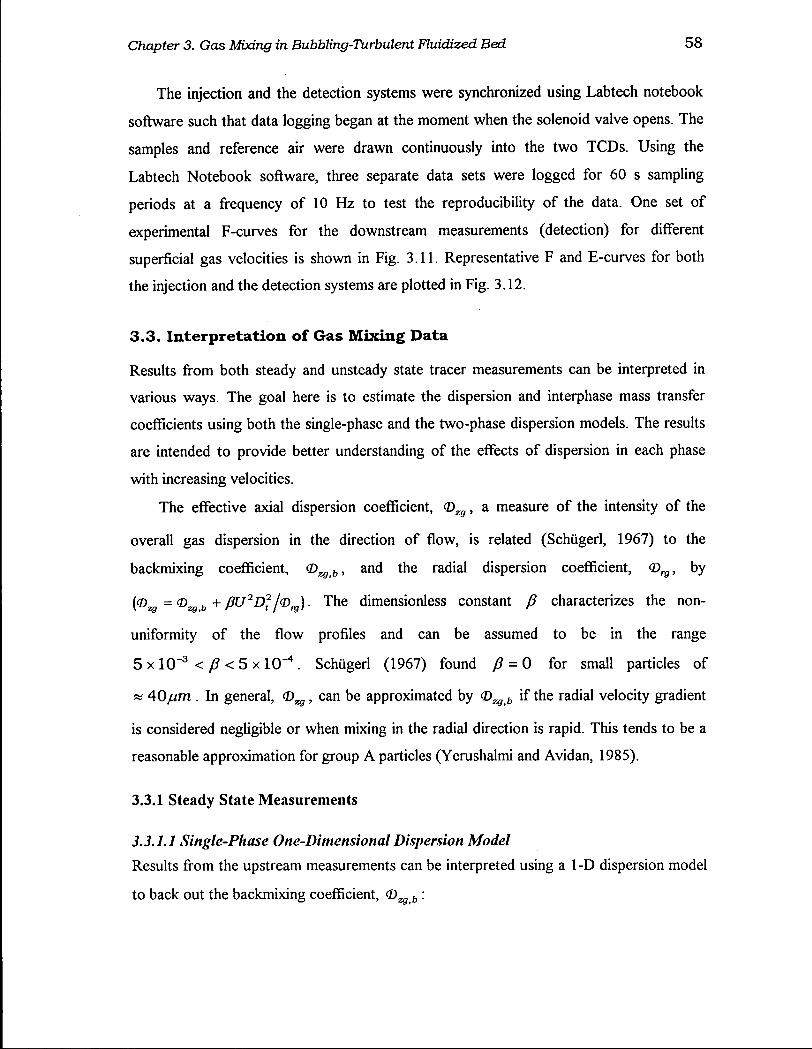
Chapter 3. Gas Mixing in Bubbling-Turbulent Fluidized Bed 58
The injection and the detection systems were synchronized using Labtech notebook
software such that data logging began at the moment when the solenoid valve opens. The
samples and reference air were drawn continuously into the two TCDs. Using the
Labtech Notebook software, three separate data sets were logged for 60 s sampling
periods at a frequency of 10 Hz to test the reproducibility of the data. One set of
experimental F-curves for the downstream measurements (detection) for different
superficial gas velocities is shown in Fig. 3.11. Representative F and E-curves for both
the injection and the detection systems are plotted in Fig. 3.12.
3.3. Interpretation of Gas Mixing Data
Results from both steady and unsteady state tracer measurements can be interpreted in
various ways. The goal here is to estimate the dispersion and interphase mass transfer
coefficients using both the single-phase and the two-phase dispersion models. The results
are intended to provide better understanding of the effects of dispersion in each phase
with increasing velocities.
The effective axial dispersion coefficient, (D^, a measure of the intensity of the
overall gas dispersion in the direction of flow, is related (Schugerl, 1967) to the
backmixing coefficient, <^>zg,b-> a n a " the radial dispersion coefficient, <D^, by
( © ^ = <D^ b + / ? f 7 2 D (
2 / © ^ ) . The dimensionless constant characterizes the non-
uniformity of the flow profiles and can be assumed to be in the range
5 x 10"3 < B < 5 x l O - 4 . Schugerl (1967) found /? = 0 for small particles of
» 40/um . In general, (D^, can be approximated by 0 ^ b if the radial velocity gradient
is considered negligible or when mixing in the radial direction is rapid. This tends to be a
reasonable approximation for group A particles (Yerushalmi and Avidan, 1985).
3.3.1 Steady State Measurements
3.3.1.1 Single-Phase One-Dimensional Dispersion Model
Results from the upstream measurements can be interpreted using a 1-D dispersion model
to back out the backmixing coefficient, <DW b :
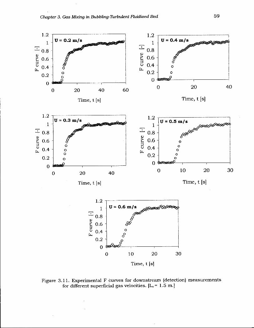
Chapter 3. Gas Mixing in Bubbling-Turbulent Fluidized Bed 59
1.2
_ 1
~ 0 .8
£ 0 .6
w 0 .4
0.2
0
U = 0.4 m/s
0 2 0
Time, t [s]
4 0
Figure 3.11. Experimental F curves for downstream (detection) measurements for different superficial gas velocities. [LQ= 1.5 m.]
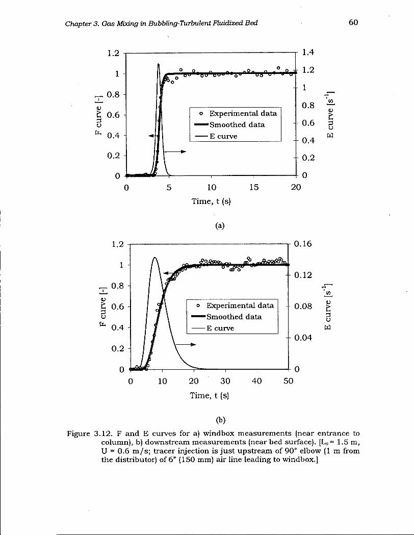
Chapter 3. Gas Mixing in Bubbling-Turbulent Fluidized Bed 60
0
O O-
o Experimental data ~ ~ Smoothed data
E curve
10 15
T i m e , t (s)
1.4
1.2
1
- 0 .8
- 0 .6
0 .4
+ 0 .2
0
2 0
CO
o
0
(a)
o Experimental data ^"Smoothed data
E curve
0 . 1 6
0 . 1 2
0
10 2 0 3 0 4 0
T i m e , t (s)
5 0
0 . 0 8 j>
o W
0 . 0 4
(b)
Figure 3.12. F and E curves for a) windbox measurements (near entrance to column), b) downstream measurements (near bed surface). [Lo= 1.5 m, U = 0.6 m/s; tracer injection is just upstream of 90° elbow (1 m from the distributor) of 6" (150 mm) air line leading to windbox.]
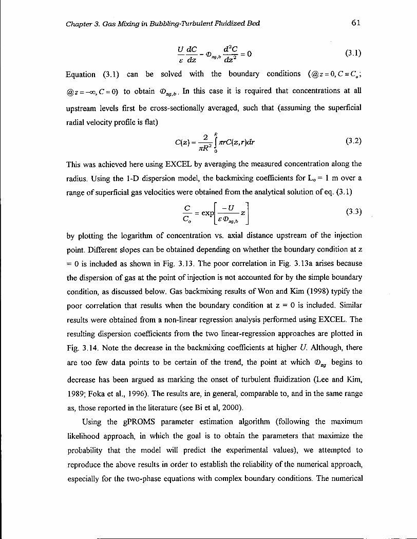
Chapter 3. Gas Mixing in Bubbling-Turbulent Fluidized Bed 61
U dC „ d2C _ n n
Equation (3.1) can be solved with the boundary conditions (@z = 0, C = C o ;
@z = - o o , C = 0) to obtain O ^ t , . In this case it is required that concentrations at all
upstream levels first be cross-sectionally averaged, such that (assuming the superficial
radial velocity profile is flat)
C{z) = -%AnrC{ztr)dr (3.2) KR %
This was achieved here using E X C E L by averaging the measured concentration along the
radius. Using the 1-D dispersion model, the backmixing coefficients for L 0 = 1 m over a
range of superficial gas velocities were obtained from the analytical solution of eq. (3.1)
~ U -z\ (3-3) C - = exP|
by plotting the logarithm of concentration vs. axial distance upstream of the injection
point. Different slopes can be obtained depending on whether the boundary condition at z
= 0 is included as shown in Fig. 3.13. The poor correlation in Fig. 3.13a arises because
the dispersion of gas at the point of injection is not accounted for by the simple boundary
condition, as discussed below. Gas backmixing results of Won and Kim (1998) typify the
poor correlation that results when the boundary condition at z = 0 is included. Similar
results were obtained from a non-linear regression analysis performed using E X C E L . The
resulting dispersion coefficients from the two linear-regression approaches are plotted in
Fig. 3.14. Note the decrease in the backmixing coefficients at higher U. Although, there
are too few data points to be certain of the trend, the point at which begins to
decrease has been argued as marking the onset of turbulent fluidization (Lee and Kim,
1989; Foka et al., 1996). The results are, in general, comparable to, and in the same range
as, those reported in the literature (see Bi et al, 2000).
Using the gPROMS parameter estimation algorithm (following the maximum
likelihood approach, in which the goal is to obtain the parameters that maximize the
probability that the model will predict the experimental values), we attempted to
reproduce the above results in order to establish the reliability of the numerical approach,
especially for the two-phase equations with complex boundary conditions. The numerical
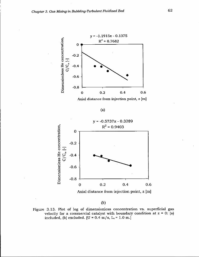
Chapter 3. Gas Mixing in Bubbling-Turbulent Fluidized Bed 62
y = -1.1915x-0.1375 o R 2 = 0.7682
Q 0 0.2 0.4 0.6
Axial distance from injection point, z [m]
(a)
y = -0.5737x - 0.3289 g R 2 = 0.9403
•i-t w v
B -0.8 -I 1 1 1 Q 0 0.2 0.4 0.6
Axial distance from injection point, z [m]
(b)
Figure 3.13. Plot of log of dimensionless concentration vs. superficial gas velocity for a commercial catalyst with boundary condition at z = 0: (a) included, (b) excluded. [U = 0.4 m/s, Lo= 1.0 m.]
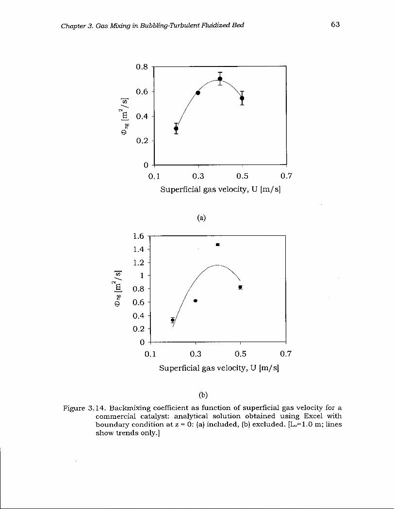
Chapter 3. Gas Mixing in BubbUng-Turbulent Fluidized Bed 63
(b)
Figure 3.14. Backmixing coefficient as function of superficial gas velocity for a commercial catalyst: analytical solution obtained using Excel with boundary condition at z = 0: (a) included, (b) excluded. [Lo=1.0 m; lines show trends only.]
Chapter 3. Gas Mixing in BubbUng-Turbulent Fluidized Bed 64
solution for the 1-D model, shown in Fig. 3.15, compares well with the least squares
fitted curve based on the analytical solution of the 1-D model when the boundary
condition at z = 0 is not considered. Note that the dispersed boundary condition was used
in the numerical solution as discussed in the next section.
3.3.1.2 One-Dimensional Two-Phase Model with Dispersion
The single-phase dispersion model can give reasonable results for fluidized beds operated
in the turbulent flow regime where homogeneity in the bed can be assumed. However, it
is inadequate for lower gas velocities up to the transition region, as it does not account for
the difference in the extent of dispersion between the two phases, nor for gas interchange
between them. In this section, we attempt to estimate the dispersion coefficients in the
two phases as well as the interphase mass transfer coefficient over a range of gas
velocities using the generalized two-phase model with dispersion. The one-dimensional
steady state two-phase mass balances (without the source term) can be written:
L-phase: V l u L ^ - \rL<D^L + KLH(CL-CH)=0 (3.4)
H-phase: WliuH 4£jL _ y,H<DVtH + KLH(c„ - C L)= 0 (3.5)
Overall: C , = + qHCiH (2.3)
where Km = kuiaiWL- The phase volume fractions (y/L and y/H) and the fractional gas
flows (qL and qn) are computed from eqs. (2.22), (2.25) and Table 2.3. Equations (3.4)
and (3.5) must be solved together to back out the model parameters ( ( D ^ , © H and
KLH). Both an analytical solution to a simplified form of the above equations and a
numerical approach that retains all terms in the equations are possible. One approach
would be to measure the He concentration in the L - and H-phases (which is very
difficult) and simplify the above equations by assuming to be negligible relative to
® z g . H ' while the interphase mass transfer coefficient is significant (van Deemter, 1961).
Another approach would be to use a robust parameter estimation technique to determine
the interphase mass transfer coefficient and the L - and H-phase dispersion coefficients
while retaining all the terms in the equations. The former approach is most common
because of its simplicity. Using this approach, eqs. (3.4) and (3.5) can be reduced to a

Chapter 3. Gas Mixing in Bubbling-Turbulent Fluidized Bed 65
Figure 3.15. Backmixing coefficient as function of superficial gas velocity for a commercial catalyst: Solution from gPROMS parameter estimation function [Lo=1.0 m; line shows trend only.]
Chapter 3. Gas Mixing in Bubbting-Turbulent Fluidized Bed 66
form similar to the dense phase axial dispersion model of Van Deemter (1961):
^ u L ^ + KLH(CL-CH)=0
¥HUH % - YHV^H + KLH(CH - Q)= 0
(3.6)
(3.7) dz '"-»»•" dz2
Equations (3.6) and (3.7) can be solved together with the boundary condition
( @ 2 = -oo, CH = 0) and the additional assumption that for U > UM/, most of the gas
passes through the dispersed or L-Phase such that ysHuH may be neglected relative to
y/LuL. The solution (van Deemter, 1961) is then:
i) for z < 0 (i.e. below injection level):
" H
c„ a- 4m
1 07 + 1 + 2m ) exp
m - 1 KLH x z
a w -1 2m m) exp
2
m-lK LH
u x z
ii) for z > 0 (i.e. above injection level):
C„ , ( m2 - 1 m - 1 — 1 + a— : + C0
—L= 1 + c„ 1
4CT 2 G J exp
U
m + l KLH x z
(3.8)
(3.9)
U
1 m + l a
m 2m exp
m + l KLH x z U
(3.10)
(3.11)
where
a 7 = ^ l + 4l/7(r„^„^H) (3.12)
Here a = 1 when the tracer is injected into the H-phase, and a = 0 when the tracer is
injected into the L-phase. Note that z is the upward positive axial distance from the
injection level. The challenge of this approach is injecting the tracer gas into one of the
L- or H-density phase. However, since it is expected that tracer injection at the wall will
give more backmixing than injection along the axis of the column, it may be possible to
inject the tracer at the wall, detect He concentrations below the injection point at different
axial locations and use eq. (3.8) to obtain the parameters by optimization.
A superior approach employs a robust parameter estimation technique to calculate all
three parameters. We accomplished this using the gPROMS parameter estimation feature.

Chapter 3. Gas Mixing in BubbUng-Turbulent Fluidized Bed 67
The possible boundary conditions for eqs. (3.4) and (3.5) are:
at z = 0 cH=c0
OR at z = 0
at z - -co
OR at z = L~
[QLCL + <1HCH = c0
da - (D , =
zg'L dz cj
dCH -c„) fct=o
'\cH=o da
- <D r — " "a'L dz = "LQ
' 1 dC„ [-*-" dz
= uHCH
( a )
(c)
(d)
(3.13)
The choice of boundary condition strongly influences the estimated parameters.
Boundary conditions (a) and (c) are commonly employed in gas mixing studies; they are
reasonable approximations when the same concentration of tracer is injected into both
phases, and for long columns in which the concentration in both phases at the distributor
can be neglected. In this study, tracer was injected at the column axis. We consider that
the tracer is dispersed in both phases right at the point of injection as represented by
boundary condition (b). The boundary condition at the distributor is obtained by
assuming that all gas that diffuses downward to the distributor is carried back upward by
the up-flowing gas through convection. A simple mass balance at the distributor then
results in the boundary condition represented by eq. 3.13d. The parameter estimator then
compares experimental data with the model predictions at the corresponding axial
positions. Agreement between model prediction and experiment is reasonable as shown
in Fig. 3.16. The Optimal parameter estimates for the interphase mass transfer coefficient,
and the L - and H-phase dispersion coefficients for superficial velocities in the range 0.2
to 0.5 m/s and boundary conditions (b) and (d) are presented in Table 3.1 and Fig. 3.17.
The results are reasonable and of the same order of magnitude as those obtained from the
analytical and numerical solutions of the 1-D model. While the dispersion coefficients in
both phases increased with increasing gas velocity as expected, the phase dispersion ratio,
®zg,L / ® z g , H ' differed considerably from its expected value of 1, even as U approached
Uc. The observed increase of interphase mass transfer with increasing gas velocity
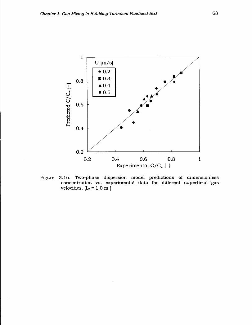
Chapter 3. Gas Mixing in Bubbling-Turbulent Fluidized Bed 68
0.2 0.4 0.6 0.8 1 Experimental C/C^, [-]
Figure 3.16. Two-phase dispersion model predictions of dimensionless concentration vs. experimental data for different superficial gas velocities. [Lo= 1.0 m.]
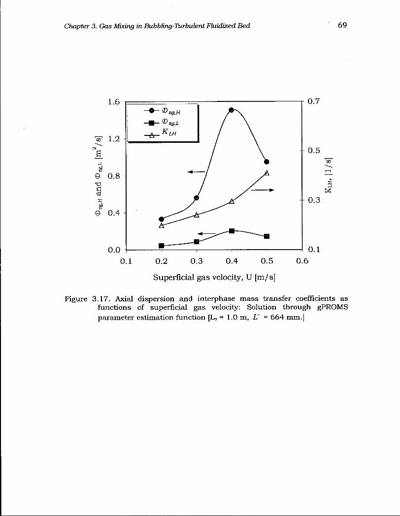
Chapter 3. Gas Mixing in Bubbling-Turbulent Fluidized Bed 69
Figure 3.17. Axial dispersion and interphase mass transfer coefficients as functions of superficial gas velocity: Solution through gPROMS parameter estimation function [L0 = 1.0 m, L~ = 664 mm.]
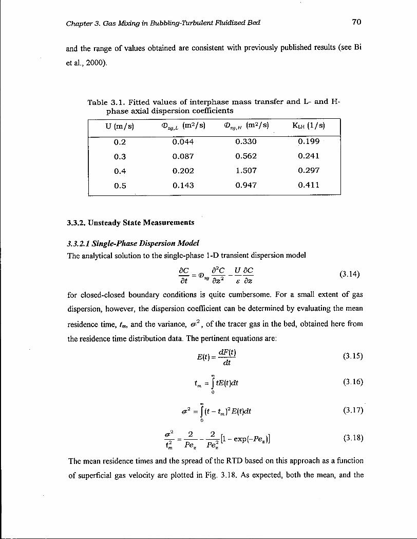
Chapter 3. Gas Mixing in BubbUng-Turbulent Fluidized Bed 70
and the range of values obtained are consistent with previously published results (see Bi
et al., 2000).
Table 3.1. Fitted values of interphase mass transfer and L- and H-phase axial dispersion coefficients
U (m/s) <D^L (m2/s) © „ . H (m2/s) KLH ( 1 /S)
0.2 0.044 0.330 0 .199
0.3 0.087 0.562 0.241
0.4 0.202 1.507 0 .297
0.5 0.143 0.947 0.411
3.3.2. Unsteady State Measurements
3.3.2.1 Single-Phase Dispersion Model
The analytical solution to the single-phase 1-D transient dispersion model
^ = <D ?C_U?£ (3.14) dt 2 3 dz2 e dz K }
for closed-closed boundary conditions is quite cumbersome. For a small extent of gas
dispersion, however, the dispersion coefficient can be determined by evaluating the mean
residence time, tm, and the variance, & 2 , of the tracer gas in the bed, obtained here from
the residence time distribution data. The pertinent equations are:
E(t) = m& (3.15) dt
dFJt) dt
tm=]tE(t)dt (3.16)
*2=](t-tm)2E(t)dt (3.17)
& 2 2 2
tl Pez Pel [l-exp(-Pej] (3.18)
The mean residence times and the spread of the RTD based on this approach as a function
of superficial gas velocity are plotted in Fig. 3.18. As expected, both the mean, and the
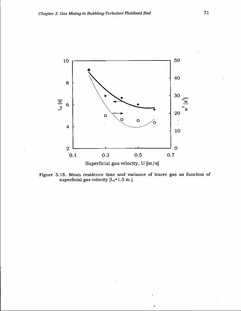
Chapter 3. Gas Mixing in BubbUng-Turbulent Fluidized Bed 71
0 0.1 0.3 0.5
Superficial gas velocity, U [m/s] 0.7
Figure 3.18. Mean residence time and variance of tracer gas as function of superficial gas velocity [Lo=1.5 m.]

Chapter 3. Gas Mixing in BubbUng-Turbulent Fluidized Bed 72
spread of the residence time distribution decrease with increasing gas velocity. However,
as seen from the figure, given the breath of the RTD (<?2 « t 2 ) , the variance approach is
not valid for estimating the dispersion coefficient. Therefore we sought a numerical
solution. The complete initial and boundary conditions for eq. (3.14) are
at t = 0 C = 0
at z = 0 -CDZQ?C=U(C\_-C) (3-19) 2 9 dz v ° '
at z = L — = 0 dz
where the imperfect step input for t > 0 is represented by the logistic regression function
C| o _=C 0 ( l + a i e - a V (3.20)
fitted to the input RTD data (see Fig. 3.12a) measured with TCD#2, shown in Fig. 3.10.
Because the tracer was injected farther from the distributor, eq. (3.20) corrects for the
delay associated with the tracer injection setting explained above. The constants ai and a 2
are functions of the superficial gas velocity.
The dispersion coefficients were estimated using gPROMS by solving eq. (3.14)
together with the initial and boundary conditions given by eqs. (3.19) and (3.20). As seen
in Fig. 3.19, the agreement between model prediction and experiment is reasonable. The
estimated parameters are shown in Fig. 3.20 as a function of superficial gas velocity.
Note the difference between these coefficients and the backmixing coefficients given in
Fig. 3.15. This difference is due to a combination of factors: different types of
coefficients as discussed above, different bed depths, and, possibly, different
experimental techniques. Note, also, that there is no maximum as the gas velocity is
increased beyond the transition velocity, Uc = 0.52 m/s (obtained from the Uc correlation
in Table 2.2). This may be due to an increase in Uc with increasing static bed height as
reported by Ellis et al. (2000) from an experimental study using the same catalysts, an
aspect not captured in the Uc correlations. In particular, Uc was reported to be -0.62 m/s
(based on differential pressure fluctuations) and 0.45 m/s (from absolute pressure
fluctuations) for L 0 = 1.5 m. The onset of turbulent fluidization, therefore, may well fall
around 0.6 m/s, explaining the lack of a maximum in the dispersion coefficient. The
values of (D^ are between 0.2 and 1.9 m2/s, consistent with the range obtained from the
backmixing studies above, while noting that the dispersion coefficients computed

Chapter 3. Gas Mixing in BubbUng-Turbulent Fluidized Bed 73
Time, t [s] Time, t [s]
1.2
Time, t [s]
Figure 3.19 1-D dispersion model predictions of transient dimensionless concentration (F curves) compared with experimental data for different superficial gas velocities. [LQ= 1.5 m.]
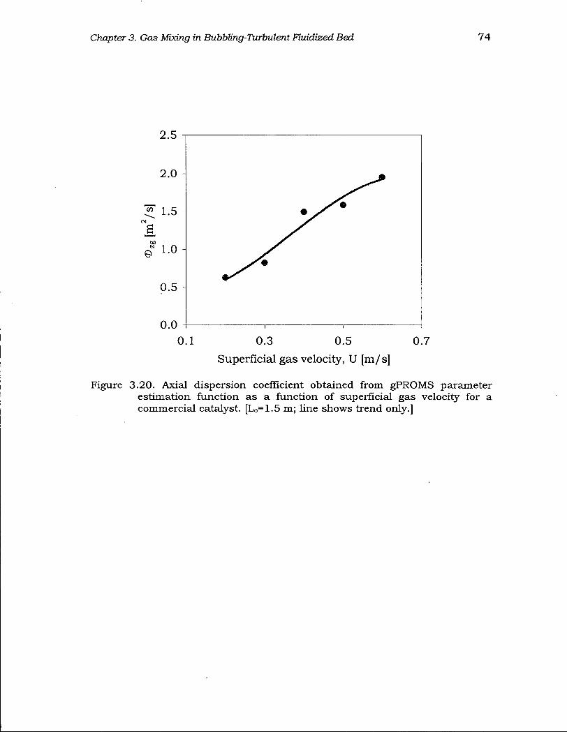
Chapter 3. Gas Mixing in BubbUng-Turbulent Fluidized Bed 74
Figure 3.20. Axial dispersion coefficient obtained from gPROMS parameter estimation function as a function of superficial gas velocity for a commercial catalyst. [L0=1.5 m; line shows trend only.]
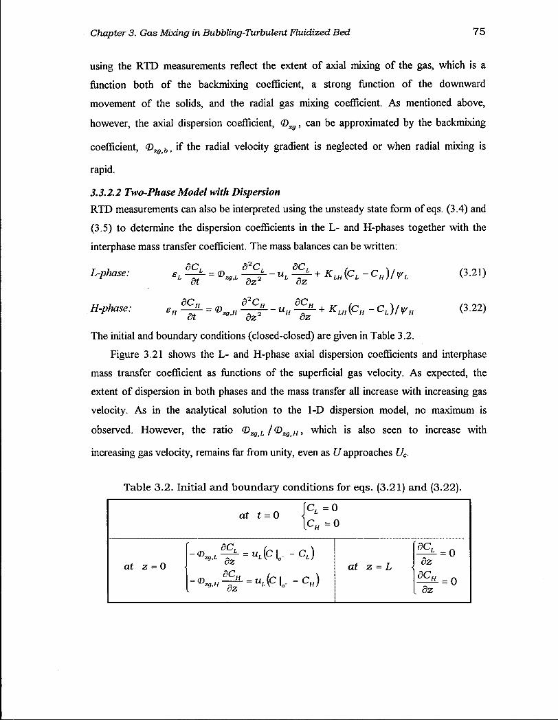
Chapter 3. Gas Mixing in BubbUng-Turbulent Fluidized Bed 75
using the RTD measurements reflect the extent of axial mixing of the gas, which is a
function both of the backmixing coefficient, a strong function of the downward
movement of the solids, and the radial gas mixing coefficient. As mentioned above,
however, the axial dispersion coefficient, , can be approximated by the backmixing
coefficient, ©z^, if the radial velocity gradient is neglected or when radial mixing is
rapid.
3.3.2.2 Two-Phase Model with Dispersion
RTD measurements can also be interpreted using the unsteady state form of eqs. (3.4) and
(3.5) to determine the dispersion coefficients in the L - and H-phases together with the
interphase mass transfer coefficient. The mass balances can be written:
L-phase: eL = „ J ^ - U L ° £ ± + K L H { C L - C H ) / ¥ L (3.21) dt ^ dz dz
H-phase: e„ = © fL^L-uH^L + KLH{CH-CL)/y,H (3.22) dt dz dz
The initial and boundary conditions (closed-closed) are given in Table 3.2.
Figure 3.21 shows the L - and H-phase axial dispersion coefficients and interphase
mass transfer coefficient as functions of the superficial gas velocity. As expected, the
extent of dispersion in both phases and the mass transfer all increase with increasing gas
velocity. As in the analytical solution to the 1-D dispersion model, no maximum is
observed. However, the ratio ©zg.z,/®zg,H > which is also seen to increase with
increasing gas velocity, remains far from unity, even as U approaches Uc.
Table 3.2. Initial and boundary conditions for eqs. (3.21) and (3.22).
at t = 0 \ L
[CH =0
af 2 = 0 - < ^ ^ = « , ( C | 0 - - C t )
at z = L dz dC»=o
. dz
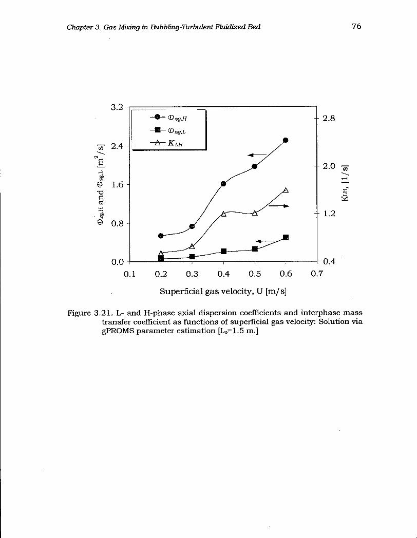
Chapter 3. Gas Mixing in BubbUng-Turbulent Fluidized. Bed 76
0.1 0.2 0.3 0.4 0.5 0.6 0.7
Superficial gas velocity, U [m/s]
Figure 3.21. L- and H-phase axial dispersion coefficients and interphase mass transfer coefficient as functions of superficial gas velocity: Solution via gPROMS parameter estimation [Lo=1.5 m.]
Chapter 3. Gas Mixing in BubbUng-Turbulent Fluidized Bed 77
3.4. Comments on Correlations for Pe z
The dispersion in the dilute or the L-phase is commonly assumed negligible relative to
that in the dense or H-phase, or approximated by using the molecular difFusivity of the
gas. Consequently, none of the numerous dispersion correlations attempted to delineate
the dispersions in the L - and the H-phases. Results from this study indicate that the
dispersion coefficients differ widely in the two phases at low gas velocities, with the
difference narrowing as the gas velocity increases. The effect of the initial solid
inventory, which affects the interfacial area available for gas interchange between the two
phases, and also affects the gas diffusion through the dense phase, has significant impact
on dispersion and interphase mass transfer. In addition, the column size also has
considerable impact on gas dispersion (Cho et al., 2000), but most reported correlations
do not account for this effect. Given the scarcity of data reported in the literature on the
effect of column size and static bed height on the Peclet number (Bi et al, 2000), it is
difficult to pin down the influence of such factors.
Unfortunately, because there are few results from our experiments, reliable
correlations cannot be developed at this point. In view of this, these results are not used in
later chapters; the correlations for Pez listed in Table 2.3 are used in conjunction with
equation (2.34) throughout the later chapters. It should be possible, however, when more
results from similar studies become available, to develop separate correlations for the
dispersion coefficients in the separate phases while accounting for the above factors.
3.5. Conclusions and Recommendations
Gas mixing experiments were conducted in a 4.4 m high by 0.286 m diameter column
with commercial catalyst particles as bed material for superficial gas velocities from 0.2
to 0.6 m/s. Data from both steady state and step change tracer injection experiments were
interpreted using a one-dimensional dispersion model and a generalized 2-phase model
with dispersion. The results are, in general, comparable to, and in the same range as,
those reported in the literature (see Bi et al., 2000). They also fall in the same range with
predictions from the correlations for interphase mass transfer and axial dispersion given

Chapter 3. Gas Mixing in BubbUng-Turbulent Fluidized Bed 78
in Table 2.3. The generalized 2-phase model effectively captures the expected trends of
increasing dispersion in both the low- and high-density phases as gas velocity is
increased. Beyond the transition velocity, Uc, however, the overall dispersion decreased
for L 0 = 1.0 m. Results for the different gas velocities and aspect ratios suggest that the
dispersion coefficients, and interphase mass transfer coefficient between the low- and
high-density phases depend on the initial solids inventory.
To provide further information for scale-up, the following are recommended:
(i) Conduct further gas mixing experiments at different static bed heights, preferably in
longer columns for the same or similar column diameters.
(ii) Conduct experiments in columns of different diameters for the same static bed
height, i.e. changing the aspect ratio, Lo/Dt, while keeping L 0 constant. Results from
this and (i) above, when treated together with the results from this study and
available literature data, will help establish the effect of the aspect ratio on both the
interphase mass transfer and gas dispersion in the bed.
(iii) It would be helpful to conduct experiments in columns of similar geometry for
superficial gas velocities beyond the range considered in this study. Specifically, it
would be valuable to study the effect of increasing velocity on the ratio
®zg,L /®zg , t f > which is expected to approach unity when the gas velocity is close to
Uc.
(iv) Using the combined information from above, it would be valuable to develop
separate correlations for the dispersion coefficients in the two phases.
Chapter 4
Validation of GFBR Model with Ozone Decomposition Data
4.1 Introduction
Although the new GFBR model is based on sound theoretical underpinnings, its true
utility lies in how well it predicts specific performance measures such as conversion,
selectivity and hydrodynamic trends. As shown in Chapter 2, the model provides a means
of covering the complete range of gas velocities and flow conditions from minimum
bubbling right up to fully fast fluidization conditions. The capability of the model in
eliminating discontinuities at the boundaries, while giving improved predictions of
particle and gas dynamics and of reactor performance, is demonstrated using
experimentally investigated ozone decomposition data from Sun (1991), covering a wide
range of superficial gas velocities and catalyst activities. The wide range of conditions
allows us to test the model across all three flow regimes considered.
4.2 Case study: Ozone Decomposition Reaction
4.2.1 Reaction Kinetics and Model Parameters
The ozone decomposition reaction is represented by
0 3 -> 1 . 5 0 2 (4.1)
This reaction has been commonly employed in laboratory investigation of the
performance of fluidized beds by several workers (e.g. Chavarie and Grace, 1975; Sun,
1991; Jiang et al., 1991, Ouyang et al., 1995) for a number of reasons: it proceeds at
atmospheric temperature and pressure; reaction kinetics are pseudo-first order; there is
negligible heat of reaction because of the low concentrations involved; and ozone is
readily determined using U V absorption. Ozone conversion data from experimental
investigation of the effect of PSD on FBR performance covering superficial gas velocities
in the range 0.1 to 1.8 m/s are used to validate the GFBR model. The particle properties
79
Chapter 4. Validation of GFBR Model with Ozone Decomposition Data 80
and operating conditions employed in the investigation are shown in Table 4.1. The
velocity range covers bubbling, turbulent and fast fluidization flow regimes (with Uc =
0.55 m/s and Use = 1.38 m/s respectively, estimated from the correlations in Table 2.2).
4.2.2 Other Considerations in Applying the GFBR Model to Sun's Data
(a) . It is assumed, for the ozone decomposition process, that temperature variations
along the column height are negligible, since the ozone decomposition reaction is
conducted at atmospheric conditions with a very small inlet concentration of
ozone. Also, the column is shallow enough (L, = 2 m) that pressure gradients are
not very significant, and pressure changes are neglected. Therefore, to reduce
C P U time, both energy and pressure balances in the GFBR model code were
turned off at this stage using the selector section of the gPROMS code.
(b) . Sun (1991) estimated that about 20% of the solids were in the solids return system
during the experiments. The exact quantity may have varied widely over the
course of the investigation, but lacking any systematic measurements that could
tie the entrainment rate to the gas velocity, the solids inventory was adjusted in all
cases so that Ms = 0.8 xM s o .
(c) . The voidage at minimum fluidization, emf, was taken as 0.48 from Grace and Sun
(1991) who reproduced experimental measurements of Ip (1989) for different
PSDs of FCC particles.
(d) . Three parameters appearing in the transition equations (Table 2.3), crucial to
correctly predicting the behavior at the limiting conditions in the GFBR model,
were first estimated by comparing model predictions with experimental data: In
particular, the (i) initial volume fraction of solids in L-phase at bubbling
conditions, (j>Lo, was estimated to be 0.0355 by matching model predictions with
data under bubbling conditions using the two-phase bubbling bed model, (ii) The
average solids flux under fast fluidization conditions, Gso, was estimated by
matching model predictions with data using the GFBR model for the intermediate
gas velocities between turbulent and fast fluidization conditions giving Gso =120
kg/m2s. This value was used throughout the simulations, (iii) Widely varying
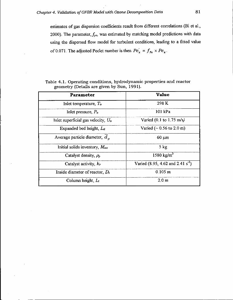
Chapter 4. Validation of GFBR Model with Ozone Decomposition Data 81
estimates of gas dispersion coefficients result from different correlations (Bi et al.,
2000). The parameter, fpe, was estimated by matching model predictions with data
using the dispersed flow model for turbulent conditions, leading to a fitted value
of 0.071. The adjusted Peclet number is then Pez = fPe x Pez.
Table 4.1. Operating conditions, hydrodynamic properties and reactor geometry (Details are given by Sun, 1991).
Parameter Value
Inlet temperature, T0 298 K
Inlet pressure, P0 101 kPa
Inlet superficial gas velocity, U0 Varied (0.1 to 1.75 m/sj
Expanded bed height, La Varied (~ 0.56 to 2.0 m)
Average particle diameter, dp 60 urn
Initial solids inventory, MSo 5 kg
Catalyst density, pp 1580 kg/m3
Catalyst activity, fa- Varied (8.95, 4.62 and 2.41 s*1)
Inside diameter of reactor, Dt 0.105 m
Column height, Lt 2.0 m
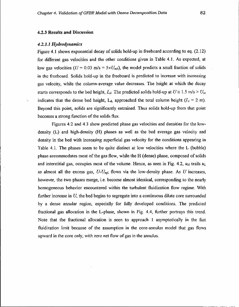
Chapter 4. Validation of GFBR Model with Ozone Decomposition Data 82
4.2.3 Results and Discussion
4.2.3.1 Hydrodynamics
Figure 4.1 shows exponential decay of solids hold-up in freeboard according to eq. (2.12)
for different gas velocities and the other conditions given in Table 4.1. As expected, at
low gas velocities (U = 0.03 m/s = 5xUmb), the model predicts a small fraction of solids
in the freeboard. Solids hold-up in the freeboard is predicted to increase with increasing
gas velocity, while the column-average value decreases. The height at which the decay
starts corresponds to the bed height, Ld. The predicted solids hold-up at U= 1.5 m/s > Use
indicates that the dense bed height, La, approached the total column height (Lt = 2 m).
Beyond this point, solids are significantly entrained. Thus solids hold-up from that point
becomes a strong function of the solids flux.
Figures 4.2 and 4.3 show predicted phase gas velocities and densities for the low-
density (L) and high-density (H) phases as well as the bed average gas velocity and
density in the bed with increasing superficial gas velocity for the conditions appearing in
Table 4.1. The phases seem to be quite distinct at low velocities where the L (bubble)
phase accommodates most of the gas flow, while the H (dense) phase, composed of solids
and interstitial gas, occupies most of the volume. Hence, as seen in Fig. 4.2, UH trails uL
as almost all the excess gas, U-Umf, flows via the low-density phase. As U increases,
however, the two phases merge, i.e. become almost identical, corresponding to the nearly
homogeneous behavior encountered within the turbulent fluidization flow regime. With
further increase in U, the bed begins to segregate into a continuous dilute core surrounded
by a dense annular region, especially for fully developed conditions. The predicted
fractional gas allocation in the L-phase, shown in Fig. 4.4, further portrays this trend.
Note that the fractional allocation is seen to approach 1 asymptotically in the fast
fluidization limit because of the assumption in the core-annulus model that gas flows
upward in the core only, with zero net flow of gas in the annulus.
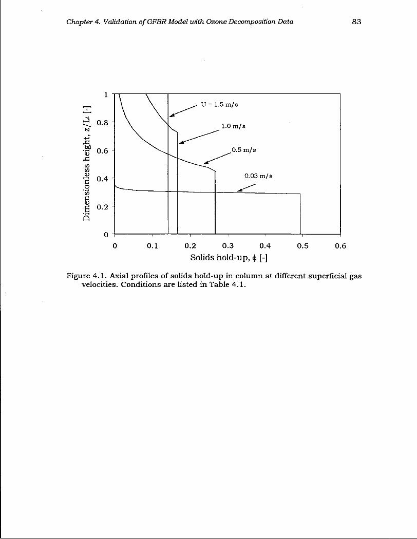
Chapter 4. Validation of GFBR Model with Ozone Decomposition Data
Figure 4.1. Axial profiles of solids hold-up in column at different superficial velocities. Conditions are listed in Table 4.1.

Chapter 4. Validation of GFBR Model with Ozone Decomposition Data 84
0 0.5 1 1.5 2 Superficial gas velocity, U [m/ s]
Figure 4.2. Predicted gas velocities in low- and high-density phases and bed average with increasing superficial gas velocity in the dense bed. Conditions are listed in Table 4.1.
Chapter 4. Validation of GFBR Model with Ozone Decomposition Data 8 5
Figure 4.3. Predicted suspension densities in low- and high-density phases and bed average with increasing superficial gas velocity in the dense bed. Conditions are listed in Table 4.1.
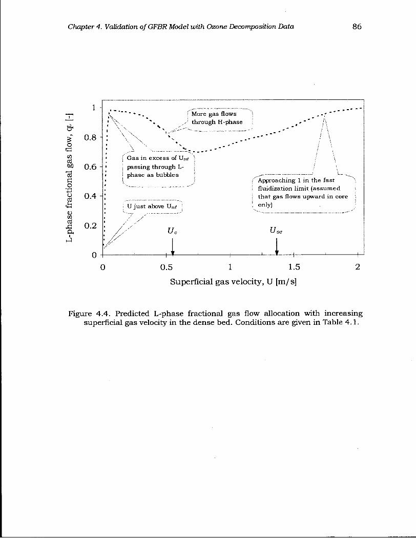
Chapter 4. Validation of GFBR Model with Ozone Decomposition Data 86
0.8
More gas flows through H-phase
0.6
0.4
Gas in excess of Umf
passing through L-phase as bubbles
U just above Umf
Approaching 1 in the fast fluidization limit (assumed that gas flows upward in core only)
0.2
0
Us
0 0.5 1 1.5
Superficial gas velocity, U [m/s]
Figure 4.4. Predicted L-phase fractional gas flow allocation with increasing superficial gas velocity in the dense bed. Condit ions are given in Table 4.1.

Chapter 4. Validation of GFBR Model with Ozone Decomposition Data 87
4.2.3.2 Reactor Performance
(a) Influence of Freeboard on Ozone Conversion
The performance of the GFBR model with the freeboard included (easel) is compared
here with case 2 where the freeboard is ignored. We also explore how the contribution of
the freeboard; (i) influences the overall conversion of ozone; and (ii) changes with
increasing superficial gas velocity. But first, we examine the difference between the
dense bed heights for the two cases (cases 1 and 2). Figure 4.5 shows the predicted dense
bed height with increasing gas velocity for both cases, where the bed heights are
computed based on
M8=App(LJa+Lfjf) (2.19)
For the case without the freeboard, the expanded bed height, Ld, is computed by
assigning all the solids to the dense region, or equivalently by setting <pf = 0 in eq.
(2.19). As expected, the bed height for case 1 continues to trail that in case 2 until the
predicted bed heights in both cases reach the column height, Lt.
Figure 4.6 shows predicted axial ozone conversions at different gas velocities for
the two cases. At low U (sufficiently high for some solids to be ejected into the
freeboard), because of the sharp exponential decay of solids hold-up, the additional
freeboard reaction occurs just above the dense bed height with the remaining freeboard
height showing a flat profile up to the column exit. Moreover, even for this low U, the
computed bed height is slightly higher when the freeboard is ignored than when included,
in line with eq. (2.19). With a further increase in U, the computed dense bed heights
diverge even further until the freeboard disappears completely, from which point there is
no difference in the predicted values for the two cases.
The performance of the GFBR model with and without the freeboard is tested by
comparing model predictions with experimental data over a wide range of superficial gas
velocities and catalysts activities in Figure 4.7. Predictions for the case with the freeboard
included gives better agreement with the data in general. At high U (U > 1.2 m/s),
predictions from the two cases merge for the reasons explained above. Overall, the
freeboard is important in columns where the freeboard height constitutes a significant
fraction of the total column height. For highly exothermic reactions, the dense region
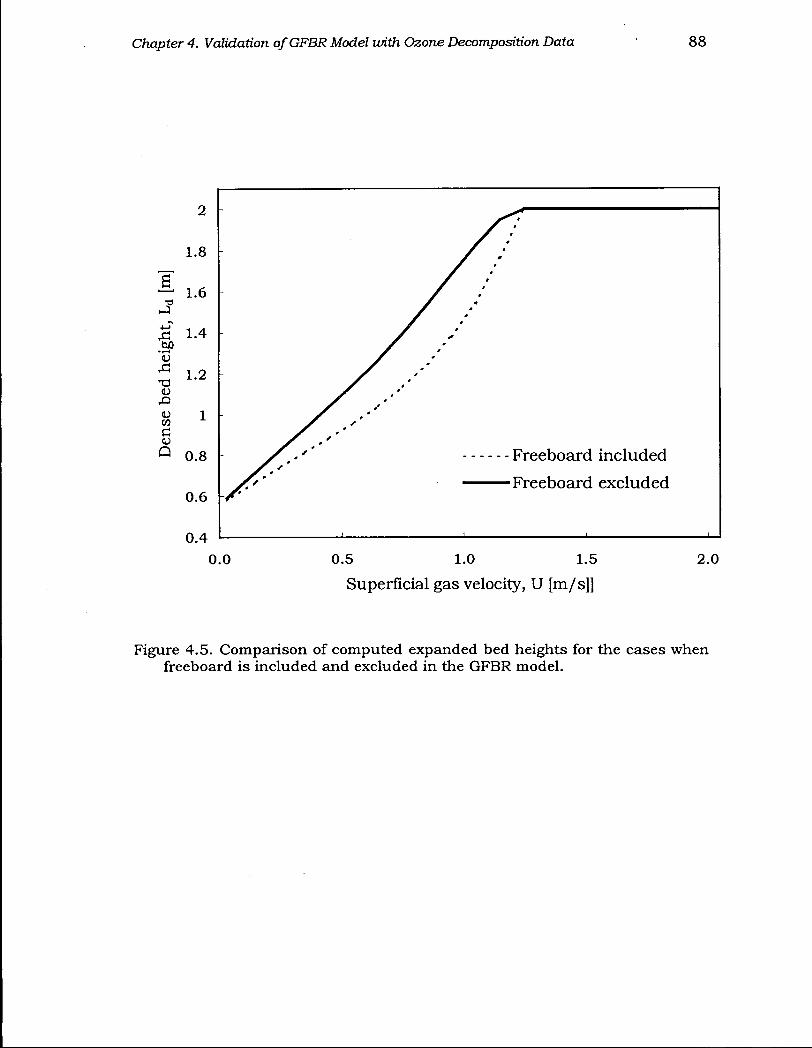
Chapter 4. Validation of GFBR Model with Ozone Decomposition Data 88
0.4 ' 1 1 1 1—1
0.0 0.5 1.0 1.5 2.0 Superficial gas velocity, U [m/s]]
Figure 4.5. Comparison of computed expanded bed heights for the cases when freeboard is included and excluded in the GFBR model.
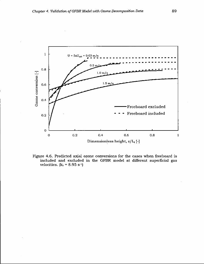
Chapter 4. Validation of GFBR Model with Ozone Decomposition Data 89
U = 5 x U m b = 0.03 m/s
0 0.2 0.4 0.6 0.8 1
Dimensionless height, z/Lt [-]
Figure 4.6. Predicted axial ozone conversions for the cases when freeboard is included and excluded in the GFBR model at different superficial gas velocities. (kr = 8.95 s-i)
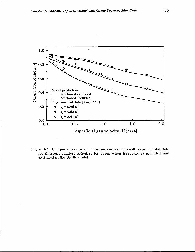
Chapter 4. Validation of GFBR Model with Ozone Decomposition Data 90
Figure 4.7. Comparison of predicted ozone conversions with experimental data for different catalyst activities for cases when freeboard is included and excluded in the GFBR model.
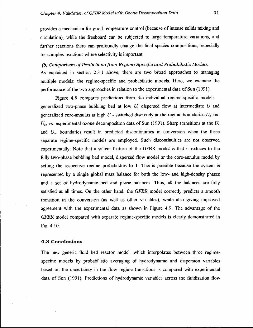
Chapter 4. Validation of GFBR Model with Ozone Decomposition Data 91
provides a mechanism for good temperature control (because of intense solids mixing and
circulation), while the freeboard can be subjected to large temperature variations, and
further reactions there can profoundly change the final species compositions, especially
for complex reactions where selectivity is important.
(b) Comparison of Predictions from Regime-Specific and Probabilistic Models
As explained in section 2.3.1 above, there are two broad approaches to managing
multiple models: the regime-specific and probabilistic models. Here, we examine the
performance of the two approaches in relation to the experimental data of Sun (1991).
Figure 4.8 compares predictions from the individual regime-specific models -
generalized two-phase bubbling bed at low U, dispersed flow at intermediate U and
generalized core-annulus at high U - switched discretely at the regime boundaries Uc and
Use vs. experimental ozone decomposition data of Sun (1991). Sharp transitions at the Uc
and Ue boundaries result in predicted discontinuities in conversion when the three
separate regime-specific models are employed. Such discontinuities are not observed
experimentally. Note that a salient feature of the GFBR model is that it reduces to the
fully two-phase bubbling bed model, dispersed flow model or the core-annulus model by
setting the respective regime probabilities to 1. This is possible because the system is
represented by a single global mass balance for both the low- and high-density phases
and a set of hydrodynamic bed and phase balances. Thus, all the balances are fully
satisfied at all times. On the other hand, the GFBR model correctly predicts a smooth
transition in the conversion (as well as other variables), while also giving improved
agreement with the experimental data as shown in Figure 4.9. The advantage of the
GFBR model compared with separate regime-specific models is clearly demonstrated in
Fig. 4.10.
4.3 Conclusions
The new generic fluid bed reactor model, which interpolates between three regime-
specific models by probabilistic averaging of hydrodynamic and dispersion variables
based on the uncertainty in the flow regime transitions is compared with experimental
data of Sun (1991). Predictions of hydrodynamic variables across the fluidization flow
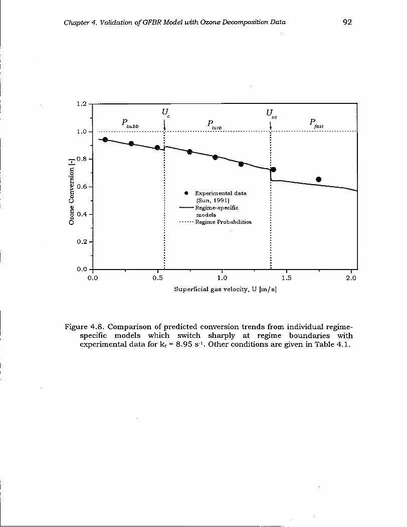
Chapter 4. Validation of GFBR Model with Ozone Decomposition Data 92
Figure 4.8. Comparison of predicted conversion trends from individual regime-specific models which switch sharply at regime boundaries with experimental data for kr = 8.95 s1. Other conditions are given in Table 4.1.
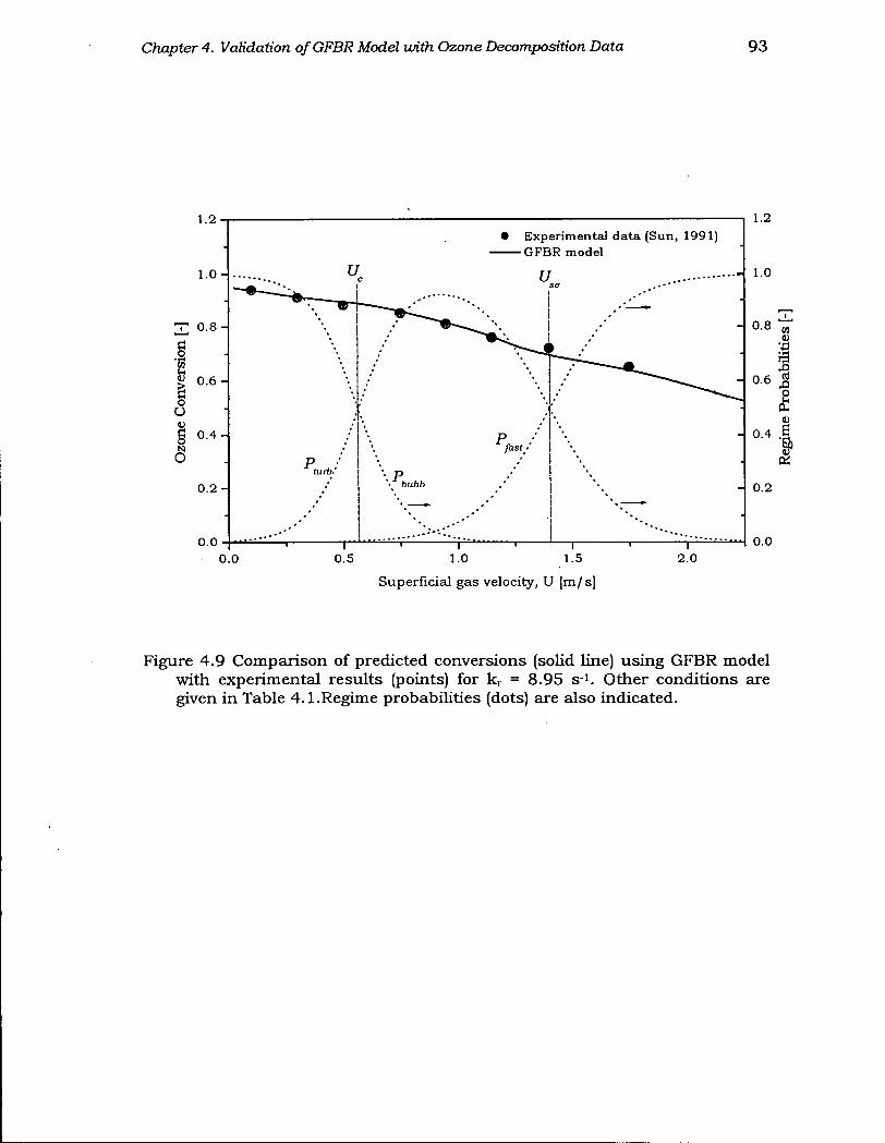
Chapter 4. Validation of GFBR Model with Ozone Decomposition Data 93
Figure 4.9 Comparison of predicted conversions (solid line) using GFBR model with experimental results (points) for kr = 8.95 s1. Other conditions are given in Table 4.1.Regime probabilities (dots) are also indicated.
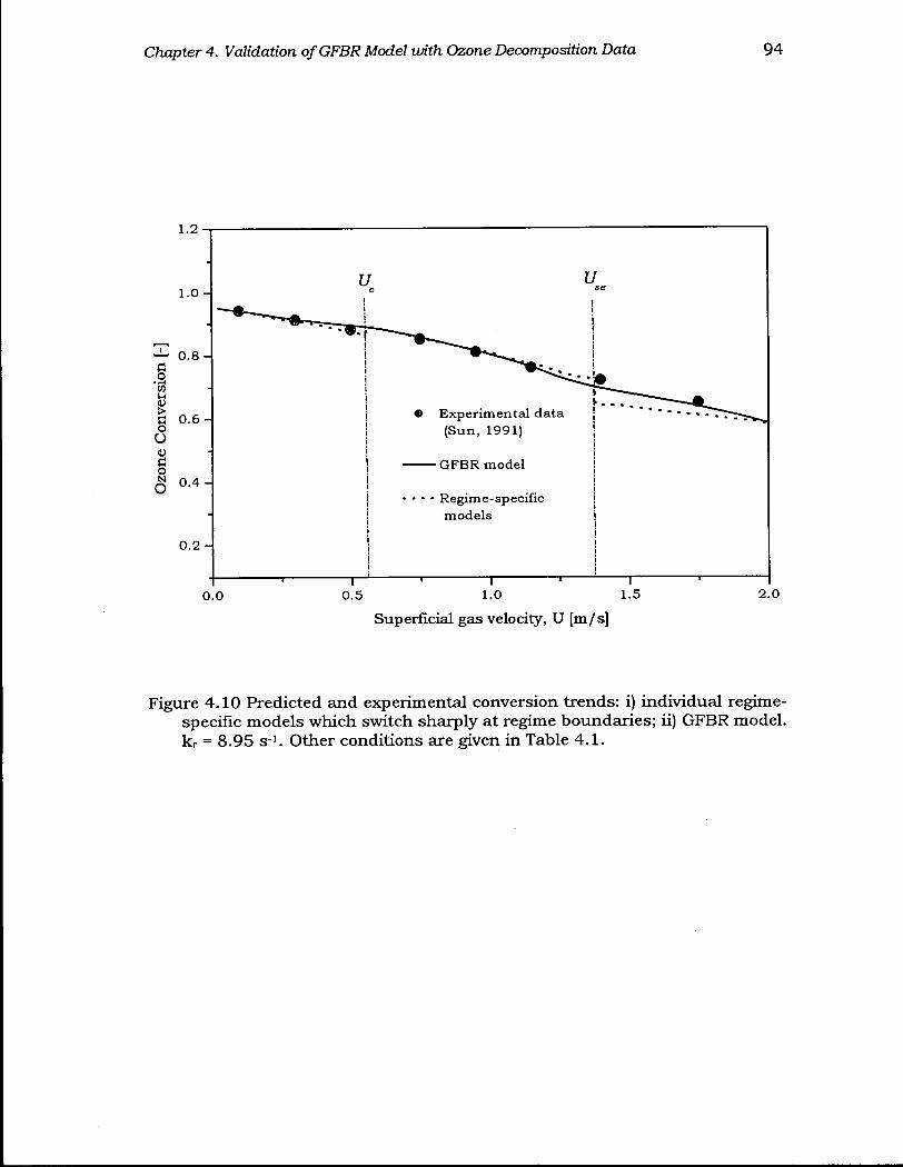
Chapter 4. Validation of GFBR Model with Ozone Decomposition Data 94
Figure 4.10 Predicted and experimental conversion trends: i) individual regime-specific models which switch sharply at regime boundaries; ii) GFBR model. kr = 8.95 s 1. Other conditions are given in Table 4.1.
Chapter 4. Validation of GFBR Model with Ozone Decomposition Data 9 5
regimes most commonly encountered in industrial scale fluid bed reactors - bubbling,
turbulent and fast fluidization - are realistic, while conversion predictions are in good
agreement with available experimental data. This approach leads to improved predictions
of reactor performance compared with any of the three separate models for individual
flow regimes, while avoiding discontinuities at the boundaries between the flow regimes.
The contribution of the freeboard is shown to be important for reactors operated well
beyond Umb and for tall columns where the freeboard height represents a significant
fraction of total column height. Although the preliminary results are encouraging, more
validation with more complex reactions, significant energy effects and industrial-scale
equipment is needed to consolidate this approach. This is the subject of Chapters 5 and 6.
Chapter 5
A p p l i c a t i o n o f G F B R M o d e l t o I n d u s t r i a l - S c a l e P r o c e s s e s
In this Chapter, the performance of the GFBR model is examined using two industrial-
scale catalytic processes (oxy-chlorination of ethylene and oxidation of naphthalene to
phthalic anhydride) and an industrial non-catalytic process (roasting of zinc sulfide). In
addition to their scale of operation, the two catalytic processes are chosen because: (a)
Plant measurements are available, accompanied by sufficient details of reactor
configuration and operating conditions, providing an opportunity for validating the model
with industrial-scale data, and for testing the model's ability to aid in "simulation
experimentation" over a wide range of operating conditions, (b) The two catalytic
processes are complex so that selectivity1 can be used as a reactor performance indicator,
(c) The reactors operate around the Uc boundary (phthalic anhydride: Pbubb = Pturb = 50 %;
oxy-chlorination: Pbubb = 20%, Pturb = 80 %), making it possible to assess the
performance of the GFBR model, as well as the limiting cases of dispersed plug flow and
the two-phase bubbling bed model.
Section 5.3 extends the GFBR model to gas solid reactions. A single particle model
is coupled with the fluid bed reactor model to create a combined model, with the zinc
sulfide roasting process addressed as a case study.
5.1 Phthalic Anhydride Process
Phthalic anhydride (PA) is an important organic chemical used mainly in the preparation
of diesters, which are widely applied as plasticizers for polyvinyl chloride. It is also used
in the preparation of alkyd and polyester resins and dyes. Until the late 1950's,
manufacture of PA was based on the oxidation of naphthalene over vanadium oxide
catalysts. The increasing demand for PA led to a search for alternative raw materials. At
present, PA is made primarily by gas-phase oxidation of ortho-xylene, available in large
1 Selectivity is defined as the ratio of moles of product formed to that of reactant consumed. (When plotted against height, the moles correspond to the values at that level.)
96
Chapter 5. Application of GFBR Model to Industrial-Scale Processes 97
quantities from refineries, over fixed catalysts containing vanadium and titanium oxides.
The technical difficulty associated with the development of long-life, attrition-resistant
catalysts (Bolthrunis, 1989) has not allowed the development of fluidized bed process for
the oxidation of o-xylene to PA. Dias et al. (1997) reviewed the catalysts, kinetics and
modeling of both the o-xylene and naphthalene phthalic anhydride processes for fixed
and fluidized beds.
Johnsson et al. (1987) published a detailed study on the naphthalene-based phthalic
anhydride process. They compared data from an industrial reactor of 2.1 m diameter with
a number of bubbling bed mechanistic models [Grace (1984) model, Kunii and
Levenspiel (1969) model, Kato and Wen (1969) model and, Partridge and Rowe (1966)
model]. The first three models all gave good overall prediction of the very limited data on
reactor performance, provided that the bubble size and the fraction of solids in bubbles
are estimated with reasonable accuracy. However, because the plant operates around the
bubbling-turbulent regime boundary (U ~ 0.4 - 0.5 m/s, while Uc = 0.436 m/s, estimated
from the correlation in Table 2.2), the use of the simple two-phase or three-phase models
is only an approximation at best. No general conclusions can be drawn on the
performance of the models, as their applicability to turbulent processes is questionable.
The sensitivity analysis done by Johnsson et al. (1987) showed that, in general, the
models performed better when the bubble size was decreased and more solids were
allocated to the bubbles - effectively approximating more homogeneous behavior as in
turbulent flow regime. This led Bolthrunis (1989) to suggest the dispersed plug flow
model rather than the bubbling bed models, to capture the shift away from the bubbling
behaviour. It is clear from the foregoing discussions that the PA process is an ideal
"candidate process" to test the performance of the GFBR model.
Here, we use plant data from an industrial-scale naphthalene-based fluidized bed
reactor, accompanied by sufficient information (Johnsson, 1986; Johnsson et al., 1987) to
assess the performance of the GFBR model. Predictions from the limiting cases of the
model at low U, i.e. the generalized two-phase bubbling bed model (2PBBM), and at
intermediate U, i.e. the dispersed plug flow model (DPFM), are also compared with the
GFBR model (GFBRM) and plant data. Sensitivity analysis is also carried out to assess
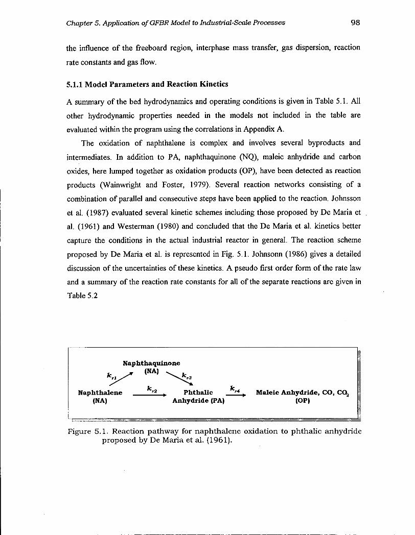
Chapter 5. Application of GFBR Model to Industrial-Scale Processes 98
the influence of the freeboard region, interphase mass transfer, gas dispersion, reaction
rate constants and gas flow.
5.1.1 Model Parameters and Reaction Kinetics
A summary of the bed hydrodynamics and operating conditions is given in Table 5.1. All
other hydrodynamic properties needed in the models not included in the table are
evaluated within the program using the correlations in Appendix A.
The oxidation of naphthalene is complex and involves several byproducts and
intermediates. In addition to PA, naphthaquinone (NQ), maleic anhydride and carbon
oxides, here lumped together as oxidation products (OP), have been detected as reaction
products (Wainwright and Foster, 1979). Several reaction networks consisting of a
combination of parallel and consecutive steps have been applied to the reaction. Johnsson
et al. (1987) evaluated several kinetic schemes including those proposed by De Maria et
al. (1961) and Westerman (1980) and concluded that the De Maria et al. kinetics better
capture the conditions in the actual industrial reactor in general. The reaction scheme
proposed by De Maria et al. is represented in Fig. 5.1. Johnsonn (1986) gives a detailed
discussion of the uncertainties of these kinetics. A pseudo first order form of the rate law
and a summary of the reaction rate constants for all of the separate reactions are given in
Table 5.2
Naphthaquinone (NA)
Naphthalene (NA)
T2 Phthalic Anhydride (PA)
r 4 ^ Maleic Anhydride, C O , CQj (OP)
Figure 5.1. Reaction pathway for naphthalene oxidation to phthalic anhydride proposed by De Maria et al. (1961).
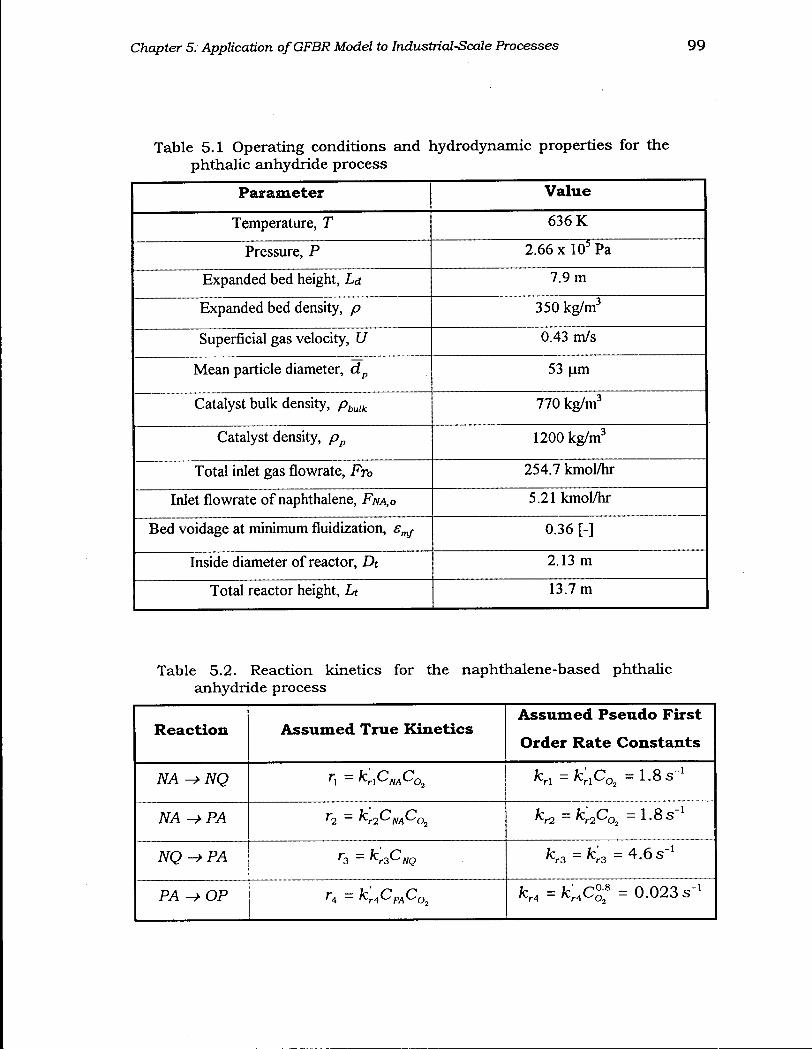
Chapter 5. Application of GFBR Model to Industrial-Scale Processes 99
Table 5.1 Operating conditions and hydrodynamic properties for the phthalic anhydride process
Parameter Value
Temperature, T 636 K
Pressure, P 2.66 x 10⁵ Pa
Expanded bed height, Ld 7.9 m
Expanded bed density, p 350 kg/m3
Superficial gas velocity, U 0.43 m/s
Mean particle diameter, dp 53 urn
Catalyst bulk density, pbulk 770 kg/m3
Catalyst density, pp 1200 kg/m3
Total inlet gas flowrate, Fro 254.7 kmol/hr
Inlet flowrate of naphthalene, FNA,O 5.21 kmol/hr
Bed voidage at minimum fluidization, emJ- 0.36 [-]
Inside diameter of reactor, Dt 2.13 m
Total reactor height, Lt 13.7 m
Table 5.2. Reaction kinetics for the naphthalene-based phthalic anhydride process
Reaction Assumed True Kinetics Assumed Pseudo First
Order Rate Constants
NA^NQ r i = Kf~^NA^02 Ki = Kico2 -1-8 s _ 1
NA^PA r2 = Kl^HA^O^ Ki ~ Krf^o2 - 1-8 S 1
NQ-+PA r3 = K^PiiQ Kz - K3 = 4.6 s
PA^OP r4 = K^PffPo^ K< =K<C°0* = 0.023 s- 1
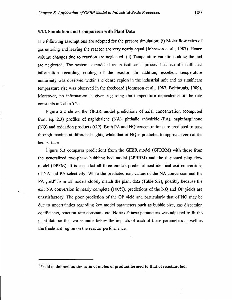
Chapter 5. Application of GFBR Model to Industrial-Scale Processes 100
5.1.2 Simulation and Comparison with Plant Data
The following assumptions are adopted for the present simulation: (i) Molar flow rates of
gas entering and leaving the reactor are very nearly equal (Johnsson et al., 1987). Hence
volume changes due to reaction are neglected, (ii) Temperature variations along the bed
are neglected. The system is modeled as an isothermal process because of insufficient
information regarding cooling of the reactor. In addition, excellent temperature
uniformity was observed within the dense region in the industrial unit and no significant
temperature rise was observed in the freeboard (Johnsson et al., 1987, Bolthrunis, 1989).
Moreover, no information is given regarding the temperature dependence of the rate
constants in Table 5.2.
Figure 5.2 shows the GFBR model predictions of axial concentration (computed
from eq. 2.3) profiles of naphthalene (NA), phthalic anhydride (PA), naphthaquinone
(NQ) and oxidation products (OP). Both PA and NQ concentrations are predicted to pass
through maxima at different heights, while that of NQ is predicted to approach zero at the
bed surface.
Figure 5.3 compares predictions from the GFBR model (GFBRM) with those from
the generalized two-phase bubbling bed model (2PBBM) and the dispersed plug flow
model (DPFM). It is seen that all three models predict almost identical exit conversions
of N A and PA selectivity. While the predicted exit values of the N A conversion and the
PA yield2 from all models closely match the plant data (Table 5.3), possibly because the
exit N A conversion is nearly complete (100%), predictions of the NQ and OP yields are
unsatisfactory. The poor prediction of the OP yield and particularly that of NQ may be
due to uncertainties regarding key model parameters such as bubble size, gas dispersion
coefficients, reaction rate constants etc. None of these parameters was adjusted to fit the
plant data so that we examine below the impacts of each of these parameters as well as
the freeboard region on the reactor performance.
2 Yield is defined as the ratio of moles of product formed to that of reactant fed.
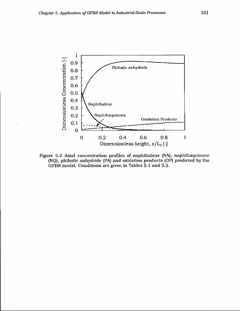
Figure 5.2 Axial concentration profiles of naphthalene (NA), naphthoquinone (NQ), phthalic anhydride (PA) and oxidation products (OP) predicted by the GFBR model. Conditions are given in Tables 5.1 and 5.2.
Chapter 5. Application of GFBR Model to Industrial-Scale Processes 102
100%
C o
*r—i CO u > o
O
<
80%
60%
40% 1 1 1 1 1 1
0 0.2 0.4 0.6 0.8 1
Dimensionless height, z / L d [-]
(a)
110%
90%
2 70%
t3 50%
co 30%
10%
0 0.2 0.4 0.6 0.8 1
Dimensionless height, z / L d [-]
(a) Figure 5.3 Predictions of axial profiles of (a) NA conversion and (b) selectivity to
PA from the three models: G F B R M , 2 P B B M and D P F M for conditions given in Tables 5.1 and 5.2.
G F B R M
DPFM
2PBBM
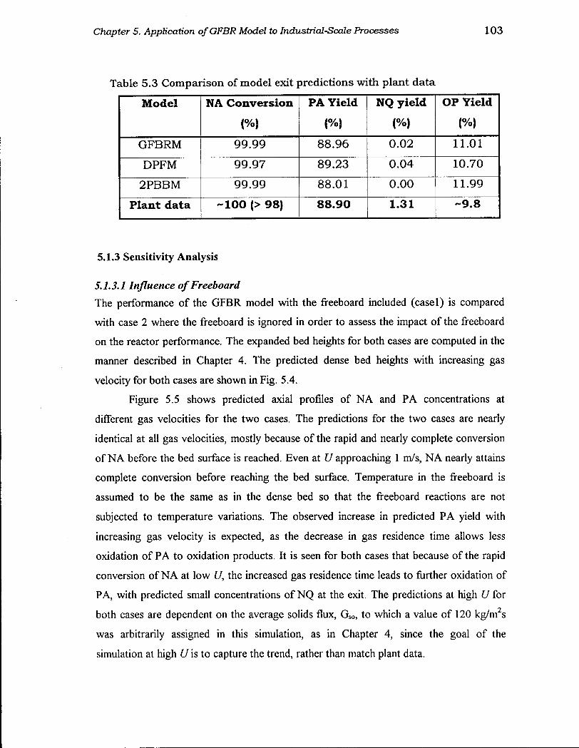
Chapter 5. Application of GFBR Model to Industrial-Scale Processes 103
Table 5.3 Comparison of model exit predictions with plant data
Model NA Conversion
(%)
PA Yield
(%)
NQ yield
1%) OP Yield
(%)
GFBRM 99.99 88.96 0.02 11.01
DPFM 99.97 89.23 0.04 10.70
2PBBM 99.99 88.01 0.00 11.99
Plant data -100 (> 98) 88.90 1.31 -9.8
5.1.3 Sensitivity Analysis
5.1.3.1 Influence of Freeboard
The performance of the GFBR model with the freeboard included (easel) is compared
with case 2 where the freeboard is ignored in order to assess the impact of the freeboard
on the reactor performance. The expanded bed heights for both cases are computed in the
manner described in Chapter 4. The predicted dense bed heights with increasing gas
velocity for both cases are shown in Fig. 5.4.
Figure 5.5 shows predicted axial profiles of N A and PA concentrations at
different gas velocities for the two cases. The predictions for the two cases are nearly
identical at all gas velocities, mostly because of the rapid and nearly complete conversion
of N A before the bed surface is reached. Even at U approaching 1 m/s, N A nearly attains
complete conversion before reaching the bed surface. Temperature in the freeboard is
assumed to be the same as in the dense bed so that the freeboard reactions are not
subjected to temperature variations. The observed increase in predicted PA yield with
increasing gas velocity is expected, as the decrease in gas residence time allows less
oxidation of PA to oxidation products. It is seen for both cases that because of the rapid
conversion of N A at low U, the increased gas residence time leads to further oxidation of
PA, with predicted small concentrations of NQ at the exit. The predictions at high U for
both cases are dependent on the average solids flux, G s o , to which a value of 120 kg/m2s
was arbitrarily assigned in this simulation, as in Chapter 4, since the goal of the
simulation at high U is to capture the trend, rather than match plant data.
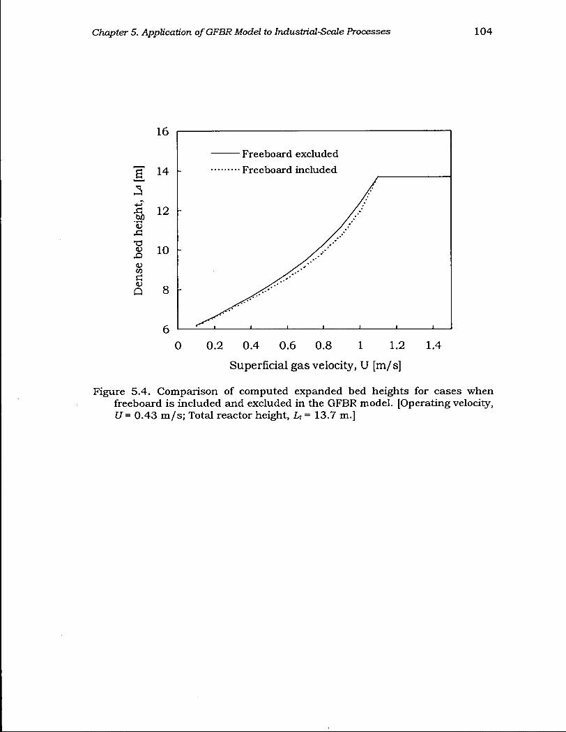
Chapter 5. Application of GFBR Model to Industrial-Scale Processes 104
0 0.2 0.4 0.6 0.8 1 1.2 1.4
Superficial gas velocity, U [m/s]
Figure 5.4. Comparison of computed expanded bed heights for cases when freeboard is included and excluded in the GFBR model. [Operating velocity, U= 0.43 m/s; Total reactor height, U = 13.7 m.]
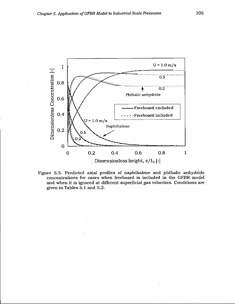
Chapter 5. Application of GFBR Model to Industrial-Scale Processes 105
U= 1.0 m/s
Dimensionless height, z / L t [-]
Figure 5.5. Predicted axial profiles of naphthalene and phthalic anhydride concentrations for cases when freeboard is included in the GFBR model and when it is ignored at different superficial gas velocities. Conditions are given in Tables 5.1 and 5.2.
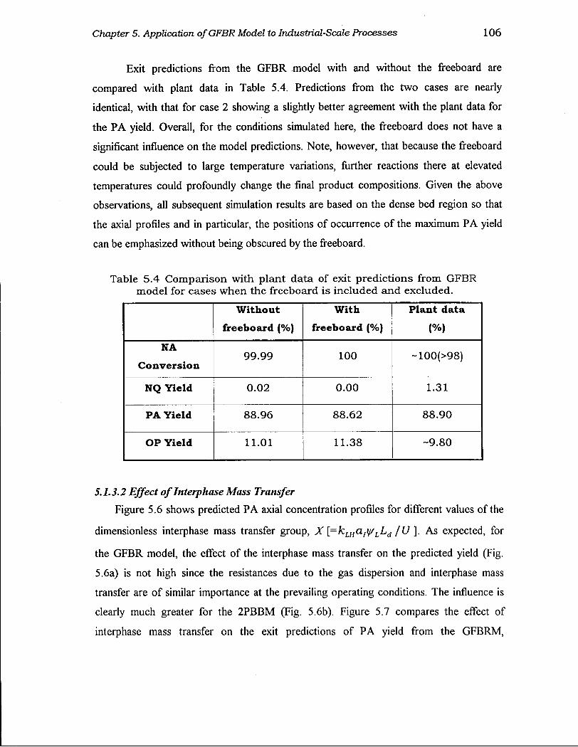
Chapter 5. Application of GFBR Model to Industrial-Scale Processes 106
Exit predictions from the GFBR model with and without the freeboard are
compared with plant data in Table 5.4. Predictions from the two cases are nearly
identical, with that for case 2 showing a slightly better agreement with the plant data for
the PA yield. Overall, for the conditions simulated here, the freeboard does not have a
significant influence on the model predictions. Note, however, that because the freeboard
could be subjected to large temperature variations, further reactions there at elevated
temperatures could profoundly change the final product compositions. Given the above
observations, all subsequent simulation results are based on the dense bed region so that
the axial profiles and in particular, the positions of occurrence of the maximum PA yield
can be emphasized without being obscured by the freeboard.
Table 5 . 4 Comparison with plant data of exit predictions from GFBR model for cases when the freeboard is included and excluded.
W i t h o u t
freeboard (%)
W i t h
freeboard (%)
P lant data
(%)
N A
C o n v e r s i o n 99.99 100 ~100(>98)
N Q Y i e l d 0.02 0.00 1.31
P A Y i e l d 88.96 88.62 88.90
O P Y i e l d 11.01 11.38 -9.80
5.1.3.2 Effect of Interphase Mass Transfer
Figure 5.6 shows predicted PA axial concentration profiles for different values of the
dimensionless interphase mass transfer group, X [=kLHa,y/LLd /U ]. As expected, for
the GFBR model, the effect of the interphase mass transfer on the predicted yield (Fig.
5.6a) is not high since the resistances due to the gas dispersion and interphase mass
transfer are of similar importance at the prevailing operating conditions. The influence is
clearly much greater for the 2PBBM (Fig. 5.6b). Figure 5.7 compares the effect of
interphase mass transfer on the exit predictions of PA yield from the GFBRM,
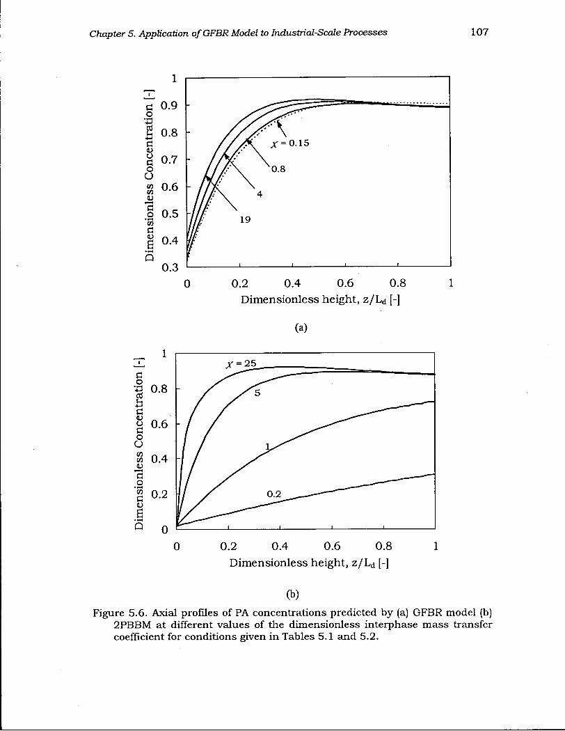
Chapter 5. Application of GFBR Model to Industrial-Scale Processes 107
C o
• i - H
+->
CO CJ C o O
CO CO
J O
C O CO
d CO
0 Q
0 .9 h
0.8 V
0.7 h
0 .6 h
0 .5
0 .4
0 .3
0 0.2 0.4 0.6 0.8
Dimensionless height, z / L d [-]
(a)
a o "•3 ° - 8
2 G co o a o o CO CO 4J
a o w C CO
6 • f - H
Q
0.6
0.4 h
0.2
0
0 0.2 0.4 0.6 0.8 1
Dimensionless height, z / L d [-]
(b)
Figure 5.6. Axial profiles of PA concentrations predicted by (a) GFBR model (b) 2PBBM at different values of the dimensionless interphase mass transfer coefficient for conditions given in Tables 5.1 and 5.2.
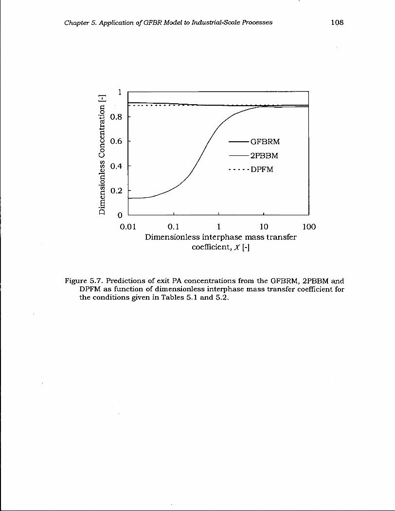
Chapter 5. Application of GFBR Model to Industrial-Scale Processes 108
1
B • r H
0.01 0.1 1 10 Dimensionless interphase mass transfer
coefficient, X [-]
Figure 5.7. Predictions of exit PA concentrations from the GFBRM, 2PBBM and DPFM as function of dimensionless interphase mass transfer coefficient for the conditions given in Tables 5.1 and 5.2.
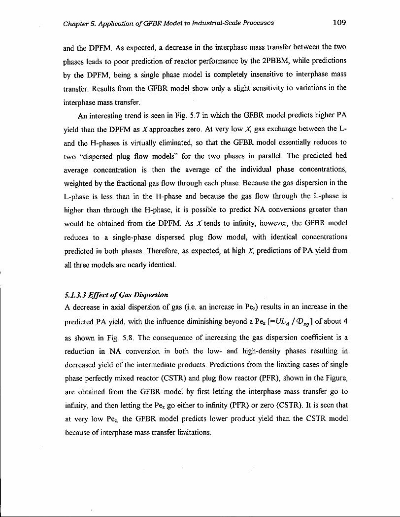
Chapter 5. Application of GFBR Model to Industrial-Scale Processes 109
and the DPFM. As expected, a decrease in the interphase mass transfer between the two
phases leads to poor prediction of reactor performance by the 2PBBM, while predictions
by the DPFM, being a single phase model is completely insensitive to interphase mass
transfer. Results from the GFBR model show only a slight sensitivity to variations in the
interphase mass transfer.
An interesting trend is seen in Fig. 5 . 7 in which the GFBR model predicts higher PA
yield than the DPFM as Xapproaches zero. At very low X gas exchange between the L -
and the H-phases is virtually eliminated, so that the GFBR model essentially reduces to
two "dispersed plug flow models" for the two phases in parallel. The predicted bed
average concentration is then the average of the individual phase concentrations,
weighted by the fractional gas flow through each phase. Because the gas dispersion in the
L-phase is less than in the H-phase and because the gas flow through the L-phase is
higher than through the H-phase, it is possible to predict N A conversions greater than
would be obtained from the DPFM. As X tends to infinity, however, the GFBR model
reduces to a single-phase dispersed plug flow model, with identical concentrations
predicted in both phases. Therefore, as expected, at high X predictions of PA yield from
all three models are nearly identical.
5.1.3.3 Effect of Gas Dispersion
A decrease in axial dispersion of gas (i.e. an increase in Pez) results in an increase in the
predicted PA yield, with the influence diminishing beyond a Pez [=ULd /(D^] of about 4
as shown in Fig. 5 . 8 . The consequence of increasing the gas dispersion coefficient is a
reduction in N A conversion in both the low- and high-density phases resulting in
decreased yield of the intermediate products. Predictions from the limiting cases of single
phase perfectly mixed reactor (CSTR) and plug flow reactor (PFR), shown in the Figure,
are obtained from the GFBR model by first letting the interphase mass transfer go to
infinity, and then letting the Pez go either to infinity (PFR) or zero (CSTR). It is seen that
at very low Pez, the GFBR model predicts lower product yield than the CSTR model
because of interphase mass transfer limitations.

Chapter 5. Application of GFBR Model to Industrial-Scale Processes 110
Figure 5.8. Axial profiles of PA concentration predicted by the GFBR model at different values of the axial Peclet number for conditions given in Tables 5.1 and 5.2.
Chapter 5. Application of GFBR Model to Industrial-Scale Processes 111
5.1.3.4 Influence of Reaction Rate Constants
To illustrate the effect of the reaction rate constants on the model predictions, the base
case values (Table 5.2) were varied over reasonable ranges as listed in Table 5.5. One
rate constant was varied for each simulation, while the others retained their base case
values. Figures 5.9 to 5.11 show the effect of the rate constants on the reactor
performance. As seen from Fig. 5.9, although the exit N A conversion remain unchanged
over the range of k r i and k^ varied, the height at which the maximum for the selectivity
to PA occurs is seen to decrease with increasing k^ and ka because of the more rapid
conversion of N A to the intermediate products at higher values of the rate constants.
Similar trends can be observed for the variations in k^ (Fig. 5.10) for the N A conversion.
Decreasing kr3 from the base value is seen to result in a decrease of both PA and OP
yields, while that of NQ is seen to increase (Fig. 5.10b). The impact of the kinetics was
further assessed by arbitrarily varying the base case values of the rate constants (Table
5.2) by ± 20%. The results, summarized in Table 5.6, show a profound influence of the
rate constants on the oxidation products and the PA yields. The observed trend is that
decreases in the rate constants favour higher PA yield while decreasing both the NQ and
OP yields. An increase in the rate constants results in more rapid conversion of N A
thereby giving more opportunity for further conversion of PA to oxidation products.
Given the sensitivity of the model predictions to the reaction kinetics, it is possible to
predict significantly different results from the model depending on the kinetic scheme
adopted.
Table 5.5. Reaction rate constants and the range of variation for the sensitivity analysis
Reaction Rate Constant Base Case Value (s1) Range explored (s1)
kri 1.8 0.18 - 10
kr2 1.8 0.18 - 10
kr3 4.6 0.25 - 20
kR4 0.023 0.003-0.1
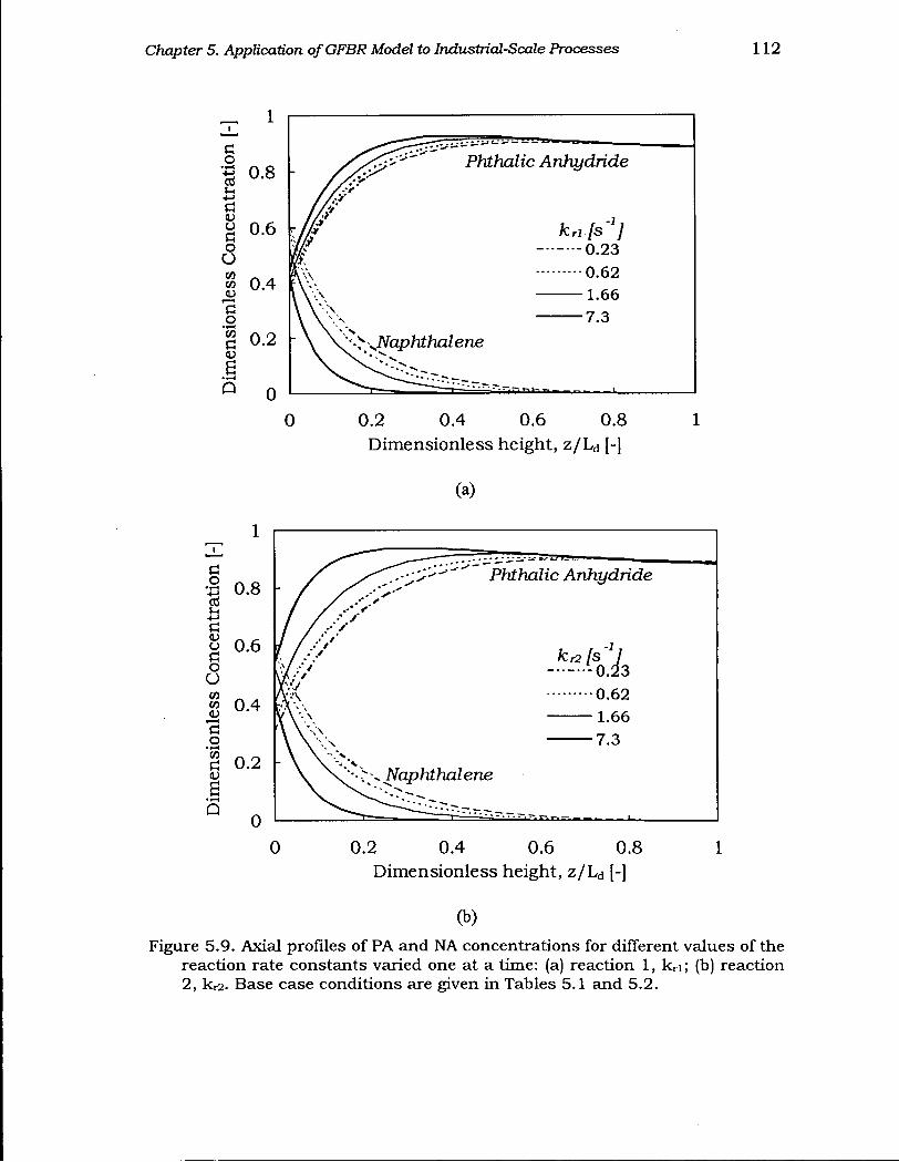
Chapter 5. Application of GFBR Model to Industrial-Scale Processes 112
_ 1 i
0 0.2 0.4 0.6 0.8 1 Dimensionless height, z / L d [-]
(b)
Figure 5.9. Axial profiles of PA and NA concentrations for different values of the reaction rate constants varied one at a time: (a) reaction 1, k r i; (b) reaction 2, kr2- Base case conditions are given in Tables 5.1 and 5.2.
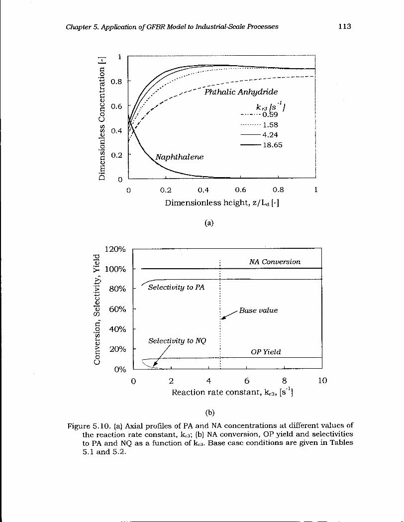
Chapter 5. Application of GFBR Model to Industrial-Scale Processes 113
T - 1
o • r - H
C <u o a o o CO CO <D 1—H
c O CO
a S
-T—I
a
0.8 f
0.6
0.4
0.2 h
0 0
Phthalic Anhydride
kr3[s~ ] — 0.59 — 1.58 — 4.24 — 18.65
0.2 0.4 0.6 0.8 Dimensionless height, z / L d [-]
(a)
120%
100%
•T—<
> 80% o
"I 60%
o 40% w
| 20% o O
0% 0
iVA Conversion i
- ^Selectivity to PA
Selectivity to NQ
- /
Base value
OP Yield
8 Reaction rate constant, k r 3, [s"1]
(b) Figure 5.10. (a) Axial profiles of PA and NA concentrations at different values of
the reaction rate constant, kr3-, (b) NA conversion, OP yield and selectivities to PA and NQ as a function of kr3- Base case conditions are given in Tables 5.1 and 5.2.
10
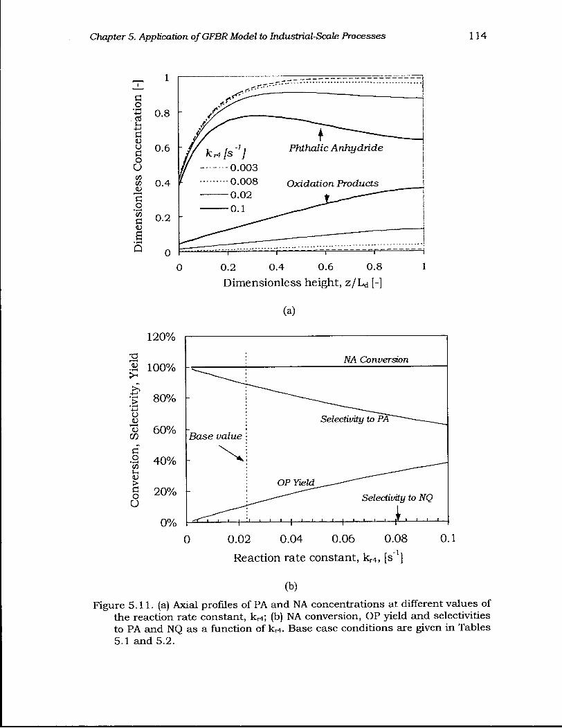
Chapter 5. Application of GFBR Model to Industrial-Scale Processes 114
fi o - M Ctf +-> fi <u fi o O CO CO
3H fi O CO
fi
B
0.8 f
0.6 r
0.4
0.2 f
0 0 0.2 0.4 0.6 0.8 1
Dimensionless height, z / L d [-]
(a)
NA Conversion
Selectivity to NQ
_ i i i — i — i —
0 0.02 0.04 0.06 0.08 0.1
Reaction rate constant, k r 4 , [s"1]
(b)
Figure 5.11. (a) Axial profiles of PA and NA concentrations at different values of the reaction rate constant, krt; (b) NA conversion, OP yield and selectivities to PA and NQ as a function of kr f. Base case conditions are given in Tables 5.1 and 5.2.
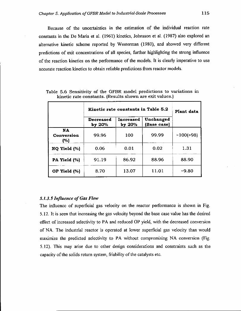
Chapter 5. Application of GFBR Model to Industrial-Scale Processes 115
Because of the uncertainties in the estimation of the individual reaction rate
constants in the De Maria et al. (1961) kinetics, Johnsson et al. (1987) also explored an
alternative kinetic scheme reported by Westerman (1980), and showed very different
predictions of exit concentrations of all species, further highlighting the strong influence
of the reaction kinetics on the performance of the models. It is clearly imperative to use
accurate reaction kinetics to obtain reliable predictions from reactor models.
Table 5.6 Sensitivity of the GFBR model predictions to variations in kinetic rate constants. (Results shown are exit values.)
K i n e t i c rate cons tants i n Table 5.2 P lant da ta
Decreased b y 20%
Increased by 20%
U n c h a n g e d (Base case)
P lant da ta
N A C o n v e r s i o n
(%) 99.96 100 99.99 ~100(>98)
N Q Y i e l d (%) 0.06 0.01 0.02 1.31
P A Y i e l d (%) 91.19 86.92 88.96 88.90
O P Y i e l d (%) 8.70 13.07 11.01 -9.80
5.1.3.5 Influence of Gas Flow
The influence of superficial gas velocity on the reactor performance is shown in Fig.
5.12. It is seen that increasing the gas velocity beyond the base case value has the desired
effect of increased selectivity to PA and reduced OP yield, with the decreased conversion
of NA. The industrial reactor is operated at lower superficial gas velocity than would
maximize the predicted selectivity to PA without compromising N A conversion (Fig.
5.12). This may arise due to other design considerations and constraints such as the
capacity of the solids return system, friability of the catalysts etc.
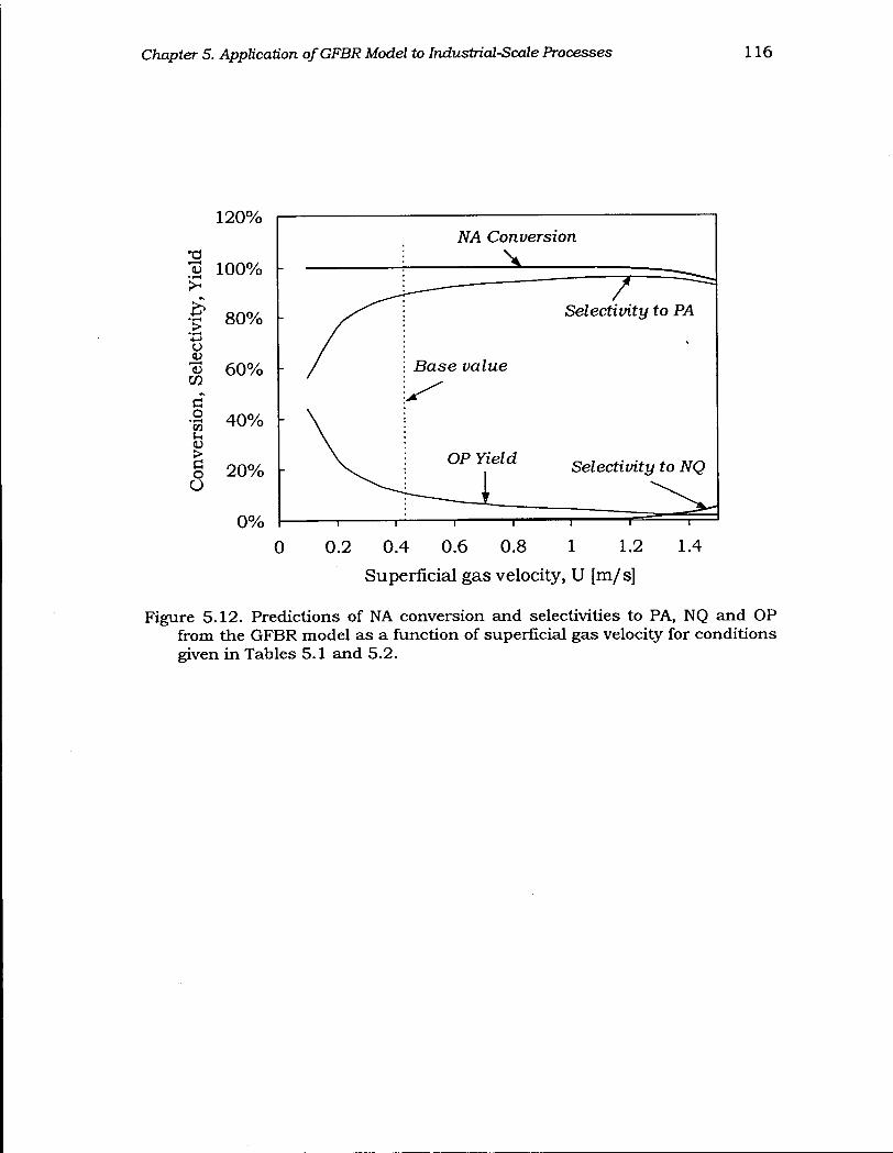
Chapter 5. Application of GFBR Model to Industrial-Scale Processes 116
1 2 0 %
'co • 1—I
• f - H
> o
'v co
o w
CO >
o O
8 0 %
6 0 %
4 0 %
2 0 %
0 %
iVA Conversion
— /
Selectimty to PA
/ Base value
OP Yield Selectivity to NQ
0 0.2 0 .4 0.6 0.8 1 1.2 1.4
Superficial gas velocity, U [m/s]
Figure 5.12. Predictions of NA conversion and selectivities to PA, NQ and OP from the GFBR model as a function of superficial gas velocity for conditions given in Tables 5.1 and 5.2.

Chapter 5. Application of GFBR Model to Industrial-Scale Processes 117
5.1.4 Conclusions
The performance of the GFBR model is assessed using an industrial-scale phthalic
anhydride process as a case study. The phthalic anhydride (PA) process operates near the
bubbling-turbulent regime boundary, which makes it an ideal candidate to test the
performance of the GFBR model. Predictions from the model for naphthalene (NA), PA
and oxidation products (OP) are seen to be reasonable and compare favourably with the
plant data within the constraints of the uncertainties in the estimation of the various
parameters (hydrodynamic, kinetic, property estimation, etc.), while the agreement for
the naphthaquinone (NQ) is poor. From the sensitivity analysis performed, it is shown
that the predictions from the GFBR model are strongly influenced by the reaction
kinetics, gas dispersion and superficial gas velocity, while the freeboard influence is
relatively small for the range of conditions covered. The NQ yield is predicted to be « 0
( « plant data) in all simulations, except when the reaction rate constant for the third
reaction, kr3, is varied, further emphasizing the strong influence of the reaction kinetics
on the model performance. Clearly, accuracy of the model predictions depends strongly
on utilizing reliable estimates of the model parameters. Use of the GFBR model to
perform simulation experiments over a wide range of conditions is demonstrated.
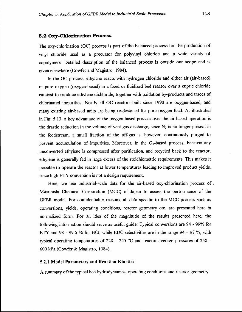
Chapter 5. Application of GFBR Model to Industricd-Scale Processes 118
5.2 Oxy-Chlorination Process
The oxy-chlorination (OC) process is part of the balanced process for the production of
vinyl chloride used as a precursor for polyvinyl chloride and a wide variety of
copolymers. Detailed description of the balanced process is outside our scope and is
given elsewhere (Cowfer and Magistro, 1984).
In the OC process, ethylene reacts with hydrogen chloride and either air (air-based)
or pure oxygen (oxygen-based) in a fixed or fluidized bed reactor over a cupric chloride
catalyst to produce ethylene dichloride, together with oxidation by-products and traces of
chlorinated impurities. Nearly all OC reactors built since 1990 are oxygen-based, and
many existing air-based units are being re-designed for pure oxygen feed. As illustrated
in Fig. 5.13, a key advantage of the oxygen-based process over the air-based operation is
the drastic reduction in the volume of vent gas discharge, since N2 is no longer present in
the feedstream; a small fraction of the off-gas is, however, continuously purged to
prevent accumulation of impurities. Moreover, in the 02-based process, because any
unconverted ethylene is compressed after purification, and recycled back to the reactor,
ethylene is generally fed in large excess of the stoichiometric requirements. This makes it
possible to operate the reactor at lower temperatures leading to improved product yields,
since high E T Y conversion is not a design requirement.
Here, we use industrial-scale data for the air-based oxy-chlorination process of .
Mitsubishi Chemical Corporation (MCC) of Japan to assess the performance of the
GFBR model. For confidentiality reasons, all data specific to the M C C process such as
conversions, yields, operating conditions, reactor geometry etc. are presented here in
normalized form. For an idea of the magnitude of the results presented here, the
following information should serve as useful guide: Typical conversions are 94 - 99% for
E T Y and 98 - 99.5 % for HC1, while E D C selectivities are in the range 94 - 97 %, with
typical operating temperatures of 220 - 245 °C and reactor average pressures of 250 -
600 kPa (Cowfer & Magistro, 1984).
5.2.1 Model Parameters and Reaction Kinetics
A summary of the typical bed hydrodynamics, operating conditions and reactor geometry
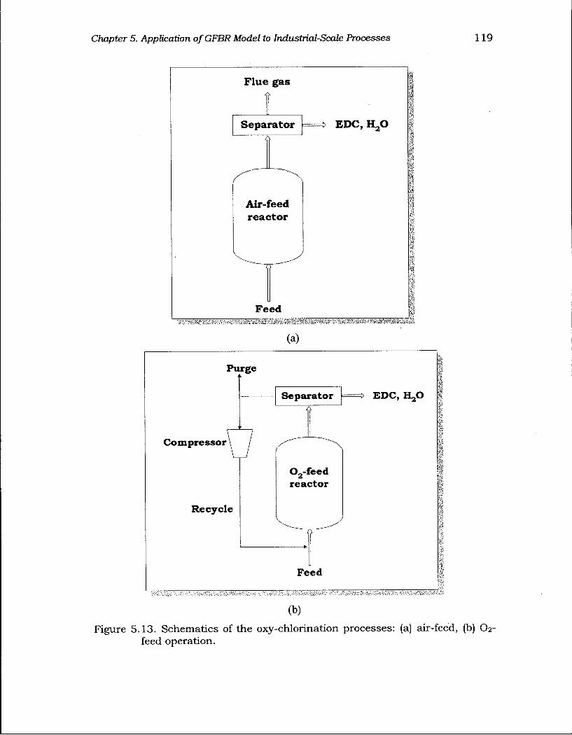
Chapter 5. Application of GFBR Model to Industrial-Scale Processes 119
Flue gas
Separator ft"
EDC, H aO
Air-feed reactor
~7>
Feed
(a)
Purge
Separator =* EDC, HLjO
Compressor
02-feed reactor
Recycle
Feed
(b)
Figure 5.13. Schematics of the oxy-cMorination processes: (a) air-feed, (b) 02-feed operation.
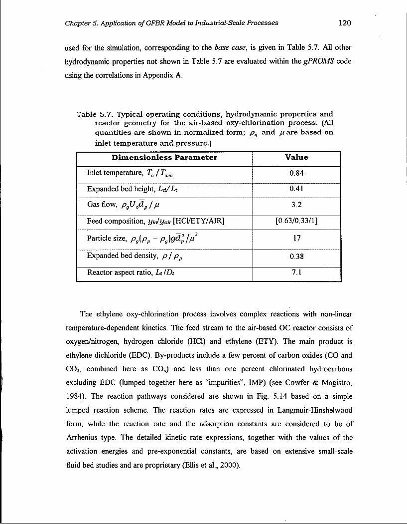
Chapter 5. Application of GFBR Model to Industrial-Scale Processes 120
used for the simulation, corresponding to the base case, is given in Table 5.7. All other
hydrodynamic properties not shown in Table 5.7 are evaluated within the gPROMS code
using the correlations in Appendix A.
Table 5.7. Typical operating conditions, hydrodynamic properties and reactor geometry for the air-based oxy-chlorination process. (All quantities are shown in normalized form; pg and ju are based on inlet temperature and pressure.)
Dimensionless Parameter Value
Inlet temperature, TJTave 0.84
Expanded bed height, Ld/Lt 0.41
Gas flow, pgU0dpf p 3.2
Feed composition, yjtjair [HC1/ETY/AIR] [0.63/0.33/1]
Particle size, pg{pp - pg)gdz
pjp 17
Expanded bed density, pf pp 0.38
Reactor aspect ratio, Lt /Dt 7.1
The ethylene oxy-chlorination process involves complex reactions with non-linear
temperature-dependent kinetics. The feed stream to the air-based OC reactor consists of
oxygen/nitrogen, hydrogen chloride (HC1) and ethylene (ETY). The main product is
ethylene dichloride (EDC). By-products include a few percent of carbon oxides (CO and
CO2, combined here as CO x ) and less than one percent chlorinated hydrocarbons
excluding EDC (lumped together here as "impurities", IMP) (see Cowfer & Magistro,
1984). The reaction pathways considered are shown in Fig. 5.14 based on a simple
lumped reaction scheme. The reaction rates are expressed in Langmuir-Hinshelwood
form, while the reaction rate and the adsorption constants are considered to be of
Arrhenius type. The detailed kinetic rate expressions, together with the values of the
activation energies and pre-exponential constants, are based on extensive small-scale
fluid bed studies and are proprietary (Ellis et al., 2000).
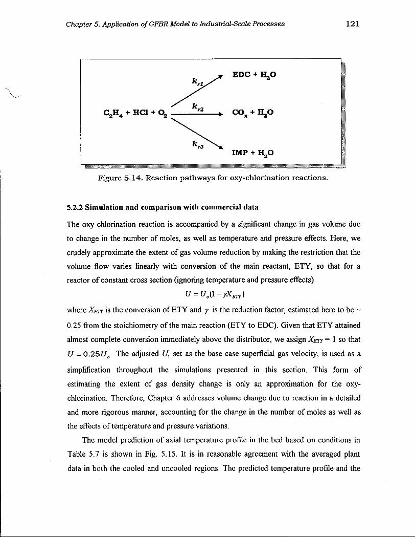
Chapter 5. Application of GFBR Model to Industrial-Scale Processes 121
EDC + HjO
C,H. + HC1 + a '2
I M P + H g O
Figure 5.14. Reaction pathways for oxy-chlorination reactions.
5.2.2 S i m u l a t i o n a n d c o m p a r i s o n w i t h c o m m e r c i a l da ta
The oxy-chlorination reaction is accompanied by a significant change in gas volume due
to change in the number of moles, as well as temperature and pressure effects. Here, we
crudely approximate the extent of gas volume reduction by making the restriction that the
volume flow varies linearly with conversion of the main reactant, E T Y , so that for a
reactor of constant cross section (ignoring temperature and pressure effects)
where XETY is the conversion of E T Y and y is the reduction factor, estimated here to be ~
0.25 from the stoichiometry of the main reaction (ETY to EDC). Given that E T Y attained
almost complete conversion immediately above the distributor, we assign XETY = 1 S O that
U = 0.25Ua. The adjusted U, set as the base case superficial gas velocity, is used as a
simplification throughout the simulations presented in this section. This form of
estimating the extent of gas density change is only an approximation for the oxy-
chlorination. Therefore, Chapter 6 addresses volume change due to reaction in a detailed
and more rigorous manner, accounting for the change in the number of moles as well as
the effects of temperature and pressure variations.
The model prediction of axial temperature profile in the bed based on conditions in
Table 5.7 is shown in Fig. 5.15. It is in reasonable agreement with the averaged plant
data in both the cooled and uncooled regions. The predicted temperature profile and the
U = U0(l + yXETY)
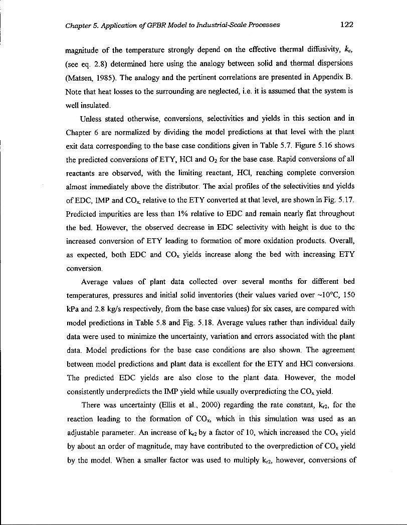
Chapter 5. Application of GFBR Model to Industrial-Scale Processes 122
magnitude of the temperature strongly depend on the effective thermal diffusivity, ke,
(see eq. 2.8) determined here using the analogy between solid and thermal dispersions
(Matsen, 1985). The analogy and the pertinent correlations are presented in Appendix B.
Note that heat losses to the surrounding are neglected, i.e. it is assumed that the system is
well insulated.
Unless stated otherwise, conversions, selectivities and yields in this section and in
Chapter 6 are normalized by dividing the model predictions at that level with the plant
exit data corresponding to the base case conditions given in Table 5.7. Figure 5.16 shows
the predicted conversions of E T Y , HC1 and O2 for the base case. Rapid conversions of all
reactants are observed, with the limiting reactant, HC1, reaching complete conversion
almost immediately above the distributor. The axial profiles of the selectivities and yields
of EDC, IMP and C O x , relative to the E T Y converted at that level, are shown in Fig. 5.17.
Predicted impurities are less than 1% relative to E D C and remain nearly flat throughout
the bed. However, the observed decrease in EDC selectivity with height is due to the
increased conversion of E T Y leading to formation of more oxidation products. Overall,
as expected, both E D C and C O x yields increase along the bed with increasing E T Y
conversion.
Average values of plant data collected over several months for different bed
temperatures, pressures and initial solid inventories (their values varied over ~10°C, 150
kPa and 2.8 kg/s respectively, from the base case values) for six cases, are compared with
model predictions in Table 5.8 and Fig. 5.18. Average values rather than individual daily
data were used to minimize the uncertainty, variation and errors associated with the plant
data. Model predictions for the base case conditions are also shown. The agreement
between model predictions and plant data is excellent for the E T Y and HC1 conversions.
The predicted E D C yields are also close to the plant data. However, the model
consistently underpredicts the IMP yield while usually overpredicting the C O x yield.
There was uncertainty (Ellis et al., 2000) regarding the rate constant, k^, for the
reaction leading to the formation of C O x , which in this simulation was used as an
adjustable parameter. An increase of kr 2 by a factor of 10, which increased the C O x yield
by about an order of magnitude, may have contributed to the overprediction of C O x yield
by the model. When a smaller factor was used to multiply k^, however, conversions of
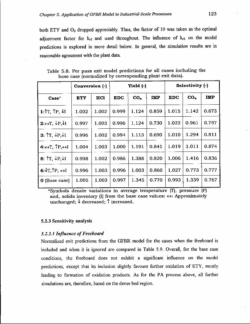
Chapter 5. Application of GFBR Model to Industrial-Scale Processes 123
both E T Y and O2 dropped appreciably. Thus, the factor of 10 was taken as the optimal
adjustment factor for k^ and used throughout. The influence of k^ on the model
predictions is explored in more detail below. In general, the simulation results are in
reasonable agreement with the plant data.
Table 5.8. Per pass exit model predictions for all cases including the base case (normalized by corresponding plant exit data).
C o n v e r s i o n (-) Y i e l d (-) Se l ec t i v i ty (-)
Case* E T Y HC1 E D C c o x IMP E D C c o x IMP
l : t T , tP , ll 1.002 1.002 0.999 1.124 0.859 1.015 1.142 0.873
2:oT, lP,<ll 0.997 1.003 0.996 1.124 0.730 1.022 0.961 0.797
3: tT, lP,U 0.996 1.002 0.994 1.113 0.690 1.010 1.294 0.811
4 :oT, tP,<^I 1.004 1.003 1.000 1.191 0.841 1.019 1.011 0.874
5: tT, IPM 0.998 1.002 0.986 1.388 0.820 1.006 1.416 0.836
6 : lT,tP, o l 0.996 1.003 0.996 1.003 0.860 1.027 0.773 0.777
0 (Base case) 1.005 1.003 0.997 1.345 0.770 0.993 1.339 0.767
*Symbols denote variations in average temperature (T), pressure (P) and, solids inventory (I) from the base case values: <->: Approximately unchanged; -l decreased; t increased.
5.2.3 Sensitivity analysis
5.2.3.1 Influence of Freeboard
Normalized exit predictions from the GFBR model for the cases when the freeboard is
included and when it is ignored are compared in Table 5.9. Overall, for the base case
conditions, the freeboard does not exhibit a significant influence on the model
predictions, except that its inclusion slightly favours further oxidation of E T Y , mostly
leading to formation of oxidation products. As for the P A process above, all further
simulations are, therefore, based on the dense bed region.

Chapter 5. Application of GFBR Model to Industrial-Scale Processes 124
0 . 9 7 0 . 9 9 1 .01
Normalized bed temperature, T / T a v e [-]
Figure 5 . 1 5 . Axial bed temperature profile normalized by bed-average plant data, Tave, based on conditions in Table 5 . 7 .
E T Y
H C 1
0.8 1 1 1 1 1 1
0 0.2 0.4 0.6 0.8 1
Dimensionless height, z / L d [-]
Figure 5 . 1 6 . Axial conversion profiles of ETY and H C 1 normalized by exit plant data for conditions given in Table 5 . 7 .

Chapter 5. Application of GFBR Model to Industrial-Scale Processes 125
Figure 5 . 1 7 . Axial profiles normalized by exit plant data: (a) selectivities of ETY to EDC, C O x and I M P , (b) yields of EDC, C 0 X and I M P for conditions in Table 5 .7 .

Chapter 5. Application of GFBR Model to Industrial-Scale Processes 126
0 2 3 4
Case number
(a)
2
N
13
o
0 2 3 4
Case number
(b)
Figure 5.18. Normalized model predictions for the six cases in Table 5.8: (a) ETY and HC1 conversions, (b) yields of EDC, COx and IMP. Case 0 is the base case in Table 5.8.
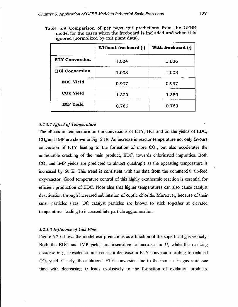
Chapter 5. Application of GFBR Model to Industrial-Scale Processes 127
Table 5.9 Comparison of per pass exit predictions from the GFBR model for die cases when the freeboard is included and when it is ignored (normalized by exit plant data).
W i t h o u t freeboard (-) W i t h freeboard (-)
E T Y C o n v e r s i o n 1.004 1.006
HC1 C o n v e r s i o n 1.003 1.003
E D C Y i e l d 0.997 0.997
C O x Y i e l d 1.329 1.389
IMP Y i e l d 0.766 0.763
5.2.3.2 Effect of Temperature
The effects of temperature on the conversions of E T Y , HC1 and on the yields of EDC,
C O x and IMP are shown in Fig. 5.19. An increase in reactor temperature not only favours
conversion of E T Y leading to the formation of more CO x , but also accelerates the
undesirable cracking of the main product, EDC, towards chlorinated impurities. Both
C O x and IMP yields are predicted to almost quadruple as the operating temperature is
increased by 60 K. This trend is consistent with the data from the commercial air-feed
oxy-reactor. Good temperature control of this highly exothermic reaction is essential for
efficient production of EDC. Note also that higher temperatures can also cause catalyst
deactivation through increased sublimation of cupric chloride. Moreover, because of their
small particles sizes, OC catalyst particles are known to stick together at elevated
temperatures leading to increased interparticle agglomeration.
5.2.3.3 Influence of Gas Flow
Figure 5.20 shows the model exit predictions as a function of the superficial gas velocity.
Both the E D C and IMP yields are insensitive to increases in U, while the resulting
decrease in gas residence time causes a decrease in E T Y conversion leading to reduced
C O x yield. Clearly, the additional E T Y conversion due to the increase in gas residence
time with decreasing U leads exclusively to the formation of oxidation products.

Chapter 5. Application of GFBR Model to Industrial-Scale Processes 128
(b)
Figure 5.19. Effect of temperature on reactor performance: (a) Normalized conversion of ETY and HC1, (b) Normalized yields of EDC, COx and IMP. (Base case conditions are given in Table 5.7.)
Chapter 5. Application of GFBR Model to Industrial-Scale Processes 129
Figure 5.20. Predicted ETY conversion and EDC, IMP and COx yields as a function of superficial gas velocity for base case conditions in Table 5.7.
Chapter 5. Application of GFBR Model to Industrial-Scale Processes 130
Increasing U is seen to favour the selectivity of E T Y to E D C at the expense of E T Y
conversion. In the air-based OC process, E T Y is fed in slight excess of stoichiometric
requirements to ensure high conversion of HC1 and to minimize losses of the excess
ethylene that remains after product condensation. Therefore, the reduced E T Y conversion
with increasing U is not favorable for the air-based operation. The observed higher
selectivity to E D C at reduced E T Y conversion is, however, desirable for the 02-feed oxy-
chlorination reactor, where virtually all unreacted E T Y is recycled back to the reactor.
5.2.3.4 Effect of Interphase Mass Transfer and Gas Dispersion
Figure 5.21 shows the effect of interphase mass transfer on reactor performance. Since
the bed operates, under the prevailing conditions outlined in Table 5.7, mostly in the
turbulent regime (Pturb being about 80%), the effect of mass transfer between the low-
density and high-density phases is minimal. As a result, the interphase mass transfer
coefficient is predicted to have almost no effect on the reactor performance in this case.
As expected, increasing Pez (i.e. decreasing the gas axial dispersion coefficient)
enhances the E T Y conversion (Fig. 5.22a). It also causes more C O x to be formed, while
HC1 conversion as well as EDC and IMP yields are predicted to remain unchanged (Fig.
5.22b). Since the mass transfer resistance is negligible under the prevailing conditions,
the model effectively functions as a dispersed plug flow model, with the limiting cases of
the perfect mixing and plug flow approached at low and high Pez, respectively.
Notwithstanding the slight change in E T Y conversion over the range of Pez shown, the
C O x yield is predicted to increase by about 17% and remains overpredicted throughout.
5.2.3.5 Influence of Reaction Rate Constants
Given the uncertainty regarding the rate constant, k^, for the second reaction leading to
the formation of C O x and the observed consistent overprediction of the oxidation
products by the model, we next examine its effect as well as the combined influence of
all three rate constants on the model predictions. As shown in Fig. 5.23, the exit E T Y
conversion is predicted to increase with increasing k^, with the additional converted E T Y
going almost entirely to CO x . As expected, the EDC and IMP yields are insensitive to
variations in k r 2 . As for the phthalic anhydride process, the impact of the kinetics was

Chapter 5. Application of GFBR Model to Industrial-Scale Processes 131
1.006
C o 't 1.004 cu > C o O | 1.002
a u o !5
1.4
1.3
1.2
1.1
1
2
>-cu .a I 0.9 u o
0.8
0.7
0.6
1 10 100 Dimensionless interphase mass transfer
group, X [-]
(a)
COx
EDC
IMP
10 100 Dimensionless interphase mass
transfer group, X [-]
(b)
Figure 5.21. Effect of interphase mass transfer on reactor performance for base case conditions given in Table 5.7: (a) Normalized conversion of ETY and HC1, (b) Normalized yields of EDC, COx and IMP.
Chapter 5. Application of GFBR Model to Industrial-Scale Processes 132
1.01
(b)
Figure 5.22. Effect of gas dispersion on reactor performance for base case conditions given in Table 5.7: (a) Normalized conversion of ETY and HC1, (b) Normalized yields of EDC, COx and IMP.
Chapter 5. Application of GFBR Model to Industrial-Scale Processes 133
Figure 5.23. Normalized conversion and yields as a function of reaction rate constant, k r 2 , for base case conditions given in Table 5.7.
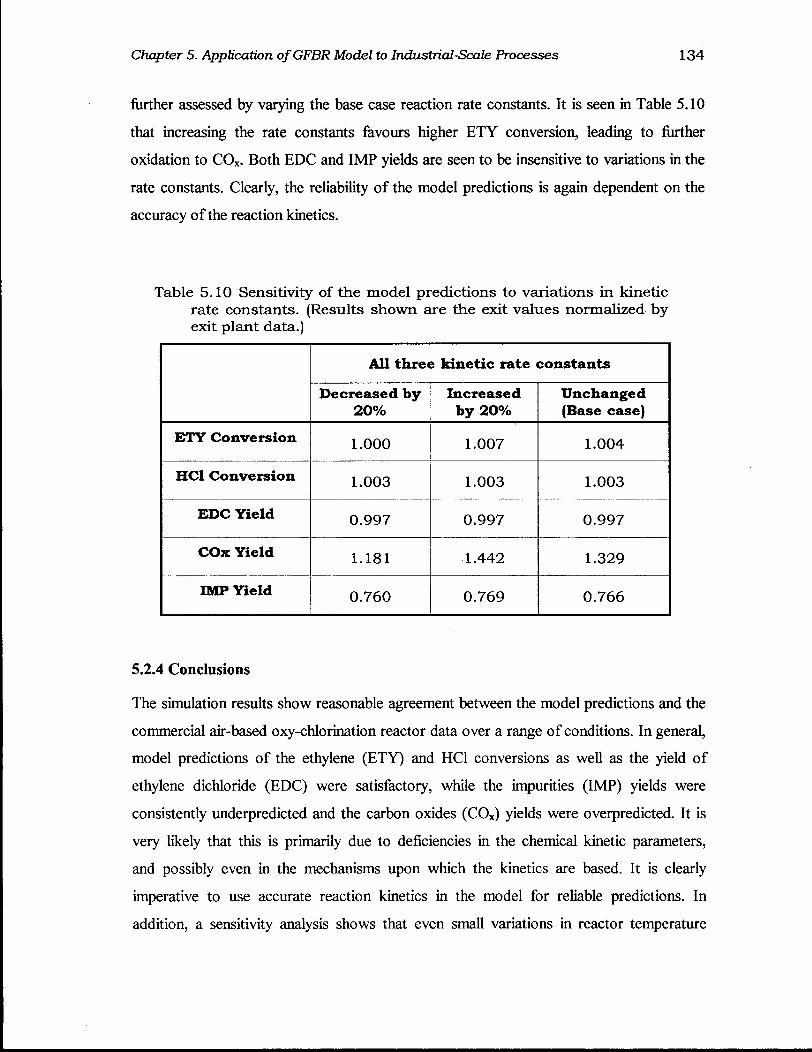
Chapter 5. Application of GFBR Model to Industrial-Scale Processes 134
further assessed by varying the base case reaction rate constants. It is seen in Table 5.10
that increasing the rate constants favours higher E T Y conversion, leading to further
oxidation to C O x . Both EDC and IMP yields are seen to be insensitive to variations in the
rate constants. Clearly, the reliability of the model predictions is again dependent on the
accuracy of the reaction kinetics.
Table 5.10 Sensitivity of the model predictions to variations in kinetic rate constants. (Results shown are the exit values normalized by exit plant data.)
A l l three k i n e t i c rate cons tant s
D e c r e a s e d b y 20%
Increased b y 20%
U n c h a n g e d (Base case)
E T Y C o n v e r s i o n 1.000 1.007 1.004
HC1 C o n v e r s i o n 1.003 1.003 1.003
E D C Y i e l d 0.997 0.997 0.997
C O x Y i e l d 1.181 1.442 1.329
IMP Y i e l d 0.760 0.769 0.766
5.2.4 Conclusions
The simulation results show reasonable agreement between the model predictions and the
commercial air-based oxy-chlorination reactor data over a range of conditions. In general,
model predictions of the ethylene (ETY) and HC1 conversions as well as the yield of
ethylene dichloride (EDC) were satisfactory, while the impurities (IMP) yields were
consistently underpredicted and the carbon oxides (CO x) yields were overpredicted. It is
very likely that this is primarily due to deficiencies in the chemical kinetic parameters,
and possibly even in the mechanisms upon which the kinetics are based. It is clearly
imperative to use accurate reaction kinetics in the model for reliable predictions. In
addition, a sensitivity analysis shows that even small variations in reactor temperature
Chapter 5. Application of GFBR Model to Industrial-Scale Processes 135
profoundly influence the C O x and IMP yields, underscoring the need to accurately
capture the reactor temperature profile through the energy balance in the model Further
analysis shows that gas flow and gas dispersion both significantly influence the reactor
performance, while the effect of interphase mass transfer is predicted to be negligible for
the conditions prevailing in the industrial reactor.
Chapter 5. Application of GFBR Model to Industrial-Scale Processes 136
5.3 Gas-Solid Reactions
5.3.1. Introduction
The GFBR model has so far been applied to gas phase catalytic processes. Application of
this model to non-catalytic processes requires coupling it with a single particle model.
The goal here is to demonstrate the application of the model for non-catalytic gas-solid
reactions in fluidized bed by coupling it with the "grain-particle model" (GPM). This can
be achieved in two ways depending on the operating conditions and particle properties:
A. Low velocity flow regimes
• Approach Al: Generally for bubbling and turbulent regimes of fluidization with
limited entrainment, the solids in the low-density (L) and high-density (H) phases can
be considered to be exposed to gaseous species of average concentration C t and
CiH respectively through the particle boundary layers. The overall conversion of
solids leaving the reactor, X , is then a function of the individual particle conversion
in the L - and H-phases, XL and XH, the solids residence time distributions, EL, and
EH, and the phase volume allocations, yrL and XJ/H-
• Approach A2: Alternatively, the solids in the bed can be considered to be exposed to
gaseous species of bed-average concentration C- through the gas film surrounding
the individual particles. The overall conversion of solids leaving the reactor, X, is
then a function of the individual particle conversion, X, and the solids RTD, E. This
is essentially a simplification of approach A l , likely to work better when the particle
mean residence time in bed » time spent within either phase before being transferred
to the other phase.
B. High velocity flow regimes
• Approach B: For flow systems with significant entrainment (typical of the fast
fluidization regime) with net solid circulation flux Gs, the particle conversion should
be tracked as a function of both time and space. To achieve this, an equation of
particle motion as a function of time must be included. The overall solids conversion
Chapter 5. Application of GFBR Model to Industrial-Scale Processes 137
is then calculated by integrating the individual particle conversion with an appropriate
compartment-in-series solids RTD model.
Approach A is presented here, which is subsequently reduced to sub-case A2 below. In
the following sections, we present the equations for the single particle and the
methodology adopted for coupling the reactor model with the particle model. The
combined model is then assessed using the zinc sulfide roasting process as a case study.
To avoid confusion, the following distinction is made in this section: reactor model refers
to the fluidized bed reactor model - the GFBR model in this case; particle model refers to
the grain particle model for a single particle - the GPM in this case.
5.3.2. Single Particle Model
5.3.2.1 Introduction
A number of models have been developed for single particle reactions, including the
Shrinking Core Model, Crackling Core Model, Pore Model, Volume Reaction Model,
Grain Particle Model, Network Model, among others (Ramachandran and Doraiswamy,
1982). The Shrinking Core Model (SCM), also referred to as the Sharp Interface Model
or Topochemical Model, is one of the earliest. It considers the solid reactants to be non-
porous and, thus, assumes that the reaction takes place at a sharp interface that divides the
exhausted outer shell (ash layer) from the unreacted core of the solid. Although the SCM
has the advantage of mathematical simplicity and is widely used, its applicability is
limited to non-porous or barely porous solids. In the GPM, the solids are considered to be
comprised of compacted grains of uniform size, usually of submicron dimensions.
Reaction of the solid is considered to take place at the surface of the grains according to
the SCM. Figure 5.23 shows the SCM and GPM schematically. The G P M is often
considered realistic for physical systems where the solid particles are agglomerates of
grains.
5.3.2.2 Model Equations3
In general, a gas-solid reaction can be written in compact form as
3 All symbols are defined in the notation
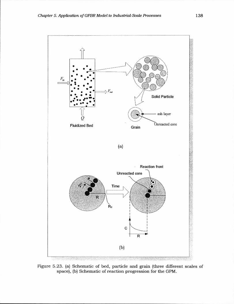
Chapter 5. Application of GFBR Model to Industrial-Scale Processes 138
Figure 5.23. (a) Schematic of bed, particle and grain (three different scales of space), (b) Schematic of reaction progression for the GPM.
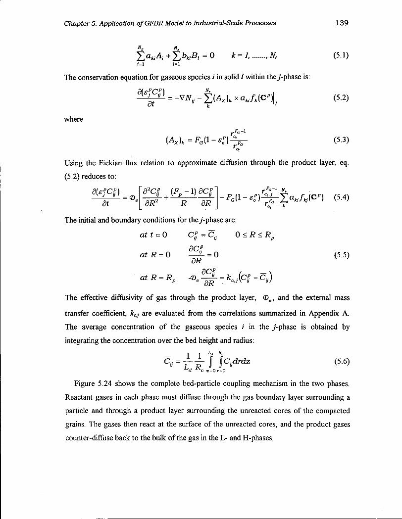
Chapter 5. Application of GFBR Model to Industrial-Scale Processes 139
.,Nr (5.1)
i=i /=i
The conservation equation for gaseous species /' in solid / within they'-phase is:
dt (5.2)
where
(Ax)k=FG[l-e^ •/•Pa
°i
(5.3)
Using the Fickian flux relation to approximate diffusion through the product layer, eq.
(5.2) reduces to:
et d2C? ( F p -1) dC?
dR2 R dR rF° ro. k
The initial and boundary conditions for they'-phase are:
at t = 0
at R = 0
>j u
dC? —^- = 0 dR
dCl
0<R<Rr
(5.5)
atR = Rp 4 > . - ^ . = K,J(C§-CV)
The effective diffusivity of gas through the product layer, <De, and the external mass
transfer coefficient, kCJ are evaluated from the correlations summarized in Appendix A.
The average concentration of the gaseous species /' in the y'-phase is obtained by
integrating the concentration over the bed height and radius:
-I I LD RC
C , = — — f [C.drdz Ud Kc 2=0 r=0
(5.6)
Figure 5.24 shows the complete bed-particle coupling mechanism in the two phases.
Reactant gases in each phase must diffuse through the gas boundary layer surrounding a
particle and through a product layer surrounding the unreacted cores of the compacted
grains. The gases then react at the surface of the unreacted cores, and the product gases
counter-diffuse back to the bulk of the gas in the L - and H-phases.
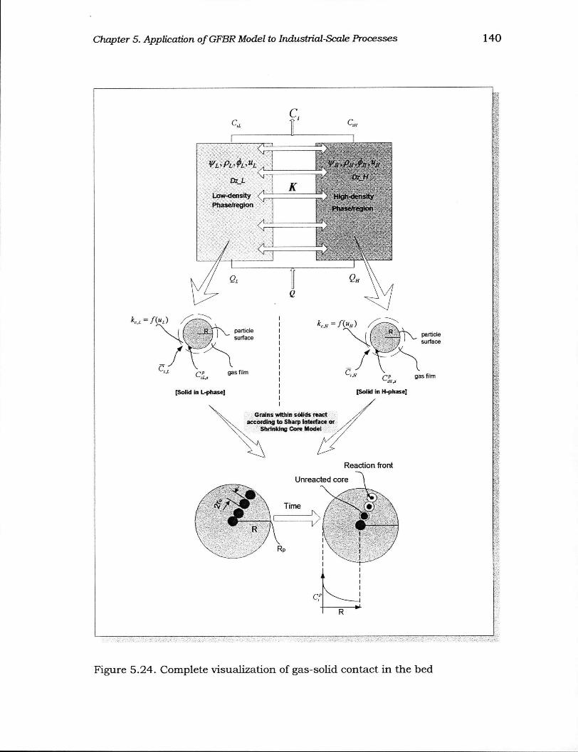
Chapter 5. Application of GFBR Model to Industrial-Scale Processes 140
Figure 5.24. Complete visualization of gas-solid contact in the bed
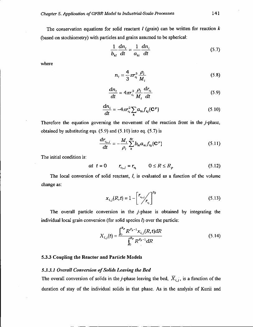
Chapter 5. Application of GFBR Model to Industrial-Scale Processes 141
The conservation equations for solid reactant / (grain) can be written for reaction k
(based on stochiometry) with particles and grains assumed to be spherical:
1 dnl _ 1 dni (5.7) Dkl at aki ai
where
n=±xr*-&- (5.8) 3 ' M,
dn, . 2 Pi — 1 = 4#r2 — dr
(5.9) dt c' M, dt
dn dt k
Therefore the equation governing the movement of the reaction front in the y-phase,
obtained by substituting eqs. (5.9) and (5.10) into eq. (5.7) is
dr M Nr
dt p, V The initial condition is:
att = 0 rCiJ =r c i 0 < R < Rp (5.12)
The local conversion of solid reactant, /, is evaluated as a function of the volume
change as:
XlJ(R,t) = l r (5.13)
The overall particle conversion in the y'-phase is obtained by integrating the
individual local grain conversion (for solid species I) over the particle:
\RrRp'-lx. :{R,t)dR = J ° f * P
J \ (5-14)
5.3.3 Coupling the Reactor and Particle Models
5.3.3.1 Overall Conversion of Solids Leaving the Bed
The overall conversion of solids in the y'-phase leaving the bed, X ; •', is a function of the
duration of stay of the individual solids in that phase. As in the analysis of Kunii and
Chapter 5. Application of GFBR Model to Industrial-Scale Processes 142
Levenspiel (1991), this is accounted for by integrating the conversion of the individual
particles with the solids RTD according to
l-XlJ=j[l-XlJ(t)]xEj(t)dt (5.15) o
Assuming that solids mixing in the bed can be represented as N compartments in series,
the solids RTD in the y'-phase can be written:
EAt) = —*" 1 -„ e"*1 (5.16)
where f • = Msj / rh^ is the mean residence time of particles in the y'-phase. Here, solids
are assumed to be perfectly mixed (N = 1) in both phases. In some cases, it may be better
to allow for separate RTDs in the two phases; the mixing pattern in the H-phase is likely
to be closer to perfect mixing, especially for bubbling fluidization while a compartment-
in-series model, closer to plug flow, is likely to be more representative of the mixing
pattern in the L-phase. However, the total residence time of particles in fluidized bed
reactors used for gas-solid reactions is usually so long (typically hours) that the
assumption of perfect mixing in each phase is reasonable.
5.3.3.2 Accounting for Solids Interchange between the L- andH-Phases
In order to calculate the final overall conversion of solids at the exit of the reactor, one
must account for the extent of solids interchange between the two phases. Let PL and PH
be the probabilities of solids being in the L - and H-phases, respectively, at any instant (PL
+ PH =1); also let f and y# be the volume-averaged solid fractions in the two phases [/L +
fn =1]. The phase-averaged conversion of solids leaving the bed, X,, is then given by
=/LPLXul + fHP„XUH (5.17)
where
A = M i M fH =V/H<I>HI(I> (518)
The above reasoning seems logical with the challenge being the assignment of
probabilities of solids having passed from one phase to the other or conversely. Given the
assumption of perfect mixing of solids adopted here, it is immaterial how the

Chapter 5. Application of GFBR Model to Industrial-Scale Processes 143
probabilities are assigned. If different RTDs of solids in the L- and H-phase were to be
considered, however, their assignment would become important.
5.3.3.3 Overall Material Balance To relate the conversion of gaseous reactant to that of solid reactant, an overall material
balance is performed over the entire bed. For k reactions, this becomes:
Z-~~~(total moles of gaseous reactants consumed) t a* (5.19)
= ^ —— (total moles of solid reactants consumed) t b,k
1 — ^ = 1 ^ ( 5 2 0 )
i a i k I °lk
For the ZnS process, for example, eq.(5.20) can be written:
1 [AUC^-AUC^ = -^-[Fin - F^]^ (5.21) — — in out JU, «
a 0 , bZnS
or J—AUCU 1 _ ^° u t
bZnS
F (5.22) ZnS
5.3.4 Case Study: Zinc Sulfide Roasting
Zinc is found in nature as a sulfide. Part of the extraction process involves converting the
sulfide to zinc oxide in a process called roasting. The main reaction is:
ZnS + 3/20 2 = ZnO + S 0 2 (5.23)
[AH = -444x 103 kJ/kmol ZnS (800 - 1000°C)]
This reaction produces sulfur dioxide which is used for the production of sulfuric acid,
but is also a precursor of acid rain. Roasting is the oldest pyrometallurgical process
commonly employed in treating such concentrates. There is currently no simple, cost-
effective alternative to remove sulfur from the sulfide on a commercial scale. However,
as environmental restrictions tighten, newer ways of treating the zinc sulfide ores are
being explored.
5.3.4.1 Assumptions, Model Parameters and Reaction Kinetics In applying the combined model to the roasting of zinc sulfide, the following additional
assumptions are made: (i) Solid concentrate is assumed to be 100% ZnS. (In practice, it is
usually about 80%, with a significant fraction of FeS and other sulphides and oxides in
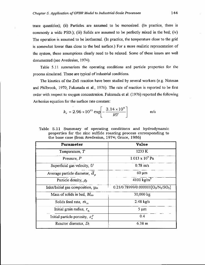
Chapter 5. Application of GFBR Model to Industrial-Scale Processes 144
trace quantities); (ii) Particles are assumed to be monosized. (In practice, there is
commonly a wide PSD.); (iii) Solids are assumed to be perfectly mixed in the bed; (iv)
The operation is assumed to be isothermal. (In practice, the temperature close to the grid
is somewhat lower than close to the bed surface.) For a more realistic representation of
the system, these assumptions clearly need to be relaxed. Some of these issues are well
documented (see Avedesian, 1974).
Table 5.11 summarizes the operating conditions and particle properties for the
process simulated. These are typical of industrial conditions.
The kinetics of the ZnS reaction have been studied by several workers (e.g. Natesan
and Philbrook, 1970; Fukunada et al., 1976). The rate of reaction is reported to be first
order with respect to oxygen concentration. Fukunada et al. (1976) reported the following
Arrhenius equation for the surface rate constant:
kr = 2.96 x l O 1 3 exp
Table 5.11 Summary of operating conditions and hydrodynamic properties for the zinc sulfide roasting process corresponding to the base case (from Avedesian, 1974; Grace, 1986)
Parameter Value
Temperature, T 1233 K
Pressure, P 1.013 x 10⁵ Pa
Superficial gas velocity, U 0.78 m/s
Average particle diameter, dp 60 um
Particle density, Pp 4100 kg/m3
Inlet/Initial gas composition, r/m 0.21/0.78999/0.000001 [O2/N2/SO2]
Mass of solids in bed, Mso 30,000 kg
Solids feed rate, min 2.48 kg/s
Initial grain radius, 5 urn
Initial particle porosity, 0.4
Reactor diameter, Dt 6.38 m
3.14x10-RT
m/s

Chapter 5. Application of GFBR Model to Industricd-Scale Processes 145
5.3.4.2 Results and Discussion
Results from approach A2 are presented here, noting that this approach is essentially a
sub-case of approach A l in which the bed-averaged gas concentration is obtained as:
U< = 7 - 5 - / f C ' d r d z ( 5 2 4 )
Ld Kc z=0r=0 where
C,- = q t C t t + q H C f f / (2.3)
Equation (5.24) is then substituted for eq. (5.6) and all phase subscripts drop out leading
to bed-averaged profiles.
Figure 5.25 shows the grain conversion along the radius of a particle as a function of
time for single particles of diameter 60 and 200 um. As expected, the grains closer to the
particle surface, exposed to more of the reactant-rich gaseous species, are converted more
than grains towards the center of the particle. Therefore, one observes a drop in the extent
of grain conversion as the reactant concentration becomes depleted towards the center of
the particle (Fig. 5.26), consistent with the expected prediction from the GPM. This is
especially the case, for the larger particle (b) in which diffusional mass transfer is seen to
be limiting. Figure 5.27 compares the particle conversion as a function of time for the
same two particle sizes. As expected, it takes much longer for larger particles to
completely react. (A similar trend can be seen in Fig. 5.25b.) A snapshot of the overall
exit conversion of gas and solids together with other transport and hydrodynamic
quantities for the 60 um particles is given in Table 5.12. It is seen that the solids mean
residence time is much greater than the time for complete conversion of particles so that
the vast majority of particles leaving the bed are nearly fully converted.
The influence of the particle size on the time required for complete conversion of
individual particles, as well as the overall solids conversion, is assessed in Fig. 5.28. The
overall conversion is seen to drop only slightly with increasing particle size even though
the time for conversion significantly increased. In the commercial operations, solids
taken out of the main product stream (overflow) of the fluidized bed roasters are
converted slightly more than those, mostly fines, which spend less time in the reactor and
are entrained (carried over) (Magoon et al., 1990). Based on the analysis of the residual
sulfide sulfur in the overflow stream, the average commercial values of solids conversion
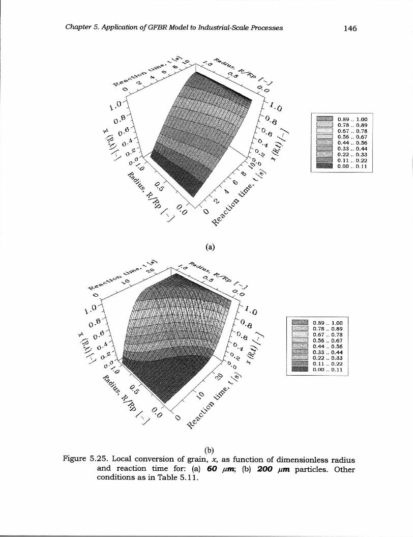
Chapter 5. Application of GFBR Model to Industrial-Scale Processes 146
(b) Figure 5.25. Local conversion of grain, x, as function of dimensionless radius
and reaction time for: (a) 60 /urn; (b) 200 //m particles. Other conditions as in Table 5.11.
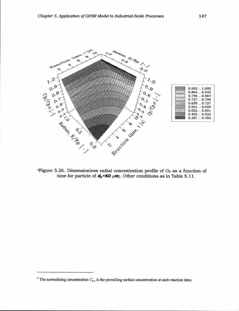
Chapter 5. Application of GFBR Model to Industrial-Scale Processes 147
4Figure 5.26. Dimensionless radial concentration profile of O2 as a function of time for particle of dp=60 fj.m;. Other conditions as in Table 5.1 L
4 The normalizing concentration C p s is the prevailing surface concentration at each reaction time.
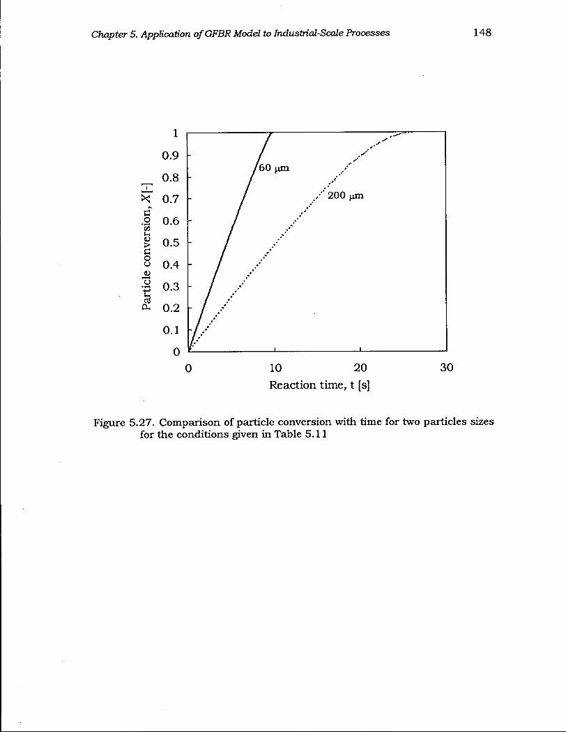
Chapter 5. Application of GFBR Model to Industrial-Scale Processes 148
0 10 20 30 Reaction time, t [s]
Figure 5.27. Comparison of particle conversion with time for two particles sizes for the conditions given in Table 5.11
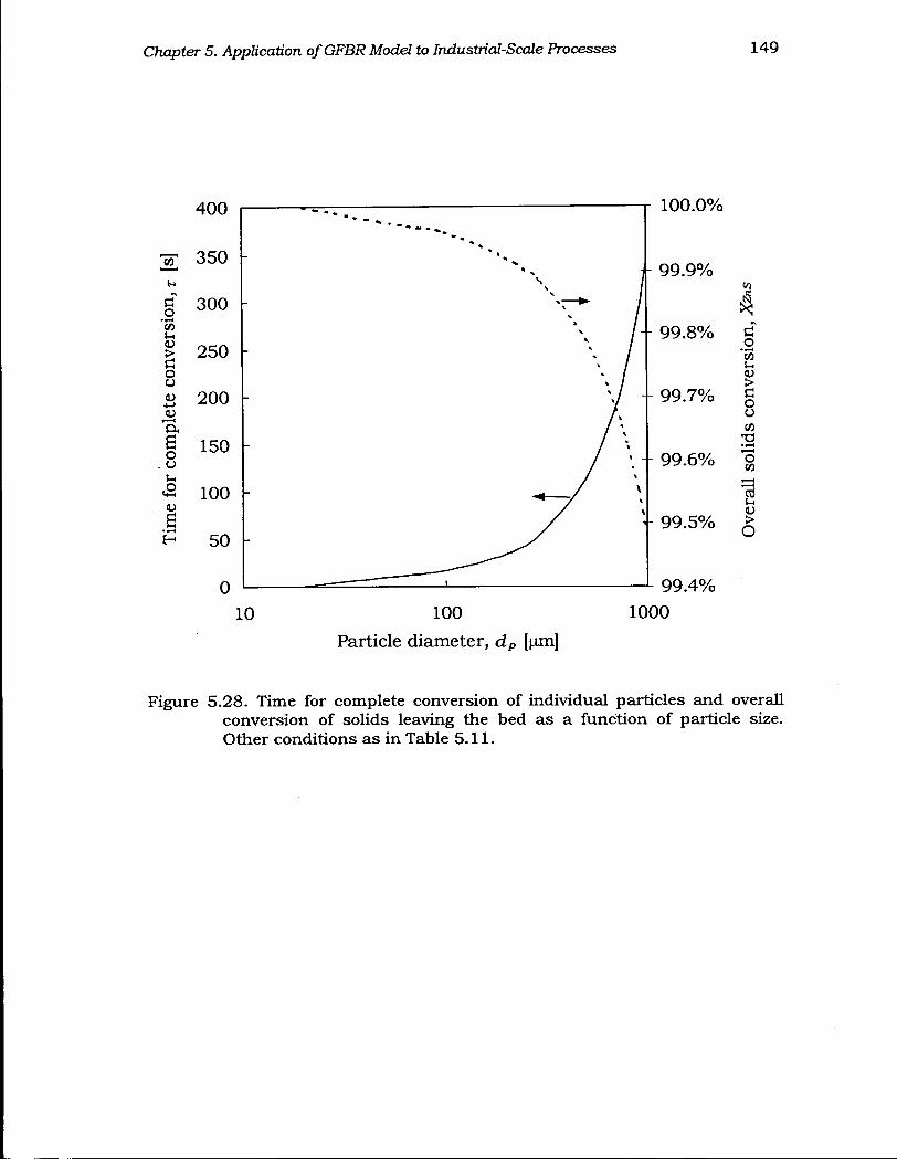
Chapter 5. AppUcation of GFBR Model to Industrial-Scale Processes 149
Figure 5.28. Time for complete conversion of individual particles and overall conversion of solids leaving the bed as a function of particle size. Other conditions as in Table 5.11.
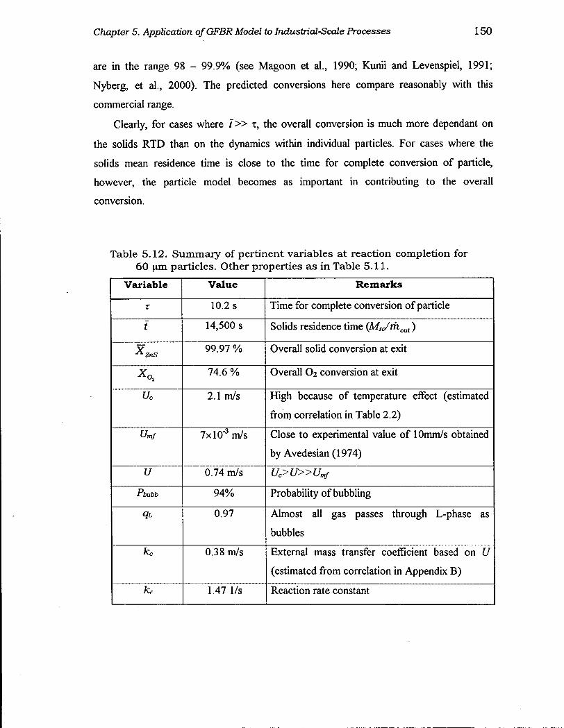
Chapter 5. Application of GFBR Model to Industrial-Scale Processes 150
are in the range 98 - 99.9% (see Magoon et al., 1990; Kunii and Levenspiel, 1991;
Nyberg, et al., 2000). The predicted conversions here compare reasonably with this
commercial range.
Clearly, for cases where f » x, the overall conversion is much more dependant on
the solids RTD than on the dynamics within individual particles. For cases where the
solids mean residence time is close to the time for complete conversion of particle,
however, the particle model becomes as important in contributing to the overall
conversion.
Table 5.12. Summary of pertinent variables at reaction completion for 60 um particles. Other properties as in Table 5.11.
Variable Value Remarks
r 10.2 s Time for complete conversion of particle
i 14,500 s Solids residence time QAsc/rhoui)
99.97 % Overall solid conversion at exit
74.6 % Overall O2 conversion at exit
Uc 2.1 m/s High because of temperature effect (estimated
from correlation in Table 2.2)
Umf 7xl0'3m/s Close to experimental value of lOmm/s obtained
by Avedesian (1974)
U 0.74 m/s Uc>U»Umf
Pbubb 94% Probability of bubbling
qt 0.97 Almost all gas passes through L-phase as
bubbles
kc 0.38 m/s External mass transfer coefficient based on U
(estimated from correlation in Appendix B)
kr 1.47 1/s Reaction rate constant
Chapter 5. Application of GFBR Model to Industrial-Scale Processes 151
5.3.3 Concluding Remarks
Application of the GFBR model to gas-solid reactions has been demonstrated using the
zinc sulfide roasting process as a study case. Preliminary model predictions at the single
particle level for the zinc sulfide roasting process are reasonable. In order to fully realize
the potential of the model, several modifications and extensions could be made to the
combined model at both the particle and the fluid bed levels, namely: (i) Allow for
separate solid RTDs in the L- and H-phases; (ii) Refine the approach of solids
interchange between phases for proper implementation of approach A l ; (iii) Consider a
wide particle size distribution in bed; (iv) Consider a variable area freeboard region, (v)
Account for change in particle porosity with time depending on whether the solids
expand, shrink or retain their original shapes as they react; (vi) Incorporate energy
balances to track temperature history in the bed and within the particles. However, these
modifications/extensions, particularly at the particle level, are not likely to change the
overall result significantly for cases where the particle mean residence time is much
greater than the time for complete conversion of individual particles (i.e. for t » x), as in
the ZnS roasting case. In such systems, the overall conversion is much more a function of
the solid RTD (which may be a function of the PSD) than the reaction model used to
describe the gas-solid reaction.

Chapter 6
I m p l e m e n t a t i o n o f V o l u m e C h a n g e w i t h R e a c t i o n
6.1 Introduction
A number of industrial gas phase reactions are accompanied by significant volume
change (reduction or expansion) due to reaction. Examples include oxy-chlorination and
steam methane reforming. The volume change can cause significant change in the
hydrodynamic behavior of the bed, as well as variations in reactor performance indicators
such as conversion, selectivity and yield. Volume reduction in a fluidized bed reactor
leads to a decrease in the gas velocity with the possibility of de-fluidization. The decrease
in the volumetric gas flow can directly affect hydrodynamics throughout the bed. It also
results in increased gas residence time leading to increased conversions and yields, but
with the possibility of decreased selectivities for desired intermediates. An increase in the
number of moles can lead not only to increased entrainment, but also to decreased gas
residence time resulting in reduced conversions, yields and selectivities.
Few fluidized bed reactor-models in the literature consider volume changes with
reaction. When such effects have been considered, models have been limited to single
reactions with simple first order kinetics (Irani et al., 1980; Kai and Furusaki, 1984;
Shiau and Liu, 1993) or single reactions with non-linear kinetics (Taffeshi et al., 2000).
Adris et al. (1997) examined the impact of volume increase for a fluidized bed membrane
steam methane reforming process with multiple reactions and non-linear kinetics. In all
Of these cases, the investigations were limited to the bubbling flow regime of fluidization
and to isothermal, isobaric conditions. No attempts have been reported to assess the
impact of volume changes on the performance of a commercial-scale reactor.
In this chapter, we treat the effect of volume change with reaction, accounting for
the changes in both temperature and pressure, as well as total molar flow rate, along the
reactor height. Multiple reactions with non-linear kinetics for the oxy-chlorination
process treated in Chapter 5 are considered to assess the impact of the volume change on
the hydrodynamics and reactor performance.
152
Chapter 6. Implementation of Volume Change with Reaction 153
6.2 Modeling Approach
The total volumetric flowrate Q can be expressed as a function of the total molar flow
rate, temperature and pressure using the basic equation of state,
FT P Q ZRT
At height z = 0\~, i.e. just below where the reaction is initiated,
(6.1)
:fk =
PQ (6.2) Qo Z0RT0
Combining eqs. (6.1) and (6.2) and assuming that the compressibility factor does not
change significantly, the volumetric flowrate at any height z is
Q = QOIJLLEO. (6.3) ° Fro T0P
For a column of constant cross-section, eq. (6.3) can be written in terms of gas velocity:
U = U0^- — ^ (6.4) Fro T0 P
For a two-phase/region system with low- and high-density phases or regions (which we
label the L - and H-phases as before), eq. (6.4) can be written (neglecting any temperature
or pressure difference between the phases at a given level):
(6.5) FT;. T PQ
F T P rTo 1o r
*-LlL^?°- (6.6) FTo Ta P
U = yLuL + VHUH (6.7)
For single reactions, the effect of change in the number of moles due to reaction
in the jth phase can be related to the conversion of the base reactant A
^L = {l + rXAJ) (6.8) ^To
where the expansion/reduction factor ^is obtained from
Y = vjLvi (6-9)
Chapter 6. Implementation of Volume Change with Reaction 154
In this way, the continuity equations can be written in terms of species concentration with
the effect of the volume change captured through the superficial gas velocity. For
example, for a single reaction
aA + bB -> cC + dD (6.10)
The low and high-density phase variables can be written for a base reactant A (with the
implicit assumption that extra moles of gas generated within one phase remain with that
phase)
u^u^l + yX^)^ (6.11) o
uH=uHo(l + r X A t H ) ^ (6.12) o
where
XAL= 1 ~ C a + / C a ° (6.13) A>L l + YCA,JCAo
V _ 1 ~ C A , H I C A o 1 4 \
CAM and CAM are obtained by solving the continuity equations for species A together with
the energy and pressure equations and appropriate boundary conditions. The
concentrations of the other species (B, C, D) are then given by
c ^ = cAO{dUL+yaxAyL) ( 6 1 5 )
''" 1 + rXA,H
Oij-C^/C^ (6.17)
^ O ^ ^ + F H ^ O (6.18)
^regime
= Z^JXPJ ( 6 T 9 )
For multiple reactions, it is generally impossible to express the volumetric flowrate in
terms of the conversion of single species because of the complexity of the reactions.
Therefore, the continuity equations and the reaction rates must be written in terms of the
Chapter 6. Implementation of Volume Change with Reaction 155
species molar flowrates F, and solved together with the volumetric flowrate from eqs.
(6.5) to (6.7). This general approach handles single reactions as well.
For the variable density generalized modeling approach, the steady state two-
phase/region mole balances representing the two-phase bubbling bed model in the low
velocity limit, dispersed plug flow model at intermediate velocities and the core-annulus
model in the high velocity limit presented in Chapter 2 for constant gas density systems
(eqs. 2.1 to 2.3) can then be re-written in terms of molar flow rates, F
L-phase: dz ^ dz2 r dr dr + K(FiL-FiH)/(Uxy,L) + ApL Rate^ = 0
d(FiH) „ d2(FiH/U) m 1 a (_d(FiH/U) (D — cry — —
H-phase: dz dz2 rg'H r dr r-
dr
(6.20)
(6.21)
+ K(FiH - F j / (U x yj,H) + ApH RateiH = 0
Overall balances: F,. = + qHFiH (6.22)
^ = I X ; Fr,H=tFiH (6-23) i = i i = i
where K = kLHa,i//L. The species conversions, yields, selectivities, etc are computed
based on the molar flowrates, F,. The concentration of the individual species /' in phase j
can be obtained from
C , , = ^ (6.24)
We assume here that exchange of gas between the L - and H-phases occurs solely via
interphase mass transfer. The effect of bulk transfer between phases is discussed below.
This system of equations is solved together with the energy and pressure balance
equations (eqs. 2.8 and 2.11) and the material balances (Table 2.1) for a given set of
reactor conditions.
6.3 Case Study: Oxy-Chlorination Process
As discussed in Chapter 5, the oxy-chlorination process is described by complex
reactions with non-linear temperature-dependent kinetics and is accompanied by a
significant change in the total number of moles. Using this process as a case study, the

Chapter 6. Implementation of Volume Change with Reaction 156
impacts o f the volume change on both the hydrodynamic and reactor performance are
examined for the four different cases listed in Table 6 .1, with reactor physical conditions
as given in Table 5 . 8 .
Table 6.1. Four different cases considered for simulating the effects of changes in the number of moles, temperature and pressure on reactor performance.
> Case 1* Q=L andH)
-Neglects volume change due to reaction
-Effects o f T and P on U are ignored
- A l l thermophysical properties are based on
average values of T and P.
> Case 2 UJ =UJo F
-Accounts for change in number of moles
-Effects of T and P on U are ignored
-Thermophysical properties vary with T and P.
> Case 3 FTJ T
U, = u^ 1 " FTo T0
-Accounts for change in number o f moles and T
-Effect o f P on Uis ignored
-Thermophysical properties vary with T and P.
> Case 4 Frj T PQ
U: - Uj. ~ ~ 3 30 FTo Ta P
-Accounts for change in number o f moles
-Accounts also for effects of both T and P on U
-Thermophysical properties vary with T and P.
*Base case
Chapter 6. Implementation of Volume Change with Reaction 157
6.4 Results and Discussion
6.4.1 Effect of volume change on the hydrodynamic variables
6.4.1.1 Gas velocity
The bed-average axial gas velocity profiles for all four cases listed in Table 6.1 are
presented in Fig. 6.1. The gas velocity for case 1 is uniform, while for case 2, a decrease
in gas velocity is observed immediately above the distributor owing to the rapid
conversion of the reactants, resulting in a reduction in volumetric flow by about 25%.
The nearly flat velocity profile over the rest of the expanded bed height occurs because
the ethylene conversion is almost complete, with relatively little further conversion. The
impacts of the temperature and pressure are shown in cases 3 and 4. The sharp decrease
in case 4 immediately above the distributor is due to the rapid conversion of ethylene as
above, while the subsequent increase stems from the decreasing hydrostatic pressure.
Figure 6.2 shows the bed-average L - and H-phase axial gas velocity profiles for case 4.
As expected, the velocities decrease rapidly immediately above the distributor where
rapid reactions occur and then continue to increase over the rest of the bed.
6.4.1.2 Gas flow distribution and phase volume fractions
Similar trends as for the gas velocity profiles can be observed when the fractional gas
flow allocation to the L-phase, qr. (= fraction of total flow passing through this phase) is
plotted vs. height as shown in Fig. 6.3. Figure 6.4 shows the expected immediate
decrease of the total gas flow through both phases due to reaction, with the relative
decrease being more pronounced in the L-phase. Since more reaction take place in the H -
phase than the L-phase (Pturb ~ 94%), a slightly higher absolute decrease occurs for the
gas flow through the H-phase. When the volumetric flow in the H-phase decreases faster,
less gas is exchanged with the L-phase via interphase mass transfer. As a result, the
volume occupied by the H-phase is predicted to increase while that of the L-phase
decreases as shown in Fig. 6.5.
So far, we have ignored bulk transfer of gas between the phases, assuming that all
gas exchange between phases occurs due to interphase mass transfer. The effect of bulk
transfer between the phases is discussed below.
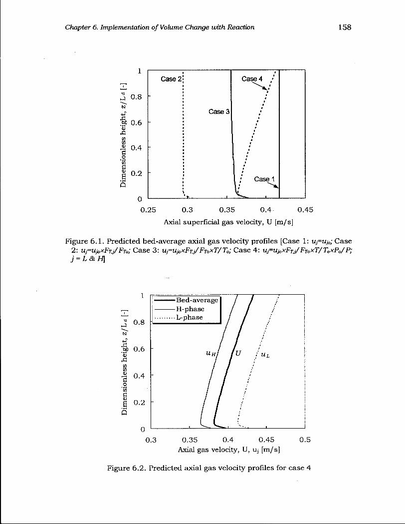
Chapter 6. Implementation of Volume Change with Reaction 158
•a
N
0 . 8
SP 0.6 •a «»-( <u CO w
iJ 0.4 G o CO ID
a Q
0.2
0
Case 2 Case 4 / f
« t
•
Case 3 • i
- « •
t f
«
-
• •
i I • *
• i t •
• • •
Case 1 i
' v . i v — - i
0.25 0.3 0.35 0.4 0.45
Axial superficial gas velocity, U [m/ s]
Figure 6.1. Predicted bed-average axial gas velocity profiles [Case 1: Uj=Uj<,; Case 2: UJ=UJOXFTJ/FTO; Case 3: UJ=UJOXFTJ/FTOXT/ T0; Case 4: UJ=UJOXFTJ/FT0XT/T0XP0/P;
Figure 6.2. Predicted axial gas velocity profiles for case 4
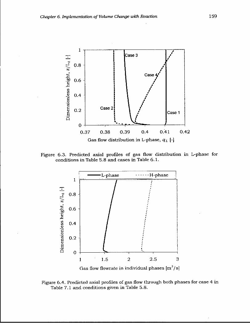
Chapter 6. Implementation of Volume Change with Reaction 159
0.37 0.38 0.39 0.4 0.41 0.42 Gas flow distribution in L-phase, qL [-]
Figure 6.3. Predicted axial profiles of gas flow distribution in L-phase for conditions in Table 5.8 and cases in Table 6.1.
L-phase H-phase
Gas flow flowrate in individual phases [m3/ s]
Figure 6.4. Predicted axial profiles of gas flow through both phases for case 4 in Table 7.1 and conditions given in Table 5.8.
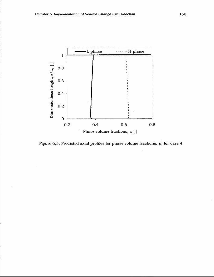
Chapter 6. Implementation of Volume Change with Reaction 160
•L-phase • H-phase
0.8 i
0.6
0.4
0.2 A
0 0.2 0.4 0.6
Phase volume fractions, vj/ [-] 0.8
Figure 6.5. Predicted axial profiles for phase volume fractions, yr, for case 4
Chapter 6. Implementation of Volume Change with Reaction 161
6.4.1.3 Regime probabilities
Since the regime probabilities are functions of the superficial gas velocity, as well as of
physical properties such as gas density and viscosity, the flow regimes within the bed
may change causing the probabilities to vary with height. As shown in Fig. 6.6 for case 2,
the probability of turbulent fluidization, Pturb, decreased sharply from nearly fully
turbulent conditions (Pturb « 93%) to approx. 83% immediately above the distributor
(where the molar composition changes rapidly) and then continued to fall, with Pturb
reaching about 75% at the bed surface. Note that although the effect of temperature and
pressure on the gas velocity is not considered for this case, they affect the regime
probabilities throughout the bed since all thermophysical properties are computed as
functions of temperature and pressure. The influence on the gas velocity of the steep
temperature rise (-85 K) at the distributor due to the strongly exothermic reactions and
the subsequent mild temperature change of about 7 K (Fig. 6.7) along the rest of the bed
is clearly captured by the plot for case 3. When the effect of pressure is also considered
(case 4), an interesting trend is observed in Fig. 6.6. Pturb first decreases slightly, then
increases gradually until near the bed surface it starts to decrease gradually again.
To explain the observed trend, consider the expanded version of the changes in the
probabilities of all three flow regimes along the bed for case 4 presented in Fig. 6.8a.
Figure 6.8b shows the generalized regime probability diagram based on the
dimensionless gas velocity; the shaded area shows the approximate range of
dimensionless gas velocity (LT ranging from 1.3 to 1.7) along the bed height. The
observed sharp change in the probabilities immediately above the distributor (Fig. 6.8a) is
caused by volume increase due to rapid reactions, as discussed above, while the
subsequent decrease can be attributed to the increase in gas velocity as the hydrostatic
pressure decreases, partially offset by the small decrease in temperature. At about 80% of
the total bed height, the probability of fast fluidization has increased enough to cause a
decrease of the probability of turbulent fluidization after the turbulent plateau is passed.
Clearly, for operations in which there is a significant swing in the regime
probabilities, multiple flow regimes can result (e.g., for an increase in the number of
moles, predominantly bubbling around the grid and predominantly turbulent fluidization
near the bed surface). The model accounts for such behaviour. It is also clear from the
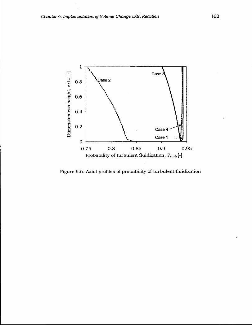
Chapter 6. Implementation of Volume Change with Reaction 162
0.75 0.8 0.85 0.9 0.95 Probability of turbulent fluidization, P t u r b [-]
Figure 6.6. Axial profiles of probability of turbulent fluidization
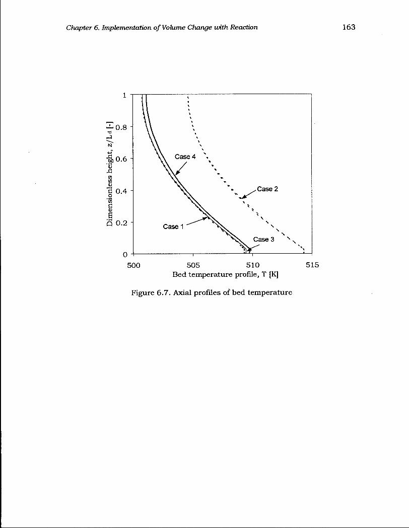
Chapter 6. Implementation of Volume Change with Reaction 163

Chapter 6. Implementation of Volume Change with Reaction 164
0.945
0.04
0.03
Turbulent Bubbling Fast fluidization
0.936
H 0.02
0.01 0 0.2 0.4 0.6 0.8
Dimensionless height, z/Ld [-]
(a)
as t—I
o 1-1
•3 o u a cu B •5b
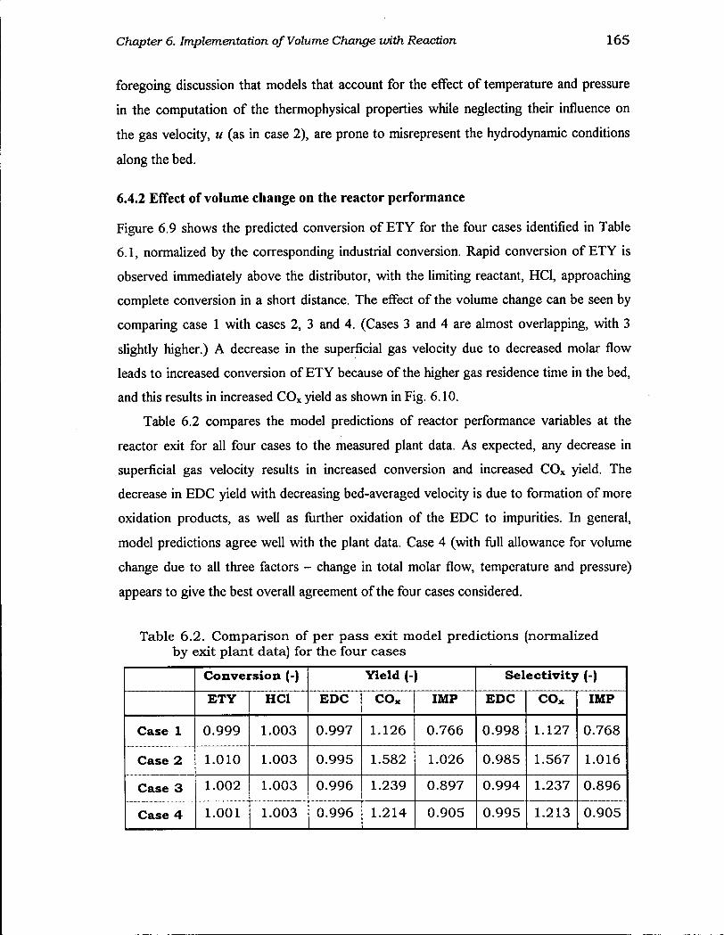
Chapter 6. Implementation of Volume Change with Reaction 165
foregoing discussion that models that account for the effect of temperature and pressure
in the computation of the thermophysical properties while neglecting their influence on
the gas velocity, u (as in case 2), are prone to misrepresent the hydrodynamic conditions
along the bed.
6.4.2 Effect of volume change on the reactor performance
Figure 6.9 shows the predicted conversion of ETY for the four cases identified in Table
6.1, normalized by the corresponding industrial conversion. Rapid conversion of ETY is
observed immediately above the distributor, with the limiting reactant, HC1, approaching
complete conversion in a short distance. The effect of the volume change can be seen by
comparing case 1 with cases 2, 3 and 4. (Cases 3 and 4 are almost overlapping, with 3
slightly higher.) A decrease in the superficial gas velocity due to decreased molar flow
leads to increased conversion of ETY because of the higher gas residence time in the bed,
and this results in increased CO x yield as shown in Fig. 6.10.
Table 6.2 compares the model predictions of reactor performance variables at the
reactor exit for all four cases to the measured plant data. As expected, any decrease in
superficial gas velocity results in increased conversion and increased CO x yield. The
decrease in EDC yield with decreasing bed-averaged velocity is due to formation of more
oxidation products, as well as further oxidation of the EDC to impurities. In general,
model predictions agree well with the plant data. Case 4 (with full allowance for volume
change due to all three factors - change in total molar flow, temperature and pressure)
appears to give the best overall agreement of the four cases considered.
Table 6.2. Comparison of per pass exit model predictions (normalized by exit plant data) for the four cases
C o n v e r s i o n (-) Y i e l d (-) Se l ec t i v i ty (-)
E T Y HC1 E D C COx IMP E D C co x IMP
Case 1 0.999 1.003 0.997 1.126 0.766 0.998 1.127 0.768
Case 2 1.010 1.003 0.995 1.582 1.026 0.985 1.567 1.016
Case 3 1.002 1.003 0.996 1.239 0.897 0.994 1.237 0.896
Case 4 1.001 1.003 0.996 1.214 0.905 0.995 1.213 0.905
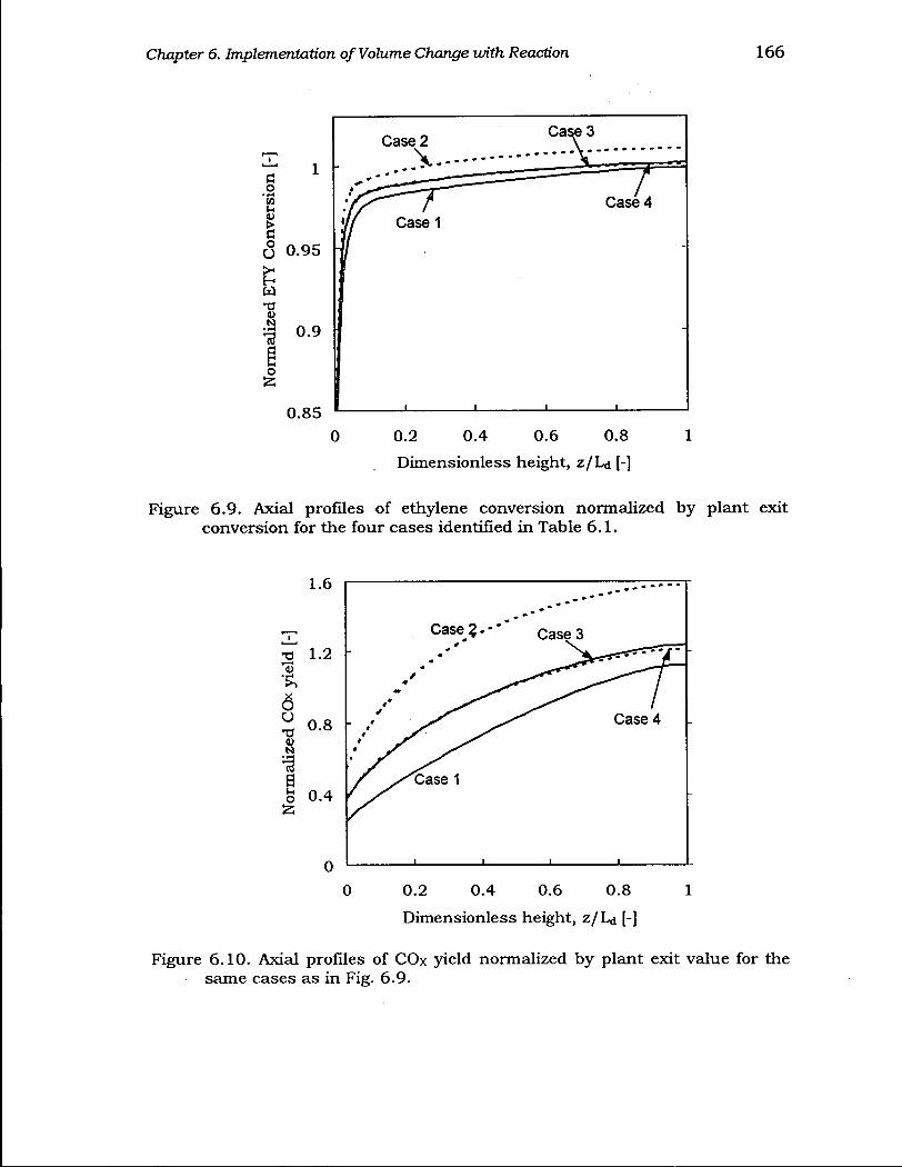
Chapter 6. Implementation of Volume Change with Reaction 166
0 0.2 0.4 0.6 0.8 1 Dimensionless height, z/Ld [-]
Figure 6.9. Axial profiles of ethylene conversion normalized by plant exit conversion for the four cases identified in Table 6.1.
1.6
0 0.2 0.4 0.6 0.8 1 Dimensionless height, z/Ld [-]
Figure 6.10. Axial profiles of COx yield normalized by plant exit value for the same cases as in Fig. 6.9.
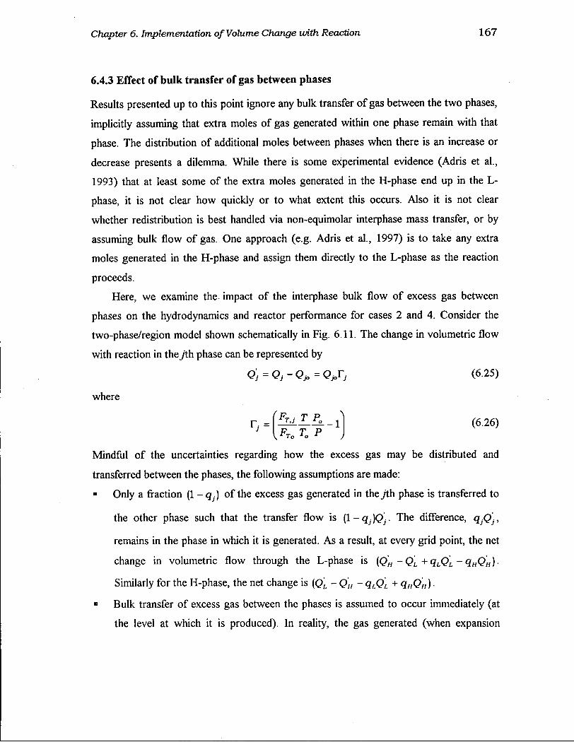
Chapter 6. Implementation of Volume Change with Reaction 167
6.4.3 Effect of bulk transfer of gas between phases
Results presented up to this point ignore any bulk transfer of gas between the two phases,
implicitly assuming that extra moles of gas generated within one phase remain with that
phase. The distribution of additional moles between phases when there is an increase or
decrease presents a dilemma. While there is some experimental evidence (Adris et al.,
1993) that at least some of the extra moles generated in the H-phase end up in the L -
phase, it is not clear how quickly or to what extent this occurs. Also it is not clear
whether redistribution is best handled via non-equimolar interphase mass transfer, or by
assuming bulk flow of gas. One approach (e.g. Adris et al., 1997) is to take any extra
moles generated in the H-phase and assign them directly to the L-phase as the reaction
proceeds.
Here, we examine the impact of the interphase bulk flow of excess gas between
phases on the hydrodynamics and reactor performance for cases 2 and 4. Consider the
two-phase/region model shown schematically in Fig. 6.11. The change in volumetric flow
with reaction in the/th phase can be represented by
Q) = °J - ° j o = Q„r, (6.25)
where
v*V„ TQ P
(6.26)
Mindful of the uncertainties regarding how the excess gas may be distributed and
transferred between the phases, the following assumptions are made:
• Only a fraction (1 - q.) of the excess gas generated in the /th phase is transferred to
the other phase such that the transfer flow is ( l -q^QJ. . The difference,
remains in the phase in which it is generated. As a result, at every grid point, the net
change in volumetric flow through the L-phase is (QH -QL +qLQL -qHQH).
Similarly for the H-phase, the net change is (QL - QH - qLQL + qHQH).
• Bulk transfer of excess gas between the phases is assumed to occur immediately (at
the level at which it is produced). In reality, the gas generated (when expansion

Chapter 6. Implementation of Volume Change with Reaction 168
Az
Convection Dispersion Reaction
L-phase
F,
Interphase mass
transfer
K+fiL
Interphase Bulk
transfer
Qo
H-phase
ir Convection Dispersion Reaction
Figure 6.11. Schematic of generalized one-dimensional, two-phase/region model

Chapter 6. Implementation of Volume Change with Reaction 169
occurs, for instance) may remain in the same phase for some distance before
transferring to the other phase.
The excess gas flow transferred from theJth phase to the other phase is
Q'j^nsj^i=0--qjrQjJ'j (6.27)
The gas flow transferred from the y'th phase per unit volume of the jth phase is
a _Qjtransferred _ (1 — QjK?jb-^} /{. n o \
J ~ AVj " ifYjAAz
The interphase mass transfer is augmented by so that eqs. (6.20) and (6.21) become:
Wo.) _ 0 r d2(Fu./U) _a 11 d_(r mJU^ L-phase: 8 z 5 z 2 ^L r dr{ dr ) (6.29)
+ [(K + A]Fa. ~(K + P„)FiH]/U x ¥l) + ApLRate^ = 0
WrI)_(n 82(FiH/U) 1 df d(FiH/U)) H-phase: d z ^ 3z 2 ^ r dr{ dr J (6-30)
+ [(K +£H)FiH-{K + A)Fu.]/(U *V„) + ApHRateiH = 0
Figure 6.12 compares model predictions of volumetric flow through the two phases for
cases 2 and 4 when the bulk flow between phases is considered and when it is ignored.
The volumetric flow through the L-phase is increased, as more gas is bulk transferred to
the L-phase. Note that the approach outlined here ensures that at all grid points along the
bed height the phase flow ratio (i.e. ratio of volumetric flow through the H-phase to that
through the L-phase, QH/QL) remains nearly constant. This approach also avoids potential
phase defluidization even if there were to be substantial volumetric flow reduction.
The effect of the change in flow distribution on the reactor performance is shown in
Fig. 6.13 for cases 2 and 4. Inclusion of allowance for bulk transfer makes prediction
slightly worse. The effect can be appreciable well away from the turbulent fluidization
flow regime where the extent of reaction in the two phases differs markedly and when the
interphase mass transfer resistance is significant. The effect of bulk flow is, however,
small in the present case because the reductions in volume in the two phases are
comparable since the bed operates under almost fully turbulent conditions (where the
phases become identical in the model). Given this insensitivity, the agreement between
the plant data and model predictions is not changed appreciably by the treatment of the
flow distribution between phases in the present case.
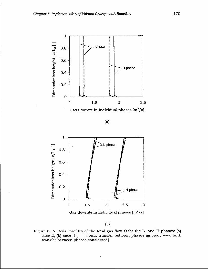
Chapter 6. Implementation of Volume Change with Reaction 170
•a ,-3
•a IU
X\ CO
o •rH
w <u
1
0.8 H
0.6
0.4
0.2
0 1
L-phase
1.5
H-phase
2 2.5
Gas flowrate in individual phases [m /s]
(a)
Figure 6.12. Axial profiles of the total gas flow Q for the L- and H-phases: (a) case 2, (b) case 4 [ : bulk transfer between phases ignored; : bulk transfer between phases considered]
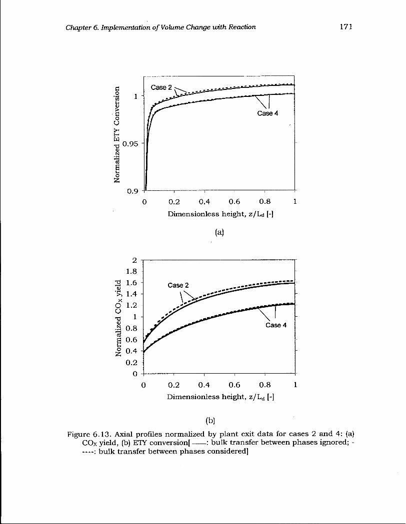
Chapter 6. Implementation of Volume Change with Reaction 171
Figure 6.13. Axial profiles normalized by plant exit data for cases 2 and 4: (a) COx yield, (b) ETY conversion[ : bulk transfer between phases ignored; -— : bulk transfer between phases considered]

Chapter 6. Implementation of Volume Change with Reaction 172
Notwithstanding the lack of sensitivity to bulk flow in the present example, the bulk
transfer of excess gas between phases should be included when considering reactions
with volume change in fluid bed reactor models. This is especially important when
operating well above, or well below, superficial velocities for maximum Pturb, since the
interphase mass transfer resistance then plays a major role and the difference between
phases is large when either the bubbling or fast fluidization probabilities are significant.
6.5 Conclusions
The generalized probabilistic fluidized bed reactor model is extended to cover variable-
gas density systems. Using the air-based oxy-chlorination process as a case study, it is
shown that a change in the number of moles due to reaction significantly affects the
hydrodynamics, conversion, selectivity and yield. Multiple flow regimes can exist in the
same reactor due to the changing volumetric flow. The impact of varying the temperature
and pressure non-uniformity along the bed height on the gas velocity and, in turn, on the
hydrodynamics and reactor performance is also examined. Allowing for the volume
change due to reaction, temperature variations and the decrease in hydrostatic pressure
with height improves the performance of the model somewhat in the oxy-chlorination
case relative to industrial data, in particular, significantly improving the impurities
predictions. Bulk transfer of gas between the phases influences both the hydrodynamics
and the reactor performance. This influence is small when the fluidized bed operates
primarily in the turbulent flow regime, but may be appreciable when bubbling or fast
fluidization predominates.
The effects of volume change on reaction may be even more important for some
other processes, e.g. where there is a larger change in the number of moles due to
reaction. The version of the GFBR model incorporating allowance for the volume change
is therefore recommended as the major product of this thesis.
Chapter 7
O v e r a l l C o n c l u s i o n s a n d R e c o m m e n d a t i o n s
7.1 Conclusions
The principal outcome of this research is the development of a new generic fluid bed
reactor (GFBR) model applicable across the fluidization flow regimes most commonly
encountered in industrial scale fluid bed reactors: bubbling, turbulent and fast
fluidization. The model interpolates between three regime-specific models - the
generalized two-phase bubbling bed model, dispersed flow model and the generalized
core-annulus model - by means of probabilistic averaging of hydrodynamic and
dispersion variables based on the uncertainty in the flow regime transitions.
Specific conclusions from the different aspects studied can be summarized as:
1) Model predictions of hydrodynamic variables across the three fluidization flow
regimes are realistic, while conversion predictions are in good agreement with
available experimental data. The probabilistic approach leads to improved predictions
of reactor performance compared with any of the three separate models for individual
flow regimes, while overcoming the difficulties in predicting the transition
boundaries among these flow regimes and avoiding discontinuities at the boundaries
between them.
2) The performance of the model is assessed using two industrial-scale catalytic
processes: oxidation of naphthalene to phthalic anhydride and oxy-chlorination of
ethylene. In both cases, model predictions were reasonable and compare favourably
with available plant data within the constraints of the uncertainties in the estimation
of the model parameters. Sensitivity analysis indicates that predictions from the
model are strongly influenced by the reaction kinetics, gas dispersion, superficial gas
velocity and reactor temperature. Accuracy of the model predictions depends strongly
on utilizing reliable estimates of the model parameters. Ability of the model to aid in
simulation experimentation over a wide range of conditions is also demonstrated.
173
Chapter 7. Overall Conclusions and Recommendations 174
3) The generic reactor model has been extended to cover systems accompanied by
volume change due to a change in the number of moles, as well as variations in
temperature and pressure along the reactor. Using the air-based oxy-chlorination
process as a case study, it is shown that these changes significantly affect the
hydrodynamics, conversion, selectivity and yield. Accounting for the volume changes
improves the performance of the model relative to industrial data. Multiple flow
regimes can exist in the same reactor due to the varying volumetric flow. The
probabilistic modeling approach effectively tracks changes in flow regimes within the
reactor. Moreover, bulk transfer of gas between the phases also influences both the
hydrodynamics and the reactor performance. This influence is small when the
fluidized bed operates primarily in the turbulent flow regime, but may be appreciable
when bubbling or fast fluidization predominates.
4) Application of the GFBR model to gas-solid reactions is demonstrated using the zinc
sulfide roasting process as a case study. Predictions from a combined model that
couples a single-particle model with the generic fluid bed reactor model are
reasonable. However, in order to fully realize the potential of the combined model,
some extensions are suggested. Such extensions are likely to have significant impact
on the model performance only for systems where the solids mean residence time is
similar to the time for complete conversion of particles.
5) Gas mixing experiments were conducted in a Plexiglas column with commercial
catalyst particles as bed material at superficial gas velocities from 0.2 to 0.6 m/s. Data
from both steady state and step change tracer injection experiments are interpreted
using a single-phase dispersion model and a generalized two-phase model with
dispersion. The generalized two-phase model captures the expected trends of
increasing dispersion in both the low- and high-density phases with increasing
superficial gas velocity. Beyond the transition velocity, Uc, however, the overall
dispersion decreased for L 0 = 1.0 m. Results for different gas velocities and aspect
ratios suggest that the dispersion coefficients and interphase mass transfer coefficient
between the low- and high-density phases depends on the initial solids inventory.
Chapter 7. Overall Conclusions and Recommendations 175
6) The GFBR model provides a means of predicting hydrodynamics regimes and
quantities in fluid bed reactors. For example, for a given set of particle properties,
operating conditions and reactor geometry, it is possible to predict the fluidization
regime(s) in which the reactor operates.
7.2 Recommendations for Future Work
1) Further gas mixing experiments are suggested to provide additional data for scale-up.
Specifically, it is recommended to: (a) Conduct experiments at different static bed
heights, preferably in taller columns for the same or similar column diameters as used
in this study, (b) Conduct experiments in columns of different diameters for the same
static bed height, i.e., changing the aspect ratio, Lo /D t , while keeping L 0 constant.
Results from this and (a) above, when combined together with the results from this
study and available literature data, would help establish the effect of the aspect ratio
on both the interphase mass transfer and gas dispersion in the bed.
2) It would be helpful to conduct experiments in columns of similar geometry for
superficial gas velocities beyond the range considered in this study. Specifically, it
would be valuable to study the effect of increasing U on the ratio, / ^ z g . H >
which is expected to approach unity for U « Uc. It would also be valuable to develop
separate correlations for the dispersion coefficients in the two phases using data from
this and (1) above.
3) Several modifications and extensions could be made to the combined "fluid-bed-
single-particle" model at both the particle and the fluid bed levels, namely: (i) Allow
for separate solid RTDs in the L - and H-phases; (ii) Refine the approach for
predicting solids interchange between phases for proper implementation of approach
A l presented in Chapter 5a; (iii) Consider a wide particle size distribution in the bed;
(v) Account for changes in particle porosity with time depending on whether the
solids expand, shrink or retain their original shapes as they react.
Chapter 7. Overall Conclusions and Recommendations 176
4) Apply the combined model to other gas-solids reactions, in particular, to
polymerization processes. For this class of applications, it is possible to fully
incorporate the particle size distribution through a particle population balance.
Preliminary simulations performed for ethylene polymerization process show good
promise. This extension, combined with the modifications in (3) above could create a
valuable tool for simulating a wide range of fluid bed processes involving gas-solid
reactions.
5) An alternative approach to constructing the generic model through probabilistic
averaging would be to consider flow regime transition from a two-phase bubbling bed
at low U to a homogeneous single-phase flow structure with both axial and radial
non-uniformities at intermediate and high U (eliminating the core-annular
consideration at the high-velocity limit). To implement this, the regime transition
equations need to be modified to ensure that the global model interpolates between
two limiting models (generalized two-phase bubbling bed model and the
axially/radially dispersed flow model). The values of the dispersion parameters would
need to be extrapolated among the limiting values of the three flow regimes as flow
condition changes. In addition to the reported success of the single-phase two-
dimensional model in the fast fluidization limit, this approach would have the
advantage of reducing the number of model parameters.
6) It would be valuable to fine tune this model and to develop a better user interface to
enable delivery of the research outcome to industry as well as other users without the
demand of familiarity with the modeling language, while recognizing that a
"standard-all-purpose-package" may lead to sub-optimal solutions in some cases
because of varying objectives.
N o m e n c l a t u r e
ai Interphase transfer surface area per unit volume of gas in low-density phase
nf1
CLki, bkl Stoichiometric coefficients of gaseous species /' and solid /, respectively, in reaction k
[-]
A Bed cross-sectional area m 2
Ai Gaseous component i as reactant or product [-]
Ar
As
Archimedes number, pg[pp - pg)gdp/p2
Covered heat transfer surface area per unit reactor volume
[-]
m"1
Ax Reaction surface or area per unit volume of reaction space m"1
Bi Solid component / as reactant or product [-]
C Concentration of helium Vol %
Co Concentration of helium at inlet Vol %
Coo Concentration of helium at infinite mixing Vol %
Ci Concentration of species / mol/m3
Bed-averaged (radially and axially) concentration of species i mol/m3
c u Concentration of species i in L-phase mol/m3
Concentration of species i in H-phase mol/m3
Cpg Specific heat of gas J/mol K
Cpp Specific heat of solids J/mol K
db Volume-equivalent bubble diameter m
dp
Mean particle diameter m
<D Molecular diffusivity of gas m2/s
(De Effective diffusivity of gases through product layer m2/s
©mix Mixture diffusivity m2/s
Dt Column/reactor diameter m
Axial gas dispersion coefficient m2/s
Radial gas dispersion coefficient m2/s
177
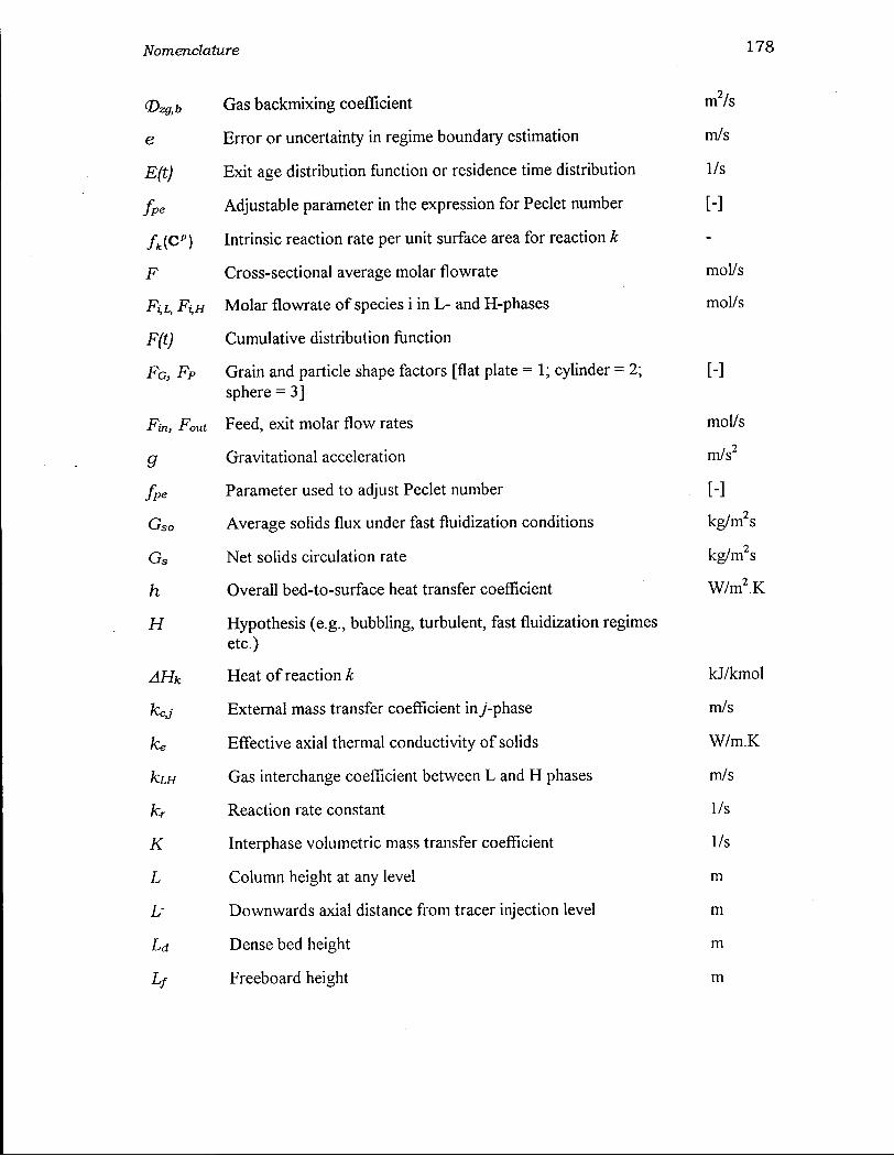
Nomenclature 178
(Dz9ib Gas backmixing coefficient m2/s
e Error or uncertainty in regime boundary estimation m/s
Eft) Exit age distribution function or residence time distribution 1/s
fpe Adjustable parameter in the expression for Peclet number [-]
fk(C") Intrinsic reaction rate per unit surface area for reaction k
F Cross-sectional average molar flowrate mol/s
Fi,L, Fi,H Molar flowrate of species i in L - and H-phases mol/s
F(t) Cumulative distribution function
FG, FP Grain and particle shape factors [flat plate = 1; cylinder = 2; [-] sphere = 3]
Fin, Fout Feed, exit molar flow rates mol/s
g Gravitational acceleration m/s2
fpe Parameter used to adjust Peclet number [-]
G s o Average solids flux under fast fluidization conditions kg/m2s
Gs Net solids circulation rate kg/m2s
h Overall bed-to-surface heat transfer coefficient W/m 2.K
H Hypothesis (e.g., bubbling, turbulent, fast fluidization regimes etc.)
AHk Heat of reaction k kJ/kmol
kcj External mass transfer coefficient in y'-phase m/s
ke Effective axial thermal conductivity of solids W/m.K
ki.H Gas interchange coefficient between L and H phases m/s
kr Reaction rate constant 1/s
K Interphase volumetric mass transfer coefficient 1/s
L Column height at any level m
L~ Downwards axial distance from tracer injection level m
Ld Dense bed height m
Lf Freeboard height m
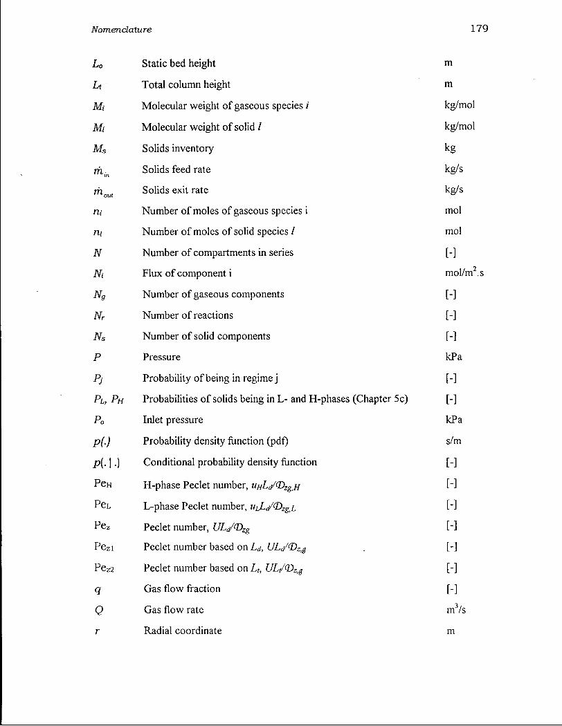
Nomenclature 179
Lo Static bed height m
Lt Total column height m
Mt Molecular weight of gaseous species i kg/mol
Mi Molecular weight of solid / kg/mol
Ms Solids inventory kg
Solids feed rate kg/s
m o u t Solids exit rate kg/s
ra Number of moles of gaseous species i mol
ni Number of moles of solid species / mol
N Number of compartments in series [-]
Ni Flux of component i mol/m2.s
N9 Number of gaseous components [-]
Nr Number of reactions [-]
Ns Number of solid components [-]
p Pressure kPa
Pj Probability of being in regime j [-]
PL, PH Probabilities of solids being in L - and H-phases (Chapter 5 c) [-]
Po Inlet pressure kPa
P(-) Probability density function (pdf) s/m
P(-1 •) Conditional probability density function [-]
Pe H H-phase Peclet number, uHLd/(DzgiH [-]
Pe L L-phase Peclet number, uJLc/^zg.L [-]
Pe z Peclet number, UL/(Dzg [-]
Pe zi Peclet number based on Ld, ULc/<Dz>g [-]
Pe z 2 Peclet number based on Lt, UL/<Dz,g [-]
<? Gas flow fraction [-]
Q Gas flow rate mVs
r Radial coordinate m
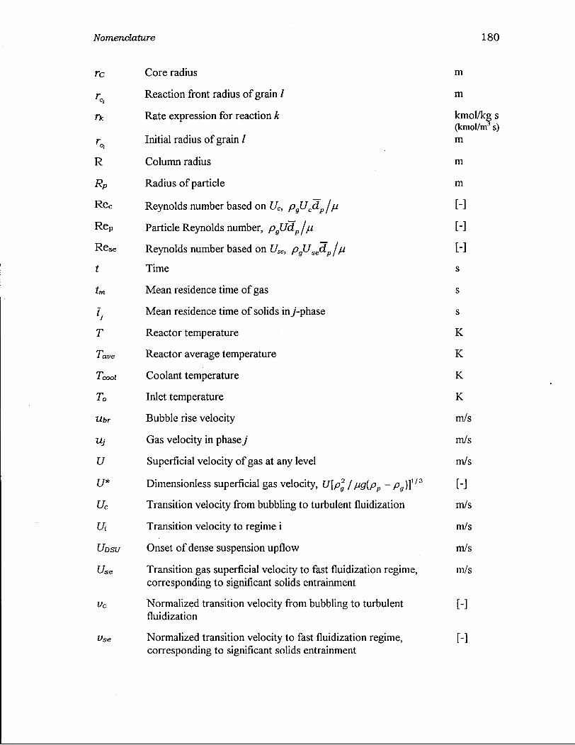
Nomenclature 180
rc Core radius m
rc Reaction front radius of grain / m
Rate expression for reaction k
Initial radius of grain /
kmol/kg s (kmol/m s) m
R Column radius m
RP Radius of particle m
Re c Reynolds number based on Uc, pgUcdpjp [-]
Re P Particle Reynolds number, pgUdpjp [-]
R6se Reynolds number based on Use, pgUsedpj p [-] t Time s
tm Mean residence time of gas s
h Mean residence time of solids in /-phase s
T Reactor temperature K
Tave Reactor average temperature K
Tcool Coolant temperature K
To Inlet temperature K
Ubr Bubble rise velocity m/s
Uj Gas velocity in phase j m/s
U Superficial velocity of gas at any level m/s
U* Dimensionless superficial gas velocity, U[pg /pg[pp - pg)]1/3 [-]
Uc Transition velocity from bubbling to turbulent fluidization m/s
Ui Transition velocity to regime i m/s
UDSU Onset of dense suspension upflow m/s
Use Transition gas superficial velocity to fast fluidization regime, corresponding to significant solids entrainment
m/s
Vc Normalized transition velocity from bubbling to turbulent fluidization
[-]
Vse Normalized transition velocity to fast fluidization regime, corresponding to significant solids entrainment
[-]
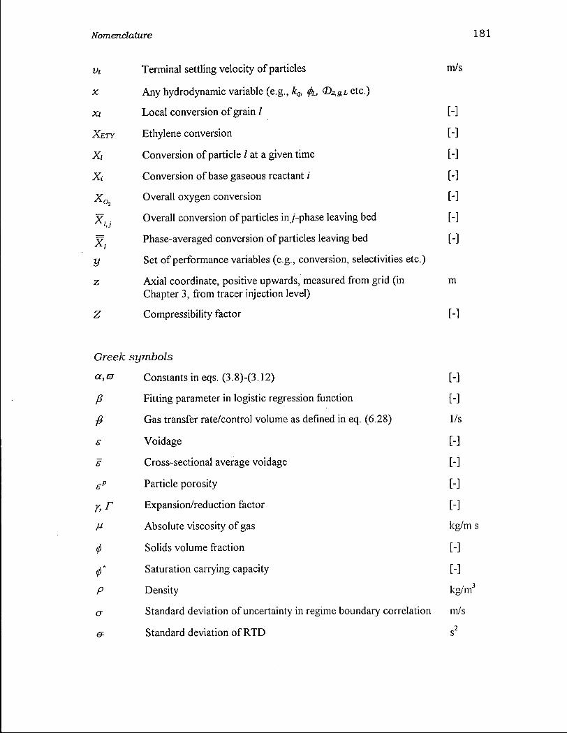
Nomenclature 181
Vt Terminal settling velocity of particles m/s
x Any hydrodynamic variable (e.g., kq, fa, (DZ&L etc.)
xi Local conversion of grain / [-]
XETY Ethylene conversion [-]
Xi Conversion of particle / at a given time [-]
Xi Conversion of base gaseous reactant /' [-]
Xn Overall oxygen conversion [-]
Xt j Overall conversion of particles in y'-phase leaving bed [-]
X Phase-averaged conversion of particles leaving bed [-]
y Set of performance variables (e.g., conversion, selectivities etc.)
z Axial coordinate, positive upwards, measured from grid (in m Chapter 3, from tracer injection level)
Z Compressibility factor [-]
Greek symbols
a,m Constants in eqs. (3.8)-(3.12) [-]
P Fitting parameter in logistic regression function [-]
Gas transfer rate/control volume as defined in eq. (6.28) 1/s
s Voidage [-]
£ Cross-sectional average voidage [-]
€P Particle porosity [-]
Expansion/reduction factor [-]
M Absolute viscosity of gas kg/m s
</> Solids volume fraction [-]
f Saturation carrying capacity [-]
P Density kg/m3
a Standard deviation of uncertainty in regime boundary correlation m/s
e- Standard deviation of RTD s2
Nomenclature 182
yz Phase volume fraction [-]
Ysup Slip factor = 1 + 5 . 6 / F r 2 + 0 . 4 7 F r (
0 4 1 [-]
0 Set of operating conditions and physical properties (e.g., To, Po, pg, etc.)
v Stoichiometric coefficient [-]
X Dimensionless interphase mass transfer coefficient [-]
Subscripts
a Annular (outer) region
b Bubble phase or bubble
bubb Bubbling flow regime
c Critical
C Core region
CA Type A or accumulative choking
d Dense phase
f Freeboard
fast Fast fluidization flow regime
9 Gas
G Grain
H High density phase
L Low density phase
mb Minimum bubbling
mf Minimum fluidization
0 Initial/Inlet
P Particle
r Radial
s Surface
se Significant entrainment
Nomenclature 183
t Total
turb Turbulent flow regime
z Axial
Superscript
* Dimensionless variable
Abbreviations
C O x Carbon oxides (CO and C0 2 )
GFBR Generic fluid bed reactor
GPM Grain particle model
IMP Chlorinated by-products/impurities
MCC Mitsubishi Chemical Corporation
NA Naphthalene
NQ Naphthaquinone
OC Oxy-chlorination
OP Oxidation products (primarily Maleic anhydride, CO, CO2)
PA Phthalic anhydride
PSD Particle size distribution
RTD Residence time distribution
UBC University of British Columbia
R e f e r e n c e s
Abed, R., The characterization of Turbulent Fluid Bed Hydrodynamics, in Fluidization IV (eds. Kunii, D. and R. Toei), Engineering Foundation, New York, pp. 137-144, (1984).
Abrahamsen, A.R. and D. Geldart, Behavior of Gas-Fluidized Beds of Fine Powders, Part I. Homogeneous Expansion, Powder Tech., 26, 35-46 (1980).
Adris, A .M. , C.J. Lim and J.R. Grace, The Effect of Gas Volume Increase due to Reaction on Bed Expansion, Bubbling and Overall Conversion in a Fluidized Bed Reactor, AIChE Annual Meeting, St. Louis, November, pp. 7-12 (1993).
Adris, A . M . , C.J. Lim and J.R. Grace, The Fluidized Bed Membrane Reactor for Steam Methane Reforming: Model Verification and Parametric Study. Chem. Eng. Sci., 52, 1609-1622 (1997).
Arena, U., Gas Mixing, Chap. 3, in Circulating Fluidized Beds, (eds. Grace, JR., A A . Avidan and T .M. Knowlton), Chapman and Hall, London (1997).
Arena, U., R. Chirone, M . D'Amore, M . Miccio and P. Salatino, Some Issues in Modeling Bubbling and Circulating Fluidized Bed Coal Combustors, Powder Tech., 82, 943-949 (1995).
Avedesian, M . M , Roasting Zinc Concentrates in Fluidized Beds - Practice and Principles, 24th CSChEMeeting, Ottawa, October 1974.
Avidan, A.A., Future Prospects, Chap. 17, in Circulating Fluidized Beds (eds. J.R. Grace, A.A. Avidan and T.M. Knowlton), Chapman and Hall, London, pp. 568-577 (1997).
Avidan, A.A., Turbulent Fluid Bed Reactors Using Fine Powder Catalysts, AIChE-CIESC. Meeting, Chemical Industry Press, Beijing, pp. 411-423 (1982).
Banerjee, A , Y. Arkun, B. Ogunnaike and R. Pearson, Estimation of Nonlinear Systems Using Linear Multiple Models, AIChE J. 43, 1204-1226(1997).
Berg, D.A., C L . Briens and M.A. Bergougnou, Reactor Development for the Ultrapyrolysis Reactor, Can. J. Chem. Eng., 67, 96-101 (1989).
Berger, J. O., Statistical Decision Theory and Bayesian Analysis, New York, McGraw-Hill (1985).
Bernardo, J. M . and A. F. M . Smith, Bayesian Theory, New York, Wiley (1994).
Berruti, F., J. Chaouki, L. Godfroy, T.S. Pugsley and G.S. Patience, Hydrodynamics of Circulating Fluidized Bed Risers: a Review, Can. J. Chem. Eng., 73, 579-602 (1995).
184
References 185
Bi, H.T., Ellis, N., Abba, LA. and Grace, J.R., A State-of-the-art Review of Gas-Solid Turbulent Fluidization, Chem. Eng. Sci., 5 5 , 4789-4825 (2000).
Bi, H.T. and J.R. Grace, Effects of Measurement Method on Velocities Used to Demarcate the Transition to Turbulent Fluidization, Chem. Eng. J., 5 7 , 261-271 (1995b).
Bi, H.T. and J.R. Grace, Flow Regime Diagrams for Gas-Solids Fluidization and Upward Transport, Int. J. Multiphase Flow, 21, 1229-1236 (1995a).
Bi, H.T., J.R. Grace and J.X. Zhu, Regime Transitions Affecting Gas-Solids Suspensions and Fluidized Beds, Trans. I. Chem. Engr., 73, 154-161 (1995).
Bi, H.T., J.X. Zhu, J, Qin and J.R. Grace, Annular Wall Layer Thickness in CFB Risers, Can. J. Chem. Eng., 74, 811-814 (1996).
Bolthrunis, C O . , An Industrial Perspective on Fluid Bed Reactor Models, Chem. Engng. Prog-.,51-54, May 1989.
Brereton, C.H.M., J.R. Grace, and J. Yu, Axial Gas mixing in Circulating Fluidized Bed, in Circulating Fluidized Bed Technology II (eds. P. Basu and J.F. Large), Pergamon, Oxford, pp. 307-314 (1988).
Chaouki, J., D. Klvana, and C. Guy, Selective and Complete Catalytic Oxidation of Natural Gas in Turbulent Fluidized Beds. K. J. Chem. Eng., 16, 494-500 (1999).
Chavarie, C. and J.R. Grace, Performance Analysis of a Fluidized Bed Reactor II. Observed Reactor Behaviour Compared with Simple Two-Phase Models, Ind. Eng. Chem. Fundam., 14, 79-85 (1975).
Cho, H., Chung, C , Han, G., Ahn, G and Kong, J., Axial Gas Dispersion in a Fluidized Bed of Polyethylene Particles, Korean J. Chem. Eng., 17, 292-298 (2000).
Choi, J.H., Ryu, H.J., Shun, D.W., Son, J.E., & Kim, S.D, Temperature Effect on the Particle Entrainment Rate in a Gas Fluidized Bed, Ind. Eng. Chem. Res., 37, 1130-1135 (1998).
Gift, R., Hydrodynamics of Bubbling Fluidized Beds, Chap. 4, in Gas Fluidization Technology, (ed. Geldart, D.), John Wiley and Sons Ltd., Chichester, pp. 53-96 (1986).
Gift, R. and J.R. Grace, Continuous Bubbling and Slugging, Chap.3 in Fluidization, 2 n d
ed., (eds. J. F. Davidson, R. Gift and D. Harrison), Academic Press, London, pp. 73-132 (1985).
Contractor, R.M., G.S. Patience, D.L Garnett, H.S. Horowitz, G.M. Sisler and H.E. Bergner, A New Process for n-Butane Oxidation to Maleic Anhydride Using a
References 186
Circulating Fluidized Bed Reactor, in Circulating Fluidized Bed Technology IV, (ed. A.A. Avidan), AIChE, New York, pp. 387-389 (1994).
Cowfer, J. A. and A.J. Magistro, Vinyl Chloride. Kirk-Othmer Encyclopedia of Chemical Technology, vol. 23, pp. 865-885 (1984).
De Maria, F., J.E. Longfield and G. Butler, Catalytic Reactor Design, lnd. Eng. Chem., 53, 259-266 (1961).
Dias, C.R., Portela, M.F. and Bond, C.G., Synthesis of Phthalic Anhydride: Catalysts, Kinetics, and Reaction Modeling, Catal. Rev.-Sci. Eng., 39, 169-207 (1997).
Ding, J. and D. Gidaspow, A Bubbling Fluidization Model Using Kinetic Theory of Granular Flow, AIChE J. 36, 523-538 (1990).
Edwards, M . and A. Avidan, Conversion Model Aids Scale-Up of Mobil's Fluid Bed M T G Process, Chem. Eng. Sci., 41, 829-835 (1986).
Ege, P., A. Grislingas and H.I. deLasa, Modeling Turbulent Fluidized Bed Reactors: Tracer and Fibre Optic Probe Studies, Chem. Eng. J., 61, 179-190 (1996).
Ellis, N., LA. Abba, H.T. Bi and J.R. Grace, Modeling and Scale-Up of 02-Feed Oxy-Chlorination Fluidized Bed Reactors, Internal Report Submitted to M C C , Fluidization Research Centre, University of British Columbia, Canada, August (2000).
Fane, A.G. and C.Y. Wen, Fluidized Bed Reactors, Chap. 8.4, in Handbook of Multiphase Systems (ed. G. Hetsroni), Hemisphere Publishing, Washington (1982).
Foka, J., C. Chaouki, D.K. Guy and D. Klvana, Natural Gas Conversion in a Catalytic Turbulent Fluidized Bed, Chem. Eng. Sci., 49, 4269-4276 (1994).
Foka, J., C. Chaouki and D. K. Guy, Gas Phase Hydrodynamics of a Gas-Solid Turbulent Fluidized Bed Reactors, Chem. Eng. Sci., 55, 713-723 (1996).
Fukunada, Y., Monta, T., Asaki, Z. and Kondo, Y., Oxidation of Zinc Sulphide in a Fluidized Bed, Metal. Trans., 7B, 307-314 (1976).
Fuller, E.N., P.D. Schettler and J.C. Giddings, A New method for Prediction of Binary Gas-Phase Diffusion Coefficients, lnd. Eng. Chem., 58, 19-27 (1966).
Geldart, D., ed., Gas Fluidization Technology, John Wiley and Sons Ltd., Chichester (1986).
Geldart, D. and A.R. Abrahamsen, Homogeneous Fluidization of Fine Particles Using Various Gases and Pressures, Powder Tech., 19, 133-136 (1978).
Geldart, D. and M.J. Rhodes, Survey of Current Worldwide Research in Gas Fluidization (January 1989 - December 1991), Powder Tech., 71, 1-46 (1992).

References 187
Grace, J.R., An Evaluation of Models for Fluidized Bed Reactors, AIChE Symp. Ser. 67, 159-167(1971).
Grace, J.R., Fluid Beds as Chemical Reactors, Chap. 11, in Gas Fluidization Technology, (ed. D. Geldart), John Wiley and Sons Ltd., Chichester (1986).
Grace, J.R., Fluidized Bed Hydrodynamics, Chap. 8 in Handbook of Multiphase Systems, (ed. G. Hetsroni), Washington Hemisphere Publishing (1982).
Grace, J.R., Generalized Models for Isothermal Fluidized Bed Reactors, in Recent Advances in the Engineering Analysis of Chemically Reacting Systems, (Ed. L.K. Doraiswamy), Wiley, New Delhi, pp. 237-255 (1984).
Grace, J.R., High Velocity Fluidized Bed Reactors, Chem. Eng. Sci. 45, 1953-1966 (1990).
Grace, J.R. Modeling and Simulation of Two-Phase Fluidized Bed Reactors, in Chemical Reactor Design and Technology (ed. De Lasa, H.I.), Martinus Nijhoff Publishers, Dordrecht, The Netherlands, pp. 245-289 (1986).
Grace, J.R., L A Abba, H.T. Bi, and M.L. Thompson, Fluidized Bed Catalytic Reactor Modeling across the Flow Regimes, Can. J. Chem. Eng, 77, 305-311 (1999).
Grace, J:R., A.A. Avidan and T.M. Knowlton, eds., Circulating Fluidized Beds, Chapman and Hall, London (1997).
Grace, J.R. and H.T. Bi, Introduction to Circulating Fluidized Beds, Chap. 1, in Circulating Fluidized Beds, (eds. Grace, J.R., A.A. Avidan and T.M. Knowlton), Chapman and Hall, London, pp. 1-20 (1997).
Grace, J.R., A.S. Issangya, D. Bai and H.T. Bi, Situating the High-Density Circulating Fluidized Bed, AIChE J., 45, 2108-2116 (1999).
Grace, J.R. and K.S. Lim, Reactor Modeling for High-Velocity Fluidized Beds, Chap. 15, in Circulating Fluidized Beds, (eds. Grace, J.R., A.A. Avidan and T. M . Knowlton), London, Chapman Hall, pp. 504-524 (1997).
Grace, J.R. and G. Sun, Influence of Particle Size Distribution on the Performance of Fluidized Bed Reactors, Can. J. Chem. Eng., 69, 1126-1134 (1991).
Han, LS. and C B . Chung, Dynamic Modeling and Simulation of a Fluidized Catalytic Cracking Process. Part I: Process Modeling, Chem. Eng. Sci., 56, 1951-1971 (2001).
Hashimoto, O., T. Haruta, S. Mori, S. Hiraoka, I. Yamada, M. Kuwa and Y. Saito, Simulation Model of Turbulent Fluidized Bed Catalytic Reactor (in Japanese), Kagaku Kogaku Ronbunshu, 15, 336-342(1989).
References 188
Hoeting, J. A., D. Madigan, A. E. Raftery, and C. T. Volinsky, Bayesian Model Averaging, Technical Report # 9814, Department of Statistics, Colorado State University, Fort Collins (1998).
Ip, T., Influence of Particle Size Distribution on Fluidized Bed Hydrodynamics, M.A.Sc. Thesis, University of British Columbia, Vancouver, Canada (1989).
Irani, K.R., B.D. Kurkarni and L.K. Doraiswamy, Analysis of Fluid Bed Reactors for Reactions Involving a Change in Volume, lnd. & Eng. Chem. Fund., 19, 424-428 (1980).
Itoh, S., Y. Okada, G. Higuchi and K Furubayshi, Combustion Properties of Wide Range Fuels of Circofluid, in Circulating Fluidized Bed Technology III, (eds. P. Basu, M. Horio and M . Hasatani), Pergamon, Oxford, pp. 3-24 (1991).
Jackson, R., Transport in Porous Catalysts, Chem. Eng. Monograph, New York, Elsevier (1977).
Jiang, P, H. Bi, R.H. Jean and L S . Fan, Baffle Effects on Performance of Catalytic Circulating Fluidized Bed Reactor, AIChE J., 37, 1392-1400 (1991).
Johanssen T.A and B.A. Foss, Operating Regime Based Modeling and Identification, Comp. Chem. Eng. 21, 159-176 (1997).
Johnsson, J.E., Fluidized Bed Reactor Model Verification on a Reactor of Industrial Scale, Research Report DIAK-1986-1 (1986).
Johnsson, J.E., J.R. Grace and J.J. Graham, Fluidized Bed Reactor Model Verification on a Reactor of Industrial Scale, AIChE J., 33, 619-627 (1987).
Kagawa, H, H. Mineo, R. Yamazaki and K. Yoshida, A Gas-Solid Contacting Model for Fast Fluidized Bed, in Circulating Fluidized Bed Technology III, (eds. P. Basu, M. Horio and M . Hasatani), Pergamon, Oxford, pp. 551-556 (1991).
Kai, T. and S. Furusaki, Effect of Volume Change on Conversions in Fluidized Catalyst Beds. Chem. Eng. Sci., 39, 1317-1319 (1984).
Kato, K. and C. Wen, Bubble Assemblage Model for Fluidized Bed Catalytic Reactors, Chem. Eng. Sci., 24, 1351-1369 (1969).
King, D.F., Estimation of Dense Bed Voidage in Fast And Slow Fluidized Beds of FCC Catalyst, in Fluidization VI (eds. J.R. Grace, L.W. Schemilt, & M.A. Bergougnou), New York, Engineering Foundation, pp. 1-8 (1989).
Krambeck, F.J., A.A. Avidan, C.K. lee and M.N. Lo, Predicting Fluid Bed Reactor Efficiency Using Adsorbing Gas Tracers, AIChE. J., 33, 1727-1738 (1987).
References 189
Kunii, D. and O. Levenspiel, Circulating Fluidized Bed Reactors, Chem. Eng. Sci., 52, 2471-2482 (1997).
Kunii, D. and O. Levenspiel, Fluidization Engineering, 2 n d ed., Butterworth-Heinemann, Massachusetts, (1991).
Kunii, D. and O. Levenspiel, Fluidization Engineering, Wiley, New York, (1969).
Kunii, D. and O. Levenspiel, The K - L Reactor Model for Circulating Fluidized Beds, Chem. Eng. Sci., 55, 4563-4570 (2000).
Lainiotis, D.G., Optimal Adaptive Estimation: Structure and Parameter Adaptation, IEEE Trans. Automat. Contr., A C -16 , 160-170 (1971)
Lee, G.S. and SD. Kim, Axial Mixing of Solids in Turbulent Fluidized Beds, Chem. Eng. J., 44, 1-9 (1990).
Lee, G.S. and S D . Kim, Gas Mixing in Slugging and Turbulent Fluidized Beds, Chem. Eng. Comm. 86, 91-111 (1989).
Li, T. and P. Wu, A Study on Axial Gas Mixing in a Fast Fluidized Bed, in Circulating Fluidized Bed Technology III, (eds. P. Basu, M . Horio and M . Hasatani), pp. 581-586 (1991).
Lim, K.S., J.X. Zhu and J.R. Grace, Hydrodynamics of Gas-Solid Fluidization, Int. J. Multiphase Flow, 21, 141-193 (1995).
Loredo, T. J., From Laplace to Supernova SN 1987A: Bayesian Inference, in Maximum Entropy and Bayesian Methods (ed. P.F. Fougere), Kluwer Academic Publishers,
- Dordrecht, Netherlands, 81-142 (1990).
Magoon, D.H., K . A Met, A R . Babcock and W.A. Van Beek, Equipment and Processes for Roasting Zinc Concentrates, Lead-Zinc '90 (eds. Mackey, T.S. and R.D. Prengaman), The Minerals, Metals and Materials Society, pp. 389-412 (1990).
Marmo, L, G. Rovero and G. Baldi, Modeling of Catalytic Gas-Solid Fluidized Bed Reactors, Catalysis Today, 52, 235-247 (1999).
Massimilla, L. , Behavior of Catalytic Beds of Fine Particles at High Gas Velocities, A.I.Ch.E. Symp. Ser. 69(128), 11-12 (1973).
Masson E.A. and S.C. Saxena, Approximate Formula for the Conductivity of Gas Mixtures, Phys. Fluids, 1, 361-369 (1958).
Matsen, J.M., Fluidized Beds, Chapter 10 in Scale-up of Chemical Processes (eds: Bisio, A. and Kabel, R. L.), 347-405 (1985).
References 190
McNab, W.W and B.P. Dooher, Uncertainty Analyses of Fuel Hydrocarbon Biodegradation Signatures in Ground Water by Probabilistic Modeling, Ground Water, 36, 691-698 (1998).
Mleczko, L . , T. Ostrowski and T. Wurzel, A Fluidized Bed Membrane Reactor for the Catalytic Partial Oxidation of Methane to Synthesis Gas, Chem. Eng. Sci., 51, 3187-3192(1996).
Mori, S. and C.Y. Wen, Estimation of Bubble Diameter in Gaseous Fluidized Beds, AIChE J., 21, 109-115 (1975).
Morikawa, H. , H.T. Bi, C.J. Lim and J.R. Grace, Entrainment from Pilot Scale Turbulent Fluidized Beds of FCC Particles, in Fluidization X, (eds. M . Kwauk, J. Li and W.C. Yang), pp. 181-188 (2001).
Murray-Smith, R. and T.A. Johanssen, eds., Multiple Model Approaches to Nonlinear Modeling and Control, Taylor and Frances, London (1997).
Natesan, K. and W.O. Philbrook, Oxidation Kinetic Studies of Zinc Sulfide in a Fluidized Bed Reactor, Met. Trans., 1, 1353-1361 (1970).
Nyberg, J., M.L. Metsarinta and A. Roine, Recent Process Developments in the Kokkola Zinc Roaster, in Lead-Zinc 2000 (eds. Dutrizac, J.E., J.A. Gonzales, D.M. Henke, S.E. James and A.H.J. Siegmund), TMS-The Metals and Materials Society, pp. 399-415 (2000).
Ouyang, S., S.G. Li and O.E. Potter, Circulating Fluidized Bed as a Chemical Reactor: Experimental Study, AIChE J., 41, 1534-1542 (1995).
Partridge, B.A. and P.N. Rowe, Chemical Reaction in a Bubbling Bed Fluidized Bed, Trans. Instn. Chem Engrs. 44, 335-348 (1966).
Patience, G.S., and J. Chaouki, Gas-Phase Hydrodynamics in the Riser of a CFB, Chem. Eng. Sci., 48, 3195-3205 (1993)
Puchyr, D. M.J., A.K. Mehrotra and L.A. Behie, Modeling a Circulating Fluidized Bed Riser Reactor with Gas-Solids Downflow at the Wall, Can. J. Chem. Eng.,75, 317-326 (1997).
Pugsley, T.S., G.S. Patience, F. Berruti and J. Chaouki, Modeling the Catalytic Oxidation of n-Butane to Maleic Anhydride Using a Circulating Fluidized Bed Reactor, lnd. Eng. Chem. Res., 31, 2652-2660 (1992).
Ramachandran* P.A. and L.K. Doraiswamy, Modeling of Non-Catalytic Gas-Solid Reactions, AIChE J. 28 881-900 (1982).
Reid, R . C , J.M. Prausnitz and B.E. Poling, The Properties of Gases and Liquids, 4 th ed., McGraw-Hill, New York (1987).
References 191
Rhodes, M , What is Turbulent Fluidization?, Powder Tech., 8 8 , 3-14 (1996).
Richardson, J.F. and J. Szekely, Mass Transfer in a Fluidized Bed, Trans. Instn. Chem. Engrs., 3 9 , 212-222 (1961).
Schoenfelder, H. , Kruse, M . and J. Werther, Two-Dimensional Model for Circulating Fluidized Bed Reactors, AIChE J., 4 2 , 1875-1888 (1996).
Schugerl, K., Experimental Comparison of Mixing Processes in Two- and Three Phase Fluidized Beds, in Proceedings of International Symposium on Fluidization (ed. A.H.H. Drinkenburg), University Press, Amsterdam, pp. 782-796 (1967).
Shiau, C.Y. and C.J. Lin, Analysis of Volume Change Effects in a Fluidized Bed Catalytic Reactor, J. Chem. Tech. & Biotech., 5 6 , 295-303 (1993).
Sinclair, J., Hydrodynamic Modeling, Chap. 5, in Circulating Fluidized Beds (eds. J.R. Grace, A.A. Avidan and T.M. Knowlton), Chapman and Hall, London, pp. 149-180 (1997).
Sit, S.P. and J.R. Grace, Effect of Bubble Interaction on Interphase Mass Transfer in Gas Fluidized Beds, Chem. Eng. Sci., 3 6 , 327-335 (1981).
Sotudeh-Gharebaagh, R., R. Legros, J. Chaouki and J. Paris, Simulation of CFB Reactors using ASPEN PLUS, Fuel 77, 327-338 (1998).
Stiel, L.I. and G. Thodos, Thermal Conductivity of Non-polar Substances in the Dense Gaseous and Liquid Regions, AIChE J., 10, 26-30 (1964).
Sun, G.L., Influence of Particle Size Distribution on the Performance of Fluidized Bed Reactors, Ph.D. Dissertation, University of British Columbia, Vancouver, Canada (1991).
Tafreshi, Z . M . , K. Opoku-Gyamfi. And A . A Adesina, A Two-Phase Model for Variable-Density Fluidized Bed Reactors with Generalized Nonlinear Kinetics. Can. J. Chem. Eng., 7 8 , 815-826 (2000).
Thompson, M.L. , H. Bi, and J.R. Grace, A Generalized Bubbling/Turbulent Fluidized Bed Reactor Model, Chem. Eng. Sci., 5 4 , 2175-2185, (1999)
Thompson, M.L. , Ph. D. Thesis, Combining Prior Models and Nonparametric Models of Chemical Processes, Massachusetts Institute of Technology, Cambridge, Mass. (1996).
Toomey, R.D. and H.F. Johnstone, Gaseous Fluidization of Solid Particles, Chem. Eng. Prog, 4 8 , 220-226 (1952).
Van Deemter, J.J., Mixing and contacting in Gas-Solid Fluidized Beds, Chem. Eng. Sci., 13 , 143-154 (1961).
References 192
Van Swaaij, W.P.M., The Design of Gas-Solids Fluid Beds and Related Reactors, ACS Symp. Ser. (eds. D. Luss and V.W. Weekman), 72, 193-222 (1978).
Venderbosch, R.H., The Role of Clusters in Gas-Solids Reactions: an Experimental Study, Research Report, Twente University, Print Partners Ipskamp, Enschede, The Netherlands (1998).
Wainwright, M.S. and N.R. Foster, Catalysis, Kinetics and Reactor Design in Phthalic Anhydride Synthesis, Catal. Rev.-Sci. Eng., 19, 211-228 (1979).
Wei F. Y. Jin, Z. Yu and W. Chen, Lateral and Axial Mixing of the Dispersed Particles in CFB, J. Chem. Eng. Japan, 28, 506-510 (1995).
Wen, C.Y., Flow Regimes and Flow Models for Fluidized Bed Reactors, in Recent Advances in the Engineering Analysis of Chemically Reacting Systems, (ed. L.K. Doraiswamy), Wiley, New Delhi, pp. 256-290 (1984).
Wen, C.Y. and Y.H. Yu, A generalized Method for Predicting the Minimum Fluidization Velocity, AIChE J., 12, 610-612 (1966).
Werther, J., and J. Wein„ Expansion Behavior of Gas Fluidized Bed in the Turbulent Regime, AIChE Symp. Ser., 90(301), 31-44 (1994).
Westerman, D.W.B., The Catalytic Oxidation of Naphthalene on Vanadia Catalysts, Ph.D. Thesis, University of New South Wales, Sydney (1980).
Wilke, C.R., A Viscosity Equation for Gas Mixtures, J. Chem. Phys., 18, 517-519 (1950).
Won, N. and Kim, S.D., Gas Backmixing in Circulating Fluidized Bed, Powder Tech., 99, 10-78 (1998).
Wurzel, T. and L. Mleczko, Engineering Model of Catalytic Partial Oxidation of Methane to Synthesis Gas in a Fluidized Bed Reactor, Chem. Eng. J., 69, 127-133 (1998).
Yerushalmi, J. and A. Avidan, High Velocity Fluidization, in Fluidization II (eds. J.F. Davidson, R. Clift and D. Harrison), Academic Press, pp.225-291 (1985).
Yerushalmi, J. and N.T. Cankurt, Further Studies of the Regimes of Fluidization, Powder Tech., 24, 187-205 (1979).
Yerushalmi, J., D.H. Turner and A.M. Squires, The Fast Fluidized Bed, lnd. & Eng. Chem. Proc. Des. &Dev. 15, 47-51 (1976).
Yoon, P. and G. Thodos, Viscosity of Non-polar Gaseous Mixtures at Normal Pressures, AIChE J., 16, 300-304 (1970).
Zhang, W., Y. Tung and F. Johnsson, Radial Voidage Profiles in Fast Fluidized Beds of Different Diameters, Chem. Eng. Sci., 46, 3045-3052 (1991).
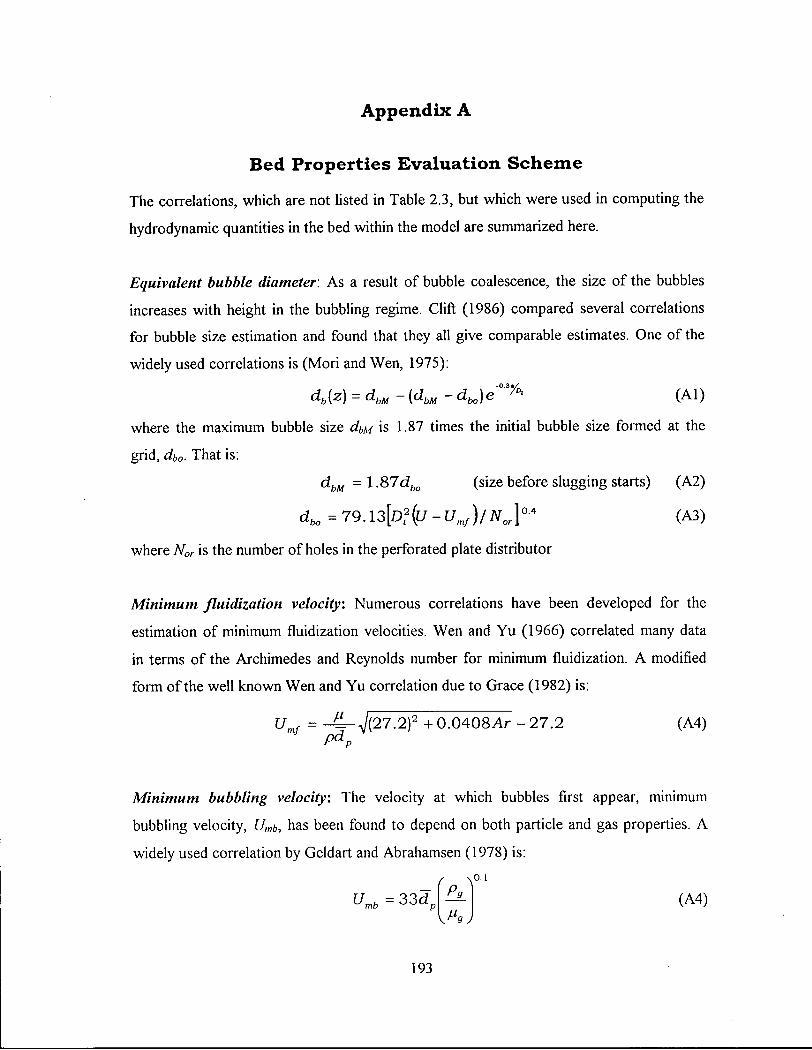
A p p e n d i x A
B e d P r o p e r t i e s E v a l u a t i o n S c h e m e
The correlations, which are not listed in Table 2.3, but which were used in computing the
hydrodynamic quantities in the bed within the model are summarized here.
Equivalent bubble diameter. As a result of bubble coalescence, the size of the bubbles
increases with height in the bubbling regime. Gift (1986) compared several correlations
for bubble size estimation and found that they all give comparable estimates. One of the
widely used correlations is (Mori and Wen, 1975):
db(z) = dbM -[dbM - d j e ^ (Al)
where the maximum bubble size dbM is 1.87 times the initial bubble size formed at the
grid, d00. That is:
dbM =\.S7dbo (size before slugging starts) (A2)
d t o =79.l3[D?(u-Umf)/Nor]0A (A3)
where Nor is the number of holes in the perforated plate distributor
Minimum fluidization velocity: Numerous correlations have been developed for the
estimation of minimum fluidization velocities. Wen and Yu (1966) correlated many data
in terms of the Archimedes and Reynolds number for minimum fluidization. A modified
form of the well known Wen and Yu correlation due to Grace (1982) is:
Umf = JL- 7(27.2)2 +0.0408Ar - 27.2 (A4)
Minimum bubbling velocity: The velocity at which bubbles first appear, minimum
bubbling velocity, U,„b, has been found to depend on both particle and gas properties. A
widely used correlation by Geldart and Abrahamsen (1978) is:
o.i
Uinb = 33d . (A4)
193
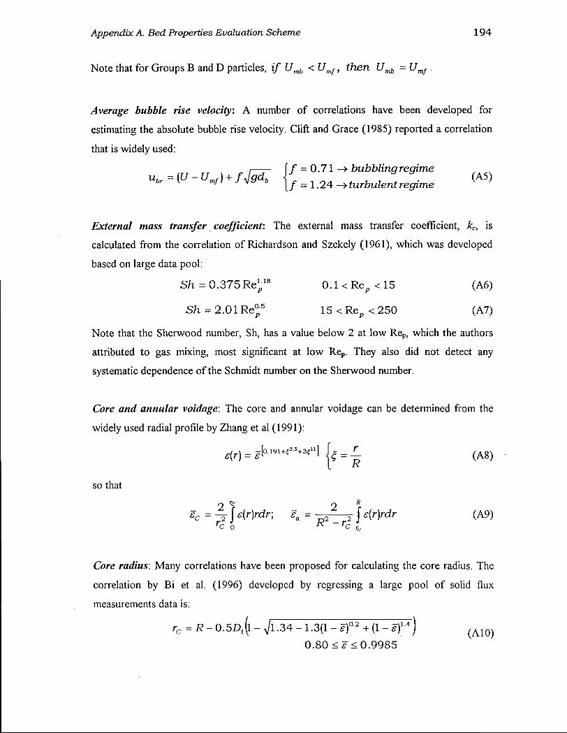
Appendix A. Bed Properties Evaluation Scheme 194
Note that for Groups B and D particles, if < Umf, then = Umf .
Average bubble rise velocity: A number of correlations have been developed for
estimating the absolute bubble rise velocity. Gift and Grace (1985) reported a correlation
that is widely used:
ITT TT \ * \—T \f = 0.71 ^bubblingregime
External mass transfer coefficient: The external mass transfer coefficient, kc, is
calculated from the correlation of Richardson and Szekely (1961), which was developed
based on large data pool:
Sh = 0.375 Re'p18 0 . 1 < R e p < 1 5 (A6)
Sh - 2.01 R e ° 5 15 < R e p < 250 (A7)
Note that the Sherwood number, Sh, has a value below 2 at low Rep, which the authors
attributed to gas mixing, most significant at low Rep. They also did not detect any
systematic dependence of the Schmidt number on the Sherwood number.
Core and annular voidage: The core and annular voidage can be determined from the
widely used radial profile by Zhang et al (1991):
so that
Core radius: Many correlations have been proposed for calculating the core radius. The
correlation by Bi et al. (1996) developed by regressing a large pool of solid flux
measurements data is:
r c = R - 0.5D((l - Vl-34 - 1.3(1 - ef2
+ (1 - e)1A) ( A 1 Q )
0.80 <s<0.9985

A p p e n d i x B
T h e r m o p h y s i c a l P r o p e r t i e s E v a l u a t i o n S c h e m e
1. The heat of reaction k can be written:
T
AHk = AH? + \ACPgXdT (Bl) •pnf
where
^ Cp f f . * = I > . 7 A , (B2)
2. The average specific heat capacity of the gas mixture is obtained from:
No
CPg,mix = Y u X i C P 9 , i t 8 3 ) i
The heat capacity is expressed as a polynomial function of temperature (Reid et al.,
1987):
CPi=A + BT + CT2 + DT3 (B4)
The coefficients A, B, C, and D are constants to calculate the isobaric heat capacity of the
ideal gas, with Cpg in J/mol K and Tin Kelvin.
3. , The thermal conductivity of a gas mixture km is not usually a linear function of mole
fraction. The equation of Mason and Saxena (1958), often used for low pressure gas
mixtures, is (Reid et al., 1987):
k-=z^X <B5> j
_[i+(rt>,r(M,/M,rF
with An = 1.0. kj and are the thermal conductivity and viscosity of pure component /.
195
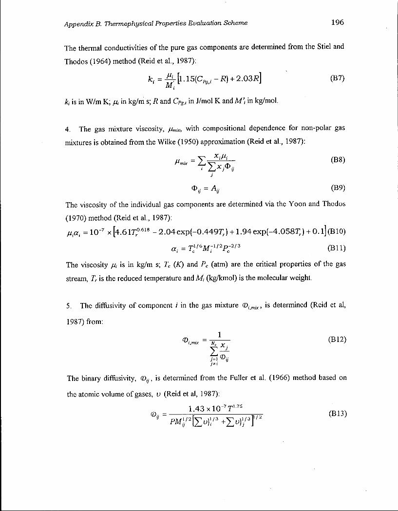
Appendix B. Thermophysical Properties Evaluation Scheme 196
The thermal conductivities of the pure gas components are determined from the Stiel and
Thodos (1964) method (Reid et al., 1987):
fc, = -gr [ l . l 5 (C P g i . - i?) + 2.03i?] (B7)
kj is in W/m K; p, in kg/m s; R and Cpgii in J/mol K and M) in kg/mol.
4. The gas mixture viscosity, fj.mix, with compositional dependence for non-polar gas
mixtures is obtained from the Wilke (1950) approximation (Reid et al., 1987):
±& ( B 8 )
j O y = Atj (139)
The viscosity of the individual gas components are determined via the Yoon and Thodos
(1970) method (Reid et al., 1987):
= 10 - 7 x [4 .61 i ; 0 6 1 8 -2.04exp(-0.449T r ) + 1.94exp(-4.058T r) + 0.l](B10)
a. = T C
1 / 6 M : 1 / 2 P ; 2 / 3 (Bl l )
The viscosity //, is in kg/m s; Tc (K) and Pc (atm) are the critical properties of the gas
stream, Tr is the reduced temperature and M , (kg/kmol) is the molecular weight.
5. The diffusivity of component /' in the gas mixture <Dimix, is determined (Reid et al,
1987) from:
(B12)
The binary diffusivity, (Dtj, is determined from the Fuller et al. (1966) method based on
the atomic volume of gases, v (Reid et al, 1987):
1 . 4 3 x l O - 7 T 1 7 5
m s
Vii = f iwT ( B 1 3 )
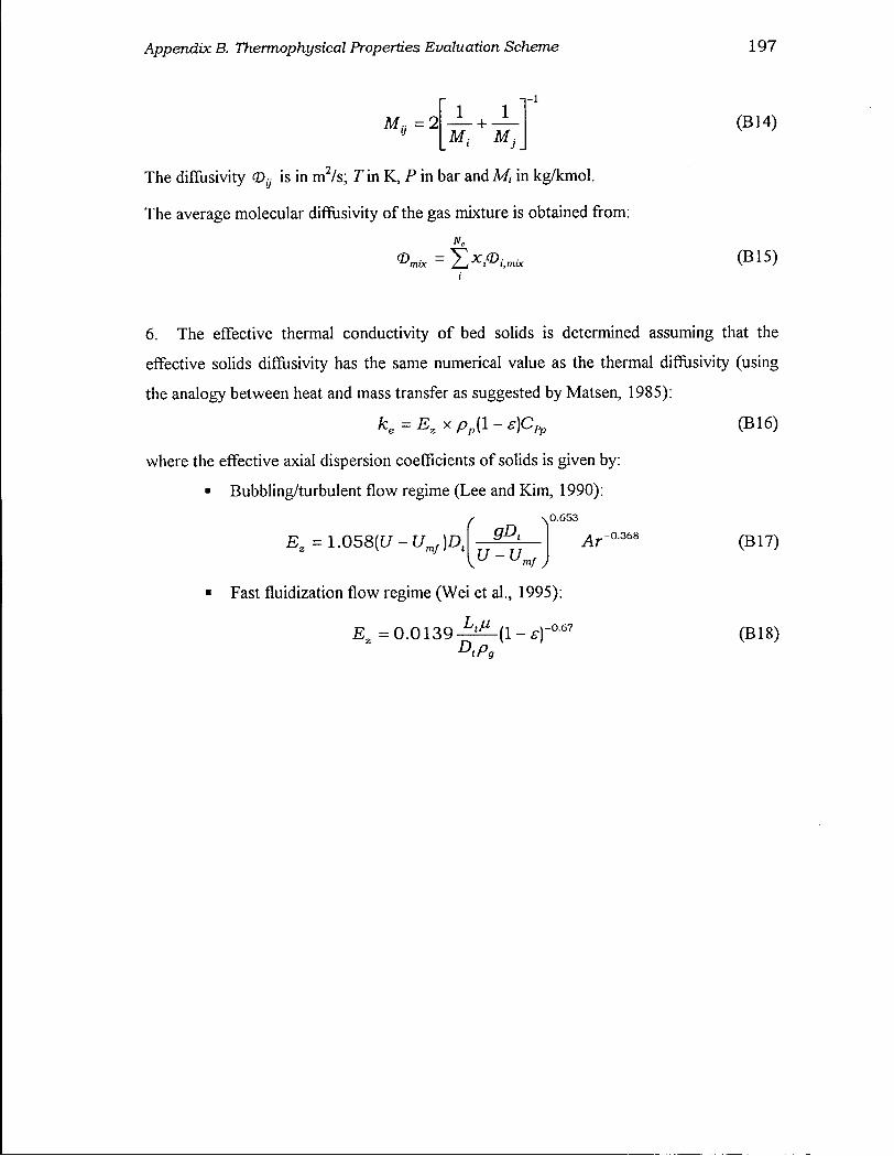
Appendix B. Thermophysical Properties Evaluation Scheme 1 9 7
M , = 2| 1 1
M , M ,
The diffusivity is in m2/s; 7 in K, P in bar andM, in kg/kmol.
The average molecular diffusivity of the gas mixture is obtained from:
(B14)
(B15)
6. The effective thermal conductivity of bed solids is determined assuming that the
effective solids diffusivity has the same numerical value as the thermal diffusivity (using
the analogy between heat and mass transfer as suggested by Matsen, 1985):
fc. = E a x p p ( l - ffJC^ (B16)
where the effective axial dispersion coefficients of solids is given by:
• Bubbling/turbulent flow regime (Lee and Kim, 1990):
£ 2 = 1.05807-t/m/)D(
, 0 . 6 5 3
Ar - 0 . 3 6 8
Fast fluidization flow regime (Wei et al., 1995)
E. =0 .0139 DtPc
-(1 - sy 0 . 6 7
(B17)
(B18)