Within-subject template estimation for unbiased longitudinal image analysis

Within-Subject Template Estimation for Unbiased Longitudinal Image Analysis

Martin Reutera,b,c,∗, Nicholas J. Schmanskya,b, H. Diana Rosasa,b,1, Bruce Fischla,b,c,1

aMassachusetts General Hospital / Harvard Medical School, Boston, MA, USAbMartinos Center for Biomedical Imaging, 143 13th Street, Charlestown, MA, USA

cMIT Computer Science and AI Lab, Cambridge, MA, USA

Abstract

Longitudinal image analysis has become increasingly important in clinical studies of normal aging and neurodegenerative disorders.Furthermore, there is a growing appreciation of the potential utility of longitudinally acquired structural images and reliable imageprocessing to evaluate disease modifying therapies. Challenges have been related to the variability that is inherent in the availablecross-sectional processing tools, to the introduction of bias in longitudinal processing and to potential over-regularization. In thispaper we introduce a novel longitudinal image processing framework, based on unbiased, robust, within-subject template creation,for automatic surface reconstruction and segmentation of brain MRI of arbitrarily many time points. We demonstrate that it isessential to treat all input images exactly the same as removing only interpolation asymmetries is not sufficient to remove processingbias. We successfully reduce variability and avoid over-regularization by initializing the processing in each time point with commoninformation from the subject template. The presented results show a significant increase in precision and discrimination power whilepreserving the ability to detect large anatomical deviations; as such they hold great potential in clinical applications, e.g. allowingfor smaller sample sizes or shorter trials to establish disease specific biomarkers or to quantify drug effects.

Keywords: Unbiased longitudinal image processing, MRI biomarkers, Reliability and Power, Within-subject template, FreeSurfer

1. Introduction

Progressive brain atrophy can be observed in a varietyof neurodegenerative disorders. Several longitudinal studieshave demonstrated a complex, regionally and temporally dy-namic series of changes, that occur in normal aging and thatare uniquely distinct in neurodegenerative disorders, such asAlzheimer’s disease, Huntington’s disease, and schizophrenia.The availability of large, high quality longitudinal datasets, hasalready begun to significantly expand our ability to evaluateselective, progressive anatomical changes. One of the majorcaveats in these studies is the use of tools that were originallydesigned for the analysis of data collected cross-sectionally. In-herent noise in cross-sectional methods, based on a single com-mon template or atlas, often shadow individual differences andresult in more heterogeneous measurements. However, by ex-ploiting the knowledge that within-subject anatomical changesare usually significantly smaller than inter-individual morpho-logical differences, it is possible to reduce within-subject noisewithout altering the between-subject variability. As such, thedevelopment of unbiased longitudinal analytical approaches arecritical in fully elucidating phenotypic variability, and in theconstruction of imaging based biomarkers to quantify responsein clinical trials and to evaluate disease modifying therapies. Inparticular, these tools can be expected to increase the sensitiv-ity and reliability of the measurements sufficiently to require

∗Corresponding authorEmail address: [email protected] (Martin Reuter)

1Senior authors

smaller sample sizes and fewer time points or shorter follow-upperiods.

The novel longitudinal methodologies described in this paperare designed to overcome the most common limitations of con-temporary longitudinal processing methods: the introduction ofprocessing bias, over-regularization, and the limitation to pro-cess only two time points. In addition, building on FreeSurfer(Fischl , 2012; Fischl et al., 2002), our methods are capable ofproducing a large variety of reliable imaging statistics, such assegmentations of subcortical structures, cortical parcellations,pial and white matter surfaces as well as cortical thickness andcurvature estimates.

Bias. Longitudinal image processing aims at reducing withinsubject variability, by transferring information across time, e.g.enforcing temporal smoothness or informing the processingof later time points with results from earlier scans. Theseapproaches, however, are susceptible to processing bias. Itis well documented that especially interpolation asymmetriescan influence downstream processing and subsequent analyses(Yushkevich et al., 2010; Thompson and Holland, 2011) andcan result in severe underestimation of sample sizes due tooverestimation of effect sizes. Interpolation asymmetries oc-cur when, for example, resampling follow-up images to thebaseline scan and thus smoothing only the follow-up imageswhile keeping the baseline image untouched. As described inReuter and Fischl (2011) and as demonstrated below, interpola-tion asymmetries are not the only source of bias. Consistentlytreating a single time point, usually baseline, differently fromothers, for instance, to construct an atlas registration or to trans-

Preprint submitted to NeuroImage April 27, 2012

fer label maps for initialization purposes, can already be suffi-cient to introduce bias. Bias is a problem that often goes un-noticed, due to large measurement noise, imprecise methods,small sample sizes or insufficient testing. Not treating all timepoints the same can be problematic as the absence of bias can-not simply be proven by not finding it. Furthermore, the as-sumption that group effects are not (or only mildly) influencedby processing bias is usually incorrect. It is rather unlikely thatbias affects all groups equally, considering that one group usu-ally shows only little longitudinal change, while the other un-dergoes significant neurodegeneration. For these reasons, wecarefully designed and implemented our longitudinal methodsto treat all time points exactly the same. Another potentialsource of bias may be induced when constraining sequential re-sults to be smooth. Temporal regularization can limit the powerof an algorithm to detect large changes. We aim at avoiding thiskind of over-regularization by initializing the processing in eachtime point with common information, but allowing the methodsto evolve freely.

It should be noted, that different types of bias, not induced bythe image analysis software but rather related to pre-processingor image acquisition steps, can already be present in the images,equally affecting both longitudinal and independent (cross-sectional) processing. Examples include the use of differentscanner hardware, different scanner software versions, differ-ent calibration, acquisition parameters or protocols across time.These biases cannot easily be removed by downstream process-ing, although they can possibly be reduced. Other types of biasare related to intrinsic magnetic properties of the tissue (e.g. T1,T2*) across time (aging) or across groups (neurodegenerativedisease) potentially introducing bias in measures of thickness orvolume (Salat et al., 2009; Westlye et al., 2009). However, sinceage and disease level are usually very similar within-subject, therate of change in a longitudinal study will be less affected thancross-sectional volume or thickness analysis.

Related Work. In SIENA, Smith et al. (2001, 2002) intro-duced the idea of transforming two input images into a halfwayspace, to ensure both undergo the same resampling steps toavoid interpolation bias. However, traditionally, the baselineimage is treated differently from the follow–up images. Of-ten longitudinal processing is approached by employing higherorder registration methods to compute and analyze the defor-mation field that aligns baseline to a follow-up scan, e.g. SPM2uses high dimensional warps (Ashburner et al., 2000)). Theseprocedures are usually not inverse consistent and resample onlythe follow-up images. SPM, for example, has been employedin longitudinal studies of neurodegeneration in two time points(Chetelat et al., 2005; Kipps et al., 2005) without specificallyattempting to avoid asymmetry-related bias. The longitudinalsegmentation algorithm CLASSIC (Xue et al., 2006) jointlysegments a 4D image via longitudinal high-order warps to thebaseline scan using an elastic warping algorithm. Also Avantset al. (2007) work in the baseline space as a reference frame.In that work, first a spatiotemporal parametrization of an indi-vidual’s image time series is created via nonlinear registration(SyN). The underlying diffeomorphism is then resampled at theone year location and compared to baseline to quantify the an-

nual atrophy. Qiu et al. (2006) present a method for longitudi-nal shape analysis of brain structures, quantifying deformationswith respect to baseline and transporting the collected infor-mation from the subject baseline to a global template. Otherauthors focus on cortical measures. Han et al. (2006) describe amethod to initialize follow-up surface reconstruction with sur-faces constructed from the baseline scans. Li et al. (2010) reg-ister follow-up images to the baseline (rigidly and nonlinearlybased on CLASSIC) and then keep the directions fixed acrosstime along which they locally compute thickness in the cortex.

Over the last few years, several authors focused morestrongly on avoiding processing bias. In 2009, initial softwareversions of our methods, relying on unbiased within-subjecttemplates as described in this paper, were made publicly avail-able (Reuter, 2009; Reuter et al., 2010a). Related efforts, how-ever, aim primarily at removing only interpolation bias. Avantset al. (2010), for example, similarly utilize within-subject tem-plates, while still treating the baseline image consistently differ-ently from follow-up time points. Nakamura et al. (2011) avoidbias only in the registration procedure by combining forwardand inverse linear registrations to construct symmetric pairwisemaps. Also combining forward and backward transformations,Holland and Dale (2011) use a nonlinear pairwise registrationand intensity normalization scheme to analyze the deformationin follow-up images by measuring volume changes of labelsdefined in baseline space.

Approach. In this work we present an automated longitu-dinal processing pipeline that is designed to enable a tempo-rally unbiased evaluation of an arbitrary number of time pointsby treating all inputs the same. First an unbiased, within-subject template is generated by iteratively aligning all inputimages to a median image using a symmetric robust registrationmethod (Reuter et al., 2010b). Because of the simultaneous co-registration of all time points, processing can be performed in aspatially normalized voxel space across time reducing variabil-ity of several procedures. Furthermore, the median image func-tions as a robust template approximating the subject’s anatomy,averaged across time, and can be used as an estimate to initial-ize the subsequent segmentations.

Cortical and subcortical segmentation and parcellation pro-cedures involve many complex nonlinear optimization prob-lems, such as topology correction, nonlinear atlas registration,and nonlinear spherical surface registration. These nonlinearproblems are typically solved with iterative methods. The fi-nal results can thus be sensitive to the selection of a particu-lar starting point. However, by initializing the processing of anew data set in a longitudinal series with common information,the variations in the processing procedures can be efficientlyreduced and the robustness and sensitivity of the overall lon-gitudinal analysis significantly improved. Increased reliabil-ity often comes at the cost of over-regularization by enforcingtemporal smoothness. Our methods do not add explicit con-straints such as temporal smoothness or higher-order within-subject warps to transfer labels, nor do they incorporate the or-der of time points at all. Higher precision is achieved solely bycommon initialization while segmentation and surface recon-struction procedures are allowed to evolve freely. We demon-

2

strate that the resulting measurements are significantly more re-liable in both healthy controls (in test–retest, simulated noiseand simulated atrophy) as well as in neurodegeneration studies.We show that the increased precision enables greater power toevaluate more subtle disease effects or to reduce sample sizes.This longitudinal processing stream is made available as partof FreeSurfer (Fischl , 2012; Fischl et al., 2002; Reuter, 2009).The FreeSurfer software package is an open access resourcethat has gained popularity in evaluating cortical and subcorticalmeasures.

Impact. An early version of the methods described in thispaper has been successfully employed in a variety of studiesanalyzing progressive changes in Alzheimer’s disease (Desikanet al., 2010; Chiang et al., 2010, 2011; Sabuncu et al., 2011),Huntington’s disease (Rosas et al., 2011), memory training (En-gvig et al., 2010) and for the validation of prospective mo-tion correction (Tisdall et al., 2012). The Alzheimer’s DiseaseNeuroimaging Initiative (ADNI), for instance, makes available2

their raw image data and derived measures, processed with theinitial version of our longitudinal method (FS 4.4). ADNI isone of the largest publicly available longitudinal image datasets, consisting of more than 3000 scans, released with the goalto determine in-vivo biomarkers for the early detection of AD.Although our initial processing methods that were used for thederived measures are less powerful than the newer version pre-sented in this paper, the available results are still of great im-portance to researchers without the possibility to locally pro-cess the raw images, as well as to function as a benchmark formethod development and comparison (Holland et al., 2011).

Currently, large datasets such as ADNI are under considera-tion for other neurological diseases. As such, the highly sensi-tive, reliable and fully automated unbiased longitudinal meth-ods described in this paper have the potential to help us un-derstand natural progression of regionally and spatially selec-tive neurodegeneration as occurs in distinct neurological disor-ders. The resulting, subject specific, morphometric measure-ments yield biomarkers that potentially serve as surrogate end-points in clinical trials, where the increase of statistical poweris of most immediate importance.

2. Methods

2.1. Overview of Longitudinal Processing Pipeline

The proposed processing of longitudinal data consists of thefollowing three steps:

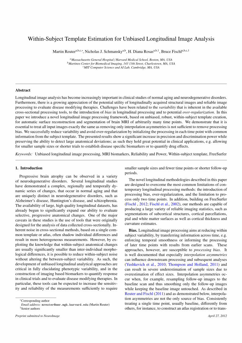
1. [CROSS]: First all time points of all subjects are pro-cessed independently. This is also called cross-sectionalprocessing. Here a full image segmentation and surfacereconstruction for each time point is constructed individ-ually. Some of this information is needed later during thelongitudinal processing and to construct the subject tem-plate in the next step.

2http://adni.loni.ucla.edu/research/mri-post-processing/

Init

Copy

Brainmask

Talairach

Normalization

Parcellations

Surfaces

Segmentation

Cort Atlas Reg

NU Intensity

AtlasNonLinReg

Step 2Step 1

Step 3

Cross 1...N Base

Long 1...N

Figure 1: Simplified diagram of the three steps involved in longitudinal pro-cessing, showing information flow at a single longitudinal run. Dashed line:information is used for initialization. Solid line: information is copied.

2. [BASE]: For each subject a template is created from alltime points to estimate average subject anatomy. Oftenthe within-subject template is also referred to as the sub-ject ’base’ (different from baseline scan!) or simply as thetemplate. Here an unbiased median image is used as thetemplate and a full segmentation and surface reconstruc-tion is performed. We describe the creation of the subjecttemplate in the following sections.

3. [LONG]: Finally each time point is processed “longi-tudinally”, where information from the subject-template[BASE] and from the individual runs [CROSS] are usedto initialize several of the algorithms. A [LONG] pro-cess usually takes about half the time to complete than a[CROSS] or [BASE] run.

The improved and more consistent results from the final setof [LONG] runs (step 3) provide the reliable input for post-processing or subsequent statistical analysis.

In step 3 above, the longitudinal processing of each timepoint is initialized with information from the subject template[BASE] and the [CROSS] results to reduce variability. How-ever, depending on the flexibility of the individual algorithms,this general procedure may sacrifice accuracy and potentiallyunderestimate changes of greater magnitude. Whenever infor-mation is transferred across time, e.g. to regularize or explicitlysmooth results, methods can become biased towards underesti-mating change and accuracy may suffer particularly when mea-suring longitudinal change over long periods of time. While aconservative estimate of change is often preferable in a poweranalysis, than an overestimation, we focus on avoiding asym-metries and over-regularization to remain as accurate and un-biased as possible. The longitudinal processing step (see alsoFig. 1) mainly consists of the following procedures (more de-tails can be found online (Reuter, 2009)).

Spatial Normalization and NU Intensity: All inputs areresampled to the unbiased template voxel space to further re-duce variability (since FS 5.1). This can be achieved during

3

the motion correction and conforming steps by composing thelinear transforms and only resampling once to avoid additionalresampling/smoothing. For this paper, we employ linear inter-polation, but recently switched to cubic B-spline interpolationfor future releases to reduce interpolation artifacts (Thevenazet al., 2000). Then acquisition bias fields in [LONG] are inde-pendently corrected using a non-parametric non-uniform inten-sity normalization (N3) (Sled et al., 1998).

Talairach Registration: The affine map from the robusttemplate [BASE] to the Talairach space is fixed across time.It can be assumed that a single global affine transformation tothe Talairach coordinate system is appropriate since the bulk ofthe anatomy within-subject is not changing. The advantages ofthis approach lie in the noise reduction obtained by avoiding theuse of individual intensity volumes for each time point and inconsistent intra-cranial volume estimation. Data is only copiedfrom the subject template if fixing it across time is meaningful,for example the affine Talairach registration or the brain mask(see green arrows in Fig. 1).

Brainmask Creation: The brain mask, including some cere-brospinal fluid (CSF), is kept constant for all time points (in[LONG] and in the subject template [BASE]) to reduce vari-ability under the assumption that the location and size of theintracranial vault are not changing (although of course the con-tents may be). The brain mask is constructed as the union (log-ical OR) of the registered brain masks across time. In otherwords, a voxel is included in the brain mask if it is included inany of the time points, to ensure no brain is accidentally clipped.Although the brain mask is fixed across time by default, it canbe adjusted in individual time points manually if necessary (e.g.by editing it or mapping it from the initial [CROSS] results).

Normalization and Atlas Registration: For the second in-tensity correction (pre-segmentation filter) (Dale et al., 1999),each [LONG] run is initialized with the common set of con-trol points that were constructed in the [BASE], to encourageconsistency across time. Similarly for the normalization to theprobabilistic atlas (Fischl et al., 2002, 2004a), the segmenta-tion labels of the [BASE] are passed as a common initializationin each time point (dashed arrows in Fig. 1). Also the nonlin-ear atlas registration is initialized with results from the [BASE].However, these procedures are intrinsically the same as beforeand are still performed for each time point to allow for the nec-essary flexibility to detect larger departures from the averageanatomy of the [BASE]. Starting these procedures without acommon initialization would only increase variability as moretime points may terminate in different local minima.

Subcortical Segmentation: Specifically for the subcorticalsegmentation we allow even more flexibility. Instead of initial-izing it with the template segmentation, a fused segmentation iscreated for each time point by an intensity based probabilisticvoting scheme. Similar to Sabuncu et al. (2010), where train-ing label maps are fused for the segmentation, we also use aweighted voting scheme to construct a fused segmentation ofeach time point from the initial segmentations of all time pointsobtained via independent processing [CROSS] (using the stan-dard atlas based registration procedure in FreeSurfer). Basedon local intensity differences between the time points at each

voxel we employ a kernel density estimation (Parzen window)using a Gaussian kernel on the registered and intensity normal-ized input images and initial labels. In other words, if the in-tensity at a given location is similar at another time point, thecorresponding label is highly probable. This weighted majorityvoting (including votes from all time points) yields the labelsto construct the fused segmentation. Since this procedure isdriven by all time point’s initial segmentations rather than thetemplate’s segmentation, it allows for more flexibility. For eachtime point, it represents the anatomy more accurately than thesegmentation of the template. In order to correct for potentialremaining noise, each fused label map is used to initialize a fi-nal run through the regular atlas based segmentation procedure.This fine-tuning step usually converges quickly.

Surfaces Reconstruction: The regular cortical surface con-struction in FreeSurfer starts with the tessellation of the graymatter / white matter boundary, automated topology correc-tion (Fischl et al., 2001; Segonne et al., 2007), and surfacedeformation following intensity gradients to optimally placethe gray/white and gray/CSF borders at the location where thegreatest shift in intensity defines the transition to the other tis-sue class (Fischl and Dale, 2000). In the longitudinal stream,the white and pial surfaces in each time point are initializedwith the surfaces from the template [BASE] and are allowed todeform freely. This has the positive effect that surfaces acrosstime demonstrate an implicit vertex correspondence. Further-more, manual editing to fix topology or surface placement isin many cases only necessary in the subject’s template [BASE]instead of in each individual time point, reducing potential man-ual intervention (and increasing reliability).

Cortical Atlas Registration and Parcellations: Once thecortical surface models are complete, a number of deformablesurface procedures are usually performed for further data pro-cessing. The spherical registration (Fischl et al., 1999b) andcortical parcellation procedures (Fischl et al., 2004b; Desikanet al., 2006) establish a coordinate system for the cortex bywarping individual surface models into register with a sphericalatlas in a way that aligns the cortical folding patterns. In thelongitudinal analysis we make the first-order assumptions thatlarge-scale folding patterns are not substantially altered by dis-ease, and thus assume the spherical transformation of the sub-ject template to be a good initial approximation. In [LONG] thesurface inflation with minimal metric distortion (Fischl et al.,1999a) is therefore copied from the [BASE] to all time points.The subsequent non-linear registration to the spherical atlas andalso the automatic parcellation of the cerebral cortex in eachtime point are initialized with the results from the [BASE]. Thisreliably assigns a neuroanatomical label to each location on thesurface by incorporating both geometric information derivedfrom the cortical model (gyral and sulcal structure as well ascurvature), and neuroanatomical convention.

Note that no temporal smoothing is employed, also the orderof time points is not considered. The above steps are meaning-ful under the assumptions that head size is relatively constantacross time which is reasonable for most neurodegenerative dis-eases but not, for example, for early childhood development.However, users can optionally keep individual brainmasks or

4

introduce manual edits to accommodate for special situations,at the cost of decreased reliability.

2.2. Within-Subject Template

Atlas construction, usually creating a template of severalsubjects, has been an active field of research. For example,Joshi et al. (2004), Avants and Gee (2004) or Ashburner (2007)approach unbiased nonlinear atlas construction by iterativelywarping several images to a mean. In order to create a robustwithin-subject template of several longitudinal scans, we needto make several design decisions. All time points need to betreated the same to avoid the possible introduction any asym-metries. Furthermore, we use only a rigid transformation modelto remove pose (or optionally an affine transformation to addi-tionally remove scanner calibration differences). Currently weavoid higher order warps to not introduce any temporal smooth-ing constraints or worse, incorrect correspondence that is reliedupon by downstream processing (e.g. when transferring labels).We do not assume exact tissue correspondence in our model.Finally, instead of the commonly used intensity mean, a voxel-wise intensity median is employed to create crisper averagesand remove outliers such as motion artifacts from the template.

Template estimation of N images Ii is usually stated as a min-imization problem of the type:

I, ϕi := argminI,ϕi

N∑i=1

E(Ii ϕi, I) + D(ϕi)2 (1)

where the template I and the transformations ϕi, that map eachinput image to the common space, need to be estimated. Forrobustness and other reasons as described below, we set the im-age dissimilarity metric E(I1, I2) =

∫Ω|I1(x)− I2(x)| dx where Ω

denotes the coordinate space. Thus, for fixed transformationsϕi the minimizing I is given by the voxel-wise median of all Ii.For a rigid transformation consisting of translation and rotationϕ = (~t, r) ∈ R3 × S O(3), we choose the following squared dis-tance with respect to identity D(~t, r)2 =‖ ~t ‖2 + ‖ R − I ‖2F ,where we compute the Frobenius norm of the difference be-tween the identity I and the 3×3 rotation matrix R representingthe rotation r. Since the inputs Ii are rather similar, I can beapproximated by the following iterative algorithm:

1. Compute the median of the N input images I.2. Register and resample each input image to I.3. Continue with step 1 until the obtained transforms ϕi con-

verge.

The registration step adjusts the location of the inputs closerto I, so that the next average can be expected to improve.This iterative algorithm is performed on a Gaussian pyramidof the images, with differently many iterations on each resolu-tion. The inexpensive low resolutions are iterated more oftento quickly align all images approximately, while the more timeconsuming higher resolutions only need to refine the registra-tion in a few steps.

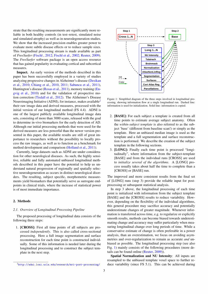
Figure 2: Unbiased template estimation for a subject with neurodegenerativedisease and significant atrophy: All time points are iteratively aligned to theirmedian image with an inverse consistent robust registration method, resultingin a template image and simultaneously a co-registration of all time points.

2.3. Robustness

For the registration of two images at the core of the tem-plate estimation, we use a robust and inverse consistent regis-tration method as described in Reuter et al. (2010b). Inverseconsistency means that the registration ϕi j of images Ii to I j

is exactly the inverse of ϕ ji = ϕ−1i j , which is usually not guar-

anteed. This property keeps individual registrations unbiasedand is achieved by a symmetric resampling step in the algo-rithm to the halfway space between the two input images, aswell as a symmetric model, to avoid estimation and averagingof both forward and backward transformations. This approach,incorporating the gradients of both inputs, additionally seems tobe less prone to local optima. While pairwise symmetry is notstrictly necessary to keep the template unbiased it avoids unnec-essary iterative averaging in the common case of only two inputimages, where both can be resampled at the halfway space aftera single registration step. Another advantage of the robust reg-istration algorithm is its ability to reduce the influence of out-lier regions resulting in highly accurate brain registrations, evenin the presence of local differences such as lesions, longitudi-nal change, skull stripping artifacts, remaining dura, jaw/neckmovement, different cropping planes or gradient nonlinearities.Reuter et al. (2010b) show the superiority of this method overstandard registration tools available in the FSL (Jenkinson et al.,2002; Smith et al., 2004) or SPM packages (Collignon et al.,1995; Ashburner and Friston, 1999) with respect to inverse con-sistency, noise, outlier data, test–retest analysis and motion cor-rection.

In spite of the fact that in the above template estimation al-gorithm convergence is not guaranteed, the procedure worksremarkably well even if significant longitudinal change is con-tained in the images (see Fig. 2), due to the robustness of themedian image. In this context see also related work in Fletcheret al. (2009) who construct a different intrinsic median for at-las creation by choosing “metamorphosis” as the metric onthe space of images that accounts for both geometric defor-mations as well as intensity changes. In a mean image outlierregions and longitudinal structural change will introduce blur-ring. Strong motion artifacts in specific time points may corrupt

5

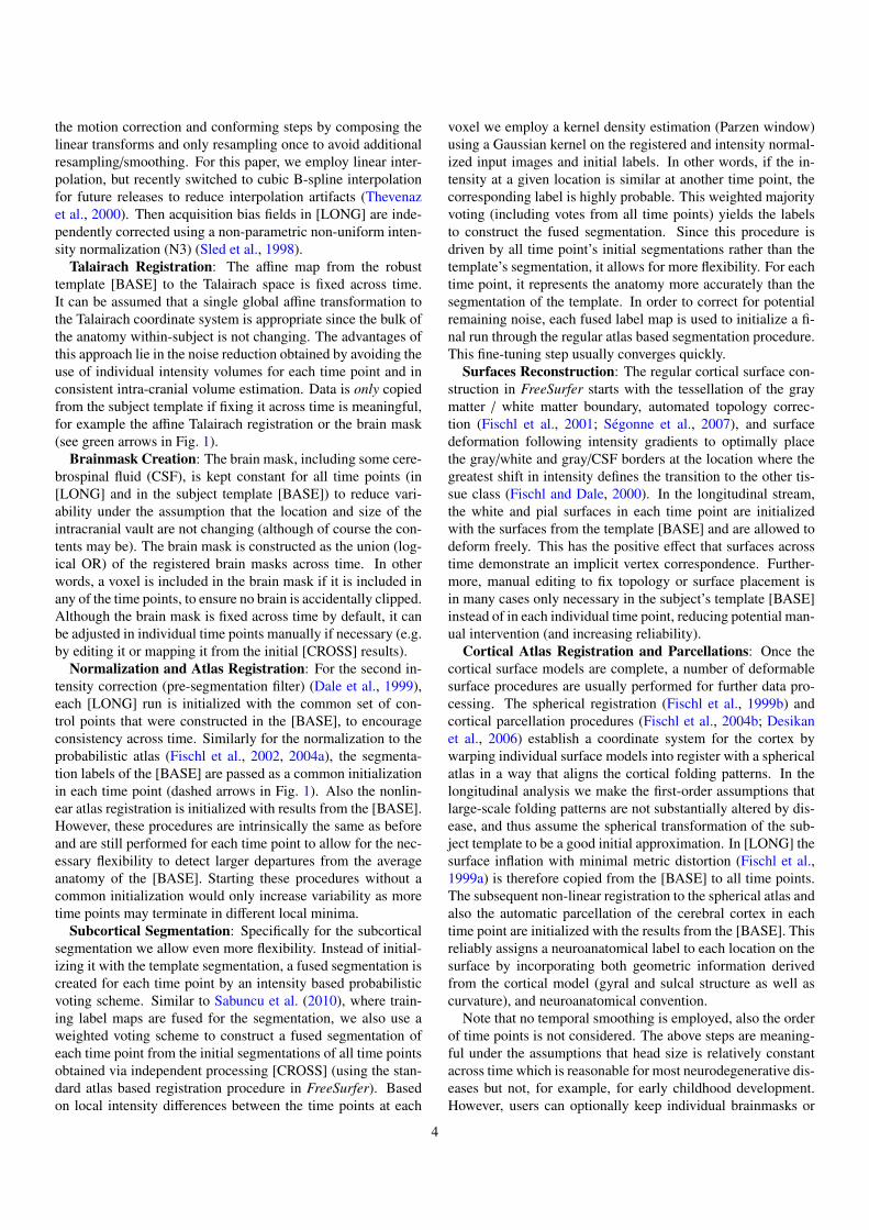
Figure 3: Comparison of mean and median template image for a series of 18images (7 years) of a subject with neurodegenerative disorder (Huntington’sdisease). The difference image (top row) between median and mean revealslarge differences in regions that change over time (e.g. ventricles, corpus cal-losum, eyes, neck, scalp). Below are close-ups of the mean image (left, softeredges) and the median image (right, crisper edges).

the whole image. The median, however, suppresses outlier arti-facts, ghosts and blurry edges and seems to be a good choiceas normality cannot be assumed due to longitudinal change,motion artifacts etc. Only for the special case of two timepoints, the median reduces to the mean and may contain twoghost images. Registration with this ill-defined average can beavoided by computing the mid-space directly from the registra-tion of the two inputs. In general, the use of the median leads tocrisper within-subject templates. It is therefore well suited forconstructing initial estimates of location and size of anatomicalstructures averaged across time or for creating white matter andpial surfaces. As described above this information is used toinform the longitudinal processing of all individual time points.

To demonstrate the effect of the median, Fig. 3 shows the dif-ference between the mean and median template of a series of 18time point images of a Huntington’s disease subject, taken overa span of 7 years. Some of the time points contain strong motionartifacts. Additionally, this subject exhibits significant atrophy,i.e. approximately 8% volume loss in the caudate and signifi-cant thinning of the corpus callosum. Due to the robustness ofthe median the template image remains crisp with well definedanatomical boundaries, in spite of the longitudinal change, asopposed to the smoother mean image. In a two bin histogramof the gradient magnitude images, the bin with larger gradientmagnitudes contains 4.4% of the voxels in the median and 3.7%in the mean image, indicating crisper edges in the median. Thedifference images in the top row of Fig. 3 localize the differ-ences between the mean and median image mainly in regionswith large longitudinal change such as the ventricles, corpuscallosum, eyes, neck and scalp. Because of the crispness of themedian image, co-registration of all 18 inputs needed only threeglobal iterations, while it took five iterations to converge for themean at a higher residual cost.

2.4. Improved Template EstimationWe found in our tests that the template estimation converges

without pre-processing. However, it may need a large numberof iterations to converge in specific cases and thus a consider-able amount of processing time (> 1h). If the early averageimages are very distorted the corresponding registrations willbe inaccurate. Once the average becomes crisper the conver-gence is fast. The following procedure is designed to speed upcomputations, by initially mapping all images to a mid-spaceand starting the algorithm there:

1. First the registration of each image Ii to a randomly se-lected image I is computed, to get estimates of where thehead/brain is located in each image with respect to the lo-cation in I. These registrations do not need to be highlyaccurate as they are only needed to find an approximationto the mid-space for the initialization. However, highlyaccurate registration in this step will reduce the number ofiterations later.

2. Then the mid-space is computed from the set of transfor-mation maps and all images are resampled at that location.See Appendix B for details on how the average space isconstructed.

3. The iterative template estimation algorithm (Section 2.2)is initialized with the images mapped to the mid-space and,in most cases, needs only two further iterations to con-verge: One to register all images to the average image andanother one to check that no significant improvements arepossible.

Since all images are remapped at the mid-space location, in-cluding image I, they all undergo a common resampling stepremoving any interpolation bias. The random asymmetry thatmay be introduced when selecting image I as the initial targetis further reduced due to the fact that the registration method isinverse consistent, so the order of registration (image I to im-age Ii or vice versa) is irrelevant. Alternatively it is possible toconstruct all pairwise registrations and compute the average lo-cation considering all the information (e.g. by constructing av-erage locations using each input as initial target independentlyand averaging the N results). This, however, significantly in-creases computational cost unless N is very small and seems un-necessarily complicated given that the above algorithm alreadyremoves resampling asymmetries and randomizes any potentialremaining asymmetry possibly induced by choosing an initialtarget.

2.5. Global Intensity ScalingIf the input images show differences in global intensity

scales, the template creation needs to adjust individual intensi-ties so that all images have an equal weight in the final average.This can be done by computing a global intensity scale param-eter in each individual registration. Once we know the intensityscale si of each image with respect to the target (initially imageI but later average template), the individual intensities can beadjusted to their geometric mean

S = n

√Πn

i=1si (2)

6

by scaling each image intensity values with siS . Note, in the

longitudinal processing stream presented in this paper, inten-sity normalized skull stripped images (norm.mgz in FreeSurfer)are used as input to construct the co-registration, thus globalintensity scaling during the registration step is not necessary,however, it can be important in other applications.

2.6. Affine Voxel Size Correction

It may be desired to adjust for changes in scanner voxelsizes, possibly induced by the use of different scanners, drift inscanner hardware, or different scanner calibrations, which arefrequently performed especially after software/hardware up-grades. Takao et al. (2011) find that even with scanners ofthe exact same model, inter-scanner variability affects longitu-dinal morphometric measures, and that scanner drift and inter-scanner variability can cancel out actual longitudinal brain vol-ume change without correction of differences in imaging ge-ometry. Clarkson et al. (2009) compare phantom based voxelscaling correction with correction using a 9 degrees of freedom(DOF) registration and show that registration is comparable togeometric phantom correction as well as unbiased with respectto disease status. To incorporate automatic voxel size correc-tion, we design an optional affine [BASE] stream, where alltime points get mapped to an average affine space by the fol-lowing procedure:

1. First perform the rigid registration as described above onthe skull stripped brain images to obtain an initial templateimage and average space.

2. Then use the rigid transforms to initialize an iterative affineregistration employing the intensity normalized full headimages.

3. Fine tune those affine registrations by using the affine mapsto initialize a final set of registrations of the skull strippedbrain images to the template, where only rigid parametersare allowed to change.

Since the registration of the brain-only images in the final step israther quick (a few minutes), especially with such a high qual-ity initialization, the fine tuning step comes at little additionaleffort and ensures accurate brain alignment. Note, that we alsopropose a full affine (12 DOF) registration as two non-uniformorthogonal scalings and a rotation/translation in the middle gen-erally cannot be represented by 9 DOF.

2.7. Adding Time Points

Opposed to independent processing, longitudinal processingevaluates concurrently scans that have been collected at differ-ent time points in order to transfer information across time. Asa result, it always implicitly requires a delay in processing un-til all of the time points are available to remain unbiased, in-dependent of the longitudinal method used. While this wouldbe standard in a clinical therapeutic study, it is less optimal inobservational studies. However, due to the robust creation ofthe subject median template, the subsequent addition of timepoints, assuming that they are not collected significantly laterin time, would not be expected to have a large influence on the

analyses if sufficient temporal information is contained in thetemplate already. The purpose of the subject template is mainlyto remove interpolation bias and to initialize processing of theindividual time points in an unbiased way. Similar to atlas cre-ation, where a small number of subjects is usually sufficient forconvergence, it can be expected that within subject template es-timation converges even faster, due to the smaller variability.Nevertheless, in order to avoid being potentially biased with re-spect to a healthier/earlier state, it is recommended, if possible,to recreate the template from all time points and reprocess alldata until further studies investigate this issue more thoroughly.

3. Results and Discussion

3.1. Data

3.1.1. TT-115Two different sets of test–retest data are analyzed below. The

first set consists of 115 controls scanned twice within the samesession and will be referred to as TT-115. Two full head scans(1 mm isotropic, T1-weighted multi-echo MPRAGE (van derKouwe et al., 2008), Siemens TIM Trio 3T, TR 2530 ms, TI1200 ms, multi echo with BW 650 Hz/px and TE = [1.64 ms,3.5 ms, 5.36 ms, 7.22 ms], 2 × GRAPPA acceleration, totalacq. time 5:54 min) were acquired using a 12 channel headcoil and then gradient unwarped. The two scans were separatedby a 60 direction 2mm isotropic EPI based diffusion scan andaccompanying prior gradient echo field map (2:08 min, 9:45min), not used here. The two multi-echo MPRAGE images areemployed to evaluate the reliability of the automatic segmen-tation and surface reconstruction methods. It can be assumedthat biological variance and variance based on the acquisitionis minimized, therefore, this data will be useful to reveal dif-ferences in the two processing streams (independent processingversus longitudinal processing).

3.1.2. TT-14We also evaluate a second test–retest set consisting of 14

healthy subjects with two time points acquired 14 days apart(TT-14). The images are T1-weighted MPRAGE full headscans (dimensions 1mm × 1mm × 1.33mm, Siemens Sonata1.5T, TR 2730 ms, TI 1000 ms, TE 3.31 ms). Each time pointconsists of two within session scans that were motion correctedand averaged to increase signal to noise ratio (SNR). This dataset exhibits a lower SNR than the TT-115 above, since it wasacquired using a volume coil and at a lower field strength of1.5T. Because of this and the larger time difference it thereforebetter reflects the expected variability of a longitudinal studyand will be used for power analyses below.

3.1.3. OA-136To study group discrimination power in dementia in both pro-

cessing streams we analyze a disease dataset: the Open AccessSeries of Imaging Studies (OASIS)3 longitudinal data. This set

3http://www.oasis-brains.org/

7

consists of a longitudinal collection of 150 subjects aged 60to 96. Each subject was scanned on two to five visits, sepa-rated by approximately one year each for a total of 373 imag-ing sessions. For each subject and each visit, 3 or 4 individ-ual T1-weighted MPRAGE scans (dimensions 1mm × 1mm ×1.25mm, TR 9.7ms, TI 20ms, TE 4ms) were acquired in sin-gle sessions on a Siemens Vision 1.5T. For each visit two ofthe scans were selected based on low noise level in the back-ground (indicating high quality, i.e., no or little motion arti-facts). These two scans were then registered and averaged toincrease signal to noise ratio and used as input. The subjectsare all right-handed and include both men and women. 72 ofthe subjects were characterized as non-demented for the dura-tion of the study and 64 subjects as demented. Here we do notinclude the third group of 14 converters who were characterizedas non-demented at the time of their initial visit and were sub-sequently characterized as demented at a later visit. The datasettherefore only includes 136 subjects and will be called OA-136.

3.1.4. HD-54To highlight improvements in situations with less statistical

power, a second and smaller disease data set is employed con-taining 10 healthy controls (C), 35 pre-symptomatic Hunting-ton’s disease subjects of which 19 are near (PHDnear) and 16far (PHDfar) from estimated onset of symptoms, and 9 pro-gressed symptomatic Huntington’s patients (HD). The near andfar groups where distinguished based on the estimated time toonset of symptoms using CAG repeat length and age (Lang-behn et al., 2004) where far means expected onset in more than11 years. Each subject has image data from three visits approx-imately half a year to a year apart (dimensions 1mm × 1mm× 1.33mm, T1-weighted MPRAGE, Siemens Avanto 1.5T, TR2730 ms, TI 1000 ms, TE 3.31 ms, 12 channel head coil).Scanner software versions have changed for several subjects be-tween the visits and in the HD group two subjects even have 1-2of their scans on an older Siemens Sonata scanner, which addspotential sources of variability. This data will be referred to asHD-54.

3.2. Bias in Longitudinal Processing

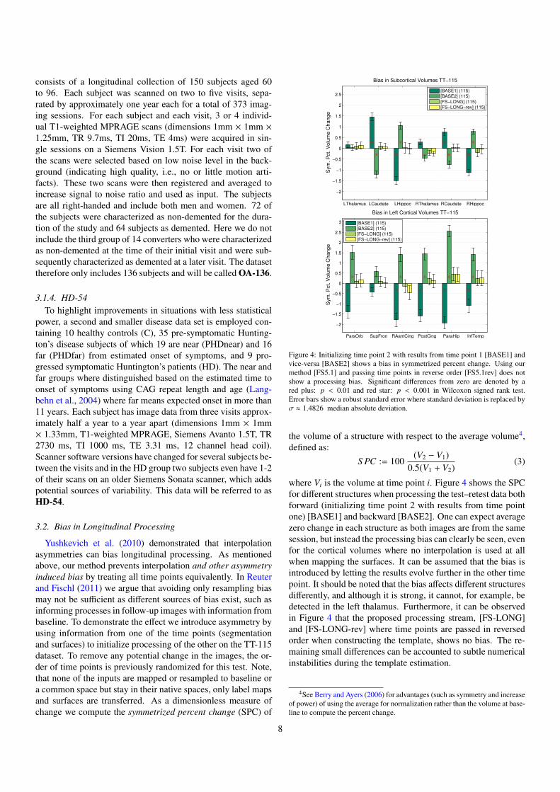
Yushkevich et al. (2010) demonstrated that interpolationasymmetries can bias longitudinal processing. As mentionedabove, our method prevents interpolation and other asymmetryinduced bias by treating all time points equivalently. In Reuterand Fischl (2011) we argue that avoiding only resampling biasmay not be sufficient as different sources of bias exist, such asinforming processes in follow-up images with information frombaseline. To demonstrate the effect we introduce asymmetry byusing information from one of the time points (segmentationand surfaces) to initialize processing of the other on the TT-115dataset. To remove any potential change in the images, the or-der of time points is previously randomized for this test. Note,that none of the inputs are mapped or resampled to baseline ora common space but stay in their native spaces, only label mapsand surfaces are transferred. As a dimensionless measure ofchange we compute the symmetrized percent change (SPC) of

LThalamus LCaudate LHippoc RThalamus RCaudate RHippoc

−2

−1.5

−1

−0.5

0

0.5

1

1.5

2

2.5

Sym

. P

ct.

Vo

lum

e C

ha

ng

e

Bias in Subcortical Volumes TT−115

[BASE1] (115)

[BASE2] (115)

[FS−LONG] (115)

[FS−LONG−rev] (115)

ParsOrb SupFron RAantCing PostCing ParaHip InfTemp

−2

−1.5

−1

−0.5

0

0.5

1

1.5

2

2.5

3

Sym

. P

ct.

Vo

lum

e C

ha

ng

e

Bias in Left Cortical Volumes TT−115

[BASE1] (115)

[BASE2] (115)

[FS−LONG] (115)

[FS−LONG−rev] (115)

Figure 4: Initializing time point 2 with results from time point 1 [BASE1] andvice-versa [BASE2] shows a bias in symmetrized percent change. Using ourmethod [FS5.1] and passing time points in reverse order [FS5.1rev] does notshow a processing bias. Significant differences from zero are denoted by ared plus: p < 0.01 and red star: p < 0.001 in Wilcoxon signed rank test.Error bars show a robust standard error where standard deviation is replaced byσ ≈ 1.4826 median absolute deviation.

the volume of a structure with respect to the average volume4,defined as:

S PC := 100(V2 − V1)

0.5(V1 + V2)(3)

where Vi is the volume at time point i. Figure 4 shows the SPCfor different structures when processing the test–retest data bothforward (initializing time point 2 with results from time pointone) [BASE1] and backward [BASE2]. One can expect averagezero change in each structure as both images are from the samesession, but instead the processing bias can clearly be seen, evenfor the cortical volumes where no interpolation is used at allwhen mapping the surfaces. It can be assumed that the bias isintroduced by letting the results evolve further in the other timepoint. It should be noted that the bias affects different structuresdifferently, and although it is strong, it cannot, for example, bedetected in the left thalamus. Furthermore, it can be observedin Figure 4 that the proposed processing stream, [FS-LONG]and [FS-LONG-rev] where time points are passed in reversedorder when constructing the template, shows no bias. The re-maining small differences can be accounted to subtle numericalinstabilities during the template estimation.

4See Berry and Ayers (2006) for advantages (such as symmetry and increaseof power) of using the average for normalization rather than the volume at base-line to compute the percent change.

8

TP1 cross TP2 cross TP1 long TP2 long−5

−4

−3

−2

−1

0

1

2

3

4

5Scatter Left Hippocampus with Noise (pct)

TP1 cross TP2 cross TP1 long TP2 long−5

−4

−3

−2

−1

0

1

2

3

4

5Scatter Right Hippocampus with Noise (pct)

Figure 5: Effect of simulated noise (σ = 1) on hippocampal volume measure-ments. The longitudinal processing is less affected.

TP1 cross TP2 cross TP1 long TP2 long−5

−4

−3

−2

−1

0

1

2

3

4

5Scatter Left Hippocampus with LH−Atropy (pct)

TP1 cross TP2 cross TP1 long TP2 long−5

−4

−3

−2

−1

0

1

2

3

4

5Scatter Right Hippocampus with LH−Atropy (pct)

Figure 6: Simulated 2% atrophy in the left hippocampus. The longitudinalprocessing manages to detect the change more precisely and at the same timereduces the variability in the right hemisphere.

3.3. Robustness, Precision and Accuracy

For the following synthetic tests only the first time pointof data set TT-14 is taken as baseline. It is resliced to 1mmisotropic voxels, intensity scaled between 0 and 255. The syn-thetic second time point is a copy of that image, but artificiallymodified to test robustness with respect to noise and measure-ment precision of the longitudinal stream. As Rician noise isnearly Gaussian at larger signal to noise ratios, robustness withrespect to noise is tested by applying Gaussian noise (σ = 1) tothe second time point. Fig. 5 shows the percent change with re-spect to the original in the hippocampal volume for both hemi-spheres for cross-sectional and longitudinal processing. Thelongitudinal stream is more robust and reduces the variability(increased precision).

In order to assess precision and accuracy of the longitudi-nal analysis we applied approximately 2% simulated atrophy tothe hippocampus in the left hemisphere and took this syntheticimage as the second time point. The atrophy was automati-cally simulated by reducing intensity in boundary voxels of thehippocampus with partial ventricle volume (labels as reportedby FreeSurfer). See Appendix C for details. Note, that realatrophy is more complex and variates among individuals anddiseases. The well defined atrophy used here should be accu-rately detected by any automatic processing method. It can beseen in Fig. 6 that the longitudinal analysis detects the atrophymore precisely and also shows less variability around the zeromean in the right hemisphere. Based on these results neithermethod can be determined to be biased and both accurately findthe ground truth, but longitudinal processing with higher preci-sion.

Thalamus Caudate Putamen Pallidum Hippocamp Amygdala0

1

2

3

4

5

6

7

8

9

10

Abs. S

ym

. P

ct. V

olu

me C

hange

Left Subcortical Structures TT−14

Cross 5.0 (14)

Long 5.0 (14)

Long 5.1b (14)

Figure 8: test–retest comparison of [CROSS] versus [LONG] on TT-14 data(subcortical volumes, left hemisphere). See also Fig. 7 for description of sym-bols. Additionally here reliability improvements of using a common voxelspace (Long 5.1b) over previous method (Long 5.0) can be seen.

3.4. test–retest Reliability

In order to evaluate the reliability of the longitudinal schemewe analyze the variability of the test–retest data sets (focus-ing on TT-115). Variability of measurements can have severalsources. Real anatomical change can occur in controls, e.g. dueto dehydration, but is unlikely in within-session scans. Morelikely, there will be variability due to acquisition procedures(motion artifacts, change of head position inside the scanneretc.). In TT-115, for example, head position has changed sig-nificantly as subjects sink into the pillow and relax their neckmuscles (mean: 1.05mm, p < 10−8) during the 12min diffu-sion scan separating the test–retest. Acquisition variability isof course identical for both processing methods. Finally thereis variability due to the image processing methods themselves,that we aim to reduce.

As a dimensionless measure of variability, similar to Eq. 3,we compute the absolute symmetrized percent change (ASPC)of the volume of a structure with respect to the average volume:

AS PC := 100|V2 − V1|

0.5(V1 + V2). (4)

The reason is that estimating a mean (here of ASPC) is more ro-bust than estimating the variance of differences or symmetrizedpercent change when not taking the absolute value. Fig. 7shows the reliability of subcortical, cortical and white mat-ter segmentation on the TT-115 data set, comparing the inde-pendently processed time points [CROSS] and the longitudinalscheme [LONG]. It can be seen that [LONG] reduces variabil-ity significantly in all regions. Morey et al. (2010) also reporthigher scan-rescan reliability of subcortical volume estimates inour method compared to independent processing in FreeSurferand compared to FSL/FIRST (Patenaude, 2011), even beforewe switched the longitudinal processing to a common voxelspace. Instead of processing time points in their native spaces(Long 5.0, and earlier versions), having all images co-registeredto the common template space (Long 5.1b) significantly im-proves reliability in several structures (see Fig. 8 for a compar-ison using TT-14).

9

Thalamus Caudate Putamen Pallidum Hippocamp Amygdala0

1

2

3

4

5

6

7

8

Ab

s.

Sym

. P

ct.

Vo

lum

e C

ha

ng

e

Left Subcortical Structures TT−115

[CROSS] (115)

[LONG] (115)

Cuneus PreCun CaMidFr SupFron PreCen SupTmp ParaHip InfPar0

1

2

3

4

5

6

7

8

Ab

s.

Sym

. P

ct.

Vo

lum

e C

ha

ng

e

Left Cortical Gray Matter Parcellation TT−115

[CROSS] (115)

[LONG] (115)

Cuneus PreCun CaMidFr SupFron PreCen SupTmp ParaHip InfPar0

1

2

3

4

5

6

7

8

Ab

s.

Sym

. P

ct.

Vo

lum

e C

ha

ng

e

Left White Matter Segmentations TT−115

[CROSS] (115)

[LONG] (115)

Figure 7: test–retest comparison of independent [CROSS] versus longitudinal [LONG] processing on TT-115 data (left hemisphere).Subcortical (left), cortical graymatter (middle), and white matter segmentations (right). The mean absolute volume difference (as percent of the average volume) is shown with standard error.[LONG] significantly reduces variability. Red dot: p < 0.05, red plus: p < 0.01, red star: p < 0.001.

Note, that often the intraclass correlation coefficient (ICC)(Shrout and Fleiss, 1979) is reported to assess reliability, whichis nearly identical to Lin’s concordance correlation coefficient(Lin, 1989; Nickerson, 1997), another common reliability mea-sure. Table A.3 in the Appendix, reports ICC among other mea-sures for subcortical volumes in TT-14. We decided to reportASPC here, as it has a more intuitive meaning.

A comparison of Dice coefficients to test for overlap of seg-mentation labels L1 and L2 at the two time points is reported inTable 1. Dice’s coefficient:

Dice :=|L1 ∩ L2|

0.5 (|L1| + |L2|)(5)

measures the amount of overlap with respect to the average size(reaching 1 for perfect overlap). For the Dice computation thesegmentation labels need to be aligned across time. In [LONG],the time points are automatically resampled to the subject tem-plate space during processing and labels can be directly com-pared. For the [CROSS] results the same transforms are usedwith nearest neighbor interpolation on the label map to alsoalign both segmentations in the subject template space for theDice computation. Therefore it is likely that resampling the la-bel map has an additional detrimental effect on the [CROSS]results due to partial voluming effects. The longitudinal streamimproves the Dice in all regions (see Table 1) and in each in-dividual subject (not shown). The reported differences are allsignificant (p < 0.001 based on the Wilcoxon signed rank test).

Finally we analyze reliability of cortical thickness maps. Inorder to compare repeated thickness measures at each vertex,a pointwise correspondence needs to be constructed on eachhemisphere within each subject and across time. Similar toHan et al. (2006) the surfaces in [CROSS] are rigidly alignedfirst, but here using the robust registration of the images as cre-ated for the [BASE] (described above). In [LONG], images andthus surfaces are in the same geometric space across time anddon’t need to be aligned. Then, to construct correspondenceon the surfaces, the nearest neighbor for each vertex is locatedon the neighboring surface. This is done for both [CROSS] and[LONG] to treat them the same for a fair comparison, in spite of

Structure C-14 L-14 C-115 L-115L WM 0.904 0.948 0.904 0.955R WM 0.902 0.948 0.902 0.956L CorticalGM 0.888 0.944 0.909 0.962R CorticalGM 0.885 0.944 0.909 0.963Subcortical GM 0.889 0.948 0.887 0.957L Lat Vent 0.922 0.968 0.904 0.966R Lat Vent 0.916 0.966 0.896 0.964L Hippocampus 0.872 0.933 0.875 0.948R Hippocampus 0.870 0.936 0.880 0.952L Thalamus 0.906 0.956 0.910 0.971R Thalamus 0.908 0.957 0.915 0.974L Caudate 0.849 0.928 0.861 0.943R Caudate 0.840 0.928 0.858 0.944L Putamen 0.864 0.929 0.874 0.943R Putamen 0.868 0.932 0.875 0.948L Pallidum 0.829 0.916 0.796 0.934R Pallidum 0.830 0.927 0.800 0.937L Amygdala 0.815 0.895 0.850 0.919R Amygdala 0.802 0.881 0.848 0.9233rd Ventricle 0.860 0.949 0.868 0.9574th Ventricle 0.860 0.929 0.847 0.941L Inf Lat Vent 0.700 0.843 0.705 0.860R Inf Lat Vent 0.684 0.841 0.715 0.864Mean 0.853 0.927 0.859 0.942StD 0.062 0.034 0.058 0.030

Table 1: Dice coefficient averaged across subjects for subcortical structuresfor both test–retest data sets (TT-14 and TT-115). Longitudinal processing (L-prefix) improves results significantly in all instances.

the fact that [LONG] implicitly creates a point-wise correspon-dence of surfaces across time. The nearest neighbor approachmakes use of the fact that surfaces are very close, which canbe assumed for the same subject across time in this test–reteststudy, and thus avoids the complex nonlinear spherical regis-tration, that is commonly used when registering surfaces acrosssubjects.

Fig. 9 (left) depicts the average vertex wise ASPC as a mea-

10

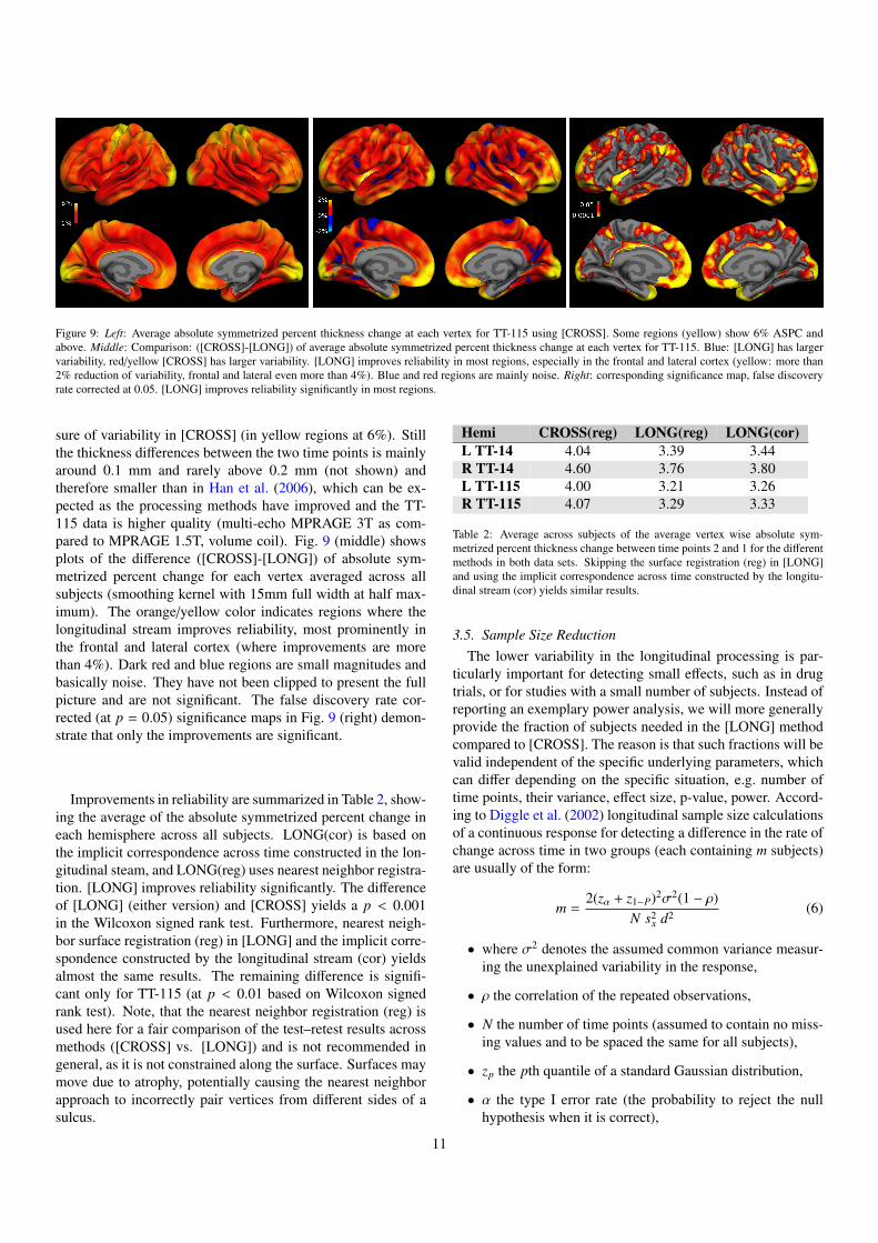
Figure 9: Left: Average absolute symmetrized percent thickness change at each vertex for TT-115 using [CROSS]. Some regions (yellow) show 6% ASPC andabove. Middle: Comparison: ([CROSS]-[LONG]) of average absolute symmetrized percent thickness change at each vertex for TT-115. Blue: [LONG] has largervariability, red/yellow [CROSS] has larger variability. [LONG] improves reliability in most regions, especially in the frontal and lateral cortex (yellow: more than2% reduction of variability, frontal and lateral even more than 4%). Blue and red regions are mainly noise. Right: corresponding significance map, false discoveryrate corrected at 0.05. [LONG] improves reliability significantly in most regions.

sure of variability in [CROSS] (in yellow regions at 6%). Stillthe thickness differences between the two time points is mainlyaround 0.1 mm and rarely above 0.2 mm (not shown) andtherefore smaller than in Han et al. (2006), which can be ex-pected as the processing methods have improved and the TT-115 data is higher quality (multi-echo MPRAGE 3T as com-pared to MPRAGE 1.5T, volume coil). Fig. 9 (middle) showsplots of the difference ([CROSS]-[LONG]) of absolute sym-metrized percent change for each vertex averaged across allsubjects (smoothing kernel with 15mm full width at half max-imum). The orange/yellow color indicates regions where thelongitudinal stream improves reliability, most prominently inthe frontal and lateral cortex (where improvements are morethan 4%). Dark red and blue regions are small magnitudes andbasically noise. They have not been clipped to present the fullpicture and are not significant. The false discovery rate cor-rected (at p = 0.05) significance maps in Fig. 9 (right) demon-strate that only the improvements are significant.

Improvements in reliability are summarized in Table 2, show-ing the average of the absolute symmetrized percent change ineach hemisphere across all subjects. LONG(cor) is based onthe implicit correspondence across time constructed in the lon-gitudinal steam, and LONG(reg) uses nearest neighbor registra-tion. [LONG] improves reliability significantly. The differenceof [LONG] (either version) and [CROSS] yields a p < 0.001in the Wilcoxon signed rank test. Furthermore, nearest neigh-bor surface registration (reg) in [LONG] and the implicit corre-spondence constructed by the longitudinal stream (cor) yieldsalmost the same results. The remaining difference is signifi-cant only for TT-115 (at p < 0.01 based on Wilcoxon signedrank test). Note, that the nearest neighbor registration (reg) isused here for a fair comparison of the test–retest results acrossmethods ([CROSS] vs. [LONG]) and is not recommended ingeneral, as it is not constrained along the surface. Surfaces maymove due to atrophy, potentially causing the nearest neighborapproach to incorrectly pair vertices from different sides of asulcus.

Hemi CROSS(reg) LONG(reg) LONG(cor)L TT-14 4.04 3.39 3.44R TT-14 4.60 3.76 3.80L TT-115 4.00 3.21 3.26R TT-115 4.07 3.29 3.33

Table 2: Average across subjects of the average vertex wise absolute sym-metrized percent thickness change between time points 2 and 1 for the differentmethods in both data sets. Skipping the surface registration (reg) in [LONG]and using the implicit correspondence across time constructed by the longitu-dinal stream (cor) yields similar results.

3.5. Sample Size ReductionThe lower variability in the longitudinal processing is par-

ticularly important for detecting small effects, such as in drugtrials, or for studies with a small number of subjects. Instead ofreporting an exemplary power analysis, we will more generallyprovide the fraction of subjects needed in the [LONG] methodcompared to [CROSS]. The reason is that such fractions will bevalid independent of the specific underlying parameters, whichcan differ depending on the specific situation, e.g. number oftime points, their variance, effect size, p-value, power. Accord-ing to Diggle et al. (2002) longitudinal sample size calculationsof a continuous response for detecting a difference in the rate ofchange across time in two groups (each containing m subjects)are usually of the form:

m =2(zα + z1−P)2σ2(1 − ρ)

N s2x d2 (6)

• where σ2 denotes the assumed common variance measur-ing the unexplained variability in the response,

• ρ the correlation of the repeated observations,

• N the number of time points (assumed to contain no miss-ing values and to be spaced the same for all subjects),

• zp the pth quantile of a standard Gaussian distribution,

• α the type I error rate (the probability to reject the nullhypothesis when it is correct),

11

• d = βB − βA smallest meaningful difference in the meanslope (rate of change) between group A and B to be de-tected (effect size),

• P the power of the test (the probability to reject the nullhypothesis when it is incorrect),

• and sx =∑

j(x j − x)2/N the within-subject variance of thetime points (more specifically of the explanatory variable,usually the duration between the first and the j-th visit,assumed to be the same for all subjects).

Eq. 6 shows that the sample size can be reduced by increasingthe number of time points N, by increasing the correlation of re-peated measures or by reducing the variability of the response.As the variability between subjects is usually fixed and cannotbe influenced, one aims at decreasing within-subject variabilityby using a more reliable measurement instrument or method.To analyze the effect of switching from independent image pro-cessing [CROSS] to longitudinal processing [LONG], it be-comes clear that all values except σ and ρ are fixed for thetwo different methods and the requisite number of subjectsdecreases with decreasing variance and increasing correlation.For a power analysis usually these values are estimated fromearlier studies with similar samples. Here we can compute thembased on the test–retest results TT-14, as 14 days between thescans sufficiently model the variability of follow-up scans on adifferent day (using the same scanner).

The fraction of necessary sample sizes when choosing[LONG] over [CROSS] is determined by the fraction of vari-ances and correlation:

S S f rac = 100mL

mC= 100

σ2L(1 − ρL)

σ2C(1 − ρC)

. (7)

This ratio specifies what percent of subjects is needed whenprocessing the data longitudinally as opposed to independentprocessing.

Based on variance and correlation results from TT-14, Fig. 10shows the ratio for several subcortical regions. Given this sin-gle test population to compute variance and correlation, we es-timate stability of these results via bootstrapping (1000 resam-ples). Fig. 10 therefore depicts the median, the error bars extendfrom the 1st to the 3rd quartile. The results indicate that samplesize can usually be reduced in [LONG] to less than half the sizeassuming same power, p-value, effect size and number and vari-ance of time points. The small reduction in the left caudate isdue to the fact that in [CROSS] the correlation of the measuresis very high and almost the same as in [LONG], which is nottrue for the other hemisphere and most of the other structureswhere the correlation in [CROSS] is usually much lower. Evenlarger improvements can be expected when switching to mod-ern acquisition hardware and methods, for example as used inthe TT-115 dataset (see improvements in Fig. 7). However, wecannot base this sample size estimation on TT-115 since within-session scans do not model the noise induced by removing andre-positioning a subject in the scanner, nor variability due tohydration levels, etc.

Thalamus Caudate Putamen Pallidum Hippocamp Amygdala0

10

20

30

40

50

60

70

80

90

100

Pe

rce

nt

Su

bje

cts

ne

ed

ed

(L

ON

G v

s.

CR

OS

S)

Sample Size Reduction (Left Hemisphere)

Thalamus Caudate Putamen Pallidum Hippocamp Amygdala0

10

20

30

40

50

60

70

80

90

100

Pe

rce

nt

Su

bje

cts

ne

ed

ed

(L

ON

G v

s.

CR

OS

S)

Sample Size Reduction (Right Hemisphere)

Figure 10: Percent of subjects needed in [LONG] with respect to [CROSS]to achieve same power at same p to detect same effect size. In most regionsless than 40% of the subjects are needed. Equivalently this figure shows thereduction in necessary time points when keeping the number of subjects andwithin-subject variance of time points the same. Variance of measurements andcorrelation were estimated based on TT-14 using bootstrap with 1000 samples.Bars show median and error bars depict 1st and 3rd quartile.

Note that the number of subjects m and the number of timepoints n can be swapped in Eq. 6, thus Fig. 10 can also be un-derstood as showing the reduction in the necessary number oftime points in a longitudinal design when keeping the numberof subjects (and variance of time points) constant. The reducednumber of subjects or necessary time points in the longitudinalstream can constitute a significant reduction in costs for longitu-dinal studies such as drug trials. Several other relevant statisticson TT-14 are reported in Table A.3 in the Appendix for differ-ent structures to establish individual power analyses. Of coursethese results are specific to the acquisition in TT-14 and maynot be transferable to other studies.

3.6. Sensitivity and Specificity in NeurodegenerationSince no longitudinal data set with manual labels is freely

available that could be taken as “ground truth”, we analyzea set of images of different disease groups and demonstratethat longitudinal processing improves discrimination among thegroups. Here we are interested in detecting differences in theyearly volume percent change. The longitudinal OASIS datasetOA-136 was selected to analyze behavior of the processingstreams in a disease study where subjects have differently manyvisits (2-5). Figure 11 highlights the improvements of longitu-dinal processing: more power due to higher precision to distin-guish the demented from the non-demented group based on the

12

LThalamus LHippo LEntorhinal RThalamus RHippo REntorhinal

−7

−6

−5

−4

−3

−2

−1

0

1

Pct. V

olu

me C

hange (

per

year

w.r

.t b

aselin

e)

Atrophy in Dementia [CROSS]

Non−Demented (72)

Demented (64)

LThalamus LHippo LEntorhinal RThalamus RHippo REntorhinal

−7

−6

−5

−4

−3

−2

−1

0

1

Pct. V

olu

me C

hange (

per

year

w.r

.t b

aselin

e)

Atrophy in Dementia [LONG]

Non−Demented (72)

Demented (64)

Figure 11: Percent volume change per year with respect to baseline of the OA-136 dataset (2 to 5 visits per subject) for both independent [CROSS] (top) andlongitudinal [LONG] (bottom) processing. [LONG] shows greater power todistinguish the two groups and smaller error bars (higher precision).

percent volume change with respect to baseline volume mainlyin the hippocampus and entorhinal cortex. Baseline volume wasnot taken directly from the results of the first time point, but in-stead we used the value of the linear fit within each subject atbaseline to obtain more robust baseline volume estimates for thepercent change computation (for both [CROSS] and [LONG]).Again the red ’.’ denotes a p ≤ 0.05, the ’+’: p ≤ 0.01 andthe ’*’: p ≤ 0.001 in the Mann-Whitney-U (also Wilcoxonrank-sum) test. Note that the Mann-Whitney-U test is closelyrelated to the area under the Receiver Operator Characteris-tic (ROC) (Mason and Graham, 2002). For a binary classifierthe ROC curve plots the sensitivity vs. the false positive rate(1−specificity). The area under the curve therefore measuresthe performance of the classifier. Thus the significant differ-ences across the groups above imply both improved sensitivityand specificity to distinguish the different disease stages basedon atrophy rate.

The other disease data set HD-54 was selected as it describesa small study with images from different scanner software ver-sions, where statistical power is relatively low. Fig. 12 (left andmiddle) shows plots of percent change averages (and standarderrors) for thalamus, caudate and putamen in both hemispheres.Percent change is computed with respect to the baseline volumehere, where baseline volume is taken from the linear fit withineach subjects as a more robust estimate. For the PHDfar we testdifference from controls, for PHDnear difference from PHDfarand for the HD difference from PHDnear. Because of the large

variability in the measurements, the cross-sectional stream can-not distinguish well between the groups. [LONG], however, iscapable of differentiating PHDfar from controls based on atro-phy rates in the caudate and putamen and PHDfar from PHD-near based on the left caudate. Caudate and putamen are struc-tures that are affected very early (in PHDfar more than 11 yearsfrom expected onset of symptoms) while other structures suchas the thalamus seem to be affected later in the disease and showa faster atrophy rate in the HD group. In HD the small atrophyrate in the caudate seem to indicate a floor effect (or difficultieswith the automatic segmentation as most of the caudate is lost).

To visualize group volume differences Figure 12 (right) de-picts the mean volumes of thalamus, caudate and putamen atbaseline (tp1) after intracranial volume (ICV) normalization.Even though here we analyze volume at a single time point,each structure’s volume and ICV are taken from the results ob-tained via longitudinal processing and should therefore be morerobust than independent processing. Due to large between-subject variability in anatomical structures, it is often not pos-sible to distinguish groups simply based on structure size (evenafter head size correction). In longitudinal studies, however, theadditional temporal information within each subject (atrophyrate) is computed with respect to average or baseline structuresize (i.e. percent change) within each subject. This removes be-tween subject variability and, at the same time, increases powerto distinguish groups based on the anatomical change in addi-tion to size. For example the atrophy rate in the putamen differssignificantly between controls and pre-symptomatic subjects farfrom disease onset, while baseline putamen volume does not.

4. Conclusion

The robust subject template yields an initial unbiased esti-mate of the location of anatomical structures in a longitudinalscheme. We demonstrated that initializing processing of indi-vidual time points with common information from the subjecttemplate improves reliability significantly as compared to in-dependent processing. Furthermore, our approach to treat allinputs the same removes asymmetry induced processing bias.This is important as the special treatment of a specific time pointsuch as baseline, e.g. to inform follow-up processing, inducesbias even in the absence of resampling asymmetries. Moreoverwe avoid imposing regularization or temporal smoothness con-straints to keep the necessary flexibility for detecting large de-viations. Therefore, in our framework, the order of time pointsis not considered at all and individual segmentation and defor-mation procedures are allowed to evolve freely. This reducesover-regularization and thus the risk of consistently underesti-mating change.

We have shown, that our method significantly improves pre-cision of the automatically constructed segmentations with re-spect to volume and location, and of the cortical thickness mea-sures. Thus, statistical power is increased, i.e. the necessarynumber of subjects or time points reduced (at same effect sizeand significance level). This may have a profound clinical im-pact particularly in drug trials where small effect sizes need tobe detected or disease processes quantified early in the course,

13

LThalamus LCaudate LPutamen RThalamus RCaudate RPutamen

−4

−3

−2

−1

0

1

2

3

Pct. V

olu

me C

hange (

per

year

w.r

.t. baselin

e)

Atrophy in Huntington’s Disease [CROSS]

[CN] (10)

[PHDfar] (16)

[PHDnear] (19)

[HD] (9)

LThalamus LCaudate LPutamen RThalamus RCaudate RPutamen

−4

−3

−2

−1

0

1

2

3

Pct. V

olu

me C

hange (

per

year

w.r

.t. baselin

e)

Atrophy in Huntington’s Disease [LONG]

[CN] (10)

[PHDfar] (16)

[PHDnear] (19)

[HD] (9)

LThalamus LCaudate LPutamen RThalamus RCaudate RPutamen0

1

2

3

4

5

6x 10

−3

Str

uctu

re V

olu

me

/ I

ntr

acra

nia

l V

olu

me

Volume at Baseline in Huntington’s Disease

CN (10)

PHDfar (16)

PHDnear (19)

HD (9)

Figure 12: Symmetric percent volume change per year of several subcortical structures. Left: [CROSS] almost no significant differences due to high variability(small group sizes). Middle: [LONG] significant differences between pre-symptomatic (PHD far from onset) and controls and between PHD far and PHD near (leftcaudate). Right: Volume means (ICV normalized) at baseline (tp1). While baseline volume distinguishes groups in several cases, the significant difference betweencontrols and PHDfar in atrophy rate in the putamen cannot be detected in the baseline volumes.

when therapeutic intervention is still possible. The presentedmethodology is capable of precisely and accurately detectingdifferences as demonstrated in simulated hippocampal atrophyand in evaluating complex, subtle changes that occur in neu-rodegenerative disorders.

A common challenge of longitudinal analyses is change inscanner hardware or software. Due to scanner drift and calibra-tion, images cannot be assumed to be sized exactly the same.Any change in pre-processing can bias results and potentiallyvoid a study trying to establish absolute measures such as therate of change in a specific disease. Group comparisons maystill be possible, if both groups underwent the same process-ing changes, but even then it likely that the processing changeinfluences one group more than the other and that influencesare regional. To account for calibration effects, we include op-tional affine template creation into our framework. However,potential image contrast changes cannot easily be removed ret-rospectively. This is of course true for both longitudinal andindependent processing, where variability will be even higher.A consistent change in input images, independent of the source,is supposed to be detected by an accurate and precise analysistool. Longitudinal methods may actually reveal these kinds ofconsistent acquisition differences, because they are more sen-sitive and need less subjects to detect them. It is therefore es-sential to control scanner hardware and software or to modelupgrades as potential shifts when running a statistical analysison the results.

Future work will include procedures to jointly estimate or op-timize results in all time points simultaneously without neces-sarily relying on the subject template. In unbiased simultaneousprocessing memory usage is scaled at least linearly by the num-ber of time points (Gaussian classifiers scale with the square iffull covariance estimation is used), which implies that hardwarerequirements may not be met by standard desktop computers.However, this is a direction we intend to pursue. For example,a joint intensity normalization and bias correction can employall the imaging data across time to estimate a high SNR imageat each time point while retaining regions that display temporalchange. It is also possible to generate an unbiased initial es-

timate of the average surface locations for both the gray/whiteand the pial surfaces by minimizing the distance to each of theindividual cross-sectional surfaces directly. Furthermore, it isexpected that variational approaches for the thickness compu-tation in each time point will improve reliability compared tothe current method, which estimates and averages the shortestdistance from the gray to white matter surface and vice versa.

The presented longitudinal scheme is freely available in thesoftware package FreeSurfer at www.freesurfer.net and hasbeen successfully applied in our lab and by others in variousstudies of e.g. Huntington’s, Alzheimer’s disease and aging.

5. Acknowledgements

Support for this research was provided in part by theNational Center for Research Resources (P41RR14075,and the NCRR BIRN Morphometric Project BIRN002,U24RR021382), the National Institute for BiomedicalImaging and Bioengineering (R01EB006758), the Na-tional Institute on Aging (R01AG022381, U01AG024904),the National Institute for Neurological Disorders andStroke (R01NS052585, R01NS042861, P01NS058793,R21NS072652, R01NS070963). Additional support wasprovided by The Autism & Dyslexia Project funded bythe Ellison Medical Foundation, the National Center forAlternative Medicine (RC1AT005728), and was made pos-sible by the resources provided by Shared InstrumentationGrants (S10RR023401, S10RR019307, S10RR023043). Forthe OASIS dataset we acknowledge the following grants(P50AG05681, P01AG03991, R01AG021910, P50MH071616,U24RR021382, R01MH56584). The authors would alsolike to thank Mert Sabuncu and Gheorghe Doros for helpfuldiscussions and advice.

Appendix A. Probabilistic Fusion

For the following discussion we assume for each subject theN normalized and skull stripped images Ii to be registeredand resampled to the common template space, together with

14

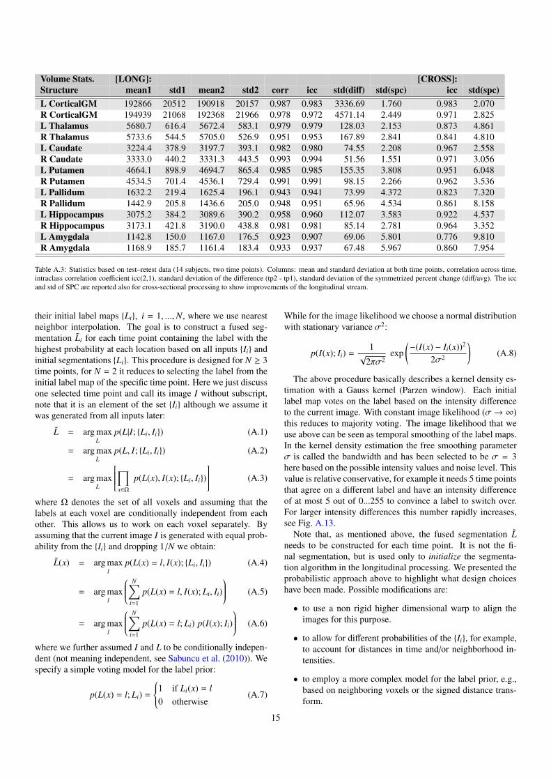
Volume Stats. [LONG]: [CROSS]:Structure mean1 std1 mean2 std2 corr icc std(diff) std(spc) icc std(spc)L CorticalGM 192866 20512 190918 20157 0.987 0.983 3336.69 1.760 0.983 2.070R CorticalGM 194939 21068 192368 21966 0.978 0.972 4571.14 2.449 0.971 2.825L Thalamus 5680.7 616.4 5672.4 583.1 0.979 0.979 128.03 2.153 0.873 4.861R Thalamus 5733.6 544.5 5705.0 526.9 0.951 0.953 167.89 2.841 0.841 4.810L Caudate 3224.4 378.9 3197.7 393.1 0.982 0.980 74.55 2.208 0.967 2.558R Caudate 3333.0 440.2 3331.3 443.5 0.993 0.994 51.56 1.551 0.971 3.056L Putamen 4664.1 898.9 4694.7 865.4 0.985 0.985 155.35 3.808 0.951 6.048R Putamen 4534.5 701.4 4536.1 729.4 0.991 0.991 98.15 2.266 0.962 3.536L Pallidum 1632.2 219.4 1625.4 196.1 0.943 0.941 73.99 4.372 0.823 7.320R Pallidum 1442.9 205.8 1436.6 205.0 0.948 0.951 65.96 4.534 0.861 8.158L Hippocampus 3075.2 384.2 3089.6 390.2 0.958 0.960 112.07 3.583 0.922 4.537R Hippocampus 3173.1 421.8 3190.0 438.8 0.981 0.981 85.14 2.781 0.964 3.352L Amygdala 1142.8 150.0 1167.0 176.5 0.923 0.907 69.06 5.801 0.776 9.810R Amygdala 1168.9 185.7 1161.4 183.4 0.933 0.937 67.48 5.967 0.860 7.954

Table A.3: Statistics based on test–retest data (14 subjects, two time points). Columns: mean and standard deviation at both time points, correlation across time,intraclass correlation coefficient icc(2,1), standard deviation of the difference (tp2 - tp1), standard deviation of the symmetrized percent change (diff/avg). The iccand std of SPC are reported also for cross-sectional processing to show improvements of the longitudinal stream.

their initial label maps Li, i = 1, ...,N, where we use nearestneighbor interpolation. The goal is to construct a fused seg-mentation Li for each time point containing the label with thehighest probability at each location based on all inputs Ii andinitial segmentations Li. This procedure is designed for N ≥ 3time points, for N = 2 it reduces to selecting the label from theinitial label map of the specific time point. Here we just discussone selected time point and call its image I without subscript,note that it is an element of the set Ii although we assume itwas generated from all inputs later:

L = arg maxL

p(L|I; Li, Ii) (A.1)

= arg maxL

p(L, I; Li, Ii) (A.2)

= arg maxL

∏x∈Ω

p(L(x), I(x); Li, Ii)

(A.3)

where Ω denotes the set of all voxels and assuming that thelabels at each voxel are conditionally independent from eachother. This allows us to work on each voxel separately. Byassuming that the current image I is generated with equal prob-ability from the Ii and dropping 1/N we obtain:

L(x) = arg maxl

p(L(x) = l, I(x); Li, Ii) (A.4)

= arg maxl

N∑i=1

p(L(x) = l, I(x); Li, Ii)

(A.5)

= arg maxl

N∑i=1

p(L(x) = l; Li) p(I(x); Ii)

(A.6)

where we further assumed I and L to be conditionally indepen-dent (not meaning independent, see Sabuncu et al. (2010)). Wespecify a simple voting model for the label prior:

p(L(x) = l; Li) =

1 if Li(x) = l0 otherwise

(A.7)

While for the image likelihood we choose a normal distributionwith stationary variance σ2:

p(I(x); Ii) =1

√2πσ2

exp(−(I(x) − Ii(x))2

2σ2

)(A.8)

The above procedure basically describes a kernel density es-timation with a Gauss kernel (Parzen window). Each initiallabel map votes on the label based on the intensity differenceto the current image. With constant image likelihood (σ → ∞)this reduces to majority voting. The image likelihood that weuse above can be seen as temporal smoothing of the label maps.In the kernel density estimation the free smoothing parameterσ is called the bandwidth and has been selected to be σ = 3here based on the possible intensity values and noise level. Thisvalue is relative conservative, for example it needs 5 time pointsthat agree on a different label and have an intensity differenceof at most 5 out of 0...255 to convince a label to switch over.For larger intensity differences this number rapidly increases,see Fig. A.13.

Note that, as mentioned above, the fused segmentation Lneeds to be constructed for each time point. It is not the fi-nal segmentation, but is used only to initialize the segmenta-tion algorithm in the longitudinal processing. We presented theprobabilistic approach above to highlight what design choiceshave been made. Possible modifications are:

• to use a non rigid higher dimensional warp to align theimages for this purpose.

• to allow for different probabilities of the Ii, for example,to account for distances in time and/or neighborhood in-tensities.

• to employ a more complex model for the label prior, e.g.,based on neighboring voxels or the signed distance trans-form.

15

1 2 3 4 5 6 7 80

2

4

6

8

10

12

14

16

18

20

Intensity Difference

Num

ber

of D

iffe

ring U

nanim

ous V

ote

s

Votes Needed to Swap Label, sigma=3

Figure A.13: Votes that need to agree on a different label to convince a timepoint to swap at σ = 3 for a given intensity difference.

However, since the fused segmentation is only an initialization,the above approach is sufficient in that it allows flexibility ofdetecting large change across time, as opposed to using the seg-mentation of the template to initialize all time points.

Appendix B. Mean Space

Here we discuss, how to compute the average location from aset of N−1 rigid transformations (step 2 in section 2.4 ). For thisa new coordinate system is defined with its origin at the centerof the random target image I with axes aligned to the right,anterior, superior directions (RAS). The first step is to find thelocation and orientation (translation and rotation) of each of theother images in this space, so that the average location can becomputed.

A rigid transformation consists of a rotation and translationand is usually written as ϕ(~x) := R~x + ~t, where R is a 3 × 3rotation matrix. R and ~t are returned when registering image Ii

to image I. Equivalently the order can be reversed, so that thetranslation will be executed before the rotation:

ϕ(~x) = R~x + t = R(~x + R−1~t) (B.1)

Note that the inverse of the rotation matrix is simply the trans-pose R−1 = RT . The rotation remains the same, while thetranslation becomes ~vi := RT

i~ti (registering image i to the first

via transform ϕi). The −~vi directly give the translation offsetof each image with respect to image I (located at the origin).Therefore the average:

~p := −1N

N∑i=1

~vi (B.2)

marks the mean of all locations. For rotations different averagescan be defined (Moakher, 2002; Sharf et al., 2010). Since rota-tional differences are rather small, it will be sufficient to com-pute the projected arithmetic mean. This is the usual arithmeticmean of 3 × 3 matrices, orthogonally projected back to SO(3),the space of rotation matrices, via a polar decomposition. To

find the rotation from I to the average position, the inverse ro-tations obtained from the registration above are averaged:

Q =1N

N∑i=1

RTi . (B.3)

Note that both sums run over all images, where the translationof I with respect to itself is of course zero and the rotation ma-trix is identity. Since the matrix mean Q is not a rotation matrixin general, its polar decomposition Q = US into an orthogonalrotation matrix U and a symmetric matrix S needs to be com-puted. S is always unique and given by S =

√QT Q. Because

the head positions in the images are sufficiently close to eachother5, Q is invertible and then U is also unique. It can be com-puted through a singular value decomposition of Q = WDVT

and is given6 by U = WVT .Once the mean location ~p and orientation U are determined,

we construct the transform ϕ(~x) := U~x + ~p from image I tothe average location. The other transforms of each image tothe average location are then created by composition ϕi := ϕ ϕi. All images are averaged at that location and serve as highquality input to the intrinsic mean algorithm.

Appendix C. Simulated Atrophy

In order to simulate atrophy in the hippocampus (see Sec-tion 3.3) we reduce the intensity of boundary voxels adjacent toventricle CSF. Let H denote the set of all hippocampus voxelsand B the subset of boundary voxels containing partial ventri-cle, then we have Vhippo(B) =

∑x∈B Vhippo(x) the sum of partial

hippocampus volumes for all voxels in B, and total hippocam-pal volume Vhippo(H). For atrophy rate p (here p = 0.02) wecompute the boundary scaling factor as:

s = 1 −Vhippo(H) pVhippo(B)

(C.1)

necessary for adjusting partial volume of boundary voxels toachieve the desired volume reduction. For this we first estimatelocal mean hippocampus intensity IH(x) and ventricle intensityIV (x) in a 153 box centered at x. Then we compute the partialhippocampal volume at x

Vhippo(x) =I(x) − IV (x)

IH(x) − IV (x)(C.2)

and update intensity according to

I(x) = IH(x) s Vhippo(x) + IV (x)(1 − s Vhippo(x)

). (C.3)

5i.e. sufficiently less than 180 away from each other to prevent the averagefrom becoming ill conditioned or even singular.

6Q = WDVT = (WVT )(VDVT ) = US and√

QT Q =√

VDWT WDVT =√

VDVT VDVT = S using VT V = WT W = I

16

References

Ashburner, J., 2007. A fast diffeomorphic image registration algorithm.NeuroImage 38 (1), 95 – 113.URL http://www.sciencedirect.com/science/article/pii/

S1053811907005848

Ashburner, J., Andersson, J., Friston, K., 2000. Image registration using a sym-metric prior–in three dimensions. Hum Brain Mapp. 9 (4), 212–225.

Ashburner, J., Friston, K., 1999. Nonlinear spatial normalization using basisfunctions. Human Brain Mapping 7 (4), 254–266.

Avants, B., Anderson, C., Grossman, M., Gee, J.C., 2007. Spatiotemporal nor-malization for longitudinal analysis of gray matter atrophy in frontotemporaldementia. In: Medical Image Computing and Computer-Assisted Interven-tion - MICCAI 2007. Vol. 4792 of Lecture Notes in Computer Science. pp.303–310.

Avants, B., Cook, P.A., McMillan, C., Grossman, M., Tustison, N.J., Zheng, Y.,Gee, J.C., 2010. Sparse unbiased analysis of anatomical variance in longitu-dinal imaging. In: MICCAI 2010, Part I. Vol. 6361 of LNCS. Springer, pp.324–331.

Avants, B., Gee, J.C., 2004. Geodesic estimation for large deformation anatom-ical shape averaging and interpolation. NeuroImage 23 (1), 139–150.

Berry, D.A., Ayers, G.D., 2006. Symmetrized percent change for treatmentcomparisons. The American Statistician 60, 27–31.

Chetelat, G., Landeau, B., Eustache, F., Mezenge, F., Viader, F., de la Sayette,V., Desgranges, B., Baron, J.-C., 2005. Using voxel-based morphometryto map the structural changes associated with rapid conversion in mci: Alongitudinal mri study. NeuroImage 27 (4), 934 – 946.URL http://www.sciencedirect.com/science/article/pii/

S1053811905003277

Chiang, G.C., Insel, P.S., Tosun, D., Schuff, N., Truran-Sacrey, D., Raptentset-sang, S., Jack, C.R., Aisen, P., Petersen, R.C., Weiner, M.W., ADNI, 2010.Hippocampal atrophy rates and CSF biomarkers in elderly APOE2 normalsubjects. Neurology 75 (22), 1976–1981.

Chiang, G.C., Insel, P.S., Tosun, D., Schuff, N., Truran-Sacrey, D., Raptentset-sang, S., Jack, C.R., Weiner, M.W., ADNI, 2011. Identifying cognitivelyhealthy elderly individuals with subsequent memory decline by using auto-mated MR temporoparietal volumes. Radiology 259 (3), 844–851.URL http://dx.doi.org/10.1148/radiol.11101637

Clarkson, M.J., Ourselin, S., Nielsen, C., Leung, K.K., Barnes, J., Whitwell,J.L., Gunter, J.L., Hill, D.L., Weiner, M.W., Jack, C.R., Fox, N.C., 2009.Comparison of phantom and registration scaling corrections using the adnicohort. NeuroImage 47 (4), 1506 – 1513.

Collignon, A., Maes, F., Delaere, D., Vandermeulen, D., Suetens, P., Marchal,G., 1995. Automated multi-modality image registration based on informa-tion theory. In: Information Processing in Medical Imaging. Kluwer, pp.263–274.

Dale, A., Fischl, B., Sereno, M.I., 1999. Cortical surface-based analysis: I.segmentation and surface reconstruction. NeuroImage 9 (2), 179 – 194.

Desikan, R.S., Sabuncu, M.R., Schmansky, N.J., Reuter, M., Cabral, H.J., Hess,C.P., Weiner, M.W., Biffi, A., Anderson, C.D., Rosand, J., Salat, D.H., Kem-per, T.L., Dale, A.M., Sperling, R.A., Fischl, B., ADNI, 2010. Seletive dis-ruption of the cerebral neocortex in alzheimer’s disease. PLoS ONE 5 (9),e12853.URL http://dx.doi.org/10.1371/journal.pone.0012853

Desikan, R.S., Segonne, F., Fischl, B., Quinn, B.T., Dickerson, B.C., Blacker,D., Buckner, R.L., Dale, A.M., Maguire, R.P., Hyman, B.T., Albert, M.S.,Killiany, R.J., 2006. An automated labeling system for subdividing the hu-man cerebral cortex on MRI scans into gyral based regions of interest. Neu-roImage 31 (3), 968 – 980.

Diggle, P.J., Heagerty, P.J., Liang, K.-Y., Zeger, S.L., 2002. Analysis of Longi-tudinal Data, 2nd Edition. Oxford University Press.

Engvig, A., Fjell, A.M., Westlye, L.T., Moberget, T., Sundseth, Ø., Larsen,V.A., Walhovd, K.B., 2010. Effects of memory training on cortical thicknessin the elderly. NeuroImage 52 (4), 1667 – 1676.

Fischl, B., Dale, A.M., 2000. Measuring the thickness of the human cere-bral cortex from magnetic resonance images. Proceedings of the NationalAcademy of Sciences of the United States of America 97 (20), 11050–11055.

Fischl, B., Liu, A., Dale, A.M., 2001. Automated manifold surgery: construct-ing geometrically accurate and topologically correct models of the humancerebral cortex. Trans Medical Imaging 20 (1), 70–80.

Fischl, B., Salat, D.H., Busa, E., Albert, M., Dieterich, M., Haselgrove, C.,van der Kouwe, A., Killiany, R., Kennedy, D., Klaveness, S., Montillo, A.,Makris, N., Rosen, B., Dale, A.M., 2002. Whole brain segmentation: Au-tomated labeling of neuroanatomical structures in the human brain. Neuron33 (3), 341–355.

Fischl, B., Salat, D.H., van der Kouwe, A., Makris, N., Segonne, F., Quinn,B.T., Dale, A.M., 2004a. Sequence-independent segmentation of magneticresonance images. NeuroImage 23 (Supplement 1), 69 – 84.

Fischl, B., Sereno, M.I., Dale, A., 1999a. Cortical surface-based analysis: II. in-flation, flattening, and a surface-based coordinate system. NeuroImage 9 (2),195 – 207.

Fischl, B., Sereno, M.I., Tootell, R.B., Dale, A.M., 1999b. High-resolutionintersubject averaging and a coordinate system for the cortical surface.Human Brain Mapping 8 (4), 272–284.URL http://dx.doi.org/10.1002/(SICI)1097-0193(1999)8:

4<272::AID-HBM10>3.0.CO;2-4

Fischl, B., van der Kouwe, A., Destrieux, C., Halgren, E., Segonne, F., Salat,D.H., Busa, E., Seidman, L.J., Goldstein, J., Kennedy, D., Caviness, V.,Makris, N., Rosen, B., Dale, A.M., 2004b. Automatically parcellating thehuman cerebral cortex. Cerebral Cortex 14 (1), 11–22.

Fischl, B., 2012. FreeSurfer. NeuroImage (in press).URL http://dx.doi.org/10.1016/j.neuroimage.2012.01.021

Fletcher, P.T., Venkatasubramanian, S., Joshi, S., 2009. The geometric medianon riemannian manifolds with application to robust atlas estimation. Neu-roImage 45 (1, Supplement 1), 143 – 152, mathematics in Brain Imaging.

Han, X., Jovicich, J., Salat, D., van der Kouwe, A., Quinn, B., Czanner, S.,Busa, E., Pacheco, J., Albert, M., Killiany, R., Maguire, P., Rosas, D.,Makris, N., Dale, A., Dickerson, B., Fischl, B., 2006. Reliability of MRI-derived measurements of human cerebral cortical thickness: The effects offield strength, scanner upgrade and manufacturer. NeuroImage 32 (1), 180–194.

Holland, D., Dale, A.M., 2011. Nonlinear registration of longitudinal imagesand measurement of change in regions of interest. Medical Image Analysis15 (4), 489 – 497.

Holland, D., McEvoy, L.K., Dale, A.M., ADNI, 2011. Unbiased comparisonof sample size estimates from longitudinal structural measures in ADNI.Human Brain Mapping online.URL http://dx.doi.org/10.1002/hbm.21386

Jenkinson, M., Bannister, P.R., Brady, J.M., Smith, S.M., 2002. Improved opti-mization for the robust and accurate linear registration and motion correctionof brain images. NeuroImage 17, 825–841.

Joshi, S., Davis, B., Jomier, B.M., Gerig, G., 2004. Unbiased diffeomorphicatlas construction for computational anatomy. NeuroImage 23, 151–160.

Kipps, C.M., Duggins, A.J., Mahant, N., Gomes, L., Ashburner, J., McCusker,E.A., 2005. Progression of structural neuropathology in preclinical hunt-ington’s disease: a tensor based morphometry study. Journal of Neurology,Neurosurgery & Psychiatry 76 (5), 650–655.URL http://jnnp.bmj.com/content/76/5/650.full.pdf

Langbehn, D., Brinkman, R., Falush, D., Paulsen, J., Hayden, M., 2004. A newmodel for prediction of the age of onset and penetrance for Huntington’sdisease based on CAG length. Clinical Genetics 65 (4), 267–277.URL http://dx.doi.org/10.1111/j.1399-0004.2004.00241.x

Li, Y., Wang, Y., Xue, Z., Shi, F., Lin, W., Shen, D., 2010. Consistent 4dcortical thickness measurement for longitudinal neuroimaging study. In:Jiang, T., Navab, J., Pluim, J., Max, V. (Eds.), Medical Image Computingand Computer-Assisted Intervention - MICCAI 2010. Vol. 6362 of LectureNotes in Computer Science. Springer Berlin / Heidelberg, pp. 133–142.

Lin, L. I.-K., 1989. A concordance correlation coefficient to evaluate repro-ducibility. Biometrics 45 (1), 255–268.

Mason, S., Graham, N., 2002. Areas beneath the relative operating character-istics (ROC) and relative operating levels (ROL) curves: Statistical signifi-cance and interpretation. Quarterly Journal of the Royal Meteorological So-ciety 128 (584), 2145–2166.

Moakher, M., 2002. Means and averaging in the group of rotations. SIAM J.Matrix Anal. Appl. 24 (1), 1–16.URL http://dx.doi.org/10.1137/S0895479801383877

Morey, R.A., Selgrade, E.S., Wagner, H.R., Huettel, S.A., Wang, L., McCarthy,G., 2010. Scan-rescan reliability of subcortical brain volumes derived fromautomated segmentation. Human Brain Mapping 31 (11), 1751–1762.URL http://dx.doi.org/10.1002/hbm.20973

Nakamura, K., Fox, R., Fisher, E., 2011. CLADA: Cortical longitudinal atrophy

17

detection algorithm. NeuroImage 54 (1), 278 – 289.Nickerson, C.A.E., 1997. A note on “A concordance correlation coefficient to

evaluate reproducibility”. Biometrics 53 (4), 1503–1507.Patenaude, B., Smith, S.M., Kennedy, D.N., Jenkinson, M., 2011. A Bayesian

model of shape and appearance for subcortical brain segmentation. Neu-roImage 56 (3), 907 – 922.URL http://dx.doi.org/10.1016/j.neuroimage.2011.02.046

Qiu, A., Bitouk, D., Miller, M.I., 2006. Smooth functional and structural mapson the neocortex via orthonormal bases of the Laplace-Beltrami operator.IEEE Transactions on Medical Imaging 25 (10), 1296–1306.

Reuter, M., 2009. Longitudinal Processing in FreeSurfer.URL http://freesurfer.net/fswiki/LongitudinalProcessing

Reuter, M., Rosas, H.D., Fischl, B., 2010. Unbiased Robust Template Esti-mation for Longitudinal Analysis in FreeSurfer. In Proceedings of the 16thAnnual Meeting of the Organization for Human Brain Mapping.

Reuter, M., Fischl, B., 2011. Avoiding asymmetry-induced bias in longitudinalimage processing. NeuroImage 57 (1), 19–21.URL http://dx.doi.org/10.1016/j.neuroimage.2011.02.076

Reuter, M., Rosas, H.D., Fischl, B., 2010. Highly accurate inverse consistentregistration: A robust approach. NeuroImage 53 (4), 1181–1196.URL http://dx.doi.org/10.1016/j.neuroimage.2010.07.020

Rosas, H.D., Reuter, M., Doros, G., Lee, S.Y., Triggs, T., Malarick, K., Fischl,B., Salat, D.H., Hersch, S.M., 2011. A tale of two factors: What determinesthe rate of progression in Huntington’s disease? A longitudinal MRI study.Movement Disorders 26 (9), 1691–1697.URL http://dx.doi.org/10.1002/mds.23762

Sabuncu, M.R., Desikan, R.S., Sepulcre, J., Yeo, B.T., Liu, H., Schmansky,N.J., Reuter, M., Weiner, M.W., Buckner, R.L., Sperling, R.A., Fischl,B., ADNI, 2011. The dynamics of cortical and hippocampal atrophy inAlzheimer’s disease. Archives of Neurology 68 (8), 1040–1048.

Sabuncu, M.R., Yeo, B.T., Van Leemput, K., Fischl, B., Golland, P., 2010. Agenerative model for image segmentation based on label fusion. IEEE TransMed Imaging 29 (10), 1714–1729.

Salat, D., Lee, S., van der Kouwe, A., Greve, D.N., Fischl, B., Rosas, H.D.,2009. Age-associated alterations in cortical gray and white matter signalintensity and gray to white matter contrast. NeuroImage 48 (1), 21 – 28.

Segonne, F., Pacheco, J., Fischl, B., 2007. Geometrically accurate topology-correction of cortical surfaces using nonseparating loops. Trans Med Imag-ing 26, 518–529.

Sharf, I., Wolf, A., Rubin, M., 2010. Arithmetic and geometric solutions foraverage rigid-body rotation. Mechanism and Machine Theory 45 (9), 1239– 1251.

Shrout, P.E., Fleiss, J.L., 1979. Intraclass correlations: Uses in assessing raterreliability. Psychological Bulletin 86 (2), 420–428.

Sled, J., Zijdenbos, A., Evans, A., 1998. A nonparametric method for automaticcorrection of intensity nonuniformity in MRI data. Transactions on MedicalImaging 17 (1), 87 – 97.

Smith, S.M., De Stefano, N., Jenkinson, M., Matthews, P., 2001. Normalizedaccurate measurement of longitudinal brain change. Journal of ComputerAssisted Tomography 25 (3), 466–475.

Smith, S.M., Jenkinson, M., Woolrich, M.W., Beckmann, C.F., Behrens, T.E.,Johansen-Berg, H., Bannister, P.R., De Luca, M., Drobnjak, I., Flitney, D.E.,Niazy, R.K., Saunders, J., Vickers, J., Zhang, Y., De Stefano, N., Brady,J.M., Matthews, P., 2004. Advances in functional and structural MR imageanalysis and implementation as FSL. NeuroImage 23, 208–219.URL http://dx.doi.org/10.1016/j.neuroimage.2004.07.051

Smith, S.M., Zhang, Y., Jenkinson, M., Chen, J., Matthews, P., Federico,A., Stefano, N.D., 2002. Accurate, robust, and automated longitudinal andcross-sectional brain change analysis. NeuroImage 17 (1), 479 – 489.

Takao, H., Hayashi, N., Ohtomo, K., 2011. Effect of scanner in longitudinalstudies of brain volume changes. Journal of Magnetic Resonance Imaging34 (2),438–444.

Thevenaz, P., Blu, T., Unser, M., 2000. Interpolation Revisited. Transactions onMedical Imaging 19(7), 739–758.

Thompson, W.K., Holland, D., 2011. Bias in tensor based morphometry Stat-ROI measures may result in unrealistic power estimates. NeuroImage 57 (1),1–4.

Tisdall, M.D., Hess, A.T., Reuter, M., Meintjes, E.M., Fischl, B.,van der Kouwe, A.J.W., 2012. Volumetric navigators for prospective mo-tion correction and selective reacquisition in neuroanatomical MRI. Mag-netic Resonance in Medicine (in press).

URL http://dx.doi.org/10.1002/mrm.23228

van der Kouwe, A., Benner, T., Salat, D.H., Fischl, B., 2008. Brain morphome-try with multiecho MPRAGE. NeuroImage 40 (2), 559 – 569.URL http://www.sciencedirect.com/science/article/pii/

S1053811907011457

Westlye, L.T., Walhovd, K.B., Dale, A.M., Espeseth, T., Reinvang, I., Raz, N.,Agartz, I., Greve, D.N., Fischl, B., Fjell, A.M., 2009. Increased sensitivityto effects of normal aging and Alzheimer’s disease on cortical thickness byadjustment for local variability in gray/white contrast: A multi-sample MRIstudy. NeuroImage 47 (4), 1545 – 1557.

Xue, Z., Shen, D., Davatzikos, C., 2006. CLASSIC: Consistent longitudinalalignment and segmentation for serial image computing. NeuroImage 30,388–399.

Yushkevich, P.A., Avants, B., Das, S.R., Pluta, J., Altinay, M., Craige, C.,ADNI, 2010. Bias in estimation of hippocampal atrophy using deformation-based morphometry arises from asymmetric global normalization: An illus-tration in ADNI 3 tesla MRI data. NeuroImage 50 (2), 434–445.

18