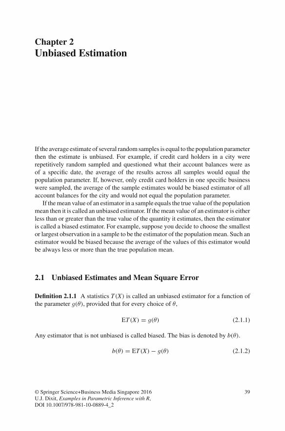
Chapter 2 Unbiased Estimation If the average estimate of several random samples is equal to the population parameter then the estimate is unbiased. For example, if credit card holders in a city were repetitively random sampled and questioned what their account balances were as of a specific date, the average of the results across all samples would equal the population parameter. If, however, only credit card holders in one specific business were sampled, the average of the sample estimates would be biased estimator of all account balances for the city and would not equal the population parameter. If the mean value of an estimator in a sample equals the true value of the population mean then it is called an unbiased estimator. If the mean value of an estimator is either less than or greater than the true value of the quantity it estimates, then the estimator is called a biased estimator. For example, suppose you decide to choose the smallest or largest observation in a sample to be the estimator of the population mean. Such an estimator would be biased because the average of the values of this estimator would be always less or more than the true population mean. 2.1 Unbiased Estimates and Mean Square Error Definition 2.1.1 A statistics T (X ) is called an unbiased estimator for a function of the parameter g(θ), provided that for every choice of θ, ET (X ) = g(θ) (2.1.1) Any estimator that is not unbiased is called biased. The bias is denoted by b(θ). b(θ) = ET (X ) − g(θ) (2.1.2) © Springer Science+Business Media Singapore 2016 U.J. Dixit, Examples in Parametric Inference with R, DOI 10.1007/978-981-10-0889-4_2 39

Welcome message from author
This document is posted to help you gain knowledge. Please leave a comment to let me know what you think about it! Share it to your friends and learn new things together.
Transcript
Chapter 2Unbiased Estimation
If the average estimate of several randomsamples is equal to the population parameterthen the estimate is unbiased. For example, if credit card holders in a city wererepetitively random sampled and questioned what their account balances were asof a specific date, the average of the results across all samples would equal thepopulation parameter. If, however, only credit card holders in one specific businesswere sampled, the average of the sample estimates would be biased estimator of allaccount balances for the city and would not equal the population parameter.
If themean value of an estimator in a sample equals the true value of the populationmean then it is called an unbiased estimator. If themean value of an estimator is eitherless than or greater than the true value of the quantity it estimates, then the estimatoris called a biased estimator. For example, suppose you decide to choose the smallestor largest observation in a sample to be the estimator of the population mean. Such anestimator would be biased because the average of the values of this estimator wouldbe always less or more than the true population mean.
2.1 Unbiased Estimates and Mean Square Error
Definition 2.1.1 A statistics T(X) is called an unbiased estimator for a function ofthe parameter g(θ), provided that for every choice of θ,
ET(X) = g(θ) (2.1.1)
Any estimator that is not unbiased is called biased. The bias is denoted by b(θ).
b(θ) = ET(X) − g(θ) (2.1.2)
© Springer Science+Business Media Singapore 2016U.J. Dixit, Examples in Parametric Inference with R,DOI 10.1007/978-981-10-0889-4_2
39
40 2 Unbiased Estimation
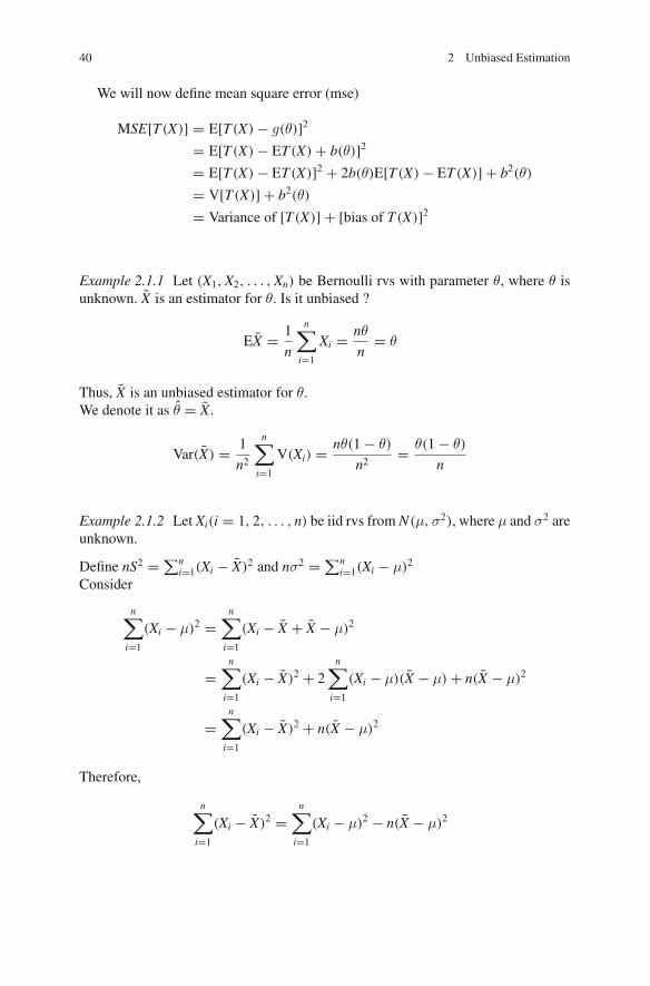
We will now define mean square error (mse)
MSE[T(X)] = E[T(X) − g(θ)]2= E[T(X) − ET(X) + b(θ)]2= E[T(X) − ET(X)]2 + 2b(θ)E[T(X) − ET(X)] + b2(θ)
= V[T(X)] + b2(θ)
= Variance of [T(X)] + [bias of T(X)]2
Example 2.1.1 Let (X1,X2, . . . ,Xn) be Bernoulli rvs with parameter θ, where θ isunknown. X̄ is an estimator for θ. Is it unbiased ?
EX̄ = 1
n
n∑
i=1
Xi = nθ
n= θ
Thus, X̄ is an unbiased estimator for θ.We denote it as θ̂ = X̄ .
Var(X̄) = 1
n2
n∑
i=1
V(Xi) = nθ(1 − θ)
n2= θ(1 − θ)
n
Example 2.1.2 Let Xi(i = 1, 2, . . . , n) be iid rvs from N(μ,σ2), where μ and σ2 areunknown.
Define nS2 =∑ni=1(Xi − X̄)2 and nσ2 =∑n
i=1(Xi − μ)2
Consider
n∑
i=1
(Xi − μ)2 =n∑
i=1
(Xi − X̄ + X̄ − μ)2
=n∑
i=1
(Xi − X̄)2 + 2n∑
i=1
(Xi − μ)(X̄ − μ) + n(X̄ − μ)2
=n∑
i=1
(Xi − X̄)2 + n(X̄ − μ)2
Therefore,
n∑
i=1
(Xi − X̄)2 =n∑
i=1
(Xi − μ)2 − n(X̄ − μ)2
2.1 Unbiased Estimates and Mean Square Error 41
E
[n∑
i=1
(Xi − X̄)2
]= E
[n∑
i=1
(Xi − μ)2
]− nE[(X̄ − μ)2]
= nσ2 − nσ2
n= nσ2 − σ2
Hence,
E(S2) = σ2 − σ2
n= σ2
(n − 1
n
)
Thus, S2 is a biased estimator of σ2.Hence
b(σ2) = σ2 − σ2
n− σ2 = −σ2
n
Further, nS2
n−1 is an unbiased estimator of σ2.
Example 2.1.3 Further, if (n − 1)S2 = ∑ni=1(Xi − X̄)2, then (n− 1)S2
σ2 has χ2 with(n − 1) df. Here, we examine whether S is an unbiased estimator of σ.
Let (n− 1)S2
σ2 = wThen
E(√w) =
∞∫
0
w12 e− w
2 wn−12 −1
�(n−12
)2
n−12
dw
= �(n2
)2
n2
�(n−12
)2
n−12
= �(n2
)2
12
�(n−12
)
E
[(n − 1)
12 S
σ
]= 2
12 �(n2
)
�(n−12
)
Hence
E(S) = 212 �(n2
)
�(n−12
) σ
(n − 1)12
=(
2
n − 1
) 12 �
(n2
)
�(n−12
)σ
Therefore,
E
(S
σ
)=(
2
n − 1
) 12 �
(n2
)
�(n−12
)
42 2 Unbiased Estimation
Therefore,
Bias(S) = σ
[(2
n − 1
) 12 �
(n2
)
�(n−12
) − 1
]
Example 2.1.4 For the family (1.5.4), p̂ is U-estimable and θ̂ is not U-estimable. For(p, θ), it can be easily seen that p̂ = r
n and Ep̂ = p. Next, we will show θ̂ is notU-estimable.
Suppose there exist a function h(r, z) such that
Eh(r, z) = θ ∀ (p, θ) ∈ �.
Since
EE[h(r, z)|r] = θ
We get
n∑
r=1
(n
r
)prqn−r
∞∫
0
h(r, z)e− z
θ zr−1dz
θr�(r)+ qnh(0, 0) = θ
Substituting pq = �, and dividing qn on both sides
n∑
r=1
�r
(n
r
) ∞∫
0
h(r, z)e− z
θ zr−1dz
θr�(r)+ h(0, 0) = θ(1 + �)n, Since q = (1 + �)−1
Comparing the coefficients of �r in both sides, we get, h(0, 0) = θ, which is acontradiction.Hence, there does not exist any unbiased estimator of θ. Thus θ is not U-estimable.
Example 2.1.5 Let X is N(0,σ2) and assume that we have one observation. What isthe unbiased estimator of σ2?
E(X) = 0
V(X) = EX2 − (EX)2 = σ2
2.1 Unbiased Estimates and Mean Square Error 43
Therefore,
E(X2) = σ2
Hence X2 is an unbiased estimator of σ2.
Example 2.1.6 Sometimes an unbiased estimator may be absurd.
Let the rv X be P(λ) and we want to estimate �(λ), where
�(λ) = exp[−kλ]; k > 0
Let T(X) = [−(k − 1)]x; k > 1
E[T(X)] =∞∑
x=0
[−(k − 1)]x e−λλx
x!
= e−λ∞∑
x=0
[−(k − 1)λ]xx!
= e−λe[−(k−1)λ]
= e−kλ
T(x) ={[−(k − 1)]x > 0; x is even and k > 1[−(k − 1)]x < 0; x is odd and k > 1
which is absurd since �(λ) is always positive.
Example 2.1.7 Unbiased estimator is not unique.
Let the rvsX1 andX2 areN(θ, 1).X1,X2, andαX1+(1−α)X2 are unbiased estimatorsof θ, 0 ≤ α ≤ 1.
Example 2.1.8 Let X1,X2, . . . ,Xn be iid rvs from Cauchy distribution with parame-ter θ. Find an unbiased estimator of θ.
Let
f (x|θ) = 1
π[1 + (x − θ)2] ; −∞ < x < ∞,−∞ < θ < ∞
F(x|θ) =x∫
−∞
dy
π[1 + (y − θ)2]
= 1
2+ 1
πtan−1(x − θ)
Let g(x(r)) be the pdf of X(r), where X(r) is the rth order statistics.
44 2 Unbiased Estimation
g(x(r)) = n!(n − r)!(r − 1)! f (x(r))[F(x(r))]r−1[1 − F(x(r))]n−r
= n!(n − r)!(r − 1)!
[1
π
1
[1 + (x(r) − θ)2]
][1
2+ 1
πtan−1(x(r) − θ)
]r−1 [ 12
− 1
πtan−1(x(r) − θ)
]n−r
E(X(r) − θ) = n!(n − r)!(r − 1)!
1
π
∞∫
−∞
x(r) − θ
[1 + (x(r) − θ)2][1
2+ 1
πtan−1(x(r) − θ)
]r−1
×[1
2− 1
πtan−1(x(r) − θ)n−r
]dx(r)
Let (x(r) − θ) = y
E(X(r) − θ) = Crn1
π
∞∫
−∞
y
1 + y2
[1
2+ 1
πtan−1 y
]r−1 [12
− 1
πtan−1 y
]n−r
dy,
where Crn = n!(n−r)!(r−1)!
Let
u = 1
2+ 1
πtan−1 y ⇒ u − 1
2= 1
πtan−1 y
⇒(u − 1
2
)π = tan−1 y ⇒ y = tan
(u − 1
2
)π ⇒ y = − cot πu
dy = π
[(cosπu)(cosπu)
sin2 πu+ sin πu
sin πu
]du
= π[cot2 πu + 1] = π[y2 + 1]du
E(X(r) − θ) = − n!(n − r)!(r − 1)!
1∫
0
ur−1(1 − u)n−r cot πudu
= −Crn
1∫
0
ur−1(1 − u)n−r cot πudu
2.1 Unbiased Estimates and Mean Square Error 45
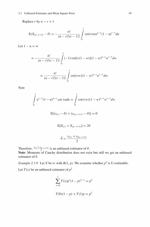
Replace r by n − r + 1
E(X(n−r+1) − θ) = − n!(n − r)!(r − 1)!
1∫
0
cot(πu)un−r(1 − u)r−1du
Let 1 − u = w
= − n!(n − r)!(r − 1)!
1∫
0
(−1) cot[π(1 − w)](1 − w)n−rwr−1dw
= n!(n − r)!(r − 1)!
1∫
0
cot(πw)(1 − w)n−rwr−1dw
Now
1∫
0
ur−1(1 − u)n−r cot πudu =1∫
0
cot(πw)(1 − w)n−rwr−1dw
E[(x(r) − θ) + (x(n−r+1) − θ)] = 0
E[X(r) + X(n−r+1)] = 2θ
θ̂ = x(r) + x(n−r+1)
2
Therefore, x(r) + x(n− r + 1)
2 is an unbiased estimator of θ.Note: Moments of Cauchy distribution does not exist but still we get an unbiasedestimator of θ.
Example 2.1.9 Let X be rv with B(1, p). We examine whether p2 is U-estimable.
Let T(x) be an unbiased estimator of p2
1∑
x=0
T(x)px(1 − p)1−x = p2
T(0)(1 − p) + T(1)p = p2
46 2 Unbiased Estimation
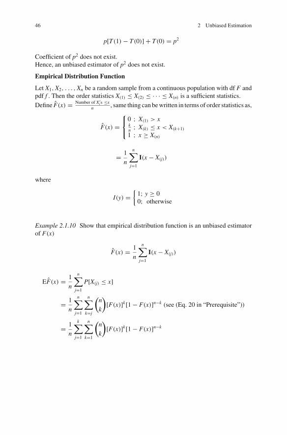
p[T(1) − T(0)] + T(0) = p2
Coefficient of p2 does not exist.Hence, an unbiased estimator of p2 does not exist.
Empirical Distribution Function
Let X1,X2, . . . ,Xn be a random sample from a continuous population with df F andpdf f . Then the order statistics X(1) ≤ X(2) ≤ · · · ≤ X(n) is a sufficient statistics.
Define F̂(x) = Number of X ′i s ≤x
n , same thing can bewritten in terms of order statistics as,
F̂(x) =⎧⎨
⎩
0 ; X(1) > xkn ; X(k) ≤ x < X(k+1)
1 ; x ≥ X(n)
= 1
n
n∑
j=1
I(x − X(j))
where
I(y) ={1; y ≥ 00; otherwise
Example 2.1.10 Show that empirical distribution function is an unbiased estimatorof F(x)
F̂(x) = 1
n
n∑
j=1
I(x − X(j))
EF̂(x) = 1
n
n∑
j=1
P[X(j) ≤ x]
= 1
n
n∑
j=1
n∑
k=j
(n
k
)[F(x)]k[1 − F(x)]n−k (see (Eq. 20 in “Prerequisite”))
= 1
n
k∑
j=1
n∑
k=1
(n
k
)[F(x)]k[1 − F(x)]n−k
2.1 Unbiased Estimates and Mean Square Error 47
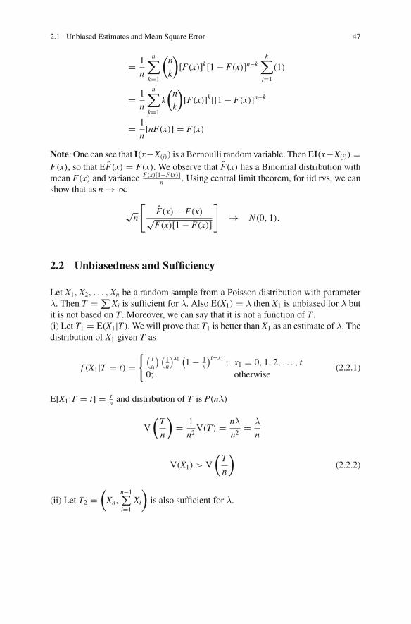
= 1
n
n∑
k=1
(n
k
)[F(x)]k[1 − F(x)]n−k
k∑
j=1
(1)
= 1
n
n∑
k=1
k
(n
k
)[F(x)]k[[1 − F(x)]n−k
= 1
n[nF(x)] = F(x)
Note: One can see that I(x−X(j)) is a Bernoulli random variable. Then EI(x−X(j)) =F(x), so that EF̂(x) = F(x). We observe that F̂(x) has a Binomial distribution withmean F(x) and variance F(x)[1−F(x)]
n . Using central limit theorem, for iid rvs, we canshow that as n → ∞
√n
[F̂(x) − F(x)√F(x)[1 − F(x)]
]→ N(0, 1).
2.2 Unbiasedness and Sufficiency
Let X1,X2, . . . ,Xn be a random sample from a Poisson distribution with parameterλ. Then T =∑Xi is sufficient for λ. Also E(X1) = λ then X1 is unbiased for λ butit is not based on T . Moreover, we can say that it is not a function of T .(i) Let T1 = E(X1|T). We will prove that T1 is better than X1 as an estimate of λ. Thedistribution of X1 given T as
f (X1|T = t) ={( t
x1
) (1n
)x1 (1 − 1n
)t−x1 ; x1 = 0, 1, 2, . . . , t0; otherwise
(2.2.1)
E[X1|T = t] = tn and distribution of T is P(nλ)
V
(T
n
)= 1
n2V(T) = nλ
n2= λ
n
V(X1) > V
(T
n
)(2.2.2)
(ii) Let T2 =(Xn,
n−1∑i=1
Xi
)is also sufficient for λ.
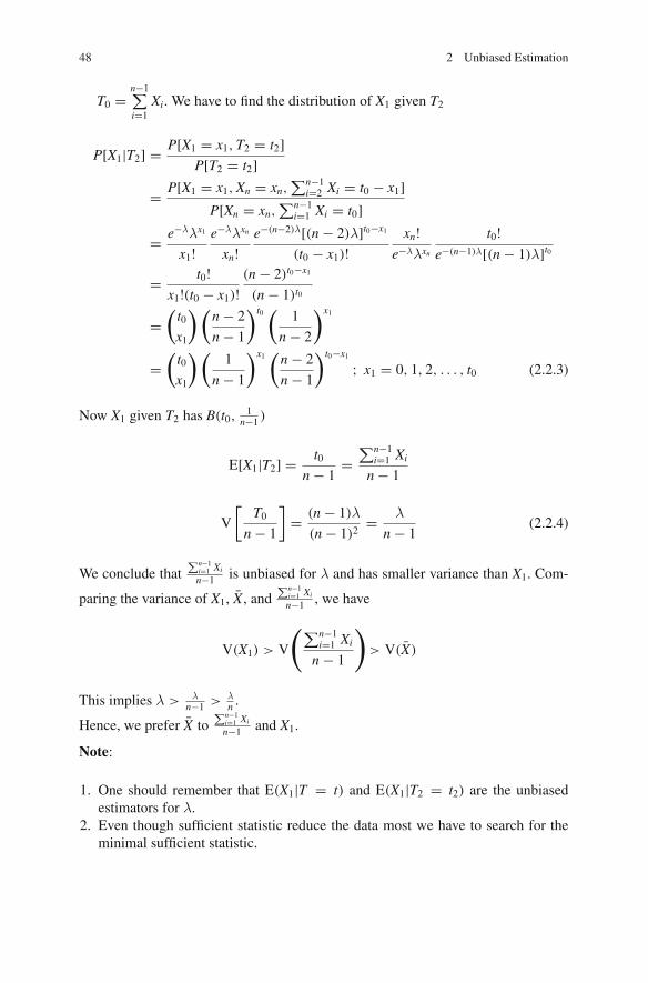
48 2 Unbiased Estimation
T0 =n−1∑i=1
Xi. We have to find the distribution of X1 given T2
P[X1|T2] = P[X1 = x1,T2 = t2]P[T2 = t2]
= P[X1 = x1,Xn = xn,∑n−1
i=2 Xi = t0 − x1]P[Xn = xn,
∑n−1i=1 Xi = t0]
= e−λλx1
x1!e−λλxn
xn!e−(n−2)λ[(n − 2)λ]t0−x1
(t0 − x1)!xn!
e−λλxn
t0!e−(n−1)λ[(n − 1)λ]t0
= t0!x1!(t0 − x1)!
(n − 2)t0−x1
(n − 1)t0
=(t0x1
)(n − 2
n − 1
)t0 ( 1
n − 2
)x1
=(t0x1
)(1
n − 1
)x1 (n − 2
n − 1
)t0−x1
; x1 = 0, 1, 2, . . . , t0 (2.2.3)
Now X1 given T2 has B(t0,1
n−1 )
E[X1|T2] = t0n − 1
=∑n−1
i=1 Xi
n − 1
V
[T0
n − 1
]= (n − 1)λ
(n − 1)2= λ
n − 1(2.2.4)
We conclude that∑n−1
i=1 Xi
n−1 is unbiased for λ and has smaller variance than X1. Com-
paring the variance of X1, X̄, and∑n−1
i=1 Xi
n−1 , we have
V(X1) > V
(∑n−1i=1 Xi
n − 1
)> V(X̄)
This implies λ > λn−1 > λ
n .
Hence, we prefer X̄ to∑n−1
i=1 Xi
n−1 and X1.
Note:
1. One should remember that E(X1|T = t) and E(X1|T2 = t2) are the unbiasedestimators for λ.
2. Even though sufficient statistic reduce the data most we have to search for theminimal sufficient statistic.
2.2 Unbiasedness and Sufficiency 49
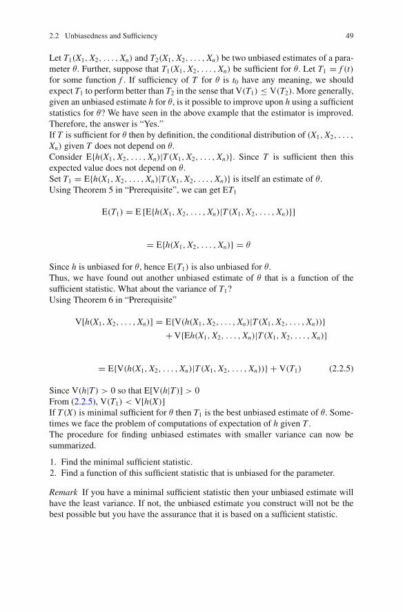
Let T1(X1,X2, . . . ,Xn) and T2(X1,X2, . . . ,Xn) be two unbiased estimates of a para-meter θ. Further, suppose that T1(X1,X2, . . . ,Xn) be sufficient for θ. Let T1 = f (t)for some function f . If sufficiency of T for θ is t0 have any meaning, we shouldexpect T1 to perform better than T2 in the sense that V(T1) ≤ V(T2). More generally,given an unbiased estimate h for θ, is it possible to improve upon h using a sufficientstatistics for θ? We have seen in the above example that the estimator is improved.Therefore, the answer is “Yes.”If T is sufficient for θ then by definition, the conditional distribution of (X1,X2, . . . ,
Xn) given T does not depend on θ.Consider E{h(X1,X2, . . . ,Xn)|T(X1,X2, . . . ,Xn)}. Since T is sufficient then thisexpected value does not depend on θ.Set T1 = E{h(X1,X2, . . . ,Xn)|T(X1,X2, . . . ,Xn)} is itself an estimate of θ.Using Theorem 5 in “Prerequisite”, we can get ET1
E(T1) = E [E{h(X1,X2, . . . ,Xn)|T(X1,X2, . . . ,Xn)}]
= E{h(X1,X2, . . . ,Xn)} = θ
Since h is unbiased for θ, hence E(T1) is also unbiased for θ.Thus, we have found out another unbiased estimate of θ that is a function of thesufficient statistic. What about the variance of T1?Using Theorem 6 in “Prerequisite”
V[h(X1,X2, . . . ,Xn)] = E{V(h(X1,X2, . . . ,Xn)|T(X1,X2, . . . ,Xn))}+V{Eh(X1,X2, . . . ,Xn)|T(X1,X2, . . . ,Xn)}
= E{V(h(X1,X2, . . . ,Xn)|T(X1,X2, . . . ,Xn))} + V(T1) (2.2.5)
Since V(h|T) > 0 so that E[V(h|T)] > 0From (2.2.5), V(T1) < V[h(X)]If T(X) is minimal sufficient for θ then T1 is the best unbiased estimate of θ. Some-times we face the problem of computations of expectation of h given T .The procedure for finding unbiased estimates with smaller variance can now besummarized.
1. Find the minimal sufficient statistic.2. Find a function of this sufficient statistic that is unbiased for the parameter.
Remark If you have a minimal sufficient statistic then your unbiased estimate willhave the least variance. If not, the unbiased estimate you construct will not be thebest possible but you have the assurance that it is based on a sufficient statistic.
50 2 Unbiased Estimation
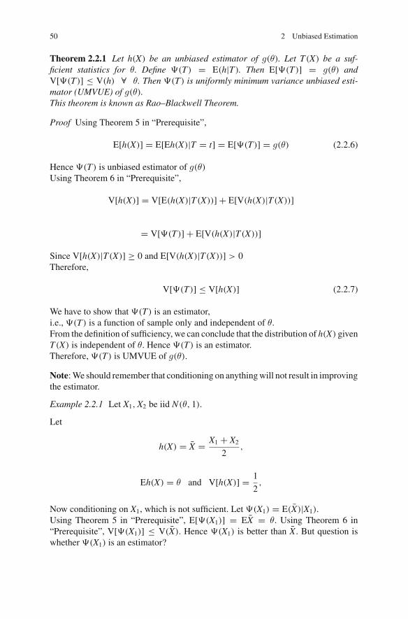
Theorem 2.2.1 Let h(X) be an unbiased estimator of g(θ). Let T(X) be a suf-ficient statistics for θ. Define �(T) = E(h|T). Then E[�(T)] = g(θ) andV[�(T)] ≤ V(h) ∀ θ. Then �(T) is uniformly minimum variance unbiased esti-mator (UMVUE) of g(θ).This theorem is known as Rao–Blackwell Theorem.
Proof Using Theorem 5 in “Prerequisite”,
E[h(X)] = E[Eh(X)|T = t] = E[�(T)] = g(θ) (2.2.6)
Hence �(T) is unbiased estimator of g(θ)Using Theorem 6 in “Prerequisite”,
V[h(X)] = V[E(h(X)|T(X))] + E[V(h(X)|T(X))]
= V[�(T)] + E[V(h(X)|T(X))]
Since V[h(X)|T(X)] ≥ 0 and E[V(h(X)|T(X))] > 0Therefore,
V[�(T)] ≤ V[h(X)] (2.2.7)
We have to show that �(T) is an estimator,i.e., �(T) is a function of sample only and independent of θ.From the definition of sufficiency, we can conclude that the distribution of h(X) givenT(X) is independent of θ. Hence �(T) is an estimator.Therefore, �(T) is UMVUE of g(θ).
Note:We should remember that conditioning on anythingwill not result in improvingthe estimator.
Example 2.2.1 Let X1,X2 be iid N(θ, 1).
Let
h(X) = X̄ = X1 + X2
2,
Eh(X) = θ and V[h(X)] = 1
2,
Now conditioning on X1, which is not sufficient. Let �(X1) = E(X̄)|X1).Using Theorem 5 in “Prerequisite”, E[�(X1)] = EX̄ = θ. Using Theorem 6 in“Prerequisite”, V[�(X1)] ≤ V(X̄). Hence �(X1) is better than X̄. But question iswhether �(X1) is an estimator?
2.2 Unbiasedness and Sufficiency 51
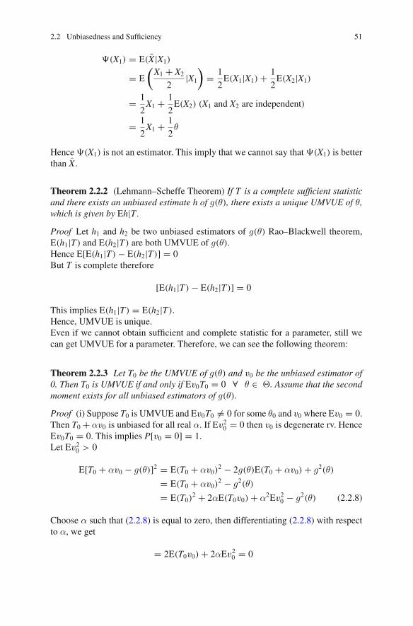
�(X1) = E(X̄|X1)
= E
(X1 + X2
2|X1
)= 1
2E(X1|X1) + 1
2E(X2|X1)
= 1
2X1 + 1
2E(X2) (X1 and X2 are independent)
= 1
2X1 + 1
2θ
Hence �(X1) is not an estimator. This imply that we cannot say that �(X1) is betterthan X̄.
Theorem 2.2.2 (Lehmann–Scheffe Theorem) If T is a complete sufficient statisticand there exists an unbiased estimate h of g(θ), there exists a unique UMVUE of θ,which is given by Eh|T.Proof Let h1 and h2 be two unbiased estimators of g(θ) Rao–Blackwell theorem,E(h1|T) and E(h2|T) are both UMVUE of g(θ).Hence E[E(h1|T) − E(h2|T)] = 0But T is complete therefore
[E(h1|T) − E(h2|T)] = 0
This implies E(h1|T) = E(h2|T).Hence, UMVUE is unique.Even if we cannot obtain sufficient and complete statistic for a parameter, still wecan get UMVUE for a parameter. Therefore, we can see the following theorem:
Theorem 2.2.3 Let T0 be the UMVUE of g(θ) and v0 be the unbiased estimator of0. Then T0 is UMVUE if and only if Ev0T0 = 0 ∀ θ ∈ �. Assume that the secondmoment exists for all unbiased estimators of g(θ).
Proof (i) Suppose T0 is UMVUE and Ev0T0 �= 0 for some θ0 and v0 where Ev0 = 0.Then T0 + αv0 is unbiased for all real α. If Ev2
0 = 0 then v0 is degenerate rv. HenceEv0T0 = 0. This implies P[v0 = 0] = 1.Let Ev2
0 > 0
E[T0 + αv0 − g(θ)]2 = E(T0 + αv0)2 − 2g(θ)E(T0 + αv0) + g2(θ)
= E(T0 + αv0)2 − g2(θ)
= E(T0)2 + 2αE(T0v0) + α2Ev2
0 − g2(θ) (2.2.8)
Choose α such that (2.2.8) is equal to zero, then differentiating (2.2.8) with respectto α, we get
= 2E(T0v0) + 2αEv20 = 0
52 2 Unbiased Estimation
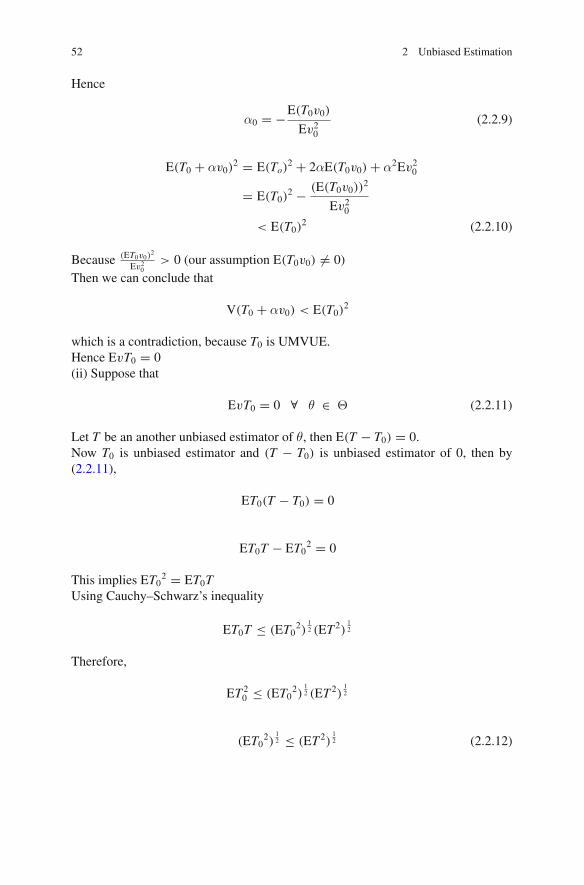
Hence
α0 = −E(T0v0)
Ev20
(2.2.9)
E(T0 + αv0)2 = E(To)
2 + 2αE(T0v0) + α2Ev20
= E(T0)2 − (E(T0v0))2
Ev20
< E(T0)2 (2.2.10)
Because (ET0v0)2
Ev20> 0 (our assumption E(T0v0) �= 0)
Then we can conclude that
V(T0 + αv0) < E(T0)2
which is a contradiction, because T0 is UMVUE.Hence EvT0 = 0(ii) Suppose that
EvT0 = 0 ∀ θ ∈ � (2.2.11)
Let T be an another unbiased estimator of θ, then E(T − T0) = 0.Now T0 is unbiased estimator and (T − T0) is unbiased estimator of 0, then by(2.2.11),
ET0(T − T0) = 0
ET0T − ET02 = 0
This implies ET02 = ET0TUsing Cauchy–Schwarz’s inequality
ET0T ≤ (ET02)
12 (ET 2)
12
Therefore,
ET 20 ≤ (ET0
2)12 (ET 2)
12
(ET02)
12 ≤ (ET 2)
12 (2.2.12)
2.2 Unbiasedness and Sufficiency 53
Now if ET02 = 0 then P[T0 = 0] = 1Then (2.2.12) is true.Next, if ET02 > 0 then also (2.2.12) is trueHence V(T0) ≤ V(T) ⇒ T0 is UMVUE.
Remark Wewould like to mention the comment made by Casella and Berger (2002).“An unbiased estimator of 0 is nothing more than random noise; that is there is noinformation in an estimator of 0. It makes sense that most sensible way to estimate0 is with 0, not with random noise. Therefore, if an estimator could be improved byadding random noise to it, the estimator probably is defective.”Casella and Berger (2002) gave an interesting characterization of best unbiased esti-mators.
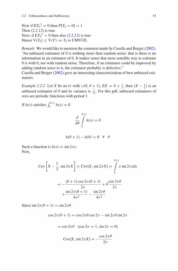
Example 2.2.2 Let X be an rv with ∪(θ, θ + 1), EX = θ + 12 , then (X − 1
2 ) is anunbiased estimator of θ and its variance is 1
12 . For this pdf, unbiased estimators ofzero are periodic functions with period 1.
If h(x) satisfies∫ θ+1θ h(x) = 0
d
dθ
θ+1∫
θ
h(x) = 0
h(θ + 1) − h(θ) = 0 ∀ θ
Such a function is h(x) = sin 2πx.Now,
Cov
[X − 1
2, sin 2πX
]= Cov[X, sin 2πX] =
θ+1∫
θ
x sin 2πxdx
= − (θ + 1) cos 2π(θ + 1)
2π+ θ
cos 2πθ
2π
+ sin 2π(θ + 1)
4π2− sin 2πθ
4π2
Since sin 2π(θ + 1) = sin 2πθ
cos 2π(θ + 1) = cos 2πθ cos 2π − sin 2πθ sin 2π
= cos 2πθ (cos 2π = 1, sin 2π = 0)
Cov[X, sin 2πX] = −cos 2πθ
2π
54 2 Unbiased Estimation
Hence(X − 1
2
)is correlated with an unbiased estimator of zero. Therefore,
(X − 1
2
)
cannot be the best unbiased estimator of θ.
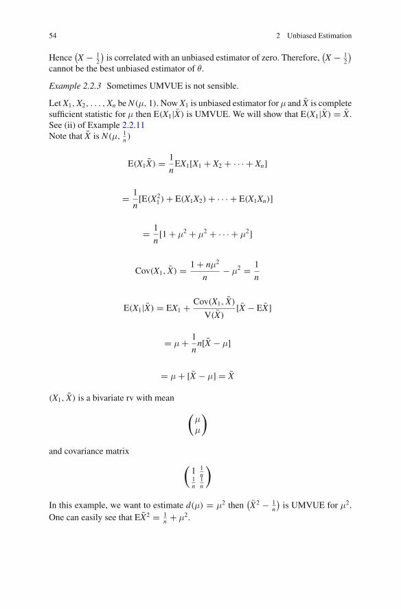
Example 2.2.3 Sometimes UMVUE is not sensible.
Let X1,X2, . . . ,Xn beN(μ, 1). Now X1 is unbiased estimator for μ and X̄ is completesufficient statistic for μ then E(X1|X̄) is UMVUE. We will show that E(X1|X̄) = X̄.See (ii) of Example 2.2.11Note that X̄ is N(μ, 1
n )
E(X1X̄) = 1
nEX1[X1 + X2 + · · · + Xn]
= 1
n[E(X2
1 ) + E(X1X2) + · · · + E(X1Xn)]
= 1
n[1 + μ2 + μ2 + · · · + μ2]
Cov(X1, X̄) = 1 + nμ2
n− μ2 = 1
n
E(X1|X̄) = EX1 + Cov(X1, X̄)
V(X̄)[X̄ − EX̄]
= μ + 1
nn[X̄ − μ]
= μ + [X̄ − μ] = X̄
(X1, X̄) is a bivariate rv with mean
(μμ
)
and covariance matrix(1 1
n1n
1n
)
In this example, we want to estimate d(μ) = μ2 then(X̄2 − 1
n
)is UMVUE for μ2.
One can easily see that EX̄2 = 1n + μ2.
2.2 Unbiasedness and Sufficiency 55
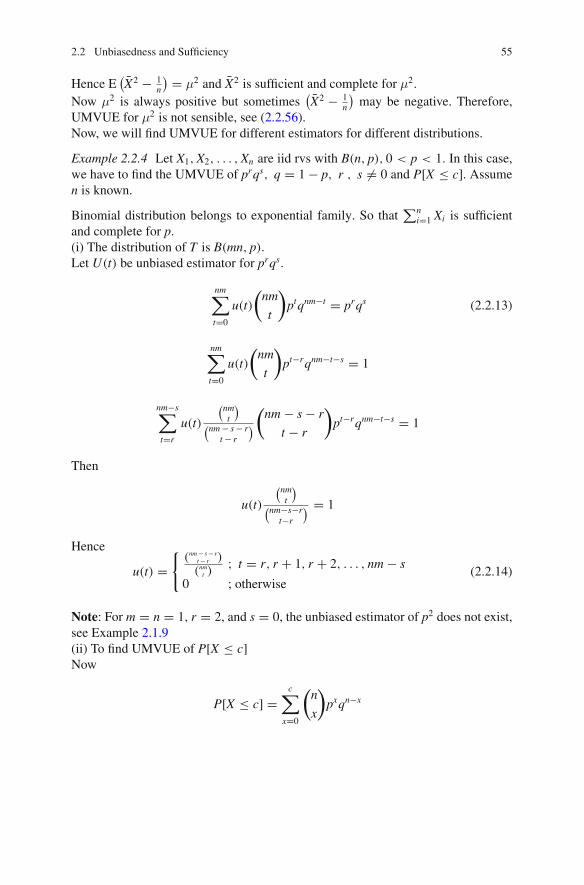
Hence E(X̄2 − 1
n
) = μ2 and X̄2 is sufficient and complete for μ2.Now μ2 is always positive but sometimes
(X̄2 − 1
n
)may be negative. Therefore,
UMVUE for μ2 is not sensible, see (2.2.56).Now, we will find UMVUE for different estimators for different distributions.
Example 2.2.4 Let X1,X2, . . . ,Xn are iid rvs with B(n, p), 0 < p < 1. In this case,we have to find the UMVUE of prqs, q = 1 − p, r , s �= 0 and P[X ≤ c]. Assumen is known.
Binomial distribution belongs to exponential family. So that∑n
i=1 Xi is sufficientand complete for p.(i) The distribution of T is B(mn, p).Let U(t) be unbiased estimator for prqs.
nm∑
t=0
u(t)
(nm
t
)ptqnm−t = prqs (2.2.13)
nm∑
t=0
u(t)
(nm
t
)pt−rqnm−t−s = 1
nm−s∑
t=r
u(t)
(nmt
)(nm− s− r
t − r
)(nm − s − r
t − r
)pt−rqnm−t−s = 1
Then
u(t)
(nmt
)(nm−s−r
t−r
) = 1
Hence
u(t) ={
(nm− s− rt − r )(nmt )
; t = r, r + 1, r + 2, . . . , nm − s
0 ; otherwise(2.2.14)
Note: For m = n = 1, r = 2, and s = 0, the unbiased estimator of p2 does not exist,see Example 2.1.9(ii) To find UMVUE of P[X ≤ c]Now
P[X ≤ c] =c∑
x=0
(n
x
)pxqn−x
56 2 Unbiased Estimation
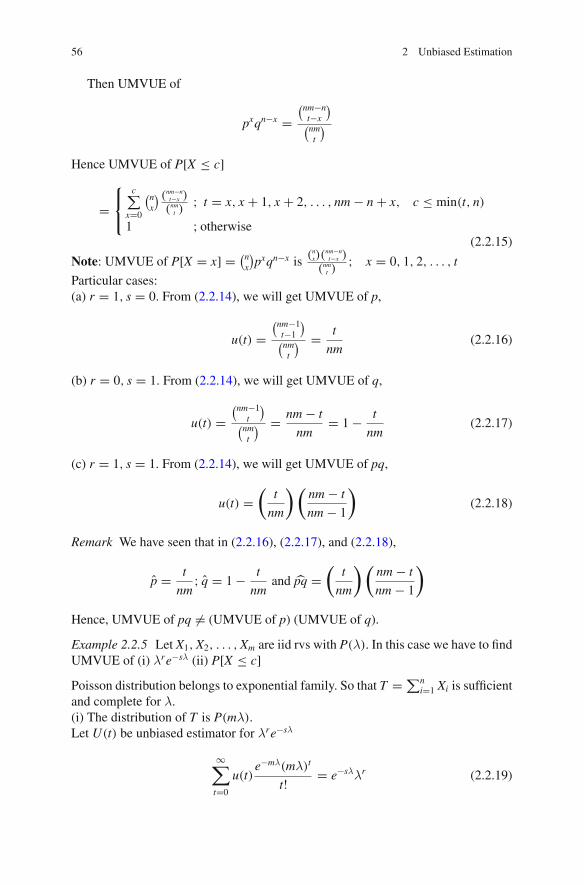
Then UMVUE of
pxqn−x =(nm−n
t−x
)(nm
t
)
Hence UMVUE of P[X ≤ c]
=⎧⎨
⎩
c∑x=0
(nx
) (nm−nt−x )(nmt )
; t = x, x + 1, x + 2, . . . , nm − n + x, c ≤ min(t, n)
1 ; otherwise(2.2.15)
Note: UMVUE of P[X = x] = (nx)pxqn−x is (nx)(
nm−nt−x )
(nmt ); x = 0, 1, 2, . . . , t
Particular cases:(a) r = 1, s = 0. From (2.2.14), we will get UMVUE of p,
u(t) =(nm−1
t−1
)(nm
t
) = t
nm(2.2.16)
(b) r = 0, s = 1. From (2.2.14), we will get UMVUE of q,
u(t) =(nm−1
t
)(nm
t
) = nm − t
nm= 1 − t
nm(2.2.17)
(c) r = 1, s = 1. From (2.2.14), we will get UMVUE of pq,
u(t) =(
t
nm
)(nm − t
nm − 1
)(2.2.18)
Remark We have seen that in (2.2.16), (2.2.17), and (2.2.18),
p̂ = t
nm; q̂ = 1 − t
nmand p̂q =
(t
nm
)(nm − t
nm − 1
)
Hence, UMVUE of pq �= (UMVUE of p) (UMVUE of q).
Example 2.2.5 Let X1,X2, . . . ,Xm are iid rvs with P(λ). In this case we have to findUMVUE of (i) λre−sλ (ii) P[X ≤ c]Poisson distribution belongs to exponential family. So that T =∑n
i=1 Xi is sufficientand complete for λ.(i) The distribution of T is P(mλ).Let U(t) be unbiased estimator for λre−sλ
∞∑
t=0
u(t)e−mλ(mλ)t
t! = e−sλλr (2.2.19)
2.2 Unbiasedness and Sufficiency 57
∞∑
t=0
u(t)e−(m−s)λmtλt−r
t! = 1
∞∑
t=r
u(t)mt
(m − s)t−r
(t − r)!t!
e−(m−s)λ[(m − s)λ]t−r
(t − r)! = 1
Then
u(t)mt
(m − s)t−r
(t − r)!t! = 1
u(t) ={
(m− s)t−r
mtt!
(t−r)! ; t = r, r + 1, . . . , s ≤ m0 ; otherwise
(2.2.20)
(ii) To find UMVUE of P[X ≤ c]
P[X ≤ c] =c∑
x=0
e−λλx
x!
Now, UMVUE of e−λλx is (m−1)(t−x)
mtt!
(t−x)!UMVUE of P[X ≤ c]
=c∑
x=0
t!(t − x)!x!
(m − 1
m
)t ( 1
m − 1
)x
={∑c
x=0
(tx
) (1m
)x (m−1m
)t−x ; c ≤ t1 ; otherwise
(2.2.21)
Remark UMVUE of P[X = x] = e−λλx
x! is(tx
) (1m
)x (m−1m
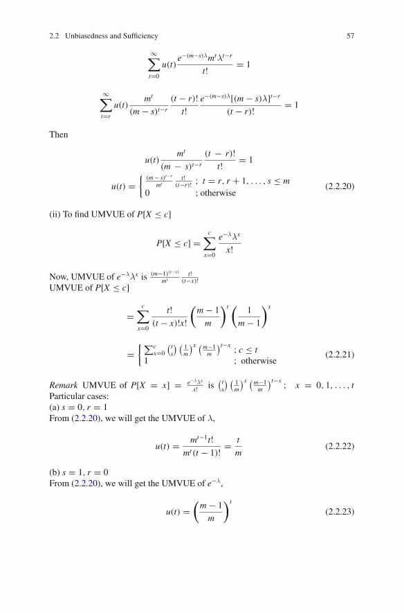
)t−x ; x = 0, 1, . . . , tParticular cases:(a) s = 0, r = 1From (2.2.20), we will get the UMVUE of λ,
u(t) = mt−1t!mt(t − 1)! = t
m(2.2.22)
(b) s = 1, r = 0From (2.2.20), we will get the UMVUE of e−λ,
u(t) =(m − 1
m
)t
(2.2.23)
58 2 Unbiased Estimation
(c) s = 1, r = 1From (2.2.20), we will get the UMVUE of λe−λ
u(t) = (m − 1)t−1t!mt(t − 1)! =
(m − 1
m
)t t
m − 1(2.2.24)
Remark UMVUE of λe−λ �= (UMVUE of λ)(UMVUE of e−λ)
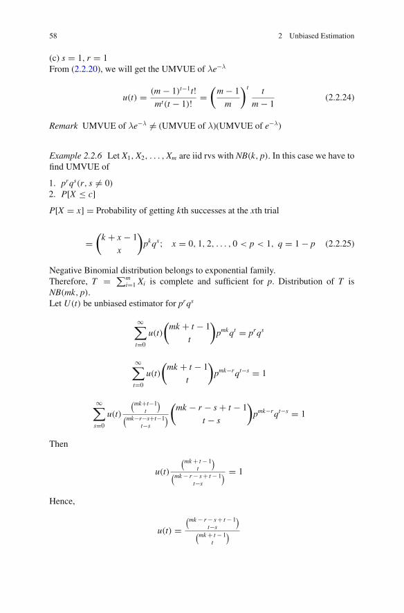
Example 2.2.6 Let X1,X2, . . . ,Xm are iid rvs with NB(k, p). In this case we have tofind UMVUE of
1. prqs(r, s �= 0)2. P[X ≤ c]P[X = x] = Probability of getting kth successes at the xth trial
=(k + x − 1
x
)pkqx; x = 0, 1, 2, . . . , 0 < p < 1, q = 1 − p (2.2.25)
Negative Binomial distribution belongs to exponential family.Therefore, T = ∑m
i=1 Xi is complete and sufficient for p. Distribution of T isNB(mk, p).Let U(t) be unbiased estimator for prqs
∞∑
t=0
u(t)
(mk + t − 1
t
)pmkqt = prqs
∞∑
t=0
u(t)
(mk + t − 1
t
)pmk−rqt−s = 1
∞∑
s=0
u(t)
(mk+t−1t
)(mk−r−s+t−1
t−s
)(mk − r − s + t − 1
t − s
)pmk−rqt−s = 1
Then
u(t)
(mk + t − 1t
)(mk − r − s+ t − 1
t−s
) = 1
Hence,
u(t) =(mk − r − s+ t − 1
t−s
)(mk + t − 1
t
)
2.2 Unbiasedness and Sufficiency 59
u(t) ={
(mk−r−s+t−1t−s )
(mk+t−1t )
; t = s, s + 1, . . . , r ≤ mk
0 ; otherwise(2.2.26)
(ii) To find UMVUE of P[X ≤ c]
P[X ≤ c] =c∑
x=0
(k + x − 1
x
)pkqx
Now UMVUE of pkqx = (mk−k−x+tt−x )
(mk+t−1t )
UMVUE of P[X ≤ c]
={∑c
x=0(k+x−1
x )(mk−k−x+tt−x )
(mk+t−1t )
; t = x, x + 1, . . .
1 ; otherwise.(2.2.27)
Remark UMVUE of P[X = x] = (k+x−1x
)pkqx is (k+x−1
x )(mk−k−x+tt−x )
(mk+t−1t )
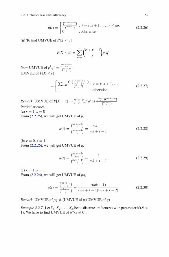
Particular cases:(a) r = 1, s = 0From (2.2.26), we will get UMVUE of p,
u(t) =(mk+t−2
t
)(mk+t−1
t
) = mk − 1
mk + t − 1(2.2.28)
(b) r = 0, s = 1From (2.2.26), we will get UMVUE of q,
u(t) =(mk+t−2
t−1
)(mk+t−1
t
) = t
mk + t − 1(2.2.29)
(c) r = 1, s = 1From (2.2.26), we will get UMVUE of pq,
u(t) =(mk+t−3
t−1
)(mk+t−1
t
) = t(mk − 1)
(mk + t − 1)(mk + t − 2)(2.2.30)
Remark UMVUE of pq �= (UMVUE of p)(UMVUE of q)
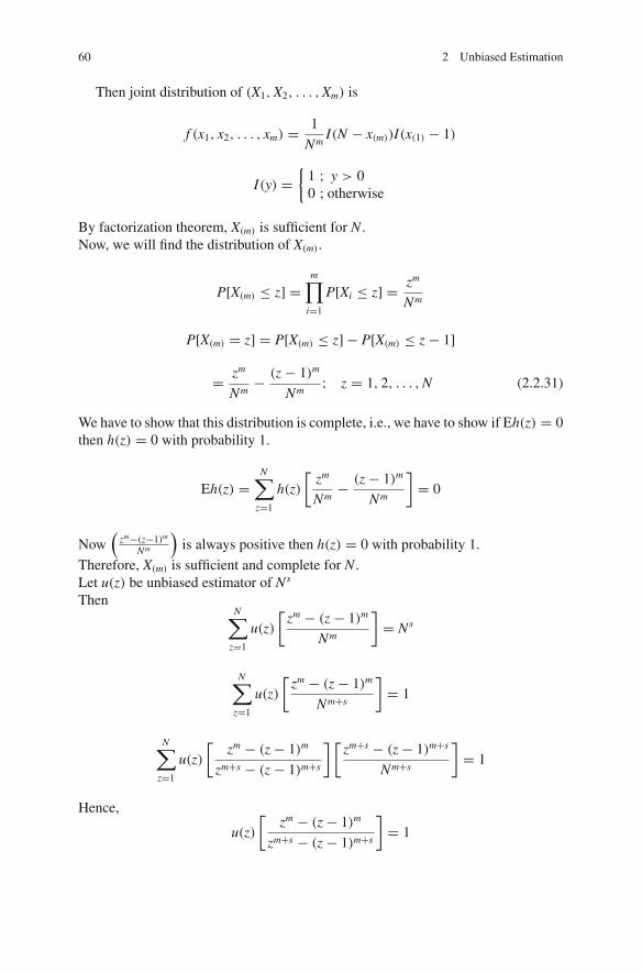
Example 2.2.7 LetX1,X2, . . . ,Xm be iid discrete uniform rvswith parameterN(N >
1). We have to find UMVUE of Ns(s �= 0).
60 2 Unbiased Estimation
Then joint distribution of (X1,X2, . . . ,Xm) is
f (x1, x2, . . . , xm) = 1
NmI(N − x(m))I(x(1) − 1)
I(y) ={1 ; y > 00 ; otherwise
By factorization theorem, X(m) is sufficient for N .Now, we will find the distribution of X(m).
P[X(m) ≤ z] =m∏
i=1
P[Xi ≤ z] = zm
Nm
P[X(m) = z] = P[X(m) ≤ z] − P[X(m) ≤ z − 1]
= zm
Nm− (z − 1)m
Nm; z = 1, 2, . . . ,N (2.2.31)
We have to show that this distribution is complete, i.e., we have to show if Eh(z) = 0then h(z) = 0 with probability 1.
Eh(z) =N∑
z=1
h(z)
[zm
Nm− (z − 1)m
Nm
]= 0
Now(zm−(z−1)m
Nm
)is always positive then h(z) = 0 with probability 1.
Therefore, X(m) is sufficient and complete for N .Let u(z) be unbiased estimator of Ns
ThenN∑
z=1
u(z)
[zm − (z − 1)m
Nm
]= Ns
N∑
z=1
u(z)
[zm − (z − 1)m
Nm+s
]= 1
N∑
z=1
u(z)
[zm − (z − 1)m
zm+s − (z − 1)m+s
] [zm+s − (z − 1)m+s
Nm+s
]= 1
Hence,
u(z)
[zm − (z − 1)m
zm+s − (z − 1)m+s
]= 1
2.2 Unbiasedness and Sufficiency 61
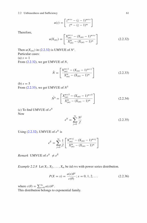
u(z) =[zm+s − (z − 1)m+s
zm − (z − 1)m
]
Therefore,
u(X(m)) =[Xm+s
(m) − (X(m) − 1)m+s
Xm(m) − (X(m) − 1)m
](2.2.32)
Then u(X(m)) in (2.2.32) is UMVUE of Ns.Particular cases:(a) s = 1From (2.2.32), we get UMVUE of N ,
N̂ =[Xm+1
(m) − (X(m) − 1)m+1
Xm(m) − (X(m) − 1)m
](2.2.33)
(b) s = 5From (2.2.33), we get UMVUE of N5
N̂5 =[Xm+5
(m) − (X(m) − 1)m+5
Xm(m) − (X(m) − 1)m
](2.2.34)
(c) To find UMVUE of eN
Now
eN =∞∑
j=0
Nj
j! (2.2.35)
Using (2.2.32), UMVUE of eN is
eN̂ =∞∑
j=0
1
j!
[Xm+j
(m) − (X(m) − 1)m+j
Xm(m) − (X(m) − 1)m
]
Remark UMVUE of eN �= eN̂
Example 2.2.8 Let X1,X2, . . . ,Xm be iid rvs with power series distribution.
P(X = x) = a(x)θx
c(θ); x = 0, 1, 2, . . . (2.2.36)
where c(θ) =∑∞x=0 a(x)θ
x.This distribution belongs to exponential family.
62 2 Unbiased Estimation
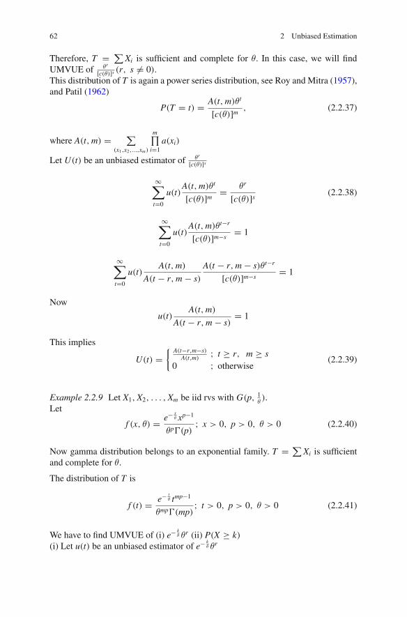
Therefore, T = ∑Xi is sufficient and complete for θ. In this case, we will find
UMVUE of θr
[c(θ)]s (r, s �= 0).This distribution of T is again a power series distribution, see Roy and Mitra (1957),and Patil (1962)
P(T = t) = A(t,m)θt
[c(θ)]m , (2.2.37)
where A(t,m) = ∑(x1,x2,...,xm)
m∏i=1
a(xi)
Let U(t) be an unbiased estimator of θr
[c(θ)]s
∞∑
t=0
u(t)A(t,m)θt
[c(θ)]m = θr
[c(θ)]s (2.2.38)
∞∑
t=0
u(t)A(t,m)θt−r
[c(θ)]m−s= 1
∞∑
t=0
u(t)A(t,m)
A(t − r,m − s)
A(t − r,m − s)θt−r
[c(θ)]m−s= 1
Now
u(t)A(t,m)
A(t − r,m − s)= 1
This implies
U(t) ={ A(t−r,m−s)
A(t,m); t ≥ r, m ≥ s
0 ; otherwise(2.2.39)
Example 2.2.9 Let X1,X2, . . . ,Xm be iid rvs with G(p, 1θ).
Let
f (x, θ) = e− xθ xp−1
θp�(p); x > 0, p > 0, θ > 0 (2.2.40)
Now gamma distribution belongs to an exponential family. T = ∑Xi is sufficient
and complete for θ.
The distribution of T is
f (t) = e− tθ tmp−1
θmp�(mp); t > 0, p > 0, θ > 0 (2.2.41)
We have to find UMVUE of (i) e− kθ θr (ii) P(X ≥ k)
(i) Let u(t) be an unbiased estimator of e− kθ θr
2.2 Unbiasedness and Sufficiency 63
∞∫
0
u(t)e− t
θ tmp−1
θmp�(mp)= e− k
θ θr
∞∫
0
u(t)e− t−k
θ tmp−1
θmp+r�(mp)= 1
∞∫
k
(u(t)
tmp−1�(mp + r)
(t − k)mp+r−1�(mp)
)(e− t−k
θ (t − k)mp+r−1
θmp+r�(mp + r)
)dt = 1
Then,
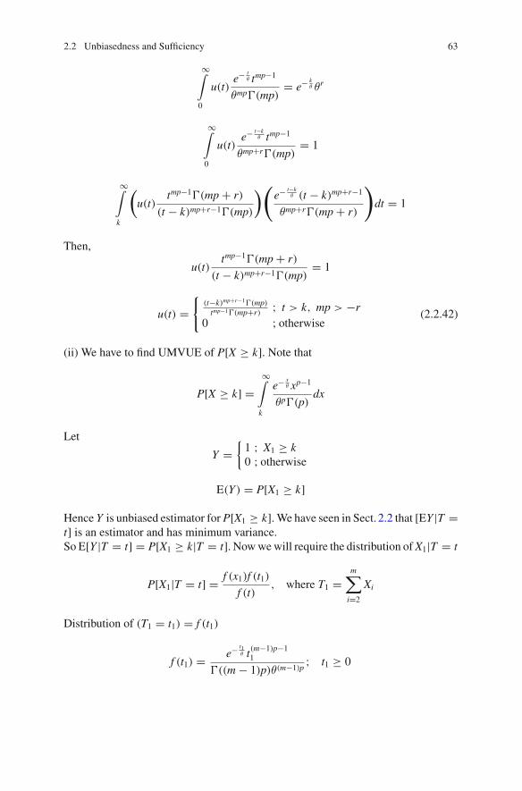
u(t)tmp−1�(mp + r)
(t − k)mp+r−1�(mp)= 1
u(t) ={
(t−k)mp+r−1�(mp)tmp−1�(mp+r) ; t > k, mp > −r
0 ; otherwise(2.2.42)
(ii) We have to find UMVUE of P[X ≥ k]. Note that
P[X ≥ k] =∞∫
k
e− xθ xp−1
θp�(p)dx
Let
Y ={1 ; X1 ≥ k0 ; otherwise
E(Y) = P[X1 ≥ k]
Hence Y is unbiased estimator for P[X1 ≥ k]. We have seen in Sect. 2.2 that [EY |T =t] is an estimator and has minimum variance.So E[Y |T = t] = P[X1 ≥ k|T = t]. Nowwewill require the distribution ofX1|T = t
P[X1|T = t] = f (x1)f (t1)
f (t), where T1 =
m∑
i=2
Xi
Distribution of (T1 = t1) = f (t1)
f (t1) = e− t1θ t(m−1)p−1
1
�((m − 1)p)θ(m−1)p; t1 ≥ 0
64 2 Unbiased Estimation
P[X1|T = t] = e− x1θ xp−1
1
�(p)θpe− t1
θ t(m−1)p−11
�((m − 1)p)θ(m−1)p
�(mp)θmp
e− tθ tmp−1
=( x1
t
)p−1 (1 − x1
t
)(m−1)p−1
tβ(p, (m − 1)p); 0 ≤ x1
t≤ 1 (2.2.43)
E[Y |T = t] = P[X1 ≥ k|T = t] =t∫
k
( x1t
)p−1 (1 − x1
t
)(m−1)p−1
tβ(p, (m − 1)p)dx1
Let x1t = w
=1∫
kt
wp−1(1 − w)(m−1)p−1
β(p, (m − 1)p)dw
= 1 −kt∫
0
wp−1(1 − w)(m−1)p−1
β(p, (m − 1)p)dw (2.2.44)
P[X1 ≥ k|T = t] ={1 − I k
t(p,mp − p) ; 0 < k < t
0 ; k ≥ t
Now
P[X ≥ k] =∞∫
k
e− xθ xp−1
θp�(p)dx
1 − I kθ(p) = Incomplete Gamma function. (2.2.45)
Hence UMVUE of 1− I kθ(p) is given by incomplete Beta function 1− I k
t(p,mp−p).
Note: Student should use R or Minitab software to calculate UMVUE.
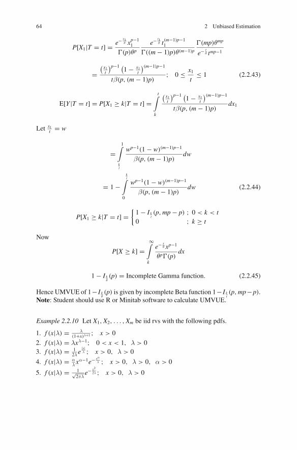
Example 2.2.10 Let X1,X2, . . . ,Xm be iid rvs with the following pdfs.
1. f (x|λ) = λ(1+x)λ+1 ; x > 0
2. f (x|λ) = λxλ−1; 0 < x < 1, λ > 03. f (x|λ) = 1
2λe|x|λ ; x > 0, λ > 0
4. f (x|λ) = αλxα−1e− xα
λ ; x > 0, λ > 0, α > 0
5. f (x|λ) = 1√2πλ
e− x2
2λ ; x > 0, λ > 0
2.2 Unbiasedness and Sufficiency 65
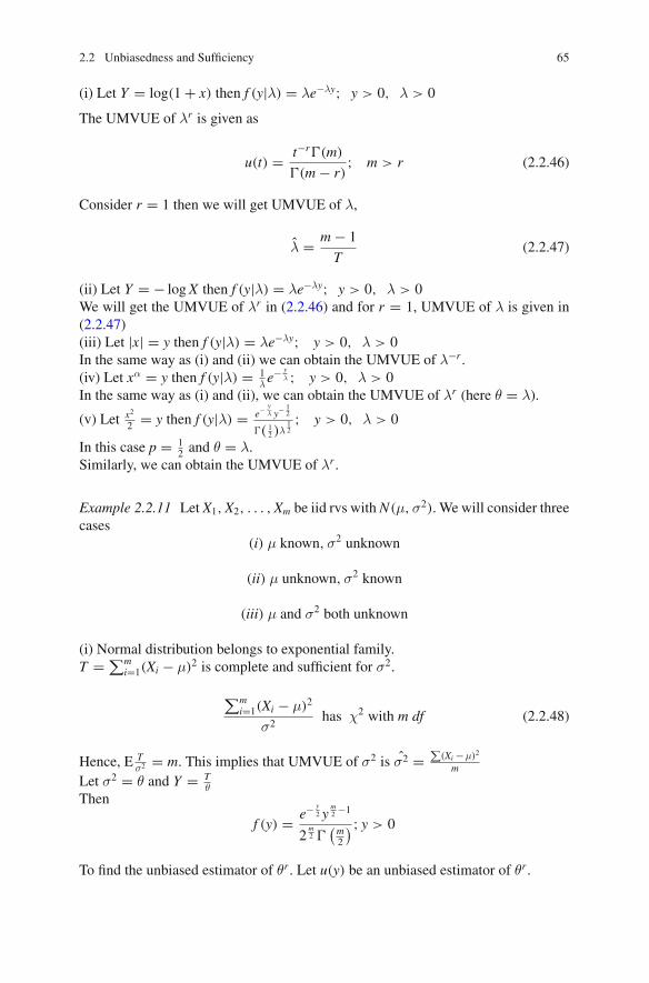
(i) Let Y = log(1 + x) then f (y|λ) = λe−λy; y > 0, λ > 0
The UMVUE of λr is given as
u(t) = t−r�(m)
�(m − r); m > r (2.2.46)
Consider r = 1 then we will get UMVUE of λ,
λ̂ = m − 1
T(2.2.47)
(ii) Let Y = − logX then f (y|λ) = λe−λy; y > 0, λ > 0We will get the UMVUE of λr in (2.2.46) and for r = 1, UMVUE of λ is given in(2.2.47)(iii) Let |x| = y then f (y|λ) = λe−λy; y > 0, λ > 0In the same way as (i) and (ii) we can obtain the UMVUE of λ−r .(iv) Let xα = y then f (y|λ) = 1
λe− y
λ ; y > 0, λ > 0In the same way as (i) and (ii), we can obtain the UMVUE of λr (here θ = λ).
(v) Let x2
2 = y then f (y|λ) = e− yλ y− 1
2
�( 12 )λ
12; y > 0, λ > 0
In this case p = 12 and θ = λ.
Similarly, we can obtain the UMVUE of λr .
Example 2.2.11 Let X1,X2, . . . ,Xm be iid rvs withN(μ,σ2). We will consider threecases
(i) μ known,σ2 unknown
(ii) μ unknown,σ2 known
(iii) μ and σ2 both unknown
(i) Normal distribution belongs to exponential family.T =∑m
i=1(Xi − μ)2 is complete and sufficient for σ2.
∑mi=1(Xi − μ)2
σ2has χ2 with m df (2.2.48)
Hence, E Tσ2 = m. This implies that UMVUE of σ2 is σ̂2 =
∑(Xi −μ)2
m
Let σ2 = θ and Y = Tθ
Then
f (y) = e− y2 y
m2 −1
2m2 �(m2
) ; y > 0
To find the unbiased estimator of θr . Let u(y) be an unbiased estimator of θr .
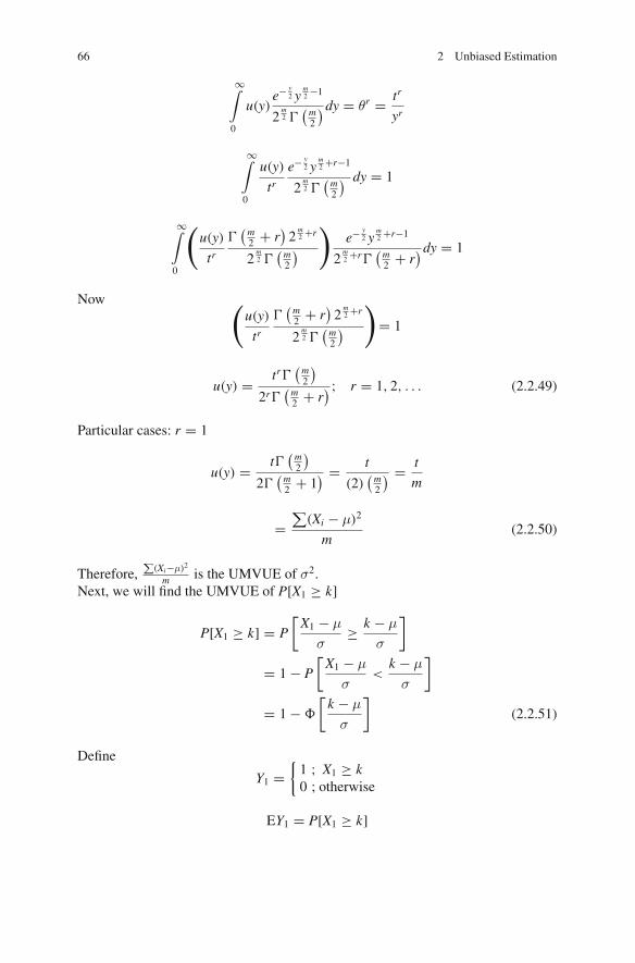
66 2 Unbiased Estimation
∞∫
0
u(y)e− y
2 ym2 −1
2m2 �(m2
)dy = θr = tr
yr
∞∫
0
u(y)
tre− y
2 ym2 +r−1
2m2 �(m2
) dy = 1
∞∫
0
(u(y)
tr�(m2 + r
)2
m2 +r
2m2 �(m2
))
e− y2 y
m2 +r−1
2m2 +r�
(m2 + r
)dy = 1
Now (u(y)
tr�(m2 + r
)2
m2 +r
2m2 �(m2
))
= 1
u(y) = tr�(m2
)
2r�(m2 + r
) ; r = 1, 2, . . . (2.2.49)
Particular cases: r = 1
u(y) = t�(m2
)
2�(m2 + 1
) = t
(2)(m2
) = t
m
=∑
(Xi − μ)2
m(2.2.50)
Therefore,∑
(Xi−μ)2
m is the UMVUE of σ2.Next, we will find the UMVUE of P[X1 ≥ k]
P[X1 ≥ k] = P
[X1 − μ
σ≥ k − μ
σ
]
= 1 − P
[X1 − μ
σ<
k − μ
σ
]
= 1 − �
[k − μ
σ
](2.2.51)
Define
Y1 ={1 ; X1 ≥ k0 ; otherwise
EY1 = P[X1 ≥ k]
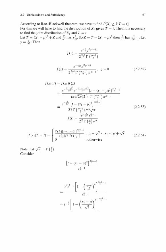
2.2 Unbiasedness and Sufficiency 67
According to Rao–Blackwell theorem, we have to find P[X1 ≥ k|T = t].For this we will have to find the distribution of X1 given T = t. Then it is necessaryto find the joint distribution of X1 and T = tLet T = (X1 − μ)2 + Z and T
σ2 has χ2m. So Z = T − (X1 − μ)2 then Z
σ2 has χ2m−1. Let
y = zσ2 . Then
f (y) = e− y2 y
m−12 −1
2m−12 �
(m−12
)
f (z) = e− z2σ2 z
m−12 −1
2m−12 �
(m−12
)σm−1
; z > 0 (2.2.52)
f (x1, t) = f (x1)f (z)
= e− (x1−μ)2
2σ2 e− [z−(x1−μ)2 ]2σ2 [t − (x1 − μ)2] m−1
2 −1
(σ√2π)2
m−12 �
(m−12
)σm−1
= e− t2σ2[t − (x1 − μ)2
] m−12 −1
2m2 �(m−12
)σm
√π
(2.2.53)
f (t) = e− t2σ2 t
m2 −1
2m2 �(m2
)σm
f (x1|T = t) =⎧⎨
⎩�( m
2 )[t−(x1−μ)2]m−12 −1
�( 12 )t
m2 −1
�( m−12 )
; μ − √t < x1 < μ + √
t
0 ; otherwise(2.2.54)
Note that√
π = �(12
)
Consider
[t − (x1 − μ)2
] m−12 −1
tm2 −1
=tm−12 −1
[1 −
(x1−μ√
t
)2] m−12 −1
tm2 −1
= t−12
[1 −
(x1 − μ√
t
)2] m−1
2 −1
68 2 Unbiased Estimation
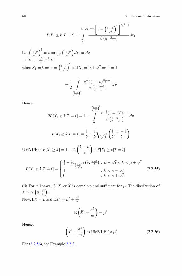
P[X1 ≥ k|T = t] =μ+√
t∫
k
t− 12
[1 −
(x1−μ√
t
)2] m−12 −1
β(12 ,
m−12
) dx1
Let(x1−μ√
t
)2 = v ⇒ 2√t
(x1−μ√
t
)dx1 = dv
⇒ dx1 =√t
2 v− 12 dv
when X1 = k ⇒ v =(k−μ√
t
)2and X1 = μ + √
t ⇒ v = 1
= 1
2
1∫
(k−μ√
t
)2
v− 12 (1 − v)
m−12 −1
β(12 ,
m−12
) dv
Hence
2P[X1 ≥ k|T = t] = 1 −
(k−μ√
t
)2∫
0
v− 12 (1 − v)
m−12 −1
β(12 ,
m−12
) dv
P[X1 ≥ k|T = t] = 1
2− 1
2I( k−μ√
t
)2
(1
2,m − 1
2
)
UMVUE of P[X1 ≥ k] = 1 − �
(k − μ
σ
)is P[X1 ≥ k|T = t]
P[X1 ≥ k|T = t] =
⎧⎪⎨
⎪⎩
12 − 1
2 I( k−μ√t
)2(12 ,
m−12
) ; μ − √t < k < μ + √
t
1 ; k < μ − √t
0 ; k > μ + √t
(2.2.55)
(ii) For σ known,∑
Xi or X̄ is complete and sufficient for μ. The distribution of
X̄ ∼ N(μ, σ2
m
).
Now, EX̄ = μ and EX̄2 = μ2 + σ2
n
E
(X̄2 − σ2
m
)= μ2
Hence, (X̄2 − σ2
m
)is UMVUE for μ2 (2.2.56)
For (2.2.56), see Example 2.2.3.
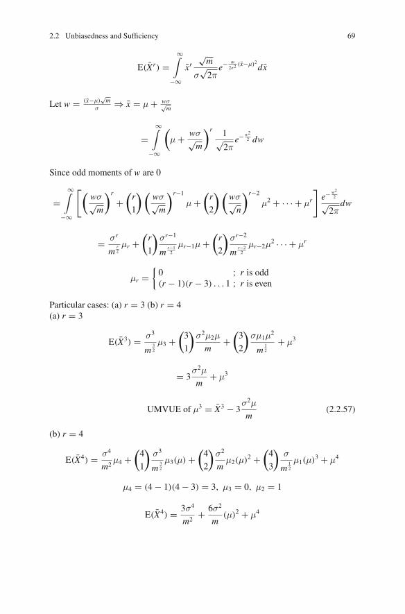
2.2 Unbiasedness and Sufficiency 69
E(X̄r) =∞∫
−∞x̄r
√m
σ√2π
e− m2σ2
(x̄−μ)2dx̄
Let w = (x̄−μ)√m
σ⇒ x̄ = μ + wσ√
m
=∞∫
−∞
(μ + wσ√
m
)r 1√2π
e− w2
2 dw
Since odd moments of w are 0
=∞∫
−∞
[(wσ√m
)r
+(r
1
)(wσ√m
)r−1
μ +(r
2
)(wσ√n
)r−2
μ2 + · · · + μr
]e− w2
2√2π
dw
= σr
mr2μr +
(r
1
)σr−1
mr−12
μr−1μ +(r
2
)σr−2
mr−22
μr−2μ2 · · · + μr
μr ={0 ; r is odd(r − 1)(r − 3) . . . 1 ; r is even
Particular cases: (a) r = 3 (b) r = 4(a) r = 3
E(X̄3) = σ3
m32
μ3 +(3
1
)σ2μ2μ
m+(3
2
)σμ1μ
2
m12
+ μ3
= 3σ2μ
m+ μ3
UMVUE of μ3 = X̄3 − 3σ2μ
m(2.2.57)
(b) r = 4
E(X̄4) = σ4
m2μ4 +
(4
1
)σ3
m32
μ3(μ) +(4
2
)σ2
mμ2(μ)2 +
(4
3
)σ
m12
μ1(μ)3 + μ4
μ4 = (4 − 1)(4 − 3) = 3, μ3 = 0, μ2 = 1
E(X̄4) = 3σ4
m2+ 6σ2
m(μ)2 + μ4
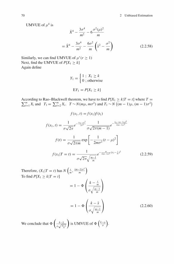
70 2 Unbiased Estimation
UMVUE of μ4 is
X̄4 − 3σ4
m2− 6
σ2(μ)2
m
= X̄4 − 3σ4
m2− 6σ2
m
(x̄2 − σ2
m
)(2.2.58)
Similarly, we can find UMVUE of μr(r ≥ 1)Next, find the UMVUE of P[X1 ≥ k]Again define
Y1 ={1 ; X1 ≥ k0 ; otherwise
EY1 = P[X1 ≥ k]
According to Rao–Blackwell theorem, we have to find P[X1 ≥ k|T = t] where T =∑mi=1 Xi and T1 = ∑m
i=2 Xi. T ∼N(mμ,mσ2) and T1 ∼N((m − 1)μ, (m − 1)σ2
)
f (x1, t) = f (x1)f (t1)
f (x1, t) = 1
σ√2π
e− (x1−μ)2
2σ21
σ√2π(m − 1)
e− [t1−(m−1)μ]2
2(m−1)σ2
f (t) = 1
σ√2πm
exp
[− 1
2mσ2(t − μ)2
]
f (x1|T = t) = 1
σ√2π√
m−1m
e− m
2(m−1)σ2(x1− t
m )2 (2.2.59)
Therefore, (X1|T = t) has N(
tm , (m−1)σ2
m
)
To find P[X1 ≥ k|T = t]
= 1 − �
⎛
⎝ k − tm
σ√
m−1m
⎞
⎠
= 1 − �
⎛
⎝ k − x̄
σ√
m−1m
⎞
⎠ (2.2.60)
We conclude that �
(k−x̄
σ√
m−1m
)is UMVUE of �
(k−μσ
).
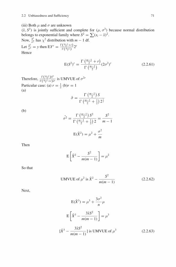
2.2 Unbiasedness and Sufficiency 71
(iii) Both μ and σ are unknown(x̄, S2) is jointly sufficient and complete for (μ,σ2) because normal distributionbelongs to exponential family where S2 =∑(xi − x̄)2.Now, S2
σ2 has χ2 distribution with m − 1 df.
Let S2
σ2 = y then EYr = �( m−12 +r)
�( m−12 )
2r
Hence
E(S2)r = �(m−12 + r
)
�(m−12
) (2σ2)r (2.2.61)
Therefore,�( m−1
2 )S2
�( m−12 +r)2r
is UMVUE of σ2r
Particular case: (a) r = 12 (b)r = 1
(a)
σ̂ = �(m−12
)S
�(m−12 + 1
2
)2
12
(b)
σ̂2 = �(m−12
)S2
�(m−12 + 1
2
)2
= S2
m − 1
E(X̄2) = μ2 + σ2
m
Then
E
[X̄2 − S2
m(m − 1)
]= μ2
So that
UMVUE of μ2 is X̄2 − S2
m(m − 1)(2.2.62)
Next,
E(X̄3) = μ3 + 3σ2
nμ
E
[X̄3 − 3x̄S2
m(m − 1)
]= μ3
[X̄3 − 3x̄S2
m(m − 1)] is UMVUE of μ3 (2.2.63)
72 2 Unbiased Estimation
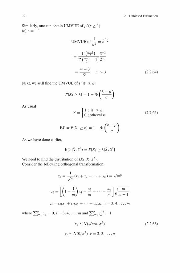
Similarly, one can obtain UMVUE of μr(r ≥ 1)(c) r = −1
UMVUE of1
σ2= σ̂−2
= �(m−12
)
�(m−12 − 1
) S−2
2−1
= m − 3
S2; m > 3 (2.2.64)
Next, we will find the UMVUE of P[X1 ≥ k]
P[X1 ≥ k] = 1 − �
(k − μ
σ
)
As usual
Y ={1 ; X1 ≥ k0 ; otherwise
(2.2.65)
EY = P[X1 ≥ k] = 1 − �
(k − μ
σ
)
As we have done earlier,
E(Y |X̄, S2) = P[X1 ≥ k|X̄, S2]
We need to find the distribution of (X1, X̄, S2).Consider the following orthogonal transformation:
z1 = 1√m
(x1 + x2 + · · · + xm) = √mx̄
z2 =[(
1 − 1
m
)x1 − x2
m− · · · − xm
m
]√m
m − 1
zi = ci1x1 + ci2x2 + · · · + cimxm i = 3, 4, . . . ,m
where∑m
j=1 cij = 0, i = 3, 4, . . . ,m and∑m
j=1 cjj2 = 1
z1 ∼ N(√mμ,σ2) (2.2.66)
zr ∼ N(0,σ2) r = 2, 3, . . . , n
2.2 Unbiasedness and Sufficiency 73
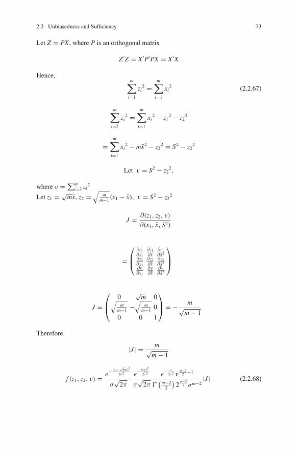
Let Z = PX, where P is an orthogonal matrix
Z ′Z = X ′P′PX = X ′X
Hence,m∑
i=1
zi2 =
m∑
i=1
xi2 (2.2.67)
m∑
i=3
zi2 =
m∑
i=1
xi2 − z1
2 − z22
=m∑
i=1
xi2 − mx̄2 − z2
2 = S2 − z22
Let v = S2 − z22,
where v =∑mi=3 zi
2
Let z1 = √mx̄, z2 =
√m
m−1 (x1 − x̄), v = S2 − z22
J = ∂(z1, z2, v)
∂(x1, x̄, S2)
=⎛
⎜⎝
∂z1∂x1
∂z1∂x̄
∂z1∂S2
∂z2∂x1
∂z2∂x̄
∂z2∂S2
∂v∂x1
∂v∂x̄
∂v∂S2
⎞
⎟⎠
J =⎛
⎜⎝0
√m 0√
mm−1 −
√m
m−1 0
0 0 1
⎞
⎟⎠ = − m√m − 1
Therefore,
|J| = m√m − 1
f (z1, z2, v) = e− (z1−√mμ)2
2σ2
σ√2π
e− (z2)2
2σ2
σ√2π
e− v
2σ2 vm−22 −1
�(m−22
)2
m−22 σm−2
|J| (2.2.68)
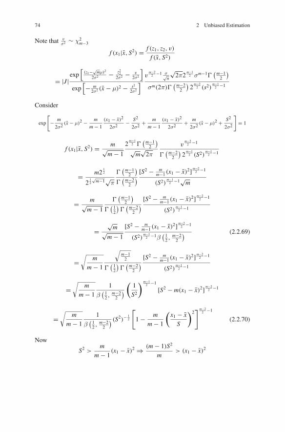
74 2 Unbiased Estimation
Note that vσ2 ∼ χ2
m−3
f (x1|x̄, S2) = f (z1, z2, v)
f (x̄, S2)
= |J|exp[
(z1−√mμ)2
2σ2 − z222σ2 − v
2σ2
]
exp[− m
2σ2 (x̄ − μ)2 − s22σ2
]v
m−22 −1 σ√
n
√2π2
m−12 σm−1�
(m−12
)
σm(2π)�(m−22
)2
m−22 (s2)
m−12 −1
Consider
exp
[− m
2σ2(x̄ − μ)2 − m
m − 1
(x1 − x̄)2
2σ2− S2
2σ2+ m
m − 1
(x1 − x̄)2
2σ2+ m
2σ2(x̄ − μ)2 + S2
2σ2
]= 1
f (x1|x̄, S2) = m√m − 1
2m−12 �
(m−12
)√m
√2π
vm−22 −1
�(m−22
)2
m−12 (S2)
m−12 −1
= m212
212
√m−1√π
�(m−12
)
�(m−22
)[S2 − m
m−1 (x1 − x̄)2] m−22 −1
(S2)m−12 −1√m
= m√m − 1
�(m−12
)
�(12
)�(m−22
)[S2 − m
m−1 (x1 − x̄)2] m−22 −1
(S2)m−12 −1
=√m√
m − 1
[S2 − mm−1 (x1 − x̄)2] m−2
2 −1
(S2)m−12 −1β
(12 ,
m−22
) (2.2.69)
=√
m
m − 1
√m−12
�(12
)�(m−22
)[S2 − m
m−1 (x1 − x̄)2] m−22 −1
(S2)m−12 −1
=√
m
m − 1
1
β(12 ,
m−22
)(
1
S2
) m−12 −1
[S2 − m(x1 − x̄)2] m−22 −1
=√
m
m − 1
1
β(12 ,
m−22
) (S2)− 12
[1 − m
m − 1
(x1 − x̄
S
)2] m−2
2 −1
(2.2.70)
Now
S2 >m
m − 1(x1 − x̄)2 ⇒ (m − 1)S2
m> (x1 − x̄)2
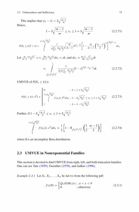
2.2 Unbiasedness and Sufficiency 75
This implies that |x1 − x̄| < S√
m−1m
Hence,
x̄ − S
√m − 1
m≤ x1 ≤ x̄ + S
√m − 1
m(2.2.71)
P[X1 ≥ k|T = t] =x̄+S
√m−1m∫
k
1
β(12 , m−2
2
)√
m
m − 1(S2)−
12
[1 − m
m − 1
(x1 − x̄
S
)2]m−22 −1
dx1
Let mm−1
(x1−x̄)2
S2 = t, 2mm−1
(x1−x̄)S2 dx1 = dt, and dx1 = m−1
2mS2
(x1−x̄)dt
=1∫
mm−1 (
k−x̄S )
2
1
2β(12 ,
m−22
) [1 − t] m−22 −1t−
12 dt (2.2.72)
UMVUE of P[X1 ≥ k] is
P[X1 ≥ k|x̄, S2] =
⎧⎪⎪⎪⎪⎪⎪⎨
⎪⎪⎪⎪⎪⎪⎩
0 ; k > x̄ + S√
m−1m
x̄+S√
m−1m∫
kf (x1|x̄, S2)dx1 ; x̄ − S
√m−1m ≤ x1 ≤ x̄ + S
√m−1m
1 ; k > x̄ − S√
m−1m
(2.2.73)
Further, if x̄ − S√
m−1m ≤ x1 ≤ x̄ + S
√m−1m
x̄+S√
m−1m∫
k
f (x1|x̄, s2)dx1 = 1
2
[1 − I m
m−1 (k−x̄s )
2
(1
2,m − 2
2
)](2.2.74)
where I is an incomplete Beta distribution.
2.3 UMVUE in Nonexponential Families
This section is devoted to find UMVUE from right, left, and both truncation families.One can see Tate (1959), Guenther (1978), and Jadhav (1996).
Example 2.3.1 Let X1,X2, . . . ,Xm be iid rvs from the following pdf:
f (x|θ) ={Q1(θ)M1(x) ; a < x < θ0 ; otherwise
(2.3.1)
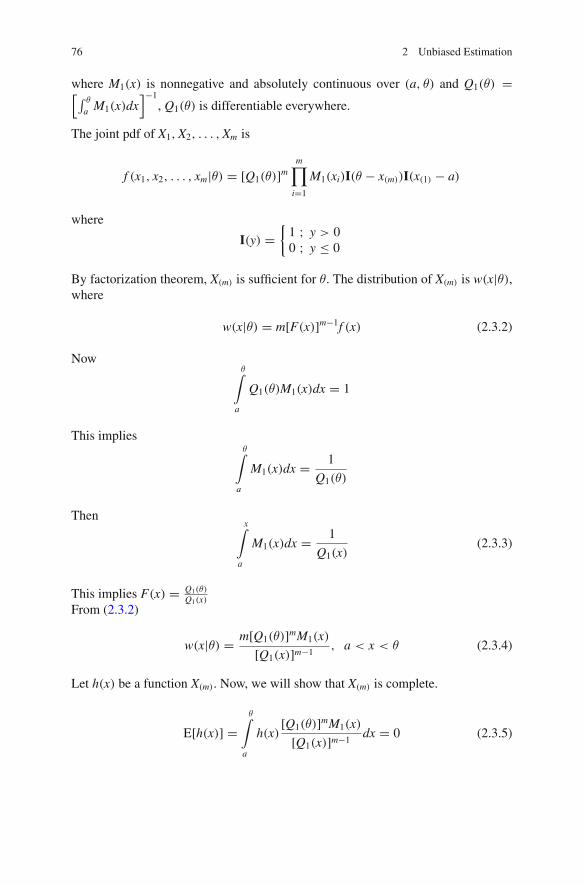
76 2 Unbiased Estimation
where M1(x) is nonnegative and absolutely continuous over (a, θ) and Q1(θ) =[∫ θ
a M1(x)dx]−1
, Q1(θ) is differentiable everywhere.
The joint pdf of X1,X2, . . . ,Xm is
f (x1, x2, . . . , xm|θ) = [Q1(θ)]mm∏
i=1
M1(xi)I(θ − x(m))I(x(1) − a)
where
I(y) ={1 ; y > 00 ; y ≤ 0
By factorization theorem, X(m) is sufficient for θ. The distribution of X(m) is w(x|θ),where
w(x|θ) = m[F(x)]m−1f (x) (2.3.2)
Nowθ∫
a
Q1(θ)M1(x)dx = 1
This impliesθ∫
a
M1(x)dx = 1
Q1(θ)
Thenx∫
a
M1(x)dx = 1
Q1(x)(2.3.3)
This implies F(x) = Q1(θ)Q1(x)
From (2.3.2)
w(x|θ) = m[Q1(θ)]mM1(x)
[Q1(x)]m−1, a < x < θ (2.3.4)
Let h(x) be a function X(m). Now, we will show that X(m) is complete.
E[h(x)] =θ∫
a
h(x)[Q1(θ)]mM1(x)
[Q1(x)]m−1dx = 0 (2.3.5)
2.3 UMVUE in Nonexponential Families 77
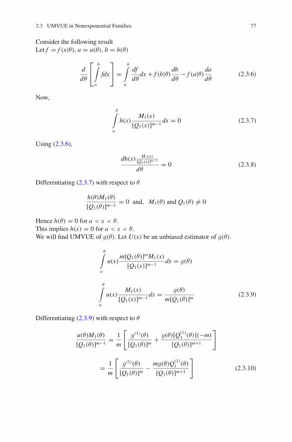
Consider the following resultLet f = f (x|θ), a = a(θ), b = b(θ)
d
dθ
⎡
⎣b∫
a
fdx
⎤
⎦ =b∫
a
df
dθdx + f (b|θ)db
dθ− f (a|θ)da
dθ(2.3.6)
Now,
θ∫
a
h(x)M1(x)
[Q1(x)]m−1dx = 0 (2.3.7)
Using (2.3.6),
dh(x) M1(x)[Q1(x)]m−1
dθ= 0 (2.3.8)
Differentiating (2.3.7) with respect to θ
h(θ)M1(θ)
[Q1(θ)]m−1= 0 and, M1(θ) and Q1(θ) �= 0
Hence h(θ) = 0 for a < x < θ.This implies h(x) = 0 for a < x < θ.We will find UMVUE of g(θ). Let U(x) be an unbiased estimator of g(θ).
θ∫
a
u(x)m[Q1(θ)]mM1(x)
[Q1(x)]m−1dx = g(θ)
θ∫
a
u(x)M1(x)
[Q1(x)]m−1dx = g(θ)
m[Q1(θ)]m (2.3.9)
Differentiating (2.3.9) with respect to θ
u(θ)M1(θ)
[Q1(θ)]m−1= 1
m
[g(1)(θ)
[Q1(θ)]m + g(θ)[Q(1)1 (θ)](−m)
[Q1(θ)]m+1
]
= 1
m
[g(1)(θ)
[Q1(θ)]m − mg(θ)Q(1)1 (θ)
[Q1(θ)]m+1
](2.3.10)
78 2 Unbiased Estimation
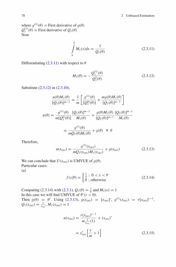
where g(1)(θ) = First derivative of g(θ)Q(1)
1 (θ) = First derivative of Q1(θ)Now
θ∫
a
M1(x)dx = 1
Q1(θ)(2.3.11)
Differentiating (2.3.11) with respect to θ
M1(θ) = −Q(1)1 (θ)
Q21(θ)
(2.3.12)
Substitute (2.3.12) in (2.3.10),
u(θ)M1(θ)
[Q1(θ)]m−1= 1
m
[g(1)(θ)
[Qm1 (θ)] + mg(θ)M1(θ)
[Q1(θ)]m−1
]
u(θ) = g(1)(θ)
m[Qm1 (θ)]
[Q1(θ)]m−1
M1(θ)+ g(θ)M1(θ)
[Q1(θ)]m−1
[Q1(θ)]m−1
M1(θ)
= g(1)(θ)
mQ1(θ)M1(θ)+ g(θ) ∀ θ
Therefore,
u(x(m)) = g(1)(x(m))
mQ1(x(m))M1(x(m))+ g(x(m)) (2.3.13)
We can conclude that U(x(m)) is UMVUE of g(θ).Particular cases:(a)
f (x|θ) ={
1θ
; 0 < x < θ0 ; otherwise
(2.3.14)
Comparing (2.3.14) with (2.3.1), Q1(θ) = 1θand M1(x) = 1
In this case we will find UMVUE of θr(r > 0).Then g(θ) = θr . Using (2.3.13), g(x(m)) = [x(m)]r , g(1)(x(m)) = r[x(m)]r−1,Q1(x(m)) = 1
x(m),M1(x(m)) = 1
u(x(m)) = r(x(m))r−1
m 1x(m)
(1)+ (x(m))
r
= xr(m)
[ rm
+ 1]
(2.3.15)
2.3 UMVUE in Nonexponential Families 79
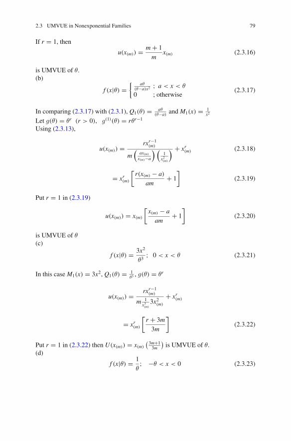
If r = 1, then
u(x(m)) = m + 1
mx(m) (2.3.16)
is UMVUE of θ.(b)
f (x|θ) ={ aθ
(θ−a)x2 ; a < x < θ
0 ; otherwise(2.3.17)
In comparing (2.3.17) with (2.3.1), Q1(θ) = aθ(θ−a) and M1(x) = 1
x2
Let g(θ) = θr (r > 0), g(1)(θ) = rθr−1
Using (2.3.13),
u(x(m)) = rxr−1(m)
m(
ax(m)
x(m)−a
) (1
x2(m)
) + xr(m) (2.3.18)
= xr(m)
[r(x(m) − a)
am+ 1
](2.3.19)
Put r = 1 in (2.3.19)
u(x(m)) = x(m)
[x(m) − a
am+ 1
](2.3.20)
is UMVUE of θ(c)
f (x|θ) = 3x2
θ3; 0 < x < θ (2.3.21)
In this case M1(x) = 3x2, Q1(θ) = 1θ3, g(θ) = θr
u(x(m)) = rxr−1(m)
m 1x3(m)
3x2(m)
+ xr(m)
= xr(m)
[r + 3m
3m
](2.3.22)
Put r = 1 in (2.3.22) then U(x(m)) = x(m)
(3m+13m
)is UMVUE of θ.
(d)
f (x|θ) = 1
θ; −θ < x < 0 (2.3.23)
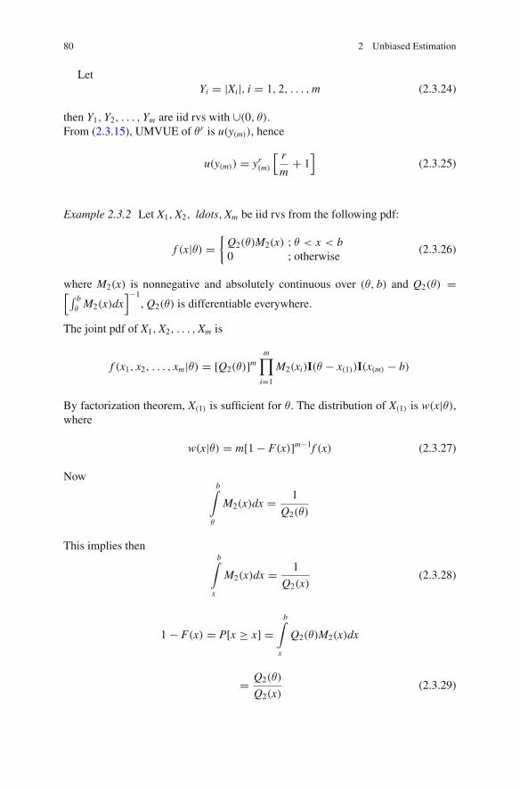
80 2 Unbiased Estimation
LetYi = |Xi|, i = 1, 2, . . . ,m (2.3.24)
then Y1,Y2, . . . ,Ym are iid rvs with ∪(0, θ).From (2.3.15), UMVUE of θr is u(y(m)), hence
u(y(m)) = yr(m)
[ rm
+ 1]
(2.3.25)
Example 2.3.2 Let X1,X2, ldots,Xm be iid rvs from the following pdf:
f (x|θ) ={Q2(θ)M2(x) ; θ < x < b0 ; otherwise
(2.3.26)
where M2(x) is nonnegative and absolutely continuous over (θ, b) and Q2(θ) =[∫ bθ M2(x)dx
]−1, Q2(θ) is differentiable everywhere.
The joint pdf of X1,X2, . . . ,Xm is
f (x1, x2, . . . , xm|θ) = [Q2(θ)]mm∏
i=1
M2(xi)I(θ − x(1))I(x(m) − b)
By factorization theorem, X(1) is sufficient for θ. The distribution of X(1) is w(x|θ),where
w(x|θ) = m[1 − F(x)]m−1f (x) (2.3.27)
Nowb∫
θ
M2(x)dx = 1
Q2(θ)
This implies thenb∫
x
M2(x)dx = 1
Q2(x)(2.3.28)
1 − F(x) = P[x ≥ x] =b∫
x
Q2(θ)M2(x)dx
= Q2(θ)
Q2(x)(2.3.29)
2.3 UMVUE in Nonexponential Families 81
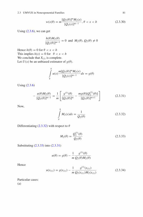
w(x|θ) = m[Q2(θ)]mM2(x)
[Q2(x)]m−1, θ < x < b (2.3.30)
Using (2.3.6), we can get
h(θ)M2(θ)
[Q2(θ)]m−1= 0 and M2(θ),Q2(θ) �= 0
Hence h(θ) = 0 for θ < x < bThis implies h(x) = 0 for θ < x < bWe conclude that X(1) is complete.Let U(x) be an unbiased estimator of g(θ).
b∫
θ
u(x)m[Q2(θ)]mM2(x)
[Q2(x)]m−1dx = g(θ)
Using (2.3.6)
− u(θ)M2(θ)
[Q2(θ)]m−1= 1
m
[g(1)(θ)
[Q2(θ)]m − mg(θ)[Q(1)2 (θ)]
[Q2(θ)]m+1
](2.3.31)
Now,b∫
θ
M2(x)dx = 1
Q2(θ)(2.3.32)
Differentiating (2.3.32) with respect to θ
M2(θ) = Q(1)2 (θ)
Q2(θ)(2.3.33)
Substituting (2.3.33) into (2.3.31)
u(θ) = g(θ) − 1
m
g(1)(θ)
Q2(θ)M2(θ)
Hence
u(x(1)) = g(x(1)) − 1
m
g(1)(x(1))
Q2(x(1))M2(x(1))(2.3.34)
Particular cases:(a)
82 2 Unbiased Estimation
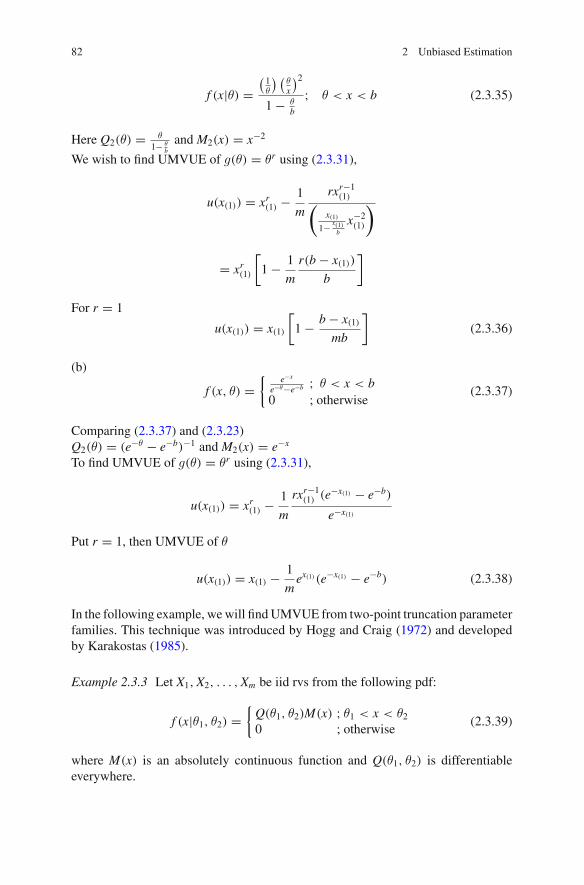
f (x|θ) =(1θ
) (θx
)2
1 − θb
; θ < x < b (2.3.35)
Here Q2(θ) = θ1− θ
b
and M2(x) = x−2
We wish to find UMVUE of g(θ) = θr using (2.3.31),
u(x(1)) = xr(1) − 1
m
rxr−1(1)(
x(1)
1− x(1)b
x−2(1)
)
= xr(1)
[1 − 1
m
r(b − x(1))
b
]
For r = 1
u(x(1)) = x(1)
[1 − b − x(1)
mb
](2.3.36)
(b)
f (x, θ) ={
e−x
e−θ−e−b ; θ < x < b0 ; otherwise
(2.3.37)
Comparing (2.3.37) and (2.3.23)Q2(θ) = (e−θ − e−b)−1 and M2(x) = e−x
To find UMVUE of g(θ) = θr using (2.3.31),
u(x(1)) = xr(1) − 1
m
rxr−1(1) (e−x(1) − e−b)
e−x(1)
Put r = 1, then UMVUE of θ
u(x(1)) = x(1) − 1
mex(1) (e−x(1) − e−b) (2.3.38)
In the following example, wewill findUMVUE from two-point truncation parameterfamilies. This technique was introduced by Hogg and Craig (1972) and developedby Karakostas (1985).
Example 2.3.3 Let X1,X2, . . . ,Xm be iid rvs from the following pdf:
f (x|θ1, θ2) ={Q(θ1, θ2)M(x) ; θ1 < x < θ20 ; otherwise
(2.3.39)
where M(x) is an absolutely continuous function and Q(θ1, θ2) is differentiableeverywhere.
2.3 UMVUE in Nonexponential Families 83
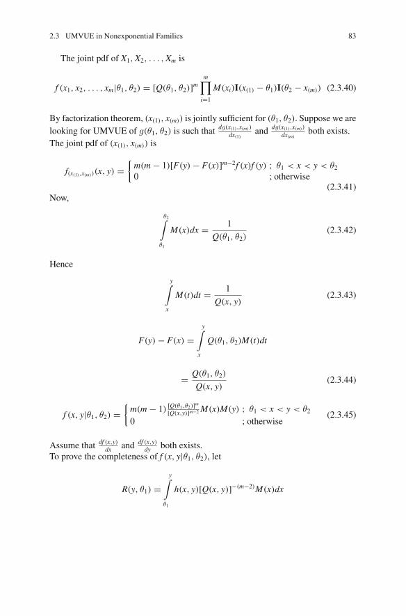
The joint pdf of X1,X2, . . . ,Xm is
f (x1, x2, . . . , xm|θ1, θ2) = [Q(θ1, θ2)]mm∏
i=1
M(xi)I(x(1) − θ1)I(θ2 − x(m)) (2.3.40)
By factorization theorem, (x(1), x(m)) is jointly sufficient for (θ1, θ2). Suppose we arelooking for UMVUE of g(θ1, θ2) is such that dg(x(1),x(m))
dx(1)and dg(x(1),x(m))
dx(m)both exists.
The joint pdf of (x(1), x(m)) is
f(x(1),x(m))(x, y) ={m(m − 1)[F(y) − F(x)]m−2f (x)f (y) ; θ1 < x < y < θ20 ; otherwise
(2.3.41)Now,
θ2∫
θ1
M(x)dx = 1
Q(θ1, θ2)(2.3.42)
Hence
y∫
x
M(t)dt = 1
Q(x, y)(2.3.43)
F(y) − F(x) =y∫
x
Q(θ1, θ2)M(t)dt
= Q(θ1, θ2)
Q(x, y)(2.3.44)
f (x, y|θ1, θ2) ={m(m − 1) [Q(θ1,θ2)]m
[Q(x,y)]m−2M(x)M(y) ; θ1 < x < y < θ20 ; otherwise
(2.3.45)
Assume that df (x,y)dx and df (x,y)
dy both exists.To prove the completeness of f (x, y|θ1, θ2), let
R(y, θ1) =y∫
θ1
h(x, y)[Q(x, y)]−(m−2)M(x)dx
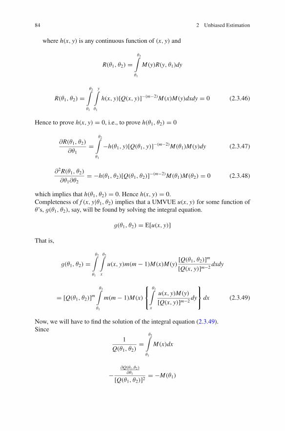
84 2 Unbiased Estimation
where h(x, y) is any continuous function of (x, y) and
R(θ1, θ2) =θ2∫
θ1
M(y)R(y, θ1)dy
R(θ1, θ2) =θ2∫
θ1
y∫
θ1
h(x, y)[Q(x, y)]−(m−2)M(x)M(y)dxdy = 0 (2.3.46)
Hence to prove h(x, y) = 0, i.e., to prove h(θ1, θ2) = 0
∂R(θ1, θ2)
∂θ1=
θ2∫
θ1
−h(θ1, y)[Q(θ1, y)]−(m−2)M(θ1)M(y)dy (2.3.47)
∂2R(θ1, θ2)
∂θ1∂θ2= −h(θ1, θ2)[Q(θ1, θ2)]−(m−2)M(θ1)M(θ2) = 0 (2.3.48)
which implies that h(θ1, θ2) = 0. Hence h(x, y) = 0.Completeness of f (x, y|θ1, θ2) implies that a UMVUE u(x, y) for some function ofθ’s, g(θ1, θ2), say, will be found by solving the integral equation.
g(θ1, θ2) = E[u(x, y)]
That is,
g(θ1, θ2) =θ2∫
θ1
θ2∫
x
u(x, y)m(m − 1)M(x)M(y)[Q(θ1, θ2)]m[Q(x, y)]m−2
dxdy
= [Q(θ1, θ2)]mθ2∫
θ1
m(m − 1)M(x)
⎧⎨
⎩
θ2∫
x
u(x, y)M(y)
[Q(x, y)]m−2dy
⎫⎬
⎭ dx (2.3.49)
Now, we will have to find the solution of the integral equation (2.3.49).Since
1
Q(θ1, θ2)=
θ2∫
θ1
M(x)dx
−∂Q(θ1,θ2)
∂θ1
[Q(θ1, θ2)]2 = −M(θ1)
2.3 UMVUE in Nonexponential Families 85
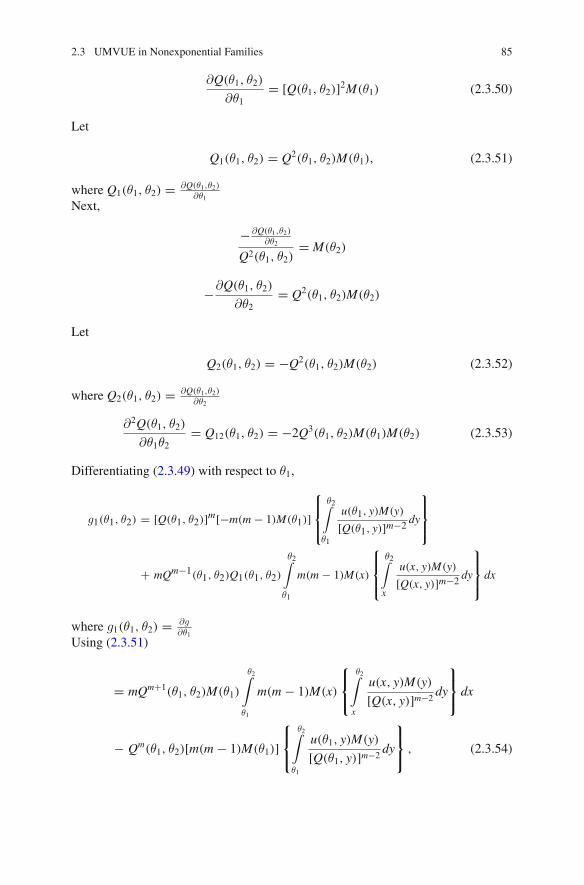
∂Q(θ1, θ2)
∂θ1= [Q(θ1, θ2)]2M(θ1) (2.3.50)
Let
Q1(θ1, θ2) = Q2(θ1, θ2)M(θ1), (2.3.51)
where Q1(θ1, θ2) = ∂Q(θ1,θ2)∂θ1
Next,
− ∂Q(θ1,θ2)∂θ2
Q2(θ1, θ2)= M(θ2)
−∂Q(θ1, θ2)
∂θ2= Q2(θ1, θ2)M(θ2)
Let
Q2(θ1, θ2) = −Q2(θ1, θ2)M(θ2) (2.3.52)
where Q2(θ1, θ2) = ∂Q(θ1,θ2)∂θ2
∂2Q(θ1, θ2)
∂θ1θ2= Q12(θ1, θ2) = −2Q3(θ1, θ2)M(θ1)M(θ2) (2.3.53)
Differentiating (2.3.49) with respect to θ1,
g1(θ1, θ2) = [Q(θ1, θ2)]m[−m(m − 1)M(θ1)]
⎧⎪⎨
⎪⎩
θ2∫
θ1
u(θ1, y)M(y)
[Q(θ1, y)]m−2 dy
⎫⎪⎬
⎪⎭
+ mQm−1(θ1, θ2)Q1(θ1, θ2)
θ2∫
θ1
m(m − 1)M(x)
⎧⎪⎨
⎪⎩
θ2∫
x
u(x, y)M(y)
[Q(x, y)]m−2 dy
⎫⎪⎬
⎪⎭dx
where g1(θ1, θ2) = ∂g∂θ1
Using (2.3.51)
= mQm+1(θ1, θ2)M(θ1)
θ2∫
θ1
m(m − 1)M(x)
⎧⎨
⎩
θ2∫
x
u(x, y)M(y)
[Q(x, y)]m−2dy
⎫⎬
⎭ dx
− Qm(θ1, θ2)[m(m − 1)M(θ1)]⎧⎨
⎩
θ2∫
θ1
u(θ1, y)M(y)
[Q(θ1, y)]m−2dy
⎫⎬
⎭ , (2.3.54)
86 2 Unbiased Estimation
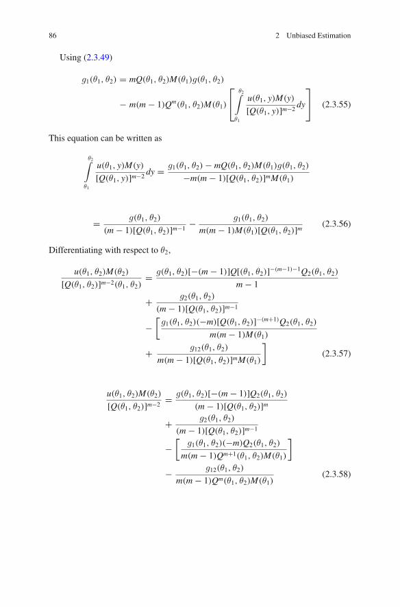
Using (2.3.49)
g1(θ1, θ2) = mQ(θ1, θ2)M(θ1)g(θ1, θ2)
− m(m − 1)Qm(θ1, θ2)M(θ1)
⎡
⎣θ2∫
θ1
u(θ1, y)M(y)
[Q(θ1, y)]m−2dy
⎤
⎦ (2.3.55)
This equation can be written as
θ2∫
θ1
u(θ1, y)M(y)
[Q(θ1, y)]m−2dy = g1(θ1, θ2) − mQ(θ1, θ2)M(θ1)g(θ1, θ2)
−m(m − 1)[Q(θ1, θ2)]mM(θ1)
= g(θ1, θ2)
(m − 1)[Q(θ1, θ2)]m−1− g1(θ1, θ2)
m(m − 1)M(θ1)[Q(θ1, θ2)]m (2.3.56)
Differentiating with respect to θ2,
u(θ1, θ2)M(θ2)
[Q(θ1, θ2)]m−2(θ1, θ2)= g(θ1, θ2)[−(m − 1)]Q[(θ1, θ2)]−(m−1)−1Q2(θ1, θ2)
m − 1
+ g2(θ1, θ2)
(m − 1)[Q(θ1, θ2)]m−1
−[g1(θ1, θ2)(−m)[Q(θ1, θ2)]−(m+1)Q2(θ1, θ2)
m(m − 1)M(θ1)
+ g12(θ1, θ2)
m(m − 1)[Q(θ1, θ2)]mM(θ1)
](2.3.57)
u(θ1, θ2)M(θ2)
[Q(θ1, θ2)]m−2= g(θ1, θ2)[−(m − 1)]Q2(θ1, θ2)
(m − 1)[Q(θ1, θ2)]m+ g2(θ1, θ2)
(m − 1)[Q(θ1, θ2)]m−1
−[
g1(θ1, θ2)(−m)Q2(θ1, θ2)
m(m − 1)Qm+1(θ1, θ2)M(θ1)
]
− g12(θ1, θ2)
m(m − 1)Qm(θ1, θ2)M(θ1)(2.3.58)
2.3 UMVUE in Nonexponential Families 87
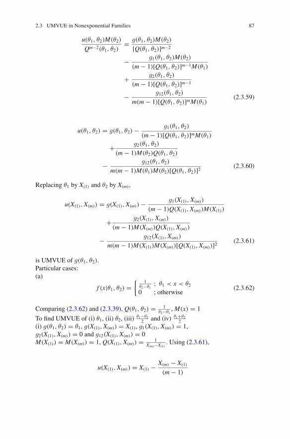
u(θ1, θ2)M(θ2)
Qm−2(θ1, θ2)= g(θ1, θ2)M(θ2)
[Q(θ1, θ2)]m−2
− g1(θ1, θ2)M(θ2)
(m − 1)[Q(θ1, θ2)]m−1M(θ1)
+ g2(θ1, θ2)
(m − 1)[Q(θ1, θ2)]m−1
− g12(θ1, θ2)
m(m − 1)[Q(θ1, θ2)]mM(θ1)(2.3.59)
u(θ1, θ2) = g(θ1, θ2) − g1(θ1, θ2)
(m − 1)[Q(θ1, θ2)]mM(θ1)
+ g2(θ1, θ2)
(m − 1)M(θ2)Q(θ1, θ2)
− g12(θ1, θ2)
m(m − 1)M(θ1)M(θ2)[Q(θ1, θ2)]2 (2.3.60)
Replacing θ1 by X(1) and θ2 by X(m),
u(X(1),X(m)) = g(X(1),X(m)) − g1(X(1),X(m))
(m − 1)Q(X(1),X(m))M(X(1))
+ g2(X(1),X(m))
(m − 1)M(X(m))Q(X(1),X(m))
− g12(X(1),X(m))
m(m − 1)M(X(1))M(X(m))[Q(X(1),X(m))]2 (2.3.61)
is UMVUE of g(θ1, θ2).Particular cases:(a)
f (x|θ1, θ2) ={ 1
θ2−θ1; θ1 < x < θ2
0 ; otherwise(2.3.62)
Comparing (2.3.62) and (2.3.39), Q(θ1, θ2) = 1θ2−θ1
,M(x) = 1
To find UMVUE of (i) θ1, (ii) θ2, (iii)θ1−θ2
2 and (iv) θ1+θ22
(i) g(θ1, θ2) = θ1, g(X(1),X(m)) = X(1), g1(X(1),X(m)) = 1,g2(X(1),X(m)) = 0 and g12(X(1),X(m)) = 0M(X(1)) = M(X(m)) = 1, Q(X(1),X(m)) = 1
X(m)−X(1). Using (2.3.61),
u(X(1),X(m)) = X(1) − X(m) − X(1)
(m − 1)
88 2 Unbiased Estimation
= mX(1) − X(1) − X(m) + X(1)
(m − 1)
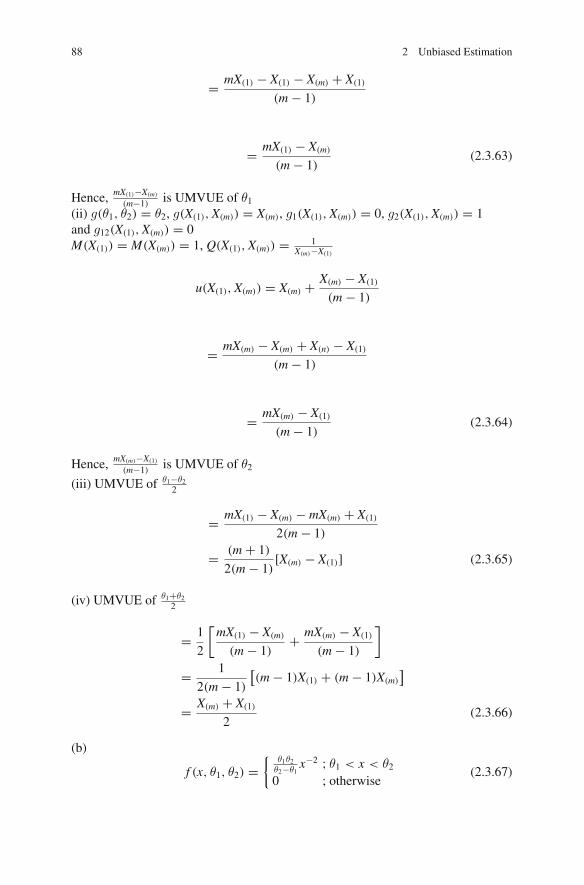
= mX(1) − X(m)
(m − 1)(2.3.63)
Hence, mX(1)−X(m)
(m−1) is UMVUE of θ1(ii) g(θ1, θ2) = θ2, g(X(1),X(m)) = X(m), g1(X(1),X(m)) = 0, g2(X(1),X(m)) = 1and g12(X(1),X(m)) = 0M(X(1)) = M(X(m)) = 1, Q(X(1),X(m)) = 1
X(m)−X(1)
u(X(1),X(m)) = X(m) + X(m) − X(1)
(m − 1)
= mX(m) − X(m) + X(n) − X(1)
(m − 1)
= mX(m) − X(1)
(m − 1)(2.3.64)
Hence, mX(m)−X(1)
(m−1) is UMVUE of θ2
(iii) UMVUE of θ1−θ22
= mX(1) − X(m) − mX(m) + X(1)
2(m − 1)
= (m + 1)
2(m − 1)[X(m) − X(1)] (2.3.65)
(iv) UMVUE of θ1+θ22
= 1
2
[mX(1) − X(m)
(m − 1)+ mX(m) − X(1)
(m − 1)
]
= 1
2(m − 1)
[(m − 1)X(1) + (m − 1)X(m)
]
= X(m) + X(1)
2(2.3.66)
(b)
f (x, θ1, θ2) ={
θ1θ2θ2−θ1
x−2 ; θ1 < x < θ20 ; otherwise
(2.3.67)
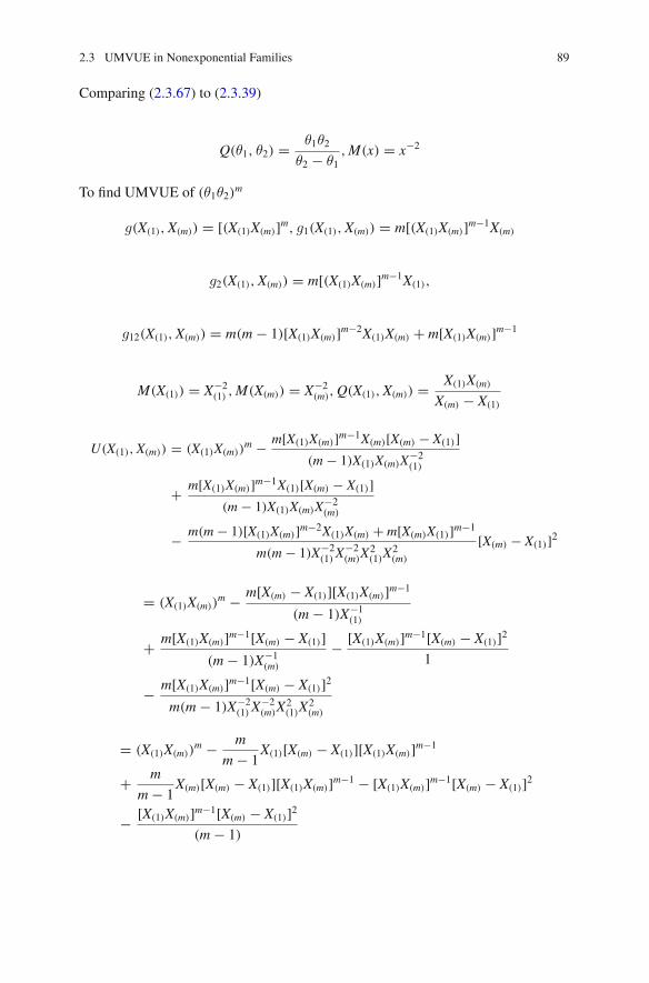
2.3 UMVUE in Nonexponential Families 89
Comparing (2.3.67) to (2.3.39)
Q(θ1, θ2) = θ1θ2
θ2 − θ1,M(x) = x−2
To find UMVUE of (θ1θ2)m
g(X(1),X(m)) = [(X(1)X(m)]m, g1(X(1),X(m)) = m[(X(1)X(m)]m−1X(m)
g2(X(1),X(m)) = m[(X(1)X(m)]m−1X(1),
g12(X(1),X(m)) = m(m − 1)[X(1)X(m)]m−2X(1)X(m) + m[X(1)X(m)]m−1
M(X(1)) = X−2(1) ,M(X(m)) = X−2
(m),Q(X(1),X(m)) = X(1)X(m)
X(m) − X(1)
U(X(1),X(m)) = (X(1)X(m))m − m[X(1)X(m)]m−1X(m)[X(m) − X(1)]
(m − 1)X(1)X(m)X−2(1)
+ m[X(1)X(m)]m−1X(1)[X(m) − X(1)](m − 1)X(1)X(m)X
−2(m)
− m(m − 1)[X(1)X(m)]m−2X(1)X(m) + m[X(m)X(1)]m−1
m(m − 1)X−2(1)X
−2(m)X
2(1)X
2(m)
[X(m) − X(1)]2
= (X(1)X(m))m − m[X(m) − X(1)][X(1)X(m)]m−1
(m − 1)X−1(1)
+ m[X(1)X(m)]m−1[X(m) − X(1)](m − 1)X−1
(m)
− [X(1)X(m)]m−1[X(m) − X(1)]21
− m[X(1)X(m)]m−1[X(m) − X(1)]2m(m − 1)X−2
(1)X−2(m)X
2(1)X
2(m)
= (X(1)X(m))m − m
m − 1X(1)[X(m) − X(1)][X(1)X(m)]m−1
+ m
m − 1X(m)[X(m) − X(1)][X(1)X(m)]m−1 − [X(1)X(m)]m−1[X(m) − X(1)]2
− [X(1)X(m)]m−1[X(m) − X(1)]2(m − 1)
90 2 Unbiased Estimation
= (X(1)X(m))m + m
m − 1[X(m) − X(1)]2[X(1)X(m)]m−1
− [X(1)X(m)]m−1[X(m) − X(1)]2 − [X(1)X(m)]m−1[X(m) − X(1)]2m − 1
= (X(1)X(m))m + [X(m) − X(1)]2[X(1)X(m)]m−1
[m
m − 1− 1 − 1
m − 1
]
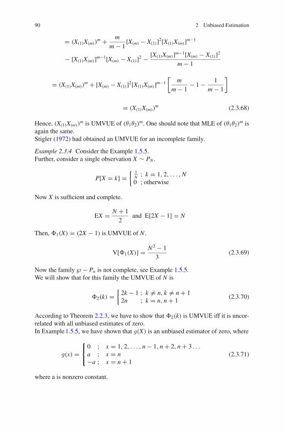
= (X(1)X(m))m (2.3.68)
Hence, (X(1)X(m))m is UMVUE of (θ1θ2)
m. One should note that MLE of (θ1θ2)m is
again the same.Stigler (1972) had obtained an UMVUE for an incomplete family.
Example 2.3.4 Consider the Example 1.5.5.Further, consider a single observation X ∼ PN .
P[X = k] ={
1N ; k = 1, 2, . . . ,N0 ; otherwise
Now X is sufficient and complete.
EX = N + 1
2and E[2X − 1] = N
Then, �1(X) = (2X − 1) is UMVUE of N .
V[�1(X)] = N2 − 1
3(2.3.69)
Now the family ℘ − Pn is not complete, see Example 1.5.5.We will show that for this family the UMVUE of N is
�2(k) ={2k − 1 ; k �= n, k �= n + 12n ; k = n, n + 1
(2.3.70)
According to Theorem 2.2.3, we have to show that �2(k) is UMVUE iff it is uncor-related with all unbiased estimates of zero.In Example1.5.5, we have shown that g(X) is an unbiased estimator of zero, where
g(x) =⎧⎨
⎩
0 ; x = 1, 2, . . . , n − 1, n + 2, n + 3 . . .
a ; x = n−a ; x = n + 1
(2.3.71)
where a is nonzero constant.

2.3 UMVUE in Nonexponential Families 91
Case (i) N < n
Eg(X) =N∑
k=1
g(x)1
N= 0
Case (ii) N > n
Eg(X) =N∑
k=1
1
Ng(x)
= 1
N[0 + · · · + 0 + (−a) + (a) + 0] = 0
Case (iii) N = n
Eg(X) =N∑
k=1
g(x)1
N
= 1
N[0 + · · · + 0 + (a)] = a
N
Eg(X) ={0 ; N = naN ; N = n
Thus we see that g(x) is an unbiased estimate of zero for the family ℘ − Pn andtherefore the family is not complete.Remark: Completeness is a property of a family of distribution rather than therandom variable or the parametric form, that the statistical definition of “complete”is related to every day usage, and that removing even one point from a parameter setmay alter the completeness of the family, see Stigler (1972).Now, we know that the family℘−{Pn} is not complete. Hence�1(X) is not UMVUEof N for the family ℘ − {Pn}. For this family consider the UMVUE of N as �2(X),where
�2(X) ={2x − 1 ; x �= n, x �= n + 12n ; x = n, n + 1
(2.3.72)
According toTheorem2.2.3,�2(X) isUMVUE iff it is uncorrelatedwith all unbiasedestimates of zero.Already, we have shown that g(x) is an unbiased estimator of zero for the family℘ − {Pn}.Since Eg(x) = 0 for N �= nNow, we have to show that Cov[g(x),�2(X)] = 0.
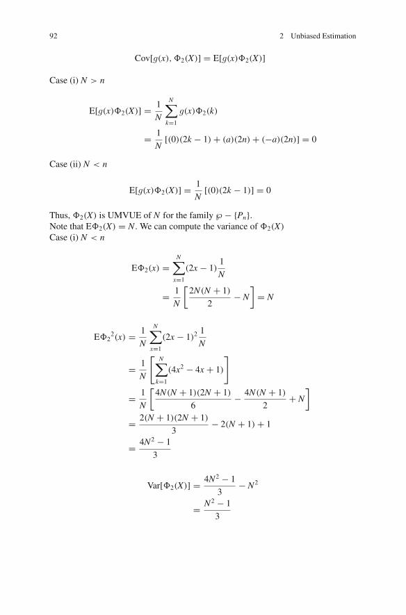
92 2 Unbiased Estimation
Cov[g(x),�2(X)] = E[g(x)�2(X)]
Case (i) N > n
E[g(x)�2(X)] = 1
N
N∑
k=1
g(x)�2(k)
= 1
N[(0)(2k − 1) + (a)(2n) + (−a)(2n)] = 0
Case (ii) N < n
E[g(x)�2(X)] = 1
N[(0)(2k − 1)] = 0
Thus, �2(X) is UMVUE of N for the family ℘ − {Pn}.Note that E�2(X) = N . We can compute the variance of �2(X)
Case (i) N < n
E�2(x) =N∑
x=1
(2x − 1)1
N
= 1
N
[2N(N + 1)
2− N
]= N
E�22(x) = 1
N
N∑
x=1
(2x − 1)21
N
= 1
N
[N∑
k=1
(4x2 − 4x + 1)
]
= 1
N
[4N(N + 1)(2N + 1)
6− 4N(N + 1)
2+ N
]
= 2(N + 1)(2N + 1)
3− 2(N + 1) + 1
= 4N2 − 1
3
Var[�2(X)] = 4N2 − 1
3− N2
= N2 − 1
3
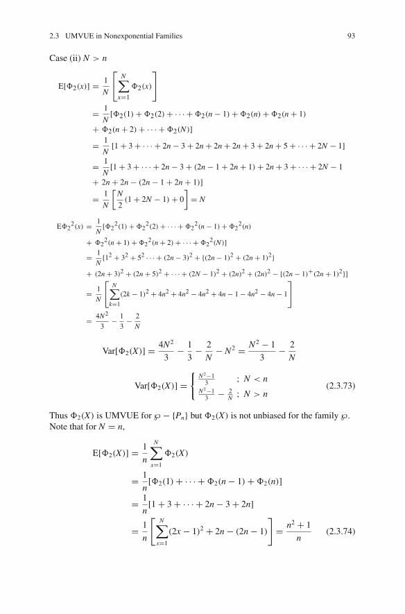
2.3 UMVUE in Nonexponential Families 93
Case (ii) N > n
E[�2(x)] = 1
N
⎡
⎣N∑
x=1
�2(x)
⎤
⎦
= 1
N[�2(1) + �2(2) + · · · + �2(n − 1) + �2(n) + �2(n + 1)
+ �2(n + 2) + · · · + �2(N)]= 1
N[1 + 3 + · · · + 2n − 3 + 2n + 2n + 2n + 3 + 2n + 5 + · · · + 2N − 1]
= 1
N[1 + 3 + · · · + 2n − 3 + (2n − 1 + 2n + 1) + 2n + 3 + · · · + 2N − 1
+ 2n + 2n − (2n − 1 + 2n + 1)]= 1
N
[N
2(1 + 2N − 1) + 0
]= N
E�22(x) = 1
N[�2
2(1) + �22(2) + · · · + �2
2(n − 1) + �22(n)
+ �22(n + 1) + �2
2(n + 2) + · · · + �22(N)]
= 1
N[12 + 32 + 52 · · · + (2n − 3)2 + {(2n − 1)2 + (2n + 1)2}
+ (2n + 3)2 + (2n + 5)2 + · · · + (2N − 1)2 + (2n)2 + (2n)2 − {(2n − 1)+(2n + 1)2}]
= 1
N
⎡
⎣N∑
k=1
(2k − 1)2 + 4n2 + 4n2 − 4n2 + 4n − 1 − 4n2 − 4n − 1
⎤
⎦
= 4N2
3− 1
3− 2
N
Var[�2(X)] = 4N2
3− 1
3− 2
N− N2 = N2 − 1
3− 2
N
Var[�2(X)] ={
N2−13 ; N < n
N2−13 − 2
N ; N > n(2.3.73)
Thus �2(X) is UMVUE for ℘ − {Pn} but �2(X) is not unbiased for the family ℘.Note that for N = n,
E[�2(X)] = 1
n
N∑
x=1
�2(X)
= 1
n[�2(1) + · · · + �2(n − 1) + �2(n)]
= 1
n[1 + 3 + · · · + 2n − 3 + 2n]
= 1
n
[N∑
x=1
(2x − 1)2 + 2n − (2n − 1)
]= n2 + 1
n(2.3.74)
94 2 Unbiased Estimation
E[�22(X)] = 1
n
[N∑
x=1
(2x − 1)2 + (2n)2 − (2n − 1)2]
= 4n2 − 1
3+ 4n − 1
n
Var[�2(X)] = 4n2 − 1
3+ 4n − 1
n−(n2 + 1
n
)2
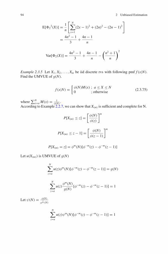
Example 2.3.5 Let X1,X2, . . . ,Xm be iid discrete rvs with following pmf f (x|N).Find the UMVUE of g(N).
f (x|N) ={
φ(N)M(x) ; a ≤ X ≤ N0 ; otherwise
(2.3.75)
where∑N
x=a M(x) = 1φ(N)
.According to Example 2.2.7, we can show that X(m) is sufficient and complete for N.
P[X(m) ≤ z] =[φ(N)
φ(z)
]m
P[X(m) ≤ z − 1] =[
φ(N)
φ(z − 1)
]m
P[X(m) = z] = φm(N)[φ−m(z) − φ−m(z − 1)]
Let u(X(m)) is UMVUE of g(N)
N∑
z=a
u(z)φm(N)[φ−m(z) − φ−m(z − 1)] = g(N)
N∑
z=a
u(z)φm(N)
g(N)[φ−m(z) − φ−m(z − 1)] = 1
Let ψ(N) = φ(N)
g1m (N)
N∑
z=a
u(z)ψm(N)[φ−m(z) − φ−m(z − 1)] = 1
2.3 UMVUE in Nonexponential Families 95
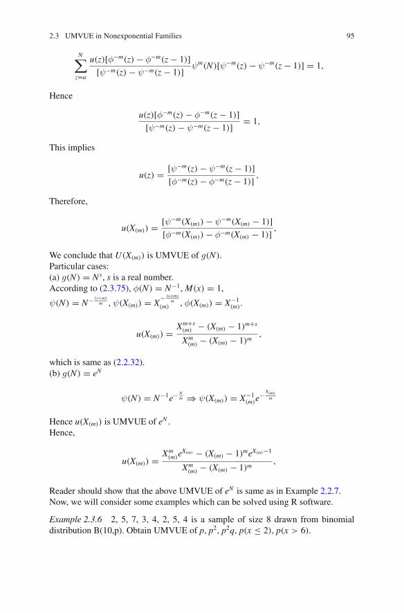
N∑
z=a
u(z)[φ−m(z) − φ−m(z − 1)][ψ−m(z) − ψ−m(z − 1)] ψm(N)[ψ−m(z) − ψ−m(z − 1)] = 1,
Hence
u(z)[φ−m(z) − φ−m(z − 1)][ψ−m(z) − ψ−m(z − 1)] = 1,
This implies
u(z) = [ψ−m(z) − ψ−m(z − 1)][φ−m(z) − φ−m(z − 1)] ,
Therefore,
u(X(m)) = [ψ−m(X(m)) − ψ−m(X(m) − 1)][φ−m(X(m)) − φ−m(X(m) − 1)] ,
We conclude that U(X(m)) is UMVUE of g(N).Particular cases:(a) g(N) = Ns, s is a real number.According to (2.3.75), φ(N) = N−1,M(x) = 1,
ψ(N) = N− (s+m)
m , ψ(X(m)) = X− (s+m)
m(m) , φ(X(m)) = X−1
(m).
u(X(m)) = Xm+s(m) − (X(m) − 1)m+s
Xm(m) − (X(m) − 1)m
,
which is same as (2.2.32).(b) g(N) = eN
ψ(N) = N−1e− Nm ⇒ ψ(X(m)) = X−1
(m)e− X(m)
m
Hence u(X(m)) is UMVUE of eN .Hence,
u(X(m)) = Xm(m)e
X(m) − (X(m) − 1)meX(m)−1
Xm(m) − (X(m) − 1)m
,
Reader should show that the above UMVUE of eN is same as in Example 2.2.7.Now, we will consider some examples which can be solved using R software.
Example 2.3.6 2, 5, 7, 3, 4, 2, 5, 4 is a sample of size 8 drawn from binomialdistribution B(10,p). Obtain UMVUE of p, p2, p2q, p(x ≤ 2), p(x > 6).

96 2 Unbiased Estimation
a=function (r,s)
{
m<-8
n<-10
x<-c(2,5,7,3,4,2,5,4)
t<-sum(x)
umvue=(choose(m*n-r-s,t-r)/choose(m*n,t))
print(umvue)
}
a(1,0) #UMVUE of p
a(2,0) #UMVUE of pˆ2
a(2,1) #UMVUE of pˆ2*q
b=function(c)
{
m<-8
n<-10
x<-c(2,5,7,3,4,2,5,4)
t<-sum(x)
g<-array(,c(1,c+1))
for (i in 1:c)
{
g[i]=((choose(n,i)*choose(m*n-n,t-i))/choose(m*n,t))
}
g[c+1]=((choose(n,0)*choose(m*n-n,t))/choose(m*n,t))
umvue=sum(g)
print (umvue)
}
b(2)#UMVUE of P(X<=2)
1-b(6)#UMVUE of P(X<=6) & P(X>6)
Example 2.3.7 0, 3, 1, 5, 5, 3, 2, 4, 5, 4 is a sample of size 10 from the Poissondistribution P(λ). Obtain UMVUE of λ, λ2, λe−λ, and P(x ≥ 4).
d=function (s,r) {
m<-10
x<-c(0,3,1,5,5,3,2,4,5,4)
t<-sum(x)
umvue=((m-s)ˆ(t-r)*factorial(t))/(mˆt*factorial(t-r))
print (umvue) } d(0,1) #UMVUE of lamda d(0,2) #UMVUE of
lamdaˆ2 d(1,1) #UMVUE of lamda*eˆ(-lamda) f=function (c) {
m<-10
x<-c(0,3,1,5,5,3,2,4,5,4)
t<-sum(x)
g<-array(,c(1,c+1))
for (i in 1:c)
2.3 UMVUE in Nonexponential Families 97
{
g[i]<-(choose(t,i)*(1/m)ˆi*(1-(1/m))ˆ(t-i))
}
g[c+1]=choose(t,0)*(1-(1/m))ˆt
umvue=sum(g)
print (umvue) } 1-f(3) #UMVUE of P(X<4) & P(X>=4)
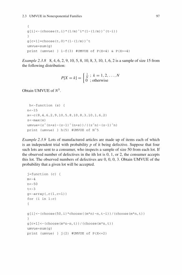
Example 2.3.8 8, 4, 6, 2, 9, 10, 5, 8, 10, 8, 3, 10, 1, 6, 2 is a sample of size 15 fromthe following distribution:
P[X = k] ={
1N ; k = 1, 2, . . . ,N0 ; otherwise
Obtain UMVUE of N5.
h<-function (s) {
n<-15
x<-c(8,4,6,2,9,10,5,8,10,8,3,10,1,6,2)
z<-max(x)
umvue=(zˆ(n+s)-(z-1)ˆ(n+s))/((zˆn)-(z-1)ˆn)
print (umvue) } h(5) #UMVUE of Nˆ5
Example 2.3.9 Lots of manufactured articles are made up of items each of whichis an independent trial with probability p of it being defective. Suppose that foursuch lots are sent to a consumer, who inspects a sample of size 50 from each lot. Ifthe observed number of defectives in the ith lot is 0, 1, or 2, the consumer acceptsthis lot. The observed numbers of defectives are 0, 0, 0, 3. Obtain UMVUE of theprobability that a given lot will be accepted.
j=function (c) {
m<-4
n<-50
t<-3
g<-array(,c(1,c+1))
for (i in 1:c)
{
g[i]<-(choose(50,i)*choose((m*n)-n,t-i))/(choose(m*n,t))
}
g[c+1]<-(choose(m*n-n,t))/(choose(m*n,t))
umvue=sum(g)
print (umvue) } j(2) #UMVUE of P(X<=2)
98 2 Unbiased Estimation
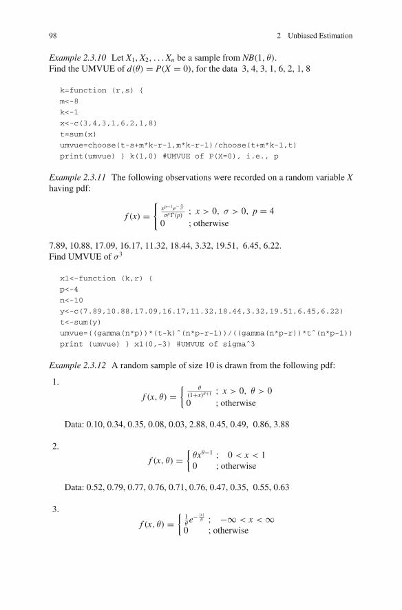
Example 2.3.10 Let X1,X2, . . .Xn be a sample from NB(1, θ).Find the UMVUE of d(θ) = P(X = 0), for the data 3, 4, 3, 1, 6, 2, 1, 8
k=function (r,s) {
m<-8
k<-1
x<-c(3,4,3,1,6,2,1,8)
t=sum(x)
umvue=choose(t-s+m*k-r-1,m*k-r-1)/choose(t+m*k-1,t)
print(umvue) } k(1,0) #UMVUE of P(X=0), i.e., p
Example 2.3.11 The following observations were recorded on a random variable Xhaving pdf:
f (x) ={
xp−1e− xσ
σp�(p) ; x > 0, σ > 0, p = 40 ; otherwise
7.89, 10.88, 17.09, 16.17, 11.32, 18.44, 3.32, 19.51, 6.45, 6.22.Find UMVUE of σ3
x1<-function (k,r) {
p<-4
n<-10
y<-c(7.89,10.88,17.09,16.17,11.32,18.44,3.32,19.51,6.45,6.22)
t<-sum(y)
umvue=((gamma(n*p))*(t-k)ˆ(n*p-r-1))/((gamma(n*p-r))*tˆ(n*p-1))
print (umvue) } x1(0,-3) #UMVUE of sigmaˆ3
Example 2.3.12 A random sample of size 10 is drawn from the following pdf:
1.
f (x, θ) ={ θ
(1+x)θ+1 ; x > 0, θ > 00 ; otherwise
Data: 0.10, 0.34, 0.35, 0.08, 0.03, 2.88, 0.45, 0.49, 0.86, 3.88
2.
f (x, θ) ={
θxθ−1 ; 0 < x < 10 ; otherwise
Data: 0.52, 0.79, 0.77, 0.76, 0.71, 0.76, 0.47, 0.35, 0.55, 0.63
3.
f (x, θ) ={
1θe− |x|
θ ; −∞ < x < ∞0 ; otherwise

2.3 UMVUE in Nonexponential Families 99
Data: 9.97, 0.64, 3.17, 1.48, 0.81, 0.61, 0.62, 0.72, 3.14, 2.99Find UMVUE of θ in (i), (ii), and (iii).
(i)
x2<-function (k,r) {
n<-10
y<-c(0.10,0.34,0.35,0.08,0.03,2.88,0.45,0.49,0.86,3.88)
x<-array(,c(1,10))
for (i in 1:10)
{
x[i]=log(1+y[i])
}
t<-sum(x)
umvue=(((t-k)ˆ(n-r-1))*gamma(n))/((tˆ(n-1))*gamma(n-r))
print (umvue) } x2(0,1) #UMVUE of theta
(ii)
x3<-function (k,r) {
n<-10
y<-c(0.52,0.79,0.77,0.76,0.71,0.76,0.47,0.35,0.55,0.63)
x<-array(,c(1,10))
for (i in 1:10)
{
x[i]=-log(y[i])
}
t<-sum(x)
umvue=(((t-k)ˆ(n-r-1))*gamma(n))/((tˆ(n-1))*gamma(n-r))
print (umvue) } x3(0,1) #UMVUE of theta
(iii)
x4<-function (k,r) {
n<-10
y<-c(9.97,0.64,3.17,1.48,0.81,0.61,0.62,0.72,3.14,2.99)
t<-sum(y)
umvue=(((t-k)ˆ(n-r-1))*gamma(n))/((tˆ(n-1))*gamma(n-r))
print (umvue) } x4(0,-1) #UMVUE of theta
Example 2.3.13 The following observations were obtained on an rv X following:
1. N(θ,σ2)
Data: 5.77, 3.81, 5.24, 8.81, 0.98, 8.44, 3.16, 11.27, 4.40, 4.87, 7.28, 8.48, 6.43,−0.00, 9.67, 12.04, −5.06, 13.71, 6.12, 4.76Find UMVUE of θ, θ2, ϑ3 and P(x ≤ 2)

100 2 Unbiased Estimation
2. N(6,σ2)
Data: 7.26, −0.23, 7.55, 3.09, 7.62, 16.79, 5.27, 8.46, 5.16, −0.66.Find UMVUE of 1
σ, σ, σ2, P(X ≥ 2)
3. N(θ,σ2)
Data: 10.59, −1.50, 6.40, 7.55, 4.70, 1.63, 0.04, 2.96, 6.47, 6.42Find UMVUE of θ, θ2, θ + 2σ,
(i)
x5<-function (sigsq,n,k)
{x<-c(5.77,3.81,5.24,8.81,0.98,8.44,3.16,11.27,4.4,4.87,7.28,
8.48,6.43,0,9.67,12.04,-5.06,13.71,6.12,4.76)
umvue1=mean(x)
umvue2=umvue1ˆ2-(sigsq/n)
umvue3=umvue1ˆ3-(3*sigsq*umvue1/n)
umvue4=pnorm((k-(mean(x)))/(sqrt((sigsq*((n-1)/n)))))
print (umvue1) #UMVUE of theta
print (umvue2) #UMVUE of thetaˆ2
print (umvue3) #UMVUE of thetaˆ3
print (umvue4) #UMVUE of P(X<=2) } x5(4,20,2)
(ii)
x6<-function (n,r) {
x<-c(7.26,-0.23,7.55,3.09,7.62,16.79,5.27,8.46,5.16,-0.66)
t<-sum((x-6)ˆ2)
umvue=(((tˆr)*gamma(n/2))/((2ˆr)*gamma((n/2)+r)))
print (umvue) } x6 (10,-0.5) #UMVUE of 1/sigma x6 (10,0.5)
#UMVUE of sigma x6 (10,1) #UMVUE of sigmaˆ2
x7<-function (n,k) {
x<-c(7.26,-0.23,7.55,3.09,7.62,16.79,5.27,8.46,5.16,-0.66)
t<-sum((x-6)ˆ2)
umvue<-(1-pbeta(((k-6)/sqrt(t))ˆ2,0.5, ((n-1)/2)))*0.5
print (umvue) } x7(10,2) #UMVUE of P(X>=2)
(iii)
x8<-function(n,r) {
x<-c(10.59,-1.5,6.4,7.55,4.7,1.63,0.04,2.96,6.47,6.42)
s<-sum((x-mean(x))ˆ2)
umvue1<-mean(x) #UMVUE of theta
umvue2<-((sˆ(r))*gamma((n-1)/2))/(gamma(((n-1)/2)+r)*(2ˆr))
#UMVUE of sigmaˆ2
print (umvue1)
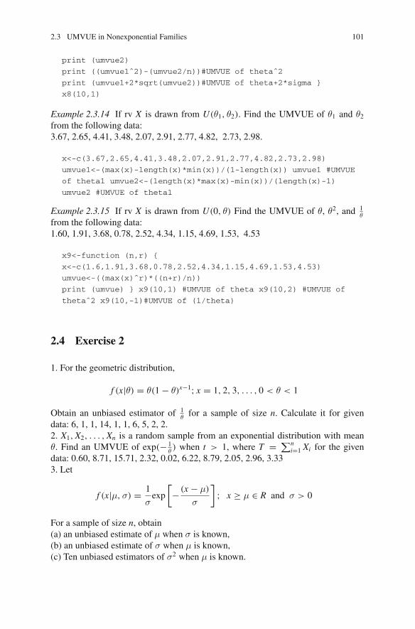
2.3 UMVUE in Nonexponential Families 101
print (umvue2)
print ((umvue1ˆ2)-(umvue2/n))#UMVUE of thetaˆ2
print (umvue1+2*sqrt(umvue2))#UMVUE of theta+2*sigma }
x8(10,1)
Example 2.3.14 If rv X is drawn from U(θ1, θ2). Find the UMVUE of θ1 and θ2from the following data:3.67, 2.65, 4.41, 3.48, 2.07, 2.91, 2.77, 4.82, 2.73, 2.98.
x<-c(3.67,2.65,4.41,3.48,2.07,2.91,2.77,4.82,2.73,2.98)
umvue1<-(max(x)-length(x)*min(x))/(1-length(x)) umvue1 #UMVUE
of theta1 umvue2<-(length(x)*max(x)-min(x))/(length(x)-1)
umvue2 #UMVUE of theta1
Example 2.3.15 If rv X is drawn from U(0, θ) Find the UMVUE of θ, θ2, and 1θ
from the following data:1.60, 1.91, 3.68, 0.78, 2.52, 4.34, 1.15, 4.69, 1.53, 4.53
x9<-function (n,r) {
x<-c(1.6,1.91,3.68,0.78,2.52,4.34,1.15,4.69,1.53,4.53)
umvue<-((max(x)ˆr)*((n+r)/n))
print (umvue) } x9(10,1) #UMVUE of theta x9(10,2) #UMVUE of
thetaˆ2 x9(10,-1)#UMVUE of (1/theta)
2.4 Exercise 2
1. For the geometric distribution,
f (x|θ) = θ(1 − θ)x−1; x = 1, 2, 3, . . . , 0 < θ < 1
Obtain an unbiased estimator of 1θfor a sample of size n. Calculate it for given
data: 6, 1, 1, 14, 1, 1, 6, 5, 2, 2.2. X1,X2, . . . ,Xn is a random sample from an exponential distribution with meanθ. Find an UMVUE of exp(− 1
θ) when t > 1, where T = ∑n
i=1 Xi for the givendata: 0.60, 8.71, 15.71, 2.32, 0.02, 6.22, 8.79, 2.05, 2.96, 3.333. Let
f (x|μ,σ) = 1
σexp
[− (x − μ)
σ
]; x ≥ μ ∈ R and σ > 0
For a sample of size n, obtain(a) an unbiased estimate of μ when σ is known,(b) an unbiased estimate of σ when μ is known,(c) Ten unbiased estimators of σ2 when μ is known.
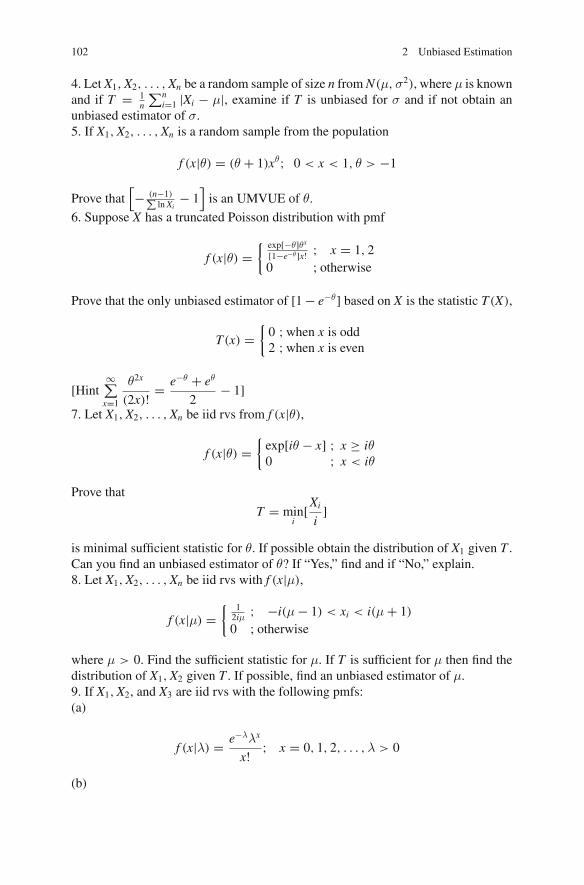
102 2 Unbiased Estimation
4. Let X1,X2, . . . ,Xn be a random sample of size n fromN(μ,σ2), where μ is knownand if T = 1
n
∑ni=1 |Xi − μ|, examine if T is unbiased for σ and if not obtain an
unbiased estimator of σ.5. If X1,X2, . . . ,Xn is a random sample from the population
f (x|θ) = (θ + 1)xθ; 0 < x < 1, θ > −1
Prove that[− (n−1)∑
lnXi− 1]is an UMVUE of θ.
6. Suppose X has a truncated Poisson distribution with pmf
f (x|θ) ={ exp[−θ]θx
[1−e−θ]x! ; x = 1, 20 ; otherwise
Prove that the only unbiased estimator of [1− e−θ] based on X is the statistic T(X),
T(x) ={0 ;when x is odd2 ;when x is even
[Hint∞∑x=1
θ2x
(2x)! = e−θ + eθ
2− 1]
7. Let X1,X2, . . . ,Xn be iid rvs from f (x|θ),
f (x|θ) ={exp[iθ − x] ; x ≥ iθ0 ; x < iθ
Prove that
T = mini
[Xi
i]
is minimal sufficient statistic for θ. If possible obtain the distribution of X1 given T .Can you find an unbiased estimator of θ? If “Yes,” find and if “No,” explain.8. Let X1,X2, . . . ,Xn be iid rvs with f (x|μ),
f (x|μ) ={ 1
2iμ ; −i(μ − 1) < xi < i(μ + 1)0 ; otherwise
where μ > 0. Find the sufficient statistic for μ. If T is sufficient for μ then find thedistribution of X1,X2 given T . If possible, find an unbiased estimator of μ.9. If X1,X2, and X3 are iid rvs with the following pmfs:(a)
f (x|λ) = e−λλx
x! ; x = 0, 1, 2, . . . ,λ > 0
(b)

2.4 Exercise 2 103
f (x|λ) =(n
x
)λx(1 − λ)n−λ; 0 < λ < 1, x = 0, 1, 2, . . . , n
(c)
f (x|λ) = (1 − λ)λx; x = 0, 1, 2, . . . λ > 0
Prove that X1 + 2X2, X2 + 3X3, and X1 + 2X2 +X3 are not sufficient for λ in (a), (b),and (c). Further, prove that 2(X1 + X2 + X3) is sufficient for λ in (a), (b), and (c).10. Let X1,X2, . . . ,Xn be iid rvs having∪(θ, 3θ), θ > 0. Then prove that (X(1),X(n))is jointly minimal sufficient statistic.11. Let {(Xi,Yi), i = 1, 2, . . . , n} be n independent random vectors having a bivariatedistribution
N =((
θ1θ2
),
(σ21 ρσ1σ2
ρσ1σ2 σ22
)); − ∞ < θ1, θ2 < ∞, σ1,σ2 > 0, − 1 ≤ ρ ≤ 1.
Prove that(∑
Xi,∑
X2i ,∑
XiYi,∑
Yi∑
Y 2i
)
is jointly sufficient (θ1,σ1, ρ, θ2,σ2).12. Let the rv X1 is B(n, θ) and X2 is P(θ) where n is known and 0 < θ < 1. Obtainfour unbiased estimators of θ.13. Let X1,X2, . . . ,Xn are iid rvs with ∪(θ, θ + 1).
(i) Find sufficient statistic for θ
(ii) Show that the sufficient statistic is not complete
(iii) Find an unbiased estimator of θ
(iv) Find the distribution of X1 given T , where T is sufficient for θ
(v) Can you find UMVUE of θ ? If “No,” give reasons.
14. Let X be a rv with pmf
f (x|p) =(p2
)|x|(1 − p)1−|x|; x = −1, 0, 1, 0 < p < 1
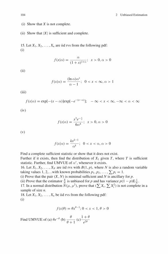
104 2 Unbiased Estimation
(i) Show that X is not complete.
(ii) Show that |X| is sufficient and complete.
15. Let X1,X2, . . . ,Xn are iid rvs from the following pdf:(i)
f (x|α) = α
(1 + x)1+α; x > 0,α > 0
(ii)
f (x|α) = (lnα)αx
α − 1; 0 < x < ∞,α > 1
(iii)
f (x|α) = exp[−(x − α)]exp[−e−(x−α)]; − ∞ < x < ∞,−∞ < α < ∞
(iv)
f (x|α) = x3e− xα
6α4; x > 0,α > 0
(v)
f (x|α) = kxk−1
αk; 0 < x < α,α > 0
Find a complete sufficient statistic or show that it does not exist.Further if it exists, then find the distribution of X1 given T , where T is sufficientstatistic. Further, find UMVUE of αr , whenever it exists.16. Let X1,X2, . . . ,XN are iid rvs with B(1, p), where N is also a random variabletaking values 1, 2,…with known probabilities p1, p2, . . . ,
∑pi = 1.
(i) Prove that the pair (X,N) is minimal sufficient and N is ancillary for p.(ii) Prove that the estimator X
N is unbiased for p and has variance p(1 − p)E 1N .
17. In a normal distribution N(μ,μ2), prove that (∑
Xi,∑
X2i ) is not complete in a
sample of size n.18. Let X1,X2, . . . ,Xn be iid rvs from the following pdf:(i)
f (x|θ) = θxθ−1; 0 < x < 1, θ > 0
Find UMVUE of (a) θe−θ (b)θ
θ + 1(c)
1 + θ
e2θ
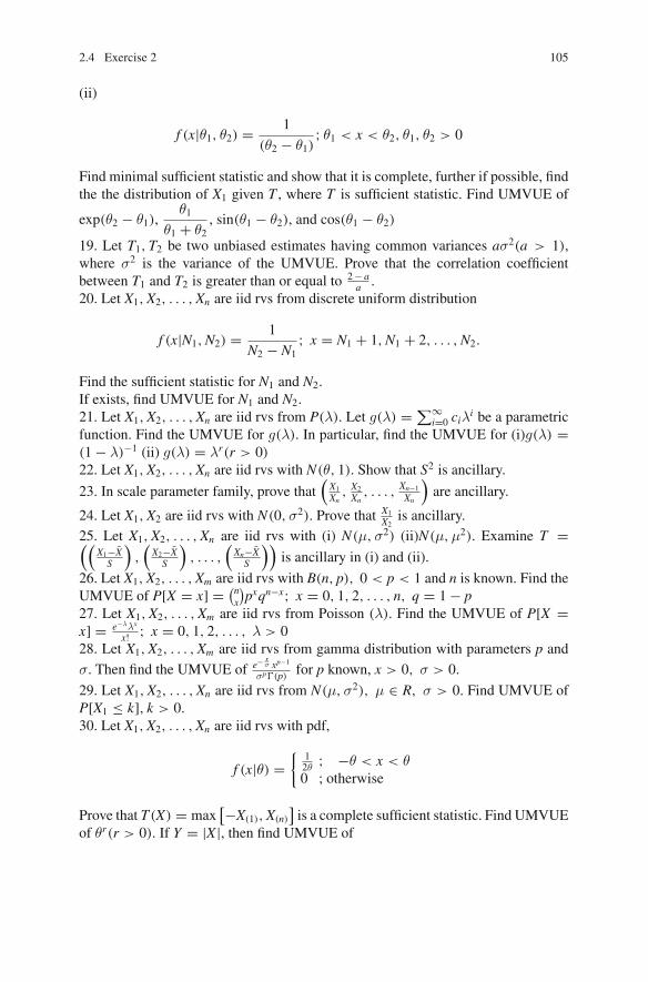
2.4 Exercise 2 105
(ii)
f (x|θ1, θ2) = 1
(θ2 − θ1); θ1 < x < θ2, θ1, θ2 > 0
Find minimal sufficient statistic and show that it is complete, further if possible, findthe the distribution of X1 given T , where T is sufficient statistic. Find UMVUE of
exp(θ2 − θ1),θ1
θ1 + θ2, sin(θ1 − θ2), and cos(θ1 − θ2)
19. Let T1,T2 be two unbiased estimates having common variances aσ2(a > 1),where σ2 is the variance of the UMVUE. Prove that the correlation coefficientbetween T1 and T2 is greater than or equal to 2− a
a .20. Let X1,X2, . . . ,Xn are iid rvs from discrete uniform distribution
f (x|N1,N2) = 1
N2 − N1; x = N1 + 1,N1 + 2, . . . ,N2.
Find the sufficient statistic for N1 and N2.If exists, find UMVUE for N1 and N2.21. Let X1,X2, . . . ,Xn are iid rvs from P(λ). Let g(λ) = ∑∞
i=0 ciλi be a parametric
function. Find the UMVUE for g(λ). In particular, find the UMVUE for (i)g(λ) =(1 − λ)−1 (ii) g(λ) = λr(r > 0)22. Let X1,X2, . . . ,Xn are iid rvs with N(θ, 1). Show that S2 is ancillary.
23. In scale parameter family, prove that(X1Xn
, X2Xn
, . . . ,Xn−1
Xn
)are ancillary.
24. Let X1,X2 are iid rvs with N(0,σ2). Prove that X1X2
is ancillary.25. Let X1,X2, . . . ,Xn are iid rvs with (i) N(μ,σ2) (ii)N(μ,μ2). Examine T =((
X1−X̄S
),(X2−X̄S
), . . . ,
(Xn−X̄S
))is ancillary in (i) and (ii).
26. Let X1,X2, . . . ,Xm are iid rvs with B(n, p), 0 < p < 1 and n is known. Find theUMVUE of P[X = x] = (nx
)pxqn−x; x = 0, 1, 2, . . . , n, q = 1 − p
27. Let X1,X2, . . . ,Xm are iid rvs from Poisson (λ). Find the UMVUE of P[X =x] = e−λλx
x! ; x = 0, 1, 2, . . . , λ > 028. Let X1,X2, . . . ,Xm are iid rvs from gamma distribution with parameters p and
σ. Then find the UMVUE of e− xσ xp−1
σp�(p) for p known, x > 0, σ > 0.
29. Let X1,X2, . . . ,Xn are iid rvs from N(μ,σ2), μ ∈ R, σ > 0. Find UMVUE ofP[X1 ≤ k], k > 0.30. Let X1,X2, . . . ,Xn are iid rvs with pdf,
f (x|θ) ={
12θ ; −θ < x < θ0 ; otherwise
Prove that T(X) = max[−X(1),X(n)
]is a complete sufficient statistic. Find UMVUE
of θr(r > 0). If Y = |X|, then find UMVUE of
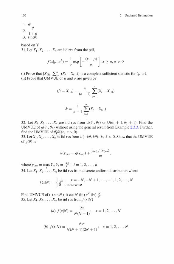
106 2 Unbiased Estimation
1. θr
2.θ
1 + θ3. sin(θ)
based on Y.31. Let X1,X2, . . . ,Xn are iid rvs from the pdf,
f (x|μ,σ2) = 1
σexp
[− (x − μ)
σ
]; x ≥ μ,σ > 0
(i) Prove that [X(1),∑n
j=1(Xj − X(1))] is a complete sufficient statistic for (μ,σ).(ii) Prove that UMVUE of μ and σ are given by
(μ̂ = X(1)) − n
(n − 1)
n∑
j=1
(Xj − X(1))
σ̂ = 1
n − 1
n∑
j=1
(Xj − X(1))
32. Let X1,X2, . . . ,Xn are iid rvs from ∪(θ1, θ2) or ∪(θ1 + 1, θ2 + 1). Find theUMVUE of g(θ1, θ2) without using the general result from Example 2.3.3. Further,find the UMVUE of θr1θ
s2(r, s > 0).
33. LetX1,X2, . . . ,Xn be iid rvs from∪(−kθ, kθ), k, θ > 0. Show that the UMVUEof g(θ) is
u(y(m) = g(y(m)) + y(m)g′(y(m))
m,
where y(m) = maxi
Yi, Yi = |Xi|k : i = 1, 2, . . . , n
34. Let X1,X2, . . . ,Xm be iid rvs from discrete uniform distribution where
f (x|N) ={
12N ; x = −N,−N + 1, . . . ,−1, 1, 2, . . . ,N0 ; otherwise
Find UMVUE of (i) sinN (ii) cosN (iii) eN (iv) NeN
35. Let X1,X2, . . . ,Xm be iid rvs from f (x|N)
(a) f (x|N) = 2x
N(N + 1); x = 1, 2, . . . ,N
(b) f (x|N) = 6x2
N(N + 1)(2N + 1); x = 1, 2, . . . ,N
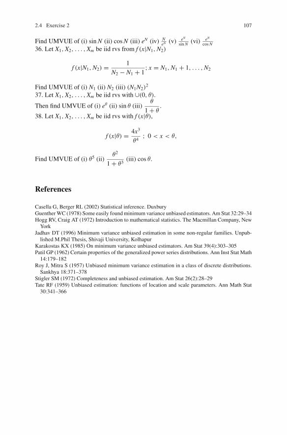
2.4 Exercise 2 107
Find UMVUE of (i) sinN (ii) cosN (iii) eN (iv) NeN (v) eN
sinN (vi) eN
cosN36. Let X1,X2, . . . ,Xm be iid rvs from f (x|N1,N2)
f (x|N1,N2) = 1
N2 − N1 + 1; x = N1,N1 + 1, . . . ,N2
Find UMVUE of (i) N1 (ii) N2 (iii) (N1N2)2
37. Let X1,X2, . . . ,Xm be iid rvs with ∪(0, θ).
Then find UMVUE of (i) eθ (ii) sin θ (iii)θ
1 + θ.
38. Let X1,X2, . . . ,Xm be iid rvs with f (x|θ),
f (x|θ) = 4x3
θ4; 0 < x < θ,
Find UMVUE of (i) θ5 (ii)θ2
1 + θ3(iii) cos θ.
References
Casella G, Berger RL (2002) Statistical inference. DuxburyGuentherWC (1978) Some easily foundminimum variance unbiased estimators. Am Stat 32:29–34Hogg RV, Craig AT (1972) Introduction to mathematical statistics. The Macmillan Company, NewYork
Jadhav DT (1996) Minimum variance unbiased estimation in some non-regular families. Unpub-lished M.Phil Thesis, Shivaji University, Kolhapur
Karakostas KX (1985) On minimum variance unbiased estimators. Am Stat 39(4):303–305Patil GP (1962) Certain properties of the generalized power series distributions. Ann Inst Stat Math14:179–182
Roy J, Mitra S (1957) Unbiased minimum variance estimation in a class of discrete distributions.Sankhya 18:371–378
Stigler SM (1972) Completeness and unbiased estimation. Am Stat 26(2):28–29Tate RF (1959) Unbiased estimation: functions of location and scale parameters. Ann Math Stat30:341–366

http://www.springer.com/978-981-10-0888-7
Related Documents