What You Do in High School Matters: The Effects of High School GPA on Educational Attainment and Labor Market Earnings in Adulthood

1

What You Do in High School Matters: The Effects of High School GPA on Educational Attainment and Labor

Market Earnings in Adulthood

Michael T. Frencha

Jenny F. Homerb

Philip K. Robinsc

Note: Authors are listed alphabetically.

a Corresponding author and reprint requests: Professor of Health Economics, Department of Sociology, University of Miami, 5202 University Drive, Merrick Building, Room 121F, P.O. Box 248162, Coral Gables, FL, 33124-2030, USA; Phone: 305-284-6039; E-mail:[email protected] b Senior Research Associate, Health Economics Research Group, Sociology Research Center, University of Miami, 5665 Ponce de Leon Blvd., Flipse Building, Room 104, Coral Gables, FL 33124-0719, USA; E-mail: [email protected] cProfessor, Department of Economics, University of Miami, Jenkins Building, 5250 University Drive, Coral Gables, FL 33146-6550, USA; Phone: 305-284-5664; E-mail: [email protected] ACKNOWLEDGEMENTS: The authors are grateful for research assistance from Christina Gonzalez and Karina Ugarte and editorial/administrative assistance from Allison Johnson and Carmen Martinez. This research uses data from Add Health, a program project directed by Kathleen Mullan Harris and designed by J. Richard Udry, Peter S. Bearman, and Kathleen Mullan Harris at the University of North Carolina at Chapel Hill and funded by grant P01-HD31921 from the Eunice Kennedy Shriver National Institute of Child Health and Human Development with cooperative funding from 23 other federal agencies and foundations. Special acknowledgment is due to Ronald R. Rindfuss and Barbara Entwisle for assistance in the original design. The Add Health website (http://www.cpc.unc.edu/addhealth) provides information on how to obtain the Add Health data files. We received no direct support from grant P01-HD31921 for this analysis.

September 15, 2010

mailto:[email protected]�



2

What You Do in High School Matters: The Effects of High School GPA on Educational Attainment and Labor

Market Earnings in Adulthood

Abstract

Using abstracted grades and other data from Add Health, we investigate the effects of cumulative

high school GPA on educational attainment and labor market earnings among a sample of young

adults (ages 24-34). We estimate several models with an extensive list of control variables and high

school fixed effects. Results consistently show that high school GPA is a positive and statistically

significant predictor of educational attainment and earnings in adulthood. Moreover, the effects are

large and economically important for each gender. Interesting and somewhat unexpected findings

emerge for race. Various sensitivity tests support the stability of the core findings.

JEL Classification: I2, J24, J31

Keywords: High school grades; Educational attainment; Earnings; Panel data

3

I. Introduction

Teenagers face numerous and often dramatic changes in physical appearance, emotional

status, character, personality, and human capital over the course of high school. From an academic

perspective, one needs to do well in high school to gain entry into a reputable college or university

or even land a lucrative job. Most people assume, however, that academic performance in high

school is less predictive of overall educational attainment and only weakly related to labor market

earnings in adulthood. If these assumptions are false, however, then one’s academic standing in

high school could be an important boost or drag on one’s educational attainment and labor market

success in adulthood.

Numerous studies have found that higher educational attainment is associated with greater

earnings (Mincer, 1974; Card, 1999; Crissey, 2009). Two general mechanisms help to explain this

relationship. According to human capital theory, education enhances an individual’s skills and ability

(Wise, 1975). Beyond skills acquisition, prospective employers use grades and academic

performance to differentiate among job candidates (Spence, 1973; Lazear, 1977; Jones and Jackson,

1990). An extensive review by Card (1999) concludes that certain observable characteristics such as

race, school quality, family background, and cognitive ability are related to the returns to education.

In contrast to the broad availability of literature on educational attainment and earnings, little

is known about the association between educational performance and earnings. The vast majority of

studies in this area focus on whether college grades, college major, and college selectivity affect

future earnings (Thomas, 2003; Loury and Garman, 1995; Hamermesh and Donald, 2008; Jones and

Jackson 1990; Monks, 2000; Hoekstra, 2009; Zhang, 2008). Although this literature indicates that

more demanding majors and higher quality institutions contribute to higher earnings (Zhang, 2008),

some studies that control for ability and/or selection have found smaller effects (Dale and Krueger,

2002; Hamermesh and Donald, 2008). Only a small number of studies control for high school

4

grades (which are usually self reported) when evaluating the relationship between academic factors in

college (e.g., GPA, major, or graduation status) and labor market outcomes. Moreover, high school

achievement does little to mediate these relationships (Wise, 1975; Grogger and Eide, 1995;

Hamermesh and Donald, 2008).

Compared to the research focusing on college performance and related characteristics, very

few studies have investigated the impact of high school performance, as measured by cumulative

GPA, on future academic and labor market outcomes. Crawford and colleagues (1997) and Bishop

and colleagues (1985) examine whether high school GPA influences short-term (three years or less)

labor market outcomes for individuals who began working immediately after completing high

school. Both find positive effects. Specifically, Crawford and colleagues (1997) estimate that a one-

point increase in high school GPA adds $800-$1000 to annual earnings after high school. Meyer

and Wise (1982) find that high school rank is positively related to weeks worked and wages for men

four years after high school graduation. The authors suggest that class rank may reflect work ethic

and that those with a strong work ethic in high school may continue to work hard in the labor force.

Wolfie and Smith’s (1956) descriptive analysis of high school class rank and earnings twenty years

after high school graduation indicates that, among individuals with college degrees, those at the top

of their high school classes earn higher incomes than those with lower class ranks, but they find no

significant differences for individuals who do not attend college.

Most of the other studies examining longer-term labor market outcomes and high school

academic performance focus primarily on high school curriculum (Altonji, 1995; Levine and

Zimmerman, 1995; Rose and Betts, 2004) or achievement tests (Lleras, 2008) rather than GPA per

se. For example, Rose and Betts (2004) investigate whether specific high school math classes (e.g.,

pre-algebra, algebra/geometry) are associated with earnings ten years after high school graduation.

They control for math GPA and school fixed effects and use an instrumental variables approach to

5

account for unobserved ability and motivation. Math courses in high school exert a large and

significant impact on earnings, with greater effects for more advanced courses.

One would expect educational performance in high school to affect ultimate educational

attainment in addition to future labor market outcomes. Although high school achievement is a

predictor of academic performance in college (Betts and Morell, 1999; Cohn et al., 2004), the

relationship between high school GPA and educational attainment for adults has not been fully

examined. Studies in which educational attainment is the dependent variable frequently include

young samples or college students with incomplete academic careers (Betts and Morell, 1999; Ou

and Reynolds, 2008; Melby et al., 2008). Other correlates of total educational attainment include

personal characteristics (e.g., race, history of delinquency), previous academic achievement (e.g.,

standardized test scores, educational expectations, grade retention, school absences), and family

background (e.g., maternal education, parental involvement in education, income) (Betts and Morell,

1999; Ou and Reynolds, 2008; Melby et al., 2008; Cameron and Heckman, 2001).

In this paper, we use data from Waves 1, 3, and 4 of the National Longitudinal Survey of

Adolescent Health (Add Health) to examine whether cumulative GPA in high school is significantly

related to educational attainment and labor market earnings during early adulthood. Our

investigation overcomes several important limitations of the existing literature in this area and offers

new insights into the complex relationship between the academic performance of teenagers and

various outcomes in young adulthood.

First, using GPA data abstracted from high school records rather than subjective measures

of student competence or self-reported grades allows us to avoid the potential measurement error

problems that plague many previous studies. Only a few studies in this area (notably Crawford et al.,

1997; Rose and Betts, 2004) do not use individual self reports of high school performance. Second,

Add Health respondents were between the ages of 24 and 34 at Wave 4, when educational

6

attainment and wages are likely to be well established. Third, some of the studies noted above are

limited to men (Loury and Garman, 1995; Hoekstra, 2009; Wise, 1975), Whites (Hoekstra, 2009;

Wise, 1975), or individuals with a common level of education (e.g., those who did not attend college

or college graduates) (Thomas, 2003; Monks, 2000; Mueller, 1988). Analyzing diverse samples is

essential since notable disparities in educational attainment as well as different returns to education

based on level of educational attainment exist for different racial, ethnic, and gender groups (U.S.

Census Bureau, 2010). Our analysis accounts for seven categories of educational attainment ranging

from those who did not finish high school to those with advanced graduate degrees. Finally, we

study males and females separately (Levine and Zimmerman, 1995) and control for numerous

personal and family background characteristics that could influence the outcomes of interest

(Cameron and Heckman, 2001; Loury and Garman, 1995; Lleras, 2008).

II. Conceptual Framework

Adolescence is a time of rapid intellectual, mental, and emotional developments with

corresponding physical and social changes (Maggs et al., 1997; Kroger, 2006). These formidable

challenges sidetrack many high school students in their academic pursuits, often leading to poor

grades and other educational difficulties. If such scholastic lapses are atypical and transitory, then

high school achievement plays a role in college admission but not thereafter. Alternatively, high

school grades may accurately characterize underlying potential and behavior, thereby serving as a

reliable signal of future success in the classroom and workplace.

Identity formation and decisions about whether to conform to or challenge adult

conventions also occur during adolescence (Erikson, 1968; Maggs et al., 1997; Kroger, 2006).

Nonconformist behaviors and academic achievement are both avenues through which adolescents

identify with their peers and rebel against or abide by adult conventions. Based partly on studies in

the educational psychology and economics literature (Anderson and Keith, 1997; Heckman, 2008;

7

Lounsbury et al., 2003; Neisser et al., 1996; Rivkin et al., 2005), we assume that each student is

endowed with a certain level of intelligence or ability (proxied by the Peabody Picture Vocabulary

Test [PVT] score in our data) as well as an innate degree of social capital. Students then make

decisions about combining these initial endowments with a host of variable resources (e.g., time

spent studying, selection of friends, participation in extracurricular activities) to achieve certain goals

related to their identities. For example, students who desire to attend college are likely to invest a

greater amount of their time in studying and developing their human capital. If high school GPA is

positively correlated with adult earnings, this suggests that academic achievement early in life is an

accurate predictor of future outcomes. Alternatively, a negative association between adult earnings

and high school GPA could reflect decisions by students to allocate time to other objectives such as

socializing rather than to schoolwork. The analysis that follows cannot definitively resolve these

possible mechanisms, but the results offer new insight into a topic that heretofore has been focused

almost exclusively on contemporaneous outcomes and predictors.

Another distinct advantage of this paper vis-à-vis most of the published literature is our

ability to control for intellectual potential (via the PVT score), adolescent living conditions, parental

education, and other important endowment factors. If these variables are missing from the models

and correlated with high school GPA, then the effects of high school GPA on years of education

and earnings may be overstated. Access to abstracted GPA data as well as these key background

characteristics allows us to estimate more fully specified models and generate more precise estimates.

Thus, while omitted variable bias remains a distinct possibility, our inclusion of a large list of

important control variables should lessen this problem considerably.

Another advantage of Add Health’s extensive data is that we can decompose the effects of

our key and secondary variables to examine extensions and masked relationships. For example, does

the estimated coefficient for high school GPA in the earnings equations drop considerably when we

8

add PVT score to the model? Do racial and ethnic minorities complete fewer years of education

relative to Whites? Does allowing for school fixed effects mediate these relationships? We discuss

these and other analyses in the Results section.

Although high school grades are almost certainly endogenous to other outcomes such as

grooming, anti-social behavior, and athletic success among teenagers, we don’t believe that high

school grades are endogenous to educational attainment and labor market earnings among adults.

Temporally, high school performance is measured from age 14 to 18 for the vast majority of

individuals whereas formal education ceases well into the 20s for most students. Our annual

earnings measure pertains to adults who are 24 to 34 years of age. Thus, reverse causality is clearly

not a concern, and endogeneity bias is unlikely.

The final conceptual point regarding sample formation concerns possible gender differences.

Some studies of academic achievement and labor market outcomes among adults have estimated

separate models for men and women (e.g., Mueller, 1988; Levine and Zimmerman, 1995). Other

studies (mainly in the educational and psychology literature) have also identified gender differences

in academic achievement, with females earning higher grades than their male counterparts (Dwyer

and Johnson, 1997; Kleinfeld, 1998). In the Add Health data, overall high school GPA is

significantly higher among females whereas males have significantly higher annual earnings at Wave

4. For these reasons, it seems appropriate to analyze males and females separately.

III. Methods

The primary variables of interest in this study are high school GPA (the key explanatory

variable), highest level of education attained (the first outcome variable), and personal earnings (the

second outcome variable). Cumulative high school GPA, the average of all classes and years during

an individual’s high school career, is reported on a 4-point scale.1

1 The cumulative GPA is calculated based on the number of years a student has course data.

Highest level of education at

9

Wave 4 contains seven categories ranging from less than or some high school to an advanced

professional degree (e.g., JD, MD, PhD). Personal earnings include all income derived from

employment before taxes during the calendar year prior to the Wave 4 interview.2 Because earnings

are highly skewed, we follow the literature by analyzing the natural logarithm of earnings.3 We

estimate the categorical measure of educational attainment using an ordered probit model, and we

estimate the log of personal earnings using robust regression, a hybrid form of OLS that down-

weights outlier observations (StataCorp, 2009).4

Although cumulative high school GPA is the explanatory variable of interest, we estimate

five distinct specifications for each dependent variable. The first specification, A, starts with a set of

demographic control variables and familial background characteristics, which provides a benchmark

set of estimates as all later specifications include this principal set of variables. Specification B adds

cumulative high school GPA to determine the full effect of this variable without any other controls

for ability/intelligence or current school attendance. Specification C adds the PVT score as a proxy

measure of ability/intelligence. We add a dummy variable for currently attending school to

Specification D, and the final specification, E, includes school fixed effects.

We can formally write the fully-specified model, E, as:

(1)

where Yi is either highest level of education attained (the categorical value) or the logarithm of

annual personal earnings for individual i, Xi is a vector of demographic and familial variables, GPAi

is cumulative grade point average in high school, PVTi is the score on the Peabody Picture

Vocabulary Test, ASi is an indicator variable for currently attending school, Sj is a vector of indicator

2 Respondents were asked to report how much income they received from personal earnings before taxes (i.e., wages or salaries, including tips, bonuses, and overtime pay, and income from self employment). The question refers to personal income earned in the calendar year prior to the interview year. 3 For non-earners, we set earnings to $1, so the natural logarithm of earnings is zero in this case. 4 As a sensitivity test, we estimate the log of personal earnings using OLS. We present these results later in the paper.

Yi = β0 + βx X i + β gpaGPAi + β pvt PVTi + βas ASi + βsS j + ε i

10

variables for the schools that participated in the Add Health project, and εi is a random error term.

We estimate separate models for males and females. The Add Health survey provides sampling

weights for a limited number of respondents, but we do not use them, choosing instead to control

directly for a number of variables related to the sampling distribution.5

After presenting results from our basic models, we perform numerous sensitivity tests to

examine the stability of the core findings. We re-estimate Equation (1) using an alternative

education measure, different exclusion criteria, different estimation techniques, and additional

control variables (some available only for a smaller sample). We also estimate several additional

models with a much more limited set of control variables to better understand the potential

mechanisms associated with variation in education and earnings. We discuss these specifications in

greater detail in the Results section.

IV. Data

The analysis uses several waves of data from Add Health, a school-based, longitudinal study

of adolescent health-related behaviors and their consequences in young adulthood. Wave 1 was

administered during 1994-1995 and included in-home interviews with 20,745 adolescents sampled

from 80 high schools and 52 middle schools. The study design ensures that the sample is

representative of U.S. schools based on region, school type, size, and ethnicity. In-home interviews

took one to two hours to complete and were administered as Computer-Assisted Personal

Interviews (CAPI)/Audio Computer-Assisted Self Interviews (CASI). In 2001-2002, 15,170

respondents were re-interviewed in Wave 3 when they were 18 to 27 years old. Wave 2

(administered approximately one year after Wave 1) only included adolescents from Wave 1 who

were still attending high school while Wave 3 conducted follow-up interviews with all Wave 1

respondents who could be contacted. Wave 4 is the most recently available data in Add Health as it 5 Although the sample is smaller, the results are qualitatively similar when we use the sampling weights. Significance levels change somewhat for a few of the variables (results available on request from the authors).

11

was completed in 2009. At the time of the Wave 4 data collection, subjects were between the ages

of 24 and 34, with a mean of 28 years. Thus, the average respondent was approximately 10 years

removed from his or her high school experience.

High school transcripts were requested and abstracted for approximately 80 percent of Wave

3 respondents. The most common reason for missing GPA data was difficulty in obtaining records

from various high schools. A careful investigation of the missing cases reveals that they have

characteristics (e.g., lower income and PVT scores, less parental education) that are typically

associated with lower GPAs. We control for these characteristics in our empirical models that

explain educational achievement and earnings. In addition, we perform a sensitivity test using

imputed GPA data for about 19 percent of the 13,034 respondents who were interviewed at Waves

1, 3, and 4. We discuss these results later in the paper.

The Add Health data have many desirable features pertinent to our study, the most notable

being an extensive list of background characteristics and official records of high school grades.

However, the education and earnings measures have some limitations. Specifically, highest level of

education is reported in categories rather than years, so we must employ a categorical estimation

technique (e.g., ordered probit model) instead of OLS. In addition, the timing of the question about

annual personal earnings does not coincide with the questions about specific job characteristics or

numbers of hours worked. Therefore, we are unable to construct an hourly wage measure or

control for job conditions using the information about personal earnings.

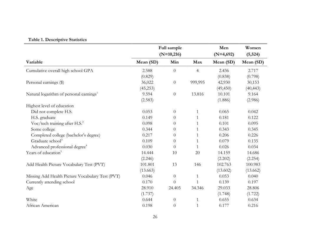
We present descriptive statistics for all variables used in the analysis in Table 1. The

cumulative high school GPA for this sample was slightly above 2.5, and the average GPA for

females (2.717) was significantly higher than that for males (2.436). Mean personal earnings for the

full sample was $36,022, with nearly a $13,000 gap between males and females. Among the seven

educational categories in Add Health, some college was the modal category for both genders, and

12

advanced professional degree was the least common category. On average, PVT scores for male

students were significantly higher than those for female students. In addition, several

socioeconomic, demographic, and familial variables displayed significant gender differences.

V. Results

A. Educational Attainment

We present the estimation results for educational attainment in Tables 2A for males and 2B

for females. For males, high school GPA is positive and significant in all the specifications, with a

magnitude of approximately 0.90, implying that an additional point in high school GPA is associated

with close to a one-category increase in educational attainment.6

Some intriguing results emerge for the other explanatory variables in Table 2A, particularly

when we examine changes across specifications. Compared to being White, being African American

is associated with lower educational attainment among males in the benchmark specification (Model

A). However, this estimate turns positive and statistically significant when we add high school GPA

to the model, and it becomes even larger in magnitude when we enter PVT score and currently

attending school. Thus, failing to control for innate ability and academic performance in high

school would lead one to incorrectly conclude that African American males complete fewer years of

education than their White counterparts. However, controlling for other personal and familial

factors indicates that the opposite is true: African American males complete about one quarter of an

educational category more than Whites.

Interestingly, this estimate is robust

and stable when we sequentially add PVT score, currently attending school, and school fixed effects

to the model. As expected, both PVT score and a dummy variable for currently attending school are

positive and highly significant.

6 See Table 1 for a description of the seven educational categories.

13

The pattern for Hispanic males is similar to that for African American males in that the

estimate changes from negative and significant in the benchmark specification to positive and

significant in the augmented models, but it loses significance in the fully-specified model with school

fixed effects (Model E). The same is true for being born in the U.S., which is negative and

significant until it also loses significance in Model E. The implication here is that high school-

specific factors (e.g., teacher credentials, honors courses, remedial courses, extracurricular activities,

class sizes) are significantly correlated with Hispanic ethnicity and place of birth, thereby creating

bias in these estimates when school fixed effects are omitted from the model.

Living in a single-parent (negative) or other non-intact household (negative) during high

school, having a residential mother (positive), having a father in a white-collar occupation (positive),

and having a residential parent who attended college (positive) have the expected signs and all are

statistically significant in Model E.

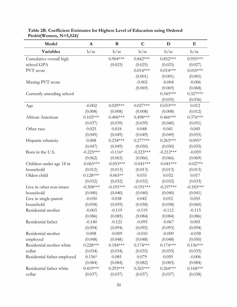
Many of the estimates for females (Table 2B) are similar to those for males. High school

GPA is positive and significant in all specifications, with a magnitude of 0.96 (Model E). PVT score

and currently attending school are also positive and significant. Only three differences vis-à-vis

males appear with the control variables. First, the coefficient estimate for being African American is

positive and significant in the benchmark specification (Model A) and becomes much larger in

successive models. Second, the number of children under age 18 in the household at Wave 1 is

negative and significant in Model E, suggesting that teenage girls may help to care for younger

siblings, thus impacting their educational progress. Third, receiving welfare in Wave 1 is negative

and significant in the fully specified model, indicating that household financial hardship impedes

academic achievement for girls but not for boys.

To further understand the effect of high school GPA on educational achievement for both

genders, we calculate the marginal effects for each of the educational categories (Table 3). For boys,

14

an additional point in cumulative high school GPA has a positive and significant effect on the

probability of attending college and completing all types of subsequent degrees. The turning point

for girls occurs at one category higher—completing a college degree—which is also the category

with the largest effects for both genders. Although the estimates are statistically significant, high

school GPA has a relatively small effect on the probability of completing a terminal degree. In other

words, academic performance in high school has a large and significant effect on educational

milestones shortly thereafter but not on the most exclusive degrees.

B. Annual Personal Earnings

We use robust regression to estimate the log of annual personal earnings for males (Table

4A) and females (Table 4B). The model specifications for earnings are similar to those used for

educational achievement, with a benchmark specification (Model A) followed by sequentially-added

variables to arrive at a fully-specified model with school fixed effects (Model E). For men,

cumulative high school GPA has a positive and significant effect on annual earnings as an adult.

Using the estimate in Column E to examine the magnitude of the effect, a one-unit increase in high

school GPA leads to a 12.2 percent (e.115 – 1) increase in annual earnings. With mean annual

earnings for males equaling $42,930, this translates into $5,237 in extra earnings, ceteris paribus.

Moreover, the effect is stable and robust across specifications. The PVT score is small and not

statistically significant, but currently attending school has a negative and statistically significant effect

on annual earnings.

Among the control variables, we include dummy variables for the educational categories

described earlier. Relative to being a high school dropout, all of the educational categories are

15

positive and significant, with effects increasing as one completes more education. Age is also

positive and significant in all specifications.7

The African-American effect for earnings is qualitatively different than it is for educational

attainment. The estimate is initially negative and significant in the benchmark specification (Model

A) and remains essentially unchanged through Model E. Relative to White males, African-American

males have 21.7 percent lower earnings at Wave 4. The finding contradicts the African-American

effect on educational attainment and might illustrate racial discrimination in labor market

compensation. We make this statement cautiously, however, because important and unobserved

individual-specific factors could significantly mediate the estimated effects.

Most of the other variables in Table 4A are not statistically significant at the 5% level or

lower. The exceptions are having a residential mother at Wave 1 (negative), a mother working in a

white-collar occupation (positive), and an employed father (positive).

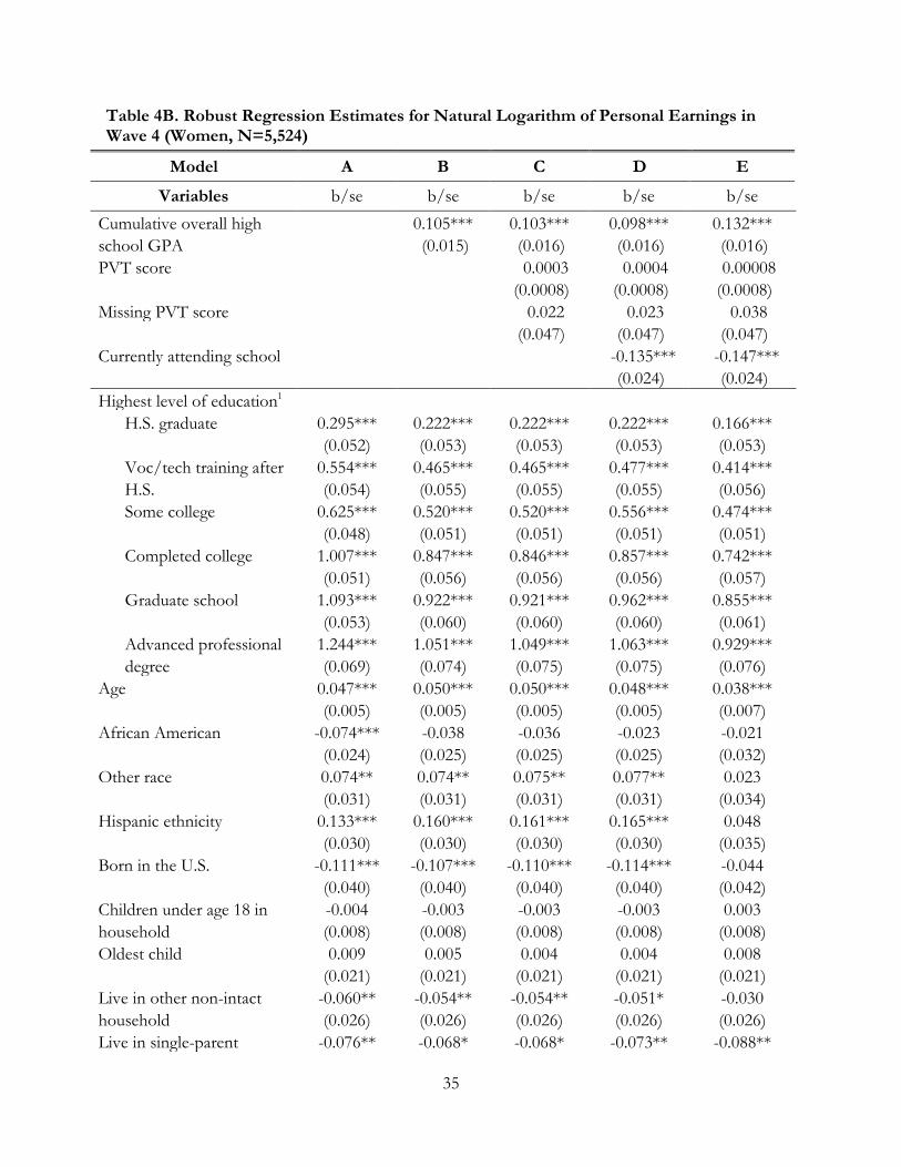
Table 4B shows that the effect for high school GPA is larger for females. With a point

estimate of 0.132, this implies that girls who raise their high school GPAs by one unit can expect to

receive 14.1 percent (e.132 – 1) higher earnings as adults. Because mean earnings for women

($30,153) are lower than the mean for men ($42,930) at Wave 4, the estimated effect converted to

dollars is not as great ($4,252). As with men, PVT score is not significant, and currently attending

school has a negative and significant effect on current earnings. Similarly, age and education are

positive and significant in all specifications.

In stark contrast to the results for men, African-American women do not have significantly

different earnings than their White counterparts for all models other than the baseline specification.

A combined group of other races as well as individuals of Hispanic ethnicity show a positive and

7 Traditional earnings models typically include age-squared as well as age to allow for eventual depreciation of human capital. However, the oldest person in our sample is 34 and unlikely to be experiencing depreciating human capital.

16

significant effect on earnings except in the model with school fixed effects. Here, both estimates are

still positive, but neither is statistically significant. The only other variable that is statistically

significant for women in Model E is a dummy variable for living in a single-parent household at

Wave 1.

C. Extensions and Sensitivity Analyses

The core findings clearly demonstrate that high school GPA has a positive, statistically

significant, and economically meaningful effect on educational attainment and future earnings. But

what are the predicted probabilities of meeting various educational thresholds given a particular high

school GPA? Appendix A presents these estimates. For both genders, having a median GPA in

high school leads to a nearly 0.50 probability of completing some college coursework, which is the

modal category. Advancing to the 75th percentile (3.058 GPA for boys and 3.333 for girls) results in

higher predicted probabilities of graduating from college and attending graduate school. This trend

accelerates through the 99th percentile of high school GPAs, as the majority of these high-achieving

students are likely to graduate from college and/or pursue an advanced degree (74.7 percent for

boys and 79.0 percent for girls). Interestingly, based on high school GPA, the top one percent of

girls have a higher predicted probability of attending graduate school and earning a terminal degree

than the top one percent of boys.

Recall that the African-American coefficient was negative and significant for men in the

educational attainment model with no controls for high school GPA, PVT score, or currently

attending school (Model A, Table 2A). The estimate then became positive and significant in the

fully specified model (Model E, Table 2A). Although the African-American coefficient was positive

and significant for women in the parsimonious model (Model A, Table 2B), it became much larger

and more significant after we included other controls and school fixed effects (Model E, Table 2B).

17

Does this imply that we may misestimate the effect of being African American on

educational attainment if we look at simple correlations or include a limited number of control

variables? To explore the mechanism underlying the African-American effect for educational

attainment and earnings, we estimate a simple ordered probit model of educational attainment, age,

race, ethnicity, and being born in the U.S. The coefficient estimates are negative and significant for

both genders and much larger in absolute value for men relative to Model A in Table 2A. We find

similar qualitative results when including the same explanatory variables in a model for earnings.

Again, these results underscore the importance of estimating fully-specified models when

investigating the effects of race on educational attainment and labor market earnings (Rose and

Betts, 2004; Lleras, 2008).8

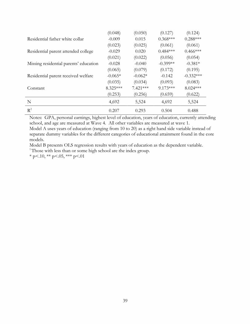
We conduct a number of sensitivity tests to evaluate the robustness of the core results.

Appendix B reports on two of these sensitivity tests. First, we replace the categorical dummies for

educational attainment with a continuous measure for years of education in the earnings regressions

(A). We construct the continuous measure by either using the typical number of years for a

completed degree or taking the midpoint for a multi-year category.

9

Next, rather than estimate the categorical measure of educational attainment with ordered

probit, we estimate the newly constructed continuous measure of years of education with OLS

After we make this change in

the specifications for men and women, the coefficient estimates for high school GPA remain

positive and statistically significant, with slightly higher values (see Tables 4A and 4B). As expected,

years of education is positive and highly significant. All other estimates are virtually identical to

those reported earlier.

8 Lleras (2008) evaluated whether high school achievement tests affect educational attainment and earnings ten years later. After controlling for cognitive and non-cognitive abilities, being African American and Hispanic were positively associated with educational attainment but negatively associated with earnings. 9We assign the value of 10 to those individuals with less than a high school degree, 12 for a high school degree, 13 for vocational/technical training after high school, 14 for some college, 16 for a college degree, 18 for graduate school, and 20 for an advanced professional degree.

18

regression (B). Cumulative high school GPA is positive and significant once again. We estimate

that raising high school GPA by one point increases educational attainment by 1.322 years for men

and 1.427 years for women. The slightly higher estimate for women is consistent with the predicted

probabilities reported in Appendix A. Again, the estimates for the other explanatory variables are

consistent in sign and significance with those in Tables 2A and 2B.

An additional sensitivity test addresses the absence of GPA data for 19 percent of the

sample interviewed at Waves 1, 3, and 4. The approach we adopt for estimation of the core models

is to drop these observations. As noted earlier, however, individuals with missing GPA data are, on

average, demographically dissimilar from the analysis sample. Thus, we impute GPA data for these

individuals using the multiple imputation routine (impute command) in Stata with all the Wave 1

control variables listed in Table 1 and some school and regional characteristics (e.g., whether the

high school was in an urban area). We then re-estimate the educational attainment and earnings

models for each gender with the augmented sample. The coefficient estimates for GPA, which now

includes both actual and imputed values, are slightly smaller than our core results but identical in

sign and statistical significance.10

We conduct three additional robustness checks for the personal earnings equation. First, we

re-estimate the personal earnings equations with OLS regression instead of robust regression, the

technique used in the core models to reduce bias from outliers. The effects of cumulative overall

high school GPA on personal earnings is larger in magnitude and highly significant (p<0.01) when

we use OLS. Second, we control for the age at which respondents first began working full time to

evaluate whether labor market experience alters the relationship between high school GPA and

personal earnings. The effects of high school GPA on personal earnings are similar in sign,

This test at least partially confirms that missing GPA data is not

seriously biasing our core results.

10 Results available on request.

19

magnitude, and significance for men and women after we control for labor market experience.

Finally, we control for three post-secondary educational institution characteristics (selectivity based

on median SAT score, private institution, and public institution).11 Because these measures are only

available for 940 men and 1,297 women, we are cautious about drawing any conclusions based on

the results. The effect of cumulative overall high school GPA is no longer significant for men12

VI. Discussion and Conclusion

but

remains significant for women (p<0.05). Unfortunately, the Add Health dataset does not provide

better information about academic performance beyond high school for a larger sample.

Academic performance in high school usually plays a major role in college selection and

admission. However, few studies have investigated whether high school grades are significantly

related to overall academic attainment and personal earnings in adulthood. Using multiple waves of

data from Add Health, we estimate the effects of cumulative high school GPA on the highest level

of education attained and annual personal earnings when respondents are 24 to 34 years of age, or

approximately 10 years removed from high school. We estimate each outcome variable with five

distinct specifications for each gender. We use the ordered probit model to estimate the seven-

category measure of educational attainment, and we estimate the natural log of earnings using robust

regression. The analyses include a long list of control variables including PVT score as a proxy for

intellectual ability, a dummy variable for currently attending school, socio-demographic variables,

household characteristics, and school fixed effects. Finally, we perform several sensitivity tests to

examine the robustness of the core findings.

11 These measures were collected by Add Health for some of the respondents attending postsecondary institutions at the time of the Wave 3 interview. 12 However, GPA is statistically significant if college selectivity based on median SAT scores is not included in the model.

20

All the main results are consistent and stable in direction and statistical significance. In

addition, the effects sizes are relatively large and economically meaningful. In quantitative terms, we

estimate that a one-unit increase in GPA leads to nearly a full category jump in educational

attainment for boys and girls. Similarly, an equivalent increase in high school GPA raises annual

earnings in adulthood by an estimated 12.2 percent for males and 14.1 percent for females.

Replacing the categorical measure of educational attainment with a continuous measure for years of

education, using multiple imputation for all missing GPA observations, and estimating all models

with a small set of unambiguously exogenous variables have little influence on the core findings.

One of the interesting ancillary findings from this research is the changing sign and

significance for African Americans in the educational attainment specifications. When we exclude

high school GPA, PVT score, currently attending school, and school fixed effects from the models,

it appears that being African American has a negative and significant effect on educational

attainment for males and a significant yet small positive effect for females. However, the estimates

are positive, significant, and considerably larger for both genders when we enter the above variables

in the fully specified model. This implies that, given the same high school GPA, PVT score, and

school characteristics, African Americans advance further in the formal educational system than

their White counterparts. It is beyond the scope of this paper to determine whether this estimated

disparity is due largely to affirmative action programs, unobserved personal characteristics and

differences in individual motivation, or some other phenomenon. Nevertheless, the findings should

encourage educators, school administrators, and policy makers who are interested in promoting

educational advancement programs for racial minorities. It is important to note, however, that

African American men continue to earn less than White men, even after controlling for these

characteristics.

21

In summary, this research quantifies and highlights the long-term importance of academic

performance in high school on two socially desirable outcomes in adulthood. Perhaps these

estimates will surprise and inspire some, particularly adolescent students, who often require

incentives and other motivations to invest more time and effort in their high school coursework.

Regardless, parents, teachers, and guidance counselors now have some tangible evidence to rouse

those high school students who may be spending too little time with their books.

22

References

Altonji, J.G. 1995. The effects of high school curriculum on education and labor market outcomes.

Journal of Human Resources 30, no. 3: 409-438.

Anderson, E.S., and T.Z. Keith, 1997. A longitudinal test of a model of academic success for at-risk

high school students. The Journal of Educational Research 90, no. 5: 259-268.

Betts, J.R., and D. Morell. 1999. The determinants of undergraduate GPA: The relative importance

of family background, high school resources, and peer group effects. The Journal of Human

Resources, 34, no. 2: 268-293.

Bishop, J., A. Blakemore, and S. Low. 1985. High school graduates in the labor market: A

comparison of the class of 1972 and 1980. National Center for Research in Vocational

Education, Ohio State University, Columbus, 1985.

Cameron, S.V., and J.J. Heckman. 2001. The dynamics of educational attainment for black, hispanic,

and white males. Journal of Political Economy 109, no. 3: 455-499.

Card, D. 1999. The causal effect of education on earnings. In Handbook of Labor Economics, Volume 3,

ed. O. Ashenfelter and D. Card.

Cohn, E., S. Cohn, D.C. Balch, and J. Bradley, Jr. 2004. Determinants of undergraduate GPAs: SAT

scores, high school GPA and high school rank. Economics of Education Review 23, no. 6: 577-

586.

Crawford, D.L., A.W. Johnson, and A.A. Summers. 1997. Schools and labor market outcomes.

Economics of Education Review 16, no. 3: 255-269.

Crissey, S. R. 2009. Educational attainment in the United States: 2007. Current Population

Reports.US Census Bureau, U.S. Department of Commerce.

Dale, S.B., and A.B. Krueger. 2002. Estimating the payoff to attending a more selective college: An

application of selection on observables and unobservables. The Quarterly Journal of Economics,

117, no. 4: 1491-1527.

Dwyer, C.A., and L.M. Johnson, 1997. Grades, Accomplishments, and Correlates. In Gender and

Fair Assessment, ed. W.W. Willimgham and N.S. Cole. Mahwah, NJ: Lawrence Erlbaum

Associates.

Erikson, E.H. (1968). Identity: Youth and Crisis. NewYork: Norton.

23

Grogger, J., and E. Eide, 1995. Changes in college skills and the rise in the college wage premium.

The Journal of Human Resources 30: 280-310.

Hamermesh, D.S., and S.G. Donald. 2008. The effect of college curriculum on earnings: An affinity

identifier for non-ignorable non-response bias. Journal of Econometrics 144, no. 2: 479-491.

Heckman, J.J., 2008. Role of income and family influence on child outcomes. Annals of the New York

Academy of Sciences 1136: 307-323.

Hoekstra, M. 2009. The effect of attending the flagship state university on earnings: A discontinuity-

based approach. The Review of Economics & Statistics 91, no. 4: 717-724.

Jones, E.B., and J.D. Jackson. 1990. College grades and labor market rewards. Journal of Human

Resources 25, no. 2: 253-266.

Kleinfeld, J. 1998. The myth that schools shortchange girls: Social science in the service of

deception. Women’s Freedom Network. (Document number ED 423 210). Washington,

DC: ERIC (Education Research Information Clearinghouse).

Kroger, J., 2006. Identity Development: Adolescence through Adulthood. 2nd ed. Sage Publications, Inc.

Lazear, E. 1977. Academic achievement and job performance: Note. The American Economic Review

67, no. 2: 252-254.

Levine, P.B., and D.J. Zimmerman. 1995. The benefit of additional high-school math and science

classes for young men and women. Journal of Business and Economic Statistics 13, no. 2: 137–149.

Lleras, C. 2008. Do skills and behaviors in high school matter? The contribution of non-cognitive

factors in explaining differences in educational attainment and earnings. Social Science Research

37: 888-902.

Lounsbury, J.W., E. Sundstrom, J.M. Loveland, and L.W. Gibson, 2003. Intelligence, “big five”

personality traits, and work drive as predictors of course grade. Personality and Individual

Differences 35, no. 6: 1231-1239.

Loury, L.D., and D. Garman. 1995. College selectivity and earnings. Journal of Labor Economics 13, no.

2: 289-308.

24

Maggs, J. L., J. Schulenberg, K. Hurrelmann., 1997. Developmental transitions during adolescence:

health promotion implications. In Health Risks and Developmental Transitions during Adolescence.

ed. J. Schulenberg, J.L. Maggs, and K. Hurrelman. New York: Cambridge University Press.

Melby, J.N., R.D. Conger, S. Fang, K. A. Wickrama, and K.J. Conger. 2008. Adolescent family

experiences and educational attainment during early adulthood. Developmental Psychology 44,

no. 6: 1519-1536.

Meyer, R.H., and D.A. Wise. 1982. High school preparation and early labor force experience. In The

Youth Labor Market Problem: Its Nature, Causes, and Consequences. ed. R.A. Freeman and D.A.

Wise. Chicago: University of Chicago Press.

Mincer, J. 1974. Schooling, Experience, and Earnings. Human Behavior & Social Institutions. No. 2.National

Bureau of Economic Research.

Monks, J. 2000. The returns to individual and college characteristics: Evidence from the National

Longitudinal Survey of Youth. Economics of Education Review 19, no. 3: 279-289.

Mueller, R.O. 1988. The impact of college selectivity on income for men and women. Research in

Higher Education 29, no. 2: 175-191.

Neisser, U., G. Boodo, T.J. Bouchard Jr., B.A. Wade, N. Brody, S.J. Ceci, D.F. Halpern, J.C.

Loehlin, R. Perlo, R.J. Sternberg, and S. Urbina, 1996. Intelligence: knowns and unknowns.

American Psychologist 51, no. 2: 77-101.

Ou, S.R., and A.J. Reynolds. 2008. Predictors of educational attainment in the Chicago Longitudinal

Study. School Psychology Quarterly 23, no. 2: 199-229.

Rivkin, S.G., E.A. Hanushek, and J.F. Kain, 2005. Teachers, schools, and academic achievement.

Econometrica 73, no. 2: 417–458.

Rose, H., and J.R. Betts. 2004. The effect of high school courses on earnings. Review of Economics

Statistics 86, no. 2: 497-513.

Spence, Michael. 1973. Job-market signaling. Quarterly Journal of Economics 87, no. 3: 355-374.

StataCorp. 2009. Stata Statistical Software: Release 11. College Station, TX: StataCorp LP.

Thomas, S.L. 2003. Longer-term economic effects of college selectivity and control. Research in

Higher Education 44, no. 3: 263-299.

http://www.nber.org/chapters/c7877�

http://www.nber.org/books/free82-1�

http://www.nber.org/books/free82-1�

25

U.S. Census Bureau. 2010. The 2010 Statistical Abstract. Retrieved June 17, 2010 from

http://www.census.gov/compendia/statab/

Wise, D.A. 1975. Academic achievement and job performance. The American Economic Review 63, no.

3: 350-366.

Wolfie, D., and J.G. Smith. 1956. The occupational value of education for superior high-school

graduates. The Journal of Higher Education 27, no. 4: 201-212+232.

Zhang, L. 2008. The way to wealth and the way to leisure: The impact of college education on

graduates’ earnings and hours of work. Research in Higher Education 49, no. 3: 199-213.

http://www.census.gov/compendia/statab/�

26

Table 1. Descriptive Statistics

Full sample (N=10,216)

Men (N=4,692)

Women (5,524)

Variable Mean (SD) Min Max Mean (SD) Mean (SD)

Cumulative overall high school GPA 2.588 0 4 2.436 2.717 (0.829) (0.838) (0.798) Personal earnings ($) 36,022 0 999,995 42,930 30,153 (45,253) (49,450) (40,443) Natural logarithm of personal earnings1 9.594 0 13.816 10.101 9.164 (2.583) (1.886) (2.986) Highest level of education

Did not complete H.S. 0.053 0 1 0.065 0.042 H.S. graduate 0.149 0 1 0.181 0.122 Voc/tech training after H.S.2 0.098 0 1 0.101 0.095 Some college 0.344 0 1 0.343 0.345 Completed college (bachelor’s degree) 0.217 0 1 0.206 0.226 Graduate school3 0.109 0 1 0.079 0.135 Advanced professional degree4 0.030 0 1 0.026 0.034

Years of education5 14.444 10 20 14.159 14.686 (2.246) (2.202) (2.254) Add Health Picture Vocabulary Test (PVT) 101.801 13 146 102.763 100.983 (13.663) (13.602) (13.662) Missing Add Health Picture Vocabulary Test (PVT) 0.046 0 1 0.053 0.040 Currently attending school 0.170 0 1 0.139 0.197 Age 28.910 24.405 34.346 29.033 28.806 (1.737) (1.748) (1.722) White 0.644 0 1 0.655 0.634 African American 0.198 0 1 0.177 0.216

27

Other race 0.158 0 1 0.168 0.150 Hispanic ethnicity 0.149 0 1 0.156 0.144 Born in the U.S. 0.928 0 1 0.922 0.933 Children under age 18 in household 1.254 0 9 1.210 1.292 (1.192) (1.149) (1.227) Oldest child 0.302 0 1 0.304 0.301 Live in other non-intact household 0.180 0 1 0.181 0.179 Live in single-parent household 0.216 0 1 0.209 0.223 Residential mother 0.952 0 1 0.950 0.953 Residential father 0.738 0 1 0.757 0.721 Residential mother employed 0.822 0 1 0.827 0.818 Residential mother white collar 0.508 0 1 0.520 0.498 Residential father employed 0.699 0 1 0.717 0.684 Residential father white collar 0.271 0 1 0.288 0.257 Residential parent attended college 0.514 0 1 0.535 0.495 Missing residential parent's education 0.016 0 1 0.019 0.014 Residential parent received welfare 0.091 0 1 0.082 0.098 Notes: GPA, personal earnings, highest level of education, years of education, currently attending school, and age are measured at Wave 4. All other variables are measured at Wave 1. 1 When personal earnings is reported as zero, the natural logarithm of personal earnings is set to zero. 2Voc/tech training after H.S. includes respondents who had only some or who completed vocational/technical training after high school. 3 Graduate school includes respondents with some graduate school, a master’s degree, and some graduate training beyond a master’s degree. 4 Advanced professional degree includes respondents who have completed a doctoral degree and who have some or who completed post baccalaureate professional education (e.g., law school, medical school). 5 Years of education ranges from 10 (less than or some high school) to 20 (doctoral degree or post baccalaureate professional education), depending on respondent’s highest level of education.

28

Table 2A. Coefficient Estimates for Highest Level of Education Using Ordered Probit (Men, N=4,692)1

Model A B C D E

Variables b/se b/se b/se b/se b/se Cumulative overall HS GPA

0.901*** 0.852*** 0.853*** 0.915*** (0.024) (0.024) (0.024) (0.026)

PVT score 0.015*** 0.015*** 0.012*** (0.001) (0.001) (0.001) Missing PVT score -0.023 -0.024 -0.031 (0.070) (0.070) (0.071) Currently attending school 0.455*** 0.440***

(0.046) (0.047) Age -0.026*** -0.004 0.0002 0.007 -0.011 (0.009) (0.009) (0.009) (0.009) (0.013) African American -0.114*** 0.182*** 0.301*** 0.297*** 0.240*** (0.044) (0.045) (0.046) (0.046) (0.060) Other race 0.056 -0.018 0.020 0.018 0.011 (0.048) (0.048) (0.048) (0.048) (0.058) Hispanic ethnicity -0.095** 0.079 0.132*** 0.126** 0.058 (0.047) (0.049) (0.049) (0.050) (0.058) Born in the U.S. -0.188*** -0.115* -0.235*** -0.214*** -0.109 (0.061) (0.064) (0.065) (0.065) (0.069) Children under age 18 in household

-0.047*** -0.040*** -0.027* -0.027* -0.016 (0.014) (0.014) (0.015) (0.015) (0.015)

Oldest child 0.043 0.003 -0.024 -0.024 -0.023 (0.034) (0.035) (0.035) (0.035) (0.036) Live in other non-intact household

-0.217*** -0.121*** -0.153*** -0.156*** -0.161*** (0.043) (0.044) (0.044) (0.044) (0.046)

Live in single-parent household

-0.179*** -0.098 -0.100 -0.109 -0.150** (0.064) (0.066) (0.067) (0.067) (0.069)

Residential mother 0.122 -0.098 -0.083 -0.087 -0.104 (0.087) (0.093) (0.093) (0.093) (0.095)

Residential father -0.015 -0.049 -0.026 -0.052 -0.013 (0.092) (0.101) (0.100) (0.100) (0.105)

Residential mother employed

0.082 0.117** 0.109** 0.107** 0.109* (0.052) (0.054) (0.054) (0.054) (0.057)

Residential mother white collar

0.169*** 0.145*** 0.124*** 0.115*** 0.114*** (0.037) (0.037) (0.037) (0.037) (0.038)

Residential father employed -0.051 -0.045 -0.062 -0.034 -0.061 (0.079) (0.087) (0.086) (0.086) (0.091)

Residential father white collar

0.458*** 0.322*** 0.300*** 0.311*** 0.233*** (0.038) (0.039) (0.039) (0.039) (0.040)

29

Residential parent attended college

0.583*** 0.455*** 0.418*** 0.406*** 0.350*** (0.036) (0.036) (0.036) (0.036) (0.037)

Missing residential parent’s education

-0.509*** -0.357*** -0.302*** -0.325*** -0.322*** (0.115) (0.111) (0.107) (0.108) (0.109)

Residential parent received welfare

-0.191*** -0.107* -0.099 -0.102* -0.106 (0.060) (0.062) (0.061) (0.062) (0.064)

cut1 _cons -2.149*** 0.168 1.613*** 1.812*** 1.134** (0.302) (0.317) (0.342) (0.342) (0.440) cut2 _cons -1.222*** 1.321*** 2.784*** 2.999*** 2.361*** (0.300) (0.316) (0.343) (0.342) (0.440) cut3 _cons -0.889*** 1.715*** 3.186*** 3.411*** 2.789*** (0.300) (0.316) (0.343) (0.343) (0.440) cut4 _cons 0.125 2.950*** 4.441*** 4.677*** 4.120*** (0.299) (0.317) (0.345) (0.345) (0.441) cut5 _cons 0.980*** 3.986*** 5.492*** 5.738*** 5.248*** (0.299) (0.319) (0.347) (0.346) (0.442) cut6 _cons 1.735*** 4.844*** 6.365*** 6.628*** 6.195*** (0.301) (0.323) (0.352) (0.352) (0.448) School fixed effects No No No No Yes Notes: GPA, personal earnings, highest level of education, years of education, currently attending school, and age are measured at Wave 4. All other variables are measured at Wave 1. 1 Categorical dependent variable is highest level of education, which is constructed using the education variable in Table 1. The variable ranges from 0 (less than or some high school) to 6 (doctoral degree or post baccalaureate professional education). Highest level of education was measured at Wave 4 when respondents were 24 to 34 years of ages. * p<.10, ** p<.05, *** p<.01.

30

Table 2B. Coefficient Estimates for Highest Level of Education using Ordered Probit(Women, N=5,524)1

Model A B C D E

Variables b/se b/se b/se b/se b/se Cumulative overall high school GPA

0.904*** 0.842*** 0.852*** 0.955*** (0.025) (0.025) (0.025) (0.027)

PVT score 0.014*** 0.014*** 0.010*** (0.001) (0.001) (0.001) Missing PVT score -0.002 -0.004 -0.006 (0.069) (0.069) (0.068) Currently attending school 0.343*** 0.327***

(0.035) (0.036) Age -0.002 0.029*** 0.027*** 0.033*** 0.012 (0.008) (0.008) (0.008) (0.008) (0.012) African American 0.102*** 0.406*** 0.498*** 0.466*** 0.376*** (0.037) (0.039) (0.039) (0.040) (0.051) Other race 0.025 0.018 0.048 0.041 0.045 (0.049) (0.049) (0.049) (0.049) (0.055) Hispanic ethnicity 0.008 0.234*** 0.277*** 0.263*** 0.095* (0.047) (0.049) (0.050) (0.050) (0.055) Born in the U.S. -0.225*** -0.116* -0.223*** -0.212*** -0.059 (0.062) (0.065) (0.066) (0.066) (0.069) Children under age 18 in household

-0.065*** -0.053*** -0.041*** -0.041*** -0.027** (0.012) (0.013) (0.013) (0.013) (0.013)

Oldest child 0.128*** 0.065** 0.035 0.032 0.017 (0.032) (0.032) (0.032) (0.032) (0.033) Live in other non-intact household

-0.308*** -0.191*** -0.191*** -0.197*** -0.183*** (0.040) (0.040) (0.040) (0.040) (0.041)

Live in single-parent household

-0.030 0.038 0.042 0.052 0.055 (0.058) (0.059) (0.058) (0.058) (0.060)

Residential mother -0.003 -0.119 -0.119 -0.112 -0.115 (0.086) (0.085) (0.084) (0.084) (0.086) Residential father -0.140 -0.121 -0.095 -0.067 0.005 (0.094) (0.094) (0.092) (0.093) (0.094) Residential mother employed

0.008 -0.009 -0.010 -0.009 -0.038 (0.048) (0.048) (0.048) (0.048) (0.050)


0.228*** 0.184*** 0.174*** 0.174*** 0.156*** (0.034) (0.034) (0.035) (0.035) (0.035)

Residential father employed 0.156* 0.085 0.079 0.059 -0.006 (0.084) (0.084) (0.082) (0.083) (0.084)


0.419*** 0.293*** 0.265*** 0.264*** 0.168*** (0.037) (0.037) (0.037) (0.037) (0.038)

31


0.568*** 0.428*** 0.382*** 0.374*** 0.315*** (0.033) (0.033) (0.034) (0.034) (0.035)

Missing residential parent’s education

-0.346*** -0.245** -0.208* -0.240** -0.226** (0.116) (0.114) (0.113) (0.112) (0.112)


-0.389*** -0.275*** -0.253*** -0.254*** -0.226*** (0.051) (0.054) (0.054) (0.054) (0.055)

cut1 _cons -1.818*** 1.096*** 2.210*** 2.407*** 1.841*** (0.280) (0.294) (0.315) (0.313) (0.415) cut2 _cons -0.978*** 2.133*** 3.259*** 3.474*** 2.948*** (0.277) (0.292) (0.314) (0.313) (0.415) cut3 _cons -0.605** 2.567*** 3.701*** 3.927*** 3.421*** (0.277) (0.293) (0.314) (0.313) (0.415) cut4 _cons 0.438 3.825*** 4.975*** 5.210*** 4.780*** (0.277) (0.294) (0.316) (0.315) (0.417) cut5 _cons 1.225*** 4.755*** 5.918*** 6.156*** 5.788*** (0.276) (0.295) (0.318) (0.317) (0.419) cut6 _cons 2.169*** 5.802*** 6.980*** 7.226*** 6.914*** (0.278) (0.298) (0.322) (0.320) (0.423) School fixed effects No No No No Yes Notes: GPA, personal earnings, highest level of education, years of education, currently attending school, and age are measured at Wave 4. All other variables are measured at Wave 1. 1 Categorical dependent variable is highest level of education, which is constructed using the education variable in Table 1. The variable ranges from 0 (less than or some high school) to 6 (doctoral degree or post baccalaureate professional education). Highest level of education was measured at Wave 4 when respondents were 24 to 35 years of ages. * p<.10, ** p<.05, *** p<.01.

32

Table 3. Marginal Effects of GPA on Highest Level of Education

Men Women

Pr(Highest level of education) dy/dx (SE) dy/dx (SE) Less than or some H.S. -0.030***

(0.003) [-0.557]

-0.016*** (0.002) [-0.529]

H.S. graduate -0.189*** (0.007) [-2.068]

-0.124*** (0.005) [-2.255]

Voc/tech training after H.S. -0.089*** (0.005) [-1.926]

-0.104*** (0.005) [-2.535]

Some college 0.030*** (0.007) [0.210]

-0.105*** (0.007) [-0.782]

Completed college 0.214*** (0.008) [3.128]

0.211*** (0.009) [2.971]

Graduate school 0.056*** (0.004) [2.273]

0.123*** (0.005) [2.989]

Advanced professional degree 0.007*** (0.001) [0.923]

0.015*** (0.002) [1.519]

Notes: Marginal effects, standard errors (in parentheses), and elasticities[in brackets] are reported. Estimates are based on Models E for men and women (see Tables 2A and 2B), which use ordered probit and include school fixed effects. The elasticities, E(i), are calculated as follows: E(i)=[dy/dx]*[xbari/ybari], where dy/dx are the marginal effects above, xbariis the mean GPA in education category i, and ybariis the proportion of the sample in category i. * p<.10, ** p<.05, *** p<.01.

33

Table 4A. Robust Regression Estimates for Natural Logarithm of Personal Earnings in Wave 4(Men, N=4,692)

Model A B C D E


0.106*** 0.104*** 0.103*** 0.115*** (0.014) (0.014) (0.014) (0.015)

PVT score 0.0003 0.0003 -0.00003 (0.0008) (0.0008) (0.0008) Missing PVT score -0.034 -0.031 -0.040 (0.039) (0.039) (0.040) Currently attending school -0.218*** -0.206***

(0.027) (0.027) Highest level of education1

H.S. graduate 0.186*** 0.096** 0.097** 0.100** 0.084** (0.041) (0.041) (0.041) (0.042) (0.042)

Voc/tech training after H.S.

0.330*** 0.217*** 0.217*** 0.228*** 0.195*** (0.045) (0.046) (0.046) (0.046) (0.047)

Some college 0.332*** 0.201*** 0.200*** 0.240*** 0.211*** (0.039) (0.041) (0.041) (0.042) (0.042)

Completed college 0.589*** 0.398*** 0.397*** 0.408*** 0.361*** (0.042) (0.047) (0.048) (0.048) (0.049)

Graduate school 0.614*** 0.405*** 0.404*** 0.472*** 0.410*** (0.049) (0.055) (0.055) (0.056) (0.057)

Advanced professional degree

0.643*** 0.421*** 0.418*** 0.450*** 0.354*** (0.067) (0.072) (0.072) (0.072) (0.074)

Age 0.054*** 0.055*** 0.056*** 0.052*** 0.050*** (0.005) (0.005) (0.005) (0.005) (0.007) African American -0.209*** -0.180*** -0.177*** -0.177*** -0.196*** (0.025) (0.025) (0.026) (0.026) (0.032) Other race 0.016 0.009 0.011 0.007 -0.054* (0.027) (0.027) (0.027) (0.027) (0.031) Hispanic ethnicity 0.028 0.047* 0.047* 0.051* 0.009 (0.028) (0.027) (0.028) (0.028) (0.032) Born in the U.S. -0.042 -0.034 -0.037 -0.045 -0.016 (0.036) (0.036) (0.036) (0.036) (0.039) Children under age 18 in household

0.009 0.010 0.010 0.011 0.016* (0.008) (0.008) (0.008) (0.008) (0.008)

Oldest child -0.009 -0.013 -0.014 -0.015 -0.018 (0.020) (0.020) (0.020) (0.020) (0.020) Live in other non-intact household

-0.044* -0.037 -0.038 -0.038 -0.044* (0.025) (0.025) (0.025) (0.025) (0.025)

Live in single-parent -0.052 -0.048 -0.048 -0.042 -0.057

34

household (0.037) (0.037) (0.037) (0.037) (0.037) Residential mother -0.080 -0.105** -0.105** -0.099* -0.102** (0.051) (0.051) (0.051) (0.051) (0.052) Residential father -0.076 -0.082 -0.081 -0.069 -0.087 (0.055) (0.054) (0.054) (0.054) (0.055) Residential mother employed

0.043 0.050 0.050* 0.050* 0.056* (0.030) (0.030) (0.030) (0.030) (0.031)


0.049** 0.049** 0.048** 0.050** 0.044** (0.021) (0.021) (0.021) (0.021) (0.022)

Residential father employed

0.110** 0.105** 0.104** 0.091* 0.103** (0.048) (0.047) (0.047) (0.047) (0.048)


0.019 0.014 0.014 0.010 -0.010 (0.023) (0.023) (0.023) (0.023) (0.023)


-0.028 -0.030 -0.030 -0.029 -0.034 (0.021) (0.021) (0.021) (0.021) (0.021)

Missing residential parents’ education

-0.024 -0.017 -0.017 -0.008 -0.020 (0.065) (0.064) (0.064) (0.065) (0.065)


-0.104*** -0.093*** -0.092*** -0.094*** -0.067* (0.035) (0.034) (0.034) (0.034) (0.035)

Constant 8.664*** 8.501*** 8.469*** 8.572*** 8.788*** (0.179) (0.179) (0.193) (0.194) (0.250) R2 0.141 0.150 0.150 0.158 0.208

School fixed effects No No No No Yes Notes: GPA, personal earnings, highest level of education, years of education, currently attending school, and age are measured at Wave 4. All other variables are measured at wave 1. 1 Those with less than or some high school are the index group. * p<.10, ** p<.05, *** p<.01.

35

Table 4B. Robust Regression Estimates for Natural Logarithm of Personal Earnings in Wave 4 (Women, N=5,524)

Model A B C D E


0.105*** 0.103*** 0.098*** 0.132*** (0.015) (0.016) (0.016) (0.016)

PVT score 0.0003 0.0004 0.00008 (0.0008) (0.0008) (0.0008) Missing PVT score 0.022 0.023 0.038 (0.047) (0.047) (0.047) Currently attending school -0.135*** -0.147***

(0.024) (0.024) Highest level of education1

H.S. graduate 0.295*** 0.222*** 0.222*** 0.222*** 0.166*** (0.052) (0.053) (0.053) (0.053) (0.053)

Voc/tech training after H.S.

0.554*** 0.465*** 0.465*** 0.477*** 0.414*** (0.054) (0.055) (0.055) (0.055) (0.056)

Some college 0.625*** 0.520*** 0.520*** 0.556*** 0.474*** (0.048) (0.051) (0.051) (0.051) (0.051)

Completed college 1.007*** 0.847*** 0.846*** 0.857*** 0.742*** (0.051) (0.056) (0.056) (0.056) (0.057)

Graduate school 1.093*** 0.922*** 0.921*** 0.962*** 0.855*** (0.053) (0.060) (0.060) (0.060) (0.061)


1.244*** 1.051*** 1.049*** 1.063*** 0.929*** (0.069) (0.074) (0.075) (0.075) (0.076)

Age 0.047*** 0.050*** 0.050*** 0.048*** 0.038*** (0.005) (0.005) (0.005) (0.005) (0.007) African American -0.074*** -0.038 -0.036 -0.023 -0.021 (0.024) (0.025) (0.025) (0.025) (0.032) Other race 0.074** 0.074** 0.075** 0.077** 0.023 (0.031) (0.031) (0.031) (0.031) (0.034) Hispanic ethnicity 0.133*** 0.160*** 0.161*** 0.165*** 0.048 (0.030) (0.030) (0.030) (0.030) (0.035) Born in the U.S. -0.111*** -0.107*** -0.110*** -0.114*** -0.044 (0.040) (0.040) (0.040) (0.040) (0.042) Children under age 18 in household

-0.004 -0.003 -0.003 -0.003 0.003 (0.008) (0.008) (0.008) (0.008) (0.008)

Oldest child 0.009 0.005 0.004 0.004 0.008 (0.021) (0.021) (0.021) (0.021) (0.021) Live in other non-intact household

-0.060** -0.054** -0.054** -0.051* -0.030 (0.026) (0.026) (0.026) (0.026) (0.026)

Live in single-parent -0.076** -0.068* -0.068* -0.073** -0.088**

36

household (0.036) (0.036) (0.036) (0.035) (0.035) Residential mother 0.013 0.001 0.002 -0.001 -0.007 (0.051) (0.051) (0.051) (0.051) (0.051) Residential father -0.079 -0.075 -0.074 -0.082 -0.088 (0.056) (0.056) (0.056) (0.056) (0.056) Residential mother employed

0.040 0.040 0.040 0.042 0.024 (0.031) (0.030) (0.030) (0.030) (0.031)


0.035 0.034 0.034 0.034 0.016 (0.022) (0.022) (0.022) (0.022) (0.022)

Residential father employed 0.019 0.008 0.008 0.015 -0.002 (0.050) (0.050) (0.050) (0.050) (0.050)


0.036 0.031 0.031 0.030 0.016 (0.025) (0.024) (0.025) (0.024) (0.025)


0.045** 0.036* 0.035* 0.037* 0.016 (0.021) (0.021) (0.022) (0.021) (0.022)

Missing residential parents’ education

-0.077 -0.070 -0.071 -0.060 -0.037 (0.079) (0.079) (0.079) (0.079) (0.079)


-0.075** -0.067** -0.067** -0.068** -0.060* (0.034) (0.034) (0.034) (0.034) (0.034)

Constant 8.189*** 7.922*** 7.896*** 7.970*** 8.344*** (0.186) (0.189) (0.199) (0.199) (0.255) R2 0.222 0.230 0.230 0.233 0.301

School fixed effects No No No No Yes Notes: GPA, personal earnings, highest level of education, years of education, currently attending school, and age are measured at Wave 4. All other variables are measured at wave 1. 1 Those with less than or some high school are the index group. * p<.10, ** p<.05, *** p<.01.

37

Appendix A. Predicted Probabilities for Highest Level of Education

Men Women

Pr(Highest level of education)

Median GPA (=2.475)

75th Percentile (=3.058)


Median GPA (=2.8)



Less than or some high school (H.S.)

0.011 0.003 0.0001 0.0046 0.0009 0.0001 [0.009, 0.014] [0.002, 0.003] [0.001, 0.001] [0.004, 0.006] [0.001, 0.001] [0.001, 0.001]

H.S. graduate 0.136 0.054 0.008 0.063 0.0216 0.0041 [0.119, 0.153] [0.046, 0.063] 0.006, 0.009] [0.053, 0.073] [0.018, 0.026] [0.003, 0.005] Voc/tech training after H.S.

0.120 0.067 0.015 0.086 0.0404 0.011 [0.108, 0.132] [0.060, 0.075] [0.013, 0.017] [0.077, 0.095] [0.036, 0.045] [0.009, 0.012]

Some college 0.494 0.446 0.231 0.4788 0.3692 0.1945 [0.476, 0.511] [0.423, 0.468] [0.213, 0.249] [0.459, 0.499] [0.348, 0.390] [0.179, 0.210] Completed college 0.206 0.335 0.426 0.2783 0.3664 0.3694 [0.202, 0.211] [0.324, 0.346] [0.423, 0.445] [0.270, 0.286] [0.352, 0.380] [0.350, 0.389] Graduate school 0.030 0.084 0.242 0.0825 0.1766 0.3286 [0.029, 0.031] [0.081, 0.087] [0.228, 0.255] [0.081, 0.084] [0.172, 0.181] [0.316, 0.342]


0.003 0.012 0.079 0.0067 0.0248 0.0924 [0.002, 0.004] [0.009, 0.016] [0.062, 0.096] [0.005, 0.008] [0.020, 0.030] [0.077, 0.108]

Predicted probabilities are reported with 95%confidence intervals in brackets. Other than cumulative overall H.S. GPA, all independent variables are set to their mean values.

38

Appendix B. Sensitivity Tests

Model Natural logarithm of personal earnings (A) Years of Education (B)

Men Women Men Women

Variables b/se b/se b/se b/se Cumulative overall high school GPA 0.122*** 0.145*** 1.322*** 1.427***

(0.014) (0.016) (0.033) (0.034) PVT score 0.000 0.000 0.016*** 0.015*** (0.001) (0.001) (0.002) (0.002) Missing PVT score -0.042 0.035 -0.051 -0.016 (0.040) (0.047) (0.107) (0.116) Currently attending school -0.215*** -0.147*** 0.593*** 0.415*** (0.026) (0.023) (0.069) (0.057) Years of education (w4) 0.051*** 0.100*** (0.006) (0.006) Age 0.048*** 0.036*** -0.009 0.023 (0.007) (0.007) (0.018) (0.018) African American -0.198*** -0.013 0.321*** 0.566*** (0.032) (0.032) (0.085) (0.077) Other race -0.055* 0.027 0.017 0.068 (0.031) (0.034) (0.083) (0.084) Hispanic ethnicity 0.007 0.046 0.078 0.148* (0.032) (0.035) (0.086) (0.086) Born in the U.S. -0.022 -0.047 -0.145 -0.085 (0.039) (0.042) (0.102) (0.103) Children under age 18 in household 0.015* 0.001 -0.014 -0.042**

(0.008) (0.008) (0.022) (0.020) Oldest child -0.016 0.006 -0.051 0.022 (0.020) (0.021) (0.054) (0.051) Live in other non-intact household -0.047* -0.030 -0.254*** -0.295***

(0.025) (0.026) (0.067) (0.064) Live in single-parent household -0.058 -0.088** -0.229** 0.050 (0.037) (0.035) (0.098) (0.087) Residential mother -0.102** -0.003 -0.135 -0.171 (0.052) (0.051) (0.137) (0.126) Residential father -0.087 -0.108* -0.030 0.036 (0.055) (0.056) (0.146) (0.139) Residential mother employed 0.057* 0.021 0.145* -0.080

(0.031) (0.031) (0.082) (0.075) Residential mother white collar 0.044** 0.018 0.152*** 0.239***

(0.022) (0.022) (0.057) (0.054) Residential father employed 0.102** 0.022 -0.098 -0.052

39

(0.048) (0.050) (0.127) (0.124) Residential father white collar -0.009 0.015 0.368*** 0.288***

(0.023) (0.025) (0.061) (0.061) Residential parent attended college -0.029 0.020 0.484*** 0.466***

(0.021) (0.022) (0.056) (0.054) Missing residential parents’ education -0.028 -0.040 -0.399** -0.381*

(0.065) (0.079) (0.172) (0.195) Residential parent received welfare -0.065* -0.062* -0.142 -0.332***

(0.035) (0.034) (0.093) (0.083) Constant 8.325*** 7.421*** 9.173*** 8.024*** (0.253) (0.256) (0.659) (0.622) N 4,692 5,524 4,692 5,524

R2 0.207 0.293 0.504 0.488 Notes: GPA, personal earnings, highest level of education, years of education, currently attending school, and age are measured at Wave 4. All other variables are measured at wave 1. Model A uses years of education (ranging from 10 to 20) as a right hand side variable instead of separate dummy variables for the different categories of educational attainment found in the core models. Model B presents OLS regression results with years of education as the dependent variable. 1 Those with less than or some high school are the index group. * p<.10, ** p<.05, *** p<.01

What You Do in High School Matters: The Effects of High School GPA on Educational Attainment and Labor Market Earnings in Adulthood

Documents