Waves in the Red Sea Response to monsoonal and mountain … · Research papers Waves in the Red Sea: Response to monsoonal and mountain gap winds David K. Ralstona,n, Houshuo Jianga,

Continental Shelf Research 65 (2013) 1–13

Contents lists available at ScienceDirect

Continental Shelf Research

0278-43http://d

n CorrE-m

journal homepage: www.elsevier.com/locate/csr

Research papers

Waves in the Red Sea: Response to monsoonal and mountaingap winds

David K. Ralston a,n, Houshuo Jiang a, J. Thomas Farrar b

a Woods Hole Oceanographic Institution, Applied Ocean Physics and Engineering Department, MS #11, Woods Hole, MA 02543, USAb Woods Hole Oceanographic Institution, Physical Oceanography Department, Woods Hole, MA, USA

a r t i c l e i n f o

Article history:Received 12 December 2012Received in revised form30 May 2013Accepted 31 May 2013Available online 7 June 2013

Keywords:Red SeaWind wavesMountain gap windsSpectral wave modelModel grid resolutionUnstructured grid

43/$ - see front matter & 2013 Elsevier Ltd. Ax.doi.org/10.1016/j.csr.2013.05.017

esponding author. Tel.: +1 508 289 2587; fax:ail address: [email protected] (D.K. Ralston)

a b s t r a c t

An unstructured grid, phase-averaged wave model forced with winds from a high resolution atmosphericmodel is used to evaluate wind wave conditions in the Red Sea over an approximately 2-year period.The Red Sea lies in a narrow rift valley, and the steep topography surrounding the basin steers thedominant wind patterns and consequently the wave climate. At large scales, the model results indicatedthat the primary seasonal variability in waves was due to the monsoonal wind reversal. During thewinter, monsoon winds from the southeast generated waves with mean significant wave heights inexcess of 2 m and mean periods of 8 s in the southern Red Sea, while in the northern part of the basinwaves were smaller, shorter period, and from northwest. The zone of convergence of winds and wavestypically occurred around 19–201N, but the location varied between 15 and 21.51N. During the summer,waves were generally smaller and from the northwest over most of the basin. While the seasonal windsoriented along the axis of the Red Sea drove much of the variability in the waves, the maximum waveheights in the simulations were not due to the monsoonal winds but instead were generated by localizedmountain wind jets oriented across the basin (roughly east–west). During the summer, a mountain windjet from the Tokar Gap enhanced the waves in the region of 18 and 201N, with monthly mean waveheights exceeding 2 m and maximumwave heights of 14 m during a period when the rest of the Red Seawas relatively calm. Smaller mountain gap wind jets along the northeast coast created large wavesduring the fall and winter, with a series of jets providing a dominant source of wave energy during theseperiods. Evaluation of the wave model results against observations from a buoy and satellites found thatthe spatial resolution of the wind model significantly affected the quality of the wave model results.Wind forcing from a 10-km grid produced higher skills for waves than winds from a 30-km grid, largelydue to under-prediction of the mean wind speed and wave height with the coarser grid. The 30-km griddid not resolve the mountain gap wind jets, and thus predicted lower wave heights in the central Red Seaduring the summer and along the northeast coast in the winter.

& 2013 Elsevier Ltd. All rights reserved.

1. Introduction

The Red Sea lies in a narrow, elongated rift valley between Africaand the Arabian Peninsula, approximately 2000 km long but aver-aging less than 300 km wide. Large-scale wind patterns in the RedSea are dominated by the seasonal monsoon reversal and by thesurrounding orography (Patzert, 1974; Clifford et al., 1997; Sofianosand Johns, 2003). North of about 19–201N, winds blow from thenorthwest year-round, but farther south the wind direction andintensity depend on the Arabian Sea monsoon. During the North-east Monsoon in the winter (typically November to April), winds inthe southern Red Sea blow from the southeast. During the

ll rights reserved.

+1 508 457 2194..

Southwest Monsoon (June to September), winds blow predomi-nantly from the northwest along the entire Red Sea. Surroundingcoastal mountains channel near-surface winds such that monthlymean wind vectors are largely parallel to the long axis of the basin.The seasonal, along-axis winds drive surface currents (Clifford et al.,1997; Sofianos and Johns, 2003), affect exchange at the sill at Bab-el-Mandeb (Patzert, 1974; Sofianos and Johns, 2002), and alter sealevel in the northern end of the basin (Patzert, 1974; Sofianos andJohns, 2001; Monismith and Genin, 2004).

In addition to channeling the large-scale, seasonal winds alongthe basin axis, the surrounding orography also generates mountaingap wind jets (Jiang et al., 2009). Strong temperature gradientsbetween the sea surface and adjacent desert can drive strongdiurnal across-shore winds, with sea breezes during the day andland breezes at night (Pedgley, 1974). These across-shore windscan be intensified by funneling through mountain gaps, resulting

D.K. Ralston et al. / Continental Shelf Research 65 (2013) 1–132

in an alternating pattern of wind jets and wakes along the coast.Prominent jets oriented perpendicular to the main axis of the RedSea occur at the Tokar Gap on the central western coast and at aseries of smaller mountain gaps along the northeastern coast(Jiang et al., 2009). These across-axis winds may help drive eddiesthat develop intermittently at selected latitudes along the coast(Clifford et al., 1997; Sofianos and Johns, 2007).

The effect of the along- or across-axis winds on waves in theRed Sea has received little attention. A wave model was used toshow differences between the northern and southern Red Seaassociated with the monsoon reversal (Metwally and Abul-Azm,2007), but the grid resolutions of the wave model (0.251) and windmodel used to force it (1.91) were coarse relative to the topo-graphic variability. The intensity of winds along the basin axisdepends on the model grid resolution, and much finer gridresolution would be needed to represent effects of the mountaingap jets on the wind and wave fields (Clifford et al., 1997; Jianget al., 2009). Based on observations and model results from othermountainous coastlines, cross-axis winds due to mountain gapjets may substantially alter the wave climate. In the Adriatic Sea,wintertime bora wind events bring cold, dry air in high-speed,topographically controlled jets (Grubišíc, 2004; Dorman et al.,2006; Pullen et al., 2007). Bora events generate strong gradientsin wind speed and wave height, making accurate modeling of theconditions challenging (Cavaleri and Bertotti, 1997; Bertotti andCavaleri, 2009; Benetazzo et al., in press). The wave fields gener-ated by the bora events can be energetic enough to alter watercolumn properties, including stratification, suspended sediment,nutrient concentrations, and hypoxia (Wang and Pinardi, 2002;Wang et al., 2007; Boldrin et al., 2009).

Mountain gap wind jets have also been observed to generatesignificantly enhanced wave heights in the Gulf of Tehuantepec, offthe Pacific coast of Mexico (Romero and Melville, 2010a, 2010b).High pressure over the Gulf of Mexico during the winter can drive

Fig. 1. Red Sea SWAN-ADCIRC model domain bathymetry, with insert showing grid resocontours are of the land topography from the WRF model grid, showing contours every 1figure caption, the reader is referred to the web version of this article.)

winds in excess of 25 m/s through a mountain gap, blowingoffshore for 500 km over periods of several days. Airborne mea-surements of wave heights found that the strong winds and fetch-limited conditions led to numerous “freak” or “rogue” waves,defined as waves greater than twice the significant wave height(Melville et al., 2005). The strong spatial gradients, intermittenttiming, and high wind and wave energy associated with mountaingap wind jets hinder many observational approaches and posechallenges to modeling, and these attributes motivate furtherstudy of their effects in the coastal ocean.

In this work, we combine high-resolution atmospheric and wavemodel simulations with in situ and remotely sensed observations toevaluate the spatial and temporal patterns of waves in the Red Sea.We investigate how the seasonal monsoon winds that are chan-neled along the basin axis affect wave height and direction at largescales. We also examine the effects of localized, orographic cross-basin winds on the wave conditions, identifying times and locationswhen the mountain gap jets provide the dominant source ofvariability in wave energy. In the following sections we describethe models and observational data sources, evaluate the modelresults against observations, analyze the spatial and temporalvariation in the wave field over approximately 2 years, and assessthe effect of model resolution on the results.

2. Methods

2.1. Models

2.1.1. SWAN+ADCIRCTo simulate wave conditions in the Red Sea, we applied a

coupled wave and circulation model utilizing an unstructured grid.The model couples the advanced circulation (ADCIRC) model withthe simulating waves nearshore (SWAN) model using a common,

lution and location of meteorological and wave buoy (red dot, NDBC # 23020). The00 m (gray) and 500 m (black). (For interpretation of the references to color in this

D.K. Ralston et al. / Continental Shelf Research 65 (2013) 1–13 3

unstructured triangular mesh (Fig. 1) (Dietrich et al., 2011). Thecommon model grid allows for shared boundary conditions anddirect passing of variables between the models without interpola-tion. The models also share a domain decomposition framework sothat they run efficiently in parallel by sharing computational coresand local memory. The unstructured grid allows variable gridspacing through the domain, and in these simulations the gridresolution varied from a maximum vertex spacing of about 40 kmnear the open boundary to about 500 m near the coast and inregions of enhanced bathymetric complexity (Fig. 1). In the centralRed Sea, the maximum grid spacing was about 5 km.

The spectral wave model is SWAN, which solves the wave-action balance equation to calculate the spatial and temporaldistribution of the wave action density spectrum in frequencyand direction (Booij et al., 1999). SWAN has been adapted tounstructured grids, solving for the wave action density spectrumat the vertices of triangles but retaining the physics of thestructured version (Zijlema, 2010). The wave action equation is

∂N∂t

þ ∇x!d ð C!g þ U

!ÞNh i

þ ∂CθN∂θ

þ ∂CsN∂s

¼ Stots

ð1Þ

where N is the wave action density spectrum as a function of space( x!), time (t), wave frequency (s), and wave direction (θ). Theterms on the left represent unsteadiness in wave action, propaga-tion in space with the wave group velocity vector C

!g and ambient

current vector U!

, refraction due to variations in depth and currentwith the propagation velocity Cθ in directional space, and fre-quency shifting due to variations in depth and current with thepropagation velocity Cs. The right side collects source, sink, andredistribution terms into Stot, including transfer of energy from thewind to waves (Sin), dissipation due to whitecapping (Swc), non-linear transfer due to quadruplet wave interaction (Snl4), dissipa-tion due to bottom friction (Sbot), depth-induced breaking (Sbrk),and non-linear triad interaction (Snl3) (Booij et al., 1999;Holthuijsen, 2007; Zijlema, 2010). SWAN version 40.91 was usedin these simulations, with 30 frequency bins and 36 directionalsectors. The wave model is forced with winds from the atmo-spheric model described in the next section. No incoming wavespectra were imposed at the open boundary, which is far from theregion of interest.

The circulation model ADCIRC was run in 2-d mode to solve forwater level and depth-averaged velocities using a continuous-Galerkin, finite element approach (Luettich et al., 1992; Kolar et al.,1994; Luettich andWesterink, 2004; Westerink et al., 2008). Waterlevels are determined by solving the Generalized Wave ContinuityEquation, and currents are found from the vertically integratedmomentum equations. ADCIRC is forced by wind stress at thesurface from the atmospheric model, and by tidal water surfaceelevation at the open boundary interpolated from the TPXO7.1global tidal inverse model (Egbert and Erofeeva, 2002). ADCIRCversion 50.84 was used in these simulations.

The wave and circulation models are coupled, with SWAN usingwater levels and currents computed by ADCIRC to calculate waveevolution, and ADCIRC using radiation stress gradients from SWANin the momentum equation. The coupled SWAN+ADCIRC has beenevaluated against observations of waves and storm surge, forexample in simulations of Hurricanes Katrina, Rita, Gustav, andIke in the Gulf of Mexico (Dietrich et al., 2011a, 2011b; Dietrichet al., 2012). ADCIRC can solve for 3-d velocity fields, but here thedepth-averaged solution was used. The vertical structure ofvelocity can affect how currents alter wave propagation as afunction of wave length (Kirby and Chen, 1989; Olabarrieta et al.,2012; Benetazzo et al., in press), but sensitivity testing of the wavemodel without any velocity data indicates that using fully 3-dvelocity fields for the wave–current interaction would not sig-nificantly alter the model results.

To evaluate the dependence of the wave results on the couplingto the circulation model, the wave model was tested in a modethat did not use any velocity inputs. The wave model results thatwere decoupled from the current model were not substantiallydifferent from the fully coupled model, with variations in sig-nificant wave height of o5% at moderate wave heights (o1.5 m)and o2% at greater wave amplitudes. The decoupled wave modeldid not produce significantly different skill scores when comparedwith buoy or satellite observations (described below) than thefully coupled model. Over much of the Red Sea, weak currents anddeep bathymetry limit the impact of mean flow on wave propaga-tion. Wave–current interactions may be more pronounced inshallow coastal regions or during the storm events, but this modelevaluation does not assess those situations directly. Wave–currentinteractions were not the focus of this study, and effectively thewave model results are the same with or without the circulationmodel. The coupled approach was used primarily for practicalconsiderations that required ADCIRC to run unstructured SWAN ina parallel implementation, which was necessary for computationalefficiency.

2.1.2. WRFBoth ADCIRC and SWAN use wind speed as a surface boundary

condition, for the surface stress inputs to the momentum equationand the generation term in the wave action equation. To calculatesurface wind fields we used the Weather Research and Forecasting(WRF) atmospheric model with Advanced Research WRF (ARW)dynamic core version 3.0.1.1 (Skamarock et al., 2008) to dynami-cally downscale the 11 NCEP Global Final Analysis (FNL) to a RedSea subdomain. The Red Sea subdomain used in this study had10-km horizontal resolution and was nested within a largerdomain of 30-km horizontal resolution covering most of theMiddle East. The WRF model is non-hydrostatic. An approach ofconsecutive integrations with daily re-initializations (Lo et al.,2008) was employed to run WRF from 1 December 2007 to1 November 2009, generating hourly data at 10-km horizontalresolution and 30-km horizontal resolution data at 3-h intervals.In the vertical, the grid had 35 terrain-following eta levels with thefirst level 100–150 m above the ground. Two high-resolution seasurface temperature (SST) analysis products were used to force thelower boundary of the WRF model. Initially, the NCEP daily data of0.0831 global SST analysis (RTG_SST_HR) (Thiébaux et al., 2003)were used for the simulation runs from 1 December 2007 to 31January 2009. However, at the Red Sea buoy location (see below),RTG_SST_HR can be 1–2 1C higher than the SST measured at thebuoy, especially during the wind jet events described below. TheMulti-sensor Improved SST (MISST) (Gentemann et al., 2009)analysis with ∼9 km horizontal grid spacing was then used forthe simulation runs from 1 October 2008 to 1 November 2009,because it compares more favorably with the buoy measured SST.

2.2. Observations

2.2.1. BuoyA 2.8-m meteorological and directional wave buoy was

deployed in the Red Sea in about 700-m water depth near 22110′N, 38130′E, approximately 100 km northwest of Jeddah, SaudiArabia (Farrar et al., 2009). The buoy was deployed on 11 October2008 and was recovered and replaced with an identically equippedbuoy on 20–22 November 2009, which was in turn recovered 17December 2010. Each buoy carried two IMET meteorologicalpackages (Hosom et al., 1995; Payne and Anderson, 1999; Colboand Weller, 2009) for measurement of wind speed and direction,air temperature and humidity, barometric pressure, and incidentsolar and infrared radiation. Each buoy also carried a wave package,

D.K. Ralston et al. / Continental Shelf Research 65 (2013) 1–134

the Wave and Meteorological Data Acquisition System (WAMDAS),consisting of an integrated motion package and controller forestimation of the directional wave spectrum. The WAMDAS,designed by the US National Data Buoy Center (NDBC), uses aMicroStrain 3DM-GX1 motion package to measure the 3-axis linearacceleration, 3-axis angular acceleration, and 3-axis magnetic field.The buoy motion was sampled at 2 Hz for 20 min each hour, andthese measurements were used to estimate the directional wavespectrum for each 20-min ensemble (Earle, 1996). Prior to theexperiment, a month-long field test was conducted near WoodsHole, Massachusetts to assess the wave-following response of thebuoy and our general methodology by comparison to directionalwave estimates from a bottom-mounted acoustic Doppler currentprofiler in 12 m of water (Churchill et al., 2006), and it wasdetermined that the buoy follows the sea surface adequately forwaves of periods exceeding about 2 s. The buoy was assigned anNDBC station number (23020), and the processed wave statisticsare available at http://www.ndbc.noaa.gov/.

2.2.2. Satellite altimetrySatellite altimeter measurements of significant wave height

were obtained from a database compiled as part of the GlobWaveproject. Estimation of significant wave heights from satellitealtimeters is made possible by the fact that the radar backscattersignal measured at the satellite depends on sea state, with abroadening of the returned microwave pulse resulting from earlierreflections from wave crests and later reflections from wavetroughs in higher seas (Chelton et al., 2001). The GlobWave projectcollects multiple sources of satellite-derived wave data, assessesdata quality, and calibrates the satellite-derived significant waveheights based on comparisons with buoy observations as well aspreviously published calibrations. Significant wave height data inthe Red Sea for the period of model simulation (December 2007 toNovember 2009) were available from the following satellites:ERS-2 (operated by the European Space Agency, or ESA), Envisat(ESA), Jason-1 (National Aeronautics and Space Administration andCentre National d'Études Spatiales, or NASA/CNES), Jason-2 (NASA/CNES), and GFO (US Navy). Specifically, we accessed a mergeddataset of altimeter significant wave height measurements fromthe IFREMER CERSAT database, which is regularly updated, vali-dated and documented (Queffeulou and Croize-Fillon, 2012). Thedatabase is constructed using the Geophysical Data Records (GDR)issued from the specific space agencies for each altimeter, and Hs

measurements were corrected according to methods developed inprevious studies (Queffeulou, 2004).

3. Results

3.1. Model evaluation

To evaluate the wave model results, we compared the simula-tions with observations from the meteorological buoy and satellitealtimetry. The buoy has the advantage of providing a continuoustime series at a location of meteorological and wave conditionsincluding significant wave height, wave periods, directional spec-tra, and wind forcing. However, the Red Sea is sparsely populatedwith scientific buoys relatively to many other coastal regions, andthus the available buoy data are limited to this single location. Thesatellite-derived wave heights provide additional spatial coverage,but those are limited in temporal resolution at any given location,and only measure significant wave height.

The model performance was assessed quantitatively usingseveral metrics. In addition to measures of error such as thecorrelation coefficient (r), mean error, and root-mean-squared(RMS) error, we also evaluated the scatter index (SI) and skill

score (SS) (Murphy, 1988). The scatter index normalizes theRMS error by the mean of the observations. The skill score (SS)discounts the correlation coefficient for discrepancies in the slopeand the intercept of the regression line, and is calculated from theRMS error normalized by the variance in the observations

SS¼ 1−1

s2obs

1N∑N

i ¼ 1ðXmod−XobsÞ2 ¼ r2− 1−smod

sobs

� �2

−Xmod−Xobs

sobs

!

ð2Þ

where X is the variable of interest, s is the standard deviation ofthe variable, and the subscripts “mod” and “obs” represent mod-eled and observed values. The second term on the right representsthe difference in variance between the model and observations,and it vanishes when the slope of the linear regression is equal to1, i.e. the model correctly predicts the amplitude of the observedvariations. The last term represents the mismatch between themeans of the model and observations, and corresponds with theintercept of the linear regression (Murphy, 1988).

The wave model was run for a period of nearly 2 years, fromDecember 2007 to November 2009. Buoy data were available forcomparison for the latter half of the simulation, beginning inOctober 2008 (Fig. 2). In addition to the wave model performance,we also compared the winds from the atmospheric model againstthe buoy observations. Most of the time, winds at the buoy werefrom the northwest, consistent with the climatology of the north-ern Red Sea (Patzert, 1974; Jiang et al., 2009). Maximum windspeeds were around 12 m s−1, and some of the higher speeds weredue to diurnal winds from east-northeast that corresponded withseaward winds channeled through coastal mountain gaps (e.g., inDecember 2008 and January 2009) (Jiang et al., 2009). In addition,there were brief, intermittent periods when winds at the buoycame from the south or southeast. These southerly wind eventsoccurred during the November–April period of the NortheastMonsoon when winds in the southern Red Sea blow from thesoutheast (Patzert, 1974). Generally the convergence between theprevailing northerlies and the Northeast Monsoon occurs around20˚N, but the southerly winds intermittently extended as far northas the buoy. The atmospheric model generally reproduces thespeed and intensity of the winds at the buoy, including theprevailing northwest winds through most of the year and theintermittent intensification of mountain gap winds from the east(see Table 1 for skill metrics).

Wave conditions at the buoy varied with the local winds (Fig. 2).The maximum observed waves had significant wave heights (Hs) ofabout 4 m, with Hs of 2–2.5 m more common. Mean wave periods(Tm) at the buoy ranged from 4–9 s. Wave direction was predomi-nantly from northwest like the wind, albeit about 30˚ to the west ofthe wind likely due to refraction toward the coast. Brief, intermittentperiods of waves from the southeast corresponded with the north-ward drift of the Northeast Monsoon winds, described above. Thewave model largely corresponded with the observed Hs, with skillmetrics similar to those for the wind (Table 1). During some of theperiods with the highest observed Hs, the model tended to under-predict wave heights by 20–30% (e.g., April 2009 event). Modelperformance metrics for wave period and direction were good, butnot as skillful as for Hs. Meanwave period had an r2 of 0.49 and a SI of0.2, both reasonable values, but SS was much lower due to a relativelylarge mean error of 0.7 s. In particular, the model tended to over-predict wave period during times with small waves, such as duringJune 2009 when Hso1 m. The difference between wind and wavedirections in the model was less than in the observations by about151, perhaps due to insufficient bathymetric data or grid resolution tothe north and northwest of the buoy. The wave model includesrefraction due to depth gradients, so errors in model bathymetry maylocally bias wave direction.

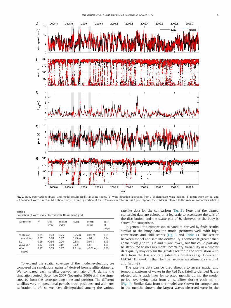
Table 1Evaluation of wave model forced with 10-km wind grid.

Parameter r2 Skillscore

Scatterindex

RMSE Meanerror

Best-fitslope

Hs (buoy)(satellite)

0.79 0.78 0.25 0.25 m 0.01 m 0.940.67 0.63 0.27 0.29 m −.04 m 0.94

Tm 0.49 −0.98 0.20 0.88 s 0.69 s 1.15Wave dir 0.37 0.03 0.19 54.21 4.81 1.01Windspeed

0.77 0.73 0.27 1.3 m/s −0.01 m/s 0.99

Fig. 2. Buoy observations (black) and model results (red). (a) Wind speed, (b) wind direction (direction from), (c) significant wave height, (d) mean wave period, and(e) dominant wave direction (direction from). (For interpretation of the references to color in this figure caption, the reader is referred to the web version of this article.)

D.K. Ralston et al. / Continental Shelf Research 65 (2013) 1–13 5

To expand the spatial coverage of the model evaluation, wecompared the simulations againstHs derived from satellite altimetry.We compared each satellite-derived estimate of Hs during thesimulation period (December 2007–November 2009) with the simu-lated Hs from the corresponding time and position. The differentsatellites vary in operational periods, track positions, and altimetercalibration to Hs, so we have distinguished among the various

satellite data for the comparison (Fig. 3). Note that the binnedscatterplot data are colored on a log scale to accentuate the tails ofthe distribution, and the scatterplot of Hs observed at the buoy isshown for comparison.

In general, the comparison to satellite-derived Hs finds resultssimilar to the buoy data–the model performs well, with highcorrelations and skill scores (Fig. 3 and Table 1). The scatterbetween model and satellite-derived Hs is somewhat greater thanat the buoy (and thus r2 and SS are lower), but this could partiallybe attributed to measurement uncertainty. Variability in altimeterdata quality may explain the greater scatter in the correlation withdata from the less accurate satellite altimeters (e.g., ERS-2 andGEOSAT Follow-On) than for the Jason-series altimeters (Jason-1and Jason-2).

The satellite data can be used directly to assess spatial andtemporal patterns of waves in the Red Sea. Satellite-derived Hs areplotted along track lines for selected months during the modelperiod, overlaying data from all satellites during each month(Fig. 4). Similar data from the model are shown for comparison.In the months shown, the largest waves observed were in the

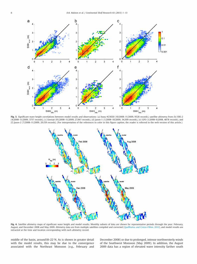
Fig. 3. Significant wave height correlations between model results and observations: (a) buoy #23020 (10/2008–11/2009, 9528 records), satellite altimetry from (b) ERS-2(4/2008–11/2009, 3757 records), (c) Envisat (01/2008–11/2009, 27,967 records), (d) Jason-1 (1/2008–10/2009, 34,509 records), (e) GFO (1/2008–9/2008, 4878 records), and(f) Jason-2 (7/2008–11/2009, 29,159 records). (For interpretation of the references to color in this figure caption, the reader is referred to the web version of this article.)

Fig. 4. Satellite altimetry maps of significant wave height and model results. Monthly subsets of data are shown for representative periods through the year: February,August, and December 2008 and May 2009. Altimetry data are from multiple satellites compiled and corrected (Queffeulou and Croize-Fillon, 2012), and model results areextracted at the time and location corresponding with each altimetry record.

D.K. Ralston et al. / Continental Shelf Research 65 (2013) 1–136

middle of the basin, around18–221N. As is shown in greater detailwith the model results, this may be due to the convergenceassociated with the Northeast Monsoon (e.g., February and

December 2008) or due to prolonged, intense northwesterly windsof the Southwest Monsoon (May 2009). In addition, the August2009 data has a region of elevated wave intensity farther south

D.K. Ralston et al. / Continental Shelf Research 65 (2013) 1–13 7

around 16.5–17.51N; model results shown later indicate that thismay be due to strong westerly winds emanating from the TokarGap. The correspondence of the model with the satellite-derivedmaps of Hs is generally good. The observations have greatervariance along a given track line than the model, but this isconsistent with the root-mean-square errors of order 0.25 mexpected for altimeter-derived Hs estimates (Chelton et al., 2001).

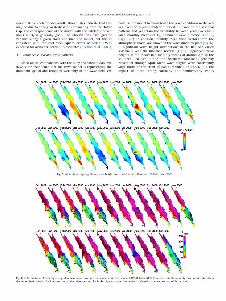
3.2. Basin-scale, seasonal wave patterns

Based on the comparisons with the buoy and satellite data, wehave some confidence that the wave model is representing thedominant spatial and temporal variability in the wave field. We

Fig. 5. Monthly average significant wave height from

Fig. 6. Color contours of monthly average dominant wave direction from model results, Dthe atmospheric model. (For interpretation of the references to color in this figure capt

now use the model to characterize the wave conditions in the RedSea over the 2-year simulation period. To examine the seasonalpatterns and yet retain the variability between years, we calcu-lated monthly means of Hs, dominant wave direction, and Tm(Figs. 5–7). In addition, monthly mean wind vectors from theatmospheric model are shown in the wave direction plots (Fig. 6).

Significant wave height distributions in the Red Sea variedseasonally with the monsoon reversal (Fig. 5). Significant waveheights in the model had monthly means of around 2 m in thesouthern Red Sea during the Northeast Monsoon, generallyNovember through April. Mean wave heights were consistentlylarge north of the Strait of Bab-el-Mandeb, 13–15.51N, but theimpact of these strong southerly and southeasterly winds

model results, December 2007–October 2009.

ecember 2007–October 2009. Also shown are the monthly mean wind vectors fromion, the reader is referred to the web version of this article.)

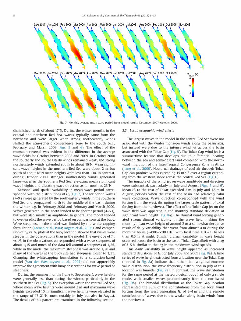
Fig. 7. Monthly average mean wave period from model results, December 2007–October 2009.

D.K. Ralston et al. / Continental Shelf Research 65 (2013) 1–138

diminished north of about 17˚N. During the winter months in thecentral and northern Red Sea, waves typically came from thenortheast and were larger when strong northeasterly windsshifted the atmospheric convergence zone to the south (e.g.,February and March 2009, Figs. 5 and 6). The effect of themonsoon reversal was evident in the difference in the averagewave fields for October between 2008 and 2009. In October 2008the southerly and southeasterly winds remained weak, and strongnortheasterly winds extended south to about 16˚N. Mean signifi-cant wave heights in the northern Red Sea were about 2 m, butsouth of about 18˚N mean heights were less than 1 m. In contrast,during October 2009, stronger southeasterly winds generatedlarge waves in the southern Red Sea, elevating mean significantwave heights and dictating wave direction as far north as 231N.

Seasonal and spatial variability in mean wave period corre-sponded with the distributions of Hs (Fig. 7). Longer period waves(7–9 s) were generated by the southeasterly winds in the southernRed Sea and propagated north to the middle of the basin duringthe winter, e.g. in February 2008 and February and March 2009.Waves generated in the north tended to be shorter period (4–6 s),but were also smaller in amplitude. In general, the model tendedto over-predict the wave period based on comparisons at the buoy.Wave steepness in the model was limited by the white-cappingformulation (Komen et al., 1984; Rogers et al., 2003), and compar-ison of Tm vs. Hs plots at the buoy location showed that waves weresteeper in the observations than in the model. The envelope of Tmvs. Hs in the observations corresponded with a wave steepness ofabout 1/15 and much of the data fell around a steepness of 1/25,while in the model the maximum steepness was around 1/20 andmany of the waves at the buoy site had steepness closer to 1/35.Changing the whitecapping formulation to a saturation-basedmodel (Van der Westhuysen et al., 2007) did not appreciablyimprove the agreement with buoy observations for wave period orsteepness.

During the summer months (June to September), wave heightswere generally less than during the winter, particularly in thesouthern Red Sea (Fig. 5). The exception was in the central Red Sea,where mean wave heights were around 2 m and maximum waveheights exceeded 10 m. Significant wave heights were elevated inthe range of 17–211N, most notably in July but also in August.The details of this pattern are examined in the following section.

3.3. Local, orographic wind effects

The largest waves in the model in the central Red Sea were notassociated with the winter monsoon winds along the basin axis,but instead were due to the intense wind jet across the basinassociated with the Tokar Gap (Fig. 5). The Tokar Gap wind jet is asummertime feature that develops due to differential heatingbetween the sea and semi-desert land combined with the north-ward migration of the Inter-Tropical Convergence Zone in Africa(Jiang et al., 2009). Nocturnal drainage of cool air through TokarGap can produce winds exceeding 15 m s−1 over a region extend-ing from the western shore across the central Red Sea (Fig. 6).

The impacts of the wind jet on wave amplitude and directionwere substantial, particularly in July and August (Figs. 5 and 6).Mean Hs to the east of Tokar exceeded 2 m in July and 1.5 m inAugust, periods when the rest of the basin had relatively calmwave conditions. Wave direction corresponded with the windforcing from the west, disrupting the larger scale pattern of axialforcing from the northwest. The effect of the Tokar Gap jet on thewave field was apparent in the monthly standard deviation ofsignificant wave height (Fig. 8a). The diurnal wind forcing gener-ated strong diurnal variability in the wave field, making themonthly mean wave height of around 2 m a somewhat deceptiveresult of daily variability that went from almost 4 m during themorning hours (∼4:00–6:00 UTC, with local time UTC+3) to lessthan 0.5 m at night. Similar diurnal variability in wave heightoccurred across the basin to the east of Tokar Gap, albeit with a lagof 3–5 h, similar to the lag in the maximum wind speeds.

This daily variability in wave height appeared as increasedstandard deviations of Hs for July 2008 and 2009 (Fig. 8a). A timeseries of wave height extracted from a location near the Tokar Gap(marked in Fig. 8a) indicate that rather than a typical extremevalue distribution, the wave frequency distribution in July at thislocation was bimodal (Fig. 9a). In contrast, the wave distributionfor the same period at the meteorological buoy had only a singlemode, with smaller waves predominantly from the northwest(Fig. 9b). The bimodal distribution at the Tokar Gap locationrepresented the sum of the contributions from the local windforcing from the west generating Hs of 2–4 m and the remotecontribution of waves due to the weaker along-basin winds fromthe northwest.

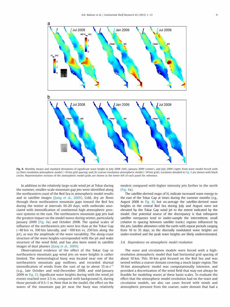
Fig. 8. Monthly means and standard deviations of significant wave height in July 2008 (left), January 2009 (center), and July 2009 (right) from wave model forced with(a) finer-resolution atmospheric model (∼10 km grid spacing) and (b) coarser-resolution atmospheric model (∼30 km grid). Locations detailed in Fig. 9 are shown with blackcircles. Representative sections of the atmospheric model grids are shown in the lower left of each panel for reference.

D.K. Ralston et al. / Continental Shelf Research 65 (2013) 1–13 9

In addition to the relatively large-scale wind jet at Tokar duringthe summer, smaller-scale mountain gap jets were identified alongthe northeastern coast of the Red Sea in atmospheric model resultsand in satellite images (Jiang et al., 2009). Cold, dry air flowsthrough these northeastern mountain gaps toward the Red Seaduring the winter at intervals 10–20 days, with outbreaks asso-ciated with intensification of continental high atmospheric pres-sure systems to the east. The northeastern mountain gap jets hadthe greatest impact on the model waves during winter, particularlyJanuary 2009 (Fig. 8a) and October 2008. The spatial scales ofinfluence of the northeastern jets were less than at the Tokar Gap(∼40 km vs. 100 km laterally, and ∼100 km vs. 250 km along thejet), as was the amplitude of the wave variability. The along-coaststructure of the wave heights corresponded with the jet and wakestructure of the wind field, and has also been noted in satelliteimages of dust plumes (Jiang et al., 2009).

Observational evidence of the effect of the Tokar Gap ornortheastern mountain gap wind jets on wave heights is ratherlimited. The meteorological buoy was located near one of thenortheastern mountain gap outflows, and recorded diurnalintensification of winds from the east of up to about 15 m s−1

(e.g., late October and mid-December 2008, and mid-January2009 in Fig. 2). Significant wave heights during with the wind jetevents reached over 2.5 m, compared with background Hs duringthose periods of 0.5–1 m. Note that in the model, the effect on thewaves of the mountain gap jet near the buoy was relatively

modest compared with higher intensity jets farther to the north(Fig. 8a).

The satellite-derived maps of Hs indicate increased wave energy tothe east of the Tokar Gap at times during the summer months (e.g.,August 2008 in Fig. 4), but on-average the satellite-derived waveheights in the central Red Sea during July and August were notelevated by the Tokar Gap wind jet to the extent indicated by themodel. One potential source of the discrepancy is that infrequentsatellite overpasses tend to under-sample the intermittent, small(relative to spacing between satellite tracks) regions influenced bythe jets. Satellite altimeters orbit the earth with repeat periods rangingfrom 10 to 35 days, so the diurnally modulated wave heights areunder-resolved and the peak wave heights are likely underestimated.

3.4. Dependence on atmospheric model resolution

The wave and circulation models were forced with a high-resolution atmospheric model that had horizontal grid spacing ofabout 10 km. This 10-km grid focused on the Red Sea and wasnested within a coarser domain covering a much larger region. The10-km atmospheric model was computationally intensive, andprovided a discretization of the wind field that may not always befeasible for modeling waves at these basin scales. To evaluate theeffect that the atmospheric model resolution had on the wave andcirculation models, we also ran cases forced with winds andatmospheric pressure from the coarser, outer domain that had a

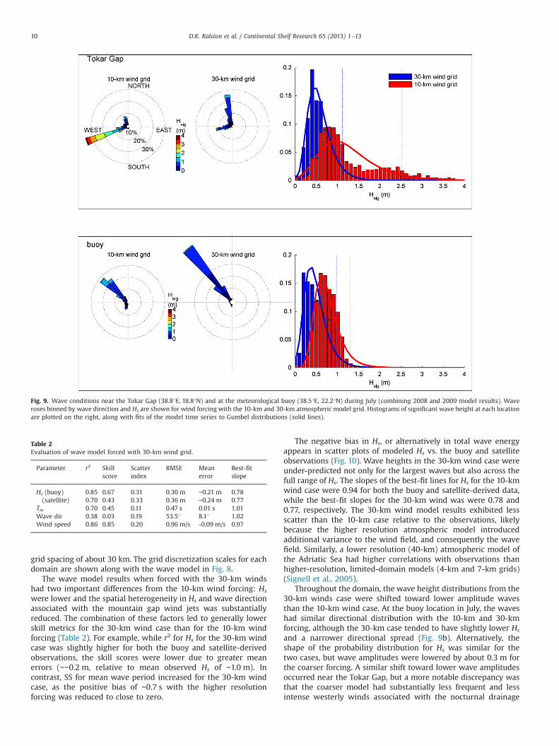
Fig. 9. Wave conditions near the Tokar Gap (38.81E, 18.81N) and at the meteorological buoy (38.51E, 22.21N) during July (combining 2008 and 2009 model results). Waveroses binned by wave direction and Hs are shown for wind forcing with the 10-km and 30-km atmospheric model grid. Histograms of significant wave height at each locationare plotted on the right, along with fits of the model time series to Gumbel distributions (solid lines).

Table 2Evaluation of wave model forced with 30-km wind grid.

Parameter r2 Skillscore

Scatterindex

RMSE Meanerror

Best-fitslope

Hs (buoy)(satellite)

0.85 0.67 0.31 0.30 m −0.21 m 0.780.70 0.43 0.33 0.36 m −0.24 m 0.77

Tm 0.70 0.45 0.11 0.47 s 0.01 s 1.01Wave dir 0.38 0.03 0.19 53.51 8.11 1.02Wind speed 0.86 0.85 0.20 0.96 m/s -0.09 m/s 0.97

D.K. Ralston et al. / Continental Shelf Research 65 (2013) 1–1310

grid spacing of about 30 km. The grid discretization scales for eachdomain are shown along with the wave model in Fig. 8.

The wave model results when forced with the 30-km windshad two important differences from the 10-km wind forcing: Hs

were lower and the spatial heterogeneity in Hs and wave directionassociated with the mountain gap wind jets was substantiallyreduced. The combination of these factors led to generally lowerskill metrics for the 30-km wind case than for the 10-km windforcing (Table 2). For example, while r2 for Hs for the 30-km windcase was slightly higher for both the buoy and satellite-derivedobservations, the skill scores were lower due to greater meanerrors (∼−0.2 m, relative to mean observed Hs of ∼1.0 m). Incontrast, SS for mean wave period increased for the 30-km windcase, as the positive bias of ∼0.7 s with the higher resolutionforcing was reduced to close to zero.

The negative bias in Hs, or alternatively in total wave energyappears in scatter plots of modeled Hs vs. the buoy and satelliteobservations (Fig. 10). Wave heights in the 30-km wind case wereunder-predicted not only for the largest waves but also across thefull range of Hs. The slopes of the best-fit lines for Hs for the 10-kmwind case were 0.94 for both the buoy and satellite-derived data,while the best-fit slopes for the 30-km wind was were 0.78 and0.77, respectively. The 30-km wind model results exhibited lessscatter than the 10-km case relative to the observations, likelybecause the higher resolution atmospheric model introducedadditional variance to the wind field, and consequently the wavefield. Similarly, a lower resolution (40-km) atmospheric model ofthe Adriatic Sea had higher correlations with observations thanhigher-resolution, limited-domain models (4-km and 7-km grids)(Signell et al., 2005).

Throughout the domain, the wave height distributions from the30-km winds case were shifted toward lower amplitude wavesthan the 10-km wind case. At the buoy location in July, the waveshad similar directional distribution with the 10-km and 30-kmforcing, although the 30-km case tended to have slightly lower Hs

and a narrower directional spread (Fig. 9b). Alternatively, theshape of the probability distribution for Hs was similar for thetwo cases, but wave amplitudes were lowered by about 0.3 m forthe coarser forcing. A similar shift toward lower wave amplitudesoccurred near the Tokar Gap, but a more notable discrepancy wasthat the coarser model had substantially less frequent and lessintense westerly winds associated with the nocturnal drainage

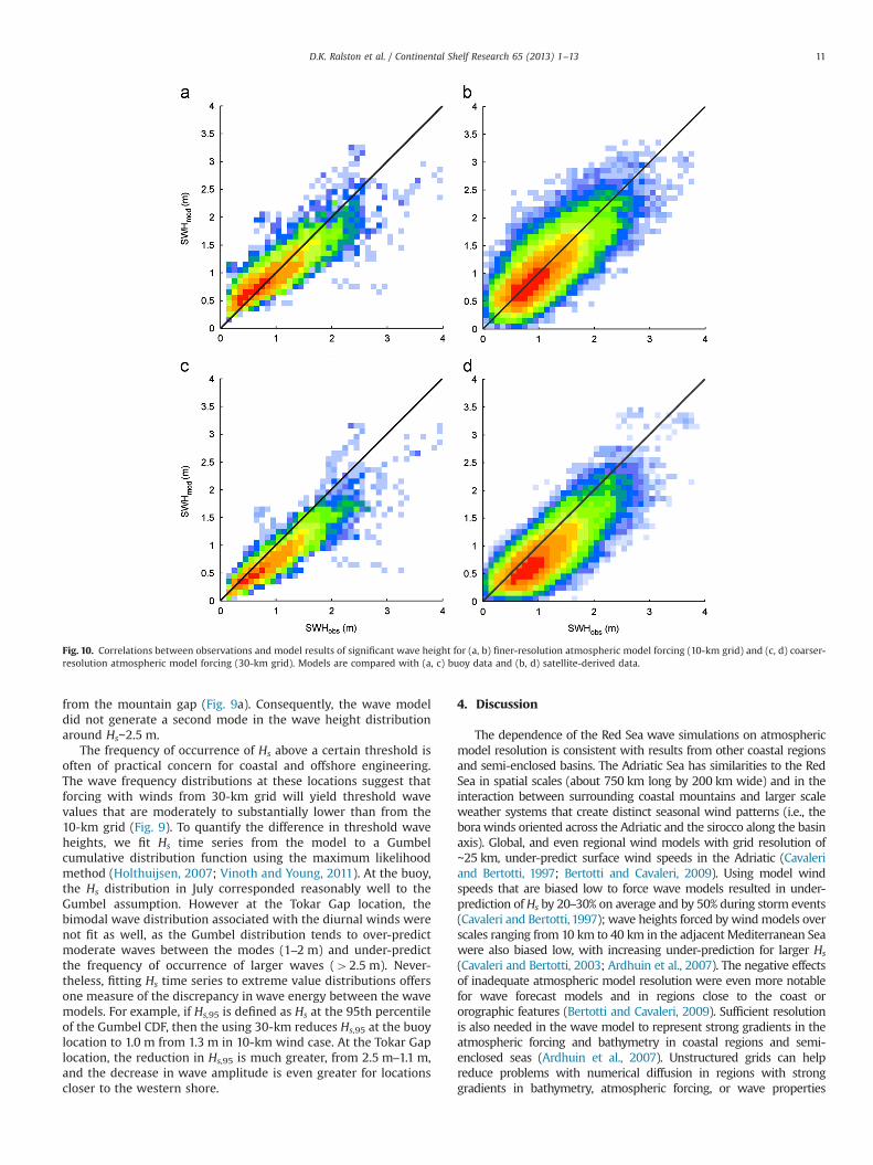
Fig. 10. Correlations between observations and model results of significant wave height for (a, b) finer-resolution atmospheric model forcing (10-km grid) and (c, d) coarser-resolution atmospheric model forcing (30-km grid). Models are compared with (a, c) buoy data and (b, d) satellite-derived data.

D.K. Ralston et al. / Continental Shelf Research 65 (2013) 1–13 11

from the mountain gap (Fig. 9a). Consequently, the wave modeldid not generate a second mode in the wave height distributionaround Hs∼2.5 m.

The frequency of occurrence of Hs above a certain threshold isoften of practical concern for coastal and offshore engineering.The wave frequency distributions at these locations suggest thatforcing with winds from 30-km grid will yield threshold wavevalues that are moderately to substantially lower than from the10-km grid (Fig. 9). To quantify the difference in threshold waveheights, we fit Hs time series from the model to a Gumbelcumulative distribution function using the maximum likelihoodmethod (Holthuijsen, 2007; Vinoth and Young, 2011). At the buoy,the Hs distribution in July corresponded reasonably well to theGumbel assumption. However at the Tokar Gap location, thebimodal wave distribution associated with the diurnal winds werenot fit as well, as the Gumbel distribution tends to over-predictmoderate waves between the modes (1–2 m) and under-predictthe frequency of occurrence of larger waves (42.5 m). Never-theless, fitting Hs time series to extreme value distributions offersone measure of the discrepancy in wave energy between the wavemodels. For example, if Hs,95 is defined as Hs at the 95th percentileof the Gumbel CDF, then the using 30-km reduces Hs,95 at the buoylocation to 1.0 m from 1.3 m in 10-km wind case. At the Tokar Gaplocation, the reduction in Hs,95 is much greater, from 2.5 m–1.1 m,and the decrease in wave amplitude is even greater for locationscloser to the western shore.

4. Discussion

The dependence of the Red Sea wave simulations on atmosphericmodel resolution is consistent with results from other coastal regionsand semi-enclosed basins. The Adriatic Sea has similarities to the RedSea in spatial scales (about 750 km long by 200 km wide) and in theinteraction between surrounding coastal mountains and larger scaleweather systems that create distinct seasonal wind patterns (i.e., theborawinds oriented across the Adriatic and the sirocco along the basinaxis). Global, and even regional wind models with grid resolution of∼25 km, under-predict surface wind speeds in the Adriatic (Cavaleriand Bertotti, 1997; Bertotti and Cavaleri, 2009). Using model windspeeds that are biased low to force wave models resulted in under-prediction ofHs by 20–30% on average and by 50% during storm events(Cavaleri and Bertotti, 1997); wave heights forced by windmodels overscales ranging from 10 km to 40 km in the adjacent Mediterranean Seawere also biased low, with increasing under-prediction for larger Hs

(Cavaleri and Bertotti, 2003; Ardhuin et al., 2007). The negative effectsof inadequate atmospheric model resolution were even more notablefor wave forecast models and in regions close to the coast ororographic features (Bertotti and Cavaleri, 2009). Sufficient resolutionis also needed in the wave model to represent strong gradients in theatmospheric forcing and bathymetry in coastal regions and semi-enclosed seas (Ardhuin et al., 2007). Unstructured grids can helpreduce problems with numerical diffusion in regions with stronggradients in bathymetry, atmospheric forcing, or wave properties

D.K. Ralston et al. / Continental Shelf Research 65 (2013) 1–1312

(Cavaleri, 2009), but the results here suggest that the predictive abilityof these wave models is still in large part controlled by the windforcing.

In this application, we did not attempt to optimize the modelparameters, but instead used mostly default settings. In the RedSea the buoy data available for model calibration are limited. Incontrast, a study of multiple atmospheric and wave models in theWestern Mediterranean used data from nearly 40 buoys andtowers distributed around the basin (Ardhuin et al., 2007). Addi-tional buoy measurements or high-resolution remote sensingsurveys (Romero and Melville, 2010a) would be particularlyvaluable in regions where mountain gap jets can generate largewaves in fetch-limited conditions.

One adjustment made in model development was a smoothingof the grid bathymetry. In regions with steep topography andinsufficient grid resolution, excessive refraction in unstructuredSWAN can focus wave energy toward a single grid point, creatingunrealistically large wave heights and long periods (Dietrich et al.,in press). Initially, the model over-predicted wave heights andperiods at the buoy due to excessive refraction in a few regionswith shallow, complex bathymetry. Modest smoothing of the gridusing spatial averaging of adjacent nodes weighted toward thecentral node was sufficient to eliminate the refraction problemareas, but the sensitivity of the results to the smoothing approachwas not quantified. Alternatively, excessive refraction on coarse,steep grids can be controlled with Courant–Friedrichs–Lewy limit-ers on the spectral propagation velocities (Dietrich et al., in press).Applying these limiters with the smoothed bathymetry did notsignificantly change the model results.

Understanding the wave climate in the Red Sea is importantbecause of the effects that waves can have on physical as well asbiological conditions along the coast. For example, the Red Seacoast features a diverse array of coral reefs, but that diversity hasbeen reported to be declining in recent decades (Riegl et al., 2012).Solar heating can lead to large diurnal swings in water tempera-ture on reefs, with substantial spatial heterogeneity in tempera-ture that is determined in large part by the rate of flushing due towave-induced circulation (Davis et al., 2011). Excessively highwater temperatures can lead to coral bleaching and mortality(Glynn, 1993), so wave intensity and exposure, particularly duringthe summer months when thermal stresses are most intense, maydetermine the suitability of a location for coral survival in aclimate with increasing water temperatures. The wave distributionin the Red Sea has implications for the health of coral at largescales, for example with shifts in the latitude of the wind and waveconvergence during the Northeast Monsoon, and at the smallerscales of individual mountain gap jets.

5. Summary

The model results indicated that at large scales the dominantseasonal variability in waves in the Red Sea corresponded with themonsoon wind reversal. During the winter, monsoon winds fromthe southeast generated waves with mean significant waveheights in excess of 2 m and mean periods of 8 s over much ofthe southern Red Sea. In the northern Red Sea, average waveheights were smaller and periods were shorter, with waves drivenby winds from the northwest. The convergence of the wind andwave fields during the Northeast Monsoon typically occurredaround 19–201N, but the location of the convergence variedthrough the winter between 15 and 21.5 1N. During the SouthwestMonsoon in the summer, waves were generally smaller than inwinter, with monthly mean Hs around 1 m or less.

The maximumwave heights in the simulations occurred not due tomonsoonal winds along the major axis of the Red Sea, but instead

resulted from mountain gap wind jets across the basin. In July 2008and 2009, the Tokar Gap jet had pronounced effects on the wavesbetween 18 and 201N across the width of the Red Sea. Monthly meanHs due to the wind jet exceeded 2m in this region during a periodwhen the rest of the basinwas relatively calm, andmaximumHs in thevicinity of the jet reached 14m. Smaller mountain gap wind jetsenhanced wave heights and variability along the northeast coast,particularly in October 2008 and January 2009. These northeasternjets altered the waves over smaller distances than the jet at the TokarGap, but the multiple jets spread along the coast provided a dominantsource of wave energy during these periods.

Evaluation of the model results against wave observations fromsatellites and a buoy indicated that the spatial resolution of the windmodel used to force the wave model significantly affected the qualityof the wave simulations. Forcing the wave model with winds from a10-km grid generally had higher skill than with winds from 30-kmgrid, largely due to an under-prediction of the mean wind speed andwave height by the coarser atmospheric model. The 30-km grid wasinsufficient to represent mountain gap wind jets, including therelatively large jet associated with the Tokar Gap, and thus predictedlower wave heights in the central Red Sea during the summer andalong the northeast coast during the winter.

Acknowledgments

We thank Casey Dietrich for providing the SWAN-ADCIRC codeand Changshen Chen for the model grid bathymetry. This researchis based on work supported by Award nos. USA00001, USA00002,KSA00011, made by the King Abdullah University of Science andTechnology (KAUST) in Saudi Arabia.

References

Ardhuin, F., Bertotti, L., Bidlot, J.-R., Cavaleri, L., Filipetto, V., Lefevre, J.-M.,Wittmann, P., 2007. Comparison of wind and wave measurements and modelsin the Western Mediterranean Sea. Ocean Engineering 34, 526–541, http://dx.doi.org/10.1016/j.oceaneng.2006.02.008.

Benetazzo, A., Carniel, S., Sclavo, M., Bergamasco, A., Wave–current interaction:Effect on the wave field in a semi-enclosed basin. Ocean Modelling http://dx.doi.org/10.1016/j.ocemod.2012.12.009, in press.

Bertotti, L., Cavaleri, L., 2009. Wind and wave predictions in the Adriatic Sea. Journalof Marine Systems 78 (Suppl.), S227–S234, http://dx.doi.org/10.1016/j.jmarsys.2009.01.018.

Boldrin, A., Carniel, S., Giani, M., Marini, M., Aubry, F.B., Campanelli, A., Grilli, F.,Russo, A., 2009. Effects of bora wind on physical and biogeochemical propertiesof stratified waters in the northern Adriatic. Journal of Geophysical Research114, C08S92, http://dx.doi.org/10.1029/2008JC004837.

Booij, N., Ris, R.C., Holthuijsen, L.H., 1999. A third-generation wave model for coastalregions 1. Model description and validation. Journal of Geophysical Research104, 7649–7666 http://dx.doi.org/199910.1029/98JC02622.

Cavaleri, L., 2009. Wave modeling—missing the peaks. Journal of Physical Oceano-graphy 39, 2757–2778, http://dx.doi.org/10.1175/2009JPO4067.1.

Cavaleri, L., Bertotti, L., 1997. In search of the correct wind and wave fields in aminor basin. Monthly Weather Review 125, 1964–1975.

Cavaleri, L., Bertotti, L., 2003. The characteristics of wind and wave fields modelledwith different resolutions. Quarterly Journal of the Royal Meteorological Society129, 1647–1662, http://dx.doi.org/10.1256/qj.01.68.

Chelton, D.B., Ries, J.C., Haines, B.J., Fu, L.-L., Callahan, P.S., 2001. Satellite altimetry.In: Fu, Lee-Lueng, Cazenave, Anny (Eds.), Satellite Altimetry and Earth SciencesA Handbook of Techniques and Applications. Academic Press, pp. 1–131.

Churchill, J.H., Plueddemann, A.J., Faluotico, S.M., 2006. Extracting wind sea andswell from directional wave spectra derived from a bottom-mounted ADCP(Technical report No. WHOI-2006-13). Woods Hole Oceanographic Institution,Woods Hole, MA p. 34.

Clifford, M., Horton, C., Schmitz, J., Kantha, L.H., 1997. An oceanographic nowcast/forecast system for the Red Sea. Journal of Geophysical Research 102,25101–25,122, http://dx.doi.org/10.1029/97JC01919.

Colbo, K., Weller, R.A., 2009. Accuracy of the IMET Sensor Package in the Subtropics.Journal of Atmospheric and Oceanic Technology 26, 1867–1890, http://dx.doi.org/10.1175/2009JTECHO667.1.

Davis, K., Lentz, S., Pineda, J., Farrar, J., Starczak, V., Churchill, J., 2011. Observationsof the thermal environment on Red Sea platform reefs: a heat budget analysis.Coral Reefs 30, 25–36, http://dx.doi.org/10.1007/s00338-011-0740-8.

D.K. Ralston et al. / Continental Shelf Research 65 (2013) 1–13 13

Dietrich, J., Tanaka, S., Westerink, J., Dawson, C., Luettich, R., Zijlema, M., Holthuij-sen, L., Smith, J., Westerink, L., Westerink, H., 2012. Performance of theunstructured-mesh, SWAN+ADCIRC model in computing hurricane waves andsurge. Journal of Scientific Computing 52, 468–497, http://dx.doi.org/10.1007/s10915-011-9555-6.

Dietrich, J.C., Westerink, J.J., Kennedy, A.B., Smith, J.M., Jensen, R.E., Zijlema, M.,Holthuijsen, L.H., Dawson, C., Luettich, R.A., Powell, M.D., Cardone, V.J., Cox, A.T.,Stone, G.W., Pourtaheri, H., Hope, M.E., Tanaka, S., Westerink, L.G., Westerink, H.J.,Cobell, Z., 2011a. Hurricane Gustav (2008) waves and storm surge: hindcast,synoptic analysis, and validation in Southern Louisiana. Monthly Weather Review139, 2488–2522, http://dx.doi.org/10.1175/2011MWR3611.1.

Dietrich, J.C., Zijlema, M., Westerink, J.J., Holthuijsen, L.H., Dawson, C., Luettich Jr., R.A.,Jensen, R.E., Smith, J.M., Stelling, G.S., Stone, G.W., 2011b. Modeling hurricanewaves and storm surge using integrally-coupled, scalable computations. CoastalEngineering 58, 45–65, http://dx.doi.org/10.1016/j.coastaleng.2010.08.001.

Dietrich, J.C., Zijlema, M., Allier, P.-E., Holthuijsen, L.H., Booij, N., Meixner, J.D., Proft,J.K., Dawson, C.N., Bender, C.J., Naimaster, A., Smith, J.M., Westetrink, J.J.,Limiters for spectral propagation velocities in SWAN. Ocean Modelling, http://dx.doi.org/10.1016/j.ocemod.2012.11.005, in press.

Dorman, C.E., Carniel, S., Cavaleri, L., Sclavo, M., Chiggiato, J., Doyle, J., Haack, T., Pullen,J., Grbec, B., Vilibić, I., Janeković, I., Lee, C., Malačič, V., Orlić, M., Paschini, E., Russo,A., Signell, R.P., 2006. February 2003 marine atmospheric conditions and the boraover the northern Adriatic. Journal of Geophysical Research 111, http://dx.doi.org/10.1029/2005JC003134C03S03, http://dx.doi.org/10.1029/2005JC003134.

Earle, M.D., 1996. Nondirectional and Directional Wave Data Analysis Procedures.(National Data Buoy Center Technical Document No. 96-01). Stennis SpaceCenter, Slidell, LA p. 37.

Egbert, G.D., Erofeeva, S.Y., 2002. Efficient inverse modeling of barotropic oceantides. Journal of Atmospheric and Oceanic Technology 19, 183–204.

Farrar, J.T., Lentz, S., Churchill, J., Bouchard, P., Smith, J., Kemp, J., Lord, J., Allsup, G.,Hosom, D., 2009. King Abdullah University of Science and Technology (KAUST)mooring deployment cruise and fieldwork report (Technical report No. WHOI-KAUST-CTR-2009-02). Woods Hole Oceanographic Institution, Woods Hole, MAp. 88.

Gentemann, C., Minnett, P., Sienkiewicz, J., DeMaria, M., Cummings, J., Jin, Y., Doyle,J., Gramer, L., Barron, C., Casey, K., Donlon, C., 2009. The multi-sensor improvedsea surface temperature (MISST) project. Oceanography 22, 76–87, http://dx.doi.org/10.5670/oceanog.2009.40.

Glynn, P.W., 1993. Coral reef bleaching: ecological perspectives. Coral Reefs 12,1–17, http://dx.doi.org/10.1007/BF00303779.

Grubišíc, V., 2004. Bora-driven potential vorticity banners over the Adriatic.Quarterly Journal of the Royal Meteorological Society 130, 2571–2603, http://dx.doi.org/10.1256/qj.03.71.

Holthuijsen, L.H., 2007. Waves in Oceanic and Coastal Waters. Cambridge UniversityPress.

Hosom, D.S., Weller, R.A., Payne, R.E., Prada, K.E., 1995. The IMET (improvedmeteorology) ship and buoy systems. Journal of Atmospheric and OceanicTechnology 12, 527–540.

Jiang, H., Farrar, J.T., Beardsley, R.C., Chen, R., Chen, C., 2009. Zonal surface wind jetsacross the Red Sea due to mountain gap forcing along both sides of the Red Sea.Geophysical Research Letters 36, L19605, http://dx.doi.org/10.1029/2009GL040008.

Kirby, J.T., Chen, T.-M., 1989. Surface waves on vertically sheared flows:approximate dispersion relations. Journal of Geophysical Research: Oceans94, 1013–1027, http://dx.doi.org/10.1029/JC094iC01p01013.

Kolar, R.L., Gray, W.G., Westerink, J.J., Luettich, R.A., 1994. Shallow water modelingin spherical coordinates: equation formulation, numerical implementation, andapplication. Journal of Hydraulic Research 32, 3–24, http://dx.doi.org/10.1080/00221689409498786.

Komen, G.J., Hasselmann, K., Hasselmann, K., 1984. On the existence of a fullydeveloped wind-sea spectrum. Journal of Physical Oceanography 14, 1271–1285http://dx.doi.org/10.1175/1520-0485(1984)014%3c1271:OTEOAF%3e2.0.CO;2.

Lo, J.C.-F., Yang, Z.-L., Sr, R.A.P., 2008. Assessment of three dynamical climatedownscaling methods using the Weather Research and Forecasting (WRF)model. Journal of Geophysical Research 113, D09112, http://dx.doi.org/10.1029/2007JD009216.

Luettich, R.A., Westerink, J.J., 2004. Formulation and numerical implementation ofthe 2D/3D ADCIRC finite element model version 44. XX. R. Luettich, ⟨http://adcirc.org/adcirc_theory_2004_12_08.pdf⟩.

Luettich, R.A., Westerink, J.J., Scheffner, N.W., 1992. ADCIRC: an advanced three-dimensional circulation model for shelves, coasts and estuaries, Report 1:Theory and methodology of ADCIRC-2DDI and ADCIRC-3DL (No. Tech. Rep.DRP-92-6). U.S. Army Corps of Engineers, 137.

Melville, W.K., Romero, L., Kleiss, J.M., 2005. Extreme wave events in the Gulf ofTehuantepec. Presented at the Rogue Waves: 14th ‘Aha Huliko ‘a HawaiianWinter Workshop, University of Hawaii at Manoa, Honolulu, HI, pp. 23–28.

Metwally, A., Abul-Azm, A.G., 2007. The Red Sea Wind-Wave ATLAS. In: TheProceedings of The Seventeenth (2007) International Offshore and PolarEngineering Conference. Lisbon, Portugal, pp. 1850–1854.

Monismith, S.G., Genin, A., 2004. Tides and sea level in the Gulf of Aqaba (Eilat).Journal of Geophysical Research 109, C04015, http://dx.doi.org/10.1029/2003JC002069.

Murphy, A.H., 1988. Skill scores based on the mean square error and their relationshipsto the correlation coefficient. Monthly Weather Review 116, 2417–2424.

Olabarrieta, M., Warner, J.C., Armstrong, B., Zambon, J.B., He, R., 2012.Ocean–atmosphere dynamics during Hurricane Ida and Nor'Ida: an applicationof the coupled ocean–atmosphere–wave–sediment transport (COAWST) mod-eling system. Ocean Modelling 43–44, 112–137, http://dx.doi.org/10.1016/j.ocemod.2011.12.008.

Patzert, W.C., 1974. Wind-induced reversal in Red Sea circulation. Deep SeaResearch and Oceanographic Abstracts 21, 109–121, http://dx.doi.org/10.1016/0011-7471(74)90068-0.

Payne, R.E., Anderson, S.P., 1999. A New Look at Calibration and Use of EppleyPrecision Infrared Radiometers. Part II: Calibration and Use of the Woods HoleOceanographic Institution Improved Meteorology Precision Infrared Radio-metern. Journal of Atmospheric and Oceanic Technology 16, 739–751 http://dx.doi.org/10.1175/1520-0426(1999)016%3c0739:ANLACA%3e2.0.CO;2.

Pedgley, D.E., 1974. An outline of the weather and climate of the Red Sea.L'Oceanographie Physique de la Mer Rouge, 9–27.

Pullen, J., Doyle, J.D., Haack, T., Dorman, C., Signell, R.P., Lee, C.M., 2007. Bora eventvariability and the role of air-sea feedback. Journal of Geophysical Research 112,C03S18, http://dx.doi.org/10.1029/2006JC003726.

Queffeulou, P., 2004. Long-Term Validation of Wave Height Measurementsfrom Altimeters. Marine Geodesy 27, 495–510, http://dx.doi.org/10.1080/01490410490883478.

Queffeulou, P., Croize-Fillon, D., 2012. Global altimeter SWH data set, Version 9,ftp://ftp.ifremer.fr/ifremer/cersat/products/swath/altimeters/waves/.

Riegl, B.M., Bruckner, A.W., Rowlands, G.P., Purkis, S.J., Renaud, P., 2012. Red Seacoral reef trajectories over 2 decades suggest increasing community homo-genization and decline in coral size. PLoS One 7, e38396, http://dx.doi.org/10.1371/journal.pone.0038396.

Rogers, W.E., Hwang, P.A., Wang, D.W., 2003. Investigation of wave growth anddecay in the SWAN Model: three regional-scale applicationsn. Journal ofPhysical Oceanography 33, 366–389 http://dx.doi.org/10.1175/1520-0485(2003)033%3c0366:IOWGAD%3e2.0.CO;2.

Romero, L., Melville, W.K., 2010a. Airborne observations of fetch-limited waves inthe Gulf of Tehuantepec. Journal of Physical Oceanography 40, 441–465, http://dx.doi.org/10.1175/2009JPO4127.1.

Romero, L., Melville, W.K., 2010b. Numerical modeling of fetch-limited waves in theGulf of Tehuantepec. Journal of Physical Oceanography 40, 466–486, http://dx.doi.org/10.1175/2009JPO4128.1.

Signell, R.P., Carniel, S., Cavaleri, L., Chiggiato, J., Doyle, J.D., Pullen, J., Sclavo, M.,2005. Assessment of wind quality for oceanographic modelling in semi-enclosed basins. Journal of Marine Systems 53, 217–233, http://dx.doi.org/10.1016/j.jmarsys.2004.03.006.

Skamarock, W.C., Klemp, J.B., Dudhia, J., Gill, D.O., Barker, D.M., Duda, M.G., Huang, X.-Y.,Wang, W., Powers, J.G., 2008. A description of the advanced research WRF version 3(NCAR Tech. Note No. NCAR/TN–475+STR). Natl. Cent. for Atmos. Res., Boulder, CO,113.

Sofianos, S.S., Johns, W.E., 2001. Wind induced sea level variability in the Red Sea.Geophysical Research Letters 28, 3175–3178, http://dx.doi.org/10.1029/2000GL012442.

Sofianos, S.S., Johns, W.E., 2002. An Oceanic General Circulation Model (OGCM)investigation of the Red Sea circulation, 1. Exchange between the Red Sea andthe Indian Ocean. Journal of Geophysical Research 107, 3196, http://dx.doi.org/10.1029/2001JC001184.

Sofianos, S.S., Johns, W.E., 2003. An Oceanic General Circulation Model (OGCM)investigation of the Red Sea circulation: 2. Three-dimensional circulation in theRed Sea. Journal of Geophysical Research 108, 3066, http://dx.doi.org/10.1029/2001JC001185.

Sofianos, S.S., Johns, W.E., 2007. Observations of the summer Red Sea circulation.Journal of Geophysical Research 112, C06025, http://dx.doi.org/10.1029/2006JC003886.

Thiébaux, J., Rogers, E., Wang, W., Katz, B., 2003. A new high-resolution blendedreal-time global sea surface temperature analysis. Bulletin of the AmericanMeteorological Society 84, 645–656, http://dx.doi.org/10.1175/BAMS-84-5-645.

Vinoth, J., Young, I.R., 2011. Global estimates of extreme wind speed and wave height.Journal of Climate 24, 1647–1665, http://dx.doi.org/10.1175/2010JCLI3680.1.

Wang, X.H., Pinardi, N., 2002. Modeling the dynamics of sediment transport andresuspension in the northern Adriatic Sea. Journal of Geophysical Research 107,3225, http://dx.doi.org/10.1029/2001JC001303.

Wang, X.H., Pinardi, N., Malacic, V., 2007. Sediment transport and resuspension dueto combined motion of wave and current in the northern Adriatic Sea during aBora event in January 2001: a numerical modelling study. Continental ShelfResearch 27, 613–633, http://dx.doi.org/10.1016/j.csr.2006.10.008.

Westerink, J.J., Luettich, R.A., Feyen, J.C., Atkinson, J.H., Dawson, C., Roberts, H.J.,Powell, M.D., Dunion, J.P., Kubatko, E.J., Pourtaheri, H., 2008. A basin- tochannel-scale unstructured grid hurricane storm surge model applied toSouthern Louisiana. Monthly Weather Review 136, 833–864, http://dx.doi.org/10.1175/2007MWR1946.1.

Van der Westhuysen, A.J., Zijlema, M., Battjes, J.A., 2007. Nonlinear saturation-based whitecapping dissipation in SWAN for deep and shallow water. CoastalEngineering 54, 151–170, http://dx.doi.org/10.1016/j.coastaleng.2006.08.006.

Zijlema, M., 2010. Computation of wind-wave spectra in coastal waters with SWANon unstructured grids. Coastal Engineering 57, 267–277, http://dx.doi.org/10.1016/j.coastaleng.2009.10.011.