The Propagation of Mountain Waves into the Stratosphere: Quantitative Evaluation of Three-Dimensional Simulations

3090 VOLUME 57J O U R N A L O F T H E A T M O S P H E R I C S C I E N C E S

q 2000 American Meteorological Society

The Propagation of Mountain Waves into the Stratosphere: Quantitative Evaluation ofThree-Dimensional Simulations

MARTIN LEUTBECHER* AND HANS VOLKERT

Institut fur Physik der Atmosphare, Deutsches Zentrum fur Luft- und Raumfahrt, Oberpfaffenhofen, Germany

(Manuscript received 9 March 1999, in final form 17 November 1999)

ABSTRACT

On 6 January 1992 measurements of a mountain wave with significant amplitude were taken over the southerntip of Greenland during an ER-2 flight at an altitude of about 20 km. This work focuses on 3D numericalsimulations of the wave generation and its propagation into the stratosphere during this event. The sensitivityof the simulated mountain wave to surface friction and horizontal resolution is explored. A nonhydrostatic modelis used for experiments with horizontal resolutions of 12, 4, and 1.3 km.

In all simulations the flow over the southern tip of Greenland generates a mountain wave, which propagatesinto the stratosphere. Changes of surface friction and horizontal resolution affect mostly the amplitude of themountain wave. Increasing surface friction on the slopes reduces the amplitude of the excited orographic gravitywave. Horizontal diffusion required for numerical stability attenuates gravity waves during their propagationinto the stratosphere. Increasing the horizontal resolution permits a smaller diffusion and thereby results in largerstratospheric wave amplitudes.

The experiment with increased surface friction at 1.3-km horizontal resolution shows the best agreement withthe observational data of the wave in the stratosphere. The differences between the simulated and measuredamplitudes of vertical displacement and temperature anomaly are less than about 20%. The disparity in verticalvelocity is larger; downward velocities were observed up to 4.8 m s21 and simulated up to 2.7 m s21. In theexperiments with lower surface friction at 4-km resolution, the accuracy regarding the amplitude of verticaldisplacement and temperature anomalies is similar, but the simulated maximum downdraft is even weaker. Theother experiments with increased surface friction at 4-km resolution and normal friction at 12-km resolutionsignificantly underestimate the wave amplitude. The results of the experiments suggest that the generation oforographic gravity waves and their propagation into the stratosphere can be simulated in three dimensions in arealistic manner provided that the magnitude of the parameterized surface friction is in a realistic range and thehorizontal resolution is sufficient.

1. Introduction

Large amplitude gravity waves are abundant in thestratosphere. Flow over orography is thought to be amajor source of these gravity waves (Nastrom and Fritts1992). The vertical propagation of orographically gen-erated gravity waves into the stratosphere is generallypossible unless critical levels are present or trappingoccurs. Trapping affects the nonhydrostatic gravitywaves that have a horizontal wavelength of about 10–20 km (Shutts 1992). The propagation of the entire grav-ity wave spectrum is prevented at a level where theambient wind vanishes. When the wind vector turns with

* Current affiliation: ECMWF, Reading, United Kingdom

Corresponding author address: Martin Leutbecher, European Cen-tre for Medium-Range Weather Forecasts, Shinfield Park, ReadingRG2 9AX, United Kingdom.E-mail: [email protected]

altitude, the vertical propagation is limited to the partof the spectrum that does not encounter a level wherethe horizontal wave vector is normal to the ambient flow(Shutts 1998).

Gravity waves are known to influence stratosphericdynamics. The dissipation of orographic gravity wavesgreatly affects the atmospheric momentum budget. Thisprocess needs to be parameterized in global circulationmodels, which either do not sufficiently resolve thesewaves or do not resolve them at all (Palmer et al. 1986;McFarlane 1987). The distribution of trace constituentsin the stratosphere is affected by the mixing induced bybreaking gravity waves (Lilly and Lester 1974). Thismixing can be relevant as the stratosphere is known tobe a region of the atmosphere where the vertical ex-change of matter is very low.

Gravity waves induce mesoscale temperature anom-alies. Thereby they can trigger microphysical processesin the stratosphere. Cold anomalies in the stratospherecan cause supersaturation with respect to water or othertrace constituents, which in turn leads to the formation

15 SEPTEMBER 2000 3091L E U T B E C H E R A N D V O L K E R T

of clouds. Potter and Holton (1995) propose a dehy-dration mechanism of the tropical lower stratospherethat involves cloud formation in the stratosphere due togravity waves caused by convection. The study of Car-slaw et al. (1998a) suggests that polar stratosphericclouds (PSCs) induced by mountain waves on the me-soscale may contribute significantly to the ozone de-pletion in the Arctic stratosphere. PSCs induced bymountain waves have been identified and characterizedby remote sensing (Carslaw et al. 1998b) and in situmeasurements (Schreiner et al. 1999).

Starting from the early work by Lyra (1943) and Que-ney (1947) linear theory has been central to the under-standing of orographic gravity waves up to present. Thelinearization well approximates small amplitude waves.When the wave amplitude is larger, the results fromlinear theory are often qualitatively similar to finite-amplitude solutions, but quantitatively large errors canoccur (Durran 1992). As the amplitude of gravity wavesincreases with altitude with the inverse square root ofdensity and density decreases vertically by an order ofmagnitude about every 15 km, large amplitude gravitywaves and wave breaking are commonplace in thestratosphere. Therefore, nonlinear numerical simula-tions are required to study orographic gravity waveseven over orography of moderate height.

Most of the previous numerical experiments of oro-graphic flows with domains extending well into thestratosphere simulated flows in two-dimensional slices(e.g., Bacmeister and Schoeberl 1989; Durran 1995).Unless the orography is almost two-dimensional this isa severe restriction, as several important processes can-not be modelled in two-dimensional settings. Three-di-mensional dispersion spreads the gravity wave energyacting to reduce the amplitude with increasing height(Smith 1980). This counteracts the growth of wave am-plitude resulting from the decreasing density. High iso-lated orography diverts the low-level flow horizontallywhereas high two-dimensional ridges block the flow up-stream (Smolarkiewicz and Rotunno 1989; Pierrehum-bert and Wyman 1985). Even if the forcing is two-dimensional the breaking of gravity waves inducesthree-dimensional motions (Clark and Farley 1984;Fritts et al. 1996; Afanasyef and Peltier 1998). Consid-ering these processes it seems appropriate to study thepropagation of orographic gravity waves into the strato-sphere in three spatial dimensions. Technical progressincluding local grid refinement and increasing comput-ing power made three-dimensional simulations possiblewith domains extending well into the stratosphere andgrids resolving orographic gravity waves (Leutbecherand Volkert 1996).

The demand for mesoscale temperature fields for theinterpretation of PSC observations with backscatteringlidars motivated several case studies using three-di-mensional simulations of orographic flows on domainsextending to an altitude of about 30 km (Dornbrack etal. 1998; Carslaw et al. 1998b; Wirth et al. 1999; Dorn-

brack et al. 1999, all four studies will be referred to asDCWD hereafter). DCWD present three cases of flowover northern Scandinavia, which were simulated at hor-izontal resolutions ranging from 36 to 4 km. Cold spotsof mesoscale extent develop in the stratosphere in thesethese simulations. The cold spots are collocated withobserved regions of PSC formation. The temperatureanomalies are caused by adiabatic cooling in mountainwaves. In some isolated patches temperatures get lowenough for the formation of ice PSCs, which can beidentified in lidar data by their large backscattering ratioin the parallel and perpendicular polarization. Based onan estimate for the stratospheric water vapor mixingratio the temperature at these patches of ice PSCs canbe inferred. Together with upstream values of temper-ature from global analyses the necessary adiabatic cool-ing can be deduced. This value of cooling is then com-pared with the numerical simulations. A conclusionfrom the studies of DCWD is that the simulated coolingdue to mountain waves depends on the horizontal res-olution. On the finest grid it is largest and attains a largepart of the cooling inferred indirectly from the lidar dataand global analyses.

To evaluate the three-dimensional simulations ofstratospheric mountain waves, DCWD additionallycompared the simulated stratospheric temperature fieldwith radiosonde ascents of high vertical resolution.Some of the ascents show oscillations in the profiles ofwind and temperature. These oscillations are interpretedas perturbations caused by mountain waves. When theactual slant path of the sondes is accounted for, thesimulated profiles reproduce the measured oscillationsquite well (e.g., Dornbrack et al. 1999). However, suchan evaluation can only test the consistency of the sim-ulations with the observations along the path of indi-vidual sondes. Due to the sparse temporal and spatialdistribution of the radiosonde ascents, it appears im-possible to disentangle errors in the upstream data usedin the simulations from deficiencies in the numericalrepresentation of the wave dynamics.

For the present study the wave event on 6 January1992 over the southern tip of Greenland has been cho-sen. The mountain wave was probed during a flight ofthe ER-2 at an altitude of about 20 km. The measure-ments are presented by Chan et al. (1993). The in situmeasurements and microwave temperature profiler(MTP) data of this case provide a more direct and com-plete measurement of a stratospheric mountain waveevent than the measurements analyzed by DCWD. Fur-thermore, the distinctly three-dimensional orography atthe southern tip distinguishes this case from the otherstudies. Therefore, this case appears to be well suitedfor a more rigorous test of the capability to simulate thethree-dimensional propagation of orographic gravitywaves into the stratosphere in a realistic manner.

The observational data allow the comparison to befocused on vertical displacements of isentropic surfacesand temperature anomalies in the stratosphere. For fu-


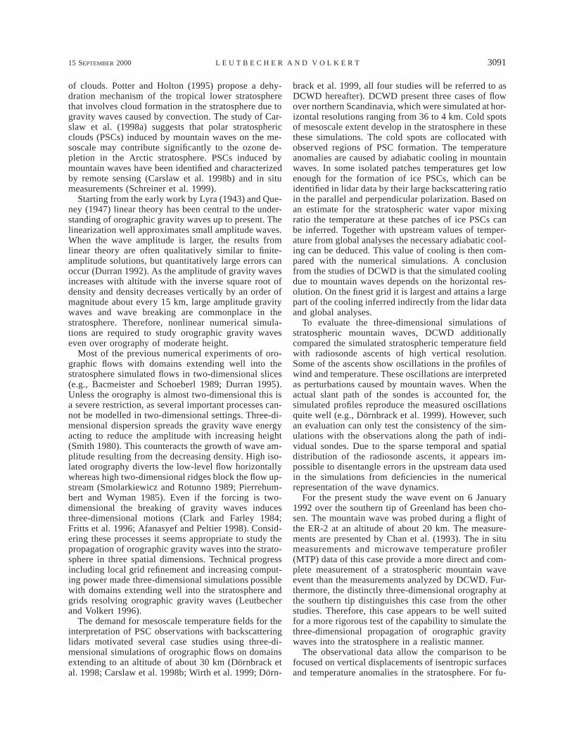
FIG. 1. Observations and manual analysis on 6 Jan 1992 (adapted from Euro. Meteor. Bull., German Weather Service, Offenbach).

ture studies of the effect of mountain waves on micro-physical processes in the stratosphere these quantitiesare of prime importance. The sensitivity of these sim-ulated quantities to parameters of the model setup isexamined for parameters that are known to be important.The sensitivity to horizontal resolution noted by DCWDis explored further. Additionally, the effect of surfacefriction is studied because previous work on flow overmountains in a shallower atmosphere stressed the roleof frictional momentum flux at the surface. Georgelinet al. (1994) found that for cases of flow over the Pyr-enees an increased surface friction reduces the waveamplitude. This is in accordance with numerical exper-iments of idealized flow over elliptical ridges by Olafs-son and Bougeault (1997).

The numerical experiments of the present study sim-ulate dry dynamics. Apart from parameterized turbulentfriction and surface friction the flow is adiabatic andinviscid. The orography and the upstream conditions arerepresented in a realistic way as they are seen as theprime factors controlling the generation and propagationof mountain waves. This simulation strategy places thepresent study between studies of highly idealized flowand case studies with operational numerical weatherforecasting models that include diabatic processes dueto radiation, moist convection, and surface fluxes ofsensible and latent heat.

The synoptic situation and the observational evidencefor the mountain wave are summarized in section 2. Thesetup of the numerical experiments is described in sec-tion 3. In section 4 the results of the numerical exper-iments are presented and compared to the observationof the mountain wave in the stratosphere. In section 5details of the dynamics of the mountain wave event are

examined based on the experiment that agrees best withthe observations. The results are summarized and dis-cussed in section 6.

2. Observations

Different sources of observational data are availablefor the case of 6 January 1992: routine soundings, es-pecially the one of Narssarssuaq at the southern tip ofGreenland; satellite images; and data taken on a flightof the ER-2 in the stratosphere.

a. Synoptic-scale flow and Narssarssuaq sounding

The zonal tropospheric flow impinges on the southerntip of Greenland while meandering between 508 and658N on 6 January 1992. At higher latitudes, north of708N, there is no significant flow across Greenland’sorography in the troposphere (Fig. 1). Upstream of thesouthern tip, at Hudson Bay and Baffin Island, westerlywinds of 40–70 kt prevail at the 500-hPa level, whereasat the southern tip itself a speed of 20 kt has beenrecorded by the sounding of Narssarssuaq.

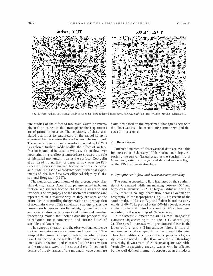
In the lowest kilometer the air is almost stagnant atNarssarssuaq according to the 1200 UTC ascent (Fig.2). The speed increases with pronounced shear in thelayers of 1–2- and 6–8-km altitude. There is little di-rectional wind shear apart from the lowest kilometer.Thus the conditions for the vertical propagation of grav-ity waves excited by the flow over the 2000-m-highorography downstream of Narssarssuaq are favorable.Vertically propagating gravity waves will be affectedby the well-defined thermal tropopause at an altitude of


FIG. 2. Sounding from Narssarssuaq (618119N, 458259W) at 1200 UTC 6 Jan 1992: Profiles oftemperature (scale folded every 30 K), buoyancy frequency, wind speed, and direction.

6.5 km. There the buoyancy frequency increases abrupt-ly from values around 0.01 to 0.02 s21.

b. Orographic clouds

Vertical motions in flow past orography often causethe formation of quasi-stationary clouds. These mayshow up in satellite images, which can be used to inferdetails of the cloud system such as location, size, andaltitude.

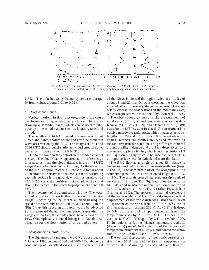
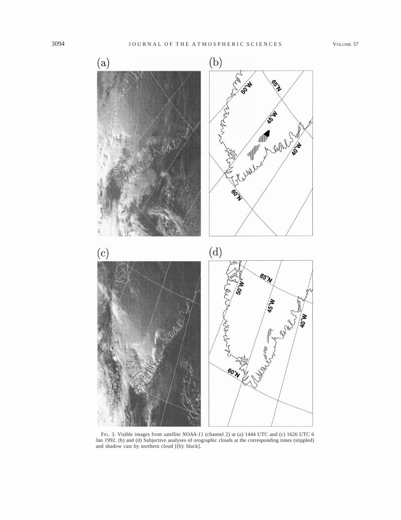
The satellite NOAA-11 passed the southern tip ofGreenland twice, shortly before and after the mountainwave observation by the ER-2. The images at 1444 and1626 UTC show a quasi-stationary cloud structure overthe eastern slope at about 62.58N (Fig. 3).

Due to the low sun the contrast in the visible channelis sharp. The cloud shadow apparent at its northern edgeis used to estimate the cloud altitude. In the 1444 UTCimage the shadow is about 30 km long. As the elevationof the sun is approximately 3.58 the cloud top is about2 km above the surface the shadow is cast on. Assumingthat this surface is the ground, which has an elevationof 1.5–2.5 km at the position of the shadow, the cloudshould be located in the lower troposphere at about 600hPa.

The movement of the cloud pattern is slow. The west-ern edge is about 30 km farther to the east in the laterimage. According to the ascent at Narssarssuaq thespeed of the westerly flow at 600 hPa is about 15 m s21

(Fig. 2). At this speed an air parcel would be advected92 km eastward during the time period separating theimages. Therefore, the clouds cannot be advected by theflow. Orographically induced lifting is a plausible ex-planation for the slow motion of this cloud pattern.

c. Stratospheric mountain wave

The signatures of a mountain wave were observed on6 January 1992 between 1600 and 1700 UTC above thesouthern tip of Greenland during a stratospheric flight

of the ER-2. It crossed the region twice at altitudes ofabout 18 and 20 km. On both crossings the wave wassituated at approximately the same location. Here webriefly discuss the observations of the mountain wave,which are presented in more detail by Chan et al. (1993).

The observations comprise in situ measurements ofwind velocity (u, y , w) and temperature as well as datafrom a MTP. Gary (1989) and Denning et al. (1989)describe the MTP system in detail. The instrument is apassive microwave radiometer, which measures at wave-lengths of 5.24 and 5.10 mm at 10 different elevationangles. Temperature profiles are derived by invertingthe radiative transfer equation. The profiles are centeredaround the flight altitude and are 3 km deep. Every 14sa scan is complete yielding a horizontal resolution of 3km. By assuming hydrostatic balance the height of is-entropic surfaces can be calculated from the data.

The ER-2 flew at an angle of about 558 relative tothe mean wind, which came from west-northwest (Figs.2 and 5b). The dominant part of the orography at thesouthern tip is a south–north-oriented ridge at 61.08N,44.38W. The aircraft crossed the southern tip south ofthe crest of this ridge (Fig. 5b). Isentropes derived fromMTP data and in situ measurements of temperature andvertical wind are shown in Fig. 7a (after Figs. 4a,b inChan et al. 1993). The apparent horizontal wavelengthof the wave is about 60 km. The peak-to-peak verticaldisplacement of isentropic surfaces attains about 0.8 km

Upstream of the wave from 44.58 to 43.58W the insitu temperature is around 200 K. At 43.88W it dropsby 5 K. To the east of this pronounced minimum thetemperature rises by 7 K over 30 km. Farther to theeast, at 42.58W, it falls again by 3 K to a value of 200K. In regions of falling (rising) temperature updrafts(downdrafts) prevail. In the vicinity of the pronouncedtemperature minimum at 43.88W significant vertical mo-tion of up to 12 m s21 and 25 m s21 occurs.

The vertical displacement of isentropic surfaces de-rived from MTP data and the in situ temperature areanticorrelated. Assuming a steady adiabatic flow the


FIG. 3. Visible images from satellite NOAA-11 (channel 2) at (a) 1444 UTC and (c) 1626 UTC 6Jan 1992. (b) and (d) Subjective analyses of orographic clouds at the corresponding times (stippled)and shadow cast by northern cloud [(b): black].


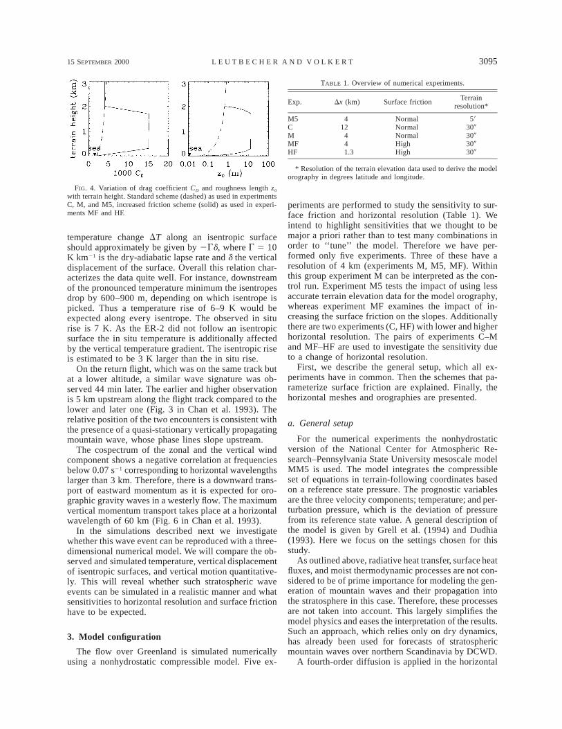
FIG. 4. Variation of drag coefficient CD and roughness length z0

with terrain height. Standard scheme (dashed) as used in experimentsC, M, and M5, increased friction scheme (solid) as used in experi-ments MF and HF.

TABLE 1. Overview of numerical experiments.

Exp. Dx (km) Surface frictionTerrain

resolution*

M5CMMF

412

44

NormalNormalNormalHigh

59300300300

HF 1.3 High 300

* Resolution of the terrain elevation data used to derive the modelorography in degrees latitude and longitude.

temperature change DT along an isentropic surfaceshould approximately be given by 2Gd, where G 5 10K km21 is the dry-adiabatic lapse rate and d the verticaldisplacement of the surface. Overall this relation char-acterizes the data quite well. For instance, downstreamof the pronounced temperature minimum the isentropesdrop by 600–900 m, depending on which isentrope ispicked. Thus a temperature rise of 6–9 K would beexpected along every isentrope. The observed in siturise is 7 K. As the ER-2 did not follow an isentropicsurface the in situ temperature is additionally affectedby the vertical temperature gradient. The isentropic riseis estimated to be 3 K larger than the in situ rise.

On the return flight, which was on the same track butat a lower altitude, a similar wave signature was ob-served 44 min later. The earlier and higher observationis 5 km upstream along the flight track compared to thelower and later one (Fig. 3 in Chan et al. 1993). Therelative position of the two encounters is consistent withthe presence of a quasi-stationary vertically propagatingmountain wave, whose phase lines slope upstream.

The cospectrum of the zonal and the vertical windcomponent shows a negative correlation at frequenciesbelow 0.07 s21 corresponding to horizontal wavelengthslarger than 3 km. Therefore, there is a downward trans-port of eastward momentum as it is expected for oro-graphic gravity waves in a westerly flow. The maximumvertical momentum transport takes place at a horizontalwavelength of 60 km (Fig. 6 in Chan et al. 1993).

In the simulations described next we investigatewhether this wave event can be reproduced with a three-dimensional numerical model. We will compare the ob-served and simulated temperature, vertical displacementof isentropic surfaces, and vertical motion quantitative-ly. This will reveal whether such stratospheric waveevents can be simulated in a realistic manner and whatsensitivities to horizontal resolution and surface frictionhave to be expected.

3. Model configuration

The flow over Greenland is simulated numericallyusing a nonhydrostatic compressible model. Five ex-

periments are performed to study the sensitivity to sur-face friction and horizontal resolution (Table 1). Weintend to highlight sensitivities that we thought to bemajor a priori rather than to test many combinations inorder to ‘‘tune’’ the model. Therefore we have per-formed only five experiments. Three of these have aresolution of 4 km (experiments M, M5, MF). Withinthis group experiment M can be interpreted as the con-trol run. Experiment M5 tests the impact of using lessaccurate terrain elevation data for the model orography,whereas experiment MF examines the impact of in-creasing the surface friction on the slopes. Additionallythere are two experiments (C, HF) with lower and higherhorizontal resolution. The pairs of experiments C–Mand MF–HF are used to investigate the sensitivity dueto a change of horizontal resolution.

First, we describe the general setup, which all ex-periments have in common. Then the schemes that pa-rameterize surface friction are explained. Finally, thehorizontal meshes and orographies are presented.

a. General setup

For the numerical experiments the nonhydrostaticversion of the National Center for Atmospheric Re-search–Pennsylvania State University mesoscale modelMM5 is used. The model integrates the compressibleset of equations in terrain-following coordinates basedon a reference state pressure. The prognostic variablesare the three velocity components; temperature; and per-turbation pressure, which is the deviation of pressurefrom its reference state value. A general description ofthe model is given by Grell et al. (1994) and Dudhia(1993). Here we focus on the settings chosen for thisstudy.

As outlined above, radiative heat transfer, surface heatfluxes, and moist thermodynamic processes are not con-sidered to be of prime importance for modeling the gen-eration of mountain waves and their propagation intothe stratosphere in this case. Therefore, these processesare not taken into account. This largely simplifies themodel physics and eases the interpretation of the results.Such an approach, which relies only on dry dynamics,has already been used for forecasts of stratosphericmountain waves over northern Scandinavia by DCWD.

A fourth-order diffusion is applied in the horizontal


to ensure numerical stability. The diffusion constant iscomposed of a background part scaling as (Dx)3 and avariable part scaling as (Dx)4D, where D denotes thelocal rate of deformation of the horizontal velocity fieldand Dx the horizontal mesh size. In the vertical directionsubgrid fluxes are represented by a diffusion term (]/]z)Ky (]/]z). The local bulk Richardson number R hasan influence on the strength of the diffusion through

1/2 2 2]u ]y R 2 Rc2K 1 l 1 , if R , R0 K c1 2 1 2K 5 [ ]]z ]z Ry c

K , if R $ R , 0 c

(1)

where the value of the critical Richardson number is R c

5 0.8, the length scale is lK 5 40 m, and the constantpart of the diffusion coefficient is K0 5 0.6 m2 s21. Thedry-adiabatic adjustment scheme in the model has beenswitched off, to avoid an artificial damping of breakingmountain waves.

In the stratosphere a relatively high vertical resolutionis necessary in order to resolve gravity waves, as theirvertical wavelength is small due to the high static sta-bility. Therefore, an approximately equidistant spacingof Dz 5 0.6 km has been chosen for the coordinatesurfaces throughout the model atmosphere. There are53 levels in total (except for one sensitivity experimentwith 100 levels). The model top is at 10 hPa, which isat approximately 30 km.

A radiation condition is used at the model top to avoidthe reflection of vertically propagating gravity waves.The upper boundary condition is derived from lineartheory of hydrostatic gravity waves in a nonrotatingatmosphere. Klemp and Durran (1983) show that thecondition provides reasonable results, even if nonhy-drostatic, Coriolis, or nonlinear effects are affecting thegravity waves.

Initial conditions and lateral boundary data are de-rived from 12-hourly analyses of the European Centrefor Medium-Range Weather Forecasts (ECMWF). Theyhave a resolution of 2.58 lat 3 2.58 long and are availableat 14 standard pressure levels from 1000 to 10 hPa. Inorder to allow sufficient time for the spinup, that is, thepropagation of orographic gravity waves into the strato-sphere, the model is initialized at 0000 UTC 6 January1992. The simulations end at 1800 UTC that day.

b. Surface friction schemes

Momentum transfer into the lowest model layer bysurface friction is represented by a bulk formula of theform

(t x, t y) 5 2rCD(u2 1 y 2)1/2 (u, y), (2)

where (t x, t y) denote the surface flux of momentumdue to friction, r density, and (u, y) the horizontal com-ponent of velocity in the lowest model layer. The drag

coefficient CD varies with terrain height. Two differentschemes are employed (Fig. 4). The standard surfacefriction scheme has a drag coefficient increasing mono-tonically with terrain height, whereas the increased sur-face friction scheme is characterized by a considerablylarger drag coefficient at elevations from 300 to 1700m. The latter scheme results in enhanced friction on therugged slopes of Greenland. This variation with terrainelevation is probably more realistic than the frictionprescribed by the former scheme, which has a ratherlow drag coefficient on the slopes and a maximum ofthe drag coefficient on the ice cap. In the increasedsurface friction scheme the drag coefficient is set to alarge value on the slopes in order to accentuate theimpact that a change of surface friction within physi-cally reasonable bounds has on the simulated mountainwave.

The drag coefficient CD can be converted into a rough-ness length z0. For this conversion we assume a neutralboundary layer with a logarithmic wind profile u(z) 5(t /r)1/2k21 ln(z/z0), where k 5 0.4 is the von Karmanconstant (Stull 1988). The roughness length is obtainedas z0 5 z1 exp( ) by inserting the wind u(z1) into21/22kC D

(2), where z1 5 350 m is the height of the lowest modellayer above ground. Maximum values of the roughnesslength are 0.8 and 13 m for the normal and increasedsurface friction schemes, respectively (Fig. 4). As theparameterization of surface friction ignores the influ-ence of static stability and the lower troposphere overGreenland is quite stable during the considered case,the increased surface friction scheme ensures a largefrictional momentum transfer.

c. Horizontal meshes and orographies

The model domain is centered at the southern tip ofGreenland, where the mountain wave was observed.Baffin Island and Iceland are on the western and easternboundary of the domain, respectively (D1 in Fig. 5a).It has a horizontal resolution of Dx 5 36 km and a sizeof 2200 km 3 2200 km.

In the vicinity of the southern tip the horizontal meshis locally refined [Grell et al. (1994), two-way nesting].Numerical experiments with one, two, and three levelsof refinement are presented (domains D2, D3, D4 inFig. 5a). Each level of mesh refinement increases thehorizontal resolution by a factor of 3. The set of ex-periments is listed in Table 1. The first letter of theexperiment labels—C, M, or H—indicates coarse, me-dium, or high resolution, respectively. The region cov-ered by the innermost domain D4 (Dx 5 1.3 km) isshown in Fig. 5b.

The model orography has been derived from terrainelevation datasets with 300 and 59 resolution in latitudeand longitude. The 59 data stem from a global datasetprovided by the Geophysical Data Center, Boulder, Col-orado. The model orography at 4-km resolution derivedfrom the 59 data (Fig. 5c) was compared with topographic


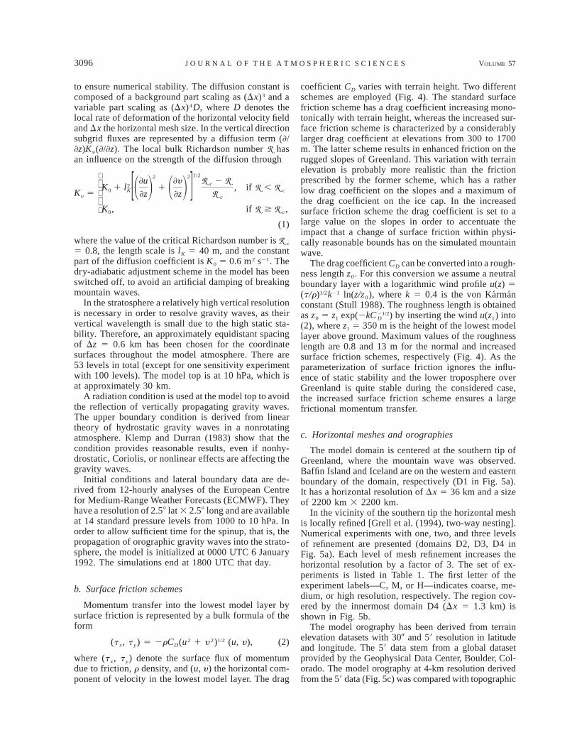
FIG. 5. Model domain, regions of grid refinement, and orography. (a) The entire domain D1 with mesh size Dx 5 36 km and regions D2,D3, and D4 of grid refinement to mesh sizes of 12, 4, and 1.3 km, respectively; size of D1: 2160 km 3 2160 km; size of D4: 200 km 3200 km. (b) The model orography in region D4 for experiment HF with radiosonde station Narssarsuaq (N) and flight track of the ER-2(solid line); (c) as in (b) but for experiment M5.

maps of the southern tip of Greenland at a scale of 1:250 000 available from the Danish Geodetic Institute.The comparison suggested that a higher-resolution da-taset is required for mesh sizes of less than about 4 km.

Therefore, 300 data were obtained from the Earth Re-sources Observation System of the U.S. Geological Sur-vey, Sioux Falls, South Dakota. Apart from a data-voidregion south of 618N and east of 448W these data agreebetter with the topographic maps than the 59 data. Thedata void was removed by inserting the coarser 59 data.These fudged 300 data were then used in all experimentsexcept experiment M5. The model orography of the finestmesh, domain D4 (Dx 5 1.3 km), is shown in Fig. 5b.

In all experiments domains D1–3 (Dx $ 4 km) areinitialized at 0000 UTC 6 January 1992. In experimentHF the innermost grid D4 (Dx 5 1.3 km) is initializedat 1200 UTC by interpolating the fields from the coarsermesh D3.

4. Sensitivity experiments

Now, we present the results of the five numericalexperiments. First, we examine the effect of surfacefriction and horizontal resolution on the simulatedmountain wave in the stratosphere. Furthermore, we in-spect the level of agreement with the measurements


TABLE 2. Timescales of diffusion t d, advection t a, and wave prop-agation t p in 103 s. Horizontal wavelength l (in km) used for theestimates.

Exp. l l/Dx t d t a t p

HFMFMC

27274242

206.7

10.53.5

331.37.80.3

1.41.42.12.1

3.23.25.05.0

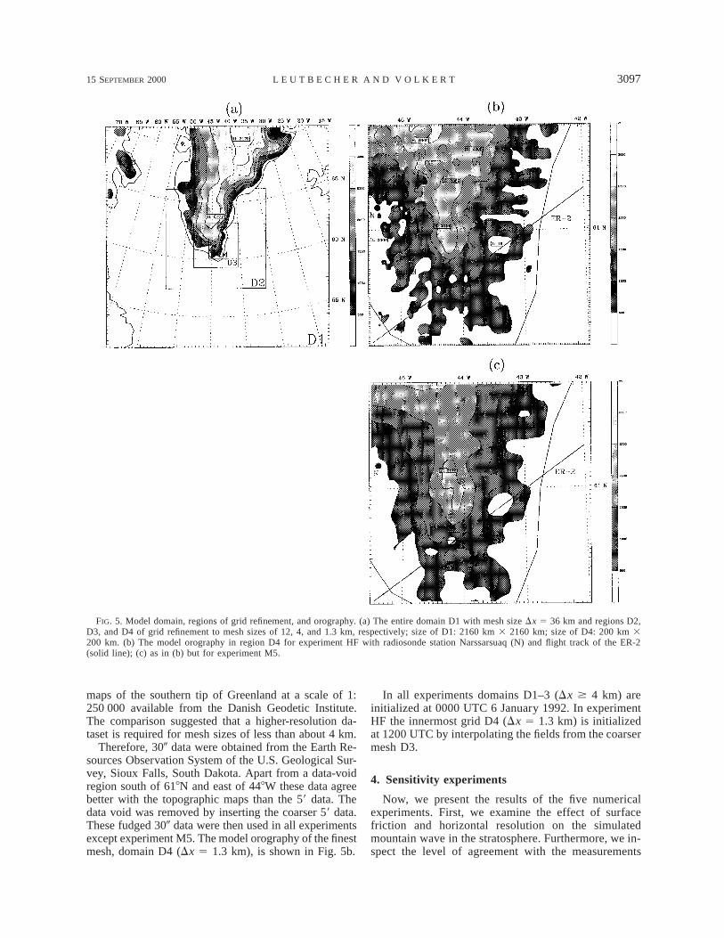
FIG. 6. Maximum upward (max d ) and downward (min d ) dis-placements of the 460-K isentropic surface in the vicinity of the ER-2 flight track for the five simulations at 1500, 1600, and 1700 UTC.See text for details about the calculation of vertical displacements.Shaded bars indicate approximate maximum displacements deter-mined from the MTP data in Fig. 7a.

from the ER-2. Next, the causes for the sensitivity tohorizontal resolution and surface friction are analyzed.Finally, the mean static stability in the vicinity of theobserved wave is discussed.

a. Comparison with observed mountain wave

In all experiments orographic gravity waves are gen-erated at the southern tip and propagate into the strato-sphere reaching the ER-2 flight level. Changes of hor-izontal resolution and surface friction change the lo-cation of the dominant simulated wave in the strato-sphere only insignificantly. The locations of thesimulated waves differ less than about 20 km from thelocation of the observed wave.

However, the wave amplitude is strongly affected bychanges of horizontal resolution or surface friction. Themaximum upward and downward displacements of anisentropic surface along the flight path are used as mea-sure of the simulated stratospheric wave amplitude (Fig.6). For this comparison the 460-K isentrope is selected.It is close to the ER-2 flight level (Fig. 7). Displacementsare calculated as height deviation from an inclinedplane, which is closest to the 460-K isentropic surfaceover the region of domain D4. Maxima slightly off theflight track are included by evaluating maximum dis-placements within a 20-km-wide corridor around theflight path. No experiment overestimates the wave am-plitude and only the coarse resolution experiment C un-derestimates the amplitude considerably. The peak-to-peak amplitude of vertical displacement in experimentC reaches only 27% of the observed 0.8 km. In the otherexperiments the peak-to-peak amplitude attains a largerfraction of the observed value (experiments HF: 92%,MF: 62%, M: 98%, and M5: 108%).

The detailed structure of the stratospheric mountainwave in these four experiments is presented next andcompared to the observations. Over a period of 30 minthe model fields hardly change. This justifies a com-parison of simulation results valid at 1600 UTC withobservations in the period of 1558–1615 UTC. As proxyto the in situ observations of vertical wind and tem-perature, model data interpolated to an altitude of 19.8km are used. Thereby, the variation of flight altitude ofabout 60.3 km is neglected.

1) EXPERIMENT HF

The signatures of the mountain wave in simulationHF are very similar to the observed signatures (Figs.7a,b). The salient feature is the upward displacement ofisentropic surfaces at 43.88W, which is correlated witha temperature minimum and an updraft and a downdrafton the upstream and downstream side, respectively. Thetemperature drop relative to upstream values amountsto about 5 K in both simulation and observation. Thesimulated temperature minimum lies 11 km farther up-stream than the observed one. Downstream of the min-imum a warming of 5 K is simulated, whereas a tem-perature rise of 7 K was observed.

Farther downstream at about 42.48W there is anotherdistinct feature present in simulation and observation.The simulated (observed) temperature falls by 2.5 (3.5)K. The simulated drop is 7 km too far downstream com-pared to the observation.

The simulation does not reproduce the observed var-iations of vertical velocity and potential temperature athorizontal scales smaller than about 10 km. The sim-ulated fields are smoother. As a consequence, the hor-izontal gradients of the simulated fields are smaller. Fur-thermore, the strong and narrow downdraft with an ob-served maximum of 24.8 m s21 attains only 22.7 ms21 in the simulation.


FIG. 7. (a) Observations vs (b)–(d) simulations of the stratospheric mountain wave. (top subpanels) Temperature T and vertical velocityw along the ER-2 flight track and (bottom subpanels, every 5 K) isentropes in a vertical section. The flow is from left to right; see Fig. 5for the baseline of the section. (a) The (top) in situ and (bottom) MTP measurements from the ER-2 flight between 1558 and 1615 UTC;(dotted, bottom) flight altitude [adapted from Chan et al. (1993)]. (b)–(d) The simulated wave at 1600 UTC in simulations HF, M, and MF,respectively.

Noise in the temperature field retrieved from the MTPdata may account for some of the small-scale variancein the potential temperature. However, at some placessmall horizontal scales appear to represent real struc-tures of the flow. The sudden upward displacements ofisentropic surfaces at 44.08 and 42.48W occur over somedepth and look like small hydraulic jumps. The jumpat 42.48W was passed by the flight track and the MTPdata are corroborated by the in situ observations, asthere is a large negative gradient of temperature and anupdraft of 1.5 m s21.

The mean static stability in all simulations is consid-erably lower in the altitude range from 18.2 to 21.2 kmthan the mean static stability derived from the MTP datadisplayed in Fig. 7a [Du/Dz 5 50 K (3 km)21 vs 35 K(3 km)21]. This difference will be further dealt with atthe end of this section.

2) EXPERIMENT MF

In experiment MF the same surface friction schemeas in HF has been employed yet the resolution is coarser.


TABLE 3. Buoyancy frequency N (1022 s21) in the layer betweenaltitude z1 and z2 (km).

z1 z2 N

Simulationa 18.2 21.2 1.94

ER-2 dataMTPb

MTPc

In situ Td

18.219.417.5

21.220.119.7

1.591.86 6 0.14

1.92

Sondee 18.119.120.4

19.120.422.7

2.071.452.25

a From Fig. 7b.b From Fig. 7a.c From range of vertical temperature gradients given in Fig. 7d in

Chan et al. (1993). The temperature gradient appears to be determinedfrom the channels of the MTP adjacent to the flight level as in theexample given by Gary (1989).

d From temperature difference at 43.78W taken from Fig. 3b inChan et al. (1993).

e From 1200 UTC radiosonde launched at Narssarssuaq.

This affects the amplitude of the wave but not the hor-izontal phase structure of the wave. Only the smallerhorizontal scales are absent, which results in evensmoother fields (Figs. 7a,b,d). An upstream tilt of thewave is apparent in contrast to simulation HF and theMTP data. In the temperature trace a minimum lies at448W and a distinct drop at 42.58W, farther upstreamthan in experiment HF. The minimum and the drop arelocated farther upstream than the corresponding featuresin the observation by 23 and 5 km, respectively. Theamplitude of the wave at 448W attains only 62% of theobserved value, whereas the amplitude of the upwarddisplacement at 42.58W is quite unaffected by the coars-er resolution.

3) EXPERIMENT M

This experiment is identical to MF apart from thelower surface friction on the slopes. Regarding the wavephase, the horizontal scales, and the locations of thetemperature minimum and drop, the results are verysimilar to experiment MF (Figs. 7c,d). The obvious dif-ference is the amplitude of the wave at 448W. The am-plitude is similar to that of experiment HF; the peak-to-peak amplitude attains 98% of the observed value.The temperature drop at 42.58W is changed only littleby reducing the surface friction.

4) EXPERIMENT M5

For this simulation the lower-resolution 59 terrain el-evation data have been used to derive the model orog-raphy (Figs. 5b,c). All other settings are equal to thoseof experiment M. The peak-to-peak amplitude reaches108% of the observed value. The different orographymainly results in a change of wave phase. As a resultthe maximum downward displacement of the 460-K is-

entrope is larger than that of the other experiments (Fig.6). The wave at 448W appears in the observation as wellas in the other simulations as isolated upward displace-ment of the isentropic surfaces. In experiment M5 (ver-tical section not shown) an upward displacement of 0.4km is simulated at 448W. This is followed immediatelyby a downward displacement of 0.7 km and anotherupward displacement of 0.4 km. Thus the misspecifi-cation of details of the orographic shape results in anerroneous wave phase in the stratosphere.

b. Horizontal resolution and diffusion

The pairs of experiments MF–HF and C–M revealthat an increased horizontal resolution results in largermountain wave amplitudes in the stratosphere. Alreadyat a resolution of Dx 5 12 km (experiment C) the mainridge at the southern tip is reasonably resolved. Increas-ing the resolution to 4 km and further to 1.3 km addssome orographic details. Parts of the slopes get steeper(Fig. 8). As the main ridge is broad enough it is onlymarginally lowered by the smoothing required at thecoarsest horizontal resolution. The change of orographyitself seems to be insufficient to explain the strong de-pendence of stratospheric wave amplitude on horizontalresolution. Here we examine whether this sensitivity canbe caused by diffusion in the numerical model.

The spatial scales of motions resolved in the numer-ical model have a lower limit due to the grid spacing.A wavelength less than 2Dx cannot be resolved on agrid of mesh size Dx. In addition, finite differencingerrors are very large for waves with wavelength closeto 2Dx. Therefore, the smallest scales are removed byapplying a hyperdiffusion in the horizontal. The dif-fusion constant is set according to the mesh size. Fur-thermore, a direct orographic forcing of wavelengthsclose to 2Dx is reduced by smoothing the model terrain.

Short waves with horizontal wavelength l greaterthan approximately 4Dx are forced directly by the orog-raphy and indirectly by the nonlinear dynamics. Theseshort waves are affected by the diffusion in the model.Here the effect of the explicit horizontal diffusion isanalyzed. It is implemented as fourth-order diffusionterm KD2f for every prognostic variable f of the mod-el, where D 5 ]2/]x2 1 ]2/]y2 denotes the horizontalLaplacian. This diffusion strongly depends on the hor-izontal resolution. For a wave of small to moderate am-plitude in an ambient flow with a low rate of defor-mation the background term of the hyperdiffusion willdominate. Its diffusion constant Kb is set to

Kb 5 3 3 1023 (Dx)4/Dt. (3)

The time step Dt is chosen proportional to the mesh sizeto guarantee numerical stability. We use Dt 5 0.25Dx/cs, where cs ø 300 m s21 denotes the speed of sound.Thus the diffusion constant turns out to be proportionalto the mesh size cubed Kb 5 4 m s21 (Dx)3. In con-sequence a wave of fixed horizontal wavelength l ex-


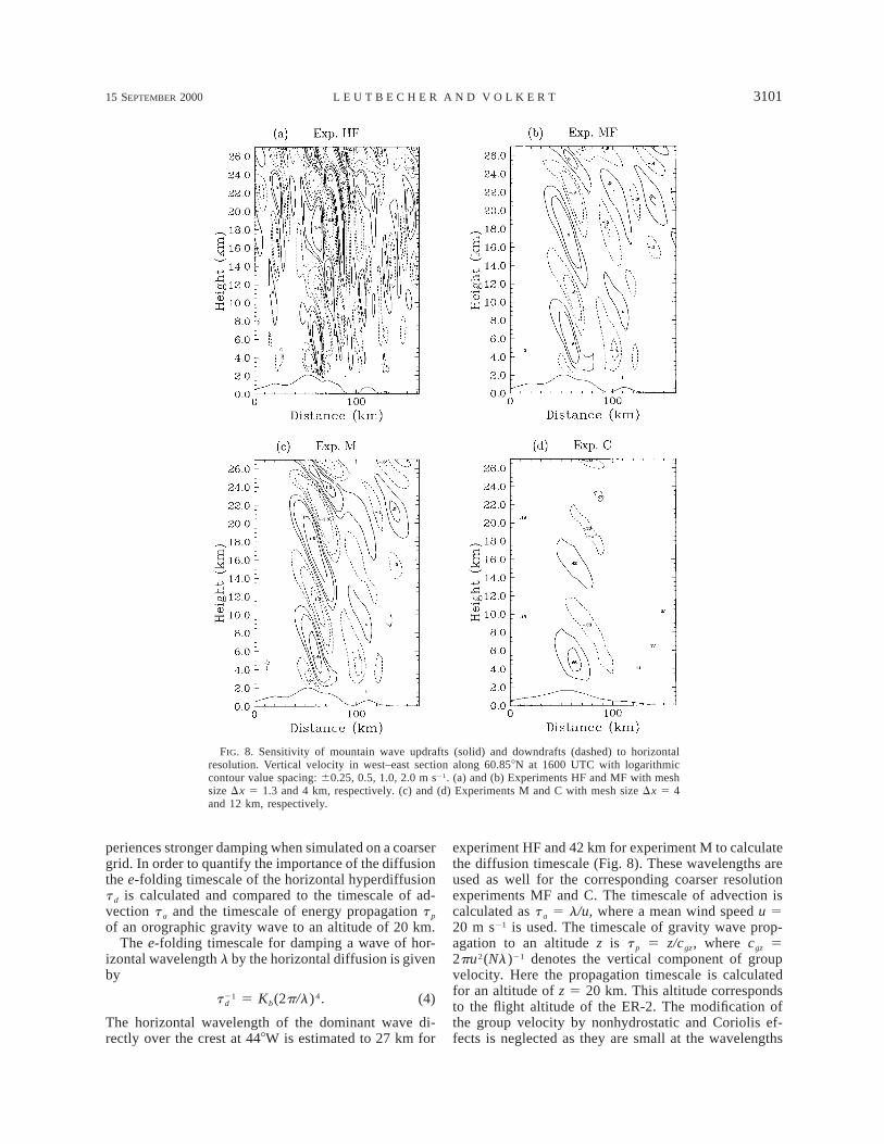
FIG. 8. Sensitivity of mountain wave updrafts (solid) and downdrafts (dashed) to horizontalresolution. Vertical velocity in west–east section along 60.858N at 1600 UTC with logarithmiccontour value spacing: 60.25, 0.5, 1.0, 2.0 m s21. (a) and (b) Experiments HF and MF with meshsize Dx 5 1.3 and 4 km, respectively. (c) and (d) Experiments M and C with mesh size Dx 5 4and 12 km, respectively.

periences stronger damping when simulated on a coarsergrid. In order to quantify the importance of the diffusionthe e-folding timescale of the horizontal hyperdiffusiont d is calculated and compared to the timescale of ad-vection t a and the timescale of energy propagation t p

of an orographic gravity wave to an altitude of 20 km.The e-folding timescale for damping a wave of hor-

izontal wavelength l by the horizontal diffusion is givenby

5 Kb(2p/l)4.21t d (4)

The horizontal wavelength of the dominant wave di-rectly over the crest at 448W is estimated to 27 km for

experiment HF and 42 km for experiment M to calculatethe diffusion timescale (Fig. 8). These wavelengths areused as well for the corresponding coarser resolutionexperiments MF and C. The timescale of advection iscalculated as t a 5 l/u, where a mean wind speed u 520 m s21 is used. The timescale of gravity wave prop-agation to an altitude z is t p 5 z/cgz, where cgz 52pu2(Nl)21 denotes the vertical component of groupvelocity. Here the propagation timescale is calculatedfor an altitude of z 5 20 km. This altitude correspondsto the flight altitude of the ER-2. The modification ofthe group velocity by nonhydrostatic and Coriolis ef-fects is neglected as they are small at the wavelengths


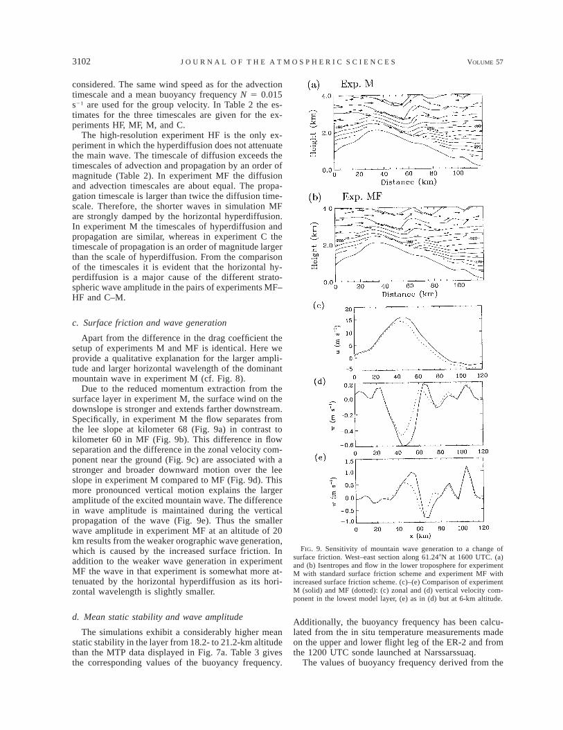
FIG. 9. Sensitivity of mountain wave generation to a change ofsurface friction. West–east section along 61.248N at 1600 UTC. (a)and (b) Isentropes and flow in the lower troposphere for experimentM with standard surface friction scheme and experiment MF withincreased surface friction scheme. (c)–(e) Comparison of experimentM (solid) and MF (dotted): (c) zonal and (d) vertical velocity com-ponent in the lowest model layer, (e) as in (d) but at 6-km altitude.

considered. The same wind speed as for the advectiontimescale and a mean buoyancy frequency N 5 0.015s21 are used for the group velocity. In Table 2 the es-timates for the three timescales are given for the ex-periments HF, MF, M, and C.

The high-resolution experiment HF is the only ex-periment in which the hyperdiffusion does not attenuatethe main wave. The timescale of diffusion exceeds thetimescales of advection and propagation by an order ofmagnitude (Table 2). In experiment MF the diffusionand advection timescales are about equal. The propa-gation timescale is larger than twice the diffusion time-scale. Therefore, the shorter waves in simulation MFare strongly damped by the horizontal hyperdiffusion.In experiment M the timescales of hyperdiffusion andpropagation are similar, whereas in experiment C thetimescale of propagation is an order of magnitude largerthan the scale of hyperdiffusion. From the comparisonof the timescales it is evident that the horizontal hy-perdiffusion is a major cause of the different strato-spheric wave amplitude in the pairs of experiments MF–HF and C–M.

c. Surface friction and wave generation

Apart from the difference in the drag coefficient thesetup of experiments M and MF is identical. Here weprovide a qualitative explanation for the larger ampli-tude and larger horizontal wavelength of the dominantmountain wave in experiment M (cf. Fig. 8).

Due to the reduced momentum extraction from thesurface layer in experiment M, the surface wind on thedownslope is stronger and extends farther downstream.Specifically, in experiment M the flow separates fromthe lee slope at kilometer 68 (Fig. 9a) in contrast tokilometer 60 in MF (Fig. 9b). This difference in flowseparation and the difference in the zonal velocity com-ponent near the ground (Fig. 9c) are associated with astronger and broader downward motion over the leeslope in experiment M compared to MF (Fig. 9d). Thismore pronounced vertical motion explains the largeramplitude of the excited mountain wave. The differencein wave amplitude is maintained during the verticalpropagation of the wave (Fig. 9e). Thus the smallerwave amplitude in experiment MF at an altitude of 20km results from the weaker orographic wave generation,which is caused by the increased surface friction. Inaddition to the weaker wave generation in experimentMF the wave in that experiment is somewhat more at-tenuated by the horizontal hyperdiffusion as its hori-zontal wavelength is slightly smaller.

d. Mean static stability and wave amplitude

The simulations exhibit a considerably higher meanstatic stability in the layer from 18.2- to 21.2-km altitudethan the MTP data displayed in Fig. 7a. Table 3 givesthe corresponding values of the buoyancy frequency.

Additionally, the buoyancy frequency has been calcu-lated from the in situ temperature measurements madeon the upper and lower flight leg of the ER-2 and fromthe 1200 UTC sonde launched at Narssarssuaq.

The values of buoyancy frequency derived from the


in situ temperature measurements by the ER-2 and thesonde suggest a higher static stability between 18- and21-km altitude than the potential temperature cross sec-tion derived from the MTP data. If the vertical tem-perature gradient is derived from the MTP data usingonly the channels adjacent to the flight level a higherstability is calculated as well (Table 3). This suggeststhat the mean buoyancy frequency derived from the en-tire section of the MTP data from 18 to 21 km is toolow and the stability in the simulation probably morerealistic.

A closer look at the temperature retrieval from theMTP data points to a likely cause of a systematic error.Large corrections of up to 30 K need to be applied tothe temperature retrieved at the distant levels above theaircraft to account for the transparency of the atmo-sphere (Gary 1989). Obviously, these corrections canresult in large errors of the mean vertical temperaturegradient.

However, no definitive conclusion can be drawn asthe alternative calculations of the buoyancy frequencyapply to slightly different altitude ranges or times. De-spite the fact that most of the observations support themean static stability in the simulations, it should benoted that the data used for the lateral boundary of themodel constitute a potential source of error. Due to thelow vertical resolution of the analysis data in the strato-sphere (100, 70, 50, 30 hPa), the initial and lateralboundary conditions contain only limited informationon the vertical structure. Shallow inhomogeneities inthe stratosphere are not represented in the upstream con-ditions of the simulations. However, such shallow struc-tures are apparent in the 1200 UTC sounding of Nars-sarssuaq above 18 km, especially in the buoyancy profile(Fig. 2, Table 3). The variations of buoyancy frequencyin the sounding can be due to variations in the meanconditions and variations caused by a passage throughthe mountain wave. Any error in the mean value of thebuoyancy frequency in the simulation would affect theamplitude and phase of the simulated mountain wave.

5. Dynamics of the stratospheric mountain waveevent

Here we further investigate the three-dimensional dy-namics of the flow over the southern tip based on resultsfrom experiment HF, which is considered as the mostrealistic simulation. We focus on the low-level flow, thethree-dimensional wave propagation, and the breakingof gravity waves.

a. Flow around versus flow over orography

The orography of Greenland is sufficiently high todecelerate and deflect the low-level flow. The Froudenumber of the flow at the southern tip is estimated toF 5 u /(Nh0) ø 0.3, where h0 5 2.2 km is the crestheight of the ridge protruding south at 448W and u , N

are vertically averaged values of wind speed and buoy-ancy frequency 150 km upstream of the southern tip.Due to the low Froude number the air impinging on theridge at the southern tip cannot pass entirely over it.The ridge partially blocks and partially deflects the flowaround it (Fig. 10a). In the vicinity of the soundingstation Narssarssuaq the flow stagnates. On the meso-a scale the low-level flow approaching Greenland at analtitude below about 1.5 km is meridionally deflected.At 628N the flow splits into two airstreams. One turnsnorth and the other to the south. The latter airstreamfollows the west coast of Greenland until it reaches thesouthern tip.

A shallow layer of the air impinging on the southerntip below crest height is able to pass over the tip. Figures10b–d show the lower-tropospheric flow in a verticalsection oriented along the flow. From the surface to analtitude of 1.5 km the upstream cross-ridge velocitycomponent is less than 2 m s21. Above there is consid-erable flow across the ridge. Air with a potential tem-perature of more than about 278 K is lifted sufficientlyto pass over the southern tip.

The flow over the orography above the layer of stag-nating and horizontally deflected air is associated withconsiderable vertical shear below crest height upstreamof the southern tip. The 1200 UTC sounding from Nars-sarssuaq corroborates this simulation result. From thesurface to an altitude of 1 km, wind speeds of less than3 m s21 are reported. Between 1- and 2-km altitude theobserved wind speed increases to 12 m s21 (Fig. 2). Inthe simulation the shear is slightly weaker; a speed of12 m s21 is attained at about 2.5-km altitude.

The dividing streamline height studied by Snyder etal. (1985) provides an estimate of the altitude that thetransition from the flow around to the flow over theridge occurs at. For the ridge at the southern tip with acrest height h0 5 2.2 km and a flow with Froude numberF 5 0.3 a dividing streamline height of Hs 5 h0(1 2F) 5 1.5 km is expected.

The 278 K isentrope, which approximately marks thetransition from flow around the ridge to flow over it,has an altitude of about 1.8 km at a distance of 60 kmupstream of the ridge (Figs. 10b,c). The simulationshows that only a shallow layer of the air below crestheight passes over the ridge in agreement with the es-timate of the dividing streamline height. The thicknessof this layer is about 400–700 m. The precision of thisestimate is limited by the vertical resolution, which isof the same order of magnitude, and by the uncertaintyabout the unperturbed height of the 278-K isentrope.

Obviously, the main source of gravity waves is theflow of the shallow layer that passes over the ridge.Thus, the horizontal scale of the excited waves is de-termined by the part of the orography that pierces thelayer of flow that is blocked and diverted around thesouthern tip (Fig. 10b). The width of this part of theridge (h $ 1500 m) is about 30 km in the direction ofthe flow. This is of the same order of magnitude as the


FIG. 10. Low-level flow in simulation HF at 1600 UTC. (a) Windat 1.25-km altitude, orography (1000 m, 1500 m, . . . , heavy solid),sounding station Narssarssuaq (dot, N), baseline of section shown inthe other panels. (b) Isentropes and flow vectors, (c) horizontal ve-locity component parallel to the section (every 2 m s21), (d) as in(c) but normal velocity component.

dominant horizontal wavelength simulated and ob-served in the stratosphere.

b. Wave propagation

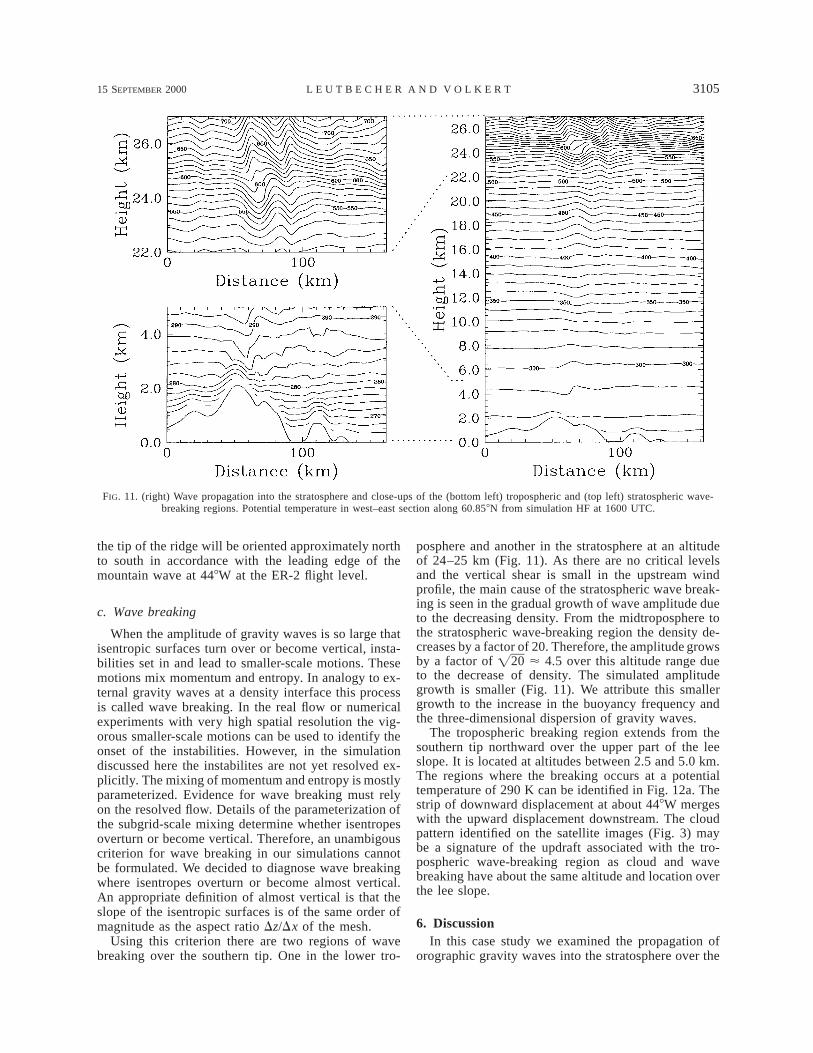
The flow over the ridge at the southern tip and downthe eastern slope of Greenland generates a large am-plitude gravity wave that propagates vertically (Fig. 11).There is evidence for two regions of wave breaking inthe simulation. One is located in the lower troposphereand the other in the stratosphere above the ER-2 flightlevel. The wave breaking is further discussed in section5c. The nonlinear interactions and mixing in the tro-pospheric breaking region will affect the amplitude ofthe wave that emanates from it. Here we inspect thewave propagation above the tropospheric wave breakinginto the stratosphere up to the altitude of the ER-2 flight.In this altitude interval no further wave breaking occursand linear theory arguments can be employed to explainthe dominant pattern simulated at the ER-2 flight level.

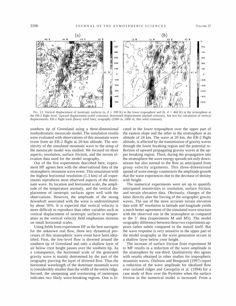
The perturbation induced by the mountain wave isillustrated by the vertical displacements of the 290- and460-K isentropic surfaces (Fig. 12). The altitudes of thetwo surfaces correspond to the altitude of the tropo-spheric wave-breaking region and the ER-2 flight level,respectively. As in the previous section the vertical dis-placement of an isentropic surface is calculated as thedifference in height between the surface and the inclinedplane that is closest to it in model domain D4.

The main perturbation of the flow at the level of thetropospheric wave breaking is located over the upperpart of the eastern slope of Greenland (Fig. 12a). The290-K isentropic surface is displaced downward by upto 0.4 km over the lee slope and immediately down-stream upward by up to 0.4 km. During the verticalpropagation the wave energy is spread horizontally. Atthe ER-2 flight level the main signature of the wave isan upward displacement of the isentropic surfaces alonga north–south-oriented band. This band is situated overthe upper part of the lee slope, but it extends farthersouth than the orography. A maximum upward displace-ment of 0.5 km is found at 44.08W close to the flighttrack of the ER-2 (Fig. 12b).

A remarkable feature of the simulated wave patternat an altitude of 20 km is that the region perturbed bythe orographic gravity wave stretches at least 70 kmfarther south than the part of the slope where the waveis generated. This is associated with the dispersion ofgravity waves originating from the end of a long ridge.Within linear theory of hydrostatic flow Smith (1980)shows that the transition zone from the unperturbed flowupstream to the region influenced by mountain wavesis located on parabolae x 5 cy2. These get wider withincreasing height. Here the x coordinate is directeddownstream and y normal to the flow. From Smith’sformula c is estimated to be 0.01 km21 for an altitudeof 20 km. As the axis of the parabola points downwind,to the southeast, the southerly branch emanating from


FIG. 11. (right) Wave propagation into the stratosphere and close-ups of the (bottom left) tropospheric and (top left) stratospheric wave-breaking regions. Potential temperature in west–east section along 60.858N from simulation HF at 1600 UTC.

the tip of the ridge will be oriented approximately northto south in accordance with the leading edge of themountain wave at 448W at the ER-2 flight level.

c. Wave breaking

When the amplitude of gravity waves is so large thatisentropic surfaces turn over or become vertical, insta-bilities set in and lead to smaller-scale motions. Thesemotions mix momentum and entropy. In analogy to ex-ternal gravity waves at a density interface this processis called wave breaking. In the real flow or numericalexperiments with very high spatial resolution the vig-orous smaller-scale motions can be used to identify theonset of the instabilities. However, in the simulationdiscussed here the instabilites are not yet resolved ex-plicitly. The mixing of momentum and entropy is mostlyparameterized. Evidence for wave breaking must relyon the resolved flow. Details of the parameterization ofthe subgrid-scale mixing determine whether isentropesoverturn or become vertical. Therefore, an unambigouscriterion for wave breaking in our simulations cannotbe formulated. We decided to diagnose wave breakingwhere isentropes overturn or become almost vertical.An appropriate definition of almost vertical is that theslope of the isentropic surfaces is of the same order ofmagnitude as the aspect ratio Dz/Dx of the mesh.

Using this criterion there are two regions of wavebreaking over the southern tip. One in the lower tro-

posphere and another in the stratosphere at an altitudeof 24–25 km (Fig. 11). As there are no critical levelsand the vertical shear is small in the upstream windprofile, the main cause of the stratospheric wave break-ing is seen in the gradual growth of wave amplitude dueto the decreasing density. From the midtroposphere tothe stratospheric wave-breaking region the density de-creases by a factor of 20. Therefore, the amplitude growsby a factor of 20 ø 4.5 over this altitude range dueÏto the decrease of density. The simulated amplitudegrowth is smaller (Fig. 11). We attribute this smallergrowth to the increase in the buoyancy frequency andthe three-dimensional dispersion of gravity waves.

The tropospheric breaking region extends from thesouthern tip northward over the upper part of the leeslope. It is located at altitudes between 2.5 and 5.0 km.The regions where the breaking occurs at a potentialtemperature of 290 K can be identified in Fig. 12a. Thestrip of downward displacement at about 448W mergeswith the upward displacement downstream. The cloudpattern identified on the satellite images (Fig. 3) maybe a signature of the updraft associated with the tro-pospheric wave-breaking region as cloud and wavebreaking have about the same altitude and location overthe lee slope.

6. DiscussionIn this case study we examined the propagation of

orographic gravity waves into the stratosphere over the


FIG. 12. Vertical displacement of isentropic surfaces (a, u 5 290 K) in the lower troposphere and (b, u 5 460 K) in the stratosphere atthe ER-2 flight level. Upward displacement (solid contours), downward displacement (dashed contours). See text for calculation of verticaldisplacements. ER-2 flight track (heavy solid line); orography (1000 m, 2000 m, thin solid contours).

southern tip of Greenland using a three-dimensionalnonhydrostatic mesoscale model. The simulation resultswere evaluated with observations of this mountain waveevent from an ER-2 flight at 20-km altitude. The sen-sitivity of the simulated mountain wave to the setup ofthe mesoscale model was studied. We focused on threeaspects: resolution, surface friction, and the terrain el-evation data used for the model orography.

Out of the five experiments described here, experi-ment HF agrees best with the observational data of thestratospheric mountain wave event. This simulation withthe highest horizontal resolution (1.3 km) of all exper-iments reproduces most observed aspects of the domi-nant wave. Its location and horizontal scale, the ampli-tude of the temperature anomaly, and the vertical dis-placement of isentropic surfaces agree well with theobservations. However, the amplitude of the strongdowndraft associated with the wave is underestimatedby about 50%. It is expected that vertical velocity ismore difficult to reproduce than other variables such asvertical displacement of isentropic surfaces or temper-ature as the vertical velocity field emphasizes motionson small horizontal scales.

Using fields from experiment HF as the best surrogatefor the unknown real flow, three key dynamical pro-cesses of this stratospheric wave event have been iden-tified. First, the low-level flow is diverted around thesouthern tip of Greenland and only a shallow layer ofair below crest height passes over the southern tip. Asa consequence, the horizontal scale of the generatedgravity wave is mainly determined by the part of theorography piercing the layer of diverted flow. Thus thehorizontal wavelength of the dominant mountain waveis considerably smaller than the width of the entire ridge.Second, the steepening and overturning of isentropesindicates two likely wave-breaking regions. One is lo-

cated in the lower troposphere over the upper part ofthe eastern slope and the other in the stratosphere at analtitude of 24 km. The wave at 20 km, the ER-2 flightaltitude, is affected by the transmission of gravity wavesthrough the lower breaking region and the potential re-flection of upward propagating gravity waves at the up-per breaking region. Third, during the propagation intothe stratosphere the wave energy spreads not only down-stream but also normal to the flow as anticipated fromgroup velocity arguments. This three-dimensionalspread of wave energy counteracts the amplitude growththat the wave experiences due to the decrease of densitywith height.

The numerical experiments were set up to quantifyanticipated sensitivities to resolution, surface friction,and terrain elevation data. Obviously, changes of thelatter directly alter the forcing of the orographic gravitywaves. The use of the more accurate terrain elevationdata with 300 resolution in latitude and longitude yieldsa much better agreement of the simulated wave structurewith the observed one in the stratosphere as comparedto the 59 data (experiments M and M5). The modelorography difference between these two experiments ap-pears rather subtle compared to the massif itself. Butthe wave response is very sensitive to the upper part ofthe model orography as the wave generation occurs ina shallow layer below crest height.

The increase of surface friction from experiment Mto MF results in a reduction of the wave amplitude inthe stratosphere by one-third. Qualitatively this agreeswith results obtained in other studies for troposphericmountain waves. Olafsson and Bougeault (1997) reporta reduction of the wave amplitude for idealized flowover isolated ridges and Georgelin et al. (1994) for acase study of flow over the Pyrenees when the surfacefriction in the numerical model is increased. From a


comparison with aircraft observations Georgelin et al.(1994) conclude that a surface friction scheme with aneffective roughness length of up to 17 m yields a morerealistic wave response than the scheme with a constantroughness length of 0.15 m. In our experiments the in-creased surface friction scheme uses a drag coefficientcorresponding to a roughness length of up to 13 m onthe slopes, whereas the standard scheme has a maximumroughness length of up to 0.6 m on the slopes. Althoughexperiment M agrees better with the observations thanMF, it cannot be concluded that the surface friction inM is more realistic. In both experiments the mountainwave is considerably damped during its propagation intothe stratosphere as the analysis of the diffusion timescaleshows. At the higher horizontal resolution (experimentHF), the increased surface friction scheme yields a re-alistic wave amplitude.

For the conversion of the drag coefficient to a rough-ness length a neutral boundary layer has been assumed.The surface friction scheme does not depend on thestability of the boundary layer. The boundary layer overthe orography is expected to be quite stable in this case.Therefore, the simulated frictional momentum transferwould correspond to even larger values of the roughnesslength if a formulation of surface friction was used thataccounts for the stability of the boundary layer. Due toour lack of knowledge of the actual frictional momen-tum transfer occuring at such an inhomogeneous com-plex topography, we are unable to decide how realisticthe surface friction in experiment HF is.

The sensitivity to horizontal resolution documentedin the experiments showed that a fine grid is required.The demanding requirements on model resolution resultfrom the fact that waves with horizontal wavelength lessthan 10 times the grid spacing are strongly affected bythe horizontal diffusion of the model on the timescaleof wave propagation into the stratosphere. The requiredhigh horizontal resolution is computationally expensive.Therefore, one would like to use a less diffusive model.However, a smaller constant of the horizontal hyper-diffusion is not possible with this code. Experimentswith idealized low mountains diverge from linear theoryresults when the diffusion coefficient is reduced. Leut-becher (1998) presents a comparison with linear theoryfor the same amount of hyperdiffusion used in this study.The analysis of the flow in the lower troposphere inexperiment HF revealed that only the upper part of theorography at the southern tip is relevant for the wavegeneration as the flow is diverted around the orographyat lower levels. This explains why a gravity wave withrelatively short horizontal wavelength is excited. Thestrong sensitivity of the simulated mountain wave tohorizontal resolution is a consequence thereof.

The vertical resolution in the experiments is sufficientto resolve the vertical wavelength of a large part of thespectrum of orographic gravity waves. Therefore, thepropagation of nonbreaking gravity waves is expectedto be insensitive to an increase of vertical resolution.

However, the wave generation in the shallow layer offlow passing over the southern tip of Greenland and thewave breaking in the lower troposphere and stratosphereare expected to be more sensitive to a change of verticalresolution. Experiment MF has been repeated with 100instead of 53 levels to quantify this suspected sensitivity.In this high vertical resolution experiment the structureof the wave is similar to that in experiments MF. Theamplitude of the vertical displacement of isentropes atER-2 flight altitude is somewhat larger than in experi-ment MF. It reaches 71% of the observed 0.8 km. Thusthe effect of increasing the vertical resolution is smallerthan that of increasing horizontal resolution or loweringthe surface friction (cf. experiments HF and M).

This case study showed encouraging agreement ofthe simulated and observed mountain wave in the strato-sphere using the high horizontal resolution of 1.3 km.It also showed considerable sensitivity with respect tochanging the horizontal resolution. Therefore, it seemsnatural to wonder whether further increasing horizontaland vertical resolution would still alter the simulatedstratospheric mountain wave. The ultimate objective isto determine the resolution threshold beyond which thesimulated stratospheric mountain wave is invariant tofurther increasing the resolution. It remains an openquestion where this resolution threshold is in a complexflow as the one presented. It is unclear whether a con-vergence of the solution can be reached with currentcomputing resources and available numerical algo-rithms. It will be hard to reach convergence for a re-alistic case study if the global solution crucially dependson the processes in the wave-breaking regions. Thereenergy is efficiently tranferred to smaller scales. In thepresent simulations the associated mixing of momentumand heat is merely parameterized by an increased dif-fusion. To actually resolve the relevant dynamics of thethree-dimensional breakdown of the gravity wave itselfa much higher resolution is required (e.g., Fritts et al.1996). Such studies are so far limited to domains thatare of the same size as the breaking region itself.

Acknowledgments. The public availability of the me-soscale model MM5 and the user support from the Na-tional Center for Atmospheric Research are greatly ap-preciated. Several of the contour plots have been pre-pared with the RIP-package from Mark Stoelinga, Uni-versity of Washington, Seattle. ECMWF provided theglobal analyses and the NOAA-11 data were obtainedfrom the Satellite Receiving Station of Dundee Uni-versity. Hermann Mannstein, Deutsches Zentrum furLuft- und Raumfahrt, Oberpfaffenhofen, helped with thedisplay and interpretation of the satellite images. TassiloKubitz, Freie Universitat Berlin, provided the Nars-sarssuaq sounding. A discussion with Philippe Bou-geault, Meteo France, Toulouse, on an earlier versionof this work sparked off the examination of the sensi-tivity to surface friction. Comments from two anony-mous reviewers helped to improve the presentation.


REFERENCES

Afanasyef, Y. D., and W. R. Peltier, 1998: The three-dimensionali-zation of stratified flow over two-dimensional topography. J.Atmos. Sci., 55, 19–39.

Bacmeister, J. T., and M. R. Schoeberl, 1989: Breakdown of verticallypropagating two-dimensional gravity waves forced by orogra-phy. J. Atmos. Sci., 46, 2109–2134.

Carslaw, K. S., and Coauthors, 1998a: Increased stratospheric ozonedepletion due to mountain-induced atmospheric waves. Nature,391, 675–678., and Coauthors, 1998b: Particle microphysics and chemistry inremotely observed mountain polar stratospheric clouds. J. Geo-phys. Res., 103, 5785–5796.

Chan, K. R., and Coauthors, 1993: A case study of the mountain leewave event of January 6, 1992. Geophys. Res. Lett., 20, 2551–2554.

Clark, T. L., and W. R. Farley, 1984: Severe downslope windstormcalculations in two and three spatial dimensions using anelasticinteractive grid nesting: A possible mechanism for gustiness. J.Atmos. Sci., 41, 329–350.

Denning, R. F., S. L. Guidero, G. S. Parks, and B. L. Gary, 1989:Instrument description of the airborne microwave temperatureprofiler. J. Geophys. Res., 94, 16 757–16 765.

Dornbrack, A., M. Leutbecher, H. Volkert, and M. Wirth, 1998: Me-soscale forecasts of stratospheric mountain waves. Meteor. Appl.,5, 117–126., , R. Kivi, and E. Kyro, 1999: Mountain wave inducedrecord low stratospheric temperatures above northern Scandi-navia. Tellus, 51A, 951–963.

Dudhia, J., 1993: A nonhydrostatic version of the Penn State–NCARmesoscale model: Validation tests and simulation of an Atlanticcyclone and cold front. Mon. Wea. Rev., 121, 1493–1513.

Durran, D. R., 1992: Two-layer solutions to Long’s equation for ver-tically propagating mountain waves: How good is linear theory?Quart. J. Roy. Meteor. Soc., 118, 415–433., 1995: Do breaking mountain waves decelerate the local meanflow? J. Atmos. Sci., 52, 4010–4032.

Fritts, D. C., J. F. Garten, and O. Andreassen, 1996: Wave breakingand transition to turbulence in stratified shear flows. J. Atmos.Sci., 53, 1057–1085.

Gary, B. L., 1989: Observational results using the microwave tem-perature profiler during the airborne Antarctic ozone experiment.J. Geophys. Res., 94, 11 223–11 231.

Georgelin, M., E. Richard, M. Petitdidier, and A. Druilhet, 1994:Impact of subgrid-scale orography parameterization on the sim-ulation of orographic flows. Mon. Wea. Rev., 122, 1509–1522.

Grell, G. A., J. Dudhia, and D. R. Stauffer, 1994: A description ofthe fifth-generation Penn-State/NCAR Mesoscale Model (MM5).NCAR Tech. Note NCAR/TN-3981IA, 120 pp.

Klemp, J. B., and D. R. Durran, 1983: An upper boundary conditionpermitting internal gravity wave radiation in numerical meso-scale models. Mon. Wea. Rev., 111, 430–444.

Leutbecher, M., 1998: Die Ausbreitung orographisch angeregterSchwerewellen in die Stratosphare—Lineare Theorie, ideali-sierte und realitatsnahe numerische Simulation. Ph.D. disserta-tion, Ludwig-Maximilians-Universitat Munchen, 177 pp. [Avail-

able from Deutsches Zentrum fur Luft- und Raumfahrt, D-51170Cologne, Germany.], and H. Volkert, 1996: Stratospheric temperature anomalies andmountain waves: A three-dimensional simulation using a multi-scale weather prediction model. Geophys. Res. Lett., 23, 3329–3332.

Lilly, D. K., and P. F. Lester, 1974: Waves and turbulence in thestratosphere. J. Atmos. Sci., 31, 800–812.

Lyra, G., 1943: Theorie der stationaren Leewellenstromung in freierAtmosphare. Z. Angew. Math. Mech., 23, 1–28.

McFarlane, N. A., 1987: The effect of orographically excited gravitywave drag on the general circulation of the lower stratosphereand troposphere. J. Atmos. Sci., 44, 1775–1800.

Nastrom, G. D., and D. C. Fritts, 1992: Sources of mesoscale vari-ability of gravity waves. Part I: Topographic excitation. J. Atmos.Sci., 49, 101–110.

Olafsson, H., and P. Bougeault, 1997: The effect of rotation andsurface friction on orographic drag. J. Atmos. Sci., 54, 193–210.

Palmer, T. N., G. J. Shutts, and R. Swinbank, 1986: Alleviation of asystematic westerly bias in general circulation and numericalweather prediction models through an orographic gravity wavedrag parameterization. Quart. J. Roy. Meteor. Soc., 112, 1001–1039.

Pierrehumbert, R. T., and B. Wyman, 1985: Upstream effects of me-soscale mountains. J. Atmos. Sci., 42, 977–1003.

Potter, B. E., and J. R. Holton, 1995: The role of monsoon convectionin the dehydration of the lower stratosphere. J. Atmos. Sci., 52,1034–1050.

Queney, P., 1947: Theory of perturbations in stratified currents withapplications to airflow over mountain barriers. Misc. Rep. 23,Department of Meteorology, University of Chicago, Illinois, 81pp. [Available from The University of Chicago Press, 5801 SouthEllis, Chicago, IL 60637.]

Schreiner, J., C. Voigt, A. Kohlmann, F. Arnold, K. Mauersberger,and N. Larsen, 1999: Chemical analysis of polar stratosphericcloud particles. Science, 283, 968–970.

Shutts, G. J., 1992: Observations and numerical model simulation ofa partially trapped lee wave over the Welsh mountains. Mon.Wea. Rev., 120, 2056–2066., 1998: Stationary gravity wave structure in flows with direc-tional wind shear. Quart. J. Roy. Meteor. Soc., 124, 1421–1442.

Smith, R. B., 1980: Linear theory of stratified hydrostatic flow pastan isolated mountain. Tellus, 32, 348–364.

Smolarkiewicz, P. K., and R. Rotunno, 1989: Low Froude numberflow past three-dimensional obstacles. Part I: Baroclinically gen-erated lee vortices. J. Atmos. Sci., 46, 1154–1164.

Snyder, W. H., R. S. Thompson, R. E. Eskridge, R. E. Lawson, I. P.Castro, J. T. Lee, J. C. R. Hunt, and Y. Ogawa, 1985: The struc-ture of strongly stratified flow over hills: Dividing-streamlineconcept. J. Fluid Mech., 152, 249–288.

Stull, R. B., 1988: An Introduction to Boundary Layer Meteorology.Kluwer, 666 pp.

Wirth, M., and Coauthors, 1999: Model guided Lagrangian obser-vation and simulation of mountain polar stratospheric clouds. J.Geophys. Res., 104, 23 971–23 981.

The Propagation of Mountain Waves into the Stratosphere: Quantitative Evaluation of Three-Dimensional Simulations

Documents