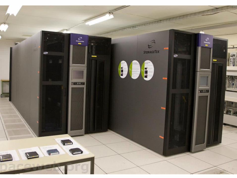
Data & Storage Services CERN IT Department CH-1211 Genève 23 Switzerland www.cern.ch/ DSS Virtual visit to the computer Centre Photo credit to Alexey Tselishchev

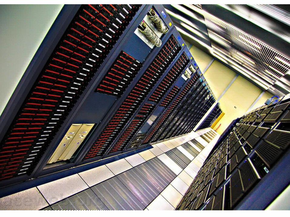
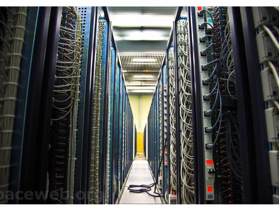
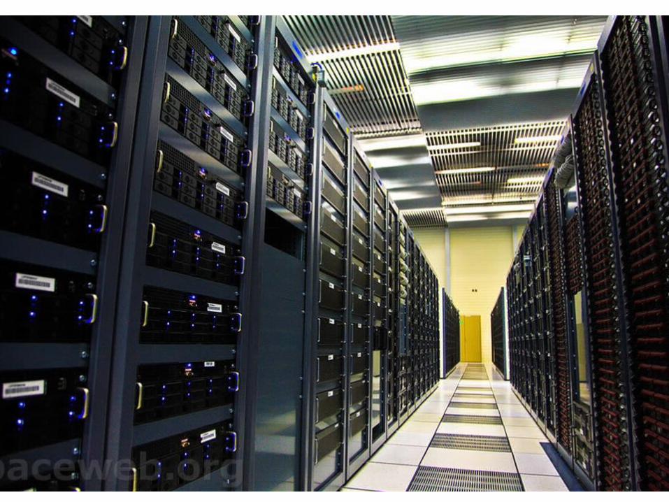
Virtual visit to the computer Centre
Jan 02, 2016
Virtual visit to the computer Centre. Photo credit to Alexey Tselishchev. And the antimatter. Introduction to data management. What is data management ?. Scientific research in recent years has exploded the computing requirements - PowerPoint PPT Presentation
Welcome message from author
This document is posted to help you gain knowledge. Please leave a comment to let me know what you think about it! Share it to your friends and learn new things together.
Transcript
Data & Storage Services
CERN IT Department
CH-1211 Genève 23
Switzerlandwww.cern.ch/
it
DSS
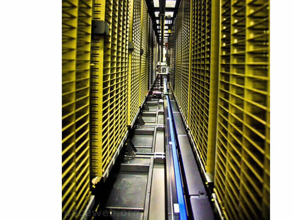
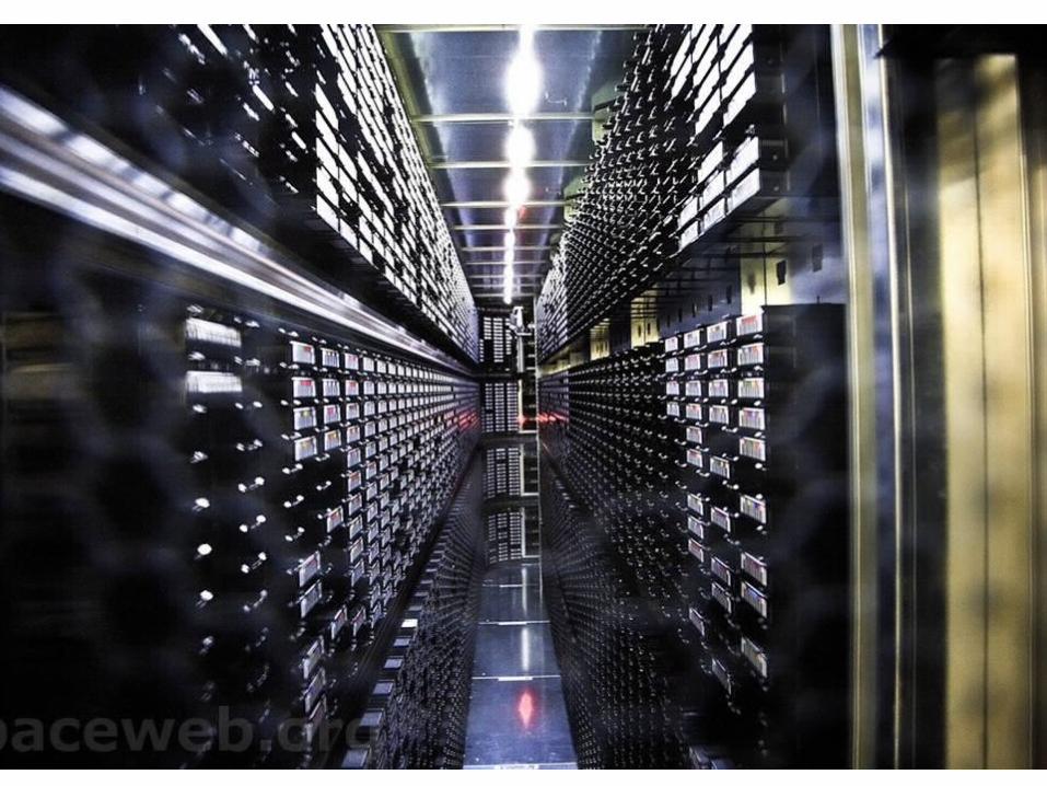
Virtual visit to the computer Centre
Photo credit to Alexey Tselishchev
CERN IT Department
CH-1211 Genève 23
Switzerlandwww.cern.ch/
it
InternetServices
DSS
CERN IT Department
CH-1211 Genève 23
Switzerlandwww.cern.ch/
it
InternetServices
DSS
CERN IT Department
CH-1211 Genève 23
Switzerlandwww.cern.ch/
it
InternetServices
DSS
CERN IT Department
CH-1211 Genève 23
Switzerlandwww.cern.ch/
it
InternetServices
DSS
CERN IT Department
CH-1211 Genève 23
Switzerlandwww.cern.ch/
it
InternetServices
DSS
CERN IT Department
CH-1211 Genève 23
Switzerlandwww.cern.ch/
it
InternetServices
DSS
CERN IT Department
CH-1211 Genève 23
Switzerlandwww.cern.ch/
it
InternetServices
DSS
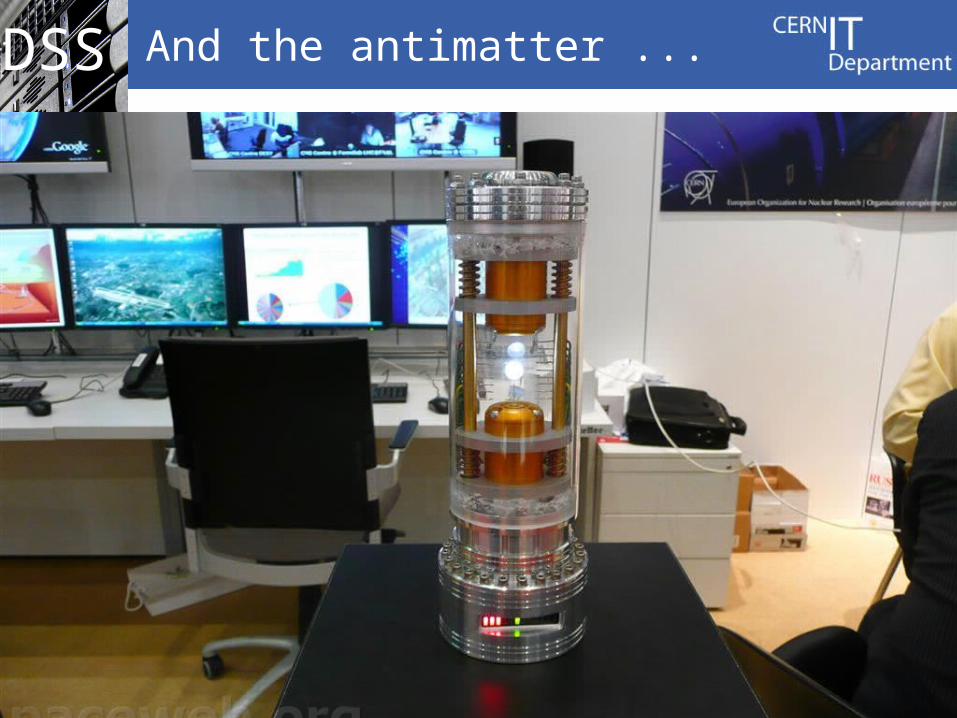
9
And the antimatter ...
Data & Storage Services
CERN IT Department
CH-1211 Genève 23
Switzerlandwww.cern.ch/
it
DSS
Introduction to data management
CERN IT Department
CH-1211 Genève 23
Switzerlandwww.cern.ch/
it
InternetServices
DSS
11
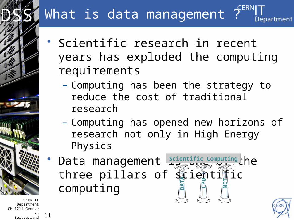
What is data management ?
• Scientific research in recent years has exploded the computing requirements– Computing has been the strategy to reduce the
cost of traditional research– Computing has opened new horizons of
research not only in High Energy Physics
• Data management is one of the three pillars of scientific computing
DA
TA
CP
U
NE
T
Scientific Computing
CERN IT Department
CH-1211 Genève 23
Switzerlandwww.cern.ch/
it
InternetServices
DSS
12
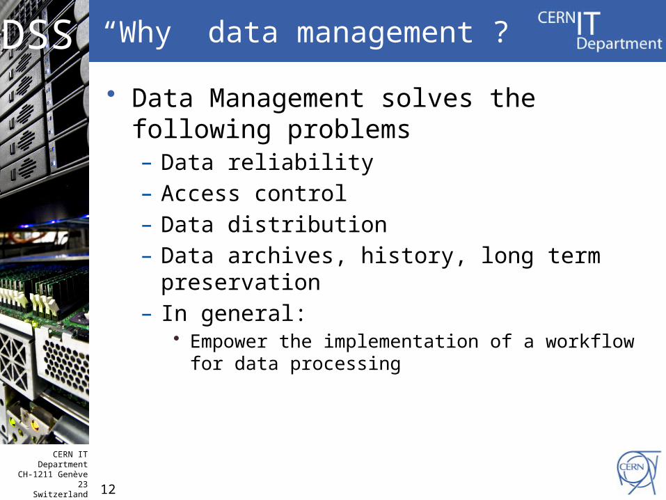
“Why” data management ?
• Data Management solves the following problems– Data reliability– Access control– Data distribution– Data archives, history, long term preservation– In general:
• Empower the implementation of a workflow for data processing
Data & Storage Services
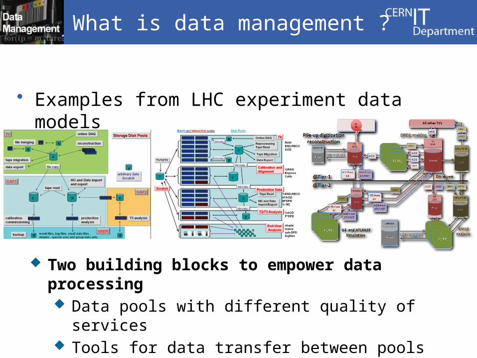
What is data management ?
• Examples from LHC experiment data models
Two building blocks to empower data processing Data pools with different quality of services Tools for data transfer between pools
CERN IT Department
CH-1211 Genève 23
Switzerlandwww.cern.ch/
it
InternetServices
DSS
14
Designing a Data Management solution
• What we would like to have– An architecture which delivers a service where
virtual resources available to end-users are much bigger than the sum of the individual parts
• What we would be happy to have– An architecture which delivers a service which
scales linearly with the sum of the individual parts
• What we usually get: – a service which delivers much less than the sum
of the individual parts
CERN IT Department
CH-1211 Genève 23
Switzerlandwww.cern.ch/
it
InternetServices
DSS
15
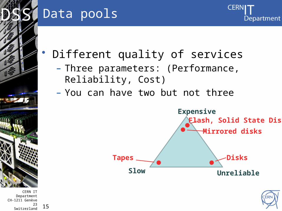
Data pools
• Different quality of services– Three parameters: (Performance, Reliability, Cost)– You can have two but not three
Slow
Expensive
Unreliable
Tapes Disks
Flash, Solid State Disks
Mirrored disks
Data & Storage Services
CERN IT Department
CH-1211 Genève 23
Switzerlandwww.cern.ch/
it
DSS
Areas of research in Data Management
Reliability, Scalability, Security, Manageability
17
Data Management – CERN School of Computing 2011
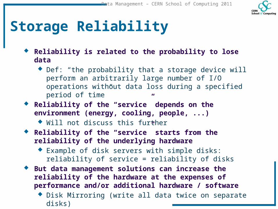
Storage Reliability
Reliability is related to the probability to lose data Def: “the probability that a storage device will perform an arbitrarily
large number of I/O operations without data loss during a specified period of time”
Reliability of the “service” depends on the environment (energy, cooling, people, ...) Will not discuss this further
Reliability of the “service” starts from the reliability of the underlying hardware Example of disk servers with simple disks: reliability of service =
reliability of disks But data management solutions can increase the reliability of the
hardware at the expenses of performance and/or additional hardware / software Disk Mirroring (write all data twice on separate disks) Redundant Array of Inexpensive Disks (RAID)

18
Data Management – CERN School of Computing 2011
Reminder: types of RAID
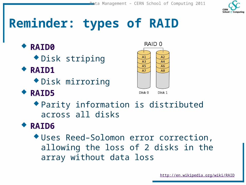
RAID0 Disk striping
RAID1 Disk mirroring
RAID5 Parity information is distributed across all disks
RAID6 Uses Reed–Solomon error correction, allowing the
loss of 2 disks in the array without data loss
http://en.wikipedia.org/wiki/RAID
19
Data Management – CERN School of Computing 2011
Reminder: types of RAID
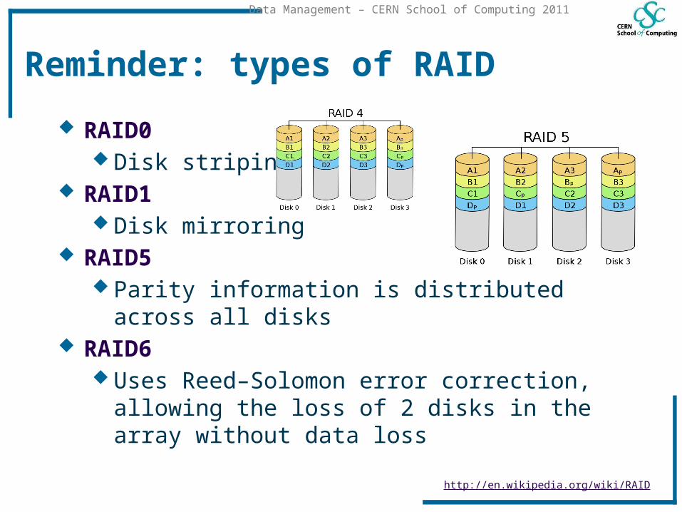
RAID0 Disk striping
RAID1 Disk mirroring
RAID5 Parity information is distributed across all disks
RAID6 Uses Reed–Solomon error correction, allowing the
loss of 2 disks in the array without data loss
http://en.wikipedia.org/wiki/RAID

20
Data Management – CERN School of Computing 2011
Reminder: types of RAID
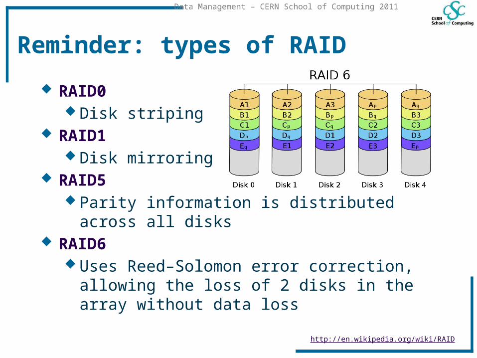
RAID0 Disk striping
RAID1 Disk mirroring
RAID5 Parity information is distributed across all disks
RAID6 Uses Reed–Solomon error correction, allowing the
loss of 2 disks in the array without data loss
http://en.wikipedia.org/wiki/RAID
21
Data Management – CERN School of Computing 2011
Reminder: types of RAID
RAID0 Disk striping
RAID1 Disk mirroring
RAID5 Parity information is distributed across all disks
RAID6 Uses Reed–Solomon error correction, allowing the
loss of 2 disks in the array without data loss
http://en.wikipedia.org/wiki/RAID
22
Data Management – CERN School of Computing 2011
Reminder: types of RAID
RAID0 Disk striping
RAID1 Disk mirroring
RAID5 Parity information is distributed across all disks
RAID6 Uses Reed–Solomon error correction, allowing the
loss of 2 disks in the array without data loss
http://en.wikipedia.org/wiki/RAID
23
Data Management – CERN School of Computing 2011
Reed–Solomon error correction ?
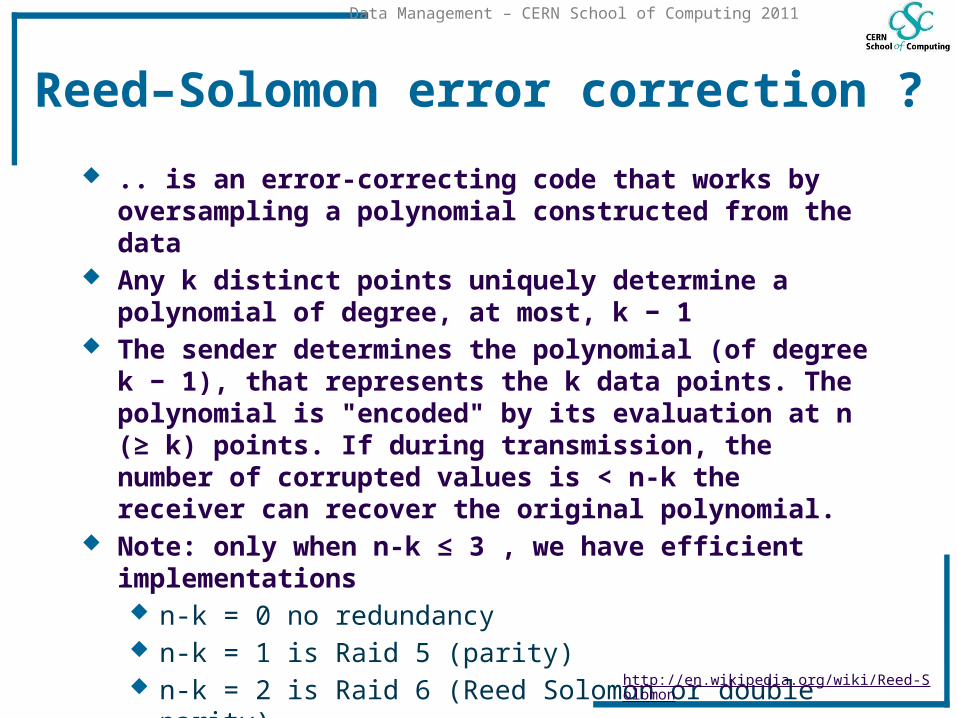
.. is an error-correcting code that works by oversampling a polynomial constructed from the data
Any k distinct points uniquely determine a polynomial of degree, at most, k − 1
The sender determines the polynomial (of degree k − 1), that represents the k data points. The polynomial is "encoded" by its evaluation at n (≥ k) points. If during transmission, the number of corrupted values is < n-k the receiver can recover the original polynomial.
Note: only when n-k ≤ 3 , we have efficient implementations n-k = 0 no redundancy n-k = 1 is Raid 5 (parity) n-k = 2 is Raid 6 (Reed Solomon or double parity) n-k = 3 is … (Triple parity)
http://en.wikipedia.org/wiki/Reed-Solomon
24
Data Management – CERN School of Computing 2011
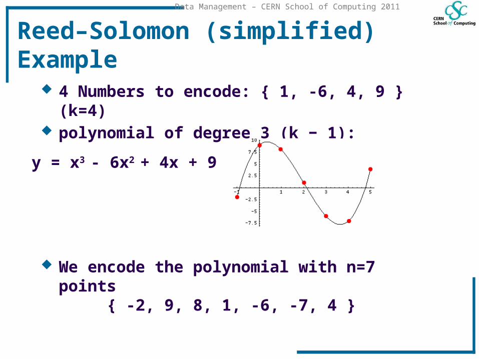
Reed–Solomon (simplified) Example
4 Numbers to encode: { 1, -6, 4, 9 } (k=4) polynomial of degree 3 (k − 1):
We encode the polynomial with n=7 points { -2, 9, 8, 1, -6, -7, 4 }
y = x3 - 6x2 + 4x + 9
25
Data Management – CERN School of Computing 2011
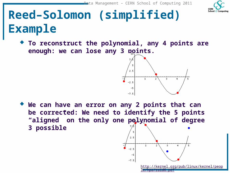
Reed–Solomon (simplified) Example
To reconstruct the polynomial, any 4 points are enough: we can lose any 3 points.
We can have an error on any 2 points that can be corrected: We need to identify the 5 points “aligned” on the only one polynomial of degree 3 possible
http://kernel.org/pub/linux/kernel/people/hpa/raid6.pdf
26
Data Management – CERN School of Computing 2011
Reliability calculations
With RAID, the final reliability depends on several parameters The reliability of the hardware The type of RAID The number of disks in the set
Already this gives lot of flexibility in implementing arbitrary reliability
27
Data Management – CERN School of Computing 2011
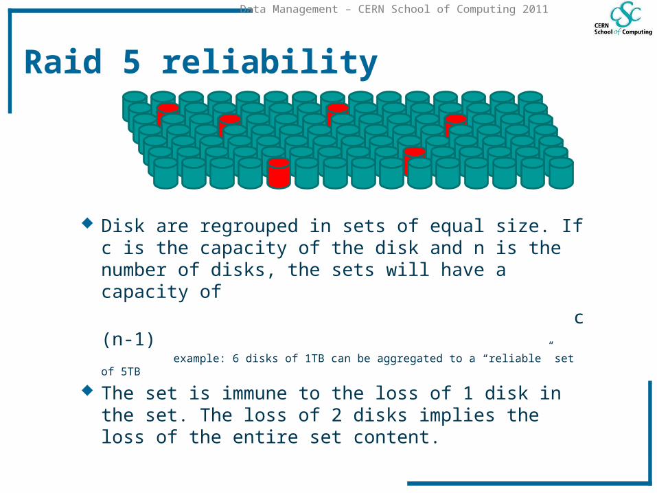
Raid 5 reliability
Disk are regrouped in sets of equal size. If c is the capacity of the disk and n is the number of disks, the sets will have a capacity of
c (n-1) example: 6 disks of 1TB can be aggregated to a “reliable” set of 5TB
The set is immune to the loss of 1 disk in the set. The loss of 2 disks implies the loss of the entire set content.
28
Data Management – CERN School of Computing 2011
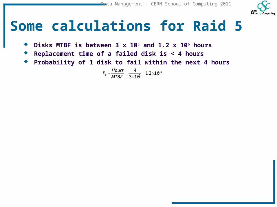
Some calculations for Raid 5 Disks MTBF is between 3 x 10⁵ and 1.2 x 10⁶ hours Replacement time of a failed disk is < 4 hours Probability of 1 disk to fail within the next 4 hours
55
103.1103
4
MTBF
HoursPf
29
Data Management – CERN School of Computing 2011
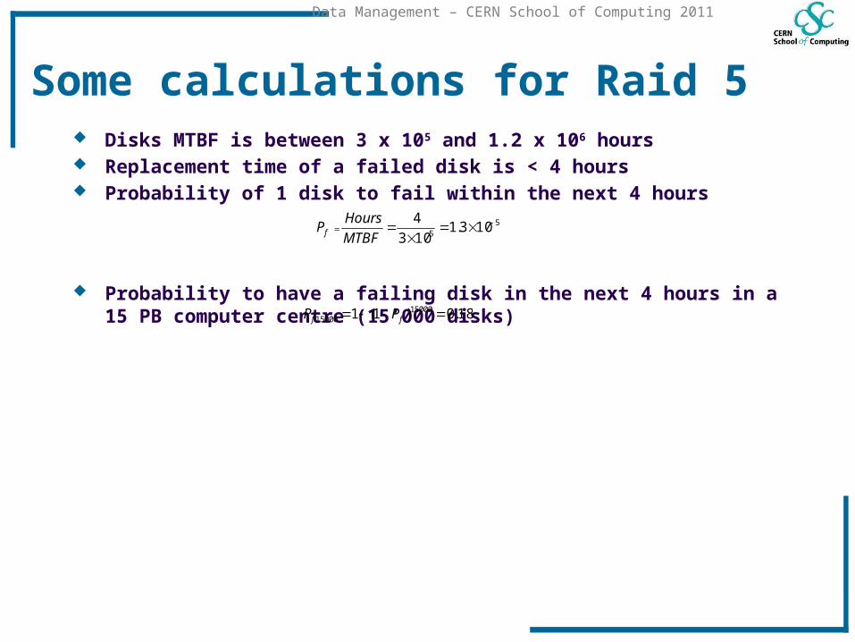
Some calculations for Raid 5 Disks MTBF is between 3 x 10⁵ and 1.2 x 10⁶ hours Replacement time of a failed disk is < 4 hours Probability of 1 disk to fail within the next 4 hours
Probability to have a failing disk in the next 4 hours in a 15 PB computer centre (15’000 disks)
55
103.1103
4
MTBF
HoursPf
18.0)1(1 1500015000 ff PP
30
Data Management – CERN School of Computing 2011
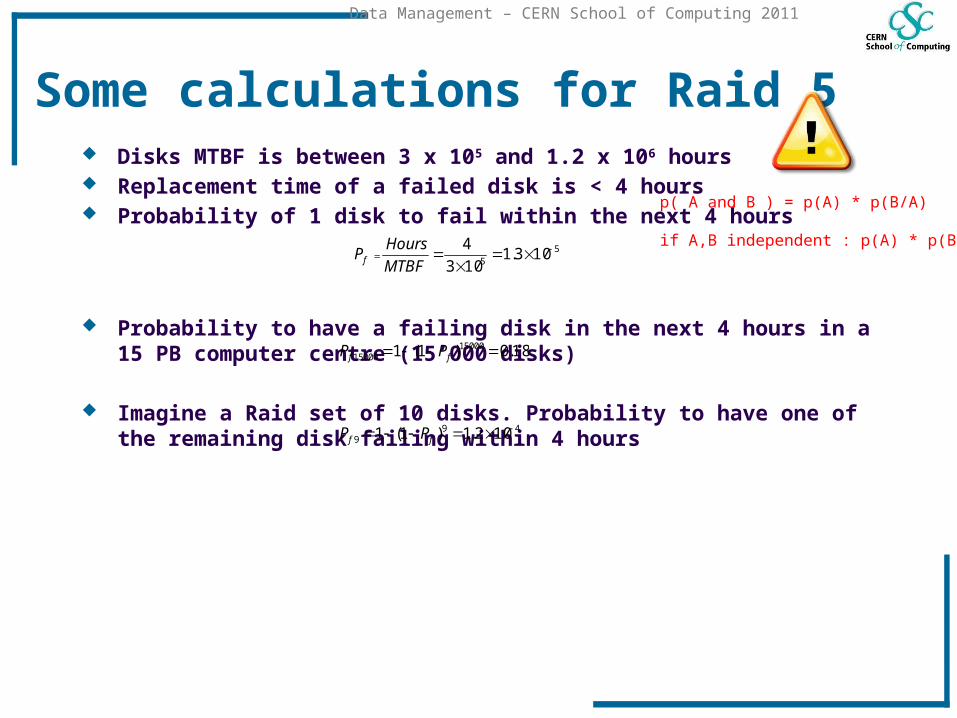
Some calculations for Raid 5 Disks MTBF is between 3 x 10⁵ and 1.2 x 10⁶ hours Replacement time of a failed disk is < 4 hours Probability of 1 disk to fail within the next 4 hours
Probability to have a failing disk in the next 4 hours in a 15 PB computer centre (15’000 disks)
Imagine a Raid set of 10 disks. Probability to have one of the remaining disk failing within 4 hours
55
103.1103
4
MTBF
HoursPf
18.0)1(1 1500015000 ff PP
499 102.1)1(1 ff PP
p( A and B ) = p(A) * p(B/A) if A,B independent : p(A) * p(B)

31
Data Management – CERN School of Computing 2011
Some calculations for Raid 5 Disks MTBF is between 3 x 10⁵ and 1.2 x 10⁶ hours Replacement time of a failed disk is < 4 hours Probability of 1 disk to fail within the next 4 hours
Probability to have a failing disk in the next 4 hours in a 15 PB computer centre (15’000 disks)
Imagine a Raid set of 10 disks. Probability to have one of the remaining disk failing within 4 hours
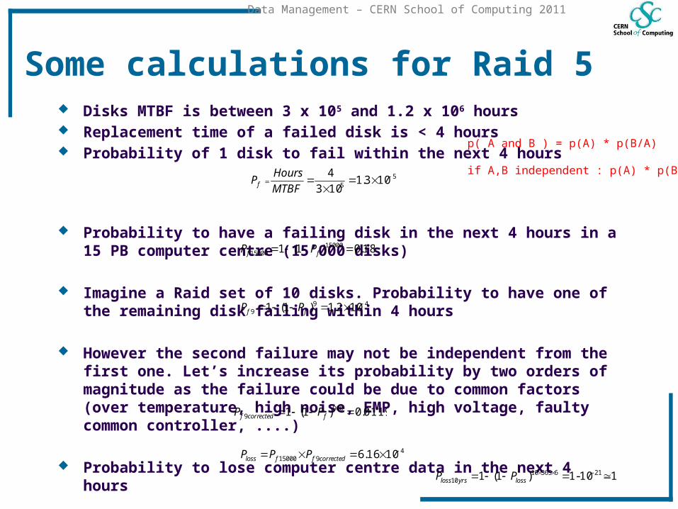
However the second failure may not be independent from the first one. Let’s increase its probability by two orders of magnitude as the failure could be due to common factors (over temperature, high noise, EMP, high voltage, faulty common controller, ....)
55
103.1103
4
MTBF
HoursPf
18.0)1(1 1500015000 ff PP
499 102.1)1(1 ff PP
0119.0)1(1 9009 fcorrectedf PP
p( A and B ) = p(A) * p(B/A) if A,B independent : p(A) * p(B)
32
Data Management – CERN School of Computing 2011
Some calculations for Raid 5 Disks MTBF is between 3 x 10⁵ and 1.2 x 10⁶ hours Replacement time of a failed disk is < 4 hours Probability of 1 disk to fail within the next 4 hours
Probability to have a failing disk in the next 4 hours in a 15 PB computer centre (15’000 disks)
Imagine a Raid set of 10 disks. Probability to have one of the remaining disk failing within 4 hours
However the second failure may not be independent from the first one. Let’s increase its probability by two orders of magnitude as the failure could be due to common factors (over temperature, high noise, EMP, high voltage, faulty common controller, ....)
Probability to lose computer centre data in the next 4 hours
Probability to lose data in the next 10 years
55
103.1103
4
MTBF
HoursPf
18.0)1(1 1500015000 ff PP
499 102.1)1(1 ff PP
4915000 1016.6 correctedffloss PPP
110-1 )1(1 -2163651010
lossyrsloss PP
0119.0)1(1 9009 fcorrectedf PP
p( A and B ) = p(A) * p(B/A) if A,B independent : p(A) * p(B)
33
Data Management – CERN School of Computing 2011
Raid 6 reliability
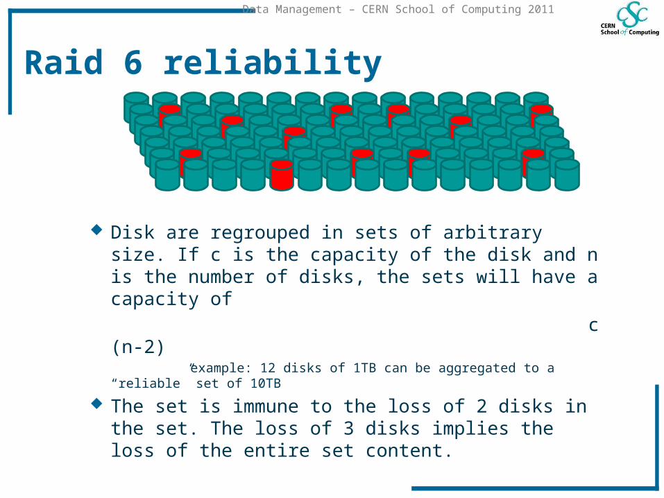
Disk are regrouped in sets of arbitrary size. If c is the capacity of the disk and n is the number of disks, the sets will have a capacity of
c (n-2) example: 12 disks of 1TB can be aggregated to a “reliable” set of 10TB
The set is immune to the loss of 2 disks in the set. The loss of 3 disks implies the loss of the entire set content.
34
Data Management – CERN School of Computing 2011
Same calculations for Raid 6
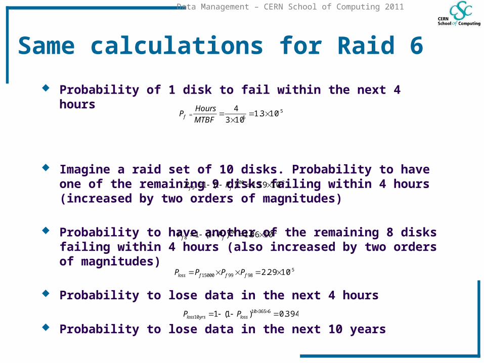
Probability of 1 disk to fail within the next 4 hours
Imagine a raid set of 10 disks. Probability to have one of the remaining 9 disks failing within 4 hours (increased by two orders of magnitudes)
Probability to have another of the remaining 8 disks failing within 4 hours (also increased by two orders of magnitudes)
Probability to lose data in the next 4 hours
Probability to lose data in the next 10 years
55
103.1103
4
MTBF
HoursPf
29009 1019.1)1(1 ff PP
5989915000 1029.2 fffloss PPPP
394.0)1(1 63651010
lossyrsloss PP
28008 1006.1)1(1 ff PP
35
Data Management – CERN School of Computing 2011
s
Arbitrary reliability
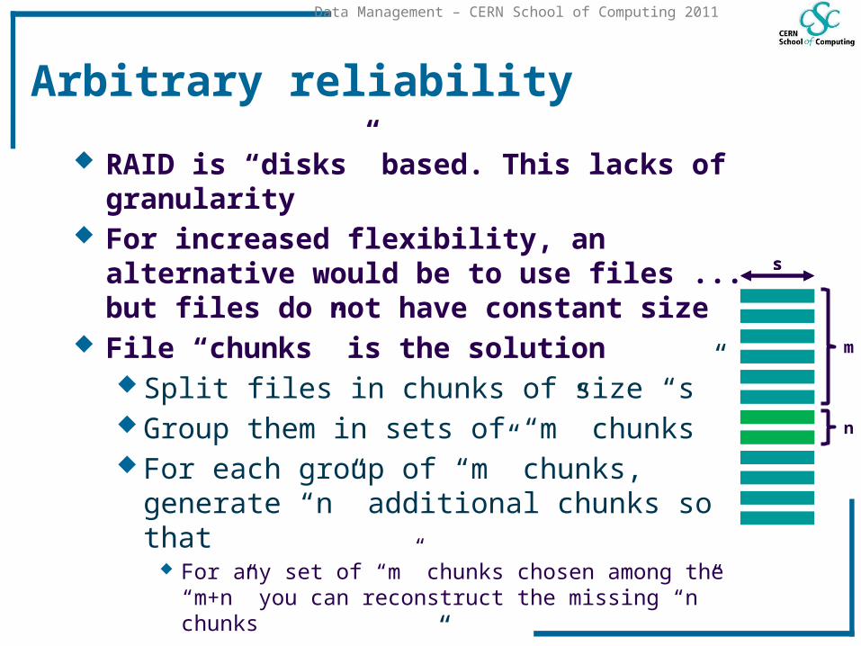
RAID is “disks” based. This lacks of granularity For increased flexibility, an alternative would be
to use files ... but files do not have constant size File “chunks” is the solution
Split files in chunks of size “s” Group them in sets of “m” chunks For each group of “m” chunks, generate “n”
additional chunks so that For any set of “m” chunks chosen among the “m+n” you can
reconstruct the missing “n” chunks
Scatter the “m+n” chunks on independent storage
n
s
m
36
Data Management – CERN School of Computing 2011
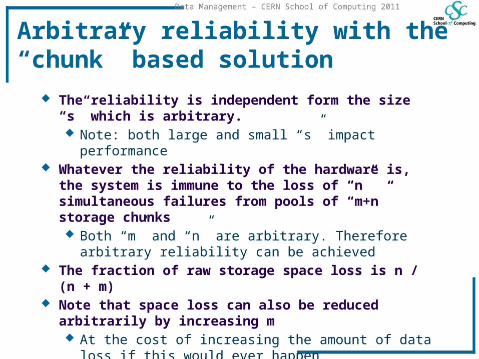
Arbitrary reliability with the “chunk” based solution
The reliability is independent form the size “s” which is arbitrary. Note: both large and small “s” impact performance
Whatever the reliability of the hardware is, the system is immune to the loss of “n” simultaneous failures from pools of “m+n” storage chunks Both “m” and “n” are arbitrary. Therefore arbitrary reliability
can be achieved The fraction of raw storage space loss is n / (n + m) Note that space loss can also be reduced arbitrarily by
increasing m At the cost of increasing the amount of data loss if this would
ever happen
37
Data Management – CERN School of Computing 2011
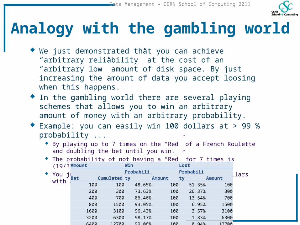
Analogy with the gambling world We just demonstrated that you can achieve “arbitrary reliability” at
the cost of an “arbitrary low” amount of disk space. By just increasing the amount of data you accept loosing when this happens.
In the gambling world there are several playing schemes that allows you to win an arbitrary amount of money with an arbitrary probability.
Example: you can easily win 100 dollars at > 99 % probability ... By playing up to 7 times on the “Red” of a French Roulette and doubling the bet
until you win. The probability of not having a “Red” for 7 times is (19/37)7 = 0.0094) You just need to take the risk of loosing 12’700 dollars with a 0.94 % probability
Amount Win Lost Bet Cumulated Probability Amount Probability Amount
100 100 48.65% 100 51.35% 100200 300 73.63% 100 26.37% 300400 700 86.46% 100 13.54% 700800 1500 93.05% 100 6.95% 1500
1600 3100 96.43% 100 3.57% 31003200 6300 98.17% 100 1.83% 63006400 12700 99.06% 100 0.94% 12700
38
Data Management – CERN School of Computing 2011
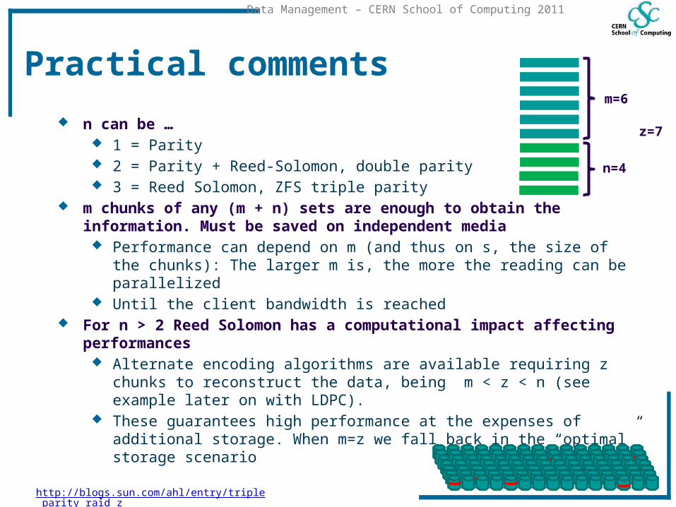
Practical comments
n can be … 1 = Parity 2 = Parity + Reed-Solomon, double parity 3 = Reed Solomon, ZFS triple parity
m chunks of any (m + n) sets are enough to obtain the information. Must be saved on independent media
Performance can depend on m (and thus on s, the size of the chunks): The larger m is, the more the reading can be parallelized
Until the client bandwidth is reached For n > 2 Reed Solomon has a computational impact affecting performances
Alternate encoding algorithms are available requiring z chunks to reconstruct the data, being m < z < n (see example later on with LDPC).
These guarantees high performance at the expenses of additional storage. When m=z we fall back in the “optimal” storage scenario
n=4
m=6
http://blogs.sun.com/ahl/entry/triple_parity_raid_z
z=7

40
Data Management – CERN School of Computing 2011
Chunk transfers
Among many protocols, Bittorrent is the most popular An SHA1 hash (160 bit digest) is created for each chunk All digests are assembled in a “torrent file” with all relevant
metadata information Torrent files are published and registered with a tracker
which maintains lists of the clients currently sharing the torrent’s chunks
In particular, torrent files have: an "announce" section, which specifies the URL of the
tracker an "info" section, containing (suggested) names for the files,
their lengths, the list of SHA-1 digests Reminder: it is the client’s duty to reassemble the initial file
and therefore it is the client that always verifies the integrity of the data received
http://en.wikipedia.org/wiki/BitTorrent_(protocol)
41
Data Management – CERN School of Computing 2011
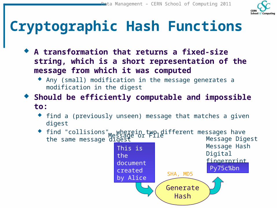
Cryptographic Hash Functions
A transformation that returns a fixed-size string, which is a short representation of the message from which it was computed
Any (small) modification in the message generates a modification in the digest
Should be efficiently computable and impossible to: find a (previously unseen) message that matches a given digest find "collisions", wherein two different messages have the same message
digest
Py75c%bn
This is the document created by Alice
Message or FileMessage DigestMessage HashDigital fingerprint
GenerateHash
SHA, MD5
42
Data Management – CERN School of Computing 2011
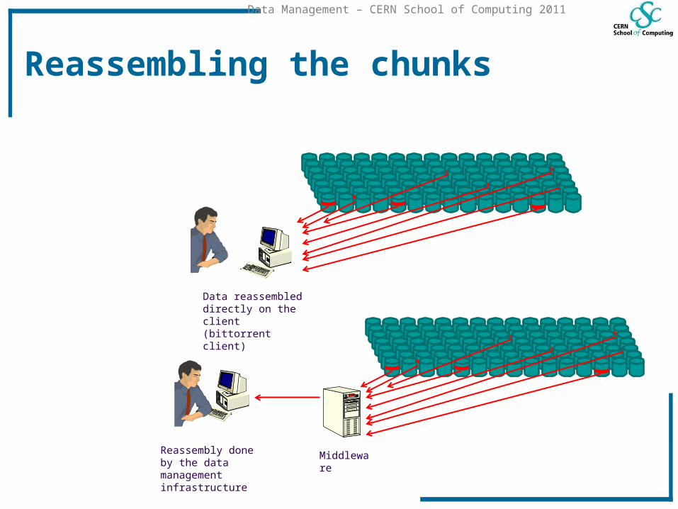
Reassembling the chunks
Data reassembled directly on the client(bittorrent client)
Reassembly done by the data management infrastructure
Middleware
43
Data Management – CERN School of Computing 2011
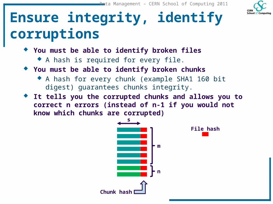
Ensure integrity, identify corruptions
You must be able to identify broken files A hash is required for every file.
You must be able to identify broken chunks A hash for every chunk (example SHA1 160 bit digest) guarantees
chunks integrity. It tells you the corrupted chunks and allows you to correct n
errors (instead of n-1 if you would not know which chunks are corrupted)
n
s
m
Chunk hash
File hash
44
Data Management – CERN School of Computing 2011
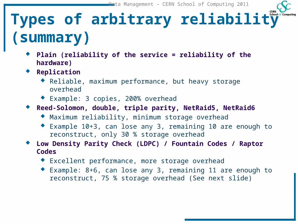
Types of arbitrary reliability (summary)
Plain (reliability of the service = reliability of the hardware)
45
Data Management – CERN School of Computing 2011
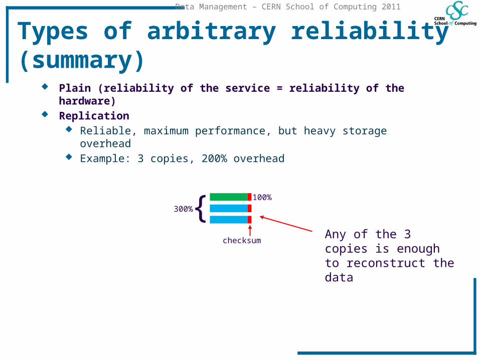
Types of arbitrary reliability (summary)
Plain (reliability of the service = reliability of the hardware) Replication
Reliable, maximum performance, but heavy storage overhead Example: 3 copies, 200% overhead
checksum
100%
300%{Any of the 3 copies is enough to reconstruct the data
46
Data Management – CERN School of Computing 2011
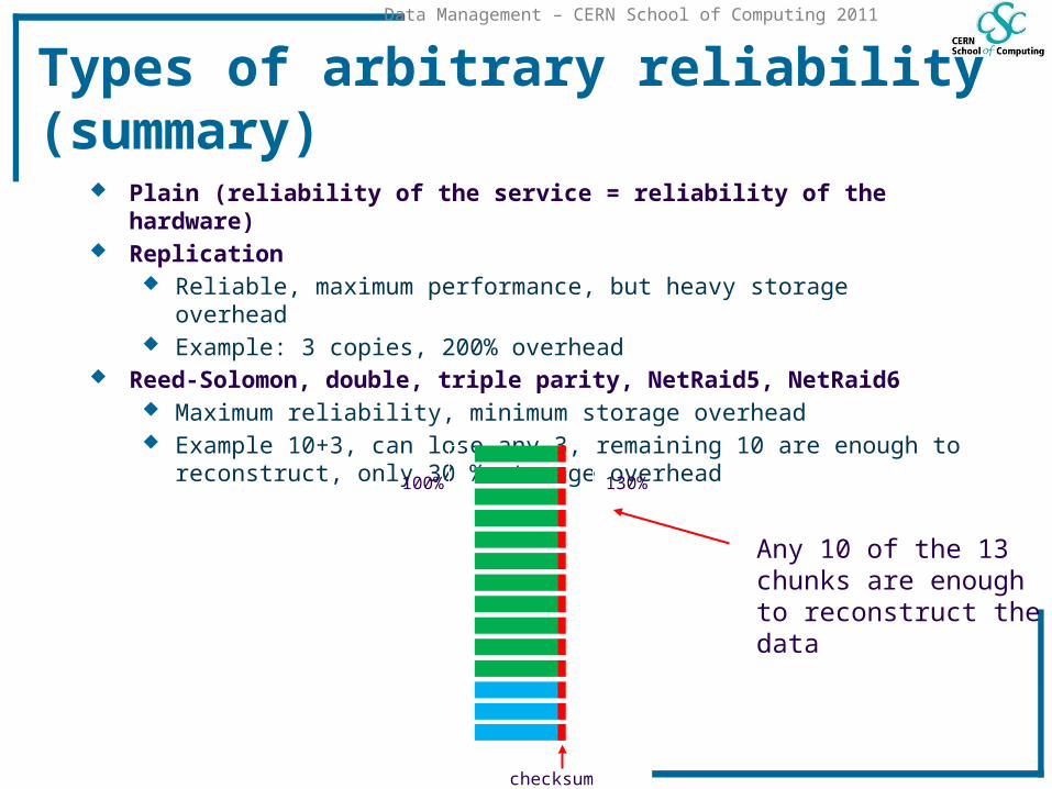
Types of arbitrary reliability (summary)
Plain (reliability of the service = reliability of the hardware) Replication
Reliable, maximum performance, but heavy storage overhead Example: 3 copies, 200% overhead
Reed-Solomon, double, triple parity, NetRaid5, NetRaid6 Maximum reliability, minimum storage overhead Example 10+3, can lose any 3, remaining 10 are enough to reconstruct,
only 30 % storage overhead
checksum
100% 130%
Any 10 of the 13 chunks are enough to reconstruct the data
47
Data Management – CERN School of Computing 2011
Types of arbitrary reliability (summary)
Plain (reliability of the service = reliability of the hardware) Replication
Reliable, maximum performance, but heavy storage overhead Example: 3 copies, 200% overhead
Reed-Solomon, double, triple parity, NetRaid5, NetRaid6 Maximum reliability, minimum storage overhead Example 10+3, can lose any 3, remaining 10 are enough to reconstruct,
only 30 % storage overhead Low Density Parity Check (LDPC) / Fountain Codes / Raptor Codes
Excellent performance, more storage overhead Example: 8+6, can lose any 3, remaining 11 are enough to reconstruct, 75
% storage overhead (See next slide)
48
Data Management – CERN School of Computing 2011
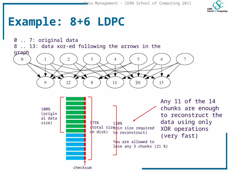
Example: 8+6 LDPC
checksum
100%(original data size)
175%(total size on disk)
Any 11 of the 14 chunks are enough to reconstruct the data using only XOR operations (very fast)
0 .. 7: original data8 .. 13: data xor-ed following the arrows in the graph
138%(min size requiredto reconstruct)
You are allowed to lose any 3 chunks (21 %)
49
Data Management – CERN School of Computing 2011
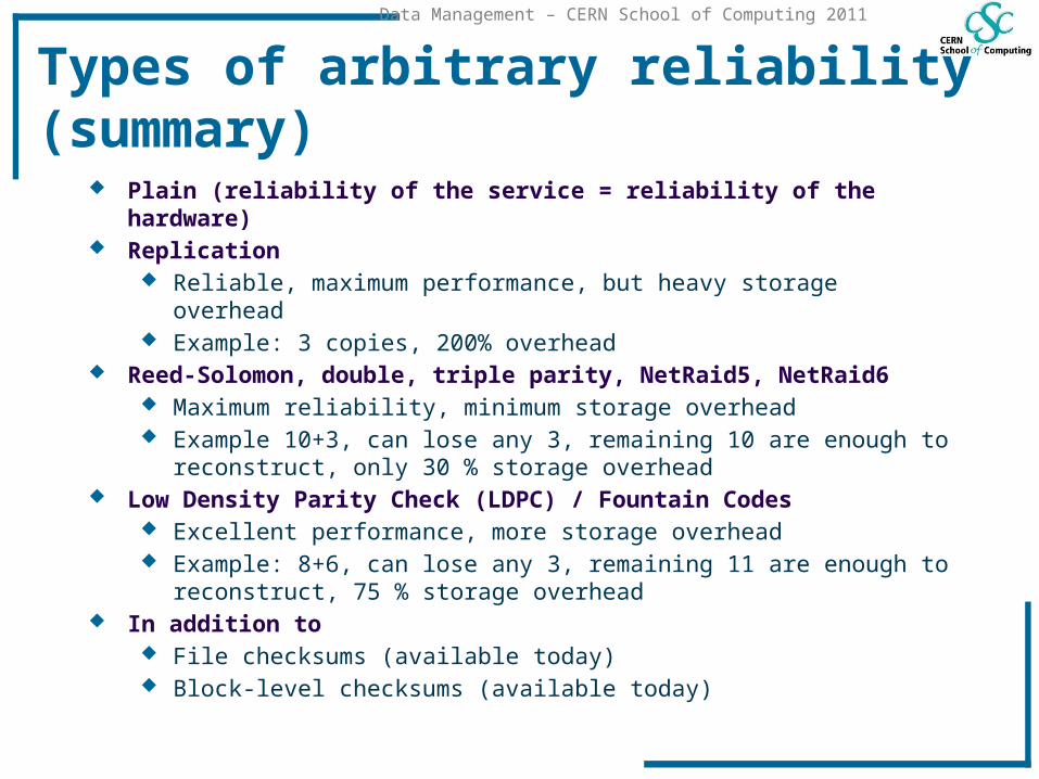
Types of arbitrary reliability (summary)
Plain (reliability of the service = reliability of the hardware) Replication
Reliable, maximum performance, but heavy storage overhead Example: 3 copies, 200% overhead
Reed-Solomon, double, triple parity, NetRaid5, NetRaid6 Maximum reliability, minimum storage overhead Example 10+3, can lose any 3, remaining 10 are enough to reconstruct,
only 30 % storage overhead Low Density Parity Check (LDPC) / Fountain Codes
Excellent performance, more storage overhead Example: 8+6, can lose any 3, remaining 11 are enough to reconstruct, 75
% storage overhead In addition to
File checksums (available today) Block-level checksums (available today)

Data & Storage Services
CERN IT Department
CH-1211 Genève 23
Switzerlandwww.cern.ch/
it
DSS
Questions ?
Related Documents