1 Viewing Conditions and Chromatic Adaptation Visual Perception Spring 2008 Instructor: Prof. Aditi Majumder Student: Hamed Pirsiavash Agenda Viewing field Chromatic adaptation Chromatic adaptation models Linear nonlinear

Welcome message from author
This document is posted to help you gain knowledge. Please leave a comment to let me know what you think about it! Share it to your friends and learn new things together.
Transcript
1
Viewing Conditions and Chromatic Adaptation
Visual Perception Spring 2008
Instructor: Prof. Aditi MajumderStudent: Hamed Pirsiavash
Agenda
Viewing fieldChromatic adaptationChromatic adaptation models
Linearnonlinear
2
Viewing field
Self-luminous displaysCRT, LCD
Reflective mediaPainting
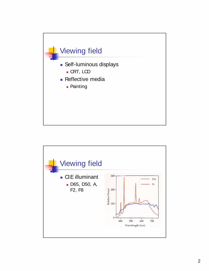
Viewing field
CIE illuminantD65, D50, A, F2, F8
3
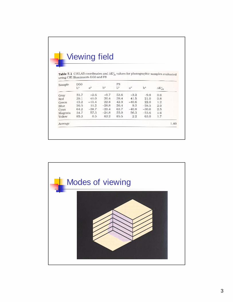
Viewing field
Modes of viewing

4
Modes of viewing
Chromatic adaptation
Light adaptationTurning on the light in dark night
Dark adaptationEntering a dark movie theater
Chromatic adaptation
5
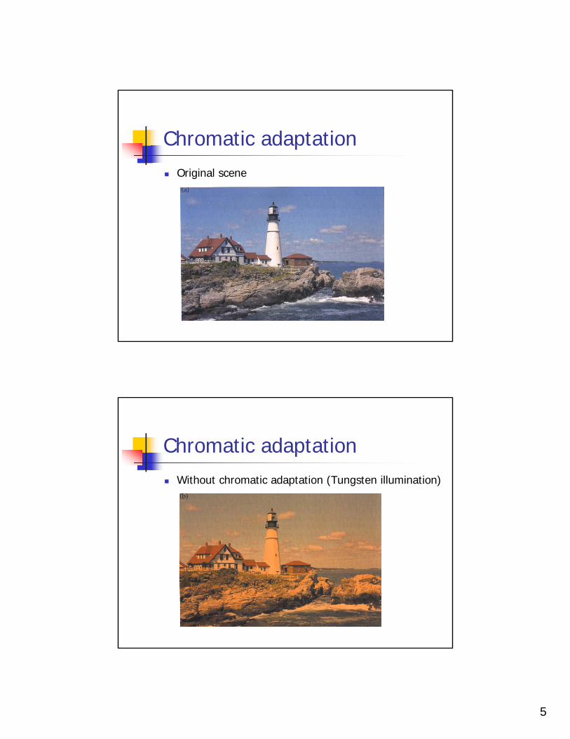
Chromatic adaptationOriginal scene
Chromatic adaptationWithout chromatic adaptation (Tungsten illumination)
6
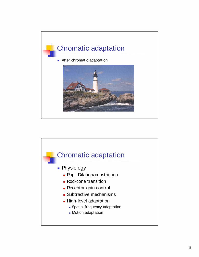
Chromatic adaptationAfter chromatic adaptation
Chromatic adaptation
PhysiologyPupil Dilation/constrictionRod-cone transitionReceptor gain controlSubtractive mechanismsHigh-level adaptation
Spatial frequency adaptationMotion adaptation

7
Chromatic adaptation models
Transformation from XYZ (tristimulus values) to LMS (cone responsitives)
Chromatic adaptation models
From XYZ to LMS
8
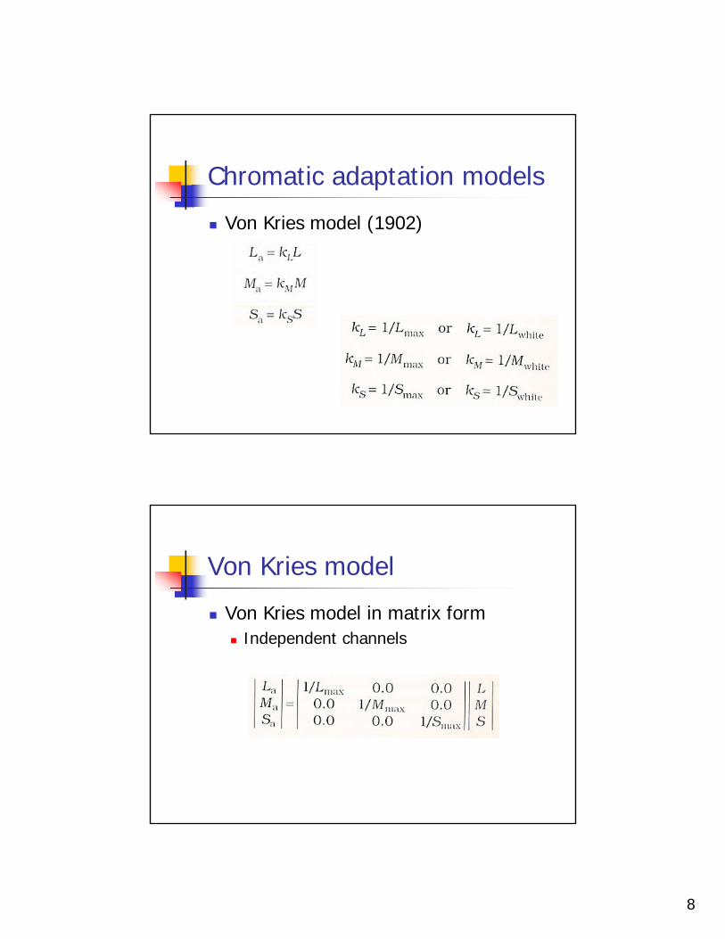
Chromatic adaptation models
Von Kries model (1902)
Von Kries model
Von Kries model in matrix formIndependent channels
9
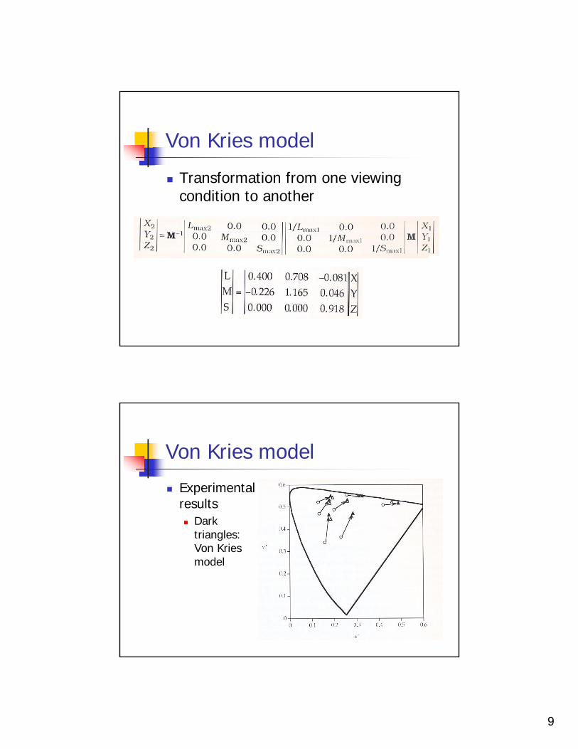
Von Kries model
Transformation from one viewing condition to another
Von Kries model
Experimental results
Dark triangles: Von Kriesmodel

10
Chromatic adaptation models
Retinex theory (1971)Use spatial distribution of scene colorsColor appearance is
Surface reflectionNot the distribution of reflected light
Normalize the output of each sensor with average over the scene.
Nayatani’s model (1980)
NonlinearClose to MacAdam’smodel (1961) Noise term is added
Helps in low inllumination

11
Guth’s model (1991)
Sigma is a noise term
Guth’s model (1991)
Comparison with Von Kriesmodel
12
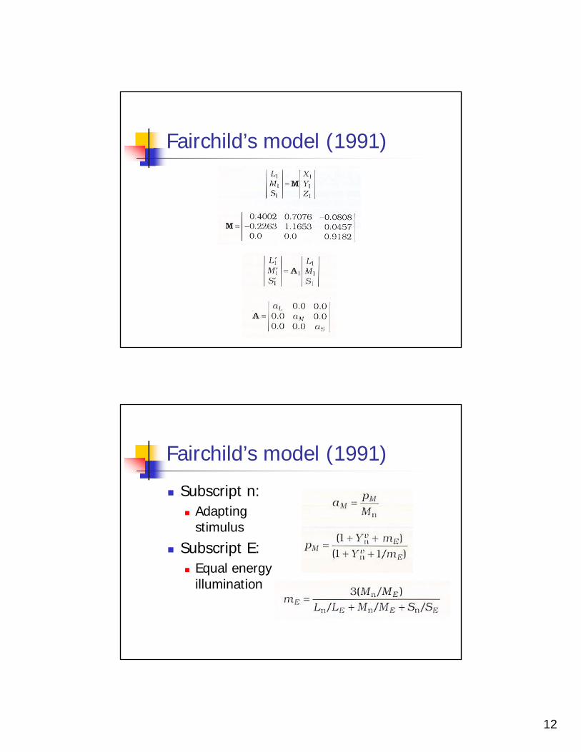
Fairchild’s model (1991)
Fairchild’s model (1991)
Subscript n:Adapting stimulus
Subscript E:Equal energy illumination

13
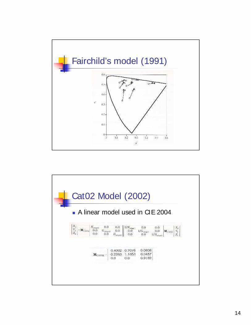
Fairchild’s model (1991)
Inter channel correlationLater he removed this matrix
Fairchild’s model (1991)
Transformation from one viewing condition to another
14
Fairchild’s model (1991)
Cat02 Model (2002)
A linear model used in CIE 2004
15
Thanks for your attention

1
1
Color Appearance Models
Arjun SatishMitsunobu Sugimoto
2
Today's topic
Color Appearance ModelsCIELABThe Nayatani et al. ModelThe Hunt ModelThe RLAB Model
2
3
Terminology recap
ColorHueBrightness/LightnessColorfulness/ChromaSaturation
4
Color
Attribute of visual perception consisting of any combination of chromatic and achromatic content.Chromatic nameAchromatic nameothers

3
5
Hue
Attribute of a visual sensation according to which an area appears to be similar to one of the perceived colorsOften refers red, green, blue, and yellow
6
Brightness
Attribute of a visual sensation according to which an area appears to emit more or less light.Absolute level of the perception

4
7
Lightness
The brightness of an area judged as a ratio to the brightness of a similarly illuminated area that appears to be whiteRelative amount of light reflected, or relative brightness normalized for changes in the illumination and view conditions
8
Colorfulness
Attribute of a visual sensation according to which the perceived color of an area appears to be more or less chromatic
5
9
Chroma
Colorfulness of an area judged as a ratio of the brightness of a similarly illuminated area that appears whiteRelationship between colorfulness and chroma is similar to relationship between brightness and lightness
10
Saturation
Colorfulness of an area judged as a ratio to its brightnessChroma – ratio to whiteSaturation – ratio to its brightness

6
11
Definition of Color Appearance Model
so much description of colorsuch as: wavelength, cone response, tristimulus values, chromaticity coordinates, color spaces, …it is difficult to distinguish them correctlyWe need a model which makes them straightforward
12
Definition of Color Appearance Model
CIE Technical Committee 1-34 (TC1-34)(Comission Internationale de l'Eclairage)They agreed on the following definition: A color appearance model is any model that includes predictors of at least the relative color-appearance attributes of lightness, chroma, and hue.CIELAB meets this criteria
7
13
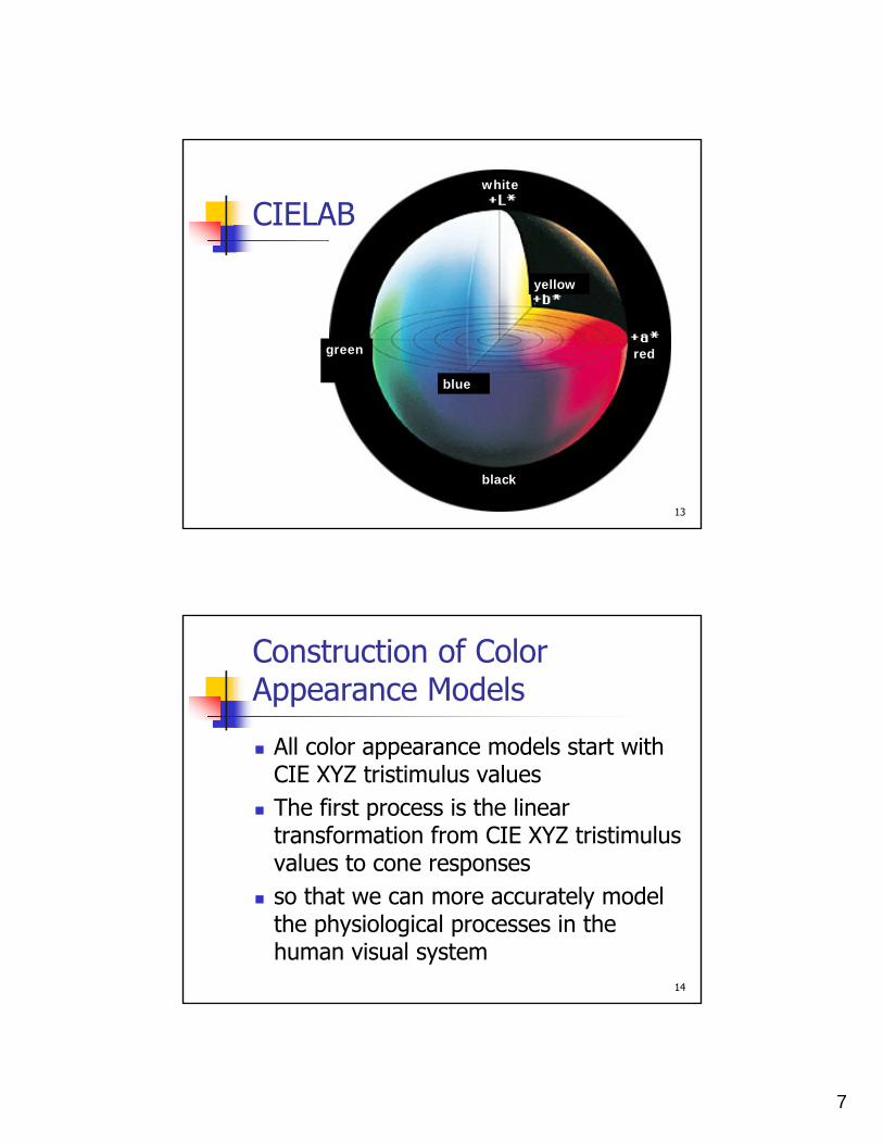
CIELABwhite
blue
green
black
red
yellow
14
Construction of Color Appearance Models
All color appearance models start with CIE XYZ tristimulus valuesThe first process is the linear transformation from CIE XYZ tristimulusvalues to cone responsesso that we can more accurately model the physiological processes in the human visual system

8
15
Calculating CIELAB Coordinate
To calculate CIELAB coordinates, one must begin with two sets of CIE XYZ tristimulus valuesStimulus XYZreference white XnYnZn
used to define the color "white"
16
Calculating CIELAB Coordinate
Then, add appropriate constantsL* = 116f(Y/Yn) – 16a* = 500[f(X/Xn) - f(Y/Yn)]b* = 200[f(Y/Yn) - f(Z/Zn)]
f(w) = w (if w > 0.008856)= 7.787(w)+16/116 (otherwise)
1/3
9
17
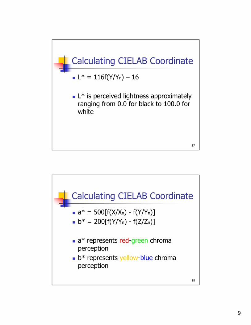
Calculating CIELAB Coordinate
L* = 116f(Y/Yn) – 16
L* is perceived lightness approximately ranging from 0.0 for black to 100.0 for white
18
Calculating CIELAB Coordinate
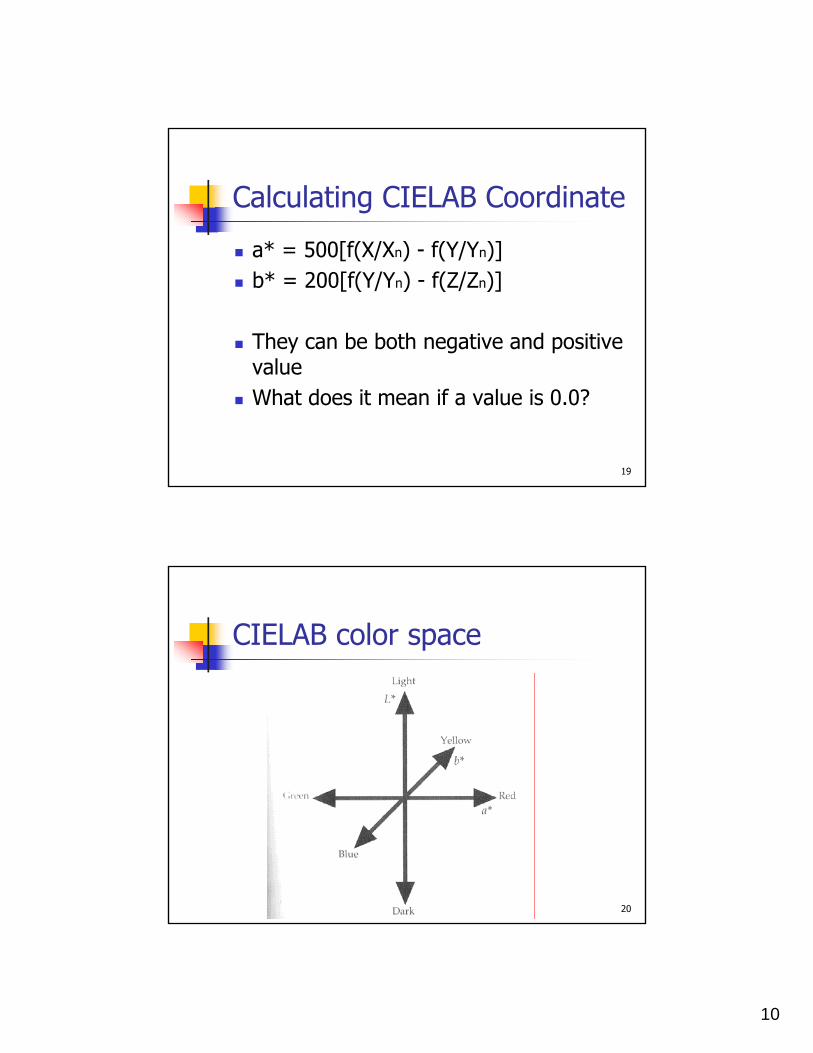
a* = 500[f(X/Xn) - f(Y/Yn)]b* = 200[f(Y/Yn) - f(Z/Zn)]
a* represents red-green chromaperceptionb* represents yellow-blue chromaperception
10
19
Calculating CIELAB Coordinate
a* = 500[f(X/Xn) - f(Y/Yn)]b* = 200[f(Y/Yn) - f(Z/Zn)]
They can be both negative and positive valueWhat does it mean if a value is 0.0?
20
CIELAB color space

11
21
Imagewhite
blue
green
black
red
yellow
22
Calculating CIELAB Coordinate
Chroma (magnitude)C*ab = [a* + b* ]Hue (angle)hab = tan (b*/a*)expressed in positive degrees starting at the positive a* axis and progressing in a counterclockwise direction
-1
2 2 1/2
12
23
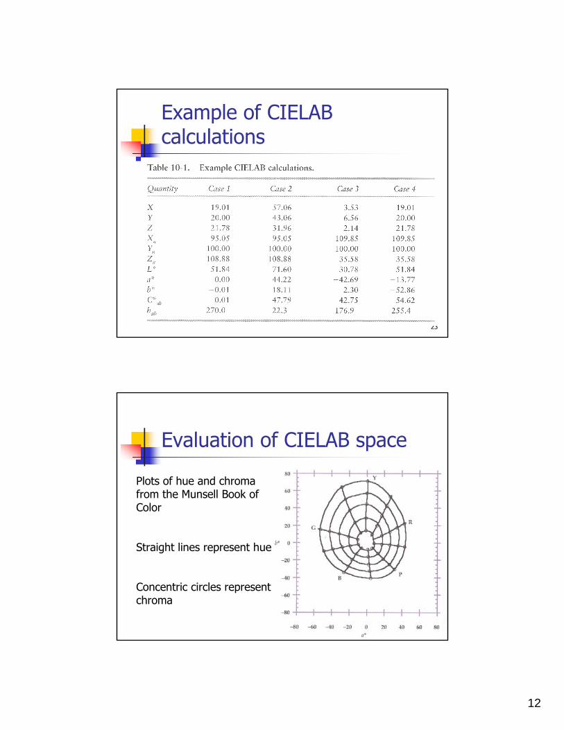
Example of CIELAB calculations
24
Evaluation of CIELAB space
Plots of hue and chromafrom the Munsell Book of Color
Straight lines represent hue
Concentric circles represent chroma
13
25
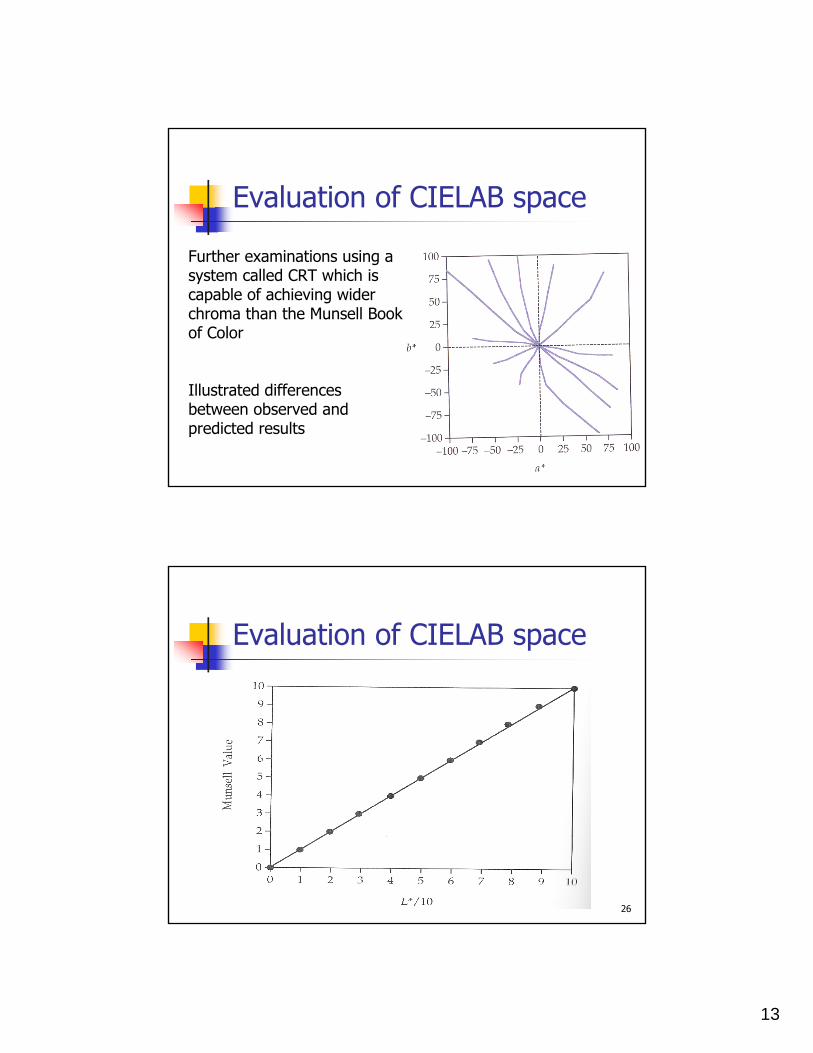
Evaluation of CIELAB space
Further examinations using a system called CRT which is capable of achieving wider chroma than the Munsell Book of Color
Illustrated differences between observed and predicted results
26
Evaluation of CIELAB space
14
27
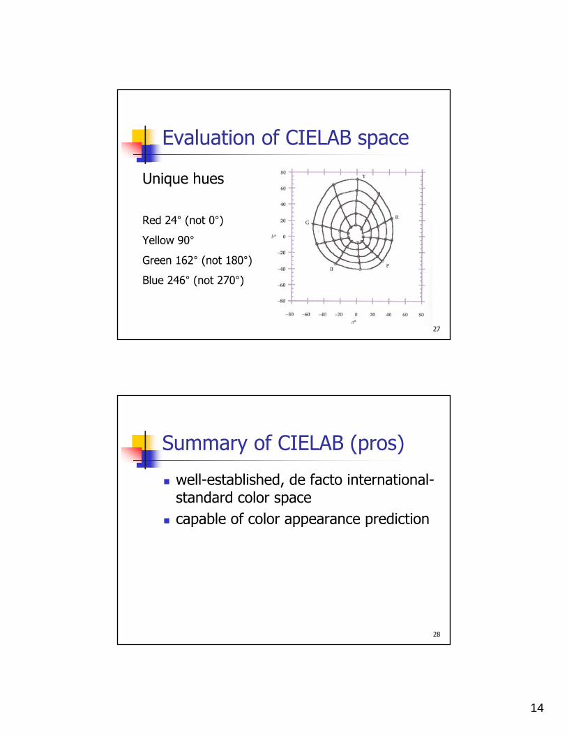
Evaluation of CIELAB space
Unique hues
Red 24° (not 0°)
Yellow 90°
Green 162° (not 180°)
Blue 246° (not 270°)
28
Summary of CIELAB (pros)
well-established, de facto international-standard color spacecapable of color appearance prediction

15
29
Summary of CIELAB (cons)
limited ability to predict hueno luminance-level dependencyno background or surround dependencyand so on...
30
Therefore...
CIELAB is used as a benchmark to measure more sophisticated models
16
31
The Hunt Model
designed to predict a wide range of visual phenomenarequires an extensive list of input datacomplete modelcomplicated
32
Input datachromaticity coordinates of the illuminant and the adapting fieldchromaticities and luminance factors of the background, proximal field, reference white, and test samplephotopic luminance LA and its color temparature Tchromatic surrounding induction factors Nc
brightness surrounding induction factors Nb
luminance of reference white Yw
luminance of background Yb
If some of these are not available, alternative values can be used

17
33
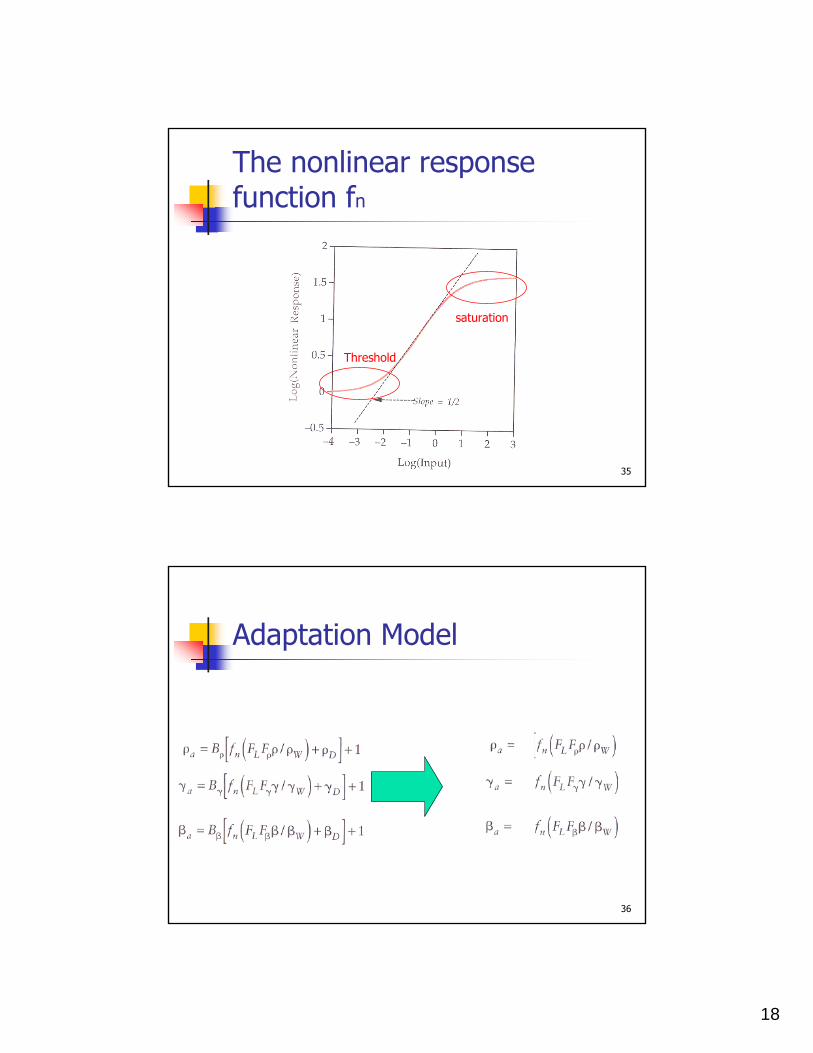
Adaptation Model
In Hunt model, the cone responses are denoted ργβ rather than LMS
34
Adaptation Model
There are many parameters need to be defined...
18
35
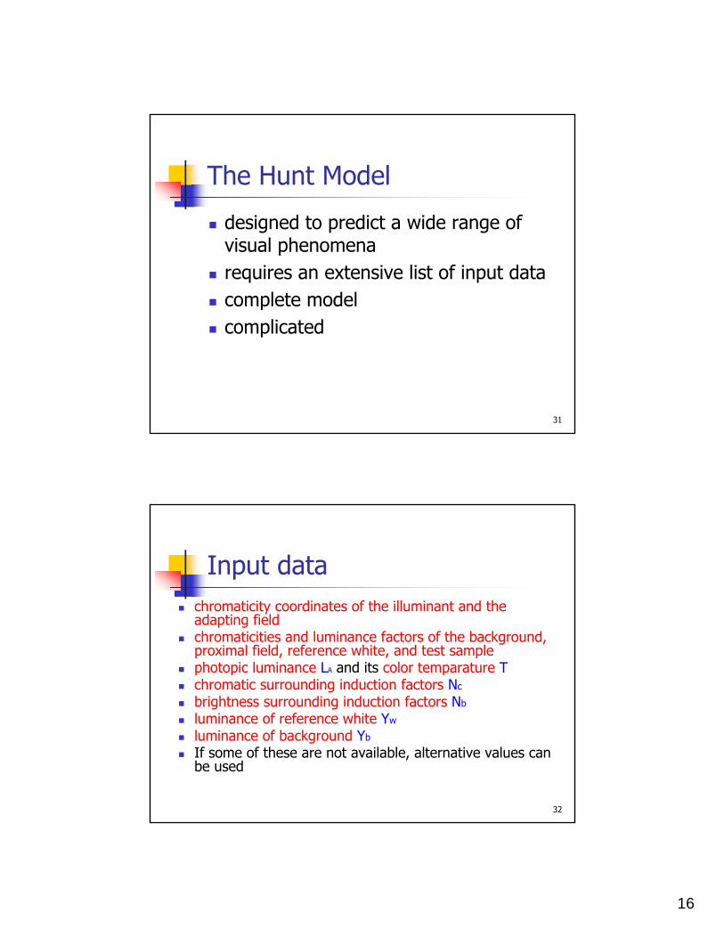
The nonlinear response function fn
saturation
Threshold
36
Adaptation Model
19
37
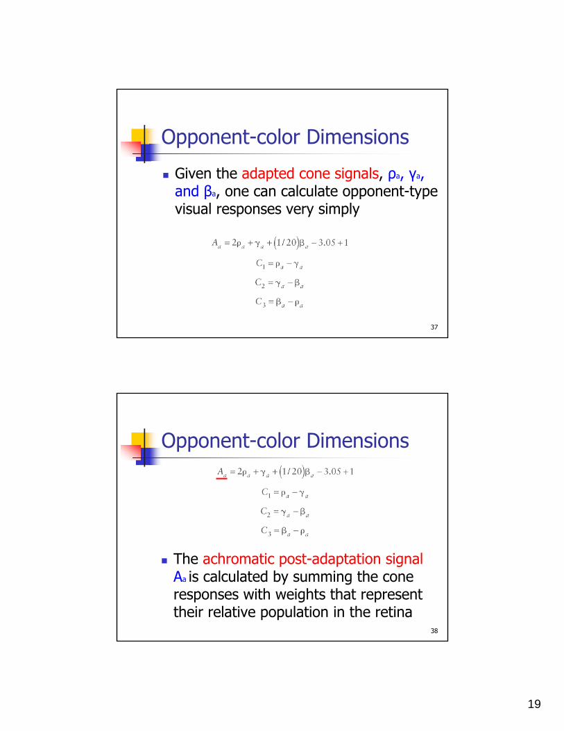
Opponent-color Dimensions
Given the adapted cone signals, ρa, γa, and βa, one can calculate opponent-type visual responses very simply
38
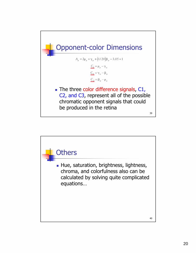
Opponent-color Dimensions
The achromatic post-adaptation signalAa is calculated by summing the cone responses with weights that represent their relative population in the retina
20
39
Opponent-color Dimensions
The three color difference signals, C1, C2, and C3, represent all of the possible chromatic opponent signals that could be produced in the retina
40
Others
Hue, saturation, brightness, lightness, chroma, and colorfulness also can be calculated by solving quite complicated equations…

21
41
Summary of the Hunt model (pros)
seem to be able to do everything that anyone could ever want from a color appearance modelextremely flexiblecapable of making accurate predictionsfor a wide range of visual experiments
42
Summary of the Hunt model (cons)
optimized parameter is required; otherwise, this model may perform extremely poorly, even worse than much simpler modelcomputationally expensivedifficult to implementRequires significant user knowledge to use consistently
1
Color Appearance Models II
Arjun SatishMitsunobu Sugimoto

2
Agenda
Nayatani et al Model. (1986) RLAB Model. (1990)
3
Nayatani et al Model
Illumination engineering Color rendering properties of light
sources. Explanation of naturally occurring natural
phenomenon.

4
Color Appearance Phenomenon
Stevens Effect Contrast Increase with luminance
Hunt Effect Colorfulness increases with luminance
Helson Judd Effect Change in hue depending on background
5
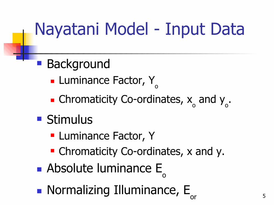
Nayatani Model - Input Data
Background Luminance Factor, Y
o
Chromaticity Co-ordinates, xo and y
o.
Stimulus Luminance Factor, Y Chromaticity Co-ordinates, x and y.
Absolute luminance Eo
Normalizing Illuminance, Eor
6
Nayatani Model - Starting Points
Use chromaticity coordinates.
7
Nayatani Model - Starting Points
Use chromaticity coordinates. Convert them to 3 intermediate values.

8
Nayatani Model - Starting Points
Use chromaticity coordinates. Convert them to 3 intermediate values.

9
Adaptation Model
Calculate the cone responses for the adapting field
10
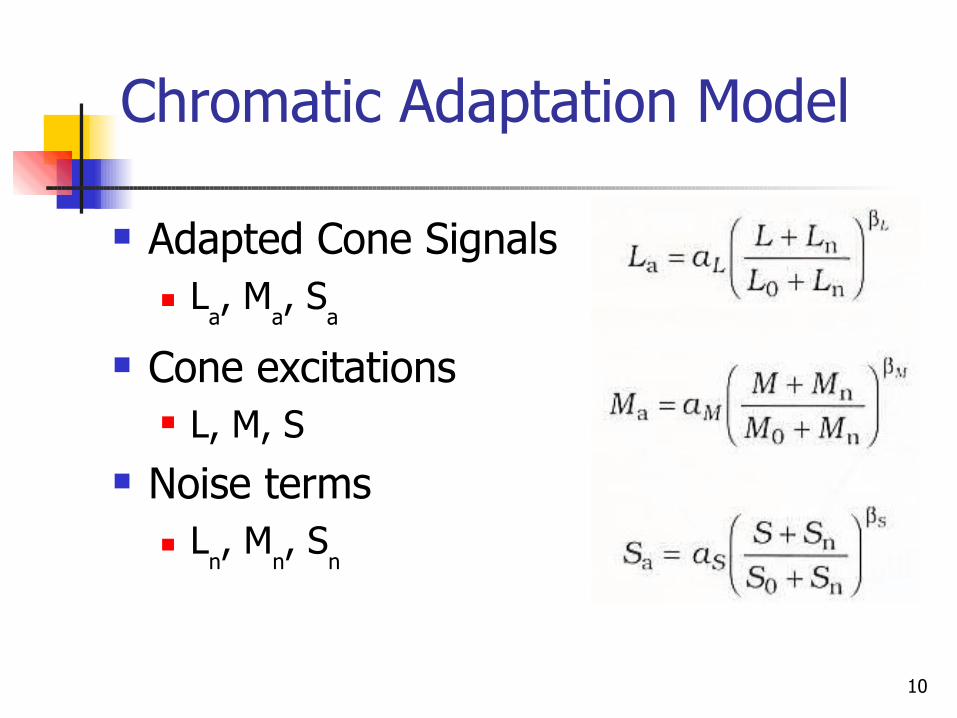
Chromatic Adaptation Model
Adapted Cone Signals L
a, M
a, S
a
Cone excitations L, M, S
Noise terms L
n, M
n, S
n

11
Adaptation Model
Compute the exponents nonlinearities used in the chromatic adaptation model
12
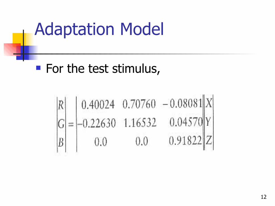
Adaptation Model
For the test stimulus,
13
Opponent Color Dimensions
Use opponent theory to represent the cone response in achromatic and chromatic channels.
Single achromatic channel. Double chromatic channels.

14
Achromatic Response
Considers only the middle and long wavelength cone response.
Logarithm -> model the nonlinearity of the human eye.
15
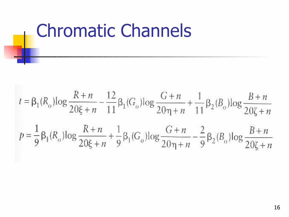
Chromatic Channels
Tritanopic and Protanopic responses. Tritanopic
Red Green Response Protanopic
Blue Yellow Response
16
Chromatic Channels
17
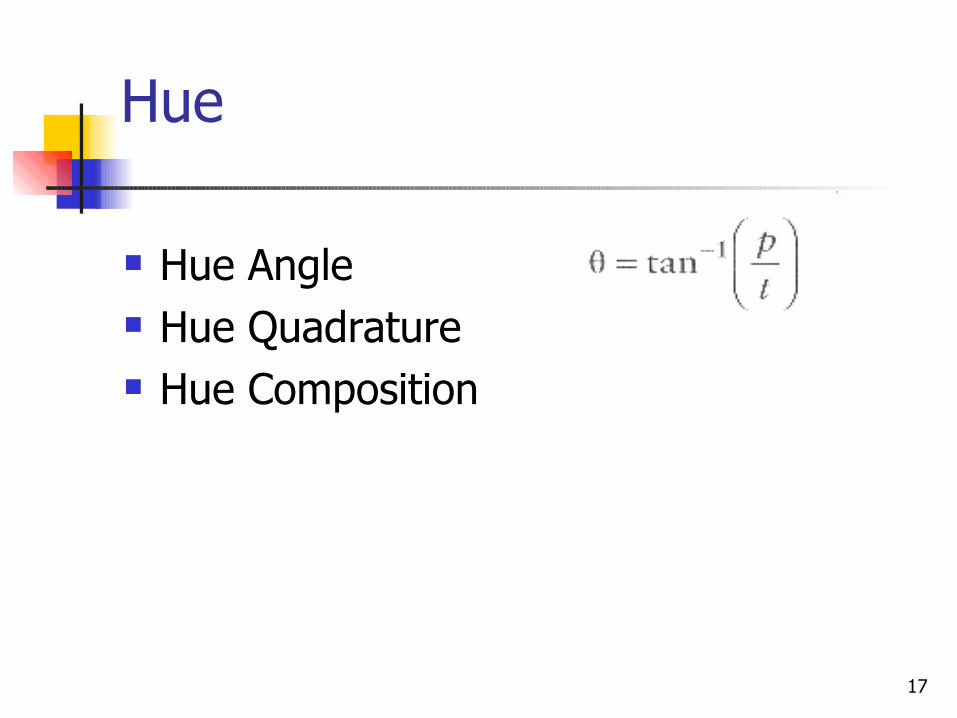
Hue
Hue Angle Hue Quadrature Hue Composition

18
Brightness

19
Lightness
Calculated from the achromatic response alone.
Lp= Q + 50.
Black => Lp = 0;
White => Lp = 100;

20
Pros and Cons
Pros 'Complete' model. Relatively simple.
Cons Changes in
background and surround
Not helpful for cross media applications.

21
The RLAB Model
A color appearance model which would be suitable for most practical applications.
simple and easy to use. takes the positive aspects of CIELAB and
tries to overcome its drawbacks. application – cross media image
reproduction.
22
Input Data
Tristimulus values of the test stimulus. Tristimulus values of the white point. Absolute luminance of a white object. Relative luminance of the surround.
23
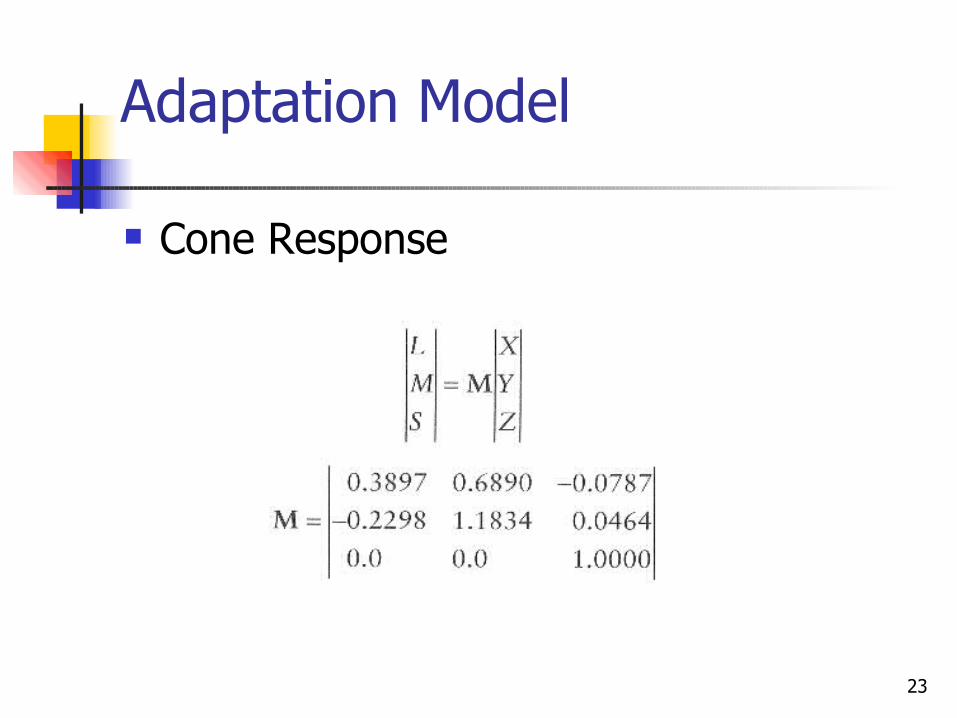
Adaptation Model
Cone Response
24
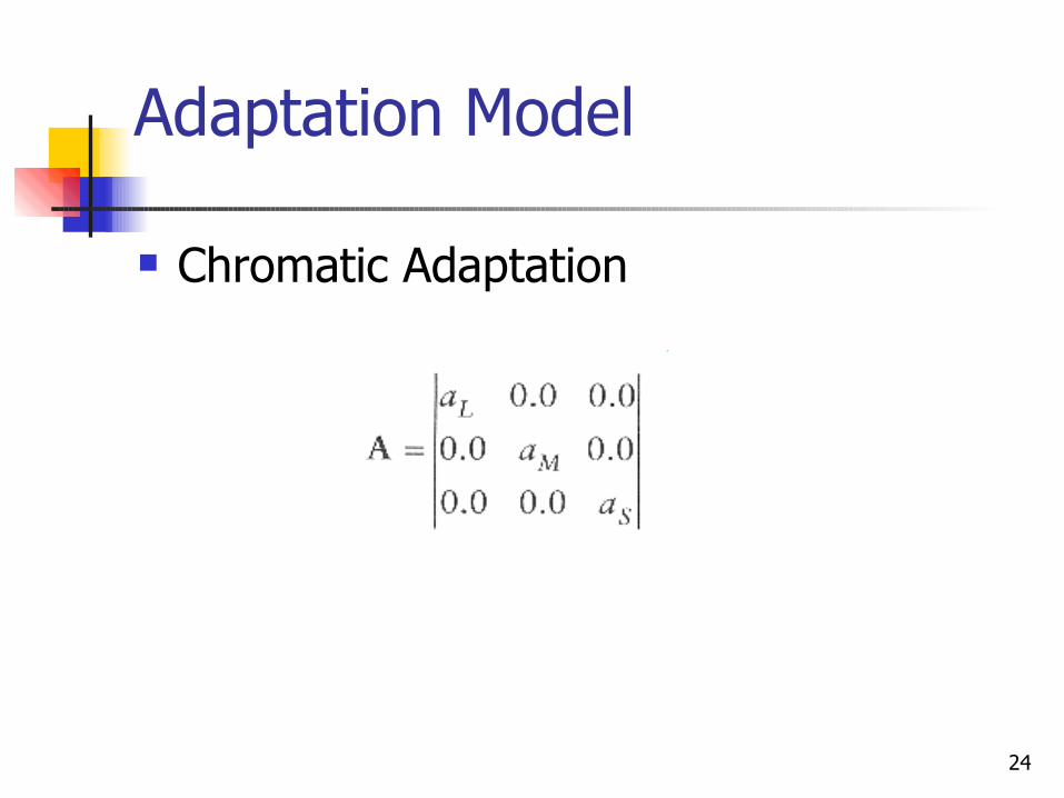
Adaptation Model
Chromatic Adaptation
25
Adaptation Model
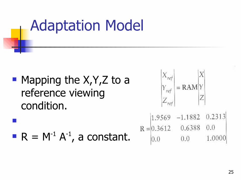
Mapping the X,Y,Z to a reference viewing condition.
R = M-1 A-1, a constant.
26
Opponent Color Dimensions
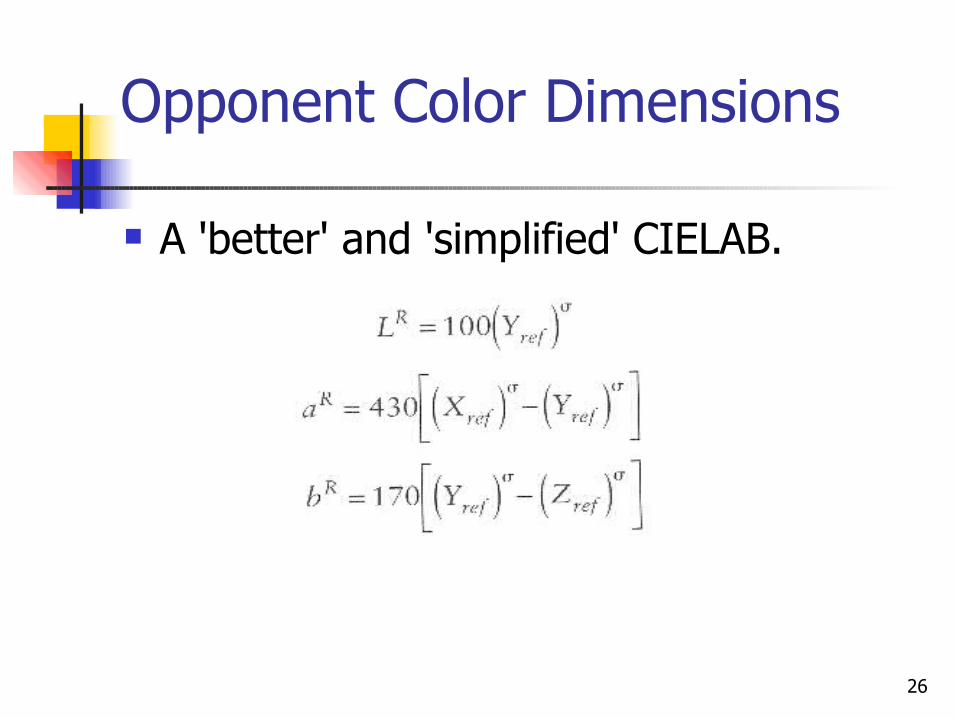
A 'better' and 'simplified' CIELAB.
27
Exponents
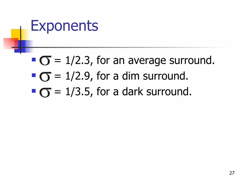
= 1/2.3, for an average surround. = 1/2.9, for a dim surround. = 1/3.5, for a dark surround.
28
Lightness
The RLAB Correlate of lightness is just LR !
29
Hue
Hue Angle, hR = tan-1(bR/aR) Hue Composition, HR - same as before.
30
Chroma and Saturation
CR = { (bR)2 + (aR)2 }1/2
SR = CR/ LR
31
Pros and Cons
Pros Simple. Straightforward. Accurate.
Cons Can't be applied to
really large luminance ranges.
Does not explain Hunt, Stevens model.
32
Thanks!
Related Documents


