Using Small Area Estimation to Produce Official Statistics - MDPI

Citation: Young, L.J.; Chen, L. Using

Small Area Estimation to Produce

Official Statistics. Stats 2022, 5,

881–897. https://doi.org/10.3390/

stats5030051

Academic Editor: Wei Zhu

Received: 20 July 2022

Accepted: 29 August 2022

Published: 8 September 2022

Publisher’s Note: MDPI stays neutral

with regard to jurisdictional claims in

published maps and institutional affil-

iations.

Copyright: © 2022 by the authors.

Licensee MDPI, Basel, Switzerland.

This article is an open access article

distributed under the terms and

conditions of the Creative Commons

Attribution (CC BY) license (https://

creativecommons.org/licenses/by/

4.0/).

Project Report

Using Small Area Estimation to Produce Official StatisticsLinda J. Young 1 and Lu Chen 1,2,*

1 United States Department of Agriculture, National Agricultural Statistics Service,1400 Independence Avenue SW, Washington, DC 20250, USA

2 National Institute of Statistical Sciences, 1750 K Street NW Suite 1100, Washington, DC 20006, USA* Correspondence: [email protected]

Abstract: The USDA National Agricultural Statistics Service (NASS) and other federal statisticalagencies have used probability-based surveys as the foundation for official statistics for over halfa century. Non-survey data that can be used to improve the accuracy and precision of estimatessuch as administrative, remotely sensed, and retail data have become increasingly available. Bothfrequentist and Bayesian models are used to combine survey and non-survey data in a principledmanner. NASS has recently adopted Bayesian subarea models for three of its national programs:farm labor, crop county estimates, and cash rent county estimates. Each program provides valuableestimates at multiple scales of geography. For each program, technical challenges had to be met anda strenuous review completed before models could be adopted as the foundation for official statistics.Moving models out of the research phase into production required major changes in the productionprocess and a cultural shift. With the implemented models, NASS now has measures of uncertainty,transparency, and reproducibility of its official statistics.

Keywords: bayesian hierarchical models; small area estimation; subarea models; data integration;official statistics

1. Introduction

The United States Department of Agriculture (USDA) National Agricultural StatisticsService (NASS), one of thirteen U.S. federal statistical agencies, provides official statisticson all facets of U.S. agriculture including crop and livestock production, acreages plantedto various crops, and prices paid and received. For more than fifty years, NASS hasconducted probability-based surveys. Over time, reliable administrative, remotely sensed,and other non-survey data that can be used to supplement the survey data have becomeincreasingly available. Traditionally, the NASS Agricultural Statistics Board has relied onexpert opinion to produce official statistics using the survey estimates as a foundationinformed by these disparate non-survey data. Although external reviews have consistentlyfound that NASS estimates are the gold standard for the agricultural industry, the processlacked transparency and reproducibility and did not lead to valid measures of uncertainty.

In the early 2000s, NASS, through collaborations with the National Institute of Statisti-cal Sciences, the University of Florida, and the University of Maryland, began exploringthe use of small area estimation as an approach to combine information from surveyand non-survey data to produce estimates with valid measures of uncertainty. In 2014,NASS entered into a cooperative agreement with the Committee on National Statistics(CNSTAT) to review the NASS county estimate programs, crop county estimates, and cashrent county estimates. In its consensus report [1], the CNSTAT panel recommended thatNASS transition to model-based estimates.

Small area models have gained increased attention by federal statistical agencies. Theycan “borrow strength” from related areas across space and/or time or through auxiliaryinformation to provide “indirect” but reliable estimates for small areas with small or evenzero sample sizes while also increasing the precision. Two major types of small area models,

Stats 2022, 5, 881–897. https://doi.org/10.3390/stats5030051 https://www.mdpi.com/journal/stats

Stats 2022, 5 882

area-level and unit-level models, have been developed based on both frequentist andBayesian methods. Pfeffermann [2] and Rao and Molina [3] provided a comprehensiveoverview of the development, methods, and applications of small area estimation includingvarious types of area-level and unit-level models. For continuous responses, the first andmost common model in small area estimation is the Fay–Herriot (FH) model [4]. TheFH model is an area-level model based on a “normal-normal-linear” assumption; that is,the direct estimates and area-level random effects are each assumed to follow a normaldistribution, and a linear regression function relates the true estimates of interest to thecovariates. Battese et al. [5] proposed the popular unit-level model, nested-error regression(NER) model, when data are available on the individual sampled units. In practice, becauseunit-level models generally require substantially more computational time, area-levelmodels are more applicable for the production of official statistics that are published withtight timelines.

In recent years, subarea-level models, which are extensions of area-level models, havebeen used to estimate small area means, not only by borrowing strength from related areas,but also by borrowing strength from subareas, to obtain more efficient subarea estimators,provided that observations are available at both the area and subarea levels. The studiesin Torabi and Rao [6] and Fuller and Goyeneche [7] illustrated frequentist approaches tomodel fitting and estimation for the subarea-level model with known sampling variances.Erciulescu et al. [8] proposed and discussed the subarea-level model using a Bayesianapproach. Because the interest for NASS programs is in constructing summaries fordifferent levels of geography (county, state, regional, and U.S. levels), the Bayesian approachto model fitting and estimation is preferable. Bayesian inference potentially improves theefficiency of estimates because prior information can be incorporated into models based onmodel requirements such as known bounds, and coherency can be enforced across surveys.Furthermore, Bayesian inference is straightforward and exact for obtaining estimates forany known functions of the model parameters.

Based on a rigorous review process of the proposed new methodology, NASS has beenmoving to adopt models for several of its programs. Small area estimation has become thebasis for official statistics in three major programs: farm labor, crop county estimates, andcash rent county estimates. For farm labor, estimates are produced for regions comprised ofadjoining states and the nation. For crop county estimates and cash rent county estimates,estimates are published for counties, states, and the nation. In Section 2, each program’spurpose, survey, and available non-survey data are described. An overview of the smallarea models that have been adopted is provided in Section 3. The process of moving themodels into production is described in Section 4. The final section focuses on the lessonslearned and opportunities for future developments.

2. Survey Programs with Small Area Estimates

The NASS has adopted small area estimation as the basis for publishing estimates forthree programs: farm labor, crop county estimates, and cash rent county estimates. Eachprogram provides valuable official statistics that are used by stakeholders to administerprograms, provide services, or set policy. A probability-based survey serves as the founda-tion for each program, and non-survey data that can inform the estimates are available. Anoverview of each program is provided in this section.

2.1. Farm Labor Program

The NASS has published wage rates for farm labor since 1866, and U.S. farm employ-ment estimates have been published since 1910. The Department of Labor needs reliableagricultural labor data for setting the adverse effect wage rates (AEWR), which is the mini-mum wage that employers of non-immigrant H-2A visa agricultural workers must offerand pay U.S. and alien workers. Currently, the AEWR is set to the annual weighted averagehourly wage rate for field and livestock workers combined. The Department of Laboralso uses the NASS estimates of farm labor wage rates in the administration of the H-2A

Stats 2022, 5 883

program for non-immigrants who enter the U.S. for temporary or seasonal agriculturalwork and to inform setting child labor regulations.

The Farm Labor Survey is conducted semi-annually in April and October in cooper-ation with the U.S. Department of Labor. The target population includes all agriculturaloperations with $1000 or more in annual sales (or potential sales). Data are collected forreference weeks in January and April during the April survey and for reference weeks inJuly and October during the October survey. The reference week is the Sunday to Saturdayperiod that includes the 12th day of the month. The NASS uses a dual frame approachconsisting of list frame and area frame components to provide complete coverage of thistarget population. The farm labor list frame and area frame samples are each selected usinga hierarchical stratified sampling design with strata defined by state and, within the state,by the peak number of farm workers or calculated farm value of sales.

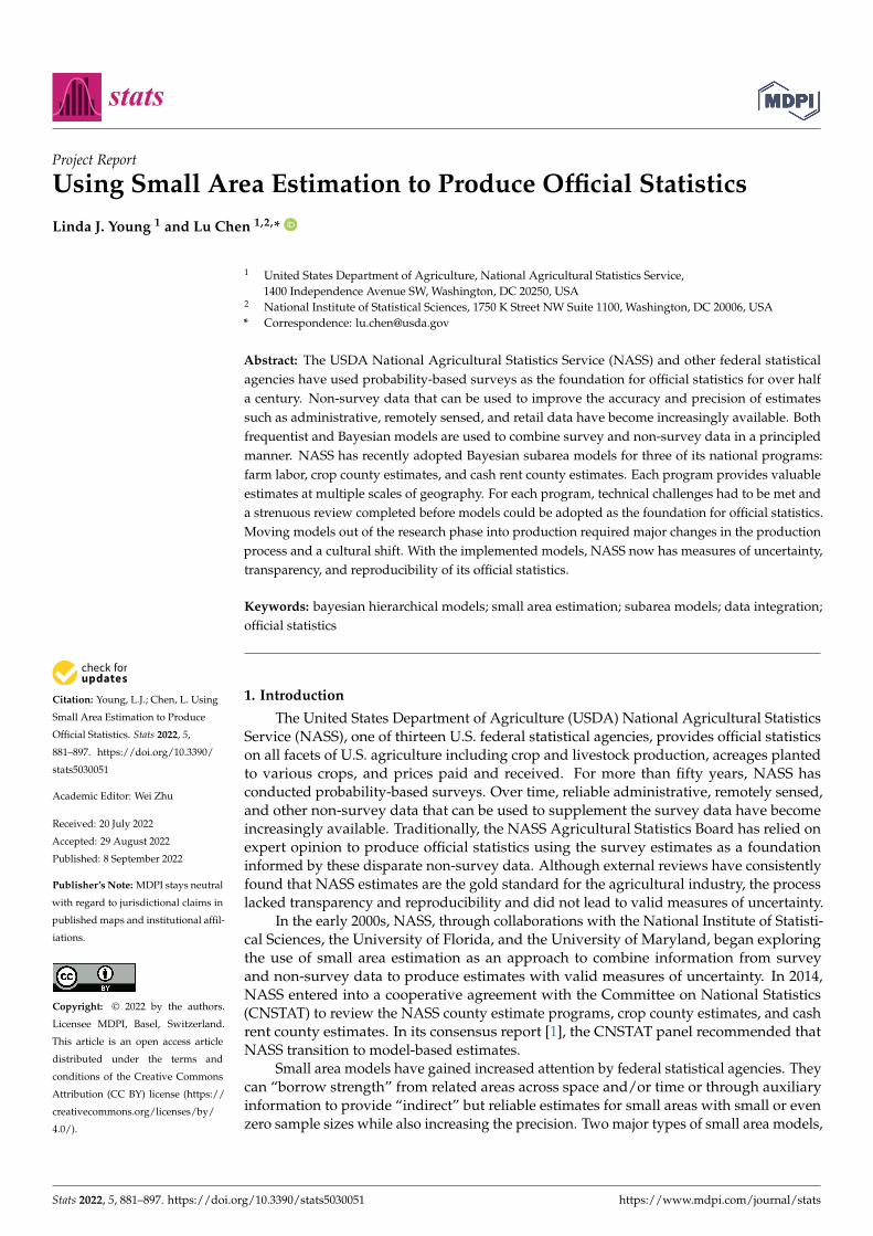
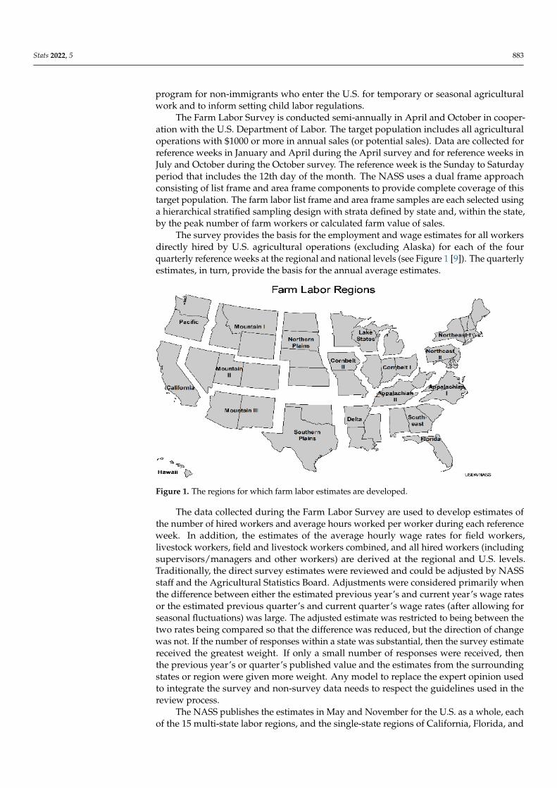
The survey provides the basis for the employment and wage estimates for all workersdirectly hired by U.S. agricultural operations (excluding Alaska) for each of the fourquarterly reference weeks at the regional and national levels (see Figure 1 [9]). The quarterlyestimates, in turn, provide the basis for the annual average estimates.

Stats 2022, 5, FOR PEER REVIEW 3

average hourly wage rate for field and livestock workers combined. The Department of Labor also uses the NASS estimates of farm labor wage rates in the administration of the H-2A program for non-immigrants who enter the U.S. for temporary or seasonal agricul-tural work and to inform setting child labor regulations.

The Farm Labor Survey is conducted semi-annually in April and October in cooper-ation with the U.S. Department of Labor. The target population includes all agricultural operations with $1000 or more in annual sales (or potential sales). Data are collected for reference weeks in January and April during the April survey and for reference weeks in July and October during the October survey. The reference week is the Sunday to Satur-day period that includes the 12th day of the month. The NASS uses a dual frame approach consisting of list frame and area frame components to provide complete coverage of this target population. The farm labor list frame and area frame samples are each selected us-ing a hierarchical stratified sampling design with strata defined by state and, within the state, by the peak number of farm workers or calculated farm value of sales.

The survey provides the basis for the employment and wage estimates for all workers directly hired by U.S. agricultural operations (excluding Alaska) for each of the four quar-terly reference weeks at the regional and national levels (see Figure 1 [9]). The quarterly estimates, in turn, provide the basis for the annual average estimates.

The data collected during the Farm Labor Survey are used to develop estimates of the number of hired workers and average hours worked per worker during each reference week. In addition, the estimates of the average hourly wage rates for field workers, live-stock workers, field and livestock workers combined, and all hired workers (including supervisors/managers and other workers) are derived at the regional and U.S. levels. Tra-ditionally, the direct survey estimates were reviewed and could be adjusted by NASS staff and the Agricultural Statistics Board. Adjustments were considered primarily when the difference between either the estimated previous year’s and current year’s wage rates or the estimated previous quarter’s and current quarter’s wage rates (after allowing for sea-sonal fluctuations) was large. The adjusted estimate was restricted to being between the two rates being compared so that the difference was reduced, but the direction of change was not. If the number of responses within a state was substantial, then the survey esti-mate received the greatest weight. If only a small number of responses were received, then the previous year’s or quarter’s published value and the estimates from the surrounding states or region were given more weight. Any model to replace the expert opinion used to integrate the survey and non-survey data needs to respect the guidelines used in the review process.

Figure 1. The regions for which farm labor estimates are developed. Figure 1. The regions for which farm labor estimates are developed.

The data collected during the Farm Labor Survey are used to develop estimates ofthe number of hired workers and average hours worked per worker during each referenceweek. In addition, the estimates of the average hourly wage rates for field workers,livestock workers, field and livestock workers combined, and all hired workers (includingsupervisors/managers and other workers) are derived at the regional and U.S. levels.Traditionally, the direct survey estimates were reviewed and could be adjusted by NASSstaff and the Agricultural Statistics Board. Adjustments were considered primarily whenthe difference between either the estimated previous year’s and current year’s wage ratesor the estimated previous quarter’s and current quarter’s wage rates (after allowing forseasonal fluctuations) was large. The adjusted estimate was restricted to being between thetwo rates being compared so that the difference was reduced, but the direction of changewas not. If the number of responses within a state was substantial, then the survey estimatereceived the greatest weight. If only a small number of responses were received, thenthe previous year’s or quarter’s published value and the estimates from the surroundingstates or region were given more weight. Any model to replace the expert opinion usedto integrate the survey and non-survey data needs to respect the guidelines used in thereview process.

The NASS publishes the estimates in May and November for the U.S. as a whole, eachof the 15 multi-state labor regions, and the single-state regions of California, Florida, and

Stats 2022, 5 884

Hawaii. In both May and November, the report includes quarterly estimates of the numberof hired workers and average hours worked per worker during each reference week. Italso includes the quarterly estimates of the average hourly wage rates for field workers,livestock workers, field and livestock workers combined, and all hired workers (includingsupervisors/managers and other workers). The November report additionally provides thefollowing annual data based on the quarterly estimates: the average number of workers;the weighted average hours worked per worker; and weighted average hourly wage ratesfor field workers, field and livestock workers combined, and all hired workers.

2.2. Crop County Estimates Program

The NASS began publishing estimates of the final acreages, yield, and production forprincipal crops in 1866 [10]. The quarterly agricultural surveys are conducted to captureactivities throughout the life cycle of the crop including planting intentions (March), earlyestimates of planted acreage (June), and estimates of the harvest and output activities forsmall grains crops (September) and major row crops (December). The annual June areasurvey sample, which is drawn from an area frame, provides an undercoverage adjustmentfor the list-based samples obtained during the September and December agriculturalsurveys. The NASS Agricultural Statistics Board releases the state and national estimatesof the planted and harvested acreages, yield, and production for small grains in lateSeptember and for row crops in January of the following year. These estimates are basedon the coverage-adjusted national and state survey estimates informed by non-survey datasuch as administrative and remotely sensed data.

County-level crop estimates have been produced since 1917 [11]. Although initiallyfederally funded, the program evolved into partnerships with the states via cooperativeagreements. The crop surveys were usually funded by the states, with NASS staff in stateoffices defining the samples, identifying the processes, and developing the estimates. Asthe USDA’s support of the farm sector has evolved so that aid is increasingly conditionedon each producer’s own revenue experience, the NASS initiated the probability-basedcounty agricultural production survey (CAPS) in a few states in 2011, and the remainingeligible states in 2012, to augment the agricultural survey for county-level estimates. TheCAPS list frame sample is stratified by state and drawn using maximal Brewer selectionwith Poisson permanent-random-number (PRN) sampling, which is sometimes referred toas multivariate probability proportional to size (MPPS) sampling [12]. The MPPS designallows for target sample sizes for all commodities of interest to be set at the county level.The agricultural survey and CAPS samples are pooled and reweighted, and the combinedsample is referred to as the CAPS sample. Sampling variances for crop acreage andproduction are estimated using a delete-a-group Jackknife and sampling variances for yieldare estimated using a second order Taylor series approximation for the ratio [12,13]. TheCAPS sample provides survey data with which to estimate the acreages and productionof selected crops at the county level for use in state and federal programs in 44 states.County-level estimates of crop acreage, yield, and production inform many agriculturalsupport and crop insurance programs administered by other USDA agencies including theFarm Service Agency and the Risk Management Agency, which manages the Federal CropInsurance Corporation.

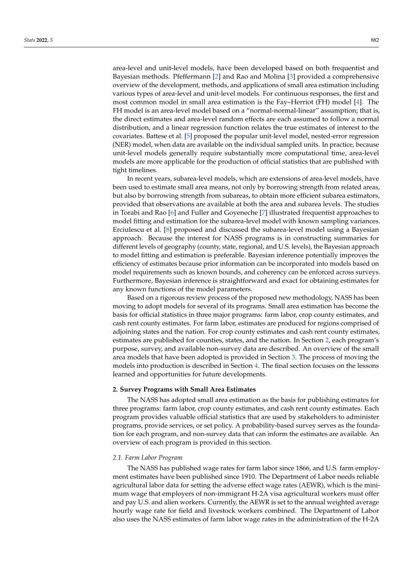
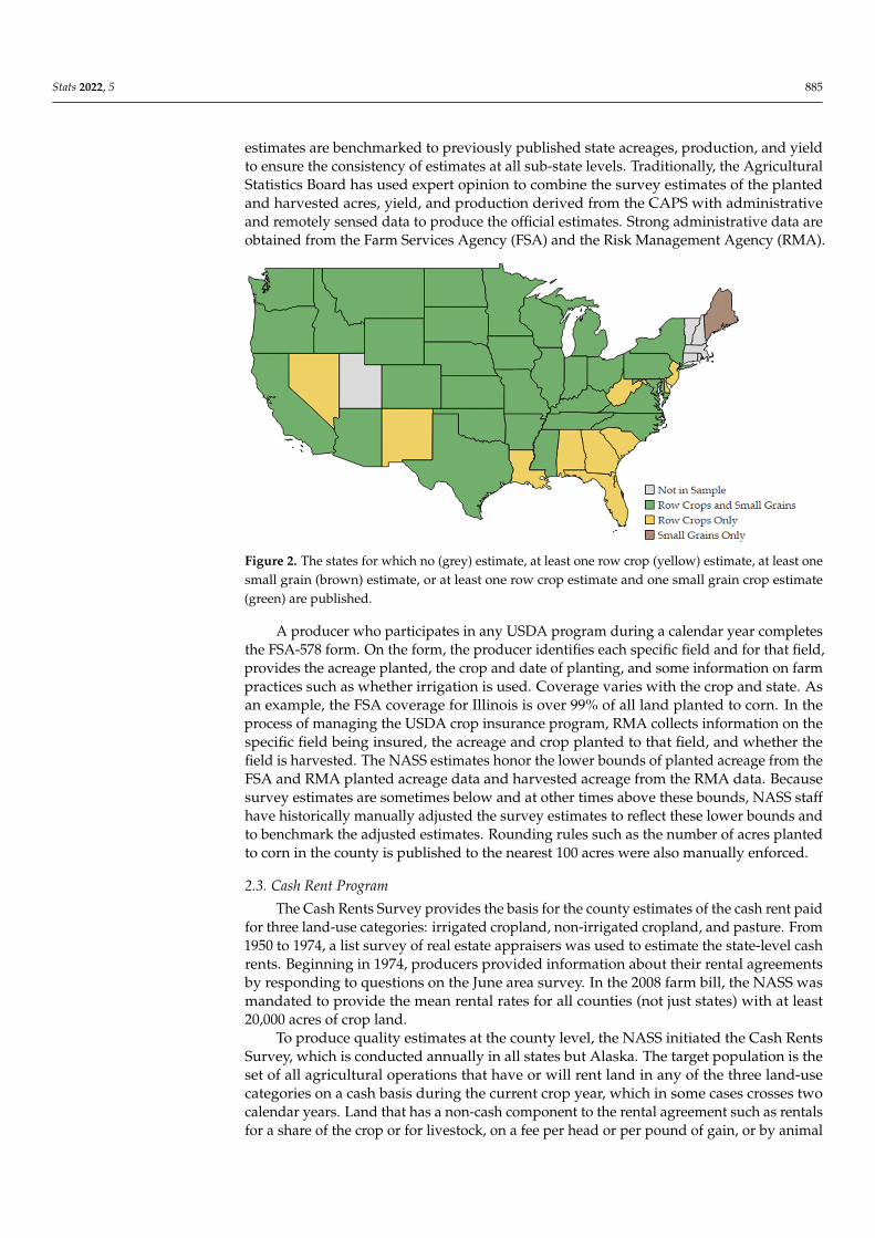
The NASS conducts the row crop CAPSs in 43 states and the small grains CAPSsin 37 states (Figure 2). The commodity crops targeted may differ from state to state andfrom year to year, depending on the required coverage for nationally reported cropsand the needs of other stakeholders such as specific state program commodities. Theofficial county estimates for small grains (e.g., barley, oats and wheat) are published inDecember. The first row crop county estimates for corn, soybeans, sunflower, and sorghumare published in February of the following calendar year. Row crop county estimatesfor additional commodities are subsequently released at intervals, concluding with therelease of the county estimates of potatoes in October. Because the CAPS data collectionextends beyond the release of the national and state-level official statistics, the county

Stats 2022, 5 885

estimates are benchmarked to previously published state acreages, production, and yieldto ensure the consistency of estimates at all sub-state levels. Traditionally, the AgriculturalStatistics Board has used expert opinion to combine the survey estimates of the plantedand harvested acres, yield, and production derived from the CAPS with administrativeand remotely sensed data to produce the official estimates. Strong administrative data areobtained from the Farm Services Agency (FSA) and the Risk Management Agency (RMA).

Stats 2022, 5, FOR PEER REVIEW 5

the county estimates of potatoes in October. Because the CAPS data collection extends beyond the release of the national and state-level official statistics, the county estimates are benchmarked to previously published state acreages, production, and yield to ensure the consistency of estimates at all sub-state levels. Traditionally, the Agricultural Statistics Board has used expert opinion to combine the survey estimates of the planted and har-vested acres, yield, and production derived from the CAPS with administrative and re-motely sensed data to produce the official estimates. Strong administrative data are ob-tained from the Farm Services Agency (FSA) and the Risk Management Agency (RMA).

A producer who participates in any USDA program during a calendar year com-pletes the FSA-578 form. On the form, the producer identifies each specific field and for that field, provides the acreage planted, the crop and date of planting, and some infor-mation on farm practices such as whether irrigation is used. Coverage varies with the crop and state. As an example, the FSA coverage for Illinois is over 99% of all land planted to corn. In the process of managing the USDA crop insurance program, RMA collects infor-mation on the specific field being insured, the acreage and crop planted to that field, and whether the field is harvested. The NASS estimates honor the lower bounds of planted acreage from the FSA and RMA planted acreage data and harvested acreage from the RMA data. Because survey estimates are sometimes below and at other times above these bounds, NASS staff have historically manually adjusted the survey estimates to reflect these lower bounds and to benchmark the adjusted estimates. Rounding rules such as the number of acres planted to corn in the county is published to the nearest 100 acres were also manually enforced.

Figure 2. The states for which no (grey) estimate, at least one row crop (yellow) estimate, at least one small grain (brown) estimate, or at least one row crop estimate and one small grain crop estimate (green) are published.

2.3. Cash Rent Program The Cash Rents Survey provides the basis for the county estimates of the cash rent

paid for three land-use categories: irrigated cropland, non-irrigated cropland, and pas-ture. From 1950 to 1974, a list survey of real estate appraisers was used to estimate the state-level cash rents. Beginning in 1974, producers provided information about their rental agreements by responding to questions on the June area survey. In the 2008 farm bill, the NASS was mandated to provide the mean rental rates for all counties (not just states) with at least 20,000 acres of crop land.

To produce quality estimates at the county level, the NASS initiated the Cash Rents Survey, which is conducted annually in all states but Alaska. The target population is the set of all agricultural operations that have or will rent land in any of the three land-use

Figure 2. The states for which no (grey) estimate, at least one row crop (yellow) estimate, at least onesmall grain (brown) estimate, or at least one row crop estimate and one small grain crop estimate(green) are published.

A producer who participates in any USDA program during a calendar year completesthe FSA-578 form. On the form, the producer identifies each specific field and for that field,provides the acreage planted, the crop and date of planting, and some information on farmpractices such as whether irrigation is used. Coverage varies with the crop and state. Asan example, the FSA coverage for Illinois is over 99% of all land planted to corn. In theprocess of managing the USDA crop insurance program, RMA collects information on thespecific field being insured, the acreage and crop planted to that field, and whether thefield is harvested. The NASS estimates honor the lower bounds of planted acreage from theFSA and RMA planted acreage data and harvested acreage from the RMA data. Becausesurvey estimates are sometimes below and at other times above these bounds, NASS staffhave historically manually adjusted the survey estimates to reflect these lower bounds andto benchmark the adjusted estimates. Rounding rules such as the number of acres plantedto corn in the county is published to the nearest 100 acres were also manually enforced.

2.3. Cash Rent Program

The Cash Rents Survey provides the basis for the county estimates of the cash rent paidfor three land-use categories: irrigated cropland, non-irrigated cropland, and pasture. From1950 to 1974, a list survey of real estate appraisers was used to estimate the state-level cashrents. Beginning in 1974, producers provided information about their rental agreementsby responding to questions on the June area survey. In the 2008 farm bill, the NASS wasmandated to provide the mean rental rates for all counties (not just states) with at least20,000 acres of crop land.

To produce quality estimates at the county level, the NASS initiated the Cash RentsSurvey, which is conducted annually in all states but Alaska. The target population is theset of all agricultural operations that have or will rent land in any of the three land-usecategories on a cash basis during the current crop year, which in some cases crosses twocalendar years. Land that has a non-cash component to the rental agreement such as rentalsfor a share of the crop or for livestock, on a fee per head or per pound of gain, or by animal

Stats 2022, 5 886

unit month, is excluded. Land that is rented free of charge or includes buildings is alsoexcluded. The Cash Rent Survey sample of about 225,000 agricultural operations is drawnfrom the NASS list frame, which is a list of all known U.S. farms. The sample is stratifiedby state and county within the state to produce state and county-level estimates. Datacollection occurs from late February until the end of June. Variances for cash rental rateestimates are constructed using a second-order Taylor series expansion for the ratio.

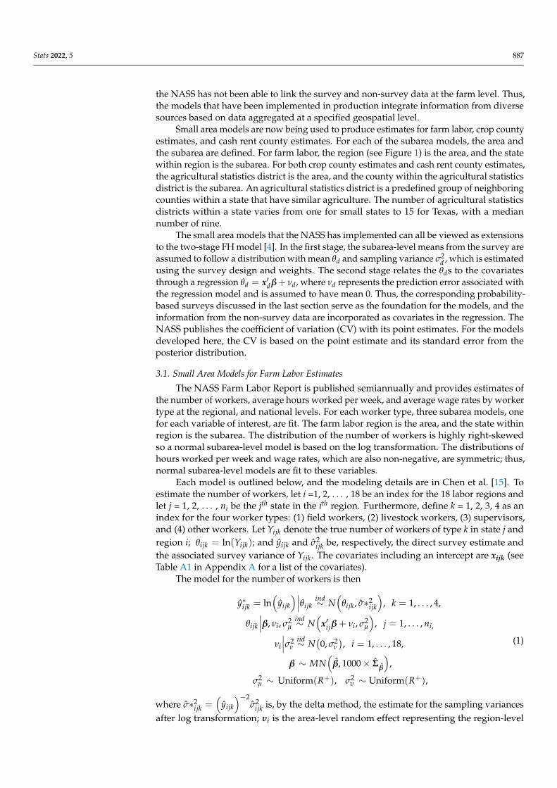
From the Cash Rents Survey, the county, state, and national rental rates ($/acre)for each land-use category (irrigated, non-irrigated, and pasture) are published (seeFigure 3 [14] for the 2021 state-level published cash rental rate estimates for non-irrigated land).

Stats 2022, 5, FOR PEER REVIEW 6

categories on a cash basis during the current crop year, which in some cases crosses two calendar years. Land that has a non-cash component to the rental agreement such as rent-als for a share of the crop or for livestock, on a fee per head or per pound of gain, or by animal unit month, is excluded. Land that is rented free of charge or includes buildings is also excluded. The Cash Rent Survey sample of about 225,000 agricultural operations is drawn from the NASS list frame, which is a list of all known U.S. farms. The sample is stratified by state and county within the state to produce state and county-level estimates. Data collection occurs from late February until the end of June. Variances for cash rental rate estimates are constructed using a second-order Taylor series expansion for the ratio.

From the Cash Rents Survey, the county, state, and national rental rates ($/acre) for each land-use category (irrigated, non-irrigated, and pasture) are published (see Figure 3 [14] for the 2021 state-level published cash rental rate estimates for non-irrigated land).

Figure 3. The state-level published estimates of the cash rental rate for non-irrigated cropland meas-ured in $/acre in 2021.

Although the total value of cash rents and acres rented on a cash basis are computed, these values have not been published. Historically, the direct survey estimates were re-viewed and, if deemed appropriate, adjusted by the NASS staff or the Agricultural Statis-tics Board. The primary reason for adjustment was a large difference between the previous year’s published cash rental rate and the current year’s survey estimate. The adjusted es-timate was restricted to being between, or on, the current survey estimate and the previ-ous year’s published estimate so that the direction of change was honored. If the number of responses within a county was substantial, then the survey estimate received the great-est weight. If only a small number of responses was received, then the previous year’s published value and the estimates from surrounding counties or the agricultural statistics district were given more weight. Any model to replace the expert opinion needs to follow the guidelines used in the review process.

The NASS releases estimates for counties in August. Of the 3112 counties in the U.S. excluding Alaska, 2758 (88.6%) had 20,000 or more acres of combined cropland and pas-ture at the time of the 2017 Census of Agriculture. Each year, the NASS has published at least one county estimate of the cash rental rate in 93 to 95% of the target counties, but some land-use practices may be underserved.

Figure 3. The state-level published estimates of the cash rental rate for non-irrigated croplandmeasured in $/acre in 2021.

Although the total value of cash rents and acres rented on a cash basis are computed,these values have not been published. Historically, the direct survey estimates werereviewed and, if deemed appropriate, adjusted by the NASS staff or the AgriculturalStatistics Board. The primary reason for adjustment was a large difference between theprevious year’s published cash rental rate and the current year’s survey estimate. Theadjusted estimate was restricted to being between, or on, the current survey estimate andthe previous year’s published estimate so that the direction of change was honored. If thenumber of responses within a county was substantial, then the survey estimate receivedthe greatest weight. If only a small number of responses was received, then the previousyear’s published value and the estimates from surrounding counties or the agriculturalstatistics district were given more weight. Any model to replace the expert opinion needsto follow the guidelines used in the review process.

The NASS releases estimates for counties in August. Of the 3112 counties in the U.S.excluding Alaska, 2758 (88.6%) had 20,000 or more acres of combined cropland and pastureat the time of the 2017 Census of Agriculture. Each year, the NASS has published at leastone county estimate of the cash rental rate in 93 to 95% of the target counties, but someland-use practices may be underserved.

3. Small Area Models

When integrating survey and non-survey data, two basic approaches are used. Oneaggregates information from each source at a specified geographic level such as a county,and then combines the information through modeling. The other links data from diversesources at the record level and then develops the model of interest. As discussed in Section 5,

Stats 2022, 5 887

the NASS has not been able to link the survey and non-survey data at the farm level. Thus,the models that have been implemented in production integrate information from diversesources based on data aggregated at a specified geospatial level.

Small area models are now being used to produce estimates for farm labor, crop countyestimates, and cash rent county estimates. For each of the subarea models, the area andthe subarea are defined. For farm labor, the region (see Figure 1) is the area, and the statewithin region is the subarea. For both crop county estimates and cash rent county estimates,the agricultural statistics district is the area, and the county within the agricultural statisticsdistrict is the subarea. An agricultural statistics district is a predefined group of neighboringcounties within a state that have similar agriculture. The number of agricultural statisticsdistricts within a state varies from one for small states to 15 for Texas, with a mediannumber of nine.

The small area models that the NASS has implemented can all be viewed as extensionsto the two-stage FH model [4]. In the first stage, the subarea-level means from the survey areassumed to follow a distribution with mean θd and sampling variance σ2

d , which is estimatedusing the survey design and weights. The second stage relates the θds to the covariatesthrough a regression θd = x′dβ+ νd, where νd represents the prediction error associated withthe regression model and is assumed to have mean 0. Thus, the corresponding probability-based surveys discussed in the last section serve as the foundation for the models, and theinformation from the non-survey data are incorporated as covariates in the regression. TheNASS publishes the coefficient of variation (CV) with its point estimates. For the modelsdeveloped here, the CV is based on the point estimate and its standard error from theposterior distribution.

3.1. Small Area Models for Farm Labor Estimates

The NASS Farm Labor Report is published semiannually and provides estimates ofthe number of workers, average hours worked per week, and average wage rates by workertype at the regional, and national levels. For each worker type, three subarea models, onefor each variable of interest, are fit. The farm labor region is the area, and the state withinregion is the subarea. The distribution of the number of workers is highly right-skewedso a normal subarea-level model is based on the log transformation. The distributions ofhours worked per week and wage rates, which are also non-negative, are symmetric; thus,normal subarea-level models are fit to these variables.

Each model is outlined below, and the modeling details are in Chen et al. [15]. Toestimate the number of workers, let i =1, 2, . . . , 18 be an index for the 18 labor regions andlet j = 1, 2, . . . , ni be the jth state in the ith region. Furthermore, define k = 1, 2, 3, 4 as anindex for the four worker types: (1) field workers, (2) livestock workers, (3) supervisors,and (4) other workers. Let Yijk denote the true number of workers of type k in state j andregion i; θijk = ln(Yijk); and yijk and σ2

ijk be, respectively, the direct survey estimate andthe associated survey variance of Yijk. The covariates including an intercept are xijk (seeTable A1 in Appendix A for a list of the covariates).

The model for the number of workers is then

y∗ijk = ln(

yijk

)∣∣∣θijkind∼ N

(θijk, σ∗2

ijk

), k = 1, . . . , 4,

θijk

∣∣∣β, νi, σ2µ

ind∼ N(

x′ijβ + νi, σ2µ

), j = 1, . . . , ni,

νi

∣∣∣σ2ν

iid∼ N(0, σ2

ν

), i = 1, . . . , 18,

β ∼ MN(

β, 1000× Σβ

),

σ2µ ∼ Uniform(R+), σ2

υ ∼ Uniform(R+),

(1)

where σ∗2ijk =

(yijk

)−2σ2

ijk is, by the delta method, the estimate for the sampling variancesafter log transformation; υi is the area-level random effect representing the region-level

Stats 2022, 5 888

variability; β and^Σβ are, respectively, the least squares estimates of β and the estimated

covariance matrix of β; and R+ represents the positive real numbers. The uniform priorsfor scale parameters σ2

µ and σ2υ are motived by Gelman [16] and Browne and Draper [17].

The uniform prior on the real line is functionally equivalent to a proper U(0,1/ε) prior forvery small ε.

After obtaining the posterior distribution of θijk, the estimators Ywkijk = exp

(θijk

),

where wk represents the number of workers, follow from back transformation and are usedto obtain the posterior means and measures of uncertainty for the number of workers byeach worker type. The aggregated regional level posterior summaries for the number ofworkers by different worker types are obtained based on state-level MCMC samples (seeChen et al. [15] for details).

Because the distributions of the average hours worked per week and the averagewage rate per hour are symmetric, a normal subarea model is applied to each of theseresponse variables.

yijk

∣∣∣θijkind∼ N

(θijk, σ2

ijk

), k = 1, . . . , 4

θijk

∣∣∣β, νi, σ2µ

ind∼ N(

x′ijβ + νi, σ2µ

), j = 1, . . . , ni

νi

∣∣∣σ2ν

ind∼ N(0, σ2

ν

), i = 1, . . . , 18

β ∼ MN(

β, 1000× Σβ

),

σ2µ ∼ Uniform(R+), σ2

ν ∼ Uniform(R+).

(2)

As in the lognormal subarea model, νi is the area-level random effect representing theregion-level variability; the coefficients of β have an empirical diffuse prior; and the priordistributions for σ2

µ and σ2ν are noninformative uniform priors (see Table A1, Appendix A

for a list of the model covariates).After obtaining the posterior distribution of θijk, for S ∈ {hr, wg}, where hr and wg

represent average hours worked per week and average wage per hour, respectively, theestimators YS

ijk = θijk follow from the identity transformation and are used to obtain theposterior means and measures of uncertainty for hr and wg by each worker type. Theaggregated regional level posterior summaries for hours and wage rate by different workertypes are obtained conditional on the state-level MCMC samples of the number of workers(see Chen et al. [15]).

The detailed model evaluations including model effectiveness, model efficiency, anda comparison between survey estimates and subarea model estimates can be found inChen et al. [15]. Furthermore, a 2020 case study illustrates the improvement in the directestimates for areas with small sample sizes by using auxiliary information and borrowinginformation across areas and subareas.

3.2. Small Area Models for Crop County Estimates

In the Crop County Estimates program, estimates of the planted and harvested acres,yield and production for each county in the target population of a specified crop areproduced. Production (or yield) can be derived from the yield (or production) and harvestedacres as the product of yield and harvested acres (or the ratio of production to harvestedacres). Thus, only three models are needed: (1) planted acres, (2) harvested acres, and(3) yield or production. Reflecting the agricultural process, the model for planted acres ismodeled first. The harvested acres model is modeled next and must reflect two constraints:(1) If the acres planted to the specified crop is zero, then the number of harvested acres iszero; and (2) the number of acres harvested can be no more than the number of plantedacres. Because the number of planted acres can vary widely from farm to farm with afew farms planting many more acres than the majority of the others, production tendsto be highly skewed whereas yield tends to be more normally distributed. Therefore, a

Stats 2022, 5 889

yield model was developed, and production was derived from the estimates of the yieldand harvested acres. Of course, yield and production must be zero if no acres are plantedor harvested.

All crop county estimates must honor two constraints that follow from the availableinformation. First, the state and U.S. estimates of the planted and harvested acres, yield,and production are published before the county estimates of those same quantities, and thestate estimates are coherent with the national estimates; that is, the estimated state-levelnumbers of the planted and harvested acres and production sum to the published U.S.estimates. To maintain coherence in the estimates, the estimates of the planted and har-vested acres and production for counties within a state must total the state-level estimates.Ratio benchmarking similar to that of Nandram and Sayit [18] enforces this coherence.Second, the yield, as the ratio of production to harvested acres, needs to aggregate tothe corresponding state-level estimates. The study by Erciulescu et al. [19] explored thepreservation of triplet relationships among the numerator totals, denominator totals, andtheir ratios for two nested, smaller-than-state geographies.

Erciulescu et al. [8] suggested a subarea model for planted acres and applied ratiobenchmarking. The area is an agricultural statistics district, and a county within a districtis the subarea.

Let θij be the number of planted acres in county j = 1, 2, . . . , nci, within agriculturalstatistics district i = 1, 2, . . . , m. Furthermore, let the county sample size be nij and θij bethe direct survey estimate with the estimated sampling variance σ2

ij. The total number

of counties in a state is ∑mi=1 nci = nc, and the state sample size is ∑m

i=1 ∑nij=1 nci = n.

The county-level auxiliary information is xij (see Table A2, Appendix A for a list of themodel covariates). Further assume that the county-level random effects have independent,normal distributions with mean 0 and variance σ2

µ and the district-level random effects areindependent, normally distributed with mean 0 and variance σ2

ν . Then,

θij

∣∣∣θijind∼ N

(θij, σ2

ij

), i = 1, . . . , m; j = 1, . . . , ni,

θij

∣∣∣β,νi, σ2µ

ind∼ N(

x′ijβ + νi, σ2µ

),

νi

∣∣∣σ2ν

iid∼ N(0, σ2

ν

),

β ∼ MN(

β, 1000× Σβ

),

σ2µ ∼ Uniform

(0, 108), σ2

υ ∼ Uniform(0, 108).

(3)

The prior distribution for the model parameter β is a normal distribution with meanand variance being the least squares estimates of β. With known σ2

ij and with no district-level effects νi, Model (1) reduces to the FH area-level model [4].

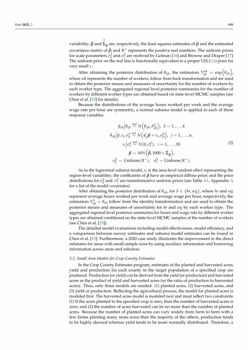
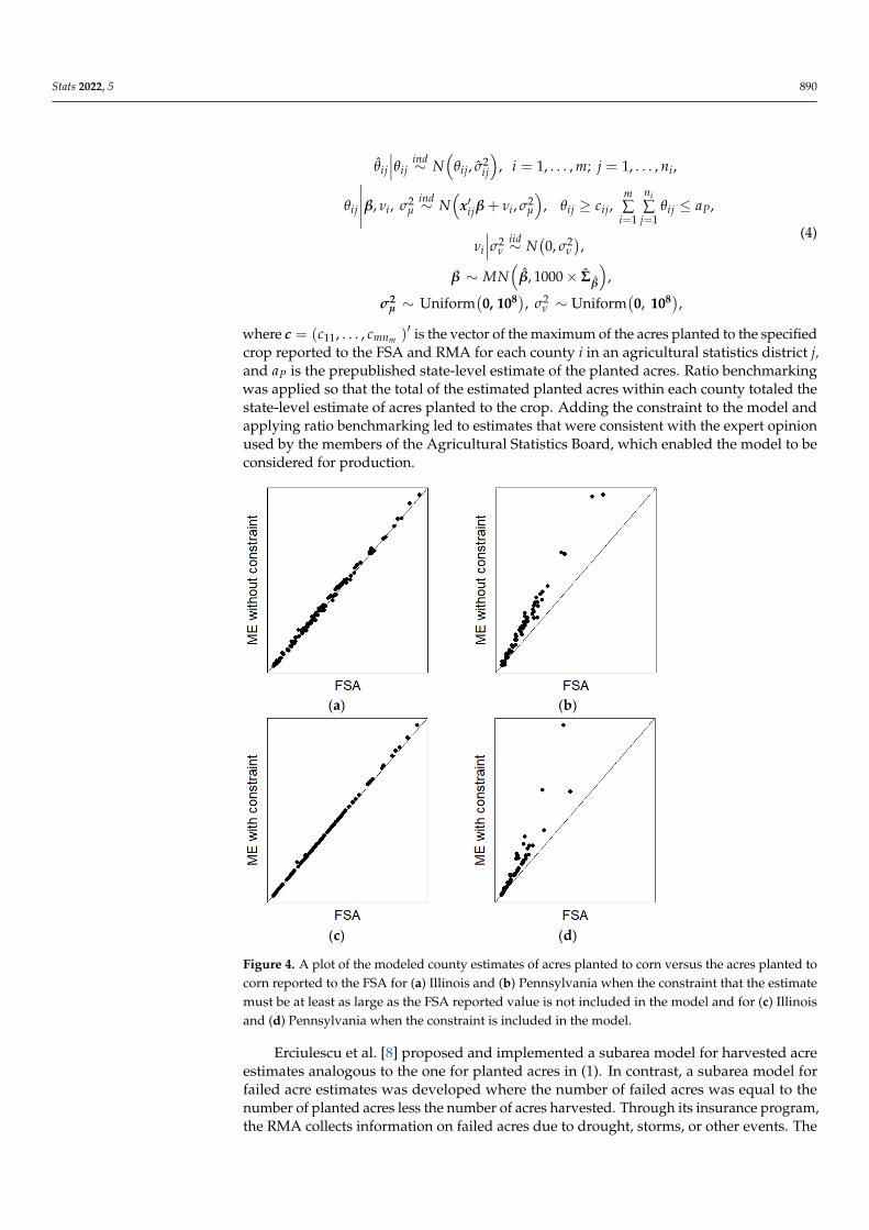
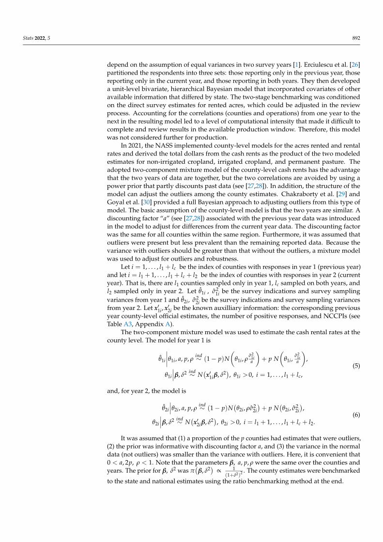
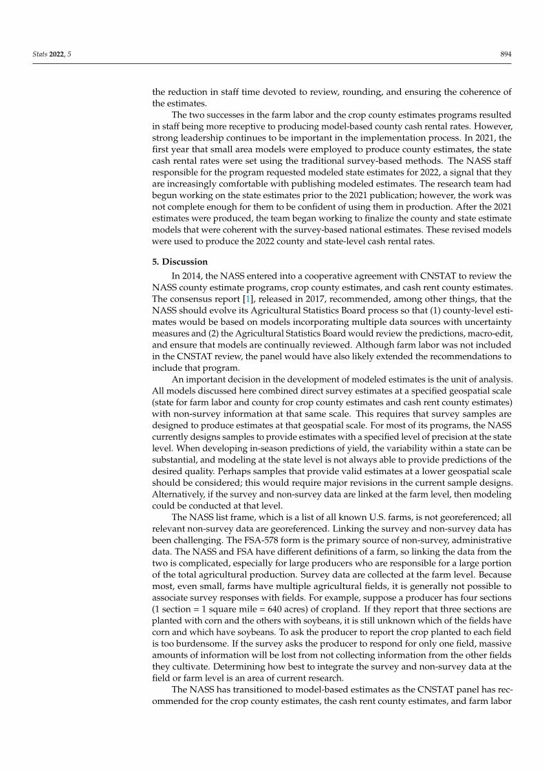
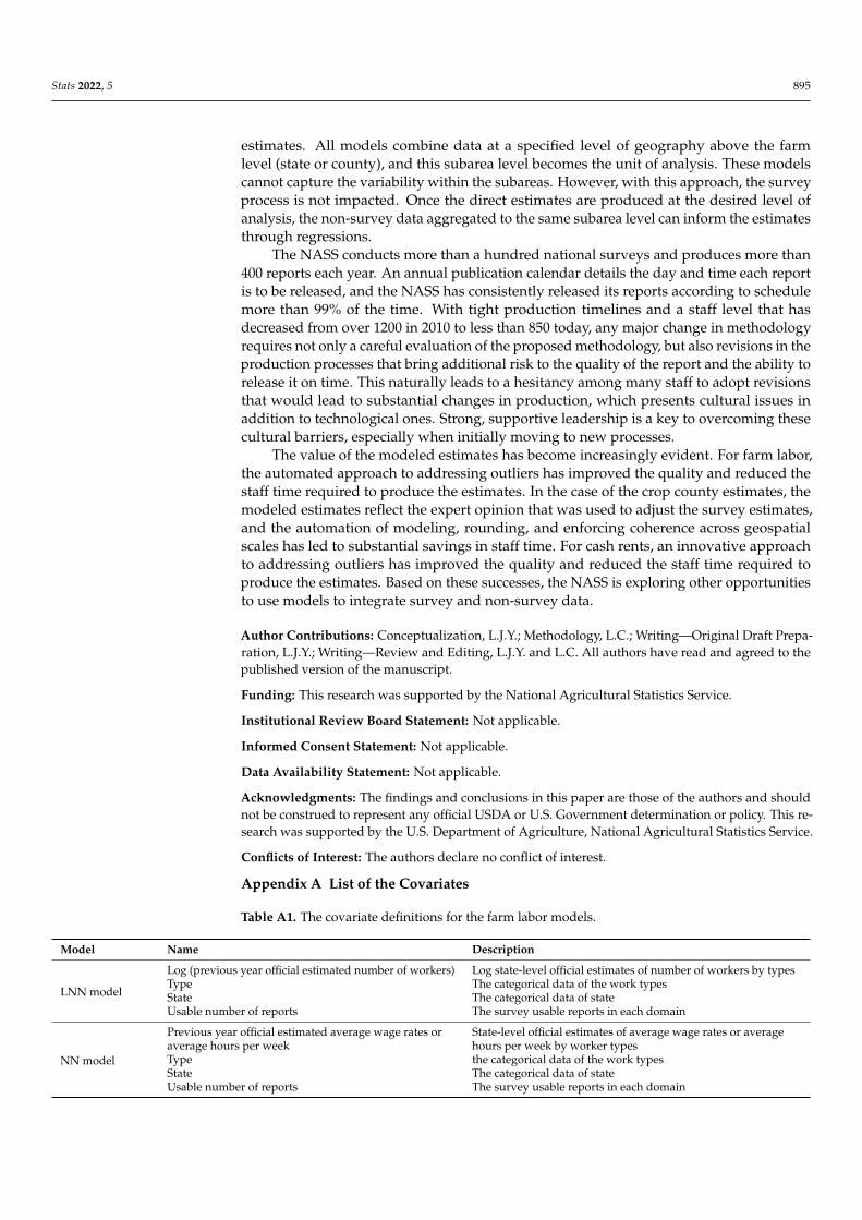
The number of acres planted to a specified crop within a county is at least as largeas the number of acres that the producers reported to either the FSA or RMA as havingbeen planted in that county. Often, the direct survey estimate of planted acres for a countyis above this lower bound, but due to sampling variation, this is not always the case(see Figure 4). The NASS has long used expert opinion to ensure that this lower boundwas honored. Developing the methodology to enforce this lower bound within (1) wastechnically challenging. Nandram et al. [20] and Chen et al. [21] proposed and implementedthe constrained model (4) for planted acres.

Stats 2022, 5 890

θij

∣∣∣θijind∼ N

(θij, σ2

ij

), i = 1, . . . , m; j = 1, . . . , ni,

θij

∣∣∣∣∣β, νi, σ2µ

ind∼ N(

x′ijβ + νi, σ2µ

), θij ≥ cij,

m∑

i=1

ni∑

j=1θij ≤ aP,

νi

∣∣∣σ2ν

iid∼ N(0, σ2

ν

),

β ∼ MN(

β, 1000× Σβ

),

σ2µ ∼ Uniform

(0, 108), σ2

ν ∼ Uniform(0, 108),

(4)

where c = (c11, . . . , cmnm )′ is the vector of the maximum of the acres planted to the specifiedcrop reported to the FSA and RMA for each county i in an agricultural statistics district j,and aP is the prepublished state-level estimate of the planted acres. Ratio benchmarkingwas applied so that the total of the estimated planted acres within each county totaled thestate-level estimate of acres planted to the crop. Adding the constraint to the model andapplying ratio benchmarking led to estimates that were consistent with the expert opinionused by the members of the Agricultural Statistics Board, which enabled the model to beconsidered for production.

Stats 2022, 5, FOR PEER REVIEW 10

where 𝒄 = 𝑐 , . . . , 𝑐 is the vector of the maximum of the acres planted to the speci-fied crop reported to the FSA and RMA for each county i in an agricultural statistics dis-trict j, and 𝑎 is the prepublished state-level estimate of the planted acres. Ratio bench-marking was applied so that the total of the estimated planted acres within each county totaled the state-level estimate of acres planted to the crop. Adding the constraint to the model and applying ratio benchmarking led to estimates that were consistent with the expert opinion used by the members of the Agricultural Statistics Board, which enabled the model to be considered for production.

Erciulescu et al. [8] proposed and implemented a subarea model for harvested acre estimates analogous to the one for planted acres in (1). In contrast, a subarea model for failed acre estimates was developed where the number of failed acres was equal to the number of planted acres less the number of acres harvested. Through its insurance pro-gram, the RMA collects information on failed acres due to drought, storms, or other events. The number of acres reported as having failed within a county provides a lower bound for that county’s number of failed acres, which is the difference in the number of acres planted and those harvested. Thus, conditioned on the model-based planted acre estimates, the model incorporated a constraint to honor the lower bound of failed acres obtained from the RMA administrative data, and the model-based harvested acre esti-mates can be derived from the planted acre and failed acre estimates. In such a model setting, the two relationships, (i) between planted acres and harvested acres and (ii) be-tween the model-based failed acres and RMA administrative failed acres can be satisfied. In the end, ratio benchmarking was applied so that the total of the estimated harvested acres within each county totaled the state-level estimate of acres harvested to the crop.

(a) (b)

(c) (d)

Figure 4. A plot of the modeled county estimates of acres planted to corn versus the acres planted to corn reported to the FSA for (a) Illinois and (b) Pennsylvania when the constraint that the estimate must be at least as large as the FSA reported value is not included in the model and for (c) Illinois and (d) Pennsylvania when the constraint is included in the model.

Figure 4. A plot of the modeled county estimates of acres planted to corn versus the acres planted tocorn reported to the FSA for (a) Illinois and (b) Pennsylvania when the constraint that the estimatemust be at least as large as the FSA reported value is not included in the model and for (c) Illinoisand (d) Pennsylvania when the constraint is included in the model.

Erciulescu et al. [8] proposed and implemented a subarea model for harvested acreestimates analogous to the one for planted acres in (1). In contrast, a subarea model forfailed acre estimates was developed where the number of failed acres was equal to thenumber of planted acres less the number of acres harvested. Through its insurance program,the RMA collects information on failed acres due to drought, storms, or other events. The

Stats 2022, 5 891

number of acres reported as having failed within a county provides a lower bound for thatcounty’s number of failed acres, which is the difference in the number of acres planted andthose harvested. Thus, conditioned on the model-based planted acre estimates, the modelincorporated a constraint to honor the lower bound of failed acres obtained from the RMAadministrative data, and the model-based harvested acre estimates can be derived fromthe planted acre and failed acre estimates. In such a model setting, the two relationships,(i) between planted acres and harvested acres and (ii) between the model-based failed acresand RMA administrative failed acres can be satisfied. In the end, ratio benchmarking wasapplied so that the total of the estimated harvested acres within each county totaled thestate-level estimate of acres harvested to the crop.

The subarea models for yield are of the same form as model (1) with θij and σ2ij

representing the direct survey estimates of yield and its associated sampling variance,respectively, for county i within agricultural statistics district j. The National CommodityCrop Productivity Indices (NCCPIs), which measure the quality of the soil for growingnon-irrigated crops in climate conditions best suited for corn (NCCPI-corn), wheat (NCCPI-wheat), and cotton (NCCPI-cotton), are incorporated as covariates in x′ij. The mean andvariance of the posterior distribution of the yield θij are, respectively, the modeled estimateof the yield of county i in agricultural statistics district j and its estimated variability.

It is worth noting that some sampling variances are not stable or are unavailabledue to zero or small sample sizes for certain counties, which differ with commodity.Erciulescu et al. [22] discussed the challenges of missing data when fitting the subarea levelmodel to obtain the crop total estimates for the whole nation. A nearest neighbor imputationmethod was proposed to impute missing data including the missing sampling variances.In addition, an approach based on Taylor’s approximation and Bayesian modeling wasapplied to smooth unstable, modeled sampling variances (see [23]).

Detailed model evaluations in terms of effectiveness and model efficiency have beenconducted. For instance, Nandram et al. [20] showed how to incorporate the area-specificinequality constraints and benchmarking into the Fay–Herriot model using simulateddatasets with properties resembling an Illinois corn crop. Chen et al. [21] examined theperformance of the model with inequality constraints and, through a case study, illustratedthe improvement in the county-level estimates in terms of accuracy and precision whilepreserving the required relationships. Erciulescu et al. [19] discussed the yield model anddifferent methods of applying benchmarking constraints to a triplet (numerator, denomi-nator, ratio) and illustrated results for 2014 for corn and soybeans in Indiana, Iowa, andIllinois. Based on these results, small area models implemented in crop county estimatesfor total acre and yield estimates provide accurate indirect estimates while improvingthe precision.

3.3. Small Area Models for Cash Rent County Estimates

The Agricultural Statistics Board began using a univariate area-level model for cashrental rates in 2013 [24]. The model was based on the average and change in the current andprevious years’ cash rental rates for county i, which are orthogonal under the normalityassumption. Information on the total value of agricultural production, the published county-level crop yield estimates, and the NCCPIs were incorporated into the model. Two-stagebenchmarking [25] was used to ensure coherence in the estimates at the county, agriculturalstatistics district, state, and national levels. However, the two-stage benchmarking led to afew negative estimates. The model did not provide estimates of the total value from thecash rentals or the total land rented, both of which are important for assessing coverage,which is a published metric of quality. Furthermore, the modeling assumption of equalityof variances in the two years is not always appropriate, and the survey outliers impact theestimates in two years, not just one. Thus, although the modeled estimates were reviewedby the Agricultural Statistics Board, they were not used as the foundation for publication.

In its review, the CNSTAT panel recommended that the NASS develops a bivariate,unit-level hierarchical Bayesian model to estimate the county-level cash rents that do not

Stats 2022, 5 892

depend on the assumption of equal variances in two survey years [1]. Erciulescu et al. [26]partitioned the respondents into three sets: those reporting only in the previous year, thosereporting only in the current year, and those reporting in both years. They then developeda unit-level bivariate, hierarchical Bayesian model that incorporated covariates of otheravailable information that differed by state. The two-stage benchmarking was conditionedon the direct survey estimates for rented acres, which could be adjusted in the reviewprocess. Accounting for the correlations (counties and operations) from one year to thenext in the resulting model led to a level of computational intensity that made it difficult tocomplete and review results in the available production window. Therefore, this modelwas not considered further for production.

In 2021, the NASS implemented county-level models for the acres rented and rentalrates and derived the total dollars from the cash rents as the product of the two modeledestimates for non-irrigated cropland, irrigated cropland, and permanent pasture. Theadopted two-component mixture model of the county-level cash rents has the advantagethat the two years of data are together, but the two correlations are avoided by using apower prior that partly discounts past data (see [27,28]). In addition, the structure of themodel can adjust the outliers among the county estimates. Chakraborty et al. [29] andGoyal et al. [30] provided a full Bayesian approach to adjusting outliers from this type ofmodel. The basic assumption of the county-level model is that the two years are similar. Adiscounting factor “a” (see [27,28]) associated with the previous year data was introducedin the model to adjust for differences from the current year data. The discounting factorwas the same for all counties within the same region. Furthermore, it was assumed thatoutliers were present but less prevalent than the remaining reported data. Because thevariance with outliers should be greater than that without the outliers, a mixture modelwas used to adjust for outliers and robustness.

Let i = 1, . . . , l1 + lc be the index of counties with responses in year 1 (previous year)and let i = l1 + 1, . . . , l1 + lc + l2 be the index of counties with responses in year 2 (currentyear). That is, there are l1 counties sampled only in year 1, lc sampled on both years, andl2 sampled only in year 2. Let θ1i , σ2

1i be the survey indications and survey samplingvariances from year 1 and θ2i, σ2

2i be the survey indications and survey sampling variancesfrom year 2. Let x′1i, x′2i be the known auxilliary information: the corresponding previousyear county-level official estimates, the number of positive responses, and NCCPIs (seeTable A3, Appendix A).

The two-component mixture model was used to estimate the cash rental rates at thecounty level. The model for year 1 is

θ1i

∣∣∣∣θ1i, a, p, ρind∼ (1− p)N

(θ1i, ρ

σ21ia

)+ p N

(θ1i,

σ21ia

),

θ1i

∣∣∣β, δ2 ind∼ N(x′1iβ, δ2), θ1i >0, i = 1, . . . , l1 + lc,

(5)

and, for year 2, the model is

θ2i

∣∣∣θ2i, a, p, ρind∼ (1− p)N

(θ2i, ρσ2

2i)+ p N

(θ2i, σ2

2i),

θ2i

∣∣∣β, δ2 ind∼ N(x′2iβ, δ2), θ2i >0, i = l1 + 1, . . . , l1 + lc + l2.

(6)

It was assumed that (1) a proportion of the p counties had estimates that were outliers,(2) the prior was informative with discounting factor a, and (3) the variance in the normaldata (not outliers) was smaller than the variance with outliers. Here, it is convenient that0 < a, 2p, ρ < 1. Note that the parameters β, a, p, ρ were the same over the counties andyears. The prior for β, δ2 was π

(β, δ2) ∝ 1

(1+δ2)2 . The county estimates were benchmarked

to the state and national estimates using the ratio benchmarking method at the end.

Stats 2022, 5 893

3.4. Computations

Markov chain Monte Carlo (MCMC) methods have been used to approximate theposterior marginals in the hierarchical Bayesian small area models described in this section.MCMC can be computationally intensive if the models are complicated and intractable. Thecomputation time is one key factor when the candidate models are evaluated for production,especially for the crop county estimates project, which involves multiple commodities forall targeted counties in the U.S.

The models were fit by MCMC simulation using RJAGS [31]. Convergence diagnosticswere conducted. The convergence was monitored using trace plots, the multiple potentialscale reduction factors (R close to 1), and the Geweke test of stationarity for each chain(see [32,33]). More details can be found in [15,19–21].

4. Moving the Models into Production

Because all models presented here rely on regressions at the subarea level (state forfarm labor and county for crops county estimates and cash rents county estimates), thesubarea direct survey estimates were used as covariates in each model. Consequently, nochanges were made in the survey process from the sample design to data collection toproduction of the direct survey estimates. The integration of the survey and non-surveydata through the modeling process led to changes in the review processes by the NASSfield office staff and the Agricultural Statistics Board. Transitioning to these models beingthe foundation for major survey programs including those associated with the principalfederal economic indicators has required substantial changes in the final stages of the NASSprocesses and a major cultural shift.

In 2020, the farm labor program was the first of the small area models to moveinto production. The leaders of the Agricultural Statistics Board clearly communicatedthe decision to move to model-based estimates. A team was formed that assumed theresponsibility for revising the NASS processes and the production schedule to incorporatethe time needed to run the models after the direct survey estimates were produced. Staffmembers outside of research were trained in how to run the models. Initially, the researchstaff assumed responsibilities for producing the modeled estimates in production. In2021, the modeling transitioned to production staff with the support of the research staff.Although some outliers were identified when generating the direct survey estimates, otheroutliers were found during modeling. The schedule had to include the time to investigateeach of the outliers to ensure that they properly represented the reported data (had no errors)and to then use the integer calibration algorithm [34] to distribute the outliers’ weightswithin the state. For the reviews within the state field offices and by the AgriculturalStatistics Board, tools are available to facilitate the review process, but were not designedfor the inclusion of modeled estimates or their measures of uncertainty. These tools had tobe revised to integrate the modeled estimates into the review process.

Following the 2020 growing season, small area models became the foundation forcrop county estimates for the 13 nationally reported crops. Whereas the staff involvedwith producing the farm labor estimates after data collection were primarily housed inheadquarters, the NASS staff in the 44 field offices were heavily involved with the countyestimates program. Prior to implementation of the modeled estimates, they had theresponsibility of reviewing the estimates, adjusting the estimates to reflect the constraintsfrom administrative data, rounding them according to prespecified rules, and ensuringtheir coherence from the county to state to national levels. Similar concerns of movingfrom a survey-based approach that used expert opinion to incorporate information toa fully model-based approach with review to verify the adequacy of the model resultswere expressed. Again, the NASS leadership, especially the leaders of the AgriculturalStatistics Board, provided clear direction and encouragement for the adoption of the newmodels. The modeled estimates were coherent, and an automated rounding process thatmaintained that coherence was implemented. Upon completion of the first year’s model-based publication, staff expressed an appreciation for the quality of the estimates and

Stats 2022, 5 894

the reduction in staff time devoted to review, rounding, and ensuring the coherence ofthe estimates.

The two successes in the farm labor and the crop county estimates programs resultedin staff being more receptive to producing model-based county cash rental rates. However,strong leadership continues to be important in the implementation process. In 2021, thefirst year that small area models were employed to produce county estimates, the statecash rental rates were set using the traditional survey-based methods. The NASS staffresponsible for the program requested modeled state estimates for 2022, a signal that theyare increasingly comfortable with publishing modeled estimates. The research team hadbegun working on the state estimates prior to the 2021 publication; however, the work wasnot complete enough for them to be confident of using them in production. After the 2021estimates were produced, the team began working to finalize the county and state estimatemodels that were coherent with the survey-based national estimates. These revised modelswere used to produce the 2022 county and state-level cash rental rates.

5. Discussion

In 2014, the NASS entered into a cooperative agreement with CNSTAT to review theNASS county estimate programs, crop county estimates, and cash rent county estimates.The consensus report [1], released in 2017, recommended, among other things, that theNASS should evolve its Agricultural Statistics Board process so that (1) county-level esti-mates would be based on models incorporating multiple data sources with uncertaintymeasures and (2) the Agricultural Statistics Board would review the predictions, macro-edit,and ensure that models are continually reviewed. Although farm labor was not includedin the CNSTAT review, the panel would have also likely extended the recommendations toinclude that program.

An important decision in the development of modeled estimates is the unit of analysis.All models discussed here combined direct survey estimates at a specified geospatial scale(state for farm labor and county for crop county estimates and cash rent county estimates)with non-survey information at that same scale. This requires that survey samples aredesigned to produce estimates at that geospatial scale. For most of its programs, the NASScurrently designs samples to provide estimates with a specified level of precision at the statelevel. When developing in-season predictions of yield, the variability within a state can besubstantial, and modeling at the state level is not always able to provide predictions of thedesired quality. Perhaps samples that provide valid estimates at a lower geospatial scaleshould be considered; this would require major revisions in the current sample designs.Alternatively, if the survey and non-survey data are linked at the farm level, then modelingcould be conducted at that level.

The NASS list frame, which is a list of all known U.S. farms, is not georeferenced; allrelevant non-survey data are georeferenced. Linking the survey and non-survey data hasbeen challenging. The FSA-578 form is the primary source of non-survey, administrativedata. The NASS and FSA have different definitions of a farm, so linking the data from thetwo is complicated, especially for large producers who are responsible for a large portionof the total agricultural production. Survey data are collected at the farm level. Becausemost, even small, farms have multiple agricultural fields, it is generally not possible toassociate survey responses with fields. For example, suppose a producer has four sections(1 section = 1 square mile = 640 acres) of cropland. If they report that three sections areplanted with corn and the others with soybeans, it is still unknown which of the fields havecorn and which have soybeans. To ask the producer to report the crop planted to each fieldis too burdensome. If the survey asks the producer to respond for only one field, massiveamounts of information will be lost from not collecting information from the other fieldsthey cultivate. Determining how best to integrate the survey and non-survey data at thefield or farm level is an area of current research.

The NASS has transitioned to model-based estimates as the CNSTAT panel has rec-ommended for the crop county estimates, the cash rent county estimates, and farm labor

Stats 2022, 5 895

estimates. All models combine data at a specified level of geography above the farmlevel (state or county), and this subarea level becomes the unit of analysis. These modelscannot capture the variability within the subareas. However, with this approach, the surveyprocess is not impacted. Once the direct estimates are produced at the desired level ofanalysis, the non-survey data aggregated to the same subarea level can inform the estimatesthrough regressions.

The NASS conducts more than a hundred national surveys and produces more than400 reports each year. An annual publication calendar details the day and time each reportis to be released, and the NASS has consistently released its reports according to schedulemore than 99% of the time. With tight production timelines and a staff level that hasdecreased from over 1200 in 2010 to less than 850 today, any major change in methodologyrequires not only a careful evaluation of the proposed methodology, but also revisions in theproduction processes that bring additional risk to the quality of the report and the ability torelease it on time. This naturally leads to a hesitancy among many staff to adopt revisionsthat would lead to substantial changes in production, which presents cultural issues inaddition to technological ones. Strong, supportive leadership is a key to overcoming thesecultural barriers, especially when initially moving to new processes.

The value of the modeled estimates has become increasingly evident. For farm labor,the automated approach to addressing outliers has improved the quality and reduced thestaff time required to produce the estimates. In the case of the crop county estimates, themodeled estimates reflect the expert opinion that was used to adjust the survey estimates,and the automation of modeling, rounding, and enforcing coherence across geospatialscales has led to substantial savings in staff time. For cash rents, an innovative approachto addressing outliers has improved the quality and reduced the staff time required toproduce the estimates. Based on these successes, the NASS is exploring other opportunitiesto use models to integrate survey and non-survey data.

Author Contributions: Conceptualization, L.J.Y.; Methodology, L.C.; Writing—Original Draft Prepa-ration, L.J.Y.; Writing—Review and Editing, L.J.Y. and L.C. All authors have read and agreed to thepublished version of the manuscript.

Funding: This research was supported by the National Agricultural Statistics Service.

Institutional Review Board Statement: Not applicable.

Informed Consent Statement: Not applicable.

Data Availability Statement: Not applicable.

Acknowledgments: The findings and conclusions in this paper are those of the authors and shouldnot be construed to represent any official USDA or U.S. Government determination or policy. This re-search was supported by the U.S. Department of Agriculture, National Agricultural Statistics Service.

Conflicts of Interest: The authors declare no conflict of interest.

Appendix A List of the Covariates

Table A1. The covariate definitions for the farm labor models.

Model Name Description

LNN model

Log (previous year official estimated number of workers) Log state-level official estimates of number of workers by typesType The categorical data of the work typesState The categorical data of stateUsable number of reports The survey usable reports in each domain

NN model

Previous year official estimated average wage rates oraverage hours per week

State-level official estimates of average wage rates or averagehours per week by worker types

Type the categorical data of the work typesState The categorical data of stateUsable number of reports The survey usable reports in each domain

Stats 2022, 5 896

Table A2. The covariate definitions for the crop county estimate models.

Model Name Description

Total acreage model Max (FSA, RMA)The maximum value between county-level FSA plantedacres and RMA planted acres for the correspondingcrop commodity

Max (FSA failed acres, RMA failed acres)The maximum value between county-level FSA failed acresand RMA failed acres for the correspondingcrop commodity

Yield model NCCPI The county-level National Commodity Crop ProductivityIndex (NCCPI)

Table A3. The covariate definitions for the cash rental rate models.

Model Name Description

Cash Rental Rate Model Previous year’s survey estimates andsampling variances

County-level survey’s direct estimates and samplingvariances from previous year by land types

Previous year’s official estimated County-level previous year’s official estimates byland types

NCCPI The county-level National Commodity CropProductivity Index (NCCPI)

Usable number of reports The county-level survey usable reports in each domain

References1. National Academies of Sciences, Engineering, and Medicine. In Improving Crop Estimates by Integrating Multiple Data Sources; The

National Academies Press: Washington, DC, USA, 2017. [CrossRef]2. Pfeffermann, D. New Important Developments in Small Area Estimation. Stat. Sci. 2013, 28, 40–68. [CrossRef]3. Rao, J.N.K.; Molina, I. Small Area Estimation; John Wiley & Sons, Inc.: New York, NY, USA, 2015. [CrossRef]4. Fay, R.E.; Herriot, R.A. Estimates of income for small places: An application of James-Stein procedures to census data. JASA 1979,

74, 269–277. [CrossRef]5. Battese, G.E.; Harter, R.M.; Fuller, W.A. An error-components model for prediction of county crop areas using survey and satellite

data. JASA 1988, 83, 28–36.6. Torabi, M.; Rao, J.N.K. On small area estimation under a subarea level model. J. Multivar. Anal. 2014, 127, 36–55. [CrossRef]7. Fuller, W.A.; Goyeneche, J.J. Estimation of The State Variance Component. 1998, unpublished manuscript.8. Erciulescu, A.L.; Cruze, N.B.; Nandram, B. Model-based county-level crop estimates incorporating auxiliary sources of informa-

tion. J. R. Stat. Soc. Ser. A 2019, 182, 283–303. [CrossRef]9. USDA National Agricultural Statistics Service. Farm Labor; Farm Labor 25 May 2022. Available online: https://downloads.usda.

library.cornell.edu/usda-esmis/files/x920fw89s/mp48tj815/0c484p887/fmla0522.pdf (accessed on 2 September 2022).10. USDA National Agricultural Statistics Service. Crop Production Historical Track Records. 2019. Available online: https://downloads.

usda.library.cornell.edu/usda-esmis/files/c534fn92g/x059ch00p/f4752r51h/croptr19.pdf (accessed on 2 September 2022).11. Iwig, W.C. The National Agricultural Statistics Service County Estimates Program. In Indirect Estimators in U.S. Federal Programs;

Schaible, W., Ed.; Springer: New York, NY, USA, 1996; (accessed on 2 September 2022). [CrossRef]12. Kott, P.S.; Bailey, J.T. The theory and practice of Maximal Brewer Selection with Poisson PRN sampling. In Proceedings of the

2000 International Conference on Establishment Surveys in Buffalo, New York, NY, USA, 17–21 June 2000; Available online:https://ww2.amstat.org/meetings/ices/2000/proceedings/S04.pdf (accessed on 2 September 2022).

13. Kott, P.S. Assessing linearization variance estimators. In Proceedings of the American Statistical Association, Survey Research MethodsSection; American Statistical Association: Alexandria, VA, USA, 1989; Available online: https://www.asasrms.org/Proceedings/papers/1989_030.pdf (accessed on 2 September 2022).

14. USDA NASS. 2021—Rent, Cash, Cropland, Non-Irrigated—Expense—Measured in $/Acre. Available online: https://www.nass.usda.gov/Data_Visualization/Commodity/index.php (accessed on 2 September 2022).

15. Chen, L.; Cruze, N.B.; Young, L.J. Model-Based Estimates for Farm Labor Quantities. Stats 2022, 5, 738–754. [CrossRef]16. Gelman, A. Prior distributions for variance parameters in hierarchical models (comment on article by Browne and Draper).

Bayesian Anal. 2006, 1, 515–534. [CrossRef]17. Browne, W.J.; Draper, D. A comparison of Bayesian and likelihood-based methods for fitting multilevel models. Bayesian Anal.

2016, 1, 473–514. [CrossRef]18. Nandram, B.; Sayit, H. A Bayesian analysis of small area probabilities under a constraint. Surv. Methodol. 2011, 37, 137–152.19. Erciulescu, A.L.; Cruze, N.B.; Nandram, B. Benchmarking A Triplet of Official Estimates. Environ. Ecol. Stat. 2018, 25, 523–547.

[CrossRef]

Stats 2022, 5 897

20. Nandram, B.; Cruze, N.B.; Erciulescu, A.L.; Chen, L. Bayesian Small Area Models under Inequality Constraints with Benchmarkingand Double Shrinkage; Research Report RDD-22-02; National Agricultural Statistics Service, USDA: Washington, DC, USA, 2022.Available online: https://www.nass.usda.gov/Education_and_Outreach/Reports,_Presentations_and_Conferences/reports/ResearchReport_constraintmodel.pdf (accessed on 2 September 2022).

21. Chen, L.; Nandram, B.; Cruze, N.B. Hierarchical Bayesian Model with Inequality Constraints for US County Estimates. J. Off. Stat.2022, accepted.

22. Erciulescu, A.L.; Cruze, N.B.; Nandram, B. Statistical challenges in combining survey and auxiliary data to produce officialstatistics. J. Off. Stat. 2020, 36, 63–88. [CrossRef]

23. Bejleri, V.; Cruze, N.; Erciulescu, A.L.; Benecha, H.; Nandram, B. Mitigating Standard Errors of County-Level Survey EstimatesWhen Data are Sparse. In JSM Proceedings, Survey Research Methods Section; American Statistical Association: Vancouver, CA,USA, 2018.

24. Berg, E.; Cecere, W.; Ghosh, M. Small area estimation for county-level farmland cash rental rates. J. Surv. Stat. Methodol. 2014, 2,1–37. [CrossRef]

25. Ghosh, M.; Steorts, R.C. Two-stage benchmarking as applied to small area estimation. Test 2013, 22, 670–687. [CrossRef]26. Erciulescu, E.; Berg, E.; Cecere, W.; Ghosh, M. Bivariate hierarchical Bayesian model for estimating cropland cash rental rates at

the county level. Surv. Methodol. 2019, 45, 199–216.27. Ibrahim, J.G.; Chen, M.-H.; Gwon, Y.; Chen, F. The Power Prior: Theory and Applications. Stat. Med. 2015, 34, 3724–3749.

[CrossRef]28. Ibrahim, J.G.; Chen, M.-H. Power prior distributions for regression models. Stat. Sci. 2000, 15, 46–60. Available online:

https://www.jstor.org/stable/2676676 (accessed on 19 July 2022).29. Chakraborty, A.; Datta, G.S.; Mandal, A. Robust hierarchical bayes small area estimation for the nested error linear regression

model. Int. Stat. Rev. 2019, 87, S158–S176. [CrossRef]30. Goyal, S.; Datta, G.S.; Mandal, A. A hierarchical Bayes unit-level small area estimation model for normal mixture populations.

Sankhya B 2021, 83, 215–241. [CrossRef]31. Plummer, M. JAGS: A Program for Analysis of Bayesian Graphical Models Using Gibbs Sampling. In Proceedings of the 3rd

International Workshop on Distributed Statistical Computing (DSC 2003), Vienna, Austria, 20–22 March 2003; Available online:https://www.r-project.org/conferences/DSC-2003/Proceedings/Plummer.pdf (accessed on 19 July 2022).

32. Geweke, J. Evaluating the Accuracy of Sampling-Based Approaches to the Calculation of Posterior Moments. Bayesian Stat. 1992,4, 169–193. [CrossRef]

33. Gelman, A.; Rubin, D.B. Inference from Iterative Simulation Using Multiple Sequences. Stat. Sci. 1992, 7, 457–472. [CrossRef]34. Sartore, L.; Toppin, K.; Spiegelman, C. Introducing a New Integer Calibration Procedure. USDA NASS Research Report RDD-a6-

STS. 2016. Washington DC. Available online: https://www.nass.usda.gov/Education_and_Outreach/Reports,_Presentations_and_Conferences/reports/New_Integer_Calibration_%20Procedure_2016.pdf (accessed on 6 September 2022).