to: Office of Scientific and Technical fnformation (OSTI)/67531/metadc693078/m2/1/high_res_d/521576.pdfstochastic modeling into the hydrogeological simulation capabilities of the Laboratory

LA-UR-97-"

2 stnbmon IS unlinnted p m v ~ brp+ ,tPlease:

Title:

Author(s):

Submiited to:

Conditioning Geological Reservoir Realizations with Time-Dependent Data with Applications to the Carpenteria Offshore Field

Richard P. Kendall, CIC-DO Katherine Campbell, EES-5

DOE Office of Scientific and Technical fnformation (OSTI)

DISCLAIMER

This report was prepared as an account of work sponsored by an agency of the United States Government. Neither the United States Government nor any agency thereof, nor any of their employees. makes any warranty, express or implied, or assumes any legal liability or responsi- bility for the accuracy, completeness, or usefulness of any information, apparatus, product, or process disclosed, or represents that its use would not infringe privately owned rights. Refer- ence herein to any specific commercial product, proccss, or service by trade name, trademark manufacturer, or otherwise does not necessarily constitute or imply its endorsement, rccom- mendation, or favoring by the United States Government or any agency thereof. The views and opinions of authors expressed hemin do not necessarily state or reflect thost of the United States Government or any agency thereof.

N A T I O N A L L A B O R A T O R Y Los Ahmos National Labaratory. an affirmative action/equal opportunity employer, is operated by the University of Caliiomia for the US. Department of Energy under contract W-7405-ENG-36. By acceptance of this article, the publisher recognizes that the US. Government retains a nonexclusive. royalty- free license to publish or reproduce the published form of this contributbn. or to albw others to do so, for US. Government purposes. Los Alamos National Laboratory requests that the pubPsher identi this article as work performed under the auspices of the U.S. Depart- of Energy. Los Alamos National Laboratory strongly supports academic lreedom and a researcher's right to publish; as an institutbn. however, the Laboratory does not endorse the viewpolnt of a publication or guarantee Is lec)#llcal correctness.

Forme36(l(y96) ST 2629

Portions of this document may be iiieghle in elecaonic image products. hag= are produced fiom the best avaiIable original docume!nt.

Conditioning Geological Reservoir Realizations with Time-Dependent Data with Applications

to the Carpenteria Offshore Field

Richard P. Kendall* and Katherine Campbell

Abstract This is the fmal report of a one-year, Laboratory-Directed Research and Development (LDRD) project at the Los Alamos National Laboratory (LANL). The project effort was dkcted toward preliminary geostatistical analysis of the Carpenteria Offshore Field as a precursor to the step of integrating time-dependent data into a geostatistical model of the Field.

Background and Research Objectives

Downhole measurements of geophysical and petrophysical reservoir properties are one source of information used in the construction of a dynamic reservoir model, and initial models are usually based on such information together with the equations describing multiphase flow in porous media. A second source of information for calibrating such models consists of results from well tests and actual production history. Current practice is for reservoir engineers to incorporate this latter information by means of an ad hoc engineering adjustment process that is not constrained to honor the original geological information. This practice is reinforced by the fact that most reservoir models in current use are deterministic, providing no information on whether a proposed adjustment is more or less consistent with the geological information.

Some questions of interest are, therefore, How might we quantify the consistency of a proposed adjustment with a stochastically-described geological model?

*Principal Investigator, E-mail: [email protected]

1

How might we indicate to the reservoir engineer the areas and parameters that are least constrained by the geological information, and therefore prime candidates for adjustment? How can we use the information provided by well tests and production histories (which are dynamic and large-scale measurements, by comparison with the static and small-scale downhole measurements informing the original geological model) to refine a stochastic geological model, Le., reduce the uncertainty in the geological description?

The last question is of particular interest to the earth scientists and is the question that we addressed.

Importance to LANL's Science and Technology Base and National R&D Needs

The Laboratory has significant earth modeling capabilities in areas such as fluid transport in porous media, computational seismology, and pore scale modeling. In application, however, the utility of these modeling capabilities is constrained by the lack of a stochastic component, which is more essential when it comes to applying dynamic models in earth-science contexts than in the hydrodynamic engineering work that has historically been the backbone of Laboratory work. The integration of recent progress in stochastic modeling into the hydrogeological simulation capabilities of the Laboratory is an essential step in the direction of positioning the Laboratory to apply these capabilities to problems related to national security, broadly defined. Examples are redeveloping a partially produced source of oil and gas to reduce dependence on foreign sources, and identifying the vulnerabilities of the hydrogeological systems that provide water for agricultural and urban needs in the semiarid Southwest.

The systems being modeled are at best sparsely observed compared to the resolution being based on considerations of convenience or engineering requirements. The scale of such observations ranges from point observations (like measurements on a small piece of bore hole core) to observations that integrate over tens or hundreds of cubic feet (like well tests and production histories). Geostatistics can handle some of these problems- -it offers some techniques for interpolating sparse observations and extrapolating them to different scales--but geostatistics is limited to the extent that it can not readily incorporate constraints imposed by physical processes. The goal of this project is thus to supplement traditional geostatistical inference with information about such constraints derived from

2

other sources, including both observation and simulation. The ultimate result would be dynamic models with greatly improved predictive capabilities for application to a specific problem.

Scientific Approach and Accomplishments

In the context of reservoir modeling, the problem is to find a feedback mechanism by which to use the results of a comparison between simulated and measured results (of a pumping test or actual production from a well, for example) to improve the geological model underlying the flow model. The basic approach requires the following steps. 1) a) Develop a stochastic geological model of the reservoir based on geophysical and

petrophysical measurements. This model incorporates all of the "static" data that contributes to the reservoir description.

b) Select an objective function or metric that measures the accuracy of the match of the forward flow simulations to well test data (e.g., shut-in pressures, perforation gas-oil ratios, water-oil ratios). Mean-squared error in simulated shut-in well pressure is one example of such an objective function.

a) Perform forward reservoir simulations with a suite of realizations from the stochastic geological model (earth science version). As it is not feasible to use a large number of realizations, methods to sample the universe of realizations for this step must be carefully designed. Each realization must be rescaled (upscaled) to a computation grid and, if there is some information about the range of acceptable values at this scale (based, for example, on a traditional engineering adjustment process), there is a possibility for some filtering at this point so that completely unsatisfactory realizations can be rejected without running the forward model.

b) Using the objective function, grade the realizations (including those filtered out as described under 2a, if any). Use these grades to revise the distributions from which the earth model realizations are generated. The general idea is similar to updating a Bayesian prior distribution to a posterior. The development of workable algorithms to implement this idea is a major part of our objective.

2)

c) Iterate 2(a,b) until the earth model distributions are relatively stable. Alternative approaches are possible. All begin with the development of a stochastic

reservoir model and was the only task attempted because of project funding and time constraints.. Specifically, we undertook a scoping study to address problems associated with the development of a stochastic model for the Carpenteria Redevelopment Field.

3

The very large data set of geophysical measurements associated with this partially developed field has been extensively analyzed by traditional methods, and a deterministic computational model is under construction. The questions addressed in the scoping study concerned the structure of a potential stochastic version of this model: 0 Can layers of similar porosity, permeability and saturation be discovered by

statistical analysis of the data?

Assuming that the answer to the first question is yes, then when analysis is confined to a relatively homogeneous layer, is there sufficient lateral continuity of the measured properties to predict their values between wells? A stochastic geological model, by contrast with a deterministic one, must provide

0

not only point estimates but also estimated probability distributions for both structural features of the reservoir (e.g., layering, channeling) and geophysical properties (e.g., transmissivity, storage). Data collected with a view to providing point estimates are not necessarily sufficient to provide distribution estimates, at least not distribution estimates that significantly constrain the universe of possible models. The focus of the Carpenteria scoping study might thus be rephrased as an attempt to answer the question: Does geostatistical analysis of the data provide additional constraints that should be honored by any stochastic reservoir model?

method was developed that accommodates both the large size of the data set and the spatial relations among the observations (which are downhole observations, vertically dense in

The first question listed above was investigated using clustering techniques. A

relatively sparse wells.) Layers are indeed suggested by the results, and boundaries between them are imperfectly defined. That is, the results are quite satisfactory from the point of view of moving towards a stochastic structural model for the Carpenteria field. This type of analysis could in fact be done with a considerably smaller number of wells than actually available (on the order of fifty, perhaps), but the number of wells available still leaves a significant amount of uncertainty to be described by the stochastic component of the earth model.

The second question was investigated within some of these layers, which for this purpose were defined manually since the first part of the study did not progress to the point of developing an automatic algorithm for defining markers or boundary surfaces. Preliminary results suggest that spatial correlation is significant at the relevant lateral scales (Le., that defined by the spacing of the wells in the field), and thus that indeed, in the Carpenteria field, there are significant second-order constraints on the realizations that should be produced by a stochastic reservoir model.

In general, identification of significant structure requires, of course, that structure be present on the sampling scale defined by the density of the wells. Again, at Carpenteria, the preliminary results suggest that the existing density of wells is sufficient. It might be possible to obtain some reasonable results with a lower density of wells, but even with the existing number of wells the uncertainty to be captued by the stochastic model is substantial and the potential for improvement based on incorporation of test and production data is correspondingly large.

An incidental result was that cluster analysis appears to be promising as a basis for cleaning up the data by indicating wells for which recalibration of the raw log data might be useful (i-e., identifying wells in which the derived parameters appear inconsistent with values in neighboring wells.)

Publications No publications have yet been prepared based on this work. However, a report on the results of the scoping study is attached.

5

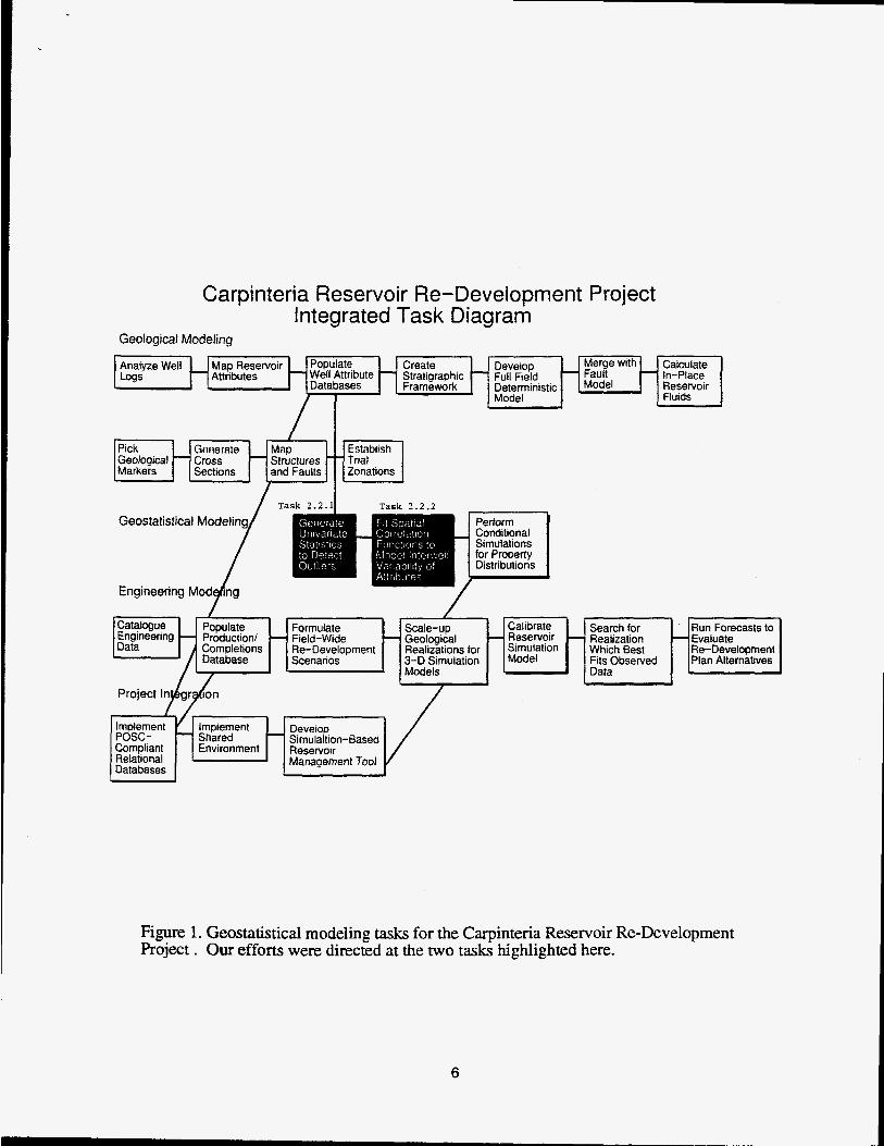
Carpinteria Reservoir Re-Development Project Integrated Task Diagram

Create Merge with - Stratigraphic - Framework

te - ~ - Model

Geological Modeling

Calculate In-Place Reservoir Fluids -

Ta Task 2 .2 .2

/ / Catalogue Populate Formulate - Scale-up Engineering - Production/ - Field-Wide Geological

Re-Development Realizations for Scenarios 3-D Simulation

Models

~

Develop

Management Tool

Shared POSC-

Databases

Calibrate Search for

Fits Observed

Run Forecasts to Evaluate Re-Development

Figure 1. Geostatistical modeling tasks for the Carpinteria Reservoir Re-Development Project . Our efforts were directed at the two tasks highlighted here.

6

(ATTACHMENT) UTILITY OF STATISTICAL AND GEOSTATISTICAL TECHNIQUES

FOR EXPLORING AND MODELING THE CARPENTERIA DATA

Richard P. Kendall Katherine Campbell

LDRD Project No. 96-446 Program Code: XAY9

Objectives of study

The questions addressed briefly in this scoping study are:

1) Can layers of similar porosity, permeability and saturation be discovered by statistical analysis of the data?

2) Assuming that the answer to the first question is yes, then when analysis is confined to a relatively homogeneous layer, is there sufficient lateral continuity of the measured properties to predict their values between wells? That is, are geostatistical approaches to estimation and simulation worthwhile?

Data

Data are provided in 170 wells from the Carpenteria leases 166 (92 wells), 240 (31 wells), 3150 (46 wells) and 4000 (one well). Thirty additional wells, most in the latter two leases, have no porosity data. Five of the 170 wells have no data between 2000 and 4500 ft depth.

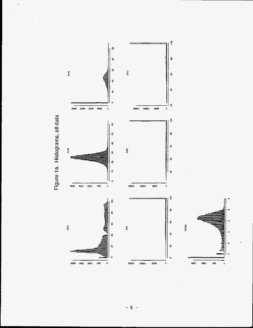
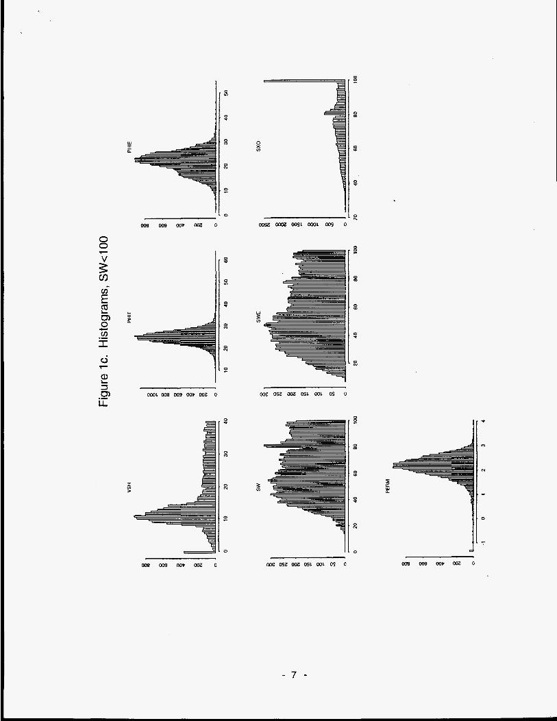
In addition to east and north coordinates and total vertical depth, seven parameters are provided. Typical histograms are shown in Figures 1 (a,b,c).

VSH

PHIT

PHlE

sw

SWE

Shale fraction Stongly bimodal, with a visible break at 40%. Values greater than 40% correspond to PHIE==O and are approximately uniformly distributed over the range of 45 to 100%. Values less than 40% peak at about 12%. (Figure la.)

Total porosity Normally distributed, with most values in the range of 15 to 35%. (Figure la.)

Effective porosity Zero for about 25% of the data, while the rest are approximately normally distributed, although the lower tail is relatively heavy. (Figure 1 b.)

Saturation of water 100% when PHIE=O and also for an additional 20% of the data. The remainder of distribution is broad and fairly uniform in the range of 25 to 100%. (Figure IC.)

Effective saturation of water

- 1 -

sxo

PERM

100% whem SW-100%. Otherwise a flat distribution, shifted somewhat to the left (downward) relative to SW. (Figure IC.)

Residual saturation 100% when SW=lOO% and for an additional 7% of the data. Otherwise a fairly flat distribution from 35-1 00%. (Figure IC).

Permeability Strongly bimodal, but most of the low values correspond to PHIE=O. Otherwise lognormally distributed, with most values in the range of 10 to 1000 millidarcies. (Figures 1 (as) include histograms of loglo(PERM).)

Discovery of Structure in the Data

The histograms suggest some immediate clusters: one for which PHIE=O, one for which PHIE>O but SW=lOO%, and one for which PHIE>O and SW<lOO% but SXO=lOO%. These three groups account for more than 50% of the data. The remainder of the data set is more nebulous. It includes, but is certainly not confined to, the high-permeability, low-saturation potential "pay" areas.

Cluster analysis was used as a technique for identifying structure in this part of the data set. An adaptation of the "partitioning around medoids" (PAM) method for large data sets was used to cluster the data The basic PAM algorithm selects k "representative points" or "medoids" from the data set such that when each point in the data set is clustered with the nearest medoid, the total sum of "dissimilariiies" between each point and its assigned medoid is minimized. (k, the number of clusters, must be specified by the user, and how "dissimilarity" is defined is also up to the user.) This method, which requires iterative "swapping" to select the best medoids, is impractical for data sets of more than about 250 points, so it was extended to the Carpenteria data set (about 550,000 logged points) in several steps.

3)

A subset of points between 2500 and 4000 ft total vertical depth in 26 wells (a total of about 33,500 points) was selected. (This is the data set shown in the histograms of Figure 1 .) The 26 wells selected are spread out across the field from east to west. Of the 33,500 points, about 54% fell into one of the "obvious" clusters defined above, leaving about 15,500 to be classified by cluster analysis.

PAM was run sequentially on ten randomly selected subsets of these 15,500 points, each of size 150 (about 1% of the total), with a large number of clusters (k=30). The variables used for clustering were VSH, PHIE, SWE, SXO and log1 o(PERM). (When PERM was reported as zero, lOg10(.05) was used.) The variables were standardized before the clustering algoriihm was run, and "dissirnilariiy" was defined as ordinary Euclidean distance in the space of the scaled variables.

Finally, the entire Carpenteria data set can be clustered relative to the final medoids. Three additional medoids based on the "obvious" clusters are added before this is done. We clustered only points between 2500 and 4000 feet from 1 10 wells near the center line of the southwest trending field.

Figure 2 shows the 33 medoids on a two-dimensional plot in the plane of their first two principal components. (The principal component computations excluded the "obvious" medoids, however.) Loadings on these components align fairly well with the original variables (Table 1). The first principal component loads heavily on permeability and moderately on porosity. The second loads on the two saturation variables, SWE and SXO, which are separated only by the fifth

- 2 -

and least important component. The third loads on the shale fraction. (In Figure 2, shale fraction is indicated by the symbol.) The first three components account for 83% of the total variability.

The "obvious" medoids are labeled 31 (PHIE=O), 32 (PHIE>O, SW=lOO), and 33 (PHIE>O, SWc100, SXO=lOO). Only Cluster 31 is very far from the remaining clusters in Figure 2. In the final clustering step (step 3 above), Cluster 31 gave up about 20% of the points originally assigned to it (most to Cluster 3, which is closest on Figure 2). Cluster 32 gave up more than half but also acquired a few from neighboring clusters, and Cluster 33 gave up 75%, acquiring very few in return.

Figure 2 suggests "superclusters", or clusters of clusters. In particular, several high permeability, low water saturation, low shale clusters occupy the upper right-hand corner of the plot of the first two principal components. Since the first principal component increases with permeability and the second decreases with water saturation, this region of the plot contains candidates for "pay" layers.

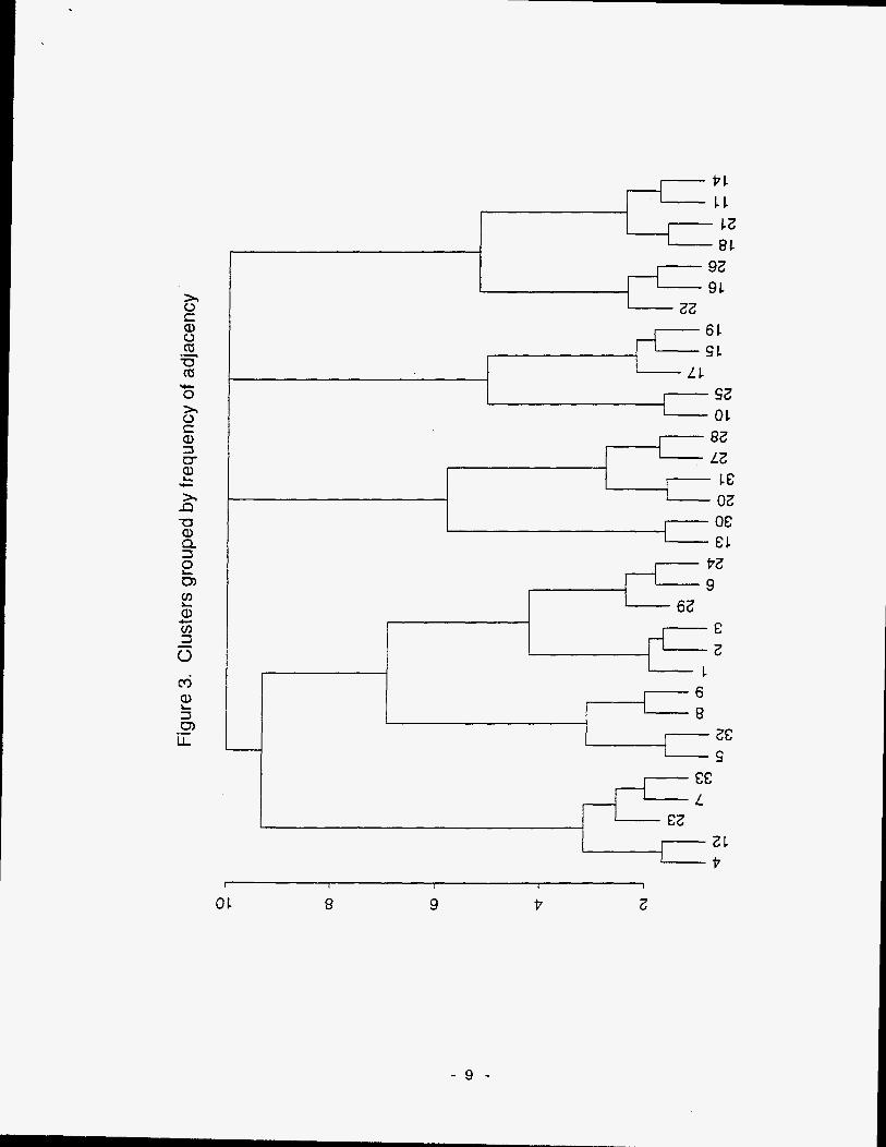
The 33 clusters were generated without reference to the location of the individual observations; they are based entirely on the logged variables (shale fraction, porosity, saturation, permeability). In order to generate groupings of related clusters, we defined a similarity matrix among the clusters whose values are high if points from two clusters are frequently adjacent within wells. The dendogram Figure 3, based on this similariiy matrix, reveals five or six major groupings and several subgroupings. These groupings and subgroupings were used as shown in Figure 2 to generate the color scheme used in Figure 4.

In Figure 4 the potential "pay" layers are shown in shades of green, becoming more yellow for clusters of lower permeability. The high shale, low permeability layers are shown in red and orange, and the saturated layers of mid- to high permeability in blues ranging from purple (relatively low permeability) to cyan (high permeability). Layers rising to the west are clearly delineated in Figure 4. In this plot the ordinate is just an ordering of the wells from southwest to northeast. Separation in the direction perpendicular to this one is not resolved, but it appears that these layers are fairly level in this direction, at least within the narrow band of wells shown here.

As Figure 4 shows, this approach is quite successful in suggesting the general spatial structure of the field, but without further development it is not entirely satisfactory for delimiting individual layers within wells because there is a great deal of variability within layers. However, these preliminary results could serve as the basis for automatic marker generation. For example, data from a single well could be transformed to the principal components coordinate space (Figure 2), and layers could be then identified based on the trace of a well in the transformed space. Some smoothing of the data, probably in the principal components space, would be useful for this purpose.

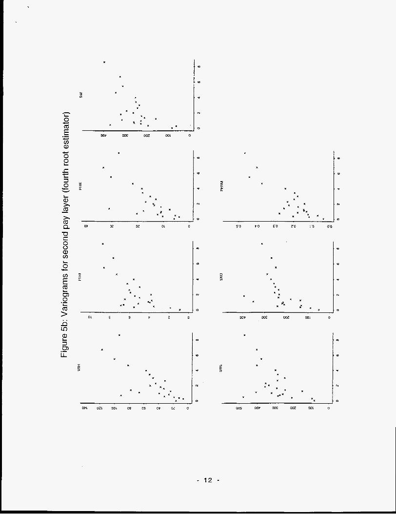
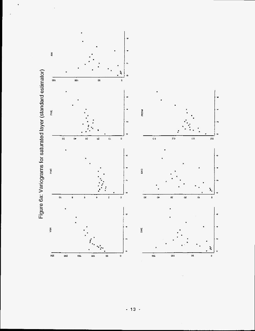
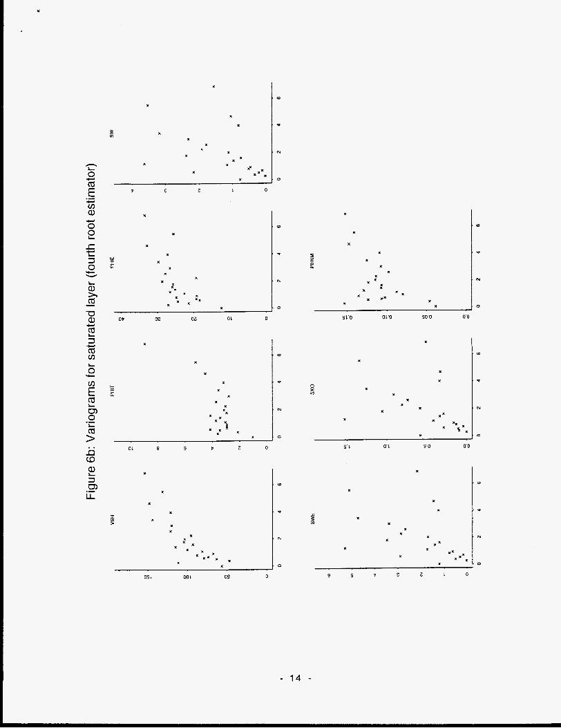
Evaluation of Continuity

For the preliminary evaluation of lateral continuity, "layers" were defined by manual interaction with plots such as Figure 4. That these definitions are crude may account for some of the noise observed in the variograms.

- 3 -

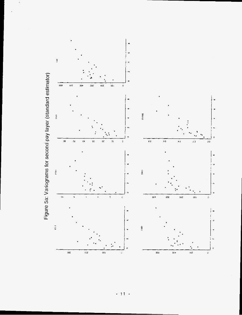
Continuity was investigated in the second "pay" layer and in the saturated layer below the first (highest) "pay' layer. Variograms were computed within these layers in the WSW direction defined by the general trend of the wells.

The empirical variograms suggest fairly good correlation over distances of at least 500 feet (Figures 5 and 6. The x-axes in these plots are labeled in thousands of feet.) In general, these empirical variograms are very noisy. Spikes at relatively short separations that might be eliminated by more careful analysis of outliers may be obscuring longer correlation distances. The "fourth root" algorithm that was used to estimate the variograms in Figures 5(b) and 6(b) is less sensitive to outliers, which tends to reduce some, but not all, of the spikes. Variogram modeling is something of an art, and it is probable that more structure will be discovered in more careful investigations.

At a depth of 3000 feet, the median distance from a well to its nearest neighbor is about 250 feet, and exceeds 500 feet for only about 10% of the wells. Thus within the field, at least in the depth range of 2500 to 4000 feet, there will usually be data within two or three hundred feet of any point at which we wish to model. Given this density of data, even the correlation distances suggested by Figures 5 and 6 are significant. This implies that improvements in modeling can be expected if geostatistical (Le., spatial-correlation-based) methods for estimation and simulation are used.

Outliers

In order to continue the investigations, much more attention needs to be paid to wells that appear to be "outliers" for one reason or another. These wells show up in Figure 4, for example, 3150- 70,3150-71 and 3150-77 at the east end of the field or 240-87 and 240-68 at the west end. Such wells can significantly distort variograms and might account for some of the spikes seen in Figures 5 and 6, although an attempt was made to eliminate outliers before the variograms were computed.

In general, indicators of problematic wells are useful byproducts of the types of analyses described above.

Conclusions

This preliminary study shows that the application of statistical and geostatistical methods has considerable promise in a data-rich field such as the Carpenteria field. Cluster analysis appears to be promising as a basis both for defining markers and also, indirectly, for cleaning up the data by indicating wells for which recalibration of the raw log data might be useful (Le., wells which currently appear inconsistent with their neighbors.) Within cleaned up, better-defined layers, even the relatively crude results reported here suggest that spatial correlation is significant at the relevant spatial scales, indicating a good potential for accurate prediction of properties and their uncertainty between wells, and eventually for more realistic flow simulation results.

I - 4 -

r B

0 ' m

0

. o -I

0 ' N

0

W I

x

0

i Y P

- 5 -

OOOL we 009 Wt 002 0

- 6 -

E- !! 0, 0 v, w .- I

OOOL 008 009 WP wz 0 -

m os2 ooz 051 WL os 0

B W n.

- 7 -

- 8 -

b

Iu

P

Second principal component -6 -4 -2 0 2 4

A P D

I

. . . , - --.-

0

z CD Q

n c-

-.

N - a - + - ' I

61 s1 - 01

8 9

- 9 -

P Z

I 1.

v) c1 3

u, P

73 al (I) m II

d-

LL

... . - .........

oosz- I

000E- I I

OOSE- OOOP-

. . , r . . . . .

, .. , . . . . . . . * .., ... ..... . . . . . . . . . . . . -. .. . . . . . ........ . .. ... . . .. , ,, . . . . . L ...

.. -.. ,., . . . . .-" .,, . ., ,.. .- . . ........ ...... . . . . .

. . . . . .I .,

- c .., . .

- 10 -

. m

rL,

09 os OP oc 02 01 1

01 0 P 2 0

WC M Z WL

c X

B O 90 Q O 2 0 0 0

I

x

W9 W t wz 3

- 11 -

x

3 v)

I

I

a x I -

a * :

0

W

9

. N

0

W P ooc ooz WL 0

~ N

OP OC 02 0L O

x

01 8 9 P 2 0

= * = x

= I..

OPL OZL W L oe 09 OP z o

x

8

s o YO E'O 20 1'0 0 0

I

WP WE ooz 001 0

0 0 5 W * o o c o o z W L 0

- 12 -

5 X x

X

I

W

*

I

WL w 0

5 c

X

os OP OE oz 01 0

x

1

01 e 9 P 2 0

x

I

I 9 x

X

a C w C

8

CO zo 1 '0 0 0

I

x

w OP OE 02 01 0

W

In 3 x

I

WL w 0

- 13 -

6

x

W

v

* I N

n I: * * 5 .= * c m

P c 2 1 0

*

w z

x

Ot M: 02 OL 0

x

x

x

I x

" I '; x

01 8 9 P 2 0

W

v I Y a.

X

I

x

x I "

51'0 01.0 500 00

x

W

v s x

X

c I

st 01 so 0 0

W x

v W

6 I

x

N

0

os1 001 os 0

x

9 s P C 2 0

- 14 -