Time series project

FORECASTING AVIATION ACTIVITY

Los Angeles International airport

Prepared by:

Rupantar Rana

MS Business Analytics Student

Marshall School of Business

University of Southern California

[email protected]

December 2015

TABLE OF CONTENTS

Introduction and Motivation .......................................................................................

Data source identification and

description………………………………………………………………….

Initial Hypothesis……………………………………………………………………

Procedure 1: Arima Time series modelling…………………………………………

Step 1: Stationarity Test

Step 2: ACF and PACF plot Evaluation

Step 3: Candidate Model selection

Step 4: Residual Diagnosis

Step 5: 12 month Forecast with Confidence Interval

Procedure 2: Econometric Modelling

Step 1: Econometric Variable Identification

Step 2: Data Gathering

Step 3: Data Cleaning and Integration

Step 4: Model building and Model Selection

Step 5: Cross Validation

Procedure 3: Exponential Smoothing

Holt Winters Technique

Procedure 4: Ensemble Modelling

Average Ensemble Model

Apply Forecast Methods and Evaluate Results ...........................................................

Executive Summary document ……………………………………………………...

Time series analysis projectRupantar Rana

Los Angeles International Airport - Passenger Traffic Prediction

Introduction and Motivation

Air traffic forecast serves as an important quantitative basis for airport planning - in particular for capacityplanning, CAPEX as well as for aeronautical and non-aeronautical revenue planning. High level decision andplanning in airports relies heavily on future airport activity. Many research have shown that airport traffic issubject to great volatility now then has been the case in the past. Many past predictive models for air trafficmodels have mixed performance due to unanticipated events and circumstances in the forcasts.

The goal of this analysis is to provide a realistic forecast based on latest available data to reflect the currentconditions at the airport, supported by information in the study providing an adequate justification for theairport planning and development.

The aim here is to develop a model that can accurately predict the volume of air traffic in Los AngelesInternational Airport using the dataset that is available from the data.gov website.

Data Description

Date Range : From 1/1/2006 to 9/1/2015

Datasource Description : The dataset contains details of the Passenger Traffic in Los Angeles InternationalAirport. It is a non-federal data set downloaded from the data.gov website. This dataset consists of 4286rows and 9 columns and contains the following variables.

Data extraction date : This is the exact date at which the data was extracted. At this stage we can ignorethis variable as it is not related to the analysis.

Report Period : This is the date variable that is used as the date variable for the time series analysis.

Terminal : The airport terminal from Terninal 1 to Terminal 8 , Misc. Terminal and Tom Bradleyinternational airport.

Arrival Departure : This variable is used to indicate whether the passengers were recorded on arrival oron departure.

Domestic International Airport : This variable indicates Whether it is a domestic or international airport

Passenger Count : The number of passengers recorded on that particular day.

https://catalog.data.gov/dataset/los-angeles-international-airport-passenger-traffic-by-terminal-756ee

Initial Hypothesis

From the research on passenger activity on airport, passenger traffic should have a time dependent structure.Additionally, socio-economic factors could be used to explain some of the causal relationship with passengertraffic. Air traffic activity could also be affected by interaction of supply and demand factors. The demand inaviation is largely a function of demographic and economic factors. Supply factors such as cost, competitionand regulations could also help determine air traffic activity.

1

Aviation forecasting background and techniques

Some of the forecasting techniques that have been traditionally used include the following:Time Series Forecasting : Time series trend and seasonality extrapolation using statistical techniquesthat rely on past data to predict the future valuesEconometric modelling with explanatory variables : This type of modelling techniques relies onexamining the relationship between traffic data and possible explanatory variables such as GDP, disposableincome, price of fuel and so forthSimulations : A method where snapshots or samples of data can be regenerated using complex models toexplore and forecast the future valuesEnsemble Modelling : Here the forecast of all the above mentioned methods can be combined to devise amodel that performs better than the individual methodsMarket share analysis : A technique used to forecast a local activity as a share of a larger some largeraggregated activity. eg. airport traffic may be based on national traffic which may have been forecasted by athird party.For our analysis we will be using time series analysis to model the time dependent structure of passengertraffic behaviour for Los Angeles international Airport.

Procedure 1 : Time Series Analysis

We shall start by performing exploratory data analysis for the data set, then we shall investivate and comeup with candidate models for forecasting. We will use the best possible model to predict passenger activity.Finally we will predict for the next 12 months from Oct-2015 to Sep-2016 with 80% and 95% confidenceintervals.

4e+06

5e+06

6e+06

7e+06

2006 2008 2010 2012 2014 2016Date/year

Pas

seng

er C

ount

Passenger traffic: Los Angeles Internation Airport

2

Stationarity Test

We can observe from the plot above that the passenger traffic in Imperial terminal at Los Angeles Internationalairport is fairly seasonal with a slight upward trend.

Next we shall perform the Augmented Dickey Fuller test and Kpss test to see if the trend and level of thepassenger traffic is stationary or non stationary.

Augmented Dickey Fuller Test

#### Augmented Dickey-Fuller Test#### data: timeseries_data## Dickey-Fuller = -4.3439, Lag order = 4, p-value = 0.01## alternative hypothesis: stationary

The Augmented Dickey fuller test has a P value of less than 0.05 which seems to suggest that the time seriesis stationary. We can clearly see a trend in data so let us perform some more formal test of stationarity.

Kwiatkowski-Phillips-Schmidt-Shin ( KPSS Test)

#### KPSS Test for Level Stationarity#### data: timeseries_data## KPSS Level = 0.4274, Truncation lag parameter = 2, p-value =## 0.06536

#### KPSS Test for Trend Stationarity#### data: timeseries_data## KPSS Trend = 0.1956, Truncation lag parameter = 2, p-value =## 0.01765

The results of the kpss test suggests that our time series is neither level stationary nor trend stationary. Formore details on stationarity you can refer to :http://www.mathworks.com/help/econ/trend-stationary-vs-difference-stationary.html

ACF and PACF Evaluation

Let us use the tsdisplay function in R to see the examine the time series plot of data along with its acf andeither its pacf, lagged scatterplot or spectrum.

3

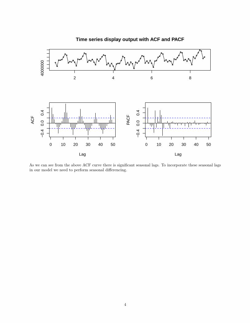
Time series display output with ACF and PACF

2 4 6 8

4000

000

0 10 20 30 40 50

−0.

40.

00.

4

Lag

AC

F

0 10 20 30 40 50

−0.

40.

00.

4

Lag

PAC

F

As we can see from the above ACF curve there is significant seasonal lags. To incorporate these seasonal lagsin our model we need to perform seasonal differencing.

4

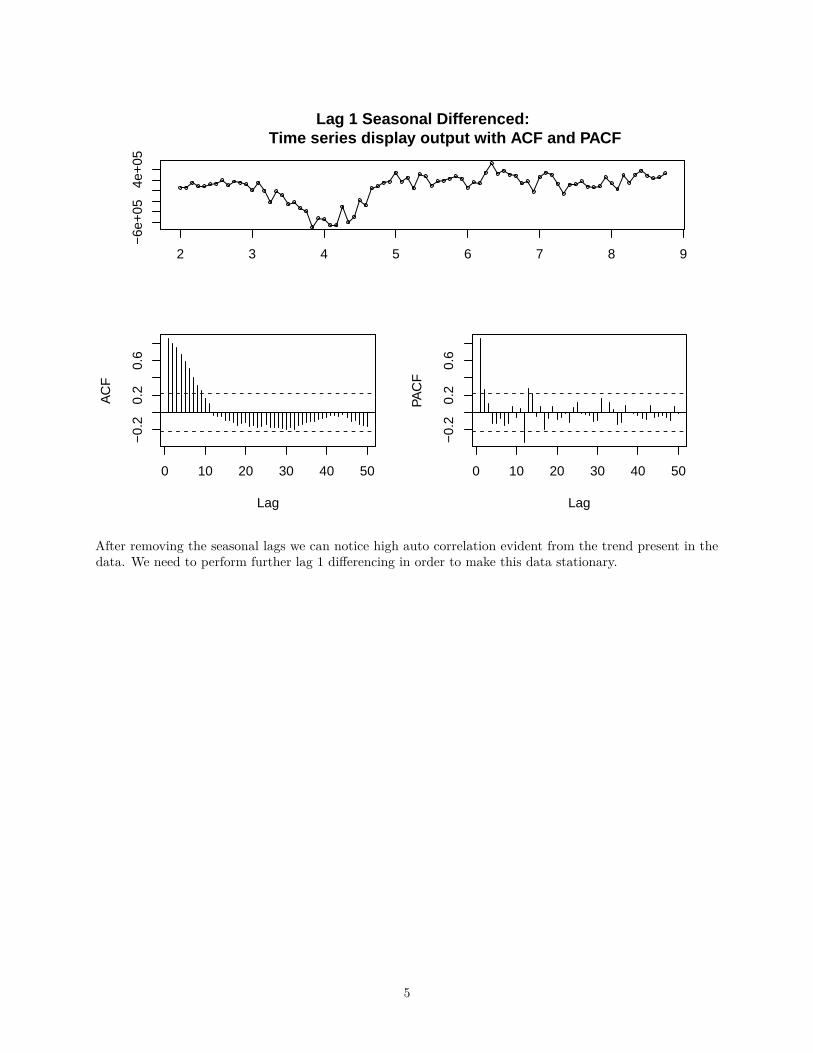
Lag 1 Seasonal Differenced: Time series display output with ACF and PACF

2 3 4 5 6 7 8 9

−6e

+05

4e+

05

0 10 20 30 40 50

−0.

20.

20.

6

Lag

AC

F

0 10 20 30 40 50

−0.

20.

20.

6

Lag

PAC

F

After removing the seasonal lags we can notice high auto correlation evident from the trend present in thedata. We need to perform further lag 1 differencing in order to make this data stationary.

5

Double differenced data: Time series display output with ACF and PACF

2 3 4 5 6 7 8 9

−3e

+05

3e+

05

0 10 20 30 40 50

−0.

40.

0

Lag

AC

F

0 10 20 30 40 50

−0.

40.

0

Lag

PAC

F

Model Building

The ACF and PACF of the double differenced data suggests that the following ARIMA model could be thebest candidates :

ARIMA(0,1,1)[0,1,1][12]

We have now built the model and need to perform residual diagnosis before we move on to predict using themodel.

6

Residual Diagnosis

Residual Diagnosis of our model

2 4 6 8

−3e

+05

3e+

05

0 5 10 15 20 25 30

−0.

30.

00.

2

Lag

AC

F

0 5 10 15 20 25 30

−0.

30.

00.

2

Lag

PAC

F

The residuals seem fairly linear in distribution and they do not show any significant auto correlation whichmeans that our model is adequately built. Let us further examine the residuals for test of significantautocorrelation by examining performing the Box test.

#### Box-Pierce test#### data: residuals_Model_Imperial_Terminal_1## X-squared = 0.1366, df = 1, p-value = 0.7117

The P-value of the Box test is high suggesting that the residuals are not auto correlated.

Let us go ahead and forecast with our model.

7

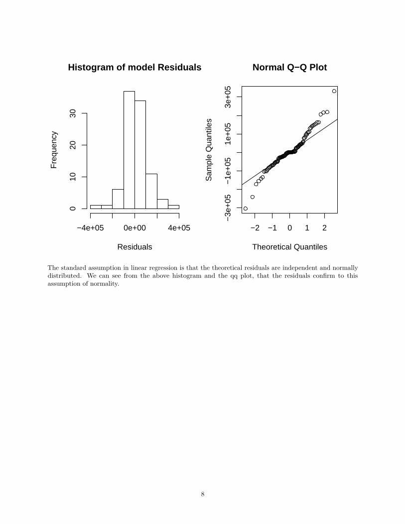
Histogram of model Residuals

Residuals

Fre

quen

cy

−4e+05 0e+00 4e+05

010

2030

−2 −1 0 1 2−

3e+

05−

1e+

051e

+05

3e+

05

Normal Q−Q Plot

Theoretical Quantiles

Sam

ple

Qua

ntile

s

The standard assumption in linear regression is that the theoretical residuals are independent and normallydistributed. We can see from the above histogram and the qq plot, that the residuals confirm to thisassumption of normality.

8

12 months forecast using the model we have built.

12 months forecast of passenger Traffic Los Angeles International Airport

2 4 6 8 10

4000

000

5500

000

7000

000

Please note that the axis is not formatted properly. I could not find a way to format the x axis while plottingthe forcasted data.

12 months from Oct-2015 to Sep-2016 passenger traffic forecast with 80% and95% confidence intervals

Forecast12months

## Point Forecast Lo 80 Hi 80 Lo 95 Hi 95## Nov 8 5262340 5128361 5396319 5057437 5467243## Dec 8 5565038 5403786 5726291 5318424 5811653## Jan 9 5296893 5112392 5481393 5014723 5579062## Feb 9 4779445 4574420 4984470 4465887 5093003## Mar 9 5661901 5438228 5885575 5319822 6003980## Apr 9 5563426 5322543 5804308 5195028 5931824## May 9 5830493 5573551 6087434 5437534 6223451## Jun 9 6162690 5890635 6434744 5746619 6578761## Jul 9 6569157 6282787 6855528 6131191 7007124## Aug 9 6444343 6144339 6744348 5985526 6903161## Sep 9 5420457 5107412 5733503 4941696 5899219## Oct 9 5626821 5301256 5952385 5128913 6124728## Nov 9 5373930 5026626 5721234 4842774 5905085## Dec 9 5675364 5310894 6039834 5117955 6232773

9

## Jan 10 5405630 5024709 5786551 4823062 5988198## Feb 10 4890188 4493782 5286595 4283937 5496439## Mar 10 5765533 5354224 6176842 5136491 6394576## Apr 10 5672429 5246739 6098120 5021392 6323467## May 10 5934131 5494530 6373733 5261819 6606444## Jun 10 6263639 5810554 6716725 5570704 6956574## Jul 10 6672152 6205972 7138332 5959192 7385113## Aug 10 6547889 6068973 7026805 5815450 7280328## Sep 10 5523925 5032603 6015248 4772512 6275339

10

Econometric Modelling with Econometric Variables

Econometric modeling is a widely used statistical modelling technique that is used in various studies.Econometric models are fitted using least-squares regression or maximum likelywood principle estimation.Regression models relate the independent variables on the right hand side of the model equation to the lefthand side of the equation. One of the econometric variables chosen is the personal income.

Econometric Variable Identification

Data Gathering and Cleaning

Model Building

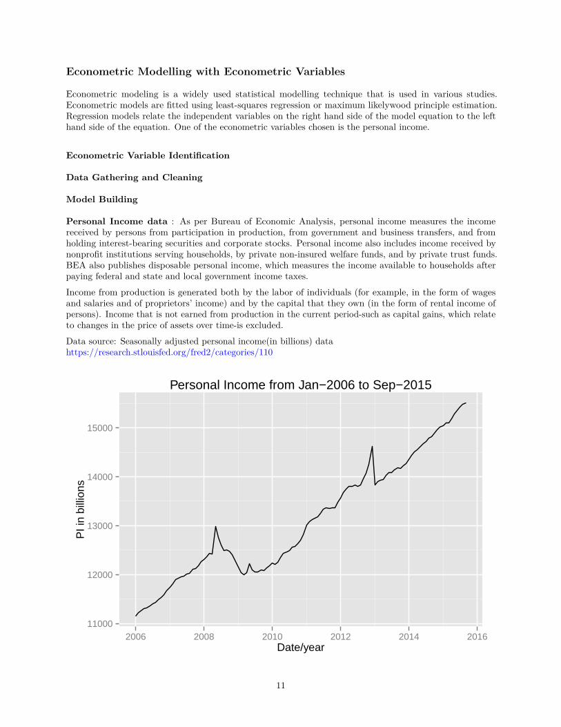
Personal Income data : As per Bureau of Economic Analysis, personal income measures the incomereceived by persons from participation in production, from government and business transfers, and fromholding interest-bearing securities and corporate stocks. Personal income also includes income received bynonprofit institutions serving households, by private non-insured welfare funds, and by private trust funds.BEA also publishes disposable personal income, which measures the income available to households afterpaying federal and state and local government income taxes.

Income from production is generated both by the labor of individuals (for example, in the form of wagesand salaries and of proprietors’ income) and by the capital that they own (in the form of rental income ofpersons). Income that is not earned from production in the current period-such as capital gains, which relateto changes in the price of assets over time-is excluded.

Data source: Seasonally adjusted personal income(in billions) datahttps://research.stlouisfed.org/fred2/categories/110

11000

12000

13000

14000

15000

2006 2008 2010 2012 2014 2016Date/year

PI i

n bi

llion

s

Personal Income from Jan−2006 to Sep−2015

11

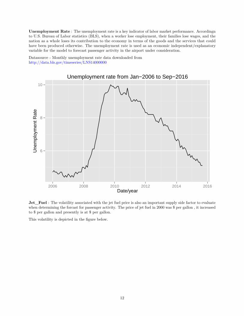
Unemployment Rate : The unemployment rate is a key indicator of labor market performance. Accordingnto U.S. Bureau of Labor statistics (BLS), when a worker lose employment, their families lose wages, and thenation as a whole loses its contribution to the economy in terms of the goods and the services that couldhave been produced otherwise. The unemployment rate is used as an economic independent/explanatoryvariable for the model to forecast passenger activity in the airport under consideration.

Datasource - Monthly unemployment rate data downloaded fromhttp://data.bls.gov/timeseries/LNS14000000

6

8

10

2006 2008 2010 2012 2014 2016Date/year

Une

mpl

oym

ent R

ate

Unemployment rate from Jan−2006 to Sep−2016

Jet_Fuel : The volatility associated with the jet fuel price is also an important supply side factor to evaluatewhen determining the forcast for passenger activity. The price of jet fuel in 2000 was $ per gallon , it increasedto $ per gallon and presently is at $ per gallon.

This volatility is depicted in the figure below.

12

2

3

4

2006 2008 2010 2012 2014 2016Date/year

Jet F

uel p

rice

in $

per

bar

rel

Jet Fuel price from Jan−2006 to Sep−2016

Model summary

Ecometric model built using the time, month, jet_fuel price and unemployment rate as the explanatoryvariable to predict the passenger traffic in the airport had a Adjusted R-squared of 0.41. Unemploymentrate and month have a low p-values suggesting that they are significant in explaning the variation in thepassenger traffic at Los Angeles international airport. Additionally the time dependent structure is more

Holtz Winters Exponential Smoothing

Holt (1957) and Winters (1960) extended Holt’s method to capture seasonality. The Holt-Winters seasonalmethod comprises the forecast equation and three smoothing equations - one for the level ???t, one for trendbt, and one for the seasonal component denoted by st, with smoothing parameters ??, ????? and ??. We usem to denote the period of the seasonality, i.e., the number of seasons in a year. For example, for quarterlydata m=4, and for monthly data m=12.

There are two variations to this method that differ in the nature of the seasonal component. The additivemethod is preferred when the seasonal variations are roughly constant through the series, while the multi-plicative method is preferred when the seasonal variations are changing proportional to the level of the series.With the additive method, the seasonal component is expressed in absolute terms in the scale of the observedseries, and in the level equation the series is seasonally adjusted by subtracting the seasonal component.Within each year the seasonal component will add up to approximately zero. With the multiplicative method,the seasonal component is expressed in relative terms (percentages) and the series is seasonally adjustedby dividing through by the seasonal component. Within each year, the seasonal component will sum up toapproximately m.

13

Forecasts from Holt−Winters' additive method

2 4 6 8 10

4000

000

5500

000

7000

000

Time Series Decomposition

The decomposition of time series is a statistical method that deconstructs a time series into notionalcomponents.

This is an important technique for all types of time series analysis, especially for seasonal adjustment. Itseeks to construct, from an observed time series, a number of component series (that could be used toreconstruct the original by additions or multiplications) where each of these has a certain characteristic ortype of behaviour. For example, time series are usually decomposed into:

1. the Trend Component that reflects the long term progression of the series (secular variation)2. the Cyclical Component that describes repeated but non-periodic fluctuations3. the Seasonal Component reflecting seasonality (seasonal variation)4. the Irregular Component (or “noise”) that describes random, irregular influences. It represents the

residuals of the time series after the other components have been removed.

Using the base R function for time series decomposition, we shall decompose the time series into seasonal,trendand irregular components using the moving averages.

[source: wikipedia]

14

4000

000

6000

000

obse

rved

4800

000

tren

d

−5e

+05

seas

onal

−1e

+05

2e+

05

2 4 6 8

rand

om

Time

Decomposition of additive time series

Ensemble Method

Ensemble modeling is the process of running two or more related but different analytical models and thensynthesizing the results into a single score or spread in order to improve the accuracy of predictive analyticsand data mining applications.

Ensemble model Rmse = 525302.2

A simple averaging ensemble model that takes the individual forecasts from Arima , Exponential smoothingand Econometric modelling, averages them to produce an entimated forecast is so far the best method interms of cross validation rmse.

Executive summary

Forecasting methods used to project airport activity should reflect not only the time dependence structureof passenger activity but also the underlying demographic and economic causal relationships that drivespassenger traffic. Demand and supply factors need to be accounted for when measuring passenger activitylevels. Supply factors such as cost, competition, and regulations could impact air passenger traffic as well.The projections of aviation activity that result from applying appropriate forecasting methods and modellingthe relationships between causal variables need to be further evaluated before using them in strategy andplanning situations. Aviation forecasters must use their professional judgement and domain expertise todetermine what is reasonable when developing quantifiable results.

15