Time Series and Forecasting Lecture 4 NonLinear Time Series Bruce E. Hansen Summer School in Economics and Econometrics University of Crete July 23-27, 2012 Bruce Hansen (University of Wisconsin) Foundations July 23-27, 2012 1 / 87

Welcome message from author
This document is posted to help you gain knowledge. Please leave a comment to let me know what you think about it! Share it to your friends and learn new things together.
Transcript

Time Series and ForecastingLecture 4
NonLinear Time Series
Bruce E. Hansen
Summer School in Economics and EconometricsUniversity of CreteJuly 23-27, 2012
Bruce Hansen (University of Wisconsin) Foundations July 23-27, 2012 1 / 87
Today’s Schedule
Density Forecasts
Threshold Regression Models
Nonparametric Regression Models
Bruce Hansen (University of Wisconsin) Foundations July 23-27, 2012 2 / 87
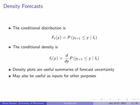
Density Forecasts
The conditional distribution is
Ft (y) = P (yt+1 ≤ y | It )
The conditional density is
ft (y) =ddyP (yt+1 ≤ y | It )
Density plots are useful summaries of forecast uncertainty
May also be useful as inputs for other purposes
Bruce Hansen (University of Wisconsin) Foundations July 23-27, 2012 3 / 87
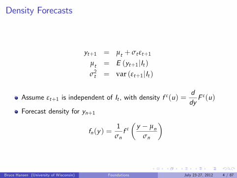
Density Forecasts
yt+1 = µt + σt εt+1
µt = E (yt+1|It )σ2t = var (εt+1|It )
Assume εt+1 is independent of It , with density f ε(u) =ddyF ε(u)
Forecast density for yn+1
fn(y) =1
σnf ε
(y − µn
σn
)
Bruce Hansen (University of Wisconsin) Foundations July 23-27, 2012 4 / 87
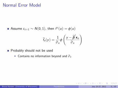
Normal Error Model
Assume εt+1 ∼ N(0, 1), then f ε(u) = φ(u)
fn(y) =1
σnφ
(y − β
′xn
σn
)
Probably should not be usedI Contains no information beyond and σt
Bruce Hansen (University of Wisconsin) Foundations July 23-27, 2012 5 / 87
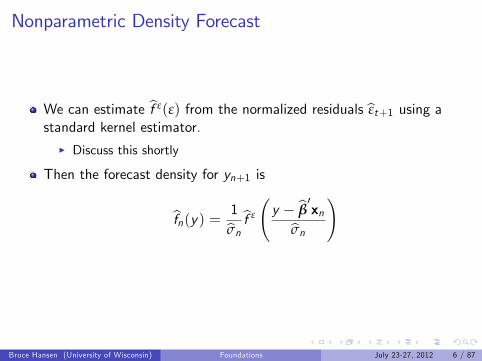
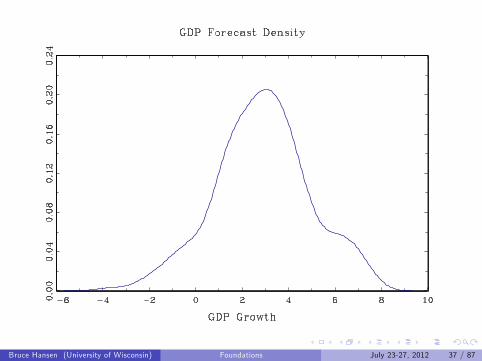
Nonparametric Density Forecast
We can estimate f ε(ε) from the normalized residuals εt+1 using astandard kernel estimator.
I Discuss this shortly
Then the forecast density for yn+1 is
fn(y) =1
σnf ε
(y − β
′xn
σn
)
Bruce Hansen (University of Wisconsin) Foundations July 23-27, 2012 6 / 87

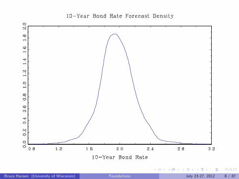
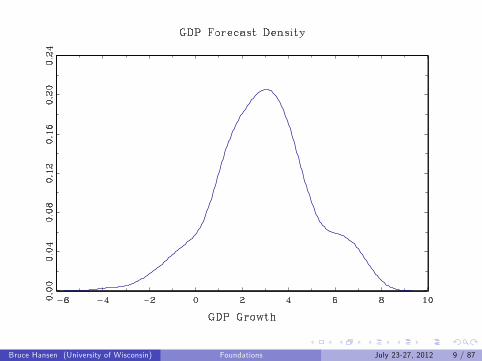
Examples:
Interest Rate
GDP Nowcast
Bruce Hansen (University of Wisconsin) Foundations July 23-27, 2012 7 / 87
Bruce Hansen (University of Wisconsin) Foundations July 23-27, 2012 8 / 87
Bruce Hansen (University of Wisconsin) Foundations July 23-27, 2012 9 / 87
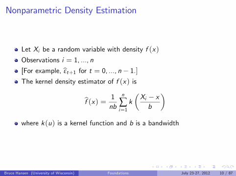
Nonparametric Density Estimation
Let Xi be a random variable with density f (x)
Observations i = 1, ..., n
[For example, εt+1 for t = 0, ..., n− 1.]The kernel density estimator of f (x) is
f (x) =1nb
n
∑i=1k(Xi − xb
)where k(u) is a kernel function and b is a bandwidth
Bruce Hansen (University of Wisconsin) Foundations July 23-27, 2012 10 / 87
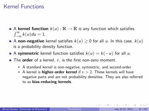
Kernel Functions
A kernel function k(u) : R→ R is any function which satisfies∫ ∞−∞ k(u)du = 1.
A non-negative kernel satisfies k(u) ≥ 0 for all u. In this case, k(u)is a probability density function.
A symmetric kernel function satisfies k(u) = k(−u) for all u.The order of a kernel, ν, is the first non-zero moment.
I A standard kernel is non-negative, symmetric, and second-orderI A kernel is higher-order kernel if ν > 2. These kernels will havenegative parts and are not probability densities. They are also referredto as bias-reducing kernels.
Bruce Hansen (University of Wisconsin) Foundations July 23-27, 2012 11 / 87
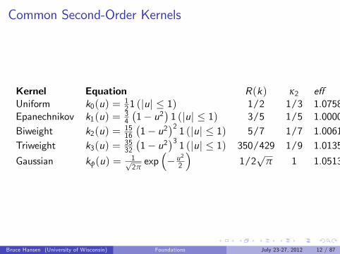
Common Second-Order Kernels
Kernel Equation R(k) κ2 effUniform k0(u) = 1
21 (|u| ≤ 1) 1/2 1/3 1.0758Epanechnikov k1(u) = 3
4
(1− u2
)1 (|u| ≤ 1) 3/5 1/5 1.0000
Biweight k2(u) = 1516
(1− u2
)2 1 (|u| ≤ 1) 5/7 1/7 1.0061Triweight k3(u) = 35
32
(1− u2
)3 1 (|u| ≤ 1) 350/429 1/9 1.0135
Gaussian kφ(u) = 1√2πexp
(− u22
)1/2√
π 1 1.0513
Bruce Hansen (University of Wisconsin) Foundations July 23-27, 2012 12 / 87

Choice of Kernel
Not as important as bandwidth
Epanechnikov (quadratic) is optimal for minimizing IMSE of f (x)
Gaussian is convenient as it is infinitely smooth and has positivesupport everywhere
I I am using Gaussian here
Bruce Hansen (University of Wisconsin) Foundations July 23-27, 2012 13 / 87
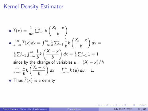
Kernel Density Estimator
f (x) =1nb
∑ni=1 k
(Xi − xb
)∫ ∞−∞ f (x)dx =
∫ ∞−∞
1n ∑n
i=11bk(Xi − xb
)dx =
1n ∑n
i=1
∫ ∞−∞
1bk(Xi − xb
)dx = 1
n ∑ni=1 1 = 1
since by the change of variables u = (Xi − x)/h∫ ∞−∞
1bk(Xi − xb
)dx =
∫ ∞−∞ k (u) du = 1.
Thus f (x) is a density
Bruce Hansen (University of Wisconsin) Foundations July 23-27, 2012 14 / 87
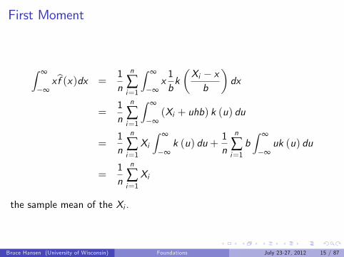
First Moment
∫ ∞
−∞xf (x)dx =
1n
n
∑i=1
∫ ∞
−∞x1bk(Xi − xb
)dx
=1n
n
∑i=1
∫ ∞
−∞(Xi + uhb) k (u) du
=1n
n
∑i=1Xi∫ ∞
−∞k (u) du +
1n
n
∑i=1b∫ ∞
−∞uk (u) du
=1n
n
∑i=1Xi
the sample mean of the Xi .
Bruce Hansen (University of Wisconsin) Foundations July 23-27, 2012 15 / 87
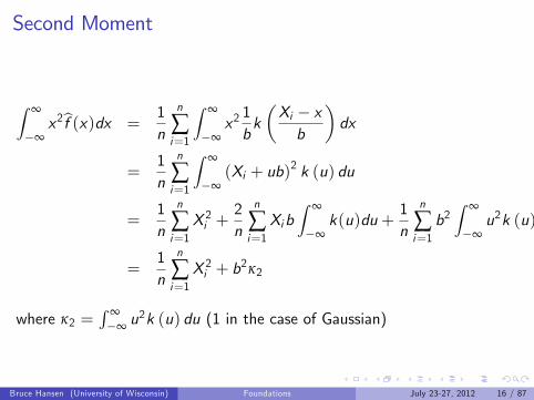
Second Moment
∫ ∞
−∞x2 f (x)dx =
1n
n
∑i=1
∫ ∞
−∞x21bk(Xi − xb
)dx
=1n
n
∑i=1
∫ ∞
−∞(Xi + ub)
2 k (u) du
=1n
n
∑i=1X 2i +
2n
n
∑i=1Xib
∫ ∞
−∞k(u)du +
1n
n
∑i=1b2∫ ∞
−∞u2k (u) du
=1n
n
∑i=1X 2i + b
2κ2
where κ2 =∫ ∞−∞ u
2k (u) du (1 in the case of Gaussian)
Bruce Hansen (University of Wisconsin) Foundations July 23-27, 2012 16 / 87
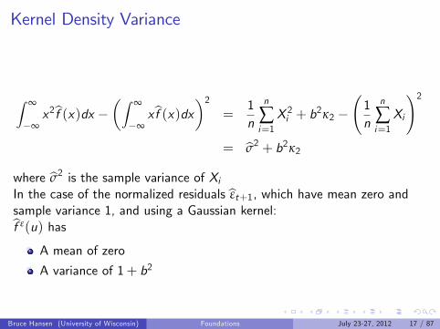
Kernel Density Variance
∫ ∞
−∞x2 f (x)dx −
(∫ ∞
−∞xf (x)dx
)2=
1n
n
∑i=1X 2i + b
2κ2 −(1n
n
∑i=1Xi
)2= σ2 + b2κ2
where σ2 is the sample variance of XiIn the case of the normalized residuals εt+1, which have mean zero andsample variance 1, and using a Gaussian kernel:f ε(u) has
A mean of zero
A variance of 1+ b2
Bruce Hansen (University of Wisconsin) Foundations July 23-27, 2012 17 / 87

Numerical Implementation for Forecast DensityPick a set of grid points for ε, e.g. u1, ..., uGFor each ε on grid, evalulate
f ε(ε) =1nb
n−1∑t=0
φ
(ε− εt+1b
)or
f εj =
1nb
n−1∑t=0
φ
(uj − εt+1
b
)Set the translated gridpoints yj = β
′xn + σnuj , for j = 1, ...,G , and
fj =1
σnf εj
The rescaling is the Jacobian of the transformation from uj to yjPlot fj on y -axis against yj on x-axis. This is a plot of
fn(y) =1
σnf ε
(y − β
′xn
σn
)Bruce Hansen (University of Wisconsin) Foundations July 23-27, 2012 18 / 87
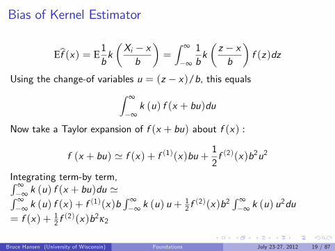
Bias of Kernel Estimator
Ef (x) = E1bk(Xi − xb
)=∫ ∞
−∞
1bk(z − xb
)f (z)dz
Using the change-of variables u = (z − x)/b, this equals∫ ∞
−∞k (u) f (x + bu)du
Now take a Taylor expansion of f (x + bu) about f (x) :
f (x + bu) ' f (x) + f (1)(x)bu + 12f (2)(x)b2u2
Integrating term-by term,∫ ∞−∞ k (u) f (x + bu)du '∫ ∞−∞ k (u) f (x) + f
(1)(x)b∫ ∞−∞ k (u) u +
12 f(2)(x)b2
∫ ∞−∞ k (u) u
2du
= f (x) + 12 f(2)(x)b2κ2
Bruce Hansen (University of Wisconsin) Foundations July 23-27, 2012 19 / 87
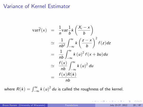
Variance of Kernel Estimator
varf (x) =1n
var1bk(Xi − xb
)' 1
nb2
∫ ∞
−∞k(z − xb
)2f (z)dz
=1nb
∫ ∞
−∞k (u)2 f (x + bu)du
' f (x)nb
∫ ∞
−∞k (u)2 du
=f (x)R(k)
nb
where R(k) =∫ ∞−∞ k (u)
2 du is called the roughness of the kernel.
Bruce Hansen (University of Wisconsin) Foundations July 23-27, 2012 20 / 87
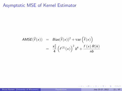
Asymptotic MSE of Kernel Estimator
AMSE (f (x)) = Bias(f (x))2 + var(f (x)
)=
κ224
(f (2)(x)
)2b4 +
f (x)R(k)nb
Bruce Hansen (University of Wisconsin) Foundations July 23-27, 2012 21 / 87
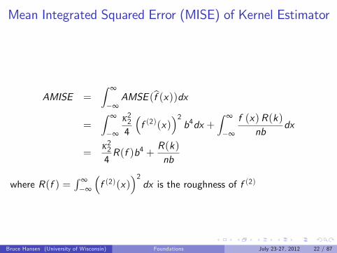
Mean Integrated Squared Error (MISE) of Kernel Estimator
AMISE =∫ ∞
−∞AMSE (f (x))dx
=∫ ∞
−∞
κ224
(f (2)(x)
)2b4dx +
∫ ∞
−∞
f (x)R(k)nb
dx
=κ224R(f )b4 +
R(k)nb
where R(f ) =∫ ∞−∞
(f (2)(x)
)2dx is the roughness of f (2)
Bruce Hansen (University of Wisconsin) Foundations July 23-27, 2012 22 / 87

Optimal bandwidth
The AMISE takes the form Ab4 + B/nbThe bandwidth b which minimizes the AMISE is
b =(4R(k)4κ22
)1/5
R(f )−1/5n−1/5
The unknown component is R(f )−1/5
The “rougher” is f (x), the larger is R(f ) so the optimal b is smaller
Bruce Hansen (University of Wisconsin) Foundations July 23-27, 2012 23 / 87
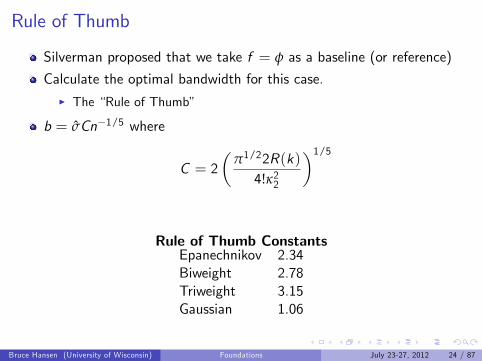
Rule of Thumb
Silverman proposed that we take f = φ as a baseline (or reference)
Calculate the optimal bandwidth for this case.I The “Rule of Thumb”
b = σCn−1/5 where
C = 2(
π1/22R(k)4!κ22
)1/5
Rule of Thumb ConstantsEpanechnikov 2.34Biweight 2.78Triweight 3.15Gaussian 1.06
Bruce Hansen (University of Wisconsin) Foundations July 23-27, 2012 24 / 87

Plug-in bandwidth Methods
Estimate R(f )Use
b =(4R(k)4κ22
)1/5
R(f )−1/5n−1/5
Bruce Hansen (University of Wisconsin) Foundations July 23-27, 2012 25 / 87
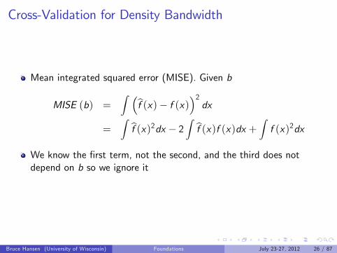
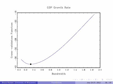
Cross-Validation for Density Bandwidth
Mean integrated squared error (MISE). Given b
MISE (b) =∫ (
f (x)− f (x))2dx
=∫f (x)2dx − 2
∫f (x)f (x)dx +
∫f (x)2dx
We know the first term, not the second, and the third does notdepend on b so we ignore it
Bruce Hansen (University of Wisconsin) Foundations July 23-27, 2012 26 / 87
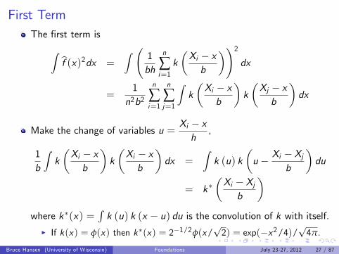
First TermThe first term is∫
f (x)2dx =∫ ( 1
bh
n
∑i=1k(Xi − xb
))2dx
=1n2b2
n
∑i=1
n
∑j=1
∫k(Xi − xb
)k(Xj − xb
)dx
Make the change of variables u =Xi − xh
,
1b
∫k(Xi − xb
)k(Xi − xb
)dx =
∫k (u) k
(u − Xi − Xj
b
)du
= k∗(Xi − Xjb
)where k∗(x) =
∫k (u) k (x − u) du is the convolution of k with itself.
I If k(x) = φ(x) then k∗(x) = 2−1/2φ(x/√2) = exp(−x2/4)/
√4π.
Bruce Hansen (University of Wisconsin) Foundations July 23-27, 2012 27 / 87

The first term is thus∫f (x)2dx =
1n2b2
n
∑i=1
n
∑j=1k∗(Xi − Xjb
)
Bruce Hansen (University of Wisconsin) Foundations July 23-27, 2012 28 / 87
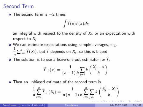
Second TermThe second term is −2 times∫
f (x)f (x)dx
an integral with respect to the density of Xi , or an expectation withrespect to XiWe can estimate expectations using sample averages, e.g.1n
∑ni=1 f (Xi ), but f depends on Xi , so this is biased
The solution is to use a leave-one-out estimator for f ,
f−i (x) =1
(n− 1) b ∑j 6=ik(Xj − xb
)Then an unbiased estimate of the second term is
1n
n
∑i=1f−i (Xi ) =
1n (n− 1) b
n
∑i=1
∑j 6=ik(Xj − Xib
)Bruce Hansen (University of Wisconsin) Foundations July 23-27, 2012 29 / 87

Cross-Validation Criterion
MISE (b) =∫f (x)2dx − 2
∫f (x)f (x)dx +
∫f (x)2dx
CV (b) =1n2b2
n
∑i=1
n
∑j=1k∗(Xi − Xjb
)− 2n (n− 1) b
n
∑i=1
∑j 6=ik(Xj − Xib
)In the case of a Gaussian kernel
CV (b) =1
n2b2√2
n
∑i=1
n
∑j=1
φ
(Xi − Xj√
2b
)− 2n (n− 1) b
n
∑i=1
∑j 6=i
φ
(Xj − Xib
)
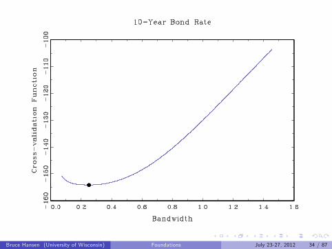
CV selected bandwidth
b = argminCV (b)
Bruce Hansen (University of Wisconsin) Foundations July 23-27, 2012 30 / 87

Evaluation
Form a grid for b
If br is the rule-of-thumb bandwidth, search over [br/3, 3br ] orsomething similar
Many authors define the CV bandwidth as the largest local minimizer
In the end, an eyeball reality check of your estimated density isimportant.
Bruce Hansen (University of Wisconsin) Foundations July 23-27, 2012 31 / 87

Theory
CV selected bandwidth is consistent
Let b0 minimize the AMISE
b− b0b0
→p 0
But the rate of convergence is slow, n−10
Bruce Hansen (University of Wisconsin) Foundations July 23-27, 2012 32 / 87

Examples
10-Year Bond Rate
GDP Growth Rate
Bruce Hansen (University of Wisconsin) Foundations July 23-27, 2012 33 / 87
Bruce Hansen (University of Wisconsin) Foundations July 23-27, 2012 34 / 87
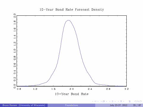
Bruce Hansen (University of Wisconsin) Foundations July 23-27, 2012 35 / 87
Bruce Hansen (University of Wisconsin) Foundations July 23-27, 2012 36 / 87
Bruce Hansen (University of Wisconsin) Foundations July 23-27, 2012 37 / 87
Threshold Models
A type of nonlinear time series models
Strong nonlinearity
Allows for switching effects
Most typically univariate (for simplicity)
Bruce Hansen (University of Wisconsin) Foundations July 23-27, 2012 38 / 87
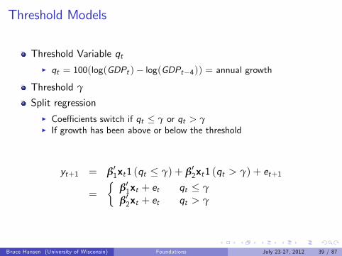
Threshold Models
Threshold Variable qtI qt = 100(log(GDPt )− log(GDPt−4)) = annual growth
Threshold γ
Split regressionI Coeffi cients switch if qt ≤ γ or qt > γI If growth has been above or below the threshold
yt+1 = β′1xt1 (qt ≤ γ) + β′2xt1 (qt > γ) + et+1
=
{β′1xt + et qt ≤ γβ′2xt + et qt > γ
Bruce Hansen (University of Wisconsin) Foundations July 23-27, 2012 39 / 87
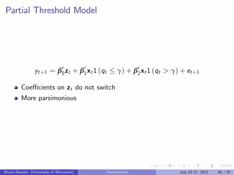
Partial Threshold Model
yt+1 = β′0zt + β′1xt1 (qt ≤ γ) + β′2xt1 (qt > γ) + et+1
Coeffi cients on zt do not switchMore parsimonious
Bruce Hansen (University of Wisconsin) Foundations July 23-27, 2012 40 / 87
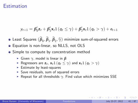
Estimation
yt+1 = β′0zt + β′1xt1 (qt ≤ γ) + β′2xt1 (qt > γ) + et+1
Least Squares (β0, β1, β2, γ) minimize sum-of-squared errors
Equation is non-linear, so NLLS, not OLS
Simple to compute by concentration methodI Given γ, model is linear in βI Regressors are zt , xt1 (qt ≤ γ) and xt1 (qt > γ)I Estimate by least-squaresI Save residuals, sum of squared errorsI Repeat for all thresholds γ. Find value which minimizes SSE
Bruce Hansen (University of Wisconsin) Foundations July 23-27, 2012 41 / 87
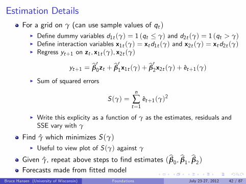
Estimation DetailsFor a grid on γ (can use sample values of qt )
I Define dummy variables d1t (γ) = 1 (qt ≤ γ) and d2t (γ) = 1 (qt > γ)I Define interaction variables x1t (γ) = xtd1t (γ) and x2t (γ) = xtd2t (γ)I Regress yt+1 on zt , x1t (γ), x2t (γ)
yt+1 = β′0zt + β
′1x1t (γ) + β
′2x2t (γ) + et+1(γ)
I Sum of squared errors
S(γ) =n
∑t=1
et+1(γ)2
I Write this explicity as a function of γ as the estimates, residuals andSSE vary with γ
Find γ which minimizes S(γ)I Useful to view plot of S(γ) against γ
Given γ, repeat above steps to find estimates (β0, β1, β2)Forecasts made from fitted model
Bruce Hansen (University of Wisconsin) Foundations July 23-27, 2012 42 / 87
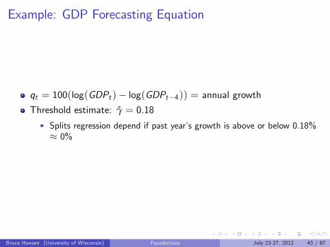
Example: GDP Forecasting Equation
qt = 100(log(GDPt )− log(GDPt−4)) = annual growth
Threshold estimate: γ = 0.18I Splits regression depend if past year’s growth is above or below 0.18%≈ 0%
Bruce Hansen (University of Wisconsin) Foundations July 23-27, 2012 43 / 87
Bruce Hansen (University of Wisconsin) Foundations July 23-27, 2012 44 / 87
Multi-Step Forecasts
Nonlinear models (including threshold models) do not have simpleiteration method for multi-step forecasts
Option 1: Specify direct threshold model
Option 2: Iterate one-step threshold model by simulation:
Bruce Hansen (University of Wisconsin) Foundations July 23-27, 2012 45 / 87
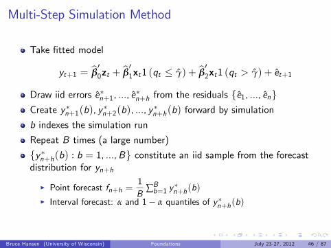
Multi-Step Simulation Method
Take fitted model
yt+1 = β′0zt + β
′1xt1 (qt ≤ γ) + β
′2xt1 (qt > γ) + et+1
Draw iid errors e∗n+1, ..., e∗n+h from the residuals {e1, ..., en}
Create y ∗n+1(b), y∗n+2(b), ..., y
∗n+h(b) forward by simulation
b indexes the simulation run
Repeat B times (a large number)
{y ∗n+h(b) : b = 1, ...,B} constitute an iid sample from the forecastdistribution for yn+h
I Point forecast fn+h =1B
∑Bb=1 y∗n+h(b)
I Interval forecast: α and 1− α quantiles of y∗n+h(b)
Bruce Hansen (University of Wisconsin) Foundations July 23-27, 2012 46 / 87
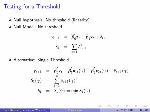
Testing for a Threshold
Null hypothesis: No threshold (linearity)
Null Model: No threshold
yt+1 = β′0zt + β
′1xt + et+1
S0 =n
∑t=1e2t+1
Alternative: Single Threshold
yt+1 = β′0zt + β
′1x1t (γ) + β
′2x2t (γ) + et+1(γ)
S1(γ) =n
∑t=1et+1(γ)2
S1 = S1(γ) = minγS1(γ)
Bruce Hansen (University of Wisconsin) Foundations July 23-27, 2012 47 / 87

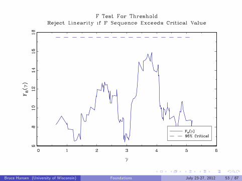
Threshold F Test
No Threshold against one threshold
F (γ) = n(S0 − S1(γ)S1(γ)
)
F = n(S0 − S1S1
)= max
γF (γ)
Bruce Hansen (University of Wisconsin) Foundations July 23-27, 2012 48 / 87
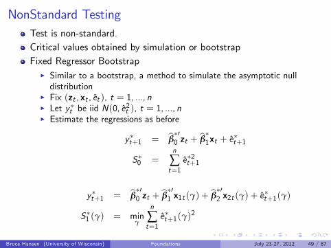
NonStandard TestingTest is non-standard.Critical values obtained by simulation or bootstrapFixed Regressor Bootstrap
I Similar to a bootstrap, a method to simulate the asymptotic nulldistribution
I Fix (zt , xt , et ), t = 1, ..., nI Let y∗t be iid N(0, e
2t ), t = 1, ..., n
I Estimate the regressions as before
y∗t+1 = β∗′0 zt + β
∗1xt + e
∗t+1
S∗0 =n
∑t=1
e∗2t+1
y∗t+1 = β∗′0 zt + β
∗′1 x1t (γ) + β
∗′2 x2t (γ) + e
∗t+1(γ)
S∗1 (γ) = minγ
n
∑t=1
e∗t+1(γ)2
Bruce Hansen (University of Wisconsin) Foundations July 23-27, 2012 49 / 87
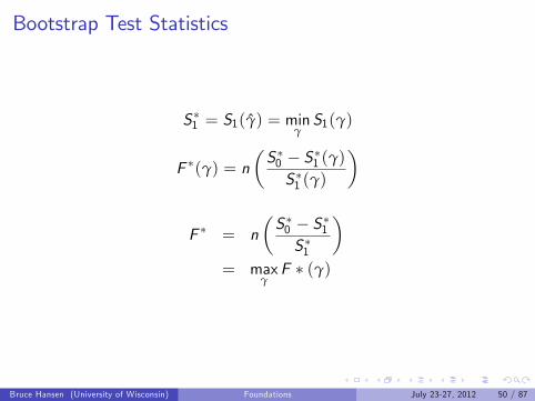
Bootstrap Test Statistics
S∗1 = S1(γ) = minγS1(γ)
F ∗(γ) = n(S∗0 − S∗1 (γ)S∗1 (γ)
)
F ∗ = n(S∗0 − S∗1S∗1
)= max
γF ∗ (γ)
Bruce Hansen (University of Wisconsin) Foundations July 23-27, 2012 50 / 87
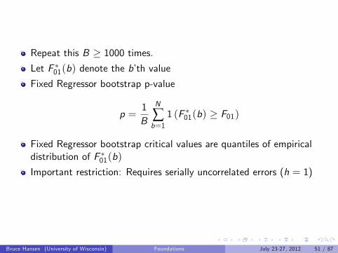
Repeat this B ≥ 1000 times.Let F ∗01(b) denote the b’th value
Fixed Regressor bootstrap p-value
p =1B
N
∑b=1
1 (F ∗01(b) ≥ F01)
Fixed Regressor bootstrap critical values are quantiles of empiricaldistribution of F ∗01(b)
Important restriction: Requires serially uncorrelated errors (h = 1)
Bruce Hansen (University of Wisconsin) Foundations July 23-27, 2012 51 / 87
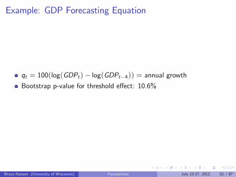
Example: GDP Forecasting Equation
qt = 100(log(GDPt )− log(GDPt−4)) = annual growth
Bootstrap p-value for threshold effect: 10.6%
Bruce Hansen (University of Wisconsin) Foundations July 23-27, 2012 52 / 87
Bruce Hansen (University of Wisconsin) Foundations July 23-27, 2012 53 / 87
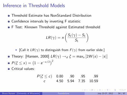
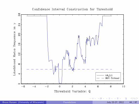
Inference in Threshold Models
Threshold Estimate has NonStandard Distribution
Confidence intervals by inverting F statistic
F Test: Kknown Threshold against Estimated threshold
LR(γ) = n(S1(γ)− S1
S1
)I [Call it LR(γ) to distinguish from F (γ) from earlier slide.]
Theory: [Hansen, 2000] LR(γ)→d ξ = maxs [2W (s)− |s |]P(ξ ≤ x) =
(1− e−x/2)2
Critical values:
P(ξ ≤ c) 0.80 .90 .95 .99c 4.50 5.94 7.35 10.59
Bruce Hansen (University of Wisconsin) Foundations July 23-27, 2012 54 / 87
Confidence Intervals for Threshold
All γ such that LR(γ) ≤ c where c is critical valueEasy to see in graph of LR(γ) against γ
Bruce Hansen (University of Wisconsin) Foundations July 23-27, 2012 55 / 87

Bruce Hansen (University of Wisconsin) Foundations July 23-27, 2012 56 / 87
Threshold Estimates
Estimate: γ = 0.18
Confidence Interval = [−1.0, 2.2]
Bruce Hansen (University of Wisconsin) Foundations July 23-27, 2012 57 / 87

Inference on Slope Parameters
Conventional
As if threshold is known
Bruce Hansen (University of Wisconsin) Foundations July 23-27, 2012 58 / 87
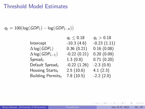
Threshold Model Estimates
qt = 100(log(GDPt )− log(GDPt−4))
qt ≤ 0.18 qt > 0.18Intercept -10.3 (4.6) -0.23 (1.11)∆ log(GDPt ) 0.36 (0.21) 0.16 (0.08)∆ log(GDPt−1) -0.22 (0.21) 0.20 (0.09)Spreadt 1.3 (0.8) 0.71 (0.20)Default Spreadt -0.22 (1.26) -2.3 (0.9)Housing Startst 2.5 (10.6) 4.1 (2.3)Building Permitst 7.8 (10.5) -2.2 (2.0)
Bruce Hansen (University of Wisconsin) Foundations July 23-27, 2012 59 / 87
NonParametric/NonLinear Time Series Regression
Optimal point forecast is g (xn) where
g (x) = E (yt+1|xt = x)
and xt are all relevant variables.In general, the form of g (x) is unknown and nonlinearLinear models used for simplicity, but they are not “true”
Bruce Hansen (University of Wisconsin) Foundations July 23-27, 2012 60 / 87
NonParametric/NonLinear Time Series Regression
Model
yt+1 = g (xt ) + et+1E (et+1|xt ) = 0
The conditional mean zero restriction holds true by construction
et+1 not necessarily iid
Bruce Hansen (University of Wisconsin) Foundations July 23-27, 2012 61 / 87
Additively Separable Model
xt = (x1t , ..., xpt )
g (xt ) = g1(x1t ) + g2(x2t ) + · · ·+ gp(xpt )
Thenyt+1 = g1(x1t ) + g2(x2t ) + · · ·+ gp(xpt ) + et+1
Greatly reduces degree of nonlinearity
Useful simplification, but should be viewed as such, not as “true”
Bruce Hansen (University of Wisconsin) Foundations July 23-27, 2012 62 / 87
Partially Linear Model
Partition xt = (x1t , x2t )
g (xt ) = g1(x1t ) + β′x2t
x2t typically includes dummy variables, controlsx1t main variables of importanceFor example, if primary dependence through first lag
yt+1 = g1(yt ) + β1yt−1 + · · ·+ βpyt−p + et+1
Bruce Hansen (University of Wisconsin) Foundations July 23-27, 2012 63 / 87
Sieve Models
For simplicity, suppose xt is scalar (real-valued)
WLOG in additively separable and partially linear models
Approximate g(x) by a sequence gm(x), m = 1, 2, ..., of increasingcomplexity
Linear sievesgm(x) = Zm(x)′βm
where Zm(x) = (z1m(x), ..., zKm(x)) are nonlinear functions of x .
“Series”: Zm(x) = (z1(x), ..., zK (x))
“Sieves”: Zm(x) = (z1m(x), ..., zKm(x))
Bruce Hansen (University of Wisconsin) Foundations July 23-27, 2012 64 / 87
Polynomial (power series)
zj (x) = x j
gm(x) =p
∑j=1
βjxj
Stone-Weierstrass Theorem: Any continuous function g(x) can bearbitrarily well approximated on a compact set by a polynomial ofsuffi ciently high order
I For any ε > 0 there exists coeffi cients p and βj such that X
supx∈X|gm(x)− g(x)| ≤ ε
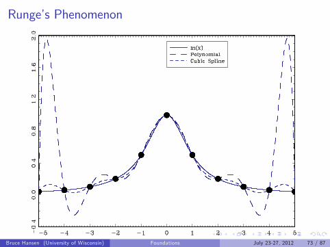
Runge’s phenomenon:I Polynomials can be poor at interpolation (can be erratic)
Bruce Hansen (University of Wisconsin) Foundations July 23-27, 2012 65 / 87
Splines
Piecewise smooth polynomials
Join points are called knotsLinear spline with one knot at τ
gm(x) =
β00 + β01 (x − τ) x < τ
β10 + β11 (x − τ) x ≥ τ
To enforce continuity, β00 = β10,
gm(x) = β0 + β1 (x − τ) + β2 (x − τ) 1 (x ≥ τ)
or equivalently
gm(x) = β0 + β1x + β2 (x − τ) 1 (x ≥ τ)
Bruce Hansen (University of Wisconsin) Foundations July 23-27, 2012 66 / 87
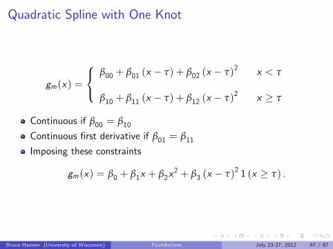
Quadratic Spline with One Knot
gm(x) =
β00 + β01 (x − τ) + β02 (x − τ)2 x < τ
β10 + β11 (x − τ) + β12 (x − τ)2 x ≥ τ
Continuous if β00 = β10Continuous first derivative if β01 = β11Imposing these constraints
gm(x) = β0 + β1x + β2x2 + β3 (x − τ)2 1 (x ≥ τ) .
Bruce Hansen (University of Wisconsin) Foundations July 23-27, 2012 67 / 87

Cubic Spline with One Knot
gm(x) = β0 + β1x + β2x2 + β3x
3 + β4 (x − τ)3 1 (x ≥ τ)
Bruce Hansen (University of Wisconsin) Foundations July 23-27, 2012 68 / 87
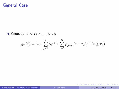
General Case
Knots at τ1 < τ2 < · · · < τN
gm(x) = β0 +p
∑j=1
βjxj +
N
∑k=1
βp+k (x − τk )p 1 (x ≥ τk )
Bruce Hansen (University of Wisconsin) Foundations July 23-27, 2012 69 / 87
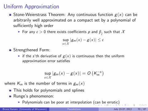
Uniform ApproximationStone-Weierstrass Theorem: Any continuous function g(x) can bearbitrarily well approximated on a compact set by a polynomial ofsuffi ciently high order
I For any ε > 0 there exists coeffi cients p and βj such that X
supx∈X|gm(x)− g(x)| ≤ ε
Strengthened Form:I if the s’th derivative of g(x) is continuous then the uniformapproximation error satisfies
supx∈X|gm(x)− g(x)| = O
(K−αm
)where Km is the number of terms in gm(x)
This holds for polynomials and splinesRunge’s phenomenon:
I Polynomials can be poor at interpolation (can be erratic)
Bruce Hansen (University of Wisconsin) Foundations July 23-27, 2012 70 / 87
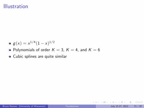
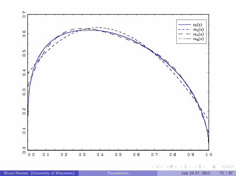
Illustration
g(x) = x1/4(1− x)1/2
Polynomials of order K = 3, K = 4, and K = 6
Cubic splines are quite similar
Bruce Hansen (University of Wisconsin) Foundations July 23-27, 2012 71 / 87
Bruce Hansen (University of Wisconsin) Foundations July 23-27, 2012 72 / 87
Runge’s Phenomenon
Bruce Hansen (University of Wisconsin) Foundations July 23-27, 2012 73 / 87

Placement of Knots
If support of x is [0, 1], typical to set τj = j/(N + 1)If support of x is [a, b], can set τj = a+ (b− a)/(N + 1)Alternatively, can set τj to equal the j/(n+ 1) quantile of thedistribution of x
Bruce Hansen (University of Wisconsin) Foundations July 23-27, 2012 74 / 87
Estimation
Fix number and location of knots
Estimate coeffi cients by least-squares
Quadratic spline
y = β0 + β1x + β2x2 +
N
∑k=1
β2+k (x − τk )2 1 (x ≥ τk ) + e
Linear model in x , x2, (x − τ1)2 1 (x ≥ τ1) , ..., (x − τN )
2 1 (x ≥ τN )
Bruce Hansen (University of Wisconsin) Foundations July 23-27, 2012 75 / 87
Selection of Number of Knots
Model selection
Pick N to minimize Cross-validation function
CV is an estimate ofI MSFEI IMSE (integrated mean-squared error)
CV selection (and combination) is asymptotically optimal forminimization of the MSFE and IMSE
Bruce Hansen (University of Wisconsin) Foundations July 23-27, 2012 76 / 87
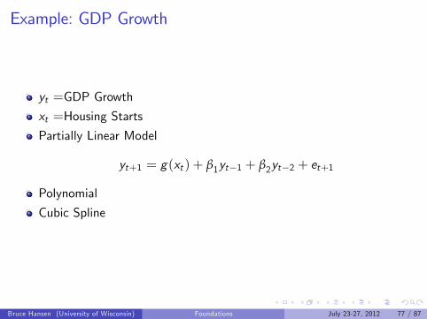
Example: GDP Growth
yt =GDP Growth
xt =Housing Starts
Partially Linear Model
yt+1 = g(xt ) + β1yt−1 + β2yt−2 + et+1
Polynomial
Cubic Spline
Bruce Hansen (University of Wisconsin) Foundations July 23-27, 2012 77 / 87
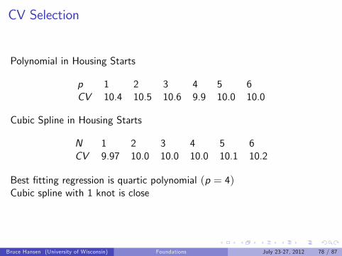
CV Selection
Polynomial in Housing Starts
p 1 2 3 4 5 6CV 10.4 10.5 10.6 9.9 10.0 10.0
Cubic Spline in Housing Starts
N 1 2 3 4 5 6CV 9.97 10.0 10.0 10.0 10.1 10.2
Best fitting regression is quartic polynomial (p = 4)Cubic spline with 1 knot is close
Bruce Hansen (University of Wisconsin) Foundations July 23-27, 2012 78 / 87
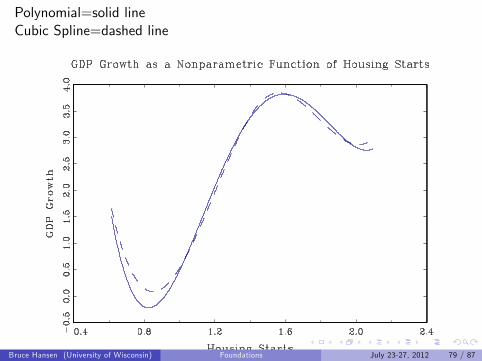
Polynomial=solid lineCubic Spline=dashed line
Bruce Hansen (University of Wisconsin) Foundations July 23-27, 2012 79 / 87
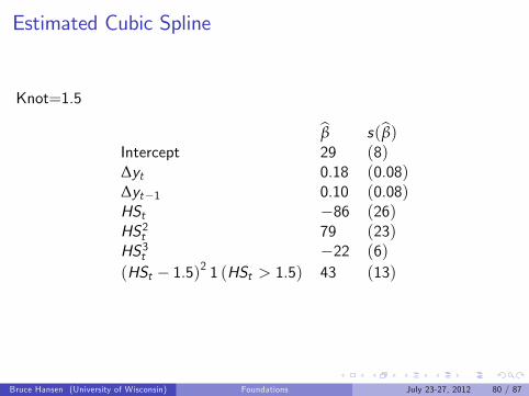
Estimated Cubic Spline
Knot=1.5
β s(β)Intercept 29 (8)∆yt 0.18 (0.08)∆yt−1 0.10 (0.08)HSt −86 (26)HS2t 79 (23)HS3t −22 (6)(HSt − 1.5)2 1 (HSt > 1.5) 43 (13)
Bruce Hansen (University of Wisconsin) Foundations July 23-27, 2012 80 / 87
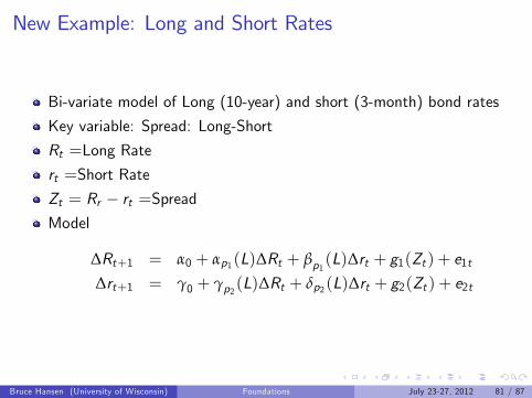
New Example: Long and Short Rates
Bi-variate model of Long (10-year) and short (3-month) bond rates
Key variable: Spread: Long-Short
Rt =Long Rate
rt =Short Rate
Zt = Rr − rt =SpreadModel
∆Rt+1 = α0 + αp1(L)∆Rt + βp1(L)∆rt + g1(Zt ) + e1t∆rt+1 = γ0 + γp2(L)∆Rt + δp2(L)∆rt + g2(Zt ) + e2t
Bruce Hansen (University of Wisconsin) Foundations July 23-27, 2012 81 / 87

CV Selection
Separately for each equationI Long Rate and Short RateI Select over number of lagsI Number of spline terms for nonlinearity in Spread
Bruce Hansen (University of Wisconsin) Foundations July 23-27, 2012 82 / 87
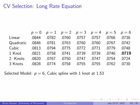
CV Selection: Long Rate Equation
p = 0 p = 1 p = 2 p = 3 p = 4 p = 5 p = 6Linear .0844 .0782 .0760 .0757 .0757 .0766 .0736Quadratic .0846 .0781 .0763 .0760 .0760 .0767 .0742Cubic .0813 .0794 .0775 .0772 .0771 .0779 .07481 Knot .0821 .0758 .0741 .0739 .0739 .0746 .07192 Knots .0820 .0767 .0750 .0747 .0747 .0754 .07243 Knots .0828 .0774 .0758 .0755 .0755 .0762 .0730
Selected Model: p = 6, Cubic spline with 1 knot at 1.53
Bruce Hansen (University of Wisconsin) Foundations July 23-27, 2012 83 / 87
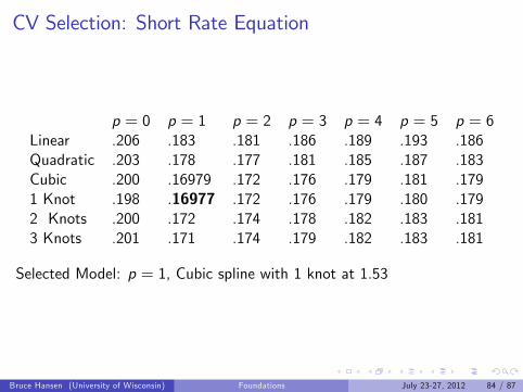
CV Selection: Short Rate Equation
p = 0 p = 1 p = 2 p = 3 p = 4 p = 5 p = 6Linear .206 .183 .181 .186 .189 .193 .186Quadratic .203 .178 .177 .181 .185 .187 .183Cubic .200 .16979 .172 .176 .179 .181 .1791 Knot .198 .16977 .172 .176 .179 .180 .1792 Knots .200 .172 .174 .178 .182 .183 .1813 Knots .201 .171 .174 .179 .182 .183 .181
Selected Model: p = 1, Cubic spline with 1 knot at 1.53
Bruce Hansen (University of Wisconsin) Foundations July 23-27, 2012 84 / 87
Bruce Hansen (University of Wisconsin) Foundations July 23-27, 2012 85 / 87
Forecasting
For h > 1, need to use forecast simulation
Simulate Rn+1, rn+1 forward using iid draws from residuals
Create time paths
Take means to estimate point forecasts
Take quantiles to construct forecats intervals
Bruce Hansen (University of Wisconsin) Foundations July 23-27, 2012 86 / 87

Assignment
Construct a nonlinear model to forecast the unemployment rate.
Use either a threshold or nonparametric model
Use appropriate methods to select the model and variables
Make a one-step forecast
If time, use simulation to create 1 through 12 step forecastdistributions. Use this to calculate point forecasts, intervals and a fanchart.
Bruce Hansen (University of Wisconsin) Foundations July 23-27, 2012 87 / 87
Related Documents