Three Essays in Macroeconomics

Department of Economics

Three Essays in Macroeconomics

Lenno Uusküla

Thesis submitted for assessment with a view to obtaining the degree of Doctor of Economics of the European University Institute

FlorenceFebruary 2011

EUROPEAN UNIVERSITY INSTITUTEDepartment of Economics

Three Essays in Macroeconomics

Lenno Uusküla

Thesis submitted for assessment with a view to obtaining the degree of

Doctor of Economics of the European University Institute

Jury Members:

Prof. Morten Ravn, University College London, SupervisorProf. Giancarlo Corsetti, EUI and University of CambridgeProf. Fabio Canova, Universitat Pompeu FabraDr. Luca Dedola, European Central Bank

© 2011, Lenno UuskülaNo part of this thesis may be copied, reproduced or transmitted without prior permission of the author

Uusküla, Lenno (2011), Three Essays in Macroeconomics European University Institute

DOI: 10.2870/25050

Dedication

To my wife Mari and daughter Karolina


DOI: 10.2870/25050

Acknowledgements

I was very lucky to have Morten O. Ravn and Giancarlo Corsetti as supervisors.

Morten O. Ravn was very patiently pushing me to write better papers. Giancarlo

Corsetti was always cheerful and encouraging even at the times when models were

not working.

The years in Florence would have been very lonely without many good friends.

Mark Le Quement and Markus Kitzmüller helped to survive the first year and made

the rest a pure pleasure. We spent together long evenings in VSP but happily not

only in VSP. With the support of many more friends I found the strength not only

to fight through, but also enjoy the study process. I hope that the future will make

our friendship only stronger. I want to thank Jessica Spataro and Lucia Vigna for

all the paperwork and Thomas Bourke for the help in getting firm turnover data.

Last but not least I grateful to my wife Mari who agreed to take the adventure in

Florence and Karolina who has kept up the good mood during the last few months.

ii


DOI: 10.2870/25050

Contents

I Introduction v

II Chapters 1

1 Monetary Transmission and Firm Turnover 2

1.1 Introduction . . . . . . . . . . . . . . . . . . . . . . . . . . . . . . . . 3

1.2 Empirical methodology . . . . . . . . . . . . . . . . . . . . . . . . . . 5

1.3 Data . . . . . . . . . . . . . . . . . . . . . . . . . . . . . . . . . . . . 9

1.4 Empirical results . . . . . . . . . . . . . . . . . . . . . . . . . . . . . 10

1.5 Robustness analysis . . . . . . . . . . . . . . . . . . . . . . . . . . . 11

1.6 Limited participation model . . . . . . . . . . . . . . . . . . . . . . . 13

1.6.1 Consumer problem . . . . . . . . . . . . . . . . . . . . . . . . 13

1.6.2 Final goods firm . . . . . . . . . . . . . . . . . . . . . . . . . 14

1.6.3 Intermediate goods firms . . . . . . . . . . . . . . . . . . . . 15

1.6.4 Financial intermediary . . . . . . . . . . . . . . . . . . . . . . 16

1.6.5 Monetary authority . . . . . . . . . . . . . . . . . . . . . . . 16

1.6.6 Market clearing conditions and the equilibrium . . . . . . . . 16

1.7 Model with pre-set prices . . . . . . . . . . . . . . . . . . . . . . . . 17

1.7.1 Consumer problem . . . . . . . . . . . . . . . . . . . . . . . . 17

1.7.2 Final goods firm . . . . . . . . . . . . . . . . . . . . . . . . . 18

1.7.3 Intermediate goods firms . . . . . . . . . . . . . . . . . . . . 18

1.7.4 Monetary authority . . . . . . . . . . . . . . . . . . . . . . . 20

1.7.5 Market clearing conditions . . . . . . . . . . . . . . . . . . . . 20

1.8 Calibration and results of the two models . . . . . . . . . . . . . . . 20

1.9 Conclusions . . . . . . . . . . . . . . . . . . . . . . . . . . . . . . . . 22

Bibliograpy . . . . . . . . . . . . . . . . . . . . . . . . . . . . . . . . . . . 23

iii


DOI: 10.2870/25050

2 Deep Habits and the Dynamic Effects of Monetary Policy Shocks 37

2.1 Introduction . . . . . . . . . . . . . . . . . . . . . . . . . . . . . . . . 38

2.2 The Model . . . . . . . . . . . . . . . . . . . . . . . . . . . . . . . . 41

2.2.1 Households . . . . . . . . . . . . . . . . . . . . . . . . . . . . 42

2.2.2 Firms . . . . . . . . . . . . . . . . . . . . . . . . . . . . . . . 45

2.2.3 Monetary Policy . . . . . . . . . . . . . . . . . . . . . . . . . 48

2.2.4 Market Clearing . . . . . . . . . . . . . . . . . . . . . . . . . 48

2.2.5 Symmetric Equilibrium . . . . . . . . . . . . . . . . . . . . . 48

2.3 Estimation . . . . . . . . . . . . . . . . . . . . . . . . . . . . . . . . 50

2.3.1 SVAR Estimates of the Impact of Monetary Policy Shocks . . 50

2.3.2 Estimation of the Structural Parameters . . . . . . . . . . . . 52

2.4 Results . . . . . . . . . . . . . . . . . . . . . . . . . . . . . . . . . . . 55

2.4.1 Constrained Markup . . . . . . . . . . . . . . . . . . . . . . . 58

2.4.2 Sub-Sample Stability . . . . . . . . . . . . . . . . . . . . . . . 59

2.5 Conclusions . . . . . . . . . . . . . . . . . . . . . . . . . . . . . . . . 60

Bibliography . . . . . . . . . . . . . . . . . . . . . . . . . . . . . . . . . . 61

3 Firm Turnover, Financial Friction and Inflation 77

3.1 Introduction . . . . . . . . . . . . . . . . . . . . . . . . . . . . . . . . 77

3.2 The model . . . . . . . . . . . . . . . . . . . . . . . . . . . . . . . . . 79

3.2.1 Household problem . . . . . . . . . . . . . . . . . . . . . . . . 80

3.2.2 Final good firms . . . . . . . . . . . . . . . . . . . . . . . . . 81

3.2.3 Intermediate good firms . . . . . . . . . . . . . . . . . . . . . 82

3.2.4 Banks . . . . . . . . . . . . . . . . . . . . . . . . . . . . . . . 85

3.2.5 The Government and the Central Bank . . . . . . . . . . . . 85

3.2.6 Aggregation and market clearing . . . . . . . . . . . . . . . . 85

3.2.7 Equilibrium . . . . . . . . . . . . . . . . . . . . . . . . . . . . 86

3.3 Data, Estimation and Priors . . . . . . . . . . . . . . . . . . . . . . . 86

3.4 Results . . . . . . . . . . . . . . . . . . . . . . . . . . . . . . . . . . . 88

3.5 Conclusions . . . . . . . . . . . . . . . . . . . . . . . . . . . . . . . . 93

Bibliography . . . . . . . . . . . . . . . . . . . . . . . . . . . . . . . . . . 95

iv


DOI: 10.2870/25050

Part I

Introduction

v


DOI: 10.2870/25050

Introduction

Does the number of firms increase or decrease after a contrationary monetary shock?

Do the predictions of a standard sticky price model match with the empirical evi-

dence? How can we explain persistent and hump shaped effects of monetary policy?

What explains inflation? These are the central questions in the thesis. Three pa-

pers have strong overlaps, but contain also major differences. The common element

in the papers is a modified New Keynesian Phillips curve, but that was never an

objective on its own. The macroeconomic models of the first and third chapter are

similar as they include a financial friction and the number of firms dynamics. Second

is based instead on a deep habits mechanism that changes the pricing behavior of

firms. In terms of econometric method, the first two chapters are alike as they help

to understand monetary shocks based on structural VAR evidence. Third paper

explains inflation using full likelihood Bayesian estimation of a DSGE model.

In the first chapter I show that based on structural VAR evidence for the postwar

U.S. economy, a contractionary monetary shock leads to a drop in the creation of

new firms and increase in the number of failures. In the theoretical part of the paper

I show that financial friction is important in understanding the firm creation and

destruction for monetary shocks. The requirement of working capital in production

helps to generate a decrease in the number of firms for a negative monetary shock.

However a standard sticky price model predicts that the number of firms increases

after a negative monetary shock. When firms do not adjust their prices immediately

aggregate demand falls. This also lower labor demand. But when wages are low, it

is cheap to create new firms. Therefore sticky prices cannot be the only and most

important mechanism for monetary transmission.

Second chapter, written together with Morten O. Ravn, Stephanie Schmitt-

Grohe and Martín Uribe introduces deep habits in a standard sticky price and sticky

wage monetary model and demonstrates how the inclusion can explains two features

of the monetary effect that are usually called puzzles in the literature. First the

deep habits leads to a persistent decline in prices after a monetary shock. Second,

the deep habits mechanism can reproduce the price puzzle often found in the papers

- inflation tends to increase rather than decrease after a contractionary monetary

shock. The deep habits work through two channels. First, intratemporally the

prices increase after a contractionary shock because the elastic part of consumption

has decreased compared to the non-elastic component, so that the optimal mark-up

increases. Second, given the expected decline in consumption firms do not have

vi


DOI: 10.2870/25050

incentives to invest into demand, so that prices increase even further. The model

impulse responses are matched with a monetary VAR evidence for the postwar U.S.

economy.

In the third chapter I ask the question what explains inflation dynamics over the

business cycle. I augment a medium scale New Keynesian DSGE model with two

features. First, I allow the number of firms to vary over the business cycle. Second,

firms need to borrow part of their wage bill in advance. Financial frictions and

firm dynamics enter both the New Keynesian Phillips curve and uncouple marginal

cost from the inflation rate. I show that the shocks to the cost of creating firms

are important in explaining inflation dynamics. A drop in the entry costs leads to

increase in inflation as many firms are created and costs are high. Inflation decreases

only gradually as the number of firms in the economy increases. I find evidence that

also shocks to the technology are important in generating volatility in inflation.

Financial friction does not play a crucial role in explaining inflation. The results

are obtained using full likelihood Bayesian estimation of a DSGE model for the U.S.

economy.

vii


DOI: 10.2870/25050

Part II

Chapters

1


DOI: 10.2870/25050

Chapter 1

Monetary Transmission and

Firm Turnover

Lenno Uusküla1

Abstract

Traditional models of monetary transmission such as sticky price and limited partic-

ipation abstract from firm creation and destruction. Only a few papers look at the

empirical effects of the monetary shock on the firm turnover measures. But what

can we learn about monetary transmission by including measures for firm turnover

into the theoretical and empirical models? Based on a large scale vector autore-

gressive (VAR) model for the U.S. economy I show that a contractionary monetary

policy shock increases the number of business bankruptcy filings and failures, and

decreases the creation of firms and net entry. According to the limited participation

model, a contractionary monetary shock leads to a drop in the number of firms.

On the contrary the same shock in the sticky price model increases the number of

firms. Therefore the empirical findings support more the limited participation type

of monetary transmission.

1I want to thank Morten O. Ravn, Giancarlo Corsetti, Saverio Simonelli, Jeff Campbell, ZenoEnders and Alan Sutherland for their valuable suggestions, Thomas Bourke for help in getting thedata. I am also grateful to the seminar participants at the European University Institute, and EestiPank, and conference participants at MAREM Conference in Bonn, International Conference onEconomic Modeling in Berlin, EEA/ESEM conference in Milan, and Money, Macro and Finance(MMF) conference in London.

2


DOI: 10.2870/25050

Keywords: monetary transmission, limited participation, sticky prices, firm

entry, firm bankruptcy, structural VAR

JEL codes: E32, C32

1.1 Introduction

Two popular approaches for understanding monetary transmission are limited par-

ticipation and sticky price models. These models rarely include firm turnover: entry

and exit of firms. What can we learn about monetary transmission by including

the number of firm dynamics into these models? What are the empirical effects of

monetary shocks on the firm turnover variables?

The empirical results of the paper show that a contractionary monetary shock

leads to an increase in the number of business failures and to a decrease in the cre-

ation of firms. The sticky price and limited participation models give contradicting

predictions about the firm turnover dynamics. According the sticky price model a

contractionary monetary policy shock leads to an increase in the number of firms,

whereas in the limited participation model the same shock leads to a decrease in the

number of firms. Therefore the empirical evidence supports limited participation

hypothesis of monetary transmission in comparison to the sticky prices.

I estimate an 11-variable vector autoregressive (VAR) model for the U.S. econ-

omy including labor productivity, total hours, GDP deflator, capacity utilization,

real wages, consumption, investment, Federal Funds Rate, money velocity, and one-

by-one alternative firm turnover measures: firm entry, net entry, business bankruptcy

filings, and failures. I adopt the recursive approach in identifying monetary shocks

which is based on contemporaneous restrictions. In addition I identify investment

specific and neutral technology shocks with long run restrictions in order to mini-

mize problems of mis-specification. The monetary policy results are robust to the

use of non-borrowed reserves and the Federal Funds Rate (FFR) in order to identify

the shock, inclusion and exclusion of the firm turnover measures from the central

bank information set, difference and level stationarity of hours, reduction of the

estimation period, etc.

My empirical findings are in line with the previous literature measuring the

effects of the monetary policy on the creation of firms. Bergin and Corsetti (2008)

use a relatively small scale VAR of monthly data and impose short run restrictions

in order to identify the monetary shock. They find that net entry decreases after a

contractionary monetary shock when either the FFR or non-borrowed reserves are

3


DOI: 10.2870/25050

used in order to identify monetary policy shocks. The firm creation decreases only if

non-borrowed reserves are used to identify the monetary shock. Lewis (forthcoming)

adopts a sign restriction approach to estimate the effect of the monetary shock to

net entry. She finds that net entry decreases only with a significant lag after a

contractionary monetary policy shock.

In the theoretical part of the paper I augment two simple models of monetary

transmission, a limited participation and a pre-set price model as a simple case of

sticky prices, with the endogenous firm creation and exogenous firm destruction

dynamics. I assume that creation and operating firms is labor intensive. According

to the limited participation model, firms pay wages before production and have to

borrow the wage bill from the financial intermediary. A contractionary monetary

policy shock decreases the liquidity of the financial intermediaries: bank lending

falls and the interest rate increases. The real wage and hours worked decrease

because firms can borrow less money to pay for their workers. The marginal cost of

production for the firm remains constant because the real wage declines and interest

rate increases. Fall in the total production leads to a drop in the creation of firms.

In a standard sticky price model, a contractionary monetary shock leads to a drop

in demand for the consumer good and consequently to a drop in demand for labor.

Therefore labor costs fall equally for production of goods, and for operating and

creating firms. Increasing profits per firm lead to higher creation of firms up to the

level where the free entry condition is satisfied. These results are the opposite of

the predictions of the limited participation model and the empirical results. Some

recent models of monetary transmission include the firm turnover dynamics.

In the Bilbiie, Ghironi, and Melitz (2007) model with quadratic adjustment cost

of prices, a contractionary monetary policy shock leads to an increase in the number

of firms (in their interpretation varieties) when creating firms is labor intensive.

Instead, in order to get a decrease in the number of firms, Bilbiie, Ghironi, and

Melitz (2007) and Bergin and Corsetti (2008) assume that for the entry cost, new

firms buy goods from the existing firms, who sell at pre-set prices. Then monetary

contractions decrease entry of firms because of the increase in the real entry cost.

However, a decrease in the demand for the output leads to a drop in wages and to

an increase in profits for the existing firms. Increasing profits should still lead to an

increase in entry in the production sector.

In order to keep entry costs fixed Mancini-Griffoli and Elkhoury (2006) assume

that in order to create a firm, entrepreneurs have to buy goods from a specific sector

in the economy that which sets their prices in advance, whereas the rest of the

4


DOI: 10.2870/25050

entrepreneurs set the prices of their goods freely. In such a set-up, a contractionary

monetary shock raises the real cost of entry and consequently the creation of firms

decreases. Lewis (forthcoming) shows that a contractionary monetary shock in the

sticky wage model can also lead to a drop in the entry of firms.

1.2 Empirical methodology

I set up the VAR model in order to estimate the effects of the monetary policy

shock to the firm turnover measures. I adopt the recursive approach in identifying

the monetary shock. In order to reduce the problem of mis-specification, I identify in

addition two technology shocks: investment specific and neutral technology shocks

with the long-run restrictions.

The reduced form VAR is given as:

yt = b0 +p∑

i=1

biyt−i + ut, (1.1)

where yt is the set of endogenous variables listed in Table 1.1 in the order as they

appear in the model, b0 represents all the deterministic terms which are used in the

estimation including constants, seasonal and impulse dummies, bi-s are matrices of

coefficients, p is the number of lags in the model, and ut is the error term.

Table 1.1: Variables used in the benchmark VAR

Notation Name of the variableip change in logarithm of investment pricelp change in logarithm of labor productivityGDPdef change in logarithm of GDP deflatorcapu level of capacity utilizationh logarithm of per capita hours worked (level)w logarithm of real labor costc logarithm of consumption share in GDPi logarithm of investment share in GDPee change in logarithm of firm demographics measureFFR federal funds rate (level)vel logarithm of money velocity

I use the Federal Funds Rate (FFR) to measure monetary conditions and the

5


DOI: 10.2870/25050

change in the log of the GDP (Gross Domestic Product) deflator as a proxy for in-

flation. I include the relative price of investment in order to identify an investment

specific technology shock and a labor productivity variable in order to identify a

neutral technology shock. I add a list of macroeconomic variables in order to re-

duce a possible omitted variable bias. The additional macroeconomic variables are

capacity utilization, hours worked, real unit labor cost (real wages), consumption

and investment shares in GDP, and money velocity. For a detailed description of

the data see Table 1.2 in the Appendix.

Several other authors have estimated similar systems of VAR models. For exam-

ple Altig, Christiano, Eichenbaum, and Linde (2005) use a 10-variable VAR including

the relative price of investment, productivity, a GDP deflator, hours, consumption,

investment, and several other variables, but do not include a measure of firm dy-

namics in their system. Ravn and Simonelli (2007) estimate a 12-dimensional VAR

adding government expenditures and, specific to their paper, several labor market

variables.

The structural VAR is given as:

A0yt = B0 +p∑

i=1

Biyt−i + ǫt (1.2)

where Bi-s are matrices of the structural coefficients, related to bi-s as follows:

bi = A−10 Bi, ǫt are the structural shocks, the variance-covariance matrix Σǫ = E(ǫ′tǫt)

is assumed to be diagonal and related to the reduced form shock variance-covariance

matrix Σu = E(u′tut) by the following formula Σu = A−10′

ΣǫA−10 .

The recursive approach of identifying the monetary policy shocks builds on a

Taylor-rule type of argument. A central banker who takes into account the con-

temporaneous values of the variables in his information set (Ω), then decides on the

shock (ζt) by setting the interest rate (Rt),

Rt = F (Ω) + ζt. (1.3)

In order to obtain identification, I impose short-run restrictions. The variables

in the information set can have a contemporaneous effect on the interest rate, but

not vice versa. I estimate the following equation:

6


DOI: 10.2870/25050

FFRt = bf0 +p∑

i=0

bf,ipi ipt−i +p∑

i=0

bf,lpi lpt−i

+p∑

i=0

bf,GDPdefi GDPdeft−i +p∑

i=0

bf,capui caput−i +p∑

i=0

bf,hi ht−i

+p∑

i=0

bf,wi wt−i +p∑

i=0

bf,ci ct−i +p∑

i=0

bf,ii it−i +p∑

i=0

bf,eei eet−i

+p∑

i=1

bf,FFRi FFRt−i +p∑

i=1

bf,veli velt−i + uft . (1.4)

All the variables placed before the interest rate can have contemporaneous effects

on it, but are assumed not to be affected contemporaneously by it. For example,

money velocity, which is the only variable after the interest rate, is contemporane-

ously influenced by the interest rate, but does not affect the FFR in the same period.

I assume that the firm turnover variables enter into the central bank’s information

set (Ω). The explanatory variables for the interest rate are all the contemporaneous

values and lags of the variables placed before it, plus the lags of the interest rate

and money velocity.

The recursive identification scheme for the monetary policy is popular in em-

pirical literature, for example it is adopted in the papers by Altig, Christiano,

Eichenbaum, and Linde (2005), Boivin, Giannoni, and Mihov (2007), and Ravn

and Simonelli (2007). The main alternative is a non-recursive approach proposed

by Sims and Zha (2006), but it has been shown to result in very similar impulse

responses to the recursive identification scheme. Uhlig (2005) proposes an identifi-

cation scheme according to which sign restrictions are set on the impulse response

functions. The sign restrictions approach challenges some of the empirical results ob-

tained by the short-run restrictions. See Christiano, Eichenbaum, and Evans (1999)

for an overview of the main results of the monetary shock and the comparison of

various identification approaches.

Bergin and Corsetti (2008) exclude the firm turnover variable from the informa-

tion set of the central bank. The reason might be the use of monthly data in their

estimation. As shown in the robustness analysis section of this paper, the results

are not sensitive to different timing.

I base the identification of the investment specific technology shock on the as-

sumption that only the investment specific technology shocks can have a long-run

7


DOI: 10.2870/25050

impact on the relative price of investment goods. Therefore, the explanatory vari-

ables for the estimated equation on the relative price of investment are the lags of

the investment price itself and the lagged values of all other variables differenced

once. The use of differenced data implements the zero long-run restrictions, see

Shapiro and Watson (1988). The contemporaneous values of the FFR and velocity

are not included because of the identification of the monetary shock.

For the permanent neutral technology shock, I assume that only the neutral

and investment embodied technology shocks can lead to permanent changes in labor

productivity. Therefore all the other variables are differenced once. Again, con-

temporaneous values of the FFR and money velocity are not included in the set of

explanatory variables in order to identify the monetary policy shock.

The embodied technology equation cannot be estimated with the ordinary least

squares technique because the contemporaneous value of productivity might be cor-

related with the residual. Therefore I estimate the equation by IV technique. The

instruments are the lagged values of the explanatory variables. The equation neutral

technology has the same problem, therefore the equation is estimated with the IV

technique using the same instruments as for the equation on the investment price

adding the residual from the investment price equation.

After estimating the two technology shocks, I proceed with the estimation of the

equations in the order of the variables in Table 1.1. I estimate all the equations by

the recursive IV technique. I include the contemporaneous values of the previous

variables in the regression and exploit all the estimated residuals as instruments.

Therefore for the estimation of the last equation on money velocity, I include all the

other contemporaneous values of the variables in the regression and residuals in the

set of instruments.

Many authors consider technology to be the key factors in the macroeconomic

fluctuations, including Kydland and Prescott (1982), Altig, Christiano, Eichenbaum,

and Linde (2005), Ravn and Simonelli (2007), etc. Several authors adopt the long-

run restrictions approach in identifying neutral technology shocks, for example see

Gali (1999), Altig, Christiano, Eichenbaum, and Linde (2005), Fisher (2006), and

Ravn and Simonelli (2007). Recently Fischer (2006) showed that the neutral technol-

ogy shock might be mis-specified if the investment technology shock is not identified.

Campbell (1998) shows that technology shocks can be important for generating vari-

ance in the plant entry and exit dynamics, which is closely related to the business

entry and failure variables.

8


DOI: 10.2870/25050

1.3 Data

The creation of firms (number of new incorporations) and the number of business

failures (number of firms failed) are available for the period 1959Q1–1998Q3, and

the net entry index (net business formation) can be obtained for the period 1959Q1–

1995Q4. This data are collected and calculated by Dun&Bradstreet Inc. available

through various sources (see Table 1.2 in the Appendix). The number of business

bankruptcy filings is from the U.S. Court of Bankruptcy. It is used in the estimations

for the period 1960Q3–2005Q4. The firm turnover data are presented in log-levels

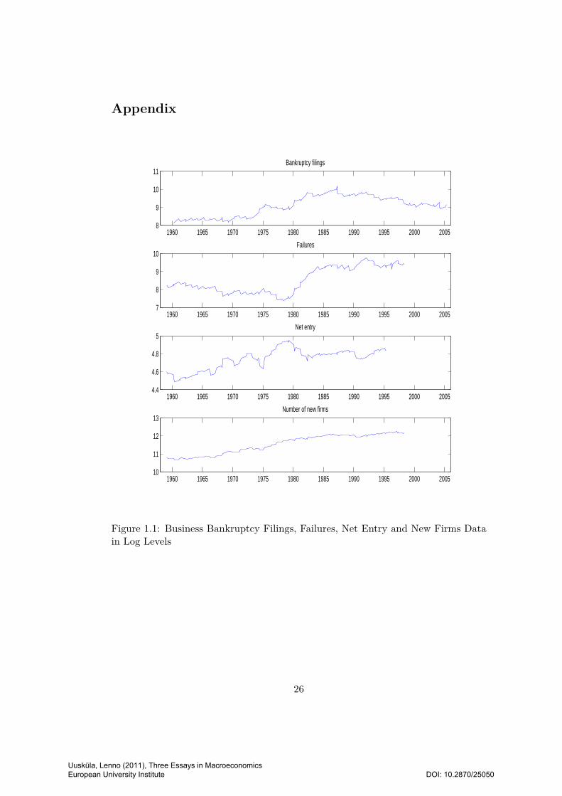
in Figure 1.1 in the Appendix.

The Dun&Bradstreet database covers around 90% of the enterprises with at least

one employee and some without employees. The registration of a company in the

Dun&Bradstreet database is voluntary and the registration of the firm can take place

some time after the actual start of the business. Therefore the entry data contain

noise. The index of the net entry of firms is not available in its aggregate numbers

because of the difficulties in counting the number of closing firms. In addition to the

abovementioned problems, Armington (2004) discusses several other weaknesses of

the firms created and net entry variables.

Up until the year 1984 the number of business failures included only commercial

and industrial sectors. In 1984 Dun&Bradstreet extended the coverage and added

banks, railroads, real estate, insurance, holding, financial companies, which made the

new data directly incomparable. Naples and Arifau (1997) propose an adjustment

which makes the post 1984 time-series comparable to the pre 1984 period. According

to their results, the number of business failures increased on average about 31%

because of the increase in the coverage. For the period 1984–1996, I use the adjusted

data. There are no adjusted failure numbers available for the years 1997 and 1998.

For these years I subtract the average increase in the coverage of 31%.

In 1978, a new bankruptcy law eased the bankruptcy procedure. The number

of failures increased steadily and stabilized at a higher level around 1983. In order

to capture the change in the law, a dummy variable is added to the equation of

business failures. The number of bankruptcy filings increases at the beginning and

decreases at the end of the period, however the inclusion of dummies for different

periods does not change the results given the confidence intervals of the estimated

results.

Table 1.3 in the Appendix presents the (augmented) Dickey-Fuller stationarity

test results for the firm turnover measures. The variables are not stationary in log-

9


DOI: 10.2870/25050

levels, but are stationary in first differences. The results are robust to the number of

lags, and the inclusion and exclusion of the trend. The number of business failures

has a statistically significant seasonal pattern. Hence for the equation on failures, I

include seasonal dummies in the set of explanatory variables. Ravn and Simonelli

(2007) show that statistical tests are not robust in determining whether the level of

hours is stationary or not. Based on their results, in the robustness analysis I also

allow for difference stationarity of hours. For all other series I assume stationarity.

1.4 Empirical results

This section presents the main empirical results. The benchmark SVAR model has

3 lags. The 68% confidence intervals are centered around the point estimates and

based on 1000 bootstrap replications.

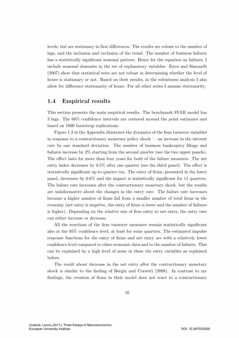
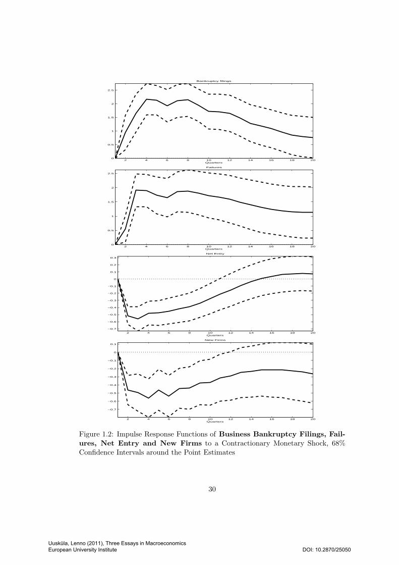
Figure 1.2 in the Appendix illustrates the dynamics of the firm turnover variables

in response to a contractionary monetary policy shock — an increase in the interest

rate by one standard deviation. The number of business bankruptcy filings and

failures increase by 2% starting from the second quarter (see the two upper panels).

The effect lasts for more than four years for both of the failure measures. The net

entry index decreases by 0.5% after one quarter (see the third panel). The effect is

statistically significant up to quarter ten. The entry of firms, presented in the lower

panel, decreases by 0.6% and the impact is statistically significant for 11 quarters.

The failure rate increases after the contractionary monetary shock, but the results

are uninformative about the changes in the entry rate. The failure rate increases

because a higher number of firms fail from a smaller number of total firms in the

economy (net entry is negative, the entry of firms is lower and the number of failures

is higher). Depending on the relative size of firm entry to net entry, the entry rate

can either increase or decrease.

All the reactions of the firm turnover measures remain statistically significant

also at the 95% confidence level, at least for some quarters. The estimated impulse

response functions for the entry of firms and net entry are with a relatively lower

confidence level compared to other economic data and to the number of failures. This

can be explained by a high level of noise in these the entry variables as explained

before.

The result about decrease in the net entry after the contractionary monetary

shock is similar to the finding of Bergin and Corsetti (2008). In contrast to my

findings, the creation of firms in their model does not react to a contractionary

10


DOI: 10.2870/25050

monetary shock when FFR is used to identify monetary shock. In comparison to

the results in Lewis (forthcoming), I find that after a contractionary monetary shock,

net entry becomes statistically significantly different from zero after one quarter, not

after 2 years.

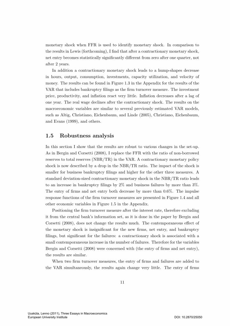
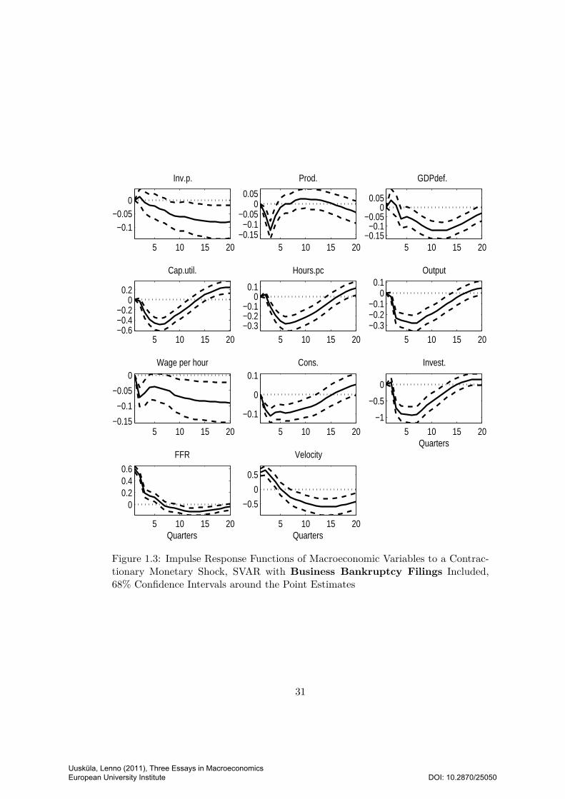
In addition a contractionary monetary shock leads to a hump-shapes decrease

in hours, output, consumption, investments, capacity utilization, and velocity of

money. The results can be found in Figure 1.3 in the Appendix for the results of the

VAR that includes bankruptcy filings as the firm turnover measure. The investment

price, productivity, and inflation react very little. Inflation decreases after a lag of

one year. The real wage declines after the contractionary shock. The results on the

macroeconomic variables are similar to several previously estimated VAR models,

such as Altig, Christiano, Eichenbaum, and Linde (2005), Christiano, Eichenbaum,

and Evans (1999), and others.

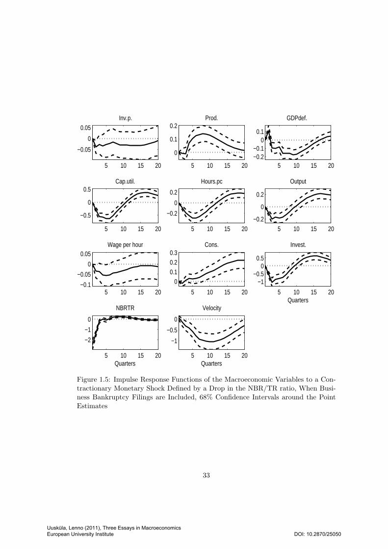
1.5 Robustness analysis

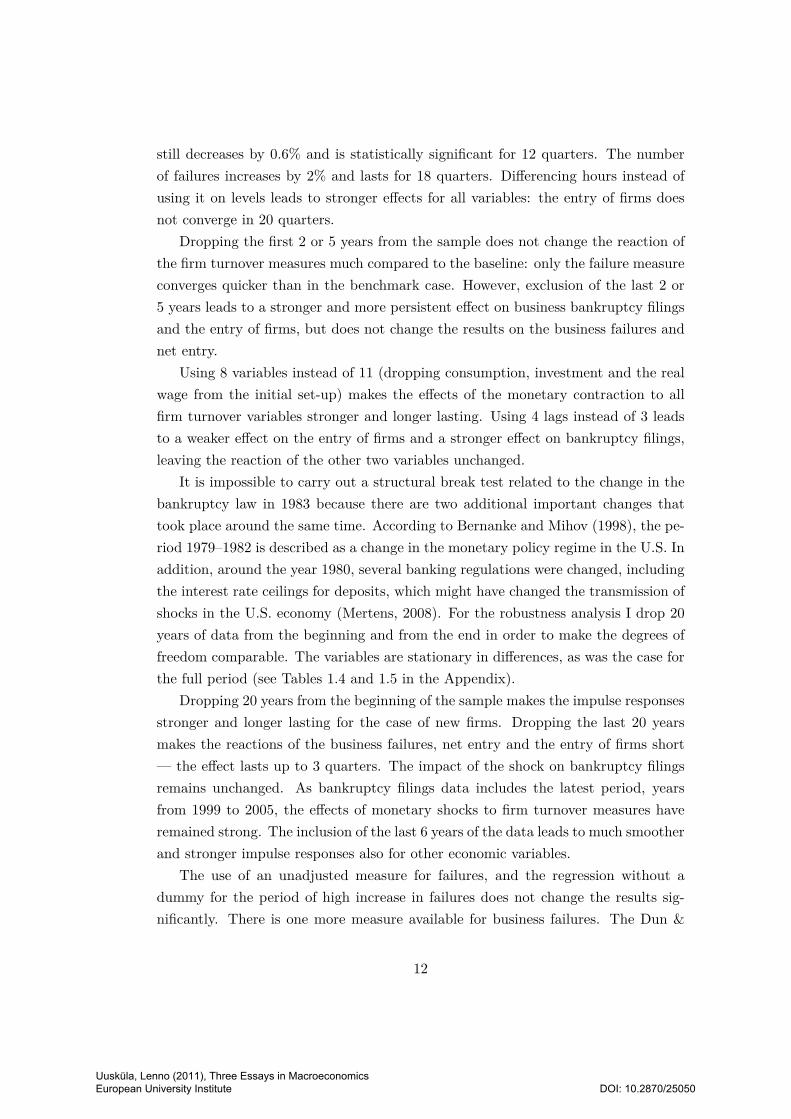
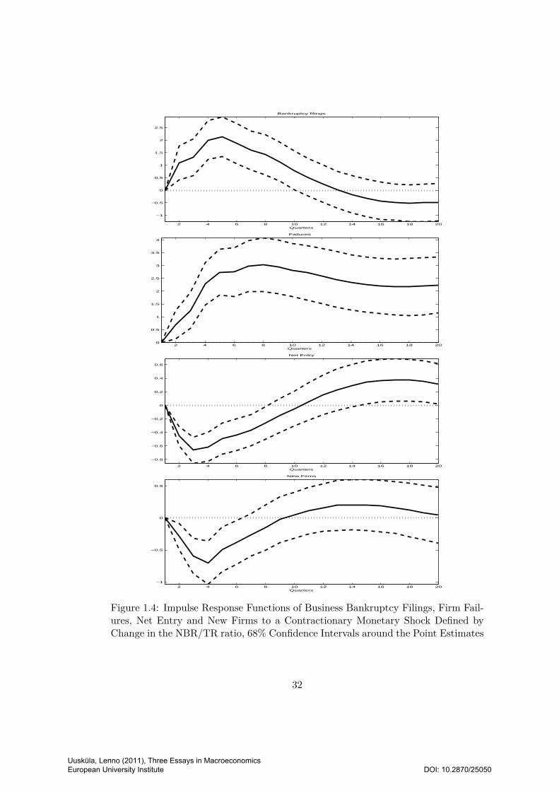
In this section I show that the results are robust to various changes in the set-up.

As in Bergin and Corsetti (2008), I replace the FFR with the ratio of non-borrowed

reserves to total reserves (NBR/TR) in the VAR. A contractionary monetary policy

shock is now described by a drop in the NBR/TR ratio. The impact of the shock is

smaller for business bankruptcy filings and higher for the other three measures. A

standard deviation-sized contractionary monetary shock in the NBR/TR ratio leads

to an increase in bankruptcy filings by 2% and business failures by more than 3%.

The entry of firms and net entry both decrease by more than 0.6%. The impulse

response functions of the firm turnover measures are presented in Figure 1.4 and all

other economic variables in Figure 1.5 in the Appendix.

Positioning the firm turnover measure after the interest rate, therefore excluding

it from the central bank’s information set, as it is done in the paper by Bergin and

Corsetti (2008), does not change the results much. The contemporaneous effect of

the monetary shock is insignificant for the new firms, net entry, and bankruptcy

filings, but significant for the failures: a contractionary shock is associated with a

small contemporaneous increase in the number of failures. Therefore for the variables

Bergin and Corsetti (2008) were concerned with (the entry of firms and net entry),

the results are similar.

When two firm turnover measures, the entry of firms and failures are added to

the VAR simultaneously, the results again change very little. The entry of firms

11


DOI: 10.2870/25050

still decreases by 0.6% and is statistically significant for 12 quarters. The number

of failures increases by 2% and lasts for 18 quarters. Differencing hours instead of

using it on levels leads to stronger effects for all variables: the entry of firms does

not converge in 20 quarters.

Dropping the first 2 or 5 years from the sample does not change the reaction of

the firm turnover measures much compared to the baseline: only the failure measure

converges quicker than in the benchmark case. However, exclusion of the last 2 or

5 years leads to a stronger and more persistent effect on business bankruptcy filings

and the entry of firms, but does not change the results on the business failures and

net entry.

Using 8 variables instead of 11 (dropping consumption, investment and the real

wage from the initial set-up) makes the effects of the monetary contraction to all

firm turnover variables stronger and longer lasting. Using 4 lags instead of 3 leads

to a weaker effect on the entry of firms and a stronger effect on bankruptcy filings,

leaving the reaction of the other two variables unchanged.

It is impossible to carry out a structural break test related to the change in the

bankruptcy law in 1983 because there are two additional important changes that

took place around the same time. According to Bernanke and Mihov (1998), the pe-

riod 1979–1982 is described as a change in the monetary policy regime in the U.S. In

addition, around the year 1980, several banking regulations were changed, including

the interest rate ceilings for deposits, which might have changed the transmission of

shocks in the U.S. economy (Mertens, 2008). For the robustness analysis I drop 20

years of data from the beginning and from the end in order to make the degrees of

freedom comparable. The variables are stationary in differences, as was the case for

the full period (see Tables 1.4 and 1.5 in the Appendix).

Dropping 20 years from the beginning of the sample makes the impulse responses

stronger and longer lasting for the case of new firms. Dropping the last 20 years

makes the reactions of the business failures, net entry and the entry of firms short

— the effect lasts up to 3 quarters. The impact of the shock on bankruptcy filings

remains unchanged. As bankruptcy filings data includes the latest period, years

from 1999 to 2005, the effects of monetary shocks to firm turnover measures have

remained strong. The inclusion of the last 6 years of the data leads to much smoother

and stronger impulse responses also for other economic variables.

The use of an unadjusted measure for failures, and the regression without a

dummy for the period of high increase in failures does not change the results sig-

nificantly. There is one more measure available for business failures. The Dun &

12


DOI: 10.2870/25050

Bradstreet published a failure rate based on 10000 listed enterprises for the period

1959Q1–1983Q4. The failure rate is stationary only if it is differenced once (see

Table 1.6 in the Appendix). A contractionary monetary shock leads to an increase

in the failure rate by 1.5% with the effect lasting for 15 quarters.

1.6 Limited participation model

In this section I present a simple limited participation model for analyzing the effects

of a monetary shock on the number of firms dynamics. In the next section I write

down the sticky price model. I keep the two models separate because this allows to

pronouce the basic mechanisms at work clearer and keep the models simple.

I adopt the model of Christiano, Eichenbaum, and Evans (1997) and add the

endogenous creation and exogenous destruction of firms in the intermediate goods

producing sector. The economy consists of a representative consumer, final and

intermediate goods producers, financial sector, and a monetary authority.

1.6.1 Consumer problem

The representative consumer maximizes her lifetime utility derived from consump-

tion and leisure:

Et

∞∑

t=0

βt(c1−σt − 11− σ

− ψ0ln(nt)

), (1.5)

where ct is real consumption at period t, and nt denotes the hours spent working.

Et is the expectations operator, 0 < β < 1 is the discount factor, and the weight on

the disutility of labor is given by ψ0 > 0. The inverse of elasticity of substitution

is denoted by σ > 1. Together with the logarithmic disutility of labor, it means

that the Frisch elasticity of the labor supply is positive. Upper-case letters denote

nominal and lower case letters real variables unless it is clear from the context.

She decides on consumption ct, labor input nt, money Mt, and deposits Ht.

The predetermined variables are cash Mt−1, the deposits Ht−1, profits from the

financial intermediaries RtXt, and profits from final and intermediate goods firms.

The consumer faces following intertemporal budget constraint:

Mt −Ht ≤Wtnt +Mt−1 −Ht−1 − Ptct +RtHt−1 +RtXt +Dt +Ot, (1.6)

13


DOI: 10.2870/25050

where Mt is the nominal money decided at period t to be used for the purchases at

t+ 1, Ht is the deposit decided at period t to be given to the financial intermediary

in the next period, Wt is the nominal wage, Pt is the price level, Rt is the gross

interest rate, RtXt are the nominal profits received from the financial intermediary,

and the nominal profits from the intermediate and final goods production firms are

denoted by Dt and Ot respectively.

In addition the consumer faces a cash-in-advance constraint. For consumption

purchases, she can only use the cash left over from one period before (Mt−1−Ht−1)

and labor income, so the condition is:

Ptct ≤Wtnt +Mt−1 −Ht−1. (1.7)

The optimality conditions are Euler Condition (Equation 1.8) and optimality

condition for labor-leisure choice (Equation 1.9).

Et

(ct+2

ct+1

)σ= βEt

Rt+1

πt+2(1.8)

ψ0cσt = wtnt (1.9)

where πt = Pt/Pt−1 is one plus the inflation rate and the real wage wt = WtPt

.

1.6.2 Final goods firm

The final goods sector produces consumption goods. It uses a constant elasticity of

substitution (CES) aggregator to combine the goods from the intermediate sector:

yt =

(∫ Ft

0y

1−1/εi,t di

)1/(1−1/ε)

, (1.10)

where yt is the output made from intermediate goods, yi,t is the input from the

intermediate good producer i at period t, Ft is the number of the intermediate input

firms, and ε > 1 is the elasticity of substitution between the intermediate goods.

The final goods firm maximizes profits:

Ot = Ptyt −

∫ Ft

0Pi,tyi,tdi, (1.11)

where Ot is the profit of the final goods firm from aggregating the intermediate

goods. As there is perfect competition and no entry or exit, it is always equal to

zero.

14


DOI: 10.2870/25050

After some rearrangements the first order condition with respect to yit gives the

following demand for each of the intermediate goods:

yi,t =(Pi,tPt

)−ε

yt, (1.12)

where Pt =(∫ Ft

0 P 1−εi,t di

)1/(1−ε)is the price index, with the empirical couterpart of

P empt = Fε/(1−ε)t

(∫ Ft0 P 1−ε

i,t di)1/(1−ε)

, where F ε/(1−ε)t removes the effects of number

of varieties from the price index.

1.6.3 Intermediate goods firms

The present value (Vi,t) of an existing intermediate goods producing firm is defined

by discounted flow of profits. Writing it in the value form for an existing firm gives

the expression:

Vi,t = Di,t + β(1− δ)Et(ct+1

ct+2

)−σ

Vi,t+1 (1.13)

where 0 < δ < 1 is the probability of a death shock to a firm and the future value

is discounted with the stochastic discount factor of the consumer.

In each period, a share of the existing firms is hit by a death shock. The death

shock is realized before the entry decisions are made, so all new firms produce. The

aggregate number of existing firms is described by the following equation:

Ft = (1− δ)Ft−1 + FNt , (1.14)

where FNt is the number of newly created firms.

The intermediate goods firms produce with the linear technology:

yi,t = ni,t. (1.15)

The market structure is monopolistic competition. The firm takes the demand

from the final goods sector as given. They pay wages in advance, and borrow the

wage bill from a financial intermediary. The marginal cost of production is equal to

the nominal wage times the gross interest rate (MCt = RtWt). The intermediate

goods firms use a fixed quantity of labor (ξop ≥ 0) to operate. The profits are sales

minus the costs:

Di,t = (Pi,t −RtWt)yi,t − ξopRtWt (1.16)

15


DOI: 10.2870/25050

In order to maximize profits, take the derivative with respect to the price Pi,t and

get the pricing rule Pi,t = εε−1RtWt. The firm set the price as a constant mark-up

over marginal cost.

The free entry condition is written as follows:

Vi,t = ξentRtWt. (1.17)

The entry of the intermediate goods to the market is free, but every entrant has to

pay a one-time fixed cost ξent > 0 in labor.

1.6.4 Financial intermediary

In the limited participation model the intermediate goods firms borrow their wage

bill from financial intermediaries: WtNt = Ht−1 +Xt. For giving out loans financial

intermediaries use deposits Ht−1 and the money injection of the monetary authority

Xt. At the end of each period, financial intermediary pays out its’ profits to con-

sumers RtXt = Rt(Ht−1 +Xt)− RtHt−1. Bank gets income from giving out loans,

and returns deposits to the consumers with gross interest rate Rt.

1.6.5 Monetary authority

In the limited participation model, the monetary authority decides on the money

injection to the financial intermediary Xt. It is a one-time shock with zero autocor-

relation.

1.6.6 Market clearing conditions and the equilibrium

The aggregate output (Equation 1.18) is consumed, including the production that is

done for creating and operating the firms. Total labor equals total output (Equation

1.19). This assumption is necessary to avoid any effects from the number of firms to

the aggregate consumption, and therefore there is no feedback from the number of

firms to the economy. The total profits by firms consists of the aggregate operating

profits minus the entry costs paid by the newly created firms (Equation 1.19).

ct = Fε/(1−ε)t yt +

∫ Ft

0ξopdi+

∫ FNt

0ξentdi (1.18)

nt = ct (1.19)

Dt =∫ Ft

0Di,tdi−

∫ FNt

0WtRtξ

entdi (1.20)

16


DOI: 10.2870/25050

Definition of equilibrium: The equilibrium of the model is the sequence of quanti-

ties ct, nt,mt+1, ht+1, dt, di,t, jt, Ft, FNt ∞

t=0, prices Pt, Rt∞t=0, given the initial con-

ditions m0, h0, F−1, and the sequence of government monetary injections Xt∞

t=0,

such that consumers maximize their lifetime utility, final and intermediate goods

firms are maximizing their profits, financial intermediaries are maximizing their

profit, the free entry condition is satisfied, and the markets clear.

1.7 Model with pre-set prices

In this section I present a simple pre-set prices model as an example of sticky prices.

Again I augment the simple model with endogenous entry and exogenous exit of

firms in the intermediate goods firms. Creation and destruction of firms in this

sector takes place after the shock and the prices are fixed before the monetary shock

is realized. The entry is determined by the free entry condition. Fully competitive

final goods sector aggregates the goods from intermediate goods sector, there is no

entry and exit. Differently from the limited participation model, there is no financial

sector.

1.7.1 Consumer problem

The representative consumer maximizes lifetime utility derived from consumption,

leisure, and money balances:

Et

∞∑

t=0

βt(c1−σt − 11− σ

− ψ0ln(nt) +1

1− ϕ

(Mt+1

Pt

)1−ϕ), (1.21)

where Mt+1 is the nominal money transferred to the next period and 0 < ϕ < 1 is

the inverse of elasticity of substitution for money demand. The consumer decides on

consumption and work today, and money left for tomorrow. For the pre-set prices

model I adopt a money-in-utility approach which is standard in the literature. The

utility function implies the neutrality of money, so the sole cause of the real effects

is the imposed price stickiness.

Each period consumer faces the following budget constraint:

Ptct +Bt+1 +Mt+1 = Wtnt + (1 + it−1)Bt +Mt +Dt +Ot, (1.22)

where Bt are the bonds at period t. In order to buy consumption good, the consumer

17


DOI: 10.2870/25050

can use all the profits received from the firms, money, and bonds: there is no cash-

in-advance condition.

In order to maximize consumer utility, take first order conditions with respect

to the bonds Bt+1, money Mt+1, consumption ct, and labor nt. There are three

optimality conditions for the consumer:

Et

(ct+1

ct

)σ= βEt

1 + itπt+1

(1.23)

ψ0cσt = wtnt (1.24)

(Mt+1

Pt

)−ϕ

=it

1 + itc−σt . (1.25)

The Euler Equation (no. 1.23) determines the optimal consumption path. It

is different from the tradeoff in the limited participation model, where the decision

was between tomorrow and the day after. Labor-leisure choice Equation 1.24 is

identical to the one in the limited participation model. The money demand is given

in Equation 1.25, which is again different from the limited participation approach,

where the money demand was determined by the cash-in-advance constraint.

1.7.2 Final goods firm

The final goods sector is identical to the limited participation model. The demand

for each of the intermediate goods is given by:

yi,t =(Pi,tPt

)−ε

yt, (1.26)

where Pt is the same as in the limited participation model.

1.7.3 Intermediate goods firms

In the intermediate goods sector there are three differences compared to the limited

participation model. First, the wages are not payed out before production: labor

costs do not include the interest rate. Second, the prices must be set one period in

advance and the new firms set the same price as all the other firms. Third, according

to the consumer problem, the stochastic part of the discount factor for firms includes

trade-off between today and tomorrow.

The value of the firm in the intermediate goods sector is given by:

Vi,t = Di,t + β(1− δ)Et(ctct+1

)−σ

Vi,t+1, (1.27)

18


DOI: 10.2870/25050

where the stochastic discount factor is taken from the consumer problem, and the

profit is given by

Di,t = Ei,t−1

((Pi,t −Wt)

(Pi,tPt

)−ε

yt − ξopWt

)(1.28)

The law of motion for the number of firms is described as before by:

Ft = (1− δ)Ft−1 + FNt . (1.29)

The production technology in the intermediate goods sector is again linear:

yi,t = ni,t. (1.30)

The nominal marginal cost of production is given by the shadow price of pro-

ducing an additional unit of output (MCt = Wt). Wages are paid out at the time

when the final output is sold.

For maximizing the firms value, take the derivative with respect to Pi,t and solve

for Pi,t to get the condition for optimal pricing, the mark-up over the expected

marginal cost:

Pi,t =ε

ε− 1Et−1Wt. (1.31)

The entry to the market of intermediate goods is free, but every entrant has to

pay a one-time fixed cost ξentWt. The free entry condition is written as follows:

Vi,t = ξentWt. (1.32)

The crucial assumption in this model in order to have the effects of a monetary

policy on the creation of firms is that the firm creation decisions are made during

the period in which the nominal rigidities are still binding. Therefore the results

also hold when I would assume longer price rigidities and let the firms to enter with

a lag.

In the present version of the model, the new firms are not allowed to set different

prices from the existing firms. Such a change would complicate the aggregation of

the demand without affecting the results much, the extension is left for the future.

19


DOI: 10.2870/25050

1.7.4 Monetary authority

The monetary authority decides on the injection of money into the economy. There

is a one-time shock to money growth gmt with zero autocorrelation.

1.7.5 Market clearing conditions

Again, all the production (Equation 1.33) is consumed and the total labor equals to

the total output (Equation 1.34). The aggregate profits by the firms are the sum of

total operating profits from each firm minus the entry costs (Equation 1.35).

ct = Fε/(1−ε)t yt +

∫ Ft

0ξopdi+

∫ FNt

0ξentdi (1.33)

nt = ct (1.34)

Dt =∫ Ft

0Di,tdi−

∫ FNt

0Wtξ

entdi (1.35)

Definition of equilibrium: Equilibrium is defined by the sequence of quantities

ct, nt, bt+1,Mt+1, jt, dt, di,t, Ft, FNt ∞

t=0, prices Pt∞t=1, given the initial conditions

m0, F−1, P0, and government money injections, such that consumers maximize

their utility, final and intermediate goods firms maximize their profit, the free entry

conditions for firms is satisfied, and markets clear.

1.8 Calibration and results of the two models

I log-linearize the model around the steady state and solve it computationally by

using the method of undetermined coefficients proposed by Uhlig (1999).

I follow traditional parameter values in the calibration of the two models for

the quarterly frequency (see Table 1.7 in the Appendix). I set the inverse of the

intertemporal elasticity substitution parameter σ = 2. The probability of the death

of a firm is calibrated to 2.5%, which is 10.7% per annum, very close to the actual

11% exit rate per year in the U.S.. I assume that shocks to the economy are small so

that there is always positive entry. The discount factor reflects a real interest rate

of 4% per year, the elasticity of substitution (ε = 17) gives a mark-up of 6%, which

is standard in the literature, but its only role together with the death probability,

operation and entry costs, is to determine the number of firms in the economy. The

cost of entry is calibrated to be higher than the operation cost. Steady state yearly

inflation in the limited participation model is 2%. The inverse of the elasticity of

20


DOI: 10.2870/25050

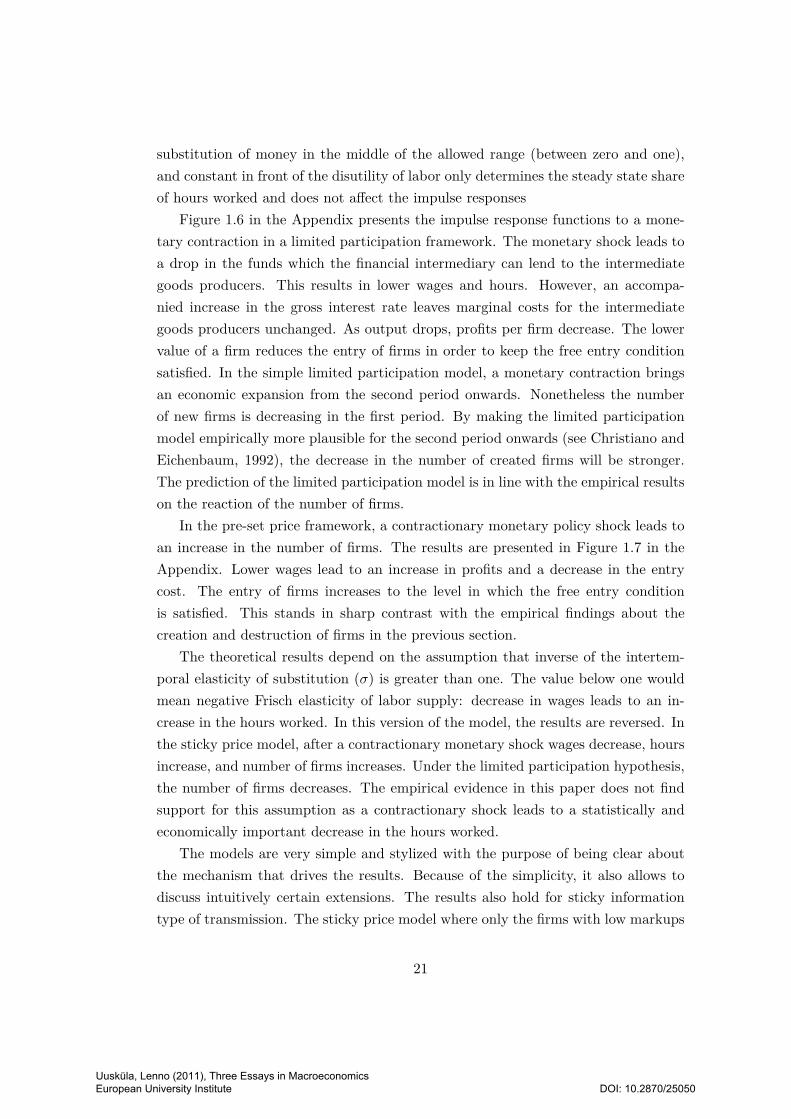
substitution of money in the middle of the allowed range (between zero and one),

and constant in front of the disutility of labor only determines the steady state share

of hours worked and does not affect the impulse responses

Figure 1.6 in the Appendix presents the impulse response functions to a mone-

tary contraction in a limited participation framework. The monetary shock leads to

a drop in the funds which the financial intermediary can lend to the intermediate

goods producers. This results in lower wages and hours. However, an accompa-

nied increase in the gross interest rate leaves marginal costs for the intermediate

goods producers unchanged. As output drops, profits per firm decrease. The lower

value of a firm reduces the entry of firms in order to keep the free entry condition

satisfied. In the simple limited participation model, a monetary contraction brings

an economic expansion from the second period onwards. Nonetheless the number

of new firms is decreasing in the first period. By making the limited participation

model empirically more plausible for the second period onwards (see Christiano and

Eichenbaum, 1992), the decrease in the number of created firms will be stronger.

The prediction of the limited participation model is in line with the empirical results

on the reaction of the number of firms.

In the pre-set price framework, a contractionary monetary policy shock leads to

an increase in the number of firms. The results are presented in Figure 1.7 in the

Appendix. Lower wages lead to an increase in profits and a decrease in the entry

cost. The entry of firms increases to the level in which the free entry condition

is satisfied. This stands in sharp contrast with the empirical findings about the

creation and destruction of firms in the previous section.

The theoretical results depend on the assumption that inverse of the intertem-

poral elasticity of substitution (σ) is greater than one. The value below one would

mean negative Frisch elasticity of labor supply: decrease in wages leads to an in-

crease in the hours worked. In this version of the model, the results are reversed. In

the sticky price model, after a contractionary monetary shock wages decrease, hours

increase, and number of firms increases. Under the limited participation hypothesis,

the number of firms decreases. The empirical evidence in this paper does not find

support for this assumption as a contractionary shock leads to a statistically and

economically important decrease in the hours worked.

The models are very simple and stylized with the purpose of being clear about

the mechanism that drives the results. Because of the simplicity, it also allows to

discuss intuitively certain extensions. The results also hold for sticky information

type of transmission. The sticky price model where only the firms with low markups

21


DOI: 10.2870/25050

change their prices can help to reduce the counterintuitive results of the sticky price

approach and lead to no effect of monetary shocks to firm turnover, but cannot

deliver reversal of the impact. When one assumes very high menu costs for changing

prices, firms could file a bankruptcy instead of lowering prices after a contractionary

monetary shock, but then menu costs should also lead to more bankruptcies for ex-

pansionary monetary shocks. Therefore the mechanism that causes the firm turnover

dynamics must be different from price stickiness.

My empirical results also show that prices do react very little to the shock within

a one-year period, whereas output, and firm entry and failures react after two quar-

ters. So if prices do not react, then in order to have increase in the profits at least

for some firms, the cost of production has to decrease. When prices are exogenously

assumed to be sticky, there is even more need for the costs to decrease.

The simple limited participation model predictions fit well the qualitative empir-

ical results. Monetary contraction leads to an increase in the interest rate, drop in

wages, no movement in prices, and increase in firm bankruptcies. The economic con-

traction that brings drop in the expected profits can explain an increase in failures

and a decrease in the creation of firms.

1.9 Conclusions

Many authors add firm creation and destruction to the traditional dynamic stochas-

tic general equilibrium models. Intuitively the extensive margin plays an important

role in propagating shocks, but it is unclear if it constitutes a different propagation

mechanism? What does firm turnover influence? These are the questions most of

the firm turnover literature tries to answer. This paper takes a different route. Here

the question is instead, What can we learn about modeling monetary transmission

by introducing firm creation in the models? The answer is that the empirical results

about firm creation and destruction reaction after a monetary shock are more in

line with the predictions of the limited participation model than those of the sticky

prices.

The paper offers extensive empirical evidence that a contractionary monetary

policy shock increases failures and decreases entry of firms. This is a robust finding

of a VAR model where the monetary shock is identified by using recursiveness as-

sumption based on the Taylor rule type of argument. When the number of firms that

file a bankruptcy after an unexpected monetary contraction increases, it is a sign

that their expected future profit decreased and restructuring of activity costs more

22


DOI: 10.2870/25050

than bankruptcy. This evidence does not necessarily say anything about amplifica-

tion of shocks in the economy because existing firms could expand their production

and possibly increase profits. But the evidence shows that some existing firms do

suffer from the shock. The same is true for some of the new firms. Monetary con-

traction means that fewer firms are created: some of the business ideas are not

realized because they are not profitable.

Although standard models of monetary transmission assume away firm creation

and destruction, it is straightforward to augment them with firm turnover. I take two

alternative approaches, limited participation and sticky price models and augment

with endogenous creation and exogenous destruction of firms. The predictions of the

two main models of monetary transmission are at odds with each other. According

to the sticky price model the number of firms increases after a contractionary mon-

etary policy shock. After the same shock, the limited participation model predicts

a decrease in the number of firms in the economy. Therefore the empirical find-

ings about firm turnover support more the limited participation type of monetary

transmission compared to the sticky prices.

Bibliography

Altig, D., Christiano, L. J., Eichenbaum, M., Linde, J., 2005. Firm-Specific Capital,

Nominal Rigidities and the Business Cycle. NBER working paper, No. 11034.

Armington, C., 2004. Development of Business Data: Tracking Firm Counts,

Growth and Turnover by Size of Firms. SBA, Office of Advocacy, Small Business

Research.

Bergin, P., Corsetti, G., 2008. The Extensive Margin and Monetary Policy. Journal

of Monetary Economics, No. 55(7).

Bernanke, B., Mihov, I., 1998. Measuring Monetary Policy. The Quarterly Journal

of Economics, No. 113(3).

Bilbiie, F. O., Ghironi, F., Melitz, M. J., 2007. Monetary Policy and Business Cycles

with Endogenous Product Variety. NBER Macroeconomics Annual 2007.

Boivin, J., Giannoni, M., Mihov, I., 2007. Sticky Prices and Monetary Policy:

Evidence from Disaggregated U.S. Data. NBER working paper, No. 12824.

23


DOI: 10.2870/25050

Campbell, J. R., 1998. Entry, Exit, Embodied Technology, and Business Cycles.

Review of Economic Dynamics, No. 1(2).

Christiano, L. J., Eichenbaum, M., 1992. Liquidity Effects and the Monetary

Transmission Mechanism. American Economic Review, Papers and Proceedings,

No. 82(2).

Christiano, L. J., Eichenbaum, M., Evans, C. L., 1997. Sticky price and limited

participation models of money: A comparison. European Economic Review, 41(6).

Christiano, L. J., Eichenbaum, M., Evans, C. L., 1999. Monetary Policy Shocks:

What Have We Learned and to What End? Handbook of Macroeconomics, Hand-

books in Economics Vol 1A, Elsevier Science, North-Holland, 65Ű-148.

Fisher, J. D. M., 2006. The Dynamic Effects of Neutral and Investment-Specific

Technology Shocks. Journal of Political Economy, No. 114(3).

Gali, J., 1999. Technology, Employment and the Business Cycle: Do Technology

Shocks Explain Aggregate Fluctuations? American Economic Review, No. 89(1).

Kydland, F., Prescott, E., 1982. Time to Build and Aggregate Fluctuations. Econo-

metrica, No. 50(6).

Lewis, V., forthcoming. Business Cycle Evidence on Firm Entry. Macroeconomic

Dynamics.

Mancini-Griffoli, T., Elkhoury, M., 2006. Monetary Policy with Endogenous Firm

Entry. mimeo.

Mertens, K., 2008. Deposit Rate Ceilings and Monetary Transmission in the US.

Journal of Monetary Economics, No. 55(7).

Naples, M. I., Arifau, A., 1997. The Rise in the US Business Failures: Correcting

the 1984 Data Discontinuity. Contributions in Political Economy, No. 16.

Ravn, M., Simonelli, S., 2007. Labor Market Dynamics and the Business Cycle:

Structural Evidence for the United States. Scandinavian Journal of Economics, No.

109(4).

Shapiro, M., Watson, M., 1988. Sources of Business Cycle Fluctuations. NBER

Macroeconomics Annual 1988, MIT Press.

24


DOI: 10.2870/25050

Sims, C. A., Zha, T., 2006. Does Monetary Policy Generate Recessions? Macroeco-

nomic Dynamics, No. 10(02).

Uhlig, H., 1999. A Toolkit for Analyzing Nonlinear Dynamic Stochastic Models

Easily. Computational Methods for the Study of Dynamic Economies.

Uhlig, H., 2005. What are the effects of monetary policy on output? Results from

an agnostic identification procedure. Journal of Monetary Economics, No. 52(2).

25


DOI: 10.2870/25050

Appendix

1960 1965 1970 1975 1980 1985 1990 1995 2000 20058

9

10

11Bankruptcy filings

1960 1965 1970 1975 1980 1985 1990 1995 2000 20057

8

9

10Failures

1960 1965 1970 1975 1980 1985 1990 1995 2000 20054.4

4.6

4.8

5Net entry

1960 1965 1970 1975 1980 1985 1990 1995 2000 200510

11

12

13Number of new firms

Figure 1.1: Business Bankruptcy Filings, Failures, Net Entry and New Firms Datain Log Levels

26


DOI: 10.2870/25050

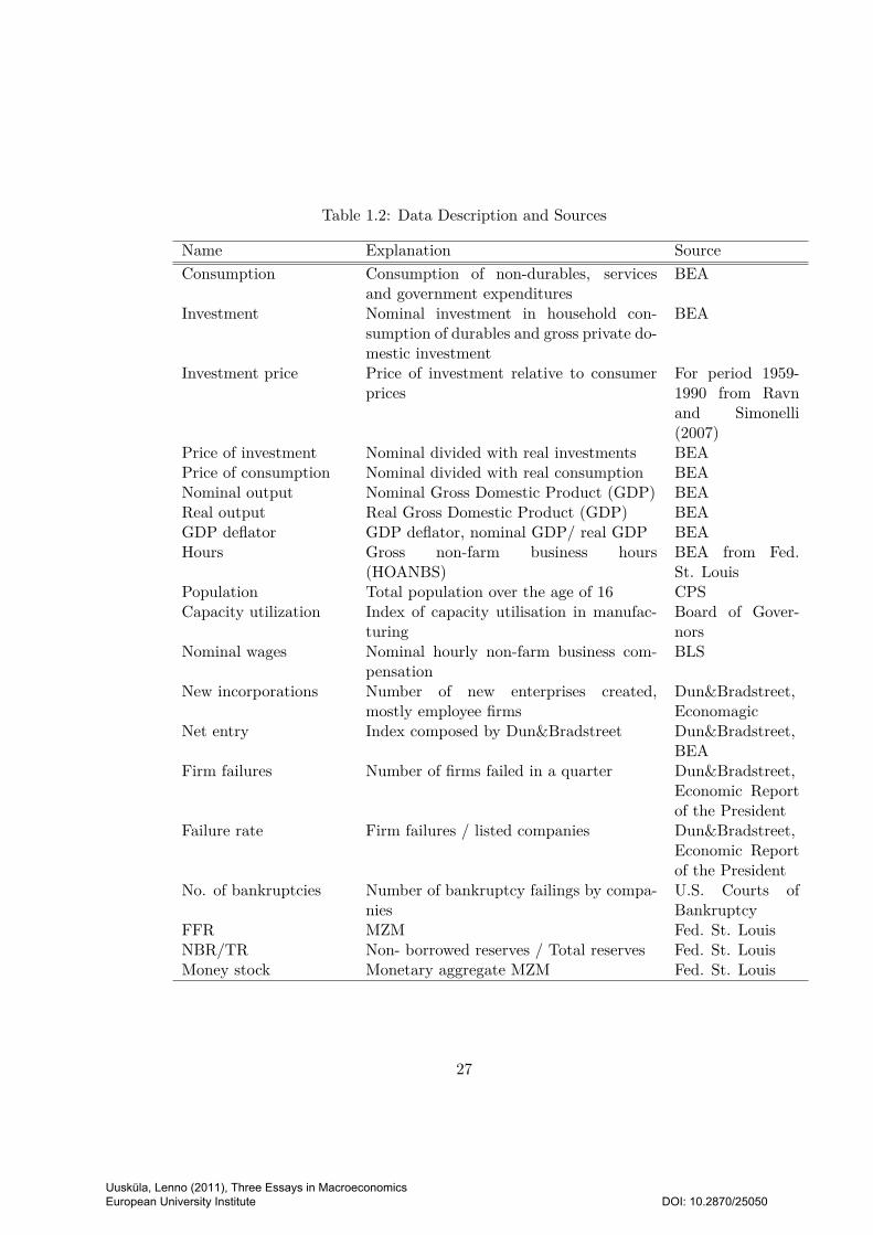
Table 1.2: Data Description and Sources

Name Explanation SourceConsumption Consumption of non-durables, services

and government expendituresBEA

Investment Nominal investment in household con-sumption of durables and gross private do-mestic investment

BEA

Investment price Price of investment relative to consumerprices

For period 1959-1990 from Ravnand Simonelli(2007)

Price of investment Nominal divided with real investments BEAPrice of consumption Nominal divided with real consumption BEANominal output Nominal Gross Domestic Product (GDP) BEAReal output Real Gross Domestic Product (GDP) BEAGDP deflator GDP deflator, nominal GDP/ real GDP BEAHours Gross non-farm business hours

(HOANBS)BEA from Fed.St. Louis

Population Total population over the age of 16 CPSCapacity utilization Index of capacity utilisation in manufac-

turingBoard of Gover-nors

Nominal wages Nominal hourly non-farm business com-pensation

BLS

New incorporations Number of new enterprises created,mostly employee firms

Dun&Bradstreet,Economagic

Net entry Index composed by Dun&Bradstreet Dun&Bradstreet,BEA

Firm failures Number of firms failed in a quarter Dun&Bradstreet,Economic Reportof the President

Failure rate Firm failures / listed companies Dun&Bradstreet,Economic Reportof the President

No. of bankruptcies Number of bankruptcy failings by compa-nies

U.S. Courts ofBankruptcy

FFR MZM Fed. St. LouisNBR/TR Non- borrowed reserves / Total reserves Fed. St. LouisMoney stock Monetary aggregate MZM Fed. St. Louis

27


DOI: 10.2870/25050

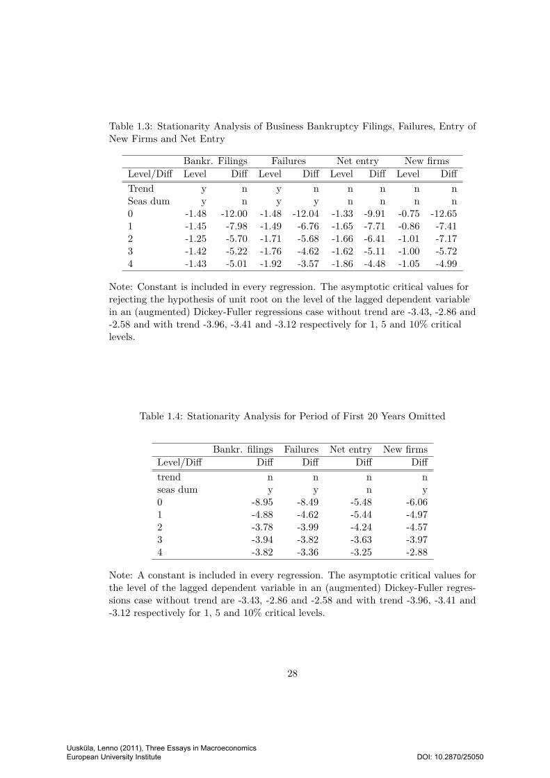
Table 1.3: Stationarity Analysis of Business Bankruptcy Filings, Failures, Entry ofNew Firms and Net Entry

Bankr. Filings Failures Net entry New firmsLevel/Diff Level Diff Level Diff Level Diff Level DiffTrend y n y n n n n nSeas dum y n y y n n n n0 -1.48 -12.00 -1.48 -12.04 -1.33 -9.91 -0.75 -12.651 -1.45 -7.98 -1.49 -6.76 -1.65 -7.71 -0.86 -7.412 -1.25 -5.70 -1.71 -5.68 -1.66 -6.41 -1.01 -7.173 -1.42 -5.22 -1.76 -4.62 -1.62 -5.11 -1.00 -5.724 -1.43 -5.01 -1.92 -3.57 -1.86 -4.48 -1.05 -4.99

Note: Constant is included in every regression. The asymptotic critical values forrejecting the hypothesis of unit root on the level of the lagged dependent variablein an (augmented) Dickey-Fuller regressions case without trend are -3.43, -2.86 and-2.58 and with trend -3.96, -3.41 and -3.12 respectively for 1, 5 and 10% criticallevels.

Table 1.4: Stationarity Analysis for Period of First 20 Years Omitted

Bankr. filings Failures Net entry New firmsLevel/Diff Diff Diff Diff Difftrend n n n nseas dum y y n y0 -8.95 -8.49 -5.48 -6.061 -4.88 -4.62 -5.44 -4.972 -3.78 -3.99 -4.24 -4.573 -3.94 -3.82 -3.63 -3.974 -3.82 -3.36 -3.25 -2.88

Note: A constant is included in every regression. The asymptotic critical values forthe level of the lagged dependent variable in an (augmented) Dickey-Fuller regres-sions case without trend are -3.43, -2.86 and -2.58 and with trend -3.96, -3.41 and-3.12 respectively for 1, 5 and 10% critical levels.

28


DOI: 10.2870/25050

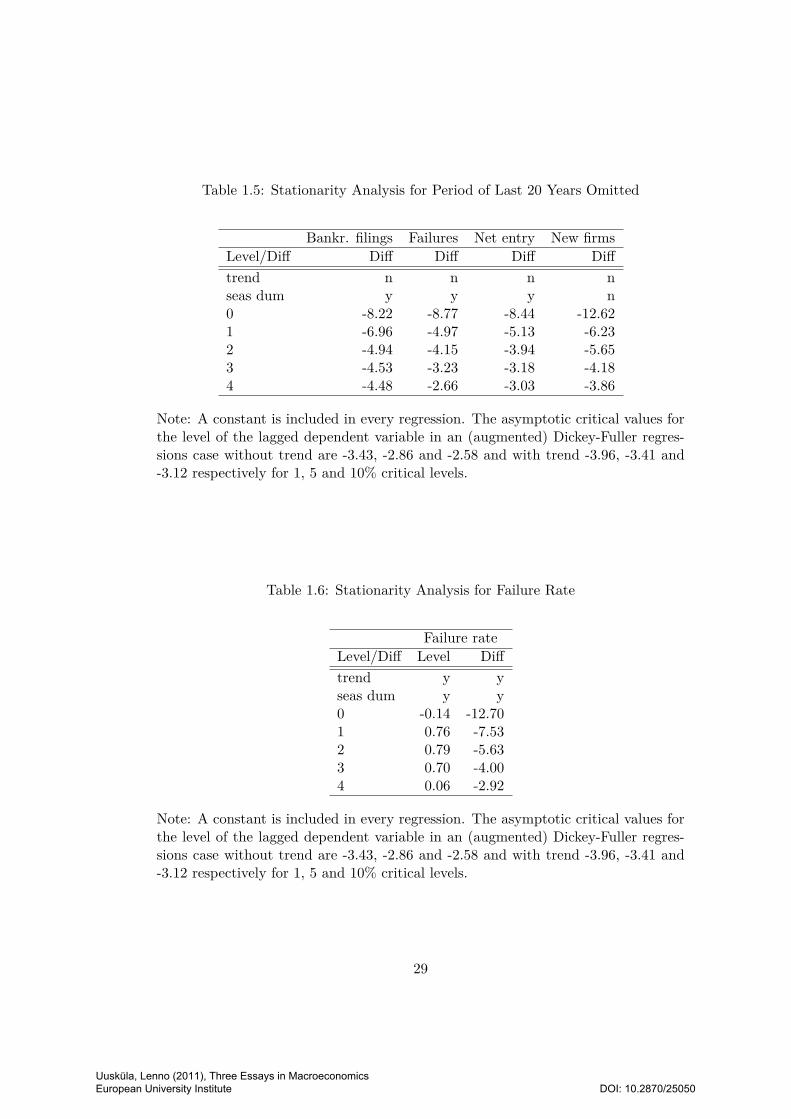
Table 1.5: Stationarity Analysis for Period of Last 20 Years Omitted

Bankr. filings Failures Net entry New firmsLevel/Diff Diff Diff Diff Difftrend n n n nseas dum y y y n0 -8.22 -8.77 -8.44 -12.621 -6.96 -4.97 -5.13 -6.232 -4.94 -4.15 -3.94 -5.653 -4.53 -3.23 -3.18 -4.184 -4.48 -2.66 -3.03 -3.86


Table 1.6: Stationarity Analysis for Failure Rate

Failure rateLevel/Diff Level Difftrend y yseas dum y y0 -0.14 -12.701 0.76 -7.532 0.79 -5.633 0.70 -4.004 0.06 -2.92


29


DOI: 10.2870/25050

2 4 6 8 10 12 14 16 18 200

0.5

1

1.5

2

2.5

Bankruptcy filings

Quarters

2 4 6 8 10 12 14 16 18 200

0.5

1

1.5

2

2.5

Failures

Quarters

2 4 6 8 10 12 14 16 18 20

−0.7

−0.6

−0.5

−0.4

−0.3

−0.2

−0.1

0

0.1

0.2

0.3

Net Entry

Quarters

2 4 6 8 10 12 14 16 18 20

−0.7

−0.6

−0.5

−0.4

−0.3

−0.2

−0.1

0

0.1

New Firms

Quarters

Figure 1.2: Impulse Response Functions of Business Bankruptcy Filings, Fail-

ures, Net Entry and New Firms to a Contractionary Monetary Shock, 68%Confidence Intervals around the Point Estimates

30


DOI: 10.2870/25050

5 10 15 20

−0.1−0.05

0

Inv.p.

5 10 15 20−0.15

−0.1−0.05

00.05

Prod.

5 10 15 20−0.15

−0.1−0.05

00.05

GDPdef.

5 10 15 20−0.6−0.4−0.2

00.2

Cap.util.

5 10 15 20−0.3−0.2−0.1

00.1

Hours.pc

5 10 15 20−0.3−0.2−0.1

00.1

Output

5 10 15 20−0.15

−0.1

−0.05

0Wage per hour

5 10 15 20

−0.1

0

0.1Cons.

5 10 15 20

−1

−0.5

0

Invest.

Quarters

5 10 15 20

00.20.40.6

FFR

Quarters5 10 15 20

−0.5

0

0.5

Velocity

Quarters

Figure 1.3: Impulse Response Functions of Macroeconomic Variables to a Contrac-tionary Monetary Shock, SVAR with Business Bankruptcy Filings Included,68% Confidence Intervals around the Point Estimates

31


DOI: 10.2870/25050

2 4 6 8 10 12 14 16 18 20

−1

−0.5

0

0.5

1

1.5

2

2.5

Bankruptcy filings

Quarters

2 4 6 8 10 12 14 16 18 200

0.5

1

1.5

2

2.5

3

3.5

4

Failures

Quarters

2 4 6 8 10 12 14 16 18 20

−0.8

−0.6

−0.4

−0.2

0

0.2

0.4

0.6

Net Entry

Quarters

2 4 6 8 10 12 14 16 18 20

−1

−0.5

0

0.5

New Firms

Quarters

Figure 1.4: Impulse Response Functions of Business Bankruptcy Filings, Firm Fail-ures, Net Entry and New Firms to a Contractionary Monetary Shock Defined byChange in the NBR/TR ratio, 68% Confidence Intervals around the Point Estimates

32


DOI: 10.2870/25050

5 10 15 20

−0.05

0

0.05

Inv.p.

5 10 15 20

0

0.1

0.2Prod.

5 10 15 20−0.2−0.1

00.1

GDPdef.

5 10 15 20

−0.5

0

0.5Cap.util.

5 10 15 20

−0.2

0

0.2

Hours.pc

5 10 15 20−0.2

0

0.2

Output

5 10 15 20−0.1

−0.05

0

0.05Wage per hour

5 10 15 20

00.10.20.3

Cons.

5 10 15 20

−1−0.5

00.5

Invest.

Quarters

5 10 15 20

−2

−1

0

NBRTR

Quarters5 10 15 20

−1

−0.5

0

Velocity

Quarters

Figure 1.5: Impulse Response Functions of the Macroeconomic Variables to a Con-tractionary Monetary Shock Defined by a Drop in the NBR/TR ratio, When Busi-ness Bankruptcy Filings are Included, 68% Confidence Intervals around the PointEstimates

33


DOI: 10.2870/25050

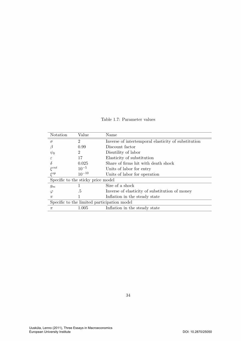
Table 1.7: Parameter values

Notation Value Nameσ 2 Inverse of intertemporal elasticity of substitutionβ 0.99 Discount factorψ0 2 Disutility of laborε 17 Elasticity of substitutionδ 0.025 Share of firms hit with death shockξent 10−5 Units of labor for entryξop 10−10 Units of labor for operationSpecific to the sticky price modelgm 1 Size of a shockϕ .5 Inverse of elasticity of substitution of moneyπ 1 Inflation in the steady stateSpecific to the limited participation modelπ 1.005 Inflation in the steady state

34


DOI: 10.2870/25050

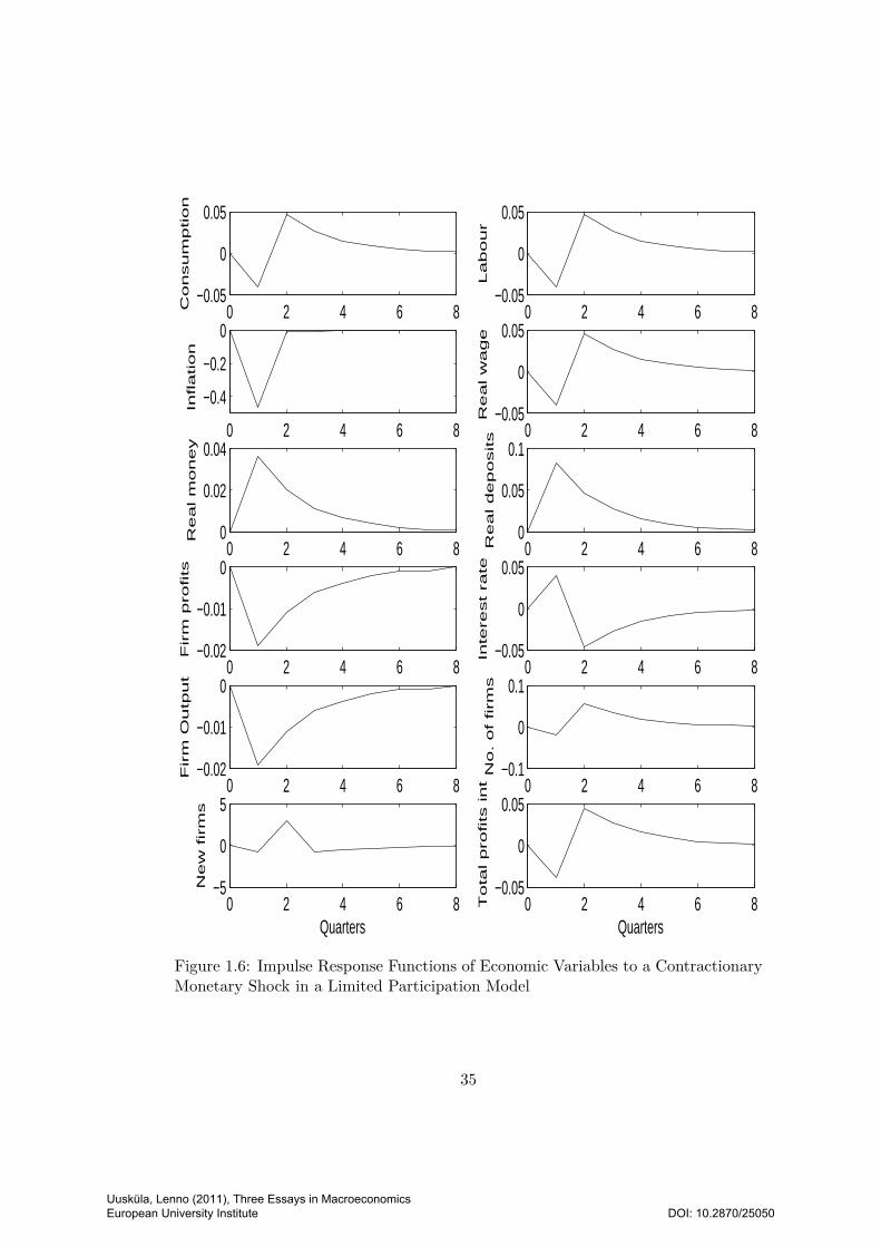
0 2 4 6 8−0.05

0

0.05

Co

nsu

mp

tio

n

0 2 4 6 8−0.05

0

0.05

La

bo

ur

0 2 4 6 8

−0.4

−0.2

0

Infla

tio

n

0 2 4 6 8−0.05

0

0.05

Re

al w

ag

e

0 2 4 6 80

0.02

0.04

Re

al m

on

ey

0 2 4 6 80

0.05

0.1

Re

al d

ep

osits

0 2 4 6 8−0.02

−0.01

0

Firm

pro

fits

0 2 4 6 8−0.05

0

0.05

Inte

rest ra

te

0 2 4 6 8−0.02

−0.01

0

Firm

Ou

tpu

t

0 2 4 6 8−0.1

0

0.1

No

. o

f firm

s

0 2 4 6 8−5

0

5

Ne

w firm

s

Quarters0 2 4 6 8

−0.05

0

0.05

To

tal p

rofits

in

t

Quarters

Figure 1.6: Impulse Response Functions of Economic Variables to a ContractionaryMonetary Shock in a Limited Participation Model

35


DOI: 10.2870/25050

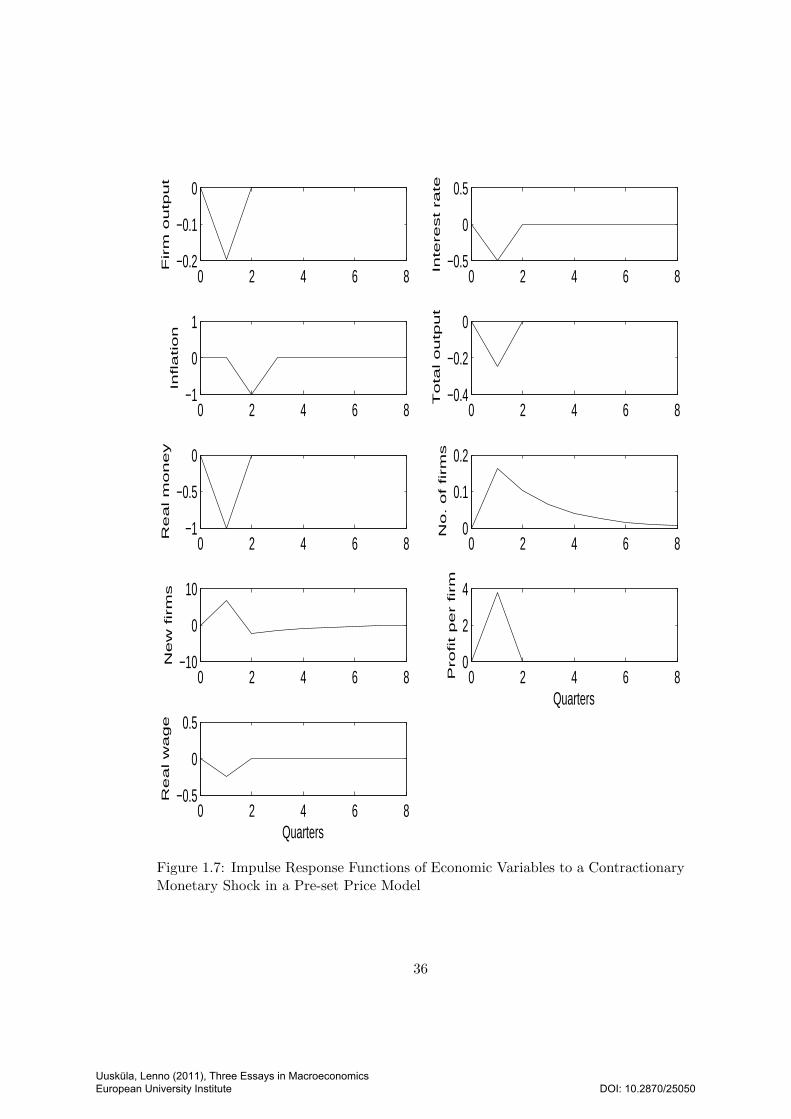
0 2 4 6 8−0.2

−0.1

0

Firm

ou

tpu

t

0 2 4 6 8−0.5

0

0.5

Inte

rest

rate

0 2 4 6 8−1

0

1

Infla

tio

n

0 2 4 6 8−0.4

−0.2

0

To

tal o

utp

ut

0 2 4 6 8−1

−0.5

0

Re

al m

on

ey

0 2 4 6 80

0.1

0.2N

o.

of

firm

s

0 2 4 6 8−10

0

10

Ne

w f

irm

s

0 2 4 6 80

2

4

Pro

fit

pe

r firm

Quarters

0 2 4 6 8−0.5

0

0.5

Re

al w

ag

e

Quarters

Figure 1.7: Impulse Response Functions of Economic Variables to a ContractionaryMonetary Shock in a Pre-set Price Model

36


DOI: 10.2870/25050

Chapter 2

Deep Habits and the Dynamic

Effects of Monetary Policy

Shocks

Morten O. Ravna,d,1, Stephanie Schmitt-Groheb,d,e,Martín Uribeb,e, and Lenno Uuskülac

University College Londona, Columbia Universityb, European University Institutec,

CEPRd, NBERe

Abstract

We introduce deep habits into a sticky-price sticky-wage economy and examine the

resulting models ability to account for the impact of monetary policy shocks. The

deep habits mechanism gives rise to countercyclical markup movements even when

prices are flexible and interacts with nominal rigidities in interesting ways. Key

parameters are estimated using a limited information approach. The deep habits

model can account very precisely for the persistent impact of monetary policy shocks

on aggregate consumption and for both the price puzzle and inflation persistence.

A key insight is that the deep habits mechanism and nominal rigidities are comple-

mentary: The deep habits model can account for the dynamic effects of monetary

policy shock at low to moderate levels of nominal rigidities. The results are shown

to be stable over time and not caused by monetary policy changes.1This paper was prepared for the 2008 CEPR/NBER/TRIO conference in Tokyo. We are grateful

for comments from Alexander Kriwoluzky, and from seminar participants at the TRIO conferenceand the European University Institute.

37


DOI: 10.2870/25050

Keywords: deep habits, monetary policy, price puzzle, inflation persistence,

countercyclical markups

JEL classifications: E21, E31, E32, E52

2.1 Introduction

A substantial body of research has studied the dynamic impact of monetary policy

shocks using vector autoregression based methods. This literature has demonstrated

that monetary policy shocks identified with timing assumptions give rise to persistent

effects on output and its components but also that the dynamic effects on prices

are associated with two puzzles: The “inflation persistence puzzle” (a slow and

delayed rise in inflation in response to an expansionary monetary policy shock)

and the “price puzzle” (a temporary drop in the price level after an expansionary

monetary policy shock). These two findings are termed puzzles because they appear

contrary to conventional monetary wisdom. This paper examines whether a model

of countercyclical markups is helpful for understanding these and other features of

the impact of monetary policy shocks. We extend a standard sticky-price sticky-

wage model with goods-specific (“deep”) habits which gives rise to a theory of time-

varying markups even in the absence of nominal rigidities. We demonstrate that

this mechanism gives rise to a model that can provide a very precise account of

the dynamic effects of monetary policy shocks and which can address both of price

puzzle and the inflation persistence puzzle.

According to the standard “New Keynesian Phillips curve” inflation is deter-

mined by current marginal costs and by expected future inflation. The purely for-

ward looking feature of this relationship implies a lack inflation persistence.2 A large

number of papers have addressed this issue by studying mechanisms that either give

rise to persistent movements in marginal costs or that introduce backward looking

features into the New Keynesian Phillips curve. Galí and Gertler (1999) allow for

the coexistence of forward looking and backward looking price setters. The presence

of backward looking price setters introduces a lagged inflation term in the Phillips

curve and therefore helps explaining the sluggish adjustment of inflation to monetary

policy shocks. Fuhrer and Moore (1995) study a relative contracting model in which

workers care about other workers’ past real wages and they show that this feature2This result holds in Calvo style sticky price models and in models where there are costs of

changing prices. Chari, Kehoe and McGrattan, 2000, show that it also holds in Taylor type staggeredcontracts models.

38


DOI: 10.2870/25050

may help explain sluggish inflation adjustments to monetary policy shocks.3 Erceg,

Henderson and Levin (2000) assume that nominal wages as well as prices adjust

sluggishly. Christiano, Eichenbaum and Evans (2005), Rabanal and Rubio-Ramirez

(2003), and Smets and Wouters (2003) have shown that the combination of sticky

prices and sticky wages is helpful for accounting for inflation persistence. There has

been less theoretical work on the price puzzle an exception being Castelnuovo and

Surico (2008) who study a model in which passive policy gives rise to indetermi-

nacy. When the equilibrium is indeterminate, inflation expectations become very

persistent and this has the consequence that a structural VAR can erroneously lead

one to conclude that expansionary monetary policy shocks give rise to a drop in the

price level.

We focus instead upon goods market features. We study a monetary model in

which it is costly for producers to change prices and for labor unions to change

nominal wages. We introduce into this environment the deep habit mechanism

proposed in Ravn, Schmitt-Grohe and Uribe (2006). The deep habits model as-

sumes that households are subject to keeping up with the Joneses effects at the

level of individual goods varieties. This feature implies that the demand function

facing individual producers depends not only on relative prices and on the level of

aggregate demand but also on the firm’s past sales. The impact of past sales on

current demand, often referred to as state dependence, captures empirically relevant

aspects of goods demand functions. Houthakker and Taylor (1970) studied goods

level demand functions and found that past sales are key for determining current

consumption of goods. Guadagni and Little’s (1983) seminal scanner data study of

ground coffee purchases documented a large predictive power of past brand choices

on current brand choices, a finding reproduced by many researchers when studying

brand demand functions, see Chintagunta, Kyriazidou and Perktold (2001) for a

recent discussion and survey. Browning and Collado (2007) study goods level con-

sumption demand functions controlling for unobserved consumer heterogeneity and

for goods-level habits at the household level and find significant habit effects for a

substantial number of goods.

According to the deep habits model, markups are time varying even when prices

are flexible. The non-constancy of the optimal markup derives from an elasticity

effect and an intertemporal effect. The elasticity effect is induced by variations in3Holden and Driscoll, 2003, challenge the results of Fuhrer and Moore, 1995, on the grounds

that the relative contracting model assumes that workers care about past not current relative realwages. They show that when workers care about other workers’ current real wages, the model hasno inflation persistence in the sense that the Phillips curve is entirely forward looking.

39


DOI: 10.2870/25050

aggregate demand that affect the price elasticity of demand facing producers. In our

model, an increase in current aggregate demand increases the price elasticity and

therefore leads producers to lower markups. The intertemporal effect arises because

a producer who expects high future demand will have an incentive to lower the

current markup in order to attract more future demand. Ravn, Schmitt-Grohe and

Uribe (2006, 2007) have shown that these mechanisms are helpful for understanding

the impact of technology shocks and of government spending shocks. In the current

paper we argue that deep habits is also an interesting mechanism when accounting

for the impact of monetary policy shocks and that it interacts in an intriguing

manner with nominal rigidities to produce a model that leads to substantial price

inertia even when nominal rigidities are moderate.

We first estimate a VAR on post-war U.S. data and derive the impact of a

timing-based identified monetary policy shock. We study a small scale VAR that

consists of aggregate consumption, the CPI inflation rate, the federal funds rate,

and the commodity price index. We include the commodity price index in the VAR

in order not to bias our results towards the existence of a price puzzle.4 The VAR

measurements of the dynamic effects of a monetary policy shock conform with the

conventional wisdom regarding inflation persistence and the price puzzle: The price

level drops for 2 quarters after an expansionary monetary policy shock and the

maximum increase in inflation appears as late as 3 years after the initial expansion

of monetary policy. We also find that aggregate consumption increases persistently

in a hump-shaped manner in response to an expansionary monetary policy shock.

We estimate key parameters of the model using a limited information approach

and compare the deep habits model with the predictions of a standard New Key-

nesian model and a New Keynesian model that allows for habits in aggregate con-

sumption. This latter economy differs from the deep habits model in that aggregate

habits do not lead to time-variation in markups when prices are flexible. We find

that the model with deep habits provides a superior fit to the identified dynamic

effects of monetary policy shocks. In particular, this model can account simultane-

ously for the persistent impact of monetary policy shocks on consumption, for the

price puzzle, and for inflation persistence. Moreover, the estimates of the extent

of nominal rigidities are significantly lower in the deep habits economy than in the

economy with aggregate habits.4A common argument is that the price puzzle is reflects misspecification of VAR models in the

sense that it is important to include variables that are forward looking. Following Sims (1992) muchof the literature has addressed this point by augmenting VARs with the commodity price index.

40


DOI: 10.2870/25050

We show that the model implies a complementarity between nominal rigidities

and deep habits. In response to an expansionary monetary policy shock, the pres-

ence of nominal rigidities implies that aggregate consumption increases. In the deep

habits economy the increase in consumption gives producers an incentive to lower

the markup. This by itself gives rise to a smaller inflation impact of an expansion-

ary monetary policy shock in the deep habits economy than in models that assume

either no habits or habits that operate at the level of aggregate consumption. When

the deep habit effect is sufficiently strong, the deep habits model generates a fall in

inflation on impact after an expansionary monetary policy shock. As the consump-

tion boom dies out, producers slowly increase prices and this implies that the model

also can account for inflation persistence.

Parts of the literature has pursued the idea that the inflation persistence puzzle

is not “structural” but caused by changes over time in monetary policy and by

instability of the inflation process. It has been pointed out that inflation persistence

appears to be sensitive to the monetary policy regime (see e.g. Benati, 2008), and

that there appears to have been breaks in the inflation process which renders inflation

less persistent when controlled for (see e.g. Levin and Piger, 2003). We repeat our

analysis for two sub-samples breaking the data in the third quarter of 1979 when

Volcker became the chairman of the Fed. We find that the early sub-sample is

associated with more pronounced price and inflation puzzles than the late sample.

We reestimate the structural parameters and find that monetary policy has become

less accommodating over time, that price rigidity has increased while wage rigidity

has declined, but the extent and importance of deep habits have remained roughly

constant.

The remainder of the paper is structured as follows. Section 2 describes the

model. Section 3 contains the details of the structural estimation approach and also

applies a structural VAR estimator to U.S. quarterly data. Section 4 analyses the

results. Finally, Section 5 concludes.

2.2 The Model

We consider an economy with monopolistically competitive firms and households

that act as monopolistically competitive suppliers of labor. Firms and households

face costs of changing nominal prices and wages, respectively. The key contribution

of the paper is the introduction of the deep habits model of Ravn, Schmitt-Grohe

and Uribe (2006) into the monetary economy.

41


DOI: 10.2870/25050

2.2.1 Households

There is a continuum of identical, infinitely lived households indexed by j ∈ [0, 1].

Households maximize the expected present discounted value of their utility stream.

They derive utility from consumption of a continuum of differentiated goods and suf-

fer disutility of supplying labor. As in Erceg, Henderson and Levin (2000), house-

holds supply a differentiated labor input and act as monopolistically competitive

labor unions in the labor market. They face costs of changing nominal wages.

Households own the firms and receive dividend payments on their equity shares.

Households are subject to good-specific habits as in the external deep habits

model of Ravn, Schmitt-Grohe and Uribe (2006). Specifically, the marginal utility of

the consumption of individual goods varieties is subject to a consumption externality

specified as catching up with the Joneses. Household j consumes a basket of goods,

cjit, i ∈ [0, 1] and supplies labor to the firms. Preferences are given as:5

V j0 = E0

∞∑

t=0

βt[

11− σ

(xjt

)1−σ−

γ

1 + κ

(hjt

)1+κ]

(2.1)

xjt =[∫ 1

0

(cjit − θ

dcit−1

)1−1/ηdi

]1/(1−1/η)

(2.2)

cit =∫ 1

0cjitdj (2.3)

where Et denotes the mathematical expectations operator contingent on all informa-

tion available at date t, β ∈ (0, 1) is the subjective discount factor, σ is a curvature

parameter, 1/κ > 0 is the Frisch elasticity of labor supply, γ > 0 is a preference

weight, and hjt denotes the household j’s labor supply in period t.

xjt is the consumption basket from which the household derives utility. According

to equation (2.2), the consumption basket is a CES-aggregate of “habit adjusted”

consumption levels of a continuum of differentiated goods. We model the habit

relating to the consumption of variety i as the past aggregate consumption of this

variety. The household take cit, as given. The parameter 0 ≤ θd < 1 measures the

importance of the habit. When θd = 0, preferences are separable over time and the

consumption aggregator is a standard CES function. In this case, η > 0 denotes

the standard intratemporal elasticity of substitution between goods. When θd > 0,

preferences display “catching up with the Joneses” at the goods level.6

5Implicitly, households also derive utility from real money balances and we assume that theutility function is separable in money and its other arguments.

6Ravn, Schmitt-Grohe and Uribe, 2006, also deal with the case of internal habits in which

42


DOI: 10.2870/25050

The goods demand functions are found as the solutions to the following expen-

diture minimization problem:

mincjit

Xjt =

∫ 1

0Pitc

jitdi

subject to:[∫ 1

0

(cjit − θ

dcit−1

)1−1/ηdi

]1/(1−1/η)

= xjt

where Pit denotes the nominal price of variety i. The demand functions that solve

this problem are given as:

cjit =(PitPt

)−η

xjt + θdcit−1 (2.4)

where Pt is an aggregate price index defined as:

Pt =[∫ 1

0P 1−ηit di

]1/(1−η)

(2.5)

According to the demand function in equation (2.4), the household’s demand for

each goods variety depends negatively on its relative price, Pit/Pt, and when θd > 0

current demand also depends positively past aggregate demand for the good.

Households act as monopolistically competitive labor unions in the labor market.

In return for their market power, they must stand ready to satisfy any demand for

their labor services at the quoted wage. The demand for household j’s labor (see

the next section) is given by:

hjt =

(W jt

Wt

)−ψ

ht (2.6)

where W jt denotes the nominal wage demand of household j, Wt is an aggregate

wage, ψ > 1 is the labor demand price elasticity, and ht is a measure of aggregate

labor demand. Individual households take Wt and ht for given.

The household makes its choices subject to the following sequence of budget

the household’s current marginal utility of consumption of variety i depends on its own past con-sumption of that variety. Nakamura and Steinsson, 2008, examine pricing implications of thisspecification.

43


DOI: 10.2870/25050

constraints:

Ptxjt + κt +Bj

t = Rt−1Bjt−1 +W j

t hjt + Φj

t − Ptζw2

(W jt

W jt−1

− πwt

)2

(2.7)

κt = θd∫ 1

0Pitcit−1di

and subject to a no-Ponzi game restriction.

The household budget constraint assumes that the household has access to a

nominal risk free bond which allows it to smooth consumption expenditure (and

labor supply) over time. Bjt denotes the household’s purchases of one-period nominal

bonds, Rt denotes the gross nominal interest rate and Φjt is the household’s receipts

of dividend payments on its equity portfolio.7

The last term on the right hand side of the budget constraint denotes nominal

costs of adjusting nominal wages. ζw ≥ 0 parametrizes the extent of nominal wage

rigidity. When ζw = 0, nominal wages are flexible while ζw > 0 implies that house-

holds incur a nominal cost of changing wages which is quadratic in the deviation of

nominal wage growth from an indexation factor πwt given as:

πwt = ϑwπ∗

w + (1− ϑw)πwt−1

where ϑw ∈ [0, 1) is a measure the degree of wage indexation. When ϑw = 1

households can costlessly adjust wages with the steady-state wage inflation rate

(π∗w) while ϑw = 0 implies that wages are fully indexed to the realized past inflation

rate of aggregate nominal wages, πwt−1 = Wt−1/Wt−2.

The household’s labor supply, the nominal wage, and its intertemporal allocation

of xjt can be found as the solutions to the maximization of (2.1) subject to (2.6)−(2.7)

taking as given Pt, ϑt, Wj0 , Rt, and Φj

t . The first-order conditions are:

γ(hjt

)κ=

(xjt

)−σ W j

t

Pt− λhj,t (2.8)

ψλhj,thjt

(xjt

)σ= hjt

W jt

Pt− ζw

W jt

W jt−1

(W jt

W jt−1

− πwt

)

+βζwEtW jt+1

W jt

(W jt+1

W jt

− πwt+1

)(xjt+1

xjt

)−σ(2.9)

(xjt

)−σ

= βRtEtPtPt+1

(xjt+1

)−σ

(2.10)

7The formulation of the budget constraint uses the fact that Ptxjt =

∫1

0Pit

(cjit − θ

dcit−1

)di.

44


DOI: 10.2870/25050

where λhj,t is the multiplier on the labor demand function in equation (2.6).

We note from (2.8)− (2.10) that the labor supply decision and the intertemporal

consumption allocation are affected by the presence of habits in the consumption

aggregator. Equation (2.9) is a forward looking “wage setting curve”. When wages

are flexible (ξw = 0), equations (2.8)− (2.9) imply that the household sets the real

wage as a fixed markup over the marginal rate of substitution between labor and

consumption. The markup is given as ψ/ (ψ − 1) ≥ 1.8 Equation (2.10) is the

intertemporal Euler equation.

2.2.2 Firms

Firms produce differentiated goods and are monopolistically competitive. They

produce output using inputs of labor and we assume that the production function

is linear:

yit = hit (2.11)

where yit denotes firm i’s output and hit is firm i’s input of labor. The labor input

is defined as:

hit =(∫ 1

0

(hjit

)1−1/ψdj

)1/(1−1/ψ)

where hjit is firm i’s input of labor variety j at date t. The firm purchases the labor

varieties at the nominal price W jt . It follows that the labor demand functions are

given as:

hjit =

(W jt

Wt

)−ψ

hit (2.12)

where Wt is defined as:

Wt =[∫ 1

0W 1−ψjt dj

]1/(1−ψ)

Aggregating (2.12) across firms gives (2.6).

The demand for firm i’s product is found by aggregating equation (2.4) across

8Given that our focus is not upon optimal monetary policy issues, we choose not to neutralizethe steady-state monopoly power by a labor supply subsidy. This does not affect our results.

45


DOI: 10.2870/25050

consumers:

cit =(PitPt

)−η

xt + θdcit−1 (2.13)

cit =∫ 1

0cjitdj

xt =∫ 1

0xjtdj

The demand function facing firm i at date t depends on the firm’s past sales

of its product whenever θd > 0. This feature of the demand function implies that

firms will set non-constant mark-ups even in the absence of nominal rigidities.9 An

increase in current demand, xt, over habitual demand (cit−1), increases the price

elasticity of the demand facing the firm and this gives firms an incentive to lower

the mark-up. Moreover, firms will lower markups when they anticipate high value

of future market share.

Firm i sets the price of its product, Pit, by maximizing profits subject to the

household demand functions taking as given all aggregate quantities and prices. In

return for having market power, firms must stand ready to serve any demand at the

announced prices, i.e. cit ≥ yit. Following Rotemberg (1982), we assume that there

are quadratic adjustment costs associated with changing nominal prices. Firms face

the following profit maximization problem:

maxPit

E0

∞∑

t=0

qtΦit (2.14)

Φit = Pitcit −Wthit −ζp2Pt

(PitPit−1

− πt

)2

(2.15)

subject to (2.13) taking as given qt, Pi0, Pt, Wt, xt and πt. Φit denotes the nominal

profits of firm i in period t and qt is the rate at which the firm’s owners (the

households) discount the stream of nominal profits. This discount factor is given

as:10

qt = βtx−σt1Pt

9Notice from the demand function that there is a price insensitive term that derives from pastsales. One might be tempted to conclude that the firm can set a price of infinity making infiniteprofits due to this term. However, in equilibrium such a policy will not be consistent with householdbudget constraints and can therefore be ruled out.

10This equation imposes homogeneity across households, an assumption that we impose below.

46


DOI: 10.2870/25050

ζp ≥ 0 parametrizes the extent of nominal rigidities. When ζ → 0 prices are

flexible while positive values of ζ implies that firms have an incentive to smooth

price changes over time. The term πt is assumed to be given as:

πt = ϑpπ∗ + (1− ϑp)πt−1

where π∗ is the steady state inflation rate and πt−1 = Pt−1/Pt−2 is the lagged

realized aggregate inflation rate. When ϑp = 1 this specification implies that there

are no adjustment costs along a balanced growth path with constant inflation. When

ϑp = 0, there is full indexation.

The first order conditions for hit, cit, and Pit, in that order, are given as:

Wt = Ptλyt (2.16)

Ptλct + Ptλ

yt − Pit = θdEt

qt+1

qtPt+1λ

ct+1 (2.17)

Etqt+1

qtζpPt+1

Pit+1

P 2it

(Pit+1

Pit− πt+1

)= ζp

PtPit−1

(PitPit−1

− πt

)

+ηPtλctcit − θ

dcit−1

Pit− cit (2.18)

where λyt is the multiplier on the production function (2.11), i.e. marginal costs,

and λct is the multiplier on the demand function in (2.13).

When there are no habits(θd = 0

)and prices are flexible (ζp = 0), equations

(2.17) − (2.18), imply that prices are set as fixed mark-up over nominal marginal

costs. When there are nominal rigidities and/or preferences display deep habits, the

markup will be time-varying in response to shocks to the economy. Consider the

two special cases when either prices are flexible or there are no deep habits. In these

special cases, equations (2.17)− (2.18) can be expressed as:

ζp = 0 : Pit(

1−1η

cit/cit−1

cit/cit−1 − θd

)= Ptλ

yt − θ

dEtqt+1

qtPit+1

1η

cit+1/citcit+1/cit − θd

θ = 0 : cit(

1− η(

1− λytPtPit

))

= ζpPtPit−1

(PitPit−1

− πt

)− ζpEt

qt+1

qtPt+1

Pit+1

P 2it

(Pit+1

Pit− πt+1

)

When there are deep habits but prices are flexible, firms will vary the markup

in response to changes in current aggregate demand and in response to expected

changes in future consumption growth. When prices are sticky but there are no deep

47


DOI: 10.2870/25050

habits, firms smooth price increases over time in response to changes in marginal

costs or in aggregate demand. When these two mechanisms are combined, firms will

vary markups in order to smooth price increases but taking into account that the

optimal (flexible price) markup is affected by changes in aggregate demand and in

expected future consumption growth.

2.2.3 Monetary Policy

We assume that the monetary policy authority sets the monetary stance according

to a simple interest rate rule:

Rt = R∗ + ρR (Rt−1 −R∗) + (1− ρR)

[απ (πt − π∗) + αy

(yt − y

∗

y∗

)]+ εt (2.19)

where εt is a stochastic “monetary policy shock” with variance υ2. R∗, π∗ and y∗ are

positive constants which denote the steady state levels of the nominal interest rate,

inflation and output, respectively. The parameter ρR ∈ [0, 1) denotes the extent of

interest rate smoothing.

2.2.4 Market Clearing

We close the model by the market clearing conditions. The labor market clearing

conditions are:

hjt =∫ 1

0hjitdi

hit =∫ 1

0hjitdj

2.2.5 Symmetric Equilibrium

We concentrate upon a symmetric equilibrium in which all consumers make the same

choice over consumption and set the same wage, and in which all firms set the same

48


DOI: 10.2870/25050

prices. The symmetric equilibrium is summarized by the following set of equations:

xt = ct − θdct−1 (2.20)

γhκt = x−σt wt − λht (2.21)

ψλht htxσt + ζwπwt (πwt − πwt) = htwt

+βζwEtπwt+1 (πwt+1 − πwt+1)x−σt+1

x−σt(2.22)

x−σt = βRtEtx−σt+1

1πt+1

(2.23)

ct = ht −ζp2

(πt − πt)2 −

ζw2

(πwt − πwt)2 (2.24)

λyt = wt (2.25)

λyt + λct = 1 + θdβEtx−σt+1

x−σtλct+1 (2.26)

ηλctxt + ζpπt (πt − πt) = ct + βζpEtx−σt+1

x−σtπt+1 (πt+1 − πt+1) (2.27)

Rt −R∗ = ρR (Rt−1 −R

∗) + (1− ρR) [απ (πt − π∗)

+αy(yt − y

∗

y∗

)] + εt (2.28)

πt = ϑpπ∗ + (1− ϑp)πt−1 (2.29)

πwt = ϑwπ∗

w + (1− ϑw)πwt−1 (2.30)

wt = wt−1 + πwt − πt (2.31)

where wt denotes the real wage, πwt is the wage inflation rate, and πt is the price

inflation rate. We solve for the equilibrium by log-linearizing this system of equations

around the steady-state.

It is instructive to consider the implications for inflation dynamics on the basis

of the log-linearized version of equation (2.27). The log-linearized version of this

equation can be expressed as:

πt =(1− ϑp)

1 + β (1− ϑp)πt−1 +

β

1 + β (1− ϑp)Etπt+1

+ψ1mct + ψ2 (Etct+1 − ct)− ψ3 (ct − ct−1)− ψ4Etλct+1 (2.32)

where we let xt denote the percentage deviation of xt from its steady-state value,

49


DOI: 10.2870/25050

and mct = λyt denotes marginal costs. The coefficients are given as:

ψ1 =(η(1− θd

)−(1− θdβ

))/

(ζpπ2

c(1 + β (1− ϑp))

)

ψ2 = σβθd

1− θd/

(ζpπ2

c(1 + β (1− ϑp))

)

ψ3 =(1 + σβθd

) θd

(1− θd)/

(ζpπ2

c(1 + β (1− ϑp))

)

ψ4 = θdβ/

(ζpπ2

c(1 + β (1− ϑp))

)

where x denotes the steady-state value of x.

In the absence of deep habits and when prices are not indexed (θd = 1−ϑp = 0),

equation (2.32) generates the standard new Keynesian Phillips curve. Indexation in-

troduces a backward looking inflation term which implies a more persistent response

to shocks to marginal costs. The presence of deep habits moderates the Phillips

curve in three important ways. First, the habit moderates the impact of marginal

cost changes on inflation. Secondly, the deep habit introduces a backward looking

term in the Phillips curve even in the absence of indexation through the impact of

the habit stock on this period’s demand. Third, the presence of habits introduces

an additional forward looking term through Etλct+1 and (Etct+1 − ct). Particularly

interesting is the implication that an increasing in the expected marginal value of

future demand (Etλct+1) has a negative impact on current inflation as it gives firms

an incentive to lower the markup in order to capture a higher future market share.

2.3 Estimation

In this section we provide empirical evidence on the dynamic effects of a monetary

policy shock and we discuss our approach to estimating the key parameters of the

model presented in the preceding section.

2.3.1 SVAR Estimates of the Impact of Monetary Policy Shocks

We study U.S. quarterly data for the sample period 1954:2 - 2008:2. The dynamic

effects of monetary policy shocks are estimated using a structural VAR estimator.

Consider the following reduced form VAR:

xt = B (L)xt−1 + et (2.33)

50


DOI: 10.2870/25050

where xt is a vector of observables, B (L) is a lag-polynomial, and et is a vector of

reduced form errors. We specify the vector of observables as:

xt = [ct, πt, pst , rt]

where ct denotes the logarithm of per capita consumption, πt is the inflation rate,

pst is the logarithm of the commodity price index divided by the CPI, and rt is the

federal funds rate. We measure consumption as personal consumption expenditure

in chained year 2000 prices divided by the civilian non-institutional population.

Inflation is measured as the change in CPI (of all urban consumers). The commodity

price index is the PPI of commodities. All variables are deseasonalized.

We include consumption rather than output in the VAR because our model

excludes investment, and, for the same reason, we measure inflation on the basis of

the CPI rather than the GDP deflator. The commodity price index is included in

order to partially address the price puzzle. The small dimension of the VAR relative

to other recent papers, see e.g. Christiano, Eichenbaum, and Evans (2005), is due to

the fact that our model is focused entirely on the impact of monetary policy shocks

on consumption and inflation.

The monetary policy shock is identified using standard timing assumptions. We

assume that the interest rate is affected contemporaneously by shocks to the first

three components of the VAR but that none of these variables respond contempo-

raneously to the monetary policy shock. Consider the structural VAR:

A0xt =p∑

i=1

Apxt−p + εt (2.34)

where Ai, i = 0, .., p, are square matrices and εt is the vector structural innovations

with the restriction that its covariance matrix is diagonal. The last component of

this vector is the monetary policy shock and it is identified by assuming that the

last column of A0 consists of zeros apart from its last element (which is normalized

to unity). We allow for constant terms and trends when estimating the VAR and

we assume that p = 8 (but shorter lag structures give almost identical results).

The impulse responses to the identified monetary policy shock are illustrated in

Figure 2.1. We show the impact of a one standard error decline in the federal funds

rate (i.e. an expansionary monetary policy shock) along with 95 percent (boot-

strapped, non-centered) confidence intervals for a forecast horizon of 20 quarters.

According to our estimates, an expansionary monetary policy shock corresponds to

51


DOI: 10.2870/25050

a decline in the nominal interest rate which remains low for around 6 quarters before

eventually returning to its long-run value.

We find that a monetary policy loosening gives rise to a bell shaped persistent

increase in aggregate consumption which peaks at 4 percent above trend around 6

quarters after the initial one standard error expansionary monetary policy shock.

The increase in consumption persists until approximately 3.5 years after the initial

decline in the interest rate. The response of inflation confirms conventional wisdom.

We find that the inflation rate declines for the first 2 quarters after the expansionary

monetary policy shock (recall that the impact response is by definition equal to zero).

Inflation starts increasing around a year and a half after the decline in the interest

rate and it then rises very persistently. The peak response occurs about 3 years

after monetary policy shock. Thus, the small-scale VAR confirms the presence of

the price puzzle and the inflation persistence puzzle.

The impact of monetary policy shocks on the vector of observables is very similar

to the estimates that derive from much larger scale VARs, see e.g. Christiano,

Eichenbaum and Evans (2005). This is reassuring since omitted variables bias could

potentially be important for both the price puzzle and the inflation persistence

puzzle. Indeed, excluding the commodity price index from the VAR leads to much

more significant price puzzle indicating the relevance of introducing forward looking

indicators in the VAR. Nonetheless, even after controlling for the informational

content of the commodity price index, we find that there is a small price puzzle

and that inflation persistence is abundant. Moreover, as we will discuss later, these

results are robust in a qualitative sense to allow for a structural change in 1979 when

Volcker took over as the chairman of the Fed. For that reason, we will interpret the

inflation and price puzzles as empirical regularities.

2.3.2 Estimation of the Structural Parameters

The model introduces quite a large number of parameters some of which we do

not have strong priors about realistic values. Let the vector of parameters be

given by Θ. We partition this vector into two subsets, Θ1 and Θ2. Θ1 consists of

parameters that we calibrate while the parameters in Θ2 are estimated by matching

the identified impulse responses discussed above. We make this distinction between

the structural parameters because not all of them are easily identifiable from our

estimation approach as they have little impact on the dynamics of the model but

instead matter for the model’s steady state. The vector of parameters that we

calibrate consists of Θ1 = [β, π∗, γ, κ, σ, ψ] while the parameters that are estimated

52


DOI: 10.2870/25050

formally are Θ2 =[η, ζp, ϑp, ζw, ϑw, θ

d, ρR, αy, απ, υ].

Calibration of Θ1

The calibration of the parameters in Θ1 is summarized in Table 2.1. We calibrate β

so that it implies a 4 percent annual real interest rate in the non-stochastic steady-

state. π∗ is normalized to 1 while γ is calibrated so that it is consistent with a

steady-state level of hours work equal to thirty percent.

Ideally, we would like to estimate the parameters κ, σ, and ψ. However, we

found that these parameters are not well-identified from the data. Following Erceg

et al (2000), we set ψ = 4. This implies that the real wage is set as a 33 percent

markup over the marginal rate of substitution between consumption and leisure.

We set κ = 0.5. This is a custom value in the macro literature. Finally, we set

σ = 3 which implies an intertemporal elasticity of substitution of consumption of

1/3 which is in the range of values that is viewed as “reasonable”.

Estimation of Θ2

We estimate Θ2 using a limited information approach. The idea is to derive estimates

of Θ2 by matching as closely the theoretical impact of a monetary policy shock with

the empirical VAR estimates. We do this the following way. Collect the empirical

estimates of the responses of consumption, inflation, and the nominal interest rate to

a one standard error monetary policy shock in the (3R− 2)x1 vector Φdata and letW

be a (3R− 2) square diagonal matrix with the inverses of the standard errors of Φdata

along its diagonal (R denotes the forecast horizon)11. The structural parameters are

then estimated from the following minimization problem:

Θ2 = arg minΘ2

(Φdata − Φ (Θ2|Θ1)theory

)W(Φdata − Φ (Θ2|Θ1)theory

)′

(2.35)

where Φ (Θ2|Θ1)theory denotes the impulse response of the observables in the model

economy given Θ2, conditional upon the calibration of Θ1.

When estimating Θ2 we need to take into account one subtle issue. Recall that

Φdata is estimated assuming that consumption and inflation do not respond within a

quarter to a monetary policy shock. In our model this identifying assumption is not

satisfied. To address this issue we introduce a simulation step in which we measure11This vector is of dimension (3R− 2) because the impact responses of consumption and inflation

to the monetary policy shock are constrained to be zero.

53


DOI: 10.2870/25050

the model’s impulse responses subject to the empirical identification strategy.12,13

Thus, Φ (Θ2|Θ1)theory does not correspond directly to the “true” responses of the

observables to the monetary policy in the model economy, but instead to the impact

of a measured monetary policy shock on the model equivalents of the observables.

That is, we derive the measure Φ (Θ2|Θ1)theory using the following strategy:

Step 1: Solve the model for a given value of Θ2 and for the assumed value of Θ1.

Step 2: Simulate N time series of length T of the observables given Θ. Let the

observables be consumption, inflation and the nominal interest rate. Add a

small amount of measurement error to each of the artificial time series.

Step 3: Estimate a VAR for each of the N artificial time series and calculate

Φi (Θ2|Θ1)theory of the i’th simulation from the impulse responses assuming

that consumption and inflation do not respond contemporaneously to the mon-

etary policy shock.

Step 4: Calculate Φ (Θ2|Θ1)theory as the mean of Φi (Θ2|Θ1)theory for i = 1, 2, ..N .

The measurement errors are added in step 2 in order to address the stochastic

singularity of the VAR using the artificial data given that there is a single source

of variation in the time series. This procedure is then continued until we find the

solution to the minimization problem in equation (2.35). We calculate the standard

errors of Θ2 following Hall et al (2007) as:

ΩΘ2= Γ (Θ2|Θ1)theory

∂Φ (Θ2|Θ1)theory′

∂Θ2WΣNW

∂Φ (Θ2|Θ1)theory′

∂Θ2Γ (Θ2|Θ1)theory

Γ (Θ2|Θ1)theory =

[∂Φ (Θ2|Θ1)theory′

∂Θ2W∂Φ (Θ2|Θ1)theory′

∂Θ2

]−1

ΣN = Σ +1N2

N∑

i=1

Σi

where Σi is the covariance matrix of Φi (Θ2|Θ1)theory and Σ is the covariance matrix

of the impulse responses in the data.12Christiano, Eichenbaum and Evans (2005) address this issue instead by introducing timing

assumptions in the model economy that renders it consistent with the identifying assumption inthe data.

13Strictly speaking, there is another difference between the empirical VAR and the model since theempirical VAR includes the commodity price index. If this variable is excluded from the empiricalVAR we find a much more pronounced price puzzle, see Sims (1993). In principle the model can beextended to include commodities but we believe that this would not generate many more insightsbut would certainly complicate the analysis very significantly.

54


DOI: 10.2870/25050

This estimator is applied subject to various parameter restrictions. We assume

that ξp, ξw, αy, υ ≥ 0, 0 ≤ ϑp, ϑw ≤ 1, η, απ > 1, 0 ≤ θd < 1, and −1 < ρR < 1. We

use 100 simulations in step 3 and the (vector of) measurement error added in step

2 is assumed to be normally distributed with mean 0 and variance 0.0001.

2.4 Results

In order to examine the impact of the deep habits mechanism we compare the results

with the estimation results for two alternative models. The first alternative model

is a standard “aggregate” habit new Keynesian model. In this model preferences are

given by:

V0 = E0

∞∑

t=0

βt[

11− σ

(cjt − θ

act−1

)1−σ−

γ

1 + κ

(hjt

)1+κ]

(2.36)

cjt =[∫ 1

0

(cjit

)1−1/ηdi

]1/(1−1/η)

(2.37)

ct =∫ 1

0cjtdj

which is the aggregate habit model studied in much of the literature. θa here denotes

the importance of the aggregate (external) habit. A crucial difference between this

model and the deep habits model is that the aggregate habit does not impact directly

on firms’ pricing policies and leaves markups constant unless there are impediments

to changing prices. The second alternative model is the standard new Keynesian

model with no habits which corresponds to our baseline model with the restriction

that θd = 0. The estimates of the parameters and their standard errors of the deep

habits model and the parameters of the two alternative models are reported in Table

2.2.

It is instructive first to consult Figures 2.2-2.4 which illustrate the VAR based

impulse responses of the observables to a monetary policy shock for the three al-

ternative models along with their empirical counterparts. The deep habits model

clearly provides a superior fit to the empirical estimates of the impact of a monetary

policy shock. The deep habits model captures very precisely the bell shaped response

of aggregate consumption and the interest rate path is also matched extremely well.

Importantly, the model can account simultaneously for the price puzzle and for in-

flation persistence. Note that the model not only is consistent with an outdrawn

increase in inflation but it also correctly identifies the period of maximum impact

55


DOI: 10.2870/25050

on the inflation rate.

The aggregate habit model gives rise to a consumption response to the monetary

policy shock that is very similar to the deep habits model. However, the aggregate

habits model provides a worse fit to both the interest rate path and, in particular, to

the inflation response. As far as the interest rate path is concerned, the initial size

of the shock appears to be under-estimated. In terms of the inflation response, the

aggregate habits model can account neither for the price puzzle nor for the extent

of the inflation persistence since the maximum impact on inflation occurs around a

year earlier in the model than in the US data.

By far the worst fit occurs in the standard new Keynesian model in which the

interest rate path is rather odd, and the consumption response is very different from

what is observed in the data. The model does appear to be consistent with the main

features of the inflation response but this is due to the rather odd interest rate path

and comes at the cost of the poor fit to the consumption dynamics.

The impression of the superior fit of the deep habits model is confirmed by

the minimized value of the quadratic form reported in the last row of Table 2.2.

The deep habits model attains a minimum of the quadratic form that is 40 percent

lower than the aggregate habits model and 70 percent lower than the standard new

Keynesian model. The parameters estimated with the standard new Keynesian

model are rather absurd. In particular, this model implies an extremely high cost of

changing nominal prices while the estimate of the nominal wage rigidity is moderate.

The former of these findings echoes results in Ireland (2001). For that reason, we

concentrate the discussion on two habit formation models.

The point estimate of the key deep habits parameter, θd, is 0.852. Interestingly,

when we instead assume a standard aggregate habit model, we find a very similar

point estimate of the aggregate habit parameter, θa = 0.826. The associated stan-

dard errors are in both cases very small. Thus, for a given real interest rate, the

two models have very similar implications for how habits affect the intertemporal

allocation of consumption but as we have seen lead to very different implications for

the dynamics of inflation.

The most interesting parameters apart from those relating to habits, are those

that relate to the extent of nominal rigidities. The estimates of ζp and ζw are much

lower in the deep habits economy relative to the aggregate habit model. When we

allow for deep habits we find that ζp = 14.5 and that ζw = 41. In the aggregate habits

economy instead we find more than twice as high estimates of both parameters,

ζp = 31 and ζw = 103. Thus, not only does the deep habits model account better

56


DOI: 10.2870/25050

for the dynamic adjustment of prices in response to a monetary policy shock, but it

does so relying on much smaller impediments to price and wage adjustment. Notice

also that both of the habit models gives estimates of ϑp that imply full indexation

of prices while the models disagree on the extent of wage indexation.

The monetary policy function parameter estimates imply a great deal of interest

rate smoothing with a point estimate of ρR of 0.74 in the deep habits economy

and 0.85 when assuming aggregate habits. However, the relative weight on inflation

varies quite substantially across the two models with the deep habits model being

consistent with a more hard nosed anti-inflationary central bank reaction function.

Recall that the impulse responses illustrated in Figures 2.2-2.4 do not correspond

directly to the impact of a monetary policy shock in the model since they are mea-

sured subject to the VAR filter. In order better to understand the results, we now

examine the exact impulse responses of the two habits models. These are illustrated

in Figure 2.5 and 2.6. The exact impulse responses for the aggregate habits model

confirm the lack of a good fit to the inflation process. In fact, this model implies that

the inflation rate rises slightly upon impact and reaches its peak two years after the

cut in the interest rate. Moreover, the consumption response is much more muted

according to the exact impulse responses than the VAR-based impulse responses.

The deep habits model instead paints a different picture. For this model the con-

sumption and interest rate paths according to the VAR-based measurement are as

good as identical to the exact impulse responses. The exact impulse responses of the

inflation dynamics instead indicate an even larger price puzzle than the VAR based

results. This is interesting since it implies that the price puzzle does not seem to be

caused by measurement.

The adjustment of markups is the key difference between the two habit models.

Figure 2.7 illustrates the paths of the markup in response to a monetary policy

shock for three different economies. The first economy is the deep habits economy

using the parameter estimates listed in the “Deep Habits” column of Table 2.2. The

second economy is the aggregate habits model using the parameter estimates of the

“Aggregate Habits” column of Table 2.2. The third economy is the aggregate habits

economy but using the parameter estimates for the deep habits economy setting

θa = θd.

Comparing paths of the markup for the first and third of these economies reveals

the impact of allowing for deep habits rather than the standard aggregate habit as-

suming that all other parameters are unchanged. The markup declines much more

significantly in response to the monetary policy shock in the deep habits economy

57


DOI: 10.2870/25050

than the standard aggregate habit model. The intuition for this result is that pro-

ducers in the deep habit economy find it optimal to lower the markup in response

to the increase in current demand (which increases the price elasticity of demand)

and the expectation of high values of future market shares. In the deep habits econ-

omy, this leads to a period of declining inflation despite the monetary injection. As

time passes, current consumption and habitual consumption become aligned and

future consumption growth declines. This reverses producers’ incentive to lower

the markup in the deep habits economy and at this point prices start rising rather

fast. This mechanism brings about a persistent increase in the inflation rate which

matches the response of inflation observed in the US data.

Finally, an important insight is that the deep habits mechanism and nominal

rigidities are complementary. Recall that our estimates of the costs of changing

prices and wages are lower when we allow for deep habits than in the standard

aggregate habit economy (see Table 2.2). Despite this, the markup declines more

in the deep habits economy than in the aggregate habit economy when we allow for

differences in parameter values. In other words, the movements in markups that arise

optimally in the deep habits economy imply a persistent rise in inflation following

a monetary policy expansion without relying on extreme degrees of impediments to

the adjustment of prices and wages.

2.4.1 Constrained Markup

The steady-state markup in the deep habits model is given as:

µ =

[η − 1η−

1− βη

θd

(1− θd)

]−1

>η

η − 1

while the steady-state markup is ηη−1 in the two alternative economies. Thus, given

the point estimates in Table 2.2, the steady-state markup in the standard new

Keynesian model is approximately 0, 24 percent in the standard habit model, but as

high as 74 percent in the deep habits model. We now investigate the consequences

of constraining the markup during the estimation procedure.

Table 2.3 reports the parameter estimates when we constrain the markup to be

50 percent. In the deep habits economy we introduce this restriction by allowing

θd to be estimated and then imposing the value of η that is consistent with a 50

percent markup. In the other two economies we instead impose η = 3 directly.

Introducing this restriction leads to much more reasonable estimates of the degree

58


DOI: 10.2870/25050

of nominal rigidities for the standard new Keynesian model but its fit is still much

worse than any of the two alternative models. The parameters of the two habit

economies are to a large extent unchanged. In particular, the estimates of θd and

θa are very similar to those reported in Table 2.2 and still indicate significant habit

effects. We find a slight drop in the estimate of the extent of nominal rigidities in

the deep habits economy but the parameters now appear more precisely estimated.

In the aggregate habits economy instead, the estimate of ζp falls but we obtain an

even higher estimate of ζw. Most importantly, according to the quadratic form, the

deep habits model still provides a much better fit to the data than the standard

habit model.

Figure 2.8 illustrates the VAR based impulse responses for the constrained ver-

sion of the deep habits model. We note that the results are approximately unchanged

relative to those shown in Figure 2.3. Thus, our results do not derive from unrea-

sonable assumptions regarding the markup.14

2.4.2 Sub-Sample Stability

During the sample period US monetary policy has undergone fundamental changes.

These changes have elsewhere been shown to have given rise to important changes

in the monetary reaction function and it has been claimed that these structural

changes are partially responsible for price puzzle and for the extent of the inflation

puzzle. Therefore, it is potentially an important issue to take into account as far as

the current exercise is concerned.

Perhaps the most fundamental change in US monetary policy took place in Au-

gust 1979 when Volcker took office at the Federal Reserve. His chairmanship marked

the beginning of a less accommodating US monetary policy regime which has been

associated with a decline in the US inflation rate. For this reason we now exam-

ine the consequences of allowing for a structural change that takes place in the

third quarter of 1979. We reestimate the empirical VAR splitting the sample into a

pre-1979:3 sample and a post-1979:2 sample. With the subsample estimates of the

impact of monetary policy shocks at hand, we reestimate the structural parameters

and investigate the extent to which the change in monetary policy affects our results.

The parameter estimates relating to the sub-samples are reported in Table 2.4.

The key message from this table is that although we find changes in some parameters,14We repeated this experiment setting the steady-state markup equal to 25 percent. We found

that the deep habits model still fits the data better than the two alternative models. This restrictionleads to higher estimates of the degrees of price and wage inflexibility.

59


DOI: 10.2870/25050

the estimates of the deep habits parameter are constant across sub-samples and very

similar to the full sample results.

Parameter instability relates instead mainly to (a) the parameters of the mone-

tary policy reaction function, and (b) the parameters that determine the extent of

nominal rigidities. As far as the interest rate rule is concerned, the late sub-sample

is associated with a hard nosed interest rate rule which depends on inflation only

while the early sample was characterized by accommodating monetary policy with

a large weight associated with fluctuations in output. We also find some decline in

the extent of interest rate smoothing. In terms of nominal rigidities we find that the

extent of rigidity of prices has increased over time while wages have become more

flexible. These results square well with conventional wisdom.

Figure 2.9 shows the impact of a monetary policy shock in the late sub-sample.

We find a smaller price puzzle and a less persistent impact of monetary policy shocks

on the inflation rate in recent sub-sample relative to the full sample. However, the

post-1979:3 sub-sample still implies a negative impact response of an expansionary

monetary policy shock on the inflation rate, and the peak response of inflation still

occurs as late as 10 quarters after the monetary loosening. Importantly, the deep

habits model provides a good fit seven in the late sub-sample. We conclude from this

that although the extent of the price puzzle and the inflation persistence puzzle are

related to structural changes, the deep habits mechanism is key for understanding

the dynamic impact of monetary policy shocks.

2.5 Conclusions

In this paper we have asked whether a parsimonious sticky-price sticky wage model

extended with deep habits can account for the dynamic effects of monetary policy

shocks. We find that this is indeed the case. In particular, when allowing for cus-

tomer market effects modeled through deep habits, one can simultaneously account

for the persistent effects of monetary policy shocks on aggregate consumption and for

the impact on inflation. One important aspect of our results is that the introduction

of deep habits allows one to account for the price puzzle and for inflation persistence

without relying on unreasonable extents of nominal rigidities. The reason for this is

that nominal rigidities in the form of impediments to price and wage adjustments

and deep habits are complementary. The existence of nominal rigidities introduces

a role for deep habits in accounting for the impact of monetary policy shocks and

the countercyclical nature of markups that derive from deep habits decreases the

60


DOI: 10.2870/25050

need for nominal rigidities when accounting for the sluggish adjustment of inflation

to monetary policy shocks. We have also shown that while inflation persistence

and the price puzzle were more pronounced pre-Volcker, the importance of the deep

habit mechanism has remained constant over time. In that sense, our paper points

towards structural reasons for the impact of monetary policy shocks on inflation.

Our results indicate that more attention should be directed towards goods market

features when examining the impact of monetary policy shocks. The previous liter-

ature has examined in great detail how marginal cost persistence, backward looking

price setting, and labor market frictions impact on monetary policy, but much less

attention has been paid to goods market features which we here have shown to be

key. We think that this may also have important implications for issues relating to

optimal monetary policy design but we leave this issue for future research.

Bibliography

Benati, Luca, 2008, “Investigating Inflation Persistence Across Monetary Regimes”,

Quarterly Journal of Economics 123(3), 1005-60.

Brissimis, Sophocles N., and Nicolas S. Magginas, 2006, “Forward-looking Informa-

tion in VAR Models and the Price Puzzle”, Journal of Monetary Economics

53(6), 1225-34.

Browning, Martin J., and Collado, Lola, 2007, “Habits and Heterogeneity in De-

mand: A Panel Data Analysis”, Journal of Applied Econometrics 22, 625-640.

Castelnuovo, Efrem, and Paolo Surico, 2006, “The Price Puzzle: Fact or Artefact”,

Bank of England Working Paper no. 288.

Chari, Varadarajan V., Ellen McGrattan and Patrick J. Kehoe, 2000, “Sticky Price

Models of the Business Cycle: Can the Contract Multiplier Solve the Persistence

Problem?”, Econometrica 68(5), 1151-80.

Chintagunta, Pradeep, Kyriazidou, Ekatarina, and Perktold, Josef, 2001, “Panel

Data Analysis of Household Brand Choices”, Journal of Econometrics 103, 111-

153.

Christiano, Lawrence J, Martin Eichenbaum and Charles Evans, 2005, “Nominal

Rigidities and the Dynamic Effects of a Shock to Monetary Policy”, Journal of

Political Economy 113, 1-45.

61


DOI: 10.2870/25050

Erceg, Christopher J., Dale W. Henderson, and Andrew T. Levin, 2000, “Optimal

Monetary Policy with Staggered Wage and Price Contracts”, Journal of Monetary

Economics 46(2), 281-313.

Fuhrer, Jeffrey and Gerald Moore, 1995, “Inflation Persistence”, Quarterly Jour-

nal of Economics 110, 127-160.

Galí, Jordi and Mark Gertler, 1999, “Inflation Dynamics: A Structural Econometric

Analysis”, Journal of Monetary Economics 44, 195-222.

Guadagni, Peter M., and John D. C. Little, 1983, “A Logit Model of Brand Choice

Calibrated On Scanner Data”, Marketing Science 1, 203-234.

Hall, Alastair, Atsushi Inoue, James N. Nason, and Barbara Rossi, 2007, “Informa-

tion Criteria for Impulse Response Function Matching Estimation of DSGE Models”,

manuscript, Duke University.

Hanson, Michael S., 2004, “The “Price Puzzle” Reconsidered”, Journal of Mone-

tary Economics 51(7), 1385-1413.

Holden, Steinar, and John C. Driscoll, 2003, “Inflation Persistence and Relative

Contracting”, American Economic Review 93(4), 1369-72.

Houthakker, Hendrik S., and Taylor, Lester D., 1970, Consumer Demand in the

United States: Analysis and Projections, Cambridge: Harvard University

Press.

Ireland, Peter N., 2001, “Money’s Role in the Monetary Transmission Mechanism”,

NBER working paper no. 8115.

Levin, Andrew T., and Jeremy Piger, 2003, “Is Inflation Persistence Intrinsic in

Industrial Economies?”, working paper no.2002-023, Federal Reserve Bank of st.

Louis.

Rabanal, Pau, and Juan F. Rubio-Ramirez, 2003, “Inflation Persistence: How Much

Can We Explain?”, Federal Reserve Bank of Atlanta Economic Review,

Second Quarter, 43-55.

Ravn, Morten, Stephanie Schmitt-Grohe and Martin Uribe, 2006, “Deep Habits”,

Review of Economic Studies 73(1), 195-218.

62


DOI: 10.2870/25050

Ravn, Morten O., Stephanie Schmitt-Grohe and Martin Uribe, 2007, “Explaining

the Effects of Government Spending on Consumption and the Real Exchange Rate”,

NBER working paper no. 13328.

Rotemberg, Julio J., 1982, “Sticky Prices in the United States”, Journal of Polit-

ical Economy 90(6), 1187-1211.

Sims, Christopher A., 1992, “Interpreting the Macroeconomic Time Series Facts:

The Effects of Monetary Policy”, European Economic Review 36, 2-16.

Smets, Frank, and Raf Wouters, 2003, “An Estimated Dynamic Stochastic General

Equilibrium Model of the Euro Area”, Journal of the European Economic

Association 1(5), 1123-1175.

Steinsson, Jon, and Emi Nakamura, 2008, “Price Setting in Forward Looking Cus-

tomer Markets”, manuscript, Columbia University.

63


DOI: 10.2870/25050

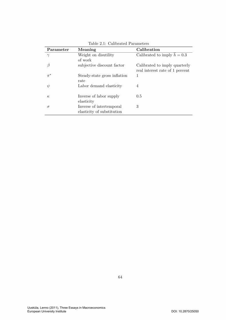
Table 2.1: Calibrated ParametersParameter Meaning Calibration

γ Weight on disutility Calibrated to imply h = 0.3of work

β subjective discount factor Calibrated to imply quarterlyreal interest rate of 1 percent

π∗ Steady-state gross inflation 1rate

ψ Labor demand elasticity 4

κ Inverse of labor supply 0.5elasticity

σ Inverse of intertemporal 3elasticity of substitution

64


DOI: 10.2870/25050

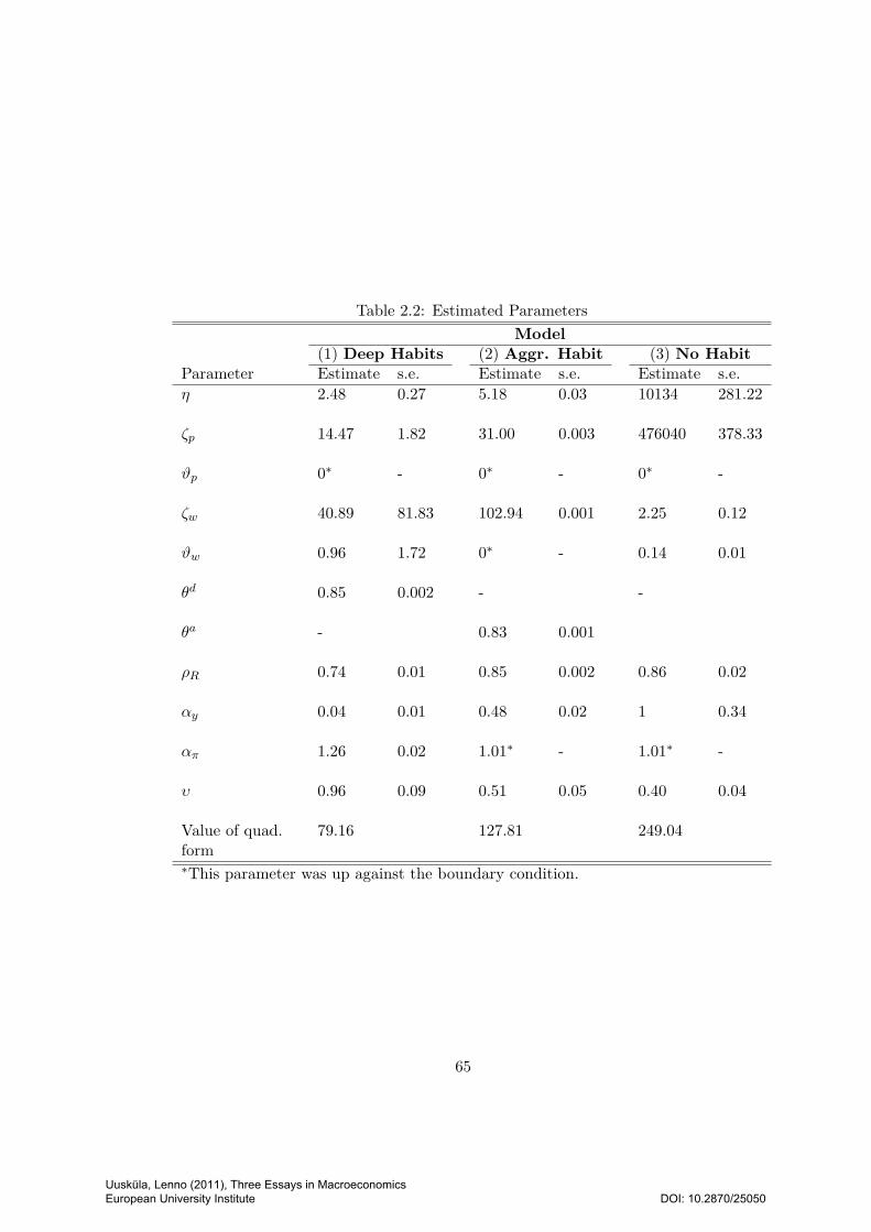
Table 2.2: Estimated ParametersModel

(1) Deep Habits (2) Aggr. Habit (3) No Habit

Parameter Estimate s.e. Estimate s.e. Estimate s.e.η 2.48 0.27 5.18 0.03 10134 281.22

ζp 14.47 1.82 31.00 0.003 476040 378.33

ϑp 0∗ - 0∗ - 0∗ -

ζw 40.89 81.83 102.94 0.001 2.25 0.12

ϑw 0.96 1.72 0∗ - 0.14 0.01

θd 0.85 0.002 - -

θa - 0.83 0.001

ρR 0.74 0.01 0.85 0.002 0.86 0.02

αy 0.04 0.01 0.48 0.02 1 0.34

απ 1.26 0.02 1.01∗ - 1.01∗ -

υ 0.96 0.09 0.51 0.05 0.40 0.04

Value of quad. 79.16 127.81 249.04form∗This parameter was up against the boundary condition.

65


DOI: 10.2870/25050

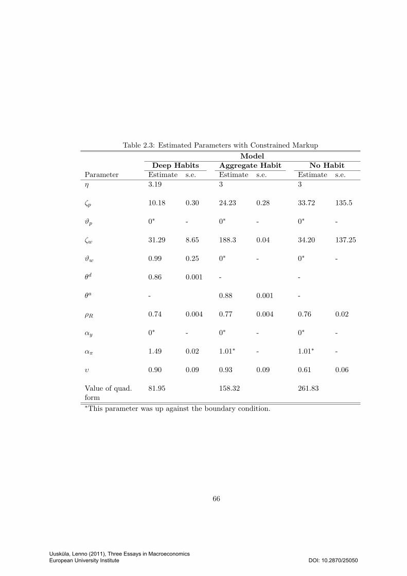
Table 2.3: Estimated Parameters with Constrained MarkupModel

Deep Habits Aggregate Habit No Habit

Parameter Estimate s.e. Estimate s.e. Estimate s.e.η 3.19 3 3

ζp 10.18 0.30 24.23 0.28 33.72 135.5

ϑp 0∗ - 0∗ - 0∗ -

ζw 31.29 8.65 188.3 0.04 34.20 137.25

ϑw 0.99 0.25 0∗ - 0∗ -

θd 0.86 0.001 - -

θa - 0.88 0.001 -

ρR 0.74 0.004 0.77 0.004 0.76 0.02

αy 0∗ - 0∗ - 0∗ -

απ 1.49 0.02 1.01∗ - 1.01∗ -

υ 0.90 0.09 0.93 0.09 0.61 0.06

Value of quad. 81.95 158.32 261.83form∗This parameter was up against the boundary condition.

66


DOI: 10.2870/25050

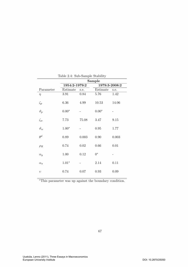
Table 2.4: Sub-Sample StabilitySample

1954:2-1979:2 1979:3-2008:2

Parameter Estimate s.e. Estimate s.e.η 3.91 0.84 5.76 1.42

ζp 6.36 4.99 10.53 14.06

ϑp 0.00∗ - 0.00∗ -

ζw 7.73 75.08 3.47 9.15

ϑw 1.00∗ - 0.95 1.77

θd 0.89 0.003 0.90 0.003

ρR 0.74 0.02 0.66 0.01

αy 1.00 0.12 0∗ -

απ 1.01∗ - 2.14 0.11

υ 0.74 0.07 0.93 0.09

∗This parameter was up against the boundary condition.

67


DOI: 10.2870/25050

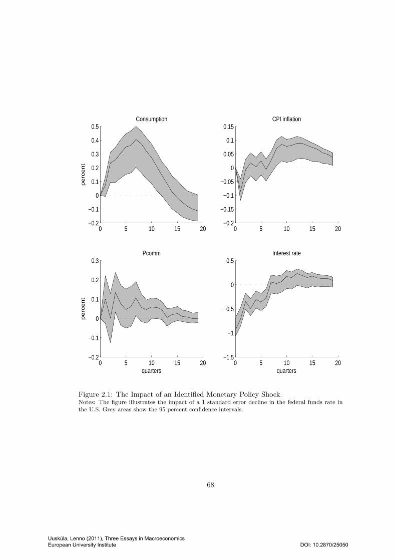
0 5 10 15 20−0.2

−0.1

0

0.1

0.2

0.3

0.4

0.5Consumption

pe

rce

nt

0 5 10 15 20−0.2

−0.15

−0.1

−0.05

0

0.05

0.1

0.15CPI inflation

0 5 10 15 20−0.2

−0.1

0

0.1

0.2

0.3Pcomm

pe

rce

nt

quarters0 5 10 15 20

−1.5

−1

−0.5

0

0.5Interest rate

quarters

Figure 2.1: The Impact of an Identified Monetary Policy Shock.Notes: The figure illustrates the impact of a 1 standard error decline in the federal funds rate inthe U.S. Grey areas show the 95 percent confidence intervals.

68


DOI: 10.2870/25050

0 5 10 15

−0.1

0

0.1

0.2

0.3

0.4

0.5Consumption

pe

rce

nt

quarters0 5 10 15

−0.1

−0.05

0

0.05

0.1

CPI inflation

0 5 10 15

−1

−0.8

−0.6

−0.4

−0.2

0

0.2

Interest rate

pe

rce

nt

quarters

Figure 2.2: The VAR-based Impact of a Monetary Policy Shock in the Deep HabitsEconomy.Notes: Lines without circles show empirical estimates of a 1 standard error decrease in the federalfunds rate. Lines with circles show theoretical impact of a 1 percentage point decrease in the interestrate in the deep habits. economy when measured with a VAR filter

69


DOI: 10.2870/25050

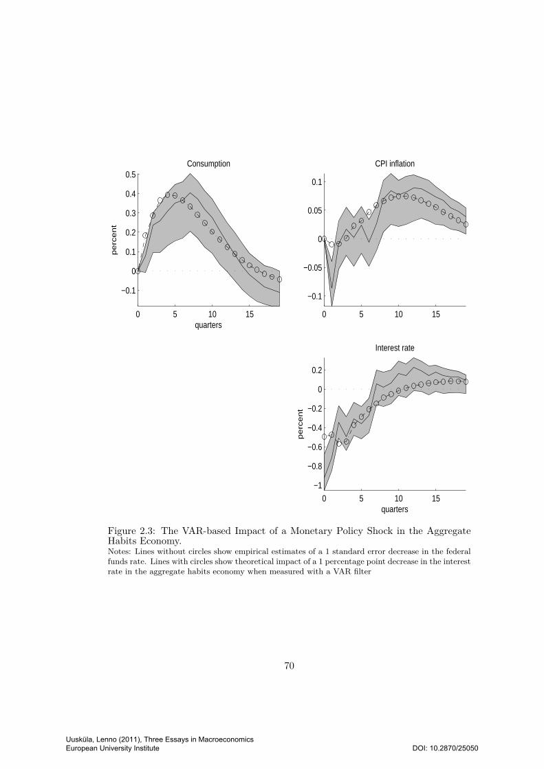
0 5 10 15

−0.1

0

0.1

0.2

0.3

0.4

0.5Consumption

pe

rce

nt

quarters0 5 10 15

−0.1

−0.05

0

0.05

0.1

CPI inflation

0 5 10 15

−1

−0.8

−0.6

−0.4

−0.2

0

0.2

Interest rate

pe

rce

nt

quarters

Figure 2.3: The VAR-based Impact of a Monetary Policy Shock in the AggregateHabits Economy.Notes: Lines without circles show empirical estimates of a 1 standard error decrease in the federalfunds rate. Lines with circles show theoretical impact of a 1 percentage point decrease in the interestrate in the aggregate habits economy when measured with a VAR filter

70


DOI: 10.2870/25050

0 5 10 15

−0.1

0

0.1

0.2

0.3

0.4

0.5

Consumption

pe

rce

nt

quarters0 5 10 15

−0.1

−0.05

0

0.05

0.1

CPI inflation

0 5 10 15

−1

−0.8

−0.6

−0.4

−0.2

0

0.2

Interest rate

pe

rce

nt

quarters

Figure 2.4: The VAR-based Impact of a Monetary Policy Shock in the Economywith No Habits.Notes: Lines without circles show empirical estimates of a 1 standard error decrease in the federalfunds rate. Lines with circles show theoretical impact of a 1 percentage point decrease in the interestrate in the economy with no habits economy when measured with a VAR filter

71


DOI: 10.2870/25050

0 5 10 15

−0.1

0

0.1

0.2

0.3

0.4

0.5Consumption

pe

rce

nt

quarters0 5 10 15

−0.1

−0.05

0

0.05

0.1

CPI inflation

0 5 10 15

−1

−0.8

−0.6

−0.4

−0.2

0

0.2

Interest rate

pe

rce

nt

quarters

Figure 2.5: The Exact Response to a Monetary Policy Shock in the Deep HabitsEconomy.Notes: Lines without circles show empirical estimates of a 1 standard error decrease in the federalfunds rate. Lines with circles show theoretical impact of a 1 percentage point decrease in the interestrate in the deep habits economy.

72


DOI: 10.2870/25050

0 5 10 15

−0.1

0

0.1

0.2

0.3

0.4

0.5Consumption

pe

rce

nt

quarters0 5 10 15

−0.1

−0.05

0

0.05

0.1

CPI inflation

0 5 10 15

−1

−0.8

−0.6

−0.4

−0.2

0

0.2

Interest rate

pe

rce

nt

quarters

Figure 2.6: The Exact Response to a Monetary Policy Shock in the Aggregate HabitsEconomy.Notes: Lines without circles show empirical estimates of a 1 standard error decrease in the federalfunds rate. Lines with circles show theoretical impact of a 1 percentage point decrease in the interestrate in the aggregate habits economy.

73


DOI: 10.2870/25050

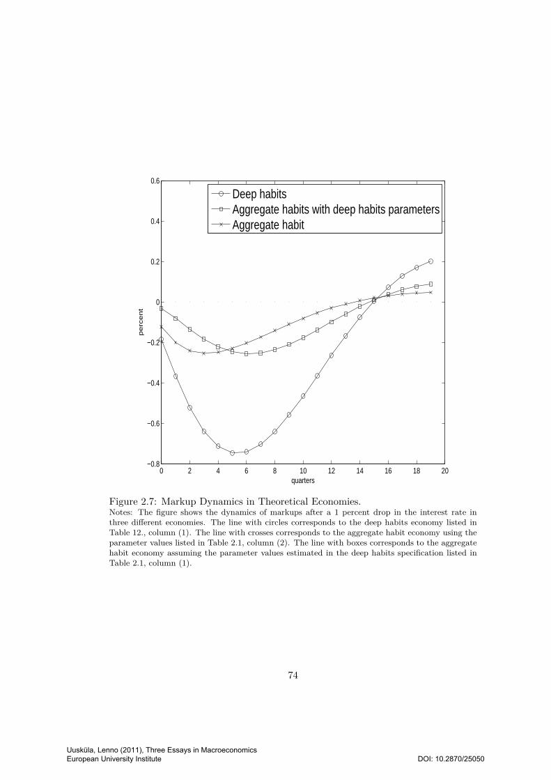
0 2 4 6 8 10 12 14 16 18 20−0.8

−0.6

−0.4

−0.2

0

0.2

0.4

0.6

quarters

pe

rce

nt

Deep habitsAggregate habits with deep habits parametersAggregate habit

Figure 2.7: Markup Dynamics in Theoretical Economies.Notes: The figure shows the dynamics of markups after a 1 percent drop in the interest rate inthree different economies. The line with circles corresponds to the deep habits economy listed inTable 12., column (1). The line with crosses corresponds to the aggregate habit economy using theparameter values listed in Table 2.1, column (2). The line with boxes corresponds to the aggregatehabit economy assuming the parameter values estimated in the deep habits specification listed inTable 2.1, column (1).

74


DOI: 10.2870/25050

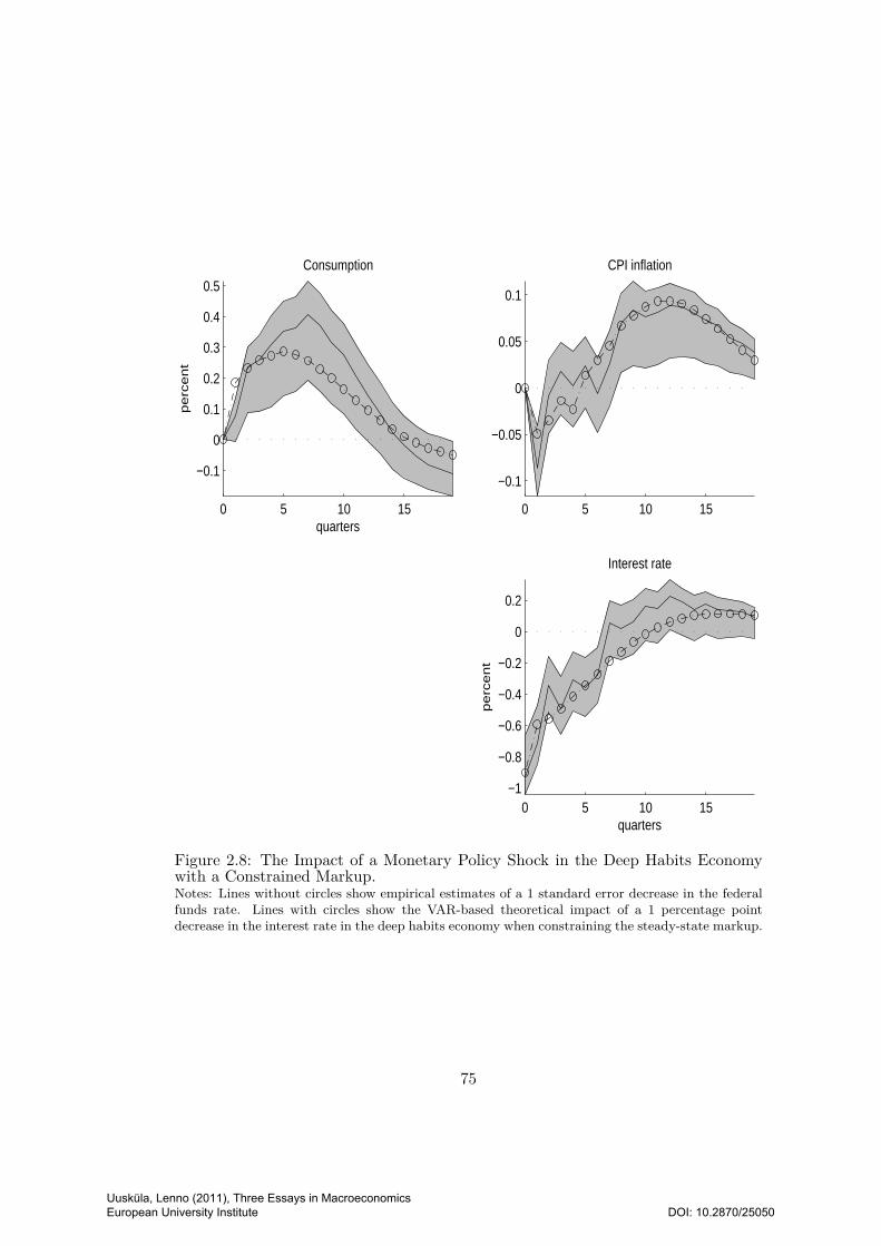
0 5 10 15

−0.1

0

0.1

0.2

0.3

0.4

0.5

Consumption

pe

rce

nt

quarters0 5 10 15

−0.1

−0.05

0

0.05

0.1

CPI inflation

0 5 10 15−1

−0.8

−0.6

−0.4

−0.2

0

0.2

Interest rate

pe

rce

nt

quarters

Figure 2.8: The Impact of a Monetary Policy Shock in the Deep Habits Economywith a Constrained Markup.Notes: Lines without circles show empirical estimates of a 1 standard error decrease in the federalfunds rate. Lines with circles show the VAR-based theoretical impact of a 1 percentage pointdecrease in the interest rate in the deep habits economy when constraining the steady-state markup.

75


DOI: 10.2870/25050

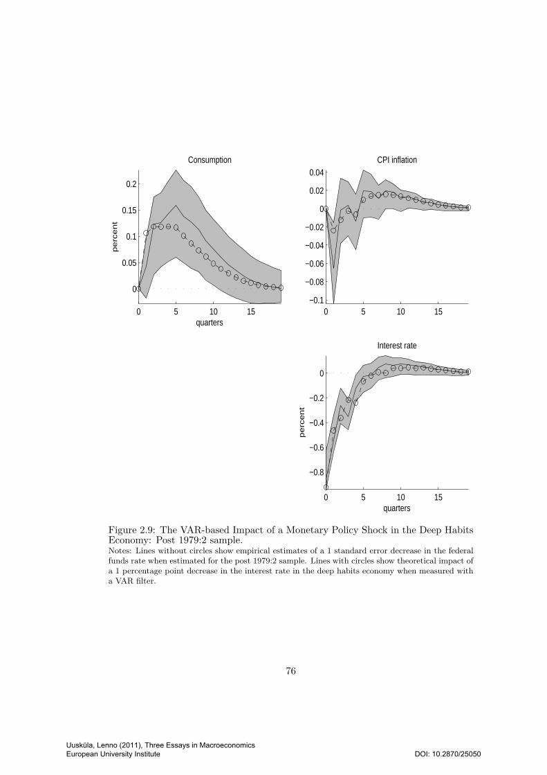
0 5 10 15

0

0.05

0.1

0.15

0.2

Consumption

pe

rce

nt

quarters0 5 10 15

−0.1

−0.08

−0.06

−0.04

−0.02

0

0.02

0.04CPI inflation

0 5 10 15

−0.8

−0.6

−0.4

−0.2

0

Interest rate

pe

rce

nt

quarters

Figure 2.9: The VAR-based Impact of a Monetary Policy Shock in the Deep HabitsEconomy: Post 1979:2 sample.Notes: Lines without circles show empirical estimates of a 1 standard error decrease in the federalfunds rate when estimated for the post 1979:2 sample. Lines with circles show theoretical impact ofa 1 percentage point decrease in the interest rate in the deep habits economy when measured witha VAR filter.

76


DOI: 10.2870/25050

Chapter 3

Firm Turnover, Financial

Friction and Inflation

Lenno Uusküla1

Abstract

In a standard New-Keynesian DSGE model exogenous price markup and cost-push

shocks generate most of the volatility in inflation. The key equation determining

inflation is the New Keynesian Phillips curve. Several authors have proposed mod-

ifications to the forward looking Phillips curve. In this paper I concentrate on the

effects of endogenous markups due to firm turnover and the importance of financial

friction. My findings show that entry cost shocks are important in explaining the

dynamics of inflation at the business cycle frequency. Financial friction does not

change the relative importance of the structural shocks in explaining inflation.

Keywords: firm turnover, financial frictions, inflation, DSGE

JEL codes: E32, C11, E23

3.1 Introduction

In a standard New-Keynesian Dynamic Stochastic General Equilibrium model in-

flation volatility is mostly explained by the exogenous price markup and cost-push1Department of Economics, European University Institute (e-mail: [email protected]). I

want to thank Morten O. Ravn and Giancarlo Corsetti for guidance, and Marco del Negro andRicardo Reis for helpful discussions at early stage of the project.

77


DOI: 10.2870/25050

shocks. For example in Smets and Wouters (1998) exogenous price markup shocks

explain more than half of the variance in inflation during first years after the shock.

Several authors have proposed modifications to the forward looking New Keyne-

sian Phillips curve which determines inflation. First, the mark-up is not exogenous

but depends on the level of competition, which is determined by the number of

firms in the economy (see Bergin and Corsetti (2008), Bilbiie et al. (2007)). Second,

Ravenna and Walsh (2003) find evidence for a financial friction - firms borrow a

share of the wage bill from the banks. I ask what is the role of firm turnover and

financial friction in explaining the dynamics of inflation over the business cycle?

I augment a standard medium scale sticky price and sticky wage New Keynesian

model such as Smets and Wouters (1998) with two features. First I assume that

the creation of firms is labor intensive, a fixed cost to start a business. I allow the

death rate of firms to be stochastic. The number of firms is determined by free entry

condition and the number of firms determines the level of markup in the economy.

The law of motion for the number of firms is based on Bilbiie et al. (2007). Second

I allow for a financial friction in the economy. Firms borrow resources from banks

to pay for a share of production costs in advance. This way changes in the interest

rate have an impact on the costs of production. The financial friction is proposed by

Christiano et al. (1997) and recently employed by Rabanal (2006) and Uhlig (2007).

The economy is described by the following 5 structural shocks: monetary policy,

labor productivity, wage cost-push shocks, a shock to the fixed cost of starting a

business, and a shock to the firm survival probability. I match the model with 5

U.S. data series: consumption, hours, inflation, the interest rate, and the creation of

firms for the period 1983Q1-1998Q3. I estimate the parameters of the model with

the Bayesian likelihood approach and use the variance decomposition at the business

cycle frequency and the forecast error variance decomposition to discuss the main

results.

My results show that the shocks to the creation of firms explain 67% of the vari-

ance in inflation at the business cycle frequency. The channel between the number

of firms and inflation is not trivial. A drop in the cost of entry leads to an increase in

the demand in labor and therefore also to an increase in marginal costs and inflation.

As more firms are created and the number of firms is increasing the markup effect

becomes stronger and inflation drops again. To the knowledge of the author this is

the first attempt to quantify the effect of entry cost shocks to the inflation rate in a

DSGE framework.

I find that 80% of the production costs are borrowed from the banks. However I

78


DOI: 10.2870/25050

find little evidence that the cost channel is important in explaining the volatility of

inflation at the business cycle frequency. The results are in line with the findings of

Ravenna and Walsh (2003) who find evidence for the cost channel. But compared

to Rabanal (2006) my estimate for the financial friction is relatively high. He also

estimates a DSGE model using Bayesian techniques and finds that 15% of the costs

are borrowed from the banks. Also Uhlig (2007) calibrates the share of costs bor-

rowed from the banks to 10%. But similarly to these papers I find that the financial

friction has little to explain in inflation dynamics.

My results assign very little importance to the wage cost-push shocks. This

is in sharp contrast with the findings of Smets and Wouters (1998). Technology

shocks explain 17% of the variance in inflation at over the business cycle. This is in

accordance with the DSGE and VAR evidence where the role of technology shocks

is around 20% (see Smets and Wouters (1998) for the DSGE and Altig et al. (2005)

for the VAR literature). Finally, monetary shocks and firm survival shocks explain

around 6% of the variance in inflation at the business cycle frequency.

The rest of the paper is organized as follows. Second chapter introduces the

model with financial frictions and firm turnover. Third chapter gives a short overview

of the data and the estimation approach. Basic results are presented in chapter four

and chapter five concludes.

3.2 The model

In the first section I present a New Keynesian dynamic stochastic general equilibrium

model with financial friction and the creation and destruction of firms. There are five

types of agents in the economy: final goods producers, intermediate goods producers,

households, banks and a government.

Households maximize their utility from consumption and leisure, firms maximize

profits. In the final goods sector, firms operate under full competition and aggregate

inputs from the intermediate firms into consumption good. In the intermediate

goods production sector firms operate under monopolistic competition structure.

The firms are subject to stochastic death shocks and the creation of firms is labor

intensive. The number of firms in the intermediate goods sector is determined by

the free entry condition.

The economy has a financial sector. It takes deposits from the households and

receives monetary injections from the government. Banks give loans to the interme-

diate firms as the firms are assumed to borrow a share ξ of their wage bill from the

79


DOI: 10.2870/25050

banks. Finally, monetary policy authority decides about the monetary injections to

commercial banks by targeting the interest rate.

3.2.1 Household problem

The representative household maximizes discounted lifetime utility from consump-

tion ct and dislikes time spent at work nt.

Ut = Et

∞∑

t=0

βt

(ct − χct−1)1− 1

σ

1− 1σ

−A

1 + 1κ

n1+ 1

κt

(3.1)

where β is the discount factor, χ is the consumption habit parameter, σ is the

intertemporal elasticity of substitution, κ is the Frisch elasticity of labor supply, A

is scaling parameter, and Et is the conditional expectations operator.

Households need cash at hand to buy a fraction η of the consumption (Ct). The

cash in advance constraint is Ht,res + ηCt = Ht−1 where Ht,res is the residual cash

holding, which in equilibrium equals zero, and Ht−1 is cash at hand in period t.

Divide the equation by Pt to get the real budget constraint

ht,res + ηct =ht−1

πCt, (3.2)

where ct = CtPt

, ht,res = Ht,resPt

, and ht−1 = Ht−1

Pt.

Households face a sequence of budget constraints. The available funds in period

t consist of the income from working, deposits, bonds, profits, transfers and residual

cash.

Ht +Dt + qtBt + (1− η)Ct = Wtnt + (1 + it)Dt−1 +Bt−1 +Ht,res + Vt +Gt (3.3)

where Dt is deposit with banks, qt is the discount price for the government bonds

Bt, 1 + it is the gross return on deposits made the previous period, Gt are the

government transfers, and Vt are the profits received from the household’s ownership

of intermediate goods firms. The money is spent on non-cash consumption, or saved

in bonds, and kept in cash or deposits.

In real terms, the equation is given by

ht + dt + qtbt + (1− η)ct = wtnt + (1 + it)dt−1

πCt+bt−1

πCt+ ht,res + vt + gt (3.4)

where dt = DtPt

, bt = BtPt

, wt = WtPt

, gt = GtPt

, vt = VtPt

, and πCt is consumer inflation

80


DOI: 10.2870/25050

defined specifically later.

Labor market is characterized by a sluggish adjustment of the nominal wage.

wt =((1− ω)wt−1 + ωΥwft

)(1 + ut,w) (3.5)

Where wft is the market clearing wage, Υ shows bargaining power of households, and

ut,w is the wage cost-push shock following an ARMA(1, 1), ut,w = ρwut−1,w + εt,w

and εt,w = ρmaw εt−1,w + ǫt,w.

Households choose consumption, bonds, cash at hand, deposits, and work hours.

The Lagrange multiplier on the cash in advance equation is t and budget constraint

λt. The first order conditions are:

ηt = −(1− η)λt + (ct − χct−1)−1

σ − βχ(ct+1 − χct)−1

σ (3.6)

λtqt = βEt

[λt+1

πCt+1

](3.7)

λt = βEt

[t+1

πCt+1

](3.8)

λt = βEt

[λt+1

1 + it+1

πCt+1

](3.9)

λtwft = An

1

κt (3.10)

The optimality condition for the labor-leisure choice gives the market clearing wage

wft .

3.2.2 Final good firms

Final good firms maximize profits

Ptyt −

∫ Nt

0pt,jyt,jdj (3.11)

where yt is the final output, Nt is the number of intermediate inputs indexed by j

with prices pt,j and quantities yt,j . Firms use a CES aggregator for production

yt =

(∫ Nt

0y

1

1+µ

t,j

)1+µ

(3.12)

81


DOI: 10.2870/25050

where µ = 1σ−1 and σ is the intertemporal elasticity of substitution between in-

termediate goods. After some algebra, the demand for the intermediate inputs is

following:

yt,j =

(Ptpt,j

) 1+µ

µ

yt (3.13)

where the price index is given by Pt =(∫Nt

0 p−

1

µ

t,j

)−µ

. The relative price is given by

ρt = pt,jPt

= Nµ.

In the equilibrium all firms are the same so pt,j = pt. Inflation πt = ptpt−1

is

described in terms of intermediate goods prices and therefore the consumer inflation

index πCt is given by πtπCt

= ρtρt−1

=(

NtNt−1

)µ. A rise in the number if firms leads to

a drop in the consumer inflation relative to the intermediate goods inflation rate.

When µ approaches zero, the elasticity of substitution approaches infinity, and the

variety effect on consumer inflation disappears.

3.2.3 Intermediate good firms

Intermediate sector firms produce goods for the final goods sector. The market

structure is monopolistic competition and the number of firms is determined by a

free entry condition.

Intermediate firms use a production technology which is linear in labor.

yt,j = γtnt,j (3.14)

where γt is a productivity shock that is assumed to follow an ARMA process γt =

ργγt−1 + εt,γ and εt,γ = ρmaγ εt−1,γ + ǫt,γ .

Firms have to pay part of the labor input in advance. They borrow funds for

this purpose from commercial banks. This gives rise to the loan condition for the

representative firm Lt,j = ξWtnt,j .

In order to change prices, firms face a price adjustment cost as in Rotemberg

(1982) with the cost parameter φ. The profits are given by Vt,j = (pt,jγt − (1 +

ξit)MCt)nt,j −Ptφ

2

(pt,j

pt−1,jπ− 1

)2, and in real terms:

vt,j =(pt,jPt− (1 + ξit)mct

)yt,j −

φ

2

(pt,j

pt−1,jπ− 1

)2

(3.15)

82


DOI: 10.2870/25050

where the real variables are vt,j = Vt,jPt

, and mct = MCtPt

.

The firm j chooses labor nt,j and price pt,j . The cost minimization problem gives

marginal cost net of interest rate payments

mct =wtγt. (3.16)

The net present value of the firm NPV today is defined as the discounted

profits of all future periods. The net present value is defined at the time when

production has already taken place, but firms do not yet know if they survive

until the next period. In this way the net present value is the same for the in-

cumbents and new firms. In nominal terms the net present value is defined as

NPVt,j = (1 − δ)Et[(1 + ut+1,surv)

λt+1

λt(Vt+1,j +NPVt+1,j)

]and in the real terms

after dividing with the price level:

npvt,j = (1− δ)Et(1 + ut+1,surv)[λt+1

λt(vt+1,j + npvt+1,j)

], (3.17)

where the λt+1

λtis the stochastic discount factor of the consumer, δ is the exogenous

death probability of the firm, and ut,surv is the exogenous survival shock of the firm.

The shock follows an ARMA(1, 1), ut,surv = ρsurvut−1,surv + εt,surv and εt,surv =

ρmasurvεt−1,surv + ǫt,surv. Previously Vilmi (2009) has a model with a stochastic rate

of firm survival. In this paper I the survival probability is modelled as an exogenous

process for the reason of simplicity. However the survival probability could also be

modeled as an endogenous factor in the model. In fact Jacobson et al. (2008) show

that macroeconomic factors are important for the the firm bankruptcy rates.

In order to enter, firms have to pay a sunk entry cost in labor. The free entry

condition is given in real terms:

npvt,j = ξentwtγt

(1 + ξit)(1 + ut,ent), (3.18)

where the entry cost shock ut,ent is ARMA(1,1) process ut,ent = ρentut−1,ent + εt,ent

and εt,ent = ρmaentεt−1,ent + ǫt,ent

New firms can only produce the following period and a fraction of firms dies at

the end of the period, so some of the new firms never produce. The law of motion

of the firms is

Nt = (1− δ)(1 + ut,surv)(Nt−1 +NEt−1) (3.19)

There are two issues writing the number of firms dynamics in this way. First, there is

83


DOI: 10.2870/25050

no guarantee that the number of firms created is not negative. However this problem

is addressed by assuming that the variance of the entry shock is small. Secondly,

there is nothing that stops from the number of firms to increase between two periods

if the positive survival shock exceeds the natural death rate of firms, so that firms

can be generated from nothing overnight. The interpretation of it would be that

some of the firms split in two but they are not accounted among the entrants.

Because of the price adjustment cost, the model is characterized by a forward

looking Phillips curve:

ρt,j =pt,jPt

= mut,jmct (3.20)

where ρt,j = pt,jPt

is the relative price, and the markup (mut,j) is given by following

equation

mut,j =(1 + µ)µ

1(1 + ξit)

...

(−

1µ−

φ

yt,j

(πtπ− 1

)πtρtπ

+φ

yt,j(1− δ)Et

[(1 + ut+1,surv)

λt+1

λt

(πt+1

π− 1

)πt+1

ρtπ

])−1

(3.21)

As this is one the key equation that is changed compared to the standard model,

I present here the log-linearized version.

πt =yiφµ

(−ρt +

ξ

1 + ξiit + mct

)+ β(1− δ)πt+1 (3.22)

where the variables without time subscript denote their steady-state levels, the vari-

ables with hats denote percentage change from the steady state with the exception

of inflation and interest rate where it is percentage point change from the steady

state, and the firm level subscript j are dropped as all firms are the same.

The equation states that the inflation rate today depends on the expected in-

flation and marginal cost as in the standard Phillips curve. However the two new

elements, financial frictions and the firm turnover, uncouple marginal cost (the wage

rate) from the inflation rate by making markups endogenous. In short, the finan-

cial friction modifies the effect of marginal cost on inflation. Decreasing marginal

cost leads to a drop in inflation. Decreasing inflation reduces the interest rate, and

thus the cost of production, magnifying the effect on the inflation rate. Any shock

that results in an increase in the number of firms pushes down markups and

84


DOI: 10.2870/25050

reduces inflation.

3.2.4 Banks

Banks lend money to the intermediate good sector firms, who pay share ξ of the

wages in advance. The funds the banks can use ar the deposits from the house-

holds dt−1 and central bank money injections ψt. By aggregating get the following

condition:

dt−1

πCt+ ψt = ξwtnt = lt (3.23)

3.2.5 The Government and the Central Bank

Central bank uses money injections to the commercial banks

mt =mt−1

πCt+ νψt (3.24)

where ψt is the money injection and ν determines what is the share of money taken

out from the economy in the end of the period.

Monetary policy is described by an interest rate rule:

it = i+ ρiit−1 + (1− ρi)

[ζπ

(πCtπC− 1

)+ ζx

(mctmc− 1

)+ ǫt,i

](3.25)

where ǫt,i is an idiosyncratic shock to the interest rate.

The budget is balanced every period:

gt = (ν + it)ψt (3.26)

3.2.6 Aggregation and market clearing

Money in this model is the sum of cash ad hand and deposits

mt = dt + ht (3.27)

The hours worked by the household are divided between creating new firms and

producing output.

nt = Ntnt,j +NEt

ξent(1 + uentt )γt

(3.28)

85


DOI: 10.2870/25050

Aggregate profits vt include the individual profits of the firm minus the cost of

starting new businesses.

vt = Ntvt,j −NEt wtξ

ent(1 + ξit)(1 + uentt )

γt(3.29)

In the total consumption I take out the effect of the number of firms on the

consumption in order to keep the productivity of the economy independent from the

number of firms,

ct = Nι−(1+µ)t yt, (3.30)

where ι = 1, so the model departs from the standard Dixit-Stiglitz aggregator.

The reason is that I focus on looking at the transmission through the Phillips curve.

Without this transformation the increasing number of firms would lead to production

technology that is not linear in labor. The issue should be dealt in a separate paper.

3.2.7 Equilibrium

The system is described by 33 variables, out of which 28 are endogenous, bt, gt, ct,

nt,j , nt, vt,j , vt, yt,j , yt, mct, dt, ht, mt, lt, ψt, it, qt, wt, wft , πt, πCt , NPVt, Nt, NE

t ,

Pt,j , Pt, ρt, and two Lagrange multipliers: t, λt.

There are 5 exogenous i.i.d shocks: ǫt,γ , ǫt,w, ǫt,ent, ǫt,i, ǫt,surv. I allow ARMA(1,1)

structure for the processes of technology γt, labor cost ut,w and entry costs ut,entshocks. The equilibrium is symmetric, in which consumers maximize utility, firms

and banks maximize profits, and all markets clear.

3.3 Data, Estimation and Priors

I estimate the model using quarterly US data for the sample period 1983Q1-1998Q3.

This sample period reflects a compromise between availability of data and institu-

tional features of the U.S. economy. Firm creation data is not available for the

period after 1998Q3. In the year 1983 a major change in the bankruptcy law was

launched. I use the following 5 series for the US economy:

• consumption - log of real non-durable consumption divided by 16 years and

older civilian population, demeaned and detrended,

• hours - log of non-agricultural sector hours worked, divided by 16 years and

older civilian population, demeaned and detrended,

86


DOI: 10.2870/25050

• inflation, CPI inflation, demeaned,

• the Federal Funds Rate, demeaned,

• the number of new firms, log of firm creation, demeaned and detrended,

The data is presented in the Figure 3.1. There is a strong positive correlation

between hours, consumption and the creation of firms. The inflation rate and the

short-term interest rate are also strongly comoving. The contemporaneous correla-

tion between hours and inflation is close to zero for the full sample. Consumption

and hours have similar variances. The variance of firm creation clearly exceeds that

of the hours.

The firm creation in the model and data are not calculated in the identical way.

The model with endogenous entry and exogenous exit is a measure for net entry.

However, in the data I prefer to use the number of new firms as a proxy for net

entry because of problems with the available quarterly net entry measure. The

main difficulty in getting a good series for net entry is to account for the closing

firms (for a more detailed discussion see Uuskula (2007).

Some of the parameters are know to be difficult to estimate, especially because

of the short sample period and will instead be calibrated using results from previous

studies for quarterly frequency in order to concentrate on the main parameters of

interest relating to firm turnover. The calibrated parameters are presented in Table

3.1. The discount rate β = .99 is set to match a 4% annual real interest rate. The

exogenous rate of firm death is set to δ = 0.025 in order to match 10.7% annual firm

closing rate in the U.S. The number of firms is set to 1 without the loss of generality

and I solve for the steady state entry cost. Steady state markup is 25% (µ = .25),

which is higher than standard in the data, but lower than often calibrated in the

entry literature (Bilbiie et al. (2007) assume steady state markup equal to 36%.)

The number of firms and the markup determine the entry cost to satisfy the free

entry condition. Steady state inflation is 1.005 to match 2% annual inflation. In

solving the model I assume that people work one third of their time n = 13 and I

solve for the value of A that satisfies this constraint.

In addition I calibrate the parameters on consumption habit χ = .7. Frisch

elasticity of labor supply κ = 1, both often used in the DSGE literature. In addition

there are a few parameters for which there was very little information in the current

set of observables. The share of cash on hand goods and the share of government

money left in the economy in the end of the period are both equal to η = ν = 0.5

87


DOI: 10.2870/25050

and the wage markup equal to 10% (Υ = 1.1).Robustness analysis is carried out

about the importance of the fixed parameters in the estimation.

I use the Bayesian likelihood approach to estimate the model using the Metropolis-

Hastings sampler as described in Canova (2006). All calculations are done in Matlab,

the model is log-linearized around the stochastic steady state and solved with the

method of undetermined coefficient of Uhlig (1999). The priors of the parameters

are selected so that they represent the theoretical restrictions and with very low

information content (see Table 3.2). The autoregressive parameters are set to be

between 0 and 1 with the mean 0.5 and variance 0.292. For the intertemporal elas-

ticity of substitution and price stickiness I assume normal distributions. For the

intertemporal elasticity of substitution I use the mean of 1 and for the Rotemberg

price adjustment cost with the mean of 17 and variance equal to 16. The prior value

for the price stickiness is taken from Ireland (2001) and adjusted for the value of

calibrated markup and units of account in the price adjustment cost.

I take 250000 draws in two chains. The initial values are chosen based on pos-

terior maximization and only the last 50% of the draws are used in calculating the

moments of the data to allow for a burn-in period. The convergence is difficult to

achieve in some the parameters, such as the ARMA processes of the shocks. The

confidence intervals for the impulse responses and variance decompositions are based

on 1000 independent non-parametric draws from the posterior.

3.4 Results

Before explaining the main results I discuss some of the parameter estimates that

are crucial for the dynamics of inflation. The posteriors of the model parameters

are presented in Table 3.3.

First, the results show the importance of the financial friction in the model. The

parameter estimate for the financial friction - the share of wages paid in advance -

is 0.8 with a relatively wide confidence interval. The results support the findings of

Ravenna and Walsh (2003) who use single equation approach in the estimation of

the cost channel. The share of costs borrowed from the banks is much higher than

the estimate of Rabanal (2006). He finds that only a small share (0.15) of costs are

borrowed from the banks. Also Uhlig (2007) calibrates the parameter to a low value

as 0.1.

Second, the price and wage stickiness parameters are lower compared to the

previous estimates. The parameter estimate for the Rotemberg price adjustment

88


DOI: 10.2870/25050

cost is 11. The posterior is much lower than the prior value 17, the transformed

value to make price adjustment cost comparable with the paper by Ireland (2001)

as discussed in the section on priors. The price stickiness parameter value cannot

be directly translated to the Calvo probability of re-setting prices since the Phillips

curve contains financial friction and the relative price.

The parameter estimate for the wage flexibility is very close to one (wage rigidity

is close to zero), leaving very little importance for the wage stickiness. The param-

eters for the nominal rigidities are well identified and do not depend very strongly

on the prior distribution as previously found by Del Negro and Schorfheide (2008).

Third, the Taylor weight on inflation is around 1.05 and the weight on marginal

costs is zero, implying that the central bank is fully inflation targeting. Interest rate

smoothing parameter is 0.73 implying sluggishness in the interest rate to react to

inflation.

The intertemporal elasticity of substitution is 0.7. The autoregressive parameters

of the shocks are strongly different from one with one exception, the autoregressive

parameter for the wage cost-push shocks is close to one. This probably reflects the

high persistence of the hours series but also difficulties in identifying the ARMA

process of the shock. Therefore in the estimated model the wages are persistent

because of the persistent wage costs. To al lthe other shocks wages react immediately.

The entry cost shock is also described by an ARMA process. This might indicate

some positive externalities in creating firms which are not explicitly modeled. The

technology shock is approximately described by an AR process and the survival

shock has only some autocorrelation.

In order to answer the question: what explains inflation dynamics, I look at vari-

ance decompositions and impulse response functions of the structural shock. The

variance decomposition at the business cycle frequency is based on the counterfac-

tual data generated by including one shock at the time. I use the Hodrick-Prescott

filter with the smoothing parameter λ = 1600 to remove long run trends, calculate

variances and the share of the respective variance from the sum of the individual

variances of the data that the five shocks produce. The results of the variance de-

composition at the business cycle frequency are presented on Table 3.4. I present

the forecast error variance decomposition (FEVD) results and the impulse response

functions for the period of 20 quarters after the shock together with the 90% confi-

dence intervals. The line in the middle is calculated at the medians of the parameter

estimates.

First column of Table 3.4 presents the benchmark results for the importance of

89


DOI: 10.2870/25050

the estimated 5 shocks in explaining the 5 data series that are matched in the estima-

tion at the business cycle frequency. The shocks to the cost of entry explain around

67% of the variance in inflation at the business cycle frequency. The importance of

the entry costs shocks in explaining inflation is also confirmed by the forecast error

variance decomposition analysis. Figure 3.2 presents the FEVD results for the entry

cost shock. Variations in the cost of entry explain more than half of the variance in

inflation during first five years after the shock.

The channel through which entry costs influence inflation is not trivial. A drop

in the entry cost, which makes creation of firms more efficient brings a hump-shaped

increase in the creation of firms and inflation. As it is good time to invest into

creating new firms, demand for labor increases (see Figure 3.3). In order to hire

more people, firms pay higher wages the workers. The increase in production costs

results in inflation. The central bank increases the interest rate, resulting the costs of

production to increase even more. As the number of firms is going up only gradually,

therefore it takes time before the increase in the creation of firms results in a higher

number of firms in the economy. So markup decreases with a relatively long lag.

But as the number of firms stays up for a period of time, the markups are low even

when the hours worked and the creation of firms have converged back to the initial

levels.

In the reaction to the shock the substitution away from consumption into creating

new firms has only little effect, but consumption still drops after the initial shock.

As the number of firms increases due to increased entry, consumption reaches back

its initial level after 3 years. However this channel moderates the reaction of hours

and wages, but does not undo the effect.

The firm survival shock explains around 6% of the variance of inflation at the

business cycle frequency and 7-8% from the FEVDs (see Figure 3.4). A drop in

the stochastic death rate increases the number of firms and lowers inflation. A 1%

increase in the number of firms brings inflation down by 0.05pp. at the time of the

impact. There are two channels which lead to a drop in inflation. First, higher

number of firms decreases the markup in the economy and lowers inflation. Second,

an increase in the number of firms lowers the need to create new firms and labor

demand drops leads to a drop in wages.

This effect of the number of firms to inflation can be compared the finding

of Cecioni (2009). She looks at the effect of change in the number of firms on

the inflation rate and concludes that the number of firms is an important factor

determining inflation. She finds that a 10% increase in the number of firms brings

90


DOI: 10.2870/25050

inflation down by 1.4 pp. in the medium horizon. My results show that in case of

costly creation of firms it is important to separate how the increase in the number

of firms is achieved. If there are many new firms created, the increase in the number

of firms can be even inflationary in the short run because of the increase in the costs

of production.

Variations in the exogenous technology are the second most important shock in

explaining inflation. The technology shocks explain around 18% of the variance in

inflation at the business cycle frequency. Technology shock explain 15-20% of the

volatility in inflation, with the impact increasing in time because of the persistence

of the shock. The share of the technology in explaining inflation is higher than

the estimates of Smets and Wouters (1998), who find that productivity can explain

around 5% of the variance in inflation at all horizons. The estimated importance

of the technology shock is much closer to the estimate of Altig et al. (2005) VAR

evidence. Their estimated technology shocks explain around 16% of the variance at

the business cycle frequency.

Cost-push shocks have little to say about inflation. In the FEVD the median

effect reaches 10% five years after the shock (see Figure 3.7) and 2.5% at the business

cycle frequency. This stands in contrasts with the findings of Smets and Wouters

(1998), who’s results show that wage markup shocks explain 50% of the inflation

2.5 years after the shock. However similar to Smets and Wouters (1998) my results

show that a higher share of variance explained in inflation by the cost-push shocks

at lower frequencies.

Monetary shocks have only some effects on the inflation at the very short run

(see Figure 3.5). In spite of the low levels of nominal rigidities and the strong

cost-channel, inflation drops after a contractionary monetary shock. The small real

effects of monetary policy are often found in the full likelihood estimation of the

DSGE models. In this paper zero effect on hours is included in the posterior of

the impulse responses. There results are consistent with the agnostic identification

approach results of Uhlig (2005).

The second column in Table 3.4 presents the variance decomposition for an

estimation of the model where the parameter on the financial friction is calibrated

very close to zero ξ = 0.01. The differences for the variance decomposition of

inflation are quite small. The share of the variance explained by the entry cost

shock is now 68%, up by one percentage point. The survival shock gains some

explanatory power, the share of the variance explained increases from 6 to 11%.

The increase comes mainly from the technology shocks, which now explain around

91


DOI: 10.2870/25050

13% of the variance. However the financial friction seems to matter for the relative

importance of the real variables.

Entry cost and firm survival shocks explain now a much higher share in hours and

consumption than before. In particular the financial friction is important in explain-

ing the qualitative effects of monetary shocks that a monetary contraction decreases

entry. In the benchmark model a drop in the interest rate leads to an increase in

the creation of firms. This result is also supported by the VAR evidence (see for ex-

ample Bergin and Corsetti (2005), Lewis (2006) or Uuskula (2007)). However in the

model where the financial friction is set to zero, the number of firms decreases after

an expansionary monetary shock. This is a common finding in the papers without

a financial friction such as Bilbiie et al. (2007)). Therefore the financial friction is

important for the real variables and has only limited impact on the relative variances

of inflation. This result also confirms the finding of Rabanal (2006) that the cost

channel is not important for the inflation variance.

In order to understand the properties of the estimated model I have conducted

a few robustness checks, mainly for the values of the calibrated parameters. One of

the important parameters is the markup in the intermediate goods sector. Cecioni

(2009) calibrates the value equal to around 6%, to a much lower value than in this

paper. Differently Bilbiie et al. (2007) fix the value of markup at 35.71%, which is

much higher compared to my benchmark results. When I fix the price markup to

10%, technology and wage cost-push shocks are less important and the stochastic

rate of survival is more important (see the last column in Table 3.4). When markup

is equal to 35.71%, wage shocks have smaller and the entry costs shocks bigger role

(third column in Table 3.4).

Following Uhlig (2007), I allow the shock to the interest rate ǫt,i to have an AR

structure. The results however show that the value of autoregressive parameter is

equal to zero. The posterior likelihood and variance decomposition results are not

sensitive to the changes in the parameters on the share of cash goods, money left

in the economy, and wage markup. A drop in the value of Frisch elasticity of labor

supply to a level consistent with the microeconometric evidence (0.2) increases the

importance of entry shocks on consumption and inflation and the magnifies the effect

of wage cost-push shocks on hours.

92


DOI: 10.2870/25050

3.5 Conclusions

In this paper I augment a medium scale sticky wage and sticky price macroeconomic

model with financial frictions and firm turnover and estimate it for the U.S. economy.

My results show that the shocks to the cost of entry are important in explaining the

variance of inflation over the business cycle. When creating firms is labor intensive,

then a drop in the cost of entry leads to increase in the labor demand as many

new firms are created. Increase labor demand results in higher marginal costs and

inflation. As number of firms increases markups decrease and inflation starts to

decrease. In this model financial frictions play only a minor role in explaining the

dynamics of inflation.

93


DOI: 10.2870/25050

Bibliography

Altig, D., Christiano, L. J., Eichenbaum, M., and Linde, J. (2005). Firm-specific cap-

ital, nominal rigidities and the business cycle. NBER working paper, (11034):59.

Bergin, P. and Corsetti, G. (2005). Towards a theory of firm entry and stabilization

policy. NBER working paper, (11821):37.

Bergin, P. and Corsetti, G. (2008). The extensive margin and monetary policy.

Journal of Monetary Economics, 55(7):1222–1237.

Bilbiie, F. O., Ghironi, F., and Melitz, M. J. (2007). NBER Macroeconomics Annual

2007, chapter Monetary Policy and Business Cycles with Endogenous Product

Variety.

Canova, F. (2006). Methods for Applied Macroeconomic Research. Princeton Uni-

versity Press.

Cecioni, M. (2009). Firm entry, competitive pressures and the u.s. inflation dynam-

ics. mimeo, page 37.

Christiano, L. J., Eichenbaum, M., and Evans, C. L. (1997). Sticky price and lim-

ited participation models of money: A comparison. European Economic Review,

41(6):1201–1249.

Del Negro, M. and Schorfheide, F. (f2008). Forming priors for dsge models (and how

it affects the assessment of nominal rigidities). Journal of Monetary Economics,

55(7):1191–1208.

Ireland, P. N. (2001). Sticky-price models of the business cycle: Specication and

stability. Journal of Monetary Economics, 47:3–18.

Jacobson, T., Kindell, R., Lindé, J., and Roszbach, K. F. (2008). Firm default and

aggregate fluctions. CEPR working paper, (7083).

94


DOI: 10.2870/25050

Lewis, V. (2006). Macroeconomic fluctuations and firm entry: theory and evidence.

National Bank of Belgium, Working paper research, (103):33.

Rabanal, P. (2006). Does inflation increase after a monetary policy tightening?

answers based on an estimated dsge model. Journal of Economic Dynamics and

Control, 31:906–937.

Ravenna, F. and Walsh, C. E. (2003). The cost channel in a new keynesian model:

Evidence and implications. mimeo, page 29.

Rotemberg, J. (1982). Monopolsitic price adjustment and aggregate output. Review

of Economic studies, 49:517–531.

Smets, F. and Wouters, R. (1998). Shocks and frictions in u.s. business cycles. a

bayesian dsge approach. NBER working paper, (6632).

Uhlig, H. (1999). Cumputational Methods for the Study of Dynamic Exonomies,

chapter A Toolkit for Analyzing Nonlinear Dynamic Stochastic Models Easily,

pages 30–61. Oxford University Press.

Uhlig, H. (2005). What are the effects of monetary policy on output? results from an

agnostic identification procedure. Journal of Monetary Economics, 52(2):381–419.

Uhlig, H. (2007). International Dimensions of Monetary Policy (National Bureau of

Economic Research Conference Report), chapter Monetary Policy in Europe vs.

the US: What Explains the Difference?, pages 489 – 533. NBER, Inc.

Uuskula, L. (2007). Limited participation or sticky prices? new evidence from the

firm entry and failures. mimeo, EUI.

Vilmi, L. (2009). The effects of firm entry and exit in macroeconomic fluctuations

and monetary policy. University of Oulu Department of Economics Working Pa-

pers, (0904):30.

95


DOI: 10.2870/25050

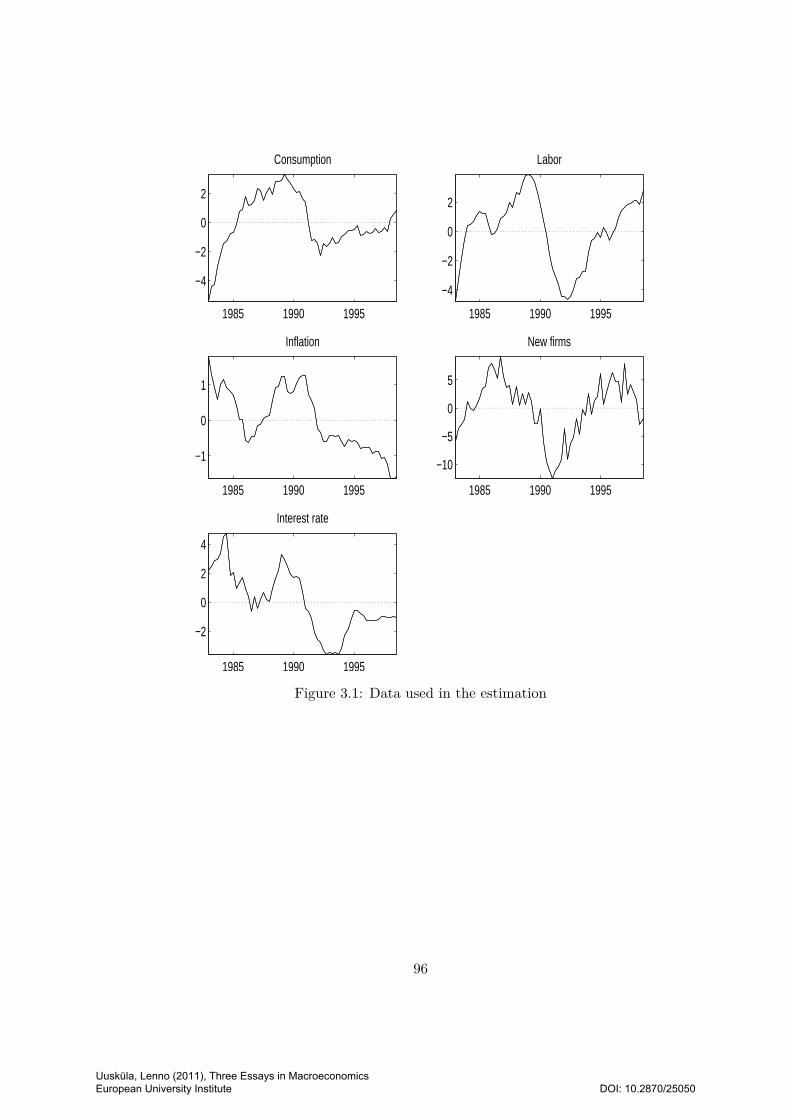
1985 1990 1995

−4

−2

0

2

Consumption

1985 1990 1995

−4

−2

0

2

Labor

1985 1990 1995

−1

0

1

Inflation

1985 1990 1995

−10

−5

0

5

New firms

1985 1990 1995

−2

0

2

4

Interest rate

Figure 3.1: Data used in the estimation

96


DOI: 10.2870/25050

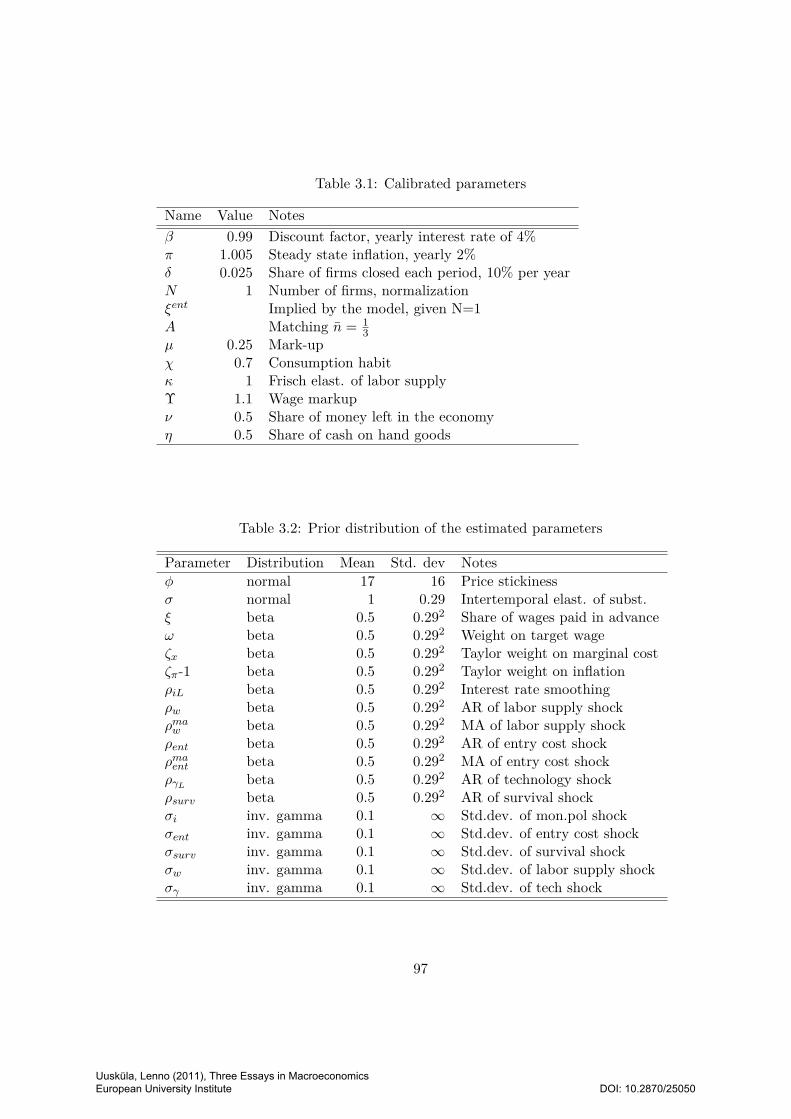
Table 3.1: Calibrated parameters

Name Value Notesβ 0.99 Discount factor, yearly interest rate of 4%π 1.005 Steady state inflation, yearly 2%δ 0.025 Share of firms closed each period, 10% per yearN 1 Number of firms, normalizationξent Implied by the model, given N=1A Matching n = 1

3µ 0.25 Mark-upχ 0.7 Consumption habitκ 1 Frisch elast. of labor supplyΥ 1.1 Wage markupν 0.5 Share of money left in the economyη 0.5 Share of cash on hand goods

Table 3.2: Prior distribution of the estimated parameters

Parameter Distribution Mean Std. dev Notesφ normal 17 16 Price stickinessσ normal 1 0.29 Intertemporal elast. of subst.ξ beta 0.5 0.292 Share of wages paid in advanceω beta 0.5 0.292 Weight on target wageζx beta 0.5 0.292 Taylor weight on marginal costζπ-1 beta 0.5 0.292 Taylor weight on inflationρiL beta 0.5 0.292 Interest rate smoothingρw beta 0.5 0.292 AR of labor supply shockρmaw beta 0.5 0.292 MA of labor supply shockρent beta 0.5 0.292 AR of entry cost shockρmaent beta 0.5 0.292 MA of entry cost shockργL beta 0.5 0.292 AR of technology shockρsurv beta 0.5 0.292 AR of survival shockσi inv. gamma 0.1 ∞ Std.dev. of mon.pol shockσent inv. gamma 0.1 ∞ Std.dev. of entry cost shockσsurv inv. gamma 0.1 ∞ Std.dev. of survival shockσw inv. gamma 0.1 ∞ Std.dev. of labor supply shockσγ inv. gamma 0.1 ∞ Std.dev. of tech shock

97


DOI: 10.2870/25050

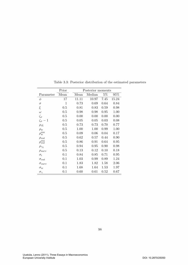
Table 3.3: Posterior distribution of the estimated parameters

Prior Posterior momentsParameter Mean Mean Median 5% 95%φ 17 11.11 10.97 7.45 15.24σ 1 0.73 0.69 0.64 0.84ξ 0.5 0.81 0.83 0.59 0.98ω 0.5 0.98 0.98 0.95 1.00ζx 0.5 0.00 0.00 0.00 0.00ζπ − 1 0.5 0.05 0.05 0.03 0.08ρiL 0.5 0.73 0.73 0.70 0.77ρw 0.5 1.00 1.00 0.99 1.00ρmaw 0.5 0.09 0.06 0.04 0.17ρent 0.5 0.62 0.57 0.44 0.90ρmaent 0.5 0.86 0.91 0.64 0.95ργL 0.5 0.94 0.95 0.90 0.98ρsurv 0.5 0.13 0.12 0.10 0.18σi 0.1 0.84 0.85 0.71 0.95σent 0.1 1.03 0.99 0.89 1.24σsurv 0.1 1.83 1.82 1.58 2.06σw 0.1 1.68 1.64 1.53 1.97σγ 0.1 0.60 0.61 0.52 0.67

98


DOI: 10.2870/25050

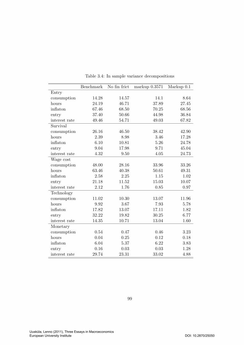
Table 3.4: In sample variance decompositions

Benchmark No fin frict markup 0.3571 Markup 0.1Entryconsumption 14.28 14.57 14.1 8.64hours 24.19 46.71 37.89 27.45inflaton 67.46 68.50 70.25 68.56entry 37.40 50.66 44.98 36.84interest rate 49.46 54.71 49.03 67.82Survivalconsumption 26.16 46.50 38.42 42.90hours 2.39 8.98 3.46 17.28inflaton 6.10 10.81 5.26 24.78entry 9.04 17.98 9.71 45.04interest rate 4.32 9.50 4.05 24.73Wage costconsumption 48.00 28.16 33.96 33.26hours 63.46 40.38 50.61 49.31inflaton 2.58 2.25 1.15 1.02entry 21.18 11.52 15.03 10.07interest rate 2.12 1.76 0.85 0.97Technologyconsumption 11.02 10.30 13.07 11.96hours 9.92 3.67 7.93 5.78inflaton 17.82 13.07 17.11 1.82entry 32.22 19.82 30.25 6.77interest rate 14.35 10.71 13.04 1.60Monetaryconsumption 0.54 0.47 0.46 3.23hours 0.04 0.25 0.12 0.18inflaton 6.04 5.37 6.22 3.83entry 0.16 0.03 0.03 1.28interest rate 29.74 23.31 33.02 4.88

99


DOI: 10.2870/25050

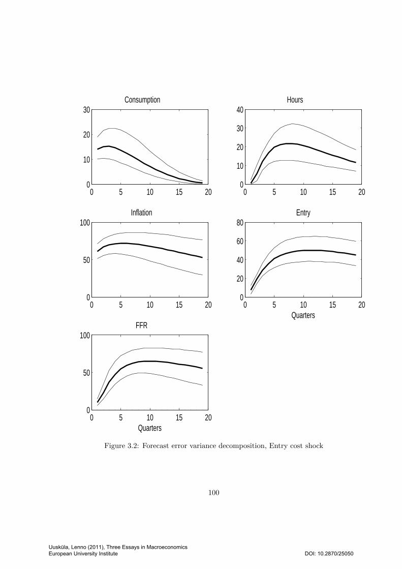
0 5 10 15 200

10

20

30Consumption

0 5 10 15 200

10

20

30

40Hours

0 5 10 15 200

50

100Inflation

0 5 10 15 200

20

40

60

80Entry

Quarters

0 5 10 15 200

50

100FFR

Quarters

Figure 3.2: Forecast error variance decomposition, Entry cost shock

100


DOI: 10.2870/25050

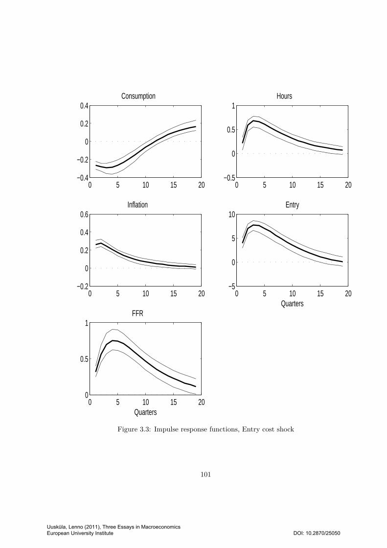
0 5 10 15 20−0.4

−0.2

0

0.2

0.4Consumption

0 5 10 15 20−0.5

0

0.5

1Hours

0 5 10 15 20−0.2

0

0.2

0.4

0.6Inflation

0 5 10 15 20−5

0

5

10Entry

Quarters

0 5 10 15 200

0.5

1FFR

Quarters

Figure 3.3: Impulse response functions, Entry cost shock

101


DOI: 10.2870/25050

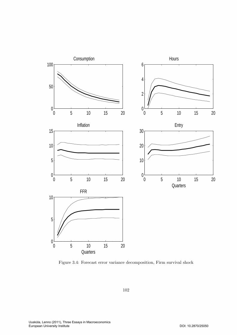
0 5 10 15 200

50

100Consumption

0 5 10 15 200

2

4

6Hours

0 5 10 15 200

5

10

15Inflation

0 5 10 15 200

10

20

30Entry

Quarters

0 5 10 15 200

5

10FFR

Quarters

Figure 3.4: Forecast error variance decomposition, Firm survival shock

102


DOI: 10.2870/25050

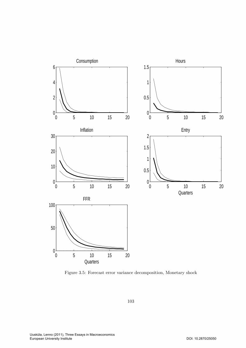
0 5 10 15 200

2

4

6Consumption

0 5 10 15 200

0.5

1

1.5Hours

0 5 10 15 200

10

20

30Inflation

0 5 10 15 200

0.5

1

1.5

2Entry

Quarters

0 5 10 15 200

50

100FFR

Quarters

Figure 3.5: Forecast error variance decomposition, Monetary shock

103


DOI: 10.2870/25050

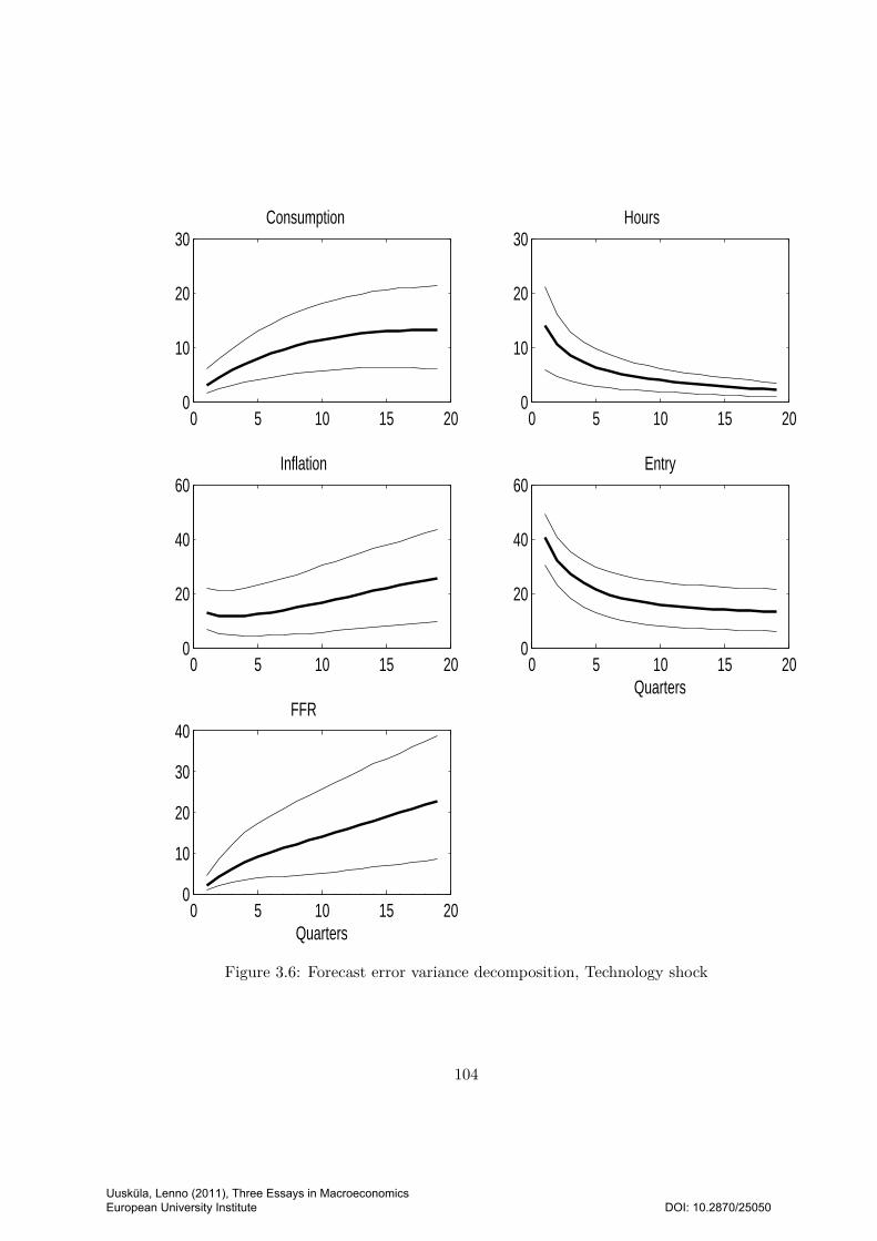
0 5 10 15 200

10

20

30Consumption

0 5 10 15 200

10

20

30Hours

0 5 10 15 200

20

40

60Inflation

0 5 10 15 200

20

40

60Entry

Quarters

0 5 10 15 200

10

20

30

40FFR

Quarters

Figure 3.6: Forecast error variance decomposition, Technology shock

104


DOI: 10.2870/25050

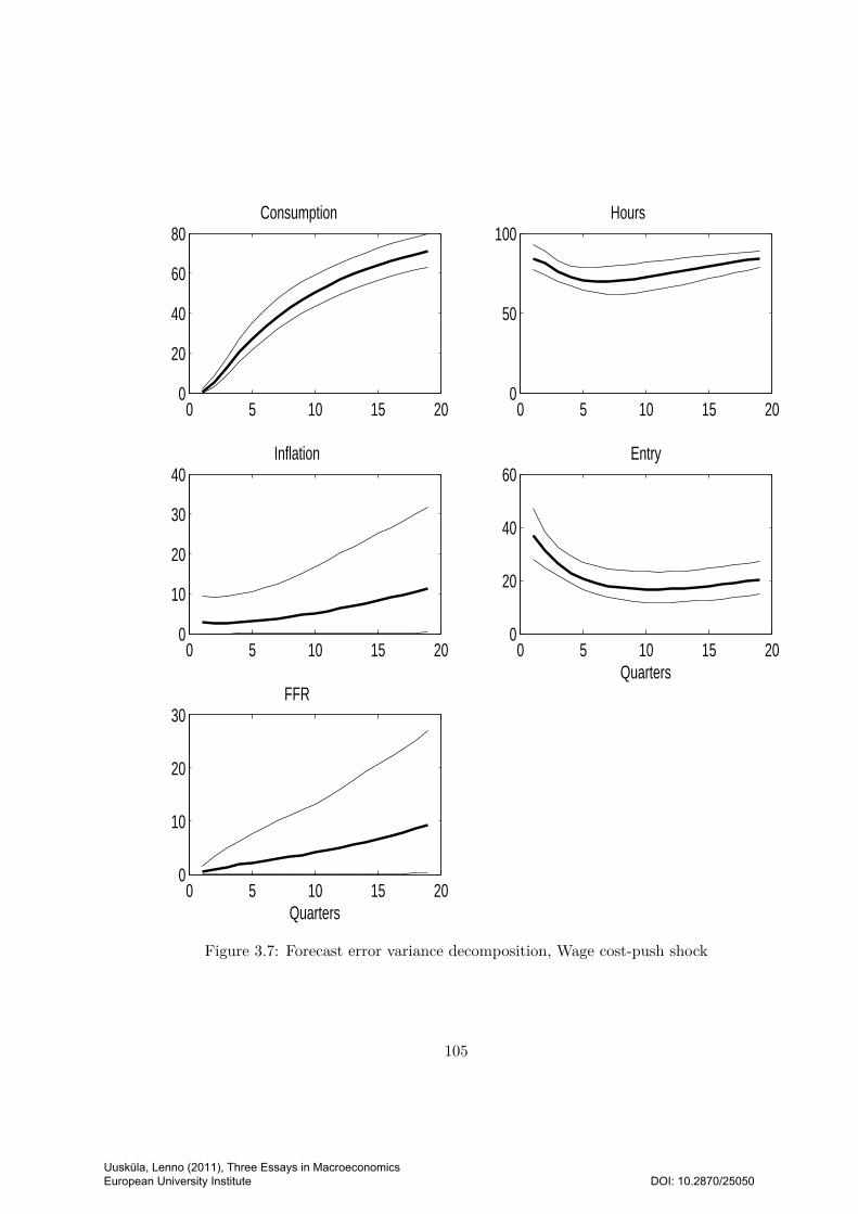
0 5 10 15 200

20

40

60

80Consumption

0 5 10 15 200

50

100Hours

0 5 10 15 200

10

20

30

40Inflation

0 5 10 15 200

20

40

60Entry

Quarters

0 5 10 15 200

10

20

30FFR

Quarters

Figure 3.7: Forecast error variance decomposition, Wage cost-push shock

105


DOI: 10.2870/25050

Three Essays in Macroeconomics

Documents