Essays in Macroeconomics and Finance by Congyan Tan A dissertation submitted in partial satisfaction of the requirements for the degree of Doctor of Philosophy in Economics in the Graduate Division of the University of California, Berkeley Committee in charge: Professor Yuriy Gorodnichenko, Co-Chair Professor Ulrike M. Malmendier, Co-Chair Professor Robert M. Anderson Professor Dmitry Livdan Fall 2011

Welcome message from author
This document is posted to help you gain knowledge. Please leave a comment to let me know what you think about it! Share it to your friends and learn new things together.
Transcript

Essays in Macroeconomics and Finance
by
Congyan Tan
A dissertation submitted in partial satisfaction of therequirements for the degree of
Doctor of Philosophy
in
Economics
in the
Graduate Division
of the
University of California, Berkeley
Committee in charge:
Professor Yuriy Gorodnichenko, Co-ChairProfessor Ulrike M. Malmendier, Co-Chair
Professor Robert M. AndersonProfessor Dmitry Livdan
Fall 2011

Essays in Macroeconomics and Finance
Copyright 2011by
Congyan Tan

1
Abstract
Essays in Macroeconomics and Finance
by
Congyan Tan
Doctor of Philosophy in Economics
University of California, Berkeley
Professor Yuriy Gorodnichenko, Co-ChairProfessor Ulrike M. Malmendier, Co-Chair
For the past two decades, economists have focused intensive effort on building Macroeco-nomics on a firm Microeconomic foundation. As Macroeconomic research are more integratedwith Microeconomics, more and better micro evidence has been examined to verify Macroe-conomic theories. One recent development in this line of research uses detailed firm-levelevidence to modify current Macroeconomic theories. In this dissertation extensive firm-levelevidence are studied to shed light on important macro issues such as investment dynamics,financial frictions, regulations and productivity growth. In this study firm behaviors arestudied and modeled by utilizing theories from a variety of fields in Corporate Finance, Pub-lic Finance, International Economics, Macroeconomic Dynamics etc. Implications of theseevidence on the economic theory are carefully examined and subsequent extension of existingmodels are proposed.
This dissertation consists of three chapters. All chapters study firm behaviors and theirimplications on macroeconomics, however, the focus of each is different. The first chap-ter studies issues of credit conditions, uncertainty and investment; the second chapter (co-authored with Zhiyong An) engages the issues of taxation and international corporate fi-nance; the third chapter show how regulations are likely impact foreign investment.
The first chapter explores the heterogeneity in firms’ response to high economic un-certainty. I show that the effect of high economic uncertainty on firms’ investment variessignificantly with the degree of financial constraints. Firm decisions are studied in a modelof non-convex adjustment costs and time-varying second moment shocks, with financialconstraints. In my model, uncertainty makes financially-constrained firms cautious in cap-ital spending and creates long periods of under-investment for these firms. Estimates fromfirm-level data show that publicly-traded companies’ investment-to-capital ratio falls by anaverage of around 15% in response to a one standard deviation increase in uncertainty. Firmswith easier access to credit are found to be much less responsive to uncertainty, consistentwith the model’s predictions. This implies that the effectiveness of stimulus policy maylargely depend on firms’ accessibility to credit in episodes of high uncertainty.
2
The second chapter (co-authored with Zhiyong An) studies how firms respond to a quasi-experiment in China. China’s new Corporate Income Tax Law was passed in March 2007and took effect on January 1, 2008. It increases the effective corporate income tax rate fromabout 15% to 25% for foreign investment enterprises (FIEs), while keeps that unchangedat 25% for domestic enterprises (DEs). This study uses a difference-in-differences approachto investigate FIEs’ response to the law. Employing the Chinese Industrial EnterprisesDatabase (2002-2008) to implement the analysis, we find evidence that FIEs are respondingto the law by shifting their income out of China. Second, the magnitude of the estimatedresponse is larger for enterprises larger in size, which suggests the greater capability of shiftingincome across countries for larger enterprises. In addition, the response is more acute forinvestment enterprises from Hong Kong, Macau, or Taiwan (HMT) than that for other FIEs,which is consistent with the tax haven status of Hong Kong and Macau.
The third chapter studies productivity spillovers to domestic firms from foreign directinvestment (FDI). Such productivity gain from FDI is considered to be the basis of policiesthat promote FDI in many countries. In this chapter, firm-level panel data from six Europeancountries are examined to test a number of hypotheses regarding the impact of FDI on theproductivity of domestic firms. I find evidence for the backward linkage channel of the FDIspillovers. Using a new dataset, Investing Across Borders 2010 that documents and scoresregulations for FDI in 87 countries, this study goes further to explore how FDI-specific poli-cies and institutions impact the spillovers from FDI inflows. Empirical evidence shows thatgood investment climate is associated with productivity gains, either by direct productivitycontribution or by productivity increase in upstream industries. Higher ownership limit isshown to be significantly and positively correlated with productivity. However, productivityimpact varies greatly across different investment climate measures.

i

ii
Contents
1 Time-Varying Uncertainty and Financially Constrained Investment 11.1 Introduction . . . . . . . . . . . . . . . . . . . . . . . . . . . . . . . . . . . . 11.2 Related Literature . . . . . . . . . . . . . . . . . . . . . . . . . . . . . . . . 51.3 Model . . . . . . . . . . . . . . . . . . . . . . . . . . . . . . . . . . . . . . . 71.4 Empirical Results . . . . . . . . . . . . . . . . . . . . . . . . . . . . . . . . . 131.5 Conclusion and Policy Implications . . . . . . . . . . . . . . . . . . . . . . . 22
2 Taxation and Income Shifting: Empirical Evidence from a Natural Exper-iment from China 542.1 Introduction . . . . . . . . . . . . . . . . . . . . . . . . . . . . . . . . . . . . 542.2 China’s New Corporate Income Tax Law . . . . . . . . . . . . . . . . . . . . 562.3 Identification Strategy . . . . . . . . . . . . . . . . . . . . . . . . . . . . . . 572.4 Econometric Models . . . . . . . . . . . . . . . . . . . . . . . . . . . . . . . 582.5 Data Description . . . . . . . . . . . . . . . . . . . . . . . . . . . . . . . . . 602.6 Empirical Results . . . . . . . . . . . . . . . . . . . . . . . . . . . . . . . . . 622.7 Conclusions . . . . . . . . . . . . . . . . . . . . . . . . . . . . . . . . . . . . 63
3 FDI Spillovers and the Investment Climate 733.1 Introduction . . . . . . . . . . . . . . . . . . . . . . . . . . . . . . . . . . . . 733.2 Literature Overview . . . . . . . . . . . . . . . . . . . . . . . . . . . . . . . 743.3 Data . . . . . . . . . . . . . . . . . . . . . . . . . . . . . . . . . . . . . . . . 783.4 Methodology . . . . . . . . . . . . . . . . . . . . . . . . . . . . . . . . . . . 803.5 Estimation . . . . . . . . . . . . . . . . . . . . . . . . . . . . . . . . . . . . . 843.6 Conclusion . . . . . . . . . . . . . . . . . . . . . . . . . . . . . . . . . . . . . 88

iii
Acknowledgments
I am very grateful to my advisors, Yuriy Gorodnichenko and Ulrike Malmendier, and com-mittee members Bob Anderson and Dmitry Livdan for their continuous guidance, supportand encouragement. I am also indebted to George Akerlof, Zhiyong An, Alan Auerbach,Nick Bloom, Steve Bond, Hui Chen, Long Chen, Luosha Du, Barry Eichengreen, NicolaeGarleanu, Pierre-Olivier Gourinchas, Kusi Hornberger, Martin Lettau, Maurice Obstfeld,Berardino Palazzo, Christine Parlour, Haonan Qu, Christina Romer, David Romer, MuratSeker, Adam Szeidl, Gewei Wang and Neng Wang for very useful comments and discus-sions. I would also like to thank seminar participants in Boston University, Cheung KongBusiness School, Shanghai Advanced Institute of Finance at Jiaotong University, PekingUniversity, The World Bank, Tsinghua University and University of California at Berkeley.My co-author Zhiyong An would like to thank Emmanuel Saez and Feila Zhang for helpfulcomments.

1
Chapter 1
Time-Varying Uncertainty andFinancially Constrained Investment1
1.1 IntroductionThis paper is a study of uncertainty, financial frictions and firm investment. In particular,
I show that a firm’s credit condition is important in determining the effect of uncertaintyon its investment. In the empirical section, I find that firms’ investment is much moresensitive to uncertainty if firms are financially constrained than if they are not. A modelthat features time-varying uncertainty, capital adjustment costs, financing costs and internalliquidity management is developed to provide an explanation for the empirical results. Dueto the asymmetrical nature of financing costs, firms wait longer periods and investmentlargely depressed when economic uncertainty is high. The empirical results from publicly-traded firms suggest more than a fifteen percentage drop in the investment-to-capital ratioin response to an increase in uncertainty. The point to emphasize is that the magnitude ofthe response of investment to uncertainty depends crucially on how financially constraineda firm is. This has important implications for the effectiveness of stimulus policy in episodesof high uncertainty.
There has been a huge surge in uncertainty during the current crisis. The increase inimplied stock market volatility is comparable in magnitude only to the Great Depressionin the 1930s (Bloom (2009)). The meltdown of the financial system made banks reluctantto lend and limited credit conditions for many firms. Since the fourth quarter of 2007,firms have cut their capital spending drastically and aggregate fixed private investment hasdropped 25%2 in the fourth quarter of 2009. Although both high economic uncertainty
1This chapter is my job market paper previously circulated under the title Time-Varying Uncertaintyand Financially Constrained Investment: Theory and Evidence
2Bureau of Economic Analysis (BEA)’s National Income and Product Account (NIPA) reports nom-inal fixed private investment for 2007Q4 and 2009Q4 of 2247.9 billion dollars and 1681.9 billion dollars,respectively.
CHAPTER 1. UNCERTAINTY & FINANCIALLY CONSTRAINED INVESTMENT 2
and worsening financing constraints significantly impact the economy, how these two factorsinteract and how they contribute to the reduction in economic activity is not straightforward.In particular, how does a sudden rise in economic uncertainty affect firm investment if thefirm faces difficult financing conditions? What if the firm has easy access to credit? Neitheracademics nor policy makers have a clear answer to these questions. Furthermore, theanswers are of great policy importance, in light of current discussions on how to stimulateeconomic recovery by increasing firms’ spending. Policy implications are derived from mystudy to contribute to this discussion.
This paper introduces a new model that incorporates a macroeconomic firm investmentproblem under time-varying uncertainty and a corporate finance model of investment underexternal financing constraints. The model is developed to study the mechanism how time-varying uncertainty and financial constraints interact with each other. It is built on themodel in Bloom (2009), which features a real-option investment model with time-varyinguncertainty. Using estimations from time-series data, he highlights the importance of time-varying uncertainty for the dynamics of economic activities. The study of investment underfinancial frictions is an area with decades of active research starting with the seminal papersby Modigliani and Miller (MM). Although time-varying uncertainty and financial constraintsare important determinants of firm investment, there is little if any research trying to mergethe two models. By incorporating these features simultaneously, I am able to show thatfinancial frictions amplify the effect of high uncertainty on investment. To the best of myknowledge, this paper is the first to study the interactions of time-varying uncertainty, creditconstraints and firm investment with firm-level data. The responsiveness of firm investmentsto uncertainty shocks depend on firms’ financial constraints. The extent of this dependenceis significantly larger than what has been implied by previous models.
My model features the time-varying uncertainty that has only recently been given moreattention in the literature. Measured by firm-level volatility3, there has been a drastic in-crease in the number of firms that experience abnormally high volatility since 2008. Thissupplements and confirms Bloom’s (2009) finding that high uncertainty is a salient featureof the current economic recession4. My model features a time-varying second moment pro-ductivity process and both convex and non-convex adjustment costs on capital. Models witha non-convex adjustment cost essentially generate a region of inaction in capital spending:firms only invest when business conditions are sufficiently good and only disinvest when theyare sufficiently bad. Upon the arrival of an uncertainty shock, firms expand the region ofwaiting–they scale back capital spending–and this behavior could lead to a sharp decline inaggregate investment.
However, Bloom’s (2009) model is one of the neoclassical models that satisfy the MM3The measure of the uncertainty shock is defined in Section 4.4Using the S&P 100 implied volatility, Bloom (2009) shows that there was a tremendous volatility shoot-
up in the recent credit crunch, the highest in the past 40 years. In terms of the effect of an uncertainty shock,Bloom (2009) argues that it has a large real impact and estimates it to be a substantial drop of around twopercent of GDP with a subsequent rebound over the following six months to one year.

CHAPTER 1. UNCERTAINTY & FINANCIALLY CONSTRAINED INVESTMENT 3
theory (no friction). As is well known, financial frictions play an important role in the deci-sion process of firm investment. The current crisis also features a shortage of credit for firms,so models that analyze the current event might be incomplete without financial constraints.There is a large literature that documents the difference in investment and financially con-strained and unconstrained firms. Theoretical work in corporate finance (Gomes (2001),Hennessy and Whited (2007)) show that costly external financing works as an adjustmentcost that makes firms cautious and cause them to choose to spend less on capital. Insteadof a model with debt contraction and equity issuance as in Hennessy and Whited (2007)and Livdan et al. (2009), my model incorporates financial frictions using the financing gap,which is defined as the difference between the funds needed and the internal funds available.In my model, financial constraints are essentially modeled as a cost function imposed on thefinancing gap. This cost function could be non-convex or convex. The non-convexity wouldmean that there is a fixed cost associated with raising external funds, whereas the linearityor convexity would make borrowing more costly as firms borrow more. Such models providea way to capture the cost of raising external finance without the complication of bond andequity finance (Whited (2006), Riddick and Whited (2009)), with cash holding as an addi-tional state. Essentially this model features two different types of adjustment costs: costsof capital adjustment and costs of external financing. I show that adding external financemakes firms more cautious, amplifying the real-options effect that further expands the in-action region of under-investment. However, the external financing cost is different fromthe investment adjustment cost, as it amplifies the real-option effect in an asymmetric way:it depresses investment but not disinvestment. Since the investment decisions depend onboth the capital-adjustment cost and external-financing cost, the magnitude of real-optionunder-investment will depend on the size of these costs. Comparative statistics from thismodel add insight to how these costs impact investment. Moreover, with a feature of cashholdings, this model offers a theoretical examination of optimal corporate cash holdings andrisk management under different levels of uncertainty; these are issues that have not beenwell understood so far (Froot et al. (1993), Bates et al. (2009) and Bolton et al. (2010b)).
This paper highlights the amplification mechanism of the time-varying uncertainty andfinancial frictions on firm investment. The following implications and predictions are de-rived from my model: firms that are more financially constrained experience a larger ex-pansion of the investment inaction region under uncertainty shocks. In contrast, financially-unconstrained firms tend to adjust investment more frequently and appear less responsiveto uncertainty shocks. Financially-constrained firms also face longer investment contractionthan unconstrained firms. Another implication is that financially constrained firms, morereluctant to pay the costs to raise external financing in the future, will hold more liquidassets in episodes of high uncertainty. These predictions are conducive to empirical research.It is much easier to use proxies for financial costs than for capital adjustment costs5. There is
5Cooper and Haltiwanger (2006) construct a structural investment model with capital adjustment costs.They estimate various cost parameters by matching model moments with moments from panel-level data.

CHAPTER 1. UNCERTAINTY & FINANCIALLY CONSTRAINED INVESTMENT 4
a commonly-used set of measures for financial constraints. The estimated coefficients acrossdifferent subsamples are evaluated to determine the impact of financial constraint on theuncertainty-investment relationship.
The predictions from the model are confirmed in the empirical results from the firm-level data. For each firm-year, I construct the measure of uncertainty as the standarddeviation of daily stock returns, a measure used by Leahy and Whited (1996) and Bloomet al. (2007). Empirical results show that the investment-to-capital ratio of publicly-tradedcompanies drops by an average of 15% in response to a one standard deviation increasein uncertainty. The drop in the growth rate of investment-to-capital ratio is around 50%.Common measures of financial constraints from the corporate finance literature are adopted(Fazzari et al. (1988), Whited (1992), Kaplan and Zingales (1997)): firm size, bond rating,dividend payout and Kaplan-Zingales index. I find that investment from firms with easieraccess to credit (larger firm size, existence of bond rating and higher dividend payout) ismuch less responsive to uncertainty. This result is consistent with my theory that firmswith a lower cost of external financing tend to show smaller real-option effects and are lessaffected by uncertainty shocks.
This paper contributes to the current debates about the effectiveness of the fiscal stimulus.The time-varying uncertainty and the real-option theory suggest that, in episodes of highuncertainty, the inaction zone expands by a significant amount so that it is less likely forfirms to reach the investment bound. By assuming that the stimulus works as a demand orproductivity shock to firms, such policies will be less effective than in normal times because itwill take a lot more to move firms out of the inaction zone when uncertainty is high. However,the policy implication of this study is that the effectiveness of the stimulus may depend onhow financially constrained firms are. If firms are financially constrained, then the real-optioneffect will be largely amplified. During the current crisis, the cost of external financing hasbeen prohibitively high, which makes the stimulus much less effective. In addition, becauseof the heterogeneity from financial constraints, policies could be customized differently forconstrained and unconstrained firms. The model also indicates that an improvement in creditconditions could help to catalyze firms’ response, especially in an episode of high uncertainty.This could be especially effective for financially constrained firms. To this end, this papercould validate the creation of the Term Asset-Backed Securities Loan Facility (TALF) inNovember 2008, which helps to provide credit to small businesses by supporting the issuanceof loans guaranteed by the Small Business Administration (SBA)6.
6Federal Reserve Governor Elizabeth A. Duke in her February 26, 2010 testimony stated:
“...the TALF program has helped finance 480,000 loans to small businesses ... and100,000 loans to larger businesses ... About half of the SBA securities issued inrecent months–corresponding to roughly $250 million in loans a month–were soldto investors that financed the acquisitions in part with TALF loans ... Thus, theTALF and other Federal Reserve programs provided critical liquidity support tothe economy until the financial system stabilized ... credit conditions for many

CHAPTER 1. UNCERTAINTY & FINANCIALLY CONSTRAINED INVESTMENT 5
By providing direct liquidity to financially constrained firms, the Federal Reserve Bankcould make those firms’ credit constraints less binding. My model suggests that such aninjection of liquidity could make credit constrained firms invest more and become moreresponsive to stimulus policies. Moreover, when uncertainty is high, financial friction mayamplify the real option effect to make firms invest even less. Therefore, in recessions withhigh uncertainty, it could be important to launch such a liquidity-provision policy along withany stimulus policy.
The rest of the paper is organized as follows. I summarize the related literature inSection 2. Section 3 presents a model, its solutions, and predictions. The empirical resultsare presented in Section 4. Section 5 provides policy implications and concludes.
1.2 Related LiteratureThis paper is related to two strands of literature: literature studying firm investment
dynamics under macroeconomic uncertainty and literature in corporate finance studyinginvestment under financial constraints.
The literature on firm production under uncertainty lays the foundation of this analysis,in particular the real options effect (Dixit and Pindyck (1994)). Because of the irreversibilityof the investment, an inaction zone is created so that firms invest only when productivity7
reaches an upper bound (sufficiently good), disinvest only when productivity reaches a lowerbound (sufficiently bad) and do nothing if productivity is in the middle. The theoreticalcomparative statistic of a rise in uncertainty would be associated with an expansion in firminvestment. In the models where the marginal revenue product of capital is convex, an in-crease in uncertainty has a positive effect on investment (Hartman (1972), Abel (1983)). Ca-ballero (1991) shows that the sign of the uncertainty-investment relationship largely dependson the degree of decreasing marginal return to capital. Hassler (1996) and Bloom (2009)study time-varying uncertainty in a real option framework. Bloom (2009) finds that thereal-option effect of aggregate investment is large either with or without the Abel-Hartmaneffect. I extend his firm production models to include firms’ financing behavior and externalfinancial constraints to study how financial frictions contribute to the real-option effects.
small businesses are likely to remain challenging this year (2010). That is whythe Federal Reserve has been placing particular emphasis on ensuring that itssupervision and examination policies do not inadvertently impede sound smallbusiness lending. If financial institutions retreat from sound lending opportu-nities because of concerns about criticism from their examiners, their long-terminterests and those of small businesses and the economy in general could be neg-atively affected, as businesses are unable to maintain or expand payrolls or tomake otherwise profitable and productive investments.”
7Productivity could reflect both technology and demand shocks.
CHAPTER 1. UNCERTAINTY & FINANCIALLY CONSTRAINED INVESTMENT 6
Uncertainty has long been a subject of interest, and its relationship with corporate in-vestment has been studied by many. Leahy and Whited (1996) is the first paper to exploreempirically the relationship of uncertainty and investment. Using a dynamic panel regressiontechnique, they find no evidence that uncertainty has an impact on investment. However,Bond and Cummins (2004) and Baum et al. (2008) find evidence that uncertainty affectsinvestment. This paper also studies the correlation between uncertainty and investment.My results generally support those of Bond and Cummins (2004) and Baum et al. (2008)and go further to show that the magnitude of impact is different across different subgroups.Bloom et al. (2007) and Bloom (2009) show, both theoretically and empirically, results onhow uncertainty reduces economic activities. I extend their work by showing both theoret-ically and empirically that financial frictions play an important role on firms’ investmentresponsiveness to uncertainty shocks.
Research in corporate finance has been studying how financial frictions affect firm behav-ior, primarily investment behavior under the Modigliani-Miller (1958) framework. Notableresearch includes Fazzari et al. (1988), Gilchrist and Himmelberg (1995), Kaplan and Zin-gales (1997), Gomes (2001), Malmendier and Tate (2005) and Hennessy and Whited (2007).This paper contributes to the corporate finance literature by showing how this investment-financial friction relationship is further complicated by the time-varying uncertainty. I alsoshow that this additional relationship is important for firm investment.
My model combines different features of the models in Bloom (2009) and Riddick andWhited (2009). Cash savings and external financing costs are constructed based on Riddickand Whited (2009) and a modified version of time-varying second moment process is fromBloom (2009). Such a model allows me to ask questions that are different from those twopapers. Bloom (2009) is among the first to analyze the effect of uncertainty shocks on realeconomic activities, such as investment. My model extends his analysis to include financialconstraints, because financial constraints provide interesting heterogeneity in the analysis offirm investment decisions.
Riddick and Whited (2009) study corporate saving in their paper. Although they haveuncertainty in their model, there is no dynamics in uncertainty–This makes their modeldifficult to match with the time-varying uncertainty which the current crisis features. Whited(2006) is another paper closely related to this paper. Whited finds in micro data that thepresence of financial constraints lowers a firm’s investment hazard. In other words, externalfinancing constraints tend to work as additional costs of adjustment and contribute to thereal-options effect of investment. Therefore, firms with easier access to credit appear tobear lower total costs8 of adjustment and respond more frequently to business conditions.Whited’s work presents both a model and evidence of how financial frictions add to the totaladjustment cost of investment for firms.
8Total costs include both capital adjustment cost and financing cost.

CHAPTER 1. UNCERTAINTY & FINANCIALLY CONSTRAINED INVESTMENT 7
1.3 ModelIn this section, I develop a discrete time and infinite horizon partial equilibrium model
of dynamic decisions in capital spending, saving, and external financing. My model is acombination of models with elements of uncertainty shocks (Bloom et al. (2007), Bloom(2009)) and models with financial constraints (Whited (2006), Riddick and Whited (2009)).First I describe my assumptions on productivity and financing. Then I solve it using dynamicprogramming and discuss the optimal policy functions.
TechnologyA risk-neutral infinite-horizon firm owns and uses capital Kt along with a variable factor
of production Lt to produce output. It faces technology, productivity and demand shocks,which is captured in At. In a manner similar to Cooper and Haltiwanger (2006), I assumethat it incurs no cost when adjusting the variable factor, so I can optimize out this variablefactor without the loss of generality. I assume concavity in the profit function π(At, Kt),either because of decreasing-return-to-scale in production, downward-sloping demand curve,or both. The profit function takes the form ofAtKθt , where θ determines the level of concavity.
π(At, Kt) = AtKθt (1.1)
The logarithm of productivity follows an AR(1) process, where At+1 denotes the state ofproductivity next period. To incorporate time-varying uncertainty in the model, I specifyan AR(1) process with a time-varying standard deviation:
log(At+1) = µ+ ρlog(At) + vt, vt ∼ N(0, σ2t ) (1.2)
For simplicity the stochastic volatility process follows a two point Markov Chain switchingbetween low uncertainty σL and high uncertainty σH
σt ∈ {σL, σH} , where Pr(σt+1 = σj|σt = σk) = pσk,j (1.3)
In every period, firms make investment decisions at the capital price of unity; the law ofmotion for capital stock is as follows:
Kt+1 = (1− δ)Kt + It (1.4)
Consistent with Cooper and Haltiwanger (2006) on the capital adjustment cost, the modelassumes both convex and non-convex capital adjustment costs. The assumption that the

CHAPTER 1. UNCERTAINTY & FINANCIALLY CONSTRAINED INVESTMENT 8
fixed cost is proportional to capital is to ensure that firms do not grow out of the fixed cost.
C(It, Kt) = 1{It ̸= 0}ψ0Kt +ψ1
2
(ItKt
)2Kt (1.5)
FinancingFollowing Riddick and Whited (2009), the firm can hold cash, Pt, via a riskless one-period
discount bond that earn interest r(1−τ). This cost τ could either reflect tax penalty on cashrelative to interest income (Graham (2000), Faulkender and Wang (2006), Whited (2006)) oragency costs associated with free cash (Jensen (1986), Eisfeldt and Rampini (2009), Boltonet al. (2010b)).
I define the financial gap as the difference between the cash spending (both capitalspending and saving for the future) and internal cash:
g(Kt, Kt+1, Pt, Pt+1, At, σt) = Pt+1
1 + (1− τ)r+Kt+1−(1−δ)Kt+C(It, Kt)−(1−τ)π(At, Kt)−Pt
(1.6)One can think of (1.6) as a dividend when gt < 0 and equity issuance when gt > 0. Firms
have to raise external funds to fill this gap. It is costly to obtain external financing, whenthe financing gap is greater than 0: gt > 0.
The adjustment cost of external financing ϕ(·) is a function of the financing gap gt. Iassume a fixed, linear and quadratic cost:
Φ(gt) =(λ0 + λ1gt +
12λ2g
2t
)1{gt > 0} (1.7)
When gt < 0, firms pay out cash and I assume that there is no cost for distribution. Sucha construction of financial constraint is similar to Whited (2006) and Riddick and Whited(2009). Because most financial constraints are various costs imposed on the financial gap,they argue that it does not affect the qualitative outcome of the model. In such a modelwith internal funds, I expect to see that firms accumulate cash reserves to avoid future cashstock-outs and costly external finance.
Define the net dividend as the dividend payout (−gt) minus the adjustment cost Φ (gt).
dt ≡ −gt − Φ (gt) (1.8)
Firm Maximization ProblemFirms maximize all future discounted net dividends subject to the driving process of
technology (1.2) along with uncertainty (1.3), the law of motion for capital stock (1.4), with

CHAPTER 1. UNCERTAINTY & FINANCIALLY CONSTRAINED INVESTMENT 9
equations for net dividend and profit (1.5), (1.6), (1.7), (1.8).
max{Ii,Pi+1}∞i=1
Et
∞∑j=0
dt+j
(1 + r)j
(1.9)
Dynamic ProgramBecause of the non-linearity of the problem, with the non-convexity in capital expendi-
ture and external financing, the firm problem needs to be solved numerically by dynamicprogramming. As a first step, I formulate the problem as a Bellman equation. There arefour state variables to keep track of: A,K, P and σ. The next period’s values are denotedas A′, K ′, P ′ and σ′. K and P are endogenous states, while the dynamics of A and σ aredetermined exogeneously. The firm chooses (K ′, P ′) each period to maximize the sum ofexpected future cash flows, discounted by r. So the value function is as follows; the motionsof A and σ are described the above.
V (K,P,A, σ) = max{V i(K,P,A, σ), V n(K,P,A, σ)
}(1.10)
where V i denotes the value with investment and V n is the value without investment.The net dividend term denotes a distribution of funds such as dividend payout (g < 0) or aninflux of funds such as equity issuance (g > 0). It is the dividend payout minus adjustmentcost.
d(K,K ′, P, P ′, A, σ) ≡ −g(K,K ′, P, P ′, A, σ)− Φ (g(K,K ′, P, P ′, A, σ)) (1.11)
Their Bellman equations are as follows:
V i(K,P,A, σ) = maxK′,P ′
{d(K,K ′, P, P ′, A, σ) + 1
1 + rEV (K ′, P ′, A′, σ′|A, σ)
}(1.12)
V n(K,P,A, σ) = maxP ′
{d(K, (1− δ)K,P, P ′, A, σ) + 1
1 + rEV ((1− δ)K,P ′, A′, σ′|A, σ)
}(1.13)
s.t
log(A′) = µ+ ρ log(A) + v, v ∼ N(0, σ2) (1.14)σ ∈ {σL, σH}, where Pr(σ′ = σj|σ = σk) = pσk,j (1.15)
This model satisfies the conditions ensuring a unique optimal policy function, (K ′, P ′) =policy(K,P,A, σ), if V iand V n are weakly concave in K and P (Theorem 9.6 and 9.8 inLucas and Stokey (1989)).

CHAPTER 1. UNCERTAINTY & FINANCIALLY CONSTRAINED INVESTMENT 10
SolutionI solve the problem numerically and investigate the relationship among optimal firm
investment, time-varying uncertainty and financial constraints under reasonable parameterchoices. I first describe each parameter for the baseline model and then explain the propertyof policy functions of firm investment. Simulations later using those policy functions showthe optimal responses of firm investment to an uncertainty shock, for financially-constrainedand unconstrained firms.
The model parametrization are based on previous literature and are listed in Table .1. θin the profit function is calibrated at 0.75, from the estimates of labor shares. Consistent withCooper and Haltiwanger’s (2006) estimates from plant-level data, I choose the persistence oftechnology process to be 0.885. The drift of the process, the low and high value of levels ofuncertainty and the transition probabilities between the low and the high uncertainty regimesare from Bloom’s (2009) estimations using aggregate series. The value of high uncertaintyis restricted to be twice the value of low uncertainty in the estimation. These parametersreflect key characteristics of the underlying driving process. Especially when the uncertaintyregimes switch from one to the other, the parameters play a critical for calculations ofconditional expectations of future profitability and variability that determine firms’ optimalinvestment response.
Cooper and Haltiwanger (2006) find evidence that both convex and fixed cost of capitaladjustment affect plant-level investment. The coefficients ψ0 and ψ1 are set equal to 0.039and 0.049 to be consistent with their estimates. The depreciation rate is 0.12, a commoncalibration in the literature. Hennessy and Whited (2007) constructed and estimated thefixed, linear and quadratic cost of financial adjustment. I set λ0, λ1 and λ2 to be 0.389, 0.053and 0.0002 based on their estimates of the costs of external equity finance for large firms.Hennessy and Whited (2007) show that 0.389 implies a fee of $50, 332 for the first milliondollars of gross equity. Discount rate and tax penalty rate are 4% and 5%, consistent withprevious literature.
I set finite set space for numerical solutions and value function iterations. 50 grid pointsare used for each variable in (K,K ′, P, P ′, A) for numerical solutions9. In order to makeV n stay on grid, I adopt the grid choices for capital from Riddick and Whited (2009):[(1− δ)jK̄, ..., (1− δ)K̄, K̄
]. For the productivity process, I use the technique in Tauchen
(1986), and Adda and Cooper (2003) to form a Markov-chain estimate of the AR(1) processwith time-varying uncertainty. This paper primarily uses the quadrature constructed byTauchen (1986) extended to include time-varying uncertainty. In Appendix A, a quadraturebased on Adda and Cooper (2003) with time-varying uncertainty is also constructed.
9Because there are 6 variables (4 states and 2 choices), I make uncertainty binary states. In this case, amatrix is created with 50× 50× 50× 50× 50× 2 entries for each iteration.

CHAPTER 1. UNCERTAINTY & FINANCIALLY CONSTRAINED INVESTMENT 11
Optimal Investment PoliciesGiven the solutions of the model, it is interesting to see how optimal investment changes
across a variety of specifications for financial constraints and different levels of uncertainty.As it is well known, the investment function should be a smooth function of productivityA without capital adjustment costs. With fixed capital adjustment costs, there will be aninaction zone–a range of A in which investment is equal to zero.
How does the investment-productivity relationship change with financing cost? First,the hypothetical case in which there is only a fixed cost of external financing and no liquid-ity buffer (zero cash holding) is studied. This case corresponds approximately to externalfinancing in the form of equity finance when there is a large flotation cost associated withit. From Figure .1, I observe different inaction zones for different cost specifications. Thesmooth line is the investment policy function with no adjustment cost. The first line withthe jump is the investment policy function associated with a fixed capital adjustment costequal to 5% of the value of its average capital stock. The three lines to the right of thatline are the cases where there is an additional 5%, 10% and 15% for external financing costs.One observes in this case that the inaction zone is wider with higher financing cost. Thus,financial frictions lead to less investment on average. One important feature of financialconstraint is that it extends the inaction area only to the region of investment to the right.The disinvestment region does not expand. Such an effect is different from the capital fixedcost: when the capital fixed cost increases, the band widens on both sides. This is becausethe capital adjustment cost often shows some degree of symmetry, in the sense that a costis incurred when firms are buying or selling capital10.
Such an effect on investment is most severe when there is a limited amount of cashreserves. Figure .2 shows that, with more corporate saving, investment is less constrained.Lines from right to left are from the least amount of cash (zero cash) at the beginning of theperiod to a high level of cash reserves.
The pattern changes when cash holdings are introduced. A sufficiently large liquiditybuffer, however, provides leeway in capital spending. With the fixed financing cost combined,firms will find it costless to spend up to their cash reserves, but any amount of investmentgreater than that will result in financing costs. Therefore, if the cash reserves are sufficientlylarge, there will be an additional range of productivity for which a flat investment policyfunction is observed in Figure .3; and this region might not coincide with the investmentinaction zone.
The analysis above indicates that fixed a financing cost further constrains investmentin two ways. First, it induces a wider inaction region on capital expansion, but a smallasymmetric effect on capital contraction. Second, it creates more inertia in capital spending,which further exacerbates underinvestment. Corporate saving alleviates this problem–withmore liquidity, the inaction and inertia regions shrink.
10Firms may face higher costs in contracting than in expanding capital stock, as in Abel and Eberly(1994, 1996).

CHAPTER 1. UNCERTAINTY & FINANCIALLY CONSTRAINED INVESTMENT 12
Figure .4 presents the financially constrained investment under the regime of low uncer-tainty (top graph) and high uncertainty (bottom graph). More capital spending is observedwhen uncertainty is mild; the inaction region is also smaller. The position of the lines withoutcapital adjustment cost does not start out differing much, suggesting that capital adjust-ment costs alone contribute little. However, when the financial cost is taken into account,the investment inertia is greatly amplified. The boundary of the investment inaction regionis pushed far along the horizontal axis due to the large financing cost.
This observed pattern is consistent with the real-option theory. Appendix B shows that,under a simple continuous-time specification, the expansion of the investment inaction regionin response to a rise in uncertainty is larger for a higher adjustment cost. Therefore, thefollowing graphs appear to illustrate a feature of real-option models: higher financing costslead to longer periods of wait-and-see for capital expansion. It is also interesting to observethat, since financing costs are absent for capital contraction, there is no change in the lowerbound of the investment inaction region.
Optimal Financing PoliciesWhy firms hold unproductive cash is puzzling. First, I use Riddick and Whited’s (2009)
explanation to underline the role of financing cost in determining corporate saving. Takingthe derivative of the Bellman equation (1.12) with respect to financing gap g and applyingthe envelope theorem leads to the following equation:
1 + (λ1 + λ2g)1{g > 0} = 1 + r(1− τ)1 + r
∫(1 + (λ1 + λ2g
′)1{g′ > 0}) dg′
If there is no financing cost, the cash holding discount τ ensures that corporate saving willbe zero. Moreover, as Riddick and Whited (2009) argued, corporate saving reflects too manyfactors for a thorough analysis. There is no robust pattern regarding corporate saving–itcould be hump-shaped or decreasing with respect to productivity. The pattern would dependon characteristics of the firm such as size. Interestingly, Riddick and Whited find that thereare two effects governing the behavior of corporate saving. One effect, which they call theincome effect, reflects the extra cash inflow associated with higher productivity. Anothereffect, the substitution effect, is defined as the substitution between cash saving and capitalspending. Figure .5 shows, that under high uncertainty, firms hold more liquidity for alllevels of productivity. Moreover, firms under high uncertainty appear to be more cautious,hoarding more cash and restraining themselves from capital spending.
Simulation and Predictions of the DynamicsTo study the impact of a sudden rise in uncertainty, I use the model solutions to simulation
an investment response for one representative firm. If only one firm makes a real option

CHAPTER 1. UNCERTAINTY & FINANCIALLY CONSTRAINED INVESTMENT 13
investment choice once every year, then there will be many investment with zero value.However, the lack of zeros in the firm-level data would reject any real-option theory. Tothis end, firm-level aggregations are used in previous literature. In this study I assume thateach firm has 300 production units. For each category, I run simulations for 300 units for 20years at an annual frequency, with a burn-in period of 180 periods to ensure that they are ina steady state. The responses of investment are plotted in Figure .6. After an uncertaintyshock (year 0), the financially constrained firms experience large investment drops, whileinvestment from the financially unconstrained firms quickly bounces back with a smallerinitial drop. This would predict a larger investment drop and longer under-investment forfinancially constrained firms.
The model with both time-varying uncertainty shocks and financial constraints providescomparative statistics of the investment-uncertainty relationship across firms with hetero-geneous external financing constraints. The rest of this paper explores firm-level data totest the model predictions. The main prediction is that investment from firms that facehigher costs when raising external funds (thus more credit constrained by definition) willfall more when uncertainty increases sharply. For firms that face smaller costs to obtainexternal financing, the magnitude of the response will be smaller. This result highlightsthe amplification effect of financial frictions for the investment response to an increase inuncertainty.
1.4 Empirical ResultsThis section studies the investment response to uncertainty for publicly-traded compa-
nies. By using different measures of financial constraints, robust results are observed acrossdifferent sample splits.
Data and Summary StatisticsThe sample contains US non-financial firms in the 2010 Compustat industrial files. The
firm-level data constitutes an unbalanced panel from 1971 to 2009. The Compustat data isaugmented with standard deviation of daily stock return data from The Center for Researchin Security Prices (CRSP) data.
I drop firm-year observations from my sample with missing or negative values for totalasset and firms that have observations for less than three consecutive years. I delete allfirms whose primary Standard Industrial Classification (SIC) code is between 4900 and4999, between 6000 and 6999, or greater than 9000, because this model of investment isinappropriate for regulated and financial firms. Observations for firms involved in significantmergers and acquisitions (greater than 15% of book asset value) during a year are alsoexcluded. The replacement value of capital stock is constructed using the perpetual inventorymethod described in Salinger and Summers (1983) (See Appendix C for details). Firm

CHAPTER 1. UNCERTAINTY & FINANCIALLY CONSTRAINED INVESTMENT 14
investment (capital expenditure), cash flow and cash holding by the replacement value ofcapital stock at the end of last fiscal year are normalized. All the variables are winsorized1% on both ends of the distribution. I construct an average measure of Tobin’s Q11 (Hayashi(1982)) by dividing the market value by the capital replacement value.
Firm-Level UncertaintyUncertainty comes in many forms. When firms make investment decisions, the future
productivity, price, wage, demand, regulations, exchange rates and taxes are all uncertain.An ideal measure of uncertainty would combine all those elements. The uncertainty I try tocapture attempts to reflect future expectations. Following Leahy and Whited (1996), Bondand Cummins (2004), and Bloom et al. (2007), I argue that the volatility of a firm’s securitiessummarizes the firm’s uncertainty. The advantage is that, since this is a stock market-basedmeasure, it reflects all information investors care about and it is forward-looking. Since theuncertainty I am measuring is related to information in the future, it is important to excludeex-post information. Implied-volatility is another natural measure of that, but limitations indata availability prevented me from constructing uncertainty based on that. Instead, I havesufficient dis-aggregate and high frequency data from CRSP stock price data. Under theassumption that a company’s stock price reflects information regarding all the uncertaintylisted above, I can construct a general measure of uncertainty. My measure of uncertaintydeviates from Leahy and Whited (1996) and Bond and Cummins (2004) because of theconcern about the normalization of the uncertainty by the market debt-to-equity ratio (SeeAppendix C for details). Nevertheless, a measure of uncertainty using normalization of thebook debt-to-equity is used for robustness checks.
The downside of this measure of uncertainty is that it is noisy. It may depart fromfundamental economic uncertainty due to a variety of observations in the market, such asbubbles, noise trading, etc. To address this concern, I take the difference between the dailyreturn and the S&P 500 market return to control for the aggregate market bubble, panic andnoise. I also construct measure of uncertainty based on monthly stock returns, which mightbe less affected by market irrationalities than high-frequency data. Bond and Cummins(2004) study three uncertainty measures: volatility from daily stock returns (the measureI use), disagreement among securities analysts on future profitability, and the variance offorecast errors. They show that all three measures are positively correlated; to some extent,they all capture the underlying movements in uncertainty. Their results indicate that thismeasure of uncertainty, despite its noise, reflects the economic uncertainty I deem important.
11It is important to include a measure of Tobin’s Q, which captures all future profitability for a firm.

CHAPTER 1. UNCERTAINTY & FINANCIALLY CONSTRAINED INVESTMENT 15
SpecificationI begin my analysis by estimating the standard model12 to identify the impact of uncer-
tainty on investment.(I
K
)it
= γσit + α(I
K
)it−1
+ βXit + ζi + ηt + ϵi,t
The above model determines investment rate(IK
)it
as a function of its lag(IK
)it−1
, thelevel of its uncertainty σit, and control variables Xit. Year dummies ηt are included. Tocontrol for time-specific effects. The model also fixes for firm-specific effect ζi. Three esti-mation strategies are used: OLS, fixed effect, and dynamic panel regression (Holtz-Eakin etal. (1988), Arellano and Bond (1991), Bond (2002)). Dynamic panel regressions are usedto partly address the endogeneity concern–it allows the regressors to be endogenous. Inaddition, this estimation first-differences all the variables for GMM estimation; this removesunobserved firm-specific effects, which could be correlated with regressors and generate bi-ased results. Following Arellano and Bond (1991) and Bond and Cummins (2004), I treatuncertainty as an endogenous variable and choose the second and third lags for uncertainty,investment, cash holding, cash flow, their interactions with uncertainty, and year dummies asinstruments. I use heteroskedasticity-consistent standard errors and test statistics. I reportthe Hansen overidentification test and Arellano and Bond’s (1991) test for first order serialcorrelations. I find it useful to compare the estimates from dynamic panel estimations tothe results from OLS and fixed effect regressions. As control variables, I use the cash flowand its lags, because the corporate finance literature shows that cash flow has a strong rela-tionship with corporate investment (Fazzari et al. (1988), Blanchard et al. (1994), Lamont(1997)). I also include cash flow’s interaction with uncertainty. Here I do not include averageQ as a control variable because of problematic measurement issues as a measure of futureinvestment opportunities. I include it later for some robustness checks.
Baseline RegressionsSummary statistics are in Table .2. The firms’ average investment rate is 0.25 and median
is 0.18. The distribution of investment rate is quite right-skewed. The model’s prediction isthat a rise in uncertainty leads to a fall in investment. In this case, the magnitude of the fallshould be compared with the investment distribution to determine its significance. Similarly,asset, capital stock and cash holding all have distributions that are right-skewed. Table .3(left panel) shows the results of the regressions of investment-to-capital ratio ( It
Kt−1, also called
investment rate) on uncertainty (σt). The coefficients are significantly negative for OLS,fixed effect and dynamic panel regressions, and their magnitudes are similar. However, since
12The variables I choose are from Lamont (1997). These are the variables typically used for regressionanalysis on COMPUSTAT panel data.

CHAPTER 1. UNCERTAINTY & FINANCIALLY CONSTRAINED INVESTMENT 16
Hansen’s overidentification test indicates that my instruments are rejected, the estimatesunder GMM in the dynamic panel regressions should be used with caution. Nonetheless,my estimates are consistent with the theoretical predictions that high uncertainty lowersinvestment. The estimates indicate that a one standard deviation increase in volatility(uncertainty) leads to a drop of 0.04~0.05 in investment-to-capital ratio (a fall of 15%~20%in terms of its mean investment-to-capital ratio 0.25). The interaction term for cash flowand uncertainty has a significant negative relationship with the investment rate: Higheruncertainty makes firms less responsive to cash flow. The drop in investment-to-capital ratiois 0.049 in absolute terms. To measure the decrease in relative terms, I construct the growthrate of investment rate, dropping all investment that is negative at the beginning of theperiod (11% of all observations) and winsorize it at 1% and 99% to avoid outliers13. Thesame regressions are estimated on the growth rate of the investment rate. I find that a onestandard deviation (0.038) increase in uncertainty leads to a 0.13 drop in OLS, a 0.16 dropin fixed effect regressions, and a 0.16 drop in dynamic panel regressions for relative terms.
Regressions for Financially Constrained FirmsI use four criteria to obtain reasonable measures of financial frictions at the firm-level.
The firm’s asset, bond rating, dividend payout and Kaplan-Zingales index, albeit their imper-fections, are widely adopted as proxies for financial constraints. I follow previous literatureto use sample splitting based upon each measure to study the behavior of firms with differentaccess to financial constraints. Following Bond et al. (2004) and Chen et al. (2010), eachfirm is marked in one subsample in all its sample years.
It is difficult for small firms to obtain external funds, big firms normally have easieraccess to various forms of financing, relationship banking, bond market, etc. I partitionfirms that differ in their asset size as proxies for a spectrum of credit conditions. Themedian asset is calculated for a firm in all its sample years and used to split my sample into10 subsamples. Table .4 shows the summary statistics of those subsamples. The investmentrates across different groups are quite similar. They are only slightly smaller for larger firms.The standard deviation of the investment rate, however, is higher for smaller firms. Foruncertainty, there seems to be an decreasing pattern: smaller firms seem to subject to largeruncertainty. It is consistent with my understanding that smaller firms have more volatilegrowth prospects than larger firms. Cash flow is on average monotonically larger for biggerfirms and its standard deviation higher for smaller firms. In addition, the asset holding isvery right skewed.
From the OLS regressions (Table .5), for subgroups from the first eight deciles, the rela-tionship between investment rate and uncertainty shows a negative sign and is statisticallysignificant from zero. In contrast, the largest firms in the top quintile (top two deciles) of
13When investment is negative, the investment growth measure of a negative investment at time t-1 andpositive increment from time t-1 to time t yields the same sign as in the case where the investment at timet-1 is positive and the increment is negative.

CHAPTER 1. UNCERTAINTY & FINANCIALLY CONSTRAINED INVESTMENT 17
the sample do not respond significantly to uncertainty shocks. Larger firms tend to havea weaker response to uncertainty shocks, although the pattern is not monotonic. The Rsquared is smaller for smaller firms (less than ten percent for the first three deciles), andgrows close to 40 percent for the largest decile. The interaction term of cash flow and uncer-tainty does not have a significant impact on investment rate. I also use the fixed effect modelto purge the time-invariant effect for each firm. The results are quite similar to those fromOLS. Larger firms appear to have a weaker relationship with the level of uncertainty, but theeffect is not monotonic. The R squared is very similar to OLS estimates. The results fromdynamic panel regressions are similar to those in fixed effect regressions. However, there isno significant uncertainty-investment relationship for the smallest size decile. The coefficientfrom this specification is larger than the other regressions. However, the Hansen J-test showsthat the result is only instrument-proof for the top two quintiles. These finding are largelyconsistent with the prediction that investment from firms that are credit constrained tendsto fall more due to uncertainty, while unconstrained firms are less responsive.
Borrowers use bond ratings to assess a firm’s credit quality. According to Whited (1992),firms that use the corporate bond market are subject to more investor scrutiny, so theyare more transparent and suffer less information asymmetries. By the same argument, firmswithout a bond rating typically find it hard to raise funds on the debt market, therefore theytend to have a more binding financial constraint. Table .6 shows us the summary statistics:first, there are many more firms without bond ratings than firms with bond ratings–the ratiois 12 to 1, meaning only one firm out of thirteen has a bond rating. Firms with bond ratingsare more than ten times larger in assets. The investment rate is slightly larger for firmswithout bond ratings and the standard deviation for unrated firms is twice the number forrated firms. Uncertainty on firms without a rating is twice as large as the firms with bondratings, both in terms of mean and standard deviation. Average cash flow is much smaller(negative) for unrated firms; the difference in mean is almost 100%. The standard deviationof cash flow on firms without rating is four folds the firms with bond ratings.
From the regression results of Table .7, coefficients on uncertainty are insignificant forfirms without bond ratings. The coefficients for uncertainty of the bond rated firms, however,are negative and significant. The results are robust across OLS, fixed effect estimations anddynamic panel estimations. R squared of firms with bond ratings is 25 percent higher ormore than firms without bond ratings. The magnitude of the drop in investment rate withrespect to uncertainty is quite similar to the credit constrained firms defined in terms ofsize: a one standard deviation increase in uncertainty would result in over ten percent lowerinvestment rate. Given the assumption that bond ratings are a valid measure of financialconstraints, the results here is also consistent with my predictions.
Dividend payout has been an important measure used in corporate finance to identifyfinancial constraints. Fazzari et al. (1988) argues that the retention practice provides a usefulmeasure, because the cost disadvantage of external finance has a larger effect on firms thatretain most of their earnings than on firms that distribute most of their earnings. Otherwork in corporate finance also shows that firms that are more constrained financially tend

CHAPTER 1. UNCERTAINTY & FINANCIALLY CONSTRAINED INVESTMENT 18
to pay out less dividends (Bolton et al. (2010b), Faulkender and Wang (2006))14. I make theassumption that the dividend payout ratio reveals the level of firms’ financial condition anduse Fazzari, Hubbard and Petersen’s methodology to proxy for financial constraints. Thesample is split into four subsamples using the amount of dividend distribution. Table .8 isthe summary statistics across these subgroups. Firms in the first subgroup pay virtuallyno dividend and firms in the second subgroup pay very little. The investment rate is notvery different, but the standard deviation across subgroups is large. Uncertainty is higherfor firms that pay less dividends, but the standard deviation is similar. Firms that pay lessdividends have a more negative cash flows and larger standard deviations than firms thatpay more dividends.
From Table .9, regression outputs show that the top quartile dividend distributors donot respond to uncertainty significantly in either OLS, fixed effect or dynamic panel specifi-cations. Under OLS and fixed effect estimations, uncertainty coefficients on investment ratefor subgroups in the first three quartiles are negative and very significant. The R squaredare lower for firms that pay no dividends and it is over twenty percent for firms in the topquartile. However, there is no significance on uncertainty for non-dividend-payers. Again, itis hard to be convinced because the Hansen test suggests the instruments are not valid. Allthe above results provide additional evidence that more financially constrained firms respondmore negatively to an uncertainty shock.
The Kaplan-Zingales Index (Kaplan and Zingales (1997), Kaplan and Zingales (2000))is another measure of financial friction, constructed based on a variables related to creditconditions. From a survey response of financial conditions, they estimate a relationship of agiven set of variables to firms’ financial state. This provides a score of financial constraintfor every firm based upon various variables of interest as follows:
−1.001909 CFitAit−1
+ 3.139193LEVit − 39.3678DIVitAit−1
− 1.314759 CitAti−1
+ 0.2826389Qit
where CFitAit−1
is cash flow over lagged assets; DIVitAit−1
is cash dividends over assets; CitAti−1
is cashbalances over assets; LEVit is leverage; and Qit is the market value of equity (price timesshares outstanding from CRSP) plus assets minus the book value of equity all over assets.Following Baker et al. (2003), I winsorize every variable at 1% and 99%. The Kaplan-Zingalesindex has been used extensively as a measure of financial constraints (Lamont et al. (2001),Hennessy et al. (2007), Baker et al. (2003), for example)15.
Summary statistics are in Table .10. There appears to be an upper trend across decilesfor investment. The less financially constrained from the left, measured by KZ index, have
14However, I am well aware of the debate on whether the dividend payout ratio provides a good measureof financial constraint (Kaplan and Zingales (1997), Fazzari et al. (2000), Kaplan and Zingales (2000)). Thispaper does not provide additional insight on whether it is a good measure of financial constraints.
15However, Almeida et al. (2004), Whited and Wu (2006) and Hadlock and Pierce (2010) question thevalidity of Kaplan-Zingales index as a measure of financial constraints.

CHAPTER 1. UNCERTAINTY & FINANCIALLY CONSTRAINED INVESTMENT 19
a lower average investment rate and lower volatility of investment rate. The mean andstandard deviation are quite close. Cash flow is lower for financially constrained firms in theupper deciles and its corresponding standard deviations higher. Financially unconstrainedfirms are larger in terms of size, especially for the bottom decile (0-10%).
From Table .11, I observe that there is only one coefficient on uncertainty that is notsignificant–that is the one for the most financially unconstrained firms measured by KZ indexin the first decile. Coefficients on the second and third deciles have significance at 5% whilethe rest are significant at 1%. Although the result is not very impressive, it is suggestive ofmy story that the investment rate from unconstrained firms, compared to the investment ratefrom constrained counterparts, are less responsive to an uncertainty shock. Table .11 alsopresents a result that is in general consistent, although the coefficient on the second decileis quite significant and its magnitude surpasses that of the third decile. From the dynamicpanel regressions, the top forty percent of the firms’ investment behaviors are significantlyaffected by uncertainty. The magnitudes of an investment adjustment are different acrossfirms.
However, Leahy and Whited (1996) find insignificant investment response in a regressionof investment rates. From my results, regression coefficients of unconstrained firms tend tobe insignificant and those of constrained firms are significant and negative. Therefore, basedon this reasoning, the overall regression might show a significant or insignificant coefficientdepending on what kind of firms dominate.
RobustnessBecause this paper studies the second-moment effect, it is important to control for the
first-order effect, which relates to the mean profitability. Because I measure the second-moment shock using the stock return volatility, I try both the mean annual stock return tocontrol for the first-order effect. Average Q, as a measure of Tobin’s Q, is also included toaccount for the mean future profitability. Leahy and Whited (1996) find that the impact ofuncertainty disappears after they control for the average Q and thus argue that uncertaintyaffects investment only through Q. However, here Q does not affect the main results.
Firm size is an important determinant of financial frictions. However, it may also affectother factors, such as productivity and industry-level effects. I include capital stock in everyregression and its coefficient appears to be significant in most regressions. The main findingsremain robust. In the regression in my web appendix, I include average Q, stock returns,capital stock and their interaction with uncertainty as additional control variables. Similarresults are reported
This section also checks the robustness for various measures of uncertainty. In addition tothe baseline measure (volatility of daily stock returns), I construct four other measures: highuncertainty, normalized uncertainty, monthly uncertainty and residual uncertainty. High un-certainty is a zero-one measure that returns one if the firm’s measured uncertainty surpassthat the firm’s sample mean by at least one standard deviation. The normalized uncertainty

CHAPTER 1. UNCERTAINTY & FINANCIALLY CONSTRAINED INVESTMENT 20
normalizes the stock-based uncertainty by the square-root of the debt-to-equity ratio. Pre-vious papers use this calculation to control for the fact that the more highly-leveraged firmshave larger risks. Monthly uncertainty based on the monthly stock returns is a less noisyalternative measure. I also use the difference between daily individual stock returns andthe market returns to substitute for the daily stock returns, and compute its volatility forthe residual uncertainty measure. Such constructions reduce the effect of aggregate shockson the uncertainty measure. Regression analysis using all those measures yield qualitativelysimilar results (see web appendix for details).
The dependent variable is the investment-to-capital ratio. I construct the the replacementvalue of capital using the perpetual inventory method in Salinger and Summers (1983).However, the results will be affected if the constructed measure of capital deviates from itstrue value. To this end, I use the reported book value of the company’s gross property, plantand equipment as an alternative measure of the capital stock. Its mean is larger than thereplacement value of capital hence the investment-to-capital ratios are smaller on average.Estimations show qualitatively similar results with smaller magnitudes.
High UncertaintyThe regression analysis provides results of contemporaneous relationship between uncer-
tainty and investment. A related question is how investment changes over time after a risein the level of uncertainty? To answer this question, I explore graphically the relationshipbetween firms’ uncertainty and investment dynamics. I first need to construct a shock ofuncertainty at firm-level to reconcile my results with Bloom’s (2009) estimated investmentdynamics after an uncertainty shock. To this end, I define a firm in a high uncertaintystate in a given year as a firm with measured uncertainty at least one standard deviationhigher than its mean uncertainty over all the company’s sample years. To visualize highuncertainty over time, for each year, I compute the fraction of firms that are in the state ofhigh uncertainty. (See Figure .7).
Interestingly, under this measure of high uncertainty, the current credit crunch from 2008brings the highest aggregate uncertainty in the past 40 years: Over 60 percent of the firmsare in a high uncertainty state in years 2008 and 2009. The second largest uncertaintyshoot-up is around the year 1999-2001, in which the LTCM bankruptcy, tech-bubble burstand September 11 attacks happened in three consecutive years. High uncertainty is alsoobserved in the OPEC oil crisis (1974), Black Monday (1987) and the first Gulf War (1991).This plot is loosely comparable to Figure 1 in Bloom (2009), which shows the monthlyimplied volatility for aggregate stock market returns. Given those uncertainty shocks, Iam particularly interested in firms’ investment and financing behaviors in episodes of highuncertainty. I try to summarize firms’ behavior under uncertainty shocks and give policyguidance, especially in the midst of the current credit crunch–a period with the highestuncertainty in the past 40 years. This result concurs with Bloom’s (2009) finding usingimplied market volatility over time.

CHAPTER 1. UNCERTAINTY & FINANCIALLY CONSTRAINED INVESTMENT 21
The Dynamic Response to UncertaintyPrevious section studies a cross-sectional response while in this section, I use my definition
of high uncertainty to see the dynamics of firms’ behavior after an increase in uncertainty.I could follow Leary and Roberts (2005) to split my sample into two portfolios–firms withhigh uncertainty during the year and those without – and track the mean investment foruncertainty firms and other firms. However, serial correlation of high uncertainty and itsfirst lag is 0.15, and the rest of lags are negative and close to zero. This imposes a seriousproblem with this methodology, making the pre- and post-uncertainty-shock investment fallas well. Therefore, I construct a simple model to account for serial correlation in uncertainty.The choice in this paper is a reduced-form specification of an autoregressive distributed lag(ADL) model with an AR(1) structure on uncertainty:
(I
K
)it
= α(I
K
)it−1
+ βXit +k∑j=0
γjσit−j + uit
σit = ϕσit−1 + ϵit
Similar to the models in previous regression analyses,(IK
)it
is the investment rate, Xit is thevector of control variables, and σit is the uncertainty measure. Three lags in the uncertaintylag specification are chosen to show the time dynamics and ensure that few data pointsare dropped due to length and consistency of the data. For simplicity, I assume the errorterms from the two equations, uit and ϵit are uncorrelated. An impulse response and itscorresponding 95% confidence band are constructed based on the panel coefficient estimates(See Appendix D for details).
Figure .8 shows the uncertainty impulse response for all firms. The horizontal axis indi-cates the year before and after high uncertainty with zero the year of impact. I see a 3%~4%contemporaneous sharp decline in investment rate when high uncertainty arrives. And aftertwo years it reverts back to its original level and overshoots after. And the changes at theyear of impact and the year after are significant in terms of the confidence band. This isconsistent with Bloom’s (2009) finding for aggregate time series.
As a first pass to study the impact of financial frictions, I decompose my sample to fivesubgroups based on size (capital). In the corporate finance literature, size is found to bean important determinant of financial frictions. For example, Fazzari et al. (1988) foundevidence that liquidity constraints tend to be systematically more binding for smaller firms.In a seminar paper on financial frictions, Petersen and Rajan (1994) observe that smalland young firms are most likely to face more information asymmetry in lending relationshipand therefore more likely to be credit rationed. Bernanke et al. (1999) explicitly use firmsize (capital) as a collateral for external financing and suggest that bigger firms are ableto obtain more financing. Firm size, albeit an imperfect measure, is commonly used for

CHAPTER 1. UNCERTAINTY & FINANCIALLY CONSTRAINED INVESTMENT 22
empirical studies of corporate financing constraints16. My results for different size quintilesin Figure .9 show that, for the firms in the top quintile (top 20% percentile), the drop oftheir investment in response to high uncertainty is merely 0.01; the drop is not statisticallysignificant and it moves back quickly after one year. The firms in the bottom quintile(bottom 20 percentile), however, have experienced a large and statistically significant fall ininvestment rate (close to 0.05) and revert back slowly to the original level after three years.
Whited (1992) splits the sample into firms with bond rating and firms without bondratings to study liquidity constraints and firm investment. She argues that firms with bondratings tend to have less information asymmetry, so it would be easier for them to obtaindebt financing; in this sense, they are less financially constrained. Following her criteria, Idivide my sample based on whether a firm has a bond rating or not. From Figure .10, thereare more striking results: firms’ investment with bond rating shows virtually no evidence ofdecrease and the coefficients are insignificant from zero after impact. There is a significantdrop in investment from firms with no bond rating.
In an influential paper, Fazzari et al. (1988) categorize firms according to dividend payoutsto study financing constraints and corporate investment. I do the same exercises in terms ofthe amount of dividend paid in Figure .11. For firms that pay a lot of dividends, the declinein investment rate is minimal and quickly reverts back. The fall in these two categories areinsignificant from zero. Firms that do not pay dividends (<25%) or pay very little (25%-50%)experience very large drop.
All the results above are consistent with the predictions that investment behavior byfinancially-constrained firms is very different from that of financially unconstrained firms.Imposing a simple structure on the dynamics of investment and uncertainty allows me tosee the dynamics of how investment behaves in response to an uncertainty shock and howresponses are different across firms with heterogeneous financial constraints. It is importantto notice this effect because it allows for further empirical investigations. The downside ofsuch a simple specification is that it might be too restrictive for my analysis. In the nextsection, I use more regressions and more proxies of financial frictions to test my predictions.
1.5 Conclusion and Policy ImplicationsIn the crisis starting in the fourth quarter of 2007, there has been a dramatic increase
in uncertainty, in magnitudes similar to the Great Depression. In such a period of highuncertainty, the usual policy instruments might not be as effective as in normal times. Inparticular, Bloom (2009) argues that high uncertainty induces more wait-and-see in invest-ment and hiring for firms, so that stimulus policies in high-uncertainty episodes may be lesseffective. From my study, I look more closely into the uncertainty-investment relationship
16An incomplete list is Devereux and Schiantarelli (1990) for UK firms, Athey and Laumas (1994) forindian firms, Gilchrist and Himmelberg (1995) for US data, Kadapakkam et al. (1998) for firms from sixOECD countries, etc.

CHAPTER 1. UNCERTAINTY & FINANCIALLY CONSTRAINED INVESTMENT 23
in historical firm-level data. The results are partially consistent with Bloom’s (2009) ar-gument. Interestingly, I find that the uncertainty-investment relationship is heterogeneousamong firms with different levels of access to the credit market. For firms that have easieraccess to the credit market, the uncertainty-investment relationship is much lower.
There are two important policy implications of my findings. First, a stimulus policyaffects firms differently. Firms without good financing opportunities are more affected inhigh-uncertainty episodes and, hence, less responsive to stimulus17. Thus, policies could becustomized for firms with and without good credit conditions. To induce a quick responsesfrom firms with high costs of accessing the credit market, policy makers would need to grantmore access to liquidity.
The second implication is related to heterogeneity across time. Firms face different creditconditions over time. Borrowing in 2008 is very difficult, while just two years earlier, firmsenjoyed very good credit conditions. The credit crunch amplifies the impact of uncertaintyon firm investment and hiring. Firms are even less willing to respond to the stimulus. Eitherimproving firms’ credit condition or lowering the level of uncertainty could help induce thefirm to spend on capital or hiring.
In conclusion, this paper studies the relationship among uncertainty, financial constraints,and investment. Investment from firms with different financial frictions responds significantlydifferently to uncertainty. This finding is consistent with a model that incorporates non-convex adjustment costs, time-varying uncertainty and financial frictions.
Theoretically, this paper is among the first models to study the interaction between allthree variables. It contributes to macroeconomic production models by incorporating thefirms’ external financing and saving along with time-varying uncertainty. My contributionto the corporate finance literature is modeling the second-order volatility effect in a modelwith investment and financing decisions. On the empirical side, this is the first paper tostudy the uncertainty-investment relationship across different firm groups, to the best ofmy knowledge. This paper contributes to a long literature studying the relationship of firminvestment and financing conditions (Fazzari et al. (1988), Kaplan and Zingales (1997) etc).I find a new systematic way in which financing conditions affect firm investment. Thisempirical finding also adds to the list of studies on the uncertainty-investment relationship(Leahy and Whited (1996), Baum et al. (2008), Bloom (2009)) .
Important policy implications can be derived from this paper. My model suggests thatan effective stimulus policy for firms would take into account the differences in firms’ creditconditions. Smaller and more credit constrained firms will be less responsive to policy in anepisode of high uncertainty. Therefore, policies targeted to effectively stimulate those firmsmust also address their liquidity concerns.
17The stimulus plan could be either a demand side stimulus, such as a plan stimulating consumer spending,or a firm stimulus, such as tax benefits.

CHAPTER 1. UNCERTAINTY & FINANCIALLY CONSTRAINED INVESTMENT 24
APPENDIX
Numerical Solution
AlgorithmI use value function iteration (Judd (1998), Adda and Cooper (2003)) on the state vari-
ables (K,P,A, σ) to achieve convergence by the following algorithm:Set grid points for each of the four states (K,P,A, σ). In this study I use 50×50×50×2 =
250, 000 points for most of my results. Finer grids up to 100 × 100 × 100 × 2 = 2, 000, 000points are also tried for some specifications. The results are similar throughout. Grids of Aand σ are defined from a quadrature I constructed in the next section. I also use a variantof quadrature from Tauchen (1986) that takes into account the changing volatility and usesa set of grids that cluster more around the inaction region, an effort to capture the changein the inaction zone more accurately. The quality of quadrature is important because thetime-varying uncertainty strongly influences expectations. To ensure that K stays on thegrid all the time, and especially in the case for inaction where investment is null and the nextperiod’s K becomes (1− δ)K, I specify grids for K as
[(1− δ)jK̄, ..., (1− δ)K̄, K̄
]. Because
I define everything on the grids and their movement is restricted to the specified grids, Ido not do interpolation. This is an advantage and produces more robust results. For theproductivity shock, because the logarithm of A has an AR(1) structure, I have to account forthe Jensen correction term when taking the exponential of it. I subtract σ2/2 from the driftterm of the AR(1) process.18 I define value function on the grid and iterate value functionusing the Bellman equation. I start with an initial value for the value function that has thesame value for every state. It takes on average 3 hours to solve the dynamic programmingprogram, although the running time varies with parameters.
Construction of QuadratureIn standard models with firm investment, firms make investment choices based upon their
forecast of future profitability A. Because this model incorporates time-varying uncertainty,the expectation of the uncertainty change is also a deterministic factor for firms’ investmentbehavior. Therefore, the numerical method must capture the expectation well. I constructa new quadrature with time-varying volatility based on Adda and Cooper (2003). Denotethe logarithm of technology shock A as x and x follows an AR(1) process with switching
18In the appendix of Bloom (2009), he also address this problem by “...uncertainty effect on the driftrate is second order compared to the real-options effect, so the simulations are virtually unchanged if thiscorrection is omitted.”

CHAPTER 1. UNCERTAINTY & FINANCIALLY CONSTRAINED INVESTMENT 25
standard deviations:
x′ = µ+ ρx+ v, v ∼ N(0, σ2)σ ∈ {σL, σH} , where Pr(σ′ = σj|σ = σk) = pk,j
µ ∈ {µL, µH} , with same transition probabilities
The reason I change µ when σ changes is because I need to account for the Jensen’scorrection term in the mean if I want to control for the same level of change in A. The trickis to define a set of grids and transition probabilities that works for both σL and σH . Firstdefine
σ =(σLxσ
Hx
) 12
where σLx = σL√1− ρ2 and σHx = σH√
1− ρ2
µ = µLx + µHx2
where µLx = µL1− ρ
and µHx = µH1− ρ
Given the normality assumption, I define the cutoff points {xi}N+1i=1 as follows:
Φ(xi+1 − µ
σ
)− Φ
(xi − µσ
)= 1N, i = 1, ..., N
where Φ(·) is the normal cdf and solve it recursively,
xi = σΦ−1(i− 1N
)+ µ, i = 1, ..., N
=(σLxσ
Hx
) 12 Φ−1
(i− 1N
)+ µLx + µHx
2, i = 1, ..., N
Then an important formula, which I am going to use extensively later, becomes the

CHAPTER 1. UNCERTAINTY & FINANCIALLY CONSTRAINED INVESTMENT 26
following:
Φ(xi+1 − µLx
σLx
)− Φ
(xi − µLxσLx
)= Φ
(σHxσLx
) 12
Φ−1(i
N
)+ µHx − µLx
2σLx
− Φ
(σHxσLx
) 12
Φ−1(i− 1N
)+ µHx − µLx
2σLx
Φ(xi+1 − µHx
σHx
)− Φ
(xi − µHxσHx
)= Φ
( σLxσHx
) 12
Φ−1(i
N
)− µHx − µLx
2σHx
− Φ
( σLxσHx
) 12
Φ−1(i− 1N
)− µHx − µLx
2σHx
Now for each interval, I define a value associated with it, zi:
zi = E(xt|xt ∈
[xi, xi+1
])= pLHpLH + pHL
σHxϕ(xi−µHxσHx
)− ϕ
(xi+1−µHxσHx
)Φ(xi+1−µHxσHx
)− Φ
(xi−µHxσHx
) + µHx
+ pHLpLH + pHL
σLxϕ(xi−µLxσLx
)− ϕ
(xi+1−µLxσLx
)Φ(xi+1−µLxσLx
)− Φ
(xi−µLxσLx
) + µLx
= pLHpLH + pHL
σHxϕ(xi−µHxσHx
)− ϕ
(xi+1−µHxσHx
)Φ((σHxσLx
) 12 Φ−1
(iN
)+ µHx −µLx
2σLx
)− Φ
((σHxσLx
) 12 Φ−1
(i−1N
)+ µHx −µLx
2σLx
) + µHx
+ pHLpLH + pHL
σLxϕ(xi−µLxσLx
)− ϕ
(xi+1−µLxσLx
)Φ((σLxσHx
) 12 Φ−1
(iN
)− µHx −µLx2σHx
)− Φ
((σLxσHx
) 12 Φ−1
(i−1N
)− µHx −µLx2σHx
) + µLx
Notice that for the third equation I replace expression that has Ai grids and normal
in the denominators with an expression that does not have Ai grids in it. This greatlyimproves accuracy. And lastly I calculate the transition probabilities. Now because I have

CHAPTER 1. UNCERTAINTY & FINANCIALLY CONSTRAINED INVESTMENT 27
two uncertainty states, the transition probabilities from grid i to grid j are based on σ:
πi,j (σH) = Prob(xt ∈
[xj, xj+1
]|xt−1 ∈
[xi, xi+1
], σH
)
=∫ xi+1
xi e− (ϵ−µHx )2
2σHx
{Φ(xj+1−µH−ρϵ
σH
)− Φ
(xj−µH−ρϵσH
)}dϵ√
2πσH2x ·
{Φ(xi+1−µHxσHx
)− Φ
(xi−µHxσHx
)}
=∫ xi+1
xi e− (ϵ−µHx )2
2σHx
{Φ(xj+1−µH−ρϵ
σH
)− Φ
(xj−µH−ρϵσH
)}dϵ√
2πσH2x ·
{Φ((σHxσLx
) 12 Φ−1
(iN
)+ µHx −µLx
2σLx
)− Φ
((σHxσLx
) 12 Φ−1
(i−1N
)+ µHx −µLx
2σLx
)}and
πi,j (σL) = Prob(At ∈
[Aj, Aj+1
]|At−1 ∈
[Ai, Ai+1
], σL
)
=∫ xi+1
xi e− (ϵ−µLx )2
2σLx
{Φ(xj+1−µL−ρϵ
σL
)− Φ
(xj−µL−ρϵσL
)}dϵ√
2πσL2x ·
{Φ(xi+1−µLxσLx
)− Φ
(xi−µLxσLx
)}
=∫ xi+1
xi e− (ϵ−µLx )2
2σLx
{Φ(xj+1−µL−ρϵ
σL
)− Φ
(xj−µL−ρϵσL
)}dϵ√
2πσL2x ·
{Φ((σLxσHx
) 12 Φ−1
(iN
)− µHx −µLx2σHx
)− Φ
((σLxσHx
) 12 Φ−1
(i−1N
)− µHx −µLx2σHx
)}Thus the complete transition probabilities are
πij,LH = pLH · πi,j (σH) , πij,LL = pLL · πi,j (σL)πij,HL = pHL · πi,j (σL) , πij,HH = pHH · πi,j (σH)
The uncertainty state here is binary. But my methodology can be extended to uncertaintystate with multiple grids.
Investment Critical Value, Uncertainty and AdjustmentCost
This section studies the question how adjustment cost affects the relationship betweeninvestment critical value and uncertainty, under a simple continuous-time framework. In asimple real-option framework, firms with higher adjustment cost will have larger investmentinaction region in response to high uncertainty shocks. The derivation closely follows Dixitand Pindyck (1994) Chapter 5. I consider the following problem: Firms decide when to invest

CHAPTER 1. UNCERTAINTY & FINANCIALLY CONSTRAINED INVESTMENT 28
with a fixed cost C in a project of value V , which follows a geometric Brownian motion:
dV = µV dt+ σV dW (.16)
Denote the present value of the project as F (V ):
F (V ) = maxE{e−ρT (VT − C)
}(.17)
T is the (unknown) time the firm decides to invest and ρis the discount rate. Becausethere is no cash from the project until it is invested, the Bellman equation becomes
ρFdt = E(dF ) (.18)
Applying Ito’s Lemma, I have
12σ2V 2F ′′(V ) + µV F ′(V )− ρF = 0 (.19)
subject to the following boundary conditions
F (0) = 0 (.20)F (V ∗) = V ∗ − C (.21)F ′(V ∗) = 1 (.22)
where V ∗denotes the critical value of investment, or equivalently the upper-bound forinvestment inaction. And I use C to denote the cost associated with investment in thisproject. Firm investment when the project value V exceeds V ∗. To formalize the argumentV ∗satisfies V ∗ − F (V ∗) = C.
I guess the solution takes the simple form:
F (V ) = AV β (.23)
By using all above equations, I have
V ∗ = β
β − 1C (.24)
where β is the positive root to the quadratic equation below:
12σ2β(β − 1) + µβ − ρ = 0 (.25)
So I have a relationship between the investment critical value, V ∗, level of uncertaintyσ2 and the non-convex cost associated with investment C. In this paper I am interested

CHAPTER 1. UNCERTAINTY & FINANCIALLY CONSTRAINED INVESTMENT 29
in how the investment-critical-value-uncertainty relationship changes as I vary the capitaladjustment cost C. This is a second derivative of V ∗ with respect to both σ2 and C: ∂2V ∗
∂σ∂C.
It is obvious from the formula for V ∗ that ∂V ∗∂C
= β1−β . And if I define the quadratic equation
of β as Q, then a total differentiation gives us
∂Q
∂β· ∂β∂σ
+ ∂Q
∂σ= 0 (.26)
Because ∂Q∂β
and ∂Q∂σ
are both greater than zero, I have
∂β
∂σ< 0 (.27)
Therefore∂2V ∗
∂σ∂C= ∂
[β
β − 1
]/∂σ = − ∂β/∂σ
(β − 1)2 > 0 (.28)
This means that in this simple real-option model, the expansion of inaction region inresponse to high uncertainty, captured by ∂V ∗
∂σ, will be larger for firms with higher capital
adjustment cost C.
Variable Construction1. Uncertainty: For each firm-year, I calculate the standard deviation of stock returns
over that fiscal year of a firm and match the financial statement information with thestandard deviation of daily stock return data. For any uncertainty observation that isgreat than five, I trim it to five. This construction of uncertainty is used by Bloom etal. (2007). However, unlike Leahy and Whited (1996) and Bond and Cummins (2004),I did not scale it by the debt-to-equity ratio in the baseline uncertainty calculation,because this normalization is rather arbitrary. I do not want to complicate the measureby adding company’s leverage, because the investment is affected by leverage ratio. Toillustrate this point I provide some statistics to justify this concern. The measure theyuse is σ ·
√equitydebt
. Calculations show that σ has a mean 0.038 and standard deviation0.022 while the mean and standard deviation for
√equitydebt
is more than 100× larger incomparison: 5.42 and 15.76. If it is normalized, the variation of uncertainty is partlydriven by the debt-to-equity, which makes us question the validity of this uncertaintymeasure. Since the average leverage ratio is about ten percentage, my measure ofuncertainty is only one tenth of the value in Leahy and Whited (1996)19 and Bondand Cummins (2004). Nevertheless, Bond and Cummins (2004) show results that aresimilar for the magnitude of investment change in response to a one standard deviation
19They calculate variances rather than standard deviations.

CHAPTER 1. UNCERTAINTY & FINANCIALLY CONSTRAINED INVESTMENT 30
increase in uncertainty. Instead of using the market equity, the book equity is used tonormalize uncertainty for robustness.
2. Replacement Value of Capital: Since the capital stock20 are recorded in historic value,it is necessary to correct for the bias by estimating the firms’ replacement value capitalstock. I follow the literature using COMPUSTAT data to construct this estimateuse the perpetual inventory method used in Salinger and Summers (1983). Severalassumptions are required to construct the series and are discussed in more detail in theSalinger and Summers paper. First, the equipment’s fixed capital has a common usefullife (L). Second, because COMPUSTAT does not report the method that firms use todepreciate their capital stock in any detail, all firms are assumed to use straight linemethods for book depreciation. Third, actual depreciation is exponential with rate 2/L,equivalent to double-declining digits depreciation. Fourth, all investments are made atthe beginning of the year, and all depreciation is taken at the end of the year. Last, thevalue of reported gross property, plant and equipment (PPE) in the initial year that thefirm appears in the sample is equal to its replacement value, thus functioning as a seedvalue for the Salinger and Summers algorithm. The formula Lt = (PPEt−1 +It)/DEPtprovides an estimate of the useful lifetime of fixed capital. PPE represents the bookvalue of gross property, plant and equipment, I is capital expenditures, and DEP isbook depreciation. Instead of allowing the estimated useful life to fluctuate from yearto year, I use each the average of each firms L. In addition, if reported depreciationis small in any given year, L becomes implausibly large. I place an upper bound offorty years and a lower bound of three years on L. The Salinger-Summers algorithmuses a method similar to perpetual inventory methods to create the replacement costestimate of K. The actual formula is: Kit = (Kit−1
PtPt−1
+ Iit)(1− 2/Lit).
ADL Impulse ResponseThe Autoregressive Distributed Lag (ADL) to investigate for the investment-uncertainty
relationship is the following:
(I
K
)it
= α(I
K
)it−1
+ βXit +k∑j=0
γjσit−j + uit (.29)
σit = ϕσit−1 + ϵit (.30)
In this construction,(IK
)it
is the investment rate, Xit is the vector of control variablesand σit is the uncertainty shocks. Given a one unit ϵit shock, the contemporaneous impact
20PPE: Property, plant and equipment

CHAPTER 1. UNCERTAINTY & FINANCIALLY CONSTRAINED INVESTMENT 31
on investment rate (I
K
)it
= γ0 (.31)
Investment rate for the first year(I
K
)it+1
= (α+ ϕ)γ0 + γ1 (.32)
Investment rate for the second year(I
K
)it+2
= α(I
K
)it+1
+ γ0ϕ2 + γ1ϕ+ γ2
= α ((α+ ϕ)γ0 + γ1) + γ0ϕ2 + γ1ϕ+ γ2 (.33)
Investment rate for the third year(I
K
)it+3
= α(I
K
)it+2
+ γ0ϕ3 + γ1ϕ
2 + γ2ϕ+ γ3
= α(α ((α+ ϕ)γ0 + γ1) + γ0ϕ
2 + γ1ϕ+ γ2)
+ γ0ϕ3 + γ1ϕ
2 + γ2ϕ+ γ3 (.34)
The number of lags for uncertainty shocks k = 3. Equation (.29) and equation (.30) areestimated separately. To justify this estimation, I show that the residuals term from equation(.29) and equation (.30) have a correlation of zero.
To construct the 95% confidence band, I randomly draw 10,000 times from (α, γ0, γ1, γ2, γ3)from from a multivariate normal distribution with their estimated coefficients and variance-covariance matrix from equation (.29). I also randomly draw 10,000 times from ϕ from froma normal distribution with the estimated coefficient and variance-covariance matrix fromequation (.30). Then I calculate the
(IK
)it,(IK
)it+1
,(IK
)it+2
,(IK
)it+3
from the above equa-tions (.31), (.32), (.33) and (.34) using the randomly drawn coefficients, sort them. The 95%confidence interval is defined by the bottom 2.5% up to the top 97.5% of the sorted series.

CHAPTER 1. UNCERTAINTY & FINANCIALLY CONSTRAINED INVESTMENT 32
Figure .1: Policy Function: Investment under Various Financing Cost (NoCash)
0.5 0.6 0.7 0.8 0.9 1 1.1 1.2 1.3
-0.4
-0.2
0
0.2
0.4
0.6
0.8
1
1.2
investment with financial constraint
productivity
inve
stm
ent
rate
no K adj cost
only K adj cost
K adj cost+low financing costK adj cost+medium financing cost
K adj cost+high financing cost
This figure depicts five optimal responses of investment rate (investment-to-capital ratio) in response tothe productivity shock, A, in the profit function AKθ, conditional on the mean value of capital and zerocash holding. The different curves correspond to firms’ response with different adjustment costs. The first(smoothest) curve is the response from firms with no cost of capital adjustment or external financing cost.The curve with the smallest region of zero investment corresponds to the optimal investment from firmswith only capital adjustment cost. The curve with the second smallest region of zero investment correspondsto the optimal investment from firms with capital adjustment cost and low financing cost. The curve withthe second largest region of zero investment corresponds to the optimal investment from firms with capitaladjustment cost and medium financing cost (baseline model). The curve with the the largest region of zeroinvestment corresponds to the optimal investment from firms with capital adjustment cost and high financingcost.

CHAPTER 1. UNCERTAINTY & FINANCIALLY CONSTRAINED INVESTMENT 33
Figure .2: Policy Function: Investment under Various Cash Holding
0.5 0.6 0.7 0.8 0.9 1 1.1 1.2 1.3-0.6
-0.4
-0.2
0
0.2
0.4
0.6
0.8
1investment with cash holding
productivity
inve
stm
ent
rate
no cash
low cashhigh cash
This figure depicts five optimal responses of investment rate (investment-to-capital ratio) in response to theproductivity shock, A, in the profit function AKθ, conditional on the mean value of capital and the baselineexternal financing cost. The different curves correspond to firms’ response with different cash holdings atbeginning of the period. The first curve from the right is the response from firms with no cash holding. Thesecond curve from the right is the response from firms with low cash holding. The third curve from the rightis the response from firms with high cash holding.

CHAPTER 1. UNCERTAINTY & FINANCIALLY CONSTRAINED INVESTMENT 34
Figure .3: Policy Function: Investment under Various Financial Con-straints (with Cash Holding)
0.6 0.7 0.8 0.9 1 1.1 1.2 1.30
0.5
1
1.5
2
2.5investment with financial constraint
productivity
inve
stm
ent
rate
no K adj cost
only K adj cost
K adj cost+low financing costK adj cost+medium financing cost
K adj cost+high financing cost
This figure depicts five optimal responses of investment rate (investment-to-capital ratio) in response to theproductivity shock, A, in the profit function AKθ, conditional on the mean value of capital and mean valueof cash holding. The different curves correspond to firms’ response with different adjustment costs. The first(smoothest) curve is the response from firms with no cost of capital adjustment or external financing cost.The curve with the smallest region of zero investment corresponds to the optimal investment from firms withonly capital adjustment cost. The curve with the second smallest region of zero investment corresponds tothe optimal investment from firms with capital adjustment cost and low financing cost. The curve with thesecond largest region of investment inertia corresponds to the optimal investment from firms with capitaladjustment cost and medium financing cost (baseline model). The curve with the the largest region ofinvestment inertia corresponds to the optimal investment from firms with capital adjustment cost and highfinancing cost.

CHAPTER 1. UNCERTAINTY & FINANCIALLY CONSTRAINED INVESTMENT 35
Figure .4: Policy Function: Investment under Various Financial Con-straints (Low and High Uncertainty)
0.5 0.6 0.7 0.8 0.9 1 1.1 1.2 1.3-0.5
0
0.5
1
1.5
2
2.5low uncertainty: investment with financial constraint
productivity
inve
stm
ent
rate
no K adj cost
K adj cost
K adj cost+low financing costK adj cost+medium financing cost
K adj cost+high financing cost
0.5 0.6 0.7 0.8 0.9 1 1.1 1.2 1.3-0.5
0
0.5
1
1.5
2
2.5high uncertainty: investment with financial constraint
productivity
inve
stm
ent
rate
no K adj cost
K adj cost
K adj cost+low financing costK adj cost+medium financing cost
K adj cost+high financing cost
This figure shows investment policy functions under the low-uncertainty regime (top) and the high-uncertainty regime (bottom). Each graph depicts five optimal responses of investment rate (investment-to-capital ratio) in response to the productivity shock, A, in the profit function AKθ. The different curvescorrespond to firms’ response with different adjustment costs. The first (smoothest) curves in both graphsare the responses from firms with no cost of capital adjustment or external financing cost. The curves inboth graphs with the smallest region of zero investment corresponds to the optimal investment from firmswith only capital adjustment cost. The curves in both graphs with the second smallest region of zero invest-ment correspond to the optimal investment from firms with capital adjustment cost and low financing cost.The curves in both graphs with the second largest region of investment inertia correspond to the optimalinvestment from firms with capital adjustment cost and medium financing cost (baseline model). The curvesin both graphs with the the largest region of investment inertia correspond to the optimal investment fromfirms with capital adjustment cost and high financing cost.

CHAPTER 1. UNCERTAINTY & FINANCIALLY CONSTRAINED INVESTMENT 36
Figure .5: Policy Function: Investment under Various Cash Holding
0.5 0.6 0.7 0.8 0.9 1 1.1 1.2 1.30
0.1
0.2
0.3
0.4hump-shaped pattern
productivity
corp
orat
e sa
ving
low uncertainty
high uncertainty
0.5 0.6 0.7 0.8 0.9 1 1.1 1.2 1.30
0.1
0.2
0.3
0.4decreasing pattern
productivity
corp
orat
e sa
ving
low uncertainty
high uncertainty
This figure depicts five optimal cash holdings in response to the productivity shock, A, in the profit functionAKθ, for the hump-shaped cash-holding policy function (top) and the decreasing cash-holding policy function(bottom). In each graph, different curves correspond to firms’ response under different uncertainty regimes.The curves on the top of the others show the cash-holding policy functions in the low uncertainty regime,whereas the other curves show the cash-holding policy functions in the high uncertainty regime.
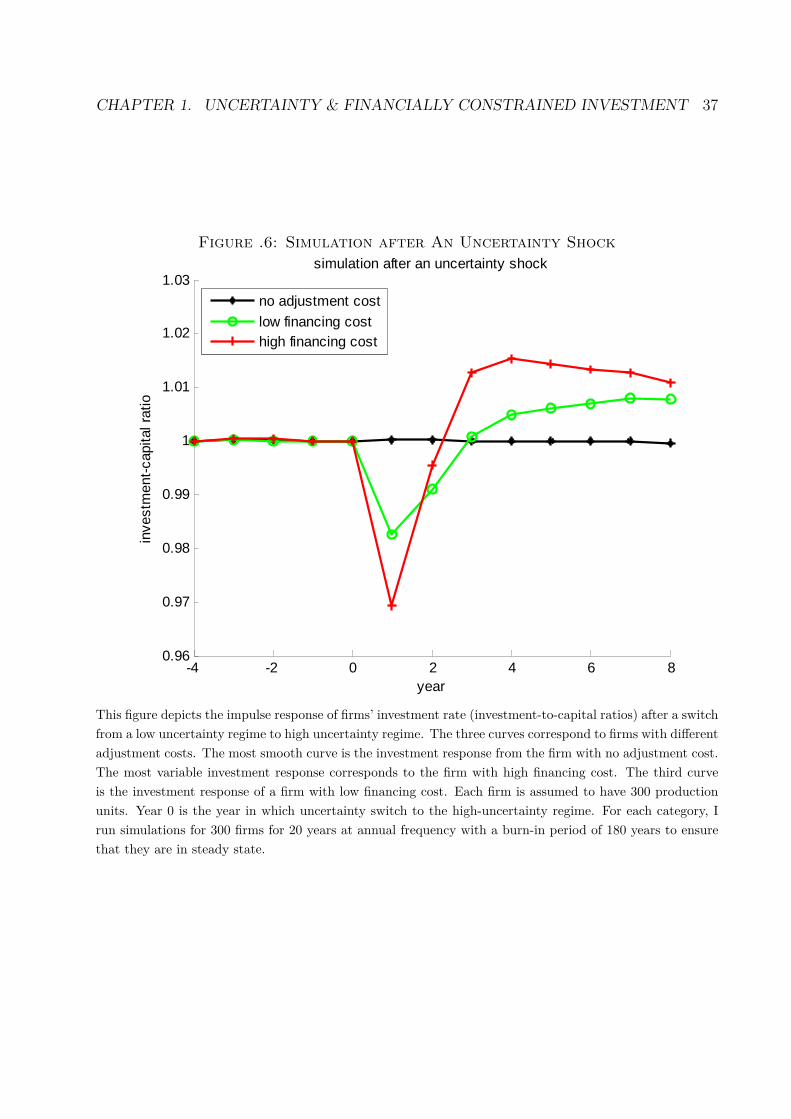
CHAPTER 1. UNCERTAINTY & FINANCIALLY CONSTRAINED INVESTMENT 37
Figure .6: Simulation after An Uncertainty Shock
-4 -2 0 2 4 6 80.96
0.97
0.98
0.99
1
1.01
1.02
1.03simulation after an uncertainty shock
year
inve
stm
ent-
capi
tal r
atio
no adjustment cost
low financing costhigh financing cost
This figure depicts the impulse response of firms’ investment rate (investment-to-capital ratios) after a switchfrom a low uncertainty regime to high uncertainty regime. The three curves correspond to firms with differentadjustment costs. The most smooth curve is the investment response from the firm with no adjustment cost.The most variable investment response corresponds to the firm with high financing cost. The third curveis the investment response of a firm with low financing cost. Each firm is assumed to have 300 productionunits. Year 0 is the year in which uncertainty switch to the high-uncertainty regime. For each category, Irun simulations for 300 firms for 20 years at annual frequency with a burn-in period of 180 years to ensurethat they are in steady state.

CHAPTER 1. UNCERTAINTY & FINANCIALLY CONSTRAINED INVESTMENT 38
Figure .7: Fraction of Firms under High Uncertainty
��������������������� ������������� �������������������� ������������ ������������ ������������������������������������������������� !����"���#
This figure depicts the fraction of firms in the high uncertainty state over the sample periods 1971-2009.Calculations are based on a sample of publicly-traded nonfinancial firms from COMPUSTAT . A firm isdefined to be in the state of high uncertainty in a given year as a firm with measured uncertainty (standarddeviation of daily equity returns) at least one standard deviation higher than its mean uncertainty over allthe company’s sample years.

CHAPTER 1. UNCERTAINTY & FINANCIALLY CONSTRAINED INVESTMENT 39
Figure .8: Uncertainty Impulse Response for All Firms
−.0
8−
.05
−.0
2.0
1.0
4.0
7in
vest
men
t rat
e
−1 0 1 2 3year
Uncertainty Impulse Response
This figure depicts the investment impulse response after a one-standard-deviation increase in uncertainty forall firms in the sample. Calculations are based on a sample of publicly-traded nonfinancial firms from COM-PUSTAT from 1971 to 2009. Year 0 is the year of uncertainty increase. The dotted lines are bootstrapped95% confidence bands. Investment rate is the investment-to-capital ratio It
Kt−1.

CHAPTER 1. UNCERTAINTY & FINANCIALLY CONSTRAINED INVESTMENT 40
Figure .9: Uncertainty Impulse Response across Various Sizes
−.0
8−
.05
−.0
2.0
1.0
4.0
7
−1 0 1 2 3year
0−20%
−.0
8−
.05
−.0
2.0
1.0
4.0
7
−1 0 1 2 3year
20%−40%
−.0
8−
.05
−.0
2.0
1.0
4.0
7
−1 0 1 2 3year
40%−60%
−.0
8−
.05
−.0
2.0
1.0
4.0
7
−1 0 1 2 3year
60%−80%
−.0
8−
.05
−.0
2.0
1.0
4.0
7
−1 0 1 2 3year
80%−100%
Vertical Axis: Investment RateSize Quintiles From Left to Right: <20%, 20%−40%, 40%−60%, 60%−80%, >80%
Uncertainty Impulse Response, by Size
This figure depicts the investment impulse response after a one-standard-deviation increase in uncertaintyfor five size-subsamples. The sample split is based on size (asset) quintiles. Calculations are based on asample of publicly-traded nonfinancial firms from COMPUSTAT from 1971 to 2009. Year 0 is the yearof uncertainty increase. The dotted lines are bootstrapped 95% confidence bands. Investment rate is theinvestment-to-capital ratio It
Kt−1.

CHAPTER 1. UNCERTAINTY & FINANCIALLY CONSTRAINED INVESTMENT 41
Figure .10: Uncertainty Impulse Response for Firms with and without BondRating
−.0
8−
.05
−.0
2.0
1.0
4.0
7
−1 0 1 2 3year
Unrated
−.0
8−
.05
−.0
2.0
1.0
4.0
7
−1 0 1 2 3year
Rated
Vertical Axis: Investment Rate
Uncertainty Impulse Response, by Bond Rating
This figure depicts the investment impulse response after a one-standard-deviation increase in uncertaintyfor two rating-subsamples. The sample split is based on whether a firm is credit rated or not. Calculationsare based on a sample of publicly-traded nonfinancial firms from COMPUSTAT from 1971 to 2009. Year 0is the year of uncertainty increase. The dotted lines are bootstrapped 95% confidence bands. Investmentrate is the investment-to-capital ratio It
Kt−1.

CHAPTER 1. UNCERTAINTY & FINANCIALLY CONSTRAINED INVESTMENT 42
Figure .11: Uncertainty Impulse Response for Various Dividend Payout
−.0
8−
.05
−.0
2.0
1.0
4.0
7
−1 0 1 2 3year
0−25%
−.0
8−
.05
−.0
2.0
1.0
4.0
7
−1 0 1 2 3year
25%−50%
−.0
8−
.05
−.0
2.0
1.0
4.0
7
−1 0 1 2 3year
50%−75%
−.0
8−
.05
−.0
2.0
1.0
4.0
7
−1 0 1 2 3year
75%−100%
Vertical Axis: Investment RateDividend Payout Quartiles From Left to Right: <25%, 25%−50%, 50%−75%, 75%−100%
Uncertainty Impulse Response, by Divdend Payout
This figure depicts the investment impulse response after a one-standard-deviation increase in uncertainty forfour dividend-payout subsamples. The sample split is based on the amount of dividend payout. Calculationsare based on a sample of publicly-traded nonfinancial firms from COMPUSTAT from 1971 to 2009. Year 0is the year of uncertainty increase. The dotted lines are bootstrapped 95% confidence bands. Investmentrate is the investment-to-capital ratio It
Kt−1.
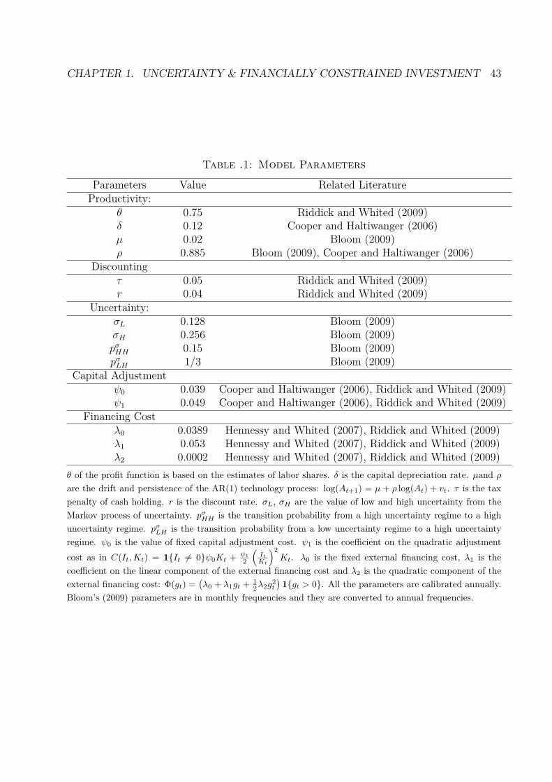
CHAPTER 1. UNCERTAINTY & FINANCIALLY CONSTRAINED INVESTMENT 43
Table .1: Model Parameters
Parameters Value Related LiteratureProductivity:
θ 0.75 Riddick and Whited (2009)δ 0.12 Cooper and Haltiwanger (2006)µ 0.02 Bloom (2009)ρ 0.885 Bloom (2009), Cooper and Haltiwanger (2006)
Discountingτ 0.05 Riddick and Whited (2009)r 0.04 Riddick and Whited (2009)
Uncertainty:σL 0.128 Bloom (2009)σH 0.256 Bloom (2009)pσHH 0.15 Bloom (2009)pσLH 1/3 Bloom (2009)
Capital Adjustmentψ0 0.039 Cooper and Haltiwanger (2006), Riddick and Whited (2009)ψ1 0.049 Cooper and Haltiwanger (2006), Riddick and Whited (2009)
Financing Costλ0 0.0389 Hennessy and Whited (2007), Riddick and Whited (2009)λ1 0.053 Hennessy and Whited (2007), Riddick and Whited (2009)λ2 0.0002 Hennessy and Whited (2007), Riddick and Whited (2009)
θ of the profit function is based on the estimates of labor shares. δ is the capital depreciation rate. µand ρ
are the drift and persistence of the AR(1) technology process: log(At+1) = µ + ρ log(At) + vt. τ is the taxpenalty of cash holding. r is the discount rate. σL, σH are the value of low and high uncertainty from theMarkov process of uncertainty. pσHH is the transition probability from a high uncertainty regime to a highuncertainty regime. pσLH is the transition probability from a low uncertainty regime to a high uncertaintyregime. ψ0 is the value of fixed capital adjustment cost. ψ1 is the coefficient on the quadratic adjustmentcost as in C(It,Kt) = 1{It ̸= 0}ψ0Kt + ψ1
2
(ItKt
)2Kt. λ0 is the fixed external financing cost, λ1 is the
coefficient on the linear component of the external financing cost and λ2 is the quadratic component of theexternal financing cost: Φ(gt) =
(λ0 + λ1gt + 1
2λ2g2t
)1{gt > 0}. All the parameters are calibrated annually.
Bloom’s (2009) parameters are in monthly frequencies and they are converted to annual frequencies.

CHAPTER 1. UNCERTAINTY & FINANCIALLY CONSTRAINED INVESTMENT 44
Tab
le.2
:Su
mm
ary
Stat
isti
csfo
rA
llF
irm
s
Cal
cula
tions
are
base
don
asa
mpl
eof
publ
icly
-tra
ded
nonfi
nanc
ialfi
rmsf
rom
CO
MPU
STAT
from
1971
to20
09.
Firm
inve
stm
ent(
capi
tal
expe
nditu
re),
cash
flow
,cas
hho
ldin
gar
eno
rmal
ized
byth
ere
plac
emen
tva
lue
ofca
pita
lsto
ckat
the
end
ofla
stfis
caly
ear.
An
aver
age
mea
sure
ofTo
bin’
sQ
(Hay
ashi
(198
2))
isco
nstr
ucte
dby
divi
ding
the
mar
ket
valu
eby
the
capi
talr
epla
cem
ent
valu
e.U
ncer
tain
tyis
mea
sure
dby
the
stan
dard
devi
atio
nof
daily
equi
tyre
turn
s.

CHAPTER 1. UNCERTAINTY & FINANCIALLY CONSTRAINED INVESTMENT 45
Tab
le.3
:R
egre
ssio
nsfo
rA
llF
irm
s
Cal
cula
tions
are
base
don
asa
mpl
eof
publ
icly
-tra
ded
nonfi
nanc
ialfi
rms
from
CO
MPU
STAT
from
1971
to20
09.
Rob
usts
tand
ard
erro
rsar
ere
port
edin
pare
nthe
ses.
***
deno
test
heca
sew
here
P-va
lue
isle
ssth
an0.
01;*
*is
the
case
whe
reP-
valu
eis
less
than
0.05
.*
isw
hen
P-va
lue
isle
ssth
an0.
1.In
vest
men
tra
teis
the
inve
stm
ent-
to-c
apita
lrat
ioIt
Kt−
1.
Inve
stm
ent
rate
grow
this
defin
edas
the
perc
enta
gech
ange
inin
vest
men
tra
te.
All
regr
essio
nsco
ntro
lfor
lags
ofin
vest
men
tra
te,s
igm
a(u
ncer
tain
ty),
cash
flow
and
thei
rin
tera
ctio
nsw
ithsig
ma.
Fixe
deff
ects
(FE)
mod
elsc
ontr
olfo
rthe
firm
fixed
-effe
cts.
The
dyna
mic
pane
lmod
els
(DPM
)firs
tdiff
eren
ces
allt
heva
riabl
efo
rG
MM
estim
atio
ns.
Inst
rum
ent
valid
ityis
test
edus
ing
the
Han
sen
test
ofth
eov
erid
entifi
catio
nre
stric
tions
.Se
rialc
orre
latio
nis
test
edus
ing
aLa
gran
gem
ultip
lier
test
onth
efir
st-d
iffer
ence
resid
uals
(Are
llano
and
Bon
d(1
991)
).A
rella
no&
Bon
dTe
stan
dH
anse
nTe
stre
port
the
P-va
lue.

CHAPTER 1. UNCERTAINTY & FINANCIALLY CONSTRAINED INVESTMENT 46
Tab
le.4
:Su
mm
ary
Stat
isti
csfo
rF
irm
sin
Eac
hSi
zeD
ecil
e
Cal
cula
tions
are
base
don
asa
mpl
eof
publ
icly
-tra
ded
nonfi
nanc
ialfi
rms
from
CO
MPU
STAT
from
1971
to20
09.
The
sam
ple
split
sto
subs
ampl
esby
ten
size
(ass
et)d
ecile
s.Fi
rmin
vest
men
t(ca
pita
lexp
endi
ture
)and
cash
flow
(cf)
are
norm
aliz
edby
the
repl
acem
entv
alue
ofca
pita
lsto
ck(K
)at
the
end
ofla
stfis
caly
ear.
Unc
erta
inty
ism
easu
red
byth
est
anda
rdde
viat
ion
ofda
ilyeq
uity
retu
rns.
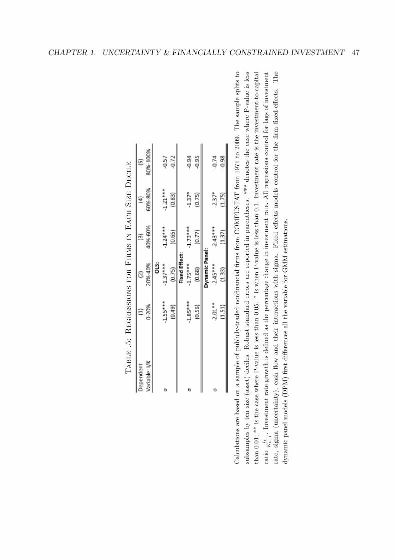
CHAPTER 1. UNCERTAINTY & FINANCIALLY CONSTRAINED INVESTMENT 47
Tab
le.5
:R
egre
ssio
nsfo
rF
irm
sin
Eac
hSi
zeD
ecil
e
Cal
cula
tions
are
base
don
asa
mpl
eof
publ
icly
-tra
ded
nonfi
nanc
ialfi
rms
from
CO
MPU
STAT
from
1971
to20
09.
The
sam
ple
split
sto
subs
ampl
esby
ten
size
(ass
et)
deci
les.
Rob
ust
stan
dard
erro
rsar
ere
port
edin
pare
nthe
ses.
***
deno
tes
the
case
whe
reP-
valu
eis
less
than
0.01
;**
isth
eca
sew
here
P-va
lue
isle
ssth
an0.
05.
*is
whe
nP-
valu
eis
less
than
0.1.
Inve
stm
ent
rate
isth
ein
vest
men
t-to
-cap
ital
ratio
It
Kt−
1.
Inve
stm
ent
rate
grow
this
defin
edas
the
perc
enta
gech
ange
inin
vest
men
tra
te.
All
regr
essio
nsco
ntro
lfor
lags
ofin
vest
men
tra
te,
sigm
a(u
ncer
tain
ty),
cash
flow
and
thei
rin
tera
ctio
nsw
ithsig
ma.
Fixe
deff
ects
mod
els
cont
rol
for
the
firm
fixed
-effe
cts.
The
dyna
mic
pane
lmod
els
(DPM
)fir
stdi
ffere
nces
allt
heva
riabl
efo
rG
MM
estim
atio
ns.

CHAPTER 1. UNCERTAINTY & FINANCIALLY CONSTRAINED INVESTMENT 48
Table .6: Summary Statistics for Firms with and without Bond Ratings
Calculations are based on a sample of publicly-traded nonfinancial firms from COMPUSTAT from 1971 to2006. The sample splits to subsamples by whether firms have a credit rating over their sample periods. Firminvestment (capital expenditure) and cash flow (cf) are normalized by the replacement value of capital stock(K) at the end of last fiscal year. Uncertainty is measured by the standard deviation of daily equity returns.

CHAPTER 1. UNCERTAINTY & FINANCIALLY CONSTRAINED INVESTMENT 49
Table .7: Regressions for Firms with and without Bond Ratings
Calculations are based on a sample of publicly-traded nonfinancial firms from COMPUSTAT from 1971 to2006. The sample splits to subsamples by whether firms have a credit rating (Rated) over their sampleperiods. Robust standard errors are reported in parentheses. *** denotes the case where P-value is lessthan 0.01; ** is the case where P-value is less than 0.05. * is when P-value is less than 0.1. Investmentrate is the investment-to-capital ratio It
Kt−1. Investment rate growth is defined as the percentage change in
investment rate. All regressions control for lags of investment rate, sigma (uncertainty), cash flow and theirinteractions with sigma. Fixed effects models control for the firm fixed-effects. The dynamic panel models(DPM) first differences all the variable for GMM estimations. Instrument validity is tested using the Hansentest of the overidentification restrictions. Serial correlation is tested using a Lagrange multiplier test on thefirst-difference residuals (Arellano and Bond (1991)). Arellano & Bond Test and Hansen Test report theP-value.
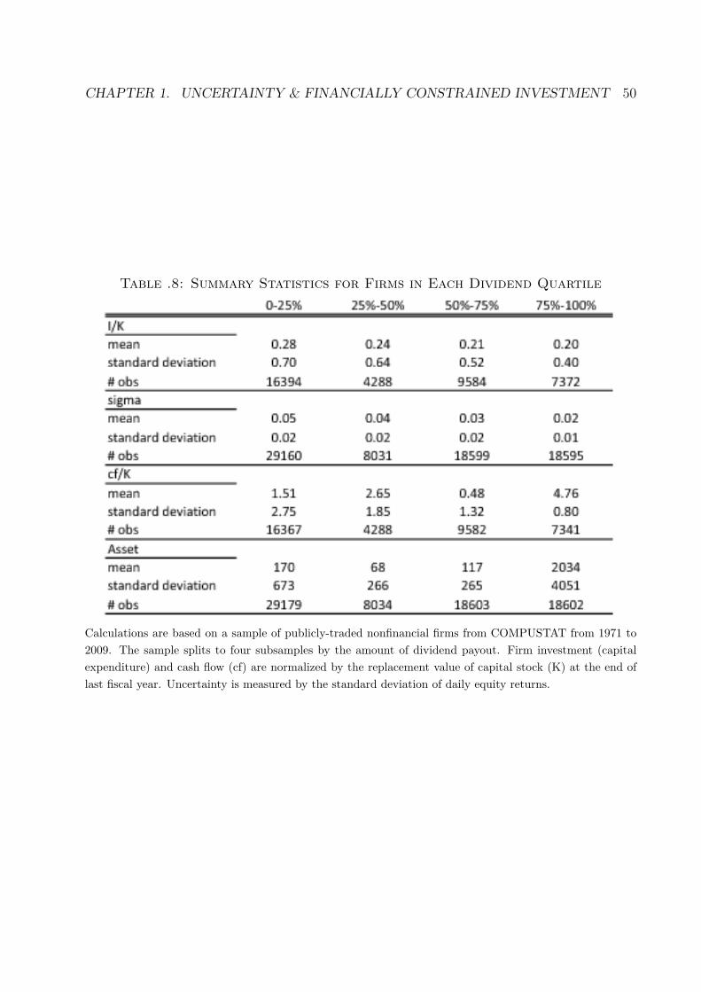
CHAPTER 1. UNCERTAINTY & FINANCIALLY CONSTRAINED INVESTMENT 50
Table .8: Summary Statistics for Firms in Each Dividend Quartile
Calculations are based on a sample of publicly-traded nonfinancial firms from COMPUSTAT from 1971 to2009. The sample splits to four subsamples by the amount of dividend payout. Firm investment (capitalexpenditure) and cash flow (cf) are normalized by the replacement value of capital stock (K) at the end oflast fiscal year. Uncertainty is measured by the standard deviation of daily equity returns.

CHAPTER 1. UNCERTAINTY & FINANCIALLY CONSTRAINED INVESTMENT 51
Table .9: Regressions for Firms in Each Dividend Quartile
Calculations are based on a sample of publicly-traded nonfinancial firms from COMPUSTAT from 1971 to2009. The sample splits to four subsamples by the amount of dividend payout. Robust standard errors arereported in parentheses. *** denotes the case where P-value is less than 0.01; ** is the case where P-valueis less than 0.05. * is when P-value is less than 0.1. Investment rate is the investment-to-capital ratio It
Kt−1.
Investment rate growth is defined as the percentage change in investment rate. All regressions control for lagsof investment rate, sigma (uncertainty), cash flow and their interactions with sigma. Fixed effects modelscontrol for the firm fixed-effects. The dynamic panel models (DPM) first differences all the variable forGMM estimations. Instrument validity is tested using the Hansen test of the overidentification restrictions.Serial correlation is tested using a Lagrange multiplier test on the first-difference residuals (Arellano andBond (1991)). Arellano & Bond Test and Hansen Test report the P-value.

CHAPTER 1. UNCERTAINTY & FINANCIALLY CONSTRAINED INVESTMENT 52
Tab
le.1
0:Su
mm
ary
Stat
isti
csfo
rF
irm
sin
Eac
hK
ZD
ecil
e
Cal
cula
tions
are
base
don
asa
mpl
eof
publ
icly
-tra
ded
nonfi
nanc
ialfi
rms
from
CO
MPU
STAT
from
1971
to20
09.
The
sam
ple
split
sto
ten
subs
ampl
esby
the
Kap
lan-
Zing
ales
inde
x.T
heK
apla
n-Zi
ngal
esin
dex
prov
ides
asc
ore
offin
anci
alco
nstr
aint
base
dup
onva
rious
varia
bles
:−
1.00
1909
CFit
Ait−
1+
3.13
9193LEVit−
39.3
678D
IVit
Ait−
1−
1.31
4759
Cit
Ati−
1+
0.28
2638
9Qit
.Fi
rmin
vest
men
t(c
apita
lexp
endi
ture
)an
dca
shflo
w(c
f)ar
eno
rmal
ized
byth
ere
plac
emen
tva
lue
ofca
pita
lsto
ck(K
)at
the
end
ofla
stfis
caly
ear.
Unc
erta
inty
ism
easu
red
byth
est
anda
rdde
viat
ion
ofda
ilyeq
uity
retu
rns.

CHAPTER 1. UNCERTAINTY & FINANCIALLY CONSTRAINED INVESTMENT 53
Tab
le.1
1:R
egre
ssio
nsfo
rF
irm
sin
Eac
hK
ZD
ecil
e
Cal
cula
tions
are
base
don
asa
mpl
eof
publ
icly
-tra
ded
nonfi
nanc
ialfi
rms
from
CO
MPU
STAT
from
1971
to20
09.
The
sam
ple
split
sto
ten
subs
ampl
esby
the
Kap
lan-
Zing
ales
inde
x.T
heK
apla
n-Zi
ngal
esin
dex
prov
ides
asc
ore
offin
anci
alco
nstr
aint
base
dup
onva
rious
varia
bles
:−
1.00
1909
CFit
Ait−
1+
3.13
9193LEVit−
39.3
678D
IVit
Ait−
1−
1.31
4759
Cit
Ati−
1+
0.28
2638
9Qit
.R
obus
tst
anda
rder
rors
are
repo
rted
inpa
rent
hese
s.**
*de
note
sth
eca
sew
here
P-va
lue
isle
ssth
an0.
01;*
*is
the
case
whe
reP-
valu
eis
less
than
0.05
.*
isw
hen
P-va
lue
isle
ssth
an0.
1.In
vest
men
tra
teis
the
inve
stm
ent-
to-c
apita
lrat
ioIt
Kt−
1.
Inve
stm
ent
rate
grow
this
defin
edas
the
perc
enta
gech
ange
inin
vest
men
tra
te.
All
regr
essio
nsco
ntro
lfor
lags
ofin
vest
men
tra
te,
sigm
a(u
ncer
tain
ty),
cash
flow
and
thei
rin
tera
ctio
nsw
ithsig
ma.
Fixe
deff
ects
mod
els
cont
rol
for
the
firm
fixed
-effe
cts.
The
dyna
mic
pane
lm
odel
s(D
PM)
first
diffe
renc
esal
lth
eva
riabl
efo
rG
MM
estim
atio
ns.
Inst
rum
ent
valid
ityis
test
edus
ing
the
Han
sen
test
ofth
eov
erid
entifi
catio
nre
stric
tions
.Se
rialc
orre
latio
nis
test
edus
ing
aLa
gran
gem
ultip
lier
test
onth
efir
st-d
iffer
ence
resid
uals
(Are
llano
and
Bon
d(1
991)
).A
rella
no&
Bon
dTe
stan
dH
anse
nTe
stre
port
the
P-va
lue.
54
Chapter 2
Taxation and Income Shifting:Empirical Evidence from a NaturalExperiment from ChinaCo-authored with Zhiyong An
2.1 IntroductionCross-border investment by multinational corporations (MNCs) is one of the most salient
features of today’s global economy. Countries around the world have made numerous taxconcessions to attract MNCs’ investments. Such cross-country differences in corporate taxrates are an enduring feature of the global fiscal environment. Only multinational corpora-tions are able to benefit from the cross-country differences in corporate tax rates to reducetheir overall tax burden by shifting income from high-tax countries to low-tax countries.Multinational corporations (MNCs) are taking advantage of the cross-country differences incorporate tax rates to reduce their overall tax burden by shifting income from high-tax coun-tries to low-tax countries. However, whether or to what extent they engage in this behaviorhas long been the subject of much debate.
By their very nature, MNCs trade goods, services, and intangible assets across nationalborders within their enterprises. MNCs typically can reduce their overall tax burden byartificially reducing transfer prices charged by affiliates in high-tax countries for goods, ser-vices, and intangible assets provided to affiliates in low-tax countries. In order to stem theflow of taxation revenues overseas and to ensure that they get to tax their fair share, mostcountries enforce tax laws based on the arm’s length principle, which requires transfer pricesfor transactions between different parts of the same MNC to be set at the same level as pricesfor similar transactions between unrelated parties. However, strict application of the arm’slength principle is often problematic in practice. For example, for many intra-corporation

CHAPTER 2. TAXATION AND INCOME SHIFTING IN CHINA 55
transactions there exists no comparable market outside the corporation. This is in partic-ular the case for intellectual property or knowledge-intensive intermediate goods that aredeveloped or produced by one part of a MNC and used by other parts of the same MNC inother countries.
MNCs’ income shifting behavior has long been documented and studied. Wheeler (1988)presents U.S. tax court cases where income was shifted for tax reasons. In one case, in 1975G. D. Searle & Company had an average return on employed assets of -42.3% in the U.S. and119% in Puerto Rico whose effective tax rate is zero. Theoretically, Horst (1971) builds asimple model that shows how MNCs choose transfer prices in order to maximize their after-tax earnings. Horst’s model analyzes the choices of a monopolistic corporation that sells intwo countries simultaneously. The corporation’s earnings are equal to the sum of its after-taxprofits in the two countries and a term that shows the impact of intra-corporation trade.The optimal transfer price chosen by the corporation to maximize its after-tax earnings iseither the lowest transfer price or the highest transfer price, depending on a comparison ofthe relative differential in tax rates between the importing and exporting countries with thetariff rate.
In a series of efforts over the past two decades, there has been systematic empiricalevidence uncovered for income shifting. Almost all of the earlier empirical studies on incomeshifting concern the U.S. and, more specifically, income shifting from the U.S. to low-taxcountries (e.g., Grubert and Mutti (1991); Grubert et al. (1993); Klassen et al.(1993); Hinesand Rice(1994); Collins et al. (1998); Grubert and Slemrod (1994); Swenson (2001); Clausing(2003))1. In the past decade, empirical studies on income shifting have been done for otherOECD countries (e.g., Bartelsman and Beetsma (2003); Mintz and Smart (2004); Buettneret al. (2009); Huizinga and Laeven (2008); Weichenrieder (2009)). These studies providesome indirect empirical evidence for tax-induced income shifting. However, to the best ofour knowledge, no empirical study on income shifting using data from developing countriesand, in particular for China, exists.
China’s new Corporate Income Tax Law was passed in March 2007 and took effect onJanuary 1st 2008. It terminates the dual corporate income tax regime by removing the taxpreferences offered to foreign investment enterprises (FIEs) by the Chinese government andunifies the corporate income tax regime for FIEs and Chinese domestic enterprises (DEs).In this paper we use a difference-in-differences approach to determine whether FIEs areresponding to the law by shifting income out of China. We employ the Chinese IndustrialEnterprises Database from 2002 to 2008 to implement the analysis. Our treatment group ismade up of FIEs affected by the law, while our control group is made up of DEs unaffectedby the law. We first show that the trends of the pre-tax profit of the treatment and controlgroups before the passage of the law are parallel to each other, which implies that theidentifying assumption of our identification strategy is satisfied and thus our difference-in-differences analysis has solid foundation. Then we conduct the difference-in-differences
1See Hines (1996; 1999) for a review of the literature on income shifting.

CHAPTER 2. TAXATION AND INCOME SHIFTING IN CHINA 56
regressions. The estimates suggest three conclusions. First, we find that FIEs seem to haveresponded to the law by shifting income out of China. Second, the magnitude of the responseis larger for larger-size enterprises, which might be due to their greater capability of shiftingincome across countries. Finally, the magnitude of response is larger for Hong Kong-Macau-Taiwan (HMT) investment enterprises than that for other FIEs. Because both Hong Kongand Macau are tax havens (Dharmapala and Hines Jr. (2009)), the pre-tax profit of HMTinvestment enterprises should be more elastic than that of other FIEs. All the three findingsare consistent with tax-induced income shifting.
Our work makes at least three contributions. First, ours is the first paper to focuson income-shifting activities of Chinese enterprises using data from China. Second, ourwork provides helpful information for Chinese policymakers. Since China opened its doorin 1978 and especially since its accession to the World Trade Organization (WTO) in 2001,International transactions have played an important role in the Chinese economy. At thesame time, the possible loss in tax revenues due to income shifting by FIEs has increasinglycome under the spotlight of China’s tax authorities. Over the past few years, the StateAdministration of Taxation (SAT) of China has blamed FIEs for substantial losses in taxationrevenues. To the best of our knowledge, no rigorous empirical study has been done to explorethe extent to which FIEs shift income out of China. Our work attempts to fill in this gap.Finally, this is the first rigorous study of China’s new Corporate Income Tax Law, the mostprofound tax reform of the decade in China.
The remainder of the paper is organized as follows. Section 2 describes the changes inthe effective corporate income tax rate brought about by China’s new Corporate IncomeTax Law. Section 3 presents our identification strategy. Section 4 presents the regressionframework and the specification of our econometric models. Section 5 describes the data indetail, and Section 6 reports the results of our data analysis. Finally, Section 7 concludesthe chapter.
2.2 China’s New Corporate Income Tax LawSince the early 1990s, China has maintained a dual corporate income tax regime: one
regime for Chinese DEs and the other one for FIEs. Under the dual corporate income taxregime, DEs and FIEs are subject to different effective corporate income tax rates. Theeffective corporate income tax rate was about 25% for DEs, while it was about 15% forFIEs. The lower effective corporate income tax rate for FIEs was made possible by certainpreferential tax treatments offered by the Chinese government for FIEs. The purpose of thedual corporate income tax regime is to entice foreign investment into China.
In order to create a level playing field and a fair fiscal environment that promotes compe-tition and transparency for all enterprises in China and in order to increase the sophisticationof China’s tax regime in general, the National People’s Congress of China drafted and passedthe new Corporate Income Tax Law in March 2007. The law came into effect on January
CHAPTER 2. TAXATION AND INCOME SHIFTING IN CHINA 57
1st 2008. The law is the most profound tax reform of the decade in China. It terminatesthe dual corporate income tax regime and unifies the corporate income tax rate to 25% forboth FIEs and DEs. In other words, it increases the corporate income tax rate for FIEs fromabout 15% to 25%, while keeps that unchanged at 25% for DEs. Thus, the law has hugeimpact on FIEs, but basically no impact on DEs.
2.3 Identification StrategyAs described in the previous section, China’s new Corporate Income Tax Law has huge
impact on foreign investment enterprises, but basically no impact on domestic enterprises.Therefore, the law presents a great opportunity for us to construct a natural experiment anduse a difference-in-differences approach to determine whether foreign investment enterprisesare responding to the law by reducing their investment in China. Our treatment group ismade up of FIEs affected by the law, while our control group is made up of DEs unaffectedby the law.
In order to identify FIEs’ investment response to China’s new Corporate Income Tax Law,a naïve identification strategy is to compare the assets of FIEs before and after January 12008 on which the law came into effect. However, since there may be underlying trends inthe assets of FIEs, we use the control group to isolate FIEs’ response to the law. In otherwords, our identification strategy is to compare the change in the assets of the treatmentgroup and that of the control group before and after the law came into effect as a meansof deducing FIEs’ investment response to the law. This is essentially the difference-in-differences methodology.2 It controls for the underlying trends in the assets of the treatmentgroup through that of the control group over the period. It is clear to see that the identifyingassumption that we make is that there is little difference between the underlying trends inthe assets of the treatment and control groups. In other words, we assume that in theabsence of China’s new Corporate Income Tax Law, the difference between the change inthe assets of the treatment group and that of the control group over the period would beequal to zero. We will show that the identifying assumption that we make is satisfied andthus our difference-in-differences analysis has solid foundation.
The change in the pre-tax profit of the treatment group before and after the law came intoeffect is given by (Profitta − Profittb), where t means the treatment group, a means “afterthe law came into effect”, and b means “before the law came into effect”. Part of this changeis due to FIEs’ investment response to the law, and part is due to the underlying trends in thepre-tax profit of the treatment group (i.e., FIEs). The identifying assumption that we makeis that the underlying trends in the pre-tax profit of the treatment group will be reflectedin the change in the pre-tax profit of the control group, given by (Profitca − Profitcb),
2See Angrist and Krueger (1999) for an excellent reference for the difference-in-differences methodologyassociated with the natural experiment approach, and see Card and Krueger (1994) for a nice application ofthe methodology.

CHAPTER 2. TAXATION AND INCOME SHIFTING IN CHINA 58
where c means the control group, a means “after the law came into effect”, and b means“before the law came into effect”. The test that FIEs are responding to the law by reducingtheir investment in China is a test that shows (Assetsta−Assetstb)− (Assetsca−Assetscb)is negative. The identifying assumption that we make essentially says that (Profitta −Profittb) − (Profitca − Profitcb) would be equal to zero in the absence of the law. Wewill show that the identifying assumptions of our identification strategy are satisfied shortlyafter.
2.4 Econometric ModelsTo examine whether FIEs are responding to China’s new Corporate Income Tax Law by
shifting their income out of China, one could estimate the following difference-in-differencesmodel by employing OLS regression:
log(Profit) = α+ βAssetReturn+ λEnterpriseScale+ ηDebtRatio
+ δZ + γ0treatment+ γ1postlegislation (2.1)+ γ2treatment× postlegislation+ ε
where ε is an error term; Profit is the pre-tax profit. We use log(Profit) as the depen-dent variable to address the potential nonlinearity problem.
The variable treatment is a dummy variable indicating whether an enterprise is includedin the treatment group or in the control group, and is equal to one if it is included in thetreatment group and is equal to zero if it is included in the control group. The type of regis-tration (denoted as RegistrationType) of each enterprise tells us the type of each enterprise.Enterprises in China can be classified into three categories: (1) domestic enterprises; (2)HMT investment enterprises; (3) other FIEs. .1 shows a table of classifications by types ofregistration. The variable is a dummy variable indicating whether an observation is madeafter the law came into effect, and is equal to one if it is made after the law came into effectand is equal to zero otherwise. The law was passed in March 2007 and came into effect onJanuary 1 2008. Data for year 2008 makes up our post-legislation observations and data foryear 2006 constitutes our pre-legislation observation. We use the data for years from 2002 to2006 to check whether the identifying assumption of our identification strategy is satisfied.
In order to reduce the residual variance of the regression and produce more efficientestimates, we include a set of control variables. First, because an enterprise’s profit mightdepend on its profitability, we include the return on assets (denoted as AssetReturn) as acontrol variable. We expect the coefficient of AssetReturn, namely β, to be positive andstatistically significant.
Second, because an enterprise’s profit might also depend on its scale of operations, weinclude the scale of an enterprise (denoted as EnterpriseScale) as a control variable in oureconometric model. The categorical variable EnterpriseScale has three categories which

CHAPTER 2. TAXATION AND INCOME SHIFTING IN CHINA 59
correspond to large-size enterprises, medium-size enterprises, and small-size enterprises re-spectively3. Because an enterprise’s scale of operation should have a positive impact onits profit, we expect to see that the estimated coefficient will increase with the size of theenterprise.
Third, because the post-legislation observation is made in year 2008 in which a globalfinancial crisis occurred, we include the debt ratio of an enterprise (denoted as DebtRatio) asone control variable in our econometric model. The higher the debt ratio of an enterprise is,the larger the impact of the 2008 global financial crisis on the enterprise would be. Therefore,we expect the coefficient of DebtRatio, namely η, to be negative and statistically significant.
Finally, Z is a vector of control variables which include: (1) a categorical variable thatindicates the area (the counterpart in the U.S. is state) where an enterprise is registered andis denoted as Location; and (2) a categorical variable that indicates the two-digit industrycategory that an enterprise belongs to and is denoted as Industry. These two categoricalcontrol variables are included to control for industry characteristics and location character-istics of enterprises that may affect the level of pre-tax profit.
The coefficient of the dummy variable , γ0, is the treatment group specific effect thataccounts for the average permanent differences between the treatment and control groups.The coefficient of the dummy variable postlegislation, γ1, captures the time trend commonto the treatment and control groups. The coefficient of the interaction term treatment ×postlegislation, γ1, gives us the difference-in-differences estimate of the treatment effect,namely, the difference between the change in log(Profit) of the treatment group and thatof the control group before and after the law came into effect. We expect γ2 to be negativeand statistically significant. In other words, we expect to find that FIEs responded to thelaw by shifting their income out of China.
Because larger-size enterprises might have more capability to shift income across coun-tries, we expect to see that the magnitude of the response is larger for larger-size enterprises.In order to test this idea, we estimate the following difference-in-differences model:
log(Profit) = α+ βAssetReturn+ λEnterpriseScale+ ηDebtRatio
+ δZ + γ0treatment+ γ1postlegislation
+ γ2treatment× postlegislation+ γ3treatment× postlegislation× dummyLargeSize (2.2)+ γ4treatment× postlegislation× dummyMediumSize
+ ε
where Large is a dummy variable that is equal to one if the enterprise is a large-size3In order to help understand the concept of EnterpriseScale, .5 gives the summary statistics of total
employees and total assets by EnterpriseScale in 2003. By .5, a larger-size enterprise has on average moretotal employees and more total assets.

CHAPTER 2. TAXATION AND INCOME SHIFTING IN CHINA 60
enterprise and is equal to zero if otherwise, and Medium is also a dummy variable that isequal to one if the enterprise is a medium-size enterprise and is equal to zero if otherwise.
Note that γ2 gives us the treatment effect for small-size enterprises; γ3 gives us the differ-ence between the treatment effect for large-size enterprises and that for small-size enterprises;and γ4 gives us the difference between the treatment effect for medium-size enterprises andthat for small-size enterprises. We expect to find the estimated coefficients γ2, γ3 and γ4 areall negative and statistically significant; and further that γ3 < γ4. In other words, we expectto see that FIEs of all sizes are responding to the law by shifting their income out of China;and that the magnitude of the response is larger for larger-size enterprises.
Hong Kong and Macau are on the list of tax havens compiled by Dharmapala andHines Jr. (2009). We expect that the pre-tax profit of HMT investment enterprises shouldbe more elastic than that of other FIEs. Therefore, we expect to see that the magnitude ofthe response is larger for HMT investment enterprises than that for other FIEs. In order totest this idea, we estimate the following difference-in-differences model instead of Equation2.1:
log(Profit) = α+ βAssetReturn+ λEnterpriseScale+ ηDebtRatio
+ δZ + γ0treatment+ γ1postlegislation
+ γ2treatment× postlegislation (2.3)+ γ3treatment× postlegislation×DummyHMT + ε
where HMT is a dummy variable that is equal to one if the enterprise is an HMT invest-ment enterprise .1 shows how we impute the value of HMT for our data. Note that gives usthe treatment effect for other FIEs that are not HMT investment enterprises. We expect tofind that both HMT investment enterprises and other FIEs responded to the law by shiftingtheir income out of China; and the magnitude of the response is larger for HMT investmententerprises than that for other FIEs.
2.5 Data DescriptionWe employ the Chinese Industrial Enterprises Database (2002-2008) to implement the
analysis. The database embodies information of enterprises whose annual sales revenue isabove 5 million RMB. The coverage of the database is identical with that of the indus-trial sector of the China Statistical Yearbook and with that of the China Industry EconomyStatistical Yearbook. The difference is that the Chinese Industrial Enterprises Database isfirm-level data, while both the industrial sector of the China Statistical Yearbook and theChina Industry Economy Statistical Yearbook are aggregated data along different dimensions.
By 2008, the database has included more than 410,000 industrial enterprises, whichaccounts for about 95% of the total industrial output value of China. The database contains

CHAPTER 2. TAXATION AND INCOME SHIFTING IN CHINA 61
about 40 general industry categories at the two-digit industry code level, and covers all the31 areas in the mainland of China, namely, 22 provinces, 5 autonomous regions (namely,Guangxi, Neimeng, Ningxia, Xinjiang, and Tibet), and 4 cities (namely, Beijing, Tianjin,Shanghai, and Chongqing) that report directly to the central government. The database isthe most complete and most authoritative firm-level database in China.
Each enterprise in the database is identified by a unique enterprise ID. The sample of theenterprises in the database changes year by year, with some enterprises entering the databaseand some others exiting the database. However, most of the enterprises are continuouslykept in the database. In other words, the database is roughly a nice panel dataset.
The database provides two types of information for each enterprise. The first type ofinformation is basically qualitative, including the ID of each enterprise, the location whereeach enterprise is registered, the type of registration of each enterprise, the industry categoryof each enterprise, the scale of each enterprise, and etc., and is coded according to predefinedmapping tables. The second type of information is basically quantitative, including forexample, almost all the variables on the balance sheet of each enterprise such as sales revenue,sales cost, total fixed assets, total assets, long term debt, total debt, total profit, total wages,and etc.
Table .7 gives the overview of the sample size information of the database. For example,the number of enterprises included in the database for year 2007 is 336,768, and the number ofenterprises included in the database for year 2008 is 412,212. Because China’s new CorporateIncome Tax Law was passed in March 2007 and came into effect on January 1, 2008, we usethe data for year 2006 as the pre-legislation observation, and use the data for year 2008 asthe post-legislation observation.
Tables .3, .4, and .5 are the frequency tables for three categorical variables by yearrespectively: Location ID, Industry ID and EnterpriseScale.
In order to fully understand the concept of EnterpriseScale, Table 6 gives the summarystatistics of total employees and total assets by EnterpriseScale in 2003. By Table .2, alarger-size enterprise has on average more total employees and more total assets.
The type of registration (denoted as RegistrationType) of each enterprise tells us thetype of each enterprise. Table .1 is the mapping table for the type of registration. Table .6is the frequency table for the type of registration by year.
According to Table .1, we impute the value of as follows: (1) if RegistrationType of anenterprise is in (‘110’, ‘120’, ‘130’, ‘141’, ‘142’, ‘143’, ‘149’, ‘151’, ‘159’, ‘160’, ‘171’, ‘172’,‘173’, ‘174’, ‘190’), then we include the enterprise in the control group (i.e., DEs) and set thevalue of treatment for the enterprise to be zero; (2) Otherwise, we include the enterprise inthe treatment group (i.e., FIEs) and set the value of treatment for the enterprise to be one.

CHAPTER 2. TAXATION AND INCOME SHIFTING IN CHINA 62
2.6 Empirical ResultsWe start by checking whether the identifying assumption of our identification strategy
is satisfied by plotting the trends of the mean of log(Profit) of the treatment and controlgroups from year 2002 to year 2008. The graph is shown in .1.
.1shows two rising trends before year 2007 that are basically parallel to each other im-plying that there is little difference between the underlying trends in the pre-tax profit ofthe treatment and control groups so that the identifying assumption of our identificationstrategy is satisfied, and thus the difference-in-differences analysis conducted in Part (2)has solid foundation. .1 also shows that the two parallel trends diverge after year 2007, Inparticular, the control group keeps its original rising trend after 2007, while the treatmentgroup switches to a slightly declining trend. This suggests that FIEs responded to the lawby shifting their income out of China.
We first estimate 2.1 to examine FIEs’ response to the. The regression results are reportedin Column “Model 1” of .8. By Column “Model 1” of .8, one could reach four conclusions.First, as expected, the estimated coefficient of is positive at 0.002 and is statistically sig-nificant at the 1% level, which intuitively makes sense because an enterprise’s profitabilityshould have a positive impact on its profit. Second, as expected, an enterprise’s scale of op-erations has a positive impact on its profit. Third, as expected, the estimated coefficient ofis negative at −1.406 and is statistically significant at the 1% level, which intuitively makessense because the 2008 global financial crisis should have a greater impact on enterprises withhigher debt ratios. Finally, the estimated coefficient of the interaction term is negative at–0.346 and is statistically significant at the 1% level, which implies that FIEs are respondingto the law by shifting their income out of China.
Then we estimate 2.2 to examine FIEs’ response to the law by enterprise scale. Theregression results are reported in Column “Model 2” of .8. By Column “Model 2” of .8, onecould reach two new points. First, the estimated coefficients of treatment× postlegislation,treatment× postlegislation×DummyLargeSize, andtreatment × postlegislation × DummyMediumSize are all negative at −0.291, −0.326,and −0.220 respectively and are all statistically significant at the 1% level. Second, theestimated coefficient of treatment×postlegislation×DummyLargeSize is less than that oftreatment× postlegislation×DummyMediumSize. These two new points are as expectedand have two implications. First, they imply that FIEs of all sizes have responded to thelaw by shifting their income out of China. Second, they imply that the magnitude of theresponse is larger for larger-size enterprises, which intuitively makes sense because larger-sizeenterprises should have more capability of shifting income across countries.
Finally, we estimate Equation (3) to examine whether FIEs from Hong Kong and Macauenterprises had a stronger response to the law in terms of income shifting. The regressionresults are reported in Column “Model 3” of .8. By Column “Model 3” of .8, one could reachanother two new points. First, the estimated coefficient of treatment × postlegislation isnegative at −0.223 and is statistically significant at the 1% level. Second, the estimated

CHAPTER 2. TAXATION AND INCOME SHIFTING IN CHINA 63
coefficient of treatment× postlegislation×DummyHMT is negative at −0.268 and is sta-tistically significant at the 1% level. These two new points also have two implications. First,they imply that FIEs responded to the law by shifting their income out of China. Second,they imply that the magnitude of the response is larger for HMT investment enterprises thanthat for other FIEs, which intuitively makes sense because both Hong Kong and Macau aretax havens (Dharmapala and Hines Jr. (2009)) so that the pre-tax profit of HMT investmententerprises should be more elastic than that of other FIEs.
The 2008 global financial crisis may have an impact on our estimates. Just like othercountries, the 2008 global financial crisis had a serious impact on the Chinese economy andon Chinese domestic enterprises. Desai et al. (2008) show that MNCs have an advantage,namely, a superior ability to overcome financing constraints during a financial crisis, whichimplies that our results might underestimate the magnitude of the response of FIEs to thelaw. In order to address this concern, we have included DE as a control variable in oureconometric models.
2.7 ConclusionsSince the early 1990s, China has maintained a dual corporate income tax regime, under
which FIEs enjoyed certain preferential tax. China’s new Corporate Income Tax Law thatwas passed in March 2007 terminated the dual corporate income tax regime by removingthe tax preferences offered to FIEs by the Chinese government and unifying the income taxregime for FIEs and DEs. This paper uses a difference-in-differences approach to determinewhether FIEs responded to the law by shifting their income out of China. We employ theChinese Industrial Enterprises Database (2002-2008) to implement the analysis. We havethree main findings. First, our estimates suggest that the law has driven FIEs to shift theirincome out of China. Second, the impact of the law is larger for larger-size enterprises, whichmight be due to their greater capability of shifting income across countries. Finally, we findthat the impact of the law is larger for HMT investment enterprises than that for other FIEs,which is consistent with the fact that both Hong Kong and Macau are tax havens. All threefindings are consistent with tax-induced income shifting.

CHAPTER 2. TAXATION AND INCOME SHIFTING IN CHINA 64
Figure .1: The Trends of the Pre-Tax Profit of the Treatment and ControlGroups (2002-2008)
5.00
6.00
7.00
8.00
9.00
2002 2003 2004 2005 2006 2007 2008
Year
me
an
of
log
(Pro
fit)
control treatment
Note: Profit is the pre-tax profit. Control group is the domestic enterprises. Treatment group is the foreign investment
enterprises. Data is from the Chinese Industrial Enterprises Database from 2002 to 2008.

CHAPTER 2. TAXATION AND INCOME SHIFTING IN CHINA 65
Table .1: The Mapping Table for the Type of Registration
Level_1_Code Level_2_Code Level_3_Code Type of Enterprise
100 Domestic Enterprises
110 110 State-Owned Enterprises
120 120 Collective-Owned Enterprises
130 130 Share Cooperative Enterprises
140 Associated Enterprises
141 State-State Associated Enterprises
142 Collective-Collective Associated Enterprises
143 State-Collective Associated Enterprises
149 Other Associated Enterprises
150 Limited Liability Company
151 State-Owned Limited Liability Company
159 Other Limited Liability Company
160 160 Limited Liability Stock Company
170 Private-Owned Enterprises
171 Private-Owned Company (only one owner)
172 Private-Owned Partnership Company
173 Private-Owned Limited Liability Company
174 Private-Owned Limited Liability Stock Company
190 190 Other Enterprises
200 HongKong-Macau-Taiwan(HMT) Investment Enterprises
210 HMT-Mainland Joint Venture
220 Enterprise Jointly Managed by Mainland and HMT
230 HMT-Owned Enterprise
240 HMT-Owned Limited Liability Stock Company
300 Foreign Investment Enterprises
310 Chinese-Foreign Joint Venture
320 Enterprise Jointly Managed by China and Foreign Countries
330 Foreign-Owned Enterprise
340 Foreign-Owned Limited Liability Stock Company
Note: Data is from the Chinese Industrial Enterprises Database from 2002 to 2008.

CHAPTER 2. TAXATION AND INCOME SHIFTING IN CHINA 66
Table .2: The Distribution of Total Employees and Total Assets by Enter-priseScale
Summary Statistics of Total Employees by Enterprise Scale
Category of EnterpriseScale N Mean Median
"Large-Size" 1,984 6,586 3,598
"Medium-Size" 21,647 886 648
"Small-Size 172,591 146 98
Summary Statistics of Total Assets by Enterprise Scale
Category of EnterpriseScale N Mean Median
"Large-Size" 1,984 3,340,587 1,572,653
"Medium-Size" 21,647 271,883 134,954
"Small-Size 172,591 25,306 10,756
Note: Data is from the Chinese Industrial Enterprises Database from 2002 to 2008.

CHAPTER 2. TAXATION AND INCOME SHIFTING IN CHINA 67
Table .3: The Frequency Table by Year for Location ID
Location_ID Area 2002 2003 2004 2005 2006 2007 2008
11 Beijing 2.51 2.05 2.47 2.32 2.12 1.9 1.67
12 Tianjin 2.94 2.72 2.32 2.26 2.09 1.89 1.85
13 Hebei 4.2 4.04 3.35 3.66 3.52 3.23 2.95
14 Shanxi 1.91 1.84 1.82 1.63 1.55 1.33 1.03
15 Neimeng 0.79 0.84 0.82 0.9 1.02 1 0.89
21 Liaoning 3.31 3.49 4.11 4.23 4.89 4.92 5.12
22 Jilin 1.42 1.16 1.24 1.02 1.08 1.18 1.25
23 Heilongjiang 1.43 1.31 1.2 1.06 0.98 0.94 1.04
31 Shanghai 5.54 5.66 5.65 5.45 4.77 4.48 4.43
32 Jiangsu 11.83 12.16 14.65 11.85 12.03 12.42 15.42
33 Zhejiang 12.06 13.01 14.82 14.82 15.13 15.32 14
34 Anhui 2.16 2.12 1.72 1.94 2.16 2.41 2.69
35 Fujian 4.11 4.69 4.28 4.56 4.56 4.51 4.1
36 Jiangxi 1.69 1.55 1.53 1.62 1.77 1.79 1.63
37 Shandong 7.42 8.24 8.57 10.13 10.58 10.73 10.16
41 Henan 5.33 4.63 4.21 4 3.94 4.01 4.31
42 Hubei 3.41 3.2 2.28 2.51 2.5 2.67 2.85
43 Hunan 3 3.04 2.73 2.95 2.98 3.03 2.75
44 Guangdong 12.46 12.48 12.45 12.93 12.42 12.55 12.39
45 Guangxi 1.6 1.46 1.34 1.36 1.34 1.31 1.23
46 Hainan 0.33 0.32 0.23 0.23 0.2 0.14 0.13
50 Chongqing 1.13 1.14 0.95 1.08 1.06 1.16 1.45
51 Sichuan 2.7 2.78 2.67 2.93 2.98 3.18 3.21
52 Guizhou 1.14 1.08 0.91 0.95 0.86 0.68 0.61
53 Yunnan 1.14 1.02 0.86 0.87 0.86 0.8 0.73
54 Tibet 0.19 0.17 0.07 0.07 0.07 0.03 0.02
61 Shaanxi 1.36 1.27 1.12 1.1 1.12 1 0.89
62 Gansu 1.76 1.47 0.72 0.64 0.57 0.55 0.44
63 Qinghai 0.22 0.2 0.17 0.15 0.14 0.14 0.11
64 Ningxia 0.21 0.21 0.24 0.25 0.25 0.22 0.21
65 Xinjiang 0.7 0.64 0.52 0.53 0.49 0.47 0.44
Sum 100% 100% 100% 100% 100% 100% 100%
Sample Size 181,557 196,222 279,092 271,835 301,961 336,768 412,212
Note: Data is from the Chinese Industrial Enterprises Database from 2002 to 2008.

CHAPTER 2. TAXATION AND INCOME SHIFTING IN CHINA 68
Table .4: The Frequency Table by Year for Industry ID
Industry_ID 2002 2003 2004 2005 2006 2007 2008
06 1.55 1.6 1.89 2.13 2.25 2.24 2.23
07 0.05 0.06 0.07 0.06 0.06 0.05 0.07
08 0.38 0.47 0.6 0.77 0.83 0.86 0.97
09 0.71 0.65 0.53 0.56 0.62 0.65
10 0.94 0.93 0.79 0.82 0.86 0.89 0.96
11 0.01 0.01 0 0.01 0.01 0.01 0.01
12 0.21
13 5.74 5.7 5.17 5.36 5.42 5.39 5.53
14 2.54 2.36 2.03 2.04 2.01 1.97 1.97
15 1.81 1.63 1.27 1.29 1.3 1.31 1.31
16 0.16 0.13 0.08 0.07 0.06 0.04 0.04
17 7.3 7.57 8.72 8.3 8.39 8.29 8.04
18 4.99 4.95 4.33 4.36 4.33 4.39 4.42
19 2.17 2.3 2.3 2.29 2.27 2.21 2.09
20 1.67 1.78 1.82 1.99 2.11 2.33 2.5
21 0.97 1.04 1.09 1.13 1.19 1.22 1.31
22 2.91 2.84 2.7 2.74 2.61 2.49 2.43
23 2.1 2.08 1.87 1.78 1.67 1.51 1.57
24 1.28 1.28 1.21 1.24 1.2 1.21 1.16
25 0.63 0.67 0.73 0.73 0.72 0.64 0.58
26 6.96 7.03 6.78 6.89 6.86 6.82 6.85
27 2.03 2.07 1.71 1.83 1.78 1.71 1.58
28 0.5 0.48 0.55 0.48 0.46 0.46 0.49
29 1 1.03 1.15 1.12 1.11 1.1 1.13
30 4.22 4.27 4.42 4.43 4.47 4.57 4.73
31 8.43 8.28 7.24 7.4 7.26 7.21 7.4
32 1.84 2.1 2.58 2.45 2.32 2.13 1.94
33 1.62 1.72 1.91 1.9 1.94 1.99
34 5.53 4.97 5.09 5.08 5.16 5.35 5.95
35 5.93 6.39 7.43 7.35 7.59 7.95 8.96
36 3.61 3.63 3.96 3.77 3.85 3.98 4.24
37 4.11 4.22 4.28 4.16 4.17 4.18 4.51
39 0.06 5.3 5.82 5.65 5.6 5.74 6.24
40 5.17 2.98 3.3 3.26 3.22 3.33 3.21
41 2.93 1.28 1.41 1.37 1.35 1.34 1.36
42 1.18 2.17 1.85 1.89 1.91 1.91 1.73
43 2.52 0.05 0.14 0.16 0.18 0.19 0.26
44 2.72 2.55 2 2.03 1.9 1.65 1.51
45 0.18 0.18 0.18 0.18 0.17 0.18 0.21
46 1.33 1.23 0.98 0.92 0.82 0.52 0.5
Sum 100% 100% 100% 100% 100% 100% 100%
Sample Size 181,557 196,222 279,092 271,835 301,961 336,768 412,212
Note: Data is from the Chinese Industrial Enterprises Database from 2002 to 2008.

CHAPTER 2. TAXATION AND INCOME SHIFTING IN CHINA 69
Table .5: The Frequency Table by Year for EnterpriseScale
EnterpriseScale 2002 2003 2004 2005 2006 2007 2008
Large-Size 4.82 1.01 0 0.92 0.89 0.86 0.72
Medium-Size 8.03 11.03 0 10.03 10.02 9.98 8.66
Small-Size 87.15 87.96 0 89.05 89.09 89.16 90.62
missing 0 0 1 0 0 0 0
Sum 100% 100% 100% 100% 100% 100% 100%
SampleSize 181,557 196,222 279,092 271,835 301,961 336,768 412,212
Note: Data is from the Chinese Industrial Enterprises Database from 2002 to 2008.
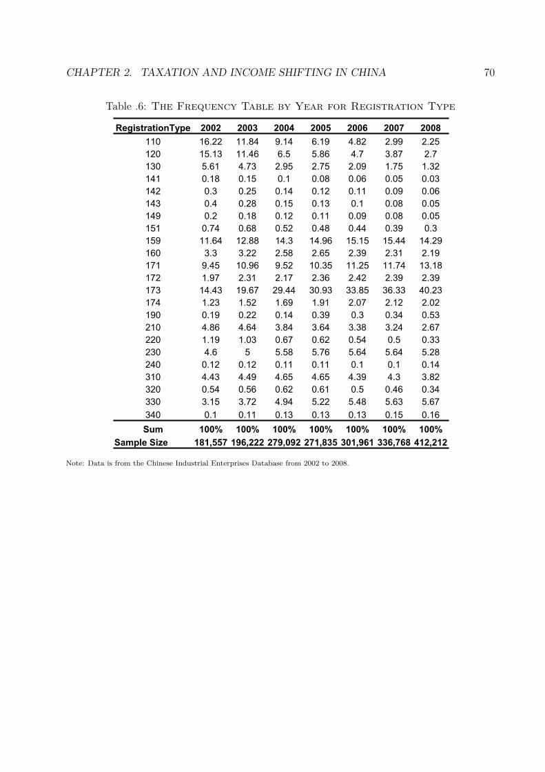
CHAPTER 2. TAXATION AND INCOME SHIFTING IN CHINA 70
Table .6: The Frequency Table by Year for Registration Type
RegistrationType 2002 2003 2004 2005 2006 2007 2008
110 16.22 11.84 9.14 6.19 4.82 2.99 2.25
120 15.13 11.46 6.5 5.86 4.7 3.87 2.7
130 5.61 4.73 2.95 2.75 2.09 1.75 1.32
141 0.18 0.15 0.1 0.08 0.06 0.05 0.03
142 0.3 0.25 0.14 0.12 0.11 0.09 0.06
143 0.4 0.28 0.15 0.13 0.1 0.08 0.05
149 0.2 0.18 0.12 0.11 0.09 0.08 0.05
151 0.74 0.68 0.52 0.48 0.44 0.39 0.3
159 11.64 12.88 14.3 14.96 15.15 15.44 14.29
160 3.3 3.22 2.58 2.65 2.39 2.31 2.19
171 9.45 10.96 9.52 10.35 11.25 11.74 13.18
172 1.97 2.31 2.17 2.36 2.42 2.39 2.39
173 14.43 19.67 29.44 30.93 33.85 36.33 40.23
174 1.23 1.52 1.69 1.91 2.07 2.12 2.02
190 0.19 0.22 0.14 0.39 0.3 0.34 0.53
210 4.86 4.64 3.84 3.64 3.38 3.24 2.67
220 1.19 1.03 0.67 0.62 0.54 0.5 0.33
230 4.6 5 5.58 5.76 5.64 5.64 5.28
240 0.12 0.12 0.11 0.11 0.1 0.1 0.14
310 4.43 4.49 4.65 4.65 4.39 4.3 3.82
320 0.54 0.56 0.62 0.61 0.5 0.46 0.34
330 3.15 3.72 4.94 5.22 5.48 5.63 5.67
340 0.1 0.11 0.13 0.13 0.13 0.15 0.16
Sum 100% 100% 100% 100% 100% 100% 100%
Sample Size 181,557 196,222 279,092 271,835 301,961 336,768 412,212
Note: Data is from the Chinese Industrial Enterprises Database from 2002 to 2008.

CHAPTER 2. TAXATION AND INCOME SHIFTING IN CHINA 71
Table .7: Overview of the Chinese Industrial Enterprises Database (2002-2008)
Year Sample Size
2002 181,557
2003 196,222
2004 279,092
2005 271,835
2006 301,961
2007 336,768
2008 412,212
Note: Data is from the Chinese Industrial Enterprises Database from 2002 to 2008.

CHAPTER 2. TAXATION AND INCOME SHIFTING IN CHINA 72
Table .8: Results for Difference-in-Difference Regressions (Dependent Vari-ables: log(Profit)
Independent Variable Model 1 Model 2 Model 3
Intercept 6.895*** 6.888*** 6.891***
(SE: 0.073) (SE: 0.073) (SE: 0.073)
AssetsReturn 0.002*** 0.002*** 0.002***
(SE: 0.000) (SE: 0.000) (SE: 0.000)
EnterpriseScale
"Large-Size" 4.433*** 4.490*** 4.427***
(SE: 0.033) (SE: 0.036) (SE: 0.033)
"Medium-Size" 2.078*** 2.115*** 2.078***
(SE: 0.011) (SE: 0.012) (SE: 0.011)
"Small-Size" 0 0 0
(SE: 0.000) (SE: 0.000) (SE: 0.000)
DebtRatio -1.406*** -1.407*** -1.405***
(SE: 0.014) (SE: 0.014) (SE: 0.014)
treatment 0.734*** 0.728*** 0.732***
(SE: 0.012) (SE: 0.012) (SE: 0.012)
postlegislation 0.521*** 0.521*** 0.521***
(SE: 0.008) (SE: 0.008) (SE: 0.008)
(treatment*postlegislation) -0.346*** -0.291*** -0.223***
(SE: 0.017) (SE: 0.018) (SE: 0.019)
(treatment*postlegislation*dummy_LargeSize) -0.326***
(SE: 0.083)
(treatment*postlegislation*dummy_MediumSize) -0.220***
(SE: 0.029)
(treatment*postlegislation*dummy_HMT) -0.268***
(SE: 0.022)
Note: * Statistically significant at the 10% level ** Statistically significant at the 5% level *** Statistically significant at the 1%
level. The estimated coefficients of other control variables are omitted. The mean, median, and standard deviation of the depen-
dent variable are 7.042, 7.056, 1.981 respectively. Data is from the Chinese Industrial Enterprises Database from 2002 to 2008.
Profit is the pre-tax profit. Control group is the domestic enterprises. Treatment group is the foreign investment enterprises.
log(Profit) is the dependent for Model 1, 2 and 3. The regressors for Model 1 are AssetReturn, EnterpriseScale,DebtRatio,Z
(controls including location and industry), treatment, postlegislation and an interaction treatment × postlegislation.
The regressors for Model 2 include AssetReturn, EnterpriseScale,DebtRatio,Z (controls including location and industry),
treatment, postlegislation and interactions treatment× postlegislation, treatment× postlegislation× dummyLargeSize and
treatment×postlegislation×dummyMediumSize. The regressor for Model 3 are AssetReturn, EnterpriseScale,DebtRatio,Z
(controls including location and industry), treatment, postlegislation and interactions treatment × postlegislation and
treatment× postlegislation×DummyHMT .

73
Chapter 3
FDI Spillovers and the InvestmentClimate
3.1 IntroductionThis paper looks into the productivity enhancing effects of foreign firms on domestic
firms (spillovers) from foreign direct investment (FDI). Such spillovers from FDI is has beena subject of debate in both the policy arena and academia for many years. Since the early1990s private capital flows have exceeded official foreign assistance to developing countriesand most of it is in the form of foreign direct investment. At the same time, governmentsin developing economies have made numerous policies to attract FDI in order to spur eco-nomic development. Those policies are based on the expectation that FDI could increaseproductivity in the economy. Such both directly through investment in a Greenfield ventureor acquisition of a domestic firm and indirectly through positive productivity spillovers onother domestic firms. Whereas there is a great deal of evidence that foreign owned firmsare more productive than domestic firms, the evidence on the FDI spillovers is mixed. Thispaper uses a firm-level panel data of European economies to increase our understanding asto when, where and under what conditions FDI has positive spillover effects on domesticfirms, and hence could improve national welfare. In particular, the hypothesis of wether andhow investment conditions could enhance FDI and FDI spillovers has been explored.
Studies have shown that one justifications of subsidizing incoming foreign investment isthe externality in the form of productivity spillovers. Productivity spillovers refer to theincrease in productivity due to the presence of foreign firms. In the case of such positivespillovers, multinationals do not fully internalize the value of these benefits and governmentpolicies to promote FDI improves economic welfare. We define horizontal spillovers as occur-ring when domestic firm productivity is positively affected by firms with foreign presence inthe same sector, while vertical spillovers occur when domestic firms are affected by firms withforeign equity in the upstream (forward linkage) or downstream sectors (backward linkages).

CHAPTER 3. FDI SPILLOVERS AND THE INVESTMENT CLIMATE 74
The transfer of technology is considered as one form of externality. Such a technologytransfer can occur through a number of channels such as the transfer of managerial practices,production methods, marketing techniques or any other knowledge embodied in a product orservice. For example, local firms may learn to imitate a new process or improve the qualityof their product through observation, interaction with foreign managers, and from employeesof foreign multinational corporations. Local firms may also benefit from the entry of newprofessional services or suppliers as a result of such multinations’ entry. Foreign firms mayact to catalyze domestic suppliers to improve the quality or efficiency of their good or serviceby demanding higher standards. On the other hand, foreign firms may have a negative effecton domestic firms’ output and productivity, especially in the short run, if they compete withdomestic firms for their market share or their best human capital. As domestic firms cutback production they may experience a higher average cost and higher unemployment, whichmay lower the overall economic welfare.
This paper explores futher the implications for policies toward FDI. There have beenmany FDI policies regarding FDI but they differ tremendously. Results from this study shedsome light on the question which FDI policies best promote host countries’ development; forinstance, whether host country’s productivity is boosted most by requiring host countriesto share technology with domestic firms, or by allowing foreign firms to access all domesticindustries, or by providing special treatment to lure foreign investors to choose the hostcountry as a base for operations?
A new and unique dataset from the World Bank, Investing Across Borders, allows usto be the first work to test these hypotheses with a rich information of FDI policies. Thisdata is a cross-country set of indicators that records and scores each countries’ FDI specificinvestment environment. Using such a comprehensive data plus a cross-country firm-levelpanel, this study contributes to the literature by providing evidence of the effectiveness ofthese FDI policies.
3.2 Literature OverviewA number of papers test for productivity spillovers for domestic firms from foreign direct
investment. In this sections extensive evidence of FDI spillovers will be reviewed. Theearlier literature on FDI spillovers generally explore how foreign presence brings productivityexternality in the same industry (horizontal spillovers), while more recent literature showsevidence on productivity externalities in the upstream or downstream industries (verticalspillovers).
Studies for horizontal spillovers use firm panel data to study whether the productivityof the domestic firms is correlated with the extent of foreign presence in the same sec-tor. Research by Haddad and Harrison (1993) on Morocco, Aitken and Harrison (1999) onVenezuela, Djankov and Hoekman (2000) on the Czech republic, Konings (2000) in Bulgaria,Romania, and Poland has failed to find positive horizontal spillovers to domestic firms. The

CHAPTER 3. FDI SPILLOVERS AND THE INVESTMENT CLIMATE 75
results cast doubts on such gains from FDI. However, evidences are found that positive hori-zontal spillovers are present in industrial countries. Haskel et al. (2007)’s estimated a robustand significant 0.5% increase in the domestic plants’ TFP given a 10% increase in the sameindustry’s foreign presence in UK. Using data in the United States from 1987-1996, Kellerand Yeaple (2009) find large FDI spillovers that accounts for 14% of growth in productivitygrowth for US firms.
Such pattern for horizontal spillovers is argued to be an outcome due to the capability ofthe domestic firms to improve productivity from technology transfers. The negative spillovereffect found in the less developed countries is argued to the result of low level of technologytransfers to the domestic firms. There is also a hypothesis explaining the evidence thatpositive spillovers are found in more technologically advanced sectors or in the more indus-trialized countries, for instance UK and US. It is argued that the larger the technology orhuman capital gap between the domestic and foreign firms, the less likely the domestic firmswill benefit from FDI. By using a variable of the share of the population with high school orhigher education as a proxy of human capital, Borensztein et al. (1998) show that FDI is animportant vehicle for the transfer of technology and economic growth, but only in countrieswhich have human capital stock above a minimum threshold. Their study uses data on FDIflows from industrial countries of 69 developing countries. Blalock and Gertler (2004) havefound that plants with more highly educated employees benefit more from the presence ofmultinational firms using firm-level data in Indonesia.
A recent stream in the literature argues that FDI is more likely to have positive pro-ductivity spillovers on the host country if the economy is open. Moran et al. (2005) foundevidence using measures of openness by trade, FDI and competitiveness. In contrast, FDI islikely to worsen economic welfare of the host country in protected and distorted economies.Moran et al. (2005) have stated that “Foreign investors in countries with domestic content,joint venture and technology sharing requirements deploy production technique lagging farbehind the frontier in international industry. Foreign affiliates with older technology and lessefficient plants are not good candidates to develop from an infant industry to a robust worldcompetitor. Local firms that sell to foreign affiliates in protected market are often subscalein size and inefficient in operation...”
By using Indian data, Aghion et al. (2005) showed that firms with higher technologyare more likely to respond to liberalization by investing in new technologies. Blalock andGertler (2005) used Indonesian data to show that sectors with more competition have higherspillovers. However, Sembenelli and Siotis (2005) found that only firms in R&D sector havethis positive correlation between competition and spillovers, using Spanish data. Therefore,heterogeneous spillover effects may be caused by different level of liberalization and com-petition. This means that foreign affiliates tend to have more spillovers due to its betterbusiness environment.
While there are numerous studies on horizontal (intra-industry) spillovers, there are rela-tively few empirical studies on vertical spillovers. Moreover, vertical spillovers are more likelyto be positive than horizontal spillovers since multinational companies have an incentive to

CHAPTER 3. FDI SPILLOVERS AND THE INVESTMENT CLIMATE 76
improve the productivity of their suppliers but not their competitors. The few empiricalpapers find evidence that is consistent with of technology transfer through backward link-ages in the manufacturing sectors. In their seminal work, Javorcik (2004) and Blalock andGertler (2008), using firm-level data from Lithuania and Indonesia respectively, find thatthe FDI spillovers are more likely to be vertical than horizontal. They argue that becausemultinationals firms have incentive to prevent information or technology leakage to its do-mestic competitors, the magnitude of horizontal spillovers tend to be very small, if any. Atthe same time, multinationals may transfer knowledge or skill to their domestic suppliersto enhance their performance. They found supporting evidence for such backward linkages.However, these studies rely only on a variable that is constructed from input-output tablesat the industry level, rather than a direct firm-specific variable.
Research in institutional economics stressed the importance of institution on a country’slong-run development (Glaeser and Shleifer (2002), Acemoglu et al. (2001), etc.). A numberof research find out that laws, regulations, contract enforceability are important determinantsfor government and economic performance. Djankov et al. (2002) studies data of numberof procedures and time to start a new business that a start-up as costs of entry. They findthat countries with heavier regulation of entry have higher corruption and larger unofficialeconomies, but not better quality of public or private goods. Countries with more democraticand limited governments have lighter regulation of entry. This paper studies the impact of arange of institutional features (local restrictions, law and regulation, contract enforceability,etc.) on the direction and the magnitude of spillovers from FDI.
Research has provided both theoretical framework and empirical evidence that businessenvironment affects spillovers. First, firms in the sectors with more competition may havegreater FDI spillovers (Blalock and Gertler (2008) and Abraham et al. (2010)). Liberalizationmay lead to higher spillovers (Aghion et al. (2005)). They developed a simple Schumpeteriangrowth model to understand how firms respond to entry threat imposed by such liberaliza-tion. They show that firms in pro-business institutions are more likely to invest in newtechnologies and production processes, in response to foreign entry threat. They use Indiandata in the period of liberization (industrial delicensing) to empirically support their theory.Therefore, the first conclusion is that firms in an open and competitive environment will havegreater spillovers. In addition, better business environment also results in more advancedtechnology.
Second, imposing FDI or trade restrictions may not serve to promote host country’seconomic development. Some developing countries have adopted policy measures such asdomestic equity requirements, joint venture mandates and technology sharing regulations.Moran et al. (2005) have shown that “intrafirm trade” and “parental supervision” of multi-national corporations are potent channel for host country’s productivity growth. RestrictiveFDI policies are most likely to interrupt those channels of development and decrease thewillingness of foreign companies to share their technology. Their book shows more strik-ing evidence in restrictive economies, FDI is likely to worsen the host country’s economicwelfare: “If FDI is motivate by the desire to service a protected and distorted domestic mar-

CHAPTER 3. FDI SPILLOVERS AND THE INVESTMENT CLIMATE 77
ket,. . . Foreign firms may find it profitable to operate, but they may do so without bringingthe best technologies and/or using the country as part of their international supply network.By contrast, impact will likely be positive when FDI is motivated by the desire to participatefully in the international sourcing networks of the parent multinational, and operations areunrestricted by rules on ownership and local content.” It is also supported by the evidencethat unsuccessful FDI policies in Africa stems from those distorted and protected economieswhile China’s success results from its openness and the multinational’s intentions of in-creasing global integration. Thus, business environment will affect the quality of FDI andits spillovers. Poor business environment could lead to outdated technology and inefficientproduction processes.
Third, information transparency and credibility are also known to strengthen FDI gains.Government of the host country trying to attract foreign direct investment would face theinformation asymmetry problem (Akerlof (1970)). Unlike used car sellers, however, hostgovernments cannot offer warranties to reduce risks, but they could address this problemby providing transparent and up-to-date information regarding foreign investment. Rodrikand Hausmann (2004) argue that providing up-to-data information for the feasibility offoreign investment leads to information externality. A World Bank FIAS (Foreign InvestmentAdvisory Service) report by Wells and Wint (2000) shows reducing entry costs increases thesocial returns: Fours dollars of estimated returns for every dollar spent. And such entry costsinclude the search cost for foreign direct investors, credibility of information, and facilitatingsite comparison etc.
Four, strength of laws and protection of property rights are also known to affect FDI.Aizenman and Spiegel (2006) used a principal-agent framework where ex-post monitoringof contracts is more costly for foreign investors than for domestic ones to argue that theshare of FDI in total investment should be lower in countries with weak enforcement ofproperty-rights. Kaufmann et al. (1999) shows evidence that regulatory burden and rule oflaw correlates significantly with FDI, using a wide range of institution variables. La Porta etal. (1998) used the International Country Risk Guide to show that the risk of repudiation ofcontracts by government, risk of expropriation and shareholder rights do matter. Moreover,the investment environment tend to impact FDI spillovers through various channels. Gorod-nichenko et al. (2007) is one of the first paper to shed light on the impact of a country’sinstitutions, especially corruption and bureaucratic red tape, and the level of developmenton the strength of vertical and horizontal spillovers. They find positive backward spilloversfor the domestically owned firms raises a domestic firm’s efficiency. Their estimation alsosuggests that buying inputs from or competing with foreign firms confers positive spilloversonly for firms in the service sector. In addition, they found no evidence for the institu-tion environment could hence spillovers effects. Regarding its ownership relationship withspillovers, Javorcik and Saggi (2010) found that firms’ ownership structures may be corre-lated with the quality of FDI. For those foreign affiliates with more advanced technology, theownership tends to be full than joint-venture to protect their technology. Thus, such firmstend to have greater spillovers.

CHAPTER 3. FDI SPILLOVERS AND THE INVESTMENT CLIMATE 78
3.3 DataIn this study I use a large European panel which cover the firm-level information from
year 2005 to 2008. This database is a standardized commercial data called Amadeus collectedby about 50 vendors across Europe. There are two main database, the financial database andthe ownership data. These two dataset are provided by the vendor separately. The financialdata records over 10 million firms’ basic financial statements, which covers the business pro-files, the balancesheet information, the cash flow/profit information and key ratios of bothpublic and private companies across 41 European countries. The ownership data containthe ownership/shareholder information. In particular, it identifies the shareholders’ countryof origin and the percentage of its ownership. In this study I use a subsample of the firmswith non-missing ownership information. For my research it is important to identify foreignfirms for each country each year. But I do not observe a firm’s foreign investment directlyin this dataset. In order to identify which FDI from this firm level data, I use the owner-ship information from the European panel to extrapolate such information. This databaseprovides information on firm ownership, with information of its major shareholders. Basedon such ownership information and the total asset value, the foreign asset holdings for eachcompany is calculated for each year. The value of firm-level foreign direct investment (FDI)in year t is the difference in value between foreign asset holdings at year t and year t-1.Following Gorodnichenko et al. (2007), my sample covers both the manufacturing and theservice sectors, excluding only the utility and financial firms. More firms are analyzed in thepaper while earlier research focuses on the manufacturing industries only.
To study how investment climate impact the strength of FDI spillovers, this paper utilizesthe Investing Across Borders (IAB) indicators. The Investment Climate Advisory Services ofthe World Bank Group constructed the indicators in July 2010. They measure FDI regula-tion across 87 economies. The indicators measure openness to FDI through equity ownershippermitted in various sectors (11 indicators), ease of starting a foreign business (3 indicatorsincluding the time spent and procedure to go through staring business), arbitrating com-mercial disputes (3 indicators which measure how well court systems develop), and accessingindustrial land (6 indicators that scores land availability). In this study all the above indica-tors are used to test the validity of hypotheses based on different sets of investment conditionmeasures. The data are compiled from detailed surveys filled out by over 2,300 respondentsall over the world. In terms of the coverage of topics, sectors, and countries, this dataset onFDI regulations is the most comprehensive to date (Wagle (2010)).
Table .2 shows the summary statistics for the whole sample. Columns 1 to 6 lists sum-mary statistics for key variables (sales, capital, labor, material costs; horizontal, forward andbackward linkages) for six European countries—Bulgaria, Czech Republic, France, Poland,Romania and Spain. The selection of such a sample is based on the availability of key vari-ables, ownership data and input-ouput tables. This is a firm-level database which containsover half a million observations. But the quality of the data varies across countries: Spainhas the best data, which covers over half of the whole sample. France has the second largest

CHAPTER 3. FDI SPILLOVERS AND THE INVESTMENT CLIMATE 79
share contributing over 20% of the sample. As the table shows, there is also variation ofkey variables across countries. French firms seem to have much lower value for all variables.There is also large dispersions for horizontal linkage and forward linkage.
The original sample of IAB indicators contains 87 countries and the European databaseconsists of company information for 41 European countries. However, the available Input-Output tables restrict our samples to ten European countries. Within the sample of these tencountries, four countries have most of their financial information missing, which disqualifythe extracted sample for economic analysis. For the rest of the countries, the final samplefor analysis also shrinks significantly from the original sample.
The IAB indicators are divided to four categories to reflect various aspect of a country’sinvestment climate: Investing Across Sectors indicators, Starting A Foreign Business indica-tors, Accessing Industrial Land indicators and Arbitrating Commercial Disputes indicators.1. The Investing Across Sectors indicators measure the maximum percentage of ownershipallowed across 33 subsectors. In this paper, I construct a country-level ownership indicatorby averaging all the sector-specific ownership within a country. The higher the indicator, themore open a country is towards foreign direct investment. 2. Starting A Foreign Businessindicators consist of three major indicators that measures the easiness of a foreign companyfor starting a business in the host country. The Ease of Establishment indicator scores theoverall environment foreign companies face to set up a business. Higher scores mean lessdifference in treating domestic and foreign business for business establishment. The Numberof Procedures indicator records the official procedures required to start a business, both pre-and post- incorporation. The Time in Days indicator is the days taken to comply with all theofficial requirement to start a business. 3. The Access Industrial Land indicator measuresthe easiness of land access for foreign business. The Time to Lease Public Land indicatorshows the days taken to lease land from the government. The Time to lease Private Landindicator shows the days taken to lease land from a private owner. The Availability of LandInformation index is constructed based on the availability of 18 pieces of information regard-ing land plots. The Access to Land information index measures the easiness of a foreignbusiness to obtain land information, based on how well a country’s land registry maintainsand shares land data. The Strength of Lease Rights index analyzes the degree of restrictionsa foreign-owned company face to lease land. The Strength of Ownership Rights Index mea-sures the restriction in terms of purchasing land by a foreign business. 4. The ArbitratingCommercial Disputes indicators capture the important legal aspect of a country’s investmentclimate. The Strength of Law index scores a country’s overall legal framework for disputeresolution. The Ease of Arbitration Process index captures the degree of restrictions andobstacles a foreign company faces in seeking a dispute resolution. The Extend of JudicialAssistance Index measures the effectiveness of interactions between arbitral tribunals anddomestic courts.
Table .3 shows the summary statistics of the IAB indicators. The first two columns showthe mean and standard deviations for each indicator for the six country in my sample. It iseasily observed that there is no variation across these countries for the variable Strength of
CHAPTER 3. FDI SPILLOVERS AND THE INVESTMENT CLIMATE 80
Ownership Rights. In fact, all six countries have scores of 100 for this variables. Therefore,there would not be any information derived from this variable, thus it is excluded for furtheranalysis. The observations of most of the indicators are on a scale of 100, except for theprocedure and time to start foreign business, time to lease public and private land. Therest of the columns show the correlations among all indicators. These correlations showthe necessities of constructing various indicators of investment climate. They help us tounderstand a country’s investment climate in different aspects. Not all the indicators arepositively correlated, meaning that investment climate measures are not all consistent. Forexample, a good investment climate defined by Average Ownership may well be measured asbad using Strength of Leaser Rights indicator, due to the very negative correlation (-83%)between the two indicators.
3.4 MethodologyTo examine the relationship between domestic firms’ productivity and FDI in the same
industry or other industry, I apply the approach used by early literature (Javorcik (2004),Gorodnichenko, Svejnar and Terrell (2007), Du, Harrison and Jefferson (2011)) that is char-acterized by the following equation for estimation.
lnYi,j,k,t = α+ β1lnKi,j,k,t + β2lnLi,j,k,t + β3lnMi,j,k,t
+ β4ForeignSharei,j,k,t + β5Horizontalj,t + β6Backwardj,t + β7Forwardj,t
+ β8Horizontalj,t · IABk + β9Backwardj,t · IABk + β10Forwardj,t · IABk+ τt + ηj + ψk + εi,j,k,t
Yi,j,k,t stands for the real output from firm i operating in sector j and country k at timet. Labor is the number of employees. Mi,j,k,t is the firm’s material cost. ForeignSharei,j,k,tshows what the proportion it is for foreign investors.
Horizontalj,t is constructed to capture the extent of foreign presence in sector j at timet. It is defined as the foreign ownership averaged over all firms in one sector:
Horizontalj,t =∑i∈j ForeignSharei,t · Yi,t∑
i∈j Yi,t
This variable measures the of share of foreign output in one industry. The same measureis adopted in Javorcik (2004) to capture the industry’s foreign presence. The larger thisvariable is, the more foreign equity or more foreign output for one industry. Backwardj,tproxies for the foreign presence in the downstream industries of sector j—industries that aresupplied by industry j. Such a variable captures the relationship between domestic suppliers

CHAPTER 3. FDI SPILLOVERS AND THE INVESTMENT CLIMATE 81
and foreign customers.
Backwardj,t =∑h ̸=j
αj,h ·Horizontalh,t
αj,h denotes the share of sector j’s output supplied to sector h, taken from Input-Outputtable at the two-digit NACE level. NACE is the standard industry classification for Eu-ropean companies. The exact firm-level information of upstream-downstream relationshipwould be ideal for this study. Since such detailed information is not available and the bestinformation of upstream-downstream relationship can be obtained is industry level, industrylevel measure of downstream foreign presence is proxied using industry-level information.Here inputs supplied within the same sector are excluded, since any effect would already becalculated in the Horizontal variable. The greater the foreign presence in the downstreamindustries, the higher the value of this. Forwardj,t captures the foreign presence in sectorj’s upstream industries—industries that supply industry j:
Forwardj,t =∑m̸=j
βj,m ·Horizontalm,t
Here βj,m is the proportion of inputs purchased by j from sectorm. Similar toBackwardj,t,the greater the foreign presence the upstream the higher this value is. Such constructionmakes all these variables both sector-specific and time-varying. Table 2 shows the Input-Output tables to use for the sample countries from 2005 to 2008. Because the input-outputrelationship between sectors may change overtime, using year-specific input-output matriceswould be ideal. Unfortunately, it shows that not all the tables are available for every year.In fact, most of the IO tables are not available. For those years where tables are unavailable,available tables that are in closest years are used instead. For example, since the 2008 IO ta-ble is not available for Czech Republic, the table for 2007 is used instead. This methodologyis also applied in other FDI spillover literature such as Javorcik (2004).
Table .3 shows the summary statistics of key variables for the six countries included in mysample. French firms seem to be distinctive in terms of the mean of log sales, capital, foreignshares, as well as spillover variables (horizontal, forward and backward linkages). Valuefrom all other countries are in similar magnitudes. Spanish companies cover more than halfof the entire sample (368,609 out of 671,961 observations) and the smallest sample comesfrom Czech Republic (5,547 observations). Therefore, power of country-specific statisticalestimation will depend on the sample size of each country. The smaller the sample size, theweaker the econometric tests.
Table .4-.9 shows the time-varying measures of horizontal, forward and backward linkagesfor each country. One can observe that those measure could change dramatically within oneyear, such as for Bulgaria, but not much so for countries like Poland. There are a feweconometric issues in the analysis. There could be firm-specific, region-specific or country-specific omitted variable bias. This may bias the relationship between productivity and

CHAPTER 3. FDI SPILLOVERS AND THE INVESTMENT CLIMATE 82
foreign presence. I will use time-differencing and control for the year, region, industry andfirm fixed effects.
△lnYi,j,k,t = β1△lnKi,j,k,t + β2△lnLi,j,k,t + β3△lnMi,j,k,t + β4△ForeignSharei,j,k,t+ β5△Horizontalj,t + β6△Backwardj,t + β7△Forwardj,t+ β8△Horizontalj,t · IABk + β9△Backwardj,t · IABk + β10△Forwardj,t · IABk+ τt + ηj + ψk + εi,j,k,t
The above specification reduces the noise in estimation and gives more weight to persis-tent changes in the variables of interest. However, differencing on the data means a reductionof sample size. Taking longer lags makes the sample even smaller. If estimated by OLS, thisanalysis has some identification limitations. Griliches and Mairesse (1995) argues that OLStreats labor and other inputs as exogenous variable, but they should be endogenously deter-mined based on productivity. Treating those inputs as exogenous will bias the results. Olleyand Pakes (1996) used a semiparametric estimation to allow for idiosyncratic firm produc-tivity over time. They assume that firms choose their desired capital stock and other inputvariables in the beginning of every period:
ki,t+1 = (1− δ)ki,t + ii,t
I take logs of the Cobb-Douglas production function:
lnYi,t = α+ βllnLi,t + βklnKi,t + βmlnMi,t + ωi,t + ηi,t
ωi,t is productivity and ηi,t denotes random error. Both of them are unobserved; thedifference between the two is that ωi,t is a state variable in firm’s decision problem, hencea determinant of factor inputs (Li,t, Ki,t, Mi,t). But ηi,t does not correlate with inputs.Estimation of the above model would yield biased results, because inputs are determinedbased on the firm’s expectation of ωi,t. And if there is serial correlation in ωi,t, current periodinputs will be positively correlated with it; in this case, an OLS procedure is likely to yieldresults with coefficients on inputs biased upwards. Since investment is a function of capitalstock and firm productivity:
ii,t = ii,t(ωi,t, ki,t)
Because the investment function if strictly monotonic in productivity, one can invert theabove equation to write the unobservable ωi,t as a function of the observables:
ωi,t = hi,t(ii,k, ki,t)
The above equation allows us to write the unobservable productivity variable ωi,t as afunction of observables. Such a formulation enable me to control for productivity in estima-tions. Olley and Pakes (1996) make two assumptions: First, there is only one unobservable
CHAPTER 3. FDI SPILLOVERS AND THE INVESTMENT CLIMATE 83
in the above equation. Second, investment is an increasing function of productivity. Al-though they are strong assumptions, Olley and Pakes (1996) argue these assumptions yieldtwo advantages: They give rise to a simple estimation algorithm for production function pa-rameters without relying on more assumptions necessary to fully specify equilibrium. Theseassumptions also generate an overidentified model and allows me to directly test these as-sumptions.
Substituting the above equation into the Cobb-Douglas function. Now the equationbecomes:
yi,t = α+ βlli,t + βkki,t + βmmi,t + hi,t(ii,t, ki,t) + ηi,t
= α+ βlli,t + βkki,t + ϕi,t(ii,t, ki,t) + ηi,t
Where yi,t, li,t, ki,t, mi,t denote the logarithm value of Li,t, Ki,t, Mi,t. In the first stageof estimation, the consistent estimates of coefficients on labor, materials and the form ofa non-parametric term ϕi,t will be obtained. But βk can not be estimated consistently inthis stage. The second step identifies the coefficient for capital by using a non-linear leastsquares.
yi,t − βlli,t − βmmi,t = ϕi,t(ii,t, ki,t) + εi,t
The above equation highlights the needs for the first stage of estimation of ϕi,t(ii,t, ki,t).Since ϕi,t is mean independent of variables pre-determined at the beginning of period t,ϕi,t(ii,t, ki,t) is mean independent of the pre-determined state variable ki,t. However, labordecision li,t is a function of ϕi,t. Such correlation calls for the first stage estimation. Forsimplicity, ϕi,t(ii,t, ki,t) is estimated by a series of polynomials. The second stage substitutethe estimated ϕi,t into the formula and run non-linear least squares for the Cobb-Douglasequation.
There are two important assumptions with this estimation procedure. One is the first-order Markov assumption of productivity ωi,t, and the timing assumption about capitalaccumulation. The first-order Markov assumption decomposes it into its conditional expec-tation at time t−1, 𝔼 (ωi,t|ωi,t−1) and a deviation from that expectation, ωi,t−𝔼 (ωi,t|ωi,t−1),which is the innovation of the productivity. These two assumptions allow it to constructan orthogonal relationship between capital and the innovation component in productivity,which is used to identify the coefficient on capital. However, one disadvantage of applyingthe Olley-Pakes procedure is that many firms report zero or negative investment. To addressthis problem, I also explore the robustness of the results to using the Levinsohn and Petrin(2000) approach. With the Olley-Pakes correction, I can get an unbiased estimate of thefirm’s productivity. Therefore, I could derive the total factor productivity (TFP) instead ofthe log of output, which is the difference between the actual and predicted output:
tfpi,t = yi,t − βlli,t − βmmi,t − βkki,t
Specifically, this is a two-stage estimation procedure when using TFP as the dependent

CHAPTER 3. FDI SPILLOVERS AND THE INVESTMENT CLIMATE 84
variable. The first step follows Olley-Pakes procedure to obtain unbiased coefficients oninput variables and then calculate TFP (residual from the production function). The secondstep is to regress TFP on firm-level controls and FDI variables.
3.5 Estimation
Estimation of FDI SpilloversThis section shows how investment environment, in particular the FDI-related policies,
could impact productivity spillovers. There has been a recent strand of literature that explorethe relationship between countries’ institutional features and FDI spillovers. Moran et al.(2005) shows evidence that countries that are more open trade and FDI policies enjoy morebenefits from FDI. For countires with more protective regulations, FDI could have negativeimpact on the productivity of the host country. Using a sample of European companies, Ifirst test the traditional hypothesis on the channels of FDI spillovers—the forward, backwardand horizontal linkages related the specification below:
lnYi,j,k,t = α+ β1lnKi,j,k,t + β2lnLi,j,k,t + β3lnMi,j,k,t + β4ForeignSharei,j,k,t
+ β5Horizontalj,t + β6Backwardj,t + β7Forwardj,t
+ τt + ηj + ψk + εi,j,k,t
I use the baseline OLS and two-stage OLS to estimate the above model. The two-stageOLS follows the usual treatment in the literature: I first obtained the TFP residual fromthe first step regressions and the second step regressions produce the coefficients of interestsfor channels of FDI spillovers.
Table .10 shows results from the ordinary least squares for six countries. Column 1-6shows baseline OLS results for each country and Column 7 shows results using the entiresample. There has been a drop in observations for all countries, due to the missing ob-servation of differencing each variable. Not surprisingly, most coefficients on productionfactors (labor, capital, material) are positive and significant. There is not much effect offoreign share on the company’s sales. The most important analysis is for the spillover effect.The table shows significant and positive spillovers effect via backward linkages for Romania,Spain and the whole sample. This results is consistent with the finding in the recent liter-ature that FDI improves economic productivity by enhancing the performance of upstreamcompanies. However, this coefficient for France is the opposite. For France and the wholesample, spillover tend to impact productivity negatively through horizontal linkages. Thisis likely due to the fact the entering of a more competitive foreign business reduces not onlythe incumbents’ but also the overall sales in the same industry. And there seems to be somenegative effects of forward linkages measures.
Table .11 provides a slight alternative empirical model to the OLS–the two-stage OLS

CHAPTER 3. FDI SPILLOVERS AND THE INVESTMENT CLIMATE 85
model. The upper panel shows the first stage regression results, while the lower panel showsthe second stage results. In the first stage, log sales are regressed on production facts andthe residual are derived as the total factor productivity (TFP). All the coefficients in thefirst stage are significant and R-square vary from 20% to around 50%. which accounts fortime-invariant unobservable characteristics. The R-squares for the second stage is quite small(all of them are less than 1%). This low R-square is partly because variables for spilloverchannels are industry-level measures thus less explanatory power. The two stage OLS resultsare very similar to the baseline OLS results. Backwards linkage could be observed for thewhole sample, but not for individual countries. The backward linkage seems to contributepositively to productivity, which is consistent with previous research. However, for eachindividual country, the effect diminishes—there is no significant backward linkage effect forBulgaria, Czech Republic and Poland, and French data even shows negative signs.
These baseline results confirm the previous finding of the recent research that FDI im-proves productivity via backward linkages. However, results seem to be noisy for individualcountries. And because spillover variables (horizontal, backward, forward) are country-specific measures. Their interactions with IAB ownership data would be correlated withthemselves, generating a collinearity problem. Therefore I will use the whole sample forfurther analysis for investment climate’s productivity enhancing effect.
Estimation of the Investment ClimateThis study future explores how FDI environment could impact the productivity spillovers
from FDI. The World Bank’s Investing Across Borders indicators are used to quantify acountry’s openness to the foreign direct investment. These indicators cover various aspectsof a country’s investment climate: foreign ownership index, easiness of starting a foreignbusiness, foreign access to land and easiness of arbitrating commercial disputes.
In this section, the impact of each indicator on FDI spillover is tested and examined indata. Recent research has shown some evidence that investment environment may affect FDIspillovers. A more competitive and open environment may enable domestic firms to betterabsorb productivity gains from foreign investment. Such empirical exercises have importantimplications for a country’s development of investment environment. Moran et al. (2005)argue that in market with worse investment environment, foreign firms’ suppliers are sub-optimal in terms of size and operation efficiency. Blalock and Gertler (2008) and Abrahamet al. (2010) find empirical support that positive spillover effect happens in industries thatare less restrictive and more competitive.
All four sets of Investing Across Borders indicators reflect a country’s openness to for-eign investments, however they measure quite different aspects of investment environment.Foreign ownership indices measure the maximum of foreign ownership allowed across themain sectors. Coefficients on the interactions of horizontal, backward and forward measuresthe incremental productivity contribution of FDI environment via the horizontal linkage,

CHAPTER 3. FDI SPILLOVERS AND THE INVESTMENT CLIMATE 86
backward linkage and forward linkage, respectively.
lnYi,j,k,t = α+ β1lnKi,j,k,t + β2lnLi,j,k,t + β3lnMi,j,k,t
+ β4ForeignSharei,j,k,t + β5Horizontalj,t + β6Backwardj,t + β7Forwardj,t
+ β8Horizontalj,t · IABk + β9Backwardj,t · IABk + β10Forwardj,t · IABk+ τt + ηj + ψk + εi,j,k,t
Table .12 shows the results from the above specification using IAB’s variable on the av-erage ownership limit across industries. Each column shows results from one econometricspecification: Baseline OLS, Two Stage OLS, and Olley-Pakes. Olley Pakes method is usedto correct for the simultaneous choice problem. The first stage of the two stage Olley-Pakesis using the Olley-Pakes model to derive the total factor productivity (TFP). The secondstage is to estimate the effects of other variables on TFP. Across all specifications, the coeffi-cients on production factors are positive and significant. The foreign share is likely to affectproductivity only in the Olley-Pakes specification. In these estimations, FDI tends to havea negative effect on productivity via backward linkages, with exception for the Olley-Pakesmodel. The ownership limit seems to directly influence productivity in a positive way, whichimplies that the higher the foreign ownership is allowed, the higher the productivity is. Thisis a direct evidence of the impact of investment climate on productivity. And the coeffi-cients on the interaction term of backward linkage variable and the ownership variable aresignificant and positive for most of the specifications. This shows the evidence of a positiveincremental effect of investment climate on FDI spillovers via backward linkages. The higherthe ownership limit a country has, the more the upstream company’s productivity improvesin response to more foreign presence. This finding is consistent with the finding from theFDI literature. Aghion et al. (2005) developed a model to understand that firms are morelikely to adopt new technology hence increase productivity in a more open and competitiveenvironment. Blalock and Gertler (2008) and Abraham et al. (2010) show evidence thatmore competitive environment leads to more productivity spillovers. Moran et al. (2005)also argue that restrictive FDI policies such as foreign equity restrictions will harm ratherthan boost economic development.
Table .13 uses another IAB measure, the index of easiness of setting up a foreign business.Because most coefficients on the index are positive, there is evidence that easiness of settingup foreign business have a direct productivity gain. However, unlike the previous results,easiness to set up foreign business hardly affects FDI spillovers. This index measures how theinstitutional environment encourage the entry of FDI. Unlike “hard” factors such as FDI lawand regulations, this indicator reflects the soft side of government effectiveness regarding FDIinflows. Kaufmann et al. (1999) find that government effectiveness appeared to a significantdeterminant of FDI. Results from Table 13 complement their finding by showing the evidenceof a correlation between government effectiveness and FDI productivity gain.
Table .14 shows the results using the number of procedures required to start foreign

CHAPTER 3. FDI SPILLOVERS AND THE INVESTMENT CLIMATE 87
business. This indicator also reflects the effectiveness of a government. More complicatedprocedures suggest a less efficient government. First, there is a direct effect of number ofprocedures on productivity. Most of the coefficient on number of procedures are negative,meaning that the less procedures to set up a foreign business, the more productivity acountry gains. The coefficients on the interaction term with backward linkages show mixedresults. This indicates that number of procedures have an ambiguous effect on spillovers viabackward linkages.
In addition to number of procedures to set up foreign business, Table .15 analyzes the timeto set up foreign business. It is a nice complement to the first two indicators that reflect theeffectiveness of institution to serve foreign direct investment. The negative and significantcoefficients indicate that such a measure of investment climate might have an enhancingeffect of productivity. The coefficients for the interaction term with forward linkages arenegative, which implies less time in setting up foreign business might increase productivityvia forward linkage. However, positive coefficient indicate an adverse incremental spillovereffect of time on productivity via backward linkage. Similar to the establishment of businessindices, the next two indicators above also to some extent reflect the effectiveness of agovernment. The time spent to lease public or private land could involve a number ofprocedures. And the more procedures the institution requires, the longer the process willbe. Existing literature only draws conclusion on more aggregate measures of governmentmeasures and did not break down to various aspects of government effectiveness. Thesenew indicators are excellent contribution to the current FDI literature. Table .16 showsthe effect of time to lease public land. The direct effect of this measure on productivityis mixed. The coefficients on the interactions with the forward spillovers linkage appearsignificant and positive, which suggest a weakening effect for the forward spillovers. Themeasurement with time to lease private land is explored in Table .17. First, the coefficientson this measurement are positive. This indicates the counter-intuitive effect that longer timemight be value-adding. And positive and negative coefficients on the interaction terms withforward and backward suggests weakening effect for FDI spillovers via forward linkages andenhancing effect via backward linkages.
Table .18 shows the results with measurement of availability of land information. Nega-tive signs on the land information availability measure and interaction with the horizontalvariable imply a negative direct productivity effect and a negative FDI spillovers effectthrough horizontal linkages. Access to land index is analyzed in Table .19. Similar to theprevious measure, all the negative coefficients seem to suggest results that better access toinformation lead to less productivity and lower spillover effects. Information asymmetry hasbeen known to be a crucial barrier to foreign investment. There has been a series of impor-tant research that studies the relationship between information and FDI. But such researchremains small because of the lack of data. The results from this paper contributes to ourunderstanding of this issue. Rodrik and Hausmann (2004) and Wells and Wint (2000) arguethat providing credible and up-to-date information is yield significant social returns. In thisresearch, however, such a productivity gain does not have empirical support from my data.

CHAPTER 3. FDI SPILLOVERS AND THE INVESTMENT CLIMATE 88
The next set of investment climate indicators measures the strength of law and protectionof property rights. Aizenman and Spiegel (2006) shows theoretically that FDI should beworse in weaker enforcement of property rights due to the difference in ex-post monitoringcost between foreign and domestic investors. La Porta et al. (1998) and Kaufmann et al.(1999) provide empirical support of this view. However, to the my knowledge there hasnot been any theoretical research that studies how the strength of law and property rightsprotection affects the gain from FDI has not been tested before. This is the first research toprovide empirical evidence of this issue. Table .20 shows the effect of strength of lease rightson productivity. It seems to suggest a negative effect for the productivity gain for weakerlease rights. The spillover effects through various channels show mixed results. The extentof judicial assistant measures legal environment for foreign investment. Table .21 showsempirical results using this measure. Positive coefficients on this measure suggest positivedirect productivity effects. But negative coefficient for the interaction term indicates aweakening effect for the FDI spillovers via the backward linkage. The IAB ease of processindicator for arbitrating commercial disputes reflects another aspect of a country’s legalenvironment. Estimations in Table .22 suggest a negative direct productivity effect and anegative incremental effect on FDI spillovers via backward linkages. But there is evidenceof a spillovers enhancing effect through forward linkages. Table .23 shows the IAB strengthof law indicator’s effect. Negative coefficients on this measure suggest negative productivityeffect. There seems to be some evidence of positive productivity effect through backwardlinkage.
The results in this paper vary a lot for different measures of investment climate. Theownership limit measure seems to have both direct positive effect on productivity and pos-itive incremental effect on productivity spillovers through backward linkage. Such a resultsis consistent with the findings of the existing literature. The three starting foreign busi-ness indicators show positive direct effect on productivity but mixed results on incrementalspillover effect. It provides some evidence in support of the current view in academia re-garding the relationship of government effectiveness and FDI. The other two categories ofindicators show results that are more noisy. Nonetheless they provide new evidence for theset of important issues that have not been studied much in the literature before due to thescarcity of cross-country and reliable data.
3.6 ConclusionThis paper studies productivity spillovers to domestic firms from foreign direct investment
(FDI). Such productivity gain from FDI is considered to be the basis of policies that promoteFDI all around the world. Although such policies are widely adopted, they are still underdebate both in the policy and academic arena. The contribution of this paper is to providenew evidence and justification on how investment climate could impact productivity gain.
The new World Bank’s Investing Across Borders dataset which records and scores a coun-

CHAPTER 3. FDI SPILLOVERS AND THE INVESTMENT CLIMATE 89
try’s FDI environment in foreign ownership restrictions, establishment of foreign business,land access and strength of law, plus a large panel data of European firms provides greatopportunity to study the important issue on how a country’s investment environment impactproductivity gain, either by evidence of a direct effect, or via externalities on upstream in-dustry. This research contributes to the existing literature by a set of novel empirical resultsregarding different aspects of investment climate.
Consistent with the existing literature, this paper suggests that ownership has a signifi-cant positive impact on productivity gain of FDI. It suggests that allowing more foreign own-ership could have a favorable impact on economic development. There is also some evidencethat more effective procedure to establish business also have a positive effect. Removing re-striction or improving procedure could have a positive effect on productivity. However, theresults vary significant for different measures of investment climate. The effect of changes inland restrictions and legal environment could yield more mixed results on FDI.
This research studies the relationship between the institutional structure and FDI. How-ever, there has been many other aspects of FDI policies that has not been addressed. Forinstance, the tax breaks, subsidies and special economic incentives are normally used bydeveloping countries normally to attract FDI inflows. Infrasound and human capital de-velopment are also issues matter significantly for FDI. Moran et al. (2005) suggest thatdeveloping countries could devote more resources to overcome the imperfection of informa-tion supply, infrastructure improvement, education and training initiatives that can benefitforeign and domestic firms alike.

CHAPTER 3. FDI SPILLOVERS AND THE INVESTMENT CLIMATE 90Ta
ble
.1:
Sum
mar
ySt
atist
ics
ofIA
BIn
dica
tors
Table1:Summary
StatisticsofIABindicators
Mean
Standard
Deviation
Average
Ownership
Start
Foreign
Business:
Ease
of
Process
Start
Foreign
Business:
Procedures
Start
Foreign
Business:
Tim
ein
Days
Tim
e
to Lease
Public
Land
Tim
e
to Lease
Private
Land
Availability
ofLand
Inform
ation
Accessto
Land
Inform
ation
Strength
of
Ownership
Rights
Strength
of
Leaser
Rights
Extent
of
Judicial
Assistant
Ease
of
Arbitrating
Process
Strength
ofLaws
Average
Ownership
91.08
3.62406
1
Start
Foreign
Business:
Ease
of
Process
76.28
6.75893
0.7388
1
Start
Foreign
Business:
Procedures
10.28
3.0347
0.3409
0.8277
1
Start
Foreign
Business:
Tim
ein
Days
39.65
24.1683
0.2638
0.7929
0.9601
1
Tim
eto
Lease
PublicLand
108.1
46.7678
0.0693
0.0698
0.4892
0.3406
1
Tim
eto
Lease
Private
Land
56.52
33.1936
0.055
0.5831
0.7897
0.6976
0.5281
1
Availability
ofLand
Inform
ation
87.8
6.2371
0.3956
0.5489
0.3695
0.1938
0.093
0.684
1
Accessto
Land
Inform
ation
51.89
11.3986
0.6076
0.9435
0.9078
0.8231
0.263
0.658
0.5462
1
Strength
of
Ownership
Rights
100
0
Strength
of
Leaser
Rights
96.35
6.72057
0.8306
0.8378
0.5943
0.4413
0.217
0.562
0.79
0.7852
1
Extentof
Judicial
Assistant
81.77
8.99609
0.0596
0.6517
0.7785
0.8856
0.02
0.4882
0.0481
0.6865
0.161
1
Ease
of
Arbitrating
Process
78.47
4.98726
0.5155
0.1357
0.4534
0.536
0.1938
0.7119
0.1925
0.1664
0.1058
0.569
1
Strength
of
Laws
92.43
6.67248
0.4902
0.8701
0.8142
0.6966
0.245
0.843
0.8283
0.9014
0.845
0.5388
0.3548
1

CHAPTER 3. FDI SPILLOVERS AND THE INVESTMENT CLIMATE 91
Table .2: Input-Output TablesYears: 2005 2006 2007 2008
Bulgaria 2005 2005 2005 2005
Czech Republic 2005 2006 2007 2007
France 2005 2006 2007 2007
Poland 2005 2006 2006 2006
Romania 2004 2006 2007 2007
Spain 2005 2006 2007 2007
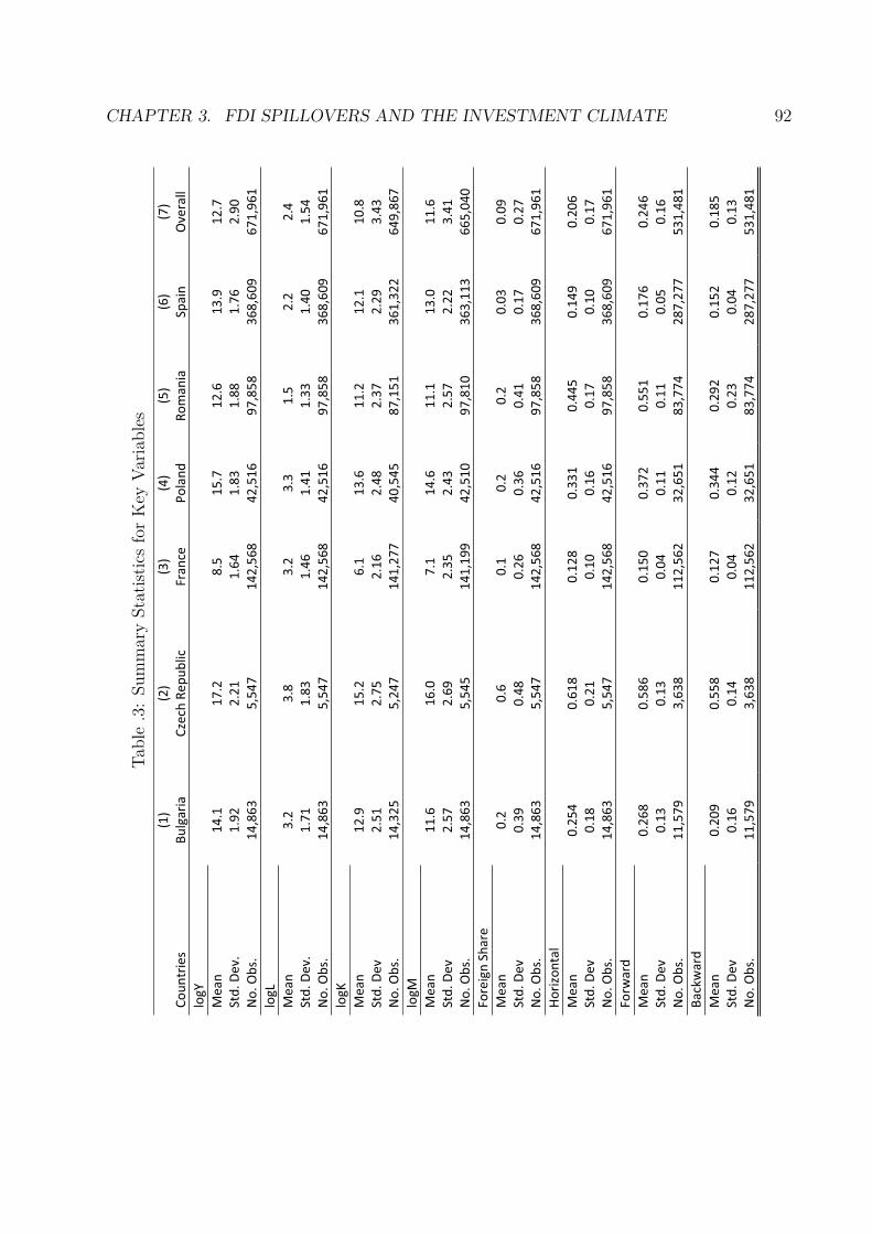
CHAPTER 3. FDI SPILLOVERS AND THE INVESTMENT CLIMATE 92Ta
ble
.3:
Sum
mar
ySt
atist
ics
for
Key
Varia
bles
Table3:Summary
StatisticsforKeyVariables
(1)
(2)
(3)
(4)
(5)
(6)
(7)
Countries
Bulgaria
Czech
Republic
France
Poland
Romania
Spain
Overall
logY
Mean
14.1
17.2
8.5
15.7
12.6
13.9
12.7
Std.Dev.
1.92
2.21
1.64
1.83
1.88
1.76
2.90
No.Obs.
14,863
5,547
142,568
42,516
97,858
368,609
671,961
logL
Mean
3.2
3.8
3.2
3.3
1.5
2.2
2.4
Std.Dev.
1.71
1.83
1.46
1.41
1.33
1.40
1.54
No.Obs.
14,863
5,547
142,568
42,516
97,858
368,609
671,961
logK
Mean
12.9
15.2
6.1
13.6
11.2
12.1
10.8
Std.Dev
2.51
2.75
2.16
2.48
2.37
2.29
3.43
No.Obs.
14,325
5,247
141,277
40,545
87,151
361,322
649,867
logM
Mean
11.6
16.0
7.1
14.6
11.1
13.0
11.6
Std.Dev
2.57
2.69
2.35
2.43
2.57
2.22
3.41
No.Obs.
14,863
5,545
141,199
42,510
97,810
363,113
665,040
ForeignShare
Mean
0.2
0.6
0.1
0.2
0.2
0.03
0.09
Std.Dev
0.39
0.48
0.26
0.36
0.41
0.17
0.27
No.Obs.
14,863
5,547
142,568
42,516
97,858
368,609
671,961
Horizontal
Mean
0.254
0.618
0.128
0.331
0.445
0.149
0.206
Std.Dev
0.18
0.21
0.10
0.16
0.17
0.10
0.17
No.Obs.
14,863
5,547
142,568
42,516
97,858
368,609
671,961
Forw
ard
Mean
0.268
0.586
0.150
0.372
0.551
0.176
0.246
Std.Dev
0.13
0.13
0.04
0.11
0.11
0.05
0.16
No.Obs.
11,579
3,638
112,562
32,651
83,774
287,277
531,481
Backward
Mean
0.209
0.558
0.127
0.344
0.292
0.152
0.185
Std.Dev
0.16
0.14
0.04
0.12
0.23
0.04
0.13
No.Obs.
11,579
3,638
112,562
32,651
83,774
287,277
531,481

CHAPTER 3. FDI SPILLOVERS AND THE INVESTMENT CLIMATE 93
Table .4: Summary Statistics for Spillover Variables (Bulgaria)Table 4: Summary Statistics for Spillover Variables (Bulgaria)
(1) (2) (3) (4)
Years 2005 2006 2007 2008
Horizontal
Mean 0.147 0.283 0.257 0.391
Std. Dev 0.113 0.176 0.176 0.214
No. Obs. 2913 5237 5629 1084
Forward
Mean 0.106 0.276 0.350 0.547
Std. Dev 0.046 0.074 0.087 0.085
No. Obs. 2897 5114 2905 663
Backward
Mean 0.081 0.183 0.324 0.460
Std. Dev 0.066 0.125 0.145 0.166
No. Obs. 2897 5114 2905 663

CHAPTER 3. FDI SPILLOVERS AND THE INVESTMENT CLIMATE 94
Table .5: Summary Statistics for Spillover Variables (Czech Republic)Table 5: Summary Statistics for Spillover Variables (Czech Republic)
(1) (2) (3) (4)
Years 2005 2006 2007 2008
Horizontal
Mean 0.726 0.625 0.615 0.555
Std. Dev 0.193 0.186 0.192 0.234
No. Obs. 688 1523 2129 1207
Forward
Mean 0.690 0.612 0.547 0.492
Std. Dev 0.108 0.068 0.113 0.163
No. Obs. 652 1278 1075 633
Backward
Mean 0.676 0.580 0.517 0.460
Std. Dev 0.116 0.059 0.131 0.168
No. Obs. 652 1278 1075 633

CHAPTER 3. FDI SPILLOVERS AND THE INVESTMENT CLIMATE 95
Table .6: Summary Statistics for Spillover Variables (France)Table 6: Summary Statistics for Spillover Variables (France)
(1) (2) (3) (4)
Years 2005 2006 2007 2008
Horizontal
Mean 0.127 0.137 0.133 0.112
Std. Dev 0.092 0.101 0.101 0.093
No. Obs. 35357 40417 31647 35147
Forward
Mean 0.170 0.146 0.148 0.120
Std. Dev 0.029 0.034 0.037 0.027
No. Obs. 35200 38992 21894 16476
Backward
Mean 0.120 0.146 0.116 0.112
Std. Dev 0.039 0.047 0.026 0.043
No. Obs. 35200 38992 21894 16476

CHAPTER 3. FDI SPILLOVERS AND THE INVESTMENT CLIMATE 96
Table .7: Summary Statistics for Spillover Variables (Poland)Table 7: Summary Statistics for Spillover Variables (Poland)
(1) (2) (3) (4)
Years 2005 2006 2007 2008
Horizontal
Mean 0.320 0.331 0.335 0.337
Std. Dev 0.177 0.150 0.169 0.169
No. Obs. 5965 18870 10417 7264
Forward
Mean 0.357 0.373 0.411 0.333
Std. Dev 0.082 0.078 0.153 0.152
No. Obs. 5910 18123 5090 3528
Backward
Mean 0.365 0.349 0.360 0.262
Std. Dev 0.088 0.107 0.169 0.145
No. Obs. 5910 18123 5090 3528

CHAPTER 3. FDI SPILLOVERS AND THE INVESTMENT CLIMATE 97
Table .8: Summary Statistics for Spillover Variables (Romania)(1) (2) (3) (4)
Years 2005 2006 2007 2008
Horizontal
Mean 0.493 0.500 0.476 0.267
Std. Dev 0.131 0.123 0.258 0.152
No. Obs. 38338 36855 1044 21621
Forward
Mean 0.566 0.571 0.570 0.389
Std. Dev 0.093 0.097 0.172 0.098
No. Obs. 38338 36855 382 8199
Backward
Mean 0.289 0.283 0.452 0.342
Std. Dev 0.239 0.242 0.194 0.132
No. Obs. 38338 36855 382 8199

CHAPTER 3. FDI SPILLOVERS AND THE INVESTMENT CLIMATE 98
Table .9: Summary Statistics for Spillover Variables (Spain)Table 9: Summary Statistics for Spillover Variables (Spain)
(1) (2) (3) (4)
Years 2005 2006 2007 2008
Horizontal
Mean 0.168 0.150 0.135 0.489
Std. Dev 0.109 0.103 0.093 0.304
No. Obs. 102656 126336 139395 222
Forward
Mean 0.170 0.168 0.198 0.428
Std. Dev 0.043 0.042 0.045 0.194
No. Obs. 101408 117642 68111 116
Backward
Mean 0.153 0.144 0.165 0.432
Std. Dev 0.034 0.034 0.066 0.180
No. Obs. 101408 117642 68111 116
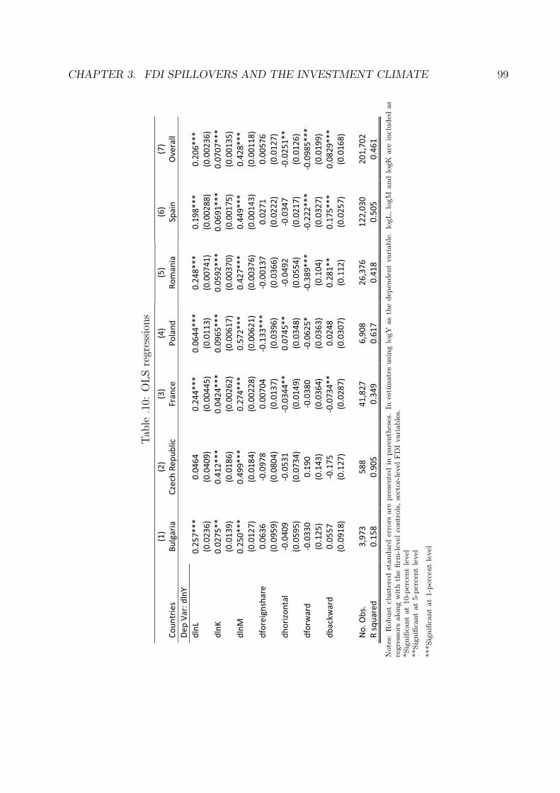
CHAPTER 3. FDI SPILLOVERS AND THE INVESTMENT CLIMATE 99
Tabl
e.1
0:O
LSre
gres
sions
(1)
(2)
(3)
(4)
(5)
(6)
(7)
Countries
Bulgaria
Czech
Republic
France
Poland
Romania
Spain
Overall
DepVar:dlnY
dlnL
0.257***
0.0464
0.244***
0.0644***
0.248***
0.198***
0.206***
(0.0236)
(0.0409)
(0.00445)
(0.0113)
(0.00741)
(0.00288)
(0.00236)
dlnK
0.0275**
0.412***
0.0424***
0.0965***
0.0592***
0.0691***
0.0707***
(0.0139)
(0.0186)
(0.00262)
(0.00617)
(0.00370)
(0.00175)
(0.00135)
dlnM
0.250***
0.499***
0.274***
0.572***
0.427***
0.449***
0.428***
(0.0127)
(0.0184)
(0.00228)
(0.00621)
(0.00376)
(0.00143)
(0.00118)
dforeignshare
0.0636
0.0978
0.00704
0.133***
0.00137
0.0271
0.00576
(0.0959)
(0.0804)
(0.0137)
(0.0396)
(0.0366)
(0.0222)
(0.0127)
dhorizontal
0.0409
0.0531
0.0344**
0.0745**
0.0492
0.0347
0.0251**
(0.0595)
(0.0734)
(0.0149)
(0.0348)
(0.0554)
(0.0217)
(0.0126)
dforw
ard
0.0330
0.190
0.0380
0.0625*
0.389***
0.222***
0.0985***
(0.125)
(0.143)
(0.0364)
(0.0363)
(0.104)
(0.0327)
(0.0199)
dbackward
0.0557
0.175
0.0734**
0.0248
0.281**
0.175***
0.0829***
(0.0918)
(0.127)
(0.0287)
(0.0307)
(0.112)
(0.0257)
(0.0168)
No.Obs.
3,973
588
41,827
6,908
26,376
122,030
201,702
Rsquared
0.158
0.905
0.349
0.617
0.418
0.505
0.461
Not
es:
Rob
ust
clus
tere
dst
anda
rder
rors
are
pres
ente
din
pare
nthe
ses.
Ines
tim
ates
usin
glo
gYas
the
depe
nden
tva
riab
le.
logL
,log
Man
dlo
gKar
ein
clud
edas
regr
esso
rsal
ong
wit
hth
efir
m-le
velc
ontr
ols,
sect
or-le
velF
DI
vari
able
s.*S
igni
fican
tat
10-p
erce
ntle
vel
**Si
gnifi
cant
at5-
perc
ent
leve
l
***S
igni
fican
tat
1-pe
rcen
tle
vel

CHAPTER 3. FDI SPILLOVERS AND THE INVESTMENT CLIMATE 100
Tabl
e.1
1:O
LSre
gres
sions
(Two
Stag
es)
Table11:OLS
Regressions(TwoStages)
(1)
(2)
(3)
(4)
(5)
(6)
(7)
Countries
Bulgaria
Czech
Republic
France
Poland
Romania
Spain
Overall
FirstStage:
DepVar:dlnY
dlnL
0.274***
0.0912*
0.243***
0.0885***
0.294***
0.205***
0.216***
(0.0192)
(0.0491)
(0.00399)
(0.00864)
(0.00767)
(0.00233)
(0.00201)
dlnK
0.0601***
0.437***
0.0482***
0.0883***
0.0849***
0.0687***
0.0768***
(0.0115)
(0.0186)
(0.00232)
(0.00490)
(0.00377)
(0.00138)
(0.00114)
dlnM
0.280***
0.456***
0.296***
0.586***
0.349***
0.442***
0.413***
(0.0107)
(0.0188)
(0.00205)
(0.00522)
(0.00351)
(0.00118)
(0.00101)
SecondStage:
DepVar:dlnTFP
dforeignshare
0.0645
0.0938
0.00655
0.132***
0.00239
0.0269
0.00565
(0.0960)
(0.0805)
(0.0137)
(0.0396)
(0.0369)
(0.0222)
(0.0128)
dhorizontal
0.0416
0.0490
0.0358**
0.0762**
0.0505
0.0348
0.0250**
(0.0596)
(0.0735)
(0.0149)
(0.0348)
(0.0559)
(0.0217)
(0.0126)
dforw
ard
0.0305
0.173
0.0388
0.0607*
0.424***
0.224***
0.103***
(0.125)
(0.144)
(0.0364)
(0.0363)
(0.105)
(0.0327)
(0.0199)
dbackward
0.0623
0.183
0.0743***
0.0252
0.236**
0.178***
0.0850***
(0.0919)
(0.127)
(0.0287)
(0.0307)
(0.112)
(0.0257)
(0.0168)
No.Obs.
3,973
588
41,827
6,908
26,376
122,030
201,702
Rsquared
0.005
0.022
0.001
0.004
0.004
0.001
0.001
Not
es:
Rob
ust
clus
tere
dst
anda
rder
rors
are
pres
ente
din
pare
nthe
ses.
Ines
tim
ates
usin
glo
gYas
the
depe
nden
tva
riab
le.
logL
,log
Man
dlo
gKar
ein
clud
edas
regr
esso
rsal
ong
wit
hth
efir
m-le
velc
ontr
ols,
sect
or-le
velF
DI
vari
able
s.*S
igni
fican
tat
10-p
erce
ntle
vel
**Si
gnifi
cant
at5-
perc
ent
leve
l
***S
igni
fican
tat
1-pe
rcen
tle
vel

CHAPTER 3. FDI SPILLOVERS AND THE INVESTMENT CLIMATE 101
Table .12: Regressions, Average OwnershipTable 12: Regressions, Average Ownership
(1) (2) (3)
Method OLS Two Stage OLS Two Stage Olley Pakes
Dep Var: dlnY
dlnL 0.207*** 0.216*** 0.112***
(0.00237) (0.00201) (0.00180)
dlnK 0.0672*** 0.0751*** 0.116***
(0.00135) (0.00114) (0.00668)
dlnM 0.428*** 0.412*** 0.566***
(0.00118) (0.00101) (0.00130)
dforeignshare 0.000129 0.000376 0.00522
(0.0127) (0.0127) (0.0132)
dhorizontal 0.170 0.165 0.311
(0.265) (0.265) (0.275)
dforward 0.152 0.171 0.635
(0.476) (0.476) (0.494)
dbackward 1.780*** 1.750*** 1.974***
(0.423) (0.423) (0.439)
IAB indicator 0.00320*** 0.00307*** 0.00264***
(0.000296) (0.000295) (0.000307)
dhorizontal*IAB indicator 0.00224 0.00219 0.00383
(0.00288) (0.00288) (0.00299)
dforward*IAB indicator 0.000130 4.58e 05 0.00526
(0.00514) (0.00514) (0.00534)
dbackward*IAB indicator 0.0203*** 0.0200*** 0.0223***
(0.00462) (0.00462) (0.00480)
No. Obs. 201,696 201,696 201,704
Notes: Robust clustered standard errors are presented in parentheses. In estimates using logY (i.e., in column (1) as thedependent variable, logL, logM, and logK are included as regressors along with the firm-level controls, sector-level FDI variables.In column (2) and (3), the estimation procedure is two-stage. In the first stage, we use the OP regression method to obtainestimates for the input coefficients and then calculate lnTFP (the residual from the production function). In the second stage,we regress lnTFP on the remaining controls (firm-level foreign share, state share, sector-level FDI variables, and interactionvariables).*Significant at 10-percent level**Significant at 5-percent level
***Significant at 1-percent level

CHAPTER 3. FDI SPILLOVERS AND THE INVESTMENT CLIMATE 102
Table .13: Regressions, Ease of Establishment IndexTable 13: Regressions,Ease of Establishment Index 0 100
(1) (2) (3)
Method OLS Two Stage OLS Two Stage Olley Pakes
Dep Var: dlnY
dlnL 0.207*** 0.216*** 0.113***
(0.00237) (0.00201) (0.00135)
dlnK 0.0686*** 0.0761*** 0.124***
(0.00136) (0.00114) (0.0474)
dlnM 0.428*** 0.412*** 0.566***
(0.00119) (0.00101) (0.00131)
dforeignshare 0.00151 0.00150 0.00356
(0.0128) (0.0128) (0.0133)
dhorizontal 0.0452 0.0524 0.208
(0.168) (0.168) (0.175)
dforward 0.463* 0.486* 0.430
(0.257) (0.257) (0.268)
dbackward 0.150 0.195 0.229
(0.220) (0.220) (0.229)
IAB indicator 0.00159*** 0.00154*** 0.00137***
(0.000152) (0.000152) (0.000158)
dhorizontal*IAB indicator 6.09e 05 0.000161 0.00328
(0.00216) (0.00216) (0.00224)
dforward*IAB indicator 0.00452 0.00477 0.00419
(0.00329) (0.00329) (0.00342)
dbackward*IAB indicator 0.000841 0.00140 0.00388
(0.00284) (0.00285) (0.00296)
No. Obs. 201,699 201,699 201,698
Notes: Robust clustered standard errors are presented in parentheses. In estimates using logY (i.e., in column (1) as thedependent variable, logL, logM, and logK are included as regressors along with the firm-level controls, sector-level FDI variables.In column (2) and (3), the estimation procedure is two-stage. In the first stage, we use the OP regression method to obtainestimates for the input coefficients and then calculate lnTFP (the residual from the production function). In the second stage,we regress lnTFP on the remaining controls (firm-level foreign share, state share, sector-level FDI variables, and interactionvariables).*Significant at 10-percent level**Significant at 5-percent level
***Significant at 1-percent level

CHAPTER 3. FDI SPILLOVERS AND THE INVESTMENT CLIMATE 103
Table .14: Regressions, Procedures to Start Foreign BusinessTable 14: Regressions,Procedures to Start Foreign Business
(1) (2) (3)
Method OLS Two Stage OLS Two Stage Olley Pakes
Dep Var: dlnY
dlnL 0.207*** 0.216*** 0.113***
(0.00237) (0.00201) (0.00222)
dlnK 0.0691*** 0.0761*** 0.124***
(0.00135) (0.00114) (0.0453)
dlnM 0.427*** 0.412*** 0.566***
(0.00119) (0.00101) (0.00124)
dforeignshare 0.00308 0.00286 1.83e 05
(0.0127) (0.0127) (0.0133)
dhorizontal 0.0786** 0.0774** 0.0919**
(0.0380) (0.0380) (0.0395)
dforward 0.171*** 0.171*** 0.150**
(0.0585) (0.0585) (0.0609)
dbackward 0.0794 0.0856 0.00499
(0.0540) (0.0540) (0.0562)
IAB indicator 0.00271*** 0.00268*** 0.00261***
(0.000331) (0.000331) (0.000345)
dhorizontal*IAB indicator 0.00393 0.00382 0.00450
(0.00406) (0.00406) (0.00423)
dforward*IAB indicator 0.0305*** 0.0309*** 0.0275***
(0.00620) (0.00620) (0.00645)
dbackward*IAB indicator 0.0171*** 0.0179*** 0.00649
(0.00542) (0.00542) (0.00564)
No. Obs. 201,699 201,699 201,698
Notes: Robust clustered standard errors are presented in parentheses. In estimates using logY (i.e., in column (1) as thedependent variable, logL, logM, and logK are included as regressors along with the firm-level controls, sector-level FDI variables.In column (2) and (3), the estimation procedure is two-stage. In the first stage, we use the OP regression method to obtainestimates for the input coefficients and then calculate lnTFP (the residual from the production function). In the second stage,we regress lnTFP on the remaining controls (firm-level foreign share, state share, sector-level FDI variables, and interactionvariables).*Significant at 10-percent level**Significant at 5-percent level
***Significant at 1-percent level

CHAPTER 3. FDI SPILLOVERS AND THE INVESTMENT CLIMATE 104
Table .15: Regressions, Time to Start Foreign BusinessTable 15: Regressions, Time to Start Foreign Business
(1) (2) (3)
Method OLS Two Stage OLS Two Stage Olley Pakes
Dep Var: dlnY
dlnL 0.207*** 0.216*** 0.113***
(0.00237) (0.00201) (0.00169)
dlnK 0.0691*** 0.0761*** 0.124***
(0.00135) (0.00114) (0.0345)
dlnM 0.427*** 0.412*** 0.566***
(0.00119) (0.00101) (0.00275)
dforeignshare 0.00273 0.00250 0.000289
(0.0127) (0.0127) (0.0133)
dhorizontal 0.0615*** 0.0601*** 0.0835***
(0.0217) (0.0217) (0.0225)
dforward 0.0997*** 0.0953** 0.0882**
(0.0382) (0.0382) (0.0398)
dbackward 0.0286 0.0314 0.0180
(0.0344) (0.0344) (0.0358)
IAB indicator 0.000326*** 0.000322*** 0.000315***
(4.10e 05) (4.10e 05) (4.26e 05)
dhorizontal*IAB indicator 0.000656 0.000618 0.00111*
(0.000571) (0.000571) (0.000594)
dforward*IAB indicator 0.00553*** 0.00554*** 0.00495***
(0.000942) (0.000943) (0.000981)
dbackward*IAB indicator 0.00313*** 0.00326*** 0.00145*
(0.000799) (0.000800) (0.000832)
No. Obs. 201,699 201,699 201,698
Notes: Robust clustered standard errors are presented in parentheses. In estimates using logY (i.e., in column (1) as thedependent variable, logL, logM, and logK are included as regressors along with the firm-level controls, sector-level FDI variables.In column (2) and (3), the estimation procedure is two-stage. In the first stage, we use the OP regression method to obtainestimates for the input coefficients and then calculate lnTFP (the residual from the production function). In the second stage,we regress lnTFP on the remaining controls (firm-level foreign share, state share, sector-level FDI variables, and interactionvariables).*Significant at 10-percent level**Significant at 5-percent level
***Significant at 1-percent level

CHAPTER 3. FDI SPILLOVERS AND THE INVESTMENT CLIMATE 105
Table .16: Regressions, Time to Lease Public Land in Days(1) (2) (3)
Method OLS Two Stage OLS Two Stage Olley Pakes
Dep Var: dlnY
dlnL 0.207*** 0.216*** 0.113***
(0.00237) (0.00201) (0.00118)
dlnK 0.0694*** 0.0761*** 0.124**
(0.00135) (0.00114) (0.0541)
dlnM 0.427*** 0.412*** 0.566***
(0.00119) (0.00101) (0.00211)
dforeignshare 0.00866 0.00844 0.00584
(0.0127) (0.0127) (0.0133)
dhorizontal 0.000521 0.00166 -0.0290
(0.0243) (0.0243) (0.0253)
dforward -0.233*** -0.238*** -0.207***
(0.0422) (0.0422) (0.0439)
dbackward 0.0885** 0.0941*** 0.0636*
(0.0359) (0.0359) (0.0373)
IAB indicator 1.90e-05 2.45e-05 5.93e-05**
(2.77e-05) (2.77e-05) (2.88e-05)
dhorizontal*IAB indicator -0.000203 -0.000213 -8.01e-05
(0.000140) (0.000140) (0.000145)
dforward*IAB indicator 0.000851*** 0.000851*** 0.000677***
(0.000246) (0.000246) (0.000256)
dbackward*IAB indicator -8.18e-05 -0.000110 -3.05e-05
(0.000230) (0.000231) (0.000240)
No. Obs. 201,699 201,699 201,698
Notes: Robust clustered standard errors are presented in parentheses. In estimates using logY (i.e., in column (1) as thedependent variable, logL, logM, and logK are included as regressors along with the firm-level controls, sector-level FDI variables.In column (2) and (3), the estimation procedure is two-stage. In the first stage, we use the OP regression method to obtainestimates for the input coefficients and then calculate lnTFP (the residual from the production function). In the second stage,we regress lnTFP on the remaining controls (firm-level foreign share, state share, sector-level FDI variables, and interactionvariables).*Significant at 10-percent level**Significant at 5-percent level
***Significant at 1-percent level

CHAPTER 3. FDI SPILLOVERS AND THE INVESTMENT CLIMATE 106
Table .17: Regressions, Time to Lease Private Land in Days(1) (2) (3)
Method OLS Two Stage OLS Two Stage Olley Pakes
Dep Var: dlnY
dlnL 0.207*** 0.216*** 0.113***
(0.00237) (0.00201) (0.00196)
dlnK 0.0694*** 0.0761*** 0.121***
(0.00135) (0.00114) (0.0466)
dlnM 0.427*** 0.412*** 0.566***
(0.00119) (0.00101) (0.00161)
dforeignshare 0.00738 0.00711 0.00477
(0.0127) (0.0127) (0.0132)
dhorizontal -0.0504* -0.0520* -0.0587**
(0.0282) (0.0282) (0.0293)
dforward -0.232*** -0.240*** -0.190***
(0.0400) (0.0400) (0.0416)
dbackward 0.211*** 0.216*** 0.158***
(0.0331) (0.0331) (0.0344)
IAB indicator 8.10e-05** 8.14e-05** 0.000116***
(3.29e-05) (3.29e-05) (3.42e-05)
dhorizontal*IAB indicator 0.000368 0.000394 0.000278
(0.000376) (0.000376) (0.000391)
dforward*IAB indicator 0.00185*** 0.00191*** 0.00140***
(0.000475) (0.000475) (0.000494)
dbackward*IAB indicator -0.00176*** -0.00181*** -0.00127***
(0.000400) (0.000400) (0.000415)
No. Obs. 201,699 201,699 201,702
Notes: Robust clustered standard errors are presented in parentheses. In estimates using logY (i.e., in column (1) as thedependent variable, logL, logM, and logK are included as regressors along with the firm-level controls, sector-level FDI variables.In column (2) and (3), the estimation procedure is two-stage. In the first stage, we use the OP regression method to obtainestimates for the input coefficients and then calculate lnTFP (the residual from the production function). In the second stage,we regress lnTFP on the remaining controls (firm-level foreign share, state share, sector-level FDI variables, and interactionvariables).*Significant at 10-percent level**Significant at 5-percent level
***Significant at 1-percent level
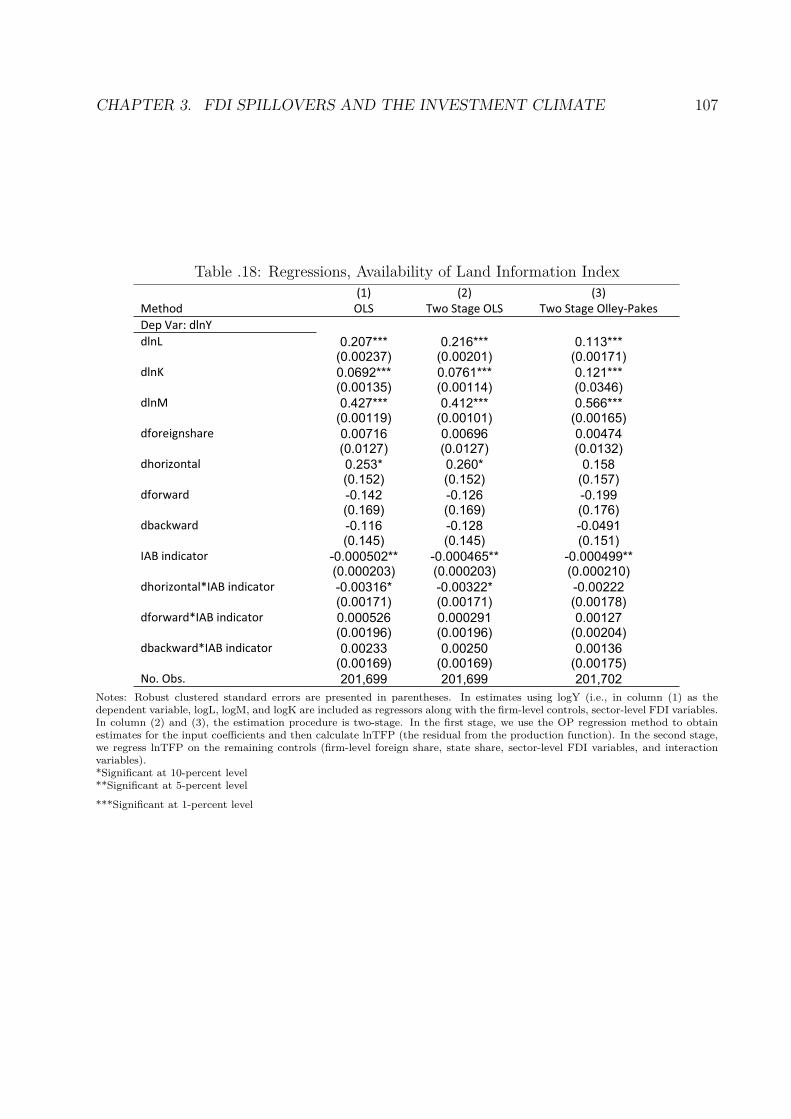
CHAPTER 3. FDI SPILLOVERS AND THE INVESTMENT CLIMATE 107
Table .18: Regressions, Availability of Land Information Index(1) (2) (3)
Method OLS Two Stage OLS Two Stage Olley Pakes
Dep Var: dlnY
dlnL 0.207*** 0.216*** 0.113***
(0.00237) (0.00201) (0.00171)
dlnK 0.0692*** 0.0761*** 0.121***
(0.00135) (0.00114) (0.0346)
dlnM 0.427*** 0.412*** 0.566***
(0.00119) (0.00101) (0.00165)
dforeignshare 0.00716 0.00696 0.00474
(0.0127) (0.0127) (0.0132)
dhorizontal 0.253* 0.260* 0.158
(0.152) (0.152) (0.157)
dforward -0.142 -0.126 -0.199
(0.169) (0.169) (0.176)
dbackward -0.116 -0.128 -0.0491
(0.145) (0.145) (0.151)
IAB indicator -0.000502** -0.000465** -0.000499**
(0.000203) (0.000203) (0.000210)
dhorizontal*IAB indicator -0.00316* -0.00322* -0.00222
(0.00171) (0.00171) (0.00178)
dforward*IAB indicator 0.000526 0.000291 0.00127
(0.00196) (0.00196) (0.00204)
dbackward*IAB indicator 0.00233 0.00250 0.00136
(0.00169) (0.00169) (0.00175)
No. Obs. 201,699 201,699 201,702
Notes: Robust clustered standard errors are presented in parentheses. In estimates using logY (i.e., in column (1) as thedependent variable, logL, logM, and logK are included as regressors along with the firm-level controls, sector-level FDI variables.In column (2) and (3), the estimation procedure is two-stage. In the first stage, we use the OP regression method to obtainestimates for the input coefficients and then calculate lnTFP (the residual from the production function). In the second stage,we regress lnTFP on the remaining controls (firm-level foreign share, state share, sector-level FDI variables, and interactionvariables).*Significant at 10-percent level**Significant at 5-percent level
***Significant at 1-percent level

CHAPTER 3. FDI SPILLOVERS AND THE INVESTMENT CLIMATE 108
Table .19: Regressions, Access to Land InformationTable 19: Regressions, Access to Land Information Index 0 100
(1) (2) (3)
Method OLS Two Stage OLS Two Stage Olley Pakes
Dep Var: dlnY
dlnL 0.207*** 0.216*** 0.113***
(0.00237) (0.00201) (0.00171)
dlnK 0.0687*** 0.0761*** 0.121***
(0.00135) (0.00114) (0.0344)
dlnM 0.427*** 0.412*** 0.566***
(0.00119) (0.00101) (0.00132)
dforeignshare -0.000583 -0.000658 -0.00185
(0.0128) (0.0128) (0.0133)
dhorizontal -0.0629 -0.0628 -0.0819
(0.0539) (0.0539) (0.0560)
dforward 0.0466 0.0488 0.0593
(0.0811) (0.0811) (0.0843)
dbackward 0.0413 0.0307 0.150**
(0.0731) (0.0731) (0.0760)
IAB indicator -0.000949*** -0.000926*** -0.000807***
(9.14e-05) (9.14e-05) (9.49e-05)
dhorizontal*IAB indicator 0.000369 0.000378 0.000556
(0.00108) (0.00108) (0.00112)
dforward*IAB indicator -0.00342** -0.00356** -0.00350**
(0.00166) (0.00166) (0.00172)
dbackward*IAB indicator 0.000797 0.00105 -0.00170
(0.00143) (0.00143) (0.00149)
No. Obs. 201,699 201,699 201,702
Notes: Robust clustered standard errors are presented in parentheses. In estimates using logY (i.e., in column (1) as thedependent variable, logL, logM, and logK are included as regressors along with the firm-level controls, sector-level FDI variables.In column (2) and (3), the estimation procedure is two-stage. In the first stage, we use the OP regression method to obtainestimates for the input coefficients and then calculate lnTFP (the residual from the production function). In the second stage,we regress lnTFP on the remaining controls (firm-level foreign share, state share, sector-level FDI variables, and interactionvariables).*Significant at 10-percent level**Significant at 5-percent level
***Significant at 1-percent level

CHAPTER 3. FDI SPILLOVERS AND THE INVESTMENT CLIMATE 109
Table .20: Regressions, Strength of Lease Right Index(1) (2) (3)
Method OLS Two Stage OLS Two Stage Olley Pakes
Dep Var: dlnY
dlnL 0.207*** 0.216*** 0.112***
(0.00237) (0.00201) (0.00173)
dlnK 0.0687*** 0.0761*** 0.121***
(0.00136) (0.00114) (0.0135)
dlnM 0.428*** 0.412*** 0.566***
(0.00119) (0.00101) (0.00184)
dforeignshare 0.000433 0.000410 -0.00526
(0.0128) (0.0128) (0.0132)
dhorizontal 0.0117 0.0161 -0.0851
(0.156) (0.156) (0.162)
dforward 0.0309 0.0536 0.0638
(0.216) (0.216) (0.224)
dbackward 0.376** 0.353* 0.486**
(0.182) (0.182) (0.189)
IAB indicator -0.00167*** -0.00161*** -0.00148***
(0.000169) (0.000169) (0.000175)
dhorizontal*IAB indicator -0.000539 -0.000580 0.000411
(0.00166) (0.00166) (0.00172)
dforward*IAB indicator -0.00186 -0.00214 -0.00205
(0.00233) (0.00233) (0.00242)
dbackward*IAB indicator -0.00310 -0.00283 -0.00447**
(0.00193) (0.00193) (0.00201)
No. Obs. 201,699 201,699 201,704
Notes: Robust clustered standard errors are presented in parentheses. In estimates using logY (i.e., in column (1) as thedependent variable, logL, logM, and logK are included as regressors along with the firm-level controls, sector-level FDI variables.In column (2) and (3), the estimation procedure is two-stage. In the first stage, we use the OP regression method to obtainestimates for the input coefficients and then calculate lnTFP (the residual from the production function). In the second stage,we regress lnTFP on the remaining controls (firm-level foreign share, state share, sector-level FDI variables, and interactionvariables).*Significant at 10-percent level**Significant at 5-percent level
***Significant at 1-percent level

CHAPTER 3. FDI SPILLOVERS AND THE INVESTMENT CLIMATE 110
Table .21: Regressions, Extent of Judicial Assistance IndexTable 21: Regressions, Extent of Judicial Assistance Index 0 100
(1) (2) (3)
Method OLS Two Stage OLS Two Stage Olley Pakes
Dep Var: dlnY
dlnL 0.207*** 0.216*** 0.112***
(0.00237) (0.00201) (0.00156)
dlnK 0.0691*** 0.0761*** 0.121***
(0.00135) (0.00114) (0.0364)
dlnM 0.427*** 0.412*** 0.566***
(0.00119) (0.00101) (0.00218)
dforeignshare 0.00451 0.00429 -0.00160
(0.0127) (0.0127) (0.0132)
dhorizontal 0.137 0.130 0.221**
(0.100) (0.100) (0.104)
dforward -0.305* -0.297 -0.226
(0.183) (0.183) (0.190)
dbackward 1.009*** 1.029*** 0.668***
(0.163) (0.163) (0.169)
IAB indicator 0.000633*** 0.000622*** 0.000566***
(0.000112) (0.000112) (0.000116)
dhorizontal*IAB indicator -0.00205* -0.00197 -0.00320**
(0.00122) (0.00122) (0.00127)
dforward*IAB indicator 0.00253 0.00235 0.00177
(0.00231) (0.00231) (0.00240)
dbackward*IAB indicator -0.0117*** -0.0119*** -0.00761***
(0.00204) (0.00204) (0.00212)
No. Obs. 201,699 201,699 201,704
Notes: Robust clustered standard errors are presented in parentheses. In estimates using logY (i.e., in column (1) as thedependent variable, logL, logM, and logK are included as regressors along with the firm-level controls, sector-level FDI variables.In column (2) and (3), the estimation procedure is two-stage. In the first stage, we use the OP regression method to obtainestimates for the input coefficients and then calculate lnTFP (the residual from the production function). In the second stage,we regress lnTFP on the remaining controls (firm-level foreign share, state share, sector-level FDI variables, and interactionvariables).*Significant at 10-percent level**Significant at 5-percent level
***Significant at 1-percent level

CHAPTER 3. FDI SPILLOVERS AND THE INVESTMENT CLIMATE 111
Table .22: Regressions, Ease of Process Index(1) (2) (3)
Method OLS Two Stage OLS Two Stage Olley Pakes
Dep Var: dlnY
dlnL 0.207*** 0.216*** 0.112***
(0.00237) (0.00201) (0.00156)
dlnK 0.0691*** 0.0761*** 0.121***
(0.00135) (0.00114) (0.0364)
dlnM 0.427*** 0.412*** 0.566***
(0.00119) (0.00101) (0.00221)
dforeignshare 0.00678 0.00651 0.000659
(0.0127) (0.0127) (0.0132)
dhorizontal -0.0615 -0.0688 0.0281
(0.133) (0.133) (0.138)
dforward -0.686*** -0.697*** -0.367
(0.226) (0.226) (0.235)
dbackward 1.548*** 1.562*** 1.436***
(0.216) (0.216) (0.224)
IAB indicator -0.000675*** -0.000637*** -0.000228
(0.000215) (0.000215) (0.000223)
dhorizontal*IAB indicator 0.000518 0.000612 -0.000768
(0.00169) (0.00169) (0.00176)
dforward*IAB indicator 0.00707** 0.00717** 0.00326
(0.00290) (0.00290) (0.00301)
dbackward*IAB indicator -0.0186*** -0.0188*** -0.0175***
(0.00273) (0.00273) (0.00284)
No. Obs. 201,699 201,699 201,704
Notes: Robust clustered standard errors are presented in parentheses. In estimates using logY (i.e., in column (1) as thedependent variable, logL, logM, and logK are included as regressors along with the firm-level controls, sector-level FDI variables.In column (2) and (3), the estimation procedure is two-stage. In the first stage, we use the OP regression method to obtainestimates for the input coefficients and then calculate lnTFP (the residual from the production function). In the second stage,we regress lnTFP on the remaining controls (firm-level foreign share, state share, sector-level FDI variables, and interactionvariables).*Significant at 10-percent level**Significant at 5-percent level
***Significant at 1-percent level

CHAPTER 3. FDI SPILLOVERS AND THE INVESTMENT CLIMATE 112
Table .23: Regressions, Strength of Laws IndexTable 23: Regressions, IAB Strength of Laws Index (0 100)
(1) (2) (3)
Method OLS Two Stage OLS Two Stage Olley Pakes
Dep Var: dlnY
dlnL 0.207*** 0.216*** 0.112***
(0.00237) (0.00201) (0.00156)
dlnK 0.0690*** 0.0761*** 0.121***
(0.00135) (0.00114) (0.0364)
dlnM 0.427*** 0.412*** 0.566***
(0.00119) (0.00101) (0.00157)
dforeignshare 0.00305 0.00291 -0.00319
(0.0127) (0.0128) (0.0132)
dhorizontal 0.116 0.124 -0.0503
(0.176) (0.176) (0.183)
dforward 0.144 0.163 0.0264
(0.212) (0.212) (0.220)
dbackward -0.234 -0.261 -0.000271
(0.180) (0.180) (0.187)
IAB indicator -0.00121*** -0.00117*** -0.00114***
(0.000166) (0.000166) (0.000172)
dhorizontal*IAB indicator -0.00165 -0.00173 7.39e-05
(0.00192) (0.00192) (0.00200)
dforward*IAB indicator -0.00275 -0.00302 -0.00130
(0.00235) (0.00235) (0.00244)
dbackward*IAB indicator 0.00354* 0.00385* 0.000751
(0.00198) (0.00198) (0.00206)
No. Obs. 201,699 201,699 201,704
Notes: Robust clustered standard errors are presented in parentheses. In estimates using logY (i.e., in column (1) as thedependent variable, logL, logM, and logK are included as regressors along with the firm-level controls, sector-level FDI variables.In column (2) and (3), the estimation procedure is two-stage. In the first stage, we use the OP regression method to obtainestimates for the input coefficients and then calculate lnTFP (the residual from the production function). In the second stage,we regress lnTFP on the remaining controls (firm-level foreign share, state share, sector-level FDI variables, and interactionvariables).*Significant at 10-percent level**Significant at 5-percent level
***Significant at 1-percent level

113
Bibliography
Abel, Andrew B, “Optimal Investment under Uncertainty,” American Economic Review,March 1983, 73 (1), 228–33.
and Janice C Eberly, “A Unified Model of Investment under Uncertainty,” AmericanEconomic Review, December 1994, 84 (5), 1369–84.
and , “Optimal Investment with Costly Reversibility,” Review of Economic Studies,October 1996, 63 (4), 581–93.
Abraham, Filip, Joep Konings, and Veerle Slootmaekers, “FDI Spillovers, firm het-erogeneity and degree of ownership: evidence from Chinese manufacturing,” Open Accesspublications from Katholieke Universiteit Leuven urn:hdl:123456789/243360, KatholiekeUniversiteit Leuven 2010.
Acemoglu, Daron, Simon Johnson, and James A. Robinson, “The Colonial Originsof Comparative Development: An Empirical Investigation,” American Economic Review,December 2001, 91 (5), 1369–1401.
Adda, Jerome and Russell W. Cooper, Dynamic Economics, Quantitative Methods andApplications, MIT Press, 2003.
Aghion, Philippe, Robin Burgess, Stephen Redding, and Fabrizio Zilibotti, “En-try Liberalization and Inequality in Industrial Performance,” Journal of the EuropeanEconomic Association, 04/05 2005, 3 (2-3), 291–302.
Aitken, Brian J. and Ann E. Harrison, “Do Domestic Firms Benefit from Direct ForeignInvestment? Evidence from Venezuela,” American Economic Review, June 1999, 89 (3),605–618.
Aizenman, Joshua and Mark M. Spiegel, “Institutional Efficiency, Monitoring Costsand the Investment Share of FDI,” Review of International Economics, 09 2006, 14 (4),683–697.
Akerlof, George A, “The Market for ’Lemons’: Quality Uncertainty and the MarketMechanism,” The Quarterly Journal of Economics, August 1970, 84 (3), 488–500.

BIBLIOGRAPHY 114
Almeida, Heitor, Murillo Campello, and Michael S. Weisbach, “The Cash FlowSensitivity of Cash,” Journal of Finance, 08 2004, 59 (4), 1777–1804.
, , and , “Corporate financial and investment policies when future financing is notfrictionless,” Journal of Corporate Finance, forthcoming.
Angrist, Joshua D. and Alan B. Krueger, “Empirical strategies in labor economics,”in O. Ashenfelter and D. Card, eds., Handbook of Labor Economics, Vol. 3 of Handbook ofLabor Economics, Elsevier, October 1999, chapter 23, pp. 1277–1366.
Arellano, Manuel and Stephen Bond, “Some Tests of Specification for Panel Data:Monte Carlo Evidence and an Application to Employment Equations,” The Review ofEconomic Studies, 1991, 58 (2), pp. 277–297.
Athey, Michael J. and Prem S. Laumas, “Internal funds and corporate investment inIndia,” Journal of Development Economics, December 1994, 45 (2), 287–303.
Baker, Malcolm, Jeremy C. Stein, and Jeffrey Wurgler, “When Does The MarketMatter? Stock Prices And The Investment Of Equity-Dependent Firms,” The QuarterlyJournal of Economics, August 2003, 118 (3), 969–1005.
Bartelsman, Eric J. and Roel M. W. J. Beetsma, “Why pay more? Corporate taxavoidance through transfer pricing in OECD countries,” Journal of Public Economics,2003, 87 (9-10), 2225–2252.
Bates, Thomas W., Kathleen M. Kahle, and René M. Stulz, “Why Do U.S. FirmsHold So Much More Cash than They Used To?,” Journal of Finance, October 2009, 64(5), 1985–2021.
Baum, Christopher F., Mustafa Caglayan, and Oleksandr Talavera, “Uncertaintydeterminants of firm investment,” Economics Letters, March 2008, 98 (3), 282–287.
Bernanke, Ben S., Mark Gertler, and Simon Gilchrist, “The financial acceleratorin a quantitative business cycle framework,” in J. B. Taylor and M. Woodford, eds.,Handbook of Macroeconomics, Vol. 1 of Handbook of Macroeconomics, Elsevier, April 1999,chapter 21, pp. 1341–1393.
Blalock, Garrick and Paul J. Gertler, “Firm Capabilities and Technology Adoption:Evidence from Foreign Direct Investment in Indonesia.,” Working Paper, Department ofApplied Economics and Management, Cornell University., 2004.
and , Does FDI Promote Development?, Washington, DC: Institute for InternationalEconomics,

BIBLIOGRAPHY 115
and , “Welfare gains from Foreign Direct Investment through technology transfer tolocal suppliers,” Journal of International Economics, March 2008, 74 (2), 402–421.
Blanchard, Olivier Jean, Florencio Lopez de Silanes, and Andrei Shleifer, “Whatdo firms do with cash windfalls?,” Journal of Financial Economics, December 1994, 36(3), 337–360.
Bloom, Nicholas, “The Impact of Uncertainty Shocks,” Econometrica, 05 2009, 77 (3),623–685.
Bloom, Nick, Stephen R. Bond, and John Van Reenen, “Uncertainty and InvestmentDynamics,” Review of Economic Studies, 04 2007, 74 (2), 391–415.
Bollerslev, Tim, George Tauchen, and Hao Zhou, “Expected Stock Returns andVariance Risk Premia,” Review of Financial Studies, November 2009, 22 (11), 4463–4492.
Bolton, Patrick, Hui Chen, and Neng Wang, “Market Timing, Investment, and RiskManagement,” Working Papers, Columbia Business School Working Papers March 2010.
, , and , “A Unified Theory of Tobin’s q, Corporate Investment, Financing, and RiskManagement,” NBER Working Papers 14845, National Bureau of Economic Research, IncApril 2010.
Bond, Stephen R., “Dynamic panel data models: a guide to microdata methods and prac-tice,” CeMMAP working papers CWP09/02, Centre for Microdata Methods and Practice,Institute for Fiscal Studies April 2002.
, Alexander Klemm, Rain Newton-Smith, Murtaza Syed, and Gertjan Vlieghe,“The roles of expected profitability, Tobin’s Q and cash flow in econometric models ofcompany investment,” Bank of England working papers 222, Bank of England June 2004.
and Jason G. Cummins, “Uncertainty and investment: an empirical investigationusing data on analysts’ profits forecasts,” Finance and Economics Discussion Series 2004-20, Board of Governors of the Federal Reserve System (U.S.) 2004.
Borensztein, E., J. De Gregorio, and J-W. Lee, “How does foreign direct investmentaffect economic growth?1,” Journal of International Economics, June 1998, 45 (1), 115–135.
Buettner, Thiess, Michael Overesch, Ulrich Schreiber, and Georg Wamser, “Tax-ation and capital structure choice–Evidence from a panel of German multinationals,” Eco-nomics Letters, 2009, 105 (3), 309–311.
Caballero, Ricardo J., “On the Sign of the Investment-Uncertainty Relationship,” TheAmerican Economic Review, 1991, 81 (1), pp. 279–288.

BIBLIOGRAPHY 116
Campello, Murillo and Dirk Hackbarth, “Corporate Financing and Investment: TheFirm-Level Credit Multiplier,” Working Paper Series, University of Illinois at Urbana-Champaign 2008.
, Erasmo Giambona, John R. Graham, and Campbell R. Harvey, “LiquidityManagement and Corporate Investment During a Financial Crisis,” Working Paper 16309,National Bureau of Economic Research August 2010.
Card, David and Alan B Krueger, “Minimum Wages and Employment: A Case Studyof the Fast-Food Industry in New Jersey and Pennsylvania,” American Economic Review,September 1994, 84 (4), 772–93.
Chen, Kaiji, Zheng Song, and Yikai Wang, “Precautionary corporate liquidity,” Work-ing Papers iewwp465, Institute for Empirical Research in Economics January 2010.
Clausing, Kimberly A., “Tax-motivated transfer pricing and US intrafirm trade prices,”Journal of Public Economics, September 2003, 87 (9-10), 2207–2223.
Collins, Julie H., Deen Kemsley, and Mark Lang, “Cross-Jurisdictional Income Shift-ing and Earnings Valuation,” Journal of Accounting Research, 1998, 36(2), 209–229.
Cooley, Thomas F. and Vincenzo Quadrini, “Financial Markets and Firm Dynamics,”American Economic Review, December 2001, 91 (5), 1286–1310.
Cooper, Russell W. and John C. Haltiwanger, “On the Nature of Capital AdjustmentCosts,” Review of Economic Studies, 07 2006, 73 (3), 611–633.
Desai, Mihir A., C. Fritz Foley, and Kristin J. Forbes, “Financial Constraints andGrowth: Multinational and Local Firm Responses to Currency Depreciations,” Review ofFinancial Studies, 2008, 21 (6), 2857–2888.
Devereux, Michael and Fabio Schiantarelli, “Investment, Financial Factors, and CashFlow: Evidence from U.K. Panel Data,” in “Asymmetric Information, Corporate Finance,and Investment” NBER Chapters, National Bureau of Economic Research, Inc, 1990,pp. 279–306.
Dharmapala, Dhammika and James R. Hines Jr., “Which countries become taxhavens?,” Journal of Public Economics, 2009, 93 (9-10), 1058–1068.
Dittmar, Amy and Jan Mahrt-Smith, “Corporate governance and the value of cashholdings,” Journal of Financial Economics, March 2007, 83 (3), 599–634.
Dixit, Avinash K. and Robert Stephen Pindyck, Investment under uncertainty,Princeton, NJ: Princeton Univ. Press, 1994.

BIBLIOGRAPHY 117
Djankov, Simeon and Bernard M Hoekman, “Foreign Investment and ProductivityGrowth in Czech Enterprises,” World Bank Economic Review, January 2000, 14 (1), 49–64.
, Rafael La Porta, Florencio Lopez-De-Silanes, and Andrei Shleifer, “The Reg-ulation Of Entry,” The Quarterly Journal of Economics, February 2002, 117 (1), 1–37.
Doms, Mark E. and Timothy Dunne, “Capital Adjustment Patterns in ManufacturingPlants,” Review of Economic Dynamics, April 1998, 1 (2), 409–429.
Duke, Elizabeth A., “Small Business Lending, Testimony Before the Committee on Fi-nancial Services and Committee on Small Business, U.S. House of Representatives, Wash-ington, D.C.,” February 26, 2010.
Eisfeldt, Andrea L. and Adriano A. Rampini, “Financing Shortfalls and the Value ofAggregate Liquidity,” Working Paper, Duke University August 2009.
Faulkender, Michael and Rong Wang, “Corporate Financial Policy and the Value ofCash,” Journal of Finance, 08 2006, 61 (4), 1957–1990.
Fazzari, Steven M., R. Glenn Hubbard, and Bruce C. Petersen, “Financing Con-straints and Corporate Investment,” Brookings Papers on Economic Activity, 1988, 1988(1), pp. 141–206.
, , and , “Investment-Cash Flow Sensitivities Are Useful: A Comment On KaplanAnd Zingales,” The Quarterly Journal of Economics, May 2000, 115 (2), 695–705.
Froot, Kenneth A, David S Scharfstein, and Jeremy C Stein, “Risk Management:Coordinating Corporate Investment and Financing Policies,” Journal of Finance, Decem-ber 1993, 48 (5), 1629–58.
Gilchrist, Simon and Charles P. Himmelberg, “Evidence on the role of cash flow forinvestment,” Journal of Monetary Economics, December 1995, 36 (3), 541–572.
, Jae Sim, and Egon Zakrajsek, “Uncertainty, Financial Frictions, and InvestmentDynamics,” Working Paper, 2010.
Glaeser, Edward L. and Andrei Shleifer, “Legal Origins,” The Quarterly Journal ofEconomics, November 2002, 117 (4), 1193–1229.
Gomes, Joao F., “Financing Investment,” American Economic Review, December 2001,91 (5), 1263–1285.
Gorodnichenko, Yuriy, Jan Svejnar, and Katherine Terrell, “When Does FDI HavePositive Spillovers? Evidence from 17 Emerging Market Economies,” IZA DiscussionPapers 3079, Institute for the Study of Labor (IZA) September 2007.

BIBLIOGRAPHY 118
Graham, John R., “How Big Are the Tax Benefits of Debt?,” Journal of Finance, October2000, 55 (5), 1901–1941.
Griliches, Zvi and Jacques Mairesse, “Production Functions: The Search for Identifi-cation,” NBER Working Papers 5067, National Bureau of Economic Research, Inc March1995.
Grubert, Harry and Joel Slemrod, “The Effect of Taxes on Investment and IncomeShifting to Puerto Rico,” NBER Working Papers 4869, National Bureau of EconomicResearch, Inc September 1994.
and John Mutti, “Taxes, Tariffs and Transfer Pricing in Multinational Corporate De-cision Making,” The Review of Economics and Statistics, May 1991, 73 (2), 285–93.
, Timothy Goodspeed, and Deborah L. Swenson, “Explaining the Low TaxableIncome of Foreign-Controlled Companies in the United States,” in “Studies in Interna-tional Taxation” NBER Chapters, National Bureau of Economic Research, Inc, July 1993,pp. 237–276.
Guo, Xin, Jianjun Miao, and Erwan Morellec, “Irreversible investment with regimeshifts,” Journal of Economic Theory, May 2005, 122 (1), 37–59.
Haddad, Mona and Ann Harrison, “Are there positive spillovers from direct foreigninvestment? : Evidence from panel data for Morocco,” Journal of Development Economics,October 1993, 42 (1), 51–74.
Hadlock, Charles J. and Joshua R. Pierce, “New Evidence on Measuring FinancialConstraints: Moving Beyond the KZ Index,” Review of Financial Studies, 2010, 23 (5),1909–1940.
Hartman, Richard, “The effects of price and cost uncertainty on investment,” Journal ofEconomic Theory, October 1972, 5 (2), 258–266.
Haskel, Jonathan E, Sonia C Pereira, and Matthew J Slaughter, “Does InwardForeign Direct Investment Boost the Productivity of Domestic Firms?,” The Review ofEconomics and Statistics, 03 2007, 89 (3), 482–496.
Hassler, John A. A., “Variations in risk and fluctuations in demand: A theoretical model,”Journal of Economic Dynamics and Control, 1996, 20 (6-7), 1115–1143.
Hayashi, Fumio, “Tobin’s Marginal q and Average q: A Neoclassical Interpretation,”Econometrica, January 1982, 50 (1), 213–24.
Hennessy, Christopher A., Amnon Levy, and Toni M. Whited, “Testing Q theorywith financing frictions,” Journal of Financial Economics, March 2007, 83 (3), 691–717.

BIBLIOGRAPHY 119
and Toni M. Whited, “How Costly Is External Financing? Evidence from a StructuralEstimation,” Journal of Finance, 08 2007, 62 (4), 1705–1745.
Hines, James R. Jr., “Lessons from Behavioral Responses to International Taxation,”National Tax Journal, 1999, 52(2), 305–322.
Hines, James R Jr and Eric M Rice, “Fiscal Paradise: Foreign Tax Havens and Amer-ican Business,” The Quarterly Journal of Economics, February 1994, 109 (1), 149–82.
Hines, Jr. James R., “Tax Policy and the Activities of Multinational Corporations,”NBER Working Papers 5589, National Bureau of Economic Research, Inc May 1996.
Holtz-Eakin, Douglas, Whitney Newey, and Harvey S Rosen, “Estimating VectorAutoregressions with Panel Data,” Econometrica, November 1988, 56 (6), 1371–95.
Horst, Thomas, “The Theory of the Multinational Firm: Optimal Behavior under DifferentTariff and Tax Rates,” Journal of Political Economy, Sept.-Oct 1971, 79 (5), 1059–72.
Huizinga, Harry and Luc Laeven, “International profit shifting within multinationals:A multi-country perspective,” Journal of Public Economics, 2008, 92 (5-6), 1164–1182.
Javorcik, Beata S. and Kamal Saggi, “Technological Asymmetry Among Foreign In-vestors And Mode Of Entry,” Economic Inquiry, 04 2010, 48 (2), 415–433.
Javorcik, Beata Smarzynska, “Does Foreign Direct Investment Increase the Productiv-ity of Domestic Firms? In Search of Spillovers Through Backward Linkages,” AmericanEconomic Review, June 2004, 94 (3), 605–627.
Jensen, Michael C, “Agency Costs of Free Cash Flow, Corporate Finance, and Takeovers,”American Economic Review, May 1986, 76 (2), 323–29.
Judd, Kenneth L., Numerical Methods in Economics, MIT Press, 1998.
Kadapakkam, Palani-Rajan, P. C. Kumar, and Leigh A. Riddick, “The impact ofcash flows and firm size on investment: The international evidence,” Journal of Banking& Finance, March 1998, 22 (3), 293–320.
Kaplan, Steven N. and Luigi Zingales, “Do Investment-Cash Flow Sensitivities ProvideUseful Measures of Financing Constraints,” The Quarterly Journal of Economics, February1997, 112 (1), 169–215.
and , “Investment-Cash Flow Sensitivities Are Not Valid Measures Of Financing Con-straints,” The Quarterly Journal of Economics, May 2000, 115 (2), 707–712.
Kaufmann, Daniel, Aart Kraay, and Pablo Zoido-Lobaton, “Aggregating governanceindicators,” Policy Research Working Paper Series 2195, The World Bank October 1999.

BIBLIOGRAPHY 120
Keller, Wolfgang and Stephen R Yeaple, “Multinational Enterprises, InternationalTrade, and Productivity Growth: Firm-Level Evidence from the United States,” TheReview of Economics and Statistics, 03 2009, 91 (4), 821–831.
Khan, Aubhik and Julia K. Thomas, “Nonconvex factor adjustments in equilibriumbusiness cycle models: do nonlinearities matter?,” Journal of Monetary Economics, March2003, 50 (2), 331–360.
and , “Idiosyncratic Shocks and the Role of Nonconvexities in Plant and AggregateInvestment Dynamics,” Econometrica, 03 2008, 76 (2), 395–436.
Klassen, Kenneth, Mark Lang, and Mark Wolfson, “Geographic Income Shifting byMultinational Corporations in Response to Tax Rate Changes,” Journal of AccountingResearch, 1993, 31, 141–173.
Konings, Jozef, “The Effects of Foreign Direct Investment on Domestic Firms: Evidencefrom Firm Level Panel Data in Emerging Economies,” William Davidson Institute WorkingPapers Series 344, William Davidson Institute at the University of Michigan October 2000.
Lamont, Owen, “Cash Flow and Investment: Evidence from Internal Capital Markets,”Journal of Finance, March 1997, 52 (1), 83–109.
, Christopher Polk, and Jesus Saa-Requejo, “Financial Constraints and Stock Re-turns,” Review of Financial Studies, 2001, 14 (2), 529–54.
Leahy, John V and Toni M Whited, “The Effect of Uncertainty on Investment: SomeStylized Facts,” Journal of Money, Credit and Banking, February 1996, 28 (1), 64–83.
Leary, Mark T. and Michael R. Roberts, “Do Firms Rebalance Their Capital Struc-tures?,” Journal of Finance, December 2005, 60 (6), 2575–2619.
Leland, Hayne E, “Corporate Debt Value, Bond Covenants, and Optimal Capital Struc-ture,” Journal of Finance, September 1994, 49 (4), 1213–52.
Levinsohn, James and Amil Petrin, “Estimating Production Functions Using Inputs toControl for Unobservables,” NBER Working Papers 7819, National Bureau of EconomicResearch, Inc August 2000.
Livdan, Dmitry, Horacio Sapriza, and Lu Zhang, “Financially Constrained StockReturns,” Journal of Finance, 08 2009, 64 (4), 1827–1862.
Lucas, Robert E. and Nancy L. Stokey, Recursive Methods in Economic Dynamics,Harvard University Press, 1989.

BIBLIOGRAPHY 121
Malmendier, Ulrike and Geoffrey Tate, “CEO Overconfidence and Corporate Invest-ment,” Journal of Finance, 02 2005, 60 (6), 2661–2700.
McDonald, Robert and Daniel Siegel, “The Value of Waiting to Invest,” The QuarterlyJournal of Economics, November 1986, 101 (4), 707–27.
Mintz, Jack and Michael Smart, “Income shifting, investment, and tax competition:theory and evidence from provincial taxation in Canada,” Journal of Public Economics,2004, 88 (6), 1149–1168.
Modigliani, Franco and Merton H. Miller, “The Cost of Capital, Corporation Financeand the Theory of Investment,” The American Economic Review, 1958, 48 (3), pp. 261–297.
Moran, Theodore H., Edward M. Graham, and Magnus (eds.) Blomström, DoesForeign Direct Investment Promote Development?, Peterson Institute, 2005.
Murillo, Graham John R. Campello and Campbell R. Harvey, “The real effects offinancial constraints: Evidence from a financial crisis,” Journal of Financial Economics,September 2010, 97 (3), 470–487.
Olley, G Steven and Ariel Pakes, “The Dynamics of Productivity in the Telecommuni-cations Equipment Industry,” Econometrica, November 1996, 64 (6), 1263–97.
Petersen, Mitchell A. and Raghuram G. Rajan, “The Benefits of Lending Relation-ships: Evidence from Small Business Data,” The Journal of Finance, 1994, 49 (1), pp.3–37.
Porta, Rafael La, Florencio Lopez de Silanes, Andrei Shleifer, and Robert W.Vishny, “Law and Finance,” Journal of Political Economy, December 1998, 106 (6),1113–1155.
Riddick, Leigh A. and Toni M. Whited, “The Corporate Propensity to Save,” Journalof Finance, 08 2009, 64 (4), 1729–1766.
Rodrik, Dani and Ricardo Hausmann, “Discovering El Salvador’s Production Poten-tial,” 2004.
Salinger, Michael and Lawrence H. Summers, “Tax Reform and Corporate Investment:A Microeconometric Simulation Study,” in “Behavioral Simulation Methods in Tax PolicyAnalysis” NBER Chapters, National Bureau of Economic Research, Inc, 1983, pp. 247–288.
Schwartz, Eduardo S. and Lenos Trigeorgis, eds, Real options and investment underuncertainty, MIT Press, 2001.

BIBLIOGRAPHY 122
Sembenelli, Alessandro and Georges Siotis, “Foreign Direct Investment, CompetitivePressure and Spillovers. An Empirical Analysis of Spanish Firm Level Data,” CEPR Dis-cussion Papers 4903, C.E.P.R. Discussion Papers February 2005.
Swenson, Deborah L., “Tax Reforms and Evidence of Transfer Pricing,” National TaxJournal, 2001, 54(1), 7–25.
Tauchen, George, “Finite state markov-chain approximations to univariate and vectorautoregressions,” Economics Letters, 1986, 20 (2), 177–181.
Thomas, Julia K., “Is Lumpy Investment Relevant for the Business Cycle?,” Journal ofPolitical Economy, June 2002, 110 (3), 508–534.
Tserlukevich, Yuri, “Can real options explain financing behavior?,” Journal of FinancialEconomics, August 2008, 89 (2), 232–252.
Wagle, Swarnim, “Investing across Borders with Heterogeneous Firms: Do Fdi-SpecificRegulations Matter,” 2010. Manuscript, the World Bank.
Weichenrieder, Alfons, “Profit shifting in the EU: evidence from Germany,” InternationalTax and Public Finance, 2009, 16 (3), 281–297.
Wells, Louis T. Jr. and Alvin G. Wint, Marketing a Country: Promotion as a Tool forAttracting Foreign Investment., The International Finance Corporation, the MultilateralInvestment Guarantee Agency, and the World Bank, 2000.
Wheeler, James, “An Academic Looks at Transfer Pricing in a Global Economy,” TaxNotes, 1988.
Whited, Toni M., “Debt, Liquidity Constraints, and Corporate Investment: Evidencefrom Panel Data,” Journal of Finance, September 1992, 47 (4), 1425–60.
, “External finance constraints and the intertemporal pattern of intermittent investment,”Journal of Financial Economics, September 2006, 81 (3), 467–502.
and Guojun Wu, “Financial Constraints Risk,” Review of Financial Studies, 2006, 19(2), 531–559.
Related Documents