Essays in Finance Dissertation zur Erlangung der Würde des Doktors der Wirtschafts- und Sozialwissenschaften des Fachbereichs Betriebswirtschaftslehre der Universität Hamburg vorgelegt von Diplom-Volkswirt Dirk Christian Schilling aus Oldenburg (Oldb) Hamburg

Welcome message from author
This document is posted to help you gain knowledge. Please leave a comment to let me know what you think about it! Share it to your friends and learn new things together.
Transcript

Essays in Finance
Dissertation
zur Erlangung der Würde des Doktors der Wirtschafts-
und Sozialwissenschaften des Fachbereichs Betriebswirtschaftslehre
der Universität Hamburg
vorgelegt von
Diplom-Volkswirt Dirk Christian Schilling
aus Oldenburg (Oldb)
Hamburg

Vorsitzende der Prüfungskommission: Prof. Dr. Jetta Frost
Erstgutachter: Prof. Dr. Wolfgang Drobetz
Zweitgutachter: Prof. Dr. Alexander Bassen
Datum der Disputation: ..

Meinen Eltern und Großeltern gewidmet.


Inhaltsverzeichnis
Tabellenverzeichnis ix
Abbildungsverzeichnis xi
Danksagung xiii
1 Zusammenhang und Beitrag der Bestandteile der Dissertation
1.1 Einleitung . . . . . . . . . . . . . . . . . . . . . . . . . . . . . . . . .
1.2 Kapitalstruktur . . . . . . . . . . . . . . . . . . . . . . . . . . . . . .
1.3 Directors’ Dealings . . . . . . . . . . . . . . . . . . . . . . . . . . . .
1.4 Risikofaktoren . . . . . . . . . . . . . . . . . . . . . . . . . . . . . . .
Literatur . . . . . . . . . . . . . . . . . . . . . . . . . . . . . . . . . . . . .
2 Dissecting the pecking order
Abstract . . . . . . . . . . . . . . . . . . . . . . . . . . . . . . . . . . . . . .
2.1 Introduction . . . . . . . . . . . . . . . . . . . . . . . . . . . . . . . .
2.2 Literature overview . . . . . . . . . . . . . . . . . . . . . . . . . . . .
2.3 Hypotheses . . . . . . . . . . . . . . . . . . . . . . . . . . . . . . . . .
2.4 Data and summary statistics . . . . . . . . . . . . . . . . . . . . . . .
2.5 Empirical results . . . . . . . . . . . . . . . . . . . . . . . . . . . . . .
2.5.1 The pecking order over time . . . . . . . . . . . . . . . . . . .
2.5.2 The pecking order and the sign of the deficits . . . . . . . . .
2.5.3 The pecking order and the deficit size . . . . . . . . . . . . .
2.5.4 The pecking order and debt constraints . . . . . . . . . . . .
2.5.5 The pecking order and the macroeconomy . . . . . . . . . . .
2.5.6 The pecking order and the decision of the firm . . . . . . . .
2.6 Conclusion . . . . . . . . . . . . . . . . . . . . . . . . . . . . . . . . .
A. Financial constraints estimation . . . . . . . . . . . . . . . . . . . . .
B. Variable definitions . . . . . . . . . . . . . . . . . . . . . . . . . . . .
References . . . . . . . . . . . . . . . . . . . . . . . . . . . . . . . . . . . .
v

Inhaltsverzeichnis
3 Illuminating the speed of adjustment
Abstract . . . . . . . . . . . . . . . . . . . . . . . . . . . . . . . . . . . . . .
3.1 Introduction . . . . . . . . . . . . . . . . . . . . . . . . . . . . . . . .
3.2 Literature review . . . . . . . . . . . . . . . . . . . . . . . . . . . . .
3.3 Econometric issues . . . . . . . . . . . . . . . . . . . . . . . . . . . .
3.4 Data and summary statistics . . . . . . . . . . . . . . . . . . . . . . .
3.5 Results . . . . . . . . . . . . . . . . . . . . . . . . . . . . . . . . . . .
3.5.1 Comparing the different estimators . . . . . . . . . . . . . . .
3.5.2 Heterogeneity . . . . . . . . . . . . . . . . . . . . . . . . . . .
3.5.2.1 Countries . . . . . . . . . . . . . . . . . . . . . . . .
3.5.2.2 Financial circumstances . . . . . . . . . . . . . . . .
3.5.2.3 Macroeconomic environment . . . . . . . . . . . . .
3.6 Conclusion . . . . . . . . . . . . . . . . . . . . . . . . . . . . . . . . .
A. Financial constraints estimation . . . . . . . . . . . . . . . . . . . . .
References . . . . . . . . . . . . . . . . . . . . . . . . . . . . . . . . . . . .
4 Haben Manager Timing-Fähigkeiten?
Zusammenfassung . . . . . . . . . . . . . . . . . . . . . . . . . . . . . . . .
4.1 Einleitung . . . . . . . . . . . . . . . . . . . . . . . . . . . . . . . . .
4.2 Regulatorisches Umfeld und Datenbeschreibung . . . . . . . . . . .
4.2.1 Gesetzliche Bestimmungen zum Insider-Trading in Deutschland
4.2.2 Datenbeschreibung . . . . . . . . . . . . . . . . . . . . . . . .
4.3 Empirische Ergebnisse . . . . . . . . . . . . . . . . . . . . . . . . . .
4.3.1 Ergebnisse der Ereignisstudie . . . . . . . . . . . . . . . . . .
4.3.2 Ergebnisse des Generalized-Calender-Time-Ansatzes . . . . .
4.4 Zusammenfassung . . . . . . . . . . . . . . . . . . . . . . . . . . . .
Literatur . . . . . . . . . . . . . . . . . . . . . . . . . . . . . . . . . . . . .
5 Common risk factors in the returns of shipping stocks
Abstract . . . . . . . . . . . . . . . . . . . . . . . . . . . . . . . . . . . . . .
5.1 Introduction . . . . . . . . . . . . . . . . . . . . . . . . . . . . . . . .
5.2 Empirical methodology . . . . . . . . . . . . . . . . . . . . . . . . .
5.3 Data . . . . . . . . . . . . . . . . . . . . . . . . . . . . . . . . . . . . .
5.3.1 Shipping stocks and spanning assets . . . . . . . . . . . . . .
5.3.2 Global risk factors . . . . . . . . . . . . . . . . . . . . . . . .
vi

Inhaltsverzeichnis
5.4 Empirical results . . . . . . . . . . . . . . . . . . . . . . . . . . . . . . 5.4.1 Market model regressions . . . . . . . . . . . . . . . . . . . . 5.4.2 Multifactor model regressions . . . . . . . . . . . . . . . . . . 5.4.3 Testing the pricing restrictions . . . . . . . . . . . . . . . . .
5.5 Conclusions . . . . . . . . . . . . . . . . . . . . . . . . . . . . . . . . A. List of shipping stocks . . . . . . . . . . . . . . . . . . . . . . . . . . References . . . . . . . . . . . . . . . . . . . . . . . . . . . . . . . . . . . .
vii


Tabellenverzeichnis
Dissecting the pecking orderI Percent of firms in different issuing groups . . . . . . . . . . . . . . . II Summary statistics: Leverage in the G . . . . . . . . . . . . . . . . . III Summary statistics: Macroeconomic variables . . . . . . . . . . . . . IV Deficit versus surplus . . . . . . . . . . . . . . . . . . . . . . . . . . V Deficit and surplus size . . . . . . . . . . . . . . . . . . . . . . . . . VI Debt constraints . . . . . . . . . . . . . . . . . . . . . . . . . . . . . . VII Pecking order and macroeconomic environment . . . . . . . . . . . . VIII Nested logit model . . . . . . . . . . . . . . . . . . . . . . . . . . . . IX Estimation of Debt Capacity . . . . . . . . . . . . . . . . . . . . . . . X Data Description . . . . . . . . . . . . . . . . . . . . . . . . . . . . . .
Illuminating the speed of adjustmentI Leverage in the G Countries . . . . . . . . . . . . . . . . . . . . . . II Summary statistics – Independent variables . . . . . . . . . . . . . . III Summary statistics – Macroeconomics . . . . . . . . . . . . . . . . . IV Different estimators of adjustment speed – Book leverage . . . . . . V Different estimators of adjustment speed – Market leverage . . . . . VI Speed of adjustment – Book leverage G . . . . . . . . . . . . . . . . VII Speed of adjustment – Market leverage G . . . . . . . . . . . . . . . VIII Speed of adjustment – Financial constraints . . . . . . . . . . . . . . IX Speed of adjustment after shocks . . . . . . . . . . . . . . . . . . . . X Speed of adjustment and macroeconomics - Book leverage . . . . . . XI Speed of adjustment and macroeconomics - Market leverage . . . . XII Estimation of debt capacity . . . . . . . . . . . . . . . . . . . . . . . .
Haben Manager Timing-Fähigkeiten?I Datenbeschreibung . . . . . . . . . . . . . . . . . . . . . . . . . . . . II Kumulierte abnormale Renditen im Ereignisfenster . . . . . . . . . . III Variablen im GCT-Ansatz . . . . . . . . . . . . . . . . . . . . . . . . . IV Regressionsergebnisse des GCT-Ansatzes für Käufe am Handelstag . V Regressionsergebnisse des GCT-Ansatzes für Verkäufe am Handelstag
ix

Tabellenverzeichnis
Common risk factors in the returns of shipping stocksI Summary statistics of stock returns . . . . . . . . . . . . . . . . . . . II Macroeconomic risk factor . . . . . . . . . . . . . . . . . . . . . . . . III Results of market model regressions . . . . . . . . . . . . . . . . . . IV Results of multifactor model regressions . . . . . . . . . . . . . . . . V Long-run risks with country indices as spanning assets . . . . . . . . VI Long-run risks with industry indices as spanning assets. . . . . . . . VII List of shipping stocks . . . . . . . . . . . . . . . . . . . . . . . . . .
x

Abbildungsverzeichnis
Dissecting the pecking orderI Leverage ratios across countries and over time . . . . . . . . . . . . . II Pecking order coefficient across countries and over time . . . . . . .
Illuminating the speed of adjustmentI Leverage ratios across countries and time frames . . . . . . . . . . . II Speed of adjustment with different financial deficits . . . . . . . . . III Speed of adjustment after leverage shocks . . . . . . . . . . . . . . .
Haben Manager Timing-Fähigkeiten?I Kumulierte abnormale Renditen rund um den Ereignistag (Handelstag)II Kumulierte abnormale Renditen rund um den Ereignistag (Veröffent-
lichungstag) . . . . . . . . . . . . . . . . . . . . . . . . . . . . . . . .
xi


Danksagung
An dieser Stelle möchte ich den Menschen danken, die mich auf dem Weg zu meiner
Promotion unterstützt haben.
Ich danke vor allem meinem Doktorvater Professor Dr. Wolfgang Drobetz. Er hat
mein Interesse an der Disziplin geweckt, mir das wissenschaftliche Arbeiten näher
gebracht und durch konstruktive Kritik das Ergebnis meiner Forschung immer
wieder verbessert. Er hat es verstanden, mich immer, wenn es nötig war, neu zu
motivieren und er hat mir bei meiner Tätigkeit an seinem Lehrstuhl große Freiheit
gelassen.
Ich danke Jörg Seidel und Tatjana Puhan. Sie haben die Zeit am Lehrstuhl durch re-
gen gedanklichen Austausch abwechslungsreich und spannend gemacht und trugen
durch ihre Anregungen zur Qualität der Dissertation und der Lehrveranstaltungen
bei.
Ich danke Lars Tegtmeier und Sven Lindner für ihr Engagement bei der gemeinsa-
men Forschung.
Ich danke meinen ehemaligen Kollegen Rebekka Haller, Robin Kazemieh, Martin
Pöhlsen, Henning Schröder und Martin Wambach für die kollegiale Zusammenarbeit
und die gute Atmosphäre am Lehrstuhl.
Ich danke Janina Schiefelbein, Chinchin Champion und Christine Brinker für ihre
Hilfe bei großen und kleinen Aufgaben.
Ich danke Bettina Kourieh für ihre ruhige Art und ihr immer offenes Ohr. Sie hat
dafür gesorgt, dass auch in unruhigen Zeiten nichts aus dem Ruder lief und hat jede
Woge geglättet.
Besonders danke ich meinen Eltern, meiner Großmutter und meiner Schwester für
die Unterstützung während meines Studiums und bei der Promotion.
Und ich danke Victoria Friese für ihre Geduld, ihre Unterstützung und ihre Liebe.
Hamburg im Februar
xiii


Kapitel 1Zusammenhang und Beitrag der
Bestandteile der Dissertation

Kapitel 1 Zusammenhang und Beitrag der Bestandteile der Dissertation
1.1 Einleitung
Die wissenschaftliche Forschung auf dem Gebiet der Finanzwirtschaft beschäftigt
sich mit der Allokation des knappen Gutes Kapital. Dreh- und Angelpunkt der
Betrachtungen sind daher die Märkte, auf denen Kapital von den Kapitalgebern
zu den Kapitalnehmern transferiert wird. Dieser Transfer kann über einen „Markt“
wie die Börse abgewickelt werden oder es können Finanzintermediäre wie Banken
und Versicherungen eingeschaltet werden. Kapital ist allerdings kein homogenes
Gut. Es existiert in zwei grundlegenden Ausgestaltungen: Eigen- und Fremdkapital.
Während Eigenkapital sich durch die Vergütung mit einem Anteil am Gewinnstrom
und einer unbegrenzten Laufzeit auszeichnet, ist bei Fremdkapital der zu zahlende
Zins pro Periode und die Laufzeit im Vorfeld festgelegt. Die moderne Finanzmarkt-
forschung beschäftigt sich u.a. mit der Allokation von Kapital aus Investorensicht
(Asset-Management), dem Verhalten von Kapitalnachfragern (im Fall von Unterneh-
men Corporate Finance), der Frage wie die Preise der Kapitalüberlassung entstehen
(Asset-Pricing) und der Frage wie Kapitalprodukte ausgestaltet werden können
(Financal Engineering). Zwischen den Bereichen gibt es große Überschneidungen.
Die Beiträge dieser Arbeit bewegen sich an der Schnittstelle der Corporate Finance
und des Asset-Pricing, dem Zusammenspiel von Unternehmensentscheidungen und
der Preisbildung am Kapitalmarkt.
1.2 Kapitalstruktur
Unternehmen treten als Nachfrager von Kapital auf, um ihrerseits Investitionspro-
jekte durchzuführen. Kapital ist dann ein Inputfaktor des Produktionsprozesses.
Modigliani und Miller () untersuchen die Frage, in welchem Verhältnis Un-
ternehmen Eigen- und Fremdkapital nachfragen, bzw. verwenden. Unter restrikti-
ven Annahmen ergibt sich, dass die Kapitalstruktur, das Verhältnis von Eigen- zu
Fremdkapital, irrelevant für den Unternehmenswert ist. Investoren können jeder
Veränderung der Kapitalstruktur in ihrem eigenen Portfolio durch Umschichtung
entgegenwirken. Die Investoren sind damit in der Lage ihr Portfolio ihrem persönli-
chen Risikoprofil anzupassen. Die Kapitalstruktur ist in diesem Modell irrelevant
für den Unternehmenswert .
In Modigliani und Miller () erweitern die Autoren ihr Modell und führen
Steuern als Friktion ein. Fremdkapital dient nun dazu, ein Steuerschild zu bilden

1.2 Kapitalstruktur
und so Gewinne von der Besteuerung abzuschirmen. Mit der Arbeit von Kraus
und Litzenberger () werden Kosten finanzieller Anspannung in das Modell
eingebracht. Unter dieser Art von Kosten werden u.a. Kosten der Insolvenz, der
Vollstreckung aber auch Kosten von Interessenkonflikten zwischen Eigen- und
Fremdkapitalgebern subsumiert. Durch einen zu hohen finanziellen Hebel (Levera-
ge) – hoher Anteil von Fremdkapital – steigen diese Kosten an. Aus diesem Modell
folgt eine optimale Kapitalstruktur (Static-Trade-Off-Theorie). Aufgabe des Unter-
nehmens ist es, Kosten und Nutzen von Fremdkapital gegeneinander abzuwiegen,
um die optimale Kapitalstruktur für das jeweilige Unternehmen zu erhalten. Eine
weitere Ergänzung erfährt dieser Modellierungsstrang durch Fischer u. a. () mit
Anpassungskosten an die Zielkapitalstruktur. Unter diesen Begriff fallen beispiels-
weise die Kosten einer Kapitalerhöhung, das vorzeitige Kündigen eines Kredits, die
Aufnahme eines Kredites und alle weiteren Kosten, die bei Veränderungen der Kapi-
talstruktur anfallen. Durch diese Veränderung ergibt sich ein dynamischer Aspekt
bei der Veränderung der Kapitalstruktur (Dynamic-Trade-Off-Theorie): Unternehmen
müssen nun die Kosten einer Abweichung von der Zielkapitalstruktur mit den
Anpassungskosten in Einklang bringen. Dies führt zu einer langsamen Anpassung
an die Zielkapitalstruktur. Eine solche Anpassung kann im Modell von Fischer u. a.
() mehrere Jahre in Anspruch nehmen.
Mit dem Beitrag von Akerlof () über den Gebrauchtwagenmarkt hat „In-
formation“ begonnen, eine Rolle in der ökonomischen Modellierung zu spielen.
Diese Neuerung wurde auch in der Finanzierungsforschung aufgenommen und
ergänzt die Modelle zur Kapitalstruktur um die Frage, welche Informationen un-
terschiedliche Entscheidungen an den Kapitalmarkt (bzw. Externe) senden, welche
Reaktionen diese Informationen hervorrufen und in welcher Weise das Wissen um
die Reaktionen die Handlungen der Unternehmen bestimmt. In den Beiträgen von
Myers () sowie Myers und Majluf () wird ein Modell entwickelt, dass zu
einer Hackordnung (Pecking-Order) der Finanzinstrumente führt. Unternehmen
bevorzugen interne Finanzierungsquellen, nutzen Fremdkapital, wenn diese auf-
gebraucht sind, und nutzen Eigenkapital nur dann, wenn kein Fremdkapital mehr
zur Verfügung steht. Diese Hackordnung entsteht, weil Manager besser über den
Wert des Unternehmens informiert sind als Investoren. Wenn eine Kapitalerhö-
hung durchgeführt wird, müssen Investoren deshalb davon ausgehen, dass das
Unternehmen überbewertet ist. Ist es das nicht, wäre es für Manager irrational
eine Kapitalerhöhung durchzuführen. Interne Mittel senden kein Signal an den

Kapitel 1 Zusammenhang und Beitrag der Bestandteile der Dissertation
Kapitalmarkt, Fremdkapital ein weniger schlechtes als Eigenkapital. Deshalb wird
nach dieser Theorie Fremdkapital gegenüber Eigenkapital bevorzugt.
Die Dynamic-Trade-Off-Theorie und die Pecking-Order-Theorie sind die vorherr-
schenden in der Modellierung der Kapitalstruktur. Beide wurden umfangreich
empirisch untersucht (u.a.Trezevant ; Frank und Goyal ; Lemmon und
Zender ; De Jong u. a. ). Vor allem die Studie von Shyam-Sunder und Myers
() stellt einen zentralen Beitrag bei der empirischen Beurteilung der beiden
Theorien dar. In dieser Studie werden beide Theorien gleichermaßen untersucht
und ein einfaches Testverfahren für die Pecking-Order-Theorie entwickelt. Aller-
dings beschränkt sich diese Untersuchung auf den Finanzmarkt der USA. Rajan
und Zingales () und La Porta u. a. () weisen auf die institutionellen und
rechtlichen Unterschiede zwischen den Finanzmärkten hin. Während in den oben
zitierten Studien mit Hilfe eines Abstraktionsgrads argumentiert wird, der von
institutionellen und rechtlichen Unterschieden absieht, wird nun explizit unter-
sucht, inwieweit diese Unterschiede Einfluss auf die Finanzierungsentscheidungen
von Unternehmen haben. Aus der Betrachtung dieser Unterschiede entwickelte
sich, vorangetrieben durch Levine (), die Unterscheidung in marktorientierte
und bankorientierte Kapitalmarktsysteme. Diese Unterscheidung bezieht sich vor
allem auf die relative Wichtigkeit und Entwicklung von Banken und Börsen. Daraus
ergeben sich ebenfalls Differenzen hinsichtlich der Finanzierung durch Fremd- und
Eigenkapital und Unterschiede in der Corporate Governance.
Der Beitrag „Dissecting the Pecking Order – When does it hold?“ schließt an
diese beiden Literaturstränge an. Er widmet sich der Frage nach der Evidenz für die
Pecking-Order-Theorie im Laufe der Zeit in einer Stichprobe von – und
in den Ländern der G. Genutzt wird dafür die Methodik von Shyam-Sunder und
Myers () mit dem Schwerpunkt auf Herausarbeitung des unterschiedlichen
Verhaltens von Unternehmen in markt- und bankorientierten Ländern. Weiterhin
wird untersucht, ob die Höhe des Finanzdefizits einen Einfluss auf das Verhalten hat,
wie weit sich Unternehmen unterscheiden, die nur begrenzten Zugang zu externen
Finanzmitteln haben und ob das wirtschaftliche Umfeld Einfluss auf Finanzierungs-
entscheidungen hat.
Es stellt sich heraus, dass der Erklärungsgehalt der Pecking-Order-Theorie über
die Betrachtungsperiode abnimmt. Die anfänglich großen Unterschiede zwischen
bankorientierten und marktorientierten Finanzsystemen werden kleiner. Allerdings
weist die Pecking-Order-Theorie über den gesamten Zeitraum einen höheren Er-

1.2 Kapitalstruktur
klärungsgehalt in bankorientieren Finanzsystemen auf. Unternehmen mit kleinen
Defiziten folgen eher einer Pecking Order als Unternehmen mit großen Defiziten.
Bei Überschüssen hat die Pecking Order einen hohen Erklärungsgehalt mit Ausnah-
me sehr großer Überschüsse, bei denen das Verhalten der Unternehmen nicht erklärt
werden kann. Hinsichtlich des begrenzten Zugangs zu extrenen Finanzmitteln ist
die Pecking-Order-Theorie eher in der Lage das Verhalten von Unternehmen mit
begrenztem und unbegrenztem Zugang zu erklären. Hingegen hat die Theorie nur
begrenzten Erklärungsgehalt für Unternehmen mit mittlerem Zugang zu externen
Quellen. Dies gilt vor allem in Ländern mit bankorientiertem Finanzsystem. Dies
deutet auf einen Verhalten nach dem Modell von Bolton und Freixas () hin: klei-
ne, risikoreiche Unternehmen nutzen Bankkapital, Unternehmen mittleren Riskos
nutzen den Kapitalmarkt und große, wenig risikoreiche Unternehmen emittieren
Anleihen.
Der Beitrag geht außerdem der Frage nach, ob das makroökonomische Umfeld
einen Einfluss auf Kapitalstrukturentscheidungen hat. Auch hier schweigt sich die
klassische Modellierung aus. Die Ergebnisse zeigen, dass Unternehmen in bankori-
entierten Ökonomien mit kleinen Defiziten eine prozyklische Fremdkapitalpolitik
verfolgen, sich also in Boomphasen verstärkt mit Fremdkapital finanzieren. Insge-
samt zeigt dieser Beitrag, dass die Pecking-Order-Theorie nur unzureichend in der
Lage ist, Kapitalstrukturentscheidungen zu erklären. Die Theorie ist in der Lage,
eine gute Beschreibung für das Verhalten von Unternehmen mit speziellen Charak-
teristika zu sein, hat aber wenig Erklärungskraft für das allgemeine Verhalten bei
Kapitalstrukturentscheidungen.
Der zweite Beitrag „Illuminating the speed of adjustment – Exploring hetero-
geneity in adjustment behavior“ widmet sich ebenso der Kapitalstrukturpolitik
und nimmt den Faden vor allem der Dynamic-Trade-Off-Theorie auf. Die unter-
schiedlichen Kapitalstrukturtheorien haben Implikationen für die Anpassungsge-
schwindigkeit zur Zielkapitalstruktur. Während die Pecking-Order-Theorie eine
Anpassungsgeschwindigkeit von 0 impliziert, impliziert die Dynamic-Trade-Off-
Theorie eine positive Anpassungsgeschwindigkeit. Modelle wie das von Fischer
u. a. () zeigen, dass allerdings schon geringe Anpassungskosten ausreichen, um
eine aüßerst langsame Anpassung zu erwirken. Zur Anpassungsgeschwindigkeit
gibt es zahlreiche Studien, die sich aber vor allem durch die verwendeten Schätzer
unterscheiden (u.a. Jalilvand und Harris ; Flannery und Rangan ; Lemmon
u. a. ; Huang und Ritter ). Ziel dieses Beitrages ist es, die Anpassungs-

Kapitel 1 Zusammenhang und Beitrag der Bestandteile der Dissertation
geschwindigkeiten unter Berücksichtigung der institutionellen und rechtlichen
Gegebenheiten zu untersuchen. Es wird weiterhin betrachtet, ob sich die Geschwin-
digkeit unterscheidet, wenn Unternehmen unterschiedlich hohe Defizite aufweisen,
einen beschränkten Zugang zu externen Kapitalmärkten haben und unterschied-
liche Abweichungen von der Zielkapitalstruktur auftreten. Außerdem wird der
Einfluss des makroökonomischen Umfelds auf die Anpassungsgeschwidigkeit un-
tersucht. Zur Bestimmung der Anpassungsgeschwindigkeit werden verschiedene
Panelschätzer eingesetzt und verglichen. Vornehmlich wird das verzerrungsfreie
Verfahren von Elsas und Florysiak () genutzt.
Insgesamt zeigt sich eine Anpassungsgeschwindigkeit von im Mittel %. Diese
ist höher in marktorientierten Ökonomien als in bankorientierten. Es zeigt sich auch,
dass Unternehmen große Finanzierungsdefizite nutzen, um schneller ihre Kapital-
struktur anzupassen. Unternehmen mit beschränktem Zugang zum Kapitalmarkt
sind gezwungen, sich schneller auf ihre Zielkapitalstruktur hinzubewegen. Die-
ser Einfluss ist insbesondere in marktorientierten Ökonomien ausgeprägt. Bei der
Betrachtung der Abweichung von der Zielkapitalstruktur zeigt sich, dass Unterneh-
men, die über ihrer Zielkapitalstruktur liegen, sich schneller anpassen, wohingegen
ein Unterschreiten der Zielkapitalstruktur nur geringen Einfluss auf die Geschwin-
digkeit hat. Auch das makroökonomische Umfeld beeinflusst die Anpassung: In
Rezessionen erfolgt die Anpassung langsamer. In marktorietierten Ländern nut-
zen Unternehmen Phasen niedriger Risikoprämien und hoher Inflation für eine
schnellere Anpassung.
Insgesamt zeigt der Beitrag, dass die Anpassungsgeschwindigkeit von einer Viel-
zahl Faktoren beeinflusst wird. Dazu gehören sowohl die Eigenschaften der Un-
ternehmen als auch das makroökonomische Umfeld. Die Anpassung erfolgt zwar
teilweise äußerst langsam mit einer mehrjährigen Halbwertszeit, ist allerdings über
alle unterschiedlichen Betrachtungen hinweg positiv.
1.3 Directors’ Dealings
Die Hackordnung der Finanzinstrumente ergibt sich aus der Informationsasym-
metrie zwischen Eigner und Manager. Kapitalstrukturentscheidungen senden ein
Signal, dass am Kapitalmarkt verarbeitet wird. Kapitalstrukturentscheidungen sind
allerdings nicht das einzige Signal, dass potentiell Einfluss auf die Preisbildung hat.
Der dritte Beitrag „Haben Manager Timing-Fähigkeiten? Eine empirische Unter-

1.3 Directors’ Dealings
suchung von Directors’-Dealings“ untersucht, welches Signal Directors’ Dealings
an den Kapitalmarkt senden. Unter Directors’ Dealings versteht man den Handel
eines Managers mit Wertpapieren des „eigenen“ Unternehmens. Dieser Handel
unterliegt in Deutschland einer Regulierung, die eine Meldepflicht einer solchen
Transaktion vorsieht. Die Bundesanstalt für Finanzdienstleistungsaufsicht (BaFin)
führt eine Datenbank dieser Transaktionen, die in dem Beitrag ausgewertet wird.
Dieser Datensatz ist der bisher umfangreichste in der deutschen Forschung zu Direc-
tors’ Dealings (u.a. Stotz ; Dymke und Walter ; Betzer und Theissen a,
b; Dickgiesser und Kaserer ). Die Auswertung wird in einem ersten Schritt
mittels der klassischen Ereignisstudienmethode (u.a. MacKinlay ) durchgeführt
und die abnormalen Renditen untersucht. Dabei stellt sich heraus, dass Manager
in der Lage sind, ihr Insiderwissen zur Erzielung kurzfristiger Renditen zu nutzen.
Um die Ergebnisse zu validieren wird im zweiten Schritt der Generalized-Calender-Time-Ansatz (GCT) genutzt (Hoechle u. a. ). Dieser hat Vorteile hinsichtlich
der ökonometrischen Eigenschaften und erlaubt es stetige exogene Variablen in
die Analyse einzubeziehen. In dem Beitrag wird darüber hinaus untersucht, ob das
Anlegerschutzverbesserungsgesetz (AnSVG) aus dem Jahr eine Verringerung
der Überrenditen mit sich bringt. In diesem Gesetz wurden die Meldepflichten und
-fristen enger gefasst.
Die Ergebnisse deuten darauf hin, dass Unternehmensinsider über ausgeprägte
Timing-Fähigkeiten verfügen. Insider verhalten sich als Contrarian-Investoren, d.h.
sie kaufen eigene Aktien nach Kursverlusten und verkaufen nach Kursanstiegen.
Während im Anschluss an Käufe die Kursanstiege zu signifikanten abnormalen
Renditen für Insider führen, vermeiden sie signifikante Kursverluste nach Verkäu-
fen. Ein Vergleich mit früheren Studien zeigt, dass die Werthaltigkeit von Insider-
Transaktionen im bankorientierten deutschen Finanzsystem nicht höher ausfallen
als in den marktorientierten angelsächsischen Finanzsystemen. Für die Information-
Hierarchy-Hypothese, wonach die Werthaltigkeit von Informationen mit steigender
Hierarchieebene eines Insiders zunimmt, kann keine Evidenz gefunden werden.
Hingegen haben die verschärften Regularien des Insiderrechts seit Oktober zu einem Abbau der Informationsasymmetrien zwischen Unternehmensinsidern
und Marktteilnehmern und zur Integrität des Marktes beigetragen. Durch die Ver-
kürzung der Veröffentlichungsfrist gelangen Informationen schneller in den Markt,
und die abnormalen Renditen sind im Zeitfenster bis zu Handelstagen nach der
Transaktion im Anschluss an die Umsetzung des AnSVG wie erwartet gesunken.

Kapitel 1 Zusammenhang und Beitrag der Bestandteile der Dissertation
Diese Ergebnisse können durch den GCT-Ansatz im Wesentlichen bestätigt werden.
Zusätzlich lassen die Koeffizienten auf die unternehmensspezifischen Variablen dar-
auf schließen, dass größere Insider-Transaktionen zu höheren abnormalen Renditen
führen.
1.4 Risikofaktoren
Die Eigenschaften von Unternehmen (Kapitalstruktur, Anpassungsgeschwindigkeit,
Managerhandeln) wie sie in den ersten Beiträgen dargestellt werden, sollten sich
auch in den Risikoeigenschaften der Aktien widerspiegeln. Zur Charakterisierung
von börsengehandelten Titeln wurde von Sharpe () ein Modell entworfen, dass
jedem Titel ein idiosynkratisches Maß für das Risiko in einem Marktgleichgewicht
zuordnet. Dieses Maß ist als β bekannt und bezeichnet den Koeffizienten einer
Regression der jeweiligen Titelrenditen auf die Rendite des Marktes. Anders aus-
gedrückt: Die mit der quadrierten Varianz des Marktes normalisierte Kovarianz
von Unternehmensaktie und Markt. Sharpe () baut auf die Vorarbeiten der
Portfolio-Theorie von Markowitz () auf, in der Risikoreduktion durch Diversifi-
kation mathematisch begründet wird. Unter diesen Voraussetzungen entwickelte
Sharpe () das Capital-Asset-Pricing-Modell (CAPM), ein Modell für den Preis der
einzelnen Unternehmensaktie in einem Marktgleichgewicht.
Das Modell wurde in der Folge ausgiebig getestet (u.a. Fama und MacBeth ;Fama und French , für eine Zusammenfassung der Literatur siehe Fama und
French ) mit sehr unterschiedlichen Ergebnissen hinsichtliche der Evidenz.
Es zeigt sich allerdings, dass ein Faktor nicht ausreicht, die Renditen der Aktien
(und die anderer Wertpapiere) abzubilden. Bei der Schätzung mittels des CAPM
zeigen sich systematische Anomalien, die das Modell nicht erklären kann. Aus dem
Gedanken, dass die Renditen mit Faktoren zu erklären sein sollten, entwickelten sich
in der Folge weitere Modelle. Die Arbitrage-Pricing-Theorie (APT) von Ross ()geht nur noch von einem arbitragefreien Markt aus. Die Renditen werden nun
durch mehrere Faktoren erklärt; jeder Risikofaktor wird durch eine Risikoprämie
entschädigt, die im Modell der Faktorladung bzw. dem Regressionskoeffizienten
entspricht.
Das Intertemporal-Capital-Asset-Pricing-Modell (ICAPM) wurde von Merton ()entwickelt und basiert auf dem Gedanken, dass in einem allgemeinen Gleichge-
wichtsmodell der Diskontfaktor, die Grenzrate des Konsums, der einzige Risiko-

1.4 Risikofaktoren
faktor sein sollte und im einfachen CAPM das Marktportfolio ein Proxy für den
Diskontfaktor ist. Cochrane () merkt an, dass aus dem ICAPM die Motivation
stammt, makroökonomische Faktoren zu verwenden (siehe auch Campbell ()für Preisbildungsmodelle (Asset-Pricing-Modelle), die auf dem Konsum aufbauen).
Cochrane () nach handelt sich bei dem -Faktor-Modell von Fama und French
() um ein APT-Modell, weil hier Portfolios (Value and Growth) als Faktoren
verwendet werden. Ein Modell mit makroökonomischen Faktoren für einen interna-
tionalen Aktienmarkt wird von Ferson und Harvey () entwickelt. Es zeigt sich,
dass die Profile unterschiedlicher Märkte sich hinsichtlich der Ausprägungen der
Faktoren (Risikoladungen) unterscheiden.
Neben Profilen einzelner Märkte ist es aber auch von Interesse, ob unterschiedli-
che Sektoren jeweils ein eigenes Risikoprofil aufweisen. Fama und French ()untersuchen die Risikoprofile von Sektoren und resultierende unterschiedliche
Kapitalkosten, die sich für die Unternehmen daraus ergeben. Der vierte Beitrag
„Common risk factors in the returns of shipping stocks“ fügt das Risikoprofil ei-
nes weiteren Sektors hinzu und untersucht das Risikoprofil des Schifffahrtssektors.
Die bisherige Literatur zur Preisbildung von Schifffahrtsaktien (Grammenos und
Marcoulis ; Kavussanos und Marcoulis , a, b; Grammenos und
Arkoulis ) wird um eine Auswertung einer umfassenderen Stichprobe, der
Verwendung eines ausgereifteren Verfahrens und dem Vergleich mit Länder- und
Industrierisikoprofilen erweitert. In den Datensatz gehen alle börsengehandelten
Schifffahrtsgesellschaften ein. Aus diesen werden Indizes für Massengutfrachter,
Containerfrachter und Öltanker gebildet. Die Schätzungen zeigen ein geringes β
für Schifffahrtsaktien; überraschend angesichts des hohen, vor allem zyklischen
Risikos in diesem Sektor. Dieses Risiko entsteht, weil die Bestellungen neuer Schiffe
in Phasen hoher Frachtraten überschießen und sich in Phasen niedriger Frachtraten
dadurch eine Überschusstonnage auf dem Markt befindet, die die Frachtraten weiter
nach unten drückt (Stopford ). Allerdings kann man aus dem niedrigen β in
Kombination mit niedrigem R2 schließen, dass die Aktien von Seeschifffahrtsge-
sellschaften vor allem durch unsystematisches Risiko gekennzeichnet sind. Diese
Schlussfolgerung legen auch die beobachteten hohen Standardabweichungen der
Renditen nahe.
Das Asset-Pricing-Modell zeigt, dass das Risiko von Schifffahrtsaktien mehrdimen-
sional erfasst werden muss. Neben einem Weltmarktaktienindex spielen Wechsel-
kursrisiken des US$, Outputrisiken, wie die Veränderung der Industrieproduktion,

Kapitel 1 Zusammenhang und Beitrag der Bestandteile der Dissertation
und Inputrisiken, wie die Veränderung des Ölpreises, eine große Rolle als Risi-
kofaktoren. Insgesamt zeigt der Beitrag, dass Schifffahrtsaktien ein von anderen
Sektoren und Ländern stark abweichendes Risikoprofil aufweisen und daher gut als
diversifizierende Portfolioergänzung geeignet sind.
Literatur
Literatur
Akerlof, G.A. . The market for „lemons“: Quality uncertainty and the market
mechanism. The Quarterly Journal of Economics (): –.
Betzer, A., und E. Theissen. a. Insider trading and corporate governance: The
case of Germany. European Financial Management (): –.
———. b. Sooner or later-delays in trade reporting by corporate insiders. Journalof Business Finance and Accounting (–): –.
Bolton, P., und X. Freixas. . Equity, bonds, and bank debt: Capital structure and
financial market equilibrium under asymmetric information. Journal of PoliticalEconomy (): –.
Campbell, J.Y. . Consumption-based asset pricing. In Handbook of the Economicsof Finance, Hrsg. G.M. Constantinides, M. Harris und R. M. Stulz, –.Elsevier.
Cochrane, J.H. . Asset pricing. Princeton: Princeton University Press.
De Jong, A., M. Verbeek und P. Verwijmeren. . The impact of financing surpluses
and large financing deficits on tests of the pecking order theory. FinancialManagement (): –.
Dickgiesser, S., und C. Kaserer. . Market Efficiency Reloaded: Why Insider
Trades do not Reveal Exploitable Information. German Economic Review ():–.
Dymke, B.M., und A. Walter. . Insider trading in Germany: Do corporate
insiders exploit inside information? (): –.
Elsas, R., und D. Florysiak. . Dynamic capital structure adjustment and the
impact of fractional dependent variables. Working Paper: Universität München.
Fama, E.F., und K.R. French. . Common risk factors in the returns on stocks
and bonds. Journal of Financial Economics (): –.
———. . The CAPM is wanted, dead or alive. Journal of Finance (): –.
———. . Industry costs of equity. Journal of Financial Economics (): –.

Literatur
Fama, E.F., und K.R. French. . The CAPM: Theory and evidence. Journal ofEconomic Perspectives (): –.
Fama, E.F., und J.D. MacBeth. . Risk, return, and equilibrium: Empirical tests.
Journal of Political Economy:–.
Ferson, W.E., und C.R. Harvey. . Sources of risk and expected returns in global
equity markets. Journal of Banking & Finance (): –.
Fischer, E.O., R. Heinkel und J. Zechner. . Dynamic capital structure choice:
Theory and tests. Journal of Finance (): –.
Flannery, M.J., und K.P. Rangan. . Partial adjustment toward target capital
structures. Journal of Financial Economics (): –.
Frank, M.Z., und V.K. Goyal. . Testing the pecking order theory of capital
structure. Journal of Financial Economics (): –.
Grammenos, C.T., und A.G. Arkoulis. . Macroeconomic factors and interna-
tional shipping stock returns. International Journal of Maritime Economics ():–.
Grammenos, C.T., und S.N. Marcoulis. . A cross-section analysis of stock returns:
The case of shipping firms. Maritime Policy & Management (): –.
Hoechle, D., M. Schmid und H. Zimmermann. . A generalization of the calendar
time portfolio approach and the performance of private investors. Working Paper:Universität Basel.
Huang, R., und J.R. Ritter. . Testing theories of capital structure and estimating
the speed of adjustment. Journal of Financial and Quantitative Analysis ():–.
Jalilvand, A., und R.S. Harris. . Corporate behavior in adjusting to capital
structure and dividend targets: An econometric study. Journal of Finance ():–.
Kavussanos, M.G., und S.N. Marcoulis. . Risk and return of u. s. water trans-
portation stocks over time and over bull and bear market conditions. MaritimePolicy & Management (): –.

Literatur
———. a. The stock market perception of industry and macroeconomic fac-
tors: the case of the U.S. water transportation industry versus other transport
industries. International Journal of Maritime Economics (): –.
———. b. The stock market perception of industry risk through the utilisation
of a general multifactor model. International Journal of Transport Economics (): –.
Kraus, A., und R.H. Litzenberger. . A state-preference model of optimal financi-
al leverage. Journal of Finance (): –.
La Porta, R.L., F. Lopez-de-Silanes, A. Shleifer und R.W. Vishny. . Law and
finance. Journal of Political Economy (): –.
Lemmon, M.L., M.R. Roberts und J.F. Zender. . Back to the Beginning: Persis-
tence and the Cross-Section of Corporate Capital Structure. Journal of Finance (): –.
Lemmon, M.L., und J.F. Zender. . Debt capacity and tests of capital structure
theories. Journal of Financial and Quantitative Analysis (): –.
Levine, R. . Bank-Based or Market-Based Financial Systems: Which Is Better?
Journal of Financial Intermediation (): –.
MacKinlay, A.C. . Event studies in economics and finance. Journal of EconomicLiterature (): –.
Markowitz, Harry. . Portfolio selection. Journal of Finance (): –.
Merton, R.C. . An intertemporal capital asset pricing model. Econometrica (): –.
Modigliani, F., und M.H. Miller. . The cost of capital, corporation finance and
the theory of investment. American Economic Review (): –.
———. . Corporate income taxes and the cost of capital: A correction. AmericanEconomic Review (): –.
Myers, S.C. . The capital structure puzzle. Journal of Finance (): –.
Myers, S.C., und Nicholas S. Majluf. . Corporate financing and investment
decisions when firms have information that investors do not have. Journal ofFinancial Economics (): –.

Literatur
Rajan, R.G., und L. Zingales. . What do we know about capital structure? Some
evidence from international data. Journal of Finance (): –.
Ross, S.A. . The arbitrage theory of capital asset pricing. Journal of EconomicTheory (): –.
Sharpe, W.F. . Capital asset prices: A theory of market equilibrium under
conditions of risk. Journal of Finance (): –.
Shyam-Sunder, L., und S.C. Myers. . Testing static tradeoff against pecking
order models of capital structure. Journal of Financial Economics (): –.
Stopford, M. . Maritime economics. London: Taylor & Francis.
Stotz, O. . Germany’s new insider law: The empirical evidence after the first
year. German Economic Review (): –.
Trezevant, R. . Debt financing and tax status: Tests of the substitution effect and
the tax exhaustion hypothesis using firms’ responses to the economic recovery
tax act of . Journal of Finance (): –.

Chapter 2Dissecting the pecking order – When
does it hold?

Chapter 2 Dissecting the pecking order
Abstract
This paper examines the performance of the pecking order theory in different set-tings by examining the pecking order coefficient, one of the key evaluators of itsstrength. We use the coefficient to check for differences in firm behavior acrosstime and under different macroeconomic conditions and firm circumstances. Westudy differences in firms with large and small deficits and with possible debtconstraints. We also study whether financial environment has an impact on firmbehavior by performing separate tests for both bank and market-based countries.We find significant differences throughout the various settings. We also find that theexplanatory power of the pecking order decreases over time. The different financialsystems seem to converge in terms of the magnitude of the pecking order coefficient;however, pecking order-like behavior is more pronounced in bank-based countries.We also find a pro-cyclical debt policy for bank-based firms with small deficits.Furthermore, we find evidence that debt markets have a dual role in bank-basedcountries, providing funding for both large risk-less firms, and for new risky ones.Our results suggest that the decision whether to use equity or debt is typically clearin market-based systems, but it is less distinct in bank-based. Overall, the peckingorder performs poorly in explaining our results, but it provides good results whenstudying firms with small deficits, and for differences among firms.
Keyword: Capital structure, pecking order, constraints, financial systems
JEL Classification Numbers: G, G

2.1 Introduction
2.1 Introduction
“Take on positive net present value projects.” This is the succint advise, for
how managers can create value operationally on the asset side of the balance sheet.
However, the subject of how they can create value operationally on the liability and
equity side of the balance sheet is far less obvious, and is at the center of a nearly
thirty-year academic debate. During this debate, several theoretical explanations
have emerged. The classic Modigliani and Miller () theorem posits that, in a
world of perfect capital markets, capital structure is irrelevant to firm value, and
whether a project is financed by equity or debt does not matter for firm value.
However, Modigliani and Miller () later extended their model to include taxes,
which found benefits from using debt as a way to shield profits from taxation. The
next extension involved managing bankruptcy costs from excessice amounts of debt.
This theory is known as the static trade-off theory: Firms must balance debt and
equity according to their respective costs and benefits (Kraus and Litzenberger ;Jensen and Meckling ).
As asymmetric information modeling (Akerlof ) increased in importance, it
also spilled over into finance and led to the development of the pecking order theory
of capital structure (Myers ; Myers and Majluf ). This theory claims that
firms follow a pecking order in their financing decisions, where equity stands both
at the top and the bottom of the hierarchy. Firms prefer to use cash, which results
in the lowest costs, followed by debt and equity offerings, which have ascending
costs of asymmetric information. And, recently, a third prominent theory has been
developed, Baker and Wurgler’s () market timing theory. Its main prediction is
that the offering behavior of firms depends on the state of the market. Firms will
offer equity when the price of equity is low, and they will offer debt otherwise.
In an empirical test of these theories, none emerged as the best explanation for
all different data patterns; rather, each theory was best explaining certain patterns.
To understand how well a theory really works, we need to explore the explanatory
power of every state of a firm or market. By examining its relative strengths and
weaknesses, we can gain a deeper understanding of pecking order theory, and deter-
mine when its predictions hold. Our first step is to use the G countries to check for
differences in explanatory power of the theory, as well as examine its development
over time. Second, we classify each country as bank- or market-based to further
explore its explanatory power under different capital market systems. Our third step

Chapter 2 Dissecting the pecking order
is to use firm characteristics to analyze whether pecking order theory performs dif-
ferently for different firm types. Fourth, we target the macroeconomic environment,
and examine how firms generate financing during periods of recessions. Finally,
we change perspectives, and look directly at a model of firms’ financial decisions,
relaxing the assumption that the financial deficit is exogenous.
We find that pecking order theory tends to lose its explanatory power over time. In
general, performance is rather weak in market-based financial systems, and it is only
slightly better in bank-based systems. However, when we study data subsamples,
we find somewhat better explanatory power. If we sort financial deficits by size, we
find that only the behavior of firms with very large deficits cannot be explained by
pecking order, while the behavior of firms with small deficits is largely explained.
Debt constraints also play a role. In market-based countries, firms are forced to use
the capital markets even when they are only medium-constrained. In bank-based
countries, we find that firms with medium debt constraints also use the capital
markets, but constrained firms use banks for financing. Further more, we find
evidence of a pro-cyclical debt policy in bank-based countries.
The remainder of the paper is organized as follows: Section provides a litera-
ture overview of past research on pecking order theory. In Section , we present
hypotheses derived from differences in capital market systems. Section gives our
data description and summary statistics. Section describes our results in detail.
2.2 Literature overview
Modern academic research on capital structure starts with Modigliani and Miller’s
() irrelevance theorem. Prior considerations about capital structure were mainly
the result of ad hoc reasoning or industry heuristics. Modigliani and Miller’s ()primary tenet was that a firm’s capital structure has no influence on market value.
However, this theory comes with strict assumptions. The irrelevance theorem also
does not explain, for example, why firms spend so much time on financing decisions,
why leverage ratios are remarkably stable in some industries (Bradley et al. ),and why IPO activity is cyclical (Ritter and Welch ). From the irrelevance
theory emerged the static trade-off theory. Modigliani and Miller () provided a
In a summary of these assumptions, Frank and Goyal () cite the absence of taxes, transactioncosts, bankruptcy costs, agency conflicts, and adverse selection, as well as a separation betweenfinancing and operation activities, stable financial market opportunities, and homogeneous investors.In other words, everything that modern finance encompasses was ruled out by the assumption.

2.2 Literature overview
model including taxes that leads to relatively cheaper debt. Kraus and Litzenberger
() next added bankruptcy costs to create a model of the benefits of using debt
as a tax shield and the costs of debt via bankruptcy cost. Decision-makers must
evaluate all of these options to come up with an adequate capital structure for each
business. The theory implies there is a target capital ratio for each firm to which
they gradually move (along with adjustment costs).
The next major theory is the pecking order theory of Myers () and Myers and
Majluf (). This theory posits a pecking order of capital structure decisions,
which is the result of agency conflicts. Firms prefer internal financing; if these
sources are depleted, they prefer debt; and only as a last resort will they use equity.
Frank and Goyal () note that using various models can lead to pecking order-
like behavior, such as adverse selection and agency conflicts. The original derivation
works with adverse selection costs, and was developed by Myers () and Myers
and Majluf (). The primary idea is that owner-managers are better informed by
knowing firm value; the estimates of outside investors are subject to errors. When
managers sell equity, outside investors tend to assume the firm is undervalued.
Hence, firms issue equity only as a last resort, while internal financing is the cheapest
option, and debt is in the middle. Another derivation uses agency conflicts, for
example, laid out by Jensen and Meckling (), who show that the consumption
of perks can lead to a pecking order.
Shyam-Sunder and Myers () note a pecking order as well for share repur-
chases. In this case, they posit that the degree of manager optimism works as the
primary mechanism: Optimistic managers (relative to investors) want to buy back
shares to reduce supply and thus obtain higher share prices. Pessimistic managers
believe their share prices are already too high, and are unlikely to buy back shares.
Thus, optimistic managers will drive prices up until their own evaluation matches
investor evaluation. In equilibrium, there will be only debt repurchases.
A third theory has also gained attention over the last few years: the market
timing theory of capital structure, developed by Baker and Wurgler (). Before
the formation of this theory, equity markets were not part of the capital structure
theories. However, Baker and Wurgler () document that firms tend to issue
equity when firm market value is high compared to book value and when the cost
of equity is low, and that they buy back shares when it is high. Baker and Wurgler
() also find evidence of issues during times of excessive investor “enthusiasm”.
The insight that firms prefer internal over external funds dates back to Donaldson ().

Chapter 2 Dissecting the pecking order
They note that, in a survey by Graham and Harvey (), managers admitted that
they tend to time the markets. Baker and Wurgler () find strong evidence of
market timing by examining past leverage ratios and market-to-book-values. The
influence (or persistence) lasts about ten years. They explicitly state that their
findings are consistent to Myers and Majluf’s () model with rational managers
and investors, as well as with varying adverse selection costs.
The relative merits of each theory have been the subject of intense discussion.
However, the empirical success of each theory is mixed. Bradley et al. ()document evidence for the static trade-off model by looking at the cross-section of
leverage ratios. Trezevant () reports strong evidence for the trade-off model by
examining a tax-code change that occurred during the s. The pecking order
theory extends the research question of which (only partially) consistent models is
more correct? Shyam-Sunder and Myers () evaluate both theories and suggest
that the pecking order model performs better in explaining data patterns. They use
a fairly simple model that regresses net debt on the financial deficit (see Section
2.5.1). If the coefficient is equal to , the variation in debt issues can be explained
completely by the pecking order theory. Using a small sample of large firms, they
find strong evidence to back up the theory. However, Frank and Goyal () use a
larger sample and obtain different results. They document that the pecking order
decreases in explanatory power. They also find that net equity issues are better at
tracking deficits than net debt issues, as the pecking order theory would predict.
Moreover, Chirinko and Singha () note that the Shyam-Sunder and Myers ()regression framework is not as powerful because of its empirical weaknesses.
Because Frank and Goyal’s () empirical results are not completely satisfac-
tory for some subsamples, however, newer studies have tested the pecking order
in different economic environments and for different firm conditions. A central
hypothesis states that firms have a limited debt capacity. Hence, firms at their
debt limit are financially constrained. These firms are not able to follow a pecking
order, and must issue equity when confronted with new investment opportunities.
Faulkender and Petersen () evaluate the relationship between the costs and the
presence of a debt rating, and find that firms with high information asymmetries
also have higher debt costs. Kisgen () further investigates firm behavior during
times of rating changes. He finds that ratings directly influence capital structure.
They note that the coefficient is biased if ) the proportion of equity in the issuance is high, )equity and debt are reversed in the pecking order, or ) firms issue in constant proportions.

2.2 Literature overview
For example, firms issue less debt if a rating change is expected and they have an
unstable outlook. One drawback of these studies is that a credit rating is only a
rough proxy for financial conditions, because not every firm relies on a rating and
the data coverage on ratings in financial databases is incomplete. To mitigate these
problems, Lemmon and Zender () use a logit model to obtain a measure of
firm-specific debt capacity. Consistent with pecking order, they find that financially
constrained firms tend to use equity, while unconstrained firms tend to use debt.
These findings are confirmed by De Jong et al. () when sorting the firms by
deficit size. De Jong et al. () also argue that deficit size is a proxy for financially
constrained firms. Their results indicate that firms with high deficits, which are
generally small firms, do not follow a pecking order. They conclude that smaller
firms have larger asymmetric information costs and should thus follow a pecking
order, but they are also debt-constrained.
The overall macroeconomic environment is another source of capital issue behav-
ior. Korajczyk and Levy () find that unconstrained firms follow a countercyclical
issue policy, while constrained firms have relatively stable debt and equity issues
over time. Moreover, unconstrained firms seem to time the market by switching
between debt and equity, while constrained firms are not able to follow this active
approach.
Fama and French () study both the pecking order and the trade-off theory.
They observe that both theories correctly predict that firms with low investments
would pay higher dividends. Only the pecking order model correctly predicted that
profitable firms have a lower leverage ratio and that short-term variation in leverage
is generally caused by debt issues, however.
In contrast, Flannery and Rangan () do not find evidence for pecking order
or market timing. Rather, they document a tendency for firms to rapidly converge
toward a specific target leverage ratio. Leary and Roberts () also report such a
ratio, but they find that only a slow adjustment is possible because of adjustment
costs. Hovakimian () argues that these studies suffer from a correlation between
historical market-to-book ratios and growth opportunities. In a recent paper Huang
and Ritter () overcome this problem by using an implied equity risk premium
(ERP). They report market timing and moderate adjustment speeds. They also
find that firms finance more of their deficits with equity when the ERP is low.
Huang and Ritter () calculate the ERP by using discounted earnings forecasts from firms inthe Dow Jones Industrial Average.

Chapter 2 Dissecting the pecking order
In yet another direction, Lemmon et al. () find that firms adjust to largely
unobservable targets by examining portfolios of ex ante similarly leveraged firms.
They find only a small variation in leverage in the portfolios over time.
However, note that all the studies mentioned above use U.S. accounting data for
their research. A notable exception is Rajan and Zingales (), who conduct a
descriptive analysis for the G. They suggest applying to financial systems and
jurisdiction outside the U.S., in order to obtain a fuller understanding of the theo-
ries. They also note that international countries can be considered an independent
sample, and could be used as a further check on capital structure theories. Using in-
ternational data, we can also check for the influence of different legal traditions and
institutions on capital structure decisions. For example, La Porta et al. () study
various legal traditions, and find differences in the levels of shareholder protection.
Rajan and Zingales () compare the capital structures of the G countries, and
find they are comparable to the U.S. structure. Bessler, Drobetz, and Pensa ()investigate a European sample, and find support for a dynamic trade-off model with
firms using market timing in the short run. Drobetz and Wanzenried () use a
sample of Swiss firms, and find correlations with the business cycle in their capital
structure decisions. On the other hand, Ball et al. () document the importance
of international institutional factors for accounting measures. Prior to our work,
Antoniou et al. () found evidence for target leverage ratios in the G, and
they also documented some influence of macroeconomic factors and market-related
variables on capital structure decisions. We use a much larger dataset and extend
the view to firm-specific characteristics such as deficit size.
However, the advantage of considering a broader scope than just the U.S. comes
at the cost of data quality. Many countries have or fewer firms in the Compustat
database, so the coverage and length of data is much less extensive. We use only Gcountries in this analysis, because they have sufficient data availability and reliable
accounting standards. The next section discusses one of the main differences among
the G countries, the historical development of their financial systems. As per
the literature, we consider each system as market- or bank-based, depending on
the main source of their external financing and the development of their capital
markets and banking systems. We also develop hypotheses for the influence on
capital structure.

2.3 Hypotheses
2.3 Hypotheses
Beck and Levine () were among the first to distinguish between bank- and
market-based system, with the primary difference being the source of corporate
finance. In market-based countries, the main source of capital is the capital markets,
i.e., the stock market and the bond market. In bank-based systems, most capital
is raised from banks. This is tied to a lower share of common equity, hence the
differences in capital structure. For example, in the ratio of stock market
capitalization to GDP was . in U.S., while it was only . in Germany (Beck
et al. ). The U.S., Canada, and the U.K. are all market-based financial systems,
Germany, France, Italy, and Japan are considered typical bank-based systems.
The systemic differences extend also to the implications for corporate governance
(Credit Suisse ; Rajan and Zingales ). The market-based system is character-
ized by an “arm’s-length” control between managers and investors: If managers do
not perform, investors sell their shares. The requirements for this type of system are
very liquid capital markets and a high degree of free float. The market for corporate
control – mergers and acquisitions, as well as leveraged buyouts – also needs to be
very active, and option-based payment systems are generally used to align manage-
ment and shareholder interests. The bank-based system is characterized by high
ownership stakes of banks and families, and less liquid capital markets. Bank debt
plays a more prominent role in financing new projects, and the market for corporate
control is not as active as in market-based countries. However, the insider-based
control system also works as a corporate governance mechanism, because banks use
their control rights to guarantee cash flows.
There is some discussion about which system has been more effective at providing
a foundation for economic growth (Levine ). However, when the costs and
benefits of both systems were fully evaluated, no clear answer emerged, and the
century-old debate fizzled out. Recently, it has started up again, particularly be-
cause bank-based countries performed better to some extend during the –financial crisis (Claessens et al. ). Another discussion relates to which system
provides better investor protection. Common law (market-based) countries gener-
ally have stronger shareholders protection, civil law (bank-based) countries tend to
protect debtholders more strongly (La Porta et al. ). For example, as La Porta
et al. () note, the U.S. common law system strongly favors reorganization, with
managers keeping their jobs. German civil law, on the other hand, strongly favors

Chapter 2 Dissecting the pecking order
liquidation to protect secured creditors. La Porta et al. () also report strong
anti-director rights in common law countries, such as strong protection for minority
shareholders, voting by mail, and the right for even relatively small shareholders
to call shareholder meetings. These differences in corporate governance should
result in different costs of equity capital. Because shareholders are less protected
in bank-based countries, and incentives for managers are not primarily aligned
with shareholder interests, they should demand a higher premium for providing
equity (La Porta et al. ). Equity should thus be relatively more expensive in
bank-based countries, and relatively cheaper in market-based countries. This insight
strengthens when we consider the costs of asymmetric information. It is higher for
equity providers in bank-based countries, because the disclosure obligations are less
severe (Levine ).
The differences between the two systems also result in different behavior in capital
structure decisions. This leads to our hypotheses:
Hypothesis I: The proportion of debt used in bank-based countries is higher than inmarket-based countries.The cost of equity capital should be relatively higher in bank-based countries. These
higher costs originate from lower investor protection and a governance mechanism
that favors debtholders. Firms in bank-based countries should be more likely to use
liabilities to finance investments. Hence, they would demonstrate more pecking
order-like behavior, as the cost differences between equity and debt are higher than
in market-based countries. This behavior should also lead to a higher pecking
order coefficient in bank-based countries in the Shyam-Sunder and Myers ()framework. It is also documented in Bessler et al. () and in Seifert and Gonenc
().
Hypothesis II: The proportion of equity and debt used to finance financial deficits becamecloser recent years.In a Shyam-Sunder and Myers () world, the pecking order coefficient is not inor-
dinately different between market- and bank-based countries. Levine () reports
that high-income countries tend to move to market-based financial systems because
of pressure from international markets, and because markets are more efficient at
providing corporate governance. The liquidation of the so called "Deutschland AG"
2.4 Data and summary statistics
is an example of this view (Höpner and Krempel ; Andres et al. ; Bessler,
Drobetz, and Holler ). Therefore, we expect to see a declining pecking order
coefficient.
Hypothesis III: Market timing is more pronounced in market-based countries than inbank-based countries.The equity risk premium (similarly to the cost of equity capital) plays a more domi-
nant role in market-based countries, because the capital market is used more heavily
to finance firm activities. The risk premium varies (Ferson and Harvey ), as
does IPO issuing activity (Ritter and Welch ). In market-based countries, firms
seem to time the market and issue equity if the cost of equity capital is low. Autore
and Kovacs () find a correlation between time-varying issuance behavior and
time-varying information asymmetries. However, this behavior should be more
pronounced in market-based countries, because in bank-based countries the equity
markets are not dominant, and banks have privileged access to crucial information.
We do not expect to find strong market timing in our bank-based subsample.
Hypothesis IV: Accounting information (i.e., firm-specific data) should be more impor-tant for debt versus equity decisions in market-based countries.The capital markets need information provided by firms to value the price of equity.
The most important piece of publicly available information is the data from annaul
balance sheets. The disclosure rules are stronger in market-based countries (La Porta
et al. ). But banks are tied more closely to the management, and use other
channels to obtain information to monitor firms. Therefore, the influence of balance
sheet data should be more pronounced in market-based countries.
To evaluate these hypotheses, we use a comprehensive dataset for the G countries
that contains firm, market, and macroeconomic data. The next section presents the
precise construction.
2.4 Data and summary statistics
We use Standard & Poor’s Compustat Global as our basic database. All data on
balance sheet items, cash flow items, and market data come from this database.
We add indicators for the macroeconomic environment from Thomson Reuters

Chapter 2 Dissecting the pecking order
Datastream.
We use observations from to for the G countries, and we obtain 125982
firm-year observations. Frank and Goyal () note that financial databases such
as Compustat are subject to outliers and anomalous observations. However, we can
manage this problem by using, e.g., rule of thumb truncations, winsorizing, and
trimming.
We start with some common rule of thumb cleansing steps. We exclude all
utilities (SIC codes –) and financial firms (SIC codes –). We set
any missing capital expenditures or convertible to zero. We also set missing research
and development expenditures to zero; however, in this case, we use a dummy to
indicate which items were missing and which originally had a zero value.
We further exclude firms with negative leverage ratios or total assets. We only
use firms with consolidated balance sheets that have not experienced any changes
in accounting method. All firm-level variables are in local currencies, except for
sales, which is measured in US$. We trim our data at the %-level.
To construct the variables, we follow Huang and Ritter () and Frank and
Goyal () for most definitions. We first look closely look at changes in net debt
(NETD) and net equity (NETE). Net debt is defined as the change in liabilities
and preferred stock relative to the beginning-of-year assets (AT ). Net equity is
the change in equity and convertible debt, minus the change in retained earnings
relative to beginning-of-year assets.
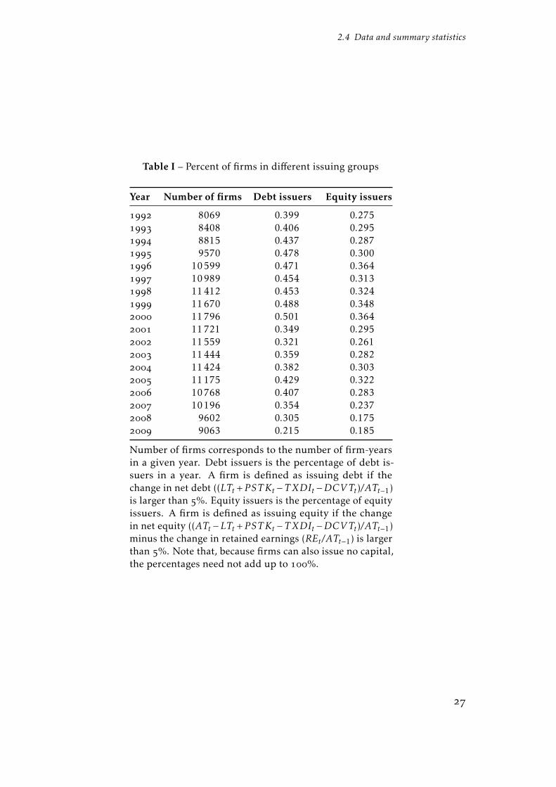
Both variables are presented in Table I. The sample is relatively balanced over the
years, varying from approximately 8000 to 12000 observations. As in Huang and
Ritter (), a firm is defined as issuing debt (equity) if the change in net debt (net
equity) is higher than %. Looking at columns and of Table I, we note that the
proportion of debt and equity issuers is time-varying. For example, in the year ,about % of firms in the sample issued debt; in , the number was only %.
Equity issuance is also time-varying. We note that the late s had the highest
percentage (up to %) of issues, and the late s had the lowest (% in ).This implies a certain amount of market timing on the part of the firms because the
years of financial turmoil have low issue proportions. However, most of the firms
We exclude financial firms because they have a different balance sheet structure. We also excludeutilities for the sake of comparability, since they are regulated in the U.S. We only use code F of Compustat item CONSOL and drop all mergers (CSTAT=AA), newcompany formation (AB), accounting changes (AC, AN), and combinations. We exclude all firm-years with divergent currencies for accounting and market data.
2.4 Data and summary statistics
Table I – Percent of firms in different issuing groups
Year Number of firms Debt issuers Equity issuers
8069 0.399 0.275 8408 0.406 0.295 8815 0.437 0.287 9570 0.478 0.300 10599 0.471 0.364 10989 0.454 0.313 11412 0.453 0.324 11670 0.488 0.348 11796 0.501 0.364 11721 0.349 0.295 11559 0.321 0.261 11444 0.359 0.282 11424 0.382 0.303 11175 0.429 0.322 10768 0.407 0.283 10196 0.354 0.237 9602 0.305 0.175 9063 0.215 0.185
Number of firms corresponds to the number of firm-yearsin a given year. Debt issuers is the percentage of debt is-suers in a year. A firm is defined as issuing debt if thechange in net debt ((LTt +P STKt −TXDIt −DCVTt)/ATt−1)is larger than %. Equity issuers is the percentage of equityissuers. A firm is defined as issuing equity if the changein net equity ((ATt −LTt +P STKt −TXDIt −DCVTt)/ATt−1)minus the change in retained earnings (REt/ATt−1) is largerthan %. Note that, because firms can also issue no capital,the percentages need not add up to %.

Chapter 2 Dissecting the pecking order
issue debt throughout the sample.
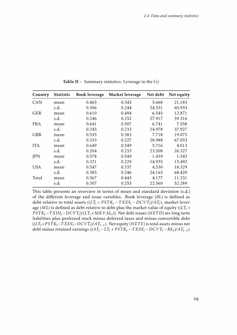
Table II presents the summary statistics of the dependent variables. Overall, we
see that leverage in market-based countries, measured as debt relative to total assets,
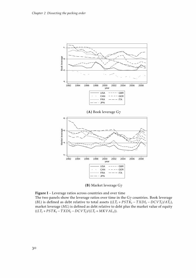
is lower than in bank-based countries. This finding is independent of the definition
of leverage. Book leverage and market leverage are lower in market-based countries
as well. This finding is also independent of the point in time, as we see from the
market leverage graph in Figure I. For book leverage, the ratio is below . for
market-based countries, and generally above . for bank-based ones. The market
leverage picture is even more distinct, as Panel B of Figure I shows. In market-based
countries, leverage is below ., while in bank-based countries it is above ..
The central variable of our study is the so-called deficit coefficient (DEF). We
define a financial deficit as the change in net debt (NETD) plus the change in net
equity minus the change in retained earnings (NETE) relative to the beginning-of-
year assets (see Appendix B for a detailed description).
One of our hypotheses states that firms time the market, and that the macroe-
conomic environment has an important influence on issuance behavior. To proxy
for the market directly, we use the equity risk premium (ERP), calculated as the
mean of the last -month return of the respective country index. The variable is
lagged months, as in Huang and Ritter (), to account for a lag in managers’
decision-making.
To proxy for the state of the economy, we use the real interest rate of every
country, the U.S. default spread as a proxy for general risk attitude, the term
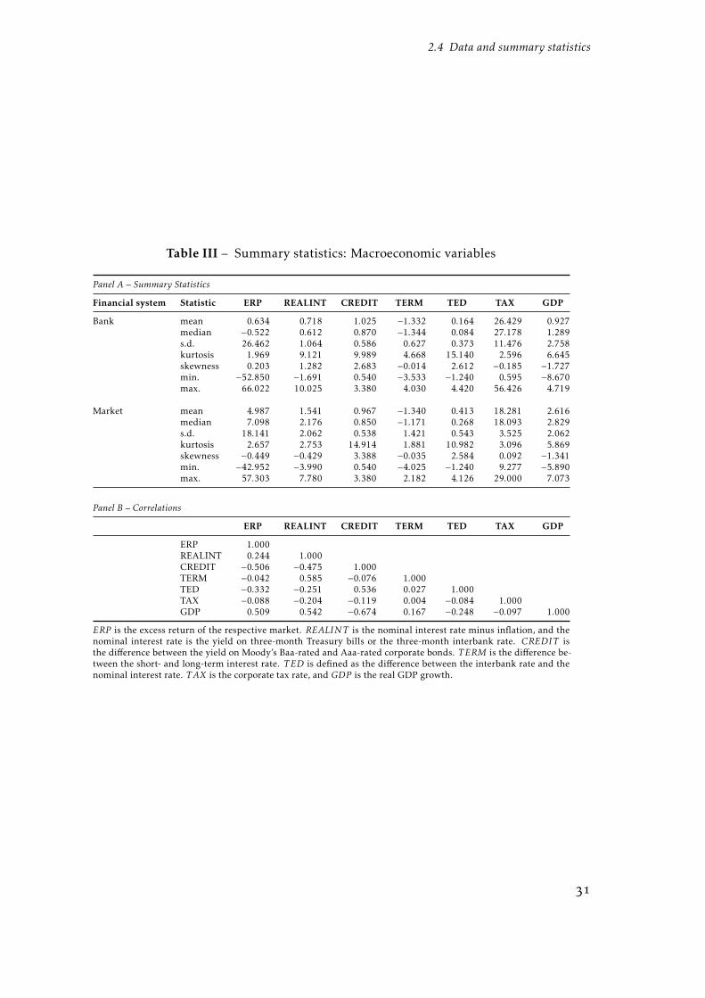
spread, the TED spread, the GDP growth rate, and the corporate tax rate. Table III
shows the correlations between the variables. We note especially low correlations
in Panel B. We conclude that each variable is needed to proxy for the economic
environment. However, we also use a dummy variable as an overall proxy for
recessions, which is equal to if the economy is entering a recession, and otherwise.
Here, we follow Halling et al. (), and use definitions from the Economic Cycle
Research Institute.
Our main goal is to investigate the theories of capital structure under different
We use the S&P for the U.S., the FTSE All-Share for the U.K., the Toronto SE for Canada,the SBF for France, the Nikkei for Japan, the BIC ALl Share for Italy, and the MDAX forGermany. REALINT is the nominal interest rate minus inflation, while the nominal interest rate is the yieldon three-month Treasury bills or the three-month interbank rate. CREDIT is the difference between the yield on Moody’s Baa-rated and Aaa-rated corporate bonds. The data come from the Economic Cycle Research Institute website (www.businesscycle.com).
2.4 Data and summary statistics
Table II – Summary statistics: Leverage in the G
Country Statistic Book leverage Market leverage Net debt Net equity
CAN mean 0.465 0.345 5.668 21.183s.d. 0.306 0.244 24.531 60.933
GER mean 0.610 0.494 6.545 12.871s.d. 0.246 0.252 27.917 59.316
FRA mean 0.641 0.507 6.741 7.558s.d. 0.245 0.233 24.978 37.927
GBR mean 0.555 0.383 7.718 19.075s.d. 0.333 0.227 28.988 67.053
ITA mean 0.649 0.549 5.716 4.013s.d. 0.204 0.233 23.508 26.327
JPN mean 0.578 0.549 1.439 1.543s.d. 0.221 0.229 14.935 15.492
USA mean 0.547 0.337 4.530 18.329s.d. 0.385 0.246 24.165 68.420
Total mean 0.567 0.443 4.177 11.231s.d. 0.307 0.255 22.560 52.289
This table presents an overview in terms of mean and standard deviation (s.d.)of the different leverage and issue variables. Book leverage (BL) is defined asdebt relative to total assets ((LTt + P STKt − TXDIt −DCVTt)/ATt), market lever-age (ML) is defined as debt relative to debt plus the market value of equity ((LTt +P STKt−TXDIt−DCVTt)/(LTt+MKVALt)). Net debt issues (NETD) are long termliabilities plus preferred stock minus deferred taxes and minus convertible debt((LTt+P STKt−TXDIt−DCVTt)/ATt−1). Net equity (NETE) is total assets minus netdebt minus retained earnings ((ATt −LTt + P STKt − TXDIt −DCVTt −REt)/ATt−1).
Chapter 2 Dissecting the pecking order
.4.5
.6.7
Boo
k le
vera
ge
1992 1994 1996 1998 2000 2002 2004 2006 2008year
USA GBRCAN GERFRA ITAJPN
(A) Book leverage G
.2.4
.6.8
Mar
ket l
ever
age
1992 1994 1996 1998 2000 2002 2004 2006 2008year
USA GBRCAN GERFRA ITAJPN
(B) Market leverage G
Figure I – Leverage ratios across countries and over timeThe two panels show the leverage ratios over time in the G countries. Book leverage(BL) is defined as debt relative to total assets ((LTt + P STKt − TXDIt −DCVTt)/ATt),market leverage (ML) is defined as debt relative to debt plus the market value of equity((LTt + P STKt − TXDIt −DCVTt)/(LTt +MKVALt)).
2.4 Data and summary statistics
Table III – Summary statistics: Macroeconomic variables
Panel A – Summary Statistics
Financial system Statistic ERP REALINT CREDIT TERM TED TAX GDP
Bank mean 0.634 0.718 1.025 −1.332 0.164 26.429 0.927median −0.522 0.612 0.870 −1.344 0.084 27.178 1.289s.d. 26.462 1.064 0.586 0.627 0.373 11.476 2.758kurtosis 1.969 9.121 9.989 4.668 15.140 2.596 6.645skewness 0.203 1.282 2.683 −0.014 2.612 −0.185 −1.727min. −52.850 −1.691 0.540 −3.533 −1.240 0.595 −8.670max. 66.022 10.025 3.380 4.030 4.420 56.426 4.719
Market mean 4.987 1.541 0.967 −1.340 0.413 18.281 2.616median 7.098 2.176 0.850 −1.171 0.268 18.093 2.829s.d. 18.141 2.062 0.538 1.421 0.543 3.525 2.062kurtosis 2.657 2.753 14.914 1.881 10.982 3.096 5.869skewness −0.449 −0.429 3.388 −0.035 2.584 0.092 −1.341min. −42.952 −3.990 0.540 −4.025 −1.240 9.277 −5.890max. 57.303 7.780 3.380 2.182 4.126 29.000 7.073
Panel B – Correlations
ERP REALINT CREDIT TERM TED TAX GDP
ERP 1.000REALINT 0.244 1.000CREDIT −0.506 −0.475 1.000TERM −0.042 0.585 −0.076 1.000TED −0.332 −0.251 0.536 0.027 1.000TAX −0.088 −0.204 −0.119 0.004 −0.084 1.000GDP 0.509 0.542 −0.674 0.167 −0.248 −0.097 1.000
ERP is the excess return of the respective market. REALINT is the nominal interest rate minus inflation, and thenominal interest rate is the yield on three-month Treasury bills or the three-month interbank rate. CREDIT isthe difference between the yield on Moody’s Baa-rated and Aaa-rated corporate bonds. T ERM is the difference be-tween the short- and long-term interest rate. T ED is defined as the difference between the interbank rate and thenominal interest rate. TAX is the corporate tax rate, and GDP is the real GDP growth.
Chapter 2 Dissecting the pecking order
capital market systems. However, firm characteristics are also important in deter-
mining capital structure, and in evaluating the pecking order theory. Some of the
control variables in the literature have had a persistent influence on capital structure
decisions (Frank and Goyal ). We use a broad set of controls to examine the
effects of cash (CASH), operating income (OINC), capital expenditures (CAPX),
Tobin’s Q (Q), research & development expenditures (RANDD), age (AGE), and
size (SIZE). All variables are scaled by total assets, except for age and size. We
construct the size variable as the natural logarithm of sales measured in US$
in order to be a sufficient proxy for overall firm size in different countries. These
variables represent standard capital structure determinants, and are frequently used
in corporate finance research(see, e.g., in Frank and Goyal (), Huang and Ritter
() and Cook and Tang (), among others).
2.5 Empirical results
2.5.1 The pecking order over time
We start with the simple model of Shyam-Sunder and Myers () to analyze how
the pecking order model performs over time. In our first step, we include only the
financial deficit, as follows:
∆Dit = at + btDEFit + εit (1)
where ∆Dit is the net debt issue, and DEFit is the financial deficit. If the pecking
order model is correct for describing a firm’s capital structure choices, the DEF
coefficient (bt) should equal . Firms prefer debt over equity because of the lower
costs of asymmetric information. Hence, they should finance their deficits with
debt. We perform the regression for all seven countries separately and examine
the development of the coefficient. We than divide the sample into bank- and
market-based capital markets, and explore the chronological development over time.
This provides a first glance at the differences and time series development of the
coefficient. According to our Hypotheses I and II, we expect to see a higher pecking
order coefficient in bank-based countries, as well as a generally converging pecking
order coefficient.
Panel A of Figure II shows that the pecking order coefficient in a market-based
system ranges from . to . and is relatively stable over time. The same pattern
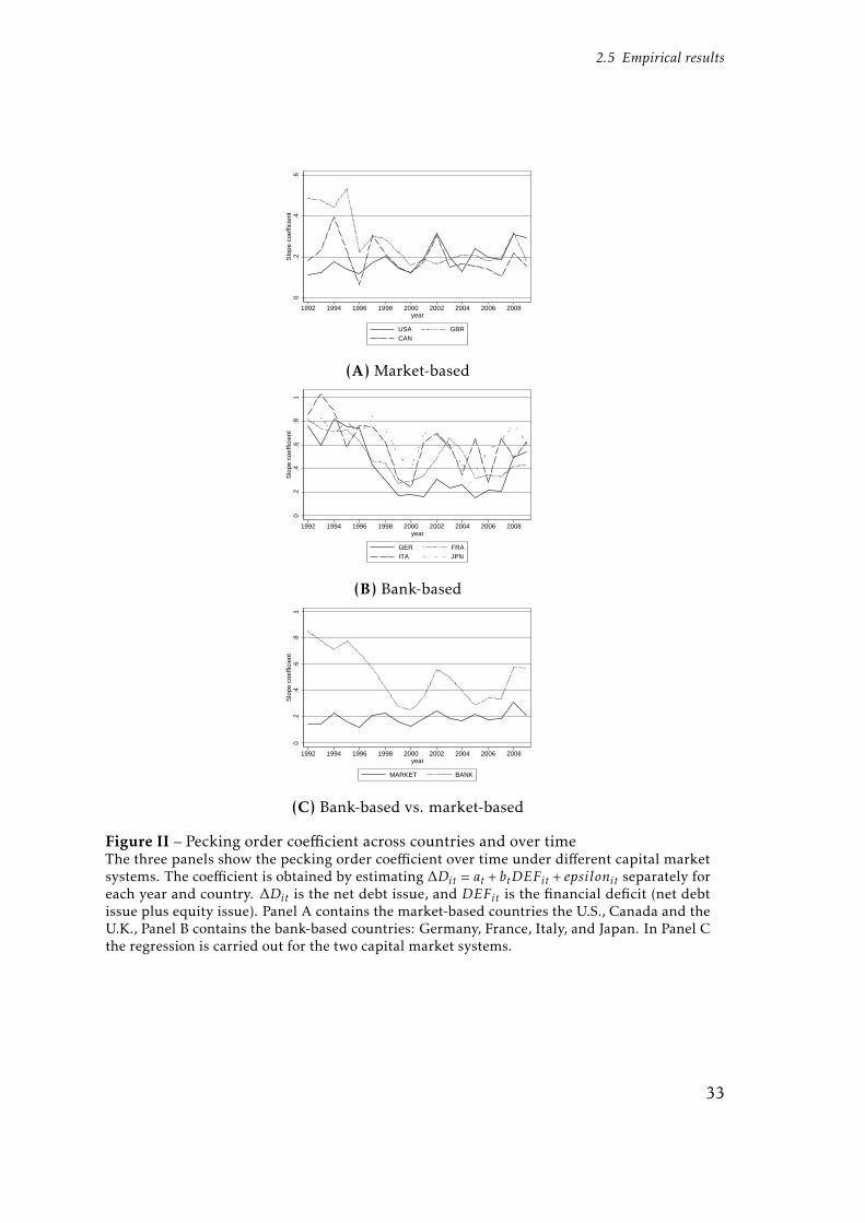
2.5 Empirical results
0.2
.4.6
Slo
pe c
oeffi
cien
t
1992 1994 1996 1998 2000 2002 2004 2006 2008year
USA GBRCAN
(A) Market-based
0.2
.4.6
.81
Slo
pe c
oeffi
cien
t
1992 1994 1996 1998 2000 2002 2004 2006 2008year
GER FRAITA JPN
(B) Bank-based
0.2
.4.6
.81
Slo
pe c
oeffi
cien
t
1992 1994 1996 1998 2000 2002 2004 2006 2008year
MARKET BANK
(C) Bank-based vs. market-based
Figure II – Pecking order coefficient across countries and over timeThe three panels show the pecking order coefficient over time under different capital marketsystems. The coefficient is obtained by estimating ∆Dit = at + btDEFit + epsilonit separately foreach year and country. ∆Dit is the net debt issue, and DEFit is the financial deficit (net debtissue plus equity issue). Panel A contains the market-based countries the U.S., Canada and theU.K., Panel B contains the bank-based countries: Germany, France, Italy, and Japan. In Panel Cthe regression is carried out for the two capital market systems.
Chapter 2 Dissecting the pecking order
is observable in all three countries, at least after . The coefficient peaks occur
in , and , which correspond to periods of recession in the respective
countries. Firms from market-based countries seem to follow a pecking order more
often during times of recession, when the access to equity capital markets is more
constrained.
In the second panel, we see that bank-based countries have a much more volatile
coefficient that declines over time. This confirms our Hypothesis II, that the propor-
tion of equity and debt used to finance deficits has converged recently. Hence, we
see the convergence of the financial systems. The different recessionary times again
show the same patterns: The pecking order coefficient seems to be higher during
economic downturns, and firms also seem to use more debt in these times. The
overall range of the pecking order coefficient in bank-based countries is from about
. to .. The coefficient seems to decline from its high in the early s.
In the third panel, we compare only bank- and market-based systems. While the
bank-based coefficient seems to decline during the late s, it is higher than that
in market-based countries. This implies that in bank-based systems, firms tend to
cover financial deficits with debt more often than in market-based countries. This
finding is consistent with our Hypothesis I.
Equity markets in bank-based countries are not as developed as they are in market-
based countries, and the legal system tends to be more lender-oriented. Conse-
quently, there is a higher level of information asymmetry between shareholders and
management. As we noted earlier, banks have the critical access to information.
Equity issues are thus more expensive than in market-based countries, because
shareholders demand a higher premium. Firms tend to have extremely close ties to
their so-called house banks, and therefore they use more debt for financing because
it is relatively cheaper. If we compare our results to Huang and Ritter (), we find
a somewhat lower coefficient for the U.S. in the years the data overlaps. The DEF
coefficient seems stable at around . in market-based countries, which confirms
the findings of Huang and Ritter (). The overall picture is also consistent with
Shyam-Sunder and Myers (), who document strong evidence for the pecking
order during the early s, and with Frank and Goyal (), who document a
declining pecking order coefficient in the s.
However, in both financial systems the coefficient is far from and thus the
pecking order theory cannot explain overall firm behavior. There are several possible
reasons why firms would not follow a pecking order, or why the simple Shyam-

2.5 Empirical results
Sunder and Myers () test does not capture the patterns. The objections of
Chirinko and Singha () are one possible explanation, but they are econometric
in nature. The authors argue that debt/equity issue policies (issues in constant
proportions) can bias the coefficient downwards. However, the focus of our study lies
in comparing the pecking order in different financial systems. Even if the problems
mentioned by Chirinko and Singha () prevent us from making exact quantitative
statements, we can still make qualitative judgments about the importance of the
pecking order in different financial systems.
2.5.2 The pecking order and the sign of the deficits
Another reason the pecking order performs so poorly could be that firms behave
differently depending on whether they have a positive or negative financial deficit.
For example, firms with a surplus might follow a pecking order, but firms with a
deficit perhaps do not (or vice versa). Therefore, we differentiate between positive
and negative financial deficits in our next step.
It is also possible that the standard DEF coefficient is incorrect because firms
behave differently depending on the sign of the financial deficit. In the case of a
positive financial deficit (a surplus) firms could use funds to buy back equities or
issue dividends, rather than paying debt back first. De Jong et al. () account for
these these differences in a study of the pecking order in the U.S. They document
a higher pecking order coefficient when firms have a surplus. However, for firms
running deficits, the DEF coefficient is low, which is contrary to pecking order
predictions. Firms with large deficits have even lower coefficients, indicating that
the pecking order model performs poorly for these firms. We extend De Jong et al.’s
() tests to our G sample, and estimate
∆Dit = at + btNDEFit + PDEFit + εit, (2)
where NDEFit are negative deficits (financial surpluses), and PDEFit are positive
deficits. Shyam-Sunder and Myers () note different implications for deficits and
surpluses (see section 2.3). Optimistic managers wish to buy back shares in order to
obtain higher prices by reducing the supply of shares. Pessimistic managers tend
to evaluate their firms’ share prices as too high, and they do not buy back shares.
As a result, only optimistic managers will be able to drive up prices until their
own evaluation meets investor evaluations. In equilibrium, only debt repurchases

Chapter 2 Dissecting the pecking order
will occur. We extend this reasoning to the difference between bank- and market-
based systems: We expect to see a lower pecking order coefficient for surpluses in
bank-based systems than in market-based systems, because the pressure to buy back
shares is less pronounced.
Our first step here is to estimate Equation (2), but with separate positive and
negative deficits. This is not exactly De Jong et al.’s () method; they use a
dummy variable to capture the effects. Nevertheless, we believe our results are
quite comparable to theirs. We find high coefficients in both systems for negative
deficits, e.g., surpluses. Both are in the range of , and indicate that firms mainly
use surpluses to buy back debt, as per Shyam-Sunder and Myers (). However,
the coefficient on positive financial deficit is much lower than is needed for pecking
order behavior. It is higher for banks, but it is below . in both cases. These results
are consistent with De Jong et al. (), who find . for deficits and . for a
surplus in the U.S. The results in Huang and Ritter’s () long U.S. sample (from
to ) are lower for surpluses and higher for deficits. But the results for
their short sample (from to ) are qualitatively similar to ours. For their
long sample, they find a . coefficient on the financial deficit. Overall, Huang and
Ritter’s () results indicate a declining pecking order coefficient, as they report a
higher coefficient for the long-run sample, and a lower coefficient for their short-run
sample.
We also need to determine how firm characteristics commonly used in the capital
structure literature (Huang and Ritter ; De Jong et al. ; Frank and Goyal
) influence the positive pecking order coefficient. To do this, we include interac-
tion terms with the positive financing deficit (PDEF) in Columns and . Equation
(3) has the definition:
∆Dit = at + btNDEFit + (c+ dCHEit + eCAPXit + f Qit
+ gRANDDit + hSIZEit + jAGEit + kTANGit)× PDEFit + εit (3)
Here, we first explore the differences between bank- and market-based systems.
A higher cash holdings variable (CHE) has a negative influence on the pecking
order coefficient in both financial systems, while capital expenditures (CAPX)
and Tobin’s Q (Q) have a negative influence. The expenditures on research and
development (RAND) have a positive influence in market-based countries and a
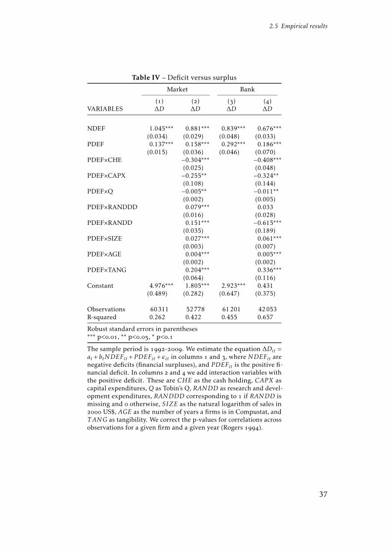
2.5 Empirical results
Table IV – Deficit versus surplus
Market Bank
() () () ()VARIABLES ∆D ∆D ∆D ∆D
NDEF 1.045*** 0.881*** 0.839*** 0.676***(0.034) (0.029) (0.048) (0.033)
PDEF 0.137*** 0.158*** 0.292*** 0.186***(0.015) (0.036) (0.046) (0.070)
PDEF×CHE −0.304*** −0.408***(0.025) (0.048)
PDEF×CAPX −0.255** −0.324**(0.108) (0.144)
PDEF×Q −0.005** −0.011**(0.002) (0.005)
PDEF×RANDDD 0.079*** 0.033(0.016) (0.028)
PDEF×RANDD 0.151*** −0.615***(0.035) (0.189)
PDEF×SIZE 0.027*** 0.061***(0.003) (0.007)
PDEF×AGE 0.004*** 0.005***(0.002) (0.002)
PDEF×TANG 0.204*** 0.336***(0.064) (0.116)
Constant 4.976*** 1.805*** 2.923*** 0.431(0.489) (0.282) (0.647) (0.375)
Observations 60311 52778 61201 42053R-squared 0.262 0.422 0.455 0.657
Robust standard errors in parentheses*** p<., ** p<., * p<.
The sample period is -. We estimate the equation ∆Dit =at + btNDEFit + PDEFit + εit in columns and , where NDEFit arenegative deficits (financial surpluses), and PDEFit is the positive fi-nancial deficit. In columns and we add interaction variables withthe positive deficit. These are CHE as the cash holding, CAPX ascapital expenditures, Q as Tobin’s Q, RANDD as research and devel-opment expenditures, RANDDD corresponding to if RANDD ismissing and otherwise, SIZE as the natural logarithm of sales in US$, AGE as the number of years a firms is in Compustat, andTANG as tangibility. We correct the p-values for correlations acrossobservations for a given firm and a given year (Rogers ).

Chapter 2 Dissecting the pecking order
negative influence in bank-based countries. Size, age and tangibility (TANG) all
have a positive influence on the pecking order coefficient in both systems.
In our second step, we relate the signs of the coefficients to the pecking order
theory. The negative sign on cash holdings is consistent with pecking order theory,
because firms generating high levels of cash can use internal financing. Capital
expenditures have a negative sign as well. We would expect that the magnitude
of expenditures does not influence decisions between equity or debt. However, a
negative sign indicates that firms with higher capital expenditures use more equity.
This finding contradicts the predictions of the pecking order theory that there would
be no influence. Moreover, Tobin’s Q has a negative influence: Firms with a high Q
tend to be growth firms, and have a lower pecking order coefficient. This is in line
with theory, because growth firms have higher costs of financial distress, and higher
degrees of asymmetric information. Research and development expenditures lead to
a higher pecking order coefficient in market-based systems, which is also consistent
with theory. The influence of research and development in bank-based countries
may be doubtful, however, as the coefficient indicates a highly significant negative
influence. RANDD has a very low mean in bank-based countries at ., and has
several missing values. An accounting problem in Compustat might be the problem.
Size and age have a positive influence on the DEF coefficient. We assume that older
and larger firms tend to have higher analyst coverage (Drobetz et al. ), and
hence lower costs of asymmetric information. This implies they can use more debt.
Tangibility has a positive impact on the pecking order coefficient. Firms with a high
proportion of property and plants have higher marginal debt issuing activity. These
firms have a lower degree of asymmetric information and lower costs of financial
distress, because their assets are easy to value and liquidate. This is in line with the
predictions of the pecking order theory.
The results indicate that the pecking order predictions hold for most of the
influences of firm characteristics; however, the overall performance of the positive
financing deficit is still poor. The influence firm characteristics, especially, Tobin’s
Q, age and tangibility, are somewhat dependent on the extend to which pecking
order theory can explain their financing behavior.
2.5.3 The pecking order and the deficit size
The next step is to investigate the magnitude of deficits. From the pecking order
theory, we know that the direction of influence is expected to be unclear. Large

2.5 Empirical results
deficits are normal for small growth firms with many investment opportunities and
large information asymmetries. In fact, because of the information asymmetries,
we would argue that firms with large deficits direct their financing activities more
toward a pecking order. However, banks and the market for corporate debt may
not be able (or willing) to grant enough debt. Small firms would therefore have to
use equity. Thus, we could argue that firms with large deficits also tend to issue
relatively more equity capital. Hypothesis I states that firms in bank-based countries
can take on more debt, and therefore the pecking order coefficient for larger deficits
should be higher. We divide our sample along the size of deficits and surpluses into
four groups (quartiles) and run the regressions separately. We do not use controls
because we are only interested in the different DEF coefficients. Table V gives the
results.
The highest pecking order coefficient, ., appears for the smallest deficits in
bank-based countries. The coefficient in market-based countries is slightly lower.
The overall coefficient in bank-based countries is higher, . to .. However, this
is quite low from a pecking order perspective. As the low coefficient shows, the
pecking order theory is not a good predictor of the largest deficit in either system.
The coefficient is below . in market-based countries, and it is . in bank-based
countries. Creditors may be more reluctant to lend when deficits are large, and
thus firms may need to go to the capital markets. This is consistent with De Jong
et al. (), who also find very low coefficients for high deficits. The effect is
even more pronounced in marked-based countries; hence, in bank-based countries,
creditors seem willing to lend more, confirming our Hypothesis I. For medium
and larger deficits, the pecking order coefficients range from . to .. In both
cases, the coefficients in bank-based systems are higher than those in market-based
systems. This observation provides further evidence for our hypothesis that firms in
bank-based system can take on more debt.
In the case of surpluses, the coefficients are – with one exception – above . and
slightly higher in market-based countries. Firms in these countries use surpluses
to buy back more debt. However, the results for the largest surpluses are not in
line with theory predictions, as they are not fully used to buy back debt. One
possible explanation may be that managers tend to smooth dividends (Allen and
Michaely ), but in years with extremely high surpluses, they buy back shares or
pay extra dividends. The pecking order theory does not account for this behavior.
Except for very large surpluses, we can confirm the arguments of Shyam-Sunder

Chapter 2 Dissecting the pecking order
Tab
leV
–D
efici
tan
dsu
rplu
ssi
ze
Pane
lA–
Mar
ket
()
()
()
()
()
()
()
()
()
()
Ove
rall
defi
cit
Smal
lest
Med
ium
smal
lM
ediu
mla
rge
Lar
gest
Ove
rall
surp
lus
Smal
lest
Med
ium
smal
lM
ediu
mla
rge
Lar
gest
VAR
IAB
LE
S∆D
∆D
∆D
∆D
NE
TD
∆D
NE
TD
∆D
∆D
∆D
PD
EF
0.12
7***
0.79
2***
0.73
9***
0.44
9***
0.06
5***
(0.0
14)
(0.0
47)
(0.0
43)
(0.0
23)
(0.0
13)
ND
EF
0.72
2***
0.84
4***
0.81
5***
0.91
3***
0.62
9***
(0.0
26)
(0.1
13)
(0.0
89)
(0.0
76)
(0.0
42)
Con
stan
t7.
253*
**−0.7
88**
*−0.6
39**
2.93
3***
23.2
40**
*−1.3
50**
*−0.6
30**
*−0.6
74*
−0.2
51−3.8
91**
*(0.5
34)
(0.1
58)
(0.2
96)
(0.3
21)
(1.4
31)
(0.2
37)
(0.2
03)
(0.3
84)
(0.5
82)
(0.7
85)
Obs
erva
tion
s39
713
1007
410
069
1006
494
9620
608
5161
5156
5154
5126
R-sq
uar
ed0.
144
0.02
90.
033
0.04
20.
033
0.36
80.
008
0.01
10.
037
0.20
9
Pane
lB–
Ban
k
Ove
rall
defi
cit
Smal
lest
Med
ium
smal
lM
ediu
mla
rge
Lar
gest
Ove
rall
surp
lus
Smal
lest
Med
ium
smal
lM
ediu
mla
rge
Lar
gest
VAR
IAB
LE
S∆D
∆D
∆D
∆D
∆D
∆D
∆D
∆D
∆D
∆D
PD
EF
0.27
2***
0.89
7***
0.84
2***
0.75
4***
0.19
9***
(0.0
43)
(0.0
33)
(0.0
37)
(0.0
32)
(0.0
37)
ND
EF
0.58
4***
0.88
5***
0.76
6***
0.77
4***
0.43
8***
(0.0
31)
(0.0
78)
(0.0
52)
(0.0
44)
(0.0
42)
Con
stan
t5.
545*
**−0.3
14**
*−0.2
220.
215
18.3
70**
*−1.6
47**
*−0.2
70*
−0.6
83**
*−0.8
42**
−5.2
48**
*(0.8
31)
(0.1
04)
(0.2
04)
(0.3
46)
(1.9
25)
(0.2
33)
(0.1
54)
(0.2
11)
(0.3
30)
(0.6
19)
Obs
erva
tion
s32
963
8256
8257
8257
8179
2825
170
6070
6370
6070
53R-
squ
ared
0.34
90.
041
0.05
60.
089
0.20
80.
364
0.02
20.
024
0.05
50.
150
Rob
ust
stan
dar
der
rors
inp
aren
thes
es**
*p<.
,**
p<.
,*p<.
The
sam
ple
per
iod
is
-.
We
esti
mat
eth
eeq
uat
ion∆Dit
=a t
+b tDEFit
+ε it,
whe
reDEFit
isei
therNDEFit
(neg
ativ
ed
efici
ts)
orPDEFit
(pos
itiv
efi
nanc
iald
efici
ts).
We
sort
the
firm
year
obse
rvat
ions
alon
gth
esi
zeof
the
defi
cits
and
buil
dqu
arti
les.
The
regr
essi
ons
are
ran
sep
arat
ely
for
pos
itiv
ean
dne
gati
ved
efici
ts.
The
p-v
alu
esar
eco
rrec
ted
for
corr
elat
ion
acro
ssob
serv
atio
nsfo
ra
give
nfi
rman
da
give
nye
ar(R
oger
s
).
2.5 Empirical results
and Myers () that firms in equilibrium should buy back debt, with coefficients
slightly below .. With the largest surpluses (. in market-based countries, . in
bank-based) managers seem to follow a different reasoning, and, surprisingly, the
coefficient is smaller in bank-based systems. It may be that buying back debt in such
large amounts is not possible, because banks do not allow firms to cancel long-term
debt contracts.
In summary, we find that pecking order theory does explain the financing behavior
of large deficits. Apart from pure size, it may be that some firms are debt-constrained.
They may be considered uncreditworthy, and thus can not follow a pecking order.
To further investigate this question, our next model uses a more direct measure of
debt constraints.
2.5.4 The pecking order and debt constraints
To broaden our understanding of which types of firms follow a pecking order in
their financing decisions, we check for the influence of financial constraints. We
hypothesize that financially constrained firms do not follow a pecking order because
they are not able to borrow. Their creditworthiness may be suspect, or banks and
debt markets may have other reasons to decline funding. We further hypothesize
that fewer firms in market-based countries will be able (or willing) to follow a
pecking order, because equity is relatively cheaper and banks are not as specialized
in monitoring highly leveraged firms.
Several approaches exist in the literature to determine, whether a firm is finan-
cially constrained. One measure used, Korajczyk and Levy (), for example, use
dividend distributions. Because many investors look at the credit rating of a firm
in their decision-making process, the rating is a natural way to observe any signs
of financial constraints. However, as we noted earlier, only a small subsample of
firms have ratings, and other solvent firms may have opted not to be rated. This
problem is especially severe in an international sample, because ratings are much
more common in market-based countries. To overcome this problem, we use Lem-
mon and Zender’s () measure, which estimates the probability that a firm will
be able to access public debt markets. In particular, they use a logit regression to
estimate the probability of a firm having a bond rating. In our regressions, we use
the natural logarithm of total assets, return on assets, tangibility, market-to-book
The results of the regression are in Appendix A.

Chapter 2 Dissecting the pecking order
Table VI – Debt constraints
Panel A – Market
() () ()Unconstrained Medium constrained Constrained
VARIABLES ∆D ∆D ∆D
DEF 0.687*** 0.147*** 0.187***(0.037) (0.016) (0.021)
Constant 0.000 2.342*** 0.729**(0.230) (0.570) (0.285)
Observations 9257 36876 14178R-squared 0.708 0.187 0.231
Panel B – Bank
Unconstrained Medium constrained ConstrainedVARIABLES ∆D ∆D ∆D
DEF 0.762*** 0.291*** 0.499***(0.021) (0.048) (0.080)
Constant 0.048 0.847* 0.722**(0.181) (0.490) (0.337)
Observations 11857 40159 9185R-squared 0.816 0.383 0.579
Robust standard errors in parentheses*** p<., ** p<., * p<.
This table contains regressions of the form ∆Dit = at + btDEFit +epsilonit , whereDEFit is the financial deficit. Firms of the years to are sorted by the probability of being financially constrained. Themeasure is the result of logit regression, where the dependent variableis the existence of a debt rating and the independent variables are sev-eral firm specific measures (see Appendix A). When firm’s probabilityof having a rating is below % we classify it as constrained. A proba-bility above % leads to a classification as unconstrained. We correctthe p-values for correlations across observations for a given firm and agiven year (Rogers ). .

2.5 Empirical results
ratio, leverage, firm age, and the standard deviation of earnings as ratings predictors.
The dependent variable is a dummy equal to when the firm has a rating, and otherwise. We use the Standard & Poor’s RatingExpress database. There are three
generally dominant rating agencies, but the resultant probability should capture the
financial health of a firm, because they all use roughly the same inputs. We then
build three groups: constrained, medium-constrained, and unconstrained, and we
perform the pecking order regressions.
The results in Table VI indicate, as in Lemmon and Zender (), that the
pecking order does not explain the behavior of constrained firms. The coefficients
are only . and ., respectively, for constrained and medium-constrained
firms in market-based countries. Unconstrained firms have a . coefficient.
In bank-based countries, the results are somewhat different: The coefficient for
unconstrained firms (.) is in the same range as for market-based firms (.),and it is only slightly higher. So for unconstrained firms, pecking order theory
provides a good explanation for firm behavior. But the coefficients on medium
(.) and constrained (.) firms are also higher than in market based countries.
This is in line with the observation that firms need lower equity stacks in bank-based
countries. It is surprising that the pecking order coefficient on medium constrained
firms (.) is the lowest for bank-based countries. this implies that unconstrained
and constrained firms seem to use debt first when external finance is needed, while
medium-constrained firms use the equity market. In bank-based countries, bank
debt for firms with high asymmetric information seems to be relatively cheaper
than for firms with medium constraints. This corresponds to the findings of Bolton
and Freixas’s () theoretical model. In equilibrium, riskier firms use bank debt,
because banks have the lowest monitoring costs. Medium-risk firms tend to issue
bonds and equity, and low-risk firms issue safe bonds.
2.5.5 The pecking order and the macroeconomy
While firms’ risk characteristics can be one source of financial constraints, capital
shortage can be another. During periods of recession, banks may be unwilling to
fund firms. We next test for the influence of the macroeconomic environment.
A firm is constrained if the probability of having a rating is below .. It is unconstrained whenthe probability is higher than .. We use a larger group for medium-constrained firms because weare mainly interested in the behavior of constrained and unconstrained firms. We also expect thatthe middle body of firms would generally be of medium health.

Chapter 2 Dissecting the pecking order
We also need to test whether firms and the two financial systems behave differently
during different businesses cycles. Capital supply and demand could depend on
the economic state. Recessions lead to deep declines in cash flows, in line with
tighter capital market and bank conditions (Halling et al. ). So, on the one hand,
banks may be more constrained than capital markets because they have long-lasting
lending relationships and may not grant new loan contracts. This should be even
more pronounced in bank-based countries, because banks are the main source of
funding, and firms will only go to the capital markets as a last resort. On the other
hand, capital markets in bank-based countries may run dry faster than banks. The
pecking order theory would then be a better description of the behavior during
downturns in bank-based countries.
Another hypothesis is that the size of the risk premium impacts a firm’s financing
behavior: Firms can use equity when the risk premium is low, and debt when it
is high. This is the main hypothesis of Baker and Wurgler’s () market timing
theory, and is in contrast to pecking order. As per our Hypothesis III, we expect this
behavior be more pronounced in market-based countries.
Our first step is include a dummy for recessions, in order to test the general
influence of economic cycles. We use it as an interaction term to determine its
influence on the pecking order coefficient. Column of Table VII gives our results
for all countries when a recession dummy is included. The dummy variable is
significant at the %-level, and is below .. A recession in a country generally leads
to a slightly higher pecking order coefficient. However, when we separate bank- and
market-based countries (columns and ), we see that the recession only affects
bank-based countries. The coefficient on the recession interaction term in market-
based countries is neither large at ., nor significant. In bank-based countries, the
coefficient is near . and quite significant. The behavior in bank-based countries
thus seems cyclical. During poor economic times, firms rely more heavily on debt,
and capital markets in bank-based countries seem to be hit harder.
In the even columns of Table VII, we further check for the influence of the macroe-
conomic environment using several indicators of economic health. We use the lagged
equity risk premium, calculated as the six-month-lagged twelve-month mean return
of the market index, the real interest rate, the U.S. credit spread, the term spread,
the corporate tax rate, the TED spread, and the real GDP growth. All variables are
interacted with the positive deficit.
We use the definition from the Economic Cycle Research Institute (www.businesscycle.com).

2.5 Empirical results
Table VII – Pecking order and macroeconomic environment
All Market Bank
() () () () () ()VARIABLES ∆D ∆D ∆D ∆D ∆D ∆D
NDEF 0.952*** 0.898*** 1.045*** 0.992*** 0.822*** 0.732***(0.037) (0.034) (0.033) (0.032) (0.046) (0.031)
PDEF 0.163*** 0.346*** 0.136*** 0.346*** 0.272*** 0.238*(0.017) (0.084) (0.015) (0.078) (0.043) (0.132)
PDEF×ERP 0.000 0.000 −0.001(0.001) (0.001) (0.001)
PDEF×REAL −0.006 0.003 0.035(0.009) (0.010) (0.023)
PDEF×CREDIT −0.067*** −0.039** 0.089(0.022) (0.019) (0.063)
PDEF×TERM 0.001 −0.006 0.011(0.011) (0.012) (0.037)
PDEF×TAX 0.002 −0.008*** 0.009***(0.002) (0.003) (0.002)
PDEF×GDP −0.027*** −0.002 −0.004(0.008) (0.007) (0.012)
PDEF×TED −0.039** 0.025* 0.004(0.017) (0.015) (0.035)
PDEF×REC 0.097** 0.028 0.220***(0.040) (0.044) (0.042)
Constant 4.145*** 3.279*** 4.963*** 4.434*** 2.616*** 0.845***(0.438) (0.324) (0.483) (0.388) (0.639) (0.308)
Observations 121512 94976 60311 43435 61201 51541R-squared 0.314 0.387 0.262 0.328 0.472 0.615
Robust standard errors in parentheses*** p<., ** p<., * p<.
The sample period lasts from –. We estimate the equation ∆Dit = at + btNDEFit +PDEFit +PDEFit×RECit +εit in column , and where NDEFit are negative deficits (finan-cial surpluses), and PDEFit are the positive deficits. PDEF ×REC is an interaction term con-structed form the positive financial deficit and a dummy for recessions. In columns , an ,we add interaction variables with the positive deficit: the equity risk premium (ERP ), the realinterest rate (REALINT ), the term spread (T ERM), the TED spread (T ED), the corporate taxrate (TAX), and real GDP growth (GDP ). We correct the p-values for correlations across obser-vations for a given firm and a given year (Rogers ).

Chapter 2 Dissecting the pecking order
Contrary to Huang and Ritter (), we do not find any significance for the
equity risk premium. The real interest rate is also insignificant. In market-based
countries, the U.S. credit spread has a significantly negative impact on the pecking
order coefficient. During riskier times, firms are thus directed to the capital markets,
which indicates that banks are less successful in providing funds than equity markets.
The U.S. credit spread also shows no significance in bank-based countries. However,
the corporate tax rates are significant, with a negative sign in market-based countries
and a positive sign in bank-based ones. This could be explained partially by different
taxation rules. A lower corporate-level tax rate would favor debt over equity, in line
with findings in bank-based countries. But in market-based countries, a high tax rate
drives down the pecking order coefficient, lowering debt issues. This is somewhat
puzzling, because some countries have tax legislation on dividends to account for
corporate taxation. And interest income, in contrast, is taxed fully. The tax code
here appears to favor equity.
In our aggregated sample in Column , the real GDP growth rate (with a negative
sign) and the TED spread (negative sign) are also significant. A negative sign on
GDP growth indicates that during times of high growth opportunities, firms will
use slightly more equity. The coefficient on the TED spread suggests that, during
risky times, firms use on average more debt. Overall, only a few macroeconomic
variables show significance. We find evidence of market timing during recessions in
bank-based countries, but not with macroeconomic proxies.
However, until now, we have only checked pecking order theory with observations
of the DEF coefficient. Because there is some methodological critique (Chirinko and
Singha ), we also calculate another model that examines the decision processes
of firms. It also serves as a robustness test.
2.5.6 The pecking order and the decision of the firm
A necessary assumption of the pecking order model is that financing decisions are
exogenous. But it is possible that firms may decide jointly whether and what kind
of securities to issue. To account for this behavior, Huang and Ritter () estimate
a nested logit model. The advantage of this type of model is that it can reduce the
influence of extreme observations. According to Flannery and Rangan (),changing firm characteristics, instead of changing market conditions, can also affect
Huang and Ritter () note that, in a nested logit model, the amount of securities being issuedis irrelevant, and firms will be assigned the same value.

2.5 Empirical results
the pecking order coefficient. Therefore, firm characteristics are also included.
The model has two decision levels: ) whether to issue securities, and ) whether
to issue debt or equity. A firm is defined as issuing debt (equity) if the change in
NETD (NETE) is larger than %. We follow Huang and Ritter’s () notation and
modeling. The probability of security issuance is thus P r(i), where issuance is (i = s),
and no issuance is (i = n). The probability of a security issue is given in Equation (5).
The conditional probabilities are P r(j |s) where (j = d) for debt, and (j = e) for equity.
These probabilities are in Equation (4):
P r(j |s) =exp(xsjβ)
exp(xseβ) + exp(xsdβ)(4)
and
P r(s) =exp(ysα + ηsIs)
exp(ysα + ηsIs) + exp(ynα + ηnIn), (5)
where Ii = ln(exp(xieβ) + exp(xidβ)), and xij and yij are vectors with i and j ex-
planatory variables. The numerator is the logistic expression for the occurrence, and
the denominator is the combined expression for every occurrence. Non-issuers are
the base for the first level, while debt is the base for the second level. The system is
estimated by using maximum likelihood.
The results are shown in Table VIII. With a few exceptions, we use the same set of
explanatory variables as Huang and Ritter (). For the base decision, “Issue or
Not”, we find results similar to Huang and Ritter () for market-based countries.
Thus, cash has a negative impact on the issue decision, consistent with pecking order.
But it is not significant in bank-based countries, where the preference for external
finance seems lower. Not surprisingly, capital expenditures have a positive impact,
along with Tobin’s Q and research and development. In this kind of regression, the
recession dummy is significant. Note that, in marked-based countries, the dummy
has a positive impact on the issuance decision; in bank-based countries, it has is
a negative impact. During times of recession, market-based firms have a higher
issue probability, and bank-based firms have a lower one. The equity risk premium,
however, has a positive impact. Thus, firms tend to issue after periods of high risk
premiums. Furthermore, the U.S. credit spread has a negative influence on issue
probability. When the price for taking on risk is too high, firms tend not to issue.
But the real GDP growth rate has a positive influence. This rate is an indicator
Contrary to Huang and Ritter (), we excluded the lagged and forwarded market return inorder to obtain a more manageable number of observations.
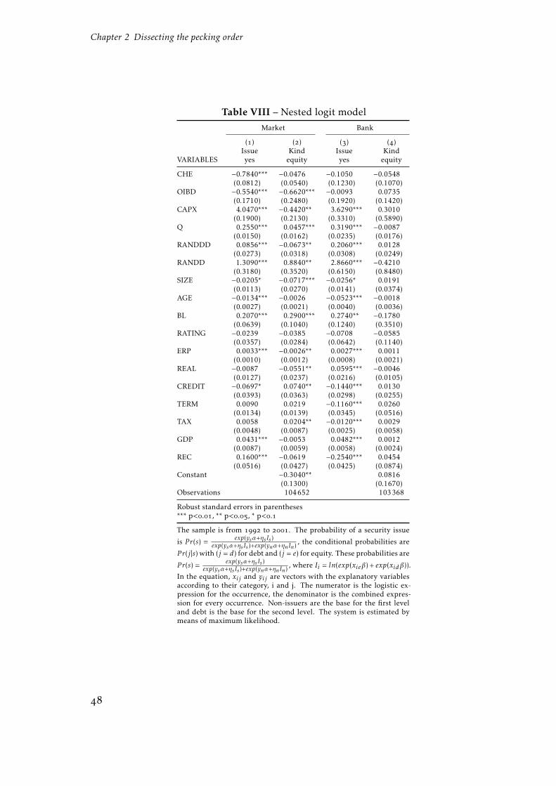
Chapter 2 Dissecting the pecking order
Table VIII – Nested logit modelMarket Bank
() () () ()Issue Kind Issue Kind
VARIABLES yes equity yes equity
CHE −0.7840*** −0.0476 −0.1050 −0.0548(0.0812) (0.0540) (0.1230) (0.1070)
OIBD −0.5540*** −0.6620*** −0.0093 0.0735(0.1710) (0.2480) (0.1920) (0.1420)
CAPX 4.0470*** −0.4420** 3.6290*** 0.3010(0.1900) (0.2130) (0.3310) (0.5890)
Q 0.2550*** 0.0457*** 0.3190*** −0.0087(0.0150) (0.0162) (0.0235) (0.0176)
RANDDD 0.0856*** −0.0673** 0.2060*** 0.0128(0.0273) (0.0318) (0.0308) (0.0249)
RANDD 1.3090*** 0.8840** 2.8660*** −0.4210(0.3180) (0.3520) (0.6150) (0.8480)
SIZE −0.0205* −0.0717*** −0.0256* 0.0191(0.0113) (0.0270) (0.0141) (0.0374)
AGE −0.0134*** −0.0026 −0.0523*** −0.0018(0.0027) (0.0021) (0.0040) (0.0036)
BL 0.2070*** 0.2900*** 0.2740** −0.1780(0.0639) (0.1040) (0.1240) (0.3510)
RATING −0.0239 −0.0385 −0.0708 −0.0585(0.0357) (0.0284) (0.0642) (0.1140)
ERP 0.0033*** −0.0026** 0.0027*** 0.0011(0.0010) (0.0012) (0.0008) (0.0021)
REAL −0.0087 −0.0551** 0.0595*** −0.0046(0.0127) (0.0237) (0.0216) (0.0105)
CREDIT −0.0697* 0.0740** −0.1440*** 0.0130(0.0393) (0.0363) (0.0298) (0.0255)
TERM 0.0090 0.0219 −0.1160*** 0.0260(0.0134) (0.0139) (0.0345) (0.0516)
TAX 0.0058 0.0204** −0.0120*** 0.0029(0.0048) (0.0087) (0.0025) (0.0058)
GDP 0.0431*** −0.0053 0.0482*** 0.0012(0.0087) (0.0059) (0.0058) (0.0024)
REC 0.1600*** −0.0619 −0.2540*** 0.0454(0.0516) (0.0427) (0.0425) (0.0874)
Constant −0.3040** 0.0816(0.1300) (0.1670)
Observations 104652 103368
Robust standard errors in parentheses*** p<., ** p<., * p<.
The sample is from to . The probability of a security issue
is P r(s) = exp(ysα+ηsIs)exp(ysα+ηsIs)+exp(ynα+ηnIn) , the conditional probabilities are
P r(j |s) with (j = d) for debt and (j = e) for equity. These probabilities are
P r(s) = exp(ysα+ηsIs)exp(ysα+ηsIs)+exp(ynα+ηnIn) , where Ii = ln(exp(xieβ) + exp(xidβ)).
In the equation, xij and yij are vectors with the explanatory variablesaccording to their category, i and j. The numerator is the logistic ex-pression for the occurrence, the denominator is the combined expres-sion for every occurrence. Non-issuers are the base for the first leveland debt is the base for the second level. The system is estimated bymeans of maximum likelihood.

2.5 Empirical results
of investment opportunities. Firms issue capital when there are high investment
opportunities.
When it comes to whether to issue equity or debt, in bank-based countries, none
of the variables is significant. It seems that the decision is not driven by either
firm-specific or macroeconomic variables, which is surprising. However, this finding
may be attributable to the fact that equity markets rely on firm disclosures. In
bank-based countries, banks are tied more directly to firms, and can monitor by
direct intervention (Hypothesis IV). So the data used does not appear to be the same
criteria on which firms and investors are relying. We find no evidence for a pecking
order with this model.
For market-based countries at this decision level, firm characteristics and the
macroeconomic environment are significant. High profitability lowers the probabil-
ity of issuing equity, while a high Tobin’s Q increases the probability, size lowers it,
and book leverage also raises it. These findings are all consistent with the pecking
order theory. As we discussed earlier, highly profitable firms can access the debt mar-
kets. They are also less likely to be debt-constrained, and can follow a pecking order.
A high Tobin’s Q indicates high growth opportunities. Firms with this characteristic
tend to be small and young, with a high degree of asymmetric information. Pecking
order theory predicts a higher use of equity as can be found in the data. The same
reasoning is valid for research and development expenditures. Book leverage has
a positive impact. But as a proxy for risk, an influence toward equity is consistent
with the pecking order. The reverse is true for size.
The lagged equity risk premium shows an influence toward debt. Thus, firms
use debt more frequently when the equity risk premium is high. Furthermore, the
real interest rate drives firms to use debt, while a high credit spread drives them
more toward equity. A high corporate tax rate would also be expected to drive them
toward equity. This finding indicates at least some market timing in the issuance
decisions of firms in market-based countries.
Overall, our results are mixed: Market timing and pecking order both offer partial
explanations. However, for market-based firms, the results show that the influence
of firm characteristics is consistent with our findings from the regression approach
and would be expected from pecking order theory. For bank-based countries, we
find no significant results for deciding what type of security to issue. We hypothesize
that the criteria for this decision may not be available from balance sheet data.
Chapter 2 Dissecting the pecking order
2.6 Conclusion
This paper evaluates the pecking order theory under different capital market systems
and economic states. We check the pecking order across time and across countries,
and we added different influences to determine the influence of various settings. We
also explore the impact of positive and negative deficits, different deficit sizes, debt
constraints, the macroeconomic environment, and firm decisions.
We find evidence of a declining pecking order coefficient. In other words, its
explanatory abilities weaken over time. However, the results are driven primarily
by large deficits. If we exclude large deficits, we find stronger evidence for the
pecking order. We also find evidence for different financing behavior in bank- and
market-based capital systems. In bank-based systems, the explanatory power of the
pecking order is higher, but it is low in the sample as a whole.
The different financial market systems come with different sources of financing
and costs. Thus, in a market-based country, the cost of using the equity capital
markets seems relatively smaller than in bank-based countries. In the case of debt
constraints, firms in market-based countries use the capital market with fewer
constraints, while bank-based firms can rely longer on debt.
But these findings are only part of the story. We find evidence for an asymmetric
cost profile in bank-based countries when it comes to debt capacity. Constrained
and unconstrained firms visit the debt market, and follow a pecking order, but
medium-constrained firms use equity to finance deficits. This suggests that debt
markets in bank-based countries may have a dual role: to finance the small deficits,
and to be the lender of last resorts for large deficits.
We also investigated how firms behave during times of recession. For firms in
bank-based countries, we find stronger pecking order behavior during recessions,
particularly for firms with small deficits. We found that firms with large deficits are
excluded from behaving pro-cyclically.
Our paper also sheeds light on firms’ decision processes. We find clear determi-
nants for decisions toward equity in market-based countries, while firm-specific and
macroeconomic variables in bank based countries are not significant.
However, it is important to note that the financing behavior of firms cannot
be explained by one theory alone. Many factors come into play for each form of
financing, whether public debt, bank debt, or equity, and each has its own benefits
and costs. We identified several influences, such as the development of capital

2.6 Conclusion
markets and banks, the size of deficits, debt constraints on a firm level, the business
cycle, and information asymmetries, characterized indirectly by firm size and age. A
theory must account for these influences in order to properly explain the variation
in corporate finance decision-making.

Chapter 2 Dissecting the pecking order
Appendix A. Financial constraints estimation
Table IX – Estimation of Debt Capacity
USA GBR CAN EUR JPNVARIABLES () () () () ()
AT 0.608*** 1.105*** 0.817*** 1.025*** 1.883***(0.010) (0.049) (0.042) (0.038) (0.076)
OIBD 1.075*** −3.560*** −0.285 −2.964*** 4.277**(0.140) (0.664) (0.560) (1.002) (1.840)
BL 1.838*** 2.548*** 2.484*** 0.337 −1.691***(0.064) (0.365) (0.312) (0.553) (0.395)
TANG −0.085 1.406*** 0.176 0.774 −0.151(0.086) (0.387) (0.265) (0.482) (0.510)
MTBV −0.111*** 0.314*** 0.120* 0.101 −0.183(0.019) (0.085) (0.067) (0.098) (0.133)
AGE 0.074 −0.075 −0.226 1.007*** 1.381***(0.049) (0.215) (0.160) (0.252) (0.462)
VOLA 0.003 −0.000 0.012 0.014 0.053**(0.004) (0.028) (0.014) (0.020) (0.022)
Constant −8.471*** −14.280*** −9.037*** −26.910*** −31.920***(0.478) (1.335) (0.505) (0.863) (1.767)
Observations 45389 11503 4937 12245 39636
Robust standard errors in parentheses*** p<., ** p<., * p<.
This table contains the estimation of the debt capacity. The dependent vari-able is a dummy equal to if the firm has rating, and otherwise. AT isthe natural logarithm of total assets; OIBD is profitability; BL is book lever-age; TANG is tangibility; MTBV is the market-to-book ratio; AGE is thenumber of years a firm is in Compustat; VOLA is the volatility of earnings.The estimation is carried out using a logit regression. The probability of arating is calculated for each firm after the estimation. A firm is classified asconstrained if the probability is below /, as unconstrained if it is higherthan / and as medium-constrained if in between.

B. Variable definitions
Appendix B. Variable definitions
Table X – Data DescriptionVariable name Description Construction Source
Dependent variables
NETD Net debt: change in debt and preferred stock scaled by begin-ning of year assets
∆(LTt + P STKt − TXDIt −DCVTt )/ATt−1
NETEQUITY Change in equity and convertible debt ∆(ATt −LTt − P STKt + TXDIt +DCVTt )/ATt−1NETE Net equity:change in equity and convertible debt minus change
in retained earningsnete −∆(REt )/ATt−1
EI Equity issuer = 1|∆NETE/At−1 > 0.05DI Debt issuer = 1|∆NETD/At−1 > 0.05BL Book leverage (LTt + P STKt − TXDIt −DCVTt )/ATML Market leverage (LTt + P STKt − TXDIt −DCVTt )/mkvalue+
LTt + P STKt − TXDIt −DCVTtExplanatory variables
DEF Financing deficit NETD +NETENDEF Negative financing deficit = def |def < 0;0|def >= 0PDEF Positive financing deficit = def |def > 0;0|def <= 0ERP Equity risk premium: stock return of broad market country in-
dex t to t- minus nominal interest rate matched to fiscal yearend
(marketRETt −marketRETt−1)/marketRETt−1 −REAl
REALINT Real country interest rate: m or m nominal interest rate mi-nus inflation
matched to m lag of fical year end
CREDIT Default spread: Moody’s aaa bond index minus abb bond index matched to m lag of fical year endTERM Term Spread: long-term interest rate minus short term interest
ratematched to m lag of fical year end Datastream
TED Ted Spread: Euribor return minus nominal m gov bond return matched to m lag of fical year end DatastreamTAX Statutory corporate tax rate OECD Tax
DatabaseGDP Real GDP growth GDPt −GDPt−1/GDPt−1CHE Cash and Cash Equivalents CHE/AT
OIBD Operating Income before Depreciation OIBD/AT
Q Tobin’s Q sum of market value of equity and book value of debtdivided by book value of assets
(MKVALt +LTt + P STKt −TXDIt −DCVTt )/AT
RANDD Research and Development Expense scaled by assets XRD/AT
RANDDD Research and Development Dummy = 1|xrd = .,0otherwiseSIZE natural logarithm of net sales in US$ log(SALE) CompustatAGE Number of years firm is in Compustat CompustatRAWRET Firm return (MKVALt −MKVALt−1)/MKVALt−1MARKETRET Market return of respective market index (INDt − INDt−1)INDt−1/MAR Difference between firm raw return and value weighted market
returnrawRET −marketRET
CAPEX Capital Expenditures CAPEX/AT
TANG Net Property, plant, and equipment P P ENT /AT
VOLA Earnings volatility ∆Earnings −mean(∆Earnings)
continued

Chapter 2 Dissecting the pecking order
Table X – (continued)Variables needed for construction
LT Total Liabilities CompustatAT Total Assets CompustatPSTK Preferred Stock CompustatTXDI Deferred Taxes CompustatDCVT Convertible Debt CompustatRE Retained Earnings CompustatDVT Dividends - Total CompustatCHE Cash and Equivalents CompustatINFLATION Inflation (cpit − cpit−12)/cpit−12 CompustatMKVAL Market value of common equity CompustatIND Respective market index CompustatNOM Nominal short term interest rate DatastreamXRD R&D Expenses CompustatOPINC Operating Income CompustatGDP Gross domestic Product CompustatCPI Consumer Price Index Compustat

References
References
Akerlof, G.A. . The market for “lemons”: Quality uncertainty and the market
mechanism. The Quarterly Journal of Economics (): –.
Allen, F., and R. Michaely. . Payout policy. In Handbook of the Economics ofFinance, ed. G.M. Constantinides, M. Harris, and R. M. Stulz, –. Vol. .Elsevier.
Andres, C., A. Betzer, and I. Bongard. . Das Ende der Deutschland AG. Kreditund Kapital (): –.
Antoniou, A., Y. Guney, and K. Paudyal. . The determinants of capital structure:
Capital market-oriented versus bank-oriented institutions. Journal of Financialand Quantitative Analysis (): –.
Autore, D.M., and T. Kovacs. . Equity issues and temporal variation in informa-
tion asymmetry. Journal of Banking & Finance (): –.
Baker, M., and J. Wurgler. . Market timing and capital structure. Journal ofFinance (): –.
Ball, R., A. Robin, and SP. Kothari. . The effect of international institutional
factors on properties of accounting earnings. Journal of Accounting and Economics (): –.
Beck, T., A. Demirgüç-Kunt, and R. Levine. . Financial institutions and markets
across countries and over time. World Bank, Washington DC: Policy ResearchWorking Paper .
Beck, T., and R. Levine. . Industry growth and capital allocation: Does having
a market-or bank-based system matter? Journal of Financial Economics ():–.
Bessler, W., W. Drobetz, and M.C. Güninger. . Information asymmetry and
financing decisions. International Review of Finance (): –.
Bessler, W., W. Drobetz, and J. Holler. . Capital markets and corporate control:
Empirical evidence from hedge fund activism in Germany. Working Paper:Justus-Liebig University Gießen.

References
Bessler, W., W. Drobetz, and P. Pensa. . Do managers adjust the capital structure
to market value changes? Evidence from Europe. Zeitschrift für Betriebswirtschaft,Special Issue: Years after MM: Recent Developments in Corporate Finance :–.
Bolton, P., and X. Freixas. . Equity, bonds, and bank debt: Capital structure and
financial market equilibrium under asymmetric information. Journal of PoliticalEconomy (): –.
Bradley, M., G.A. Jarrell, and E.H. Kim. . On the existence of an optimal capital
structure: Theory and evidence. Journal of Finance (): –.
Chirinko, R.S., and A.R. Singha. . Testing static tradeoff against pecking order
models of capital structure: A critical comment. Journal of Financial Economics (): –.
Claessens, S., G. Dell’Ariccia, D. Igan, and L. Laeven. . Cross-country experi-
ences and policy implications from the global financial crisis. Economic Policy (): –.
Cook, D.O., and T. Tang. . Macroeconomic conditions and capital structure
adjustment speed. Journal of Corporate Finance (): –.
Credit Suisse. . Systeme der Unternehmensfinanzierung. Economic Briefing .
De Jong, A., M. Verbeek, and P. Verwijmeren. . The impact of financing surpluses
and large financing deficits on tests of the pecking order theory. FinancialManagement (): –.
Donaldson, G. . Corporate debt capacity: A study of corporate debt policy and thedetermination of corporate debt capacity. Division of Research, Graduate School
of Business Administration, Harvard University.
Drobetz, W., M.C. Grüninger, and S. Hirschvogl. . Information asymmetry and
the value of cash. Journal of Banking & Finance (): –.
Drobetz, W., and G. Wanzenried. . What determines the speed of adjustment to
the target capital structure? Applied Financial Economics (): –.
Fama, E.F., and K.R. French. . Testing trade-off and pecking order predictions
about dividends and debt. Review of Financial Studies (): –.
References
Faulkender, M.W., and M.A. Petersen. . Does the source of capital affect capital
structure? Review of Financial Studies (): .
Ferson, W.E., and C.R. Harvey. . The variation of economic risk premiums.
Journal of Political Economy (): –.
Flannery, M.J., and K.P. Rangan. . Partial adjustment toward target capital
structures. Journal of Financial Economics (): –.
Frank, M.Z., and V.K. Goyal. . Testing the pecking order theory of capital
structure. Journal of Financial Economics (): –.
———. . Trade-off and pecking order theories of debt. In Handbook of corporatefinance: Empirical corporate finance, ed. E.B. Eckbo, –. Vol. . Amsterdam:
North-Holland.
———. . Capital structure decisions: Which factors are reliably important?
Financial Management (): –.
Graham, J.R., and C.R. Harvey. . The theory and practice of corporate finance:
Evidence from the field. Journal of Financial Economics (-): –.
Halling, M., J. Yu, and J. Zechner. . Leverage Dynamics Over the Business Cycle.
Working Paper: Universität Wien.
Höpner, M., and L. Krempel. . Ein Netzwerk in Auflösung: Wie die Deutschland
AG zerfällt. Max-Planck-Institut für Gesellschaftsforschung Jahrbuch :–.
Hovakimian, A. . Are observed capital structures determined by equity market
timing? Journal of Financial and Quantitative Analysis (): –.
Huang, R., and J.R. Ritter. . Testing theories of capital structure and estimating
the speed of adjustment. Journal of Financial and Quantitative Analysis ():–.
Jensen, M.C., and W.H. Meckling. . Theory of the firm: Managerial behavior,
agency costs and ownership structure. Journal of Financial Economics (): –.
Kisgen, D.J. . Credit ratings and capital structure. Journal of Finance ():–.

References
Korajczyk, R.A., and A. Levy. . Capital structure choice: Macroeconomic condi-
tions and financial constraints. Journal of Financial Economics (): –.
Kraus, A., and R.H. Litzenberger. . A state-preference model of optimal financial
leverage. Journal of Finance (): –.
La Porta, R.L., F. Lopez-de-Silanes, and A. Shleifer. . The economic conse-
quences of legal origins. Journal of Economic Literature (): –.
La Porta, R.L., F. Lopez-de-Silanes, A. Shleifer, and R.W. Vishny. . Law and
finance. Journal of Political Economy (): –.
Leary, M.T., and M.R. Roberts. . Do firms rebalance their capital structures?
Journal of Finance (): –. issn: -.
Lemmon, M.L., M.R. Roberts, and J.F. Zender. . Back to the Beginning: Persis-
tence and the Cross-Section of Corporate Capital Structure. Journal of Finance (): –.
Lemmon, M.L., and J.F. Zender. . Debt capacity and tests of capital structure
theories. Journal of Financial and Quantitative Analysis (): –.
Levine, R. . Bank-Based or Market-Based Financial Systems: Which Is Better?
Journal of Financial Intermediation (): –.
Modigliani, F., and M.H. Miller. . The cost of capital, corporation finance and
the theory of investment. American Economic Review (): –.
———. . Corporate income taxes and the cost of capital: A correction. AmericanEconomic Review (): –.
Myers, S.C. . The capital structure puzzle. Journal of Finance (): –.
Myers, S.C., and Nicholas S. Majluf. . Corporate financing and investment
decisions when firms have information that investors do not have. Journal ofFinancial Economics (): –.
Rajan, R.G., and L. Zingales. . What do we know about capital structure? Some
evidence from international data. Journal of Finance (): –.
———. . Banks and markets: The changing character of European finance. In
The transformation of the european financial system, ed. V. Gaspar, P. Hartrmann,
and O. Sleijpen, –. Frankfurt a. Main: European Central Bank.

References
Ritter, J.R., and I. Welch. . A review of IPO activity, pricing, and allocations.
Journal of Finance (): –.
Rogers, W. . Regression standard errors in clustered samples. Stata TechnicalBulletin (): –.
Seifert, B., and H. Gonenc. . The international evidence on the pecking order
hypothesis. Journal of Multinational Financial Management (): –.
Shyam-Sunder, L., and S.C. Myers. . Testing static tradeoff against pecking
order models of capital structure. Journal of Financial Economics (): –.
Trezevant, R. . Debt financing and tax status: Tests of the substitution effect and
the tax exhaustion hypothesis using firms’ responses to the economic recovery
tax act of . Journal of Finance (): –.


Chapter 3Illuminating the speed of adjustment
– Exploring heterogeneity inadjustment behavior
Chapter 3 Illuminating the speed of adjustment
Abstract
This paper explores heterogeneity in the speed of adjustment. We estimate speedof adjustment using several different econometric methods to ensure robust resultsagainst misspecification. The mean speed in our sample is %. We compare adjust-ment speeds in both market- and bank-based economies of the G countries and finda higher adjustment speed in market-based countries. Furthermore, we explore het-erogeneity in the speed of adjustment induced by different financial circumstances.We find higher speeds for firms with a high financial deficit, medium constrainedfirms, and highly over-leveraged firms. Finally, we explore how the macroeconomicenvironment influences the speed of adjustment. Our results indicate a lower speedof adjustment during periods of recession, and reveal market timing in readjustmentbehavior.
Keywords: Speed of adjustment, constraints, financial systems
JEL Classification Numbers: G, G

3.1 Introduction
3.1 Introduction
One of the main questions in modern corporate finance is how fast firms adjust to
their target leverage. Huang and Ritter () have called this “the most important
issue in capital structure research.” This question is important because an estimate of
the speed of adjustment is a good guide to the theories underlying capital structure
adjustment behavior. A positive speed of adjustment can be interpreted as evidence
for a target leverage ratio, or, in other words, a dynamic trade-off model.
Fischer et al. () provide a theoretical formulation of such a model. Their
dynamic trade-off model illustrates how even small adjustment costs can lead
to large capital structure swings. While a dynamic trade-off model with low or
moderate adjustment costs implies a positive speed of adjustment, other capital
structure theories find different implications for adjustment speed.
It is interesting to note that the primary competing theory of corporate issue
behavior, pecking order theory, predicts no measurable speed of adjustment (Fama
and French ). Pecking order theory posits that firms prefer internal over
external financing and debt over equity, and thus are more likely use the preferred
available funding (Myers and Majluf ). A negative speed of adjustment is also
possible: For example, if firms respond to low equity prices by issuing equity, the
measured speed will even be lower than zero (Baker and Wurgler ; Dittmar
and Thakor ). The speed of adjustment is related to every theory of capital
structure, and can provide important clues to the soundness of the various theories.
However, when examining the speed of adjustment, it is not only the theoretical
implications that are important. All the theories generally state that firms act
within the same institutional environment, and generally face the same capital
markets, banks and institutional rules. But the global financial environment can
have important differences even in developed countries (La Porta et al. ; Beck et
al. ). For example, firms in countries with a more bank-oriented capital market
system are often confronted with a less liquid equity market and thus with higher
costs of equity. These different institutional environments and macroeconomic
conditions may play a role in the differing speeds of adjustment. And a period of
recession could lead to a shortage of capital, which could also impact firms’ abilities
to adjust.
However, besides the extensive U.S. research, there has been relatively little re-
search on the behavior in different countries under different capital market systems.

Chapter 3 Illuminating the speed of adjustment
Notable exceptions are Antoniou et al. (), who studies the speed of adjustment
in the G countries with a focus on cross-country differences, Halling et al. (),who uses a set of nineteen countries to study the dynamics over the business cycle,
and Dang, Garrett, et al. (), who also use G countries.
In this paper, we extend and combine the approaches of these three papers, using
the G as a data set. While the U.S. is still the benchmark for the depth and scope of
the data, the G have a reliable data structure and enough years to allow the use
of different estimators. We explore the heterogeneity in the speed of adjustment in
three ways: First, we compare countries to determine whether there are differences
between bank- and market-based countries. Second, we examine whether a firm’s
financial circumstances influence the speed of adjustment. We explore the influence
of any financing deficits, financial constraints, or deviations from target leverage.
Third, we compare the speed of adjustment through different macroeconomic states,
with a broad set of indicators for good and bad states, and for recessions.
But in addition to exploring heterogeneity in the speed of adjustment, we also
impose a large set of estimators on our data. This can be seen as an out-of-sample
test, because the estimators are tested primarily on U.S. data. Thus, in order to
overcome some of the older biases inherent in speed of adjustment research (Iliev
and Welch ), we use a new estimator for the speed of adjustment developed by
Elsas and Florysiak ().
We find a % speed of adjustment of using all observations and taking the mean
of the estimators. However, we find a higher speed of adjustment in market-based
countries. Furthermore, we find evidence that firms use high financial deficits to
adjust faster. Firms also adjust faster when there is a large deviation from the target
capital structure. We also find that the macroeconomic environment influences the
speed of adjustment, as firms tend to adjust more slowly during periods of recession.
This is especially true for book leverage. Finally, we find evidence of market timing
behavior, because firms adjust more quickly when inflation is high and the equity
risk premium is low.
This paper proceeds as follows: Section gives an overview of the literature on
the speed of adjustment, while Section explores the econometric problems of
estimating speed. Section gives the data descriptions and the summary statistics,
and Section presents our results and their implications. Section concludes.

3.2 Literature review
3.2 Literature review
The modern formulation of capital structure theory begins with the irrelevance
hypothesis of Modigliani and Miller (). By studying restrictive assumptions,
they conclude that capital structure is irrelevant to a firm’s value. In a summary,
Frank and Goyal () cite the absence of taxes, transaction costs, bankruptcy costs,
agency conflicts and adverse selection, separation between financing and operation
activities, stable financial market opportunities, and homogeneous investors as nec-
essary assumptions. This model implies no adjustment to a target capital structure
and, therefore, no speed of adjustment. The restrictive assumptions are a major
drawback of this model. For example, it cannot explain why certain industries tend
to have stable capital structures. Later models investigate the results of relaxing
some of the assumptions.
Modigliani and Miller () extend their own model to include corporate in-
come taxes, showing how debt can act to shield the negative effect of income taxes.
Bankruptcy costs were later added by Kraus and Litzenberger (). Now the model
incorporates both the benefits of debt, and the costs of bankruptcy resulting from
debt. This leads to an optimal capital structure for each business type, depending
on the extent of the bankruptcy costs and the tax shield. However, in this model,
firms offset shocks immediately, implying an infinite adjustment speed.
Fischer et al. () extended this model further by adding adjustment costs. They
examined the trade-off to firms between the costs of adjustment on the one hand,
and the benefits of being at the target capital structure on the other. Even with low
adjustment costs, however, Fischer et al.’s () model generates large swings in
the debt-to-equity ratio. According to Fama and French (), the pecking order
theory implies zero adjustment, because firms tend to prefer debt over equity. The
capital structure thus depends on a firm’s ability to generate internal funds, as
well as gain access to debt and equity markets. In market timing theories (Baker
and Wurgler ; Dittmar and Thakor ) the speed of adjustment can even be
negative, because firms use high stock prices and a low equity premium to issue
equity, thereby increasing the debt-to-equity ratio.
Fischer et al.’s () theoretical model also formulates an explicit speed of
adjustment. They build a dynamic capital structure model with adjustment costs,
in which firms can have large deviations from their target leverage ratios. In their
model, firms with different size, risk, and tax characteristics have different speeds of

Chapter 3 Illuminating the speed of adjustment
adjustment, because these measures influence the cost of deviating from the target.
Hackbarth et al.’s () model also has important implications for the speed of
adjustment. They show that firms should align their financing policies to the state of
the economy when macroeconomic conditions have an impact on cash flows. Their
model predicts that firms have a higher speed of adjustment during good economic
states. There is also survey evidence for a target capital structure. Graham and
Harvey () use a sample of surveys and find that % of firms have a target
debt/equity ratio.
The speed of adjustment has also been measured empirically. Among the first
was Marcus (), who estimated the adjustment speed for banks. Jalilvand and
Harris () investigated industrial firms, and found adjustment speeds as high as
% for long-term debt. More recent research has found lower adjustment speeds.
For example, Fama and French () find a %–% speed for dividend payers
and %–% for non-payers. Flannery and Rangan () estimate a partial
adjustment model and find a rather high speed of adjustment of % per year in
the U.S., while Roberts () estimates a half life of about one year by using a
state-space framework.
Kayhan and Titman () use OLS regressions and find a % speed of adjust-
ment for book leverage, and .% for market leverage. Banerjee et al. () also
use an OLS approach. They find adjustment speeds in the U.S. of % for book
leverage and % for market leverage; in the U.K., the speeds are about % for
book and % for market leverage. Lemmon et al. (), using GMM estimation,
find a % speed of adjustment for book leverage. Byoun’s () results are also in
this range, at about % when firms are below their targets and % when they are
above. Huang and Ritter () estimate a lower adjustment speed in the U.S. of
between %–% using a long-difference panel estimator.
Antoniou et al. () find that the speed of adjustment differs among the Gcountries, ranging from % in Japan to % in France. They find a % speed in
the U.S. for market leverage. Drobetz and Wanzenried () study Switzerland and
find that the influence of macroeconomic factors results in low adjustment speeds
of % to %. An international focus is also used by Getzmann et al. (), who
investigates large firms in Asia, Europe, and the U.S. Their results indicate a high
adjustment speed of % for European firms, % for Asian firms and % for U.S.
firms. The past research does not clearly illustrate, whether the adjustment speed
See Figure in Graham and Harvey ().

3.2 Literature review
is faster in bank- or market-based countries, but this because of influence of Japan.
Except for Japan, bank-based countries generally tend to adjust more slowly than
market-based countries.
In Halling et al. () the speed of adjustment is studied over the course of the
business cycle. The authors find a lower speed of adjustment during recessions,
which is more pronounced for financially constrained firms. Cook and Tang ()also relate the speed of adjustment to macroeconomic conditions. They find higher
speeds during strong economic times. This finding is robust for both constrained
and unconstrained firms. They find adjustment speeds ranging from % to %.
Elsas and Florysiak () investigate whether there is heterogeneity in the speed
of adjustment. They find a % adjustment speed for their entire U.S. sample. They
also find heterogeneity in the speed of adjustment for different industries, which
is higher for growth firms and lower for large firms. The financing deficit has also
been shown to strongly impact adjustment speed, as firms with large deficits tend
to adjust more quickly. This is in line with the findings of Faulkender and Petersen
(), who also study how cash flows influence the speed of adjustment. They find
faster speeds for over-leveraged firms and firms with high cash flows.
Elsas and Florysiak () also note that default risk has an impact, as low-rated
firms adjust the fastest, medium-rated firms adjust slowly, and high-rated firms
also adjust quickly. Overall, they find evidence that the high opportunity costs of
deviating from the target are positively correlated with the speed of adjustment.
Thus, a large deviation from the target combined with high default risk will further
increase adjustment speed.
Most of the studies noted above work with different versions of dynamic panel
estimators. Chang and Dasgupta () have formulated a general critique of this
type of estimators using simulated time series. They show that classic dynamic
panel estimators generally have a low power to reject the null of no adjustments.
However, the simulated time series have only a very low speed of adjustment at %,
compared to the the estimated speeds in the studies above.
Furthermore, Iliev and Welch () investigate the different estimators, and find
a mechanical mean reversion problem that results in a biased estimate of the speed
of adjustment (see Section 3.3. Elsas and Florysiak () propose an estimator that
considers the fractional nature of the dependent variable and thus does not suffer
from these biases.

Chapter 3 Illuminating the speed of adjustment
3.3 Econometric issues
Estimating the speed of adjustment requires the use of a dynamic panel model.
In order for firms to make adjustments properly, the leverage of today must be
dependent on the lagged leverage. Flannery and Hankins () provide an overview
of dynamic panel data models. The econometric specification of the speed of
adjustment in the most stylized manner is (Flannery and Hankins ; Flannery
and Rangan ):Li,t −Li,t−1 = λ(L∗i,t −Li,t−1) + εi,t. (1)
The change in leverage depends on the speed of adjustment λ and the distance be-
tween today’s leverage and the target leverage (L∗i,t+1). Rearranging and substituting
βXi,t−1 for the target leverage (L∗i,t+1) results in:
Li,t = (1−λ)Li,t−1 +λβXi,t−1 + εi,t, (2)
where L is a measure of leverage, X is a vector using firm-specific determinants as
proxies for the target leverage ratio, and β is the coefficient vector. However, as
Nickell () notes, standard OLS estimation is biased. We can divide the error
term εi,t into a firm fixed effect and a white noise term, as follows:
Li,t = (1−λ)Li,t−1 +λβXi,t−1 +µi + δi,t (3)
The lagged leverage is correlated with the firm fixed effect. Baltagi () notes
that introducing a dummy variable for the firm fixed effect does not remove the
bias in this case, however, because the lagged leverage (Li,t−1) is still correlated
with the error term (over µi). Following Flannery and Hankins (), a within
transformation to remove the firm fixed (FE) effect (µi) yields:
Li,t −Li = (1−λ)(Li,t−1 −Li,) + β(Xit −Xi) + (µi −µi) + (δi,t − δi) (4)
Now a new bias appears: The transformed lagged leverage (Li,t−1 −Li,) is correlated
with the transformed error (δi,t−δi) because the average error (δ =∑δit) includes the
lagged error (δt−1). The estimated speed of adjustment λ is still biased downward.
Flannery and Hankins () note that the same kind of bias appears when the
This type of bias declines with longer panels. However, Monte Carlo evidence presented by Judsonand Owen () shows quite a large bias, even in panels containing thirty observations over time.

3.3 Econometric issues
equation is first-differenced.
One way to remove the biases is to instrument the variables. However, Flannery
and Hankins () note that good instruments are rare in practice and that weak
instruments can result in worse estimates than biased ones. Arellano and Bond
() develop a GMM estimator with valid instruments (AB), which has become
known difference GMM estimator. By differentiating (3), we can remove the time-
invariant effect:
∆Li,t = (1−λ)∆Li,t−1 +λβ∆Xi,t−1 +∆δi,t (5)
The past levels of the lagged depended variable (Li,t−2, . . . ,Li,0) can then be used to
instrument the first-differenced lagged dependent variable (∆Li,t−1). The estimator
will not be subject to any biases if there is no second-order serial correlation present
in the residuals.
However, the estimator can be problematic if there is little information in the
instruments, or, in other words, when the lagged leverage ratio contains little infor-
mation about the change in leverage. This is especially true when the coefficient on
the lagged dependent variable is close to (Blundell and Bond ), as we would
expect for the persistent leverage time series (Huang and Ritter ). Blundell
and Bond () thus extend the AB-estimator, and develop a system GMM esti-
mator (BB). In addition to the equation in first differences, this estimation uses the
following level equations:
Li,t = (1−λ)Li,t−1 +λβXi,t−1 +µi + δi,t (6)
∆Li,t = (1−λ)∆Li,t−1 +λβ∆Xi,t−1 +∆δi,t (7)
For the equation in first differences (7), the lagged levels (Li,t−2, . . . ,Li,0) are still
used as instruments. For (6) the lagged first differences (∆Li,t−2, . . . ,∆Li,1) are used.
The estimator continues to be problematic when the coefficient on the lagged de-
pendent variable is close to (Huang and Ritter ), and in the presence of
second-order correlation in the errors (Flannery and Hankins ). This problem
is addressed by Hahn et al. (), who propose a long-difference estimator that
uses longer differences (k) on the following equation:
∆kLi,t = (1−λ)∆kLi,t−1 +λβ∆kXi,t−1 +∆kδi,t. (8)
As Hahn et al. () illustrate, this estimator is much less biased than BB- and

Chapter 3 Illuminating the speed of adjustment
AB-estimators, especially when λ is close to 0, as would be implied in the case
of no adjustment. Huang and Ritter () use this estimator with lags of four,
eight, eighteen and twenty-eight, and Flannery and Hankins () use it with the
maximum available number of lags. The number of firm years in a global sample is
somewhat limited (the mean time firms in our sample have been in the Compustat
Global database is eight years). So we use four years in our estimation (LD) as well
as the longest available number of lags (LD).
Another approach to correcting for the bias is the Least Squares Dummy Variable
Correction (LSDV), developed by Kiviet (, ) and Bun and Kiviet ().They start with Equation (3) and include a dummy for each firm. Afterward, the
bias (1−λ)LSDV −(1−λ) is calculated, and the coefficients are corrected. Bruno (a)
shows how this technique can also be used in unbalanced panels. Using Monte Carlo
analysis Judson and Owen () show that the LSDV-estimator performs better
than the GMM pendants in panels with short time dimensions. However, it is not
possible to correct standard errors for a potential bias. Therefore, we cannot present
standard errors for the LSDV-estimator.
Instead of estimating the target leverage and the speed of adjustment in one step,
Hovakimian and Li () use a two-step approach, estimating the target leverage
first and the speed of adjustment second. However, this methodology is also biased
toward larger adjustment speeds. Hovakimian and Li () find biased estimates
in simulated data even when using corrected estimators. They find that the using
contemporaneous data to proxy for the target leverage can lead to a look-ahead bias,
and can upward-bias the estimates of the speed of adjustment.
As mentioned earlier, mechanical mean reversion can be another reason for biased
estimates (Chang and Dasgupta ), because debt ratios are bounded between
and . When only the leverage ratio is under investigation, it is bounded at .However, zero debt ratios by definition cannot decrease, and debt ratios already set
at cannot increase.
Hovakimian and Li () also report a bias that favors a highly significant
speed of adjustment. They suggest overcoming this problem by ) using a two-step
approach, that focuses on the coefficient of the lagged target leverage L∗ which
results in:
Li,t −Li,t−1 = α +λ1L∗i,t +λ2Li,t−1 + δi,t, (9)
and ) dropping all debt ratios to above ., which would reduce the upward bias.
From this, they obtain the fixed effects regression estimator results (Baltagi ).
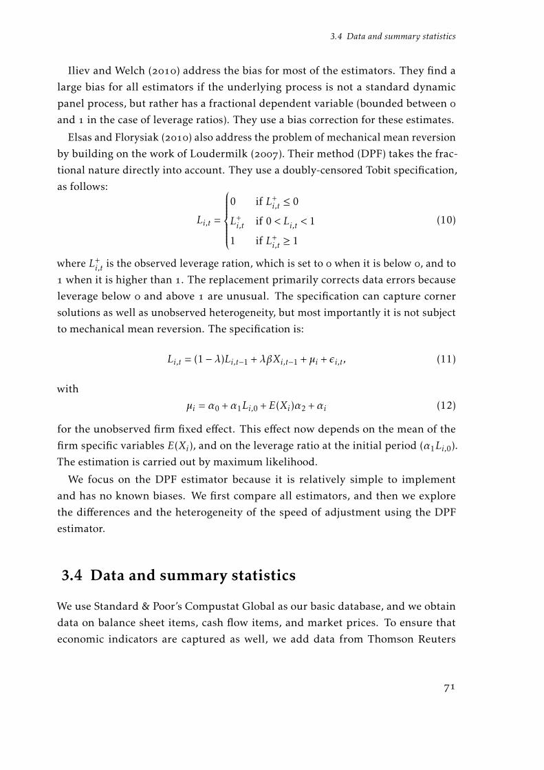
3.4 Data and summary statistics
Iliev and Welch () address the bias for most of the estimators. They find a
large bias for all estimators if the underlying process is not a standard dynamic
panel process, but rather has a fractional dependent variable (bounded between and in the case of leverage ratios). They use a bias correction for these estimates.
Elsas and Florysiak () also address the problem of mechanical mean reversion
by building on the work of Loudermilk (). Their method (DPF) takes the frac-
tional nature directly into account. They use a doubly-censored Tobit specification,
as follows:
Li,t =
0 if L+
i,t ≤ 0
L+i,t if 0 < Li,t < 1
1 if L+i,t ≥ 1
(10)
where L+i,t is the observed leverage ration, which is set to when it is below , and to
when it is higher than . The replacement primarily corrects data errors because
leverage below and above are unusual. The specification can capture corner
solutions as well as unobserved heterogeneity, but most importantly it is not subject
to mechanical mean reversion. The specification is:
Li,t = (1−λ)Li,t−1 +λβXi,t−1 +µi + εi,t, (11)
with
µi = α0 +α1Li,0 +E(Xi)α2 +αi (12)
for the unobserved firm fixed effect. This effect now depends on the mean of the
firm specific variables E(Xi), and on the leverage ratio at the initial period (α1Li,0).
The estimation is carried out by maximum likelihood.
We focus on the DPF estimator because it is relatively simple to implement
and has no known biases. We first compare all estimators, and then we explore
the differences and the heterogeneity of the speed of adjustment using the DPF
estimator.
3.4 Data and summary statistics
We use Standard & Poor’s Compustat Global as our basic database, and we obtain
data on balance sheet items, cash flow items, and market prices. To ensure that
economic indicators are captured as well, we add data from Thomson Reuters
Chapter 3 Illuminating the speed of adjustment
Datastream. Using information for the G countries from to obtain
125982 firm year observations. Frank and Goyal () note that financial databases
such as Compustat are often subject to outliers and anomalous observations. We
can manage such problems by using rule of thumb truncations, winsorizing, and
trimming.
We start with some common cleansing steps. We exclude all utilities (SIC codes
–) and financial firms (SIC –). Missing capital expenditures
and missing convertible debt are set to zero. We also set missing research and
development expenditures to zero, but we use a dummy variable to indicate which
ones were missing and which ones were originally.
We further exclude firm years with negative leverage ratios or negative total assets.
We also only use firms with consolidated balance sheets that have not changed their
accounting method. All firm-level variables are in local currencies, except for
sales, which is measured in U.S. dollars. We trim our data at a % level.
In our study, we use the leverage ratio as the dependent variable, under Huang
and Ritter’s () definition of leverage. We construct book leverage (BL) as
total liabilities plus preferred stock, minus deferred taxes, minus convertible debt
over total assets ((LTt + P STKt − TXDIt −DCVTt)/AT ). We then construct market
levverage as the book value of debt (the same nominator as for book leverage),
divided by the market value of equity, plus the book value of debt (LTt + P STKt −TXDIt −DCVTt)/(MKVAL+LTt + P STKt − TXDIt).
Table I gives an overview of the leverage variables. Note from Column that
the mean book leverage in market-based countries ranges from % in Canada to
% in Great Britain. In bank-based countries, it is even higher, from % in Japan,
increasing to % in Italy. The standard deviation of book leverage ranges from %in Italy to % in the U.S., indicating a large variation in leverage. In Column , we
report the mean of the yearly percentage change of book leverage. While the mean
change in total at % is rather small, the % standard deviation also indicates a
large variation.
Columns and give the information on market leverage (ML). As with book
We exclude financial firms because they have a different balance sheet structure. We also excludeutilities for the sake of comparability, since they are regulated in the US. We use anly code F of Compustat item CONSOL and we exclude all mergers (CSTAT=AA), newcompany formation (AB), accounting changes (AC, AN) and combinations. We exclude all firm years with divergent currencies for accounting and market data. All the data variable abbreviations identify the respective data item in Compustat Global forvariables that have not been calculated

3.4 Data and summary statistics
Table I – Leverage in the G Countries
BL ∆BL ML ∆ML
CANmean 0.468 0.096 0.341 0.051s.d 0.265 0.620 0.250 0.511N 5494 3460 4770 2849
DEUmean 0.612 0.046 0.497 0.078s.d 0.238 0.494 0.254 0.426N 8507 7081 6938 5659
FRAmean 0.636 0.014 0.509 0.028s.d 0.223 0.255 0.236 0.243N 8049 6489 6606 5233
GBRmean 0.547 0.085 0.382 0.084s.d 0.282 0.618 0.229 0.464N 18882 14625 16562 12426
ITAmean 0.651 0.012 0.552 0.033s.d 0.202 0.219 0.241 0.234N 2446 1904 2038 1570
JPNmean 0.579 0.001 0.549 0.028s.d 0.217 0.186 0.229 0.236N 45953 41859 43099 39031
USAmean 0.530 0.069 0.342 0.044s.d 0.319 0.603 0.252 0.389N 43266 30047 39716 27124
Totalmean 0.561 0.039 0.444 0.044s.d 0.270 0.453 0.258 0.345N 132597 105465 119729 93892
This table presents an overview of the different leveragevariables and summary statistics in terms of mean, stan-dard deviation (s.d.) and number of observations (N).Book leverage (BL) is defined as book debt relative to to-tal assets ((LTt+P STKt−TXDIt−DCVTt)/ATt), and mar-ket leverage (ML) is defined as book debt relative to bookdebt plus the market value of equity ((LTt + P STKt −TXDIt − DCVTt)/(MKVAL + LTt + P STKt − TXDIt)).Columns and give the percentage changes. The datacover through .
Chapter 3 Illuminating the speed of adjustment
leverage, we find that market leverage is lower in market-based countries than in
bank-based. For example, the U.S. has a mean market leverage of %, while Italy’s
is %. The standard deviation is in a similar range as for book leverage and the
total mean of the the yearly percentage change (%). The standard deviation of the
change in market leverage is lower than for book leverage. Thus, firms in bank-based
countries have a higher leverage ratio than those in market-based countries.
This finding persists when examining the development over time. Panel A of
Figure I shows the development for book and market leverage. Firms in bank-based
countries are more leveraged than those in market-based countries over the entire
period. This may because the laws in bank-based countries are more oriented toward
lender protection, and thus firms are able to carry more debt.
We observe some cyclicality in market value in Panel B of Figure I. During eco-
nomic downturns, such as during the aftermath of the global financial crisis,
leverage tends to rise. The pattern for each country looks quite similar, except
for Japan, possibly because of its long economic stagnation. To estimate the target
leverage ratio, we use variables introduced by Flannery and Rangan (), which
have been used extensively to estimate the speed of adjustment by, e.g., Elsas and
Florysiak (). We use a measure of profitability (EBIT ), the market-to-book
ratio (MB), depreciation (DEP ), size (SIZE), asset tangibility (TANG), research and
development expenditures (R&D), and the median industry market leverage. In
contrast to Flannery and Rangan (), we do not use rating as a control variable
for two reasons: ) Firms outside the U.S. have a shorter rating history, and ) we will
use the rating later to generate a measure for financial constraints. We define the fi-
nancial deficit (DEF) as the change in net debt (∆(LT +P STK−TXDI−DCVT )/AT ),
plus the change in net equity (∆(AT − LT − P STK + TXDI +DCVT )/AT ), minus
the change in retained earnings (∆RE/AT ). We use this as a conditional variable to
estimate adjustment speed.
One of our hypotheses states that the macroeconomic environment can strongly
impact the speed of adjustment, so we need to establish proxies for the state of
EBIT is defined as income before extraordinary items plus interest expenses plus income taxes overtotal assets ((IB+XINT +TXT )/AT );MB is defined as market value over total assets (MKVAL+LT +P STK − TXDI)/AT ; DEP is depreciation over total assets (DP /AT ); SIZE is the natural logarithmof net sales in US$ (ln(SALE)), and TANG is property, plant, and equipment over total assets(P P ENT /AT ). Our definition of industry classification follows Fama and French (), and is obtained from Ken-neth French’s Homepage (http://mba.tuck.dartmouth.edu/pages/faculty/ken.french/data_library.html).

3.4 Data and summary statistics
.4.5
.6.7
Boo
k le
vera
ge
1992 1994 1996 1998 2000 2002 2004 2006 2008year
USA GBRCAN GERFRA ITAJPN
(A) Book leverage G
.2.4
.6.8
Mar
ket l
ever
age
1992 1994 1996 1998 2000 2002 2004 2006 2008year
USA GBRCAN GERFRA ITAJPN
(B) Market leverage G
Figure I – Leverage ratios across countries and time framesThis figure illustrates the development over time of the leverage ratios in the G. Bookleverage (BL) is defined as book debt relative to total assets ((LTt + P STKt − TXDIt −DCVTt)/ATt), and market leverage (ML) is defined as book debt relative to book debtplus the market value of equity ((LTt+P STKt−TXDIt−DCVTt)/(LTt+P STKt−TXDIt+MKVALt)). The data covers through .
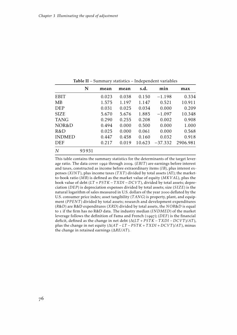
Chapter 3 Illuminating the speed of adjustment
Table II – Summary statistics – Independent variables
N mean mean s.d. min max
EBIT 0.023 0.038 0.150 −1.198 0.334MB 1.575 1.197 1.147 0.521 10.911DEP 0.031 0.025 0.034 0.000 0.209SIZE 5.670 5.676 1.885 −1.097 10.348TANG 0.290 0.255 0.208 0.002 0.908NOR&D 0.494 0.000 0.500 0.000 1.000R&D 0.025 0.000 0.061 0.000 0.568INDMED 0.447 0.458 0.160 0.032 0.918DEF 0.217 0.019 10.623 −37.332 2906.981
N 93931
This table contains the summary statistics for the determinants of the target lever-age ratio. The data cover through . (EBIT ) are earnings before interestand taxes, constructed as income before extraordinary items (IB), plus interest ex-penses (XINT ), plus income taxes (TXT ) divided by total assets (AT); the market-to-book ratio (MB) is defined as the market value of equity (MKVAL), plus thebook value of debt (LT + P STK − TXDI −DCVT ), divided by total assets; depre-ciation (DEP ) is depreciation expenses divided by total assets; size (SIZE) is thenatural logarithm of sales measured in U.S. dollars of the year deflated by theU.S. consumer price index; asset tangibility (TANG) is property, plant, and equip-ment (P P ENT ) divided by total assets; research and development expenditures(R&D) are R&D expenditures (XRD) divided by total assets, the NOR&D is equalto if the firm has no R&D data. The industry median (INDMED) of the marketleverage follows the definition of Fama and French (); (DEF) is the financialdeficit, defined as the change in net debt (∆(LT + P STK − TXDI −DCVT )/AT ),plus the change in net equity (∆(AT −LT − P STK + TXDI +DCVT )/AT ), minusthe change in retained earnings (∆RE/AT ).

3.5 Results
the economy. We use the U.S. default spread as a proxy for the general attitude
toward risk, the term spread, the TED spread, and the GDP growth rate. Table
III shows the correlations between variables. We note especially low correlations
in Panel B of Table III. We conclude that each variable is needed to fully capture
the economic environment. We also use a dummy variable as an overall proxy for
recessions. It is equal to if the economy appears headed toward a recession, and
otherwise. In this study, we follow Halling et al. (), and use the definitions
from the Economic Cycle Research Institute. To examine whether the speed of
adjustment follows market timing considerations, we use inflation and the equity
risk premium, calculated as the twelve-month mean stock return of a broad market
index.
3.5 Results
3.5.1 Comparing the different estimators
Our first step is to investigate the results of the different panel estimators. We
examine whether the Monte Carlo and theoretical considerations from earlier papers
appear in our sample. For the OLS estimator (OLS), Huang and Ritter () and
Iliev and Welch () note it is biased upward: The estimated speed of adjustment
is too low. The bias of the fixed effects (FE) model, however, is downward. For the
speed of adjustment, this means the estimation is too high. This bias is especially
severe if the time dimension is short, which is often the case with firms in the
Compustat Global sample.
The GMM estimators also suffer from biases. The Arellano and Bond ()estimator (AB) suffers from a small sample bias if the coefficient on the lagged
dependent variable is close to in a negative direction (Bruno b). This a
reasonable expectation for series as persistent as leverage ratios. The BB estimator,
in contrast, is slightly biased upward, as Bruno (b) shows in a Monte Carlo study.
Hahn et al. () renew the critique of weak instruments for the system estimator
CREDIT is the difference between the yield on Moody’s Baa-rated and Aaa-rated corporate bonds. Data come from the Economic Cycle Research Institute website, www.businesscycle.com. Inflation is calculated as the percentage change in a country’s consumer price index. We use the S&P for the U.S., the FTSE All-Share for the U.K., the Toronto SE for Canada,the SBF for France, the Nikkei for Japan, the BIC All-Share for Italy, and the MDAX forGermany. The mean time that firms in our sample have been in the Compustat database is eight years.
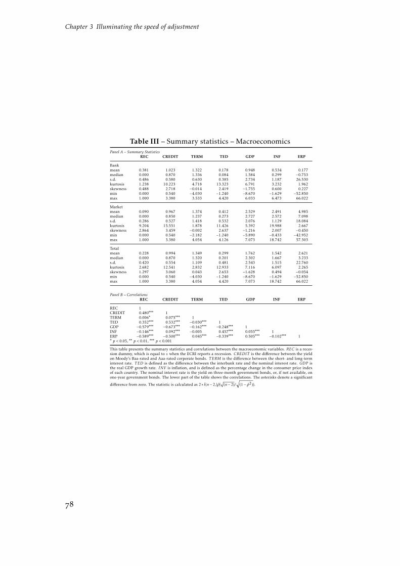
Chapter 3 Illuminating the speed of adjustment
Table III – Summary statistics – MacroeconomicsPanel A – Summary Statistics
REC CREDIT TERM TED GDP INF ERP
Bankmean 0.381 1.023 1.322 0.178 0.948 0.534 0.177median 0.000 0.870 1.336 0.084 1.584 0.299 −0.753s.d. 0.486 0.580 0.630 0.385 2.734 1.187 26.530kurtosis 1.238 10.223 4.718 13.323 6.791 3.232 1.962skewness 0.488 2.718 −0.014 2.419 −1.755 0.600 0.227min 0.000 0.540 −4.030 −1.240 −8.670 −1.629 −52.850max 1.000 3.380 3.533 4.420 6.033 6.473 66.022
Marketmean 0.090 0.967 1.374 0.412 2.529 2.491 4.985median 0.000 0.850 1.237 0.273 2.727 2.572 7.098s.d. 0.286 0.527 1.418 0.532 2.076 1.129 18.084kurtosis 9.204 15.551 1.878 11.426 5.392 19.988 2.667skewness 2.864 3.459 −0.002 2.637 −1.216 2.007 −0.450min 0.000 0.540 −2.182 −1.240 −5.890 −0.433 −42.952max 1.000 3.380 4.054 4.126 7.073 18.742 57.303
Totalmean 0.228 0.994 1.349 0.299 1.762 1.542 2.621median 0.000 0.870 1.320 0.201 2.302 1.667 3.233s.d. 0.420 0.554 1.109 0.481 2.543 1.515 22.760kurtosis 2.682 12.541 2.832 12.933 7.116 6.097 2.265skewness 1.297 3.060 0.043 2.653 −1.628 0.494 −0.054min 0.000 0.540 −4.030 −1.240 −8.670 −1.629 −52.850max 1.000 3.380 4.054 4.420 7.073 18.742 66.022
Panel B – CorrelationsREC CREDIT TERM TED GDP INF ERP
REC 1CREDIT 0.480∗∗∗ 1TERM 0.006∗ 0.075∗∗∗ 1TED 0.352∗∗∗ 0.532∗∗∗ −0.030∗∗∗ 1GDP −0.579∗∗∗ −0.673∗∗∗ −0.162∗∗∗ −0.248∗∗∗ 1INF −0.146∗∗∗ 0.092∗∗∗ −0.005 0.457∗∗∗ 0.055∗∗∗ 1ERP −0.589∗∗∗ −0.500∗∗∗ 0.045∗∗∗ −0.339∗∗∗ 0.505∗∗∗ −0.102∗∗∗ 1∗ p < 0.05, ∗∗ p < 0.01, ∗∗∗ p < 0.001
This table presents the summary statistics and correlations between the macroeconomic variables. REC is a reces-sion dummy, which is equal to when the ECRI reports a recession. CREDIT is the difference between the yieldon Moody’s Baa-rated and Aaa-rated corporate bonds. T ERM is the difference between the short- and long-terminterest rate. T ED is defined as the difference between the interbank rate and the nominal interest rate. GDP isthe real GDP growth rate. INF is inflation, and is defined as the percentage change in the consumer price indexof each country. The nominal interest rate is the yield on three-month government bonds, or, if not available, onone-year government bonds. The lower part of the table shows the correlations. The asterisks denote a significant
difference from zero. The statistic is calculated as 2 ∗ t̃(n− 2, |ρ̂|√
(n− 2)/√
(1− ρ̂2)).

3.5 Results
(BB) first proposed by Blundell and Bond (), and instead focus on using longer
lags as instruments (LD). They perform a simulation, and show that when the true
parameter is ., the system GMM (BB) produces a biased estimate of ., while
the long-differencing estimator (LD) produces an estimate of .. Huang and
Ritter () use this estimator with a lag of four (LD), and Flannery and Hankins
() use it with the longest available lag (LD). Flannery and Hankins () show
that the GMM estimators and the Least Squares Dummy Variable correction perform.
Elsas and Florysiak () and Iliev and Welch () note that the leverage ratio is
a bounded variable, and therefore all estimators assuming a standard dynamic panel
process are biased. Elsas and Florysiak () propose using a fractional dependent
variable estimator instead, and arguing that it is bias-free.
We expect FE to yield the lowest estimate, followed by AB, the LD, the LD,the LSDVC, and the DPF estimators. The BB and OLS estimators should yield the
highest estimates.
Tables IV (for book leverage) and V (for market leverage) give our results for
all estimators. As expected, the OLS estimate for book leverage is relatively high
with a ρ of ., implying a slow adjustment of only .% per year. We observe
the lowest coefficient, ., using the fixed effects estimator. This implies a %adjustment per year. The coefficient for the AB estimator is ., and the system
GMM generates a . estimate, implying a negative speed of adjustment. The bias
corrected estimator produces a . coefficient, and the remaining coefficients are
. (DPF), . (LD), and . (LD). However, the high number of lags for
instrumenting means the long-difference estimators losing many observations, and,
therefore, information. The mean speed is % per annum, which equates to a half
live of about three years.
For market leverage, Welch () finds that firms do not adjust to changes
in the leverage ratio caused by stock price changes. So we expect to see a lower
speed of adjustment for market leverage ratios. Table V presents the results for the
estimation with market leverage. However, it is not clear on average whether the
speed of adjustment is higher or lower than with the book leverage estimation. For
example, the OLS estimator has a slightly lower coefficient (BL:. to ML:.),implying a higher speed of adjustment. But the fractional dependent estimator
exhibits a higher coefficient (BL:. to ML:.), implying a lower speed of
adjustment. Huang and Ritter () argue that the effect described by Welch
The half life can be calculated as: half lif e = ln(2)/ln(λ).

Chapter 3 Illuminating the speed of adjustment
() can be offset by the fact that, after stock price decreases, the leverage ratio
sharply increases. There are two possibilities: The firm may declare bankruptcy
and be dropped from the sample, or the stock price will increase again, and the
leverage ratio will decrease. We only capture the second alternative here, which
might overestimate the market leverage speed of adjustment.
Quantitatively, our findings fall in the middle of the range found by newer studies.
For example, Huang and Ritter () obtain a . coefficient for book leverage
and . for market leverage using their four-lag difference estimator on U.S. data.
Elsas and Florysiak () obtain . for market leverage.
We can also interpret the signs of the variables determining the target leverage
ratios. Because the coefficients interact with the speed of adjustment, the value can
not be interpreted. Profitability has a negative effect on leverage: Firms with high
profits the previous year have a lower leverage. This is consistent with pecking order
theory, since firms have a preference for internal funds. MB also has a negative
sign in most of the regressions. A high market-to-book ratio lowers leverage. This
is consistent with the trade-off-theory, because a high MB ratio is associated with
higher bankruptcy costs. Depreciation also lowers leverage, which is consistent with
the trade-off theory, size, tangibility, R&D, and the median industry leverage all
have a positive influence as well.
3.5.2 Heterogeneity
3.5.2.1 Countries
We next present the results for the speed of adjustment in the G countries. We
perform this regression with the DPF estimator separately for each country, followed
by estimations for market- and bank-based countries. We expect to find a lower
speed of adjustment in bank-based countries. Speed of adjustment depends on two
concepts: the cost of deviating from the target capital structure, and adjustment
costs. Firms must middle ground between these two costs after external shocks
to the capital structure, caused, for example, by unexpected decline in product
demand. We expect the costs of deviating from target leverage to be lower in bank-
based countries than in market-based ones. Because the banking sector is the main
source of capital, the corporate governance system does not operate at arm’s length
as in a market-based systems. Rather banks can exert much more control, and
deviations from the target can be negotiated with house banks, instead of being

3.5 Results
Tab
leIV
–D
iffer
ent
esti
mat
ors
ofad
just
men
tsp
eed
–B
ook
leve
rage
OL
SFE
AB
BB
LSD
VD
PF
LD
LD
LB
L0.
911∗∗∗
0.61
9∗∗∗
0.85
6∗∗∗
1.01
5∗∗∗
0.76
20.
791∗∗∗
0.84
3∗∗∗
0.58
7∗∗∗
(115.3
81)
(175.2
30)
(39.
853)
(59.
995)
(210.7
61)
(70.
891)
(27.
219)
SOA
(in
%)
8.9
38.1
14.4
−1.5
2.38
20.9
15.7
41.3
EB
IT−0.0
93∗∗∗
−0.0
95∗∗∗
0.24
0∗∗∗
0.26
6∗∗∗
−0.0
73−0.0
16∗∗∗
−0.0
85∗∗∗
−0.1
91∗∗∗
(−9.
306)
(−20.9
04)
(25.
497)
(18.
194)
(−3.
869)
(−5.
497)
(−6.
798)
MB
−0.0
02−0.0
07∗∗∗
−0.0
12∗∗∗
−0.0
10∗∗∗
−0.0
07−0.0
07∗∗∗
−0.0
04∗∗
0.00
9∗∗
(−1.
697)
(−11.9
08)
(−15.6
06)
(−6.
755)
(−14.4
18)
(−3.
161)
(2.9
61)
DE
P0.
095∗∗
−0.0
51−0.0
74−0.0
47−0.1
13−0.1
99∗∗∗
−0.0
280.
726∗∗∗
(3.0
28)
(−1.
752)
(−1.
606)
(−0.
659)
(−7.
450)
(−0.
341)
(10.
343)
SIZ
E0.
001∗
0.00
6∗∗∗
−0.0
39∗∗∗
−0.0
42∗∗∗
0.00
3−0.0
00−0.0
01−0.0
03∗∗
(2.0
80)
(6.6
40)
(−16.1
09)
(−11.6
25)
(−0.
041)
(−0.
294)
(−2.
596)
TAN
G−0.0
030.
030∗∗∗
0.02
20.
026
0.02
20.
032∗∗∗
0.02
9∗−0.0
11(−
0.96
7)(4.8
62)
(1.8
63)
(1.4
67)
(5.8
05)
(2.4
26)
(−1.
279)
NO
_R&
D0.
009∗∗∗
0.00
4∗−0.0
010.
003
0.00
40.
004∗∗
−0.0
01−0.0
04(5.3
66)
(2.3
49)
(−0.
377)
(0.7
89)
(2.7
22)
(−0.
487)
(−1.
200)
R&
D0.
001
0.09
0∗∗∗
0.09
9∗∗∗
0.05
70.
076
0.01
6−0.0
300.
043
(0.0
70)
(5.6
07)
(3.9
86)
(1.1
29)
(1.0
73)
(−0.
621)
(0.6
30)
IND
ME
D0.
011∗∗
0.02
5∗∗
−0.0
11−0.0
250.
016
0.00
8−0.0
03−0.0
18(2.7
29)
(3.0
99)
(−0.
798)
(−1.
739)
(1.1
20)
(−0.
288)
(−1.
582)
Obs
erva
tion
s74
482
7448
256
949
7448
274
482
7166
026
943
3350
7
tsta
tist
ics
inp
aren
thes
es∗p<
0.05
,∗∗p<
0.01
,∗∗∗p<
0.00
1
All
esti
mat
ors
are
des
crib
edin
Sect
ion
II.T
hed
epen
den
tvar
iabl
eis
book
leve
rage
,as
des
crib
edin
Tabl
eI.
Tabl
eII
cont
ains
anex
pla
na-
tion
ofth
ein
dep
end
entv
aria
bles
.OL
Sis
the
ord
inar
yle
asts
quar
eses
tim
ator
;FE
isth
efi
xed
effec
tses
tim
ator
;AB
isth
eA
rell
ano-
Bon
dd
iffer
ence
GM
Mes
tim
ator
;B
Bis
the
Blu
ndel
l-B
ond
syst
emG
MM
;LSD
Vis
the
leas
tsq
uar
esdu
mm
yva
riab
leco
rrec
tion
,fo
rw
hom
stan
dar
der
rors
cann
otbe
calc
ula
ted
;DP
Fis
the
dyn
amic
pan
elw
ith
frac
tion
ald
epen
den
tva
riab
lees
tim
ator
;LD
isth
elo
nges
tla
ges
tim
ator
usi
ngla
g,
and
LD
isth
elo
nges
td
iffer
ence
esti
mat
orw
ith
the
long
est
lag.
Tim
edu
mm
ies,
cons
tant
s,in
itia
lle
vera
ge,a
ndm
ean
exog
enou
sva
riab
les
are
omit
ted
.SO
Ais
min
us
the
coeffi
cien
ton
lagg
edbo
okle
vera
ge(B
L).

Chapter 3 Illuminating the speed of adjustment
Tab
leV
–D
iffer
ent
esti
mat
ors
ofad
just
men
tsp
eed
–M
arke
tle
vera
geO
LS
FEA
BB
BL
SDV
DP
FL
D
LD
LM
L0.
895∗∗∗
0.56
2∗∗∗
0.87
3∗∗∗
1.06
2∗∗∗
0.71
70.
880∗∗∗
0.93
2∗∗∗
0.43
9∗∗∗
(233.0
67)
(149.9
92)
(44.
702)
(77.
996)
(277.8
34)
(105.7
89)
(27.
631)
SOA
(in
%)
10.5
33.8
12.7
−6.2
28.3
12.0
6.8
56.1
EB
IT−0.0
29−0.0
56∗∗∗
0.18
1∗∗∗
0.17
4∗∗∗
−0.0
320.
051∗∗∗
−0.0
26−0.1
44∗∗∗
(−1.
690)
(−13.2
46)
(23.
689)
(14.
765)
(8.4
42)
(−1.
828)
(−5.
144)
MB
0.00
4∗∗
−0.0
02∗∗∗
0.04
3∗∗∗
0.04
9∗∗∗
0.00
40.
017∗∗∗
0.01
5∗∗∗
−0.0
65∗∗∗
(3.0
82)
(−4.
015)
(32.
389)
(27.
465)
(21.
205)
(10.
312)
(−13.8
14)
DE
P−0.2
04∗
−0.2
16∗∗∗
−0.1
16∗
−0.5
85∗∗∗
−0.2
24−0.2
71∗∗∗
−0.0
86−0.1
47(−
2.15
6)(−
7.86
6)(−
2.48
5)(−
9.63
3)(−
6.63
7)(−
1.11
7)(−
1.44
1)SI
ZE
0.00
00.
023∗∗∗
0.01
5∗∗∗
0.00
6∗0.
018
0.01
2∗∗∗
0.01
2∗∗∗
−0.0
09∗∗∗
(0.2
85)
(26.
683)
(6.9
00)
(2.2
31)
(10.
600)
(3.6
27)
(−6.
048)
TAN
G0.
005
0.01
4∗−0.0
33∗∗
−0.0
35∗
0.00
1−0.0
13−0.0
13−0.0
06(0.5
81)
(2.4
02)
(−2.
776)
(−2.
303)
(−1.
757)
(−1.
111)
(−0.
454)
NO
_R&
D0.
010∗∗∗
0.00
5∗∗
0.00
2−0.0
050.
008
0.01
0∗∗∗
0.01
1∗∗∗
−0.0
03(4.3
56)
(2.9
93)
(0.7
74)
(−1.
141)
(4.7
35)
(4.3
87)
(−0.
651)
R&
D−0.1
13∗∗∗
−0.0
110.
148∗∗∗
0.09
8∗∗
0.01
20.
014
0.01
40.
187∗∗
(−4.
991)
(−0.
739)
(5.9
12)
(2.7
50)
(0.5
86)
(0.3
20)
(2.6
03)
IND
ME
D0.
024∗
0.02
1∗∗
−0.1
40∗∗∗
−0.1
67∗∗∗
0.00
1−0.0
31∗∗
−0.0
57∗∗∗
0.14
0∗∗∗
(2.3
66)
(2.6
52)
(−9.
448)
(−10.0
76)
(−3.
139)
(−4.
744)
(7.7
35)
Obs
erva
tion
s74
919
7491
957
284
7491
974
919
4151
627
052
2057
6
tsta
tist
ics
inp
aren
thes
es∗p<
0.05
,∗∗p<
0.01
,∗∗∗p<
0.00
1
All
esti
mat
ors
are
des
crib
edin
Sect
ion
II.T
hed
epen
den
tvar
iabl
eis
book
leve
rage
,as
des
crib
edin
Tabl
eI.
Tabl
eII
cont
ains
anex
pla
na-
tion
ofth
ein
dep
end
entv
aria
bles
.OL
Sis
the
ord
inar
yle
asts
quar
eses
tim
ator
;FE
isth
efi
xed
effec
tses
tim
ator
;AB
isth
eA
rell
ano-
Bon
dd
iffer
ence
GM
Mes
tim
ator
;B
Bis
the
Blu
ndel
l-B
ond
syst
emG
MM
;L
SDV
isth
ele
ast
squ
ares
dum
my
vari
able
corr
ecti
onfo
rw
hom
stan
dar
der
rors
cann
otbe
calc
ula
ted
;DP
Fis
the
dyn
amic
pan
elw
ith
frac
tion
ald
epen
den
tva
riab
lees
tim
ator
;LD
isth
elo
nges
tla
ges
tim
ator
usi
ngla
g,
and
LD
isth
elo
nges
td
iffer
ence
esti
mat
orw
ith
the
long
est
lag.
Tim
edu
mm
ies,
cons
tant
s,in
itia
lle
vera
ge,a
ndm
ean
exog
enou
sva
riab
les
are
omit
ted
.SO
Ais
min
us
the
coeffi
cien
ton
lagg
edm
arke
tle
vera
ge(M
L).

3.5 Results
punished immediately by the market. We also expect the adjustment costs to be
higher, primarily because equity markets are less developed and thus less liquid.
Therefore, seasoned equity offerings (SEOs) should be more expensive. Long-term
debt contracts may also have to be renegotiated at more costly rates.
The findings in Tables VI and VII confirm our hypothesis. We find a % adjust-
ment speed Canada and the U.K., and % for the U.S. The bank-based countries
have slightly lower speeds of adjustment: Germany %, France %, Japan %, and
Italy %. The average speed of adjustment for the market-based countries is %,
and it is % for bank-based countries. In the last column of Table VI, we examine
whether the difference is significant by including a dummy variable for the financial
system interacting with the lagged leverage ratio. It is highly significant, and shows
a lower adjustment speed of percentage points. Although difference is not quite
large, it is in terms of half life. For market-based countries, we find that it takes .years for half of a shock to be adjusted, for bank-based countries, it is . years.
When comparing the results for book leverage to those for market leverage, we
note form Table VII that it is unclear which adjusts more quickly. In Canada,
the adjustment speeds are nearly the same; in the U.K. and in the U.S., the speed
for book leverage is percentage points lower. In Germany, Italy, and Japan, the
speed for market leverage shocks is lower, while in France it is percentage points
higher. If we examine the aggregated market and bank samples, we find that, in
market-based countries, the adjustment speed of the market leverage is percentage
points lower than the speed of book leverage (Column , Tables VI and VII); in
bank-based countries, the difference is also points (Column , Tables VI and VII).
This difference is again significant, and at .% it is in the same range as for book
leverage.
The finding that book leverage adjusts more quickly than market leverage is
consistent with Welch’s () finding that firms do not adjust to stock price-induced
changes in leverage. But it is contrary to Huang and Ritter (), who estimate a
higher adjustment speed for market leverage. This difference might be the result of
Huang and Ritter’s () longer time horizon.
Overall, we find a lower adjustment speed for bank-based countries, in line with
Halling et al. () and Antoniou et al. (), whose findings are in the %–%range. By using an unbiased estimator, we believe our results are more reliable.
Dang, Garrett, et al.’s () results are also much higher, and provide no conclusive
evidence for higher speed in market- or bank-based countries. Our empirical find-

Chapter 3 Illuminating the speed of adjustment
Tab
leV
I–
Spee
dof
adju
stm
ent
–B
ook
leve
rage
G
CA
NG
BR
USA
GE
RFR
AIT
AJP
NM
AR
KE
TBA
NK
DIF
F
LB
L0.
739∗∗∗
0.74
3∗∗∗
0.78
7∗∗∗
0.78
9∗∗∗
0.92
0∗∗∗
0.77
4∗∗∗
0.85
5∗∗∗
0.77
6∗∗∗
0.82
5∗∗∗
0.77
6∗∗∗
(35.
589)
(75.
772)
(128.8
11)
(55.
032)
(41.
600)
(64.
021)
(105.6
52)
(153.9
12)
(149.6
98)
(199.6
23)
SOA
(in
%)
26.1
25.7
21.3
21.1
8.0
22.6
14.5
22.4
17.5
22.4
EB
IT0.
003
−0.0
03−0.0
47∗∗∗
−0.0
52∗∗
0.17
0∗∗∗
−0.0
220.
065∗∗∗
−0.0
27∗∗∗
0.01
9∗∗
−0.0
18∗∗∗
(0.0
92)
(−0.
277)
(−5.
874)
(−3.
134)
(4.0
60)
(−1.
238)
(8.2
28)
(−4.
425)
(3.1
61)
(−4.
190)
MB
−0.0
03−0.0
09∗∗∗
−0.0
10∗∗∗
−0.0
000.
006
−0.0
03−0.0
08∗∗∗
−0.0
10∗∗∗
−0.0
04∗∗∗
−0.0
07∗∗∗
(−1.
052)
(−6.
175)
(−10.3
04)
(−0.
178)
(1.2
23)
(−1.
519)
(−9.
926)
(−12.5
22)
(−5.
861)
(−14.5
49)
DE
P−0.1
43−0.2
14∗∗
−0.3
48∗∗∗
−0.1
180.
020
0.02
1−9
0.40
8∗−0.2
54∗∗∗
−0.0
64−0.1
91∗∗∗
(−0.
971)
(−3.
287)
(−6.
194)
(−1.
608)
(0.1
20)
(0.2
77)
(−2.
515)
(−6.
265)
(−1.
759)
(−7.
157)
SIZ
E0.
000
0.00
20.
002
0.00
3−0.0
15∗
0.00
7∗−0.0
12∗∗∗
0.00
0−0.0
04∗∗∗
0.00
1(0.0
14)
(1.0
63)
(1.2
98)
(1.0
41)
(−2.
536)
(2.4
98)
(−7.
761)
(0.3
24)
(−3.
346)
(0.8
64)
TAN
G−0.0
07−0.0
050.
061∗∗∗
0.01
70.
006
0.02
90.
058∗∗∗
0.02
7∗∗
0.04
7∗∗∗
0.02
9∗∗∗
(−0.
209)
(−0.
323)
(4.9
75)
(0.7
84)
(0.1
54)
(1.1
79)
(7.8
97)
(3.0
05)
(7.0
79)
(5.3
23)
NO
_R&
D−0.0
070.
014∗∗
−0.0
10−0.0
15∗∗
0.01
1−0.0
070.
005∗∗
0.00
20.
001
0.00
4∗∗
(−0.
466)
(2.6
40)
(−1.
686)
(−2.
598)
(1.0
56)
(−1.
346)
(2.9
48)
(0.5
07)
(0.6
81)
(2.7
92)
R&
D−0.3
39∗∗∗
0.07
60.
031
−0.1
67∗
0.14
2−0.1
150.
211∗∗∗
0.02
60.
015
0.02
0(−
4.00
3)(1.8
75)
(1.2
26)
(−2.
504)
(0.7
44)
(−1.
822)
(5.3
83)
(1.2
38)
(0.5
55)
(1.3
58)
IND
ME
D0.
172∗∗∗
−0.0
180.
049∗∗
−0.0
400.
035
−0.0
85∗∗
0.00
70.
038∗∗
−0.0
17∗
0.01
1(3.3
98)
(−0.
753)
(2.9
86)
(−1.
500)
(0.9
06)
(−3.
265)
(0.8
10)
(2.9
47)
(−2.
318)
(1.4
88)
LB
L×B
AN
K0.
030∗∗∗
(15.
315)
Obs
erva
tion
s18
1410
075
1960
947
8014
6945
6429
349
3149
840
162
7166
0
tsta
tist
ics
inp
aren
thes
es∗p<
0.05
,∗∗p<
0.01
,∗∗∗p<
0.00
1
Thi
sta
ble
give
sth
esp
eed
ofad
just
men
tfo
rd
iffer
ent
cou
ntri
esan
dca
pit
alm
arke
tsy
stem
s.A
lles
tim
atio
nsar
eob
tain
edby
usi
ngth
eD
PF
esti
mat
or:Li,t
=(1−λ
)Li,t−
1+λβXi,t−
1+µi
+ε i,t
,wit
hmui
=α
0+α
1Li,
0+E
(Xi)α
2+αi.
The
dep
end
ent
vari
able
isbo
okle
vera
geas
des
crib
edin
Tabl
eI.
Tabl
eII
cont
ains
aex
pla
na-
tion
ofth
ein
dep
end
ent
vari
able
s.LBL×BANK
isan
inte
ract
ion
vari
able
for
lagg
edbo
okle
vera
gean
dth
efi
nanc
ials
yste
m.
TheBANK
vari
able
iseq
ual
to
whe
nth
efi
nanc
ials
yste
mis
bank
-bas
ed.
Tim
edu
mm
ies,
cons
tant
s,in
itia
llev
erag
e,an
dm
ean
exog
enou
sva
riab
les
are
omit
ted
.SO
Ais
min
us
the
coeffi
cien
ton
lagg
edbo
okle
vera
ge.
3.5 Results
Tab
leV
II–
Spee
dof
adju
stm
ent
–M
arke
tle
vera
geG
CA
NG
BR
USA
GE
RFR
AIT
AJP
NM
AR
KE
TBA
NK
DIF
F
LM
L0.
744∗∗∗
0.81
5∗∗∗
0.85
8∗∗∗
0.83
8∗∗∗
0.88
0∗∗∗
0.89
9∗∗∗
0.91
1∗∗∗
0.84
7∗∗∗
0.90
7∗∗∗
0.86
1∗∗∗
(23.
182)
(76.
745)
(130.9
71)
(30.
577)
(60.
737)
(38.
373)
(220.9
48)
(155.6
68)
(239.5
71)
(240.8
62)
SOA
(in
%)
25.6
18.5
14.2
16.2
12.0
10.1
8.9
15.3
9.3
13.9
EB
IT−0.0
090.
052∗∗∗
0.00
9−0.1
04∗∗
0.08
4∗0.
035
0.15
2∗∗∗
0.02
7∗∗
0.10
4∗∗∗
0.04
6∗∗∗
(−0.
267)
(3.5
35)
(0.8
49)
(−3.
173)
(2.5
70)
(0.6
23)
(13.
905)
(3.2
48)
(10.
889)
(7.6
95)
MB
0.01
0∗0.
011∗∗∗
0.01
1∗∗∗
0.01
5∗∗∗
0.02
5∗∗∗
0.06
0∗∗∗
0.02
4∗∗∗
0.01
1∗∗∗
0.02
6∗∗∗
0.01
6∗∗∗
(2.1
46)
(4.7
50)
(8.6
41)
(3.3
55)
(6.2
74)
(6.2
34)
(17.
071)
(10.
073)
(20.
807)
(20.
419)
DE
P−0.0
32−0.4
89∗∗∗
−0.5
16∗∗∗
−0.0
02−0.3
23∗
−0.2
5612.3
53−0.4
40∗∗∗
0.05
3−0.2
65∗∗∗
(−0.
186)
(−5.
114)
(−7.
166)
(−0.
016)
(−2.
466)
(−0.
843)
(0.2
22)
(−8.
093)
(0.7
43)
(−6.
487)
SIZ
E0.
004
0.01
5∗∗∗
0.01
3∗∗∗
0.00
60.
012∗∗
0.00
10.
011∗∗∗
0.01
0∗∗∗
0.01
2∗∗∗
0.01
3∗∗∗
(0.7
35)
(4.6
47)
(6.1
92)
(1.2
71)
(2.8
53)
(0.1
41)
(4.6
87)
(6.0
61)
(6.6
51)
(11.
499)
TAN
G−0.0
420.
036
0.04
4∗∗
0.02
10.
002
−0.0
64−0.0
27∗
0.02
3∗−0.0
39∗∗∗
−0.0
16∗
(−1.
095)
(1.9
09)
(2.8
59)
(0.5
84)
(0.0
46)
(−1.
412)
(−2.
406)
(2.0
57)
(−3.
930)
(−2.
153)
NO
_R&
D0.
027
0.00
4−0.0
11−0.0
19∗
0.00
20.
026
0.00
7∗∗
−0.0
060.
010∗∗∗
0.01
0∗∗∗
(1.4
97)
(0.5
27)
(−1.
615)
(−2.
106)
(0.2
30)
(1.3
13)
(3.0
44)
(−1.
145)
(4.6
18)
(5.0
40)
R&
D−0.3
18∗
0.04
7−0.0
27−0.0
280.
016
0.82
90.
229∗∗∗
−0.0
120.
163∗∗∗
0.01
4(−
2.51
3)(0.7
18)
(−0.
790)
(−0.
254)
(0.1
41)
(1.3
47)
(3.6
56)
(−0.
395)
(3.4
69)
(0.6
27)
IND
ME
D0.
172∗∗
0.01
7−0.0
13−0.0
04−0.0
120.
117
−0.0
34∗∗
0.01
4−0.0
29∗
−0.0
27∗∗
(2.6
93)
(0.5
66)
(−0.
654)
(−0.
085)
(−0.
275)
(1.9
17)
(−2.
736)
(0.8
46)
(−2.
513)
(−2.
777)
LM
L×B
AN
K0.
026∗∗∗
(11.
854)
Obs
erva
tion
s12
5652
4611
076
1832
1968
861
1927
717
578
2393
841
516
tsta
tist
ics
inp
aren
thes
es∗p<
0.05
,∗∗p<
0.01
,∗∗∗p<
0.00
1
Thi
sta
ble
give
sth
esp
eed
ofad
just
men
tfo
rd
iffer
ent
cou
ntri
esan
dca
pit
alm
arke
tsy
stem
s.A
lles
tim
atio
nsar
eob
tain
edby
usi
ngth
eD
PF
esti
mat
or:Li,t
=(1−λ
)Li,t−
1+λβXi,t−
1+µi
+ε i,t
,wit
hmui
=α
0+α
1Li,
0+E
(Xi)α
2+αi.
The
dep
end
ent
vari
able
ism
arke
tle
vera
geas
des
crib
edin
Tabl
eI.
Tabl
eII
cont
ains
aex
pla
-na
tion
ofth
ein
dep
end
ent
vari
able
s.LBL×BANK
isan
inte
ract
ion
vari
able
for
lagg
edm
arke
tle
vera
gean
dth
efi
nanc
ial
syst
em.
TheBANK
vari
able
iseq
ual
to
whe
nth
efi
nanc
ial
syst
emis
bank
-bas
ed.
Tim
edu
mm
ies,
cons
tant
s,in
itia
lle
vera
ge,a
ndm
ean
exog
enou
sva
riab
les
are
omit
ted
.SO
Ais
min
us
the
coeffi
cien
ton
lagg
edm
arke
tle
vera
ge.

Chapter 3 Illuminating the speed of adjustment
ings imply either higher adjustment costs or lower costs of deviating from the target
in bank-based countries. Although our estimation cannot discriminate between
these two concepts, we find evidence of different behavior between the two capital
market systems.
3.5.2.2 Financial circumstances
Differing legal environments and financial systems can be one source of hetero-
geneity in the speed of adjustment; different firm financial circumstances can be
another. In this section, we investigate the heterogeneity resulting form differences
in magnitude of financial deficits, health, and distance from target.
Financial deficit. The financial deficit refers to the amount of capital a firm issues
on the financial markets or generates as net profits. If a firm has high profits, it
can easily adjust its capital structure by either buying back shares or renegotiating
and lowering its long-term debt. The reasoning also works the other way: Firms
that have investment opportunities and need to raise capital can easily adjust using
either debt or equity, depending on leverage status. As Faulkender et al. ()mentions, this would lower the cost of adjustment, because the firm needed to go to
the market anyway.
In contrast, if the firm has no financing deficit, it would either lack profits or
investment opportunities. Thus, any capital structure activity would be done for
readjustment only and would be subject to the full costs. We expect firms with a
high financing deficit, whether positive or negative, to adjust faster than firms with
a low deficit.
We tackle this question by grouping the firms in deciles according to their mean
financial deficit. The financial deficit is defined, as in Huang and Ritter (), as
change in net debt (∆(LT + P STK − TXDI −DCVT )/AT ), plus change in net equity
(∆(AT − LT − P STK + TXDI + DCVT )/AT ), minus change in retained earnings
(∆RE/AT ). The results for different definitions of the financial deficit can be seen
in Figure II. We group the first two panels by the absolute value of the magnitude
of the deficit. The adjustment of firms with very small deficits is % in bank-based
countries and % in market-based countries. The speed remains relatively constant
If we use firm years, we would lose vast amounts of data and destroy the panel structure. Weperformed a robustness test using firm years as grouping variable; the results were qualitatively thesame.
3.5 Results
0.00
0.10
0.20
0.30
0.40
0.50
0.60
Spe
ed o
f adj
ustm
ent
1 2 3 4 5 6 7 8 9 10Decile
BANK MARKET
(A) Absolute financial deficit– Book leverage
0.00
0.10
0.20
0.30
0.40
0.50
0.60
Spe
ed o
f adj
ustm
ent
1 2 3 4 5 6 7 8 9 10Decile
BANK MARKET
(B) Absolute financial deficit– Market leverage
0.00
0.10
0.20
0.30
0.40
0.50
0.60
Spe
ed o
f adj
ustm
ent
1 2 3 4 5 6 7 8 9 10Decile
BANK MARKET
(C) Positive financial deficit– Book leverage
0.00
0.10
0.20
0.30
0.40
0.50
0.60
Spe
ed o
f adj
ustm
ent
1 2 3 4 5 6 7 8 9 10Decile
BANK MARKET
(D) Positive financial deficit– Market leverage
0.00
0.10
0.20
0.30
0.40
0.50
0.60
Spe
ed o
f adj
ustm
ent
1 2 3 4 5 6 7 8 9 10Decile
BANK MARKET
(E) Negative financial deficit– Book leverage
0.00
0.10
0.20
0.30
0.40
0.50
0.60
Spe
ed o
f adj
ustm
ent
1 2 3 4 5 6 7 8 9 10Decile
BANK MARKET
(F) Negative financial deficit– Market leverage
Figure II – Speed of adjustment with different financial deficitsThese figures show the speed of adjustment conditional on the mean financial deficit, which is calculated as the changein net debt (∆(LT +P STK−TXDI−DCVT )/AT ), plus the change in net equity (∆(AT −LT −P STK+TXDI+DCVT )/AT ),minus the change in retained earnings (∆RE/AT ). The two top panels use the mean of the absolute value of deficitsize, the middle panels use only firm years with positive deficits, and the lower panels use the years with negativefinancial deficits. The firms are sorted and the estimation is performed decile-wise, where is the decile with thelowest financial deficit, and is the highest decile. All estimations are done by means of the DPF estimator: Li,t =(1−λ)Li,t−1 +λβXi,t−1 + µi + εi,t , with mui = α0 +α1Li,0 +E(Xi )α2 +αi . The solid line gives the estimate of the speedof adjustment; the dashed line gives the % interval.

Chapter 3 Illuminating the speed of adjustment
up to decile , and then increases to %–% by decile . Firms with a large
financial deficit seem to use it to effect a faster adjustment. This effect is also visible
for market leverage in Panel B of Figure II, but is less pronounced.
If we examine only positive deficits, we also note that the speed of adjustment
increases with the financial deficit. It is at %–% in the lower and mid deciles,
and increases to %–% in the deciles with the highest financial deficits.
Firms with negative financial deficits (surpluses) can use these funds to adjust
capital structure by buying back shares or debt. For some firms, however, considera-
tions such as dividend payments may have a higher priority. As Panels E and F of
II show, the speed of adjustment is relatively stable at % over the deciles, except
for the lowest decile (which shows the firms with the highest profits), where it is
between % and %.
Our findings of a U-shaped pattern for the magnitude of the financial deficit
confirm Faulkender et al.’s () results. They also find larger adjustment speeds
for U.S. firms with large positive or negative financing deficits.
For the absolute value of financing deficits, we can compare our results directly to
those of Elsas and Florysiak (). For the deciles with large financing deficits, we
find the same speeds of adjustment, up to % for market-based firms at the top
range of absolute deficits, and up to % at the bottom range. However, the speed of
adjustment is higher in market-based countries than in bank-based countries. This
might be attributable to the more frequent use of share repurchases and SEOs, which
make the leverage more flexible and cheaper to adjust in market-based countries.
Financial constraints. Our next step is to examine how the financial health influ-
ences adjustment speed. As Dang, Kim, et al. () argue, financial health can
have an important influence on the costs of deviating from the target leverage ratio.
They note that over-leveraged firms face debt constraints and tend to have higher
bankruptcy and liquidation costs. Therefore, their costs of deviating from the target
are higher than for unconstrained firms. We thus believe constrained firms will ad-
just more quickly. Gilson () notes that, under Chapter , debt restructuring is
rather cheap. Therefore, the costs of adjustment should also be lower for constrained
firms, which is another reason they adjust adjust faster.
In the literature, several approaches exist to determine whether a firm is finan-
cially constrained. For example, Korajczyk and Levy () use dividend distribu-
tions. Because many investors look at a firm’s rating during their decision process,

3.5 Results
Tab
leV
III
–Sp
eed
ofad
just
men
t–
Fina
ncia
lcon
stra
ints
Pane
lA–
Boo
kLe
vera
geM
arke
t-ba
sed
Ban
k-ba
sed
Con
stra
ined
Med
ium
-con
stra
ined
Unc
onst
rain
edD
iffer
ence
Con
stra
ined
Med
ium
-con
stra
ined
Unc
onst
rain
edD
iffer
ence
Lag
BL
0.81
5∗∗∗
0.73
0∗∗∗
0.84
70.
865∗∗∗
0.84
4∗∗∗
0.80
8∗∗∗
0.93
8∗∗∗
0.87
3∗∗∗
(79.
631)
(111.7
31)
(90.
684)
(130.6
16)
(82.
428)
(131.3
56)
(205.0
42)
(113.3
93)
SOA
(in
%)
18.5
27.0
15.3
13.5
15.6
19.2
6.2
12.7
Lag
BL×C
ON
−0.0
49∗∗∗
−0.0
04(−
7.49
3)(−
0.94
5)
N69
7018
421
6107
1307
765
3824
545
9079
1561
7
Pane
lB–
Mar
ketL
ever
age
Mar
ket-
base
dB
ank-
base
d
Con
stra
ined
Med
ium
cons
trai
ned
Unc
onst
rain
edD
iffer
ence
Con
stra
ined
Med
ium
cons
trai
ned
Unc
onst
rain
edD
iffer
ence
Lag
ML
0.78
4∗∗∗
0.84
7∗∗∗
0.87
0∗∗∗
0.85
6∗∗∗
0.84
7∗∗∗
0.89
9∗∗∗
0.90
4∗∗∗
0.92
3∗∗∗
(44.
698)
(116.8
28)
(77.
135)
(100.8
89)
(38.
514)
(179.1
51)
(132.3
67)
(149.4
84)
SOA
(in
%)
21.6
15.3
23.0
25.2
25.3
10.1
9.6
9.3
Lag
BL×C
ON
−0.0
43∗∗∗
−0.0
14∗∗
(−5.
038)
(−3.
021)
N31
9110
225
4162
7353
2793
1381
073
3510
128
tsta
tist
ics
inp
aren
thes
es∗p<
0.05
,∗∗p<
0.01
,∗∗∗p<
0.00
1
Thi
sta
ble
give
sth
esp
eed
ofad
just
men
tco
ndit
iona
lon
fina
ncia
lhea
lth.
All
esti
mat
ions
are
obta
ined
usi
ngth
eD
PF
esti
mat
or:Li,t
=(1−λ
)Li,t−
1+λβXi,t−
1+µi+
ε i,t
,wit
hmui
=α
0+α
1Li,
0+E
(Xi)α
2+αi.
The
dep
end
ent
vari
able
isbo
ok/m
arke
tle
vera
geas
des
crib
edin
Tabl
eI.
Tabl
eII
cont
ains
anex
pla
nati
onfo
rth
ein
de-
pen
den
tva
riab
les.
Det
ails
onth
ees
tim
atio
nof
fina
ncia
lcon
stra
ints
can
befo
und
inA
pp
end
ixA
.SOA
is
min
us
the
coeffi
cien
ton
lagg
edm
arke
tle
vera
ge.T
heva
riab
leLagBL/M
L×CON
isan
inte
ract
ion
term
betw
een
the
lagg
edle
vera
gean
dth
efi
nanc
ialc
onst
rain
tdu
mm
y,w
hich
iseq
ual
to
for
fina
ncia
lly
cons
trai
ned
firm
s.T
hed
iffer
ence
sam
ple
isco
nsis
tent
for
all
firm
s,ex
cep
tm
ediu
mco
nstr
aine
don
es.
Tim
edu
mm
ies,
cons
tant
s,in
itia
lle
vera
ge,a
ndm
ean
exog
enou
sva
ri-
able
sar
eom
itte
d.

Chapter 3 Illuminating the speed of adjustment
the rating is a natural means to determine financial constraints. However, only a
small subsample of firms are rated, and some perfectly solvent firms have foregone
a rating. This problem can be especially severe in an international sample, because
ratings are more common in market-based countries. To overcome this problem,
we use Lemmon and Zender’s () method, which estimates the probability that
a firm will be able to access public debt markets. In particular, they use a logit
regression to estimate the probability of a firm having a bond rating. In our re-
gressions, we use the log of total assets, return on assets, tangibility, market-to-book
ratio, leverage, firm age, and the standard deviation of earnings as predictors for
rating probability. The dependent variable is a dummy equal to if the firm has
a rating, and otherwise. We use Standard and Poor’s RatingExpress database.
Although there are three dominant rating agencies, the resulting probability should
capture the financial health of a firm because the rating methods use roughly the
same inputs. We then build three groups: constrained, medium-constrained and
unconstrained, and perform the speed of adjustment estimation.
The results are in Table VIII. For book leverage, we find the highest adjustment
speed for medium-constrained firms in both market- and bank-based countries.
The speed of adjustment is higher for constrained firms, however, by only per-
centage points for market-based countries and by for bank-based countries. Con-
strained firms also adjust faster than unconstrained firms, but not as fast as medium-
constrained ones. Moreover, the costs of deviating from the target drive medium-
constrained firms to a faster adjustment. For constrained firms, these costs are even
higher, but here also the costs of adjustment seem to be higher, resulting in a lower
adjustment speed. We note that the accounting data available in Compustat Global
for bankrupt firms is often somewhat murky. Therefore, our cleansing steps could
have led to their deletion. This would explain why Gilson’s () argument of a
faster adjustment in bankruptcy does not seem to apply to our data.
Firms with debt constraints also face higher costs of equity issuing, and, therefore,
they can not adjust as quickly as desired. Unconstrained firms in bank-based
countries have only have an adjustment speed of .%. For them, the cost of
deviating from their target capital levels seems very low.
The results of the regression are in Appendix A. A firm is considered constrained if the probability of it being rated is below .; when theprobability is higher than ., it is considered unconstrained. We use a larger group for medium-constrained firms, because we are primarily interested in constrained and unconstrained firms. It isalso natural that the main group of firms would be of medium health.

3.5 Results
For market leverage (Panel B of Table VIII) in market-based countries, we find the
highest speed of adjustment (%) for constrained firms. This may be attributable
to the fact that the market is the main source of capital in these countries. This
arm’s length drives them more quickly to their targets, forcing them to issue equity
or buy back debt. We also find the highest speed of adjustment (.%) in bank-
based countries for constrained firms. Here, market leverage seems to be a more
dominant measure than for unconstrained firms. Furthermore, as Welch ()notes, unconstrained firms do not adjust market leverage, as constrained firms do.
We could conclude that these firms thus face higher costs from deviating from the
market leverage ratio. For financially distressed firms, market valuation might be a
faster and more direct indicator of financial health than book leverage, because it
reacts faster to restructuring announcements and might be more easily adjusted.
Elsas and Florysiak () investigate the influence of the rating on the speed of
adjustment. Because our measure of financial deficits is derived from bond ratings,
it is somewhat comparable. They find the highest speed of adjustment to market
leverage targets at % for CCC+ to D-rated firms, which are clearly financially
constrained. Here, Gilson’s () findings can explain the results: Firms in distress
have low adjustment costs, because restructuring debt is fairly simple under Chapter
. The speed of adjustment for BB+ and B-rated firms is %, which is rather low,
as we find for our constrained sample. And Elsas and Florysiak () find that
unconstrained firms (AAA to AA-rated firms) adjust rather quickly at %, but we
cannot confirm this. Our sample of unconstrained firms is larger, with a broader
definition of what constitutes unconstrained. Therefore, we don’t focus on this
effect.
We find that financial constraints have a larger impact in market-based countries,
with a .% faster adjustment of constrained firms for book leverage, and .%for market leverage. For bank-based countries, the differences are only .% for
book leverage and .% for market leverage. Easier access to capital markets for
constrained firms also seems to result in lower adjustment costs in market-based
countries. The lower costs of deviating from the target may be another source of
influence, because banks use insider-oriented corporate governance mechanisms.
Distance from target. Another determinant of the speed of adjustment might be
the distance of a firm from its target. The costs of deviating from the target should
increase with this distance, because bankruptcy costs increase for over-leveraged

Chapter 3 Illuminating the speed of adjustment
firms, and, free cash flow problems increase for under-leveraged firms (Jensen ).Therefore, these firms should adjust more quickly than those near or at their targets.
To explore this issue more fully we follow Elsas and Florysiak’s () and use an
event approach. We calculate target leverage at each firm year by using the results
of the FE regression in Table IV for book leverage and Table V for market leverage.
We then calculate the distance from the target leverage by subtracting the actual
leverage. We sort the firms into quintiles according to distance from target and look
at the development of leverage over time after a leverage shock. Figure III shows the
development of the mean of the deviation in years t−1 to t5.
Panel A shows the reaction after a book leverage shock in market-based countries.
Note that highly over- or under-leveraged firms adjust the fastest (the slope is the
steepest). For bank-based countries, Panel B shows the adjustment is slower and the
shocks also seem smaller in magnitude. Panels C and D show the results for market
leverage. Here, the results provide some evidence of asymmetry in adjustment
behavior. Firms that are highly over-leveraged after the shock tend to adjust quickly;
highly under-leveraged firms, on the other hand, adjust more slowly. Also, for
market leverage, positive shocks have a larger impact on adjustment than negative
shocks, as can be seen by the steeper slope of the green line.
We illustrate the speed of adjustments after shocks in Table IX. We find high
speed of adjustment for book leverage for highly over-leveraged firms: % in
market-based countries and % in bank-based ones. For highly under-leveraged
firms, we find a % adjustment speed in market-based countries, and % in
bank-based ones. The speed of under-leveraged firms is lower than that of firms at
their targets (%), over-leveraged firms (%), and under-leveraged firms (%)
in market-based countries. We also find in bank-based countries that the speed of
highly under-leveraged firms is only slightly higher than the speed of firms at target
(%), over-leveraged (%), or under-leveraged. Examining market leverage, we
find a similar pattern for market-based countries: a high speed of adjustment for
highly over-leveraged firms (%) and a moderate speed for highly under-leveraged
firms (%), while the other speeds fall somewhere in between. For bank-based
countries, there is one difference: Highly over-leveraged firms adjust more slowly
(%) than over-leveraged firms (%). The highly over-leveraged firms in terms of
market leverage seem to face higher adjustment costs. So to adjust, firms must either
issue equity, which might be harder to place in the less developed capital markets of
bank-based countries, or buy back debt.
3.5 Results
−.4
−.2
0.2
.4M
ean(
Dev
iatio
n)
−1 0 1 2 3 4 5Event time
Highly over−leveraged Over−leveragedAt target Under−leveragedHighly under−leveraged
(A) Book leverage – Market-based
−.4
−.2
0.2
Mea
n(D
evia
tion)
−1 0 1 2 3 4 5Event time
Highly over−leveraged Over−leveragedAt target Under−leveragedHighly under−leveraged
(B) Book leverage – Bank-based
−.4
−.2
0.2
Mea
n(D
evia
tion)
−1 0 1 2 3 4 5Event time
Highly over−leveraged Over−leveragedAt target Under−leveragedHighly under−leveraged
(C) Market leverage – Market-based
−.4
−.2
0.2
Mea
n(D
evia
tion)
−1 0 1 2 3 4 5Event time
Highly over−leveraged Over−leveragedAt target Under−leveragedHighly under−leveraged
(D) Market leverage – Bank-based
Figure III – Speed of adjustment after leverage shocksThis figure presents the leverage after a financial shock with the method of Elsas andFlorysiak (). We sort firm years according to their difference from the target leveragein t0, and build quintiles from highly over-leveraged firms to highly under-leveragedfirms. We than plot the mean deviation in each quintile from t−1 to t5.

Chapter 3 Illuminating the speed of adjustment
Table IX – Speed of adjustment after shocks
Book-leverage Market-leverage
Market Bank Market Bank
Panel A – Highly over-leveraged
LBL/LML 0.463∗∗∗ 0.617∗∗∗ 0.628∗∗∗ 0.759∗∗∗
(17.087) (21.814) (16.315) (13.654)SOA (in %) 53.7 38.3 37.2 24.1
N 1131 1635 1064 1647
Panel B – Over-leveraged
LBL/LML 0.620∗∗∗ 0.759∗∗∗ 0.704∗∗∗ 0.597∗∗∗
(20.040) (20.845) (21.580) (21.540)SOA (in %) 38.0 24.1 29.6 40.3
N 1022 1498 979 1670
Panel C – At target
LBL/LML 0.688∗∗∗ 0.811∗∗∗ 0.752∗∗∗ 0.782∗∗∗
(19.214) (32.008) (19.341) (33.397)SOA (in %) 31.2 18.9 24.8 21.8
N 796 1217 904 1257
Panel D – Under-leveraged
LBL/LML 0.603∗∗∗ 0.723∗∗∗ 0.663∗∗∗ 0.811∗∗∗
(14.646) (21.228) (19.196) (15.646)SOA (in %) 39.7 27.7 33.7 28.9
N 762 1257 902 1180
Panel E – Highly under-leveraged
LBL/LML 0.655∗∗∗ 0.801∗∗∗ 0.770∗∗∗ 0.834∗∗∗
(15.890) (21.065) (17.609) (29.161)SOA (in %) 24.5 19.1 23.0 16.6
N 561 1151 589 1030t statistics in parentheses∗ p < 0.05, ∗∗ p < 0.01, ∗∗∗ p < 0.001
This table shows the speed of adjustment conditional on the differ-ence from target leverage. We sort firm years according to their differ-ence from the target leverage in t0, and build quintiles from highlyover-leveraged to highly under-leveraged firms. We then estimatethe speed of adjustment using the firm years from t−1 to t5 to es-timate the after-shock speed. All estimations are done by meansof the DPF estimator: Li,t = (1 − λ)Li,t−1 + λβXi,t−1 + µi + εi,t , withmui = α0 + α1Li,0 + E(Xi)α2 + αi . SOA is minus the coefficient onlagged market leverage. Time dummies, constants, initial leverage,and mean exogenous variables are omitted.
3.5 Results
Contrary to Elsas and Florysiak (), we do not find extremely high speeds
of adjustment for under-leveraged firms, and we cannot confirm their U-shaped
pattern. However, our results are consistent with those of Faulkender et al. (),who find high adjustment speeds for over-leveraged firms. We find that firms tend
to deleverage quickly after large positive shocks, but do not releverage after large
negative shocks in the same speed. We thus find evidence for asymmetric behavior
in terms of higher adjustment speeds for over-leveraged firms, and only moderate
adjustment speeds for under-leveraged firms. This confirms the asymmetry in the
costs of deviating from the target (Faulkender et al. ): Bankruptcy costs from
over leveraging seems to be more expensive than the costs of having too little debt
(e.g., agency conflicts and free cash flow problems).
3.5.2.3 Macroeconomic environment
In addition to a firm’s overall financial health, we posit that the speed of adjustment,
may also be impacted by macroeconomic events and the state of the market. We
investigate the influence of recessions to determine whether firms react to market
state by market timing.
Recession indicators. During a recession, capital markets are often less liquid and
banks tend to tighten credit, which results in higher adjustment costs. Therefore,
we expect a lower speed of adjustment during recessions. We test this hypothesis by
using several measures. As a broad indicator of recessions, we use the classification
of the Economic Cycle Research Institute. Approximately % of the years are
classified as recessionary in market based countries, while % are in bank-based
countries. The reason for the low number of recession years in market-based coun-
tries is that the data comes monthly and we only classify a firm year as recessionary
if the financial year end is in a recession month. The high number in bank-based
countries is attributable to the long lasting Japanese recession. In fact, according to
the ECRI, more than % of the months in the database are classified as recessionary
in Japan.
To further classify recessions, we use a broad set of macroeconomic indicators,
such as the U.S. credit spread, to obtain a broad indicator of risk, the TED spread,
the term spread, and the GDP growth rate. We then build quintiles, and compare
the high-performing states (the quintile with the best observations) with the poor-
The data come form the Economic Cycle Research Institute website (www.businesscycle.com).

Chapter 3 Illuminating the speed of adjustment
performing states (the quintile with the worst observations), as in Cook and Tang
(). Using an interaction term, we examine the differences between the different
periods of recession and the normal adjustment rates.
Table X gives our results for book leverage, and Table XI for market leverage.
First, by looking at the recession dummy for book leverage, we observe a higher
speed of adjustment during good states of the economy than during bad states. In
market-based countries, we find a % speed for good states; during bad states, it
slows down to just %. The difference in speed for the bad state is significant, at
. percentage points lower. In bank-based countries, we observe the same pattern:
% during good states, % during bad states, and a significant difference of .%.
Next, by looking at the credit spread in Panel B of Table X, we see that market-
based firms do not appear to be sensible to this measure. For bank-based countries,
it also shows that, during bad states, firms adjust more slowly. Note that the credit
spread is an international measure of risk attitude and pricing of risk, and is thus
more critical to firms that rely more heavily on debt. It is not surprising that this
measure has an impact on the speed of adjustment in bank-based countries.
For the TED-spread, we find only a small significant difference between the good
and bad states. For bank-based countries, it is .% higher, and exhibits a highly
significant coefficient on the difference dummy. The term spread shows significantly
different behavior only in market-based countries: The speed of adjustment is
higher in times of an inverse term structure. As an inverse term structure is leading
recession indicator, we conclude that the speed is higher if a recession is on the
horizon. indicating a higher speed at a . However, the GDP growth rate has a strong
influence on the speed of adjustment. During times of high GDP growth, the speeds
of adjustment are % and %, respectively; but during poorer-performing times,
they are only % and %. Firms seem to use periods of strong economic growth
and investment opportunities to adjust their capital structure.
For market leverage in Table X, we can confirm the overall finding that the speed
of adjustment is generally slower than for book leverage. The reaction of the speed
of adjustment is not as dependent on the state of the economy as for book leverage.
However, there are some differences: The recession dummy shows about a % influ-
ence in market-based countries, and only % in bank-based countries. This implies
the speed of adjustment of market leverage reacts more strongly during recessions
in market-based countries. For the credit spread, we find no differences . The TED
spread shows different behavior for both states, with an .% lower speed for bad
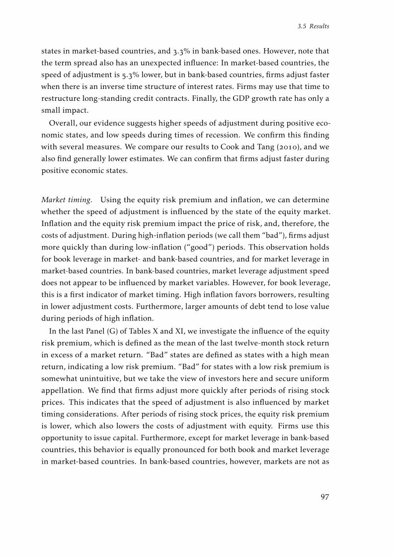
3.5 Results
states in market-based countries, and .% in bank-based ones. However, note that
the term spread also has an unexpected influence: In market-based countries, the
speed of adjustment is .% lower, but in bank-based countries, firms adjust faster
when there is an inverse time structure of interest rates. Firms may use that time to
restructure long-standing credit contracts. Finally, the GDP growth rate has only a
small impact.
Overall, our evidence suggests higher speeds of adjustment during positive eco-
nomic states, and low speeds during times of recession. We confirm this finding
with several measures. We compare our results to Cook and Tang (), and we
also find generally lower estimates. We can confirm that firms adjust faster during
positive economic states.
Market timing. Using the equity risk premium and inflation, we can determine
whether the speed of adjustment is influenced by the state of the equity market.
Inflation and the equity risk premium impact the price of risk, and, therefore, the
costs of adjustment. During high-inflation periods (we call them “bad”), firms adjust
more quickly than during low-inflation (“good”) periods. This observation holds
for book leverage in market- and bank-based countries, and for market leverage in
market-based countries. In bank-based countries, market leverage adjustment speed
does not appear to be influenced by market variables. However, for book leverage,
this is a first indicator of market timing. High inflation favors borrowers, resulting
in lower adjustment costs. Furthermore, larger amounts of debt tend to lose value
during periods of high inflation.
In the last Panel (G) of Tables X and XI, we investigate the influence of the equity
risk premium, which is defined as the mean of the last twelve-month stock return
in excess of a market return. “Bad” states are defined as states with a high mean
return, indicating a low risk premium. “Bad” for states with a low risk premium is
somewhat unintuitive, but we take the view of investors here and secure uniform
appellation. We find that firms adjust more quickly after periods of rising stock
prices. This indicates that the speed of adjustment is also influenced by market
timing considerations. After periods of rising stock prices, the equity risk premium
is lower, which also lowers the costs of adjustment with equity. Firms use this
opportunity to issue capital. Furthermore, except for market leverage in bank-based
countries, this behavior is equally pronounced for both book and market leverage
in market-based countries. In bank-based countries, however, markets are not as
Chapter 3 Illuminating the speed of adjustment
Table X – Speed of adjustment and macroeconomics - Book leverageMarket-based Bank-based
Good Bad G.vs.B. Good Bad G.vs.B.
Panel A – States determined by recession indicator
LBL 0.772∗∗∗ 0.842∗∗∗ 0.774∗∗∗ 0.861∗∗∗ 0.914∗∗∗ 0.805∗∗∗
(145.373) (74.804) (151.299) (180.570) (168.987) (144.488)SOA (in %) 22.8 15.8 22.6 13.9 8.6 19.5LBL×REC 0.024∗∗ 0.056∗∗∗
(2.707) (16.553)REC −0.004 −0.031∗∗∗
(−0.657) (−13.311)
N 28092 3406 31498 22966 17196 40162
Panel B – States determined by spread on Moody’s AAA to BBB bond index
LBL 0.833∗∗∗ 0.842∗∗∗ 0.840∗∗∗ 0.867∗∗∗ 0.933∗∗∗ 0.875∗∗∗
(107.442) (105.093) (122.563) (119.515) (165.773) (147.570)SOA (in %) 16.7 15.8 16.0 13.3 6.7 12.5LBL×BADDUMCREDIT 0.008 0.045∗∗∗
(1.039) (8.140)BADDUMCREDIT −0.011 −0.024∗∗∗
(−0.521) (−4.925)
N 7980 6493 14473 6525 9796 16321
Panel C – States determined by TED spread
LBL 0.837∗∗∗ 0.859∗∗∗ 0.835∗∗∗ 0.860∗∗∗ 0.918∗∗∗ 0.857∗∗∗
(119.022) (109.795) (121.976) (156.453) (115.872) (154.300)SOA (in %) 16.3 14.1 16.5 14.0 8.2 14.3LBL×BADDUMTED 0.019∗ 0.065∗∗∗
(2.186) (9.345)BADDUMTED 0.000 −0.037∗∗∗
(0.013) (−6.298)
N 7031 5875 12906 8651 4052 12703
Panel D – States determined by term spread
LBL 0.853∗∗∗ 0.814∗∗∗ 0.854∗∗∗ 0.911∗∗∗ 0.916∗∗∗ 0.915∗∗∗
(101.167) (106.438) (115.637) (122.802) (158.318) (144.631)SOA (in %) 14.7 18.6 14.6 8.9 8.4 8.5LBL×BADDUMTERM −0.034∗∗∗ 0.004
(−3.692) (0.689)BADDUMTERM −0.018 −0.011
(−0.828) (−1.787)
N 5556 6160 11716 4617 9214 13831
continued

3.5 Results
Table X – (continued)Market-based Bank-based
Good Bad G.vs.B. Good Bad G.vs.B.
Panel E – States determined by GDP growth rate
LBL 0.795∗∗∗ 0.871∗∗∗ 0.805∗∗∗ 0.893∗∗∗ 0.954∗∗∗ 0.883∗∗∗
(88.040) (102.935) (105.794) (164.666) (168.278) (168.628)SOA (in %) 20.5 22.9 19.5 10.7 4.6 11.7LBL×BADDUMGDP 0.054∗∗∗ 0.064∗∗∗
(5.961) (13.220)BADDUMGDP −0.023∗∗ −0.039∗∗∗
(−2.982) (−11.314)
N 7224 5192 12416 9445 8632 18077
Panel F – States determined by inflation
LBL 0.846∗∗∗ 0.823∗∗∗ 0.841∗∗∗ 0.940∗∗∗ 0.928∗∗∗ 0.940∗∗∗
(103.391) (104.020) (104.850) (145.263) (189.869) (172.440)SOA (in %) 15.4 17.7 15.9 6.0 7.2 6.0LBL×BADDUMINF −0.029∗∗ −0.021∗∗∗
(−3.225) (−3.858)BADDUMINF 0.013∗ 0.015∗
(2.146) (2.269)
N 5606 6326 11932 6298 9277 15575
Panel G – States determined by equity risk premium
LBL 0.844∗∗∗ 0.818∗∗∗ 0.844∗∗∗ 0.918∗∗∗ 0.890∗∗∗ 0.908∗∗∗
(105.544) (109.565) (114.689) (172.137) (154.719) (164.753)SOA (in %) 15.6 18.2 15.6 8.2 11.0 9.2LBL×BADDUMERP −0.034∗∗∗ −0.043∗∗∗
(−3.840) (−8.985)BADDUMERP −0.021∗ 0.003
(−2.387) (0.475)
N 6254 6405 12659 11048 8370 19418t statistics in parentheses∗ p < 0.05, ∗∗ p < 0.01, ∗∗∗ p < 0.001
This table shows the speed of adjustment conditional on the macroeconomic environment. The column Good refersto good macroeconomic states. We classify states as good if the recession indicator is zero, the credit spread is low,the TED spread is low, the term spread is low, the GDP growth rate is high, the inflation rate is low, and the equityrisk premium is low. The classification for Bad is the opposite. The G.vs.B column estimates whether the differencebetween good and poor states is significant. BADDUM is a dummy variable equal to in bad states. LBL×BADDUMis an interaction term between lagged leverage and the bad dummy. All estimations are done by the DPF estimator:Li,t = (1−λ)Li,t−1 +λβXi,t−1 +µi +εi,t , with mui = α0 +α1Li,0 +E(Xi )α2 +αi . SOA is minus the coefficient on laggedbook leverage. Time dummies, constants, initial leverage, and mean exogenous variables are omitted.

Chapter 3 Illuminating the speed of adjustment
Table XI – Speed of adjustment and macroeconomics - Market leverageMarket-based Bank-based
Good Bad G.vs.B. Good Bad G.vs.B.
Panel A – States determined by recession indicator
LML 0.838∗∗∗ 0.905∗∗∗ 0.838∗∗∗ 0.897∗∗∗ 0.882∗∗∗ 0.902∗∗∗
(148.539) (44.383) (150.435) (131.760) (106.534) (207.158)SOA (in %) 16.2 9.5 16.2 10.3 11.8 9.8LML×REC 0.086∗∗∗ 0.010∗
(6.923) (2.237)REC −0.033∗∗∗ 0.021∗∗∗
(−4.659) (6.594)
N 16056 1522 17578 13133 10805 23938
Panel B – States determined by spread on Moody’s AAA to BBB bond index
LML 0.847∗∗∗ 0.860∗∗∗ 0.846∗∗∗ 0.956∗∗∗ 0.906∗∗∗ 0.930∗∗∗
(76.727) (66.942) (86.847) (99.066) (109.069) (123.256)SOA (in %) 15.3 14.0 15.4 4.4 9.4 7.0LML×BADDUMCREDIT 0.014 −0.002
(1.320) (−0.233)BADDUMCREDIT −0.007 0.020∗∗
(−0.278) (2.766)
N 5115 3109 8224 4311 5595 9906
Panel C – States determined by TED spread
LML 0.825∗∗∗ 0.913∗∗∗ 0.828∗∗∗ 0.947∗∗∗ 0.942∗∗∗ 0.939∗∗∗
(74.714) (61.694) (83.387) (112.239) (69.481) (122.470)SOA (in %) 17.5 8.7 17.2 5.3 5.8 6.1LML×BADDUMTED 0.082∗∗∗ 0.033∗∗∗
(7.116) (3.370)BADDUMTED −0.026∗∗ −0.011
(−2.636) (−1.186)
N 3640 3126 6766 4958 2240 7198
Panel D – States determined by term spread
LML 0.816∗∗∗ 0.868∗∗∗ 0.817∗∗∗ 0.927∗∗∗ 0.895∗∗∗ 0.943∗∗∗
(64.687) (66.002) (81.287) (76.195) (102.442) (94.363)SOA (in %) 18.5 13.2 18.3 7.3 10.5 5.7LML×BADDUMTERM 0.053∗∗∗ −0.058∗∗∗
(4.476) (−6.311)BADDUMTERM 0.055 0.014
(0.987) (1.386)
N 3036 3532 6568 2549 5513 8062
continued

3.5 Results
Table XI – (continued)Market-based Bank-based
Good Bad G.vs.B. Good Bad G.vs.B.
Panel E – States determined by GDP growth rate
LML 0.852∗∗∗ 0.869∗∗∗ 0.850∗∗∗ 0.886∗∗∗ 0.899∗∗∗ 0.897∗∗∗
(72.378) (64.946) (82.012) (103.377) (100.034) (138.224)SOA (in %) 14.8 13.1 15.0 11.4 10.1 10.3LML×BADDUMGDP 0.024∗ 0.009
(2.066) (1.312)BADDUMGDP −0.019∗ 0.021∗∗∗
(−2.161) (3.939)
N 4572 2609 7181 6077 4953 11030
Panel F – States determined by inflation
LML 0.893∗∗∗ 0.812∗∗∗ 0.877∗∗∗ 0.894∗∗∗ 0.887∗∗∗ 0.893∗∗∗
(63.243) (66.335) (74.988) (82.396) (124.966) (115.406)SOA (in %) 10.7 18.8 12.3 10.6 11.3 10.7LML×BADDUMINF −0.055∗∗∗ −0.002
(−4.388) (−0.319)BADDUMINF 0.031∗∗∗ −0.004
(3.980) (−0.338)
N 2845 3361 6206 3481 5737 9218
Panel G – States determined by equity risk premium
LML 0.860∗∗∗ 0.831∗∗∗ 0.880∗∗∗ 0.865∗∗∗ 0.871∗∗∗ 0.887∗∗∗
(61.131) (76.622) (86.120) (102.381) (98.656) (146.410)SOA (in %) 14.0 16.9 12.0 13.5 12.9 11.3LML×BADDUMERP −0.067∗∗∗ −0.007
(−5.995) (−0.978)BADDUMERP −0.061∗∗∗ −0.066∗
(−3.463) (−2.572)
N 3234 4013 7247 6555 5308 11863t statistics in parentheses∗ p < 0.05, ∗∗ p < 0.01, ∗∗∗ p < 0.001
This table shows the speed of adjustment conditional on the macroeconomic environment. The column Good refers togood macroeconomic states. We classify states as good if the recession indicator is zero, the credit spread is low, theTED spread is low, the term spread is low, the GDP growth rate is high, the inflation rate is low, and the equity riskpremium is low. The classification for Bad is the opposite. The G.vs.B column estimates whether the difference be-tween good and poor states is significant. BADDUM is a dummy variable equal to in bad states. LML×BADDUMis an interaction term between lagged leverage and the bad dummy. All estimations are done by the DPF estimator:Li,t = (1−λ)Li,t−1 +λβXi,t−1 +µi +εi,t , with mui = α0 +α1Li,0 +E(Xi )α2 +αi . SOA is minus the coefficient on laggedmarket leverage. Time dummies, constants, initial leverage, and mean exogenous variables are omitted.

Chapter 3 Illuminating the speed of adjustment
important for financing, so an equity risk premium-induced difference in market
leverage is not measurable.
Overall, we find that firms in market-based countries have higher adjustment
speeds, which are induced by high inflation and a low equity risk premium. This
indicates market timing behavior. In bank-based countries, only the adjustment
speed of book leverage is affected by inflation and the equity risk premium.
3.6 Conclusion
Adjustment speed varies for firms and during different economic states. To explore
what causes the differences, we perform an in-depth investigation of adjustment
speed and look for differences according to firms’ financial systems, financial condi-
tions, and the macroeconomic environments. We use an estimator that accounts for
the fractional nature of the dependent variable leading to unbiased estimates.
We find a % mean speed of adjustment, which is lower than in most historical
studies, but is well within the range of studies using advanced estimators that do
not suffer from a priori known biases. We find a higher speed of adjustment in
market-based countries than in bank-based countries. This is further evidence that
there are in fact two different financial systems, and firms face different adjustment
costs and different costs of deviating from their targets within these two systems.
Future articles may want to explore this concept further, in an effort to shed more
light on the different mechanisms of determining of the capital structure.
Furthermore, we find that firms tend to use periods of high financial deficits to
adjust faster. Financially constrained firms can adjust faster than unconstrained
firms, but they are slower than medium-constrained firms. Even if they desire to
adjust more quickly, we find they face higher costs of deviating from their targets,
and will thus be prevented by the concurrent high costs of adjustment. Highly
over-leveraged firms also adjust faster than highly under-leveraged firms. There
seems to be some asymmetry in the costs of deviating from targets here: the costs
appear to be higher for over-leveraged firms.
The speed of adjustment is also dependent on the state of the economy. We find
a lower adjustment speed during times of recession. This phenomenon is more
pronounced for book leverage. Market leverage speeds do not react as strongly to
the economic environment, particularly in bank-based countries. Moreover, we find
evidence of market timing, as firms adjust faster during periods of high inflation

3.6 Conclusion
and low equity risk premiums.
Our results are helpful in judging capital structure models, and they can provide
evidence for a target leverage over the medium and long term. However, as we note,
the speed of adjustment is not greatly affected by short-run deviations from the
target. We would suggest that future research on this topic focus on the differences
even more strongly, and illuminate how the institutional environment and the
macroeconomy impact the speed of adjustment. As our results show, firm behavior
is ultimately conditional on these factors.
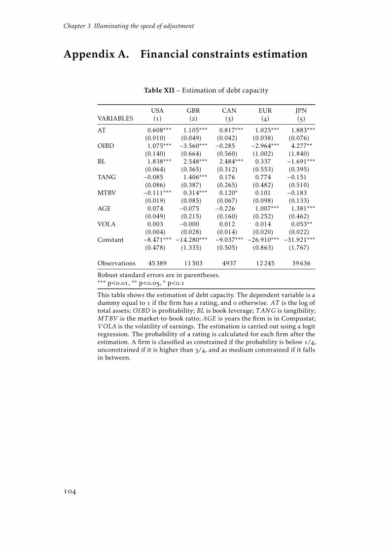
Chapter 3 Illuminating the speed of adjustment
Appendix A. Financial constraints estimation
Table XII – Estimation of debt capacity
USA GBR CAN EUR JPNVARIABLES () () () () ()
AT 0.608*** 1.105*** 0.817*** 1.025*** 1.883***(0.010) (0.049) (0.042) (0.038) (0.076)
OIBD 1.075*** −3.560*** −0.285 −2.964*** 4.277**(0.140) (0.664) (0.560) (1.002) (1.840)
BL 1.838*** 2.548*** 2.484*** 0.337 −1.691***(0.064) (0.365) (0.312) (0.553) (0.395)
TANG −0.085 1.406*** 0.176 0.774 −0.151(0.086) (0.387) (0.265) (0.482) (0.510)
MTBV −0.111*** 0.314*** 0.120* 0.101 −0.183(0.019) (0.085) (0.067) (0.098) (0.133)
AGE 0.074 −0.075 −0.226 1.007*** 1.381***(0.049) (0.215) (0.160) (0.252) (0.462)
VOLA 0.003 −0.000 0.012 0.014 0.053**(0.004) (0.028) (0.014) (0.020) (0.022)
Constant −8.471*** −14.280*** −9.037*** −26.910*** −31.921***(0.478) (1.335) (0.505) (0.863) (1.767)
Observations 45389 11503 4937 12245 39636
Robust standard errors are in parentheses.*** p<., ** p<., * p<.
This table shows the estimation of debt capacity. The dependent variable is adummy equal to if the firm has a rating, and otherwise. AT is the log oftotal assets; OIBD is profitability; BL is book leverage; TANG is tangibility;MTBV is the market-to-book ratio; AGE is years the firm is in Compustat;VOLA is the volatility of earnings. The estimation is carried out using a logitregression. The probability of a rating is calculated for each firm after theestimation. A firm is classified as constrained if the probability is below /,unconstrained if it is higher than /, and as medium constrained if it fallsin between.

References
References
Antoniou, A., Y. Guney, and K. Paudyal. . The determinants of capital structure:
Capital market-oriented versus bank-oriented institutions. Journal of Financialand Quantitative Analysis (): –.
Arellano, M., and S. Bond. . Some tests of specification for panel data: Monte
Carlo evidence and an application to employment equations. Review of EconomicStudies (): –.
Baker, M., and J. Wurgler. . Market timing and capital structure. Journal ofFinance (): –.
Baltagi, B.H. . Econometric analysis of panel data. Hoboken, New Jersey: John
Wiley & Sons.
Banerjee, S., A. Heshmati, and C. Wihlborg. . The dynamics of capital structure.
In Monetary integration, markets and regulation, ed. M. Bagella, L. Becchetti, I.
Hasan, and W.C. Hunter. Amsterdam: Elsevier.
Beck, T., A. Demirgüç-Kunt, and R. Levine. . Financial institutions and markets
across countries and over time. World Bank, Washington DC: Policy ResearchWorking Paper .
Blundell, R., and S. Bond. . Initial conditions and moment restrictions in
dynamic panel data models. Journal of Econometrics (): –.
Bruno, G.S.F. a. Approximating the bias of the LSDV estimator for dynamic
unbalanced panel data models. Economics Letters (): –.
———. b. Estimation and inference in dynamic unbalanced panel-data models
with a small number of individuals. Stata Journal (): –.
Bun, M.J.G., and J.F. Kiviet. . On the diminishing returns of higher-order terms
in asymptotic expansions of bias. Economics Letters (): –.
Byoun, S. . How and when do firms adjust their capital structures toward
targets? Journal of Finance (): –.
Chang, X., and S. Dasgupta. . Target Behavior and Financing: How Conclusive
is the Evidence? Journal of Finance (): –.

References
Cook, D.O., and T. Tang. . Macroeconomic conditions and capital structure
adjustment speed. Journal of Corporate Finance (): –.
Dang, V.A., I. Garrett, and C. Nguyen. . Asymmetric Partial Adjustment toward
Target Leverage: International Evidence. Working Paper: Manchester BusinessSchool.
Dang, V.A., M. Kim, and Y. Shin. . Asymmetric capital structure adjustments:
New evidence from dynamic panel threshold models. Working Paper: Universityof Manchester & University of Leeds.
Dittmar, A., and A. Thakor. . Why do firms issue equity? Journal of Finance (): –.
Drobetz, W., and G. Wanzenried. . What determines the speed of adjustment to
the target capital structure? Applied Financial Economics (): –.
Elsas, R., and D. Florysiak. . Dynamic capital structure adjustment and the
impact of fractional dependent variables. Working Paper: Universität München.
———. . Heterogeneity in the speed of adjustment toward target leverage.
International Review of Finance (): –.
Fama, E.F., and K.R. French. . Industry costs of equity. Journal of FinancialEconomics (): –.
———. . Testing trade-off and pecking order predictions about dividends and
debt. Review of Financial Studies (): –.
Faulkender, M.W., M.J. Flannery, K.W. Hankins, and J.M. Smith. . Cash flows
and leverage adjustments. Journal of Financial Economics, Forthcoming.
Faulkender, M.W., and M.A. Petersen. . Does the source of capital affect capital
structure? Review of Financial Studies (): .
Fischer, E.O., R. Heinkel, and J. Zechner. . Dynamic capital structure choice:
Theory and tests. Journal of Finance (): –.
Flannery, M.J., and K.W. Hankins. . Estimating dynamic panel models in corpo-
rate finance. Working Paper: University of Florida.
Flannery, M.J., and K.P. Rangan. . Partial adjustment toward target capital
structures. Journal of Financial Economics (): –.

References
Frank, M.Z., and V.K. Goyal. . Trade-off and pecking order theories of debt.
In Handbook of corporate finance: Empirical corporate finance, ed. E.B. Eckbo,
–. Vol. . Amsterdam: North-Holland.
Getzmann, A., S. Lang, and K. Spremann. . Determinants of the target capi-
tal structure and adjustment speed–evidence from Asian, European and U.S.-
capital markets. Working Paper: Universität St. Gallen.
Gilson, S.C. . Transactions costs and capital structure choice: Evidence from
financially distressed firms. Journal of Finance (): –.
Graham, J.R., and C.R. Harvey. . The theory and practice of corporate finance:
Evidence from the field. Journal of Financial Economics (-): –.
Hackbarth, D., J. Miao, and E. Morellec. . Capital structure, credit risk, and
macroeconomic conditions. Journal of Financial Economics (): –.
Hahn, J., J. Hausman, and G. Kuersteiner. . Long difference instrumental vari-
ables estimation for dynamic panel models with fixed effects. Journal of Econo-metrics (): –.
Halling, M., J. Yu, and J. Zechner. . Leverage Dynamics Over the Business Cycle.
Working Paper: Universität Wien.
Hovakimian, A., and G. Li. . In search of conclusive evidence: How to test for
adjustment to target capital structure. Journal of Corporate Finance (): –.
Huang, R., and J.R. Ritter. . Testing theories of capital structure and estimating
the speed of adjustment. Journal of Financial and Quantitative Analysis ():–.
Iliev, P., and I. Welch. . Reconciling estimates of the speed of adjustment of
leverage ratios. Working Paper: Brown University.
Jalilvand, A., and R.S. Harris. . Corporate behavior in adjusting to capital
structure and dividend targets: An econometric study. Journal of Finance ():–.
Jensen, M.C. . Agency costs of free cash flow, corporate finance, and takeovers.
American Economic Review (): –.

References
Judson, R.A., and A.L. Owen. . Estimating dynamic panel data models: A guide
for macroeconomists. Economics Letters (): –.
Kayhan, A., and S. Titman. . Firms’ histories and their capital structures. Journalof Financial Economics (): –.
Kiviet, J.F. . On bias, inconsistency, and efficiency of various estimators in
dynamic panel data models. Journal of Econometrics (): –.
———. . Expectations of expansions for estimators in a dynamic panel data
model: Some results for weakly exogenous regressors. In Analysis of panel dataand limited dependent variables, ed. C. Hsiao, K. Lahiri, L.-F. Lee, and M.H.
Pesaran. Cambridge: Cambridge University Press.
Korajczyk, R.A., and A. Levy. . Capital structure choice: Macroeconomic condi-
tions and financial constraints. Journal of Financial Economics (): –.
Kraus, A., and R.H. Litzenberger. . A state-preference model of optimal financial
leverage. Journal of Finance (): –.
La Porta, R.L., F. Lopez-de-Silanes, A. Shleifer, and R.W. Vishny. . Law and
finance. Journal of Political Economy (): –.
Lemmon, M.L., M.R. Roberts, and J.F. Zender. . Back to the Beginning: Persis-
tence and the Cross-Section of Corporate Capital Structure. Journal of Finance (): –.
Lemmon, M.L., and J.F. Zender. . Debt capacity and tests of capital structure
theories. Journal of Financial and Quantitative Analysis (): –.
Loudermilk, M.S. . Estimation of fractional dependent variables in dynamic
panel data models with an application to firm dividend policy. Journal of Busi-ness and Economic Statistics (): –.
Marcus, A.J. . The bank capital decision: A time series–cross section analysis.
Journal of Finance (): –.
Modigliani, F., and M.H. Miller. . The cost of capital, corporation finance and
the theory of investment. American Economic Review (): –.
———. . Corporate income taxes and the cost of capital: A correction. AmericanEconomic Review (): –.

References
Myers, S.C., and Nicholas S. Majluf. . Corporate financing and investment
decisions when firms have information that investors do not have. Journal ofFinancial Economics (): –.
Nickell, S. . Biases in dynamic models with fixed effects. Econometrica:–.
Roberts, M.R. . The dynamics of capital structure: An empirical analysis of a
partially observable system. Working Paper: Duke University.
Welch, I. . Capital structure and stock returns. Journal of Political Economy (): –.


Kapitel 4Haben Manager Timing-Fähigkeiten?
Eine empirische Untersuchung vonDirectors’-Dealings
mit Wolfgang Drobetza und Sven Lindnerb
Januar
eingereicht bei der Zeitschrift für Betriebswirtschaft
a Wolfgang Drobetz, Lehrstuhl für Unternehmens- und Schiffsfinanzierung, Universität Hamburg,
Von-Melle-Park , Hamburg, Tel.: +---, Mail: [email protected]
hamburg.de.b Sven Lindner, NRS Norddeutsche Retail-Service AG, Börsenbrücke a, Hamburg, Mail:
sven.lindner@ nrs-ag.de.

Kapitel 4 Haben Manager Timing-Fähigkeiten?
Zusammenfassung
In dieser Untersuchung wird die Performance deutscher Unternehmensinsider beiTransaktionen in Aktien ihrer „eigenen“ Unternehmen analysiert. Grundlage sinddie Mitteilungen der BaFin-Datenbank für Directors’ Dealings über den Zeitraumvom . Juli bis . März . Die Ergebnisse deuten darauf hin, dass Unterneh-mensinsider über ausgeprägte Timing-Fähigkeiten verfügen. Insider verhalten sichals Contrarian-Investoren, d.h. sie kaufen Aktien nach Kursverlusten und verkaufennach Kursanstiegen. Während im Anschluss an Käufe die Kursanstiege zu signi-fikanten abnormalen Renditen für die Insider führen, vermeiden sie signifikanteKursverluste nach Verkäufen. Für die Information-Hierarchy-Hypothese, wonachdie Werthaltigkeit von Informationen mit steigender Hierarchieebene eines Insi-ders zunimmt, gibt es keine empirische Evidenz. Hingegen haben die verschärftenRegularien des Insiderrechts seit Oktober zu einem Abbau der Informations-symmetrien zwischen Unternehmensinsidern und Marktteilnehmern und damitzur Integrität des Marktes beigetragen. Daneben enthält die Untersuchung aucheinen zentralen methodischen Beitrag. Die empirischen Ergebnisse sind robust undkönnen sowohl durch eine klassische Ereignisstudie als auch in Panelregressionenim Rahmen eines generalisierten Kalenderzeitansatzes bestätigt werden.
Stichwörter: Insidertransaktionen, Directors’ Dealings, Markteffizienz, Ereignisstu-die, Kalenderzeitverfahren
JEL Klassifikation: G, G, G, G

4.1 Einleitung
4.1 Einleitung
Das Informationsgefälle zwischen Unternehmensinsidern und allen anderen
Marktteilnehmern (Outsidern) ist ein zentrales Element der Finanzierungslehre.
Unternehmensinsider, also insbesondere Vorstände und Aufsichtsratsmitglieder
börsennotierter Gesellschaften, besitzen wertvollere Informationen über den wahren
Zustand ihres „eigenen“ Unternehmens als Kleinaktionäre. Es erstaunt daher nicht,
dass die Handelsaktivitäten von Unternehmensinsidern in zahlreichen Studien
untersucht wurden (Jaffe ; Seyhun ; Lakonishok und Lee ; Fidrmuc
u. a. ). Im Mittelpunkt steht dabei die Frage nach der Profitabilität von Insider-
Transaktionen vor dem Hintergrund der Informationseffizienz der Kapitalmärkte
(Fama ). Eine Analyse der Profitabilität von Insider-Transaktionen stellt einen
Test der starken Form der Markteffizienz dar. Im Gegensatz dazu ermöglicht die
Analyse der Profitabilität von Mimicking-Strategien (d.h. Käufe und Verkäufe von
Marktteilnehmern im Anschluss an die Veröffentlichung von Insider-Käufen bzw.
Insider-Verkäufen) einen Test der mittelstarken Form der Markteffizienz.
In der Regulierungsliteratur werden Insider-Transaktionen sehr ambivalent beur-
teilt. Insider-Transaktionen können einerseits einen Beitrag zur verbesserten Wertpa-
pierpreisbildung und damit zur effizienten Ressourcenallokation liefern, sie bergen
jedoch anderseits auch die Gefahr eines opportunistischen Verhaltens der Insider.
Leland () argumentiert, dass die Aktienkurse einen höheren Informationsgehalt
aufweisen und das allgemeine Bewertungsniveau höher ausfällt, wenn Unterneh-
mensinsider Wertpapiere des eigenen Unternehmens handeln dürfen. Nach Manne
(a, b) stellt der Handel mit Unternehmensaktien einen effizienten Vergü-
tungsmechanismus für die Leistungen der Insider dar, weil der Vertrag zwischen
Managern und Anteilseignern nicht ständig den sich wandelnden Umweltbedingun-
gen angepasst werden muss. Insider könnten ihren Informationsvorteil aber auch
opportunistisch ausnutzen. Bereits Lin und Howe () dokumentieren, dass die
abnormalen Renditen der Outsider im Rahmen von Mimicking-Strategien geringer
ausfallen als jene der Insider. Auch wenn dieses Ergebnis aufgrund der asymmetri-
schen Informationsverteilung nicht grundsätzlich überrascht, ist aus eben diesem
Grund Insider-Trading auf entwickelten Kapitalmärkten einer starken Regulierung
durch den Gesetzgeber unterworfen. Ziel der gesetzlichen Regelung ist es, zu ver-
Im Rahmen dieser Arbeit werden unter dem Begriff „Outsider“ alle Kapitalmarktteilnehmerverstanden, die keine Insider nach der Definition des Wertpapierhandelsgesetzes (WpHG) sind.

Kapitel 4 Haben Manager Timing-Fähigkeiten?
meiden, dass die Marktintegrität durch Missbrauch in Form von Insiderhandel und
Marktmanipulation in Zweifel gezogen wird, was wiederum zum Vertrauensverlust
der Anleger führen könnte (Seyhun ). Entsprechend liegt in Deutschland nach
dem Wertpapierhandelsgesetz (WpHG) ein gesetzeswidriges Insider-Geschäft dann
vor, wenn die der Transaktion zugrunde liegende Insiderinformation konkret ist
und einen Tatsachenkern enthält. Die Information muss zusätzlich das Potential
haben, den Kurs des Insiderpapiers zu beeinflussen.
Ein zentrales Ergebnis früherer empirischer Studien ist, dass Unternehmensin-
sider über ausgeprägte Timing-Fähigkeiten beim Handel eigener Aktien besitzen.
Zu den ersten Studien zählen Jaffe () und Finnerty (), die beide für den
US-Markt kurzfristige abnormale Renditen für Insider dokumentieren. Beispielswei-
se misst Finnerty () im Handelsmonat abnormale Renditen für Insider-Käufe
in Höhe von ,% und für Insider-Verkäufe in Höhe von -,%. Seyhun ()dokumentiert, dass die abnormalen Renditen in den Tagen nach einer Insider-
Transaktion ,% bei Käufen und -,% bei Verkäufen betragen. Während abnor-
male Renditen am Ereignistag selbst nicht überraschen, deuten die langfristigen
Bewertungseffekte darauf hin, dass der Markt die Insiderinformation nur langsam
verarbeitet. Neben diesen Beobachtungen zur Kapitalmarkteffizienz weisen viele
Studien auf Handelsmuster der Insider hin. Ein regelmäßig dokumentiertes Muster
ist die Fähigkeit der Insider, die kurzfristige Wertentwicklung des Unternehmens
prognostizieren zu können. Insider kaufen Aktien, wenn das Unternehmen aus
ihrer Sicht unterbewertet ist und verkaufen Aktien, wenn sie das Unternehmen als
überbewertet erachten. Da sich die Insider gegenläufig zur beobachteten Preisent-
wicklung verhalten, verfolgen sie eine „Contrarian-Investment-Strategie“ (Givoly
und Palmon ; Seyhun ; Rozeff und Zaman ). Ob sich daraus allerdings
profitable „Mimicking-Strategien“ auch für andere Marktteilnehmer ergeben, wird
in der empirischen Literatur mit teilweise widersprüchlichen Befunden diskutiert
(Lin und Howe ; Bettis u. a. ; Lakonishok und Lee ; Jeng u. a. ).
Die Determinanten der Profitabilität von Insider-Transaktionen stellen einen wei-
teren wichtigen Aspekt in den früheren Studien dar. Potentielle Einflussfaktoren
sind die Unternehmensgröße (Seyhun ; Chari u. a. ; Lakonishok und Lee
Auch für andere nationale Kapitalmärkte außerhalb der USA liegen empirische Ergebnisse zumInsider-Trading vor. Die Studien von Pope u. a. () und Friederich u. a. () für Großbritannien,Bajo und Petracci () für Italien, Biesta u. a. () für die Niederlande, Fowler und Rorke() für Kanada und Zhu u. a. () für China bestätigen die US-amerikanischen Ergebnisse. ImGegensatz dazu scheinen die Timing-Fähigkeiten der Insider in Spanien (Del Brio u. a. ) undNorwegen (Eckbo und Smith ) weniger stark ausgeprägt zu sein.

4.1 Einleitung
; Jeng u. a. ), die Nähe des Insiders zum operativen Geschäft (Seyhun
), das Transaktionsvolumen und deren Frequenz (Barclay und Warner ;Friederich u. a. ; Jeng u. a. ), die finanzielle Situation des Unternehmens
(Gosnell u. a. ; Fidrmuc u. a. ), die Branche (Aboody und Lev ) sowie
die Anleger- und Eigentümerstruktur (Fidrmuc u. a. ). Ein zentraler Gegenstand
der empirischen Forschung ist schließlich die Frage, ob Insider ihren Informations-
vorteil opportunistisch nutzen, oder ob die Profitabilität der Unternehmensinsider
auf Preisdruckeffekte zurückzuführen ist, die durch Mimicking-Strategien der Out-
sider erzeugt werden. Die empirischen Befunde zeigen, dass Insider regelmäßig
im Vorfeld von wichtigen Finanzierungsentscheidungen stattfinden, also etwa vor
Dividendenerhöhungen (John und Lang ), Kapitalerhöhungen (Karpoff und
Lee ), Aktienrückkäufen (Lee u. a. ), Gewinnankündigungen (Elliott u. a.
; Noe ; Ke u. a. ) oder vor einem Konkurs (Seyhun und Bradley ).Diese Ergebnisse deuten darauf hin, dass Insider ihren Informationsvorsprung aktiv
zu ihrem eigenen Vorteil ausnutzen. Im Gegensatz dazu können Givoly und Pal-
mon () keinen systematischen Zusammenhang zwischen der Profitabilität von
Insider-Transaktionen und der Veröffentlichung wichtiger und sehr breit gefasster
Unternehmensnachrichten (d.h. nicht ausschließlich aus dem Finanzierungsbereich)
messen.
Die Anzahl wissenschaftlicher Studien zum Insider-Trading in Deutschland ist
bedingt durch die relativ späte Implementierung zwingender Gesetzesnormen und
der damit verbundenen Datenverfügbarkeit gering. Zu den prominentesten Arbei-
ten zählen die Studien von Stotz (), Dymke und Walter (), Betzer und
Theissen (a, b) sowie Dickgiesser und Kaserer (). Stotz () weist
über die Handelstage nach dem Ereignistag abnormale Renditen von insgesamt
,% bei Käufen und -,% bei Verkäufen aus. Dabei verhalten sich Insider als
„Contrarian-Investors“, d.h. sie kaufen Wertpapiere des Unternehmens, nachdem
der Aktienkurs gesunken ist, und sie verkaufen Wertpapiere nach einem Kursanstieg.
Von diesen Timing-Fähigkeiten der Insider können auch Outsider profitieren, weil
selbst im Anschluss an die Veröffentlichung der Transaktion signifikante abnormale
Renditen zu beobachten sind. Betzer und Theissen (a) dokumentieren ähnliche
Handelsmuster und untersuchen zusätzlich den Einfluss der Corporate-Governance
auf die Profitabilität von Insider-Transaktionen. Aus ihren Ergebnissen leiten sie
Frühere Studien mit kleineren Stichproben für Deutschland stammen von Rau (), Heidornu. a. () sowie Tebroke und Wollin ().

Kapitel 4 Haben Manager Timing-Fähigkeiten?
die Wirksamkeit von Handelssperren für Insider vor Gewinnveröffentlichungen ab
(„Blackout-Perioden“). In Bezug auf die Anteilsstruktur finden sie höhere abnormale
Renditen bei Unternehmen mit atomistischer Aktionärsstruktur. Die Position des
Insiders im Unternehmen (also Vorstand bzw. Aufsichtsrat; Information-Hierarchy-
Hypothese) scheint hingegen keine systematische Determinante für die Werthaltig-
keit von privaten Informationen zu sein. Dymke und Walter () dokumentieren,
dass Insider ihren Informationsvorsprung aktiv ausnutzen und systematisch vor der
Veröffentlichung von Unternehmensnachrichten handeln. Diese Art des als rechtlich
problematisch einzustufenden „Front-Running“ äußert sich darin, dass jene Insider-
Transaktionen am profitabelsten sind, die unmittelbar vor einer Veröffentlichung im
Rahmen der ad-hoc Publizitätspflichten erfolgen. Dickgiesser und Kaserer ()untersuchen die Profitabilität von Mimicking-Strategien. Ihre Ergebnisse deuten
darauf hin, dass Mimicking-Strategien nach Berücksichtigung der Transaktionskos-
ten keine signifikanten Überrenditen erzeugen. Die Unterreaktion des Marktes im
Anschluss an die Veröffentlichung von Insider-Transaktionen ist nach Dickgiesser
und Kaserer () durch die Kosten von „Risky-Arbitrage“ (Shleifer und Vishny
) zu erklären. Damit kann der Markt als effizient in Sinne von Jensen ()interpretiert werden.
Die vorliegende Studie ergänzt die bisherigen Ergebnisse für Deutschland in
mehrfacher Hinsicht. Erstens liegt unserer Untersuchung die mit Abstand größte
Strichprobe von Insider-Transaktionen zugrunde. Gegenstand unserer empirischen
Analyse sind sämtliche Mitteilungen über Transaktionen, deren Handelstag zwi-
schen dem . Juli und dem . März liegt. Damit können die Ergebnisse
der früheren Studien auf ihre Stabilität überprüft werden. Eine zweite Besonder-
heit unserer Stichprobe ist, dass der Beobachtungszeitraum die Anpassungen im
deutschen Insiderrecht umfasst, die im Oktober durch das Anlegerschutz-
verbesserungsgesetzes (AnSVG) hervorgerufen wurden. Die wichtigste Änderung
ist die gesetzliche Pflicht zur Veröffentlichung einer Transaktion innerhalb von
fünf Werktagen (anstatt „ohne schuldhaftes Verzögern“ unter der vorhergehenden
Rechtslage). Man würde vermuten, dass durch die Einführung einer kürzeren Veröf-
Betzer und Theissen (b) untersuchen die zeitliche Verzögerung zwischen dem Handelstagund der Veröffentlichung einer Insider-Transaktion. Die Höhe der abnormalen Rendite nach demVeröffentlichungstag ist unabhängig von der zeitlichen Verzögerung. Es ist daher zu vermuten, dasses zu Verzerrungen der Aktienpreise zwischen dem Handels- und dem Veröffentlichungstag kommt. Beispielsweise analysieren Stotz () sowie Betzer und Theissen (a) Insider-Transaktionen,die zwischen dem . Juli und der letzten Gesetzesänderung im Oktober liegen. Die bislangaktuellste Untersuchung von Dickgiesser und Kaserer () verwendet Daten bis Oktober .

4.1 Einleitung
fentlichungsfrist die Wahrscheinlichkeit erhöht wurde, verbotenen Insiderhandel
aufzudecken. Beim Auftreten eines meldepflichtigen Ereignisses unmittelbar nach
einer Transaktion liegt der Verdacht auf einen regelwidrigen Insiderhandel nahe,
der auf einem Tatsachenkern beruht (Dymke und Walter ). Im Vergleich zur
Regelung vor der Gesetzesänderung im Oktober sollten demnach geringere
abnormale Renditen zu beobachten sein, weil der diskretionäre Spielraum der Insi-
der verringert wurde und eine Transaktion, die auf einer langfristigen Einschätzung
statt auf einer eindeutigen Information beruht, weniger profitabel sein dürfte.
Ein dritter zentraler Beitrag unserer Studie liegt im methodischen Bereich. Das
Standardverfahren in allen bisherigen empirischen Untersuchungen stellt die tra-
ditionelle Ereignisstudie („Event-Study“) dar. Im Anschluss an die Schätzung der
abnormalen Renditen werden diese im Rahmen von Querschnittregressionen auf de-
ren Einflussfaktoren untersucht (z.B. Unternehmensgröße, Transaktionsgröße oder
Stellung des Insiders im Unternehmen). Diese zweistufige Methode ist allerdings
nicht in der Lage, im Rahmen der Querschnittregressionen Schätzkoeffizienten zu
messen, die stabil gegenüber Abhängigkeiten der untersuchten Einheiten (Insider)
im Querschnitt sind. Gerade dieses Problem der „Cross-Sectional-Dependence“ dürf-
te in unserem Panel-Datensatz auftreten, in dem nur wenige Beobachtungen über
die Zeit aber viele Beobachtungen über die Einheiten (Insider) enthalten sind (Fama
; Lyon u. a. ; Mitchell und Stafford ). Die Performance der Insider-
Trades wird daher zunächst im Rahmen der klassischen Ereignisstudie ermittelt.
Im Anschluss kommt auch der Generalized-Calendar-Time-Ansatz (GCT-Ansatz)
nach Hoechle u. a. () zum Einsatz. Anders als das klassische Kalenderzeitver-
fahren erlaubt es der GCT-Ansatz, die Ereignisrenditen zu messen und neben den
systematischen Renditetreibern auch unternehmensspezifische Erklärungsvariablen
in das Modell aufzunehmen. Damit ist dieses alternative Verfahren in der Modell-
spezifikation ebenso flexibel wie eine Querschnittregression. Die Korrektur um
die systematischen Renditetreiber und die firmenspezifischen Erklärungsvariablen
erfolgt dabei nicht in zwei getrennten Schritten, sondern simultan in einem Panelm-
odell. Ein weiterer methodischer Vorteil ist, dass im GCT-Ansatz – im Gegensatz
zum traditionellen Kalenderzeitverfahren – auf eine Portfoliobildung am Beginn
jeder Periode verzichtet werden kann. Loughran und Ritter () kritisieren den
klassischen Kalenderzeitansatz, weil jeder Zeitpunkt und nicht jede Beobachtung
eine Gleichgewichtung erfährt, was zu Verzerrungen in den geschätzten abnormalen
Renditen führen kann. Da der GCT-Ansatz ein Panelverfahren darstellt, kommt es

Kapitel 4 Haben Manager Timing-Fähigkeiten?
durch die Kleinst-Quadrat-Schätzung automatisch zu einer Gleichgewichtung aller
Beobachtungen. Insgesamt liegt mit dem GCT-Ansatz ein ökonometrisch geeignetes
Schätzverfahren vor, das eine umfassende Überprüfung der Ergebnisse der früheren
Studien in einem einheitlichen Schätzmodell erlaubt.
Unsere Ergebnisse deuten darauf hin, dass Unternehmensinsider über ausgepräg-
te Timing-Fähigkeiten verfügen. Insider verhalten sich als Contrarian-Investoren,
d.h. sie kaufen eigene Aktien nach Kursverlusten und verkaufen nach Kursanstiegen.
Während im Anschluss an Käufe die Kursanstiege zu signifikanten abnormalen
Renditen für Insider führen, vermeiden sie signifikante Kursverluste nach Verkäu-
fen. Ein Vergleich mit früheren Studien zeigt, dass die Werthaltigkeit von Insider-
Transaktionen im bankbasierten deutschen Finanzsystem nicht höher ausfallen
als in den marktbasierten angelsächsischen Finanzsystemen. Für die Information-
Hierarchy-Hypothese, wonach die Werthaltigkeit von Informationen mit steigender
Hierarchieebene eines Insiders zunimmt, kann ebenfalls keine Evidenz gefunden
werden. Hingegen haben die verschärften Regularien des Insiderrechts seit Oktober
zu einem Abbau der Informationssymmetrien zwischen Unternehmensinsidern
und Marktteilnehmern und zur Integrität des Marktes beigetragen. Durch die Ver-
kürzung der Veröffentlichungsfrist gelangen Informationen schneller in den Markt,
und die abnormalen Renditen sind im Zeitfenster bis zu Handelstagen nach
der Transaktion im Anschluss an die Umsetzung des Anlegerverbessrungsschutz-
gesetzes wie erwartet gesunken. Diese Ergebnisse können durch den GCT-Ansatz
im Wesentlichen bestätigt werden. Zusätzlich lassen die Koeffizienten auf die fir-
menspezifischen Variablen darauf schließen, dass größere Insider-Transaktionen zu
höheren abnormalen Renditen führen.
Die weiteren Ausführungen gliedern sich wie folgt. Zunächst werden in Abschnitt
das regulatorische Umfeld und die Daten beschrieben. In Abschnitt werden die
empirischen Ergebnisse der Ereignisstudie und des GCT-Ansatzes dargestellt und
ausführlich diskutiert. Abschnitt fasst die Ergebnisse zusammen und gibt einen
Ausblick auf die künftige Forschung.

4.2 Regulatorisches Umfeld und Datenbeschreibung
4.2 Regulatorisches Umfeld und Datenbeschreibung
4.2.1 Gesetzliche Bestimmungen zum Insider-Trading in
Deutschland
Im Vergleich zu anderen Rechtskulturen hat sich das deutsche Insiderrecht relativ
spät entwickelt und gilt daher als neues Rechtsgebiet. Als Vorbild bei der Regu-
lierung von Insidergeschäften dient insbesondere das US-amerikanische Recht, in
dem der Eingriff in die Transaktionsaktivitäten von Insidern seit dem „Securities
Exchange Act of “ besteht. Die Insiderüberwachung ist im deutschen Recht
im WpHG festgeschrieben. In der ursprünglichen Fassung, die per . Januar in
Kraft getreten ist, hatte das Verbot des Insiderhandels noch keinen allgemein ver-
pflichtenden Charakter. Erst durch die Rechtsfortbildung des WpHG per . Januar
wurde eine Meldepflicht von Insidergeschäften im Rahmen der sogenannten
„Directors’ Dealings“ umgesetzt. Die gesetzliche Verpflichtung zur Mitteilung von
Geschäften in eigenen Aktien und anderen Finanzinstrumenten verfolgt die Ziel-
setzung der verbesserten Publizität. Allgemein wird Regelungen dieser Art eine
Erhöhung der Markttransparenz, eine Verringerung der Informationsasymmetrie
zwischen Insidern und Anteilseignern, eine Gleichbehandlung der Anleger sowie ei-
ne Erhöhung der Aufdeckungswahrscheinlichkeit von regelwidrigem Insiderhandel
zugeschrieben.
Vor der Einführung der gesetzlichen Meldepflicht gab es in Deutschland privat-
rechtliche Vorschriften. Ein Beispiel war das Regelwerk am Börsensegment Neuer
Markt, das Vorstands- und Aufsichtsratsmitglieder verpflichtet, jedes Geschäft in
Finanzinstrumenten des eigenen Unternehmens anzuzeigen. Seit . Januar muss die Veröffentlichung unverzüglich (ohne schuldhaftes Verzögern) erfolgen,
eine genaue Definition des Handlungsspielraums ist allerdings nicht gegeben.
Darüber hinaus ist die Meldung nur erforderlich, wenn die Wertpapiertransaktio-
nen innerhalb von Tagen die Bagatellgrenze in Höhe von 25000€ übersteigen.
Eine weitere Verschärfung erfuhr das deutsche Insiderrecht durch die Vorgaben der
Marktmissbrauchsrichtline, die von der Europäischen Kommission am . Mai
Der Securities Exchange Act of regelt den Wertpapierhandel auf dem Sekundärmarkt in denUSA. Das Gesetz trat am . Juni in Kraft ( Stat. , U.S.C. § a). Bainbridge () lieferteine ausführliche Beschreibung der Entwicklung der Insiderüberwachung in den USA. Vgl. hierzu WpHG, BGBl. I S. vom .., zuletzt geändert durch Artikel des Gesetzesvom . Juli (BGB. I S. ). Die folgenden Ausführungen basieren auf Hower-Knobloch ().

Kapitel 4 Haben Manager Timing-Fähigkeiten?
vorgelegt wurden. Zweck dieser Richtlinie soll eine weitere Vereinheitlichung des
europäischen Rechtsrahmens zum Schutz der Kapitalmarktintegrität sein. Deren
Leitgedanke ist, dass die Marktintegrität durch Marktmissbrauch in Form von Insi-
derhandel und Marktmanipulation gefährdet wird, was zum Vertrauensverlust der
Anleger führen könnte. Wenn eine Veröffentlichung der Wertpapiergeschäfte von
Unternehmensinsidern unterbleibt, dann erhöht sich die Informationsasymmetrie
zwischen den Insidern und den Anlegern noch zusätzlich, die von den Insidern
opportunistisch ausgenutzt werden könnte.
Die Marktmissbrauchsrichtline wurde durch das Anlegerschutzverbesserungsge-
setz (AnSVG) vom . Oktober in deutsches Recht umgesetzt. Die wichtigsten
Änderungen beziehen sich auf die Reduzierung der Bagatellgrenze auf nunmehr
5000€ pro Jahr und die Pflicht zur Veröffentlichung der Transaktion innerhalb
von fünf Werktagen. Darüber hinaus erfasst die Regelung nach der gesetzlichen
Änderung nicht mehr nur Organmitglieder, sondern alle Personen mit Zugang
zu Insiderinformationen und sämtliche sich auf die Unternehmensaktie beziehen-
den Finanzinstrumente. Außerdem wurde mit §b die Pflicht zur Führung von
Insiderverzeichnissen eingeführt, in denen sämtliche Personen, die Zugang zu Insi-
derinformation haben, geführt werden müssen.
Aktuell beruht die deutsche Insiderüberwachung auf dem WpHG in der Fassung
vom . Juli . Die zentrale Norm des Insiderrechts stellt das Verbot von Insi-
dergeschäften nach §WpHG dar. Demnach sind der Erwerb oder die Veräußerung
von Insiderpapieren unter Verwendung einer Insiderinformation, die unbefugte
Weitergabe oder Zugänglichmachung einer Insiderinformation und die auf den Kauf
oder Verkauf gerichtete Empfehlung auf der Grundlage einer Insiderinformation
verboten. Eine Insiderinformation liegt vor, wenn die Information konkret ist (diese
also einen Tatsachenkern enthält und keine bloße Bewertung darstellt), wenn die
Information nicht öffentlich ist, wenn sich die Information auf einen Emittenten
oder ein Wertpapier bezieht, und wenn die Information das Potenzial hat, den Kurs
des Insiderpapiers zu beeinflussen (§WpHG). Eine weitere Voraussetzung für
ein Insidergeschäft ist die Börsenzulassung des betroffenen Finanzinstruments (§Abs. a WpHG) an einer inländischen oder europäischen Börse (§ S. Nr. und
Für umfassende Ausführungen siehe auch das AnSVG, BGBl. I , S. . Siehe Assmann und Schneider (). Für eine Diskussion über die Reichweite der Insiderverzeichnisse siehe von Neumann-Cosel(). Siller () liefert eine grundsätzliche Darstellung des WpHG.

4.2 Regulatorisches Umfeld und Datenbeschreibung
WpHG). Insider im Sinne des Gesetzes sind persönlich haftende Gesellschafter
oder Mitglieder eines Leitungs-, Verwaltungs- oder Aufsichtsorgans des Emittenten
sowie sonstige Personen, die regelmäßig Zugang zu Insiderinformationen haben
und zu wesentlichen unternehmerischen Entscheidungen ermächtigt sind (§aAbs. WpHG). Diese Definition umfasst ebenfalls die den Insidern nahe stehen-
den Personen (z.B. Ehepartner oder Kinder) als auch juristische Personen. Somit
werden gleichermaßen Primärinsider als auch Sekundärinsider von dem Gesetz
angesprochen.
Als Konsequenz aus dem Verbot des Insidergeschäfts sind Finanztransaktionen
von Insidern mitteilungspflichtig. Die Mitteilungspflicht erstreckt sich auf alle
eigene Geschäfte, die Insider mit Finanzinstrumenten des Emittenten durchführen.
Die Mitteilung hat innerhalb von fünf Werktagen an den Emittenten sowie die
Bundesanstalt für Finanzdienstleistungsaufsicht (BaFin) zu erfolgen (§a Abs.
WpHG). Die Meldepflicht besteht nicht, wenn Insider Finanzinstrumente im
Rahmen von Vergütungsplänen erhalten (z.B. Aktienoptionen), wenn die oben
erwähnte Bagatellgrenze nicht überschritten wird, oder wenn die Finanzinstrumente
im Freiverkehr gehandelt werden. Auch ehemalige Unternehmensinsider sind von
der Regelung ausgenommen. Ein Verstoß gegen das Insiderrecht kann sowohl eine
Ordnungswidrigkeit als auch eine Straftat darstellen. Eine wichtige Besonderheit
des deutschen Insiderrechtes ist schließlich, dass es keine „Blackout-Perioden“ gibt.
Während in den USA oder in Großbritannien Insider-Geschäfte -Monate vor einer
Gewinnankündigung untersagt sind, liegt eine ähnliche Regelung in Deutschland
nicht vor (Betzer und Theissen a).
4.2.2 Datenbeschreibung
Die Grundlage für die empirische Untersuchung bildet die Datenbank für Directors’
Dealings der Bundesanstalt für Finanzdienstleistungsaufsicht (BaFin). Die Daten-
bank umfasst neben den Mitteilungen über Wertpapiergeschäfte, die aus der gesetz-
lichen Verpflichtung entstehen, auch solche, für die keine Verpflichtung besteht.
Der zweiten Kategorie können beispielsweise auf freiwilliger Basis übermittelte
Meldungen zugeordnet werden, die unterhalb der gesetzlichen Mitteilungsschwelle
liegen. Gegenstand der empirischen Analysen sind die Mitteilungen über Direc-
Der Freiverkehr ist (neben dem regulierten Markt) ein gesetzliches Marktsegment, das durchrelativ niedrige Zulassungs- sowie Zulassungsfolgepflichten gekennzeichnet ist. Der Freiverkehr sollden Kapitalmarkt auch für kleine und mittelständische Unternehmen zugänglichen machen.

Kapitel 4 Haben Manager Timing-Fähigkeiten?
tors’ Dealings von deutschen Emittenten, deren Handelstag zwischen dem . Juli
und dem . März liegt. Bis einschließlich . März wurden die
Meldungen in anonymisierter Form, d.h. unter Angabe der beruflichen Rolle aber
ohne Nennung des Namens des Insiders, durch die BaFin zur Verfügung gestellt.
Ab dem . April stammen die Meldungen aus der öffentlich zugänglichen
Internet-Datenbank der BaFin, welche die Mitteilungen mit Informationen über die
Identität des Insiders enthält. Insgesamt liegt ein Datensatz bestehend aus 21527
Mitteilungen nach §a WpHG vor, der im Folgenden einem Selektionsprozess an-
hand verschiedener Kriterien unterzogen wird. Die Selektion hat eine Minimierung
möglicher Verzerrung zum Ziel und orientiert sich an der Vorgehensweise von Stotz
(), Dymke und Walter () sowie Betzer und Theissen (a).
Im ersten Schritt werden alle Mitteilungen entfernt, die auf eine für die Un-
tersuchung nicht ausreichende Datenqualität der Datenbank hindeuten. In diese
Kategorie fallen unvollständige Mitteilungen – also solche ohne Angabe des Handels-
kurses, der beruflichen Rolle (Primär- oder Sekundärinsider) oder des gehandelten
Volumens – und unrichtige Mitteilungen. Unter unrichtigen Mitteilungen werden in
diesem Zusammenhang zum Beispiel Mitteilungen mit einem Veröffentlichungstag
vor dem Handelstag, Mitteilungen mit einem Handelstag, an dem die Börse nicht
offiziell geöffnet ist, und Mitteilungen von nicht meldepflichtigen Emittenten (Emit-
tent ist kein börsennotiertes Unternehmen, sondern wird als Personengesellschaft
geführt) verstanden. Insgesamt werden durch diesen Bereinigungsschritt 1158 Mit-
teilungen (inklusive Duplikate) eliminiert. Da der Untersuchungsgegenstand
lediglich Aktientransaktionen umfasst, werden im zweiten Schritt Mitteilungen
über den Wertpapierhandel im Rahmen von Vergütungssystemen, den Handel mit
Options- oder Bezugsrechten, den Tausch von Aktien in eine andere Gattung sowie
die Leihe oder Schenkung von Wertpapieren aus der Datenbank entfernt. Der Grund
für dieses Vorgehen ist die Annahme, dass sich die Motive dieser Transaktionen von
denen einer „normalen“ Transaktion unterscheiden. Beispielsweise erfolgt der Bezug
von Aktien oder Optionsrechten als Bestandteil der anreizkompatiblen Vergütung
auf Basis des Arbeitsvertrages und nicht aufgrund von Unternehmensinformationen.
Der Datensatz wurde dabei um weitere 1578 Mitteilungen reduziert. Der dritte
Bereinigungsschritt zielt auf die Kausalbeziehung zwischen Informationen und
Wertpapiertransaktionen ab. Mitteilungen ohne erkennbaren Informationsgehalt
fließen demnach nicht in die weitere Analyse ein. Dieser Kategorie sind Intra-Insider
Trades (also der taggleiche Wertpapierhandel zwischen zwei unterschiedlichen Insi-

4.2 Regulatorisches Umfeld und Datenbeschreibung
dern zum identischen Kurs) zuzuordnen. Man kann vermuten, dass Intra-Insider
Transaktion steuerrechtlich motiviert sind und damit keine Signalwirkung auf den
Markt haben. Auf diese Weise werden Mitteilungen über Intra-Insider Geschäf-
te aus dem Datensatz entfernt. Der vierte Bereinigungsschritt konzentriert sich
auf die gesetzlichen Bestimmungen. Einerseits werden Mitteilungen, die unterhalb
der gesetzlichen Meldefrist – also auf freiwilliger Basis – erfolgt sind, eliminiert.
Andererseits werden alle Mitteilungen entfernt, die außerhalb der gesetzlichen
Veröffentlichungsfrist erfolgt sind. Für den Zeitraum vom . Juli bis . Ok-
tober wurde aufgrund der nicht eindeutigen Regulierung eine Frist von Werktagen gesetzt, innerhalb der die Veröffentlichung als „unverzüglich“ angesehen
wird. Im darauffolgenden Zeitraum vom . Oktober bis . März hat
die Veröffentlichung innerhalb der gesetzlichen Frist von Werktagen zu erfolgen.
Insgesamt genügen 2233 Mitteilungen nicht den beschriebenen Kriterien. Der fünfte
Bereinigungsschritt ist durch den Handelsmechanismus begründet. Bedingt durch
das Angebots- und Nachfrageverhalten auf dem Markt, werden Wertpapiergeschäfte,
und insbesondere solche mit großen Volumina, in Teiltransaktionen durchgeführt.
Da diesen Teiltransaktionen die gleiche Insiderinformation zugrunde liegt, wer-
den taggleiche Transaktionen desselben Insiders unter Bildung eines gewichteten
Mischkurses verdichtet. Dadurch werden weitere 4384 Mitteilungen aus dem Da-
tensatz zusammengefügt. Anschließend werden die verbleibenden Mitteilungen
auf die Verfügbarkeit von Preisinformationen der gehandelten Aktien geprüft. Die
Quelle für Preisinformationen ist Thomson Reuters Datastream. Für Mitteilun-
gen konnten die notwendigen Informationen nicht ermittelt werden. Nach allen
Bereinigungsschritten umfasst der Datensatz schließlich 11135 Mitteilungen über
Directors’ Dealings. Tabelle I gibt einen Überblick der deskriptiven Statistiken für
die Mitteilungen (aufgeteilt in Käufe und Verkäufe) nach der Anwendung aller
Selektionskriterien.
Die täglichen Preisinformationen aus Thomson Reuters Datastream wurden für
die empirische Analyse der Korrektur von Ince und Porter () unterzogen. Bei-
spielsweise wurden die konstanten Preisinformationen von nicht mehr börsennotier-
ten Unternehmen durch den Wert Null ersetzt. Ebenso wurden tägliche Renditen
von mehr als % manuell auf Richtigkeit geprüft und gegebenenfalls aus der
Analyse entfernt.

Kapitel 4 Haben Manager Timing-Fähigkeiten?
Tabelle I – Datenbeschreibung
Käufe Verkäufe
Mitteilungen:Vorstand 4131 2061
Primärinsider 3403 1656Sekundärinsider 728 405
Aufsichtsrat 3242 1701Primärinsider 1897 1184Sekundärinsider 1345 517
bis . Oktober 1176 935ab . Oktober 6197 2827
Gesamt 7373 3762
Emittenten:Anzahl 528 445
Mittleres Transaktionsvolumen (in €):Gesamt 679274,17 2456181,22Vorstand 208411,37 1617722,00
Primärinsider 119299,72 1283177,05Sekundärinsider 624959,35 2985639,44
Aufsichtsrat 1279253,88 3472092,14Primärinsider 408240,73 1329098,79Sekundärinsider 2507738,60 8379837,05
Median Transaktionsvolumen (in €):Gesamt 24990,00 98760,00Vorstand 24000,00 138875,00
Primärinsider 23400,00 125500,00Sekundärinsider 26628,50 184826,44
Aufsichtsrat 26498,53 65380,26Primärinsider 21462,00 55072,83Sekundärinsider 41200,00 124231,82
Werktage zwischen Handelstag und Veröffentlichungstag:bis . Oktober
Minimum 0 0Maximum 56* 29Mittelwert 5,31 3,77Standardabweichung 6,28 4,37
ab . Oktober Minimum 0 0Maximum 5 5Mittelwert 1,99 2,44Standardabweichung 1,39 1,43
Die Tabelle fasst die Beschreibung der Stichprobe nach Anwendung aller Selektionskriterien zusammen. Unterteilt nach Käufen und Verkäufen wer-den die Anzahl der Mitteilungen nach der Position des Insiders im bzw. zum Unternehmen sowie den rechtlichen Rahmenbedingungen ausgewiesen.Zusätzlich werden die Anzahl der Emittenten, das mittlere Transaktionsvolumen (in €) sowie statistische Maße für die Verzögerung zwischen demZeitpunkt der Transaktion und der Veröffentlichung der Insider-Transaktion dargestellt.* Obwohl die maximale Differenz zwischen dem Handelstag und dem Tag der Veröffentlichung Werktage beträgt, kann das Maximum einen höhe-ren Wert annehmen. Grund ist das Überschreiten der Bagatellgrenze zu einem späteren Zeitpunkt. Die Bagatellgrenze hat vor dem Anlegerschutzver-besserungsgesetz (AnSVG) eine zeitliche Dimension von einem Jahr.

4.3 Empirische Ergebnisse
4.3 Empirische Ergebnisse
Dieser Abschnitt untersucht die Kursentwicklung rund um Kauf- und Verkaufsent-
scheidungen von Insidern. Abschnitt 4.3.1 stellt die Ergebnisse einer klassischen
Ereignisstudie dar. Dabei wird die Stichprobe anhand verschiedener Kriterien dif-
ferenziert. Abschnitt 4.3.2 beschreibt die Ergebnisse, die sich auf der Basis des
von Hoechle et al. () entwickelten Generalized-Calendar-Time-Ansatz (GCT-
Ansatz) ergeben. Aus der empirischen Analyse können Rückschlüsse auf die Timing-
Fähigkeiten der Insider und die Werthaltigkeit von Insider-Trades für die Anleger
gezogen werden.
4.3.1 Ergebnisse der Ereignisstudie
Um den Informationsgehalt von Insider Transaktionen zu analysieren, wird im
ersten Schritt eine Ereignisstudie durchgeführt. Die Vorgehensweise orientiert sich
an der Darstellung von MacKinlay (). Zunächst wird für jede Beobachtung der
Achsenabschnitt α und der Steigungsparameter β eines Marktmodells mit Hilfe einer
Kleinst-Quadrat-Schätzung ermittelt. Dabei wird ein Schätzfenster mit einer Länge
von Handelstagen vor dem Tag - relativ zum Ereignistag, der als Handelstag
des Insiders definiert ist, verwendet. Anschließend erfolgt die Berechnung der
abnormalen Rendite:
ARi,t = Ri,t − α̂i − β̂iRm,t, (1)
wobei ARi,t die abnormale Rendite einer Aktie i am Tag t darstellt. Ri,t und Rm,tbezeichnen die Rendite des Wertpapiers i bzw. des Marktportfolios am Tag t. α̂iund β̂i sind die firmenspezifischen Parameter aus der Marktmodellregression, die
während des zeitlich vorhergehenden Zeitfensters [-;-] geschätzt werden.
Als Stellvertreter für das Markportfolio wird der CDAX der Deutsche Börse AG
verwendet. Die täglichen abnormalen Renditen werden über das Ereigniszeitfenster
T − τ und alle Ereignisse i (mit i = 1, . . . ,N ) zur durchschnittlichen kumulierten
abnormalen Rendite (CAR) aggregiert:
CARτ,T =1
T − τ
T∑t=τ
1N
N∑i=1
ARi,τ
. (2)
Von den 11135 in der Stichprobe verbliebenen Mitteilungen werden zusätzlich die
Mitteilungen sogenannter „Penny-Stocks“ entfernt. Dabei handelt es sich um

Kapitel 4 Haben Manager Timing-Fähigkeiten?
Aktien, deren Handelskurs € oder einen geringeren Wert beträgt. Nach Conrad und
Kaul () erhöhen die Renditen von „Penny-Stocks“ die Stichprobenvarianz, was
zu verzerrten Schätzern in der Marktmodellregression und damit zu Messfehlern
bei den abnormalen Renditen führen kann. In einem weiteren Bereinigungsschritt
werden sämtliche 498 Mitteilungen jener Unternehmen ausgeschlossen, für die
nicht ausreichende Preisinformationen zur Schätzung der Marktmodellparameter
verfügbar sind. Der endgültige Datensatz für die Ereignisstudie besteht somit aus
10172 Mitteilungen über Directors’ Dealings.
Die Ergebnisse der Ereignisstudie werden in Tabelle II dargestellt. Unterneh-
mensinsider erzielen signifikante abnormale Renditen nach Käufen und vermeiden
Verluste nach Verkäufen, womit die Werthaltigkeit von privaten Informationen
der Insider bestätigt werden kann. Betrachtet man das Ereigniszeitfenster [;]in der letzten Zeile der Tabelle, dann sind Käufe insgesamt mit einer kumulier-
ten abnormalen Rendite von ,% verbunden. Für den gleichen Zeitraum ist die
abnormale Performance nach Verkäufen negativ und beträgt -,%. Insider ver-
meiden durch den Verkauf von Wertpapieren Kursrückgänge und damit Verluste
in ihren Portfolios. In beiden Fällen sind die kumulierten abnormalen Renditen
statistisch signifikant am %-Niveau. Eine ähnliche Interpretation lässt sich auch
aus den längeren Ereignisfenstern ableiten. Beispielsweise betragen die kumulierten
abnormalen Renditen im Ereigniszeitfenster [;] rund ,% für Insider-Käufe
und -,% für Insider-Verkäufe. Demnach werden private Informationen nicht
sofort eingepreist, sondern durch den Markt erst im Laufe der Zeit verarbeitet. Dies
gilt insbesondere für Insider-Verkäufe; in diesem Fall ergibt sich eine kumulative
abnormale Rendite in Höhe von -,% über das spätere Zeitfenster [;], was
einen großen Teil der abnormalen Rendite von -,% über das gesamte Zeitfenster
[;] ausmacht. Positive Unternehmensinformationen, die zu Insider-Käufen füh-
ren dürften, werden hingegen durch den Markt schneller verarbeitet und führen im
folgenden Zeitfenster [;] zu einer abnormalen Rendite von nur ,%.
Eine gegenläufige Entwicklung zeigt sich für das Zeitfenster vor dem Ereignistag
(Transaktionstag). Die kumulierten abnormalen Renditen der Insider-Käufe weisen
ein negatives Vorzeichen auf, die der Insider-Verkäufe hingegen ein positives. Die
absolute Höhe der kumulierten abnormalen Renditen steigt mit zunehmender Länge
des Zeitintervalls vor dem Ereignis. Insider kaufen Wertpapiere nach einer kumulier-
ten abnormalen Rendite im Ereigniszeitfenster [-;-] in der Höhe von -,%, und
sie verkaufen Wertpapiere während des gleichen Zeitraums nach einer kumulierten
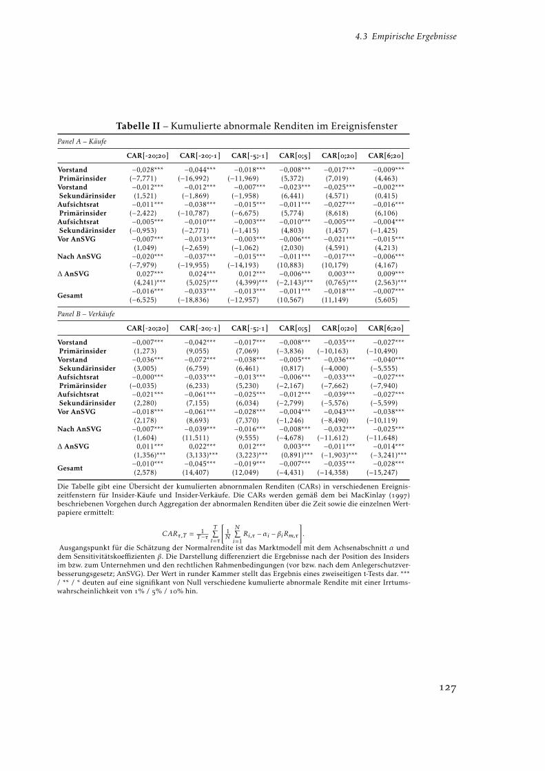
4.3 Empirische Ergebnisse
Tabelle II – Kumulierte abnormale Renditen im EreignisfensterPanel A – Käufe
CAR[-;] CAR[-;-] CAR[-;-] CAR[;] CAR[;] CAR[;]
Vorstand −0,028*** −0,044*** −0,018*** −0,008*** −0,017*** −0,009***Primärinsider (−7,771) (−16,992) (−11,969) (5,372) (7,019) (4,463)
Vorstand −0,012*** −0,012*** −0,007*** −0,023*** −0,025*** −0,002***Sekundärinsider (1,521) (−1,869) (−1,958) (6,441) (4,571) (0,415)
Aufsichtsrat −0,011*** −0,038*** −0,015*** −0,011*** −0,027*** −0,016***Primärinsider (−2,422) (−10,787) (−6,675) (5,774) (8,618) (6,106)
Aufsichtsrat −0,005*** −0,010*** −0,003*** −0,010*** −0,005*** −0,004***Sekundärinsider (−0,953) (−2,771) (−1,415) (4,803) (1,457) (−1,425)
Vor AnSVG −0,007*** −0,013*** −0,003*** −0,006*** −0,021*** −0,015***(1,049) (−2,659) (−1,062) (2,030) (4,591) (4,213)
Nach AnSVG −0,020*** −0,037*** −0,015*** −0,011*** −0,017*** −0,006***(−7,979) (−19,955) (−14,193) (10,883) (10,179) (4,167)
∆ AnSVG 0,027*** 0,024*** 0,012*** −0,006*** 0,003*** 0,009***(4,241)*** (5,025)*** (4,399)*** (−2,143)*** (0,765)*** (2,563)***
Gesamt −0,016*** −0,033*** −0,013*** −0,011*** −0,018*** −0,007***(−6,525) (−18,836) (−12,957) (10,567) (11,149) (5,605)
Panel B – Verkäufe
CAR[-;] CAR[-;-] CAR[-;-] CAR[;] CAR[;] CAR[;]
Vorstand −0,007*** −0,042*** −0,017*** −0,008*** −0,035*** −0,027***Primärinsider (1,273) (9,055) (7,069) (−3,836) (−10,163) (−10,490)
Vorstand −0,036*** −0,072*** −0,038*** −0,005*** −0,036*** −0,040***Sekundärinsider (3,005) (6,759) (6,461) (0,817) (−4,000) (−5,555)
Aufsichtsrat −0,000*** −0,033*** −0,013*** −0,006*** −0,033*** −0,027***Primärinsider (−0,035) (6,233) (5,230) (−2,167) (−7,662) (−7,940)
Aufsichtsrat −0,021*** −0,061*** −0,025*** −0,012*** −0,039*** −0,027***Sekundärinsider (2,280) (7,155) (6,034) (−2,799) (−5,576) (−5,599)
Vor AnSVG −0,018*** −0,061*** −0,028*** −0,004*** −0,043*** −0,038***(2,178) (8,693) (7,370) (−1,246) (−8,490) (−10,119)
Nach AnSVG −0,007*** −0,039*** −0,016*** −0,008*** −0,032*** −0,025***(1,604) (11,511) (9,555) (−4,678) (−11,612) (−11,648)
∆ AnSVG 0,011*** 0,022*** 0,012*** 0,003*** −0,011*** −0,014***(1,356)*** (3,133)*** (3,223)*** (0,891)*** (−1,903)*** (−3,241)***
Gesamt −0,010*** −0,045*** −0,019*** −0,007*** −0,035*** −0,028***(2,578) (14,407) (12,049) (−4,431) (−14,358) (−15,247)
Die Tabelle gibt eine Übersicht der kumulierten abnornmalen Renditen (CARs) in verschiedenen Ereignis-zeitfenstern für Insider-Käufe und Insider-Verkäufe. Die CARs werden gemäß dem bei MacKinlay ()beschriebenen Vorgehen durch Aggregation der abnormalen Renditen über die Zeit sowie die einzelnen Wert-papiere ermittelt:
CARτ,T = 1T−τ
T∑t=τ
[1N
N∑i=1
Ri,τ −αi − βiRm,τ].
Ausgangspunkt für die Schätzung der Normalrendite ist das Marktmodell mit dem Achsenabschnitt α unddem Sensitivitätskoeffizienten β. Die Darstellung differenziert die Ergebnisse nach der Position des Insidersim bzw. zum Unternehmen und den rechtlichen Rahmenbedingungen (vor bzw. nach dem Anlegerschutzver-besserungsgesetz; AnSVG). Der Wert in runder Kammer stellt das Ergebnis eines zweiseitigen t-Tests dar. ***/ ** / * deuten auf eine signifikant von Null verschiedene kumulierte abnormale Rendite mit einer Irrtums-wahrscheinlichkeit von % / % / % hin.

Kapitel 4 Haben Manager Timing-Fähigkeiten?
abnormalen Rendite in Höhe von ,%. Insgesamt deuten die abnormalen Renditen
vor und nach dem Ereignistag auf ausgeprägte Timing-Fähigkeiten der Insider hin.
Diese Timing-Fähigkeiten werden in Abbildung I dargestellt, in der die kumulierten
abnormalen Renditen über das gesamte Ereigniszeitfenster [-;] abgetragen sind.
Unternehmensinsider verhalten sich als Contrarian-Investoren. Sie kaufen „eigene“
Aktien nach Kursverlusten und verkaufen nach Kursanstiegen. Im Anschluss an
Käufe führen die signifikanten Kursanstiege zu signifikanten abnormalen Renditen
für die Insider. Gleichzeitig sind Insider in der Lage, signifikante Kursverluste nach
Verkäufen zu vermeiden. Zudem sind in beiden Fällen die kumulierten abnormalen
Renditen über das gesamte Ereigniszeitfenster [-;] statistisch signifikant von
Null verschieden.
In Abbildung II wird die gleiche Analyse durchgeführt, allerdings dient als Ereig-
nistag alternativ zum Handelstag der Veröffentlichungstag. Aus Sicht der Anleger
scheint diese Betrachtungsweise geeigneter, weil erst mit einer Verzögerung von
einigen Tagen gehandelt werden kann (siehe Tabelle I). Die Ergebnisse deuten darauf
hin, dass die abnormalen Renditen nach der Veröffentlichung von Insider-Käufen
(Insider-Verkäufen) weiter steigen (sinken). Allerdings dokumentieren Dickgiesser
und Kaserer (), dass Anleger zu diesem späteren Zeitpunkt nicht mehr von
den Timing-Fähigkeiten der Insider profitieren und die abnormalen Renditen nach
Berücksichtigung von Transaktionskosten verschwinden.
Vergleich mit früheren nationalen und internationalen Studien: Insgesamt sind diese
Ergebnisse mit denen in den früheren Studien von Stotz () sowie Betzer und
Theissen (a) für Deutschland vergleichbar. Es ist zudem keine Evidenz für
die Hypothese zu beobachten, dass die Werthaltigkeit von Insider-Transkationen
in Deutschland, das von Allen und Michaely () als Prototyp eines bankbasier-
ten Finanzsystems charakterisiert wird, signifikant höher ist als in marktbasierten
Finanzsystemen. Fidrmuc u. a. () weisen für einen englischen Datensatz ab-
normale Renditen in ähnlicher Höhe aus. Vergleicht man allerdings die absolute
Höhe der abnormalen Renditen zwischen Käufen und Verkäufen, sind diese anders
als bei Betzer und Theissen (a) in der hier verwendeten deutlich umfangrei-
cheren Stichprobe im Ereigniszeitfenster [;] statistisch signifikant voneinander
verschieden. Die Ereignisrendite von ,% für Käufe ist im Betrag signifikant höher
als die ,% für Verkäufe; ein Test auf Gleichheit der Mittelwerte liefert einen
t-Wert von ,, was auf Signifikanz am %-Niveau hindeutet. Mit zunehmen-
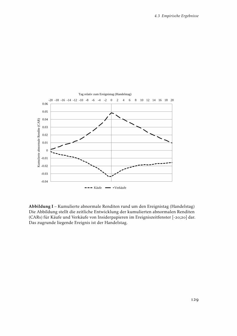
4.3 Empirische Ergebnisse
-0.04
-0.03
-0.02
-0.01
0
0.01
0.02
0.03
0.04
0.05
0.06-20 -18 -16 -14 -12 -10 -8 -6 -4 -2 0 2 4 6 8 10 12 14 16 18 20
Kum
ulie
rte a
bnor
mal
e R
endi
te (C
AR
)
Tag relativ zum Ereignistag (Handelstag)
Käufe Verkäufe
Abbildung I – Kumulierte abnormale Renditen rund um den Ereignistag (Handelstag)Die Abbildung stellt die zeitliche Entwicklung der kumulierten abnormalen Renditen(CARs) für Käufe und Verkäufe von Insiderpapieren im Ereigniszeitfenster [-;] dar.Das zugrunde liegende Ereignis ist der Handelstag.

Kapitel 4 Haben Manager Timing-Fähigkeiten?
-0.04
-0.03
-0.02
-0.01
0
0.01
0.02
0.03
0.04
0.05-20 -18 -16 -14 -12 -10 -8 -6 -4 -2 0 2 4 6 8 10 12 14 16 18 20
Kum
ulie
rte a
bnor
mal
e R
endi
te (C
AR
)
Tag relativ zum Ereignistag (Veröffentlichungstag)
Käufe Verkäufe
Abbildung II – Kumulierte abnormale Renditen rund um den Ereignistag (Veröffentli-chungstag)Die Abbildung stellt die zeitliche Entwicklung der kumulierten abnormalen Renditen(CARs) für Käufe und Verkäufe von Insiderpapieren im Ereigniszeitfenster [-;] dar.Das zugrunde liegende Ereignis ist der Tag der Veröffentlichung.

4.3 Empirische Ergebnisse
dem Zeithorizont steigen allerdings die abnormalen Renditen der Insider-Verkäufe
deutlich stärker an als die der Insider-Käufe. Im längeren Ereigniszeitfenster [;]beträgt die kumulative abnormale Rendite nach Insider-Käufen ,% und nach
Insider-Verkäufen -,%. Ein t-Test auf Gleichheit der Mittelwerte (im Betrag)
zeigt, dass die Nullhypothese mit einem t-Wert von , am %-Niveau verworfen
werden muss. Diese Ergebnisse deuten darauf hin, dass negative Unternehmens-
informationen höhere Auswirkungen auf den Kurswert haben als positive, die im
Markt jedoch erst mit erheblicher Verzögerung verarbeitet werden. Sie widerspre-
chen der Beobachtung von Fidrmuc u. a. (), die höhere abnormale Renditen
bei Insider-Käufen im Vergleich zu Insider-Verkäufen dokumentieren. Die geringere
Werthaltigkeit von Insider-Verkäufen wird darauf zurückgeführt, dass Verkäufe
häufig durch das Liquiditätsbedürfnis der Insider, also ohne weiteren Informati-
onsgehalt über die zukünftigen Cashflows des Unternehmens, ausgelöst werden.
Gleichzeitig stellt der Kauf eigener Aktien durch Insider ein glaubwürdiges Signal
dar, weil mit der Kaufentscheidung erhebliche Kosten einer suboptimalen Diversifi-
kation auf privater Ebene verbunden sind. Im Gegensatz dazu könnte die höhere
Werthaltigkeit von Insider-Verkäufen im Vergleich zu Insider-Käufen, wie sie in
Tabelle II zumindest für das längere Ereigniszeitfenster dokumentiert wird, durch
die Verlustaversion der Unternehmensinsider erklärt werden (Tversky und Kahne-
man ; Thaler u. a. ). Da Verluste mehr schmerzen als Gewinne erfreuen,
werden Insider ihren Informationsvorsprung nutzen, um Verluste auf die eigene
Aktie zu vermeiden. Die Untersuchung von Chan () stützt diese Hypothese.
Seine empirischen Ergebnisse für den US-Aktienmarkt deuten ebenfalls darauf hin,
dass negative Unternehmensnachrichten zu einer stärkeren Preisreaktion führen
als gute Nachrichten. Demnach unterreagieren Anleger insbesondere auf schlechte
Nachrichten, was auf Marktfriktionen zurückzuführen sein könnte. Als Beispiel
nennt Chan () Leerverkaufsrestriktionen, die eine schnelle Preisanpassung
nach dem Ereignis verhindern.
Information-Hierarchy-Hypothese: Gemäß der Information-Hierarchy-Hypothese
von Seyhun () und Lin und Howe () nimmt die Werthaltigkeit von Infor-
mationen mit steigender Hierarchieebene eines Insiders zu. In der Führungsstruktur
Hong u. a. () argumentieren ebenfalls, dass Anleger langsam auf negative Nachrichtenreagieren. Kleine Unternehmen mit einer geringen Anzahl von Analysten weisen das höchste Ren-ditemomentum auf, wobei dieser Effekt bei Unternehmen mit negativen Renditen über die letztenMonate am stärksten ausgeprägt ist.

Kapitel 4 Haben Manager Timing-Fähigkeiten?
deutscher Unternehmen ist dabei zwischen Mitgliedern des Vorstandes und Mitglie-
dern des Aufsichtsrates zu unterscheiden. Man würde erwarten, dass die abnormalen
Renditen nach Käufen und Verkäufen der Vorstandmitglieder, die das Unternehmen
operativ leiten, höher ausfallen als bei Aufsichtsratsmitgliedern, denen lediglich
eine Kontrollfunktion zukommt. Auf beiden Ebenen ist außerdem zwischen Pri-
märinsidern und Sekundärinsidern zu unterscheiden. Primärinsider umfassen die
Mitglieder des Vorstandes oder des Aufsichtsrates, während Sekundärinsider (also
Lebensgefährten oder Nachkommen von Vorstands- und Aufsichtsratsmitgliedern)
nicht im Unternehmen beschäftigt sind. Man würde vermuten, dass zwischen Primär-
und Sekundärinsider wiederum ein Informationsgefälle vorherrscht, das zu einer
Abnahme der abnormalen Renditen führt.
Die Ergebnisse in Tabelle II lassen, ähnlich wie bei Fidrmuc u. a. () sowie Bet-
zer und Theissen (a), keine Evidenz für die Information-Hierarchy-Hypothese
erkennen. Überraschend ist das Ergebnis, dass die Sekundärinsider des Vorstandes
im Ereigniszeitfenster [;] nach einem Kauf eine sehr hohe abnormale Rendite von
,% erzielen. Die abnormalen Renditen nach Käufen der übrigen Personenkreise
fallen im gleichen Zeitfenster deutlich geringer aus und liegen bei rund %. Die ab-
normalen Renditen steigen mit zunehmender Länge des betrachteten Zeitintervalls.
Lediglich für Sekundärinsider des Aufsichtsrates sind die abnormalen Renditen
im Ereignisfenster [;] nicht signifikant von Null verschieden. Basierend auf der
Renditeentwicklung in diesem Zeitintervall ergibt sich folgende Reihenfolge der
Werthaltigkeit der verfügbaren Information bei Wertpapierkäufen: () Primärinsider
des Aufsichtsrates, () Sekundärinsider des Vorstandes, () Primärinsider des Vor-
standes und () Sekundärinsider des Aufsichtsrates. Diese Reihenfolge widerspricht
der Information-Hierarchy-Hypothese.
Die Betrachtung der Insider-Verkäufe führt zu ebenso unerwarteten Ergebnis-
sen. Im Ereigniszeitfenster [;] sind die abnormalen Renditen sehr gering. Wie-
derum steigen die abnormalen Renditen mit zunehmender Länge des Intervalls
an. Im Ereigniszeitfenster [;] vermeiden alle Insidergruppen durch einen Ver-
kauf einen abnormalen Verlust von über %. Es ergibt sich folgende Reihenfolge
der Werthaltigkeit der Informationen bei Verkäufen: () Sekundärinsider des Auf-
sichtsrates, () Sekundärinsider des Vorstandes, () Primärinsider des Vorstandes
und () Primärinsider des Aufsichtsrates. Auch diese Reihenfolge widerspricht der
Information-Hierarchy-Hypothese.
Höhere abnormale Renditen nach Käufen von Aufsichtsratsmitgliedern könnten

4.3 Empirische Ergebnisse
gemäß Jeng u. a. () dadurch erklärt werden, dass Vorstandsmitglieder zwar
über bessere Informationen verfügen, gleichzeitig aber auch unter stärkerer Kon-
trolle durch Aktionäre und Regulatoren stehen. Deshalb sind Vorstandmitglieder
zurückhaltend, auf Basis ihres Informationsvorsprungs Aktien zu kaufen. Die Art
der Kommunikation zwischen Vorstand und Aufsichtsrat könnte eine schlechtere
Performance (d.h. eine geringere Verlustvermeidung) der Aufsichtsratsmitglieder
nach Verkäufen erklären. Vorstandsmitglieder haben keinen Anreiz, den Aufsichts-
ratsmitgliedern schlechte Informationen sofort weiterzuleiten, und damit sind sie
lange vor dem Aufsichtsrat über negative Informationen informiert. Eine stärker
ausgeprägte Preisentwicklung nach Transaktionen von Sekundärinsidern im Ver-
gleich zu Primärinsidern könnte auf das individuell wahrgenommene Risiko einer
Transaktion zurückzuführen sein. Wenn Primärinsider private Informationen nicht
auf eigene Rechnung nutzen, werden sie an Sekundärinsider nur gut abgesicherte
Informationen weitergeben, die sich dann in einer höheren abnormalen Rendite
niederschlagen. Außerdem könnten Primärinsider durch Übertragung werthaltiger
Informationen auf Sekundärinsider Insidergewinne strategisch verschleiern.
Auswirkungen des Anlegerschutzverbesserungsgesetz: Als Folge des Verbotes des Han-
dels aufgrund von Insiderinformation (§ WpHG) im Zusammenspiel mit der
Veröffentlichungspflicht (§a WpHG) ergibt sich, dass Insider nur solche Geschäfte
durchführen dürfen, die nicht auf Insiderinformation beruhen, also keinen Tatsa-
chenkern enthalten, sondern die aufgrund einer langfristigen Erfolgseinschätzung
getätigt werden. Man würde daher vermuten, dass durch die Einführung der -tägigen Veröffentlichungsfrist im Anlegerschutzverbesserungsgesetz (AnSVG) die
Wahrscheinlichkeit erhöht wurde, regelwidrigen Insiderhandel aufzudecken. Beim
Auftreten eines meldepflichtigen Ereignisses unmittelbar nach einer Transaktion
liegt der Verdacht auf einen Insiderhandel nahe, der auf einem Tatsachenkern beruht
(Dymke und Walter ). Im Vergleich zur Regelung vor der Gesetzesänderung
am . Oktober sollten demnach geringere abnormale Renditen zu beobach-
ten sein, weil der diskretionäre Spielraum der Insider verringert wurde und eine
Transaktion, die auf einer langfristigen Einschätzung statt auf einer eindeutigen
Information beruht, lediglich ein Signal darstellt und weniger profitabel sein dürfte.
Die grundsätzliche Forderung nach einer kürzeren Veröffentlichungsfrist ergibt sich
auch aus den Ergebnissen von Betzer und Theissen (b), wonach es zu einer
ineffizienten Kursbildung zwischen dem Handels- und dem Veröffentlichungstag

Kapitel 4 Haben Manager Timing-Fähigkeiten?
kommt.
Die empirischen Ergebnisse in Tabelle II geben Hinweise auf eine negative Wir-
kung des Anlegerschutzverbesserungsgesetzes (AnSVG) auf die Ereignisrenditen.
Vor der Gesetzesänderung (vor AnSVG) zeigen sich bei Insider-Käufen nur
geringe abnormale Renditen in den kürzeren Ereigniszeitfenstern, die allerdings
im längeren Zeitfenster [;] auf ,% ansteigen. Nach der Gesetzesänderung
(nach AnSVG) steigen die anormalen Renditen im Ereigniszeitfenster [;] auf ,%an. Dies ist darauf zurückzuführen, dass sich – wie das Gesetz auch vorsieht – die
Anzahl Handelstage zwischen Transaktion und Veröffentlichung von , Tage auf
, Tage verkürzt hat (siehe Tabelle I). Dadurch werden die Geschwindigkeit der
Informationsverarbeitung und die Werthaltigkeit der Informationen im kürzeren
Ereigniszeitfenster [;] erhöht. Bei Insider-Käufen ist allerdings im Anschluss nur
noch ein geringer Renditeeffekt zu beobachten. Im Ereigniszeitfester [;] steigen
die abnormalen Renditen nochmals um rund Basispunkte. Somit ist die abnor-
male Rendite während des Ereignisfensters [;] im Anschluss an Insider-Käufe
mit ,% nach der Einführung des AnSVG geringer als zuvor mit ,%; allerdings
ist die Differenz statistisch nicht signifikant.
Bei einer Betrachtung der Insider-Verkäufe scheint die Wirkung des Anlegerschutz-
verbesserungsgesetzes (AnSVG) stärker ausgeprägt zu sein. Erwartungsgemäß sind
wiederum die (negativen) abnormalen Renditen im kurzen Ereigniszeitfenster [;]nach der Gesetzesänderung stärker ausgeprägt als vorher. Wichtiger ist die Beob-
achtung, dass die abnormalen Renditen im Ereigniszeitfenster [;] vor und nach
der Gesetzesänderung unterschiedlich sind; die Differenz zwischen den -,% vor
und den -,% nach der Einführung des AnSVG ist mit einem t-Wert von ,am %-Niveau statistisch signifikant. Insgesamt scheinen damit die verschärften
Regularien des Insiderrechts zum Abbau der Informationssymmetrien zwischen
Insidern und Marktteilnehmern und zur Integrität des Marktes beizutragen. Durch
die Verkürzung der Veröffentlichungsfrist gelangen Informationen schneller in den
Markt und werden insbesondere bei Insider-Käufen aber auch bei Verkäufen schnel-
ler verarbeitet. Es scheint schwieriger geworden zu sein, regelwidrige Insider-Trades
auf Basis publikationspflichtiger Ereignisse durchzuführen. Man würde deshalb
vermuten, dass die Stichprobe nach der Gesetzesänderung einen höheren Anteil
an Transaktionen enthält, die lediglich ein Signal an den Markt über die langfristi-
gen Erwartungen der Insider senden. Diese Hypothese wird durch die geringeren
abormalen Renditen im längeren Ereigniszeitfenster [;] unterstützt.

4.3 Empirische Ergebnisse
4.3.2 Ergebnisse des Generalized-Calender-Time-Ansatzes
Um die empirischen Ergebnisse in Abschnitt 4.3.1 auf ihre Stabilität zu überprü-
fen, wird in diesem Abschnitt der Generalized-Calender-Time-Ansatz (GCT-Ansatz)
verwendet, der bei Hoechle u. a. () ausführlich beschrieben wird. Beim tradi-
tionellen Kalenderzeitverfahren werden die Renditen von Portfolios gemessen, die
zu jedem Zeitpunkt t aus Ereignisunternehmen bestehen, und danach im Rahmen
einer Multifaktorenregression hinsichtlich ihrer Faktorsensitivitäten („Exposures“)
untersucht. Die Vorgehensweise ist in zwei Schritte unterteilt (Kothari und Warner
). Zunächst wird zu jedem Zeitpunkt t ein Portfolio jener Unternehmen gebil-
det, für die in der vorherigen Zeitperiode t-k das zu analysierende Ereignis vorliegt.
Die Länge der Verzögerung k kann frei gewählt werden. Anschließend wird die
Zeitreihe der Überschussrenditen des Kalenderzeitportfolios auf systematische Risi-
kofaktoren regressiert, um die risikoadjustierte Rendite zu bestimmen. Häufig wird
das -Faktorenmodell von Fama und French () verwendet:
Rpt −Rf t = ap + bp(Rmt −Rf t) + spSMBt + hpHMLt + ept, (3)
wobei Rpt die Rendite des gleich- oder wertgewichteten Portfolios der Ereignisun-
ternehmen zum Zeitpunkt t bezeichnet. Rf t und Rmt sind der risikofreie Zinssatz
bzw. die Rendite des Marktportfolios zum Zeitpunkt t. Das Faktorportfolio SMB
stellt die Renditedifferenz zwischen einem Portfolio mit kleinen Unternehmen und
einem Portfolio mit großen Unternehmen dar, wobei die Größe basierend auf der
Marktkapitalisierung gemessen wird. HML misst die Renditedifferenz zwischen
einem Portfolio mit Unternehmen, die ein hohes Buch-Markt-Verhältnis aufwei-
sen, und einem Portfolio mit Unternehmen, die durch ein geringes Buch-Markt-
Verhältnis gekennzeichnet sind. Beide Faktorportfolios stellen selbstfinanzierende
Strategien dar und können nach Fama und French () als Stellvertreter für
die nicht beobachtbaren systematischen Risikofaktoren interpretiert werden. Der
Achsenabschnitt der Regression, ap, misst die durchschnittliche abnormale Rendite
(Jensen’s Alpha) des Ereignisportfolios. bp, sp und hp stellen Sensitivitätskoeffizien-
Da das Ereignisportfolio in jeder Periode neu gebildet wird, schwankt die Anzahl der Unter-nehmen je nach Häufigkeit des Ereignisses, dem Beobachtungszeitpunkt und der Verzögerung k.Das Portfolio kann gleich- oder wertgewichtet sein, wobei die Rendite gleichgewichteter Portfoliosaufgrund der Übergewichtung kleiner Unternehmen höher ist als die wertgewichteter Portfolios(Fama ). Alternativ kann auch das -Faktorenmodell von Carhart () verwendet werden.

Kapitel 4 Haben Manager Timing-Fähigkeiten?
ten (Exposures) dar, und ept ist weißes Rauschen.
Ein wesentlicher Nachteil des traditionellen Kalenderzeitverfahrens ist, dass un-
ternehmensspezifische Erklärungsvariablen nicht in die Regressionsgleichung (3)
integriert werden können. Um diesen Schwachpunkt in der Modellspezifikation
zu beheben, stellen Hoechle u. a. () ein erweitertes Kalenderzeitverfahren, den
Generalized-Calendar-Time-Ansatz (GCT-Ansatz), vor. Anders als das klassische Ka-
lenderzeitverfahren erlaubt es diese alternative Methode, neben den systematischen
Renditetreibern auch unternehmensspezifische Erklärungsvariablen in das Modell
aufzunehmen. Damit ist der GCT-Ansatz ebenso flexibel in der Modellspezifikation
wie eine klassische Querschnittregression. Die Korrektur um systematische Rendite-
treiber und firmenspezifische Erklärungsvariablens erfolgt dabei aber nicht in zwei
getrennten Schritten sondern simultan in einem Panelmodell. Ausgangspunkt ist
zunächst folgendes Panelmodell:
yit = (zit ⊗ xt)d + vit, (4)
wobei yit die Überschussrendite des Unternehmens i in Periode t bezeichnet. d ist
ein Vektor mit Schätzkoeffizienten, vit ist der Fehlerterm der Regression, und die
erklärenden Variablen ergeben sich als Kronecker-Produkt (⊗) der Vektoren zit und
xt. Dabei enthält xt die Risikofaktoren, die in der zeitlichen Dimension variabel
aber im Querschnitt der Unternehmen konstant sind. Wie beim traditionellen
Kalenderzeitverfahren wird der Vektor xt auf der Grundlage des -Faktorenmodells
nach Fama und French () spezifiziert:
xt = [1 RMRFt SMBt HMLt] . (5)
Der Vektor zit enthält unternehmensspezifische Erklärungsvariablen zm,it (m =
1, . . . ,M). In der hier verwendeten Modellspezifikation werden auch mitteilungsspe-
zifische Variablen berücksichtigt. Im Gegensatz zu den Risikofaktoren variieren die
unternehmensspezifischen Variablen sowohl über die Zeit als auch den Querschnitt
der Unternehmen. Der Vektor zit hat somit folgende Struktur:
zit =[1 z1,it . . . zM,it
]. (6)
Um den Informationsgehalt der gesamten Panelstichprobe zu nutzen und die
Ereignisunternehmen von den restlichen Unternehmen („Matching-Firms“) der

4.3 Empirische Ergebnisse
Stichprobe zu trennen, wird das Modell noch zusätzlich um den Vektor pit erweitert.
Der Vektor pit enthält eine Konstante sowie eine mitteilungsspezifische Dummy-
Variable:
pit = [1 Dit] , (7)
wobei die Dummy-Variable Dit den Handelstag t für ein Ereignisunternehmen i
kennzeichnet; sie wird im weiter unten dargestellten im Grundmodell mit Event
bezeichnet. Die Dummy-Variable nimmt für Ereignisunternehmen am Tag einer
Insider-Transaktion den Wert 1 und an allen anderen Tagen den Wert 0 an. Für
alle Matching-Unternehmen aus dem CDAX nimmt die Dummy-Variable über die
gesamte Stichprobenperiode den Wert 0 an. Das erweiterte Panelmodell ist dann
wie folgt spezifiziert:
yit = ((pit ⊗ zit)⊗ xt)d + vit. (8)
Der Vektor xt umfasst die Risikofaktoren des Fama und French () -Faktoren-
modells. Hierfür wird der Marktfaktor RMRF als Differenz zwischen der Rendite
des CDAX Total Return Index und der -Monats Frankfurt-Interbank-Offered-Rate
(FIBOR) ermittelt. Die beiden Faktorportfolios SMB und HML werden durch die
Differenzrenditen der MSCI Style-Indizes für Deutschland approximiert.
Der Vektor zit im Regressionsmodell (8) enthält unternehmens- und mitteilungs-
spezifische (Kontroll-) Variablen, die sowohl über die Zeit als auch über den Un-
ternehmensquerschnitt variieren. Die beiden wichtigsten mitteilungsspezifischen
Variablen werden als Dummy-Variablen kodiert, um die Perioden vor einem Ereignis
(Runup) und nach einem Ereignis (Drift) zu identifizieren. Diese Variablen nehmen
für die Ereignisunternehmen im GCT-Grundmodell während der Handelstage
vor bzw. Handelstage nach dem Ereignis den Wert 1 und an allen anderen Tagen
den Wert 0 an. In einer alternativen Modellspezifikation kennzeichnen mitteilungs-
spezifische Dummy-Variablen Käufe und Verkäufe von Vorstands-Primärinsidern
(VsPrim), Vorstands-Sekundärinsidern (VsSek), Aufsichtsrats-Primärinsidern (Asr-
Prim) und Aufsichtsrats-Sekundärinsidern (AsrSek). In einer weiteren Modellvarian-
te wird mit dem relativen Transaktionsvolumen des Insider-Geschäfts (TradeValue)
eine zusätzliche mitteilungsspezifische Erklärungsvariable in das Modell aufgenom-
men. Diese Variable wird als Quotient des Transaktionswertes und dem Marktwert
der ausstehenden Aktien berechnet. Als unternehmensspezifische Kontrollvariablen
werden in allen Modellvarianten der Bid-Ask-Spread (Bid/Ask), die Marktkapita-
lisierung (MV), eine Maßzahl für die Liquidität der gehandelten Aktie (TV), der

Kapitel 4 Haben Manager Timing-Fähigkeiten?
Verschuldungsgrad (LEV), das Markt-Buch-Verhältnis (MB), die Ausschüttungsquo-
te (POR), der Freefloat der Aktie (Freefloat), der Gewinn pro Aktie (EPS) sowie die
Dividendenrendite (DY) verwendet. Tabelle III gibt eine Übersicht aller Variablen,
die in der Panelregression verwendet werden.
Das im Folgenden zu schätzende Grundmodell des GCT-Verfahrens enthält die
mitteilungsspezifischen Dummy-Variablen Event, Runup und Drift sowie aller un-
ternehmensspezifischen Kontrollvariablen. Die Spezifikation dieser Panelregression
ist daher:
yit =α + β1RMRFt + β2SMBt + β3HMLt + β4Eventit + β5Runupit
+ β6Drif tit + β7RMRFt ×Eventit + β8SMBt ×Eventit+ β9HMLt ×Eventit + β10Bid/Askit + β11MVit + β12T Vit + β13LEVit
+ β14MBit + β15PORit + β16Freef loatit + β17EP Sit + β18DYit + vit.
(9)
Dabei beschreibt der Achsenabschnitt α die risikoajdustierte Rendite für den
Fall, dass keine Insider-Transaktion stattfindet. Die Koeffizienten β1 bis β3 messen
den Einfluss der systematischen Risikofaktoren. Im Mittelpunkt stehen die Ko-
effizienten β4 bis β9, mit denen der Informationsgehalt und die Performance von
Insider-Transaktionen gemessen werden können. Der Koeffizient β4 auf die Event-
Dummy misst den Unterschied in der risikoadjustierten Rendite am Handelstag im
Vergleich zu allen CDAX Matching-Unternehmen ohne Insider-Transaktionen. Die
Risikoadjustierung erfolgt durch die geschätzten Koeffizienten β7 bis β9 auf die Inter-
aktionsterme zwischen der Marktrisikoprämie und den beiden Faktorportfolios mit
der Event-Dummy-Variable. Die Koeffizienten β5 und β6 messen den Unterschied in
der risikoadjustierten Rendite während der Runup-Periode bzw. der Drift-Periode
im Vergleich zu allen CDAX Matching-Unternehmen ohne Insider-Transaktionen.
Anders als die Event-Study-Methodik ist der CGT-Ansatz in der Lage, Schätz-
koeffizienten zu generieren, die robust gegenüber möglichen Abhängigkeiten der
untersuchten Einheiten (Insider) im Querschnitt (Cross-Sectional-Dependency) sind.
Dieses Problem könnte in unserem Datensatz auftreten, der nur wenige Beobach-
tungen über die Zeit aber viele Beobachtungen über die Einheiten (Insider) enthält
(Fama ; Lyon u. a. ; Mitchell und Stafford ). Ein weiterer methodischer
Die geschätzten Koeffizienten α, β1, β2 und β3 werden in den Ergebnistabellen nicht ausgewiesen.α ist in jeder Regression negativ und beträgt bei Käufen -,% und bei Verkäufen -,%. β1(,) sowie β2 (,) sind in allen Regressionen positiv, während β3 (-,) durchgängig negativist. Alle genannten Koeffizienten sind mindestens auf dem % Niveau statistisch signifikant. DerErklärungsgehalt (R2) beträgt modellunabhängig rund %.

4.3 Empirische Ergebnisse
Tabelle III – Variablen im GCT-AnsatzVariable Kennzeichnung Berechnungsmethode Quelle
Überschussrendite — Rendite des Wertpapiers abzüglich desrisikofreien Zinses (FIBOR, Monate)
DataStream
Ereignis Event Zeitpunkt des Events BAFinPeriode vor demEreignis
Runup binär; im Zeitraum von Tagen vorEvent, sonst
./.
Periode nach demEreignis
Drift binär; im Zeitraum von Tagen nachEvent, sonst
./.
Vorstand -Primärinsider
VsPrim binär; bei Transaktion durchVorstandsmitglied, sonst
BAFin
Vorstand -Sekundärinsider
VsSek binär; bei Transaktion durch Vorstandnahestehende Person, sonst
BAFin
Aufsichtsrat -Primärinsider
AsrPrim binär; bei Transaktion durchAufsichtsratsmitglied, sonst
BAFin
Aufsichtsrat -Sekundärinsider
AsrSek binär; bei Transaktion durch Aufsichtsratnahestehende Person, sonst
BAFin
Vor Anleger-verbesserungsschutzgesetz
Vor AnSVG binär; bei Transaktion vor .., sonst
./.
Nach Anleger-verbesserungsschutzgesetz
Nach AnSVG binär; bei Transaktion nach .., sonst
./.
Transaktionsvolumen TradeValue (Anzahl gehandelte Aktien * Kurs) /Marktkapitalisierung
BAFin /DataStream
Bid-Ask-Spread Bid/Ask (Ask + Bid) / (, * (Ask - Bid)) DataStreamMarktkapitalisierung MV log(Marktkapitalisierung) DataStreamLiquidität TV (Anzahl gehandelter Aktien * Kurs) /
MarktkapitalisierungDataStream
Verschuldungsgrad LEV Nettoverschuldung / Marktkapitalisierung DataStreamAusschüttungsquote POR Ausschüttungsquote in % DataStreamMarkt-Buch-Verhältnis MB Markt-Buch-Verhältnis in % DataStreamFreefloat Freefloat Streubesitz in % DataStreamGewinn pro Aktie EPS Gewinn pro Aktie in EUR DataStreamDividendenrendite DY Dividendenrendite in % DataStreamRMRF RMRF Fama-French-Faktor (Marktfaktor) DataStreamSMB SMB Fama-French-Faktor (Größenfaktor) DataStreamHML HML Fama-French-Faktor(Wachstums-
/Substanzfaktor)DataStream
Die Tabelle fasst die in der Panelregression im Rahmen des GCT-Ansatzes verwendeten Variablen, deren Kennzeich-nung im Text und die Berechnungsmethode zusammen.

Kapitel 4 Haben Manager Timing-Fähigkeiten?
Vorteil des CGT-Ansatzes ist, dass es nicht notwendig ist, zu jedem Zeitpunkt ein
Portfolio aus Ereignisunternehmen zu bilden. Loughran und Ritter () kritisie-
ren den Kalenderzeitansatz, weil jeder Zeitpunkt und nicht jede Beobachtung eine
Gleichgewichtung erfährt, was zu Verzerrungen in den geschätzten abnormalen
Renditen führen kann. Da der CGT-Ansatz ein Panelverfahren darstellt, kommt es
durch die Kleinst-Quadrat-Schätzung automatisch zu einer Gleichgewichtung aller
Beobachtungen. Das Panelmodell in Gleichung (9) wird mittels gepoolter Regression
geschätzt, wobei die Standardfehler basierend auf der Methode von Driscoll und
Kraay () ermittelt werden. Hoechle u. a. () dokumentieren, dass sich damit
heteroskedastie-konsistente Standardfehler ergeben, die stabil gegenüber allgemei-
nen Formen der Abhängigkeit in den Residuen sowohl über den Querschnitt als
auch über die Zeit sind.
Die Verwendung eines Paneldatensatzes erfordert eine weitere Bereinigung der
zu analysierenden Mitteilungen. Erstens sind von den verbleibenden 11135 Mit-
teilungen (siehe Abschnitt ..) diejenigen zu entfernen, für deren Emittenten
die ausgewählten Kontrollvariablen nicht vorliegen. Dadurch fallen 1031 Mittei-
lungen aus der Stichprobe. Zweitens können taggleiche Ereignisse aufgrund der
unterschiedlichen mitteilungsspezifischen Variablen nicht zusammengefügt werden,
weshalb diese eliminiert werden müssen. Hierdurch werden 798 weitere Mittei-
lungen von der Analyse ausgeschlossen. Damit verbleiben 9306 Mitteilungen für
die Analyse auf Basis des GCT-Verfahrens. Wie bei der klassischen Ereignisstudie
erfolgt eine getrennte Betrachtung der Insider-Käufe und der Insider-Verkäufe. Die
Ergebnisse sind in den Tabellen IV (Käufe) und V (Verkäufe) dargestellt.
Die Ergebnisse des Grundmodells in Gleichung (9) für Insider-Käufe werden
im Modell in der Tabelle IV ausgewiesen. Am Tag eines Insider-Kaufes reagiert
der Markt positiv. Der Koeffizient auf die Event-Dummy-Variable macht deutlich,
dass die risikoadjustierte Rendite um ,%-Punkte höher ausfällt als an Tagen
ohne Insider-Transaktionen. Zudem lassen die positiven Sensitivitäten der Inter-
aktionsterme jeweils zwischen den beiden Faktorportfolios RMRF und HML mit
der Event-Dummy-Variable vermuten, dass Insider tendenziell in steigenden Märk-
ten kaufen und dabei Aktien von Substanzunternehmen (d.h. mit hohen Buch-
Markt-Verhältnissen) erwerben. Die Unternehmensgröße scheint keinen Einfluss
auf Insider-Käufe zu haben, was aus dem nicht signifikanten Koeffizienten auf das
Hoechle u. a. () beschreiben den genauen Zusammenhang zwischen dem traditionellenKalenderzeitverfahren, dem GCT-Ansatz und dem Querschnittregressionsansatz.
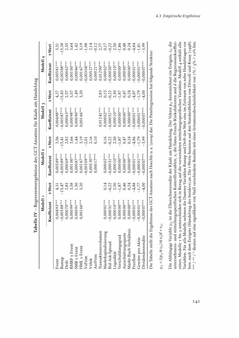
4.3 Empirische Ergebnisse
Tab
elle
IV–
Reg
ress
ions
erge
bnis
sed
esG
CT-
Ans
atze
sfü
rK
äufe
amH
and
elst
ag
Mod
ell
Mod
ell
Mod
ell
Mod
ell
Koe
ffizi
ent
t-W
ert
Koe
ffizi
ent
t-W
ert
Koe
ffizi
ent
t-W
ert
Koe
ffizi
ent
t-W
ert
Eve
nt0,
004
93**
*4,
310,
005
89**
*3,
560,
004
88**
*4,
270,
005
81**
*3,
51R
unu
p−0,0
0388
***−1
5,47
−0,0
0389
***−1
5,41
−0,0
0387
***−1
5,43
−0,0
0388
***−1
5,38
Dri
ft0,
000
70**
*2,
850,
000
69**
*2,
820,
000
63**
*2,
570,
000
62**
*2,
55R
MR
Fx
Eve
nt0,
000
99**
*3,
580,
001
00**
*3,
660,
000
98**
*3,
570,
001
00**
*3,
64SM
Bx
Eve
nt0,
000
91**
*1,
500,
000
87**
*1,
440,
000
90**
*1,
490,
000
86**
*1,
42H
ML
xE
vent
0,00
166
***
3,20
0,00
167
***
3,19
0,00
166
***
3,20
0,00
167
***
3,19
VsP
rim
−0,0
0309
***
−2,0
1−0,0
0304
***
−1,9
8V
sSek
0,00
530
***
2,16
0,00
527
***
2,14
Asr
Pri
m0,
000
17**
*0,
100,
000
21**
*−0,1
2Tr
ansa
ktio
nsvo
lum
en0,
012
41**
*2,
830,
012
00**
*2,
77M
arkt
kap
ital
isie
rung
0,00
001
***
0,14
0,00
002
***
0,16
0,00
002
***
0,15
0,00
002
***
0,17
Bid
-Ask
-Sp
read
−0,0
0051
***
−0,2
2−0,0
0051
***
−0,2
2−0,0
0051
***
−0,2
2−0,0
0050
***
−0,2
2L
iqu
idit
ät0,
000
10**
*2,
500,
000
10**
*2,
500,
000
10**
*2,
500,
000
10**
*2,
50V
ersc
huld
ung
sgra
d0,
000
00**
*−1,8
70,
000
00**
*−1,8
70,
000
00**
*−1,8
70,
000
00**
*−1,8
6A
uss
chü
ttu
ngsq
uot
e0,
000
00**
*0,
460,
000
00**
*0,
470,
000
00**
*0,
470,
000
00**
*0,
48M
arkt
-Bu
ch-V
erhä
ltni
s0,
000
00**
*0,
240,
000
00**
*0,
240,
000
00**
*0,
240,
000
00**
*0,
24Fr
eefl
oat
−0,0
0001
***
−4,8
8−0,0
0001
***
−4,8
6−0,0
0001
***
−4,8
7−0,0
0001
***
−4,8
4G
ewin
np
roA
ktie
−0,0
0001
***
−1,7
7−0,0
0001
***
−1,7
9−0,0
0001
***
−1,7
9−0,0
0001
***
−1,8
1D
ivid
end
enre
ndit
e−0,0
0007
***
−4,0
0−0,0
0007
***
−3,9
9−0,0
0007
***
−4,0
0−0,0
0007
***
−3,9
9
Die
Tabe
lle
stel
ltd
ieE
rgeb
niss
ed
esG
CT-
Ans
atze
sna
chH
oech
leu
.a.(
)dar
.Die
Pane
lreg
ress
ion
hat
folg
end
eSt
rukt
ur:
y it
=((p it⊗z it)⊗x t
)d+v it.
Die
Abh
ängi
geV
aria
bley it
ist
die
Übe
rsch
uss
ren
dit
ed
erK
äufe
amH
and
elst
ag.D
erV
ekto
rp it
ken
nze
ichn
etei
nE
reig
nis
,zit
die
unt
erne
hmen
s-u
ndm
itte
ilu
ngss
pez
ifisc
hen
Kon
trol
lvar
iabl
en,xt
die
Fam
a-Fr
ench
-Ris
ikof
akto
ren
und
dd
ieR
egre
ssio
nsko
effizi
-en
ten
.Mod
elle
bis
unt
ersc
heid
ensi
chin
Bez
ug
auf
die
verw
end
eten
mit
teil
un
gssp
ezifi
sche
nV
aria
blen
.Mod
ell
enth
ält
alle
Var
iabl
en.F
üral
leM
odel
lene
hmen
die
Dum
my-
Var
iabl
enR
unup
und
Dri
ftde
nW
erte
ins
imZ
eitr
aum
von
zehn
Han
dels
tage
nvo
rbz
w.n
ach
dem
Ere
igni
s(H
ande
lsta
gde
sIn
side
rs)a
n.D
iet-
Wer
teba
sier
enau
fde
nSt
anda
rdfe
hler
nvo
nD
risc
ollu
ndK
raay
()
.**
*/
**/
*de
uten
auf
eine
sign
ifika
ntvo
nN
ullv
ersc
hied
ene
Ren
dite
mit
eine
rIr
rtum
swah
rsch
einl
ichk
eit
von%
/%
/
%hi
n.

Kapitel 4 Haben Manager Timing-Fähigkeiten?
Tab
elle
V–
Reg
ress
ions
erge
bnis
sed
esG
CT-
Ans
atze
sfü
rV
erkä
ufe
amH
and
elst
ag
Mod
ell
Mod
ell
Mod
ell
Mod
ell
Koe
ffizi
ent
t-W
ert
Koe
ffizi
ent
t-W
ert
Koe
ffizi
ent
t-W
ert
Koe
ffizi
ent
t-W
ert
Eve
nt−0,0
0972
***
−4,7
1−0,0
1006
***
−3,1
7−0,0
0970
***
−4,7
0−0,0
1001
***
−3,1
5R
unu
p0,
002
96**
*10,8
80,
002
95**
*10,8
70,
002
96**
*10,8
90,
002
95**
*10,8
8D
rift
−0,0
0107
***
−4,2
3−0,0
0107
***
−4,2
2−0,0
0109
***
−4,2
8−0,0
0108
***
−4,2
6R
MR
Fx
Eve
nt−0,0
0248
***
−3,9
4−0,0
0253
***
−4,0
1−0,0
0247
***
−3,9
3−0,0
0253
***
−4,0
0SM
Bx
Eve
nt−0,0
0036
***
−0,3
0−0,0
0038
***
−0,3
2−0,0
0035
***
−0,2
9−0,0
0037
***
−0,3
1H
ML
xE
vent
0,00
222
***
1,83
0,00
233
***
1,92
0,00
222
***
1,83
0,00
233
***
1,91
VsP
rim
−0,0
0128
***
−0,4
8−0,0
0123
***
−0,4
7V
sSek
0,00
677
***
1,52
0,00
682
***
1,53
Asr
Pri
m−0,0
0083
***
−0,2
9−0,0
0079
***
−0,2
8Tr
ansa
ktio
nsvo
lum
en0,
000
28**
*0,
610,
000
28**
*0,
61M
arkt
kap
ital
isie
rung
0,00
006
***
0,56
0,00
006
***
0,57
0,00
006
***
0,57
0,00
006
***
0,58
Bid
-Ask
-Sp
read
−0,0
0029
***
−0,1
0−0,0
0028
***
−0,1
0−0,0
0028
***
−0,1
0−0,0
0028
***
−0,1
0L
iqu
idit
ät0,
000
07**
*2,
410,
000
07**
*2,
410,
000
07**
*2,
410,
000
07**
*2,
41V
ersc
huld
ung
sgra
d0,
000
00**
*−3,5
80,
000
00**
*−3,5
80,
000
00**
*−3,6
30,
000
00**
*−3,6
3A
uss
chü
ttu
ngsq
uot
e0,
000
00**
*1,
230,
000
00**
*1,
230,
000
00**
*1,
230,
000
00**
*1,
22M
arkt
-Bu
ch-V
erhä
ltni
s0,
000
00**
*0,
380,
000
00**
*0,
380,
000
00**
*0,
380,
000
00**
*0,
37Fr
eefl
oat
−0,0
0001
***
−3,9
9−0,0
0001
***
−3,9
9−0,0
0001
***
−3,9
9−0,0
0001
***
−3,9
8G
ewin
np
roA
ktie
−0,0
0010
***
−7,0
2−0,0
0010
***
−7,0
1−0,0
0010
***
−7,0
2−0,0
0010
***
−7,0
2D
ivid
end
enre
ndit
e−0,0
0012
***
−4,5
5−0,0
0012
***
−4,5
5−0,0
0012
***
−4,5
5−0,0
0012
***
−4,5
5
Die
Tabe
lle
stel
ltd
ieE
rgeb
niss
ed
esG
CT-
Ans
atze
sna
chH
oech
leu
.a.(
)dar
.Die
Pane
lreg
ress
ion
hat
folg
end
eSt
rukt
ur:
y it
=((p it⊗z it)⊗x t
)d+v it.
Die
Abh
ängi
geV
aria
bley it
istd
ieÜ
bers
chus
sren
dite
der
Ver
käuf
eam
Han
dels
tag.
Der
Vek
torp it
kenn
zeic
hnet
ein
Ere
igni
s,z it
die
unte
rneh
men
s-un
dm
itte
ilun
gssp
ezifi
sche
nK
ontr
ollv
aria
blen
,xt
die
Fam
a-Fr
ench
-Ris
ikof
akto
ren
undd
die
Reg
ress
ions
koeffi
zi-
ente
n.M
odel
le
bis
unt
ersc
heid
ensi
chin
Bez
ug
auf
die
verw
ende
ten
mit
teil
ung
ssp
ezifi
sche
nV
aria
blen
.Mod
ell
enth
ält
alle
Var
iabl
en.F
üral
leM
odel
lene
hmen
die
Dum
my-
Var
iabl
enR
unup
und
Dri
ftde
nW
erte
ins
imZ
eitr
aum
von
zehn
Han
dels
tage
nvo
rbz
w.n
ach
dem
Ere
igni
s(H
ande
lsta
gde
sIn
side
rs)a
n.D
iet-
Wer
teba
sier
enau
fden
Stan
dard
fehl
ern
von
Dri
scol
lund
Kra
ay()
.**
*/
**/
*de
uten
auf
eine
sign
ifika
ntvo
nN
ullv
ersc
hied
ene
Ren
dite
mit
eine
rIr
rtum
swah
rsch
einl
ichk
eitv
on%
/%
/
%hi
n.

4.3 Empirische Ergebnisse
Faktorportfolio SMB geschlossen werden kann. Die Koeffizienten auf die Dummy-
Variablen Runup und Drif t deuten wie bei der Ereignisstudie wiederum darauf hin,
dass Insider den Kauf eigener Aktien strategisch steuern. Insider kaufen Wertpa-
piere nach einer Periode mit negativer Kursentwicklung. Die abnormale Rendite
während der Tage vor einem Kauf beträgt -,%. Im Anschluss profitieren
Insider allerdings von einer positiven Wertentwicklung der eigenen Aktie; die abnor-
male Rendite während der Tage nach einem Kauf beträgt ,%. Auch wenn die
Höhe der Timing-Effekte in der multivariaten Analyse damit geringer ausfällt als in
der Ereignisstudie, deuten diese Ergebnisse darauf hin, dass Insider über private
kursrelevante Informationen verfügen, die für Outsider aufgrund asymmetrischer
Informationsverteilung nicht zugänglich sind. Der Einfluss der unternehmens-
spezifischen Kontrollvariablen ist relativ gering. Lediglich die Kontrollvariablen
T V , LEV , Freef loat, EP S und DY haben einen signifikanten Einfluss auf die Über-
schussrendite. Die Überschussrendite sinkt mit zunehmendem Verschuldungsgrad,
höherem Streubesitz, einem höheren Gewinn pro Aktie und einer höheren Dividen-
denrendite. Sie steigt hingegen mit zunehmender Liquidität der Aktie.
Bei Verkäufen ist die abnormale Rendite am Handelstag im Grundmodell des GCT-
Ansatzes betragsmäßig höher als bei Käufen. Der Koeffizient auf die Event-Dummy-
Variable im Modell in der Tabelle V weist einen Wert von -,%-Punkten auf.
Wie bei Insider-Käufen lassen sich auch bei Insider-Verkäufen Timing-Fähigkeiten
messen. Insider verkaufen nach einer Periode positiver Kursentwicklung, und die
abnormale Rendite Tage vor einem Insider-Verkauf beträgt ,%. Die abnormale
Rendite in den Tagen nach einem Insider-Verkauf beträgt hingegen -,%, d.h.
Unternehmensinsider vermeiden eine negative Wertentwicklung relativ zu den
CDAX Matching-Unternehmen.
Zur Analyse der Werthaltigkeit der Informationen in Abhängigkeit von der Po-
sition des Insiders wird das Grundmodell durch die mitteilungsspezifischen Er-
klärungsvariablen VsPrim, VsSek und AsrPrim im Vektor zit ergänzt. Die Variable
AsrSek dient als Referenzkategorie und wird nicht in die Regression aufgenom-
men. Die Ergebnisse werden jeweils im Modell in den Tabellen IV und V dar-
gestellt. Bei den Insider-Käufen ergeben sich signifikante Koeffizienten lediglich
für Primär- und Sekundärinsider des Vorstandes. Demnach erzielen Primärinsider
des Vorstandes eine um ,%-Punkte geringere abnormale Rendite im Vergleich
Abweichungen in den Ergebnissen der beiden Methoden sind darauf zurückzuführen, dassbeim GCT-Ansatz neben der Aufnahme der firmenspezifischen Variablen auch eine umfassendereRisikokorrektur durch den Einbezug der SMB- und HML-Faktoren erfolgt.

Kapitel 4 Haben Manager Timing-Fähigkeiten?
zu Sekundärinsidern des Aufsichtsrates. Hingegen erzielen Sekundärinsider des
Vorstandes eine um ,%-Punkte höhere abnormale Rendite als Sekundärinsider
des Aufsichtsrates. Daraus ergibt sich folgende Reihenfolge für die Werthaltigkeit
der Informationen bei Käufen: () Sekundärinsider des Vorstandes, () Primär- und
Sekundärinsider des Aufsichtsrates, () Primärinsider des Vorstandes. Damit kann
auch im GCT-Ansatz – ebenso wie in der Ereignisstudie – keine Bestätigung für
die Information-Hierarchy-Hypothese bei Insider-Käufen festgestellt werden. Für
Insider-Verkäufe ist überhaupt keine Beziehung zwischen Werthaltigkeit der In-
formation und der Position des Unternehmensinsiders auszumachen. Keiner der
drei Schätzkoeffizienten der Dummy-Variablen, die auf die Position des Insiders im
Unternehmen abstellen, ist statistisch signifikant.
Im Modell in den beiden Tabellen IV und V wird der Transaktionswert des
Insider-Geschäfts (T radeV alue) als eine weitere mitteilungsspezifische Erklärungs-
variable in das Modell aufgenommen. Man würde erwarten, dass größere Trans-
aktionen aufgrund der asymmetrischen Informationsverteilung zwischen Insidern
und Outsidern ein stärkeres Signal an den Markt senden und daher zu höheren
abnormalen Renditen führen (Jeng u. a. ). Anders als bei Betzer und Theissen
(a) wird diese Vermutung durch den signifikant positiven Koeffizienten auf
T radeV alue bei Insider-Käufen bestätigt. Für Insider-Verkäufe scheint die Größe
der Transaktion hingegen keinen Einfluss auf die abnormalen Renditen zu haben.
Dies könnte nach Jeng u. a. () damit begründet werden, dass die Beziehung
zwischen der Transaktionsgröße und der abnormalen Rendite verschwindet, wenn
die betragsmäßig größten Insider-Verkäufe aus Überlegungen hinsichtlich der op-
timalen Diversifikation oder aufgrund von Liquiditätsbedürfnissen der Manager
durchgeführt werden.
Um den Einfluss des Anlegerschutzverbesserungsgesetzes zu untersuchen, könnte
man eine weitere mitteilungsspezifische Dummy-Variable in das GCT-Regressions-
modell aufnehmen, die Insider-Transaktionen vor bzw. nach der Umsetzung des
Anlegerschutzverbesserungsgesetzes identifiziert. Entsprechend würde diese Va-
riable den Wert für Ereignisse vor und nach dem . Oktober annehmen.
Im Gegensatz dazu berichten Barclay und Warner () sowie Chakravarty (), dass Insider-Trades mittleren Volumens die größten Preisbewegungen nach sich ziehen. Dieser empirische Befundist mit der Hypothese des „Stealth-Trading“ konsistent. Demnach werden Insider ihre Transaktionenin mehrere (nicht zu kleine und nicht zu große) Pakete aufteilen, um bereits zu profitieren, bevor derMarkt die zugrundeliegenden Informationen verarbeitet (Kyle ; Admati und Pfleiderer ).Auch Friederich u. a. () dokumentieren, dass zeitlich aufeinanderfolgende Transaktionen einstärkeres Signal darstellen als großvolumige Transkationen.

4.4 Zusammenfassung
Allerdings ergibt sich dabei möglicherweise ein Problem der Multikollinearität, das
durch die hohe Korrelation mit den beiden Runup- und Drift-Variablen hervorge-
rufen wird. Es ist daher schwierig, die separate Wirkung der Gesetzesänderung
eindeutig zu messen. Dies könnte erklären, weshalb der Koeffizient auf eine AnSVG-
Dummy-Variable nicht signifikant gemessen wird und daher in den Tabellen nicht
ausgewiesen ist. Um die Robustheit des Modells zu überprüfen, werden zunächst im
Modell in den Tabellen IV und V sämtliche Erklärungsvariablen in einer gemeinsa-
men Spezifikation verwendet. Alle Ergebnisse der GCT-Schätzung bleiben qualitativ
unverändert. Zusätzlich werden die Ergebnisse auf Robustheit hinsichtlich von
„Thin-Trading-Effekten“ bei der Berechnung der abnormalen Renditen überprüft,
die als abhängige Variable dienen. Hierzu wird das Verfahren von Dimson ()zur Adjustierung des Marktbetas mit zwei Leads und Lags verwendet. Da sich
aber kein Hinweis auf Thin-Trading-Probleme ergibt, werden die Ergebnisse nicht
ausgewiesen.
4.4 Zusammenfassung
In dieser Untersuchung wird die Performance deutscher Unternehmensinsider bei
Transaktionen in Aktien ihrer „eigenen“ Unternehmen analysiert. Grundlage sind
die Mitteilungen der BaFin-Datenbank für Directors’ Dealings nach § a WpHG
im Zeitraum vom . Juli bis . März . Die empirische Analyse erfolgt
auf der Basis zweier Bewertungsmodelle: () der klassischen Ereignisstudie ()und () dem Generalized-Calender-Time-Ansatz (GCT-Ansatz). Die empirischen
Ergebnisse belegen, dass Unternehmensinsider im Vergleich zu anderen Marktteil-
nehmern über werthaltigere Informationen verfügen und diese im Rahmen von
Insider-Transaktionen nutzen. Die kumulierten abnormalen Renditen in der klassi-
schen Ereignisstudie betragen im Intervall von Tagen nach dem Handelstag ,%bei Käufen und -,% bei Verkäufen. Anhand der Ergebnisse des GCT-Ansatzes
erzielen Insider am Handelstag bei Käufen eine Rendite von maximal ,%; bei
Verkäufen vermeiden sie maximal einen Verlust von ,%. In den darauffolgenden
zehn Börsentagen führen Käufe (Verkäufe) zu einer abnormalen Rendite in Höhe
von ,% (-,%). Damit führen beide Methoden qualitativ zu sehr ähnlichen Er-
gebnissen. Die Höhe der Schätzkoeffizienten ist allerdings nur bedingt vergleichbar,
Thin-Trading bezeichnet nach Dimson () die geringe Handelsfrequenz von Wertpapieren.Die hieraus resultierende positive Autokorrelation und die negativ verzerrten Beta-Schätzungenkönnen zu Messproblemen bei den abnormalen Renditen führen.

Kapitel 4 Haben Manager Timing-Fähigkeiten?
weil der GCT-Ansatz eine umfangreichere Korrektur der Renditen rund um den
Ereignistag vornimmt als die Ereignisstudie (z.B. durch die Interaktion der Runup-
und Drift-Variablen mit den Fama-French Faktoren).
Zudem ermöglichen die Ergebnisse Rückschlüsse auf strategisches Verhalten der
Insider bei Wertpapiertransaktionen. Insider haben auf Basis ihrer privaten Infor-
mationen die Fähigkeit, die Wertentwicklung des Unternehmens zu prognostizieren.
Diese Timing-Fähigkeiten der Insider kommen durch negative (positive) CARs vor
Käufen (Verkäufen) sowie durch den negativen (positiven) Regressionskoeffizienten
der Variable Runup bei Käufen (Verkäufen) im GCT-Ansatz zum Ausdruck. Rendite-
unterschiede zwischen Käufen und Verkäufen sind bei kurzfristiger Betrachtung
durch die Geschwindigkeit der Informationsverarbeitung des Kapitalmarktes erklär-
bar. Während bei positiven Informationen eine schnelle Preisanpassung erfolgt, sind
bei negativen Informationen Preisreaktionen über einen längeren Zeitraum messbar.
Negative Informationen bzw. Verkäufe von Insiderpapieren scheinen insgesamt eine
höhere Werthaltigkeit für den Kapitalmarkt zu besitzen.
Einheitliche Aussagen zum Zusammenhang zwischen der Position des Insiders
und der Werthaltigkeit der verfügbaren Informationen gemäß der Information-
Hierarchy-Hypothese sind nicht möglich. In Bezug auf die Auswirkungen der Im-
plementierung des Anlegerverbesserungsschutzgesetzes liefert die Ereignisstudie
neue Ergebnisse. Die CARs im Ereigniszeitfenster [;] weisen einen Rückgang
der Insidergewinne um ,%-Punkte bei Käufen und rund %-Punkt bei Verkäufen
auf. Die Anpassung der gesetzlichen Rahmenbedingungen für Insidergeschäfte –
und insbesondere die kürzere Veröffentlichungsfrist von Insider-Transaktionen –
reduziert die Dauer des Informationsgefälles zwischen Insidern und Outsidern und
fördert insgesamt die Gleichberechtigung aller Marktteilnehmer.
Angesichts der Ergebnisse in dieser Arbeit bleiben allerdings Zweifel, ob die
gegenwärtigen rechtlichen Rahmenbedingungen die Absichten des Gesetzgebers
umfassend erfüllen. Die Timing-Fähigkeiten der Insider könnten als Hinweise auf
ein Umgehen der gesetzlichen Vorschriften interpretiert werden, woraus die Forde-
rung nach differenzierteren Mechanismen zur Eindämmung von Insidergewinnen
erwächst. Da ein generelles Verbot von Insider-Trades schon aufgrund der Gewäh-
rung von Aktienoptionen im Rahmen von anreizkompatiblen Vergütungssystemen
nicht sachgerecht ist, und der Nachweis von Insiderinformationen im Einzelfall
nur unter prohibitiv hohen Kosten zu erbringen sein dürfte, sollte zumindest eine
Durchführung von Insider-Transaktionen im Vorfeld von planbaren Informationsver-

4.4 Zusammenfassung
öffentlichungen (z.B. Quartals- oder Jahresberichte) verboten sein. Diese Forderung
wird bereits durch die früheren Ergebnisse von Dymke und Walter () sowie
Betzer und Theissen (a) unterstützt und könnte eine effizientere Regulierung
des Insider-Tradings in Deutschland bewirken.

Literatur
Literatur
Aboody, D., und B. Lev. . Information asymmetry, R&D, and insider gains.
Journal of Finance (): –.
Admati, A.R., und P. Pfleiderer. . A theory of intraday patterns: Volume and
price variability. Review of Financial Studies (): .
Allen, F., und R. Michaely. . Payout policy. In Handbook of the Economics ofFinance, Hrsg. G.M. Constantinides, M. Harris und R. M. Stulz, –. Bd. .Elsevier.
Assmann, H.D., und U.H. Schneider. . Wertpapierhandelsgesetz: Kommentar.Köln: Verlag Dr. Otto Schmidt.
Bainbridge, S. . Insider trading. In The encyclopedia of law and economics, Hrsg.
B. Bouckaert und G. De Geest. Bd. III. New York: Edward Elgar Publishing.
Bajo, E., und B. Petracci. . Do what insiders do. Studies in Economy and Finance ().
Barclay, M.J., und J.B. Warner. . Stealth trading and volatility: Which trades
move prices? Journal of Financial Economics (): –.
Bettis, C., D. Vickrey und D.W. Vickrey. . Mimickers of corporate insiders who
make large-volume trades. Financial Analysts Journal (): –.
Betzer, A., und E. Theissen. a. Insider trading and corporate governance: The
case of Germany. European Financial Management (): –.
———. b. Sooner or later-delays in trade reporting by corporate insiders. Journalof Business Finance and Accounting (–): –.
Biesta, M.A., R.Q. Doeswijk und H.A. Donker. . The profitability of insider
trades in the dutch stock market. VBA Journaal (): –.
Carhart, M.M. . On persistence in mutual fund performance. Journal of Finance (): –.
Chakravarty, S. . Stealth-trading: Which traders’ trades move stock prices?
Journal of Financial Economics (): –.
Literatur
Chan, W.S. . Stock price reaction to news and no-news: Drift and reversal after
headlines. Journal of Financial Economics (): –.
Chari, V.V., R. Jagannathan und A.R. Ofer. . Seasonalities in security returns:
The case of earnings announcements. Journal of Financial Economics (): –.
Conrad, J., und G. Kaul. . Long-term market overreaction or biases in computed
returns? Journal of Finance (): –.
Del Brio, E.B., A. Miguel und J. Perote. . An investigation of insider trading
profits in the spanish stock market. The Quarterly Review of Economics andFinance (): –.
Dickgiesser, S., und C. Kaserer. . Market Efficiency Reloaded: Why Insider
Trades do not Reveal Exploitable Information. German Economic Review ():–.
Dimson, E. . Risk measurement when shares are subject to infrequent trading.
Journal of Financial Economics (): –.
Driscoll, J.C., und A.C. Kraay. . Consistent covariance matrix estimation with
spatially dependent panel data. Review of Economics and Statistics (): –.
Dymke, B.M., und A. Walter. . Insider trading in Germany: Do corporate
insiders exploit inside information? (): –.
Eckbo, B.E., und D.C. Smith. . The conditional performance of insider trades.
Journal of Finance (): –.
Elliott, J., D. Morse und G. Richardson. . The association between insider
trading and information announcements. The Rand Journal of Economics ():–.
Fama, E.F. . Efficient capital markets: A review of theory and empirical work.
Journal of Finance (): –.
———. . Market efficiency, long-term returns, and behavioral finance. Journalof Financial Economics (): –.

Literatur
Fama, E.F., und K.R. French. . Common risk factors in the returns on stocks
and bonds. Journal of Financial Economics (): –.
Fidrmuc, J.P., M. Goergen und L. Renneboog. . Insider trading, news releases,
and ownership concentration. Journal of Finance (): –.
Finnerty, J.E. . Insiders and market efficiency. Journal of Finance (): –.
Fowler, D.J., und C.H. Rorke. . Insider trading profits on the toronto stock
exchange, –. Canadian Journal of Administrative Sciences/Revue Canadi-enne des Sciences de l’Administration (): –.
Friederich, S., A. Gregory, J. Matatko und I. Tonks. . Short-run returns around
the trades of corporate insiders on the london stock exchange. European FinancialManagement (): –.
Givoly, D., und D. Palmon. . Insider trading and the exploitation of inside
information: Some empirical evidence. Journal of Business (): –.
Gosnell, T., A.J. Keown und J.M. Pinkerton. . Bankruptcy and insider trading:
Differences between exchange-listed and OTC firms. Journal of Finance ():–.
Heidorn, T., B. Meyer und A. Pietrowiak. . Performance-Effekte nach Direc-
tors’ Dealings in Deutschland, Italien und den Niederlanden. Working Paper:Hochschule für Bankwirtschaft, Frankfurt am Main, Arbeitspapier Nr. .
Hoechle, D., M. Schmid und H. Zimmermann. . A generalization of the calendar
time portfolio approach and the performance of private investors. Working Paper:Universität Basel.
Hong, H., T. Lim und J. Stein. . Bad News Travels Slowly: Size, Analyst Coverage
and the Profitability of Momentum Strategies. Journal of Finance (): –.
Hower-Knobloch, C. . Directors’ Dealings gem. a WpHG: Eine ökonomischeAnalyse einer Mitteilungspflicht über Wertpapiergeschäfte von Personen mit Füh-rungsaufgaben. Baden-Baden: Nomos Verlagsgesellschaft.
Ince, O.S., und R.B. Porter. . Individual equity return data from thomson
datastream: Handle with care. Journal of Financial Research (): –.
Literatur
Jaffe, J.F. . Special information and insider trading. Journal of Business ():–.
Jeng, L.A., A. Metrick und R. Zeckhauser. . Estimating the returns to insider tra-
ding: A performance-evaluation perspective. Review of Economics and Statistics (): –.
Jensen, M.C. . Some anomalous evidence regarding market efficiency. Journal ofFinancial Economics (/): –.
John, K., und L.H.P. Lang. . Insider trading around dividend announcements:
Theory and evidence. Journal of Finance (): –.
Karpoff, J.M., und D.S. Lee. . Insider trading before new issue announcements.
Financial Management (): –.
Ke, B., S. Huddart und K. Petroni. . What insiders know about future earnings
and how they use it: Evidence from insider trades. Journal of Accounting andEconomics (): –.
Kothari, SP, und J.B. Warner. . Econometrics of event studies. In Handbook ofcorporate finance: empirical corporate finance, Hrsg. E.B. Eckbo. North-Holland:
Elsevier.
Kyle, A.S. . Continuous auctions and insider trading. Econometrica (): –.
Lakonishok, J., und I. Lee. . Are insider trades informative? Review of financialstudies (): .
Lee, D.S., W.H. Mikkelson und M.M. Partch. . Managers’ trading around stock
repurchases. Journal of Finance (): –.
Leland, H.E. . Insider trading: Should it be prohibited? Journal of PoliticalEconomy (): –.
Lin, J.C., und J.S. Howe. . Insider trading in the OTC market. Journal of Finance (): –.
Loughran, T., und J.R. Ritter. . Uniformly least powerful tests of market effi-
ciency. Journal of Financial Economics (): –.

Literatur
Lyon, J.D., B.M. Barber und C.L. Tsai. . Improved methods for tests of long-run
abnormal stock returns. Journal of Finance (): –.
MacKinlay, A.C. . Event studies in economics and finance. Journal of EconomicLiterature (): –.
Manne, H.G. a. In defense of insider trading. Harvard Business Review ():–.
———. b. Insider trading and the stock market. New York: The Free Press.
Mitchell, M.L., und E. Stafford. . Managerial decisions and long-term stock
price performance. Journal of Business (): –.
Noe, C.F. . Voluntary disclosures and insider transactions. Journal of Accountingand Economics (): –.
Pope, P.F., R.C. Morris und D.A. Peel. . Insider trading: Some evidence on market
efficiency and directors’ share dealings in great britain. Journal of BusinessFinance & Accounting (): –.
Rau, M. . Directors’ Dealings am deutschen Aktienmarkt: empirische Analysemeldepflichtiger Wertpapiergeschäfte. Wiesbaden: Gabler Edition Wissenschaft.
Rozeff, M.S., und M.A. Zaman. . Overreaction and insider trading: Evidence
from growth and value portfolios. Journal of Finance (): –.
Seyhun, H.N. . Insiders’ profits, costs of trading, and market efficiency. Journalof Financial Economics (): –.
Seyhun, H.N., und M. Bradley. . Corporate bankruptcy and insider trading.
Journal of Business (): –.
Shleifer, A., und R.W. Vishny. . The limits of arbitrage. Journal of Finance ():–.
Siller, C. . Kapitalmarktrecht. München: Verlag Vahlen.
Stotz, O. . Germany’s new insider law: The empirical evidence after the first
year. German Economic Review (): –.
Tebroke, H.J., und A. Wollin. . Directors’ Dealings, Informationseffizienz und
Handelsstrategien. Die Unternehmung (): –.

Literatur
Thaler, R.H., A. Tversky, D. Kahneman und A. Schwartz. . The effect of myopia
and loss aversion on risk taking: An experimental test. Quarterly Journal ofEconomics (): –.
Tversky, A., und D. Kahneman. . Advances in prospect theory: Cumulative
representation of uncertainty. Journal of Risk and uncertainty (): –.
von Neumann-Cosel, M.S. . Die Reichweite des Insiderverzeichnisses nach §bWpHG. Frankfurt a.M.: Peter Lang.
Zhu, J., E.C. Chang und J.M. Pinegar. . Insider trading in hong kong: concen-
trated ownership versus the legal environment. Working Paper: Brigham YoungUniversity.


Chapter 5Common risk factors in the returns of
shipping stocks
mit Wolfgang Drobetza und Lars Tegtmeierb
März
veröffentlicht in Maritime Policy & Management , (): –
a Wolfgang Drobetz, Lehrstuhl für Unternehmens- und Schiffsfinanzierung, Universität Hamburg,
Von-Melle-Park , Hamburg, Tel.: +---, Mail: [email protected]
hamburg.de.b Lars Tegtmeier, TKL.Fonds Gesellschaft für Fondsconception und -analyse mbH, Neuer Wall , Hamburg, Germany

Chapter 5 Common risk factors in the returns of shipping stocks
Abstract
The knowledge of risk factors that determine an industry’s expected stock returns isimportant to assess whether this industry serves as a separate asset class. This studyanalyses the macroeconomic risk factors that drive expected stock returns in theshipping industry and its three sectors: container, tanker, and bulker shipping. Oursample consists of the monthly returns of publicly-listed shipping companies overthe period from January to December . We use shipping stocks togetherwith a set of country or other industry indices to estimate the macroeconomic riskprofiles and the corresponding factor risk premiums. Using a Seemingly UnrelatedRegressions (SUR) model to estimate factor sensitivities, we document that shippingstocks exhibit remarkably low stock market betas. We also provide evidence that amultidimensional definition of risk is necessary to capture the risk-return spectrumof shipping stocks. A one-factor model produces large pricing errors, and henceit must be rejected based on tests of the model’s orthogonality conditions usingthe Generalized Method of Moments (GMM). In contrast, when the change in thetrade-weighted value of the US$, the change in G- industrial production, and thechange in the oil price are added as additional risk factors, the resulting multifactormodel is able to explain the cross-section of expected stock returns. The risk-returnprofile of shipping stocks differs from country and other industry indices. However,the sensitivities to global systematic risk factors are similar across all three sectorsof the shipping industry. Overall, our results suggest that shipping stocks havethe potential to serve as a separate asset class. Our findings also have importantimplications for computing the cost of equity capital in the shipping industry.
Keyword: Risk factors, shipping stocks, asset pricing, GMM
JEL Classification: G, G
Acknowledgements: We thank Ilias Visvikis, two anonymous referees, and par-ticipants of the IAME conference in Copenhagen for valuable comments.

5.1 Introduction
5.1 Introduction
An asset class can be determined by its sensitivities to and its co-movements with
underlying risk factors. A specific industry may be viewed as a separate asset class
if its risk-return profile based on factor sensitivities (or exposures) to common risk
factors is sufficiently different from those of other industries. In this study, we
investigate whether the shipping industry has the potential to serve as a separate
asset class that enhances the risk-return spectrum of an already diversified investor.
We also examine which risk factors are important for the pricing of publicly listed
shipping stocks. Knowing both the sensitivities to systematic risk factors and the
associated risk premiums, there are implications for the cost of equity capital of
shipping companies.
Analyzing ship markets has a long tradition in economics. Already Koopmans
() studied the relationship between freight rates and the construction of oil
tankers. Nevertheless, the shipping industry has never received the attention in
the literature it deserves given its economic importance. The shipping industry is
responsible for the carriage of about % of world trade by volume (Lloyd’s List
). Without shipping, it would be impossible to conduct international trade,
the bulk transport of raw materials as well as the import and export of food or
manufactured goods. The operation of ships generates an estimated annual income
of almost US$ billion in freight rates, representing about % of the total global
economy (International Maritime Organization ). The relatively low cost and
the efficiency of maritime transport supported globalization and enabled the shift
of industrial production to emerging countries. With growing world trade and
increasing international division of labor, the shipping industry has enjoyed the
longest sustained period of buoyant markets until late . The industry has
responded by building new ships, thereby generating new investment opportunities
and attracting the interest of investors. Presumably, this cyclical behavior has
contributed to the severity of the current crises in the shipping markets.
In spite of the economic importance of the shipping industry, there is only limited
research that examines shipping stocks in an asset pricing context. For example,
Grammenos and Marcoulis () use the stock market beta and firm-specific factors
to explain the cross-section of shipping stock returns. They report a market beta
lower than unity in a small sample of shipping companies over the sample
period from to . Similarly, Kavussanos and Marcoulis (a) analyze

Chapter 5 Common risk factors in the returns of shipping stocks
the market risk of shipping stocks and compare the average beta to the overall U.S.
stock market. They cannot detect a significant difference between the average betas
of the shipping industry and Standard & Poors (S&P) stocks during their sample
period from to . In another empirical study, Kavussanos and Marcoulis
(b) compare the return structure of different transportation sectors. They report
a stock market beta lower than unity in the water transportation sector and low
explanatory power of accounting data for shipping stock returns (e.g., the assets-
to-book ratio). Kavussanos and Marcoulis () emphasize the observation that
the systematic risk of the shipping industry is low, as measured by the explanatory
power of market model regressions over the period from to . In related
studies, Kavussanos and Marcoulis (a, b) use macro-and micro-factors
to explain the cross-section of U.S. transport industry returns. For example, their
results reveal some explanatory power of the changes in industrial production and
the changes in the oil price for stock returns. Grammenos and Arkoulis ()relate international shipping stock returns to a set of macroeconomic factors. They
report that oil prices and laid-up tonnage are negatively related to shipping stock
returns, whereas a US$ depreciation implies higher shipping stock returns. No
significant relationship can be detected between shipping stock returns and global
measures of inflation as well as industrial production. Kavussanos et al. ()look at a sample of international shipping stocks in order to compare the return
structure of different sectors in the shipping industry. They cannot detect notable
differences in the systematic (market) risk across sectors, but they report a stock
market beta smaller than unity for most sectors. In many instances, the estimated
alpha indicates mispricing in the shipping industry. Most recently, Gong et al. ()examine the stability of the beta estimates in the shipping industry using different
estimation techniques. For example, they use the Scholes and Williams ()approach to account for a potential thin-trading bias. The estimated betas vary
considerably depending on the estimation technique over their sample period from
to . In contrast to what one would expect, they also report betas lower
than unity in the water transportation sector. Finally, Kavussanos and Marcoulis
() review this strand of the empirical literature. The current consensus seems to
be that the returns on shipping stocks are related to both firm-specific and common
macroeconomic factors. These results from the previous empirical literature are
practically important because investors will be concerned about the risk-return
profile of shipping stocks in their asset allocation decisions. The risk-return profile

5.1 Introduction
of shipping stocks indicates how returns react to contemporaneous changes in
macroeconomic risk factors, e.g., exchange rate changes, changes in interest rates,
and changes in the oil price. More specifically, knowledge of the risk factors and the
factor sensitivities is important for the following applications:
Fundamental analysis: Factor sensitivities (or exposures) and the explanatory power
of factor models provide information about the economic determinants of stock
return volatility. This information enables an efficient allocation of resources in the
data gathering and transformation process of financial analysis.
Diversification: The cross-sectional patterns of factor risk profiles provide valuable
information about the diversification effects across industries. A well-diversified
portfolio not only incorporates the idiosyncratic risks of individual stocks or entire
industries, but also the various risk factors and the factor exposures provide the
necessary information.
Pricing potential: Cross-sectional differences in expected returns can be related to
common risk factors if the respective factor exposures differ across stocks and are
different from zero.
Hedging: Because the factor sensitivities incorporate the correlation between stocks
and the underlying risk factors, factor exposures are also the basis for minimum-
variance hedging strategies.
In this article, we address the first three issues. In a first step, we examine the
risk-return profile of stocks from the three sectors of the shipping industry: bulker,
tanker, and container shipping. In the spirit of international asset pricing tests
(Harvey ; Ferson and Harvey ; Dumas and Solnik ), we consistently
use aggregate information about global sources of systematic risk. This choice as-
sumes that global stock markets are integrated, i.e., stocks denominated in different
currencies or from different countries exhibit the same risk-adjusted expected rate
of return (Bekaert and Harvey ). If shipping stocks exhibit different factor sen-
sitivities than the aggregate stock market or other industry indices, they presumably
offer diversification benefits for an investor by enhancing the available risk-return
spectrum. In this case, shipping stocks constitute a separate asset class.
A caveat is that shipping stocks are only one out of several investment vehicles
that allow an investor to participate in the economic cycles of the shipping industry.
Chapter 5 Common risk factors in the returns of shipping stocks
One prominent example for an alternative way to take on exposure to ships is a
closed-end ship fund, e.g., under the German KG model (Bessler et al. ). In
fact, the investment opportunities into ships are broad: in the risk-return spectrum
they range from the Schiffspfandbrief and corporate bonds, managed trusts and
closed-end ship funds to freight derivatives and shipping hedge funds. Based on
their risk-adjusted performance potential, shipping stocks are presumably in the
middle of this range.
The main advantage of using shipping stocks in our empirical analysis is that
reliable price data are available on a daily basis. In a second step, we extend the
previous empirical shipping literature and conduct an asset pricing test. Following
Ferson and Harvey (), we examine the pricing potential of predefined risk
factors and simultaneously estimate the factor sensitivities and the corresponding
factor risk premiums. The underlying notion is that if the common factors represent
sources of systematic risk, an investor earns a premium for taking on these types of
risk. The empirical results are important for two reasons. First, from an investor’s
perspective they indicate the performance attributes of shipping stocks and the
sources of expected returns. Second, from a company’s perspective, the results have
implications for the cost of equity capital, which is a required input parameter for
the valuation of ships and, more generally, any project in the shipping industry.
We use a sample of listed shipping companies that are classified into the three
main sectors of the shipping industry. The sample period ranges from January to December . To estimate the risk-return profile of the shipping industry
and compare it with other industries, we construct indices of these single stocks.
Country and other industry indices are used as spanning assets for pricing; they
are assumed to constitute separate asset classes. In a first step, we run regressions
of portfolio returns on a broad market factor and test for differences in the market
betas. In a second step, we extend our regression analysis to include a set of global
risk factors that presumably have a pricing impact. The estimated factor sensitivities
(or exposures) indicate the risk-return profile of ships as a potential asset class. In a
final step, we estimate the factor sensitivities and the corresponding risk premiums
simultaneously in a system of equations using Hansen’s () generalized method
of moments (GMM). This approach allows us to examine the attributes of expected
shipping stock returns. To our knowledge, this is the first study that uses a full-
fledged asset pricing model – where factor sensitivities and risk premiums are
estimated simultaneously – to price shipping stocks within a broad asset universe.

5.2 Empirical methodology
The article closest to ours is Grammenos and Arkoulis (). They also estimate the
risk-return profile of shipping stocks by relating macroeconomic factors that contain
global information to stock returns. However, they do not test whether their set
of macroeconomic factors represent systematic sources of risk. We simultaneously
estimate the sensitivities of shipping stocks on global risk factors and the associated
risk premiums given the cross-sectional pricing restrictions (which are incorporated
in a set of orthogonality conditions). Therefore, our results also provide the basis to
compute the cost of equity capital, and hence they have important implications for
financing and investment decisions in the shipping industry in general.
In line with former research, we document that shipping stocks have remarkably
low stock market betas. We also report that shipping stocks exhibit a unique risk-
return spectrum compared to other equity investments. For the set of spanning
assets that consists of shipping stocks and country or sector indices, the one-factor
model leads to large pricing errors and is rejected based on the GMM orthogonality
conditions. In contrast, when the change in industrial production, the change in
the trade-weighted value of the US$, and the change in the oil price are added as
additional risk factors, the resulting multifactor model is able to price the cross-
section of expected stock returns. The sensitivities (or exposures) of shipping
stocks to global systematic risk factors are different than those of country and other
industry indices. However, the risk-return profiles are similar across all three sectors
of the shipping industry. The remainder of this article is structured as follows.
Section describes our empirical methodology and Section presents our data set.
Section contains a discussion of our empirical findings. Finally, Section provides
a conclusion and an outlook for further research.
5.2 Empirical methodology
According to the capital asset pricing model (CAPM) of Sharpe (); Lintner ()and Mossin (), the expected return on a firm’s equity can be explained as a linear
function of a single risk factor, i.e., the expected return on the market portfolio.
In the empirical asset pricing literature, a broad index of stocks must be chosen
to represent the market portfolio. Multifactor extensions of this model use either
portfolio returns, such as the returns on size, value, or momentum portfolios (Fama
and French ; Carhart ), or macroeconomic variables (Ferson and Harvey
; Chen et al. as proxies for additional sources of priced risk. We follow the

Chapter 5 Common risk factors in the returns of shipping stocks
latter approach and examine the multidimensional risk-return structure of global
shipping stocks. Specifically, we expect that in addition to the world stock market
factor, a set of macroeconomic risk factors impact the cross-section of expected
shipping stock returns. Macroeconomic factors describe the current and future
economic environment, which in turn determines the stream of expected freight
earnings, and hence these factors will affect shipping stock returns. Therefore, our
analysis leads to a deeper understanding of the risk-return profile of shipping stocks.
Ultimately, we are interested in whether the risk-return profile of shipping stocks
is different from country and other industry indices. The shipping industry exhibits
several peculiar characteristics. Most important, it is characterized by very high
cyclicality (Stopford ). Due to choppy revenue streams, shipping companies
usually have some years of abnormal profits followed by some years of losses. The
vessels constitute almost % of the fixed assets of shipping companies. Since the
cost of vessels can range between US$ – million, the industry in addition
to being cyclical is also highly capital intensive. The standardized nature of the
shipping services and the fragmentation of the industry make it difficult for any
single company to gain significant pricing power, leading to severe international
competition and low profit margins. Grammenos and Arkoulis () argue that
this international nature of the shipping industry and the complex mechanism
through which freight rates – which are the most important source of income of
shipping companies – are determined by the interaction of supply and demand
makes the influence of macroeconomic factors on shipping stock returns particularly
interesting. Stopford () identifies five factors that determine the demand and
supply of shipping transport. The demand factors are: the world economy; seaborne
commodity trades; average haul; random shocks; and transport cost. The supply
factors are: the world fleet; fleet productivity; shipbuilding production; scrapping
and losses; and freight revenues. This set of influence factors depends strongly
on the macroeconomic environment, and hence it presumably generates a distinct
risk return-profile of shipping stocks in comparison to different country and other
industry indices. We interpret the latter sets of indices as traditional asset classes
that span the global risk-return spectrum of equity investments.
In our empirical analysis, we use an unconditional beta pricing model to examine
the structure of stock returns in the shipping industry. Analyzing the pricing po-
tential of global risk factors in an unconditional framework is particularly useful
from the viewpoint of investors who think in terms of constant long-run compensa-

5.2 Empirical methodology
tions for taking on multidimensional risks. Our valuation framework is consistent
with the Arbitrage Pricing Theory (APT) developed by Ross (); Huberman
(); Chamberlain (); Chamberlain and Rothschild () and Ingersoll
() among others. A theoretical foundation for using the APT in an international
context is provided by Solnik () and Ikeda (). Their models suggest that
multiple international risk factors have an impact on expected returns and standard
deviations of international assets. Moreover, only global factors represent sources of
systematic risk, and hence a set of observable global risk factors serves as a represen-
tation of the true (but unobservable) factor structure that drives stock returns. The
assumptions that are required to use an international beta pricing model are rather
strong. Most important, one has to assume that national equity markets (and the
sector markets aggregated over the national barriers) are perfectly integrated and
that there are no distorting taxes or transaction costs. Only under these assumptions
is a set of global risk factors sufficient to capture the pricing restrictions; otherwise
local risk factors must also be included. However, our approach is justified based
on previous empirical findings. For example, Bekaert and Harvey () report
evidence that the degree of integration on international stock markets is rising. De
De Santis and Gerard () deny the pricing potential of national risk factors in
an international context. Their results strongly emphasize the importance of global
risk factors.
In order to examine the risk-return profile of shipping stocks, we use a standard
factor model structure. Specifically, the excess return on asset i is determined by K
risk factors:
rit = αi +K∑j=1
βijFjt +uit, (1)
where rit denotes the continuously compounded excess return on stock i over the
risk-free rate in period t − 1 to t. The βij ’s are the sensitivities or betas of stock i
to the K global macroeconomic risk factors, denoted as Fjt (with j = 1, . . . ,K). The
factor betas relate to the systematic sources of risk, which are assumed to earn a
risk premium. In contrast, the error term uit represents unsystematic risk that is
not rewarded in an asset pricing context. The CAPM posits that pricing over the
cross-section of stock returns implies that the intercept term, labelled αi , is zero for
each asset i. A negative (positive) indicates that a stock is overpriced (underpriced),
and hence its return is higher (lower) than expected on the basis of securities market
line (SML) analysis. In theory, this notion also applies for multifactor asset pricing
Chapter 5 Common risk factors in the returns of shipping stocks
models.
In a first step, we estimate the market model and only use a broad stock market
factor in order to examine if the market betas are different across the three sectors
of the shipping industry and to compare them with the market betas of country
and other industry indices. We test the null hypothesis that all beta coefficients are
equal across the shipping sectors as well as across all equity indices using a Wald
test. In general, the market beta is a measure of a stock’s sensitivity to changes in
the market portfolio. A stock with a market beta greater than one carries above
average covariance risk, implying that an investor would require a higher expected
return to hold it, and vice versa. Given the peculiar characteristics of the shipping
industry, one would clearly expect a market beta above unity for shipping stocks.
The shipping industry is highly cyclical and capital intensive, and it is well known
that operating and financial leverage add up and further reinforce cyclicality (Ross
et al. ). Therefore, in contrast to previous empirical evidence, we hypothesize to
observe high covariance risk and a market beta greater than one for shipping stocks.
In a second step, we examine additional global risk factors that are described in
more detail in Section . Specifically, we regress excess stock returns on a set of
global macroeconomic risk factors Fjt (with j = 1, . . . ,K) and examine the resulting
risk-return profiles (defined as the set of factor sensitivities). There is no consensus
about the choice of risk factors in the asset pricing literature, and for most potential
risk factors the direction of impact on returns can be ambiguous. Kavussanos and
Marcoulis (a) argue that there are no theoretical a priori expectations as to what
the effect of macroeconomic risk factors on stock returns might be. Therefore, in
contrast to the market beta, we abstain from formulating detailed hypotheses for
the factor sensitivities of shipping stocks and simply let the question be answered
empirically. Nevertheless, we provide detailed explanations for the signs of the
estimated coefficients when we discuss our empirical results in Section . In all
time-series regressions, we use Zellner’s () seemingly unrelated regressions
(SUR) technique that allows for contemporaneous shocks across equations. In our
setup, the resulting coefficients are the same as in a simple ordinary least squares
(OLS) framework, but the standard errors are more efficient.
In a third step, we estimate a full-fledged asset pricing model in order to analyze
the cross-section of expected stock returns. We follow the framework proposed in
Ferson and Harvey (), which is able to extract the factor sensitivities (betas) and

5.2 Empirical methodology
the risk premiums simultaneously. The model for expected returns is:
E(ri) =K∑j=1
βijλj i = 1, . . . ,N (2)
where λj is the risk premium of factor j (with j = 1, . . . ,K). The interpretation
of the factor betas is economically the same as in Equation (). We estimate the
specification in Equation () as follows:
rit =K∑j=1
βij(fit +λj) +uit i = 1, . . . ,N (3)
where fjt denotes the demeaned risk factor Fjt. We implicitly assume that the
intercept term is equal to zero. Hansen’s () GMM is used to estimate the system
of equations in Equation (). This technique does not require strong assumptions on
the data generating process. The data has to follow a strictly stationary and ergodic
stochastic process, but the error terms do not have to be normally distributed.
The system of equations in Equation () implies the following two moment condi-
tions: E(uit) = 0 and E(uitFit) = 0. While the first moment condition is well known
from linear regression models, the second expectation (a covariance term) captures
the asset pricing condition for the cross-section of expected stock returns. Intu-
itively, this restriction requires that all information in a specific risk factor Fjt that is
pricing relevant is fully exploited in a simultaneous estimation of factor sensitivities
and risk premiums using GMM, and hence there is no remaining information that
correlates with the error terms. We use a vector of ones and the contemporaneous
values of the risk factors as instruments. The weighting matrix in the quadratic form
that is being minimized in the GMM estimation accounts for heteroskedasticity and
serial correlation. Following Cochrane (), we use a two-step GMM iteration
procedure.
Using the demeaned factors, we do not need to assume that the factor means are related to the riskpremiums.
Chapter 5 Common risk factors in the returns of shipping stocks
5.3 Data
5.3.1 Shipping stocks and spanning assets
Our empirical work focuses on the container, tanker, and bulker sector of the
shipping industry. These three sectors represent approximately % of the world
fleet measured by dead weight. Our sample is based on the stocks of container,
tanker, and bulker companies that are included in the following indices or stock lists:
the Clarksons liner share price index, the Clarksons tanker share price index, and dry
bulk insight, a monthly report published by Drewry Publications. In addition, we
consulted the shipping news service, Trade Winds. We identify a sample of stocks
with a minimum of monthly observations over the period from January to
December . From these companies, six are represented in two or all three
subsectors. The Appendix presents a list of the shipping companies. Stock prices are
taken from Thomson Financial Datastream; they are denominated on a US$ basis and
adjusted for capital actions and dividends. While we cannot make sure to include
all listed shipping stocks, our sample of traded stocks is collected from prominent
sources in the shipping industry and seems comprehensive. As a comparison,
Grammenos and Arkoulis () examine shipping stocks, and the numbers of
stocks that are directly classified into the three shipping sectors in the Kavussanos
et al. () study are also slightly lower. Therefore, to the best of our knowledge,
our results should not suffer from any sample selection bias. Nevertheless, we cannot
rule out that the results are partly driven by the fact that our sample firms in the
different sectors represent different fractions of total worldwide tonnage capacity.
Estimation biases could arise if our subsamples are not representative and the return
drivers identified from our regression analysis are different from the underlying
factors that impact the aggregate sector. Presumably, the container stocks in our
sample represent a larger proportion of the total existing container fleet than the
tanker and bulker stocks in their respective sectors. Unfortunately, without return
However, they also use a larger number of stocks that they classify as “diversified”, i.e., these firmsare simultaneously active in different sectors of the maritime industry. In fact, the restriction that we require a minimum of monthly return observations is responsiblefor the fact that our sample does not contain some of the largest shipping companies in terms ofmarket capitalization that did not go public before the end of (the latest possible IPO date inour sample). This is particularly the case for companies in the tanker sector (e.g., General Maritimeand Teekay) and the bulker sector (e.g., Diana Shipping, Dry Ships, Genco Shipping & Trading, andNavios Maritime Holding).
5.3 Data
data from other privately held shipping companies, it is impossible to assess the
degree of potential biases in our results.
We calculate continuously compounded returns on a monthly basis for each
company and the Morgan Stanley Capital International (MSCI) world stock market
index as our proxy for the global market portfolio. Rather than using single stocks,
we form portfolios. For each sector of the shipping industry, we construct a value-
weighted and an equally-weighted portfolio. While value-weighted portfolios are
more in line with the predictions of the CAPM about market equilibrium, equally-
weighted portfolios give more weight to smaller stocks. Sercu et al. () report
that beta estimations of portfolios are more reliable than those of single stocks.
Building portfolios avoids the problem of thin-trading biases, which may arise when
stocks are not traded continuously (Gong et al. ; Scholes and Williams ;Dimson ). This problem is particularly severe for smaller and illiquid stocks,
and hence it may be present in our sample of mainly small-cap shipping stocks.
However, using monthly returns of portfolios of shipping stocks in our empirical
analysis alleviates this problem.
In order to compare the results for shipping stocks with other asset classes and
to have sufficient spanning assets in estimating factor risk premiums, we use two
sets of equity indices: () the MSCI country indices for the United States, Ger-
many, the United Kingdom, and Japan, and () the MSCI industry indices for
energy, materials, industrials, consumer discretionary, consumer staples, healthcare,
financials, information technology, telecommunication services, and utilities (all
measured in US$). To calculate excess stock returns, we subtract the short-term
country interest rate. The sector indices contain stocks from outside the United
States, Germany, the United Kingdom, and Japan, and hence it draws from a larger
universe of stocks. Nevertheless, given that these four markets account for a large
part of total world stock market capitalization and that their stock market indices
constitute well-diversified portfolios, it is reasonable to assume that both sets of
country and industry indices contains similar pricing information. Therefore, one
We use the yield on -month Treasury Bills for the United States, the shipping indices, and theother industry indices, while we apply a local short-term interest rate for the other country indices. Our sample is restricted to the four country indices of the United States, Germany, the UnitedKingdom, and Japan. Taken together, these countries accounted for more than % of worldstock market capitalization during all the sample period. Adopting the framework of Hansen andJagannathan’s volatility bounds for stochastic discount factors (SDF) (Hansen and Jagannathan ),Drobetz () documents that a small number of country indices is sufficient to span the globalrisk-return spectrum in unconditional asset pricing tests.
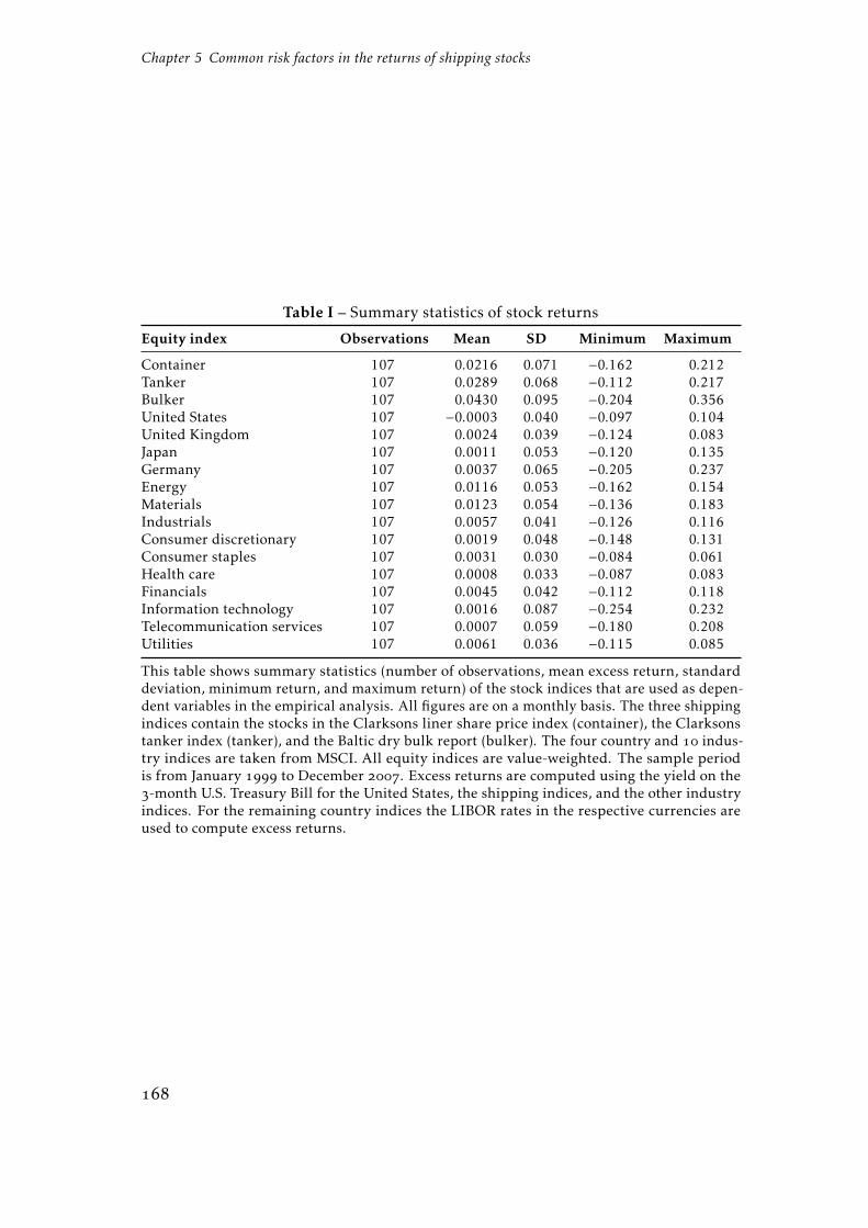
Chapter 5 Common risk factors in the returns of shipping stocks
Table I – Summary statistics of stock returns
Equity index Observations Mean SD Minimum Maximum
Container 107 0.0216 0.071 −0.162 0.212Tanker 107 0.0289 0.068 −0.112 0.217Bulker 107 0.0430 0.095 −0.204 0.356United States 107 −0.0003 0.040 −0.097 0.104United Kingdom 107 0.0024 0.039 −0.124 0.083Japan 107 0.0011 0.053 −0.120 0.135Germany 107 0.0037 0.065 −0.205 0.237Energy 107 0.0116 0.053 −0.162 0.154Materials 107 0.0123 0.054 −0.136 0.183Industrials 107 0.0057 0.041 −0.126 0.116Consumer discretionary 107 0.0019 0.048 −0.148 0.131Consumer staples 107 0.0031 0.030 −0.084 0.061Health care 107 0.0008 0.033 −0.087 0.083Financials 107 0.0045 0.042 −0.112 0.118Information technology 107 0.0016 0.087 −0.254 0.232Telecommunication services 107 0.0007 0.059 −0.180 0.208Utilities 107 0.0061 0.036 −0.115 0.085
This table shows summary statistics (number of observations, mean excess return, standarddeviation, minimum return, and maximum return) of the stock indices that are used as depen-dent variables in the empirical analysis. All figures are on a monthly basis. The three shippingindices contain the stocks in the Clarksons liner share price index (container), the Clarksonstanker index (tanker), and the Baltic dry bulk report (bulker). The four country and indus-try indices are taken from MSCI. All equity indices are value-weighted. The sample periodis from January to December . Excess returns are computed using the yield on the-month U.S. Treasury Bill for the United States, the shipping indices, and the other industryindices. For the remaining country indices the LIBOR rates in the respective currencies areused to compute excess returns.

5.3 Data
would expect that the estimated factor risk premiums using two different sets of
spanning assets do not strongly differ; i.e., they should not be affected by the way
the information contained in the underlying stocks is being bundled into indices.
Summary statistics of the equity indices are presented in Table I. The mean return
on shipping stocks during the sample period from January to December (using month-end stock prices) is remarkably high compared to the returns of both
the country and other industry indices. For example, the monthly average excess
return of .% in the container sector corresponds to a return of roughly % per
year, while the yearly excess return on the U.S. stock market was -.% during
the sample period. As one would expect for a highly cyclical industry with mainly
smaller firms, the higher mean return in the shipping industry is accompanied by a
higher volatility as compared to most other indices.
5.3.2 Global risk factors
The global risk factors must represent pervasive sources of risk for international
investments. We consistently apply aggregate information on potential global
sources of systematic risk. Three of the nine global factors are constructed by
aggregating economic data from the G- countries. These major industrialized
countries are Canada, France, Germany, Italy, Japan, the United Kingdom, and
the United States. The remaining six risk factors are derived from economic and
financial time-series and represent information on global aggregates. All time series
are taken from Datastream. Since there is no commonly accepted asset pricing model,
the choice of risk factors is not straightforward and ultimately requires economic
intuition. We use risk factors that are common in the asset pricing literature (Ferson
and Harvey ; Zimmermann et al. ). Standard models of international asset
pricing theory motivate some of these risk factors (Adler and Dumas ; Sercu
; Solnik ; Stulz a). Earlier empirical studies on multibeta asset pricing
models in an international environment provide further guidelines for our model
(Ferson and Harvey ; Harvey ; Dumas and Solnik ; Brown and Otsuki
). Finally, empirical studies on the pricing of risks on national stock and bond
markets influence our selection of risk factors (Fama and French ; Chen et al.
; Elton et al. ; Ferson and Korajczyk ).We use the MSCI world stock market index as a proxy for the global market
Cavaglia et al. () and Gerard et al. () provide a discussion of the benefits of country versussector indices for asset allocation.

Chapter 5 Common risk factors in the returns of shipping stocks
portfolio. The monthly log changes of this variable are denoted as dWRLDE. The
MSCI world stock market index is a broad equity index of developed countries,
whose stock market capitalization represents roughly % of the total world stock
market capitalization.
The monthly log changes of a weighted currency basket, labeled dCURB, consist
of the exchange rates between the US$ and the Euro, Canadian dollar, Japanese
yen, British pound, Swiss franc, Australian dollar, and Swedish krona (defined as
foreign currency/US$). The weights are derived from the relative trade position of
the United States against the corresponding country. The monthly log changes of
this currency basket mirror changes in the external value of the US$, which is still
the lead currency in the shipping industry. Dumas and Solnik () and De Santis
and Gerard () document that currency risk is pricing relevant in international
factor models. Ferson and Harvey () note that one implicitly assumes that
relative purchasing power parity holds if currency risk is excluded. Shipping
markets are heavily oriented toward international trade, and hence exchange rate
changes may have a large impact on shipping stock returns. The problem arises from
the imposition of a volatile foreign exchange market on a freight market structure
which fixes revenues in US$. Leggate () documents that operating profits in the
shipping industry can rise and fall dramatically simple because of exchange rate
movements.
We expect that shipping stocks are sensitive to variations in international eco-
nomic activity and global trade. According to Stopford (), industrial production
is a main parameter that affects the demand for sea transport through world trade.
To proxy for these influences, we incorporate two additional risk factors: the change
in industrial production in the G- countries and the change in industrial produc-
tion in China. The change in the G- industrial production (dIPG) is the weighted
average of the contemporaneous log changes of monthly industrial production in
these countries. The change in the Chinese industrial production (dIPChina) is
the contemporaneous monthly log change of industrial production in this largest
emerging country.
Previous studies in the asset pricing literature document that stock returns are
sensitive to risk factors that are condensed out of interest rates (Harvey ; Ferson
and Harvey ). We use measures for the short-term interest rate, the long-term
interest rate, and the TED spread (i.e., the difference between the interbank lending
For a theoretical derivation, see Stulz (b).

5.3 Data
rate and the risk-free rate). The short-and long-term G- interest rates (dMIGand dYIG) are proxied by the yields on -month and -year government bonds,
respectively. We weigh the interest rates of the G- countries according to their
share of the G- gross domestic product (GDP) in the previous quarter. The TED
spread is defined as the difference between the -months Eurodollar rate and the
yield on the -day U.S. Treasury Bill. We use the monthly log changes of the TED
spread (dTED). The TED spread is affected by three factors: () world political
stability, () balance of trade, and () fiscal policy of the United States (Ferson and
Harvey ). When political uncertainty is high and the risk of disruption in the
global financial system increases, the yield differential widens. When the balance
of trade is decreasing, the TED spread also rises. Presumably, the TED spread is
an indicator of the current health of the economy. The yield differential should
be higher during phases of economic recessions (when investors are seeking safer
assets), and it decreases during expansionary phases.
Inflation is another factor that is related to interest rates. We use a measure
derived from the G- producer price index (INFLG). In general, higher inflation
may signal higher levels of economic uncertainty, which makes investors worse
off. More specifically, many products transported by ships are preproducts that are
finished at the place of destination. Prices determine the demand for these products,
and hence inflation presumably will have an influence on returns in the shipping
industry.
Finally, the oil price could be a potential return driver of shipping stock returns
for two reasons. First, oil is the main input factor for producing carriage service.
Second, oil is the main product of carriage of tankers. The demand for tanker freight
is a derived demand from oil; if oil prices are high, the demand for oil will be high,
and the demand for tanker transport tends to be high as well. Therefore, the oil
price can have a negative or a positive impact on shipping stock returns. We use the
changes in the price of Brent crude oil (dOIL).
Panel A of Table II shows summary statistics of our global risk factors. The mean
excess return on the world stock market portfolio is .% per month. Surprisingly,
the mean of the changes in industrial production in China is lower than in the G-countries, while the standard deviation of Chinese industrial production is higher
than in the G- countries. The mean change in G- interest rates indicates that our
sample period covers an environment of declining interest rates. The rise in the oil
price during our sample period leads to a high mean return on oil, accompanied by a

Chapter 5 Common risk factors in the returns of shipping stocks
Tab
leII
–M
acro
econ
omic
risk
fact
or
Pane
lA.S
umm
ary
stat
isti
csV
aria
ble
Ob
serv
atio
ns
Mea
nSD
Min
imu
mM
axim
um
dW
RL
DE
107
0.00
200.
039
−0.1
020.
097
dC
UR
B10
7−0.0
024
0.01
9−0.0
500.
045
dO
IL10
70.
0199
0.11
1−0.3
270.
332
dIP
G
107
0.00
130.
005
−0.0
130.
011
dIP
Chi
na10
70.
0005
0.03
9−0.1
440.
151
INFL
G
107
0.00
190.
005
−0.0
130.
013
dT
ED
107
0.01
310.
407
−0.8
651.
194
dM
IG
107
−0.0
007
0.04
5−0.2
360.
085
d
YIG
107
−0.0
007
0.04
5−0.1
010.
164
cont
inue
d

5.3 Data
Tab
leII
–(c
onti
nued
)
Pane
lB:C
orre
lati
onst
ruct
ure
dW
RL
DE
dC
UR
Bd
OIL
dIP
G
dIP
Ch
ina
INFL
G
dT
ED
dM
IG
d
YIG
DC
UR
B−0.3
45**
*1.
000
(0.0
00)
dO
IL0.
122
−0.1
141.
000
(0.2
10)
(0.2
43)
DIP
G
0.05
9−0.0
070.
104
1.00
0(0.5
47)
(0.9
46)
(0.2
86)
DIP
Chi
na−0.0
980.
036
0.07
0−0.0
611.
000
(0.3
16)
(0.7
14)
(0.4
75)
(0.5
33)
INFL
G
−0.0
47−0.0
140.
544*
**−0.0
060.
002
1.00
0(0.6
31)
(0.8
87)
(0.0
00)
(0.9
49)
(0.9
81)
dT
ED
−0.0
830.
054
−0.0
920.
061
0.13
60.
023
1.00
0(0.3
94)
(0.5
82)
(0.3
45)
(0.5
31)
(0.1
63)
(0.8
16)
dM
IG
0.15
7−0.0
260.
131
0.34
9***
−0.0
130.
084
−0.2
58**
*1.
000
(0.1
05)
(0.7
91)
(0.1
79)
(0.0
00)
(0.8
91)
(0.3
88)
(0.0
07)
d
YIG
0.21
9**
0.28
3***
0.00
80.
076
−0.1
580.
036
−0.0
480.
242*
*1.
000
(0.0
26)
(0.0
03)
(0.9
39)
(0.4
36)
(0.1
04)
(0.5
02)
(0.6
26)
(0.0
12)
Pan
elA
ofth
ista
ble
show
ssu
mm
ary
stat
isti
cs(n
um
ber
ofob
serv
atio
ns,
mea
nch
ange
,SD
,min
imu
mch
ange
,an
dm
axim
um
chan
ge)f
orth
em
acro
econ
omic
risk
fact
ors
that
are
use
das
ind
epen
den
tva
riab
les
inth
eem
pir
ical
anal
ysis
.All
figu
res
are
ona
mon
thly
basi
s.T
hegl
obal
risk
fact
ors
are
the
exce
ssre
turn
onth
eM
SCI
wor
ldst
ock
mar
ket
ind
ex(d
WR
LD
E),
the
chan
gein
aw
eigh
ted
curr
ency
bask
et(d
CU
RB
),th
ech
ange
inth
eoi
lpri
ce(d
OIL
),th
ech
ange
sin
the
indu
stri
alp
rodu
ctio
nof
the
G-
cou
ntri
es(d
IPG)
and
Chi
na(d
IPC
hina
),th
ein
flat
ion
rate
(IN
FLG)
,the
chan
gein
the
TE
Dsp
read
(dT
ED
),an
dth
ech
ange
sin
the
shor
t-te
rm(dM
IG)
and
the
long
-ter
min
tere
stra
te(d
YIG)
.The
sam
ple
per
iod
isfr
omJa
nuar
y
toD
ecem
ber
.Pan
elB
show
sth
eco
rrel
atio
nm
atri
xof
the
mac
roec
onom
icfa
ctor
s.T
hep
-val
ues
are
rep
orte
du
nd
ern
eath
the
corr
elat
ion
coeffi
cien
ts.
Wit
hn
bein
gth
enu
mbe
rof
obse
rvat
ion
san
dρ̂
the
sam
ple
corr
elat
ion,
the
corr
esp
ond
ingt-
test
stat
isti
cis
2∗t̃
(n−
2,|ρ̂|√ (n
−2)/√ (1
−ρ̂
2))
.**
*,**
and
*d
enot
esst
atis
tica
lsig
nifi
canc
eat
the,
and
%le
vels
.

Chapter 5 Common risk factors in the returns of shipping stocks
high standard deviation. The sharp increase in the TED spread due to the beginning
of the financial crises in the last months of leads to a high mean and a high
standard deviation of this variable.
The correlation structure of our global risk factors is shown in Panel B of Table
II. The highest correlation (.) is measured between G- inflation and oil price
changes. In fact, some of the correlation coefficients are significant, implying poten-
tial multicollinearity problems and unstable coefficients depending on the variables
included in the model. However, an examination of the variance inflation factors
(VIFs) indicates that all of them are well below (and the mean VIF is only .),which is usually interpreted as low multicollinearity.
5.4 Empirical results
5.4.1 Market model regressions
Given that firm-specific risk can be diversified through portfolio formation, one
should consider market or systematic risk (captured by the stock market beta)
rather than total risk (return volatility) as the appropriate risk measure. Table
III shows the results of market model regressions, i.e., the model in Equation
() with the world stock market index as the single source of risk. The market
betas of the three shipping sectors (container, tanker, and bulker shipping) are all
around one, and none of them is distinguishable from unity in a statistical sense.
Moreover, according to a Wald test based on the SUR estimates, the three sector
betas in the shipping industry are not distinguishable from each other. Compared
to previous empirical studies (Kavussanos and Marcoulis a; Kavussanos et
al. ), we document slightly higher market betas. Nevertheless, market betas
around one are against our hypothesis and clearly surprising for the highly cyclical
shipping industry that additionally exhibits high operating and high financial
leverage (Stopford ). It is well known that these risks add up and reinforce
covariance risk (Ross et al. ). Therefore, one would expect a market beta greater
than one for an industry with these risk characteristics. The observation that the
betas of the three shipping sectors are not different from each other is also in line
with the findings in Kavussanos et al. ().
We compute a Wald test to test the null hypothesis that the shipping betas are equal to one. In allthree cases, the null hypothesis cannot be rejected.

5.4 Empirical results
All beta coefficients shown in Table III are significant at the % level. Compared
to the country indices, the market betas of shipping stocks are similar to the beta of
the United States (.). They are higher than the betas of the United Kingdom
(.) and Japan (.), but lower than the beta of Germany (.). A Wald
test rejects the null hypothesis that all shipping and country betas are equal at the
% level. Moreover, the shipping stock betas are in the middle of the industry
betas. The information technology industry exhibits the highest (.) and the
health-care industry the lowest (.) beta. The water transportation sector is part
of the industrials sector, which has a world market beta of .. As one would
expect, the shipping betas are very similar to this beta of the industrials sector.
The constant (intercept) terms in the market model regressions of the three ship-
ping sectors are all positive and strongly significant. Given that returns are in excess
of the risk-free rate, this observation indicates that the shipping industry is system-
atically underpriced in a securities market line (SML) analysis. A similar result has
been reported in Grammenos and Arkoulis () and Kavussanos et al. ().One explanation for potential mispricing is high asset specificity coupled with pro-
nounced information asymmetry in the shipping industry, and hence investors do
not have access to the information that is required to price shipping stocks correctly.
Low liquidity of the mainly small-cap shipping stocks could be another explanation.
The R-squares of the market model regressions for the shipping sectors fall into
the range between . and .. These values are very low compared to the market
model regressions involving country and most industry indices, but they are still in
the upper range of previous studies. For example, Kavussanos et al. () document
market model R-squares in the range between . and . for different subsectors
of the water transportation industry in an earlier sample period. Our results may
indicate that the systematic part of total risk in the shipping industry has increased
over the recent years. Nevertheless, even in our more recent sample period a low
proportion of the variance of shipping stocks is attributable to a single stock market
factor. This observation indicates that a multifactor model may be better able to
describe the risk-return spectrum of shipping stocks than a one-factor model.
5.4.2 Multifactor model regressions
In this section, we use a multifactor model to estimate the relationship between
stock returns and the set of macroeconomic risk factors described in Section . The
regression results using the SUR method are shown in Table IV. A first observation

Chapter 5 Common risk factors in the returns of shipping stocks
is that the market betas of the three shipping sectors are smaller than in the market
model; they fall into the range between . (for bulkers) and . (for tankers) and
are significant at the % level. These figures are more in line with the market beta
estimates in Kavussanos and Marcoulis (a). Given the high cyclicality of the
shipping industry coupled with high operating and high financial leverage, these
results are again against our initial hypothesis. Moreover, the market betas of the
three shipping sectors are lower than those of the country indices (except Japan).
Using a Wald test, we reject the null hypotheses that all market betas are equal to
zero and that they are all equal among each other. In contrast, the null hypothesis of
equality of market betas across the three shipping sectors again cannot be rejected
(not reported in Table IV).
The coefficient on changes in the trade-weighted value of the US$ (dCURB) is
statically significant in all three shipping sectors. The negative sign indicates that a
stronger US$ has a negative effect on shipping stock returns; this result confirms
previous findings by Grammenos and Arkoulis (). An explanation could be that
most shipping related contracts are denominated in US$. A stronger dollar implies
higher operating costs for non-U.S. shipping firms and a lower income in the home
currency (Stopford ). At the same time, the income side of a shipping company
(e.g., the freight contracts) is denominated in US$, and hence a company can buy
more units of the home currency (Leggate ). The estimated coefficient indicates
that the first effect outweighs the second in our sample. The country indices also
exhibit a negative exposure to the currency factor.
The coefficient on changes in industrial production in the G- countries (dIPG)is marginally significant only in the container sector. The coefficient implies that a
% increase in industrial production leads to a .% increase in monthly returns
in the container sector. Only the Japanese stock market benefits even stronger
from an increase in G- industrial production than the container sector. This high
exposure is consistent with the general notion that the demand for sea transport
is derived from the growth of the global economy and international trade. The
negative (albeit insignificant) coefficient on industrial production in the tanker
sector is clearly surprising. One would expect that with rising output the demand
for oil as an input factor increases as well. It is also against expectations that the
coefficient on changes in industrial production in China (dIPChina) is not estimated
significantly in any sector of the shipping industry. Grammenos and Arkoulis ()also cannot detect a significant relationship between shipping stock returns and
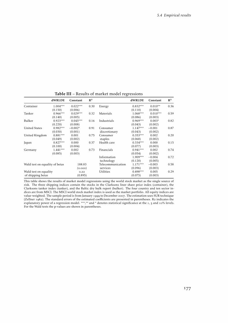
5.4 Empirical results
Table III – Results of market model regressionsdWRLDE Constant R dWRLDE Constant R
Container 1.004*** 0.022*** 0.30 Energy 0.832*** 0.010** 0.36(0.150) (0.006) (0.110) (0.004)
Tanker 0.966*** 0.029*** 0.32 Materials 1.068*** 0.010*** 0.59(0.140) (0.005) (0.086) (0.003)
Bulker 0.923*** 0.045*** 0.16 Industrials 0.969*** 0.003* 0.82(0.220) (0.008) (0.043) (0.002)
United States 0.982*** −0.002* 0.91 Consumer 1.147*** −0.001 0.87(0.030) (0.001) discretionary (0.043) (0.002)
United Kingdom 0.881*** 0.001 0.75 Consumer 0.353*** 0.002 0.20(0.049) (0.002) staples (0.068) (0.002)
Japan 0.827*** 0.000 0.37 Health care 0.334*** 0.000 0.15(0.100) (0.004) (0.077) (0.003)
Germany 1.441*** 0.002 0.73 Financials 0.941*** 0.002 0.74(0.085) (0.003) (0.054) (0.002)
Information 1.909*** −0.004 0.72technology (0.120) (0.005)
Wald test on equality of betas 188.83 Telecommunication 1.171*** −0.003 0.58(.) services (0.096) (0.003)
Wald test on equality . Utilities 0.498*** 0.005 0.29of shipping betas (0.895) (0.075) (0.003)
This table shows the results of market model regressions using the world stock market as the single source ofrisk. The three shipping indices contain the stocks in the Clarksons liner share price index (container), theClarksons tanker index (tanker), and the Baltic dry bulk report (bulker). The four country and ten sector in-dices are from MSCI. The MSCI world stock market index is used as the market portfolio. All equity indices arevalue-weighted. The sample period is from January to December . The estimation uses SUR technique(Zellner ). The standard errors of the estimated coefficients are presented in parentheses. R indicates theexplanatory power of a regression model. ***,** and * denotes statistical significance at the , and % levels.For the Wald tests the p-values are shown in parentheses.
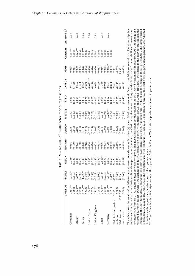
Chapter 5 Common risk factors in the returns of shipping stocks
Tab
leIV
–R
esu
lts
ofm
ult
ifac
tor
mod
elre
gres
sion
sd
WR
LD
Ed
CU
RB
dIP
G
dIP
Ch
nia
dM
IG
d
YIG
dT
ED
INFL
G
dO
ILC
onst
ant
Ad
just
edR
Con
tain
er0.
851*
**−0.7
20**
2.23
8*0.
054
−0.1
230.
050
−0.0
21−0.8
010.
095*
0.01
7***
0.38
(0.1
60)
(0.3
40)
(1.3
20)
(0.1
40)
(0.1
40)
(0.1
40)
(0.0
14)
(1.4
10)
(0.0
57)
(0.0
06)
Tank
er0.
872*
**−0.5
97*
−0.5
050.
093
0.10
10.
028
0.00
40.
697
0.07
00.
026*
**0.
38(0.1
50)
(0.3
20)
(1.2
70)
(0.1
40)
(0.1
40)
(0.1
30)
(0.0
14)
(1.3
60)
(0.0
55)
(0.0
06)
Bu
lker
0.79
6***
−1.2
23**
1.34
00.
070
−0.0
14−0.1
420.
012
0.39
30.
078
0.03
9***
0.25
(0.2
40)
(0.4
90)
(1.9
30)
(0.2
10)
(0.2
10)
(0.2
00)
(0.0
21)
(2.0
60)
(0.0
84)
(0.0
09)
Uni
ted
Stat
es1.
060*
**0.
368*
**0.
065
−0.0
04−0.0
25−0.0
41*
0.00
0−0.6
71**
*0.
000
0.00
00.
94(0.0
27)
(0.0
56)
(0.2
20)
(0.0
24)
(0.0
24)
(0.0
23)
(0.0
02)
(0.2
40)
(0.0
10)
(0.0
01)
Uni
ted
Kin
gdom
0.82
7***
−0.3
29**
*−1.4
60**
*−0.0
030.
102*
*−0.0
26−0.0
050.
634
−0.0
30*
0.00
20.
82(0.0
48)
(0.1
00)
(0.3
90)
(0.0
43)
(0.0
43)
(0.0
42)
(0.0
04)
(0.4
20)
(0.0
17)
(0.0
03)
Jap
an0.
735*
**−0.3
75*
2.56
3***
−0.0
76−0.1
110.
015
0.00
41.
360
0.05
6−0.0
08*
0.48
(0.1
10)
(0.2
30)
(0.8
90)
(0.0
97)
(0.0
96)
(0.0
94)
(0.0
10)
(0.9
50)
(0.0
38)
(0.0
04)
Ger
man
y1.
351*
**−0.4
15**
−0.0
170.
120
0.00
80.
207*
**−0.0
020.
304
−0.0
66**
0.00
20.
76(0.0
91)
(0.1
90)
(0.7
50)
(0.0
82)
(0.0
81)
(0.0
79)
(0.0
08)
(0.8
00)
(0.0
32)
(0.0
04)
Wal
dte
ston
equ
alit
y37.1
946.6
724.4
22.
849.
1110.4
46.
359.
477.
99of
beta
s(0.0
00)
(0.0
00)
(0.0
00)
(0.8
29)
(0.1
68)
(0.1
08)
(0.3
85)
(0.1
49)
(0.2
39)
Wal
dte
ston
1372
0.97
54.8
325.9
23.
2110.4
010.6
26.
8810.2
813.9
0ze
robe
tas
(0.0
00)
(0.0
00)
(0.0
01)
(0.8
65)
(0.1
67)
(0.1
56)
(0.4
42)
(0.1
73)
(0.0
53)
Thi
sta
ble
show
sth
ere
sult
sof
mu
ltif
acto
rm
odel
regr
essi
ons
show
nin
Equ
atio
n(
)u
sing
glob
alm
acro
econ
omic
fact
ors
asm
ult
iple
sou
rces
ofri
sk.
The
thre
esh
ipp
ing
ind
ices
cont
ain
the
stoc
ksin
the
Cla
rkso
nsli
ner
shar
ep
rice
ind
ex(c
onta
iner
),th
eC
lark
sons
tank
erin
dex
(tan
ker)
,and
the
Bal
tic
dry
bulk
rep
ort
(bu
lker
).T
hefo
ur
cou
n-tr
yin
dic
esar
efr
omM
SCI.
All
equ
ity
ind
ices
are
valu
e-w
eigh
ted
.The
glob
alri
skfa
ctor
sar
eth
ere
turn
ofth
eM
SCI
wor
ldst
ock
mar
ket
ind
ex(d
WR
LD
E),
the
chan
geof
aw
eigh
ted
curr
ency
bask
et(d
CU
RB
),th
ech
ange
sin
indu
stri
alp
rodu
ctio
nof
the
G-
cou
ntri
es(d
IPG)
and
Chi
na(d
IPC
hina
),th
ech
ange
inth
eT
ED
-sp
read
(dT
ED
),th
ech
ange
sin
the
shor
t-te
rm(dM
IG)
and
the
long
-ter
m(d
YIG)
inte
rest
rate
s,th
eG
-in
flat
ion
rate
(IN
FLG)
,and
the
chan
gein
the
oilp
rice
(dO
IL).
The
sam
ple
per
iod
isfr
omJa
nuar
y
toD
ecem
ber
.The
esti
mat
ion
use
sSU
Rte
chni
que
(Zel
lner
).T
hest
and
ard
erro
rsof
the
coeffi
cien
tsar
ep
rese
nted
inp
aren
thes
es.A
dju
sted
R
ind
icat
esth
ead
just
edex
pla
nato
ryp
ower
ofa
regr
essi
onm
odel
.**
*,**
and
*d
enot
esst
atis
tica
lsig
nifi
canc
eat
the,
and
%le
vels
.For
the
Wal
dte
sts
the
p-v
alu
esar
esh
own
inp
aren
thes
es.
5.4 Empirical results
changes in industrial production. They argue that the influence changes in industrial
production may have on shipping stock returns is already captured by the remaining
macroeconomic factors. Another explanation for our results may be that the sample
of listed tanker and bulker companies (in contrast to our container sample) may not
capture a representative fraction of total worldwide tonnage capacity in these sectors,
and hence our coefficient estimates may not reflect all underlying macroeconomic
relationships. However, without additional public data, we cannot address this
potential problem. Finally, problems related to the accuracy and reliability of
Chinese industrial production data could drive our results (Chow ).The term structure of interest rates (dMIG and dYIG), the TED spread
(dTED), and the inflation rate (INFLG) also do not exert a significant impact on
shipping stock returns. Given that interest rates are related to the state of the
economy, it is clearly surprising that none of the factors related to interest rates
shows up significantly in regressions with shipping stock returns as the dependent
variables. Our final risk factor, the change in the oil price (dOIL), is estimated
significantly for the container sector, but it shows no significance in the other
shipping sectors. The direction of influence tends to be positive: a higher oil price
leads to an increase in the returns on shipping stocks. Given that oil is one of
the main input factors in the production of freight services, one could expect a
negative influence. Grammenos and Arkoulis () are able to confirm this notion
for shipping stocks in their earlier sample period. However, the oil price also serves
as a proxy for the state of the world economy, and hence it may exert a positive
influence on shipping stock returns in particular. This notion is reasonable for
our sample period, which covers a long phase of economic prosperity. In contrast,
the sensitivities of the country indices to oil price changes tend to be negative,
presumably because oil is a major input factor. The high coefficient (in absolute
terms) for Germany could be explained by the export orientation of the German
economy.
In results not reported here, we use several alternative explanatory variables to
check the robustness of our results. An exclusion of the MSCI world stock market
index does not qualitatively alter our findings. We also include a direct measure of
international trade, such as the International Monetary Fund (IMF) export index,
but it does not enter significantly into the regressions. One would further expect
However, our sample changes in G- industrial production are only significantly correlated withchanges in the short-term interest rate (see Table II), and the latter is also insignificant in multifactorregressions that involve the three shipping sectors (see Table IV).
Chapter 5 Common risk factors in the returns of shipping stocks
that measures of stock market volatility (e.g., the VIX index, which is a measure
of the implied volatility of S&P index options) and a down-market dummy
variable that account for an asymmetric perception of risk have explanatory power
for stock returns. However, both measures turn out to be insignificant. Finally, we
replace the changes in the oil price with the changes in the Dow Jones commodity
spot index. The significance levels of the corresponding coefficients decrease and the
regression R-squares are also slightly lower. Looking at the intercept terms (alphas),
we get similar results in the multifactor model in Table IV as in the market model in
Table III. Most important, the estimated alphas for shipping stocks are significantly
positive at the % level. Although these results need to be interpreted with due care
because there is no general consensus on what constitutes the correct asset pricing
model, they again indicate that shipping stocks tend to be underpriced. However,
the abnormal returns are smaller in the multifactor model than in the market model,
implying that part of the alpha is captured by the additional macroeconomic factors.
This notion is strengthened by the observation that the multifactor R-squares (albeit
still relatively low) are higher compared to the market model. Most important,
the inclusion of macroeconomic factors increases the fraction of explained variance
between and percentage points in the multifactor model for the shipping sectors.
Finally, we report the results of two Wald tests. First, we test the null hypothesis
that the beta coefficients are equal across all assets for a given factor. We reject this
hypothesis for the coefficients on the world stock market index, the currency basket
against the US$, and G- industrial production. Second, we test the null hypothesis
that the beta coefficients are simultaneously equal to zero across all assets for a
given factor. This null hypothesis is rejected for the coefficients on the world stock
market index, the currency basket against the US$, G- industrial production, and
the oil price. From these results, we hypothesize that the latter four factors are
not only drivers of stock return volatility, but that they also have the potential to
represent sources of systematic risk. Exposure to the common risk factors should be
rewarded with a risk premium. To validate this hypothesis, it is necessary to include
a cross-sectional pricing restriction into the model. Accordingly, in the final step of
our analysis, we test a full-fledged asset pricing model by exploiting the moment
conditions imposed by full information processing.
Cochrane () argues that the regressions of returns on factors can have low R-squares in thecontext of Merton’s () intertemporal capital asset pricing model (ICAPM). In fact, factor pricing(as examined in Section ..) does not necessarily require a factor structure (as assumed in Equation()).
5.4 Empirical results
5.4.3 Testing the pricing restrictions
In our asset pricing model, we use those global risk factors from the multifactor
regressions for which the null hypothesis that the coefficients are simultaneously
equal to zero across all assets can be rejected. Specifically, our four macroeconomic
risk factors (in changes) are: the world stock market index (dWRLDE), the trade-
weighted value of the US$ dollar (dCURB), G- industrial production (dIPG), and
the oil price (dOIL). We use country and sector indices as spanning assets in two
separated factor pricing models. The results from estimating the system of equations
in Equation () using the GMM with country and industry indices as spanning assets
are shown in Tables V and VI respectively.
In a first step, we use the MSCI world stock market index as the only risk fac-
tor. Using country indices as spanning assets in Table V, the market betas for the
shipping sectors are between . for bulker and . for container. This reinforces
our previous finding that the covariance risk of shipping stocks is lower than the
risk of the overall stock market. The world market betas of the four countries are
also similar to those in the multifactor model in Table IV. The estimated market
risk premium is .% per month, which is much smaller than the historical stock
market excess return of .% per month, as reported in Table II. One explanation
for this result is that the US stock market earned a negative mean excess return
during our sample period, which was coupled with a relatively low standard devia-
tion. The GMM estimator puts a heavy weight on those assets with low standard
deviations (Cochrane ), and hence the world stock market risk premium may
be underestimated. Given this very low estimate for the world stock market risk
premium, one expects that the one-factor model is not powerful in explaining the
cross-section of expected stock returns. In fact, as indicated by the chi-square test
of over-identification (a test for the goodness of fit; Hamilton ), the model
violates the moment conditions that capture the cross-sectional pricing restriction.
Our findings are strengthened on the basis of the average pricing error, which is
similar in magnitude to the average monthly excess return. Overall, we conclude
that the world stock market index alone is not able to price all assets in the system
of equations with sufficient accuracy.
The four-factor asset pricing model with the additional macroeconomic risk factors
again generates lower market betas for the shipping sectors, while the country betas
remain virtually unchanged. The market risk premium is now .% per month.
Surprisingly, this is much higher than the mean market excess return during our

Chapter 5 Common risk factors in the returns of shipping stocks
Tab
leV
–L
ong-
run
risk
sw
ith
cou
ntry
ind
ices
assp
anni
ngas
sets
One
-fac
tor
mod
elFo
ur-
fact
orm
odel
dW
RL
DE
Mea
nex
cess
Ave
rage
pri
cing
dW
RL
DE
dC
UR
Bd
IPG
dO
ILA
vera
gep
rici
ngbe
tare
turn
(%)
erro
r(%
)be
tabe
tabe
tabe
taer
ror
(%)
Con
tain
er0.
966
0.02
160.
0234
0.81
4−0.7
631.
572
0.07
50.
0010
(0.1
29)
(0.0
08)
(0.1
04)
(0.2
29)
(0.6
48)
(0.0
23)
(0.0
08)
Tank
er0.
864
0.02
890.
0303
0.85
3−0.5
360.
373
0.06
2−0.0
005
(0.1
19)
(0.0
08)
(0.0
54)
(0.1
63)
(0.7
15)
(0.0
23)
(0.0
07)
Bu
lker
0.68
00.
0430
0.04
830.
616
−1.3
630.
546
0.09
0−0.0
015
(0.1
95)
(0.0
12)
(0.1
34)
(0.2
91)
(0.9
43)
(0.0
29)
(0.0
10)
Uni
ted
Stat
es0.
875
−0.0
003
−0.0
009
1.03
60.
319
−0.1
87−0.0
13−0.0
001
(0.0
32)
(0.0
01)
(0.0
16)
(0.0
34)
(0.1
58)
(0.0
06)
(0.0
01)
Uni
ted
Kin
gdom
0.84
60.
0024
0.00
230.
856
−0.2
73−0.5
80−0.0
33−0.0
002
(0.0
38)
(0.0
02)
(0.0
21)
(0.0
72)
(0.2
11)
(0.0
12)
(0.0
02)
Jap
an0.
891
0.00
110.
0014
0.73
1−0.3
852.
253
0.05
50.
0015
(0.0
81)
(0.0
05)
(0.0
62)
(0.1
65)
(0.5
87)
(0.0
23)
(0.0
04)
Ger
man
y1.
378
0.00
370.
0042
1.41
0−0.2
47−0.1
37−0.0
230.
0004
(0.0
80)
(0.0
03)
(0.0
71)
(0.0
98)
(0.3
40)
(0.0
15)
(0.0
03)
Mea
np
rici
nger
ror
(%)
0.01
560.
0001
χ2
-tes
ton
over
-χ
2-t
est
onov
er-
iden
tifi
cati
onid
enti
fica
tion
Ris
kp
rem
ium
0.00
0137.3
90.
0052
−0.0
116
−0.0
131
0.37
5912.8
5(0.0
00)
(0.0
00)
(0.0
02)
(0.0
10)
(0.0
10)
(0.2
19)
(0.9
98)
Thi
sta
ble
show
sth
ere
sult
sfr
omes
tim
atio
nsof
the
syst
emof
equ
atio
nsin
Equ
atio
n(
),w
here
fact
orse
nsit
ivit
ies
and
risk
pre
miu
ms
are
det
er-
min
edsi
mu
ltan
eou
sly.
Cou
ntry
ind
ices
are
use
das
span
ning
asse
ts.
The
thre
esh
ipp
ing
ind
ices
cont
ain
the
stoc
ksin
the
Cla
rkso
nsli
ner
shar
eP
rice
ind
ex(c
onta
iner
),th
eC
lark
sons
tank
erin
dex
(tan
ker)
,and
the
Bal
tic
dry
bulk
rep
ort
(bu
lker
).T
hefo
ur
cou
ntry
ind
ices
are
from
MSC
I.A
lleq
uit
yin
dic
esar
eva
lue-
wei
ghte
d.I
nth
eon
e-fa
ctor
mod
el,t
hew
orld
stoc
km
arke
tis
the
sing
leso
urc
eof
risk
.The
MSC
Iwor
ldst
ock
mar
ket
ind
ex,w
hose
retu
rns
are
den
oted
asd
WR
LD
E,i
su
sed
asa
pro
xyfo
rth
em
arke
tp
ortf
olio
.T
hefo
ur-
fact
orm
odel
inco
rpor
ates
thre
ead
dit
iona
lgl
obal
mac
roec
onom
icfa
ctor
sth
atha
vebe
enid
enti
fied
inth
eSU
Rm
odel
inTa
ble
IV:t
hech
ange
ina
wei
ghte
dcu
rren
cyba
sket
(dC
UR
B),
the
chan
gein
indu
stri
alp
rodu
ctio
nof
the
G-
cou
ntri
es(d
IPG)
,and
the
chan
gein
the
oilp
rice
(dO
IL).
The
sam
ple
per
iod
isfr
omJa
nuar
y
toD
ecem
ber
.In
ord
erto
cap
ture
the
cros
s-se
ctio
nala
sset
pri
cing
cond
itio
ns,t
hefa
ctor
sens
itiv
itie
sar
eas
set-
spec
ific,
but
the
risk
pre
miu
ms
app
lyfo
ral
lass
ets.
The
mod
el’s
orth
ogon
alit
yco
ndit
ions
are
esti
mat
edu
sing
Han
sen’
s()
GM
M.R
etu
rns
and
pri
cing
erro
rsar
ein
per
cent
per
mon
th.S
tand
ard
erro
rsar
egi
ven
inp
aren
thes
es.F
orth
eχ
2-t
ests
onov
er-i
den
tifi
cati
onth
ep
-val
ues
are
show
nin
par
enth
eses
.

5.4 Empirical results
sample period, but it is similar to the figures reported in Dimson et al. () based
on very long-run averages. The currency risk premium on the US$ is negative
with -.% per month. However, all sensitivities on the currency factor apart from
the United States are negative, which implies a positive total return contribution
from taking on currency risk. The U.S. market itself exhibits a positive exposure to
currency risk, and hence a stronger US$ induces a lower expected rate of return on
U.S. firms. A stronger US$ weakens exports and strengthens imports, which has an
adverse impact on the cash flow of U.S. firms. With respect to changes in industrial
production, we find notable differences across assets. The strongest impact of this
factor is observable in the container sector, while the impact on the other shipping
sectors is smaller (albeit still positive). In contrast, industrial production has a
negative impact on three of the four country indices. In this respect, shipping stocks
tend to differ fundamentally from country indices. Shipping stocks profit from
higher contemporaneous production in the G- countries, whereas the coefficients
on the country indices are mixed (as in Table IV) potentially because the stock
market also serves as a leading indicator of the business cycle. However, the risk
premium is negative with -.% per month during our sample period, which implies
that the total return attribution for shipping stocks from industrial production
risk is negative. There are similar differences with respect to changes in the oil
price, also suggesting that shipping stocks are different in their risk characteristics
from stocks overall. The change in the oil price has a positive impact on shipping
stock returns (as in Table IV). In contrast, all country indices (except Japan) exhibit
negative exposures to oil price changes. As in Ferson and Harvey (), taking on
one unit of risk related to oil price changes earns a huge risk premium during our
sample period.
Most important from an asset pricing perspective, the average pricing error of the
four-factor model is much smaller than that of the one-factor model (. versus
.). Obviously, the multifactor model is better able to explain the cross-section of
expected stock returns. This conclusion is also justified by looking at the chi-squared
test of over-identification (test for the goodness of fit). The orthogonality conditions
cannot be rejected, indicating that the model no longer violates the cross-sectional
pricing conditions. Therefore, we conclude that a multidimensional definition of
systematic risk is necessary to correctly price shipping stocks when country indices
The effect of this high-risk premium on expected returns is mitigated by the low-sensitivitycoefficients.

Chapter 5 Common risk factors in the returns of shipping stocks
Tab
leV
I–
Lon
g-ru
nri
sks
wit
hin
dust
ryin
dic
esas
span
ning
asse
ts.
One
-fac
tor
mod
elFo
ur-
fact
orm
odel
dW
RL
DE
Mea
nex
cess
Ave
rage
pri
cin
gd
WR
LD
Ed
CU
RB
dIP
G
dO
ILA
vera
gep
rici
ng
bet
are
turn
(%)
erro
r(%
)b
eta
bet
ab
eta
bet
aer
ror
(%)
Con
tain
er0.
915
0.02
160.
0206
0.88
6−0.5
001.
020
0.07
4−0.0
022
(0.1
21)
(0.0
08)
(0.2
52)
(0.4
30)
(1.5
67)
(0.0
56)
(0.0
02)
Tank
er0.
992
0.02
890.
0273
0.81
8−0.7
030.
228
0.09
00.
0018
(0.0
93)
(0.0
07)
(0.2
26)
(0.3
75)
(1.7
13)
(0.0
68)
(0.0
02)
Bu
lker
0.89
00.
0430
0.04
290.
682
−1.3
040.
982
0.08
20.
0003
(0.1
60)
(0.0
11)
(0.3
23)
(0.5
78)
(1.9
84)
(0.0
72)
(0.0
01)
Ene
rgy
0.98
20.
0116
0.00
960.
750
−0.2
27−1.5
980.
153
−0.0
007
(0.0
76)
(0.0
04)
(0.1
44)
(0.1
77)
(1.0
49)
(0.0
66)
(0.0
01)
Mat
eria
ls1.
119
0.01
230.
0096
0.99
8−0.3
78−1.0
160.
030
0.00
08(0.0
60)
(0.0
04)
(0.1
32)
(0.2
19)
(1.1
56)
(0.0
56)
(0.0
02)
Indu
stri
als
0.93
70.
0057
0.00
350.
966
0.03
30.
449
0.00
50.
0006
(0.0
32)
(0.0
01)
(0.0
91)
(0.1
60)
(0.4
80)
(0.0
22)
(0.0
02)
Con
sum
erd
iscr
etio
nary
1.12
40.
0019
−0.0
011
1.18
50.
228
0.35
50.
002
0.00
10(0.0
30)
(0.0
02)
(0.0
91)
(0.1
62)
(0.4
88)
(0.0
26)
(0.0
02)
Con
sum
erst
aple
s0.
499
0.00
310.
0023
0.32
9−0.2
92−0.2
91−0.0
46−0.0
011
(0.0
58)
(0.0
03)
(0.1
21)
(0.1
30)
(0.8
47)
(0.0
37)
(0.0
02)
Hea
lth
care
0.40
40.
0008
−0.0
002
0.34
8−0.0
600.
325
−0.0
720.
0012
(0.0
57)
(0.0
03)
(0.1
38)
(0.2
12)
(0.6
16)
(0.0
37)
(0.0
02)
Fina
ncia
ls0.
968
0.00
450.
0024
0.94
3−0.1
300.
108
−0.0
540.
0007
(0.0
42)
(0.0
02)
(0.1
00)
(0.1
12)
(0.5
36)
(0.0
35)
(0.0
01)
Info
rmat
ion
tech
nolo
gy1.
521
−0.0
016
−0.0
056
1.99
60.
624
−0.0
070.
091
0.00
00(0.1
09)
(0.0
05)
(0.2
31)
(0.2
63)
(1.1
80)
(0.0
69)
(0.0
02)
Tele
com
mu
nica
tion
1.04
1−0.0
007
−0.0
033
1.19
80.
094
0.50
2−0.0
55−0.0
016
serv
ices
(0.0
63)
(0.0
04)
(0.1
71)
(0.2
38)
(1.0
41)
(0.0
72)
(0.0
03)
Uti
liti
es0.
709
0.00
610.
0048
0.45
2−0.4
19−0.6
53−0.0
36−0.0
011
(0.0
76)
(0.0
03)
(0.1
60)
(0.1
72)
(0.8
67)
(0.0
49)
(0.0
01)
Mea
np
rici
nger
ror
(%)
0.00
870.
0000
cont
inue
d

5.4 Empirical results
Tab
leV
I–
(con
tinu
ed)
One
-fac
tor
mod
elFo
ur-
fact
orm
odel
dW
RL
DE
Mea
nex
cess
Ave
rage
pri
cin
gd
WR
LD
Ed
CU
RB
dIP
G
dO
ILA
vera
gep
rici
ng
bet
are
turn
(%)
erro
r(%
)b
eta
bet
ab
eta
bet
aer
ror
(%)
χ2
-tes
ton
over
-χ
2-t
est
onov
er-
iden
tifi
cati
onid
enti
fica
tion
Ris
kp
rem
ium
0.00
1460.6
90.
0031
−0.0
249
0.00
400.
0658
19.2
5(0.0
00)
(0.0
00)
(0.0
01)
(0.0
14)
(0.0
06)
(0.0
54)
(0.9
99)
Thi
sta
ble
show
sth
ere
sult
sfr
omes
tim
atio
nsof
the
syst
emof
equ
atio
nsin
Equ
atio
n(
),w
here
fact
orse
nsit
ivit
ies
and
risk
pre
miu
ms
are
det
erm
ined
sim
ult
aneo
usl
y.In
dust
ryin
dic
esar
eu
sed
assp
anni
ngas
sets
.T
heth
ree
ship
pin
gin
dic
esco
ntai
nth
est
ocks
inth
eC
lark
sons
line
rsh
are
pri
cein
dex
(con
tain
er),
the
Cla
rkso
nsta
nker
ind
ex(t
anke
r),a
ndth
eB
alti
cd
rybu
lkre
por
t(b
ulk
er).
The
ten
indu
stry
ind
ices
are
from
MSC
I.A
lleq
uit
yin
dic
esar
eva
lue-
wei
ghte
d.I
nth
eon
e-fa
ctor
mod
el,t
hew
orld
stoc
km
arke
tis
the
sing
leso
urc
eof
risk
.The
MSC
Iw
orld
stoc
km
arke
tin
dex
,who
sere
turn
sar
ed
enot
edas
dW
RL
DE
,is
use
das
ap
roxy
for
the
mar
ket
por
tfol
io.
The
fou
r-fa
ctor
mod
elin
corp
orat
esth
ree
add
itio
nal
glob
alm
acro
econ
omic
fact
ors
that
have
been
iden
tifi
edin
the
SUR
mod
elin
Tabl
eIV
:the
chan
gein
aw
eigh
ted
curr
ency
bask
et(d
CU
RB
),th
ech
ange
inin
dust
rial
pro
duc-
tion
ofth
eG
-co
unt
ries
(dIP
G)
,and
the
chan
gein
the
oil
pri
ce(d
OIL
).T
hesa
mp
lep
erio
dis
from
Janu
ary
toD
ecem
ber
.In
ord
erto
cap
ture
the
cros
s-se
ctio
nala
sset
pri
cing
cond
itio
ns,t
hefa
ctor
sens
itiv
itie
sar
eas
set-
spec
ific,
but
the
risk
pre
miu
ms
app
lyfo
ral
lass
ets.
The
mod
el’s
orth
ogon
alit
yco
ndit
ions
are
esti
mat
edu
sing
Han
sen’
s()
GM
M.R
etu
rns
and
pri
cing
erro
rsar
ein
per
cent
per
mon
th.S
tand
ard
erro
rsar
egi
ven
inp
aren
thes
es.
For
theχ
2-t
ests
onov
er-i
den
tifi
cati
onth
ep
-val
ues
are
show
nin
par
enth
eses
.***
,**
and
*d
enot
esst
atis
tica
lsi
gnifi
canc
eat
the,
and
%le
vels
.

Chapter 5 Common risk factors in the returns of shipping stocks
are used as spanning assets. The four risk factors shown in Table V seem to be
systematic sources of risk, and the risk-return profile of shipping stocks differs from
those of country indices.
To check the robustness of our results, we alternatively estimate the model using
sector indices as the spanning assets. The results are shown in Table VI. If the system
of equations in Equation () represents a valid asset pricing model, the estimated risk
premiums should be independent of the choice of spanning assets as long as they
represent sufficiently diversified portfolios. In fact, the estimated risk premiums on
the world stock market index and on the currency basket are of similar magnitude
in Table VI as those in Table V, while the risk premium on industrial production
is now positive (and the sensitivities being mixed again). The risk premium on oil
decreases substantially, but it is still positive. Overall, we observe lower standard
errors and conclude that the model with sector indices rather than country indices
as spanning assets is better in explaining the cross-section of expected stock returns.
Explanations for the differences between Tables V and VI may be that we analyze a
relatively short sample period with peculiar risk-return characteristics and that the
industry indices cover a broader set of stocks than the country indices. However,
similar to the country index model, the moment conditions of the one-factor model
using sector indices as the spanning assets are rejected using the chi-square test of
over-identification. In contrast, the four-factor model is again able to capture the
cross-sectional pricing restrictions.
Looking at shipping stocks, the market betas remain quite stable in Table VI and
are well below unity. Again, shipping stocks exhibit low covariance risk with the
overall market. Their sensitivities to the currency basket and the oil price remain
negative and positive, respectively, while they carry a positive exposure to industrial
production risk. Most important, the risk-return profile of shipping stocks seems to
be specific, as none of the other industry indices exhibits the same factor loadings
on the four macroeconomic risk factors. Even the broad industrials sector, which
contains water transportation as a subsector, exhibits a different risk-return profile
with a positive exposure to currency risk. This observation clearly supports our
notion that ships represent a distinct investment and have the potential to serve as a
unique and distinguishable asset class.
5.5 Conclusions
5.5 Conclusions
This study investigates the risk-return profile of listed companies from the shipping
industry and its three sectors: container, tanker, and bulker shipping. Our empirical
findings suggest that the shipping industry exhibits lower (covariance) risk in terms
of beta than the overall stock market. Similar to previous studies that investigate
the risk characteristics of the shipping industry, we document that shipping stocks
exhibit a beta lower than one and a high proportion of unsystematic risk. Moreover,
the results from our asset pricing tests indicate that market risk alone is not sufficient
to price an equity universe that includes shipping stocks. One implication is that
the decision to invest in the shipping industry cannot be made from looking at the
market beta alone. Instead, risk is multidimensional and additional macroeconomic
risk factors must be taken in consideration. Specifically, we identify the world
stock market index, currency fluctuations against the US$, changes in industrial
production, and changes in the oil price as long-run systematic risk factors that
drive expected stock returns. The sensitivities to these global risk factors have a
significant contribution in explaining the expected stock return differential in the
cross-section of asset. The pricing error is small enough that a GMM-based test
cannot reject the moment conditions imposed by full information processing.
The different global risk-return profile of the shipping industry compared to
country and other industry indices suggest that shipping stocks should be regarded
as a separate asset class. The distinct risk-return profile of the shipping industry is
of utmost importance for investors whose goal is to achieve maximal diversification.
While a look at the market beta indicates a nearly average-risk profile, the sensitivi-
ties (or exposures) to the macroeconomic risk factors suggest that an investor who
has already invested in country or other industry indices could further enhance the
risk-return spectrum by investing in shipping stocks.
Finally, our results also have important implications for estimating the cost of
equity capital in the shipping industry. In practice, the cost of capital in the industry
is often based on simple heuristics. Having estimates for the exposures of different
subsectors of the shipping industry to the macroeconomic risk factors and the
associated risk premiums, an obvious extension would be to calculate the cost of
equity capital. We leave this task for future research.

Chapter 5 Common risk factors in the returns of shipping stocks
Appendix A. List of shipping stocks
Table VII – List of shipping stocks
Container Time Period
Alexander & Baldwin January –December AP Moeller Maersk A January –December AP Moeller Maersk B January –December China Shipping Container Lines (CSCL) June –December Compania Sud Americana January –December De Vapores S.A. (CSAV)Evergreen Marine January –December Finnlines January –December Hanjin Shipping Co. Ltd. January –December Heung–A Shipping Co. Ltd. January –December Hyundai Merchant Marine Co. Ltd. January –December Kawasaki Kisen (K–Line) January –December MISC Berhad January –December Mitsui OSK Lines (MOL) January –December Neptune Orient Lines (NOL) January –December Nippon Yusen Kabushiki Kaisha (NYK) January –December Orient Overseas Intl. January –December Regional Container Line (RCL) January –December Samudera Shipping Line January –December Sinotrans Ltd. February –December Trailer Bridge Inc. January –December Wan Hai Lines January –December Wilh. Wilhelmsen ASA January –December Yang Ming Marine Transport Corp. January –December
Tanker
Brostrom January –December Concordia Maritime January –December Dampskibsselskabet "NORDEN" A/S (D/S Norden) January –December Dampskibsselskabet "Torm" A/S (D/S Torm) January –December Euronav December –December Frontline Ltd. January –December Great Eastern Shipping January –December I.M. Skaugen ASA January –December James Fisher & Sons January –December Jinhui Shipping & Transportation Ltd. January –December Knightsbridge Tankers Ltd. January –December Mitsui OSK Lines (MOL) January –December Neptune Orient Lines (NOL) January –December Nordic American Tanker Shipping January –December Odfjell "A" January –December Overseas Shipholding Group (OSG) January –December Shinwa Kaiun January –December
continued

A. List of shipping stocks
Table VII – (continued)
Ship Finance Intl. June –December Stolt Nielsen January –December Teekay Corporation January –December Tsakos Energy Navigation March –December
Bulker
Cosco Corp. January –December Dampskibsselskabet "NORDEN" A/S (D/S Norden) January –December Dampskibsselskabet "Torm" A/S (D/S Torm) January –December Excel Maritime Carriers August –December Golden Ocean Group December –December Great Eastern Shipping January –December Mitsui OSK Lines (MOL) January –December Pacific Basin Shipping June –December Percious Shipping January –December U-Ming Marine Transport January –December

References
References
Adler, M., and B. Dumas. . International portfolio choice and corporation
finance: A synthesis. Journal of Finance (): –.
Bekaert, G., and C.R. Harvey. . Time-varying world integration. Journal ofFinance (): –.
Bessler, W., W. Drobetz, and J. Seidel. . Ship funds as a new asset class: An
empirical analysis of the relationship between spot and forward prices in freight
markets. Journal of Asset Management (): –.
Brown, S.J., and T. Otsuki. . Risk premia in pacific-basin capital markets. Pacific-Basin Finance Journal (): –.
Carhart, M.M. . On persistence in mutual fund performance. Journal of Finance (): –.
Cavaglia, S., C. Brightman, and M. Aked. . The increasing importance of indus-
try factors. Financial Analysts Journal (): –.
Chamberlain, G. . Funds, factors, and diversification in arbitrage pricing models.
Econometrica (): –.
Chamberlain, G., and M. Rothschild. . Arbitrage factor structure and mean-
variance analysis on large asset markets. Econometrica (): –.
Chen, N.F., R. Roll, and S.A. Ross. . Economic forces and the stock market.
Journal of Business:–.
Chow, G. . Are chinese official statistics reliable? CESifo Economic Studies ():.
Cochrane, J.H. . Asset pricing. Princeton: Princeton University Press.
De Santis, G., and B. Gerard. . International asset pricing and portfolio diversi-
fication with time-varying risk. Journal of Finance (): –.
———. . How big is the premium for currency risk? Journal of Financial Eco-nomics (): –.
Dimson, E. . Risk measurement when shares are subject to infrequent trading.
Journal of Financial Economics (): –.

References
Dimson, E., P. Marsh, and M. Staunton. . The world equity premium: A smaller
puzzle. In Handbook of the equity risk premium, ed. R. Mehra. Amsterdam: Else-
vier.
Drobetz, W. . Volatility bounds for stochastic discount factors on global stock
markets. Journal of Applied Social Science Study((Schmollers Jahrbuch)) ():–.
Dumas, B., and B. Solnik. . The world price of foreign exchange rate risk. Journalof Finance (): –.
Elton, E.J., M.J. Gruber, and C.R. Blake. . Fundamental economic variables,
expected returns, and bond fund performance. Journal of Finance (): –.
Fama, E.F., and K.R. French. . Common risk factors in the returns on stocks and
bonds. Journal of Financial Economics (): –.
Ferson, W.E., and C.R. Harvey. . The risk and predictability of international
equity returns. Review of Financial Studies (): .
———. . Sources of risk and expected returns in global equity markets. Journalof Banking & Finance (): –.
Ferson, W.E., and R.A. Korajczyk. . Do arbitrage pricing models explain the
predictability of stock returns? Journal of Business (): –.
Gerard, B., P. Hillion, F. de Roon, and E. Eiling. . International portfolio diversi-
fication: Currency, industry and country effects revisited.
Gong, S.X.H., M. Firth, and K. Cullinane. . Beta estimation and stability in the
us-listed international transportation industry. Review of Pacific Basin FinancialMarkets and Policies (): –.
Grammenos, C.T., and A.G. Arkoulis. . Macroeconomic factors and international
shipping stock returns. International Journal of Maritime Economics (): –.
Grammenos, C.T., and S.N. Marcoulis. . A cross-section analysis of stock returns:
The case of shipping firms. Maritime Policy & Management (): –.
Hamilton, J.D. . Time series analysis. Cambridge: Cambridge Univ Press.
References
Hansen, L.P. . Large sample properties of generalized method of moments
estimators. Econometrica (): –.
Hansen, L.P., and R. Jagannathan. . Implications of security market data for
models of dynamic economics. Journal of Political Economy (): –.
Harvey, C.R. . The world price of covariance risk. Journal of Finance ():–.
———. . Predictable risk and return in emerging markets. Review of FinancialStudies (): –.
Huberman, G. . Arbitrage pricing theory: A simple approach. Journal of Eco-nomic Theory (): –.
Ikeda, S. . Arbitrage asset pricing under exchange risk. Journal of Finance ():–.
Ingersoll, J.E. . Some results in the theory of arbitrage pricing. Journal of Finance (): –.
International Maritime Organization. . International shipping carrier of worldtrade. Published by Maritime International Secretariat Services. http://www.
marisec.org/worldtradeflyer.pdf.
Kavussanos, M.G., A. Juell-Skielse, and M. Forrest. . International comparison of
market risks across shipping-related industries. Maritime Policy & Management (): –.
Kavussanos, M.G., and S.N. Marcoulis. a. Risk and return of u. s. water trans-
portation stocks over time and over bull and bear market conditions. MaritimePolicy & Management (): –.
———. b. The stock market perception of industry risk and microeconomic
factors: the case of the U.S. water transportation industry versus other transport
industries. Transportation Research Part E: Logistics and Transportation Review (): –.
———. . Beta comparisons across industries? A water transportation industry
perspective. Maritime Policy & Management (): –.

References
———. a. The stock market perception of industry and macroeconomic fac-
tors: the case of the U.S. water transportation industry versus other transport
industries. International Journal of Maritime Economics (): –.
———. b. The stock market perception of industry risk through the utilisation
of a general multifactor model. International Journal of Transport Economics (): –.
———. . Cross-industry comparisons of the behaviour of stock returns in
shipping, transportation and other industries. In Shipping economics(research intransportation economics), ed. K. Cullinane, –. Amsterdam.
Koopmans, T.C. . Tanker freight rates and tankship builiding: An analysis of cyclicalfluctuations. Haarlem: De erven F. Bohn.
Leggate, H.K. . Norwegian shipping: Measuring foreign exchange risk. MaritimePolicy & Management (): –.
Lintner, J. . The valuation of risk assets and the selection of risky investments
in stock portfolios and capital budgets. Review of Economics and Statistics ():–.
Matthews, S., ed. . Lloyd’s Shipping Economist, no. .
Merton, R.C. . An intertemporal capital asset pricing model. Econometrica (): –.
Mossin, J. . Equilibrium in a capital asset market. Econometrica (): –.
Ross, S.A. . The arbitrage theory of capital asset pricing. Journal of EconomicTheory (): –.
Ross, S.A., R. Westerfield, and J. Jaffe. . Corporate finance. Berkshire: McGraw-
Hill Education.
Scholes, M., and J. Williams. . Estimating betas from nonsynchronous data.
Journal of Financial Economics (): –.
Sercu, P. . A generalization of the international asset pricing model. Revue del’Association Française de Finance (): –.
Sercu, P., M. Vandebroek, and T. Vinaimont. . Thin-trading effects in beta: Bias v.
estimation error. Journal of Business Finance & Accounting (-): –.

References
Sharpe, W.F. . Capital asset prices: A theory of market equilibrium under
conditions of risk. Journal of Finance (): –.
Solnik, B. . An equilibrium model of the international capital market. Journal ofEconomic Theory (): –.
———. . International arbitrage pricing theory. Journal of Finance (): –.
Stopford, M. . Maritime economics. London: Taylor & Francis.
Stulz, R.M. a. A model of international asset pricing. Journal of Financial Eco-nomics (): –.
———. b. On the effects of barriers to international investment. Journal ofFinance (): –.
Zellner, A. . An efficient method of estimating seemingly unrelated regressions
and tests for aggregation bias. Journal of the American Statistical Association (): –.
Zimmermann, H., W. Drobetz, and P. Oertmann. . Global asset allocation: Newmethods and applications. Vol. . Hoboken, New Jersey: Wiley & Sons.
Related Documents


![[2005] Three Essays in International Finance](https://static.cupdf.com/doc/110x72/577d34e81a28ab3a6b8f2476/2005-three-essays-in-international-finance.jpg)