Laura Candido de Souza Essays in Macroeconomics Tese de Doutorado Thesis presented to the Postgraduate Program in Economics of the Departamento de Economia, PUC–Rio as partial fulfillment of the requirements for the degree of Doutor em Economia Advisor : Prof. Carlos Viana de Carvalho Co–Advisor: Prof. Eduardo Zilberman Rio de Janeiro March 2015

Welcome message from author
This document is posted to help you gain knowledge. Please leave a comment to let me know what you think about it! Share it to your friends and learn new things together.
Transcript

Laura Candido de Souza
Essays in Macroeconomics
Tese de Doutorado
Thesis presented to the Postgraduate Program in Economics ofthe Departamento de Economia, PUC–Rio as partial fulfillmentof the requirements for the degree of Doutor em Economia
Advisor : Prof. Carlos Viana de CarvalhoCo–Advisor: Prof. Eduardo Zilberman
Rio de JaneiroMarch 2015

Laura Candido de Souza
Essays in Macroeconomics
Thesis presented to the Postgraduate Program in Economics ofthe Departamento de Economia, PUC–Rio as partial fulfillmentof the requirements for the degree of Doutor em Economia.Approved by the following commission:
Prof. Carlos Viana de CarvalhoAdvisor
Departamento de Economia — PUC–Rio
Prof. Eduardo ZilbermanCo–Advisor
Departamento de Economia — PUC–Rio
Prof. Tiago BerrielDepartamento de Economia — PUC–Rio
Prof. Marcio GarciaDepartamento de Economia — PUC–Rio
Prof. Marcos CavalcantiDepartamento de Economia — PUC–Rio
Prof. Marcos ChamonFundo Monetario Internacional
Prof. Monica HerzCoordinator of the Social Science Center — PUC–Rio
Rio de Janeiro — March 20, 2015

All rights reserved.
Laura Candido de Souza
Laura Souza graduated from Pontifıcia Universidade Catolicado Rio de Janeiro.
Bibliographic data
Souza, Laura Candido
Essays in Macroeconomics / Laura Candido de Souza; advisor: Carlos Viana de Carvalho; co–advisor: EduardoZilberman. — 2015.
102 f. : il. ; 30 cm
Tese (Doutorado em Economia)-Pontifıcia UniversidadeCatolica do Rio de Janeiro, Rio de Janeiro, 2015.
Inclui bibliografia
1. Economia – Teses. 2. aprofundamento de credito;friccoes financeiras; credito por convenio; credito de nomina;credito consignado; desigualdade de renda; expansao decredito; crescimento do consumo; mercados incompletos; in-tervencoes cambiais; controle sintetico. I. Viana de Carva-lho, Carlos. II. Zilberman, Eduardo. III. Pontifıcia UniversidadeCatolica do Rio de Janeiro. Departamento de Economia. IV.Tıtulo.
CDD: 330

To my beloved parents, Jose Augusto and Jussara.

Acknowledgments
To my husband Bruno Pitta for his love that made all the work easier.
To my family, especially my sister Lıvia Souza and my grandmother
Alvanir Candido, for support and love.
To my advisors Carlos Carvalho and Eduardo Zilberman for their pati-
ence, teachings and encouragement.
To professor Marcio Garcia for his support and orientation.
To my friend and co-author Nilda Pasca for her friendship and part-
nership.
To Capes and to CNPq for financial support.
To the professors who were part of the thesis committee for their
comments and suggestions.
To the department’s faculty and administrative assistants that helped
me on this journey.
AbstractSouza, Laura Candido; Viana de Carvalho, Carlos (Advisor); Zilberman,Eduardo (Co-advisor). Essays in Macroeconomics. Rio de Janeiro,2015. 102p. PhD Thesis — Departamento de Economia, Pontifıcia Uni-versidade Catolica do Rio de Janeiro.
This dissertation is composed of three articles in macroeconomics. The
first article explores the macroeconomics effects of the credit deepening pro-
cesses observed in Peru and Mexico using a standard New Keynesian dynamic
general equilibrium model with financial frictions. From the perspective of the
model, the effects on consumption, GDP and investment are small. Hence, our
results suggest only a modest contribution of credit expansion to the above-
trend growth experienced by Peruvian and Mexican economies during our sam-
ple period. In the second article, we documented that the association between
consumption growth and credit expansion is stronger in countries with higher
income inequality. We use an incomplete-markets model with heterogeneous
households, idiosyncratic risk and borrowing constraints to corroborate this
empirical finding. A loosening of credit constraints mitigates precautionary
motives, inducing households to reduce savings along the transition path to
the new steady-state. Therefore, consumption grows more rapidly in the short-
run. This consumption boom is amplified in economies with more constrained
households. We consider two sources of income inequality in our model: the
variance of the idiosyncratic risk and the households’ fixed level of human ca-
pital. They have different implications for the extent to which households are
credit constrained in equilibrium. We show that when the source of income ine-
quality comes from households’ lowest fixed level of human capital, our model
can rationalize the empirical evidence. In the other cases, the opposite occurs.
The third article tests the effects of a major program of interventions in foreign
exchange markets announced by the Central Bank of Brazil to fight excess vo-
latility and exchange rate overshooting. We use a synthetic control approach
to determine whether or not the intervention program was successful. Our re-
sults suggest that the first foreign exchange intervention program mitigated
the depreciation of the real against the dollar. A second announcement made
later in the year that the program was going to continue on a smaller basis
had a smaller effect, which was not significant. This result is corroborated by a
standard event study methodology. We also document that both program did
not have an impact on the volatility of the exchange rate.
Keywordscredit deepening; financial frictions; credito por convenio; credito de
nomina; payroll lending; income inequality; credit expansion; consumption
growth; incomplete markets; FX interventions; synthetic control.

Resumo
Souza, Laura Candido; Viana de Carvalho, Carlos (Orientador); Zilber-man, Eduardo (Co-orientador). Ensaio em Macroeconomia. Rio deJaneiro, 2015. 102p. Tese de Doutorado — Departamento de Economia,Pontifıcia Universidade Catolica do Rio de Janeiro.
Esta tese e composta por tres artigos relacionados a macroeconomia. O
primeiro artigo analisa os efeitos macroeconomicos dos processos de aprofun-
damento de credito observados no Peru e no Mexico atraves de um modelo
padrao Novo Keynesiano dinamico de equilıbrio geral com friccoes financeiras.
Do ponto de vista do modelo, os efeitos sobre o consumo, o PIB e o inves-
timento sao pequenos. Assim, nossos resultados sugerem apenas uma contri-
buicao modesta da expansao do credito para o crescimento acima do potencial
das economias peruana e mexicana durante o perıodo considerado. No segundo
artigo, documentamos que a associacao entre o crescimento do consumo e ex-
pansao do credito e maior para paıses com maior desigualdade de renda. Nos
usamos um modelo de mercados incompletos com agentes heterogeneos, risco
idiossincratico e restricoes ao credito para verificar em que medida este arca-
bouco teorico e capaz de racionalizar a evidencia empırica. Em nosso modelo,
consideramos duas fontes de desigualdade de renda: a variancia do risco idios-
sincratico e o nıvel fixo de capital humano dos agentes. Mostramos que, quando
a fonte de desigualdade de renda vem da menor nıvel fixo das famılias do capi-
tal humano, o nosso modelo pode racionalizar a evidencia empırica. Nos outros
casos, o resultado oposto ocorre. O terceiro artigo testa os efeitos de um grande
programa de intervencoes no mercado cambial anunciado pelo Banco Central
do Brasil afim de combater o excesso de volatilidade e overshooting da taxa de
cambio. Nos usamos uma abordagem de controle sintetico para determinar se
o programa de intervencao foi bem sucedido ou nao. Nossos resultados suge-
rem que o primeiro programa de intervencao cambial mitigou a depreciacao do
real frente ao dolar. Todavia, um segundo anuncio feito no final do ano que o
programa ia continuar com uma intensidade menor teve um efeito menor e nao
significativo. Esse resultado e corroborado por uma metodologia de estudo de
evento padrao. Nos tambem documentamos que o programa e a continuacao
do mesmo nao tiveram impacto sobre a volatilidade da taxa de cambio.
Palavras–chaveaprofundamento de credito; friccoes financeiras; credito por convenio;
credito de nomina; credito consignado; desigualdade de renda; expansao de
credito; crescimento do consumo; mercados incompletos; intervencoes cambiais;
controle sintetico.

Contents
1 Macroeconomic Effects of Credit Deepening in Latin America: Peru andMexico1 13
1.1 Introduction 131.2 Related Literature 171.3 The Baseline Model 171.4 Quantitative Analysis 231.5 Conclusion 40
2 Consumption Boom and Credit Deepening: The Role of Inequality2 422.1 Introduction 422.2 Empirical Evidence 442.3 Model 482.4 Quantitative analysis 522.5 Conclusion 65
3 FX interventions in Brazil: a synthetical control approach 663.1 Introduction 663.2 Methodology 693.3 Data 723.4 Results 743.5 Conclusion 87
4 References 89A Quantitative Analysis: Mexico 94B Households’ fixed level of human capital: mean preserving exercise 100C Predictor Means for the Synthetic Estimates 102
1This is a joint work with Nilda Pasca.2This is a joint work with Nilda Pasca.
List of Figures
1.1 Domestic credit to private sector over GDP. Domestic credit toprivate sector refers to financial resources provided to the privatesector, such as through loans, purchases of nonequity securities, andtrade credits and other accounts receivable that establish a claim forrepayment. For some countries these claims include credit to publicenterprises. Source: World Bank, available at data.worldbank.org. 13
1.2 Nonearmarked credit outstanding to GDP ratio in Peru andMexico, by borrower type. Source: Central Reserve Bank ofPeru, available at www.bcrp.gob.pe; Bank of Mexico, available atwww.banxico.org.mx. 15
1.3 Ratio of households nonearmarked credit outstanding to GDPin Peru and Mexico, by type. Central Reserve Bank of Peru,available at www.bcrp.gob.pe; Bank of Mexico, available atwww.banxico.org.mx. 16
1.4 Credit deepening experiment for Peru: evolution of τKt , τWLt and τHt . 26
1.5 Credit deepening experiment for Peru: credit variables (model anddata). 27
1.6 Credit deepening experiment for Peru: macro variables (model). 281.7 Credit deepening experiment for Peru: consumption, investment
and stocks. 291.8 Credit deepening experiment for Peru: labor market outcomes. 301.9 Credit deepening experiment for Peru: financial market outcomes.
The spread is calculated using the BCRP reference interest rate,which is the interest rate that the BCRP fixed in order to establisha level of reference interest rate for interbank transactions, and theCorporate prime interest rate, which is the lending interest rate thatbanks charge their best corporate clients. Source: Central ReserveBank of Peru, available at www.bcrp.gob.pe. 31
1.10 Sensitivity analysis - Peru: βe and βi. 331.11 Sensitivity analysis - Peru: γ. 341.12 Sensitivity analysis - Peru: η. 351.13 Sensitivity analysis - Peru: Small open economy-macro variables
(model). 371.14 Sensitivity analysis - Peru: κP . 381.15 Credit deepening experiment for Peru (non-smooth): credit vari-
ables (data and model). 391.16 Credit deepening experiment for Peru (non-smooth): macro vari-
ables (model). 40
2.1 Optimal consumption and assets holdings at s = s2 and θ1 = 1 -Benchmark Economy. 54
2.2 θ1: Cumulative consumption growth ad Debt to GDP by incomeinequality. 56
2.3 θ1: Optimal consumption and assets holdings at s = s2 by incomeinequality. 57

2.4 θ1: Marginal density of assets holdings by income inequality. 582.5 θ2: Cumulative consumption growth ad Debt to GDP by income
inequality. 592.6 θ2: Optimal consumption and assets holdings at s = s2 by income
inequality. 602.7 θ2:: Marginal density of assets holdings for households with by
income inequality. 612.8 σ2
ε : Cumulative consumption growth ad Debt to GDP by incomeinequality. 62
2.9 σ2ε : Marginal density of assets holdings by income inequality. 63
2.10 σ2ε : Optimal consumption and assets holdings at s = s2 and θ1 = 1
by income inequality. 64
3.1 Cumulative Swap Interventions, Cumulative Credit Lines Interven-tions and Exchange Rate (BRL). Source: BCB and AC Pastore. 67
3.2 Brazilian Real Option-Implied Volatility. Notes: Vertical bars indic-ate the program announcement and extensions. Source: Bloomberg. 73
3.3 Brazilian Real Option-Implied Risk Reversal. Notes: Vertical barsindicate the program announcement and extensions. Risk Reversalmeasures the difference between implied volatility of out-of-the-money put and out-of-the-money call (25 delta). Source: Bloomberg. 73
3.4 Effect of the Program Announcement on the Level of the ExchangeRate and Placebo Tests. Notes: Figures plot gap between thecumulative change in the log of the actual exchange rate and thatimplied by the synthetic estimates. Thick dark line indicates the gapfor Brazil, and light gray lines indicate the gap for estimates fromother countries (placebos). For ease of illustration, gaps are set tozero on the last observation prior to the announcement, which isindicated by the vertical line. Panel A based on the methodologyin Abadie et al. (2010) and Panel B based on Carvalho et al. (2015). 76
3.5 Effect of the Program Announcement on the Option-Implied Volat-ility of the Exchange Rate and Placebo Tests. Notes: Figures plotgap between the cumulative change in the option-implied volatilityand that implied by the synthetic estimates. Thick dark line indic-ates the gap for Brazil, and light gray lines indicate the gap forestimates from other countries (placebos). For ease of illustration,gaps are set to zero on the last observation prior to the announce-ment, which is indicated by the vertical line. Panel A based on themethodology in Abadie et al. (2010) and Panel B based on Carvalhoet al. (2015). 78
3.6 Effect of the Program Announcement on the Option-Implied RiskReversal of the Exchange Rate and Placebo Tests. Notes: Figuresplot gap between the cumulative change in the risk reversal and thatimplied by the synthetic estimates. Thick dark line indicates the gapfor Brazil, and light gray lines indicate the gap for estimates fromother countries (placebos). For ease of illustration, gaps are set tozero on the last observation prior to the announcement, which isindicated by the vertical line. Based on the methodology in Abadieet al. (2010). 79
3.7 Effect of the December 2013 Announcement on the Level of theExchange Rate and Placebo Tests. Notes: See notes to Figure 3.4. 80
3.8 Effect of the December 2013 Announcement on the Option-ImpliedVolatility of the Exchange Rate and Placebo Tests. Notes: See notesto Figure 3.5. 82
3.9 Effect of the December 2013 Announcement on the Option-ImpliedRisk Reversal of the Exchange Rate and Placebo Tests. Notes: Seenotes to Figure 3.6. 83
3.10 Effects of the June 2014 Announcement on the Level of theExchange Rate and Placebo Tests. Notes: See notes to Figure 3.4. 83
3.11 Effects of the December 2014 Announcement on the Level of theExchange Rate and Placebo Tests. Notes: See notes to Figure 3.4. 84
3.12 Cumulative Changes in the Exchange Rate Around Program An-nouncement and Extension. Notes: Dashed lines correspond to +/-2 Standard Deviations. Cumulative changes start at 0 for both andafter period. 86
3.13 Cumulative Changes in the Option-Implied Volatility and RiskReversal of the Exchange Rate Around Program Announcementand Extension. Notes: Dashed lines correspond to +/- 2 StandardDeviations. Cumulative changes start at 0 for both and after period. 87
A.1 Credit deepening experiment for Mexico: evolution of τKt , τWLt and
τHt . 96A.2 Credit deepening experiment for Mexico: credit variables (model
and data). 96A.3 Credit deepening experiment for Mexico: macro variables (model). 97A.4 Credit deepening experiment for Mexico: consumption, investment
and stocks. 98A.5 Credit deepening experiment for Mexico: labor market outcomes. 99A.6 Credit deepening experiment for Mexico: financial market out-
comes. The spread is calculated using the bank funding rate, whichis an interbank rate that banks use to lend to each other (proxy formonetary policy rate), and the implicit interest rate to enterprisewhich is the lending interest rate that banks charge their clients.Source: Bank of Mexico, available at www.banxico.org.mx. 100
B.1 σ2ε : Cumulative consumption growth ad Debt to GDP by income
inequality. 101

List of Tables
1.1 Calibration: Peruvian Economy. 251.2 Credit expansion experiment for Peru: comparison with the real
data between 2007-2012. Growth rates of GDP, consumption andinvestment are obtained from Central Reserve Bank of Peru, avail-able at www.bcrp.gob.pe. 32
2.1 Results: Summary of main results. 432.2 Empirical Evidence 482.3 Benchmark Economy: US. 542.4 θ1: Policy functions and Assets distribution. 562.5 θ2: Policy functions and Assets distribution. 602.6 σ2
ε : Policy functions and Assets distribution. 62
A.1 Calibration: Mexican economy. 95A.2 Credit expansion experiment for Mexico: comparison with the
real data between 2006-2013. Growth rates of GDP, consumptionand investment are obtained from Bank of Mexico, available atwww.banxico.org.mx. 100
B.1 θ1 and θ2 - Mean preserving spread: Policy functions and Assetsdistribution. 102
C.1 Notes: Treatment corresponds to the means for Brazil, and Syn-thetic to the means for its synthetic estimates in the Figure indic-ated by the different columns. For example, the results under theFigure 3.4(a) heading correspond to the means and synthetic forthe log change in the exchange rate in the sample around the pro-gram announcement. For ease of illustration, variables are scaledto 100 times the log change in the exchange rate, equity and bondindices, and volatility, risk reversal and capital flows are measuredin percentage terms. 102

1Macroeconomic Effects of Credit Deepening in Latin Amer-ica: Peru and Mexico1
1.1Introduction
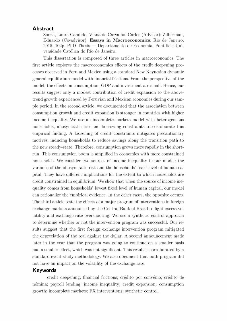
In the last decade, Latin America (LA) countries experienced significant
growth in different types of credits, which remained sustained despite of the
fact that these economies were affected by the last financial crisis.2 As shown
in Figure 1.1, the domestic credit as a percentage of GDP in many countries
of LA has shown an increasing trend, specially, since 2005.
2000 2001 2002 2003 2004 2005 2006 2007 2008 2009 2010 2011 2012 201310
20
30
40
50
60
70
80
Brazil
Colombia
Ecuador
Mexico
Paraguay
Peru
Figure 1.1: Domestic credit to private sector over GDP. Domestic credit to
private sector refers to financial resources provided to the private sector, such
as through loans, purchases of nonequity securities, and trade credits and other
accounts receivable that establish a claim for repayment. For some countries
these claims include credit to public enterprises. Source: World Bank, available
at data.worldbank.org.
1This is a joint work with Nilda Pasca.2After the crisis, the monetary authorities have adopted various measures to mitigate the
effect of the crisis on their economies.

Essays in Macroeconomics 14
During this period, there were also several structural changes in LA,
which allowed these economies to maintain macroeconomic stability and higher
economic dynamism. For this reason, the expansion of credit is often cited as
one of the factors that contributed to their growth. In this paper, we follow
Carvalho et al. (2014) to quantify the macroeconomic effects of the credit
deepening in LA, in particular, in Peru and Mexico.
To achieve our goal, we calibrate a New Keynesian dynamic general
equilibrium model with financial frictions for Mexican and Peruvian economies.
We consider an economy populated by patient households that engage with
impatient households and entrepreneurs in the credit market through a stylized
banking sector. Both impatient households and entrepreneurs face credit
constraints.
Concerning the impatient households, the amount they can borrow is
constrained by their next period’s labor income and by the value of their
next period’s stock of housing. We do so motivated by the fact that in many
countries of LA, as in Peru and Mexico, a sizable part of the increase of credit
directed to households was due to a type of credit that is not associated with
any type of collateral, known as “payroll loan.”In particular, this type of credit
is part of the personal credit and the borrowers are charged directly from their
payroll. Note that this type of credit has different names in different countries of
LA. For example, in Peru, this type of credit is called “credito por convenio,”in
Brazil, “credito consignado,”in Colombia, “libranza,” and in Mexico, “credito
de nomina.”
We also consider that the amount that impatient households can borrow
is tied to the value of their next period’s stock of housing. Our motivation is
due to the intense growth of housing credit experienced by several countries of
LA in recent years. For example, in Peru, the expansion of this type of credit
was accompanied by a boom in the construction sector, mainly real estate.3
Moreover, in Mexico, recently, the allocation of new loans for housing credit
tripled, without considering the subsidized housing credit by the government.
In addition, we consider that entrepreneurs are credit constrained by the
value of their collateral asset. In their case, this asset is capital. Hence, we
incorporate credit to corporations into our model. As depicted in Figure 1.2,
for Peru, this type of credit has increased significantly, growing at a higher
rate than credit to households, whereas for Mexico, the opposite occurs.
We calibrate the model to replicate the credit expansion experienced
by Peru between 2007 and 2012, and by Mexico between 2006 and 2013. In
3In 2008, the construction sector grew 16.5% being one of the sectors that led the PeruvianGDP to grow 9.84% in this year.

Essays in Macroeconomics 15
particular, we calibrate the credit trajectories of the model to match the credit
expansion in data, both credit to corporations and households - including
personal and housing credit (see Figure 1.3). We exogenously perturb three
time-varying parameters that dictate the tightness of the credit constraints for
impatient households and entrepreneurs to match their counterparts in data.
The purpose of this exercise is consistent with the idea that a large fraction
of these credit expansions was due to exogenous policies that fueled these
credit deepening processes. In Peru, there were reforms to stimulate credit
to households since 2008. In 2010, a law was promulgated to allow credito
por convenio. Since then, this type of credit has shown a strong growth rate,
between 2010 and 2012, its participation in personal credit rose from 14.7%
to 21.1%. For Mexico, we were not able to find a law related to credito de
nomina, but through data available, we found that this type of credit started
in 2011.
2007 2008 2009 2010 2011 20125
10
15
20
25
30(a) Peru
Households
Corporations
Total
2006 2007 2008 2009 2010 2011 2012 20135
10
15
20
25 (b) Mexico
Figure 1.2: Nonearmarked credit outstanding to GDP ratio in Peru and
Mexico, by borrower type. Source: Central Reserve Bank of Peru, available
at www.bcrp.gob.pe; Bank of Mexico, available at www.banxico.org.mx.

Essays in Macroeconomics 16
2007 2008 2009 2010 2011 20120
2
4
6
8
10
12(a) Peru
Personal Credit
Housing Credit
Total (Households)
2006 2007 2008 2009 2010 2011 2012 20132
4
6
8
10
12
14
16 (b) Mexico
Figure 1.3: Ratio of households nonearmarked credit outstanding to GDP
in Peru and Mexico, by type. Central Reserve Bank of Peru, available at
www.bcrp.gob.pe; Bank of Mexico, available at www.banxico.org.mx.
From the perspective of our calibrated model, the aggregate effects of the
credit deepening process witnessed in Peru and in Mexico are modest. In the
case of Peruvian economy, GDP increases only 1.5 percent, consumption barely
grows 0.7 percent and investment increases 2.5 percent during the period under
review. For Mexican economy, credit deepening increases GDP by almost 0.7%
between first quarter of 2006 and third quarter of 2013. During the same period,
consumption barely increases and investment grows only 1.3 percent. However,
our model does not consider trend growth. For this reason, we need to compare
the results generated by our model with above-trend growth experienced by
Peru and Mexico during the period of analysis to quantify the macroeconomics
effects of these credit deepening processes. If one assumes a trend growth of 5.0
percent per year for Peru, the credit expansion process accounts for 15.6, 6.8
and 3.7 percent of above-trend growth in GDP, consumption and investment,
respectively. For Mexico, if we consider a trend growth of 1.5 percent per year,
credit deepening accounts for 9.6, 3.5 and 8.4 percent of above-trend growth
in GDP, consumption and investment, respectively. Hence, our results suggest
that the macroeconomic implications of these credit expansions are modest
and accounted for a mild part of above trend growth of these economies.
The remainder of the paper is organized as follows. Section 1.2 presents
the related literature. Section 1.3 outlines the baseline model. Section 1.4
describes the quantitative analysis, including the calibration procedure, results
and sensitivity analysis. Finally, section 1.5 concludes.

Essays in Macroeconomics 17
1.2Related Literature
Our work belongs to a burgeoning strand of literature that incorporates
financial frictions into New Keynesian models. This literature builds on the
seminal works by Bernanke et al. (1999) and Kiyotaki and Moore (1997). For
recent surveys, see Gertler and Kiyotaki (2010), Liu et al. (2013), Iacovello
(2014) and Justiniano et al. (2014).
There is a limited literature for Peru and Mexico that uses financial
frictions. Recently, some papers use New Keynesian (DSGE) models with
financial frictions to address questions related to these countries – e.g., Castillo
et al. (2014); Mendoza (2010). However, none of these studies is concerned with
the main question of this paper.
Our paper is closely related to Carvalho et al. (2014). Our analyses differ
in that, in addition to what they did, we entertain an open-economy version
of the model, and experiment with different assumptions about the extent to
which the credit deepening process was anticipated. In addition, we contribute
to the literature on Latin American economies by providing, to our knowledge,
the first assessment of the macroeconomic effects of credit expansions observed
in Mexico and Peru.
Similar to Carvalho et al. (2014), we consider the following financial fric-
tions. First, a la Kiyotaki and Moore (1997) and Iacovello (2005), we bind the
amount that the entrepreneurs can borrow to the value of their collateral asset,
in this case, capital. Note that, through relaxing this borrowing constraint, we
can replicate the credit expansion we observe for corporations. Second, we tie
the capacity of the impatient household to borrow to his collateral given by
the future labor income and, different from Carvalho et al. (2014), we consider
housing as well. This financial friction is in line with Peruvian and Mexican
experiences, where these types of collateral played a prominent role. Therefore,
by relaxing this financial friction, we can emulate consumer credit (personal
and housing credit) expansion we observe in practice.
At last, we follow Curdia and Woodford (2010) for modelling the banking
sector in which we can generate an endogenous spread between borrowing and
lending rates.
1.3The Baseline Model
This section presents the quantitative model used to analyze the macroe-
conomics effects of credit expansion in Peru and Mexico, which follows the one
in Carvalho et al. (2014). It features eight types of agents: patient households
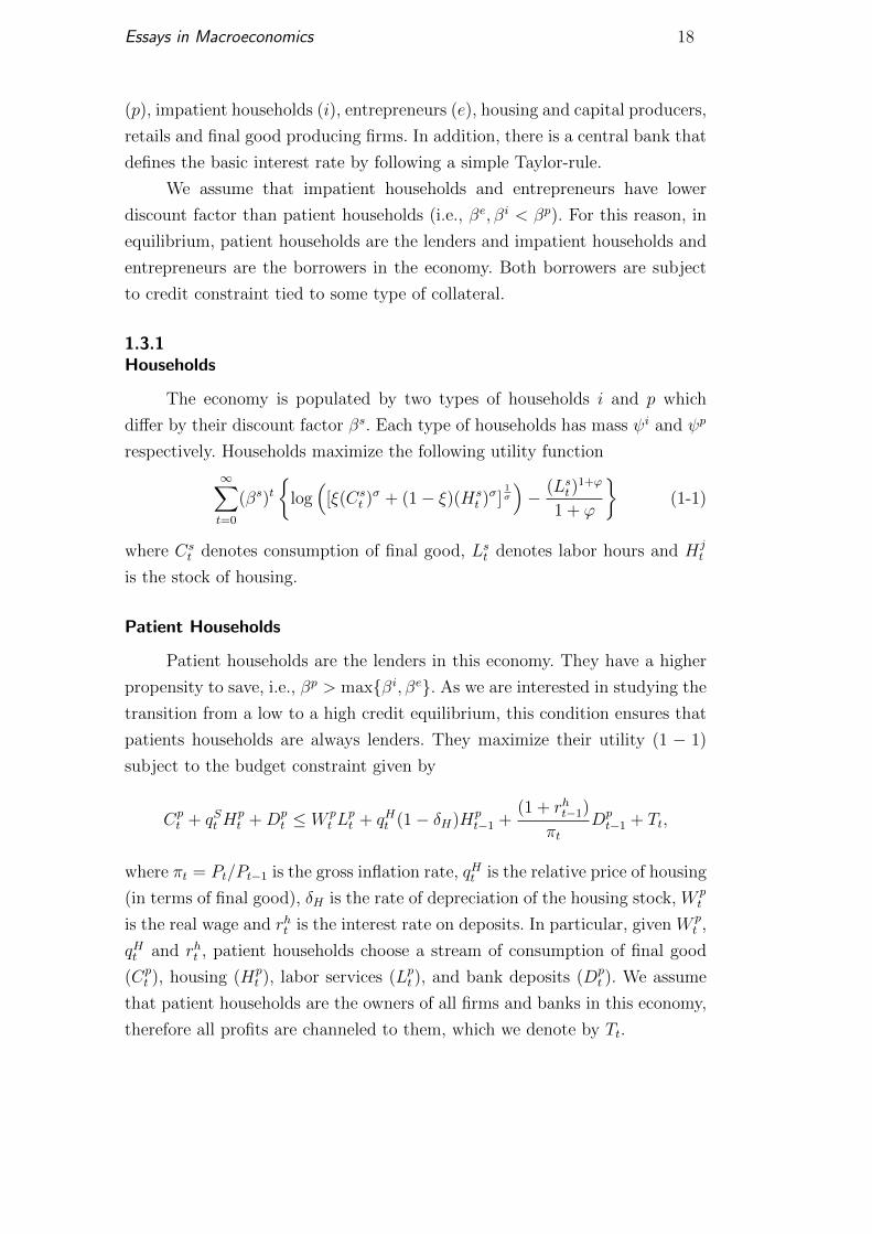
Essays in Macroeconomics 18
(p), impatient households (i), entrepreneurs (e), housing and capital producers,
retails and final good producing firms. In addition, there is a central bank that
defines the basic interest rate by following a simple Taylor-rule.
We assume that impatient households and entrepreneurs have lower
discount factor than patient households (i.e., βe, βi < βp). For this reason, in
equilibrium, patient households are the lenders and impatient households and
entrepreneurs are the borrowers in the economy. Both borrowers are subject
to credit constraint tied to some type of collateral.
1.3.1Households
The economy is populated by two types of households i and p which
differ by their discount factor βs. Each type of households has mass ψi and ψp
respectively. Households maximize the following utility function
∞∑t=0
(βs)t{
log(
[ξ(Cst )σ + (1− ξ)(Hs
t )σ]
1σ
)− (Lst)
1+ϕ
1 + ϕ
}(1-1)
where Cst denotes consumption of final good, Lst denotes labor hours and Hj
t
is the stock of housing.
Patient Households
Patient households are the lenders in this economy. They have a higher
propensity to save, i.e., βp > max{βi, βe}. As we are interested in studying the
transition from a low to a high credit equilibrium, this condition ensures that
patients households are always lenders. They maximize their utility (1 − 1)
subject to the budget constraint given by
Cpt + qSt H
pt +Dp
t ≤ W pt L
pt + qHt (1− δH)Hp
t−1 +(1 + rht−1)
πtDpt−1 + Tt,
where πt = Pt/Pt−1 is the gross inflation rate, qHt is the relative price of housing
(in terms of final good), δH is the rate of depreciation of the housing stock, W pt
is the real wage and rht is the interest rate on deposits. In particular, given W pt ,
qHt and rht , patient households choose a stream of consumption of final good
(Cpt ), housing (Hp
t ), labor services (Lpt ), and bank deposits (Dpt ). We assume
that patient households are the owners of all firms and banks in this economy,
therefore all profits are channeled to them, which we denote by Tt.
Essays in Macroeconomics 19
Impatient Households
Impatient households are one of the borrowers in this economy (i.e.,
βi < βp). They maximize (1 − 1) subject to a budget and a borrowing
constraint. The first one is given by
Cit + qHt H
it +
1 + rht−1πt
Bit−1 ≤ W i
tLit + qHt (1− δH)H i
t−1 +Bit,
And the second constraint is the following
(1 + rht )Bit ≤ τWL
t πt+1Wit+1L
it+1 + τHt q
Ht+1πt+1(1− δH)H i
t .
Then, given W it , q
Ht and rht , impatient households choose a stream of consump-
tion of final good (Cit), housing (H i
t), labor services (Lit), and debt (Bit).
Similar to Kiyotaki and Moore (1997), Iacoviello (2005) and Gerali et al.
(2010), households’ ability to borrow is limited to a fraction τHt of the value of
next period’s stock of housing, plus a fraction τWLt of the value of next period’s
labor income, which is similar to Carvalho et al. (2014).
Adjusting the collateral requirements by changing τWLt to replicate
the expansion of personal credit (which includes credito convenio for Peru
and credito de nomina for Mexico) and also τHt to study the expansion of
collateralized credit, i.e. mortgage credit for households, we can study the
macroeconomic effects of such credit expansion over the period of analysis. In
addition, we assume that the household credit rates and the deposit rate rht
are the same, motivated by the fact that payroll loan and, mainly, consumer
credits apply the lowest interest rate.
1.3.2Entrepreneurs
The economy is also populated by entrepreneurs that have mass ψe. They
have the following utility function
∞∑t=0
(βe)t log(Cet ), (1-2)
where Cet is their consumption of final good.
As for impatient households, entrepreneurs are also borrowers agents in
the economy (i.e., βe < βp). They use capital Kt and labor (Lpt , Lit) as inputs
to produce a wholesale good Y et applying the following production function
Y et = Kα
t−1[(µpLpt )
θ(µiLit)1−θ]1−α,
Essays in Macroeconomics 20
where Y et denotes the output for each entrepreneur, Kt−1 denotes the capital
input with its share given by the parameter α ∈ (0, 1) and as in Iacoviello and
Neri (2010), we assume complementarity across labor types Lpt and Lit, which
participation is measured by the parameter θ ∈ (0, 1).
Entrepreneurs maximize their utility function subject to the budget
constraint
Cet +W p
t Lpt +W i
tLit +
(1 + ret−1)Bet−1
πt+ qKt Kt ≤ qWt Y
et +Be
t + qKt (1− δK)Kt−1,
where δK is the depreciation rate of capital, qKt is the price of capital in terms
of the final good, and qWt ≡ PWt /Pt is the relative price of the wholesale good
Y et . In addition, they are borrowers agents subject to a borrowing constraint
given by
(1 + ret )Bet ≤ τKt q
Kt+1πt+1(1− δK)Kt,
where ret is the nominal interest rate faced by entrepreneurs.4 The amount
that entrepreneurs can borrow is limited by a fraction τKt of the value of the
collateral asset. In their case, this asset is capital.
Finally, we interpret τKt as an exogenous shock on the entrepreneurs’
ability to borrow. Thus, imposing an exogenous path to τKt , we can replicate
the expansion of corporate credit in Peru and Mexico and study the macroe-
conomics effects of the expansion credit over the period of analysis.
1.3.3Firms
In this section, we study four types of firms: retail firms operating in a
monopolistic competitive market, final goods producers, producers of housing
and capital producers. All firms are owned by patient households.
Retail Firms and Final Goods Producers
Retailers buy the intermediate good from entrepreneurs at the wholesale
price PWt . It takes one unit of intermediate output to make a unit of retail
output. We introduce nominal rigidities through Rotemberg pricing scheme.
In particular, we assume that each firm operates in a monopolistic competitive
environment and faces a quadratic cost for adjusting the nominal prices.
Moreover, each retailer’s price is indexed to a combination of past and steady-
state inflation with relative price equal to ι and (1− ι), respectively.
4In the section of Banks, we explain how the credit spread, ωt = (1 + ret )/(1 + rht )− 1, isdetermined endogenously.

Essays in Macroeconomics 21
Final good producers are competitive, and their role is to simply aggreg-
ate, using a CES composite, the continuous sequence of differentiated varieties
produced by retailers. The final output composite is given by
Yt =
[∫ 1
0
Yt(f)ε−1ε df
] εε−1
,
where Yt(f) is the output produced by retailer f , ε is the elasticity of sub-
stitution between varieties and Pt is the associated Dixit-Stiglitz price index.
This final good is purchased by patient households, impatient households and
entrepreneurs for consumption, and by capital goods and housing producers
for production.
Retailer pricing problem is to choose the optimal price Pt(f) that solves
the maximization of its profit
∞∑t=0
∆t
[Pt(f)Yt(f)− PW
t Yt(f)− κP2
(Pt(f)
Pt(f − 1)− πιt−1π1−ι
)2
PtYt
],
subject to a demand schedule deriving from the cost-minimization problem of
final goods producers
Yt(f) =
(Pt(f)
Pt
)−εYt.
where the parameter κP rules the degree of price stickiness, Rotemberg type,
and π denotes steady-state inflation. Finally, all profits generated in this sector
are transferred to patient households.
Producers of Housing
At the beginning of each period t, the production of new housing is
performed by competitive firms. They buy an amount of final good IHt from
final goods firms and the stock of undepreciated housing (1 − δH)Ht−1 at
relative price qHt from both patient and impatient households. The stock
of undepreciated housing is transformed one-to-one into new housing, while
the transformation of final goods into new housing is subject to a quadratic
adjustment cost. Then, the level of production is chosen to maximize
∞∑t=0
∆t[qHt (Ht − (1− δH)Ht−1)− IHt ],
subject to the following law of motion of housing
Ht = (1− δH)Ht−1 +
[1− κH
2
(IHtIHt−1− 1
)2]IHt ,

Essays in Macroeconomics 22
where κH > 0 is the adjustment cost parameter and, ∆t is the stochastic
discount factor of patient households. The new capital Ht is sold at relative
price qHt to both patient and impatient households.
Capital Producers
At the beginning of each period t, competitive capital producing firms
buy a stock of undepreciated capital (1 − δK)Kt−1 from entrepreneurs at a
nominal price qKt and an amount of the final good IKt from final goods firms.
The undepreciated capital is transformed one-to-one into new capital, while
the transformation of final goods into new capital is subject to a quadratic
adjustment cost. Then, the level of production is chosen to maximize
∞∑t=0
∆t[qKt (Kt − (1− δK)Kt−1)− IKt ],
subject to the following law of motion of capital
Kt = (1− δK)Kt−1 +
[1− κK
2
(IKtIKt−1− 1
)2]IKt ,
where κK > 0 is the adjustment cost parameter and, ∆t is the stochastic
discount factor of patient households. The new capital Kt is sold back to
entrepreneurs at relative price qKt .
1.3.4Banks
We assume competition among banks, both in the loan market and
deposit market. Thus, rht and ret are taken as given. Each bank collects deposits
from patient households Dt, which are used as resources to lend to impatient
households and entrepreneurs. Following Curdia and Woodford (2010), we
consider that there is a real resource cost in loans to entrepreneurs. Such cost
is given by η(Bet )γ, where η > 0 and γ > 1, and it can be interpreted as agency
and operational costs that are not considered in our model.
All excess funds of the banks are transferred to patient households,
Dt − Bet − Bi
t − η(Bet )γ. Credit spread ωt is defined implicitly by (1 + ret ) =
(1 +ωt)(1 + rht ). Since assets must be equal to liabilities Dt = (1 +ωt)Bet +Bi
t,
it follows thatωtB
et − η(Be
t )γ (1-3)
Thus, banks maximize (1 − 3) to choose Bet . The first order condition for

Essays in Macroeconomics 23
optimal credit supply is given by
Bet = (ηγ/ωt)
1/(1−γ)
Note that, since γ > 1, there is a positive correlation between the credit spread
ωt and loans to entrepreneurs Bet .
1.3.5Monetary Policy
We assume that monetary policy is conducted by means of a Taylor-type
interest rate rule of the form
(1 + rht ) = (1 + r)1−ρ(1 + rht−1)ρ(πtπ
)φπ(1−ρ)( ytyt−1
)φy(1−ρ),
where ρ is the parameter that measures the smoothing of the interest rate,
φπ and φy are the weights assigned to inflation and output stabilization,
respectively, and π and r are the steady-state levels of inflation and the policy
rate, respectively.
1.3.6Market Clearing
The market clearing condition for the wholesale good is given by:∫ 1
0
Yt(m)dm = µeY et .
Equilibrium in the final good market is expressed by the resource
constraint:
Yt = Ct + IHt + IKt + η(Bet )γ + all adjustment costs.
where Ct = µpCpt + µiCi
t + µeCet .
We consider that both types of labor markets are competitive.
1.4Quantitative Analysis
We calibrate our baseline model, then we use it to quantify the mac-
roeconomic effects of the credit expansion observed in Peru and Mexico by
solving for the time-varying paths of τWLt , τHt and τKt that generate paths for
personal credit, housing credit to households, and credit to corporations that
correspond their counterparts in the data (see Figures 1.2 and 1.3). Due to

Essays in Macroeconomics 24
a better data availability for the calibration of the model, we focus in Per-
uvian economy in the main body of our paper and we present the quantitative
analysis for Mexico in the appendix. In addition, we perform some sensitivity
analysis to test the robustness of our results.
1.4.1Calibration
Table 1.1 lists the choice of parameter values for our baseline model that
matches with the statistics for Peruvian economy. We consider its average
between 2007 and 2012. Time is in quarters. Steady state inflation is 3.37% to
match the average inflation rate for the period. We use βp = 0.9984 to generate
an average interbank nominal interest rate (proxy of monetary policy rate) of
4.03%.
We set the discount factor of impatient and entrepreneurs agents as
βi = βe = 0.91, implying an annual time-discount rate of 52 percent. We
calibrate this extreme value motivated, mainly, to maintain the borrowing
constraints active during all the transition period and because with a greater
degree of impatience, i.e βi,e < βp, the model increases its capacity to produce
significant aggregate effects.
We also pick the inverse of the Frisch elasticity of labor supply equal to
ϕ = 2. This value is standard in the literature for Peruvian economy. Following
Fernandez-Villaverde and Krueger (2004), we calibrate the parameters asso-
ciated with preferences for final goods and housing in the utility function. In
the absence of estimates for σ, we set it to zero. Then, the aggregator func-
tion takes a Cobb-Douglas form (Cjt )ξ(Hj
t )1−ξ, j = i, p. We define the share
of consumption of final goods and housing in the Cobb-Douglas aggregator of
the utility with ξ equals to 0.8.
For the capital share in the entrepreneurs’ production function, we choose
α = 0.26 following Castillo et al. (2009). Since information on patient and
impatient labor income shares in Peru is not available, we set θ = 0.7 following
Carvalho et al. (2014). The depreciation rates for capital and housing are set,
respectively, to δK = δH = 0.025. The adjustment cost parameter for capital
and housing is set κK = κH = 2.53 following Carvalho et al. (2014).
The parameter governing price stickiness (Rotemberg adjustment cost)
in the retail sector κP is set at 58 which is equivalent to 0.75 in the Calvo
model. As usual, it is possible to map these two types of price stickiness since
this entails the same first order dynamics of the two models in the case of zero
steady state inflation. The elasticity of substitution between varieties is ε = 6,
which yields a steady state mark-up of 20 percent. Finally, ι, which governs

Essays in Macroeconomics 25
indexation, is set to 0.158, as in Gerali et al.(2010).
For the monetary policy rule, we use estimates from Castillo et al. (2009).
In particular, we choose φy = 0.16, φπ = 1.5 and ρ = 0.79.
Concerning the calibration of the banking sector parameters, we set γ = 2
and η = 0.01 to generate a spread of roughly 0.7 percent per year. This value
corresponds to the average difference between the corporate prime interest rate,
which is the lending interest rate that banks charge their best corporate clients
and the reference interest rate, which is the interest rate that BCRP fixes in
order to establish a level of reference interest rate for interbank transactions.
Loans to these firms embed lower default risk than loans to other firms. Hence,
the targeted value of 0.7 percent per year underestimates the average spread in
Peruvian economy. As we show below, in the sensibility section, the calibration
of γ and η helps to produce more significant aggregate effects in response to the
credit deepening process. Finally, the masses of different agents in the economy
ψp, ψi and ψe is set to one.
Parameter Description Value
βp Discount Factor - Patients 0.9984
βi, βe Discount Factor - Impatients and Entrepreneurs 0.91
ψp, ψi, ψe Mass - Patients, Impatients and Entrepreneurs 1
ϕ Inverse of the Frisch Elasticity 2
σ Elasticity Between Final Good and Housing 0
ξ Weight of the Final Good on the Utility Function 0.8
δK , δS Depreciation - Capital Goods and Housing 0.025
κK , κS Adjustment Cost - Capital Goods and Housing 2.53
α Capital Share in the Production Function 0.26
θ Share of Patient Households in the Production Function 0.7
κP Price Adjustment Cost - Final Good 58
ι Steady State Inflation Weight - Indexation 0.158
ε Elasticity of Substitution - Final Good 6
ρ Smoothing Parameter of the Taylor Rule 0.7
φy Output Weight of Taylor Rule 0.1
φπ Inflation Weight of Taylor Rule 1.5
η Spread 0.008
γ Spread 2
Table 1.1: Calibration: Peruvian Economy.
Essays in Macroeconomics 26
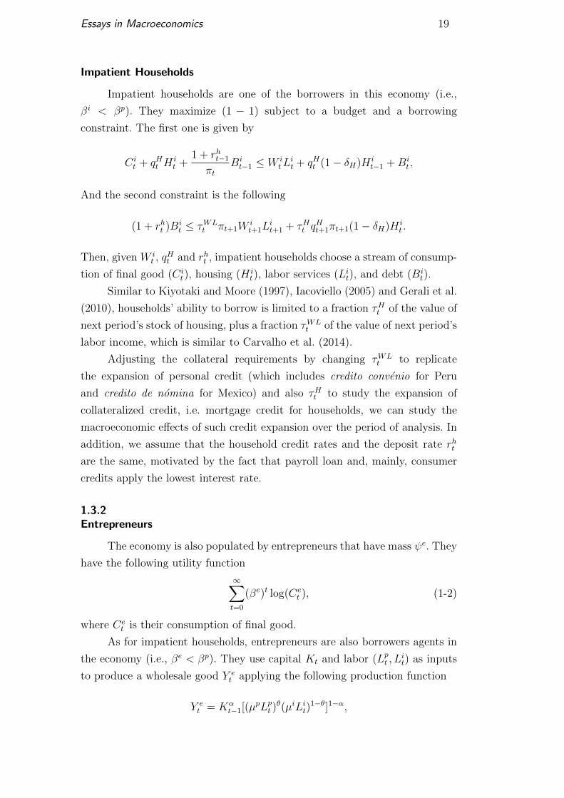
1.4.2Results
In this section, we study the macroeconomics effects of a credit deepening
using the calibrated model for Peruvian economy.5 For such aim, we solve
for the time-varying paths of τWLt , τHt and τKt that generate paths for
personal credit, housing credit to impatient households and corporate credit for
entrepreneurs. We follow Justiano et al. (2014) and assume that the evolution
of τWLt , τHt and τKt are perfectly foreseen after the start of the credit expansion
process in 2007, which is an initial unforeseen shock. After 2012, we set τWLt ,
τHt and τKt constant. In addition, we smooth the paths of τWLt , τHt and τKt
using a third degree polynomial.
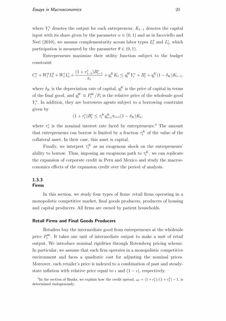
Figure 1.4 shows their calibrated paths and Figure 1.5 compares the
credit expansion generated by our model and their counterparts in the data.
Note that our model replicates well enough the trajectories of considered types
of credit during the period of analysis.6
2006 2007 2008 2009 2010 2011 2012
0.05
0.06
0.07
0.08
0.09
0.1
0.11
τK
2006 2007 2008 2009 2010 2011 2012
0.18
0.2
0.22
0.24
0.26
0.28
0.3
0.32
0.34
0.36
τWL
2006 2007 2008 2009 2010 2011 2012
0.04
0.05
0.06
0.07
0.08
0.09
0.1
0.11
τH
Figure 1.4: Credit deepening experiment for Peru: evolution of τKt , τWLt and
τHt .
5We used the shooting algorithm in Dynare to solve our model.6Carvalho et al. (2014) report, through a robustness test, that their results do not change
once they considered non-smooth paths.
Essays in Macroeconomics 27
2006 2007 2008 2009 2010 2011 20123
3.5
4
4.5
5
5.5
6
6.5
Personal Credit to Impatient Households over GDP(%)
Data
Model
2006 2007 2008 2009 2010 2011 20121.5
2
2.5
3
3.5
4
4.5
Housing Credit to Impatient Households over GDP (%)
2006 2007 2008 2009 2010 2011 20129
10
11
12
13
14
15
16
17
18
19
Credit to Entrepreneurs over GDP (%)
2006 2007 2008 2009 2010 2011 201214
16
18
20
22
24
26
28
30
Total Credit over GDP (%)
Figure 1.5: Credit deepening experiment for Peru: credit variables (model and
data).
The macroeconomic effects of a credit expansion in our model are depic-
ted in Figure 1.6, through the trajectories of GDP, consumption, investment
and inflation. The aggregate implications are small in absolute terms. Among
the main key variables, investment increases 2.5 percent, which is the highest
macroeconomic effect followed by GDP that increases 1.5 percent. Finally,
consumption barely grows 0.75 percent.

Essays in Macroeconomics 28
2006 2007 2008 2009 2010 2011 2012
100
100.2
100.4
100.6
100.8
101
101.2
101.4
101.6
GDP
2006 2007 2008 2009 2010 2011 2012100
100.1
100.2
100.3
100.4
100.5
100.6
100.7
100.8
Consumption
2006 2007 2008 2009 2010 2011 201299.5
100
100.5
101
101.5
102
102.5
103
Investment
2006 2007 2008 2009 2010 2011 20123.35
3.4
3.45
3.5
3.55
3.6
3.65
3.7
3.75
3.8
3.85
Inflation (% p. y.)
Figure 1.6: Credit deepening experiment for Peru: macro variables (model).
Concerning the effects on disaggregated level, the evolution of investment
as well as the stock of housing, capital and consumption of final goods for all
agents in the model are presented in Figure 1.7. Note that when collateral
constraints are loosened for impatient households and entrepreneurs, their
consumption and investment in housing and in capital, respectively, increase.
As a consequence of a higher demand, the price of the final good increases (see
Figure 1.6) and patient households reduce their consumption of final goods and
investment in housing. As the process evolves, consumption and investment of
patient households also increase.
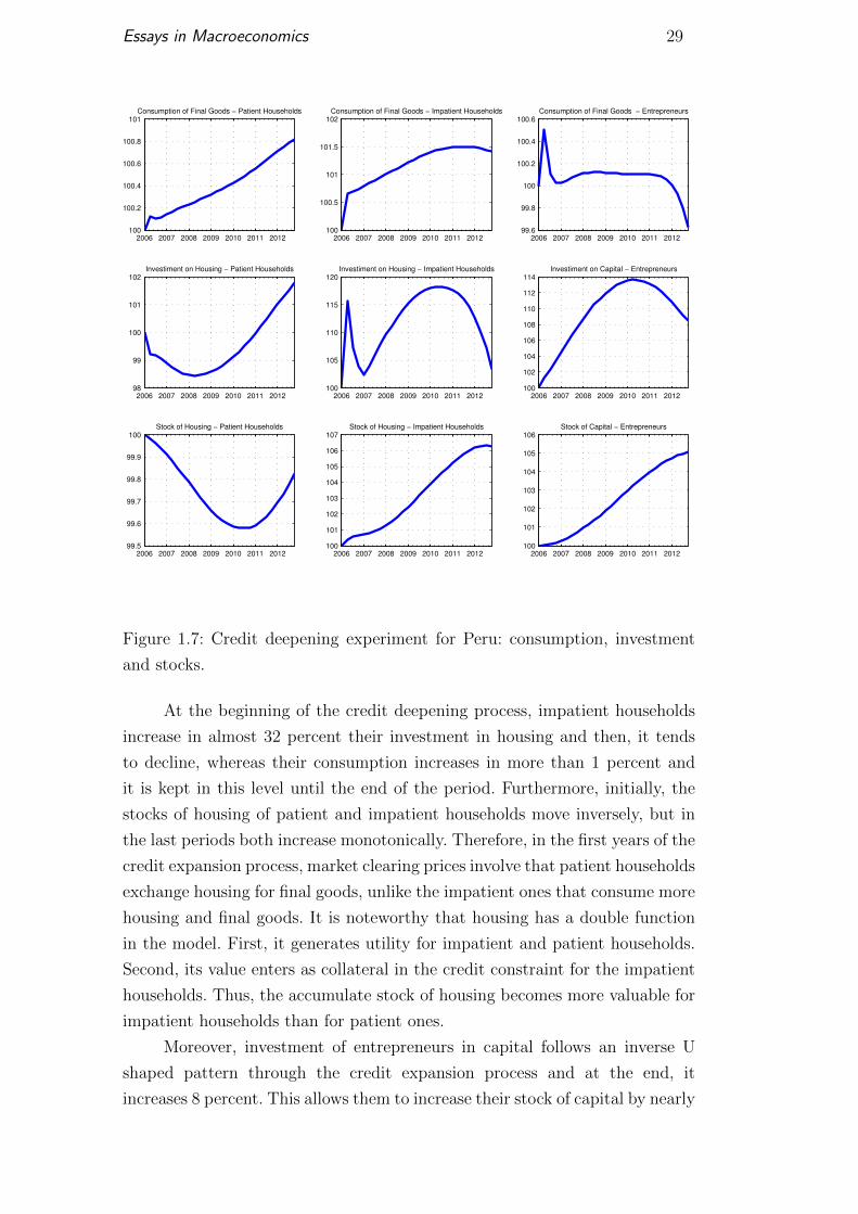
Essays in Macroeconomics 29
2006 2007 2008 2009 2010 2011 2012100
100.2
100.4
100.6
100.8
101Consumption of Final Goods − Patient Households
2006 2007 2008 2009 2010 2011 2012100
100.5
101
101.5
102Consumption of Final Goods − Impatient Households
2006 2007 2008 2009 2010 2011 201299.6
99.8
100
100.2
100.4
100.6Consumption of Final Goods − Entrepreneurs
2006 2007 2008 2009 2010 2011 201298
99
100
101
102Investiment on Housing − Patient Households
2006 2007 2008 2009 2010 2011 2012100
105
110
115
120Investiment on Housing − Impatient Households
2006 2007 2008 2009 2010 2011 2012100
102
104
106
108
110
112
114Investiment on Capital − Entrepreneurs
2006 2007 2008 2009 2010 2011 201299.5
99.6
99.7
99.8
99.9
100Stock of Housing − Patient Households
2006 2007 2008 2009 2010 2011 2012100
101
102
103
104
105
106
107Stock of Housing − Impatient Households
2006 2007 2008 2009 2010 2011 2012100
101
102
103
104
105
106Stock of Capital − Entrepreneurs
Figure 1.7: Credit deepening experiment for Peru: consumption, investment
and stocks.
At the beginning of the credit deepening process, impatient households
increase in almost 32 percent their investment in housing and then, it tends
to decline, whereas their consumption increases in more than 1 percent and
it is kept in this level until the end of the period. Furthermore, initially, the
stocks of housing of patient and impatient households move inversely, but in
the last periods both increase monotonically. Therefore, in the first years of the
credit expansion process, market clearing prices involve that patient households
exchange housing for final goods, unlike the impatient ones that consume more
housing and final goods. It is noteworthy that housing has a double function
in the model. First, it generates utility for impatient and patient households.
Second, its value enters as collateral in the credit constraint for the impatient
households. Thus, the accumulate stock of housing becomes more valuable for
impatient households than for patient ones.
Moreover, investment of entrepreneurs in capital follows an inverse U
shaped pattern through the credit expansion process and at the end, it
increases 8 percent. This allows them to increase their stock of capital by nearly

Essays in Macroeconomics 30
5 percent. Also, at the beginning, their consumption of final goods increases
by almost 3 percent, but the cumulative effect at the end of the process is zero.
Overall, our model implies that the effects are larger for impatient
households, specially, on their investment in housing that increases almost
3 percent and their consumption that rises 1.4 percent.
Figure 1.8 presents the evolution of labor market outcomes. Once credit
expansion started, labor services and wages of patient and impatient house-
holds move in the same direction, but in different magnitudes. For impatient
households, their labor services increase more than their wages, which reflects
an extra motive to supply labor due to the fact that it relaxes their credit
constraint. For patient households, their wages increase more than their labor
services, which could be explained by forces coming from the side of labor de-
mand. The same interpretations are valid for the cumulative effect at the end
of the period.
2006 2007 2008 2009 2010 2011 2012100
100.1
100.2
100.3
100.4
100.5
100.6
100.7
100.8
100.9
101
Wage − Impatient Households
2006 2007 2008 2009 2010 2011 2012100
100.5
101
101.5
Wage − Patient Households
2006 2007 2008 2009 2010 2011 2012
99.9
100
100.1
100.2
100.3
100.4
100.5
100.6
Labor Services − Impatient Households
2006 2007 2008 2009 2010 2011 201299.9
99.95
100
100.05
100.1
100.15
100.2
100.25
Labor Services − Patient Households
Figure 1.8: Credit deepening experiment for Peru: labor market outcomes.

Essays in Macroeconomics 31
Figure 1.9 illustrates the evolution for the interest rates and the spread.
At the beginning of the period, the deposit interest rate set by the Central Bank
increases around 0.4 percentage points and as the credit deepening process
unfolds, this interest rate fluctuates between 4.0-4.5 percent. Concerning the
interest rate faced by entrepreneurs, at first, it rises substantially and so does
the spread. This behavior is due to the fact that credit to entrepreneurs
increases, then the intermediation costs associated with these funds also
increases, which leads to higher interest rate and spread.
2006 2007 2008 2009 2010 2011 20124
4.05
4.1
4.15
4.2
4.25
4.3
4.35rh (% p.y.)
2006 2007 2008 2009 2010 2011 20124.5
4.6
4.7
4.8
4.9
5
5.1
5.2
5.3
5.4
5.5
re (% p.y.)
2006 2007 2008 2009 2010 2011 20120.2
0.4
0.6
0.8
1
1.2
1.4
1.6
1.8
Spread (% p.y.)
Data
Model
Figure 1.9: Credit deepening experiment for Peru: financial market outcomes.
The spread is calculated using the BCRP reference interest rate, which is the
interest rate that the BCRP fixed in order to establish a level of reference
interest rate for interbank transactions, and the Corporate prime interest rate,
which is the lending interest rate that banks charge their best corporate clients.
Source: Central Reserve Bank of Peru, available at www.bcrp.gob.pe.
In conclusion, these results suggest that the credit deepening experienced
by Peru had relatively modest effects on its main macroeconomic variables.
However, our model do not consider trend growth. For this reason, we follow
Carvalho et al. (2014) and consider six scenarios for trend growth for Peru,
in particular, a range between 3.5 to 6 percent per year, so we can quantify
the share of above-trend growth in GDP, consumption and investment between
2007 and 2012 that can be explained by the credit expansion. For each scenario,
we divide the cumulative effect in our model for each aggregate variable by the
cumulative above-trend growth in the real data.
Among the different scenarios depicted in Table 1.2, we highlight the
trend growth of 5.0 percent per year. In this case, the credit expansion
process accounts for 15.6, 6.8 and 3.7 percent of above-trend growth in GDP,
consumption and investment, respectively. If we consider the worst scenario for
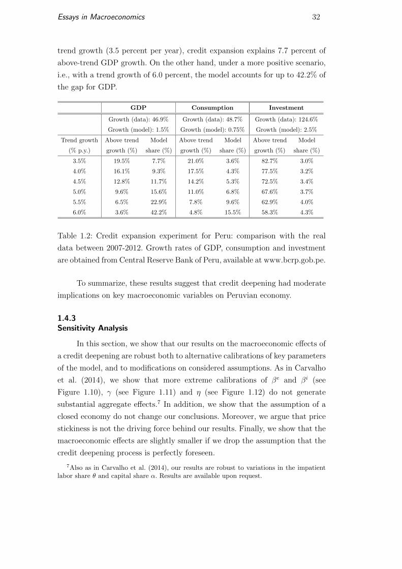
Essays in Macroeconomics 32
trend growth (3.5 percent per year), credit expansion explains 7.7 percent of
above-trend GDP growth. On the other hand, under a more positive scenario,
i.e., with a trend growth of 6.0 percent, the model accounts for up to 42.2% of
the gap for GDP.
GDP Consumption Investment
Growth (data): 46.9% Growth (data): 48.7% Growth (data): 124.6%
Growth (model): 1.5% Growth (model): 0.75% Growth (model): 2.5%
Trend growth Above trend Model Above trend Model Above trend Model
(% p.y.) growth (%) share (%) growth (%) share (%) growth (%) share (%)
3.5% 19.5% 7.7% 21.0% 3.6% 82.7% 3.0%
4.0% 16.1% 9.3% 17.5% 4.3% 77.5% 3.2%
4.5% 12.8% 11.7% 14.2% 5.3% 72.5% 3.4%
5.0% 9.6% 15.6% 11.0% 6.8% 67.6% 3.7%
5.5% 6.5% 22.9% 7.8% 9.6% 62.9% 4.0%
6.0% 3.6% 42.2% 4.8% 15.5% 58.3% 4.3%
Table 1.2: Credit expansion experiment for Peru: comparison with the real
data between 2007-2012. Growth rates of GDP, consumption and investment
are obtained from Central Reserve Bank of Peru, available at www.bcrp.gob.pe.
To summarize, these results suggest that credit deepening had moderate
implications on key macroeconomic variables on Peruvian economy.
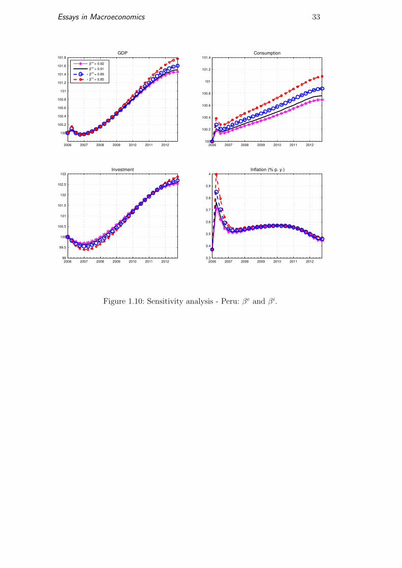
1.4.3Sensitivity Analysis
In this section, we show that our results on the macroeconomic effects of
a credit deepening are robust both to alternative calibrations of key parameters
of the model, and to modifications on considered assumptions. As in Carvalho
et al. (2014), we show that more extreme calibrations of βe and βi (see
Figure 1.10), γ (see Figure 1.11) and η (see Figure 1.12) do not generate
substantial aggregate effects.7 In addition, we show that the assumption of a
closed economy do not change our conclusions. Moreover, we argue that price
stickiness is not the driving force behind our results. Finally, we show that the
macroeconomic effects are slightly smaller if we drop the assumption that the
credit deepening process is perfectly foreseen.
7Also as in Carvalho et al. (2014), our results are robust to variations in the impatientlabor share θ and capital share α. Results are available upon request.
Essays in Macroeconomics 33
2006 2007 2008 2009 2010 2011 2012
100
100.2
100.4
100.6
100.8
101
101.2
101.4
101.6
101.8
GDP
β
i,e = 0.92
βi,e
= 0.91
βi,e
= 0.89
βi,e
= 0.85
2006 2007 2008 2009 2010 2011 2012100
100.2
100.4
100.6
100.8
101
101.2
101.4
Consumption
2006 2007 2008 2009 2010 2011 201299
99.5
100
100.5
101
101.5
102
102.5
103
Investment
2006 2007 2008 2009 2010 2011 20123.3
3.4
3.5
3.6
3.7
3.8
3.9
4
Inflation (% p. y.)
Figure 1.10: Sensitivity analysis - Peru: βe and βi.

Essays in Macroeconomics 34
2004 2005 2006 2007 2008 2009 2010 2011 201299.5
100
100.5
101
101.5
102GDP
γ = 3
γ = 2
γ = 1.5
2004 2005 2006 2007 2008 2009 2010 2011 2012100
100.5
101
101.5Consumption
2004 2005 2006 2007 2008 2009 2010 2011 201299
100
101
102
103
104Investment
2004 2005 2006 2007 2008 2009 2010 2011 2012
5.4
5.5
5.6
5.7
5.8Inflation (% p. y.)
2004 2005 2006 2007 2008 2009 2010 2011 20120
2
4
6
8
10Spread (% p.y.)
Figure 1.11: Sensitivity analysis - Peru: γ.

Essays in Macroeconomics 35
2004 2005 2006 2007 2008 2009 2010 2011 201299.5
100
100.5
101
101.5
102GDP
2004 2005 2006 2007 2008 2009 2010 2011 201299.5
100
100.5
101Consumption
2004 2005 2006 2007 2008 2009 2010 2011 201299
100
101
102
103
104Investment
2004 2005 2006 2007 2008 2009 2010 2011 2012
5.4
5.5
5.6
5.7
5.8Inflation (% p.y.)
2004 2005 2006 2007 2008 2009 2010 2011 20120
5
10
15Spread (% p.y.)
η = 0.081
η =0.031
η = 0.021
Figure 1.12: Sensitivity analysis - Peru: η.
A small open economy version of our model As we mentioned before,
patient and impatient households behave in opposite ways in response to
a credit deepening, which might mitigate the aggregate effects. This occurs
because borrowers and lenders are the only agents engaged in the credit market
in our closed economy. Hence, we consider an extreme opposite case of a small
open economy (SOE) without lenders as in Justiniano et al. (2014).
In our SOE version of the baseline model, the economy is populated
by impatient households and entrepreneurs with discount factors βi and βe,
respectively. Both types of agents borrow from abroad. We consider a constant
real world interest rate r∗, which is applied in loans for impatient households.
There is a credit spread in loans for entrepreneurs that is the same as in the
baseline. Moreover, the final goods market is competitive (i.e., there are no
retailers) and prices are flexible. Then, market clearing condition of final good
is given by
Yt + CADt = Ct + IHt + IKt + η(Bet )γ + all adjustment costs,

Essays in Macroeconomics 36
where ret is the real interest rate faced by entrepreneurs and CADt =
(Bit − (1 + r∗)Bi
t−1) + (Bet − (1 + ret )B
et−1) is the current account deficit. The
specifications for producers of housing and capital goods are the same as in
the closed economy version.
We calibrate the constant real world interest rate to 1% p.y., which is the
steady state real interest rate in our closed economy model. The paths of τWLt ,
τHt and τKt are recalculated so the model can replicate the same smooth credit
expansion as in the baseline. Finally, we set η = 0.006 to generate the same
average spread as in the closed economy. The rest of the parameters remains
unchanged.
Figure 1.13 shows these results. Consumption grows more at the begin-
ning than the closed economy, but the cumulative effect is smaller. This occurs
because, in the baseline, consumption of patient households also grows as the
credit deepening process evolves (see Figure 7). Investment expands 8 percent,
which is higher than the closed economy. GDP decreases at the beginning due
to the effect on the current account deficit of interest payments on a higher
stock of debt. Also the cumulative effect is lower. These results suggest that the
modest aggregate effects to credit expansion is not due to the closed economy
assumption.

Essays in Macroeconomics 37
2006 2007 2008 2009 2010 2011 2012
100
100.2
100.4
100.6
100.8
101
101.2
101.4
101.6
GDP
SOE
Benchmark
2006 2007 2008 2009 2010 2011 2012100
100.1
100.2
100.3
100.4
100.5
100.6
100.7
100.8
100.9
101
Consumption
2006 2007 2008 2009 2010 2011 201299
100
101
102
103
104
105
106
107
108
109
Investment
2006 2007 2008 2009 2010 2011 2012−0.4
−0.2
0
0.2
0.4
0.6
0.8
1
Current Account Deficit to GDP (%)
Figure 1.13: Sensitivity analysis - Peru: Small open economy-macro variables
(model).
Flexible prices One may wonder about the relevance of price stickiness for
our results. To analyze this issue, we set the parameter that determines the
degree of price stickiness, κP , equal to zero – thus eliminating price rigidities
from the model. Results in Figure 1.14 show that, except for small differences in
the first few observations, the trajectories of output, investment, consumption,
and inflation overlap almost perfectly with those produced by the baseline
calibration. We can conclude that price rigidities are not the driving force
behind our results.

Essays in Macroeconomics 38
2006 2007 2008 2009 2010 2011 2012
100
100.2
100.4
100.6
100.8
101
101.2
101.4
101.6
GDP
κ
p = 0
κp = 58.4738
2006 2007 2008 2009 2010 2011 2012100
100.1
100.2
100.3
100.4
100.5
100.6
100.7
100.8
Consumption
2006 2007 2008 2009 2010 2011 201299.5
100
100.5
101
101.5
102
102.5
103
Investment
2006 2007 2008 2009 2010 2011 20123.3
3.4
3.5
3.6
3.7
3.8
3.9
4
4.1
4.2
Inflation (% p.y.)
Figure 1.14: Sensitivity analysis - Peru: κP .
Unanticipated shocks The assumption that agents perfectly foresee the
intensity of the credit deepening process over such a long horizon might
be unrealistic. Hence, as a last robustness exercise, we solve the model
under an assumption on the other extreme of the “foresight spectrum”.
Namely, we assume that the credit deepening process takes the form of a
sequence of unanticipated shocks to the parameters that govern the credit
constraints. Reality should arguably be somewhere in between these two
extremes assumptions about agents’ foresight. In each period, agents are
surprised by new values of τWLt , τHt , and τKt , chosen to fit the trajectories
of the credit variables (see Figure 1.15). Figure 1.16 reports the trajectories
of the macroeconomic variables that result from this alternative version of
the model. The macroeconomic effects of credit deepening are slightly smaller
in this case. Output and consumption, for instance, increase by 1.1 and 0.5
percent, respectively, rather than 1.5 and 0.75 percent under the perfect
foresight assumption.

Essays in Macroeconomics 39
2007 2008 2009 2010 2011 20123.5
4
4.5
5
5.5
6
6.5
Personal Credit to Impatient Households over GDP(%)
Data
Perfect Foresight
Unanticipated Shocks
2007 2008 2009 2010 2011 20121.5
2
2.5
3
3.5
4
4.5
Housing Credit to Impatient Households over GDP (%)
2007 2008 2009 2010 2011 20129
10
11
12
13
14
15
16
17
18
19
Credit to Entrepreneurs over GDP (%)
2007 2008 2009 2010 2011 201215
20
25
30
Total Credit over GDP (%)
Figure 1.15: Credit deepening experiment for Peru (non-smooth): credit vari-
ables (data and model).

Essays in Macroeconomics 40
2007 2008 2009 2010 2011 2012100
100.2
100.4
100.6
100.8
101
101.2
101.4
101.6
GDP
Perfect Foresight
Unanticipated Shocks
2007 2008 2009 2010 2011 2012100
100.1
100.2
100.3
100.4
100.5
100.6
100.7
100.8
Consumption
2007 2008 2009 2010 2011 201299.5
100
100.5
101
101.5
102
102.5
103
Investment
2007 2008 2009 2010 2011 20123.3
3.4
3.5
3.6
3.7
3.8
3.9
4
4.1
4.2
Inflation (% p. y.)
Figure 1.16: Credit deepening experiment for Peru (non-smooth): macro
variables (model).
1.5Conclusion
Recently, Mexico and Peru experienced an intense credit expansion and
Peru, in particular, experienced strong economic growth. In order to quantify
the macroeconomic effects of these credit deepening processes, we calibrate
a standard New Keynesian dynamic general equilibrium model with financial
frictions for Peruvian and Mexican economies. Our results suggest that the
macroeconomic effects of these credit expansions are modest and accounted
for only a small part of above-trend growth in these economies. In addition,
we show that these results are robust both to alternative calibrations of
key parameters of the model, and to different modeling assumptions. Even
when we consider a small open economy version of the model, the effects
are still relatively small. One possible reason of these results is that these
credit deepening processes coincided with surges in commodity prices, which
improved substantially the terms of trade of most of Latin American countries,

Essays in Macroeconomics 41
specially, for Peru. These surges might be one of the leading driving forces
behind recent growth. This is a channel that we do not consider in the model,
and which we believe should be analyzed in future research.

2Consumption Boom and Credit Deepening: The Role ofInequality1
2.1Introduction
Does income inequality play a role in the association between the
variation of credit and consumption growth? It is not clear a priori how the
relationship between income inequality, credit and consumption growth works.
In this paper, we address this question through two approaches. First, we
document, through cross-country and panel estimations, that the association
between consumption growth and credit expansion is stronger in countries with
higher income inequality. Second, we use a Aiyagari model to check to which
extent this theoretical framework can rationalize the empirical finding. We
choose this model because it is the workhorse macroeconomic model used to
study quantitatively the interactions between inequality and macroeconomic
outcomes. Our interest lies on the role of income inequality on the response of
consumption to a credit deepening.
We consider an incomplete markets model with heterogeneous house-
holds, idiosyncratic risk and borrowing constraints. The mechanism behind
our theoretical model is the following: a loosening of credit constraints mitig-
ates precautionary motives, inducing households to reduce savings along the
transition path to the new steady-state. Hence, consumption grows more rap-
idly in the short-run. This consumption boom is amplified in economies with
more households close to the borrowing constraint.
Since we are interested in the role of income inequality on the response of
consumption to a credit deepening, we consider two sources of income inequal-
ity in our model: the variance of the idiosyncratic risk and the households’
fixed level of human capital. They have different implications for the extent to
which households are credit constrained in equilibrium.
Our quantitative experiment consists of analyzing, for each source of
income inequality, the consumption response to an exogenous credit deepening
1This is a joint work with Nilda Pasca.

Essays in Macroeconomics 43
in economies with different levels of income inequality. We consider the Unites
States (US) as the benchmark economy and calibrate our model using standard
parameters in the literature. We also consider four economies: two with lower
income inequality and the other two with higher income inequality than the
benchmark. In each case, we change only one source of income inequality and
we set the others in the same level as in the benchmark economy.
Table 2.1 summarizes our main results. The consumption growth at the
peak in the benchmark economy is 1.79 percent. We show that when the
source of income inequality comes from households’ lowest fixed level of human
capital, our model can rationalize the empirical evidence. In this case, the
economy with the highest income inequality grows at the peak 2.06 percent
and the one with the lowest inequality, 1.69 percent. Once other sources of
income inequality are considered, the opposite occurs.
Consumption per capita peak growth
Benchmark economy: 1.79%
Source of Inequality Highest Inequality Lowest Inequality
Households’ lowest fixed level of human capital 2.06% 1.69%
Households’ highest fixed level of human capital 1.24% 2.21%
Variance of the idiosyncratic risk 0.13% 5.45%
Table 2.1: Results: Summary of main results.
In addition, we perform an exercise to understand the mechanisms behind
our model by calculating the contribution of assets distribution and policy
functions on the consumption growth at the peak. Our results suggest that each
source of income inequality has different implications for the extent to which
households are credit constrained in equilibrium. While households become
more close to the borrowing constraint when income inequality comes from
households’ lowest fixed level of human capital, the opposite occurs when the
source of income inequality is the variance of the idiosyncratic risk. Also, the
reduction of the precautionary savings due to a credit deepening is higher
in economies with income inequality driven by households’ lowest fixed level
of human capital. For this reason, consumption per capita peak growth is
higher. However, the opposite occurs when the source of income inequality is
the variance of the idiosyncratic risk.
This paper is organized as follows. Section 2.2 presents the empirical
evidence, including the related literature and data description. In section 2.3,
we describe our model and include the description of our experiment. In section
Essays in Macroeconomics 44
2.4, we present our calibration strategy and our main results. Finally, section
2.5 concludes.
2.2Empirical Evidence
2.2.1Related literature
Our work is related to a vast literature that has been studying the
relation between initial inequality, typically measured by the Gini index,
and subsequent economic growth. Alesina and Rodrik (1994) and Persson
and Tabellini (1994) found a negative association through a cross-country
estimation. Whereas Forbes (2000), estimating a panel with fixed effects, found
a positive relationship between initial inequality and subsequent growth in the
short run and negative in the long run.
Moreover, there is a literature that has focused on the role of poverty on
economic growth. Ravallion (2012) evaluates the relationship between growth
(measured by consumption) and initial poverty, using a new database for a
set of developing countries. His results suggest that there is an adverse effect
of high initial poverty on growth and high initial poverty dulls the impact of
growth on poverty. Ravallion also shows that high initial inequality matters to
growth and poverty reduction if it entails a high incidence of poverty relative
to the mean.
Another strand of the literature that has incorporated credit-market
failures suggests that high inequality reduces economy’s aggregate efficiency
and, therefore, it reduces growth. For example, Banerjee and Newman (1993)
and Aghion and Bolton (1997) found that inequality lead to lower economic
growth due to credit-market imperfections. They argued that in the short run
the relationship might be positive, but in the long run, more income inequality
hampered economic growth. Galor and Zeira (1993) show, using a theoretical
model, that in the presence of credit-market failures and indivisibilities in
investment in human capital, the initial distribution of wealth affects aggregate
output and investment, both in the short and in the long run, as there are
multiple steady states. Finally, Ravallion (2001, 2007) argues intuitively that
poverty retards growth when there are credit-market failures.
There has been considerable interest among economists in the idea that,
for various reasons, inequality could actually reduce growth. Recently, this line
of inquiry was brought into focus by the latest financial crisis, which has led to
a vigorous debate if widening inequality was one of the causes of the crisis. For
Essays in Macroeconomics 45
example, Pegurini et al. (2013), using a panel estimation, finds a statistically
significant and positive relationship betweeen income concentration and private
sector indebtedness, controlling for conventional credit determinants. This
result calls attention to the importance of the distribution of income to
macroeconomics outcomes.
Unlike the literature mentioned, the purpose of this paper is to analyze
if income inequality plays a role in the association between consumption
growth and credit expansion. For such purpose, we use cross-country and
panel estimations. Our results show that the association between consumption
growth and credit expansion is stronger in countries with higher income
inequality.
2.2.2Data
We use annual data. Our dependent variable is the average growth of
household consumption per capita, which is available in the World Bank data-
base. Household final consumption expenditure per capita (private consump-
tion per capita) is calculated using private consumption in constant 2005 prices
and World Bank population estimates.
We use the Gini index to measure income or consumption inequality
in each country, it measures the extent to which the distribution of income
or consumption expenditure among households within an economy deviates
from a perfectly equal distribution.2 We choose to use two datasets of Gini
indexes.3 The first one is constructed by Ravallion (2012). The autor calculates
income inequality using directly primary data from household surveys for
92 developing and transition countries. This method eliminates some of the
inconsistencies and comparability problems found in existing data compilations
from secondary sources. The other dataset is a compilation made by the United
Nations University - World Institute for Development Economics Research
(UNU-WIDER) that ranks available Gini indexes by the quality of their
sources and methods.
At last, for credit data, we use two datasets. The first one is from the
Financial Access Survey (FAS) developed by the International Monetary Fund
(IMF). This survey collects annual data on access to and the use of financial
services around the world, from 2004 to 2011. We consider only household
2A Gini index of 0 represents perfect equality, while an index of 100 implies perfectinequality.
3Unlike national accounts data which are in principle comparable across countries, thereis no agreed basis of definition for the construction of distribution data. Sources and methodsmight vary, especially across but also within countries. This may be the case even if the datacomes from the same source.
Essays in Macroeconomics 46
outstanding loans with commercial banks. The other database is from the
World Bank, which is the domestic credit to private sector, and is bigger than
the IMF database. For this reason, we use the domestic credit to private sector
to construct the panel data.
2.2.3Results
In this section we provide evidence on the link between the average
consumption per capita growth and the interaction between initial inequality
and the variation of credit. We estimate the following regression:
Cgrowtht:T = α+β1 ln(ct)+β2ginit+β3creditt+β4∆T−tcredit+β5gini∆T−tcredit+εt
(2-1)The dependent variable Cgrowtht:T = 100[ln(cT )−ln(ct)]
T−t is the average consump-
tion per capita growth rate between years t and T . We follow an extensive
literature of economic growth to choose our controls, especially, Alesina and
Rodrik (1994) and Person and Tabellini (1994): ginit is the Gini index for year
t, ln(ct) is the consumption per capita in year t and creditt is the initial credit
to GDP ratio. The main difference from other studies is that we consider the
variation of credit between years t and T (∆T−tcredit) and the interaction
between ∆T−tcredit and ginit, because we are interested to show that inequal-
ity plays a roll in the relation between consumption growth and the variation
of credit.
Table 2.2 shows our results. In the first two columns, we consider the Gini
index constructed by Ravalion (2012) and the credit to households from the
IMF. In this case, our sample consists of thirty one developing countries and the
initial and final years are 2004 and 2007, respectively. In column 1, we do not
include the interaction gini∆T−tcredit, hence the coefficient of the variation of
credit (β4) is positive and significant at 1 percent. On the other hand, in column
2, we introduce the interaction and its coefficient (β5) is positive and significant
at 5 percent, but the coefficient of the variation of credit becomes negative and
insignificant. This result suggests that initial income inequality of countries in
2004 intensifies the association between the variation of credit and the average
consumption per capita growth between 2004 and 2007.4 The average Gini
index in this sample is 39.25, thus the correlation estimated between credit
expansion and consumption growth is approximately 0.57, all other variables
remain constant. This is our main evidence as we use the best source of Gini
index and household debt data.
4Note that we are not interested in the size of the estimated coefficients. Our interest liesonly on their signals.

Essays in Macroeconomics 47
In addition, we repeat the same regressions in columns 1 and 2 using
different databases and present a panel specification. In columns 3 and 4, we
use the Gini index calculated by UNU-WIDER and the credit to households
from the IMF. Our sample consists of fifty countries and we consider the same
years as before (2004 and 2007). Note that the results persist: the coefficient
of the interaction between ∆T−tcredit and ginit is positive and significant at
5 percent and the coefficient of the variation of credit becomes negative and
insignificant once the interaction is considered.
In columns 5 and 6, we also consider the Gini index from UNU-WIDER
but we use the domestic credit to the private sector from the World Bank,
which is a good proxy for household credit, the correlation coefficient between
these series is greater than 0.7. This occurs because household credit is in the
private sector credit. In this case, we have 93 countries and the initial and
final years are 2000 and 2007, respectively. Most of the results are maintained,
but the coefficient of the variation of credit is negative and significant at 10
percent once the interaction gini∆T−tcredit is considered.
Furthermore, we show that the evidence presented above persists once
we use a panel estimation with fixed-effects for years and countries. These
results are in columns 7 and 8. Our sample consists of thirty one countries
and we consider four windows of five years between 1990 and 2009. In this
specification, we also use the Gini index calculated by UNU-WIDER and the
domestic credit to private sector from the World Bank. Note that the coefficient
of the interaction between ∆T−tcredit and ginit is positive and significant at
10 percent, but it is smaller than the cross-section estimates.
In conclusion, we find evidences that the association between average
consumption per capita growth and the variation of credit is stronger in
countries with higher income inequality. In the following section, we provide a
theoretical framework and we test if this model can corroborate the empirical
finding.

Essays in Macroeconomics 48
Ravallion (2012) UNU-WIDER
(1) (2) (3) (4) (5) (6) (7) (8)
VARIABLES 04-07 04-07 04-07 04-07 00-07 00-07 90-09 90-09
ginivarcreditHH 0.0350** 0.0180**
(0.0151) (0.00794)
ginivarcreditDO 0.00280*** 0.00157*
(0.00106) (0.000828)
consupinitial -0.812 -0.524 -1.347*** -1.154** -0.666** -0.588** -8.849** -8.976**
(0.532) (0.531) (0.487) (0.506) (0.294) (0.295) (3.589) (3.452)
giniinitial 0.0533 -0.0823 0.0741 0.0203 -0.0137 -0.0420 0.0339 0.0196
(0.0639) (0.0685) (0.0597) (0.0554) (0.0244) (0.0256) (0.0492) (0.0448)
credGDPinitialHH -0.0392 -0.0519 -0.0429 -0.0424
(0.0718) (0.0690) (0.0328) (0.0341)
varcreditHH 0.548*** -0.804 0.328*** -0.271
(0.0861) (0.619) (0.111) (0.213)
credGDPinitialDO -0.0120* -0.0128* -0.0159** -0.0119*
(0.00679) (0.00681) (0.00749) (0.00700)
varcreditDO 0.0376*** -0.0621* 0.00955 -0.0516
(0.0130) (0.0345) (0.0103) (0.0310)
Constant 6.937 10.80** 11.23** 11.54** 9.129*** 9.796*** 72.59** 73.83**
(4.188) (4.606) (4.661) (4.379) (2.720) (2.824) (29.90) (28.70)
Observations 31 31 50 50 93 93 124 124
R-squared 0.493 0.562 0.290 0.319 0.242 0.285 0.294 0.317
F test model 11.80 24.84 7.458 8.625 5.563 4.989 3.276 3.127
Number of countries 31 31
Robust standard errors in parentheses: *** p<0.01, ** p<0.05, * p<0.1
Table 2.2: Empirical Evidence
2.3Model
2.3.1The baseline model
Our model is based on Aiyagari (1994) and it is related to papers that
consider incomplete markets with heterogeneous agents, idiosyncratic risk and
borrowing constraint, such as Aiyagari (1994) and Bewley (1977). Our aim is
to study the consumption response to a credit deepening in economies with
different levels of income inequality.
Recently, Guerrieri and Lorenzoni (2010), using a model a la Bewley-
Huggett, evaluate the effects of a credit tightening on consumer spending and
aggregate output. Their results show that overly indebted agents reduce their
spending and increase their labor supply. But the precautionary motive is
strong enough that the reduction in consumer spending dominates. As a result,
there is a decrease in the aggregate output that causes recession.
Essays in Macroeconomics 49
Endowments
There is a continuum with unit mass of households which live infinitely
and faces idiosyncratic income uncertainty. Households differ in their labor
endowments. There are two channels that contribute to determinate the total
efficiency units supplied by the households to the labor market. First, there is
a stochastic component st that is the efficiency units of labor whose log follows
a finite state Markov chain, which is approximated by a stationary AR(1)
process log(st) = ρ log(st−1) + εt with εt ∼ N(0, σ2ε). Second, there is a fixed
component θ ∈ {θ1, θ2}, that is the household level of human capital drawn by
nature from a distribution in which each θ has mass µθ and∑
θ µθ = 1.
The total efficiency units that a household is endowed is the product of
these two components, and labor earnings are given by wθst, where w is the
wage per efficiency unit.
Preferences
Preferences are described by:
E0
∞∑t=0
βtU (ct) (2-2)
The future is discounted at rate β ∈ (0, 1). We assume that U(ct) =
ln(ct).
Production technology
There is a representative firm that produces consumption goods with a
Cobb-Douglas function:f (kt, nt) = kαt n
1−αt (2-3)
where α ∈ (0, 1), kt and nt are aggregate capital and efficient labor units,
respectively.
At each period, capital depreciates at the exogenous rate δ and the firm
hires capital and labor from competitive markets.
The problem of the representative firm is given by:
maxnt,kt
f(kt, nt)− wtnt − (rt + δ)kt
The first order conditions of the firm provide the expressions for the net
real return of capital rt and the wage rate per efficiency unit wt:
fk (kt, nt)− δ = rt (2-4)

Essays in Macroeconomics 50
fn (kt, nt) = wt (2-5)
Other market arrangements
There are no insurance markets for the idiosyncratic shock, but house-
holds can self-insure by saving through the risk-free asset. Moreover, there is
an exogenous borrowing limit, b > 0, which is tighter than the natural limit.
Hence, in our model, markets are incomplete in the sense that households can
smooth consumption by borrowing and lending only through one type of asset.
We also consider a small open economy in the financial market and a
closed one in the labor market. Thus, at each period, the interest rate r is
exogenously determined in the international capital market, but the wage rate
w clears the domestic labor market.
2.3.2Stationary equilibrium
Our focus is on the properties of a stationary competitive equilibrium in
which the measure of agents, defined over an appropriate family of subsets of
the individual state space, remains invariant over time.
Household problem
The value function of a household with current asset holdings a, current
labor endowment s and fixed level of human capital θ is denoted by V (a, s; θ).
The household problem in its recursive form can be represented as follow:
V (a, s; θ) = maxc,a′{log(c) + β
∑s′
V (a′, s′; θ)Π(s′, s)}
subject to
c+ a′ = (1 + r)a+ wθs
c > 0, a′ > −b
The first restriction is the budget constraint. The last set of restrictions
implies that consumption is feasible and households are borrowing constrained.
As denoted before, s is an uninsured idiosyncratic risk that follows a finite state
Markov chain with transition probabilities Π(s′, s) = Prob(st+1 = s′|st = s),
where s, s′ ∈ {s1, s2, ..., sn}.We obtain the decision rules for consumption c(a, s; θ) and asset holdings
a(a, s; θ) by solving the problem above.

Essays in Macroeconomics 51
Recursive Equilibrium
The definition of stationary competitive equilibrium is given by
[V (a, s; θ), c(a, s; θ), a(a, s; θ), r, w, k, n, T , τ ] and a distribution λ(a, s; θ)
such that:
(i) Given prices (r, w), [V (a, s; θ), c(a, s; θ), a(a, s; θ)] are the solutions of the
agent’s problem.5
(ii) The wage per efficient unit and the price of capital are given by:
fn (k, n) = w (2-6)
δ = fk (k, n)− r (2-7)
(iii) λ(a, s; θ) is a stationary distribution associated with the transition func-
tion implied by the decision of a(a, s; θ) and the law of motion s:
λ(a, s; θ) =
∫A×S
P (a, s, a, s; θ)dλ (2-8)
for all a× s ⊆ A× S. The transition function P is the probability that
a household with state (a, s) will have a state belonging to a × s next
period.
(iv) Labor market clears:
n =∑θ
µθ
∫A×S
θsλ(a, s; θ)dads (2-9)
2.3.3Description of the experiment
We consider a credit deepening as an unexpected shock that increases
permanently the borrowing limit b to b′. Note that there are two sources
of income inequality in our model: variance of the idiosyncratic risk σ2ε and
households’ fixed level of human capital θ.6 We are interested in analyzing the
consumption response to a credit deepening in economies with different levels
of income inequality measured by the Gini index. Therefore, we consider a
benchmark economy and four alternative economies: two with higher income
inequality and the other two with lower inequality than the benchmark. We
5We use the endogenous grid point method proposed by Carroll (2006) to solve thehousehold problem.
6We tried to incorporate this sources of income inequality on the empirical exercise inspite of using only the Gini index, but we were not able to find data that correspond to eachinequality source in our model.
Essays in Macroeconomics 52
consider extreme values of income inequality in order to check if our results
are monotonic. In our experiment, we analyze the consumption growth at the
peak.
Since we have two different sources of income inequality, we change only
one source at each experiment and we set the other source at the benchmark
level. For the variance of the idiosyncratic risk (σ2ε), we consider different values
of σ2ε to generate economies with lower and higher income inequality than the
benchmark. Thus, we modify the grid of possible values of st to generate a mean
preserving spread in the distribution of labor efficient units, so the aggregate
labor units (n) are not changed.
In addition, we perform another exercise to understand the mechanisms
behind our model. When we generate economies with different levels of income
inequality, there are two effects. First, the policy functions (consumption
and assets) are changed and second, the asset distributions that come from
these policies also change. Then we calculate the contribution of the policy
functions and the assets distribution in the consumption growth driven by a
credit deepening. In order to calculate the contribution of the policy function,
we keep assets distribution as in the benchmark economy and calculate the
consumption peak growth under this scenario. Concerning the contribution of
the assets distribution, we keep the same policy functions as in the benchmark
economy and calculate the consumption growth at the peak when the assets
distribution is changed from the benchmark to another distribution, which
corresponds to a different level of income inequality.
2.4Quantitative analysis
We analyze the consumption growth driven by a credit deepening in
economies that have different levels of income inequality. There are two sources
of income inequality in our model:7 the variance of the idiosyncratic risk σ2ε
and the households’ fixed level of human capital θ. In this section, we present
the results for these two cases.
7Note that ρ is another source of inequality in the model, but changes in this parametermodify the transition probabilities. We want to compare economies with different levels ofinequality and with the same transition probabilities.

Essays in Macroeconomics 53
2.4.1Calibration
Each period corresponds to one year. We calibrate our model for the
US economy,8 considering standard parameters in the literature therefore our
results would not be biased by the calibration.
We solve the stationary recursive equilibrium of the model and the
transitional dynamics numerically using the algorithm of Rıos-Rull (1999).
We consider that the log of the efficiency units of labor st follows a finite
state Markov chain, which is approximated by a stationary AR(1) process
log(st) = ρ log(st−1) + εt with εt ∼ N(0, σ2ε). We use Rouwenhorst (1995)’s
algorithm with 3 states to approximate this AR(1) process using a Markov
chain.9
We choose the parameters ρ and variance σ2ε in line with the evidence
found in Floden and Linde (2001) that use yearly panel data from PSID
to calculate these parameters for the US economy. We set the persistence
parameter ρ to 0.96 and the variance of the idiosyncratic risk σ2ε is set to
0.0441. Thus, our calibrated model has an income distribution with a Gini
index equals to 42.
We consider a Cobb Douglas production function. The share of capital
α is equal to 0.36, which is a common value for the US economy (e.g. Ayagari
(1994)). We calibrate the interest rate r = 0.03, which is in line with US
data. Furthermore, we follow Aiyagari (1994) to calibrate the discount factor
β = 0.96.
We follow Erosa and Ventura (2002) to approximate households’ fixed
level of human capital θ. These parameters are calculated using data from
the US Census Bureau. The population is divided in two groups according to
education levels and their labor earnings are computed. The parameters θ1
and θ2 are approximated by the ratio of labor earnings between the high labor
earnings group with respect to low labor earnings. Thus, θ1 = 1 and θ2 = 1.84
with share of households in each group µθ1 = 0.69 and µθ2 = 0.31, respectively.
Finally, we set the borrowing limit b to the wage per efficiency unit
w = 1.18 in our calibrated economy. This value corresponds to an initial credit-
to-GDP ratio of 8 percent, which we compute using the sum of households debt
divided by the product in our model.
Table 2.3 summarizes this information.
8In our model, we consider an open economy. One may argue that this hypothesis isnot valid for the US, but the mechanisms behind our results would be the same in a closedeconomy.
9We choose this method because it is superior to the commonly used Tauchen (1986)procedure as it perfectly matches persistence of the process even for low number of states.

Essays in Macroeconomics 54
Parameter Description Value Sources
α Capital Share 0.36 Aiyagari (1994)
β Rate of time preference 0.96 Aiyagari (1994)
σ2ε ,ρ Variance and Persistence 0.0441; 0.96 Floden and Linde (2001)
b Borrowing Limit w = 1.18 -
r Interest rate 0.03 U.S data
θ1, θ2 Households’ fixed level of human capital {1; 1.84} Erosa and Ventura (2002)
Table 2.3: Benchmark Economy: US.
2.4.2Credit deepening
We explore the response of our economy to a credit deepening. We
consider an economy that at t = 0 is in steady state with the borrowing
limit b = w = 1.18. We then look at the effects of an unexpected shock at
t = 1 that permanently rises the borrowing limit to b′ = 2w = 2.36.
Figure 2.1 shows the optimal values of consumption and assets as a
function of households’ assets holdings (a) with θ1 = 1 and efficiency units
of labor equals to s = s2 in two steady states: before and after the credit
shock.10
−2 0 2 41
1.1
1.2
1.3
1.4
1.5
a
Consumption
−2 0 2 4−3
−2
−1
0
1
2
3
4
a
Assets Holdings
Before credit shock
After credit shock
Figure 2.1: Optimal consumption and assets holdings at s = s2 and θ1 = 1 -
Benchmark Economy.
At high levels of a, household behavior is close to the permanent income
hypothesis and the consumption function is almost linear in a. For lower levels
of assets holdings, the consumption function is concave, as it is common in
10We choose this type of household as an example, but the interpretation in this sectionis valid for all other types and levels of efficiency units.

Essays in Macroeconomics 55
precautionary savings models.11 Also, the optimal values of assets holdings
increase as a increases.
After the credit shock, consumption is higher for all levels of assets
holdings. Besides, their savings are reduced for all levels of a because an
increase in the borrowing limit reduces the precautionary motive in the
economy.
Note that consumption response differs with the level of assets holdings.
For households close to the borrowing constraint, precautionary motive is
higher. Then, their consumption response to the credit shock is higher than
households with high level of assets holdings.
2.4.3Households’ fixed level of human capital θ
One source of income inequality in our model is the households’ fixed level
of human capital, θ ∈ {θ1, θ2}. In this section, we analyze the consumption
response to a credit deepening in economies with different levels of income
inequality driven by each type of θ.12
Households’ lowest fixed level of human capital θ1
We change θ1 in order to generate four economies with different levels of
income inequality relative to the benchmark (Gini index of 42). Therefore, a
higher (lower) value of θ1 reduces (increases) income inequality. Particularly,
we set θ1 equals to 0.7 and 0.5 to generate economies with a Gini index of
47 and 52, respectively. On the other hand, to generate economies with less
income inequality than the benchmark, we set θ1 equals to 1.5 and 2 which
correspond to a Gini index of 32 and 37, respectively.
Figure 2.2 shows the results of this experiment which are in line with
the empirical evidence found: the response of consumption per capita to a
credit deepening is higher in economies with higher income inequality. Note
that in the economy with the highest income inequality (the lowest θ1) than
the benchmark, consumption per capita grows at the peak 2.06 percent.
However, in the other one with the lowest income inequality (the highest θ1),
consumption per capita at the peak grows 1.37 percent.
11See Carroll and Kimball (1996).12In the appendix, we show a mean preserving spread exercise for this source of income
inequality.

Essays in Macroeconomics 56
0 5 10 15 20−0.5
0
0.5
1
1.5
2
2.5
Years
Cumulative Consumption Growth (%)
θ
1 = 2; Gini = 32
θ1 = 1.5; Gini = 37
θ1 = 1; Gini = 42
θ1 = 0.7, Gini = 47
θ1 = 0.5, Gini = 52
0 5 10 15 200
5
10
15
20
25
30
Years
Debt to GDP (%)
Figure 2.2: θ1: Cumulative consumption growth ad Debt to GDP by income
inequality.
Table 2.4 presents the contributions of the policy functions and the
assets distribution on consumption growth at the peak. For the first case, we
consider the same assets distribution as in the benchmark and then calculate
consumption growth at the peak. Our results suggest that consumption growth
at the peak for economies with higher inequality than the benchmark is higher,
even when we consider the same assets distribution as in the benchmark. For
example, in the economy with Gini index of 47 and 52, consumption growth
at the peak is 1.85 and 1.93 percent, respectively, which is higher than the
benchmark growth of 1.79 percent. The opposite occurs when we consider
the economies with lower income inequality than the benchmark. Hence, the
reduction of the precautionary motive due to a credit deepening is higher in
economies with higher income inequality driven by lower θ1, as a result the
consumption growth is also higher.
Consumption growth at peak (%)
θ1 Gini Index Total Policy Distribution
2 32 1.37 1.76 -0.20
1.5 37 1.55 1.69 -0.32
1 42 1.79 - -
0.7 47 1.89 1.85 0.03
0.5 52 2.06 1.93 0.14
Table 2.4: θ1: Policy functions and Assets distribution.
For the second case, we analyze the contribution of the assets distri-
bution. For such objective, we consider the same policy functions as in the
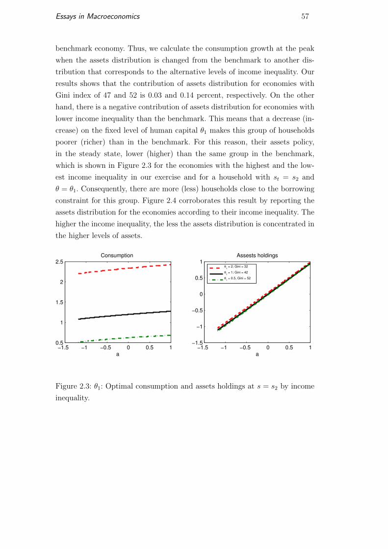
Essays in Macroeconomics 57
benchmark economy. Thus, we calculate the consumption growth at the peak
when the assets distribution is changed from the benchmark to another dis-
tribution that corresponds to the alternative levels of income inequality. Our
results shows that the contribution of assets distribution for economies with
Gini index of 47 and 52 is 0.03 and 0.14 percent, respectively. On the other
hand, there is a negative contribution of assets distribution for economies with
lower income inequality than the benchmark. This means that a decrease (in-
crease) on the fixed level of human capital θ1 makes this group of households
poorer (richer) than in the benchmark. For this reason, their assets policy,
in the steady state, lower (higher) than the same group in the benchmark,
which is shown in Figure 2.3 for the economies with the highest and the low-
est income inequality in our exercise and for a household with st = s2 and
θ = θ1. Consequently, there are more (less) households close to the borrowing
constraint for this group. Figure 2.4 corroborates this result by reporting the
assets distribution for the economies according to their income inequality. The
higher the income inequality, the less the assets distribution is concentrated in
the higher levels of assets.
−1.5 −1 −0.5 0 0.5 10.5
1
1.5
2
2.5
a
Consumption
−1.5 −1 −0.5 0 0.5 1−1.5
−1
−0.5
0
0.5
1
a
Assests holdings
θ
1 = 2; Gini = 32
θ1 = 1; Gini = 42
θ1 = 0.5, Gini = 52
Figure 2.3: θ1: Optimal consumption and assets holdings at s = s2 by income
inequality.
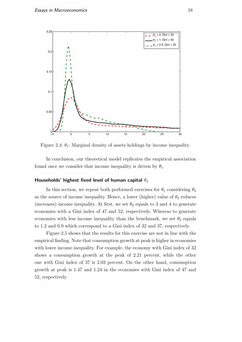
Essays in Macroeconomics 58
−5 0 5 10 15 20 25 300
0.05
0.1
0.15
0.2
0.25
θ
1 = 2; Gini = 32
θ1 = 1; Gini = 42
θ1 = 0.5, Gini = 52
Figure 2.4: θ1: Marginal density of assets holdings by income inequality.
In conclusion, our theoretical model replicates the empirical association
found once we consider that income inequality is driven by θ1.
Households’ highest fixed level of human capital θ2
In this section, we repeat both performed exercises for θ1 considering θ2
as the source of income inequality. Hence, a lower (higher) value of θ2 reduces
(increases) income inequality. At first, we set θ2 equals to 3 and 4 to generate
economies with a Gini index of 47 and 52, respectively. Whereas to generate
economies with less income inequality than the benchmark, we set θ2 equals
to 1.2 and 0.9 which correspond to a Gini index of 32 and 37, respectively.
Figure 2.5 shows that the results for this exercise are not in line with the
empirical finding. Note that consumption growth at peak is higher in economies
with lower income inequality. For example, the economy with Gini index of 32
shows a consumption growth at the peak of 2.21 percent, while the other
one with Gini index of 37 is 2.03 percent. On the other hand, consumption
growth at peak is 1.47 and 1.24 in the economies with Gini index of 47 and
52, respectively.

Essays in Macroeconomics 59
0 5 10 15 20−0.5
0
0.5
1
1.5
2
2.5
Years
Cumulative Consumption Growth (%)
θ
2 = 0.9; Gini = 32
θ2 = 1.2; Gini = 37
θ2 = 1.84; Gini = 42
θ2 = 3, Gini = 47
θ2 = 4, Gini = 52
0 5 10 15 205
10
15
20
25
Years
Debt to GDP (%)
Figure 2.5: θ2: Cumulative consumption growth ad Debt to GDP by income
inequality.
Table 2.5 shows the contributions of the policy functions and the assets
distribution on consumption growth at the peak. Concerning the contribution
of the policy functions, consumption growth at the peak for economies with
higher inequality than the benchmark is lower. For example, in the economy
with Gini index of 47 and 52, consumption growth at the peak is 1.63 and 1.49
percent, respectively. The opposite occurs when we consider the economies with
lower income inequality than the benchmark. This means that the reduction
of the precautionary motive due to a credit deepening is lower in economies
with higher income inequality driven by higher θ2, so the consumption growth
is also lower. Concerning the contribution of the assets distribution, there is a
positive contribution for economies with lower income inequality and a negative
one for economies with higher income inequality than the benchmark. This
occurs because the assets policy functions are, in equilibrium, higher (lower)
in economies with higher (lower) income inequality than the benchmark, which
is shown in Figure 2.6 for economies with the highest and the lowest Gini index
in our exercises. Therefore, there are more households close to the borrowing
constraint in economies with low income inequality and the opposite happens
for the ones with high income inequality driven by θ2, as shown in Figure 2.7.

Essays in Macroeconomics 60
Consumption growth at peak (%)
θ2 Gini Index Total Policy Distribution
0.9 32 2.21 1.93 0.27
1.2 37 2.03 1.89 0.14
1.84 42 1.79 - -
3 47 1.47 1.63 -0.16
4 52 1.24 1.49 -0.25
Table 2.5: θ2: Policy functions and Assets distribution.
−1.5 −1 −0.5 0 0.5 10
1
2
3
4
5
a
Consumption
−1.5 −1 −0.5 0 0.5 1−1.5
−1
−0.5
0
0.5
1
1.5
a
Assests holdings
θ
2 = 0.9; Gini = 32
θ2 = 1.84; Gini = 42
θ2 = 4, Gini = 52
Figure 2.6: θ2: Optimal consumption and assets holdings at s = s2 by income
inequality.

Essays in Macroeconomics 61
−5 0 5 10 15 20 25 300
0.02
0.04
0.06
0.08
0.1
0.12
0.14
0.16
θ
2 = 0.9; Gini = 32
θ2 = 1.84; Gini = 42
θ2 = 4, Gini = 52
Figure 2.7: θ2:: Marginal density of assets holdings for households with by
income inequality.
Finally, when we consider economies with income inequality driven by
θ2, our model does not rationalize the empirical finding.
2.4.4Variance of the idiosyncratic risk σ2
ε
One of the sources of inequality inherent in our model is given by the
variance of the idiosyncratic risk, σ2ε . This parameter determines the possible
values of efficiency units of labor. The effect of a higher variance of the
idiosyncratic risk on income inequality is twofold. First, a higher σ2ε implies that
the grid of possible values of st has more extreme values,13 as a result income
inequality increases. Second, a higher σ2ε increases the precautionary motive in
the economy, then households increase their savings. Mainly, households close
to the borrowing constraint increase their savings more than the others as their
precautionary motive is higher, consequently, income inequality decreases. We
show that the first effect dominates.
We calibrate four different economies with different levels of income
inequality relative to the benchmark and, for each case, we consider a mean
preserving spread by adjusting the possible values of st to generate the same
aggregate labor units as in the benchmark economy. Specifically, we set σ2ε
13In Rouwenhorst (1995)’s algorithm, changes in σ2ε modify the values of the states st but
the matrix of transition remains the same.

Essays in Macroeconomics 62
equals to 0.0941 and 0.1410 to generate economies with a Gini index of 47 and
52, respectively. In order to generate economies with less income inequality
than the benchmark (42), we set σ2ε equals to 0.0141 and 0.0241 that correspond
to a Gini index of 32 and 37, respectively. After these economies are calibrated,
we analyze the effect of a credit deepening on consumption per capita. Figure
2.8 presents the results for this experiment.
These results show that in economies with higher inequality driven by
more uncertainty on households’ income, a credit deepening has a lower effect
on consumption per capita than in an economy with lower inequality, driven by
less uncertainty. In order to understand the mechanisms behind these results,
we quantify the contributions of the assets distribution and the policy functions
for each case. Table 2.6 presents these exercises.
0 5 10 15 20−1
0
1
2
3
4
5
6
Years
Cumulative Consumption Growth (%)
σ
ε
2 = 0.0141; Gini = 32
σε
2 = 0.0241; Gini = 37
σε
2 = 0.0441; Gini = 42
σε
2 = 0.0941, Gini = 47
σε
2 = 0.1441, Gini = 52
0 5 10 15 200
10
20
30
40
50
Years
Debt to GDP (%)
Figure 2.8: σ2ε : Cumulative consumption growth ad Debt to GDP by income
inequality.
Consumption growth at peak (%)
σ2ε Gini Index Total Policy Distribution
0.0141 32 5.45 2.19 3.19
0.0241 37 3.77 1.95 1.78
0.0441 42 1.79 - -
0.0941 47 0.46 1.35 -0.88
0.1410 52 0.13 0.91 -0.77
Table 2.6: σ2ε : Policy functions and Assets distribution.
To calculate the contribution of the assets distribution, we keep the same
policy functions as in the benchmark economy. Then, we calculate the con-
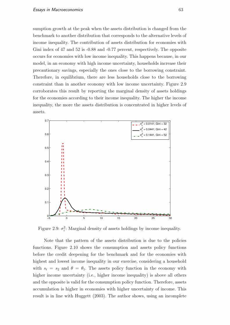
Essays in Macroeconomics 63
sumption growth at the peak when the assets distribution is changed from the
benchmark to another distribution that corresponds to the alternative levels of
income inequality. The contribution of assets distribution for economies with
Gini index of 47 and 52 is -0.88 and -0.77 percent, respectively. The opposite
occurs for economies with low income inequality. This happens because, in our
model, in an economy with high income uncertainty, households increase their
precautionary savings, especially the ones close to the borrowing constraint.
Therefore, in equilibrium, there are less households close to the borrowing
constraint than in another economy with low income uncertainty. Figure 2.9
corroborates this result by reporting the marginal density of assets holdings
for the economies according to their income inequality. The higher the income
inequality, the more the assets distribution is concentrated in higher levels of
assets.
−5 0 5 10 15 20 25 300
0.1
0.2
0.3
0.4
0.5
0.6
0.7
σε
2 = 0.0141; Gini = 32
σε
2 = 0.0441; Gini = 42
σε
2 = 0.1441, Gini = 52
Figure 2.9: σ2ε : Marginal density of assets holdings by income inequality.
Note that the pattern of the assets distribution is due to the policies
functions. Figure 2.10 shows the consumption and assets policy functions
before the credit deepening for the benchmark and for the economies with
highest and lowest income inequality in our exercise, considering a household
with st = s2 and θ = θ1. The assets policy function in the economy with
higher income uncertainty (i.e., higher income inequality) is above all others
and the opposite is valid for the consumption policy function. Therefore, assets
accumulation is higher in economies with higher uncertainty of income. This
result is in line with Huggett (2003). The author shows, using an incomplete

Essays in Macroeconomics 64
markets framework, that given two economies with the same borrowing limit,
but with different earnings processes, the one with the riskier earning process
has more assets accumulation.
−2 0 2 4
0.8
1
1.2
1.4
1.6
1.8
2
a
Consumption
−2 0 2 4−2
−1
0
1
2
3
4
5
a
Assests holdings
σ
ε
2 = 0.0141; Gini = 32
σε
2 = 0.0441; Gini = 42
σε
2 = 0.1441, Gini = 52
Figure 2.10: σ2ε : Optimal consumption and assets holdings at s = s2 and θ1 = 1
by income inequality.
Concerning the contribution of the policy function, consumption growth
at the peak for economies with higher inequality than the benchmark is lower,
even when we consider the same assets distribution as in the benchmark.
For example, in the economy with Gini index of 47 and 52, consumption
growth at the peak is 1.35 and 0.91 percent, respectively, which is lower
than the benchmark growth of 1.79 percent. The opposite occurs when we
consider the economies with less income inequality than the benchmark.
Hence, considering the assets distribution fixed, consumption growth at the
peak is higher in economies with higher income inequality driven by income
uncertainty. This means that the reduction of the precautionary motive due
to a credit deepening is smaller in economies with higher income inequality
due to higher income uncertainty, as a result the consumption growth is also
smaller. The intuition behind this result is the fact that, in an economy with
high income uncertainty, households have more incentives to do not stay close
to the borrowing constraint, because their precautionary motive is higher.
Furthermore, these results are robust to changes in b. Note that, once
the borrowing limit increases, our model approximates to a complete market
framework. Therefore, the consumption policies in economies with different
levels of income inequality become more linear due to the fact that a higher
b corresponds to a decrease in the precautionary motive. But the incentive to
households to stay out of the borrowing remains the same.
Essays in Macroeconomics 65
All in all, when we consider economies with income inequality driven by
income uncertainty, our model does not rationalize the empirical finding.
2.5Conclusion
In this paper, we study the role of income inequality in the association
between credit deepening and consumption growth. We do so through two
approaches. First, we use cross-country and panel estimations. Second, we use
a workhorse Aiyagari model to check to which extent this theoretical approach
can rationalize this empirical finding. Our results in the empirical part show
that the association between consumption growth and credit expansion is
stronger in countries with higher income inequality.
In the theoretical part, we consider two sources of income inequality in
our model: the variance of the idiosyncratic risk and the households’ fixed
level of human capital. Our results suggest that when the source of income
inequality comes from the households’ lowest fixed level of human capital, our
model can rationalize the empirical evidence. In the other cases, the opposite
occurs.

3FX interventions in Brazil: a synthetical control approach
3.1Introduction
The Fed’s taper announcement on May 2013 led to a major repricing of
risk, adding pressure on several emerging market currencies. The Brazilian real
(BRL) depreciated about 15 percent during the following three months, despite
sizable interventions by the Central Bank of Brazil (BCB in the Portuguese
acronym) in the foreign exchange market. On August 22, 2013, the BCB
announced a major program of intervention through FX swaps, with the aim
of satisfying the excess demand for hedging and providing liquidity to the
FX market. The program consisted of daily sales of US$ 500 million worth of
currency forwards (US dollar swaps) in the Brazilian markets, that provided
investors insurance against a depreciation of the real. These swaps settle in
domestic currency and provide investors the very same hedging they would
obtain by buying spot dollars and holding them until the maturity of the
swap.1 The program also indicated that on Fridays, the central bank would
offer US$ 1 billion on the spot market through repurchase agreements (short
term credit lines in USD). The program announcement stated it would last
until at least December 31, 2013. On December 18, 2013, the BCB announced
that it would extend the program until at least mid-2014, although the daily
interventions were reduced to US$ 200 million. On June 24, 2013, that program
was extended until at least end-2014, and eventually extended until March 31,
2015.2
Figure 3.1 shows the behavior of the BRL exchange rate (an increase in
the exchange rate denotes a depreciation of the BRL) and the magnitude
of these interventions. The BRL was depreciating at a rapid pace prior
to the announcement. That trend is immediately reversed, with the BRL
appreciating 10 percent in the month following the announcement. All in
all, the announcement implied a cumulative intervention of about US$ 50
1Because they settle in real, they involve convertibility risk. For a detailed discussion ofthese contracts, please refer to Garcia and Volpon (2014).
2For a detailed discussion of the program, please refer to Kang and Saborowski (2015).
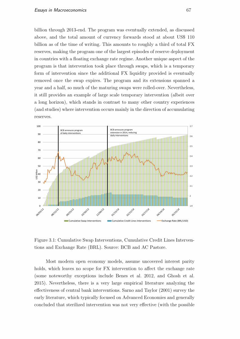
Essays in Macroeconomics 67
billion through 2013-end. The program was eventually extended, as discussed
above, and the total amount of currency forwards stood at about US$ 110
billion as of the time of writing. This amounts to roughly a third of total FX
reserves, making the program one of the largest episodes of reserve deployment
in countries with a floating exchange rate regime. Another unique aspect of the
program is that intervention took place through swaps, which is a temporary
form of intervention since the additional FX liquidity provided is eventually
removed once the swap expires. The program and its extensions spanned a
year and a half, so much of the maturing swaps were rolled-over. Nevertheless,
it still provides an example of large scale temporary intervention (albeit over
a long horizon), which stands in contrast to many other country experiences
(and studies) where intervention occurs mainly in the direction of accumulating
reserves.
1.9
2
2.1
2.2
2.3
2.4
2.5
2.6
2.7
0
10
20
30
40
50
60
70
80
90
100
Cumulative Swap Interventions Cumulative Credit Lines Interventions Exchange Rate (BRL/USD)
US$
bill
ion
BCB annouces program of daily interventions
BCB annouces program extension in 2014, reducing daily interventions
Figure 3.1: Cumulative Swap Interventions, Cumulative Credit Lines Interven-
tions and Exchange Rate (BRL). Source: BCB and AC Pastore.
Most modern open economy models, assume uncovered interest parity
holds, which leaves no scope for FX intervention to affect the exchange rate
(some noteworthy exceptions include Benes et al. 2012, and Ghosh et al.
2015). Nevertheless, there is a very large empirical literature analyzing the
effectiveness of central bank interventions. Sarno and Taylor (2001) survey the
early literature, which typically focused on Advanced Economies and generally
concluded that sterilized intervention was not very effective (with the possible
Essays in Macroeconomics 68
exception of signaling future monetary policy). That is not surprising, since the
amount of FX intervention pursued in advanced economies was a tiny fraction
of the size of their bond markets. But in the case of Emerging Markets (EMEs),
FX intervention has a non-trivial effect on the relative supply of local currency
bonds. For example, in the case of Brazil, the stock of reserves corresponds to
about a quarter of the stock of government bonds. So it seems reasonable to
expect that a change in the relative supply of assets of that magnitude to have
some effect on the exchange rate. A number of more recent papers focusing
on emerging markets tends to find more supportive evidence for an effect, but
the evidence remains somewhat mixed. Menkhoff (2013) provides an excellent
survey of that literature.
In the Brazilian context, a number of papers have shown that FX
intervention, including through swaps, can affect the exchange rate. For
example, Andrade and Kohlscheen (2014) show that the Brazilian real moved
about 0.33 bps following the announcement of a currency swap auction.
Barroso (2014) estimates that a purchase or sale of US$ 1 billion lead to a
0.51 percent depreciation or appreciation of the Brazilian real. Werther (2010)
found that the effects of sterilized interventions are very small on its magnitude
(between 0.10 and 1.14 percent for each US$ 1 billion) and of low duration.
More generally, estimates for the effect of a US$ 1 billion dollar intervention
on the exchange rate typically range from 0.10 to 0.50 percent.
Studies on FX intervention face a substantial, perhaps insurmountable,
endogeneity problem, since a central bank tends to purchase FX when it
wants to slow down an appreciation, and vice-versa. That can bias regression
estimates (perhaps even to the point of flipping the sign of the effect).
Different strategies have been used to address this problem, including VARs, IV
strategies, and relying on high-frequency data. All of these strategies have some
drawbacks, including the extent to which they truly tackle this endogeneity.
In this paper we use a synthetic control approach to estimate the effects
of the Brazilian swap program. To our knowledge, we are the first paper to use
this technique to study the effects of FX interventions.3 We follow Abadie et al.
(2010), which in a nutshell, consists of constructing a synthetic control group
that provides a counterfactual exchange rate against which we can compare
the evolution of the Brazilian real after that announcement. This methodology
is not appropriate for studying the effect of frequent interventions, but it is
well suited for an event-study setting where a large change in intervention
3Jinjarak et al. (2013) use the synthetic control method to analyze the effects of theadoption and removal of capital controls in Brazil on capital flows and the exchange rate.Their results show that capital controls had no effect on capital flows and small effects onthe the exchange rate.
Essays in Macroeconomics 69
policy is announced, as in the case of Brazil. Our counterfactual uses data
from other countries, with weights that are based on the pre-announcement
co-movement with Brazil. As a result, whatever noise and error is involved
in this type of analysis, it will be orthogonal to the endogeneity problem that
plagues the literature on FX intervention. Our findings point to an appreciation
of the BRL in the first few weeks following the announcement of the program
in excess of 10 percentage points. This is consistent with a surprise effect
on the market, which by all accounts was not expecting the program. This
result is particularly striking, once we take into account that the BCB was
already intervening substantially in the market prior to the program, albeit
in a discretionary fashion. In fact, the pace of intervention declined after the
program (as shown in Figure 3.1). We also construct synthetic control groups
using the methodology proposed by Carvalho et al. (2015), which allows us
to make inference of the results. That approach points to a similar effect
on the BRL (if anything stronger) following the announcement of the FX
swap program, and that effect is statistically significant. Our results on the
option-implied volatility are more mixed, with some of our estimates pointing
to a tangible decline while others do not. A similar analysis of the follow-
up announcements (extending the program) point to a more muted effect,
which is not surprising since by most accounts the market was expecting the
program to be extended in some form (so the surprise element was much smaller
than in the previous announcements). Finally, as a robustness check, we also
perform a more standard event-study analysis, which confirms a large effect on
the exchange rate following the August announcement, but not for the latter
announcements.
The remainder of the paper is organized as follows. Section 3.2 outlines
the methodologies used, section 3.3 presents data description and section 3.4
shows our results. Finally, section 3.5 concludes.
3.2Methodology
In this section, we present the synthetic control approach proposed by
Abadie et al. (2010) and by Carvalho et al. (2015). Then, we use these
methodologies to evaluate the effects of the BCB intervention programs on
the Brazilian exchange rate.
Essays in Macroeconomics 70
3.2.1Abadie et al. (2010)
Let Y Iit denote the exchange rate in a country i in period t for a country
that adopts a policy (e.g. an FX intervention program) at time T0, and Y Nit
denote non-observed exchange rate that would have occurred had the country
not adopted the FX interventions program.
We assume that there is no effect of the intervention program in the
period preceding the policy change (t < T0), i.e., Y Nit = Y I
it . Hence, the effect
of the intervention program is given by αit = Y Iit − Y N
it from period T0+1 to
T . Without loss of generality, suppose the policy change occurred on country
i = 1 (Brazil in our case). We assume that Y Nit follows a factor model given
by:Y Nit = δt + θtZi + λiµt + εit (3-1)
where λi is a factor loadings, Zi is a vector of observable variables, θt is a vector
of parameters and µt is an unknown common factor that depends on time. At
last, εit is a mean zero iid shock.
In addition, consider W = (ω2, ..., ωj+1)′ as a vector of weights such that
ωi ≥ 0 and∑j+1
i=2 ωi = 1. Suppose that there is an optimal weight vector W
that can accurately replicate pre-treatment observations in Brazil. Abadie et
al. (2010) show that under regular conditions Y Nit =
∑j+1i=2 ωiYit. Thus, we can
calculate α1t = Yit −∑j+1
i=2 ωiYit for t ≥ T0.
Define X1 as a vector of pre-treatment characteristics of the Brazilian
exchange rate that contains Y and Z, and similarlyX0 for the control countries.
Hence, the optimal weight vector W is chosen through the minimization of the
following equation √(X1 −X0W )′V (X1 −X0W ) (3-2)
where V is a k × k symmetric and positive semi-definite matrix (k is the
number of explanatory variables). Also V is chosen to minimize the mean
square prediction error in the period prior to the policy change. We use the
STATA synth routine to obtain V .
Finally, we use permutations tests to examine the significance of our
results, due to the fact that the usual statistical inference is not available.
For each control country in our sample, we assume that it implemented a FX
intervention program in T0. We then produce counterfactual synthetic control
for each “placebo control” and calculate the effect αPit for t ≥ T0. Therefore,
we can check if the effect found for Brazilian exchange rate is different from
the effects on the control currencies.

Essays in Macroeconomics 71
3.2.2Carvalho et al. (2015)
Consider n countries for T periods indexed by i ∈ {1, ..., n}. As in Abadie
et al. (2010), assume that one country implemented a policy change in T0.
Furthermore, consider that we observe q variables for each country i and that
they all follow jointly a covariance-stationary process. We can then stack all
the n countries in a vector yt = (y1t, ..., ynt)′ and use the Wold decomposition
to write the following equation for 1 ≤ t ≤ T
yt − µt =∞∑j=0
φt−jεt−j (3-3)
where each φt−j is a (nq×nq) matrix and the constraint∑∞
j=0 φ2t−j <∞ must
be satisfied for 1 ≤ t ≤ T . Also, εt is a nq-dimensional serially uncorrelated
white noise with covariance matrix Σt.
Moreover, consider that Brazil is indexed by 1 and define the direct effect
in our variable of interest y1t as
δ1t = y1t − y∗1t (3-4)
where y∗1t is our variable of interest without the FX intervention program. But,
y∗1t is not observed, therefore, we have to estimate y∗1t before estimate δ1t. For
this reason, we consider the best linear predictor as (E(y∗1t|1, y∗−1t))
y1t = y∗1t = w0 + w1y−1t + v1t, 1 ≤ t ≤ T0. (3-5)
where y−1t is a matrix with all q variables for all n−1 countries (not including
Brazil), w1 is a (q × (n− 1)q) matrix and w0 is (q × 1) vector.
We estimate w by OLS for all the q equations.4 Note that Abadie et al.
(2010) approach consider that the weights should be non-negative and their
sum should be equal to one. These restrictions provide a possible interpretation
for the weights. However, Carvalho et al. (2015) argues that it is not clear the
relevance of the interpretation when all that is needed is a strong correlation.
For example, consider an extreme case where there is a perfectly negatively
correlated country with Brazil. Under the restrictions adopted by Abadie et
al. (2010), this peer would be disregarded despite the fact that using it would
result in an almost perfect synthetic counterfactual. The opposite case is also
troublesome, consider that all the peers are uncorrelated to Brazil. Due to
the restriction to sum to one, the estimator automatically assign weights to
countries that have no contribution in explaining the counterfactual trajectory.
4As stressed by Carvalho et al. (2015), it is one of the possible ways to estimate equation(3− 4).

Essays in Macroeconomics 72
Differently from Abadie et al. (2010), Carvalho et al. (2015) presents the
statistical inference for the average direct effect between period T0+1 and T .
Hence, we can test if the effect of the intervention programs on the Brazilian
exchange rate is statistically significant. In addition, another moments can be
tested. In our case, we are also interested to analyze if the FX swap program
had an effect on the variance of the exchange rate. We consider the same
linear specification as in (3-5) and our dependent and independent variables
becomes y1t = (y1t− y1t)2 and y−1t = (y−1t− y−1t)
2, respectively. Therefore,
the average effect is also estimated and all the hypothesis testing can be carried
on (see Carvalho et al. (2015) for more details.).
3.3Data
Our analysis consider three outcome variables of interest: the exchange
rate (bilateral exchange rate with respect to the USD), its 3-month option-
implied volatility, and risk reversal. The latter measures the difference between
the volatility implied by an out-of- the-money put option (25 delta) and an
equivalent out-of-the-money call option, which is a measure of the insurance
premium investors are willing to pay to insure against a risk-off episode. Figures
3.2 plots the evolution of the option-implied volatility over time. There was a
rapid increase in volatility following the ”tapering” speech. Volatility declines
substantially after the program announcement, eventually settling at a lower
level (although still higher than the volatility prior to the tapering speech).
Volatility does not respond much in the immediate aftermath of the program
extension announcements. Figure 3.3 is analogous to Figure 3.2 but plots the
evolution of the option-implied risk reversal. There is a marked reduction
following the program and the first extension.

Essays in Macroeconomics 73
Figure 2. Brazilian Real Option-Implied Volatility.
Notes: Vertical bars indicate the program announcement and extensions. Source: Bloomberg. Figure 3. Brazilian Real Option-Implied Risk Reversal.
Notes: Vertical bars indicate the program announcement and extensions. Risk Reversal measures the difference between implied volatility of out-of-the-money put and out-of-the-money call (25 delta). Source: Bloomberg.
510
1520
Percent
01jan2013 01oct2013 01jul2014 01apr2015Date
1.5
22.5
33.5
4Percent
01jan2013 01oct2013 01jul2014 01apr2015Date
Figure 3.2: Brazilian Real Option-Implied Volatility. Notes: Vertical bars
indicate the program announcement and extensions. Source: Bloomberg.
Figure 2. Brazilian Real Option-Implied Volatility.
Notes: Vertical bars indicate the program announcement and extensions. Source: Bloomberg. Figure 3. Brazilian Real Option-Implied Risk Reversal.
Notes: Vertical bars indicate the program announcement and extensions. Risk Reversal measures the difference between implied volatility of out-of-the-money put and out-of-the-money call (25 delta). Source: Bloomberg.
510
1520
Percent
01jan2013 01oct2013 01jul2014 01apr2015Date
1.5
22.5
33.5
4Percent
01jan2013 01oct2013 01jul2014 01apr2015Date
Figure 3.3: Brazilian Real Option-Implied Risk Reversal. Notes: Vertical bars
indicate the program announcement and extensions. Risk Reversal measures
the difference between implied volatility of out-of-the-money put and out-of-
the-money call (25 delta). Source: Bloomberg.
In addition to these outcome variables, explanatory variables include
capital flows, and stock and bond market indices. The source of all data is
Bloomberg, except for the capital flow series which comes from the Emerging
Portfolio Fund Research (EPFR) database. We use weekly data in our synthetic
estimates (the highest frequency at which the capital flows series is available).
For each event, we consider a window consisting of the 12 weeks prior to the
announcement, the week of the announcement, and the 12 weeks afterwards.
We consider a sample of 16 countries when estimating the synthetic for
Brazil, which includes: Australia, Brazil, Chile, Colombia, India, Indonesia,

Essays in Macroeconomics 74
Korea, Malaysia, Mexico, New Zealand, Peru, Philippines, Poland, Russia,
South Africa, Thailand, and Turkey. We included all the emerging market
countries with EPFR data plus Korea, and Australia and New Zealand (the
latter two because they are major carry trade currencies).
For the implementation of both methodologies, the series used should
be stationary. For this reason, we use the log difference of the exchange rate,
equity and bond indices, and the difference of the option-implied volatility and
risk-reversal in our analysis. Capital flows to each country are scaled by the
2012 GDP in US dollars for each country.
3.4Results
In this section, we use the approaches presented on the methodology
section to analyze the FX intervention programs in Brazil. In addition, we
present an event study to check the robustness of our results.
3.4.1Program Announcement
Level effect
Figure 3.4 presents our estimates for the effect of the program announce-
ment on the exchange rate. As mentioned above, the estimation uses the log
change in the exchange rate as the dependent variable. But in order to more
easily illustrate the resulting effect on the level, we accumulate the weekly log
differences for the actual and for the synthetic exchange rates, and report the
gap between the two. That gap is set to zero on the last observation prior to
the announcement (so the level at any date t corresponds to the gap in the ac-
cumulated log differences from t to the announcement, and vice-versa). Figure
3.4(a) shows the estimates using Abadie et al. (2010) approach. In addition
to the log change in the exchange rate, the explanatory variables considered
include capital flows, the change in volatility, and the log change in the equity
and bond indices. The thick dark line indicates the gap between the actual
BRL and its synthetic (a negative value indicates that the BRL was more
appreciated than its synthetic), while light gray lines indicate the gap for the
other countries, which is used as a placebo test. The gap for the BRL is slightly
negative and broadly stable during most of the pre-announcement period. But
the gap declines sharply after the announcement, remaining at a substantially
negative level. The bulk of the change takes place in the first week (about 10
percentage points). But the trend persists with the gap peaking at close to

Essays in Macroeconomics 75
15 percentage points before narrowing slightly. These results imply that the
BRL was over 10 percentage points stronger than what its synthetic would
suggest weeks after the announcement. Moreover, please note that the gap for
the BRL is a major outlier vis-a-vis the placebos in the post-announcement
period, with none of the placebos experiencing nearly as large a shift (in the
pre-announcement period, both the BRL and placebos should hover around
zero by construction). The weights and countries used for the construction of
the synthetic control group do not have an economic interpretation, a point
that is stressed in the literature (e.g. Abadie et al. 2010).5,6 The means for
Brazil and for its synthetic are reported in Table C.1.
The effect of this program is also estimated using a univariate approach
that considers only the exchange rate, following the methodology proposed in
Carvalho et al. (2015). Under this approach, we cannot consider all peers and
control variables (otherwise there would be more parameters being estimated
than the data available). We choose 3 peers that maximize the fit of the
exchange rate regression: South Africa, Thailand and Peru. The counterfactual
is estimated through a regression of the BRL on the others peers’ change in log
of exchange rate and a constant.7 The gap between the actual and synthetic
BRL is reported in Figure 3.4(b). The results point to a cumulative effect that is
even stronger, peaking at around 20 percentage points. This approach provides
a statistical inference for the average effect, which is statistically significant
(with a p-value below 2 percent at four lags). The effect is smaller when the
counterfactual is estimated without a constant (around five percentage points).
5With that caveat in mind, the synthetic draws from India, Indonesia and Malaysia, withweights of 14, 76, and 9 percent, respectively.
6Results are similar when we consider only Inflation Targeting countries.7The R2 of a regression of BRL in these currencies is equal to 0.8.
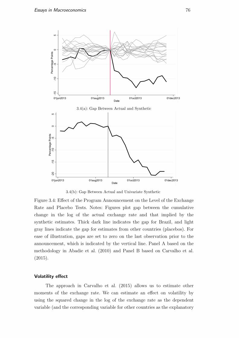
Essays in Macroeconomics 76
Figure 4. Effect of the Program Announcement on the Level of the Exchange Rate and Placebo tests. Figure 4A. Gap Between Actual and Synthetic Control
Figure 4B. Gap Between Actual and Univariate Synthetic Control
Notes: Figures plot gap between the cumulative change in the log of the actual exchange rate and that implied by the synthetic cohort estimates. Thick dark line indicates the gap for Brazil, and light gray lines indicate the gap for estimates from other countries (placebos). For ease of illustration, gaps are set to zero on the last observation prior to the announcement, which is indicated by the vertical line. Panel A based on the methodology in Abadie et al. (2010) and Panel B based on Carvalho et al. (2015).
-15
-10
-50
5Pe
rcen
tage
Poi
nts
01jun2013 01aug2013 01oct2013 01dec2013Date
-20
-15
-10
-50
5Pe
rcen
tage
Poi
nts
01jun2013 01aug2013 01oct2013 01dec2013Date
3.4(a): Gap Between Actual and Synthetic
Figure 4. Effect of the Program Announcement on the Level of the Exchange Rate and Placebo tests. Figure 4A. Gap Between Actual and Synthetic Control
Figure 4B. Gap Between Actual and Univariate Synthetic Control
Notes: Figures plot gap between the cumulative change in the log of the actual exchange rate and that implied by the synthetic cohort estimates. Thick dark line indicates the gap for Brazil, and light gray lines indicate the gap for estimates from other countries (placebos). For ease of illustration, gaps are set to zero on the last observation prior to the announcement, which is indicated by the vertical line. Panel A based on the methodology in Abadie et al. (2010) and Panel B based on Carvalho et al. (2015).
-15
-10
-50
5Pe
rcen
tage
Poi
nts
01jun2013 01aug2013 01oct2013 01dec2013Date
-20
-15
-10
-50
5Pe
rcen
tage
Poi
nts
01jun2013 01aug2013 01oct2013 01dec2013Date
3.4(b): Gap Between Actual and Univariate Synthetic
Figure 3.4: Effect of the Program Announcement on the Level of the Exchange
Rate and Placebo Tests. Notes: Figures plot gap between the cumulative
change in the log of the actual exchange rate and that implied by the
synthetic estimates. Thick dark line indicates the gap for Brazil, and light
gray lines indicate the gap for estimates from other countries (placebos). For
ease of illustration, gaps are set to zero on the last observation prior to the
announcement, which is indicated by the vertical line. Panel A based on the
methodology in Abadie et al. (2010) and Panel B based on Carvalho et al.
(2015).
Volatility effect
The approach in Carvalho et al. (2015) allows us to estimate other
moments of the exchange rate. We can estimate an effect on volatility by
using the squared change in the log of the exchange rate as the dependent
variable (and the corresponding variable for other countries as the explanatory

Essays in Macroeconomics 77
variable). The estimates suggest the average effect on the variance is close to
zero and not statistically significant.
We can also assess the impact of the program on volatility using the
option-implied exchange rate volatility. This readily available series provides
a forward-looking measure of volatility (since it is based on option prices)
that can quickly respond to the program (unlike say, measures of volatility
constructed from past exchange rate data). Figure 3.5 reports the results for
the change in the volatility. In Figure 3.5(a) we use the changes in the exchange
rate, equity and bond indices, and capital flows as explanatory variables.
For ease of illustration, we accumulate all the changes so as to report the
resulting level of effect (setting the level at the last observation prior to the
announcement to zero). Again, the thick dark line corresponds to the BRL
while the thin gray lines to the placebo tests. There is a sharp decline in the gap
in volatility after the announcement, by 5 percentage points, which is driven
mainly by an increase in volatility among the countries in the synthetic control
(India in particular) rather than an absolute decline in volatility for Brazil).8
If we drop India from the pool of potential countries for the synthetic control,
the results continue to point to a decline in volatility, but of only 2 percentage
points.9 That would still be a sizable decline (to put magnitudes in perspective,
the volatility of the BRL was about 17 percent in the last observation prior
to the announcement, so a 2 percentage point decline amounts to over 10
percent of the original volatility). The placebo tests point to the BRL being
an outlier after the announcement. But the discrepancy between the BRL and
the placebos is much smaller than in Figure 3.5(a).
Figure 3.5(b) reports the results using the univariate approach, drawing
on Peru and India. The results are more muted, and not statistically significant.
Finally, Figure 3.6 is analogous to Figure 3.5(a) but reports results for
the risk-reversal measure. There is a sharp decline following the announcement
(driven mainly by a decline in that variable for Brazil, which goes from 3.5 to
2.7 in the two observations before and after the announcement). A comparison
with the placebos suggests the behavior of the BRL was an outlier in the two
weeks following the announcement, but not afterwards.
8The synthetic draws on Australia and India, with weights of 31 and 69 percent,respectively.
9The synthetic would draw on Australia and Indonesia, with weights of 64 and 36 percent,respectively.

Essays in Macroeconomics 78
Figure 5. Effect of the Program Announcement on the Option-Implied Volatility of the Exchange Rate and Placebo tests. Figure 5A. Gap Between Actual and Synthetic Control
Figure 5B. Gap Between Actual and Univariate Synthetic Control
Notes: Figures plot gap between the cumulative change in the option-implied volatility and that implied by the synthetic cohort estimates. Thick dark line indicates the gap for Brazil, and light gray lines indicate the gap for estimates from other countries (placebos). For ease of illustration, gaps are set to zero on the last observation prior to the announcement, which is indicated by the vertical line. Panel A based on the methodology in Abadie et al. (2010) and Panel B based on Carvalho et al. (2015).
-50
5Pe
rcen
tage
Poi
nts
01jun2013 01aug2013 01oct2013 01dec2013Date
-50
5Pe
rcen
tage
Poi
nts
01jun2013 01aug2013 01oct2013 01dec2013Date
3.5(a): Gap Between Actual and Synthetic
Figure 5. Effect of the Program Announcement on the Option-Implied Volatility of the Exchange Rate and Placebo tests. Figure 5A. Gap Between Actual and Synthetic Control
Figure 5B. Gap Between Actual and Univariate Synthetic Control
Notes: Figures plot gap between the cumulative change in the option-implied volatility and that implied by the synthetic cohort estimates. Thick dark line indicates the gap for Brazil, and light gray lines indicate the gap for estimates from other countries (placebos). For ease of illustration, gaps are set to zero on the last observation prior to the announcement, which is indicated by the vertical line. Panel A based on the methodology in Abadie et al. (2010) and Panel B based on Carvalho et al. (2015).
-50
5Pe
rcen
tage
Poi
nts
01jun2013 01aug2013 01oct2013 01dec2013Date
-50
5Pe
rcen
tage
Poi
nts
01jun2013 01aug2013 01oct2013 01dec2013Date
3.5(b): Gap Between Actual and Univariate Synthetic
Figure 3.5: Effect of the Program Announcement on the Option-Implied
Volatility of the Exchange Rate and Placebo Tests. Notes: Figures plot gap
between the cumulative change in the option-implied volatility and that
implied by the synthetic estimates. Thick dark line indicates the gap for
Brazil, and light gray lines indicate the gap for estimates from other countries
(placebos). For ease of illustration, gaps are set to zero on the last observation
prior to the announcement, which is indicated by the vertical line. Panel A
based on the methodology in Abadie et al. (2010) and Panel B based on
Carvalho et al. (2015).

Essays in Macroeconomics 79
Figure 6. Effect of the Program Announcement on the Option-Implied Risk Reversal of the Exchange Rate and Placebo tests. Figure 6A. Gap Between Actual and Synthetic Control
Notes: Figures plot gap between the cumulative change in the risk reversal and that implied by the synthetic cohort estimates. Thick dark line indicates the gap for Brazil, and light gray lines indicate the gap for estimates from other countries (placebos). For ease of illustration, gaps are set to zero on the last observation prior to the announcement, which is indicated by the vertical line. Based on the methodology in Abadie et al. (2010).
-2-1
01
23
Perc
enta
ge P
oint
s
01jun2013 01aug2013 01oct2013 01dec2013Date
Figure 3.6: Effect of the Program Announcement on the Option-Implied Risk
Reversal of the Exchange Rate and Placebo Tests. Notes: Figures plot gap
between the cumulative change in the risk reversal and that implied by the
synthetic estimates. Thick dark line indicates the gap for Brazil, and light
gray lines indicate the gap for estimates from other countries (placebos).
For ease of illustration, gaps are set to zero on the last observation prior
to the announcement, which is indicated by the vertical line. Based on the
methodology in Abadie et al. (2010).
3.4.2Program Extension Announcement
Level effect
On December 18, 2013, the intervention program was extended until mid-
2014, but with reduced daily interventions. There were expectations that the
swap sales would continue (i.e. the market did not expect it to end abruptly at
the end of 2013), but the announcement removed that uncertainty and clarified
the scope of the program going forward. Therefore, the announcement could
still impact the exchange rate, but that impact should be less dramatic than
the one following the first announcement.
Figure 3.7 is analogous to Figure 3.4, but reports the results for the
cumulative changes in the exchange rate around this second announcement.
Figure 3.7(a) points to a gradual appreciation of the BRL vis-a-vis its synthetic,
with that gap reaching about 5 percentage points, and remaining close to that
level. A comparison with the gaps for the placebos suggest that the BRL was
clearly on the stronger side, but was not nearly as much of an outlier as in

Essays in Macroeconomics 80
Figure 3.4(a).10
Figure 3.7(b) reports the result under the univariate approach. The
results also point to a decline of around 5 percentage points over the first four
weeks, but that is gradually reversed over time. The effect is not statistically
significant under any lag structure.
Figure 7. Effect of the December 2013 Announcement on the Level of the Exchange Rate and Placebo tests. Figure 7A. Gap Between Actual and Synthetic Control
Figure 7B. Gap Between Actual and Univariate Synthetic Control
Notes: See notes to Figure 4.
-10
-50
510
Perc
enta
ge P
oint
s
01oct2013 01dec2013 01feb2014 01apr2014Date
-10
-50
510
Perc
enta
ge P
oint
s
01oct2013 01dec2013 01feb2014 01apr2014Date
3.7(a): Gap Between Actual and Synthetic
Figure 7. Effect of the December 2013 Announcement on the Level of the Exchange Rate and Placebo tests. Figure 7A. Gap Between Actual and Synthetic Control
Figure 7B. Gap Between Actual and Univariate Synthetic Control
Notes: See notes to Figure 4.
-10
-50
510
Perc
enta
ge P
oint
s
01oct2013 01dec2013 01feb2014 01apr2014Date
-10
-50
510
Perc
enta
ge P
oint
s
01oct2013 01dec2013 01feb2014 01apr2014Date
3.7(b): Gap Between Actual and Univariate Synthetic
Figure 3.7: Effect of the December 2013 Announcement on the Level of the
Exchange Rate and Placebo Tests. Notes: See notes to Figure 3.4.
Volatility effect
Figure 3.8 is analogous to Figure 3.5, but reports the effect on the option-
implied volatility following the second announcement. There is virtually no
change in volatility under neither of the methodologies considered. We also
do not find any statistically significant effect of the second announcement
when we estimate the synthetic for the squared log change in the exchange
10The synthetic draws on Australia, Indonesia, Peru and Turkey, with weights of 19, 9, 5and 67 percent, respectively.
Essays in Macroeconomics 81
rate, using the univariate approach. There is also virtually no effect on the
risk reversal following the second announcement (Figure 3.9). While there is a
sharp decline in risk reversal for Brazil following the second announcement, as
shown in Figure 3.3, the same was true for its synthetic (which draws heavily
from Peru, where a sizable decline also took place around that time).
3.4.3Addition Program Extensions
There were two additional announcements. One on June 24, 2014 ex-
tending the program until at least 2014-end, and a final announcement on
December 30, 2014 extending the program until March 31, 2015. Figures 3.10
and 3.11 reports the results for the level of the exchange rate. The estimates
suggest virtually no effect on the BRL exchange rate following the June 2014
announcement. The results point to a larger gap following the December 2014
announcement, which peaks at an appreciation of around 5 percent before
quickly reversing. But overall, the results for the BRL are broadly in line with
the placebos during most of the post-announcement period, suggesting no sig-
nificant effect. The results for the volatility and risk reversal also point to little
or no effect, and are not reported for the sake of conciseness.

Essays in Macroeconomics 82
Figure 8. Effect of the December 2013 Announcement on the Option-Implied Volatility of the Exchange Rate and Placebo tests. Figure 8A. Gap Between Actual and Synthetic Control
Figure 8B. Gap Between Actual and Univariate Synthetic Control
Notes: See notes to Figure 5.
-10
-50
510
Perc
enta
ge P
oint
s
01oct2013 01dec2013 01feb2014 01apr2014Date
-10
-50
510
Perc
enta
ge P
oint
s
01oct2013 01dec2013 01feb2014 01apr2014Date
3.8(a): Gap Between Actual and Synthetic
Figure 8. Effect of the December 2013 Announcement on the Option-Implied Volatility of the Exchange Rate and Placebo tests. Figure 8A. Gap Between Actual and Synthetic Control
Figure 8B. Gap Between Actual and Univariate Synthetic Control
Notes: See notes to Figure 5.
-10
-50
510
Perc
enta
ge P
oint
s
01oct2013 01dec2013 01feb2014 01apr2014Date
-10
-50
510
Perc
enta
ge P
oint
s
01oct2013 01dec2013 01feb2014 01apr2014Date
3.8(b): Gap Between Actual and Univariate Synthetic
Figure 3.8: Effect of the December 2013 Announcement on the Option-Implied
Volatility of the Exchange Rate and Placebo Tests. Notes: See notes to Figure
3.5.

Essays in Macroeconomics 83
Figure 9. Effect of the December 2013 Announcement on the Option-Implied Risk Reversal of the Exchange Rate and Placebo tests.
Notes: See notes to Figure 6.
-4-2
02
4Pe
rcen
tage
Poi
nts
01oct2013 01dec2013 01feb2014 01apr2014Date
Figure 3.9: Effect of the December 2013 Announcement on the Option-Implied
Risk Reversal of the Exchange Rate and Placebo Tests. Notes: See notes to
Figure 3.6.
Figure 10. Effect of the June 2014 Announcement on the Level of the Exchange Rate and Placebo tests.
Notes: See notes to Figure 4. Figure 11. Effect of the December 2014 Announcement on the Level of the Exchange Rate and Placebo tests.
Notes: See notes to Figure 4.
-50
510
Perc
enta
ge P
oint
s
01apr2014 01may2014 01jun2014 01jul2014 01aug2014 01sep2014Date
-50
510
Perc
enta
ge P
oint
s
01oct2014 01nov2014 01dec2014 01jan2015 01feb2015 01mar2015Date
Figure 3.10: Effects of the June 2014 Announcement on the Level of the
Exchange Rate and Placebo Tests. Notes: See notes to Figure 3.4.

Essays in Macroeconomics 84
Figure 10. Effect of the June 2014 Announcement on the Level of the Exchange Rate and Placebo tests.
Notes: See notes to Figure 4. Figure 11. Effect of the December 2014 Announcement on the Level of the Exchange Rate and Placebo tests.
Notes: See notes to Figure 4.
-50
510
Perc
enta
ge P
oint
s
01apr2014 01may2014 01jun2014 01jul2014 01aug2014 01sep2014Date
-50
510
Perc
enta
ge P
oint
s
01oct2014 01nov2014 01dec2014 01jan2015 01feb2015 01mar2015Date
Figure 3.11: Effects of the December 2014 Announcement on the Level of the
Exchange Rate and Placebo Tests. Notes: See notes to Figure 3.4.
3.4.4Event Study
As a robustness check, we complement our analysis with a standard
event-study analysis around the announcement of the FX swap program.11
Using daily data, we estimate:
∆log(et) = c+ γ1∆(CDIt − LIBORt) + γ2∆log(V IXt)
+γ3∆log(Commoditiest) + γ4∆log(DollarIndext)
+γ5∆(Dollar − AsiaIndext) + γ6FXIntt + εt (3-6)
Where e is the dollar-real bilateral exchange rate, and explanatory variables
include the change in the spread between the one-month CDI (Brazil’s
interbank rate) and the one-month LIBOR, the change in the log of the
V IX, the change in the log of the CRB commodity price index, the change
in the log of an index constructed by the Federal Reserve for the value of
the dollar relative to major currencies of advanced economies weighted by US
trade shares, the change in the log of the Bloomberg JP Morgan Asia and
Latin America currency indices (we recomputed the latter, based on published
weights, to exclude the BRL), and the Foreign Exchange Intervention by the
central bank (based on announced swaps, netting out maturing ones).12
11Please refer to Campbell, Lo and MacKinlay (1996) for a description of the event studyapproach.
12The data sources are: Central Bank of Brazil for the exchange rate; Federal ReserveEconomic Data for the dollar index, and Bloomberg for the remaining series.
Essays in Macroeconomics 85
We estimate this regression using data for January 2013 until 20 days
prior to the August 22 announcement. We then compute the change in the
log of the exchange rate beyond what would have been implied by that fitted
model (analogous to the Cumulative Abnormal Returns in a standard finance
event study) and the corresponding error bands around that estimate. We
consider a +/- 20 working day window around the two announcements. Figure
3.12 reports the results, which point to a statistically significant cumulative
appreciation of about 10 percent after the August 22 announcement, in line
with our synthetic cohort estimates. In contrast, there is virtually no response
following the December 18 announcement.
We estimate a similar regression but using the change in the option-
implied volatility and risk reversal as the dependent variables. Figure 3.13(a)
reports the results for volatility. While there is a decline following both
announcements, it is not statistically significant (the error bands are too wide
and span a zero effect). Figure 3.13(b) reports the results for the risk reversal. It
declines following both announcements. That cumulative decline is statistically
significant in the immediate aftermath for the first announcement, but over
time the error bands become wider and that is no longer the case. In the case
of the second program, the error bands initially span zero, but that is no longer
the case towards the end of the post-announcement window the cumulative
effect. The cumulative effect points to a 1.4 percentage point decline, which is
sizable (the risk reversal stood at 2.8 prior to the announcement).

Essays in Macroeconomics 86
Figure 12. Cumulative Changes in the Exchange Rate Around Program Announcement and Extension.
Notes: Dashed lines correspond to +/- 2 Standard Deviations. Cumulative changes start at 0 for both before and after period.
-10
-50
510
Perc
ent
-20 -10 0 10 20Days from Announcement
Aug 22 2013
-10
-50
510
Perc
ent
-20 -10 0 10 20Days from Announcement
Dec 18 2013
Figure 3.12: Cumulative Changes in the Exchange Rate Around Program
Announcement and Extension. Notes: Dashed lines correspond to +/- 2
Standard Deviations. Cumulative changes start at 0 for both and after period.
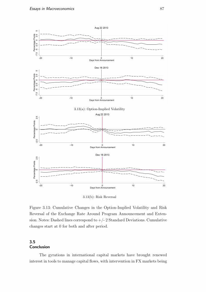
Essays in Macroeconomics 87
Figure 13. Cumulative Changes in the Option-Implied Volatility and Risk Reversal of the Exchange Rate Around Program Announcement and Extension. Figure 13A: Volatility
Figure 13B: Risk Reversal
Notes: Dashed lines correspond to +/- 2 Standard Deviations. Cumulative changes start at 0 for both before and after period.
-7.5
-5-2
.50
2.5
5Pe
rcen
tage
Poi
nts
-20 -10 0 10 20Days from Announcement
Aug 22 2013
-7.5
-5-2
.50
2.5
5Pe
rcen
tage
Poi
nts
-20 -10 0 10 20Days from Announcement
Dec 18 2013
-2.5
02.
5Pe
rcen
tage
Poi
nts
-20 -10 0 10 20Days from Announcement
Aug 22 2013
-2.5
02.
5Pe
rcen
tage
Poi
nts
-20 -10 0 10 20Days from Announcement
Dec 18 2013
3.13(a): Option-Implied Volatility
Figure 13. Cumulative Changes in the Option-Implied Volatility and Risk Reversal of the Exchange Rate Around Program Announcement and Extension. Figure 13A: Volatility
Figure 13B: Risk Reversal
Notes: Dashed lines correspond to +/- 2 Standard Deviations. Cumulative changes start at 0 for both before and after period.
-7.5
-5-2
.50
2.5
5Pe
rcen
tage
Poi
nts
-20 -10 0 10 20Days from Announcement
Aug 22 2013
-7.5
-5-2
.50
2.5
5Pe
rcen
tage
Poi
nts
-20 -10 0 10 20Days from Announcement
Dec 18 2013
-2.5
02.
5Pe
rcen
tage
Poi
nts
-20 -10 0 10 20Days from Announcement
Aug 22 2013
-2.5
02.
5Pe
rcen
tage
Poi
nts
-20 -10 0 10 20Days from Announcement
Dec 18 2013
3.13(b): Risk Reversal
Figure 3.13: Cumulative Changes in the Option-Implied Volatility and Risk
Reversal of the Exchange Rate Around Program Announcement and Exten-
sion. Notes: Dashed lines correspond to +/- 2 Standard Deviations. Cumulative
changes start at 0 for both and after period.
3.5Conclusion
The gyrations in international capital markets have brought renewed
interest in tools to manage capital flows, with intervention in FX markets being

Essays in Macroeconomics 88
one of the most commonly used tools. This paper has analyzed the effect of
the large scale program of FX swaps that the BCB has embarked following the
market’s “taper tantrum” of 2013. This program was fairly unique because
of its large scale (amounting to about a quarter of reserves) and the fact
that the intervention took place through swaps (which makes the intervention
temporary in nature, despite the long horizon of the program).
Immediately after announcement of the program, on August 22 2013,
the Brazilian real reverted its depreciation trend, and eventually stabilized
at a significantly more appreciated level. Our synthetic estimates point to an
eventual appreciation relative to the synthetic in the range of 10-19 percentage
points. The event-study analysis in the previous section also points to an
appreciation of around 10 percent. If we compare this effect with the total
volume of intervention mobilized during that program, it would be broadly in
line with the point estimates for the effectiveness of FX intervention in Brazil
from previous studies. Despite this large effect on the level of the exchange
rate following the first announcement, the results on the volatility are more
mixed. Some estimates point to a sizable decline, but overall the estimates are
less robust than those for the level. Our estimates for the announcement of
the extension of the program on December of 2013 had smaller effect on the
exchange rate, ranging from no effect to 5 percent, and does not seem to have
had an effect on its volatility. This smaller response may be the result of that
extension being already expected and priced-in by the market. The third and
fourth extensions had a fairly muted effect, likely for the same reason.
Our results are consistent with the view that FX interventions can
be effective in deter- ring exchange rate overshooting in times of market
turmoil. The large size of the program, and the market surprise following its
announcements facilitate the identification of an effect, which would be more
challenging in the context of small and frequent interventions that have come
to be expected by the market.
4References
ABADIE, A., DIAMOND, A., HAINMUELLER, J. Synthetic control methods
for comparative case studies: estimating the effect of California’s tobacco
control program. Journal of the American Statistical Association 105
(490), 493-505, 2010.
AGHION, P., BOLTON, P. A Theory of Trickle-Down Growth and Develop-
ment. Review of Economic Studies 64: 151-172, 1997.
AIYAGARI, R. Uninsured Idiosyncratic Risk and Aggregate Saving.
Quarterly Journal of Economics 109 (3): 659-84, 1994.
ALESINA, A., RODRIK D. Distributive Politics and Economic Growth. The
Quarterly Journal of Economics 109 (2): 465-490, 1994.
ANDRADE, S., KOHLSCHEEN, E. OFFICIAL INTERVENTIONS through
Derivatives: affecting the demand for foreign exchange. Journal of Interna-
tional Money and Finance, vol. 47, pages 202-216, 2013.
BANERJEE, A., V., NEWMAN, A., F. Occupational Choice and the Process
of Development. Journal of Political Economy, 101(2): 274-298, 1993.
BARROSO, J. Realized Volatility as an Instrument to Official Intervention.
Banco Central do Brasil Working Paper Series, 363, 2014.
BENES, J., BERG, A., PORTILLO, R., VAVRA, D. Modeling Sterilized
Interventions and Balance Sheet Effects of Monetary Policy. IMF Working
Paper, 2013.
BEWLEY, T. The Permanent Income Hypothesis: A Theoretical Formulation.
Journal of Economics Theory 16(2): 252-92, 1977.
BONSER-NEAL, C., TANNER, G. Central bank intervention and the volat-
ility of foreign exchange rates: evidence from the options market. Journal of
International Money and Finance, vol. 15(6), pages 853-878, 1996.

Essays in Macroeconomics 90
CAMPBELL, J.Y., LO, A.W., MACKINLAY, A.C. The econometrics of
financial markets. Princeton University Press, 1998.
CARROLL, CHRISTOPHER D., KIMBALL, M. S. On the Concavity of the
Consumption Function. Econometrica, 64(4): 981-92, 1996.
CARROLL, CHRISTOPHER D. The Method of Endogenous Gridpoints for
Solving Dynamic Stochastic Optimization Problems. Economics Letters
91(3): 312-320, 2006.
CARVALHO C., MASINI, R., MEDEIROS, M. Intervention Impact Evalu-
ation on Aggregated Data: The Artificial Counterfactual Approach for Sta-
tionary Processes. Working Paper, 2015.
CARVALHO, C., PASCA, N., SOUZA, L., ZILBERMAN, E. Macroeconomic
Effects of Credit Deepening in Latin America. Working Paper, 2014.
CASTILLO, P., CARRERA, C., ORTIZ, M., VEGA, H. Spillovers, capital
flows and prudential regulation in small open economies. BIS Working
Paper, N. 459, 2014.
CASTILLO, P., MONTORO, C., TUESTA, V. Un Modelo de Equilibrio
General con Dolarizaciøn para la Economıa Peruana. Estudios Econømicos
CRBP 17: 9-50, 2009.
CICCO, J. Estimating models for monetary policy analysis in emerging
countries. Central Bank of Chile Working Paper, N. 561, 2010.
COMIN, D., LOAYZA, N., PASHA, F., SERVEN, L. Medium term business
cycles in developing countries. NBER Working Paper, N. 15428, 2009.
CURDIA, V., WOODFORD, M. Credit Spread and Monetary Policy. Jornal
of Money, Credit and Banking, 42: 3-35, 2010.
DOMINGUEZ, K. Central bank intervention and exchange rate volatility
Journal of International Money and Finance, vol. 17, pages 161-190,
1998.
EROSA, A., VENTURA, G. On inflation as a regressive consumption tax.
Journal of Monetary Economics, 49(4): 761-795, 2002.
FERNANDEZ-VILLAVERDE, J., KRUEGUER, D. Life-Cycle Consumption,
Debt Constraints and Durable Goods. Macroeconomic Dynamics 15(5):
725-770, 2004.

Essays in Macroeconomics 91
FLODEN, M., LINDE, J. diosyncratic Risk in the United States and Sweden: Is
There a Role for Government Insurance? Review of Economic Dynamics,
4(2): 406-437, 2001.
FORBES, KRISTIN J. A Reassessment of the Relationship between Inequality
and Growth.American Economic Review 90(4):869-887, 2000.
FRENCH, E. The effects of health, wealth, and wages on labour supply and
retirement behavior. Review of Economic Studies, 72(2): 395-427, 2005.
GALOR, O., ZEIRA, J. Income Distribution and Macroeconomics. Review
of Economic Studies, 60(1): 35-52, 1993.
GARCIA, M., VOLPON, T. DNDFs: a more efficient way to intervene in FX
markets? Working Paper, 2014.
GERALI, A., NERI, S., SESSA, L., SIGNORETTI, F. Credit and Banking in
a DSGE Model of the Euro Area. Journal of Money, Credit and Banking
42: 107-141, 2010.
GERTLER, M., KIYOTAKI, N. Financial Intermediation and Credit Policy
in Business Cycle Analysis. In: Handbook of Monetary Economics, Vol.
3, edited by Friedman, B., Woodford, M, 2010.
GUERRIERI, L., IACOVIELLO, M. Collateral Constraints and Macroeco-
nomic Asymmetries. Working Paper, 2014.
GUERRIERI, V., LORENZONI, G. Credit Crises, Precautionary Savings and
the Liquidity Trap. Working Paper, 2011.
HUGGETT, M. Precautionary Wealth Accumulation. The Review of Eco-
nomic Studies, 71 (3):769-781, 2004.
HUMALA, A., RODRIGUEZ, G. Foreign exchange intervention and exchange
rate volatility in Peru. Applied Economics Letters, vol. 17 (15), pages
1485-1491, 2010.
HUNG, J. Intervention strategies and exchange rate volatility: a noise trading
perspective. Journal of International Money and Finance, vol. 16 (5),
pages 779-793, 1997.
IACOVIELLO, M. House Prices, Borrowing Constraints, and Monetary Policy
in the Business Cycle. American Economic Review 95(3): 739-764, 2005.

Essays in Macroeconomics 92
IACOVIELLO, M., NERI, S. Housing market spillovers: evidence from an
estimated DSGE model. American Economic Journal: Macroeconomics
2: 125-164, 2010.
JINJARAK, Y., NOY, I., ZHENG, H. Capital controls in Brazil - Stemming a
tide with a signal? Journal of Banking and Finance, Elsevier, vol. 37(8),
pages 2938-2952, 2013.
JUSTINIANO. A, PRIMICERI, G., TAMBALOTTI, A. Household Leveraging
and Deleveraging.NBER Working Paper, N. 18941, 2014.
KANG, H. AND SABOROWSKI, C. Assessment of Foreign Exchange Inter-
vention. Mimeo IMF, 2015.
KIYOTAKI, N., MOORE, J. Credit Cycles. Journal of Political Economy
105(2):211-248, 1997.
LIU, Z., WANG, P., ZHA, T. Land-Price Dynamics and Macroeconomic
Fluctuations. Econometrica 81(3): 1147-1184, 2013.
MENDOZA, E. Sudden Stops, Financial Crises, and Leverage. American
Economic Review 100(5):1941-1966, 2010.
MENKHOFF, L. Foreign Exchange Intervention in Emerging Markets: A
Survey of Empirical Studies.World Economy, vol. 36: 1187-1208, 2013.
OSTRY, J. D., GHOSH, A. R., CHAMON, M. Two Targets, Two Instru-
ments: Monetary and Exchange Rate Policies in Emerging Market Economies.
Journal of International Money and Finance, forthcoming, 2015.
PERUGINI, C., HOLSCHER, J., COLLIE, S. Inequality, credit expansion and
financial crises. MPRA Working paper, N. 51336, 2013.
PERSSON, T., TABELLINI, G. Is Inequality Harmful for Growth? American
Economic Association 84(3): 600-621, 1994.
RAVALLION, M. Why Don’t We See Poverty Convergence? American Eco-
nomic Review 102 (1): 504-523, 2012.
RAVALLION, M. Inequality is Bad for the Poor. In J. Micklewright and S.
Jenkins (eds.), Inequality and Poverty Re-Examined, Oxford University
Press, 2007.
Essays in Macroeconomics 93
RAVALLION, M. Growth, Inequality and Poverty: Looking Beyond Averages.
World Development 29(11): 1803-1815, 2001.
RIOS-RULL, J.V. Computation of Equilibria in Heterogeneous Agent Models.
Computational methods for the study of dynamic economies, 238-264,
1999.
ROUWENHORST, K.G. Asset pricing implications of equilibrium business
cycle models. In: Cooley, T.F. (Ed.), Frontiers of Business Cycle Re-
search. Princeton University Press, Princeton, 294-330, 1995.
SARNO, L., TAYLOR, M. Official Intervention in the Foreign Exchange
Market: Is It Effective and, If So, How Does It Work? Journal of Economic
Literature, American Economic Association, vol. 39(3), pages 839-868,
September, 2001.
TAUCHEN, G. Finite State Markov Chain Approximations to Univariate and
Vector Autoregressions.Economic Letters 20 (2): 177-181, 1986.
VERVOLET, W. Brazil’s Central Bank Sterilized Interventions: Effects on the
Exchange Rate. MSc Dissertation - Department of Economics, PUC-
Rio, 2010.
Essays in Macroeconomics 94
AQuantitative Analysis: Mexico
In this appendix, we calibrate our baseline model for Mexican economy.
Then, in order to assess the macroeconomic effects of the credit expansion
observed, we solve for the time-varying paths of τWLt , τHt and τKt that
generate paths for personal credit, housing credit to households, and credit
to corporations that resemble their counterparts in the data (see Figures 1.2
and 1.3).
A.1Calibration
Table A.1 summarizes our calibration of the main parameters for Mexican
economy. Our analysis is between the first quarter of 2006 and third quarter of
2013. As in the calibration for Peru, we follow the literature to set the values of
some parameters when estimates are not available. For Mexican economy, we
can not find the values of some parameters in the literature. In these cases, we
use the values as for Peruvian economy. Then, calibration for Mexico deviates
from the Peru specification along the following dimensions. We set steady state
inflation to 4.09% to match the average inflation in the period. For the discount
factor of patient households, we choose βp = 0.996 to generate an average bank
funding rate (a proxy for monetary policy rate) of 5.74%.
We also pick the inverse of the Frisch elasticity of labor supply equal to
ϕ = 1. This value is standard in the literature for Mexican economy. For the
capital share in the entrepreneurs’ production function, we choose α = 0.33
following Comin et al. (2010).
The parameter that measures price stickiness (Rotemberg adjustment
cost) in the final goods market κP is set at 81.97, which is equivalent to 0.78
in the Calvo model.
For the monetary policy rule, we use estimates from Cicco (2010). In
particular, φy = 0.54, φπ = 1.35 and ρ = 0.56.
For the banking sector parameters, we set γ = 2 and η = 0.06 to generate
a spread of roughly 3.1 percent per year. This value corresponds to the average
difference between the implicit interest rate to enterprise, which is the lending
interest rate that banks charge their clients and the bank funding rate, which
is an interbank rate that banks use to lend to each other in the period of
analysis.
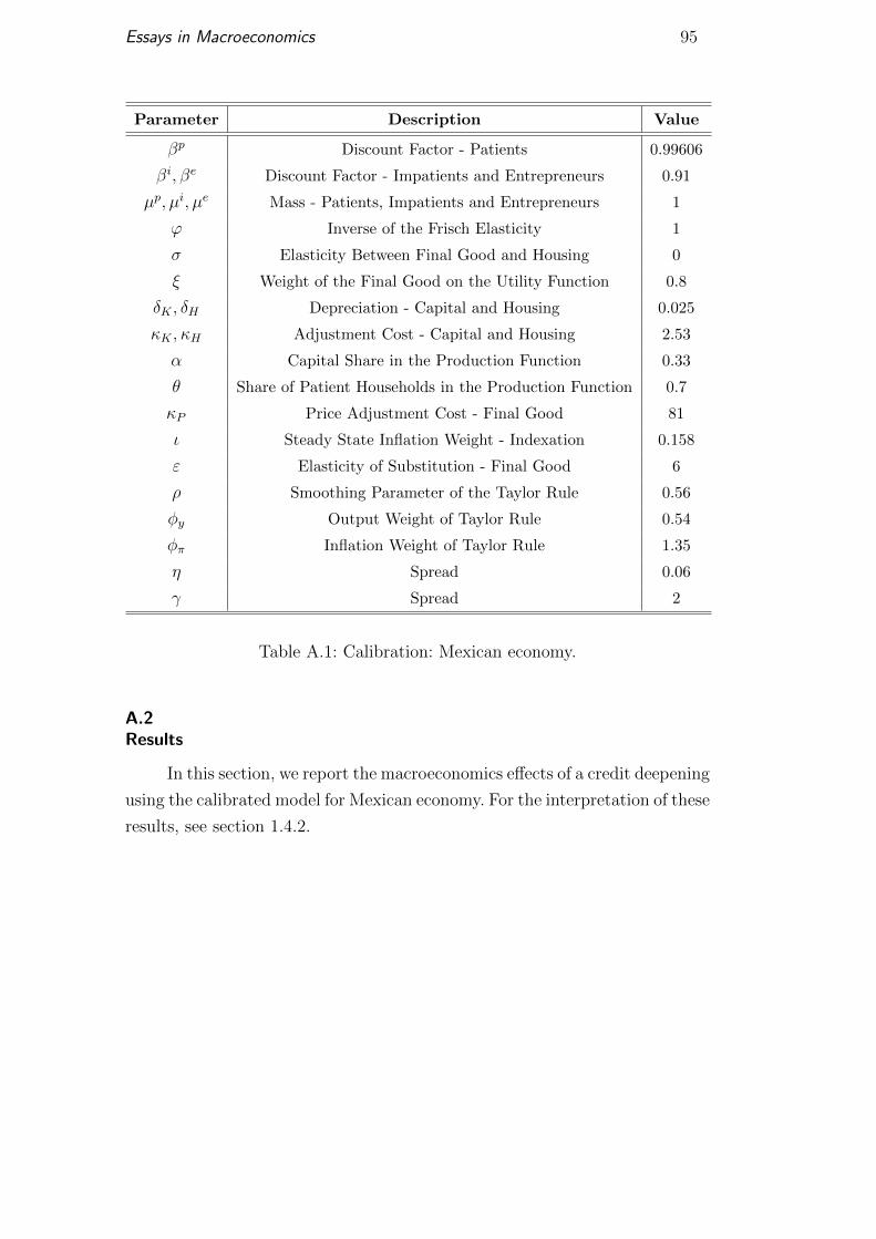
Essays in Macroeconomics 95
Parameter Description Value
βp Discount Factor - Patients 0.99606
βi, βe Discount Factor - Impatients and Entrepreneurs 0.91
µp, µi, µe Mass - Patients, Impatients and Entrepreneurs 1
ϕ Inverse of the Frisch Elasticity 1
σ Elasticity Between Final Good and Housing 0
ξ Weight of the Final Good on the Utility Function 0.8
δK , δH Depreciation - Capital and Housing 0.025
κK , κH Adjustment Cost - Capital and Housing 2.53
α Capital Share in the Production Function 0.33
θ Share of Patient Households in the Production Function 0.7
κP Price Adjustment Cost - Final Good 81
ι Steady State Inflation Weight - Indexation 0.158
ε Elasticity of Substitution - Final Good 6
ρ Smoothing Parameter of the Taylor Rule 0.56
φy Output Weight of Taylor Rule 0.54
φπ Inflation Weight of Taylor Rule 1.35
η Spread 0.06
γ Spread 2
Table A.1: Calibration: Mexican economy.
A.2Results
In this section, we report the macroeconomics effects of a credit deepening
using the calibrated model for Mexican economy. For the interpretation of these
results, see section 1.4.2.

Essays in Macroeconomics 96
2006 2007 2008 2009 2010 2011 2012 2013
0.024
0.026
0.028
0.03
0.032
0.034
0.036
0.038
0.04
0.042
0.044
τK
2006 2007 2008 2009 2010 2011 2012 2013
0.18
0.2
0.22
0.24
0.26
0.28
0.3
τWL
2006 2007 2008 2009 2010 2011 2012 2013
0.19
0.195
0.2
0.205
0.21
0.215
0.22
0.225
0.23
0.235
0.24
τH
Figure A.1: Credit deepening experiment for Mexico: evolution of τKt , τWLt and
τHt .
2006 2007 2008 2009 2010 2011 2012 20133
3.2
3.4
3.6
3.8
4
4.2
4.4
4.6
Personal Credit to Impatient Households over GDP(%)
Data
Model
2006 2007 2008 2009 2010 2011 2012 20137
7.5
8
8.5
9
9.5
10
Housing Credit to Impatient Households over GDP (%)
2006 2007 2008 2009 2010 2011 2012 20135.5
6
6.5
7
7.5
8
8.5
9
9.5
Credit to Entrepreneurs over GDP (%)
2006 2007 2008 2009 2010 2011 2012 201316
17
18
19
20
21
22
23
24
Total Credit over GDP (%)
Figure A.2: Credit deepening experiment for Mexico: credit variables (model
and data).

Essays in Macroeconomics 97
2006 2007 2008 2009 2010 2011 2012 201399.9
100
100.1
100.2
100.3
100.4
100.5
100.6
100.7
100.8
100.9
GDP
2006 2007 2008 2009 2010 2011 2012 2013100
100.05
100.1
100.15
100.2
100.25
100.3
100.35
100.4
100.45
Consumption
2006 2007 2008 2009 2010 2011 2012 2013
100
100.2
100.4
100.6
100.8
101
101.2
101.4
Investment
2006 2007 2008 2009 2010 2011 2012 20133.95
4
4.05
4.1
4.15
4.2
4.25
Inflation (% p. y.)
Figure A.3: Credit deepening experiment for Mexico: macro variables (model).

Essays in Macroeconomics 98
2006 2007 2008 2009 2010 2011 2012 201399.9
100
100.1
100.2
100.3
100.4
100.5Consumption of Final Goods − Patient Households
2006 2007 2008 2009 2010 2011 2012 2013100
100.2
100.4
100.6
100.8
101Consumption of Final Goods − Impatient Households
2006 2007 2008 2009 2010 2011 2012 2013
100
100.2
100.4
100.6
100.8Consumption of Final Goods − Entrepreneurs
2006 2007 2008 2009 2010 2011 2012 201399
99.5
100
100.5
101Investiment on Housing − Patient Households
2006 2007 2008 2009 2010 2011 2012 2013100
105
110
115
120
125Investiment on Housing − Impatient Households
2006 2007 2008 2009 2010 2011 2012 2013100
101
102
103
104Investiment on Capital − Entrepreneurs
2006 2007 2008 2009 2010 2011 2012 201399.75
99.8
99.85
99.9
99.95
100
100.05Stock of Housing − Patient Households
2006 2007 2008 2009 2010 2011 2012 2013100
101
102
103
104
105Stock of Housing − Impatient Households
2006 2007 2008 2009 2010 2011 2012 2013100
100.5
101
101.5
102Stock of Capital − Entrepreneurs
Figure A.4: Credit deepening experiment for Mexico: consumption, investment
and stocks.

Essays in Macroeconomics 99
2006 2007 2008 2009 2010 2011 2012 2013100
100.1
100.2
100.3
100.4
100.5
100.6
Wage − Impatient Households
2006 2007 2008 2009 2010 2011 2012 2013100
100.1
100.2
100.3
100.4
100.5
100.6
Wage − Patient Households
2006 2007 2008 2009 2010 2011 2012 201399.7
99.8
99.9
100
100.1
100.2
100.3
100.4
100.5
100.6
100.7
Labor Services − Impatient Households
2006 2007 2008 2009 2010 2011 2012 2013100
100.05
100.1
100.15
100.2
100.25
Labor Services − Patient Households
Figure A.5: Credit deepening experiment for Mexico: labor market outcomes.

Essays in Macroeconomics 100
2006 2007 2008 2009 2010 2011 2012 20135.62
5.64
5.66
5.68
5.7
5.72
5.74
5.76
5.78
5.8
rh (% p.y.)
2006 2007 2008 2009 2010 2011 2012 20137.8
8
8.2
8.4
8.6
8.8
9
9.2
9.4
9.6
9.8
re (% p.y.)
2006 2007 2008 2009 2010 2011 2012 20131
1.5
2
2.5
3
3.5
4
4.5
5
5.5
Spread (% p.y.)
Data
Model
Figure A.6: Credit deepening experiment for Mexico: financial market out-
comes. The spread is calculated using the bank funding rate, which is an inter-
bank rate that banks use to lend to each other (proxy for monetary policy
rate), and the implicit interest rate to enterprise which is the lending in-
terest rate that banks charge their clients. Source: Bank of Mexico, available
at www.banxico.org.mx.
GDP Consumption Investment
Growth (data): 19.1% Growth (data): 20.5% Growth (data): 28.2%
Growth (model): 0.7% Growth (model): 0.7% Growth (model): 1.3%
Trend growth Above trend Model Above trend Model Above trend Model
(% p.y.) growth (%) share (%) growth (%) share (%) growth (%) share (%)
1.0% 11.1% 6.3% 12.4% 2.4% 19.6% 6.6%
1.5% 7.3% 9.6% 8.6% 3.5% 15.5% 8.4%
2.0% 3.7% 19.0% 4.9% 6.1% 11.6% 11.2%
2.5% 0.2% 359.5% 1.4% 21.9% 7.9% 16.6%
Table A.2: Credit expansion experiment for Mexico: comparison with the real
data between 2006-2013. Growth rates of GDP, consumption and investment
are obtained from Bank of Mexico, available at www.banxico.org.mx.
BHouseholds’ fixed level of human capital: mean preserving exercise
For the households’ fixed level of human capital θ, we also consider a mean
preserving exercise. Therefore, we change θ1 and θ2 to generate economies with
different levels of income inequality, but the aggregate labor units is kept at the
same level as in the benchmark. In this case, a lower (higher) θ1 and a higher
(lower) θ2 increase (reduce) income inequality. Specially, for economies with

Essays in Macroeconomics 101
higher levels of income inequality than the benchmark, we set θ1 equals to 0.8
(0.7) and θ2 equals to 2.28 (2.5) that corresponds to a Gini index of 47 (52).
Moreover, for economies with lower levels of income inequality, we consider θ1
equals to 1.3 (1.5) and θ2 equals to 1.17 (0.72) to generate economies with a
Gini index of 37 (32).
Figure B.1 shows these results, which are not in line with the empirical
finding: consumption growth at peak is higher in economies with lower income
inequality. However, this result is not monotonic. For example, the economy
with Gini index of 32 shows a consumption growth at the peak of 1.81 percent,
while the other one with Gini index of 37 is 1.73 percent. On the other hand,
consumption grows at the peak 1.73 and 1.63 in the economies with Gini index
of 47 and 52, respectively. This occurs because the results on this exercise
depends on the share and on the values of θ1 and θ2, which influence how
households are credit constrained in equilibrium.
0 5 10 15 20 25−0.5
0
0.5
1
1.5
2
Years
Cumulative Consumption Growth (%)
θ
1 = 1.5, θ
2 = 0.72; Gini = 32
θ1 = 1.3, θ
2 = 1.17; Gini = 37
θ1 = 1, θ
2 = 1.84; Gini = 42
θ1 = 0.8, θ
2 = 2.28, Gini = 47
θ1 = 0.7, θ
2 = 2.5, Gini = 52
0 5 10 15 206
8
10
12
14
16
18
20
Years
Debt to GDP (%)
Figure B.1: σ2ε : Cumulative consumption growth ad Debt to GDP by income
inequality.
Table B.1 decomposes these results in the contribution of assets distribu-
tion and policies functions. Note that, when we consider the assets distributions
fixed, results are monotonic: consumption at the peak grows 1.86 percent in
the economy with highest income inequality and grows 1.65 percent in the
one with lowest income inequality. Also considering the contribution for the
assets distribution, results are not monotonic: there is a negative contribution
for economies with Gini index of 32, 37 and 52, however, there is a positive
contribution for the one with Gini index of 47.
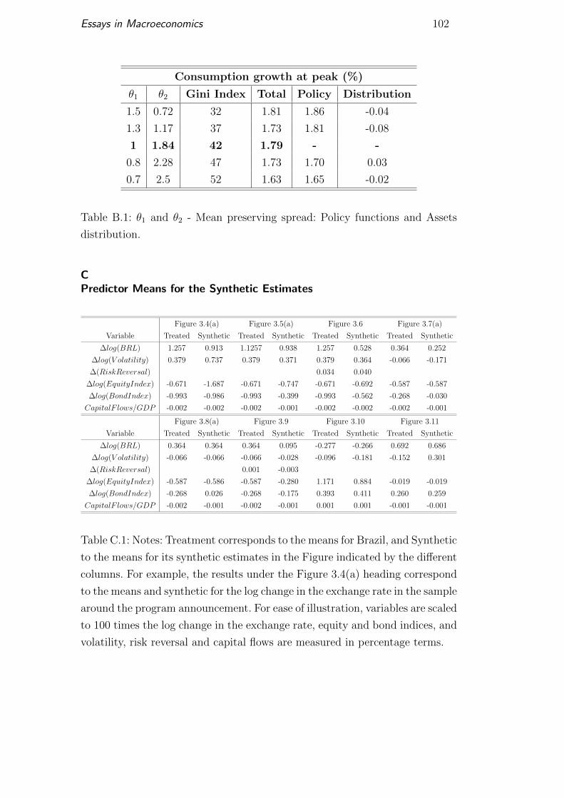
Essays in Macroeconomics 102
Consumption growth at peak (%)
θ1 θ2 Gini Index Total Policy Distribution
1.5 0.72 32 1.81 1.86 -0.04
1.3 1.17 37 1.73 1.81 -0.08
1 1.84 42 1.79 - -
0.8 2.28 47 1.73 1.70 0.03
0.7 2.5 52 1.63 1.65 -0.02
Table B.1: θ1 and θ2 - Mean preserving spread: Policy functions and Assets
distribution.
CPredictor Means for the Synthetic Estimates
Figure 3.4(a) Figure 3.5(a) Figure 3.6 Figure 3.7(a)
Variable Treated Synthetic Treated Synthetic Treated Synthetic Treated Synthetic
∆log(BRL) 1.257 0.913 1.1257 0.938 1.257 0.528 0.364 0.252
∆log(V olatility) 0.379 0.737 0.379 0.371 0.379 0.364 -0.066 -0.171
∆(RiskReversal) 0.034 0.040
∆log(EquityIndex) -0.671 -1.687 -0.671 -0.747 -0.671 -0.692 -0.587 -0.587
∆log(BondIndex) -0.993 -0.986 -0.993 -0.399 -0.993 -0.562 -0.268 -0.030
CapitalF lows/GDP -0.002 -0.002 -0.002 -0.001 -0.002 -0.002 -0.002 -0.001
Figure 3.8(a) Figure 3.9 Figure 3.10 Figure 3.11
Variable Treated Synthetic Treated Synthetic Treated Synthetic Treated Synthetic
∆log(BRL) 0.364 0.364 0.364 0.095 -0.277 -0.266 0.692 0.686
∆log(V olatility) -0.066 -0.066 -0.066 -0.028 -0.096 -0.181 -0.152 0.301
∆(RiskReversal) 0.001 -0.003
∆log(EquityIndex) -0.587 -0.586 -0.587 -0.280 1.171 0.884 -0.019 -0.019
∆log(BondIndex) -0.268 0.026 -0.268 -0.175 0.393 0.411 0.260 0.259
CapitalF lows/GDP -0.002 -0.001 -0.002 -0.001 0.001 0.001 -0.001 -0.001
Table C.1: Notes: Treatment corresponds to the means for Brazil, and Synthetic
to the means for its synthetic estimates in the Figure indicated by the different
columns. For example, the results under the Figure 3.4(a) heading correspond
to the means and synthetic for the log change in the exchange rate in the sample
around the program announcement. For ease of illustration, variables are scaled
to 100 times the log change in the exchange rate, equity and bond indices, and
volatility, risk reversal and capital flows are measured in percentage terms.
Related Documents