The unexplained part of public debt

Inter-American Development Bank

Banco Interamericano de Desarrollo (BID) Research Department

Departamento de Investigación Working Paper #554

The Unexplained Part of Public Debt

by

Camila F.S. Campos* Dany Jaimovich**

Ugo Panizza**

*Yale University **Inter-American Development Bank, Washington, D.C.

March 2006

2

Cataloging-in-Publication data provided by the Inter-American Development Bank Felipe Herrera Library Campos, Camila F.S.

The unexplained part of public debt / by Camila F.S. Campos, Dany Jaimovich, Ugo

Panizza.

p. cm. (Research Department working paper series ; 554) Includes bibliographical references. 1. Debts, Public. 2. Budget deficits. 3. Financial statements. I. Jaimovich, Dany. II.

Panizza, Ugo. III. Inter-American Development Bank. Research Dept. IV. Title. V. Series.

336.34 C448 --------dc22 ©2006 Inter-American Development Bank 1300 New York Avenue, N.W. Washington, DC 20577 The views and interpretations in this document are those of the authors and should not be attributed to the Inter-American Development Bank, or to any individual acting on its behalf. This paper may be freely reproduced provided credit is given to the Research Department, Inter-American Development Bank. The Research Department (RES) produces a quarterly newsletter, IDEA (Ideas for Development in the Americas), as well as working papers and books on diverse economic issues. To obtain a complete list of RES publications, and read or download them please visit our web site at: http://www.iadb.org/res.

3

Abstract1

This paper shows that budget deficits account for a relatively small fraction of debt growth and that stock-flow reconciliation, which is often considered a residual entity, is one of the key determinants of debt dynamics. After having explained the importance of the stock-flow reconciliation, the paper shows that this residual entity can be partly explained by contingent liabilities and balance-sheet effects.

Keywords: Public Debt, Deficit, Balance-Sheet Effects JEL Codes: H63, F34, C82

1 The views expressed in this paper are the authors and do not necessarily reflect those of the Inter-American Development Bank. The usual caveats apply. Camila Campos: [email protected], Dany Jaimovich: [email protected], Ugo Panizza: [email protected].

4

1. Introduction How do countries get into debt? The answer to this question may seem trivial. Countries

accumulate debt whenever they run a budget deficit (i.e., whenever public expenditure is higher

than revenues). In fact, the standard Economics 101 debt accumulation equation states that the

change in the stock of debt is equal to the budget deficit:

ttt DEFICITDEBTDEBT =− −1 (1)

and that the stock of debt is equal to the sum of past budget deficits: ∑=

−=t

iitt DEFICITDEBT

0.

Whoever has worked with actual debt and deficit data knows that Equation (1) rarely holds and

that debt accumulation can be better described as:

tttt SFDEFICITDEBTDEBT +=− −1 (2)

where tSF is what is usually called “stock-flow reconciliation.” Clearly, Equation (1) is a good

approximation of debt accumulation only if one assumes that tSF is not very large. The purpose

of this paper is to describe some of tSF ’s main characteristics. The paper shows that, contrary to

what is usually assumed, the budget deficit accounts for a small fraction of the within-country

variance of the change in debt over GDP and that stock-flow reconciliation plays an important

role in explaining debt dynamics. The paper also shows that, on average, tSF tends to be positive

and that there are large cross-country differences in the magnitude of this residual entity. This

suggests that the magnitude of stock-flow reconciliation is not likely to be purely due to random

measurement error. In particular, the paper shows that the problem is especially serious in

developing countries and, among this group of countries, the difference between debt and deficit

is particularly large in Latin America and Sub-Saharan Africa.

The paper also runs a set of regressions aimed at explaining the main determinants of the

magnitude of the stock-flow reconciliation and finds that balance-sheet effects due to real

depreciations and contingent liabilities that arise at time of banking crises are strongly correlated

with the difference between deficit and change in debt. However, the paper also shows that the

regressions can only explain 20 percent of the within-country variance of the stock-flow

5

reconciliation and that there is still much that we do not understand about one of the main

determinants of debt accumulation.

While we are not the first to show that stock-flow reconciliation is an important part of

debt dynamic (see, among others IMF, 2003; Martner and Tromben, 2004; European

Commission, 2005; Budina and Fiess, 2005), we are not aware of any other paper that

systematically describes the main characteristics of this residual, but extremely important,

determinant of debt accumulation.

The rest of the paper is organized as follows. Section 2 describes our main sources of

data and presents some basic facts on public debt and deficit. Section 3 focuses on a detailed

description of the stock-flow reconciliation. Section 4 runs a set of regressions aimed at

explaining the main determinants of the stock flow reconciliation. Section 5 concludes.

2. Data

The purpose of this section is to describe our data on fiscal deficit and public debt. In this

context, it is worth mentioning that obtaining reliable and comparable data on the stock public

debt is a rather difficult exercise. In fact, the IMF International Financial Statistics (IFS) and

IMF Government Finance Statistics (GFS), which are the most common sources of cross-country

data on government statistics, report data for a rather limited set of countries. This is even the

case for industrial countries; these sources do not report recent data on public debt for Japan and

Italy, for example. Furthermore, most cross-country datasets do not make an effort to make the

data comparable across countries (for a discussion of these issues, see IMF, 2003).2

Although there are now some papers that attempt to build comparable cross-country data-

sets on public debt (Cowan et al., 2005; Jeanne and Guscina, 2006; IMF, 2003; Budina and

Fiess, 2005), some of these data sets are not publicly available and all of them have a limited

country and time coverage. As a consequence, we do not rely on these new data and only use

publicly available sources (hence, the caveats mentioned above should be kept in mind). In

particular, we start with IFS and GFS and supplement them with data collected from national

sources (mostly from the websites or publications of the various Ministries of Finance), the UN

Economic Commission for Latin America and Caribbean (ECLAC, see Martner and Tromben,

2004), and the Organization for Economic Cooperation and Development (OECD). 2 The most important problems include the treatment of sub-national governments and the use of gross versus net debt (for a methodological note, see Cowan et al., 2005).

6

Using these various sources, we assemble an unbalanced panel covering 117 countries

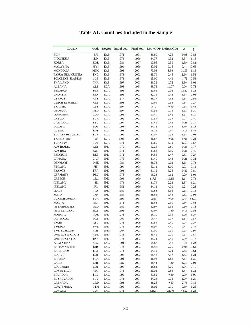
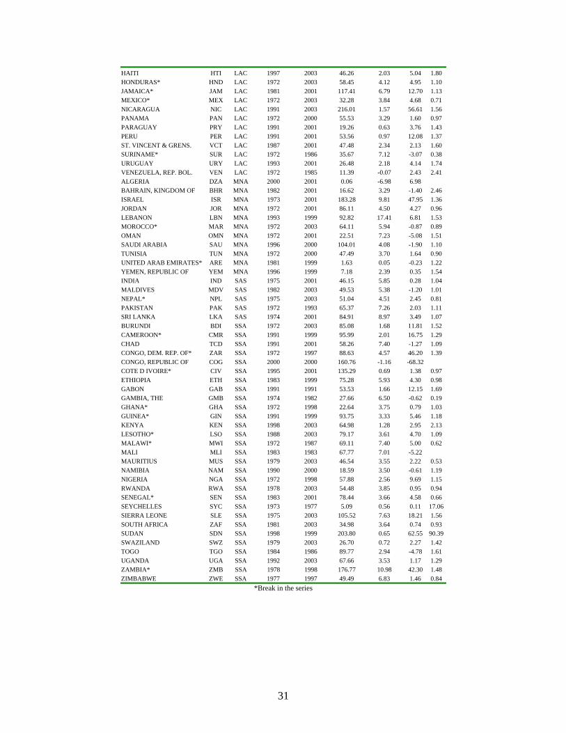
and consisting of approximately 1,900 observations. Table A1 in the Appendix lists all the

countries included in our dataset, the time coverage for each country, and summary statistics for

debt and deficit ratios. Our sample includes 24 high-income countries, 59 middle-income

countries and 34 low-income countries. The regions with the largest number of countries are

Sub-Saharan Africa (27 countries) and Latin America (25 countries). South Asia and East Asia

are the regions with the smallest number of countries (five and eight countries, respectively).

While long time series are available for some countries (e.g., Bahamas, Burundi, Costa Rica,

Iceland, Norway and the US have more than 30 years of data), for others there are very few

observations (Albania, Algeria, Gabon, Sudan, Togo, and Yemen are among the countries with

less than five years of data).

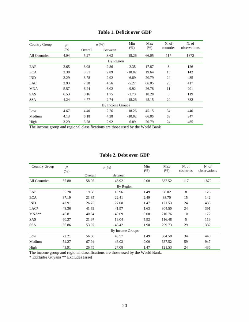
Table 1 shows that the sample mean of the deficit to GDP ratio is 4.04 percent and that

average deficit tends to decrease with the level of income. The region with the highest average

deficit is South Asia (6.5 percent), followed by the Middle East (5.6 percent), and Sub-Saharan

Africa (4.2 percent). Latin American countries tend to have fairly low levels of average deficit

(just below the cross-country average) but the region is far from being homogeneous and is

characterized by the largest variance in the sample.

Table 2 reports summary statistics for the debt-to-GDP ratio and shows that the cross-

country average is close to 56 percent. South Asia and Sub-Saharan Africa are the regions with

the highest levels of debt (67 and 60 percent, respectively) and East Asia and Eastern Europe and

Central Asia are the regions with the lowest level of debt (35 and 37 percent, respectively). Latin

America has a level of debt that is just below the sample average and is not much higher than

that of the industrial countries included in our sample. Again, we find that Latin America is one

of the most heterogeneous regions in our sample (in this case, second only to Sub-Saharan

Africa). As one may expect, we find that most of the variance in debt-to-GDP is due to

differences across countries (this is the between standard deviation). However, there is also

substantial variance within countries. In fact, the within standard deviation (not reported in the

table) is often close to 50 percent of the between standard deviation.

7

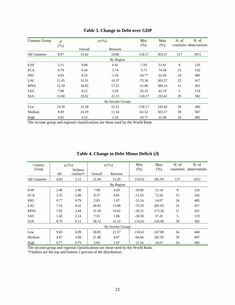
Table 3 focuses on the change in debt divided by GDP ( tid , ).3 If Equation (1) were to

hold, the change in debt should be equal to the budget deficit. By comparing Table 2 with Table

3, we find that the value of tid , is almost five percentage points higher than average deficit over

GDP, indicating that more than 50 percent of the average change in debt is not explained by

deficit.4 The Table also shows that while the difference between tid , and the deficit is fairly small

in industrial countries (about 0.3 percentage points), this difference is extremely large in Latin

America and Sub-Saharan Africa, where the average deficit is about one-third the average

change in debt.

We can now describe the characteristics of the stock-flow reconciliation by defining the

following measure of the difference between change in debt and deficit for country i at time t.

( )100

,

,1,,, ×

−−= −

ti

titititi Y

DEFICITDEBTDEBTδ (3)

Clearly, ti ,δ is just the stock-flow reconciliation of Equation (1) expressed in terms of

GDP (ti

ti

ti Y

SF

,

,

, =δ ). Table 4 describes ti ,δ and shows that the change in debt is nearly five

percentage points higher than the deficit (with the highest values in Latin America and Sub-

Saharan Africa). However, the Table also shows that there are several countries with extremely

large values of ti ,δ (in some cases well above 200 percent). In Latin America, for instance, the

difference between the change in debt and deficit has a range of 350 percentage points (from –73

3 It is important to note that we do not use the change in the debt-over-GDP ratio (i.e., 1001

1, ×⎟⎟

⎠

⎞⎜⎜⎝

⎛−=

−

−

t

t

t

tti Y

DYDθ )

but the change in debt divided by GDP at time t (i.e., 100)1(1

1, ×⎟⎟

⎠

⎞⎜⎜⎝

⎛+

−=−

−

gYD

YD

dt

t

t

tti ). As nominal GDP

growth (g) tends to be positive, tid , is usually larger than ti,θ . We use this measure, rather than the standard ti,θ because we want to isolate changes in debt from changes in the level of GDP. 4 Using a different methodology and a shorter sample, IMF (2003) also finds similar but less drastic results. In particular, it finds that more than 25 percent of the increase in the debt-to-GDP ratio of a sample of emerging market countries over the 1997-2003 period is due to off balance-sheet factors. In a sample of 21 market-access countries, Budina and Fiess (2005) find that debt over GDP increased by 22.8 percentage points from 1994 to 2002, while real GDP grew by 9.3 percent, yielding a change in debt of approximately 37 percent. The deficit (primary plus interest rate bill) explained about one-third of this change while other factors (including the real exchange rate) explained the remaining two-thirds.

8

to 281). The industrial countries have the smallest range, but even in this case the range is close

to 30 percentage points. These extreme values are due either to exceptional events or

measurement error. In the second column of Table 5, the average value of ti ,δ is computed by

dropping the top and bottom 2 percent of the distribution. After dropping these outliers, we find

that ti ,δ has an average value of 3 percent and that the average values of ti ,δ for Latin America

and the Middle East drop from 7 percent to 4 and 2 percent, respectively.

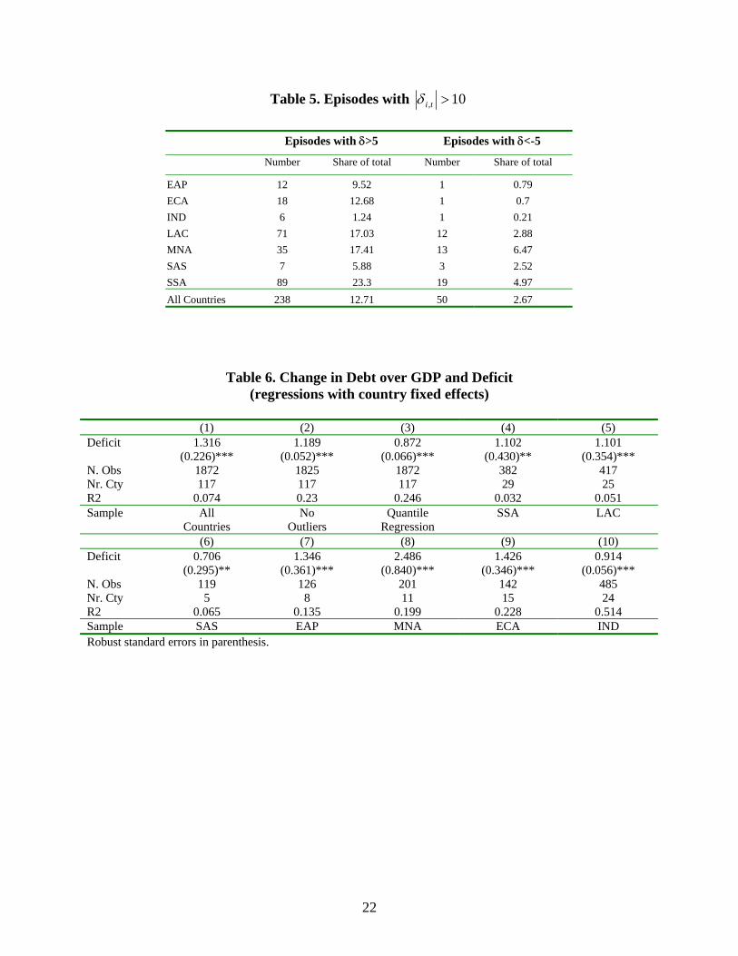
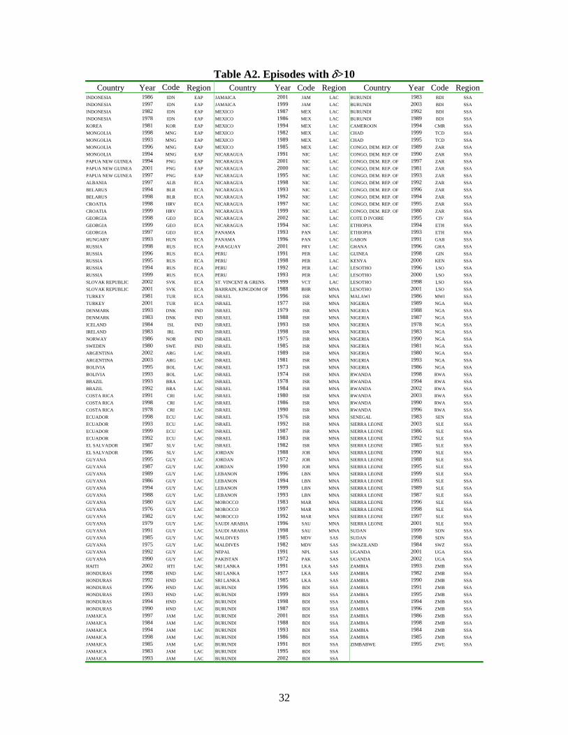
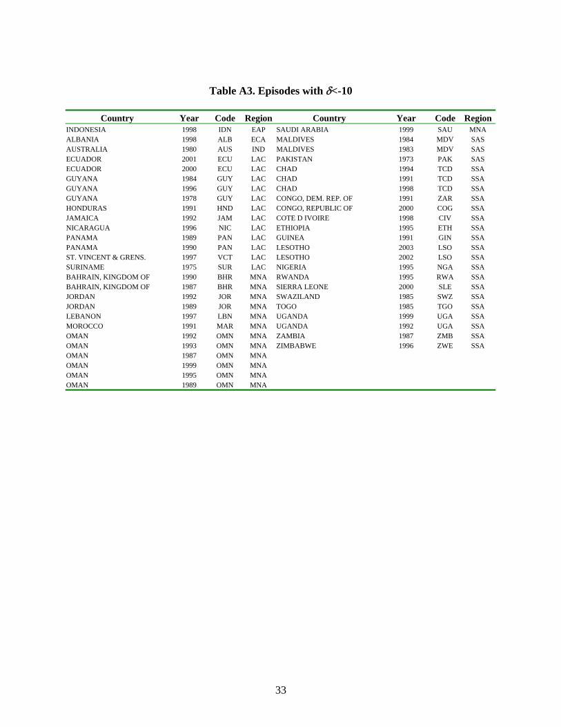
It is also interesting to see which countries tend to have large values of ti ,δ . Table 5

summarizes all the episodes for which 10, >tiδ (a full list of episodes is reported in Tables A2

and A3 in the appendix). There are 238 country-years (corresponding to 13 percent of

observations) for which 10, >tiδ , and 50 country-years (3 percent of observations) for

which 10, −<tiδ . The industrial countries, East Asia, and South Asia are the regions with the

lowest number of episodes (and very few episodes where 10, −<tiδ ). Sub Saharan Africa, the

Middle East and North Africa, and Latin America are the regions with the largest number of

episodes.

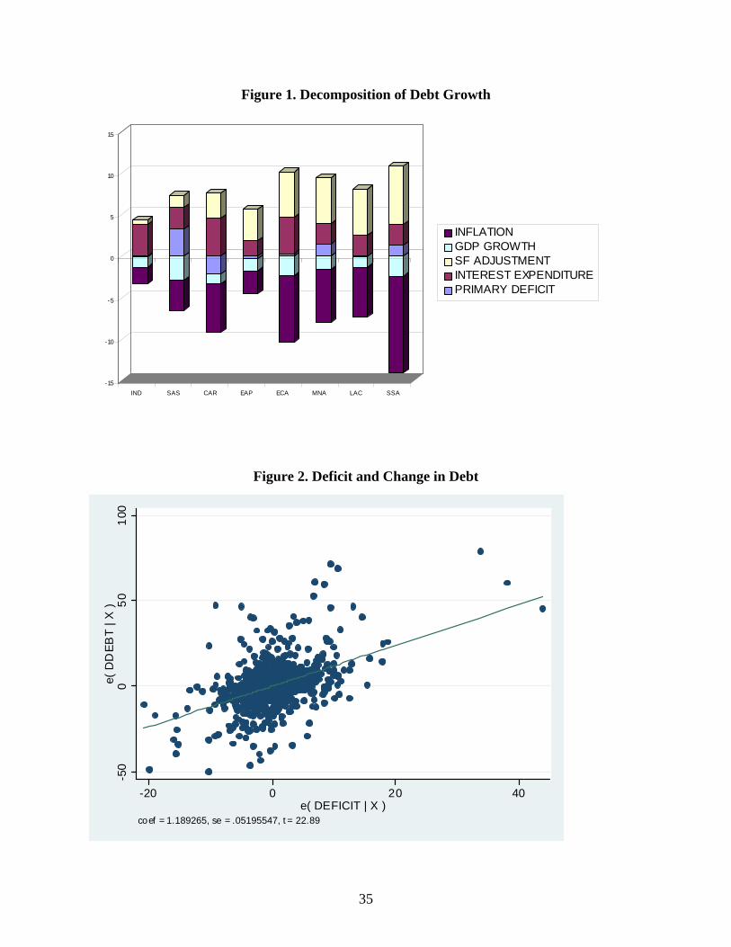
While this paper focuses on change in debt, we obtain the same results if we use the

standard decomposition of the change in debt over GDP (θ).5 Figure 1 shows that in most regions

the stock flow adjustment is the main determinant of debt growth and inflation is the main

determinant of debt reduction

3. Debt and Deficit

The previous section showed that simple comparisons of average values of deficit over GDP and

change in debt indicate that Equation (1) is far from being a good approximation of the main

determinants of debt accumulation and that what is usually considered a residual entity (the

5 The standard decomposition takes the following form:

( )t

t

t

t

t

t

t

t

t

t

t

t

YSF

gYDEBT

grgY

DEBTi

YPD

YDEBT

YDEBT

++

+−+

+=−−

−

−

−

−

−

)1()1( 1

1

1

1

1

1 π

where the first term on the RHS of the equation is the contribution of the primary deficit, the second term is the interest bill, the third term is the contribution of nominal growth (which can be split into real growth and inflation) and the last term is the stock-flow adjustment.

9

stock-flow reconciliation) is a key determinant of debt accumulation. In this section, we use

different strategies to provide more evidence in this direction.

3.1 Regressions Analysis

One way to assess the importance of tSF is to divide debt and deficit by current GDP and use

our large panel to estimate the following fixed effects regression:

ititiit defd ,,, * εβα ++= (4)

where iα is a country fixed effect (the country fixed effects control for the fact that the data

come from different sources, countries have different levels of debt, and they use different

methodologies for computing debt and deficit) and itdef , is deficit over GDP. If Equation (1)

holds, we expect a high R2 (the regression’s R2 should be 1 if Equation 1 holds exactly), iα =0,

and β =1. Hence, the regression’s coefficients and R2 can be used to asses the relative

(un)importance of the deficit in explaining changes in debt. Table 6 reports the results of the

estimation of Equation (4) for different sub-samples of countries. Column 1 describes the basic

pattern. First of all, we find that β is greater than 1 (but not significantly different from 1)

indicating that a 1 percent increase in the deficit to GDP ratio tends to translate into a 1.3 percent

increase of the debt to GDP ratio. More interestingly, the regression’s R2 shows that, in our

sample of countries, deficits explain less than 8 percent of the within country variance of itd , and

that tSF explains more than 90 percent of the variance.6

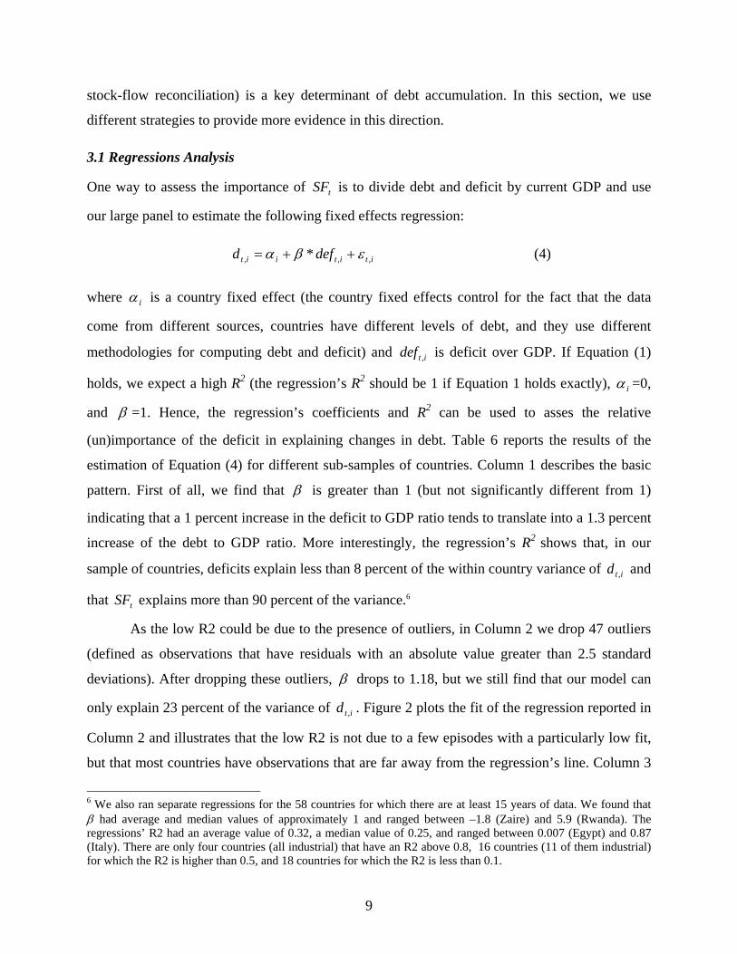
As the low R2 could be due to the presence of outliers, in Column 2 we drop 47 outliers

(defined as observations that have residuals with an absolute value greater than 2.5 standard

deviations). After dropping these outliers, β drops to 1.18, but we still find that our model can

only explain 23 percent of the variance of itd , . Figure 2 plots the fit of the regression reported in

Column 2 and illustrates that the low R2 is not due to a few episodes with a particularly low fit,

but that most countries have observations that are far away from the regression’s line. Column 3

6 We also ran separate regressions for the 58 countries for which there are at least 15 years of data. We found that β had average and median values of approximately 1 and ranged between –1.8 (Zaire) and 5.9 (Rwanda). The regressions’ R2 had an average value of 0.32, a median value of 0.25, and ranged between 0.007 (Egypt) and 0.87 (Italy). There are only four countries (all industrial) that have an R2 above 0.8, 16 countries (11 of them industrial) for which the R2 is higher than 0.5, and 18 countries for which the R2 is less than 0.1.

10

of Table 4 addresses the outlier issues by running the same regression as in Column 1 using a

median quantile regression with bootstrapped standard errors (STATA’s BSQREG) and shows

that in this case, the coefficient of the deficit variable drops to 0.87 and the R2 goes to 0.24.

The remaining columns run separate regressions for different regions of the world.

Column 4 focuses on 29 countries located in Sub-Saharan Africa and finds that the deficit

explains only 3 percent of the variance of itd , . Columns 5 and 6 show that in Latin America and

the Caribbean (25 countries) and South Asia (5 countries), the deficit explains between 5 and 6

percent of the variance of itd , . Columns 7 and 8 focus on East Asia (8 countries) and the Middle

East and North Africa (11 countries) and show that the deficit explains between 14 and 20

percent of the within country variance of itd , . The developing region with the best fit is East

Europe and Central Asia (Column 9, 15 countries). In this case, the deficit explains 23 percent of

the variance of itd , . Only in the sub-group of industrial countries (Column 10, 24 countries) does

the deficit explain more than one-quarter of the within country variation of itd , but even in this

case, the regression can only explain half of the variance of the dependent variable.

3.2 Theoretical R2

As an alternative way to describe the pattern documented above, we build a measure aimed at

determining which countries have the largest deviation from the theoretical identity defd = .

Clearly, such a measure cannot be the country average of ti ,δ described in Table 5 because

negative and positive values of ti ,δ would compensate each other. One possibility would be to

adopt a strategy similar to the one of the previous section and run country-by-country regressions

of DEBTΔ over DEFICIT and use the fit of these regressions (their R2) as a measure of how

much a country deviates from defd = . One problem with this strategy is that it would not help

to differentiate countries that have a good fit in which defd = holds, from countries that have a

good fit but where the relationship between debt and deficit can be better described with an

equation of the type: ttt defd εβα ++= * with 0≠α and 1≠β . An index that addresses these

problems and relates to a regression’s R2 can be defined as:

11

( )

( )∑

∑

=

=

−= T

titi

T

tti

i

dd1

2,

1

2,δ

φ (5)

Note that iφ is always non-negative and naturally relates to the R2 of a regression of

tid , over def. In fact, if we write ttt defd εβα ++= * and, if instead of estimating the

regression’s parameter, we force 0=α and 1=β , the R2 of the model would be 1- iφ . Hence, if

the true parameters describing the relationship between debt and deficit were 0=α and 1=β ,

iφ would be equal to 0. Thus, higher values of iφ indicate larger deviations of the true

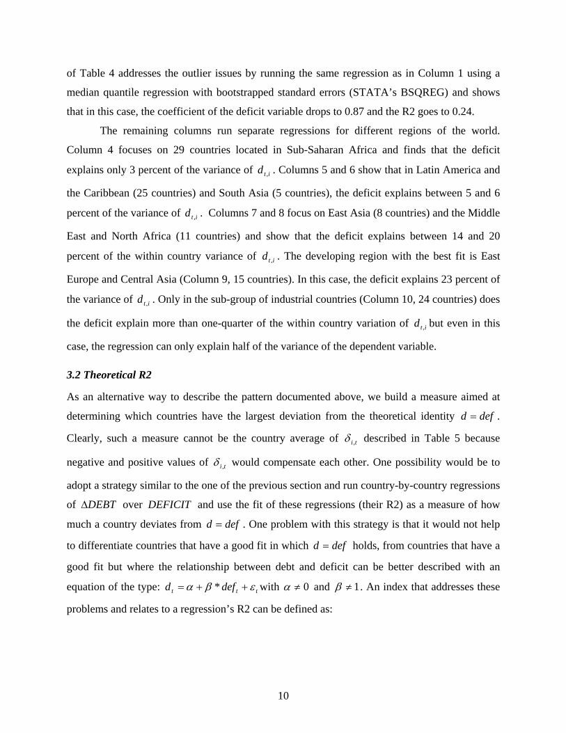
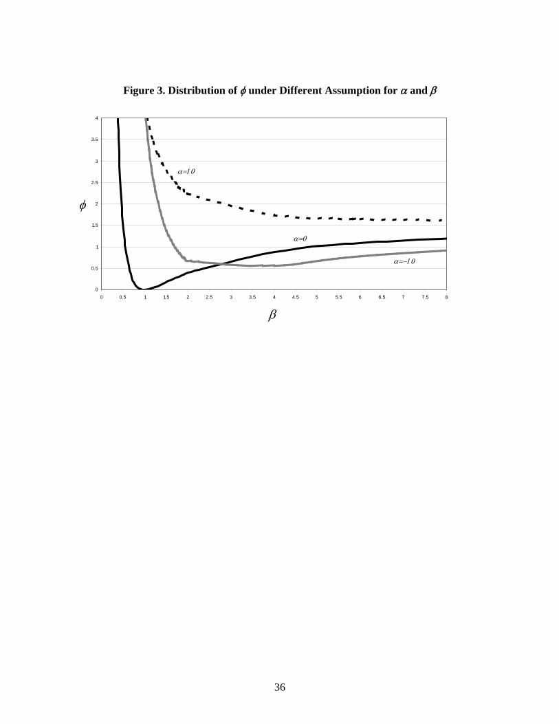
parameters from 0=α and 1=β . Figure 3 illustrates the theoretical distribution of iφ for

different values of β under the assumptions that 0=α , 10=α , and 10−=α . The figure shows

that when 0=α the distribution is asymmetrical with iφ rapidly going towards infinite when β

tends to 0, and iφ converging to around 1.5 when β goes to infinite, the figure also shows that

iφ is equal to 0 when β =1. When 10=α , the distribution becomes monotone but still going to

infinite when β goes to 0 and converging to approximately 1.5 when β goes to infinite. When

10−=α the distribution reaches a minimum when β is around 4 and then starts increasing and,

again, converges at around 1.5.

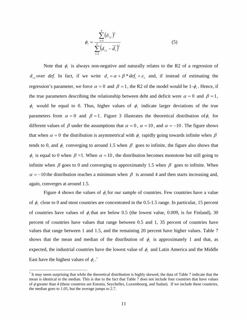
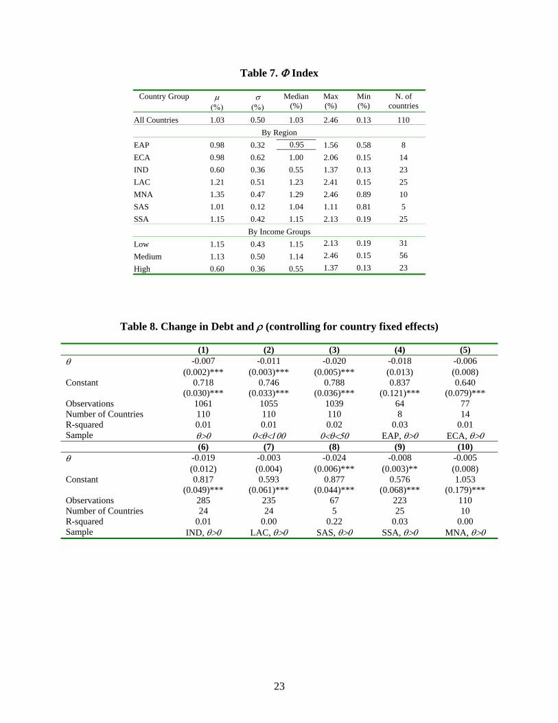
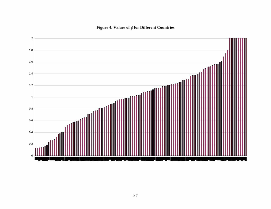
Figure 4 shows the values of iφ for our sample of countries. Few countries have a value

of iφ close to 0 and most countries are concentrated in the 0.5-1.5 range. In particular, 15 percent

of countries have values of iφ that are below 0.5 (the lowest value, 0.009, is for Finland), 30

percent of countries have values that range between 0.5 and 1, 35 percent of countries have

values that range between 1 and 1.5, and the remaining 20 percent have higher values. Table 7

shows that the mean and median of the distribution of iφ is approximately 1 and that, as

expected, the industrial countries have the lowest value of iφ and Latin America and the Middle

East have the highest values of iφ .7

7 It may seem surprising that while the theoretical distribution is highly skewed, the data of Table 7 indicate that the mean is identical to the median. This is due to the fact that Table 7 does not include four countries that have values of φ greater than 4 (these countries are Estonia, Seychelles, Luxembourg, and Sudan). If we include these countries, the median goes to 1.05, but the average jumps to 2.7.

12

3.3 Debt Explosions

So far, we documented that there are a large differences between deficit and change in debt. Now

we explore whether the difference between these two variables is positively correlated with debt

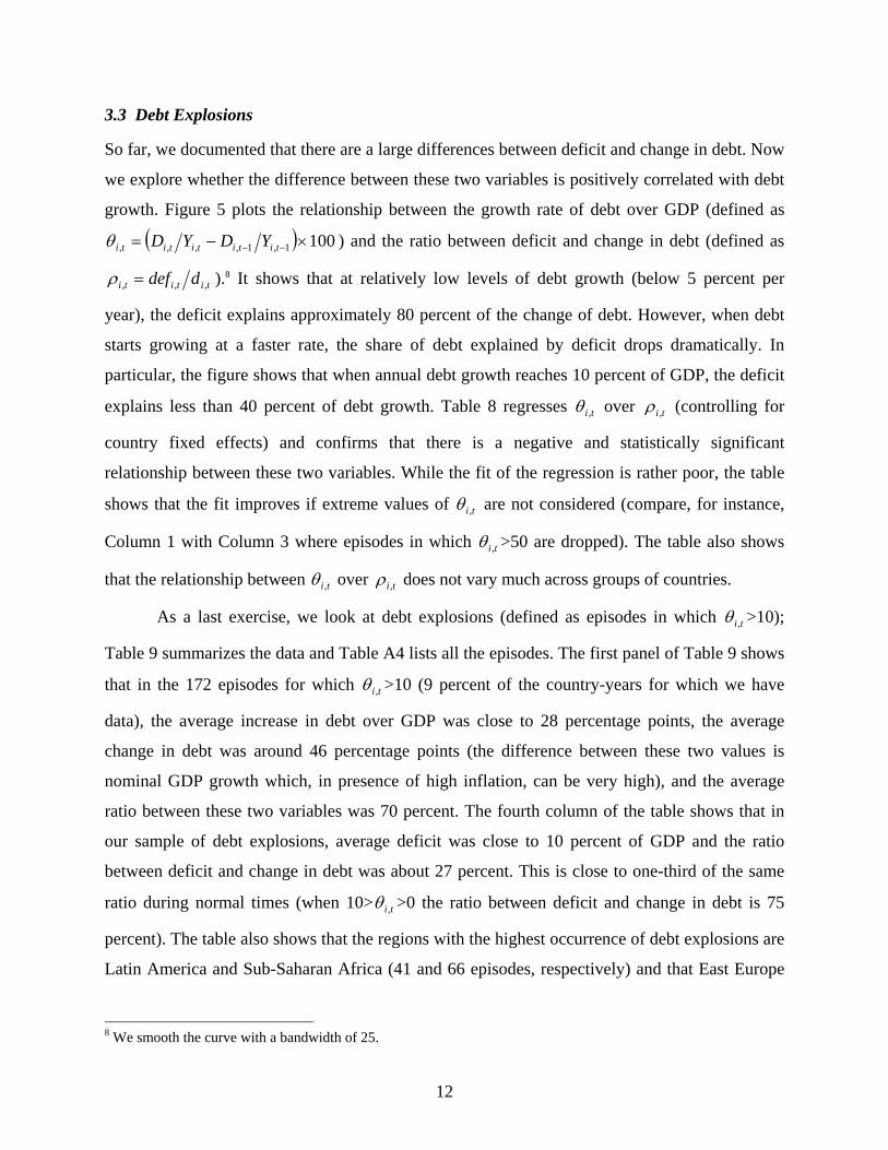
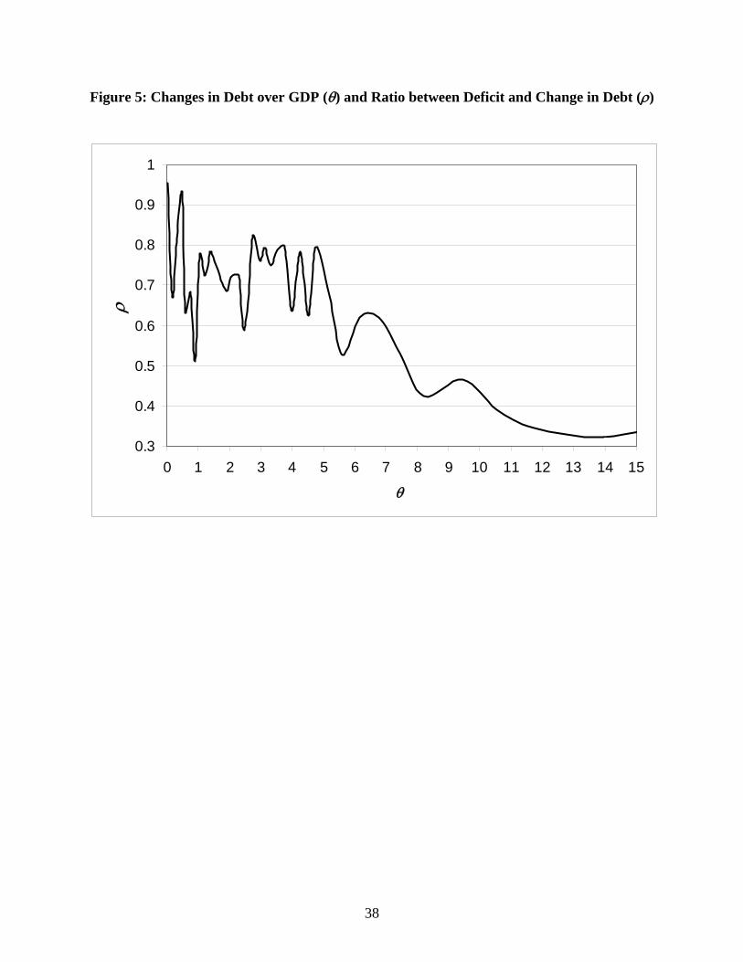
growth. Figure 5 plots the relationship between the growth rate of debt over GDP (defined as

( ) 1001,1,,,, ×−= −− tititititi YDYDθ ) and the ratio between deficit and change in debt (defined as

tititi ddef ,,, =ρ ).8 It shows that at relatively low levels of debt growth (below 5 percent per

year), the deficit explains approximately 80 percent of the change of debt. However, when debt

starts growing at a faster rate, the share of debt explained by deficit drops dramatically. In

particular, the figure shows that when annual debt growth reaches 10 percent of GDP, the deficit

explains less than 40 percent of debt growth. Table 8 regresses ti,θ over ti,ρ (controlling for

country fixed effects) and confirms that there is a negative and statistically significant

relationship between these two variables. While the fit of the regression is rather poor, the table

shows that the fit improves if extreme values of ti,θ are not considered (compare, for instance,

Column 1 with Column 3 where episodes in which ti,θ >50 are dropped). The table also shows

that the relationship between ti,θ over ti,ρ does not vary much across groups of countries.

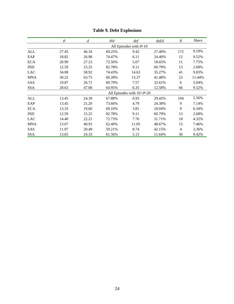
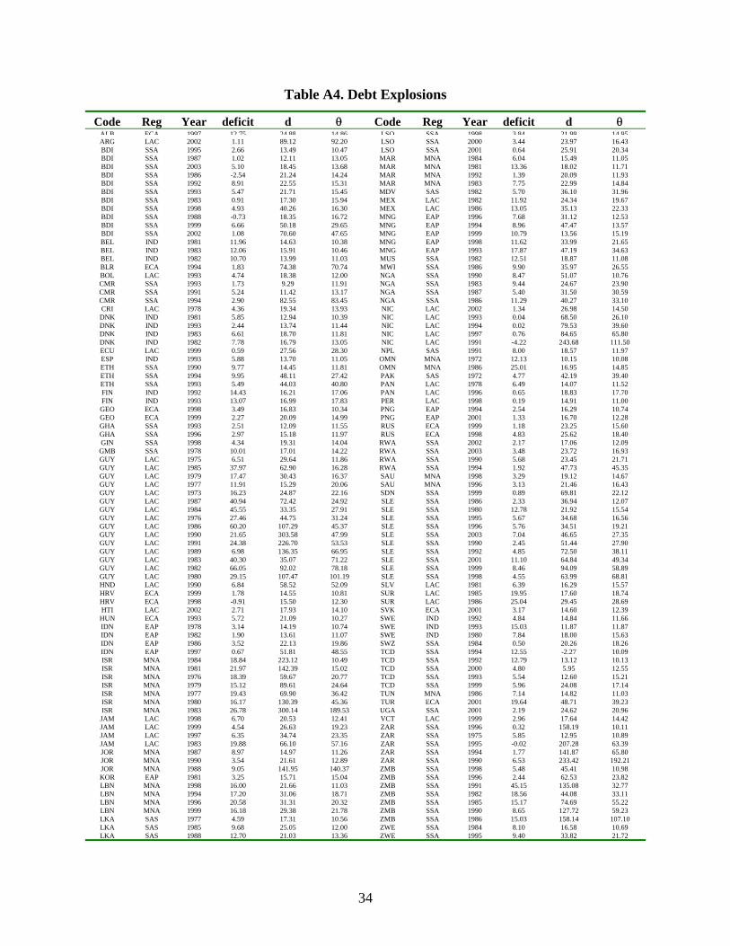
As a last exercise, we look at debt explosions (defined as episodes in which ti,θ >10);

Table 9 summarizes the data and Table A4 lists all the episodes. The first panel of Table 9 shows

that in the 172 episodes for which ti,θ >10 (9 percent of the country-years for which we have

data), the average increase in debt over GDP was close to 28 percentage points, the average

change in debt was around 46 percentage points (the difference between these two values is

nominal GDP growth which, in presence of high inflation, can be very high), and the average

ratio between these two variables was 70 percent. The fourth column of the table shows that in

our sample of debt explosions, average deficit was close to 10 percent of GDP and the ratio

between deficit and change in debt was about 27 percent. This is close to one-third of the same

ratio during normal times (when 10> ti,θ >0 the ratio between deficit and change in debt is 75

percent). The table also shows that the regions with the highest occurrence of debt explosions are

Latin America and Sub-Saharan Africa (41 and 66 episodes, respectively) and that East Europe

8 We smooth the curve with a bandwidth of 25.

13

and Sub-Saharan Africa are the regions with the lowest average ratio between deficit and change

in debt (18 and 13 percent, respectively).

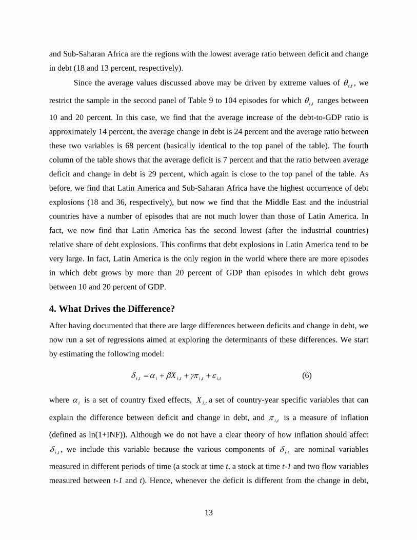
Since the average values discussed above may be driven by extreme values of ti,θ , we

restrict the sample in the second panel of Table 9 to 104 episodes for which ti,θ ranges between

10 and 20 percent. In this case, we find that the average increase of the debt-to-GDP ratio is

approximately 14 percent, the average change in debt is 24 percent and the average ratio between

these two variables is 68 percent (basically identical to the top panel of the table). The fourth

column of the table shows that the average deficit is 7 percent and that the ratio between average

deficit and change in debt is 29 percent, which again is close to the top panel of the table. As

before, we find that Latin America and Sub-Saharan Africa have the highest occurrence of debt

explosions (18 and 36, respectively), but now we find that the Middle East and the industrial

countries have a number of episodes that are not much lower than those of Latin America. In

fact, we now find that Latin America has the second lowest (after the industrial countries)

relative share of debt explosions. This confirms that debt explosions in Latin America tend to be

very large. In fact, Latin America is the only region in the world where there are more episodes

in which debt grows by more than 20 percent of GDP than episodes in which debt grows

between 10 and 20 percent of GDP.

4. What Drives the Difference?

After having documented that there are large differences between deficits and change in debt, we

now run a set of regressions aimed at exploring the determinants of these differences. We start

by estimating the following model:

tititiiti X ,,,, εγπβαδ +++= (6)

where iα is a set of country fixed effects, tiX , a set of country-year specific variables that can

explain the difference between deficit and change in debt, and ti,π is a measure of inflation

(defined as ln(1+INF)). Although we do not have a clear theory of how inflation should affect

ti ,δ , we include this variable because the various components of ti ,δ are nominal variables

measured in different periods of time (a stock at time t, a stock at time t-1 and two flow variables

measured between t-1 and t). Hence, whenever the deficit is different from the change in debt,

14

the value of ti ,δ should be positively correlated with nominal GDP growth, which is heavily

influenced by inflation.

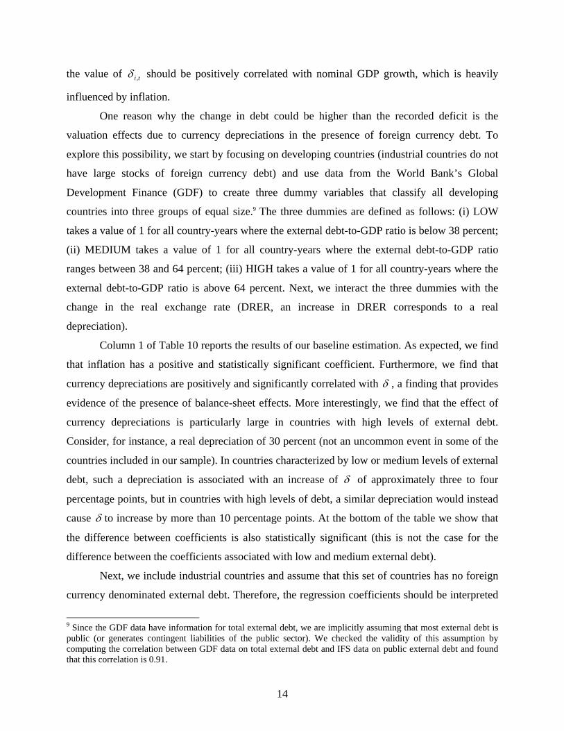
One reason why the change in debt could be higher than the recorded deficit is the

valuation effects due to currency depreciations in the presence of foreign currency debt. To

explore this possibility, we start by focusing on developing countries (industrial countries do not

have large stocks of foreign currency debt) and use data from the World Bank’s Global

Development Finance (GDF) to create three dummy variables that classify all developing

countries into three groups of equal size.9 The three dummies are defined as follows: (i) LOW

takes a value of 1 for all country-years where the external debt-to-GDP ratio is below 38 percent;

(ii) MEDIUM takes a value of 1 for all country-years where the external debt-to-GDP ratio

ranges between 38 and 64 percent; (iii) HIGH takes a value of 1 for all country-years where the

external debt-to-GDP ratio is above 64 percent. Next, we interact the three dummies with the

change in the real exchange rate (DRER, an increase in DRER corresponds to a real

depreciation).

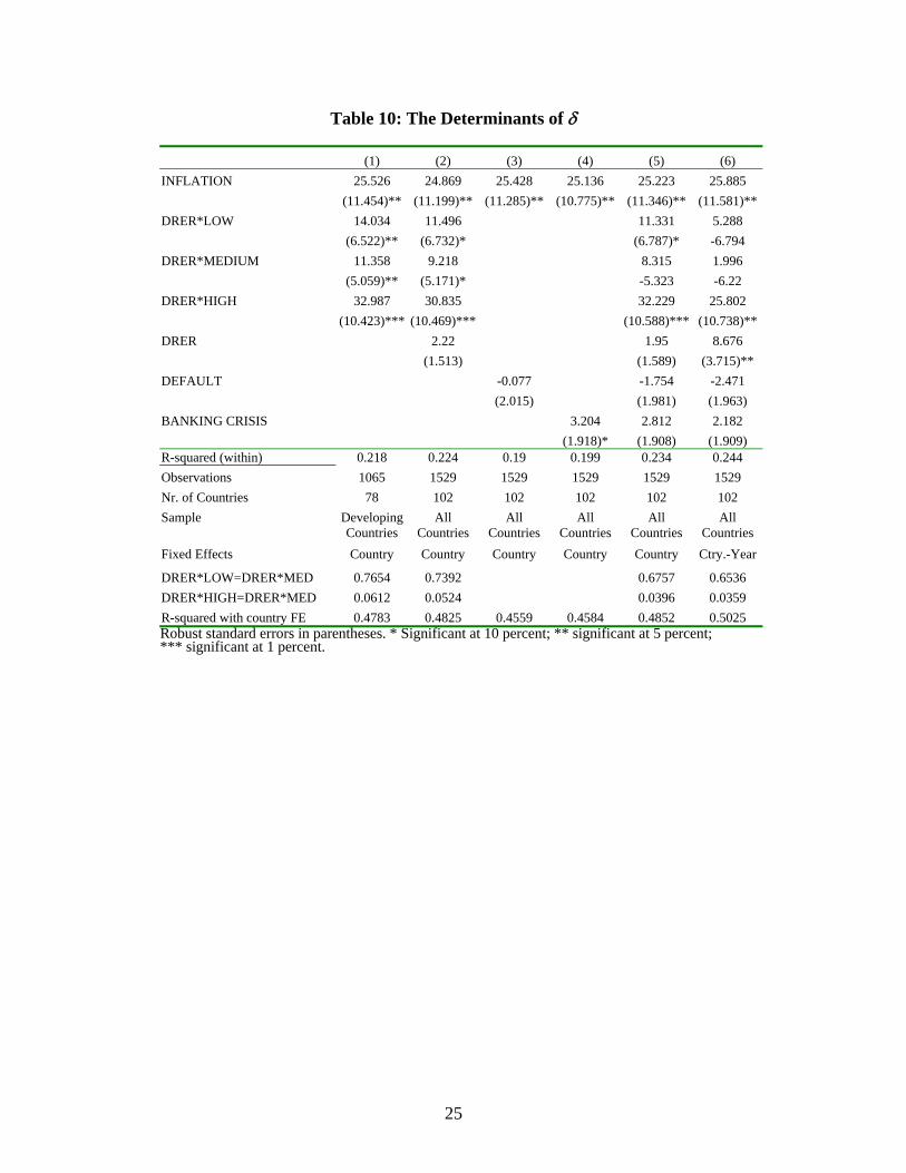
Column 1 of Table 10 reports the results of our baseline estimation. As expected, we find

that inflation has a positive and statistically significant coefficient. Furthermore, we find that

currency depreciations are positively and significantly correlated with δ , a finding that provides

evidence of the presence of balance-sheet effects. More interestingly, we find that the effect of

currency depreciations is particularly large in countries with high levels of external debt.

Consider, for instance, a real depreciation of 30 percent (not an uncommon event in some of the

countries included in our sample). In countries characterized by low or medium levels of external

debt, such a depreciation is associated with an increase of δ of approximately three to four

percentage points, but in countries with high levels of debt, a similar depreciation would instead

cause δ to increase by more than 10 percentage points. At the bottom of the table we show that

the difference between coefficients is also statistically significant (this is not the case for the

difference between the coefficients associated with low and medium external debt).

Next, we include industrial countries and assume that this set of countries has no foreign

currency denominated external debt. Therefore, the regression coefficients should be interpreted

9 Since the GDF data have information for total external debt, we are implicitly assuming that most external debt is public (or generates contingent liabilities of the public sector). We checked the validity of this assumption by computing the correlation between GDF data on total external debt and IFS data on public external debt and found that this correlation is 0.91.

15

as follows: DRER measures the effect of real depreciations in industrial countries;

DRER+DRER*LOW measures the effect of a real depreciation in developing countries with low

levels of external debt; DRER+DRER*MEDIUM measures the effect of a real depreciation in

developing countries with average levels of external debt; and DRER+DRER*HIGH measures

the effect of a real depreciation in developing countries with high levels of external debt. Column

2 shows that the coefficient of DRER is low and not statistically significant, indicating that there

are no balance-sheet effects in industrial countries. As before, we find that balance-sheet effects

are important in developing countries and that the effect of a real depreciation in all three groups

of developing countries is significantly different (both in economic and statistical terms) from

the effect of a depreciation in industrial countries. Finally, we still find that balance-sheet effects

tend to be particularly important in countries with high levels of debt.

Column 3 explores the role of default, w expect defaults to be associated with debt

reduction and hence negatively correlated with δ . To capture the effect of default, we use data

from Standard and Poor’s and build a dummy variable that takes a value of 1 around the last year

of a default episode (in particular, it takes a value of 1 in the last year of the episode and in the

year before and the year after the last year of the episode). Next, we build a default dummy that

takes a value of 1 in the last year of a Paris club rescheduling and then another dummy that takes

a value of 1 whenever the GDF reports that a country has rescheduled its debt. Finally, we build

a dummy called DEFAULT that takes a value of 1 whenever one of the previously described

dummies takes a value of 1. Column 3 shows that the default dummy has the expected negative

sign but that the coefficient is small and not statistically significant (we obtain similar results if

we use the three dummies separately).

Column 4 uses data from Caprio and Klingebiel (2003) to explore the role of banking

crises. These are important events because they generate a series of contingent liabilities and

other off-balance sheet activities that can translate into debt explosions. As expected, we find

that the coefficient of the banking crisis dummy is positive and statistically significant. The

coefficient is also quantitatively important, indicating that the average banking crisis is

associated with an increase of three percentage points in δ .

Column 5 jointly includes all the variables discussed above. We find that the results are

qualitatively similar to previous ones, but that the coefficient of DRER*MEDIUM is no longer

statistically significant (however, DRER+ DRER*MEDIUM remains significant) and that the

16

same is true for banking crisis. In the last column of the table, we control for year fixed effects

(which implicitly control for global shocks) and show that their inclusion does not affect our

basic results.

It is interesting to note that the set of controls included in the regressions of Table 10

explains about 20 percent of the variance of δ and that the country fixed effects explain about

30 percent of the variance of δ (see last row of Table 10). This indicates that country specific

factors explain most of the variance of δ and corroborates the findings of Table 4, which

showed that there are large cross-country differences in the average value of δ . There are two

possible explanations for this finding. The first has to do with the fact that measurement errors

that lead to an underestimation of the deficit are more important in some countries than in others,

which is probably related to the fact that poorer countries have less sophisticated accounting and

budgeting systems. The other has to do with the fact that the importance of contingent liabilities

that lead to debt explosions vary across countries and that our set of controls does not capture all

these contingent liabilities.10

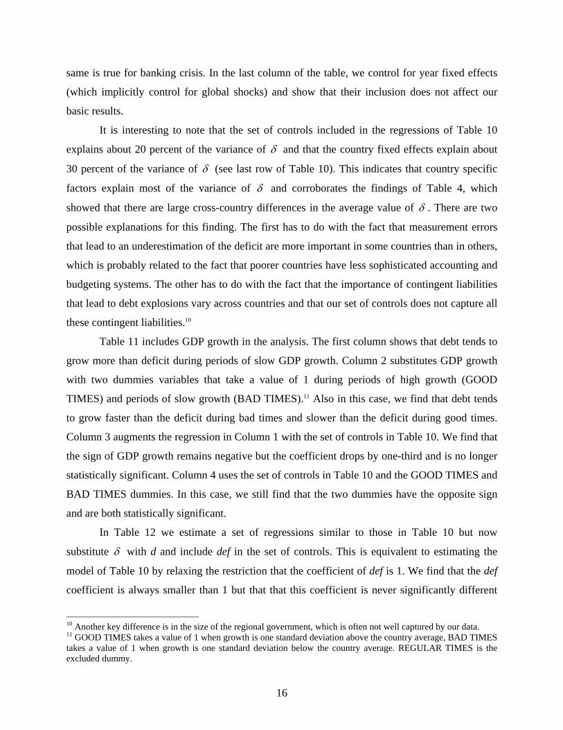
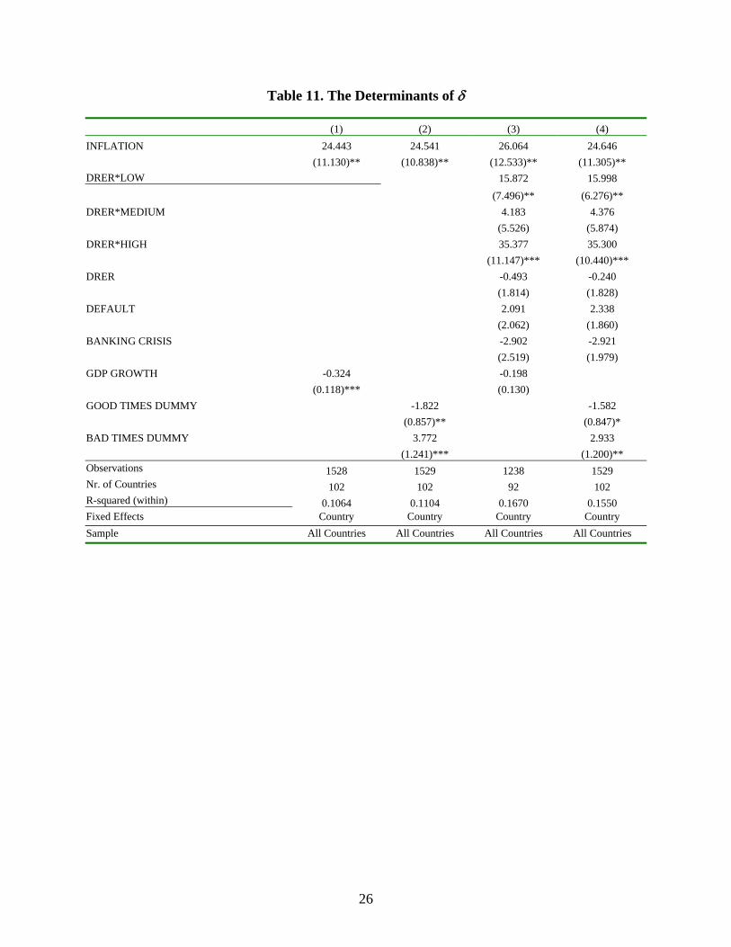
Table 11 includes GDP growth in the analysis. The first column shows that debt tends to

grow more than deficit during periods of slow GDP growth. Column 2 substitutes GDP growth

with two dummies variables that take a value of 1 during periods of high growth (GOOD

TIMES) and periods of slow growth (BAD TIMES).11 Also in this case, we find that debt tends

to grow faster than the deficit during bad times and slower than the deficit during good times.

Column 3 augments the regression in Column 1 with the set of controls in Table 10. We find that

the sign of GDP growth remains negative but the coefficient drops by one-third and is no longer

statistically significant. Column 4 uses the set of controls in Table 10 and the GOOD TIMES and

BAD TIMES dummies. In this case, we still find that the two dummies have the opposite sign

and are both statistically significant.

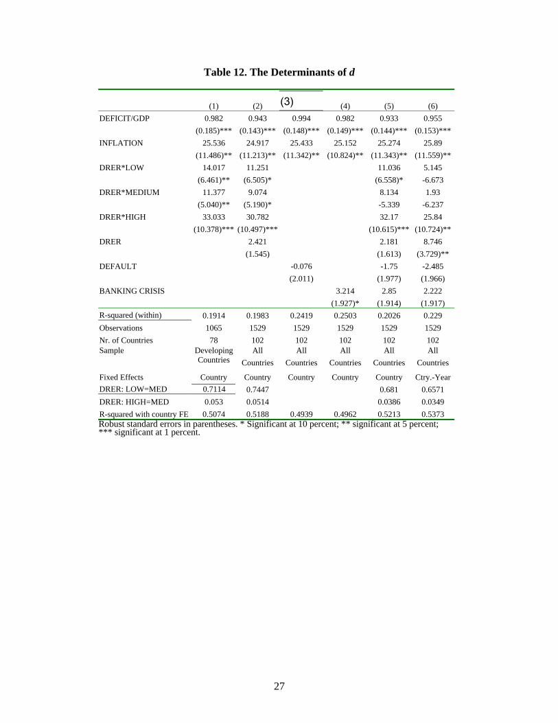
In Table 12 we estimate a set of regressions similar to those in Table 10 but now

substitute δ with d and include def in the set of controls. This is equivalent to estimating the

model of Table 10 by relaxing the restriction that the coefficient of def is 1. We find that the def

coefficient is always smaller than 1 but that that this coefficient is never significantly different

10 Another key difference is in the size of the regional government, which is often not well captured by our data. 11 GOOD TIMES takes a value of 1 when growth is one standard deviation above the country average, BAD TIMES takes a value of 1 when growth is one standard deviation below the country average. REGULAR TIMES is the excluded dummy.

17

from 1. All our other results are unchanged (this was expected because Table 6 already indicated

that the deficit by itself explains an extremely small share of the within-country variance of the

change in debt).

One problem with the regressions of Tables 10, 11 and 12 is that they assume a linear

relationship between the dependent variable and the set of independent variables. Therefore, the

estimated results might be driven by extreme values of δ . To address this issue, we relax the

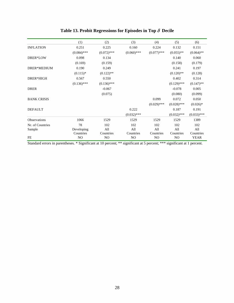
linearity assumption and run two sets of Probit regressions. In the first set of Probits, the

dependent variable is a dummy that takes a value of 1 for all country years in the top decile of

the distribution of δ . In the second set of Probits, we repeat the experiment using the bottom

decile of the distribution of δ. 12

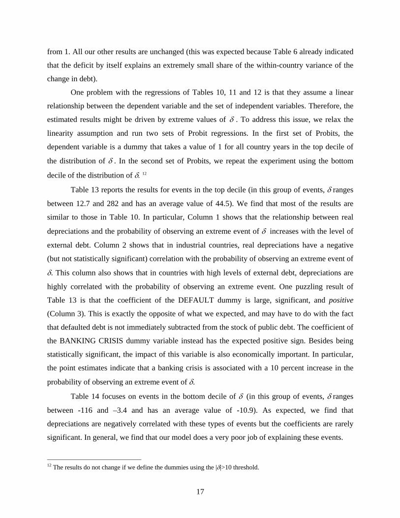
Table 13 reports the results for events in the top decile (in this group of events, δ ranges

between 12.7 and 282 and has an average value of 44.5). We find that most of the results are

similar to those in Table 10. In particular, Column 1 shows that the relationship between real

depreciations and the probability of observing an extreme event of δ increases with the level of

external debt. Column 2 shows that in industrial countries, real depreciations have a negative

(but not statistically significant) correlation with the probability of observing an extreme event of

δ. This column also shows that in countries with high levels of external debt, depreciations are

highly correlated with the probability of observing an extreme event. One puzzling result of

Table 13 is that the coefficient of the DEFAULT dummy is large, significant, and positive

(Column 3). This is exactly the opposite of what we expected, and may have to do with the fact

that defaulted debt is not immediately subtracted from the stock of public debt. The coefficient of

the BANKING CRISIS dummy variable instead has the expected positive sign. Besides being

statistically significant, the impact of this variable is also economically important. In particular,

the point estimates indicate that a banking crisis is associated with a 10 percent increase in the

probability of observing an extreme event of δ.

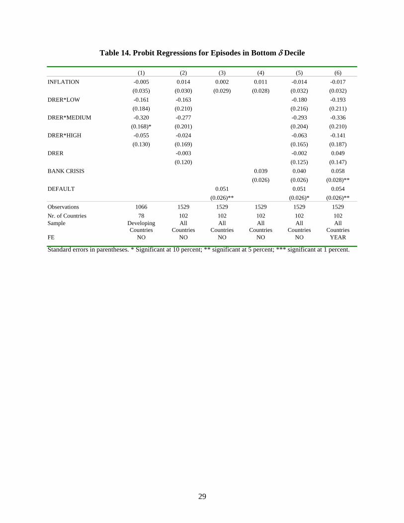
Table 14 focuses on events in the bottom decile of δ (in this group of events, δ ranges

between -116 and –3.4 and has an average value of -10.9). As expected, we find that

depreciations are negatively correlated with these types of events but the coefficients are rarely

significant. In general, we find that our model does a very poor job of explaining these events.

12 The results do not change if we define the dummies using the |δ|>10 threshold.

18

5. Conclusions

The purpose of this paper was to document the fact that what is often considered a residual entity

is indeed one of the key determinants of debt dynamic. After demonstrating the importance of

the stock-flow reconciliation, this paper shows that this residual entity can be partly explained by

contingent liabilities and balance-sheet effects. These results suggest that building a safer debt

structure and implementing policies aimed at avoiding the creation of contingent liabilities are

key to avoiding debt explosions (for contrasting views on how this can be achieved, see

Goldstein and Turner, 2004 and Eichengreen, Hausmann and Panizza, 2003). However, this

paper also shows that a large fraction of the variance of the stock-flow reconciliation cannot be

explained by balance-sheet effects and our simple regressions.13

13 One variable that is likely to be important but that we do not control for is the effect of court decisions that force the government to make payments (to public sector workers, for instance) that were not budgeted. We would like to thank Vito Tanzi for pointing this out.

19

References Budina, N. and N. Fiess. 2005. “Public Debt and its Determinants in Market Access Countries.”

Washington, D.C.: The World Bank.

Caprio, G., and D. Klingebiel. 2003. “Episodes of Systematic and Borderline Financial Crises.”

Washington, DC, United States: World Bank. Mimeographed document.

http://econ.worldbank.org/view.php?type=18&id=23456

Cowan, K., E. Levy-Yeyati, U. Panizza and F. Sturzenegger. 2006. “Public Debt in the

Americas.” (In progress).

Eichengreen, B., R. Hausmann and U. Panizza. 2003. “Currency Mismatches, Debt Intolerance

and Original Sin: Why Are Not the Same and Why It Matters.” NBER Working Paper

10036. Cambridge, United States: National Bureau of Economic Research.

European Commission. 2005. “General Government Data. General Government Expenditure,

Balances and Gross Debt.” Brussels, Belgium: European Commission.

Goldstein, M., and P. Turner. 2004. Controlling Currency Mismatches in Emerging Markets.

Washington D.C.: Institute for International Economics.

International Monetary Fund. 2003. “Public Debt in Emerging Markets: Is it Too High?” World

Economic Outlook, Chapter 3. Washington, DC, United States: International Monetary

Fund.

Jeanne, O. and A. Guscina. 2006. Government Debt in Emerging Market Countries. A New

Dataset. Mimeo, IMF

Levy-Yeyati, E., and F. Sturzenegger. 2005. “Methodological Note on the Construction of the

Debt Database.” Buenos Aires: Universidad Torcuato Di Tella.

Martner, R., and V. Tromben. 2004. “Public Debt Indicators in Latin American Countries:

Snowball Effect, Currency Mismatch and the Original Sin.” In: Public Debt. Perugia,

Italy: Banca d’Italia.

Reinhart, C., K. Rogoff and M. Savastano. 2003. “Debt Intolerance.” Brookings Papers on

Economic Activity 1: 1-74.

20

Table 1. Deficit over GDP

Country Group σ (%)

μ (%) Overall Between

Min (%)

Max (%)

N. of countries

N. of observations

All Countries 4.04 5.27 3.62 -18.26 66.05 117 1872 By Region

EAP 2.65 3.08 2.86 -2.35 17.87 8 126 ECA 3.38 3.51 2.89 -10.02 19.64 15 142 IND 3.29 3.78 2.92 -6.89 20.79 24 485 LAC 3.93 7.38 4.56 -5.27 66.05 25 417 MNA 5.57 6.24 6.02 -9.92 26.78 11 201 SAS 6.53 3.16 1.75 -1.73 18.28 5 119 SSA 4.24 4.77 2.74 -18.26 45.15 29 382

By Income Groups Low 4.67 4.40 2.76 -18.26 45.15 34 440 Medium 4.13 6.18 4.28 -10.02 66.05 59 947 High 3.29 3.78 2.92 -6.89 20.79 24 485 The income group and regional classifications are those used by the World Bank

Table 2. Debt over GDP

Country Group σ (%)

μ (%)

Overall Between

Min (%)

Max (%)

N. of countries

N. of observations

All Countries 55.80 58.05 46.92 0.00 637.52 117 1872 By Region

EAP 35.28 19.58 19.96 1.49 98.02 8 126 ECA 37.19 21.85 22.41 2.49 88.70 15 142 IND 43.91 26.75 27.08 1.47 121.53 24 485 LAC* 48.36 41.62 41.97 1.63 304.50 24 391 MNA** 46.81 40.84 40.09 0.00 210.76 10 172 SAS 60.27 21.97 16.04 5.92 116.48 5 119 SSA 66.86 53.97 46.42 1.98 299.73 29 382

By Income Groups Low 72.21 56.50 49.57 1.49 304.50 34 440 Medium 54.27 67.94 48.02 0.00 637.52 59 947 High 43.91 26.75 27.08 1.47 121.53 24 485 The income group and regional classifications are those used by the World Bank. * Excludes Guyana ** Excludes Israel

21

Table 3. Change in Debt over GDP

σ (%) Country Group

μ (%)

Overall Between

Min (%)

Max (%)

N. of countries

N. of observations

All Countries 8.97 23.42 14.66 -118.17 303.57 117 1872 By Region

EAP 5.11 9.08 6.42 -7.05 51.81 8 126 ECA 6.74 9.34 5.74 -5.71 74.38 15 142 IND 4.05 4.52 3.16 -10.77 22.49 24 485 LAC 11.45 31.31 16.37 -72.38 303.57 25 417 MNA 12.59 34.05 17.25 -31.86 300.14 11 201 SAS 7.98 8.12 3.18 -35.33 42.19 5 119 SSA 13.00 29.02 22.13 -118.17 233.42 29 382

By Income Groups Low 14.30 31.28 22.25 -118.17 243.68 34 440 Medium 9.00 24.39 11.54 -61.52 303.57 59 947 High 4.05 4.52 3.16 -10.77 22.49 24 485 The income group and regional classifications are those used by the World Bank

Table 4. Change in Debt Minus Deficit (δ)

μ (%) σ (%) Country Group

All Without Outliers* Overall Between

Min (%)

Max (%)

N. of countries

N. of observations

All Countries 4.93 3.15 21.84 13.29 -116.61 281.93 117 1872 By Region

EAP 2.46 2.46 7.99 4.28 -10.00 51.14 8 126 ECA 3.35 2.86 8.37 4.91 -11.03 72.56 15 142 IND 0.77 0.79 2.83 1.07 -12.16 14.07 24 485 LAC 7.52 4.32 28.82 13.68 -73.29 281.93 25 417 MNA 7.02 2.44 31.39 14.62 -39.15 273.36 11 201 SAS 1.45 2.14 7.55 1.86 -38.58 37.41 5 119 SSA 8.76 6.11 28.12 21.22 -116.61 226.90 29 382

By Income Groups Low 9.63 6.09 30.85 21.57 -116.61 247.90 34 440 Medium 4.87 3.09 21.88 8.87 -64.66 281.93 59 947 High 0.77 0.79 2.83 1.07 -12.16 14.07 24 485 The income group and regional classifications are those used by the World Bank. *Outliers are the top and bottom 2 percent of the distribution.

22

Table 5. Episodes with 10, >tiδ

Episodes with δ>5 Episodes with δ<-5

Number Share of total Number Share of total

EAP 12 9.52 1 0.79 ECA 18 12.68 1 0.7 IND 6 1.24 1 0.21 LAC 71 17.03 12 2.88 MNA 35 17.41 13 6.47 SAS 7 5.88 3 2.52 SSA 89 23.3 19 4.97 All Countries 238 12.71 50 2.67

Table 6. Change in Debt over GDP and Deficit (regressions with country fixed effects)

(1) (2) (3) (4) (5) Deficit 1.316 1.189 0.872 1.102 1.101 (0.226)*** (0.052)*** (0.066)*** (0.430)** (0.354)*** N. Obs 1872 1825 1872 382 417 Nr. Cty 117 117 117 29 25 R2 0.074 0.23 0.246 0.032 0.051 Sample All

Countries No

Outliers Quantile

Regression SSA LAC

(6) (7) (8) (9) (10) Deficit 0.706 1.346 2.486 1.426 0.914 (0.295)** (0.361)*** (0.840)*** (0.346)*** (0.056)*** N. Obs 119 126 201 142 485 Nr. Cty 5 8 11 15 24 R2 0.065 0.135 0.199 0.228 0.514 Sample SAS EAP MNA ECA IND Robust standard errors in parenthesis.

23

Table 7. Φ Index

Country Group μ (%)

σ (%)

Median (%)

Max (%)

Min (%)

N. of countries

All Countries 1.03 0.50 1.03 2.46 0.13 110 By Region

EAP 0.98 0.32 0.95 1.56 0.58 8 ECA 0.98 0.62 1.00 2.06 0.15 14 IND 0.60 0.36 0.55 1.37 0.13 23 LAC 1.21 0.51 1.23 2.41 0.15 25 MNA 1.35 0.47 1.29 2.46 0.89 10 SAS 1.01 0.12 1.04 1.11 0.81 5 SSA 1.15 0.42 1.15 2.13 0.19 25

By Income Groups Low 1.15 0.43 1.15 2.13 0.19 31 Medium 1.13 0.50 1.14 2.46 0.15 56 High 0.60 0.36 0.55 1.37 0.13 23

Table 8. Change in Debt and ρ (controlling for country fixed effects)

(1) (2) (3) (4) (5) θ -0.007 -0.011 -0.020 -0.018 -0.006 (0.002)*** (0.003)*** (0.005)*** (0.013) (0.008) Constant 0.718 0.746 0.788 0.837 0.640 (0.030)*** (0.033)*** (0.036)*** (0.121)*** (0.079)*** Observations 1061 1055 1039 64 77 Number of Countries 110 110 110 8 14 R-squared 0.01 0.01 0.02 0.03 0.01 Sample θ>0 0<θ<100 0<θ<50 EAP, θ>0 ECA, θ>0 (6) (7) (8) (9) (10) θ -0.019 -0.003 -0.024 -0.008 -0.005 (0.012) (0.004) (0.006)*** (0.003)** (0.008) Constant 0.817 0.593 0.877 0.576 1.053 (0.049)*** (0.061)*** (0.044)*** (0.068)*** (0.179)*** Observations 285 235 67 223 110 Number of Countries 24 24 5 25 10 R-squared 0.01 0.00 0.22 0.03 0.00 Sample IND, θ>0 LAC, θ>0 SAS, θ>0 SSA, θ>0 MNA, θ>0

24

Table 9. Debt Explosions θ d θ/d def def/d N Share All Episodes with θ>10 ALL 27.45 46.34 69.25% 9.42 27.40% 172 9.19% EAP 18.82 26.98 74.47% 6.11 24.40% 12 9.52% ECA 20.90 27.23 72.50% 5.07 18.65% 11 7.75% IND 12.59 15.25 82.78% 9.11 60.79% 13 2.68% LAC 34.08 58.92 74.43% 14.63 35.27% 41 9.83% MNA 30.22 63.75 60.28% 13.37 41.48% 23 11.44% SAS 19.87 26.71 69.79% 7.57 32.61% 6 5.04% SSA 28.63 47.08 64.95% 6.35 12.58% 66 9.52% All Episodes with 10<θ<20 ALL 13.45 24.39 67.88% 6.93 29.42% 104 5.56% EAP 13.45 21.20 73.66% 4.79 24.38% 9 7.14% ECA 13.33 19.60 69.10% 3.81 18.04% 9 6.34% IND 12.59 15.25 82.78% 9.11 60.79% 13 2.68% LAC 14.40 22.21 72.73% 7.76 31.71% 18 4.32% MNA 13.07 40.93 62.40% 11.05 48.67% 15 7.46% SAS 11.97 20.49 59.21% 8.74 42.15% 4 3.36% SSA 13.65 24.33 61.56% 5.13 11.64% 36 9.42%

25

Table 10: The Determinants of δ

(1) (2) (3) (4) (5) (6) INFLATION 25.526 24.869 25.428 25.136 25.223 25.885 (11.454)** (11.199)** (11.285)** (10.775)** (11.346)** (11.581)**DRER*LOW 14.034 11.496 11.331 5.288 (6.522)** (6.732)* (6.787)* -6.794 DRER*MEDIUM 11.358 9.218 8.315 1.996 (5.059)** (5.171)* -5.323 -6.22 DRER*HIGH 32.987 30.835 32.229 25.802 (10.423)*** (10.469)*** (10.588)*** (10.738)**DRER 2.22 1.95 8.676 (1.513) (1.589) (3.715)** DEFAULT -0.077 -1.754 -2.471 (2.015) (1.981) (1.963) BANKING CRISIS 3.204 2.812 2.182 (1.918)* (1.908) (1.909) R-squared (within) 0.218 0.224 0.19 0.199 0.234 0.244 Observations 1065 1529 1529 1529 1529 1529 Nr. of Countries 78 102 102 102 102 102 Sample Developing

Countries All

Countries All

Countries All

Countries All

Countries All

Countries Fixed Effects Country Country Country Country Country Ctry.-Year

DRER*LOW=DRER*MED 0.7654 0.7392 0.6757 0.6536 DRER*HIGH=DRER*MED 0.0612 0.0524 0.0396 0.0359 R-squared with country FE 0.4783 0.4825 0.4559 0.4584 0.4852 0.5025 Robust standard errors in parentheses. * Significant at 10 percent; ** significant at 5 percent; *** significant at 1 percent.

26

Table 11. The Determinants of δ (1) (2) (3) (4) INFLATION 24.443 24.541 26.064 24.646 (11.130)** (10.838)** (12.533)** (11.305)** DRER*LOW 15.872 15.998 (7.496)** (6.276)** DRER*MEDIUM 4.183 4.376 (5.526) (5.874) DRER*HIGH 35.377 35.300 (11.147)*** (10.440)*** DRER -0.493 -0.240 (1.814) (1.828) DEFAULT 2.091 2.338 (2.062) (1.860) BANKING CRISIS -2.902 -2.921 (2.519) (1.979) GDP GROWTH -0.324 -0.198 (0.118)*** (0.130) GOOD TIMES DUMMY -1.822 -1.582 (0.857)** (0.847)* BAD TIMES DUMMY 3.772 2.933 (1.241)*** (1.200)** Observations 1528 1529 1238 1529 Nr. of Countries 102 102 92 102 R-squared (within) 0.1064 0.1104 0.1670 0.1550 Fixed Effects Country Country Country Country Sample All Countries All Countries All Countries All Countries

27

Table 12. The Determinants of d

(1) (2) (3) (4) (5) (6) DEFICIT/GDP 0.982 0.943 0.994 0.982 0.933 0.955 (0.185)*** (0.143)*** (0.148)*** (0.149)*** (0.144)*** (0.153)***INFLATION 25.536 24.917 25.433 25.152 25.274 25.89 (11.486)** (11.213)** (11.342)** (10.824)** (11.343)** (11.559)**DRER*LOW 14.017 11.251 11.036 5.145 (6.461)** (6.505)* (6.558)* -6.673 DRER*MEDIUM 11.377 9.074 8.134 1.93 (5.040)** (5.190)* -5.339 -6.237 DRER*HIGH 33.033 30.782 32.17 25.84 (10.378)*** (10.497)*** (10.615)*** (10.724)**DRER 2.421 2.181 8.746 (1.545) (1.613) (3.729)** DEFAULT -0.076 -1.75 -2.485 (2.011) (1.977) (1.966) BANKING CRISIS 3.214 2.85 2.222 (1.927)* (1.914) (1.917) R-squared (within) 0.1914 0.1983 0.2419 0.2503 0.2026 0.229 Observations 1065 1529 1529 1529 1529 1529 Nr. of Countries 78 102 102 102 102 102

All All All All All Sample Developing Countries Countries Countries Countries Countries Countries

Fixed Effects Country Country Country Country Country Ctry.-YearDRER: LOW=MED 0.7114 0.7447 0.681 0.6571 DRER: HIGH=MED 0.053 0.0514 0.0386 0.0349 R-squared with country FE 0.5074 0.5188 0.4939 0.4962 0.5213 0.5373 Robust standard errors in parentheses. * Significant at 10 percent; ** significant at 5 percent;

*** significant at 1 percent.

28

Table 13. Probit Regressions for Episodes in Top δ Decile

(1) (2) (3) (4) (5) (6) INFLATION 0.251 0.225 0.160 0.224 0.132 0.151 (0.084)*** (0.072)*** (0.060)*** (0.077)*** (0.055)** (0.064)** DRER*LOW 0.098 0.134 0.140 0.060 (0.169) (0.159) (0.158) (0.179) DRER*MEDIUM 0.190 0.249 0.241 0.197 (0.115)* (0.122)** (0.120)** (0.128) DRER*HIGH 0.567 0.550 0.402 0.314 (0.136)*** (0.136)*** (0.129)*** (0.147)** DRER -0.067 -0.078 0.005 (0.075) (0.080) (0.099) BANK CRISIS 0.099 0.072 0.050 (0.029)*** (0.028)*** (0.026)* DEFAULT 0.222 0.187 0.191 (0.032)*** (0.032)*** (0.033)*** Observations 1066 1529 1529 1529 1529 1389 Nr. of Countries 78 102 102 102 102 102 Sample Developing

Countries All

Countries All

Countries All

Countries All

Countries All

Countries FE NO NO NO NO NO YEAR

Standard errors in parentheses. * Significant at 10 percent; ** significant at 5 percent; *** significant at 1 percent.

29

Table 14. Probit Regressions for Episodes in Bottom δ Decile

(1) (2) (3) (4) (5) (6) INFLATION -0.005 0.014 0.002 0.011 -0.014 -0.017 (0.035) (0.030) (0.029) (0.028) (0.032) (0.032) DRER*LOW -0.161 -0.163 -0.180 -0.193 (0.184) (0.210) (0.216) (0.211) DRER*MEDIUM -0.320 -0.277 -0.293 -0.336 (0.168)* (0.201) (0.204) (0.210) DRER*HIGH -0.055 -0.024 -0.063 -0.141 (0.130) (0.169) (0.165) (0.187) DRER -0.003 -0.002 0.049 (0.120) (0.125) (0.147) BANK CRISIS 0.039 0.040 0.058 (0.026) (0.026) (0.028)** DEFAULT 0.051 0.051 0.054 (0.026)** (0.026)* (0.026)** Observations 1066 1529 1529 1529 1529 1529 Nr. of Countries 78 102 102 102 102 102 Sample Developing

Countries All

Countries All

Countries All

Countries All

Countries All

Countries FE NO NO NO NO NO YEAR

Standard errors in parentheses. * Significant at 10 percent; ** significant at 5 percent; *** significant at 1 percent.

30

Table A1. Countries Included in the Sample

Country Code Region Initial year Final year Debt/GDP Deficit/GDP δ φ

FIJI* FJI EAP 1972 1998 30.69 4.24 -0.93 0.88 INDONESIA IDN EAP 1973 1999 34.77 1.32 4.34 1.15 KOREA KOR EAP 1981 1997 13.96 0.59 1.59 0.82 MALAYSIA MYS EAP 1991 1999 47.02 0.15 0.41 0.65 MONGOLIA MNG EAP 1993 2001 73.08 8.94 11.99 1.15 PAPUA NEW GUINEA PNG EAP 1976 2002 45.79 2.45 2.66 1.56 SOLOMON ISLANDS* SLB EAP 1976 1984 15.00 4.41 -1.72 0.58 THAILAND THA EAP 1997 2003 20.26 1.72 2.30 1.02 ALBANIA ALB ECA 1996 1998 48.78 11.07 0.00 0.76 BELARUS BLR ECA 1993 1998 23.65 2.05 13.32 1.26 CROATIA HRV ECA 1996 2002 42.75 1.48 4.98 2.06 CYPRUS CYP ECA 1977 2003 48.77 4.68 1.14 0.83 CZECH REPUBLIC CZE ECA 1994 2003 12.69 1.38 0.18 0.27 ESTONIA EST ECA 1997 2001 3.72 -0.95 0.88 6.46 GEORGIA GEO ECA 1997 2003 61.53 2.78 5.52 1.31 HUNGARY HUN ECA 1992 2003 67.49 5.46 3.54 1.16 LATVIA LVA ECA 1996 2003 12.54 1.37 0.04 0.41 LITHUANIA LTU ECA 1999 2002 27.65 2.43 -0.23 0.15 POLAND POL ECA 1994 2001 44.71 1.63 2.49 1.18 RUSSIA RUS ECA 1994 2003 55.76 2.60 13.06 1.49 SLOVAK REPUBLIC SVK ECA 1996 2003 27.07 1.38 2.88 2.04 TAJIKISTAN TJK ECA 2001 2001 80.87 -0.06 -5.65 0.28 TURKEY* TUR ECA 1972 2001 21.80 5.12 2.93 0.57 AUSTRALIA AUS IND 1979 2002 12.25 0.80 -0.35 0.77 AUSTRIA AUT IND 1972 1994 31.85 3.99 -0.35 0.41 BELGIUM BEL IND 1972 1998 84.55 6.47 0.53 0.27 CANADA CAN IND 1975 2001 41.40 3.43 -0.21 0.32 DENMARK DNK IND 1981 2000 66.78 1.02 3.65 0.78 FINLAND FIN IND 1991 1998 52.11 8.00 0.03 0.13 FRANCE FRA IND 1993 1997 41.12 5.25 -0.89 0.81 GERMANY DEU IND 1976 1999 19.23 1.62 0.29 1.03 GREECE GRC IND 1994 1999 117.34 10.15 2.14 0.73 ICELAND ISL IND 1973 2003 31.74 2.22 2.87 1.21 IRELAND IRL IND 1982 1999 84.11 4.01 1.21 0.24 ITALY ITA IND 1981 1999 93.88 9.56 0.65 0.13 JAPAN JPN IND 1981 1993 48.65 3.45 0.52 0.98 LUXEMBOURG* LUX IND 1991 1997 2.89 -0.06 0.45 81.77 MALTA* MLT IND 1972 1998 25.61 2.30 0.56 0.86 NETHERLANDS NLD IND 1981 1998 52.97 3.56 0.10 0.14 NEW ZEALAND NZL IND 1993 2001 43.07 -1.40 -0.14 0.54 NORWAY NOR IND 1972 2003 26.19 0.61 1.39 1.37 PORTUGAL PRT IND 1981 1998 56.47 6.17 2.17 0.59 SPAIN ESP IND 1972 1999 31.84 3.45 0.68 0.37 SWEDEN SWE IND 1972 1999 46.97 4.40 0.47 0.49 SWITZERLAND CHE IND 1987 2003 21.00 0.50 0.83 0.99 UNITED KINGDOM GBR IND 1972 1999 45.46 3.25 0.51 0.55 UNITED STATES USA IND 1972 2003 35.71 2.45 0.00 0.17 ARGENTINA ARG LAC 1994 2003 59.87 1.56 11.56 1.22 BAHAMAS, THE BHS LAC 1972 2003 25.55 2.29 -0.08 0.60 BARBADOS BRB LAC 1978 2003 54.32 3.74 0.58 0.64 BOLIVIA BOL LAC 1991 2003 65.45 4.37 3.53 1.24 BRAZIL* BRA LAC 1992 1998 26.98 6.86 7.67 1.31 CHILE CHL LAC 1989 2001 25.41 -1.20 2.78 2.03 COLOMBIA COL LAC 1991 2003 25.81 3.79 1.96 0.71 COSTA RICA CRI LAC 1972 2002 30.01 2.86 2.54 1.38 ECUADOR ECU LAC 1991 2003 63.52 -0.30 0.79 1.01 EL SALVADOR SLV LAC 1972 2001 34.26 1.72 2.70 1.21 GRENADA GRD LAC 1994 1995 39.28 -0.57 -2.75 0.15 GUATEMALA GTM LAC 1991 2003 16.02 1.19 0.69 1.25 GUYANA GUY LAC 1972 1997 324.91 22.46 44.22 1.23

31

HAITI HTI LAC 1997 2003 46.26 2.03 5.04 1.80 HONDURAS* HND LAC 1972 2003 58.45 4.12 4.95 1.10 JAMAICA* JAM LAC 1981 2001 117.41 6.79 12.70 1.13 MEXICO* MEX LAC 1972 2003 32.28 3.84 4.68 0.71 NICARAGUA NIC LAC 1991 2003 216.01 1.57 56.61 1.56 PANAMA PAN LAC 1972 2000 55.53 3.29 1.60 0.97 PARAGUAY PRY LAC 1991 2001 19.26 0.63 3.76 1.43 PERU PER LAC 1991 2001 53.56 0.97 12.08 1.37 ST. VINCENT & GRENS. VCT LAC 1987 2001 47.48 2.34 2.13 1.60 SURINAME* SUR LAC 1972 1986 35.67 7.12 -3.07 0.38 URUGUAY URY LAC 1993 2001 26.48 2.18 4.14 1.74 VENEZUELA, REP. BOL. VEN LAC 1972 1985 11.39 -0.07 2.43 2.41 ALGERIA DZA MNA 2000 2001 0.06 -6.98 6.98 BAHRAIN, KINGDOM OF BHR MNA 1982 2001 16.62 3.29 -1.40 2.46 ISRAEL ISR MNA 1973 2001 183.28 9.81 47.95 1.36 JORDAN JOR MNA 1972 2001 86.11 4.50 4.27 0.96 LEBANON LBN MNA 1993 1999 92.82 17.41 6.81 1.53 MOROCCO* MAR MNA 1972 2003 64.11 5.94 -0.87 0.89 OMAN OMN MNA 1972 2001 22.51 7.23 -5.08 1.51 SAUDI ARABIA SAU MNA 1996 2000 104.01 4.08 -1.90 1.10 TUNISIA TUN MNA 1972 2000 47.49 3.70 1.64 0.90 UNITED ARAB EMIRATES* ARE MNA 1981 1999 1.63 0.05 -0.23 1.22 YEMEN, REPUBLIC OF YEM MNA 1996 1999 7.18 2.39 0.35 1.54 INDIA IND SAS 1975 2001 46.15 5.85 0.28 1.04 MALDIVES MDV SAS 1982 2003 49.53 5.38 -1.20 1.01 NEPAL* NPL SAS 1975 2003 51.04 4.51 2.45 0.81 PAKISTAN PAK SAS 1972 1993 65.37 7.26 2.03 1.11 SRI LANKA LKA SAS 1974 2001 84.91 8.97 3.49 1.07 BURUNDI BDI SSA 1972 2003 85.08 1.68 11.81 1.52 CAMEROON* CMR SSA 1991 1999 95.99 2.01 16.75 1.29 CHAD TCD SSA 1991 2001 58.26 7.40 -1.27 1.09 CONGO, DEM. REP. OF* ZAR SSA 1972 1997 88.63 4.57 46.20 1.39 CONGO, REPUBLIC OF COG SSA 2000 2000 160.76 -1.16 -68.32 COTE D IVOIRE* CIV SSA 1995 2001 135.29 0.69 1.38 0.97 ETHIOPIA ETH SSA 1983 1999 75.28 5.93 4.30 0.98 GABON GAB SSA 1991 1991 53.53 1.66 12.15 1.69 GAMBIA, THE GMB SSA 1974 1982 27.66 6.50 -0.62 0.19 GHANA* GHA SSA 1972 1998 22.64 3.75 0.79 1.03 GUINEA* GIN SSA 1991 1999 93.75 3.33 5.46 1.18 KENYA KEN SSA 1998 2003 64.98 1.28 2.95 2.13 LESOTHO* LSO SSA 1988 2003 79.17 3.61 4.70 1.09 MALAWI* MWI SSA 1972 1987 69.11 7.40 5.00 0.62 MALI MLI SSA 1983 1983 67.77 7.01 -5.22 MAURITIUS MUS SSA 1979 2003 46.54 3.55 2.22 0.53 NAMIBIA NAM SSA 1990 2000 18.59 3.50 -0.61 1.19 NIGERIA NGA SSA 1972 1998 57.88 2.56 9.69 1.15 RWANDA RWA SSA 1978 2003 54.48 3.85 0.95 0.94 SENEGAL* SEN SSA 1983 2001 78.44 3.66 4.58 0.66 SEYCHELLES SYC SSA 1973 1977 5.09 0.56 0.11 17.06 SIERRA LEONE SLE SSA 1975 2003 105.52 7.63 18.21 1.56 SOUTH AFRICA ZAF SSA 1981 2003 34.98 3.64 0.74 0.93 SUDAN SDN SSA 1998 1999 203.80 0.65 62.55 90.39 SWAZILAND SWZ SSA 1979 2003 26.70 0.72 2.27 1.42 TOGO TGO SSA 1984 1986 89.77 2.94 -4.78 1.61 UGANDA UGA SSA 1992 2003 67.66 3.53 1.17 1.29 ZAMBIA* ZMB SSA 1978 1998 176.77 10.98 42.30 1.48 ZIMBABWE ZWE SSA 1977 1997 49.49 6.83 1.46 0.84

*Break in the series

32

Table A2. Episodes with δ>10 Country Year Code Region Country Year Code Region Country Year Code Region

INDONESIA 1986 IDN EAP JAMAICA 2001 JAM LAC BURUNDI 1983 BDI SSA INDONESIA 1997 IDN EAP JAMAICA 1999 JAM LAC BURUNDI 2003 BDI SSA INDONESIA 1982 IDN EAP MEXICO 1987 MEX LAC BURUNDI 1992 BDI SSA INDONESIA 1978 IDN EAP MEXICO 1986 MEX LAC BURUNDI 1989 BDI SSA KOREA 1981 KOR EAP MEXICO 1994 MEX LAC CAMEROON 1994 CMR SSA MONGOLIA 1998 MNG EAP MEXICO 1982 MEX LAC CHAD 1999 TCD SSA MONGOLIA 1993 MNG EAP MEXICO 1989 MEX LAC CHAD 1995 TCD SSA MONGOLIA 1996 MNG EAP MEXICO 1985 MEX LAC CONGO, DEM. REP. OF 1989 ZAR SSA MONGOLIA 1994 MNG EAP NICARAGUA 1991 NIC LAC CONGO, DEM. REP. OF 1990 ZAR SSA PAPUA NEW GUINEA 1994 PNG EAP NICARAGUA 2001 NIC LAC CONGO, DEM. REP. OF 1997 ZAR SSA PAPUA NEW GUINEA 2001 PNG EAP NICARAGUA 2000 NIC LAC CONGO, DEM. REP. OF 1981 ZAR SSA PAPUA NEW GUINEA 1997 PNG EAP NICARAGUA 1995 NIC LAC CONGO, DEM. REP. OF 1993 ZAR SSA ALBANIA 1997 ALB ECA NICARAGUA 1998 NIC LAC CONGO, DEM. REP. OF 1992 ZAR SSA BELARUS 1994 BLR ECA NICARAGUA 1993 NIC LAC CONGO, DEM. REP. OF 1996 ZAR SSA BELARUS 1998 BLR ECA NICARAGUA 1992 NIC LAC CONGO, DEM. REP. OF 1994 ZAR SSA CROATIA 1998 HRV ECA NICARAGUA 1997 NIC LAC CONGO, DEM. REP. OF 1995 ZAR SSA CROATIA 1999 HRV ECA NICARAGUA 1999 NIC LAC CONGO, DEM. REP. OF 1980 ZAR SSA GEORGIA 1998 GEO ECA NICARAGUA 2002 NIC LAC COTE D IVOIRE 1995 CIV SSA GEORGIA 1999 GEO ECA NICARAGUA 1994 NIC LAC ETHIOPIA 1994 ETH SSA GEORGIA 1997 GEO ECA PANAMA 1993 PAN LAC ETHIOPIA 1993 ETH SSA HUNGARY 1993 HUN ECA PANAMA 1996 PAN LAC GABON 1991 GAB SSA RUSSIA 1998 RUS ECA PARAGUAY 2001 PRY LAC GHANA 1996 GHA SSA RUSSIA 1996 RUS ECA PERU 1991 PER LAC GUINEA 1998 GIN SSA RUSSIA 1995 RUS ECA PERU 1998 PER LAC KENYA 2000 KEN SSA RUSSIA 1994 RUS ECA PERU 1992 PER LAC LESOTHO 1996 LSO SSA RUSSIA 1999 RUS ECA PERU 1993 PER LAC LESOTHO 2000 LSO SSA SLOVAK REPUBLIC 2002 SVK ECA ST. VINCENT & GRENS. 1999 VCT LAC LESOTHO 1998 LSO SSA SLOVAK REPUBLIC 2001 SVK ECA BAHRAIN, KINGDOM OF 1988 BHR MNA LESOTHO 2001 LSO SSA TURKEY 1981 TUR ECA ISRAEL 1996 ISR MNA MALAWI 1986 MWI SSA TURKEY 2001 TUR ECA ISRAEL 1977 ISR MNA NIGERIA 1989 NGA SSA DENMARK 1993 DNK IND ISRAEL 1979 ISR MNA NIGERIA 1988 NGA SSA DENMARK 1983 DNK IND ISRAEL 1988 ISR MNA NIGERIA 1987 NGA SSA ICELAND 1984 ISL IND ISRAEL 1993 ISR MNA NIGERIA 1978 NGA SSA IRELAND 1983 IRL IND ISRAEL 1998 ISR MNA NIGERIA 1983 NGA SSA NORWAY 1986 NOR IND ISRAEL 1975 ISR MNA NIGERIA 1990 NGA SSA SWEDEN 1980 SWE IND ISRAEL 1985 ISR MNA NIGERIA 1981 NGA SSA ARGENTINA 2002 ARG LAC ISRAEL 1989 ISR MNA NIGERIA 1980 NGA SSA ARGENTINA 2003 ARG LAC ISRAEL 1981 ISR MNA NIGERIA 1993 NGA SSA BOLIVIA 1995 BOL LAC ISRAEL 1973 ISR MNA NIGERIA 1986 NGA SSA BOLIVIA 1993 BOL LAC ISRAEL 1974 ISR MNA RWANDA 1998 RWA SSA BRAZIL 1993 BRA LAC ISRAEL 1978 ISR MNA RWANDA 1994 RWA SSA BRAZIL 1992 BRA LAC ISRAEL 1984 ISR MNA RWANDA 2002 RWA SSA COSTA RICA 1991 CRI LAC ISRAEL 1980 ISR MNA RWANDA 2003 RWA SSA COSTA RICA 1998 CRI LAC ISRAEL 1986 ISR MNA RWANDA 1990 RWA SSA COSTA RICA 1978 CRI LAC ISRAEL 1990 ISR MNA RWANDA 1996 RWA SSA ECUADOR 1998 ECU LAC ISRAEL 1976 ISR MNA SENEGAL 1983 SEN SSA ECUADOR 1993 ECU LAC ISRAEL 1992 ISR MNA SIERRA LEONE 2003 SLE SSA ECUADOR 1999 ECU LAC ISRAEL 1987 ISR MNA SIERRA LEONE 1986 SLE SSA ECUADOR 1992 ECU LAC ISRAEL 1983 ISR MNA SIERRA LEONE 1992 SLE SSA EL SALVADOR 1987 SLV LAC ISRAEL 1982 ISR MNA SIERRA LEONE 1985 SLE SSA EL SALVADOR 1986 SLV LAC JORDAN 1988 JOR MNA SIERRA LEONE 1990 SLE SSA GUYANA 1995 GUY LAC JORDAN 1972 JOR MNA SIERRA LEONE 1988 SLE SSA GUYANA 1987 GUY LAC JORDAN 1990 JOR MNA SIERRA LEONE 1995 SLE SSA GUYANA 1989 GUY LAC LEBANON 1996 LBN MNA SIERRA LEONE 1999 SLE SSA GUYANA 1986 GUY LAC LEBANON 1994 LBN MNA SIERRA LEONE 1993 SLE SSA GUYANA 1994 GUY LAC LEBANON 1999 LBN MNA SIERRA LEONE 1989 SLE SSA GUYANA 1988 GUY LAC LEBANON 1993 LBN MNA SIERRA LEONE 1987 SLE SSA GUYANA 1980 GUY LAC MOROCCO 1983 MAR MNA SIERRA LEONE 1996 SLE SSA GUYANA 1976 GUY LAC MOROCCO 1997 MAR MNA SIERRA LEONE 1998 SLE SSA GUYANA 1982 GUY LAC MOROCCO 1992 MAR MNA SIERRA LEONE 1997 SLE SSA GUYANA 1979 GUY LAC SAUDI ARABIA 1996 SAU MNA SIERRA LEONE 2001 SLE SSA GUYANA 1991 GUY LAC SAUDI ARABIA 1998 SAU MNA SUDAN 1999 SDN SSA GUYANA 1985 GUY LAC MALDIVES 1985 MDV SAS SUDAN 1998 SDN SSA GUYANA 1975 GUY LAC MALDIVES 1982 MDV SAS SWAZILAND 1984 SWZ SSA GUYANA 1992 GUY LAC NEPAL 1991 NPL SAS UGANDA 2001 UGA SSA GUYANA 1990 GUY LAC PAKISTAN 1972 PAK SAS UGANDA 2002 UGA SSA HAITI 2002 HTI LAC SRI LANKA 1991 LKA SAS ZAMBIA 1993 ZMB SSA HONDURAS 1998 HND LAC SRI LANKA 1977 LKA SAS ZAMBIA 1982 ZMB SSA HONDURAS 1992 HND LAC SRI LANKA 1985 LKA SAS ZAMBIA 1990 ZMB SSA HONDURAS 1996 HND LAC BURUNDI 1996 BDI SSA ZAMBIA 1991 ZMB SSA HONDURAS 1993 HND LAC BURUNDI 1999 BDI SSA ZAMBIA 1995 ZMB SSA HONDURAS 1994 HND LAC BURUNDI 1998 BDI SSA ZAMBIA 1994 ZMB SSA HONDURAS 1990 HND LAC BURUNDI 1987 BDI SSA ZAMBIA 1996 ZMB SSA JAMAICA 1997 JAM LAC BURUNDI 2001 BDI SSA ZAMBIA 1986 ZMB SSA JAMAICA 1984 JAM LAC BURUNDI 1988 BDI SSA ZAMBIA 1998 ZMB SSA JAMAICA 1994 JAM LAC BURUNDI 1993 BDI SSA ZAMBIA 1984 ZMB SSA JAMAICA 1998 JAM LAC BURUNDI 1986 BDI SSA ZAMBIA 1985 ZMB SSA JAMAICA 1985 JAM LAC BURUNDI 1991 BDI SSA ZIMBABWE 1995 ZWE SSA JAMAICA 1983 JAM LAC BURUNDI 1995 BDI SSA JAMAICA 1993 JAM LAC BURUNDI 2002 BDI SSA

33

Table A3. Episodes with δ<-10

Country Year Code Region Country Year Code RegionINDONESIA 1998 IDN EAP SAUDI ARABIA 1999 SAU MNA ALBANIA 1998 ALB ECA MALDIVES 1984 MDV SAS AUSTRALIA 1980 AUS IND MALDIVES 1983 MDV SAS ECUADOR 2001 ECU LAC PAKISTAN 1973 PAK SAS ECUADOR 2000 ECU LAC CHAD 1994 TCD SSA GUYANA 1984 GUY LAC CHAD 1991 TCD SSA GUYANA 1996 GUY LAC CHAD 1998 TCD SSA GUYANA 1978 GUY LAC CONGO, DEM. REP. OF 1991 ZAR SSA HONDURAS 1991 HND LAC CONGO, REPUBLIC OF 2000 COG SSA JAMAICA 1992 JAM LAC COTE D IVOIRE 1998 CIV SSA NICARAGUA 1996 NIC LAC ETHIOPIA 1995 ETH SSA PANAMA 1989 PAN LAC GUINEA 1991 GIN SSA PANAMA 1990 PAN LAC LESOTHO 2003 LSO SSA ST. VINCENT & GRENS. 1997 VCT LAC LESOTHO 2002 LSO SSA SURINAME 1975 SUR LAC NIGERIA 1995 NGA SSA BAHRAIN, KINGDOM OF 1990 BHR MNA RWANDA 1995 RWA SSA BAHRAIN, KINGDOM OF 1987 BHR MNA SIERRA LEONE 2000 SLE SSA JORDAN 1992 JOR MNA SWAZILAND 1985 SWZ SSA JORDAN 1989 JOR MNA TOGO 1985 TGO SSA LEBANON 1997 LBN MNA UGANDA 1999 UGA SSA MOROCCO 1991 MAR MNA UGANDA 1992 UGA SSA OMAN 1992 OMN MNA ZAMBIA 1987 ZMB SSA OMAN 1993 OMN MNA ZIMBABWE 1996 ZWE SSA OMAN 1987 OMN MNA OMAN 1999 OMN MNA OMAN 1995 OMN MNA OMAN 1989 OMN MNA

34

Table A4. Debt Explosions

Code Reg Year deficit d θ Code Reg Year deficit d θ ALB ECA 1997 12 75 24 88 14 86 LSO SSA 1998 3 84 21 99 14 95ARG LAC 2002 1.11 89.12 92.20 LSO SSA 2000 3.44 23.97 16.43BDI SSA 1995 2.66 13.49 10.47 LSO SSA 2001 0.64 25.91 20.34BDI SSA 1987 1.02 12.11 13.05 MAR MNA 1984 6.04 15.49 11.05BDI SSA 2003 5.10 18.45 13.68 MAR MNA 1981 13.36 18.02 11.71BDI SSA 1986 -2.54 21.24 14.24 MAR MNA 1992 1.39 20.09 11.93BDI SSA 1992 8.91 22.55 15.31 MAR MNA 1983 7.75 22.99 14.84BDI SSA 1993 5.47 21.71 15.45 MDV SAS 1982 5.70 36.10 31.96BDI SSA 1983 0.91 17.30 15.94 MEX LAC 1982 11.92 24.34 19.67BDI SSA 1998 4.93 40.26 16.30 MEX LAC 1986 13.05 35.13 22.33BDI SSA 1988 -0.73 18.35 16.72 MNG EAP 1996 7.68 31.12 12.53BDI SSA 1999 6.66 50.18 29.65 MNG EAP 1994 8.96 47.47 13.57BDI SSA 2002 1.08 70.60 47.65 MNG EAP 1999 10.79 13.56 15.19BEL IND 1981 11.96 14.63 10.38 MNG EAP 1998 11.62 33.99 21.65BEL IND 1983 12.06 15.91 10.46 MNG EAP 1993 17.87 47.19 34.63BEL IND 1982 10.70 13.99 11.03 MUS SSA 1982 12.51 18.87 11.08BLR ECA 1994 1.83 74.38 70.74 MWI SSA 1986 9.90 35.97 26.55BOL LAC 1993 4.74 18.38 12.00 NGA SSA 1990 8.47 51.07 10.76CMR SSA 1993 1.73 9.29 11.91 NGA SSA 1983 9.44 24.67 23.90CMR SSA 1991 5.24 11.42 13.17 NGA SSA 1987 5.40 31.50 30.59CMR SSA 1994 2.90 82.55 83.45 NGA SSA 1986 11.29 40.27 33.10CRI LAC 1978 4.36 19.34 13.93 NIC LAC 2002 1.34 26.98 14.50DNK IND 1981 5.85 12.94 10.39 NIC LAC 1993 0.04 68.50 26.10DNK IND 1993 2.44 13.74 11.44 NIC LAC 1994 0.02 79.53 39.60DNK IND 1983 6.61 18.70 11.81 NIC LAC 1997 0.76 84.65 65.80DNK IND 1982 7.78 16.79 13.05 NIC LAC 1991 -4.22 243.68 111.50ECU LAC 1999 0.59 27.56 28.30 NPL SAS 1991 8.00 18.57 11.97ESP IND 1993 5.88 13.70 11.05 OMN MNA 1972 12.13 10.15 10.08ETH SSA 1990 9.77 14.45 11.81 OMN MNA 1986 25.01 16.95 14.85ETH SSA 1994 9.95 48.11 27.42 PAK SAS 1972 4.77 42.19 39.40ETH SSA 1993 5.49 44.03 40.80 PAN LAC 1978 6.49 14.07 11.52FIN IND 1992 14.43 16.21 17.06 PAN LAC 1996 0.65 18.83 17.70FIN IND 1993 13.07 16.99 17.83 PER LAC 1998 0.19 14.91 11.00GEO ECA 1998 3.49 16.83 10.34 PNG EAP 1994 2.54 16.29 10.74GEO ECA 1999 2.27 20.09 14.99 PNG EAP 2001 1.33 16.70 12.28GHA SSA 1993 2.51 12.09 11.55 RUS ECA 1999 1.18 23.25 15.60GHA SSA 1996 2.97 15.18 11.97 RUS ECA 1998 4.83 25.62 18.40GIN SSA 1998 4.34 19.31 14.04 RWA SSA 2002 2.17 17.06 12.09GMB SSA 1978 10.01 17.01 14.22 RWA SSA 2003 3.48 23.72 16.93GUY LAC 1975 6.51 29.64 11.86 RWA SSA 1990 5.68 23.45 21.71GUY LAC 1985 37.97 62.90 16.28 RWA SSA 1994 1.92 47.73 45.35GUY LAC 1979 17.47 30.43 16.37 SAU MNA 1998 3.29 19.12 14.67GUY LAC 1977 11.91 15.29 20.06 SAU MNA 1996 3.13 21.46 16.43GUY LAC 1973 16.23 24.87 22.16 SDN SSA 1999 0.89 69.81 22.12GUY LAC 1987 40.94 72.42 24.92 SLE SSA 1986 2.33 36.94 12.07GUY LAC 1984 45.55 33.35 27.91 SLE SSA 1980 12.78 21.92 15.54GUY LAC 1976 27.46 44.75 31.24 SLE SSA 1995 5.67 34.68 16.56GUY LAC 1986 60.20 107.29 45.37 SLE SSA 1996 5.76 34.51 19.21GUY LAC 1990 21.65 303.58 47.99 SLE SSA 2003 7.04 46.65 27.35GUY LAC 1991 24.38 226.70 53.53 SLE SSA 1990 2.45 51.44 27.90GUY LAC 1989 6.98 136.35 66.95 SLE SSA 1992 4.85 72.50 38.11GUY LAC 1983 40.30 35.07 71.22 SLE SSA 2001 11.10 64.84 49.34GUY LAC 1982 66.05 92.02 78.18 SLE SSA 1999 8.46 94.09 58.89GUY LAC 1980 29.15 107.47 101.19 SLE SSA 1998 4.55 63.99 68.81HND LAC 1990 6.84 58.52 52.09 SLV LAC 1981 6.39 16.29 15.57HRV ECA 1999 1.78 14.55 10.81 SUR LAC 1985 19.95 17.60 18.74HRV ECA 1998 -0.91 15.50 12.30 SUR LAC 1986 25.04 29.45 28.69HTI LAC 2002 2.71 17.93 14.10 SVK ECA 2001 3.17 14.60 12.39HUN ECA 1993 5.72 21.09 10.27 SWE IND 1992 4.84 14.84 11.66IDN EAP 1978 3.14 14.19 10.74 SWE IND 1993 15.03 11.87 11.87IDN EAP 1982 1.90 13.61 11.07 SWE IND 1980 7.84 18.00 15.63IDN EAP 1986 3.52 22.13 19.86 SWZ SSA 1984 0.50 20.26 18.26IDN EAP 1997 0.67 51.81 48.55 TCD SSA 1994 12.55 -2.27 10.09ISR MNA 1984 18.84 223.12 10.49 TCD SSA 1992 12.79 13.12 10.13ISR MNA 1981 21.97 142.39 15.02 TCD SSA 2000 4.80 5.95 12.55ISR MNA 1976 18.39 59.67 20.77 TCD SSA 1993 5.54 12.60 15.21ISR MNA 1979 15.12 89.61 24.64 TCD SSA 1999 5.96 24.08 17.14ISR MNA 1977 19.43 69.90 36.42 TUN MNA 1986 7.14 14.82 11.03ISR MNA 1980 16.17 130.39 45.36 TUR ECA 2001 19.64 48.71 39.23ISR MNA 1983 26.78 300.14 189.53 UGA SSA 2001 2.19 24.62 20.96JAM LAC 1998 6.70 20.53 12.41 VCT LAC 1999 2.96 17.64 14.42JAM LAC 1999 4.54 26.63 19.23 ZAR SSA 1996 0.32 158.19 10.11JAM LAC 1997 6.35 34.74 23.35 ZAR SSA 1975 5.85 12.95 10.89JAM LAC 1983 19.88 66.10 57.16 ZAR SSA 1995 -0.02 207.28 63.39JOR MNA 1987 8.97 14.97 11.26 ZAR SSA 1994 1.77 141.87 65.80JOR MNA 1990 3.54 21.61 12.89 ZAR SSA 1990 6.53 233.42 192.21JOR MNA 1988 9.05 141.95 140.37 ZMB SSA 1998 5.48 45.41 10.98KOR EAP 1981 3.25 15.71 15.04 ZMB SSA 1996 2.44 62.53 23.82LBN MNA 1998 16.00 21.66 11.03 ZMB SSA 1991 45.15 135.08 32.77LBN MNA 1994 17.20 31.06 18.71 ZMB SSA 1982 18.56 44.08 33.11LBN MNA 1996 20.58 31.31 20.32 ZMB SSA 1985 15.17 74.69 55.22LBN MNA 1999 16.18 29.38 21.78 ZMB SSA 1990 8.65 127.72 59.23LKA SAS 1977 4.59 17.31 10.56 ZMB SSA 1986 15.03 158.14 107.10LKA SAS 1985 9.68 25.05 12.00 ZWE SSA 1984 8.10 16.58 10.69LKA SAS 1988 12.70 21.03 13.36 ZWE SSA 1995 9.40 33.82 21.72

35

Figure 1. Decomposition of Debt Growth

-15

-10

-5

0

5

10

15

IND SAS CAR EAP ECA MNA LAC SSA

INFLATIONGDP GROWTHSF ADJUSTMENTINTEREST EXPENDITUREPRIMARY DEFICIT

Figure 2. Deficit and Change in Debt

-50

050

100

e( D

DEB

T | X

)

-20 0 20 40e( DEFICIT | X )

coef = 1.189265, se = .05195547, t = 22.89

36

Figure 3. Distribution of φ under Different Assumption for α and β

0

0.5

1

1.5

2

2.5

3

3.5

4

0 0.5 1 1.5 2 2.5 3 3.5 4 4.5 5 5.5 6 6.5 7 7.5 8

β

φ

α=0

α=10

α=−10

37

Figure 4. Values of φ for Different Countries

0

0.2

0.4

0.6

0.8

1

1.2

1.4

1.6

1.8

2

38

Figure 5: Changes in Debt over GDP (θ) and Ratio between Deficit and Change in Debt (ρ)

0.3

0.4

0.5

0.6

0.7

0.8

0.9

1

0 1 2 3 4 5 6 7 8 9 10 11 12 13 14 15

θ

ρ