The Tip of the Iceberg: Modeling Trade Costs and ... · The Tip of the Iceberg: Modeling Trade Costs and Implications for Intra-industry Reallocation Alfonso Irarrazabaly, Andreas

The Tip of the Iceberg: Modeling Trade Costs and

Implications for Intra-industry Reallocation�

Alfonso Irarrazabaly, Andreas Moxnesz, and Luca David Opromollax

May 2010

Abstract

International economics has overwhelmingly relied on Samuelson�s (1954) as-

sumption that trade costs are proportional to value. We build a general equi-

librium heterogeneous �rms model of trade that allows for both ad valorem and

per-unit costs. Using a novel minimum distance estimator we are able to iden-

tify per unit trade costs from the distribution of foreign sales across markets.

Estimated average per-unit costs are substantial being, on average, between 35

and 45 percent of the average consumer price. This leads us to reject the pure

ad valorem cost assumption. An important theoretical �nding is that non-ad

valorem trade costs create an additional channel of gains from trade through

within-industry reallocation. Thus, we show that standard welfare assessments

of trade liberalization may be understated.

JEL Classi�cation: F10 Keywords: Trade Costs, Heterogeneous Firms, Intra-

Industry Reallocation, Exports, Trade Liberalization

�Acknowledgements: We would like to thank Costas Arkolakis, Gregory Corcos, Samuel Kortum, Ralph

Ossa, Arvid Raknerud, Alexandre Skiba, Karen Helene Ulltveit-Moe, and Kjetil Storesletten for their helpful

suggestions, as well as seminar participants at Banco de Portugal, Dartmouth, DIME-ISGEP Workshop, IIES

Stockholm, ITSG-Bocconi Workshop, LMDG Workshop, LSE, Norwegian School of Management, University

of Oslo, and Yale. We thank Statistics Norway for data preparation and clari�cations. We thank the project

�European Firms in a Global Economy: Internal Policies for External Competitiveness�(EFIGE) for �nancial

support. Alfonso Irarrazabal thanks the hospitality of the Chicago Booth School of Business where part of

this research was conducted. The analysis, opinions, and �ndings represent the views of the authors, they are

not necessarily those of Banco de Portugal.yUniversity of Oslo, Department of Economics, [email protected] of Oslo, Department of Economics, [email protected] de Portugal, Research Department and Research Unit on Complexity and Economics (UECE),

[email protected].

1

1 Introduction

The costs of international trade are the costs associated with the exchange of goods

and services across borders.1 Trade costs impede international economic integration

and may also explain a great number of empirical puzzles in international macro-

economics (Obstfeld and Rogo¤ 2000). Since Samuelson (1954), economists usually

model variable trade costs as an ad valorem tax equivalent (iceberg costs), implying

that pricier goods are also costlier to trade. Trade costs change the relative price of

domestic to foreign goods and therefore alter the worldwide allocation of production

and consumption. Gains from trade typically occur because freer trade allows prices

across markets to converge.

In this paper we take a di¤erent approach. We depart from Samuelson�s framework

and model trade costs as comprising both an ad valorem part and a per-unit part.

Even though more expensive varieties of a given product might be costlier to ship,

shipping costs are presumably not proportional to product price. For example, a

$200 pair of shoes will typically face much lower ad valorem costs than a $20 pair

of shoes.2 A signi�cant share of tari¤s is also per-unit: According to WTO�s tari¤

database, the great majority of member governments (96 out of the 131 included in

the database) apply non-ad valorem duties. Among these, Switzerland is the country

with the highest percentage of non-ad valorem tari¤ lines: 83 percent in 2008. The

percentage of non-ad valorem active tari¤ lines in the European Union, the U.S., and

1 In this paper trade costs are broadly de�ned to include �...all costs incurred in getting a good to a

�nal user other than the production cost of the good itself. Among others this includes transportation

costs (both freight costs and time costs), policy barriers (tari¤s and non-tari¤ barriers), information

costs, contract enforcement costs, costs associated with the use of di¤erent currencies, legal and

regulatory costs, and local distribution costs (wholesale and retail) � (Anderson and van Wincoop,

2004).2According to UPS rates at the time of writing, a fee of $125 is charged for shipping a one kilo

package from Oslo to New York (UPS Standard). They charge an additional 1% of the declared value

for full insurance. Given that each pair of shoes weighs 0:2 kg, the ad-valorem shipping costs are in

this case 126 and 13:5 percent for the $20 and $200 pair of shoes respectively.

2

Norway is 10.1, 13.2, and 55, respectively, in 2008.3 Quotas are also non-ad valorem

and can be treated as per-unit.4 In the European Union, U.S., and Norway 15.1,

9.5, and 39.7 percent of Harmonized System six-digit subheadings in the schedule

of agricultural concession is covered by tari¤ quotas (partial coverage is taken into

account on a pro rata basis).

This modeling choice has important consequences when �rms are heterogeneous

as in Melitz (2003), Chaney (2008), or Eaton et al. (2008). When trade costs are

incurred per-unit, trade costs not only alter relative prices across markets but also

relative prices within markets.5 Hence, we identify an additional channel of gains

from trade through within-industry intensive margin reallocation. The intuition is

that more e¢ cient �rms, characterized by lower production costs, will be hit harder

by (per-unit) trade costs than less e¢ cient �rms, since trade costs will account for a

larger share of their �nal consumer price.6 As a consequence, per-unit costs tend to

wash out the relationship between �rm productivity and prices. On the other hand,

when trade costs are of the iceberg type exclusively, relative prices within markets

are independent of trade costs.

The �rst contribution of this paper is therefore to present a stylized theory of

international trade with heterogeneous �rms that encompasses both iceberg costs

and per-unit costs. We emphasize the di¤erent welfare implications of per-unit versus

ad valorem trade frictions. In the special case where iceberg is the only type of trade

3Data come from the WTO Integrated Database (IDB) (see http://tari¤data.wto.org). This source

reports information, supplied annualy by member governments, on tari¤s applied normally under the

non-discrimination principle of most-favored nation (MFN). The share of so-called NAVs (non-ad

valorem duties) is calculated as the number of NAVs relative to the total number of active tari¤ lines.4Demidova et al. (2009) use a trade model with heterogeneous �rms to analyze the behavior of

Bangladeshi garments exporters selling their products to the EU and to the U.S. and facing quotas

as well as other types of barriers.5Relative prices within markets are independent of iceberg costs when per-unit costs are zero and

markups do not depend on an interaction between �rm characteristics and iceberg costs.6Say that the prices of two varieties are 1 and 10 and that per-unit costs are 2. The relative

domestic price is 10, while the relative export price is 4.

3

cost, our model collapses to the model of Chaney (2008). The second contribution

is to structurally �t the model to Norwegian �rm-product-destination level export

data, using a novel minimum distance estimator. Using the model as our guide, we

show that the magnitude of per-unit trade costs is identi�ed by using higher-order

moments of the distribution of exports.

Several strong results emerge from the analysis. First of all, per-unit costs are per-

vasive. The grand mean of per-unit trade costs, expressed relative to the consumer

price, is 35�45%, depending on the elasticity of substitution. The pure iceberg model

is therefore rejected. Second, we show that the costs of per-unit frictions are much

higher than the costs of iceberg frictions. Speci�cally, we check what level of govern-

ment revenue would be obtained by (a) imposing a per-unit tari¤ or (b) imposing a

welfare-neutral iceberg tari¤.7 Using plausible parameter values, we �nd that revenue

in (b) is much higher than revenue in (a). The �ip side is that welfare gains from

reducing per-unit frictions are substantially higher than gains from reducing iceberg

frictions. Therefore, we conclude that the somewhat technical issue of the functional

form of trade costs is quantitatively important for our assessment of the e¤ects of

trade distortions. We therefore ask whether the bene�t of the iceberg model, in

terms of analytical tractability, is worth the costs, in terms of severely biased welfare

e¤ects.

More �exible modeling of trade costs is not new in international economics.

Alchian and Allen (1964) pointed out that per-unit costs imply that the relative

price of two qualities of some good will depend on the level of trade costs and that

relative demand for the high quality good increases with trade costs (�shipping the

good apples out�). More recently, Hummels and Skiba (2004) found strong empirical

support for the Alchian-Allen hypothesis. Speci�cally, the elasticity of freight rates

with respect to price was estimated to be well below the unitary elasticity implied

by the iceberg assumption. Also, their estimates implied that doubling freight costs

7 I.e. obtaining the same level of welfare as in case (a). The condition of welfare neutrality makes

the two cases comparable.

4

increases average free on board (f.o.b.) export prices by 80 � 141 percent, consis-

tent with high quality goods being sold in markets with high freight costs. However,

the authors could not identify the magnitude of per-unit costs, as we do here. Also,

our methodology identi�es all kinds of trade costs, whereas their paper is concerned

with shipping costs exclusively. Furthermore, Lugovskyy and Skiba (2009) introduce

a generalized iceberg transportation cost into a representative �rm model with en-

dogenous quality choice, showing that in equilibrium the export share and the quality

of exports decrease in the exporter country size. However, the existing literature

has not addressed the crucial combination of per-unit costs and heterogeneous �rms,

which are the two ingredients that drive the results in our model. Also, although we

acknowledge that the relationship between trade costs and quality is an important

one, in this paper we bypass this question and instead focus on what we think is the

core issue: that trade costs alter within-market relative demand.8 Whether the level

of relative demand is due to quality, productivity, or taste di¤erences is of less impor-

tance. Bypassing quality is also convenient in estimation, since quality is unobserved

in the data.

Our work also connects to the papers that quantify trade costs. Anderson and van

Wincoop (2004) provides an overview of the literature, and recent contributions are

Anderson and van Wincoop (2003), Eaton and Kortum (2002), Head and Ries (2001),

Hummels (2007), and Jacks, Meissner, and Novy (2008). This strand of the literature

either compiles direct measures of trade costs from various data sources, or infers a

theory-consistent index of trade costs by �tting models to cross-country trade data.9

Our approach of using within-market dispersion in exports is conceptually di¤erent

and provides an alternative approach to inferring trade barriers from data. This

8 In the Alchian-Allen framework demand for a high-quality relative to low-quality good is increas-

ing in trade costs. In our model demand for a high-price relative to low-price good is increasing in

trade costs.9Helpman, Melitz and Rubinstein (2008) develop a gravity model that controls both for �rm

heterogeneity and �xed costs of exporting and make predictions about the response of trade to

changes in trade costs.

5

is possible thanks to the recent availability of detailed �rm-level data. Furthermore,

whereas the traditional approach can only identify iceberg trade costs relative to some

benchmark, usually domestic trade costs, our method identi�es the absolute level of

(per-unit) trade costs.

Furthermore, this paper relates to the extensive literature on gains from trade.

Most recently, Arkolakis, Costinot, and Rodríguez-Clare (2010) show that gains from

trade can be expressed by a simple formula that is valid across a wide range of trade

models. Speci�cally, the total size of the gains from trade is pinned down by the

expenditure share on domestic goods and the import elasticity with respect to trade

costs. Gains from trade in the presence of per-unit costs are, however, not discussed

in their paper. A set of other papers such as Broda and Weinstein (2006), Hummels

and Klenow (2005), Kehoe and Ruhl (2009), Klenow and Rodríguez-Clare (1997) and

Romer (1994) emphasize welfare gains due to increased imported variety. Although

variety gains are present in our model as well, we focus our discussion on the gains

from trade due to relative price movements among incumbents.

Finally, our work relates to a recent paper by Berman, Martin, and Mayer (2009).

They also introduce a model with heterogeneous �rms and per-unit costs, but in

their model the per-unit component is interpreted as local distribution costs that are

independent of �rm productivity. Their research question is very di¤erent, however,

as their paper analyzes the reaction of exporters to exchange rate changes. They

show that, in response to currency depreciation, high productivity �rms optimally

raise their markup rather than the volume, while low productivity �rms choose the

opposite strategy.

The rest of the paper is organized as follows. Section 2 presents the model and

proposes a simple method for comparing the e¤ect of per-unit costs and iceberg costs

on welfare. Section 3 lays out the econometric strategy and presents the baseline

estimates as well as a number of robustness checks. Finally, Section 4 concludes.

6

2 Theory

In this section, we present a stylized theory of international trade that encompasses

both iceberg and per-unit costs. We keep the model as parsimonious as possible with

the purpose of showing that this simple modi�cation has important consequences

when �rms are heterogeneous.10

2.1 The Basic Environment

We consider a world economy comprising N asymmetric countries and multiple �nal

goods sectors indexed by k = 1; :::;K. Each country n is populated by a measure Ln

of workers. Each sector k consists of a continuum of di¤erentiated goods.11

Preferences across varieties within a sector k have the standard CES form with an

elasticity of substitution � > 1.12 Each variety enters the utility function symmetri-

cally. These preferences generate, in country n, for every variety within a sector k, a

quantity demanded function xkin =�pkin��� �

P kn���1

�kYn, where pkin is the consumer

price of a variety produced in country i, P kn is the consumption-based price index

in sector k, Yn is total expenditure, and �k is the share of expenditure in sector k.

We assume that workers are immobile across countries, but mobile across sectors,

�rms produce one variety of a particular product, and technology is such that all cost

functions are linear in output. Finally, market structure is monopolistic competition.

10 In the special case where iceberg is the only type of variable trade cost, our model collapses to

Chaney (2008).11 In the econometric section, a sector k is interpreted as a product group according to the har-

monized system nomenclature, at the 8 digit level (HS8). A di¤erentiated good within a sector k is

interpreted as a �rm observation within an HS8 code.12Following Chaney (2008), preferences across sectors are Cobb-Douglas.

7

2.2 Variable Trade Costs

Unlike much of the earlier trade literature (e.g. Melitz, 2003, Chaney, 2008, Eaton

et al., 2008),13 the economic environment also consists of a transport sector, whose

services are used as an intermediate input in �nal goods production, in order to

transfer the goods from a �rm�s plant to the consumer�s hands. Transport services

are freely traded and produced under constant returns to scale.

�metkin units of labor are necessary for transferring one unit of a sector-k good froma plant in i to its �nal destination in n, using shipping services from country m. The

sector is perfectly competitive, so there is a global shipping service price wm�metkinfor each product and route, where wm is the wage in country m.14 Relative wages

between any two pair of countries i and n are then pinned down in all markets, as

long as each country produces the shipping service, and are equal to wi=wn = �n=�i.

By normalizing the price on a particular shipping route to one, say from i to n for

product k, all nominal wages are pinned down.

Firms need labor and transport services in production. Technology is assumed

to be Leontief, so demand for the shipping service is proportional to the quantity

produced (not proportional to value).

Additionally, the economic environment consists of a standard iceberg cost �kin,

so that �kin units of the �nal good must be shipped in order for one unit to arrive.

The presence of iceberg costs ensures that any correlation between product value and

shipping costs is captured by the model.

13Hummels and Skiba (2004) and Lugovskyy and Skiba (2009) introduce more general trade costs

functions.14Hummels, Lugovskyy, and Skiba (2009) �nd evidence for market power in international shipping.

An extension of our model with increasing returns in shipping would generate lower per-unit trade

costs for more e¢ cient �rms. In other words, per-unit trade costs would become more like ad

valorem costs, since they would be correlated with the price of the good shipped. We focus on perfect

competition here in order to isolate the pure per-unit cost case (although the model also allows for

pure iceberg costs).

8

2.3 Prices and Quantities

A �rm owns a technology associated with productivity z. A �rm in country i, operat-

ing in sector k, can access market n only after paying a sector- and destination-speci�c

�xed cost fkin, in units of the numéraire. For notational convenience, let tkin � �ietkin,

i.e. tkin is the labor unit requirement of the shipping service if using a domestic ship-

ping company.15 Pro�ts are then16

xkin (z)hpkin (z)� wi

��kin=z + t

kin

�i� fkin:

Given market structure and preferences, a �rm with e¢ ciency z maximizes pro�ts

by setting its consumer price as a constant markup over total marginal production

cost,17

pkin(z) =�

� � 1wi��kinz+ tkin

�: (1)

Relative prices within markets are now altered as long as tkin > 0. Speci�cally,

the relative price of two varieties with e¢ ciencies z1 and z2 within a sector k is

pkin(z1)=pkin(z2) =

��kin=z1 + t

kin

�=��kin=z2 + t

kin

�. In general, both iceberg and per-

unit costs will a¤ect within-market relative prices. Relative prices are una¤ected by

trade frictions only in the special case with tkin = 0.

As in many of the previous trade models, the quantity sold by a �rm is linear (in

logs) in the price charged to the consumer. Speci�cally, using (1), the quantity sold

by a �rm with e¢ ciency z is

xkin(z) =

��

� � 1wi��� ��kin

z+ tkin

��� �P kn

���1�kYn:

15The �rm is indi¤erent between using a domestic or foreign shipping supplier, since the costs are

the same, wm�metkin = wi�ietkin = witkin.16As a convention, we assume that per unit costs are paid on the "melted" output.17The corresponding producer price is ~pkin(z) =

�pkin � witkin

�=�kin =

�= (� � 1)�1 + ztkin=

���kin

��wi=z. Note that the markup over production costs is no longer

constant. All else equal, a more e¢ cient �rm will charge a higher markup, since the perceived

elasticity of demand that such a �rm faces is lower. In other words, the markup is higher for more

e¢ cient �rms since, due to the presence of per-unit trade costs, a larger share of the consumer price

does not depend on the producer price. This mechanism is explored theoretically and empirically in

Berman et al. (2009).

9

However, while in previous models the sensitivity of quantity sold (and value of sales)

to iceberg trade cost depended only on the elasticity of substitution �, in our model

the e¤ect is more complex. The elasticity of the quantity sold to each type of variable

trade cost also depends on the per-unit trade cost, on the iceberg trade cost, and

on the e¢ ciency of the �rm itself. The elasticity of the quantity sold by a �rm with

e¢ ciency z with respect to per-unit and ad valorem trade cost is,18

"tkin= ��

��kinztkin

+ 1

��1and

"�kin�1= ��

�tkinz

�kin+ 1

��1�kin � 1�kin

:

The following proposition summarizes a series of important properties of the model.

Proposition 1 When per-unit trade costs are positive,

� j"tkin j is increasing in z while j"�kin�1j is decreasing in z and j"tkin j > j"�kin�1j if z >��kin � 1

�=tkin;

� j"tkin j is increasing in tkin=��kin � 1

�while j"�kin�1j is decreasing in t

kin=��kin � 1

�;

� both j"tkin j and j"�kin�1j have an upper bound equal to �:

Proof. See Appendix A.1.

The �rst statement in Proposition 1 emphasizes an asymmetry that a¤ects most

of the results in this paper. The higher the e¢ ciency of a �rm, the higher the elas-

ticity of quantities to per-unit trade costs, and the lower the elasticity of quantities

to iceberg costs. In other words, a reduction in tkin will bene�t the high e¢ ciency

�rms disproportionately more than the low productivity �rms, in terms of increased

quantities sold. As a consequence, factors of production are reallocated from low to

high e¢ ciency �rms. The intuition is simple once we consider the optimal price (1).

18The following elasticities are computed without accounting for changes in the price index.

10

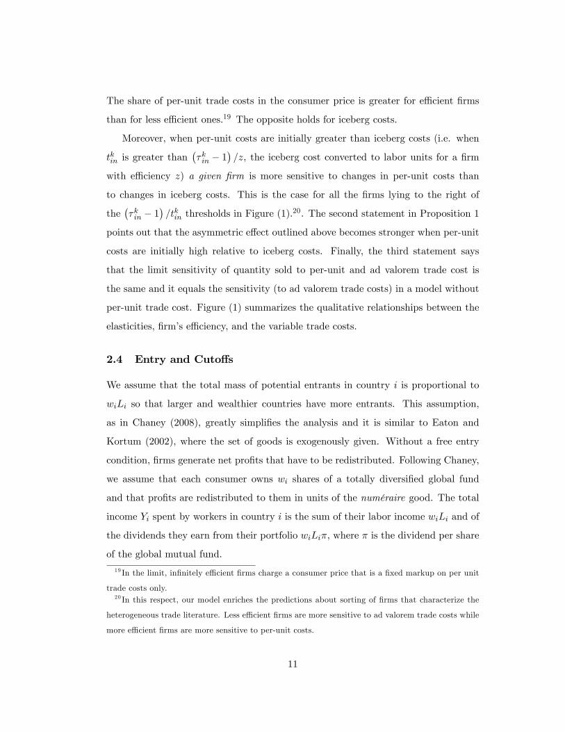
The share of per-unit trade costs in the consumer price is greater for e¢ cient �rms

than for less e¢ cient ones.19 The opposite holds for iceberg costs.

Moreover, when per-unit costs are initially greater than iceberg costs (i.e. when

tkin is greater than��kin � 1

�=z, the iceberg cost converted to labor units for a �rm

with e¢ ciency z) a given �rm is more sensitive to changes in per-unit costs than

to changes in iceberg costs. This is the case for all the �rms lying to the right of

the��kin � 1

�=tkin thresholds in Figure (1).

20. The second statement in Proposition 1

points out that the asymmetric e¤ect outlined above becomes stronger when per-unit

costs are initially high relative to iceberg costs. Finally, the third statement says

that the limit sensitivity of quantity sold to per-unit and ad valorem trade cost is

the same and it equals the sensitivity (to ad valorem trade costs) in a model without

per-unit trade cost. Figure (1) summarizes the qualitative relationships between the

elasticities, �rm�s e¢ ciency, and the variable trade costs.

2.4 Entry and Cuto¤s

We assume that the total mass of potential entrants in country i is proportional to

wiLi so that larger and wealthier countries have more entrants. This assumption,

as in Chaney (2008), greatly simpli�es the analysis and it is similar to Eaton and

Kortum (2002), where the set of goods is exogenously given. Without a free entry

condition, �rms generate net pro�ts that have to be redistributed. Following Chaney,

we assume that each consumer owns wi shares of a totally diversi�ed global fund

and that pro�ts are redistributed to them in units of the numéraire good. The total

income Yi spent by workers in country i is the sum of their labor income wiLi and of

the dividends they earn from their portfolio wiLi�, where � is the dividend per share

of the global mutual fund.

19 In the limit, in�nitely e¢ cient �rms charge a consumer price that is a �xed markup on per unit

trade costs only.20 In this respect, our model enriches the predictions about sorting of �rms that characterize the

heterogeneous trade literature. Less e¢ cient �rms are more sensitive to ad valorem trade costs while

more e¢ cient �rms are more sensitive to per-unit costs.

11

Firms will enter market n only if they can earn positive pro�ts there. Some

low productivity �rms may not generate su¢ cient revenue to cover their �xed costs.

We de�ne the productivity threshold �zkin from �kin(�zkin) = 0 as the lowest possible

productivity level consistent with non-negative pro�ts in export markets,

�zkin =

"�k1

�fkinYn

�1=(1��)P knwi�kin

� tkin�kin

#�1; (2)

with �k1 a constant.21

2.5 Closing the Model

Following Chaney (2008) and others, we assume that productivity shocks are drawn

from a Pareto distribution with density dF (z), shape parameter , and support

[1;+1).22 The price index in sector k of country n is then�P kn

�1��=Xi

wiLi

Z 1

�zkin

�pkin

�1��dF (z) dz.

We can summarize an equilibrium with the following set of equations:

P kn = h��zk1n; �z

k2n; ::; �z

kNn

�8 n

�zkin = f�P kn ; �

�8 i ; n

� = g��zk11; ::; �z

k1N ; �z

k21; ::; �z

k2N ; ::; �z

kNN

�The �rst equation states that the price index is a function the endogenous entry

cuto¤s (all exogenous variables are suppressed). The second states that the cuto¤s

are a function of the price index and the dividend share � (� is part of income Yn).

The third states that the dividend share is a function of all entry cuto¤s. We show

why this is so in Appendix A.2.1.

21Speci�cally, �k1 = (�=�k)1=(1��) (� � 1) =�.

22Unlike in earlier models (e.g. Chaney, 2008), we do not need to impose the condition > � � 1

for the size distribution of �rms to have a �nite mean, as long as per-unit trade costs are positive.

When t > 0 even the most productive �rms have �nite revenue.

12

All in all, this constitutes a system of N (N + 1)+1 equations and N (N + 1)+1

unknowns. It is not possible to �nd a closed-form solution for the price index when

tkin > 0. In Appendix A.2 we show how to solve the model numerically.

2.6 Welfare and Trade Costs

In this section we show that per-unit frictions lead to higher welfare losses than

comparable iceberg frictions. The fundamental problem in comparing welfare e¤ects

is that changes in per-unit trade costs are not directly comparable to changes in

iceberg costs. E.g. it makes little sense to compare a one percent increase in � in to a

one percent increase in tin. One way to deal with this is the following.23

� Start with a frictionless equilibrium and impose either (A) a per-unit import

barrier t on imports from m to n or (B) an ad valorem barrier � on imports

from m to n.

� Make (A) and (B) comparable by requiring that welfare in n is identical in the

two situations. This amounts to requiring that the price index in country n is

identical.24 From this, we obtain a function ~� (t) that maps per-unit costs to

welfare-neutral iceberg costs.

� Now ask how much is collected in import tari¤s in (A) and (B). We suspect that

revenue is higher in (B), as the price distortions are less severe in this case. If

this is the case, the �ip side is that welfare gains from reducing per-unit frictions

are higher than gains from reducing iceberg frictions.

23For simplicity, in this subsection, we consider one sector only and drop the k subscript.24Welfare also depends on income from pro�ts, but as in Chaney (2008), income from pro�ts is

constant.

13

In Appendix A.3 we derive the function ~� (t) and relative tari¤ revenue GB=GA.

They are25:

~� = (1 + �zt) ��+1

Z 1

1z��1dF (z)Z 1

1(1=z + �zt)1�� dF (z)

and

GBGA

=�

� � 1

Z 1

1(1=z + �zt)1�� dF (z)Z 1

1(1=z + �zt)�� dF (z)

~� � 1�zt

(3)

where �z is the entry hurdle in equilibrium A.26

Relative revenue is related to only three variables: �zt, �, and . �zt is simply per-

unit costs relative to production-unit costs of the least e¢ cient exporter, and serves

as a convenient measure of the distortion imposed by per-unit costs.27

We now show how the ratio relates to di¤erent combinations of these variables.

In Figure 2 we plot �zt on the x-axis and GB=GA as well as ~� on the y-axis. The four

graphs show four di¤erent choices of � and , � = 4; 6; 8; and = � � 1; � + 1.28

In all cases, GB=GA > 1, implying that iceberg tari¤s generate more revenue

than per-unit tari¤s, holding welfare constant.29 For example, if per-unit costs are

40 percent of production costs for the least e¢ cient exporter, then the alternative

strategy of imposing a welfare-neutral iceberg cost will increase tari¤ revenue by

roughly 200 percent, on average (taking the mean over all � and values).30 The

25Compared to the expressions in Appendix A.2, we simplify notation by calling the variable of

integration z, instead of ~zA and ~zB . Also, we de�ne �z = �zAkn.26Here we assume that > � � 1, since equilibrium (B) is unde�ned otherwise.27The fact that we can express the G ratio as a function of t�zAkn instead of t and �zAkn separately

makes the calculations much simpler, since we do not have to evaluate the e¤ect of t on �zAkn (which

involves calculating the price index).28The values for chosen here are higher than the ones estimated in the next section (see Table

1). The reason is that the G ratio is de�ned only when > � � 1. Figure 2 shows that the G ratio

increases for lower , so using the estimated value for instead would presumably increase the G

ratio even more.29We have tried a range of combinations of parameter values, and we always �nd that GB=GA > 1.30 In this case tari¤ revenue (in equilibrium B) is slightly less than the value of imports.

14

intuition is that per-unit costs will hit the more productive �rms especially hard (their

prices will increase by more than less e¢ cient �rms, in percent), which will translate

into lower welfare compared to iceberg costs. In order to stay on the same welfare

level, iceberg costs must increase, raising the GB=GA ratio.

One concern is that quality heterogeneity might weaken these theoretical �ndings.

For example, if e¢ cient �rms are producing high quality goods at high prices, then

per-unit costs will hit low quality goods harder than high quality ones.31 The welfare

e¤ect of per-unit costs in such a model is not clear cut. We explore this possibility in

Appendix A.4. We �nd that the GB=GA ratio can indeed become less than 1, but that

for the large majority of parameter values GB=GA > 1. Our simulations suggest that

the additional distortion generated by per-unit frictions are quantitatively important,

even in the presence of quality heterogeneity, and that reducing trade frictions may

give higher welfare gains than in standard models.

2.7 The Export Volume Distribution

In this section we examine some properties of the distribution of exports, across �rms

for a given product-destination pair. We will make extensive use of these properties

further below when we estimate the model. We �rst derive the theoretical exports

volume distribution for every destination n and product k. Source country subscripts

are dropped because Norway is always the source in the data. Given that productivity

among potential entrants is distributed Pareto, the productivity distribution among

exporters of product k to destination n is also Pareto with cumulative distribution

function F�zj�zkn

�= 1 �

�z=�zkn

�� . The Pareto shape coe¢ cient is assumed to

be equal across products and destinations. Then the exports volume cumulative

31Johnson (2009) proposes a model where �rms are heterogeneous both in terms of unit costs and

quality.

15

distribution function (CDF), conditional on z > �zkn, is32

Q�xj�zkn

�= Pr

�X < xjZ > �zkn

�= 1�

�Aknx

�1=� �Bkn� ; (4)

where Akn and Bkn are two clusters of parameters,

Akn =� � 1�

�zkn

�P kn

�(��1)=��1=�k

Y1=�n

�knw;

Bkn =tkn

�kn=�zkn

:

2.7.1 Properties of the Distribution

As with the scale parameter for the Pareto distribution, Akn will a¤ect the location of

the distribution. For example, an increase in market size Yn will shift the probability

density function to the right, so that it becomes more likely to sell greater quantities.

Since Bkn = tkn=��kn=�z

kn

�, Bkn simply measures per-unit trade costs (t

kn) relative to

the unit costs of the least e¢ cient �rm, inclusive ad valorem costs (�kn=�zkn). When

tkn = 0 =) Bkn = 0, the distribution is identical to Pareto with shape parameter

=�. This is similar to Chaney (2008), where the sales distribution preserves the

shape of the underlying e¢ ciency distribution and the sales distribution is identical

across markets. When tkn > 0, Bkn will a¤ect the dispersion of quantity sold. This can

be seen by �nding the inverse CDF:

xkn (#) = Q�1(#) =

"(1� #)1= +Bkn

Akn

#��:

Dispersion, as measured by the ratio between the #th2 and #th1 percentiles (0 < #1 <

#2 < 1) is then

D�#2; #1;B

kn; ; �

�� xkn (#2)

xkn (#1)=

"(1� #1)1= +Bkn(1� #2)1= +Bkn

#�: (5)

32The cdf is well-behaved when�1+Bk

n

Akn

���� xkminn < 0 and xkmaxn �

�Bkn

Akn

���< 0 where xkminn is

the minimum export volume and xkmaxn is maximum export volume.

16

When tkn = 0, this ratio is constant across destinations. When tkn > 0, the ratio

declines as Bkn goes up. That is, exports volume becomes less dispersed with higher

per-unit costs. The intuition is that higher per-unit costs will hit the high productiv-

ity/low cost �rms harder than �rms with low productivity/high cost, since more trade

costs will force the high productivity �rms to increase their price by more than the

low productivity �rms, in percentage terms. This will translate into a larger reduction

in quantity sold for the high productivity �rms relative to the low productivity �rms,

so that dispersion will decrease. The following proposition summarizes our �ndings:

Proposition 2 When per-unit costs are positive (tkin > 0), dispersion, as measured

by the ratio between the #th2 and #th1 percentiles, is decreasing in tkin and increasing in

�kin. Moreover, when per-unit costs are zero (tkin = 0), then dispersion is invariant to

a change in variable trade costs �kin.

Proof. See Appendix A.5.

In Appendix A.5 we prove this proposition allowing for trade costs to alter the

entry cuto¤s and the price index.

In Figure 3 we plot the theoretical exports volume complementary cumulative

distribution function, on log scales. The value of the complementary CDF is on

the horizontal axis, while quantity exported is on the vertical axis. The solid line

represents the case when Bkn = tkn=��kn=�z

kn

�= 0. The gradient is then equal to ��= .

The dotted line represents the case when per-unit costs are positive. As Bkn increases,

the complementary CDF becomes more and more concave. The concavity re�ects the

fact that large �rms (low cost �rms) are hit harder by per-unit costs than small �rms

(high cost �rms).

The properties of the exports volume distribution also survive, under some as-

sumptions, in a framework where �rms are heterogeneous both in terms of unit costs

and quality.33 In Appendix A.6 we also investigate whether departures from the CES

33More speci�cally, the result that dispersion decreases with per-unit trade costs carries through as

long as the relationship between production unit costs and quality is not too convex (as we show in

17

framework in models with ad valorem costs can generate predictions similar to those

of our model. We show that for a popular class of linear demand systems (and with

zero per-unit costs), dispersion in exports will increase in ad valorem costs - the op-

posite of the case with per-unit costs.34 We provide additional information about the

properties of the distribution in Section 3.4 (identi�cation).

3 Estimating the Model

In this section we structurally estimate the magnitude of per-unit trade costs. We

showed in the theory section that per-unit costs introduce curvature in the export vol-

ume CDF, leading to less dispersion in exports volume as per-unit trade costs increase.

When per-unit trade costs are zero, dispersion in exports volume is una¤ected by (ad

valorem) trade costs. This is the identifying assumption that allows us to recover

estimates of trade costs consistent with our model.35 The econometric strategy con-

sists of using a minimum distance estimator that matches the empirical distribution

of exports volume (per product-destination) to the theoretical distribution.36

Our approach of estimating trade costs from an economic model is very di¤erent

from the earlier literature.37 First, most studies model trade costs as ad valorem

exclusively, omitting the presence of per-unit costs. A notable exception is Hummels

Appendix A.5.1). In our particular dataset, as we will show below, this is the case for an overwhelming

majority of product-destination pairs.34 In Appendix A.6.1, we also consider an extension of our model where �rms have to sustain

marketing costs in order to promote their products and reach consumers, following Arkolakis (2008).

It turns out that, in the extended model, as long as the market penetration e¤ect is not too strong

compared to the per-unit trade cost e¤ect, we can interpret our results as a lower bound on the true

magnitude of the ad valorem equivalent of per-unit trade costs.35 In Section 3.2 below, we provide evidence that is consistent with the identifying assumption.36We choose to use data for export volume (quantities) instead of export sales for the following

reasons. First, a closed-form solution for the sales distribution does not exist. Second, using quantities

instead of sales avoids measurement error due to imperfect imputation of transport/insurance costs.

Third, we avoid transfer pricing issues when trade is intra-�rm (Bernard, Jensen and Schott 2006).37Anderson and van Wincoop (2004) provide a comprehensive summary of the literature.

18

and Skiba (2004), who distinguish between them and �nd evidence for the presence of

per-unit shipping costs.38 Compared to our work, they study freight costs exclusively,

whereas we consider all types of international trade costs. Second, our methodology

utilizes within-country dispersion in exports volume to achieve identi�cation of trade

costs, whereas earlier studies utilize cross-country variation in trade. Third, whereas

the traditional approach can only identify trade costs relative to some benchmark,

usually domestic trade costs, our method identi�es the absolute level of trade costs

(although conditional on a value of the elasticity of substitution). Fourth, we do not

impose trade cost symmetry (tkin and �kin can di¤er from, respectively, t

kni and �

kni).

3.1 Data

The data consist of an exhaustive panel of Norwegian non-oil exporters in the 1996-

2004 period. Data come from customs declarations. Every export observation is

associated with a �rm, a destination and a product id and for every export observation

we observe the quantity transacted and the total value.39 Since identi�cation in the

empirical model is based solely on cross-sectional variation, we chose to work, in our

baseline speci�cation, with the 2004 cross-section, the most recent available to us.

The product id is based on the Harmonized System 8-digit (HS8) nomenclature, and

there are 5; 391 active HS8 products in the data. 203 unique destinations are recorded

in the dataset.

In 2004, 17; 480 �rms were exporting and the total export value amounted to

NOK 232 billion (� USD 34:4 billion), or 48 percent of the aggregate manufacturing

revenue. On average, each �rm exported 5:6 products to 3:4 destinations for NOK 13:3

million (� USD 2:0 million). On average, there are 3:0 �rms per product-destination38They �nd an elasticity of freight rates with respect to price around 0:6, well below the unitary

elasticity implied by the iceberg assumption on shipping costs.39Firm-product-year observations are recorded in the data as long as the export value is NOK 1000

(� USD 148) or higher. The unit of measurement is kilos for all the products. Moreover, 27:5% of

the products are additionally measured in quantities, while 4:7% are additionally measured in other

units (m3, carat, etc.). In the baseline estimation we use kilos unless a di¤erent unit is available.

19

(standard deviation 7:8). As we will see, we utilize the distribution of export quantity

across �rms within a product-destination in the econometric model. We therefore

choose to restrict the sample to product-destinations where more than 40 �rms are

present.40 In the robustness section, we evaluate the e¤ect of this restriction by

estimating the model on an expanded set of destination-product pairs. Below, extreme

values of quantity sold, de�ned as values below the 1st percentile or above the 99th

percentile for every product-destination, are eliminated from the dataset. All in all,

this brings down the total number of products to 121 and the number of destinations

to 21.41

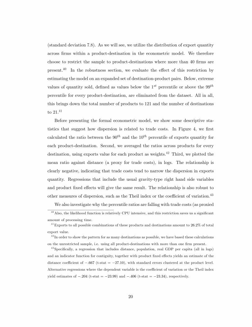
Before presenting the formal econometric model, we show some descriptive sta-

tistics that suggest how dispersion is related to trade costs. In Figure 4, we �rst

calculated the ratio between the 90th and the 10th percentile of exports quantity for

each product-destination. Second, we averaged the ratios across products for every

destination, using exports value for each product as weights.42 Third, we plotted the

mean ratio against distance (a proxy for trade costs), in logs. The relationship is

clearly negative, indicating that trade costs tend to narrow the dispersion in exports

quantity. Regressions that include the usual gravity-type right hand side variables

and product �xed e¤ects will give the same result. The relationship is also robust to

other measures of dispersion, such as the Theil index or the coe¢ cient of variation.43

We also investigate why the percentile ratios are falling with trade costs (as proxied

40Also, the likelihood function is relatively CPU intensive, and this restriction saves us a signi�cant

amount of processing time.41Exports to all possible combinations of these products and destinations amount to 26:2% of total

export value.42 In order to show the pattern for as many destinations as possible, we have based these calculations

on the unrestricted sample, i.e. using all product-destinations with more than one �rm present.43Speci�cally, a regression that includes distance, population, real GDP per capita (all in logs)

and an indicator function for contiguity, together with product �xed e¤ects yields an estimate of the

distance coe¢ cient of �:667 (t-stat = �27:10), with standard errors clustered at the product level.

Alternative regressions where the dependent variable is the coe¢ cient of variation or the Theil index

yield estimates of �:204 (t-stat = �23:99) and �:406 (t-stat = �23:34), respectively.

20

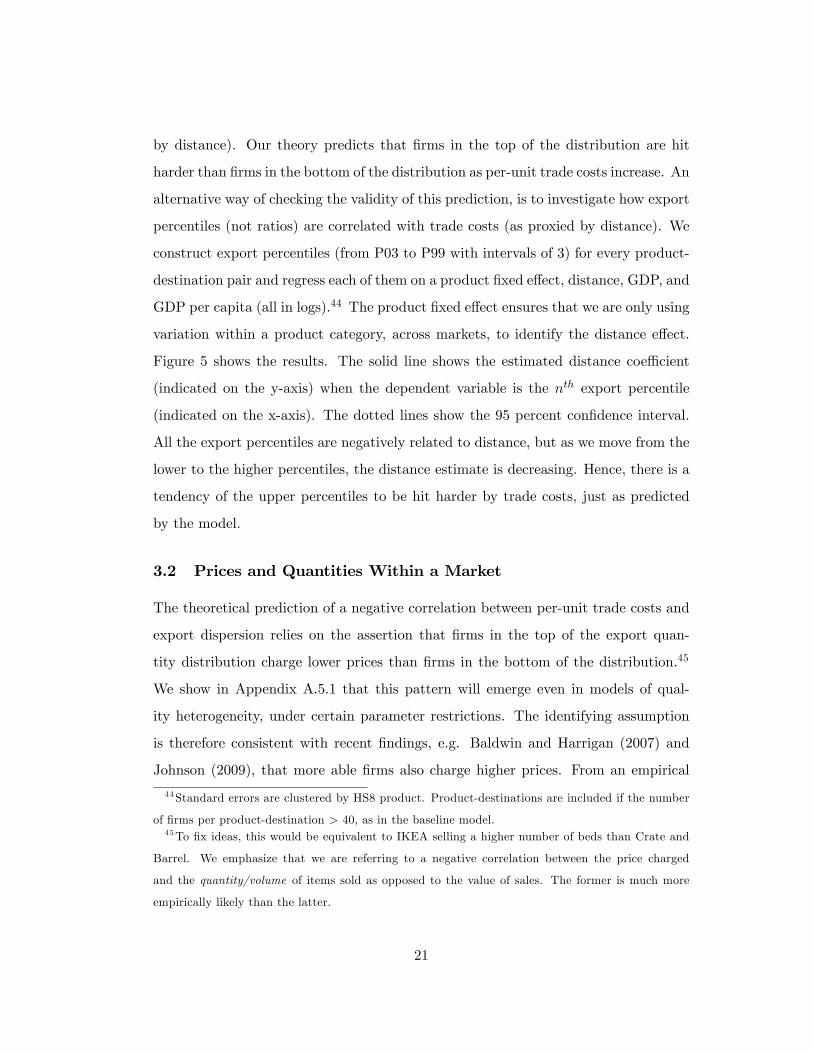
by distance). Our theory predicts that �rms in the top of the distribution are hit

harder than �rms in the bottom of the distribution as per-unit trade costs increase. An

alternative way of checking the validity of this prediction, is to investigate how export

percentiles (not ratios) are correlated with trade costs (as proxied by distance). We

construct export percentiles (from P03 to P99 with intervals of 3) for every product-

destination pair and regress each of them on a product �xed e¤ect, distance, GDP, and

GDP per capita (all in logs).44 The product �xed e¤ect ensures that we are only using

variation within a product category, across markets, to identify the distance e¤ect.

Figure 5 shows the results. The solid line shows the estimated distance coe¢ cient

(indicated on the y-axis) when the dependent variable is the nth export percentile

(indicated on the x-axis). The dotted lines show the 95 percent con�dence interval.

All the export percentiles are negatively related to distance, but as we move from the

lower to the higher percentiles, the distance estimate is decreasing. Hence, there is a

tendency of the upper percentiles to be hit harder by trade costs, just as predicted

by the model.

3.2 Prices and Quantities Within a Market

The theoretical prediction of a negative correlation between per-unit trade costs and

export dispersion relies on the assertion that �rms in the top of the export quan-

tity distribution charge lower prices than �rms in the bottom of the distribution.45

We show in Appendix A.5.1 that this pattern will emerge even in models of qual-

ity heterogeneity, under certain parameter restrictions. The identifying assumption

is therefore consistent with recent �ndings, e.g. Baldwin and Harrigan (2007) and

Johnson (2009), that more able �rms also charge higher prices. From an empirical

44Standard errors are clustered by HS8 product. Product-destinations are included if the number

of �rms per product-destination > 40, as in the baseline model.45To �x ideas, this would be equivalent to IKEA selling a higher number of beds than Crate and

Barrel. We emphasize that we are referring to a negative correlation between the price charged

and the quantity/volume of items sold as opposed to the value of sales. The former is much more

empirically likely than the latter.

21

point of view, the correlation between price and quantity sold is something we can

easily check in the data, as prices can be approximated by unit values. In the data,

we �nd that the average correlation between unit value and (quantity) market share

is �:59 (the unweighted average over product-destination pairs, using only the pairs

that we estimate on) and that 96:7 percent of the correlations are negative.46 The

histogram of the correlation coe¢ cients is shown in Figure 6. If the negative relation-

ship between quantity and price is weaker than our model suggests, possibly due to

quality heterogeneity within an HS8 category, then the link between per-unit trade

costs and dispersion will also be weaker. In that case, our estimate of per-unit trade

costs will be biased downward, since our model will interpret high dispersion as low

trade costs. However, the strong negative correlations for most of the products in our

sample indicate that the bias is relatively small.

3.3 Estimation

We use a minimum distance estimator that matches empirical dispersion in exports

volume (per product-destination) to simulated dispersion in exports volume. Speci�-

cally, denote the empirical ratio between the #th2 and #th1 percentiles for product k in

destination n as eDkn (#2; #1) and stack a set of (#2; #1) ratios in theM�1 column vec-

tor eDkn. Denote its simulated counterpart D

�#2; #1;B

kn; ; �

�, as de�ned in equation

(5), and stack a set of (#2; #1) ratios in the M �1 column vector D�Bkn; ; �

�. De�ne

the criterion function as the squared di¤erence between lnD�Bkn; ; �

�and ln eDk

n:

d () =NXn

Xk2n

hlnD

�Bkn; ; �

�� ln eDk

n

i0 hlnD

�Bkn; ; �

�� ln eDk

n

i;

where is the vector of coe¢ cients to be estimated, N is the total number of des-

tinations and n is the set of products sold in market n. We minimize d () with

46Using an alternative dataset (see Section 3.6) of Portugal-based exporters, we �nd that the

average correlation between unit value and export quantity is �:36 and 97:5 percent of the correlations

are negative. Manova and Zhang (2009), using data on Chinese trading �rms, also �nd a negative

correlation between �rm f.o.b. export prices and quantity sold (see Table 4, column 2).

22

respect to and denote b the equally weighted minimum distance estimator.47

We model Bkn as the product of sector and destination �xed e¤ects,

Bkn = �kbn;

and normalize �1 = 1.48 This decomposition enables us to identify the share of trade

costs that is due to product characteristics and the share that is due to market charac-

teristics. Also, note that even though �k is estimated relative to some normalization,

the estimates of the B values are invariant to the choice of normalization. Finally,

we condition the criterion function on a guess of � (see next section). The coe¢ cient

vector then consists of = (�k; bn; ), in total K +N parameters.

We choose the following percentile ratio moments: (:95; :05), (:90; :10), (:75; :25),

(:60; :40), (:20; :10), (:30; :20), (:40; :30), (:50; :40), (:60; :50), (:70; :60), (:80; :70), (:90; :80);

in total M = 12 moments per product-destination.49

As the covariance matrix of the vector of empirical percentile ratios (eDkn) is un-

known, the standard error of the estimator is not available using standard formulas.

Instead, we employ a nonparametric bootstrap (empirical distribution function boot-

strap). Speci�cally, we sample with replacement within each product-destination pair,

obtaining the same number of observations as in the original sample. After performing

500 bootstrap replications, we form the standard errors by calculating the standard

deviation for each coe¢ cient in .47Theory suggests that for overidenti�ed models it is best to use optimal GMM. In implementation,

however, the optimal GMM estimator may su¤er from �nite-sample bias (Altonji and Segal 1996).

Furthermore, it is di¢ cult to calculate the optimal weighting matrix in our context, as it would

necessitate evaluating the variance of the percentile ratios for every product-destination (see e.g.

Cameron and Trivedi, 2005, section 6.7).48The normalization is similar to the one adopted in the estimation of two-way �xed e¤ects in the

employer-employee literature (see Abowd, Creecy, and Kramarz 2002). We also need to ensure that

all products and destinations belong to the same mobility group. The intuition is that if a given

product is sold only in a destination where no other products are sold, then one cannot separate the

product from the destination e¤ect.49We experimented with other combinations of moments as well and the results remained largely

unchanged.

23

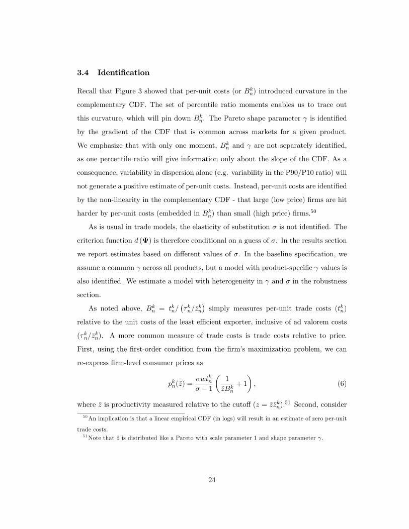
3.4 Identi�cation

Recall that Figure 3 showed that per-unit costs (or Bkn) introduced curvature in the

complementary CDF. The set of percentile ratio moments enables us to trace out

this curvature, which will pin down Bkn. The Pareto shape parameter is identi�ed

by the gradient of the CDF that is common across markets for a given product.

We emphasize that with only one moment, Bkn and are not separately identi�ed,

as one percentile ratio will give information only about the slope of the CDF. As a

consequence, variability in dispersion alone (e.g. variability in the P90/P10 ratio) will

not generate a positive estimate of per-unit costs. Instead, per-unit costs are identi�ed

by the non-linearity in the complementary CDF - that large (low price) �rms are hit

harder by per-unit costs (embedded in Bkn) than small (high price) �rms.50

As is usual in trade models, the elasticity of substitution � is not identi�ed. The

criterion function d () is therefore conditional on a guess of �. In the results section

we report estimates based on di¤erent values of �. In the baseline speci�cation, we

assume a common across all products, but a model with product-speci�c values is

also identi�ed. We estimate a model with heterogeneity in and � in the robustness

section.

As noted above, Bkn = tkn=��kn=�z

kn

�simply measures per-unit trade costs (tkn)

relative to the unit costs of the least e¢ cient exporter, inclusive of ad valorem costs

(�kn=�zkn). A more common measure of trade costs is trade costs relative to price.

First, using the �rst-order condition from the �rm�s maximization problem, we can

re-express �rm-level consumer prices as

pkn(~z) =�wtkn� � 1

�1

~zBkn+ 1

�; (6)

where ~z is productivity measured relative to the cuto¤ (z = ~z�zkn).51 Second, consider

50An implication is that a linear empirical CDF (in logs) will result in an estimate of zero per-unit

trade costs.51Note that ~z is distributed like a Pareto with scale parameter 1 and shape parameter .

24

the average price (charged by Norwegian exporters) of product k in destination n:

�pkn =1

1� F (�zkn)

Z�zkn

pkn (z) dF (z)

=��zkn

� Z�zkn

pkn (z) z� �1dz

=

Z1pkn (~z) dF (~z) ;

where we used the substitution z = ~z�zkn in the last equality. Third, inserting equation

(6) and solving for wtkn=�pkn yields:

wtkn�pkn

=� � 1�

Bkn ( + 1)

+Bkn ( + 1):

The ratio wtkn=�pkn measures (per-unit) trade costs relative to the average consumer

price.52 Given our estimate of Bkn and , the expression on the right hand side can be

easily computed. Note that integrating over productivities allows us to express trade

costs only as a function of Bkn, and �: This is due to the fact that a Pareto density

is parameterized only by the cuto¤ (�zkn) and the shape parameter ( ). Our estimates

of Bkn and are therefore su¢ cient to obtain a meaningful measure of per-unit trade

costs.

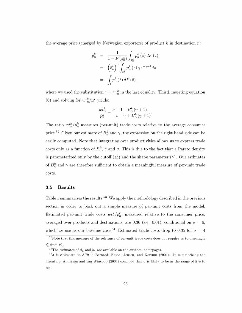
3.5 Results

Table 1 summarizes the results.53 We apply the methodology described in the previous

section in order to back out a simple measure of per-unit costs from the model.

Estimated per-unit trade costs wtkn=�pkn, measured relative to the consumer price,

averaged over products and destinations, are 0:36 (s.e. 0:01), conditional on � = 6,

which we use as our baseline case.54 Estimated trade costs drop to 0:35 for � = 4

52Note that this measure of the relevance of per-unit trade costs does not require us to disentagle

tkn from �kn.53The estimates of �k and bn are available on the authors�homepages.54� is estimated to 3:79 in Bernard, Eaton, Jensen, and Kortum (2004). In summarizing the

literature, Anderson and van Wincoop (2004) conclude that � is likely to be in the range of �ve to

ten.

25

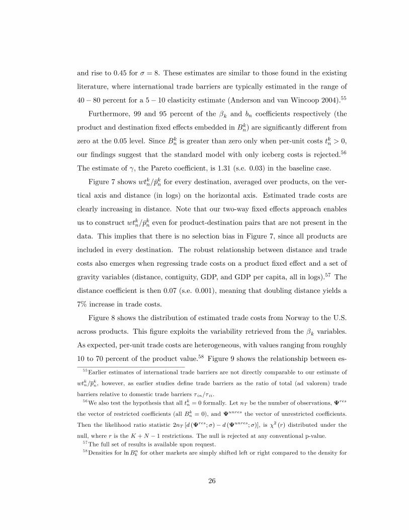
and rise to 0:45 for � = 8. These estimates are similar to those found in the existing

literature, where international trade barriers are typically estimated in the range of

40� 80 percent for a 5� 10 elasticity estimate (Anderson and van Wincoop 2004).55

Furthermore, 99 and 95 percent of the �k and bn coe¢ cients respectively (the

product and destination �xed e¤ects embedded in Bkn) are signi�cantly di¤erent from

zero at the 0:05 level. Since Bkn is greater than zero only when per-unit costs tkn > 0,

our �ndings suggest that the standard model with only iceberg costs is rejected.56

The estimate of , the Pareto coe¢ cient, is 1:31 (s.e. 0:03) in the baseline case.

Figure 7 shows wtkn=�pkn for every destination, averaged over products, on the ver-

tical axis and distance (in logs) on the horizontal axis. Estimated trade costs are

clearly increasing in distance. Note that our two-way �xed e¤ects approach enables

us to construct wtkn=�pkn even for product-destination pairs that are not present in the

data. This implies that there is no selection bias in Figure 7, since all products are

included in every destination. The robust relationship between distance and trade

costs also emerges when regressing trade costs on a product �xed e¤ect and a set of

gravity variables (distance, contiguity, GDP, and GDP per capita, all in logs).57 The

distance coe¢ cient is then 0:07 (s.e. 0:001), meaning that doubling distance yields a

7% increase in trade costs.

Figure 8 shows the distribution of estimated trade costs from Norway to the U.S.

across products. This �gure exploits the variability retrieved from the �k variables.

As expected, per-unit trade costs are heterogeneous, with values ranging from roughly

10 to 70 percent of the product value.58 Figure 9 shows the relationship between es-

55Earlier estimates of international trade barriers are not directly comparable to our estimate of

wtkn=pkn, however, as earlier studies de�ne trade barriers as the ratio of total (ad valorem) trade

barriers relative to domestic trade barriers � in=� ii.56We also test the hypothesis that all tkn = 0 formally. Let nT be the number of observations,

res

the vector of restricted coe¢ cients (all Bkn = 0), and unres the vector of unrestricted coe¢ cients.

Then the likelihood ratio statistic 2nT [d (res;�)� d (unres;�)], is �2 (r) distributed under the

null, where r is the K +N � 1 restrictions. The null is rejected at any conventional p-value.57The full set of results is available upon request.58Densities for lnBn

k for other markets are simply shifted left or right compared to the density for

26

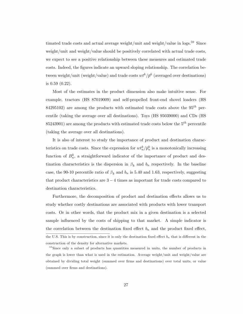
timated trade costs and actual average weight/unit and weight/value in logs.59 Since

weight/unit and weight/value should be positively correlated with actual trade costs,

we expect to see a positive relationship between these measures and estimated trade

costs. Indeed, the �gures indicate an upward sloping relationship. The correlation be-

tween weight/unit (weight/value) and trade costs wtk=�pk (averaged over destinations)

is 0:59 (0:22).

Most of the estimates in the product dimension also make intuitive sense. For

example, tractors (HS 87019009) and self-propelled front-end shovel loaders (HS

84295102) are among the products with estimated trade costs above the 95th per-

centile (taking the average over all destinations). Toys (HS 95039000) and CDs (HS

85243901) are among the products with estimated trade costs below the 5th percentile

(taking the average over all destinations).

It is also of interest to study the importance of product and destination charac-

teristics on trade costs. Since the expression for wtkn=�pkn is a monotonically increasing

function of Bkn, a straightforward indicator of the importance of product and des-

tination characteristics is the dispersion in �k and bn respectively. In the baseline

case, the 90-10 percentile ratio of �k and bn is 5:40 and 1:63, respectively, suggesting

that product characteristics are 3� 4 times as important for trade costs compared to

destination characteristics.

Furthermore, the decomposition of product and destination e¤ects allows us to

study whether costly destinations are associated with products with lower transport

costs. Or in other words, that the product mix in a given destination is a selected

sample in�uenced by the costs of shipping to that market. A simple indicator is

the correlation between the destination �xed e¤ect bn and the product �xed e¤ect,

the U.S. This is by construction, since it is only the destination �xed e¤ect bn that is di¤erent in the

construction of the density for alternative markets.59Since only a subset of products has quantities measured in units, the number of products in

the graph is lower than what is used in the estimation. Average weight/unit and weight/value are

obtained by dividing total weight (summed over �rms and destinations) over total units, or value

(summed over �rms and destinations).

27

averaged over the products actually exported there. Formally, we correlate bn with

(1=Kn)Pk2n �k, where Kn is the number of products exported to destination n and

n is the set of products exported to n. The results indicate that there is not much

support for the hypothesis. The correlation is slightly positive but not signi�cantly

di¤erent from zero.

We also investigate whether the unweighted average of trade costs is di¤erent from

the weighted average.60 When using export values per product-destination as weights,

the weighted average of trade costs is 0:27. This suggests that product-destinations

associated with high costs have below average exports.

Finally, Figure 10 shows actual and simulated percentile ratios (95=05, 90=10,

75=25, and 60=40), for all product-destination pairs. Most observations lie close to

the 45 degree line, although the �t of the model is declining closer to the median.

Overall, this leads us to conclude that the model is able to �t the data quite well.

3.6 Robustness

3.6.1 Variations of the Baseline Model

Next we present some re-estimations of the model that address several issues. The

results are summarized in Table 2. One concern is our reliance on the Pareto distrib-

ution. Even though the Pareto is known to approximate the US �rm size distribution

quite well (e.g. Luttmer 2007), one could argue that dispersion is decreasing with

trade costs due to extensive margin e¤ects. As is well known, the fractal nature of

the Pareto distribution implies that a percentile ratio is independent of truncation.

As a consequence, movements in the entry cuto¤ do not a¤ect the percentile ratio

(when t = 0). However, under other distributions this may no longer be the case.

For example, with the lognormal distribution and t = 0, dispersion will decrease with

higher entry hurdles simply because the density is truncated from below, not due

to intensive margin reallocation. One way of controlling for this, is to estimate the

60We focus mainly on the unweighted average because otherwise we would have a selection problem

when comparing trade costs across destinations.

28

model on a subsample where the set of exporters is identical in every destination (for

each product). Speci�cally, we take the three most popular destinations, Sweden,

Denmark, and Germany, and extract the �rms that are present in all three markets,

for each product. Since this procedure reduces the sample size dramatically, we are

forced to lower the threshold of �rms present in a product-destination pair, from 40

to 10, resulting in three destinations and 11 products. With only 10 or more �rms

per product-destination, we must also reduce the number of estimating moments per

product-destination, so we choose four moments: The (95; 05), (90; 10), (75; 25) and

(60; 40) percentile ratios. The results are shown in column (R1) in Table 2. Although

the sample size is much smaller, the trade cost estimates are nearly unchanged and

estimated with high precision. Therefore, we conclude that truncation of the export

distribution is not driving our results, nor are other types of selection e¤ects.

Second, a concern is that quality heterogeneity within an HS8 product group

might bias our results, something we brie�y discussed in Section 3.2. One way to

check whether this is an issue, is to re-estimate the model on homogeneous goods

exclusively. If the results become very di¤erent, there is reason for concern. We use

the Rauch (1999) classi�cation of di¤erentiated and homogeneous goods and choose

products that are classi�ed as non-di¤erentiated.61 The number of products declines

quite substantially in this case, so as in (R1), we set the �rm threshold to more than

10 �rms per product-destination and restrict the set of moments to four. Estimates

are reported in column (R2), and the results are reassuring. The grand mean of trade

costs (conditional on � = 6) is identical to the baseline case.

Third, we investigate whether the choice of truncating the dataset to only product-

destinations with more than 40 �rms a¤ects the results. We choose product-destinations

with more than 10 �rms present, resulting in 42 destinations and 826 products. Again,

the lower threshold forces us to reduce the number of moments used in estimation,

61Goods classi�ed as �goods traded on an organized exchange� or �reference

priced� in the Rauch (1999) database. We use Jon Haveman�s concordances at

http://www.macalester.edu/research/economics/page/haveman/Trade.Resources/TradeData.html

to convert SITC to HS codes.

29

so as in (R1), we choose four moments: The (95; 05), (90; 10), (75; 25), and (60; 40)

percentile ratios. The estimate of trade costs increases slightly, to 0:43, as shown in

column (R3).62 This suggests that although the product-destination pairs we esti-

mate on are not a random sample, the selection bias resulting from truncation is not

very large.

Fourth, we investigate whether the choice of units a¤ects the results. The high

share of products that are measured in kilos might bias the results if weight per-unit

is varying across both destinations and �rms. For example, if high productivity �rms

are able to reduce unit weight in remote markets, while low productivity �rms are

not, then dispersion will decrease. We address this issue by selecting the subsample

of products that are measured in units, not kilos. This truncates the dataset to 40

products and six markets. Again, the results do not change much, as shown in column

(R4) in the table.

Fifth, we re-estimate the model on the 2003 cross-section instead of the 2004

cross-section. The results in column (R5) show that the grand mean of trade costs is

identical to the baseline result.

Sixth, we estimate the model on a dataset of Portuguese exporters. The data have

the same structure as the Norwegian one.63 The results in column (R6) show that

the mean of per-unit trade costs for Portugal is 0:34, very close to the Norwegian

estimates (for � = 6).

Finally, we also check the sensitivity of the results to heterogeneity in the elasticity

of substitution � and the Pareto coe¢ cient . First, we take estimates of the �

from Broda and Weinstein (2006), and take the unweighted average of their HS 10-

digit estimates for every 4-digit product.64 Second, we allow for product-speci�c

62Our estimation algorithm spent 15 hours minimizing the objective function in this case. There-

fore, we do not report standard errors in column (R2), as bootstrapping becomes prohibitively costly.63A detailed description of the dataset of Portuguese exporters can be found in Martins and Opro-

molla (2009). The average correlation between unit value and export quantity is �:36 (the unweighted

average over product-destination pairs, using only the pairs that we estimate on) and 97:5 percent of

the correlations are negative.64We average up to the 4-digit level because i) only the �rst six digits are internationally comparable

30

values, so that the theoretical percentile ratios become D�#2; #1;B

kn; k; �k

�and the

coe¢ cient vector to be estimated becomes = (�k; bn; k), in total 2K + N � 1

coe¢ cients. The results are reported in column (R7).65 Again, per-unit costs are

large and signi�cant, although the point estimate falls somewhat compared to the

baseline case.

3.6.2 Other Robustness Checks

We have shown that the concavity of the export distribution is systematically related

to market characteristics and that per-unit trade costs are a reasonable explanation

for this fact. However, we would like the model to �t other aspects of the data as

well, in dimensions that are not easily explained in competing models. One such

feature is f.o.b. export prices. Our model predicts that f.o.b. prices are increasing in

per-unit trade costs (see theory section).66 The reason is that the perceived elasticity

of demand is lower when per-unit costs are high, leading �rms to charge a higher

markup.67 In Table 3 we provide evidence that this is indeed the case in the data.

We regress �rm-product-destination level unit values on a �rm-product �xed e¤ect,

distance, GDP, and GDP per capita. Standard errors are clustered on HS8 products.

The distance coe¢ cient is identi�ed purely from the variation within a �rm-product

pair across destinations. The coe¢ cient is positive and signi�cant, using both Norwe-

gian and Portuguese �rm-level data, suggesting that a given exporter charges a higher

price for the same HS8 good in more remote markets. This result is di¢ cult to recon-

cile with existing heterogeneous �rms trade models, as noted by Manova and Zhang

and (ii) not all products are jointly present in the Norwegian and U.S. data.65We do not report standard errors in this case, because bootstrapping is prohibitively time-

consuming.66A model with endogenous quality choice and per-unit costs will also generate a positive correlation

between f.o.b. prices and per-unit trade costs.67Note that, as in Berman et al. (2009), our model is consistent with incomplete exchange rate

pass-through. The elasticity of the f.o.b. price to a real depreciation is less than one as long as

per-unit trade costs are �nite. Our model predicts that this elasticity (and therefore the degree of

exchange rate pass-through) is increasing in t=� .

31

(2009). In standard models with CES demand, e.g. Melitz (2003), �rms charge the

same f.o.b. price in all locations. In standard models with linear demand, e.g. Melitz

and Ottaviano (2008), �rms charge lower markups in remote markets. In standard

quality-sorting models, e.g. Baldwin and Harrigan (2007), �rms are assumed to sell

the same quality worldwide.

Eaton, Kortum, and Kramarz (2008) argue that sales and entry shocks are needed

in order to explain the entry and sales patterns of French exporters. Our model, on

the other hand, has only variability along the productivity dimension. Although

additional error components would certainly increase the �t of the model, we decided

to choose a somewhat simpler setup in this paper.68 First, the de�ning feature of

the data we have attempted to explain is the varying dispersion in exports across

destinations. A model with entry and sales shocks but without per-unit costs cannot

explain this,69 unless one assumes that the variances and/or covariances of the shocks

are correlated with distance. Second, our econometric model is expressed in closed-

form, even though analytical expressions for many key relationships do not exist. This

helps to keep the run-time of the estimation algorithm down to an acceptable level.

4 Conclusions

In this paper we have �rst explored theoretically the implications of introducing more

�exible trade costs in an otherwise standard Melitz (2003) heterogeneous �rm model

of international trade. An important �nding is that we identify an additional channel

of gains from trade through intensive margin reallocation compared to the standard

model. The mechanism behind the result is that the more productive �rms are hit

harder by trade costs compared to the less productive �rms when trade costs are

independent of e¢ ciency (and price). It is thus the marriage of per-unit costs and

heterogeneity in e¢ ciency that drives the theoretical results in this paper.

68 In an earlier paper (Irarrazabal, Moxnes, and Opromolla 2009) we estimated demand and �xed

cost shocks in a model with heterogeneous �rms, exports, and multinational production.69Abstracting from possible e¤ects of truncation of the distribution on dispersion.

32

We tie the stylized model to a rich �rm-level dataset of exports, by product and

destination. By using the identifying assumption from theory that higher-order mo-

ments from the export quantity distribution (for a given product-destination pair) are

systematically related to (per-unit) trade costs, we are able to back out a structural

estimate of trade costs. Our empirical results indicate that per-unit costs are not

just a theoretical possibility: they are pervasive in the data, and the grand mean of

trade costs, expressed relative to the consumer price, is between 35% and 45%. We

therefore conclude that pure iceberg is rejected, and that empirical work, especially

at this level of disaggregation, must account for both the tip of the iceberg, as well

as the part of trade costs that are largely hidden under the surface: per-unit costs.

A broader implication of our work is related to the skill premium. To the extent

that more productive �rms demand more high-skill labor (e.g. as in Verhoogen 2008),

lowering trade barriers will increase aggregate demand for high skill labor through the

intensive margin reallocation channel emphasized in this paper. As a consequence,

our model makes clear an additional link between trade (the decline in international

transportation costs) and the skill premium.

Finally, we explore the welfare implications of per-unit versus iceberg frictions. We

introduce either a per-unit friction or an iceberg friction and impose that they are

welfare neutral. We then check what the government would collect in tari¤ revenue in

both cases. Using plausible parameter values, we �nd that iceberg frictions generate

much higher revenue than per-unit frictions. The �ip side is that welfare gains from

reducing per-unit frictions are substantially higher than gains from reducing iceberg

frictions. This suggests that existing estimates of the potential for gains from trade

may be too low. A fairly robust policy implication of our work is that, if governments

are determined to raise revenue through import duties, they should impose ad valorem

duties rather than per-unit duties, due to the additional distortions associated with

per-unit duties.

33

References

[1] Abowd, John M., Robert H. Creecy, and Francis Kramarz, �Computing Person

and Firm E¤ects Using Linked Longitudinal Employer-Employee Data,�Cornell

University Working Paper, 2002.

[2] Alchian, Armen A., and William R. Allen, University Economics (Belmont, CA:

Wadsworth Publishing Company, 1964).

[3] Altonji, Joseph G., and Lewis M. Segal, �Small-Sample Bias in GMM Estimation

of Covariance Structures,�Journal of Business & Economic Statistics, 3 (1996),

353-366.

[4] Anderson, James E., and Eric van Wincoop, �Gravity with Gravitas: A Solution

to the Border Puzzle,�American Economic Review, 1 (2003), 170-192.

[5] Anderson, James E., and Eric van Wincoop, �Trade Costs,�Journal of Economic

Literature, 3 (2004), 691-751.

[6] Arkolakis, Konstantinos, �Market Penetration Costs and the New Consumers

Margin in International Trade,�NBER working paper No. 14214, 2008.

[7] Arkolakis, Konstantinos, Arnaud Costinot, and A. Rodríguez-Clare, �New Trade

Models, Same Old Gains?,�mimeo, 2010.

[8] Baldwin, Richard and James Harrigan, �Zeros, Quality and Space: Trade Theory

and Trade Evidence,�NBER Working Paper No. 13214, 2007.

[9] Berman, Nicolas, Philippe Martin, and Thierry Mayer, � How Do Di¤erent Ex-

porters React to Exchange Rate Changes? Theory, Empirics and Aggregate

Implications,�mimeo, 2009.

[10] Bernard, Andrew B., Jonathan Eaton, Bradford J. Jensen, and Samuel Kortum,

�Plants and Productivity in International Trade,�American Economic Review,

4(2003), 1268-1290.

34

[11] Bernard, Andrew, Bradford J. Jensen, and Peter Schott, �Transfer Pricing by

US-Based Multinational Firms,�NBER Working Paper 12493, 2006.

[12] Broda, Christian, and David Weinstein, �Globalization and the Gains from Va-

riety,�Quarterly Journal of Economics, 2 (2006), 541-585.

[13] Cameron A. Colin, and Pravin K. Trivedi, Microeconometrics: Methods and

Applications, (New York, NY: Cambridge University Press, 2005).

[14] Chaney, Thomas, �Distorted Gravity: The Intensive and Extensive Margins of

International Trade,�American Economic Review, 98 (2008), 1707�1721.

[15] Demidova, Svetlana, Hiau Looi Kee, and Kala Krishna, �Do Trade Policy

Dixoerences Induce Sorting? Theory and Evidence From Bangladeshi Apparel

Exporters,�mimeo, 2009.

[16] Eaton, Jonathan, and Samuel Kortum, �Technology, Geography, and Trade,�

Econometrica, 70 (2002), 1741-1779.

[17] Eaton, Jonathan, Samuel Kortum, and Francis Kramarz, �An Anatomy of Inter-

national Trade: Evidence from French Firms," NBER Working Paper No. 14610,

2008.

[18] Keith Head, and John Ries, �Increasing Returns versus National Product Dif-

ferentiation as an Explanation for the Pattern of U.S.-Canada Trade,�American

Economic Review, 4 (2001), 858-876.

[19] Helpman, Elhanan, Marc J. Melitz, and Yona Rubinstein. 2008. �Estimating

Trade Flows: Trading Partners and Trading Volumes.�Q.J.E., 123 (May): 441-

487.

[20] Hummels, David, �Transportation Costs and International Trade in the Second

Era of Globalization,�Journal of Economic Perspectives, 21 (2007), 131-154.

35

[21] Hummels, David, and Alexandre Skiba, �Shipping the Good Apples Out? An

Empirical Con�rmation of the Alchian-Allen Conjecture,� Journal of Political

Economy, 6(2004), 1384-1402.

[22] Hummels, David and Peter J. Klenow, �The Variety and Quality of a Nation�s

Exports,�American Economic Review, 3 (2005), 704-723.

[23] Hummels, David, Volodymyr Lugovskyy, and Alexandre Skiba, �The Trade Re-

ducing E¤ects of Market Power in International Shipping,�Journal of Develop-

ment Economics, 1 (2009), 84-97.

[24] Irarrazabal, Alfonso, Moxnes Andreas, and Luca David Opromolla, �The Margins

of Multinational Production and the Role of Intra-�rm Trade,�CEPR Discussion

Paper 7145, 2008.

[25] Jacks, David S., Christopher M. Meissner, and Dennis Novy, �Trade Costs, 1870�

2000,�American Economic Review Papers & Proceedings, 2 (2008), 529�534.

[26] Johnson, Robert C., �Trade and Prices with Heterogeneous Firms,�mimeo, 2009.

[27] Kehoe, Timothy J., and Kim J. Ruhl, �How Important is the New Goods Margin

in International Trade?,�Federal Reserve Bank of Minneapolis Sta¤Report 324,

2009.

[28] Klenow, Pete, and Andrés Rodríguez-Clare, �Quantifying variety gains from

trade liberalization,�mimeo, 1997.

[29] Lugovskyy, Volodymyr, and Alexandre Skiba, �Quality Choice: E¤ects of Trade,

Transportation Cost, and Relative Country Size,�mimeo, 2009.

[30] Luttmer, Erzo G. J., �Selection, Growth, and the Size Distribution of Firms,�

The Quarterly Journal of Economics, 3 (2007), 1103-1144.

[31] Manova, Kalina, and Zhiwei Zhang, �Quality Heterogeneity across Firms and

Export Destinations,�NBER Working Paper 15342, 2009.

36

[32] Martins, Pedro S., and Luca David Opromolla, �Exports, Imports and Wages:

Evidence from Matched Firm-Worker-Product Panels,� IZA Discussion Papers

4646, 2009.

[33] Melitz, Mark J., �The Impact of Trade on Intra-Industry Reallocations and Ag-

gregate Industry Productivity,�Econometrica, 71(2003), 1695-1725.

[34] Melitz, Mark J., and Giammarco Ottaviano, �Market Size, Trade, and Produc-

tivity,�Review of Economic Studies 1(2008), 295-316.

[35] Obstfeld, Maurice, and Kenneth Rogo¤, �The Six Major Puzzles in International

Macroeconomics: Is There a Common Cause?,�NBER Macroeconomics Annual,

15 (2000), 339-390.

[36] Ottaviano, Giammarco, Takatoshi Tabuchi and Jacques-François Thisse, �Ag-

glomeration and Trade Revisited,� International Economic Review, 43(2002),

409-435.

[37] Rauch, James E., �Networks versus markets in international trade,�Journal of

International Economics, 1(1999), 7-35.

[38] Romer, Paul, �New Goods, Old Theory, and the Welfare Costs of Trade Restric-

tions,�Journal of Development Economics, XLIII(1994), 5�38.

[39] Samuelson, Paul A., �The Transfer Problem and the Transport Costs II: Analy-

sis of E¤ects of Trade Impediments,� The Economic Journal, June 1954, 64,

264-89; reprinted in Joseph Stiglitz, ed., Collected Scienti�c Papers of Paul A.

Samuelson, Vol. 2, Cambridge, Mass., ch. 75.

[40] Verhoogen, Eric, �Trade, Quality Upgrading, and Wage Inequality in the Mexi-

can Manufacturing Sector,�The Quarterly Journal of Economics, 2(2008), 489-

530.

37

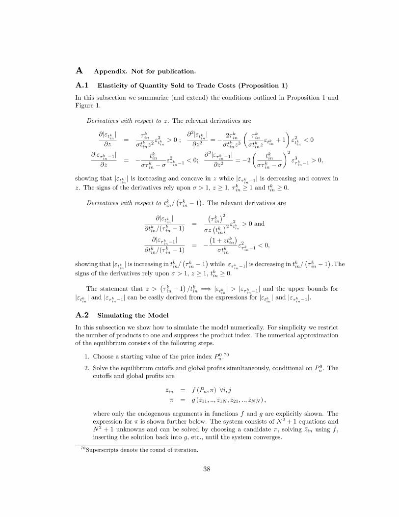
A Appendix. Not for publication.

A.1 Elasticity of Quantity Sold to Trade Costs (Proposition 1)

In this subsection we summarize (and extend) the conditions outlined in Proposition 1 andFigure 1.

Derivatives with respect to z. The relevant derivatives are

@j"tkin j@z

=�kin

�tkinz2"2tkin

> 0 ;@2j"tkin j@z2

= � 2�kin�tkinz

3

��kin�tkinz

"tkin + 1

�"2tkin

< 0

@j"�kin�1j@z

= � tkin��kin � �

"2�kin�1< 0;

@2j"�kin�1j@z2

= �2�

tkin��kin � �

�2"3�kin�1

> 0;

showing that j"tkin j is increasing and concave in z while j"�kin�1j is decreasing and convex inz. The signs of the derivatives rely upon � > 1, z � 1, �kin � 1 and tkin � 0.

Derivatives with respect to tkin=��kin � 1

�. The relevant derivatives are

@j"tkin j@tkin=(�

kin � 1)

=

��kin�2

�z�tkin�2 "2tkin > 0 and

@j"�kin�1j@tkin=(�

kin � 1)

= ��1 + ztkin

��tkin

"2�kin�1< 0;

showing that j"tkin j is increasing in tkin=��kin � 1

�while j"�kin�1j is decreasing in t

kin=��kin � 1

�:The

signs of the derivatives rely upon � > 1, z � 1, tkin � 0.

The statement that z >��kin � 1

�=tkin =) j"tkin j > j"�kin�1j and the upper bounds for

j"tkin j and j"�kin�1j can be easily derived from the expressions for j"tkin j and j"�kin�1j.

A.2 Simulating the Model

In this subsection we show how to simulate the model numerically. For simplicity we restrictthe number of products to one and suppress the product index. The numerical approximationof the equilibrium consists of the following steps.

1. Choose a starting value of the price index P 0n .70

2. Solve the equilibrium cuto¤s and global pro�ts simultaneously, conditional on P 0n . Thecuto¤s and global pro�ts are

�zin = f (Pn; �) 8i; j� = g (�z11; ::; �z1N ; �z21; ::; �zNN ) ;

where only the endogenous arguments in functions f and g are explicitly shown. Theexpression for � is shown further below. The system consists of N2 + 1 equations andN2 + 1 unknowns and can be solved by choosing a candidate �, solving �zin using f ,inserting the solution back into g, etc., until the system converges.

70Superscripts denote the round of iteration.

38

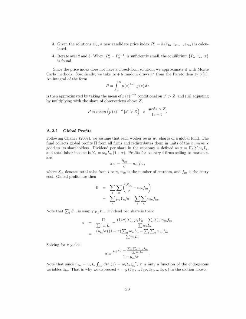
3. Given the solutions �z0in, a new candidate price index P1n = h (�z1n; �z2n; ::; �zNn) is calcu-

lated.

4. Iterate over 2 and 3. When��P rn � P r�1n

�� is su¢ ciently small, the equilibrium fPn; zin; �gis found.

Since the price index does not have a closed-form solution, we approximate it with MonteCarlo methods. Speci�cally, we take 1e + 5 random draws zr from the Pareto density g (z).An integral of the form

P =

Z 1

Z

p (z)1��

g (z) dz

is then approximated by taking the mean of p (z)1�� conditional on zr > Z, and (iii) adjustingby multiplying with the share of observations above Z,

P � mean�p (z)

1�� jzr > Z�� #obs > Z

1e+ 5:

A.2.1 Global Pro�ts

Following Chaney (2008), we assume that each worker owns wn shares of a global fund. Thefund collects global pro�ts � from all �rms and redistributes them in units of the numérairegood to its shareholders. Dividend per share in the economy is de�ned as � = �=

PwiLi,

and total labor income is Yn = wnLn (1 + �). Pro�ts for country i �rms selling to market nare

�in =Sin�� ninfin;

where Sin denotes total sales from i to n, nin is the number of entrants, and fin is the entrycost. Global pro�ts are then

� =Xi

Xn

�Sin�� ninfin

�=

Xn

�kYn=� �Xi

Xn

ninfin:

Note thatP

i Sin is simply �kYn: Dividend per share is then:

� =�Pi wiLi

=(1=�)

Pn �kYn �

Pi

Pn ninfinP

wiLi

=(�k=�) (1 + �)

Pn wnLn �

Pi

Pn ninfinP

wiLi:

Solving for � yields

� =�k=� �

Pi

Pn ninfinPwiLi

1� �k=�:

Note that since nin = wiLiR�zin

dF1 (z) = wiLi�z� in , � is only a function of the endogenous

variables �zin. That is why we expressed � = g (�z11; ::; �z1N ; �z21; ::; �zNN ) in the section above.

39

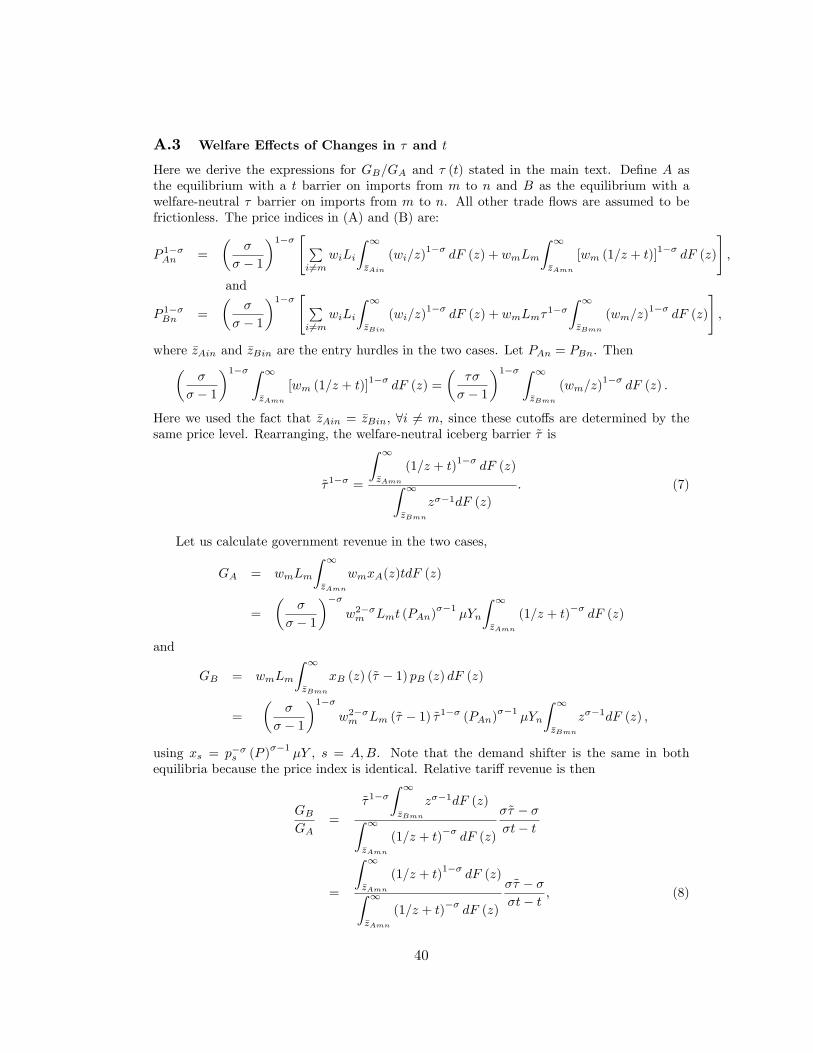
A.3 Welfare E¤ects of Changes in � and t

Here we derive the expressions for GB=GA and � (t) stated in the main text. De�ne A asthe equilibrium with a t barrier on imports from m to n and B as the equilibrium with awelfare-neutral � barrier on imports from m to n. All other trade �ows are assumed to befrictionless. The price indices in (A) and (B) are:

P 1��An =

��

� � 1

�1�� " Pi 6=m

wiLi

Z 1

�zAin

(wi=z)1��

dF (z) + wmLm

Z 1

�zAmn

[wm (1=z + t)]1��

dF (z)

#;

and

P 1��Bn =

��

� � 1

�1�� " Pi 6=m

wiLi

Z 1

�zBin

(wi=z)1��

dF (z) + wmLm�1��

Z 1

�zBmn

(wm=z)1��

dF (z)

#;

where �zAin and �zBin are the entry hurdles in the two cases. Let PAn = PBn. Then��

� � 1

�1�� Z 1

�zAmn

[wm (1=z + t)]1��

dF (z) =

���

� � 1

�1�� Z 1

�zBmn

(wm=z)1��

dF (z) :

Here we used the fact that �zAin = �zBin, 8i 6= m, since these cuto¤s are determined by thesame price level. Rearranging, the welfare-neutral iceberg barrier ~� is

~�1�� =

Z 1

�zAmn

(1=z + t)1��

dF (z)Z 1

�zBmn

z��1dF (z)

: (7)

Let us calculate government revenue in the two cases,

GA = wmLm

Z 1

�zAmn

wmxA(z)tdF (z)

=

��

� � 1

���w2��m Lmt (PAn)

��1�Yn

Z 1

�zAmn

(1=z + t)��

dF (z)

and

GB = wmLm

Z 1

�zBmn

xB (z) (~� � 1) pB (z) dF (z)

=

��

� � 1

�1��w2��m Lm (~� � 1) ~�1�� (PAn)��1 �Yn

Z 1

�zBmn

z��1dF (z) ;

using xs = p��s (P )��1

�Y , s = A;B. Note that the demand shifter is the same in bothequilibria because the price index is identical. Relative tari¤ revenue is then

GBGA

=

~�1��Z 1

�zBmn

z��1dF (z)Z 1

�zAmn

(1=z + t)��

dF (z)

�~� � ��t� t

=

Z 1

�zAmn

(1=z + t)1��

dF (z)Z 1

�zAmn

(1=z + t)��

dF (z)

�~� � ��t� t ; (8)

40

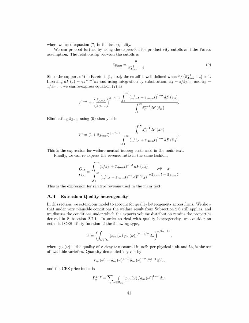
where we used equation (7) in the last equality.We can proceed further by using the expression for productivity cuto¤s and the Pareto

assumption. The relationship between the cuto¤s is

�zBmn =~�

�z�1Amn + t: (9)

Since the support of the Pareto is [1;+1], the cuto¤ is well de�ned when ~�=��z�1Amn + t

�> 1.

Inserting dF (z) = z� �1dz and using integration by substitution, ~zA = z=�zAmn and ~zB =z=�zBmn, we can re-express equation (7) as

~�1�� =

��zAmn�zBmn

��� �1 Z 1

1

(1=~zA + �zAmnt)1��

dF (~zA)Z 1

1

~z��1B dF (~zB)

:

Eliminating �zBmn using (9) then yields

~� = (1 + �zAmnt) ��+1

Z 1

1

~z��1B dF (~zB)Z 1

1

(1=~zA + �zAmnt)1��

dF (~zA)

:

This is the expression for welfare-neutral iceberg costs used in the main text.Finally, we can re-express the revenue ratio in the same fashion,

GBGA

=

Z 1

1

(1=~zA + �zAmnt)1��

dF (~zA)Z 1

1

(1=~zA + �zAmnt)��

dF (~zA)

�~� � ���zAmnt� �zAmnt

:

This is the expression for relative revenue used in the main text.

A.4 Extension: Quality heterogeneity

In this section, we extend our model to account for quality heterogeneity across �rms. We showthat under very plausible conditions the welfare result from Subsection 2.6 still applies, andwe discuss the conditions under which the exports volume distribution retains the propertiesderived in Subsection 2.7.1. In order to deal with quality heterogeneity, we consider anextended CES utility function of the following type,

U =

�Z!2n

[xin (!) qin (!)](��1)=�

d!

��=(��1);

where qin (!) is the quality of variety ! measured in utils per physical unit and n is the setof available varieties. Quantity demanded is given by

xin (!) = qin (!)��1

pin (!)��

P��1n �Yn;

and the CES price index is

P 1��n =Xi

R!2in

[pin (!) =qin (!)]1��

d!:

41

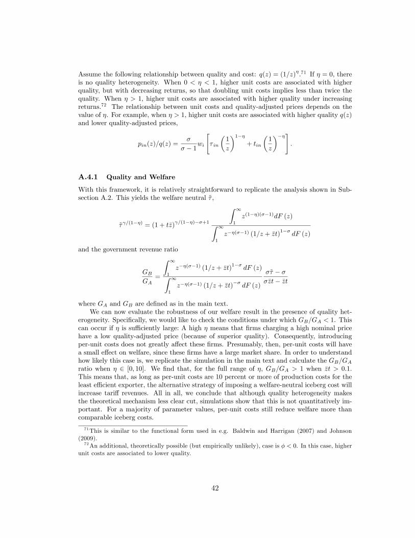
Assume the following relationship between quality and cost: q(z) = (1=z)�.71 If � = 0, thereis no quality heterogeneity. When 0 < � < 1, higher unit costs are associated with higherquality, but with decreasing returns, so that doubling unit costs implies less than twice thequality. When � > 1, higher unit costs are associated with higher quality under increasingreturns.72 The relationship between unit costs and quality-adjusted prices depends on thevalue of �. For example, when � > 1, higher unit costs are associated with higher quality q(z)and lower quality-adjusted prices,

pin(z)=q(z) =�

� � 1wi

"� in

�1

z

�1��+ tin

�1

z

���#:

A.4.1 Quality and Welfare

With this framework, it is relatively straightforward to replicate the analysis shown in Sub-section A.2. This yields the welfare neutral ~� ,

~� =(1��) = (1 + t�z) =(1��)��+1

Z 1

1

z(1��)(��1)dF (z)Z 1

1

z��(��1) (1=z + �zt)1��

dF (z)

and the government revenue ratio

GBGA

=

Z 1

1

z��(��1) (1=z + �zt)1��

dF (z)Z 1

1

z��(��1) (1=z + �zt)��

dF (z)

�~� � ���zt� �zt

where GA and GB are de�ned as in the main text.We can now evaluate the robustness of our welfare result in the presence of quality het-

erogeneity. Speci�cally, we would like to check the conditions under which GB=GA < 1. Thiscan occur if � is su¢ ciently large: A high � means that �rms charging a high nominal pricehave a low quality-adjusted price (because of superior quality). Consequently, introducingper-unit costs does not greatly a¤ect these �rms. Presumably, then, per-unit costs will havea small e¤ect on welfare, since these �rms have a large market share. In order to understandhow likely this case is, we replicate the simulation in the main text and calculate the GB=GAratio when � 2 [0; 10]. We �nd that, for the full range of �, GB=GA > 1 when �zt > 0:1.This means that, as long as per-unit costs are 10 percent or more of production costs for theleast e¢ cient exporter, the alternative strategy of imposing a welfare-neutral iceberg cost willincrease tari¤ revenues. All in all, we conclude that although quality heterogeneity makesthe theoretical mechanism less clear cut, simulations show that this is not quantitatively im-portant. For a majority of parameter values, per-unit costs still reduce welfare more thancomparable iceberg costs.

71This is similar to the functional form used in e.g. Baldwin and Harrigan (2007) and Johnson(2009).72An additional, theoretically possible (but empirically unlikely), case is � < 0. In this case, higher

unit costs are associated to lower quality.

42

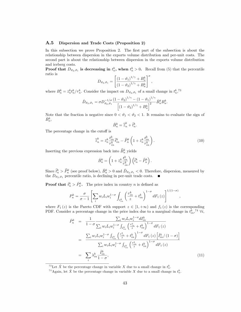
A.5 Dispersion and Trade Costs (Proposition 2)

In this subsection we prove Proposition 2. The �rst part of the subsection is about therelationship between dispersion in the exports volume distribution and per-unit costs. Thesecond part is about the relationship between dispersion in the exports volume distributionand iceberg costs.Proof that D#2;#1 is decreasing in tkn, when tkn > 0. Recall from (5) that the percentileratio is

D#2;#1 =

"(1� #1)1= +Bkn(1� #2)1= +Bkn

#�;

where Bkn = �zkntkn=�

kn. Consider the impact on D#2;#1 of a small change in t

kn,73

D#2;#1 = �D�1=�#2;#1

(1� #2)1= � (1� #1)1= h(1� #2)1= +Bkn

i2 BknBkn:

Note that the fraction is negative since 0 < #1 < #2 < 1. It remains to evaluate the sign ofBkn,

Bkn = b�zkn + btkn:The percentage change in the cuto¤ is

b�zkn = �zkn tkin�kinbtkin � bP kn �1 + �zkn tkin�kin�: (10)

Inserting the previous expression back into bBkn yieldsBkn =

�1 + �zkn

tkin�kin

��btkn � bP kn� :Since btkn > bP kn (see proof below), Bkn > 0 and D#2;#1 < 0. Therefore, dispersion, measured bythe D#2;#1 percentile ratio, is declining in per-unit trade costs.

Proof that tkn > P kn . The price index in country n is de�ned as

P kn =�

� � 1

"Xi

wiLiw1��i

Z�zkin

��kinz+ tkin

�1��dF1 (z)

#1=(1��);

where F1 (z) is the Pareto CDF with support z 2 [1;+1) and f1 (z) is the correspondingPDF. Consider a percentage change in the price index due to a marginal change in tkin,

74 8i,

P kn =1

1� �

Pi wiLiw

1��i dIkinP

i wiLiw1��i

R�zkin

��kinz + tkin

�1��dF1 (z)

=

Pi wiLiw

1��i

R�zkin

��kinz + tkin

�1��dF1 (z)

hIkin= (1� �)

iP

i wiLiw1��i

R�zkin

��kinz + tkin

�1��dF1 (z)

=Xi

�kinIkin1� � ; (11)

73Let X be the percentage change in variable X due to a small change in tkn.74Again, let X be the percentage change in variable X due to a small change in tkn.

43

where

Ikin �Z�zkin

��kinz+ tkin

�1��dF1 (z) ;

and �kin is the share of country n�s total expenditure that is devoted to goods from country i(the import share),

�kin =wiLiw

1��i

R�zkin

��kin=z + t

kin

�1��dF1 (z)P

j wjLjw1��j

R�zkjn

��kjn=z + t

kjn

�1��dF1 (z)

:

Applying Leibnitz�s Rule, the percentage change in Ikin is

Ikin = (1� �) tkin�kin � ��in�zkinbzkin;where

�kin =

R�zkin

tkin

��kinz + tkin

���dF1 (z)R

�zkin

��kinz + tkin

�1��dF1 (z)

and ��kin =

��kin�zkin+ tkin

�1��f1��zkin�

R�zkin

��kinz + tkin

�1��dF1 (z)

:

Note that �kin is always less than one.Consider a change in per-unit costs (dtkn) from a particular country (ex. Norway) to

country n. Denote with �kn, Ikn, �

kn, ��

kn, �z

kn the values of the corresponding variables when

associated with the source country under consideration. Disregard any possible second-ordere¤ects so that d�zkin = 0 whenever the source country is not Norway. Then

P kn = �knIkn1� � = �kn

��knbtkn + ��kn

� � 1 �zknb�zkn� :

The �rst term in the expression above captures the intensive margin e¤ect on the price index,while the second term captures the extensive margin e¤ect. Using (10) and solving for bP knyields

P kn =�kn�

kn + �

kn��kn��1 �z

kn

��zkn

tkn�kn

�1 + �kn

��kn��1 �z

kn

�1 + �zkn

tkn�kn

� tknSince �kn�

kn < 1, the fraction is less than one and therefore P

kn < tkn.

Proof that D#2;#1 is increasing in �kn, when tkn > 0. Consider the impact on D#2;#1

of a small change in �kn. The expression for D#2;#1 remains the same as above, but Bkn now

becomes

Bkn = b�zkn � �kn � 1�kn

b�kn;and the percentage change in cuto¤ becomes

b�zkn = �kn � 1�kn

b�kin � bP kn �1 + �zkn tkin�kin�:

Inserting this back into Bkn yields

Bkn = �P kn�1 + �zkn

tkin�kin

�:

44

Note that Bkn < 0 since Pkn > 0. Therefore D#2;#1 > 0 and dispersion rises with iceberg costs.

Proof that D�2;�1 is independent of �kn, when tkn = 0. Consider the impact on D#2;#1

of a small change in �kn when tkin = 0. The percentile ratio then collapses to

D#2;#1 =

"(1� #1)1=

(1� #2)1=

#�;

clearly showing that dispersion is independent of variable trade costs in the Chaney (2008)model.

A.5.1 Quality and the Export Distribution

In this subsection, we explore how the exports volume distribution responds to an increasein per-unit trade costs in the presence of quality heterogeneity. In particular, we analyzethe conditions under which the distribution becomes less dispersed as per-unit trade costsincrease. This is equivalent to determining the circumstances under which �rms charging lowprices also sell higher quantities. The optimal quantity sold is xin = P��1n �Ynq

��1p��in . Usingthe expression for quality, we get xin = P��1n �Ynz

��(��1)p��in , or equivalently,

xin = P��1n �Yn

��

� � 1wi� in���(��1)

p��+�(��1)in ;

using the fact that pin(z) = ���1wi

� inz () z = �

��1wi� inpin(z)�1 under tin = 0. As

a consequence, low price �rms sell more when � < �= (� � 1).75 Higher per-unit costs willnow reduce dispersion since the low price �rms (in the top of the distribution) will be hitharder by per-unit costs than the high price �rms (in the bottom of the distribution). Thefundamental identifying assumption in the econometric model is therefore consistent withquality heterogeneity, as long as the (positive) relationship between unit costs and qualityis not too convex.76 In our particular dataset, we know that for an overwhelming majorityof product-destination pairs, the correlation between quantity and price is negative. Thissuggests that � is less than �= (� � 1) (but not necessarily zero). As a comparison, Johnson(2009) �nds that � > 1 in most of the SITC 4-Digit sectors in his data. Since �= (� � 1) > 1,our results are fully compatible with his.

A.6 Extension: Departures from CES

In this subsection we consider two departures from standard CES preferences: marketingcosts à la Arkolakis (2008) and linear demand with horizontal product di¤erentiation à laOttaviano, Tabuchi, and Thisse (2002).

75This condition is necessary and su¢ cient when tin = 0 but only necessary when tin > 0.76Returning to a previous example, this would be the case if, for example, IKEA were selling fewer

beds than Crate and Barrel.

45

A.6.1 Marketing Costs

We consider an extension of our model that includes marketing costs à la Arkolakis (2008).The problem of the �rm is now the following:

maxhin(z);pin(z)

xin (z)hpin (z)� wi

�� inz+ tin

�i� w�nw1��i

L�n

1� [1� hin(z)]1��

1� � ;

s.t. hin(z) 2 [0; 1]:

where demand is

xin(z) =[pin(z)]

��

(Pn)1�� ynhin(z)Ln;

yn is per-capita spending in country n, Ln is population of country n, and hin(z) is the fractionof country n consumers reached by the �rm. The remaining parameters and the functionalform adopted to describe marketing costs are discussed extensively in Arkolakis (2008). Theoptimal price charged by an exporter to country n is the same as in our framework and equalto (1). The elasticity of the total volume of goods exported to country n to trade costs ("tinand "� in�1) is equal to the sum of (i) the elasticity of the per-consumer volume to tradecosts and (ii) the elasticity of the fraction of consumers reached to trade costs ("hin(z);tin and"hin(z);� in�1). The elasticity of the per-consumer volume to trade costs in this modi�ed modelis equal to the elasticity of total volume to trade costs in our baseline model. Overall,

"tin = ���� inztin

+ 1

��1+ "hin(z);tin ;

"� in�1 = ���tinz

� in+ 1

��1� in � 1� in

+ "hin(z);� in�1:

We can now draw two conclusions. The �rst conclusion is that in a standard Arkolakis (2008)model (that is when tin = 0) the dispersion of the export volume distribution is increasingin ad valorem trade costs. To see this note that: (i) the elasticity of per-consumer volumeto ad-valorem trade costs reduces to �� (� in � 1) =� in and therefore does not depend on theproductivity of the �rm; (ii) the elasticity of the fraction of consumers reached to ad-valoremtrade costs is negative and its absolute value is lower for more productive �rms.77 Therefore,a higher � reduces the volume sold per consumer for all �rms in the same proportion, but thefraction of consumers reached (the customer base) decreases less the higher is the productivityof the �rm. The overall volume sold by more productive �rms increases relative to that soldby less productive �rms.

The second conclusion regards the e¤ects of per-unit trade costs. It turns out that

@"hin(z);tin@z

> 0 iff hin(z) <� � 1�

� �h;

so that, within the set of �rms that reach a fraction of consumers lower than �h, the moste¢ cient ones (those with a higher initial customer base) adjust proportionally less the �newconsumer margin�than the less e¢ cient �rms. Therefore, in this extended model, while moree¢ cient �rms are still the ones that decrease the most the volume of goods sold to eachcustomer, they are also the ones that reduce less, in percentage terms, their customer base inthe event of a rise in per-unit trade costs. The overall e¤ect on the total volume of exportsdepends on how strong the �marketing e¤ect�is compared to the �per-unit trade costs�e¤ect.

77Proof available upon request.

46

A.6.2 Endogenous Markups

The CES assumption in the main text ensures that markups (over production plus trans-portation costs) are constant. A model with non-CES preferences will typically generateendogenous markups, which may have an e¤ect on the dispersion of exports. In this sectionwe explore this case, and discuss whether departures from CES alone (with no per-unit costs)can generate the observed correlation between dispersion in exports and trade costs. Specif-ically, we examine the model of Melitz and Ottaviano (2008), who incorporate endogenousmarkups using the linear demand system with horizontal product di¤erentiation developedby Ottaviano, Tabuchi, and Thisse (2002). The assumed linear demand system implies thathigher prices are associated with higher demand elasticities and therefore lower markups.Speci�cally, the price charged by an exporter with cost c from country h selling in market nis78

plh (c) =1

2

�chD + �

lhc�

where cD is the domestic cost cuto¤ (see Appendix A.3 in Melitz and Ottaviano, 2008).Absolute markups are plh (c) � �c = 1

2

�chD � � lhc

�, so that more e¢ cient �rms, facing lower

demand elasticities, are charging higher markups. An increase in trade costs � lh will in thiscase lead to more dispersion in prices. To see this, let c1 < c2, so that plh (c1) < plh (c2). ThenEl� lhp

lh = c�=�chD + �

lhc�, so that prices will increase more, in percentage terms, among the

low-e¢ ciency (high cost) �rms when � lh increases. As a consequence, plh (c2) =plh (c1) rises.The intuition behind this result is that, as � goes up, markups are reduced the most amonghigh e¢ ciency �rms, since they are already charging high markups and face lower demandelasticities.

Naturally, when price dispersion increases, export (volume) dispersion increases as well.Using the expression for optimal exports in Melitz and Ottaviano (2008) we �nd that relativeexports are

qlh (c1)

qlh (c2)=chD � � lhc1chD � � lhc2

If c1 < c2, then this ratio increases, i.e. the more e¢ cient �rm increases its market share astrade costs rise.

All in all, this shows that introducing a standard model of endogenous markups (with onlyiceberg costs) will not generate the observed correlation between dispersion in exports andtrade costs. However, the structural point estimate of trade costs would surely be a¤ected,introducing endogenous markups. Speci�cally, since dispersion is increasing with trade costsin Melitz-Ottaviano, an extension of their model with per-unit costs would require higherper-unit costs (compared to what we estimate) in order to match the dispersion in the data.Therefore, we can interpret our estimate as a lower bound of trade costs if endogenous markupsare believed to be important.

78 In this subsection we use, for simplicity, Melitz and Ottaviano (2008) notation.

47

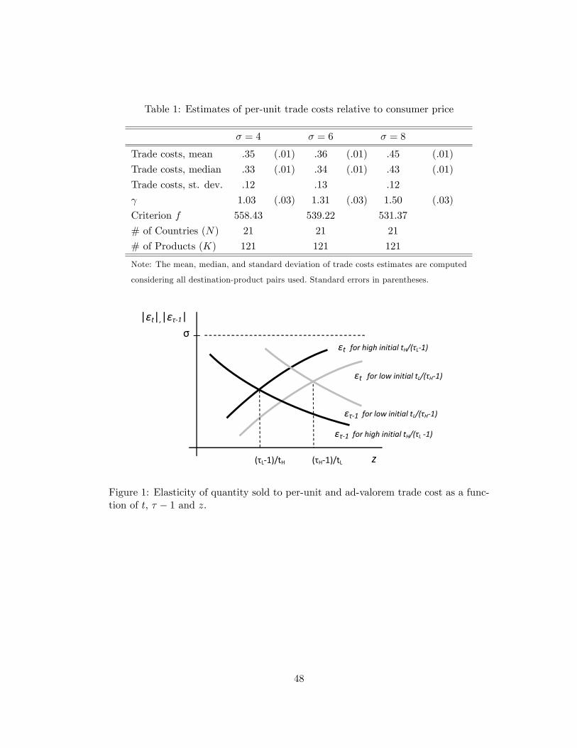
Table 1: Estimates of per-unit trade costs relative to consumer price

� = 4 � = 6 � = 8

Trade costs, mean :35 (:01) :36 (:01) :45 (:01)

Trade costs, median :33 (:01) :34 (:01) :43 (:01)

Trade costs, st. dev. :12 :13 :12

1:03 (:03) 1:31 (:03) 1:50 (:03)

Criterion f 558:43 539:22 531:37

# of Countries (N) 21 21 21

# of Products (K) 121 121 121

Note: The mean, median, and standard deviation of trade costs estimates are computed

considering all destination-product pairs used. Standard errors in parentheses.

z

|εt|,|ετ­1|σ

εt for high initial tH/(τL­1)

εt for low initial tL/(τH­1)

ετ­1 for low initial tL/(τH­1)

ετ­1 for high initial tH/(τL ­1)

(τL­1)/tH (τH­1)/tL

Figure 1: Elasticity of quantity sold to per-unit and ad-valorem trade cost as a func-tion of t, � � 1 and z.

48

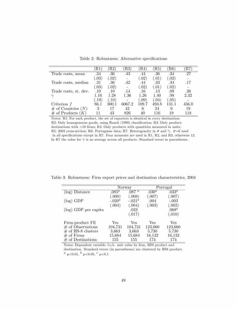
Table 2: Robustness: Alternative speci�cations

(R1) (R2) (R3) (R4) (R5) (R6) (R7)Trade costs, mean .34 .36 .43 .44 .36 .34 .27

(.03) (.02) - (.02) (.01) (.02) -Trade costs, median .31 .36 .42 .44 .33 .34 .17

(.03) (.02) - (.02) (.01) (.02) -Trade costs, st. dev. .10 .10 .14 .16 .13 .09 .26 1.16 1.28 1.36 1.26 1.40 .98 2.32

(.19) (.10) - (.09) (.04) (.05) -Criterion f 86.1 300.1 6067.2 109.7 493.8 131.1 456.0# of Countries (N) 3 17 42 6 24 9 19# of Products (K) 11 43 826 40 116 19 118Notes: R1: For each product, the set of exporters is identical in every destination;R2: Only homogeneous goods, using Rauch (1999) classi�cation; R3: Only product-destinations with >10 �rms; R4: Only products with quantities measured in units;R5: 2003 cross-section; R6: Portuguese data; R7: Heterogeneity in � and . �=6 usedin all speci�cations except in R7. Four moments are used in R1, R2, and R3, otherwise 12.In R7 the value for is an average across all products. Standard errors in parentheses.

Table 3: Robustness: Firm export prices and destination characteristics, 2004

Norway Portugal(log) Distance .085a .087 a .030a .033a

(.008) (.008) (.007) (.007)(log) GDP -.020a -.021a .004 -.003

(.004) (.004) (.003) (.002)(log) GDP per capita .023 .068a

(.017) (.010)

Firm-product FE Yes Yes Yes Yes# of Observations 104,731 104,731 123,660 123,660# of HS-8 clusters 3,663 3,663 5,730 5,730# of Firms 15,684 15,684 16,132 16,132# of Destinations 155 155 174 174Notes: Dependent variable: f.o.b. unit value by �rm, HS8 product anddestination. Standard errors (in parentheses) are clustered by HS8 product.a p<0.01, b p<0.05, c p<0.1

49

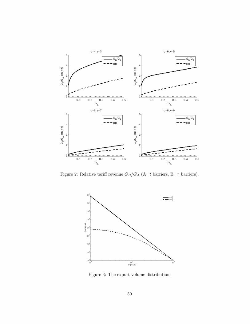
0.1 0.2 0.3 0.4 0.51

2

3

4

5

t*zA

GB/G

A a

ndτ(

t)

σ=4, γ=3

GB/GAτ(t)

0.1 0.2 0.3 0.4 0.51

2

3

4

5

t*zA

GB/G

A a

ndτ (

t)

σ=6, γ=5

GB/GAτ(t)

0.1 0.2 0.3 0.4 0.51

2

3

4

5

t*zA

GB/G

A a

ndτ(

t)

σ=6, γ=7

GB/GAτ(t)

0.1 0.2 0.3 0.4 0.51

2

3

4

5

t*zA

GB/G

A a

ndτ (

t)

σ=8, γ=9

GB/GAτ(t)

Figure 2: Relative tari¤ revenue GB=GA (A=t barriers, B=� barriers).

10­2 10­1 100100

101

102

103

104

105

106

107

108

P r[X >x0]

Qua

ntity

 x0

t=0t>0

Figure 3: The export volume distribution.

50

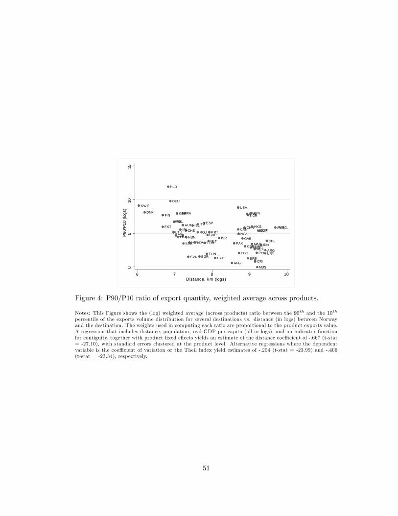
AFG

ARG

AUTAUS

BRB

BEL

BGR

BHS

CAN

COD

CHE

CHL

CHN

CRICYP

CZE

DEU

DNK

ESTESP

FIN FRA

GAB

GBR

GRC

HKG

HRVHUN

IDN

IRL

ISR

ISLITA

JPNKOR

LTULUX

MDA MACMLT

MUS

MEX

NGA

NLD

NZL

PHL

PAK

POL

PRTROU

SWE

SGP

SVN

SVK

TGOTUN

TURTWN

USA

URY

VEN

ZAF

05

1015

P90/

P10 

(logs

)

6 7 8 9 10Distance, km (logs)

Figure 4: P90/P10 ratio of export quantity, weighted average across products.

Notes: This Figure shows the (log) weighted average (across products) ratio between the 90th and the 10th

percentile of the exports volume distribution for several destinations vs. distance (in logs) between Norwayand the destination. The weights used in computing each ratio are proportional to the product exports value.A regression that includes distance, population, real GDP per capita (all in logs), and an indicator functionfor contiguity, together with product �xed e¤ects yields an estimate of the distance coe¢ cient of -.667 (t-stat= -27.10), with standard errors clustered at the product level. Alternative regressions where the dependentvariable is the coe¢ cient of variation or the Theil index yield estimates of -.204 (t-stat = -23.99) and -.406(t-stat = -23.34), respectively.

51

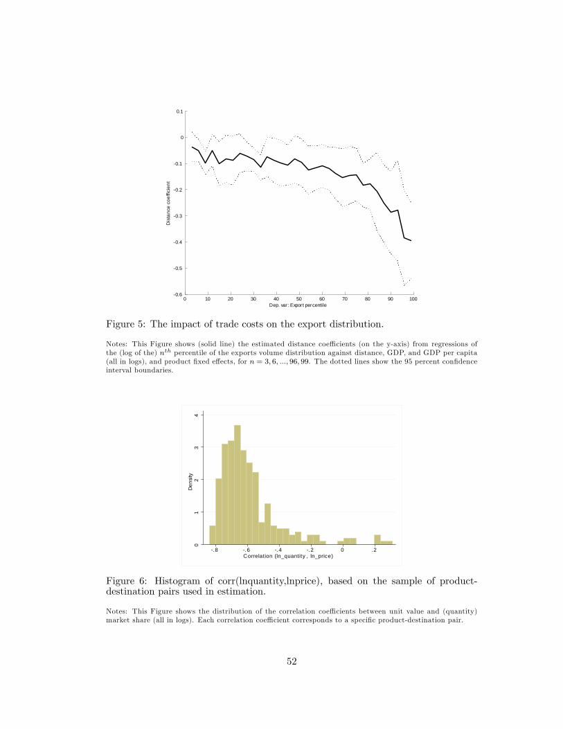
0 10 20 30 40 50 60 70 80 90 100­0.6

­0.5

­0.4

­0.3

­0.2

­0.1

0

0.1

Dep. var: Export percentile

Dis

tanc

e co

effic

ient

Figure 5: The impact of trade costs on the export distribution.

Notes: This Figure shows (solid line) the estimated distance coe¢ cients (on the y-axis) from regressions ofthe (log of the) nth percentile of the exports volume distribution against distance, GDP, and GDP per capita(all in logs), and product �xed e¤ects, for n = 3; 6; :::; 96; 99. The dotted lines show the 95 percent con�denceinterval boundaries.

01

23

4D

ensi

ty

­.8 ­.6 ­.4 ­.2 0 .2Correlation (ln_quantity ,  ln_price)

Figure 6: Histogram of corr(lnquantity,lnprice), based on the sample of product-destination pairs used in estimation.

Notes: This Figure shows the distribution of the correlation coe¢ cients between unit value and (quantity)market share (all in logs). Each correlation coe¢ cient corresponds to a speci�c product-destination pair.

52

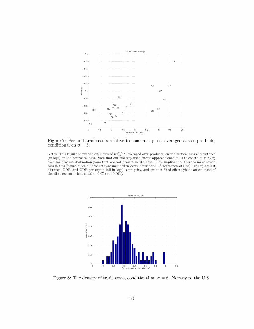
6 6.5 7 7.5 8 8.5 9 9.5 10

0.32

0.34

0.36

0.38

0.4

0.42

0.44

0.46

0.48

0.5

AU

BE

CA

CH

CL

DE

DK

ES

FI

FRGB

IE

IS

IT

JP

KRNL

PL

SE

SG

US

Distance, km (logs)

wt/a

vg(p

)

T rade costs, average

Figure 7: Per-unit trade costs relative to consumer price, averaged across products,conditional on � = 6.

Notes: This Figure shows the estimates of wtkn=�pkn, averaged over products, on the vertical axis and distance

(in logs) on the horizontal axis. Note that our two-way �xed e¤ects approach enables us to construct wtkn=�pkn

even for product-destination pairs that are not present in the data. This implies that there is no selectionbias in this Figure, since all products are included in every destination. A regression of (log) wtkn=�p

kn against

distance, GDP, and GDP per capita (all in logs), contiguity, and product �xed e¤ects yields an estimate ofthe distance coe¢ cient equal to 0.07 (s.e. 0.001).

0 0.1 0.2 0.3 0.4 0.5 0.6 0.7 0.80

0.02

0.04

0.06

0.08

0.1

0.12

0.14T rade c os ts , US

P er uni t trade c os ts , wt/avg(p)

Shar

e of

 pro

duct

s

Figure 8: The density of trade costs, conditional on � = 6. Norway to the U.S.

53

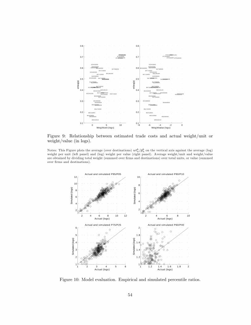
0 5 100.1

0.2

0.3

0.4

0.5

0.6

0.7

0.8

4407100444152000

61091000

6110300061109000

62033300

62034209

62043300

62043900

62045300

62046309

64039900

84138100

84295102

84713000

84714900

84715000

84716005

84716008

8471800084719009

84798909

85044010

85044099

85175000

85243200

85243901

85243906

85252009

8531100085438909

8701900987042209

8704230987163909

90189000

90318090

94016119

9403300994034009

94036099

95039000

95069909

Weig ht/unit (log s)

wt/a

vg(p

)

­8 ­6 ­4 ­2 00.1

0.2

0.3

0.4

0.5

0.6

0.7

0.8

4407100444152000

61091000

6110300061109000

62033300

62034209

62043300

62043900

62045300

62046309

64039900

84138100

84295102

84713000

84714900

84715000

84716005

84716008

8471800084719009

84798909

85044010

85044099

85175000

85243200

85243901

85243906

85252009

8531100085438909

8701900987042209

8704230987163909

90189000

90318090

94016119

9403300994034009

94036099

95039000

95069909

Weig ht/value ( log s)

wt/a

vg(p

)Figure 9: Relationship between estimated trade costs and actual weight/unit orweight/value (in logs).

Notes: This Figure plots the average (over destinations) wtkn=�pkn on the vertical axis against the average (log)

weight per unit (left panel) and (log) weight per value (right panel). Average weight/unit and weight/valueare obtained by dividing total weight (summed over �rms and destinations) over total units, or value (summedover �rms and destinations).

2 4 6 8 10 12

2

4

6

8

10

12Actual and s im ulated P95/P05

Sim

ulat

ed (l

ogs)

Ac tual (logs)2 4 6 8 10

2

4

6

8

10Actual and s im ulated P90/P10

Sim

ulat

ed (l

ogs)

Ac tual (logs)

1 2 3 4 5 61

2

3

4

5

6Actual and s im ulated P75/P25

Sim

ulat

ed (l

ogs)

Ac tual (logs)1 1.2 1.4 1.6 1.8 2

1

1.2

1.4

1.6

1.8

2Actual and s im ulated P60/P40

Sim

ulat

ed (l

ogs)

Ac tual (logs)

Figure 10: Model evaluation. Empirical and simulated percentile ratios.

54