The Particle Spectrum of Heterotic Compactifications

arX

iv:h

ep-t

h/04

0501

4v1

3 M

ay 2

004

UPR-1080-T

The Particle Spectrum of Heterotic Compactifications

Ron Donagi1, Yang-Hui He2, Burt A. Ovrut2, and Rene Reinbacher3

1 Department of Mathematics, University of Pennsylvania

Philadelphia, PA 19104–6395, USA

2 Department of Physics, University of Pennsylvania

Philadelphia, PA 19104–6396, USA

3 Department of Physics and Astronomy, Rutgers University

Piscataway, NJ 08855-0849, USA

Abstract

Techniques are presented for computing the cohomology of stable, holomorphic

vector bundles over elliptically fibered Calabi-Yau threefolds. These cohomology groups

explicitly determine the spectrum of the low energy, four-dimensional theory. Generic

points in vector bundle moduli space manifest an identical spectrum. However, it is

shown that on subsets of moduli space of co-dimension one or higher, the spectrum can

abruptly jump to many different values. Both analytic and numerical data illustrating

this phenomenon are presented. This result opens the possibility of tunneling or phase

transitions between different particle spectra in the same heterotic compactification.

In the course of this discussion, a classification of SU(5) GUT theories within a specific

context is presented.

∗[email protected]; yanghe, [email protected]; [email protected]

1 Introduction

The work of Horava and Witten [1] opened the door to constructing phenomenologically

realistic N = 1 supersymmetric vacua of strongly coupled heterotic string theory. A key in-

gredient in such constructions is the method presented in [2, 3, 4] and [5, 6] for finding stable,

holomorphic vector bundles on elliptically fibered Calabi-Yau threefolds. Using this tech-

nique, a large number of GUT theories with gauge groups SU(5) and SO(10) were produced

in [5, 6, 7]. These ideas were generalized in [8, 9, 10], where it was shown how to construct

stable, holomorphic vector bundles on torus-fibered Calabi-Yau threefolds. Using these gen-

eralized techniques, standard-like models were produced using Wilson lines to spontaneously

break both SU(5) [8] and SO(10) [9] GUT groups. Within this context, a number of new

phenomena were discussed such as small instanton phase transitions [11], non-perturbative

superpotentials [12, 13], five-brane moduli space [14], brane worlds [15] and a new theory of

the Big Bang [16].

One aspect of such theories that was left unsolved was how to compute the complete

particle spectrum of the low-energy, four-dimensional theory. The existence of precisely

three families of quarks and leptons was guaranteed in these theories by choosing the third

Chern class of the holomorphic vector bundle appropriately. However, the number of other

particles, such as the Higgs or exotic particles, was not specified. To compute their spectrum,

it is necessary to construct the complete cohomology of the vector bundle V on the Calabi-

Yau threefold X. This was carried out [17] in the case of the “standard embedding,” that

is, when V = TX, where TX is the tangent bundle. In this case, the spectrum is directly

related to Betti numbers of TX, which are known. However, this is manifestly not the

case for the bundles discussed above. For these more general vector bundles, the relevant

cohomology groups are unrelated to the Dolbeault cohomology and, hence, are much more

difficult to compute.

We discussed a general approach to this problem in [18]. It is the purpose of this paper

to give explicit techniques for calculating the cohomology of stable, holomorphic vector

bundles on elliptically fibered Calabi-Yau threefolds. That is, we will show how to compute

the complete spectrum for the low energy GUT theories that arise in this context. In the

process of doing this, we have found what we believe to be an interesting phenomenon in

particle physics. This is the following. Holomorphic vector bundles have complex moduli.

In the present context, these have been discussed and enumerated in [12, 14, 19]. For

generic values of these moduli, we find a specific particle spectrum. However, on loci of

1

co-dimension one or higher in the vector bundle moduli space we find that the spectrum

“jumps,” changing abruptly by integer values. In this paper, we will conclusively demonstrate

that this phenomenon exists. We will discuss the mathematical underpinnings of this result

and give a concrete example using both analytic and numerical techniques.

Specifically, in this paper we will do the following. In section 2, we briefly review some

salient facts about elliptically fibered Calabi-Yau threefolds. These spaces are fibered over

base surfaces B, whose properties are discussed in Section 3. Section 4 is devoted to a short

discussion of the method of constructing stable, holomorphic vector bundles from spectral

data via the Fourier-Mukai transformation. In Section 5, we present the three physical

constraints required of any phenomenologically relevant heterotic string vacuum. Using the

mathematical constraints arising from these conditions, we present a classification of SU(5)

GUT theories that can arise in our context. This is given in Section 6. In Section 7, we

present the general techniques for computing the low energy spectrum from the cohomology

of the holomorphic vector bundle. First, we discuss the relationship between the spectrum

and cohomology, as well as the constraints on the spectrum arising from the index theorem.

We then present methods for computing the cohomology based on Leray spectral sequences

and the Riemann-Roch theorem. For convenience, this is carried out within the context of

vector bundles with an SU(5) structure group. Section 8 is devoted to using these techniques

to compute the complete cohomology of a specific SU(5) GUT model satisfying the three

physical constraints. The spectrum of this theory is then presented. We note and discuss

the phenomenon that part of the cohomology and, hence, some of the spectrum is dependent

upon the vector bundle moduli for which they are evaluated. Finally, in Section 9 we indicate

why one expects the spectrum to be moduli dependent for general holomorphic bundles, as

opposed to the standard embedding where this phenomenon does not occur. Appendices A

and B present various aspects of topological data required in the text. Appendix C gives

a general method for computing a large set of cohomology groups that are required in our

discussion. Several matrices that are central to the calculation of the spectrum are defined

and explicitly constructed in Appendix D, including their exact dependence on the vector

bundle moduli. The spectra of these representations depend on the rank of one of these

matrices. The rank is computed both analytically and numerically in Appendix E. Explicit

data is presented, showing that the rank of this matrix is dependent upon where in moduli

space it is evaluated.

Although much of this paper is presented within the context of SU(5) GUT theories, the

techniques introduced are completely general. They can be used to compute the spectrum

2

of any heterotic vacuum.

2 Elliptically Fibered Calabi-Yau Threefolds

We will consider elliptically fibered threefolds X. Each such manifold has a base surface

B and a mapping π : X → B such that π−1(b) is a smooth torus, Eb, for each generic

point b ∈ B. Additionally, there are special points in the base over each of which the fiber is

singular. These fibers are typically of type I1, in the Kodaira classification, but may be more

singular. What makes this torus fibration elliptic is the existence of a zero section; that is,

there exists an analytic map σ : B → X that assigns to every element b of B an element

σ(b) ∈ Eb. The point σ(b) acts as the zero element for an Abelian group which turns Eb into

an elliptic curve and X into an elliptic fibration. We will denote the fiber class by F .

In terms of explicit coordinates, one can express X as a Weierstrass model

y2z = x3 + g2xz2 + g3z3 (1)

which describes X as a divisor in a P2-bundle P over B. The coefficients g2 and g3 are

sections of line bundles on the base. The bundle P is the projectivization P(L2⊕L3⊕OB),

where L is a line bundle on B which is the conormal bundle to the section σ. Subsequently,

we have

x ∼ OP (1)⊗ L2, y ∼ OP (1)⊗ L3, z ∼ OP (1) (2)

and

g2 ∼ L4, g3 ∼ L

6 , (3)

where we have used ∼ to denote “global section of.’

An important property of elliptic fibrations is that X has a Z2 symmetry τ = (−1)X ,

which, on the Weierstrass coordinates defined in (1) acts as

τ : y → −y (4)

while leaving x and z invariant. Clearly this action leaves the Weierstrass equation (1)

unchanged. In other words τ is a natural involution on X. It acts trivially on the base B

and maps each element b ∈ Eb to its inverse −b.

N = 1 supersymmetry in four-dimensions demands that X be a Kahler manifold with

vanishing first Chern class of its tangent bundle TX; that is,

c1(TX) = 0 . (5)

3

Such manifolds always admit a Kahler metric of SU(3) holonomy and are called Calabi-Yau

manifolds. Henceforth, we will choose X to be a Calabi-Yau threefold. In general, the Chern

classes of X can be conveniently expressed in terms of those of the base B [3, 20]. In addition

to (5), one finds that

c2(TX) = 12σ · π∗(c1(TB)) + π∗(c2(TB) + 11c21(TB)),

c3(TX) = −60(c1(TB)2 · B)pt , (6)

where c1(TB) and c2(TB) are the first and second Chern classes of B respectively and pt

is the class of a point. When X is a Calabi-Yau threefold, severe restrictions are placed

on the base surface B. It turns out that B can only be Enriques, del Pezzo, Hirzebruch

and blowups of Hirzebruch surfaces [21]. We will present some relevant properties of these

surfaces shortly.

Throughout this paper we will make frequent use of the intersection relation

σ · σ = −π∗(c1(TB)) · σ , (7)

which follows from the adjunction formula.

3 Properties of the Base Surface

We now present the requisite properties, such as Chern classes and homology groups, of the

surfaces B. Before doing so, however, it is helpful to define some fundamental notions.

Consider a complex surface B and its second homology group H2(B, Z). Let C ⊂ B be a

holomorphic curve in B and [C] ∈ H2(B, Z) the class of curves equivalent to C. Then [C] is

called an “effective” class. Clearly, not every class, such as −[C], is effective. If [C] and [D]

are two effective classes, then so is m[C] + n[D] where m, n ∈ Z≥0. Therefore, the subset of

effective classes forms a cone in H2(B, Z), called the Mori cone. The Mori cone is spanned

by a countable number of generators, [Ci], where Ci ⊂ B are irreducible curves. That is,

any effective class [C] can be expressed as

[C] =∑

i

ri[Ci], ri ∈ Z≥0 . (8)

The reader is referred to [22, 23, 24], for example, for details. The Mori cone is not necessarily

finitely generated over Z≥0, although for all surfaces discussed below, with the exception of

dP9, the associated Mori cones are indeed finitely generated. We will shortly present their

4

bases explicitly. For dP9, the Mori cone has an infinite number of generators. Nevertheless,

there is a convenient description of them.

Let C ⊂ B be a holomorphic curve in a complex surface B. Since C is a divisor of B,

there exists a line bundle OB(C) which has a section sC , unique up to scalar multiplication,

whose zero locus is C. Now, consider another curve C ′ 6= C with the property that OB(C ′) ≃

OB(C). Then, there exists a section sC′ of OB(C) whose zero locus is C ′. Note that sC/sC′

is a meromorphic function f on B. Two such divisors C and C ′ are said to be linearly

equivalent. The set of all divisors linearly equivalent to C, denoted by |C|, is called the

linear system associated with C. A crucial property of linear systems is the following. A

base point of a linear system |C| of curves on B is the intersection of all its members. If

there is no such common point, then |C| is called base point free. Furthermore, note that

all numerical properties of a divisor C, such as its self-intersection number, are completely

determined by its linear system.

We have restricted the discussion in this section to divisor classes [C], divisors C, and

to bundles OB(C) associated with B. However, all of our remarks apply to classes, divisors

and line bundles of any complex manifold, such as the threefold X.

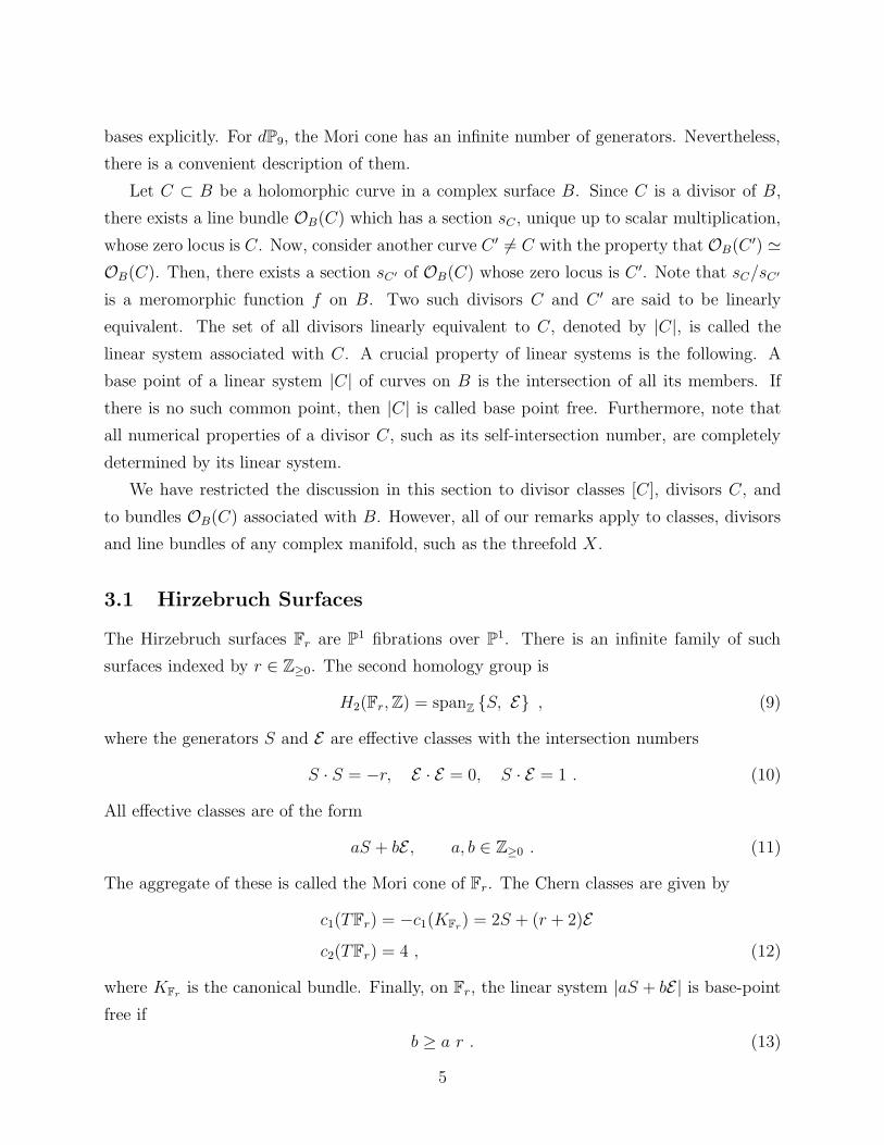
3.1 Hirzebruch Surfaces

The Hirzebruch surfaces Fr are P1 fibrations over P

1. There is an infinite family of such

surfaces indexed by r ∈ Z≥0. The second homology group is

H2(Fr, Z) = spanZS, E , (9)

where the generators S and E are effective classes with the intersection numbers

S · S = −r, E · E = 0, S · E = 1 . (10)

All effective classes are of the form

aS + bE , a, b ∈ Z≥0 . (11)

The aggregate of these is called the Mori cone of Fr. The Chern classes are given by

c1(TFr) = −c1(KFr) = 2S + (r + 2)E

c2(TFr) = 4 , (12)

where KFris the canonical bundle. Finally, on Fr, the linear system |aS + bE| is base-point

free if

b ≥ a r . (13)

5

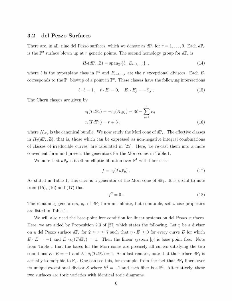
3.2 del Pezzo Surfaces

There are, in all, nine del Pezzo surfaces, which we denote as dPr for r = 1, . . . , 9. Each dPr

is the P2 surface blown up at r generic points. The second homology group for dPr is

H2(dPr, Z) = spanZℓ, Ei=1,...,r , (14)

where ℓ is the hyperplane class in P2 and Ei=1,...,r are the r exceptional divisors. Each Ei

corresponds to the P1 blowup of a point in P2. These classes have the following intersections

ℓ · ℓ = 1, ℓ · Ei = 0, Ei · Ej = −δij . (15)

The Chern classes are given by

c1(TdPr) = −c1(KdPr) = 3ℓ−

r∑

i=1

Ei

c2(TdPr) = r + 3 , (16)

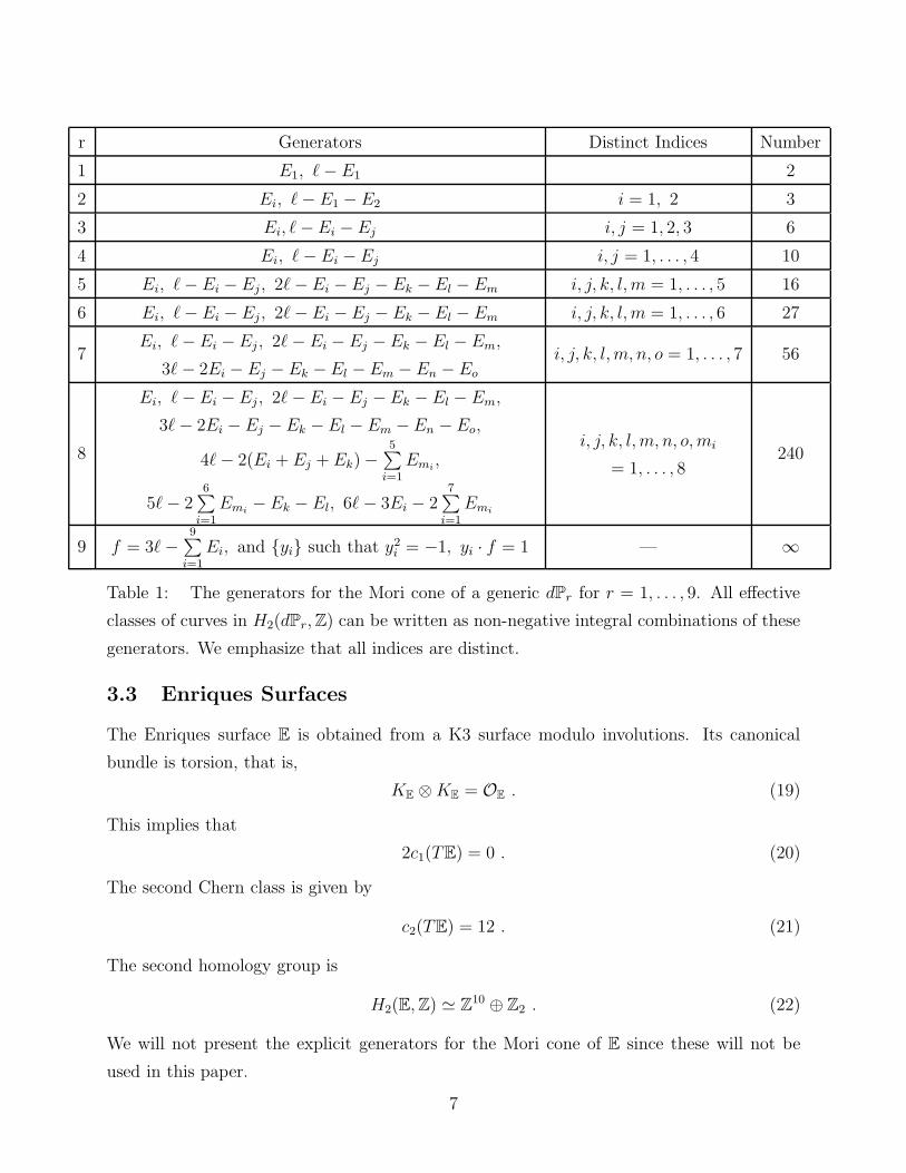
where KdPris the canonical bundle. We now study the Mori cone of dPr. The effective classes

in H2(dPr, Z), that is, those which can be expressed as non-negative integral combinations

of classes of irreducible curves, are tabulated in [25]. Here, we re-cast them into a more

convenient form and present the generators for the Mori cones in Table 1.

We note that dP9 is itself an elliptic fibration over P1 with fiber class

f = c1(TdP9) . (17)

As stated in Table 1, this class is a generator of the Mori cone of dP9. It is useful to note

from (15), (16) and (17) that

f 2 = 0 . (18)

The remaining generators, yi, of dP9 form an infinite, but countable, set whose properties

are listed in Table 1.

We will also need the base-point free condition for linear systems on del Pezzo surfaces.

Here, we are aided by Proposition 2.3 of [27] which states the following. Let η be a divisor

on a del Pezzo surface dPr for 2 ≤ r ≤ 7 such that η · E ≥ 0 for every curve E for which

E · E = −1 and E · c1(TdPr) = 1. Then the linear system |η| is base point free. Note

from Table 1 that the bases for the Mori cones are precisely all curves satisfying the two

conditions E · E = −1 and E · c1(TdPr) = 1. As a last remark, note that the surface dP1 is

actually isomorphic to F1. One can see this, for example, from the fact that dP1 fibers over

its unique exceptional divisor S where S2 = −1 and each fiber is a P1. Alternatively, these

two surfaces are toric varieties with identical toric diagrams.

6

r Generators Distinct Indices Number

1 E1, ℓ− E1 2

2 Ei, ℓ− E1 − E2 i = 1, 2 3

3 Ei, ℓ−Ei − Ej i, j = 1, 2, 3 6

4 Ei, ℓ− Ei − Ej i, j = 1, . . . , 4 10

5 Ei, ℓ− Ei − Ej , 2ℓ−Ei −Ej − Ek − El − Em i, j, k, l, m = 1, . . . , 5 16

6 Ei, ℓ− Ei − Ej , 2ℓ−Ei −Ej − Ek − El − Em i, j, k, l, m = 1, . . . , 6 27

7Ei, ℓ−Ei −Ej , 2ℓ− Ei − Ej −Ek − El − Em,

3ℓ− 2Ei − Ej − Ek −El −Em − En − Eo

i, j, k, l, m, n, o = 1, . . . , 7 56

8

Ei, ℓ−Ei −Ej , 2ℓ− Ei − Ej −Ek − El − Em,

3ℓ− 2Ei − Ej − Ek − El − Em −En −Eo,

4ℓ− 2(Ei + Ej + Ek)−5∑

i=1

Emi,

5ℓ− 26∑

i=1

Emi−Ek − El, 6ℓ− 3Ei − 2

7∑

i=1

Emi

i, j, k, l, m, n, o, mi

= 1, . . . , 8240

9 f = 3ℓ−9∑

i=1

Ei, and yi such that y2i = −1, yi · f = 1 — ∞

Table 1: The generators for the Mori cone of a generic dPr for r = 1, . . . , 9. All effective

classes of curves in H2(dPr, Z) can be written as non-negative integral combinations of these

generators. We emphasize that all indices are distinct.

3.3 Enriques Surfaces

The Enriques surface E is obtained from a K3 surface modulo involutions. Its canonical

bundle is torsion, that is,

KE ⊗KE = OE . (19)

This implies that

2c1(TE) = 0 . (20)

The second Chern class is given by

c2(TE) = 12 . (21)

The second homology group is

H2(E, Z) ≃ Z10 ⊕ Z2 . (22)

We will not present the explicit generators for the Mori cone of E since these will not be

used in this paper.

7

4 Vector Bundles on Elliptically Fibered Calabi-Yau

Threefolds

We consider rank n stable holomorphic vector bundles V on X. These bundles have a

convenient description, known as the spectral cover construction [2, 3, 4, 5, 6]. The spectral

data is given by two objects, an effective divisor CV of X, called the spectral cover, and a

spectral line bundle NV on CV . The spectral cover, CV , is a surface in X that is an n-fold

cover, p : CV → B, of the base B. Its general form is

CV ∈ |nσ + π∗η| , (23)

where σ is the zero section associated with π, and η is some effective curve in B. The spectral

line bundle NV is defined by its first Chern class

c1(NV ) = n(1

2+ λ)σ + (

1

2− λ)π∗η + (

1

2+ nλ)π∗c1(TB) , (24)

where λ is a rational number such that

λ = m, n even

λ = m + 12, n odd

(25)

for some m ∈ Z. When n is even, we must also impose that

η = c1(TB) mod 2 . (26)

Note that, as defined in (24), NV is actually a line bundle on X. It can, of course, be

restricted to be a line bundle over CV . Throughout this paper, we will, in general, not

distinguish between NV and NV |CV, denoting both by NV .

4.1 Fourier-Mukai Transformation

Given the spectral data (CV ,NV ), one can construct the vector bundle V explicitly, using

the Fourier-Mukai transformation

(CV ,NV )FM←→ V . (27)

We briefly remind the reader of the structure of this transformation [2, 3, 4, 5, 6]. Let us

form the fiber product X ×B X ′, where X ′ ≃ X is another copy of X. We let π : X → B

8

and π′ : X ′ → B be the projections onto the base B with sections σ and σ′ respectively. The

fiber product is a four-dimensional space defined as

X ×B X ′ = (x, x′) ∈ X ×X ′ | π(x) = π′(x′) . (28)

Therefore, over any generic point b ∈ B we have a fiber Eb×E ′b, where Eb and E ′

b are elliptic

curves. We define the Poincare sheaf P to be

P = OX×BX′(∆− σ ×B X ′ −X ×B σ′)⊗KB , (29)

where ∆ is the (diagonal) divisor given by the set of points (x, x) in X×B X ′. Recall [8] that

P is a bundle except at points (x, x′) ∈ X ×B X ′ where both x and x′ are singular points of

their respective fibers.

Now, let us take the spectral cover CV ⊂ X and form the fiber product CV ×B X ′. Then,

we have the following diagram, with projection maps π1 and π2 appropriately defined.

NV

↓

CVπ2←− CV ×B X ′ π1−→ X ′

(30)

The Fourier-Mukai transformation is the explicit map that re-constructs the vector bundle

V from the spectral data in accordance with (30)

V = π1∗ ((π∗2NV )⊗ P) . (31)

We emphasize that we are using, as it is standard in the literature, the canonical isomorphism

of X ≃ X ′ so that saying V is a vector bundle on X ′ is equivalent to saying that V is a

vector bundle on X. In the same way, we could have defined the spectral data (C′V ,N ′V ) in

X ′ and produced a vector bundle V on X.

Altogether, we have the following commutative diagram

π∗2NV ⊗ P

π1∗−→ V

↓ ↓

CV ×B X ′ π1−→ X ′

π2 ↓ ↓ π′

CVπC−→ B .

(32)

The Chern classes of V are found to be [2, 3, 4]

c1(V ) = 0,

c2(V ) = σ · π∗(η)−1

24c1(TB)2(n3 − n)F +

1

2(λ2 −

1

4)n η · (η − n c1(TB))F,

c3(V ) = 2λη · (η − n c1(TB))pt . (33)

9

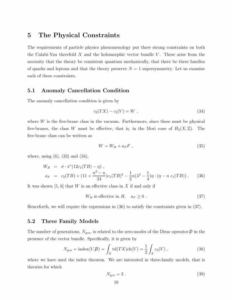
5 The Physical Constraints

The requirements of particle physics phenomenology put three strong constraints on both

the Calabi-Yau threefold X and the holomorphic vector bundle V . These arise from the

necessity that the theory be consistent quantum mechanically, that there be three families

of quarks and leptons and that the theory preserve N = 1 supersymmetry. Let us examine

each of these constraints.

5.1 Anomaly Cancellation Condition

The anomaly cancellation condition is given by

c2(TX)− c2(V ) = W , (34)

where W is the five-brane class in the vacuum. Furthermore, since these must be physical

five-branes, the class W must be effective, that is, in the Mori cone of H2(X, Z). The

five-brane class can be written as

W = WB + aFF , (35)

where, using (6), (33) and (34),

WB = σ · π∗(12c1(TB)− η) ,

aF = c2(TB) + (11 +n3 − n

24)c1(TB)2 −

1

2n(λ2 −

1

4)η · (η − n c1(TB)) . (36)

It was shown [5, 6] that W is an effective class in X if and only if

WB is effective in B, aF ≥ 0 . (37)

Henceforth, we will require the expressions in (36) to satisfy the constraints given in (37).

5.2 Three Family Models

The number of generations, Ngen, is related to the zero-modes of the Dirac operator /D in the

presence of the vector bundle. Specifically, it is given by

Ngen = index(V, /D) =

∫

X

td(TX)ch(V ) =1

2

∫

X

c3(V ) , (38)

where we have used the index theorem. We are interested in three-family models, that is

theories for which

Ngen = 3 . (39)

10

It then follows from (33), (38) and (39) that

3 = λη · (η − n c1(TB)) . (40)

We will, henceforth, require that this constraint be satisfied. Note that (40) simplifies

the expression for aF in (36). It follows that the condition on aF in (37) becomes

aF = c2(TB) + (11 +n3 − n

24)c1(TB)2 −

3

2λn(λ2 −

1

4) ≥ 0 . (41)

5.3 Irreducibility of the Spectral Cover

In order for the gauge connection to preserve N = 1 supersymmetry, it must satisfy the

hermitian Yang-Mills equation. The theorems of Uhlenbeck and Yau [28] and Donaldson

[29] state that a rank n holomorphic vector bundle V will admit such a connection if V is

stable. We will, therefore, impose stability as a constraint on V . It was shown in [2, 3, 4]

that if V is constructed via a Fourier-Mukai transformation from spectral data, then V will

be stable if the spectral cover is irreducible1. What are the conditions on the linear system

|CV | such that it contains an irreducible divisor? This will be the case when the following

two conditions are met [11].

(1) |π∗η| contains an irreducible divisor in X ,

(2) c1(π∗K⊗n

B ⊗OX(π∗η)) is effective in H4(X, Z) . (42)

We will satisfy these two conditions if we impose

(1) The linear system |η| is base-point free in B ,

(2) η + nc1(KB) is effective in B . (43)

In order to preserve N = 1 supersymmetry, the conditions in (43) must be imposed in

addition to (37) and (40).

5.4 Summary of the Constraints

For clarity, we summarize here the physical constraints, namely (37), (40), and (43), which

we impose on our vector bundle. These become the following conditions on the effective base

1More precisely, the notion of stability requires the choice of an ample class H ∈ H2(X, Z) and, in the

situation that the cover is irreducible, we can find an ample class H such that V is stable.

11

curve η as well as on the parameter λ.

(1) WB effective : 12c1(TB)− η is effective,

(2) aF > 0 : c2(TB) + (11 + n3−n24

)c1(TB)2 − 32λ

n(λ2 − 14) ≥ 0,

(3) Three families : λ η · (η − n c1(TB)) = 3, λ ∈

Z, n even

Z/2, n odd,

(4) Stability of V : |η| is base-point free,

(5) Stability of V : η − nc1(TB) is effective .

(44)

In this paper, for specificity, we will restrict our attention to the case

n = 5 . (45)

This corresponds to constructing an SU(5) GUT model at low energy. Because n = 5 is

odd, λ has to be half integral by (25). Thus, the third condition in (44) implies, since

η · (η − n c1(TB)) is integral, that the only possibilities for λ are

λ = ±1

2, ±

3

2. (46)

Therefore, (44) simplifies to the constraints

(1) 12c1(TB)− η is effective,

(2) c2(TB) + 16c1(TB)2 − 152λ

(λ2 − 14) ≥ 0,

(3) λ η · (η − 5 c1(TB)) = 3, λ = ±12

or ± 32

,

(4) |η| is base-point free,

(5) η − 5c1(TB) is effective .

(47)

6 A Classification of SU(5) GUT Theories from

Heterotic M-Theory Compactification

6.1 Eliminating the Enriques Surfaces

In [6] it was shown that Enriques surfaces will never satisfy the first condition in constraint

(37), that is, condition (1) in (44) and (47). We briefly present a simplified version of this

argument. Recalling the expression for WB in (36), we have

WE = σ · π∗(12c1(TE)− η) . (48)

12

Furthermore, from (19), we know that

K⊗12E

= OE (49)

because 12 is even. Therefore, expression (48) then becomes

WE = −σ · π∗η . (50)

Since η is an effective class, it follows that WE can be effective only if η is trivial. This, of

course, would violate the three-family condition (3) of (47). We conclude that the Enriques

surface is not consistent with the anomaly cancellation and three-family conditions.

6.2 dP9 Surfaces

We now show that the generic dP9 is ruled out as well. Recall from (17) that

f = c1(TdP9) (51)

is the fiber class over P1. It then follows from condition (1) of (47) that

WdP9 = 12f − η (52)

must be effective. Since we are considering generic dP9, we can use the results in Table 1

and show that

12f − η = αf +∑

i

βiyi , for some α, βi ∈ Z≥0 , (53)

where yi are such that

y2i = −1, yi · f = 1 . (54)

We remark that, for a non-generic dP9, expressions (53) and (54) need not be valid. Now,

by (18) and (54),

(12f − η) · f = −η · f = (∑

i

βiyi) · f =∑

i

βi ≥ 0 . (55)

On the other hand, η must be effective, so we can write

η = α′f +∑

j

β ′jyj , for some α′, β ′

j ∈ Z≥0 . (56)

It follows that

η · f =∑

j

β ′j ≥ 0 . (57)

13

Combining (55) and (57), we have

η · f = −∑

i

βi =∑

j

β ′j . (58)

However, all βi and β ′j are non-negative. Therefore, we must have

βi = β ′j = 0 , (59)

which implies that

η = α′f . (60)

That is, η is proportional to the fiber class. Finally, the three-family condition (3) of (47)

requires that

λη · (η − n f) = 3 . (61)

However, the left hand side of (61) vanishes due to (17) and (60). It follows that on a generic

dP9 surface the effectiveness condition for five-branes and the three family constraint are in

contradiction. Therefore, to obtain phenomenologically acceptable theories of this type, one

must consider special non-generic dP9 base surfaces. See, for example, [8, 9].

6.3 Hirzebruch Surfaces

The remaining possibilities for the base surfaces are then the Hirzebruch surfaces Fr, certain

blowups of these surfaces and the del Pezzo surfaces dPr for r = 1, . . . , 8. In this paper, we

will not discuss the blowups of Fr. Let us first consider the case of Fr. Using (11), we can

write the effective class of the base curve in the spectral cover (23) as

η = aS + bE , a, b ∈ Z≥0 . (62)

Next, we must satisfy the five requirements in (47). Recalling the Chern classes from

(12) and the intersection numbers from (10), these translate into the following conditions

for a, b, r ∈ Z≥0 and λ = ±12, ±3

2.

(1) 24− a ≥ 0 , 12(r + 2)− b ≥ 0,

(2) 44−5

2λ(λ2 −

1

4) ≥ 0,

(3) λ(2 a b− 10 a− 10 b− a2 r + 5a r) = 3,

(4) b ≥ a r,

(5) a− 10 ≥ 0 , b− 5(r + 2) ≥ 0 . (63)

14

Note that in the fourth condition in (63) we have used (13). The five expressions in (63)

constitute a system of Diophantine inequalities. We have studied these inequalities for the

four allowed values of λ and found that only

λ =1

2(64)

permits solutions. Subject to this constraint, the only solutions are

(a, b, r) = (12, 15, 1), (13, 15, 1) . (65)

That is,

B = F1, η = 12S + 15E , 13S + 15E . (66)

We see that our physical conditions are so stringent that they restrict the Hirzebruch surfaces

to F1 and the possible spectral covers on it to those specified by the two curves in (66).

6.4 The dP2 Surface

Let us now consider the del Pezzo surfaces. Since, as we remarked at the end of Subsection

3.2, dP1 ≃ F1, we can start with the next surface in the del Pezzo series, namely, dP2.

Referring to Table 1, we write the effective base curve η as

η = aE1 + b(ℓ− E1 −E2) + cE2 , a, b, c ∈ Z≥0 . (67)

Next, we must satisfy the constraints (47). The difficult constraint to satisfy is condition

(4), which requires that the linear system |η| be base-point free. Using the theorem stated

in Subsection 3.2 we have that the base-point-free condition (4) of (47) becomes, for dP2,

η · E1 ≥ 0 , η · (ℓ− E1 −E2) ≥ 0 , η · E2 ≥ 0 . (68)

Substituting expression (67) for η and using the intersection relations (15), the condition

becomes

b− a ≥ 0 , a− b + c ≥ 0 , b− c ≥ 0 . (69)

Using (16) and (69), the full set of constraints in (47) explicitly becomes a system of Dio-

phantine inequalities for the parameters a, b, c ∈ Z≥0 in (67) and λ = ±12, ±3

2. They are

(1) 24 ≥ a, 36 ≥ b, 24 ≥ c,

(2) 39−5

2λ(λ2 −

1

4) ≥ 0,

(3) λ(−a2 + 2ab− b2 + 2bc− c2 − 5a− 5b− 5c) = 3,

(4) b− a ≥ 0, a− b + c ≥ 0, b− c ≥ 0,

(5) a ≥ 10, b ≥ 15, c ≥ 10. (70)

15

We have studied these equations numerically for the four allowed values of λ. Once again,

we find that only λ = 12

is allowed. For this λ, the allowed values of a, b, c are found to be

(a, b, c) = (10, 15, 12), (10, 15, 13), (10, 17, 10), (10, 18, 10), (12, 15, 10), (13, 15, 10). (71)

The six solutions in (71) correspond to the following classes

η = 15ℓ− 5E1 − 3E2, 15ℓ− 5E1 − 2E2, 17ℓ− 7E1 − 7E2,

18ℓ− 8E1 − 8E2, 15ℓ− 3E1 − 5E2, 15ℓ− 2E1 − 5E2. (72)

We conclude that for B = dP2, exactly six types of vector bundles corresponding to the

curves in (72) will satisfy all of the physical constraints.

6.5 dP3 Surface

We move on to the third del Pezzo surface. Again, referring to Table 1, we write the effective

base class η as

η = n1E1 +n2(ℓ−E1−E2)+n3E2 +n4(ℓ−E1−E3)+n5(ℓ−E2−E3)+n6E3 , ni ∈ Z≥0 .

(73)

As above, we can use the theorem in Subsection 3.2 to obtain the following conditions for

the linear system |η| to be base-point free. They are

− n1 + n2 + n4 ≥ 0, n1 − n2 + n3 ≥ 0, n2 − n3 + n5 ≥ 0, (74)

n1 − n4 + n6 ≥ 0, n3 − n5 + n6 ≥ 0, n4 + n5 − n6 ≥ 0 .

The conditions (1) and (5) for effectiveness in (47) are now more complicated than previously.

For example, condition (1) becomes

12c1(TdP3)− η = (36− n2 − n4 − n5)ℓ + (−12− n1 + n2 + n4)E1 +

(−12 + n2 − n3 + n5)E2 + (−12 + n4 + n5 − n6)E3 . (75)

This can be written as

12c1(TdP3)− η =

36 − a3 − a6 − n1 − n3 − n6

24 − a6 − n2 − n6

a3

24 − a3 − n3 − n4

−12 + a3 + a6 + n3 − n5 + n6

a6

· v , (76)

16

where

v = E1, ℓ− E1 − E2, E2, ℓ−E1 − E3, ℓ− E2 −E3, E3 (77)

is the basis of the Mori cone of dP3 and a3, a6 ∈ Z are arbitrary parameters. Similarly,

condition (2) becomes

η − 5c1(TdP3) =

−10 − b5 + n1 + n5

−10 − b6 + n2 + n6

−5 + b5 − b6 + n3 − n5 + n6

−5 − b5 + b6 + n4 + n5 − n6

b5

b6

· v (78)

for arbitrary parameters b3, b6 ∈ Z. Effectiveness of the two classes η − 5c1(TdP3) and

12c1(TdP3) − η means that the components of the two vectors in brackets must be non-

negative for at least one choice of the parameters a3, a6 and b3, b6 respectively. Using these

results and (74), the five conditions in (47) for dP3 translates into the following system of

Diophantine inequalities for ni=1,...6 ∈ Z≥0, a3, a6, b5, b6 ∈ Z and λ = ±12

or ±32. They are

(1)36− a3 − a6 − n1 − n3 − n6 ≥ 0, 24− a6 − n2 − n6 ≥ 0, a3 ≥ 0,

24− a3 − n3 − n4 ≥ 0, −12 + a3 + a6 + n3 − n5 + n6 ≥ 0, a6 ≥ 0,

(2) 34−5

2λ(λ2 −

1

4) ≥ 0,

(3)λ (−5n1 − n2

1 − 5n2 + 2n1n2 − n22 − 5n3 + 2n2n3 − n2

3 − 5n4 + 2n1n4

−n24 − 5n5 + 2n3n5 − n2

5 − 5n6 + 2n4n6 + 2n5n6 − n26) = 3,

(4)−n1 + n2 + n4 ≥ 0, n1 − n2 + n3 ≥ 0, n2 − n3 + n5 ≥ 0,

n1 − n4 + n6 ≥ 0, n3 − n5 + n6 ≥ 0, n4 + n5 − n6 ≥ 0,

(5)−10− b5 + n1 + n5 ≥ 0, −10− b6 + n2 + n6 ≥ 0, −5 + b5 − b6 + n3 − n5 + n6 ≥ 0,

−5− b5 + b6 + n4 + n5 − n6 ≥ 0, b5 ≥ 0, b6 ≥ 0.

(79)

We can find all solution to (79) numerically by testing all lattice points in the polytope

defined by the above inequalities. We find precisely 6930 solutions for λ = 32

and 6990

solutions for λ = 12, giving a total of 13,920 solutions. Presenting all these solutions is

obviously un-illustrative. A few examples are the following. For

λ =1

2, (80)

we find one solution to be

(n1, n2, n3, n4, n5, n6) = (0, 0, 5, 5, 10, 12). (81)

17

This corresponds to the vacuum defined by

η = 15ℓ− 5E1 − 5E2 − 3E3 . (82)

For

λ =3

2, (83)

we find one solution to be

(n1, n2, n3, n4, n5, n6) = (2, 4, 8, 2, 10, 1), (84)

corresponding to the vacuum

η = 22ℓ− 10E1 − 14E2 − 17E3 . (85)

We will not present any further solutions for the higher del Pezzo surfaces because the exercise

is not enlightening. In general, we see that because the inequality signs in constraints (1)

and (5) in (47) run in opposite directions, the solutions will always be within some finite

polytope. Additionally, the solutions are constrained to be special lattice points within the

polytope which also obey (2), (3) and (4). In other words, for each generic base surface,

there will always be a finite number of solutions. A very crude upper-bound to the number

of solutions is, of course, the size of the polytope. For the del Pezzo surfaces, this is roughly

16N , where N is the number of generators of the Mori cone in Table 1.

7 The Particle Spectrum in Heterotic

Compactifications

We now address the key issue of this paper, namely, computing the particle spectra of grand

unified theories in four dimensions arising from the compactification of heterotic theory on

a Calabi-Yau threefold X endowed with a vector bundle V . We briefly review the requisite

quantities in such a calculation.

Consider the E8×E8 gauge group of heterotic theory. In heterotic M-theory, one E8 lives

on the “observable” nine-brane while the other E8 is restricted to the “hidden” brane. We

will focus on the observable brane only and, hence, consider a single E8 gauge group. Now

compactify on a Calabi-Yau threefold X. A vector bundle V on X breaks this E8 group

down to some GUT group in the low energy theory. The canonical example is to take

V = TX , (86)

18

where TX is the tangent bundle of X. See, for example, [17]. Since X has SU(3) holonomy,

it follows that V has the structure group SU(3). This is known as the “standard embedding.”

The gauge connection on V is then identified with the spin connection of X. The low-energy

GUT group is the commutant of SU(3) in E8, which is E6. In other words, we have the

breaking pattern

E8 → SU(3)× E6 . (87)

The relevant fermionic fields in the low-energy four dimensional theory arise from the de-

composition of the gauginos in the vector supermultiplet of the ten dimensional theory which

transforms as the 248 of E8. Under the decomposition (87), one finds that

248→ (1, 78)⊕ (3, 27)⊕ (3, 27)⊕ (8, 1) . (88)

To be observable at low energy, the fermion fields transforming under the E6 must be massless

modes of the Dirac operator on X [17, 30]. It was shown in [30] that the number of massless

modes for a given representation equals the dimension of a certain cohomology group. Let

us first consider the representation (1, 78) in (88). In this case, we note that h1(X,OX)

vanishes while

n78 = h0(X,OX) = 1 . (89)

These are the gauginos of a vector supermultiplet transforming in the 78 representation of

E6. For the other representations, the zeroth cohomology groups vanish and we have the

following.

n27 = h1(X, TX), n27 = h1(X, TX∗), (90)

and

n1 = h1(X, End(TX)) = h1(X, TX ⊗ TX∗) . (91)

Now

H1(X, TX) ≃ H2,1

∂(X), H1(X, TX∗) ≃ H1,1

∂(X), (92)

where Hp,q

∂(X) are the Dolbeault cohomology groups of X. It follows that

n27 = h2,1, n27 = h1,1 (93)

where h1,1 and h2,1 are the Betti numbers of the Calabi-Yau threefold X. Each such multiplet

is the fermionic component of a chiral superfield transforming in the 27 or 27 representation

of E6. The remaining quantity, h1(X, TX⊗TX∗), is a familiar object in deformation theory.

It corresponds to the number of moduli of infinitesimal deformations of the tangent bundle

19

TX. Therefore, the complex scalar superpartners of the fermions transforming as singlets

under E6 are the bundle moduli of V . These form n1 = h1(X, TX⊗TX∗) chiral superfields,

each an E6 singlet. We remark that the 8 of SU(3) is actually in the traceless part Ad(TX)

of TX ⊗ TX∗. Note, however, that TX ⊗ TX∗ = OX ⊕ Ad(TX), where OX is the trivial

bundle on X, and that h1(X,OX) vanishes. Therefore h1(X, Ad(X)) = h1(X, TX ⊗ TX∗).

Since the Dolbeault cohomology groups for Calabi-Yau threefolds are known, one can

compute the 27 and 27 part of the E6 particle spectrum. Furthermore, the number of moduli

of V can be found in a straight-forward manner. This has been discussed, for example, in

[17]. It is important to note, however, that this can only be accomplished because one has

chosen the standard embedding V = TX.

Having discussed the standard embedding, let us move on to so-called “non-standard”

embeddings. It was realized in [5, 6, 30] that using such vector bundles one could get, in

addition to E6, more appealing GUT groups such as SU(5) and SO(10). This is done by

taking V not to be the tangent bundle TX as was done above, but some more general

holomorphic vector bundle V with structure group G. Since V is no longer TX, G need

not be SU(3). Then, the low-energy effective theory has gauge group H , where H is the

commutant of G in E8. For example, if we take V to be an SU(4) bundle, then the low-

energy GUT group is SO(10). If V has structure group SU(5), the low-energy GUT group

is SU(5). The decomposition of the 248 of E8 under these groups is as follows.

E8 → G×H

SU(3)× E6 248 → (1, 78)⊕ (3, 27)⊕ (3, 27)⊕ (8, 1)

SU(4)× SO(10) 248 → (1, 45)⊕ (4, 16)⊕ (4, 16)⊕ (6, 10)⊕ (15, 1)

SU(5)× SU(5) 248 → (1, 24)⊕ (5, 10)⊕ (5, 10)⊕ (10, 5)⊕ (10, 5)⊕ (24, 1)

(94)

For a non-standard vector bundle V , the zero mode spectrum continues to depend on the

dimensions of certain cohomology groups. In this paper, for specificity, we will be primarily

interested in SU(5) GUTS. To differentiate the two SU(5) groups in SU(5)×SU(5), denote

the structure group of V , the first factor, by SU(5)G and the low energy GUT group, the

second factor, by SU(5)H . From (94), we see that the 1 , 5, 5, 10, 10 and 24 representations

of SU(5)G are paired with the 24 ,10, 10, 5, 5, and 1 respectively of SU(5)H . Furthermore,

note that the 5, 5, 10, 10 and 24 representations of SU(5)G are associated with the vector

bundles V , V ∗, ∧2V , ∧2V ∗ and V ⊗V ∗. Then, the spectrum of zero mass fields transforming

as the 24 ,10, 10, 5, 5, and 1 of SU(5)H are the following. First, as previously,

n24 = 1 , (95)

20

indicating that there is a single vector supermultiplet transforming in the adjoint 24 repre-

sentation of SU(5)H . The remaining representations all occur as chiral superfields. Their

spectrum is given by

n10 = h1(X, V ), n10 = h1(X, V ∗),

n5 = h1(X,∧2V ), n5 = h1(X,∧2V ∗) (96)

and

n1 = h1(X, V ⊗ V ∗) . (97)

This is a straightforward generalization of the formula for the spectrum in the standard

embedding case. Now, however, these cohomology groups are unrelated to the Dolbeault

cohomology of X and, hence, far more difficult to calculate. It will be the task of the

remainder of this paper to present a general method for computing the quantities in (96)

and (97). Finally, note that even though we will work within the context of SU(5) GUTs,

our formalism and results generalize in a straight-forward manner to any vector bundle V .

7.1 Constraints from the Index Theorem

Before computing the cohomology groups in (96) and (97), let us see what simplifications

can be achieved using the index theorem. First, we apply Serre duality. This states that

H i(X, V ) ≃ H3−i(X, V ∗ ⊗KX) ≃ H3−i(X, V ∗), (98)

where we have used the fact that KX is trivial on a Calabi-Yau threefold X. Therefore, we

have

H0(X, V ) ≃ H3(X, V ∗), H0(X, V ∗) ≃ H3(X, V ) (99)

and

H1(X, V ) ≃ H2(X, V ∗), H1(X, V ∗) ≃ H2(X, V ). (100)

It can be shown that for a stable vector bundle V of rank greater than one and with vanishing

first Chern class,

H0(X, V ) = H0(X, V ∗) = 0 . (101)

It then follows from (99) that

H3(X, V ∗) = H3(X, V ) = 0 . (102)

21

The Atiyah-Singer index theorem states that

3∑

i=0

(−1)ihi(X, V ) =

∫

X

ch(V )td(X) =1

2

∫

X

c3(V ), (103)

where, in deriving the final term, we have used the facts from (5) and (33) that c1(TX) and

c1(V ) both vanish. Expressions (99), (100), (101) and (102) allow us to simplify (103) to

− h1(X, V ) + h1(X, V ∗) =1

2

∫

X

c3(V ). (104)

Now, recall the physical condition (39) that our theory have three quark/lepton generations.

It then follows from (38) that1

2

∫

X

c3(V ) = 3. (105)

Therefore, the index theorem becomes

− h1(X, V ) + h1(X, V ∗) = 3. (106)

This will be an important constraint for us. It implies that, of the two terms h1(X, V ) and

h1(X, V ∗) that we need to compute the spectrum, it suffices to calculate only one of them

and the other will differ from it by ±3.

Similarly, we have that

H0(X,∧2V ) = H0(X,∧2V ∗) = 0, (107)

since ∧2V and ∧2V ∗ are both stable bundles and have vanishing first Chern class. Therefore,

the above arguments lead to the index theorem

− h1(X,∧2V ) + h1(X,∧2V ∗) =1

2

∫

X

c3(∧2V ) . (108)

We have computed the Chern classes of the antisymmetrized products of V in Appendix B.

Using (33), (339) and the fact that we have chosen the structure group of V to be SU(5), it

follows that

c3(∧2V ) = c3(V ). (109)

Therefore, the physical constraint (105) simplifies the index relation (108) to

− h1(X,∧2V ) + h1(X,∧2V ∗) = 3 . (110)

As above, this constraint says that we need to compute only one of h1(X,∧2V ) and h1(X,∧2V ∗).

The other will be determined by adding or subtracting 3 according to (110).

22

Finally, the above index theorem is inert when applied to V ⊗ V ∗. This is because Serre

duality (98) implies

H0(X, V ⊗ V ∗) ≃ H3(X, (V ⊗ V ∗)∗) = H3(X, V ⊗ V ∗) (111)

and

H1(X, V ⊗ V ∗) ≃ H2(X, V ⊗ V ∗). (112)

Therefore, application of the index theorem gives

0 =1

2

∫

X

c3(V ⊗ V ∗). (113)

This is consistent with the fact that

c3(V ⊗ V ∗) = 0, (114)

which holds since for any vector bundle W , c3(W∗) = −c3(W ), and for W = V ⊗ V ∗ we

have W = W ∗. Hence, we must compute h1(X, V ⊗ V ∗) directly.

7.2 Determining The Spectral Data

It follows from the previous discussion that the vector bundles over X that we will need to

determine the spectrum are of five types

U = V, V ∗, ∧2V, ∧2V ∗, V ⊗ V ∗ . (115)

For the first four bundles, it will be necessary to extract the relevant cohomological data

using the associated spectral data. The relevant quantity for the bundle V ⊗ V ∗, namely

h1(X, V ⊗V ∗), can be computed using a different technique and will be discussed separately

in a later section.

Recall, from the discussion in Section 4.1, that the Fourier-Mukai transformation relates

U to its spectral data as

(CU ,NU)FM←→ U (116)

where CU and NU are a divisor on X and a line bundle on CU respectively. As we will see,

for U = V, V ∗ the line bundle NU on CU is the restriction of a line bundle on X. We

will extend the notation discussed previously and not distinguish between NU on X and

NU restricted to CU , denoting both as NU . In fact, to simplify our notation, if L is any

line bundle on X we will denote both L and L|CUas L. Note, however, that not all line

23

bundles on CU are restrictions of line bundles on X. Specifically, we will show that this

is the case for U = ∧2V, ∧2V ∗. We turn, therefore, to computing the spectral data for

each of U = V, V ∗, ∧2V, ∧2V ∗. Before computing, we note that the curve defined by the

intersection of the spectral cover with the zero section, that is,

cU = CU ∩ σ , (117)

will play an important role in our analysis. We will refer to this as the “support curve.”

Note that in (117) we use the actual intersection “∩”, as opposed to the intersection “·” in

cohomology, since CU and σ are specific surfaces. Henceforth, writing CU · σ, for example,

will refer to the intersection of the class [CU ] with the class [σ]. As defined, cU is a curve

in σ, CU and X. Now, consider πσ(cU) in B. Since πσ : σ → B is an isomorphism we will,

henceforth, not distinguish between πσ(cU) and cU , denoting them both by cU .

7.2.1 Spectral Data for V

The spectral data for U = V was presented in Section 4. For the readers’ convenience, we

repeat those expressions here. The spectral cover for a rank n vector bundle V has the form

CV ∈ |nσ + π∗η| , (118)

where η is some effective curve class in B. The spectral line bundle NV is specified by

expression (24)

c1(NV ) = n(1

2+ λ)σ + (

1

2− λ)π∗η + (

1

2+ nλ)π∗c1(TB) , (119)

where λ is a rational number satisfying conditions (25).

7.2.2 Spectral Data for V ∗

Let us now proceed to determine the necessary data for U = V ∗. We first recall from (4)

that there is a natural involution τ on X. The spectral cover CV ∗ is given by τCV . Since the

linear system |CV | is invariant under τ , we have that |CV ∗| = |CV |. Now, note that the Chern

classes have the property that

ci(V∗) = (−1)ici(V ) (120)

for any vector bundle V . Using this relation and expressions (33) we can compute the Chern

classes V ∗. We see that, since |CV ∗| = |CV |, these Chern classes will be consistent with

choosing NV ∗ to be NV in (24) with

λ→ −λ . (121)

24

In summary, we have

|CV ∗| = |CV |

c1(NV ∗) = n(1

2− λ)σ + (

1

2+ λ)π∗η + (

1

2− nλ)π∗c1(TB) . (122)

7.2.3 Spectral Data for ∧2V

Next, let us construct the spectral data for U = ∧2V . The linear system of the spectral

cover is easily determined, again, by considering the Chern classes. In Appendix B, we

compute the Chern classes of the antisymmetric products of a vector bundle. The result

in (339) confirms that the vector bundle ∧2V must have rank 12n(n − 1), as expected from

antisymmetry. Furthermore, since for our vector bundle c1(V ) = 0, it follows from (339)

that

c2(∧2V ) = (n− 2)c2(V ), (123)

where c2(V ) is given in (33). We can now try to recast c2(∧2V ) in the same form as (33),

but with n replaced by 12n(n− 1) and possibly new values for η and λ. We see that the first

term in c2(∧2V ), the horizontal component of the Chern class, can be put in the same form

as (33) by choosing a new base curve η′ defined as η′ = (n − 2)η. Since one can show that

this horizontal term only depends on the spectral cover, we can conclude that the spectral

cover for ∧2V is given by

C∧2V ∈

∣

∣

∣

∣

n(n− 1)

2σ + (n− 2)π∗η

∣

∣

∣

∣

. (124)

However, the remaining terms in c2(∧2V ) do not arise from any line bundle on X of the form

specified in (24). It follows that N∧2V is a line bundle on C∧2V which is not the restriction

of any bundle on X. That is, c1(N∧2V ) is represented by some curve in C∧2V , but this curve

is not the complete intersection of C∧2V with any divisor in X 2. What then is c1(N∧2V )?

This is a daunting problem. Happily, as we will show in the next section, to compute the

cohomology of ∧2V it will be necessary to find not all of N∧2V but, rather, its restriction

N∧2V |c∧2V

, where c∧2V is the support curve defined by

c∧2V = C∧2V ∩ σ. (125)

This we can accomplish, as we now show.

2A theorem of Lefschetz shows that any curve class on CV comes from a divisor in X , when CV is smooth

and very ample. But C∧2V has no reason to satisfy these conditions, so the Lefschetz theorem does not apply.

25

Consider the action of the involution τ , defined in (4), on the spectral cover surface CV .

Denote the transformed surface by τCV and intersect it with CV to obtain the curve τCV ∩CV .

It is not hard to show that this curve, which has multiple components, decomposes as

τCV ∩ CV = (CV ∩ σ) ∪ (CV ∩ σ2) ∪D , (126)

where σ, we recall, is the zero section and σ2 is the trisection that intersects each fiber at

the three non-trivial points of order 2. It is given by

σ2 ∈ |3σ + 3π∗(c1(TB))|. (127)

Note, however, that there is a third component curve in (126) which we denote by D. Now,

the linear system |CV | is invariant under τ . Therefore, using expressions (23) and (127), we

can solve for D. We find that it is a representative of the class

D ∈[

σ · π∗((2n− 4)η − (n2 − n)c1(TB)) + (η2 − 3η · c1(TB))F]

. (128)

Note that D is contained in X. Let c∧2V be the curve in the base associated with c∧2V defined

in (125). We remind the reader that, notationally, we are not distinguishing these curves.

Then, one can show that D is actually the double cover of the support curve c∧2V , with

covering map πD : D → c∧2V . There are, in principle, a number of branch points and the

associated ramification points of this mapping. The branch divisor in c∧2V will be denoted

by Br, whereas the ramification divisor in D is written as R. The numbers of branch points

and ramification points are given by deg(Br) and deg(R) respectively. Note that

deg(Br) = deg(R) . (129)

In the following, we may, for simplicity, denote both the divisor and its degree by the same

symbol. For example, we will write R for both the ramification divisor and its degree. This

divisor can be obtained as the intersection of D with the zero section and the points of order

two. That is,

R = D ∩ (σ + σ2) . (130)

Numerically, R can be computed using

R = D · (4σ + 3π∗(c1(TB)) , (131)

where D is given in (128). While the integer R is always defined by formula (131), the

divisor R is not always determined by formula (130) unless the intersection is proper. In

26

a crucial situation which we will encounter, a component of D is actually contained in

σ. In this situation, the divisor cannot be uniquely determined. To our rescue comes

intersection theory [26], which says that the line bundle OD(R) is nevertheless well defined.

It is given by a refinement of (131), namely, OD(R) is the restriction to D of the line bundle

OX(R) = OX(4σ + 3π∗c1(TB)) on X. That is,

OD(R) = OX(4σ + 3π∗c1(TB))|D . (132)

The definition of D as a double cover of c∧2V allows us to relate the spectral line bundle

N∧2V |c∧2V

to N⊗2V |D. After a detailed analysis, we can prove that

π∗DN∧2V |c

∧2V= N⊗2

V |D ⊗OD(−R), (133)

or, equivalently,

N⊗2V |D = π∗

DN∧2V |c∧2V⊗OD(R) (134)

where OD(R) is given in (132). Here and henceforth, we use the following notation. As

discussed earlier, NU denotes a line bundle both on X and restricted to CU . In either case

NU |cUis well-defined. Now consider πσ|cU∗(NU |cU

), which is a line bundle on the curve

cU in the base B. Since πσ : σ → B is an isomorphism, we will not distinguish between

πσ|cU∗(NU |cU) and NU |cU

, denoting them both by NU |cU. It then follows that

c1(N⊗2V |D) = 2c1(N∧2V |c

∧2V) + R, (135)

where we have used the fact that πD is of degree two and that c1(OD(R)) = R. Now, note

that

c1(N⊗2V |D) = 2c1(NV ) ·D, (136)

where c1(NV ) is given in (24). Combining (135) and (136) yields the desired result

c1(N∧2V |c∧2V

) = c1(NV ) ·D −R

2. (137)

In summary, from (124) and (137), we conclude that the required part of the spectral data

for ∧2V is given by

C∧2V ∈

∣

∣

∣

∣

n(n− 1)

2σ + (n− 2)π∗η

∣

∣

∣

∣

,

c1(N∧2V )|c∧2V

=

(

n(1

2+ λ)σ + (

1

2− λ)π∗η + (

1

2+ nλ)π∗c1(TB)

)

·D −R

2, (138)

with D and R are defined in (128) and (131) respectively.

27

We can be even more specific about the structure of N∧2V |c∧2V

. Pushing equation (134)

down onto c∧2V , one finds that

πD∗(N⊗2V |D) = N∧2V |c

∧2V⊗ πD∗(OD(R)) . (139)

However, OD(R) pushed down onto c∧2V is a rank two vector bundle which is the direct sum

of two line bundles,

πD∗(OD(R)) = Oc∧2V⊕Oc

∧2V(Br

2) , (140)

where Br = πD(R) is the divisor of branch points in c∧2V . Substituting (140) into (139)

gives

πD∗(N⊗2V |D) = N∧2V |c

∧2V⊕

(

N∧2V |c∧2V⊗Oc

∧2V(Br

2)

)

. (141)

This implicitly contains an expression for N∧2V |c∧2V

, not just its first Chern class, that we

will find useful later in the paper.

7.2.4 Spectral Data for ∧2V ∗

First, using the fact that

∧2 V ∗ = (∧2V )∗ , (142)

we conclude that

|C∧2V ∗| = |C∧2V |. (143)

Furthermore, we know from (120) and (121) that the Chern classes of V ∗ are obtained

from those of V by letting λ → −λ. Using this and expression (138) we can compute

c1(N∧2V ∗)|c∧2V ∗

. In summary, we find, using (125) and (138), that

C∧2V ∗ ∈

∣

∣

∣

∣

n(n− 1)

2σ + (n− 2)π∗η

∣

∣

∣

∣

,

c1(N∧2V ∗)|c∧2V ∗

=

(

n(1

2− λ)σ + (

1

2+ λ)π∗η + (

1

2− nλ)π∗c1(TB)

)

·D −R

2. (144)

Similarly, for the bundle ∧2V ∗, expression (141) becomes

πD∗(N⊗2V ∗ |D) = N∧2V ∗|c

∧2V ∗⊕

(

N∧2V ∗|c∧2V ∗⊗Oc

∧2V ∗(Br

2)

)

. (145)

where Br is the divisor of branch points in c∧2V ∗ . It is not hard to show that c∧2V ∗ = c∧2V .

28

7.3 Computing the Particle Spectrum

We know from the discussions at the beginning of this section that to determine the particle

spectrum one must compute H1(X, U) for U = V, V ∗,∧2V,∧2V ∗ and V ⊗ V ∗. Now, recall

that any such U and X have the following structure

U

↓

Xπ→ B .

(146)

The standard technique for finding H1(X, U) on such a structure is to evoke the Leray

spectral sequence. This reduces the cohomology of U over X to that of derived functors

Riπ∗U over the base B. Since the fibers of the projection map π : X → B are one-

dimensional, we see that for any vector bundle U on X, the Leray spectral sequence reduces

to a single long exact sequence

0→ H1(B, π∗U)→ H1(X, U)→ H0(B, R1π∗U)→ H2(B, π∗U)→ . . . (147)

where Riπ∗ is the i-th right derived functor for the push-forward map π∗. The reader is

referred to [22, 23] for a discussion of Leray sequences. We first recall some key facts from

[31] concerning the properties of π∗V and R1π∗V . On the base surface B of our elliptic

fibration, we have

π∗V = 0, rkB(R1π∗V ) = 0 . (148)

This follows from the fact that V is a vector bundle corresponding to an irreducible spectral

cover. Similarly, this holds for U = V ∗,∧2V and ∧2V ∗. That is

π∗U = 0, rkB(R1π∗U) = 0 (149)

for U = V, V ∗,∧2V,∧2V ∗. For U = V ⊗ V ∗, however, it is not true that π∗U vanishes.

For this reason, as mentioned earlier, we will compute H1(X, V ⊗ V ∗) separately, using a

different formalism. Here, we will restrict U to be V, V ∗,∧2V,∧2V ∗ only.

It follows from the first equation in (149) that

H1(B, π∗U) = H2(B, π∗U) = 0. (150)

The sequence (147) then implies

H1(X, U) ≃ H0(B, R1π∗U). (151)

29

The first direct image R1π∗U does not vanish identically on B but, rather, is a torsion sheaf.

It is supported on the curve

cU = CU ∩ σ (152)

in B. The genus of cU can be obtained from the adjunction formula

2g − 2 = cU · (cU + c1(KB)) . (153)

To recapitulate, our spectrum calculation simplifies to finding the global holomorphic sections

of R1π∗U on the support curve cU ⊂ B. That is,

H1(X, U) ≃ H0(cU , R1π∗U |cU) . (154)

It is important to note, however, that even though π∗U and rkB(R1π∗U) vanish, R1π∗U need

not be zero.

7.4 The First Image R1π∗U

Let us determine, using the Fourier-Mukai techniques presented in Section 4.1, the torsion

sheaf R1π∗U . The commutativity of the diagram in (32) allows us to write

π′ π1 = πC π2 . (155)

This implies that, in the derived category, the functors R of these projection maps obey

Rπ′∗ Rπ1∗ = RπC∗ Rπ2∗ . (156)

However, π1 and πC are finite covering maps so their higher direct images vanish. This means

that

Rπ1∗ = π1∗, RπC∗ = πC∗ . (157)

Subsequently, (156) becomes

Riπ′∗ π1∗ = πC∗ Riπ2∗ , i ≥ 0. (158)

Applying the i = 1 case of (158) to the sheaf π∗2NU ⊗ P, we have that

R1π′∗ π1∗(π

∗2NU ⊗ P) = πC∗ R1π2∗(π

∗2NU ⊗P) . (159)

Now we recall the definition of U from (31) and use the projection formula

R1π2∗(π∗2NU ⊗ P) = NU ⊗ R1π2∗P. (160)

30

Then (159) simplifies to

R1π′∗U = πC∗(NU ⊗ R1π2∗P) . (161)

From now on, using the fact that X ≃ X ′, we will omit the prime and replace π′ by π.

The left hand side is precisely the term we desire, while the right hand side can be further

simplified using the following commutative diagram

CU ×B X ′ iC×BX′

- X ×B X ′← P

CU

π2

?

iC- X

?

πX . (162)

Therefore,

R1π2∗P = i∗C(R1πX∗P) . (163)

Finally, we know that

R1πX∗P = σ∗KB , (164)

and thus

R1π2∗P = i∗Cσ∗KB , (165)

where σ : B → X is the zero section map discussed in Section 2. Substituting this into (161)

gives us

R1π∗U = πC∗(NU ⊗ (i∗Cσ∗KB)) . (166)

It is clear that i∗Cσ∗KB is a sheaf on CU with support on the curve cU = CU ∩ σ. Note that

this can be thought of as π∗CKB|cU

. Then, for any line bundle NU , we can identify

NU ⊗ (i∗Cσ∗KB) = (NU ⊗ π∗CKB)|cU

. (167)

For U = V, V ∗, when NU is defined globally on X, we can replace π∗C by π∗ in (167) and

write

NU ⊗ (i∗Cσ∗KB) = (NU ⊗ π∗KB)|cU. (168)

Note that this latter equation does not apply to U = ∧2V, ∧2V ∗ since, in these cases, NU is

defined on CU only. Be that as it may, to avoid having to give separate discussions we will,

henceforth, always denote this sheaf by (NU ⊗ π∗KB)|cU. Whether the lift is by π∗ or π∗

C

will be clear from the context. Since, as discussed previously, we will not distinguish a line

bundle on cU ⊂ CU from the associated line bundle on cU ⊂ B, we can write

πC∗(NU ⊗ (i∗Cσ∗KB)) = (NU ⊗ π∗KB)|cU. (169)

31

Combining (166) and (169) with expression (154), we have

H1(X, U) ≃ H0(cU , (NU ⊗ π∗KB)|cU). (170)

Since we know cU , NU |cUand KB|cU

, this expression allows us, in principle, to compute

H1(X, U) for U = V, V ∗,∧2V,∧2V ∗. In practice, this calculation will depend on the proper-

ties of the support curve cU .

7.5 Riemann-Roch Theorem on a Smooth Support Curve

Generically, the support curve cU will be smooth and irreducible. However, our three-family

constraint may make it reducible and even non-reduced and, therefore, much more difficult to

analyze. Even in these cases, however, cU may contain a smooth, irreducible component. It

is of interest, therefore, to discuss the Riemann-Roch theorem for smooth curves. As we will

see, this theorem is very helpful in computing either all, or part, of H0(cU , (NU ⊗π∗KB)|cU).

The Riemann-Roch theorem states that for a smooth curve C and a line bundle F on C,

we have

h0(C,F)− h1(C,F) = deg(F)− g(C) + 1, (171)

where g(C) is the genus of the curve and

deg(F) = c1(F) (172)

is the degree of F . In our problem, we need to calculate the term h0(C,F). If deg(F) < 0,

the term h0(C,F) simply vanishes because there are no global holomorphic sections to a line

bundle of negative degree. Now, we assume that deg(F) ≥ 0. Using Serre duality, we have

h1(C,F) = h0(C,F∗ ⊗KC), (173)

where KC is the canonical bundle of C. Then, (171) becomes

h0(C,F)− h0(C,F∗ ⊗KC) = deg(F)− g(C) + 1. (174)

Now,

deg(F∗ ⊗KC) = − deg(F) + deg(KC) = − deg(F) + 2g(C)− 2, (175)

where we have used the fact that

deg(KC) = 2g(C)− 2. (176)

32

When deg(F∗ ⊗KC) < 0, h0(C,F∗ ⊗KC) vanishes and (174) becomes

h0(C,F) = deg(F)− g(C) + 1. (177)

Thus, for line bundles F on C for which deg(F∗ ⊗ KC) < 0, the so-called “stable range,”

we can compute h0(C,F) explicitly using (177). Note, however, that outside this range the

Riemann-Roch theorem is not sufficient in determining h0(C,F).

As a simple example, let us assume that the support curve cU is smooth and consider the

line bundle (NU ⊗ π∗KB)|cU. That is, take C = cU and F = (NU ⊗ π∗KB)|cU

. Let us denote

d = deg((NU ⊗ π∗KB)|cU) =

∫

cU

c1(NU ⊗ π∗KB). (178)

If d < 0, then h0(cU , (NU ⊗ π∗KB)|cU) vanishes. Now assume that d ≥ 0. It follows from

(175) that

deg((NU ⊗ π∗KB)|∗cU⊗KcU

) = −d + 2g(cU)− 2 . (179)

If expression (179) is non-negative, the Riemann-Roch theorem is insufficient to determine

h0(cU , (NU ⊗ π∗KB)|cU). However, if

− d + 2g(cU)− 2 < 0, (180)

that is, if (NU ⊗ π∗KB)∗ ⊗KC is in the stable range, (177) implies that

h0(cU , (NU ⊗ π∗KB)|cU) = d− g(cU) + 1 . (181)

To complete this computation, note that

c1((NU ⊗ π∗KB)|cU) = c1(NU |cU

) + c1(KB|cU). (182)

Then, expression (181) becomes

h0(cU , (NU ⊗ π∗KB)|cU) = (−c1(TB) + c1(NU)) · cU − g(cU) + 1. (183)

Recalling that the genus g(cU) can be computed by adjunction (153), and using (170), the

above expression simplifies to

h1(X, U) =

(

c1(NU)−1

2c1(TB)−

1

2cU

)

· cU . (184)

Note that the first intersection is to be carried out in X where the remaining two intersections

occur in the base B. This result is the final expression for h1(X, U) in the simple case that

the support curve cU is smooth and the degree of NU ⊗π∗KB falls in the stable range (180).

Unfortunately, as we will see below, this simplified example is not realised in the realistic

three-family constrained models of interest. Be that as it may, the general analysis of the

Riemann-Roch theorem presented here will play an important role in determining part of

h1(X, U) on smooth components of cU .

33

8 An Explicit Calculation

The calculation of H1(X, U) for U = V, V ∗,∧2V and ∧2V ∗ on the complicated curves cU

that are encountered in phenomenologically realistic theories is rather intricate. We find it

expedient, and more enlightening, to present an explicit example that will illustrate all of

the techniques necessary to compute H1(X, U). These techniques can be applied to most

other examples that could arise. With this in mind, we choose the following example from

the SU(5) GUT vacua classified in Section 6. Recall from (64) and (66) that

B = F1, n = 5, η = 12S + 15E , λ =1

2(185)

is an explicit solution which satisfies all of the physical constraints. We proceed to calculate

H1(X, U) for U = V, V ∗,∧2V and ∧2V ∗ as well as V ⊗V ∗ within the context of this example.

8.1 Calculation of h1(X, V ) and h1(X, V ∗)

It follows from (118), (24) and (185) that the spectral data for V is given by

CV ∈ |5σ + π∗(12S + 15E)| (186)

and

c1(NV ) = 5σ + π∗(3c1(TF1)), (187)

where, using (12),

c1(TF1) = −c1(KF1) = 2S + 3E . (188)

It follows from (170) that

h1(X, V ) = h0(cV , (NV ⊗ π∗KF1)|cV), (189)

so we need to find expressions for both cV and (NV ⊗ π∗KF1)|cV. The support curve cV is

easily calculated from (7), (10), (117), (186) and (188) to be

cV = 2S. (190)

Furthermore, it follows from (187) and (188) that

c1(NV ⊗ π∗KF1) = 5σ + π∗(4S + 6E) (191)

and, hence, using (7), (10) and (190) that

c1(NV ⊗ π∗KF1) · cV = −6. (192)

34

Unfortunately, the support curve (190) is non-reduced, being scheme-theoretically twice the

sphere S. The linear system |2S| contains only one curve, this element is given by the unique

global section of OF1(2S), which vanishes along S to second order. Since such a curve is not

smooth, we can not apply the above Riemann-Roch analysis. How then, can we proceed to

evaluate h1(X, V )? To do this, we first note that

S ≃ P1. (193)

Now, for simplicity, denote the line bundle NV ⊗ π∗KF1 on X by

L = NV ⊗ π∗KF1 . (194)

When restricted to S, this bundle has degree

c1(L)|S = −3, (195)

where we have used (7), (10) and (191). However, since S is a P1, it follows that L|S is none

other than the line bundle

L|S = OP1(−3). (196)

Let us now invoke the following short exact sequence for the non-reduced scheme 2S,

0→ OS(−S)→ O2S → OS → 0 , (197)

which, since S is a P1 in F1, becomes

0→ OP1(1)→ O2S → OP1 → 0 . (198)

Tensoring this sequence with L|S in (196) gives us

0→ OP1(−2)→ L|2S → OP1(−3)→ 0 . (199)

Now neither OP1(−2) nor OP1(−3) has global holomorphic sections, being of negative degree.

This implies that L|2S also has no global sections. But

L|2S = (NV ⊗ π∗KF1)|cV. (200)

It then follows from (189) that

h1(X, V ) = h0(cV , L|cV) = 0 . (201)

35

Thus by exploiting the exact sequence (197) on S ≃ P1, we have succeeded in computing

h1(X, V ).

As discussed previously, the dimensions of the first cohomology group of the dual bundle,

h1(X, V ∗), can be immediately computed from the index theorem result (106)

− h1(X, V ) + h1(X, V ∗) = 3. (202)

It follows, using (201), that

h1(X, V ∗) = 3. (203)

It is reassuring to calculate h1(X, V ∗) directly using the method employed to compute

h1(X, V ). Hopefully, this will reproduce the result in (203). It follows from (122), (185)

and (188) that the spectral data for V ∗ is given by

CV ∗ ∈ |5σ + π∗(12S + 15E)| (204)

and

c1(NV ∗) = π∗(8S + 9E). (205)

Note that since CV ∗ is in the same linear system as CV , it follows that

cV ∗ = cV = 2S. (206)

Defining

L′ = NV ∗ ⊗ π∗KF1, (207)

we see, using (188) and (205), that

c1(L′) = π∗(6S + 6E) (208)

and, hence, using (10)

c1(L′)|S = 0. (209)

That is,

L′|S = OP1. (210)

Tensoring the short exact sequence in (198) with L′|S in (210) gives

0→ OP1(1)→ L′|2S → OP1 → 0 . (211)

Now, recall that

h0(P1,OP1(n)) =

0, n < 0

n + 1, n ≥ 0,(212)

36

for integer n. It then follows from (211) and (212) that the number of global holomorphic

sections of L′|2S is simply

h0(S,OP1(1)) + h0(S,OP1) = 3. (213)

In deriving this result, we have used the fact that h1(P1,OP1(1)) = 0. Noting that

L′|2S = (NV ∗ ⊗ π∗KF1)|cV ∗ , (214)

it follows from (189) that

h1(X, V ∗) = h0(cV ∗ , (NV ∗ ⊗ π∗KF1)|cV ∗ ) = 3 , (215)

which is consistent with the index theorem result presented in (203).

8.2 Calculation of h1(X,∧2V ) and h1(X,∧2V ∗)

We will calculate the term h1(X,∧2V ∗) first because it will turn out to be computationally

easier. We then use the index theorem (110) to compute h1(X,∧2V ).

It follows from the first equation in (144) and (185) that the spectral cover for ∧2V ∗ is

C∧2V ∗ ∈ |10σ + π∗3(12S + 15E)| . (216)

Using (7), (117) and (188), we find that the associated support curve is given by

c∧2V ∗ ∈ [16S + 15E ] . (217)

Note that every curve in this linear system is reducible, and decomposes into two generically

non-intersecting components as follows.

c∧2V ∗ = C1 ∪ C2, (218)

where

C1 ∈ [S], C2 ∈ [15(S + E)]. (219)

Using (10) we see that

C1 · C2 = 0. (220)

So either C1 and C2 are disjoint, or C2 must decompose further, with S a component of C2.

Since c∧2V ∗ splits into C1 and C2, D also splits into two generically disjoint components,

D = D1 ∪D2, (221)

37

where D1 and D2 are double covers of C1 and C2 respectively. It can be shown that

D1 ∈ [2S], (222)

and

D2 ∈ [30(S + E) + 90F ] . (223)

The restriction of πD : D → C gives a double cover πD2 : D2 → C2 with branch divisor Br2

and ramification R2. However, D1, as mentioned earlier, is actually contained in σ, and is,

in fact, non-reduced so there is no divisor candidate for Br1 and R1.

The term we wish to compute is h1(X,∧2V ∗). In principle, one could try to compute it

in a manner similar to the calculation of h1(X, U) for U = V, V ∗ above. However, this is

not possible in the present case. Recall that in the previous section cV = cV ∗ = 2S, where

S ≃ P1 is a rigid curve in F1. This allowed us to use a short exact sequence to relate the

spectral line bundle twisted with KF1 on 2S to line bundles on P1. The result then followed.

Unfortunately, in the present case c∧2V contains a component, C2 ∈ [15(S + E)], that is

not a multiple copy of an isolated P1. This greatly complicates the problem, and makes a

solution along the lines of the last section impossible. One might try to directly apply the

Riemann-Roch theorem to the curve C2. However, one finds that the associated line bundle

lies outside the stable range. How then, can we proceed?

Let us first define the bundles

W = N⊗2V ∗ ⊗ π∗KF1 (224)

and

Z = N∧2V ∗ ⊗ π∗KF1 . (225)

Then, the term we wish to compute is h0(c∧2V ∗ , Z|c∧2V ∗

). Applying (145) to π2 : D2 → C2

gives

πD2∗(N⊗2V ∗ |D2) = N∧2V ∗|C2 ⊕

(

N∧2V ∗|C2 ⊗OC2(Br2

2)

)

. (226)

Tensoring with KF1 and taking h0, this becomes

h0(D2, W |D2) = h0(C2, Z|C2) + h0(C2, (Z ⊗OC2(Br2

2))|C2) . (227)

Putting this together with (170) and using the definitions (224) and (225), we obtain

h1(X,∧2V ∗) = h0(c∧2V ∗ , Z|c∧2V ∗

)

= h0(C1, Z|C1) + h0(C2, Z|C2)

38

= h0(C1, Z|C1) + h0(D2, W |D2)− h0(C2, (Z ⊗OC2(Br2

2))|C2)

= −h0(D1, W |D1) + h0(C1, Z|C1)− h0(C2, (Z ⊗OC2(Br2

2))|C2) + h0(D, W |D)

(228)

Therefore, we need to compute four terms, h0(D1, W |D1), h0(C1, Z|C1) h0(C2, (Z⊗OC2(Br2

2))|C2)

and h0(D, W |D) in (228) to finish our calculation.

We begin by calculating the first term h0(D1, W |D1). Since D1 = 2S, we see that this

term can be computed exactly as in the previous section. First, we note that on S, W is

simply

W |S = OP1(1). (229)

Next, recall from (198) that, for S ≃ P1, we have the exact sequence

0→ OP1(1)→ O2S → OP1 → 0 . (230)

Then, tensoring by W |S in (229) gives

0→ OP1(2)→ W |2S → OP1(1)→ 0. (231)

It now follows that

h0(D1, W |D1) = h0(P1,OP1(2)) + h0(P1,OP1(1)) = 5 (232)

where we have used (212).

Next, we compute the second of the four terms in (228), namely, h0(C1, Z|C1). Recalling

that C1 = S, this can also be readily computed. Note that

Z|C1 = (N∧2V ∗ ⊗ π∗KF1)|C1 ≃WS(−S) = OP1(2). (233)

Therefore, using (212), we find

h0(C1, Z|C1) = 3. (234)

Now, we move on to the third requisite term h0(C2, (Z ⊗ OC2(Br2

2))|C2) in (228). One

way to do this is to try to use the Riemann-Roch theorem on the support curve as outlined

in Subsection 7.5. In this regard, define the line bundle

F = (Z ⊗OC2(Br2

2))|C2 (235)

and recall that

deg(F) = c1(F) . (236)

39

The restriction of (144) to C2 implies

c1(N∧2V ∗|C2) = c1(NV ∗) ·D2 −R2

2(237)

where, by definition

c1(OC2(Br2

2)) =

R2

2(238)

and R2 are the ramification points on D2. It follows that

deg(F) = c1(N⊗2V ∗ ) ·D2 + c1(KF1) · C2. (239)

Evaluating (122) for the vacuum given in (185) and using (188) and the curves C2 and D2

presented in (219) and (223) respectively, we find

deg(F) = 225. (240)

Now we compute the genus of C2 using (153). Using (188) and (219), we find that

2g(C2)− 2 = 180. (241)

We note that the quantity

− deg(F) + 2g(C2)− 2 = −45 < 0. (242)

Thus, the line bundle F is in the stable range discussed in Subsection 7.5. Therefore, we

can use (177) to determine h0(C2,F). It follows from (177), (240) and (241) that

h0(C2, (Z ⊗OC2(Br2

2))|C2) = h0(C2,F) = 225− g(C2) + 1 = 135. (243)

This completes the calculation of the third of the four required terms.

Finally, we proceed to compute the remaining term h0(D, W |D) in (228) to complete our

computation. Unfortunately, evaluating this quantity is considerably more difficult. The

term we need to compute is h0(D, W |D). We will use the fact that W |D is a restriction

of the global line bundle W on X. For such cases we have the technology to count global

sections. In our particular example,

W = π∗OB(2η − 5c1(TF1)) = π∗OB(14S + 15E) , (244)

where we have used (122) and (185). We proceed by considering the short exact sequence

on CV

0→W |CV(−D)→ W |CV

→W |D → 0 , (245)

40

where, using standard notation, we denote W |CV⊗OCV

(−D) by W |CV(−D). This induces a

long exact sequence in cohomology

0 → H0(CV , W |CV(−D)) → H0(CV , W |CV

) → H0(D, W |D) →

→ H1(CV , W |CV(−D))

M3−→ H1(CV , W |CV) → H1(D, W |D) →

→ H2(CV , W |CV(−D)) → H2(CV , W |CV

) → H2(D, W |D) →

→ H3(CV , W |CV(−D)) → H3(CV , W |CV

) → H3(D, W |D) → 0 ,

(246)

where, in the third column, we have used the fact that for all i ≥ 0,

H i(CV , W |D) ≃ H i(D, W |D) (247)

because we are restricting W to D. Note that the cohomology group we are interested in,

H0(D, W |D), occurs in this sequence. For emphasis, we have boxed this term and indicated

an explicit map, which we call M3 and which will be essential in our calculation.

In general, for an exact sequence

. . .→ A1d1−→ A2

d2−→ A3d3−→ A4

d4−→ A5 −→ . . . , (248)

we have

dimA3 = dimA2 + dimA4 − rkd1 − rkd4 . (249)

Therefore, (246) would give us

h0(D, W |D) = h0(CV , W |CV) + h1(CV , W |CV

(−D))− h0(CV , W |CV(−D))− rkM3 . (250)

We have used the fact that the rank of the map between H0(CV , W |CV(−D)) and H0(CV , W |CV

)

is simply equal to h0(CV , W |CV(−D)) because this map, being the first in an exact sequence,

is injective. We subsequently need to compute the cohomologies of W |CV(−D) and W |CV

for

which there are two more short exact sequences, both on X. These are

0→ W (−CV )→W → W |CV→ 0 , (251)

inducing the long exact sequence

0 → H0(X, W (−CV )) → H0(X, W ) → H0(CV , W |CV) →

→ H1(X, W (−CV ))M2−→ H1(X, W ) → H1(CV , W |CV

) →

→ H2(X, W (−CV )) → H2(X, W ) → H2(CV , W |CV) →

→ H3(X, W (−CV )) → H3(X, W ) → H3(CV , W |CV) → 0 ,

(252)

41

as well as the sequence

0→W (−CV −D)→W (−D)→W |CV(−D)→ 0 , (253)

which induces the long exact sequence

0 → H0(X, W (−CV −D)) → H0(X, W (−D)) → H0(CV , W |CV(−D)) →

→ H1(X, W (−CV −D))M1−→ H1(X, W (−D)) → H1(CV , W |CV

(−D)) →

→ H2(X, W (−CV −D)) → H2(X, W (−D)) → H2(CV , W |CV(−D)) →

→ H3(X, W (−CV −D)) → H3(X, W (−D)) → H3(CV , W |CV(−D)) → 0 .

(254)

Note that D, as defined in (126) and given in (128), is a curve in CV . However, it is not

hard to show from (126) that D is the intersection of a divisor CV − σ − σ2 on X with CV .

Somewhat abusing notation, we will also denote this divisor by D. That is, let

D = CV − σ − σ2 . (255)

It is this divisor of X that occurs in the terms W (−CV −D) and W (−D) of (253) and (254),

whereas D in W |CV(−D) is the curve (128). Which D we are referring to will be clear by

context. As before, in the third column of (252) and (254), we have used the fact that for

all i ≥ 0,

H i(X, W |CV) ≃ H i(CV , W |CV

) (256)

and

H i(X, W |CV(−D)) ≃ H i(CV , W |CV

(−D)) (257)

because of the restriction to CV . Again, we have boxed the requisite terms in (252) and

(254) that we need in (250). We have also labeled two more maps, M1 and M2, which will

be required in our calculation.

Now, the dimensions of the cohomology groups in the first two columns of the exact

sequences (252) and (254) can be determined. We show how this is done in Appendix

C. Using the techniques therein, we can fill in these dimensions as subscripts in the two

sequences. We find that

0 → H0(X, W (−CV ))0 → H0(X, W )135 → H0(CV , W |CV) →

→ H1(X, W (−CV ))180M2−→ H1(X, W )91 → H1(CV , W |CV

) →

→ H2(X, W (−CV ))2 → H2(X, W )0 → H2(CV , W |CV) →

→ H3(X, W (−CV ))0 → H3(X, W )0 → H3(CV , W |CV) → 0

(258)

42

and

0 → H0(X, W (−CV −D))0 → H0(X, W (−D))0 → H0(CV , W |CV(−D)) →

→ H1(X, W (−CV −D))84M1−→ H1(X, W (−D))28 → H1(CV , W |CV

(−D)) →

→ H2(X, W (−CV −D))0 → H2(X, W (−D))0 → H2(CV , W |CV(−D)) →

→ H3(X, W (−CV −D))26 → H3(X, W (−D))0 → H3(CV , W |CV(−D)) → 0 .

(259)

Applying (249) to (258), we have

h0(CV , W |CV) = 135 + 180− rk (M2) = 315− rk(M2) . (260)

Note that the matrix M2 has dimensions

(M2)91×180 . (261)

Similarly, we can use (249) for (259) to obtain

h0(CV , W |CV(−D)) = 84− rk(M1) , (262)

and

h1(CV , W |CV(−D)) = 28− rk(M1) . (263)

The matrix M1 has the dimensions

(M1)28×84 . (264)

Substituting (260), (262) and (263) into (250) gives

h0(D, W |D) = 259− rk(M2)− rk(M3) . (265)

Let us study some limiting cases. It follows from (264) that M1 has maximal rank 28

while its minimal rank is 0. Let us first assume that

rk(M1) = 28. (266)

Then, it follows from (263) that

H1(CV , W |CV(−D)) = 0 (267)

and, hence, from the sequence (246) that M3 is the zero map. That is,

rk(M3) = 0 . (268)

43

Also, we see from (261) that the rank of M2 is in the range

rk(M2) ∈ [0, 91] . (269)

Throughout the remainder of this paper, we will use the symbol [m, n] to indicate the range

of integers from m to n. It does not imply that the quantity in question must assume

all values in this range. Therefore expression (265) becomes a bound on the dimension of

h0(D, W |D) given by

h0(D, W |D) = 259− rk(M2) ∈ [168, 259] . (270)

On the other hand, let us assume that M1 has its minimal rank. That is,

rk(M1) = 0. (271)

In this case, it follows from (262) and (263) that

h0(CV , W |CV(−D)) = 84, h1(CV , W |CV

(−D)) = 28. (272)

Since H1(CV , W |CV(−D)) is not trivial, the mapping M3 in sequence (246) is no longer the

zero map. From (269), we know that rk(M2) ∈ [0, 91]. What are the possible ranks for M3?

First, assume M2 has its maximal rank, that is,

rk(M2) = 91. (273)

By inspecting (258), we see that, in this case,

h0(CV , W |CV) = 224, h1(CV , W |CV

) = 2. (274)

It then follows from (246) that the rank of M3 is in the range

rk(M3) ∈ [0, 2] . (275)

On the other hand, if we assume

rk(M2) = 0 , (276)

then (258) implies that

h0(CV , W |CV) = 315, h1(CV , W |CV

) = 93 . (277)

Then, from (246) and (263) we find

rk(M3) ∈ [0, 28]. (278)

44

Putting this information together, we can conclude the following. When M1 has its minimal

rank, that is rk(M1) = 0, then

rk(M2) = 91⇒ rk(M3) ∈ [0, 2], h0(D, W |D) = 259− rk(M2)− rk(M3) ∈ [166, 168] (279)

and

rk(M2) = 0⇒ rk(M3) ∈ [0, 28], h0(D, W |D) = 259− rk(M2)− rk(M3) ∈ [231, 259]. (280)

Having discussed these limiting ranges, we now need to explicitly compute the ranks of the

maps Mi=1,2,3 to finish our calculation. This is a rather technical exercise and we leave the

exposition of the method to Appendix D. We see from our discussion in the Appendix that

the maps Mi depend on various complex parameters. These are the moduli associated with

the vector bundle V . As we will show in the next section, there are 223 such moduli and,

hence, the calculation of the ranks is rather complicated.

It will be very helpful if one can choose M1 to have its maximal rank of 28. Then, by the

above discussion, M3 is the zero map and the requisite calculations are greatly simplified.

To show that M1 can, in fact, have maximal rank, at least for some subclass of vector bundle

moduli, we explicitly compute the matrix M1 given in (388), setting all moduli appearing in

it to zero except those in the m(3)0, m(2)0 and m(1)0 sub-blocks. The sub-blocks m(R)i of M1

are defined in (395). If, in addition, we identify the moduli in these sub-blocks with a single

modulus φ, the matrix M1 can be explicitly written as

M1 = φ

111,1 0 0 0 0 0 0 0 0

0 112,2 0 0 0 0 0 0 0

0 0 113,3 0 113,3 0 0 0 0

0 0 0 114,4 0 114,4 0 0 0

0 0 0 0 0 0 115,5 0 0

0 0 0 0 0 0 0 116,6 0

0 0 0 0 0 0 0 0 117,7

28×35

[

0]

28×49

,

(281)

where 11n,n is the identity matrix of size n. For φ 6= 0, the rank of this matrix is clearly 28,

as required. Now turn on all other moduli in M1. In general, it is not hard to show that, for

generic values of these moduli, the rank of M1 remains 28, decreasing only on specific loci

of co-dimension one, or greater, in the moduli space. That is,

rk(M1) = 28 generically. (282)

45

Therefore, not only can we choose M1 to have rank 28 but it is the generic value. Then, as

discussed above, the matrix M3 is the zero matrix and we have

h0(D, W |D) = 259− rk(M2) . (283)

In Appendix D, we explicitly construct M2 and find that it is a 91×180 matrix depending

on 139 complex moduli

φ[(4)i]p , φ[(6)i]

q

, i = 1, . . . , 9, p = 1, . . . , i + 1, j = 3, . . . , 12, q = 1, . . . , j + 1 . (284)

The quantity rk(M2) is discussed in Appendix E. It is found to be extremely sensitive to

the choice of these parameters. Figure 2, the table in (410) and Figure 3 show us that,

depending on the values one chooses for these moduli,

rk(M2) ∈ [28, 85] (285)

and is, in fact, expected to attain all integer values between these bounds. The generic value

is 85. It follows from this and (283) that

h0(D, W |D) = [174, 231] , (286)

where 174 is the generic value.

We have now computed the last term h0(D, W |D) of the four requisite terms in (228).

Substituting (232), (234), (243) and (283) into (228), we obtain

h1(X,∧2V ∗) = 122− rk(M2) . (287)

Therefore, substituting (285) into (287), we find at last that

h1(X,∧2V ∗) = [37, 94] , (288)

where

h1(X,∧2V ∗) = 37 generically . (289)

Let us comment on what the result (288) means. One can make a plethora of choices when

computing the ranks of the explicit maps M1, M2 and M3. These correspond to the choice

of the moduli on which each of these matrices depend. The final answer for h1(X,∧2V ∗) will

also depend, rather dramatically, on the values of these parameters. The generic result of 37

in (289) occurs for rk(M1) = 28 and rk(M2) = 85, which are their respective generic ranks.

This means that as we move in the moduli space of the vector bundle V , we generically

46

expect h1(X,∧2V ∗) to be 37. However, as we hit special loci of co-dimension one or higher,

as will be shown in Figure 1, the value of h1(X,∧2V ∗) can jump to higher integers lying in

the range (288). We conclude that the particle spectrum of the low-energy effective theory

in heterotic compactifications depends crucially on the choice of the moduli of the vector

bundle and can change as the values of the moduli change.

We have gone to great lengths to determine h1(X,∧2V ∗) and to elucidate the fact that

its value depends on the vector bundle moduli. To obtain h1(X,∧2V ), we simply use the

index relation (110)

h1(X,∧2V ) = h1(X,∧2V ∗)− 3 . (290)

Given a value for h1(X,∧2V ∗), this relation uniquely fixes h1(X,∧2V ). It then follows from

(288) and (289) that

h1(X,∧2V ) = [34, 91] , (291)

where

h1(X,∧2V ) = 34 generically . (292)

It is important to note that even though the values of h1(X,∧2V ) and h1(X,∧2V ∗) depend

dramatically upon the choice of moduli, their difference is constrained by the index theorem

to be 3.

8.3 Calculation of h1(X, V ⊗ V ∗)

As discussed earlier, we will compute the term h1(X, V ⊗ V ∗) using a different technique.

We know that h1(X, V ⊗ V ∗) are the number of moduli associated with the vector bundle

V . In Section 4 of [19], it was shown that this is equal to

h1(X, V ⊗ V ∗) = (h0(X,OX(CV ))− 1) + h1(CV ,OCV). (293)

Furthermore, h0(X,OX(CV )) was computed and h1(CV ,OCV) was shown to vanish in the case

when the spectral cover CV is positive. The conditions for positivity of a spectral cover

CV ∈ |nσ + π∗(aS + bE)| (294)

over a base surface B = Fr were shown in [19] to be

b > a r − n(r − 2), a > 2n. (295)

Under these circumstances, it was found that

h1(X, V ⊗ V ∗) =n

3(4n2 − 1) + nab− (n2 − 2)(a + b) + ar(

n2

2− 1)−

n

2ra2 − a. (296)

47

Can we use this expression to compute h1(X, V ⊗V ∗) in the explicit example (185) being

considered? Recall that, in this case,

CV ∈ |5σ + π∗(12S + 15E)| (297)

is the spectral cover over B = F1. Putting the data r = 1, n = 5 and (a, b) = (12, 15) into

(295), we see that the requisite inequalities are violated. That is, in our specific example

CV is not a positive divisor and, hence, we can not use (296) to compute h1(X, V ⊗ V ∗).

Unfortunately, for the SU(5) GUT theories classified in the paper, this will often be the case.

We, therefore, must use a different technique to compute h0(X,OX(CV )) and h1(CV ,OCV).

8.3.1 Moduli for the Spectral Cover

First, let us compute the term h0(X,OX(CV )). These are the moduli associated with the

spectral cover CV . To do this, first use (341) and (342) in Appendix C to push H0(X,OX(5σ+

π∗(12S + 15E))) onto the base F1. We obtain

H0(X,OX(5σ + π∗(12S + 15E))) = H0(F1, π∗OX(5σ)⊗OF1(12S + 15E)) (298)

= H0(F1, (OF1 ⊕5⊕

i=2

OF1(−ic1(TF1)))⊗OF1(12S + 15E))

Since F1 is itself a P1-fibration over P

1, one can use (347) and (348) to push this result down

further to P1. The answer is

H0(X,OX(5σ + π∗(12S + 15E)))

=

15⊕

i=3

H0(P1,OP1(i))⊕9⊕

i=1

H0(P1,OP1(i))⊕6⊕

i=0

H0(P1,OP1(i))

⊕3⊕

i=−1

H0(P1,OP1(i))⊕0⊕

i=−2

H0(P1,OP1(i)). (299)

Using (212), expression (299) gives

h0(X,OX(5σ + π∗(12S + 15E))) = 223. (300)

8.3.2 Moduli for the Spectral Line Bundle

Next, we compute the term h1(CV ,OCV). These are the moduli associated with the spectral

line bundle, that is, the continuous moduli of the Picard group H1(CV ,O∗CV

) of line bundles

on CV . To show this, consider the exact sequence

→ H1(CV , Z)→ H1(CV ,OCV)→ H1(CV ,O∗

CV)→ H2(CV , Z)→ . (301)

48

Now note that H1(CV , Z) and H2(CV , Z) are rigid lattices. Therefore, the only contin-

uous moduli of H1(CV ,O∗CV

) come from H1(CV ,OCV). Hence, we need only to compute

h1(CV ,OCV). To do this, we use the short exact sequence

0→ OX(−CV )→ OX → OCV→ 0 , (302)

which implies the long exact sequence

→ H1(X,OX)→ H1(CV ,OCV)→ H2(X,OX(−CV ))→ H2(X,OX)→ . (303)

Now,

H1(X,OX) = H0,1

∂(X, C), H2(X,OX) = H0,2

∂(X, C) (304)

for the Dolbeault cohomolgy groups H0,1

∂(X, C) and H0,1

∂(X, C), both of which vanish for a

Calabi-Yau threefold X. Therefore, (303) implies that

H1(CV ,OCV) ≃ H2(X,OX(−CV )) . (305)

We can simplify this expression further by using Serre duality (98), which dictates that

H2(X,OX(−CV )) ≃ H1(X,OX(CV )) (306)

on a Calabi-Yau threefold X. In summary, (305) and (306) together imply that the number

of moduli associated with the spectral line bundle is

h1(CV ,OCV) = h1(X,OX(CV )) . (307)

Recalling from (186) that CV ∈ |5σ+π∗(12S+15E)|, we see that the computation of (307) can

be carried out using the techniques presented in Appendix C, in complete analogy with the

above calculation for the moduli associated with the spectral cover. We find, after pushing

everything onto the base P1, that we have

h1(CV ,OCV) = 1. (308)

Substituting (300) and (308) into (293), we finally obtain

h1(X, V ⊗ V ∗) = 223. (309)

That is, in our explicit example, there are 223 vector bundle moduli.

49

8.3.3 Checking Against the Case of Positive Spectral Cover

As a check on our method, let us derive an expression for h1(X, V ⊗V ∗) in the case of B = F1

and η = aS + bE with a, b ∈ Z≥0 where n, a, b satisfy (295), that is, when CV is a positive

spectral cover. In the case of positive spectral cover, it was shown in [19] that h1(CV ,OCV)

vanishes. Therefore, we need only compute h0(X,OX(CV )). Then,

h1(X, V ⊗ V ∗) = h0(X,OX(CV )− 1 . (310)

First, recalling that n is always positive, we have

h0(X,OX(nσ + π∗η)) = h0(B, (OB ⊕n⊕

i=2

OB(−ic1(TF1)))⊗OB(η))

= h0(B,OB(aS + bE)) +

n∑

i=2

h0 (B,OB((a− 2i)S + (b− 3i)E)) ,

(311)

where we have used the expression for c1(TF1) in (12). Now, (295) clearly requires that

a > 0, so the first term in (311) becomes

h0(B,OB(aS + bE)) = h0(P1, (OP1 ⊕a⊕

i=1

OP1(−i))⊗OP1(b)) , (312)

where we have used (348) to push down onto the base P1 of F1. Similarly, the second term

in (311) becomes

n∑

i=2

(h0(P1,OP1(b− 3i)) +a−2i∑

j=1

h0(P1,OP1((b− 3i)− j))) . (313)

Note that the bound a−2i in the second sum is always positive since the positivity conditions

for CV in (295) require that a > 2n. Furthermore, the degrees (b−3i)− j in the second term

of (313) are always positive for j ≤ a−2i because (295) requires that b > a+n. Substituting

(312) and (313) into (311) and using (212), we have at last

h0(X,OX(CV )) = (b + 1) +

a∑

i=1

(b− i + 1) +

n∑

i=2

((b− 3i + 1) +

a−2i∑

j=1

(b− 3i− j + 1))

= a + 2 b−n

3−

a2 n

2+ a b n−

a n2

2− b n2 +

4 n3

3, (314)

which implies, using (310), that

h1(X, V ⊗ V ∗) =n

3(4n2 − 1) + nab− (n2 − 2)(a + b) + a(

n2

2− 1)−

n

2a2 − 1 . (315)

This result agrees completely with (296) and Eq.4.39 of [19] which were computed by other

methods for positive spectral cover. By this we are thus much assured.

50

8.4 Summary of the Particle Content

It is useful to summarize here the results of our calculation. We have compactified heterotic

M-theory on an elliptic Calabi-Yau threefold whose base surface is F1 and on which there is

a stable holomorphic vector bundle V with a structure group G = SU(5) and spectral data

CV ∈ |5σ + π∗(12S + 15E)| (316)

and

c1(NV ) = 5σ + π∗(3c1(TF1)) . (317)

This compactification satisfies the three physical constraints discussed in Section 5, that is,

it is anomaly free, has three families of quarks and leptons and admits a gauge connection

satisfying the hermitian Yang-Mills equation. The low energy GUT group is H = SU(5). To

distinguish the structure group of V from the GUT group, we will denote them by SU(5)G

and SU(5)H respectively. The 5, 5, 10, 10 and 24 representations of SU(5)G are associated

with the bundles V , V ∗, ∧2V , ∧2V ∗ and V ⊗V ∗ respectively. The dimensions of the relevant

cohomologies of these bundles were computed in the previous two sections and found to be

SU(5)G cohomology spectrum

5 h1(X, V ) 0

5 h1(X, V ∗) 3

10 h1(X,∧2V ) [34, 91], generically 34

10 h1(X,∧2V ∗) [37, 94], generically 37

24 h1(X, V ⊗ V ∗) 223

(318)

The low energy theory is a four-dimensional N = 1 supersymmetric GUT theory with

gauge group SU(5)H . The expressions for the spectrum of chiral superfields transforming

as the 10, 10, 5, 5, and 1 of SU(5)H were discussed in Section 7 and given in (96) and

(97). Combining these expressions, we have the following. Trivially, there is one vector

supermultiplet transforming as the adjoint 78 representation of SU(5)H . That is,

n78 = 1 . (319)

The number of chiral supermultiplets in the 10 and 10 representations of SU(5)H are

n10 = 0, n10 = 3 (320)

respectively. The number of chiral supermultiplets in the 5 representation of SU(5)H depends

on the values of the vector bundle moduli. Generically, we find that

n5 = 37. (321)

51

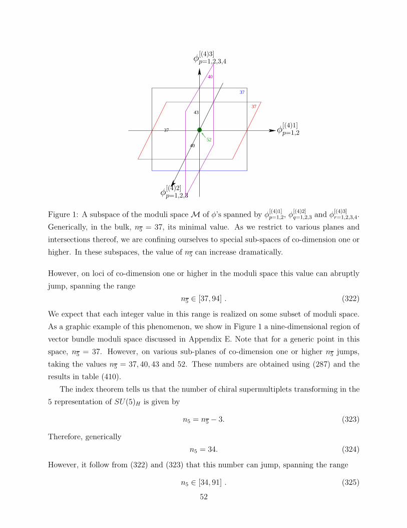
40

37

37

37

4052

43

φ[(4)1]p=1,2

φ[(4)3]p=1,2,3,4

φ[(4)2]p=1,2,3

Figure 1: A subspace of the moduli spaceM of φ’s spanned by φ[(4)1]p=1,2, φ

[(4)2]q=1,2,3 and φ

[(4)3]r=1,2,3,4.

Generically, in the bulk, n5 = 37, its minimal value. As we restrict to various planes and

intersections thereof, we are confining ourselves to special sub-spaces of co-dimension one or

higher. In these subspaces, the value of n5 can increase dramatically.

However, on loci of co-dimension one or higher in the moduli space this value can abruptly

jump, spanning the range

n5 ∈ [37, 94] . (322)

We expect that each integer value in this range is realized on some subset of moduli space.

As a graphic example of this phenomenon, we show in Figure 1 a nine-dimensional region of

vector bundle moduli space discussed in Appendix E. Note that for a generic point in this

space, n5 = 37. However, on various sub-planes of co-dimension one or higher n5 jumps,

taking the values n5 = 37, 40, 43 and 52. These numbers are obtained using (287) and the

results in table (410).

The index theorem tells us that the number of chiral supermultiplets transforming in the

5 representation of SU(5)H is given by

n5 = n5 − 3. (323)

Therefore, generically

n5 = 34. (324)

However, it follow from (322) and (323) that this number can jump, spanning the range

n5 ∈ [34, 91] . (325)

52

Note, however, that the index theorem guarantees that at every point in moduli space

n5 − n5 = 3 . (326)

Finally, the number of chiral superfields transforming as singlets under SU(5)H , that is, the

number of vector bundle moduli, is given by

n1 = 223 . (327)

We have succeeded, therefore, in computing the exact particle spectrum of our SU(5)

GUT theory. Rather remarkably, we find that, although the difference n5 − n5 is fixed by

the three family condition to be 3, the individual values of n5 and n5 depend on the location

in vector bundle moduli space at which they are evaluated.

9 Conclusions

We have shown, for general heterotic vacua, that the calculation of the particle spectrum

consists of computing the sheaf cohomology of five vector bundles: V, V ∗,∧2V,∧2V ∗, V ⊗V ∗.

Among these, the cohomology group H1(X, V ⊗ V ∗) has a topological interpretation as the

number of deformation moduli of the vector bundle V and, therefore, is always deformation

invariant. Hence, it cannot jump when the bundle moduli are varied continuously. However,

no such topological interpretation is available for the cohomologies of the remaining bundles.

In fact, we have shown that, as V varies continuously, the cohomologies of ∧2V and ∧2V ∗

do jump in the particular theory under consideration in this paper.

The novelty of these results is seen when contrasted with the standard embedding. In this

latter case, there are two distinct ways to deform the vector bundle. The first is to deform

the Calabi-Yau threefold X while keeping V = TX. In this case, jumps in the spectrum can

never occur since all the cohomologies in question do have a topological interpretation. By

definition, in the standard embedding we have V = ∧2V ∗ = TX = Ω2X and V ∗ = ∧2V =

T ∗X = Ω1X . Hence, the cohomologies are all of the form H i(Ωj

X), j = 1, 2 and i = 0, . . . , 3

where ΩjX is the sheaf of holomorphic j-forms on X. On our Calabi-Yau threefold X these

are topological invariants since their Hodge numbers can be related to the Betti numbers as

h1,1 = b2, 2h2,1 + 2 = b3. (328)

This explains why jumps in the spectrum as the moduli of the Calabi-Yau threefold are varied

were never observed in heterotic compactifications based on the standard embedding. The

53

second way to deform the vector bundle is to start with the standard embedding V = TX

on a fixed Calabi-Yau threefold and to deform its tangent bundle, as in [33]. In this case, it

is not excluded, and is in fact quite likely, that jumps in the particle spectrum will occur.

Acknowlegements

We are grateful to V. Braun, E. Buchbinder and T. Pantev for many insightful comments

and conversations. This Research was supported in part by the Dept. of Physics and the

Maths/Physics Research Group at the University of Pennsylvania under cooperative research

agreement #DE-FG02-95ER40893 with the U. S. Department of Energy and an NSF Focused

Research Grant DMS0139799 for “The Geometry of Superstrings.” R. D. further acknowl-

edges an NSF grant DMS 0104354. R. R. would like to thank Dmitriy Boyarchenko for

interesting discussions and is also supported by the Department of Physics and Astronomy

of Rutgers University under grant DOE-DE-FG02-96ER40959.

54

Appendices

A Chern and Todd Classes

For convenience, we remind the reader of the expansion of the Chern and Todd classes for a

vector bundle U on a complex manifold X.

td(U) = 1 + td1(U) + td2(U) + td3(U) + . . .

ch(U) = ch0(U) + ch1(U) + ch2(U) + ch3(U) + . . . (329)

with

td1(U) =1

2c1(U), td2(U) =

1

12(c2(U) + c1(U)2), td3(U) =

1

24(c1(U)c2(U)) , . . . (330)

and

ch0(U) = rk(U), ch1(U) = c1(U), ch2(U) =1

2(c1(U)2 − 2c2(U)),

ch3(U) =1

6(c1(U)3 − 3c1(U)c2(U) + 3c3(U)) . . . . (331)

We will make frequent use of these formulas.

B Chern Classes of Antisymmetric Products

In this Appendix, we obtain the expressions for the Chern classes of the antisymmetric

product ∧2V of a rank n vector bundle V on a threefold X. Using the splitting principle,

let us first decompose V into n line bundles Li as

V =

n⊕

i=1

Li . (332)

Then, we have that

ch(V ) =

n∑

i=1

exi (333)

where

xi = c1(Li) . (334)

Since X is a threefold, (333) can be expanded as

ch(V ) =

n∑

i=1

1 + xi +1

2x2

i +1

6x3

i . (335)

55

Therefore, we can read off from (335) that

ch0(V ) = rk(V ) = n, ch1(V ) =

n∑

i=1

xi, ch2(V ) =1

2

n∑

i=1

x2i , ch3(V ) =

1

6

n∑

i=1

x3i . (336)

The result we are after is

ch(∧2V ) =

n∑

i<j

exiexj , (337)

which, using (335), becomes

ch(∧2V ) =n∑

i<j

1 + (xi + xj) +1

2(xi + xj)

2 +1

6(xi + xj)

3

=n(n− 1)

2+ (n− 1)

n∑

i=1

xi +1

4

(

2n

n∑

i=1

x2i + 2

n∑

i=1

xi

n∑

j=1

xj − 4

n∑

i=1

x2i

)

+

1

12

(

2n

n∑

i=1

x3i + 6

n∑

i=1

x2i

n∑

j=1

xj − 8

n∑

i=1

x3i

)

=

[

n(n− 1)

2

]

+[

(n− 1) ch1(V )]

+

[

(n− 2)ch2(V ) +1

2ch1(V )2

]

+

[

(n− 4)ch3(V ) + ch1(V )ch2(V )]

. (338)

Using the relations given in (329) and (331), we conclude that the Chern classes of ∧2V are

rk(∧2V ) =n(n− 1)

2,

c1(∧2V ) = (n− 1)c1(V ),

c2(∧2V ) =

(n− 1)(n− 2)

2c1(V )2 + (n− 2)c2(V ),

c3(∧2V ) =

(n− 1)(n− 2)(n− 3)

6c1(V )3 + (n− 2)2c1(V )c2(V ) + (n− 4)c3(V ). (339)

C Determining H i(X,OX(nσ)⊗ π∗L)

In this Appendix, we determine, using the Leray spectral sequence, the cohomology groups

H i(X, T ) for line bundles of the form T = OX(nσ)⊗π∗L where L is some line bundle on the

base B. In particular, we will be interested in the dimensions of these groups and the explicit

maps between them. We will use the Leray spectral sequence to reduce the calculation of

the cohomology on X to that on the base B. Then, we specialize to the case when B = F1,

which is itself a P1 fibration over P1. In this case, we use the Leray spectral sequence again

to reduce the cohomology on B to that on P1 with which we are familiar. In all, for B = F1,

56

we can compute the cohomology groups H i(X,OX(nσ)⊗ π∗L) in general by reducing them

to direct sums of cohomologies over P1.

For π : X → B, with B being a surface and T a line bundle, the Leray spectral sequence

becomes the long exact sequence

0 → H1(B, π∗T ) → H1(X, T ) → H0(B, R1π∗T ) →

→ H2(B, π∗T ) → H2(X, T ) → H1(B, R1π∗T ) →

→ H3(B, π∗T ) → H3(X, T ) → H2(B, R1π∗T ) → 0.

(340)

For T of the form T = OX(nσ)⊗ π∗L, (340) gives us

n > 0 R1π∗T = 0

H i(X, T ) = H i(B, π∗OX(nσ)⊗ L), i = 0, 1, 2

H3(X, T ) = 0

n < 0 π∗T = 0

H0(X, T ) = 0

H i(X, T ) = H i−1(B, R1π∗T )

= H i−1(B, R1π∗(OX(nσ))⊗ L), i = 1, 2, 3

n = 0π∗T = L,

R1π∗T = KB ⊗ L

H0(X, π∗L) = H0(B, L)

H1(X, π∗L) = H1(B, L)⊕H0(B, KB ⊗ L) if H2(B, L) = 0

(341)

where, for n > 0 and n < 0, we have used the fact that

π∗(OX(nσ)) =

OB ⊕OB(−2c1(TB))⊕ . . .⊕OB(−nc1(TB)) for n > 0

0 for n < 0

R1π∗(OX(nσ)) =

0 for n > 0

OB((−n− 1)c1(TB))⊕ . . .⊕OB(c1(TB))⊕OB(−c1(TB)) for n < 0 .

(342)

In the last case of n = 0 in (341), we have used the relation

R1π∗OX = KB (343)

and the fact that (340) reduces, for n = 0, to

0→ H1(B, L)→ H1(X, π∗L)→ H0(B, R1π∗OX ⊗ L)→ H2(B, L)→ . . . . (344)

Now the Hirzebruch surface B = F1 is a P1 fibration over P1. Therefore, there is a

projection map

β : B → P1 . (345)

57

Any line bundle L on B = F1 can be written, by (11), as

L = OB(aS + bE) , a, b ∈ Z . (346)

A similar application as (340), replacing X, B and T by B, P1 and OB(aS+bE) respectively,

gives us

H0(B,OB(aS + bE)) = H0(P1, β∗OB(aS)⊗OP1(b)),

H1(B,OB(aS + bE)) = H0(P1, R1β∗OB(aS)⊗OP1(b))⊕H1(P1, β∗OB(aS)⊗OP1(b)),

H2(B,OB(aS + bE)) = H1(P1, R1β∗OB(aS)⊗OP1(b)) . (347)

where we have, for β∗O(aS) and R1β∗O(aS),

β∗O(aS) R1β∗O(aS)

a ≥ 0 OP1 ⊕OP1(−1)⊕ . . .⊕OP1(−a) 0

a < 0 0 OP1(1)⊕ . . .⊕OP1(−a− 1)

(348)

Combining the results in (341) and (347) gives us a method of expressing H i(X,OX(nσ)⊗

π∗L) in terms of a much more familiar object which can be handled with ease, namely

H1(P1,OP1(a)).

Let us demonstrate this technique by computing H1(X, W ) for a specific example. Choose

n = 0 and

L = OB(14S + 15E). (349)

Note this corresponds to choosing

T = W , (350)

where the line bundle W is defined in (244). That is, the sheaf cohomology group we wish

to consider is H1(X, π∗L). First, we note that

H2(B, L) = H1(P1, R1β∗OB(14S)⊗OP1(15)) = 0, (351)

since R1β∗OB(14S) vanishes by (348). Therefore, using (341), we conclude that

H1(X, π∗OB(14S+15E)) = H1(B,OB(14S+15E))⊕H0(B,OB(−c1(F1)+14S+15E)). (352)

Using (348), this becomes

H0(P1, R1β∗OB(14S)⊗OP1(15))⊕H1(P1, β∗OB(14S)⊗OP1(15))⊕H0(B, β∗OB(12S)⊗OP1(12)).

(353)

58

Upon simplifying (353), we at last have

H1(X, W ) ≃12⊕

i=0

H0(P1,OP1(i)). (354)

We can similarly determine the other cohomology groups for W , in summary, one finds

that

H0(X, W ) ≃15⊕

i=0

H0(P1,OP1(i)) ,

H1(X, W ) ≃12⊕

i=0

H0(P1,OP1(i)) ,

H2(X, W ) ≃ H3(X, W ) = 0 . (355)

Using the dimensions of the cohomology groups on P1 given in (212), we readily find that

h0(X, W ) = 135, h1(X, W ) = 91, h2(X, W ) = h3(X, W ) = 0 . (356)

D Constructing the Maps Mi Explicitly

In order to construct the linear maps Mi in (246), (252) and (254), we first need to determine

the relevant cohomology groups H i(X, T ) as vector spaces. This was done in Appendix C.

Next, we will construct explicit bases for these vector spaces. Finally, we write the matrix

representative for Mi by finding the multiplication rules which transform a basis of the

domain to a basis for the range.

We illustrate our technique with M1 which, we recall from (259), is the following mapping

H1(X, W (−CV −D))84M1−→ H1(X, W (−D))28 . (357)

The method we use is similar to that of [32]. We will need the bases for three vector spaces,

the domain H1(X, W (−CV −D))84, the range H1(X, W (−D))28 and H0(X,OX(CV )). This

last space classifies the mapping M1. To see this, note that our map on cohomology

M1 ∈ Hom(H1(X, W (−CV −D)), H1(X, W (−D))) (358)

is induced by a sheaf map

M1 : W (−CV −D)→W (−D) (359)

59

and both are given by the cup product with a class in

H0(X, W (−CV −D)∗ ⊗W (−D)) = H0(X,OX(CV )) . (360)

We will illustrate our technique with the space H1(X, W (−D))28, the range of the map M1.

From (244), we have

W (−D) = OX(−σ + π∗(8S + 9E)). (361)

The method of expressing a cohomology group of this form in terms of those on the base F1

and then on the base P1 of F1 has already been presented in Appendix C using the Leray

spectral sequence. By (341), (342), (347) and (12), we have

H1(X, W (−D)) = H1(X,OX(−σ + π∗(8S + 9E)))

H0(B,OB(6S + 6E))

π∗

?

H0(P1,OP1(6)⊕OP1(5)⊕OP1(4)⊕OP1(3)⊕OP1(2)⊕OP1(1)⊕OP1) .

β∗

?

(362)

We now describe the vector space on P1 explicitly by defining

B(3)k = H0(P1,OP1(k)) (363)

for k = 0, 1, . . . , 6 where

dimB(3)k = k + 1. (364)

The vector space at the bottom of (362), the cohomology group on P1, can now be written

as6⊕

k=1

B(3)k. (365)

Next, we pull back this space to F1 using β∗ and define

b(3)k = β∗B(3)k . (366)

Note that b(3)k is the space of sections of OB(kE). That is,

b(3)k = H0(B,OB(kE)). (367)

60

In order to embed this as a subspace of H0(B,OB(6S+6E)), each element of H0(B,OB(kE))

must be multiplied by a fixed section of OB(6S + 6E − kE). Defining

s(3)k = 3c1(TF1)− kE , (368)

the reader can readily verify, using (12), that

s(3)k − 3E = 6S + 6E − kE . (369)

Let us denote the fixed section by

s(3)k ∈ H0(B,OB(s(3)k − 3E)) (370)

and the space of sections of OB(kE) multiplied by s(3)k as b(3)k s(3)k. Then, we can write the

middle term in (362) as

H0(B,OB(6S + 6E)) =

6⊕

k=0

b(3)k s(3)k . (371)

Finally, we pull back this space to X using π∗. We find that

H1(X, W (−D)) =

6⊕

k=0

b(3)kˆs(3)ka, (372)

where

a = −σ + π∗(c1(F1)), b(3)k = π∗(b(3)k), ˆs(3)k = π∗(s(3)k) (373)

and

a ∈ H0(X,OX(a)) . (374)

The factor a arises for the same reason as the s(3)k factor and we use similar notation.

That is, a is required so that each term on the right hand side of (372) is a subspace

of H1(X, W (−D)). Specifically, the notation in (372) indicates that one should take the

element a of H1(X,OX(a)) and multiply each element of6⊕

k=0

b(3)kˆs(3)k by it. In summary, for

61

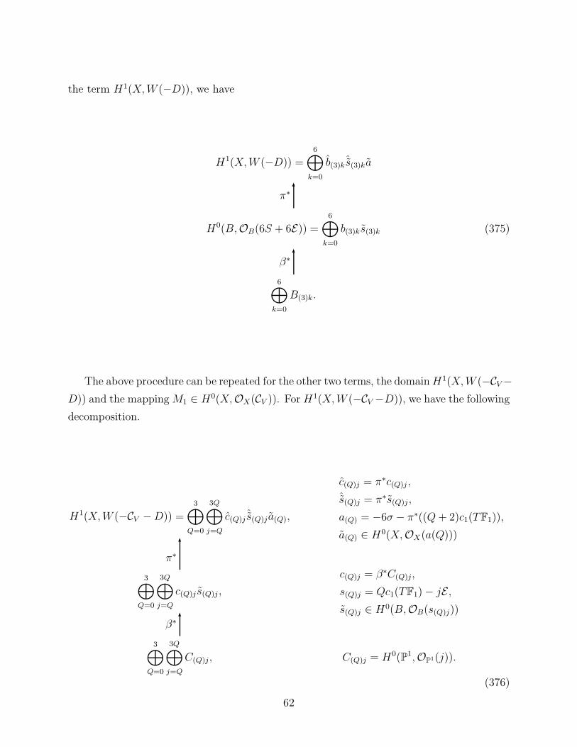
the term H1(X, W (−D)), we have

H1(X, W (−D)) =6⊕

k=0

b(3)kˆs(3)ka

H0(B,OB(6S + 6E)) =

6⊕

k=0

b(3)k s(3)k

π∗ 6

6⊕

k=0

B(3)k.

β∗ 6

(375)

The above procedure can be repeated for the other two terms, the domain H1(X, W (−CV−

D)) and the mapping M1 ∈ H0(X,OX(CV )). For H1(X, W (−CV −D)), we have the following

decomposition.

H1(X, W (−CV −D)) =

3⊕

Q=0

3Q⊕

j=Q

c(Q)jˆs(Q)j a(Q),

c(Q)j = π∗c(Q)j ,

ˆs(Q)j = π∗s(Q)j ,

a(Q) = −6σ − π∗((Q + 2)c1(TF1)),

a(Q) ∈ H0(X,OX(a(Q)))

3⊕

Q=0

3Q⊕

j=Q

c(Q)j s(Q)j ,

π∗

6

c(Q)j = β∗C(Q)j,

s(Q)j = Qc1(TF1)− jE ,

s(Q)j ∈ H0(B,OB(s(Q)j))

3⊕

Q=0

3Q⊕

j=Q

C(Q)j,

β∗ 6

C(Q)j = H0(P1,OP1(j)).

(376)

62

Finally, the space H0(X,OX(CV )), in which the map M1 lives, has the basis

H0(X,OX(CV )) =⊕

R=1,2,3,4,6

3R−3⊕

i=R−3

m(R)iˆs(R)iA(R),

m(R)i = π∗m(R)i,

ˆs(R)i = π∗s(R)i,

A(R)i = 5σ + π∗((6− R)c1(TF1)),

A(R)i ∈ H0(X,OX(A(R)i))

⊕

R=1,2,3,4,6

3R−3⊕

i=R−3

m(R)is(R)i ,

π∗

6

m(R)i = β∗M(R)i,

s(R)i = Rc1(TF1)− iE ,

s(R)i ∈ H0(B,OB(s(R)i))

⊕

R=1,2,3,4,6

3R−3⊕

i=R−3

M(R)i,

β∗ 6

M(R)i = H0(P1,OP1(i)).

(377)

We have now explicitly constructed the bases for the vector spaces of concern. In partic-

ular, M1 ∈ H0(X,OX(CV )) given in (377) must map H1(X, W (−CV −D))84 given in (376)

linearly to H1(X, W (−D))28 given in (375). The matrix for M1 is straight-forward to con-

struct. We multiply the basis in (376) with the matrix elements in (377) and demand that

the result be in (375). More specifically, we must guarantee that

(

m(R)iˆs(R)iA(R)

)

·(

c(Q)jˆs(Q)j a(Q)

)

= b(3)kˆs(3)ka . (378)

This requires that

A(R) · a(Q) = a , (379)

ˆs(R)i · ˆs(Q)j = ˆs(3)k (380)

and

m(R)i · c(Q)j = b(3)k (381)

be satisfied individually. Using the definitions of these quantities given in (375), (376) and

(377), we find from (379) that only terms with

R + Q = 3 (382)

can pair non-trivially. Substituting this relation into (380) and (381) then constrains i, j and

k to satisfy

i + j = k . (383)

63

We still must show that the sections A(R), a(S), a and ˆs(R)i, ˆs(Q)j , ˆs(3)k can be chosen to

satisfy (379) and (380) respectively. This can be done as follows. Fix once and for all a

generic section ℓ ∈ H0(B,OB(S + E)). Now, each of our ˆs-type sections is the lift of a

section s ∈ H0(B,OB(aS + bE)) for some integers a ≥ b ≥ 0. We will simply set

s = ℓbSa−b, (384)

where S is a fixed section of OB(S). Note that (384) is a section of the desired bundle

OB(aS + bE). Furthermore, these sections clearly satisfy (380). We can make similar choices

for the a-type sections, thus satisfying (379) as well. Having established the above, we see

that any element of m(R)iˆs(R)iA(R), c(Q)j

ˆs(Q)ja(Q) or b(3)kˆs(3)ka can be explicitly labeled by

an element of M(R)i, C(Q)j or B(3)k respectively.

Now, consider the matrix M1 ∈ H0(X,OX(CV )). Any matrix block in M1 that does not

satisfy one or both of (382) and (383) must be a zero entry. On the other hand, any entry in

M1 that satisfies both (382) and (383) is a potentially non-vanishing sub-matrix which we

denote by

m(R)i ∈M(R)i = H0(P1,OP1(i)) . (385)

Note that m(R)i may occur as many different sub-matrices within M1 with the (R)i subscripts

fixing its location. This is most easily understood by simply looking at the result. Using the

data from (375), (376) and (377) subject to the constraints (382) and (383), we find

m(3)0 0 0 0 0 0 0 0 0 0 0 0 0 0 0 0

m(3)1 m(2)0 0 0 0 0 0 0 0 0 0 0 0 0 0 0

m(3)2 m(2)1 m(2)0 0 m(1)0 0 0 0 0 0 0 0 0 0 0 0

m(3)3 m(2)2 m(2)1 m(2)0 0 m(1)0 0 0 0 0 0 0 0 0 0 0

m(3)4 m(2)3 m(2)2 m(2)1 0 0 m(1)0 0 0 0 0 0 0 0 0 0

m(3)5 0 m(2)3 m(2)2 0 0 0 m(1)0 0 0 0 0 0 0 0 0

m(3)6 0 0 m(2)3 0 0 0 0 m(1)0 0 0 0 0 0 0 0

28×84

·

C(0)0

C(1)1

C(1)2

C(1)3

C(2)2

C(2)3

C(2)4

C(2)5

C(2)6

C(3)3

C(3)4

C(3)5

C(3)6

C(3)7

C(3)8

C(3)9

84

=

B(3)0

B(3)1

B(3)2

B(3)3

B(3)4

B(3)5

B(3)6

28 .

(386)

Of course, each non-zero sub-matrix m(R)i maps a space B(Q)j = H0(P1,O(j)) linearly to

a space B(3)k = H0(P1,OP1(k)) where R + Q = 3 and i + j = k. That is, m(R)i is a

(k +1)× (j +1) matrix. We can emphasize this by extending our notation and writing m(R)i

64

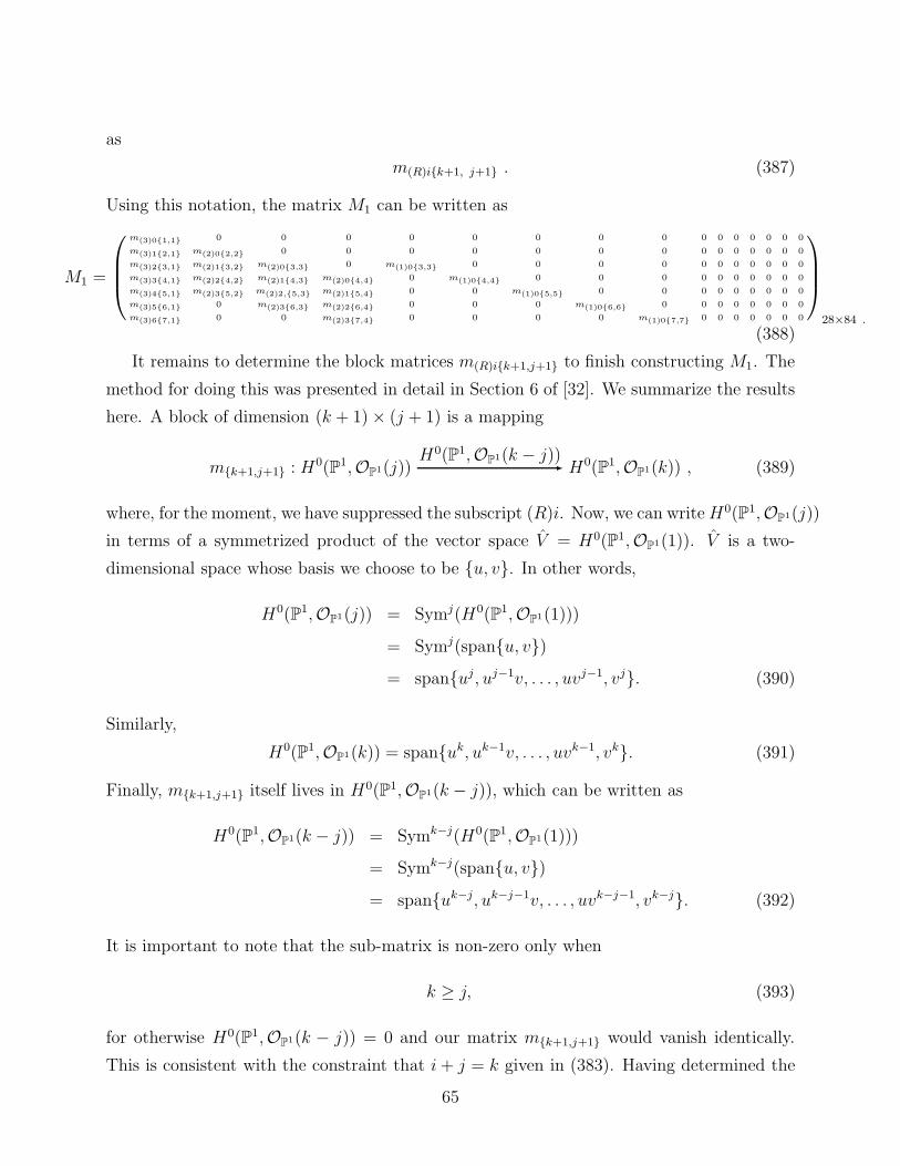
as

m(R)ik+1, j+1 . (387)

Using this notation, the matrix M1 can be written as

M1 =

m(3)01,1 0 0 0 0 0 0 0 0 0 0 0 0 0 0 0

m(3)12,1 m(2)02,2 0 0 0 0 0 0 0 0 0 0 0 0 0 0

m(3)23,1 m(2)13,2 m(2)03,3 0 m(1)03,3 0 0 0 0 0 0 0 0 0 0 0

m(3)34,1 m(2)24,2 m(2)14,3 m(2)04,4 0 m(1)04,4 0 0 0 0 0 0 0 0 0 0

m(3)45,1 m(2)35,2 m(2)2,5,3 m(2)15,4 0 0 m(1)05,5 0 0 0 0 0 0 0 0 0

m(3)56,1 0 m(2)36,3 m(2)26,4 0 0 0 m(1)06,6 0 0 0 0 0 0 0 0

m(3)67,1 0 0 m(2)37,4 0 0 0 0 m(1)07,7 0 0 0 0 0 0 0

28×84 .

(388)

It remains to determine the block matrices m(R)ik+1,j+1 to finish constructing M1. The

method for doing this was presented in detail in Section 6 of [32]. We summarize the results

here. A block of dimension (k + 1)× (j + 1) is a mapping

mk+1,j+1 : H0(P1,OP1(j))H0(P1,OP1(k − j))- H0(P1,OP1(k)) , (389)

where, for the moment, we have suppressed the subscript (R)i. Now, we can write H0(P1,OP1(j))

in terms of a symmetrized product of the vector space V = H0(P1,OP1(1)). V is a two-

dimensional space whose basis we choose to be u, v. In other words,

H0(P1,OP1(j)) = Symj(H0(P1,OP1(1)))

= Symj(spanu, v)

= spanuj, uj−1v, . . . , uvj−1, vj. (390)

Similarly,

H0(P1,OP1(k)) = spanuk, uk−1v, . . . , uvk−1, vk. (391)

Finally, mk+1,j+1 itself lives in H0(P1,OP1(k − j)), which can be written as

H0(P1,OP1(k − j)) = Symk−j(H0(P1,OP1(1)))

= Symk−j(spanu, v)

= spanuk−j, uk−j−1v, . . . , uvk−j−1, vk−j. (392)

It is important to note that the sub-matrix is non-zero only when

k ≥ j, (393)

for otherwise H0(P1,OP1(k − j)) = 0 and our matrix mk+1,j+1 would vanish identically.

This is consistent with the constraint that i + j = k given in (383). Having determined the

65

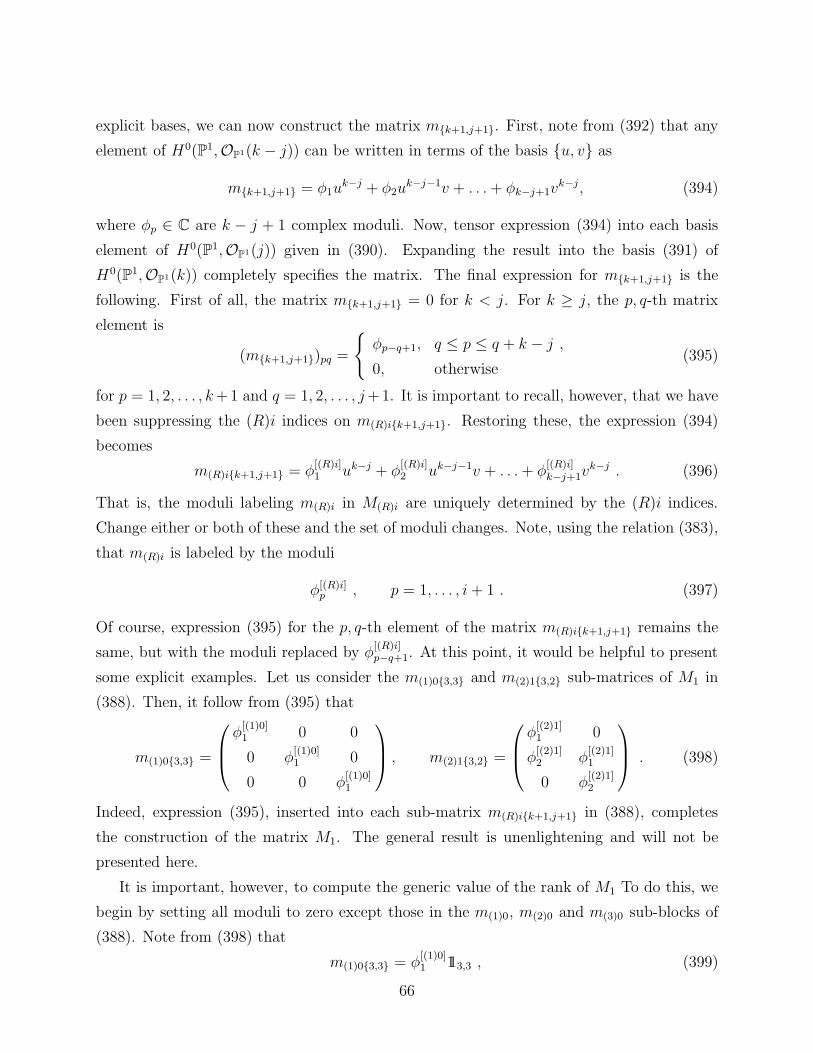
explicit bases, we can now construct the matrix mk+1,j+1. First, note from (392) that any

element of H0(P1,OP1(k − j)) can be written in terms of the basis u, v as

mk+1,j+1 = φ1uk−j + φ2u

k−j−1v + . . . + φk−j+1vk−j, (394)

where φp ∈ C are k − j + 1 complex moduli. Now, tensor expression (394) into each basis

element of H0(P1,OP1(j)) given in (390). Expanding the result into the basis (391) of

H0(P1,OP1(k)) completely specifies the matrix. The final expression for mk+1,j+1 is the

following. First of all, the matrix mk+1,j+1 = 0 for k < j. For k ≥ j, the p, q-th matrix

element is

(mk+1,j+1)pq =

φp−q+1, q ≤ p ≤ q + k − j ,

0, otherwise(395)

for p = 1, 2, . . . , k +1 and q = 1, 2, . . . , j +1. It is important to recall, however, that we have

been suppressing the (R)i indices on m(R)ik+1,j+1. Restoring these, the expression (394)

becomes

m(R)ik+1,j+1 = φ[(R)i]1 uk−j + φ

[(R)i]2 uk−j−1v + . . . + φ

[(R)i]k−j+1v

k−j . (396)

That is, the moduli labeling m(R)i in M(R)i are uniquely determined by the (R)i indices.

Change either or both of these and the set of moduli changes. Note, using the relation (383),

that m(R)i is labeled by the moduli

φ[(R)i]p , p = 1, . . . , i + 1 . (397)

Of course, expression (395) for the p, q-th element of the matrix m(R)ik+1,j+1 remains the

same, but with the moduli replaced by φ[(R)i]p−q+1. At this point, it would be helpful to present

some explicit examples. Let us consider the m(1)03,3 and m(2)13,2 sub-matrices of M1 in

(388). Then, it follow from (395) that

m(1)03,3 =

φ[(1)0]1 0 0

0 φ[(1)0]1 0

0 0 φ[(1)0]1

, m(2)13,2 =

φ[(2)1]1 0

φ[(2)1]2 φ

[(2)1]1

0 φ[(2)1]2

. (398)

Indeed, expression (395), inserted into each sub-matrix m(R)ik+1,j+1 in (388), completes

the construction of the matrix M1. The general result is unenlightening and will not be

presented here.

It is important, however, to compute the generic value of the rank of M1 To do this, we

begin by setting all moduli to zero except those in the m(1)0, m(2)0 and m(3)0 sub-blocks of

(388). Note from (398) that

m(1)03,3 = φ[(1)0]1 113,3 , (399)

66

where 113,3 is the 3 × 3 identity matrix. In fact, all m(1)0, m(2)0 and m(3)0 sub-matrices

are proportional to φ[(1)0]1 , φ

[(2)0]1 and φ

[(3)0]1 moduli respectively times the unit matrix of the

appropriate size. If we then set

φ[(1)0]1 = φ

[(2)0]1 = φ

[(3)0]1 ≡ φ, (400)

we find the matrix M1 given in (281). For any φ 6= 0, this matrix has

rk(M1) = 28. (401)

One can also consider the complete expression for M1, randomly initialize the values of its

moduli and numerically compute the rank. We have done this for a large number of random

initial sets with the caveat, to be explained below, that we insist that all moduli be non-zero.

Generically, we recover the result (401). This justifies the important assumption in Subsec-

tion 8.2 that we can choose rk(M1) = 28, thus simplifying the calculation of h0(D, W |D) to

expression (283).

Similarly, we can construct the matrix M2, which we recall from (258) is the mapping

H1(X, W (−CV ))180M2−→ H1(X, W )91 . (402)

The result, in block-form, is

M2 =

0 0 0 0 0 0 0 0 0 0 0 0 0 0 0 0 0 0 0 0

0 0 0 0 0 0 0 0 0 0 0 0 0 0 0 0 0 0 0 0

0 0 0 0 0 0 0 0 0 0 0 0 0 0 0 0 0 0 0 0

0 0 0 0 m(6)34,1 0 0 0 0 0 0 0 0 0 0 0 0 0 0 0

0 0 0 0 m(6)45,1 m(6)35,2 0 0 0 0 0 0 0 0 0 0 0 0 0 0

0 0 0 0 m(6)56,1 m(6)46,2 m(6)36,3 0 0 0 0 0 0 0 0 0 0 0 0 0

0 0 0 0 m(6)67,1 m(6)57,2 m(6)47,3 m(6)37,4 0 0 0 0 0 0 0 0 0 0 0 0

0 0 0 0 m(6)78,1 m(6)68,2 m(6)58,3 m(6)48,4 m(6)38,5 0 0 0 0 0 0 0 0 0 0 0

0 0 0 0 m(6)89,1 m(6)79,2 m(6)69,3 m(6)59,4 m(6)49,5 m(6)39,6 0 0 0 0 0 0 0 0 0 0

0 0 0 0 m(6)910,1 m(6)810,2 m(6)710,3 m(6)610,4 m(6)510,5 m(6)410,6 m(6)310,7 0 0 0 0 0 0 0 0 0

0 0 0 0 m(6)1011,1 m(6)911,2 m(6)811,3 m(6)711,4 m(6)611,5 m(6)511,6 m(6)411,7 0 0 0 0 0 0 0 0 0

0 0 0 0 m(6)1112,1 m(6)1012,2 m(6)912,3 m(6)812,4 m(6)712,5 m(6)612,6 m(6)512,7 0 0 0 0 0 0 0 0 0

0 0 0 0 m(6)1213,1 m(6)1113,2 m(6)1013,3 m(6)913,4 m(6)813,5 m(6)713,6 m(6)613,7 0 0 0 0 0 0 0 0 0

· · ·

· · ·

0 0 0 0 0 0 0 0 0 0 0

0 0 0 0 0 0 0 0 0 0 0

0 0 0 0 0 0 0 0 0 0 0

m(4)14,3 0 0 0 0 0 0 0 0 0 0

m(4)25,3 m(4)15,4 0 0 0 0 0 0 0 0 0

m(4)36,3 m(4)26,4 m(4)16,5 0 0 0 0 0 0 0 0

m(4)47,3 m(4)37,4 m(4)27,5 m(4)17,6 0 0 0 0 0 0 0

m(4)58,3 m(4)48,4 m(4)38,5 m(4)28,6 m(4)18,7 0 0 0 0 0 0

m(4)69,3 m(4)59,4 m(4)49,5 m(4)39,6 m(4)29,7 m(4)19,8 0 0 0 0 0

m(4)710,3 m(4)610,4 m(4)510,5 m(4)410,6 m(4)310,7 m(4)210,8 m(4)110,9 0 0 0 0

m(4)811,3 m(4)711,4 m(4)611,5 m(4)511,6 m(4)411,7 m(4)311,8 m(4)211,9 m(4)11,10 0 0 0

m(4)912,3 m(4)812,4 m(4)712,5 m(4)612,6 m(4)512,7 m(4)412,8 m(4)312,9 m(4)212,10 m(4)112,11 0 0

0 m(4)913,4 m(4)813,5 m(4)713,6 m(4)613,7 m(4)513,8 m(4)413,9 m(4)313,10 m(4)213,11 m(4)113,12 0

91×180 .

(403)

67

As explicit examples of sub-matrices in M2, we present the following two which we will use

in our analyses below. They are

m(4)14,3

φ[(4)1]1 0 0

φ[(4)1]2 φ

[(4)1]1 0

0 φ[(4)1]2 φ

[(4)1]1

0 0 φ[(4)1]2

, m(4)25,3 =

φ[(4)2]1 0 0

φ[(4)2]2 φ

[(4)2]1 0

φ[(4)2]3 φ

[(4)2]2 φ

[(4)2]1

0 φ[(4)2]3 φ

[(4)2]2

0 0 φ[(4)2]3

. (404)

We have computed all other m(R)ik+1,j+1 sub-blocks in (403) but, of course, will not present

them here. This completes the construction of the matrix M2.

E The Rank of M2

It is not enlightening to display M2 in its full form in terms of the moduli. However, it is

important for us to compute its rank. To do this, we begin by randomly selecting the values

of all moduli assuming, however, that each is non-zero. We then numerically compute the

rank of M2. This process is continued for a large number of different random, but non-zero,

initializations. The results of an explicit numerical calculation involving 100,000 random

integer initializations between 1 and 3 of the moduli are shown in Figure 2. The horizontal

axis indicates the ranks of M2 found in the survey, while the vertical axis gives the number

of occurrences. We see that the rank of 85 by far dominates over any other possibilities. It

follows that at generic points in moduli space

rk(M2) = 85. (405)

This is, in fact, the maximal possible rank, as can be seen by examining (403) and noting

that 6 out of the 91 rows have all zero entries.

Importantly, however, we notice that there are isolated initializations of the moduli for

which the rank of M2 jumps to values smaller than 85. This phenomenon is clearly seen in

Figure 2 where rk(M2) is shown to attain all integer values between 79 and 84, in addition

to its generic value of 85. It is clear from the low statistics of these other values, that they

occur at non-generic points in the vector bundle moduli space. In this set of 100,000 integer

randomizations, we have not seen any ranks lower than 79. However, as we increase the

number of randomizations we expect to see smaller values of rk(M2). Statistically, this is

expected. For example, with a smaller set of only 1,000 randomizations, only 2 values of

rk(M2) were observed.

68

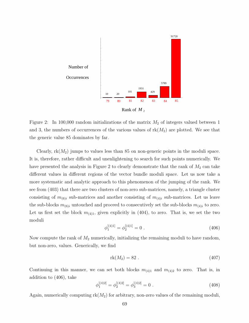
1 2 3 4 5 6 7

200

400

600

800

79 80 81 82 83 84 85

10 20101

1931429

5789

91720

2

Number of

Occurrences

MRank of

Figure 2: In 100,000 random initializations of the matrix M2 of integers valued between 1

and 3, the numbers of occurrences of the various values of rk(M2) are plotted. We see that

the generic value 85 dominates by far.

Clearly, rk(M2) jumps to values less than 85 on non-generic points in the moduli space.

It is, therefore, rather difficult and unenlightening to search for such points numerically. We

have presented the analysis in Figure 2 to clearly demonstrate that the rank of M2 can take

different values in different regions of the vector bundle moduli space. Let us now take a

more systematic and analytic approach to this phenomenon of the jumping of the rank. We

see from (403) that there are two clusters of non-zero sub-matrices, namely, a triangle cluster

consisting of m(6)i sub-matrices and another consisting of m(4)i sub-matrices. Let us leave

the sub-blocks m(6)i untouched and proceed to consecutively set the sub-blocks m(4)i to zero.

Let us first set the block m(4)1, given explicitly in (404), to zero. That is, we set the two

moduli

φ[(4)1]1 = φ

[(4)1]2 = 0 . (406)

Now compute the rank of M2 numerically, initializing the remaining moduli to have random,

but non-zero, values. Generically, we find

rk(M2) = 82 . (407)

Continuing in this manner, we can set both blocks m(4)1 and m(4)2 to zero. That is, in

addition to (406), take

φ[(4)2]1 = φ

[(4)2]2 = φ

[(4)2]3 = 0 . (408)

Again, numerically computing rk(M2) for arbitrary, non-zero values of the remaining moduli,

69

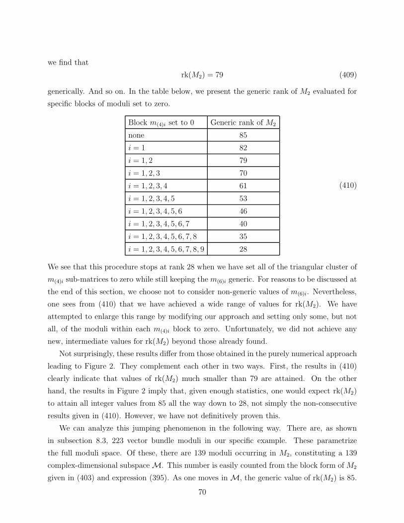
we find that

rk(M2) = 79 (409)

generically. And so on. In the table below, we present the generic rank of M2 evaluated for

specific blocks of moduli set to zero.

Block m(4)i set to 0 Generic rank of M2

none 85

i = 1 82

i = 1, 2 79

i = 1, 2, 3 70

i = 1, 2, 3, 4 61

i = 1, 2, 3, 4, 5 53

i = 1, 2, 3, 4, 5, 6 46

i = 1, 2, 3, 4, 5, 6, 7 40

i = 1, 2, 3, 4, 5, 6, 7, 8 35

i = 1, 2, 3, 4, 5, 6, 7, 8, 9 28

(410)

We see that this procedure stops at rank 28 when we have set all of the triangular cluster of

m(4)i sub-matrices to zero while still keeping the m(6)i generic. For reasons to be discussed at

the end of this section, we choose not to consider non-generic values of m(6)i. Nevertheless,

one sees from (410) that we have achieved a wide range of values for rk(M2). We have

attempted to enlarge this range by modifying our approach and setting only some, but not

all, of the moduli within each m(4)i block to zero. Unfortunately, we did not achieve any

new, intermediate values for rk(M2) beyond those already found.

Not surprisingly, these results differ from those obtained in the purely numerical approach

leading to Figure 2. They complement each other in two ways. First, the results in (410)

clearly indicate that values of rk(M2) much smaller than 79 are attained. On the other

hand, the results in Figure 2 imply that, given enough statistics, one would expect rk(M2)

to attain all integer values from 85 all the way down to 28, not simply the non-consecutive

results given in (410). However, we have not definitively proven this.

We can analyze this jumping phenomenon in the following way. There are, as shown

in subsection 8.3, 223 vector bundle moduli in our specific example. These parametrize

the full moduli space. Of these, there are 139 moduli occurring in M2, constituting a 139

complex-dimensional subspaceM. This number is easily counted from the block form of M2

given in (403) and expression (395). As one moves inM, the generic value of rk(M2) is 85.

70

However, as one touches certain sub-spaces of M of co-dimension one or higher, the rank

of M2 drops. At the various intersections of these sub-spaces, that is, at sub-spaces of even

higher co-dimension, the rank may drop further. In the example (410), the sub-spaces, in

particular, are the coordinate planes inM where some moduli are set to zero. To be specific,

let us consider a particular subspace of M, with three axes corresponding respectively to

φ[(4)1]p=1,2, φ

[(4)2]q=1,2,3 and φ

[(4)3]r=1,2,3,4. In the bulk of this space, rk(M2) = 85 generically. If we hit

the plane φ[(4)1]p=1,2 = 0, (410) tells us that rk(M2) = 82. If we hit the intersection of the planes

φ[(4)1]p=1,2 = 0 and φ

[(4)2]p=1,2,3 = 0, then the rank drops to 79. And so on. We present this plot

in Figure 3, indicating the various ranks as we restrict to various intersections of the planes

within this region of moduli space. We conclude that the rank of M2 is highly sensitive to

where one evaluates it within the moduli space M.

There is one final issue that must be addressed. Recall that the spectral cover CV must

be irreducible to ensure the stability of V . Now, CV is a section of

H0(X,OX(CV )) = H0(X,OX(5σ + π∗η)) . (411)

We can decompose this vector space into cohomology groups on P1 exactly as was done in the

explicit construction of the matrix M1. This was carried out in Appendix D and presented

in (377). For convenience, we remind the reader that

H0(X,OX(CV )) =⊕

R=1,2,3,4,6

3R−3⊕

i=R−3

m(R)i(s(R)i − 3π∗E)A(R), (412)

with

m(R)i = π∗m(R)i, s(R)i = π∗s(R)i, A(R)i = 5σ + π∗((6− R)c1(TF1))

m(R)i = β∗M(R)i, s(R)i = Rc1(TF1)− iE

M(R)i = H0(P1,OP1(i)) . (413)

It turns out that a sufficient criterion for the irreducibility of CV lies only in the first step in

the projection π∗ to the base B = F1. The conditions for the irreducibility of CV are found

to be

(1) m(1)i 6= 0,

(2) m(6)i generic, (414)

where m(R)i ∈ M(R)i are the sub-matrices defined in (385). Therefore, in our matrices M1

and M2, whose constituent blocks are the m(R)i sub-matrices, we must make sure that the

71

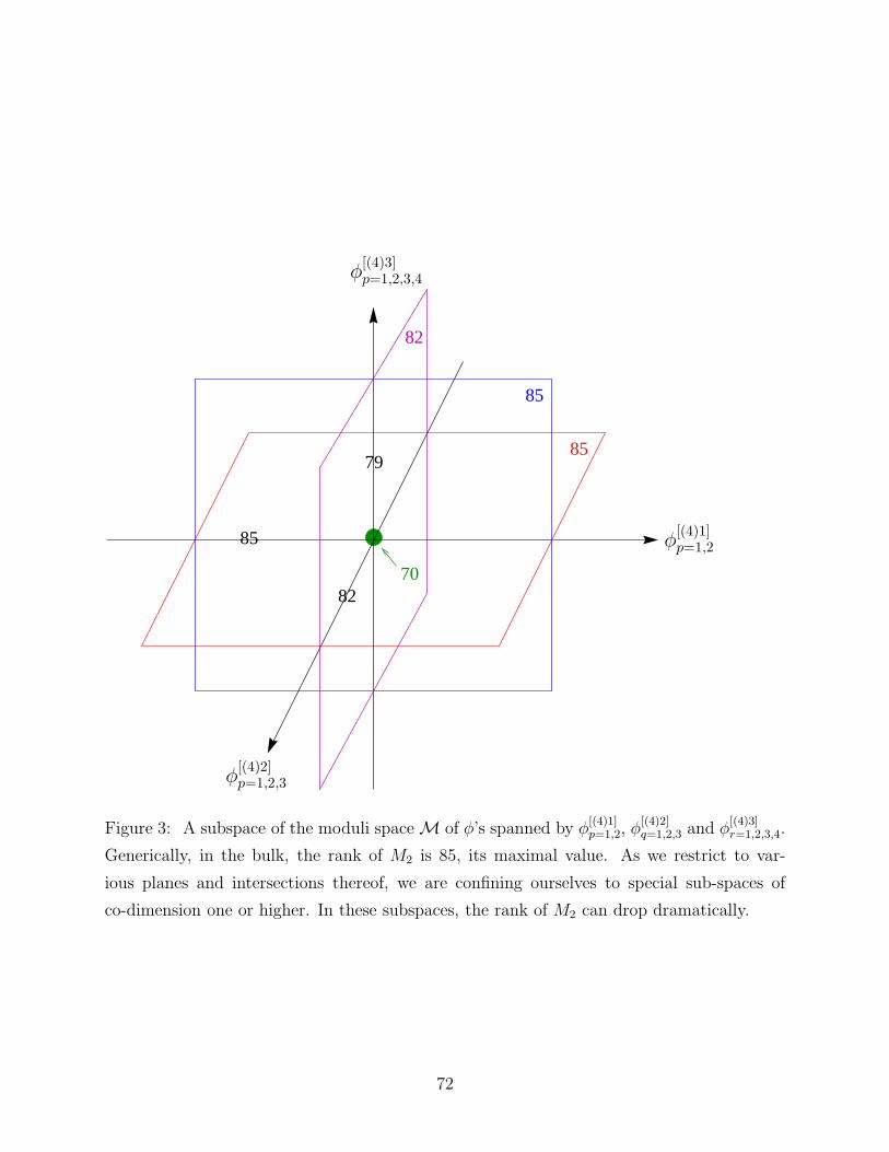
82

85

85

85

79

8270

φ[(4)1]p=1,2

φ[(4)2]p=1,2,3

φ[(4)3]p=1,2,3,4

Figure 3: A subspace of the moduli spaceM of φ’s spanned by φ[(4)1]p=1,2, φ

[(4)2]q=1,2,3 and φ

[(4)3]r=1,2,3,4.

Generically, in the bulk, the rank of M2 is 85, its maximal value. As we restrict to var-

ious planes and intersections thereof, we are confining ourselves to special sub-spaces of

co-dimension one or higher. In these subspaces, the rank of M2 can drop dramatically.

72

two conditions (414) are satisfied when making our choices of the moduli. Now, M2 does not

depend on m(1)i and we have been careful to set m(6)i to generic non-zero values in the above

discussions. Furthermore, M1 does not depend on m(6)i and in our choice of the maximal

rank of 28, we have always made sure that m(1)0, the only m(1)i sub-block occurring in M1,

is non-zero. Therefore, (414) is indeed satisfied in our choices and the spectral cover CV

remains irreducible throughout.

References

[1] P. Horava and E. Witten, “Heterotic and Type I String Dynamics from Eleven Dimen-

sions,” Nucl. Phys. B460, 506 (1996) [hep-th/9510209].

P. Horava and E. Witten, “Eleven-Dimensional Supergravity on a Manifold with Bound-

ary,” Nucl. Phys. B475, 94 (1996) [hep-th/9603142].

E. Witten, Strong Coupling Expansion Of Calabi-Yau Compactification, Nucl. Phys.

B471 (1996) 135.

[2] R. Donagi, Principal bundles on elliptic fibrations Asian J. Math. Vol. 1 (1997), 214-223,

alg-geom/9702002.

[3] R. Friedman, J. Morgan, E. Witten, Vector Bundles And F Theory, Com-

mun.Math.Phys. 187 (1997) 679-743

[4] R. Friedman, J. Morgan, E. Witten Vector Bundles over Elliptic Fibrations,

alg-geom/9709029.

[5] R. Donagi, A. Lukas, B. Ovrut, and D. Waldram, Non-Perturbative Vacua and Particle

Physics in M-Theory, JHEP 9905 (1999) 018.

[6] R. Donagi, A. Lukas, B. A. Ovrut and D. Waldram, “Holomorphic vector bundles and

non-perturbative vacua in M-theory,” JHEP 9906, 034 (1999) [arXiv:hep-th/9901009].

[7] B. Andreas, G. Curio and A. Klemm, “Towards the standard model spectrum from

elliptic Calabi-Yau,” arXiv:hep-th/9903052.

[8] R. Donagi, B. Ovrut, T. Pantev, and D. Waldram, Spectral involutions on rational

elliptic surfaces, Adv.Theor.Math.Phys. 5 (2002) 499-561, math.AG/0008011.

R. Donagi, B. Ovrut, T. Pantev, and D. Waldram, Standard-Model bundles,

73

Adv.Theor.Math.Phys. 5 (2002) 563-615, math.AG/0008010.

R. Donagi, B. Ovrut, T. Pantev, and D. Waldram, Standard-Model bundles on non-

simply connected Calabi-Yau threefolds, JHEP, 0108 (2001) 053, hep-th/0008008.

R. Donagi, B. Ovrut, T. Pantev, and D. Waldram, Standard Models from Heterotic

M-theory, Adv.Theor.Math.Phys., 5 (2002) 93-137.

[9] B. Ovrut, T. Pantev, R. Reinbacher, Torus-Fibered Calabi-Yau Threefolds with Non-

Trivial Fundamental Group, UPR 1015-T, hep-th/0212221.

B. Ovrut, T. Pantev, R. Reinbacher, Invariant Homology on Standard Model Manifolds,

UPR 1016-T, hep-th/0303020.

R. Donagi, B. A. Ovrut, T. Pantev and R. Reinbacher, “SU(4) instantons on

Calabi-Yau threefolds with Z(2) x Z(2) fundamental group,”JHEP 0401, 022 (2004)

[arXiv:hep-th/0307273].

R. Thomas, Examples of bundles on Calabi-Yau 3-folds for string theory compactifica-

tions, Adv.Theor.Math.Phys. 4 (2000) 231-247.

[10] R. Donagi, T. Pantev, Torus fibrations, gerbes, and duality, math.AG/0306213.

[11] Burt A. Ovrut, Tony Pantev, Jaemo Park, “Small Instanton Transitions in Heterotic

M-Theory,” JHEP 0005, 045 (2000), hep-th/0001133.

[12] E.I. Buchbinder, R. Donagi, B.A. Ovrut, Vector Bundle Moduli Superpotentials in

Heterotic Superstrings and M-Theory, JHEP 0207 (2002) 066.

E.I. Buchbinder, R. Donagi, B.A. Ovrut, Superpotentials for Vector Bundle Moduli,

Nucl.Phys. B653 (2003) 400-420.

[13] E. I. Buchbinder and B. A. Ovrut, “Vacuum stability in heterotic M-theory,”

arXiv:hep-th/0310112.

E. Lima, B. A. Ovrut, J. Park and R. Reinbacher, “Non-perturbative superpoten-

tial from membrane instantons in heterotic M-theory,” Nucl. Phys. B 614, 117 (2001)

[arXiv:hep-th/0101049].

[14] R. Donagi, B.A. Ovrut, D. Waldram, Moduli Spaces of Fivebranes on Elliptic Calabi-

Yau Threefolds, JHEP 9911 (1999) 030.

[15] A. Lukas, B.A. Ovrut, and D. Waldram, Non-standard embedding and five-branes in

heterotic M-Theory, Nucl.Phys. B552 (1999) 246-290.

74

A. Lukas, B.A. Ovrut, K.S. Stelle and D. Waldram, The Universe as a Domain Wall,

Phys.Rev. D59 (1999) 086001.

A. Lukas, B.A. Ovrut, K.S. Stelle and D. Waldram, Heterotic M–theory in Five Di-

mensions, Nucl.Phys. B552 (1999) 246-290.

A. Lukas, B.A. Ovrut, D. Waldram, Gaugino Condensation in M-theory on S1/Z2,

Phys.Rev. D57 (1998) 7529-7538.

A. Lukas, B.A. Ovrut, D. Waldram, Five–Branes and Supersymmetry Breaking in

M–Theory, JHEP 9904 (1999) 009.

[16] J. Khoury, B.A. Ovrut, P.J. Steinhardt, N. Turok, The Ekpyrotic Universe: Colliding

Branes and the Origin of the Hot Big Bang, Phys.Rev. D64 (2001) 123522.

[17] See M. Green, J. Schwarz, E. Witten, Superstring theory, Loop Amplitudes, Anomalies

& Phenomenology, Cambridge Monographs on Mathematical Physics Vol. 2 (1987) and

references therein.

[18] R. Donagi, Yang-Hui He, Burt A. Ovrut, and Rene Reinbacher, “Moduli Dependent

Spectra of Heterotic Compactifications,” [arXiv:hep-th/0403291].

[19] E. Buchbinder, R. Donagi and B. A. Ovrut, “Vector bundle moduli and small instanton

transitions,” JHEP 0206, 054 (2002) [arXiv:hep-th/0202084].

[20] B. Andreas, “N = 1 heterotic/F-theory duality,” Fortsch. Phys. 47, 587 (1999)

[arXiv:hep-th/9808159].

[21] D. R. Morrison and C. Vafa, “Compactifications of F-Theory on Calabi–Yau Threefolds

– I,” Nucl. Phys. B 473, 74 (1996) [arXiv:hep-th/9602114].

D. R. Morrison and C. Vafa, “Compactifications of F-Theory on Calabi–Yau Threefolds

– II,” Nucl. Phys. B 476, 437 (1996) [arXiv:hep-th/9603161].

[22] R. Hartshorne, “Algebraic geometry,” New York : Springer-Verlag, c1977.

[23] P. Griffith and J. Harris, “Principles of Algebraic Geometry,” Wiley NY 1994.

[24] M. Andreatta, “An introduction to Mori theory: the case of surface,”

alpha.science.unitn.it/ andreatt/scuoladott1.pdf

[25] Demazure, Pinkham et Teissier, “Seminaire sur les Singularities des Surfaces,” Ecole

Polytechnique, 1976-1977.

75

[26] W. Fulton, “Intersection Theory,” Springer 1985.

[27] Victor V. Batyrev and Oleg N. Popov, “The Cox ring of a Del Pezzo surface,”

math.AG/0309111.

[28] K. Uhlenbeck and S.-T. Yau, “On the existence of Hermitian Yang-Mills connections in

stable bundles,” Comm. Pure App. Math. 39 257 (1986), 42 703 (1986).

[29] S. Donaldson, “Anti Self-Dual Yang-Mills Connections over Complex Algebraic Surfaces

and Stable Vector Bundles,” Proc. London Math. Soc. 3 1 (1985).

[30] E. Witten, “New issues in manifolds of SU(3) holonomy,” Nucl. Phys. B 268 (1986) 79.

[31] Yang-Hui He, Burt A. Ovrut, and Rene Reinbacher, “The Moduli of Reducible Vector

Bundles,” JHEP 0403, 043 (2004) [arXiv:hep-th/0306121].

[32] E. I. Buchbinder, R. Donagi and B. A. Ovrut, “Vector bundle moduli superpotentials in

heterotic superstrings and M-theory,” JHEP 0207, 066 (2002) [arXiv:hep-th/0206203].

[33] Paul S. Aspinwall, Ron Y. Donagi, “The Heterotic String, the Tangent Bundle, and

Derived Categories,” Adv.Theor.Math.Phys. 2 (1998) 1041-1074, hep-th/9806094].)

76