Ann. Sc. Norm. Super. Pisa Cl. Sci. (5) Vol. XII (2013), 309-367 Hecke modifications, wonderful compactifications and moduli of principal bundles MICHAEL LENNOX WONG Abstract. In this paper we obtain parametrizations of the moduli space of princi- pal bundles over a compact Riemann surface using spaces of Hecke modifications in several cases. We begin with a discussion of Hecke modifications for princi- pal bundles and give constructions of “universal” Hecke modifications of a fixed bundle of fixed type. This is followed by an overview of the construction of the “wonderful,” or De Concini–Procesi, compactification of a semi-simple algebraic group of adjoint type. The compactification plays an important role in the de- formation theory used in constructing the parametrizations. A general outline to construct parametrizations is given and verifications for specific structure groups are carried out. Mathematics Subject Classification (2010): 14D20 (primary); 32G08 (sec- ondary). Introduction The main goal of this paper is to parametrize the moduli space of principal bun- dles over a compact Riemann surface using appropriate (symmetric) products of spaces of Hecke modifications of a fixed bundle. A Hecke modification of a fixed bundle is obtained by “twisting” the transition function of that bundle near a point. While neither the idea nor the application to moduli questions is new, the theory in the principal bundle setting does not seem to be well-developed and another goal here is to begin to fill in this lacuna. The notion of a Hecke modification has its roots in Weil’s concept of a “matrix divisor” [20], and is the basis of A.N. Tjurin’s parametrization of the moduli space of rank n, degree ng vector bundles over a Rie- mann surface of genus g [19]. The notion has even further reach, as it is related to that of a Hecke operator acting on spaces of cusp forms (see [7]); thus, they play an important role in the geometrization of the Langlands program. Tjurin’s construction was later generalized to bundles of arbitrary degree by J. Hurtubise [9]. The latter work makes use of the fact that GL n C is open and dense in the space of n ⇥ n matrices, so for a more general structure group, one Received October 25, 2010; accepted in revised form August 22, 2011.

Welcome message from author
This document is posted to help you gain knowledge. Please leave a comment to let me know what you think about it! Share it to your friends and learn new things together.
Transcript
Ann. Sc. Norm. Super. Pisa Cl. Sci. (5)Vol. XII (2013), 309-367
Hecke modifications, wonderful compactificationsand moduli of principal bundles
MICHAEL LENNOX WONG
Abstract. In this paper we obtain parametrizations of the moduli space of princi-pal bundles over a compact Riemann surface using spaces of Hecke modificationsin several cases. We begin with a discussion of Hecke modifications for princi-pal bundles and give constructions of “universal” Hecke modifications of a fixedbundle of fixed type. This is followed by an overview of the construction of the“wonderful,” or De Concini–Procesi, compactification of a semi-simple algebraicgroup of adjoint type. The compactification plays an important role in the de-formation theory used in constructing the parametrizations. A general outline toconstruct parametrizations is given and verifications for specific structure groupsare carried out.
Mathematics Subject Classification (2010): 14D20 (primary); 32G08 (sec-ondary).
Introduction
The main goal of this paper is to parametrize the moduli space of principal bun-dles over a compact Riemann surface using appropriate (symmetric) products ofspaces of Hecke modifications of a fixed bundle. A Hecke modification of a fixedbundle is obtained by “twisting” the transition function of that bundle near a point.While neither the idea nor the application to moduli questions is new, the theory inthe principal bundle setting does not seem to be well-developed and another goalhere is to begin to fill in this lacuna. The notion of a Hecke modification has itsroots in Weil’s concept of a “matrix divisor” [20], and is the basis of A.N. Tjurin’sparametrization of the moduli space of rank n, degree ng vector bundles over a Rie-mann surface of genus g [19]. The notion has even further reach, as it is related tothat of a Hecke operator acting on spaces of cusp forms (see [7]); thus, they play animportant role in the geometrization of the Langlands program.
Tjurin’s construction was later generalized to bundles of arbitrary degree byJ. Hurtubise [9]. The latter work makes use of the fact that GLnC is open anddense in the space of n ⇥ n matrices, so for a more general structure group, one
Received October 25, 2010; accepted in revised form August 22, 2011.
310 MICHAEL LENNOX WONG
would like to embed the group as an open dense set in some larger space. This isthe entry point of the wonderful compactification. Originally conceived to attackproblems in enumerative geometry, this construction was first obtained by C. DeConcini and C. Procesi in the early 1980s, yielding compactifications for certainsymmetric varieties, and in particular, for semisimple algebraic groups of adjointtype [1]. The use of these compactifications in the parametrization of the modulispace of bundles is one of the innovations of this paper.
The notion of a Hecke modification of a principal bundle is widely referredto in the literature (for example, see [5, 12, 16]), however statements and resultsare often quite fragmented and given without justification, so a conscious attemptto systematize the exposition has been made in Section 1. After setting conven-tions with respect to root systems and weights, we discuss the loop group of acomplex algebraic group and its corresponding affine Grassmannian, an infinite-dimensional homogeneous space. The most relevant objects for us will be certainfinite-dimensional subvarieties in the Grassmannian, known as Bruhat cells, whichmay be identified with certain double cosets in the loop group. These Bruhat cellsgive the correct parameter spaces for Hecke modifications of a given bundle at afixed point. The structure theory here depends heavily on the work of Iwahori andMatsumoto [10], and to allow for a clear understanding of it, we review the notionsof the affine root system and the affine Weyl group. We then proceed to describehow these constructions can be made intrinsic to a point on a Riemann surface, andhence describe the spaces of Hecke modifications of a fixed principal bundle. Thesection is concluded with the constructions of universal families of Hecke modifi-cations of a fixed bundle, first for one and then for several modifications.
Section 2 gives an overview of the construction of the wonderful compactifica-tion, largely following the treatment of S. Evens and B.F. Jones [3]. The structureof the “standard” open affine sets as well as the divisor at infinity are explicitly de-scribed. The compactification admits left and right actions of the group analogousto those of GLnC on the space of n⇥n matrices; we obtain explicit expressions forthe associated infinitesimal actions, which become useful later for the deformationtheory. We also prove the existence of an involution extending the inversion mapon G.
The main purpose that the wonderful compactification serves is in the develop-ment of the deformation theory for moduli of principal bundles, and this is carriedout in Chapter 3. In the vector bundle case, when one bundle is given as a Heckemodification of another, there is still a map between the respective sheaves of sec-tions. However, these sheaves of sections are not available to us in the principalbundle context, but what we can do is compactify the fibres of the fixed bundle, andconsider families of bundles that map into this compactified bundle. This construc-tion allows us to define the sheaf whose global sections give us the infinitesimaldeformations of the parameter space and to compute the Kodaira–Spencer map forthe family of bundles we have constructed.
In Section 4, we give a general outline laying out sufficient conditions for whenwe obtain a parametrization of the moduli space. The idea is that we introducea number of modifications to the fixed bundle to obtain another bundle which is
HECKE MODIFICATIONS, WONDERFUL COMPACTIFICATIONS 311
reducible to a maximal torus. While this bundle will not be stable, if the familyof bundles so constructed is of the right dimension, then nearby there will be anopen set of stable bundles. The surjectivity of the Kodaira–Spencer map amountsto the vanishing of the first cohomology of a certain vector bundle. This vanishingrequires that the locations of the modifications are chosen suitably generically. Thisis also discussed in Section 4.
In the final section, we attempt to construct families satisfying the conditionsdeveloped previously in specific instances. Unfortunately, because each Heckemodification introduces a certain number of parameters dependent on the rootsystem, we are not always able to construct families of the requisite dimension,but are only able to obtain parametrizations for bundles with structure groupscorresponding to the root systems of type A3,Cl , and Dl (i.e., the groupsPGL4C, PSp2lC, PSO2lC), and these only when the genus is even.
One of the motivations for this paper was to extend results of I. Krichever [13]and Hurtubise [9], which give a hamiltonian interpretation to the difference of twoisomonodromic splittings on the moduli space of local systems, to the principalbundle case. So as to maintain a reasonable length here, these considerations willbe the subject of a forthcoming paper.
This paper is adapted from part of a doctoral thesis written under the supervi-sion of Jacques Hurtubise. I would like to thank him for his many ideas and for hisencouragement over the course of innumerable discussions; these have contributedgreatly to what appears here. I would also like to thank the referee for spurring meto write a much improved first section.
1. Hecke modifications of principal bundles
1.1. Notation for roots and weights
Let G be a semisimple algebraic group of rank l over C and let T ✓ G be amaximal torus, g, t their respective Lie algebras. Let 8 be the corresponding rootsystem and W the associated Weyl group. We will think of a root ↵ 2 8 as beingeither an element of the character group X (T ) or an element of t⇤ as the contextdictates. We will denote the root space corresponding to ↵ by g↵ . The root lattice3r in the group of characters X (T ) will be denoted by3r and the weight lattice by3 and weights by � 2 3. The following relation among these lattices holds:
3r ✓ X (T ) ✓ 3 ✓ t⇤. (1.1)
Coroots and coweights will be denoted by ↵_ and �_, respectively. If Y (T ) is thegroup of cocharacters, then we have the dualization of (1.1):
3_r ✓ Y (T ) ✓ 3_ ✓ t. (1.2)
312 MICHAEL LENNOX WONG
To be clear, if � 2 X (T ) and �_ 2 Y (T ) are thought of as homomorphisms T !C⇥, C⇥ ! T , respectively, then � � �_ : C⇥ ! C⇥ is the map
z 7! zh�_,�i,
where the pairing on the right side is the one we use when thinking of � and �_ aselements of t⇤ and t, respectively.
The quotient Y (T )/3_r is called the fundamental group of G and indeed it
coincides with the topological fundamental group ⇡1(G) [2, Proposition 3.11.1],which will be a finite abelian group. The identification is obtained by restricting acocharacter to S1 ✓ C⇥ and taking the homotopy class. Observe that this impliesthat the coroot lattice is precisely the subgroup of null-homotopic cocharacters.
A choice of a Borel subgroup B containing T (say with Lie algebra b) is equiv-alent to a choice of a set of simple roots1 := {↵1, . . . ,↵l}. Let8+,8� denote thecorresponding sets of positive and negative roots, respectively. Then there is a basis1_ := {↵_
1 , . . . ,↵_l } of t such that in the natural pairing h , i : t ⌦ t⇤ ! C, if
ai j := h↵_i ,↵ j i
then A = (ai j ) is the Cartan matrix (of finite type) from which g arises.1 The set1_ gives a set of simple roots for the dual root system 8_ ✓ t. The fundamentalweights {�i }li=1 and coweights {�_
i }li=1 are bases of t⇤ and t, respectively, dual to1 and 1_. A coweight �_ 2 3_ is called dominant if h�_,↵i i � 0 for all simpleroots ↵i , 1 i l; clearly, this holds if and only if h�_,↵i � 0 for all ↵ 2 8+.We will write 3+,Y (T )+ and 3r+ for the sets of dominant weights, cocharactersand elements of the coroot lattice, respectively. As is standard, we will denote by ⇢the half sum of the positive roots: 2⇢ =
P↵28+ ↵; this coincides with the sum of
the fundamental weights.
1.2. Loop groups and the affine Grassmannian
1.2.1. Definitions
The loop group. Standard definitions and results on loop groups can be found inthe book of Pressley and Segal [17], which gives an analytic exposition, or in thework of Faltings [4] for an algebro-geometric one. However, we will consider thefollowing version as it is most amenable to our intended applications. We will saythat a map from an open subset of C to G is meromorphic if upon choosing anembedding G ,! GLnC the component functions are meromorphic on the openset. Since these component functions for any such representation generate the co-ordinate ring of G, it is not hard to see that this is well-defined (in the sense that ifthe component functions are meromorphic in one representation, then they cannot
1 This is the convention taken in [11]; one should note that the convention in [8] is to take thetranspose of this matrix.
HECKE MODIFICATIONS, WONDERFUL COMPACTIFICATIONS 313
acquire essential singularities in another). On the other hand, the order of a polefor such a function is not a well-defined notion. We will define the loop groupLmeroG = LG to be the group of germs of meromorphic G-valued functions at0 2 C, the operation being pointwise multiplication in G; its elements will be calledloops. The subgroup L+G ✓ LG will be defined to be the subgroup of germs ofholomorphic G-valued functions at 0 and its elements will be referred to as positiveloops. Observe that we may realize G as a subgroup of L+G by considering theconstant loops. The cocharacter group Y (T ) may also be realized as a subgroup ofLG.
If K denotes the field of germs of meromorphic functions at 0, and R the ringof germs of holomorphic functions at 0, then it is clear that LG = G(K ) is the setof K -valued points of G and L+G = G(R) is the set of R-valued points. Fixingthe standard coordinate z on C, we will typically identify K with the field C{(z)} ofconvergent Laurent series and R with the convergent power series ring C{{z}}.
Since a loop � 2 LG is defined as a germ of a meromorphic function, itsdomain can always be taken to be a punctured disc centred at the origin. As such, itdefines a class in ⇡1(G). Clearly, elements of L+G define null-homotopic paths.
Proposition 1.1. [2, Proposition 1.13.2 and its proof] The map LG ! ⇡1(G)which sends a loop to its homotopy class defines a group homomorphism whosekernel contains L+G. The connected components of LG are indexed by ⇡1(G).
The affine Grassmannian. The loop or affine Grassmannian is defined as the ho-mogeneous space
GrG := LG/L+G,
where we are simply quotienting by right multiplication. GrG has the structure ofa projective ind-variety, which means that there are projective varieties X j , j 2 Nand closed immersions X j ,! X j+1 such that GrG =
Sj2N X j . We will not go
into how the ind-variety structure is defined (the interested reader may consult [14,Section 7.1]), but will later give descriptions of certain open sets in some of thesubvarieties of GrG .
By Proposition 1.1, any two representatives of a class in GrG define the samehomotopy class, which fact allows the following.
Corollary 1.2. The connected components of GrG are indexed by ⇡1(G).
If " 2 ⇡1(G), then GrG(") will denote the component of GrG correspondingto ". If "1, "2 2 ⇡1(G), then there is a bijection GrG("1)
⇠�! GrG("2) given by
[� ] 7! [� "�11 "2], (1.3)
where "i 2 LG is a loop representing the homotopy class "i for i = 1, 2.
314 MICHAEL LENNOX WONG
1.2.2. The affine Weyl group and affine roots
To a root system 8 with Weyl group W , we can associate an affine root system 8afand affine Weyl groupWaf, which play the roles in the Bruhat decomposition of LGthat W and 8 do in the decomposition of G.The affine Weyl group. Recall that the Weyl group W acts on the coweight lattice3_ mapping the coroot lattice 3_
r to itself. We define the affine Weyl group to bethe semi-direct product Waf := 3_
r o W . If �_ 2 3_r , we will often write t (�_)
when we think of it as an element of Waf. It is straightforward to check that
wt (�_)w�1 = t (w · �_). (1.4)
The affine root system. The set of affine roots associated to 8 can be defined as8af := 8⇥Z. There is a decomposition8af = 8+
af`8�af into positive and negative
roots, where
8+af := 8⇥ Z>0 [8+ ⇥ {0}, 8�
af := 8⇥ Z<0 [8� ⇥ {0}.
The set8af carries an action of the group Waf which can be described as follows: ifw 2 W, �_ 2 3_
r , then
w · (↵, n) = (w · ↵, n), t (�_) · (↵, n) = (↵, n + h�_,↵i). (1.5)
Simple reflections. If8 = 81[· · ·[8m is the decomposition of8 into irreducibleroot systems 8 j , 1 j m, let ✓ j denote the highest root in 8 j , and ✓_
j thecorresponding coroot. With this notation, Waf is a Coxeter group with involutivegenerators
S := {s0,1, . . . , s0,m, s1, . . . , sl},
where si , 1 i l are the simple reflections corresponding to the simple roots (theusual generators for W ), s✓ j , 1 j m are the reflections corresponding to theroots ✓ j , and
s0, j := s✓ j t (✓_j ).
Since the coroot lattice is generated by the Z-span of the W -orbits of the ✓_j , 1
j m, by (1.4) these do indeed generate Waf. We will set ↵0, j := (�✓ j , 1) 2 8+af.
The length function. There is a length function ` : Waf ! N which takes s 2 Wafto the smallest k such that s can be written as a product of k elements of S. Thisextends the usual length function on W . If `(s) = k and s = si1 . . . sik is anexpression with i j 2 {(0, 1), . . . , (0,m), 1, . . . , l}, then this expression is calledreduced. For s 2 Waf, let us denote
8saf := {� 2 8+
af : s�1� 2 8�af}.
HECKE MODIFICATIONS, WONDERFUL COMPACTIFICATIONS 315
Lemma 1.3.
(a) For i 2 I , 8siaf = {↵i }.
(b) [14, Lemma 1.3.14] If s 2 Waf, and s = si1 . . . sik is a reduced expression, then
8saf = {↵i1, si1↵i2, si1si2↵i3, . . . , si1 . . . sik�1↵ik }.
In particular,
`(s) = #8saf.
(c) If s 2 Waf and i 2 I , then ↵i lies in exactly one of 8saf or 8
si saf , and ↵i 2 8s
af ifand only if `(si s) < `(s).
(d) Let Ws := {w 2 W : ws = sv for some v 2 W }. Then for �_ 2 3_r ,
Wt (�_) = {w 2 W : wt (�_) = t (�_)w} = {w 2 W : w · �_ = �_}.
(e) If �_ 2 3r+ and si 62 Wt (�_), then `(si t (�_)) < `(t (�_)). More generally,
`�t (�_)
�= max{`
�wt (�_)
�: w 2 bW/Wt (�_)c},
if bW/Wt (�_)c is a set of coset representatives of minimal length.
Proof. If 1 i l, then if (↵, n) 2 8+af and si (↵, n) = (si↵, n) 2 8�
af, it followsthat n = 0 and si↵ 2 8�, so ↵ = ↵i . By dealing with each irreducible componentseparately, we may assume that 8 is irreducible and that the remaining simple rootis ↵0. Suppose (↵, n) 2 8+
af and s0(↵, n) = s✓ t (✓_)(↵, n) = (s✓↵, n + h↵, ✓_i) 28�af. Since ✓ is a long root h↵, ✓
_i 2 {0,±1}; also, it is clear that h↵, ✓_i 0, so infact, h↵, ✓_i 2 {0, 1}. If h↵, ✓_i = 0, then s✓↵ = ↵ and n = 0, so we get s0(↵, 0) =(↵, 0) 2 8+
af, a contradiction. If h↵, ✓_i = �1, then s✓↵ = ↵ + ✓ 2 8 forces↵ 2 8� and so n > 0, but then (↵ + ✓, n + h↵, ✓_i) 2 8+
af, again a contradiction.It follows that ↵ = ±✓ , and since h↵, ✓_i 0, we must have ↵ = �✓ , in whichcase h↵, ✓_i = �2. This means that (s✓↵, n + h↵, ✓_i) = (✓, n � 2), and the onlypossibility is n = 1. Hence (↵, n) = (�✓, 1) = ↵0. Part (b) is obtained from (a) bya straightforward induction.
Observe that (si s)�1↵i = s�1si↵i = �s�1↵i . This implies that ↵i lies inprecisely one of 8s
af or 8si saf . If ↵i 2 8s
af, then one can check that
� 7! si�
gives an injection8si saf ! 8s
af, but8saf contains one more element. The converse is
exactly the same. This proves (c).Clearly, if wt (�_) = t (�_)w, then w 2 Wt (�_). Conversely, if wt (�_) =
t (�_)v for some v 2 W , then writing wt (�_) = t (w · �_)w = t (�_)v, by unique-ness of the factorization in a semi-direct product, it follows that w · �_ = �_ andv = w.
316 MICHAEL LENNOX WONG
If si 62 Wt (�_), then since �_ 6= si�_ = �_ � h�_,↵i i↵_i , it follows that
h�_,↵i i > 0, since �_ 2 3r+. But then, t (�_)�1 · (↵i , 0) = (↵i ,�h�_,↵i i) 2 8�af
and so ↵i 2 8t (�_)af . So the first part of (e) follows from (c).
Suppose w 2 bW/Wt (�_)c. Then we can write w = siv for some 1 i land v 2 bW/Wt (�_)c with `(v) = `(w) � 1. By (c), ↵i 2 8w
af, i.e. w�1↵i 2 8�.
Then t (�_)�1w�1↵i 2 8�af, hence ↵i 62 8
wt (�_)af . Therefore ↵i 2 8
vt (�_)af , and so
again by (c), `(wt (�_)) < `(vt (�_)) `(t (�_)), by induction, with equality ifand only if v = e.
Interpretation in terms of affine transformations. The affine Weyl group is com-monly described as a group of affine transformations of the real vector space tR ✓ tspanned by 8_. In this realization, W acts in the usual manner and 3_
r acts bytranslations. If ↵ 2 8, n 2 Z, let P↵,n denote the hyperplane
P↵,n := {�_ 2 tR : h�_,↵i = n}.
With this notation, the elements s0, j , 1 j m correspond to reflections in theplanes P↵0, j ,1. Since P�↵,�n = P↵,n , we may always assume that ↵ 2 8+. Anyplane P↵,n divides tR into two half-planes
P+↵,n := {�_ 2 tR : h�_,↵i � n}, P�
↵,n := {�_ 2 tR : h�_,↵i n}.
With this, it is clear that Waf acts on the set 80af of such half-planes. It is not hard
to see that 80af and the set 8af of affine roots are isomorphic as Waf-sets.
A Weyl alcove is defined as a connected component of the complement ofS↵28,n2Z P↵,n . It is a basic fact, though one that we will not need, that Waf acts
simply transitively on the set of the Weyl alcoves [10, Corollary 1.8].
1.2.3. Bruhat decomposition
As a set of left cosets of L+G in LG, it is clear that GrG admits a left L+G-action.Understanding the L+G orbits in GrG thus amounts to understanding the doubleL+G cosets in LG. The orbits we are particularly interested in are those of thedominant cocharacters �_ 2 Y (T ); such orbits will be denoted Gr�_
G and are calledthe Bruhat cells of GrG . Since LG is a group over the field K with a discretevaluation, we may apply the results of [10] to obtain a Bruhat decomposition. Tothis end, we now introduce some relevant subgroups of LG.The extended affine Weyl group. If N is the normalizer of LT in LG, then theextended affine Weyl group is defined as
eWaf := N/L+T ⇠= Y (T ) oW.
Going back to (1.2), we see that eWaf contains the affine Weyl groupWaf = 3_r oW
as a subgroup. Since for any �_ 2 3_, w 2 W , �_ � w · �_ 2 3_r , it follows
that Waf is normal in eWaf with quotient isomorphic to Y (T )/3_r
⇠= ⇡1(G). In fact,
HECKE MODIFICATIONS, WONDERFUL COMPACTIFICATIONS 317
there is a subgroup of Y (T )which maps isomorphically onto ⇡1(G) under the abovequotient so that eWaf ⇠= Wafo⇡1(G). This subgroup may be realized as the elementsof eWaf which map the fundamental Weyl alcove to itself [10, Section 1.7]. Sinceany element of eWaf can be written uniquely in the form s" with s 2 Waf, " 2 ⇡1(G),we can extend the length function ` to eWaf by setting
`(s") = `(s).
Root groups. Given a root ↵ 2 8, consider the root groups U↵ ✓ G, whereU↵ = exp(C⇠↵) for a root vector ⇠↵ 2 g↵ . Given n 2 Z, we may restrict theisomorphism
Ga(K )exp��! LU↵ = U↵(K ) ✓ LG,
to the additive subgroup Czn ✓ Ga(K ). The image will be a subgroup of LU↵isomorphic to Ga(C) = C. We will denote this subgroup by
U↵,n = exp(Czn⇠↵),
so that the set of all such subgroups is indexed by elements of 8af. If w 2 W andew 2 N is a representative, then
Adew(U↵,n) = Uw·↵,n,
and if �_ 2 Y (T ) then
Ad �_(U↵,n) = U↵,n+h�_,↵i.
Thus, eWaf permutes these root groups in such a way that the restriction to Waf actson the indices as in (1.5).
There is an evaluation map ev : L+G ! G which simply takes a germ toits value at 0. We will denote by I := ev�1(B) its pre-image in L+G; this isthe Iwahori subgroup. Using the arguments of [10, Corollary 2.7(ii),(iii)], one canchoose coset representatives for I as follows.
Proposition 1.4.
(a) For 1 i l, we have I si I = U↵i ,0si I .(b) For 1 j m, we have I s0, j I = U�✓ j ,1s0, j I .
Therefore, if we identify ↵ 2 8 with (↵, 0) 2 8af and (�✓ j , 1) with ↵0, j , then if ilies in the index set {(0, 1), . . . , (0,m), 1, . . . , l}, we have
I si I = U↵i si I.
318 MICHAEL LENNOX WONG
Bruhat decomposition. Wewill use the following information about double cosetsin LG in our main result about the Gr�_
G .
Proposition 1.5. Let s 2 Waf. Then
I s I =
0
@Y
�28saf
U�
1
A s I,
and
L+GsL+G =a
w2bW/Wsc
0
@Y
�28wsaf
U�
1
AwsL+G,
where Ws is as in Lemma 1.3(d).
Proof. Suppose s = si1 · · · sik is a reduced expression. Then using an argumentof [15, Sections 3, 5], by repeated application of Proposition 1.4, we obtain
I s I = I si1 · · · sik I = I si1 I si2 I · · · I sik I = U↵i1 si1 I si2 I · · · I sik I
= U↵i1 si1U↵i2 si2 I · · · I sik I = U↵i1 si1U↵i2 si2 · · ·U↵ik sik I
= U↵i1Usi1↵i2 · · ·Usi1 ···sik�1↵ik s I =
0
@Y
�28saf
U�
1
A s I.
This is the first equality.For the second, we will begin by noting that it follows from [10, Proposition
2.4] that L+G = IW I . Hence,
L+GsL+G =a
w2WIwI sL+G =
[
w2WIws I L+G =
[
w2WIwsL+G.
Observe that Ws is precisely the set of w 2 W for which IwsL+G = I sL+G. Sothe above union need only be taken over a set of coset representatives, which wemay assume to be minimal in their respective cosets. Hence,
L+GsL+G =a
w2bW/Wsc
IwsL+G =a
w2bW/Wsc
0
@Y
�28wsaf
U�
1
AwsL+G.
We now come to some of the most relevant information about the Gr�_
G for us.
HECKE MODIFICATIONS, WONDERFUL COMPACTIFICATIONS 319
Theorem 1.6.
(a) The affine Grassmannian is a disjoint union of the Gr�_
G :
GrG =a
�_2Y (T )+
Gr�_
G .
(b) Gr�_
G is a rational variety of dimension
dimGr�_
G = `�t (�_)
�=X
↵28+
h�_,↵i = 2h�_, ⇢i.
In fact,
V :=
0
B@
Y
�28t (�_)af
U�
1
CA�_L+G
is an open set in Gr�_
G and
Gr�_
G =[
w2bW/Wt (�_)c
Vw, (1.6)
where Vw := w · V is the w-translation of V , is an open covering by affinespaces.
(c) Each Gr�_
G is a homogeneous space for a group G(C[z]/(zn+1)) for some n � 0.
Proof. The statement in (a) follows directly from [10, Corollary 2.35(ii)] (cf. [17,Proposition 8.6.5]).
For (b), first we note that given �_ 2 Y (T )+, Gr�_
G = Gr�_1 "G for some �_
1 2
3_r , " 2 ⇡1(G). But then we will have an isomorphism Gr�
_1G
⇠= Gr�_1 "G via a map
as in (1.3), so it suffices to assume that �_ 2 3r+ ✓ Waf. In this case, it followsfrom Proposition 1.5 that Gr�_
G is a finite union of affine spaces. The largest one willbe an open set and its dimension will give the dimension of Gr�_
G ; but by Lemma1.3(e), this is precisely the set V . It is straightforward to check that
8t (�_)af = {(↵, n) 2 8+ ⇥ Z�0 : 0 n h�_,↵i � 1},
and so
dimGr�_
G = #8t (�_)af = `
�t (�_)
�=X
↵28+
h�_,↵i = 2h�_, ⇢i.
320 MICHAEL LENNOX WONG
Observe that for w 2 bW/Wt (�_)c, we have w�1�wt (�_)af ✓ 8
t (�_)af , so that
0
B@
Y
�28wt (�_)af
U�
1
CAw�_L+G = w ·
0
B@
Y
�28wt (�_)af
Uw�1�
1
CA�_L+G ✓ w · V,
and hence the expression in (1.6) then comes from Proposition 1.5.If we let Rn = C[z]/(zn+1), then there are natural maps R ! Rn for n � 0,
which yield natural homomorphisms ⇡n : L+G = G(R) ! G(Rn). Then (c)amounts to saying that there is some n such that ker⇡n lies in the isotropy of �_. Butfor a fixed �_, there will be a finite number of root groupsU� that appear in a doublecoset decomposition as in Proposition 1.5. One sees that taking n large enough, anelement of ker⇡n , after rearranging factors, will not have any component in theseroot groups, so it does indeed stabilize �_.
Remark 1.7. An alternative way of computing dimGr�_
G is indicated in [16, Sec-tion 2.2]. The isotropy group of �_ in L+G is readily computed to be L+G \(Ad �_)L+G, and so the tangent space to Gr�_
G at [�_] can be identified withL+g/
�L+g \ (Ad �_)L+g
�. But now the computation of the dimension of this
space is essentially the same as finding `(t (�_)).The proof of the theorem shows us a way to choose coset representatives for
Gr�_
G over an open set isomorphic to an affine space. Since it is a homogeneousspace, this open set can be translated to obtain an open covering of Gr�_
G . Thereforewe may record the following.
Corollary 1.8. The projection maps ⇡ : L+G · �_ · L+G ! Gr�_
G admit localsections: for w 2 bW/Wt (�_)c, there are fw : Vw ! L+G · �_ · L+G such that⇡ � fw = 1Vw
and for which the loop fw(� ) is convergent on C⇥, for all � 2 Vw.
Proof. The statement about the convergence comes from noting that the value offw(� ) is a finite product of elements of the root groups, each of which convergeson all of C, multiplied by a cocharacter, which is convergent on C⇥.
Corollary 1.9. The group of local changes of the coordinate z acts holomorphi-cally on Gr�_
G
Proof. By Theorem 1.6(c), the action factors through Aut C[z]/(zn+1) ⇠=(C[z]/(zn+1))⇥, which acts algebraically on Gr�_
G .
1.2.4. Intrinsic Grassmannians
Let X be a Riemann surface and let x 2 X . Let G 0(x) be the sheaf on X whosevalue at U ✓ X is the group of holomorphic G-valued maps U \ {x} ! G. LetG (x) ✓ G 0(x) be the sheaf of meromorphic G-valued functions with poles only atx (we determine whether a G-valued function on X is meromorphic by choosing
HECKE MODIFICATIONS, WONDERFUL COMPACTIFICATIONS 321
a coordinate centred at x ; clearly, this is independent of the choice of coordinate).Let G be the subsheaf of holomorphic G-valued functions. Then we may considerthe stalks G (x)x ,G x at x and the quotient
GrG(x) := G (x)x/G x .
Observe that G x = G(O X,x ),G (x)x = G(KX,x ), where O X,x is the (analytic)local ring at x and KX,x its quotient field. A choice of coordinate z centred at xfixes an isomorphism O X,x
⇠�! C{{z}} and hence isomorphisms
G (x)x⇠�! LG, G x
⇠�! L+G,
finally yielding one
GrG(x) ⇠�! LG/L+G = GrG . (1.7)
We would like to stratify these intrinsic Grassmannians GrG(x) as in (1.6) sim-ply by transporting the stratification across one of these isomorphisms. However,to legitimize this, we need to see that the types are independent of the choice ofcoordinate.
Suppose � : U \ {x} ! G represents a class in GrG(x) (where U is a neigh-bourhood of x); upon choosing a coordinate z, we may assume � (z) = �+(z)�_(z)for some �_ 2 Y (T ). We observe that there is no canonical group structure onU (or any of its subsets), so it does not make sense to think of �_ as a homomor-phism unless a coordinate is chosen. But once we do, and realize an isomorphismT ⇠= (C⇥)l , then we may write
�_(z) = (zr1, . . . , zrl )
for some r = (r1, . . . , rl) 2 Zl ; indeed �_ is determined by r . If w is anotherchoice of coordinate, then
z = z(w) = w f (w),
for some holomorphic nowhere-vanishing function f (w). Then
�_�z(w)�
= �_(w)�_� f (w)�.
We note then that �+(w f (w)), �_( f (w)) 2 L+G, and so
� (w) = �+�w f (w)
��_(w)�_� f (w)
�
is also of type �_.
Proposition 1.10. There are Bruhat decompositions
GrG(x) =a
�_23_+
Gr�_
G (x),
where Gr�_
G (x) is the preimage of Gr�_
G under an isomorphism (1.7).
322 MICHAEL LENNOX WONG
1.3. Hecke modifications
We will let G be as above and fix a principal G-bundle Q over X . P. Norbury [16]defines a Hecke modification of a principal bundle Q (supported) at x 2 X as a pair(P, s) consisting of a G-bundle P and an isomorphism
s : P|X0 ! Q|X0, (1.8)
where X0 := X\{x}. We will want to restrict this definition somewhat so as to makesense of a meromorphic modification. Let X1 be a neighbourhood of x on whichwe can choose trivializations 1 and '1 of Q|X1 and P|X1 , respectively. Since s|X0is an isomorphism, the composition
X01 ⇥ G'�11��! P|X01
s�! Q|X01
1�! X01 ⇥ G
is an isomorphism of trivial G-bundles over X01, so is of the form 1X01 ⇥ L� forsome holomorphic � : X01 ! G. Shrinking X1 simply restricts � , and so � definesan element in the stalk G 0(x)x , which we will also denote by � . We will say thatthe modification is meromorphic if � 2 G (x)x , i.e., if � is a meromorphic germ.
It is not hard to see that a change in the trivialization for P or Q, respectively,amounts to multiplying � on the right or the left, respectively, by a positive loop, soour definition of a modification as being meromorphic is independent of the choiceof trivializations. In all that follows, we will assume that we are working withmeromorphic Hecke modifications.
By Proposition 1.10, [� ] 2 Gr�_
G (x) for some dominant coweight �_. A changein the P-trivialization amounts to right multiplication, so does not change the classof � at all; changing the Q-trivialization is the same as multiplication on the left, sowe remain in the G x -orbit Gr�
_
G (x). Therefore the orbit coweight �_ is independentof the choices made, so we can define the modification to be of type �_. Indeed,once we have chosen a coordinate z, by choosing the trivializations '1, 1 appro-priately, we may assume � (z) = �_(z) is itself a cocharacter. If G is of adjointtype, then Y (T ) = 3_, so the fundamental coweights are all cocharacters. In thiscase, a modification will be called simple if its type �_ is one of the fundamentalcoweights.
If we choose trivializations 0 and '0 of Q|X0 and P|X0 , respectively (this ispossible by a theorem of Harder [6]), then we can form the respective transitionfunctions h01, g01. These are related by
g01 = h01�. (1.9)
We will say that two modifications s1 : P1|X0 ! Q|X0 and s2 : P2|X0 ! Q|X0 areequivalent or isomorphic if there is an isomorphism ↵ : P1 ! P2 and a commuta-
HECKE MODIFICATIONS, WONDERFUL COMPACTIFICATIONS 323
tive diagram
P1|X0↵
//
s1⌧⌧
9
9
9
9
9
9
9
9
9
9
P2|X0
s2⇥⇥⇧
⇧
⇧
⇧
⇧
⇧
⇧
⇧
⇧
⇧
Q|X0 .
The following statement is straightforward to prove.
Lemma 1.11. Two Hecke modifications (P1, s1), (P2, s2) of Q are isomorphic ifand only if the corresponding �1, �2 (using the same choices of trivializations) asconstructed above yield the same class in GrG(x).
1.3.1. Topological considerations
Using the notation above, then the topological types of P and Q, respectively aregiven by the homotopy classes of g01 and h01 [18, proof of Proposition 5.1], butthese are related by (1.9), so the following relationship arises as a result of Propo-sition 1.1.
Proposition 1.12. If "(P), "(Q) 2 ⇡1(G) represent the topological types of P andQ, respectively, and P is obtained from Q by introducing a Hecke modification oftype �_, then
"(P) = "(Q) + "(�_),
if the modification lies in GrG("(�_)), i.e. �_ yields the class "(�_) 2 ⇡1(G).
Here we have used additive notation for ⇡1(G).
1.4. Spaces of Hecke modifications
1.4.1. Meromorphic sections and modifications
We define a section of Q over an openU ✓ X to bemeromorphic if when composedwith a trivialization Q|U
⇠�! U ⇥ G, and thus written in the form
1U ⇥ �
for some G-valued function � : U ! G, � is meromorphic.Fix x 2 X . We may consider the sheaf of sets Lx Q whose value at an open
U ✓ X is the set of meromorphic sections of Q over U with poles only at x . Thenthere is a point-wise right action of G onLx Q. Then we can identify the space of(meromorphic) Hecke modifications of Q supported at x with the quotient of thestalks
GrQ(x) := (Lx Q)x/G x .
324 MICHAEL LENNOX WONG
Proposition 1.13. The set GrQ(x) corresponds precisely to the set of all (meromor-phic) Hecke modifications of Q supported at x .
Proof. Given & 2 GrQ(x), we can choose a representative section & of Q over somesmall disc X1 centred at x . Let 1 be a trivialization of Q over X1 and consider themeromorphic map � : X1 ! G defined by
X1&�! Q|X1
1�! X1 ⇥ GpG�! G.
Then � is holomorphic on X01 so choosing a trivialization 0 of Q on X0 = X\{x},so that Q has transition function h01, we can form the transition function g01 :=h01� for a bundle P , which we will say has trivializations 'i : P|Xi ! Xi ⇥G, i =0, 1. Then the map
s := �10 � '0 : P|X0 ! Q|X0
is a bundle isomorphism, and we obtain a Hecke modification of Q supported at x .It is then not difficult to show that (P, s) is independent of the choices made.
Conversely, given a modification s : P|X0 ! Q|X0 , a choice of trivialization'1 : P|X1 ! X1 ⇥ G gives a meromorphic section & of Q over X1 given by
y 7! s � '�11 (y, e).
A different choice of '1 amounts to multiplying this section on the right by a holo-morphic G-valued function on X1, so we get a well-defined class & := [&] inGrQ(x). It is clear that these constructions are inverse to each other.
1.4.2. Construction of spaces of Hecke modifications
Since we have just shown that GrQ(x) is precisely the space of (meromorphic)Hecke modifications of Q supported at x , it follows that we have a stratification
GrQ(x) =a
�_2Y (T )+
Gr�_
Q (x).
As in the proof of Proposition 1.13, a choice of trivialization 1 of Q in a neigh-bourhood of x essentially gives an identification of GrQ(x) with GrG(x), and wepull the stratification back through this identification; as before, this will be inde-pendent of the choice of 1.
The union
Gr�_
Q :=a
x2XGr�
_
Q (x),
is thus the set of all Hecke modifications of Q of type �_. It can be given thestructure of a fibre bundle over X with fibre isomorphic to Gr�_
G as follows. Thereis an obvious projection map ⇡ : Gr�_
Q ! X whose fibre over x 2 X is⇣Gr�
_
Q
⌘
x= ⇡�1(x) := Gr�
_
Q (x).
HECKE MODIFICATIONS, WONDERFUL COMPACTIFICATIONS 325
SupposeU ✓ X is an open set over which we have a coordinate z : U ! z(U) ✓ Cand a trivialization : Q|U
⇠�! U ⇥ G. We obtain a bijection
`x2U Gr
,�_
Q (x) ⇠�!
U⇥Gr�_
G as follows. If & 2 Gr�_
Q (x) and & is a locally defined meromorphic sectionof Q representing & , then we map
& 7!⇣x, [pG � � & � z�1]
�z + z(x)
�⌘;
here pG : U ⇥ G ! G is the projection map, so that pG � � & � z�1 is a mero-morphic G-valued function defined in a neighbourhood of 0 2 C, i.e. an element ofLG, and by [pG � � & � z�1], we mean its class in GrG , which obviously lies inGr�_
G . The inverse is given by
(x, [� ]) 7!ny 7! �1�x, � (z(y) � z(x))
�o,
where � 2 LG is a representative for [� ]. It is easy to see that these maps areindependent of the choices of representatives.
Suppose now that V ✓ X is an open set on which we have a coordinate t :V ! C and a trivialization ' : Q|V ! V ⇥ G, then if ( , z), (', t) denote therespectively trivializations of Gr�_
Q , we have for x 2 U \ V
( , z) � (', t)�1(x, � ) =⇣x, gUV
�z�1(z + z(x))
���t � z�1(z + z(x)) � t (x)
�⌘,
where gUV : U \ V ! G is the transition function for the trivializations ,' ofQ. We want to see that this gives a holomorphic map U \ V ! AutGr�_
G . ByCorollary 1.9, changes of coordinate act holomorphically, so we may assume thatt = z. But since gUV is holomorphic, so is
x 7! gUV✓z�1
�z + z(x)
�◆
.
Therefore Gr�_
Q is indeed a holomorphic fibre bundle over X . We will call Gr�_
Q thespace of Hecke modifications of Q of type �_. We see that
dimGr�_
Q = dimGr�_
G + 1 = 2h�_, ⇢i + 1 = `�t (�_)
�+ 1. (1.10)
1.5. Construction of a universal Hecke modification of a fixed type
Fix a G-bundle Q over X and a dominant cocharacter �_ 2 Y (T )+. In this subsec-tion, we give a construction of a universal Hecke modification Q(�_) of Q of type�_. This will be a G-bundle over X⇥Gr�_
Q of which we will demand two propertieswhich we now explain.
Let p : X ⇥ Gr�_
Q ! X and q : X ⇥ Gr�_
Q ! Gr�_
Q denote the respective pro-jections. We also have the projection ⇡ : Gr�_
Q ! X from Section 1.4.2. Therefore,
326 MICHAEL LENNOX WONG
there is a map 1X ⇥ ⇡ : X ⇥ Gr�_
Q ! X ⇥ X , and we will define the closed subset0 ✓ X ⇥ Gr�_
Q as the preimage of the diagonal 1 ✓ X ⇥ X :
0 := (1X ⇥ ⇡)�1(1).
Since 1 is a divisor on X ⇥ X , 0 is a divisor on X ⇥ Gr�_
Q . Let us denote itscomplement by
XGr0 = XGr�_Q0 := X ⇥ Gr�
_
Q \ 0.
The first property we require ofQ(�_) is for there to be an isomorphism
µ : Q(�_)|XGr0⇠�! p⇤Q|XGr0
. (1.11)
If & 2 Gr�_
Q , then we will denote by (Q& , s& ) the Hecke modification of Q corre-sponding to & 2 Gr�_
Q . The second property we will want Q(�_) to satisfy is thatof a universal family of modifications in the sense that if Q(�_)& := Q(�_)|X⇥&and µ& := µ|X⇥& , then
�Q(�_)& , µ&� ⇠= (Q& , s& ) (1.12)
for all & 2 Gr�_
Q . A bundle Q(�_) satisfying (1.11) and (1.12) will be called auniversal Hecke modification of Q of type �_.
First, we prove a local uniqueness property.
Lemma 1.14. Suppose B ✓ X ⇥ Gr�_
Q is an open set over which there exist G-bundles Q1 and Q2 and isomorphisms µ1 and µ2 as in (1.11), defined over B \XGr0 = B \ 0, satisfying (1.12) for all & 2 q(B). Then there exists a uniqueisomorphism a : Q1 ! Q2 such that
Q1|B\0a
//
µ1��
@
@
@
@
@
@
@
@
@
@
@
Q2|B\0
µ2��~
~
~
~
~
~
~
~
~
~
~
p⇤Q|B\0
(1.13)
commutes.
Proof. We will note that (1.13) determines a on an open dense set, so by continuityany such isomorphism will necessarily be unique. The problem is thus reduced todefining a.
If B ✓ XGr0 , then there is virtually nothing to prove. Let D be a neighbourhoodof a point in B \0. By taking intersections if necessary, we may take D to be such
HECKE MODIFICATIONS, WONDERFUL COMPACTIFICATIONS 327
that it is contained in a set of the form U ⇥ ⇡�1(U), where U ✓ X is an open setover which there exists a trivialization : Q|U
⇠�! U ⇥ G. This will induce a
trivialization : p⇤Q|U⇥Gr�_Q
⇠�! U ⇥ Gr�_
Q ⇥ G. We may assume that D is smallenough so that we may choose trivializations bi : Qi |D ! D ⇥ G, i = 1, 2. Thenwe may write
� µi � b�1i = 1⇥ L⌘i
for some holomorphic G-valued functions ⌘i : D \ 0 ! G. By (1.12), if wefix & 2 q(D), then if D& := p�1(x) \ B, the function ⌘&i : D& \ {⇡(&)} !G gives a representative for the twist in the transition function which yields theHecke modification & . Since we are assuming that bothQ1 andQ2 satisfy (1.12), itfollows that (⌘&2 )
�1⌘&1 gives a holomorphic function on all of D& . This implies that
⌘�12 ⌘1 is bounded near D \ 0 and so extends to a holomorphic function D ! G.We may thus define an isomorphism aD : Q1|D ! Q2|D by
aD := b�12 � (1D ⇥ L
⌘�12 ⌘1
) � b1. (1.14)
It is easy to check that we get a commutative diagram (1.13) over D \ 0.Verification that aD is well-defined is also relatively straightforward. We made
choices of trivializations and b1, b2. A change of the trivialization replaces ⌘iby ⌫⌘i for some holomorphic G-valued function ⌫ : D ! G. Then (⌫⌘2)
�1(⌫⌘1)=⌘�12 ⌘1 and this does not affect the definition of aD . A change in the trivialization bimeans it is replaced by (1 ⇥ ⌧i ) � bi for some holomorphic ⌧i : D ! G, i = 1, 2.Then ⌘i is replaced by ⌘i⌧�1
i and so making these replacements yields the sameexpression in (1.14). Finally, we can cover B \ 0 by such sets D and we geta : Q1 ! Q2 defined on all of B.
Theorem 1.15. There exists a universal Hecke modificationQ(�_) of Q of type �_
for any G-bundle Q over X and dominant cocharacter �_ 2 Y (T )+.
Proof. In view of Lemma 1.14, it suffices to construct bundlesQ↵ over open subsetsXGr↵ ✓ X ⇥Gr�_
Q satisfying (1.11) and (1.12) for an open cover {XGr↵ } of X ⇥Gr�_
Q .For in this case, we will obtain isomorphisms a↵� : Q↵|XGr↵�
⇠�! Q� |XGr↵�
, where
XGr↵� := XGr↵ \ XGr� . The cocycle condition on the a↵� will be satisfied by theuniqueness statement of the Lemma. Thus, we obtain a bundle on X ⇥ Gr�_
Q withthe required properties.
First, we observe that taking p⇤Q over XGr0 gives the required bundle on XGr0 .It remains to show that 0 can be covered by open sets over which we have localuniversal bundles. Let {U↵} be an open cover of X so that over each U↵ we have acoordinate z↵ : U↵ ! z↵(U↵) ✓ C and a trivialization ↵ : Q|U↵
⇠�! U↵ ⇥ G. Set
XGr↵ := U↵ ⇥ ⇡�1(U↵).
328 MICHAEL LENNOX WONG
The XGr↵ cover 0 and hence {XGr↵ } [ {XGr0 } gives an open cover of X ⇥ Gr�_
Q . Wewill construct Q(�_) by giving a bundle over each open set in a refinement of thiscover.
There are isomorphisms (z↵, ↵) : ⇡�1(U↵)⇠�! U↵⇥Gr�_
Q as in Section 1.4.2,so we obtain
m↵ := 1⇥ (z↵, ↵) : XGr↵⇠�! U↵ ⇥U↵ ⇥ Gr�
_
G .
It is clear that under this isomorphism 0 \ XGr↵ corresponds to 1U↵ ⇥ Gr�_
G .Let Vw ✓ Gr�_
G be an open set as in Theorem 1.6(b); then if we set
XGr↵,w := m�1↵ (U↵ ⇥U↵ ⇥ Vw),
it follows that
XGr↵ =[
w2bW/Wt (�_)c
XGr↵,w.
We will construct a bundleQ↵,w on each XGr↵,w with the required properties.Corollary 1.8 provides us with a section
fw : Vw ! LG
which allows us to define a function gw : (U↵ ⇥U↵ \1U↵ ) ⇥ Vw ! G by
gw(x, y, � ) = fw(� )�z↵(x) � z↵(y)
�.
The same corollary ensures that gw is well-defined. We now define a bundle Q↵,w
on XGr↵,w by taking trivializations
'↵,w,0 : Q↵,w|XGr↵,w\0 ! XGr↵,w \ 0 ⇥ G, '↵,w,1 : Q↵,w ! XGr↵,w ⇥ G,
and with transition function gw � m↵ , i.e.
'↵,w,0 � '�1↵,w,1(x, &, g) =
�x, &, gw � m↵(x, &)g
�.
Observe that if we think of a fixed & 2 ⇡�1(U↵) as a meromorphic section of Q,then
gw � m↵(x, &) = ↵ � &(x),
where the choice of representative & section is determined by the section fw overVw. One will notice that Q↵,w is a trivial bundle, but what is important is therelationship to p⇤Q. We now show thatQ↵,w satisfies (1.11) and (1.12).
HECKE MODIFICATIONS, WONDERFUL COMPACTIFICATIONS 329
The trivialization ↵ yields one ↵ : p⇤Q|XGr↵⇠�! XGr↵ ! XGr↵ ⇥G, which we
may restrict to XGr↵,w \ 0, and so we can define µ↵,w : Q↵,w|XGr↵,w\0⇠�! p⇤Q|XGr↵,w\0
by the composition
µ↵,w := �1↵ � '↵,w,0.
This is (1.11). Now, fix & 2⇡�1(U↵), say with x := ⇡(&), and considerQ↵,w|U↵⇥& .Take the trivialization '↵,w,1|U↵⇥& : Q↵,w|U↵⇥&
⇠�! U↵ ⇥ G. We have an isomor-
phism
µ↵,w|U↵⇥& : Q↵,w|U↵\{x}⇥&⇠�! Q|U↵\{x}
and the meromorphic section
y 7! µ↵,w|U↵⇥& � '↵,w,1|�1U↵⇥& (y, e) = �1
↵
�y, gw � m↵(y, &)
�
yields the class of & by the remarks in the previous paragraph. This proves theproperty (1.12).
1.5.1. Multiple modifications
Suppose & 2 Gr�_
Q ,$ 2 Grµ_
Q are Hecke modifications of types �_, µ_ 2 Y (T )+supported at the respective distinct points x and y. Consider the modification(Q& , s& ) obtained from & . Then since $ is supported away from x , viewing itas a class of a meromorphic section of Q, the composition s�1& �$ gives a mero-morphic section of Q& of the same type, so we may think of $ as an element ofGrµ
_
Q& , and we get a bundle (Q& )$ and an isomorphism
(Q& )$ |X0s$ �s&���! Q|X0,
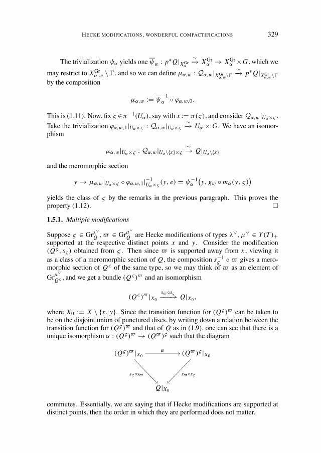
where X0 := X \ {x, y}. Since the transition function for (Q& )$ can be taken tobe on the disjoint union of punctured discs, by writing down a relation between thetransition function for (Q& )$ and that of Q as in (1.9), one can see that there is aunique isomorphism ↵ : (Q& )$ ! (Q$ )& such that the diagram
(Q& )$ |X0↵
//
s&�s$��
>
>
>
>
>
>
>
>
>
>
>
(Q$ )& |X0
s$ �s&���
�
�
�
�
�
�
�
�
�
�
Q|X0
commutes. Essentially, we are saying that if Hecke modifications are supported atdistinct points, then the order in which they are performed does not matter.
330 MICHAEL LENNOX WONG
For k � 2, consider the k-fold product Xk and the projection pi : Xk ! Xonto the i th factor. For i < j , we then get the projections onto two factors (pi , p j ) :Xk ! X ⇥ X . We let 1i j := (pi , p j )�1(1), and set
1k :=[
1i< jk1i j ✓ Xk = {(x1 . . . , xk) 2 Xk : xi = x j for some 1 i, j k},
so that 1k is the “fat” diagonal. Note that 1k is a divisor on Xk .Let �_
1 , . . . , �_k 2 Y (T )+. If ⇡i : Gr�
_iQ ! X is the projection map, then we
can form the product map
⇡1 ⇥ · · · ⇥ ⇡k : Gr�_1Q ⇥ · · · ⇥ Gr�
_kQ ! Xk,
and so we may consider the divisor
e1k := (⇡1 ⇥ · · · ⇥ ⇡k)�1(1k) ✓ Gr�
_1Q ⇥ · · · ⇥ Gr�
_kQ .
We will let
Gr�_1 ,··· ,�_
kQ,0 := Gr�
_1Q ⇥ · · · ⇥ Gr�
_kQ \ e1k,
so that Gr�_1 ,··· ,�_
kQ,0 consists of k-tuples of Hecke modifications of Q supported at
distinct points. Set
0k := (1X ⇥ ⇡1 ⇥ · · · ⇥ ⇡k)�1(1k+1) ✓ X ⇥ Gr�
_1 ,··· ,�_
kQ,0 .
We will let p : X ⇥ Gr�_1 ,··· ,�_
kQ,0 ! X and qi : X ⇥ Gr�
_1 ,··· ,�_
kQ,0 ! Gr�
_iQ denote
the relevant projection maps. A universal sequence of Hecke modifications of Qsupported at distinct points will be a G-bundleQ(�_
1 , . . . , �_k ) over X ⇥Gr�
_1 ,··· ,�_
kQ,0
and an isomorphism
µ : Q(�_1 , . . . , �_
k )|XGr0⇠�! p⇤Q|XGr0
, (1.15)
where XGr0 := X ⇥ Gr�_1 ,··· ,�_
kQ,0 \ 0k , for which
�Q(�_1 , . . . , �_
k )(&1,...,&k), µ(&1,...,&k)� ⇠= (Q&1···&k , s&k � · · · � s&1), (1.16)
for all (&1, . . . , &k) 2 Gr�_1 ,··· ,�_
kQ,0 . One has analogous results as above.
HECKE MODIFICATIONS, WONDERFUL COMPACTIFICATIONS 331
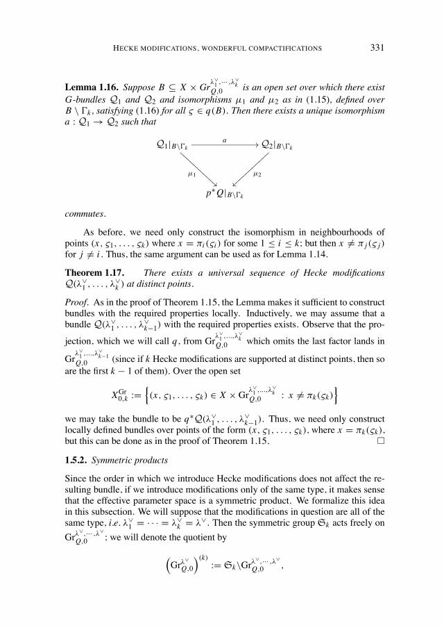
Lemma 1.16. Suppose B ✓ X ⇥ Gr�_1 ,··· ,�_
kQ,0 is an open set over which there exist
G-bundles Q1 and Q2 and isomorphisms µ1 and µ2 as in (1.15), defined overB \ 0k , satisfying (1.16) for all & 2 q(B). Then there exists a unique isomorphisma : Q1 ! Q2 such that
Q1|B\0ka
//
µ1
A
A
A
A
A
A
A
A
A
A
A
Q2|B\0k
µ2~~}
}
}
}
}
}
}
}
}
}
}
p⇤Q|B\0k
commutes.
As before, we need only construct the isomorphism in neighbourhoods ofpoints (x, &1, . . . , &k) where x = ⇡i (&i ) for some 1 i k; but then x 6= ⇡ j (& j )for j 6= i . Thus, the same argument can be used as for Lemma 1.14.
Theorem 1.17. There exists a universal sequence of Hecke modificationsQ(�_
1 , . . . , �_k ) at distinct points.
Proof. As in the proof of Theorem 1.15, the Lemma makes it sufficient to constructbundles with the required properties locally. Inductively, we may assume that abundle Q(�_
1 , . . . , �_k�1) with the required properties exists. Observe that the pro-
jection, which we will call q, from Gr�_1 ,...,�_
kQ,0 which omits the last factor lands in
Gr�_1 ,...,�_
k�1Q,0 (since if k Hecke modifications are supported at distinct points, then so
are the first k � 1 of them). Over the open set
XGr0,k :=n(x, &1, . . . , &k) 2 X ⇥ Gr�
_1 ,...,�_
kQ,0 : x 6= ⇡k(&k)
o
we may take the bundle to be q⇤Q(�_1 , . . . , �_
k�1). Thus, we need only constructlocally defined bundles over points of the form (x, &1, . . . , &k), where x = ⇡k(&k),but this can be done as in the proof of Theorem 1.15.
1.5.2. Symmetric products
Since the order in which we introduce Hecke modifications does not affect the re-sulting bundle, if we introduce modifications only of the same type, it makes sensethat the effective parameter space is a symmetric product. We formalize this ideain this subsection. We will suppose that the modifications in question are all of thesame type, i.e. �_
1 = · · · = �_k = �_. Then the symmetric groupSk acts freely on
Gr�_,··· ,�_
Q,0 ; we will denote the quotient by
⇣Gr�
_
Q,0
⌘(k):= Sk\Gr�
_,··· ,�_
Q,0 ,
332 MICHAEL LENNOX WONG
and can think of it as unordered k-tuples of Hecke modifications supported at dis-tinct points. Observe that the projection map ⇡ ⇥ · · · ⇥ ⇡ : Gr�
_,··· ,�_
Q,0 ! Xk theninduces a map
⇡ (k) :⇣Gr�
_
Q,0
⌘(k)! X (k)
to the kth symmetric product of X , which we may identify with the space of effec-tive degree k divisors on X . Since we are considering tuples of modifications withsupport at distinct points, it follow that the image is the open set of X (k) consistingof reduced divisors.
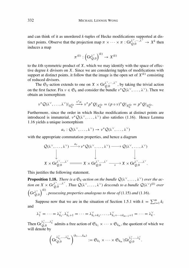
The Sk-action extends to one on X ⇥ Gr�_,··· ,�_
Q,0 , by taking the trivial actionon the first factor. Fix ⌫ 2 Sk and consider the bundle ⌫⇤Q(�_, . . . , �_). Then weobtain an isomorphism
⌫⇤Q(�_, . . . , �_)|XGr0⌫⇤µ��! ⌫⇤ p⇤Q|XGr0
= (p � ⌫)⇤Q|XGr0= p⇤Q|XGr0
.
Furthermore, since the order in which Hecke modifications at distinct points areintroduced is immaterial, ⌫⇤Q(�_, . . . , �_) also satisfies (1.16). Hence Lemma1.16 yields a unique isomorphism
a⌫ : Q(�_, . . . , �_) ! ⌫⇤Q(�_, . . . , �_)
with the appropriate commutation properties, and hence a diagram
Q(�_, . . . , �_)a⌫
//
✏✏
⌫⇤Q(�_, . . . , �_) //
✏✏
Q(�_, . . . , �_)
✏✏
X ⇥ Gr�_,...,�_
Q,0 X ⇥ Gr�_,...,�_
Q,0 ⌫// X ⇥ Gr�
_,...,�_
Q,0 .
This justifies the following statement.
Proposition 1.18. There is a Sk-action on the bundle Q(�_, . . . , �_) over the ac-tion on X ⇥ Gr�
_,...,�_
Q,0 . Thus Q(�_, . . . , �_) descends to a bundle Q(�_)(k) over⇣Gr�_
Q,0
⌘(k), possessing properties analogous to those of (1.15) and (1.16).
Suppose now that we are in the situation of Section 1.5.1 with k =Pm
i=1 kiand
�_1 = · · · = �_
k1, �_k1+1 = · · · = �_
k1+k2, . . . , �_k1+···+km�1+1 = · · · = �_
k .
Then Gr�_1 ,...,�_
kQ,0 admits a free action ofSk1 ⇥ · · · ⇥ Skm , the quotient of which we
will denote by✓Gr�_k1
,...,�_km
Q,0
◆(k1,...,km)
:= Sk1 ⇥ · · · ⇥ Skm\Gr�_1 ,...,�_
kQ,0 .
HECKE MODIFICATIONS, WONDERFUL COMPACTIFICATIONS 333
This carries a projection to X (k1) ⇥ · · ·⇥ X (km) which carries a further projection to
X (k). Then (Gr�_k1
,...,�_km
Q,0 )(k1,...,km) is precisely the subset of
✓Gr�_k1Q,0
◆(k1)⇥ · · · ⇥
✓Gr�_m1Q,0
◆(km)
that maps to the set of reduced divisors in X (k).The same arguments as above allow us the following.
Proposition 1.19. There is an action ofSk1 ⇥ · · ·⇥Skm onQ(�_1 , . . . , �_
k ) which
lifts the action on Gr�_1 ,...,�_
kQ,0 . There is a universal Hecke modification (i.e. bundle
satisfying (1.15) and (1.16))Q(�_k1, . . . , �
_km )(k1,...,km) over
✓Gr
�_k1
,...,�_km
Q,0
◆(k1,...,km)
.
2. Overview of the wonderful compactification
2.1. Construction of the compactification
We will now assume that G is semisimple of adjoint type. We will use the samenotation as in Section 1.1; for our choice of Borel subgroup B = B+ ✓ G, itsopposite Borel is denoted B�, and their respective unipotent radicals by U+ ✓ Band U� ✓ B�.
The compactification G of G is constructed as follows. Let V be a regular irre-ducible representation of the universal cover G of G with highest weight � (regular-ity means that h�,↵_
i i > 0 for 1 i l) and define a map : G ,! P(End V ) by
g 7! [g],
where g 2 G is a lift of g and [ ] indicates the class in the projectivization. Then Gis defined as the closure of (G) in P(End V ). We will often identify an elementof G with its image in G, which will usually mean abbreviating (g) to g.
There is a natural (G ⇥ G)-action on G given by
(g, h) · ['] = [g'h�1].
We may realize this as separate G-actions, which we will call the left and rightG-actions, corresponding to the action of the first and second factors of G ⇥ G,respectively. We will denote these actions G ⇥ G ! G by L and R, respectively.Remark 2.1. While we call R the “right” action, h 2 G acts by (e, h) which takes['] to ['h�1], so it is in fact a left action, in the sense that we obtain a homomor-phism G ! AutG, rather than an anti-homomorphism, but we say “right” sincewe mean right multiplication.
334 MICHAEL LENNOX WONG
2.1.1. The open affine piece
We choose a basis v0, . . . , vn of weight vectors of V , say with vk of weight �k insuch a way that
1. v0 is a highest weight vector (hence of weight �); and2. v1, . . . , vl are of weights �1 = �� ↵1, . . . , �l = �� ↵l , respectively.
The remaining weights are of the form �k = � �Pnik↵i for some non-negative
integers nik . Let
P0 = {['] 2 P(End V ) | v⇤0('v0) 6= 0}.
If ' =Pai jvi ⌦ v⇤
j , then P0 consists of precisely those ['] with a00 6= 0. Thus P0is a standard open affine subset of P(End V ) using the basis vi ⌦ v⇤
j of End V . LetG0 := G \ P0; then G0 is an open affine subset of G.
Lemma 2.2. [3, Lemma 2.6] G0 \ (G) = (U�TU+).
We write Z := (T )\P0. Let t 2 T and t 2 T be a lift, where T is a maximaltorus of G mapping onto T . Then if we write 'k for vk ⌦ v⇤
k , we have
t � 'k = t � vk ⌦ v⇤k = �k(t)vk ⌦ v⇤
k = �k(t)'k,
so
(t) = [t]=[t � e]=
"nX
k=0�k(t)'k
#
=
"
'0 +lX
i=1
1↵i (t)
'i +X
k>l
Y 1↵i (t)nik
'k
#
.
(2.1)
Since any two lifts of t differ by an element of Z(G), which is precisely the inter-section of the ker ↵i , 1 i l, the values ↵i (t) are independent of the choice oflift, so we are justified in dropping the tildes from the notation.
Since G is adjoint, X (T ) = 3r , so 1 is a basis of characters of T , hencewe may take zi = 1/↵i (t), 1 i l as coordinates on T , and define a mapF : (C⇥)l ! Z by
(z1, . . . , zl) 7!
"
'0 +lX
i=1zi 'i +
X
k>l
Yzniki 'k
#
. (2.2)
Clearly, this extends to an isomorphism Cl ⇠�! Z which we will also denote by F .
To lighten notation, we will define
pk = pk(z1, . . . , zl) :=
(zk 1 k lQl
i=1 zniki k > l,
HECKE MODIFICATIONS, WONDERFUL COMPACTIFICATIONS 335
so that F may be written somewhat more compactly as
(z1, . . . , zl) 7!
"
'0 +nX
k=1pk'k
#
.
The following statement gives a parametrization of the open affine piece just de-scribed that will be basic to the computations in our deformation theory later.
Theorem 2.3. [3, Theorem 2.8] The map A : U� ⇥U+ ⇥ Z ⇠�! G0 given by
(u�, u+, t) 7! (u�, u+) · [t] = [u�tu�1+ ]
is an isomorphism. Hence G0 ⇠= Cdim G .
The structure of the (G ⇥ G)-orbits of G has a ready description, and orbitrepresentatives can be chosen in the closure of the torus.
Theorem 2.4. [3, Theorem 2.22] The compactification G is the union of the (G⇥G)-translates of G0. In fact, the (G ⇥ G)-orbit structure of G can be described asfollows. For a subset I ✓ 1, set
zI := F(✏1, . . . , ✏l),
where ✏i = 1 if ↵i 62 I and ✏i = 0 if ↵i 2 I . Then
G =a
I✓1(G ⇥ G) · zI ,
so G is the union of 2l (G ⇥ G)-orbits. Also, G ✓ G corresponds to the (open)orbit of z; = e.
2.2. The infinitesimal action on TG
2.2.1. The action at a point
We now fix a point z = F(z1, . . . , zl) 2 Z and give an explicit description of thedifferentials dR, dL : g ! TzG. The isomorphism A : U� ⇥ U+ ⇥ Z ! G0 ofTheorem 2.3 yields an isomorphism of tangent spaces
d A(e,e,z) : T (U� ⇥U+ ⇥ Z) = u� � u+ � Cl ! TzG0 = TzG,
which we may use to obtain a basis for TzG. We will shorten to R, L the mapsRz, Lz : G ! G given by
Rz(g) = g · z, Lz(g) = z · g.
We will also abbreviate d A(e,e,z) to d A.
336 MICHAEL LENNOX WONG
For ↵ 2 8+, we will let x↵ 2 g↵, y↵ 2 g�↵, h↵ = ↵_ 2 t be a standardsl(2) triple, so that {x↵ |↵ 2 8+} is a basis for u+, {y↵ |↵ 2 8+} one for u�,{h↵ |↵ 2 1} one for t. A basis for TzG is given by
{d A(x↵), d A(y↵) |↵ 2 8+} [ {d A(e j ) | 1 j l}. (2.3)
Observe that
d A(y↵) = dR(y↵), d A(x↵) = �dL(x↵). (2.4)
Since z lies in G0 ✓ P0, we will identify TzG with a subspace of TzP0, and sinceP0 is the standard open affine piece of PEnd V with a00 6= 0, we may identify itwith the vector space spanned by vi ⌦ v⇤
j with (i, j) 6= (0, 0).We will now be more explicit about the maps dL , dR. If ⇠ 2 u� or u+ we
obtain
dL(⇠)=dd✏
����✏=0
z exp(✏⇠)=dd✏
����✏=0
⇥z � exp(✏⇠)
⇤=
dd✏
����✏=0
[z + ✏(z � ⇠)]= z � ⇠.
Here we are identifying z 2 G with the endomorphism of V it represents (as atangent vector with reference to the identifications made above). Observe that theterms of z � ⇠ will be of the form vi ⌦ v⇤
i � ⇠ and hence there is no ✏ term involvingv0 ⌦ v⇤
0 , so we are using the appropriate affine coordinates in which we are takingthe derivative. Now, if ⇠ 2 t, the right action on 'k is
'k � ⇠ = �vk ⌦ ⇠(v⇤k ) = h⇠, �kivk ⌦ v⇤
k = h⇠, �ki'k .
Therefore the infinitesimal action of ⇠ 2 t on z looks like
dL(⇠)=dd✏
����✏=0
"�1+ ✏h⇠, �i
�'0 +
nX
k=1
�1+ ✏h⇠, �ki
�pk'k
#
=dd✏
����✏=0
"
'0 +nX
k=1
⇥1+ ✏
�h⇠, �ki � h⇠, �i
�⇤pk'k
#
=nX
k=1h⇠, �k � �ipk'k =�
lX
i=1h⇠,↵i izi'i +
X
k>l
*
⇠,lX
i=1nik↵i
+lY
i=1zniki 'k
!
Note that we need to normalize the coefficient of '0 = v0⌦v⇤0 . We can repeat these
calculations for dR as well and sum up our results in the following.
Lemma 2.5. Explicit descriptions of the infinitesimal action can be given by
dL(⇠) =
8><
>:
z � ⇠ ⇠ 2u�� u+
�
lX
i=1h⇠,↵i izi'i +
X
k>l
*
⇠,lX
i=1nik↵i
+lY
i=1zniki 'k
!
⇠ 2 t
HECKE MODIFICATIONS, WONDERFUL COMPACTIFICATIONS 337
and
dR(⇠) =
8><
>:
⇠ � z ⇠ 2u� � u+
�
lX
i=1h⇠,↵i izi'i +
X
k>l
*
⇠,lX
i=1nik↵i
+lY
i=1zniki 'k
!
⇠ 2 t.
By (2.4), this gives expressions for d A(y↵), d A(x↵). Finally, d A(e j ) can be com-puted as
d A(e j ) =dd✏
����✏=0
F(z1, . . . , z j + ✏, . . . , zl) = ' j +X
k>l
@pk@z j
'k .
This allows us to write down the image of the infinitesimal action of t in terms ofthe basis (2.3) for TzG. We will let hi := h↵i = ↵_
i for 1 i l, so that theh1, . . . , hl give a basis for t. By Lemma 2.5, using the fact that for a weight µ,µ(h↵) = h↵_, µi, we get
dL(hi ) = dR(hi ) = �lX
j=1ai j z j d A(e j ),
where (ai j ) = (h↵_i ,↵ j i) is the Cartan matrix.
Wewould also like to write dL(y↵) in terms of the basis vectors dA(x↵), dA(y↵)and d A(e j ) for TzG. Assume first that z 2 T ✓ G; then since ↵ =
Pli=1h�
_i ,↵i↵i
dL(y↵) = dR � Ad z(y↵) = ↵(z)�1dR(y↵) =lY
i=1zh�
_i ,↵i
i d A(y↵).
By continuity, the formula must also hold for any z 2 Z . We repeat for dR(x↵) andsummarize our findings as follows.
Lemma 2.6. The infinitesimal actions in terms of the bases for g and TzG chosenabove are given by
dL(x↵)=�d A(x↵), dL(y↵)=lY
i=1zh�
_i ,↵i
i d A(y↵), dL(hi )=�lX
j=1ai j z j d A(e j ),
and
dR(x↵)=�lY
i=1zh�
_i ,↵i
i d A(x↵), dR(y↵)=d A(y↵), dR(hi )=�lX
j=1ai j z j d A(e j ).
338 MICHAEL LENNOX WONG
2.2.2. Weyl twists
Let z 2 Z ✓ T be as in the previous subsection. Recall that the Weyl groupW = NG(T )/T acts on T and hence on T . However, if z 62 T and ⌫ 2 W is notthe identity, then ⌫ · z 62 G0. In any case, if w 2 NG(T ) is a representative for ⌫,then ⌫ · z lies in the open affine set wG0w�1. Composing the isomorphism A withconjugation by w gives an isomorphism A⌫ : U� ⇥U+ ⇥ Z ! wG0w�1:
(u�, u+, z) 7! [wu�zu�1+ w�1] =
h�Adw(u�)
�(⌫ · z)
�Adw(u�1
+ )�i
.
Since Adw�1 gives an automorphism of u� � u+, we can take
{d A⌫(Adw�1x↵), d A⌫(Adw�1y↵) |↵ 2 8+} [ {d A⌫(ei ) | 1 i l}
as a basis of T⌫zG.We may now compute the infinitesimal actions as in Lemma 2.6 using this
basis. We have for ⇠ 2 u� � u+,
dL⌫·z(⇠) =dd✏
����✏=0
wzw�1 exp(✏⇠) =dd✏
����✏=0
wz exp(✏Adw�1⇠)w�1.
If ↵ 2 ⌫8+, then ⌫�1↵ 2 8+ and Adw�1x↵ is a positive root vector, so
dL⌫·z(x↵) =dd✏
����✏=0
A⌫(e, exp(�✏Adw�1x↵), z) = �d A⌫(Adw�1x↵).
Also,
dL⌫·z(y↵) =dd✏
����✏=0
w exp(✏Adzw�1y↵)zw�1
=dd✏
����✏=0
A⌫�exp(✏Adzw�1y↵), e, z
�
= d A⌫(Ad z � Adw�1y↵) = (⌫�1↵)(z)�1d A⌫(Adw�1y↵)
=lY
i=1zh�
_i ,⌫�1↵i
i d A⌫(Adw�1y↵).
We record this here.
Lemma 2.7. If z 2 Z , ⌫ 2 W and w 2 NG(T ) is a chosen representative for ⌫,then the infinitesimal action of the root vectors on ⌫ · z is given by
dL⌫·z(x↵) = �d A⌫(Adw�1x↵), dL⌫·z(y↵) =lY
i=1zh�
_i ,⌫�1↵i
i d A⌫(Adw�1y↵).
HECKE MODIFICATIONS, WONDERFUL COMPACTIFICATIONS 339
2.2.3. Transposes
Returning back to the situation where z 2 Z , we obtain the following mirror imagesto the infinitesimal action maps, which will be useful in the sequel.
Lemma 2.8. With respect to the basis dual to that used above the transposes of theinfinitesimal actions, dLt , dRt : T ⇤
zI G ! g⇤ are given by
dLt�d A(x↵)⇤
�= �x⇤
↵,
dLt�d A(y↵)⇤
�=
lY
i=1zh�
_i ,↵i
i y⇤↵,
dLt�d A(ei )⇤
�= �zi
lX
j=1a ji h⇤
j .
and
dRt (d A(x↵)⇤) = �lY
i=1zh�
_i ,↵i
i x⇤↵,
dRt (d A(y↵)⇤) = y⇤↵,
dRt (d A(ei )⇤) = �zilX
j=1a ji h⇤
j .
Recall that the Killing form gives a Ad-invariant non-degenerate symmetric pair-ing on g and hence gives an Ad-equivariant isomorphism : g⇤ ! g. For ↵ 2 8+,there will be c↵ 2 C⇥ such that
(x⇤↵) = c↵ y↵, (y⇤
↵) = c↵x↵,
It is straightforward to see that in the case g 2 G, the maps
T ⇤g G
dLtg
dRtg// g⇤
// gdLgdRg
// TgG.
agree. For in this case Lg = Rg � Ad g and hence
dLg � � dLtg = dRg � Ad g � � (dRg � Ad g)t
= dRg � Ad g � � (Ad g�1)⇤ � dRtg= dRg � � dRtg.
In fact, this is true at any point of G.
340 MICHAEL LENNOX WONG
Proposition 2.9. If a 2 G, then the maps
T ⇤a G
dL⇤
dR⇤// g⇤
// g dLdR
// TaG
agree.
Proof. If a 2 Z , it is straightforward to verify this using the expressions in Lemmas2.6 and 2.8. In general, we may write a = gzh for some g, h 2 G, z 2 Z , use theequalities
La = Lg � Lz � Lh, Ra = Rh � Rz � Rg,
and the fact that R, L commute.
2.3. Extension of the inversion map to G
We show that if ◆ : G ! G is the inversion map taking g to g�1, then it extendsto an involution ◆ : G ! G. The idea is as follows. We consider an open affineset G! of G, this time built from the lowest weight vector rather than the highestweight vector. Then we construct an isomorphism of Cl ⇠= Z ✓ G0 onto a subsetW ✓ G!, and then show that inversion in T extends to Z . We can then extend itfrom G0 to G! and from there to all of G by using the (G ⇥ G)-action on G.
LetW denote theWeyl group corresponding to T and let ! 2 W be (the uniqueelement) such that !(1) = �1; write
!(↵i ) = �↵!i ,
where we are using ! also to denote the permutation of the indices. Note that!2 = 1.
Now, !� will be a lowest weight vector for V . By relabelling, we may assumethat �n = !�. Further, for 1 i l, we may also assume
�n�i = !�i = !(�� ↵i ) = �n + ↵!i .
We now set
P! := {['] 2 P(End V ) | v⇤n('vn) 6= 0}
and let G! := G \ P!. Then as for Lemma 2.2, we can show that
G! \ (G) = (U+TU�)
and that ⌫ : U+ ⇥U� ⇥ W ! G! given by
(v+, v�, s) = [v+sv�1� ]
is an isomorphism.
HECKE MODIFICATIONS, WONDERFUL COMPACTIFICATIONS 341
Repeating the calculation of (2.1) above, if t 2 T and t 2 T is a lift, then
(t) =
"X
k<n�l
lY
i=1↵!i (t)mik'k +
lX
i=1↵!i (t)'n�i + 'n
#
,
where if k < n � l, then �k = �n +Pmik↵!i with the mik � 0.
We let W := (T ) \ P!. Then as in (2.2), we can construct an isomorphismH : Cl ! W :
(w1, . . . , wl) 7!
"X
k<n�l
lY
i=1wmiki 'k +
lX
i=1wi'n�i + 'n
#
.
We now define a : Cl ! Cl by
(z1, . . . , zl) 7! (z!1, . . . , z!l).
Then ◆ := H � a � F�1 gives an isomorphism Z ! W and if t 2 T , we may verifythat
◆(t) = H � a � F�1(t) = t�1
by writing
t =
"
'0 +nX
k=1
lY
i=1↵i (t�1)nik'k
#
,
and using the definitions of the nik,mik .We can extend this map to ◆ : G0 ⇠= U� ⇥U+ ⇥ Z ! G! ⇠= U+ ⇥U� ⇥W
by
◆([u�tu�1+ ]) = [u+◆(t)u�1
� ].
We observe that if g 2 G \ X0, then ◆(g) = g�1.To extend ◆ to all of G, we will need the following lemma, which can be proved
in the same way as Proposition 2.25 of [3] by replacing v0 by vn where appropriate.
Lemma 2.10. Let zI be as in Theorem 2.4. If we define wI := ◆(zI ), then (g, h) 2(G ⇥ G)zI if and only if (h, g) 2 (G ⇥ G)wI .
The extension of ◆ to all of G now proceeds straightforwardly as follows. Fora 2 G, let (g, h) 2 G ⇥ G be such that (g, h) · zI = a (Theorem 2.4). We define
◆(a) := (h, g) · wI = (h, g) · ◆(zI ).
The Lemma above guarantees that this is well-defined.
342 MICHAEL LENNOX WONG
Observe that if a 2 G, then a = (a, e) · e = (a, e) · z;, so
◆(a) = (e, a) · w; = (e, a) · e = a�1.
So ◆ does indeed restrict to the inversion map on G. From this it follows that ◆2 isthe identity on an open dense subset of G, so this holds on all of G; that is, ◆ is aninvolution. Further, if3(g,h) denotes the map G ! G given by the action of (g, h):
a 7! (g, h) · a,
then we have ◆ � 3(g,h) = 3(h,g) � ◆ on the open dense set G ✓ G and again thismust hold on G. We now summarize our results.
Proposition 2.11. There exists an involution ◆ : G ! G such that if a 2 G, then
◆(a) = a�1
and
◆�(g, h) · a
�= (h, g) · ◆(a)
for all a 2 G, (g, h) 2 G ⇥ G.
3. Deformation theory using the compactifications
3.1. Constructions
Here we explain how the wonderful compactification can be used to compactifythe fibres of a principal bundle. We may then map Hecke modifications of theoriginal bundle into this compactified bundle. The deformation space we want willbe the quotient of vector bundles derived from this constructions. First, we beginby setting down some notational conventions.
3.1.1. Conventions and notation
We will take X and G as before and fix a G-bundle Q. If : Q|U⇠�! U ⇥ G is a
trivialization of Q over an open U ✓ X , we will denote the corresponding sectionby b : U ! Q|U , so that
b(y) = �1(y, e)
for y 2 U . When subscripts are used on , they will likewise be appended to thecorresponding b.
Since our discussion will centre around Hecke modifications, we will oftenhave occasion to trivialize Q on the complement X0 of a point x 2 X , say via 0.
HECKE MODIFICATIONS, WONDERFUL COMPACTIFICATIONS 343
If X1 is a neighbourhood of x over which 1 : Q|X1 ! X1 ⇥ G is a trivialization,then the transition function h01 : X01 ! G satisfies
0 � �11 (y, g) =
�y, h01(y)g
�.
If we sethi := pG � i : Q|Xi ! G,
where pG : Xi ⇥ G ! G is the projection, then we haveb0(y)h01(y) = b1(y), q = bi
�⇡(q)
�hi (q), hi � b j (y) = hi j (y) (3.1)
for y 2 X, q 2 Q, wherever the expressions make sense.For a bundle P , we will typically call its trivializations 'i : P|Xi ! Xi ⇥ G,
the corresponding sections ai : Xi ! P|Xi , its transition function g01, and theG-components gi := pG � 'i . The relations (3.1) hold mutatis mutandis.
3.1.2. Compactifying bundles
Since the principal bundle Q comes with fibres isomorphic to G, we may wish touse the compactification G to compactify the fibres of Q. Recall that G comes withboth a left and right G-action (see Section 2.1). We form the associated bundleQ := Q ⇥G G using the left action, i.e. we take
(q, a) ⇠ (q · g, g�1a) = (q · g, Lg�1a).
The equivalence class of (q, a) will be denoted [q : a]. Then Q still admits a rightaction
[q : a] · g = [q : ag] = [q : Rg�1a].This achieves the compactification of the fibres of Q suggested above. We have anatural inclusion Q ,! Q explicitly given by
q 7! [q : e],which is equivariant with respect to the right action.Remark 3.1. One will observe that the action of g 2 G on Q is via Rg�1 . Re-call from Remark 2.1 that R is really a left action—in the sense that we obtain ahomomorphism G ! Aut(G), and hence one G ! Aut(Q), rather than an anti-homomorphism—so putting in the inverse legitimately turns it into a right actionwhich coincides with right multiplication on G and hence with the (right) action ofG on Q, considered as a subvariety of Q.
By an automorphism of Q we mean an equivariant bundle automorphism (i.e.,covering the identity) over X . An automorphism of Q determines one of any associ-ated bundle and hence one of Q. On the other hand, any equivariant automorphismof Q maps Q to Q, so restricting to Q allows us to recover the automorphism of Qfrom which the one of Q arises.Lemma 3.2. We may identify
Aut Q = Aut Q.
344 MICHAEL LENNOX WONG
3.1.3. Compactification and Hecke modifications
Let X,G, Q, Q, x 2 X, X0 be as above. Let & 2 Gr�_
Q (x) ✓ Gr�_
Q be a Heckemodification of Q of type �_ supported at x . Let P = P& be the bundle we obtainand
s : P|X0⇠�! Q|X0
the given isomorphism (1.8). Recall that a choice of trivialization 1 of Q in aneighbourhood X1 of x over which a representative of & is defined identifies & withan element of GrG(x, �_). A choice of trivialization '1 of P|X1 then allows us towrite
1 � s � '�11 = 1X01 ⇥ L�
for some holomorphic � : X01 ! G which will then be a representative for & .Since X01 := X1\{x} and G is complete, � extends uniquely to a holomorphic
map X1 ! G which we will also denote by � . This extension allows us to define amap P ! Q, which we also denote by s, by
s(p) =
( �10 � '0(p) if ⇡P(p) 2 X0 �11 � (1⇥ L� ) � '1(p) if ⇡P(p) 2 X1,
where L� means left multiplication by � . Using (1.9), it is elementary to see thats is well-defined. Further, we may observe that s extends the isomorphism of P|X0onto Q|X0 ✓ Q|X0 and is equivariant with respect to the right action, since thetrivializations and 1⇥ L� all commute with the right action.
3.1.4. The dual construction
Since everything we have done so far is symmetric in P and Q, we may turn itall aroundand consider the map ⌧ := ��1 = ◆� : X01 ! G, which must extenduniquely to a map ⌧ : X1 ! G. Since the relation between transition functionsof P and Q above can be rewritten as h01 = g01��1 = g01⌧ , we may likewiseconstruct a map t = ◆s : Q ! P , which will be an isomorphism of Q|X0 ontoP|X0 .
3.2. Deformation theory
3.2.1. A local description of the deformation space
We now consider the deformation theory of the construction given in the precedingsubsection. We begin concretely with a local description of infinitesimal deforma-tions. Since the map s : P ! Q is given locally by � : X1 ! G, an infinitesimaldeformation of s is determined by one of � . The latter is given by a section of� ⇤TG over X1. Since what is important is the class of � in GrG(x, �_), trivial
HECKE MODIFICATIONS, WONDERFUL COMPACTIFICATIONS 345
changes to � are given by right multiplication by elements of G (X1), i.e. holomor-phic G-valued functions over X1. Therefore, the trivial deformations are preciselythose arising from the infinitesimal right action of g on G.
Here and later, we will use the following notation: if Y is a space with structuresheaf O Y , then for any (finite-dimensional) vector space W , we will write OW
Y forthe sheaf of W -valued functions on Y .
Since G is open and dense in G and is acted upon freely by the right action, theinfinitesimal right action gives an inclusion of sheaves dR : O
g
G! TG. Pulling
back via � : X1 ! G we get another inclusion of sheaves on X1:
OgX1 = � ⇤O
g
G� ⇤dR���! � ⇤TG. (3.2)
If we denote by u⇠ the fundamental vector field on G generated by the right in-finitesimal action of ⇠ 2 g, then the image of (y, ⇠) 2 X1 ⇥ g is
u⇠�� (y)
�= dL� (y)(⇠). (3.3)
Therefore, the non-trivial deformations are given by sections of0(X1, � ⇤TG)mod-ulo those of the form just given; so we may identify our deformation space with
0(X1, � ⇤TG)/0(X1,OgX1). (3.4)
Since � (X01) ✓ G, � ⇤dR is an isomorphism on X01 and so the quotient will besupported at x . Since � is holomorphic at x , the space of sections will be finite-dimensional.
3.2.2. Invariant construction of the deformation space
We now describe the infinitesimal deformation space of in terms of the bundlesP, Q and various associated cohomology groups. In what follows, v⇠ , w⇠ will de-note the fundamental vector fields determined by ⇠ 2 g on P (or P), and Q (or Q),respectively.
We now realize the space of infinitesimal deformations of s as the global sec-tions of a torsion sheaf on X , depending on P and Q, which requires the followingconstruction to define. If ⇡P ,⇡Q are the projection maps to X , we let
V P := ker d⇡P , V Q := ker d⇡Q
be the respective vertical tangent bundles. Then since ⇡P = ⇡Q � s, we haveds(V P) ✓ V Q and there is a map of sheaves ds : V P ! s⇤V Q on P . Explicitly,this map is
v⇠ (p) 7!�p, ds(v⇠ (p))
�=�p, w⇠ (s(p))
�,
346 MICHAEL LENNOX WONG
where we are realizing s⇤V Q as
s⇤V Q = {(p, w) 2 P ⇥ V Q |w 2 Vs(p)Q}.
Since ⇡P ,⇡Q are G-invariant maps, V P and V Q are G-invariant sub-bundles ofT P and T Q, respectively, so they admit G-actions, linear on the fibres, for whichds is equivariant (since s is). Quotienting, we get a map of sheaves on X ,
V P/G = ad Pds/G���! s⇤V Q/G =: EPQ .
Since s⇤V Q = {(p, w) |w 2 Vs(p)Q}, we may concretely write ds/G : ad P !EPQ as
[p : ⇠ ] 7!⇥p : w⇠
�s(p)
�⇤.
3.2.3. Trivializations for EPQ
We now describe trivializations for the bundle EPQ just constructed to specify thelink between the local description of the infinitesimal deformation space and thebundle EPQ in the previous subsection, and also to facilitate later calculations. Webegin by giving trivializations for the bundle s⇤V Q on P , and then using these toobtain trivializations for EPQ . We will make heavy use of the notation of Section3.1.1 and will often write E for EPQ when no confusion will arise.
Since s|X0 is an isomorphism of P|X0 onto the open subset Q|X0 of Q|X0 ,we get an isomorphism ds|X0 : V P|X0
⇠�! s⇤V Q|X0 , and so the trivialization
P|X0 ⇥ g ! V P|X0 extends to one ↵�10 : P|X0 ⇥ g ! s⇤V Q|X0 by composing
with ds:
(p, ⇠) 7!�p, w⇠ (s(p))
�.
The vertical tangent bundle on the trivial G-bundle X1 ⇥ G is given by
V (X1 ⇥ G) = p⇤GTG,
where pG : X1 ⇥ G ! G is the projection. Then the trivialization 1 : Q|X1 !
X1 ⇥ G induces an isomorphism V Q|X1⇠�! ⇤
1 p⇤GTG = h⇤
1TG:
w 2 VqQ 7!�q, dh1(w)
�,
noting dh1(w) 2 Th1(q)G. We pull this isomorphism back to P via s to obtain anisomorphism ↵1 : s⇤V Q|X1 ! s⇤h⇤
1TG|X1 = (h1 � s)⇤TG|X1 :
(p, w) 7!�p, dh1(w)
�.
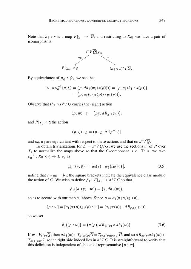
HECKE MODIFICATIONS, WONDERFUL COMPACTIFICATIONS 347
Note that h1 � s is a map P|X1 ! G, and restricting to X01 we have a pair ofisomorphisms
s⇤V Q|X01↵0
zzu
u
u
u
u
u
u
u
u
↵1
%%
K
K
K
K
K
K
K
K
K
K
P|X01 ⇥ g (h1 � s)⇤TG.
By equivariance of pG � 1, we see that
↵1 � ↵�10 (p, ⇠) =
�p, dh1(w⇠ (s(p)))
�=�p, u⇠ (h1 � s(p))
�
=�p, u⇠ (� (⇡(p)) · g1(p))
�.
Observe that (h1 � s)⇤TG carries the (right) action
(p, w) · g =�pg, dRg�1(w)
�,
and P|X0 ⇥ g the action
(p, ⇠) · g = (p · g,Ad g�1 ⇠)
and ↵0,↵1 are equivariant with respect to these actions and that on s⇤V Q.To obtain trivializations for E = s⇤V Q/G, we use the sections ai of P over
Xi to normalize the maps above so that the G-component is e. Thus, we take��10 : X0 ⇥ g ! E |X0 as
��10 (y, ⇠) =
⇥a0(y) : w⇠
�b0(y)
�⇤, (3.5)
noting that s � a0 = b0; the square brackets indicate the equivalence class modulothe action of G. We wish to define �1 : E |X1 ! � ⇤TG so that
�1�[a1(y) : w]
�=�y, dh1(w)
�,
so as to accord with our map ↵1 above. Since p = a1(⇡(p))g1(p),
[p : w] = [a1(⇡(p))g1(p) : w] = [a1(⇡(p)) : dRg1(p)(w)],
so we set
�1�[p : w]
�=�⇡(p), dRg1(p) � dh1(w)
�. (3.6)
If w2Vs(p)Q, then dh1(w)2Th1�s(p)G=T� (⇡(p))g1(p)G, and so dRg1(p)dh1(w) 2T� (⇡(p))G, so the right side indeed lies in � ⇤TG. It is straightforward to verify thatthis definition is independent of choice of representative [p : w].
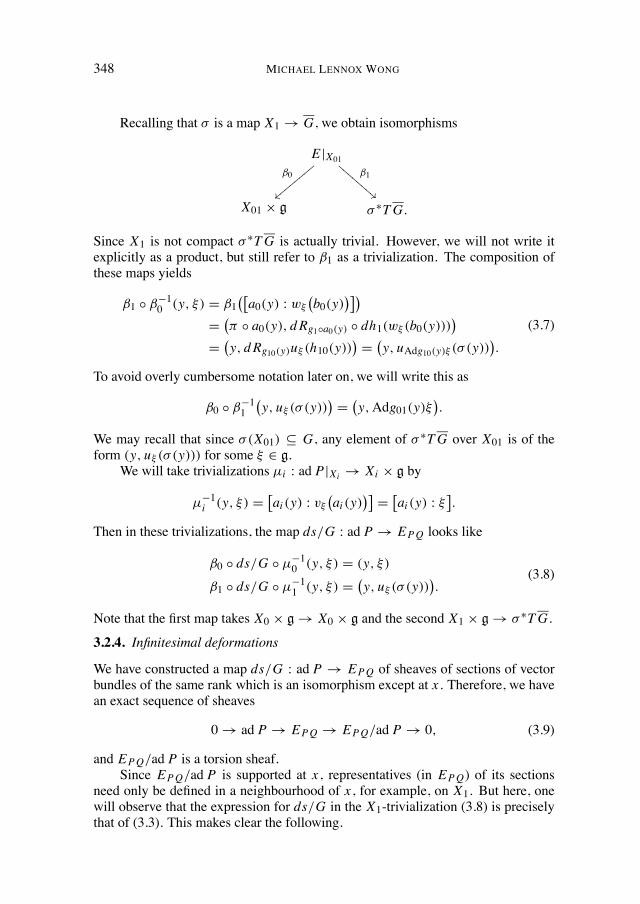
348 MICHAEL LENNOX WONG
Recalling that � is a map X1 ! G, we obtain isomorphisms
E |X01�0
||z
z
z
z
z
z
z
z
�1
!!
C
C
C
C
C
C
C
C
X01 ⇥ g � ⇤TG.
Since X1 is not compact � ⇤TG is actually trivial. However, we will not write itexplicitly as a product, but still refer to �1 as a trivialization. The composition ofthese maps yields
�1 � ��10 (y, ⇠) = �1
�⇥a0(y) : w⇠
�b0(y)
�⇤�
=�⇡ � a0(y), dRg1�a0(y) � dh1(w⇠ (b0(y)))
�
=�y, dRg10(y)u⇠ (h10(y))
�=�y, uAdg10(y)⇠ (� (y))
�.
(3.7)
To avoid overly cumbersome notation later on, we will write this as
�0 � ��11�y, u⇠ (� (y))
�=�y,Adg01(y)⇠
�.
We may recall that since � (X01) ✓ G, any element of � ⇤TG over X01 is of theform (y, u⇠ (� (y))) for some ⇠ 2 g.
We will take trivializations µi : ad P|Xi ! Xi ⇥ g by
µ�1i (y, ⇠) =
⇥ai (y) : v⇠
�ai (y)
�⇤=⇥ai (y) : ⇠
⇤.
Then in these trivializations, the map ds/G : ad P ! EPQ looks like
�0 � ds/G � µ�10 (y, ⇠) = (y, ⇠)
�1 � ds/G � µ�11 (y, ⇠) =
�y, u⇠ (� (y))
�.
(3.8)
Note that the first map takes X0 ⇥ g ! X0 ⇥ g and the second X1 ⇥ g ! � ⇤TG.
3.2.4. Infinitesimal deformations
We have constructed a map ds/G : ad P ! EPQ of sheaves of sections of vectorbundles of the same rank which is an isomorphism except at x . Therefore, we havean exact sequence of sheaves
0 ! ad P ! EPQ ! EPQ/ad P ! 0, (3.9)
and EPQ/ad P is a torsion sheaf.Since EPQ/ad P is supported at x , representatives (in EPQ) of its sections
need only be defined in a neighbourhood of x , for example, on X1. But here, onewill observe that the expression for ds/G in the X1-trivialization (3.8) is preciselythat of (3.3). This makes clear the following.
HECKE MODIFICATIONS, WONDERFUL COMPACTIFICATIONS 349
Lemma 3.3. There is an isomorphism
H0(X, EPQ/ad P) ⇠= 0(X1, � ⇤TG)/0(X1,OgX1).
If P corresponds to & 2 Gr�_
Q , then this allows us to make the identification
T&Gr�_
Q = H0(X, EPQ/ad P).
3.2.5. Comparison with the dual construction
We now consider the dual construction to EPQ given in Section 3.1.4; we obtain abundle EQP := t⇤V P/G which will have transition function (cf. (3.7))
(y, ⇠) 7!�y, uAd h10(y)⇠ (� (y)�1)
�. (3.10)
We claim that EQP ⇠= EPQ . For this, we use the following.
Lemma 3.4. There is an isomorphism d ◆ : � ⇤TG ⇠�! ⌧⇤TG under which
uAd g10(y)⇠ (� (y)) 7! uAd h10(y)⇠ (⌧ (y)).
Proof. To construct this, we use the involution ◆ : G ! G, extending the inversionmap on G (Proposition 2.11). This induces an involution on the tangent bundled◆ : TG ! TG. We define d ◆ : � ⇤TG ! ⌧⇤TG by
(y, v) 7!�y,�d◆(v)
�.
Note that v 2 T� (y)G and so �d◆(v) 2 T◆(� (y))G = T⌧ (y)G, so this makes sense.This map is clearly an involution. Verification of the mapping property is unprob-lematic.
Proposition 3.5. There is an isomorphism
M : EPQ⇠�! EQP .
Proof. From the above calculations, using the trivializations �i (3.5, 3.6) for EPQand the analogous trivializations �i for EQP , we define a map M : EPQ ! EQPby
u 7!
(��10 � �0(u) u 2 EPQ |X0��11 � d ◆ � �1(u) u 2 EPQ |X1 .
(3.11)
Using (3.7) and (3.10) shows that M is well-defined, and it is straightforward toconstruct an inverse. This proves that EQP ⇠= EPQ .
350 MICHAEL LENNOX WONG
Since the isomorphism : g⇤ ! g induced by the Killing form is Ad-equivariant, it induces isomorphisms
(ad P)⇤ ! ad P, (ad Q)⇤ ! ad Q,
which we will also denote by ; explicitly, if p 2 P, q 2 Q, f 2 g⇤,
[p : f ] 7! [p : ( f )], [q : f ] 7! [q : ( f )].
We may now consider the compositions
E⇤PQ
(ds/G)t// (ad P)⇤
// ad P
ds/G// EPQ (3.12)
and
E⇤PQ
(M�1)t
⇠// E⇤
QP(dt/G)t
// (ad Q)⇤
// ad Qdt/G
// EQP M�1// EPQ, (3.13)
and thus get a square
E⇤PQ //
✏✏
ad Q
✏✏
ad P // EPQ .
(3.14)
Verifying that it is indeed commutative involves tracing through the maps in thetrivializations for the various bundles given above. In the following, we will denoteby a tilde the trivializations for a dual bundle induced by the trivializations on theoriginal bundle. We wish to check that (3.12) and (3.13) yield the same map, whichamounts to verifying
�i � ds/G � � (ds/G)t � ��1i =�i � M�1� dt/G � � (dt/G)t � (M�1)t � ��1
i
for i = 0, 1. It is easy to see from (3.8) and (3.11) that in the X0 trivialization,these maps are all given by the identity on the g factor, so we need only check theequality in the X1 trivialization. Using (3.8), we may compute the left side actingon (y, f ) 2 � ⇤TG as
�1 � ds/G � � (ds/G)t � ��11 (y, f ) =
�y, dR� (y) � � dRt� (y)( f )
�. (3.15)
In a similar manner, if we use trivializations of ad Q analogous to the µi for ad P ,as well as (3.11), the right side acting on (y, f ) becomes
�y, d◆ � dR⌧ (y) � � dRt⌧ (y) � d◆t ( f )
�. (3.16)
Therefore, it suffices to show that (3.15) and (3.16) are equal. But ◆ � R⌧ (y) =L� (y) � ◆ and since ◆ restricts to the inversion map on G, d◆ : TeG = g ! TeG = gis �1, so this equality can be readily checked using Corollary 2.9. This completesthe verification that (3.14) commutes.
HECKE MODIFICATIONS, WONDERFUL COMPACTIFICATIONS 351
3.3. Calculations for cocharacters
We now give a concrete description of the space of infinitesimal deformationsH0(X, EPQ/ad P)which, by Lemma 3.3, amounts to describing the quotient space
0(X1, � ⇤TG)/0(X1,OgX1).
As in Section 2.1.1, we can use 1/↵1, . . . , 1/↵l to coordinatize T . Since Y (T ) =3_, 1/�_
1 , . . . , 1/�_l give a dual basis of cocharacters of T . Thus, if (writing addi-
tively now) �_ = �Pl
i=1 ri�_i is an arbitrary cocharacter, then we may write
�_(z) = (zr1, . . . , zrl ). (3.17)
As noted in Section 1.3, by choosing our trivializations 1,'1 and a coordinate zon X1 centred at x appropriately, we may assume � is a cocharacter. We will thusassume that such choices have been made and that � is of the form (3.17) above.Using the notation of Section 2.1.1, we are setting zi = zri :
� (z) = F(zr1, . . . , zrl ) =
"
'0 +lX
i=1zri'i +
X
k>lzPl
i=1 ri nik'k
#
.
Recall that the map OgX1 ! � ⇤TG is given by (3.3). Therefore, the image of
0(X1,OgX1) consists of all those sections of the form
dL(⇠) = dL� (z)(⇠)
with ⇠ 2 g. Now, the sections
d A(e,e,� (z))(x↵), d A(e,e,� (z))(y↵), d A(e,e,� (z))(e j )
give a trivialization of � ⇤TG, so we want to consider these modulo the image. Butfrom Lemma 2.6, we see that
dL(x↵) = �d A(x↵), dL(y↵) =lY
i=1zri h�
_i ,↵i dL(hi ) = �
lX
j=1ai j zr j d A(e j ),
(3.18)
recalling that (ai j ) is the Cartan matrix. By inverting it, we can see that the sections
zri d A(ei ), 1 i l
lie in the image. Therefore, we can take the sections(z j d A(y↵), 0 j
Pri h�_
i ,↵i � 1, ↵ 2 8+,
zkd A(ei ), 0 k ri � 1, 1 i l,
352 MICHAEL LENNOX WONG
as representative sections for the quotient. We get analogous expressions if insteadwe consider the cocharacter ⌫ · �_ with ⌫ 2 W .
To simplify the counting of the dimensions, we will take � = ��_i to be of the
form � (z) = F(1, . . . , z, . . . , 1), with the z in the i th position, so that r j = 0 forj 6= i and ri = 1. Thus � gives a simple modification. In this case, the quotientwill have representative sections
(z j d A(y↵), 0 j h�_
i ,↵i � 1, ↵ 2 8+,
d A(ei ).
Therefore, the dimension of the deformation space isX
↵28+
h�_i ,↵i + 1 = 2h�_
i , ⇢i + 1,
which is precisely what we obtained for the dimension of the space of Hecke mod-ifications of type �_
i (1.10).
3.4. Multiple modifications
Consider now a family of bundles given by introducing Hecke modifications oftypesµ_
1 ,..., µ_m , say with a modification of typeµ_
i at the distinct points xi1, ..., x
iki .
Then from Proposition 1.19, the appropriate parameter space is
⇣Grµ
_1 ,...,µ_
mQ,0
⌘(k1,...,km)
.
Proposition 3.6. Suppose P is obtained from Q by a sequence of Hecke modifica-tions at distinct points x11 , . . . , x
1k1, x
21 , . . . , x
2k2, . . . , x
m1 , . . . , xmkm with a modifica-
tion of type µ_i at x
ij , 1 j ki , and suppose this corresponds to
& 2⇣Grµ
_1 ,...,µ_
mQ,0
⌘(k1,...,km)
.
Let s& : P ! Q be the corresponding map of bundles. Then one may make theidentification
T&⇣Grµ
_1 ,...,µ_
mQ,0
⌘(k1,...,km)
= H0(X, EPQ/ad P).
The Kodaira–Spencer map for the family of bundles provided by Proposition 1.19is given by the connecting homomorphism for the short exact sequence (3.9):
H0(X, EPQ/ad P) ! H1(X, ad P).
HECKE MODIFICATIONS, WONDERFUL COMPACTIFICATIONS 353
To see why the last statement holds, observe that a section of H0(X, EPQ/ad P)can be represented by a section of E over an open set containing the support of theHecke modifications, e.g. the union of discs X1 that was used above. In terms ofthe trivializations described in Section 3.2.3, the inclusion ad P ! EPQ is pre-cisely the map in (3.2), and H0(X, EPQ/ad P) can be identified with the group in(3.4). Recall that in terms of Cech representatives, the connecting homomorphismis obtained by applying the Cech differential to such a lift, so in our case, we arerestricting this lift to the set X01, a disjoint union of punctured discs on which ad Pis isomorphic to EPQ , so we may think of this as a section of ad P over X01, andhence we get a 1-cocycle with values in ad P . This is at the same time the image ofthe connecting homomorphism and precisely the deformation of P induced by thesection of EPQ/ad P we started with.
4. Parametrization of the moduli space
4.1. Outline
The moduli space of stable bundles of topological type " 2 ⇡1(G) will be writtenN G,", omitting subscripts when there is no ambiguity; the moduli space of (equiv-alence classes of) semi-stable bundles will be written N ss
G,". We now outline ourgeneral procedure for constructing parametrizations of the moduli spaces of stablebundles to give a framework for the detailed calculations for specific groups in thenext section. We will start with a fixed bundle Q and consider a family of bundlesas in Section 3.4 parametrized by
⇣Grµ
_1 ,...,µ_
mQ,0
⌘(k1,...,km)
.
Breaking with previous notation, we will write P = P& for the bundle correspond-ing to the sequence & 2 (Grµ
_1 ,...,µ_
mQ,0 )(k1,...,km) of Hecke modifications of Q at dis-
tinct points. If specification is required, we will write E& for EP&Q . We will writeN for the dimension of this parameter space:
N := dim⇣Grµ
_1 ,...,µ_
mQ,0
⌘(k1,...,km)
=mX
i=1ki�2hµ_
i , ⇢i + 1�
= h0(X, E&/ad P),
the last by Proposition 3.6. We should observe that by repeated application ofProposition 1.12, the bundles in this family will have topological type
" := "(Q) +mX
i=1ki [µ_
i ] 2 ⇡1(G). (4.1)
Recall that to & 2 (Grµ_1 ,...,µ_
mQ,0 )(k1,...,km), there corresponds an equivariant map s& :
P& ! Q. Since we are only interested in the isomorphism classes of P& that arise,
354 MICHAEL LENNOX WONG
rather than the maps s themselves, we will want to quotient out by the action ofAut Q = Aut Q (Lemma 3.2). Therefore we wish to form families of
N = dimN G + dimAut Q = dim G(g � 1) + h0(X, ad Q)
parameters.We will fix a P in such a family. From our basic deformation sequence (3.9),
we obtain an exact sequence
H0(X, E) ! H0(X, E/ad P) ! H1(X, ad P) ! H1(X, E) ! 0
and the connecting homomorphism is the Kodaira–Spencer map. In order for usto obtain a parametrization, the family must necessarily be locally complete and sothis map must be surjective. This is equivalent to
H1(X, E) = 0.
In such a case,
h0(X, E)= �(E) = �(E/ad P) + �(ad P)=N + dim G(1� g) = h0(X, ad Q).
Since ad Q ! E is an injective map of sheaves, it follows that
H0(X, ad Q) ! H0(X, E)
is an isomorphism (it is injective and we have just seen that both spaces are of thesame dimension). Extending (3.14) into a morphism of short exact sequences, wesee that there is a commutative square
H0(X, ad Q) //
✏✏
H0(X, ad Q/E⇤)
✏✏
H0(X, E) // H0(X, E/ad P),
it then follows that image of the infinitesimal automorphisms H0(X, ad Q) of Q inthe infinitesimal deformation space H0(X, E/ad P) is precisely the kernel of theKodaira–Spencer map, and therefore the Kodaira–Spencer map
H0(X, E/ad P)/H0(X, ad Q) ! H1(X, ad P)
for our effective parameter space (i.e., for the quotient by Aut Q) is an isomorphism.By a semicontinuity argument, if H1(X, E& ) = 0, then H1(X, E# ) = 0 for
all # in an open neighbourhood of & . We then get a submersion from an open setin (Grµ
_1 ,...,µ_
mQ,0 )(k1,...,km) onto one inN ss
G and hence the family of bundles obtainedmust contain stable ones. Indeed, as this is the case, the modifications yielding
HECKE MODIFICATIONS, WONDERFUL COMPACTIFICATIONS 355
stable bundles form a Zariski open set in the parameter space [18, Proposition 4.1]and hence we get an isomorphism of an open set
� ✓⇣Grµ
_1 ,...,µ_
mQ,0
⌘(k1,...,km)
modulo the action of Aut Q onto an open set in N G . To recap, we make the fol-lowing statement.
Proposition 4.1. Suppose we construct a family of bundles via a sequence of Heckemodifications of Q such that the dimension of the parameter space of the family is
dim G(g � 1) + dimAut Q.
Then if some P& in this family is such that H1(X, EPQ) = 0, then in a neighbour-hood of & , we obtain a parametrization of N G .
4.2. Bundles reducible to a torus
Here we will outline a method of constructing families satisfying the hypothesesof Proposition 4.1. We do this by starting with Q being the trivial bundle andintroducing modifications taking values in T ; this is done to facilitate the calculationof H1(X, E). Therefore, from Proposition 4.1, we will want a family of
N = dim G · g
parameters. The bundle P that we obtain will be reducible to T , and hence willnot be stable, but in an open neighbourhood of this P in the moduli space, therewill still be a Zariski open set consisting of stable bundles. This is why we need toappeal to the semicontinuity argument mentioned above, to ensure that H1(X, E)also vanishes for these bundles.
From the root space decomposition of g, it follows that ad Q has a decomposi-tion
ad Q = O g = O t �M
↵28
O g↵ .
Let x 2 X and X0, X1 be as before, and consider a modification at x such that withrespect to the trivialization of Q and a suitable choice of coordinate z at x it can berepresented by the cocharacter � = �_ of (3.17). Then this is the transition functiong01 for a T -bundle R and we may write P = R ⇥T G as the induced bundle. Onehas a decomposition
ad P = O t �M
↵28
(ad P)↵.
where (ad P)↵ := R ⇥Ad T g↵ .
356 MICHAEL LENNOX WONG
We observe
↵�� (z)
�= zh�
_,↵i
and hence these are the transition functions for (ad P)↵ so it follows that
(ad P)↵ = O (�h�_,↵ix).
From the relations (3.18), if ↵ 2 8+ (respectively, ↵ 2 8�) and we let L↵ ✓ E bethe line bundle spanned by x↵ (respectively, y↵) in the X0-trivialization and d A(x↵)(respectively, d A(y↵)) in the X1-trivialization, then we see that E is of the form
E = V �M
↵28
L↵,
where V is a rank l vector bundle. We will often refer to the L↵ as the root bundlesof E . Since our goal is to arrange for H1(X, E) = 0, it is clearly enough to showthat H1(X, L↵) = 0 for each ↵ 2 8 and that H1(X, V ) = 0.
Under ds/G : ad P ! E , we have
O t ! V, (ad P)↵ ! L↵, ↵ 2 8.
Indeed, (3.18) tells us what the maps look like in the X1-trivialization:
hi =↵_i 7! �
lX
j=1ai j zr j d A(e j ), x↵ 7! �d A(x↵), y↵ 7! z�h�_,↵id A(y↵). (4.2)
We see that if ↵ 2 8+, then
L↵ ⇠= (ad P)↵ = O (�h�_,↵ix), L�↵ ⇠= (ad P)�↵(h�_,↵ix) = O . (4.3)
If instead of �_, we use the modification corresponding to ⌫�_, i.e. twisted by anelement of the Weyl group, then L↵ will be spanned by x↵ in the X0-trivializationand by d A⌫(Adw�1x↵) in the X1-trivialization (cf. Lemma 2.7). Replacing x↵ byy↵ as appropriate for the negative root spaces, we see that for ↵ 2 ⌫8+,
L↵⇠= (ad P)↵=O (�h�_, ⌫�1↵ix), L�↵⇠=(ad P)�↵(h�_, ⌫�1↵ix)=O . (4.4)
Now, assume that we introduce modifications at the points x1, . . . , xM , with themodification at x j being the cocharacter �⌫ j�i( j), 1 j M . Then it followsfrom (4.3) and (4.4) that if we define the effective divisors D↵ by
D↵ :=MX
j=1n↵j x j ,
HECKE MODIFICATIONS, WONDERFUL COMPACTIFICATIONS 357
where
n↵j = max{0, h�i( j), ⌫�1j ↵i} =
(0 if ↵ 2 ⌫ j8�
h�i( j), ⌫�1j ↵i if ↵ 2 ⌫ j8+
then
L↵ = O (D↵).
To arrange for H1(X, L↵) = 0, we will need deg D↵ � g; for a generic choiceof D↵ , in a sense explained more fully below, equality will be sufficient. In thenext section, what we will attempt to do is to start with a number of simple Heckemodifications so that we get a parameter space of dimension dim G · g, and thenapply various elements of the Weyl group so that the root parameters are distributedamong the root spaces in a manner just described to ensure that H1(X, L↵) = 0 forall ↵ 2 8.
We also need to arrange for H1(X, V ) = 0. As mentioned above, V is obtainedby upper Hecke modification of the trivial bundleO t; indeed, since a simple Heckemodification introduces a single toral parameters, it is obtained via a sequence ofsimple upper Hecke modifications, so that there is an exact sequence
0 ! O t ! V ! V/O t ! 0, (4.5)
with the quotient a sum of skyscraper sheaves. If we use the cocharacter��_i at the
point x 2 X , then from (4.2), we can see that the kernel of the fibre at x is spannedby
⇠i :=lX
k=1aik↵_
k , (4.6)
considered as an element of t = (O t)x , where (aik) is the inverse of the Cartanmatrix. If instead of ��_
i , we use the modification corresponding to �⌫�_i , then
the kernel is spanned by ⌫⇠i .
4.3. Choosing points generically
We now make precise what is meant by a “generic” choice of divisor and use this togive a sufficient condition for the vanishing of H1(X, V ) in a situation as in (4.5).
Proposition 4.2. Let m � 1. Then there exists D 2 X (m) such that if (g1, . . . , gk)is a partition of g and xi1, . . . , xik 2 supp D and we set
D =kX
j=1g j xi j ,
358 MICHAEL LENNOX WONG
then
H1(X,O (D)) = 0. (4.7)
In fact, the set of such D is dense in X (m). In particular, ifm � g and D is a reduceddivisor of degree m (i.e., a sum of m distinct points), then for any 0 D D withdeg D = g, (4.7) holds.
Proof. First, consider the partition (g1 = g) and let x 2 X , so that D = g · x . Then
h1(X,O (D)) = h0(X,O (g · x)) � 1
and this vanishes except when x is a Weierstrass point, of which there are finitelymany.
Now, fix an arbitrary partition (g1, . . . , gk), consider the map Xk ! X (g)
given by
(x1, . . . , xk) 7! D :=kX
j=1g j x j ,
and consider the family of line bundles O (D) as D ranges over the image of thismap. Taking x1 = · · · = xk = x , and this to be a non-Weierstrass point, we seethat there exists a line bundle in this family with vanishing first cohomology. Bythe semi-continuity theorem, there is a Zariski open, non-empty and hence dense,subset of Xk for which we have H1(X,O (D)) = 0.
Let m � 1 be given. If m < k, then choosing the xi j in the support of a degreem divisor and forming D as above, there will necessarily be repeated points, so weconsider the maps Xm ! Xk
(x1, . . . , xm) 7! (x1, . . . , xm, xr1, . . . , xrk�m ),
where the r j 2 {1, . . . ,m}. The set of points in Xm for which we have vanish-ing will be the union of the preimages of the open set in Xk for which we havevanishing, so is open and dense in Xm and hence in X (m).
Assume m � k. Then choosing a subset of k points amounts to taking aprojection map Xm ! Xk onto a set of k factors. This time, the sets for which wehave vanishing for all such choices is the intersection of the preimages of the openset in Xk constructed above. But since there are finitely many such projections, thisis a finite intersection and again we have an open dense subset in Xm and henceX (m) for which we have vanishing. Thus, for any m and for any partition, we canfind a dense open set of D 2 X (m) for which the conclusion holds.
Finally, for a fixed m � 1, since there are only finitely many partitions of g,we can take the intersection of the open sets just constructed for each partition andthe statement follows.
HECKE MODIFICATIONS, WONDERFUL COMPACTIFICATIONS 359
The next statement follows easily from the above.
Corollary 4.3. If m � g, then for a generic choice of m points in X , no g of themwill form part of a canonical divisor.
Proposition 4.4. Let v1, . . . , vl 2 Cl be a basis of Cl . Choose points xi j 2 X, 1 i l, 1 j g such that no g of them form part of a canonical divisor (bythe preceding corollary, a generic choice of points satisfies this condition), andsuppose V is the vector bundle obtained from the trivial bundle by the upper Heckemodification determined by (the subspace spanned by) vi at xi j for 1 i g. Then
H1(X, V ) = 0.
Proof. In (4.5), if we replace O t by O �l , we obtain an exact sequence
H0(X, V/O �l) ⇠= Cgl ! H1(X,O �l) =�H0(X, K )⇤
��l! H1(X, V ) ! 0.
Then H1(X, V ) = 0 if and only if the connecting homomorphism is surjective, andthis holds if and only if the transpose map
H0(X, K )�l ! H0(X, V/O �l)⇤ (4.8)
is injective. This is the statement we prove.Recall that sections of H0(X, V/O �l) are given by collections of l-tuples
fi j = t ( f 1i j , . . . , fli j )
of functions meromorphic in a neighbourhood of xi j for each 1 i l, 1 j g,having at most a simple pole along vi . The map (4.8) is given by
t! = (!1, . . . ,!l) 7!
( fi j ) 7!lX
i=1
gX
j=1Resxi j
t fi j!
!
,
where
t fi j! =lX
k=1f ki j!k .
Consider the following basis of H0(X, V/O �l): let si j = ( f (i, j)rs) where
f (i, j)rs =
(0 if (i, j) 6= (r, s)z�1i j vi if (i, j) = (r, s),
where, zi j is a coordinate centred at xi j .
360 MICHAEL LENNOX WONG
If ! 2 H0(X, K )�l lies in the kernel of this map, then
Resxi j z�1i j (tvi )! = 0
for 1 i l, 1 j g. Fixing i , we see that tvi! is a fixed linear combination of!1, . . . ,!l , and this differential vanishes at the g points xi1, . . . , xig. By our choiceof points, it follows that tvi! = 0. But since v1, . . . , vl are linearly independent,we can solve for each !k to obtain !1 = · · · = !l = 0. This proves the claimedinjectivity.
Remark 4.5. One will observe that for the proof to go through one needs only thateach tvi! vanishes and that the vi are a basis. If in our hypothesis, we allow morepoints, then this vanishing still holds, and the conclusion of the Proposition goesthrough. Also, introducing more Hecke modifications only increases the degrees ofthe root bundles, which does not affect the vanishing of the first cohomology onceit is achieved. Thus, if we construct a family of large enough dimension, possiblymuch larger than dim G · g, we can always obtains submersions from a parameterspace onto the moduli space.
5. Calculations for specific groups
In this section we show that the conditions of Proposition 4.1 are satisfied in severalsituations: namely, for the adjoint forms of the semisimple groups with root systemsA3,Cl , Dl when the genus of X is even. We use the standard labelling of the simpleroots for each of the root systems (as used in Chapter 11 of [8], for example). Foreach Hecke modification corresponding to the negative of a fundamental coweight��_
i , we find the roots which get twisted as in (4.3); these are precisely the ↵ 2 8+
in which ↵i appears when written as a sum of simple roots. We compute the numberof parameters obtained for each of these modification types, namely the coefficientof the ↵i which is h�_
i ,↵i. Also, we will explain how to use the Weyl group todistribute the parameters among the root bundles.
5.1. Calculations for Al
For the root system Al , the positive roots are all of the formP j�1
k=i ↵k for some1 i < j l + 1. It is not hard to see that each ↵i appears in i(l + 1� i) positiveroots and each with multiplicity one. Therefore
2h�_i , ⇢i + 1 = i(l + 1� i) + 1.
Because of the symmetry of the root system under
↵i 7! ↵l�i ,
we need only consider modification types ��_i for 1 i b12 (l + 1)c.
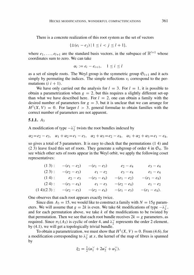
HECKE MODIFICATIONS, WONDERFUL COMPACTIFICATIONS 361
There is a concrete realization of this root system as the set of vectors
{±(ei � e j ) | 1 i < j l + 1},
where e1, . . . , el+1 are the standard basis vectors, in the subspace of Rl+1 whosecoordinates sum to zero. We can take
↵i := ei � ei+1, 1 i l
as a set of simple roots. The Weyl group is the symmetric group Sl+1 and it actssimply by permuting the indices. The simple reflections ⌫i correspond to the per-mutations (i i + 1).
We have only carried out the analysis for l = 3. For l = 1, it is possible toobtain a parametrization when g = 2, but this requires a slightly different set-upthan what we have described here. For l = 2, one can obtain a family with thedesired number of parameters for g = 3, but it is unclear that we can arrange forH1(X, V ) = 0. For larger l > 3, general formulae to obtain families with thecorrect number of parameters are not apparent.
5.1.1. A3
A modification of type ��_2 twists the root bundles indexed by
↵2=e2 � e3, ↵1 + ↵2=e1 � e3, ↵2 + ↵3=e2 � e4, ↵1 + ↵2 + ↵3=e1 � e4,
so gives a total of 5 parameters. It is easy to check that the permutations (1 4) and(2 3) leave fixed this set of roots. They generate a subgroup of order 4 in S4. Tosee which other sets of roots appear in the Weyl orbit, we apply the following cosetrepresentatives:
(1 3) : �(e1 � e2) �(e1 � e3) e2 � e4 e3 � e4(2 3) : �(e2 � e3) e1 � e2 e3 � e4 e1 � e4(1 4) : e2 � e3 �(e3 � e4) �(e1 � e2) �(e1 � e4)(2 4) : �(e3 � e4) e1 � e3 �(e2 � e4) e1 � e2
(1 4)(2 3) : �(e2 � e3) �(e2 � e4) �(e1 � e3) �(e1 � e4).
One observes that each root appears exactly twice.Since dim A3 = 15, we would like to construct a family with N = 15g param-
eters. We will assume that g = 2k is even. We take 6k modifications of type ��_2 ,
and for each permutation above, we take k of the modifications to be twisted bythat permutation. Then we see that each root bundle receives 2k = g parameters, asrequired. Since ⇡1(A3) is cyclic of order 4, and �_
2 represents the order 2 element,by (4.1), we will get a topologically trivial bundle.
To obtain a parametrization, we must show that H1(X, V ) = 0. From (4.6), fora modification corresponding to �_
2 at x , the kernel of the map of fibres is spannedby
⇠2 = 12 (↵
_1 + 2↵_
2 + ↵_3 ).
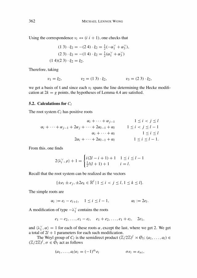
362 MICHAEL LENNOX WONG
Using the correspondence ⌫i $ (i i + 1), one checks that
(1 3) · ⇠2 = �(2 4) · ⇠2 = 12 (�↵
_1 + ↵_
3 ),
(2 3) · ⇠2 = �(1 4) · ⇠2 = 12 (↵
_1 + ↵_
3 )
(1 4)(2 3) · ⇠2 = ⇠2.
Therefore, taking
v1 = ⇠2, v2 = (1 3) · ⇠2, v3 = (2 3) · ⇠2,
we get a basis of t and since each vi spans the line determining the Hecke modifi-cation at 2k = g points, the hypotheses of Lemma 4.4 are satisfied.
5.2. Calculations for Cl
The root system Cl has positive roots
↵i + · · · + ↵ j�1 1 i < j l↵i + · · · + ↵ j�1 + 2↵ j + · · · + 2↵l�1 + ↵l 1 i < j l � 1
↵i + · · · + ↵l 1 i l2↵i + · · · + 2↵l�1 + ↵l 1 i l � 1.
From this, one finds
2h�_i , ⇢i + 1 =
(i(2l � i + 1) + 1 1 i l � 112 l(l + 1) + 1 i = l.
Recall that the root system can be realized as the vectors
{±ei ± e j ,±2ek 2 Rl | 1 i < j l, 1 k l}.
The simple roots are
↵i := ei � ei+1, 1 i l � 1, ↵l := 2el .
A modification of type ��_1 contains the roots
e1 � e2, . . . , e1 � el , e1 + e2, . . . , e1 + el , 2e1,
and h�_1 ,↵i = 1 for each of these roots ↵, except the last, where we get 2. We get
a total of 2l + 1 parameters for each such modification.The Weyl group of Cl is the semidirect product (Z/2Z)l o Sl ; (a1, . . . , al) 2
(Z/2Z)l , � 2 Sl act as follows
(a1, . . . , al)ei = (�1)ai ei �ei = e� i ,
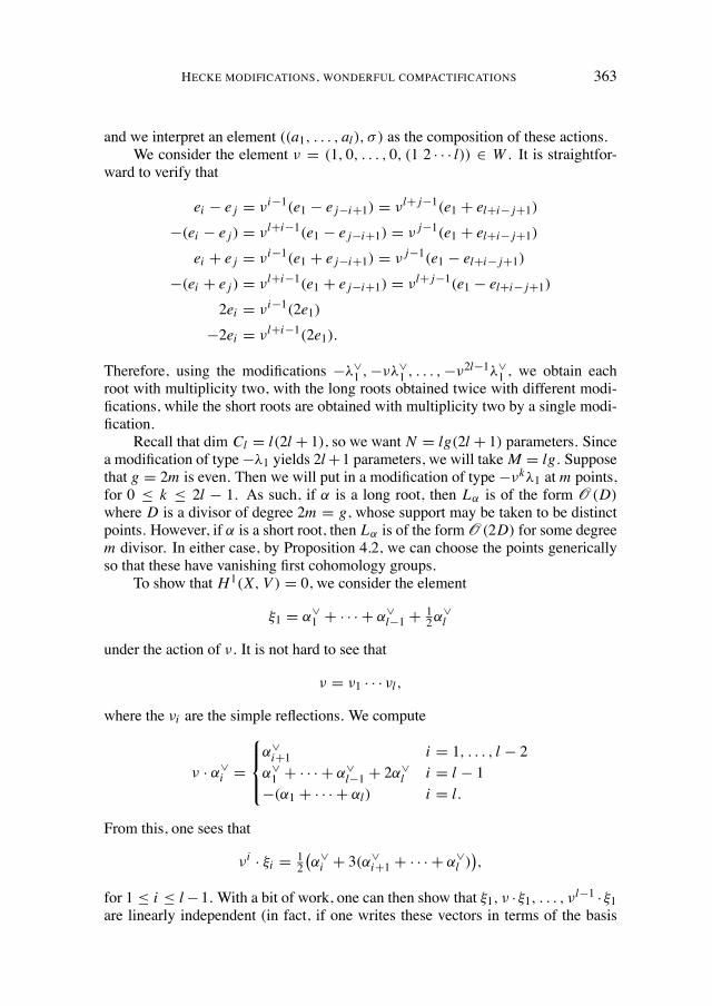
HECKE MODIFICATIONS, WONDERFUL COMPACTIFICATIONS 363
and we interpret an element ((a1, . . . , al), � ) as the composition of these actions.We consider the element ⌫ = (1, 0, . . . , 0, (1 2 · · · l)) 2 W . It is straightfor-
ward to verify that
ei � e j = ⌫i�1(e1 � e j�i+1) = ⌫l+ j�1(e1 + el+i� j+1)
�(ei � e j ) = ⌫l+i�1(e1 � e j�i+1) = ⌫ j�1(e1 + el+i� j+1)
ei + e j = ⌫i�1(e1 + e j�i+1) = ⌫ j�1(e1 � el+i� j+1)
�(ei + e j ) = ⌫l+i�1(e1 + e j�i+1) = ⌫l+ j�1(e1 � el+i� j+1)
2ei = ⌫i�1(2e1)�2ei = ⌫l+i�1(2e1).
Therefore, using the modifications ��_1 ,�⌫�_
1 , . . . ,�⌫2l�1�_1 , we obtain each
root with multiplicity two, with the long roots obtained twice with different modi-fications, while the short roots are obtained with multiplicity two by a single modi-fication.
Recall that dim Cl = l(2l + 1), so we want N = lg(2l + 1) parameters. Sincea modification of type��1 yields 2l+1 parameters, we will take M = lg. Supposethat g = 2m is even. Then we will put in a modification of type �⌫k�1 at m points,for 0 k 2l � 1. As such, if ↵ is a long root, then L↵ is of the form O (D)where D is a divisor of degree 2m = g, whose support may be taken to be distinctpoints. However, if ↵ is a short root, then L↵ is of the formO (2D) for some degreem divisor. In either case, by Proposition 4.2, we can choose the points genericallyso that these have vanishing first cohomology groups.
To show that H1(X, V ) = 0, we consider the element
⇠1 = ↵_1 + · · · + ↵_
l�1 + 12↵
_l
under the action of ⌫. It is not hard to see that
⌫ = ⌫1 · · · ⌫l ,
where the ⌫i are the simple reflections. We compute
⌫ · ↵_i =
8><
>:
↵_i+1 i = 1, . . . , l � 2↵_1 + · · · + ↵_
l�1 + 2↵_l i = l � 1
�(↵1 + · · · + ↵l) i = l.
From this, one sees that
⌫i · ⇠i = 12�↵_i + 3(↵_
i+1 + · · · + ↵_l )�,
for 1 i l�1. With a bit of work, one can then show that ⇠1, ⌫ · ⇠1, . . . , ⌫l�1 · ⇠1are linearly independent (in fact, if one writes these vectors in terms of the basis
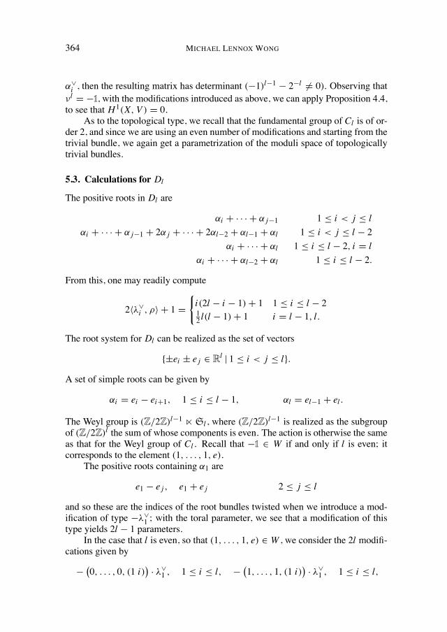
364 MICHAEL LENNOX WONG
↵_i , then the resulting matrix has determinant (�1)
l�1 � 2�l 6= 0). Observing that⌫l = �1, with the modifications introduced as above, we can apply Proposition 4.4,to see that H1(X, V ) = 0.
As to the topological type, we recall that the fundamental group of Cl is of or-der 2, and since we are using an even number of modifications and starting from thetrivial bundle, we again get a parametrization of the moduli space of topologicallytrivial bundles.
5.3. Calculations for Dl
The positive roots in Dl are
↵i + · · · + ↵ j�1 1 i < j l↵i + · · · + ↵ j�1 + 2↵ j + · · · + 2↵l�2 + ↵l�1 + ↵l 1 i < j l � 2
↵i + · · · + ↵l 1 i l � 2, i = l↵i + · · · + ↵l�2 + ↵l 1 i l � 2.
From this, one may readily compute
2h�_i , ⇢i + 1 =
(i(2l � i � 1) + 1 1 i l � 212 l(l � 1) + 1 i = l � 1, l.
The root system for Dl can be realized as the set of vectors
{±ei ± e j 2 Rl | 1 i < j l}.
A set of simple roots can be given by
↵i = ei � ei+1, 1 i l � 1, ↵l = el�1 + el .
The Weyl group is (Z/2Z)l�1 n Sl , where (Z/2Z)l�1 is realized as the subgroupof (Z/2Z)l the sum of whose components is even. The action is otherwise the sameas that for the Weyl group of Cl . Recall that �1 2 W if and only if l is even; itcorresponds to the element (1, . . . , 1, e).
The positive roots containing ↵1 are
e1 � e j , e1 + e j 2 j l
and so these are the indices of the root bundles twisted when we introduce a mod-ification of type ��_
1 ; with the toral parameter, we see that a modification of thistype yields 2l � 1 parameters.
In the case that l is even, so that (1, . . . , 1, e) 2 W , we consider the 2l modifi-cations given by
��0, . . . , 0, (1 i)
�· �_1 , 1 i l, �
�1, . . . , 1, (1 i)
�· �_1 , 1 i l,
HECKE MODIFICATIONS, WONDERFUL COMPACTIFICATIONS 365
where for i = 1 by (1 i) we mean the identity permutation. Observe that
ei � e j =�0, . . . , 0, (1 i)
�· (e1 � e j )=
�1, . . . , 1, (1 j)
�· (e1 � ei ) 1 i l
�(ei � e j )=�1, . . . , 1, (1 i)
�· (e1 � e j )=
�0, . . . , 0, (1 j)
�· (e1 � ei ) 1 i l
ei + e j =�0, . . . , 0, (1 i)
�· (e1 + e j )=
�0, . . . , 0, (1 j)
�· (e1 + ei ) 1 i l
�(ei + e j )=�1, . . . , 1, (1 i)
�· (e1 + e j )=
�1, . . . , 1, (1 j)
�· (e1 + ei ) 1 i l.
Hence each root appears exactly twice.In the case that l is odd, if ⌫ := (1, . . . , 1, 0, e) 2 W , we consider the 2l
modifications given by
� (1 i) · �_1 , 1 i l, � (1 i)⌫ · �_
1 , 1 i l.
Here, we can see that
ei � e j = (1 i) · (e1 � e j ) = (1 j)⌫ · (e1 � ei ) 1 i < j l�(ei � e j ) = (1 i)⌫ · (e1 � e j ) = (1 j) · (e1 � ei ) 1 i < j l
ei + e j = (1 i) · (e1 + e j ) = (1 j) · (e1 + ei ) 1 i < j l�(ei + e j ) = (1 i)⌫ · (e1 + e j ) = (1 j)⌫ · (e1 + ei ) 1 i < j l.
Again, every root appears exactly twice.We will assume that g = 2k is even. Recall that dim Dl = 2l2 � l = l(2l � 1),
so that we want N = lg(2l � 1) = 2kl(2l � 1) total parameters. Since eachmodification introduces 2l � 1 parameters, we will use lg = 2kl of them. We havejust seen that with 2l modifications, we can introduce 2 parameters to each rootbundle, so with 2kl, we get 2k = g in each bundle, as required.
We now show that H1(X, V ) = 0. We consider the orbit of
⇠1 =lX
k=1a1k↵_
k = ↵_1 + · · · + ↵_
l�2 + 12 (↵
_l�1 + ↵_
l )
under the elements of the Weyl group used above. Using this expression, one maycheck that for 2 i l � 3, we have
⌫i · ⇠1 = ⇠1.
Since ⌫i corresponds to the permutation (i i + 1) for 1 i l � 1, the correspon-dence
(1 i) $ ⌫i�1⌫i�2 · · · ⌫2⌫1⌫2 · · · ⌫i�2⌫i�1,
for 2 i l, follows. So, by induction, one obtains
(1 i) · ⇠1 = ⇠1 � (↵_1 + · · · + ↵_
i�1),
366 MICHAEL LENNOX WONG
for 2 i l � 2. Also,
(1 l � 1) · ⇠1 = ⌫l�2�↵_l�2 + 1
2 (↵_l�1 + ↵_
l )�
= 12 (↵
_l�1 + ↵_
l ),
(1 l) · ⇠1 = ⌫l�1 · 12 (↵_l�1 + ↵_
l ) = 12 (�↵
_l�1 + ↵_
l ).
From all of this, it is not hard to see that
⇠1, (1 2) · ⇠1, . . . , (1 l) · ⇠1
are linearly independent.Consider the element ⌫ = (1, . . . , 1, 0, e) in the case that l is odd. Then we
can see that
⌫ · ↵i = �↵i , 1 i l � 2, ⌫ · ↵l�1 = �↵l , ⌫ · ↵l = �↵l�1.
Since the matrix for ⌫ acting on t with respect to the basis ↵_i is the same as that for
its action on t⇤ with respect to the basis ↵i , it follows that
⌫ · ⇠1 = �⇠1.
Therefore, in the case where l is odd, the same argument as above can be used toshow that we can arrange for H1(X, V ) = 0.
One will recall that ⇡1(Dl) is either Z/4Z or Z/2Z⇥Z/2Z, depending on theparity of l. However, in either case, �_
1 represents an element of order 2, and sincewe are using an even number of modifications and starting with the trivial bundle,we again get a parametrization of the moduli space of topologically trivial bundles.
Remark 5.1. There are two obstacles for us in obtaining the parametrizations weseek. The first is to construct families of the requisite dimension N = dim G · g,given the number of parameters yielded by modifications of each type. As wementioned, this is a problem for Al when l > 3. It is also a problem for Bl : amodification of type ��_
i yields i(2l � i) + 1 parameters and dim G = l(2l + 1).It is not clear what combination of these types would yield the correct number ofparameters.
The second obstacle is to find a way to evenly distribute the parameters amongthe root bundles using the Weyl action. In the case of G2, one of the simple Heckemodifications yields 7 parameters. Since dim G2 = 14, one can always obtainthe desired number of parameters. However, the problem is that this modificationintroduces 2 parameters corresponding to short roots and 4 corresponding to thelong roots, yet there are the same number of short and long roots in G2. Thereforeit is impossible to obtain the required g parameters in the short root spaces with thegiven number of modifications.
HECKE MODIFICATIONS, WONDERFUL COMPACTIFICATIONS 367
References
[1] C. DE CONCINI and C. PROCESI, Complete symmetric varieties, In: “Invariant Theory(Proceedings, Montecatini 1982)”, 996 Lecture Notes in Math., Springer, 1982, 1–44.
[2] J. DUISTERMAAT and J. KOLK, “Lie Groups”, Springer, 2000.[3] S. EVENS and B. F. JONES, On the wonderful compactification, arXiv:0801.0456v1
[math.AG] 3 Jan 2008, 2008.[4] G. FALTINGS, Algebraic loop groups and moduli spaces of bundles, J. Eur. Math. Soc. 5
(2003), 41–68.[5] E. FRENKEL and D. BEN-ZVI, “Vertex Algebras and Algebraic Curves”, Second Edition,
American Mathematical Society, 2004.[6] G. HARDER, Halbeinfache Gruppenschemata uber Dedekindringen, Invent. Math. 4
(1967), 165–191.[7] G. HARDER and D. KAZHDAN, Automorphic forms on GL2 over function fields, In: “Proc.
Sympos. Pure Math.”, 33, part 2 (1979), 357–379.[8] J. E. HUMPHREYS, “Introduction to Lie Algebras and Representation Theory”, Springer,
New York, NY, 1972.[9] J. HURTUBISE,On the geometry of isomonodromic deformations, J. Geom. Phys. 58 (2008),
1394–1406.[10] N. IWAHORI and H. MATSUMOTO, On some Bruhat decomposition and the structure of the
Hecke rings of p-adic Chevalley groups, Publ. Math. I.H.E.S. 25 (1965), 5–48.[11] V. G. KAC, “Infinite Dimensional Lie algebras”, Cambridge University Press, 1990.[12] A. KAPUSTIN and E. WITTEN, Electric-magnetic duality and the geometric langlands pro-
gram, arXiv:hep-th/0604151, 2006.[13] I. KRICHEVER, Isomonodromy equations on algebraic curves, canonical transformations
and Whitham equations, Mosc. Math. J. 2 (2002), 717–752.[14] S. KUMAR, “Kac-Moody Groups, their Flag Varieties and Representation Theory”,
Birkhauser, 2002.[15] J. M. LANSKY, Decomposition of double cosets in p-adic groups, Pacific J. Math. 197
(2001), 97–117.[16] P. NORBURY, Magnetic monopoles on manifolds with boundary, Trans. Amer. Math. Soc.,
S 0002-9947(2010)04934-7, arXiv:0804.3649v2 [math.DG] 14 Oct 2008, 2008.[17] A. PRESSLEY and G. SEGAL, “Loop Groups”, Oxford University Press, New York, NY,
1986.[18] A. RAMANATHAN, Stable principal bundles on a compact Riemann surface, Math. Ann.
213 (1975), 129–152.[19] A. TJURIN, Classification of n-dimensional vector bundles over an algebraic curve of ar-
bitrary genus, Izv. Ross. Akad. Nauk Ser. Mat. 30 (1966), 1353–1366.[20] A. WEIL, Generalisation des fonctions abeliennes, J. Math. Pures Appl. 17 (1938), 47–87.
EPFL SB Mathgeom GeomMA B1 457Station 81015 Lausanne, Switzerland
Related Documents


![Compactifications of moduli of abelian varieties: an ...library.msri.org/books/Book59/files/65olsson.pdf · Definition 6.1] that if S is a scheme then an abelian scheme over S is](https://static.cupdf.com/doc/110x72/5f9eeb816299bf16c22d118e/compactifications-of-moduli-of-abelian-varieties-an-deinition-61-that-if.jpg)


