Heterotic G 2-manifold compactifications with fluxes and fermionic condensates

ITP–UH–14/13

Heterotic G2-manifold compactifications

with fluxes and fermionic condensates

Karl-Philip Gemmer† and Olaf Lechtenfeld†×

†Institut fur Theoretische Physik

Leibniz Universitat Hannover

Appelstraße 2, 30167 Hannover, Germany

×Riemann Center for Geometry and Physics

Leibniz Universitat Hannover

Appelstraße 2, 30167 Hannover, Germany

Abstract

We consider flux compactifications of heterotic string theory in the presence of fermionic condensates on

M1,2 ×X7 with both factors carrying a Killing spinor. In other words, M1,2 is either de Sitter, anti-de

Sitter or Minkowski, and X7 possesses a nearly parallel G2-structure or has G2-holonomy. We solve

the complete set of field equations and the Bianchi identity to order α′. The latter is satisfied via a

non-standard embedding by choosing the gauge field to be a G2-instanton. It is shown that none of the

solutions to the field equations is supersymmetric.

arX

iv:1

308.

1955

v1 [

hep-

th]

8 A

ug 2

013

1 Introduction and summary

Many compactifications of string theory suffer from the severe problem of moduli stabilization, the existence

of scalar fields whose vacuum expectation values are not fixed by a potential. A promising method for

the heterotic string to stabilize these scalar fields is the introduction of fluxes and fermionic condensates,

i.e. vacuum expectation values of some tensor fields and some fermionic bilinears along the internal manifold.

Without fluxes and condensates, the Killing spinor equations demand the internal manifold to have reduced

holonomy, e.g. SU(3) (G2) for compactifications on a six-(seven-)dimensional manifold. Fluxes lead to a

deformation of the internal manifold, resulting in an internal space with only reduced structure group but

no reduced holonomy.

For compactifications on six-dimensional manifolds, deformations to non-Kahler SU(3)-manifolds have

already been studied in detail [1, 2]. Also the effect of implementing gaugino and dilatino condensates has

been analyzed [3–7]. Here, we investigate which aspects of these results carry over to compactifications on

seven-dimensional manifolds X7.

More specifically, we discuss compactifications on manifolds with G2-holonomy as well as on their defor-

mations to nearly parallel G2-manifolds, in the presence of fermionic condensates. Assuming the space-time

background to be a product of X7 and a maximally symmetric Lorentzian space M1,2, we solve the field

equations to order α′ and discuss the conditions under which the solutions preserve supersymmetry. The

Bianchi identity is also satisfied to guarantee the absence of anomalies. The gauge field is taken to be a

generalized instanton on the internal manifold X7. This choice allows us to solve the Bianchi identity by

a non-standard embedding and immediately takes care of the Yang-Mills equation. Furthermore, it also

ensures the vanishing of the gaugino supersymmetry variation.

There are several aspects in which the considered compactifications to three dimensions differ from those

to four dimensions. Most importantly, the fermionic condensates cannot be restricted to the internal manifold

X7 but must extend to M1,2. Therefore, the field equations do not decouple into separate equations on M1,2

and X7. As a first consequence, the equations of motion allow not only for anti-de Sitter solutions but admit

de Sitter and Minkowski space-times as well. Secondly, the radius of the de Sitter or anti-de Sitter space is

not fixed but related to the amplitudes of the condensates and H-flux by the equations of motion. It turns

out that none of these heterotic vacua is supersymmetric.

The paper is organized as follows. In Section 2, we briefly review the action and the equations of

motion of heterotic supergravity to first order in α′. We decompose the fields and their equations according

to the space-time factorization M1,2 × X7, including the effect of gaugino and dilatino condensates. The

geometric properties of manifolds with G2-structure are the subject of Section 3. In Section 4 we solve the

heterotic equations of motion for the six possible combinations of M1,2 being either de Sitter, anti-de Sitter

or Minkowski space-times and for X7 carrying either G2-holonomy or just a nearly parallel G2-structure.

Furthermore, we present the conditions for supersymmetric solutions and compute the fermion masses for

all considered backgrounds.

2 Heterotic string with fermionic condensates

Action and equations of motion. The low-energy field theory limit of heterotic string theory is given by

d = 10, N = 1 supergravity coupled to a super-Yang-Mills multiplet, and it is defined on a ten-dimensional

space-time M . The supergravity multiplet consists of the graviton g, which is a metric on M , the left-handed

Rarita-Schwinger gravitino Ψ, the Kalb-Ramond two-form field B, the scalar dilaton φ and the right-handed

Majorana-Weyl dilatino λ. Moreover, the vector supermultiplet consists of the gauge field one-form A and

its superpartner, the left-handed Majorana-Weyl gaugino χ.

Rather than presenting the full action describing the propagation and interactions of the above fields [8,9],

we shall restrict ourselves to the part which is relevant for our purposes. In this paper we shall consider

vacuum solutions where the fermionic expectation values are forced to vanish by requiring Lorentz invariance,

but certain fermionic bilinears may acquire non-trivial vacuum expectation values. However, these vacuum

expectation values will not involve the gravitino, whence we set the gravitino to zero from the very beginning,

Ψ = 0. Then, in the string frame, the low-energy action up to and including terms of order α′ reads as [10]

S =

∫M

d10x√

det g e−2φ[Scal + 4|dφ|2 − 1

2 |H|2 + 1

2 (H,Σ)− 2(H,∆) + 14 (Σ,∆)− 1

8 |Σ|2+

+ 14α′(

tr|R|2 − tr(|F |2 − 2〈χ,Dχ〉 − 1

3 〈λ, γMγABFABγMλ〉

))+ 8〈λ,Dλ〉

]. (2.1)

Here, Scal is the scalar curvature of the Levi-Civita connection Γg on TM . Furthermore, R is the curvature

form of a connection Γ on the TM . The choice of this connection is ambiguous and will be discussed in

Section 4. Here and in the following, traces are taken in the adjoint representation of SO(9,1) or of the gauge

group, respectively, depending on the context.

The field strength H is defined by

H = dB + 14α′(ωCS(Γ)− ωCS(A)

), (2.2)

where the Chern-Simons forms of the connections Γ and A are given by

ωCS(Γ) = tr(R ∧ Γ− 2

3 Γ ∧ Γ ∧ Γ)

and ωCS(A) = tr(F ∧A− 2

3A ∧A ∧A). (2.3)

For any two p-forms α, β we use the definitions

(α, β) :=1

p!αM1,...,Mp

βM1,...,Mp , |α|2 := (α, α) . (2.4)

D = γM∇M denotes the Dirac operator coupled to Γg and A. Finally, we have defined the fermion bilinears

Σ = 124α′tr〈χ, γMNPχ〉 eMNP and ∆ = 1

6 〈λ, γMNPλ〉eMNP , (2.5)

with eMNP ≡ eM ∧ eN ∧ eP and {eM} being an othonormal frame on the space-time background M . By

〈·, ·〉 we denote the inner product of spinors.

2

The action (2.1) is invariant under N = 1 supersymmetry transformations, which act on the fermions as

δΨM = ∇M ε− 18HMNP γ

NP ε+ 196Σ · γM ε , (2.6a)

δλ = −√24 (dφ− 1

12H −148Σ + 1

48∆) · ε , (2.6b)

δχ = − 14F · ε+ 〈χ, λ〉 ε− 〈ε, λ〉χ+ 〈χ, γM ε〉 γMλ , (2.6c)

where ε is the supersymmetry parameter, a left-handed Majorana-Weyl spinor.

The equations of motion may be obtained by varying the action (2.1) and take the form

0 = RicMN + 2(∇dφ)MN − 18 (H − 1

2Σ + 2∆)PQ(MHN)PQ+

14α′[RMPQRR

PQRN − tr

(FMPFN

P + 12 〈χ, γ(M∇N)χ〉

)]+ 2〈λ, γ(M∇N)λ〉 ,

(2.7a)

0 = Scal− 4∆φ+ 4|dφ|2 − 12 |H|

2 + 12 (H,Σ)− 2(H,∆) + 1

4 (Σ,∆)− 18 |Σ|

2

+ 14α′tr[|R|2 − |F |2 − 2〈χ,Dχ〉

]+ 8〈λ,Dλ〉 ,

(2.7b)

0 = e2φd ∗ (e−2φF ) +A ∧ ∗F − ∗F ∧A+ ∗(H − 12Σ + 2∆) ∧ F , (2.7c)

0 = d ∗ e−2φ(H − 12Σ + 2∆) , (2.7d)

0 =(D − 1

24 (H − 12Σ + 1

2∆) ·)e−2φχ , (2.7e)

0 =(D − 1

24 (H − 18Σ) ·

)e−2φλ . (2.7f)

They are complemented by the Bianchi identity

dH = 14α′(

tr(R ∧ R)− tr(F ∧ F )), (2.8)

which follows from the definition (2.2). In order to simplify the equations of motion, we will assume for the

remainder of the paper that the dilation vanishes, i.e.

φ = 0 . (2.9)

Space-time and spinor factorization. We will consider space-time backgrounds M of the form

M = M1,2 ×X7 , (2.10)

with M1,2 being a maximally symmetric Lorentzian manifold and X7 a being seven-dimensional compact

Riemannian manifold. Furthermore, we assume that X7 possesses a nowhere vanishing real Killing spinor1,

i.e. a spinor satisfying

∇gXη = i µ2X · η (2.11)

for some real constant µ2. If µ2 = 0, then X7 admits G2-holonomy. Manifolds with non-vanishing µ2 are

known as nearly parallel G2-manifolds (see Section 3). We denote the metric on M by g, whereas the metrics

on M1,2 and X7 will be labeled by g3 and g7, respectively.

1Note that the notion of real an imaginary Killing spinors differs from parts of the mathematical literature, due to a different

sign in the definition of the Clifford algebra (see (2.12)).

3

The factorization of the space-time background M induces a splitting of the SO(9,1) Clifford algebra.

We employ a standard representation of the SO(9,1) Clifford algebra

{γA, γB} = 2ηAB = 2 diag(−1,+1, . . . ,+1)AB (2.12)

via

γµ = γµ(3) ⊗ 18 ⊗ σ2 for µ = 0, 1, 2 , (2.13a)

γa+2 = 12 ⊗ γa(7) ⊗ σ1 for a = 1, . . . , 7 . (2.13b)

Here, 1n are n× n-unit matrices and γa(7) are SO(7) gamma matrices. Furthermore, γµ(3) and σi denote the

SO(2,1) gamma matrices and Pauli matrices, respectively:

γ0(3) =

(0 −1

1 0

), γ1(3) =

(0 1

1 0

), γ2(3) =

(1 0

0 −1

), (2.14)

σ1 =

(0 1

1 0

), σ2 =

(0 −ii 0

), σ3 =

(1 0

0 −1

). (2.15)

The chirality and the charge conjugation operator in this representation read

Γ11 = 12 ⊗ 18 ⊗ σ3 and C = C(3) ⊗ C(7) ⊗ 12 , (2.16)

with

C(7) = iγ2(7)γ4(7)γ

6(7) and C(3) = γ0(3) . (2.17)

We assume that the dilatino and gaugino decompose as

χ = χ⊗ η ⊗ (1, 0)t , (2.18a)

λ = λ⊗ η ⊗ (0, 1)t , (2.18b)

with χ and λ being Grassmann-valued SO(2,1) Majorana spinors and η being the real Majorana Killing

spinor on X7. The last factor in the products accounts for the opposite chirality of the gaugino and the

dilatino. The only non-vanishing spinor bilinears constructed with a single spinor η are 〈η, η〉 and 〈η, γabcη〉.Hence, Σ and ∆ simplify to

Σ = m (−vol(3) + Q) , (2.19)

∆ = n (−vol(3) + Q) , (2.20)

with

m = 124α′tr〈χ, χ〉 and n = 1

6 〈λ, λ〉 . (2.21)

Here, vol(3) is the volume form on M1,2, and

Q = − i

3!〈η, (γ(7))mnp η〉 emnp . (2.22)

4

The properties of the three-form Q will be discussed in Section 3.

From now on, we will replace all terms depending on fermion bilinears by their quantum expectation

values. Furthermore, we assume that the only non-vanishing expectation values are Σ and ∆. Note that

the form of the condensates (2.19) and (2.20) differs crucially from condensates considered previously in

compactifications to four-dimensional space-times. In the latter case one may consistently confine the con-

densate to the compactification space. For a compactification to a three-dimensional space-time, however, a

non-vanishing condensate must always have a space-time component, due to the fact that

Γ0Γ1Γ2 = −1 . (2.23)

Geometric data of maximally symmetric Lorentzian manifolds. For future reference we review

some aspects of the geometry of maximally symmetric Lorentzian manifolds, i.e. de Sitter, anti-de Sitter

and Minkowski spaces. These spaces possess a Killing spinor with Killing number µ1, meaning a spinor ζ

satisfying

∇gXζ = µ1X · ζ . (2.24)

For de Sitter space, µ1 is real, whereas for anti-de Sitter space, µ1 is purely imaginary. It vanishes on

Minkowski space. We define the (anti-)de Sitter radius |ρ1| by setting

µ1 =

ρ−11 for de Sitter space

i ρ−11 for anti-de Sitter space. (2.25)

The Ricci tensor and scalar curvature of (anti-)de Sitter space are given by

Scal3 = ±24

ρ21and Ric3 = ± 8

ρ21g3 . (2.26)

Moreover, the curvature dependent quantities entering the Einstein and dilaton equations (2.7a) and (2.7b)

are given by

(R3)µαβγ(R3)ναβγ =

64

ρ41g3 and |R|2 =

192

ρ41. (2.27)

Note that the curvature only depends on even powers of ρ1 and, hence, the sign of ρ1 will only enter the

supersymmetry variations but not the equations of motion.

3 The geometry of manifolds with G2-structure

G2-manifolds. Manifolds with a G2-structure are by definition seven-dimensional Riemannian manifolds

possessing a nowhere vanishing G2-invariant three-form Q. Equivalently, they can be defined by the existence

of a nowhere vanishing spinor η. One can always find an orthonormal frame {ea} such that the three-form

Q can be written as

Q = e135 + e425 + e416 + e326 + e127 + e347 + e567 . (3.1)

5

Here and in the following we use the abbreviation eabc ≡ ea ∧ eb ∧ ec. The G2-structure defined by Q is

compatible with the metric g7 in the sense that ∗((XyQ) ∧ (Y yQ) ∧Q) = 6 g7(X,Y ) for all vector fields X

and Y . The three-form Q is related to the spinor η by

Q = − i

3!〈η, γmnpη〉 emnp . (3.2)

From this, one can deduce the action of Q on η under Clifford multiplication:

Q · η = 7i η , (3.3)

Q · (X · η) = −i X · η , (3.4)

(XyQ) · η = 6i X · η . (3.5)

Form decomposition. Under the action of G2 the spaces of p-forms on X7, Λp, split into irreducible

representations. For the subsequent discussion we need the decompositions [11]

Λ2 = Λ2(7) ⊕ Λ2

(14) , (3.6)

Λ4 = Λ4(1) ⊕ Λ4

(7) ⊕ Λ4(27) , (3.7)

with

Λ2(7) = {vyQ|v ∈ TmX7} , (3.8a)

Λ2(14) = {β ∈ Λ2|(∗Q) ∧ β = 0} (3.8b)

and

Λ4(1) = {µ ∗Q|µ ∈ R} , (3.9a)

Λ4(7) = {α ∧Q|α ∈ T ∗mX7} , (3.9b)

Λ4(27) = {γ ∈ Λ4|γ ∧Q = 0 and ∗ γ ∧Q = 0} ∼= S2

0 . (3.9c)

The subscripts of Λp label the dimension of the G2 representation, and S20 is the space of traceless symmetric

two-tensors.

Manifolds with G2-holonomy. G2-structure manifolds are classified by the derivative of the three-form

Q or equivalently of the spinor η. On manifolds with G2-holonomy, the three-form Q is closed and coclosed,

and the spinor η is parallel everywhere with respect to the Levi-Civita connection,

dQ = d ∗Q = 0 and ∇gη = 0 . (3.10)

On the other hand, either the closedness and coclosedness of Q or the vanishing of ∇gη imply that the

holonomy is contained in G2. As a result of (3.10), manifolds with G2-holonomy are Ricci flat.

6

Nearly parallel G2-manifolds. By definition, the exterior derivative of the three-form Q on a nearly

parallel G2-manifold [12] is proportional to its Hodge dual,

dQ = −8µ2 ∗Q (3.11)

for some µ2 ∈ R\{0}. This is equivalent to demanding the spinor η to be a real Killing spinor with nonzero

Killing number µ2,

∇gXη = i µ2X · η . (3.12)

Since the Killing number transforms under a conformal transformation g → λ2g as µ2 → λ−1µ2, its inverse

modulus |µ−12 | measures the size of the nearly parallel G2-manifold. Thus, analogously to the parameter ρ1

for (A)dS3-spaces, on nearly parallel G2-manifolds we set

µ2 = ρ−12 . (3.13)

On every nearly parallel G2-manifold we have two prominent connections: the Levi-Civita connection

∇g and the canonical connection ∇C . The latter is defined as the unique metric connection with respect

to which Q and equivalently η are constant [12]. It differs from the Levi-Civita connection by a totally

skew-symmetric torsion T ,

g7(∇CXY, Z) = g7(∇gXY, Z) + T (X,Y, Z) with T = − 43 µ2 Q . (3.14)

For later reference, we additionally define an interpolating connection

∇κ = κ∇g + (1− κ)∇C with κ ∈ R . (3.15)

Curvature of nearly parallel G2-manifolds. With respect to the Levi-Civita connection, nearly parallel

G2-manifolds are Einstein [12] with Einstein constant 24µ22,

Ricg = 24µ22 g7 . (3.16)

Note that, analogously to de Sitter and anti-de Sitter spaces, the curvature only depends on the square of

µ2 and, hence, the sign of µ2 or equivalently ρ2 will enter only the supersymmetry variations but not the

equations of motion.

The canonical connection ∇C is a G2-instanton connection, meaning that its curvature form RC satisfies

∗RC = −Q ∧RC . (3.17)

This is equivalent to RC annihilating the Killing spinor η by its Clifford action,

RC · η = 0 . (3.18)

Beyond that, we also need the quantities RabcdRebcd, |R|2 and tr(R ∧ R) to discuss the field equations

(2.7) of the action (2.1). We do not calculate these quantities explicitly, but relate them for the connection

7

∇κ to their value for the canonical connection. In this way, the curvature tensor Rκ of the connection ∇κ

reads

(Rκ)abcd = (RC)abcd −16

9µ22 κ

2 (∗Q)abcd +4

9µ22 κ

2 ((g7)ac(g7)bd − (g7)ad(g7)bc) . (3.19)

For κ = 1 we obtain the curvature of the Levi-Civita connection. Using the identities for Q in (A.2) we

obtain

(Rκ)acde(Rκ)b

cde= (RC)acde(R

C)bcde − 64

9µ42 κ

2 (16− 11κ2) (g7)ab , (3.20)

|Rκ|2 = |RC |2 − 448

9µ42 κ

2 (16− 11κ2) , (3.21)

tr(Rκ ∧Rκ) = tr(RC ∧RC)− 256

27µ42 κ

2 (1 + κ2) (∗Q) . (3.22)

At this point we also note the following fact [13]: For a generic two-form β ∈ Λ2(14), the wedge product β ∧β

lies in Λ4(1)⊕Λ4

(27). Furthermore, the components of β∧β in Λ4(1) and Λ4

(27) cannot vanish separately. As the

curvature form of the canonical connection is in Λ2(14) ⊗ g2, this also applies to tr(RC ∧ RC). Moreover, as

tr(Rκ ∧Rκ) differs from tr(RC ∧RC) by a term in Λ4(1), the Λ4

(27) component of tr(Rκ ∧Rκ) cannot vanish

for any choice of κ. This fact will pose severe constraints on the possible ansatze for the gauge field.

4 The heterotic string on nearly parallel G2-manifolds

In this section we discuss the solutions of the field equations and Bianchi identity of the heterotic string on

M = M1,2 ×X7 , (4.1)

with M1,2 being three-dimensional de Sitter, anti-de Sitter or Minkowski space, and X7 being a nearly parallel

G2-manifold or a manifold with G2-holonomy. Moreover, we calculate the supersymmetry variations and

the masses of the fermions for any of these solutions.

As the gaugino and dilatino condensates possess components on both M1,2 and X7, the vanishing of the

dilatino supersymmetry variation (2.6b) demands that the same holds true for the three-form flux H. Hence,

it is natural to choose

H = −h1 vol(3) + h2 Q (4.2)

with h1, h2 ∈ R, as an ansatz also for not necessarily supersymmetric solutions.

The possible ansatze for the gauge field F and the connection Γ are highly restricted by the Bianchi

identity. Here, we choose F to be the curvature of the canonical connection ∇C on X7. Although it is

in principle possible to find non-instanton solutions, instanton solutions are distinguished by allowing for

a non-standard embedding in the Bianchi identity and by immediately solving the Yang-Mills equation.

Furthermore, for an instantonic gauge field, supersymmetry variation of the gaugino vanishes. We identify

the curvature R of the connection Γ with the curvature of the interpolating connection ∇κ. As discussed

in Section 3, this choice ensures the vanishing of the Λ4(27) component of the right hand side of the Bianchi

8

identity (2.8), which is required as its left hand side, dH, is proportional to ∗Q ∈ Λ4(1). Summarizing, our

ansatz is

F = RC and R = Rκ . (4.3)

4.1 Equations of motion

For our ansatz, the equations of motion (2.7) reduce to a set of algebraic equations for the parameters

µ1, µ2, h1, h2,m, n and κ. It is convenient to replace the parameters m and n by m and n, defined as

2 m = 4n−m and 2 n = 3m− 4n . (4.4)

The Einstein equation splits into one equation on M1,2 and one on X7:

64µ21(1 + 2α′µ2

1)− 2h1(h1 + m) = 0 , (4.5a)

64µ22(1− 2

27α′µ2

2a(κ))− 2h2(h2 + m) = 0 , (4.5b)

with

a(κ) = κ2(16− 11κ2) . (4.5c)

Furthermore, the dilaton equation and the Bianchi identity read

− 48µ21(1− α′µ2

1) + 336µ22 − 112

9 α′µ42 a(κ)− h21 − 7h22 − 2(h1 + 7h2)m+ m2 − n2 = 0 (4.5d)

and

µ2h2 =8

27µ42 α′ b(κ) (4.6)

with

b(κ) = κ2(1 + κ2) , (4.7)

respectively. Note that n enters the equations of motions only quadratically. Hence, solely n2 will be

determined by the field equations, but the sign of n will not be fixed.

4.2 Solution to the equations of motion

4.2.1 De Sitter and anti-de Sitter solutions

Nearly parallel G2 compactifications. We begin with the more general situation of compactifications

on nearly parallel G2-manifolds, i.e. we assume µ2 6= 0. As discussed in Section 3, we set µ2 = ρ−12 in this

case, where |ρ2| measures the size of X7. As the solutions for de Sitter and anti-de Sitter backgrounds are

very similar, we treat them in parallel. We remind the reader that the radius of the (anti-) de Sitter space

is given by |ρ1| = |µ1|−1, with µ2 being either real or purely imaginary. The equations of motion (4.5) and

the Bianchi identity (4.6) form a system of four algebraic equations for the seven parameters of our ansatz,

ρ1, ρ2, κ, h1, h2, m and n . (4.8)

9

It can be solved for the parameters of the H-flux and the fermionic condensates,

h1(ρ1, ρ2, κ) , h2(ρ1, ρ2, κ) , m(ρ1, ρ2, κ) , n(ρ1, ρ2, κ) . (4.9)

The explicit expressions are as follows,

h±1 = −ρ2[

54

α′b(κ)− 4a(κ)

ρ22b(κ)− 4α′b(κ)

27ρ42

]± ρ2

√[54

α′b(κ)− 4a(κ)

ρ22b(κ)− 4α′b(κ)

27ρ42

]2+

32 (2α′ + δρ21)

ρ41ρ22

, (4.10a)

h2 =8α′

27ρ32b(κ) (4.10b)

and

m = 2ρ2

[54

α′b(κ)− 4a(κ)

ρ22b(κ)− 4α′b(κ)

27ρ42

], (4.10c)

(n±)2 = −16α′ − δρ21

ρ41+ 16

[2187ρ22

2α′2b(κ)2− 162a(κ)

α′b(κ)2− 13

ρ22+

6a(κ)2

ρ22b(κ)2+

47α′a(κ)

27ρ42+

34α′2b(κ)2

729ρ62

]

± 2ρ22

[54

α′b(κ)− 4a(κ)

ρ22b(κ)− 4α′b(κ)

27ρ42

]√[54

α′b(κ)− 4a(κ)

ρ22b(κ)− 4α′b(κ)

27ρ42

]2+

32(2α′ + δρ21)

ρ41ρ22

,

(4.10d)

respectively, with the plus/minus signs in (4.10a) and (4.10d) being correlated. We have also defined

δ =

−1 for anti-de Sitter backgrounds

1 for de Sitter backgrounds. (4.11)

For fixed values of ρ1, ρ2 and κ, the field equations possess up to four solutions for the parameters h1, h2, m

and n, distinguished by the choice of the plus/minus-signs in (4.10a) and (4.10d) and the sign of n. However,

the equations of motion are not solvable for all values of (ρ1, ρ2, κ). The excluded regions in the parameter

space (ρ1, ρ2, κ) are discussed in Appendix B.

The dependence of h1, m and n on the parameters ρ1, ρ2 and κ cannot be read off easily from (4.10a),

(4.10b) and (4.10d). It is depicted qualitatively in the Figures 4.1, 4.2, 4.3 and 4.4.

Solutions with h1 = 0 or h2 = 0. In general, the tensor field H has components proportional to Q as

well as to vol(3). We remark that there is no solution with h2 = 0: In this case, the Bianchi identity (4.6)

implies κ = 0, but obviously the Einstein equation (4.5b) possesses no solution with h2 = κ = 0. On the

other hand, h1 = 0 is possible: From (4.5a) we can read off that, in anti-de Sitter backgrounds, h1 = 0 only

implies ρ21 = 2α′. Since h2 and m do not depend on ρ1, their expressions are not simplified for this special

solution. However, (4.10d) reduces to

(n)2 = −12

α′− 112

ρ22+

560α′k(κ)

27ρ42+

448α′2b(κ)2

729ρ62+ 4ρ22

[54

α′b(κ)− 4k(κ)

ρ22b(κ)− 4α′b(κ)

27ρ42

]2. (4.12)

10

(a) Anti-de Sitter backgrounds (b) De Sitter backgrounds

Figure 4.1: Plots of h±1 for a fixed value of ρ2 and κ.

Figure 4.2: Contour plots of h±1 for a fixed value of ρ1.

G2-holonomy compactifications. If we choose, more specially, X7 to have G2-holonomy, the Bianchi

identity can only be solved by the standard embedding,

F = R ⇒ κ = 0 . (4.13)

The reason is that, on G2-holonomy manifolds, the three form Q, and thus H, is closed, and thereby the

left-hand side of the Bianchi identity (2.8) vanishes. Furthermore, since µ2 = 0, we send ρ2 → ∞. This

leaves us with 3 equations for 5 parameters, which we can solve for

h1(ρ1, m) , h2(ρ1, m) and n(ρ1, m) . (4.14)

The Einstein equation on (A)dS3 (4.5a) is solved by

h±1 = −m2± 1

ρ21

√32(2α′ + δρ21) + 1

4mρ41 . (4.15a)

11

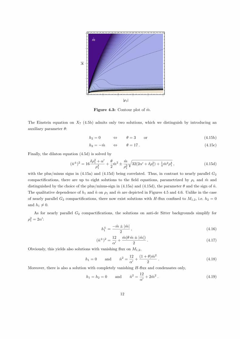
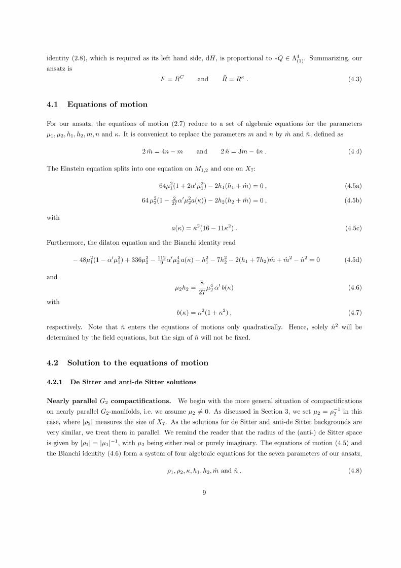
Figure 4.3: Contour plot of m.

The Einstein equation on X7 (4.5b) admits only two solutions, which we distinguish by introducing an

auxiliary parameter θ:

h2 = 0 ⇔ θ = 3 or (4.15b)

h2 = −m ⇔ θ = 17 . (4.15c)

Finally, the dilaton equation (4.5d) is solved by

(n±)2 = 16δρ21 + α′

ρ41+θ

2m2 ± m

ρ21

√32(2α′ + δρ21) + 1

4m2ρ41 , (4.15d)

with the plus/minus signs in (4.15a) and (4.15d) being correlated. Thus, in contrast to nearly parallel G2

compactifications, there are up to eight solutions to the field equations, parametrized by ρ1 and m and

distinguished by the choice of the plus/minus-sign in (4.15a) and (4.15d), the parameter θ and the sign of n.

The qualitative dependence of h1 and n on ρ1 and m are depicted in Figures 4.5 and 4.6. Unlike in the case

of nearly parallel G2 compactifications, there now exist solutions with H-flux confined to M1,2, i.e. h2 = 0

and h1 6= 0.

As for nearly parallel G2 compactifications, the solutions on anti-de Sitter backgrounds simplify for

ρ21 = 2α′:

h±1 =−m± |m|

2, (4.16)

(n±)2 =12

α′+m(θ m± |m|)

2. (4.17)

Obviously, this yields also solutions with vanishing flux on M1,2,

h1 = 0 and n2 =12

α′+

(1 + θ)m2

2. (4.18)

Moreover, there is also a solution with completely vanishing H-flux and condensates only,

h1 = h2 = 0 and n2 =12

α′+ 2m2 . (4.19)

12

(a) Anti-de Sitter backgrounds (b) De Sitter backgrounds

Figure 4.4: Plots of n± for a fixed value of ρ2 and κ (top) and contour plots of n− (bottom) for a fixed

value of ρ1. In the striped area, no solution to the equations of motion exist.

4.2.2 Minkowski solutions

Nearly parallel G2 compactifications. For compactifications to three-dimensional Minkowski space, we

have to set µ1 = 0. The solutions to the Bianchi identity (4.6) and the Einstein equation on X7 (4.5b) are

the same as in the (A)dS-case,

h2 =8α′

27ρ32b(κ) . (4.20a)

m = 2ρ2

[54

α′b(κ)− 4a(κ)

ρ22b(κ)− 4α′b(κ)

27ρ42

]. (4.20b)

The Einstein equation on M1,2 (4.5a) on the other hand is solved by either

h−1 = 0 or (4.20c)

h+1 = −2ρ2

[54

α′b(κ)− 4a(κ)

ρ22b(κ)− 4α′b(κ)

27ρ42

]. (4.20d)

13

(a) Anti-de Sitter background (b) De Sitter background

Figure 4.5: Contour plots of h−1 for compactifications on manifolds with G2-holonomy.

Finally, the solution to the equation of motion for the dilaton (4.5d) yields

(n±)2 = 112

(− 1

ρ22+

5α′a(κ)

27ρ42+

4α′2b(κ)2

729ρ62

)+ (6± 2)ρ22

(54

α′b(κ)− 4a(κ)

ρ22b(κ)− 4α′b(κ)

27ρ42

)2

. (4.20e)

The superscripts + and − refer to the solutions (4.20c) and (4.20d) for H1. As for the solutions on de Sitter

and anti-de Sitter backgrounds, the dependence of m and n on ρ2 and κ cannot be easily seen from (4.20a)

and (4.20e). The solution for m, however, is identical to the (anti-)de Sitter case (see (4.10b) and Figure

4.3). Furthermore, the qualitative dependence of the solution for n on ρ2 and κ is the same as for (anti-)de

Sitter backgrounds (see Figure 4.4), as (4.20e) is the |ρ1| → ∞ limit of (4.10d).

G2-holonomy compactifications. Finally, we discuss the case of compactifications to Minkowski space

on manifolds with G2-holonomy. As in the previous cases of G2-holonomy compactifications, the Bianchi

identity requires

R = F ⇒ κ = 0 . (4.21)

After sending ρ2 →∞, the field equations are solved by

h2 = −m (4.22a)

and either

h1 = 0 , n2 = 8m2 or (4.22b)

h1 = −m , n2 = 9m2 . (4.22c)

14

(a) Anti-de Sitter background (b) De Sitter background

Figure 4.6: Plots of n± for compactifications on manifolds with G2-holonomy. In the striped area, no

solution to the equations of motion exist.

Hence, there are four independent solutions to the field equations. In contrast to the previous cases, the

equations of motion possess solutions for all values of the parameter m.

4.3 Supersymmetry conditions and supersymmetric solutions

It is of interest to find out which subset of our heterotic backgrounds are supersymmetric. To this end, we

investigate the supersymmetry conditions (2.6). We begin with the gravitino variation (2.6a). Recall that

M1,2 carries either a real or imaginary Killing spinor ζ with Killing number µ1 and that X7 possesses a real

Killing spinor with Killing number µ2. Furthermore, using (3.3) and (3.5) it is straightforward to compute

(XyH) · ε =

−2h1 (X · ε)⊗ η ⊗ (1, 0)t for X ∈ TM1,2

6i h2 ε⊗ (X · η)⊗ (1, 0)t for X ∈ TX7

(4.23)

and

Σ ·X · ε =

−m (X · ε)⊗ η ⊗ (1, 0)t for X ∈ TM1,2

−7im ε⊗ (X · η)⊗ (1, 0)t for X ∈ TX7

. (4.24)

Inserting these relations in the gravitino variation yields

96µ1 = 12h1 +m = 12h1 + m+ n , (4.25a)

96µ2 = 12h2 + 7m = 12h2 + 7(m+ n) . (4.25b)

15

As we set the dilaton to zero, the dilatino variation (2.6b) reads

4H + Σ−∆ = 0 (4.26)

and therefore we obtain

16h1 = 16h2 = 4(n−m) = −m− 3n . (4.27)

As already mentioned at the beginning of this section, the gaugino variation (2.6c) vanishes since F is an

instanton.

Together with the equations of motion, the conditions for the vanishing of the gravitino and the dilatino

variation, (4.25) and (4.27), form a set of eight equations for the seven parameters µ1, µ2, h1, h2, m, n and

κ. It can be checked straightforwardly that this system is not solvable. Hence, our compactifications on

nearly parallel G2-manifolds do not yield any supersymmetric solutions for either de Sitter, anti-de Sitter or

Minkowski space-times, not even in the G2-holonomy limit.

4.4 Fermion masses

Employing the decomposition of the fermions (2.18) and the Killing property of η as well as the knowledge

of the Clifford action of vol(3) (2.23) and Q (3.3), it is straightforward to rewrite the Dirac equations for the

gaugino (2.7e) and dilatino (2.7f) as

0 =(D +D− − 1

24 (H − 12Σ + 1

2∆)·)χ = (D −Mχ) χ , (4.28)

0 =(D +D− − 1

24 (H − 18Σ)·

)λ = (D −Mλ) λ , (4.29)

where D is the Dirac operator on M1,2. The masses of the gaugino and dilatino are readily computed to be

M =1

24(h1 + 7h2 − m− cn) with cχ = 3 and cλ = 1 . (4.30)

In the following, we give the expressions of the masses in terms of the parameters (ρ1, ρ2, κ) or (ρ1, m),

respectively, for the compactifications considered previously.

De Sitter and anti-de Sitter backgrounds. Recall that for given values of (ρ1, ρ2, κ) the field equations

possess up to four solutions in the case of compactifications on nearly parallel G2-manifolds and up to eight

solutions for compactifications on manifolds with G2-holonomy. There are up to two solutions for h1 labeled

by the superscript ±. Then, for a given solution for h1, the field equations fix the value of n2, but not the

sign of n (see (4.10d)). Hence, in the following we set

n = ν |n| with ν ∈ {−1,+1} . (4.31)

16

For compactifications on nearly parallel G2-manifolds the fermion masses are given by

M± = − 27ρ24α′b(κ)

+a(κ)

2ρ2b(κ)+

17α′b(κ)

162ρ32∓ ρ2

12

√8 (2α′ + δρ21)

ρ41ρ22

+

(27

α′b(κ)− 2a(κ)

ρ22b(κ)− 2α′b(κ)

27ρ42

)2

− νc|ρ2|6√

2

±( 27

α′b(κ)− 2a(κ)

ρ22b(κ)− 2α′b(κ)

27ρ42

)√8 (2α′ + δρ21)

ρ41ρ22

+

(27

α′b(κ)− 2a(κ)

ρ22b(κ)− 2α′b(κ)

27ρ42

)2

2(δρ21 + α′

)ρ41ρ

22

+3(27ρ22 − 2α′a(κ)

)2α′2b(κ)2ρ42

− 26

ρ42+

94α′a(κ)

27ρ62+

68α′2b(κ)2

729ρ82

]1/2, (4.32)

whereas for compactifications on manifolds with G2-holonomy they read2

M± = −θ m48± 1

48ρ41

√128ρ41(δρ21 + 2α′) + ρ81m

2

− cν

24√

2ρ21

√32 (δρ21 − α′) + θρ41m

2 ± ρ21m√

128(δρ21 + 2α′) + ρ41m2 . (4.33)

Minkowski backgrounds. On Minkowski backgrounds, the masses of the gaugino and dilatino are given

by

M± =(6± 2)k(κ)

3ρ2b(κ)− 9(6± 2)ρ2

2α′b(κ)+

(13± 2)α′b(κ)

81ρ32

− cν

8

√112

(− 1

ρ22+

5α′a(κ)

27ρ42+

4α′2b(κ)2

729ρ62

)+ (6± 2)ρ22

(54

α′b(κ)− 4a(κ)

ρ22b(κ)− 4α′b(κ)

27ρ42

)2

(4.34)

for compactifications on nearly parallel G2-manifolds.

Finally, for compactifications on manifolds with G2-holonomy the fermion masses read

M± = − 124 (a m+ c b ν|m|) . (4.35)

The values of (a, b) are given in the following table for all solutions to the field equations:

(a, b) h1 = 0 h1 = −m

h2 = 0 (1, 1) (2,√

2)

h2 = m (4, 2√

2) (9, 3)

(4.36)

Acknowledgements

We thank Alexander Haupt and Alexander Popov for helpful comments. This work was supported in part by

Deutsche Forschungsgemeinschaft grant LE 838/13 and the Graduiertenkolleg 1463 “Analysis, Geometry and

String Theory“. Furthermore, Karl-Philip Gemmer thanks the Volkswagen Foundation for partial support

under the grant I/84 496.

2Recall, that θ = 3 for solutions with h2 = 0 and θ = 17 for h2 = −m (see (4.15)).

17

A Useful identities for nearly parallel G2-manifolds

In this appendix we will list some useful identities for the G2-invariant three-form Q on manifolds with

G2-structure. In the following we will denote the Hodge-dual of Q by Q,

Q ≡ ∗Q = e3456 + e2467 + e2357 + e1457 + e1367 + e1256 + e1234 . (A.1)

It is straightforward to derive the following identities of contractions of Q and Q [14]:

QabeQcde = −Qabcd + δacδbd − δadδbc , (A.2a)

QacdQbcd = 6 δab , (A.2b)

QabpQpcde = 3Qa[cdδe]b − 3Qb[cdδe]a , (A.2c)

QabcpQdefp = −3Qab[deδf ]c − 2Qdef [aδb]c − 3Qab[dQef ]c + 6δ[da δebδf ]c , (A.2d)

QabpqQpqc = −4Qabc , (A.2e)

QabpqQpqcd = −2Qabcd + 4(δacδbd − δadδbc) , (A.2f)

QapqrQbpqr = 24δab , (A.2g)

QabpQpcqQqde = Qabdδce −Qabeδcd −Qadeδbc +Qbdeδac

−Qacdδbe +Qaceδbd +Qbcdδae −Qbceδad , (A.2h)

QpaqQqbsQscp = 3Qabc . (A.2i)

B Restrictions on the parameter space of solutions

In general, the equations of motion do not possess solutions for all values of the parameters µ1, µ2, h1, h2, m, n

and κ of the ansatz considered in Section 4. In this appendix we discuss for which values of the parameters

the field equations are not solvable.

B.1 Nearly parallel G2 compactifications

For both, anti-de Sitter and de Sitter backgrounds, the equations of motion were solved for h1, h2, m and n

and are parametrized by ρ1 = µ−11 , ρ2 = µ−12 and κ. In both cases it is obvious that there exists a lower

bound for |ρ1| imposed by demanding the solution for n2, (4.10d) or (4.10d), respectively, to be positive.

The same conditions exclude for fixed values of ρ1 a region in the parameter space spanned by ρ2 and κ

in which no solution to the field equations exists. Additionally, in the case of anti-de Sitter backgrounds,

the argument in the square root in (4.10a) and (4.10d) becomes negative for certain values of ρ1, ρ2 and κ.

Contour plots of the resulting lower bound on |ρ1| and the excluded region in the parameter space spanned

by ρ2 and κ are depicted in Figure B.1.

18

For compactifications on Minkowski backgrounds, the parameter µ1 vanishes. The parameter spaces

spanned by ρ2 and κ on the other hand is restricted by the same conditions as in the de Sitter and anti-de

Sitter cases. The area in the parameter spaces in which no solutions to the field equations with Minkowski

background can be given is depicted in Figure B.2.

(a) Anti-de Sitter backgrounds (b) De Sitter backgrounds

Figure B.1: Contour plot of the lower bound for |ρ1| for which solutions to the equations of motion for

(anti-)de Sitter backgrounds exists. For ρ2 → 0 or κ → 0 the lower bound approaches zero. In the striped

area, the equations of motion cannot be solved for any value of ρ1.

Figure B.2: Plot of the area in the parameter space spanned by ρ2 and κ for which no solutions to the

field equations exist.

19

B.2 G2-holonomy compactifications

The solutions to the equations for compactifications on G2-holonomy manifolds as discussed in Section 4

depend on the parameters ρ1 and m. For anti-de Sitter backgrounds, as in the nearly parallel G2 case, the

field equations only possess solutions if the value |ρ1| exceeds a lower bound. For de Sitter backgrounds on

the other hand, there is no lower bound on |ρ1|. Additionally, on both backgrounds, there is a lower bound

on |m|. Plot of the areas in the parameter space excluded by these lower bounds are shown in Figure B.3.

Finally, for compactifications to Minkowski space on G2-holonomy manifolds, the equations of motion are

solvable for all values of the parameters.

(a) Anti-de Sitter backgrounds (b) De Sitter backgrounds

Figure B.3: Plot of the area in the parameter space spanned by ρ1 and m for which no solutions to the

field equations for G2-holonomy compactifications exist.

20

References

[1] A. Strominger, Superstrings with torsion, Nuclear Physics B 274 (1986) 253.

[2] G. Cardoso, G. Curio, G. Dall’Agata, D. Lust, P. Manousselis, and G. Zoupanos, Non-Kahler string

backgrounds and their five torsion classes, Nuclear Physics B 652 (2003) 5, [hep-th/0211118].

[3] G. L. Cardoso, G. Curio, G. Dall’Agata, and D. Lust, Heterotic string theory on non-Kahler manifolds

with H-flux and gaugino condensate, Fortschritte der Physik 52 (2004) 483, [hep-th/0310021].

[4] A. Frey and M. Lippert, AdS strings with torsion: Noncomplex heterotic compactifications, Physical

Review D 72 (2005) 42, [hep-th/0507202].

[5] P. Manousselis, N. Prezas, and G. Zoupanos, Supersymmetric compactifications of heterotic strings

with fluxes and condensates, Nuclear Physics B 739 (2006) 85, [hep-th/0511122].

[6] O. Lechtenfeld, C. Nolle, and A. D. Popov, Heterotic compactifications on nearly Kahler manifolds,

Journal of High Energy Physics 1009 (2010) 74, [arXiv:1007.0236].

[7] A. Chatzistavrakidis, O. Lechtenfeld, and A. D. Popov, Nearly Kahler heterotic compactifications with

fermion condensates, Journal of High Energy Physics 1204 (2012) 114, [arXiv:1202.1278].

[8] E. Bergshoeff, M. de Roo, B. de Wit, and P. van Nieuwenhuizen, Ten-dimensional Maxwell-Einstein

supergravity, its currents, and the issue of its auxiliary fields, Nuclear Physics B 195 (1982) 97.

[9] G. Chapline and N. Manton, Unification of Yang-Mills theory and supergravity in ten-dimensions,

Physics Letters B 120 (1983) 105.

[10] E. A. Bergshoeff and M. de Roo, The quartic effective action of the heterotic string and

supersymmetry, Nuclear Physics B 328 (1989) 439.

[11] M. Fernandez and A. Gray, Riemannian manifolds with structure group G2, Annali di Matematica

Pura ed Applicata 132 (1982) 19.

[12] T. Friedrich, I. Kath, A. Moroianu, and U. Semmelmann, On nearly parallel G2-structures, Journal of

Geometry and Physics 23 (1997) 259.

[13] R. L. Bryant, Some remarks on G2-structures, in Proceedings of Gokova Geometry-Topology

Conference 2005 (T. O. S. Akbulut and R. Stern, eds.), pp. 75–109, International Press, 2006.

[14] A. Bilal, J.-P. Derendinger, and K. Sfetsos, (Weak) G2 holonomy from self-duality, flux and

supersymmetry, Nuclear Physics B 628 (2002) 112, [hep-th/0111274].

21