Adv. Appl. Clifford Algebras © 2011 Springer Basel AG DOI 10.1007/s00006-011-0285-5 On Conformal Infinity and Compactifications of the Minkowski Space Arkadiusz Jadczyk Abstract. Using the standard Cayley transform and elementary tools it is reiterated that the conformal compactification of the Minkowski space involves not only the “cone at infinity” but also the 2-sphere that is at the base of this cone. We represent this 2-sphere by two ad- ditionally marked points on the Penrose diagram for the compactified Minkowski space. Lacks and omissions in the existing literature are de- scribed, Penrose diagrams are derived for both, simple compactification and its double covering space, which is discussed in some detail using both the U (2) approach and the exterior and Clifford algebra meth- ods. Using the Hodge operator twistors (i.e. vectors of the pseudo- Hermitian space H2,2) are realized as spinors (i.e., vectors of a faithful irreducible representation of the even Clifford algebra) for the conformal group SO(4, 2)/Z2. Killing vector fields corresponding to the left action of U (2) on itself are explicitly calculated. Isotropic cones and corre- sponding projective quadrics in Hp,q are also discussed. Applications to flat conformal structures, including the normal Cartan connection and conformal development has been discussed in some detail. Keywords. Compactification, Minkowski space-time, Conformal spinors, Twistors, SU(2), SU(2,2), U(2), SO(4,2), Null geodesics, Penrose dia- gram, Conformal infinity, Conformal group, Conformal inversion, Hodge star, bivectors, Grassmann manifold, Clifford algebra C(4, 2) . 1. Introduction The term compactification can have several different meanings. Given a man- ifold M we may try to embed it into a compact one and take its closure. Or, we can attach to M ideal boundary points or boundary components so as to obtain a compact space. In physics compactification of space-time can be used either in order to study its conformal invariance, or to study its asymptotic flatness, or its singularities. In the available literature the differences between Advances in Applied Clifford Algebras

Welcome message from author
This document is posted to help you gain knowledge. Please leave a comment to let me know what you think about it! Share it to your friends and learn new things together.
Transcript
Adv. Appl. Cliff ord Algebras© 2011 Springer Basel AG DOI 10.1007/s00006-011-0285-5
On Conformal Infinity andCompactifications of the Minkowski Space
Arkadiusz Jadczyk
Abstract. Using the standard Cayley transform and elementary toolsit is reiterated that the conformal compactification of the Minkowskispace involves not only the “cone at infinity” but also the 2-spherethat is at the base of this cone. We represent this 2-sphere by two ad-ditionally marked points on the Penrose diagram for the compactifiedMinkowski space. Lacks and omissions in the existing literature are de-scribed, Penrose diagrams are derived for both, simple compactificationand its double covering space, which is discussed in some detail usingboth the U(2) approach and the exterior and Clifford algebra meth-ods. Using the Hodge � operator twistors (i.e. vectors of the pseudo-Hermitian space H2,2) are realized as spinors (i.e., vectors of a faithfulirreducible representation of the even Clifford algebra) for the conformalgroup SO(4, 2)/Z2. Killing vector fields corresponding to the left actionof U(2) on itself are explicitly calculated. Isotropic cones and corre-sponding projective quadrics in Hp,q are also discussed. Applications toflat conformal structures, including the normal Cartan connection andconformal development has been discussed in some detail.
Keywords. Compactification, Minkowski space-time, Conformal spinors,Twistors, SU(2), SU(2,2), U(2), SO(4,2), Null geodesics, Penrose dia-gram, Conformal infinity, Conformal group, Conformal inversion, Hodgestar, bivectors, Grassmann manifold, Clifford algebra C�(4, 2) .
1. Introduction
The term compactification can have several different meanings. Given a man-ifold M we may try to embed it into a compact one and take its closure. Or,we can attach to M ideal boundary points or boundary components so as toobtain a compact space. In physics compactification of space-time can be usedeither in order to study its conformal invariance, or to study its asymptoticflatness, or its singularities. In the available literature the differences between
Advances inApplied Cliff ord Algebras
A. Jadczyk
these different approaches are not always made clear and the mathematicallanguage involved is not always as precise as one would wish.
This paper is a compromise between being completely self-containedand a typical specialized article. We use techniques of algebra and geometrybut we avoid twistor notation of Penrose school which can be confusing tomany mathematicians. The paper is aimed at mathematicians interested inmathematical properties of Minkowski space related to projective geometry,and at mathematical physicists interested in the subject. Relativists will findnext to nothing of interest for them in the material below (perhaps except ofa warning about how errors can easily propagate). They have their own aimsand techniques and, as a rule, are usually not interested in generalizationsgoing beyond four space-time dimensions.
In section 2 we review the conformal compactification M = U(2) of theMinkowski space M. We are following there the elegant and simple methodof A. Uhlmann [1] by using 2× 2 matrices and the Cayley transform. We arealso investigating in some detail the structure of the “light cone at infinity”,that is the set difference M \M and point out that it consists not only of the(double) light cone, but also of a 2-sphere that connects the two cones – a factthat was known to Roger Penrose [2, p. 178]. This fact was not always realizedby other authors writing on this subject even when they quoted Penrose (cf.e.g., Sec. 3). Additionally, as a complement to this particular representationof M, in Appendix A, we calculate vector fields on M corresponding to one-parameter subgroups of U(2) acting on itself by left translations.
In section 3, as an educational example, we discuss in some detail thefaulty argument and the missing 2-sphere in [3]. In particular we reproducea crucial part of reasoning used in [3] and point out the omission explicitly.Similar omissions, this time taken from [14] and also from recent papers onconformal field theory, are discussed in section 3.2.
In section 4, geometrical representation of the conformal compactifi-cation M is discussed using the cylinder representation of Einstein’s staticuniverse – the standard representation in general relativity. This leads to atwo-dimensional diagram – a version of the Penrose diagram (cf. Fig. 1), withthe two 2-spheres that need to be identified. Owing to this identification nointrinsic distinction between J + and J− is possible. In Fig. 3 and Fig. 6 wemark these two parts of the conformal infinity in order to be able to comparethis diagram with those (as in Fig. 4) found in the standard literature.
In section 5, the explicit action of the Poincare group on the conformalinfinity is calculated, where it is in particular shown that this action is transi-tive there. A lack of a mathematical precision in the mathematical literatureon the subject is also elucidated.
Section 6 starts with a simple exercise showing a geometrically amusingfact that null geodesics can be completely trapped at infinity. A role of theconformal inversion, and the signature of the induced metric is also discussedthere. Then, a pictorial representation of the infinity is given, first as a double
Conformal Infi nity and Compactifi cations of Minkowski Space
cone with identified vertices in Fig. 3, then, more correct as far as its differ-entiability properties are concerned, as a squeezed torus in Fig. 6. A typical,almost identically looking, but with a different meaning, picture – taken from[4] – is shown in Fig. 4. The squeeze point in Fig. 6 corresponds to what isusually denoted as I0, I+, I− (or i0, i+, i−) in the standard literature. Allthree points coincide in our case.1 A correct image, which we reproduce herein Fig. 5 can be found in Fig. 2 of [5]. It may be worth quoting the followingremarks from the monograph of Penrose and Rindler [2, p. 298]:
“Having this natural association between the points of J−and J +, for Minkowski space, it is in some respect naturalto make identification between J− and J +, the point A−
being identified with A+ and J− and J + written as J . Ifwe do this, then, for the sake of continuity we should alsoidentify I− with I0, and I0 with I+.”
To which they added:“For reasons that we shall see in more detail later, suchidentification cannot be satisfactorily carried out in curvedasymptotically flat spaces. (Not only is there apparently nocanonical way of performing such identifications in general,but, when the total mass is non-zero any identification wouldlead to failure of the required regularity conditions along theidentification hypersurface.) For many purposes, the identi-fication of J− with J + may, even in Minkowski space, seemunphysical (and, of course, it need not be made). However,for various mathematical purposes the identification is veryuseful. . . ”
In subsection 6.4 we discuss the double cover of M, that can be obtained bythe same method as in section 3 but by considering positive rays rather thangenerator lines.2 This leads us to the compactification with the past infinityJ− and future infinity J + different, but I− and I+ are identified, thoughdifferent from I0. The resulting Penrose diagram is given in Fig. 2, and theensuing graphic representation of the conformal infinity is pictured in Fig. 7and in Fig. 8.
We follow here the method used by Kopczynski and Woronowicz in [9],but this time applied to the double cover of M. Moreover, we identify the anti-linear map x �→ x⊥ used by these authors as a Hodge � operator adapted for acomplex vector space V equipped with a non-degenerate sesquilinear form.3
After a general introduction, for an arbitrary signature, starting with theGrassmann algebra endowed with the natural scalar product, we specialize
1A. Uhlmann [1] conjectured that it may be a squeezed Klein’s bottle. Klein’s bottle is
unnecessary as long as we do not care about the embedding. Squeezed torus does the job.2This construction is also briefly mentioned in [6, p. 180]. It is also worthwhile to mentionthat (U(1)×SU(2))/Z2, Z2 = {I,−I}, with the topology of (S1×S3)/Z2 is homeomorphic,as a manifold, to its double cover U(1)× SU(2) – cf. [7] and [8].3For a discussion in case of positive definite scalar product cf. e.g., [10].
A. Jadczyk
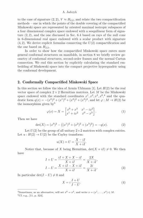
to the case of signature (2, 2), V ≈ H2,2, and relate the two compactificationmethods – one in which the points of the double covering of the compactifiedMinkowski space are represented by oriented maximal isotropic subspaces ofa four dimensional complex space endowed with a sesquilinear form of signa-ture (2, 2), and the one discussed in Sec. 6.4 based on rays of the null conein 6-dimensional real space endowed with a scalar product with signature(4, 2). We derive explicit formulas connecting the U(2) compactification andthe one based on H2,2.
In order to show how the compactified Minkowski space enters moregeneral conformal structures on manifolds, in section 8 we briefly review ge-ometry of conformal structures, second-order frames and the normal Cartanconnection. We end this section by explicitly calculating the standard em-bedding of Minkowski space into the compact projective hyperquadric usingthe conformal development.
2. Conformally Compactified Minkowski Space
In this section we follow the idea of Armin Uhlmann [1]. Let H(2) be the realvector space of complex 2 × 2 Hermitian matrices. Let M be the Minkowskispace endowed with the standard coordinates x1, x2, x3, x0,4 and the qua-dratic form q(x) = −(x0)2 + (x1)2 + (x2)2 + (x3)2, and let ϕ : M → H(2) bethe isomorphism given by5
ϕ(x) = X =[x0 + x3 x1 − ix2
x1 + ix2 x0 − x3
]. (1)
Then we have
det(X) = (x0)2 −((x1)2 + (x2)2 + (x3)2
)= −q(x). (2)
Let U(2) be the group of all unitary 2×2 matrices with complex entries.Let u : H(2) → U(2) be the Cayley transform:
u(X) = U =X − iI
X + iI.
Notice that, because of X being Hermitian, det(X + iI) �= 0. We thenhave
I + U =iI + X + X − iI
X + iI=
2XX + iI
,
I − U =X + iI −X + iI
X + iI=
2iX + iI
. (3)
In particular det(I − U) �= 0 and
X = iI + U
I − U. (4)
4Sometimes, as an alternative, will set x0 = x4, and write x = (x1, . . . , x4) ∈M.5Cf. e.g., [11, p. 324].
Conformal Infi nity and Compactifi cations of Minkowski Space
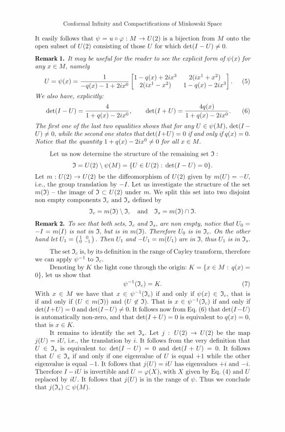
It easily follows that ψ = u ◦ ϕ : M → U(2) is a bijection from M onto theopen subset of U(2) consisting of those U for which det(I − U) �= 0.
Remark 1. It may be useful for the reader to see the explicit form of ψ(x) forany x ∈ M, namely
U = ψ(x) =1
−q(x) − 1 + 2ix0
[1 − q(x) + 2ix3 2(ix1 + x2)
2(ix1 − x2) 1 − q(x) − 2ix3
]. (5)
We also have, explicitly:
det(I − U) =4
1 + q(x) − 2ix0, det(I + U) =
4q(x)1 + q(x) − 2ix0
. (6)
The first one of the last two equalities shows that for any U ∈ ψ(M), det(I−U) �= 0, while the second one states that det(I+U) = 0 if and only if q(x) = 0.Notice that the quantity 1 + q(x) − 2ix0 �= 0 for all x ∈ M.
Let us now determine the structure of the remaining set I :
I = U(2) \ ψ(M) = {U ∈ U(2) : det(I − U) = 0}.Let m : U(2) → U(2) be the diffeomorphism of U(2) given by m(U) = −U,i.e., the group translation by −I. Let us investigate the structure of the setm(I) – the image of I ⊂ U(2) under m. We split this set into two disjointnon empty components Ic and Is defined by
Ic = m(I) \ I, and Is = m(I) ∩ I.
Remark 2. To see that both sets, Ic and Is, are non empty, notice that U0 =−I = m(I) is not in I, but is in m(I). Therefore U0 is in Ic. On the otherhand let U1 =
(1 00 −1
). Then U1 and −U1 = m(U1) are in I, thus U1 is in Is.
The set Ic is, by its definition in the range of Cayley transform, thereforewe can apply ψ−1 to Ic.
Denoting by K the light cone through the origin: K = {x ∈ M : q(x) =0}, let us show that
ψ−1(Ic) = K. (7)
With x ∈ M we have that x ∈ ψ−1(Ic) if and only if ψ(x) ∈ Ic, that isif and only if (U ∈ m(I)) and (U �∈ I). That is x ∈ ψ−1(Ic) if and only ifdet(I+U) = 0 and det(I−U) �= 0. It follows now from Eq. (6) that det(I−U)is automatically non-zero, and that det(I +U) = 0 is equivalent to q(x) = 0,that is x ∈ K.
It remains to identify the set Is. Let j : U(2) → U(2) be the mapj(U) = iU, i.e., the translation by i. It follows from the very definition thatU ∈ Is is equivalent to: det(I − U) = 0 and det(I + U) = 0. It followsthat U ∈ Is if and only if one eigenvalue of U is equal +1 while the othereigenvalue is equal −1. It follows that j(U) = iU has eigenvalues +i and −i.Therefore I− iU is invertible and U = ϕ(X), with X given by Eq. (4) and Ureplaced by iU . It follows that j(U) is in the range of ψ. Thus we concludethat j(Is) ⊂ ψ(M).
A. Jadczyk
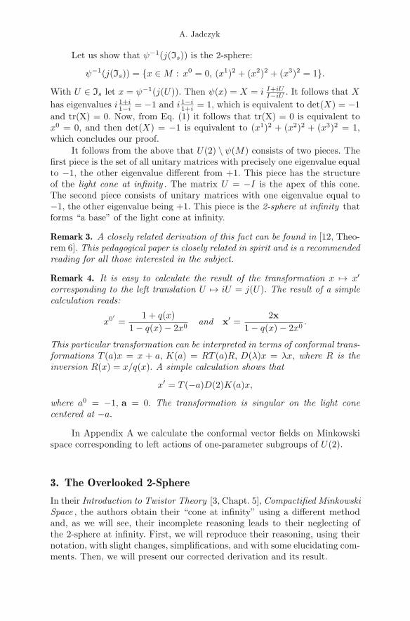
Let us show that ψ−1(j(Is)) is the 2-sphere:
ψ−1(j(Is)) = {x ∈ M : x0 = 0, (x1)2 + (x2)2 + (x3)2 = 1}.
With U ∈ Is let x = ψ−1(j(U)). Then ψ(x) = X = i I+iUI−iU . It follows that X
has eigenvalues i 1+i1−i = −1 and i 1−i
1+i = 1, which is equivalent to det(X) = −1and tr(X) = 0. Now, from Eq. (1) it follows that tr(X) = 0 is equivalent tox0 = 0, and then det(X) = −1 is equivalent to (x1)2 + (x2)2 + (x3)2 = 1,which concludes our proof.
It follows from the above that U(2) \ ψ(M) consists of two pieces. Thefirst piece is the set of all unitary matrices with precisely one eigenvalue equalto −1, the other eigenvalue different from +1. This piece has the structureof the light cone at infinity . The matrix U = −I is the apex of this cone.The second piece consists of unitary matrices with one eigenvalue equal to−1, the other eigenvalue being +1. This piece is the 2-sphere at infinity thatforms “a base” of the light cone at infinity.
Remark 3. A closely related derivation of this fact can be found in [12, Theo-rem 6]. This pedagogical paper is closely related in spirit and is a recommendedreading for all those interested in the subject.
Remark 4. It is easy to calculate the result of the transformation x �→ x′
corresponding to the left translation U �→ iU = j(U). The result of a simplecalculation reads:
x0′ =1 + q(x)
1 − q(x) − 2x0and x′ =
2x1 − q(x) − 2x0
.
This particular transformation can be interpreted in terms of conformal trans-formations T (a)x = x + a, K(a) = RT (a)R, D(λ)x = λx, where R is theinversion R(x) = x/q(x). A simple calculation shows that
x′ = T (−a)D(2)K(a)x,
where a0 = −1, a = 0. The transformation is singular on the light conecentered at −a.
In Appendix A we calculate the conformal vector fields on Minkowskispace corresponding to left actions of one-parameter subgroups of U(2).
3. The Overlooked 2-Sphere
In their Introduction to Twistor Theory [3, Chapt. 5], Compactified MinkowskiSpace , the authors obtain their “cone at infinity” using a different methodand, as we will see, their incomplete reasoning leads to their neglecting ofthe 2-sphere at infinity. First, we will reproduce their reasoning, using theirnotation, with slight changes, simplifications, and with some elucidating com-ments. Then, we will present our corrected derivation and its result.
Conformal Infi nity and Compactifi cations of Minkowski Space
3.1. Reasoning of Huggett and Tod
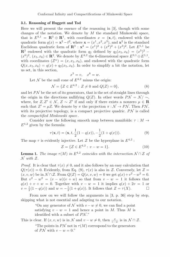
Here we will present the essence of the reasoning in [3], though with somechanges of the notation. We denote by M the standard Minkowski space,that is E3,1 = R3 ⊕ R1, with coordinates x = (x, t), endowed with thequadratic form q(x) = x2− t2, where x = (x1, x2, x3), and x2 is the standardEuclidean quadratic form of R3 : x2 = (x1)2 + (x2)2 + (x3)2. Let E1,1 beR2 endowed with the quadratic form q2 defined by q2(x5, x6) = (x5)2 −(x6)2, (x5, x6) ∈ R2. We denote by E4,2 the 6-dimensional space E3,1⊕E1,1,with coordinates (Zα) = (x, x5, x6), and endowed with the quadratic formQ(x, x5, x6) = q(x) + q2(x5, x6). In order to simplify a bit the notation, letus set, in this section,
x5 = v, x6 = w.
Let N be the null cone of E4,2 minus the origin:
N = {Z ∈ E4,2 : Z �= 0 and Q(Z) = 0}, (8)
and let PN be the set of its generators, that is the set of straight lines throughthe origin in the directions nullifying Q(Z). In other words PN = N/ ∼,where, for Z,Z ′ ∈ N , Z ∼ Z ′ if and only if there exists a nonzero μ ∈ Rsuch that Z ′ = μZ. We denote by π the projection π : N → PN . Then PN ,with its projective topology, is a compact projective quadric. PN is calledthe compactified Minkowski space .
Consider now the following smooth map between manifolds: τ : M →E4,2 given by the formula:
τ(x, t) = (x, t,12(1 − q(x)),−1
2(1 + q(x))). (9)
The map τ is evidently injective. Let Z be the hyperplane in E4,2 :
Z = {Z ∈ E4,2 : v − w = 1}. (10)
Lemma 1. The image τ(M) in E4,2 coincides with the intersection N ∩Z ofN with Z.
Proof. It is clear that τ(x) �= 0, and it also follows by an easy calculation thatQ(τ(x)) = 0. Evidently, from Eq. (9), τ(x) is also in Z. Conversely, let Z =(x, v, w) be in N ∩Z. From Q(Z) = Q(x, v, w) = 0 we get q(x)+v2−w2 = 0.But v2 − w2 = (v − w)(v + w) so that from v − w = 1 it follows thatq(x) + v + w = 0. Together with v − w = 1 it implies q(x) + 2v = 1 orv = 1
2 (1 − q(x)) and w = − 12 (1 + q(x)). It follows that Z = τ(X). �
From now on we will follow the arguments in [3, p. 36] step by step,skipping what is not essential and adapting to our notation.
“On any generator of N with v−w �= 0, we can find a pointsatisfying v − w = 1 and hence a point in M. Thus M isidentified with a subset of PN .”
This is clear. If (x, v, w) is in N and v − w �= 0, then xv−w is in N ∩ Z.
“The points in PN not in τ(M) correspond to the generatorsof PN with v − w = 0.”
A. Jadczyk
This is evident from the definition. Now there comes an unclear paragraphwith an erroneous conclusion:
“This is the intersection of N with a null hyperplane throughthe origin. All such hyperplanes are equivalent under O(4, 2)so to see what these extra points represent, we consider thenull hyperplane v + w = 0. From Eq. (9) we see that thepoints of M corresponding to generators of N which lie inthis hyperplane are just the null cone of the origin. Thus PNconsists of τ(M) with an extra cone at infinity.”
It is rather hard to follow this fuzzy reasoning, therefore we will study thestructure of the “extra part” directly from the definition. The extra part isthe projection by π of those points in N for which v − w = 0. Now thefollowing two cases must be considered separately: either v = w = 0 orv = w �= 0. Let Nc = {Z ∈ N : v = w �= 0, and Ns = {Z ∈ N : v = w = 0}.Each element of π(Nc) has a unique representative Z ′ = (x′, v′, w′) in Nwith v′ = w′ = 1. Since Q(Z ′) = 0, we have q(x′) = 0. Therefore π(Nc)has the structure of the null cone at zero in M. But there is also the secondpart, π(Ns). If Z = (x, t, 0, 0) is in Ns, then t �= 0, otherwise, because ofQ(Z) = q(x) = 0 we would have x = 0. Therefore each Z = (x, t, 0, 0) in Ns
has a unique representative with t = 1. From q(x) = 0 it follows then thatx2 = 1. It follows that π(Ns) has the structure of the 2-sphere. This part ismissing in the conclusion of [3]. One of the possible reasons for this omissioncan be a possibly misleading statement in Penrose and Rindler [2, p. 303],where we can read
“. . . and the remainder of the intersection of the 4-planewith M is J (the identified surfaces J +,J− of the previousconstruction).”
The point is that in J of Penrose and Rindler one has to first identify thetwo 2-spheres, one of J + and one of J−, though with opposite orientations– see the next subsection. This lack of precision in [2] may have confused theauthors of [3, 13].
3.2. The 2-sphere missed by Akivis and Goldberg
A similar inadvertency takes place in a monograph on conformal geometry byM. A. Akivis and V. V. Goldberg [14]. In the introductory chapter the authorsanalyze the Euclidean case. They start with the equation of a hyperspherein the conformal space Cn, which is just En,0 endowed with an Euclideanscalar product defined up to a non-zero multiplicative constant. The equation,in polyspherical coordinates s0, si, sn+1, reads: s0
∑ni=1(x
i)2 + 2∑n
i=1 sixi +
2sn+1 = 0. When s0 �= 0, this can be put in the form:n∑
i=1
(xi−ai)2 = r2, where ai = − si
s0, r2 =
1(s0)2
(n∑
i=1
(si)2 − 2s0sn+1
).
In order to describe a hypersphere of zero radius (centered at ai) we musthave (X,X) :=
∑ni=1(s
i)2 − 2s0sn+1 = 0, which is just the equation (8) of
Conformal Infi nity and Compactifi cations of Minkowski Space
the null cone N in En+1,1 with s0 = 12 (w − v), sn+1 = (w + v), adapted
to the Euclidean signature. Hyperspheres of zero radius correspond to thepoints (their centers) in Cn. The remaining set of non-zero solutions of Eq.(8) is the line s0 = 0, xi = 0, 1,≤ i ≤ n, sn+1 �= 0 – the point at infinity.
The same strategy is then used in Chapter 4.1 in the pseudo-Euclideancase. With slight changes of the notation the authors state [14, p. 127] that
“. . . after compactification the tangent space Tx(M) is en-larged by the point at infinity y with coordinates (0, 0, . . . , 0, 1)and by the isotropic cone Cx, with vertex at this point ywhose equation is the same as the equation of the cone Cx,namely gijx
ixj = 0.”
There is a subtle inadvertency there. The change of notation is not important,so let us use the same notation as in the Euclidean case. When s0 �= 0 we havethe same situation as in the Euclidean case, except that the “hypersphereof zero radius” becomes now a cone (light cone in the Minkowski case). Itremains to consider the case of s0 = 0. Here we have two possibilities: eithersn+1 = 0 or sn+1 �= 0. If sn+1 = 0, then, necessarily, the n-vector (si) �= 0,and gijs
isj = 0. But then, we should consider the set of lines and not the setof points.
For example in the case of Minkowski space we find that the set of linesis the quadric (S2), and not the “isotropic cone”, as falsely stated in [14].On the other hand, if sn+1 �= 0, the we can choose sn+1 = 1. In this case nofreedom of choosing the scale remains and we get gijs
isj = 0 – the isotropiccone, including its origin.
Another mistake takes place during the discussion of the conformal in-version in [14, p. 15-16]. The authors state that
“In the pseudo-Euclidean space Rnq , the inversion in a hy-
persphere S with center at a point A is defined exactly in thesame manner as it was defined in the Euclidean space Rn
(. . . ). However, in contrast to the space Rn, under an inver-sion in the space Rn
q not only does the center a of the hyper-sphere S not have an image but also points of the isotropiccone Cx with vertex at the point a does not have images. Toinclude these points in the domain of the mapping definedby the inversion in Rn
q , we enlarge the space Rnq not only
by the point at infinity, ∞, corresponding to the point a butalso by the isotropic cone C∞ with the vertex at this point.The manifold obtained as the result of this enlargement isdenoted by Cn
q :
Cnq = Rn
q
⋃{C∞}
and is called a pseudoconformal sphere of index q. (. . . ) Justlike conformal space Cn, the pseudoconformal space Cn
q ishomogeneous.”
A. Jadczyk
Adding the image of the isotropic cone under inversion does not result in thehomogeneous space. In section 6.1 we show that the conformal inversion withrespect to the isotropic cone C0 centered at the origin 0 ∈ M is implementedby the map (x, v, w) �→ (x,−v, w). Using the embedding τ : M → E4,1 givenby Eq. 9 we find that the image of C0 consists of vectors of the form (x, 1
2 ,−12 )
and therefore τ(C0) consists of vectors of the form (x,− 12 ,−
12 ). Let now x be
a nonzero vector in C0, and let a be a vector satisfying x · a = 12 . The action
of the translation group is given by Eq. (15). It is clear that after translationby a the point (x,− 1
2 ,−12 ) is mapped to (x, 0, 0), which is not in the image
of C0 under inversion. Therefore the statement in [14] that adding just theimage of C0 under inversion gives a homogeneous space is erroneous. It isnecessary to add the missing sphere.
A similar misleading statement can be found in a paper by N. M. Nikolovand I. T. Todorov in [15], where the authors state that “The points at infinityin M form a D − 1 dimensional cone with tip at p∞, quoting Penrose [18],and then state that “. . . the Weyl inversion . . . interchanges the light coneat the origin with the light cone at infinity”.6
4. From Einstein’s Static Universe to PNThe group U(1) can be identified withe the group of complex numbers z ∈ Cwith |z| = 1, and the group SU(2) can be thought of as the group of unitquaternions {q = v + xi + yj + zk ∈ H : |q|2 = v2 + x2 = 1}. Let E4,1
denote R5, with coordinates (x, v, ψ), and endowed with the quadratic formq5(x, v, ψ) = x2 + v2 −ψ2. Writing z = eiψ, we can then represent the groupU(1) × SU(2) (topologically S1 × S3) as the cylinder K in E4,1:
K = {(x, v, ψ)} : x2 + v2 = 1, ψ ∈ [−π, π)}.
Lemma 2. With E4,2 endowed with the coordinates Z = (X, T, V,W ), as inthe previous section (but we will use capital letters here) let λ : E4,1 → E4,2,be the map
λ : (x, v, ψ) �→ (X, T, V,W ) = (x, sin(ψ), v,− cos(ψ)). (11)
Then π ◦ λ restricted to K, is 2 : 1 and surjective: π ◦ λ(K) = PN . Givenany two points (x1, v1, ψ1) and (x2, v2, ψ2) in K, we have π ◦ λ(x1, v1, ψ1) =π ◦ λ(x2, v2, ψ2) if and only if the following conditions (i)–(iii) hold:
(i) |ψ2 − ψ1| = π, (ii)x2 = −x1, and (iii) v2 = −v1.
Proof. The proof is evident after noticing that Q(Z) = X2−T 2+V 2−W 2 = 0can be written as X2 + V 2 = T 2 + W 2, and, if Z �= 0, then V 2 + X2 > 0.
6In a private exchange one of the authors (N.M.N) explained to me that the precise state-ment should read: “The Weyl inversion . . . interchanges the compact light cone at theorigin with the compact light cone at infinity, where the compact light “cone” with a tipat p is defined as {q ∈ M : p and q are mutually isotropic }. ” These concepts have beendescribed in [16, Appendix A,C] and [17], and will be developed in their future paper.
Conformal Infi nity and Compactifi cations of Minkowski Space
Therefore on each generator line of N there are exactly two points Z,−Z,with V 2 + X2 = 1. �
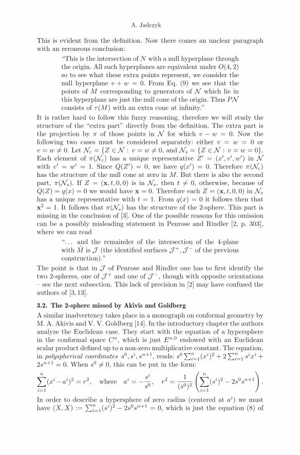
In order to be able to represent PN graphically, on a plane, let usintroduce the map ρ : K → [0, π] × [−π, π] ⊂ R2 given by
ρ : (x, v, ψ) �→ (ξ = arccos(v), ψ).
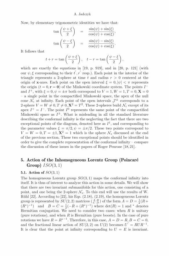
In Figure 1 the resulting “Penrose diagram” is shown, using the notation
−π
+π
0
I−
I+
I0
π
ξ
ψ
J−
J−
J+
J+
S
S
Figure 1. The “Penrose diagram” of Minkowski space.
as in [19, p. 919], but with two distinguished points denoted as S. In thisrealization they represent one and the same 2-sphere – they need to be iden-tified. The region inside the triangle with vertices at (0,−π), (0,+π), (π, 0)corresponds to the points in the Minkowski space. In order to understand thiscorrespondence, let us first notice that owing to the equation v2 +x2 = 1, wehave the following relations:
X = x, T = sin(ψ), V = cos(ξ), W = − cos(ψ), |X| = sin(ξ).
When V −W �= 0, we get the corresponding point in Minkowski space withcoordinates (r, t) given by the formulae:
r =X
V −W=
x
cos(ψ) + cos(ξ)
t =T
V −W=
sin(ψ)cos(ψ) + cos(ξ)
r = |r| =sin(ξ)
cos(ψ) + cos(ξ).
A. Jadczyk
Now, by elementary trigonometric identities we have that:
tan(ψ + ξ
2
)=
sin(ψ) + sin(ξ)cos(ψ) + cos(ξ)
,
tan(ψ − ξ
2
)=
sin(ψ) − sin(ξ)cos(ψ) + cos(ξ)
.
It follows that
t + r = tan(ψ + ξ
2
), t− r = tan
(ψ − ξ
2
),
which are exactly the equations in [19, p. 919], and in [20, p. 121] (withour ψ, ξ corresponding to their t
′, r
′resp.). Each point in the interior of the
triangle represents a 2-sphere at time t and radius r > 0 centered at theorigin of x-axes. Each point on the open interval ξ = 0, |ψ| < π representsthe origin (t = 0, r = 0) of the Minkowski coordinate system. The points I−
and I+, with ξ = 0, ψ = ±π both correspond to V = 1,W = 1, T = 0,X = 0– a single point in the compactified Minkowski space, the apex of the nullcone Nc at infinity. Each point of the open intervals J± corresponds to a2-sphere V = W �= 0, T �= 0,X2 = T 2. These 2-spheres build Nc except of itsapex I+ = I−. The point I0 represents the same point of the compactifiedMinkowski space as I±. What is misleading in all the standard literaturedescribing the conformal infinity is the neglecting the fact that there are twoexceptional points of the diagram, denoted here as I1, and corresponding tothe parameter values ξ = π/2, ψ = ±π/2. These two points correspond toV = W = 0, T = ±1,X2 = 1 which is the sphere Ns discussed at the endof the previous section. These two exceptional points should be identified inorder to give the complete representation of the conformal infinity – comparethe discussion of these issues in the papers of Roger Penrose [18, 21].
5. Action of the Inhomogeneous Lorentz Group (PoincareGroup) ISO(3, 1)
5.1. Action of SO(3, 1)The homogeneous Lorentz group SO(3, 1) maps the conformal infinity intoitself. It is thus of interest to analyze this action in some details. We will showthat there are two invariant submanifolds for this action, one consisting of apoint, and one being the 2-sphere Ns. To this end will use the results of W.Ruhl [22]. According to [22], his Eqs. (2.18), (2.19), the homogeneous Lorentzgroup is represented by SU(2, 2) matrices ( A B
C D ) of the form A = D = 12 (R+
(R∗)−1) and B = C = 12 (−R + (R∗)−1) where det(R) = 1 and ∗ denotes
Hermitian conjugation. We need to consider two cases: when R is unitary(pure rotations), and when R is Hermitian (pure boosts). In the case of purerotations we have R = R∗−1. Therefore, in this case, A = D = R,B = C = 0,and the fractional linear action of SU(2, 2) on U(2) becomes U
′= RUR−1.
It is clear that the point at infinity corresponding to U = E is invariant.
Conformal Infi nity and Compactifi cations of Minkowski Space
Also the spectrum of U is an invariant of this transformation, therefore the2-sphere Ns corresponding to U with eigenvalues ±1 is mapped into itself.
Now consider the boosts, with R = R∗. Denote R+ = R + (R∗)−1,R− = −R + (R∗)−1. The fractional linear transformation corresponding tothe boosts are then of the form:
U′= (R+U + R−)(R−U + R+)−1. (12)
Evidently the point U = E is left invariant. Consider now the 2-sphere Ns
corresponding to the unitary operators U with eigenvalues ±1. These pointsare characterized by the property U2 = E. Therefore we can rewrite the Eq.(12) as (R+U + R−)((R− + R+U)U)−1 = ZUZ−1, where Z = R+U + R−.It follows that then also (U
′)2 = E, therefore the Lorentz boosts map the
2-sphere Ns onto itself. Thus Ns is an O(3, 1)-invariant submanifold of theconformal infinity.
5.2. Action of the translations
Consider the translation by a four-vector a ∈ M. Using Clifford algebramethods and the formula for the translations in [23, p. 87] it is easy tocalculate the effect of the translation in terms of variables (x, v, w) of section3.1:
x′ = x− (v − w)a (13)
v′ = v + (x · a) − a2
2(v − w) (14)
w′ = w + (x · a) − a2
2(v − w) (15)
At the conformal infinity we have v = w, therefore x′ = x, but, for x �= 0, thecoordinates v and w change. If v = w = 0, then, after the generic translation,v′ = w′ �= 0. The coordinate description of the 2-sphere Ns, which is thecommon part of J + and J− changes. What is invariant is the set J + ∪J−,and the fact that J + and J− have a common 2-sphere.
5.3. Transitivity of ISO(3, 1) on the conformal infinity
Let J denote the conformal infinity, minus the singular point I0 = I+ = I−.It is easy to see that action of ISO(3, 1) on J is transitive. J has the topol-ogy of a cylinder R× S2. The group of translations acts along the R, whileSO(3, 1) acts transitively on S2 in a standard way – Lorentz transformationsact on directions of light rays through the origin of the Minkowski space. Itfollows that any splitting of J into J + and J− is not translation invariantand not intrinsic. The article of Roger Penrose [24] is extremely unclear inthis respect. Penrose mentions for instance that “There is another versionof compactified Minkowski space in which the future boundary hypersurfaceis identified with the past”, and quotes his earlier paper [25], as well as theclassic one by Kuiper [26], but he does not bother to define precisely whatwould be the alternative for the projective model. The same lack of clar-ity concerns the discussion in [20] and [19]. B.G. Schmidt, in an apparently
A. Jadczyk
mathematically precise paper [13] proves a Theorem stating that The con-formal boundary of Minkowski space is J +∪J−∪I+∪I−∪I0, without everbothering to define the sets on the right hand side of his statement.
In [27, p. 178] Penrose writes:
“There is one property of R, however, which seems unde-sirable when these ideas are applied to interacting fields, orcurved space-times. This is the fact that the ‘future infinity’turns out to have been identified with the ‘past infinity’ inthe definition of R. To avoid this feature it will be desirableeffectively to ‘cut’ this manifold along the hypersurface Jand to consider instead the resulting manifold with bound-ary. This boundary consists essentially of two copies of J ,one in ‘future’ which will be called J + and one in the ‘pastto be called J− . . . ”
Nowhere a precise definition of J + and J− is given. We are not told how thePoincare group acts on these ‘boundaries’. Also the authors of recent paperslike, for instance [28], when asked about the definition of J + and J− forMinkowski space, refer to Penrose [27] or Geroch [29]. In fact Geroch doesnot define J + and J− for the Minkowski space. He considers Schwarzschildspace-time with the topology S2 ×R2, proposes some coordinate-dependentconstructions and does not really discuss global symmetries.
6. Trapped at Infinity
We start this section by demonstrating that a light ray can be trapped inthe conformal infinity and circulate there “forever” – unless disturbed bysome quantum effect. It is well known (cf. e.g., [9] for a clear and self-contained exposition) that null geodesics are described by two-dimensionaltotally isotropic subspaces of E4,2. Using the coordinates (x, v, w) as in Sec.3.1, let x0 be a fixed non-zero null vector in E3,1, and let n1 and n2 be thevectors in E4,2 defined by n1 = (x0, 0, 0) and n2 = (0, 1, 1). Then the two-dimensional (real) plane spanned by n1 and n2 is totally isotropic – thereforeit is describing a null geodesic in the compactified Minkowski space. A gen-eral vector in this plane is of the form αn1 + βn2 = (αx0, β, β), therefore itis completely contained in the conformal infinity that consists of null vectors(x, v, w) with v = w. We can completely parameterize our null geodesic by aparameter τ ∈ [0, π] by choosing the representatives of its points in the form
(cos(τ)x0, sin(τ), sin(τ)). (16)
For τ = 0 the geodesic is on the 2-sphere Ns, for τ = π/2 it reaches theexceptional point I+ = I− = I0, then it circulates further towards the 2-sphere Ns. Notice that for τ = π we get the point (−x0, 0, 0) which projectsonto the same point of PN as (x0, 0, 0). Replacing x0 by λx0, λ ∈ R doesnot change the plane spanned by n1, n2, therefore in this way we get a familyof null geodesics, all trapped in the conformal infinity. We can always choose
Conformal Infi nity and Compactifi cations of Minkowski Space
a representative of x0 of the form (r, 1), r2 = 1, so that we have a trappednull geodesic for every point of the unit sphere in R3.
6.1. Conformal inversion
Consider the following linear map R of E4,2 : R : (x, v, w) �→ (x,−v, w). It isclear that R ∈ O(4, 2) (though not in SO(4, 2)). It is instructive to see thatR implements the conformal inversion x �→ x/x2 of the Minkowski space.To this end let x be a point in the Minkowski space M and let, writing x2
for q(x), τ(x) =(x, (1 − x2)/2,−(1 + x2)/2
)be its image in E4,2 as in Eq.
(9).7 We apply the inversion R to obtain(x,−(1 − x2)/2,−(1 + x2)/2
)and
represent it as an image of a new point x′. Therefore we should have(x′,−1
2(1 − x′2),−1
2(1 + x′2)
)= λ
(x,
12(1 − x2),−1
2(1 + x2)
). (17)
Now, from x′ = λx it follows that x′2 = λ2x2. Substituting this value of x′2
into the two other equations and adding them we get λ = 1/x2, thereforex′ = x
x2 , which is the well known conformal inversion in Minkowski space.The formula (17) becomes then an identity.8
Let us now apply the conformal inversion R to the light rays circulatingat infinity, given by the formula (16). We obtain the family
(x0,− sin(τ), sin(τ)) = −2 sin(τ)(x(τ),
12(1 − x(τ)2),−1
2(1 + x(τ)2
),
where x(τ) = − 12 cot(τ)x0. This is nothing else but a family of light rays
through the origin of the Minkowski space in the directions of null vectors x0.The parameter τ is, of course, not an affine parameter of these null geodesics.
6.2. The signature of the metric at infinity
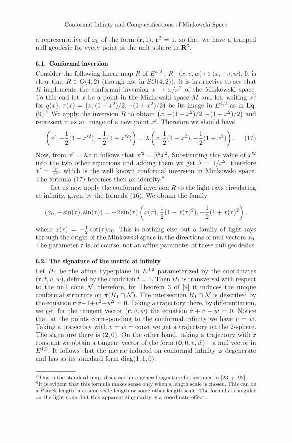
Let H1 be the affine hyperplane in E4,2 parameterized by the coordinates(r, t, v, w), defined by the condition t = 1. Then H1 is transversal with respectto the null cone N , therefore, by Theorem 3 of [9] it induces the uniqueconformal structure on π(H1 ∩ N ). The intersection H1 ∩ N is described bythe equation r·r−1+v2−w2 = 0. Taking a trajectory there, by differentiation,we get for the tangent vector (r, v, w) the equation r + v − w = 0. Noticethat at the points corresponding to the conformal infinity we have v = w.Taking a trajectory with v = w = const we get a trajectory on the 2-sphere.The signature there is (2, 0). On the other hand, taking a trajectory with rconstant we obtain a tangent vector of the form (0, 0, v, w) – a null vector inE4,2. It follows that the metric induced on conformal infinity is degenerateand has as its standard form diag(1, 1, 0).
7This is the standard map, discussed in a general signature for instance in [23, p. 92].8It is evident that this formula makes sense only when a length scale is chosen. This can bea Planck length, a cosmic scale length or some other length scale. The formula is singularon the light cone, but this apparent singularity is a coordinate effect.
A. Jadczyk
6.3. A pictorial representation of the infinity
In order to get an idea about the manifold structure of the conformal infinityand to obtain its pictorial representation, it is convenient to use the formulasfrom Lemma 2. At the conformal boundary we have v = w, thus v = cos(ψ),and since v2 + x2 = 1, we get x2 = sin2(ψ). Furthermore, because (x, t, v, w)and (−x,−t,−v,−w) describe the same point of PN , it is enough to considerψ ∈ [0, π]. The whole conformal infinity is then described by one equation:
x2 = sin2(ψ), ψ ∈ [0, π],
where (x, ψ = 0) and (x, ψ = π) describe the same point. This is nothingelse but a squeezed torus. Replacing the spheres S2 by circles S1 we get thegraphic representation as shown in Fig. 6. Topology itself is represented by adouble cone with two vertices identified, as in Fig. 3. This picture must notbe confused with a similarly looking picture taken from [4, p. 178], which wereproduce here in Fig. 4.
6.4. The double covering
It is possible to repeat the constructions of Sects 3.1 and 4, but replacing theequivalence relation Z ∼ Z ′ by a stronger one: we identify two vectors Z andZ ′ in E4,2 if and only if Z ′ = λZ, λ > 0. The manifold resulting by takingthe quotient of N by this new equivalence relation will be denoted by PN .Instead of one map τ as in Eq. (9) we define now two maps:
τ+(x) = (x,12(1 − q(x)),−1
2(1 + q(x))). (18)
τ−(x) = (x,−12(1 − q(x)),
12(1 + q(x))). (19)
Similarly we define
Z± = {Z ∈ E4,2 : v − w = ±1}, (20)
and then show that
Lemma 3. The image τ±(E3,1) in E4,2 coincides with the intersection N∩Z±of N with Z±.
The manifold PN contains now two copies of Minkowski space, we maycall them M+ and M−, joined by a common boundary.
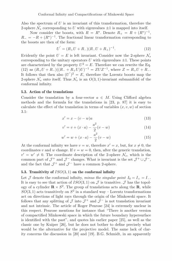
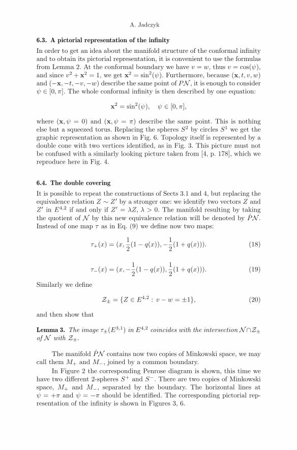
In Figure 2 the corresponding Penrose diagram is shown, this time wehave two different 2-spheres S+ and S−. There are two copies of Minkowskispace, M+ and M−, separated by the boundary. The horizontal lines atψ = +π and ψ = −π should be identified. The corresponding pictorial rep-resentation of the infinity is shown in Figures 3, 6.
Conformal Infi nity and Compactifi cations of Minkowski Space
−π
+π
0
I−
I+
I0
π
ξ
ψ
J−
J−
J+
J+
S−
S+
M+
M+
M−
M−
Figure 2. The second version of the “Penrose diagram” ofMinkowski space.
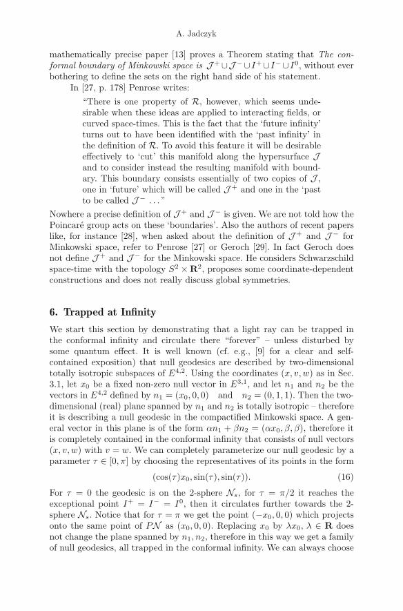
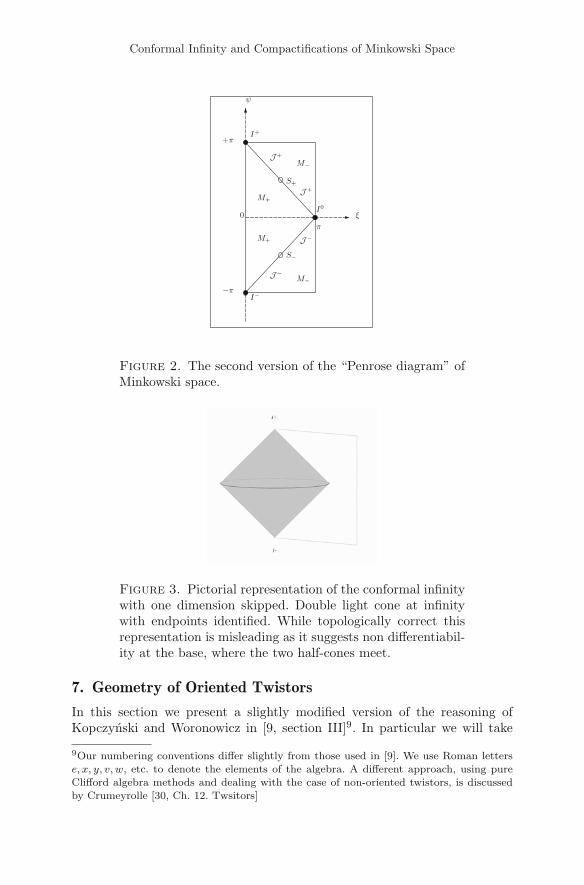
Figure 3. Pictorial representation of the conformal infinitywith one dimension skipped. Double light cone at infinitywith endpoints identified. While topologically correct thisrepresentation is misleading as it suggests non differentiabil-ity at the base, where the two half-cones meet.
7. Geometry of Oriented Twistors
In this section we present a slightly modified version of the reasoning ofKopczynski and Woronowicz in [9, section III]9. In particular we will take
9Our numbering conventions differ slightly from those used in [9]. We use Roman letterse, x, y, v, w, etc. to denote the elements of the algebra. A different approach, using pureClifford algebra methods and dealing with the case of non-oriented twistors, is discussedby Crumeyrolle [30, Ch. 12. Twsitors]
A. Jadczyk
i+
J +
J−
i0
i−
r = 0
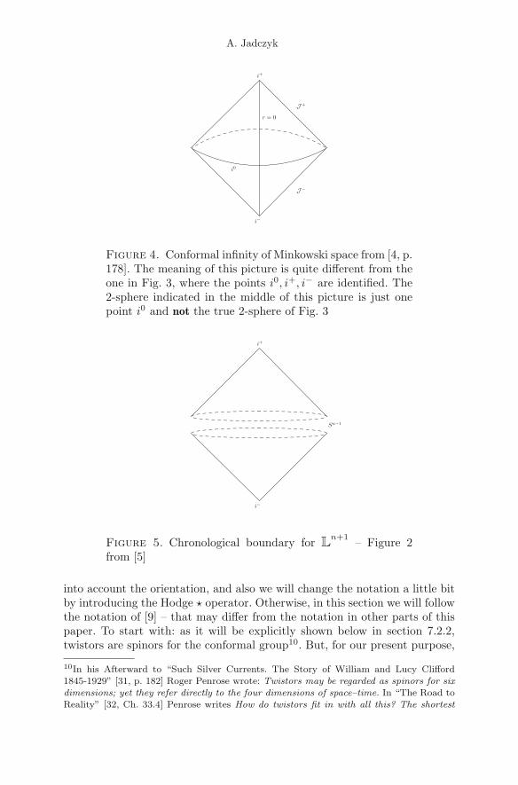
Figure 4. Conformal infinity of Minkowski space from [4, p.178]. The meaning of this picture is quite different from theone in Fig. 3, where the points i0, i+, i− are identified. The2-sphere indicated in the middle of this picture is just onepoint i0 and not the true 2-sphere of Fig. 3
i+
i−
Sn−1
Figure 5. Chronological boundary for Ln+1 – Figure 2
from [5]
into account the orientation, and also we will change the notation a little bitby introducing the Hodge � operator. Otherwise, in this section we will followthe notation of [9] – that may differ from the notation in other parts of thispaper. To start with: as it will be explicitly shown below in section 7.2.2,twistors are spinors for the conformal group10. But, for our present purpose,
10In his Afterward to “Such Silver Currents. The Story of William and Lucy Clifford1845-1929” [31, p. 182] Roger Penrose wrote: Twistors may be regarded as spinors for six
dimensions; yet they refer directly to the four dimensions of space–time. In “The Road toReality” [32, Ch. 33.4] Penrose writes How do twistors fit in with all this? The shortest
Conformal Infi nity and Compactifi cations of Minkowski Space
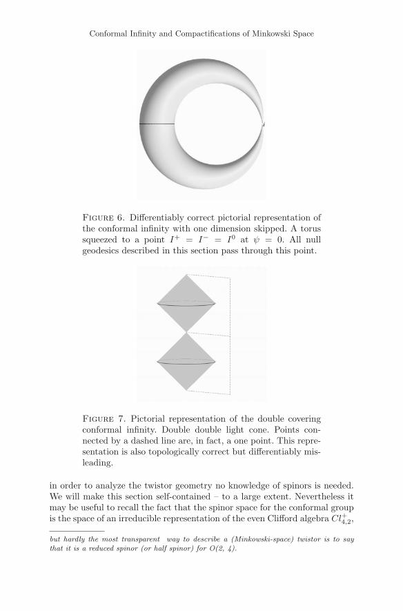
Figure 6. Differentiably correct pictorial representation ofthe conformal infinity with one dimension skipped. A torussqueezed to a point I+ = I− = I0 at ψ = 0. All nullgeodesics described in this section pass through this point.
Figure 7. Pictorial representation of the double coveringconformal infinity. Double double light cone. Points con-nected by a dashed line are, in fact, a one point. This repre-sentation is also topologically correct but differentiably mis-leading.
in order to analyze the twistor geometry no knowledge of spinors is needed.We will make this section self-contained – to a large extent. Nevertheless itmay be useful to recall the fact that the spinor space for the conformal groupis the space of an irreducible representation of the even Clifford algebra Cl+4,2,
but hardly the most transparent way to describe a (Minkowski-space) twistor is to saythat it is a reduced spinor (or half spinor) for O(2, 4).
A. Jadczyk
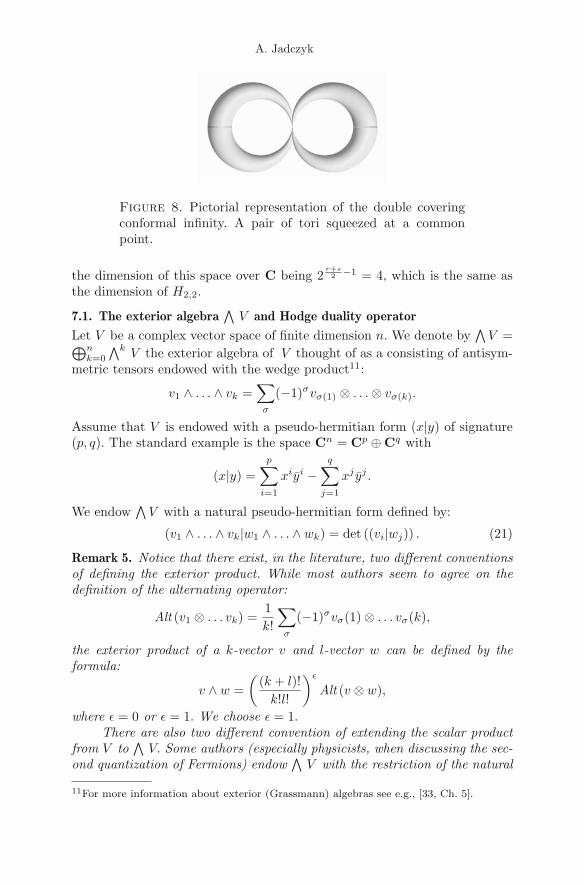
Figure 8. Pictorial representation of the double coveringconformal infinity. A pair of tori squeezed at a commonpoint.
the dimension of this space over C being 2r+s2 −1 = 4, which is the same as
the dimension of H2,2.
7.1. The exterior algebra∧
V and Hodge duality operator
Let V be a complex vector space of finite dimension n. We denote by∧V =⊕n
k=0
∧kV the exterior algebra of V thought of as a consisting of antisym-
metric tensors endowed with the wedge product11:
v1 ∧ . . . ∧ vk =∑σ
(−1)σvσ(1) ⊗ . . .⊗ vσ(k).
Assume that V is endowed with a pseudo-hermitian form (x|y) of signature(p, q). The standard example is the space Cn = Cp ⊕Cq with
(x|y) =p∑
i=1
xiyi −q∑
j=1
xj yj .
We endow∧V with a natural pseudo-hermitian form defined by:
(v1 ∧ . . . ∧ vk|w1 ∧ . . . ∧ wk) = det ((vi|wj)) . (21)
Remark 5. Notice that there exist, in the literature, two different conventionsof defining the exterior product. While most authors seem to agree on thedefinition of the alternating operator:
Alt (v1 ⊗ . . . vk) =1k!
∑σ
(−1)σvσ(1) ⊗ . . . vσ(k),
the exterior product of a k-vector v and l-vector w can be defined by theformula:
v ∧ w =(
(k + l)!k!l!
)ε
Alt (v ⊗ w),
where ε = 0 or ε = 1. We choose ε = 1.There are also two different convention of extending the scalar product
from V to∧
V. Some authors (especially physicists, when discussing the sec-ond quantization of Fermions) endow
∧V with the restriction of the natural
11For more information about exterior (Grassmann) algebras see e.g., [33, Ch. 5].
Conformal Infi nity and Compactifi cations of Minkowski Space
scalar product defined on the tensor product. For k-vectors this gives k! timesour scalar product.
Given x ∈∧p
V we have the coordinate representation of x in a basis{ei} of V :
x =1p!
xi1...ip ei1 ∧ . . . ∧ eip .
The wedge product is then given by the formula:
(x ∧ y)i1...ip+q =1
p!q!δi1... ...ip+q
j1...jpjp+1...jp+qxj1...jp yjp+1...jp+q ,
where δa...bc...d is the (generalized) Kronecker delta symbol. We also have thecoordinate representation:
(x|y) =1p!
Gi1j1 ..Gipjpxi1...ip yj1...jp , (22)
where Gij = 〈ei, ej〉.Let now {ei} be an orthonormal basis for V with (ei|ei) = +1 for
i = 1, . . . , p, and = −1 for i = p+1, . . . , p+ q, and let e = e1 ∧ . . .∧ en. Then(e|e) = (−1)q. Let e ∈
∧nV be a unit n-vector. We call e an orientation
of V. An orthonormal basis {ei} will be called oriented if e1 ∧ . . . ∧ en = e.Any two oriented bases are then related by a unique transformation from thegroup SU(p, q).
For each x ∈∧V let C(x) be the linear operator on
∧V defined by
C(x)y = x ∧ y.
Clearly, for x ∈∧k
V, we have C(x) :∧l
V →∧k+l
V, and v �→ C(v), v ∈ Vis a linear map from V to L(
∧V ), with
C(v)C(w) + C(w)C(v) = 0, (23)
for all v, w ∈ V. Notice that it follows from the definition that C(x ∧ y) =C(x)C(y).
Let C(x)∗ be the Hermitian adjoint of C(x), defined by
(C(x)∗y|z) = (y|C(x)z), y, z ∈∧
V.
Then, for x ∈∧k
V, C(x)∗ :∧l
V →∧l−k
V, the map x �→ C(x)∗ is anti-linear, and for v, w ∈ V we have the anti-commutation relations:
C(v)C(w)∗ + C(w)∗C(v) = (v|w). (24)
Notice that for all x, y ∈∧V we have C(x ∧ y)∗ = C(y)�C(x)∗.
Remark 6. The anti-commutation relations (23),(24) are known as CAR –canonical commutation relations – in our case finite-dimensional and gen-eralized for the case of an indefinite scalar product. If we define φ(v) =2−
12 (C(v) + C(v)∗) , then the real linear map v �→ φ(v) is a Clifford map for
V considered as a 2n-dimensional real vector space endowed with the scalarproduct � ((v|w)) – cf. [34]12.
12For a complex number z = α+ iβ we denote �(z) = α, �(z) = β.
A. Jadczyk
Assuming V oriented with an orientation e, we define the Hodge oper-ator � :
∧kV →
∧n−kV as an antilinear map � : x �→ �x uniquely defined
by the formula
x ∧ �y = (x|y)e, x, y ∈k∧
V. (25)
It is easy to see that an equivalent definition of the Hodge � operator is givenby:
�x = C(x)∗ e.
It easily follows from the definition that for x ∈∧k
V, y ∈∧n−k
V we have:
(x| � y) = (−1)k(n−k)(y| � x). (26)
A little bit more effort13 is required to check that we have
� � x = (−1)k(n−k)+q x, ∀x ∈k∧V.
Remark 7. A k-vector x �= 0 is called decomposable if x is of the formx = x1 ∧ .. ∧ xk for x1, . . . , xk ∈ V. If x is decomposable, then also �x isdecomposable. Moreover the (n − k)-dimensional subspace corresponding to�x is the orthogonal complement of the subspace corresponding to x – cf.[42, Exercise 8, p. 62].
Another important property involving creation and annihilation opera-tors and the Hodge star operator in [10, eq. 139] is14
�C(x)∗�−1 = C(x)(−1)d(x)N ,
where d(x) is the grade of x (d(x) = k for x ∈∧k
V ) and N is the numberoperator – Ny = ly for y ∈
∧lV.
We define a bilinear form
〈x, y〉 = (x| � y), x, y ∈∧
V.
Notice that the following formulas hold:
〈x, y〉 = (−1)q〈y, x〉, 〈x, y〉 = (−1)k(n−k)+q〈x, y〉
In an orthonormal basis ei such that e = e1 ∧ . . . en we have the explicitexpression for the star operator for x ∈
∧pV :
(�x)ip+1...in =1p!
Gi1j1 . . . Gipjp εi1...ipip+1...in xj1...jp . (27)
13Cf. e.g., [35, p. 167], [36, p. 118]14While only positive definite scalar product is discussed in [10], this particular propertycan be easily seen to hold also for pseudo-Hermitian spaces.
Conformal Infi nity and Compactifi cations of Minkowski Space
7.2. The case of signature (2, 2)In this section we specialize to the case of the signature (2, 2) that is relevantfor our purposes, and has been studied in [9].
Let G be the diagonal matrix G = diag(+1,+1,−1,−1). Let H2,2 bea four-dimensional complex vector space endowed with a pseudo-Hermitianform (·|·) of signature (2.2). A basis ei of H2,2 is said to be orthonormal if(ei|ej) = Gij . Any two orthonormal bases are related by a transformationfrom the group U(2, 2). We fix an orientation e ∈
∧4H2,2 and define the
Hodge � duality operator as in previous subsection. Notice that on∧2
H2,2
we have �2 = 1. Let �∧2
H2,2 be the space of self-dual bivectors:
�2∧H2,2 = {x ∈
2∧H2,2 : x = �x}.
Then �∧2
H2,2 is a six-dimensional real vector space, and the real-bilinearform 〈x, y〉 is real-valued and symmetric on �
∧2H2,2. It can be easily seen
(Cf. [9, Theorem 7]) that �∧2
H2,2 equipped with the scalar product 〈x, y〉is of signature (4, 2). It follows that all the constructions of section 6.4 applyand in the following we will use the notation of this section. In particular wewill use the identification E4,2 = �
∧2H2,2.
In a complex vector space the concept of an orientation of a subspaceis not well defined. In our case, however we can define what is meant by anoriented two-dimensional subspace. Given a k-dimensional subspace S we canassociate with it a simple (i.d. decomposable) nonzero k−vector x, unique upto a non-zero complex factor. For λ �= 0, x and λx define the same subspace.For k = 2 we can restrict the freedom of choice by demanding that x shouldbe self-dual: �x = x. This restricts the freedom of choice to λ real – that iseither positive or negative. By an “oriented two-space” we will thus mean anequivalence class of simple self-dual bivectors, where x and y define the sameoriented subspace if and only if y = λx, λ > 0.
Consider now the Grassmann manifold of oriented totally isotropic(complex) subspaces of H2,2. We can repeat now, slightly modified, argu-ment of [9].15
Theorem 1. There is a one-to-one correspondence between the elements ofPN (the double covering of the compactified Minkowski space), and the ori-ented isotropic subspaces of H2,2.
Proof. If p ∈ PN , then there exists a unique up to a multiplication by apositive constant, non-zero element x of E4,2 in the equivalence class of p.Since x is a null vector of E4,2, and since, as a bivector, it is self-dual, itfollows that x ∧ x = x ∧ �x = (x|x)e = (x| � x)e = 〈x, x〉e = 0. Therefore x isdecomposable and it represents a two-dimensional subspace S(q). Now, sincex is self dual, x = �x, it follows from the Remark 7 that S(q) is orthogonal toitself, and thus totally isotropic as a subspace of H2,2. Conversely, let x be a
15For an additional information related to this subject, see also [6, 37].
A. Jadczyk
self-dual bivector representing an oriented totally isotropic subspace S. Then(x|x) = 0 (since the subspace is totally isotropic), and, since �x = x, we have〈x, x〉 = 0, thus x is an isotropic vector of E4,2, and therefore determinesp ∈ PN. �
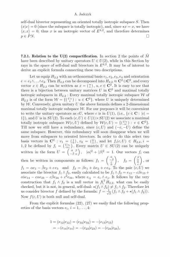
7.2.1. Relation to the U(2) compactification. In section 2 the points of Mhave been described by unitary operators U ∈ U(2), while in this Section byrays in the space of self-dual null bivectors in E4,2. It may be of interest toderive an explicit formula connecting these two descriptions.
Let us equip H2,2 with an orthonormal basis e1, e2, e3, e4 and orientatione = e1∧. . .∧e4. Then H2,2 can be decomposed into H2,2 ≈ C2⊕C2, and everyvector x ∈ H2,2 can be written as x = ( u
v ) , u, v ∈ C2. It is easy to see thatthere is a bijection between unitary matrices U in C2 and maximal totallyisotropic subspaces in H2,2 : Every maximal totally isotropic subspace W ofH2,2 is of the form W = {( Uv
v ) : u ∈ C2}, where U is uniquely determinedby W. Conversely, given unitary U the above formula defines a 2-dimensionalmaximal totally isotropic subspace W. For our purposes it will be convenientto write the unitary operators as cU, where c is in U(1), (i.e., {c ∈ C : |c| =1}), and U is in SU(2). To each (c, U) ∈ U(1)×SU(2) we associate a maximaltotally isotropic subspace W(c, U) defined by W(c, U) = {( Uv
cv ) : v ∈ C2}.Till now we still have a redundancy, since (c, U) and (−c,−U) define thesame subspace. However, this redundancy will soon disappear when we willmove from subspaces to oriented bivectors. In order to do this select twobasis vectors in C2 : v1 = ( 1
0 ) , v2 = ( 01 ) , and let fi(c, U) ∈ H2,2, i =
1, 2 be defined by fi =(Uvicvi
). Every matrix U ∈ SU(2) can be uniquely
written in the form U =(
α β−β α
), |α|2 + |β|2 = 1. Our vectors fi can
then be written in components as follows: f1 =(
α−βc0
), f2 =
(βα0c
), or
f1 = αe1 − βe2 + c e3 and f2 = βe1 + αe2 + c e4. To the pair (c, U) weassociate the bivector f1 ∧ f2, easily calculated to be f1 ∧ f2 = e12 − cβe13 +cαe14 − cαe23 − cβe24 + c2e34, where eij = ei ∧ ej . It follows by the veryconstruction that f1 ∧ f2 is a null vector in
∧2H2,2, what can be easily
checked, but it is not, in general, self-dual: �(f1 ∧ f2) �= f1 ∧ f2. Therefore letus consider bivector f defined by the formula: f = 1√
2(f1 ∧ f2 + �(f1 ∧ f2)) .
Now f(c, U) is both null and self-dual.
From the explicit formulas (22), (27) we easily find the following prop-erties of the basis vectors ei, i = 1, . . . , 4:
1 = (e12|e12) = (e34|e34) = −(e13|e13)= −(e14|e14) = −(e23|e23) = −(e24|e24),
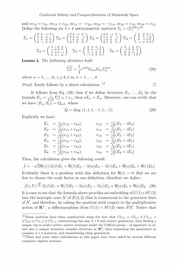
Conformal Infi nity and Compactifi cations of Minkowski Space
and �e12 = e34, �e13 = e24, �e14 = −e23, �e23 = −e14, �e24 = e13, �e34 = e12.Define the following six 4 × 4 antisymmetric matrices Σi = (ΣAB
i ):16
Σ1 =(
0 0 −i 00 0 0 ii 0 0 00 −i 0 0
)Σ2 =
(0 0 −1 00 0 0 −11 0 0 00 1 0 0
)Σ2 =
(0 0 −1 00 0 0 −11 0 0 00 1 0 0
)Σ3 =
(0 0 0 i0 0 i 00 −i 0 0−i 0 0 0
)
Σ4 =(
0 i 0 0−i 0 0 00 0 0 −i0 0 i 0
)Σ5 =
(0 0 0 10 0 −1 00 1 0 0−1 0 0 0
)Σ6 =
(0 1 0 0−1 0 0 00 0 0 10 0 −1 0
)
Lemma 4. The following identities hold:
Σijα =
12εijklGkmGlnΣmn
α , (28)
where α = 1, . . . , 6, i, j, k, l,m, n = 1, . . . , 4.
Proof. Easily follows by a direct calculation. 17 �
It follows from Eq. (28) that if we define bivectors E1, . . . , E6 by theformula Eα = 1
2√2
Σijα ei ∧ ej , then �Eα = Eα. Moreover, one can verify that
we have 〈Eα, Eβ〉 = Qαβ , where
Q = diag (1, 1, 1,−1, 1,−1). (29)
Explicitly we have:
E1 = i√2(e13 − e24), e12 = −1√
2(E6 − iE4)
E2 = 1√2(e13 + e24), e13 = 1√
2(E2 − iE1)
E3 = −i√2(e14 + e23), e14 = −1√
2(E5 − iE3)
E4 = −i√2(e12 − e34), e23 = 1√
2(E5 + iE3)
E5 = −1√2(e14 − e23), e24 = 1√
2(E2 + iE1)
E6 = −1√2(e12 + e34), e34 = −1√
2(E6 + iE4)
Then, the calculation gives the following result:
f = −√
2�(c) (�(β)E1 + �(β)E2 −�(α)E3 −�(c)E4 + �(α)E5 + �(c)E6)
Evidently there is a problem with this definition for �(c) = 0. But we arefree to choose the scale factor in our definition, therefore we define :
f(c, U)df= �(β)E1 + �(β)E2 −�(α)E3 −�(c)E4 + �(α)E5 + �(c)E6. (30)
It is easy to see that the formula above provides an embedding of U(1)×SU(2)into the isotropic cone N of E(4, 2) that is transversal to the generator linesof N , and therefore, by taking the quotient with respect to the multiplicativeaction of R+, a diffeomorphism from U(1) × SU(2) onto PN . Notice that
16These matrices have been constructed using the fact that Cl4,2 = Cl3,1 ⊗ Cl1,2 =
(Cl2,0 ⊗Cl1,1)⊗Cl1,1, constructing this way 8× 8 real matrix generators, then finding aunique (up to scale) metric matrix invariant under the Clifford group – of signature (4, 4),and also a unique invariant complex structure in R8, then expressing the generators ascomplex 4× 4 matrices, and renumbering them generators.17These and some other calculations in this paper have been aided by several differentcomputer algebra systems.
A. Jadczyk
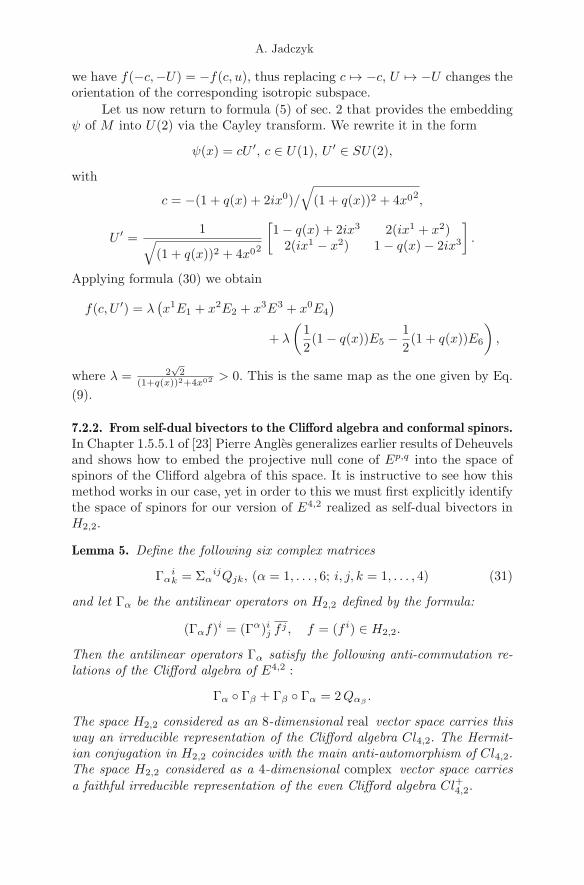
we have f(−c,−U) = −f(c, u), thus replacing c �→ −c, U �→ −U changes theorientation of the corresponding isotropic subspace.
Let us now return to formula (5) of sec. 2 that provides the embeddingψ of M into U(2) via the Cayley transform. We rewrite it in the form
ψ(x) = cU ′, c ∈ U(1), U ′ ∈ SU(2),
with
c = −(1 + q(x) + 2ix0)/√
(1 + q(x))2 + 4x02,
U ′ =1√
(1 + q(x))2 + 4x02
[1 − q(x) + 2ix3 2(ix1 + x2)
2(ix1 − x2) 1 − q(x) − 2ix3
].
Applying formula (30) we obtain
f(c, U ′) = λ(x1E1 + x2E2 + x3E3 + x0E4
)+ λ
(12(1 − q(x))E5 −
12(1 + q(x))E6
),
where λ = 2√2
(1+q(x))2+4x02 > 0. This is the same map as the one given by Eq.(9).
7.2.2. From self-dual bivectors to the Clifford algebra and conformal spinors.In Chapter 1.5.5.1 of [23] Pierre Angles generalizes earlier results of Deheuvelsand shows how to embed the projective null cone of Ep,q into the space ofspinors of the Clifford algebra of this space. It is instructive to see how thismethod works in our case, yet in order to this we must first explicitly identifythe space of spinors for our version of E4,2 realized as self-dual bivectors inH2,2.
Lemma 5. Define the following six complex matrices
Γαik = Σα
ijQjk, (α = 1, . . . , 6; i, j, k = 1, . . . , 4) (31)
and let Γα be the antilinear operators on H2,2 defined by the formula:
(Γαf)i = (Γα)ij f j , f = (f i) ∈ H2,2.
Then the antilinear operators Γα satisfy the following anti-commutation re-lations of the Clifford algebra of E4,2 :
Γα ◦ Γβ + Γβ ◦ Γα = 2Qαβ.
The space H2,2 considered as an 8-dimensional real vector space carries thisway an irreducible representation of the Clifford algebra Cl4,2. The Hermit-ian conjugation in H2,2 coincides with the main anti-automorphism of Cl4,2.The space H2,2 considered as a 4-dimensional complex vector space carriesa faithful irreducible representation of the even Clifford algebra Cl+4,2.
Conformal Infi nity and Compactifi cations of Minkowski Space
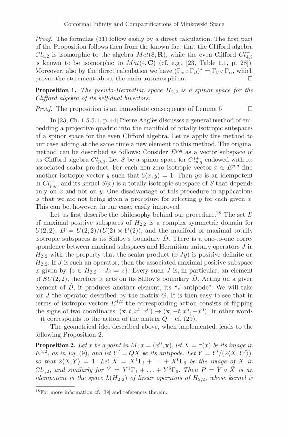
Proof. The formulas (31) follow easily by a direct calculation. The first partof the Proposition follows then from the known fact that the Clifford algebraCl4,2 is isomorphic to the algebra Mat(8,R), while the even Clifford Cl+4,2is known to be isomorphic to Mat(4,C) (cf. e.g., [23, Table 1.1, p. 28]).Moreover, also by the direct calculation we have (Γα ◦Γβ)∗ = Γβ ◦Γα, whichproves the statement about the main automorphism. �Proposition 1. The pseudo-Hermitian space H2,2 is a spinor space for theClifford algebra of its self-dual bivectors.
Proof. The proposition is an immediate consequence of Lemma 5 �In [23, Ch. 1.5.5.1, p. 44] Pierre Angles discusses a general method of em-
bedding a projective quadric into the manifold of totally isotropic subspacesof a spinor space for the even Clifford algebra. Let us apply this method toour case adding at the same time a new element to this method. The originalmethod can be described as follows: Consider Ep,q as a vector subspace ofits Clifford algebra Clp,q. Let S be a spinor space for Cl+p,q endowed with itsassociated scalar product. For each non-zero isotropic vector x ∈ Ep,q findanother isotropic vector y such that 2〈x, y〉 = 1. Then yx is an idempotentin Cl+p,q, and its kernel S(x) is a totally isotropic subspace of S that dependsonly on x and not on y. One disadvantage of this procedure in applicationsis that we are not being given a procedure for selecting y for each given x.This can be, however, in our case, easily improved.
Let us first describe the philosophy behind our procedure.18 The set Dof maximal positive subspaces of H2,2 is a complex symmetric domain forU(2, 2), D = U(2, 2)/(U(2) × U(2)), and the manifold of maximal totallyisotropic subspaces is its Shilov’s boundary D. There is a one-to-one corre-spondence between maximal subspaces and Hermitian unitary operators J inH2,2 with the property that the scalar product (x|Jy) is positive definite onH2,2. If J is such an operator, then the associated maximal positive subspaceis given by {z ∈ H2,2 : Jz = z}. Every such J is, in particular, an elementof SU(2, 2), therefore it acts on its Shilov’s boundary D. Acting on a givenelement of D, it produces another element, its “J-antipode”. We will takefor J the operator described by the matrix G. It is then easy to see that interms of isotropic vectors E4,2 the corresponding action consists of flippingthe signs of two coordinates: (x, t, x5, x6) �→ (x,−t, x5,−x6). In other words– it corresponds to the action of the matrix Q – cf. (29).
The geometrical idea described above, when implemented, leads to thefollowing Proposition 2.
Proposition 2. Let x be a point in M, x = (x0,x), let X = τ(x) be its image inE4,2, as in Eq. (9), and let Y ′ = QX be its antipode. Let Y = Y ′/(2〈X,Y ′〉),so that 2〈X,Y 〉 = 1. Let X = X1Γ1 + . . . + X6Γ6 be the image of X in
Cl4,2, and similarly for Y = Y 1Γ1 + . . . + Y 6Γ6. Then P = Y ◦ X is anidempotent in the space L(H2,2) of linear operators of H2,2, whose kernel is
18For more information cf. [39] and references therein.
A. Jadczyk
a maximal totally isotropic subspace of H2,2 consisting of vectors of the form( Uv
v ) , where U is the unitary matrix given by Eq. (5).
Proof. The proof follows by a straightforward though lengthy direct calcula-tion. �
8. Flat Conformal Structures
While the present paper concentrates on the Minkowski space, the resultsapply also to tangent space structures in more general case – they may alsoapply to conformally flat manifolds. In this section we will introduce the mainconcepts needed for such an extension and show that the embedding τ givenby Eq. 9 of section 3.1 can be understood geometrically by the conformaldevelopment with respect to the normal Cartan connection.
8.1. The bundle P 2(M)Let M be a smooth n-dimensional manifold. Two maps from open neighbor-hoods of the origin 0 ∈ Rn to M define the same 2-jet at 0 if and only if theirpartial derivatives up to the second order coincide. The 2-jet determined bysuch a map e is denoted j20(e). If e is a diffeomorphism, then j20(e) is called asecond order frame at the point p = e(0). The set of all second-order framesis denoted by P 2(M).19
Let (xμ) be a local chart of M , and let (ta) be the standard coordi-nates on Rn. Given j20(e) such that p is in the domain of the chart, a set ofcoordinates of j20(e) is defined by:⎧⎪⎨
⎪⎩eμ
.= xμ(p)eμa
.= ∂(x◦e)μ∂ta |t=0
eμab.= ∂2(x◦e)μ
∂ta∂tb|t=0
If (xμ) is replaced by (xμ′), the coordinates of j20(e) change:⎧⎪⎨⎪⎩
eμ′ = xμ′(p)eμ′a = ∂xμ′
∂xμ (p)eμaeμ′ab = ∂xμ′
∂xμ (p)eμab + ∂2xμ′∂xμxν e
μae
νb
It follows that eμa may be considered as an ordinary (i.e., first order) frame atp. A natural projection P 2(M) → P 1(M) exists, and is given by j20(e) �→ j10(e)or, in coordinates, by (eμ, eμa, e
μab) �→ (eμ, eμa). A simple interpretation can
be given to eμab. First notice that the matrix eμa is always invertible. Leteaμ denote the inverse matrix, so that we have eμae
aν = δμν and eaμe
μb = δab .
Define “connection coordinates of e” by
eμρσ.= −erρe
sσe
μrs.
It follows from the transformation properties of the coordinates of e abovethat eμρσ transform as connection coefficients at p. Therefore each section of
19For a somewhat different version cf. also [23, pp. 138-152]
Conformal Infi nity and Compactifi cations of Minkowski Space
P 2(M) determines a pair: a section of P 1(M) (i.e., a frame) and a torsion-freeaffine connection on M , the correspondence being bijective. In particular, ifP 1(M) is reduced to the orthogonal or pseudo-orthogonal group, the Hilbert-Palatini principle for General Relativity can be considered as a functional onthe space of sections of P 2(M). Also notice that the diffeomorphisms groupof M acts on P 2(M) and on the space of its sections in a natural way. Ife is a map from an open neighborhood of the origin 0 ∈ Rn to M , andif φ : M → M is a local diffeomorphism defined at p = e(0), then φ ◦ e isanother map from an open neighborhood of the origin 0 ∈ Rn to M. If e1 ande2 define the same second order frame: j20(e1) = j20(e2), then the composedmaps define the same second order frame as well: j20(φ ◦ e1) = j20(φ ◦ e2).
8.2. The structure group G2(n)
Let G2(n) denote the set of all second-order frames at 0 ∈ Rn. G2(n) is agroup with the group multiplication law given by j20(h)j20(k) .= j20(h ◦ k).The group G2(n) acts on P 2(M) from the right j20(e)j20(h) .= j20(e ◦ h).Corresponding to the canonical coordinates in Rn, there are natural coor-dinates in G2(n): (ha
b, habc), and each j20(h) can be uniquely represented
by the map Rn → Rn given by ta �→ hart
r + 12h
arst
rts. In terms of nat-ural coordinates the group composition law in G2(n) can be written as(ha
b, habc)(k
ab, k
abc) = (ha
rkrb, h
arsk
rbk
sc +ha
rkrbc). While the group G2(n)
acts on P 2(M) from the right, and P 2(M) is a principal bundle over M withG2(n) as its structure group, the group Diff(M) of diffeomorphisms of Macts on P 2(M) from the left, by fibre preserving transformations, commutingwith the right action of G2(n) – thus as an automorphism group of P 2(M).An affine connection can be considered as a section of a bundle associated toP 2(M) via an appropriate representation of G2(n) by affine transformations.
8.3. Reduction of P 2(M) induced by a conformal structure
Let now M be an orientable and oriented n-dimensional differentiable mani-fold. Let GL+(n) be the group of n×n real matrices of positive determinant.We denote by TM the tangent bundle of M, and by F+ the GL+(n) principalbundle of oriented linear frames of M. We denote by Λn
+ the bundle of ori-ented non-vanishing n-vectors. Λn
+ is, in a natural way, a principal R+ bundle.Given a real number w, let V w be the bundle associated to F+ via the repre-sentation ρw of GL+(n) on R defined by ρw : GL+(n) � A �→ det(A)−w ∈ R.Since any oriented frame e defines an oriented n-vector e1 ∧ . . . ∧ en, it fol-lows that V w can be also considered as the bundle associated to Λn
+ via therepresentation R+ � x �→ xwR.
Cross-sections of V w are called densities of weight w. In what followswe will use the “hat” symbol ˆ to distinguish densities from tensorial objectsof weight w = 0. If e = {ei, i = 1, . . . , n} is a frame at p, and if φ is anelement in the fibre V r
p , then we denote by φ[e] the real number representingφ with respect to the frame e. We write φ > 0 if φ[e] > 0 for some (and thus
A. Jadczyk
for every) oriented frame. It follows from the very definition of the associatedbundle that if A ∈ GL+(n), then φ[eA] = det[A]wφ[e].
Let r, s be a pair of real numbers, and let φ, ψ be positive densitiesof weight w = r and w = s respectively. Then (φψ)[e] = φ[e]ψ[e] defines adensity of weight w = r + s, while φs[e] = φ[e]s defines a density of weightw = rs.
Let xμ, μ = 1, . . . n be a local coordinate system on M, and let ∂μbe the basis made of vectors tangent to the coordinate lines. Then a cross-section φ of V w is represented by a real-valued function φ(x). When thelocal coordinate system changes to another one, xμ′
, then the coordinatebases changes accordingly: ∂μ′ = ∂xμ
∂xμ′ ∂μ, and the corresponding numericalrepresentation of φ changes as follows: φ′(x′) = |∂x′
∂x |−w φ(x), where |∂x′∂x | is
the Jacobian of the coordinate transformation.By taking tensor products of tensor bundles with the line bundle V w
we can define, in an obvious way, tensor densities of weight w.
Although much of what will follow is true in a general case of an ar-bitrary (pseudo-)Riemannian manifold, we will assume in the following thatwe are dealing with the signature (n− 1, 1), that our manifold M is orientedand time-oriented, and that all our local coordinate systems have positiveorientation and time-orientation.
Let ηij = diag (1, . . . 1,−1, . . . ,−1), (signature (p, q)) and let O(η) bethe subgroup of GL(n) consisting of matrices Λ = (Λi j) ∈ GL(n) such thatΛtηΛ = η, det Λ = 1, and let SO0(η) be the connected component of theidentity in O(η). By a (pseudo-) Riemannian structure on M we will mean areduction of the GL(n) principal bundle of the linear frames of M to SO0(η).
There are several equivalent ways of defining a conformal structure onM. Probably the most intuitive way is to define it as “a Riemannian metricup to a scale”. Let g and g be two metrics of M. Then g and g are said tobe conformally related if there exists a positive function φ on M such thatg(p) = φ(p)g(p) for all p ∈ M. Being “conformally related” is, in fact, anequivalence relation, so that we can define a conformal structure on M as theequivalence class consisting of conformally related metrics.
Let C be a conformal structure on M. For any g ∈ C, given a localcoordinate system xμ, we can define |g| to be the absolute value of the de-terminant det gμν , where gμν = g(∂μ, ∂ν). Then from the transformation law:gμ′ν′ = ∂xμ
∂xμ′∂xν
∂xν′ gμν we find that |g′| = | ∂x∂x′ |2 |g|, so that |g| is a scalar densityof weight −2. Let us define γμν = gμν
|g|1/n . Then det γμν = −1, γμν is a sym-metric tensor density of weight −2/n, and γμν is independent of the choice ofthe representative gμν in the conformal class C. In other words: a conformalstructure is uniquely characterized by a symmetric tensor density of weight−2/n, and signature (p, q).
Let T M be the vector bundle of vector densities of weight w = 1/n.Then, for any two vectors u, v ∈ TpM the number (u, v) = γμν u
μvν is in-dependent of the local coordinate system at p – it defines a bilinear form of
Conformal Infi nity and Compactifi cations of Minkowski Space
signature (p, q) on T M. This bilinear form characterizes uniquely the confor-mal structure C.
Let a conformal structure C be given on M. A general torsion-free affineconnection which preserves C is of the form
Γαβγ = Γα
βγ +(δαβ pγ + δαγ pβ − γβγγ
αρpρ),
where Γαβγ = 1
2 (∂βγγρ + ∂γγβρ − ∂ργβγ) , and γμν is the inverse matrix ofγμν . Therefore P 2(M) can be reduced to P 2
C(M) defined as consisting ofsecond-order frames e such that eμa are conformal frames and eμρσ are thecoefficients of conformal connections. It is easy to see that the structure groupH of P 2
C(M) is a subgroup of G2(n) consisting of pairs (hab, h
abc), with
hab ∈ CO0(η), and ha
bc = har (δrbvc + δrcvb − ηbcη
rsvs) , where CO0(η) =SO0(η) ×R+, v = (va) ∈ Rn∗. It follows that H is isomorphic to the semi-direct product CO0(η) �Rn∗ with the multiplication law
(hab, va) (kab, wa) = (ha
rkrb, vrk
ra + wa) ,
where hab = exp(σ)Λa
b, with exp(σ) ∈ R+ and Λ ∈ SO0(η). With (hab, va)
written as (θ,Λab, va), one can easily verify that the following formula defines
a representation R of H on Rn+2 = Rn ⊕R2 :
R(θ,Λ, v) =
(Λr
s ηrsvs ηrsvs−vrθ
1+θ2−v2
2θ − 1−θ2+v2
2θ
vrθ − 1−θ2−v2
1θ1+θ2+v2
2θ
).
With S =(
η 0 00 1 00 0 −1
)we then have R(θ,Λ, v)tSR(θ,Λ, v) = S, therefore the
representation R realizes H as a subgroup of the group G = SO0(p+1, q+1).The part of G that is missing in H is the translation group given by thefollowing SO0(p + 1, q + 1) matrices T (a), a ∈ Rn :
T (a) =(
δrs −ar ar
ηrsas 1−a2/2 a2/2
ηrsas −a2/2 1+a2/2
), (32)
- Cf. section 5.2. The Lie algebra generators so(p + 1, q + 1) take now thefollowing form:
D =dD(exp(σ), E, 0)
dσ|σ=0 =
(0 0 00 0 10 1 0
),
12ωr
sMsr =
(0 0 00 ωr
s 00 0 0
)
vrKr =
(0 ηrsvs ηrsvs−vr 0 0vr 0 0
), wrPr =
(0 −wr wr
ηrsws 0 0
ηrsws 0 0
).
8.4. The enlarged conformal bundle and the normal Cartan connection
With H being a subgroup of G, as above, we can build now the associatedbundle P 2
C(M) = P 2C(M)×HG, which is a principal G-bundle (cf. e.g., [40, p.
4] and references therein). If n = p+ q ≥ 3, then this new bundle is naturallyequipped with a principal connection, the normal Cartan connection, whichcan be described as follows.
Let g be a metric in the conformal class C, let ea be a (local) orthonormalframe of g, and R its curvature tensor. Then, in a coordinate system xμ,the covariant derivative ∇μZ of a section Z of the associated vector bundle
A. Jadczyk
P ×R Ep+1,q+1 is given by the following expression - cf. e.g., [38, Ch. 4.4],[40, p. 14], [23, p. 196]:
∇μZ = ∂μZ + ΓμZ,
with Γμ = 12Γr
μsMsr + 1
n−2
(Rμσ − 1
2(n−1)Rgμσ
)Kσ − Pμ, where Kμ = eμr ,
and Pμ = erμPr.
In a natural way we can then build the associate bundle P ×GEp+1,q+1
with Ep+1,q+1 as a typical fibre, and we can construct the projective quadricMx at each point x ∈ M.
Now, suppose M is connected and simply connected and the conformalstructure is flat. In this case we can choose (cf. [38, Ch. I.2]) gμν = ημν . Thecovariant derivative ∇μZ reduces in this case to ∇μZ = ∂μZ − PμZ. In anadapted coordinate system xμ we choose the “origin” of the “compactifiedtangent space” to correspond to the point (0, 1
2 ,−12 ) of Ep+1,q+1. Connecting
the point x ∈ M with 0 ∈ M by the path x(t) = (1 − t)x we can thentransport parallely the origin (0, 1
2 ,−12 ) at x to the point 0 ∈ M. The parallel
transport rule gives us 0 = DZ(x(t))/dt = dZ(x(t))/dt−dxμ/dtPμZ(x(x(t)),or, in our case, dZ/dt = −xμPμZ, which solves to Z(1) = exp(xμPμ)Z(0),or, applying Eq. (32): Z(1) = (x, (1− x2)/2),−(1 + x2)/2), which is nothingbut the standard embedding (9).
9. Concluding Remarks
This paper has provided a mathematical analysis of algebraic and geometri-cal aspects of the Minkowski space compactification. Some omissions, faultyreasoning and lack of precision in the existing literature dealing with thissubject has been pointed out and analyzed in some detail. In addition to thestandard compactification by adding a “light cone and a 2-sphere at infinity”also its double covering isomorphic to U(1) × SU(2) has been discussed. Apictorial representation has been proposed and the corresponding “Penrosediagrams” have been derived. The role of the conformal inversion and therepresentation of null geodesics has been touched upon as well. Applicationsto flat conformal structures, including the normal Cartan connection andconformal development has been discussed in some detail.
Acknowledgments
Thanks are due to Pierre Angles for his encouragement, for critical readingof the manuscript and for many constructive discussions. I also thank Rafa�lAb�lamowicz for the discussion and many suggestions concerning the formand the content of this paper. Thanks are due to Don Marolf for pointingout a possible usefulness of adding the analysis of the IO(3, 1) action, alsoto Alexander Levichev for useful suggestions. Special thanks are also due toPawe�l Nurowski for sharing with me some of his knowledge and for pointingto me the question discussed in Appendix A. I am indebted to Nikolay M.Nikolov for sending me some of his papers and for discussion.
Conformal Infi nity and Compactifi cations of Minkowski Space
Appendix
A. Killing Vector Fields for the Left Action of U(2) on Itself
A.1 The Problem
We take the group U(2) in the standard matrix form. It has the manifoldstructure of (S1 × S3)/Z2 – the same as the compactified Minkowski space.
Now, let ω be the Maurer-Cartan form of U(2), a 2 × 2 matrix of one-forms. Taking the determinant of ω with understanding that the multiplica-tion of one-forms is to be understood as a symmetrized tensor product, weobtain a symmetric bilinear form g = det(ω). This form is non-degenerateof Lorentzian signature and is conformal to the flat Minkowski metric underthe standard identification of U(2) as the compactification of the Minkowskispace M . The metric g obtained this way is, by its very construction, invari-ant under the left action of U(2) on itself. Therefore the left action of U(2)on itself leads to conformal transformations of M.
Precisely which subgroup of the conformal group corresponds to thisleft action of U(2) on itself?
A.2 The solution
It is well known that the group SU(2, 2) acts by conformal automorphisms onthe compactified Minkowski space (see e.g., [9]). The group U(2, 2) consists ofblock matrices ( A B
C D ) with entries A,B,C,D which are 2×2 complex matricessatisfying the relations A∗A−C∗C = D∗D−B∗B = E and A∗B−C∗D = 0.Its action on U(2) is given by the fractional linear transformations:
U �→ U ′ = (AU + B)(CU + D)−1, (33)
with CU + D being automatically invertible for U ∈ U(2). By specifyingB = C = 0, D = E, we see that A is in U(2). Therefore the left action ofU(2) on itself is a particular case of the linear fractional transformations asabove.
In order to describe these transformations in the Minkowski space, wecan use the Cayley transform as in [1]. Or, we can invert Cayley-transform thematrices of U(2, 2) and act on the Minkowski space represented by hermitian2 × 2 matrices in the standard form: X = xμσμ, where σ0 = ( 1 0
0 1 ) , σ1 =( 0 11 0 ) , σ2 =
(0 −ii 0
), σ3 =
(1 00 −1
). The action of U(2, 2) is still described by
fractional linear transformations
X �→ X ′ = (RX + S)(TX + Q)−1, (34)
where (cf. [22, (2.16)]) A = 12 (R+iS−iT+Q), B = 1
2 (−R+iS+iT+Q), C =12 (−R−iS−iT+Q), D = 1
2 (R−iS+iT+Q). With B = C = 0 and D = E weeasily find that R = 1
2 (A+E), Q = 12 (A+E), S = −i 12 (A−E), T = i 12 (A−E).
Consider now a one-parameter subgroup A(τ) of U(2). By differentiating theequation X(τ) = (R(τ)X + S(τ))(T (τ)X + Q(τ))−1 at τ = 0, and puttingA(0) = E, A(0) = iσ we obtain: X = i
2 (σX−Xσ)+ 12σ+ 1
2XσX. Denoting by
A. Jadczyk
Zμ the vector fields corresponding to σ = σμ we easily find their componentsusing the simple algebra: (Zμ)ν = 1
2 tr(Xσν). The result is as follows:
Z0 =12(1 + t2 + x2 + y2 + z2
)∂t + t(x∂x + y∂y + z∂z),
Z1 = tx ∂t +12(1 + t2 + x2 − y2 − z2
)∂x + (xy + z)∂y + (xz − y)∂z
Z2 = ty ∂t + (xy − z)∂x +12(1 + t2 − x2 + y2 − z2
)∂y + (xz + y)∂z
Z3 = tz ∂t + (xz + y)∂x + (yz − x)∂y +12(1 + t2 − x2 − y2 + z2
)∂z.
We can now compare these vector fields with the formulas for the standardgenerators Pμ, Kμ, Mμν of the conformal group as given, for instance, in [41]:
Pμ = −∂μ, Mμν = xμ∂ν − xν∂μ, Kμ = −2xμ(xν∂ν) + x2∂μ.
By an easy calculation we find: Z0 = 12 (K0 + P0), Zi = 1
2 (Ki − Pi) +Li, (i = 1, 2, 3), where Li = εijkMjk.
References
[1] Armin Uhlmann, The Closure of Minkowski Space . Acta Physica Polonica, Vol.XXIV, Fasc. 2(8) (1963), pp. 295–296.
[2] R. Penrose and W. Rindler, Spinors and Space-Time, Vol. 2 – Spinor andTwistor Methods in Space-Time Geometry. Cambridge University Press, Cam-bridge, England, 1984.
[3] S. A. Huggett and K. P. Tod, An Introduction to Twistor Theory . CambridgeUniversity Press (1994).
[4] John K. Beem, Paul E. Ehrlich, Kevin L. Easley, Global Lorentzian Geometry,Second Edition . Marcel Dekker, Inc., New York (1996).
[5] Jose L. Flores, The Causal Boundary of Spacetimes Revisited . Commun. Math.Phys. 276 (2007), pp. 611–643.
[6] David E. Lerner, Global Properties of Massless Free Fields . Commun. Math.Phys. 55 (1977), pp. 179–182.
[7] Claude Chevalley, Theory of Lie Groups I . Princeton Mathematical Series, no.8, Princeton University Press, (1946), Chapter I, §X, Proposition 6.
[8] A. V. Levichev, Parallelizations of Chronometric Bundles Based on the Sub-group U(2) . Izvestia RAEN, ser.MMMIU, 10 (2006), n.1-2, pp. 51–61, (in Rus-sian).
[9] W. Kopczynski and L. S. Woronowicz, A geometrical approach to the twistorformalism . Rep. Math. Phys. Vol 2 (1971), pp. 35–51.
[10] Leszek Z. Stolarczyk, The Hodge Operator in Fermionic Fock Space . Collect.Czech. Chem. Commun. 70 (2005), pp. 979–1016.
[11] Rene Deheuvels, Formes quadratiques et groupes classiques . Presse Universi-taires de France, Paris (1981).
[12] Aubert Daigneault, Irving Segal’s axiomatization of spacetime and its cosmo-logical consequences . Preprint http://arxiv.org/abs/gr-qc/0512059.
Conformal Infi nity and Compactifi cations of Minkowski Space
[13] B. G. Schmidt, A New Definition of Conformal and Projective Infinity of Space-Times . Commun. math. Phys. 36 (1974), pp. 73–90.
[14] Maks A. Akivis, Vladislav V. Goldberg, Conformal Differential Geometry andits Generalizations . A Wiley Interscience Publications, New York (1996).
[15] N. M. Todorov, I. T. Todorov, Conformal Quantum Field Theory in Two andFour Dimensions . Vienna, Preprint ESI 1155 (2002), http://www.esi.ac.at/preprints/esi1155.ps.
[16] Nikolay M. Nikolov, Rationality of Conformally Invariant Local CorrelationFunctions on Compactified Minkowski Space . Commun. Math. Phys. 218(2001), pp. 417–436.
[17] Nikolay M. Nikolov, Vertex Algebras in Higher Dimensions and Globally Con-formal Invariant Quantum Field Theory . Commun. Math. Phys. 253 (2005),pp. 283–322.
[18] Roger Penrose, Conformal traetment of Infinity . In “Relativity, groups andtopology”, Lectures delivered at Les Houches during the 1963 session of theSummer School of Theoretical Physics, University of Grenoble, ed. DeWitt,Gordon and Brach, New York (1964), pp. 563–584.
[19] C. W. Misner, K. S. Thorne, J. A. Wheeler, Gravitation . Freeman and Co.,New York (1973).
[20] S. W. Hawking, G. F. R. Ellis, The large scale structure of space-time . Cam-bridge University Press, Cambridge (1976).
[21] Roger Penrose, The Light Cone at Infinity . In Relativistic Theories of Gravi-tation, ed. L. Infeld, Pergamon Press, Oxford (1964), pp. 369–373.
[22] W. Ruhl, Distributions on Minkowski Space and their Connection with AnalyticRepresentations of the Conformal Group . Commun. math. Phys. 27 (1972), pp.53-86.
[23] Pierre Angles, Conformal Groups in Geometry and Spin Structures. Birkhau-ser, Progress in Mathematical Physics, Vol. 50 (2008).
[24] Roger Penrose, Structure of space-time . In Battelle Rencontres, ed. byC. M. DeWitt, J. A. Wheeler, Benjamin, New York (1969), pp. 121–235.
[25] Roger Penrose, Twistor Algebra . J. Math. Phys. 8 (1967), pp. 345–366.
[26] N. H. Kuiper, On conformally flat spaces in the large . Ann. of Math. 50 (1949),pp. 916–924.
[27] R. Penrose, Zero Rest-Mass Fields Including Gravitation: Asymptotic Be-haviour . Proc. R. Soc. London 284 (1965), pp. 159–203.
[28] Anıl Zenginoglu, Hyperboloidal foliations and scri-fixing . http://arxiv.org/abs/0712.4333.
[29] Robert Geroch, Asymptotic Structure of Space-Time . In Asymptotic Structureof Space-Time, ed. F. Esposito and L. Witten, Plenum Press (1977), pp. 1–105.
[30] Albert Crumeyrolle, Orthogonal and Symplectic Clifford Algebras. Spinorstructures . Kluwer Academic Publishers (1990).
[31] M. Chisholm, Such Silver Currents. The Story of William and Lucy Clifford1845–1929 . The Lutterworth Press, Cambridge (2002).
[32] Roger Penrose, The Road to Reality . Jonathan Cape, London (2004).
[33] Werner Greub, Multilinear Algebra . Springer (1978).
A. Jadczyk
[34] John. C. Baez, Irving E. Segal, Zhengfang Zhou, Introduction to Algebraic andConstructive Quantum Field Theory . Princeton University Press (1992).
[35] W. D. Curtis, F. R. Miller, Differential Manifolds and Theoretical Physics .Academic Press, New York (1985).
[36] M. Fecko, Differential Geometry and Lie Groups for Physicists . CambridgeUniversity Press, Cambridge (2006).
[37] David E. Lerner, Twistors and induced representations of SU(2,2) . J. Math.Phys. 18 (1977), pp. 1812–1817.
[38] Shoshichi Kobayashi, Transformation Groups in Differential Geometry . Sprin-ger (1972).
[39] A. Jadczyk, Born’s Reciprocity in the Conformal Domain . In Z. Oziewicz etal (eds.); Spinors, Twistors, Clifford Algebras and Quantum Deformations .Kluwer Academic Publishers (1993), pp. 129–140.
[40] Felipe Leitner, Twistor Spinors and Normal Cartan Connections in Con-formal Geometries . ftp://ftp-sfb288.math.tu-berlin.de/pub/Preprints/preprint471.ps.gz.
[41] J. Mickelsson, J. Niederle, Conformally invariant field equations . Ann. del’I.H.P., section A, tome 23, no 3 (1975), p. 277–295.
[42] Bourbaki Nicolas, Elements de Mathematique. Algebre, Chapitre 9 . Springer(2007). First edition: Hermann, Paris (1959).
Arkadiusz JadczykCenter CAIROSInstitut de Mathematiques de ToulouseUniversite Paul Sabatier31062 Toulouse Cedex 9Francee-mail: [email protected]
Received: August 31, 2010.
Revised: November 30, 2010.
Accepted: December 17, 2010.
Related Documents