The Fed, the Bond Market, and Gradualism in Monetary Policy Files/gradualism 20160705_8a1a87d5... · The Fed, the Bond Market, and Gradualism in Monetary Policy ∗ Jeremy C. Stein

The Fed, the Bond Market, and Gradualism in Monetary Policy∗

Jeremy C. Stein [email protected]

Harvard University and NBER

Adi Sunderam [email protected]

Harvard University and NBER

First draft: June 2015 This draft: July 2016

Abstract We develop a model of monetary policy with two key features: (i) the central bank has some private information about its long-run target for the policy rate; and (ii) the central bank is averse to bond-market volatility. In this setting, discretionary monetary policy is gradualist: the central bank only adjusts the policy rate slowly in response to changes in its target. Such gradualism represents an attempt to not spook the bond market. However, this effort is unsuccessful in equilibrium, as long-term rates rationally react more to a given move in short rates when the central bank moves more gradually. The same desire to mitigate bond-market volatility can lead the central bank to lower short rates sharply when publicly-observed term premiums rise. In both cases, there is a time-consistency problem, and society would be better off with a central banker who cares less about the bond market.

∗ This paper was previously circulated under the title “Gradualism in Monetary Policy: A Time-Consistency Problem?” We are grateful to Adam Wang-Levine for research assistance and to Ryan Chahrour, Eduardo Davila, Valentin Haddad, and seminar participants at numerous institutions for their feedback. A special thanks to Michael Woodford and David Romer for extremely helpful comments on an earlier draft of the paper.

1

I. Introduction

Fed watching is serious business for bond-market investors and for the financial-market press

that serves these investors. Speeches and policy statements by Federal Reserve officials are dissected

word-by-word, for clues they might yield about the future direction of policy. Moreover, the

interplay between the central bank and the market goes in two directions: not only is the market

keenly interested in making inferences about the Fed’s reaction function, the Fed also takes active

steps to learn what market participants think the Fed is thinking. In particular, before every Federal

Open Market Committee (FOMC) meeting, the Federal Reserve Bank of New York performs a

detailed survey of primary dealers, asking such questions as: “Of the possible outcomes below,

provide the percent chance you attach to the timing of the first increase in the federal funds target rate

or range. Also, provide your estimate for the most likely meeting for the first increase.”1

In this paper, we build a model that aims to capture the main elements of this two-way

interaction between the Fed and the bond market. The two distinguishing features of the model are

that the Fed is assumed to have private information about its preferred value of the target rate and that

the Fed is averse to bond-market volatility. These assumptions yield a number of positive and

normative implications for the term structure of interest rates and the conduct of monetary policy.

However, for the sake of concreteness, and to highlight the model’s empirical content, we focus most

of our attention on the well-known phenomenon of gradualism in monetary policy.

As described by Bernanke (2004), gradualism is the idea that “the Federal Reserve tends to

adjust interest rates incrementally, in a series of small or moderate steps in the same direction.” This

behavior can be represented empirically by an inertial Taylor rule, with the current level of the

federal funds rate modeled as a weighted average of a target rate—which is itself a function of

inflation and the output gap as in, e.g., Taylor (1993)—and the lagged value of the funds rate. In this

specification, the coefficient on the lagged funds rate captures the degree of inertia in policy. In

recent U.S. samples, estimates of the degree of inertia are strikingly high, on the order of 0.85 in

quarterly data.2

1 This particular question appeared in the September 2015 survey, among others. All the surveys, along with a tabulation of responses, are available at https://www.newyorkfed.org/markets/primarydealer_survey_questions.html 2 Coibion and Gorodnichenko (2012) provide a comprehensive recent empirical treatment; see also Rudebusch (2002,

2

Several authors have proposed theories in which this kind of gradualism is optimal behavior

on the part of the central bank. One influential line of thinking, due originally to Brainard (1967) and

refined by Sack (1998), is that moving gradually makes sense when there is uncertainty about how

the economy will respond to a change in the stance of policy. An alternative rationale comes from

Woodford (2003), who argues that committing to move gradually gives the central bank more

leverage over long-term rates for a given change in short rates, a property which is desirable in the

context of his model.

In what follows, we offer a different take on gradualism. In our model, the observed degree

of policy inertia is not optimal from an ex ante perspective, but rather reflects a time-consistency

problem. The time-inconsistency problem arises from our two key assumptions. First, we assume the

Fed has private information about its preferred value of the target rate. In other words, the Fed

knows something about its reaction function that the market does not. Although this assumption is

not standard in the literature on monetary policy, it should be emphasized that it is necessary to

explain the basic observation that financial markets respond to monetary policy announcements, and

that market participants devote considerable time and energy to Fed watching.3 Moreover, our

results only depend on the Fed having a small amount of private information. The majority of the

variation in the Fed’s target can come from changes in publicly-observed variables like

unemployment and inflation; all that we require is that some variation also reflects innovations to the

Fed’s private information.

Second, we assume that the Fed behaves as if it is averse to bond-market volatility. We model

this concern in reduced form, by simply putting the volatility of long-term rates into the Fed’s

objective function. A preference of this sort can ultimately be rooted in an effort to deliver on the

Fed’s traditional dual mandate, however. For example, a bout of bond-market volatility may be

undesirable not in its own right, but rather because it is damaging to the financial system and hence to

real economic activity and employment.

2006). Campbell, Pflueger, and Viceira (2015) argue that the degree of inertia in Federal Reserve rate-setting became more pronounced after about 2000. 3 Said differently, if the Fed mechanically followed a policy rule that was a function only of publicly-observable variables (e.g., the current values of the inflation rate and the unemployment rate), then the market would react to news releases about movements in these variables but not to Fed policy statements.

3

Nevertheless, in a world of private information and discretionary meeting-by-meeting

decision making, an attempt by the Fed to moderate bond-market volatility can be welfare-reducing.

The logic is similar to that in signal-jamming models (Holmstrom, 1999; Stein, 1989). Suppose the

Fed observes a private signal that its long-run target for the funds rate has permanently increased by

100 basis points. If it adjusts fully in response to this signal, raising the funds rate by 100 basis

points, long-term rates will move by a similar amount. If it is averse to such a movement in long-

term rates, the Fed will be tempted to announce a smaller change in the funds rate, trying to fool the

market into thinking that its private signal was less dramatic. Hence, it will under-adjust to its signal,

perhaps raising the funds rate by only 25 basis points.

However, if bond-market investors come to understand this dynamic, the Fed’s efforts to

reduce volatility will be frustrated in equilibrium. The market will see the 25 basis-point increase in

the funds rate and understand that it is likely to be just the first in a series of similar moves, so long-

term rates will react more than one-for-one to the change in short rates. Indeed, in a rational-

expectations equilibrium, the Fed’s private signal will always be fully inferred by the market,

regardless of the degree of gradualism. Still, if it acts on a discretionary basis, the Fed will always try

to fool the market. This is because when it decides how much to adjust the policy rate, it takes as

given the market’s conjecture about the degree of inertia in its rate-setting behavior. As a result, the

Fed’s behavior is inefficient from an ex ante perspective: moving gradually does not succeed in

reducing bond-market volatility, but does mean that the policy rate is further from its long-run target

than it otherwise would be.

This inefficiency reflects a commitment problem. In particular, the Fed cannot commit to not

trying to smooth the private information that it communicates to the market via its changes in the

policy rate.4 One institutional solution to this problem, in the spirit of Rogoff (1985), would be to

appoint a central banker who cares less about bond-market volatility than the representative member

of society. More broadly, appointing such a market-insensitive central banker can be thought of as a

4 The literature on monetary policy has long recognized a different commitment problem, namely that, under discretion, the central bank will be tempted to create surprise inflation so as to lower the unemployment rate. See, e.g., Kydland and Prescott (1977), and Barro and Gordon (1983). More recently, Farhi and Tirole (2012) have pointed to the time-consistency problem that arises from the central bank’s ex post desire to ease monetary policy when the financial sector is in distress; their focus on the central bank’s concern with financial stability is somewhat closer in spirit to ours.

4

metaphor for building an institutional culture and set of norms inside the central bank such that bond-

market movements are not given as much weight in policy deliberations.

We begin with a simple static model that is designed to capture the above intuition in as

parsimonious a way as possible. The main result here is that in any rational-expectations equilibrium,

there is always under-adjustment of the policy rate, compared to the first-best outcome in which the

Fed adjusts the policy rate fully in response to changes in its privately-observed target. Moreover, for

some parameter values, there can be Pareto-ranked multiple equilibria with different degrees of

under-adjustment. The intuition for these multiple equilibria is that there is two-way feedback

between the market’s expectations about the degree of gradualism on the one hand and the Fed’s

optimal choice of gradualism on the other.5 Specifically, if the market conjectures that the Fed is

behaving in a highly inertial fashion, it will react more strongly to an observed change in the policy

rate: in an inertial world, the market knows that there are further changes to come. But this strong

sensitivity of long-term rates to changes in the policy rate makes the Fed all the more reluctant to

move the policy rate, hence validating the initial conjecture of extreme inertia.

As noted above, our results generalize to the case where, in addition to private information,

there is also public information about changes in the Fed’s target. Strikingly, it turns out that the Fed

moves just as gradually with respect to this public information as it does with respect to private

information. This is true independent of the relative contributions of public and private information

to the total variance of the target. The logic is as follows. When public information arrives

suggesting that the target has risen—e.g., inflation increases—the Fed is tempted to pretend that it

has at the same time received dovish private information, so as to mitigate the overall impact on the

bond market. This means that it raises the funds rate by less than it otherwise would in response to

the publicly-observed increase in inflation. Said differently, the Fed and the market care about the

sum of public and private information, and given any amount of private information, the sum is

essentially private information. Thus, our model shows that even a small amount of private

information can lead the Fed to move gradually with respect to all information.

Next, we ask whether the commitment problem that we have identified can be mitigated with

forward guidance, whereby the Fed announces in advance a preferred path for future short rates. We

5 For an informal description of this two-way feedback dynamic, see Stein (2014).

5

show that it cannot. Because its future private information is by definition not forecastable, forward

guidance is a one-sided commitment device. It can only commit the Fed to incorporating new private

information more slowly, not more quickly. Moreover, we argue that once the economy is away from

the zero lower bound, forward guidance can actually be harmful if it is not implemented carefully. If

we are in a region of the parameter space where there are multiple equilibria, forward guidance can

increase the risk of getting stuck in the Pareto-inferior, more inertial equilibrium.

We then enrich the model by adding publicly-observed term premium shocks as an additional

source of variation in long-term rates. We show that, similar to the case of public information about

its target, the Fed’s desire to moderate bond-market volatility leads to it to try to offset term premium

shocks, cutting the policy rate when term premiums rise. Again, this tactic is unsuccessful in reducing

volatility in equilibrium. Thus, the presence of term premium shocks exacerbates the Fed’s time-

consistency problem.

Finally, we extend the model to an explicitly dynamic setting, which allows us to more fully

characterize how a given innovation to the Fed’s target works its way into the funds rate over time.

These dynamic results enable us to draw a closer link between the mechanism in our model and the

empirical evidence on the degree of inertia in the funds rate.

The remainder of the paper is organized as follows. Section II discusses some motivating

evidence, based on readings of FOMC transcripts. Section III presents the static version of the model

and summarizes our basic results on under-adjustment of the policy rate, multiple equilibria, forward

guidance, and term premiums. Section IV develops a dynamic extension of the model. Section V

discusses a variety of other implications of our framework, and Section VI concludes.

II. Motivating Evidence from FOMC Transcripts

In their study of monetary-policy inertia, Coibion and Gorodnichenko (2012) use FOMC

transcripts to document two key points. First, FOMC members sometimes speak in a way that is

suggestive of a gradual-adjustment model—that is, they articulate a target for the policy rate and then

put forward reasons why it is desirable to adjust only slowly in the direction of that target. Second,

one of the stated rationales for such gradualism appears to be a desire not to create financial-market

instability. Coibion and Gorodnichenko highlight the following quote from Chairman Alan

Greenspan at the March 1994 FOMC meeting:

6

“My own view is that eventually we have to be at 4 to 4½ percent. The question is not whether but when. If we are to move 50 basis points, I think we would create far more instability than we realize, largely because a half-point is not enough to remove the question of where we are ultimately going. I think there is a certain advantage in doing 25 basis points….” In a similar spirit, at the August 2004 meeting, shortly after the Fed had begun to raise the

funds rate from the low value of one percent that had prevailed since mid-2003, Chairman Greenspan

remarked:

“Consequently, the sooner we can get back to neutral, the better positioned we will be. We were required to ease very aggressively to offset the events of 2000 and 2001, and we took the funds rate down to extraordinarily low levels with the thought in the back of our minds, and often said around this table, that we could always reverse our actions. Well, reversing is not all that easy….We’ve often discussed that ideally we’d like to be in a position where, when we move as we did on June 30 and I hope today, the markets respond with a shrug. What that means is that the adjustment process is gradual and does not create discontinuous problems with respect to balance sheets and asset values.”

These sorts of quotes help motivate our basic modeling approach, in which gradualism in

monetary policy reflects the Fed’s desire to keep bond-market volatility in check—in Greenspan’s

words, to “not create discontinuous problems with respect to balance sheets and asset values.” This

same approach may also be helpful in thinking about changes in gradualism over time. Campbell,

Pflueger, and Viceira (2015) show that the degree of inertia in Fed rate-setting behavior became

significantly more pronounced after about 2000; given the logic of our model, one might wonder

whether this heightened inertia was associated with an increase over time in the Fed’s concern with

financial markets. In a crude attempt to speak to this question, we examine all 200 FOMC transcripts

for the 25-year period 1985-2009, and for each meeting, simply measure the frequency of words

related to financial markets.6 Specifically, we count the number of times the terms “financial

market,” “equity market,” “bond market,” “credit market,” “fixed income,” and “volatility” are

mentioned.7 For each year, we aggregate this count and divide by the total number of words in that

year’s transcripts.

6 Given the five-year lag in making transcripts public, 2009 is the last available year. 7 We obtain similar results if we use different subsets of these terms. For instance, the results are similar if we only count the frequency of the term “financial market”.

7

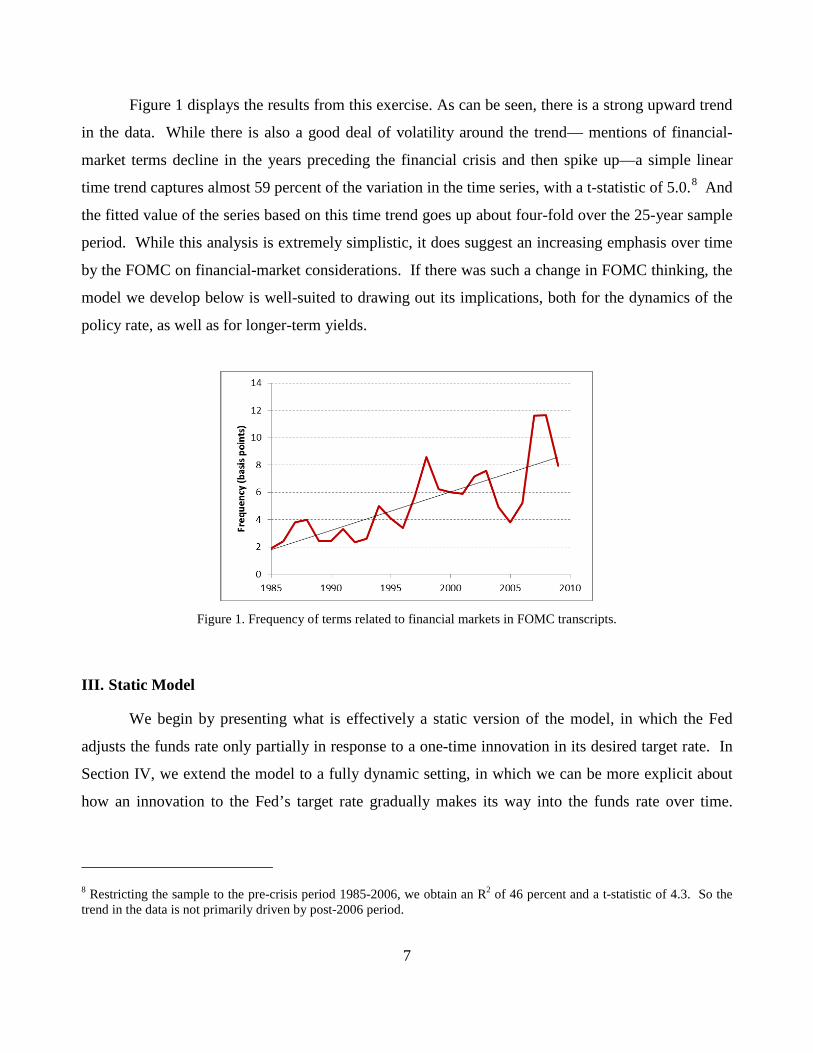
Figure 1 displays the results from this exercise. As can be seen, there is a strong upward trend

in the data. While there is also a good deal of volatility around the trend— mentions of financial-

market terms decline in the years preceding the financial crisis and then spike up—a simple linear

time trend captures almost 59 percent of the variation in the time series, with a t-statistic of 5.0.8 And

the fitted value of the series based on this time trend goes up about four-fold over the 25-year sample

period. While this analysis is extremely simplistic, it does suggest an increasing emphasis over time

by the FOMC on financial-market considerations. If there was such a change in FOMC thinking, the

model we develop below is well-suited to drawing out its implications, both for the dynamics of the

policy rate, as well as for longer-term yields.

Figure 1. Frequency of terms related to financial markets in FOMC transcripts.

III. Static Model

We begin by presenting what is effectively a static version of the model, in which the Fed

adjusts the funds rate only partially in response to a one-time innovation in its desired target rate. In

Section IV, we extend the model to a fully dynamic setting, in which we can be more explicit about

how an innovation to the Fed’s target rate gradually makes its way into the funds rate over time.

8 Restricting the sample to the pre-crisis period 1985-2006, we obtain an R2 of 46 percent and a t-statistic of 4.3. So the trend in the data is not primarily driven by post-2006 period.

8

Though it is stylized, the static model highlights the main intuition for why a desire to limit bond-

market volatility creates a time-consistency problem for the Fed.

A. Model Setup

We begin by assuming that at any time t, the Fed has a target rate based on its traditional dual-

mandate objectives. This target rate is the Fed’s best estimate of the value of the federal funds rate

that keeps inflation and unemployment as close as possible to their desired levels. For tractability,

we assume that the target rate, denoted by *ti , follows a random walk, so that:

* *1 ,t t ti i ε−= + (1)

where 2 10,t N εε

ε σt

≡

is normally distributed. Our key assumption is that *

ti is private

information of the Fed and is unknown to market participants before the Fed acts at time t. One can

think of the private information embodied in *ti as arising from the Fed’s attempts to follow

something akin to a Taylor rule, where it has private information about either the appropriate

coefficients to use in the rule (i.e., its reaction function), or about its own forecasts of future inflation

or unemployment. As noted above, an assumption of private information along these lines is

necessary if one wants to understand why asset prices respond to Fed policy announcements.

Once it knows the value of *ti , the Fed acts to incorporate some of its new private information

tε into the federal funds rate ti , which is observable to the market. We assume that the Fed picks ti

on a discretionary period-by-period basis to minimize the loss function Lt, given by:

( ) ( )2 2* ,t t t tL i i iθ ∞= − + ∆ (2)

where ti∞ is the infinite-horizon forward rate. Thus, the Fed has the usual concerns about inflation

and unemployment, as captured in reduced form by a desire to keep *ti close to ti . However, when

0θ > , the Fed also cares about the volatility of long-term bond yields, as measured by the squared

change in the infinite-horizon forward rate.

For simplicity, we start by assuming that the expectations hypothesis holds, so there is no

time-variation in the term premium. This implies that the infinite-horizon forward rate is equal to the

expected value of the funds rate that will prevail in the distant future. Because the target rate *ti

follows a random walk, the infinite-horizon forward rate is then given by the market’s best estimate

9

of the current target *ti at time t. Specifically, we have * .t t ti E i∞ = In Section III.F below, we relax

the assumption that the expectations hypothesis holds so that we can also consider the Fed’s reaction

to term-premium shocks.

Several features of the Fed’s loss function are worth discussing. First, in our simple

formulation, θ reflects the degree to which the Fed is concerned about bond-market volatility, over

and above its desire to keep ti close to *ti . To be clear, this loss function need not imply that the Fed

cares about asset prices for their own sake. An alternative interpretation is that volatility in financial-

market conditions can affect the real economy and hence the Fed’s ability to satisfy its traditional

dual mandate. This linkage is not modeled explicitly here, but as one example of what we have in

mind, the Fed might believe that a spike in bond-market volatility could damage highly-levered

financial intermediaries and interfere with the credit-supply process. With this stipulation in mind, we

take as given that θ reflects the socially “correct” objective function—in other words, it is exactly

the value that a well-intentioned social planner would choose. We then ask whether there is a time-

consistency problem when the Fed tries to optimize this objective function period-by-period, in the

absence of a commitment technology.

Second, note that the Fed’s target in the first term of (2) is the short-term policy rate, which it

directly controls, whereas the bond-market volatility that it worries about in the second term of (2)

refers to the variance of long-term market-determined rates. This short-versus-long divergence is

crucial for our results on time consistency. To see why, consider two alternative loss functions:

( ) ( )2 2* ,t t t tL i i iθ= − + ∆ (2ꞌ)

( ) ( )2 2* ,t t t tL i i iθ∞ ∞ ∞= − + ∆ (2ꞌꞌ)

In (2ꞌ), the Fed cares about the volatility of the funds rate, rather than the volatility of the

long-term rate. This objective function mechanically produces gradual adjustment of the funds rate,

but because there is no forward-looking long rate, there is no issue of the Fed trying to manipulate

market expectations and hence no time-consistency problem. In other words, a model of this sort

delivers a strong form of gradualism, but the resulting gradualism is entirely optimal from the Fed’s

perspective. However, by emphasizing only short-rate volatility, this formulation arguably fails to

capture the financial-stability goal articulated by Greenspan, namely to “not create discontinuous

10

problems with respect to balance sheets and asset values.” We believe that putting the volatility of

the long-term rate directly in the objective function, as in (2), does a better job in this regard.

In (2ꞌꞌ), the Fed pursues its dual-mandate objectives not by having a target *ti for the funds

rate, but instead by explicitly targeting a long rate of *ti∞ . It can be shown that in this case, too, given

that the same rate ti∞ appears in both parts of the objective function, there is no time-consistency

problem.9 Moreover, one might argue that the first term in (2ꞌꞌ) is a reasonable reduced-form way to

model the Fed’s efforts to achieve its dual mandate. In particular, in standard New-Keynesian

models, it is long-term real rates, not short rates, that matter for inflation and output stabilization.

Nevertheless, our preferred formulation of the Fed’s objective function in (2) can be

motivated in a couple of ways. First, (2) would appear to be more realistic than (2ꞌꞌ) as a simple

description of how the Fed actually behaves, and—importantly for our purposes—communicates

about its future intentions. For example, in a number of recent statements, the Fed has referred to r*,

defined as the equilibrium (or neutral) value of the short rate, and has argued that one motive for

adjusting policy gradually is the fact that r* is itself slow-moving.10 But the concept of a slow-

moving r* can only make logical sense if the short rate matters directly for real outcomes. If instead

real outcomes were entirely a function of long rates, the near-term speed of adjustment of the short

rate would be irrelevant, holding fixed the total expected adjustment. Second, in many models of the

monetary transmission mechanism, including those based on a bank lending channel or a reaching-

for-yield effect, the short rate has an independent effect on economic activity. This could help

explain why it might make sense for the Fed to target the short rate per se.11

9 We are grateful to Mike Woodford for emphasizing this point to us, and for providing a simple proof. 10 In Chair Janet Yellen’s press conference of December 16, 2015, she said: “This expectation (of gradual rate increases) is consistent with the view that the neutral nominal federal funds rate—defined as the value of the federal funds rate that would be neither expansionary nor contractionary if the economy were operating near potential—is currently low by historical standards and is likely to rise only gradually over time.” See http://www.federalreserve.gov/mediacenter/files/FOMCpresconf20151216.pdf 11 The large literature on the bank lending channel includes Bernanke and Blinder (1992), Kashyap and Stein (2000), and Drechsler, Savov, and Schnabl (2015); all of these make the case that bank loan supply is directly influenced by changes in the short rate, because the short rate effectively governs the availability of low-cost deposit funding. A few noteworthy recent papers on reaching for yield and its implications for the pricing of credit risk are Gertler and Karadi (2015), Jimenez, Ongena, Peydro, and Saurina (2014), and Dell’Ariccia, Laeven and Suarez (2013).

11

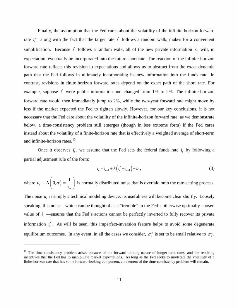
Finally, the assumption that the Fed cares about the volatility of the infinite-horizon forward

rate ti∞ , along with the fact that the target rate *

ti follows a random walk, makes for a convenient

simplification. Because *ti follows a random walk, all of the new private information tε will, in

expectation, eventually be incorporated into the future short rate. The reaction of the infinite-horizon

forward rate reflects this revision in expectations and allows us to abstract from the exact dynamic

path that the Fed follows in ultimately incorporating its new information into the funds rate. In

contrast, revisions in finite-horizon forward rates depend on the exact path of the short rate. For

example, suppose *ti were public information and changed from 1% to 2%. The infinite-horizon

forward rate would then immediately jump to 2%, while the two-year forward rate might move by

less if the market expected the Fed to tighten slowly. However, for our key conclusions, it is not

necessary that the Fed care about the volatility of the infinite-horizon forward rate; as we demonstrate

below, a time-consistency problem still emerges (though in less extreme form) if the Fed cares

instead about the volatility of a finite-horizon rate that is effectively a weighted average of short-term

and infinite-horizon rates.12

Once it observes *ti , we assume that the Fed sets the federal funds rate ti by following a

partial adjustment rule of the form:

( )*1 1 ,t t t t ti i k i i u− −= + − + (3)

where 2 10,t uu

u N σt

≡

is normally distributed noise that is overlaid onto the rate-setting process.

The noise tu is simply a technical modeling device; its usefulness will become clear shortly. Loosely

speaking, this noise—which can be thought of as a “tremble” in the Fed’s otherwise optimally-chosen

value of ti —ensures that the Fed’s actions cannot be perfectly inverted to fully recover its private

information *ti . As will be seen, this imperfect-inversion feature helps to avoid some degenerate

equilibrium outcomes. In any event, in all the cases we consider, 2uσ is set to be small relative to 2

εσ ,

12 The time-consistency problem arises because of the forward-looking nature of longer-term rates, and the resulting incentives that the Fed has to manipulate market expectations. As long as the Fed seeks to moderate the volatility of a finite-horizon rate that has some forward-looking component, an element of the time-consistency problem will remain.

12

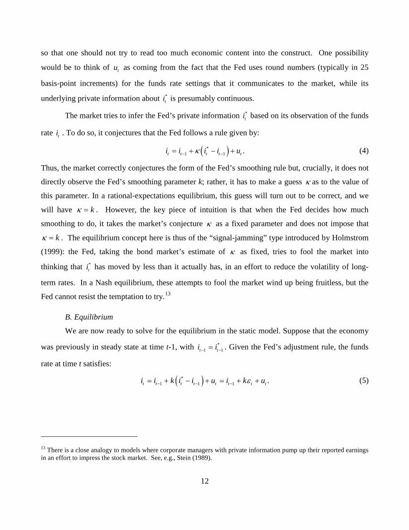
so that one should not try to read too much economic content into the construct. One possibility

would be to think of tu as coming from the fact that the Fed uses round numbers (typically in 25

basis-point increments) for the funds rate settings that it communicates to the market, while its

underlying private information about *ti is presumably continuous.

The market tries to infer the Fed’s private information *ti based on its observation of the funds

rate ti . To do so, it conjectures that the Fed follows a rule given by:

( )*1 1 .t t t t ti i i i uκ− −= + − + (4)

Thus, the market correctly conjectures the form of the Fed’s smoothing rule but, crucially, it does not

directly observe the Fed’s smoothing parameter k; rather, it has to make a guess κ as to the value of

this parameter. In a rational-expectations equilibrium, this guess will turn out to be correct, and we

will have kκ = . However, the key piece of intuition is that when the Fed decides how much

smoothing to do, it takes the market’s conjecture κ as a fixed parameter and does not impose that

kκ = . The equilibrium concept here is thus of the “signal-jamming” type introduced by Holmstrom

(1999): the Fed, taking the bond market’s estimate of κ as fixed, tries to fool the market into

thinking that *ti has moved by less than it actually has, in an effort to reduce the volatility of long-

term rates. In a Nash equilibrium, these attempts to fool the market wind up being fruitless, but the

Fed cannot resist the temptation to try.13

B. Equilibrium

We are now ready to solve for the equilibrium in the static model. Suppose that the economy

was previously in steady state at time t-1, with *1 1t ti i− −= . Given the Fed’s adjustment rule, the funds

rate at time t satisfies:

( )*1 1 1 .t t t t t t t ti i k i i u i k uε− − −= + − + = + + (5)

13 There is a close analogy to models where corporate managers with private information pump up their reported earnings in an effort to impress the stock market. See, e.g., Stein (1989).

13

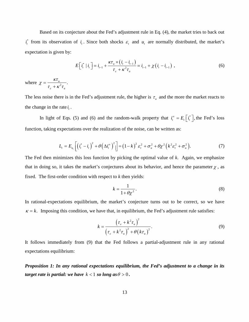
Based on its conjecture about the Fed’s adjustment rule in Eq. (4), the market tries to back out *ti from its observation of ti . Since both shocks tε and tu are normally distributed, the market’s

expectation is given by:

( ) ( )1*1 1 12| u t t

t t t t t tu

i iE i i i i i i

ε

κtχ

t κ t−

− − −

× − = + = + − +

, (6)

where 2 .u

uε

κtχ

t κ t=

+

The less noise there is in the Fed’s adjustment rule, the higher is ut and the more the market reacts to

the change in the rate ti .

In light of Eqs. (5) and (6) and the random-walk property that * ,t t ti E i∞ = the Fed’s loss

function, taking expectations over the realization of the noise, can be written as:

( ) ( ) ( ) ( )2 2 2* 2 2 2 2 2 21 .

tt u t t t t u t uL E i i i k kθ ε σ θχ ε σ∞ = − + ∆ = − + + + (7)

The Fed then minimizes this loss function by picking the optimal value of k. Again, we emphasize

that in doing so, it takes the market’s conjectures about its behavior, and hence the parameter χ , as

fixed. The first-order condition with respect to k then yields:

2

1 .1

kθχ

=+

(8)

In rational-expectations equilibrium, the market’s conjecture turns out to be correct, so we have

.kκ = Imposing this condition, we have that, in equilibrium, the Fed’s adjustment rule satisfies:

( )

( ) ( )

22

2 22.u

u u

kk

k k

ε

ε

t t

t t θ t

+=

+ + (9)

It follows immediately from (9) that the Fed follows a partial-adjustment rule in any rational

expectations equilibrium:

Proposition 1: In any rational expectations equilibrium, the Fed’s adjustment to a change in its

target rate is partial: we have 1k < so long as 0θ > .

14

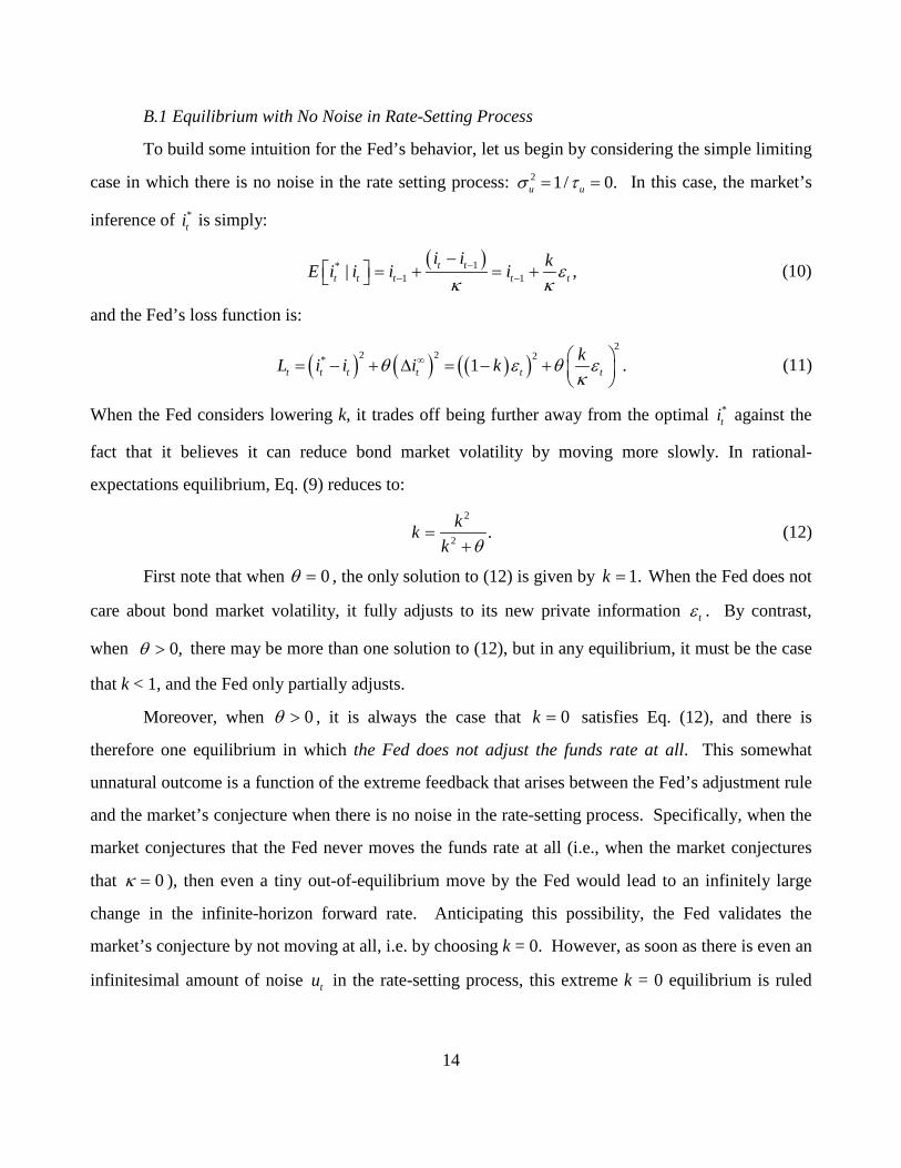
B.1 Equilibrium with No Noise in Rate-Setting Process

To build some intuition for the Fed’s behavior, let us begin by considering the simple limiting

case in which there is no noise in the rate setting process: 2 1/ 0.u uσ t= = In this case, the market’s

inference of *ti is simply:

( )1*1 1| ,t t

t t t t t

i i kE i i i i εκ κ

−− −

− = + = + (10)

and the Fed’s loss function is:

( ) ( ) ( )( )2

2 2 2* 1 .t t t t t tkL i i i kθ ε θ εκ

∞ = − + ∆ = − +

(11)

When the Fed considers lowering k, it trades off being further away from the optimal *ti against the

fact that it believes it can reduce bond market volatility by moving more slowly. In rational-

expectations equilibrium, Eq. (9) reduces to:

2

2 .kkk θ

=+

(12)

First note that when 0θ = , the only solution to (12) is given by 1.k = When the Fed does not

care about bond market volatility, it fully adjusts to its new private information tε . By contrast,

when 0,θ > there may be more than one solution to (12), but in any equilibrium, it must be the case

that k < 1, and the Fed only partially adjusts.

Moreover, when 0θ > , it is always the case that 0k = satisfies Eq. (12), and there is

therefore one equilibrium in which the Fed does not adjust the funds rate at all. This somewhat

unnatural outcome is a function of the extreme feedback that arises between the Fed’s adjustment rule

and the market’s conjecture when there is no noise in the rate-setting process. Specifically, when the

market conjectures that the Fed never moves the funds rate at all (i.e., when the market conjectures

that 0κ = ), then even a tiny out-of-equilibrium move by the Fed would lead to an infinitely large

change in the infinite-horizon forward rate. Anticipating this possibility, the Fed validates the

market’s conjecture by not moving at all, i.e. by choosing k = 0. However, as soon as there is even an

infinitesimal amount of noise tu in the rate-setting process, this extreme k = 0 equilibrium is ruled

15

out, as small changes in the funds rate now lead to bounded market reactions. This explains our

motivation for keeping a tiny amount of rate-setting noise in the more general model.

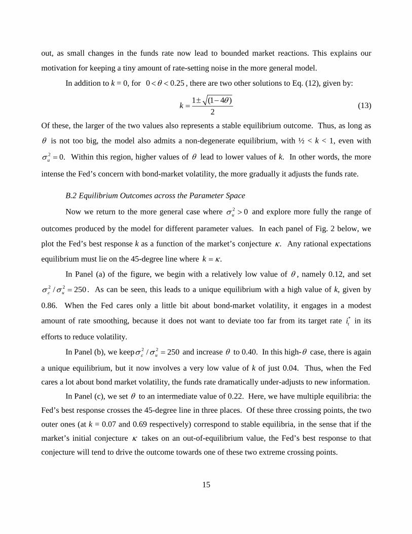
In addition to k = 0, for 0 0.25θ< < , there are two other solutions to Eq. (12), given by:

1 (1 4 )2

kθ± −

= (13)

Of these, the larger of the two values also represents a stable equilibrium outcome. Thus, as long as

θ is not too big, the model also admits a non-degenerate equilibrium, with ½ < k < 1, even with 2 0.uσ = Within this region, higher values of θ lead to lower values of k. In other words, the more

intense the Fed’s concern with bond-market volatility, the more gradually it adjusts the funds rate.

B.2 Equilibrium Outcomes across the Parameter Space

Now we return to the more general case where 2 0uσ > and explore more fully the range of

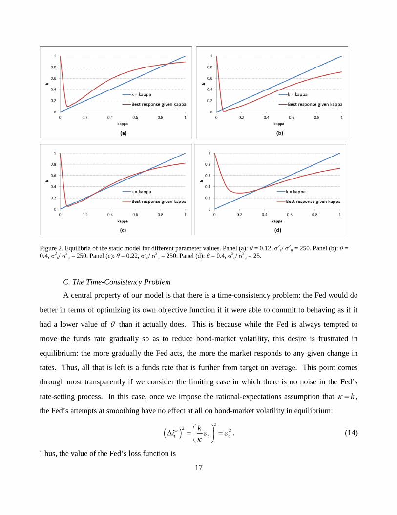
outcomes produced by the model for different parameter values. In each panel of Fig. 2 below, we

plot the Fed’s best response k as a function of the market’s conjecture .κ Any rational expectations

equilibrium must lie on the 45-degree line where .k κ=

In Panel (a) of the figure, we begin with a relatively low value of θ , namely 0.12, and set 2 2/ 250uεσ σ = . As can be seen, this leads to a unique equilibrium with a high value of k, given by

0.86. When the Fed cares only a little bit about bond-market volatility, it engages in a modest

amount of rate smoothing, because it does not want to deviate too far from its target rate *ti in its

efforts to reduce volatility.

In Panel (b), we keep 2 2/ 250uεσ σ = and increase θ to 0.40. In this high-θ case, there is again

a unique equilibrium, but it now involves a very low value of k of just 0.04. Thus, when the Fed

cares a lot about bond market volatility, the funds rate dramatically under-adjusts to new information.

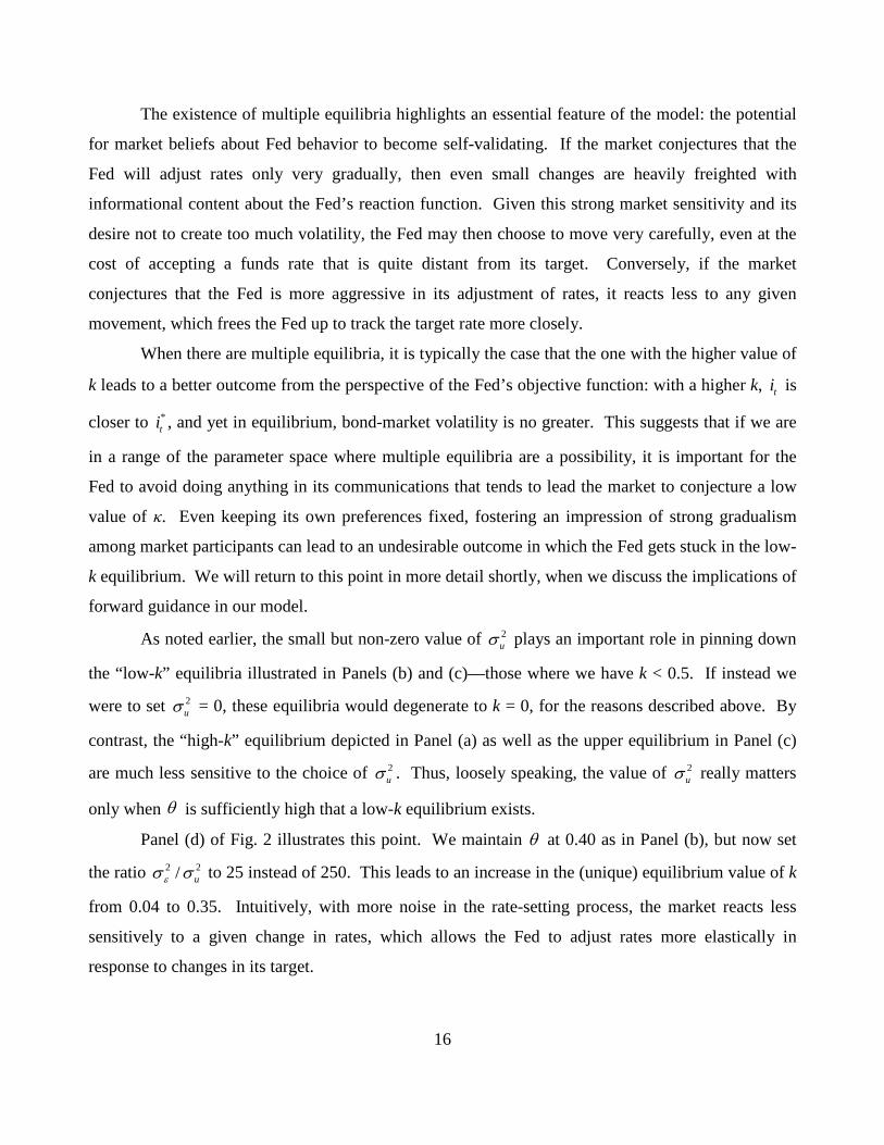
In Panel (c), we set θ to an intermediate value of 0.22. Here, we have multiple equilibria: the

Fed’s best response crosses the 45-degree line in three places. Of these three crossing points, the two

outer ones (at k = 0.07 and 0.69 respectively) correspond to stable equilibria, in the sense that if the

market’s initial conjecture κ takes on an out-of-equilibrium value, the Fed’s best response to that

conjecture will tend to drive the outcome towards one of these two extreme crossing points.

16

The existence of multiple equilibria highlights an essential feature of the model: the potential

for market beliefs about Fed behavior to become self-validating. If the market conjectures that the

Fed will adjust rates only very gradually, then even small changes are heavily freighted with

informational content about the Fed’s reaction function. Given this strong market sensitivity and its

desire not to create too much volatility, the Fed may then choose to move very carefully, even at the

cost of accepting a funds rate that is quite distant from its target. Conversely, if the market

conjectures that the Fed is more aggressive in its adjustment of rates, it reacts less to any given

movement, which frees the Fed up to track the target rate more closely.

When there are multiple equilibria, it is typically the case that the one with the higher value of

k leads to a better outcome from the perspective of the Fed’s objective function: with a higher k, ti is

closer to *ti , and yet in equilibrium, bond-market volatility is no greater. This suggests that if we are

in a range of the parameter space where multiple equilibria are a possibility, it is important for the

Fed to avoid doing anything in its communications that tends to lead the market to conjecture a low

value of κ. Even keeping its own preferences fixed, fostering an impression of strong gradualism

among market participants can lead to an undesirable outcome in which the Fed gets stuck in the low-

k equilibrium. We will return to this point in more detail shortly, when we discuss the implications of

forward guidance in our model.

As noted earlier, the small but non-zero value of 2uσ plays an important role in pinning down

the “low-k” equilibria illustrated in Panels (b) and (c)—those where we have k < 0.5. If instead we

were to set 2uσ = 0, these equilibria would degenerate to k = 0, for the reasons described above. By

contrast, the “high-k” equilibrium depicted in Panel (a) as well as the upper equilibrium in Panel (c)

are much less sensitive to the choice of 2uσ . Thus, loosely speaking, the value of 2

uσ really matters

only when is sufficiently high that a low-k equilibrium exists.

Panel (d) of Fig. 2 illustrates this point. We maintain θ at 0.40 as in Panel (b), but now set

the ratio 2 2/ uεσ σ to 25 instead of 250. This leads to an increase in the (unique) equilibrium value of k

from 0.04 to 0.35. Intuitively, with more noise in the rate-setting process, the market reacts less

sensitively to a given change in rates, which allows the Fed to adjust rates more elastically in

response to changes in its target.

θ

17

Figure 2. Equilibria of the static model for different parameter values. Panel (a): θ = 0.12, σ2

ε/ σ2u = 250. Panel (b): θ =

0.4, σ2ε/ σ2

u = 250. Panel (c): θ = 0.22, σ2ε/ σ2

u = 250. Panel (d): θ = 0.4, σ2ε/ σ2

u = 25.

C. The Time-Consistency Problem

A central property of our model is that there is a time-consistency problem: the Fed would do

better in terms of optimizing its own objective function if it were able to commit to behaving as if it

had a lower value of θ than it actually does. This is because while the Fed is always tempted to

move the funds rate gradually so as to reduce bond-market volatility, this desire is frustrated in

equilibrium: the more gradually the Fed acts, the more the market responds to any given change in

rates. Thus, all that is left is a funds rate that is further from target on average. This point comes

through most transparently if we consider the limiting case in which there is no noise in the Fed’s

rate-setting process. In this case, once we impose the rational-expectations assumption that kκ = ,

the Fed’s attempts at smoothing have no effect at all on bond-market volatility in equilibrium:

( )2

2 2t t t

ki ε εκ

∞ ∆ = =

. (14)

Thus, the value of the Fed’s loss function is

18

( ) ( ) ( )( )2 2 2* 21 ,t t t t t tL i i i kθ ε θε∞= − + ∆ = − + (15)

which is decreasing in k for 1.k <

To the extent that the target rate *ti is non-verifiable private information, it is hard to think of a

contracting technology that can readily implement the first-best outcome under commitment: how

does one write an enforceable rule that says that the Fed must always react fully to its private

information? Thus, discretionary monetary policy will inevitably be associated with some degree of

inefficiency. However, even in the absence of a binding commitment technology, there may still be

scope for improving on the fully discretionary outcome. One possible approach follows in the spirit

of Rogoff (1985), who argues that society should appoint a central banker who is more hawkish on

inflation than is society itself. The analogy in the current context is that society should aim to appoint

a central banker who cares less about financial-market volatility (i.e., has a lower value of θ ) than

society as a whole. Or put differently, society—and the central bank itself—should seek to foster an

institutional culture and set of norms that discourages the monetary policy committee from being

overly attentive to market-volatility considerations.

To see this, consider the problem of a social planner choosing a central banker whose concern

about financial market volatility is given by cθ . This central banker will implement the rational

expectations adjustment rule ( )ck θ , where k is given by Eq. (12), replacing θ with cθ . The

planner’s ex ante problem is then to pick cθ to minimize its ex ante loss, recognizing that its own

concern about financial-market volatility is given by θ :

( ) ( ) ( )( )( ) ( )( )( )22 2 2* 2 21 1 .t t t t c t t cE i i i E k kε εθ θ ε θε θ θ σ∞ − + ∆ = − + = − +

(16)

Since ( )ck θ is decreasing in cθ , the ex ante loss is minimized by picking 0cθ = , as the following

proposition states.14

14 In the alternative case where rate-setting noise is small but non-zero, a mild generalization of Proposition 2 obtains. While it is no longer true that the Fed would like to commit to behaving as if θ was exactly equal to zero, it would still like to commit to behaving as if θ was very close to zero and much smaller than its actual value. For example, for the parameter values in Panel D of Fig. 2, where the Fed’s actual θ = 0.4, it would minimize its loss function if it were able to commit to θ = 0.04. In the appendix, we provide a fuller treatment of the optimal solution under commitment in the case of non-zero noise.

19

Proposition 2: In the absence of rate-setting noise, it is ex ante optimal to appoint a central banker

with 0cθ = , so that ( ) 1ck θ = .

The time-consistency problem is especially stark in our setting because the Fed is assumed to

care about the volatility of the infinite-horizon rate. As can be seen in (14), this volatility is a fixed

constant in any rational-expectations equilibrium, independent of the degree of gradualism. Thus, the

Fed’s efforts to control the volatility of the infinite-horizon rate are completely unsuccessful in

equilibrium, which is why it is ex ante optimal to appoint a central banker who does not care at all

about this infinite-horizon volatility. By contrast, if we instead assume that the Fed cares about the

volatility of a finite-horizon rate (e.g., the 10-year rate), there is still a time-consistency problem, but

it is attenuated. If the expectations hypothesis holds, then the finite-horizon rate is given by the

expected path of the funds rate over that finite horizon. By moving gradually, the Fed can actually

reduce the volatility of the realized path. However, it still cannot fool the market about its ultimate

destination.

One way to develop this intuition in our setting is to note that any finite-horizon rate can be

approximated by a weighted average of the current funds rate ti and the infinite-horizon forward rate

ti∞ , as long as we pick the weights correctly. This follows from the fact that there is only one factor,

namely tε , in our model of the term structure of interest rates. Using this observation, it is

straightforward to establish the following proposition, which is proven in the appendix.

Proposition 3: Suppose that 0θ > and that the Fed cares about the volatility of a finite-horizon rate, which can be represented as a weighted average of the short rate and the infinite-horizon rate. Then, it is ex ante optimal to appoint a central banker with a strictly positive value of cθ , but to have cθ θ< . Under discretion, the Fed has two motives when it moves gradually. First, it aims to reduce

the volatility of the component of the finite-horizon rate that is related to the current short rate ti .

Second, it hopes to reduce the volatility of the component of the finite-horizon rate that is related to

the infinite-horizon forward rate ti∞ by fooling the market about its private information tε . The first

goal can be successfully attained in rational-expectations equilibrium, but the second cannot—as in

the baseline model, the Fed cannot fool the market about its private information in equilibrium.

20

Under commitment, only one of these motives for moving gradually remains, and thus it is

less appealing to move gradually than it would be under discretion. Thus, if society is appointing a

central banker whose concern about financial market volatility is given by cθ , it would like to

appoint one with cθ θ< . In other words, there is still a time-consistency problem. However, unlike

the case where the social planner cares about the volatility of the infinite-horizon forward rate, here

the planner no longer wants to go to the extreme where 0cθ = .

D. Public Information about the Fed’s Target

Thus far, we have assumed that the Fed’s target value of the short rate is entirely private

information. A more empirically realistic assumption is that the target depends on both public and

private information, where the former might include current values of inflation, the unemployment

rate, and other macroeconomic variables. It turns out that our basic results carry over to this

setting—that is, the Fed adjusts gradually to both publicly and privately observed innovations to its

target.15 Specifically, suppose that the target rate follows the process:

* *1 .t t t ti i ε ν−= + + (17)

As before, tε is private information observable only to the Fed. However tν is publicly

observed by both the Fed and the bond market. Given the more complicated nature of the setting, the

Fed’s optimal choice as to how much to adjust the short rate no longer depends on just its private

information tε ; it also depends on the public information tν . To allow for a general treatment, we

posit that this adjustment can be described by some potentially non-linear function of the two

variables and also assume that there is no noise in the Fed’s adjustment rule ( 2uσ = 0):

( )1 ; .t t t ti i f ε ν−= + (18)

Moreover, the market conjectures that the Fed is following a potentially non-linear rule:

( )1 ; .t t t ti i φ ε ν−= + (19)

In the appendix, we use a calculus-of-variations type of argument to establish that, in a

rational-expectations equilibrium in which , the Fed’s adjustment rule is given by:

15 We thank David Romer for pointing out this generalization of the model to us.

( ); ( ; )f φ⋅ ⋅ = ⋅ ⋅

21

1 ,t t t ti i k kε νε ν−= + + (20)

where

k kν ε= ; and 2 .k kε ε θ= + (21)

The following proposition summarizes the key properties of the equilibrium.

Proposition 4: The Fed responds as gradually to public information about changes in the target

rate as it does to private information. This is true regardless of the relative contributions of public

and private information to the total variance of the target. As the Fed’s concern with bond-market

volatility θ increases, both kε and kν fall.

The proposition is striking and may at first glance seem counter-intuitive. Given our previous

results, one might have thought that there is no reason for the Fed to move gradually with respect to

public information. However, while this instinct is correct in the limit case where there is no private

information whatsoever, it turns out to be wrong as soon as we introduce a small amount of private

information. The logic goes as follows. Suppose there is a piece of public information that suggests

that the funds rate should rise by 100 basis points—e.g., there is a sharp increase in the inflation rate.

This news, if released on its own, would tend to also create a spike in long-term bond yields. In an

effort to mitigate this spike, the Fed is tempted to show a more dovish hand than it had previously,

i.e., to act as if it has simultaneously received a negative innovation to the privately-observed

component of its target. To do so, it raises the funds rate by less than it otherwise would in response

to the increase in inflation, which—in an out-of-equilibrium sense—represents the attempt to convey

the offsetting change in its private information.

As before, this effort to fool the market is not successful in equilibrium, but the Fed cannot

resist the temptation to try. And as long as there is just a small amount of private information, the

temptation always exists, because at the margin, the existence of private information leads the Fed to

act as if it can manipulate market beliefs. Hence, even if private information does not represent a

large fraction of the total variance of the target, the degree of gradualism predicted by the model is

the same as in an all-private-information setting.

22

E. Does Forward Guidance Help or Hurt?

Because the Fed’s target rate *ti is non-verifiable private information, it is impossible to write

a contract that effectively commits the Fed to rapid adjustment of the funds rate in the direction of *ti .

So to the extent that the problem has not already been solved by appointing a central banker with the

appropriate disregard for bond-market volatility, the first-best is generally unattainable. But this

raises the question of whether there are other, more easily enforced contracts that might be of some

help in addressing the time-consistency problem.

In this section, we ask whether something along the lines of forward guidance could fill this

role. By “forward guidance”, we mean an arrangement whereby the Fed announces at time t a value

of the funds rate that it expects to prevail at some point in the future. Since both the announcement

itself and the future realization of the funds rate are both publicly observable, market participants can

easily tell ex post whether the Fed has honored its guidance, and one might imagine that it will suffer

a reputational penalty if it fails to do so. In this sense, a “guidance contract” is more enforceable than

a “don’t-smooth-with-respect-to-private-information contract.”

It is well understood that a semi-binding commitment to adhere to a pre-announced path for

the short rate can be of value when the short rate is at the zero lower bound (ZLB); see e.g., Krugman

(1998), Eggertsson and Woodford (2003), and Woodford (2012). We do not take issue with this

observation here. Rather, we ask a different question, namely whether guidance can also be useful

away from the ZLB, as a device for addressing the central bank’s tendency to adjust rates too

gradually. It turns out the answer is no. Forward guidance can never help with the time-consistency

problem we have identified, and attempts to use guidance away from the ZLB can potentially make

matters strictly worse.

We develop the argument in two steps, working backwards. First, we assume that it is time t,

and the Fed comes into the period having already announced a specific future rate path at time t-1.

We then ask how the existence of this guidance influences the smoothing incentives analyzed above.

Having done so, we then fold back to time t-1 and ask what the optimal guidance announcement

looks like and whether the existence of the guidance technology increases or decreases the Fed’s

expected utility from an ex ante perspective.

23

To be more precise, suppose we are in steady state at time t-1, and suppose again that the Fed

cares about the volatility of the infinite horizon forward rate. We allow the Fed to publicly announce

a value 1f

ti − as its guidance regarding ti , the funds rate that will prevail one period later, at time t. To

make the guidance partially credible, we assume that once it has been announced, the Fed bears a

reputational cost of deviating from the guidance, so that its augmented loss function at time t is now

given by:

( ) ( ) ( )2 2 2*1 .f

t t t t t tL i i i i iθ γ∞−= − + ∆ + − (22)

When it arrives at time t, the Fed takes the reputational penalty γ as exogenously fixed, but when we

fold back to analyze guidance from an ex-ante perspective, it is more natural to think of γ as a choice

variable for the Fed at time t-1. That is, the more emphatically it talks about its guidance ex ante or

the more reputational chips it puts on the table, the greater will be the penalty if it deviates from the

guidance ex post.

We start at time t and take the forward guidance 1f

ti − as given. To keep things simple, we go

back to the all-private-information case and also assume that there is no noise in the Fed’s adjustment

rule ( 2uσ = 0). Recall from Eq. (13) above that, in this case, there only exists a stable non-degenerate

(i.e. positive k) equilibrium when θ < ¼, a condition that we assume to be satisfied in what follows.

Moreover, in such an equilibrium, we have ½ < k < 1. The solution method in this case is similar to

that used for public information in Section III.D above. As before, we assume the Fed’s adjustment

rule can be an arbitrary non-linear function of both the new private information tε that the Fed learns

at time t as well as its previous forward guidance 1f

ti − .

In the appendix, we show that in a rational-expectations equilibrium, the Fed’s adjustment

behavior is given by:

( )1 1 1 ,1

ft t t t ti i k i iγε

γ− − −= + + −+

(23)

where the partial-adjustment coefficient k now satisfies:

( ) 21 .k kγ θ= + + (24)

Two features of the Fed’s modified adjustment rule are worth noting. First, as can be seen in

(23), the Fed moves ti more strongly in the direction of its previously-announced guidance 1f

ti − as γ

24

increases, which is intuitive. Second, as (24) indicates, the presence of guidance also alters the way

that the Fed incorporates its new time-t private information into the funds rate ti . Given that any

equilibrium necessarily involves k > ½, we can show that / 0k γ∂ ∂ < . In other words, the more the

Fed cares about deviating from its forward guidance, the less it responds to its new private

information tε . In this sense, the presence of semi-binding forward guidance has an effect similar to

that of increasing θ : both promote gradualism with respect to the incorporation of new private

information. The reason is straightforward: by definition, when guidance is set at time t-1, the Fed

does not yet know the realization of tε . So tε cannot be impounded in the t-1 guidance, and

anything that encourages the time-t rate to hew closely to the t-1 guidance must also discourage the

incorporation of tε into the time-t rate. This is the key insight for why guidance is not helpful away

from the ZLB.

To make this point more formally, let us now fold back to time t-1 and ask two questions.

First, assuming that 0γ > , what is the optimal guidance announcement 1f

ti − for the Fed to make?

And second, supposing that the Fed can choose the intensity of its guidance γ —i.e., it can choose

how many reputational chips to put on the table when it makes the announcement—what is the

optimal value of γ ? In the appendix, we demonstrate the following:

Proposition 5: Suppose we are in steady state at time t-1, with *1 1.t ti i− −= If the Fed takes 0γ > as

fixed, its optimal choice of forward guidance at time t-1 is to announce 1 1.f

t ti i− −= Moreover, given

this announcement policy, the value of the Fed’s objective function is decreasing in γ . Thus, if it

can choose, it is better off foregoing guidance altogether, i.e. setting 0.γ =

The first part of the proposition reflects the fact that because the Fed is already at its target at

time t-1 and has no information about how that target will further evolve at time t, the best it can do is

to set 1f

ti − at its current value of 1ti − . This guidance carries no incremental information to market

participants at t-1. Nevertheless, even though it is uninformative, the guidance has an effect on rate-

setting at time t. As Eq. (24) highlights, a desire to not renege on its guidance leads the Fed to

underreact by more to its new time-t private information. Since this is strictly undesirable, the Fed is

better off not putting guidance in place to begin with.

25

This negative result about the value of forward guidance in Proposition 5 should be qualified

in two ways. First, as we have already emphasized, this result only speaks to the desirability of

guidance away from the ZLB; there is nothing here that contradicts Krugman (1998), Eggertsson and

Woodford (2003), and Woodford (2012), who make the case for using a relatively strong form of

guidance (i.e., with a significantly positive value of γ ) when the economy is stuck at the ZLB.

Second, and more subtly, an advocate of using forward guidance away from the ZLB might

argue that if it is done with a light touch, it can help to communicate the Fed’s private information to

the market, without reducing the Fed’s future room to maneuver. In particular, if the Fed is careful to

make it clear that its guidance embodies no attempt at a binding commitment whatsoever (i.e., that γ

= 0), the guidance may serve as a purely informational device and cannot hurt.

The idea that guidance can play a useful informational role strikes us as perfectly reasonable,

even though it does not emerge in our model. The Fed’s private information here is unidimensional,

and because it is already fully revealed in equilibrium, there is no further information for guidance to

transmit. However, it is quite plausible that, in a richer model, things would be different, and

guidance could be incrementally informative. On the other hand, our model also suggests that care

should be taken when claiming that light-touch (γ = 0) guidance has no negative effects in terms of

increasing the equilibrium degree of gradualism in the funds rate.

This point is most easily seen by considering the region of the parameter space where there are

multiple equilibria. In this region, anything that influences market beliefs can have self-fulfilling

effects. So, for example, suppose that the Fed puts in place a policy of purely informational forward

guidance, and FOMC members unanimously agree that the guidance does not in any way represent a

commitment on their parts—that is, they all plan to behave as if 0γ = and indeed manage to follow

through on this plan ex post. Nevertheless, if some market participants think that guidance comes

with a degree of commitment (γ > 0), there can still be a problem. These market participants expect

smaller deviations from the announced path of rates, and if we are in the multiple-equilibrium region,

this expectation can be self-validating. Thus, the mistaken belief that guidance entails commitment

can lead to an undesirable outcome where the Fed winds up moving more gradually in equilibrium,

thereby lowering its utility. Again, this effect arises even if all FOMC members actually behave as if

0γ = and attach no weight to keeping rates in line with previously-issued guidance. Thus, at least in

26

the narrow context of our model, there would appear to be some potential downside associated with

even the mildest forms of forward guidance once the economy is away from the ZLB.

F. Term Premium Shocks

We next enrich the model in another direction, to consider how the Fed behaves when

financial-market conditions are not purely a function of the expected path of interest rates.

Specifically, we relax the assumption that the expectations hypothesis holds and instead assume that

the infinite-horizon forward rate consists of both the expected future short rate and an exogenous

term premium component tr :

* .t t t ti E i r∞ = + (25)

The term premium is assumed to be common information, observed simultaneously by

market participants and the Fed. We allow the term premium to follow an arbitrary process and let

tη denote the innovation in the term premium:

[ ]1 .t t t tr E rη −= − (26)

The solution method is again similar to that in the two preceding sections. Specifically, we

assume that: there is only private information about the Fed’s target; there is no noise in the Fed’s

rate-setting rule ( 2uσ = 0); and the rule can be an arbitrary non-linear function of both the new private

information tε that the Fed learns at time t as well as the term premium shock tη , which is publicly

observable.

In the appendix, we show that in rational expectations equilibrium, the Fed’s adjustment rule

is given by:

1 ,t t t ti i k kε ηε η−= + + (27)

where

2 and

.

k k

kk

ε ε

ηε

θθ

= +

= − (28)

The following proposition summarizes the key properties of the equilibrium.

Proposition 6: The Fed acts to offset term premium shocks, lowering the funds rate when the term

premium shock is positive and raising it when the term premium shock is negative. It does so even

27

though term premium shocks are publically observable and in spite of the fact that its efforts to

reduce the volatility associated with term premium shocks are fruitless in equilibrium. As the

Fed’s concern with bond-market volatility θ increases, kε falls and kη increases in absolute

magnitude. Thus, when it cares more about the bond market, the Fed reacts more gradually to

changes in its private information about its target rate, but more aggressively to changes in term

premiums.

Why does the Fed respond to publicly-observed term premium shocks? The intuition here is

similar to that for why the Fed underreacts to public information about its target. Essentially, when

the term premium spikes up, the Fed is unhappy about the prospective increase in the volatility of

long rates. So even if its private information about *ti has in fact not changed, it would like to make

the market think it has become more dovish so as to offset the rise in the term premium. Therefore, it

cuts the short rate in response to the term premium shock in an effort to create this impression.

Again, in equilibrium, this attempt to fool the market is not successful, but taking the market’s

conjectures at any point in time as fixed, the Fed is always tempted to try.

One way to see why the equilibrium must involve the Fed reacting to term premium shocks is

to think about what happens if we try to sustain an equilibrium where it does not—that is, if we try to

sustain an equilibrium in which 0kη = . In such a hypothetical equilibrium, Eq. (27) tells us that

when the market sees any movement in the funds rate, it attributes that movement entirely to changes

in the Fed’s private information tε about its target rate. But if this is the case, then the Fed can indeed

offset movements in term premiums by changing the short rate, thereby contradicting the assumption

that 0kη = . Hence, 0kη = cannot be an equilibrium.

A noteworthy feature of the equilibrium is that the absolute magnitude of kη becomes larger

as θ rises and as kε becomes smaller: when it cares more about bond-market volatility, the Fed’s

responsiveness to term premium shocks becomes more aggressive even as its adjustment to new

information about its target becomes more gradual. In particular, because we are restricting ourselves

to the region of the parameter space where the simple no-noise model yields a non-degenerate

equilibrium for kε , this means that we must have 0 < θ < ¼ from Eq. (13) above. As θ moves from

28

the lower to the upper end of this range, kε declines monotonically from 1 to ½, and kη increases in

absolute magnitude from 0 to –½.

This latter part of the proposition is especially useful, as it yields a sharp testable empirical

implication. As noted earlier, Campbell, Pflueger, and Viceira (2015) have shown that the Fed’s

behavior has become significantly more inertial in recent years. If we think of this change as

reflecting a lower value of kε , we might be tempted to use the logic of the model to claim that the

lower kε is the result of the Fed placing increasing weight over time on the bond market, i.e. having a

higher value of θ than it used to. While the evidence on financial-market mentions in the FOMC

transcripts that we plotted in Fig. 1 is loosely consistent with this hypothesis, it is obviously far from

being a decisive test. However with Proposition 6 in hand, if we want to attribute a decline in kε to

an increase in θ , then we also have to confront the additional prediction that we ought to observe the

Fed responding more forcefully over time to term premium shocks. That is, the absolute value of kη

must have gone up. If this is not the case, it would represent a rejection of the hypothesis.

IV. Dynamic Model

In the static model considered to this point, the phenomenon of “gradualism” is really nothing

more than under-adjustment of the policy rate to a one-time shock to the Fed’s target. We now

introduce a dynamic version of the model, which allows us to fully trace out how a shock to the Fed’s

target works its way into the policy rate over time. This dynamic analysis generates predictions that

can be more directly compared to the empirical evidence on gradualism.

A. The Fed’s Adjustment Rule

To study dynamics, we need to consider the Fed’s behavior when the economy is not in steady

state at time t-1. Suppose we enter period t with a pre-existing gap between the time t-1 target rate

and the time t-1 federal funds rate of *1 1 1.t t tX i i− − −≡ − We focus on the pure private-information case

and allow the Fed to have a more general adjustment rule of the following form:

1 1 .t t X t ti i k X kεε− −= + + (29)

29

In other words, we allow the Fed to adjust differentially to the pre-existing gap 1tX − and to the

innovation to its target tε .

B. No Uncertainty about 1tX −

The first case to consider is one in which the gap 1tX − is exactly known by investors as of time

t. By the logic outlined in Section III above, this would be the case in a rational-expectations

equilibrium if there is no rate-setting noise 2( 0)uσ = . The gap is a function of past realizations of the

ε’s, and as we have seen, these are fully revealed in a no-noise equilibrium. Investors conjecture that

the Fed is following a rule of the form:

1 1 .t t X t ti i X εκ κ ε− −= + + (30)

Given this conjecture, investors’ estimate of the innovation to the Fed’s target tε , and hence their

estimate of the innovation to the short rate that will prevail in the distant future, is given by:

[ ] 1( ).t X t

ti X

Eε

κε

κ−∆ −

= (31)

This is similar to what we had in Eq. (10) in the static model, except that now investors adjust for the

expected rate change of 1X tXκ − when making inferences about tε . In other words, when the funds

rate goes up at time t, the investors understand that it is not necessarily due entirely to a

contemporaneous upwards revision to the Fed’s target at time t. Rather, part of the change in the

funds rate may reflect the fact that the Fed is playing catch-up: it could be that the Fed has entered

period t with a positive pre-existing gap between its target and the prior value of the funds rate and is

working to close that gap.

It is straightforward to show that in this case, the Fed’s equilibrium behavior can be

characterized as follows.16

16 As we discuss further in the appendix, to simplify the problem, we also assume that at any time t, the Fed picks kε and

Xk taking 1tX − as given, but before knowing the realization of tε . This timing convention is purely a technical trick that makes the problem more tractable without changing anything of economic substance.

30

Proposition 7: In the dynamic model with no uncertainty about 1tX − , we have that 1Xk = , and

1kε < , with kε (as before) being given by: 2

2 .kkk

εε

ε θ=

+

In the absence of uncertainty about 1tX − , the Fed still under-adjusts to a contemporaneous

shock to its target tε , in exactly the same way as before. However, the under-adjustment is short-

lived: in the next period, it fully impounds what was left of the time-t innovation into the rate. In

other words, 1Xk = implies that all the Fed’s time-t private information has made its way into the

funds rate by time t+1. Intuitively, by time t+1, investors have already figured out all of the Fed’s

time-t private information. Given that the Fed can no longer fool investors about this old

information, there is no motive to continue to incorporate it into rates slowly.

Why is it that the Fed underreacts to public news about the target tν in Proposition 4 but does

not smooth over the publicly known gap 1tX − in Proposition 7? The key difference is timing. In

Proposition 4, we have two simultaneous innovations to the target rate, so the Fed can try to offset

public news by pretending it has private news. In Proposition 7, the bond market volatility due to 1tε −

has already been realized at time t-1. So being more dovish at time t when 1tX − is large does not help

to reduce volatility at time t.

Proposition 7 makes clear that there can be a considerable distance between our earlier

theoretical results on under-adjustment and the empirical evidence on gradualism. In the empirical

literature, a typical finding (in quarterly data) would be that *10.85 0.15t t ti i i−= ⋅ + ⋅ , which implies

that changes in the short rate are significantly positively correlated even when they are several

quarters apart. In other words, there is relatively long-lasting momentum in short-rate changes. By

contrast, the fact that that 1Xk = in Proposition 7 implies that cov( , ) 0t t ji i −∆ ∆ = for all j > 1: changes

in the short rate more than one period apart are uncorrelated with one another. Thus, Proposition 7

would appear to be strongly counterfactual.

C. Allowing for Some Uncertainty about 1tX −

One way to bring the model more closely into alignment with the empirical evidence is to

allow investors to have some uncertainty about 1tX − . This uncertainty emerges endogenously once

31

we allow for some rate-setting noise 2( 0)uσ > , because in the presence of such noise the Fed’s private

signal tε cannot be perfectly inverted from its actions at time t.

The fully rational solution to the market’s inference problem about 1tX − in this case is

extremely complex, because the cumulative gap 1tX − is a function of all of the past t jε − for 0j ≥ ,

and estimating each t jε − requires a separate filter over all of the past realizations of the funds rate.

To simplify this intractable problem, we adopt a reduced-form representation and assume that just

after time t-1, but before time t, investors observe a noisy signal of 1tX − :

1 1 1 ,t t ts X z− − −= + (32)

where ( )2~ 0,t zz N σ . The market’s expectation of 1tX − given 1ts − is therefore impounded into the

infinite horizon forward rate before the Fed sets the funds rate at time t. Thus, the change in the

infinite horizon forward rate at time t is the revision in the market’s expectations about the target rate

given the change in the federal funds rate:

[ ] [ ]

* *1 1 1

1 1 1 1

| , |

| | .t t t t t t

t t t t t t

i E i s i E i s

E X s i E X sε

∞− − −

− − − −

∆ = ∆ − = + ∆ −

(33)

As before, we assume that the Fed follows a rule where it can adjust to the innovation to its

target tε and the pre-existing gap 1tX − at different speeds, as described in Eq. (29). We further

assume that the Fed conditions on 1tX − but not on the market’s signal 1ts − , which it cannot directly

observe.17 With these assumptions in place, we are able to establish the following proposition:

Proposition 8: In the dynamic model with rate-setting noise, we have 1Xk kε < < . As the noise increases, Xk declines and approaches kε . 17 If there are no term premium shocks, the Fed could in principle infer 1ts − by looking at the long rate. However, if we were to add term premium shocks that are not directly observable, these would complicate the inference and make it impossible to uniquely invert 1ts − from the long-term rate. Recall that in Section III.F, we assumed that term premium shocks were publicly observed. However, in the setting of that section, it would have been equivalent to assume that term premium shocks could not be seen directly but rather were perfectly inferred from observation of the long rate, given knowledge of the expected future short rate. In other words, there need be no logical tension between our approach in Section III.F and our approach here of taking 1ts − to be unobservable by the Fed.

32

The basic intuition behind the proposition is the following. Because they do not perfectly

observe 1tX − , investors treat all changes in the funds rate—whether they are driven by tε or by 1tX −

—as informative about changes in future expected short rates, and hence as relevant for pricing long-

maturity bonds. Thus, the Fed is now motivated to move gradually in incorporating both tε and 1tX −

into the current funds rate. In other words, since investors cannot perfectly discriminate between tε

and 1tX − , there is a tendency for the Fed to treat these two variables similarly as well, that is, to push

Xk closer to kε . This effect gets us away from the empirically unrealistic implication that 1Xk = .

Table 1 below illustrates the numerical outcomes that obtain in the dynamic model with noise.

We vary how much the Fed cares about bond market volatility (θ ) and how much noise ( zσ ) there is

in investors’ signal of 1tX − , while holding fixed the amount of new private information the Fed

receives at time t ( εσ ). The first row shows that when there is no noise, we have and kε given

by Eq. (13) as in the static model without noise. As we add noise, Xk decreases monotonically,

eventually converging towards kε .18 In the limiting case where there is so much noise that investors’

signal about 1tX − is completely uninformative, the Fed moves equally slowly over both 1tX − and tε

because both are effectively private information of the Fed. In this case both, Xk and kε are given by

Eq. (13) as in the static model without noise.

Interestingly, the table shows that so long as the noise in investors’ signal about 1tX − is

similar in magnitude to the amount of new private information the Fed receives at time t—for

example, when /z εσ σ equals ½ or 1—we obtain values of kε and Xk that are quite close together.

This would seem to be a plausible case; it amounts to assuming that after any given FOMC meeting,

having observed the most recent policy decision, investors are approximately as uncertain about the

level of the Fed’s long-run target as they are about the next innovation to that target. If this is indeed

18 The behavior of kε is more subtle; there is a slight non-monotonicity as /z εσ σ increases, with kε first rising, and then eventually falling back to its no-noise value. A loose intuition is that in the presence of noise, there is an incentive for the Fed to treat tε and 1tX − similarly, i.e. to have kε be closer to Xk . For low levels of noise, when Xk is near

one, this exerts an upwards pull on kε . However, as noise increases and Xk declines, this upwards effect on kε dissipates.

1Xk =

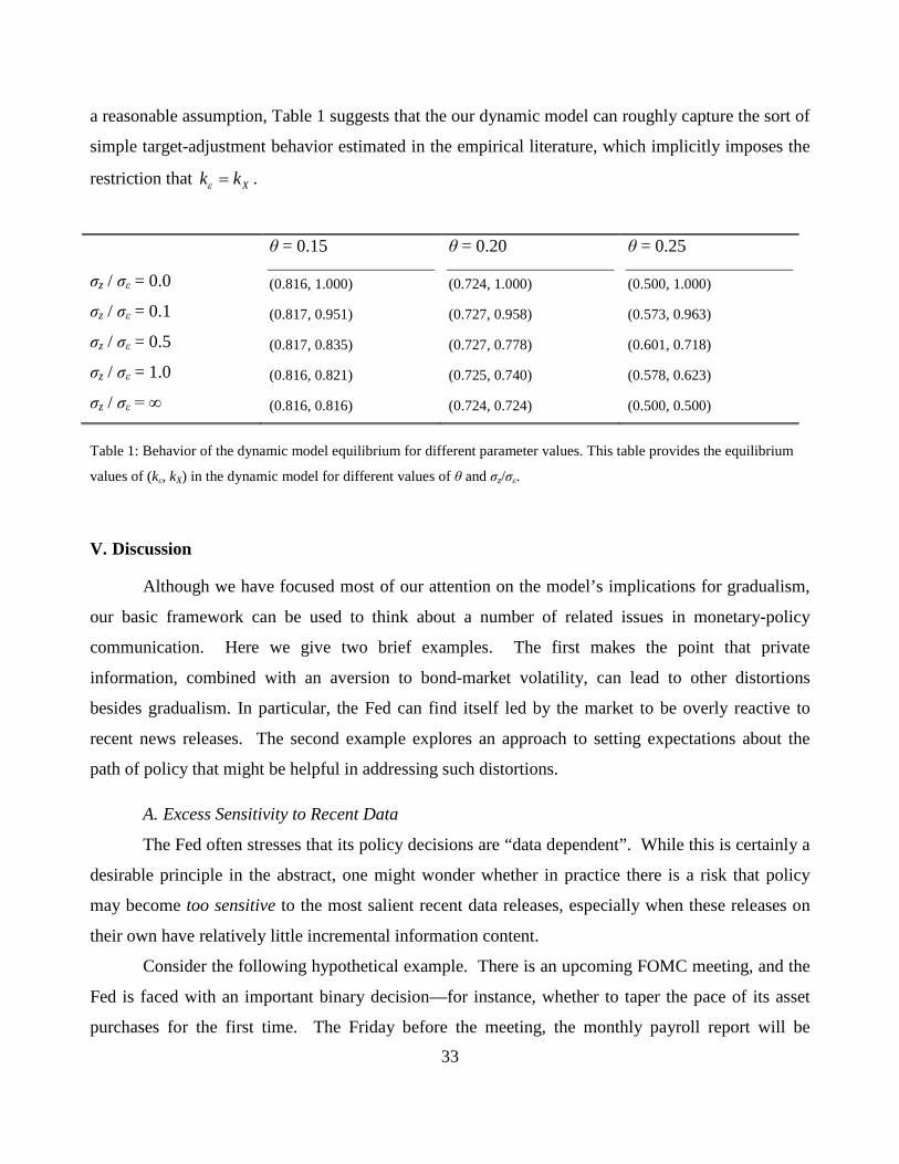
33

a reasonable assumption, Table 1 suggests that the our dynamic model can roughly capture the sort of

simple target-adjustment behavior estimated in the empirical literature, which implicitly imposes the

restriction that Xk kε = .

θ = 0.15 θ = 0.20 θ = 0.25

σz / σε = 0.0 (0.816, 1.000) (0.724, 1.000) (0.500, 1.000)

σz / σε = 0.1 (0.817, 0.951) (0.727, 0.958) (0.573, 0.963)

σz / σε = 0.5 (0.817, 0.835) (0.727, 0.778) (0.601, 0.718)

σz / σε = 1.0 (0.816, 0.821) (0.725, 0.740) (0.578, 0.623)

σz / σε = ∞ (0.816, 0.816) (0.724, 0.724) (0.500, 0.500)

Table 1: Behavior of the dynamic model equilibrium for different parameter values. This table provides the equilibrium

values of (kε, kX) in the dynamic model for different values of θ and σz/σε.

V. Discussion

Although we have focused most of our attention on the model’s implications for gradualism,

our basic framework can be used to think about a number of related issues in monetary-policy

communication. Here we give two brief examples. The first makes the point that private

information, combined with an aversion to bond-market volatility, can lead to other distortions

besides gradualism. In particular, the Fed can find itself led by the market to be overly reactive to

recent news releases. The second example explores an approach to setting expectations about the

path of policy that might be helpful in addressing such distortions.

A. Excess Sensitivity to Recent Data

The Fed often stresses that its policy decisions are “data dependent”. While this is certainly a

desirable principle in the abstract, one might wonder whether in practice there is a risk that policy

may become too sensitive to the most salient recent data releases, especially when these releases on

their own have relatively little incremental information content.

Consider the following hypothetical example. There is an upcoming FOMC meeting, and the

Fed is faced with an important binary decision—for instance, whether to taper the pace of its asset

purchases for the first time. The Friday before the meeting, the monthly payroll report will be

34

released. Market participants anticipate that the policy decision will be data dependent, and they

naturally focus attention on the payroll report, even though it is common knowledge that this report

only contains a small amount of new information about the underlying state of the economy.

Suppose that investors develop an initially arbitrary conjecture that the Fed will taper if and only if

the payroll number exceeds 200,000 new jobs. There is a sense in which this conjecture can be

partially self-validating.

To see why, imagine that the payroll number turns out to be only 160,000. Given their

conjecture, investors sharply revise downward their assessment of the likelihood of the Fed tapering.

This means that if the Fed was indeed to follow through with the taper, it would be seen as a hawkish

surprise. The market would infer that the innovation in the Fed’s private information about its target

was unusually high, and bond yields would spike upwards accordingly. Given an aversion to such

volatility, the Fed might decide to sit tight, thereby validating the market’s initial conjecture. This

could happen even if the Fed fully recognizes that there is little meaningful difference between a

payroll number of 200,000 and 160,000.

As a rough sketch of how one might capture this intuition more formally, assume the Fed can

either taper (Y) or not taper (N). The Fed has private information ε about its long-run target for the

funds rate, and this private information is distributed symmetrically on some interval [ ], .H H−

Initially, before the arrival of the news release, the optimal decision if the Fed ignored bond-market

volatility is to taper if 0ε > . Thus, the prior probability of a Y decision is ½. If the market holds

such priors, then no matter how concerned the Fed is with bond-market volatility, it will follow

through with the taper if and only if 0ε > . This is because a Y decision and an N decision are seen

as equally likely ex ante, and so the amount of information about ε that is conveyed is the same

either way. The Fed cannot affect market volatility by choosing one option or the other.

Now suppose instead that there is a small bit of bad public news right before the meeting, for

example a disappointing payroll number. Further suppose that the market interprets this news as

being both quite informative and pessimistic, so the market now believes the Fed will only taper if

Xε > for some positive X. In other words, the market thinks the likelihood of a Y decision has

declined. Given this revision in market beliefs, a concern with bond-market volatility will now make

the Fed less inclined to taper, even if it believes the news release was totally uninformative. For if

the market thinks that a Y decision implies Xε > , then a Y decision conveys more information

35

about the Fed’s long run target, and hence creates more movement in long-term rates, than does an N

decision. Hence, the market’s belief that the news release influences Fed behavior is at least partially

fulfilled in equilibrium.19

B. The Usefulness of Default Presumptions

The fundamental tension in our model arises because the Fed’s decisions convey its private

information and, all else equal, the Fed would prefer that the market not update as strongly about this

private information. So it is natural to think about ways to coarsen the mapping from the Fed’s

private information to its actions. For example, taking the model literally, if one could somehow

exogenously increase the rate-setting noise 2uσ , this would reduce the equilibrium degree of

gradualism, as can be seen from a comparison of panels (b) and (d) of Fig. 2, and might improve

overall efficiency. The intuition is that when there is more rate-setting noise observed changes in the

funds rate are less informative about changes in the Fed’s long-run target and hence have less impact

on long-term rates. Thus, the Fed faces less pressure to smooth the funds rate.

A real-world example of such a coarsening effect comes from the period subsequent to the

Fed’s initial taper of asset purchases in December of 2013. The first $10 billion reduction in the pace

of purchases was viewed as a significant change in the stance of policy, and the run-up to it was

associated with a great deal of market volatility. Things changed dramatically, however, in the

meetings following the first reduction. The Fed continued to cut asset purchases by $10 billion more

at each meeting, and it quickly became the consensus market view that this mechanical decrease was

the Fed’s default behavior.20 Given this belief on the part of the market, it was easy for the Fed to

follow through with the remaining $10 billion cuts, as the informational content had been largely

stripped from them.

To be a bit more precise, a default in our setting can be thought of like an (S, s) policy: a

range over which the Fed takes the same action independent of local variation in its private

19 We are not, however, claiming that this is a full rational-expectations equilibrium, in the sense that the market’s conjecture X about the revision in the Fed’s threshold is matched exactly one-for-one by a change in the Fed’s actual threshold. Rather, we are only making the weaker statement that a change in the former induces a positively correlated change in the latter. 20 This occurred despite the fact the Fed explicitly vowed to remain data dependent. Each FOMC statement during this period contained a line saying that: “…asset purchases are not on a preset course, and the Committee’s decisions about their pace will remain contingent on the Committee’s outlook for the labor market and inflation….”

36

information. As with rate-setting noise, the benefit is a coarsening of the mapping from private

information to actions. A given action becomes less freighted with informational content, and hence

easier for the Fed to take.

Generalizing from this example, and from the (S, s) intuition, it is unclear that the Fed should

always aim to respond sensitively to small changes in public or private information. Of course, policy

must necessarily be data-dependent in some global sense—substantial changes in the economic

environment must be met with commensurate changes in the stance of policy. At the same time,

however, it may be better to foster a market expectation that there is a default path of policy that will

be followed so long as things do not change too much. For example, in the midst of a tightening

cycle, there may be some virtue to establishing a default presumption that the funds rate will be

mechanically raised by 25 basis points at every other FOMC meeting, so long as the economy

continues to perform broadly as expected. At the margin, a default sacrifices some local fine-tuning

of policy to economic conditions, but has the advantage of making each move in rates less of an

incremental informational event.

Admittedly, setting defaults in this manner may be complicated in practice. In the model,

changes in the funds rate are the only thing that reveals the Fed’s private information to the market.

In reality, FOMC statements, speeches, and testimony also transmit such information. One might

hypothesize that something of a substitution effect could come into play—to the extent that the Fed

makes changes in the funds rate less informative, market participants may begin to scrutinize other

forms of communication more intensely.21 Nevertheless, even if crafting such purely verbal

communication remains a challenge, it might have less consequence for economic efficiency.

Attempting to manage bond-market volatility with words is not the same thing as managing it by

distorting the short rate away from the ideal target level. Analyzing a richer version of the model in

which both the Fed’s words and its actions convey some of its private information is an interesting

avenue for future work.

21 Casual observation does suggest that in the period when policy was stuck at the ZLB, so that there was nothing to be learned from rate changes, there was enormous focus on the wording of FOMC statements, and small adjustments to the statement were often met with strong market reactions.

37

VI. Conclusion

This paper has examined the complicated strategic interplay between the Fed and the bond

market that arises when the Fed has some private information about its long-run target for the policy

rate and is averse to bond-market volatility. From a positive-economics perspective, we have argued

that a model with these ingredients can help explain the phenomenon of gradualism in monetary

policy, and can also shed light on how the Fed responds to other shocks, such as changes in market

risk premiums and salient data releases. From a normative perspective, we have emphasized that in

our setting, it can be valuable for a central bank to develop an institutional culture such that a concern

with bond-market volatility does not play an outsized role in policy deliberations. In other words, it

can be useful for policymakers to build a reputation for not caring too much about the bond market.

We close by highlighting an important caveat with respect to this reputational argument. As

we have framed it, our key point rests on a comparison of equilibrium outcomes with different values

of the parameter cθ , which measures the appointed central banker’s concern about financial-market

volatility. But crucially, an implicit assumption in making this comparison is that in any given

equilibrium, the market has come to fully know the true value of cθ . We have not addressed the

more difficult question of out-of-equilibrium dynamics: how is it that the market learns about cθ

from the central bank’s observed behavior and other forms of communication?

For this reason, our model offers no guidance on the best way to make the transition to a less

bond-market-sensitive equilibrium, one in which there is less inertia in the policy rate, and the market

eventually comes to understand that cθ has declined. At any point in time, taking market conjectures

as fixed, a “cold turkey” approach that involves an unexpectedly sharp adjustment in the path of the

policy rate, relative to prevailing expectations of gradualism, is likely to cause significant market

volatility and perhaps some collateral costs for the real economy. Nothing in our analysis should be

taken as advocating such an approach. To the extent that an institution-building effort of the sort we

have in mind is at all useful, it may be something that is better undertaken over a longer horizon, such

that market expectations regarding Fed behavior are given more of a chance to adjust.

38

References

Barro, Robert J., and David B. Gordon, 1983. “Rules, Discretion and Reputation in a Model of Monetary Policy,” Journal of Monetary Economics 12, 101-121.

Bernanke, Ben, 2004. “Gradualism,” Remarks at an economics luncheon co-sponsored by the Federal

Reserve Bank of San Francisco and the University of Washington, Seattle, Washington. Bernanke, Ben, and Alan Blinder, 1992. “The Federal Funds Rate and the Channels of Monetary Transmission,” American Economic Review 82, 901-921. Brainard, William, 1967. “Uncertainty and the Effectiveness of Policy,” American Economic Review

57, 411-425. Coibion, Olivier, and Yuriy Gorodnichenko, 2012. “Why Are Target Interest Rate Changes So

Persistent?” American Economic Journal: Macroeconomics 4, 126-62. Campbell, John Y., Carolin Pflueger, and Luis Viceira, 2015. “Monetary Policy Drivers of Bond and

Equity Risks,” Harvard University working paper. Dell’Ariccia, Giovanni, Luc Laeven, and Gustavo Suarez, 2013. “Bank Leverage and Monetary Policy’s Risk-Taking Channel: Evidence from the United States,” IMF working paper. Drechsler, Itamar, Alexi Savov, and Philipp Schnabl, 2015. “The Deposits Channel of Monetary Policy,” NYU working paper. Eggertsson, Gauti B. and Michael Woodford, 2003. “The Zero Bound on Interest Rates and Optimal

Monetary Policy,” Brookings Papers on Economic Activity, 139-211. Farhi, Emmanuel, and Jean Tirole, 2012. “Collective Moral Hazard, Maturity Mismatch, and

Systemic Bailouts,” American Economic Review 102, 60-93. Gertler, Mark, and Peter Karadi, 2015. “Monetary Policy Surprises, Credit Costs, and Economic

Activity,” American Economic Journal: Macroeconomics 7, 44-76. Holmstrom, Bengt, 1999. “Managerial Incentive Problems: A Dynamic Perspective,” Review of

Economic Studies 66, 169-182. Jimenez, Gabriel, Steven Ongena, Jose-Luis Peydro, and Jesus Saurina, 2014. “Hazardous Times for

Monetary Policy: What do 23 Million Loans Say About the Impact of Monetary Policy on Credit Risk-Taking?,” Econometrica 82, 463-505.

Kashyap, Anil K, and Jeremy C. Stein, 2000. “What Do a Million Observations on Banks Say About

the Transmission of Monetary Policy?,” American Economic Review 90, 407-428.

39

Krugman, Paul, 1998. It’s Baaack: Japan’s Slump and the Return of the Liquidity Trap,” Brookings Papers on Economic Activity, 137-2006.

Kydland, Finn, and Edward Prescott, 1977. “Rules Rather Than Discretion: The Inconsistency of

Optimal Plans,” Journal of Political Economy 85, 473-491. Rogoff, Kenneth, 1985. “The Optimal Degree of Commitment to an Intermediate Monetary Target,”

Quarterly Journal of Economics 100, 1169-1189. Rudebusch, Glenn D., 2002. “Term Structure Evidence on Interest Rate Smoothing and Monetary

Policy Inertia,” Journal of Monetary Economics 49, 1161-1187. Rudebusch, Glenn D., 2006. “Monetary Policy Inertia: Fact or Fiction?” International Journal of

Central Banking 2, 85-135. Sack, Brian, 1998. “Uncertainty, Learning, and Gradual Monetary Policy,” FEDS Working Paper

Series, number 98-34. Stein, Jeremy C., 1989. “Efficient Capital Markets, Inefficient Firms: A Model of Myopic Corporate

Behavior,” Quarterly Journal of Economics 104, 655−669. Stein, Jeremy C., 2014. “Challenges for Monetary Policy Communication,” Remarks at the Money

Marketeers of New York University, New York, May 6. Taylor, John, 1993. “Discretion versus Policy Rules in Practice,” Carnegie-Rochester Conference

Series on Public Policy 39: 195-214. Woodford, Michael, 2003. “Optimal Interest-Rate Smoothing,” Review of Economic Studies 70, 861-

886. Woodford, Michael, 2012. “Methods of Policy Accommodation at the Interest-Rate Lower Bound,”

The Changing Policy Landscape: 2012 Jackson Hole Symposium, Federal Reserve Bank of Kansas City.

Appendix Proofs of Propositions

A.1 Generalization of Proposition 2 to case of non-zero rate-setting noise

Society’s ex ante problem is to choose a central banker with concern about market volatility θc. Inthe absence of noise, this central banker will implement the rational-expectations equilibrium k (θc)given by Equation (12) in the main text replacing θ with θc. In the absence of noise, society’s exante loss function is given by (

(1− k (θc))2 + θ

)σ2ε,

which is minimized by setting θc = 0 so that k (θc) = 1.In the presence of noise, the appointed central banker will implement the rational-expectations

equilibrium k (θc) given by Equation (9) in the main text replacing θ with θc. Differentiating k (θc)with respect to θc yields

∂k

∂θc= −

1−2θckτ

2u

(τ ε + k2τu

) (k2τu − τ ε

)((τ ε + k2τu)2 + θc (kτu)2

)2−1 (

τ ε + k2τu)2

(kτu)2((τ ε + k2τu)2 + θc (kτu)2

)2 < 0.

In the presence of noise, society’s ex ante loss function is given by

L = E[((1− k) εt + ut)

2 + θ (χ (kε+ ut))2]

= (1− k)2 σ2ε + σ2u + θχ2(k2σ2ε + σ2u

).

Substituting in for the rational-expectations definition of χ and differentiating with respect to θcgives the first order condition

∂L

∂θc=

[−2 (1− k)σ2ε +

2kθτu

(τ ε + k2τu)3(k2τu + τ ε

)] ∂k∂θc

.

At the optimum θc in the presence of noise, the term in square brackets will be zero. When wediscuss the optimal θc in the presence of noise in footnote 14 of the main text, we numerically solvefor the value of θc and therefore k that sets the term in square brackets to zero.

A.2 Proof of Proposition 3

We begin by characterizing the behavior of an appointed central banker who care about a finite-horizon yield, which can be represented as a weighted average of the short rate and the infinite-horizon rate:

ifinitet = αit + (1− α) i∞t .

The degree of concern about the volatility of the finite-horizon yield is parameterized by θc. Thecentral banker follows a rule of the form

it = it−1 + k (θc) · εt,

while the market conjectures that the central banker is following a rule of the form

it = it−1 + κ (θc) · εt.

Given this, the market’s conjecture about εt is

ε̃t =k

κεt

40

and it sets the infinite-horizon forward rate to

i∞t = it−1 + ε̃t.

Thus, the change in the finite-horizon yield is

∆ifinitet = α (it − it−1) + (1− α) ε̃t.

The central banker picks k (θc) to minimize the loss function

Et

[(i∗t − it)

2 + θc

(∆ifinitet

)2]= (1− k)2 σ2ε + θcα

2k2σ2ε

+θc(1− α)

κ2

2

k2σ2ε + 2θcα (1− α)k2

κσ2ε.

Differentiating with respect to k yields the first order condition

0 = − (1− k)σ2ε + θcα2kσ2ε + θc

(1− α)

κ2

2

kσ2ε + 2θcα (1− α)k

κσ2ε.

In rational expectations we have κ = k, so this reduces to

0 = − (1− k)σ2ε + θcα2kσ2ε︸ ︷︷ ︸A

+ θc(1− α)

k

2

σ2ε︸ ︷︷ ︸B

+ 2θcα (1− α)σ2ε︸ ︷︷ ︸C

. (A.1)

Term A reflects the direct effect of changing k on the short-rate component of our representationof the finite-horizon yield. Term B reflects the effect of changing k on the inferred shock ε̃t, andterm C reflects the interaction of the two effects. Note that (A.1) implies that

∂k

∂θc=

−(σ2ε(1 + θcα

2k)− θc (1−α)k2

2σ2ε

)−1×(α2kσ2ε + (1−α)

k

2σ2ε + 2θcα (1− α)σ2ε

) < 0.

Society’s ex ante loss is given by

Et

[(i∗t − it)

2 + θ(

∆ifinite)2]

= (1− k (θc))2 σ2ε + θ

(α2k (θc)

2 σ2ε + (1− α)2 σ2ε+2α (1− α) k (θc)σ

2ε

).

Differentiating with respect to θc yields the first order condition[− (1− k)σ2ε + θαkσ2ε + θα (1− α)σ2ε

] ∂k∂θc

= 0.

Evaluating at θc = θ and using the appointed central banker’s first order condition (A.1), we havethat the term in the square brackets is

− (1− k)σ2ε + θαkσ2ε︸ ︷︷ ︸A

+ θα (1− α)σ2ε︸ ︷︷ ︸C/2

= −θ (1− α)

k

2

σ2ε︸ ︷︷ ︸-B

− θα (1− α)σ2ε︸ ︷︷ ︸-(C/2)

< 0.

Since ∂k/∂θc < 0, this implies that society’s first order condition is positive at θc = θ and its exante loss can be reduced by setting θc < θ.

41

A.3 Proof of Proposition 4

Given its conjecture about the rule the Fed is following, φ (εt; νt), the market’s conjecture about εtis

ε̃t = φ−1 (f (εt; νt) ; νt)

and the Fed’s loss function is

(εt + νt − f (εt; νt))2 + θ

(φ−1 (f (εt; νt) ; νt) + νt

)2.

Consider the effect on the value of the loss function of a small perturbation in the value of f (εt; νt),df . The effect of this perturbation is zero at the optimal f (·; ·) so we have

− (εt + νt − f (εt; νt)) + θ(φ−1 (f (εt; νt) ; νt) + νt

) ∂φ−1∂i|i=f(εt;νt) = 0. (A.2)

Since φ(φ−1 (x)

)= x, we have

∂φ−1

∂i|i=f(εt;νt) =

1∂φ∂i |ε=φ−1(f(εt;νt);νt)

.

Substituting into (A.2) gives

− (εt + νt − f (εt; νt)) + θ(φ−1 (f (εt; νt) ; νt) + νt

) 1∂φ∂i |ε=φ−1(f(εt;νt);νt)

= 0.

Imposing rational expectations, we have φ = f so that this reduces to the differential equation

∂f

∂ε|ε=εt (εt + νt − f (εt; νt)) = θ (εt + νt) ,

which the optimal f (·; ·) must satisfy.Now conjecture that f = kεεt + c. In this case the differential equation reduces to

kε (εt + νt − kεεt − c) = θ (εt + νt)

orkε (1− kε) εt + kε (νt − c) = θεt + θνt

Matching coeffi cients yields

kε (1− kε) = θ and

c = νt

(1− θ

kε

)Thus, we can write the optimal f (·; ·) as

f = kεεt + kννt

where kε (1− kε) = θ and kν = 1− θ/kε. From the definition of kε we have

kν = 1− θ

kε= 1− (1− kε) = kε.

42

A.4 Proof of Proposition 5

We begin by solving the time t problem, taking the forward guidance ift−1 as given. Given its

conjecture about the rule the Fed is following, φ(εt; i

ft−1

), the market’s conjecture about εt is

ε̃t = φ−1(f(εt; i

ft−1

); ift−1

)and the Fed’s loss function is(

εt − f(εt; i

ft−1

))2+ θ

(φ−1

(f(εt; i

ft−1

); ift−1

))2+ γ

(ift−1 − it−1 − f

(εt; i

ft−1

))2.

Consider the effect on the value of the loss function of a small perturbation in the value of

f(εt; i

ft−1

), df . The effect of this perturbation is zero at the optimal f (·; ·) so we have

−(εt − f

(εt; i

ft−1

))+θ(φ−1

(f(εt; i

ft−1

); ift−1

)) ∂φ−1∂i|i=f

(εt;i

ft−1

)−γ (ift−1 − it−1 − f (εt; ift−1)) = 0.

Since φ(φ−1 (x)

)= x, we have

∂φ−1

∂i|i=f

(εt;i

ft−1

) =1

∂φ∂i |ε=φ−1

(f(εt;i

ft−1

);ift−1

) .

So the optimal f (·; ·) satisfies:

−(εt − f

(εt; i

ft−1

))+θ(φ−1

(f(εt; i

ft−1

); ift−1

)) 1∂φ∂i |ε=φ−1

(f(εt;i

ft−1

);ift−1

)−γ(ift−1 − it−1 − f

(εt; i

ft−1

))= 0.

Imposing rational expectations, we have φ = f so that this reduces to the differential equation

∂f

∂ε|ε=εt

(εt − f

(εt; i

ft−1

)+ γ

(ift−1 − it−1 − f

(εt; i

ft−1

)))= θεt,

which the optimal f (·; ·) must satisfy.Now conjecture that f = kεt + c. In this case the differential equation reduces to

k(εt − kεt − c+ γ

(ift−1 − it−1 − kεt − c

))= θεt

ork (1− k − γk) εt − kc+ kγ

(ift−1 − it−1 − c

)= θεt

Matching coeffi cients implies that

k (1− k − γk) = θ and (A.3)

−kc+ kγ(ift−1 − it−1 − c

)= 0.

Given the rule f(εt; i

ft−1

)the Fed will follow at time t , we can now solve for the optimal

forward guidance at t− 1. The loss function at time t is given by

((1− k) εt − c)2 + θε2t + γ(ift−1 − it−1 − kεt − c

)2= ((1− k) εt − c)2 + θε2t + γ

(kεt +

1

γc

)243

which in expectation at t− 1 is equal to((1− k)2 + γk2 + θ

)σ2ε +

γ

1 + γ

(ift−1 − it−1

)2. (A.4)

This is minimized by setting ift−1 = it−1.Finally we solve for the optimal γ. Differentiating (A.3) with respect to γ, we have

∂k

∂γ=

−k22k (1 + γ)− 1

< 0

so long as k > 1/2, which it will be in the parameter space we study. Setting ift−1 = it−1 anddifferentiating the ex ante loss function (A.4) with respect to γ yields(

−2 (1− k)∂k

∂γ+ k2

(1− 2kγ

2k (1 + γ)− 1

))σ2ε > 0

since ∂k/∂γ < 0 and k > 1/2. Since the ex ante loss is increasing in γ, it is optimal to set γ = 0.

A.5 Proof of Proposition 6

Given its conjecture about the rule the Fed is following, φ (εt; ηt), the market’s conjecture about εtis

ε̃t = φ−1 (f (εt; ηt) ; ηt)

and the Fed’s loss function is

(εt − f (εt; ηt))2 + θ

(φ−1 (f (εt; ηt) ; ηt) + ηt

)2.

Consider the effect on the value of the loss function of a small perturbation in the value of f (εt; ηt),df . The effect of this perturbation is zero at the optimal f (·; ·) so we have

− (εt − f (εt; ηt)) + θ(φ−1 (f (εt; ηt) ; ηt) + ηt

) ∂φ−1∂i|i=f(εt;ηt) = 0. (A.5)

Since φ(φ−1 (x)

)= x, we have

∂φ−1

∂i|i=f(εt;ηt) =

1∂φ∂i |ε=φ−1(f(εt;ηt);ηt)

.

Substituting into (A.5) gives

− (εt − f (εt; ηt)) + θ(φ−1 (f (εt; ηt) ; ηt) + ηt

) 1∂φ∂i |ε=φ−1(f(εt;ηt);ηt)

= 0.

Imposing rational expectations, we have φ = f so that this reduces to the differential equation

∂f

∂ε|ε=εt (εt − f (εt; ηt)) = θ (εt + ηt) ,

which the optimal f (·; ·) must satisfy.

44

Now conjecture that f = kεεt + c. In this case the differential equation reduces to

kε (εt − kεεt − c) = θ (εt + ηt)

orkε (1− kε) εt − kεc = θεt + θηt

Matching coeffi cients yields

kε (1− kε) = θ and

c = − θ

kεηt.

Thus, we can write the optimal f (·; ·) as

f = kεεt + kηηt

where kε (1− kε) = θ and kη = −θ/kε.

A.6 Proof of Proposition 7

Given εt (new private information about the target i∗t ) and Xt−1 (the existing gap between i∗t−1and it−1, which is public information), the central banker follows a rule of the form

it = it−1 + kX ·Xt−1 + kε · εt.

Rational investors understand that the Fed treats Xt−1 and εt differently and conjecture it isfollowing a rule of the form

it = it−1 + κX ·Xt−1 + κε · εt.Given the conjecture and it, the investors back out

ER [εt] =it − it−1 − κXXt−1

κε.

To further simplify the problem, we also assume the following timing convention. First, based onits knowledge of Xt−1, the Fed decides on the value of the adjustment parameters kX and kε it willuse for the time t FOMC meeting. After making this decision, it deliberates further, and in so doingdiscovers the committee’s consensus value of εt. Thus, the Fed picks kX and kε, taking as givenXt−1, but before knowing the realization of εt. This timing convention is purely a technical trickthat makes the problem more tractable without really changing anything of economic substance.Without it, the Fed’s adjustment rule would turn out to depend on the realization of the productXt−1εt. With the timing trick, what matters instead is the expectation of the product, which iszero. This simplification maintains the linearity of the Fed’s optimal adjustment rule. We shouldemphasize that even with this somewhat strained intra-meeting timing, the Fed still behaves on adiscretionary basis from one meeting to the next. Thus, while it agrees to values of kX and kε inthe first part of the time-t meeting, it has no ability to bind itself to those values across meetings.Hence the basic commitment problem remains.

Thus, the central banker picks kX and kε to minimize the loss function

Et

[(i∗t − it)

2 + θ (∆i∞t )2]

= Et

[((1− kX)Xt−1 + (1− kε) εt)2 + θ

(ER [εt]

)2]= (1− kX)2X2

t−1 + (1− kε)2 σ2ε + θ

((1

κε(kX − κX)

)2X2t−1 +

(kεκε

)2σ2ε

).

45

Differentiating with respect to kX yields

− (1− kX) + θ

(1

κε(kX − κX)

)= 0.

Imposing rational expectations we have kX = κX which implies that kX = 1.Differentiating with respect to kε yields

0 = − (1− kε) + θ

(kεκ2ε

).

Imposing rational expectations we have kε = κε which implies that

kε =k2ε

k2ε + θ

as before.

A.7 Proof of Proposition 8

We now assume that investors do not perfectly observe Xt−1. Instead they observe

st−1 = Xt−1 + zt−1

where zt−1 ∼ N(0, σ2z

). We assume that investors observe st−1 before it, so that the expectation

of Xt−1 given st−1,

E [Xt−1|st−1] =Cov (Xt−1, st−1)

V ar (st−1)st−1 =

σ2Xσ2X + σ2z

st−1,

is already impounded into the infinite horizon forward rate before the Fed picks it.Thus, the changein the infinite horizon forward rate at time t is the revision in the market’s expectations about thetarget rate given the change in the federal funds rate:

∆i∞t = E [i∗t |∆it, st−1]− E[i∗t−1|st−1

]= E [Xt−1 + εt|∆it, st−1]− E [Xt−1|st−1] = χi∆it − χsst−1

where computation of the conditional expectations shows that

χi =κεσ

2ε

(σ2X + σ2z

)+ κXσ

2Xσ

2z

κ2εσ2ε

(σ2X + σ2z

)+ κ2Xσ

2Xσ

2z

χs =κε (κX − κε)σ2εσ2X

κ2εσ2ε

(σ2X + σ2z

)+ κ2Xσ

2Xσ

2z

+σ2X

σ2X + σ2z.

Note that when σ2z = 0, we have

χi =1

κε

χs =κXκε

so thatχi (kεεt + kXXt−1)− χsXt−1 = εt

46

in rational expectations and we are back to the expressions we had in Proposition 7 where investorsobserved Xt−1 with no noise. In addition, note that when σz →∞, we have

χi →κεσ

2ε + κXσ

2X

κ2εσ2ε + κ2Xσ

2X

χs → 0

so investors put no weight on the signal st−1.We retain the timing convention used in Proposition 7, so that the Fed picks kX and kε and

then εt and zt are realized. The loss function is then

Et

[(i∗t − it)

2 + θ (∆i∞t )2]

= Et

[(i∗t−1 + εt − it−1 − kX ·Xt−1 − kε · εt

)2+ θ (∆i∞t )2

]= (1− kX)2X2

t−1 + (1− kε)2 σ2ε+θ(

(kXχi − χs)2X2t−1 + χ2i k

2εσ2ε + χ2sσ

2z

)Differentiating with respect to kX yields

kX =1 + θχiχs1 + θχ2i

For θ > 0, this implies kX < 1 since χi > χs.Differentiating with respect to kε yields

kε =1

1 + θχ2i

This implies that kX > kε and kX = kε when χs = 0, which happens as σz →∞.When σ2z →∞, we have kX = kε so that

kX =

(k2εσ

2ε + k2Xσ

2X

)2(k2εσ

2ε + k2Xσ

2X

)2+ θ

(kεσ2ε + kXσ2X

)2=

1

1 + θ(1kX

)2which is our baseline expression in the static model. Thus, when σ2z → ∞ the Fed moves equallyslowly over Xt−1 and εt and the speed is given by the same expression as in the static model withno noise.

47