FEDERAL RESERVE BANK OF ST. LOUIS REVIEW JULY / AUGUST 2008 447 Rules-of-Thumb for Guiding Monetary Policy William Poole This article was originally published in the Board of Governors of the Federal Reserve System Open Market Policies and Operating Procedures—Staff Studies, July 1971. It is reprinted here as an addendum to these conference proceedings. Federal Reserve Bank of St. Louis Review, July/August 2008, 90(4), pp. 447-97. tory section outlines the structure of the study so that the reader can see how the various parts fit together. The reader interested only in a summary of the analysis and empirical findings should read this introductory section and then turn directly to the summary in Section V. This sum- mary concentrates on the theoretical analysis while only briefly stating the most important empirical findings. It omits completely the tech- nical details of both the theoretical and empirical work. The reader interested in the technical details should, of course, turn to the appropriate parts of Sections I through IV. Insofar as possible these sections have been written so that the reader can understand any one section without having to wade through all of the other sections. Section I contains the theoretical argument comparing interest rates and the money stock as policy-control variables under conditions of uncer- tainty. The analysis is verbal and graphical, using the simple Hicksian IS-LM model with random terms added. This model is general enough to include both Keynesian and monetarist outlooks, depending on the specific assumptions as to the shapes of the functions. Since the theoretical analysis emphasizes the importance of the relative INTRODUCTION T his study has been motivated by the recognition that the key to understanding policy problems is the analysis of uncer- tainty. Indeed, in the absence of uncertainty it might be said that there can be no policy prob- lems, only administrative problems. It is sur- prising, therefore, that there has been so little systematic attention paid to uncertainty in the policy literature in spite of the fact that policy- makers have repeatedly emphasized the impor- tance of the unknown. In the past, the formal models used in the analysis of monetary policy problems have almost invariably assumed complete knowledge of the economic relationships in the model. Uncertainty is introduced into the analysis, if at all, only through informal consideration of how much difference it makes if the true relationships differ from those assumed by the policymakers. In this study, on the other hand, uncertainty plays a key role in the formal model. Since this study is so long, a few comments at the outset may assist the reader in finding his way through it. The remainder of this introduc- William Poole is a former president of the Federal Reserve Bank of St. Louis. At the time this article was written, he was a senior economist in the special studies section of the division of research and statistics at the Board of Governors of the Federal Reserve System. Joan Walton, Lillian Humphrey, and Debra Bellows provided research assistance. © 2008, The Federal Reserve Bank of St. Louis. The views expressed in this article are those of the author(s) and do not necessarily reflect the views of the Federal Reserve System, the Board of Governors, or the regional Federal Reserve Banks. Articles may be reprinted, reproduced, published, distributed, displayed, and transmitted in their entirety if copyright notice, author name(s), and full citation are included. Abstracts, synopses, and other derivative works may be made only with prior written permission of the Federal Reserve Bank of St. Louis.

Welcome message from author
This document is posted to help you gain knowledge. Please leave a comment to let me know what you think about it! Share it to your friends and learn new things together.
Transcript
FEDERAL RESERVE BANK OF ST. LOUIS REVIEW JULY/AUGUST 2008 447
Rules-of-Thumb for Guiding Monetary Policy
William Poole
This article was originally published in the Board of Governors of the Federal Reserve SystemOpen Market Policies and Operating Procedures—Staff Studies, July 1971. It is reprinted here asan addendum to these conference proceedings.
Federal Reserve Bank of St. Louis Review, July/August 2008, 90(4), pp. 447-97.
tory section outlines the structure of the study sothat the reader can see how the various parts fittogether. The reader interested only in a summaryof the analysis and empirical findings shouldread this introductory section and then turndirectly to the summary in Section V. This sum-mary concentrates on the theoretical analysiswhile only briefly stating the most importantempirical findings. It omits completely the tech-nical details of both the theoretical and empiricalwork. The reader interested in the technical detailsshould, of course, turn to the appropriate partsof Sections I through IV. Insofar as possible thesesections have been written so that the reader canunderstand any one section without having towade through all of the other sections.
Section I contains the theoretical argumentcomparing interest rates and the money stock aspolicy-control variables under conditions of uncer-tainty. The analysis is verbal and graphical, usingthe simple Hicksian IS-LMmodel with randomterms added. This model is general enough toinclude both Keynesian and monetarist outlooks,depending on the specific assumptions as to theshapes of the functions. Since the theoreticalanalysis emphasizes the importance of the relative
INTRODUCTION
T his study has been motivated by therecognition that the key to understandingpolicy problems is the analysis of uncer-
tainty. Indeed, in the absence of uncertainty itmight be said that there can be no policy prob-lems, only administrative problems. It is sur-prising, therefore, that there has been so littlesystematic attention paid to uncertainty in thepolicy literature in spite of the fact that policy-makers have repeatedly emphasized the impor-tance of the unknown.
In the past, the formal models used in theanalysis of monetary policy problems have almostinvariably assumed complete knowledge of theeconomic relationships in the model. Uncertaintyis introduced into the analysis, if at all, onlythrough informal consideration of how muchdifference it makes if the true relationships differfrom those assumed by the policymakers. In thisstudy, on the other hand, uncertainty plays a keyrole in the formal model.
Since this study is so long, a few commentsat the outset may assist the reader in finding hisway through it. The remainder of this introduc-
William Poole is a former president of the Federal Reserve Bank of St. Louis. At the time this article was written, he was a senior economist inthe special studies section of the division of research and statistics at the Board of Governors of the Federal Reserve System. Joan Walton,Lillian Humphrey, and Debra Bellows provided research assistance.
© 2008, The Federal Reserve Bank of St. Louis. The views expressed in this article are those of the author(s) and do not necessarily reflect theviews of the Federal Reserve System, the Board of Governors, or the regional Federal Reserve Banks. Articles may be reprinted, reproduced,published, distributed, displayed, and transmitted in their entirety if copyright notice, author name(s), and full citation are included. Abstracts,synopses, and other derivative works may be made only with prior written permission of the Federal Reserve Bank of St. Louis.

stability of the expenditures and money demandfunctions, an examination of the evidence onrelative stability appears in Section II.
Given the conclusion of Section II on thesuperiority of a policy operating through adjust-ments in themoney stock, the next question is howthe money stock should be adjusted to achievethe best results. While policymakers generallylook askance at suggestions for policy rules, theonly way that economists can give long-run adviceis in terms of rules. That is to say, the economistis not being helpful at all if he in effect says, “Lookat the rate of inflation, at the rate of unemploy-ment, at the forecasts of the government budgetdeficit, and at other relevant factors, and then actappropriately.” Advice requires the specificationof exactly how policy should be adjusted, and forthis advice to be more than an ad hoc recommen-dation for the current situation, it must involvespecification of how the money stock or someother control variable should be adjusted underhypothetical future conditions of inflation, unem-ployment, and so forth. The purpose of Section IIIis to develop such a rule-of-thumb, or policyguideline, based on the theoretical and empiricalanalyses of Sections I and ll.
A number of technical problems of monetarycontrol are examined in Section IV. After a shortintroduction to the issues, the first part of thissection discusses the relative merits of a numberof monetary aggregates including various reservemeasures, the narrowly and broadly definedmoney stocks, and bank credit. The second partexamines whether policy should specify desiredrates of change of an aggregate in terms of weekly,monthly, or quarterly averages, or in some othermanner. The third part examines in a very incom-plete fashion a few of the problems of adjustingopen market operations so as to reach the desiredlevel of an aggregate.
Finally, Section V consists of a summary ofSections I through IV. To avoid undue repetition,woven into this summary section are a number ofgeneral observations not examined in the othersections.
I. THE THEORY OF MONETARYPOLICY UNDER UNCERTAINTYBasic Concepts
The theory of optimal policy under uncer-tainty has provided many insights into actualpolicy problems (Theil, 1964; Brainard, 1967; Holt,1962; Poole, 1970). While much of this theory isnot accessible to the nonmathematical economist,it is possible to explain the basic ideas withoutresort to mathematics.
The obvious starting point is the observationthat with our incomplete understanding of theeconomy and our inability to predict accuratelythe occurrence of disturbing factors such as strikes,wars, and foreign exchange crises, we cannotexpect to hit policy goals exactly. Some periodsof inflation or unemployment are unavoidable.The inevitable lack of precision in reaching policygoals is sometimes recognized by saying that thegoals are “reasonably” stable prices and “reason-ably” full employment.
While the observation above is trite, itsimplications are not. Two points are especiallyimportant. First, policy should aim at minimizingthe average size of errors. Second, policy can bejudged only by the average size of errors over aperiod of time and not by individual episodes.Because this second point is particularly subject tomisunderstanding, it needs further amplification.
Since policymakers operate in a world thatis inherently uncertain, they must be judged bycriteria appropriate to such a world. Consider theanalogy of betting on the draw of a ball from anurnwith nine black balls and one red ball. Anyoneoffered a $2 payoff for a $1 bet would surely beton a black ball being drawn. If the draw producedthe red ball, no one would accuse the bettor of astupid bet. Similarly, the policymaker must playthe economic odds. The policymaker should notbe accused of failure if an inflation occurs as theresult of an improbable and unforeseeable event.
Now consider the reverse situation from thatconsidered in the previous paragraph. Supposethe bettor with the same odds as above bets on thered ball and wins. Some would claim that the betwas brilliant, but assuming that the draw was not
Poole
448 JULY/AUGUST 2008 FEDERAL RESERVE BANK OF ST. LOUIS REVIEW

rigged inanyway, thebet, even thoughawinning one,must be judged foolish. It is foolish because, onthe average, such a betting strategy will lead tosubstantially worse results than the oppositestrategy. Betting on red will prove brilliant onlyone time out of 10, on the average. Similarly, aparticular policy action may be a bad bet eventhough it works in a particular episode.
There is a well-known tendency for gamblersto try systems that according to the laws of prob-ability cannot be successful over any length oftime. Frequently, a gambler will adopt a foolishsystem as the result of an initial chance successsuch as betting on red in the above example. Thesame danger exists in economic policy. In fact, thedanger is more acute because there appears to bea greater chance to “beat the system” by applyingeconomic knowledge and intuition. There can beno doubt that it will become increasingly possibleto improve on simple, naive policies throughsophisticated analysis and forecasting and so ina sense “beat the system.” But evenwith improvedknowledge some uncertainty will always exist,and therefore so will the tendency to attempt toperform better than the state of knowledge reallypermits.
Whatever the state of knowledge, there mustbe a clear understanding of how to cope withuncertainty, even though the degree of uncertaintymay have been drastically reduced through theuse of modern methods of analysis. The principalpurpose of this section is to improve understand-ing of the importance of uncertainty for policy byexamining a simple model in which the policyproblem is treated as one of minimizing errorson the average. Particular emphasis is placed onwhether controlling policy by adjusting the inter-est rate or by adjusting the money stock will leadto smaller errors on the average. The basic argu-ment is designed to show that the answer to whichpolicy variable—the interest rate or the moneystock—minimizes average errors depends on therelative stability of the expenditures and moneydemand functions and not on the values of param-eters that determine whether monetary policy isin some sense more or less “powerful” than fiscalpolicy.
Monetary Policy Under Uncertainty ina Keynesian Model1
The basic issues concerning the importanceof uncertainty for monetary policy may be exam-ined within the Hicksian IS-LM version of theKeynesian system. This elementary model hastwo sectors, an expenditure sector and a monetarysector, and it assumes that the price level is fixedin the short run.2 Consumption, investment, andgovernment expenditures functions are combinedto produce the IS function in Figure 1, while thedemand and supply of money functions are com-bined to produce the LM function. If monetarypolicy fixes the stock of money, then the resultingLM function is LM1, while if policy fixes the inter-est rate at r0 the resulting LM function is LM2. Itis assumed that incomes above “full employmentincome” are undesirable due to inflationary pres-sures while incomes below full employmentincome are undesirable due to unemployment.
If the positions of all the functions could bepredicted with no errors, then to reach fullemployment income, Yf , it would make no differ-
Poole
FEDERAL RESERVE BANK OF ST. LOUIS REVIEW JULY/AUGUST 2008 449
r
r0
LM1
LM2
Yf Y
IS
Figure 1
SOURCE: Originally published version, p. 139.
1 For the most part this section represents a verbal and graphicalversion of the mathematical argument in Poole (1970).
2 Simple presentations of this model may be found in Reynolds(1969, pp. 275-82) and Samuelson (1967, pp. 327-32).
ence whether policy fixed the money stock or theinterest rate. All that is necessary in either caseis to set the money stock or the interest rate sothat the resulting LM function will cut the IS func-tion at the full employment level of income.
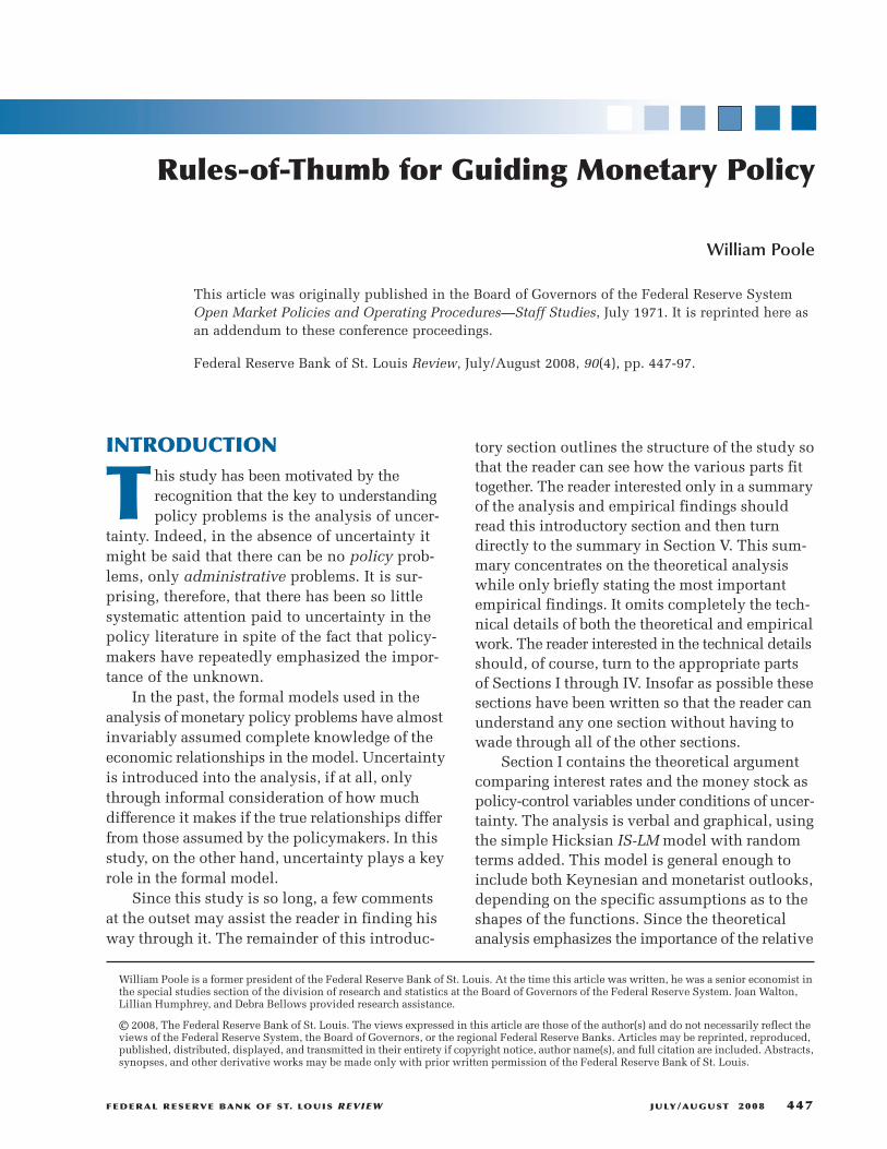
Significance of Disturbances. The positionsof the functions are, unfortunately, never pre-cisely known. Consider first uncertainty over theposition of the IS function—which, of course,results from instability in the underlying con-sumption and investment functions—whileretaining the unrealistic assumption that theposition of the LM function is known. What isknown about the IS function is that it will liebetween the extremes of IS1 and IS2 in Figure 2.If the money stock is set at some fixed level, thenit is known that the LM function will be LM1, andaccordingly income will be somewhere betweenthe extremes of Y1 and Y2. On the other hand,suppose policymakers follow an interest ratepolicy and set the interest rate at r0. In this caseincome will be somewhere between Y1′ and Y2′,a wider range than Y1 to Y2, and so the moneystock policy is superior to the interest rate policy.3
The money stock policy is superior because anunpredictable disturbance in the IS function willaffect the interest rate, which in turn will producespending changes that partly onset the initialdisturbance.
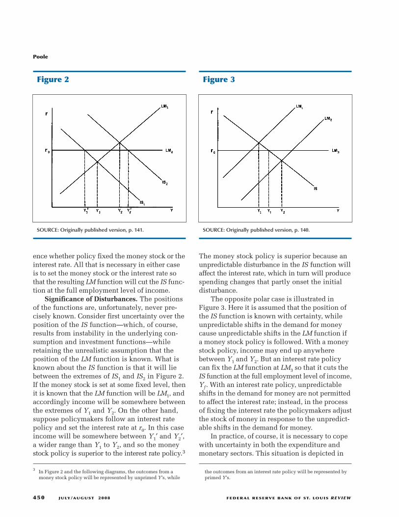
The opposite polar case is illustrated inFigure 3. Here it is assumed that the position ofthe IS function is known with certainty, whileunpredictable shifts in the demand for moneycause unpredictable shifts in the LM function ifa money stock policy is followed. With a moneystock policy, income may end up anywherebetween Y1 and Y2. But an interest rate policycan fix the LM function at LM3 so that it cuts theIS function at the full employment level of income,Yf . With an interest rate policy, unpredictableshifts in the demand for money are not permittedto affect the interest rate; instead, in the processof fixing the interest rate the policymakers adjustthe stock of money in response to the unpredict-able shifts in the demand for money.
In practice, of course, it is necessary to copewith uncertainty in both the expenditure andmonetary sectors. This situation is depicted in
the outcomes from an interest rate policy will be represented byprimed Y’s.
Poole
450 JULY/AUGUST 2008 FEDERAL RESERVE BANK OF ST. LOUIS REVIEW
Figure 2
SOURCE: Originally published version, p. 141.
Figure 3
SOURCE: Originally published version, p. 140.
3 In Figure 2 and the following diagrams, the outcomes from amoney stock policy will be represented by unprimed Y’s, while

Figure 4, where the unpredictable disturbances arelarger in the expenditure sector, and in Figure 5where the unpredictable disturbances are largerin the monetary sector.
The situation is even more complicated thanshown in Figures 4 and 5 by virtue of the factthat the disturbances in the two sectors may notbe independent. To illustrate this case, considerFigure 5 in which the interest rate policy is supe-rior to the money stock policy if the disturbancesare independent. Suppose that the disturbanceswere connected in such a way that disturbanceson the LM1 side of the average LM function werealways accompanied by disturbances on the IS2side of the average IS function. This would meanthat income would never go as low as Y1, butrather only as low as the intersection of LM1 andIS2, an income not as low as Y1′ under the interestrate policy. Similarly, the highest income wouldbe given by the intersection of LM2 and IS1, anincome not so high as Y2′.4
Importance of Interest Elasticities and OtherParameters. So far the argument has concentratedentirely on the importance of the relative sizesof expenditure and monetary disturbances. Butis it also important to consider the slopes of thefunctions as determined by the interest elastici-ties of investment and of the demand for money,and by other parameters? Consider the pair of ISfunctions, IS1 and IS2, as opposed to the pair, IS3and IS4, in Figure 6. Each pair represents themaximum and minimum positions of the IS func-tion as a result of disturbances, but the pairs havedifferent slopes. Each pair assumes the samemaximum and minimum disturbances, as shownby the fact that the horizontal distance betweenIS1 and IS2 is the same as between IS3 and IS4.For convenience, but without loss of generality,the functions have been drawn so that underan interest rate policy represented by LM2 bothpairs of IS functions produce the same range ofincomes. To keep the diagram from becoming
Poole
FEDERAL RESERVE BANK OF ST. LOUIS REVIEW JULY/AUGUST 2008 451
4 The diagram could obviously have been drawn so that an interestrate policy would be superior to a money stock policy even thoughthere was an inverse relationship between the shifts in the IS andLM functions. However, inverse shifts always reduce the margin
Figure 4
SOURCE: Originally published version, p. 141.
Figure 5
SOURCE: Originally published version, p. 141.
of superiority of an interest rate policy, possibly to the point ofmaking a money stock policy superior. Conversely, positivelyrelated shifts favor an interest rate policy.

Poole
452 JULY/AUGUST 2008 FEDERAL RESERVE BANK OF ST. LOUIS REVIEW
Figure 7
SOURCE: Originally published version, p. 141.
Figure 6
SOURCE: Originally published version, p. 141.
Figure 8
SOURCE: Originally published version, p. 143.
Figure 9
SOURCE: Originally published version, p. 143.
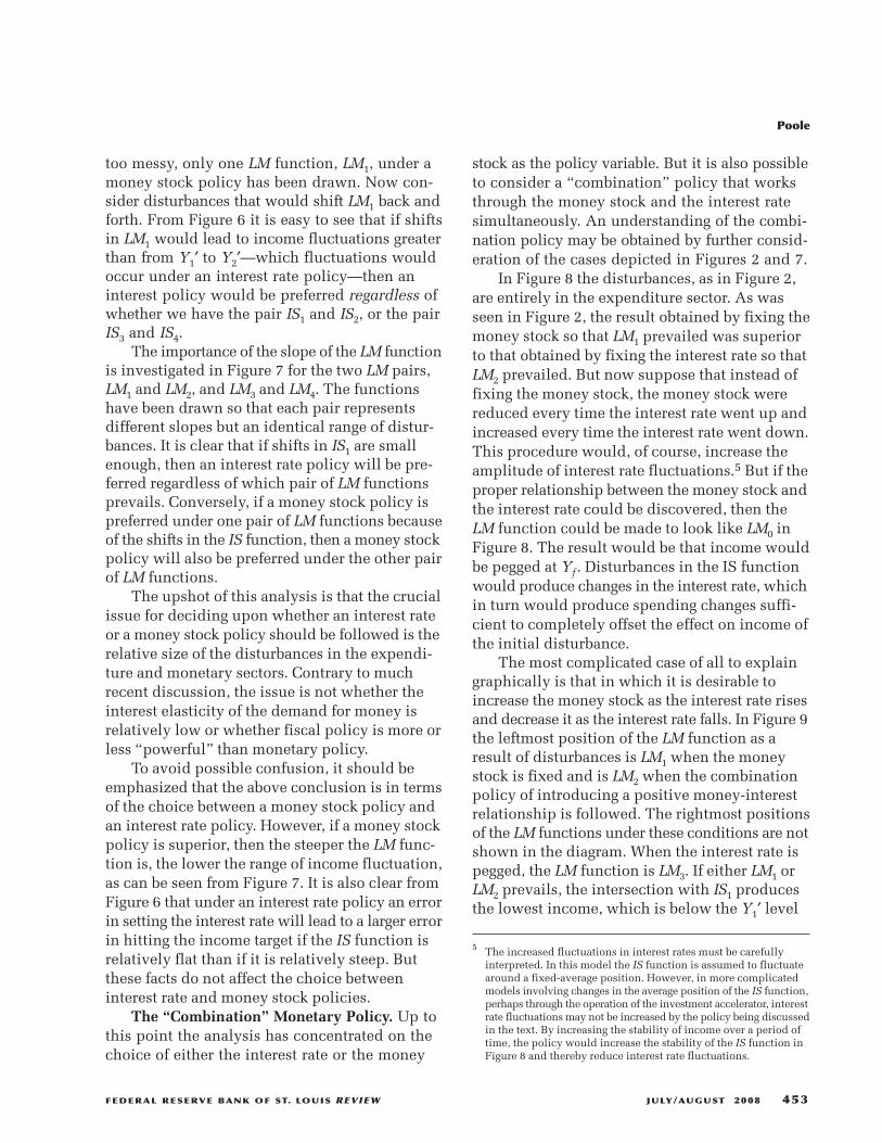
too messy, only one LM function, LM1, under amoney stock policy has been drawn. Now con-sider disturbances that would shift LM1 back andforth. From Figure 6 it is easy to see that if shiftsin LM1 would lead to income fluctuations greaterthan from Y1′ to Y2′—which fluctuations wouldoccur under an interest rate policy—then aninterest policy would be preferred regardless ofwhether we have the pair IS1 and IS2, or the pairIS3 and IS4.
The importance of the slope of the LM functionis investigated in Figure 7 for the two LM pairs,LM1 and LM2, and LM3 and LM4. The functionshave been drawn so that each pair representsdifferent slopes but an identical range of distur-bances. It is clear that if shifts in IS1 are smallenough, then an interest rate policy will be pre-ferred regardless of which pair of LM functionsprevails. Conversely, if a money stock policy ispreferred under one pair of LM functions becauseof the shifts in the IS function, then a money stockpolicy will also be preferred under the other pairof LM functions.
The upshot of this analysis is that the crucialissue for deciding upon whether an interest rateor a money stock policy should be followed is therelative size of the disturbances in the expendi-ture and monetary sectors. Contrary to muchrecent discussion, the issue is not whether theinterest elasticity of the demand for money isrelatively low or whether fiscal policy is more orless “powerful” than monetary policy.
To avoid possible confusion, it should beemphasized that the above conclusion is in termsof the choice between a money stock policy andan interest rate policy. However, if a money stockpolicy is superior, then the steeper the LM func-tion is, the lower the range of income fluctuation,as can be seen from Figure 7. It is also clear fromFigure 6 that under an interest rate policy an errorin setting the interest rate will lead to a larger errorin hitting the income target if the IS function isrelatively flat than if it is relatively steep. Butthese facts do not affect the choice betweeninterest rate and money stock policies.
The “Combination” Monetary Policy. Up tothis point the analysis has concentrated on thechoice of either the interest rate or the money
stock as the policy variable. But it is also possibleto consider a “combination” policy that worksthrough the money stock and the interest ratesimultaneously. An understanding of the combi-nation policy may be obtained by further consid-eration of the cases depicted in Figures 2 and 7.
In Figure 8 the disturbances, as in Figure 2,are entirely in the expenditure sector. As wasseen in Figure 2, the result obtained by fixing themoney stock so that LM1 prevailed was superiorto that obtained by fixing the interest rate so thatLM2 prevailed. But now suppose that instead offixing the money stock, the money stock werereduced every time the interest rate went up andincreased every time the interest rate went down.This procedure would, of course, increase theamplitude of interest rate fluctuations.5 But if theproper relationship between the money stock andthe interest rate could be discovered, then theLM function could be made to look like LM0 inFigure 8. The result would be that income wouldbe pegged at Yf . Disturbances in the IS functionwould produce changes in the interest rate, whichin turn would produce spending changes suffi-cient to completely offset the effect on income ofthe initial disturbance.
The most complicated case of all to explaingraphically is that in which it is desirable toincrease the money stock as the interest rate risesand decrease it as the interest rate falls. In Figure 9the leftmost position of the LM function as aresult of disturbances is LM1 when the moneystock is fixed and is LM2 when the combinationpolicy of introducing a positive money-interestrelationship is followed. The rightmost positionsof the LM functions under these conditions are notshown in the diagram. When the interest rate ispegged, the LM function is LM3. If either LM1 orLM2 prevails, the intersection with IS1 producesthe lowest income, which is below the Y1′ level
Poole
FEDERAL RESERVE BANK OF ST. LOUIS REVIEW JULY/AUGUST 2008 453
5 The increased fluctuations in interest rates must be carefullyinterpreted. In this model the IS function is assumed to fluctuatearound a fixed-average position. However, in more complicatedmodels involving changes in the average position of the IS function,perhaps through the operation of the investment accelerator, interestrate fluctuations may not be increased by the policy being discussedin the text. By increasing the stability of income over a period oftime, the policy would increase the stability of the IS function inFigure 8 and thereby reduce interest rate fluctuations.
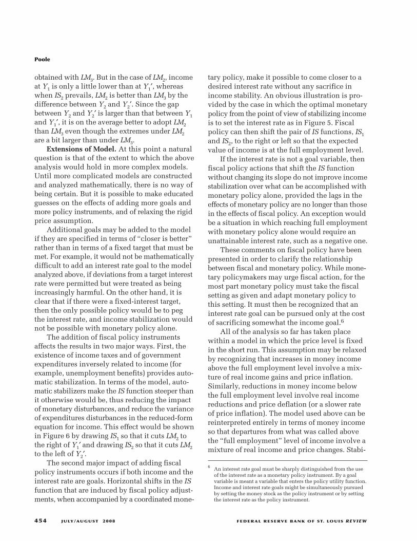
obtained with LM3. But in the case of LM2, incomeat Y1 is only a little lower than at Y1′, whereaswhen IS2 prevails, LM2 is better than LM3 by thedifference between Y2 and Y2′. Since the gapbetween Y2 and Y2′ is larger than that between Y1and Y1′, it is on the average better to adopt LM2
than LM3 even though the extremes under LM2
are a bit larger than under LM3.Extensions of Model. At this point a natural
question is that of the extent to which the aboveanalysis would hold in more complex models.Until more complicated models are constructedand analyzed mathematically, there is no way ofbeing certain. But it is possible to make educatedguesses on the effects of adding more goals andmore policy instruments, and of relaxing the rigidprice assumption.
Additional goals may be added to the modelif they are specified in terms of “closer is better”rather than in terms of a fixed target that must bemet. For example, it would not be mathematicallydifficult to add an interest rate goal to the modelanalyzed above, if deviations from a target interestrate were permitted but were treated as beingincreasingly harmful. On the other hand, it isclear that if there were a fixed-interest target,then the only possible policy would be to pegthe interest rate, and income stabilization wouldnot be possible with monetary policy alone.
The addition of fiscal policy instrumentsaffects the results in two major ways. First, theexistence of income taxes and of governmentexpenditures inversely related to income (forexample, unemployment benefits) provides auto-matic stabilization. In terms of the model, auto-matic stabilizers make the IS function steeper thanit otherwise would be, thus reducing the impactof monetary disturbances, and reduce the varianceof expenditures disturbances in the reduced-formequation for income. This effect would be shownin Figure 6 by drawing IS1 so that it cuts LM2 tothe right of Y1′ and drawing IS2 so that it cuts LM2
to the left of Y2′.The second major impact of adding fiscal
policy instruments occurs if both income and theinterest rate are goals. Horizontal shifts in the ISfunction that are induced by fiscal policy adjust-ments, when accompanied by a coordinatedmone-
tary policy, make it possible to come closer to adesired interest rate without any sacrifice inincome stability. An obvious illustration is pro-vided by the case in which the optimal monetarypolicy from the point of view of stabilizing incomeis to set the interest rate as in Figure 5. Fiscalpolicy can then shift the pair of IS functions, IS1and IS2, to the right or left so that the expectedvalue of income is at the full employment level.
If the interest rate is not a goal variable, thenfiscal policy actions that shift the IS functionwithout changing its slope do not improve incomestabilization over what can be accomplished withmonetary policy alone, provided the lags in theeffects of monetary policy are no longer than thosein the effects of fiscal policy. An exception wouldbe a situation in which reaching full employmentwith monetary policy alone would require anunattainable interest rate, such as a negative one.
These comments on fiscal policy have beenpresented in order to clarify the relationshipbetween fiscal and monetary policy. While mone-tary policymakers may urge fiscal action, for themost part monetary policy must take the fiscalsetting as given and adapt monetary policy tothis setting. It must then be recognized that aninterest rate goal can be pursued only at the costof sacrificing somewhat the income goal.6
All of the analysis so far has taken placewithin a model in which the price level is fixedin the short run. This assumption may be relaxedby recognizing that increases in money incomeabove the full employment level involve a mix-ture of real income gains and price inflation.Similarly, reductions in money income belowthe full employment level involve real incomereductions and price deflation (or a slower rateof price inflation). The model used above can bereinterpreted entirely in terms of money incomeso that departures from what was called abovethe “full employment” level of income involve amixture of real income and price changes. Stabi-
6 An interest rate goal must be sharply distinguished from the useof the interest rate as a monetary policy instrument. By a goalvariable is meant a variable that enters the policy utility function.Income and interest rate goals might be simultaneously pursuedby setting the money stock as the policy instrument or by settingthe interest rate as the policy instrument.
Poole
454 JULY/AUGUST 2008 FEDERAL RESERVE BANK OF ST. LOUIS REVIEW
lizing money income, then, involves a mixtureof the two goals of stabilizing real output and ofstabilizing the price level.
However, interpreted in this way the structureof the model is deficient because it fails to dis-tinguish between real and nominal interest rates.Price level increases generate inflationary expec-tations, which in turn generate an outward shiftin the IS function. The model may be patched upto some extent by assuming that price changesmake up a constant fraction of the deviation ofincome from its full employment level and assum-ing further that the expected rate of inflation is aconstant multiplied by the actual rate of inflation.Expenditures are then made to depend on the realrate of interest, the difference between the nomi-nal rate of interest and the expected rate of infla-tion. The result is to make the IS function, whendrawn against the nominal interest rate, flatter andto increase the variance of disturbances to the ISfunction. These elects are more pronounced: (a)the larger is the interest sensitivity of expendi-tures; (b) the larger is the fraction of price changesin money income changes; and (c) the larger isthe effect of price changes on price expectations.The conclusion is that since price flexibility ineffect increases the variance of disturbances inthe IS function, a money stock policy tends to befavored over an interest rate policy.
II. EVIDENCE ON THE RELATIVEMAGNITUDES OF REAL ANDMONETARY DISTURBANCESNature of Available Evidence
Little evidence is available that directly teststhe relative stability of the expenditure andmoneydemand functions. It is necessary, therefore, toproceed somewhat indirectly. First, simulation ofthe FR-MIT model7 is used to show the probablesize of the effect on gross national product (GNP),the GNP deflator, and the unemployment rate ofan assumed expenditure disturbance. This evi-
dence provides some indication of the extent towhich the impact of an expenditure disturbancedepends on the choice between the money stockand the Treasury bill rate as monetary policy con-trol variables. This evidence bears only on thequestion of what happens if an expenditure dis-turbance occurs, not on the relative stability ofthe expenditure and money demand functions.However, this approach is useful when combinedwith intuitive feelings about relative stability.
The second type of evidence, derived fromreduced-form studies, is more directly related tothe question of relative stability; nevertheless, itis not entirely satisfactory because the studiesexamined were not designed to answer the ques-tion at hand. To supplement these studies byother investigators, there follows a simple test ofthe stability of the demand for money function.
Impact of an Expenditure Disturbance
Simulation of the FR-MIT model providessome insight as to how the size of the impact ofan expenditure disturbance depends on the choiceof the monetary policy instrument. The simula-tion technique is necessary because the FR-MITmodel is nonlinear, making it impossible to obtainan explicit expression for the reduced form.8
However, comparison of two sets of simulationsprovides some interesting results. Except as indi-cated below, the simulations all used the actualhistorical values of the model’s exogenous vari-ables and all simulations started with 1962-I, astarting date selected arbitrarily.
The first set of five simulations assumes anexogenous money stock that grows by 1 percentper quarter, starting with the actual money stockin 1961-IV as the base. To investigate the impactof a disturbance in an exogenous expendituresvariable, the exogenous variable “federal expen-ditures on defense goods” was set in one simula-tion at its actual level minus $10 billion; in anotherat actual minus $5 billion; and in three furthersimulations at actual, actual plus $5 billion, andactual plus $10 billion. This procedure produces
Poole
FEDERAL RESERVE BANK OF ST. LOUIS REVIEW JULY/AUGUST 2008 455
7 For a general description of the model, see de Leeuw and Gramlich(1968).
8 In a reduced-form equation, an endogenous (that is, simultaneouslydetermined) variable is expressed as depending only on exogenousand predetermined variables (variables taken as given for thecurrent period).
four hypothetical observations on “disturbances”in defense expenditures, of –10, –5, +5, and +10,and the simulation provides four correspondingobservations for the change in income (and otherendogenous variables). By using income as anexample, the change in an endogenous variablein response to a disturbance in defense expendi-tures is the difference between income simulatedby the model when defense expenditures wereset at actual historical values and when set atactual plus 10, plus 5, and so forth. The incomeobtained in the simulations, even when defenseexpenditures are set at actual levels, is not thesame as the actual historical level of income bothbecause the assumedmonetary policy differs from
the policy actually followed and because of errorsin the model itself.
By calculating the ratio of the change in anendogenous variable to the disturbance in defenseexpenditures for the four observations, fourestimates of the linear approximation to thereduced-form parameter, or multiplier, of defenseexpenditures are obtained, and these four esti-mates have been averaged to produce a singleestimate. Since the effects of a disturbance accu-mulate over time, the reduced-form parameterestimate has been calculated for the 12 quartersfrom 1962-I through 1964-IV. Exactly the sameprocedure has been used for the simulations witha fixed rate for 3-month Treasury bills. Finally, theratio of the parameter estimates for the reducedforms under the money stock and interest ratepolicies has been calculated with the parameterestimates from the simulations with the exoge-nous money stock in the numerator of the ratio.
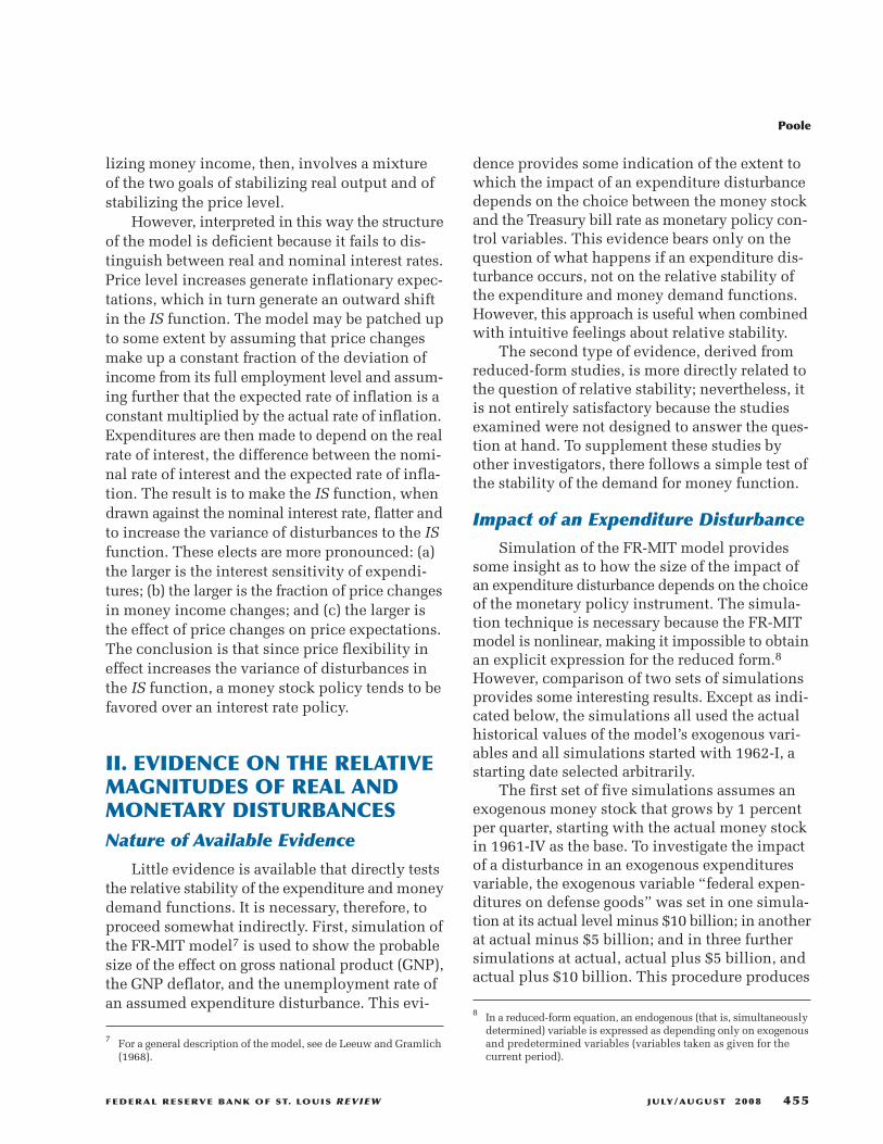
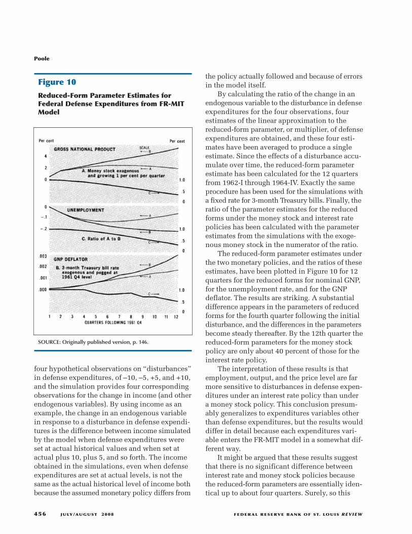
The reduced-form parameter estimates underthe two monetary policies, and the ratios of theseestimates, have been plotted in Figure 10 for 12quarters for the reduced forms for nominal GNP,for the unemployment rate, and for the GNPdeflator. The results are striking. A substantialdifference appears in the parameters of reducedforms for the fourth quarter following the initialdisturbance, and the differences in the parametersbecome steady thereafter. By the 12th quarter thereduced-form parameters for the money stockpolicy are only about 40 percent of those for theinterest rate policy.
The interpretation of these results is thatemployment, output, and the price level are farmore sensitive to disturbances in defense expen-ditures under an interest rate policy than undera money stock policy. This conclusion presum-ably generalizes to expenditures variables otherthan defense expenditures, but the results woulddiffer in detail because each expenditures vari-able enters the FR-MIT model in a somewhat dif-ferent way.
It might be argued that these results suggestthat there is no significant difference betweeninterest rate and money stock policies becausethe reduced-form parameters are essentially iden-tical up to about four quarters. Surely, so this
Poole
456 JULY/AUGUST 2008 FEDERAL RESERVE BANK OF ST. LOUIS REVIEW
Figure 10
Reduced-Form Parameter Estimates forFederal Defense Expenditures from FR-MITModel
SOURCE: Originally published version, p. 146.
argument goes, mistakes could be discovered andonset within four quarters. There are two diffi-culties with this argument. The first is that theFR-MIT model may overstate the length of thelags and therefore understate the differences inreduced-form parameters for the two policies forthe quarters immediately following a disturbance.But the second and more important reason is thatit may not be easy to reverse the effects of thedisturbance after the disturbance has been dis-covered. With an interest rate policy, a very largechange in the rate might be required to offset theeffects appearing after the fourth quarter, and sucha change might not be feasible, or at least notdesirable in terms of its effects on security marketsand on income in the more distant future.
The numerical results reported above depend,of course, on the FR-MIT model, and this modelis deficient in a number of respects. But anymodel in which, other things being equal, invest-ment and other interest-sensitive expendituresdecline when interest rates rise will show resultsin the same direction.
These results may be extended to analyze thesignificance of errors in forecasting exogenousvariables. Consider an explicit expression for thereduced form for income. Let the exogenous vari-ables such as government expenditures, perhapscertain categories of investment, strikes, weather,population growth, and so forth, be X1, X2, …, Xn,and let the coefficients of these variables be α1, α2,…, αn when the interest rate is the policy instru-ment, and λ1, λ2, …, λn when the money stock isthe instrument. Then the reduced form for incomewhen the interest rate is the instrument is
(1)
where αr is the coefficient of the interest rate andu is the random disturbance. On the other hand,when the money stock is the instrument, thereduced form is
(2)
As discussed in Section II, the disturbance νtmay have either a larger or a smaller variance thanthe disturbance ut. One factor tending to makeνt smaller than ut is that a money stock policy
Y X X X Mn n M= + + +…+ + +λ λ λ λ λ ν0 1 1 2 2
Y X X X r un n r= + + +…+ + +α α α α α0 1 1 2 2
reduces the impact of expenditures disturbances,but another factor, the introduction into thereduced form of money demand disturbances,tends to make νt larger. The net result of thesetwo factors cannot be determined a priori.
But in formulating policy it is not possible toreason directly from equations 1 and 2 becausemany of the Xi cannot be predicted in advancewith perfect accuracy. For scientific purposes expost it may be possible to say that a change inincome was caused by a change in some Xi; forpolicy purposes ex ante this scientific knowledgeis useless unless the change inXi can be predicted.It is necessary to think of each Xi as being com-posed of a predictable part, Xi, and an unpredict-able part, Ei.
For policy purposes the error term in thereduced form includes both the disturbances tothe equation and the errors in forecasting exoge-nous variables. The two types of errors ought tobe treated exactly alike in formulating policy.Equations 1 and 2 can then be rewritten as follows:
(3)
(4)
For policy purposes the error term in the reduced-form equation 3 is the sum of the terms from α1E1tthrough ut and in the reduced-form equation 4the sum of the term λ1E1t through νt.
A systematic study of the importance of theEi terms cannot be made because no formal recordof errors in forecasting exogenous variables existsinsofar as the author knows. However, someinsight into the problem may be obtained by list-ing the variables that must be forecast. Whichvariables have to be forecast depends, of course,on the model being used. The larger econometricmodels generally have relatively few exogenousvariables that raise forecasting problems becauseso many variables are explained endogeneouslyby the model itself. The FR-MIT model has 63
X X Ei i i= +ˆ
Y X X X
r E Ei n n
r
= + + +…++ + + +…+α α α αα α α α
0 1 2 2
1 1 2 2
ˆ ˆ ˆ
� nn nE u+
Y X X X
M E Ei n N
M
= + + +…++ + + +…+λ λ λ λλ λ λ λ
0 1 2 2
1 1 2 2
ˆ ˆ ˆ
� nn nE +ν
Poole
FEDERAL RESERVE BANK OF ST. LOUIS REVIEW JULY/AUGUST 2008 457
exogenous variables; some of these are relativelyeasy to forecast, but others are subject to consid-erable forecasting error. The latter include suchvariables as exports, number of mandays idle dueto strikes, armed forces, and federal expenditures.Furthermore, this model involves lagged endoge-nous variables in many equations; hence an inac-curate forecast of GNP next quarter will increasethe error in forecasting GNP two quarters into thefuture, which in turn will lead to errors in fore-casting GNP three quarters into the future, and soforth. Errors in forecasting exogenous variables,therefore, produce cumulative errors in forecast-ing GNP in future quarters.
In simpler models the forecasting problem ismore severe. Consider, for example, the oppositeextreme from the large econometric model, thesingle-equationmodel. Convenient representativesof such models are those spawned in the contro-versy over the Friedman-Meiselman paper (1963)on the stability of the money/income relationship.The various definitions of exogenous, or “autono-mous,” spending utilized by the various authorsin this controversy are as follows :
a) Friedman-Meiselman definition: Autono-mous expenditures consist of the “netprivate domestic investment plus the gov-ernment deficit on income and productaccount plus the net foreign balance”(Friedman and Meiselman, 1963, p. 184).
b)Ando-Modigliani definition: Autonomousexpenditures consist of two variables whichenter the reduced form with different coef-ficients. One variable is “property tax por-tion of indirect business taxes” plus “netinterest paid by government” plus “govern-ment transfer payment” minus “unemploy-ment insurance benefits” plus “subsidiesless current surplus of government enter-prises” minus “statistical discrepancy”minus “excess of wage accruals over dis-bursement.” The second variable is “netinvestment in plant and equipment, andin residential houses” plus “exports” (AndoandModigliani, 1965a, pp. 695-96, 702).
c) DePrano-Mayer definition: The basic defini-tion is “investment in producers’ durable
equipment, nonresidential construction,residential construction, federal govern-ment expenditures on income and productaccount, and exports. One variant of thishypothesis subtracts capital consumptionestimates, and the other does not” (DePranoand Mayer, 1965a, p. 739). DePrano andMayer also tested 18 other definitions ofautonomous expenditures (DePrano andMayer, 1965a, pp. 739-40).
d)Hester definition: Autonomous expendi-tures consist of the “sum of governmentexpenditure, net private domestic invest-ment, and the trade balance” (Hester, 1964a,p. 366). Hester also experimented withthree other definitions involving alterna-tive treatments of imports, capital consump-tion allowances, and inventory investment(Hester, 1964a, pp. 366-67).
To a considerable extent the diversity in thesedefinitions is misleading because except for theFriedman-Meiselman definition all the definitionsare in fact rather similar. But whichever definitionis used, it is impossible to escape the feeling thatinaccurate forecasting of exogenous variables islikely to be a major source of uncertainty. Andwhile this discussion has taken place within thecontext of formal models, exactly the same prob-lem plagues judgmental forecasting. Every fore-casting method can be viewed as starting fromforecasts of “input,” or exogenous, variables andthen proceeding to judge the implications of theseinputs for GNP and other dependent, or endoge-nous, variables.
Regardless of what type of model is used, itappears that for the foreseeable future it will benecessary to forecast exogenous variables thatsimply cannot be forecast accurately by usingpresent methods. As a result, it seems very likelythat the error term including forecast errors hasa far smaller variance in equation 4 than in equa-tion 3. Indeed, it might be argued that as a sourceof uncertainty the Ei terms are far more importantthan the u or ν terms, and therefore that thesmaller size of the λi parameters as compared tothe α i parameters is of great importance. If theparameter estimates from the FR-MIT model areaccepted, the standard deviation of the total ran-
Poole
458 JULY/AUGUST 2008 FEDERAL RESERVE BANK OF ST. LOUIS REVIEW
dom term relevant for policy (that is, includingerrors in forecasting exogenous variables) wouldbe over twice as large under an interest rate policyas under a money stock policy. If this argumentis correct, shifting from the current policy ofemphasizing interest rates to one of controllingthe money stock might cut average errors in half,where errors are measured in terms of the devia-tions of employment, output, and price level fromtarget levels for these variables.
Evidence from Reduced-Form Equations
Additional insight into the relative sizes ofdisturbances under interest rate and money stockpolicies may be obtained by examining the con-troversy generated by the Friedman-Meiselmanpaper on the stability of the money/income rela-tionship (Friedman andMeiselman, 1963). In thispaper equations almost the same as equations 1and 2 above were estimated. The equation corre-sponding to equation 1 differs in that the exoge-nous variables were assumed to consist only of asingle autonomous spending variable, as definedabove. The equation corresponding to equation 2has the same disability for our purposes, but italso did not include an interest rate as a variable.
Before examining the implications of theFriedman-Meiselman findings for this study, itshould be noted that their approach was sharplycriticized in papers by Donald D. Hester (1964a),Albert Ando and Franco Modigliani (1965a), andMichael DePrano and Thomas Mayer (1965a).These critics particularly attacked the Friedman-Meiselman definition of autonomous expendi-tures, and proposed and tested the alternativedefinitions listed above. However, they alsoattacked the single-equation approach and recom-mended the use of large models instead.
The tests of alternative equations must beregarded as inconclusive in terms of which vari-able—the money stock or autonomous spending—is more closely related to the level of income.9
Both approaches achieve values for R2 of 0.98 or0.99 so that the unexplained variance is very smallin both cases. It seems very unlikely that the addi-tion of an interest rate variable to the equationsby using autonomous expenditures as the explana-tory variable, which addition would make theequations correspond to equation 1 above, wouldmake any substantial difference.
From this evidence it appears that ex postexplanations of the level of income are about asaccurate by using autonomous expenditures aloneas are those by using money stock alone. But giventhe inaccuracies in forecasting autonomous expen-ditures, it must be concluded that ex ante expla-nations by using themoney stock are substantiallymore accurate than those with forecasts of autono-mous expenditures. From this evidence, the totalrandom term in equation 4 appears to have asubstantially smaller variance than the total ran-dom term in equation 3.
For the reasons mentioned by the Friedman-Meiselman critics, evidence from single-equationstudies cannot be considered definitive. But nei-ther can the evidence be ignored, especially inlight of the difficulties encountered in the con-struction and the use of large econometric modelssuch as the FR-MIT model.
Evidence on Stability of Demand forMoney Function
One of the shortcomings of the single-equationstudies discussed above is that their authors paidtoo little attention to the stability of regressioncoefficients over time. Consider the followingstatement by Friedman and Meiselman:
The income velocity of circulation of moneyis consistently and decidedly stabler than theinvestment multiplier except only during theearly years of the Great Depression after 1929.There is throughout, including those years, aclose and consistent relation between the stockof money and consumption or income, andbetween year-to-year changes in the stock ofmoney and in consumption or income(Friedman and Meiselman, 1963, p. 186).
This conclusion is based on correlation coef-ficients betweenmoney and income (or consump-
Poole
FEDERAL RESERVE BANK OF ST. LOUIS REVIEW JULY/AUGUST 2008 459
9 For reasons that need not be explained here, most of this contro-versy was conducted in terms of equations with consumptionrather than GNP as the dependent variable. In the Friedman-Meiselman study, however, results are reported for equations withGNP (Friedman and Meiselman, 1963, p. 227). Such results arealso reported in Andersen and Jordan (1968, p. 17).
tion), but what is relevant for policy is theregression coefficient, which determines howmuch income will change for a given change inthe money stock. In the Friedman-Meiselmanstudy, a table (Friedman and Meiselman, 1963,p. 227) reports the regression coefficient forincome on money as being 1.469 for annual data1897-1958. However, the same table reports regres-sion coefficients for 12 subperiods, some of whichare overlapping, ranging from 1.092 to 2.399.
With a few exceptions, most economistsagree that velocity changes can be explained inpart by interest rate changes.10 Thus, variabilityin the regression coefficients when income isregressed on money is not evidence of the insta-bility of the demand for money function. To obtain
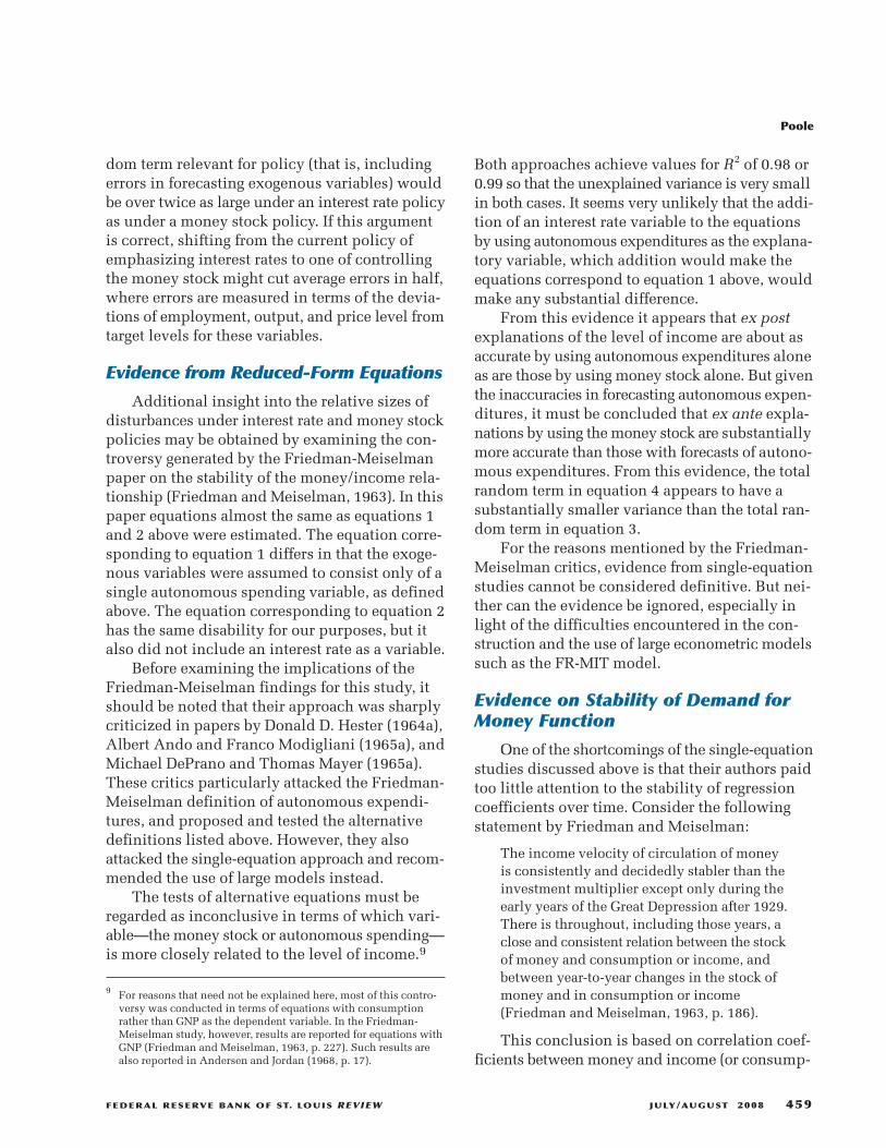
some evidence on the stability of this function,the following simple procedure was used. Quar-terly data were collected on themoney stock, GNP,and Aaa corporate bond yields for 1947 through1968. A demand for money function was fittedby regressing the log of the interest rate on thelog of velocity, and vice versa. The regressionswere run for the four periods, 1947 through 1960,1947 through 1962, 1947 through 1964, and 1947through 1966. The results inside each estimationperiod were then compared with the results out-side the estimation period.
The results of this process for the 1947-60estimation period are shown in Figure 11. Theobservations for 1947 through 1960 are repre-sented by dots, and the observations for 1961through 1968 by X’s. The two least-squares regres-sions—log interest rate on log velocity and viceversa—fitted for the 1947-60 period have beendrawn. From Figure 11 it appears that the rela-tionship since 1960 has been quite similar to theone prior to 1960.
Table 1 presents the results of applying astandard statistical test to the regression andpostregression periods to determine whether thedemand for money function was stable. To under-stand this table, refer first to section A of the table,and to the 1947-60 estimation period. Section Areports results from regressing the log of velocityon the log of the Aaa corporate bond rate, and thefirst row refers to the regression for 1947 through1960. The square of the regression’s standard errorof estimate is 0.00517 with 54 degrees of freedom.There were 32 quarters in the postregressionperiod 1961 through 1968, and for this period themean-square error of velocity from the velocitypredicted by the regression is 0.00836. The ratioof the mean-square errors from regression outsideto those inside the estimation period is given inthe column labeled “F.” Since the ratio of twomean squares has the F distribution under thehypothesis that both mean squares were producedby the same process, an F test may be used to testwhether the demand for money function has beenstable. If the function has been stable, then errorsfrom regression outside the period of estimation
10 For a convenient review of evidence on this subject, see Laidler(1969).
Poole
460 JULY/AUGUST 2008 FEDERAL RESERVE BANK OF ST. LOUIS REVIEW
Figure 11
Velocity and Interest Rate Regressions(regressions fitted to quarterly data, 1947-60)
SOURCE: Originally published version, p. 150.

should be, on the average, the same size as theerrors inside the period of estimation. For the1947-60 regression being discussed, F = 1.62 andis significant at the 10 percent level but not atthe 5 percent level.
Looking at Table 1 as a whole it can be seenthat, for three of the regressions, the errors outsidethe period of estimation are not statistically sig-nificantly larger than those inside the period ofestimation. Indeed, for the bond rate regressionfor the 1947-60 period, the errors outside theperiod of estimation were actually smaller, onthe average, than those inside the period of esti-mation. Overall, however, these results taken atface value cast some doubt on the stability of thedemand for money function.
However, there is reason to believe that thereare problems in applying the F test in this situa-tion. The reason is that the residuals from regres-sion exhibit a very high positive serial correlationas indicated by Durbin-Watson test statistics ofaround 0.15 for all of the regressions. What thismeans is that the effective number of degrees offreedom is actually less than indicated in the table,and with fewer degrees of freedom the F ratioscomputed have less statistical significance than
the significance levels reported in the table. Theonly way around this problem is to run a morecomplex regression that removes the serial cor-relation of the residuals, but there is no generalagreement among economists as to exactly whatvariables belong in such a regression. The virtueof the simple regressions of velocity on an inter-est rate and vice versa is that this form has beenused successfully by many investigators startingin 1954 (Latané, 1954).
The appropriate conclusion to be drawn fromthis evidence would seem to be that the relation-ship between velocity and the Aaa corporate bondrate is too close and too stable to be ignored, butnot close enough and stable enough to eliminateall doubts. However, the question is not whetheran ironclad case for a money stock policy existsbut rather whether the evidence taken as a wholeargues for the adoption of such a policy. Whilethere is certainly room for differing interpreta-tions of Figure 11 and Table 1, and of the otherevidence examined above, on the whole all ofthese results seem to point in the same direction.It appears that the money stock rather than inter-est rates should be used as the monetary policycontrol variable.
Poole
FEDERAL RESERVE BANK OF ST. LOUIS REVIEW JULY/AUGUST 2008 461
Table 1Tests of the Stability of the Demand for Money Function by Using Quarterly Data
Regression Progression
Estimation period (SEE)2 d.f. MSE d.f. F Significance level
A. Log velocity regressed on log Aaa corporate bond yield
1947-60 .00517 54 .00836 32 1.62 .10
1947-62 .00484 62 .00746 24 1.54 .10
1947-64 .00509 70 .00587 16 1.15 >.25
1947-66 .00502 78 .00986 8 1.96 .10
B. Log Aaa corporate bond yield regressed on log velocity
1947-60 .00684 54 .00589 32 1.16* >.25
1947-62 .00614 62 .00723 24 1.18 >.25
1947-64 .00570 70 .01162 16 2.04 .025
1947-66 .00537 78 .02192 8 4.08 .005
NOTE: *MSE < (SEE)2.
III. A MONETARY RULE FORGUIDING POLICYRationale for a Rule-of-Thumb
The purpose of this section is to develop arule-of-thumb to guide policy. Such a rule—notmeant to be followed slavishly—would incorpo-rate advice in as systematic a way as possible. Therule proposed here is based upon the theory andevidence in Sections II and III and upon a closeexamination of post-accord experience.
Individual policymakers inevitably useinformal rules-of-thumb in making decisions.Like everyone else, policymakers develop cer-tain standard ways of reacting to standard situa-tions. These standard reactions are not, of course,unchanging over time, but are adjusted and devel-oped according to experience and new theoreti-cal ideas. If there were no standard reactions tostandard situations, behavior would have to beregarded as completely random and unpredict-able. The word “capricious” is often, and notunfairly, used to describe such unpredictablebehavior.
There are several difficulties with relying onunspecified rules-of-thumb. For one thing, therules may simply be wrong. But an even moreimportant factor, because formally specified rulesmay also be wrong, is that the use of unspecifiedrules allows little opportunity for cumulativeimprovements over time. A policymaker may havean extremely good operating rule in his head andexcellent intuition as to the application of therule but unless this rule can be written downthere is little chance that it can be passed on tosubsequent generations of policymakers.
An explicit operating rule provides a way ofincorporating the lessons of the past into currentpolicy. For example, it is generally felt that mone-tary policy was too expansive following the impo-sition of the tax surcharge in 1968. Unless thelesson of this experience is incorporated into anoperating rule, it may not be remembered in 1975or 1980. How many people now remember theoverly tight policy in late 1959 and early 1960that was a result of miscalculating the effects ofthe long steel strike in 1959? Since the FOMCmembership changes over time, many of the cur-
rent members will not have learned firsthand thelesson from a policy mistake or a policy success10 years ago. If the FOMCmember is not an econ-omist, he may not even be aware of the 10-year-old lesson.
It is for these reasons that an attempt is madein this section to develop a practical policy rulethat incorporates the lessons from past experience.The rule is not offered as one to be followed tothe last decimal place or as one that is good forall time. Rather, it is offered as a guide—or as abenchmark—against which current policy maybe judged.
A rule may take the form of a formal modelthat specifies what actions should be taken toachieve the goals decided upon by the policy-makers. Such a model would provide forecastsof goal variables, such as GNP, conditional onthe policy actions taken. The structure of themodel and the estimates of its parameters would,of course, be derived from past data and in thatsense the model would incorporate the lessonsof the past.
But in spite of advances in modelbuildingand forecasting, it is clear that forecasts are stillquite inaccurate on the average. In a study of theaccuracy of forecasts by several hundred fore-casters between 1953 and 1963, Zarnowitz con-cluded that the mean absolute forecast error wasabout 40 percent of the average year-to-yearchange in GNP (Zarnowitz, 1967, p. 4). He alsoreported, “there is no evidence that forecasters’performance improved steadily over the periodcovered by the data” (Zarnowitz, 1967, p. 5).
Not only are forecasts several quarters aheadinaccurate but also there is considerable uncer-tainty at, and after, the occurrence of business-cycle turning points as to whether a turning pointhas actually occurred. In a study of FOMC recog-nition of turning points for the period 1947-60,Hinshaw concluded that (Fels and Hinshaw, 1968,p. 122):
The beginning data of the Committee’s recog-nition pattern varied from one to nine monthsbefore the cyclical turn…On the other hand,the ending of the recognition pattern variedfrom one to seven months after the turn…With
Poole
462 JULY/AUGUST 2008 FEDERAL RESERVE BANK OF ST. LOUIS REVIEW
the exception of the 1948 peak, the Committeewas certain of a turning point within sixmonths after the NBER date of the turn. At thedate of the turn, the estimated probability wasgenerally below 50; it reached the vicinity of50 about two months after the turn.
This recognition record, which is as good as thatin 10 widely circulated publications whoseforecasts were also studied in (Friedman andMeiselman, 1963) casts further doubt on the valueof placing great reliance on the forecasts.11
Given the accuracy of forecasts at the currentstate of knowledge,12 it seems likely that for sometime to come forecasts will be used primarily tosupplement a policy-decisionmaking process thatconsists largely of reactions to current develop-ments. Only gradually will policymakers placegreater reliance on formal forecasting models.13
While a considerable amount of work is beingdone on such models, essentially no attention isbeing paid to careful specification of how policyshould react to current developments. Whilesophisticated models will no doubt in time bedeveloped into highly useful policy tools, itappears that in the meantime relatively simpleapproaches may yield substantial improvementsin policy. Given that knowledge accumulatesrather slowly, it can be expected that carefullyspecified but simple methods will be successfulbefore large-scale models will lie. Careful speci-fication of policy responses to current develop-ments is but a small step beyond intuitive policyresponses to current developments. This stepsurely represents a logical evolution of the policy-formation process.
Post-Accord Monetary Policy
That an operating guideline is needed can beseen from the experience since the Treasury–Federal Reserve accord. In order that this experi-ence may be understood better, subperiods weredefined in terms of “stable,” “easing,” or “firming”policy as determined from the minutes of theFederal Open Market Committee. The minutesused are those published in the Annual Reportsof the Board of Governors of the Federal ReserveSystem for 1950 to 1968. The definitions of “sta-ble,” “easing,” and “firming” periods are neces-sarily subjective as are the determinations ofdates when policy changed.14 The dating of pol-icy changes was based primarily on the FOMCminutes, although the dates of changes in thediscount rate and in reserve requirements wereused to supplement the minutes. “Stable” periodsare those in which the policy directive wasunchanged except for relatively minor wordingchanges. In some cases the directive was essen-tially unchanged although the minutes reflectedthe belief that policy might have to be changed inthe near future. While the Manager of the SystemOpen Market Account might change policysomewhat as a result of such discussions, theunchanged directive was taken at face value indefining policy turning points.
More difficult problems of interpretationwere raised by such directives as “unchangedpolicy, but err on the side of ease,” or “resolvedoubts on the side of ease.” Such statements wereused to help in defining several periods duringwhich policy was progressively eased (or tight-ened). For example, in one meeting the directivemight call for easier policy, the next meetingmightcall for unchanged policy but with doubts to beresolved on the side of ease, and a third meetingmight call for further ease. These three meetingswould then be taken together as defining an
Poole
FEDERAL RESERVE BANK OF ST. LOUIS REVIEW JULY/AUGUST 2008 463
11 For further analysis of forecasting accuracy, see Mincer (1969).
12 The accuracy of forecasts may now be better than in the periodsexamined in the studies cited above. But without a number of yearsof data there would be no way of knowing whether forecasts haveimproved, and so forecasts must in any case be assumed to besubject to a wide margin of error at the present time.
13 It may be objected that great reliance is already placed on forecasts,at least on judgmental forecasts. However, these forecasts typicallyinvolve a large element of extrapolation of current developments.It seems fair to say that in most cases in which conditions forecasta number of quarters ahead differ markedly from current conditions,policy has followed the dictates of current conditions rather thanof the forecasts.
14 The author was greatly assisted in these judgments by Joan Waltonof the Special Studies Section of the Board’s Division of Researchand Statistics. MissWalton, who is not an economist, carefully readthe minutes of the entire period and in a large table recorded theprincipal items that seemed important at each FOMC meeting.Having a noneconomist read the minutes tempered the inevitabletendency for an economist to read either too much or too littleinto the minutes. However, the final interpretation of the minutesrested with the author.
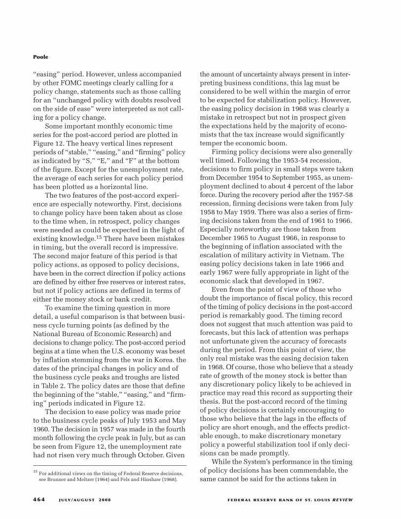
“easing” period. However, unless accompaniedby other FOMC meetings clearly calling for apolicy change, statements such as those callingfor an “unchanged policy with doubts resolvedon the side of ease” were interpreted as not call-ing for a policy change.
Some important monthly economic timeseries for the post-accord period are plotted inFigure 12. The heavy vertical lines representperiods of “stable,” “easing,” and “firming” policyas indicated by “S,” “E,” and “F” at the bottomof the figure. Except for the unemployment rate,the average of each series for each policy periodhas been plotted as a horizontal line.
The two features of the post-accord experi-ence are especially noteworthy. First, decisionsto change policy have been taken about as closeto the time when, in retrospect, policy changeswere needed as could be expected in the light ofexisting knowledge.15 There have been mistakesin timing, but the overall record is impressive.The second major feature of this period is thatpolicy actions, as opposed to policy decisions,have been in the correct direction if policy actionsare defined by either free reserves or interest rates,but not if policy actions are defined in terms ofeither the money stock or bank credit.
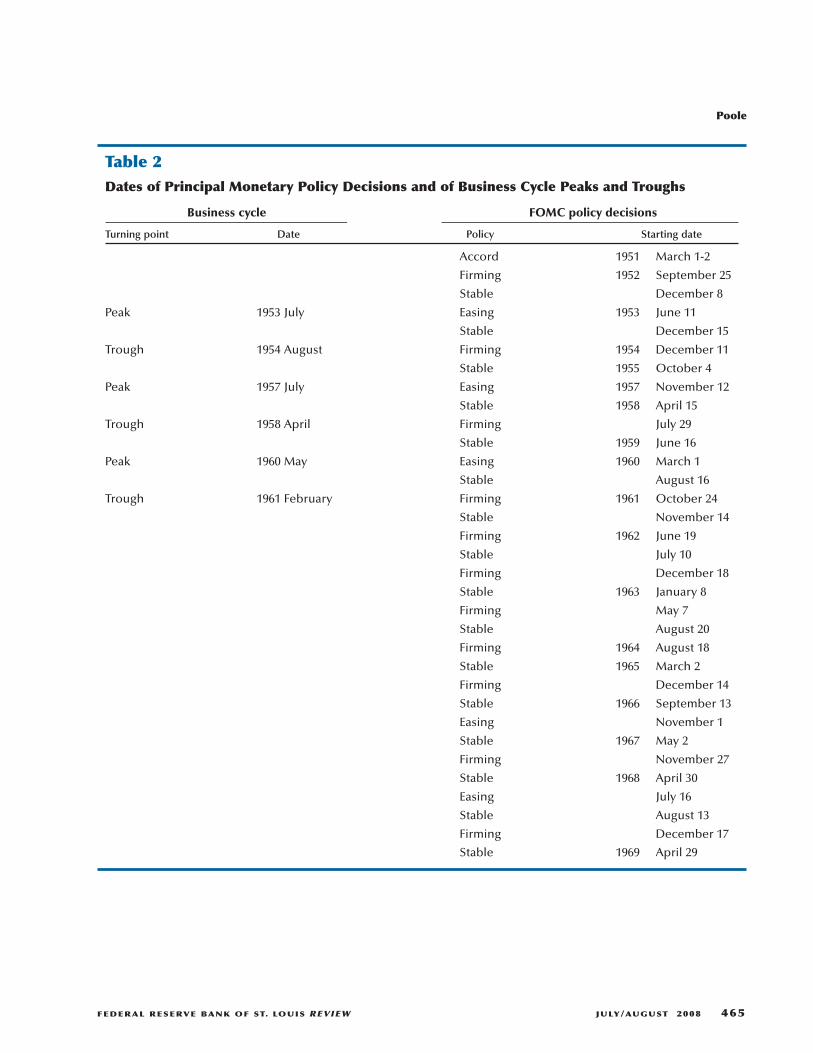
To examine the timing question in moredetail, a useful comparison is that between busi-ness cycle turning points (as defined by theNational Bureau of Economic Research) anddecisions to change policy. The post-accord periodbegins at a time when the U.S. economywas besetby inflation stemming from the war in Korea. thedates of the principal changes in policy and ofthe business cycle peaks and troughs are listedin Table 2. The policy dates are those that definethe beginning of the “stable,” “easing,” and “firm-ing” periods indicated in Figure 12.
The decision to ease policy was made priorto the business cycle peaks of July 1953 and May1960. The decision in 1957wasmade in the fourthmonth following the cycle peak in July, but as canbe seen from Figure 12, the unemployment ratehad not risen very much through October. Given
the amount of uncertainty always present in inter-preting business conditions, this lag must beconsidered to be well within the margin of errorto be expected for stabilization policy. However,the easing policy decision in 1968 was clearly amistake in retrospect but not in prospect giventhe expectations held by the majority of econo-mists that the tax increase would significantlytemper the economic boom.
Firming policy decisions were also generallywell timed. Following the 1953-54 recession,decisions to firm policy in small steps were takenfrom December 1954 to September 1955, as unem-ployment declined to about 4 percent of the laborforce. During the recovery period after the 1957-58recession, firming decisions were taken from July1958 to May 1959. There was also a series of firm-ing decisions taken from the end of 1961 to 1966.Especially noteworthy are those taken fromDecember 1965 to August 1966, in response tothe beginning of inflation associated with theescalation of military activity in Vietnam. Theeasing policy decisions taken in late 1966 andearly 1967 were fully appropriate in light of theeconomic slack that developed in 1967.
Even from the point of view of those whodoubt the importance of fiscal policy, this recordof the timing of policy decisions in the post-accordperiod is remarkably good. The timing recorddoes not suggest that much attention was paid toforecasts, but this lack of attention was perhapsnot unfortunate given the accuracy of forecastsduring the period. From this point of view, theonly real mistake was the easing decision takenin 1968. Of course, those who believe that a steadyrate of growth of the money stock is better thanany discretionary policy likely to be achieved inpractice may read this record as supporting theirthesis. But the post-accord record of the timingof policy decisions is certainly encouraging tothose who believe that the lags in the effects ofpolicy are short enough, and the effects predict-able enough, to make discretionary monetarypolicy a powerful stabilization tool if only deci-sions can be made promptly.
While the System’s performance in the timingof policy decisions has been commendable, thesame cannot be said for the actions taken in
15 For additional views on the timing of Federal Reserve decisions,see Brunner and Meltzer (1964) and Fels and Hinshaw (1968).
Poole
464 JULY/AUGUST 2008 FEDERAL RESERVE BANK OF ST. LOUIS REVIEW
Poole
FEDERAL RESERVE BANK OF ST. LOUIS REVIEW JULY/AUGUST 2008 465
Table 2Dates of Principal Monetary Policy Decisions and of Business Cycle Peaks and Troughs
Business cycle FOMC policy decisions
Turning point Date Policy Starting date
Accord 1951 March 1-2
Firming 1952 September 25
Stable December 8
Peak 1953 July Easing 1953 June 11
Stable December 15
Trough 1954 August Firming 1954 December 11
Stable 1955 October 4
Peak 1957 July Easing 1957 November 12
Stable 1958 April 15
Trough 1958 April Firming July 29
Stable 1959 June 16
Peak 1960 May Easing 1960 March 1
Stable August 16
Trough 1961 February Firming 1961 October 24
Stable November 14
Firming 1962 June 19
Stable July 10
Firming December 18
Stable 1963 January 8
Firming May 7
Stable August 20
Firming 1964 August 18
Stable 1965 March 2
Firming December 14
Stable 1966 September 13
Easing November 1
Stable 1967 May 2
Firming November 27
Stable 1968 April 30
Easing July 16
Stable August 13
Firming December 17
Stable 1969 April 29

Poole
466 JULY/AUGUST 2008 FEDERAL RESERVE BANK OF ST. LOUIS REVIEW
Figure 12
Post-Accord Monetary Policy
SOURCE: Originally published version, p. 154.

Poole
FEDERAL RESERVE BANK OF ST. LOUIS REVIEW JULY/AUGUST 2008 467
Figure 12, cont’d
Post-Accord Monetary Policy
SOURCE: Originally published version, p. 155.

response to the decisions. In the earlier discussionthe purposely vague terms “easing,” “firming,”and “stable” were used to describe policy deci-sions. These terms were meant to convey thenotions that policymakers wanted, respectively,to accelerate, decelerate, or maintain the pace ofeconomic advance. The question that must nowbe examined is whether policy actions did in facttend to accelerate, decelerate, or maintain thelevel of economic activity.
Policy actions were in accord with policydecisions if these actions are measured by eitherthe 3-month Treasury bill rate or free reserves. Thebill rate rose in “firming” periods, fell in “easing”periods, and tended to remain unchanged in“stable” periods. However, there was some ten-dency for the bill rate to rise in “stable” periodsfollowing “firming” periods, and to fall in “stable”periods following “easing” periods, a pattern notinconsistent with the interpretation of policybeing offered in this study. Similar commentsapply to free reserves.
But the picture is quite different if policyactions are measured by the rate of growth of themoney stock. Careful study of Figure 12 will makethis point clear. The growth rate declined inresponse to the “firming” policy decision in late1952, and again in the “stable” period in early1953. This behavior was, of course, consistentwith the “firming” decision. But the rate of growthdeclined further following the “easing” decisionin June 1953 and remained low until the middleof 1954. The unemployment rate rose rapidlyfrom its low of 2.6 percent at the cycle peak inJuly 1953 to 6.0 percent in August 1954, the cycletrough; the money stock was at the same level inApril 1954, 9 months following the cycle peakand 10 months following the decision to adoptan “easing” policy, as it had been at the peak.
The same pattern that had appeared duringthe 1953-54 recession appeared again at the timeof the 1957-58 recession. The rate of growth ofthe money stock declined in 1957 prior to thecycle peak. (The Treasury bill rate also rose sub-stantially.) But after the decision to adopt an“easing” policy in November 1957, the growthrate of the money stock declined further. FromOctober 1957 to January 1958, the money stock
fell at a 2.9 percent annual rate; from the cyclepeak in July to October it had fallen at a 1.5 per-cent annual rate.
The rate of growth of the money stockincreased substantially in February 1958, and itremained at the higher level during the “stable”policy period April to July. There followed aperiod of “firming” policy decisions from the endof July 1958 to May 1959; however, the averagegrowth rate of the money stock during this periodwas virtually identical to the average in the pre-ceding “stable” period. But in the “stable” periodfrom June 1959 to February 1960, the rate ofgrowth of money, at –2.2 percent, was much lowerthan in the preceding “firming” period. This rateof growth of money can hardly be consideredappropriate in the light of the fact that except forone month the unemployment rate was continu-ously above 5 percent. However, the picture wasconfused by a long steel strike.
The decision to ease policy was taken onMarch 1, 1960, but the rate of growth of themoneystock remained negative until July. The rate ofgrowth of money fell following the “firming”policy decisions of October 1961 and June 1962.In spite of another firming decision in December1962 the rate of growth then increased, and itcontinued to rise during the “firming” period in1963, maintaining the same rate in the following“stable” period. In August 1964, another “firming”decision was taken, and the growth rate trendeddown during the “firming” period from August1964 to February 1965.
During the “stable” period from March toNovember 1965, the Vietnam war heated up. Inthe second half of 1965 the growth rate of moneywas 6.1 percent compared with 3.0 percent duringthe first half. The “firming” policy decision camein December, but the rate of growth of moneyaveraged over 6 percent for the months Decemberthrough April 1966. At this point monetary growthceased. In January 1967 the money stock wasactually less than in May 1966—there havingbeen no increase in the growth rate in the monthsimmediately following the “easing” decision ofNovember 1, 1966.
The growth rate of money then acceleratedduring the “stable” period from May through
Poole
468 JULY/AUGUST 2008 FEDERAL RESERVE BANK OF ST. LOUIS REVIEW

October 1967; for the period as a whole growthaveraged 8.7 percent. In the following “firming”period November 1967 through April 1968, therate of growth of the money stock was lower but itwas still relatively high at 5.1 percent. The growthrate then rose to 9.6 percent in the “stable” periodMay through July 1968 and thereafter fell to a littleless than 6 percent in the July-November 1968period following the “easing” decision of July 16,1968.
There ensued a “firming” period fromDecember 1968 through April 1969. Althoughoriginal figures indicated that monetary growthwas relatively little during this period, a revisionin the money stock series showed that the rateaveraged 5.5 percent for the period as a whole.The rate following April was lower, especially inthe June-December 1969 period, which saw nonet growth in the money stock.
A broadly similar view of the timing of policyactions is obtained from a careful examination ofthe rate of growth of total bank credit. However,as shown in Figure 12, this series is quite erraticand much more difficult to interpret than theseries on the rate of growth of the money stock.
The proper way to interpret these resultswould seem to be as follows. When interest ratesfell in a recession, policy was easier than it wouldhave been if interest rates had not been permittedto fall. But if the money stock was also falling, orgrowing at a below-average rate, policy wastighter than it would have been had money beengrowing at its long-run average rate. Similar state-ments apply to rising interest rates and above-average monetary growth in a boom.
A Monetary Rule
Given the arguments of Sections I and II onthe advantages of controlling the money stock asopposed to interest rates, a logical first step indeveloping a policy guideline is to examine casesclearly calling for ease or restraint. Consider firsta recession. To insure that monetary policy isexpansionary, the rule might be that interest ratesshould fall and the money stock should rise atan above-average rate. This policy avoids twopossible errors.
The first is illustrated in Figure 13. If the ISfunction shifts down from IS1 to IS2 while the LMfunction shifts from LM1 to LM2, the interest ratewill fall from r1 to r2. The shift from LM1 to LM2
could be caused by a shift in the demand formoney with the stock of money unchanged. Butthis shift could also be caused by a decline in thestock of money, perhaps because of an attemptby policymakers to keep the interest rate fromfalling too rapidly. However, in terms of incomeit is clearly better to permit the interest rate to fallto r3 by maintaining the stock of money fixed, andbetter yet to shift the LM function to the right ofLM1 by increasing the stock of money.
The point is the simple one that monetarypolicy should not rely simply on a declininginterest rate in recession but should also insurethat the money stock is growing at an adequaterate. The LM function may still shift to LM2 inspite of monetary growth because of an increaseddemand for money; without the monetary growth,however, this shift in the demand for moneywould push the LM function to the left of LM2 andincome would be even lower.
The second type of error avoided by the pro-posed policy rule is illustrated in Figure 14. Again,it is assumed that the situation is one of recession.With a fixed money stock, an increase in thedemand for money will shift the LM functionfrom LM1 to LM2, tending to reduce income. How-ever, if the interest rate is prevented from risingabove r1, the increased demand for money is metby an increased supply of money.
Maintaining monetary growth and a declininginterest rate in recession insures that the contri-bution of monetary policy is expansive. Increasesin the demand for money, unless accompaniedby a falling IS function, are fully offset by prevent-ing increases in the interest rate. The greater thefall in the IS function the smaller the offset to anincreased demand for money. However, in nocase should a fall in the IS function be permittedto cause a fall in the money stock.
The policy proposed does not, of course,guarantee an expansion of income. No such guar-antee is possible because downward shifts in theIS function may exceed any specified shift in theLM function. But more important than theoretical
Poole
FEDERAL RESERVE BANK OF ST. LOUIS REVIEW JULY/AUGUST 2008 469

possibilities are empirical probabilities. For allpractical purposes the problem is not how toinsure expansion in a recession but how to tradeoff the risks of too much expansion against toolittle. The discussion of Figures 13 and 14 wasentirely in terms of encouraging income expan-sion, or limiting further declines, in the face ofdepressing disturbances. But disturbances maybe expansionary in a recession, and such distur-bances may combine with expansionary policyto create overly rapid recovery from the recession.
Consider again Figure 13, but suppose theinitial position is as shown by IS2 and LM2. If theinterest rate is not permitted to rise, a shift to IS1will lead to a large increase in income to the levelgiven by the intersection of IS1 with a horizontalLM function drawn at r2. This situation can beavoided only if the interest rate is permitted torise. The natural question is how the interest ratecan be permitted to rise within a recession policyof pushing the interest rate down and maintain-ing above-average monetary growth. The answeris that the recession policy should be followed
only if the interest rate can be kept from risingwith a monetary growth rate below some upperbound.
Exactly the same analysis running in reverseapplies to a policy for checking an inflationaryboom. In a boom interest rates should rise andmonetary growth should be below average. How-ever, there must be a lower limit on monetarygrowth to avoid an unduly contractionary policy.Having presented the basic ideas behind the for-mulation of a monetary rule, it is now necessaryto become more specific about the rule. Afterspecifying the rule in detail, it will be possible todiscuss the considerations behind the specificnumbers chosen.
The proposed monetary policy rule-of-thumbis given in Table 3. The rule assumes that fullemployment exists when unemployment is in the4.0 to 4.4 percent range and that monetary growthin the 3 to 5 percent range is consistent with pricestability. At full employment the Treasury bill ratemay rise or fall, either because of market pressuresor because of small adjustments in monetary
Poole
470 JULY/AUGUST 2008 FEDERAL RESERVE BANK OF ST. LOUIS REVIEW
Figure 14
SOURCE: Originally published version, p. 159.
Figure 13
SOURCE: Originally published version, p. 159.

policy; however, monetary growth should remainin the 3 to 5 percent range.
When unemployment drops below 4 percent,the rule calls for a restrictive monetary policy.The bill rate should rise and monetary growthshould be reduced. If the bill rate and monetarygrowth guidelines are not compatible, then themonetary guideline should be binding. For exam-ple, suppose that unemployment is in the 3.5 to3.9 percent range. If monetary growth below 2percent would be required to obtain a rising billrate, then monetary growth should be 2 percentand the bill rate be permitted to fall. If this situa-tion persists so that the bill rate falls for severalmonths in spite of the low monetary growth, thenthe limits onmonetary growth should be increasedas indicated in footnote 2 to Table 3. The reasonfor this prescription is that the bill rate on theaverage turns down 1 month before the peak ofthe business cycle (Holt, 1962, p. 111). Unemploy-ment, on the other hand, may increase relativelylittle in the early months following a cycle peak.Tying monetary growth to the bill rate in the wayindicated in footnote 2 of Table 3 produces a moretimely adjustment of policy than relying on theunemployment rate alone.
The proposed rule calls for a falling bill rateand a relatively higher rate of monetary growthas unemployment rises above the 4.0 to 4.4 per-cent range. The rule for high unemployment sit-uations calls for adjusting the monetary growthrate downward when the bill rate is consistentlyrising as indicated by footnote 3 to Table 3. Thereasoning behind this adjustment is exactly par-allel to the reasoning above for low unemploymentsituations.
The proposed monetary rule has the virtuesof simplicity and dependence on relatively well-established economic doctrine. Because of itssimplicity, the basic ideas behind the rule can beexplained to the noneconomist. The simplicity ofthe rule also will make possible relatively easyevaluations of the rule’s performance in the futureif the rule is followed. With more complicatedrules it would be much more difficult to knowhow to improve the rule in the future because itwould be difficult to judge what part of the rulewas unsatisfactory. Since, as has been repeatedlyemphasized above, the rule is not proposed asbeing good for all time, it is best to start with asimple rule and then gradually to introduce morevariables into the rule as experience accumulates.
Poole
FEDERAL RESERVE BANK OF ST. LOUIS REVIEW JULY/AUGUST 2008 471
Table 3Proposed Monetary Policy Rule-of-Thumb (Percent)
Rule for month*
Direction of Treasury bill rate Growth of money stockUnemployment rate previous month (3-month) (annual rate)
0-3.4 Rising 1-3†
3.5-3.9 Rising 2-4†
4.0-4.4 Rising or falling 3-5
4.5-4.9 Falling 4-6‡
5.0-5.4 Falling 5-7‡
5.5-5.9 Falling 6-8‡
6.0-100.0 Falling 6-8
NOTE: *The 3-month bill rate is to be adjusted in the indicated direction provided that monetary growth is in the indicated range. Ifthe bill rate change cannot be achieved within the monetary growth rate guideline, then the bill rate guideline should be abandoned.†If the bill rate the previous month was below the bill rate 3 months prior to that, then the upper and lower limits on monetary growthare both increased by 1 percent. ‡If the bill rate the previous month was above the bill rate 3 months prior to that, then the upper andlower limits on monetary growth are both reduced by 1 percent.
In designing the rule, the attempt was made tobase the rule on fairly well-established economicknowledge. There is, of course, a great deal ofdebate as to just what is and what is not wellestablished. What can be done, and must be done,is to explain as carefully as possible the assump-tions uponwhich the rule is based, with full recog-nition that other economists may not accept theseassumptions.
First, the evidence for the importance ofmoney is impressive. It seems fair to say that veryfew economists believe today that changes in thestock of money have nothing to do with businessfluctuations. Rather, the argument is over theextent to which monetary factors are important.Some no doubt will feel that the 2-percentage-point ranges on monetary growth specified by therule are excessively narrow; however, it shouldbe noted that a 4 percent growth rate is double a2 percent growth rate. Also important is the factthat the rule is meant to serve as a guideline ratherthan be absolutely binding. Since policy shoulddeviate from the rule if there is good and sufficientreason—such as wartime panic buying—a furtherelement of flexibility exists within the frameworkof the rule.
The rule is specified in terms of changes inthe bill rate and the monetary growth rate, withthe monetary growth rate being tied to the unem-ployment rate and to changes in the bill rate in therecent past. This formulation has been designedto avoid what seem to be the most obvious errorsof the past. Over the years the monetary growthrate has been lowest at business cycle peaks andin the early stages of business contractions, andhighest at cycle troughs and in the middle stagesof business expansions. The highest rate of mon-etary growth since the Treasury–Federal Reserveaccord has been during the inflation associatedwith escalation of military operations in Vietnam.For purposes of smoothing the business cycle, sofar as this author knows, there is no theory pro-pounded by any economist that would call forhigh monetary growth during inflationary boomsand lowmonetary growth during recessions. Suchbehavior of themoney stock could only be optimalwithin a theory in which money had little or noeffect on business fluctuations and in which other
goals such as interest rate stability were important.Being based on the unemployment rate and
bill rate changes in the recent past, the proposedmonetary rule does not rely on forecasting. Nordoes the rule depend on the current and projectedstance of fiscal policy. Both of these factors oughtto be included in applying the rule by adjustingthe rate of growth of the money stock within therule limits, or even by going outside the limits.But given the accuracy of economic forecastsunder present methods, and given the currentuncertainty over the size of the impact of fiscalpolicy (not to mention the hazards in forecastingfederal receipts and expenditures), it does notappear that these variables can be systematicallyincorporated into a rule at the current state ofknowledge.
Tests of the Proposed Rule
Three types of evidence on the value of the ruleare examined below. The first approach involvesa simple comparison of the rule with the histori-cal record to show that the rule would generallyhave been more expansionary (contractionary)than actual policy when actual policy—in the lightof subsequent economic developments—might bejudged to have been too contractionary (expan-sionary). The second approach examines thecyclical behavior of the estimated residuals froma simple demand for money function to show thatit is unlikely that the proposed rule would inter-act with the disturbances to produce an exces-sively inflationary or deflationary impact. Boththese approaches are deficient because they relyheavily on the historical record, a record thatwould have been quite different had the rule beenfollowed in the past. To avoid this difficulty, athird approach uses simulation of the FR-MITmodel, but the results do not appear very usefulbecause of shortcomings in this model.
An Impressionistic Examination of the Rule.Broadly speaking, the results of comparing therule with the historical record since the Treasury–Federal Reserve accord in March 1951 are these.The rule would have provided a substantiallytighter monetary policy than the actual duringthe inflationary period from the accord untilabout September 1952. At that point, actual
Poole
472 JULY/AUGUST 2008 FEDERAL RESERVE BANK OF ST. LOUIS REVIEW

policy as measured both by the rate of growthof the money stock and by the 3-month bill ratebecame considerably tighter. In the last quarterof 1952, actual policy was in accord with therule, but thereafter it tightened even further. Inthe 9 months following the cyclical peak in July1953, the money stock had a zero rate of growthwhile the unemployment rate rose from 2.6 per-cent to 5.9 percent. Under the rule the rate ofgrowth of the money stock would never havegone below 1 percent and would have steadilyincreased as unemployment rose.
Actual policy became more expansive in thesecond quarter of 1954, and the cycle trough wasreached in August. However, the rule would havebeen considerably more expansive, and it wouldhave remained more expansive than the actualall through the 1955-56 boom. Inasmuch as theunemployment rate remained near 4.0 percentfrom May 1955 through August 1957, the rulewould have been too inflationary during thisperiod. However, it can be argued that monetarypolicy was overly restrictive before the cycle peakin July 1957, since in the year prior to the peakthe money stock grew only by 0.7 percent. Lesssubject to dispute is the fact that policy was fartoo restrictive after the peak; in the 6 monthsfollowing the peak the money stock fell at anannual rate of 2.2 percent, and at the same timethe unemployment rate rose from 4.2 percent to5.8 percent.
The rule would have been considerably moreexpansive all during the high unemploymentperiod of 1958-59, and it would have preventedthe declines in the money stock in late 1959 andearly 1960. At the peak in May 1960 the unem-ployment rate was 5. 1 percent, and the moneystock had fallen by 2.1 percent in the previous12 months. Unlike the periods following peaksin 1954 and 1957, policy became more expansiveimmediately after the May 1960 peak, althoughnot so expansive as called for by the proposedrule.
From the trough in February 1961 throughJune 1964, the unemployment rate never declinedbelow 5 percent. Under the rule, policy wouldhave been more expansive than the actual policy
followed throughout this period, especially ascomparedwith theMarch-September 1962 period,during which the money stock fell slightly. Unem-ployment fell rapidly in 1965 with the Vietnambuild-up; the rule would have been more expan-sive than actual through July 1965 and then lessexpansive than actual through April 1966. Indeed,in the 9-month period prior to April 1966, withthe unemployment rate falling from 4.4 percentto 3.8 percent, monetary growth accelerated to a6.6 percent annual rate; the proposed rule wouldhave first called for monetary growth in the 3 to5 percent range, and then in the 2 to 4 percentrange starting in February 1966, following thedrop in the unemployment rate below 4.0 percentin January. Finally, the negative growth rates ofmoney in the 1966 credit crunch would havebeen avoided under the rule, as would the highrates of growth in 1967 and 1968.
This impressionistic look at the proposedrule may be supplemented by a simple scoringsystem for judging when the rule would havebeen in error. For each month during the sampleperiod it was determined whether the rule wouldhave been more or less expansive than the actualpolicy, or about the same as the actual policy. Theunemployment rate 12 months from the monthin question was used to indicate whether or notthe policy was correct, with a desired range ofunemployment of 4.0 to 4.4 percent. The rule wasdeemed to have made an error if: (1) the actualpolicy was in accord with the rule, but unemploy-ment 12 months later was not in the desired range;(2) the rule called for a more expansive policythan the actual, and unemployment 12 monthslater was below the desired range; and (3) therule called for a less expansive policy than theactual, and unemployment 12 months later wasabove the desired range.
Since the latest data used in this analysiswere for July 1969, comparison of the rule withactual policy ends July 1968. Starting the samplewith 1952, the first full year after the accord, pro-vides a total of 199 months. Based on the criteriondescribed above, the rule would have been inerror in 63 months. If the criterion is changed bysubstituting the unemployment rate 9 months
Poole
FEDERAL RESERVE BANK OF ST. LOUIS REVIEW JULY/AUGUST 2008 473
ahead instead of 12 months ahead, the rule has62 errors; using the unemployment rate 6 monthsahead yields 59 errors.
Some of these errors are of negligible import.For example, in March 1953 the rule calls for amoney growth rate of 2 to 4 percent, but the actualwas 1.9 percent. Thus, the rule would have beenmore expansive than the actual this particularmonth, a mistake since unemployment was toolow and inflation too high during this period.However, the rule would have been less expan-sive than actual in every one of the preceding 6months and in all but one of the 6 months follow-ing this “mistake.” Except for scattered errorssuch as the one just discussed, most of the ruleerrors occurred in two separate periods. The firstis the 2-year period following the cycle trough inAugust 1954, during which time the rule wouldhave been too expansive. The second is the lasthalf of 1964 and the first half of 1965, when therule would have been too expansive in light ofthe subsequent sharp decline in unemployment.
Unless one has completed a careful examina-tion of the data, there is a tendency to underesti-mate how rapidly the economy can change. Forexample, from the cycle peak in July 1953 to thecycle trough 13 months later, the unemploymentrate rose by 3.4 percentage points; and from thepeak in July 1957 to the trough 9 months later inApril 1958, it rose by 3.2 percentage points.Changes in the other direction have tended to besomewhat less rapid, but significant nonetheless.In the year following the trough in August 1954,the unemployment rate declined 2.0 percentagepoints, and it declined 2.2 percentage points inthe year following the trough in April 1958. InJanuary 1965 unemployment was 4.8 percent andthe problem was still one of how to reach fullemployment. A year later the rate was 3.9 percentand the problem was inflation.
Thus, it appears that for the most part the rulewould have been superior to policy actually fol-lowed. Of course, the rule is not infallible andwould have erred on a number of occasions. Butin spite of these errors—and it should be recog-nized that some errors are inevitable no matterwhat rule or which discretionary policymakersare in charge—the proposed rule has the great
virtue of turning policy around promptly asimbalances develop.
Relationship of the Rule to MonetaryDisturbances. Since the rule was developed onthe basis of the theoretical and empirical analysisof Sections I and II, which emphasized the rela-tive stability of the demand for money, it is appro-priate to conduct a systematic examination ofthe disturbances in the demand for money. Itwill be recalled that the rule was formulated insuch a way as to insure expansionary policyaction in a recession and contractionary policyaction in a boom. However, it was recognizedthat disturbances in the expenditure sector and/orin the monetary sector might reinforce policyactions leading to an excessively expansionaryor contractionary effect on income. If there werea significant chance of these excessive effectsoccurring, then the rule proposed would be overly“aggressive” and a rule involving a smaller rangeof monetary growth rates would be in order.
To provide some evidence of the effect ofdisturbances in the money demand function, theresiduals from the simple velocity function testedin Section II were examined carefully. The tech-nique involved regressing velocity on the Aaa cor-porate bond rate, and vice versa, for the 1947-68period and then comparing the residuals withturning points in the business cycle. The readermay make these comparisons visually fromFigure 15. At the bottom of this figure cyclepeaks and troughs are identified by “P” and “T,”respectively.
The residuals from the estimated equationssuggest that the demand for money has contrac-tionary disturbances near business cycle peaksand expansionary disturbances near cycle troughs.The residuals have the same turning points forthe regression of velocity on the interest rate asfor the regression of the interest rate on velocity.The residual peaks occur at or before the cyclepeaks, while the residual troughs occur at orafter the cycle troughs.
To assess the significance of these endings,consider the following simple view as to thedynamics of monetary elects. In the short run,income is a predetermined variable in the demandfor money function. An increase in the money
Poole
474 JULY/AUGUST 2008 FEDERAL RESERVE BANK OF ST. LOUIS REVIEW
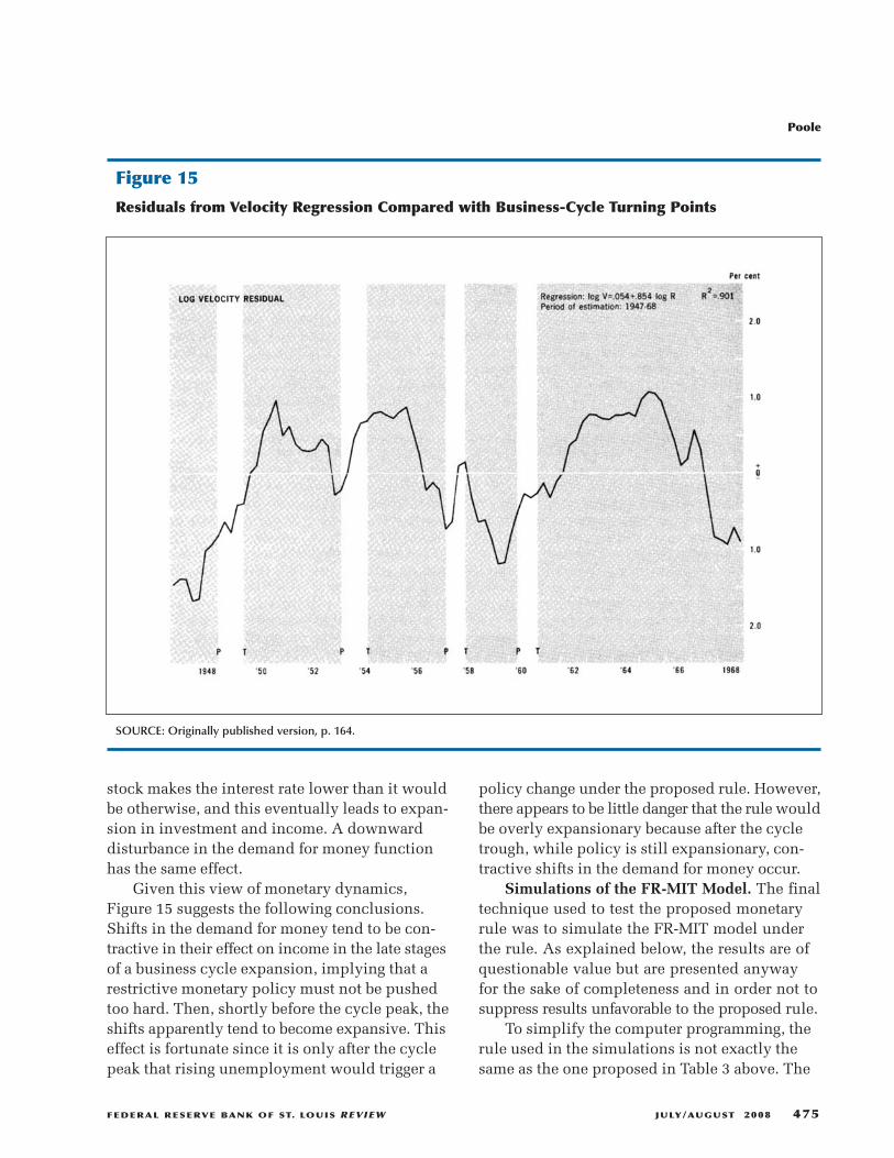
stock makes the interest rate lower than it wouldbe otherwise, and this eventually leads to expan-sion in investment and income. A downwarddisturbance in the demand for money functionhas the same effect.
Given this view of monetary dynamics,Figure 15 suggests the following conclusions.Shifts in the demand for money tend to be con-tractive in their effect on income in the late stagesof a business cycle expansion, implying that arestrictive monetary policy must not be pushedtoo hard. Then, shortly before the cycle peak, theshifts apparently tend to become expansive. Thiseffect is fortunate since it is only after the cyclepeak that rising unemployment would trigger a
policy change under the proposed rule. However,there appears to be little danger that the rule wouldbe overly expansionary because after the cycletrough, while policy is still expansionary, con-tractive shifts in the demand for money occur.
Simulations of the FR-MIT Model. The finaltechnique used to test the proposed monetaryrule was to simulate the FR-MIT model underthe rule. As explained below, the results are ofquestionable value but are presented anywayfor the sake of completeness and in order not tosuppress results unfavorable to the proposed rule.
To simplify the computer programming, therule used in the simulations is not exactly thesame as the one proposed in Table 3 above. The
Poole
FEDERAL RESERVE BANK OF ST. LOUIS REVIEW JULY/AUGUST 2008 475
Figure 15
Residuals from Velocity Regression Compared with Business-Cycle Turning Points
SOURCE: Originally published version, p. 164.
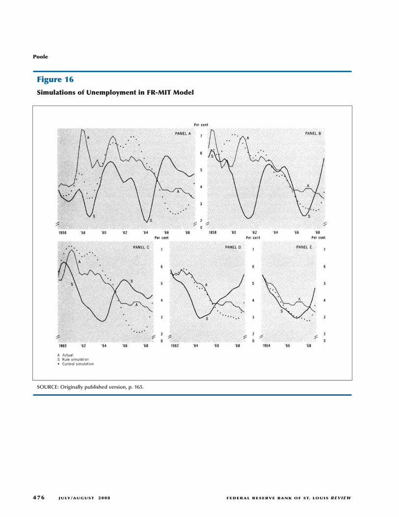
Poole
476 JULY/AUGUST 2008 FEDERAL RESERVE BANK OF ST. LOUIS REVIEW
Figure 16
Simulations of Unemployment in FR-MIT Model
SOURCE: Originally published version, p. 165.

proposed rule, it will be recalled, involved a billrate guideline and a money stock guideline. If, forexample, the bill rate cannot be pushed up with-out pushing monetary growth below the lowerlimit in the money guideline, the proposed rulecalls for setting monetary growth at its lower limit.The simulation rule, on the other hand, ignoresthe bill rate guideline and simply sets the mone-tary growth rate at the midpoint of the range speci-fied by the proposed rule.
Another difference, and no doubt a moreimportant one, between the proposed rule and thesimulation rule is that the simulation rule had tobe specified in terms of quarterly data since theFR-MIT model uses quarterly data. In the simu-lation rule, the growth rate of the money stockdepends on the level of unemployment deter-mined by the model in the previous quarter. Thegrowth rate of the money stock was modified bypast changes in the bill rate, as in footnotes 2 and 3to Table 3, except that the relevant bill rate changewas in terms of the previous quarter before that.The simulation rule, then, reacts somewhat moreslowly to unemployment trends than does theproposed rule.
In order to investigate the importance of thestarting point, simulations were run with startingdates in the first quarters of 1956, 1958, 1960,1962, and 1964. The simulated unemploymentrate for the five simulations is shown in the fivepanels of Figure 16 by the curves marked “S.”The actual unemployment rate is shown by thecurves marked “A” and control simulations, tobe explained below, by the unconnected points.
It is clear from Figure 16 that the simulationrule for money growth produces an unstableunemployment rate. However, because of defi-ciencies in the model this result is probably notvery meaningful. That the model is defective canbe seen by comparing unemployment in the con-trol simulations with the actual unemployment.In the control simulations all of the model’s exoge-nous variables, including the money stock, wereset at their actual levels.16 Even with the exoge-
nous variables set at their actual levels, the simu-lated level of unemployment at times differs fromthe actual level.
Because of the role of the stochastic distur-bances in the model, especially as they feedthrough lagged endogenous variables, it cannotbe expected that control simulations will exactlyduplicate the actual results. But the fact that thecontrol simulations differ from the actual byconsiderable margins over long periods of timestrongly suggests that the money rule simulationsdo not provide much useful information on theproperties of the proposed rule.
The simulations are valuable in one respect,however. An examination of Figure 16 stronglysuggests that the money rule is interacting withthe rest of the model to produce a cycle of 5 to 6years. Such a cycle is particularly evident in thesimulations starting in 1956 and 1958. That themonetary rule has very powerful effects in themodel is shown by the simulations beginning in1960 and 1962. In both simulations unemploy-ment reaches a trough in 1964 and then rises inspite of the 1964-65 tax cuts and the stimulus ofspending for military operations in Vietnam start-ing at the end of 1965.
There is no doubt that the monetary rule istoo aggressive within the context of the FR-MITmodel. A simulation of a perfectly steady rate ofgrowth of money is shown in Figure 17. The rateof growth in this simulation is 2.76 percent peryear, the same as the actual rate of growth overthe period 1955-IV through 1969-I. In Figure 17,the curve labeled S2 is the simulated unemploy-ment rate with the steady rate of growth of money.The simulated unemployment rate under themonetary rule is shown by S1, which is the sameas S in panel A of Figure 16. The unconnectedpoints show the same control simulation as shownin panel A of Figure 16.
Poole
FEDERAL RESERVE BANK OF ST. LOUIS REVIEW JULY/AUGUST 2008 477
16 The FR-MIT model was estimated with the money stock as anendogenous variable. There are separate equations for currencyand demand deposits, both of which are endogenous, while unbor-rowed reserves are exogenous. In the simulations the money stock
was made exogenous by suppressing the equation that makesdemand deposits depend on unborrowed reserves. To simulatethe effects of a particular rate of growth of money, the currencyequation was retained, but demand deposits were set at whateverlevel was required to obtain the desired rate of growth of demanddeposits plus currency. In the control simulations demand depositswere set at their actual levels, but currency remained an endoge-nous variable and differed somewhat from actual since simulatedGNP differed somewhat from actual GNP.

It appears impossible to draw any firm con-clusions from the simulations. However, thesimulations clearly raise the possibility that theproposed monetary rule may produce economicinstability. If anything, the proposed rule is tooaggressive, and so policy should probably err onthe side of producing growth rates inmoney closerto a steady 3 to 5 percent rather than farther fromthe extremes in the proposed rule.
IV. SELECTION AND CONTROLOF A MONETARY AGGREGATEBasic Issues
Up to this point, the analysis has been entirelyin terms of optimal control of the money stock.The theoretical analysis has been general enoughthat no precise definition of the money stock hasbeen required. The empirical work, however, hasused the narrow definition of demand depositsadjusted plus currency, for the simple reason thatthis definition seems to be the most appropriateone.
In principle there is no reason not to looksimultaneously at all of the aggregates and, ofcourse, at all other information as well. But inpractice, at the present state of knowledge, theresimply is no way of knowing how all of thesevariousmeasures ought to be combined.17 Further-more, the selection of a single aggregate for oper-ating purposes would permit the FOMC to be farmore precise in its policy deliberations and in itsinstructions to the Manager of the Open MarketAccount. Thus, the best procedure would seemto be to select one aggregate as the policy controlvariable, and insofar as the state of knowledgepermits, to incorporate other information intopolicy by making appropriate adjustments in therate of growth of the aggregate selected.
In principle the aggregate singled out as thecontrol variable should be subject to exact deter-mination by the Federal Reserve. The reason isthat errors in reaching an aggregate that cannotbe precisely controlled may interact with distur-bances in the relationships between the aggregateand goal variables such as GNP to produce a sub-optimal policy. However, as argued later in thissection, this consideration is likely to be quiteunimportant in practice for any of the aggregatescommonly considered. Therefore, the analysis ofwhich aggregate should be singled out will beconducted under the assumption that all of thevarious aggregates can be precisely controlled bythe Federal Reserve.
Selection of a Monetary Aggregate
At the outset it must be emphasized that thevarious aggregates frequently discussed are allhighly correlated with one another in the post-war period. This is true for total bank credit, thenarrow money stock, the broad money stock (nar-row money stock plus time deposits), the bankcredit proxy (total member bank deposits), the
Poole
478 JULY/AUGUST 2008 FEDERAL RESERVE BANK OF ST. LOUIS REVIEW
Figure 17
Simulations of FR-MIT Model
SOURCE: Originally published version, p. 166.
17 This point is an especially important one since those favoringsimple approaches are frequently castigated for ignoring relevantinformation, and for applying “simplistic solutions to inherentlycomplex problems.” For this charge to be upheld, it must be shownexplicitly and in detail how this other information is to be used,and evidence must be produced to support the proposed complexapproach. As far as this author knows, there is essentially no evi-dence sorting out the separate effects of various components ofmonetary aggregates.

monetary base (member bank reserves plus cur-rency held by the public and nonmember banks),and several other figures that can be computed.
While these various aggregates are highlycorrelated over substantial periods of time, theyshow significantly different trends for shortperiods. In selecting an aggregate, the most impor-tant considerations are the theoretical relevanceof the aggregate and the extent to which the the-oretical notions have been given empirical sup-port. Both of these considerations point to theselection of the narrowly defined money stock.
The most important theoretical dispute isbetween those who emphasize the importance ofbank deposit liabilities—the “monetary” view—and those who emphasize the importance ofbanks’ earning assets—the “credit” view. Thiscontroversy, which dates back well into the 19thcentury, is difficult to resolve because historicallybanks have operated on a fractional reserve basisand so have had both earning assets and depositliabilities. Since balance sheets must balance,bank credit and bank deposits are perfectly corre-lated except insofar as there are changes in non-earning assets—such as reserves—or nondepositliabilities—such as borrowing from the FederalReserve System. If these factors never changed,the perfect correlation between bank deposits andbank credit would make it impossible ever toobtain evidence to distinguish between the mone-tary and the credit views. Since the correlation,while not perfect, has historically been very high,it has been very difficult to obtain evidence.Hence, it is still necessary to place major relianceon theoretical reasoning.
There would be little reason to examine theissue closely if we could be confident that thevery high correlation between deposits and bankcredit would continue into the indefinite future.But there are already substantial differences inthe short-run movements of bank credit and bankdeposits, and these differences are likely to becomegreater and of a longer-term character in the future.Banks are raising increasingly large amounts offunds through nondeposit sources such as salesof commercial paper and of capital certificatesand through borrowing from the Euro-dollar mar-ket and the Federal Reserve System. (Borrowings
from the System would probably expand signifi-cantly if proposed changes in discount-windowadministration were implemented.)
The easiest way to examine the theoreticalissues is to consider some hypothetical experi-ments. Consider first the experiment in whichthe Federal Reserve raises reserve requirementsby $10 billion at the initial level of deposits butsimultaneously buys $10 billion in U.S. govern-ment securities in the open market. Deposits neednot change, but banks must hold more reservesand fewer earning assets. Under the monetaryview the effects would be nil (except for veryminor effects examined below) because depositswould be unchanged, but under the credit viewthe effect would be a tendency for income to con-tract because bank credit would be lower.
The monetary view is easily explained. Sup-pose first that the banks initially hold U.S. govern-ment securities in excess of $10 billion. Whenreserve requirements are raised, the banks simplysell $10 billion of these securities, and this isexactly the amount being purchased by the FederalReserve. Thus, since deposits are unchangedand bank loans to the nonbank private sector—hereinafter called simply the “private sector”—are also unchanged, there should be no effectson that sector.
Now suppose that the banks do not have $10billion in government securities. In this case theymust sell private securities, say corporate bonds,to the private sector. The private sector obtainsthe funds to buy these bonds from the sale of $10billion of government securities to the FederalReserve. The amount of credit in the private sectoris again unchanged. The banks own fewer privatesecurities, while the public owns more privatesecurities and fewer government securities.
Thus, the amount of credit extended to theprivate sector need not change at all even thoughbank credit falls. However, two minor effects arepossible: First, the Federal Reserve purchase ofgovernment securities changes the compositionof portfolios. Thus, even if banks have over $10billion of government securities, they may beexpected to adjust their portfolios by selling somegovernment securities and some private securities.For ease of exposition, run-offs of loans may be
Poole
FEDERAL RESERVE BANK OF ST. LOUIS REVIEW JULY/AUGUST 2008 479

included in the sale of private securities. The netresult, then, is that the banks have more reserves,fewer government securities, and fewer privatesecurities; the private sector has fewer governmentsecurities and fewer liabilities to the banks. Theprivate sector may have—but it will not neces-sarily have—fewer claims within the sector. It isquite possible that private units may substituteclaims on other private units for the governmentsecurities sold to the Federal Reserve.
Looked at from the liability side, those unitsinitially with liabilities outstanding to banks mayhave those liabilities shifted to other private sec-tor units. This occurs, of course, when banks sellsecurities to the private sector or allow loans torun off that are then replaced by firms selling com-mercial paper to other firms, drawing on sourcesof trade credit, and/or borrowing from nonbankfinancial institutions. A net effect can occur onlywhen the combined portfolios of banks and theprivate sector contain fewer government securities,though more reserves, than before; such a changemay be looked upon as a reduction in liquidityand thereby lead to a greater demand for moneyand a reduced willingness to undertake additionalexpenditures on goods and services.
The second effect of the hypothetical experi-ment being discussed is that bank earnings willbe reduced by the increase in reserve require-ments. Banks will eventually adjust by raisingservice charges on demand deposits and/or reduc-ing interest paid on time deposits. For simplicity,assume that the change in reserve requirementsapplies only to demand deposits so that there isno reason for banks to change the interest paidon time deposits. With higher service charges ondemand deposits, lower interest rates on securi-ties are required if people are to hold the samestock of money as before. Since the hypotheticalexperiment assumed that deposits did not change,interest rates must fall by the same amount as theincrease in service charges, an effect that will tendto expand investment and national income.
The portfolio effect tends to contract incomewhile the service charge effect tends to expandincome. These effects individually seem likelyto be small, and the net effect may well be nil. Inthis regard, it is interesting to note that the rela-
tionship of velocity to the Aaa corporate bond rateis about the same for observations in the 1950’sas in the 1920’s (Latané, 1954, 1960) in spite ofthe enormous changes in financial structure andin government bonds outstanding.
Consider another hypothetical experiment—one that is in fact not so hypothetical at the cur-rent time. Suppose that banks suddenly startissuing large amounts of commercial paper andinvesting the proceeds in business loans. It ispossible that the loans simply go to corporationsthat have stopped issuing their own commercialpaper. In this case the bank would be purely amiddlemanwith no effect on the aggregate amountof commercial paper outstanding. The increasein bank credit would not represent an increasein total credit.
But, of course, banks issuing commercialpaper must perform some function. This functionis clearly that of increasing the efficiency of thefinancial sector in transferring funds from theultimate savers to the ultimate borrowers. Theefficiencies arise in several ways. First, underfractional reserve banking, banks have naturallydeveloped expertise in lending. It is efficient tomake use of this expertise by permitting banks tohave more lendable funds than they would haveif restricted to demand deposits alone. The effi-ciency takes the form of fewer administrativeresources being required to transfer funds fromsavers to borrowers.
The second form of efficiency results fromthe fact that financial markets function best whenthere is a large amount of trading in a standard-ized instrument. For example, the shares of largecorporations are much more easily marketed thanthose of small corporations. Many investors want,and require, readily marketable securities, andthey can be persuaded to buy securities in smallfirms only if the yields are high. As a result fundsmay go to large corporations to finance relativelylow-yielding investment projects while high-yielding projects available to small firms cannotbe financed. Commercial banks, and other finan-cial intermediaries, improve the allocation ofcapital by issuing relatively standardized securi-ties with good markets and lending the proceedsto small firms.
Poole
480 JULY/AUGUST 2008 FEDERAL RESERVE BANK OF ST. LOUIS REVIEW

The question is whether there is any effect oneconomic activity from an increase in bank creditfinanced by commercial paper—assuming thatthe money stock is not affected. To begin with, itmust be emphasized that an increase in the effi-ciency of investment does not necessarily affectthe total of investment. The same resources maybe absorbed either in building a factory that willproduce a product that cannot be sold or in build-ing a factory to produce a highly profitable prod-uct in great demand.
Banks, and financial intermediaries in gen-eral, have the effect of reducing somewhat thecost of capital for small firms. Because interme-diaries bid funds away from large corporations,the cost of capital for large corporations tends tobe somewhat higher than it would be if there wereno intermediaries. At this stage in the analysisthe net effect on investment is impossible to pre-dict since it depends on whether the reductionin investment by large corporations is larger orsmaller than the increase in investment by smallcorporations.
In examining the effects of intermediation,however, another factor must be considered. Sup-pose it is assumed that the interest rates relevantfor the demand for money are rates on high-qualitysecurities. It was argued above that intermediationtends unambiguously to raise the yields on high-quality securities above what they otherwisewould be. Since the assumption throughout hasbeen that the stock of money is unchanged, thelevel of income must increase if the quantity ofmoney demanded is to be unchanged with thehigher interest rate of high-quality securities. Theconclusion, therefore, is that the increase in bankcredit is expansionary in the hypothetical experi-ment being discussed.
This conclusion, however, does not warrantthe further conclusion that bank credit is theappropriate monetary aggregate for policy pur-poses. The effect examined above occurs whenany financial intermediary expands. Not only isthere the problem that data for all intermediariesare simply not available on a current basis butalso there are serious problems in even definingan intermediary. A particularly good example ofthis difficulty is afforded by trade credit. A large
nonfinancial corporationmay advance trade creditto customers, many of whom may be small, andmay also advance funds to suppliers throughprepayments. The large corporation financesthese forms of credit through the sale of securities,or through retained earnings diverted from itsown investment opportunities and/or from divi-dends. In this case the large corporation is servingexactly the same function as the financial inter-mediaries are. But tracing these credit flows isobviously impossible at the present time.
Another problem with bank credit as a guideto policy is that changes in bank credit dependboth on changes in bank deposits and on changesin nondeposit sources of funds. As demonstratedby the hypothetical experiments examined above,the effect of a change in bank credit dependsheavily on whether or not deposits change.
One final hypothetical experiment will beconsidered. Suppose the U.S. Treasury sells addi-tional government securities to the public tofinance an increase in cash balances at commer-cial banks. Since banks have received no addi-tional reserves, total deposits cannot change.Deposits owned by the public are transferred tothe Treasury. Bank credit is unchanged, but theimpact on the private sector is clearly contraction-ary. The private sector holds more governmentbonds and fewer deposits. Equilibrium can berestored only through some combination of arise in interest rates and a decline in income.
The conclusion is that it appears to be funda-mentally wrong for policymakers to place primaryreliance on bank credit. This is not to say thatthere is no information to be gained from analysisof bank and other credit flows. However, selectionof bank credit as the monetary aggregate wouldbe a mistake. Instead, information on credit flowsmay be used to adjust the desired rate of growth ofthe money stock, however it is defined, althoughit is not clear that the knowledge presently existsas to how to interpret credit flows.
From this analysis it appears that neitherbank credit nor any deposit total that includesTreasury deposits is an appropriate monetaryaggregate for monetary policy purposes. Beforeconsidering the narrow and broad definitions of
Poole
FEDERAL RESERVE BANK OF ST. LOUIS REVIEW JULY/AUGUST 2008 481
the money stock, let us examine the monetarybase, total reserves, and unborrowed reserves.
It is clear that different levels of the moneystock may be supported by the same level of themonetary base. Given the monetary base, differentlevels of the money stock result from changes inreserve requirement ratios; from shifts of depositsbetween demand and time, which of course aresubject to different reserve requirement ratios;from shifts of deposits among classes of bankswith different reserve ratios; and from shiftsbetween currency and deposits. These effects arewidely understood, and they have led to the con-struction of monetary base figures adjusted forchanges in reserve requirements. Similar adjust-ments are applied to total and nonborrowedreserves. If enough adjustments are made, theadjusted monetary base is simply some constantfraction of the money stock, while adjustedreserves are some constant fraction of deposits.It is obviously much less confusing to adopt somedefinition of the money stock as the appropriateaggregate rather than to use the adjusted monetarybase or an adjusted reserve figure.
There can be no doubt that FOMC instructionsto the Manager in terms of nonborrowed reserveswould be more precise and more easily followedthan instructions in terms of the money stock.But the simplicity of reserve instructions woulddisappear if adjusted reserves were used, for thenthe Manager would have to predict such factorsas shifts between demand and time deposits, thesame factors that must be predicted in controllingthe money stock. No one would argue that suchfactors—and others such as changes in bank bor-rowings and shifts in Treasury deposits—shouldbe ignored. lf the FOMC met daily, instructionscould go out in unadjusted form with the FOMCmaking the adjustments. But surely this technicalmatter should be handled not by the FOMC butby the Manager and his staff in order to permitthe FOMC to concentrate on basic policy issues.
The only aggregates left to consider are thenarrowly and broadly defined money stocks.There is a weak theoretical case favoring thenarrow definition because time deposits must betransferred into demand deposits or currencybefore they can be spent. The case is weak because
the cost of this transfer is relatively low. If thecost were zero, then there would be no effectivedistinction between demand and time deposits.Indeed, since time deposits earn interest, all fundswould presumably be transferred to time deposits.
No strong empirical case exists favoring onedefinition over the other. The broad and narrowmoney stocks are so highly correlated over timethat it is impossible to distinguish separate effects.It appears, however, that there is a practical casefavoring the adoption of the narrow money stock.Time deposits include both passbook accounts,which can be readily transferred into demanddeposits, and certificates of deposit, which can-not. Since CD’s appear to be economically muchmore like commercial paper than like passbooktime accounts, they ought to be excluded fromthe broadly defined money stock.
There is, of course, no reason why CD’s cannotbe excluded from the definition of money. Theproblem is that banks may in the future inventnew instruments that will be classified as timedeposits for regulatory purposes but that are notreally like passbook accounts. In retrospect itmay be clear how the new instrument should betreated, but the situation may be confused for atime. The same sort of problem exists withdemand deposits—consider the compensatingbalance requirements imposed by many banks—but it seems likely that the problem will remainmore serious for time deposits.
In summary, there is a strong case favoringthe selection of some definition of the moneystock as the monetary aggregate, and there appearsto be a marginal case for preferring the narrowlydefined money stock.
Technical Problems of ControllingMoney Stock
In the preceding sections it has been arguedthat the monetary policy control instrumentshould be the money stock. The purpose of thissection is to investigate some of the technicalproblems in controlling the money stock. Thefirst topic examined is that of the form of instruc-tions to the Manager of the System Open MarketAccount. Following this discussion is an exami-
Poole
482 JULY/AUGUST 2008 FEDERAL RESERVE BANK OF ST. LOUIS REVIEW
nation of the feedback method of control. Finally,there is an examination of the significance ofdata revisions. All of this discussion is in termsof the narrowly defined money stock, but muchof it also applies to other aggregates.
Specification of the Desired Money Stock.There are two major issues connected with theform of FOMC instructions to the Manager. Thefirst is whether the desired money stock shouldbe expressed in seasonally adjusted or unadjustedform, while the second is whether the desiredmoney stock should be expressed in terms of acomplete path week by week over time or of anaverage over some period of time. The first issueturns out to be closely related to the questionof data revisions, and so its discussion will bedeferred for the moment. It is to the second issuethat we now turn.
Since required reserves are specified in termsof a statement-week average, the statement weekis the natural basic time unit for which to measurethe money stock, and the measure takes the formof the average of daily money stock figures overthe statement week. The fact that daily data maynot be available on all components of the moneystock does not affect the argument; however esti-mated, the weekly-average figure is the mostappropriate starting point in the analysis.
The weekly money stock is clearly not subjectto precise control because of data lags and uncon-trollable random fluctuations. Furthermore, no onebelieves that these weekly fluctuations have anysignificant impact. The natural conclusion to bedrawn is that there is no point in specifyinginstructions in terms of weekly data but rather thatsome average level over a period of weeks shouldbe used. Upon closer examination, however, thisconclusion can be shown to be unjustified.
The difficulty in expressing the instructionsin terms of averages can be explained very simplyby two examples. To keep the examples frombecoming too complicated, it will be assumedthat instructions take the form of simple rates ofgrowth on a base money stock of $200 billion.The neglect of compounding makes no essentialdifference to the argument.
For the first example, assume that the policyinstruction is for a growth rate of 4 percent per
annum, which is $8 billion per year or about$154 million per week. If the money stock grewby $154 million per week for 8 weeks, then thefigure for the eighth week would be above thebase week figure by an amount representing a 4percent annual growth rate. The average of weeks5 through 8 would be above the average of weeks1 through 4 by $616 million, an amount also rep-resenting a 4 percent annual growth rate. So far,there is no reason to favor the path specificationover a specification in terms of 4-week averages.
Now suppose that the increase in weeks 1through 4 was on schedule, but that a large uncon-trollable increase of $500 million occurred in thefifth week. Starting from a base-week figure of$200 billion, the average money stock for weeks1 through 4 would be $200.385 billion, and if theinstruction were in terms of 4-week averages itwould specify an averagemoney stock of $201.001billion for weeks 5 through 8.
Since by hypothesis the money stock grewby $154 million in each of the first 4 weeks, inthe fourth week the level was $200.616 billion.The jump of $500 million in the fifth week wouldtake the level to $201.116 billion, a figure alreadyabove the desired average of $201.001 billion forweeks 5 through 8. To reach this desired averagegiven the jump in week 5, the money stock inweeks 6 through 8 would have to average lessthan $201.001 billion, and so the money stockwould have to be forced below the level of thefifth week for weeks 6 through 8. Furthermore,as the reader may calculate, it would be necessaryto have higher than normal weekly growth inweeks 9 through 12 if the average of these weekswere to be above the average of weeks 5 through 8by $616 million. On the other hand, if the instruc-tion were in terms of the desired weekly path, theinstruction would read that the desired moneystock in the eighth week was $201.232 billion,and therefore the Manager would not have toforce the money stock down in weeks 6 through8. Instead, he could aim for a growth of about$39 million in each of the weeks 6 through 8 tobring the level in week 8 to the desired figure of$201.232 billion.
From this example it can be seen that specifi-cation in terms of averages of levels of the money
Poole
FEDERAL RESERVE BANK OF ST. LOUIS REVIEW JULY/AUGUST 2008 483
stock forces the Manager to respond to randomfluctuations in a whipsawing fashion. Sinceweek-by-week fluctuations have essentially nosignificance, there is no point in wrenching thefinancial markets in order to undo a randomfluctuation. If averaging is to be used, the averageshould be specified in terms of the desired averageweekly change over, say, the next 4 weeks ratherthan in terms of the average level of the next 4weeks. Specification in terms of the averageweekly change is equivalent to a specificationstating that the Manager should aim for a partic-ular target level in the fourth week.
The second example illustrating the hazardsof specification in terms of the average level willshow what happens when policy changes. Asbefore, assume that the money stock in the baseweek is $200 billion and that the desired growthis at a 4 percent rate in weeks 1 through 4. In thisexample it is assumed that there are no errors inhitting the desired money stock. Thus, the moneystock is assumed to grow by $154 million perweek, reaching a level of $200.616 billion in thefourth week and an average level of $200.385billion for weeks 1 through 4.
Now suppose that in week 4 the FOMCdecides on a policy change and specifies a 1 per-cent growth rate for the money stock for weeks 5through 8. If the specification were in terms of theaverage level, then it would require an increasein the average level of $154 million, which wouldbring the average level to $200.539 billion forweeks 5 through 8. But the figure for week 4 isalready $200.616 billion, and so the money stockin weeks 5 through 8 would have to average lessthan the figure already achieved in week 4.
Thus, after a steady 4 percent growth weekby week, an average-level policy specificationwould actually require a negative week-by-weekgrowth before the new 1 percent growth rate couldbe achieved. On the other hand, a policy specifi-cation in terms of the weekly path would requirea weekly growth of $38.5 million each week forweeks 5 through 8.
To make the point clear, this example wasconstructed so that the policy shift from a 4 to a1 percent growth rate would actually require anegative growth rate for a time on a week-by-week
basis when the instructions are in terms of averagelevels. In general, when average levels are used,a policy shift to a lower growth rate will requirein the short term a growth rate lower than thenew policy rate set, and a policy shift to a highergrowth rate will require a short-term growth rateabove the new policy rate. Since policymakers willtypically want to shift policy gradually, the levelsspecification is especially damaging because itin fact instructs the Manager to shift policy morerapidly than the policymakers had desired. Itshould be noted that the larger the number ofweeks included in the average-level specification,the more severe this problem becomes.
Because the money stock cannot be controlledexactly, there is a natural tendency to feel thatinstructions stated in terms of averages are moreattainable. In actuality, of course, this effect isillusory; averaging produces a smaller number tomeasure the errors, but does not improve control.Nevertheless, if averages are to be used in theinstructions, the above examples demonstratethat the averages should be calculated in termsof weekly (or perhaps monthly) changes but notin terms of averages of levels.
Use of average changes does have one advan-tage, however. An instruction in this form permitsthe Manager to correct an error in week 1 over thenext few weeks rather than instructing him tocorrect the error entirely in week 2. As explainedabove, an instruction in terms of the averageweekly change over the next 4 weeks is equivalentto an instruction in terms of the desired level inweek 4, leaving unspecified the desired levels inweeks 1 through 3.
Control Through the Feedback Principle. Itis useful to begin by comparing the problems ofcontrolling the money stock with the problemsof controlling interest rates. In controlling interestrates, the availability of continuous readings onrates makes it possible for the Manager to exer-cise very accurate control without understandingthe causes of rate changes. Being in continuouscontact with the market, the Manager can inter-vene with open market purchases or sales assoon as the federal funds rate, the Treasury billrate, or any other rate starts to change in an unde-sirable fashion. This feedback control is not exact
Poole
484 JULY/AUGUST 2008 FEDERAL RESERVE BANK OF ST. LOUIS REVIEW

since interest rate information arrives with somelag, and there are other lags such as the timerequired to decide upon and execute an openmarket transaction and the time it takes for themarket to react to the transaction.
More precise control over interest ratescould be achieved if the Manager were willing toannounce Federal Reserve buying and sellingprices for, say, 3-month Treasury bills availableto all comers. This is essentially the way in whichgovernment securities were pegged during WorldWar II. In principle, there is no reason why such apeg could not be operated in peacetime, althoughit would certainly be desirable to change the pegfrequently, perhaps as often as every day or evenevery hour. However, in terms of actual behaviorof interest rates there is no significant differencebetween a frequently adjusted peg and continuousintervention by the Manager as described in theprevious paragraph.
The main point of this discussion of interestrate control is to emphasize that with frequentinterest rate readings it is not necessary to knowexactly what causes interest rate changes. In timethe Manager develops a feel for the market thatenables him to guess accurately which interestrate changes are temporary and which are likelyto be “permanent” and so require offsetting openmarket operations. Furthermore, his feel for themarket will enable him to know how large theoperations should be. Finally, when he guesseswrongly on these matters, his continuous contactwith the market enables him to correct mistakesrapidly.
The same arguments apply to controlling themoney stock. The difference between interest ratecontrol and money stock control is a matter ofdegree rather than kind. Data on the money stockbecome available with a greater lag, and the dataare more subject to revision. But since it is notnecessary to control the money stock down tothe last dollar, the question is whether it is tech-nically possible to have control that is accurateenough for policy purposes. The answer to thisquestion would certainly appear to be in theaffirmative.
The weekly-average figure for the money stockis released to the public 8 days following the end
of the week to which the average refers. Of course,data are available internally with a shorter lag.Since the policy rule in the previous section isbased on controlling the monthly-average moneystocks it would appear that the data are at thepresent time available with a short enough lagthat feedback methods of control are feasible.
To see how feedback control would work,suppose that the Manager were instructed to comeas close as possible to a target money stock ofM4*in week 4 of a 4-week operating horizon. TheManager knows that the weekly change in themoney stock depends on open market purchases,P, which he controls, and many other factors aswell, which for simplicity of exposition will bedenoted by one factor, z. These factors cannot bepredicted exactly, and so the Manager will thinkof z as consisting of a predictable part, z, and anunpredictable part, u. These relationships maybe expressed as
(5)
where α is the coefficient giving the change inmoney per dollar of open market purchases.
If there were no errors inmeasuring themoneystock, the analysis could be completed on thebasis of equation 5. But of course there are errorsin measuring the money stock. To analyze thesignificance of measurement errors, letMi be themoney stock for week i as measured at the end ofweek i.18 Also, letMi
f be the final “true” moneystock figure for week i, and let ei =Mi
f –Mi.The Manager starts out the 4-week period
with an estimated money stock ofM0 for weekzero. Of course, the figure forM0 is a preliminaryone, but revisions in this figure as more data accu-mulate will affect the estimates for the moneystock in later weeks and so affect the Manager’sactions in later weeks. It will be assumed thathe wants to increase the money stock by equalamounts in eachweek to reach the desired figure of
∆M P z P z u= + = + +α α ˆ
Poole
FEDERAL RESERVE BANK OF ST. LOUIS REVIEW JULY/AUGUST 2008 485
18 If a money stock estimate is not directly available at the end ofweek i, one can be constructed by taking the estimate from actualdeposit data for week i – 1 and adding to it a projection for theeffects of open market operations and other factors for week i. Thisprojection would, of course, come from equation 5.

M4* inweek 4. Inweek 1, therefore, hewants to pro-duce a change in the money stock 1/4(M4* –M0).Substituting this figure into equation 5 we obtain
Thus, the Manager sets P1 according to
(6)
At the end of the first week the Manager hasthe estimate,M1, for themoney stock for that week,and again it is assumed that he wants to spreadthe desired changeM* –M1 equally over the next3 weeks. Thus, the Manager sets P2 according to
(7)
Similarly, he sets P3 and P4 according to equations8 and 9.
(8)
(9)
From equations 9 and 5 it can be seen thatthe actual money stock in week 4 is
(10)
This expression for the fourth week of a planningperiod generalizes to the nth week of a planningperiod of any length merely by replacing thesubscript 4 by the subscript n. We can, therefore,express the annual rate of growth, g, over an nweek period by
(11)
From equation 11 it can be seen that the actualgrowth rate, g, equals the desired growth rate plusan error term that becomes smaller as n becomeslarger.
gn
M MM
nM M
M
nf f
f
nf
f
=−
=−
+
∗
52
52 5
0
0
0
0
221n
e un n− +( )
14 4 0 1 1 1� ˆM M P z u∗ −( ) = + +α
P M M z1 4 0 11 1
4= −( ) −
∗
αˆ
P M M z2 4 1 21 1
3= −( ) −
∗
αˆ
M M M M z z M e uf f4 3 3 4 4 3 4= + − − + = + +∗ ∗ˆ
P M M z4 4 3 41= −( ) −
∗
αˆ
P M M z3 4 2 31 1
2= −( ) −
∗
αˆ
This analysis shows that a feedback controlsystem that continuously adjusts open marketoperations as data on the money stock in therecent past become available can achieve a targetrate of growthwith amargin of error that is smallerthe longer the period over which the rate of growthis calculated. It also provides a framework inwhich to examine the relative importance ofoperating errors, the ui, and data errors, the ei.
To obtain an accurate estimate of the sizes ofthese errors is beyond the scope of this study.However, a very crude method may be used toobtain an estimate of the maximum size of thetotal error. Monthlymoney stock changes at annualrates were computed for the period January 1951through September 1969 on the basis of seasonallyadjusted data. This time period yields a total of225 monthly changes. Then each monthly changewas expressed in terms of its deviation from theaverage of the changes for the previous 3 months.For example, the September deviation was calcu-lated by subtracting from the September monthlychange the average of the changes for August, July,and June. The use of deviations allows in partfor longer-run trends in the money stock, whichtrends are assumed to be readily controllable.Since the deviations were calculated over a periodduring which little or no attention was paid tocontrolling the money stock, they surely representan upper limit to the degree of volatility in themoney stock to be expected under a policydirected at control of the money stock.
These monthly deviations have a standarddeviation of 3.12 percent per annum. Applyingequation 11, except for replacing 52 by 1 to reflectthe fact that the rates of change were expressedat annual rates in the first place, it is found thatthe standard deviation over a 3-month periodwould be 1.04 percent per annum. If it is assumedthat these deviations are normally distributed,the conclusion is that over 3-month periods theactual growth rate would be within plus or minus1.04 percent of the desired growth rate about 68percent of the time, and would be within plus orminus 2.08 percent about 95 percent of the time.Inasmuch as these limits would be cut in halfover 6-month periods, the actual growth rate 95percent of the time would be in the range of plus
Poole
486 JULY/AUGUST 2008 FEDERAL RESERVE BANK OF ST. LOUIS REVIEW
or minus 1.04 percent of the desired growth rate.19
When it is recalled that these calculations arebased on an estimate of variability over a periodin which very little attention was paid to stabi-lizing money stock growth rates, it is clear thatfears as to the ability of the Federal Reserve tocontrol the money stock accurately are completelyunfounded.20
This conclusion justifies the approach usedat the beginning of this section on the selectionof a monetary aggregate, at least for the narrowlydefined money stock and most probably for otheraggregates as well. That approach, it will berecalled, analyzed the selection issue on theassumption that every one of the aggregates con-sidered could be precisely controlled for all prac-tical purposes. There can be no doubt that errorsin reaching targets for goal variables such as GNP,at the present state of knowledge, are due almostentirely to incomplete knowledge of the relation-ships between instrument variables (such as vari-ous aggregates and interest rates) and the goalvariables, and hardly at all to errors in settinginstrument variables at desired levels.
Problems of Data Revisions and ChangingSeasonality. Another topic that needs examina-tion is the effect of data revisions. While weekly-average data are released with an 8-day lag, thesefigures are subject to revision. Not much weightcan be given to early availability of data that arelater revised substantially. To investigate thisproblem, two money stock series were compared,one “preliminary” and one “final.” Since theanalysis below is based on published monthlydata, it obviously provides little insight into the
accuracy of weekly data. However, since policyinstructions may be based on monthly data, theanalysis is of some value in assessing data accu-racy. Furthermore, the conclusions on the impor-tance of revisions in seasonal factors can beexpected to hold for the weekly data.
A “preliminary” series of monthly growthrates of the money stock was constructed by cal-culating the growth rate for each month from datareported in the Federal Reserve Bulletin for thefollowing month. For example, the Bulletin datedSeptember reports money stock data for 13monthsthrough August; it is the annual rate of change ofAugust over July that is called the “preliminary”August rate-of-change observation. The “final”series is the annual rate of growth calculated fromthe monthly money stock series covering 1947through September 1969, reported in the FederalReserve Bulletin for October 1969, pp. 790-93.Data were gathered on both a seasonally adjustedbasis and an unadjusted basis for January 1961through August 1969.
The correlation between the preliminary andfinal seasonally adjusted series is 0.767, whilefor the unadjusted series the correlation is 0.997.Another way to compare the preliminary andfinal series is to examine the differences in thetwo series.21 For the seasonally adjusted data, thedifferences have a mean of 0.122 and a standarddeviation of 3.704, and the mean absolute differ-ence is 2.891. On the other hand, for the season-ally unadjusted data the differences have a meanof 0.150 and a standard deviation of 1.366, andthe mean absolute difference is 0.955.22
These results make it abundantly clear thatthe major reason why the preliminary and final
Poole
FEDERAL RESERVE BANK OF ST. LOUIS REVIEW JULY/AUGUST 2008 487
19 If the calculations are based on the variability of the monthlychanges themselves rather than on the deviations of the monthlychanges, the results are not greatly changed. The standard deviationof the monthly changes over the same period used before is 3.53per cent per annum, which yields a 95 percent chance of the growthrate being in a range around the desired rate of plus or minus 2.36(1.18) per cent per annum for 3-month (6-month) periods.
20 Compare “First, however, it may be worthwhile to touch on theextensively debated subject whether the Federal Reserve, if itwanted to, could control the rate of money supply growth. In myview, this lies well within the power of the Federal Reserve toaccomplish provided one does not require hair-splitting precisionand is thinking in terms of a time span long enough to avoid theerratic, and largely meaningless, movements of money supplyover short periods” (Holmes, 1969, p. 75).
21 The analysis of the differences inadvertently runs from February1961 through August 1969 while the correlation analysis runsfrom January 1961 through August 1969.
22 To take account of the fact that the “final” money stock series maybe further revised for months near the October 1969 publicationdate of this series, the analysis of differences between the prelimi-nary and final series was also run on the period February 1961through December 1968. The mean difference, the standard devi-ation of the differences, and the mean absolute difference, are,respectively, for the seasonally adjusted data 0.026, 3.779, and2.922, while the figures for the seasonally unadjusted data are0.038, 1.280, and 0.890. In spite of the fact that the “final” seriesis not really final for 1969 data, the average differences are gener-ally larger for the longer period due to the relatively large datarevisions in the middle of 1969.
figures on the money stock differ is revision ofseasonal adjustment factors. While such revisionsmay produce substantial differences betweenpreliminary and final monthly growth rates, thedifferences must be lower for the average of severalmonths’ growth rates. The reason, of course, isthat revision of seasonal factors must make thefigures for somemonths higher and those for othermonths lower, leaving the annual average aboutunchanged.
The significance of revisions in seasonal fac-tors can be understood only after a discussion ofthe significance of seasonality for a money stockrule. If the monetary rule were framed in termsof the seasonally unadjusted money stock, theresult would be to introduce substantially moreseasonality into short-term interest rates than nowexists. It can be argued not only that greater sea-sonality in interest rates would not be harmfulbut also that it would be positively beneficial.Greater seasonality in interest rates would pre-sumably tend to push production from busy, high-interest seasons into slack, low-interest seasons.
Although the argument for seasonality ininterest rates could be pushed further, there is animportant practical reason for not initially adopt-ing a money rule stated in terms of the seasonallyunadjusted money stock. The reason is that therule ties the growth rate of the money stock to theseasonally adjusted unemployment rate and tothe interest rate. The rule has been developedthrough an examination of past experience. If theseasonal were taken out of the money stock, adifferent seasonal would be put into interest rates,and possibly into the unemployment rate as well.Seasonal factors for these variables, especially forthe unemployment rate, determined from past datawould no longer be correct if the money stockseasonal were removed. Seasonally adjusting theunemployment index by the old factors couldproduce considerable uncertainty over the appli-cation of the monetary rule. Thus, application ofthe rule through the seasonally unadjusted moneystock, if desirable at all, should only come aboutthrough gradual reduction rather than immediateelimination of seasonality. A further reason for agradual approach would be to permit the finan-cial markets to adjust more easily to changedseasonality.
The point of this discussion is not to urgeacceptance of a rule framed in terms of the unad-justed money stock, since this step would not beinitially desirable in any case. Rather, the pointis to emphasize that seasonality is in the moneystock only in order to reduce the seasonality ofother variables, primarily interest rates. The sea-sonality of the money stock, unlike variables suchas agricultural production, is not inherent in theworkings of the economy but rather exists becausethe Federal Reserve wants it to exist. The moneystock can be made to assume any seasonal patternthe Federal Reserve wants it to assume.
The monetary rule should be framed, at leastinitially, in terms of the seasonally adjustedmoney stock—using the latest estimated seasonalfactors. In subsequent years changes in theseseasonal factors should not result from mechani-cal application of seasonal adjustment techniquesto the money stock data but rather should be theresult of a deliberate policy choice. The policychoice would be based on the desire to changeseasonality of other variables. For example, if itwere thought desirable to take the seasonality outof short-term interest rates, the seasonal factorsfor the money stock would then be changed totake account of changes in tax dates and otherfactors.
Under a money stock policy, whether or notguided by amonetary rule, revised seasonal factorscannot properly be applied to past data. If thechanges are applied to past data with the resultthat some monthly growth rates of adjusted databecome relatively high while others become rela-tively low, the conclusion to be drawn is not thatpolicy was mistaken as a result of using faultyseasonal factors. Instead, the conclusion is merelythat seasonal policy differed in the past from cur-rent policy or from the seasonal pattern assumedby the investigator who computed the seasonalfactors. Seasonal policy can be shown to be“wrong” only by showing that undesirable sea-sonals exist in other variables.
One final problem deserves discussion. Whileit appears from the analysis of seasonally unad-justed money stock data that revisions of the data
Poole
488 JULY/AUGUST 2008 FEDERAL RESERVE BANK OF ST. LOUIS REVIEW
are relatively unimportant, at least from the evi-dence for 1961-69, how should the policy rule beadjusted when there are major data revisions—as in the middle of 1969? For example, supposethat revisions indicate that monetary growth hasbeen much higher than had been expected, andhigher thanwas desirable. On the one hand, policycould ignore the past high rate of growth andsimply maintain the current rate of growth of therevised series in the desired range. On the otherhand, the policy could be to return the moneystock to the level implied by applying the desiredgrowth rate to the money stock in some past baseperiod. The first alternative involves ratifying anundesirable high past rate of growth, while thesecond may involve a wrenching change in themoney stock to return it to the desired growthpath. The proper policy would no doubt have tobe decided on a case-by-case basis. However, auseful presumption might be to adopt the secondalternative, but to set as the base the money stock6 months in the past and to return to the desiredgrowth path over a period of several months.
Improving Control Over the Money Stock.The analysis above has shown that under presentconditions the money stock can be controlledquite accurately. However, it should be empha-sized that there are numerous possibilities forimproving control. Although detailed treatmentof this subject is beyond the scope of this study,a few very brief comments appear appropriate.
There are three basic methods for improvingcontrol. The first method is that of improving thedata. The more quickly the deposit data are avail-able, the more quickly undesirable movementsin the money stock can be recognized and cor-rected. And the more accurate the deposit data,the fewer the mistakes caused by acting on erro-neous information. It is clear that expenditures ofmoney on expanding the number and coverageof deposit surveys and on more rapid processingof the raw survey data can improve deposit data.
The second method of improving control isthrough research, which increases our under-standing of the forces making for changes in themoney stock. For example, transfers between
demand and time deposits might be more accu-rately predicted through research into the causesof such transfers.
The third method of improving control isthrough institutional changes. To reduce fluctua-tions in excess reserves and thereby achieve amore dependable relationship between totalreserves and deposits, the federal funds marketmight be improved by making possible transfersbetween the East and West Coasts after east coastbanks are closed. Also helpful would be a changefrom lagged to contemporaneous reserve require-ments. More radical reforms such as equalizationof reserve requirements for city, country, andnonmember banks and elimination of reserverequirements on time deposits should also beconsidered.
V. SUMMARYPurposes of the Study
The primary purpose of this study has beento argue that a major improvement in monetarypolicy would result through a systematic policyapproach based on adjustments in the moneystock. Equal emphasis has been placed on the“systematic” part and the “money stock” part ofthis approach. The analysis has proceeded firstby showing why policy adjustments should bemade through money stock adjustments, andsecond by showing how these policy adjustmentsmight be systematically linked to the currentbusiness situation through a policy guideline orrule-of-thumb. A third, and subsidiary, part ofthis study is an analysis of the reasons for prefer-ring the money stock over other monetary aggre-gates, and of some of the problems in reachingdesired levels of the money stock.
It has been emphasized throughout that thispolicy approach is one that is justified for theintermediate-term future on the basis of knowledgenow available. The specific recommendationsare not intended to be good for all time. Indeed,the approach has been designed to encourageevaluation of the results so that the informationobtained thereby can be incorporated into policydecisions in the future.
Poole
FEDERAL RESERVE BANK OF ST. LOUIS REVIEW JULY/AUGUST 2008 489

The Theory of Monetary Policy UnderUncertainty
Since policymakers have repeatedly empha-sized the importance of uncertainty, it is necessaryto analyze policy problems within a model thatexplicitly takes uncertainty into account. In par-ticular, only within such a model is it possible toexamine the important current issue of whetherpolicy adjustments should proceed throughinterest rate or money stock changes.
A monetary policy operating through interestrate changes sets interest rates either throughexplicit pegging as was used in World War II orthrough open market operations directed towardthe maintenance of rates in some desired range.Under such a policy the money stock is permittedto fluctuate to whatever extent is necessary to keepinterest rates at the desired levels. On the otherhand, a policy operating through money stockchanges uses open market operations to set themoney stock at its desired level while permittinginterest rates to fluctuate freely.
If there were perfect knowledge of the relation-ships between the money stock and interest rates,the issue of money stock versus interest rateswould be nonexistent. With perfect knowledge,changes in interest rates would be perfectly pre-dictable on the basis of policy-induced changesin themoney stock, and vice versa. It would, there-fore, be a matter of preference or prejudice, butnot of substance, whether policy operated throughinterest rates or the money stock.
To analyze the interest versus money issue,then, it is necessary to assume that there is a sto-chastic link between the two variables. And, ofcourse, this is in fact the case. There are two fun-damental reasons for the stochastic link. First, thedemand for money depends not only on interestrates and the level of income but also on otherfactors, which are not well understood. As a result,the demand for money fluctuates in a randomfashion even if income and interest are unchanged.If the stock of money is fixed by policy, theserandom demand fluctuations will force changesin interest and/or income in order to equate theamount demanded with the fixed supply.
The second source of disturbances betweenmoney and interest stems from disturbances in
the relationship between expenditures—especiallyinvestment-type expenditures—and interest rates.Given an interest rate fixed by policy, these dis-turbances produce changes in income throughthe multiplier process, and these income changesin turn change the quantity of money demanded.With interest fixed by policy, the stock of moneymust change when the demand for money changes.On the other hand, if the money stock were fixedby policy, since the expenditure disturbancechanges the relationship between income andinterest, some change in the levels of incomeand/or interest would be necessary for the quan-tity of money demanded to equal the fixed stock.
Money stock and interest rate policies areclearly not equivalent in their effects, given thatdisturbances in money demand and in expendi-tures do occur. Since the effects of these policiesare different, which policy to prefer depends onhow the effects differ and on policy goals. At thislevel of abstraction, it is clearly appropriate toconcentrate on the goals of full employment andprice stability. Unfortunately, the formal modelthat has beenworked out, which is examined care-fully in Section I above, applies only to the goalof stabilizing income. If “income” is interpretedto mean “money income,” then the goals ofemployment and price level stability are includedbut are combined in a crude fashion.
The basic differences in the effects of moneystock and interest rate policies can be seen quiteeasily by examining extreme cases. Suppose firstthat there are no expenditure disturbances, sothere is a perfectly predictable relationshipbetween the interest rate and the level of income.In that case, a policy that sets the interest ratesets income, and policymakers can choose thelevel of the interest rate to obtain the level ofincome desired. When the interest rate is set bypolicy, disturbances in the demand for moneychange the stock of money but not the level ofincome. On the other hand, if policy sets themoney stock, then the money demand distur-bances would affect interest and income leadingto less satisfactory stabilization of income thanwould occur under an interest rate policy.
The other extreme case is that in which thereare disturbances in expenditures but not in money
Poole
490 JULY/AUGUST 2008 FEDERAL RESERVE BANK OF ST. LOUIS REVIEW
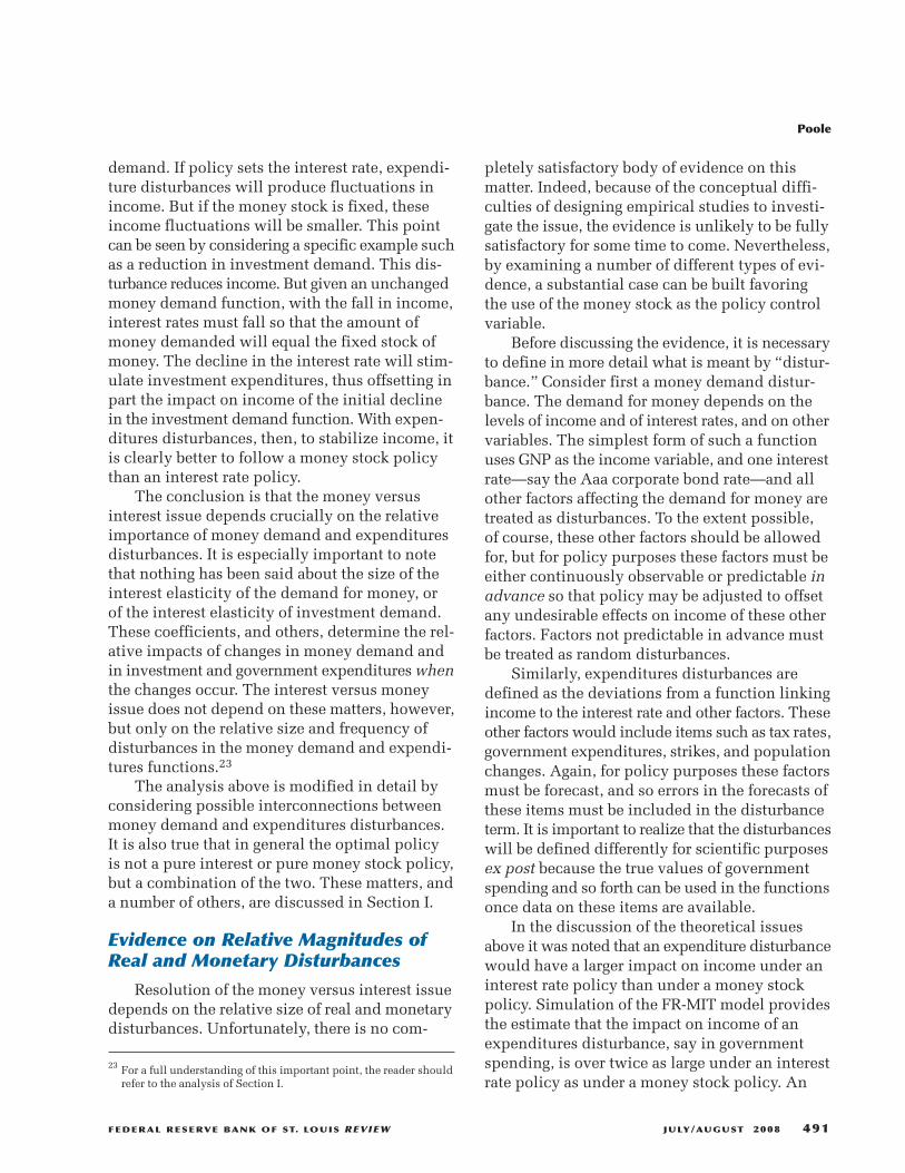
demand. If policy sets the interest rate, expendi-ture disturbances will produce fluctuations inincome. But if the money stock is fixed, theseincome fluctuations will be smaller. This pointcan be seen by considering a specific example suchas a reduction in investment demand. This dis-turbance reduces income. But given an unchangedmoney demand function, with the fall in income,interest rates must fall so that the amount ofmoney demanded will equal the fixed stock ofmoney. The decline in the interest rate will stim-ulate investment expenditures, thus offsetting inpart the impact on income of the initial declinein the investment demand function. With expen-ditures disturbances, then, to stabilize income, itis clearly better to follow a money stock policythan an interest rate policy.
The conclusion is that the money versusinterest issue depends crucially on the relativeimportance of money demand and expendituresdisturbances. It is especially important to notethat nothing has been said about the size of theinterest elasticity of the demand for money, orof the interest elasticity of investment demand.These coefficients, and others, determine the rel-ative impacts of changes in money demand andin investment and government expenditureswhenthe changes occur. The interest versus moneyissue does not depend on these matters, however,but only on the relative size and frequency ofdisturbances in the money demand and expendi-tures functions.23
The analysis above is modified in detail byconsidering possible interconnections betweenmoney demand and expenditures disturbances.It is also true that in general the optimal policyis not a pure interest or pure money stock policy,but a combination of the two. These matters, anda number of others, are discussed in Section I.
Evidence on Relative Magnitudes ofReal and Monetary Disturbances
Resolution of the money versus interest issuedepends on the relative size of real and monetarydisturbances. Unfortunately, there is no com-
pletely satisfactory body of evidence on thismatter. Indeed, because of the conceptual diffi-culties of designing empirical studies to investi-gate the issue, the evidence is unlikely to be fullysatisfactory for some time to come. Nevertheless,by examining a number of different types of evi-dence, a substantial case can be built favoringthe use of the money stock as the policy controlvariable.
Before discussing the evidence, it is necessaryto define in more detail what is meant by “distur-bance.” Consider first a money demand distur-bance. The demand for money depends on thelevels of income and of interest rates, and on othervariables. The simplest form of such a functionuses GNP as the income variable, and one interestrate—say the Aaa corporate bond rate—and allother factors affecting the demand for money aretreated as disturbances. To the extent possible,of course, these other factors should be allowedfor, but for policy purposes these factors must beeither continuously observable or predictable inadvance so that policy may be adjusted to offsetany undesirable effects on income of these otherfactors. Factors not predictable in advance mustbe treated as random disturbances.
Similarly, expenditures disturbances aredefined as the deviations from a function linkingincome to the interest rate and other factors. Theseother factors would include items such as tax rates,government expenditures, strikes, and populationchanges. Again, for policy purposes these factorsmust be forecast, and so errors in the forecasts ofthese items must be included in the disturbanceterm. It is important to realize that the disturbanceswill be defined differently for scientific purposesex post because the true values of governmentspending and so forth can be used in the functionsonce data on these items are available.
In the discussion of the theoretical issuesabove it was noted that an expenditure disturbancewould have a larger impact on income under aninterest rate policy than under a money stockpolicy. Simulation of the FR-MIT model providesthe estimate that the impact on income of anexpenditures disturbance, say in governmentspending, is over twice as large under an interestrate policy as under a money stock policy. An
Poole
FEDERAL RESERVE BANK OF ST. LOUIS REVIEW JULY/AUGUST 2008 491
23 For a full understanding of this important point, the reader shouldrefer to the analysis of Section I.

error in forecasting government spending, then,would lead to twice as large an error in incomeunder an interest rate policy. Since there is nosystematic record of forecasting errors for vari-ables such as government spending and strikes,there is no way of producing evidence on the sizeof such forecasting errors. However, after listingthe variables that must be forecast, as is done inSection II, it is difficult to avoid feeling that errorsin forecasting are likely to be quite significant.
These real disturbances, including forecasterrors in government expenditures, strikes, andso forth, must be compared with the disturbancesin money demand. The reduced-form studiesconducted by a number of investigators providesome evidence on this issue. These studies com-pare the relative predictive power of monetaristand Keynesian approaches in explaining fluctu-ations in income. From these studies the predic-tive power of both approaches appears aboutequal. However, the predictive power of theKeynesian approach relies on ex post observationof “autonomous” expenditures, and it is clearthat these expenditures are subject to forecastingerrors ex ante whereas the money stock can becontrolled by policy.
The evidence from the reduced-form studiessuggests that when forecast errors of autonomousexpenditures are included in the disturbanceterm, the disturbances are larger on the real sidethan on the monetary side. There are many diffi-culties with the reduced-form approach and sothese results must be interpreted cautiously.Nevertheless, the results cannot be ignored.
The final piece of evidence offered in Section IIis a study by the author of the stability of thedemand for money function over time. Using avery simple function relating the income velocityof money to the Aaa corporate bond rate, he foundthat a function fitted to quarterly data for 1947-60also fits data for 1961-68 rather well. The readerinterested in the precise meaning of “rather well”should turn to the technical discussion inSection II.
Evidence on relative stability is difficult toobtain and subject to varying interpretations. Nosingle piece of evidence is decisive, but all thevarious scraps point in the same direction. The
evidence is not such that a reasonable man cansay that he has no doubts whatsoever. But sincepolicy decisions cannot be avoided, the reason-able decision based on the available evidence isto adopt the money stock as the monetary policycontrol variable.
A Monetary Rule for Guiding Policy
The conclusion from the theoretical andempirical analysis is that the money stock oughtto be the policy control variable. For this conclu-sion to be very useful, it must be shown in detailhow the money stock ought to be used. It is notenough simply to urge policymakers to make the“appropriate” adjustments in the money stock inthe light of all “relevant” information.
There is no general agreement on exactly whattypes of adjustments are appropriate. However, itwould probably be possible to obtain agreementamongmost economists that ordinarily the moneystock should not grow faster than its long-run aver-age rate during a period of inflation and shouldnot grow slower than its long-run average rateduring recession. But many economists wouldwant to qualify even this weak statement by sayingthat there may at times be special circumstancesrequiring departures from the implied guideline.Others would say that there is no hope at presentof gauging correctly the impact of special circum-stances (or even of “standard” circumstances) sothat policy should maintain an absolutely steadyrate of growth of the money stock.
The basic issues are, first, whether policy-makers can forecast disturbances well enough toadjust policy to offset them, and second, theextent to which money stock adjustments to off-set short-run disturbances will cause undesirablelonger-run changes in income and other variables.The theoretical possibilities are many, but theempirical knowledge does not exist to determinewhich theoretical cases are important in practice.It is for this reason that a systematic policyapproach is needed so that policy can be easilyevaluated and improved with experience.
Policy could be linked in a systematic way toa large-scale model of the economy. Target valuesof GNP and other goal variables could be selected
Poole
492 JULY/AUGUST 2008 FEDERAL RESERVE BANK OF ST. LOUIS REVIEW

by policymakers, and then the model solved forthe values of the money stock and other controlvariables (for example, discount rate) needed toachieve policy goals. While this approach maybe feasible in the future, it is not feasible nowbecause a sufficiently accurate model does notexist. Instead, policy decisions are now madelargely on the basis of intuitive reactions to cur-rent business developments.
Given this situation, the obvious approach isto specify precisely how policy decisions oughtto depend on current developments, and this isthe approach taken in Section III. The specifica-tion there takes the form of a policy guideline, orrule-of-thumb. The proposed rule is purposelysimple so that evaluation of its merits would berelatively easy. Routine evaluation of an operat-ing guideline would over time produce a body ofevidence that could be used to modify and com-plicate the rule. But it is necessary to begin witha simple rule because the knowledge that wouldbe necessary to construct a sophisticated ruledoes not exist.
The proposed rule assumes that full employ-ment exists when the unemployment rate is in the4.0 to 4.4 percent range. The rule also assumes thatat full employment, a growth rate of the moneystock of 3 to 5 percent per annum is consistentwith price stability. Therefore, when unemploy-ment is in the full employment range, the rule callsfor monetary growth at the 3 to 5 percent rate.
The rule calls for higher monetary growthwhen unemployment is higher, and lower mone-tary growth when unemployment is lower.Furthermore, when unemployment is relativelyhigh the rule calls for a policy of pushing theTreasury bill rate down providedmonetary growthis maintained in the specified range; similarly,when unemployment is relatively low the rulecalls for a policy of pushing the bill rate up pro-vided monetary growth is in the specified range.Finally, the rule provides for adjusting the rate ofgrowth of money according to movements in theTreasury bill rate in the recent past. The exact ruleproposed is in Table 3 and the detailed rationalefor the various components of the rule is explainedin the discussion accompanying that table.
The rule is specified throughout in terms of2 percent ranges for the rate of growth of themoney stock on a month-by-month basis. Byexpressing the rule in terms of a range, leeway isprovided for smoothing undesirable interest ratefluctuations and for minor policy adjustments inresponse to other information. Furthermore, it isnot proposed that this rule-of-thumb or guidelinebe followed if there is good reason for a departure.But departures should be justified by evidenceand not be based on vague intuitive feelings ofwhat is needed since the rule was carefullydesigned from the theoretical and empiricalanalysis of Sections I and II, and from a carefulreview of post-accord policy.
There is no way of really testing the proposedrule short of actually using it. However, it is use-ful to compare the rule with post-accord policy.A detailed comparisonmay be found in Section III.A summary comparison suggests, however, thatfor the period January 1952 through July 1968the rule would have provided a less appropriatepolicy than the actual policy in only 63 of the199 months in the period. The rule was judgedto be less appropriate if it called for a higher—lower—rate of monetary growth than actuallyoccurred and unemployment 12 months hencewas below—above—the desired range of 4.0 to4.4 percent. The rule was also judged less appro-priate than the actual policy if actual policy wasnot within the rule but unemployment neverthe-less was in the desired range 12 months hence.The rule actually has slightly fewer errors if thecriterion is unemployment either 6 or 9 monthsfollowing the months in question.
The rule has the great virtue of turning policyaround promptly as imbalances develop and ofavoiding cases such as the 2.2 percent rate ofdecline in themoney stock from July 1957 throughJanuary 1958, during which time the unemploy-ment rate rose from 4.2 percent to 5.8 percent.Furthermore, it seems most unlikely that the rulewould produce greater instability than the policyactually followed. Actual policy has, as measuredby the money stock, been most expansionaryduring the early and middle stages of businesscycle expansions and most contractionary duringthe last stages of business expansions and early
Poole
FEDERAL RESERVE BANK OF ST. LOUIS REVIEW JULY/AUGUST 2008 493

Ultimately the issue again becomes that ofthe stability of various functions. If the demandand supply functions for all of the various creditinstruments, including those of financial inter-mediaries, were stable and were known, then itwould be possible to focus on any aggregate thatwas convenient. For if all the functions wereknown, then there would be known relationshipsamong various credit instruments, the moneystock, and stocks and flows of goods. But thedemand and supply functions for the variouscredit instruments are not known, and it isunlikely that they ever will be known with anydegree of precision. There are two basic reasonsfor this state of affairs. The first, and less impor-tant, is that given the great degree of substitutabil-ity among credit instruments, substitutions areconstantly taking place as a result of changes inregulations, including tax regulations. But secondandmore important, individual credit instrumentsare greatly influenced by changes in tastes andtechnology, factors that economists do not under-stand well.
As an example of the effects of regulations,consider the substitution in recent years of deben-tures for preferred stock as a result of the tax lawspermitting deduction of interest. As examples ofthe effects of changes in tastes and technology,consider the inventions of new instruments suchas CD’s and the shares in dual-purpose investmentfunds. Furthermore, the relationships amongcredit instruments will change as attitudes towardrisk change due to numerous factors includingperhaps fading memories of the last recession ordepression.
Money viewed as the medium of exchangeseems to be substantially less subject to changesin tastes and technology than do other financialassets. Of course, money is not immune to theseproblems, as shown by the uncertainty presentlyexisting over the impact of credit cards. But agreat deal of empirical work on money has beencompleted and the major findings have been sub-stantiated by a number of different investigators.And the interpretation of the empirical findingsis usually clear because the empirical work hasbeen conducted within the framework of a well-developed theory of money. There is, on the other
Poole
494 JULY/AUGUST 2008 FEDERAL RESERVE BANK OF ST. LOUIS REVIEW
stages of business contractions. Unless a veryimprobable lag structure exists, the rule wouldsurely be more stabilizing than the actual histori-cal pattern of monetary growth.
Selection and Control of a MonetaryAggregate
The analysis in this study is almost entirelyin terms of the narrowly defined money stock.The reasons for using the narrowly defined moneystock as opposed to other monetary aggregatesmay be stated fairly simply.
Some economists favor the use of bank creditas the monetary aggregate because they viewpolicy as operating through changes in the costand availability of credit. The major difficultywith this view is that there is no unambiguousway of defining the amount of credit in the econ-omy. And even if a satisfactory definition couldbe worked out, there is no current possibility ofobtaining timely data on the total amount of creditor of controlling the total amount.
The definitional problem arises largely fromthe activities of financial intermediaries. Suppose,for example, that an individual sells some corpo-rate debentures and invests the proceeds in afixed-income type of investment fund, which inturn uses the funds to buy the very same deben-tures sold by the individual. If both the debenturesand the investment fund shares are counted aspart of total credit, then in this example total credithas risen without any additional funds beingmade available to the corporation to finance newfacilities and so forth.
As another example, it is difficult to see thatit would make any substantial difference to aggre-gate economic activity whether a corporationfinanced inventories through sales of commercialpaper to the public or through borrowing frombanks that raised funds through sales of CD’s tothe public. Since there are numerous close sub-stitutes for bank credit, the amount of bank creditis most unlikely to be an appropriate figure toemphasize. Furthermore, since bank credit is onlya small part of total credit there is essentially nopossibility of controlling total credit, howeverdefined, through adjustments in bank credit.

hand, no satisfactory theory of bank credit toguide empirical work and to permit interpretationof the significance of empirical findings.
For these reasons, and others, bank creditdoes not appear to be an appropriate monetaryaggregate for policy to control. However, becausebank credit and the money stock were so highlycorrelated in the past, it must be admitted that itprobably would not have made much differencewhich one was used. From recent experience,however, it appears that changes in banks’ non-deposit sources of funds are likely to becomemore,rather than less, important, and so in the future thecorrelation between money and bank credit islikely to be lower than in the past. If this predic-tion is correct, then the issue is a significant one.
As a monetary aggregate, to be used for policyadjustments, the money stock has clear advan-tages over the monetary base and various reservemeasures. These aggregates are almost alwaysexamined in adjusted form, where the adjustmentsallow for such factors as changes in the currency/deposit ratio, in reserve requirements, and inshifts between time and demand deposits. Theadjustments are made because the effects of thesevarious factors are understood and are thoughtto be worth offsetting. The adjustments have theeffect of making the base an almost constant frac-tion of the money stock, or making total reservesan almost constant fraction of demand deposits.It obviously makes more sense to look directly atthe money stock, especially since given the natureof the adjustments it is no easier to control theadjusted base or adjusted total reserves than tocontrol the money stock.
The final aggregate to be considered is thebroadly defined money stock—the narrow stockplus time deposits. No strong case can be madeagainst the broad money stock. From existingempirical work both definitions of money appearto work equally well. The theoretical distinctionbetween demand deposits and passbook savingsdeposits depends on the costs of transferringbetween the two types of deposits, and these costsappear to be quite low. However, CD’s do appearto be theoretically different and probably shouldbe excluded from the definition of money. Themajor reason for excluding all time deposits from
the definition is that in the future banks mayinvent new instruments that will be classified astime deposits for regulatory purposes but forwhich the matter of definition as money may notbe at all clear.
The issue of controllability is a technical oneand need not be discussed carefully in this sum-mary. However, two conclusions may be stated.First, instructions from the FOMC to the Managerof the OpenMarket Account should take the formof a specified average weekly change in the moneystock over the period between FOMC meetings.Such an instruction must be distinguished fromone in terms of the average level of the moneystock over the period between FOMC meetings.The average-level specification has several tech-nical difficulties and should be avoided.
The second conclusion is that it is possibleto control the rate of growth of the money stockover a 3-month period in a range of 1 percent oneither side of a desired rate of growth. This conclu-sion is based on an analysis of monthly changesin the money stock over the 1951-68 period, aperiod during which little or no attention waspaid to stabilizing monetary growth, and it takesthe historical record at face value. Assuming thatefforts to control the money stock would in factsucceed in part rather than make money growthless stable than in the past, the estimate of plusor minus 1 percent is an upper limit to the errorsin controlling the growth rate of money over 6-month periods.
Concluding Remarks
The orientation throughout this study hasbeen the redirection of monetary policy on thebasis of currently available theory and evidence.The recommendations are not utopian; in theauthor’s view they are supported by currentknowledge and are operationally feasible. Theapproach has been in terms of what ought to bedone in the near future, rather than in terms ofwhat might be done eventually if enough infor-mation accumulates.
No effort has been made to slide over gaps inour knowledge; rather, the emphasis has been onhow policy should be formed given the huge gapsin our knowledge. Indeed, it is precisely these
Poole
FEDERAL RESERVE BANK OF ST. LOUIS REVIEW JULY/AUGUST 2008 495
gaps in our knowledge that lead to the conclusionfavoring policy adjustments through the moneystock.
It is the contention of this study that policycan be improved if there is explicit recognitionof the importance of uncertainty. As much atten-tion should be given to the consequences of errorsin projections as to the projections themselves.Policy may be improved more by “don’t know”answers to questions than by projections believedby no one.
This is the static view. If policy can beimproved now through greater attention to uncer-tainty, in the long run it can be improved furtheronly through a reduction in uncertainty. Thislonger view underlies the proposal for a policyrule-of-thumb. Policy successes and failures oughtto be incorporated into a policy design in a formthat will repeat the successes and prevent therecurrence of the failures. Policymaking willalways require judgment, but the judgment willbe applied to changing problems at a movingfrontier of knowledge. A systematic formulationof policy will speed the accumulation of knowl-edge so that the policy problems of today willbecome the technical staff problems of tomorrow.
REFERENCESAndersen, Leonall C. and Jordan, Jerry L. “Monetaryand Fiscal Actions: A Test of Their RelativeImportance in Economic Stabilization.” FederalReserve Bank of St. Louis Review, November 1968,pp. 11-24.
Ando, Albert and Modigliani, Franco. “The RelativeStability of Monetary Velocity and the InvestmentMultiplier.” American Economic Review,September 1965a, 55, pp. 693-728.
Ando, Albert and Modigliani, Franco. “Rejoinder.”American Economic Review, September 1965b, 55,pp. 786-90.
Brainard, William. “Uncertainty and the Effectivenessof Policy.” American Economic Review: Papersand Proceedings of the 79th Annual Meeting of theAmerican Economic Association, May 1967, 57,pp. 411-25.
Brunner, Karl and Meltzer, Allan H. “The FederalReserve’s Attachment to the Free Reserve Concept.”Subcommittee on Domestic Finance, Banking, andCurrency Committee, House of Representatives,88th Congress, 2nd Session. Washington, DC:Government Printing Office, 1964.
de Leeuw, Frank and Gramlich, Edward. “The FederalReserve–MIT Econometric Model.” Federal ReserveBulletin, January 1968, 54, pp. 11-40.
DePrano, Michael and Mayer, Thomas. “Tests of theRelative Importance of Autonomous Expendituresand Money.” American Economic Review,September 1965a, 55, pp. 729-52.
DePrano, Michael and Mayer, Thomas. “Rejoinder.”American Economic Review, September 1965b, 55,pp. 791-92.
Fels, Rendigs and Hinshaw, C. Elton. Forecastingand Recognizing Business Cycle Turning Points.New York: National Bureau of Economic Research,1968.
Friedman, Milton and Meiselman, David. TheRelative Stability of Monetary Velocity and theInvestment Multiplier in the United States, 1897-1958. Commission on Money and Credit,Stabilization Policies. Englewood Cliffs, NJ:Prentice-Hall, Inc., 1963.
Friedman, Milton and Meiselman, David. “Reply toDonald Hester.” Review of Economics and Statistics,November 1964, 46, pp. 369-76.
Friedman, Milton and Meiselman, David. “Reply toAndo and Modigliani and to DePrano and Mayer.”American Economic Review, September 1965, 55,pp. 753-85.
Hester, Donald D. “Keynes and the Quantity Theory:A Comment on the Friedman-Meiselman CMCPaper.” Review of Economics and Statistics,November 1964a, 46, pp. 364-68.
Hester, Donald D. “Rejoinder.” Review of Economicsand Statistics, November 1964b, 46, pp. 376-77.
Holmes, Alan R. “Operational Constraints on theStabilization of Money Supply Growth,” Controlling
Poole
496 JULY/AUGUST 2008 FEDERAL RESERVE BANK OF ST. LOUIS REVIEW
Monetary Aggregates. Boston: Federal ReserveBank of Boston, 1969.
Holt, Charles C. “Linear Decision Rules for EconomicStabilization and Growth.” Quarterly Journal ofEconomics, February 1962, 76, pp. 20-45.
Laidler, David E.W. The Demand for Money: Theoriesand Evidence. Scranton, PA: International TextbookCompany, 1969.
Latané, Henry A. “Cash Balances and the InterestRate—A Pragmatic Approach.” Review of Economicsand Statistics, November 1954, 36, pp. 456-60.
Latané, Henry A. “Income Velocity and InterestRates—A Pragmatic Approach.” Review ofEconomics and Statistics, November 1960, 42,pp. 445-49.
Mincer, Jacob, ed. Economic Forecasting andExpectations. New York: National Bureau ofEconomic Research, 1969.
Moore, Geoffrey H. and Shiskin, Julius. “Indicatorsof Business Expansions and Contractions.”Occasional Paper 103, National Bureau of EconomicResearch, 1967.
Poole, William. “Optimal Choice of Monetary PolicyInstruments in a Simple Stochastic Macro Model.”Quarterly Journal of Economics, May 1970, 84,pp. 197-216.
Reynolds, Lloyd G. Economics. Third Edition.Homewood, IL: Richard D. Irwin, Inc., 1969.
Samuelson, Paul A. Economics. Seventh Edition.New York: McGraw-Hill, 1967.
Theil, Henri. Optimal Decision Rules for Governmentand Industry. Amsterdam: North-Holland PublishingCompany, 1964.
Zarnowitz, Victor. “An Appraisal of Short-TermEconomic Forecasting.” Occasional Paper 104,National Bureau of Economic Research, 1967.
Poole
FEDERAL RESERVE BANK OF ST. LOUIS REVIEW JULY/AUGUST 2008 497

498 JULY/AUGUST 2008 FEDERAL RESERVE BANK OF ST. LOUIS REVIEW
Related Documents