THE JOURNAL OF FINANCE • VOL. LXXIII, NO. 3 • JUNE 2018 The Fed, the Bond Market, and Gradualism in Monetary Policy JEREMY C. STEIN and ADI SUNDERAM ∗ ABSTRACT We develop a model of monetary policy with two key features: the central bank has private information about its long-run target rate and is averse to bond market volatil- ity. In this setting, the central bank gradually impounds changes in its target into the policy rate. Such gradualism represents an attempt to not spook the bond mar- ket. However, this effort is partially undone in equilibrium, as markets rationally react more to a given move when the central bank moves more gradually. This time- consistency problem means that society would be better off if the central bank cared less about the bond market. FED WATCHING IS SERIOUS BUSINESS for bond market investors and for the finan- cial market press that serves these investors. Speeches and policy statements by Federal Reserve officials are dissected word by word for clues they might yield about the future direction of policy. Moreover, the interplay between the central bank and the market goes in two directions: not only is the market keenly interested in making inferences about the Fed’s reaction function, the Fed also takes active steps to learn what market participants think the Fed is thinking. In particular, before every Federal Open Market Committee (FOMC) meeting, the Federal Reserve Bank of New York performs a detailed survey of primary dealers, asking such questions as “Of the possible outcomes below, provide the percent chance you attach to the timing of the first increase in the federal funds target rate or range. Also, provide your estimate for the most likely meeting for the first increase.” 1 In this paper, we build a model that aims to capture the main elements of this two-way interaction between the Fed and the bond market. The two ∗ Stein is with Harvard University. Sunderam is with Harvard Business School. This paper was previously circulated under the title “Gradualism in Monetary Policy: A Time-Consistency Problem?” We are grateful to Adam Wang-Levine for research assistance and to Ryan Chahrour, Eduardo Davila, Valentin Haddad, and seminar participants at numerous institutions for their feedback. Special thanks to Michael Woodford and David Romer for extremely helpful comments on an earlier draft of the paper. The authors have no conflicts of interest, as identified by the Journal of Finance’s disclosure policy; however, complete statements of their outside activities are available at https://scholar.harvard.edu/stein/pages/outside-activities and http://people.hbs.edu/asunderam/ outside_activities.pdf. 1 This particular question appeared in the September 2015 survey, among others. All the sur- veys, along with a tabulation of responses, are available at https://www.newyorkfed.org/markets/ primarydealer_survey_questions.html. DOI: 10.1111/jofi.12614 1015

Welcome message from author
This document is posted to help you gain knowledge. Please leave a comment to let me know what you think about it! Share it to your friends and learn new things together.
Transcript
THE JOURNAL OF FINANCE • VOL. LXXIII, NO. 3 • JUNE 2018
The Fed, the Bond Market, and Gradualismin Monetary Policy
JEREMY C. STEIN and ADI SUNDERAM∗
ABSTRACT
We develop a model of monetary policy with two key features: the central bank hasprivate information about its long-run target rate and is averse to bond market volatil-ity. In this setting, the central bank gradually impounds changes in its target intothe policy rate. Such gradualism represents an attempt to not spook the bond mar-ket. However, this effort is partially undone in equilibrium, as markets rationallyreact more to a given move when the central bank moves more gradually. This time-consistency problem means that society would be better off if the central bank caredless about the bond market.
FED WATCHING IS SERIOUS BUSINESS for bond market investors and for the finan-cial market press that serves these investors. Speeches and policy statementsby Federal Reserve officials are dissected word by word for clues they mightyield about the future direction of policy. Moreover, the interplay between thecentral bank and the market goes in two directions: not only is the marketkeenly interested in making inferences about the Fed’s reaction function, theFed also takes active steps to learn what market participants think the Fed isthinking. In particular, before every Federal Open Market Committee (FOMC)meeting, the Federal Reserve Bank of New York performs a detailed surveyof primary dealers, asking such questions as “Of the possible outcomes below,provide the percent chance you attach to the timing of the first increase in thefederal funds target rate or range. Also, provide your estimate for the mostlikely meeting for the first increase.”1
In this paper, we build a model that aims to capture the main elementsof this two-way interaction between the Fed and the bond market. The two
∗Stein is with Harvard University. Sunderam is with Harvard Business School. This paperwas previously circulated under the title “Gradualism in Monetary Policy: A Time-ConsistencyProblem?” We are grateful to Adam Wang-Levine for research assistance and to Ryan Chahrour,Eduardo Davila, Valentin Haddad, and seminar participants at numerous institutions for theirfeedback. Special thanks to Michael Woodford and David Romer for extremely helpful commentson an earlier draft of the paper. The authors have no conflicts of interest, as identified by the Journalof Finance’s disclosure policy; however, complete statements of their outside activities are availableat https://scholar.harvard.edu/stein/pages/outside-activities and http://people.hbs.edu/asunderam/outside_activities.pdf.
1 This particular question appeared in the September 2015 survey, among others. All the sur-veys, along with a tabulation of responses, are available at https://www.newyorkfed.org/markets/primarydealer_survey_questions.html.
DOI: 10.1111/jofi.12614
1015

1016 The Journal of Finance R©
distinguishing features of the model are that (i) the Fed has private informationabout its preferred value of the target rate and (ii) the Fed is averse to bondmarket volatility. These assumptions yield a number of positive and normativeimplications for the term structure of interest rates and the conduct of monetarypolicy. For the sake of concreteness, and to highlight the model’s empiricalcontent, we focus most of our attention on the well-known phenomenon ofgradualism in monetary policy.
As described by Bernanke (2004), gradualism is the idea that “the FederalReserve tends to adjust interest rates incrementally, in a series of small ormoderate steps in the same direction.” This behavior can be represented em-pirically by an inertial Taylor rule, with the current level of the federal fundsrate modeled as a weighted average of a target rate—which itself is a functionof inflation and the output gap as in, for example, Taylor (1993)—and the laggedvalue of the funds rate. In this specification, the coefficient on the lagged fundsrate captures the degree of inertia in policy. In recent U.S. samples, estimatesof the degree of inertia are strikingly high, on the order of 0.85 in quarterlydata.2
Several authors have proposed theories of this kind of gradualism on the partof the central bank. One influential line of thinking, due originally to Brainard(1967) and refined by Sack (1998), is that moving gradually makes sense whenthere is uncertainty about how the economy will respond to a change in thestance of policy. An alternative rationale, proposed by Woodford (2003), arguesthat committing to move gradually gives the central bank more leverage overlong-term rates for a given change in the short rate, a property that is desirablein the context of his model.
In what follows, we offer a different take on gradualism. In our model, theobserved degree of policy inertia is not optimal from an ex ante perspective,but rather reflects a time-consistency problem. This time-consistency problemarises from our two key assumptions. First, we assume the Fed has privateinformation about its preferred value of the target rate. In other words, theFed knows something about its reaction function that the market does not.Although this assumption is not standard in the literature on monetary policy,it is necessary to explain the basic observation that financial markets respondto monetary policy announcements, and that market participants devote con-siderable time and energy to Fed watching.3 Notably, our basic results dependonly on the Fed having a small amount of private information. The majority ofthe variation in the Fed’s target can come from changes in publicly observedvariables such as unemployment and inflation. All that we require is that somevariation also reflects innovations to the Fed’s private information.
2 Coibion and Gorodnichenko (2012) provide a comprehensive recent empirical treatment; seealso Rudebusch (2002, 2006). Campbell, Pflueger, and Viceira (2015) argue that the degree ofinertia in Federal Reserve rate-setting became more pronounced after about 2000.
3 Put differently, if the Fed mechanically followed a policy rule that was a function of onlypublicly observable variables (e.g., the current values of the inflation rate and the unemploymentrate), then the market would react to news releases about movements in these variables but notto Fed policy statements.

The Fed and the Bond Market 1017
Second, we assume that the Fed behaves as if it is averse to bond marketvolatility. We model this concern in reduced form by simply putting the volatil-ity of long-term rates into the Fed’s objective function. However, a preferenceof this sort can be rooted in an effort to deliver on the Fed’s traditional dualmandate. For example, a bout of bond market volatility may be undesirablenot in its own right, but rather because it is damaging to the financial systemand hence to real economic activity and employment.
Nevertheless, in a world of private information and discretionary meeting-by-meeting decision making, an attempt by the Fed to moderate bond marketvolatility can be welfare-reducing. The logic is similar to that in signal-jammingmodels (Stein (1989), Holmstrom (1999)). Suppose the Fed observes a privatesignal that its long-run target for the funds rate has permanently increased by100 basis points (bps). If it adjusts fully in response to this signal, raising thefunds rate by 100 bps, long-term rates will move by a similar amount. If it isaverse to such a large movement in long-term rates, the Fed will be temptedto announce a smaller change in the funds rate, trying to fool the market intothinking that its private signal was less dramatic. Hence, it will underadjustto its signal, raising the funds rate by perhaps only 25 bps.
However, if bond market investors understand this dynamic, the Fed’s effortsto reduce volatility will be partially frustrated in equilibrium. The market willsee the 25- basis point increase in the funds rate and understand that it is likelyto be the first in a series of similar moves, so long-term rates will react morethan one-for-one to the change in the short rate. Still, if it acts on a discretionarybasis, the Fed will always try to fool the market. This is because when it decideshow much to adjust the policy rate, it takes as given the market’s conjectureabout the degree of inertia in its rate-setting behavior. As a result, the Fed’sbehavior is inefficient from an ex ante perspective: Because in equilibriumthe market understands the Fed’s incentives, moving gradually has limitedeffectiveness in reducing bond market volatility, but causes the policy rate tobe further from its long-run target than it otherwise would be.
This inefficiency reflects a commitment problem. In particular, the Fed can-not commit to not trying to smooth the private information that it commu-nicates to the market via its changes in the policy rate.4 One institutionalsolution to this problem, in the spirit of Rogoff (1985), would be to appoint acentral banker who cares less about bond market volatility than the represen-tative member of society. More broadly, appointing such a market-insensitivecentral banker can be thought of as a metaphor for building an institutionalculture and set of norms inside the central bank such that high-frequency bondmarket movements are not given as much weight in policy deliberations.
4 The literature on monetary policy has long recognized a different commitment problem, namelythat, under discretion, the central bank will be tempted to create surprise inflation so as to lowerthe unemployment rate. See, for example, Kydland and Prescott (1977) and Barro and Gordon(1983). More recently, Farhi and Tirole (2012) have pointed to the time-consistency problem thatarises from the central bank’s ex post desire to ease monetary policy when the financial sector isin distress; their focus on the central bank’s concern with financial stability is somewhat closer inspirit to ours.

1018 The Journal of Finance R©
We begin with a simple static model that is designed to capture the aboveintuition in as parsimonious a way as possible. The main result here is that inany rational expectations equilibrium, there is always underadjustment of thepolicy rate compared to the first-best outcome. Moreover, for some parametervalues, there can be Pareto-ranked multiple equilibria with different degreesof underadjustment. The intuition for these multiple equilibria is that thereis two-way feedback between the market’s expectations about the degree ofgradualism on the one hand and the Fed’s optimal choice of gradualism onthe other.5 Specifically, if the market conjectures that the Fed is behaving ina highly inertial fashion, it will react more strongly to an observed change inthe policy rate. In an inertial world, the market knows that there are furtherchanges to come. But this strong sensitivity of long-term rates to changes inthe policy rate makes the Fed all the more reluctant to move the policy rate,validating the initial conjecture of extreme inertia.
As noted above, our results in the static model generalize to the case in which,in addition to private information, there is public information about changes inthe Fed’s target. Strikingly, the Fed moves just as gradually with respect to thispublic information as it does with respect to private information. This is trueindependent of the relative contributions of public and private information tothe total variance of the target. The logic is as follows. When public informationarrives suggesting that the target has risen—for example, inflation increases—the Fed is tempted to act as if it has received dovish private information at thesame time to mitigate the overall impact on the bond market. This meansthat it raises the funds rate by less than it otherwise would in response tothe publicly observed increase in inflation. Thus, our model shows that even asmall amount of private information can lead the Fed to move gradually withrespect to all information.
We next enrich the model by adding publicly observed term-premium shocksas an additional source of variation in long-term rates. We show that, similarto the case of public information about its target, the Fed’s desire to moderatebond market volatility leads it to try to offset term-premium shocks, cuttingthe policy rate when term premiums rise. Again, this tactic is partially undoneby the market in equilibrium. Thus, the presence of term-premium shocksexacerbates the Fed’s time-consistency problem.
Finally, we extend the model to an explicitly dynamic setting, which allowsus to more fully characterize how a given innovation to the Fed’s target worksits way into the funds rate over time. These dynamic results enable us to drawa closer link between the mechanism in our model and the empirical evidenceon the degree of inertia in the funds rate.
Overall, this paper carries two distinct messages, one positive and one norma-tive. On the positive front, we argue that the Fed’s private information can helpexplain the well-documented phenomenon of gradualism in monetary policy. Tobe clear, we do not claim that our private-information story by itself provides acomplete quantitative explanation for the degree of gradualism observed in the
5 For an informal description of this two-way feedback dynamic, see Stein (2014).

The Fed and the Bond Market 1019
data. Other motives, such as Brainard’s (1967) instrument-uncertainty mech-anism, are likely to play a role as well. Nevertheless, our model shows thatprivate information amplifies the extent of gradualism and can therefore helpmake sense of the empirical magnitudes. In addition, the model provides a uni-fied explanation for both gradualism and the Fed’s reaction to term-premiumshocks.
On the normative front, we show that in the presence of private informa-tion, a concern on the part of the Fed about bond market volatility can lead towelfare losses in the discretionary outcome as compared to the solution withcommitment—in other words, there is a time-consistency problem. This nor-mative implication of the model is more unique and suggests that it can besocially valuable to foster a central-banking culture that leads high-frequencybond market movements to be given less attention in policy deliberations.
The remainder of the paper is organized as follows. Section I discusses mo-tivating evidence based on readings of FOMC transcripts. Section II presentsthe static version of the model and summarizes our basic results on underad-justment of the policy rate, multiple equilibria, and term premiums. SectionIII develops a dynamic extension of the model. Section IV discusses a varietyof other implications of our framework. Section V concludes.
I. Motivating Evidence from FOMC Transcripts
In their study of monetary policy inertia, Coibion and Gorodnichenko (2012)use FOMC transcripts to document two key points. First, FOMC memberssometimes speak in a way that suggests a gradual adjustment model—thatis, they articulate a target for the policy rate and then put forward reasons toadjust only slowly toward that target. Second, one rationale for such gradualismappears to be a desire not to create financial market instability. Coibion andGorodnichenko (2012, p. 150) highlight the following quote from ChairmanAlan Greenspan at the March 1994 FOMC meeting:
My own view is that eventually we have to be at 4 to 4½%. The question isnot whether but when. If we are to move 50 basis points, I think we wouldcreate far more instability than we realize, largely because a half-pointis not enough to remove the question of where we are ultimately going. Ithink there is a certain advantage in doing 25 basis points . . .
In a similar spirit, at the August 2004 meeting, after the Fed had begun toraise the funds rate from the low value of 1% that had prevailed since mid-2003,Chairman Greenspan remarked:
Consequently, the sooner we can get back to neutral, the better positionedwe will be. We were required to ease very aggressively to offset the eventsof 2000 and 2001, and we took the funds rate down to extraordinarily lowlevels with the thought in the back of our minds, and often said around thistable, that we could always reverse our actions. Well, reversing is not allthat easy . . . We’ve often discussed that ideally we’d like to be in a position

1020 The Journal of Finance R©
where, when we move as we did on June 30 and I hope today, the marketsrespond with a shrug. What that means is that the adjustment processis gradual and does not create discontinuous problems with respect tobalance sheets and asset values.
These sorts of quotes help motivate our basic modeling approach, in whichgradualism reflects the Fed’s desire to keep bond market volatility in check—in Greenspan’s words, to “not create discontinuous problems with respect tobalance sheets and asset values.” This same approach may also be helpful inthinking about changes in gradualism over time. Campbell, Pflueger, and Vi-ceira (2015) show that inertia in Fed rate-setting behavior became significantlymore pronounced after 2000. Given the logic of our model, this heightened iner-tia could be driven by an increase in the Fed’s concern about financial marketsover time.
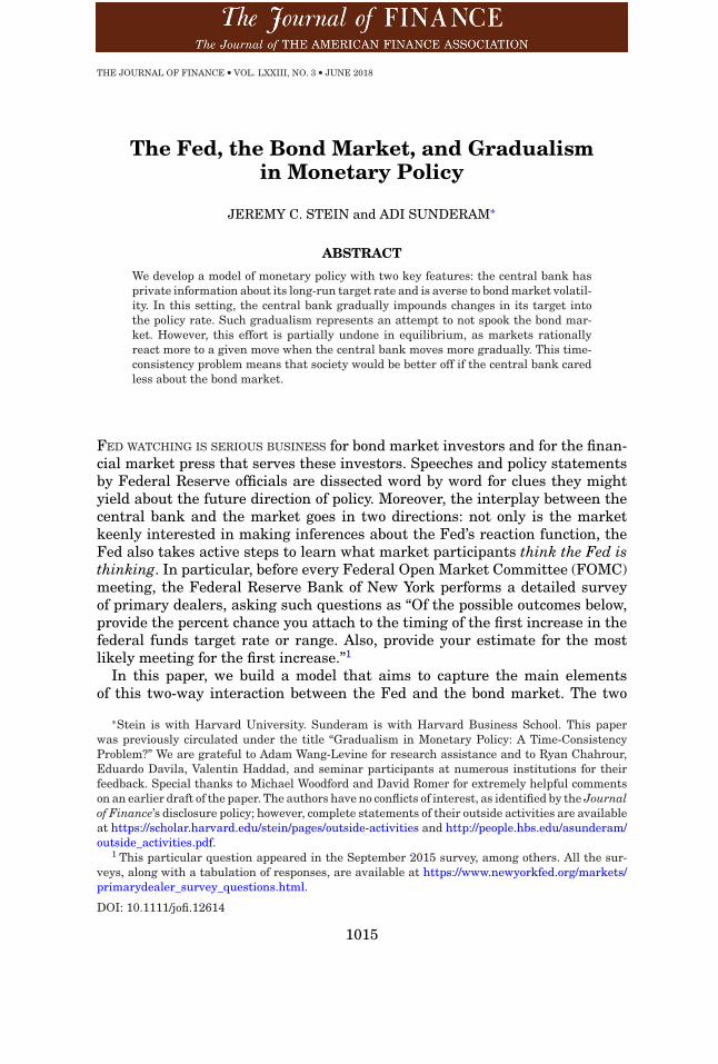
In a crude attempt to speak to this question, we examine all 216 FOMCtranscripts over the 27-year period from 1985 to 2011 and simply measurethe frequency of words related to financial markets.6 Specifically, we count thenumber of times the terms “financial market,” “equity market,” “bond market,”“credit market,” “fixed income,” and “volatility” are mentioned.7 For each year,we aggregate this count and divide by the total number of words in that year’stranscripts.
Figure 1 displays the results from this exercise. As can be seen, there is astrong upward trend in the data. While there is also a good deal of volatilityaround the trend, a simple linear time trend captures almost 52% of the vari-ation in the time series, with a t-statistic of 4.6.8 Moreover, the fitted valueof the series based on this time trend goes up about fourfold over the 27-yearsample period. While extremely simplistic, this analysis does suggest an in-creasing emphasis over time by the FOMC on financial market considerations.If there was such a change in FOMC thinking, the model we develop below iswell suited to drawing out its implications, both for the dynamics of the policyrate and for longer-term yields.
II. Static Model
We begin by presenting what is effectively a static version of the model, inwhich the Fed adjusts the funds rate only partially in response to a one-timeinnovation in its desired target rate. In Section IV, we extend the model to afully dynamic setting in which we can be more explicit about how an innovationto the Fed’s target rate gradually makes its way into the funds rate over time.
6 Given the five-year lag in making transcripts public, 2011 is the last available year. Cieslakand Vissing-Jorgenson (2017) perform a similar but more sophisticated exercise to understand whythe Fed responds to the stock market.
7 We obtain similar results if we use different subsets of these terms. For instance, the resultsare similar if we only count the frequency of the term “financial market.”
8 Restricting the sample to the precrisis period from 1985 to 2006, we obtain an R2 of 49% anda t-statistic of 4.4. So the trend in the data is not driven primarily by the post-2006 period.
The Fed and the Bond Market 1021
1985 1990 1995 2000 2005 2010 20150
5
10
15
Fre
quen
cy (
basi
s po
ints
)
Figure 1. Frequency of terms related to financial markets in FOMC transcripts, 1985–2011. The figure plots the moving average of the frequency of terms related to financial marketsover the last eight FOMC meetings. (Color figure can be viewed at wileyonlinelibrary.com)
Though it is stylized, the static model highlights the main intuition for why adesire to limit bond market volatility creates a time-consistency problem forthe Fed.
A. Model Setup
We begin by assuming that, at any time t, the Fed has a target rate basedon its traditional dual-mandate objectives. This target rate is the Fed’s bestestimate of the value of the federal funds rate that keeps inflation and unem-ployment as close as possible to their desired levels. For tractability, we assumethat the target rate, denoted by i∗
t , follows a random walk, so that
i∗t = i∗
t−1 + εt, (1)
where εt ∼ N(0, σ 2ε ≡ 1
τε) is normally distributed. Our key assumption is that i∗
tis private information of the Fed and is unknown to market participants beforethe Fed acts at time t. One can think of the private information embodied ini∗t as arising from the Fed’s attempts to follow something akin to a Taylor rule,
where it has private information about the appropriate coefficients to use inthe rule (i.e., its reaction function) or about its own forecasts of future inflationor unemployment. As noted above, an assumption of private information alongthese lines is necessary if one wants to understand why asset prices respondto Fed policy announcements.

1022 The Journal of Finance R©
Once it knows the value of i∗t , the Fed acts to incorporate some of its new
private information εt into the federal funds rate it, which is observable to themarket. We assume that the Fed picks it on a discretionary period-by-periodbasis to minimize the loss function Lt, given by
Lt = (i∗t − it
)2 + θ(�i∞
t
)2, (2)
where i∞t is the infinite-horizon forward rate. Thus, the Fed has the usual
concerns about inflation and unemployment, as captured in reduced form by adesire to keep i∗
t close to it. However, when θ > 0, the Fed also cares about thevolatility of long-term bond yields, as measured by the squared change in theinfinite-horizon forward rate.
For simplicity, we start by assuming that the expectations hypothesis holds,so there is no time-variation in the term premium. This implies that the infinite-horizon forward rate is equal to the expected value of the funds rate that willprevail in the distant future. Because the target rate i∗
t follows a random walk,the infinite-horizon forward rate is then given by the market’s best estimate ofthe current target i∗
t at time t. Thus, we have i∞t = Et[i∗
t ] so long as we are in anequilibrium where rates eventually adjust toward the target, no matter howslowly. In Section III.E.2, we relax the assumption that the expectations hy-pothesis holds so that we can also consider the Fed’s reaction to term-premiumshocks.
Several features of the Fed’s loss function are worth discussing. First, in oursimple formulation, θ reflects the degree to which the Fed is concerned aboutbond market volatility, over and above its desire to keep it close to i∗
t . To be clear,this loss function need not imply that the Fed cares about asset prices for theirown sake. An alternative interpretation is that volatility in financial marketconditions can affect the real economy and hence the Fed’s ability to satisfy itstraditional dual mandate. This linkage is not modeled explicitly here, but asone example of what we have in mind, the Fed might believe that a spike inbond market volatility could damage highly levered financial intermediariesand interfere with the credit supply process. With this stipulation in mind, wetake as given that θ reflects the socially “correct” objective function—in otherwords, it is exactly the value that a well-intentioned social planner wouldchoose. We then ask whether there is a time-consistency problem when theFed tries to optimize this objective function period by period, in the absence ofa commitment technology.
Second, note that the Fed’s target in the first term of equation (2) is theshort-term policy rate, whereas the bond market volatility that it is con-cerned about in the second term of equation (2) refers to the variance of long-term market-determined rates. This short versus long divergence is crucialfor our results on time-consistency. To see why, consider two alternative lossfunctions:
Lt = (i∗t − ii
)2 + θ (�ii)2, (2′)

The Fed and the Bond Market 1023
Lt = (i∞∗t − i∞
t
)2 + θ(�i∞
t
)2. (2′′)
In equation (2′), the Fed cares about the volatility of the funds rate, ratherthan the volatility of the long-term rate. This objective function mechanicallyproduces gradual adjustment of the funds rate, but because there is no forward-looking long rate, there is no issue of the Fed trying to manipulate marketexpectations and hence no time-consistency problem. Thus, in positive terms, amodel of this sort delivers gradualism, but in normative terms this gradualismis entirely optimal from the Fed’s perspective. However, by emphasizing onlyshort-rate volatility, this formulation arguably fails to capture the financialstability goal articulated by Greenspan, namely, to “not create discontinuousproblems with respect to balance sheets and asset values.” We believe thatputting the volatility of the long-term rate directly in the objective function, asin equation (2), does a better job in this regard.
In equation (2′′), the Fed pursues its dual-mandate objective not by havinga target for the funds rate, but instead by explicitly targeting the long rateof i∞∗
t . In this case, given that the same rate i∞t appears in both parts of the
objective function, there is again no time-consistency problem.9 Moreover, onemight think that the first term in equation (2′′) is a reasonable reduced-formway to model the Fed’s efforts to achieve its mandate. In particular, in standardNew Keynesian models, it is long-term real rates, not short rates, that matterfor inflation and output stabilization.
Nevertheless, our formulation of the Fed’s objective function in equation (2)can be motivated in a couple of ways. First, equation (2) is arguably morerealistic than equation (2′′) as a description of how the Fed actually behaves,and—importantly for our purposes—communicates about its future intentions.For example, in recent statements, the Fed has argued that one motive foradjusting policy gradually is the fact that r*, defined as the equilibrium (orneutral) value of the short rate, is itself slow-moving.10 But the concept of aslow-moving r* can only make logical sense if the short rate matters directlyfor real outcomes. If instead real outcomes were entirely a function of longrates, the near-term speed of adjustment of the short rate would be irrelevant,holding fixed the total expected adjustment.
Second, in many other models of the monetary transmission mechanismoutside of the New Keynesian genre, the short rate does have an importantindependent effect on economic activity. For instance, the literature on thebank lending channel, including Bernanke and Blinder (1992), Kashyap andStein (2000), and Drechsler, Savov, and Schnabl (2017), finds that bank loan
9 We are grateful to Mike Woodford for emphasizing this point to us and for providing a simpleproof.
10 In Chair Janet Yellen’s press conference of December 16, 2015, she said: “This expecta-tion (of gradual rate increases) is consistent with the view that the neutral nominal federalfunds rate—defined as the value of the federal funds rate that would be neither expansionarynor contractionary if the economy were operating near potential—is currently low by histori-cal standards and is likely to rise only gradually over time.” See http://www.federalreserve.gov/mediacenter/files/FOMCpresconf20151216.pdf.

1024 The Journal of Finance R©
supply is directly influenced by changes in the short rate because the shortrate effectively governs the availability of low-cost deposit funding. Similarly,recent papers on “reaching for yield,” including Gertler and Karadi (2015),Jimenez et al. (2014), and Dell’Ariccia, Laeven, and Suarez (2013), argue thatrisk premiums and ultimately real activity respond to the level of the shortrate. Both of these channels help explain why it can make sense for the Fed totarget the short rate per se.
The assumption that the Fed cares about the volatility of the infinite-horizonforward rate i∞
t , along with the fact that the target rate i∗t follows a random
walk, makes for a convenient simplification. Because i∗t follows a random walk,
all of the new private information εt will, in expectation, eventually be incorpo-rated into the future short rate. Focusing on the reaction of the infinite-horizonforward rate reflects this revision in expectations and allows us to abstractfrom the exact dynamic path that the Fed follows in ultimately incorporatingits new information into the funds rate. In contrast, revisions in finite-horizonrates depend on the exact path of the short rate. For example, suppose i∗
t werepublic information and changed from 1% to 2%. The infinite-horizon forwardrate would immediately jump to 2%, while the two-year forward rate wouldmove less if the market expected a slow tightening. However, for our key con-clusions, it is not necessary that the Fed care about the volatility of the infinite-horizon forward rate; as we demonstrate below, a time-consistency problem stillemerges if the Fed cares instead about the volatility of a finite-horizon rate thatis effectively a weighted average of short-term and infinite-horizon rates.11
Finally, our formulation in equation (2) assumes that the Fed optimizes amyopic period-by-period objective function, so that when it acts at time t, itcares only about the consequences for bond market volatility at t, and notabout volatility in future periods. However, in Sections III.D.1 and IV.A, weshow that we obtain very similar results when the Fed has a forward-lookingobjective function that incorporates a concern about both future as well ascurrent volatility.
B. Equilibrium
With the Fed’s objective function in place, we are now ready to describe thenature of equilibrium in the static model. Once it observes i∗
t , we assume thatthe Fed sets the federal funds rate it by following a partial adjustment rule ofthe form
it = it−1 + k(i∗t − it−1
)+ ut, (3)
where ut ∼ N(0, σ 2u ≡ 1
τu) is normally distributed noise that is overlaid onto the
rate-setting process. The noise ut is a modeling device the usefulness of which
11 The time-consistency problem arises because of the forward-looking nature of longer termrates, and the resulting incentives that the Fed has to manipulate market expectations. As longas the Fed seeks to moderate the volatility of a finite-horizon rate that has some forward-lookingcomponent, an element of the time-consistency problem will remain.
The Fed and the Bond Market 1025
will become clear shortly. Loosely speaking, this noise, which can be thoughtof as a “tremble” in the Fed’s otherwise optimally chosen value of it, ensuresthat the Fed’s actions cannot be perfectly inverted to fully recover its privateinformation i∗
t . As will be seen, this imperfect inversion feature helps avoidsome degenerate equilibrium outcomes. For a concrete interpretation, one canthink of ut as coming from the Fed’s use of round numbers (typically in 25 bpsincrements) for the funds rate settings that it communicates to the market,while its underlying private information about i∗
t is presumably continuous.The market tries to infer the Fed’s private information i∗
t based on its obser-vation of the funds rate it. To do so, it conjectures that the Fed follows a rulegiven by
it = it−1 + κ(i∗t − it−1
)+ ut. (4)
Thus, the market correctly conjectures the form of the Fed’s smoothingrule but, crucially, does not directly observe the Fed’s smoothing parameterk; rather, it has to make a guess κ as to the value of this parameter. In a ratio-nal expectations equilibrium, this guess will turn out to be correct, and we willhave κ = k. However, the key piece of intuition is that when the Fed choosesk, it takes the market’s conjecture κ as a fixed parameter and does not imposeκ = k. The equilibrium concept is thus of the signal-jamming type introducedby Holmstrom (1999): The Fed, taking the market’s estimate of κ as fixed, triesto fool the market into thinking that i∗
t has moved by less than it actuallyhas, in an effort to reduce the volatility of long-term rates. In equilibrium, themarket will rationally unwind the Fed’s actions and not be misled, but the Fedcannot resist the temptation to try.12
Suppose that the economy was previously in steady state at time t − 1, withit−1 = i∗
t−1. Given the Fed’s adjustment rule, the funds rate at time t satisfies
it = it−1 + k(i∗t − it−1
)+ ut = it−1 + kεt + ut. (5)
Based on its conjecture about the Fed’s adjustment rule in equation (4), themarket tries to back out i∗
t from its observation of it. Because both shocks εtand ut are normally distributed, the market’s expectation is given by
E[i∗t |it
] = it−1 + κτu
τε + κ2τu(it − it−1) = it−1 + χ (it − it−1) , (6)
where χ = κτuτε+κ2τu
.
The less noise there is in the Fed’s adjustment rule, the higher is τu and themore the market reacts to the change in the rate it.
12 There is a close analogy to models in which corporate managers with private informationpump up their reported earnings in an effort to impress the stock market. See, for example, Stein(1989).
1026 The Journal of Finance R©
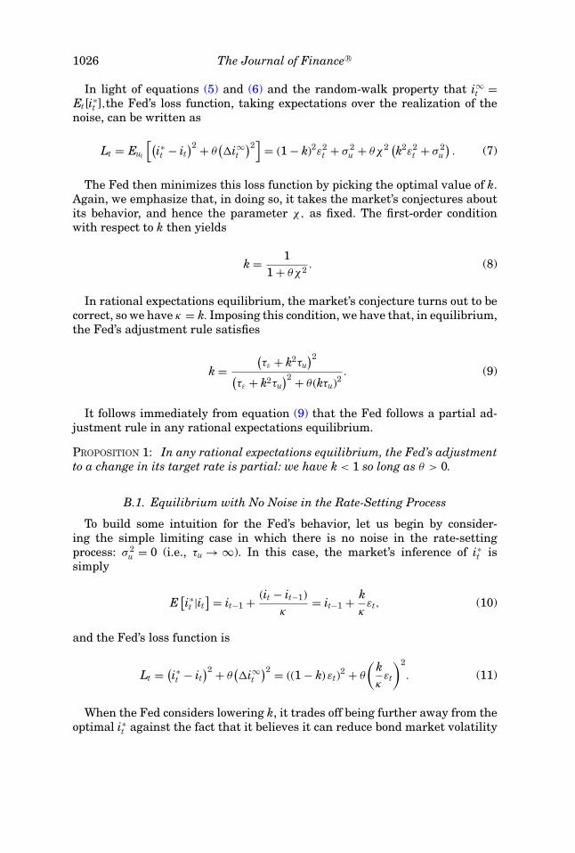
In light of equations (5) and (6) and the random-walk property that i∞t =
Et[i∗t ],the Fed’s loss function, taking expectations over the realization of the
noise, can be written as
Lt = Eut
[(i∗t − it
)2 + θ(�i∞
t
)2]
= (1 − k)2ε2t + σ 2
u + θχ2 (k2ε2t + σ 2
u
). (7)
The Fed then minimizes this loss function by picking the optimal value of k.Again, we emphasize that, in doing so, it takes the market’s conjectures aboutits behavior, and hence the parameter χ, as fixed. The first-order conditionwith respect to k then yields
k = 11 + θχ2 . (8)
In rational expectations equilibrium, the market’s conjecture turns out to becorrect, so we have κ = k. Imposing this condition, we have that, in equilibrium,the Fed’s adjustment rule satisfies
k =(τε + k2τu
)2(τε + k2τu
)2 + θ (kτu)2. (9)
It follows immediately from equation (9) that the Fed follows a partial ad-justment rule in any rational expectations equilibrium.
PROPOSITION 1: In any rational expectations equilibrium, the Fed’s adjustmentto a change in its target rate is partial: we have k < 1 so long as θ > 0.
B.1. Equilibrium with No Noise in the Rate-Setting Process
To build some intuition for the Fed’s behavior, let us begin by consider-ing the simple limiting case in which there is no noise in the rate-settingprocess: σ 2
u = 0 (i.e., τu → ∞). In this case, the market’s inference of i∗t is
simply
E[i∗t |it
] = it−1 + (it − it−1)κ
= it−1 + kκ
εt, (10)
and the Fed’s loss function is
Lt = (i∗t − it
)2 + θ(�i∞
t
)2 = ((1 − k) εt)2 + θ
(kκ
εt
)2
. (11)
When the Fed considers lowering k, it trades off being further away from theoptimal i∗
t against the fact that it believes it can reduce bond market volatility

The Fed and the Bond Market 1027
by moving more slowly. In rational expectations equilibrium, the optimal k nowsatisfies:13
k = k2
k2 + θ. (12)
First note that when θ = 0, the only solution to equation (12) is given byk = 1. When the Fed does not care about bond market volatility, it fully adjuststo its new private information εt. By contrast, when θ > 0, there may be morethan one solution to equation (12), but in any equilibrium it must be the casethat k < 1, and the Fed only partially adjusts.
Moreover, when θ > 0, it is always the case that k = 0 satisfies equation(12). Thus, there is a degenerate solution in which the Fed does not adjustthe funds rate at all. This somewhat unnatural outcome is a function of theextreme feedback that arises between the Fed’s adjustment rule and the mar-ket’s conjecture when there is no noise in the rate-setting process. Specifically,when the market conjectures that the Fed never moves the funds rate at all(i.e., that κ = 0), then even a tiny out-of-equilibrium move by the Fed leads toan infinitely large change in the infinite-horizon forward rate. Thus, the Fedvalidates the market’s conjecture by not moving at all, that is, by choosingk = 0.
However, as soon as there is even an infinitesimal amount of noise ut inthe rate-setting process, this extreme k = 0 equilibrium is ruled out, as smallchanges in the funds rate now lead to bounded market reactions. This explainsour motivation for keeping rate-setting noise in the more general model.
In addition to k = 0, for 0 < θ < 0.25, there are two other solutions to equation(12), given by
k = 1 ± √(1 − 4θ )2
. (13)
Of these, the larger of the two values also represents a stable equilibriumoutcome. Thus, as long as θ is not too big, the model also admits a nondegenerateequilibrium, with½< k < 1, even with σ 2
u = 0. Within this region, higher valuesof θ lead to lower values of k. In other words, the more intense the Fed’s concernabout bond market volatility, the more gradually it adjusts the funds rate.
B.2. Equilibrium Outcomes across the Parameter Space
Now we return to the general case in which σ 2u > 0 and explore the range of
outcomes produced by the model for different parameter values. In each panelof Figure 2, we plot the Fed’s best response k as a function of the market’sconjecture κ. Any rational expectations equilibrium must lie on the 45° linewhere k = κ.
13 Equation (12) can be derived from equation (9) by taking the limit as τu goes to infinity andapplying L’Hopital’s Rule.

1028 The Journal of Finance R©
Panel A Panel B
Panel C Panel D
0 0.1 0.2 0.3 0.4 0.5 0.6 0.7 0.8 0.9 10
0.1
0.2
0.3
0.4
0.5
0.6
0.7
0.8
0.9
1
k
0 0.1 0.2 0.3 0.4 0.5 0.6 0.7 0.8 0.9 10
0.1
0.2
0.3
0.4
0.5
0.6
0.7
0.8
0.9
1
k
0 0.1 0.2 0.3 0.4 0.5 0.6 0.7 0.8 0.9 10
0.1
0.2
0.3
0.4
0.5
0.6
0.7
0.8
0.9
1
k
0 0.1 0.2 0.3 0.4 0.5 0.6 0.7 0.8 0.9 10
0.1
0.2
0.3
0.4
0.5
0.6
0.7
0.8
0.9
1k
= kBest response given
= kBest response given
= kBest response given
= kBest response given
Figure 2. Equilibria of the static model for different parameter values. θ indexes theFed’s aversion to volatility, τ ε is the precision of innovations to the target rate, τu is the precisionof rate-setting noise, κ is the market’s conjecture about the Fed’s degree of adjustment, k is theFed’s best response degree of adjustment. Panel A: θ = 0.2, τ ε = 1, and τu = 10. Panel B: θ = 1.0,τ ε = 1, and τu = 10. Panel C: θ = 1.0, τ ε = 1, and τu = 250. Panel D: θ = 0.2, τ ε = 1, and τu = 250.(Color figure can be viewed at wileyonlinelibrary.com)
In Panel A of the figure, we begin with a relatively low value of θ , namely,0.2, and set σ 2
ε /σ 2u = 10, so that the variance of rate-setting noise is one-tenth
the variance of innovations to the target rate. As can be seen, this leads to aunique equilibrium with a high value of k of 0.81. When the Fed cares only abit about bond market volatility, it adjusts rates fairly aggressively because itdoes not want to deviate too far from its target rate i∗
t .In Panel B, we raise θ to 1.0, while keeping σ 2
ε /σ 2u = 10 as in Panel A. In
this high-θ case, the unique equilibrium involves a lower value of k of 0.29.Thus, when the Fed cares a lot about bond market volatility, the funds ratesignificantly underadjusts to new information.
In Panel C, we keep θ = 1.0 but decrease the rate-setting noise, so thatσ 2
ε /σ 2u = 250. Now the equilibrium involves an extremely low value of k of just

The Fed and the Bond Market 1029
0.03. The difference between Panels B and C is the degree of rate-setting noise.The greater amount of noise in Panel B allows the Fed to hide the informationcontent of its actions, so that it can be more responsive to changes in its targetwithout changing the market’s inference about its private information by asmuch.14
Finally, in Panel D, we set θ = 0.2 and σ 2ε /σ 2
u = 250. Here, we have multipleequilibria: the Fed’s best response crosses the 45° line in three places. Of thesethree crossing points, the two outer ones (at k = 0.08 and 0.73) correspond tostable equilibria, in the sense that if the market’s initial conjecture κ takes anout-of-equilibrium value, the Fed’s best response to that conjecture will tend todrive the outcome toward one of these two extreme crossing points.
The existence of multiple equilibria highlights an essential feature of themodel: the potential for market beliefs about Fed behavior to become self-validating. If the market conjectures that the Fed adjusts rates only very grad-ually, then even small changes are heavily freighted with informational contentabout the Fed’s reaction function. Given this strong market sensitivity and itsdesire not to create too much volatility, the Fed may then choose to move verycarefully, even at the cost of accepting a funds rate that is quite far from itstarget. Conversely, if the market conjectures that the Fed is more aggressive inits adjustment of rates, it reacts less to any given movement, which frees theFed up to track the target rate more closely.
When there are multiple equilibria, the one with the higher value of k typ-ically leads to a better outcome from the perspective of the Fed’s objectivefunction: With a higher k, it is closer to i∗
t , but in equilibrium, bond marketvolatility is not much greater. Thus, if we are in a range of the parameter spacewhere multiple equilibria are possible, it is important for the Fed to avoiddoing anything in its communications that tends to lead the market to con-jecture too low a value of κ. Even keeping its own preferences fixed, fosteringan impression of strong gradualism among market participants can lead to anundesirable outcome in which the Fed gets stuck in the low-k equilibrium.
C. The Time-Consistency Problem
A central property of our model is that there is a time-consistency problem:The Fed would do better in terms of optimizing its own objective function if itwere able to commit to behaving as if it had a lower value of θ than it actuallydoes. This is because while the Fed is always tempted to move the funds rategradually so as to reduce bond market volatility, this desire is partially undonein equilibrium: The more gradually the Fed acts, the more the market respondsto any change in rates, and yet the Fed is still left with a funds rate that isfurther from target on average.
This point is most transparent if we consider the limiting case in which thereis no noise in the Fed’s rate-setting process. In this case, once we impose the
14 This is similar to the intuition in Kyle (1985). When there are more noise traders, the insidercan trade more aggressively on his private information without as much market impact.

1030 The Journal of Finance R©
rational expectations assumption that κ = k,the Fed’s attempts at smoothinghave no effect on bond market volatility in equilibrium:
(�i∞
t
)2 =(
kκ
εt
)2
= ε2t . (14)
Thus, the value of the Fed’s loss function is
Lt = (i∗t − it
)2 + θ(�i∞
t
)2 = ((1 − k) εt)2 + θε2t , (15)
which is decreasing in k for k < 1.To the extent that the target rate i∗
t is nonverifiable private information, itis hard to think of a contracting technology that can readily implement thefirst-best outcome under commitment: How does one write an enforceable rulethat says that the Fed must always react fully to its private information? Thus,discretionary monetary policy will inevitably be associated with some degree ofinefficiency. However, even in the absence of a binding commitment technology,there may still be scope for improving on the fully discretionary outcome. Onepossible approach follows in the spirit of Rogoff (1985), who argues that societyshould appoint a central banker who is more hawkish on inflation than issociety itself. The analogy in the current context is that society should appointa central banker who cares less about financial market volatility (i.e., has alower value of θ ) than society as a whole. Put differently, society—and thecentral bank itself—should foster an institutional culture and set of normsthat discourage the monetary policy committee from being overly attentive toshort-term market volatility considerations.
To see this, consider the problem of a social planner choosing a central bankerwhose concern about financial market volatility is given by θc. This centralbanker will implement the rational expectations adjustment rule k(θc), wherek is given by equation (9), replacing θ with θc. In the rational expectationsequilibrium, this will result in bond market volatility
Var [χ (k (θc) εt + ut)] = k(θc)2τu
τε
(τε + k(θc)2τu
) . (16)
In contrast to the no-noise case, here bond market volatility is not invariant tothe choice of k. Thus, the planner’s ex ante problem is to pick θc to minimize itsex ante loss, recognizing that its own concern about financial market volatilityis given by θ :
Eεt
[(i∗t − it
)2 + θ(�i∞
t
)2]
= E[((1 − k (θc)) εt + ut)2 + θ (χ (k (θc) εt + ut))2
]. (17)
The following proposition characterizes the optimal θ c.
PROPOSITION 2: In the presence of rate-setting noise, it is ex ante optimal toappoint a central banker with θc < θ . In the absence of rate-setting noise, it is exante optimal to appoint a central banker with θc = 0, so that k(θc) = 1.
The Fed and the Bond Market 1031
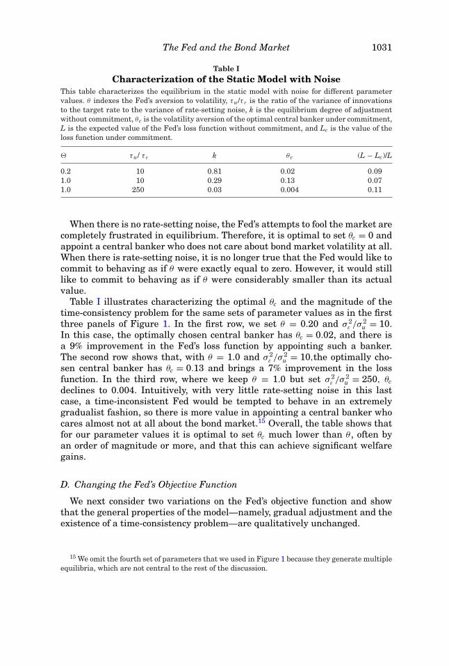
Table ICharacterization of the Static Model with Noise
This table characterizes the equilibrium in the static model with noise for different parametervalues. θ indexes the Fed’s aversion to volatility, τu/τ ε is the ratio of the variance of innovationsto the target rate to the variance of rate-setting noise, k is the equilibrium degree of adjustmentwithout commitment, θ c is the volatility aversion of the optimal central banker under commitment,L is the expected value of the Fed’s loss function without commitment, and Lc is the value of theloss function under commitment.
τu/ τ ε k θ c (L − Lc)/L
0.2 10 0.81 0.02 0.091.0 10 0.29 0.13 0.071.0 250 0.03 0.004 0.11
When there is no rate-setting noise, the Fed’s attempts to fool the market arecompletely frustrated in equilibrium. Therefore, it is optimal to set θc = 0 andappoint a central banker who does not care about bond market volatility at all.When there is rate-setting noise, it is no longer true that the Fed would like tocommit to behaving as if θ were exactly equal to zero. However, it would stilllike to commit to behaving as if θ were considerably smaller than its actualvalue.
Table I illustrates characterizing the optimal θc and the magnitude of thetime-consistency problem for the same sets of parameter values as in the firstthree panels of Figure 1. In the first row, we set θ = 0.20 and σ 2
ε /σ 2u = 10.
In this case, the optimally chosen central banker has θc = 0.02, and there isa 9% improvement in the Fed’s loss function by appointing such a banker.The second row shows that, with θ = 1.0 and σ 2
ε /σ 2u = 10,the optimally cho-
sen central banker has θc = 0.13 and brings a 7% improvement in the lossfunction. In the third row, where we keep θ = 1.0 but set σ 2
ε /σ 2u = 250, θc
declines to 0.004. Intuitively, with very little rate-setting noise in this lastcase, a time-inconsistent Fed would be tempted to behave in an extremelygradualist fashion, so there is more value in appointing a central banker whocares almost not at all about the bond market.15 Overall, the table shows thatfor our parameter values it is optimal to set θc much lower than θ , often byan order of magnitude or more, and that this can achieve significant welfaregains.
D. Changing the Fed’s Objective Function
We next consider two variations on the Fed’s objective function and showthat the general properties of the model—namely, gradual adjustment and theexistence of a time-consistency problem—are qualitatively unchanged.
15 We omit the fourth set of parameters that we used in Figure 1 because they generate multipleequilibria, which are not central to the rest of the discussion.

1032 The Journal of Finance R©
D.1. Forward-Looking Objective: A Concern with Future Volatility
We first consider what happens when the Fed has a forward-looking objec-tive rather than a myopic period-by-period one. Note that in the loss functionspecified in equation (2), when the Fed acts at time t, it worries about its impacton bond market volatility at t but does not take into account the consequencesof its decision for volatility in future periods. One might suspect that if it did,its temptation to act gradually would be reduced, since by doing so it simplydefers any adjustment of prices to the future.
To address this issue, suppose that there is a single realization of privateinformation εt at time t and no further shocks after that. For simplicity, supposefurther that the Fed follows the partial adjustment rule in equation (3) attime t and then fully impounds εt into the funds rate at time t + 1. That is,it+1 = i∗
t+1 = i∗t−1 + εt. Finally, assume that the Fed is forward-looking and takes
time t + 1 into account when it picks its partial adjustment speed at time t.Specifically, it has the following loss function:
Lt = (i∗t − it
)2 + θ(�i∞
t
)2 + (i∗t+1 − it+1
)2 + θ(�i∞
t+1
)2. (18)
In the Appendix, we prove the following proposition, which states that bothgradualism and the time-consistency problem remain in this setting.
PROPOSITION 3: With a forward-looking objective function in the static modelwith noise, both partial adjustment and the time-consistency problem remain:k < 1 so long as θ > 0, and it is ex ante optimal to appoint a central banker withθc = 0.
The intuition for the proposition is as follows. On the one hand, taking themarket’s conjectures about its behavior as given, when the Fed tries to reducethe size of a move in bond prices at time t by adjusting the funds rate gradually,it recognizes that, if it is successful, this will lead to a larger move at timet + 1—because eventually its private information must come out. On the otherhand, because its loss function is convex in the size of price moves in eachperiod, distributing the price change over time is still attractive. A motive toact gradually therefore remains.16
An interesting feature of this variation is that the time-consistency problemis starker, in the sense that, even with nonzero rate-setting noise, it is nowalways optimal to appoint a central banker who does not care at all aboutthe bond market, that is, who has θc = 0. With a myopic loss function, a Fedthat acts gradually in the presence of rate-setting noise partially succeeds inreducing the size of this period’s move in the infinite-horizon forward rate.
16 In a more fully dynamic setup, the Fed might act as if private information suppressed attime t would not come out all at once at t+1, but would make its way into prices more slowly overseveral subsequent periods. This case actually behaves more like the baseline one with the myopicobjective function, again due to the convex nature of the loss function—the more future periods theremainder of a shock can be spread over, the less the volatility incurred in future periods mattersto the Fed. So arguably, the objective functions in equations (2) and (18) span the full range ofpossibilities.
The Fed and the Bond Market 1033
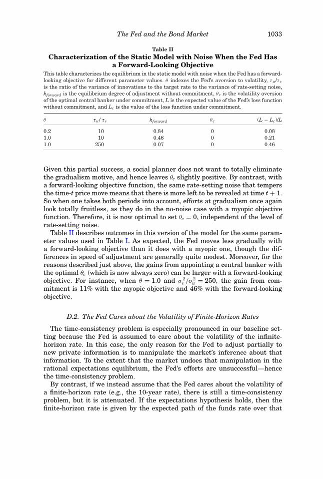
Table IICharacterization of the Static Model with Noise When the Fed Has
a Forward-Looking ObjectiveThis table characterizes the equilibrium in the static model with noise when the Fed has a forward-looking objective for different parameter values. θ indexes the Fed’s aversion to volatility, τu/τ ε
is the ratio of the variance of innovations to the target rate to the variance of rate-setting noise,kforward is the equilibrium degree of adjustment without commitment, θc is the volatility aversionof the optimal central banker under commitment, L is the expected value of the Fed’s loss functionwithout commitment, and Lc is the value of the loss function under commitment.
θ τu/ τ ε kforward θ c (L − Lc)/L
0.2 10 0.84 0 0.081.0 10 0.46 0 0.211.0 250 0.07 0 0.46
Given this partial success, a social planner does not want to totally eliminatethe gradualism motive, and hence leaves θc slightly positive. By contrast, witha forward-looking objective function, the same rate-setting noise that tempersthe time-t price move means that there is more left to be revealed at time t + 1.So when one takes both periods into account, efforts at gradualism once againlook totally fruitless, as they do in the no-noise case with a myopic objectivefunction. Therefore, it is now optimal to set θc = 0, independent of the level ofrate-setting noise.
Table II describes outcomes in this version of the model for the same param-eter values used in Table I. As expected, the Fed moves less gradually witha forward-looking objective than it does with a myopic one, though the dif-ferences in speed of adjustment are generally quite modest. Moreover, for thereasons described just above, the gains from appointing a central banker withthe optimal θc (which is now always zero) can be larger with a forward-lookingobjective. For instance, when θ = 1.0 and σ 2
ε /σ 2u = 250, the gain from com-
mitment is 11% with the myopic objective and 46% with the forward-lookingobjective.
D.2. The Fed Cares about the Volatility of Finite-Horizon Rates
The time-consistency problem is especially pronounced in our baseline set-ting because the Fed is assumed to care about the volatility of the infinite-horizon rate. In this case, the only reason for the Fed to adjust partially tonew private information is to manipulate the market’s inference about thatinformation. To the extent that the market undoes that manipulation in therational expectations equilibrium, the Fed’s efforts are unsuccessful—hencethe time-consistency problem.
By contrast, if we instead assume that the Fed cares about the volatility ofa finite-horizon rate (e.g., the 10-year rate), there is still a time-consistencyproblem, but it is attenuated. If the expectations hypothesis holds, then thefinite-horizon rate is given by the expected path of the funds rate over that

1034 The Journal of Finance R©
finite horizon. The finite-horizon rate therefore responds to both informationabout the Fed’s ultimate destination and the particular path that the Fedchooses to get there. By moving gradually, the Fed can succeed in reducingthe volatility of the realized path. However, its attempts to manipulate themarket’s inference about its ultimate destination will still be partially undonein equilibrium, leaving some element of time-inconsistency.
To develop this intuition, we observe that, in our one-factor model of the termstructure, any finite-horizon rate can be approximated by a weighted averageof the current funds rate it and the infinite-horizon forward rate i∞
t , as longas we pick the weights correctly. Using this approximation, we establish thefollowing proposition, which is proven in the Appendix.
PROPOSITION 4: Suppose that θ > 0 and that the Fed cares about the volatil-ity of a finite-horizon rate, approximated as a weighted average of the shortrate and the infinite-horizon rate. Then it is ex ante optimal to appoint a cen-tral banker with θc being an increasing function of the weight on the shortrate.
Under discretion, the Fed has two motives when it moves gradually. First,it aims to reduce the volatility of the component of the finite-horizon ratethat is related to the current short rate it. Second, it hopes to reduce thevolatility of the component of the finite-horizon rate that is related to theinfinite-horizon forward rate i∞
t by fooling the market about its privateinformation εt. The first goal can be successfully attained in rational expecta-tions equilibrium, but the second will be partially undone, as in the baselinemodel.
Under commitment, the second motive is weakened, and thus it is less ap-pealing to move gradually than it would be under discretion. Thus, if societyis appointing a central banker whose concern about financial market volatil-ity is given by θc, it would like to appoint one with θc < θ . In other words,there is still a time-consistency problem. However, it is not as extreme as thecase in which the social planner cares about the volatility of the infinite-horizonforward rate.
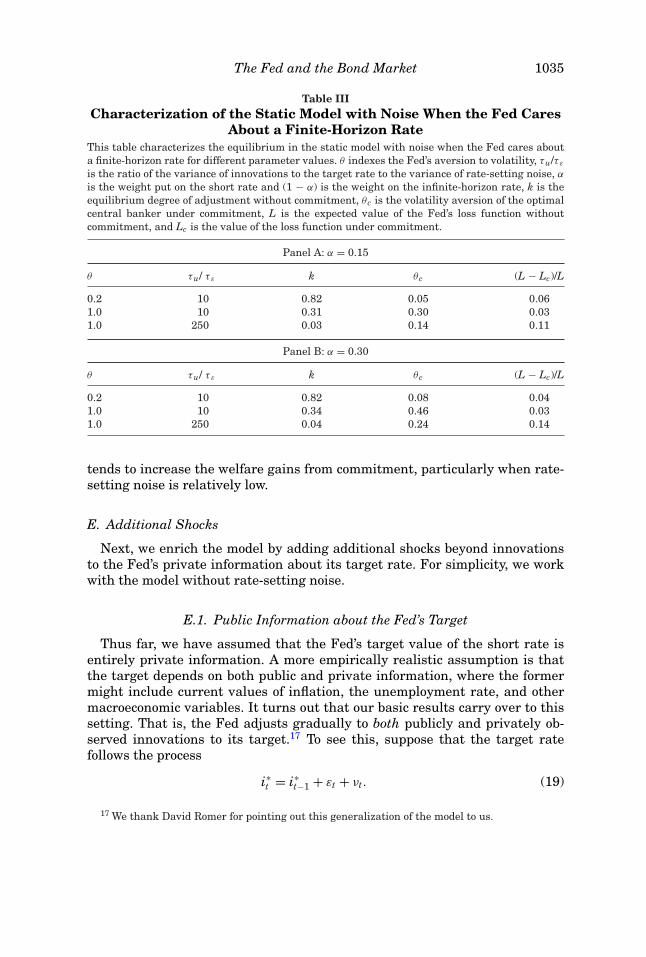
Table III demonstrates this intuition numerically. The table replicatesTable I, but now considers different finite-horizon rates, which put weightα on the funds rate and weight (1 – α) on the infinite-horizon rate. In Panel A ofTable III we set α = 0.15, and in Panel B we set α = 0.30. The table shows thatas α increases, it is optimal to appoint a central banker with a higher valueof θc. Still, there are significant improvements in the Fed’s loss function undercommitment.
We have also tried combining the assumption that the Fed cares about afinite-horizon rate with the assumption that is has a forward-looking objectivefunction, as in Table II. The results (not tabulated) are as one would expectbased on the two mechanisms operating in isolation. That is, there are noparticularly surprising interaction effects. Relative to Table III, making theobjective function forward-looking leads to somewhat less gradualism, but also
The Fed and the Bond Market 1035
Table IIICharacterization of the Static Model with Noise When the Fed Cares
About a Finite-Horizon RateThis table characterizes the equilibrium in the static model with noise when the Fed cares abouta finite-horizon rate for different parameter values. θ indexes the Fed’s aversion to volatility, τu/τ ε
is the ratio of the variance of innovations to the target rate to the variance of rate-setting noise, α
is the weight put on the short rate and (1 − α) is the weight on the infinite-horizon rate, k is theequilibrium degree of adjustment without commitment, θc is the volatility aversion of the optimalcentral banker under commitment, L is the expected value of the Fed’s loss function withoutcommitment, and Lc is the value of the loss function under commitment.
Panel A: α = 0.15
θ τu/ τ ε k θ c (L − Lc)/L
0.2 10 0.82 0.05 0.061.0 10 0.31 0.30 0.031.0 250 0.03 0.14 0.11
Panel B: α = 0.30
θ τu/ τ ε k θ c (L − Lc)/L
0.2 10 0.82 0.08 0.041.0 10 0.34 0.46 0.031.0 250 0.04 0.24 0.14
tends to increase the welfare gains from commitment, particularly when rate-setting noise is relatively low.
E. Additional Shocks
Next, we enrich the model by adding additional shocks beyond innovationsto the Fed’s private information about its target rate. For simplicity, we workwith the model without rate-setting noise.
E.1. Public Information about the Fed’s Target
Thus far, we have assumed that the Fed’s target value of the short rate isentirely private information. A more empirically realistic assumption is thatthe target depends on both public and private information, where the formermight include current values of inflation, the unemployment rate, and othermacroeconomic variables. It turns out that our basic results carry over to thissetting. That is, the Fed adjusts gradually to both publicly and privately ob-served innovations to its target.17 To see this, suppose that the target ratefollows the process
i∗t = i∗
t−1 + εt + νt. (19)
17 We thank David Romer for pointing out this generalization of the model to us.
1036 The Journal of Finance R©
As before, εt is the Fed’s private information. However, νt is publicly observedby both the Fed and the bond market.18 Given the more complicated nature ofthe setting, the Fed’s optimal choice regarding how much to adjust the shortrate no longer depends only on its private information εt. It also depends onthe public information νt. To allow for a general treatment, we posit that thisadjustment can be described by a potentially nonlinear function of the twovariables and that there is no noise in the Fed’s adjustment rule (σ 2
u = 0):
it = it−1 + f (εt; νt) . (20)
Moreover, we assume that the market conjectures that the Fed is followinga potentially nonlinear rule:
it = it−1 + φ (εt; νt) . (21)
In the Appendix, we use a calculus-of-variations type of argument to establishthat, in a rational expectations equilibrium in which f (·; ·) = φ(·; ·), the Fed’sadjustment rule is given by
it = it−1 + kεεt + kννt, (22)
where
kν = kε and kε = k2ε + θ. (23)
The following proposition summarizes the key properties of the equilibrium.
PROPOSITION 5: The Fed responds as gradually to public information aboutchanges in the target rate as it does to private information. This is true re-gardless of the relative contributions of public and private information to thetotal variance of the target. As the Fed’s concern about bond market volatility θ
increases, both kε and kν fall.
Proposition 5 is striking and may at first glance seem counterintuitive. Givenour previous results, one might think that there is no reason for the Fed to movegradually with respect to public information. However, while this is correct inthe limit case where there is no private information whatsoever, it turns outto be wrong as soon as we introduce a small amount of private information.The logic is as follows. Suppose there is a piece of public information thatsuggests that the funds rate should rise by 100 bps, for example, there is asharp increase in the inflation rate. This news, if released on its own, wouldtend to also create a spike in long-term bond yields. In an effort to mitigate thisspike, the Fed is tempted to show a more dovish hand than it had previously,
18 We assume that the Fed is equally averse to volatility in the infinite-horizon rate induced byeither εt or νt. For example, suppose that the Fed’s aversion to volatility is rooted in the recognitionthat (i) sharp bond market movements can affect the solvency of financial institutions and (ii)distressed financial institutions can adversely affect the real economy. If this is the case, the Fedwill want to spread volatility out over time, regardless of its source.

The Fed and the Bond Market 1037
that is, to act as if it has simultaneously received a negative innovation to theprivately observed component of its target. To do so, it raises the funds rate byless than it otherwise would. In an out-of-equilibrium sense, this is an attemptto convey that it has offsetting private information.
As before in the no-noise case, this effort to fool the market is not successfulin equilibrium, but the Fed cannot resist the temptation to try. And as longas there is just a small amount of private information, the temptation alwaysexists because, at the margin, the existence of private information leads the Fedto act as if it can manipulate market beliefs. Hence, even if private informationdoes not represent a large fraction of the total variance of the target, the degreeof underadjustment predicted by the model is the same as in an all-private-information setting.
E.2. Term-Premium Shocks
We next enrich the model in another direction, to consider how the Fedbehaves when financial market conditions are not purely a function of theexpected path of interest rates. Here we relax the assumption that the expec-tations hypothesis holds and instead assume that the infinite-horizon forwardrate consists of both the expected future short rate and an exogenous term-premium component rt:
i∞t = Et
[i∗t
]+ rt. (24)
The term premium is assumed to be public information, observed simultane-ously by market participants and the Fed. We allow the term premium to followan arbitrary process and let ηt denote the innovation in the term premium:
ηt = rt − Et−1 [rt] . (25)
The solution method is similar to that in the preceding section. Specifically,we assume that there is only private information about the Fed’s target, there isno noise in the Fed’s rate-setting rule (σ 2
u = 0), and the rule can be an arbitrarynonlinear function of both the new private information εt that the Fed learnsat time t as well as the term-premium shock ηt, which is publicly observable.
In the Appendix, we show that in equilibrium, the Fed’s adjustment rule isgiven by
it = it−1 + kεεt + kηηt, (26)
where
kε = k2ε + θ and
kη = − θkε
.(27)
The following proposition summarizes the key properties of the equilibrium.
PROPOSITION 6: The Fed acts to offset publicly observable term-premium shocks,lowering the funds rate when the term-premium shock is positive and raising
1038 The Journal of Finance R©
it when the term-premium shock is negative. As the Fed’s concern with bondmarket volatility θ increases, kε falls and kη increases in absolute magnitude.Thus, when it cares more about the bond market, the Fed reacts more graduallyto changes in its private information about its target rate, but more aggressivelyto changes in term premiums.
The intuition here is similar to that for why the Fed underreacts to publicinformation about its target. When the term premium spikes up, the Fed isunhappy about the prospective increase in the volatility of long rates. So evenif its private information about i∗
t has not changed, it would like the market tothink it has become more dovish. It therefore cuts the short rate to create thisimpression. Again, in a no-noise equilibrium, this attempt to fool the marketis not successful, but taking the market’s conjectures at any point in time asfixed, the Fed is always tempted to try.
To see why the equilibrium must involve the Fed reacting to term-premiumshocks, think about what happens if we try to sustain an equilibrium in whichit does not. That is, consider what happens if we try to sustain an equilibriumin which kη = 0. In such a hypothetical equilibrium, when the market sees anymovement in the funds rate, it attributes that movement entirely to changes inthe Fed’s private information εt about its target rate. But if this is the case, thenthe Fed can indeed offset movements in term premiums by changing the shortrate, thereby contradicting the assumption that kη = 0. Hence, kη = 0 cannotbe an equilibrium.
A noteworthy feature of the equilibrium is that the absolute magnitude ofkη increases as θ rises and as kε decreases: When it cares more about bondmarket volatility, the Fed’s responsiveness to term-premium shocks becomesmore aggressive even as its adjustment to new information about its targetbecomes more gradual. In particular, because we are restricting ourselves tothe region of the parameter space over which the simple no-noise model yields anondegenerate equilibrium for kε, this means that we must have 0 < θ< ¼ fromequation (13) above. As θ moves from the lower to the upper end of this range,kε declines monotonically from 1 to ½, and kη increases in absolute magnitudefrom 0 to –½.
This property yields a sharp testable empirical implication. As noted earlier,Campbell, Pflueger, and Viceira (2015) show that the Fed’s behavior has becomesignificantly more inertial in recent years. We might be tempted to use the logicof the model to claim that this is a result of the Fed placing increasing weightover time on the bond market, that is, having a higher value of θ than it usedto. While the evidence on financial market mentions in the FOMC transcriptsthat we plot in Figure 1 is loosely consistent with this hypothesis, it is obviouslyfar from being a decisive test. However, with Proposition 6 in hand, if we wantto attribute a decline in kε to an increase in θ , then we also have to confrontthe additional prediction that we should observe the Fed responding moreforcefully over time to term-premium shocks. That is, the absolute value of kη
must have gone up. If this is not the case, it would represent a rejection of thehypothesis.

The Fed and the Bond Market 1039
III. Dynamic Model
In the static model considered thus far, the phenomenon of gradualism isreally nothing more than underreaction of the policy rate to a one-time shockto the Fed’s target. This leaves open the important question of dynamic adjust-ment: If a private-information shock of εt is only partially incorporated intothe funds rate at time t, how long before it is fully impounded? As we showbelow, in the absence of any rate-setting noise (σ 2
u = 0), the adjustment processis trivially fast —εt is fully reflected in the funds rate one period later, by timet + 1. In this case, one might question whether the model captures economicallymeaningful effects, given that the FOMC meets twice per quarter.
Things become more interesting in the case with nonzero rate-setting noise(σ 2
u > 0). Here, the dynamic adjustment process is more protracted, and thepositive and normative implications of the model correspondingly more sub-stantial. However, this case is technically challenging to analyze in its fullgenerality because, in the presence of noise, the fully rational solution to themarket’s inference problem becomes extremely complex. Loosely speaking, ateach point in time t, in order to estimate the current Fed target i∗
t , the marketneeds to have a separate running estimate of each of the past innovations in theFed’s private information, εt− j , each of which it then updates using a separatefiltering process over all of the past realizations of the funds rate.
To attack this difficult problem, we proceed in two steps. We first solve a fullyrational three-period version of the model. Here, the filtering problem is easyenough to handle, and we can use this setup to show that when there is nonzerorate-setting noise, the dynamic adjustment process is no longer trivial. That is,a private-information shock εt can remain substantially underreflected in thefunds rate not only at time t, but at time t + 1 as well. This suggests, albeit onlyqualitatively, that the positive and normative implications of the model may bemore economically interesting, even when Fed meetings are spaced relativelyclosely together.
We next turn to an approximate but fully dynamic version of the model withan infinite horizon. This allows us to compare our model’s quantitative pre-dictions more directly with the existing empirical evidence on gradualism. Tomake things tractable, we model the market’s inferences about the Fed’s targetrate using a heuristic, near-rational approximation of the optimal Bayesian fil-tering process. As can be seen by comparison to the fully rational three-periodmodel, our heuristic arguably allows us to capture the broad spirit of how up-dating about i∗
t works when there is rate-setting noise, but greatly simplifiesthe analytics.
A. Three-Period Model
We begin with a fully rational, three-period model with rate-setting noise.Suppose we start at time 0 in steady state with i0 = i∗
0 . At time 1, the Fedreceives new private information ε1, and there are no further innovations to thetarget rate afterward, so i∗
1 = i∗2 = i∗
0 + ε1. The Fed follows partial adjustment

1040 The Journal of Finance R©
rules with noise at both times 1 and 2, and then fully incorporates its privateinformation into the funds rate at time 3. Thus, we have
i1 = i0 + k1ε1 + u1i2 = i0 + k2ε1 + u2i3 = i0 + ε1.
(28)
We assume that the noise shocks at times 1 and 2 are independent, and thatboth u1 and u2 have variance σ 2
u . The market conjectures that the Fed followsthe adjustment rules
i1 = i0 + κ1ε1 + u1i2 = i0 + κ2ε1 + u2i3 = i0 + ε1.
(29)
Finally, the Fed’s loss function is given by(i1 − i∗
1
)2 + θ(�i1
∞)2 + (i2 − i∗
2
)2 + θ(�i2
∞)2 + (i3 − i∗
3
)2 + θ(�i3
∞)2. (30)
The Fed picks the optimal k1 and k2 with this forward-looking objective, butwithout the ability to commit to moving at a particular speed. In other words,k2 is set on a discretionary basis at time 2 and cannot be locked in at time 1.In the Appendix, we show that the rational expectations equilibrium in thisversion of the model has the following properties.
PROPOSITION 7: In the three-period model with noise, there is partial adjustmentat both times 1 and 2 : k1 < 1 and E[k2] < 1 if and only if σ 2
u > 0. In addition,the time-consistency problem remains, and it is ex ante optimal to appoint acentral banker with θc = 0.
As before, we have partial adjustment at time 1. If there is no rate-settingnoise, then the underadjustment is short-lived: In the next period, the Fed fullyimpounds what was left of the time-t innovation into the rate. In other words,k2 = 1 if σ 2
u = 0. Intuitively, with no noise, investors have already figured outall of the Fed’s time-1 private information by time 2. Given that the Fed can nolonger fool investors about this old information, there is no remaining motivefor it to continue to incorporate it into rates slowly.19
However, if there is noise in the rate-setting process so that σ 2u > 0,then
the market still has some residual uncertainty about the Fed’s time-1 privateinformation ε1 at time 2. By moving gradually once again at time 2, the Fedhopes to keep this information from hitting the market all at once in the nextgo-round.20 As in the static model with noise, this hope is partially frustrated in
19 Why is it that the Fed underreacts to public news about the target νt in Proposition 5 but doesnot continue to underreact to what is now (by time 2) public information about ε1 in Proposition 7?The key difference is timing. In Proposition 5, we have two simultaneous innovations to the targetrate, so the Fed can try to offset the public news by pretending it has offsetting private news. InProposition 7, the bond market volatility due to ε1 has already been realized at time 1. So beingmore dovish at time 2 does not help reduce volatility at time 2.
20 The actual value of k2 depends on the realizations of ε1 and u1. For this reason, Proposition 7characterizes E[k2].

The Fed and the Bond Market 1041
Table IVCharacterization of the Three-Period Model with Noise
This table characterizes the equilibrium in the three-period model with noise for different parame-ter values. θ indexes the Fed’s aversion to volatility, τu/τ ε is the ratio of the variance of innovationsto the target rate to the variance of rate-setting noise, k1 and k2 are the equilibrium degrees ofadjustment without commitment at times 1 and 2, respectively, θc is the volatility aversion ofthe optimal central banker under commitment, L is the expected value of the Fed’s loss functionwithout commitment, and Lc is the value of the loss function under commitment.
θ τu/ τ ε k1 k2 θ c (L − Lc)/L
0.20 10 0.83 0.99 0 0.071.0 10 0.40 0.85 0 0.241.0 250 0.05 0.11 0 0.63
rational expectations equilibrium, and the time-consistency problem persists.Indeed, given the forward-looking nature of the objective function, a general-ization of Proposition 3 applies, and we can show that it is ex ante optimal toappoint a central banker with θc = 0.
Table IV illustrates the outcomes in the three-period model for differentparameter values. The first row shows that when θ = 0.20 and σ 2
ε /σ 2u = 10, there
is partial adjustment at time 1 but near-full adjustment by time 2. Nonetheless,committing to a central banker with θc = 0 results in a 7% improvement inthe Fed’s loss function. The second row shows that as we increase the Fed’sconcern about bond market volatility (θ = 1.0), we get slower adjustment atboth times 1 and 2, and there is significant underincorporation of the Fed’sprivate information into the funds rate even as of time 2, with k2 = 0.85. Here,committing to a central banker with θc = 0 would result in a 23% improvementin the Fed’s loss function. Finally, the third row shows that, with θ = 1.0 andrelatively little rate-setting noise (σ 2
ε /σ 2u = 250), the Fed can get stuck in a
very gradual equilibrium at both times 1 and 2. In this case, k2 falls all theway to 0.11, so that most of the time-1 private information still has not beenimpounded into the funds rate as of time 2. With so little noise, the Fed hasalmost no cover to adjust the funds rate at either date if it does not want tochange the market’s inference much. Here, committing to a central bankerwith θc = 0 would result in a 63% improvement in the Fed’s loss function, sothe time-consistency problem is quite severe.
Overall, the results of the three-period model suggest that the key implica-tions of our model survive in a dynamic setting. Partial adjustment can persistover multiple periods, amplifying the welfare impact of the time-consistencyproblem.
B. Near-Rational Dynamic Model
To more satisfactorily explore the positive properties of the model, we needa more fully articulated dynamic framework. Moreover, if we want to directlycompare the model to empirical evidence, we need to consider the case in which

1042 The Journal of Finance R©
there are both public- and private-information shocks to the Fed’s target rate.Accordingly, we assume that
i∗t = i∗
t−1 + εt + νt, (31)
where εt is the Fed’s private information and the νt is public information—forexample, news about inflation or unemployment.
Suppose that we enter period t with a preexisting gap between the timet − 1 target rate and the time t − 1 federal funds rate of
i∗t−1 − it−1 ≡ Xt−1 + Yt−1, (32)
where Xt−1 is the private-information component of the gap and Yt−1 is thepublic-information component. Even in the presence of rate-setting noise, Yt−1is known by the market with certainty. In contrast, the market must infer Xt−1from the Fed’s previous actions, and with rate-setting noise may still have animperfect estimate as of time t. As mentioned above, modeling the fully rationalBayesian filtering problem for estimating Xt−1 is extremely complicated in thissetting. Therefore, to maintain tractability, we adopt a simpler “near-rational”representation of the effects of rate-setting noise and assume that just aftertime t − 1, but before time t, investors observe a noisy signal of Xt−1:
st−1 = Xt−1 + zt−1, (33)
where zt ∼ N(0, σ 2z ).
The market’s expectation of Xt−1 given st−1 is therefore impounded into theinfinite-horizon forward rate before the Fed sets the funds rate at time t. Thus,the change in the infinite-horizon forward rate at time t is the revision in themarket’s expectations about the target rate given the change in the federalfunds rate:
�i∞t = E
[i∗t |st−1, Yt−1,�it, νt
]− E[i∗t−1|st−1, Yt−1
]= E
[Xt−1 + Yt−1 + εt + νt|st−1, Yt−1,�it, νt
]− E[Xt−1 + Yt−1|st−1, Yt−1
].
(34)
We assume that the Fed follows the most general possible rule, accordingto which it can adjust to each of the four components of the target, Xt−1, Yt−1,
εt, and vt, at different speeds. We further assume that the Fed conditions onXt−1 but not on the market’s signal st−1, which it cannot directly observe.21
21 If there are no term-premium shocks, the Fed could in principle infer st−1 by looking at thelong rate. However, if we were to add term-premium shocks that are not directly observable, thesewould complicate the inference problem and make it impossible to uniquely invert st−1 from thelong-term rate. Recall that, in Section III.E.2, we assumed that term-premium shocks are publiclyobserved. However, in the setting of that section, it would have been equivalent to assume thatterm-premium shocks cannot be seen directly but rather are perfectly inferred from observation ofthe long rate, given knowledge of the expected future short rate. In other words, there need be no
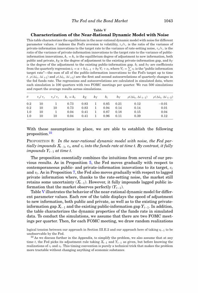
The Fed and the Bond Market 1043
Table VCharacterization of the Near-Rational Dynamic Model with Noise
This table characterizes the equilibrium in the near-rational dynamic model with noise for differentparameter values. θ indexes the Fed’s aversion to volatility, τ z/τ ε is the ratio of the variance ofprivate-information innovations to the target rate to the variance of rate-setting noise, τ v/τ ε is theratio of the variance of private-information innovations to the target rate to the variance of public-information innovations, kε = kv is the equilibrium degree of adjustment to new information, bothpublic and private, kX is the degree of adjustment to the existing private-information gap, and kYis the degree of the adjustment to the existing public-information gap. bi and bV are coefficientsfrom the quarterly regression it = a + biit−1 + bV Vt + et,where Vt = ∑
νt is the “public informationtarget rate”—the sum of all of the public-information innovations to the Fed’s target up to timet. ρ(�it, �i t-1) and ρ(�it, �i t-2) are the first and second autocorrelations of quarterly changes inthe fed funds rate. The regressions and autocorrelations are calculated in simulated data, whereeach simulation is 100 quarters with two FOMC meetings per quarter. We run 500 simulationsand report the average results across simulations.
θ τ z/ τ ε τ v/ τ ε kε = kv kX kY bi bV ρ(�it, �i t−1) ρ(�it, �i t−2)
0.2 10 1 0.73 0.83 1 0.85 0.21 0.12 −0.010.2 10 10 0.73 0.83 1 0.94 0.14 0.14 0.011.0 10 1 0.04 0.41 1 0.87 0.18 0.15 0.041.0 10 10 0.04 0.41 1 0.96 0.11 0.39 0.12
With these assumptions in place, we are able to establish the followingproposition.22
PROPOSITION 8: In the near-rational dynamic model with noise, the Fed par-tially impounds Xt−1, εt, and vt into the funds rate at time t. By contrast, it fullyimpounds Yt−1 at time t.
The proposition essentially combines the intuitions from several of our pre-vious results. As in Proposition 5, the Fed moves gradually with respect tocontemporaneous public- and private-information innovations to its target, εtand vt. As in Proposition 7, the Fed also moves gradually with respect to laggedprivate information where, thanks to the rate-setting noise, the market stillretains some uncertainty (Xt−1). However, it fully impounds lagged public in-formation that the market observes perfectly (Yt−1).
Table V illustrates the behavior of the near-rational dynamic model for differ-ent parameter values. Each row of the table displays the speed of adjustmentto new information, both public and private, as well as to the existing private-information gap Xt−1 and the existing public-information gap Yt−1. In addition,the table characterizes the dynamic properties of the funds rate in simulateddata. To conduct the simulations, we assume that there are two FOMC meet-ings per quarter. Then, for each FOMC meeting, we draw random realizations
logical tension between our approach in Section III.E.2 and our approach here of taking st−1 to beunobservable by the Fed.
22 As we discuss further in the Appendix, to simplify the problem, we also assume that at anytime t, the Fed picks its adjustment rule taking Xt−1 and Yt−1 as given, but before knowing therealizations of εt and vt. This timing convention is purely a technical trick that makes the problemmore tractable without changing anything of economic substance.
1044 The Journal of Finance R©
of εt and vt and compute the resulting funds rate path using all of the speed-of-adjustment coefficients generated by the model.
We next use the simulated data to conduct two exercises. First, we estimatean inertial Taylor rule. Specifically, we run the following quarterly regressionon the simulated data:
it = a + biit−1 + bV Vt + et, (35)
where Vt = ∑νt is the “public information target rate,” that is, the sum of all
of the public information innovations to the Fed’s target up to time t. We thinkof this variable as the analog of the target rate that is used in the empiricalliterature, which is typically based on the output gap and inflation. In thisliterature, a typical finding in quarterly data is that it = 0.85 × it−1 + 0.15 × Vt(Coibion and Gorodnichenko (2012)). Second, we estimate the first and secondquarterly autocorrelations of changes in the funds rate in the simulated data,ρ(�it, �i t-1) and ρ(�it, �i t-2). In our data, we find that the first and secondquarterly autocorrelations are both around 0.30. Each simulation covers 100quarters with two FOMC meetings per quarter. In other words, each simulationhas 200 periods. For each set of parameter values in the table, we run 500simulations and report the average moments across these simulations.
In the first row of Table V, the Fed cares modestly about bond market volatil-ity (θ = 0.20), and public and private shocks to its target have equal variance(σ 2
ε /σ 2ν = 1). There is partial adjustment to new public and private information
(kε = kv = 0.73), slightly more adjustment to the existing private-informationgap Xt−1 (kX = 0.83), and full adjustment to the public-information gap Yt−1(kY = 1). The table also shows that we do well in terms of replicating the in-ertial Taylor rule regression, with an inertia coefficient bi of 0.85, very close tothat reported by Coibion and Gorodnichenko (2012). This is true despite thefact that there is full adjustment to the existing public information gap Yt−1(kY = 1). The reason is that both the lagged funds rate and the public data Vtare informative about the public-information part of the Fed’s target, but onlythe lagged funds rate is informative about the private-information part. Thus,if there is any private information, the only way the regression can load on itis by loading on the lagged funds rate. And given that the lagged funds rate isalso informative about the public-information part of the Fed’s target, there islittle reason for the regression to incrementally load on Vt.
The first row of Table V also shows that we generate a positive first autocor-relation of 0.12 for quarterly changes in the funds rate with these parametervalues, but essentially a zero second autocorrelation. Because there is partialadjustment to both public- and private-information shocks, both contribute tothe first autocorrelation. The parts of εt and vt that are not impounded into thefunds rate at time t will continue to be impounded at time t + 1. However, onlyprivate information contributes to the second autocorrelation, since kY = 1 andtherefore the public shock vt is fully incorporated after time t + 1. In contrast,because kX < 1, the private shock εt continues to contribute to changes in thefed funds rate at times t+2 and beyond. In this case, however, the contribution
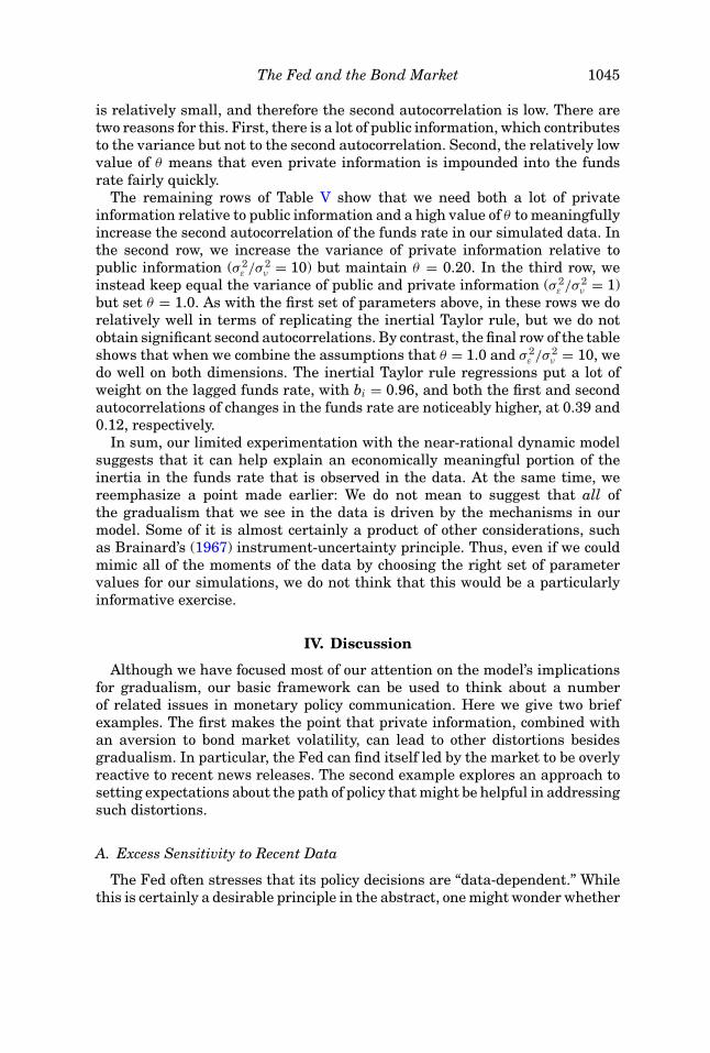
The Fed and the Bond Market 1045
is relatively small, and therefore the second autocorrelation is low. There aretwo reasons for this. First, there is a lot of public information, which contributesto the variance but not to the second autocorrelation. Second, the relatively lowvalue of θ means that even private information is impounded into the fundsrate fairly quickly.
The remaining rows of Table V show that we need both a lot of privateinformation relative to public information and a high value of θ to meaningfullyincrease the second autocorrelation of the funds rate in our simulated data. Inthe second row, we increase the variance of private information relative topublic information (σ 2
ε /σ 2ν = 10) but maintain θ = 0.20. In the third row, we
instead keep equal the variance of public and private information (σ 2ε /σ 2
ν = 1)but set θ = 1.0. As with the first set of parameters above, in these rows we dorelatively well in terms of replicating the inertial Taylor rule, but we do notobtain significant second autocorrelations. By contrast, the final row of the tableshows that when we combine the assumptions that θ = 1.0 and σ 2
ε /σ 2ν = 10, we
do well on both dimensions. The inertial Taylor rule regressions put a lot ofweight on the lagged funds rate, with bi = 0.96, and both the first and secondautocorrelations of changes in the funds rate are noticeably higher, at 0.39 and0.12, respectively.
In sum, our limited experimentation with the near-rational dynamic modelsuggests that it can help explain an economically meaningful portion of theinertia in the funds rate that is observed in the data. At the same time, wereemphasize a point made earlier: We do not mean to suggest that all ofthe gradualism that we see in the data is driven by the mechanisms in ourmodel. Some of it is almost certainly a product of other considerations, suchas Brainard’s (1967) instrument-uncertainty principle. Thus, even if we couldmimic all of the moments of the data by choosing the right set of parametervalues for our simulations, we do not think that this would be a particularlyinformative exercise.
IV. Discussion
Although we have focused most of our attention on the model’s implicationsfor gradualism, our basic framework can be used to think about a numberof related issues in monetary policy communication. Here we give two briefexamples. The first makes the point that private information, combined withan aversion to bond market volatility, can lead to other distortions besidesgradualism. In particular, the Fed can find itself led by the market to be overlyreactive to recent news releases. The second example explores an approach tosetting expectations about the path of policy that might be helpful in addressingsuch distortions.
A. Excess Sensitivity to Recent Data
The Fed often stresses that its policy decisions are “data-dependent.” Whilethis is certainly a desirable principle in the abstract, one might wonder whether

1046 The Journal of Finance R©
in practice there is a risk that policy may become too sensitive to the mostsalient recent data releases, especially when these releases on their own haverelatively little incremental information content.
Consider the following hypothetical example. There is an upcoming FOMCmeeting, and the Fed faces an important binary decision, for instance, whetherto taper the pace of its asset purchases for the first time. The Friday beforethe meeting, the monthly payroll report will be released. Market participantsanticipate that the policy decision will be data-dependent, and they naturallyfocus attention on the payroll report, even though it is common knowledgethat this report only contains a small amount of new information about theunderlying state of the economy. Suppose that investors develop an initiallyarbitrary conjecture that the Fed will taper if and only if the payroll numberexceeds 200,000 new jobs. There is a sense in which this conjecture can bepartially self-validating.
To see why, imagine that the payroll number turns out to be only 160,000.Given their conjecture, investors sharply revise downward their assessmentof the likelihood of the Fed tapering. This means that if the Fed was indeedto follow through with the taper, it would be seen as a hawkish surprise. Themarket would infer that the innovation in the Fed’s private information aboutits target was unusually high, and bond yields would spike upward accordingly.Given an aversion to such volatility, the Fed might decide to sit tight, therebyvalidating the market’s initial conjecture. This could happen even if the Fedfully recognizes that there is little meaningful difference between a payrollnumber of 200,000 and 160,000.
As a rough sketch of how one might capture this intuition more formally,assume that the Fed can either taper (Y) or not taper (N). The Fed has privateinformation ε about its long-run target for the funds rate, and this privateinformation is distributed symmetrically on some interval [−H, H]. Initially,before the arrival of the news release, the optimal decision if the Fed ignoredbond market volatility is to taper if ε > 0. Thus, the prior probability of a Ydecision is ½. If the market holds such priors, then no matter how concernedthe Fed is with bond market volatility, it will follow through with the taperif and only if ε > 0. This is because a Y decision and an N decision are seenas equally likely ex ante, and so the amount of information about ε that isconveyed is the same either way. The Fed cannot affect market volatility bychoosing one option or the other.
Now suppose instead that there is a small bit of bad public news right beforethe meeting, for example, a disappointing payroll number. Further supposethat the market interprets this news as being both quite informative and pes-simistic, so the market now believes that the Fed will only taper ifε > X forsome positive X. In other words, the market thinks the likelihood of a Y deci-sion has declined. Given this revision in market beliefs, a concern with bondmarket volatility will now make the Fed less inclined to taper, even if it be-lieves that the news release was totally uninformative. The reason is that ifthe market thinks that a Y decision implies ε > X, then a Y decision conveysmore information about the Fed’s long-run target, and hence creates more
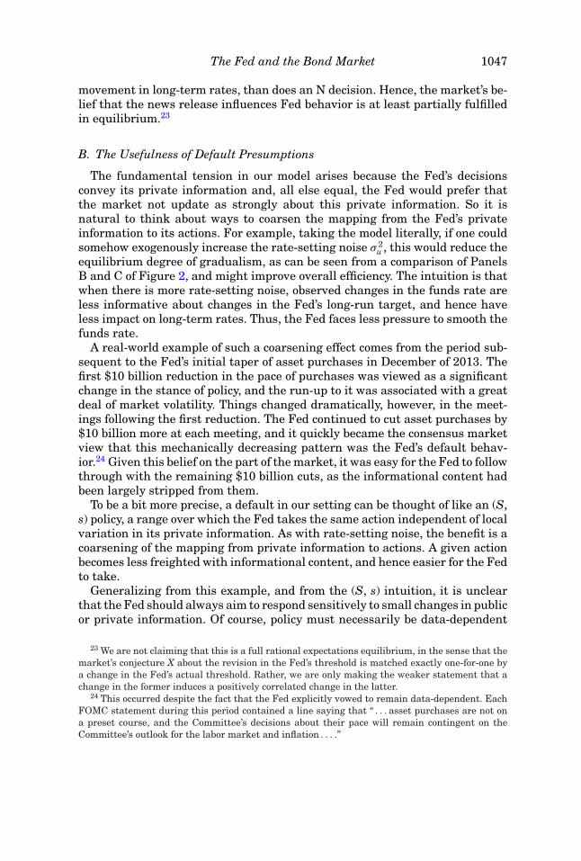
The Fed and the Bond Market 1047
movement in long-term rates, than does an N decision. Hence, the market’s be-lief that the news release influences Fed behavior is at least partially fulfilledin equilibrium.23
B. The Usefulness of Default Presumptions
The fundamental tension in our model arises because the Fed’s decisionsconvey its private information and, all else equal, the Fed would prefer thatthe market not update as strongly about this private information. So it isnatural to think about ways to coarsen the mapping from the Fed’s privateinformation to its actions. For example, taking the model literally, if one couldsomehow exogenously increase the rate-setting noise σ 2
u , this would reduce theequilibrium degree of gradualism, as can be seen from a comparison of PanelsB and C of Figure 2, and might improve overall efficiency. The intuition is thatwhen there is more rate-setting noise, observed changes in the funds rate areless informative about changes in the Fed’s long-run target, and hence haveless impact on long-term rates. Thus, the Fed faces less pressure to smooth thefunds rate.
A real-world example of such a coarsening effect comes from the period sub-sequent to the Fed’s initial taper of asset purchases in December of 2013. Thefirst $10 billion reduction in the pace of purchases was viewed as a significantchange in the stance of policy, and the run-up to it was associated with a greatdeal of market volatility. Things changed dramatically, however, in the meet-ings following the first reduction. The Fed continued to cut asset purchases by$10 billion more at each meeting, and it quickly became the consensus marketview that this mechanically decreasing pattern was the Fed’s default behav-ior.24 Given this belief on the part of the market, it was easy for the Fed to followthrough with the remaining $10 billion cuts, as the informational content hadbeen largely stripped from them.
To be a bit more precise, a default in our setting can be thought of like an (S,s) policy, a range over which the Fed takes the same action independent of localvariation in its private information. As with rate-setting noise, the benefit is acoarsening of the mapping from private information to actions. A given actionbecomes less freighted with informational content, and hence easier for the Fedto take.
Generalizing from this example, and from the (S, s) intuition, it is unclearthat the Fed should always aim to respond sensitively to small changes in publicor private information. Of course, policy must necessarily be data-dependent
23 We are not claiming that this is a full rational expectations equilibrium, in the sense that themarket’s conjecture X about the revision in the Fed’s threshold is matched exactly one-for-one bya change in the Fed’s actual threshold. Rather, we are only making the weaker statement that achange in the former induces a positively correlated change in the latter.
24 This occurred despite the fact that the Fed explicitly vowed to remain data-dependent. EachFOMC statement during this period contained a line saying that “ . . . asset purchases are not ona preset course, and the Committee’s decisions about their pace will remain contingent on theCommittee’s outlook for the labor market and inflation . . . .”

1048 The Journal of Finance R©
in some global sense—substantial changes in the economic environment mustbe met with commensurate changes in the stance of policy. At the same time,however, it may be better to foster a market expectation that the default policypath will be followed so long as things do not change too much. For example,in the midst of a tightening cycle, there may be some virtue to establishing adefault presumption that the funds rate will be mechanically raised by 25 bpsat every other FOMC meeting, so long as the economy continues to performbroadly as expected. At the margin, a default of this sort sacrifices some fine-tuning of policy to economic conditions, but has the advantage of making eachmove in rates less of an incremental informational event.
Admittedly, setting defaults in this manner may be complicated in prac-tice. In the model, changes in the funds rate are the only thing that revealsthe Fed’s private information to the market. In reality, FOMC statements,speeches, and testimony also transmit such information. One might hypothe-size that something of a substitution effect could come into play—to the extentthat the Fed makes changes in the funds rate less informative, market partic-ipants may begin to scrutinize other forms of communication more intensely.25
Nevertheless, even if crafting such purely verbal communication remains achallenge, it might have less consequence for economic efficiency. Attemptingto manage bond market volatility with words is not the same thing as manag-ing it by distorting the short rate away from the ideal target level. Analyzinga richer version of the model in which both the Fed’s words and its actionsconvey some of its private information is an interesting avenue for futurework.
V. Conclusion
This paper examines the complicated strategic interplay between the Fedand the bond market that arises when the Fed has some private informationabout its long-run target for the policy rate and is averse to bond marketvolatility. From a positive-economics perspective, we argue that a model withthese ingredients can help explain the phenomenon of gradualism in monetarypolicy, and can also shed light on how the Fed responds to other shocks, such aschanges in market risk premiums and salient data releases. From a normativeperspective, we emphasize that, in our setting, it can be valuable for a centralbank to develop an institutional culture such that a concern with bond marketvolatility does not play an outsized role in policy deliberations. In other words,it can be useful for policy makers to build a reputation for not caring too muchabout the bond market.
We close by highlighting an important caveat with respect to this reputa-tional argument. As we have framed it, our key point rests on a comparison
25 Casual observation suggests that in the period when policy was stuck at the zero lower bound,so there was nothing to be learned from rate changes, there was enormous focus on the wordingof FOMC statements, with small adjustments to the statement often met with strong marketreactions.
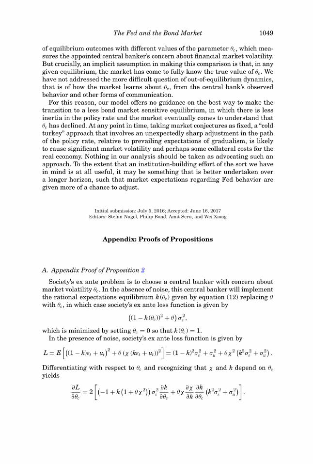
The Fed and the Bond Market 1049
of equilibrium outcomes with different values of the parameter θc, which mea-sures the appointed central banker’s concern about financial market volatility.But crucially, an implicit assumption in making this comparison is that, in anygiven equilibrium, the market has come to fully know the true value of θc. Wehave not addressed the more difficult question of out-of-equilibrium dynamics,that is of how the market learns about θc, from the central bank’s observedbehavior and other forms of communication.
For this reason, our model offers no guidance on the best way to make thetransition to a less bond market sensitive equilibrium, in which there is lessinertia in the policy rate and the market eventually comes to understand thatθc has declined. At any point in time, taking market conjectures as fixed, a “coldturkey” approach that involves an unexpectedly sharp adjustment in the pathof the policy rate, relative to prevailing expectations of gradualism, is likelyto cause significant market volatility and perhaps some collateral costs for thereal economy. Nothing in our analysis should be taken as advocating such anapproach. To the extent that an institution-building effort of the sort we havein mind is at all useful, it may be something that is better undertaken overa longer horizon, such that market expectations regarding Fed behavior aregiven more of a chance to adjust.
Initial submission: July 5, 2016; Accepted: June 16, 2017Editors: Stefan Nagel, Philip Bond, Amit Seru, and Wei Xiong
Appendix: Proofs of Propositions
A. Appendix Proof of Proposition 2
Society’s ex ante problem is to choose a central banker with concern aboutmarket volatility θc. In the absence of noise, this central banker will implementthe rational expectations equilibrium k (θc) given by equation (12) replacing θ
with θc, in which case society’s ex ante loss function is given by((1 − k (θc))2 + θ
)σ 2
ε ,
which is minimized by setting θc = 0 so that k (θc) = 1.In the presence of noise, society’s ex ante loss function is given by
L = E[(
(1 − k)εt + ut)2 + θ (χ (kεt + ut))2
]= (1 − k)2σ 2
ε + σ 2u + θχ2 (k2σ 2
ε + σ 2u
).
Differentiating with respect to θc and recognizing that χ and k depend on θcyields
∂L∂θc
= 2[(−1 + k
(1 + θχ2)) σ 2
ε
∂k∂θc
+ θχ∂χ
∂k∂k∂θc
(k2σ 2
ε + σ 2u
)].

1050 The Journal of Finance R©
Evaluating this expression at θc = θ , the first term is zero by the definition ofk(θ ). Thus, we have
∂L∂θc
|θc=θ = 2θχ(k2σ 2
ε + σ 2u
) ∂χ
∂k∂k∂θc
.
Further, we have
∂χ
∂k= −τu
(k2τu − τε
)(τε + k2τu
)2
and
∂k∂θc
= −
⎛⎜⎝1 − 2θckτ 2u
(τε + k2τu
) (k2τu − τε
)((τε + k2τu
)2 + θc (kτu)2)2
⎞⎟⎠−1 (
τε + k2τu)2
(kτu)2((τε + k2τu
)2 + θc (kτu)2)2 .
Finally, note that when we write k as a function of κ in equation 8, this func-tion is minimized at κ = √
τε/τu. This means that the upper stable equilibriumin any rational expectations equilibrium will have k >
√τε/τu . This implies
that k2τu − τε > 0 so that ∂χ
∂k < 0, ∂k∂θc
< 0, and ∂L∂θc
|θc=θ > 0.
B. Appendix Proof of Proposition 3
As before, the market’s inference about the Fed’s private information at timet is
ε̃t = χ (kεt + ut) ,
where
χ = κτu
τε + κ2τu.
Now, however, the Fed understands that there will be a time t + 1 surprise
εt+1 − ε̃t = (1 − kχ )εt − χut.
Plugging this into the Fed’s objective function, we have
E[(
(1 − k)εt + ut)2 + θ (χ (kεt + ut))2 + 0 + θ
((1 − kχ )εt − χut
)2]
= (1 − k)2ε2t + σ 2
u + θχ2k2ε2t + θχ2σ 2
u + θ (1 − kχ )2ε2t + θχ2σ 2
u .
The first-order condition with respect to k is
k = 1 + θχ
1 + 2θχ2 .
Thus, we have k < 1 whenever θ > 0 since χ > 0.

The Fed and the Bond Market 1051
Society’s ex ante loss function is given by
L = (1 − k)2σ 2ε + σ 2
u + θχ2k2σ 2ε + θχ2σ 2
u + θ (1 − kχ )2σ 2ε + θχ2σ 2
u .
Differentiating with respect to θc and recognizing that χ and k depend on θc,we have
dLdθc
= 2[(
−1 + k + 2θχdχ
dkk2 + 2θχ2k − θk
dχ
dk− θχ
)σ 2
ε + 2θχdχ
dkσ 2
u
]dkdθc
.
Evaluating this at θc = 0, which implies k = 1, χ = τu/(τε + τu), and dχ/dk =(τε − τu)τu/(τε + τu)2, yields zero. The second-order condition is positive at θc = 0,ensuring that this is a minimum.
C. Appendix Proof of Proposition 4
Suppose there is rate-setting noise and the Fed cares about the volatility ofa finite-horizon rate given by
�i f initet = α�it + (1 − α)�i∞
t .
The Fed continues to have adjustment rule
it = it−1 + kεt + ut,
and the market conjectures the adjustment rule is
it = it−1 + κεt + ut.
As in the case with noise in the paper, the market’s inference is that
ε̃t = χ�it = χ (kεt + ut) ,
where
χ = κτu
τε + κ2τu.
Thus, the change in the finite-horizon yield is
�ifinitet = α�it + (1 − α)ε̃t
= (α + (1 − α)χ1
)�it.
The Fed picks k to minimize the loss function
Eut
[(i∗t − it
)2 + θ(�i f inite
t
)2]
= Eut
[((1 − k)εt + ut
)2 + θ((
α + (1 − α)χ)
(kεt + ut))2]
= (1 − k)2ε2t + σ 2
u + θ(α + (1 − α)χ
)2 k2ε2t
+ θ(α + (1 − α)χ
)2σ 2
u .
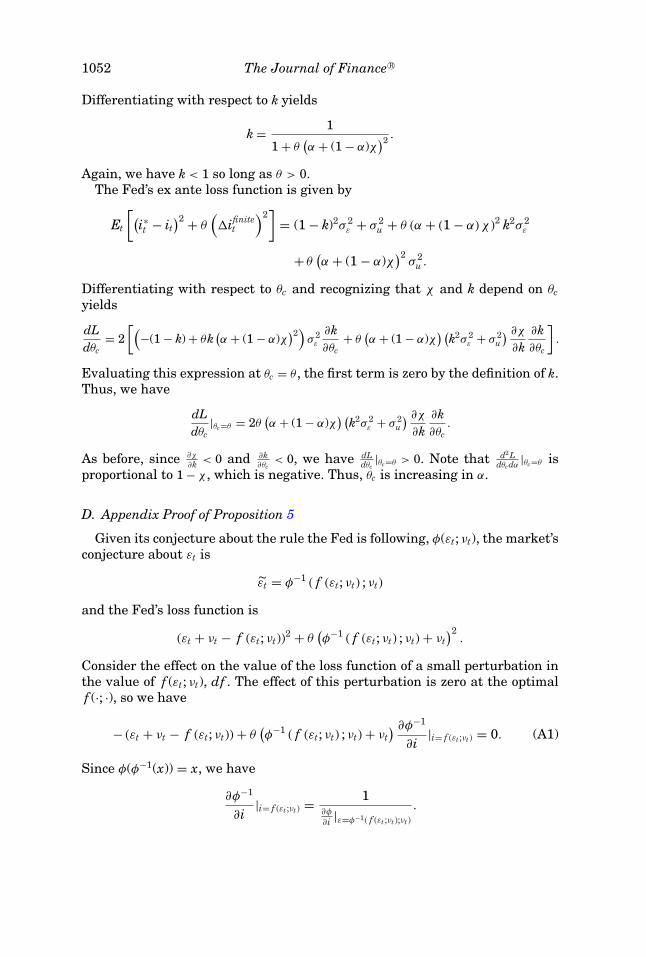
1052 The Journal of Finance R©
Differentiating with respect to k yields
k = 1
1 + θ(α + (1 − α)χ
)2 .
Again, we have k < 1 so long as θ > 0.The Fed’s ex ante loss function is given by
Et
[(i∗t − it
)2 + θ(�ifinite
t
)2]
= (1 − k)2σ 2ε + σ 2
u + θ (α + (1 − α) χ )2 k2σ 2ε
+ θ(α + (1 − α)χ
)2σ 2
u .
Differentiating with respect to θc and recognizing that χ and k depend on θcyields
dLdθc
= 2[(
−(1 − k) + θk(α + (1 − α)χ
)2)
σ 2ε
∂k∂θc
+ θ(α + (1 − α)χ
) (k2σ 2
ε + σ 2u
) ∂χ
∂k∂k∂θc
].
Evaluating this expression at θc = θ , the first term is zero by the definition of k.Thus, we have
dLdθc
|θc=θ = 2θ(α + (1 − α)χ
) (k2σ 2
ε + σ 2u
) ∂χ
∂k∂k∂θc
.
As before, since ∂χ
∂k < 0 and ∂k∂θc
< 0, we have dLdθc
|θc=θ > 0. Note that d2 Ldθcdα
|θc=θ isproportional to 1 − χ , which is negative. Thus, θc is increasing in α.
D. Appendix Proof of Proposition 5
Given its conjecture about the rule the Fed is following, φ(εt; νt), the market’sconjecture about εt is
ε̃t = φ−1 ( f (εt; νt) ; νt)
and the Fed’s loss function is
(εt + νt − f (εt; νt))2 + θ(φ−1 ( f (εt; νt) ; νt) + νt
)2.
Consider the effect on the value of the loss function of a small perturbation inthe value of f (εt; νt), df . The effect of this perturbation is zero at the optimalf (·; ·), so we have
− (εt + νt − f (εt; νt)) + θ(φ−1 ( f (εt; νt) ; νt) + νt
) ∂φ−1
∂i|i= f (εt;νt) = 0. (A1)
Since φ(φ−1(x)) = x, we have
∂φ−1
∂i|i= f (εt ;νt) = 1
∂φ
∂i |ε=φ−1( f (εt;νt);νt)
.
The Fed and the Bond Market 1053
Substituting into (A1) gives
− (εt + νt − f (εt; νt)) + θ(φ−1 ( f (εt; νt) ; νt) + νt
) 1∂φ
∂i |ε=φ−1( f (εt;νt);νt)
= 0.
Imposing rational expectations, we have φ = f , so that this reduces to thedifferential equation
∂ f∂ε
|ε=εt (εt + νt − f (εt; νt)) = θ (εt + νt) ,
which the optimal f (·; ·) must satisfy.Now conjecture that f = kεεt + c. In this case the differential equation re-
duces to
kε (εt + νt − kεεt − c) = θ (εt + νt) ,
or
kε(1 − kε)εt + kε(νt − c) = θεt + θνt.
Matching coefficients yields
kε(1 − kε) = θ and
c = νt
(1 − θ
kε
).
Thus, we can write the optimal f (·; ·) as
f = kεεt + kννt,
where kε(1 − kε) = θ and kν = 1 − θ/kε. From the definition of kε, we have
kν = 1 − θ
kε
= 1 − (1 − kε) = kε.
E. Appendix Proof of Proposition 6
Given its conjecture about the rule the Fed is following, φ(εt; ηt), the market’sconjecture about εt is
ε̃t = φ−1 ( f (εt; ηt) ; ηt)
and the Fed’s loss function is
(εt − f (εt; ηt))2 + θ(φ−1 ( f (εt; ηt) ; ηt) + ηt
)2.
1054 The Journal of Finance R©
Consider the effect on the value of the loss function of a small perturbation inthe value of f (εt; ηt), df . The effect of this perturbation is zero at the optimalf (·; ·), so we have
− (εt − f (εt; ηt)) + θ(φ−1 ( f (εt; ηt) ; ηt) + ηt
) ∂φ−1
∂i|i= f (εt ;ηt) = 0. (A2)
Since φ(φ−1(x)) = x, we have
∂φ−1
∂i|i= f (εt;ηt) = 1
∂φ
∂i |ε=φ−1( f (εt ;ηt);ηt)
.
Substituting into (A2) gives
− (εt − f (εt; ηt)) + θ(φ−1 ( f (εt; ηt) ; ηt) + ηt
) 1∂φ
∂i |ε=φ−1( f (εt ;ηt);ηt)
= 0.
Imposing rational expectations, we have φ = f , so that this reduces to thedifferential equation
∂ f∂ε
|ε=εt (εt − f (εt; ηt)) = θ (εt + ηt) ,
which the optimal f (·; ·) must satisfy.Now conjecture that f = kεεt + c. In this case the differential equation re-
duces to
kε (εt − kεεt − c) = θ (εt + ηt) ,
or
kε(1 − kε)εt − kεc = θεt + θηt.
Matching coefficients yields
kε(1 − kε) = θ and
c = − θ
kε
ηt.
Thus, we can write the optimal f (·; ·) as
f = kεεt + kηηt,
where kε(1 − kε) = θ and kη = −θ/kε.
F. Appendix Proof of Proposition 7
We start at time 2 and work backwards. Assume that the market’s conjectureabout ε1 entering the period is given by
�y1 = ε̃1,1 = χ11 (i1 − i0) = χ11k1ε1 + χ11u1,
The Fed and the Bond Market 1055
where
χ11 = τuκ1
τε + τuκ21
.
After observing i2, the market will believe that ε1 is given by
ε̃2,1 = χ21(i1 − i0) + χ22(i2 − i0)
= χ21 (k1ε1 + u1) + χ22 (k2ε1 + u2) ,
where
χ21 = τuκ1
τε + τu(κ2
1 + κ22
)χ22 = τuκ2
τε + τu(κ2
1 + κ22
) .Thus, the change in the forward rate at time 2 will be
�y2 = ε̃2,1 − ε̃1,1 = (χ21 − χ11) (k1ε1 + u1) + χ22 (k2ε1 + u2) ,
and the change in the forward rate at time 3 will be
�y3 = ε1 − ε̃2,1 = (1 − χ21k1 − χ22k2) ε1 − χ21u1 − χ22u2.
The Fed’s objective at time 2 is
E[(
i2 − i∗2
)2 + θ (�y2)2 + (i3 − i∗
3
)2 + θ (�y3)2]
= (1 − k2)2ε21 + σ 2
u
+ θ
(((χ21 − χ11) k1 + χ22k2)2 ε2
1 + (χ21 − χ11)2 u21 + χ2
22σ2u
+2 ((χ21 − χ11) k1 + χ22k2) (χ21 − χ11) ε1u1
)
+ θ
((1 − χ21k1 − χ22k2)2 ε2
1 + χ221u2
1 + χ222σ
2u
−2 (1 − χ21k1 − χ22k2) χ21ε1u1
).
The first-order condition with respect to k2 is
k2 = 1 + θχ22
1 + 2θχ222
+ θχ22 (χ11 − 2χ21)1 + 2θχ2
22
k1 + θχ22 (χ11 − 2χ21)1 + 2θχ2
22
u1
ε1.
Since χ21 < χ11 and k1 < 1, we have E[k2] < 1 when σ 2u > 0 and θ > 0.
We next fold this back to time 1. For simplicity assume that the Fed acts asthough k2 takes its expected value:
E[k2] = 1 + θχ22 (1 + (χ11 − 2χ21) k1)1 + 2θχ2
22
.
Let
δ = dk2
dk1= θχ22 (χ11 − 2χ21)
1 + 2θχ222
.

1056 The Journal of Finance R©
Folding back to time 1, we have the Fed’s objective at time 1:
E[(
i1 − i∗1
)2 + θ (�y1)2 + (i2 − i∗
2
)2 + θ (�y2)2 + (i3 − i∗
3
)2 + θ (�y3)2]
= (1 − k1)2ε21 + σ 2
u + θχ211k2
1ε21 + θχ2
11σ2u + (1 − k12)2ε2
1 + σ 2u
+ θ ((χ21 − χ11) k1 + χ22k12)2 ε21 + θ (χ21 − χ11)2 σ 2
u + θχ222σ
2u
+ θ (1 − χ21k1 − χ22k2)2 ε21 + θχ2
21σ2u + θχ2
22σ2u .
The first-order condition with respect to k1 is
k1 = 1 + δ + θ (χ21 + χ22δ)1 + θχ11 (2χ11 − χ21) + θ (2χ21 − χ11) (χ21 + χ22δ)
− δ + θχ22 (2 (χ21 + χ22δ) − χ11)1 + θχ11 (2χ11 − χ21) + θ (2χ21 − χ11) (χ21 + χ22δ)
k12.
The Fed’s ex ante loss function is
L = E
⎡⎢⎣((1 − k1)ε1 + u1
)2 + θ (χ11k1ε1 + χ11u1)2 + ((1 − k2)ε1 + u1
)2
+θ (((χ21 − χ11) k1 + χ22k2) ε1 + (χ21 − χ11) u1 + χ22u2)2 + 0
+θ ((1 − χ21k1 − χ22k2) ε1 − χ21u1 − χ22u2)2
⎤⎥⎦= (1 − k1)2σ 2
ε + σ 2u + θχ2
11k21σ 2
ε + θχ211σ
2u + (1 − k2)2σ 2
ε + σ 2u
+ θ ((χ21 − χ11) k1 + χ22k2)2 σ 2ε + θ (χ21 − χ11)2 σ 2
u + θχ222σ
2u
+ θ (1 − χ21k1 − χ22k2)2 σ 2ε + θχ2
21σ2u + θχ2
22σ2u .
Differentiating with respect to θc and recognizing that k1, k2, χ11, χ21, and χ22all depend on θc we have
dLdθc
= −2(1 − k1)dk1
dθcσ 2
ε + 2θχ211k1
dk1
dθcσ 2
ε + 2θχ11k21
dχ11
dk1
dk1
dθcσ 2
ε
+ 2θχ11dχ11
dk1
dk1
dθcσ 2
u − 2(1 − k2)dk2
dθcσ 2
ε + 2θ ((χ21 − χ11) k1 + χ22k2)
×⎛⎝ (
dχ21dk1
dk1dθc
+ dχ21dk2
dk2dθc
− dχ11dk1
dk1dθc
)k1
+ (χ21 − χ11) dk1dθc
+(
dχ22dk1
dk1dθc
+ dχ22dk2
dk2dθc
)k2 + χ22
dk2dθc
⎞⎠ σ 2ε
+ 2θ (χ21 − χ11)(
dχ21
dk1
dk1
dθc+ dχ21
dk2
dk2
dθc− dχ11
dk1
dk1
dθc
)σ 2
u
+ 2θχ22
(dχ22
dk1
dk1
dθc+ dχ22
dk2
dk2
dθc
)σ 2
u − 2θ (1 − χ21k1 − χ22k2)
×((
dχ21
dk1
dk1
dθc+ dχ21
dk2
dk2
dθc
)k1 + χ21
dk1
dθc+(
dχ22
dk1
dk1
dθc+ dχ22
dk2
dk2
dθc
)k2 + χ22
dk2
dθc
)σ 2
ε
+ 2θχ21
(dχ21
dk1
dk1
dθc+ dχ21
dk2
dk2
dθc
)σ 2
u + 2θχ22
(dχ22
dk1
dk1
dθc+ dχ22
dk2
dk2
dθc
)σ 2
u .
The Fed and the Bond Market 1057
At θc = 0 we have k1 = k2 = 1. In addition, we have χ11 = τuτε+τu
, χ21 = χ22 =τu
τε+2τu, dχ11
dk1= τu(τε−τu)
(τε+τu)2 ,dχ21dk1
= dχ22dk2
= τετu(τε+2τu)2 , and dχ21
dk2= dχ22
dk1= −2τ 2
u(τε+2τu)2 . Recogniz-
ing this, the derivative simplifies to
dLdθc
= τuτε
σ 2u τu − 1
(τu + τε)3
dk1
dθc= 0.
G. Appendix Proof of Proposition 8
Assume we enter period t with a preexisting gap between the time t − 1target and the time t − 1 rate of
i∗t−1 − it−1 = Xt−1 + Yt−1,
where Xt−1 is the private-information part of the gap and Yt−1 is the public-information part. The innovation in the target rate has both public and privatecomponents
i∗t = i∗
t−1 + εt + νt,
where εt is new private information and νt is new public information. Assumethat the Fed follows an adjustment rule of the form
it = it−1 + kXXt−1 + kY Yt−1 + f (εt; νt) ,
and the market conjectures that the Fed is following a rule of the form
it = it−1 + κXXt−1 + κY Yt−1 + φ (εt; νt) .
We assume the following timing convention. The Fed picks kX, kY , and f (·; ·)knowing Xt−1 and Yt−1, but not knowing the realizations of εt and vt. This timingconvention is purely a technical trick that makes the problem more tractablewithout really changing anything of economic substance. Without it, the Fed’sadjustment rule would turn out to depend on the realization of cross-productslike Xt−1εt. With the timing trick, what matters instead is the expectationof the product, which is zero. In addition, when choosing f (·; ·), the Fed stillunderstands it will know εt and νt at the same time— this is important to getpartial adjustment to νt. We should emphasize that, even with this somewhatstrained intra meeting timing, the Fed still behaves on a discretionary basisfrom one meeting to the next. Thus, while it agrees to values of kX, kY , andf (·; ·) in the first part of the time-t meeting, it has no ability to bind itself tothose values across meetings. Hence, the basic commitment problem remains.
We assume that the market gets a noisy signal of Xt−1
st−1 = Xt−1 + zt−1,
1058 The Journal of Finance R©
where zt˜ N(0, σ 2z ). The change in the infinite horizon forward rate is then given
by
�i∞t = E
[i∗t |st−1,�it, Yt−1, vt
]− E[i∗t−1|st−1, Yt−1
]= E
[Xt−1 + Yt−1 + εt + νt|st−1,�it, Yt−1, vt
]− E[Xt−1 + Yt−1|st−1, Yt−1
].
For the second term, we have
E[Xt−1 + Yt−1, |st−1, Yt−1
] = Yt−1 + σ 2X
σ 2X + σ 2
zst−1.
For the first term, we have
E[Xt−1 + Yt−1 + εt + νt|st−1,�it, Yt−1, vt
] = E[Xt−1 + εt|st−1,�it, Yt−1, vt
]+ Yt−1 + νt.
Using Stein’s Lemma, we have
E[Xt−1 + εt|st−1,�it, Yt−1, vt
] = 1E [φ′]2 σ 2
ε
(σ 2
X + σ 2z
)+ κ2Xσ 2
Xσ 2z
×((
E[φ′] σ 2
ε
(σ 2
X + σ 2z
)+ κXσ 2Xσ 2
z
)(�it − κY Yt−1)
+E[φ′] (E [
φ′]− κX)σ 2
ε σ 2Xst
).
Thus, we have
�i∞t = χi�it − χiκY Yt−1 + vt − χsst−1,
where
χi = E[φ′] σ 2
ε
(σ 2
X + σ 2z
)+ κXσ 2Xσ 2
z
E [φ′]2 σ 2ε
(σ 2
X + σ 2z
)+ κ2Xσ 2
Xσ 2z
and
χs = E[φ′] (κX − E
[φ′]) σ 2
ε σ 2X
E [φ′]2 σ 2ε
(σ 2
X + σ 2z
)+ κ2Xσ 2
Xσ 2z
+ σ 2X
σ 2X + σ 2
z.
The Fed’s objective function is then
Et
[(i∗t − it
)2 + θ(�i∞
t
)2]
= Et
[ (i∗t−1 + εt + νt − it−1 − kXXt−1 − kY Yt−1 − f (εt; νt)
)2
+θ (χi�it − χiκY Yt−1 − χsst−1 + vt)2
]= (1 − kX)2 X2
t−1 + (1 − kY )2 Y 2t−1 + 2 (1 − kX) (1 − kY ) Xt−1Yt−1
+ (εt + νt − f (εt; νt))2
+ θ
((χikX − χs)2 X2
t−1 + χ2i (kY − κY )2 Y 2
t−1 + (χi f (εt; νt))2 + χ2s σ 2
z + σ 2ν
+2 (χikX − χs) χi (kY − κY ) Xt−1Yt−1
).
The Fed and the Bond Market 1059
Differentiating with respect to kY we have
−2(1 − kY )Y 2t−1 − 2(1 − kX)Xt−1Yt−1 + 2θχ2
i (kY − κY )Y 2t−1
+ 2θ (χikX − χs) χi Xt−1Yt−1 = 0.
Differentiating with respect to kX we have
−2(1 − kX)X2t−1 − 2(1 − kY )Xt−1Yt−1 + 2θ (χikX − χs) χi X2
t−1
+ 2θχ2i (kY − κY )Xt−1Yt−1 = 0.
If we have kY = κY = 1 in a rational expectations equilibrium, these two equa-tions reduce to
−(1 − kX) + θ (χikX − χs) χi = 0
and
−(1 − kX) + θ (χikX − χs) χi = 0,
or
kX = 1 + θχiχs
1 + θχ2i
.
Now consider a perturbation of f around the optimum. The correspondingfirst-order condition is
f (εt; νt) = 11 + θχ2
i
εt + 11 + θχ2
i
νt.
Finally, to close the loop, we note that Xt = (1 − kX)Xt−1 + (1 − kε)εt implies
σ 2X = (1 − kε)2
1 − (1 − kX)2 σ 2ε .
REFERENCES
Barro, Robert J., and David B. Gordon, 1983, Rules, discretion and reputation in a model ofmonetary policy, Journal of Monetary Economics 12, 101–121.
Bernanke, Ben, 2004, Gradualism, Remarks at an economics luncheon co-sponsored by the FederalReserve Bank of San Francisco and the University of Washington, Seattle, WA. Available athttps://www.federalreserve.gov/boarddocs/speeches/2004/200405202/default.htm.
Bernanke, Ben, and Alan Blinder, 1992, The federal funds rate and the channels of monetarytransmission, American Economic Review 82, 901–921.
Brainard, William, 1967, Uncertainty and the effectiveness of policy, American Economic Review57, 411–425.
Campbell, John Y., Carolin Pflueger, and Luis Viceira, 2015, Monetary policy drivers of bond andequity risks, Working paper, Harvard University.
Cieslak, Anna, and Annette Vissing-Jorgenson, 2017, The economics of the Fed put, Working paper,UC Berkeley.
Coibion, Olivier, and Yuriy Gorodnichenko, 2012, Why are target interest rate changes so persis-tent? American Economic Journal: Macroeconomics 4, 126–162.
1060 The Journal of Finance R©
Dell’Ariccia, Giovanni, Luc Laeven, and Gustavo Suarez, 2013, Bank leverage and monetary pol-icy’s risk-taking channel: Evidence from the United States, Working paper, InternationalMonetary Fund.
Drechsler, Itamar, Alexi Savov, and Philipp Schnabl, 2017, The deposits channel of monetarypolicy, Quarterly Journal of Economics 132, 1819–1876.
Farhi, Emmanuel, and Jean Tirole, 2012, Collective moral hazard, maturity mismatch, and sys-temic bailouts, American Economic Review 102, 60–93.
Gertler, Mark, and Peter Karadi, 2015, Monetary policy surprises, credit costs, and economicactivity, American Economic Journal: Macroeconomics 7, 44–76.
Holmstrom, Bengt, 1999, Managerial incentive problems: A dynamic perspective, Review of Eco-nomic Studies 66, 169–182.
Jimenez, Gabriel, Steven Ongena, Jose-Luis Peydro, and Jesus Saurina, 2014, Hazardous timesfor monetary policy: What do 23 million loans say about the impact of monetary policy oncredit risk-taking? Econometrica 82, 463–505.
Kashyap, Anil K., and Jeremy C. Stein, 2000, What do a million observations on banks say aboutthe transmission of monetary policy? American Economic Review 90, 407–428.
Kydland, Finn, and Edward Prescott, 1977, Rules rather than discretion: The inconsistency ofoptimal plans, Journal of Political Economy 85, 473–491.
Kyle, Albert, 1985, Continuous auctions and insider trading, Econometrica 53, 1315–1336.Rogoff, Kenneth, 1985, The optimal degree of commitment to an intermediate monetary target,
Quarterly Journal of Economics 100, 1169–1189.Rudebusch, Glenn D., 2002, Term structure evidence on interest rate smoothing and monetary
policy inertia, Journal of Monetary Economics 49, 1161–1187.Rudebusch, Glenn D., 2006, Monetary policy inertia: Fact or fiction? International Journal of
Central Banking 2, 85–135.Sack, Brian, 1998, Uncertainty, learning, and gradual monetary policy, FEDS Working Paper
Series no. 98-34, Board of Governors of the Federal Reserve System.Stein, Jeremy C., 1989, Efficient capital markets, inefficient firms: A model of myopic corporate
behavior, Quarterly Journal of Economics 104, 655−669.Stein, Jeremy C., 2014, Challenges for monetary policy communication, Remarks at the Money
Marketeers of New York University, New York. Available at https://www.federalreserve.gov/newsevents/speech/stein20140506a.htm.
Taylor, John, 1993, Discretion versus policy rules in practice, Carnegie-Rochester Conference Serieson Public Policy 39, 195–214.
Woodford, Michael, 2003, Optimal interest-rate smoothing, Review of Economic Studies 70, 861–886.
Supporting Information
Additional Supporting Information may be found in the online version of thisarticle at the publisher’s website:
Replication Code.
Related Documents