HAL Id: tel-03649078 https://tel.archives-ouvertes.fr/tel-03649078 Submitted on 22 Apr 2022 HAL is a multi-disciplinary open access archive for the deposit and dissemination of sci- entific research documents, whether they are pub- lished or not. The documents may come from teaching and research institutions in France or abroad, or from public or private research centers. L’archive ouverte pluridisciplinaire HAL, est destinée au dépôt et à la diffusion de documents scientifiques de niveau recherche, publiés ou non, émanant des établissements d’enseignement et de recherche français ou étrangers, des laboratoires publics ou privés. The European strutural funds : allocation and economic effectiveness Benoit Dicharry To cite this version: Benoit Dicharry. The European strutural funds : allocation and economic effectiveness. Economics and Finance. Université de Strasbourg, 2021. English. NNT : 2021STRAB015. tel-03649078

Welcome message from author
This document is posted to help you gain knowledge. Please leave a comment to let me know what you think about it! Share it to your friends and learn new things together.
Transcript
HAL Id: tel-03649078https://tel.archives-ouvertes.fr/tel-03649078
Submitted on 22 Apr 2022
HAL is a multi-disciplinary open accessarchive for the deposit and dissemination of sci-entific research documents, whether they are pub-lished or not. The documents may come fromteaching and research institutions in France orabroad, or from public or private research centers.
L’archive ouverte pluridisciplinaire HAL, estdestinée au dépôt et à la diffusion de documentsscientifiques de niveau recherche, publiés ou non,émanant des établissements d’enseignement et derecherche français ou étrangers, des laboratoirespublics ou privés.
The European strutural funds : allocation and economiceffectivenessBenoit Dicharry
To cite this version:Benoit Dicharry. The European strutural funds : allocation and economic effectiveness. Economicsand Finance. Université de Strasbourg, 2021. English. �NNT : 2021STRAB015�. �tel-03649078�
UNIVERSITÉ DE STRASBOURG
ÉCOLE DOCTORALE AUGUSTIN COURNOT ED 221
BUREAU D’ÉCONOMIE THÉORIQUE ET APPLIQUÉE UMR 7522
THÈSE
pour l’obtention du titre de Docteur en Sciences Économiques
Présentée et soutenue publiquement le 14 décembre 2021 par
Benoit Dicharry
LES FONDS STRUCTURELS EUROPEENS:
ALLOCATION ET EFFICACITE ECONOMIQUE
Préparée sous la direction de Meixing DAI, de Phu NGUYEN-VAN et de Thi Kim Cuong PHAM
Composition du jury :
Jean-Louis Combes Professeur, Université Clermont Auvergne ExaminateurMeixing Dai Maître de Conférences HDR, Université de Strasbourg Directeur de thèseJan Fidrmuc Directeur de Recherche CNRS, Université de Lille Rapporteur
Valérie Mignon Professeure, Université Paris Nanterre RapportricePhu Nguyen-Van Directeur de Recherche CNRS, Université Paris Nanterre Co-directeur de thèse
Thi Kim Cuong Pham Professeure, Université Paris Nanterre Co-directrice de thèseAnne Stenger Directeur de Recherche INRAE, Université de Strasbourg Présidente du juryLionel Védrine Chargé de Recherche INRAE, UMR CESAER Examinateur

2

L’Université de Strasbourg n’entend donner aucune approbation, ni improbationaux opinions émises dans cette thèse ; elles doivent être considérées comme propresà leur auteur.
3

4
Remerciements
Je voudrais en tout premier lieu exprimer toute ma reconnaissance à Madame laProfesseure Thi Kim Cuong Pham et Phu Nguyen-Van, Directeur de Rechercheau CNRS, pour avoir accepté de m’encadrer dès mon mémoire de master. Leurgrande rigueur scientifique, leurs conseils, mais aussi leur confiance, ont grandementcontribué à mon épanouissement durant ces cinq années de collaboration. Je suiscertain qu’il ne s’agira que des cinq premières. Je n’oublie évidemment pas lesinnombrables retours et relectures de Meixing Dai qui ont grandement amélioré laqualité de cette thèse.Je voudrais également remercier Madame Anne Stenger, Directrice de Recherche àl’INRAE, Madame la Professeure Valérie Mignon, Monsieur Jan Fidrmuc, Directeurde Recherche au CNRS, Monsieur Lionel Védrine, Chargé de Recherche à l’INRAEpour m’avoir fait l’honneur de composer mon jury. Mes remerciements vont aussi àMonsieur le Professeur Jean-Louis COMBES qui en plus accepté de faire partie demon Comité de Suivi dès ma seconde année de thèse. I would also like to especiallythank Lubica Stlibarova for our collaborations, past, present and hopefully future.Je remercie le Bureau d’Économie Théorique et Appliquée (BETA) et l’Écoledoctorale Augustin Cournot pour avoir mis à ma disposition l’ensemble des moyensintellectuels et financiers pour la réalisation de ce travail.
Je tiens à remercier particulièrement certains doctorant.e.s et docteur.e.s quim’ont accompagné durant ce long périple: Agathe, dite la Pouteau, pour tous cesinnombrables moments de rires, de terreur, de larmes et de cris; Anne-Gaëlle pourWadafaké; Antoine, pour toutes ces années de Z... la mouche à Angus, ; Cyriellepour ses fréquentations et surtout soirées "incroyables"; Deborah pour avoir étémon meilleur public; Emilien pour sa filiation avec Michel Drucker et son aide; Huy pour avoir été mon meilleur étudiant; Kenza pour m’avoir fait découvrirAya Nakamura malgré moi; Laulau, égérie du Printemps le temps d’une soirée,pour ses conseils vestimentaires; Laeti pour nos very bad situations, de Belfort àKonstanz; Nono pour tous ces exquisite times, du bureau 126 à la guest house;Pauline pour ses trajets difficiles vers le 68; Pierre qui a redonné vie à mon vélo;Quiqui pour avoir lancé ma carrière solo; Rémy pour toutes ces discussions sereineset sa blague du lab; Samuel pour ces soirées au bord de l’Ill; Sila pour tous ces kilosde Mirabelle; Thomas alias La Castagne; Yanto qui me supporte encore malgréquatre années de collocation pas "très tranquilles".
Je n’oublie également pas mes ami.e.s hors de murs du BETA que j’ai pufréquenter à Strasbourg durant toutes ces années: Axel & Noémie, les caillots,
5

désormais mes voisiens parisiens; Damien (qui a toujours cru en ma thèse) &Marjo; Pierrick & Amandine, amateurs de Jésus et de Sangria, qui ont retardé maconversion au végétarisme; Ted & Marcelle qui m’ont connu dans tous mes états,mais le plus souvent alcoolisé quand même, chez qui je vais squatter dorénavantquand je serai à Strasbourg. Je tiens également à donner une mention spéciale àArnaud F., Julie, Irwin, Matthieu et Richard. Avant Strasbourg, il y a eu Bordeauxet mes amis de longue date qui sont venus me rendre visite: Benjamin & Cédric,Hyunah, Joy, Maxime et Rémi.
Je tiens enfin à exprimer ma reconnaissance éternelle à ma famille pour leursoutien indéfectible depuis le début de mes années d’études. Cela va de mesparents, ma soeur, mes cousins et cousine, oncles et tantes, à André & Mado. Sansleur soutien moral, mais aussi matériel pour mes parents qui ont beaucoup travaillépour moi, je n’aurais sans doute jamais pu réaliser cette thèse.
6

Je dédie cette thèse à Amatxi
7

8
Table of contents
Reading note / Note de lecture 13
General introduction 15
Introduction générale 25
1 Positive externalities of the EU Cohesion Policy: toward more syn-chronised economies? 351.1 Introduction . . . . . . . . . . . . . . . . . . . . . . . . . . . . . . . . 371.2 Related literature . . . . . . . . . . . . . . . . . . . . . . . . . . . . . 411.3 Methodology and data . . . . . . . . . . . . . . . . . . . . . . . . . . 44
1.3.1 Panel instrumental variables estimation . . . . . . . . . . . . . 441.3.2 Variables definition and data . . . . . . . . . . . . . . . . . . . 47
1.4 Results and discussion . . . . . . . . . . . . . . . . . . . . . . . . . . 501.5 Conclusion . . . . . . . . . . . . . . . . . . . . . . . . . . . . . . . . . 551.6 Appendices . . . . . . . . . . . . . . . . . . . . . . . . . . . . . . . . 57
1.6.1 Additional tables . . . . . . . . . . . . . . . . . . . . . . . . . 571.6.2 Additional figures . . . . . . . . . . . . . . . . . . . . . . . . 60
2 Impact of European Cohesion Policy on regional growth: Whentime isn’t money 612.1 Introduction . . . . . . . . . . . . . . . . . . . . . . . . . . . . . . . . 632.2 Related literature . . . . . . . . . . . . . . . . . . . . . . . . . . . . . 662.3 Methodology and data . . . . . . . . . . . . . . . . . . . . . . . . . . 68
2.3.1 Regression discontinuity design estimation . . . . . . . . . . . 682.3.2 Data and descriptive statistics . . . . . . . . . . . . . . . . . . 712.3.3 Validity of RDD setup and estimates of HLATE . . . . . . . . 73
2.4 Results and discussion . . . . . . . . . . . . . . . . . . . . . . . . . . 752.4.1 Estimation results . . . . . . . . . . . . . . . . . . . . . . . . . 752.4.2 Additional results . . . . . . . . . . . . . . . . . . . . . . . . . 812.4.3 General discussion . . . . . . . . . . . . . . . . . . . . . . . . 83
2.5 Conclusion . . . . . . . . . . . . . . . . . . . . . . . . . . . . . . . . . 852.6 Appendices . . . . . . . . . . . . . . . . . . . . . . . . . . . . . . . . 87
9
3 “The winner takes it all” or a story of the optimal allocation of theEuropean Cohesion Fund 933.1 Introduction . . . . . . . . . . . . . . . . . . . . . . . . . . . . . . . . 953.2 Related literature . . . . . . . . . . . . . . . . . . . . . . . . . . . . . 983.3 A theoretical framework for the ECF optimal allocation . . . . . . . 993.4 Estimation of the growth equation . . . . . . . . . . . . . . . . . . . . 103
3.4.1 Determinants of economic growth . . . . . . . . . . . . . . . . 1033.4.2 Econometric specification . . . . . . . . . . . . . . . . . . . . 1043.4.3 Data and variables . . . . . . . . . . . . . . . . . . . . . . . . 1063.4.4 Estimation results . . . . . . . . . . . . . . . . . . . . . . . . . 107
3.5 Simulation of the optimal allocation of ECF . . . . . . . . . . . . . . 1093.5.1 Observed allocation and optimal allocation . . . . . . . . . . . 109
3.6 Conclusion . . . . . . . . . . . . . . . . . . . . . . . . . . . . . . . . . 1143.7 Appendices . . . . . . . . . . . . . . . . . . . . . . . . . . . . . . . . 116
4 Regional decentralisation and the European Cohesion Policy: theleader takes it all 1214.1 Introduction . . . . . . . . . . . . . . . . . . . . . . . . . . . . . . . . 1234.2 Related literature . . . . . . . . . . . . . . . . . . . . . . . . . . . . . 1274.3 Theoretical model . . . . . . . . . . . . . . . . . . . . . . . . . . . . . 131
4.3.1 Signalling game . . . . . . . . . . . . . . . . . . . . . . . . . 1324.3.2 Central government’s welfare maximisation . . . . . . . . . . . 1364.3.3 Theoretical predictions . . . . . . . . . . . . . . . . . . . . . . 137
4.4 Empirical study . . . . . . . . . . . . . . . . . . . . . . . . . . . . . . 1384.4.1 Official allocation criteria . . . . . . . . . . . . . . . . . . . . 1384.4.2 Political forces shaping the allocation process . . . . . . . . . 1394.4.3 Empirical model . . . . . . . . . . . . . . . . . . . . . . . . . 1424.4.4 Baseline results . . . . . . . . . . . . . . . . . . . . . . . . . . 1434.4.5 Additional results . . . . . . . . . . . . . . . . . . . . . . . . . 144
4.5 Conclusion . . . . . . . . . . . . . . . . . . . . . . . . . . . . . . . . . 1484.6 Appendices . . . . . . . . . . . . . . . . . . . . . . . . . . . . . . . . 148
General conclusion 151
Conclusion générale 157
Bibliography 175
List of tables 178
10

List of figures 179
11

12

Reading note / Note de lecture
This thesis was written entirely in English to ease the discussion and the diffusion ofits results. For French readers, translated versions of the general introduction andconclusion are available. The thesis is made of four independent chapters. In orderto make each chapter readable independently from the others, some elements are tobe found in several chapters, especially those relating to the economic literature andthe institutional context. Each chapter also contains its own contextual elementsand a literature review specific to the issue addressed in the chapter. For this reason,the general introduction remains brief on the literature, in order to avoid excessiveredundancies.
? ? ? ? ?
Cette thèse a été rédigée intégralement en anglais afin de faciliter la discus-sion et la diffusion de ses résultats. Pour les lecteurs francophones, une versiontraduite de l’introduction générale et de la conclusion générale est proposée. Lathèse est composée de quatre chapitres autonomes. Pour permettre la lecture dechaque chapitre indépendamment des autres, certains éléments sont mentionnésdans plusieurs chapitres, notamment parmi ceux ayant trait à la littérature ou laprésentation du contexte institutionnel. Chaque chapitre contient également ses pro-pres éléments de contexte et une revue de littérature spécifique à la problématiqueétudiée. Pour cette raison, l’introduction générale demeure brève sur les élémentsde littérature, dans l’objectif de limiter les redondances.
13

14
General introduction
"Expression of the solidarity between Member States and regions which do not havethe same level of development, an opportunity to give everyone a chance and
strengthen the competitiveness of the whole, the cohesion policy has become, inbudgetary terms, the second policy of the Union."
This sentence pronounced by Jacques Delors during the speech marking theend of his mandate at the head of the European Commission, on January 16, 1995in Strasbourg, is still true today. The cohesion policy represents some 291 billioneuros, or 27.1% of the European budget for the multiannual financial framework(MFF) 2021-2027. Established in the 1980s, it responds to a founding objectiveof the Treaty of Rome (1957) where the Member States declare that they are"concerned about strengthening the unity of their economies and ensuring theirharmonious development, by reducing the the gap between the different regionsand the backwardness of the less favored”.1
This policy is based on five structural funds, the three main ones being theEuropean Regional Development Fund (ERDF), the European Social Fund (ESF)and the Cohesion Fund (CF).2 All EU regions are eligible for the European fundsbut the level of financial assistance granted to each region depends mainly on theirrelative GDP per capita to the EU average. Thus, regions located below the 75%threshold, known as convergence regions, are the main beneficiaries of the cohesionpolicy.
As such, the EU funds co-finance public and private investment projects aimedat stimulating the accumulation of physical and human capital to increase theGDP per capita in the beneficiary regions in fine. The ERDF especially supportstechnological progress by devoting more than 50% of its resources to the following3 thematic objectives: "Strengthening Innovation and Research and Development(R&D)", "Information and Communication Technology" and "Support for InnovativeSMEs ”. The role of the ESF is rather to increase the quality of the labor factorby devoting nearly 75% of its resources to the objectives "Employment and LaborMobility" and "Education, training and lifelong learning". As for the CF, it isonly intended for the poorest countries in the area, those with a level of GDP percapita below 90% of the European average. It concentrates half of its resources to
1Source: Preamble of Communautés Européennes. Bureau de représentation (France) (1957).2There is also the European Agricultural Fund for Rural Development (EAFRD), which sup-
ports rural development and constitutes the second pillar of the common agricultural policy (CAP).Then, there is the European Maritime and Fisheries Fund (EMFF) which is part of the commonfisheries policy.
15
General Introduction
contribute to the construction of the trans-European transport network (TEN-T)by financing infrastructures such as railways, highways, airports or port facilities.The other part of the FC finances environmental infrastructure such as drinkingwater networks or recycling centers.
The challenge of the economic convergence within the EU has changed with ashift from the East to the South. Central and Eastern European countries, suchas the Czech Republic, Hungary, Poland and the Baltic States, which have grownsignificantly over the past decade, will experience a significant reduction in theirallocations. At the same time, weakened by the economic crisis of sovereign debtin the euro zone and by the Covid-19 pandemic economic downturn, Italy, Spain,Greece and Portugal will see their support being reinforced. With the effectivedeparture of the United Kingdom from the European Union (EU) at 1er January2021, the resource constraint on the European budget has increased. As well, theemergence of new challenges, such as ecological transition and internal security,make the EU diversify its spending. In this context, the economic effectiveness ofthe structural funds rhymes with necessity.
This thesis answers to four research questions built around the notions of eco-nomic effectiveness and allocation of the European structural funds:
— Do the European structural funds have an impact on the synchronizationof economic business cycles so that the EMU could be closer to an optimalmonetary area?
— Is there a dilemma between rapid absorption of the European funds and a higheconomic effectiveness in the convergence regions?
— In the case of the Cohesion Fund, is it optimally alocated? How would thisfund be allocated to maximise the recipient countries’ economic growth toachieve economic convergence in the EU?
— Is the intranational allocation of the European funds subject to political fac-tors? Especially, have the reforms towards more regional autonomy been detri-mental to national lagging regions?
The first general contribution of this thesis is related to the analysis of economiceffectiveness of the EU funds. Traditionally, in the context of the Europeanstructural funds, the latter is defined as the capacity of funds to increase thelevel of economic growth of a recipient region. The goal of economic convergencemust therefore be achieved by a more sustained increase in the GDP per capita
16
General Introduction
of lagging regions, and more particularly of convergence regions, which are thosesituated below 75% of the European average. However, the literature shows theEuropean funds does not have any direct positive effect on the economic activityof the beneficiary regions. In particular, Ederveen et al. (2002) and Cappelenet al. (2003) open the field of the conditional study of the economic impact ofstructural funds by showing that they perform poorly in the lagging regions, thecore recipient regions, characterized by a lack of activities focused on research anddevelopment (R&D) activities and a low level of economic openness. The followingliterature highlights a variety of factors which condition the effectiveness of the EUfunds without overturning the postulate that they exhibit the highest economicefficiency in the most advanced regions. Indeed, the most developed regions havemore administrative and bureaucratic resources (Barro (1990); Rodríguez-Pose& Fratesi (2004); Huliaras & Petropoulos (2016)), of better institutional quality(Becker (2012); Becker et al. (2013); Becker et al. (2013); Rodríguez-Pose &Garcilazo (2015)), and economic activities involving a higher level of human capital(Becker (2012); Becker et al. (2013)). Therefore, the leading regions have a higherabsorption capacity, while the economic effectiveness of the European transfers isreduced above a certain threshold of aid intensity in the lagging regions (Beckeret al. (2010)).
Still about the notion of economic effectiveness, this thesis exploits the growinginterweaving of the EU’s economic objectives with those of the Economic andMonetary Union (EMU) since the departure of the United-Kingdom. Indeed,the Meseberg declaration of June 19, 2018 resulted in the proposition of anEU budget instrument for convergence and competitiveness, specifically to theEMU’s Member States financed by the 2021-27 EU budget. But given the scaleof the economic shock of the global Covid-19 pandemic, this instrument has beensubstituted by the NextGeneration EU recovery plan. Endowed with 750 billioneuros, it is mostly designed as a traditional European structural fund, and itwill be spent in the economies the most impacted by the economic shock of thepandemic. It constitutes a system of transfers between countries which are ina favorable economic situation via contributions to a common fund reversed toeconomies in difficulty in the form of subsidies. Therefore, the NextGenerationEU recovery plan has a contractual dimension, theorized by Johnson (1970),and seeks to push the EMU towards an optimal monetary zone by helping tosynchronize its business cyles. This optimality condition is essential to makethe monetary policy of the European Central Bank (ECB) be suited for all theEMU as these 19 economies must achieve totally synchronized business cycles
17
General Introduction
(Mundell (1961); Darvas & Szapáry (2008)). A substantial literature identifiesthe main beneficiary countries of the structured funds, namely Mediterranean,Central and Eastern Europe, as periphery of the EMU characterized by pooreconomic synchronization with the major European economies of the West (Fidr-muc & Korhonen (2006); Darvas & Szapáry (2008); Stiblarova & Sinicakova (2020)).
The second general contribution is related to the allocation process of theEuropean funds. The latter is made up of three sequences: the first involves theMember States and the European Commission, which results in the distribution ofthe overall envelope of the cohesion budget between EU Member States. Secondly,Member States establish partnership agreements. It is a document bringing togetherall investment projects where the European funds will play their role of co-fundinginvestment tool. This stage is characterized by interactions between the regionsand their respective central government and results in a regional allocation offunds within each of the Member States. Finally, each Member State sends itspartnership agreement to the European Commission, which decides whether or notto accept this document as it is. If the partnership agreement is not validated, itmust be redefined, with the European Commission having the last word.
The negotiations between the central government and its constituent regions,which therefore lead to the regional allocation of funds, has been particularlystudied (Kemmerling & Bodenstein (2006); Bodenstein & Kemmerling (2011);Charron (2016); Dellmuth et al. (2017) ). In particular, a dilemma between theoriginal objective of supporting the economic growth of the poorest regions onthe one hand, and a complete and rapid absorption of funds on the other, wasput forward. Thus, this literature underlines the primacy of the objective of afast absorption of the European funds over the principle of cohesion. Consideredas a signal of an efficient management of funds, the speed of absorption of thelatter constitutes a political objective, the Member States seeking to send a signalfor complete and efficient absorption of funds to the European Commission. Thedilemma between absorption and cohesion lies in the fact that the poorest regionsare those with the lowest absorption capacity levels. The emergence of this dilemmais particularly visible with a growing share of the European funds directed to theregions characterized by the presence of large metropolitan areas (Faludi et al.(2015)). This trend has been accelerated over the last decade since the Barcareport (Barca (2009)). The aim of the latter was to reform the EU’s cohesionpolicy by territorializing the design of the economic and social agenda, in orderto give greater responsibility to local actors (Solly (2016)). However, only urban
18
General Introduction
regions have been able to adapt to the reform of the cohesion policy, peripheral re-gions that did not have the means (Gruber et al. (2019); Medeiros & Rauhut (2020)).
This thesis is organized into 4 chapters which provide both empirical andtheoretical contributions. Chapter 1 extends the notion of economic effectivenessof the European structural funds by evaluating their impact on the synchronizationof economic cycles. Chapter 2 illustrates the trade-off between fast absorption offunds and high economic effectiveness in the lagging regions of the EU. Chapter3 presents an optimal allocation of the Cohesion Fund by emphasizing the biasesof the observed allocation. Finally, Chapter 4 focuses on the allocation of thestructural funds by formalizing the existing strategic interactions between theregions and the central government leading to a diversion of the European fundstowards the wealthier regions in the majority of the Member States. The role ofregional autonomy is particularly highlighted.
Chapter 1 assesses the impact of the cohesion policy on the synchronization ofeconomic cycles. This is discussed not only in the context of the EMU, but alsoin the perspective of future enlargements to other Central and Eastern Europeancountries, which are the main beneficiaries of cohesion policy. The latter canbe seen as a common fiscal policy instrument to reduce idiosyncratic shocks byincreasing the degree of synchronization of recipient economies. In particular, thestructural funds aim to accelerate the economic integration of recipient countriesvia strengthening trade and financial linkages within the EU. By considering morethan 3000 bilateral observations over the period 2000-2016, this chapter shows thatthe European structural funds generate a positive externality in terms of increasedsynchronicity between EU countries. The empirical results are qualitativelysimilar and robust to the use of different estimators (OLS, panel IV) and differenttechniques of filtering the business cycle (Hodrick-Prescott, Christiano-Fitzgerald).The effects are larger if one takes into account membership to the EMU, whichsuggests that the common currency accentuates the positive effects of structuralfunds. The driving forces systematically identified are the ERDF and the CF,through which most projects financing transport infrastructure and technologicaldevelopment are supported.
The main contribution of this chapter is to broaden the notion of economicefficiency which can be associated to the structural funds by including them in the
19
General Introduction
list of potential driving forces of the synchronization of economic cycles. Beyondthe fiscal discipline resulting from the Maastricht criteria (nominal convergence)systematically associated with more synchronized economic cycles (Darvas et al.(2005)), it is shown here that the structural funds can make the EMU tend towardsan optimal monetary zone. In addition, the political implications of these resultsmay be relevant for a future enlargement of the EMU, as a support from thecohesion policy would ensure greater monetary integration. Finally, this chaptervalidates the growing interweaving of the objectives of the EU and the EMU byshowing that stronger economic support for the poorest economies in the EU goesin the direction of greater homogeneity in the economic cycles, which is necessaryfor the stability of the EMU.
Chapter 2 comes back to the economic effectiveness apprehended as theimpact of the European structural funds on economic growth. This chapter is partof the literature dealing with the effects of the EU funds on per capita GDP growthby revealing the causal impact of the speed of regional absorption. This chapteris particularly interested in regions characterized by a GDP per capita below than75% of the average European GDP per capita, which makes them eligible for theObjective 1 status by allowing them to benefit from significantly increased Europeantransfers. The rapid absorption of the EU funds is a political objective for theEuropean Commission. To speed up absorption, a part of each budgetary envelopeis even automatically suspended by the Commission if it has not been used, or ifno payment request has been received two years after the end of the MultiannualFinancial Framework (MFF) (rule of n +2 ). By focusing on 256 NUTS-2 regionsover the period 2000-2016 and using a regression on discontinuity (RDD) withheterogeneous treatment effect, this chapter shows that a higher absorption speed ofthe European funds is associated with a lower impact of the Objective 1 treatmenton regional GDP per capita growth. This result is especially in the lagging regionswith low economic growth patterns, particularly the Mediterranean regions. Thisabsorption speed has been approximated as the share of actual payments allocatedfor a given MFF implemented after the last year of the corresponding MFF.These results are robust to a change in estimator (fixed-effect OLS), a changein the dependent variable (growth of per capita investment), and to differentsample windows around the treatment eligibility threshold. The estimation resultsindicate that the incentives provided by the European Commission to acceleratethe absorption of the EU funds have a counterproductive impact on the economiceffectiveness of the cohesion policy.
The main contribution of the chapter lies in showing the existence of a dilemma
20
General Introduction
between the political objective of rapid absorption and achieving a high economiceffectiveness for Objective 1 regions. Given that lagging regions are characterizedby low absorption capacity patterns (Ederveen et al. (2006); Becker et al. (2013);Rodríguez-Pose & Garcilazo (2015)), it seems therefore likely that faster absorptionof the EU funds may be associated with lower economic effectiveness, referring tothe easy-spend solutions mentioned by Huliaras & Petropoulos (2016). The secondcontribution of this chapter is to give a theoretical basis to the trade-off basedon a complete and rapid absorption of the European funds on the one hand, andthe objective of achieving economic convergence within the EU by helping theless advanced regions on the other hand (Bouvet & Dall’Erba (2010); Bodenstein& Kemmerling (2011); Dellmuth & Stoffel (2012); Charron (2016)). In terms ofeconomic policy recommendation, this chapter reveals that the decommitment rulesuffers from a major design issue: it is characterised by a one-size fits all logic.Therefore, a differentiated decommitment rule between Objective 1 and wealthierregions, or even a suspension of the rule for the Objective 1 regions, could helpto mitigate the use of strategies detrimental to the effectiveness of the CohesionPolicy.
In a context where the European budget resource constraint is increasing,Chapter 3 determines whether one of the five European structural funds, theCohesion Fund (CF), which is distributed only to Member States with a GDP percapita below than 90% of the EU average, could have been better allocated tofoster economic convergence in the EU during the 2014-2020 MFF. This approachis normative, it highlights the biases of the observed CF allocation by comparingthe latter with the calculated optimal allocation. This work is based in particularon the development aid literature which has highlighted the concept of optimalallocation with the objective of reducing the level of absolute poverty (Burnside& Dollar (2000); Collier & Dollar (2001); Llavador & Roemer (2001); Collier &Dollar (2002)); Cogneau & Naudet (2007)). The optimal CF allocation calculatedin this chapter is the solution to an optimization problem of a global altruisticdonor, represented by the European Commission, which maximizes the GDP percapita of the recipient countries. This solution has been empirically simulatedwith the estimation results of a growth equation covering the 17 recipient countriesfor the period 1995-2015 with the generalized moments method of Blundell &Bond (1998). Estimates show that the impact of the CF on per capita GDPdepends positively on the level of economic freedom of the recipient country, but isalso conditional on inflation and public debt. Recipient countries with moderatenational debt and low inflation levels are those where the CF is the most effective.
21
General Introduction
The calculated optimal allocation gives more funds to Poland and Romania thanksto their high economic efficiency, low relative GDP per capita and high relativedemographic weight. These two countries stand for over 80% of total funds,compared to around 48% in the observed allocation. This allocation satisfies boththe principle of equity because these countries have a low relative GDP per capitaand a significant demographic weight. The principle of effectiveness is not omittedbecause the optimal allocation allows the CF to stimulate further the economicgrowth of the beneficiary countries: the economic gain is at least 13% according tothe specifications retained, by putting forward the need for sound macroeconomicmanagement which is explicitly mentioned in EU legislative texts. The resultingoptimal allocation therefore complies with the European legislative texts and givesa theoretical legitimacy to the European fiscal rules. In terms of public policies,this chapter contributes to the debate on the criteria for allocating structural funds:new extensions could be added on the basis of more political criteria such as therespect of the European democratic principles in the countries benefiting from theCF, or environmental issues such as the compliance with commitments to reducegreenhouse gas emissions.
This chapter completes the substantial literature which criticises the wayin which the structural funds are distributed among the beneficiary countriesbecause this sub-optimal allocation undermines the overall effectiveness of thecohesion policy (Cappelen et al. (2003); Rodríguez-Pose & Fratesi (2004); Becker(2012); Rodríguez-Pose & Garcilazo (2015); Crescenzi & Giua (2016)). One ofthe limitations of this literature is the absence of any suggestion of an allocationcapable of maximizing the impact of structural funds on economic growth. Themain contribution of this chapter is therefore to propose an allocation of the CFthat is optimal in the sense of meeting the founding economic objective of thecohesion policy, namely the achievement of economic convergence within the EU.
Chapter 4 focuses on the strategic interactions taking place during theallocation process of the EU funds. It proposes a signalling game model between acentral government and its constituent poor region. This model is complementedby a problem of welfare maximisation of the altruistic central government whichresults in the regional allocation of European funds. In particular, this chapterillustrates how the level of regional decentralization reinforces these strategicinteractions. Theoretically, it is shown that a central government is less willingto direct structural funds towards its less advanced regions when their level ofregional autonomy is high. Also, this model shows that a central government thatperceives a higher risk of moral-hazard in a poor region will reduce its allocation
22
General Introduction
in European funds. These theoretical forecasts are partially confirmed on thebasis of a set of data of 119 NUTS-2 nationally lagging regions of 18 MemberStates over the period 1989-2020, using the generalized method of Blundell & Bond(1998). It is thus empirically shown that increased regional decentralization isindeed detrimental to these regions. Regional decentralization reduces the centralgovernment’s control, so it tends to disadvantage regions with low absorptioncapacity, i.e, the poorest regions. These results are supported by various indicatorsof regional decentralization. In contrast, empirical estimates indicate that betterregional absorption performance does not have any significant impact on thefinal regional allocation of funds. This result can be explained by the fact that,according to the conclusions of the previous chapter, a high absorption rate is notassociated to a high economic effectiveness in the lagging regions. Since centralgovernments can themselves put in place strategies to artificially inflate the speedof absorption of funds, such as the use of retroactive projects, it makes sense thatcentral governments do not reward poor regions with faster absorption patterns.
The contributions of this chapter are twofold: first, it is the first theoreticalstudy to formalize the strategic interactions linked to European funds betweenregions and central governments. The only existing study on this subject, Védrine(2020), considers only strategic interactions at the regional level. Second, thischapter is the first empirical study considering a large sample of regions over anextended period: 119 regions belonging to 18 Member States along the period1989-2020. It enriches the existing literature which has only been focused on theabsolute regional amounts over a single MFF, mainly 2000-2006 and 2007-2013(see, for example, Bouvet & Dall’Erba (2010); Bodenstein & Kemmerling (2011);Dellmuth & Stoffel (2012); Chalmers (2013); Charron (2016); Rodríguez-Pose &Courty (2018)). From a policy perspective, our results emphasize that reformstowards more regional decentralization could have contributed to reduce theredistributive degree of the cohesion policy at the national level. In a context ofpersistent intra-national regional disparities, these results call for a reform of thestructural fund allocation methods to ensure greater redistribution to nationallagging regions.
23

24
Introduction générale
"Expression de la solidarité entre États et régions qui n’ont pas le même niveau dedéveloppement, moyen de donner à chacun sa chance et de renforcer la
compétitivité de l’ensemble, la politique de cohésion est devenue, en termesbudgétaires, la deuxième politique de l’Union."
Cette phrase prononcée par Jacques Delors lors du discours marquant la fin deson mandat à la tête de la Commission européenne, le 16 janvier 1995 à Strasbourg,est toujours vraie aujourd’hui. La politique de cohésion représente quelques291 milliards d’euros, soit 27,1 % du budget européen pour le cadre financierpluriannuel (CFP) 2021-2027. Mise en place dans les années 1980, elle répond à unobjectif fondateur du traité de Rome (1957) où les États membres déclarent être «soucieux de renforcer l’unité de leurs économies et d’en assurer le développementharmonieux, en réduisant l’écart entre les différentes régions et le retard des moinsfavorisées » .3
Cette politique est basée sur cinq fonds structurels, les trois principaux étantle Fonds européen de développement régional (FEDER), le Fonds social européen(FSE) et le Fonds de cohésion (FC).4 L’ensemble des régions de l’UE est éligibleaux fonds européens mais le niveau d’assistance financière accordé à chaque régiondépend principalement de leur PIB par habitant relativement à la moyenne de l’UE.Ainsi, les régions se situant en dessous du seuil de 75 % de la moyenne européenne,dites régions de convergence, sont les principales bénéficiaires de la politique decohésion.
À ce titre, les fonds européens co-financent des projets d’investissement publicset privés ayant pour but de stimuler l’accumulation de capital, physique et humain,pour augmenter le PIB par habitant dans les régions bénéficiaires in fine. LeFEDER soutient principalement le progrès technique en consacrant plus de 50 % deses ressources aux 3 objectifs thématiques suivants : « Renforcement de l’innovationet R&D », « technologie de l’information et de la communication » et « soutienaux PME innovantes ». Le FSE a plutôt pour rôle d’augmenter la qualité dufacteur travail en consacrant près de 75 % de ses ressources aux objectifs « Emploiet mobilité de la main d’œuvre » et « Éducation, formation et apprentissage toutau long de la vie ». Quant au FC, il est uniquement destiné aux pays les plus
3Source: Communautés Européennes. Bureau de représentation (France) (1957). Préambule.4Il existe aussi le Fonds européen agricole pour le développement rural (FEADER), qui soutient
le développement rural qui constitue le second pilier de la politique agricole commune (PAC). Onretrouve ensuite le Fonds européen pour les affaires maritimes et la pêche (FEAMP) qui s’inscritdans la politique commune de la pêche.
25
Introduction générale
pauvres de la zone, ceux ayant un niveau de PIB par habitant inférieur à 90% dela moyenne européenne. Il concentre la moitié de ses ressources pour contribuerà la construction du réseau trans-européen de transports (RTE-T) en finançantdes infrastructures telles que les chemins de fer, les autoroutes, les aéroportsou les équipements portuaires. L’autre part du FC finance des infrastructuresenvironnementales telles que les réseaux d’eau potable ou les centres de recyclage.
Le défi de la convergence économique au sein de l’UE s’est transformé avecun basculement de l’Est vers le Sud. Les pays d’Europe centrale et orientale, telsque la République tchèque, la Hongrie, la Pologne et les États baltes, qui se sontdéveloppés de manière significative au cours de la dernière décennie, vont connaîtreune réduction considérable de leurs allocations. Dans le même temps, doublementaffaiblis par la crise économique des dettes souveraines de la zone euro et par cellede la pandémie du Covid-19, l’Italie, l’Espagne, la Grèce et le Portugal verront leursoutien renforcé. Avec le départ effectif du Royaume-Uni de l’Union Européenne(UE) au 1er janvier 2021, la contrainte de ressources pesant sur le budget européens’est accrue. On notera aussi l’émergence de nouveaux défis, comme la transitionécologique et la sécurité intérieure, qui contraint l’UE à diversifier ses dépenses.Dans ce contexte, l’efficacité économique des fonds structurels rime avec nécessité.
Cette thèse répond à quatre questions de recherche bâties autour des notionsd’efficacité économique et d’allocation des fonds structurels européens:
— Les fonds structurels européens ont-ils un impact sur la synchronisation descycles économiques pour permettre à l’UEM de se rapprocher d’une zone moné-taire optimale ?
— Existe-t-il un dilemme entre une absorption rapide des fonds européens et uneefficacité économique élevée dans les régions de convergence ?
— Dans le cas du Fonds de cohésion, est-il alloué de manière optimale ?Sinon, comment ce fonds pourrait-il être alloué pour maximiser la croissanceéconomique des pays bénéficiaires afin d’accélérer la convergence économiqueau sein de l’UE ?
— L’allocation intranationale des fonds européens est-elle soumise à des facteurspolitiques ? En particulier, les réformes vers plus d’autonomie régionale ont-elles été préjudiciables aux régions nationales les moins développées ?
La première contribution générale de cette thèse est liée à la notion d’efficacitééconomique. Traditionnellement, dans le contexte des fonds structurels, cette
26
Introduction générale
dernière est définie comme la capacité des fonds à augmenter le niveau de croissanceéconomique d’une région bénéficiaire. L’objectif de convergence économique doitdonc être réalisé par une augmentation plus soutenue du PIB par habitant desrégions pauvres, et plus particulièrement des régions de convergence qui sontcelles se situant en-dessous de 75 % de la moyenne de l’UE. Or, la littératuremontre que les fonds structurels européens n’ont pas d’effet direct positif surl’activité économique des régions bénéficiaires. Notamment, Ederveen et al. (2002)et Cappelen et al. (2003) ouvrent le champ de l’étude conditionnelle de l’impactéconomique des fonds structurels en montrant qu’ils ne sont que peu performantsdans les régions les plus pauvres, caractérisées par un manque d’activités portéessur les activités de recherche et développement (R&D) et une faible ouvertureéconomique, mais qui constituent pourtant le coeur des bénéficiaires de la politiquede cohésion. La littérature qui s’en suit met en avant une diversité de facteursqui conditionnent l’efficacité des fonds sans renverser le postulat que ces derniersstimulent le plus la croissance économique des régions les plus avancées. En effet,les régions les plus développées disposent de plus de ressources administrativeset bureaucratiques (Rodríguez-Pose & Fratesi (2004); Huliaras & Petropoulos(2016)), d’une meilleure qualité institutionnelle (Becker (2012); Becker et al. (2013);Rodríguez-Pose & Garcilazo (2015)), ou d’activités économiques impliquant unniveau de capital humain plus élevé (Becker (2012); Becker et al. (2013)). Lesrégions les plus avancées disposent donc d’une capacité d’absorption plus élevée, cequi est d’autant plus important car les fonds structurels perdent en efficacité audelà d’une certaine intensité (Becker et al. (2010)).
Toujours sur la notion d’efficacité économique, cette thèse exploite l’imbricationcroissante des objectifs économiques de l’UE avec ceux de l’Union économiqueet monétaire (UEM) depuis le départ du Royaume-Uni. Ainsi, la déclaration deMeseberg du 19 juin 2018 a abouti sur la proposition d’un instrument budgétaire deconvergence et de compétitivité (IBCC), un outil budgétaire propre à la zone eurofinancé par le budget pluriannuel pour la période 2021-27. Mais face à l’ampleurdu choc économique de la pandémie mondiale de Covid-19, l’IBCC a laissé placeau plan de relance NextGeneration EU. Doté de 750 milliards d’euros, il seradépensé à plus de 90 % à la manière d’un fonds structurel européen traditionneldans les économies les plus touchées par le choc économique lié à la pandémie. Ilconstitue donc un système de transferts entre pays qui connaissent une situationéconomique favorable via des contributions à un fonds commun reversé auxéconomies en difficulté sous forme de subventions afin de compenser les écarts deconjoncture et d’aboutir à une synchronisation des cycles économiques. Le plan
27
Introduction générale
NextGeneration EU revêt donc une dimension contracylique, théorisée par Johnson(1970), cherchant à faire tendre l’UEM vers une zone monétaire optimale. Or, lapolitique monétaire de la Banque centrale européenne (BCE) n’est optimale quesi les 19 économies de l’UEM ont des cycles économiques synchronisés (Mundell(1961); Darvas & Szapáry (2008)). Une littérature conséquente identifie les princi-paux pays bénéficiaires des fonds structurels, à savoir l’Europe méditerranéenne,centrale et orientale, comme une périphérie de l’UEM caractérisée par une faiblesynchronisation économique avec les économies majeures d’Europe de l’Ouest (Fidr-muc & Korhonen (2006); Darvas & Szapáry (2008); Stiblarova & Sinicakova (2020)).
La seconde contribution générale concerne le processus d’allocation des fondseuropéens. Ce dernier est composé de trois séquences. La première fait intervenirles États membres et la Commission européenne, ce qui aboutit sur la répartitionde l’enveloppe globale du budget de la cohésion entre États membres de l’UE.Deuxièmement, les États membres établissent des accords de partenariat. Il s’agitd’un document rassemblant tous les projets d’investissement où les fonds européensjoueront leur rôle de co-financeur. Cette étape est caractérisée par des interactionsentre les régions et leur gouvernement central respectif et aboutit à une allocationrégionale des fonds au sein de chacun des États membres. Enfin, chaque Étatmembre envoie son accord de partenariat à la Commission européenne qui décided’accepter ou non ce document en l’état. Dans le cas où l’accord de partenariatn’est pas validé, celui-ci doit être redéfini, la Commission européenne ayant ledernier mot.
Les négociations entre gouvernement central et ses régions constituantes, quiaboutissent donc à la répartition régionale des fonds, ont particulièrement étéétudiées (Kemmerling & Bodenstein (2006); Bodenstein & Kemmerling (2011);Charron (2016); Dellmuth et al. (2017)). Notamment, un dilemme entre l’objectiforiginel d’un soutien à la croissance économique des régions les plus pauvres d’unepart, et une absorption complète et rapide des fonds d’autre part, a été mis enavant. Ainsi, cette littérature souligne la primauté de l’objectif d’une absorptionélevée des fonds européens sur le principe de cohésion. Considérée comme un signald’une gestion efficace des fonds, la vitesse d’absorption de ces derniers constitue unobjectif politique, les États membres cherchant à ne pas envoyer de signal montrantune absorption incomplète des fonds à la Commission Européenne. Le dilemmeentre absorption et cohésion réside dans le fait que les régions les plus pauvres sontcelles ayant les capacités d’absorption les moins élevées. L’émergence de ce dilemmeest particulièrement visible avec une part croissante des fonds européens dirigés vers
28
Introduction générale
les régions caractérisées par la présence de grands ensembles métropolitains (Faludiet al. (2015)). Cette tendance s’est accélérée au cours de la dernière décenniedepuis le rapport Barca (Barca (2009)). Ce dernier a eu pour but de réformer lapolitique de cohésion de l’UE en la territorialisant, notamment dans la conceptionde l’agenda économique et social, pour donner une responsabilité accrue aux acteurslocaux (Solly (2016)). Cependant, seules les régions urbaines ont été en mesure des’adapter à la réforme de la politique de Cohésion, les régions périphériques n’enn’ayant pas eu les moyens (Gruber et al. (2019); Medeiros & Rauhut (2020)).
La thèse est organisée en 4 chapitres qui fournissent des contributions à la foisempiriques et théoriques. Le chapitre 1 étend la notion d’efficacité économiquedes fonds structurels européens en évaluant leur impact sur la synchronisationdes cycles économiques. Le chapitre 2 illustre l’incompatibilité entre absorptionrapide des fonds et efficacité économique élevée dans les régions les plus pauvresde l’UE. Le chapitre 3 présente une allocation optimale du FC faisant apparaîtreles biais de l’allocation actuelle. Enfin, le chapitre 4 formalise les intéractionsstratégiques existant entre les régions et le gouvernement central à l’origine d’undétournement des fonds européens des régions les plus pauvres dans la majorité desÉtats membres. Le rôle de l’autonomie régionale y est notamment mis en avant.
Le chapitre 1 évalue l’impact de la politique de cohésion sur la synchronisationdes cycles économiques. Ceci est examiné non seulement dans le contexte del’UEM, mais également dans la perspective des futurs élargissements à d’autrespays d’Europe centrale et orientale, qui sont les principaux bénéficiaires de lapolitique de cohésion. Cette dernière peut être considérée comme un instrument depolitique budgétaire commune permettant de réduire les chocs idiosyncratiques enaugmentant le degré de synchronisation des économies bénéficiaires. Notamment,les fonds structurels ont pour but d’accélérer l’intégration économique des paysreceveurs via un renforcement des liens commerciaux et financiers au sein de l’UE.En considérant plus de 3000 observations bilatérales sur la période 2000-2016,ce chapitre montre que les fonds structurels génèrent une externalité positive entermes de synchronicité accrue entre les pays de l’UE. Les résultats empiriquessont qualitativement similaires et robustes à l’utilisation de différents estimateurs(MCO, panel IV) et de différentes techniques de filtrage du cycle économique(Hodrick-Prescott, Christiano-Fitzgerald). Les effets sont plus importants si l’on
29
Introduction générale
tient compte de l’adhésion à l’UEM, ce qui suggère que la monnaie communeaccentue les effets positifs des fonds structurels. Les forces motrices systématique-ment identifiées sont le FEDER et le FC, à travers desquels la plupart des projetsde financement des infrastructures de transport et du développement technologiquesont soutenus.
La principale contribution de ce chapitre est d’élargir la notion d’efficacitééconomique qui peut être associée aux fonds structurels en les intégrant dans laliste des potentielles forces motrices de la synchronisation des cycles économiques.Au delà de la discipline budgétaire issue des critères de Maastricht (convergencenominale) systématiquement associée à des cycles économiques plus synchronisés(Darvas et al. (2005)), il est montré ici que les fonds structurels peuvent rapprocherl’UEM d’une zone monétaire optimale. De plus, les implications politiques de cesrésultats pourraient s’avérer tout aussi pertinentes pour un futur élargissement del’UEM dans la mesure où un soutien de la politique de cohésion garantirait uneintégration monétaire accrue. Enfin, ce chapitre valide l’imbrication croissante desobjectifs de l’UE et de l’UEM en montrant qu’un soutien économique renforcé deséconomies les plus pauvres de l’UE va dans le sens d’une plus grande homogénéitédans les cycles économiques de l’UEM, ce qui est l’objet du plan NextGenerationEU.
Le chapitre 2 revient à l’efficacité économique appréhendée par l’impactdes fonds structurels sur la croissance économique. Ce chapitre s’inscrit dansla littérature traitant des effets des fonds structurels européens sur la croissancedu PIB en révélant l’impact causal de la vitesse d’absorption régionale. Cechapitre s’intéresse particulièrement aux régions caractérisées par un PIB parhabitant inférieur à 75 % de la moyenne du PIB européen par habitant, ce qui lesrend éligibles au statut Objectif 1 en leur permettant de bénéficier de transfertseuropéens nettement accrus. L’absorption rapide des fonds de l’UE constitue unobjectif politique pour la Commission européenne. Pour accélérer l’absorption, unepartie de l’enveloppe budgétaire d’un CFP est même automatiquement suspenduepar la Commission si elle n’a pas été utilisée ou si aucune demande de paiementn’a été reçue deux ans après la fin du cadre financier pluriannuel (CFP) (règle dun +2 ). En s’intéressant à 256 régions NUTS-2 sur la période 2000-2016 à l’aided’une régression sur discontinuité (RDD) à traitement hétérogène, ce chapitremontre qu’une vitesse d’absorption plus élevée des fonds européens, en particulierdans les régions méditerranéennes où la croissance économique est faible, estassociée à un impact moindre du traitement Objectif 1 sur la croissance du PIB parhabitant régional. Cette vitesse d’absorption a été approchée comme la part des
30
Introduction générale
paiements réels allouée pour un CFP donné mis en œuvre après la dernière annéedu CFP correspondant. Ces résultats sont robustes à un changement d’estimateur(MCO à effets fixes), un changement de la variable dépendante (croissance del’investissement par tête), et à différentes fenêtres d’échantillon autour du seuild’éligibilité du traitement. Les résultats d’estimation indiquent que les incitationsfournies par la Commission européenne pour accélérer l’absorption des fonds ontun impact contre-productif sur l’efficacité économique de la politique de cohésion.
La contribution principale de chapitre réside dans le fait de montrer l’existenced’un dilemme entre l’objectif politique d’une absorption rapide et celui d’uneefficacité économique élevée pour les régions Objectif 1. Étant donné que les régionsen retard sont souvent caractérisées par une faible capacité d’absorption (Ederveenet al. (2006); Becker et al. (2013); Rodríguez-Pose & Garcilazo (2015)), il sembledonc probable qu’une absorption plus rapide des fonds puissent être associée à uneefficacité moindre, reflétant les projets à dépenses faciles mentionnés par Huliaras& Petropoulos (2016). La seconde contribution de ce chapitre est de donnerun fondement théorique au dilemme qui repose sur deux objectifs qui sont uneabsorption complète et rapide des fonds européens d’une part, et l’objectif d’uneconvergence économique au sein de l’UE en aidant les régions les moins avancéesd’autre part (Bouvet & Dall’Erba (2010); Bodenstein & Kemmerling (2011);Dellmuth & Stoffel (2012); Charron (2016)). En termes de politiques économiques,ces résultats suggèrent de limiter les incitations visant à accélérer l’absorption desfonds européens dans les régions de l’Objectif 1. Le retour à la règle n + 2 pourla période de programmation 2021-2027 serait donc préjudiciable à la performanceéconomique globale de la politique de cohésion.
Dans un contexte où les contraintes budgétaires qui pèsent sur le budgeteuropéen sont croissantes, le chapitre 3 détermine si l’un des cinq fonds structurelseuropéens, le FC, qui est distribué uniquement aux États membres avec un PIBpar habitant inférieur à 90% de la moyenne de l’UE, aurait pu être mieux allouépour favoriser la convergence économique dans l’UE lors du CFP 2014-2020. Cetteapproche est normative, elle met en lumière les biais de l’allocation actuelle duFC en comparant cette dernière avec l’allocation optimale calculée. Ce travails’appuie notamment sur la littérature de l’aide au développement (APD) qui amis en lumière le concept d’allocation optimale dans un objectif de réduction duniveau de pauvreté absolue (Burnside & Dollar (2000); Collier & Dollar (2001);Llavador & Roemer (2001); Collier & Dollar (2002)); Cogneau & Naudet (2007)).L’allocation optimale du FC calculée dans ce chapitre est la solution d’un problèmed’optimisation d’un donneur global, représenté par la Commission européenne, qui
31
Introduction générale
maximise le PIB par habitant des pays bénéficiaires. Cette solution a été simuléeempiriquement avec les résultats d’estimation d’une équation de croissance couvrant17 pays pour la période 1995-2015 avec la méthode des moments généralisés deBlundell & Bond (1998). Les estimations montrent que l’impact du FC sur lePIB par habitant dépend positivement du niveau de liberté économique du paysreceveur, mais est aussi conditionnel à l’inflation et à la dette publique. Les paysbénéficiaires ayant une dette nationale modérée et des niveaux d’inflation faiblessont ceux où le FC est le plus efficace. L’allocation optimale calculée donne plusde fonds à la Pologne et à la Roumanie grâce à leur efficacité économique élevée,à leur faible PIB par habitant relatif et à leur poids démographique relatif élevé.Ces deux pays représentent plus de 80% du total des fonds, alors que ce chiffreest d’environ 48% avec l’allocation observée. Cette allocation satisfait à la fois leprincipe d’équité car ces pays ont un faible PIB par habitant relatif et un poidsdémographique important. Le principe d’efficacité n’est pas omis car l’allocationoptimale permet au FC de stimuler plus fortement la croissance économique despays bénéficiaires, le gain est d’au moins 13% selon les spécifications retenues,en mettant en avant la nécessité d’une gestion macroéconomique saine qui estexplicitement mentionnée dans les textes législatifs de l’UE. L’allocation optimalequi en résulte que nous calculons est donc conforme aux textes législatifs européenset donne une légitimité théorique aux règles budgétaires européennes. En termesde politiques publiques, ce chapitre contribue au débat sur les critères d’allocationdes fonds structurels : de nouvelles extensions pourraient être ajoutées sur la basede critères plus politiques comme le respect des principes démocratiques européensdans les pays bénéficiaires de la FC, ou environnementaux comme le respect desengagements de réduction d’émissions de gaz à effet de serre.
Ce chapitre complète la littérature conséquente qui critique la manière dontles fonds structurels sont répartis entre les pays bénéficiaires car cette allocationsous-optimale réduit l’efficacité globale de la politique de cohésion (Cappelenet al. (2003); Rodríguez-Pose & Fratesi (2004); Becker (2012); Rodríguez-Pose &Garcilazo (2015);Crescenzi & Giua (2016)). Une des limites de cette littératureest l’absence de suggestion d’une allocation capable de maximiser l’impact desfonds structurels sur la croissance économique. La principale contribution de cechapitre est donc de proposer une allocation du FC qui soit optimale au sens d’unesatisfaction de l’objectif économique fondateur de la politique de cohésion, à savoirla réalisation de la convergence économique au sein de l’UE.
Le chapitre 4 formalise les intéractions stratégiques dont le fondement aété révélé dans le chapitre 2 en proposant un modèle de jeu de signal entre un
32
Introduction générale
gouvernement central et sa région pauvre constituante. Ce modèle est complété parun problème de maximisation du bien-être du gouvernement central altruiste quiaboutit à l’allocation de fonds européens destinés à la région pauvre. Particulière-ment, ce chapitre illustre comment le niveau de décentralisation régionale renforceces intéractions stratégiques. Théoriquement, il est montré qu’un gouvernementcentral est moins disposé à orienter les fonds structurels vers ses régions les moinsavancées lorsque leur niveau d’autonomie régionale est élevé. Aussi, ce modèlemontre qu’un gouvernement central qui perçoit un risque d’aléa moral plus élevédans une région pauvre diminuera sa dotation en fonds européens. Ces prévisionsthéoriques ne sont que partiellement confirmées empiriquement sur la base d’un en-semble de données de 119 régions NUTS-2 ayant un PIB par habitant inférieur à lamoyenne nationale de chacun des 18 États membres auxquels elles appartiennent surla période 1989-2018, en utilisant la méthode des moments généralisés de Blundell& Bond (1998). Il est ainsi montré empiriquement qu’une décentralisation régionaleaccrue est effectivement préjudiciable aux régions en retard. La décentralisationrégionale réduit le contrôle du gouvernement central, elle tend donc à défavoriserles régions à faible capacité d’absorption qui sont les régions pauvres. Ces résultatssont étayés par différents indicateurs de décentralisation régionale. En revanche,les estimations empiriques indiquent qu’une meilleure performance d’absorptionrégionale n’a pas d’impact significatif sur l’allocation finale des fonds. Ce résultatpeut s’expliquer par le fait que, conformément aux conclusions du chapitre 2, unevitesse d’absorption élevée n’est pas synonyme d’efficacité économique élevée. Lesgouvernements centraux pouvant eux-même mettre en place des stratégies pourgonfler artificiellement la vitesse d’absorption des fonds, comme l’usage des projetsrétroactifs, il fait donc sens que les gouvernements centraux ne récompensent pasles régions pauvres ayant une vitesse d’absorption plus élevée.
D’un point de vue théorique, ce chapitre est théorique car il s’agit de la premièreétude formalisant les intéractions stratégiques liées aux fonds européens entrerégions et gouvernement central. La seule étude existante sur ce sujet, Védrine(2020), considère uniquement les intéractions stratégiques au niveau régional. Cechapitre formalise donc les interactions stratégiques entre les différent acteurs de lapolitique de cohésion de l’UE.
Sur le plan empirique, ce chapitre est la première étude à considérer ladynamique régionale de l’allocation des fonds structurels avec un échantillonlarge de régions sur une période étendue : 119 régions appartenant à 18 Étatsmembres sur la période 1989-2018. Elle enrichit la littérature existante qui nes’est concentrée que sur les montants régionaux absolus pour un CFP donné,
33
Introduction générale
principalement 2000-2006 et 2007-2013 (Bouvet & Dall’Erba (2010) ; Bodenstein &Kemmerling (2011); Dellmuth & Stoffel (2012); Chalmers (2013); Charron (2016);Rodríguez-Pose & Courty (2018)). L’interprétation relative aux implicationspolitiques est que les réformes allant vers plus de décentralisation régionale ontdiminué le degré redistributif de la politique de cohésion à l’échelle nationale. Dansl’optique d’une réduction des disparités régionales persistantes dans chaque Étatmembre, ces résultats appellent à une réforme des modalités d’allocation des fondsstructurels pour assurer une plus grande redistribution entre les régions en limitantles intéractions stratégiques existantes.
34
Chapter 1
Positive externalities of the EU Cohe-sion Policy: toward more synchronisedeconomies?
This chapter is co-authored withLubica Stiblarova
Summary
This chapter explores a dimension of economic effectiveness that has not be treatedin the literature dealing with the EU funds by exploring the impact of the EUfunds on business cycle synchronisation. Using over 3,000 bilateral country-pairsduring three programming periods, this chapter assess the impact of the EuropeanCohesion policy on business cycle synchronisation in the Economic and MonetaryUnion (EMU). Panel instrumental variables estimation results suggest that the ECPprovides a positive externality in terms of increased synchronicity. The effects areeven stronger when taking into account the EMU membership, which would sug-gest the less synchronised non-euro Central and Eastern European member statesto become a part of the EMU. Further analysis reveals that the systematically iden-tified driving forces are the European Regional Development Fund (ERDF) and theCohesion Fund (CF). Following the European Council from July 17-21 2020, theEuropean recovery plan Next Generation EU could have a promoting effect on theEMU’s monetary policy if it is designed as an additional structural investment fundpromoting financial and trade integration, as are both the CF and the ERDF.
35
Chapter 1
Acknowledgements
We would like to thank participants the 3rd ERMEES macroeconomic workshop2019 in Strasbourg; conference participants at the Czech Economic Society andSlovak Economic Association Meeting 2019 in Brno and participants of the RuhrGraduate School Meeting 2020 in Dortmund for their helpful comments and sugges-tions on previous versions of this chapter. We also thank Marianna Sinicakova fortheir insightful comments.
Publication process
This Chapter is in a peer reviewing process in the journal International Journal ofFinance and Economics.
36
Positive externalities
1.1 Introduction
Are countries in the Economic and Monetary Union (EMU) really advancing towardgreater business cycle synchronisation? Existing empirical research shows mixedresults regarding this matter. Whereas some authors find evidence of increasingsynchronisation in time (Fatas (1997); Artis & Zhang (1999); Darvas & Szapáry(2008)), others claim that converging and diverging periods of synchronisationtend to alternate (Massmann & Mitchell (2005); De Haan et al. (2008)) or raisedoubts as to whether a common monetary policy would be suitable to implementin more recently joined members, as the differences in the business cycles may notbe alleviated (Inklaar & De Haan (2001)).
The synchronisation aspect in the monetary unions has been mostly highlightedin the Optimum Currency Areas (OCA) theory pioneered by Mundell (1961),according to which the optimality of the common monetary policy depends noton the fulfilment of the formally determined, Maastricht criteria, which might notprevent imbalances among the member states after the adoption of a commoncurrency (Angelini & Farina (2012); Lukmanova & Tondl (2017)), but instead onthe extent to which economies willing to adopt the common currency share specificcommon characteristics, the so-called OCA properties ( Frankel & Rose (1998);Campos & Macchiarelli (2016)). Synchronisation of business cycles (that is, theextent to which output gaps among the member states are correlated), is oftenassumed to be the crucial criterion within the OCA framework (Darvas & Szapáry(2008)).
The issue of business cycle synchronisation has been predominantly discussedin the context of the EMU. Given the heterogeneity of the EMU, researchers oftenidentify the core (initial member states, mostly) and the periphery (later members).While most Western European countries (EU-15) are identified as the core countries(Bayoumi & Eichengreen (1992); Artis & Zhang (1999); Darvas & Szapáry (2008);Soares et al. (2011); Belke et al. (2017)), the research on the Central and EasternEuropean (CEE) countries remains still scarce and limited, and treats them as apart of the periphery (Fidrmuc & Korhonen (2006); Darvas & Szapáry (2008);
37
Chapter 1
Soares et al. (2011); Stiblarova & Sinicakova (2020)).1 2
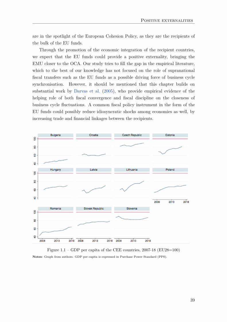
The reason for this may lie in the fact that these economies have experiencedtwo remarkable transitions in the last two decades. Transformation in the truesense of the word happened, first, during the switch from planned to marketeconomies, and second, during the period of entry and integration within the EU,accompanied by the latter’s outstanding trade openness, financial integration, andcapital account liberalisation (Mody et al. (2009)). In this chapter, we focus onthe latter type of transition, because, aside from the last step of adopting thecommon currency, the euro, the transition is still ongoing for the majority of theCEE countries. Although several reforms have been implemented to improve theinstitutional establishment of the EMU and strengthen cooperation between themember states, the future shape of the EMU remains uncertain, as do the potentialfor enlargements (Blesse et al. (2020)). One may note that those countries classifiedas belonging to the periphery regarding business cycle synchronisation are still thepoorest ones in the EU (see Figure 1.1), variously lagging behind the EU averagedue to the heterogeneous speed of real income convergence.
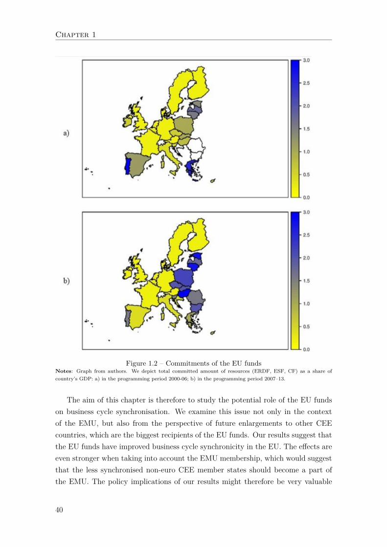
To support economic development and convergence between the EU memberstates in terms of GDP per capita, five main EU funds (officially, the EuropeanStructural and Investment Funds), have been established: the European RegionalDevelopment Fund (ERDF), the European Social Fund (ESF), the Cohesion Fund(CF), the European Agricultural Fund for Rural Development (EAFRD), and theEuropean Maritime and Fisheries Fund (EMFF). These EU funds constitute thesecond-largest budget line after the EU’s agricultural expenses for the currentprogramming period 2014-20.3 The EU funds provide financing for a wide rangeof projects and programmes in different areas (such as regional or agriculturaldevelopment, transport infrastructure, and research) to promote economic growth,mostly in the EU’s lagging countries. As Figure 1.2 indicates, the CEE countries
1Germany, Austria, France, Belgium, and the Netherlands are unanimously identified as thecore countries, whereas Greece, Portugal, Ireland, and Finland are often considered the periphery.These findings are illustrated in the annex, Table A1.1 ; Austria can be considered the EMUeconomy with the highest average level of business cycle synchronisation with Germany (one ofthe EMU’s core main economies, considered as a reference EMU business cycle) during 2000-2014.Conversely, Greece exhibits the lowest average value.
2We follow the OECD term CEE countries, comprising the Visegrad countries (Hungary,Poland, Slovakia, and the Czech Republic), the Baltic countries (Estonia, Latvia, and Lithua-nia), and the Southeastern countries (Bulgaria, Croatia, Romania, and Slovenia).
3For more information concerning the legislation of the EU funds, see regulation (EU) No.1303/2013 of the European Parliament and of the Council and repealing Council Regulation (EC)No. 1083/2006 or particular Fund-specific regulations – the ERDF Regulation No. 1301/2013; theESF Regulation No. 1304/2013; the CF Regulation No. 1300/2013; the EAFRD Regulation No1305/2013; the EMFF Regulation No. 508/2014.
38
Positive externalities
are in the spotlight of the European Cohesion Policy, as they are the recipients ofthe bulk of the EU funds.
Through the promotion of the economic integration of the recipient countries,we expect that the EU funds could provide a positive externality, bringing theEMU closer to the OCA. Our study tries to fill the gap in the empirical literature,which to the best of our knowledge has not focused on the role of supranationalfiscal transfers such as the EU funds as a possible driving force of business cyclesynchronisation. However, it should be mentioned that this chapter builds onsubstantial work by Darvas et al. (2005), who provide empirical evidence of thehelping role of both fiscal convergence and fiscal discipline on the closeness ofbusiness cycle fluctuations. A common fiscal policy instrument in the form of theEU funds could possibly reduce idiosyncratic shocks among economies as well, byincreasing trade and financial linkages between the recipients.
Figure 1.1 – GDP per capita of the CEE countries, 2007-18 (EU28=100)Notes: Graph from authors. GDP per capita is expressed in Purchase Power Standard (PPS).
39
Chapter 1
Figure 1.2 – Commitments of the EU fundsNotes: Graph from authors. We depict total committed amount of resources (ERDF, ESF, CF) as a share ofcountry’s GDP: a) in the programming period 2000-06; b) in the programming period 2007–13.
The aim of this chapter is therefore to study the potential role of the EU fundson business cycle synchronisation. We examine this issue not only in the contextof the EMU, but also from the perspective of future enlargements to other CEEcountries, which are the biggest recipients of the EU funds. Our results suggest thatthe EU funds have improved business cycle synchronicity in the EU. The effects areeven stronger when taking into account the EMU membership, which would suggestthat the less synchronised non-euro CEE member states should become a part ofthe EMU. The policy implications of our results might therefore be very valuable
40
Positive externalities
not only for the implementation and regulation of the recent European CohesionPolicy, but also when considering potential future enlargement of the EMU. Thesystematically identified driving forces are the ERDF and the CF, through whichmost projects financing transport infrastructure and technological development aresupported. These estimates are robust to different estimators and different businesscycle filtering techniques.
The remainder of this chapter is organised as follows: the second sectionprovides a related literature review. The third section deals with the methodologyand data used to conduct our analysis: we apply a panel instrumental variablesapproach to account for the possible endogeneity problem of the business cyclesynchronisation driving forces. The fourth section provides the estimation resultsfor the full sample, as well as for the sub-samples with particular country-pairsand EU funds. We conclude our findings in the last section, with regard to EUcooperation in the areas of supranational fiscal transfers and common economicgovernance. We also give perspectives for future research.
1.2 Related literature
Previous research about the EU funds has mostly attempted to determine whetherthese expenditures can be considered as an important policy instrument promot-ing economic growth (Becker et al. (2010); Mohl & Hagen (2010); Pellegrini et al.(2013)), the level of convergence (Cappelen et al. (2003); Becker et al. (2013)), oremployment rates of the member states (Bondonio & Greenbaum (2006); Mohl &Hagen (2010)). However, it is important to note that the literature acknowledgesthat the impact of the EU funds on GDP is conditional on certain factors. Somecommonly identified determinants of this conditional impact are quality of insti-tutions and government (Ederveen et al. (2006); Becker (2012); Rodríguez-Pose& Garcilazo (2015)), absorption capacity (Tătulescu & Pătruţi (2014); Huliaras& Petropoulos (2016)), socio-economic conditions (Crescenzi & Giua (2016)), andquality of macroeconomic management (Tomova et al. (2013)). However, to ourknowledge no systematic empirical research directly addresses the question of po-tential linkage between the EU funds and business cycle synchronicity.
Can these payments promote business cycle synchronisation in the EMU to makeit closer to an OCA? The very few existing studies mostly focus on the examinationof a cyclical component of the EU funds in the years following the Great Recession of2008-09 to underline a counter-cyclical component of the European Cohesion Policy.
41

Chapter 1
Smail (2010) highlights the reactivity of the European authorities to this economicdownturn in form of series of amending regulations aimed at increasing the level ofadvances to member states in order to use the EU funds as a tool for macroeco-nomic stabilisation. These advances accounted for more than eight percent of allfunds in the programming period 2007-13. Such a strategy has also been pursued inthe programming period 2014-20, as, for instance, when an additional €1.375 billionwas allocated for Greece, or €1 billion for Portugal.4
Another key measure has been to simplify the EU funds regulations to makethe implementation of projects easier and speed up recipient countries’ absorption.According to Kondor-Tabun & Staehr (2015), this measure led to a faster executionof programmes in the Baltic countries after the global financial crisis. Besides that,this study points out that in Poland (the biggest EU funds recipient country), asimilar pattern can be observed. On the other hand, some studies such as thatby Tătulescu & Pătruţi (2014) describe the EU funds as procyclical, owing to thereduced ability to draw allocated funds during economic downturns. Indeed, duringrecessions, the available resources for national co-financing are reduced as a result ofincreased national expenditure and of a reduction on the revenue side of public bud-gets. Covering the period 2004-15 for the Czech Republic, Chmelová et al. (2018)examines and concludes that EU funds are procyclical, as a 1 percent increase of theCzech economy’s output gap is associated with an increase in European transfers byCZK 8.4 billion. However, Chmelová et al. (2018) concludes that this procyclicalitymust be considered a purely random effect resulting from the restricted time frameof the programming periods. The ability to prepare projects and implement themin the context of the national and EU legal framework are identified as the maindeterminants of this procyclicality. Indeed, the first years of a programming periodare characterised by few payments, as a large amount of investment projects arejust being constituted and await the approval of the European Commission. Giventhat all of EU’s economies are recipients of the EU funds, their pro-cyclicity orcounter-cyclicity might promote business synchronisation, as payments are imple-mented simultaneously.
To the best of our knowledge, empirical literature lacks a study exploring thepotential role of the Cohesion Policy on business cycle synchronisation among its re-cipient countries, a gap that we will try to fill. In the context of the EU, three driversof business synchronisation have already been widely identified in the literature.First, trade intensity has so far been the most examined potential driver (Frankel &Rose (1998); Baxter & Kouparitsas (2005); Silvestre & Mendonça (2007)), leading
4See Annex VII of the EU Regulation No. 1303/2013 for more details.
42
Positive externalities
to more synchronised business cycles by boosting demand shocks among countries.Frankel and Rose (1998) find a positive relationship between trade and synchroni-sation based on the dataset of industrialised countries, and many other empiricalstudies of industrialised countries confirm their findings (see, for instance, Fatas(1997), and Clark & Van Wincoop (2001)). A second driving force is the similar-ity of economic structures, as when, in the presence of sector-specific shocks, twoeconomies producing the same types of goods are likely to face similar economicconditions (Imbs (2004); Calderon et al. (2007); Beck (2014)). This evidence hasalso been supported when studying the economic integration of eight CEE countrieswhich joined the EU in 2004; the similarity of economic structures in these countrieshad a direct positive and significant effect on business cycle synchronisation withthe euro area members over the period 1990-2003 (Siedschlag & Tondl (2011)). Thisstudy also draws attention to the endogeneity of business cycle correlations, the sim-ilarity of economic structures, and the trade intensity resulting from membershipin the EMU. Indeed, this study concludes that the new EU countries will betterqualify for the monetary union after the adoption of the euro, and that thereforethey should not postpone joining the euro area. The promoting role of the euro onCEE countries’ economic integration has also been supported by researchers suchas Jiménez-Rodriguez et al. (2010) and Nguyen & Rondeau (2019). The pioneeringwork of Darvas et al. (2005) invokes the fiscal rules inherited from the Maastricht(nominal convergence) criteria as a factor fostering fiscal convergence and makingmember states’ business cycles fluctuate more closely with one another. By pro-moting economic integration of their recipient economies, the EU funds may actas an additional driver of business cycle synchronisation in the Common Market,especially for the countries that share the euro.
Our analysis contributes to the existing empirical literature in two ways. Firstly,we investigate whether the EU funds have a positive externality on the commonmonetary policy, that is, whether such payments have contributed to the overalllevel of synchronisation in the EU, and especially in the EMU. Secondly, we tacklethe issue of economic integration of the CEE countries within the EU, by studyingthe role of the EU funds in promoting business synchronisation between the CEEand the EU-15 countries.
43
Chapter 1
1.3 Methodology and data
1.3.1 Panel instrumental variables estimation
Our instrumental variable strategy builds on studies of Frankel & Rose (1998), Imbs(2004) and Darvas et al. (2005), taking into account the possible endogeneity prob-lem of the business cycle synchronisation driving forces. We estimate the followingregression model:
SyncFisheri,j,τ = β1Actual EUi,j,τ + β2Tradei,j,τ + β3Specialisationi,j,τ
+C∑c=1
δcXci,j,τ + µi,j + γτ + εi,j,τ(1.1)
where SyncFisheri,j,τ represents a level of the business cycle synchronisation be-tween country i and country j within time span τ . The variable of our interest,Actual EUi,j,τ denotes a total amount of actual expenditure from the EU funds incountries i and j within time span τ .5 The model specification also covers the keydeterminants of the business cycle co-movement, mostly highlighted in the previousempirical literature: Tradei,j,τ , which denotes trade intensity between countries iand j within time span τ , and Specialisation EUi,j,τ , which stands for the similarityin industry specialisation between countries i and j within time span τ . We alsoinclude a set of control variables (Xci,j,τ ), country-pair fixed effects (µi,j) and timefixed effects (γτ ) to account for country-pair/time heterogeneity.
We consider the following set of control variables. First, we take into accounta variable related to human capital, which presents an education proxy measuringthe labour enrolments in high school and tertiary education. Dellas & Sakellaris(2003) and Ductor & Leiva-Leon (2016) find that countries with different levels ofschooling are more likely to be in different business cycle phases, as during periodsof expansion, individuals tend to substitute human capital investment with othereconomic activities because of the higher opportunity costs of schooling. Second, weconsider the urbanisation rate as an exogenous control for level of economic develop-ment (Bloom et al. (2008)); urban areas induce economies of scale and consequently,
5As the EC declares: " Data collected on annual real expenditure from the EU funds follows thecycle of the EC member states’ reimbursement and not exactly the date, on which payments tookplace. This may negatively bias evaluation of the policy implications while performing analyses.In order to prevent from that, the EC develops more realistic estimate of the annual expenditure,which presents the mean of 100 000 simulations on the historic annual EU payments". Hence, weconsider this modelled annual expenditure as our actual EU funds expenditure variable. Infor-mation regarding the robustness and sensitivity of assumptions are available in Lo Piano et al.(2017).
44
Positive externalities
a higher level of income. Examination of country-pairs shows that deep income dif-ferences should lead to synchronised business cycles (Antonakakis & Tondl (2014)).Third, we consider a proxy for institutional setting (namely, control of corruption),as previous studies find significant linkages to business cycle synchronisation (Al-tug & Canova (2014); Antonakakis & Tondl (2014)). For instance, Altug & Canova(2014) conclude that for a full sample of the European and Mediterranean countries,differences in the quality of governance and in civil liberties reduce business cyclesynchronisation. However, one should be careful when using simple OLS estimationof the relationship between business cycle synchronisation and its determinants.Trade intensity and industry specialisation are proven to be the endogenous de-terminants of business cycle synchronisation (Frankel & Rose (1998); Imbs (2004);Antonakakis & Tondl (2014)).6
Similarly, the final allocation of the EU funds, which can be considered a fis-cal instrument, is plausibly driven by contemporaneous economic conditions. Forinstance, countries in deteriorated economic condition may be likely to receive agreater share of the EU payments than others, confirming counter-cyclical characterand a greater business cycle synchronisation, which would likely bias our estimates.On the other hand, there might exist an upward bias, which would occur if the ex-pansionary periods are positively correlated with an increase in aggregate demand,a growing number of co-financed projects, and the final allocation of the EU fundspayments. This would imply a cyclical character of the EU payments, reducing thelevel of the business cycle synchronisation, which can be also associated with theparadox of decreased ability to draw the EU’s resources in the recessionary periods.Taking these facts into account, we also cannot consider actual expenditure fromthe EU funds as an exogenous variable with respect to business cycle fluctuations,due to expenditure’s demand-driven nature (counter-cyclical or cyclical).
Without correcting for possible endogeneity, our estimates would be biased, in-validating basic assumption of uncorrelated error term with the independent vari-able. To address this issue, we employ a panel instrumental variable strategy usingtwo stage least squares (2SLS) estimation, where the first stage estimation has the
6Since the impact of trade intensity and industry specialisation on business cycle co-movementhas already been investigated by numerous authors, it is not central to this chapter. We ratherrecommend to the reader the vast empirical literature on this matter.
45
Chapter 1
following form:
Actual EUi,j,τ =N∑n=1
θ1,nZn,i,j,τ + α1Tradei,j,τ + α2Specialisationi,j,τ
+C∑c=1
π1c,iXc,i,j,τ + λ1i,j + v1τ + ζ1i,j,τ
(1.2)
Tradei,j,τ =N∑n=2
θ2,nZn,i,j,τ + α3Actual EUi,j,τ + α4Specialisationi,j,τ
+C∑c=1
π2c,iXc,i,j,τ + λ2i,j + v2τ + ζ2i,j,τ
(1.3)
Specialisationi,j,τ =N∑n=3
θ3,nZn,i,j,τ + α5Actual EUi,j,τ + α6Tradei,j,τ
+C∑c=1
π3c,iXc,i,j,τ + λ3i,j + v3τ + ζ3i,j,τ
(1.4)
where Zn,i,j,τ denotes n-th instrumental variable (instrument) used to estimateendogenous determinants of the synchronisation: actual payments from the EUfunds/trade intensity/specialisation, varying over both time span τ and country-pairs i,j. Estimated dependent variables from (Eq. 1.2), (Eq. 1.3) and (Eq. 1.4)are consequently used in (Eq. 1.1), which presents the second stage estimation.
Empirical research of trade intensity and industry specialisation offers many op-tions regarding possible instruments. Trade instruments include commonly knowngravity variables, such as geographical distance, and dummy variables denoting com-mon borders or common language (Frankel & Rose (1998)). However, because oftheir time-invariant nature, we have to follow Imbs (2004), Bravo-Ortega & Di Gio-vanni (2006) and use time-variant measures: the non-tariff barriers and the remote-ness index, which defines the propensity to trade between countries i and j.7 Forspecialisation, we apply GDP gap and GDP product of both economies, showingtwo stages of specialisation: initial diversification, followed by re-specialisation at arelatively high level of income (Imbs & Wacziarg (2003)), alongside the capital ac-count restrictions or liberalisation, which serve as the instruments for specialisationarising from access to financial markets (Imbs (2004)).
7Imbs (2004) also suggests other instruments, such as local trade agreements and import duties.Unfortunately, these do not seem relevant for the current EU institutional framework and theEuropean single market.
46
Positive externalities
To account for the endogeneity in the actual payments from the EU funds, theliterature is not so extensive. We need to find an instrument Zn,i,j,τ which is un-correlated with contemporaneous economic conditions (and the error term), butstrongly linked to the actual EU funds expenditure. In this chapter, we decide touse planned EU payments (commitments) as an instrument to the actual paymentsfrom the EU funds; this constitutes our innovation in business cycle synchronisationresearch.8 The argument behind using the commitments as a source of exogenousvariation in the actual EU payments is that their allocation rule, provided in theannex (Table A1.2), is based on past values of variables such as one NUTS-2 region’srelative GDP per capita, unemployment rate, and demographic and geographiccharacteristics.9 Consequently, the commitments allocation is determined at theregional NUTS-2 level at the beginning of each programming period, independentlyof contemporaneous business cycle conditions. It is driven by supranational politicalfactors—negotiations and the final approval by the European Council and the Euro-pean Parliament based on the proposal by the European Commission, which occursseveral years prior to considered programming periods—rather than by endogenousbusiness cycle conditions. At the same time, it goes without saying that commit-ments allocation is closely connected to the actual allocation (see in the annex,Figure A1.1), although many member states do not draw all committed resourcesfrom the EU funds, due to their low absorptive capacity (Becker et al. (2013)). Theinstrument relevance (strength) is tested using F-test of the first stage regressionfor weak instruments and the consistency of the 2SLS estimation by Wu-Hausmantest for endogeneity. We report heteroscedasticity and serial correlation consistentstandard errors for within-groups estimators throughout the chapter (Arellano et al.(1987)).
1.3.2 Variables definition and data
In line with previous studies (see, for instance, Imbs (2004); Darvas et al. (2005);Siedschlag & Tondl (2011); Antonakakis & Tondl (2014)), we choose the Pearsoncorrelation coefficient of real GDP time series as the indicator measuring the levelof the business cycle synchronisation. We calculate bilateral correlation coefficientsbetween each country i and country j within time span τ using input data v (real
8However, we follow recent empirical contributions regarding estimation of the impact of gov-ernment spending on the (local) economy, in which authors use planned funds resources as instru-ments (see, for instance, Coelho (2019) and Dupor & Guerrero (2017)).
9See the EU Council Regulations 502/1999, 595/2006, and 189/2007 for further details. Forthe CF, allocation criteria are first established at the member state’s level with the 90 percentthreshold rule.
47
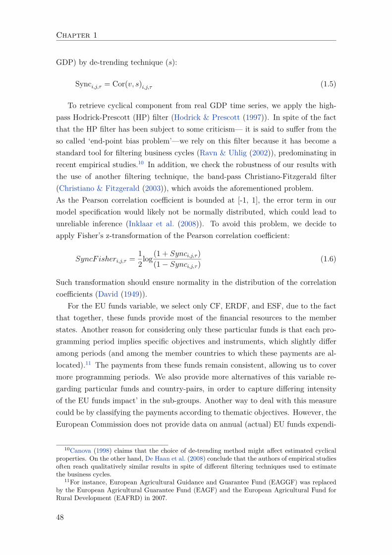
Chapter 1
GDP) by de-trending technique (s):
Synci,j,τ = Cor(v, s)i,j,τ (1.5)
To retrieve cyclical component from real GDP time series, we apply the high-pass Hodrick-Prescott (HP) filter (Hodrick & Prescott (1997)). In spite of the factthat the HP filter has been subject to some criticism— it is said to suffer from theso called ‘end-point bias problem’—we rely on this filter because it has become astandard tool for filtering business cycles (Ravn & Uhlig (2002)), predominating inrecent empirical studies.10 In addition, we check the robustness of our results withthe use of another filtering technique, the band-pass Christiano-Fitzgerald filter(Christiano & Fitzgerald (2003)), which avoids the aforementioned problem.As the Pearson correlation coefficient is bounded at [-1, 1], the error term in ourmodel specification would likely not be normally distributed, which could lead tounreliable inference (Inklaar et al. (2008)). To avoid this problem, we decide toapply Fisher’s z-transformation of the Pearson correlation coefficient:
SyncF isheri,j,τ = 12 log
(1 + Synci,j,τ )(1− Synci,j,τ )
(1.6)
Such transformation should ensure normality in the distribution of the correlationcoefficients (David (1949)).
For the EU funds variable, we select only CF, ERDF, and ESF, due to the factthat together, these funds provide most of the financial resources to the memberstates. Another reason for considering only these particular funds is that each pro-gramming period implies specific objectives and instruments, which slightly differamong periods (and among the member countries to which these payments are al-located).11 The payments from these funds remain consistent, allowing us to covermore programming periods. We also provide more alternatives of this variable re-garding particular funds and country-pairs, in order to capture differing intensityof the EU funds impact’ in the sub-groups. Another way to deal with this measurecould be by classifying the payments according to thematic objectives. However, theEuropean Commission does not provide data on annual (actual) EU funds expendi-
10Canova (1998) claims that the choice of de-trending method might affect estimated cyclicalproperties. On the other hand, De Haan et al. (2008) conclude that the authors of empirical studiesoften reach qualitatively similar results in spite of different filtering techniques used to estimatethe business cycles.
11For instance, European Agricultural Guidance and Guarantee Fund (EAGGF) was replacedby the European Agricultural Guarantee Fund (EAGF) and the European Agricultural Fund forRural Development (EAFRD) in 2007.
48
Positive externalities
ture per country and per objective.12 We create a dataset of annual committed andactual EU funds expenditure covering three programming periods (2000-06, 2007-13,and 2014-16) from multiple documents and databases published by the EuropeanCommission. In the programming period 2000-06, data on annual committed pay-ments from the CF are not available; here, we follow an amended proposal from2003 for a Council Regulation establishing a Cohesion Fund, and calculate missingdata.13
Trade intensity is calculated in the standard way as bilateral trade over countryi’s and country j’s nominal GDP (Imbs (2004)). Trade instrument, the remotenessindex presents the standard remoteness index of Bravo-Ortega & Di Giovanni (2006)at the EU level:
Remotenessi,j,τ =∑
j, τDi,j,τ
Tj,τ/Tτ(1.7)
where Di,j,τ denotes the population-weighted distance from country i to country jand Tj,τ stands for the bilateral trade flows (imports and exports) between i andj in period τ , whereas Tτ represents the total intra-European trade. This variablecaptures an expected increase in trade for bilateral trading partners that are remotefrom the rest of the EU. For example, it would be expected that Ireland and the UKwould trade more with each other not only because of their geographic closeness,but also because of their remote geographic positions in the EU.
For the specialisation, we compute the Krugman (1991) specialisation index(KSI) based on 18 industrial categories, which ranges between 0 and 2; whereasa value 2 indicates total specialisation (with regard to the EU-average, in our case),a value 0 represents perfect similarity.14 As we work with the country-pairs, wecompute the ratio of KSI between countries i and j to obtain a similarity in industryspecialisation that takes values between 0 and 1. The higher the value, the moresimilar the relative industrial structure in the country-pair.
12This is due to the fact that there was no harmonised system or information available regardingclassification of the payments per objective across different funds and programming periods. Onlyannual commitments per country and objective are available.
13In the programming period 2000-06, the financial resources from the CF should be allocatedto 14 EU member states (from 1 January 1, 2000: Greece, Spain, Portugal, and Ireland; fromdate of accession to the EU: the Czech Republic, Estonia, Cyprus, Latvia, Lithuania, Hungary,Malta, Poland, Slovenia, and Slovakia). Commitment appropriations for the latter should be:€2.6168 billion in 2004, €2.1517 billion in 2005, and €2.8220 billion in 2006. We calculate annualcommitments for each country by multiplying total annual commitment appropriations by meanindicative allocation coefficient per country. Total resources available for commitments for Greece,Spain, Portugal, and Ireland are only available for the whole period 2000-06; here, we calculateannual committed payments per country based on annual committed payments from remainingfunds under Objective 1 (Convergence).
14NACE Rev. 2 1-digit industry classification.
49
Chapter 1
All variables used in the model estimation undergo several transformations.Firstly, the variables are expressed as an annual percentage change or percentage ofpopulation/GDP to account for the country’s size and population. Consequently,we calculate bilateral values of each variable (such as correlation coefficients, a sumof actual/committed payments) between each country-pair. The last step of trans-formation presents a log-transformation of the smoothed data; we apply five yearrolling window transformation (time span τ), by which we lose a few observations,but eliminate redundant fluctuations/noise in time series and take into account pos-sible persistent effect by using a lag term of the EU funds expenditure on businesscycle synchronisation. 15
Our sample covers a panel dataset of the EU–28 countries in time period 2000-16.We construct bilateral measures, which means that in total the model can be es-timated as using a maximum of 4,914 observations. We provide all the variablesdefinitions and sources in the annex, (Table A1.3) .
1.4 Results and discussion
In this section, we present the main results from performed analysis regarding thepotential linkage between the supranational fiscal transfers from the EU funds andbusiness cycle synchronisation, which are available in Table 1.1, Table 1.2 andTable 1.3. In general, our results support the view that the EU funds enhancebusiness cycle synchronisation. Both weak instruments test and Wu-Hausman testfor the endogeneity of the instrument are satisfied while using control variables inour model’s specifications. Firstly, estimation results for the impact of total EUfunds in the EU-28 are provided in Table 1.1.16
15Deciding on the length of rolling window might be problematic especially when using correla-tion coefficients (due to the trade-off between statistical confidence and ability to isolate significantchanges in time). Here, we follow the studies of Antonakakis & Tondl (2014) and Lukmanova &Tondl (2017), who use five year rolling windows while investigating potential business cycle syn-chronisation driving forces.
16For the sake of brevity, the OLS estimation results suggesting limited bias are not reported(available upon request).
50
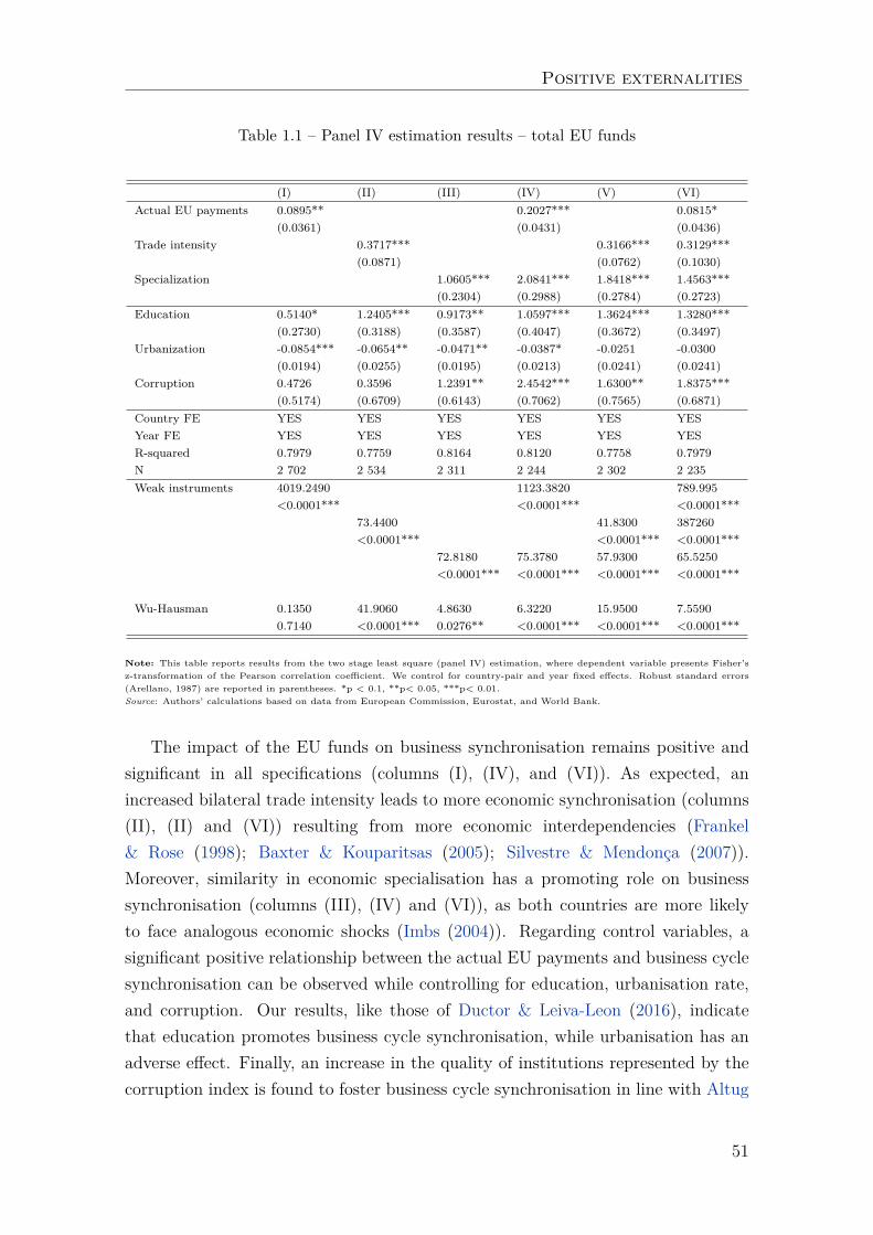
Positive externalities
Table 1.1 – Panel IV estimation results – total EU funds
(I) (II) (III) (IV) (V) (VI)Actual EU payments 0.0895** 0.2027*** 0.0815*
(0.0361) (0.0431) (0.0436)Trade intensity 0.3717*** 0.3166*** 0.3129***
(0.0871) (0.0762) (0.1030)Specialization 1.0605*** 2.0841*** 1.8418*** 1.4563***
(0.2304) (0.2988) (0.2784) (0.2723)Education 0.5140* 1.2405*** 0.9173** 1.0597*** 1.3624*** 1.3280***
(0.2730) (0.3188) (0.3587) (0.4047) (0.3672) (0.3497)Urbanization -0.0854*** -0.0654** -0.0471** -0.0387* -0.0251 -0.0300
(0.0194) (0.0255) (0.0195) (0.0213) (0.0241) (0.0241)Corruption 0.4726 0.3596 1.2391** 2.4542*** 1.6300** 1.8375***
(0.5174) (0.6709) (0.6143) (0.7062) (0.7565) (0.6871)Country FE YES YES YES YES YES YESYear FE YES YES YES YES YES YESR-squared 0.7979 0.7759 0.8164 0.8120 0.7758 0.7979N 2 702 2 534 2 311 2 244 2 302 2 235Weak instruments 4019.2490 1123.3820 789.995
<0.0001*** <0.0001*** <0.0001***73.4400 41.8300 387260<0.0001*** <0.0001*** <0.0001***
72.8180 75.3780 57.9300 65.5250<0.0001*** <0.0001*** <0.0001*** <0.0001***
Wu-Hausman 0.1350 41.9060 4.8630 6.3220 15.9500 7.55900.7140 <0.0001*** 0.0276** <0.0001*** <0.0001*** <0.0001***
Note: This table reports results from the two stage least square (panel IV) estimation, where dependent variable presents Fisher’sz-transformation of the Pearson correlation coefficient. We control for country-pair and year fixed effects. Robust standard errors(Arellano, 1987) are reported in parentheses. *p < 0.1, **p< 0.05, ***p< 0.01.Source: Authors’ calculations based on data from European Commission, Eurostat, and World Bank.
The impact of the EU funds on business synchronisation remains positive andsignificant in all specifications (columns (I), (IV), and (VI)). As expected, anincreased bilateral trade intensity leads to more economic synchronisation (columns(II), (II) and (VI)) resulting from more economic interdependencies (Frankel& Rose (1998); Baxter & Kouparitsas (2005); Silvestre & Mendonça (2007)).Moreover, similarity in economic specialisation has a promoting role on businesssynchronisation (columns (III), (IV) and (VI)), as both countries are more likelyto face analogous economic shocks (Imbs (2004)). Regarding control variables, asignificant positive relationship between the actual EU payments and business cyclesynchronisation can be observed while controlling for education, urbanisation rate,and corruption. Our results, like those of Ductor & Leiva-Leon (2016), indicatethat education promotes business cycle synchronisation, while urbanisation has anadverse effect. Finally, an increase in the quality of institutions represented by thecorruption index is found to foster business cycle synchronisation in line with Altug
51
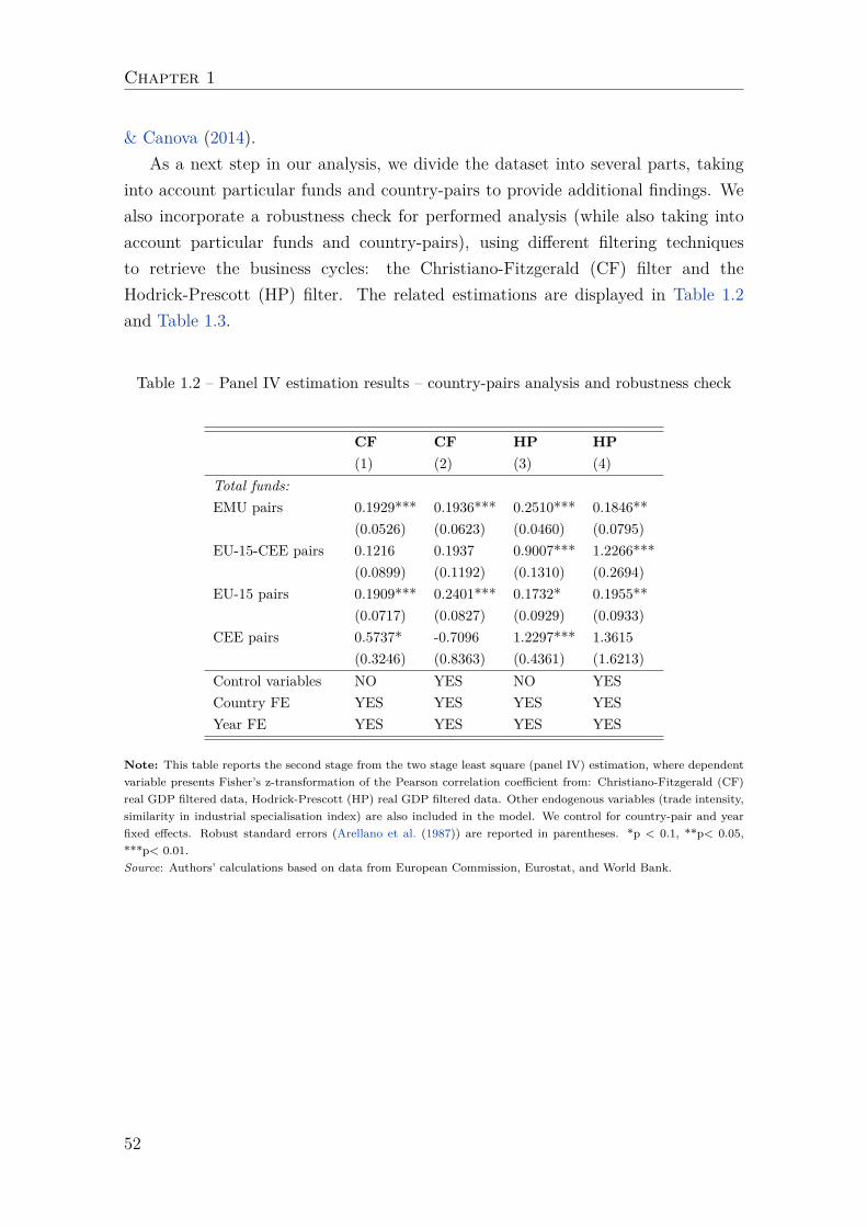
Chapter 1
& Canova (2014).As a next step in our analysis, we divide the dataset into several parts, taking
into account particular funds and country-pairs to provide additional findings. Wealso incorporate a robustness check for performed analysis (while also taking intoaccount particular funds and country-pairs), using different filtering techniquesto retrieve the business cycles: the Christiano-Fitzgerald (CF) filter and theHodrick-Prescott (HP) filter. The related estimations are displayed in Table 1.2and Table 1.3.
Table 1.2 – Panel IV estimation results – country-pairs analysis and robustness check
CF CF HP HP(1) (2) (3) (4)
Total funds:EMU pairs 0.1929*** 0.1936*** 0.2510*** 0.1846**
(0.0526) (0.0623) (0.0460) (0.0795)EU-15-CEE pairs 0.1216 0.1937 0.9007*** 1.2266***
(0.0899) (0.1192) (0.1310) (0.2694)EU-15 pairs 0.1909*** 0.2401*** 0.1732* 0.1955**
(0.0717) (0.0827) (0.0929) (0.0933)CEE pairs 0.5737* -0.7096 1.2297*** 1.3615
(0.3246) (0.8363) (0.4361) (1.6213)Control variables NO YES NO YESCountry FE YES YES YES YESYear FE YES YES YES YES
Note: This table reports the second stage from the two stage least square (panel IV) estimation, where dependentvariable presents Fisher’s z-transformation of the Pearson correlation coefficient from: Christiano-Fitzgerald (CF)real GDP filtered data, Hodrick-Prescott (HP) real GDP filtered data. Other endogenous variables (trade intensity,similarity in industrial specialisation index) are also included in the model. We control for country-pair and yearfixed effects. Robust standard errors (Arellano et al. (1987)) are reported in parentheses. *p < 0.1, **p< 0.05,***p< 0.01.Source: Authors’ calculations based on data from European Commission, Eurostat, and World Bank.
52
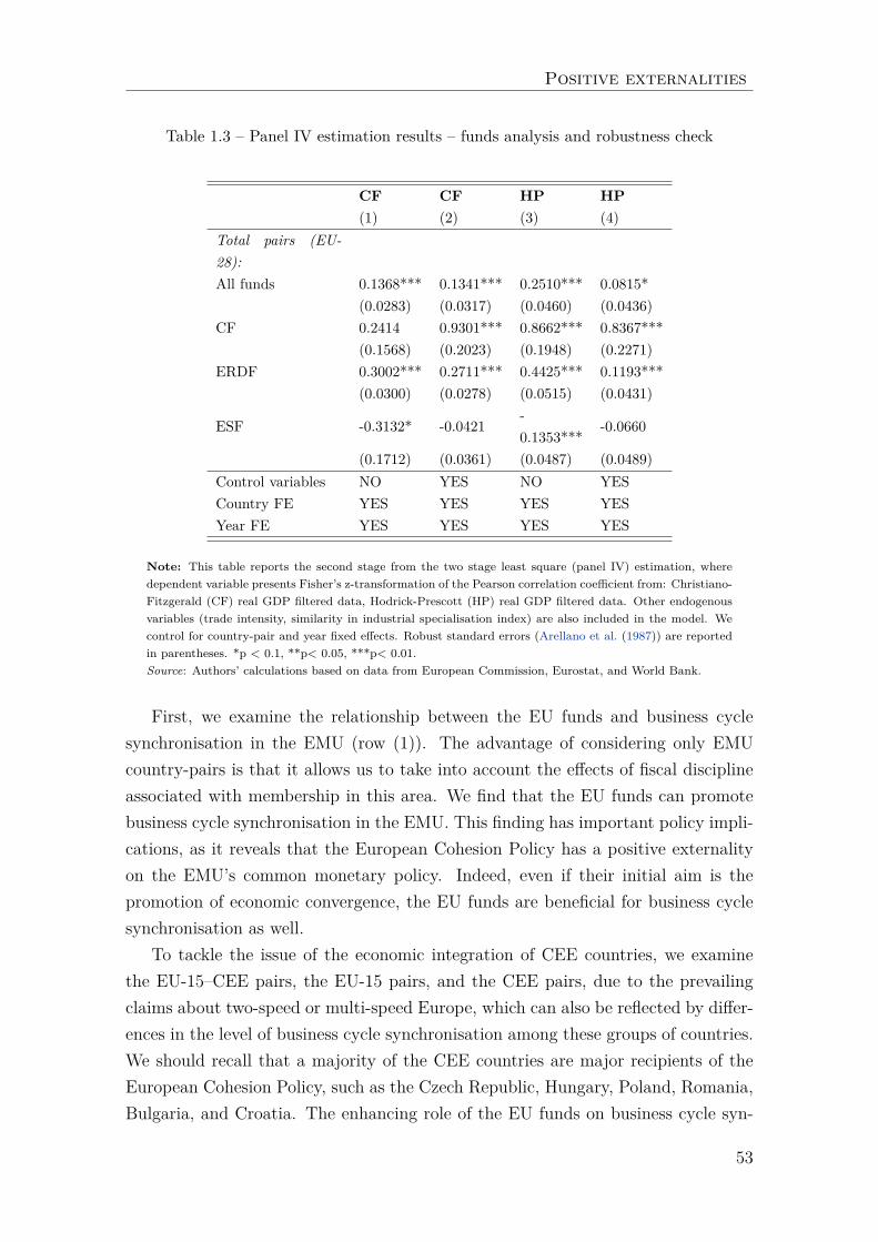
Positive externalities
Table 1.3 – Panel IV estimation results – funds analysis and robustness check
CF CF HP HP(1) (2) (3) (4)
Total pairs (EU-28):All funds 0.1368*** 0.1341*** 0.2510*** 0.0815*
(0.0283) (0.0317) (0.0460) (0.0436)CF 0.2414 0.9301*** 0.8662*** 0.8367***
(0.1568) (0.2023) (0.1948) (0.2271)ERDF 0.3002*** 0.2711*** 0.4425*** 0.1193***
(0.0300) (0.0278) (0.0515) (0.0431)
ESF -0.3132* -0.0421-0.1353***
-0.0660
(0.1712) (0.0361) (0.0487) (0.0489)Control variables NO YES NO YESCountry FE YES YES YES YESYear FE YES YES YES YES
Note: This table reports the second stage from the two stage least square (panel IV) estimation, wheredependent variable presents Fisher’s z-transformation of the Pearson correlation coefficient from: Christiano-Fitzgerald (CF) real GDP filtered data, Hodrick-Prescott (HP) real GDP filtered data. Other endogenousvariables (trade intensity, similarity in industrial specialisation index) are also included in the model. Wecontrol for country-pair and year fixed effects. Robust standard errors (Arellano et al. (1987)) are reportedin parentheses. *p < 0.1, **p< 0.05, ***p< 0.01.Source: Authors’ calculations based on data from European Commission, Eurostat, and World Bank.
First, we examine the relationship between the EU funds and business cyclesynchronisation in the EMU (row (1)). The advantage of considering only EMUcountry-pairs is that it allows us to take into account the effects of fiscal disciplineassociated with membership in this area. We find that the EU funds can promotebusiness cycle synchronisation in the EMU. This finding has important policy impli-cations, as it reveals that the European Cohesion Policy has a positive externalityon the EMU’s common monetary policy. Indeed, even if their initial aim is thepromotion of economic convergence, the EU funds are beneficial for business cyclesynchronisation as well.
To tackle the issue of the economic integration of CEE countries, we examinethe EU-15–CEE pairs, the EU-15 pairs, and the CEE pairs, due to the prevailingclaims about two-speed or multi-speed Europe, which can also be reflected by differ-ences in the level of business cycle synchronisation among these groups of countries.We should recall that a majority of the CEE countries are major recipients of theEuropean Cohesion Policy, such as the Czech Republic, Hungary, Poland, Romania,Bulgaria, and Croatia. The enhancing role of the EU funds on business cycle syn-
53
Chapter 1
chronisation holds for the EU-15 pairs, but is not robust to the CF filter between theEU-15 and the CEE countries. Moreover, we do not find any positive relationship atall between the EU funds and business cycle synchronisation among the CEE pairs,which is in line with Stanišić et al. (2013), who rejects the hypothesis of a commonbusiness cycle between the CEE countries. Regarding the economic integration ofCEE countries, these results may suggest that the European Cohesion Policy hasa fostering role in economic integration, provided that the country adopt the euro,as did the Baltics, Slovenia and the Slovak Republic. Such a result suggests thatthe degree of economic integration underwent more significant increases for the CEEcountries that have adopted the euro than it did the other CEE countries. (Jiménez-Rodriguez et al. (2010); Siedschlag & Tondl (2011); Nguyen & Rondeau (2019)).
Besides our main results, we examine the effects of particular funds (CF, ERDFand ESF) on business cycle synchronisation to understand which EU fund drivesbusiness cycle synchronisation the most. The estimation results are available inTable 1.3. We find that both the CF (row (1)) and the ERDF (row (2)) have pro-moted business cycle synchronisation, although the same could not be said for theESF (row (3)). To interpret our estimation results and understand why the ERDFand the CF are the only funds promoting business cycle synchronisation in the EU,we rely on the extensive empirical literature which has acknowledged these funds’role in promoting trade integration and, consequently, business cycle synchronicity(Basile et al. (2008); Breuss et al. (2010); Grigoraş & Stanciu (2016)).
To illustrate this point, we could mention that about €59.1 billion from theERDF and the CF was spent on transport infrastructure for the current program-ming period. Moreover, about €86.9 billion was spent from the ERDF on technolog-ical development. Also, during the period 2015-17, the ERDF and the CF accountedfor more than 50 percent of gross fixed capital formation by the general governmentin Portugal, Lithuania, Latvia, and the Slovak Republic.17 The ERDF and the CFare the only EU funds financing transport infrastructure and projects supportingtechnological development, and it should be mentioned that both these EU fundsrepresent a large portion of public investment expenditures in the EMU countriesbelonging to the periphery. However, the ESF is usually targeted at disadvantagedgroups of people that are not included in the labour market. For instance, for theperiod 2014-17, projects with the theme ‘Employment, social inclusion and educa-tion,’ to which the ESF devotes a majority of its resources, covered 15.3 millionpeople, of which 7.9 million were unemployed and 4.9 million inactive.18 Hence, our
17Source: European Commission. Permalink: https://cohesiondata.ec.europa.eu/Other/-of-cohesion-policy-funding-in-public-investment-p/7bw6-2dw3
18See EC (2019) 816 final/2 of 01.04.2019.
54
Positive externalities
results suggest that the ESF payments of a non-investment nature do not seem toboost synchronisation as the CF or the ERDF do their with technological, morelong-term-growth generating programmes.
1.5 Conclusion
The aim of this study was to investigate the potential role of the EU payments inbusiness cycle synchronisation, a topic rarely addressed in the previous empiricalliterature. Our sample covered a panel dataset of the EU-28 countries for the period2000-16. We considered several variants of the country-pairs and of particular EUfunds to confirm robustness of our results.
Overall, our estimation results suggest the enhancing role of the EU funds onbusiness cycle synchronisation. Our findings are qualitatively similar and robust tothe use of different estimators (OLS, panel IV) and different business cycle filter-ing techniques (the Hodrick-Prescott filter, the Christiano-Fitzgerald filter). Moredetailed findings suggest that the EU funds promoted business synchronisation espe-cially in the EMU, which constitutes a positive externality of the European CohesionPolicy. Even if its main aim is to increase member states’ competitiveness and con-vergence, the goal of alleviating asymmetries of the members’ business cycles bymeans of the EU funds might present an additional motive to support lagging EUeconomies. Although each EU member state is obliged to join the EMU after meet-ing Maastricht criteria, some CEE candidate countries are not currently consideringadoption of the euro; our results, however, suggest that the degree of economic inte-gration was greater for the CEE countries that have adopted the euro than for theother CEE countries.
Moreover, we find that both the ERDF and the CF have fostered business cyclesynchronisation, which can be explained by the fact that both of these EU fundsrepresent a large part of public investment expenditures in the EMU countries be-longing to the periphery. This result confirms previous empirical evidence that theEU funds have increased financial and trade integration in the recipient countries.Following the European Council of July 17-21, 2020, the European recovery plan‘Next Generation EU’ could therefore have a promoting effect on the EMU’s mon-etary policy if it is designed as an additional structural investment fund promotingfinancial and trade integration, as are both the CF and the ERDF.
With this chapter, we enlarged the list of potential driving forces of business cy-cle synchronisation. Besides previously examined fiscal variables—fiscal convergenceand fiscal discipline, which are encouraged by the Maastricht (nominal convergence)
55
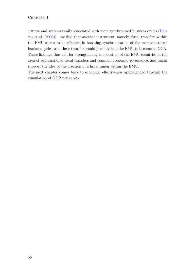
Chapter 1
criteria and systematically associated with more synchronised business cycles (Dar-vas et al. (2005))—we find that another instrument, namely, fiscal transfers withinthe EMU seems to be effective in boosting synchronisation of the member states’business cycles, and these transfers could possibly help the EMU to become an OCA.These findings thus call for strengthening cooperation of the EMU countries in thearea of supranational fiscal transfers and common economic governance, and mightsupport the idea of the creation of a fiscal union within the EMU.The next chapter comes back to economic effectiveness apprehended through thestimulation of GDP per capita.
56
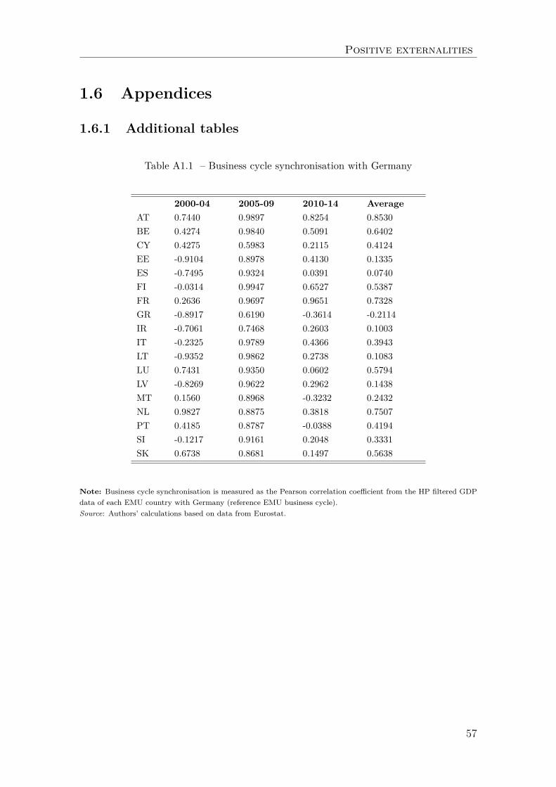
Positive externalities
1.6 Appendices
1.6.1 Additional tables
Table A1.1 – Business cycle synchronisation with Germany
2000-04 2005-09 2010-14 AverageAT 0.7440 0.9897 0.8254 0.8530BE 0.4274 0.9840 0.5091 0.6402CY 0.4275 0.5983 0.2115 0.4124EE -0.9104 0.8978 0.4130 0.1335ES -0.7495 0.9324 0.0391 0.0740FI -0.0314 0.9947 0.6527 0.5387FR 0.2636 0.9697 0.9651 0.7328GR -0.8917 0.6190 -0.3614 -0.2114IR -0.7061 0.7468 0.2603 0.1003IT -0.2325 0.9789 0.4366 0.3943LT -0.9352 0.9862 0.2738 0.1083LU 0.7431 0.9350 0.0602 0.5794LV -0.8269 0.9622 0.2962 0.1438MT 0.1560 0.8968 -0.3232 0.2432NL 0.9827 0.8875 0.3818 0.7507PT 0.4185 0.8787 -0.0388 0.4194SI -0.1217 0.9161 0.2048 0.3331SK 0.6738 0.8681 0.1497 0.5638
Note: Business cycle synchronisation is measured as the Pearson correlation coefficient from the HP filtered GDPdata of each EMU country with Germany (reference EMU business cycle).Source: Authors’ calculations based on data from Eurostat.
57
Chapter 1
Table A1.2 – Allocation method of the EU funds for the programming period 2014-2020
LDR TR MDR Cohesion FundPopulation Yes Yes Yes (25%)
Member State population Yes
Member State surface area Yes
Member State’s relative GDP/capto the EU’s average
Yes Yes Yes
Relative GDP/cap to the wealthiestNUTS 2 region
Yes (7.5%)
Relative unemployment rate to theLDR’s average
Yes Yes
Relative unemployment rate to theMDR’s average
Yes (20%)
Minimal threshold of €19.8 percapita
Yes Yes
Maximal threshold: 40% of theamount obtained by a LDR
Yes
Population density NUTS 3 level Yes (2.5%)
Europe 2020 targets Yes (45%)
Note: Less developed regions (LDR) have a GDP per capita in Purchase Power Standard (PPS) lower than 75% ofthe EU-28’s average. Transition regions (TR): between 75% and 90%. Most developed regions (MDR): more than90%. LDR, TR and MDR refer to the allocation criteria of the ERDF and the ESF only.Source: ANNEX VII, EU Regulation 1303/2013.
58
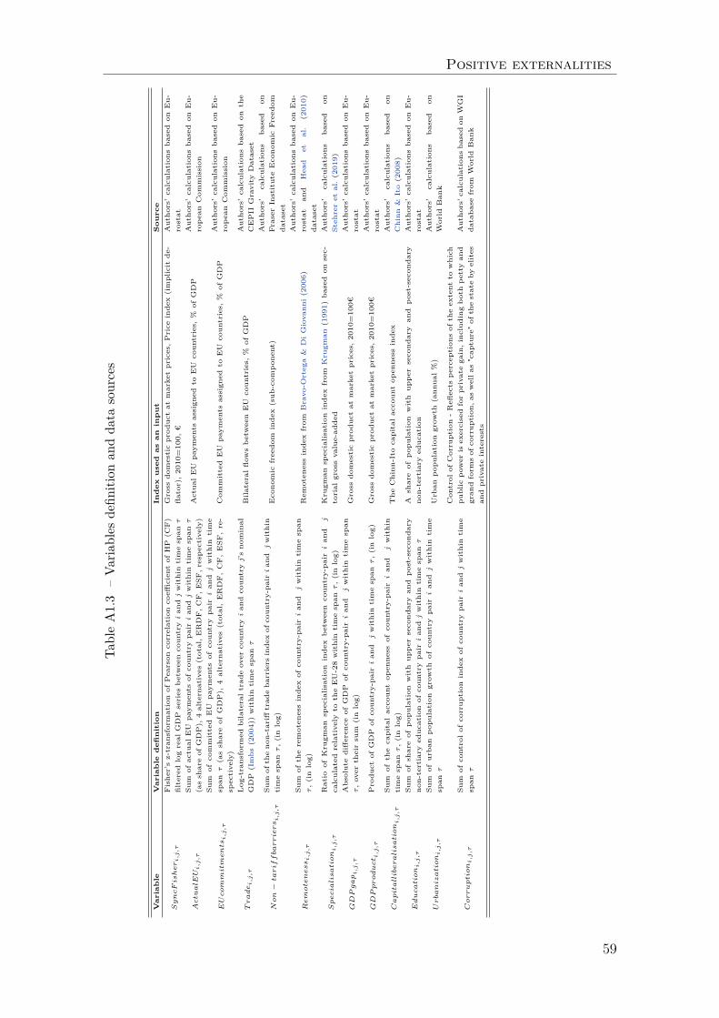
Positive externalities
TableA1.3
–Va
riables
defin
ition
andda
tasources
Variable
Variable
defi
nition
Index
usedas
aninput
Source
SyncFisheri,j,τ
Fisher’sz-tran
sformationof
Pearson
correlationcoeffi
cientof
HP(C
F)
filtered
logreal
GDPseries
betweencoun
try
ian
djwithintimespan
τ
Gross
domesticprod
uctat
marketprices,Price
index(implicit
de-
flator),
2010=100,
€Autho
rs’calculations
basedon
Eu-
rostat
ActualEUi,j,τ
Sum
ofactual
EU
paym
ents
ofcoun
trypa
irian
djwithintimespan
τ
(asshareof
GDP),4alternatives
(total,ERDF,CF,ESF
,respectively)
Actua
lEU
paym
ents
assign
edto
EU
coun
tries,
%of
GDP
Autho
rs’calculations
basedon
Eu-
ropeanCom
mission
EUcommitmentsi,j,τ
Sum
ofcommittedEU
paym
ents
ofcoun
trypa
irian
djwithintime
span
τ(asshareof
GDP),
4alternatives
(total,ERDF,CF,ESF
,re-
spectively)
Com
mittedEU
paym
ents
assign
edto
EU
coun
tries,
%of
GDP
Autho
rs’calculations
basedon
Eu-
ropeanCom
mission
Tradei,j,τ
Log-transform
edbilateraltrad
eover
coun
try
ian
dcoun
try
j’sno
minal
GDP
(Imbs
(2004))withintimespan
τBilateral
flow
sbetweenEU
coun
tries,
%of
GDP
Autho
rs’calculations
basedon
the
CEPII
Gravity
Dataset
Non−tariffbarriersi,j,τ
Sum
oftheno
n-tarifftrad
eba
rriers
indexof
coun
try-pa
irian
djwithin
timespan
τ,(inlog)
Econo
mic
freedo
mindex(sub
-com
pon
ent)
Autho
rs’
calculations
based
onFraserInstituteEcono
mic
Freedom
dataset
Remotenessi,j,τ
Sum
oftheremotenessindexof
coun
try-pa
irian
djwithintimespan
τ,(inlog)
Rem
otenessindexfrom
Bravo-O
rtega&
DiGiovann
i(2006)
Autho
rs’calculations
basedon
Eu-
rostat
and
Head
etal.
(2010)
dataset
Specialisationi,j,τ
Ratio
ofKrugm
anspecialisation
indexbetweencoun
try-pa
irian
dj
calculated
relatively
totheEU-28withintimespan
τ,(inlog)
Krugm
anspecialisation
indexfrom
Krugm
an(1991)
basedon
sec-
torial
grossvalue-ad
ded
Autho
rs’
calculations
based
onStehreret
al.(2019)
GDPgapi,j,τ
Absolutedifference
ofGDP
ofcoun
try-pa
irian
djwithintimespan
τ,over
theirsum
(inlog)
Gross
domesticprod
uctat
marketprices,2010=100€
Autho
rs’calculations
basedon
Eu-
rostat
GDPproduct i,j,τ
Produ
ctof
GDP
ofcoun
try-pa
irian
djwithintimespan
τ,(inlog)
Gross
domesticprod
uctat
marketprices,2010=100€
Autho
rs’calculations
basedon
Eu-
rostat
Capitalliberalisationi,j,τ
Sum
ofthecapitalaccoun
top
enness
ofcoun
try-pa
irian
djwithin
timespan
τ,(inlog)
The
Chinn
-Ito
capitalaccoun
top
enness
index
Autho
rs’
calculations
based
onChinn
&Ito(2008)
Educationi,j,τ
Sum
ofshareof
pop
ulationwithup
per
second
aryan
dpost-second
ary
non-tertiary
educationof
coun
trypa
irian
djwithintimespan
τ
Ashareof
pop
ulation
with
upper
second
aryan
dpost-second
ary
non-tertiary
education
Autho
rs’calculations
basedon
Eu-
rostat
Urbanizationi,j,τ
Sum
ofurba
npop
ulationgrow
thof
coun
trypa
irian
djwithintime
span
τUrban
pop
ulationgrow
th(ann
ual%)
Autho
rs’
calculations
based
onWorld
Ban
k
Corruptioni,j,τ
Sum
ofcontrolof
corrup
tion
indexof
coun
trypa
irian
djwithintime
span
τ
Con
trol
ofCorruption-Refl
ects
perceptions
oftheextent
towhich
public
pow
erisexercisedforprivategain,includ
ingbothpetty
and
gran
dform
sof
corrup
tion
,as
wella
s"cap
ture"of
thestateby
elites
andprivateinterests
Autho
rs’calculation
sba
sedon
WGI
databa
sefrom
World
Ban
k
59
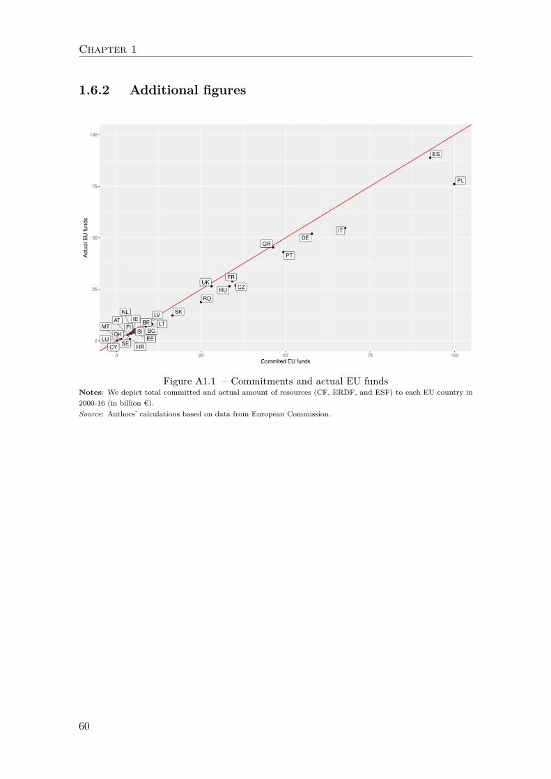
Chapter 1
1.6.2 Additional figures
Figure A1.1 – Commitments and actual EU fundsNotes: We depict total committed and actual amount of resources (CF, ERDF, and ESF) to each EU country in2000-16 (in billion €).Source: Authors’ calculations based on data from European Commission.
60
Chapter 2
Impact of European Cohesion Policy onregional growth: When time isn’t money
Summary
Considering economic effectiveness via the stimulation of per capita GDP, this chap-ter gives a theoretical basis to the trade-off based on a complete and rapid absorptionof the European funds on the one hand, and the objective of achieving economicconvergence within the EU by helping the less advanced regions on the other hand.It contributes to the literature discussing the effects of the EU Funds on GDPgrowth by revealing the causal impact of regional absorption’s speed. The analysisis conducted using a regression discontinuity design approach with heterogeneoustreatment on NUTS-2 regions during the period 2000-2016. We show that a fasterabsorption, especially in the Mediterranean regions, is associated with worse eco-nomic outcomes of the Objective 1 treatment. The opposite holds for non-treatedregions. Regarding policy implications, this study suggests that the decommitmentrule should be softened, or even removed for Objective 1 regions.
61
Chapter 2
Acknowledgements
I am grateful to the participants at the AFSE DG Trésor meeting (Paris, 2020),the "Theoretical reflections on the EU Cohesion Policy" workshop (2021), the Eu-ropean Public Choice Society congress (Lille, 2021), the European Regional ScienceAssociation congress (Bocconi, 2021), the International Institute of Public Financecongress (Reykjavik, 2021), the Conference of European Studies (Milan, 2021) andother internal seminars for helpful comments on a previous draft of this chapter.I am also grateful to Emilien Veron for his very valuable help. The usual caveatapplies.
Publication process
This Chapter is in a Revise and Resubmit process in the journal Regional Studies.
62
When time isn’t money
2.1 Introduction
Cohesion Policy is designed to foster economic homogeneity across countriesand regions of the EU to make their market integration be successful. In 1989,Jacques Delors, president of the European Commission between 1985 and 1995,argued that the Cohesion Policy is meant “ to give every region an opportunityto benefit from the enormous advantages the single market will bring”.1 For thecurrent programming period 2014-20, they constitute the second-largest budgetline after the EU’s Common Agricultural Policy as they stand for almost a thirdof the European budget. A special scheme has been designed for NUTS-2 regionscharacterised by GDP per capita lower than 75% of the per capita European GDPaverage making them eligible for the Objective 1 treatment. Since the programmingperiod 1989-94, this status allows some regions to benefit from markedly increasedEU transfers to fasten their convergence process.
To make an efficient use of this European rent, recipient regions must use thesetransfers in investment projects generating additional economic growth. A highregional absorption capacity is therefore necessary to reach these policy goals.The European Commission defines absorption capacity as "the ability to use thefinancial resources made available [...] on the agreed actions and according to theagreed timetable.2 Therefore, the absorption speed of the EU funds constitutes apolicy target for the European Commission as it is considered as a signal for theabsorption capacity of a recipient region. 3
To accelerate absorption, a portion of the budgetary commitment is even automat-ically decommitted by the Commission if it has not been used or if no paymentapplication has been received by the end of the second year following that of thebudgetary commitment (n+2 rule). This rule has been introduced in 1999 dueto a growing concern at the EU level about the poor financial performance ofsome EU regional development programmes. The programming period 2014-20 hasbeen characterised by a softer rule since the decommitment procedure has beenpostponed 3 years after the end of the programming period (n+3 rule). Observinga slowdown in the absorption speed, the Commission has proposed to return to then+2 rule for the programming period 2021-27 (Bachtler et al. (2019)).
1From the Programme of the Commission for 1989. Address by Jacques Delors, President ofthe European Commission, to the European Parliament and his reply to the debate. Strasbourg,16 February 1989.
2Final report - ERDF and CF expenditure. Contract No 2007.CE.16.0.AT.036.3The financial implementation of the EU Funds is even updated on a daily basis by the Euro-
pean Commission.See https://cohesiondata.ec.europa.eu/overview#
63
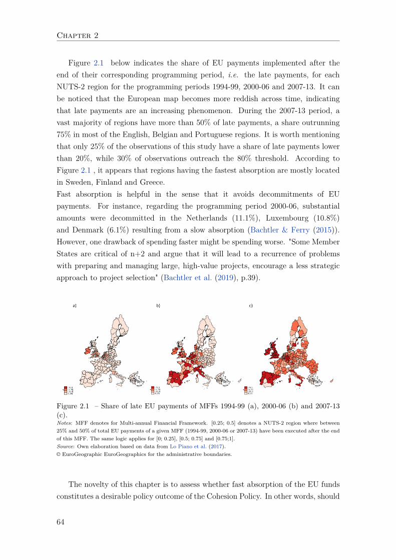
Chapter 2
Figure 2.1 below indicates the share of EU payments implemented after theend of their corresponding programming period, i.e. the late payments, for eachNUTS-2 region for the programming periods 1994-99, 2000-06 and 2007-13. It canbe noticed that the European map becomes more reddish across time, indicatingthat late payments are an increasing phenomenon. During the 2007-13 period, avast majority of regions have more than 50% of late payments, a share outrunning75% in most of the English, Belgian and Portuguese regions. It is worth mentioningthat only 25% of the observations of this study have a share of late payments lowerthan 20%, while 30% of observations outreach the 80% threshold. According toFigure 2.1 , it appears that regions having the fastest absorption are mostly locatedin Sweden, Finland and Greece.Fast absorption is helpful in the sense that it avoids decommitments of EUpayments. For instance, regarding the programming period 2000-06, substantialamounts were decommitted in the Netherlands (11.1%), Luxembourg (10.8%)and Denmark (6.1%) resulting from a slow absorption (Bachtler & Ferry (2015)).However, one drawback of spending faster might be spending worse. "Some MemberStates are critical of n+2 and argue that it will lead to a recurrence of problemswith preparing and managing large, high-value projects, encourage a less strategicapproach to project selection" (Bachtler et al. (2019), p.39).
Figure 2.1 – Share of late EU payments of MFFs 1994-99 (a), 2000-06 (b) and 2007-13(c).Notes: MFF denotes for Multi-annual Financial Framework. [0.25; 0.5] denotes a NUTS-2 region where between25% and 50% of total EU payments of a given MFF (1994-99, 2000-06 or 2007-13) have been executed after the endof this MFF. The same logic applies for [0; 0.25], [0.5; 0.75] and [0.75;1].Source: Own elaboration based on data from Lo Piano et al. (2017).© EuroGeographic EuroGeographics for the administrative boundaries.
The novelty of this chapter is to assess whether fast absorption of the EU fundsconstitutes a desirable policy outcome of the Cohesion Policy. In other words, should
64
When time isn’t money
we trust absorption speed in evaluating the absorption capacity of a recipient re-gion? Is it a suitable proxy for absorption capacity?To study this question, this chapter contributes to existing research by exploiting anew source of the conditional impact of the Cohesion Policy on regional economicgrowth: the absorption speed of the EU funds in recipient NUTS-2 regions. Ouranalysis aims to determine whether the delays in EU payments may generate aheterogeneity in the Objective 1 treatment’s effect on economic growth of recipientregions. In other words, we intend to determine whether the magnitude of the im-pact of the EU funds in lagging regions is fully determined by their pace of spending.The estimation methodology of this chapter is based on Becker et al. (2013) whichexploits the discrete jump in the probability of EU transfer receipt at the 75%threshold to conduct a fuzzy regression discontinuity design (RDD) with heteroge-neous local average treatment effect (HLATE). While Becker et al. (2013) estimatesthe impact of the Objective 1 treatment based on regional governance quality andhuman capital level, we are focused on the regional absorption rate of the EU funds.To increase the reliability of our estimates, we consider real EU payments from thedatabase of Lo Piano et al. (2017) that follows the dates in which expenditurestook place on the ground. This is not the case of commitments, usually employedin the literature studying the economic effectiveness of the Cohesion Policy (seee.g.,Becker et al. (2010, 2013), Pellegrini et al. (2013), Rodríguez-Pose & Garcilazo(2015), Gagliardi & Percoco (2017), Percoco (2017), Becker et al. (2018)).
This chapter shows that a faster absorption of the EU funds reduces the effec-tiveness of the Cohesion Policy in Objective 1 regions, or the ability of the EU fundsto stimulate economic growth. In other words, faster the EU funds are absorbed inObjective 1 regions, lower is the impact on economic growth. This result reveals thetension between spending good and spending fast in the European lagging regions asthey are generally characterised by a lower absorption capacity.
This illustrates the fact that fast absorption might be the outcome of a strategicbehaviour of recipient regions or governments to send a signal of good manage-ment to the European authorities (Huliaras & Petropoulos (2016), Aivazidou et al.(2020)). A quantile regression analysis suggests that this result is especially validin regions with the lowest economic growth performances, the latter being mostlylocated in the Mediterranean Europe. A second result is that slow absorption hasa negative impact on economic growth in non-treated regions. As they are wealth-ier, they receive significantly less EU transfers and are generally characterised by ahigher absorption capacity (Becker (2012)), which gives little room to conduct thestrategic behaviours aimed at increasing absorption rates. Therefore, in non-treated
65
Chapter 2
regions, slow absorption would rather be the outcome of a lower management qual-ity (Dudek (2005), Milio (2007), Tosun (2014), Surubaru (2017), Incaltarau et al.(2020)). These results are robust to different specifications, sample compositionsand outcome variables.
The interpretation pertaining to policy implications is easily implementable bypolicymakers as we propose to remove the one-size fits all logic of the decommit-ment rule. We suggest to introduce a place-based approach dimension consideringthe lower absorption capacity of Objective 1 regions. Therefore, a differentiateddecommitment rule between Objective 1 and wealthier regions, or even a suspensionof the rule for the Objective 1 regions, could help to mitigate the use of strategiesdetrimental to the effectiveness of the Cohesion Policy.
The remainder of this chapter is organised as follows: Section 2 provides a re-lated literature review. Section 3 deals with the methodology and data used toconduct our analysis. Section 4 provides the estimation results, the robustness testsalongside with the discussion. We conclude in Section 5.
2.2 Related literature
Among the large literature dealing with the Cohesion Policy, the local quality ofgovernments has unanimously been investigated as a promoting factor of the condi-tional impact of the EU funds on regional economic growth resulting from a higherabsorption capacity (see e.g., Ederveen et al. (2006), Becker et al. (2013), Mendezet al. (2013a), Rodríguez-Pose & Garcilazo (2015), Dall’Erba & Fang (2017)). Forinstance, Dall’Erba & Fang (2017) offers a meta-regression analysis of the impactof EU funds on regional growth of recipient regions based on 323 estimates in 17econometric studies. Human capital and quality of institutions are identified as"characteristics of the recipient regions that condition the effectiveness of the funds(Dall’Erba & Fang (2017), p.10).
Some recent studies highlight that fast absorption is a signal for high absorp-tion capacity resulting from a sound institutional environment (Dudek (2005), Milio(2007), Tosun (2014), Surubaru (2017), Incaltarau et al. (2020)).Tosun (2014) ex-plores the determinants of the absorption pace with regard to the European RegionalDevelopment Fund’s (ERDF) 2000–06 programming period and finds that MemberStates’ government effectiveness is positively associated with the speed of absorp-tion of the ERDF. As well, Surubaru (2017) associates faster absorption to betterinstitutions and stronger administrative capacity. This comparative study mentionsthat in the case of Bulgaria, the result of the favourable political and institutional
66
When time isn’t money
environments has been a higher progression of the absorption speed than the Ro-manian one for the period 2007-13. A similar study conducted by Incaltarau et al.(2020) concludes on the promoting role of government effectiveness on national ab-sorption rate.
However, the view that fast absorption results from high absorption capac-ity is not unanimously acknowledged (ECA (2004), Polverari et al. (2007), CSIL(2010), Huliaras & Petropoulos (2016), Aivazidou et al. (2020)). Notably, Huliaras& Petropoulos (2016) provides a case study on Greece for the programming period2007-13. The authors highlight the weaknesses of the administrative capacity andthe bad institutional environment of authorities in charge of the implementation ofthe Cohesion Policy. As a result, the observed fast absorption has been more theresult of easy-to-spend solutions than a good use of the EU funds resulting from ahigh absorption capacity. Indeed, "In 2010, one of the top priorities of the newlyelected government was not to lose ‘a single euro’ of the National Strategic Refer-ence Framework 2007–2013 money" (p.8, Huliaras & Petropoulos (2016)). Similarly,Aivazidou et al. (2020) concludes that low-performance of the EU funds in the Ital-ian regions for the programming period 2007-13 can be held accountable for thestrategies aiming at increasing absorption percentages instead of fostering adminis-trative capacity.
Regarding the decommitment rule specifically, it has been effective to fastenabsorption (Bachtler & Ferry (2015), but it led the authorities in charge of the im-plementation of the Cohesion Policy to focus on the pace of spending rather than thequality of interventions (Polverari et al. (2007); CSIL (2010)). Moreover, this rulehad a detrimental impact on the ability of the Cohesion Policy to adapt to specificregional and national contexts (EC (2011)). It could be mentioned as well that thedecommitment rule put a strong pressure on local administrative resources as 50%of payments are submitted between September and December (ECA (2004)). Tosum up, the faster absorption induced by the n+2 rule might have been detrimentalto the conduct of the Cohesion Policy and its ability to foster regional economicgrowth. Therefore, our study provides insights whether fast absorption has a fos-tering or detrimental impact on the ability of Objective 1 treatment to stimulategrowth at the regional level.
Regarding the estimation approach, Becker et al. (2010) is the first study toadopt a RDD design to exploit the existence of a threshold in the attribution ofthe treatment status (set as 75% of the EU per capita GDP in purchasing powerparity). An extended use of the RDD is then proposed in Becker et al. (2013) whereheterogeneous local effects are estimated. The analysis based on heterogeneous local
67
Chapter 2
average treatment effect (HLATE) showed that the degree of absorptive capacity isimportant in explaining differences in outcomes. This approach has then been fol-lowed by numerous studies to reveal different sources of heterogeneity on the impactof the EU funds on regional growth: Gagliardi & Percoco (2017) provides evidencethat the initial distribution of land matters since rural areas closed to city centres arethose where the impact of EU funds is the strongest. For example, Percoco (2017)finds that that the size of the regional service sector is detrimental to the impactof the EU funds on regional growth. Becker et al. (2018) explores heterogeneityacross recipient regions in terms of their exposure to the last European financialand economic crisis and reveals that in spite of a positive impact, the effects of theEuropean transfers are weaker in countries that have been hit harder by the crisis.
The next section presents the methodology and data employed in our analysis.
2.3 Methodology and data
2.3.1 Regression discontinuity design estimation
In this study, we focus on the potential heterogeneity of treatment effect accordingto the share of late payments ai,ρ which is defined as:
ai,ρ = eui,ρ−1late
eui,ρ−1(2.1)
where eui,ρ−1late denotes the payments of the last programming period ρ − 1 made
for a region i after the end of this corresponding programming period. We considerthe programming periods 1994-99, 2000-06 and 2007-13. 4 eui,ρ−1 denotes the totalallocation provided to region i for the associated programming period ρ−1. To sumup, late payments can be defined as the payments of programming period ρ -1 madein programming period ρ. Finally, ai,ρ is bounded to [0;1].
We recall that the main contribution of this study is to analyse whether ai,ρ, canbe considered as a suitable proxy for regional absorption capacity by evaluating itsimpact on the effectiveness of the Objective 1 treatment. To answer this question, wemake the hypothesis that ai,ρ−1 is associated with the programming period ρ. Moreprecisely, the share of late payments of period 1994-99 is associated with 2000-06,the one of 2000-06 is associated with 2007-13, and the one of 2007-13 is associated
4It should be mentioned that the n+2 rule states that a sum committed to a programme shouldbe claimed by the end of the second year following a given programming period. Therefore, becauseof the European authorities’ processing time, last payments are executed 3 years after the end ofa given programming period (2002 for 1994-1999, 2009 for 2000-2006 and 2016 for 2007-2013).
68
When time isn’t money
with 2014-20. The motivations behind this assumption are threefold: (i) Operationalprogrammes, or the detailed plans in which the Member States set out how moneyfrom the EU funds will be spent during the programming period ρ, are built in thefinal years of the programming period ρ − 1; (ii) The way how the EU funds aremanaged in the first years of ρ might be crucially determined by the absorptioncapacity inherited from the period ρ − 1; (iii) Regarding the empirical strategy, ithas the advantage to avoid potential endogeneity of the interaction variable.
To conduct the analysis, we adopt a Heterogeneous Local Average Treatment(HLATE) estimation where the absorption rate may amplify or reduce the treatmenteffect. We rely on a Regression Discontinuity Design (RDD) in line with recentstudies (see e.g., Becker et al. (2013); Gagliardi & Percoco (2017); Percoco (2017);Becker et al. (2018); Cerqua & Pellegrini (2018)). RDD is based on the principlethat there is an exogenous eligibility rule built on an observable variable, called theforcing variable. In this study, this is the relative GDP per capita of one NUTS-2region expressed in purchase power parity (PPS) regarding the European average.For the programming period 2000-06, the eligibility status is determined on thebasis of years 1994-96 (1997-99 for countries that have joined the EU in 2004), years2000-02 for the programming period 2007-13 and years 2007-09 for the programmingperiod 2014-20.5
The treatment is a binary Objective 1 indicator for a NUTS-2 region i. Werecall that Objective 1 status leads to increased transfers aiming at reducing thegap in per capita GDP between non-treated and treated regions. One key featureis that the treatment rule is not perfectly respected. Indeed, in reality, there aresome exceptions from the treatment rule due to several reasons. We could mentionthat the sparsely populated regions in Austria, Finland and Sweden are eligible forfunds despite being above the relevant threshold of 75%. Another group comprisesthe outermost regions of France, Portugal and Spain, where the Canary Islands areabove the 75% threshold. Finally, the last exception is the phasing-out status, i.e.NUTS-2 regions that were granted Objective 1 transfers in 1994-99 with a GDPhigher than the 75% threshold for the period 2000-06. In a nutshell, due to theimperfect compliance of the eligibility rule, we must implement a fuzzy RDD design.As indicated by Imbens & Lemieux (2008), applying ordinary least squares (OLS)would lead to biased estimates because of the fuzziness of the treatment. Therefore,a two-stage least squares (2SLS) where the actual treatment is instrumented by theeligibility rule should be implemented to provide reliable estimates. We highly relyon follow Becker et al. (2013) for the entire econometric strategy.
5See the EU Council Regulations 595/2006 and 189/2007 for instance.
69
Chapter 2
The second stage of the 2SLS under fuzzy with a HLATE identification where theinteraction variable is the share of late EU payments is given by:
yi,ρ = α2+τ ˆti,ρ+ζ0n(1−ti,ρ)xi,ρ+η0q(1−ti,ρ)ai,ρ+ζ1nti,ρxi,ρ+η1q ti,ρai,ρ+θkK∑k
ki,ρ+µi,ρ
(2.2)
where yi,ρ represents the GDP per capita growth of region i averaged for the pro-gramming period ρ, α2 is a constant and µi,ρ is the error term. xi,ρ is the deviationfrom the 75% threshold while ai,ρ and ∑K
k ki,ρ, a set of K control variables, are ex-pressed as the deviation from their sample mean. τ denotes the coefficient directlyassociated with the fitted value of the treatment ˆti,ρ. ai,ρ is associated to coefficientsζ1,n and η1,q when the treatment is switched-on ( ˆti,ρ = 1). ζ0,n and µ0,q are the samecoefficients when the treatment is switched-off.
Regarding the first stage regression, we use the eligibility rule that is representedthrough a binary variable taking the value of 1 if the NUTS-2 region has a GDP percapita below 75% of the EU average, and 0 otherwise. A linear probability modelis implemented, the first stage regression is given by:
ti,ρ =α1 + σri,ρ + β0n(1− ri,ρ)xi,ρ + γ0q(1− ri,ρ)ai,ρ + δri + β1nri,ρxi,ρ + γ1qri,ρai,ρ + εi,ρ
(2.3)
where ti,ρ represents the instrumented variable that is the treatment status of regioni for the programming period ρ, α1 is a constant and εi,ρ is the error term of thefirst-stage estimation. Eligibility rule for treatment in programming period ρ, ri,ρ, isdetermined according to the 75% threshold for region i that is eligible for treatment:ri,ρ = 1 when the forcing variable is lower or equal to 75%, ri,ρ = 0 in the oppositecase. xi,ρ,T is the forcing variable normalised around the 75% threshold. ai,ρ,T , theinteraction variable, normalised around its mean value, is associated to coefficientsζ1,n and η1,q when there is eligibility for the treatment (ri,ρ = 1). ζ0,n and µ0,q arethe same coefficients when ri,ρ = 0, or when a region is not eligible for Objective 1treatment.
The following subsection describes the data used in the analysis and their de-scriptive statistics.
70
When time isn’t money
2.3.2 Data and descriptive statistics
We collected most of the data from Eurostat Regional Statistics. They have beencompleted with data from Cambridge Econometrics. The information about Ob-jective 1 status and eligibility and about expenditures come from the EuropeanCommission. We provide all data sources in Table A3.1 . Our sample covers a paneldata set of the the EU’s NUTS-2 regions for the period 2000-16. We do not includeBulgaria, Romania, and Croatia for reasons of data availability. The resulting num-ber of NUTS-2 regions is 244. We used the NUTS2-2013 classification employed byEC (2019) which provides the input data used to build the following index. Regard-ing the time dimension of the dataset, data employed in the analysis are averagedfor each programming period: 2000-06 and 2007-13. Regarding the programmingperiod 2014-20, the latest available year is 2016, so the data correspond to averagesof period 2014-16.6 Such a transformation is implemented because the treatmentvariable is determined for each programming period ρ.
It should be mentioned that only actual received payments have been consideredin this study, and not commitments as most of studies of the literature (see e.g.,Becker et al. (2010), Becker (2012), Becker et al. (2013), Pellegrini et al. (2013),Tosun (2014), Rodríguez-Pose & Garcilazo (2015), Gagliardi & Percoco (2017), Su-rubaru (2017), Becker et al. (2018), Cerqua & Pellegrini (2018), Incaltarau et al.(2020)). As Lo Piano et al. (2017) declares, this dataset has the advantage to followthe dates in which expenditures took place on the ground. This is not the case ofcommitments, which" may negatively affect the analytic work subsequently done bythe experts to carry out policy assessments or to run counterfactual impact evalu-ations estimating the effects of the varying intensities of the EU funds on regionalgrowth variables. The misalignment between COM reimbursement cycle and dateof the interventions on the ground (beneficiaries’ expenditures) may represent a dis-turbance acting either as a noise or as a bias." (Lo Piano et al. (2017), p.6). Hence,we consider this modelled annual expenditure as our actual EU funds expenditurevariable to increase the reliability of our estimates.
As control variables, we include population density as the European authoritiesconsider that a low population density is a structural handicap to achieve economicgrowth. We also use both the share of the manufacturing sector and the share offinancial and business services in regional gross added value (GVA). Moreover, weconsider the share of the active population and the unemployment rate to have aproxy for the size of the labour force, and the share of the active population having
6This is not problematic for the programming period 2007-13 as the latest payments are madein 2016.
71
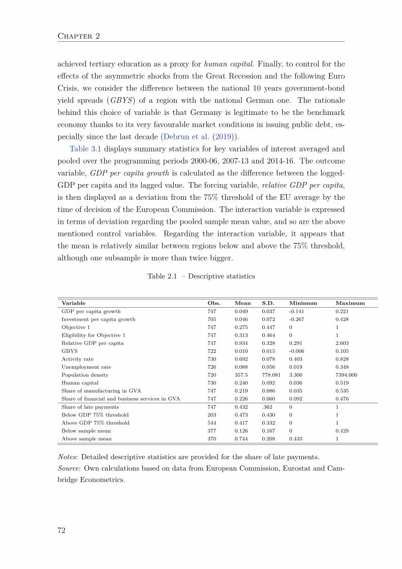
Chapter 2
achieved tertiary education as a proxy for human capital. Finally, to control for theeffects of the asymmetric shocks from the Great Recession and the following EuroCrisis, we consider the difference between the national 10 years government-bondyield spreads (GBYS) of a region with the national German one. The rationalebehind this choice of variable is that Germany is legitimate to be the benchmarkeconomy thanks to its very favourable market conditions in issuing public debt, es-pecially since the last decade (Debrun et al. (2019)).
Table 3.1 displays summary statistics for key variables of interest averaged andpooled over the programming periods 2000-06, 2007-13 and 2014-16. The outcomevariable, GDP per capita growth is calculated as the difference between the logged-GDP per capita and its lagged value. The forcing variable, relative GDP per capita,is then displayed as a deviation from the 75% threshold of the EU average by thetime of decision of the European Commission. The interaction variable is expressedin terms of deviation regarding the pooled sample mean value, and so are the abovementioned control variables. Regarding the interaction variable, it appears thatthe mean is relatively similar between regions below and above the 75% threshold,although one subsample is more than twice bigger.
Table 2.1 – Descriptive statistics
Variable Obs. Mean S.D. Minimum MaximumGDP per capita growth 747 0.049 0.037 -0.141 0.221Investment per capita growth 705 0.046 0.072 -0.267 0.428Objective 1 747 0.275 0.447 0 1Eligibility for Objective 1 747 0.313 0.464 0 1Relative GDP per capita 747 0.934 0.328 0.291 2.603GBYS 722 0.010 0.015 -0.006 0.105Activity rate 730 0.692 0.078 0.403 0.828Unemployment rate 726 0.088 0.056 0.019 0.348Population density 720 357.5 778.081 3.300 7394.000Human capital 730 0.240 0.092 0.036 0.519Share of manufacturing in GVA 747 0.219 0.086 0.035 0.535Share of financial and business services in GVA 747 0.226 0.060 0.092 0.476Share of late payments 747 0.432 .362 0 1Below GDP 75% threshold 203 0.473 0.430 0 1Above GDP 75% threshold 544 0.417 0.332 0 1Below sample mean 377 0.126 0.167 0 0.429Above sample mean 370 0.744 0.208 0.433 1
Notes: Detailed descriptive statistics are provided for the share of late payments.Source: Own calculations based on data from European Commission, Eurostat and Cam-bridge Econometrics.
72
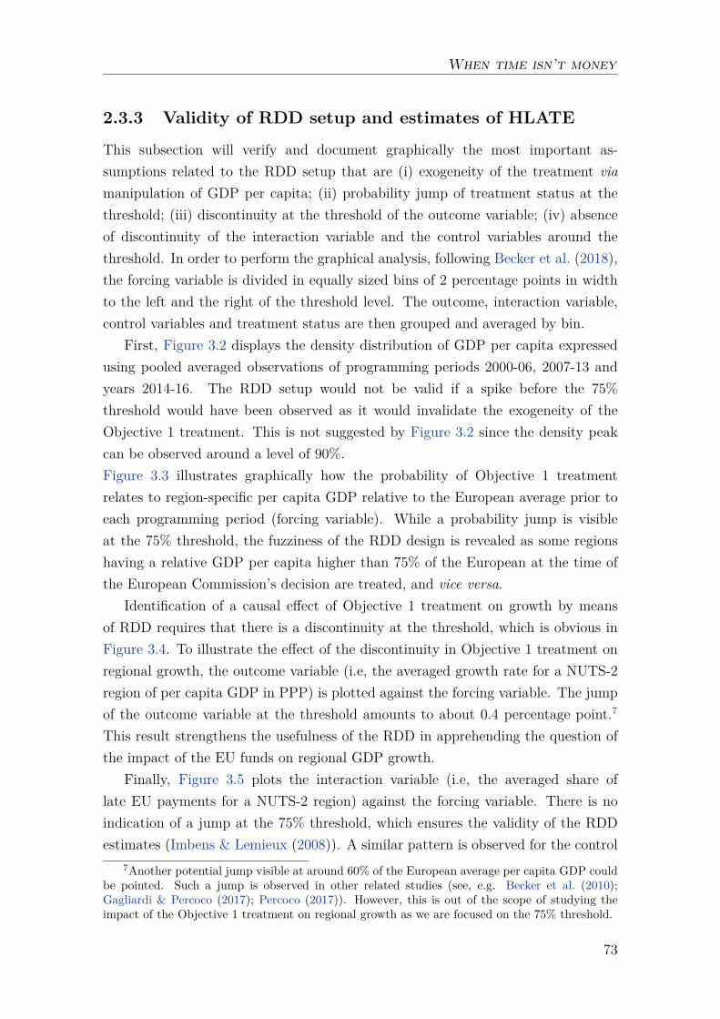
When time isn’t money
2.3.3 Validity of RDD setup and estimates of HLATE
This subsection will verify and document graphically the most important as-sumptions related to the RDD setup that are (i) exogeneity of the treatment viamanipulation of GDP per capita; (ii) probability jump of treatment status at thethreshold; (iii) discontinuity at the threshold of the outcome variable; (iv) absenceof discontinuity of the interaction variable and the control variables around thethreshold. In order to perform the graphical analysis, following Becker et al. (2018),the forcing variable is divided in equally sized bins of 2 percentage points in widthto the left and the right of the threshold level. The outcome, interaction variable,control variables and treatment status are then grouped and averaged by bin.
First, Figure 3.2 displays the density distribution of GDP per capita expressedusing pooled averaged observations of programming periods 2000-06, 2007-13 andyears 2014-16. The RDD setup would not be valid if a spike before the 75%threshold would have been observed as it would invalidate the exogeneity of theObjective 1 treatment. This is not suggested by Figure 3.2 since the density peakcan be observed around a level of 90%.Figure 3.3 illustrates graphically how the probability of Objective 1 treatmentrelates to region-specific per capita GDP relative to the European average prior toeach programming period (forcing variable). While a probability jump is visibleat the 75% threshold, the fuzziness of the RDD design is revealed as some regionshaving a relative GDP per capita higher than 75% of the European at the time ofthe European Commission’s decision are treated, and vice versa.
Identification of a causal effect of Objective 1 treatment on growth by meansof RDD requires that there is a discontinuity at the threshold, which is obvious inFigure 3.4. To illustrate the effect of the discontinuity in Objective 1 treatment onregional growth, the outcome variable (i.e, the averaged growth rate for a NUTS-2region of per capita GDP in PPP) is plotted against the forcing variable. The jumpof the outcome variable at the threshold amounts to about 0.4 percentage point.7
This result strengthens the usefulness of the RDD in apprehending the question ofthe impact of the EU funds on regional GDP growth.
Finally, Figure 3.5 plots the interaction variable (i.e, the averaged share oflate EU payments for a NUTS-2 region) against the forcing variable. There is noindication of a jump at the 75% threshold, which ensures the validity of the RDDestimates (Imbens & Lemieux (2008)). A similar pattern is observed for the control
7Another potential jump visible at around 60% of the European average per capita GDP couldbe pointed. Such a jump is observed in other related studies (see, e.g. Becker et al. (2010);Gagliardi & Percoco (2017); Percoco (2017)). However, this is out of the scope of studying theimpact of the Objective 1 treatment on regional growth as we are focused on the 75% threshold.
73
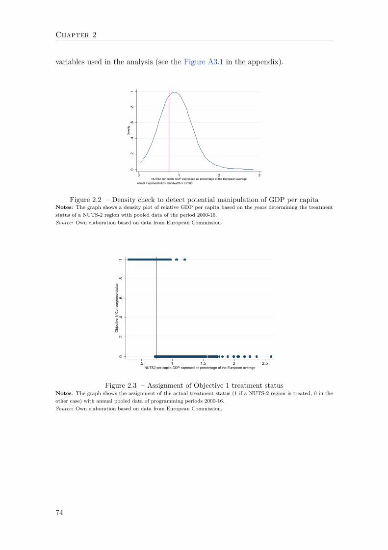
Chapter 2
variables used in the analysis (see the Figure A3.1 in the appendix).
0.2
.4.6
.81
Den
sity
0 1 2 3NUTS2 per capita GDP expressed as percentage of the European average
kernel = epanechnikov, bandwidth = 0.2500
Figure 2.2 – Density check to detect potential manipulation of GDP per capitaNotes: The graph shows a density plot of relative GDP per capita based on the years determining the treatmentstatus of a NUTS-2 region with pooled data of the period 2000-16.Source: Own elaboration based on data from European Commission.
0.2
.4.6
.81
Obj
ectiv
e 1/
Con
verg
ence
sta
tus
.5 1 1.5 2 2.5NUTS2 per capita GDP expresed as percentage of the European average
Figure 2.3 – Assignment of Objective 1 treatment statusNotes: The graph shows the assignment of the actual treatment status (1 if a NUTS-2 region is treated, 0 in theother case) with annual pooled data of programming periods 2000-16.Source: Own elaboration based on data from European Commission.
74
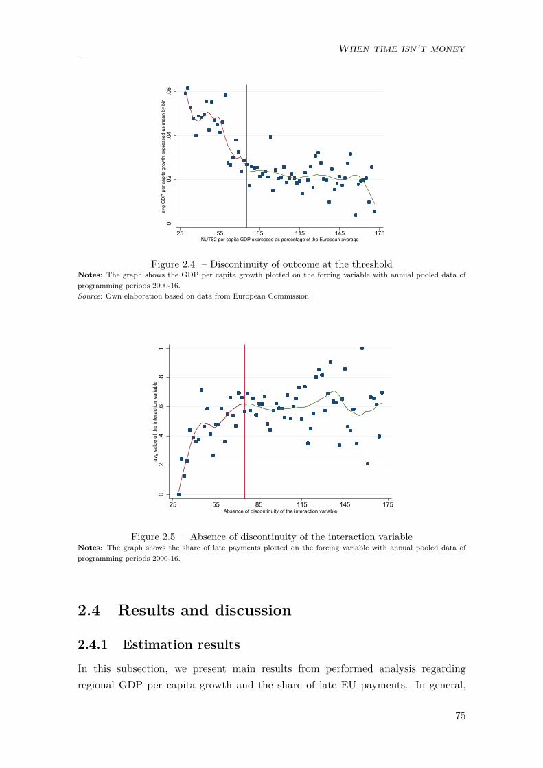
When time isn’t money
0.0
2.0
4.0
6av
g G
DP
per c
apita
gro
wth
exp
ress
ed a
s m
ean
by b
in
25 55 85 115 145 175NUTS2 per capita GDP expressed as percentage of the European average
Figure 2.4 – Discontinuity of outcome at the thresholdNotes: The graph shows the GDP per capita growth plotted on the forcing variable with annual pooled data ofprogramming periods 2000-16.Source: Own elaboration based on data from European Commission.
0.2
.4.6
.81
avg
valu
e of
the
inte
ract
ion
varia
ble
25 1751451158555Absence of discontinuity of the interaction variable
Figure 2.5 – Absence of discontinuity of the interaction variableNotes: The graph shows the share of late payments plotted on the forcing variable with annual pooled data ofprogramming periods 2000-16.
2.4 Results and discussion
2.4.1 Estimation results
In this subsection, we present main results from performed analysis regardingregional GDP per capita growth and the share of late EU payments. In general,
75
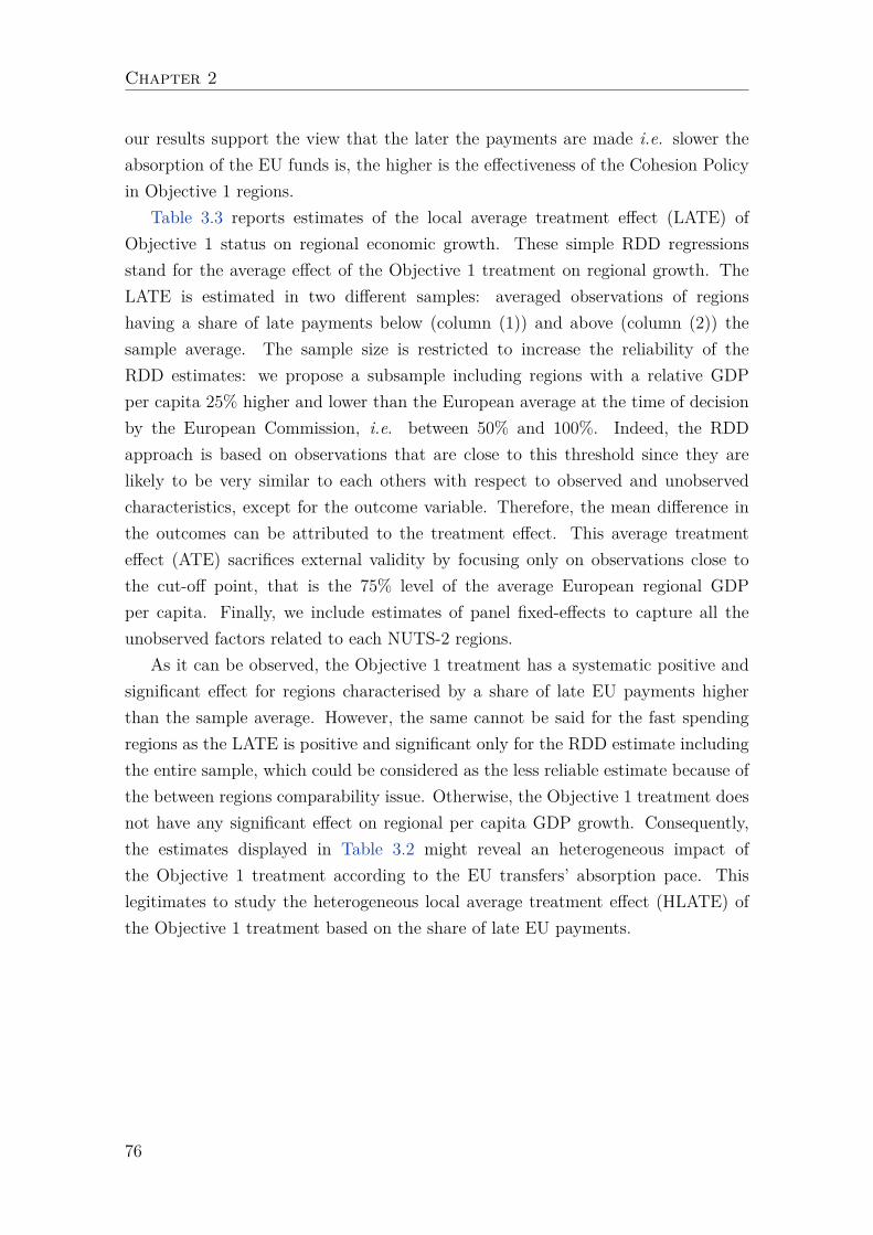
Chapter 2
our results support the view that the later the payments are made i.e. slower theabsorption of the EU funds is, the higher is the effectiveness of the Cohesion Policyin Objective 1 regions.
Table 3.3 reports estimates of the local average treatment effect (LATE) ofObjective 1 status on regional economic growth. These simple RDD regressionsstand for the average effect of the Objective 1 treatment on regional growth. TheLATE is estimated in two different samples: averaged observations of regionshaving a share of late payments below (column (1)) and above (column (2)) thesample average. The sample size is restricted to increase the reliability of theRDD estimates: we propose a subsample including regions with a relative GDPper capita 25% higher and lower than the European average at the time of decisionby the European Commission, i.e. between 50% and 100%. Indeed, the RDDapproach is based on observations that are close to this threshold since they arelikely to be very similar to each others with respect to observed and unobservedcharacteristics, except for the outcome variable. Therefore, the mean difference inthe outcomes can be attributed to the treatment effect. This average treatmenteffect (ATE) sacrifices external validity by focusing only on observations close tothe cut-off point, that is the 75% level of the average European regional GDPper capita. Finally, we include estimates of panel fixed-effects to capture all theunobserved factors related to each NUTS-2 regions.
As it can be observed, the Objective 1 treatment has a systematic positive andsignificant effect for regions characterised by a share of late EU payments higherthan the sample average. However, the same cannot be said for the fast spendingregions as the LATE is positive and significant only for the RDD estimate includingthe entire sample, which could be considered as the less reliable estimate because ofthe between regions comparability issue. Otherwise, the Objective 1 treatment doesnot have any significant effect on regional per capita GDP growth. Consequently,the estimates displayed in Table 3.2 might reveal an heterogeneous impact ofthe Objective 1 treatment according to the EU transfers’ absorption pace. Thislegitimates to study the heterogeneous local average treatment effect (HLATE) ofthe Objective 1 treatment based on the share of late EU payments.
76
When time isn’t money
Table 2.2 – Heterogeneity of the Objective 1 treatment effect on regional GDP per capitagrowth: sample decomposition according to the share of late payments.
(1) (2)Estimator Late payments below the average Late payments above the averageRDD 0.016*** 0.019***
(0.003) (0.003)Panel fixed-effects -0.008 0.026***
(0.008) (0.008)Observations 313 419
RDD 50-100 0.004 0.017***(0.006) (0.004)
Observations 157 237
Notes: This table reports results from the two stage least square estimation of the LATE with a sample restrictedto the observations with a share of late payments below (column (1)) and above (column (2)) the European average.RDD refers to the estimation of the Local Average Treatment Effect (LATE) of the Objective 1 treatment for theentire sample, while RDD 50-100 considered only the observations with a relative GDP per capita between 50%and 100% of the European average. The forcing variable is the relative GDP per capita of 1996-98 (97-99) for years2000-06, 2000-02 for years 2007-13 and 2007-09 for years 2014-16. Panel fixed effects describes the two stage leastsquare (panel IV) estimation using regional fixed effects.The dependent variable presents regional GDP per capita growth. Robust standard errors are reported in paren-theses. * denotes p < 0.10; ** p < 0.05; ***p < 0.01.Source: Own calculations based on data from European Commission and Eurostat.
The estimation results for the heterogeneous effects (HLATE) are displayed inTable 3.3. To increase the reliability of RDD estimates as much as possible, werestrict our sample to 12.5% around the eligibility threshold, i.e. NUTS-2 regionshaving a GDP per capita from 62.5% to 87.5% of the European average (columns(1)-(2)). One drawback of this procedure is the sharp reduction of sample size sincethe number of observations falls to 219. Columns (3) and (4) include regions witha relative GDP per capita between 50% and 100% of the European average, whichallow us to nearly double the sample size to 394 observations. Columns (5) and (6)include the entire sample as only regional fixed effects are included with the use ofpanel fixed-effects. It is not worth mentioning to indicate that some non-linearityis introduced with the squared term of the share of late payments in columns (2),(4) and (6). The analysis shows that weak instruments and endogeneity tests aregenerally verified. For sake of brevity, we report only second-stage estimates.
The first striking result is that a faster absorption of the EU funds reduces theeffectiveness of the Cohesion Policy in Objective 1 regions, or the ability of the EUfunds to stimulate economic growth. Indeed, in all specifications, the coefficienton the term of interaction between the share of late payments and the treatmentexhibits a positive sign. The introduction of a quadratic interaction term even re-inforces this result. In all specifications, we obtain ∂yi,ρ
∂ai,ρ> 0 for Objective 1 regions
77
Chapter 2
which indicates that the net effect of an increase in the share of late payments isbeneficial to regional growth. This result validates that fast absorption might be theoutcome of a strategic behaviour of recipient regions or governments to send a signalof good management to the European authorities (Huliaras & Petropoulos (2016);Aivazidou et al. (2020)). This finding gives ground to the conflict between spendingfast and spending good in lagging regions as they are generally characterised by alower absorption capacity (Becker et al. (2013)). In other words, local managingauthorities may encounter more difficulties to spend a European subsidy efficientlyfor a given time period compared to a wealthy region.
A second result is that slow absorption has a negative impact on economic growthin regions having a relative GDP per capita higher than 75% of the European av-erage. Indeed, as they do not benefit from the Objective 1 treatment, we find that∂yi,ρ∂ai,ρ
< 0. As these regions are wealthier than the Objective 1 regions, they receivesignificantly less EU transfers and are generally characterised by a higher absorptioncapacity (Becker (2012)), which gives little room to conduct the strategic behavioursaimed at increasing absorption rates. Therefore, in non-treated regions, slow absorp-tion would rather be the outcome of a lower management quality (Dudek (2005),Milio (2007), Tosun (2014), Surubaru (2017), Incaltarau et al. (2020)).
A third result is the treatment does not have any robust direct impact on regionaleconomic growth, making its impact purely conditional. Indeed, in all regressions,the magnitude of the impact of the EU funds in lagging regions is fully determinedby their pace of spending. Therefore, the Objective 1 treatment does not promoteeconomic growth per se. This finding is in line with a large majority of the literatureunderlining that the effectiveness of the Cohesion Policy mostly relies on regionalgovernance quality and human capital level (see e.g., Cappelen et al. (2003), Beckeret al. (2013), Rodríguez-Pose & Garcilazo (2015), Becker et al. (2018)).
Regarding control variables, half of them are characterised by insignificant ef-fects. The remaining ones are associated with the expected significant effects: (i) itcould be noticed that the proxy for human capital, i.e. tertiary education achieve-ment, is associated to a positive and significant impact on per capita GDP growthin most of specifications; (ii) a similar outcome appears for the share of the manu-facturing sector in regional gross added value, indicating that the industrial sectoris a powerful growth driver (Baumol (2001)); (iii) it is worth mentioning the robustnegative significant impact of the GBYS on per capita GDP growth. This featurereveals that the the inclusion of this control variable is relevant to capture the shocksinherited from the Great Recession and the following Euro Crisis.
78
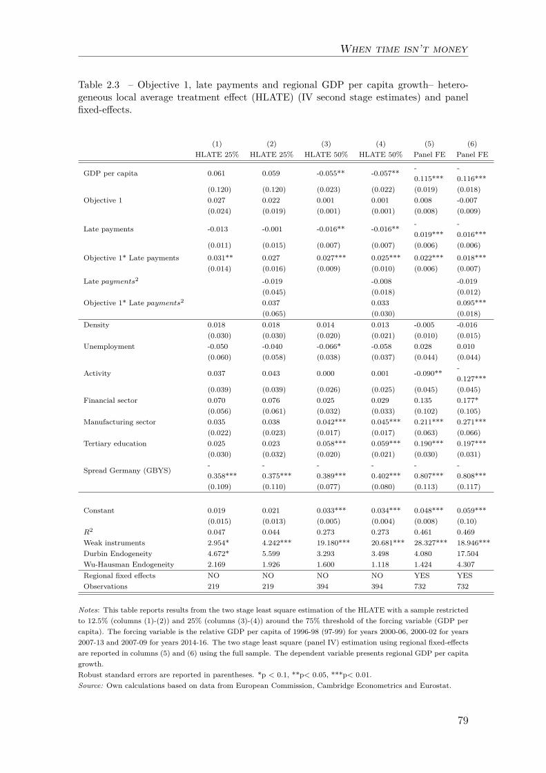
When time isn’t money
Table 2.3 – Objective 1, late payments and regional GDP per capita growth– hetero-geneous local average treatment effect (HLATE) (IV second stage estimates) and panelfixed-effects.
(1) (2) (3) (4) (5) (6)HLATE 25% HLATE 25% HLATE 50% HLATE 50% Panel FE Panel FE
GDP per capita 0.061 0.059 -0.055** -0.057**-0.115***
-0.116***
(0.120) (0.120) (0.023) (0.022) (0.019) (0.018)Objective 1 0.027 0.022 0.001 0.001 0.008 -0.007
(0.024) (0.019) (0.001) (0.001) (0.008) (0.009)
Late payments -0.013 -0.001 -0.016** -0.016**-0.019***
-0.016***
(0.011) (0.015) (0.007) (0.007) (0.006) (0.006)Objective 1* Late payments 0.031** 0.027 0.027*** 0.025*** 0.022*** 0.018***
(0.014) (0.016) (0.009) (0.010) (0.006) (0.007)Late payments2 -0.019 -0.008 -0.019
(0.045) (0.018) (0.012)Objective 1* Late payments2 0.037 0.033 0.095***
(0.065) (0.030) (0.018)Density 0.018 0.018 0.014 0.013 -0.005 -0.016
(0.030) (0.030) (0.020) (0.021) (0.010) (0.015)Unemployment -0.050 -0.040 -0.066* -0.058 0.028 0.010
(0.060) (0.058) (0.038) (0.037) (0.044) (0.044)
Activity 0.037 0.043 0.000 0.001 -0.090**-0.127***
(0.039) (0.039) (0.026) (0.025) (0.045) (0.045)Financial sector 0.070 0.076 0.025 0.029 0.135 0.177*
(0.056) (0.061) (0.032) (0.033) (0.102) (0.105)Manufacturing sector 0.035 0.038 0.042*** 0.045*** 0.211*** 0.271***
(0.022) (0.023) (0.017) (0.017) (0.063) (0.066)Tertiary education 0.025 0.023 0.058*** 0.059*** 0.190*** 0.197***
(0.030) (0.032) (0.020) (0.021) (0.030) (0.031)
Spread Germany (GBYS)-0.358***
-0.375***
-0.389***
-0.402***
-0.807***
-0.808***
(0.109) (0.110) (0.077) (0.080) (0.113) (0.117)
Constant 0.019 0.021 0.033*** 0.034*** 0.048*** 0.059***(0.015) (0.013) (0.005) (0.004) (0.008) (0.10)
R2 0.047 0.044 0.273 0.273 0.461 0.469Weak instruments 2.954* 4.242*** 19.180*** 20.681*** 28.327*** 18.946***Durbin Endogeneity 4.672* 5.599 3.293 3.498 4.080 17.504Wu-Hausman Endogeneity 2.169 1.926 1.600 1.118 1.424 4.307Regional fixed effects NO NO NO NO YES YESObservations 219 219 394 394 732 732
Notes: This table reports results from the two stage least square estimation of the HLATE with a sample restrictedto 12.5% (columns (1)-(2)) and 25% (columns (3)-(4)) around the 75% threshold of the forcing variable (GDP percapita). The forcing variable is the relative GDP per capita of 1996-98 (97-99) for years 2000-06, 2000-02 for years2007-13 and 2007-09 for years 2014-16. The two stage least square (panel IV) estimation using regional fixed-effectsare reported in columns (5) and (6) using the full sample. The dependent variable presents regional GDP per capitagrowth.Robust standard errors are reported in parentheses. *p < 0.1, **p< 0.05, ***p< 0.01.Source: Own calculations based on data from European Commission, Cambridge Econometrics and Eurostat.
79
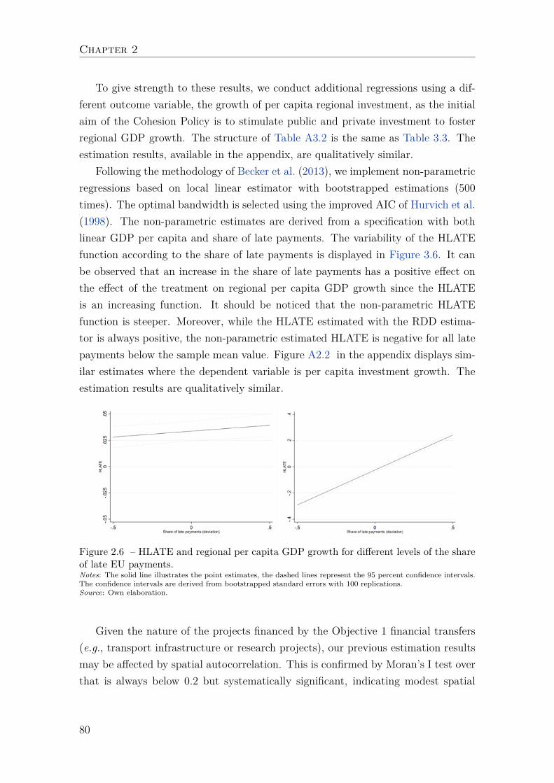
Chapter 2
To give strength to these results, we conduct additional regressions using a dif-ferent outcome variable, the growth of per capita regional investment, as the initialaim of the Cohesion Policy is to stimulate public and private investment to fosterregional GDP growth. The structure of Table A3.2 is the same as Table 3.3. Theestimation results, available in the appendix, are qualitatively similar.
Following the methodology of Becker et al. (2013), we implement non-parametricregressions based on local linear estimator with bootstrapped estimations (500times). The optimal bandwidth is selected using the improved AIC of Hurvich et al.(1998). The non-parametric estimates are derived from a specification with bothlinear GDP per capita and share of late payments. The variability of the HLATEfunction according to the share of late payments is displayed in Figure 3.6. It canbe observed that an increase in the share of late payments has a positive effect onthe effect of the treatment on regional per capita GDP growth since the HLATEis an increasing function. It should be noticed that the non-parametric HLATEfunction is steeper. Moreover, while the HLATE estimated with the RDD estima-tor is always positive, the non-parametric estimated HLATE is negative for all latepayments below the sample mean value. Figure A2.2 in the appendix displays sim-ilar estimates where the dependent variable is per capita investment growth. Theestimation results are qualitatively similar.
Figure 2.6 – HLATE and regional per capita GDP growth for different levels of the shareof late EU payments.Notes: The solid line illustrates the point estimates, the dashed lines represent the 95 percent confidence intervals.The confidence intervals are derived from bootstrapped standard errors with 100 replications.Source: Own elaboration.
Given the nature of the projects financed by the Objective 1 financial transfers(e.g., transport infrastructure or research projects), our previous estimation resultsmay be affected by spatial autocorrelation. This is confirmed by Moran’s I test overthat is always below 0.2 but systematically significant, indicating modest spatial
80
When time isn’t money
autocorrelation. 8 To tackle this issue, spatial auto-regressive fixed effects estimatesare conducted. A weighting contiguity matrix based on the 244 NUTS-2 regions ofour sample is created where first and second order neighbours have the same weight.The estimation results are reported in Table 3.4. Whilst remaining robust, it canbe noticed that the significance of late payments is reduced to the 10% level whereper capita GDP growth is the dependent variable. It can still be observed that: (i)an increase in the share of late payments in Objective 1 regions is not detrimentalto economic growth; (ii) the opposite holds in non-treated regions (iii) the effect ofthe Objective 1 treatment is mostly conditional.
The next subsection deals with additional regressions to increase the precision ofour estimates. First, quantile regressions are implemented to investigate whether thetreatment effects are homogeneous across per capita GDP growth levels. Moreover,following the conclusions of Becker (2012), we investigate whether the intensity of theEuropean transfers is relevant in determining their capacity to stimulate economicgrowth in recipient regions.
2.4.2 Additional results
Let us now turn to Table A3.3 that reports results for the simultaneous-quantileregressions with the regional economic growth (columns (1)-(2)) and investment percapita growth (columns (3)-(4)) as outcome variables. Regions having a GDP percapita 12.5% around the eligibility threshold have been selected. Again, the purelyconditional impact of the Objective 1 treatment is validated for both the outcomevariables.
An interesting additional result provided by Table A3.4 is that the absorptionspeed appears to be relevant only in regions exhibiting the lowest economic growthpatterns, which are mostly located in Southern Europe. Considering that most ofthe Objective 1 regions are located in the Mediterranean and the Central EasternEuropean (CEE) countries, 47% of the regions in the lowest 25% quantile, in termsof economic growth, belongs to the Mediterranean Europe and 5% to the CEEcountries.9 On the contrary, if we consider the upper 25% quantile, where theabsorption speed appears to be irrelevant, the CEE countries stand for 31% of thesample and this share falls to 30% for the Mediterranean ones.10
8For sake of brevity, the test values are not reported. They are available upon request.9In details, 18% are Greek, 13% Spanish, 9% Italian, 6% Portuguese and 1% Cypriot ( Mediter-
ranean regions) . 3% Slovenian and 2% Czech (regions from CEE countries).10Mediterranean Europe: 17% Spanish, 8% Greek, 3% Portuguese, 1% Cypriot and 1% and 1%
Maltese. CEE: 12% Czech, 9% Polish, 4% Hungarian, 3% Slovenian, 1% Slovak 1% Latvian and1% Lithuanian.
81
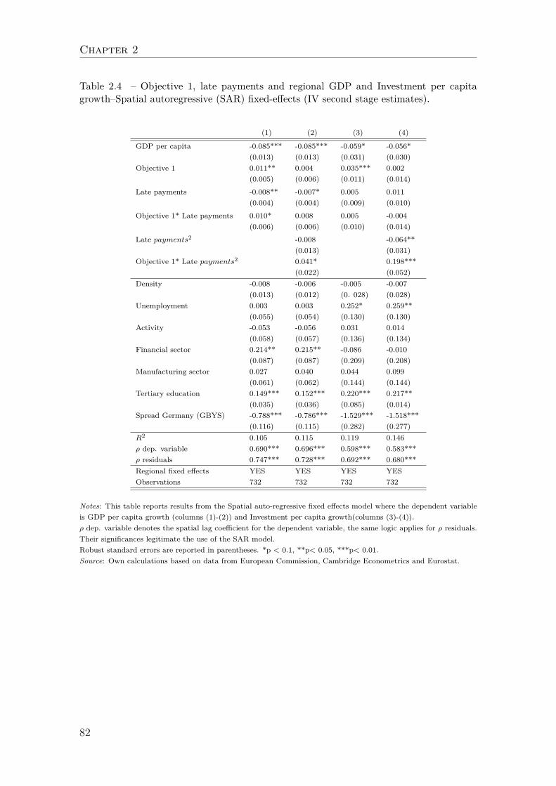
Chapter 2
Table 2.4 – Objective 1, late payments and regional GDP and Investment per capitagrowth–Spatial autoregressive (SAR) fixed-effects (IV second stage estimates).
(1) (2) (3) (4)
GDP per capita -0.085*** -0.085*** -0.059* -0.056*(0.013) (0.013) (0.031) (0.030)
Objective 1 0.011** 0.004 0.035*** 0.002(0.005) (0.006) (0.011) (0.014)
Late payments -0.008** -0.007* 0.005 0.011(0.004) (0.004) (0.009) (0.010)
Objective 1* Late payments 0.010* 0.008 0.005 -0.004(0.006) (0.006) (0.010) (0.014)
Late payments2 -0.008 -0.064**(0.013) (0.031)
Objective 1* Late payments2 0.041* 0.198***(0.022) (0.052)
Density -0.008 -0.006 -0.005 -0.007(0.013) (0.012) (0. 028) (0.028)
Unemployment 0.003 0.003 0.252* 0.259**(0.055) (0.054) (0.130) (0.130)
Activity -0.053 -0.056 0.031 0.014(0.058) (0.057) (0.136) (0.134)
Financial sector 0.214** 0.215** -0.086 -0.010(0.087) (0.087) (0.209) (0.208)
Manufacturing sector 0.027 0.040 0.044 0.099(0.061) (0.062) (0.144) (0.144)
Tertiary education 0.149*** 0.152*** 0.220*** 0.217**(0.035) (0.036) (0.085) (0.014)
Spread Germany (GBYS) -0.788*** -0.786*** -1.529*** -1.518***(0.116) (0.115) (0.282) (0.277)
R2 0.105 0.115 0.119 0.146ρ dep. variable 0.690*** 0.696*** 0.598*** 0.583***ρ residuals 0.747*** 0.728*** 0.692*** 0.680***Regional fixed effects YES YES YES YESObservations 732 732 732 732
Notes: This table reports results from the Spatial auto-regressive fixed effects model where the dependent variableis GDP per capita growth (columns (1)-(2)) and Investment per capita growth(columns (3)-(4)).ρ dep. variable denotes the spatial lag coefficient for the dependent variable, the same logic applies for ρ residuals.Their significances legitimate the use of the SAR model.Robust standard errors are reported in parentheses. *p < 0.1, **p< 0.05, ***p< 0.01.Source: Own calculations based on data from European Commission, Cambridge Econometrics and Eurostat.
82
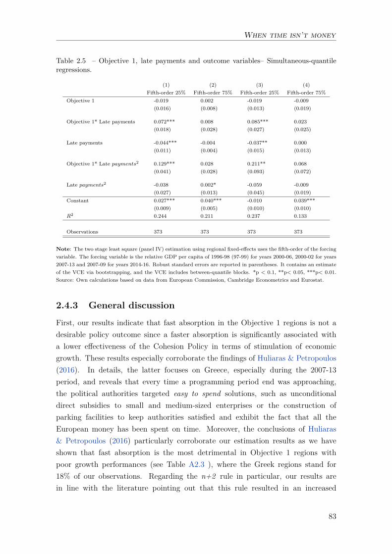
When time isn’t money
Table 2.5 – Objective 1, late payments and outcome variables– Simultaneous-quantileregressions.
(1) (2) (3) (4)Fifth-order 25% Fifth-order 75% Fifth-order 25% Fifth-order 75%
Objective 1 -0.019 0.002 -0.019 -0.009(0.016) (0.008) (0.013) (0.019)
Objective 1* Late payments 0.072*** 0.008 0.085*** 0.023(0.018) (0.028) (0.027) (0.025)
Late payments -0.044*** -0.004 -0.037** 0.000(0.011) (0.004) (0.015) (0.013)
Objective 1* Late payments2 0.129*** 0.028 0.211** 0.068(0.041) (0.028) (0.093) (0.072)
Late payments2 -0.038 0.002* -0.059 -0.009(0.027) (0.013) (0.045) (0.019)
Constant 0.027*** 0.040*** -0.010 0.039***(0.009) (0.005) (0.010) (0.010)
R2 0.244 0.211 0.237 0.133
Observations 373 373 373 373
Note: The two stage least square (panel IV) estimation using regional fixed-effects uses the fifth-order of the forcingvariable. The forcing variable is the relative GDP per capita of 1996-98 (97-99) for years 2000-06, 2000-02 for years2007-13 and 2007-09 for years 2014-16. Robust standard errors are reported in parentheses. It contains an estimateof the VCE via bootstrapping, and the VCE includes between-quantile blocks. *p < 0.1, **p< 0.05, ***p< 0.01.Source: Own calculations based on data from European Commission, Cambridge Econometrics and Eurostat.
2.4.3 General discussion
First, our results indicate that fast absorption in the Objective 1 regions is not adesirable policy outcome since a faster absorption is significantly associated witha lower effectiveness of the Cohesion Policy in terms of stimulation of economicgrowth. These results especially corroborate the findings of Huliaras & Petropoulos(2016). In details, the latter focuses on Greece, especially during the 2007-13period, and reveals that every time a programming period end was approaching,the political authorities targeted easy to spend solutions, such as unconditionaldirect subsidies to small and medium-sized enterprises or the construction ofparking facilities to keep authorities satisfied and exhibit the fact that all theEuropean money has been spent on time. Moreover, the conclusions of Huliaras& Petropoulos (2016) particularly corroborate our estimation results as we haveshown that fast absorption is the most detrimental in Objective 1 regions withpoor growth performances (see Table A2.3 ), where the Greek regions stand for18% of our observations. Regarding the n+2 rule in particular, our results arein line with the literature pointing out that this rule resulted in an increased
83
Chapter 2
focus on the pace of spending rather than the quality of the investment projects(CSIL (2010)), especially in regions with limited administrative resources (ECA(2004)), as the Objective 1 regions. While a strand of the literature concludes ona positive association between regional administrative capacity and the speed ofthe implementation of the Cohesion in Spain (Dudek (2005)), Italy (Milio (2007)),Romania and Bulgaria (Tosun (2014)), we posit that absorption pace is failing signalfor absorption capacity. Indeed, it does not capture local strategies implementedto fasten absorption at the cost of lower economic effectiveness. For instance,the use of retrospective projects consists on funding projects which have incurredexpenditure, or are completed before the EU co-financing has been formally applied,i.e. they are financed retrospectively. As these projects are often selected, initiatedor carried out without having been expressly linked to a programme’s objectivesor to specific legal requirements linked to EU assistance, they exhibit a significantrisk of low economic effectiveness (ECA (2018)). Aivazidou et al. (2020) mentionsas well the reduction of regional share of contribution as a strategy to increaseabsorption rates. This study proposes then an alternative measure of absorption,the net absorption rate of total funding based on the initial total commitments (netITAR) to alleviate the bias of this strategy on absorption rates.
Our results give ground to the tension between spending fast and spendinggood. The origins of this trade-off have been somewhat theorised by the literaturedealing with the political economy of the EU funds (see e.g., Dellmuth (2011),Charron (2016)). This literature underlines the existence of two objectives: (i) afull and fast absorption of the European funds on one side, (ii) achieving regionalcohesion by aiding lagging regions on the other side. During the implementationof the Cohesion Policy, the European Commission and the Member States can beconsidered as Principals, and recipient regions as Agents. The policy goal of theEuropean Commission is to maximise the absorption rates of recipient regions tosend a signal that the EU funds are fully used, so as to provide incentives to theMember States to increase their financial contribution for the next programmingperiod, it tends therefore to favour regions with high absorption rate past trackswhen it comes to the allocation decision (Dellmuth (2011)). Charron (2016) showsthat even Member States do not have full interest to go against the full absorptionpolicy goal of the European Commission to send a good signal of the use of theEU funds to the European Commission. As a result, Member States push to fosterabsorption rate of EU funds in recipient regions, even the poorest ones. Resortingto restrospective projects or reducing regional share of contribution illustrate thestrategic behaviours aiming at fastening absorption.
84
When time isn’t money
2.5 Conclusion
This study investigates the effects of EU funds on regional growth in Objective1 NUTS-2 regions with a panel dataset of 244 regions for the period 2000-16 byusing a RDD with heterogeneous treatment based on the methodology of Beckeret al. (2013). We focus on the speed of the EU funds’ absorption that has beenapproached as the share of real payments allocated for a given programming periodimplemented after the end of this corresponding programming period.
The main result of this study is that a faster absorption of the EU funds reducesthe effectiveness of the Cohesion Policy in Objective 1 regions, or the ability of theEU funds to stimulate economic growth. This result validates that fast absorptionmight be the outcome of a strategic behaviour of recipient regions or governmentsaiming at increasing absorption rates to send a signal of good management to theEuropean authorities (Huliaras & Petropoulos (2016); Aivazidou et al. (2020)). Thisfinding gives ground to the conflict between spending fast and spending good inlagging regions as they are generally characterised by a lower absorption capacity(Becker et al. (2013)). A more detailed analysis suggests that this result is especiallyvalid in regions with the lowest economic growth performances, the latter beingmostly located in the Mediterranean Europe. A second result is that slow absorptionhas a negative impact on economic growth in non-treated regions. As they arewealthier, they receive significantly less EU transfers and are generally characterisedby a higher absorption capacity (Becker (2012)), which gives little room to conductthe strategic behaviours aiming at fastening absorption. Therefore, in non-treatedregions, slow absorption would rather be the outcome of a lower management quality(Milio (2007); Tosun (2014); Surubaru (2017); Incaltarau et al. (2020)). A thirdresult is that the treatment does not have any robust direct impact on regionaleconomic growth, making its impact purely conditional. Indeed, the magnitude ofthe impact of the EU funds in lagging regions is strongly determined by their paceof spending. This finding is in line with a large majority of the literature underliningthe conditional effectiveness of the Cohesion Policy (see e.g., Cappelen et al. (2003);Becker et al. (2013) ; Rodríguez-Pose & Garcilazo (2015); Becker et al. (2018)).
Regarding policy implications, we believe that the decommitment rule suffersfrom a major design issue: it is characterised by a one-size fits all logic. The earlywork of Batterbury (2002) already mentioned the need of a place-based approach("The Commission needs to adapt better its Structural Fund policies to suit the
85
Chapter 2
characteristics of particular regions having diverse cultures and norms" (Batterbury(2002), p.15), that has been applied in several areas of the Cohesion Policy sincethe Barca report (Barca (2009)). Therefore, a differentiated decommitment rulebetween Objective 1 and wealthier regions, or even a suspension of the rule for theObjective 1 regions, could help to mitigate the use of strategies detrimental to theeffectiveness of the Cohesion Policy. This would be especially relevant for the period2021-27 as the budget allocated to the Cohesion Policy would globally be reducedbut increasingly focused on the lagging regions, a trend likely to be valid for futureprogramming periods.
The next chapter completes the substantial literature which criticises the wayin which the structural funds are distributed among the beneficiary countries. Thissub-optimal allocation has an impact on the overall effectiveness of the cohesionpolicy in terms of per capita GDP growth.
86
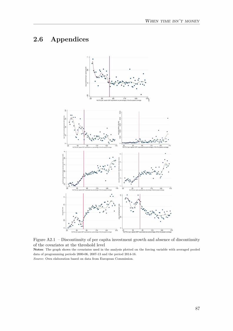
When time isn’t money
2.6 Appendices
Figure A2.1 – Discontinuity of per capita investment growth and absence of discontinuityof the covariates at the threshold levelNotes: The graph shows the covariates used in the analysis plotted on the forcing variable with averaged pooleddata of programming periods 2000-06, 2007-13 and the period 2014-16.Source: Own elaboration based on data from European Commission.
87
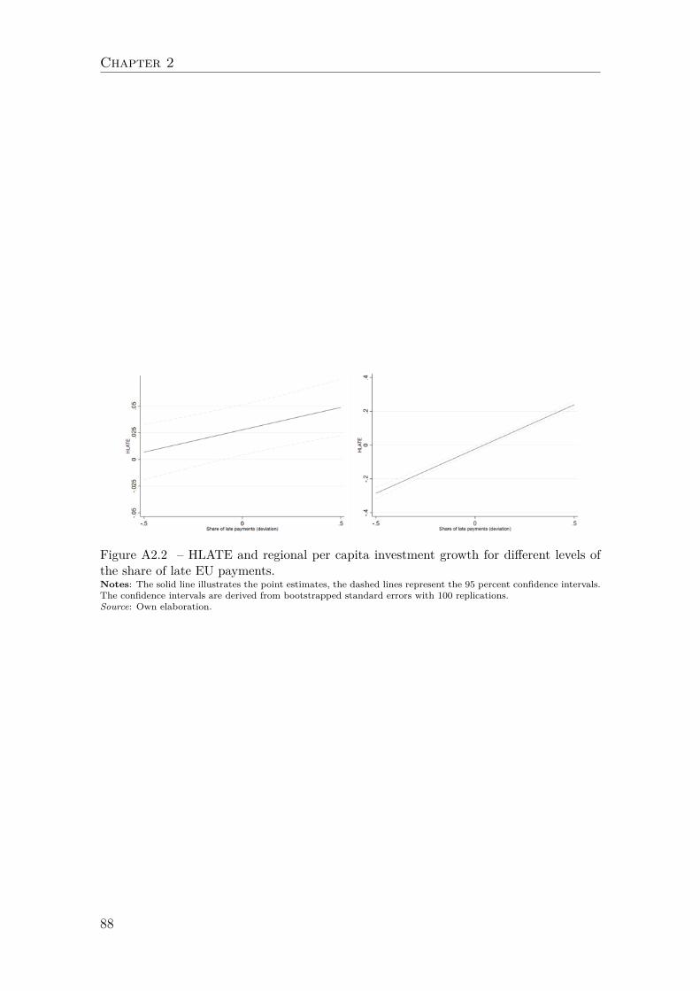
Chapter 2
Figure A2.2 – HLATE and regional per capita investment growth for different levels ofthe share of late EU payments.Notes: The solid line illustrates the point estimates, the dashed lines represent the 95 percent confidence intervals.The confidence intervals are derived from bootstrapped standard errors with 100 replications.Source: Own elaboration.
88
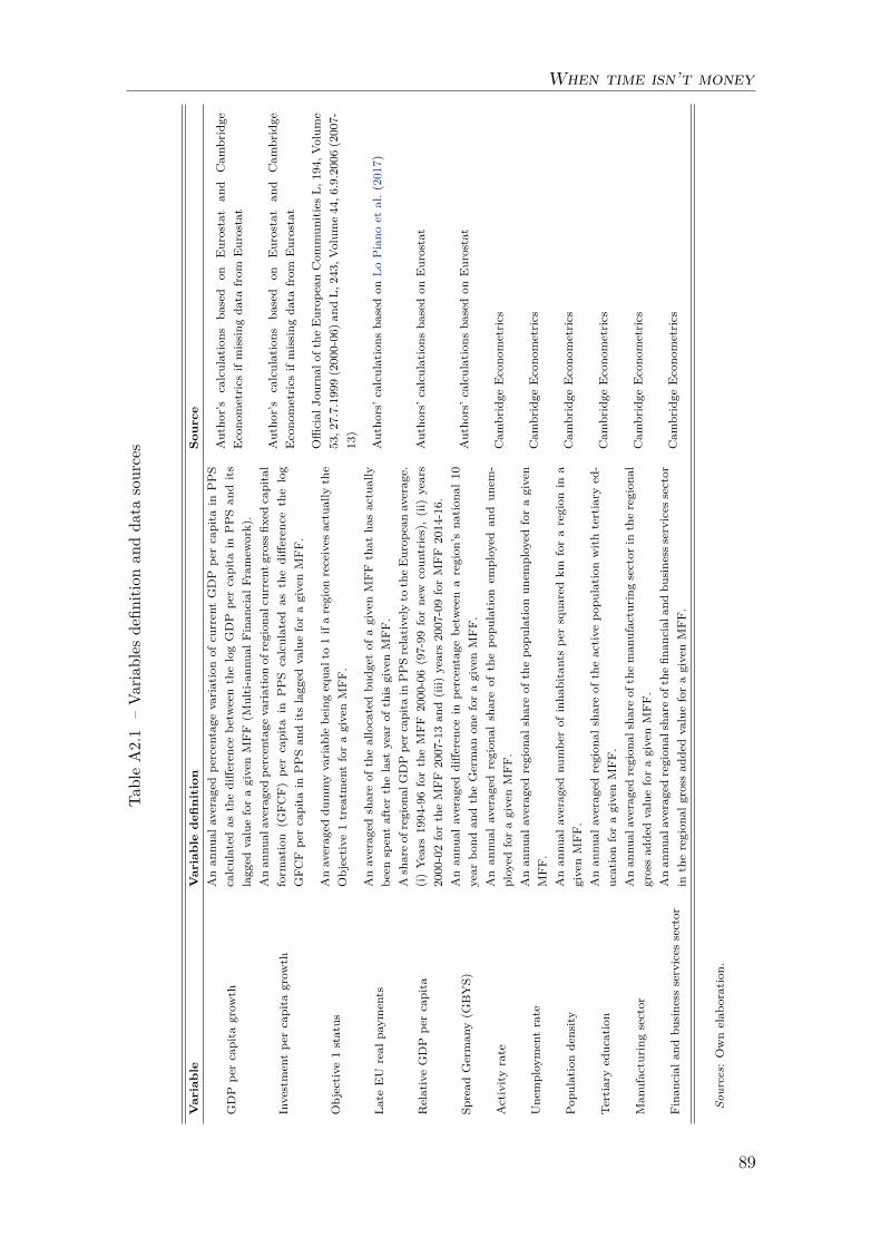
When time isn’t money
TableA2.1
–Va
riables
defin
ition
andda
tasources
Variable
Variablede
finition
Source
GDP
percapita
grow
thAnan
nual
averaged
percentage
variationof
currentGDP
percapita
inPPS
calculated
asthediffe
rencebe
tweenthelogGDP
percapita
inPPSan
dits
lagged
valueforagivenMFF
(Multi-ann
ualF
inan
cial
Fram
ework).
Autho
r’s
calculations
based
onEurostat
and
Cam
bridge
Econo
metrics
ifmissing
data
from
Eurostat
Investmentpe
rcapita
grow
thAnan
nual
averaged
percentage
variationof
region
alcurrentg
ross
fixed
capital
form
ation
(GFC
F)pe
rcapita
inPPS
calculated
asthediffe
rencethelog
GFC
Fpe
rcapita
inPPSan
dits
lagged
valueforagivenMFF
.
Autho
r’s
calculations
based
onEurostat
and
Cam
bridge
Econo
metrics
ifmissing
data
from
Eurostat
Objectiv
e1status
Anaveraged
dummyvariab
lebe
ingequa
lto1ifaregion
receives
actually
the
Objectiv
e1treatm
entforagivenMFF
.
Official
Journa
lofthe
Europ
eanCom
mun
ities
L,194,
Volume
53,2
7.7.1999
(2000-06)a
ndL,
243,
Volume44,6
.9.2006(2007-
13)
Late
EU
real
paym
ents
Anaveraged
shareof
theallocatedbu
dget
ofagivenMFF
that
hasactually
been
spentafterthelast
year
ofthis
givenMFF
.Autho
rs’c
alculatio
nsba
sedon
LoPiano
etal.(2017)
RelativeGDP
percapita
Ashareof
region
alGDPpe
rcap
itain
PPSrelativ
elyto
theEurop
eanaverage.
(i)Ye
ars1994-96fortheMFF
2000-06(97-99
fornew
coun
tries),(ii)
years
2000-02fortheMFF
2007-13an
d(iii)
years2007-09forMFF
2014-16.
Autho
rs’c
alculatio
nsba
sedon
Eurostat
Spread
German
y(G
BYS)
Anan
nual
averaged
diffe
rencein
percentage
betw
eenaregion
’sna
tiona
l10
year
bond
andtheGerman
oneforagivenMFF
.Autho
rs’c
alculatio
nsba
sedon
Eurostat
Activity
rate
Anan
nual
averaged
region
alshareof
thepo
pulatio
nem
ployed
andun
em-
ployed
foragivenMFF
.Cam
bridge
Econo
metrics
Unemploy
mentrate
Anan
nual
averaged
region
alshareof
thepo
pulatio
nun
employed
foragiven
MFF
.Cam
bridge
Econo
metrics
Popu
latio
ndensity
Anan
nual
averaged
numbe
rof
inha
bitantspe
rsqua
redkm
foraregion
ina
givenMFF
.Cam
bridge
Econo
metrics
Tertiary
education
Anan
nual
averaged
region
alshareof
theactiv
epo
pulatio
nwith
tertiary
ed-
ucationforagivenMFF
.Cam
bridge
Econo
metrics
Man
ufacturing
sector
Anan
nual
averaged
region
alshareof
theman
ufacturing
sector
intheregion
algrossad
dedvalueforagivenMFF
.Cam
bridge
Econo
metrics
Fina
nciala
ndbu
siness
services
sector
Anan
nual
averaged
region
alshareof
thefin
ancial
andbu
sine
ssservices
sector
intheregion
algrossad
dedvalueforagivenMFF
.Cam
bridge
Econo
metrics
Sources:
Ownelab
oration.
89
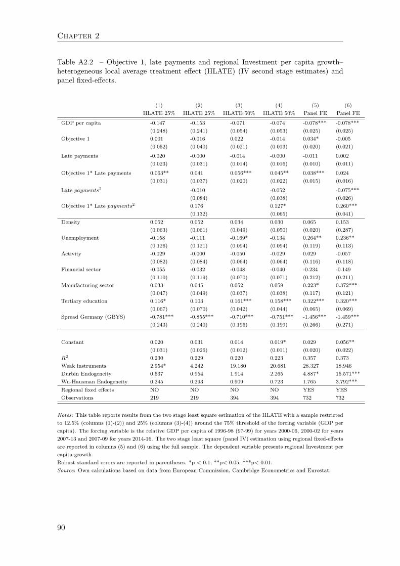
Chapter 2
Table A2.2 – Objective 1, late payments and regional Investment per capita growth–heterogeneous local average treatment effect (HLATE) (IV second stage estimates) andpanel fixed-effects.
(1) (2) (3) (4) (5) (6)HLATE 25% HLATE 25% HLATE 50% HLATE 50% Panel FE Panel FE
GDP per capita -0.147 -0.153 -0.071 -0.074 -0.078*** -0.078***(0.248) (0.241) (0.054) (0.053) (0.025) (0.025)
Objective 1 0.001 -0.016 0.022 -0.014 0.034* -0.005(0.052) (0.040) (0.021) (0.013) (0.020) (0.021)
Late payments -0.020 -0.000 -0.014 -0.000 -0.011 0.002(0.023) (0.031) (0.014) (0.016) (0.010) (0.011)
Objective 1* Late payments 0.063** 0.041 0.056*** 0.045** 0.038*** 0.024(0.031) (0.037) (0.020) (0.022) (0.015) (0.016)
Late payments2 -0.010 -0.052 -0.075***(0.084) (0.038) (0.026)
Objective 1* Late payments2 0.176 0.127* 0.260***(0.132) (0.065) (0.041)
Density 0.052 0.052 0.034 0.030 0.065 0.153(0.063) (0.061) (0.049) (0.050) (0.020) (0.287)
Unemployment -0.158 -0.111 -0.169* -0.134 0.264** 0.236**(0.126) (0.121) (0.094) (0.094) (0.119) (0.113)
Activity -0.029 -0.000 -0.050 -0.029 0.029 -0.057(0.082) (0.084) (0.064) (0.064) (0.116) (0.118)
Financial sector -0.055 -0.032 -0.048 -0.040 -0.234 -0.149(0.110) (0.119) (0.070) (0.071) (0.212) (0.211)
Manufacturing sector 0.033 0.045 0.052 0.059 0.223* 0.372***(0.047) (0.049) (0.037) (0.038) (0.117) (0.121)
Tertiary education 0.116* 0.103 0.161*** 0.158*** 0.322*** 0.320***(0.067) (0.070) (0.042) (0.044) (0.065) (0.069)
Spread Germany (GBYS) -0.781*** -0.855*** -0.710*** -0.751*** -1.456*** -1.459***(0.243) (0.240) (0.196) (0.199) (0.266) (0.271)
Constant 0.020 0.031 0.014 0.019* 0.029 0.056**(0.031) (0.026) (0.012) (0.011) (0.020) (0.022)
R2 0.230 0.229 0.220 0.223 0.357 0.373Weak instruments 2.954* 4.242 19.180 20.681 28.327 18.946Durbin Endogeneity 0.537 0.954 1.914 2.265 4.887* 15.571***Wu-Hausman Endogeneity 0.245 0.293 0.909 0.723 1.765 3.792***Regional fixed effects NO NO NO NO YES YESObservations 219 219 394 394 732 732
Notes: This table reports results from the two stage least square estimation of the HLATE with a sample restrictedto 12.5% (columns (1)-(2)) and 25% (columns (3)-(4)) around the 75% threshold of the forcing variable (GDP percapita). The forcing variable is the relative GDP per capita of 1996-98 (97-99) for years 2000-06, 2000-02 for years2007-13 and 2007-09 for years 2014-16. The two stage least square (panel IV) estimation using regional fixed-effectsare reported in columns (5) and (6) using the full sample. The dependent variable presents regional Investment percapita growth.Robust standard errors are reported in parentheses. *p < 0.1, **p< 0.05, ***p< 0.01.Source: Own calculations based on data from European Commission, Cambridge Econometrics and Eurostat.
90
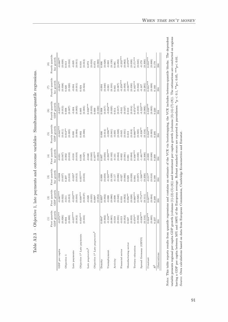
When time isn’t money
TableA2.3
–Objectiv
e1,
late
paym
ents
andou
tcom
evaria
bles–Simultane
ous-qu
antileregressio
ns.
(1)
(2)
(3)
(4)
(5)
(6)
(7)
(8)
First
quartile
First
quartile
First
quartile
First
quartile
Fou
rthqu
artile
Fou
rthqu
artile
Fou
rthqu
artile
Fou
rthqu
artile
GDP
grow
thGDP
grow
thInvgrow
thInvgrow
thGDP
grow
thGDP
grow
thInvgrow
thInvgrow
th
GDP
per
capita
-0.075***
-0.087***
-0.0308
-0.051
-0.045***
-0.037***
-0.094**
-0.080**
(0.026)
(0.022)
(0.037)
(0.047)
(0.011)
(0.013)
(0.038
)(0.039)
Objective1
0.004
-0.011
0.207
-0.002
0.012*
*0.008
0.020
0.013
(0.009)
(0.013)
(0.018)
(0.018)
(0.005)
(0.007)
(0.020
)(0.016)
Latepa
yments
-0.037***
-0.032***
-0.025*
-0.018
0.000
-0.004
-0.004
-0.005
(0.012)
(0.010)
(0.013)
(0.019)
(0.004)
(0.003)
(0.011
)(0.011)
Objective1*
Latepa
yments
0.050***
0.038***
0.057***
0.036
0.002
0.005
0.024
0.016
(0.016)
(0.0137)
(0.018)
(0.027)
(0.006)
(0.005)
(0.024)
(0.013)
Latepayments
2-0.028
-0.048
0.030***
0.073
(0.035)
(0.040)
(0.010)
(0.016)
Objective1*
Latepayments
20.098*
0.167**
0.009
0.073
(0.052)
(0.083)
(0.020)
(0.069)
Density
0.004*
0.005*
-0.009
0.007
0.006
0.008
-0.004
0.006
(0.002)
(0.002)
(0.059)
(0.050)
(0.014)
(0.017)
(0.040
)(0.028)
Unemploy
ment
-0.134**
-0.088
-0.323***
-0.293***
-0.096**
-0.094***
-0.061
-0.063
(0.061)
(0.086)
(0.120)
(0.102)
(0.041)
(0.025)
(0.101
)(0.130)
Activity
-0.018
-0.008
-0.117
-0.101
-0.005
0.014
0.041
0.081
(0.031)
(0.040)
(0.096)
(0.064)
(0.028)
(0.017)
(0.067
)(0.059)
Finan
cial
sector
-0.013
0.016
-0.027
-0.002
-0.045
-0.041
-0.259***
-0.232***
(0.052)
(0.062)
(0.066)
(0.091)
(0.031)
(0.027)
(0.058
)(0.062)
Man
ufacturing
sector
0.047
0.056**
0.029
0.081
0.013
0.010
-0.067**
-0.079**
(0.033)
(0.028)
(0.039)
(0.064)
(0.018)
(0.014)
(0.030
)(0.038)
Tertiaryeducation
0.070**
0.080***
0.094
0.108***
0.080***
0.074***
0.165***
0.171***
(0.032)
(0.026)
(0.057)
(0.038)
(0.025)
(0.019)
(0.042
)(0.045)
Spread
German
y(G
BYS)
-0.636***
-0.774***
-1.500***
-1.481***
-0.338**
-0.323***
-0.167
-0.170
(0.116)
(0.111)
(0.230)
(0.308)
(0.134)
(0.066)
(0.281)
(0.300)
Con
stan
t0.024***
0.027***
-0.017*
-0.009
0.042***
0.038***
0.041***
0.033***
(0.005)
(0.004)
(0.010)
(0.008)
(0.003)
(0.003)
(0.009
)(0.008)
R2
0.237
0.249
0.199
0.209
0.205
0.220
0.16
00.179
Observation
s394
394
394
394
394
394
394
394
Notes:Thistablerepo
rtsresults
from
quan
tileregression
san
dcontains
anestim
ateof
theVCE
viabo
otstrapp
ing,
theVCE
includ
esbe
tween-qu
antileblocks.The
depe
ndent
variab
lepresents
region
alpe
rcapita
GDPgrow
th(colum
ns(1)-(2)-(5)-(6))
andinvestmentpe
rcapita
grow
th(colum
ns(3)-(4)-(7)-(8)).The
estim
ations
arecond
uctedon
region
sha
ving
aGDP
percapita
betw
een50%
and100%
oftheEurop
eanaverage.
Rob
uststan
dard
errors
arerepo
rted
inpa
rentheses.
*p<
0.1,
**p<
0.05,*
**p<
0.01.
Source:Owncalculations
basedon
data
from
Europ
eanCom
mission
,Cam
bridge
Econo
metrics
andEurostat.
91
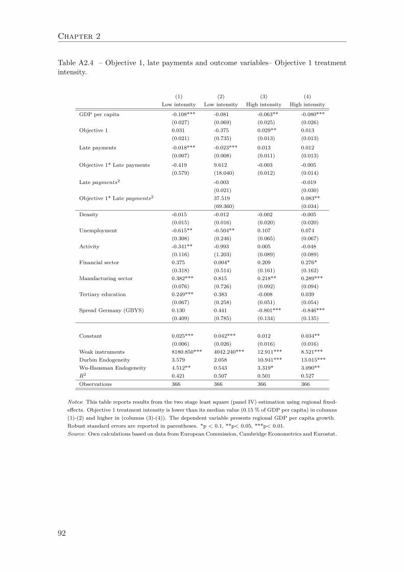
Chapter 2
Table A2.4 – Objective 1, late payments and outcome variables– Objective 1 treatmentintensity.
(1) (2) (3) (4)Low intensity Low intensity High intensity High intensity
GDP per capita -0.108*** -0.081 -0.063** -0.080***(0.027) (0.069) (0.025) (0.026)
Objective 1 0.031 -0.375 0.029** 0.013(0.021) (0.735) (0.013) (0.013)
Late payments -0.018*** -0.023*** 0.013 0.012(0.007) (0.008) (0.011) (0.013)
Objective 1* Late payments -0.419 9.612 -0.003 -0.005(0.579) (18.040) (0.012) (0.014)
Late payments2 -0.003 -0.019(0.021) (0.030)
Objective 1* Late payments2 37.519 0.083**(69.360) (0.034)
Density -0.015 -0.012 -0.002 -0.005(0.015) (0.016) (0.020) (0.020)
Unemployment -0.615** -0.504** 0.107 0.074(0.308) (0.246) (0.065) (0.067)
Activity -0.341** -0.993 0.005 -0.048(0.116) (1.203) (0.089) (0.089)
Financial sector 0.375 0.004* 0.209 0.276*(0.318) (0.514) (0.161) (0.162)
Manufacturing sector 0.382*** 0.815 0.218** 0.289***(0.076) (0.726) (0.092) (0.094)
Tertiary education 0.249*** 0.383 -0.008 0.039(0.067) (0.258) (0.051) (0.054)
Spread Germany (GBYS) 0.130 0.441 -0.801*** -0.846***(0.409) (0.785) (0.134) (0.135)
Constant 0.025*** 0.042*** 0.012 0.034**(0.006) (0.026) (0.016) (0.016)
Weak instruments 8180.850*** 4042.240*** 12.911*** 8.521***Durbin Endogeneity 3.579 2.058 10.941*** 13.015***Wu-Hausman Endogeneity 4.512** 0.543 3.319* 3.090**R2 0.421 0.507 0.501 0.527Observations 366 366 366 366
Notes: This table reports results from the two stage least square (panel IV) estimation using regional fixed-effects. Objective 1 treatment intensity is lower than its median value (0.15 % of GDP per capita) in columns(1)-(2) and higher in (columns (3)-(4)). The dependent variable presents regional GDP per capita growth.Robust standard errors are reported in parentheses. *p < 0.1, **p< 0.05, ***p< 0.01.Source: Own calculations based on data from European Commission, Cambridge Econometrics and Eurostat.
92
Chapter 3
“The winner takes it all” or a story ofthe optimal allocation of the European Co-hesion Fund
This chapter is co-authored withPhu Nguyen-Van and Thi Kim Cuong Pham.
Summary
This third chapter aims to determine an optimal allocation of the European CohesionFund (ECF) and compares it with the observed allocation. This optimal allocationis the solution of a donor optimisation problem which maximises recipient countries’GDP per capita to achieve economic convergence in the EU. Compared to the ob-served allocation, our solution can identify the recipient countries that can benefitfrom higher ECF transfers than the observed levels, as those having low relativeGDP per capita, large population size and where the ECF has a strong capacity tosupport economic growth. Results are robust to changes in the specification of thedonor’s utility function.
93
Chapter 3
Acknowledgments
The authors are grateful to two anonymous referees, the participants at the Eu-ropean Public Choice Society congress (Roma, 2018), Journées LAGV (Aix-en-Provence, 2018), and AFSE congress (Paris, 2018), and other seminars for helpfulcomments on a previous draft of this chapter. The usual caveat applies.
Publication
This Chapter was published in a similar version as:
Dicharry, B., Nguyen-Van, P., and Pham, T. K. C. (2019). “The winner takes itall” or a story of the optimal allocation of the European Cohesion Fund. EuropeanJournal of Political Economy, 59, 385-399.
94
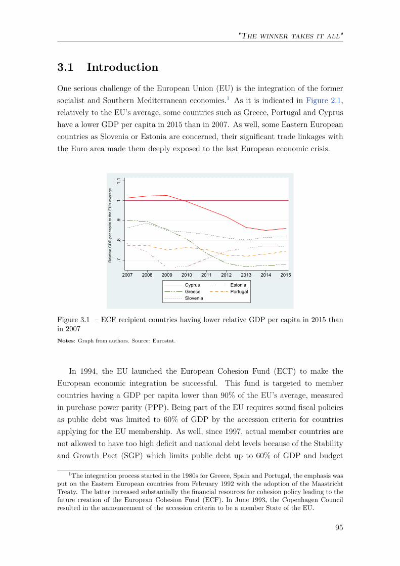
"The winner takes it all"
3.1 Introduction
One serious challenge of the European Union (EU) is the integration of the formersocialist and Southern Mediterranean economies.1 As it is indicated in Figure 2.1,relatively to the EU’s average, some countries such as Greece, Portugal and Cyprushave a lower GDP per capita in 2015 than in 2007. As well, some Eastern Europeancountries as Slovenia or Estonia are concerned, their significant trade linkages withthe Euro area made them deeply exposed to the last European economic crisis.
.7.8
.91
1.1
Rel
ativ
e G
DP
per c
apita
to th
e EU
's a
vera
ge
2007 2008 2009 2010 2011 2012 2013 2014 2015
Cyprus EstoniaGreece PortugalSlovenia
Figure 3.1 – ECF recipient countries having lower relative GDP per capita in 2015 thanin 2007Notes: Graph from authors. Source: Eurostat.
In 1994, the EU launched the European Cohesion Fund (ECF) to make theEuropean economic integration be successful. This fund is targeted to membercountries having a GDP per capita lower than 90% of the EU’s average, measuredin purchase power parity (PPP). Being part of the EU requires sound fiscal policiesas public debt was limited to 60% of GDP by the accession criteria for countriesapplying for the EU membership. As well, since 1997, actual member countries arenot allowed to have too high deficit and national debt levels because of the Stabilityand Growth Pact (SGP) which limits public debt up to 60% of GDP and budget
1The integration process started in the 1980s for Greece, Spain and Portugal, the emphasis wasput on the Eastern European countries from February 1992 with the adoption of the MaastrichtTreaty. The latter increased substantially the financial resources for cohesion policy leading to thefuture creation of the European Cohesion Fund (ECF). In June 1993, the Copenhagen Councilresulted in the announcement of the accession criteria to be a member State of the EU.
95
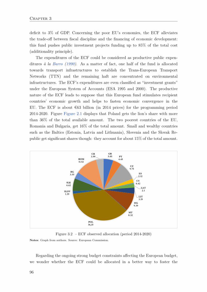
Chapter 3
deficit to 3% of GDP. Concerning the poor EU’s economies, the ECF alleviatesthe trade-off between fiscal discipline and the financing of economic development:this fund pushes public investment projects funding up to 85% of the total cost(additionality principle).
The expenditures of the ECF could be considered as productive public expen-ditures à la Barro (1990). As a matter of fact, one half of the fund is allocatedtowards transport infrastructures to establish the Trans-European TransportNetworks (TTN) and the remaining haft are concentrated on environmentalinfrastructures. The ECF’s expenditures are even classified as “investment grants”under the European System of Accounts (ESA 1995 and 2000). The productivenature of the ECF leads to suppose that this European fund stimulates recipientcountries’ economic growth and helps to fasten economic convergence in theEU. The ECF is about €63 billion (in 2014 prices) for the programming period2014-2020. Figure Figure 2.1 displays that Poland gets the lion’s share with morethan 36% of the total available amount. The two poorest countries of the EU,Romania and Bulgaria, get 16% of the total amount. Small and wealthy countriessuch as the Baltics (Estonia, Latvia and Lithuania), Slovenia and the Slovak Re-public get significant shares though: they account for about 15% of the total amount.
GR5.05 PT
4.45
CZ9.75
ES2.12
CY0.42
LAT2.1
LIT3.19
HG9.39
MT0.32
POL36,15
SLOV1.39
SLK6.62
BG3.55
ROM11.52
CR3.99
Figure 3.2 – ECF observed allocation (period 2014-2020)Notes: Graph from authors. Source: European Commission.
Regarding the ongoing strong budget constraints affecting the European budget,we wonder whether the ECF could be allocated in a better way to foster the
96
"The winner takes it all"
economic convergence in the EU. The EU cohesion policy results in transfers be-tween a global donor i.e. the European Commission, and some recipient countries.2
Moreover, some criticism was addressed to the way European structural funds (SF)are allocated between recipient countries, which affects the global effectiveness ofthe European cohesion policy (Cappelen et al. (2003), Rodríguez-Pose & Fratesi(2004), Ederveen et al. (2006), Becker (2012), Mendez et al. (2013b), Tomovaet al. (2013), Rodríguez-Pose & Garcilazo (2015), Huliaras & Petropoulos (2016),Crescenzi & Giua (2016)). However, there was no suggestion about an allocationof SF able to maximise the impact of the European cohesion policy on economicgrowth in order to promote economic convergence. Through a normative approach,our study fills this gap by providing an optimal allocation of the ECF and comparethe latter with the observed one.
In this chapter, we posit a theoretical problem where an altruistic donor choosesan allocation of ECF to maximise the global welfare of recipient countries. Ouranalysis is implemented in two steps: First, we estimate the ability of the ECF tostimulate GDP per capita thanks to a growth equation using data covering the 15ECF recipient countries for the period 1995-2015. Based on GMM estimation, wefind that the ECF mostly has a conditional effect on growth, depending on recipientcountries’ national debt and inflation levels. Second, thanks to the estimationresults of the growth equation, we run simulations of the ECF’s optimal allocationwhich corresponds to the solution of the donor’s optimisation problem. Our resultsindicate that the ECF should be concentrated on poor countries having a largepopulation, and where the ECF has a strong ability to promote economic growth(i.e. low inflation and low public debt). More precisely, the findings suggest toshift the ECF away from small and wealthy countries (such as the Czech Republic,Malta, Cyprus, Slovenia or the Slovak Republic) and concentrate the fund onbigger, poorer and more efficient countries (Poland and Romania). This result isrobust to changes in the specification of the donor’s utility function.
The remaining of the chapter is structured as follows. Section 2 discusses therelated literature on the conditional effectiveness of financial transfers betweendonors and recipient countries focusing on foreign aid and European structuralfunds. Section 3 provides the theoretical framework where the donor’s problem andits solution are exposed. Section 4 describes the data of the growth equation, andpresents estimation results. Section 5 is related to the simulation of the optimal
2The EU cohesion policy is based on five European structural funds (SF) that are the Euro-pean regional development fund (ERDF), the European social fund (ESF), the European cohesionfund (ECF), the European agricultural fund for rural development (EAFRD), and the Europeanmaritime and fisheries fund (EMFF).
97
Chapter 3
allocation of the ECF and policy implications regarding the observed allocation ofthe fund. We finally conclude our study in Section 6 and provide some researchperspectives.
3.2 Related literature
The discussion about the effectiveness of ECF can be based on the previous workson foreign development aid. One major issue highlighted by this literature isthe conditional effectiveness of financial transfers between donors and recipientcountries. In their seminal chapter, Burnside & Dollar (2000) found that foreign aidhas a positive effect on growth only in recipient countries which have good fiscal,monetary and trade policies. Collier & Dollar (2002) used the World Bank’s Coun-try Policy and Institutional Assessment (CPIA) as a measure of policy quality andshowed that aid may promote economic growth and reduce the poverty in recipientcountries if the quality of their policies is sufficiently high. Guillaumont & Chauvet(2001) and Chauvet & Guillaumont (2009) indicated that the marginal effect of aidon growth is conditional on the recipient countries’ economic vulnerability, i.e. themarginal effect of aid on growth is an increasing function of economic vulnerability.
Regarding European structural funds (SF), an important literature underlinedtheir conditional impact on economic growth (Cappelen et al. (2003), Rodríguez-Pose & Fratesi (2004), Ederveen et al. (2006), Becker (2012), Mendez et al. (2013b),Tomova et al. (2013), Rodríguez-Pose & Garcilazo (2015), Huliaras & Petropoulos(2016), Crescenzi & Giua (2016)). The quality of institutions or government arekey variables driving this conditional effectiveness (Ederveen et al. (2006), Becker(2012), Rodríguez-Pose & Garcilazo (2015)). Ederveen et al. (2006) used tradeopenness as a proxy for institutional quality considering that the more a country isopen, the more it is under trade competition, which increases the pressure for anefficient use of SF. They found that the impact of the ERDF on economic growthpositively depends on the level of trade openness.
As well, Becker (2012) concluded that regions with poorer governance andlower levels of education fail to make good use of EU transfers. Rodríguez-Pose& Garcilazo (2015) emphasised that SF’s impact on GDP in regions receivingmore than €150 per capita, which is the case of most of the Eastern Europeanregions, is purely conditioned by the quality of government. Other studies pointed
98
"The winner takes it all"
out low planning capacity, inefficient bureaucratic procedures and lack of experi-enced staff as factors delaying decisions and thwarting outcomes (Cappelen et al.(2003), Rodríguez-Pose & Fratesi (2004)). These issues refer to the importanceof administrative capacity in determining the ability of SF to promote economicgrowth. Mendez et al. (2013b) defined administrative capacity as the capacity ofnational and regional institutions to design robust strategies, to allocate resourcesand to administer EU funding efficiently. In a study focused on Greece, Huliaras &Petropoulos (2016) described the consequences of a weak administrative capacityand bad quality of government: As with foreign aid, SF in Greece have ended upsupporting a bloated bureaucracy, strengthening patronage patterns and reinforcingclientelistic networks. They also had a negative impact on incentives. They weretreated by Greek government officials as an external rent, rather than a support fordomestic efforts.
Other variables as sound fiscal and macroeconomic policies (Tomova et al.(2013)) or favourable socio-economic conditions (Crescenzi & Giua (2016)) are aswell mentioned by the literature. More precisely, Tomova et al. (2013) showed thatsound fiscal policies (proxied by low levels of government debt and deficit) andsound macroeconomic policies (proxied by low levels of net foreign liabilities) arebeneficial to ESF’s efficiency. Crescenzi & Giua (2016) found that the relationshipbetween Regional Policy funding and regional growth is the strong and positive inareas with favourable socio-economic conditions (proxied by the social filter index).
3.3 A theoretical framework for the ECF optimalallocation
Our theoretical framework is based on the literature of foreign aid allocation wherea normative approach is used in order to determine its optimal allocation (Burnside& Dollar (2000), Collier & Dollar (2001), Llavador & Roemer (2001), Collier &Dollar (2002), Cogneau & Naudet (2007), Carter (2014)). In their seminal works,Collier & Dollar (2001, 2002) proposed an optimal aid allocation maximising a socialwelfare function which is the sum of utilities of aid-recipient countries. A country’sutility is measured in terms of number of poor reduced thanks to economic growth.The latter is in turn influenced by aid, institutional quality, and policy quality.Consequently, the aid allocation reducing the poverty is determined by the initialpoverty of recipient countries and the aid effectiveness which depend on the recipient
99
Chapter 3
countries’ institutional quality, and their policy quality.Related to this literature, we use a theoretical framework to determine an opti-
mal allocation of the ECF. This fund is a financial assistance designed to take thechallenge of the European economic convergence by increasing EU lagging countries’GDP per capita. We assume that an altruistic donor maximises the sum of recipientcountries’ utilities. In the case of the ECF, the donor is represented by the EuropeanCommission which decides how the ECF is allocated among recipient countries, i.ecountries having a GDP per capita lower than 90% of the EU’s average.3
We assume that, for each recipient country i, its utility depends on the extent ofits economic gap relatively to the EU, i.e the ratio between its own GDP per capitayi and 90% of the EU’s average, (noted as 0.9y). We assume that yi depends onthe ECF transfers Ai. The term 0.9y, indicating 90% of the EU’s average GDP percapita, is assumed constant and taken as given by recipient countries. As well, weexclude the case of yi > 0.9y: otherwise, a recipient country would not be eligibleanymore for the ECF.4 We assume that the European Commission, thanks to theECF, intends to maximise recipient countries’ GDP per capita relatively to the EU’saverage. For a sake of simplicity, we consider a CRRA function as follows:
U
(yi
0.9y
)= 1
1− σ
(yi(Ai)0.9y
)1−σ
(3.1)
where σ = −U ′′(R)RU ′(R) , with R ≡ yi
0.9y , is interpreted as the donor’s aversion to thegap R between recipient countries GDP and the EU’s average GDP per capita. Inother words, σ may be interpreted as the donor’s aversion to the recipient countries’poverty compared to the EU’s average GDP per capita. As σ increases, the altruisticdonor is more concerned with recipient countries having low relative GDP per capita.U is increasing and concave with yi, i.e. Uyi > 0 and Uyiyi ≤ 0.
The donor chooses then the optimal ECF allocation maximising the sum ofutilities of n recipient countries:
max{Ai}ni=1
∑ni=1 αiU
(yi(Ai)0.9y
)(P )
s.t. ∑ni=1AiNi ≤ A (3.2)
Ai ≥ 0,∀i = 1, 2, ..., n (3.3)
3It should be mentioned that the ECF is in fact mostly funded by Western European coun-tries. These countries are above the 90% threshold, which makes them be net contributors to theEuropean budget.
4For instance, Ireland and Spain have been excluded from the list of beneficiaries respectivelyin 2003 and 2013 because of their GDP per capita levels higher than 90% of the EU average .
100
"The winner takes it all"
where αi corresponds to the weight of each recipient country in the utility function ofthe donor. In our analysis, we consider that αi is the demographic weight of recipientcountry i in the total population of all recipient countries. Ni is the total populationof recipient country i, Ai is the ECF transfer to country i in terms of percentage ofits GDP, and AiNi corresponds to the ECF amount received by country i. (Eq. 2.2)represents the constraint of funds availability where A is the total available amount.The constraint on the positiveness of the ECF transfers is given by (Eq. 2.3) .
The Lagrangian of the optimisation problem (P) is:
L(Ai, λ, µi) =n∑i=1
αiU
(yi(Ai)0.9y
)+ λ
(A−
n∑i=1
AiNi
)+
n∑i=1
µiAi, (3.4)
where and λ and µi are the Lagrange multipliers of constraints (2) and (3), respec-tively. A solution of the model (A1, A2, ..., An), λ and µi must satisfy the followingfirst order conditions (FOCs), ∀i = 1, ..., n :
∂L(A)∂Ai
= −λNi − µi + αiUyyA = 0, (3.5)n∑i=1
NiAi = A, (3.6)
µi ≥ 0, Ai ≥ 0. (3.7)
where Uy denotes the marginal utility of GDP per capita and yA the marginal effectof the ECF on GDP per capita. (Eq. 2.7) corresponds to the complementaritycondition between Ai and µi. For a country i receiving a strictly positive ECFamount Ai > 0, we have µi = 0 . On the opposite, if Ai = 0, we must have µi > 0.
If we consider the case of a country receiving a strictly positive ECF amount,i.e. Ai > 0 and µi = 0, (Eq. 2.5) gives us the optimal value of λ:
λ = αiUy(yi(Ai))yA(Ai)
Ni
,∀i = 1, ..., n such that Ai > 0 (3.8)
This expression gives the value for λ which equalises the right hand side term in overall the ECF recipient countries at the optimal solution of the optimisation program(P ). As λ stands for the shadow value of the ECF, it represents the marginal benefitof one extra-unit of ECF expressed in utility units. This equality shows that, whenthe optimisation problem is solved, the marginal cost of one extra-unit of ECF is thesame as its marginal benefit for every recipient countries. If we now consider onlythe case of a country j receiving no ECF transfer (Aj = 0), we obtain the following
101
Chapter 3
conditions:
µj = λNi − αjUy(yi(Ai))yA(Ai),∀j = 1, ..., n such that Aj = 0 (3.9)
The results above can be summarised in the following proposition:
Proposition 1. Considering the donor’s optimisation program (P), the ECF opti-mal allocation {Ai}ni=1 must respect the three following conditions:
1. Ai > 0 if λ = αiUy(yi(Ai))yA(Ai)
Ni
and µi = 0,
2. Aj=0 if µj = λNj − αjUy(yi(Ai))yA(Ai), and µj > 0,
3. ∑ni=1 AiNi = A.
where λ is the multiplier associated to the total amount of ECF, and µi is the mul-tiplier associated to the positiveness of recipient countries’ ECF transfers.
The second derivative of Ui with respect to Ai is :
∂2U(Ai)∂Ai
2 = Uyyy2A + yAAUy, (3.10)
where Uyy is the second derivative of U with respect to yi and yAA is the secondderivative of yi with respect to Ai. As the budget constraint is linear with respectto Ai, this second derivative of Ui must be non positive to ensure the existence of asolution. Thus, from (Eq. 2.10), the following condition should be satisfied:
yAAy2A
≤ −UyyUy
. (3.11)
The right-hand side term of equation (11) is always positive because of the in-creasing and concave utility function with respect to GDP per capita. However, wedo not know the sign of the left-hand side term of (Eq. 2.11). An empirical estima-tion of the growth equation will allow us to conclude whether there exists a solutionwith real data. This will be the object of the following section. More precisely,we consider the role of the ECF and other factors being likely to affect recipientcountries’ GDP per capita such as the quality of macroeconomic management andinstitutions. We will see that estimation results satisfy (Eq. 2.11), leading to theexistence of a solution of the optimisation problem. The estimation results of thisgrowth equation will then be employed to make simulations of the ECF’s optimalallocation, the latter being the solution of the donor’s optimisation program (P ).
102
"The winner takes it all"
3.4 Estimation of the growth equation
3.4.1 Determinants of economic growth
This subsection describes the set of variables employed in our growth equation. Wefirst consider some relevant exogenous factors able to explain recipient countries’growth such as geographical localisation and history after World War Two (WW2).Concerning the former, De Menil (2003) underlined the importance of being closeto a EU-15 country to explain the satisfying growth performances of Poland, Hun-gary and the Czech Republic during the 1990s. These authors argued that thisfavourable localisation lowered the political cost of implementing market orientedstructural reforms, citizens being more directly confronted to Western Europeanhigh living standards. As well, Bevan & Estrin (2004) stressed the role of localisa-tion on foreign direct investment inflows (FDI) for Poland and the Czech Republic.These countries have greatly benefited from the European integration by becomingpart of the German supply chain (Hinterland) since being a neighbour of Germanyhelped reducing their transactions costs.5 Regarding the history of ECF recipientcountries after WW2 , we focus on countries having experienced a socialist era andthe length of this period or market memory, as it has been called by De Melo et al.(2001) in order to capture the lack of familiarity with market institutions. Theseauthors found that the initial degree of macroeconomic distortions caused by centralplanning has an adverse impact on current economic performance.
One other determinant of GDP per capita is the level of economic freedom (Gold-smith (1995), Dawson (2003)).6 It has been observed that the former socialist coun-tries that joined the EU as soon as 2004 are those which implemented a so-calledshock therapy to increase the level of national economic freedom.7 Pitek et al. (2013)found that moderate government spending, high monetary and investment freedomshave been significant determinants of economic growth between 1990 and 2008 inEastern European countries. Besides, Dell’Anno & Villa (2013) analysed the impactof the speed of these reforms on economic growth and found that the contempora-neous speed of transition lowers current economic growth, but the impact becomespositive in the medium-long run.8 Therefore, we could expect that countries having
5Transports and communication costs, costs of dealing with a different language, informationalcosts and those related to sending personnel abroad.
6Economic freedom is based on the security of property rights, the ability to trade with anydomestic or foreign entity and the extent of property confiscation through the taxation and inflationlevels.
7We refer to Poland, the Czech and Slovak republics, the Baltics, Hungary and Slovenia.8See also Aghion & Blanchard (1994) who estimated that the past level of reforms leads to
higher economic growth and this effect reaches its greatest value with a lag of 3 years.
103
Chapter 3
implemented significant market reforms would benefit from higher GDP per capita.We finally estimate the impact of the ECF on GDP per capita, i.e yA and yAA
from condition (11), in order to check the existence of a solution to our optimisationproblem (P). Referring to the literature dealing with the European cohesion policy,we study the ECF’s conditional impact on GDP per capita. As Ederveen et al.(2006), Becker (2012), Rodríguez-Pose & Garcilazo (2015), Crescenzi & Giua (2016),these conditioned factors correspond to quality of institutions and government.
Moreover, we consider macroeconomic management conditions as in Tomovaet al. (2013). We put an emphasis on public debt because of the crowding-out effectthat may rise from an excessive public debt level regarding the ECF’s ability topromote economic growth. As a matter of fact, high public debt could be harmfulto the ECF’s economic performance because of the additionality principle. This rulerelated to EU cohesion policy make ECF recipient country’s managing authorityprovide, at least, the remaining 15% of a project’s cost. If it does so with additionaldebt, the initial positive effects on growth could be offset because of a crowding-outeffect arising with a high initial national debt level. In other words, countries re-specting the SGP should be those where SF are the most efficient. Note that theEU condemns slack budget discipline since European transfers could be suspendedfollowing an excessive deficit procedure that can be launched by the European Com-mission.9 We therefore expect that high public debt levels will be detrimental tothe ECF’s marginal effect on GDP per capita.
In a nutshell, the conditional effect of the ECF on GDP per capita will bestudied through the inclusion of interaction terms between the ECF and variablesdealing with macroeconomic management, quality of institutions and government.The following section deals with the specification of the growth equation.
3.4.2 Econometric specification
Our growth equation is estimated by using a panel data framework (Islam (1995),Caselli et al. (1996)). To avoid business cycles effects, we use 4-years average datafor all variables excepted GDP per capita and its lagged value. We use current GDPper capita and its lagged values from observations with a 4 years interval, i.e. 1995,1999, 2003, 2007, 2011 and 2015. Concerning explanatory variables, we use their
9Member States which run excessive budget deficits of more than 3% of GDP, or which failto reduce their excessive debts (above 60% of GDP) at a sufficient pace, follow a particular setof rules known as the Excessive Deficit Procedure (EDP). A suspension of the Cohesion fundscommitments could then be decided if the qualified majority is obtained following a vote of theEuropean Council. See EU regulation 1303/2013, article 23, Measures linking effectiveness of ESIfunds to sound economic governance.
104
"The winner takes it all"
average values over the following 4 years periods: 1995-1998, 1999-2002, 2003-2006,2007-2010 and 2011-2014. The resulting data are an unbalanced panel data samplecovering 17 countries and period 1995-2015 (5 waves of 4 years intervals).10
Our dependent variable is the log real GDP per capita in international pricesPPP 2011 (yi,t). We assume that the latter depends on its lagged value (yi,t−1). GDPper capita of country i in period t also depends on the log of ECF per capita (Ai,t)expressed in international prices PPP 2011. We then consider one dummy variablerelated to geographical location (Geoi) and one variable indicating the number ofyears under socialism after WW2, (Socialismi). As well, we assume that GDP percapita depends on levels of economic freedom (Efreedomi,t), inflation (Inflationi,t),national debt (Debti,t) and its squared term (Debt2i,t) to capture a non linear ef-fect à la Reinhart and Rogoff (2010). We also include human capital (Humani,t).We finally control for the effects of the other EU funds through a single variable(EUfundsi,t) aggregating the ERDF, EAFRD and the ESF. We hence consider thefollowing baseline model:
yi,t = ρyi,t−1 +X ′i,tβ + +λAAi,t + γ2Period99−02 + γ3Period03−06 + γ4Period07−10
+ γ5Period11−14 + vt + εi,t(3.12)
In Model (1), Xi,t includes (Geoi, Socialismi, Efreedomi,t, Debti,t, Debt2i,t,EUfundsi,t) and (Humani,t). (vt) is the time effect and (εi,t) is the error termof the regression. Individual fixed effects are not included because they are removedby system-GMM.
In order to determine a conditional effect of ECF on growth, we include inter-action terms in our baseline model. We then estimate Model (2) where we considerthe interaction between the ECF and macroeconomic management variables thatare national debt and inflation. Testing those interactions is in line with the fiscalrules related to the SGP and Tomova et al. (2013). We also fit with Ederveen et al.(2006), Becker (2012), Rodríguez-Pose & Garcilazo (2015) and Crescenzi & Giua(2016) by estimating the role of institutional quality and quality of government onthe ECF’s effect on growth with Model (3): Model (3a) adds interactions betweenthe ECF and the corruption index (Corruptioni,t) as a proxy of institutional quality,and Model (3b) uses the government effectiveness index (Governmenti,t) as a proxyof quality of government.11
The presence of the lagged dependent variable term in the right hand side of
10As the data correspond to series of average values with a small T (T=5), the non-stationarityissue is not a major issue here. Moreover, the model also includes time dummies to control fortrend effects.
11Those two interactions are not estimated simultaneously because of multicollinearity issues.
105
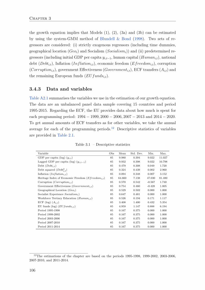
Chapter 3
the growth equation implies that Models (1), (2), (3a) and (3b) can be estimatedby using the system-GMM method of Blundell & Bond (1998). Two sets of re-gressors are considered: (i) strictly exogenous regressors (including time dummies,geographical location (Geoi) and Socialism (Socialismi)) and (ii) predetermined re-gressors (including initial GDP per capita yi,t−1, human capital (Humani,t), nationaldebt (Debti,t), Inflation (Inflationi,t), economic freedom (Efreedomi,t), corruption(Corruptioni,t), government Effectiveness (Governmenti,t), ECF transfers (Ai,t) andthe remaining European funds (EUfundsi,t).
3.4.3 Data and variables
Table A2.1 summarises the variables we use in the estimation of our growth equation.The data are an unbalanced panel data sample covering 15 countries and period1995-2015. Regarding the ECF, the EU provides data about how much is spent foreach programming period: 1994− 1999, 2000− 2006, 2007− 2013 and 2014− 2020.To get annual amounts of ECF transfers as for other variables, we take the annualaverage for each of the programming periods.12 Descriptive statistics of variablesare provided in Table 2.1.
Table 3.1 – Descriptive statistics
Variable Obs Mean Std. Dev. Min. Max.GDP per capita (log) (yi,t) 85 9.980 0.394 9.022 11.027Lagged GDP per capita (log) (yi,t−1) 85 9.932 0.398 9.022 10.798Debt (Debti,t) 85 0.479 0.308 0.049 1.720Debt squared (Debt2i,t) 85 0.324 0.439 0.002 2.960Inflation (Inflationi,t) 85 0.094 0.348 0.007 3.152Heritage Index of Economic Freedom (Efreedomi,t) 85 64.660 7.138 47.030 81.480Corruption (Corruptioni,t) 85 0.570 0.542 -0.567 1.740Government Effectiveness (Governmenti,t) 85 0.754 0.460 -0.428 1.805Geographical Location (Geoi) 85 0.529 0.502 0.000 1.000Socialist Experience Socialismi) 85 0.647 0.481 0.000 1.000Workforce Tertiary Education (Humani,t) 85 0.526 0.194 0.171 1.117ECF (log) (Ai,t) 85 3.408 1.400 0.432 5.354EU funds (log) (EUfundsi,t) 85 4.959 1.147 0.888 6.194Period 1995-1998 85 0.167 0.375 0.000 1.000Period 1999-2002 85 0.167 0.375 0.000 1.000Period 2003-2006 85 0.167 0.375 0.000 1.000Period 2007-2010 85 0.167 0.375 0.000 1.000Period 2011-2014 85 0.167 0.375 0.000 1.000
12The estimations of the chapter are based on the periods 1995-1998, 1999-2002, 2003-2006,2007-2010, and 2011-2014.
106
"The winner takes it all"
3.4.4 Estimation results
Our analysis shows that Arellano-Bond tests in the regressions residuals, AR(1)and AR(2), the Sargan and Hansen overidentifying restrictions tests and tests forexogeneity are generally verified. Our dynamic panel data is unbalanced with moreindividual dimensions than time dimension (T=5 and N=15 ). Following Roodman(2009), it is therefore preferable to use the system GMM method of Blundell &Bond (1998) when N is larger than T. Table 2.2 displays the estimation results ofModels (1), (2), (3a) and (3b) with the measure of Economic Freedom from HeritageFoundation.
We also do estimation with Fraser Institute’s measure of Economic Freedomand its 5 sub-areas (government size, sound monetary policy, regulation, legal sys-tem, and trade). Analyses using Fraser Index on Economic Freedom are reportedin the appendix. Table A2.2 provides definition of Fraser Institute’s measure ofEconomic Freedom, Table A2.3 presents its descriptive statistics and Table A2.4provides growth equation’s estimations using this index. Figure A2.1 indicates in-deed that the both measures of Economic Freedom are strongly correlated. Wealso observe that because the five Fraser sub-area indexes encompass some eco-nomic and policy variables (e.g. government size vs debt, sound monetary policyvs inflation, legal system and regulation vs corruption), the latter were excludedfrom the corresponding regressions. Results using those two different measures ofEconomic Freedom are quite similar. In particular, the effect of Fraser Institute’sgeneral Economic Freedom index is positive like the Heritage counterpart (even itis not statistically significant). While the regressions with Fraser sub-area indexesgive an additional information that three of the five dimensions of economic freedom(sound monetary policy, regulation, and trade) can have an impact on growth, theirinteractions with ECF remain similar to the case with Heritage index.
Results obtained with system-GMM estimators indicate that the lagged term ofGDP per capita is highly significant and has a positive effect on current GDP percapita. The high significance of the lagged term of GDP per capita gives strengthto the use of system GMM. The size of this effect is rather similar across all speci-fications. Concerning the other regressors, Economic Freedom exhibits a significantpositive impact on GDP per capita in all models, which is in line with Dell’Anno &Villa (2013). Those estimates highlight the returns on the market-oriented reformsimplemented in the 1990s in most of recipient countries. In addition, we also observethat other European funds (variable EU funds per capita) do not directly exert asignificant effect on GDP per capita of recipient countries (except a negative weaklysignificant effect in model 3a). Similar results have been founded by previous studies
107
Chapter 3
such as Rodríguez-Pose & Fratesi (2004), Dall’Erba & Le Gallo (2008), Le Galloet al. (2011), Fratesi & Perucca (2014). Moreover, this variable includes the Euro-pean Agricultural Fund for Rural Development whose specific impact on economicgrowth has been found insignificant by Crescenzi & Giua (2016). We could men-tion as well that the European Social Fund included in this variable aims to financeessentially social expenditures that are not productive in the sense of Barro (1990).
Let us now turn to the analysis of the ECF’s estimation results. They indicatethat the ECF’s impact is purely conditional as the direct term is insignificant. Weobserve that the impact of the ECF on GDP per capita is not conditioned to re-cipient countries’ institutional quality. Indeed, both the interaction terms relatedto corruption and government effectiveness do not exhibit any significance, whichgoes against studies like Ederveen et al. (2006). Instead of institutional quality, theimpact of the ECF on GDP per capita appears to be conditioned to public debt andinflation as it is indicated by models (2), (3a) and (3b). For instance, from Model(2), the marginal effect of the ECF on GDP per capita can be expressed as:
∂yi,t∂Ai,t
= −0.473Ii,t + 0.367Di,t − 0.316D2i,t. (3.13)
We find that inflation reduces the marginal effect of ECF on GDP per capita, whichgives rationales to the aim pursued by the EU’s monetary authorities to keep in-flation to a low level. Regarding public debt, we notice that the ECF is efficientin countries having moderate national debt levels with a pattern à la Reinhart &Rogoff (2010). (Eq. 2.13) indicates that national debt is complementary to theECF up to a estimated ratio of 61.36% of GDP.13 Beyond this level, national debt isdetrimental to the ECF’s effect. This result, in line with Tomova et al. (2013), legit-imates the rules imposed by the SGP where national debt of one country cannot gobeyond 60% of its GDP. This result is even more relevant in the context of the ECFand its additionality principle, i.e national governments must fund at least 15% ofan investment project’s cost. Indeed, national debt could harm the ECF’s economicimpact in significantly indebted countries because of a strong crowding-out effectrising from a high initial national debt level.14
13Estimation results of Model (3a) indicate a rather similar number, 60.93% of GDP.14Table 2.4 indicates that the marginal impact of the ECF is even negative in countries where
public debt is very high such as Greece and Portugal.
108
"The winner takes it all"
3.5 Simulation of the optimal allocation of ECF
3.5.1 Observed allocation and optimal allocation
In this section, estimation results of Model (2) are employed to simulate the optimalsolution of the donor’s optimization problem (P). We can then compare this optimalallocation to the observed one in 2015. As it has been shown in the first orderconditions of our optimization problem, an optimal allocation of the ECF leads tothe same λ for every recipient countries. The optimal allocation sets Ai is definedin Proposition 1. For all Ai > 0, the optimal value of λ (equation (8)) is rewrittenas:
λ = αi1
0.9y
(yi
0.9y
)−σ yA(Ai)Ni
. (3.14)
The ECF’s optimal allocation is estimated for the programming period 2014-2020with data from the year 2015. A total of 15 countries have been receiving theECF during this period. The estimation results from Model (2) allow us to givethe empirical values of yA(Ai). We then set the value of the parameter σ whichindicates to what extent the donor is adverse to low relative GDP per capita. Weconsider three cases: (i) σ = 0.2, (i) σ = 0.5, and (iii) σ = 0.8. A higher value of σmeans that the donor is more sensitive to the ratio ratio yi/0.9y between recipientscountries’ GDP per capita and the average level of GDP per capita in the EUcountries. Empirical simulations of three ECF optimal allocations are provided inTable 2.3.
109
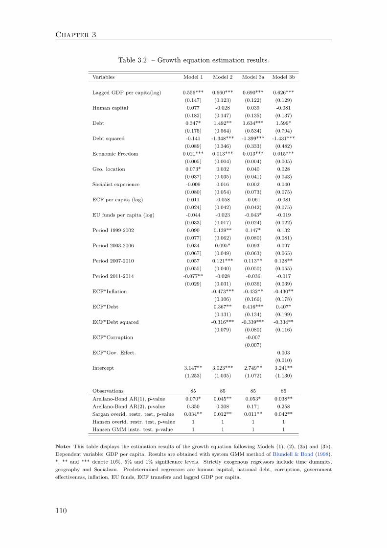
Chapter 3
Table 3.2 – Growth equation estimation results.
Variables Model 1 Model 2 Model 3a Model 3b
Lagged GDP per capita(log) 0.556*** 0.660*** 0.690*** 0.626***(0.147) (0.123) (0.122) (0.129)
Human capital 0.077 -0.028 0.039 -0.081(0.182) (0.147) (0.135) (0.137)
Debt 0.347* 1.492** 1.634*** 1.599*(0.175) (0.564) (0.534) (0.794)
Debt squared -0.141 -1.348*** -1.399*** -1.431***(0.089) (0.346) (0.333) (0.482)
Economic Freedom 0.021*** 0.013*** 0.013*** 0.015***(0.005) (0.004) (0.004) (0.005)
Geo. location 0.073* 0.032 0.040 0.028(0.037) (0.035) (0.041) (0.043)
Socialist experience -0.009 0.016 0.002 0.040(0.080) (0.054) (0.073) (0.075)
ECF per capita (log) 0.011 -0.058 -0.061 -0.081(0.024) (0.042) (0.042) (0.075)
EU funds per capita (log) -0.044 -0.023 -0.043* -0.019(0.033) (0.017) (0.024) (0.022)
Period 1999-2002 0.090 0.139** 0.147* 0.132(0.077) (0.062) (0.080) (0.081)
Period 2003-2006 0.034 0.095* 0.093 0.097(0.067) (0.049) (0.063) (0.065)
Period 2007-2010 0.057 0.121*** 0.113** 0.128**(0.055) (0.040) (0.050) (0.055)
Period 2011-2014 -0.077** -0.028 -0.036 -0.017(0.029) (0.031) (0.036) (0.039)
ECF*Inflation -0.473*** -0.432** -0.430**(0.106) (0.166) (0.178)
ECF*Debt 0.367** 0.416*** 0.407*(0.131) (0.134) (0.199)
ECF*Debt squared -0.316*** -0.339*** -0.334**(0.079) (0.080) (0.116)
ECF*Corruption -0.007(0.007)
ECF*Gov. Effect. 0.003(0.010)
Intercept 3.147** 3.023*** 2.749** 3.241**(1.253) (1.035) (1.072) (1.130)
Observations 85 85 85 85Arellano-Bond AR(1), p-value 0.070* 0.045** 0.053* 0.038**Arellano-Bond AR(2), p-value 0.350 0.308 0.171 0.258Sargan overid. restr. test, p-value 0.034** 0.012** 0.011** 0.042**Hansen overid. restr. test, p-value 1 1 1 1Hansen GMM instr. test, p-value 1 1 1 1
Note: This table displays the estimation results of the growth equation following Models (1), (2), (3a) and (3b).Dependent variable: GDP per capita. Results are obtained with system GMM method of Blundell & Bond (1998).*, ** and *** denote 10%, 5% and 1% significance levels. Strictly exogenous regressors include time dummies,geography and Socialism. Predetermined regressors are human capital, national debt, corruption, governmenteffectiveness, inflation, EU funds, ECF transfers and lagged GDP per capita.
110
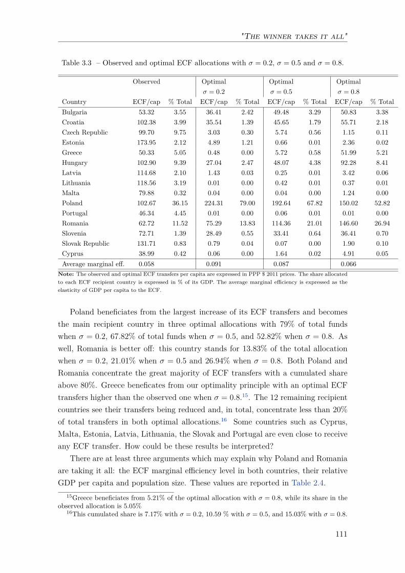
"The winner takes it all"
Table 3.3 – Observed and optimal ECF allocations with σ = 0.2, σ = 0.5 and σ = 0.8.
Observed Optimal Optimal Optimalσ = 0.2 σ = 0.5 σ = 0.8
Country ECF/cap % Total ECF/cap % Total ECF/cap % Total ECF/cap % TotalBulgaria 53.32 3.55 36.41 2.42 49.48 3.29 50.83 3.38Croatia 102.38 3.99 35.54 1.39 45.65 1.79 55.71 2.18Czech Republic 99.70 9.75 3.03 0.30 5.74 0.56 1.15 0.11Estonia 173.95 2.12 4.89 1.21 0.66 0.01 2.36 0.02Greece 50.33 5.05 0.48 0.00 5.72 0.58 51.99 5.21Hungary 102.90 9.39 27.04 2.47 48.07 4.38 92.28 8.41Latvia 114.68 2.10 1.43 0.03 0.25 0.01 3.42 0.06Lithuania 118.56 3.19 0.01 0.00 0.42 0.01 0.37 0.01Malta 79.88 0.32 0.04 0.00 0.04 0.00 1.24 0.00Poland 102.67 36.15 224.31 79.00 192.64 67.82 150.02 52.82Portugal 46.34 4.45 0.01 0.00 0.06 0.01 0.01 0.00Romania 62.72 11.52 75.29 13.83 114.36 21.01 146.60 26.94Slovenia 72.71 1.39 28.49 0.55 33.41 0.64 36.41 0.70Slovak Republic 131.71 0.83 0.79 0.04 0.07 0.00 1.90 0.10Cyprus 38.99 0.42 0.06 0.00 1.64 0.02 4.91 0.05Average marginal eff. 0.058 0.091 0.087 0.066
Note: The observed and optimal ECF transfers per capita are expressed in PPP $ 2011 prices. The share allocatedto each ECF recipient country is expressed in % of its GDP. The average marginal efficiency is expressed as theelasticity of GDP per capita to the ECF.
Poland beneficiates from the largest increase of its ECF transfers and becomesthe main recipient country in three optimal allocations with 79% of total fundswhen σ = 0.2, 67.82% of total funds when σ = 0.5, and 52.82% when σ = 0.8. Aswell, Romania is better off: this country stands for 13.83% of the total allocationwhen σ = 0.2, 21.01% when σ = 0.5 and 26.94% when σ = 0.8. Both Poland andRomania concentrate the great majority of ECF transfers with a cumulated shareabove 80%. Greece beneficates from our optimality principle with an optimal ECFtransfers higher than the observed one when σ = 0.8.15. The 12 remaining recipientcountries see their transfers being reduced and, in total, concentrate less than 20%of total transfers in both optimal allocations.16 Some countries such as Cyprus,Malta, Estonia, Latvia, Lithuania, the Slovak and Portugal are even close to receiveany ECF transfer. How could be these results be interpreted?
There are at least three arguments which may explain why Poland and Romaniaare taking it all: the ECF marginal efficiency level in both countries, their relativeGDP per capita and population size. These values are reported in Table 2.4.
15Greece beneficiates from 5.21% of the optimal allocation with σ = 0.8, while its share in theobserved allocation is 5.05%
16This cumulated share is 7.17% with σ = 0.2, 10.59 % with σ = 0.5, and 15.03% with σ = 0.8.
111
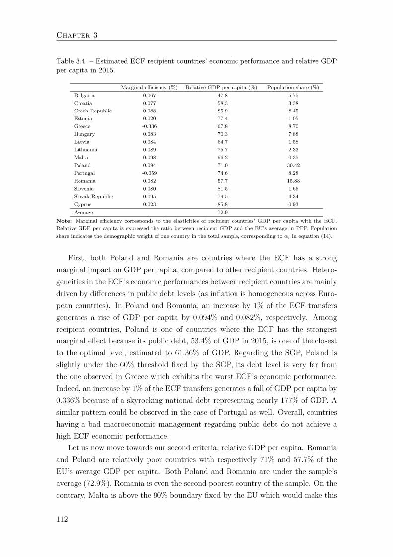
Chapter 3
Table 3.4 – Estimated ECF recipient countries’ economic performance and relative GDPper capita in 2015.
Marginal efficiency (%) Relative GDP per capita (%) Population share (%)Bulgaria 0.067 47.8 5.75Croatia 0.077 58.3 3.38Czech Republic 0.088 85.9 8.45Estonia 0.020 77.4 1.05Greece -0.336 67.8 8.70Hungary 0.083 70.3 7.88Latvia 0.084 64.7 1.58Lithuania 0.089 75.7 2.33Malta 0.098 96.2 0.35Poland 0.094 71.0 30.42Portugal -0.059 74.6 8.28Romania 0.082 57.7 15.88Slovenia 0.080 81.5 1.65Slovak Republic 0.095 79.5 4.34Cyprus 0.023 85.8 0.93Average 72.9
Note: Marginal efficiency corresponds to the elasticities of recipient countries’ GDP per capita with the ECF.Relative GDP per capita is expressed the ratio between recipient GDP and the EU’s average in PPP. Populationshare indicates the demographic weight of one country in the total sample, corresponding to αi in equation (14).
First, both Poland and Romania are countries where the ECF has a strongmarginal impact on GDP per capita, compared to other recipient countries. Hetero-geneities in the ECF’s economic performances between recipient countries are mainlydriven by differences in public debt levels (as inflation is homogeneous across Euro-pean countries). In Poland and Romania, an increase by 1% of the ECF transfersgenerates a rise of GDP per capita by 0.094% and 0.082%, respectively. Amongrecipient countries, Poland is one of countries where the ECF has the strongestmarginal effect because its public debt, 53.4% of GDP in 2015, is one of the closestto the optimal level, estimated to 61.36% of GDP. Regarding the SGP, Poland isslightly under the 60% threshold fixed by the SGP, its debt level is very far fromthe one observed in Greece which exhibits the worst ECF’s economic performance.Indeed, an increase by 1% of the ECF transfers generates a fall of GDP per capita by0.336% because of a skyrocking national debt representing nearly 177% of GDP. Asimilar pattern could be observed in the case of Portugal as well. Overall, countrieshaving a bad macroeconomic management regarding public debt do not achieve ahigh ECF economic performance.
Let us now move towards our second criteria, relative GDP per capita. Romaniaand Poland are relatively poor countries with respectively 71% and 57.7% of theEU’s average GDP per capita. Both Poland and Romania are under the sample’saverage (72.9%), Romania is even the second poorest country of the sample. On thecontrary, Malta is above the 90% boundary fixed by the EU which would make this
112
"The winner takes it all"
country not eligible anymore for the ECF.Finally, both these countries benefit more of the optimal allocations thanks to a
large demographic weight: Poland stands for 30.42% of the total sample population,Romania is the second most populated country. Because the demographic weight ofeach recipient country is considered in the donor’s utility function with the parameterαi, countries having the largest population sizes receive more ECF transfers. Mostof remaining countries are characterised by either low ECF economic efficiency, highrelative GDP per capita or small population size. For instance, despite one of themost important ECF economic efficiency and population size, the Czech Republicloses nearly all of its ECF funds because this country has the second highest GDPper capita of our sample.
It should be noticed as well that as σ is risen from 0.2 to 0.5 and to 0.8, ECFtransfers directed towards Hungary, Greece, Croatia, Romania, and Bulgaria aresharply increased (Table 3). Those countries respectively have the tenth, eleventh,thirteenth, fourteenth and fifteenth GDP per capita of our sample which meansthat they are among the poorest ECF recipient countries (Table 2.4). The cases ofHungary, Greece and Romania are striking: these countries see their ECF transfersincreasing considerably with σ. For instance, the optimal ECF transfers to Greecemoves from 0% when when σ = 0.2 to 5.21% when σ = 0.8 while ECF funds seem donot contribute to economic performance of this country. This result strengthens thefact that while economic efficiency is rewarded, economic fairness is not forgotten.
We recall that the aim of our optimal allocation is to increase the ECF’s eco-nomic efficiency in order to help the EU achieving economic convergence. Table 2.3indicates that both the optimal allocations perform better than the observed one:on average, a 1% increase of the ECF transfers generates a 0.091% increase of GDPper capita when σ = 0.2, a 0.087 increase of GDP per capita when σ = 0.5 and0.066% when σ = 0.8 which is more than the 0.058% of the observed allocation.These results are driven by the good performances of Poland and Romania. Thelower performance of the optimal allocations with σ = 0.5 and σ = 0.8 is mainly dueto a larger share directed towards Greece which drags down the overall economicperformance of the ECF.
As it has been underlined, the ECF’s observed allocation is very different fromthe optimal allocation we have computed. This may be as well related to some issuesdealing with the political economy of the European Cohesion policy highlighted inthe works of Rodden (2002), Wonka (2007), Gehring & Schneider (2018). Rodden(2002) stated that “empirical analysis demonstrates a close connection between thedistribution of votes and fiscal transfers in the legislative institutions of the European
113
Chapter 3
Union.” Given that small countries’ electoral weight in the European Parliament ishigher than their actual demographic weight, this helps explaining why we notice asmall country bias in the observed allocation while the optimal allocations removethis bias by taking into account the real demographic weight of each recipient coun-tries. One another political economy issue is related to an assumption made aboutthe donor’s behaviour. Indeed, in our theoretical model, we have assumed that thedonor is purely altruistic, which may not be the case in reality. Wonka (2007) sug-gested a principal-agent structure, where governments select reliable actors who areexpected to take national interests into account at the EU-level. Gehring & Schnei-der (2018) strengthened this idea as they demonstrated that the nationalities of EUCommissioners influence budget allocation decisions in favour of their country oforigin. They focused on the Commissioners for Agriculture and, on average, provid-ing the Commissioner causes a 1 percentage point increase in a country’s share ofthe overall EU budget, which corresponds to 850 million euros per year. This issuewould constitute an interesting topic for our further investigation.
3.6 Conclusion
The European Cohesion Fund is an additional tool used by the EU to promoteeconomic convergence between its member states. The ECF is targeted to thosehaving a relative GDP per capita lower than 90% of the EU’s average.
This study has dealt with the issue of the allocation of the ECF between recipientcountries. We have adopted a normative approach where an optimal allocation ofthe ECF is computed and compared to the observed allocation for the period 2014-2020. To obtain this optimal allocation, we have solved an optimization problemwhere a purely altruistic donor has maximised the global welfare of ECF recipientcountries. The optimal solution of this theoretical problem has been then empiricallysimulated thanks to the estimation results of a growth equation based on systemGMM estimators using a database covering 17 countries for the period 1995-2015.
We find that GDP per capita is significantly and positively affected by its ownlagged value and the level of economic freedom. As well, our estimates show thatthe ECF’s impact on GDP per capita is conditional to inflation and public debt.Recipient countries with moderate national debt and low inflation levels are thosewhere the ECF is the most efficient. The optimal ECF allocation gives more fundsto Poland and Romania thanks to their high ECF economic efficiency, low relativeGDP per capita and large population size. Both these countries stand for more than80% of total funds while this figure is about 48% with the observed ECF allocation in
114
"The winner takes it all"
2015. Regarding economic efficiency, optimal allocation exhibits a higher marginalimpact than the observed allocation.
The ECF optimal allocation we propose is based on economic criteria thatare the initial relative GDP per capita and the ECF’s economic performanceconditioned on the quality of macroeconomic management. The necessity of asound macroeconomic management is explicitly mentioned in EU regulations. Theresulting optimal allocation we compute is therefore in line with the Europeanlegislative texts and gives additional theoretical background to the European fiscalrules. As well, we have considered a demographic criterion where recipient countriesare weighted according to their population size, which avoids any demographicbias towards small recipient countries. This chapter is a contribution to the debaterelating to European structural funds’ allocation criteria: further extensions couldbe added to this study based on more political criteria such as the respect ofEuropean democratic principles in the ECF recipient countries.
The last chapter focuses on the politic forces related to the allocation processof the EU funds between a central government and its constituent regions tounderstand the determinants of the final regional allocation.
115
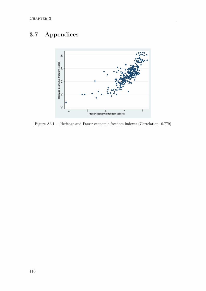
Chapter 3
3.7 Appendices
4050
6070
80H
erita
ge e
cono
mic
free
dom
(sco
re)
4 5 6 7 8Fraser economic freedom (score)
Figure A3.1 – Heritage and Fraser economic freedom indexes (Correlation: 0.779)
116

"The winner takes it all"
TableA3.1
–Dataan
dvaria
bles
defin
ition
.
Variab
lena
me
Definitio
nUnit
Source
GDP
percapita
(yi,t)
PPP
2011
$World
Ban
kLa
gged
GDP
percapita
(yi,t−
1)
GDP
percapita
ofthelast
period
(4yearsago)
PPP
2011
$World
Ban
kHum
anCap
ital(Humani,t)
Working
labo
urforceha
ving
achieved
tertiary
educa-
tion
Percentage
ofworking
labo
urforce
World
Ban
k
Geograp
hicallocalization
(Geoi,
)Beaneighb
ourof
aEU-15coun
try
Dum
myvariab
leSo
cialistExp
erience
(Socialism
i)
Leng
thun
derasocialistgovernmentafterW
W2
Num
berof
years
Governm
entEffe
ctiveness
(Government i,t
)Pe
rceptio
nsof
thequ
ality
ofpu
blic
services,p
olicyfor-
mulationan
dim
plem
entatio
n,an
dthecredibility
ofthe
government’s
commitm
ent
Scorebe
tween-2.5
to2.5(bestscore)
Worldwidegovernan
ceindicators
Corruption
(Corruptioni,t)
Perceptio
nsof
theextent
towhich
publicpo
wer
isexer-
cisedforprivategain,including
both
pettyan
dgran
dform
sof
corrup
tion,
aswella
s"cap
ture"of
thestateby
elite
san
dprivateinterests
Scorebe
tween-2.5
to2.5(bestscore)
Worldwidegovernan
ceindicators
Econo
mic
Freedo
m(Efreedomi,t)
Ruleof
Law,g
overnm
ents
ize,regu
latory
efficiency,a
ndpe
rforman
ceon
Market’s
openness
(fina
ncial,
invest-
mentan
dtrad
efreedo
ms)
Scorebe
tween0an
d100(bestscore)
Herita
geFo
unda
tion
Infla
tion
(Inflationi,t)
Variationof
consum
erpriceindex
Percentage
ofpriceindex
World
Ban
kNationa
lDebt
(Debt i,t
)General
governmentconsolidated
grossdebt
Percentage
ofGDP
Eurostat
ECFpe
rcapita
(Ai,t)
Levelo
fEurop
eanCoh
esionFu
nd(E
CF)
tran
sfers
PPP
2011
$Europ
eanCom
mission
EU
fund
spe
rcapita
(EUfunds i,t
)Su
mof
Europ
eanRegiona
lDevelop
mentF
und(E
RDF)
,Europ
ean
Social
Fund
(ESF
)an
dEurop
ean
Agricul-
turalF
undforRural
Develop
ment(E
AFR
D)tran
sfers
PPP
2011
$Europ
eanCom
mission
117

Chapter 3
TableA3.2
–Measure
ofEc
onom
icFreedo
man
ddiffe
rent
compo
nentsof
Econ
omic
Freedo
mfrom
theFraser
Institu
te
Variab
lena
me
Definitio
nUnit
Source
Econo
mic
Freedo
m(Fraser)
Governm
entsize,s
ound
mon
etarypo
licy,
levelo
fregulation,
quality
oflegals
ystem,freedom
totrad
eScorebe
tween0an
d10
(bestscore)
Fraser
Foun
datio
n
Size
ofgovernment
(Sizegov.
Fraser)
Governm
entconsum
ption,
tran
sfersan
dsubsidies,
governmententer-
prises
andinvestment,
topmargina
lincom
etaxrate,t
opmargina
lin-
comean
dpa
yrolltax
rate
Scorebe
tween0an
d10
(bestscore)
Fraser
Foun
datio
n
Soun
dmon
etarypo
licy
(Sou
ndmon
etaryFraser)
Mon
eygrow
th,stan
dard
deviation
ofinfla
tion,
infla
tion
ofthemost
recent
year,freedom
toow
nforeigncurrency
bank
accoun
tScorebe
tween0an
d10
(bestscore)
Fraser
Foun
datio
n
Legals
ystem
andprop
erty
righ
tsFR
ASE
R(Legal
system
Fraser)
Judicial
indepe
ndence,im
partialcourts,protectio
nof
prop
erty
righ
ts,
military
interference
inRuleof
Law
andpo
litics,
integrity
ofthelegal
system
,legalenforcem
entof
contracts,
regu
latory
restrictions
onthe
sale
ofreal
prop
erty,r
eliabilityof
police,
business
costsof
crim
e
Scorebe
tween0an
d10
(bestscore)
Fraser
Foun
datio
n
Levelo
fregulation
(RegulationFraser)
Creditm
arketr
egulations,lab
ormarketr
egulation,
business
regu
latio
nsScorebe
tween0an
d10
(bestscore)
Fraser
Foun
datio
nFreedo
mto
trad
e(T
rade
Fraser)
Tariffs,regulatorytrad
eba
rriers,B
lack
marketexchan
gerates,controls
ofthemovem
entof
capitala
ndpe
ople
Scorebe
tween0an
d10
(bestscore)
Fraser
Foun
datio
n
118
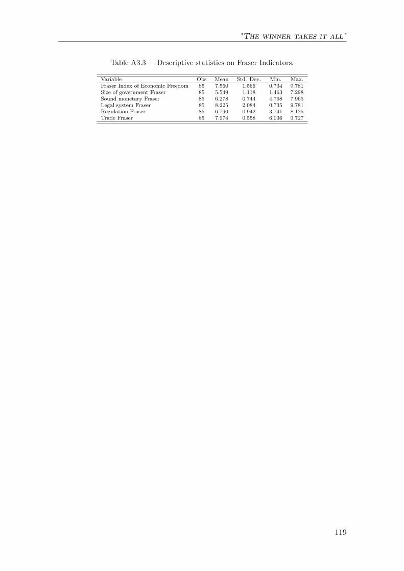
"The winner takes it all"
Table A3.3 – Descriptive statistics on Fraser Indicators.
Variable Obs Mean Std. Dev. Min. Max.Fraser Index of Economic Freedom 85 7.560 1.566 0.734 9.781Size of government Fraser 85 5.549 1.118 1.463 7.298Sound monetary Fraser 85 6.278 0.744 4.798 7.965Legal system Fraser 85 8.225 2.084 0.735 9.781Regulation Fraser 85 6.790 0.942 3.741 8.125Trade Fraser 85 7.974 0.558 6.036 9.727
119
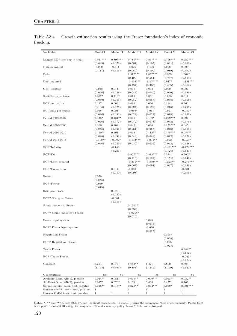
Chapter 3
Table A3.4 – Growth estimation results using the Fraser foundation’s index of economicfreedom.
Variables Model I Model II Model III Model IV Model V Model VI
Lagged GDP per capita (log) 0.921*** 0.893*** 0.786*** 0.877*** 0.796*** 0.782***(0.085) (0.076) (0.084) (0.107) (0.081) (0.099)
Human capital -0.080 -0.011 -0.005 -0.106 0.068 0.025(0.111) (0.115) (0.080) (0.100) (0.089) (0.092)
Debt 1.977*** 1.857*** -0.955 1.364*(0.490) (0.554) (0.737) (0.664)
Debt squared -1.459*** -1.557*** 0.947* -1.181***(0.291) (0.360) (0.465) (0.400)
Geo. location -0.018 0.011 0.031 0.003 0.000 0.027(0.026) (0.028) (0.043) (0.040) (0.030) (0.040)
Socialist experience 0.087* 0.110* 0.010 0.031 -0.008 0.011(0.050) (0.053) (0.052) (0.057) (0.048) (0.050)
ECF per capita 0.127 0.003 0.080 0.020 0.194 0.360(0.108) (0.075) (0.097) (0.170) (0.216) (0.239)
EU funds per capita 0.018 0.021 -0.059* -0.011 -0.021 -0.053*(0.026) (0.031) (0.028) (0.023) (0.018) (0.029)
Period 1999-2002 0.138* 0.181** 0.041 0.139* 0.259*** 0.097(0.076) (0.072) (0.072) (0.078) (0.053) (0.070)
Period 2003-2006 0.100 0.108 0.042 0.096 0.172*** 0.045(0.058) (0.066) (0.064) (0.057) (0.046) (0.061)
Period 2007-2010 0.110** 0.101 0.034 0.118** 0.175*** 0.084**(0.046) (0.059) (0.048) (0.041) (0.042) (0.038)
Period 2011-2014 -0.102** -0.092* -0.113*** -0.064** -0.022 -0.055*(0.036) (0.049) (0.030) (0.029) (0.032) (0.028)
ECF*Inflation -0.148 -0.481*** -0.474***(0.261) (0.125) (0.147)
ECF*Debt 0.437*** 0.383*** 0.224 0.306*(0.116) (0.128) (0.151) (0.148)
ECF*Debt squared -0.331*** -0.340*** -0.223** -0.275***(0.067) (0.084) (0.097) (0.088)
ECF*Corruption 0.014 -0.000 -0.001(0.010) (0.008) (0.009)
Fraser 0.079(0.058)
ECF*Fraser -0.019(0.015)
Size gov. Fraser 0.076(0.080)
ECF* Size gov. Fraser -0.007(0.017)
Sound monetary Fraser 0.171***(0.039)
ECF* Sound monetary Fraser -0.025**(0.010)
Fraser legal system 0.046(0.075)
ECF* Fraser legal system -0.010(0.017)
Regulation Fraser 0.195*(0.098)
ECF* Regulation Fraser -0.028(0.023)
Trade Fraser 0.284**(0.102)
ECF*Trade Fraser -0.047*(0.024)
Constant 0.264 0.676 1.862** 1.421 0.860 0.385(1.125) (0.965) (0.851) (1.341) (1.179) (1.143)
Observations 85 85 85 85 85 85Arellano-Bond AR(1), p-value 0.044** 0.081* 0.036** 0.009*** 0.013** 0.032**Arellano-Bond AR(2), p-value 0.087* 0.070* 0.136 0.403 0.457 0.163Sargan overid. restr. test, p-value 0.018** 0.016** 0.021** 0.004*** 0.069* 0.001***Hansen overid. restr. test, p-value 1 1 1 1 1 1Hansen GMM instr. test, p-value 1 1 1 1 1 1
Note:: *, ** and *** denote 10%, 5% and 1% significance levels. In model II using the component “Size of government”, Public Debtis dropped. In model III using the component “Sound monetary policy Fraser”, Inflation is dropped.
120
Chapter 4
Regional decentralisation and the Euro-pean Cohesion Policy: the leader takes itall
Summary
How does regional decentralisation affect the allocation of the EU funds at thenational level? This chapter formalises and shows that regional autonomy intensifiesthe political economy of the European Cohesion Policy (ECP) based on a signallinggame between a central government and its constituent lagging region. The centralgovernment is less willing to provide European transfers to more autonomous laggingregions. This theoretical prediction is empirically confirmed by a study based on a119 NUTS-2 regions belonging to 18 Member states dataset over the period 1989-2018. However, this study does not find any evidence of significant relation betweenabsorption performance and the intranational regional allocation.
121

Chapter 4
Acknowledgements
I would like to thank Gisèle Umbhauer and the participants of the CPnet workshop"Territorialisation of Cohesion Policy" for their useful comments.
122
"The leader takes it all"
4.1 Introduction
The European Cohesion Policy (ECP) has been set to foster economic and socialcohesion in the EU. To this purpose, this supranational policy targets the laggingregions trough the co-financing of investment projects. One issue faced by the ECPis that its core recipient regions, the lagging regions, are those where the absorp-tion capacity is the lowest (Becker et al. (2010)). In other words, this is where theECP’s investment returns are the lowest in terms of economic growth stimulation.One determinant of absorption capacity is the quality of local government, which isacknowledged to be at a low level in most of the European lagging regions (Beckeret al. (2013); Teorell et al. (2013)).
One feature of the ECP is that its institutional set could be defined as sig-nalling framework between the European Commission, the Member states and theconstituent regions (Dellmuth & Stoffel (2012)). The European Commission seeksto structure intergovernmental transfers in ways that promote EU funding goals.Because the Commission has only imperfect information and control over the fis-cal activities of decentralised governments and sanctions are costly, its monitoringand enforcement capacities are largely ineffective (Blom-Hansen (2005)). Therefore,Member states bear most of the responsibility of monitoring since the set of controlmechanisms remains quite limited (Bachtler & Ferry (2015).1
The efficient management and implementation of the ECP is ensured by a man-aging authority which must provide to the European Commission an annual im-plementation report. A managing authority may be a national ministry, a regionalauthority, a local council, or another public or private body that has been nominatedand approved by a Member state. As indicated in Table 4.1 , the European funds aremostly managed by regional authorities. Indeed, excepted in Spain and Romania,the implementation of the European funds is shared with regions (Germany, Italy,Poland, Portugal and the Czech Republic) or exclusively managed by them (France,United-Kingdom, Netherlands, Belgium and Sweden).
During the last decades, a majority of Member states have conducted regionaldecentralisation reforms to increase the autonomy of regional authorities. This canbe measured by the regional level of self-rule, i.e. the constitutional strength and po-litical and fiscal autonomy. As indicated in Figure 4.1 , the self-rule index of Hooghe
1Member states are required to appoint monitoring committees to assess the effectiveness andthe quality of the investment projects, make periodical reviews and propose revisions where nec-essary. These committees are chaired by the relevant managing authority and comprise regional,economic and social partners. However, their influence is very limited. For more information, seeCartwright & Batory (2012).
123
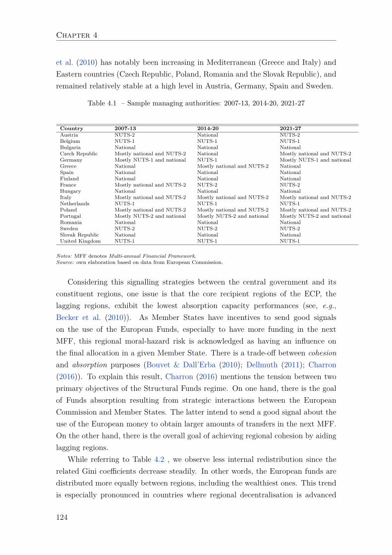
Chapter 4
et al. (2010) has notably been increasing in Mediterranean (Greece and Italy) andEastern countries (Czech Republic, Poland, Romania and the Slovak Republic), andremained relatively stable at a high level in Austria, Germany, Spain and Sweden.
Table 4.1 – Sample managing authorities: 2007-13, 2014-20, 2021-27
Country 2007-13 2014-20 2021-27Austria NUTS-2 National NUTS-2Belgium NUTS-1 NUTS-1 NUTS-1Bulgaria National National NationalCzech Republic Mostly national and NUTS-2 National Mostly national and NUTS-2Germany Mostly NUTS-1 and national NUTS-1 Mostly NUTS-1 and nationalGreece National Mostly national and NUTS-2 NationalSpain National National NationalFinland National National NationalFrance Mostly national and NUTS-2 NUTS-2 NUTS-2Hungary National National NationalItaly Mostly national and NUTS-2 Mostly national and NUTS-2 Mostly national and NUTS-2Netherlands NUTS-1 NUTS-1 NUTS-1Poland Mostly national and NUTS-2 Mostly national and NUTS-2 Mostly national and NUTS-2Portugal Mostly NUTS-2 and national Mostly NUTS-2 and national Mostly NUTS-2 and nationalRomania National National NationalSweden NUTS-2 NUTS-2 NUTS-2Slovak Republic National National NationalUnited Kingdom NUTS-1 NUTS-1 NUTS-1
Notes: MFF denotes Multi-annual Financial Framework.Source: own elaboration based on data from European Commission.
Considering this signalling strategies between the central government and itsconstituent regions, one issue is that the core recipient regions of the ECP, thelagging regions, exhibit the lowest absorption capacity performances (see, e.g.,Becker et al. (2010)). As Member States have incentives to send good signalson the use of the European Funds, especially to have more funding in the nextMFF, this regional moral-hazard risk is acknowledged as having an influence onthe final allocation in a given Member State. There is a trade-off between cohesionand absorption purposes (Bouvet & Dall’Erba (2010); Dellmuth (2011); Charron(2016)). To explain this result, Charron (2016) mentions the tension between twoprimary objectives of the Structural Funds regime. On one hand, there is the goalof Funds absorption resulting from strategic interactions between the EuropeanCommission and Member States. The latter intend to send a good signal about theuse of the European money to obtain larger amounts of transfers in the next MFF.On the other hand, there is the overall goal of achieving regional cohesion by aidinglagging regions.
While referring to Table 4.2 , we observe less internal redistribution since therelated Gini coefficients decrease steadily. In other words, the European funds aredistributed more equally between regions, including the wealthiest ones. This trendis especially pronounced in countries where regional decentralisation is advanced
124
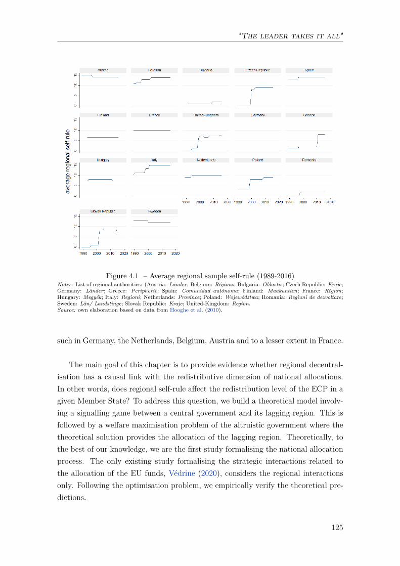
"The leader takes it all"
Figure 4.1 – Average regional sample self-rule (1989-2016)Notes: List of regional authorities: (Austria: Länder ; Belgium: Régions; Bulgaria: Öblastis; Czech Republic: Kraje;Germany: Länder ; Greece: Peripherie; Spain: Comunidad autónoma; Finland: Maakuntien; France: Région;Hungary: Megyék; Italy: Regioni; Netherlands: Province; Poland: Województwa; Romania: Regiuni de dezvoltare;Sweden: Län/ Landstinge; Slovak Republic: Kraje; United-Kingdom: Region.Source: own elaboration based on data from Hooghe et al. (2010).
such in Germany, the Netherlands, Belgium, Austria and to a lesser extent in France.
The main goal of this chapter is to provide evidence whether regional decentral-isation has a causal link with the redistributive dimension of national allocations.In other words, does regional self-rule affect the redistribution level of the ECP in agiven Member State? To address this question, we build a theoretical model involv-ing a signalling game between a central government and its lagging region. This isfollowed by a welfare maximisation problem of the altruistic government where thetheoretical solution provides the allocation of the lagging region. Theoretically, tothe best of our knowledge, we are the first study formalising the national allocationprocess. The only existing study formalising the strategic interactions related tothe allocation of the EU funds, Védrine (2020), considers the regional interactionsonly. Following the optimisation problem, we empirically verify the theoretical pre-dictions.
125
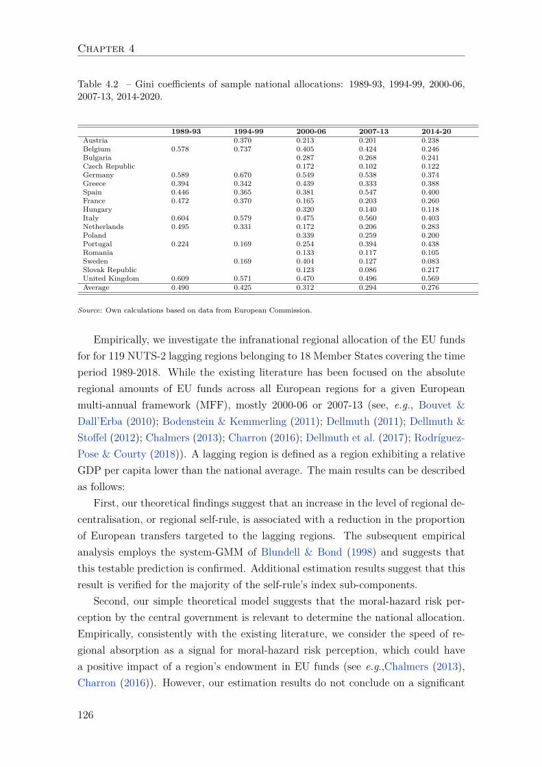
Chapter 4
Table 4.2 – Gini coefficients of sample national allocations: 1989-93, 1994-99, 2000-06,2007-13, 2014-2020.
1989-93 1994-99 2000-06 2007-13 2014-20Austria 0.370 0.213 0.201 0.238Belgium 0.578 0.737 0.405 0.424 0.246Bulgaria 0.287 0.268 0.241Czech Republic 0.172 0.102 0.122Germany 0.589 0.670 0.549 0.538 0.374Greece 0.394 0.342 0.439 0.333 0.388Spain 0.446 0.365 0.381 0.547 0.400France 0.472 0.370 0.165 0.203 0.260Hungary 0.320 0.140 0.118Italy 0.604 0.579 0.475 0.560 0.403Netherlands 0.495 0.331 0.172 0.206 0.283Poland 0.339 0.259 0.200Portugal 0.224 0.169 0.254 0.394 0.438Romania 0.133 0.117 0.105Sweden 0.169 0.404 0.127 0.083Slovak Republic 0.123 0.086 0.217United Kingdom 0.609 0.571 0.470 0.496 0.569Average 0.490 0.425 0.312 0.294 0.276
Source: Own calculations based on data from European Commission.
Empirically, we investigate the infranational regional allocation of the EU fundsfor for 119 NUTS-2 lagging regions belonging to 18 Member States covering the timeperiod 1989-2018. While the existing literature has been focused on the absoluteregional amounts of EU funds across all European regions for a given Europeanmulti-annual framework (MFF), mostly 2000-06 or 2007-13 (see, e.g., Bouvet &Dall’Erba (2010); Bodenstein & Kemmerling (2011); Dellmuth (2011); Dellmuth &Stoffel (2012); Chalmers (2013); Charron (2016); Dellmuth et al. (2017); Rodríguez-Pose & Courty (2018)). A lagging region is defined as a region exhibiting a relativeGDP per capita lower than the national average. The main results can be describedas follows:
First, our theoretical findings suggest that an increase in the level of regional de-centralisation, or regional self-rule, is associated with a reduction in the proportionof European transfers targeted to the lagging regions. The subsequent empiricalanalysis employs the system-GMM of Blundell & Bond (1998) and suggests thatthis testable prediction is confirmed. Additional estimation results suggest that thisresult is verified for the majority of the self-rule’s index sub-components.
Second, our simple theoretical model suggests that the moral-hazard risk per-ception by the central government is relevant to determine the national allocation.Empirically, consistently with the existing literature, we consider the speed of re-gional absorption as a signal for moral-hazard risk perception, which could havea positive impact of a region’s endowment in EU funds (see e.g.,Chalmers (2013),Charron (2016)). However, our estimation results do not conclude on a significant
126
"The leader takes it all"
association between the absorption speed of a lagging region and its EU funds allo-cation.
Overall, our results highlight an harvesting of the ECP in national leading re-gions marked by political decentralisation reforms that led to more regional auton-omy. Regarding policy implications, an institutional reform of the ECP could beimplemented to ensure more redistribution between the constituent regions of ev-ery Member States. For instance, an allocation rule guaranteeing a minimal sharededicated to the national lagging regions could help to maintain a minimum levelof intra-national redistribution.
The remainder of this chapter is organised as follows: Section 2 provides a relatedliterature review. Section 3 deals with the theoretical model. Section 4 presents theanalysis implemented to test the validity of the theoretical predictions. We concludeand provide some policy recommendations in Section 5.
4.2 Related literature
The ECP’s allocation criteria are characterised by transparency for regions under75% of the average EU GDP per capita qualifies for a certain amount of transfers("Objective 1 or Convergence regions"). In this case, there is very little roomfor negotiation by any actor—be it at national, regional, or EU level—to adjustthe appropriation of funding levels. However, criteria for the transfer of funds toregions that are relatively more economically developed (e.g. over 75% of the EUaverage; formerly known as "Objective 2/Regional Competitiveness and Employ-ment regions") are less predetermined. Following this fact, a recent literature hasanalysed the political determinants of EU budgetary allocations across Europeanregions (see e.g., Kemmerling & Bodenstein (2006); Bouvet & Dall’Erba (2010);Bodenstein & Kemmerling (2011); Dellmuth (2011); Dellmuth & Stoffel (2012);Chalmers (2013); Schraff (2014); Charron (2016); Dotti (2016); Dellmuth et al.(2017); Rodríguez-Pose & Courty (2018); Koala & Védrine (2020); Védrine (2020)).
First, a branch of the literature has pointed out the importance of partisanpolitical factors, but results are contrasted across studies. The political partyposition of the leading regional government, i.e. left-wing or right-wing, has foundsupport in earlier studies (Kemmerling & Bodenstein (2006); Bouvet & Dall’Erba(2010); Dellmuth (2011)), but its effect has been found as insignificant in morerecent studies (Chalmers (2013); Dellmuth et al. (2017)). Another investigatedfactor has been the number of parties in the regional political panorama as areduced number of parties weakens regional collective action issues and make
127
Chapter 4
easier the targeting of national political actors to gain favour with the winner andtheir constituents (Bodenstein & Kemmerling (2011)). A third political factorthat scholars have examined has been the extent to which a region is collectivelyEurosceptic as a central government may intend to compensate this hostility withmore European transfers. However, the "the side-payment thesis" has not foundempirical support (Dellmuth (2011); Chalmers (2013)) .
A second type of investigated criteria are those related to the vote-buyingbehaviours of a central government. The goal of such strategies is to obtain regionalelectoral support, and several articles show that a central government rewardsregions that are politically aligned as a positive association between the regionalsupport for the party of the Prime Minister and the amount of EU transfers isfound (Bouvet & Dall’Erba (2010); Dellmuth & Stoffel (2012); Chalmers (2013)),Dellmuth et al. (2017)).2 Two types of vote-buying behaviours are mentioned.First, national executives may distribute EU funds across regions with the aimto enhance their re-election chances in regions where their electoral margin ishigh. The core-voters hypothesis formulated by Cox & McCubbins (1986) hasfound important empirical support in the case of the EU funds (Dellmuth &Stoffel (2012); Schraff (2014); Dellmuth et al. (2017)). Earlier studies mostlydid not support this hypothesis (Bouvet & Dall’Erba (2010); Chalmers (2013)),but the most recent ones have put on emphasis a conditional impact of a highregional electoral margin on the amount of received European transfers. In astudy conducted for the German Länders, Schraff (2014) shows that Länder ’sgovernment has incentives to follow a strategy that rewards loyalists only whereelectoral mobilisation is important. Indeed, risk-averse incumbents anticipate thestructural character of regional mobilisation and concentrate their vote-maximisingstrategies on high turnout counties since investments in voters who are less likelyto turn out might be wasted. The study exploits the stability of turnout patternsin German NUTS-3 counties and concludes that the effect of the 1998 Landtagelections’ turnout levels on later turnout is large, highly significant, and explainsover 80% of the variance in the 2003 turnout. Still related to the conditionalimpact of a high regional electoral margin, Dellmuth et al. (2017), by focusing on202 NUTS-3 counties in France and Italy, concludes that counties with many corevoters receive more EU funds in France, characterised by a majority voting regime,than in Italy which has proportional representation voting. On the opposite, thesecond mentioned vote-buying behaviour is the swing-voters hypothesis formulatedby Lindbeck & Weibull (1993) that states closer the two main parties in the run-up
2Chalmers (2013) finds a significant effect only for "Convergence fundings".
128
"The leader takes it all"
towards the election, the higher the stakes become for central governments to winthis constituency. However, in the case of the European funds, this hypothesis hasfound little support as only Bodenstein & Kemmerling (2011) find that electoralcompetition in a region increases its EU transfers, an insignificant (Koala & Védrine(2020); Védrine (2020)) or even detrimental effect is even found by Bouvet &Dall’Erba (2010).
A third category of political determinants of the regional allocation of theEuropean transfers is the institutional strength of regions. The literature hasinvestigated four channels through which this institutional strength can influencethe regional final allocation of the EU funds. There are: (a) the capacity to havesome lobbying activities in Brussels, (b) the regional co-funding capacity, (c) theability to influence central government’s decisions and (d) the regional autonomy.
Regarding lobbying capacity, the results of studies as Chalmers (2013)Rodríguez-Pose & Courty (2018) indicate that regional offices have a negligibleeffect on the distribution of EU funds. Bigger offices in Brussels did not necessarilylead to greater shares of funding going to the regions that made the biggest effortto lobby Brussels. In some cases, the efforts have even proven to be detrimental(Rodríguez-Pose & Courty (2018)).
Regarding the additionality principle that states that regional or nationalauthorities should provide at least 25% of a project cost funded by the EU, regionsthe most able to secure larger have a higher bargaining power as they dependless on the willingness of national governments to co-finance projects (Bouvet &Dall’Erba (2010)), but this did not find any empirical support in Chalmers (2013).
Another investigated factor related to institutional strength is the level ofregional shared-rule, or the ability of a region to participate in co-decision-makingprocesses, have routine and institutionalised interactions with the central gov-ernment and being invested in countrywide or aggregate outcomes. Consideringthe bargaining that occurs between a central government and its regions, regionalshared-rule may be especially relevant in the case of the EU funds. Using theRegional Autority Index (RAI) of Hooghe et al. (2010), and particularly theshared-rule component, Chalmers (2013) finds that the more a region has theextent to co-determine the distribution of national tax revenues and constitutionalchange, the more funds it gets.3 Similarly to regional shared-rule, the regional
3In the RAI, shared-rule is the sum of: law-making (the extent to which regional representativesco-determine national legislation); executive control (the extent to which a regional governmentco-determines national policy in intergovernmental meetings); fiscal control (the extent to whichregional representatives co-determine the distribution of national tax revenues); and constitutionalreform (the extent to which regional representatives co-determine constitutional change).
129
Chapter 4
representation in the national parliament also affects positively the allocation ofEuropean structural funds (Koala & Védrine (2020); Védrine (2020)).
With the ability of a region to co-determine national decisions, regional auton-omy has been vastly investigated. Using the rough index of federalism providedby Lijphart (2012), Dellmuth (2011) did not find any significant direct impactof regional authority on the amount of EU funding.4 Another index that hasbeen used for proxying regional authority is the regional self-rule, taken from theRAI of Hooghe et al. (2010). However, studies find a weak (Chalmers (2013)) orinsignificant (Dellmuth et al. (2017)) empirical support in determining regionalallocation of the EU funds by the level of regional autonomy. However, most of theexisting studies point out a conditional impact of the level of regional autonomy onthe amount of EU transfers. Dellmuth (2011) finds that more transfers are providedto constitutionally weak regions if these regions have a good track of absorption inprevious rounds. The rationale behind this result is that less autonomous regionsare characterised by less financial resources, and therefore a lower administrativecapacity. Therefore, more transfers are provided to constitutionally weak regionsonly if these regions have a reputation of actually spending the funds they claimedand received. On the contrary, Charron (2016) supports constitutionally weakregions with low quality of governance tend to get awarded more funding percapita on average using the self-rule from the RAI and the European Quality ofGovernment Index (EQI) of Charron et al. (2014) to measure regional quality ofgovernance.5 Similarly, regions with high quality of governance and a high level ofautonomy are found to receive more EU funding. In cases of low regional autonomy,principals prefer to allocate greater levels of Funds to regions with lower qualityof government in order to increase cohesion. In cases of high regional autonomy,risks associated with absorption failure in lower capacity regions lead principals tostrategically allocate greater levels of transfers to regions with higher quality ofgovernment as they exhibit a higher absorption capacity.
Overall, a very few studies have considered how the actual decentralisation ofthe management of the ECP may affect the regional allocation of the EU funds.One of the only existing studies is Védrine (2020), which addresses this issue with
4The federalism index of Lijphart (2012) ranges from 1 in centralised states to 5 in federalistones.
5Available for 206 NUTS-1 and NUTS-2 regions, the EQI of Charron et al. (2014) is basedon a survey of 85000 citizens. The measure incorporates both perceptions and experiences ofcitizens and captures the quality of governance, level of corruption, and extent to which publicservices are delivered impartially. The index focuses on areas such as health care, education, andlaw enforcement, which are appropriate because it is these that are most often administered byregional actors).
130
"The leader takes it all"
a both theoretical and empirical contribution in the case of the EU-15 for the MFF2000-06 revealing a regional yardstick competition mechanism. This study concludesthat in member states where the Cohesion Policy has been decentralised suchas Germany, Austria, Belgium, Denmark, Finland, the Netherlands and Sweden,constituent regions attracts more EU funds. Indeed, Védrine (2020) explains thatwhen Cohesion Policy is not decentralised, the weight of the decision of the localgovernment in the utility of voters is low so that a regional government has noincentives to make efforts. However in a decentralised system, the voter in eachregion has a stronger incentive to acquire information, which allows the voter todiscipline better their own government. The effort of this local government will behigher, leading this region to obtain larger amounts of funding. With this reasoningbreeding within each region, one obtains a positive effect on the amount of fundsreceived by a region on those received by its neighbours. This result thereforesuggests a complex interaction between geographical factors and the institutionalscheme of this policy.6 However, this study does not take into account the existinginteractions between the central government and its constituent regions even ifthey are acknowledged as having an important impact on the national allocation( see e.g., Bodenstein & Kemmerling (2011); Dellmuth (2011); Chalmers (2013);Charron (2016)).
Therefore, our study considers the role of the decentralisation of the ECPon final regional allocation by focusing on a signalling game between a centralgovernment and its lagging region. Next section presents the theoretical modelemployed in the analysis.
4.3 Theoretical model
The theoretical model is built on two pillars: (i) a signalling game between thecentral government and its lagging region resulting in a Perfect Bayesian Equilibriumproviding the theoretical grounds of the central government’s welfare function; (ii)a maximisation of the altruistic central government’s welfare function providing theEU funds allocation targeted to the lagging region.
6About the role of geography, see Koala & Védrine (2020) who conclude that it seems moreprofitable to a regional government to react to an increase in the lobbying effort of its neighboursby decreasing its own lobbying effort to distort the allocation of EU funds in his favour thanks tothe existence of a geographical spillover between the two neighbours regions.
131
Chapter 4
4.3.1 Signalling game
We consider the European Commission which intends to fund the production ofpublic goods in a lagging region to achieve the goal of economic convergence in theEU. However, we assume that the European Commission delegates the managementof the Cohesion Policy to the central government. The Cohesion policy budget, Gt istargeted to the lagging region, which is in charge of the production of public goodsfunded by the European transfers provided by the central government.The lagging region can either be good type (honest) or bad type (dishonest). Thesetypes are independent random draws from an identical distribution, where goodtypes are drawn with probability, π and bad types are drawn with probability 1−π,where 0 < π < 1. A region’s type is his private information.
We assume that θ is the production cost of public goods and a binary randomvariable which can be high or low in each period.7 That is, θ ∈ {θl, θh} and θh >θl > 0. The probability that the unit cost is high is Pr(θh) = q, so Pr(θl) = 1− q,where 0 < q < 1. We assume that the realisation of θ is private information to thelagging region. The lagging region knows its ability and has to chose a productionlevel of public goods, gt, in t = 1 and t = 2.
To deal with the lagging region’s moral hazard behaviour, the central governmentinvests an exogenous share m ∈]0; 1[ of G1 in monitoring activities. This monitoringeffort increases the probability of an inspection conducted at the end of periodt = 1 to be successful. The probability of success of the inspection, δ(m, η) is anincreasing function of m. However, it is a decreasing function of the autonomy levelof the lagging region, η as the central government could exert less control on theregion’s activities. We then consider:
δ(m, η) = mη. (4.1)
If η = 0, i.e. full centralisation, the central government will always find out the typeof the lagging region. However, if η = 1, i.e. full decentralisation, δ(m, η) will beat its lowest value since m < 1. There is no monitoring activities in period t = 2 asthe game ends in the second period.
The lagging region can produce g1 ≡ (1−m)G1θ
units of the public good in periodt = 1, and g2 ≡ G2
θin t = 2, where θ > 0 is the cost of a unit of the public good.
Following this, the provision of the public good cannot exceed (1−m)Gtθl
. If the laggingregion is bad type, its goal will be to extract a rent Gt − gt. If it is good type, we
7An alternative approach would have been to consider the productivity of public spending suchas 1
θhwould have been the low productivity level, and 1
θlthe high one.
132

"The leader takes it all"
assume that the region does not have any strategic behaviour so that any rent isextracted.
Regarding the timing of the game, it can be summed up as the following:
— Beginning of period 1. Nature distributes the region’s type (Good or Bad).
— Period 1. The central government has its own beliefs on the lagging region’stype and make a take-it or leave-it offer to the region. The lagging regionproduces a quantity of public goods.
— End of period 1. The central government observes the production of publicgoods, determines its beliefs on the lagging region’s type and transfers thefunds. An inspection is carried by the central government and may reveal thetype of the lagging region.
— Beginning of period 2. The central government makes a take-it or leave-it offerto the lagging region.
— End of period 2. End of the game.
We look to the perfect Bayesian equilibrium of this game.
Let ρt ≡ ρt(gt−1) be the central government’s posterior belief in period t thatthe lagging region is good given that it observed a level of public good productionin the previous period, gt−1. We necessarily have ρ1 = π . Since the game endsin period 2, the production of public goods in period 2 has no effect on the centralgovernment’s behaviour.Consider the following candidate Perfect Bayesian Equilibrium:
— In period t = 1, a good lagging region produces gtl ≡ (1−m)Gtθl
of the publicgood if θ = θl and gt
h ≡ (1−m)Gtθh
of the public good if θ = θh. However, ifθ = θl, a bad type lagging region chooses g1
h ≡ (1−m)G1θh
. If θ = θh, a bad typelagging region sets g1 = 0 (embezzles all transfers) in period 1. Therefore, inour candidate equilibrium, a bad type lagging region with θ = θl has the sameproduction of public goods level as a good type lagging region with θ = θh.However, a bad type lagging region separates when θ = θh since there is anypublic good production. A bad type lagging region embezzles all transfers inperiod 2, regardless of θ.
— The central government’s belief in period 1 is given by ρ1 = π. The allocationprovided to the central government in period t = 1, Gt(ρ1) can therefore be
133
Chapter 4
considered as exogenous and fixed. However, in period t = 2, the centralgovernment’s beliefs can be defined in three different ways: (i) ρ2(g1 = 0) = 0meaning that when the central government observes a production level of 0by the end of period t = 1, it does not believe that the lagging region isgood type and does not provide any allocation to the lagging region in periodt = 2; (ii) ρ2(g1
h) = qπqπ+(1−π)(1−q) where qπ is the probability of a good type
region producing gh1 , and (1− π)(1− q) is the probability of a bad type regionproducing gh1 ; (iii) ρ2(g1
l) = 1, meaning that the central government infersthat the lagging region is good type as gl1 is observed.8
We now show that our candidate equilibrium is a Perfect Bayesian Equilibrium.If the Agent is a good type, it will be not be strategic: the maximum productionlevel gt is guaranteed in t = 1 and t = 2, so that any rent is extracted.
However, if the lagging region is a bad type, it will have a strategic behaviourin period t = 1. Therefore, we must define 3 incentive constraints that have to berespected to make the candidate pooling equilibrium, i.e a bad type region withlow production cost has the same production level as a good type region with highproduction cost, be a Perfect Bayesian Equilibrium.9
— If the bad type lagging region faces θ = θl.
Produce (1−m)G1θh
(> 0) instead of 0. This so-called discipline effect restraints thebad type lagging region to embezzle all the European transfers because the fundsare suspended in t = 2 if the central government finds out that the lagging regionis bad type. It exercises restraint in period t = 1 by providing a quantity of publicgoods that would have been produced with costs θh. Assuming extraction costs θlwhen the bad lagging region pools with the good one, the extracted rent is:
(1−m)G1
θl− (1−m)G1
θh> 0 (4.2)
8Note that if the central government observes any level of public good production in periodt = 1 such that (1−m)G1
θh< g1 <
(1−m)G1θl
, then it knows that the lagging region got a cost draw ofθl since g1 >
(1−m)G1θh
is not possible if θ = θh. But since g1 <(1−m)G1
θl, it can infer that the lagging
region has embezzled some European transfers. Also, if g1 <(1−m)G1
θh, the central government can
correctly infer that the lagging region is bad type. Therefore, a reasonable out-of-equilibrium belieffor the central government is ρ2(g1) = 0 if g1 /∈ {g1
h, g1l}. In this case, the central government
does not provide any allocation to the lagging region in period t = 2.9As the game finishes at the end of period 2, it is optimal for the bad Agent to embezzle all
European transfers in period t = 2 so that no public good production is expected in t = 2.
134
"The leader takes it all"
where θh > θl. The above restraint can be written as:
(1−m)(θh − θl)G1(ρ1)θhθl
(4.3)
where θh − θl is the cost differential between high production cost θh and the lowproduction cost θl. Considering that ρ2(g1) = 0 if g1 6= {g1
h, g1l}, a bad type lagging
region will not deviate from pooling with a good Agent facing θ = θh. For this tobe an equilibrium strategy, we require that:
(1−m)(θh − θl)G1(ρ1)θhθl
+ β(1− δ(m, η))G2(ρ2) ≥ (1−m)G1(ρ1) (4.4)
where β denotes the discount factor between t = 1 and t = 2. 1 − δ(m, η) is theprobability that a bad type region is not detected after the inspection carried atthe end of period t = 1. To sum up, β(1− δ(m, η))G2(ρ2) is the expected gain of abad type lagging region in period t = 2. Finally, the right-hand side (1−m)G1(ρ1)is the rent extracted in period t = 1 when the bad type lagging region does notproduce any public good.
Produce (1−m)G1θh
instead of (1−m)G1θl
. We must ensure that a bad type laggingregion does not benefit from being good, i.e. producing (1−m)G1
θlwhen it faces θl.
The resulting incentive constraint is:
(1−m)(θh − θl)G1(ρ1)θhθl
+ β(1− δ(m, η))G2(ρ2) ≥ β(1− δ(m, η))G2(1), (4.5)
where the right-hand side term denotes the gain of the bad type lagging region whenit produces (1−m)G1
θlin period t = 1.
— If a bad type lagging region faces θ = θh.
Produce 0 instead of (1−m)G1θh
We must ensure that when a bad type lagging regionfaces θ = θh , it will embezzle all European transfers in period 1 as it is our candidatePerfect Bayesian Equilibrium. Similarly to the previous incentive constraints, thislast one can be written as:
(1−m)G1(ρ1) ≥ β(1− δ(m, η))G2(ρ2). (4.6)
It follows that a bad type lagging region will not deviate from our candidateequilibrium in periods t = 1 and t = 2. Therefore, our candidate equilibrium isindeed a Perfect Bayesian Equilibrium. The game tree representing this equilibrium
135
Chapter 4
can be found in Figure A.1 in the appendix.
4.3.2 Central government’s welfare maximisation
In the previous sub-section, the production levels of both types of lagging regionshave been determined. We can move to the amount of European transfers providedby the altruistic central government to the lagging region. The central governmentis considered as altruistic since its welfare depends on the public goods productionachieved in its constituent lagging region. Given the strategies of bad and goodtypes previously discussed, the central government’s utility associated with G1(ρ1)is given by the function WP (ρ1):
WP 1(G1(ρ1)) = ρ1
((1−q)gl1
1/2+qg1h1/2
)+(1−ρ1)(1−q)g1
h1/2+δ(m, η)mG1(ρ1)−G1(ρ1)
which is rewritten as:
WP 1 = ρ1
((1−q)gl1
1/2 +qg1h1/2
)+(1−ρ1)(1−q)g1
h1/2 +(mη+1−1)G1(ρ1). (4.7)
where gl1 and gh1 are the public good productions generated by the input G1(ρ1). mrefers to the share of G1(ρ1) that has been allocated in the monitoring effort. Weassume that the success of monitoring δ(m, η) leads to the monitoring expendituremG1 have a positive welfare as monitoring efforts help detecting bad type regionsat the end of t = 1, avoiding the loss of European transfers in t = 2. This effort isweighted by the probability of bad type detection, δ(m, η) that depends negativelyon η. In other words, if η = 0, i.e. full centralisation, the monitoring effort is lesscostly since the central government will find out the pooling of a bad type witha good one more easily than if η = 1, i.e. full decentralisation. The cost of theCohesion budget financed by the central government’s resources is represented bythe term −G1.
Noting that the lagging region embezzles all transfers in period t = 2 and withoutany monitoring expenditure, it follows that the central government’s welfare functionis:
WP 2(G2(ρ2)) = ρ2
((1− q)gh2
1/2 + qgh21/2)−G2(ρ2). (4.8)
In an independent way, the central government maximises its utility in both
136
"The leader takes it all"
t = 1 and t = 2. Regarding t = 1, ∂WP (∂ρ1)∂G1(ρ1) = 0 leads to:
G1(ρ1)∗ = (1−m)ρ1
(1−qθl
1/2 + q
θh1/2
)+ (1− ρ1) (1−q)
θh1/2
2(1−mη+1)
2
. (4.9)
Similarly for the period t = 2, we have:
G2(ρ2)∗ =ρ2
(1−qθl
1/2 + q
θh1/2
)2
2
. (4.10)
4.3.3 Theoretical predictions
Let us now turn to the impact of a higher decentralisation on the lagging region’sallocation. To answer this question we must study ∂G1(ρ1)∗
∂η. We then have:
∂G1(ρ1)∗
∂η= (1−m)2mη+1ln(m)
(1−mη+1)3
ρ1
(1−qθl
1/2 + q
θh1/2
)+ (1− ρ1) (1−q)
θh1/2
2
(4.11)
where ∂G1(ρ1)∂η
< 0 as ln(m) < 0 since m < 1. We can notice that η does not haveany impact on G2(ρ2)∗ because of the absence of inspection at the end of periodt = 2. This leads us to our first theoretical proposition:
Proposition 1. As a monitoring mechanism exists, an increase in the level of re-gional decentralisation reduces the transfers provided to the lagging region.
This proposition stems from the fact as decentralisation is increased, the centralgovernment’s monitoring investment becomes less efficient in detecting bad regionalgovernments. As a result, it increases the expected deadweight loss associated withmoral-hazard behaviour, which makes the lagging region’s transfers less valuable forthe central government.
Referring to equations (4.9) and (4.10), it is easily verifiable that when the centralgovernment is more confident about the lagging region’s being a good type, thelagging region’s allocation increases as the cost savings due to a draw of θ ∈ {θl, θh}are more likely to be realised. The partial derivative of G1(ρ1) with ρ1 is given by:
∂G1(ρ1)∗
∂ρ1= (1−m)
2(1−mη+1)2
1− qθl
1/2 +2q − 1θh
1/2
ρ1
(1− qθl
1/2 + q
θh1/2
)+(1−ρ1)1− q
θh1/2
> 0.
(4.12)
137
Chapter 4
This condition is fulfilled when q ≥ 1/2. It is reasonable to assume that q = 1/2:the probability to face high production cost is the same as for low production cost.A similar pattern can be observed through the partial derivative of G2 with ρ2:
∂G2(ρ2)∗
∂ρ2= 2ρ2
(
1−qθl
1/2 + q
θh1/2
)2
2
> 0. (4.13)
The following proposition can be made:
Proposition 2. A reduction of the moral-hazard risk perception by the central gov-ernment increases the allocation of the lagging region.
The next section deals with the empirical validation of these two testable theo-retical predictions.
4.4 Empirical study
Our empirical analysis relies on both a country and regional level dataset whereeach time period is defined by a MFF for 119 NUTS-2 lagging regions belonging to18 countries over the MFFs 1994-99, 2000-06, 2007-13 and years 2014-18 belongingto the 2014-20 MFF.10 In this study, we focus on a region’s i share in the totalEU payments of its country c for a given MFF t, eui,c,t, divided by its demographicweight demi,c,t. Hence, when eui,c,t > 1, region i is relatively supported by theCohesion Policy compared to the remaining constituent regions, and vice versa.
We consider a set of explanatory variables related to official criteria affecting theallocation process, and the political forces that could influence the latter.
4.4.1 Official allocation criteria
To fulfil its main purpose, the promotion of real convergence for the least-developedEU regions, the first allocation criterion of the EU funds is the GDP per capita of aregion. More precisely, relative GDP per capita of a given NUTS-2 region expressedin purchase power parity (PPS) regarding the European average is considered. Forthe MFF 1994-99, years 1988-90 are considered. After the accession of Central andEastern countries (CEE) in the 2000-06 MFF, the eligibility status is differentiatedas it is determined on the basis of years 1994-96 for EU-15 countries and 1997-99 for
10Croatia, Cyprus, Estonia, Ireland, Latvia, Lithuania, Ireland, Luxembourg and Malta havebeen excluded since they are constituted by not more than two NUTS-2 region, which would biasour estimates. Data availability issues led us to do not consider Denmark in the analysis. Theserestrictions conduct to a loss of 19 NUTS-2 regions.
138
"The leader takes it all"
accession countries. Finally, years 2000-02 and 2007-09 are respectively consideredfor the 2007-13 and 2014-20 MFF.11 As we are focusing on the national allocationbetween lagging and advanced regions of a given Member State, regional relativeGDP per capita regarding the European average, gdpi,c,t, is normalised with thenational one expressed relatively to the European average as well, gdpc,t. Therefore,gdpi,c,t > 1 indicates that region i is wealthier than the national average, whilegdpi,c,t < 1 suggests that region i is lagging at the country-level. Therefore, thesample of this study considers regions characterised by gdpi,c,t < 1.
The second main policy goal of the ECP is Regional Competitiveness andEmployment: this objective targets industrial regions with a rate of unemploymentabove the EU average and had the aim of strengthening regional competitiveness,attractiveness, and employment. Therefore, we take into account the normalisedregional unemployment level, unpi,c,t as the ratio between the regional unemploy-ment rate and its national average.
Finally, we consider the normalised regional population density, deni,c,t. Thedensity of a region also affects the territorial distribution of funds. In more denselypopulated and in highly urbanised regions the cost per head or per unit of GDP ofproviding most public goods is significantly lower than in more scarcely populatedareas. Consequently, regions more densely populated are acknowledged to receiveless funding than the sparsely populated ones (ESPON (2005)).
4.4.2 Political forces shaping the allocation process
We consider factors related to pork-barrel politics, side-payments theories and boththe testable predictions presented in Section 3. Especially, we are interested in howthese political forces shape the allocation process during the bargaining phase. Fora given MFF, the reference bargaining year is the last year before the beginning ofthis given MFF. Therefore, for instance, we assume that the bargaining determiningthe allocation of the EU funds of the MFF 1989-93 has been conducted in 1988.Following this rule, we consider year 1993 for the MFF 1994-99, year 1999 for theMFF 2000-06, year 20006 for year 2007-13 and year 2013 for the MFF 2014-2020.
The first variable dealing with pork-barrel politics is the political alignment ofa region with the central government. National executives’ vote-buying behaviourmay be constrained by partisan alignment with regional chief executives. In line
11See the EU Council Regulations 595/2006 and 189/2007. The same time periods are consid-ered for the remaining official allocation criteria: regional unemployment and regional populationdensity.
139
Chapter 4
with this reasoning, there is evidence that regional executives politically alignedwith national executives receive larger amounts of EU funding (Bouvet & Dall’Erba(2010); Bodenstein & Kemmerling (2011); Chalmers (2013)). Therefore, we considerthe variable alii,c,t that takes the value -1 if a region i is not politically aligned withthe central government during the bargaining process. When NUTS-2 regions ofour sample are only administrative units, mostly in the UK and CEE countries, weconsider that alii,c,t is attributed the value of 0.
The political party position of the leading regional authority, i.e. left-wing orright-wing, has found support in earlier studies (Kemmerling & Bodenstein (2006);Bouvet & Dall’Erba (2010); Dellmuth (2011)), but its effect has been found as in-significant in more recent studies (Chalmers (2013); Dellmuth et al. (2017)). Totake into account this potential effect, we include the variable posi,c,t that stands forthe political position on a left-right scale of a region i normalised by the politicalposition of the central government during the bargaining process. That stands forthe political position on a left-right scale of a region i normalised by the politicalposition of the central government during the bargaining process.12
We finally investigate the core-voters hypothesis that has found important empir-ical support in the case of the EU funds with a positive conditional impact of a highregional electoral margin on the amount of received European transfers (Dellmuth& Stoffel (2012); Schraff (2014); Dellmuth et al. (2017)). To this effect, we introducethe variable mari,c,t that stands for the electoral margin of a region i normalised bythe electoral margin of the central government in the last national election preced-ing the bargaining process of a given MFF. mari,c,t > 1 indicates that the electoralmargin of region i is higher than the one obtained by the central government, whilethe opposite holds when mari,c,t < 1.
Switching to side-payments theories, we first consider the role of the Euroscepticvote, that has not found empirical support (Dellmuth (2011); Chalmers (2013)).The variable euri,c,t represents the eurosceptic vote of a region i normalised by thenational eurosceptic vote share in the last national election preceding the bargainingprocess of a given MFF. euri,c,t > 1 indicates that the eurosceptic vote of region i ishigher than the national one, while the opposite holds when euri,c,t < 1.
Finally, let us consider the variables dealing with the testable predictions em-phasised in the model of Section 3.
Our first testable prediction is the impact of regional autonomy on the allocationreceived by a given region. To investigate this hypothesis, we consider the regional
12It is worth mentioning that in the absence of a formal leading regional authority, we considera missing value
140
"The leader takes it all"
self-rule level of Hooghe et al. (2010) during the bargaining process of a given MFF,sfri,t, as a proxy for regional autonomy. A positive and significant coefficient asso-ciated to the regional self-rule would validate the first theoretical prediction. Wechoose the regional self-rule index of Hooghe et al. (2010) consistently with severalstudies on this topic to proxy for regional autonomy (see, e.g., Chalmers (2013),Charron (2016), Dellmuth et al. (2017)). It should be mentioned that sfri,t hasnot be centred relatively to national average values. Indeed, a substantial num-ber of member states are characterised by homogeneous level of sfri,t across theirconstituent regions, such a procedure would bias the estimation of the impact ofregional self-rule as many regions with different level of regional autonomy wouldhave a centred self-rule of 0.
Secondly, to study the impact of the moral-hazard risk perception by the centralgovernment, we must define the regional absorption rate absi,c,t as:
absi,c,t = budgeti,t−1spent
budgeti,t−1(4.14)
where budgeti,t−1spent denotes the payments of the last MFF t − 1 made for a
region i during this given MFF. For instance, if ai,c,t is 0.1, it means that only10% of payments have been made on time. It goes without saying that the laggedterm of absorption performance (t − 1 associated to t) is chosen because a centralgovernment observes the last absorption performance of a given constituent region.We then normalise ai,c,t with the national average absorption rate to obtain absi,c,t.When absi,c,t is higher than 1, region i is characterised by a higher absorption thanthe national average, while the opposite holds when absi,c,t is lower than one. It isworth mentioning that absi,c,1994−99 is related to expenditure of the MFF 1989-1993,absi,c,2000−06 to the MFF 1994-99 and so on. We choose this proxy as the absorptionspeed of the EU funds constitutes a policy target for the European Commission.Indeed, it is considered as a pillar of absorption capacity as the latter is defined as"the ability to use the financial resources made available [...] on the agreed actionsand according to the agreed timetable" by the European Commission.13 While thesecond chapter of this thesis has shown the adverse impact of absorption speed onthe economic effectiveness of the EU funds, we still consider this variable in thisanalysis since the absorption speed is a determinant of the regional allocation ofthe EU funds (see, e.g., Chalmers (2013)).
Table 4.3 presents summary statistics of the variables used in the analysis. Afew interesting observations can be made: (i) on average, national lagging regions
13Final report - ERDF and CF expenditure. Contract No 2007.CE.16.0.AT.036.
141
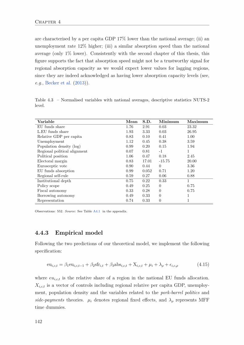
Chapter 4
are characterised by a per capita GDP 17% lower than the national average; (ii) anunemployment rate 12% higher; (iii) a similar absorption speed than the nationalaverage (only 1% lower). Consistently with the second chapter of this thesis, thisfigure supports the fact that absorption speed might not be a trustworthy signal forregional absorption capacity as we would expect lower values for lagging regions,since they are indeed acknowledged as having lower absorption capacity levels (see,e.g., Becker et al. (2013)).
Table 4.3 – Normalised variables with national averages, descriptive statistics NUTS-2level.
Variable Mean S.D. Minimum MaximumEU funds share 1.76 2.91 0.03 23.32L.EU funds share 1.93 3.33 0.03 26.95Relative GDP per capita 0.83 0.10 0.41 1.00Unemployment 1.12 0.45 0.38 3.59Population density (log) 0.99 0.20 0.15 1.94Regional political alignment 0.07 0.81 -1 1Political position 1.06 0.47 0.18 2.45Electoral margin 0.83 17.01 -15.75 20.00Eurosceptic vote 0.90 0.44 0 3.36EU funds absorption 0.99 0.052 0.71 1.20Regional self-rule 0.59 0.27 0.06 0.88Institutional depth 0.75 0.22 0.33 1Policy scope 0.49 0.25 0 0.75Fiscal autonomy 0.33 0.28 0 0.75Borrowing autonomy 0.49 0.33 0 1Representation 0.74 0.33 0 1
Observations: 552. Source: See Table A4.1 in the appendix.
4.4.3 Empirical model
Following the two predictions of our theoretical model, we implement the followingspecification:
eui,c,t = β1eui,c,t−1 + β2sfri,t + β3absi,c,t + Xi,c,t + µi + λρ + εi,c,ρ (4.15)
where eui,c,t is the relative share of a region in the national EU funds allocation.Xi,c,t is a vector of controls including regional relative per capita GDP, unemploy-ment, population density and the variables related to the pork-barrel politics andside-payments theories. µi denotes regional fixed effects, and λρ represents MFFtime dummies.
142
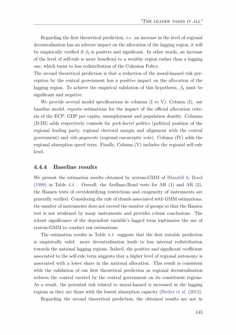
"The leader takes it all"
Regarding the first theoretical prediction, i.e. an increase in the level of regionaldecentralisation has an adverse impact on the allocation of the lagging region, it willbe empirically verified if β2 is positive and significant. In other words, an increaseof the level of self-rule is more beneficial to a wealthy region rather than a laggingone, which turns to less redistribution of the Cohesion Policy.The second theoretical prediction is that a reduction of the moral-hazard risk per-ception by the central government has a positive impact on the allocation of thelagging region. To achieve the empirical validation of this hypothesis, β3 must besignificant and negative.
We provide several model specifications in columns (I to V). Column (I), ourbaseline model, reports estimations for the impact of the official allocation crite-ria of the ECP: GDP per capita, unemployment and population density. Columns(II-III) adds respectively controls for pork-barrel politics (political position of theregional leading party, regional electoral margin and alignment with the centralgovernment) and side-payments (regional eurosceptic vote). Column (IV) adds theregional absorption speed term. Finally, Column (V) includes the regional self-rulelevel.
4.4.4 Baseline results
We present the estimation results obtained by system-GMM of Blundell & Bond(1998) in Table 4.4 . Overall, the Arellano-Bond tests for AR (1) and AR (2),the Hansen tests of overidentifying restrictions and exogeneity of instruments aregenerally verified. Considering the rule of thumb associated with GMM estimations,the number of instruments does not exceed the number of groups so that the Hansentest is not weakened by many instruments and provides robust conclusions. Therobust significance of the dependent variable’s lagged term legitimates the use ofsystem-GMM to conduct our estimations.
The estimation results in Table 4.4 suggests that the first testable predictionis empirically valid: more decentralisation leads to less internal redistributiontowards the national lagging regions. Indeed, the positive and significant coefficientassociated to the self-rule term suggests that a higher level of regional autonomy isassociated with a lower share in the national allocation. This result is consistentwith the validation of our first theoretical prediction as regional decentralisationreduces the control exerted by the central government on its constituent regions.As a result, the potential risk related to moral-hazard is increased in the laggingregions as they are those with the lowest absorption capacity (Becker et al. (2013).
Regarding the second theoretical prediction, the obtained results are not in
143
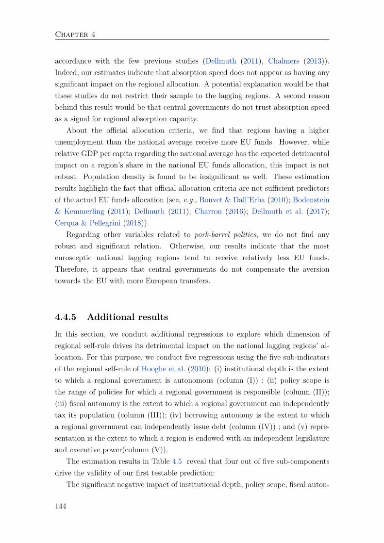
Chapter 4
accordance with the few previous studies (Dellmuth (2011), Chalmers (2013)).Indeed, our estimates indicate that absorption speed does not appear as having anysignificant impact on the regional allocation. A potential explanation would be thatthese studies do not restrict their sample to the lagging regions. A second reasonbehind this result would be that central governments do not trust absorption speedas a signal for regional absorption capacity.
About the official allocation criteria, we find that regions having a higherunemployment than the national average receive more EU funds. However, whilerelative GDP per capita regarding the national average has the expected detrimentalimpact on a region’s share in the national EU funds allocation, this impact is notrobust. Population density is found to be insignificant as well. These estimationresults highlight the fact that official allocation criteria are not sufficient predictorsof the actual EU funds allocation (see, e.g., Bouvet & Dall’Erba (2010); Bodenstein& Kemmerling (2011); Dellmuth (2011); Charron (2016); Dellmuth et al. (2017);Cerqua & Pellegrini (2018)).
Regarding other variables related to pork-barrel politics, we do not find anyrobust and significant relation. Otherwise, our results indicate that the mosteurosceptic national lagging regions tend to receive relatively less EU funds.Therefore, it appears that central governments do not compensate the aversiontowards the EU with more European transfers.
4.4.5 Additional results
In this section, we conduct additional regressions to explore which dimension ofregional self-rule drives its detrimental impact on the national lagging regions’ al-location. For this purpose, we conduct five regressions using the five sub-indicatorsof the regional self-rule of Hooghe et al. (2010): (i) institutional depth is the extentto which a regional government is autonomous (column (I)) ; (ii) policy scope isthe range of policies for which a regional government is responsible (column (II));(iii) fiscal autonomy is the extent to which a regional government can independentlytax its population (column (III)); (iv) borrowing autonomy is the extent to whicha regional government can independently issue debt (column (IV)) ; and (v) repre-sentation is the extent to which a region is endowed with an independent legislatureand executive power(column (V)).
The estimation results in Table 4.5 reveal that four out of five sub-componentsdrive the validity of our first testable prediction:
The significant negative impact of institutional depth, policy scope, fiscal auton-
144
"The leader takes it all"
Table 4.4 – System-GMM estimation results
(I) (II) (III) (IV) (V)L. EU funds 0.548*** 0.459*** 0.389*** 0.406*** 0.412***
(0.090) (0.138) (0.132) (0.112) (0.111)GDP per capita -0.053 -0.566 -3.044 -3.878 -2.375
(1.960) (2.981) (2.776) (3.548) (2.853)Unemployment 1.199*** 1.876 2.101*** 1.945*** 2.351***
(0.417) (1.160) (0.553) (0.500) (0.552)Density 0.798 1.138 2.125 1.877 1.869
(1.254) (3.051) (2.124) (1.764) (1.697)Position -0.202 0.055 0.097 0.053
(0.263) (0.272) (0.288) (0.269)Margin 0.002 0.006 0.005 0.006
(0.007) (0.009) (0.009) (0.009)Alignment 0.070 0.077 0.075 0.072
(0.118) (0.083) (0.081) (0.108)Eurosceptic -0.780** -0.836** -0.963**
(0.341) (0.319) (0.395)L.Absorption 0.660 -0.286
(1.725) (2.305)Self-rule -1.678**
(0.711)Constant -1.524 0.084 0.083 0.036 0.969
(2.556) (2.571) (2.571) (3.762) (3.521)Observations 552 353 353 353 353Number of regions 184 119 119 119 119Number of instruments 42 45 55 65 64Arellano-Bond TestsArellano-Bond AR(1) 0.070* 0.099* 0.070* 0.066* 0.100*Arellano-Bond AR(2) 0.196 0.327 0.322 0.319 0.303Hansen overid. restrictions, p.value 0.204 0.070* 0.242 0.551 0.078*Hansen exogeneity instruments, p.value 0.208 0.194 0.317 0.782 0.169
Notes: This table reports the estimation results using the system GMM estimator developed by Blundell & Bond(1998), where dependent variable presents the share of a NUTS-2 region in the total national allocation. EU fundsvariable is treated as endogenous, whereas other regressors (excluding time dummies and population density) areconsidered to be predetermined. All variables excepted regional alignment and self-rule are normalised around thenational average value.Strictly exogenous regressors: Margin, Alignment, Position, Self-rule and time dummies.Pre-determined regressors: L. EU funds, GDP per capita, Unemployment, Density, Unemployment, Eurosceptic, L.Absorption.Time fixed effects included. Robust standard errors in parentheses. * denotes p < 0.10; ** p < 0.05; ***p < 0.01.
145
Chapter 4
omy and representation illustrate that the more a lagging region’s government hasa broader range of policies that can be conducted independently from the influenceof the central government, the less important is the allocation of the national lag-ging region. This emphasises the importance of the control that could be exertedby the central government on lagging regions, in a context of moral-hazard risk, todetermine the final regional allocation of the EU funds.
However, regarding absorption speed performance, we do not observe any signif-icant impact on the regional relative share of EU funds. This confirmation indicatesthat central governments do not trust absorption speed as a signal for regional ab-sorption capacity. This result is complementary to the second chapter of this thesiswhere it has been shown that a faster absorption leads to less economic effective-ness in the lagging region. Especially, high absorption speed can be the outcomeof manipulations from central governments to send good signals to the EuropeanCommission (Huliaras & Petropoulos (2016)) with the use of strategies such as ret-rospective projects (Aivazidou et al. (2020)).
About the remaining variables, the estimation results are qualitatively similar:(i) official allocation criteria are insufficient predictors as only unemployment has arobust and positive impact on the allocation of a lagging region; (ii) Euroscepticismappears to be a penalising factor, (iii) pork-barrel politics variables do not show anysignificant impact.
146
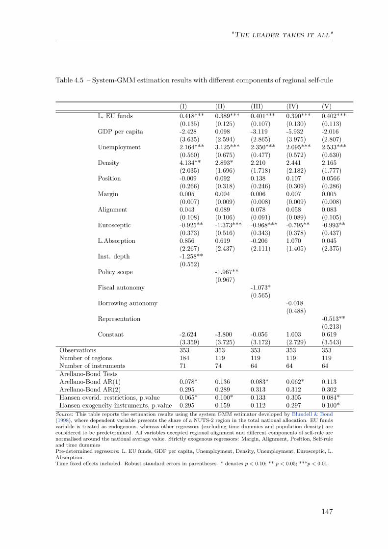
"The leader takes it all"
Table 4.5 – System-GMM estimation results with different components of regional self-rule
(I) (II) (III) (IV) (V)L. EU funds 0.418*** 0.389*** 0.401*** 0.390*** 0.402***
(0.135) (0.125) (0.107) (0.130) (0.113)GDP per capita -2.428 0.098 -3.119 -5.932 -2.016
(3.635) (2.594) (2.865) (3.975) (2.807)Unemployment 2.164*** 3.125*** 2.350*** 2.095*** 2.533***
(0.560) (0.675) (0.477) (0.572) (0.630)Density 4.134** 2.893* 2.210 2.441 2.165
(2.035) (1.696) (1.718) (2.182) (1.777)Position -0.009 0.092 0.138 0.107 0.0566
(0.266) (0.318) (0.246) (0.309) (0.286)Margin 0.005 0.004 0.006 0.007 0.005
(0.007) (0.009) (0.008) (0.009) (0.008)Alignment 0.043 0.089 0.078 0.058 0.083
(0.108) (0.106) (0.091) (0.089) (0.105)Eurosceptic -0.925** -1.373*** -0.968*** -0.795** -0.993**
(0.373) (0.516) (0.343) (0.378) (0.437)L.Absorption 0.856 0.619 -0.206 1.070 0.045
(2.267) (2.437) (2.111) (1.405) (2.375)Inst. depth -1.258**
(0.552)Policy scope -1.967**
(0.967)Fiscal autonomy -1.073*
(0.565)Borrowing autonomy -0.018
(0.488)Representation -0.513**
(0.213)Constant -2.624 -3.800 -0.056 1.003 0.619
(3.359) (3.725) (3.172) (2.729) (3.543)Observations 353 353 353 353 353Number of regions 184 119 119 119 119Number of instruments 71 74 64 64 64Arellano-Bond TestsArellano-Bond AR(1) 0.078* 0.136 0.083* 0.062* 0.113Arellano-Bond AR(2) 0.295 0.289 0.313 0.312 0.302Hansen overid. restrictions, p.value 0.065* 0.100* 0.133 0.305 0.084*Hansen exogeneity instruments, p.value 0.295 0.159 0.112 0.297 0.100*
Source: This table reports the estimation results using the system GMM estimator developed by Blundell & Bond(1998), where dependent variable presents the share of a NUTS-2 region in the total national allocation. EU fundsvariable is treated as endogenous, whereas other regressors (excluding time dummies and population density) areconsidered to be predetermined. All variables excepted regional alignment and different components of self-rule arenormalised around the national average value. Strictly exogenous regressors: Margin, Alignment, Position, Self-ruleand time dummiesPre-determined regressors: L. EU funds, GDP per capita, Unemployment, Density, Unemployment, Eurosceptic, L.Absorption.Time fixed effects included. Robust standard errors in parentheses. * denotes p < 0.10; ** p < 0.05; ***p < 0.01.
147
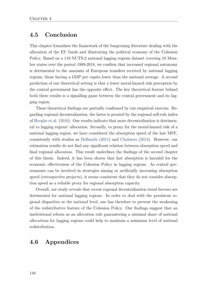
Chapter 4
4.5 Conclusion
This chapter formalises the framework of the burgeoning literature dealing with theallocation of the EU funds and illustrating the political economy of the CohesionPolicy. Based on a 119 NUTS-2 national lagging regions dataset covering 18 Mem-ber states over the period 1989-2018, we confirm that increased regional autonomyis detrimental to the amounts of European transfers received by national laggingregions, those having a GDP per capita lower than the national average. A secondprediction of our theoretical setting is that a lower moral-hazard risk perception bythe central government has the opposite effect. The key theoretical feature behindboth these results is a signalling game between the central government and its lag-ging region.
These theoretical findings are partially confirmed by our empirical exercise. Re-garding regional decentralisation, the latter is proxied by the regional self-rule indexof Hooghe et al. (2010). Our results indicate that more decentralisation is detrimen-tal to lagging regions’ allocation. Secondly, to proxy for the moral-hazard risk of anational lagging region, we have considered the absorption speed of the last MFF,consistently with studies as Dellmuth (2011) and Chalmers (2013). However, ourestimation results do not find any significant relation between absorption speed andfinal regional allocation. This result underlines the findings of the second chapterof this thesis. Indeed, it has been shown that fast absorption is harmful for theeconomic effectiveness of the Cohesion Policy in lagging regions. As central gov-ernments can be involved in strategies aiming at artificially increasing absorptionspeed (retrospective projects), it seems consistent that they do not consider absorp-tion speed as a reliable proxy for regional absorption capacity.
Overall, our study reveals that recent regional decentralisation trend favours aredetrimental for national lagging regions. In order to deal with the persistent re-gional disparities at the national level, one has therefore to prevent the weakeningof the redistributive feature of the Cohesion Policy. Our findings suggest that aninstitutional reform as an allocation rule guaranteeing a minimal share of nationalallocations for lagging regions could help to maintain a minimum level of nationalredistribution.
4.6 Appendices
148
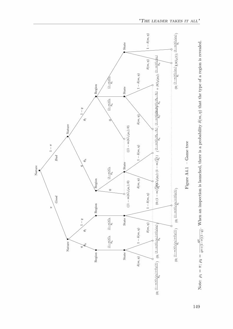
"The leader takes it all"
Nature
Nature
Region
State
(0;(1−m
)G1
(ρ1
)+G
2(1
)θh
)
δ(m,η
) (0;(1−m
)G1
(ρ1
)+G
2(ρ
2)
θh
)
1−δ(m,η
)
(1−m
)G1
θh
q θ h
Region
State
(0;(1−m
)G1
(ρ1
)+G
2(1
)θl
)
δ(m,η
) (0;(1−m
)G1
(ρ1
)+(G
2(1
)θl
)
1−δ(m,η
)
(1−m
)G1
θl
θ l1−q
π
Good
Nature
Region
((1−m
)G1(ρ
1);
0)
0
State
(0;(
1−m
)G1
θh
)
δ(m,η
)
β(G
2(ρ
2);
(1−m
)G1
θh
)
1−δ(m,η
)
(1−m
)G1
θh
qθ h
Region
((1−m
)G1(ρ
1);
0)
0
State
((1−m
)G1
(θh−θl)
θh
;(1−m
)G1
(ρ1
)θh
)
δ(m,η
) ((1−m
)G1
(θh−θl)
θh
+βG
2(ρ
2);
(1−m
)G1
(ρ1
)θh
1−δ(m,η
)
(1−m
)G1
θh
State
(0;(1−m
)G1
(ρ1
)θl
)
δ(m,η
)
(βG
2(1
);(1−m
)G1
(ρ1
)θl
)
1−δ(m,η
)
(1−m
)G1
θl
1−q
θ l
1−π
Bad
Figu
reA4.1
–Gam
etree
Note:ρ
1=π;ρ
2=
qπ
qπ
+(1−π
)(1−q).
Whe
nan
inspectio
nis
laun
ched
,the
reis
aprob
abilityδ(m,η
)that
thetype
ofaregion
isrevealed
.
149
Chapter 4
TableA4.1
–Va
riables
defin
ition
andda
tasources
Variable
Variablede
finition
Source
EU
fund
sshare
Regiona
lsha
rein
thetotaln
ationa
lallo
catio
nof
theEFR
D,E
SFan
dCFin
agivenMFF
(%)
Regiona
lisation
ofESIF
paym
ents
1989-2018
databa
sefrom
LoPiano
etal.(2017).
Regiona
lrelativeGDP
percapita
Ashareof
region
alGDP
percapita
inPPSrelativ
elyto
theEurop
eanav
-erage.
(i)Ye
ars1983-85forprogrammingpe
riod
1989-93(ii)
Years1988
-90
forprogrammingpe
riod
1994-99(iii)
Years1994-96forprogrammingpe
riod
2000-06(97-99
fornew
coun
tries),(iv)years2000-02forprogrammingpe
riod
2007-13an
d(v)years2007-09forprogrammingpe
riod
2014-16
Eurostatan
dCam
bridge
Econo
metrics.
Regiona
lunemploy
ment
Regiona
lun
employ
ment(%
)an
dsamereferenceyearsthan
RelativeGDP
percapita
Cam
bridge
Econo
metrics.
Regiona
lpop
ulationdensity
Regiona
lpo
pulatio
ndensity
(num
berof
inha
bitantspe
rsqua
red
km)an
dsamereferenceyearsthan
RelativeGDP
percapita
Cam
bridge
Econo
metrics.
Regiona
lpoliticala
lignm
ent
Discretevariab
lewith
thevalue1if
aregion
isaligned
with
thena
tiona
lgovernment,-1
ifno
tand
0in
thecase
ofab
senceof
anyregion
algovernment.
Variou
sda
tasources.
Regiona
lrelativepo
litical
positio
nRegiona
lgovernm
ent’s
lead
ingpa
rtyisplaced
ona10-point
scalewith
0be
ing
theextrem
eleft,5
beingcentre
and10
beingtheextrem
erigh
t.Indexof
Benoit&
Laver(2006)
from
ParlGov
databa
se.
Regiona
lelectoral
margin
Regiona
ldifference
betw
eenthena
tiona
lleading
partyan
dits
challeng
erin
thelast
natio
nale
lection
Europ
eanElectionDatab
asefrom
theNorwegianCentre
forResearchData(N
SD).
Eurosceptic
vote
Regiona
lsha
reof
theeurosceptic
political
partiesinthelast
natio
nalelection.
Euroscepticism
ismeasuredon
a1to
7scale,
with
1be
ing"stron
glyop
posed"
and7be
ing"stron
glyin
favour".
Lower
scores
correspo
ndto
greateran
ti-EU
sentim
ents.A
scorelower
than
3.5ha
sbe
entakenon
.
Indexof
Hoo
gheet
al.(
2008)from
theCha
pelH
illelec-
toralsurveyto
describe
apo
litical
partyas
aneurosceptic
party.
Europ
eanElectionDatab
asefrom
theNSD
tomea-
sure
itsvo
teshare.
Regiona
lself-r
ule
Con
stitu
tiona
lstreng
th,po
litical
and
fiscalau
tono
mymeasured
ona0to
17-point
scale.
0be
ingthelowestregion
alau
tono
mylevela
nd17
beingthe
high
est.
Regiona
lAutho
rity
Index
(RAI)
from
Hoo
ghe
etal.
(2010).
Regiona
lEU
fund
sab
sorptio
nRegiona
lsha
reof
theallocatedbu
dget
ofagivenMFF
spentd
uringthisMFF
Regiona
lisation
ofESIF
paym
ents
1989-2018
databa
sefrom
LoPiano
etal.(2017).
Notes:wepresenton
lyregion
alvariab
lesforsake
ofbrevity
.Nationa
lvariables
have
theexactsamedefin
ition
san
dda
tasources.
150
General conclusion
The European structural funds have aimed to reduce the economic disparitiesbetween the regions of the EU since the creation of the European Economic Com-munity in 1957. Over the last decade, the challenge of economic convergence seemsto have shifted from the East towards the South with an economic catching-upprocess which is coming to an end for certain central European economies, butwith a dynamic of emerging divergence in the Mediterranean economies. The latterwere notably characterized by a lack of growth in GDP per capita as the economiesof Western and Northern Europe experienced a phase of expansion in the yearsfollowing the euro zone sovereign debt crisis. It follows that the interests of theEU and the EMU converge, as evidenced by the adoption of the NextGenerationEU recovery plan at the European Council of 21 July 2020. The latter aims toaccelerate the recovery phase following the recession of the Covid-19 pandemic,which could generate de facto an alignment of the economic cycles of the South andof the other Member States of the Euro zone. The concept of economic effectivenessattributed to the structural funds must therefore be broadened to consider theimpact on economic growth on the one hand, but also on the economic cycles ofrecipient countries on the other hand. In a context where the Union’s priorities arediversifying, in particular with the environmental challenge, and where its budgetconstraint has been accentuated since the departure of the United Kingdom, theeconomic effectiveness of the Cohesion policy is central. However, the latter isreduced by the way in which the Cohesion policy is implemented. The allocationof funds between regions and beneficiary countries is not optimal in the sense thatit does not allow maximum economic growth gain to be achieved. But also, thestrategic interactions linked to the process of allocating structural funds at theregional level, in particular the risk of moral hazard which threatens a completeabsorption of European funds, diverts structural funds from support to the poorestregions and reduces the quality of some EU-funded investment projects. Overall,this thesis is composed of four studies having their own research questions tobring both empirical and theoretical contributions around the analysis of economiceffectiveness of the structural funds, and their allocation. The three main Europeanstructural funds are considered, namely the European Regional Economic Develop-ment Fund (ERDF), the European Social Fund (ESF) and the Cohesion Fund (CF).
Regarding the aspect of the economic effectiveness, this thesis offers to broadenthe field of economic effectiveness associated to the European funds by considering
151
General Conclusion
their impact on the business cycles. In this context, the chapter 1 is the firstempirical work that considers the impact of the EU funds on the synchronizationof economic cycles in the EMU. It attempts to analyze this for the 28 EUcountries over the period 2000-2016. This chapter shows that structural fundsgenerate a positive externality in terms of increased synchronicity between EUcountries. The empirical results are qualitatively similar and robust to the use ofdifferent estimators (OLS, panel IV) and different business cycle filtering techniques(Hodrick-Prescott, Christiano-Fitzgerald). The effects are larger if one takes intoaccount the EMU membership, which suggests that the adoption of the commoncurrency accentuates these positive effects.
The chapter 2 adds a new dimension in the study of this conditional economiceffectiveness by highlighting the dilemma between a fast absorption and a highimpact on economic growth in the Objective 1 regions. Indeed, this chapter showsthat the desire to accelerate the absorption of European funds, in particular forthe poorest regions, is a harmful political objective which reduces the economiceffectiveness of the cohesion policy. It studies the impact of the Objective 1treatment in 256 regions of the EU over the period 2000-2016 using regressions ondiscontinuity with heterogeneous effects. In particular, this chapter highlights thatObjective 1 regions, which are the core recipient regions of the Cohesion policy,sell off the quality of their investment project with easy-to-spend solutions in orderto meet the deadlines for the implementation of investment projects financed bythe EU. Central governments can also artificially increase the rate of absorption ofstructural funds with strategies such as the use of retroactive projects. This chaptertherefore highlights that fast absorption is not a reliable signal of high absorptioncapacity. The incentives put in place to accelerate the absorption of funds, suchas the (n +2 rule), are therefore detrimental to the economic effectiveness of theCohesion policy.
Regarding the allocation of the European funds, the chapter 3 considers thefinal allocation of the European funds between beneficiary countries and exposesthat the observed allocation of the European funds is different from an optimalallocation maximising the economic effectiveness. It highlights that political biasesin the allocation of structural funds lead to a sub-optimality in their allocation inthe sense that economic growth is not maximized in the beneficiary Member States.Through a normative approach, this is demonstrated in the case of the CohesionFund. An optimization problem is posed there, the theoretical solution simulatedusing empirical simulations of a growth equation constitutes the optimal allocation
152
General Conclusion
of the Cohesion Fund for the multiannual financial framework 2014-2020. Thissolution was empirically simulated with the estimation results of a growth equationcovering 17 countries for the period 1995-2015 with the generalized momentsmethod of Blundell & Bond (1998). The optimality of this allocation is basedon the principles of effectiveness and equity which allow, respectively, a greatereconomic impact on a global scale, and a reorientation of financial support towardspoorer economies with a greater relative demographic weight. The significantdifferences between the optimal allocation and the observed allocation highlightthe existing political biases that undermine the achievement of the objective ofeconomic convergence as the over-representation of small countries.
Finally, the chapter 4 shows that the intranational allocation of the structuralfunds is subject to political forces. The interactions between the constituentregions and the central government are modelled and tested empirically. One ofthe characteristics of the Cohesion policy is that a negotiation between a centralgovernment and its constituent regions determines the final allocation of structuralfunds. With a view to ensuring a relatively rapid complete absorption of funds,central governments may be tempted to favour the most advanced regions, ortheir own lagging regions if they can exercise control therein to minimize anyrisk of moral-hazard. The chapter 4 therefore proposes a theoretical model ofthe signalling game between a central government and its lagging regions whichmakes it possible to formalize the strategic incentives which the latter is subjectto. This game is followed by a problem of maximizing the welfare of the altruisticcentral government, which relies entirely on the production of public goods of itsconstituent regions. It shows that a central government is less willing to directstructural funds towards its less advanced regions when their level of regionalautonomy is high. Considering a sample of 119 regions with a GDP per capitalower than their national average over the period 1989-2018, the estimations carriedout with the method of generalized moments of Blundell & Bond (1998) illustratethat an increasing level of regional autonomy apprehended with the self-rule levelof Hooghe et al. (2010) reduces the control of the central government over itsconstituent regions. Reforms in favour of regional decentralization therefore tendto favor regions with a strong absorption capacity, which are the most advancedregions. This trend has accelerated over the last decade since the Barca report(Barca (2009) which aimed to reform the Cohesion policy by territorializingit. However, only urban regions have been in able to adapt to this reform, theperipheral regions did not have the means to do so, in particular due to limitedadministrative resources. A second theoretical result of the chapter 4 is that
153
General Conclusion
a reduced perception of moral hazard risk is beneficial for the poorest regions.However, by considering the speed of absorption of funds as a signal for moralhazard risk, the empirical estimations carried out do not validate this secondtheoretical prediction. This echoes discussions in chapter 3 that concluded thatabsorption rate is not a reliable signal of absorptive capacity.
Limits and future research pespectives
In general, the study of the economic effectiveness of the structural funds mustbe extended to other fields than economic growth, the economic policy targets ofthe EMU must also be taken into account. Thus, although this thesis has beenconsidering the impact of structural funds on the synchronization of economiccycles, only the direct impact of these funds has been measured in the first chapterof this thesis. A more detailed analysis seeking to determine which variablesincrease or decrease this impact could be carried out. In addition, a dis-aggregationof data based on the type of projects financed, i.e transport infrastructure or R&Dprojects, would provide more information on the nature of the impact of structuralfunds on economic cycles. Within the framework of the European Semester, suchknowledge would allow a better quality of economic governance within the EU, andparticularly within the EMU.
This thesis also calls for broadening the field of economic effectiveness studiesby considering the institutional architecture of the Cohesion policy. Thus, ithas been shown here that the incentives aimed at accelerating the absorption ofstructural funds have a negative impact on the capacity of the European funds tostimulate the economic growth in the Objective 1 regions. Moreover, the secondchapter has shown that the speed of absorption of structural funds is not a reliablesignal for the absorption capacity. This raises the question of finding an indicatorcapable of measuring the good use of the structural funds. This indicator shouldbe measurable in near real time in order to be used by policymakers.
Regarding the allocation of the EU funds, the third chapter, which resulted inan optimal allocation of the Cohesion Fund, paves the way for other definitionsof optimality that can be applied to other structural funds. Thus, other criteria,policies such as respect for the rule of Law, or environmental criteria such as thereduction of greenhouse gases, could be considered. In addition, the donor wasassumed to be totally benevolent, or altruistic. Other extensions with an interesteddonor with specific objectives can be carried out in other analytical frameworks.
Finally, the broader future research implications are undoubtedly given by the
154
General Conclusion
last chapter, exploratory in the formalization of the forces which are exerted duringthe process of allocation of the structural funds. This allocation process involvesstrategic interactions between the European Commission, the Member States andtheir constituent regions. A Principal-Agent framework involving these actorscould be a more advanced theoretical framework to explore this research question.Finally, in a context where the reduction of economic disparities within the EU hasmainly been driven by the catching up of the economies of Central and EasternEurope, i.e. a reduction in inter-regional inequalities, this chapter calls for furtherwork on regional inequalities at the intranational level.
155

156
Conclusion générale
Les fonds structurels européens ont pour objectif de réduire les disparitéséconomiques entre les régions de l’UE depuis la création de la CommunautéÉconomique Européenne en 1957. Depuis la dernière décennie, le défi de laconvergence économique semble s’être déplacé de l’Est vers le Sud avec un pro-cessus de rattrapage économique qui arrive à son terme pour certaines économiesd’Europe centrale, mais avec une dynamique de divergence émergente des économiesméditerranéennes. Ces dernières ont notamment été caractérisées par une absencede croissance du PIB par habitant alors que les économies d’Europe de l’Ouest etdu Nord ont expérimenté une phase d’expansion dans les années suivant la crisedes dettes souveraines de la zone Euro. Il en découle que les intérêts de l’UE et del’UEM convergent, en témoigne l’adoption du plan de relance NextGeneration EUlors du conseil européen du 21 juillet 2020. Ce dernier a pour but d’accélérer laphase de reprise suivant la récession de la pandémie du Covid-19, ce qui pourraitgénérer de facto un alignement des cycles économiques du Sud et des autres ÉtatsMembres de la zone Euro. La notion d’efficacité économique attribuée aux fondsstructurels doit donc s’élargir pour considérer l’impact sur la croissance économiqued’une part, mais aussi sur les cycles économiques des pays receveurs d’autre part.Dans un contexte où les priorités de l’Union se diversifient, notamment avec le défienvironnemental, et où sa contrainte budgétaire s’est accentuée depuis le départ duRoyaume-Uni, l’efficacité économique de la politique de Cohésion est un central. Or,cette dernière est réduite par la manière dont la politique de Cohésion est menée.L’allocation des fonds entre régions et pays bénéficiaires n’y est pas optimale ausens où elle ne permet pas d’atteindre un gain de croissance économique maximal.Mais aussi, les intéractions stratégiques liées au processus d’allocation des fondsstructurels à l’échelle régionale, notamment le risque d’aléa-moral qui menaceune absorption complète des fonds européens, détournent les fonds structurelsdu soutien vers les régions les plus pauvres et réduisent la qualité de certainsprojets d’investissement financés par l’UE. Globalement, cette thèse est composéede quatre études ayant leurs propres questions de recherche pour apporter descontributions à la fois empiriques et théoriques autour de l’analyse de la efficacitééconomique des fonds structurels, et de leur allocation. Les trois principaux fondsstructurels européens sont considérés, à savoir le Fonds européen de développementéconomique régional (FEDER), le Fonds social européen (FSE) et le Fonds decohésion (FC).
157
Conclusion générale
Concernant la notion d’efficacité économique, cette thèse propose d’en élargirle champ en considérant l’impact des fonds européens sur les cycles économiques.Dans ce contexte, le chapitre 1 est le premier travail empirique qui considèrel’impact des fonds de l’UE sur la synchronisation des cycles économiques dansl’UEM. Il analyse cela pour les 28 pays de l’UE sur la période 2000-2016. Cechapitre montre que les fonds structurels génèrent une externalité positive entermes de synchronicité accrue entre les pays de l’UE. Les résultats empiriquessont qualitativement similaires et robustes à l’utilisation de différents estimateurs(OLS, panel IV) et de différentes techniques de filtrage du cycle économique(Hodrick-Prescott, Christiano-Fitzgerald). Les effets sont plus importants si l’onprend en compte l’adhésion à l’UEM, ce qui suggère que l’adoption de la monnaiecommune accentue ces effets positifs.
Le chapitre 2 ajoute une nouvelle dimension à l’étude de cette efficacitééconomique conditionnelle en mettant en évidence le dilemme entre une absorptionrapide et un impact élevé sur la croissance économique dans les régions de con-vergence. En effet, ce chapitre montre que la volonté d’accélérer l’absorption desfonds européens, en particulier pour les régions les plus pauvres, est un objectifpolitique néfaste qui réduit l’efficacité économique de la politique de cohésion. Ilétudie l’impact du traitement Objectif 1 dans 256 régions de l’UE sur la période2000-2016 en utilisant des régressions sur la discontinuité à effets hétérogènes.En particulier, ce chapitre souligne que les régions de l’Objectif 1, qui sont lesprincipales régions bénéficiaires de la politique de cohésion, bradent la qualité deleur projet d’investissement avec des solutions de dépenses faciles afin de respecterles délais de mise en œuvre des projets d’investissement financés par l’UE. Lesgouvernements centraux peuvent également augmenter artificiellement la vitessed’absorption des fonds structurels avec des stratégies telles que l’utilisation deprojets rétroactifs. Ce chapitre souligne donc qu’une absorption rapide n’est pasun signal fiable de capacité d’absorption élevée. Les incitations mises en place pouraccélérer l’absorption des fonds, comme le (règle n+2 ), sont donc préjudiciablespour l’efficacité économique de la politique de cohésion.
Concernant le processus d’allocation des fonds européens, le chapitre 3considère l’allocation finale des fonds européens entre pays bénéficiaires et exposeque l’allocation observée des fonds européens est différente d’une allocation opti-male maximisant l’efficacité économique. Il souligne que les biais politiques dansl’allocation des fonds structurels conduisent à une sous-optimalité dans le sens oùla croissance économique n’est pas maximisée dans les États membres bénéficiaires.
158
Conclusion générale
À travers une approche normative, cela est démontré dans le cas du Fonds decohésion. Un problème d’optimisation y est posé, la solution théorique simuléeempiriquement constitue l’allocation optimale du Fonds de Cohésion pour le cadrefinancier pluriannuel 2014-2020. Cette solution a été simulée empiriquement avec lesrésultats d’estimation d’une équation de croissance couvrant 17 pays pour la période1995-2015 avec la méthode des moments généralisés de Blundell & Bond (1998).L’optimalité de cette allocation repose sur les principes de efficacité et de équité quipermettent, respectivement, un plus grand impact économique à l’échelle mondiale,et une réorientation du soutien financier vers les économies les plus pauvres avecune plus grande démographie relative. poids. Les différences significatives entrel’allocation optimale et l’allocation observée mettent en évidence les biais politiquesexistants qui compromettent l’atteinte de l’objectif de convergence économiquecomme la sur-représentation des petits pays.
Enfin, le chapitre 4 montre que l’allocation intranationale des fonds structurelsest soumise à des forces politiques. Les interactions entre régions et gouvernementcentral sont modélisées et testées empiriquement. L’une des caractéristiques de lapolitique de cohésion est qu’une négociation entre un gouvernement central et sesrégions constituantes détermine l’allocation finale des fonds structurels. En vued’assurer une absorption complète et relativement rapide des fonds, les gouverne-ments centraux peuvent être tentés de privilégier les régions les plus avancées, ouleurs propres régions en retard s’ils peuvent y exercer un contrôle pour minimisertout risque d’aléa moral. Le chapitre 4 propose donc un modèle théorique avec unjeu de signal entre un gouvernement central et ses régions pauvres, ce qui permetde formaliser les incitations stratégiques du processus d’allocation des fonds.Ce jeu est suivi d’un problème de maximisation du bien-être du gouvernementcentral altruiste, qui repose entièrement sur la production de biens publics de sesrégions constituantes. Il montre qu’un gouvernement central est moins disposé àorienter les fonds structurels vers ses régions les moins avancées lorsque leur niveaud’autonomie régionale est élevé. Considérant un échantillon de 119 régions ayant unPIB par habitant inférieur à leur moyenne nationale sur la période 1989-2018, lesestimations réalisées avec la méthode des moments généralisés de Blundell & Bond(1998) illustrent qu’un niveau croissant d’autonomie régionale appréhendé avec laself-rule niveau de Hooghe et al. (2010) réduit le contrôle du gouvernement centralsur ses régions constituantes. Les réformes en faveur de la décentralisation régionaletendent donc à privilégier les régions à forte capacité d’absorption, qui sont lesrégions les plus avancées. Cette tendance s’est accélérée au cours de la dernièredécennie depuis le rapport Barca (Barca (2009) qui visait à réformer la politique
159
Conclusion générale
de cohésion en la territorialisant. Cependant, seules les régions urbaines ont sus’adapter à cette réforme, les les régions n’en avaient pas les moyens, notammenten raison de ressources administratives limitées. Un deuxième résultat théoriquedu chapitre 4 est qu’une perception réduite du risque d’aléa moral est bénéfiquepour les régions les plus pauvres. Cependant, empiriquement, en considérant lavitesse d’absorption des fonds comme signal de risque d’aléa moral, les estimationsréalisées ne valident pas cette seconde prédiction théorique, ce qui fait écho auxdiscussions du chapitre 3 qui concluaient que le taux d’absorption n’est pas unsignal fiable de la capacité d’absorption .
Limites et pespectives de recherches futures
De manière générale, l’étude de la notion d’efficacité économique des fonds struc-turels doit s’élargir vers d’autres champs que celui de la croissance économique, lesintérêts économiques de l’UEM doivent également être pris en compte. Ainsi, bienque cette thèse ait considéré l’impact des fonds structurels sur la synchronisationdes cycles économiques, seul l’impact direct de ces fonds a été mesuré dans lepremier chapitre de cette thèse. Une analyse plus fine cherchant à déterminerquelles variables augmentent ou diminuent cet impact pourrait être réalisée. Deplus, une désagrégation des données selon le type de projets financés, i.e infras-tructures de transport ou projets de R&D, fournirait plus d’informations sur lanature de l’impact des fonds structurels sur les cycles économiques. Dans le cadredu Semestre européen, une telle connaissance permettrait une meilleure qualité dela gouvernance économique au sein de l’UE, et en particulier au sein de l’UEM.
Cette thèse appelle aussi à élargir le champ d’étude de l’efficacité économiquedes fonds structurels en considérant l’architecture institutionnelle de la politique deCohésion. Ainsi, il a été montré ici que les incitations visant à accélérer l’absorptiondes fonds structurels a eu impact négatif sur la capacité des fonds européens àstimuler la croissance économique des régions Objectif 1. Le deuxième chapitre aaussi montré que la vitesse d’absorption des fonds structurels n’est pas un signalfiable pour la capacité d’absorption. Cela pose la question de trouver un indicateurcapable de mesurer le bon usage des fonds structurels. Cet indicateur devraitêtre facilement mesurable en temps quasi réel afin d’être utilisé par les décideurspolitiques.
Concernant l’étude du processus d’allocation des fonds européens, le troisièmechapitre, qui a abouti à une allocation optimale du Fonds de cohésion, ouvre la voieà d’autres définitions de l’optimalité qui peuvent être appliquées à d’autres fonds
160
Conclusion générale
structurels. Ainsi, d’autres critères, politiques comme le respect de l’Etat de droit,ou encore des critères environnementaux comme la réduction des émissions de gazà effet de serre, pourraient être envisagés. De plus, le donneur était supposé êtretotalement bienveillant, ou altruiste. D’autres extensions avec un donneur intéresséavec des objectifs spécifiques peuvent être réalisées dans d’autres cadres d’analyse.
Enfin, les implications les plus larges de recherche future sont sans doutedonnées par le dernier chapitre, exploratoire dans la formalisation des forces quis’exercent au cours du processus d’allocation des fonds structurels. Ce processusd’allocation implique des interactions stratégiques entre la Commission européenne,les États membres et leurs régions constitutives. Un cadre principal-agent im-pliquant ces acteurs pourrait constituer un cadre théorique plus avancé pourexplorer cette question de recherche. Enfin, dans un contexte où la réduction desdisparités économiques au sein de l’UE a été principalement tirée par le rattrapagedes économies d’Europe centrale et orientale, soit une réduction des inégalitésinterrégionales, ce chapitre appelle à des travaux supplémentaires sur les inégalitésrégionales au niveau intranational.
161

162
Bibliography
Aghion, P. & Blanchard, O. J. (1994), ‘On the speed of transition in Central Europe’,NBER Macroeconomics Annual 9, 283–320.
Aivazidou, E., Cunico, G. & Mollona, E. (2020), ‘Beyond the EU Structural Funds’Absorption Rate: How Do Regions Really Perform?’, Economies 8(3), 55.
Altug, S. & Canova, F. (2014), ‘Do institutions and culture matter for businesscycles?’, Open Economies Review 25(1), 93–122.
Angelini, E. C. & Farina, F. (2012), ‘Current account imbalances and systemicrisk within a monetary union’, Journal of Economic Behavior & Organization83(3), 647–656.
Antonakakis, N. & Tondl, G. (2014), ‘Does integration and economic policy coordi-nation promote business cycle synchronization in the EU?’, Empirica 41(3), 541–575.
Arellano, M. et al. (1987), ‘Computing robust standard errors for within-groupsestimators’, Oxford Bulletin of Economics and Statistics 49(4), 431–434.
Artis, M. J. & Zhang, W. (1999), ‘Further evidence on the international businesscycle and the ERM: is there a European business cycle?’, Oxford Economic Papers51(1), 120–132.
Bachtler, J. & Ferry, M. (2015), ‘Conditionalities and the performance of europeanstructural funds: A principal–agent analysis of control mechanisms in europeanunion cohesion policy’, Regional Studies 49(8), 1258–1273.
Bachtler, J., Mendez, C. & Wishlade, F. (2019), ‘Reforming theMFF and CohesionPolicy 2021-27: Pragmatic drift or paradigmatic shift?’.
Barca, F. (2009), Agenda for a reformed cohesion policy, European CommunitiesBrussels.
Barro, R. J. (1990), ‘Government spending in a simple model of endogeneousgrowth’, Journal of Political Economy 98(5, Part 2), 103–125.
Basile, R., Castellani, D. & Zanfei, A. (2008), ‘Location choices of multinationalfirms in Europe: The role of EU Cohesion Policy’, Journal of International Eco-nomics 74(2), 328–340.
163
Bibliography
Batterbury, S. C. (2002), ‘Evaluating policy implementation: The European Union’ssmall and medium sized enterprise policies in Galicia and Sardinia’, RegionalStudies 36(8), 861–876.
Baumol, W. (2001), Paradox of the Services: exploding costs, persistent demand,Chapter 1 in “The growth of Service Industries–The Paradox of Exploding Costsand Persistent Demand”, Edward Elgar Publishing Limited.
Baxter, M. & Kouparitsas, M. A. (2005), ‘Determinants of business cycle comove-ment: a robust analysis’, Journal of Monetary Economics 52(1), 113–157.
Bayoumi, T. & Eichengreen, B. (1992), Shocking aspects of European monetaryunification, Technical report, National Bureau of Economic Research.
Beck, K. (2014), ‘Structural similarity as a determinant of business cycle synchro-nization in the European Union: A robust analysis’, Research in Economics andBusiness: Central and Eastern Europe 5(2).
Becker, S. O. (2012), EU structural funds: Do they generate more growth?, Citeseer.
Becker, S. O., Egger, P. H. & Von Ehrlich, M. (2010), ‘Going NUTS: The effectof EU structural funds on regional performance’, Journal of Public Economics94(9-10), 578–590.
Becker, S. O., Egger, P. H. & Von Ehrlich, M. (2013), ‘Absorptive capacity andthe growth and investment effects of regional transfers: A regression disconti-nuity design with heterogeneous treatment effects’, American Economic Journal:Economic Policy 5(4), 29–77.
Becker, S. O., Egger, P. H. & von Ehrlich, M. (2018), ‘Effects of EU regional policy:1989-2013’, Regional Science and Urban Economics 69, 143–152.
Belke, A., Domnick, C. & Gros, D. (2017), ‘Business cycle synchronization in theEMU: Core vs. periphery’, Open Economies Review 28(5), 863–892.
Benoit, K. & Laver, M. (2006), Party Policy in Modern Democracies, Lon-don:Routledge.
Bevan, A. A. & Estrin, S. (2004), ‘The determinants of foreign direct investment intoEuropean transition economies’, Journal of Comparative Economics 32(4), 775–787.
164
Blesse, S., Havlik, A. & Heinemann, F. (2020), ‘Euro area reform preferences ofCentral and Eastern European economic experts’, Empirica pp. 1–25.
Blom-Hansen, J. (2005), ‘Principals, agents, and the implementation of EU cohesionpolicy’, Journal of European Public Policy 12(4), 624–648.
Bloom, D. E., Canning, D. & Fink, G. (2008), ‘Urbanization and the wealth ofnations’, Science 319(5864), 772–775.
Blundell, R. & Bond, S. (1998), ‘Initial conditions and moment restrictions in dy-namic panel data models’, Journal of Econometrics 87(1), 115–143.
Bodenstein, T. & Kemmerling, A. (2011), ‘Ripples in a rising tide: Why some EUregions receive more structural funds than others’, European Integration OnlinePapers 16(1).
Bondonio, D. & Greenbaum, R. T. (2006), ‘Do business investment incentives pro-mote employment in declining areas? evidence from EU Objective-2 regions’,European Urban and Regional Studies 13(3), 225–244.
Bouvet, F. & Dall’Erba, S. (2010), ‘European regional structural funds: How largeis the influence of politics on the allocation process?’, Journal of Common MarketStudies 48(3), 501–528.
Bravo-Ortega, C. & Di Giovanni, J. (2006), ‘Remoteness and real exchange ratevolatility’, IMF Staff Papers 53(1), 115–132.
Breuss, F., Egger, P. & Pfaffermayr, M. (2010), ‘Structural funds, EU enlarge-ment, and the redistribution of FDI in Europe’, Review of World Economics146(3), 469–494.
Burnside, C. & Dollar, D. (2000), ‘Aid, policies, and growth’, American EconomicReview 90(4), 847–868.
Calderon, C., Chong, A. & Stein, E. (2007), ‘Trade intensity and business cyclesynchronization: Are developing countries any different?’, Journal of InternationalEconomics 71(1), 2–21.
Campos, N. F. & Macchiarelli, C. (2016), ‘Core and periphery in the EuropeanMonetary Union: Bayoumi and Eichengreen 25 years later’, Economics Letters147, 127–130.
165
Bibliography
Canova, F. (1998), ‘Detrending and Business cycle facts’, Journal of Monetary Eco-nomics 41(3), 475–512.
Cappelen, A., Castellacci, F., Fagerberg, J. & Verspagen, B. (2003), ‘The impact ofEU regional support on growth and convergence in the European Union’, JCMS:Journal of Common Market Studies 41(4), 621–644.
Carter, P. (2014), ‘Aid allocation rules’, European Economic Review 71, 132–151.
Cartwright, A. & Batory, A. (2012), ‘Monitoring committees in cohesion policy:Overseeing the distribution of structural funds in hungary and slovakia’, Journalof European Integration 34(4), 323–340.
Caselli, F., Esquivel, G. & Lefort, F. (1996), ‘Reopening the convergence debate:A new look at cross-country growth empirics’, Journal of Economic Growth1(3), 363–389.
Cerqua, A. & Pellegrini, G. (2018), ‘Are we spending too much to grow? the caseof Structural Funds’, Journal of Regional Science 58(3), 535–563.
Chalmers, A. W. (2013), ‘Regional authority, transnational lobbying and the allo-cation of structural funds in the e uropean u nion’, JCMS: Journal of CommonMarket Studies 51(5), 815–831.
Charron, N. (2016), ‘Explaining the allocation of regional Structural Funds:The conditional effect of governance and self-rule’, European Union Politics17(4), 638–659.
Charron, N., Dijkstra, L. & Lapuente, V. (2014), ‘Regional governance matters:Quality of government within European Union member states’, Regional Studies48(1), 68–90.
Chauvet, L. & Guillaumont, P. (2009), ‘Aid, volatility, and growth again: Whenaid volatility matters and when it does not’, Review of Development Economics13(3), 452–463.
Chinn, M. D. & Ito, H. (2008), ‘A new measure of financial openness’, Journal ofComparative Policy Analysis 10(3), 309–322.
Chmelová, P. et al. (2018), ‘Vliv realizace strukturální pomoci Evropské uniena hospodářsky cyklus a fiskální politiku české republiky’, Politická ekonomie66(2), 157–177.
166
Christiano, L. J. & Fitzgerald, T. J. (2003), ‘The band pass filter’, InternationalEconomic Review 44(2), 435–465.
Clark, T. E. & Van Wincoop, E. (2001), ‘Borders and business cycles’, Journal ofInternational Economics 55(1), 59–85.
Coelho, M. (2019), ‘Fiscal stimulus in a monetary union: Evidence from eurozoneregions’, IMF Economic Review 67(3), 573–617.
Cogneau, D. & Naudet, J.-D. (2007), ‘Who deserves aid? equality of opportunity,international aid, and poverty reduction’, World Development 35(1), 104–120.
Collier, P. & Dollar, D. (2001), ‘Can the World cut poverty in half? How PolicyReform and Effective Aid Can Meet International Development Goals’, WorldDevelopment 29(11), 1787–1802.
Collier, P. & Dollar, D. (2002), ‘Aid allocation and poverty reduction’, EuropeanEconomic Review 46(8), 1475–1500.
Communautés Européennes. Bureau de représentation (France) (1957), ‘Le traitéde rome instituant la communauté économique européenne’.https://catalogue.bnf.fr/ark:/12148/cb32964509w.public.
Cox, G. W. & McCubbins, M. D. (1986), ‘Electoral politics as a redistributive game’,The Journal of Politics 48(2), 370–389.
Crescenzi, R. & Giua, M. (2016), ‘The EU Cohesion Policy in context: Does abottom-up approach work in all regions?’, Environment and Panning A: Economyand Space 48(11), 2340–2357.
CSIL (2010), ’Lessons from shared management in cohesion, rural development andfisheries policies’, Technical report, European Commission.
Dall’Erba, S. & Fang, F. (2017), ‘Meta-analysis of the impact of European UnionStructural Funds on regional growth’, Regional Studies 51(6), 822–832.
Dall’Erba, S. & Le Gallo, J. (2008), ‘Regional convergence and the impact of Euro-pean structural funds over 1989–1999: A spatial econometric analysis’, Papers inRegional Science 87(2), 219–244.
Darvas, Z., Rose, A. K. & Szapáry, G. (2005), Fiscal divergence and business cy-cle synchronization: irresponsibility is idiosyncratic, Technical report, NationalBureau of Economic Research.
167
Bibliography
Darvas, Z. & Szapáry, G. (2008), ‘Business cycle synchronization in the enlargedEU’, Open Economies Review 19(1), 1–19.
David, F. N. (1949), Probability theory for statistical methods, London, Cambridge:University Press.
Dawson, J. W. (2003), ‘Causality in the freedom–growth relationship’, EuropeanJournal of Political Economy 19(3), 479–495.
De Haan, J., Inklaar, R. & Jong-A-Pin, R. (2008), ‘Will business cycles in theeuro area converge? A critical survey of empirical research’, Journal of economicsurveys 22(2), 234–273.
De Melo, M., Denizer, C., Gelb, A. & Tenev, S. (2001), ‘Circumstance and choice:The role of initial conditions and policies in transition economies’, World BankEconomic Review 15(1), 1–31.
De Menil, G. (2003), History, Policy and Performance in Two Transition Countries–Poland and Romania, in D. Rodrik, ed., ‘In Search of Prosperity. Analytic Narra-tives on Economic Growth’, Princeton University Press, chapter 10, pp. 271–296.
Debrun, X., Ostry, J. D., Willems, T. & Wyplosz, C. (2019), Public Debt Sustain-ability, Technical report, Centre for Economic Policy Research.
Dell’Anno, R. & Villa, S. (2013), ‘Growth in transition countries’, Economics ofTransition 21(3), 381–417.
Dellas, H. & Sakellaris, P. (2003), ‘On the cyclicality of schooling: theory andevidence’, Oxford Economic Papers 55(1), 148–172.
Dellmuth, L. M. (2011), ‘The cash divide: the allocation of European Union regionalgrants’, Journal of European Public Policy 18(7), 1016–1033.
Dellmuth, L. M., Schraff, D. & Stoffel, M. F. (2017), ‘Distributive politics, electoralinstitutions and European structural and investment funding: Evidence from Italyand France’, Journal of Common Market Studies 55(2), 275–293.
Dellmuth, L. M. & Stoffel, M. F. (2012), ‘Distributive politics and intergovernmentaltransfers: The local allocation of European Union structural funds’, EuropeanUnion Politics 13(3), 413–433.
Dotti, N. F. (2016), ‘Unwritten factors affecting structural funds: The influenceof regional political behaviours on the implementation of EU cohesion policy’,European Planning Studies 24(3), 530–550.
168
Ductor, L. & Leiva-Leon, D. (2016), ‘Dynamics of global business cycle interdepen-dence’, Journal of International Economics 102, 110–127.
Dudek, C. M. (2005), EU accession and Spanish regional development: Winners andlosers, number 4, Peter Lang.
Dupor, B. & Guerrero, R. (2017), ‘Local and aggregate fiscal policy multipliers’,Journal of Monetary Economics 92, 16–30.
EC (2011), Results of the Public Consultation on the Conclusions of the Fifth Re-port on Economic, Social and Territorial Cohesion. Commission Staff WorkingPaper, SEC(2011) 590 final, 13 May, Commission of the European Communities.Brussels.
EC (2019), European structural and investment funds 2014-2020, The EuropeanCommission, Brussels.
ECA (2004), Court of Auditors – annual report concerning the financial year 2003,Official Journal of the European Union C293, Vol. 47(28 November).
ECA (2018), Court of Auditors – Special Report—Commission’s and Member States’Actions in the Last Years of the 2007–2013 Programmes Tackled Low Absorptionbut Had Insufficient Focus on Results, Official Journal of the European UnionJOC 2018 329 R 0002.
Ederveen, S., De Groot, H. L. & Nahuis, R. (2006), ‘Fertile soil for structural funds?a panel data analysis of the conditional effectiveness of European cohesion policy’,Kyklos 59(1), 17–42.
Ederveen, S., Gorter, J., de Mooij, R. & Nahuis, R. (2002), ‘Funds and games’, TheEconomics of European Cohesion Policy. CPB Special Publication (41).
ESPON (2005), Territorial Effects of Structural Funds, Luxembourg: ESPON.
Faludi, A., Stead, D. & Humer, A. (2015), ‘Conclusions: services of general interest,territorial cohesion and competitiveness in Europe’, Services of General Interestand Territorial Cohesion: European Perspectives and National Insights pp. 259–267.
Fatas, A. (1997), ‘EMU: Countries or regions? Lessons from the EMS experience’,European Economic Review 41(3-5), 743–751.
169
Bibliography
Fidrmuc, J. & Korhonen, I. (2006), ‘Meta-analysis of the business cycle correla-tion between the euro area and the CEECs’, Journal of Comparative Economics34(3), 518–537.
Frankel, J. A. & Rose, A. K. (1998), ‘The endogenity of the optimum currency areacriteria’, The Economic Journal 108(449), 1009–1025.
Fratesi, U. & Perucca, G. (2014), ‘Territorial capital and the effectiveness of cohesionpolicies: An assessment for CEE regions’, Investigaciones Regionales-Journal ofRegional Research (29).
Gagliardi, L. & Percoco, M. (2017), ‘The impact of European Cohesion Policy inurban and rural regions’, Regional Studies 51(6), 857–868.
Gehring, K. & Schneider, S. A. (2018), ‘Towards the Greater good? EU com-missioners’ nationality and budget allocation in the European Union’, AmericanEconomic Journal: Economic Policy 10(1), 214–39.
Goldsmith, A. A. (1995), ‘Democracy, property rights and economic growth’, Jour-nal of Development Studies 32(2), 157–174.
Grigoraş, V. & Stanciu, I. E. (2016), ‘New evidence on the (de) synchronisation ofbusiness cycles: Reshaping the European business cycle’, International Economics147, 27–52.
Gruber, E., Rauhut, D. & Humer, A. (2019), ‘Territorial cohesion under pressure?Welfare policy and planning responses in Austrian and Swedish Peripheries’, Pa-pers in Regional Science 98(1), 115–132.
Guillaumont, P. & Chauvet, L. (2001), ‘Aid and performance: a reassessment’,Journal of Development Studies 37(6), 66–92.
Head, K., Mayer, T. & Ries, J. (2010), ‘The erosion of colonial trade linkages afterindependence’, Journal of International Economics 81(1), 1–14.
Hodrick, R. J. & Prescott, E. C. (1997), ‘Postwar Us business cycles: an empiricalinvestigation’, Journal of Money, Credit, and Banking pp. 1–16.
Hooghe, L., Marks, G. N. & Schakel, A. H. (2010), The rise of regional authority:A comparative study of 42 democracies, Routledge.
Hooghe, L., Marks, G. & Schakel, A. H. (2008), ‘Operationalizing regional authority:a coding scheme for 42 countries, 1950–2006’, Regional and Federal Studies 18(2-3), 123–142.
170
Huliaras, A. & Petropoulos, S. (2016), ‘European money in Greece: In search of thereal impact of EU structural funds’, JCMS: Journal of Common Market Studies54(6), 1332–1349.
Hurvich, C. M., Simonoff, J. S. & Tsai, C.-L. (1998), ‘Smoothing parameter se-lection in nonparametric regression using an improved Akaike information crite-rion’, Journal of the Royal Statistical Society: Series B (Statistical Methodology)60(2), 271–293.
Imbens, G. W. & Lemieux, T. (2008), ‘Regression discontinuity designs: A guide topractice’, Journal of Econometrics 142(2), 615–635.
Imbs, J. (2004), ‘Trade, finance, specialization, and synchronization’, Review ofEconomics and Statistics 86(3), 723–734.
Imbs, J. & Wacziarg, R. (2003), ‘Stages of diversification’, American EconomicReview 93(1), 63–86.
Incaltarau, C., Pascariu, G. C. & Surubaru, N.-C. (2020), ‘Evaluating the deter-minants of eu funds absorption across old and new member states–the role ofadministrative capacity and political governance’, Journal of Common MarketStudies 58(4), 941–961.
Inklaar, R. & De Haan, J. (2001), ‘Is there really a European business cycle? acomment’, Oxford Economic Papers 53(2), 215–220.
Inklaar, R., Jong-A-Pin, R. & De Haan, J. (2008), ‘Trade and business cycle syn-chronization in OECD countries—a re-examination’, European Economic Review52(4), 646–666.
Islam, N. (1995), ‘Growth empirics: A panel data approach’, Quarterly Journal ofEconomics 110(4), 1127–1170.
Jiménez-Rodriguez, R., Morales-Zumaquero, A. & Égert, B. (2010), ‘The effectof foreign shocks in Central and Eastern Europe’, Journal of Policy Modeling32(4), 461–477.
Johnson, H. G. (1970), ‘is there an Optimal Money Supply?’, The Journal of Finance25(2), 435–442.
Kemmerling, A. & Bodenstein, T. (2006), ‘Partisan politics in regional redistribu-tion: do parties affect the distribution of EU structural funds across regions?’,European Union Politics 7(3), 373–392.
171
Bibliography
Koala, Y. & Védrine, L. (2020), Spatial allocation of european structural funds:What is the role of strategic interactions?, in ‘Innovations in Urban and RegionalSystems’, Springer, pp. 257–279.
Kondor-Tabun, K. & Staehr, K. (2015), ‘Eu cohesion policy funding in Estonia:Background, developments and challenges’, TTU Economic Research Series .
Krugman, P. (1991), ‘Increasing returns and economic geography’, Journal of Po-litical Economy 99(3), 483–499.
Le Gallo, J., Dall’Erba, S. & Guillain, R. (2011), ‘The local versus global dilemmaof the effects of structural funds’, Growth and Change 42(4), 466–490.
Lijphart, A. (2012), Patterns of democracy: Government forms and performance inthirty-six countries, Yale University Press.
Lindbeck, A. & Weibull, J. W. (1993), ‘A model of political equilibrium in a repre-sentative democracy’, Journal of Public Economics 51(2), 195–209.
Llavador, H. G. & Roemer, J. E. (2001), ‘An equal-opportunity approach to theallocation of international aid’, Journal of Development Economics 64(1), 147–171.
Lo Piano, S., Chifari, R., Saltelli, A., Vidoni, D. & Strand, R. (2017), Regionalisationof ESIF payments 1989-2015, Technical report, Directorate General for Regionaland Urban Policy (DG REGIO).
Lukmanova, E. & Tondl, G. (2017), ‘Macroeconomic imbalances and business cyclesynchronization. Why common economic governance is imperative for the euro-zone’, Economic Modelling 62, 130–144.
Massmann, M. & Mitchell, J. (2005), ‘Reconsidering the evidence: Are euro areabusiness cycles converging?’, Journal of Business cycle Measurement and analysis2004(3), 275–307.
Medeiros, E. & Rauhut, D. (2020), ‘Territorial Cohesion Cities: a policy recipe forachieving Territorial Cohesion?’, Regional Studies 54(1), 120–128.
Mendez, C., Bachtler, J. & Granqvist, K. (2013a), ‘European Commission perspec-tives on the 2014-2020 partnership agreements & programmes: A comparativereview of the Commission’s position papers’, European Policy Research Paper(84), 9.
172
Mendez, C., Bachtler, J. & Granqvist, K. (2013b), ‘European Commission Perspec-tives on the 2014-2020 Partnership agreements and programmes: A comparativereview of the Commission’s Position Papers’, European Policy Research Paper84, 1–9.
Milio, S. (2007), ‘Can administrative capacity explain differences in regional per-formances? evidence from structural funds implementation in southern italy’,Regional Studies 41(4), 429–442.
Mody, A., Leigh, D. & Fabrizio, S. (2009), ‘The second transition: Eastern europein perspective’, IMF Working Papers pp. 1–33.
Mohl, P. & Hagen, T. (2010), ‘Do EU structural funds promote regional growth?new evidence from various panel data approaches’, Regional Science and UrbanEconomics 40(5), 353–365.
Mundell, R. A. (1961), ‘A theory of optimum currency areas’, The American Eco-nomic Review 51(4), 657–665.
Nguyen, H. S. & Rondeau, F. (2019), ‘The transmission of business cycles: Lessonsfrom the 2004 enlargement of the EU and the adoption of the euro’, Economicsof Transition and Institutional Change 27(3), 729–743.
Pellegrini, G., Terribile, F., Tarola, O., Muccigrosso, T. & Busillo, F. (2013), ‘Mea-suring the effects of European Regional policy on economic growth: A regressiondiscontinuity approach’, Papers in Regional Science 92(1), 217–233.
Percoco, M. (2017), ‘Impact of European Cohesion Policy on regional growth: doeslocal economic structure matter?’, Regional Studies 51(6), 833–843.
Pitek, D., Szarzec, K. & Pilc, M. (2013), ‘Economic freedom, democracy and eco-nomic growth: a causal investigation in transition countries’, Post-CommunistEconomies 25(3), 267–288.
Polverari, L., Mendez, C., Gross, F. & Bachtler, J. (2007), Making Sense of EuropeanCohesion Policy: 2007-13 Ongoing Evaluation and Monitoring Arrangements,European Policy Research Papers, University of Strathclyde.
Ravn, M. O. & Uhlig, H. (2002), ‘On adjusting the Hodrick-Prescott filter for thefrequency of observations’, Review of Economics and Statistics 84(2), 371–376.
Reinhart, C. M. & Rogoff, K. S. (2010), ‘Growth in a Time of Debt’, AmericanEconomic Review 100(2), 573–78.
173
Bibliography
Rodden, J. (2002), ‘Strength in numbers? representation and redistribution in theEuropean Union’, European Union Politics 3(2), 151–175.
Rodríguez-Pose, A. & Courty, J. (2018), ‘Regional lobbying and structural funds:do regional representation offices in Brussels deliver?’, Regional & Federal Studies28(2), 199–229.
Rodríguez-Pose, A. & Fratesi, U. (2004), ‘Between development and social policies:the impact of European Structural Funds in Objective 1 regions’, Regional Studies38(1), 97–113.
Rodríguez-Pose, A. & Garcilazo, E. (2015), ‘Quality of government and the returns ofinvestment: Examining the impact of cohesion expenditure in European regions’,Regional Studies 49(8), 1274–1290.
Roodman, D. (2009), ‘How to do xtabond2: An introduction to difference andsystem GMM in stata’, Stata Journal 9(1), 86–136.
Schraff, D. (2014), ‘Buying turnout or rewarding loyalists? electoral mobiliza-tion and eu structural funding in the german länder’, European Union Politics15(2), 277–288.
Siedschlag, I. & Tondl, G. (2011), ‘Regional output growth synchronisation with theEuro Area’, Empirica 38(2), 203–221.
Silvestre, J. & Mendonça, A. (2007), ‘The endogeneity of optimum currency areascriteria: Some evidence from the European Union and Portugal’, InternationalAdvances in Economic Research 13(1), 1–18.
Smail, R. (2010), ‘The response of Cohesion Policy to the economic crisis’, EIPAS-COPE,(2) pp. 27–34.
Soares, M. J. et al. (2011), ‘Business cycle synchronization and the Euro: A waveletanalysis’, Journal of Macroeconomics 33(3), 477–489.
Solly, A. (2016), ‘Place-based innovation in Cohesion Policy: meeting and measuringthe challenges’, Regional Studies, Regional Science 3(1), 193–198.
Stanišić, N. et al. (2013), ‘Convergence between the business cycles of Central andEastern European countries and the Euro area’, Baltic Journal of Economics13(1), 63–74.
174
List of tables
Stehrer, R., Bykova, A., Jager, K., Reiter, O. & Schwarzhappel, M. (2019), IndustryLevel Growth and Productivity Data with Special Focus on Intangible Assets.WIIW report on methodologies and data construction for the EU KLEMS Release2019, Technical report, The Vienna Institute for International Economic Studies.
Stiblarova, L. & Sinicakova, M. (2020), ‘Two sides of the same union? Reviving theOptimum Currency Areas theory from the business cycle synchronisation perspec-tive’, Post-Communist Economies 32(3), 330–351.
Surubaru, N.-C. (2017), ‘Administrative capacity or quality of political governance?EU Cohesion Policy in the new Europe, 2007–13’, Regional Studies 51(6), 844–856.
Tătulescu, A. & Pătruţi, A. (2014), ‘Structural funds and economic crises: Roma-nia’s absorption paradox’, Procedia Economics and Finance 16, 64–72.
Teorell, J., Charron, N., Dahlberg, S., Holmberg, S., Rothstein, B., Sundin, P. &Svensson, R. (2013), ‘The quality of government dataset’, University of Gothen-burg: The Quality of Government Institute, http://www. qog. pol. gu. se .
Tomova, M., Rezessy, A., Lenkowski, A., Maincent, E. et al. (2013), EU governanceand EU funds-testing the effectiveness of EU funds in a sound macroeconomicframework, Technical report, Directorate General Economic and Financial Affairs(DG ECFIN), European Commission.
Tosun, J. (2014), ‘Absorption of regional funds: A comparative analysis’, JCMS:Journal of Common Market Studies 52(2), 371–387.
Védrine, L. (2020), ‘Allocation of European Structural Funds, decentralization andstrategic spatial interactions’, Regional Studies 54(1), 72–82.
Wonka, A. (2007), ‘Technocratic and independent? the appointment of Europeancommissioners and its policy implications’, Journal of European Public Policy14(2), 169–189.
175

176
List of Tables
1.1 Panel IV estimation results – total EU funds . . . . . . . . . . . . . . 511.2 Panel IV estimation results – country-pairs analysis and robustness
check . . . . . . . . . . . . . . . . . . . . . . . . . . . . . . . . . . . . 521.3 Panel IV estimation results – funds analysis and robustness check . . 53A1.1 Business cycle synchronisation with Germany . . . . . . . . . . . . . 57A1.2 Allocation method of the EU funds for the programming period 2014-
2020 . . . . . . . . . . . . . . . . . . . . . . . . . . . . . . . . . . . . 58A1.3 Variables definition and data sources . . . . . . . . . . . . . . . . . . 59
2.1 Descriptive statistics . . . . . . . . . . . . . . . . . . . . . . . . . . . 722.2 Heterogeneity of the Objective 1 treatment effect on regional GDP
per capita growth: sample decomposition according to the share oflate payments. . . . . . . . . . . . . . . . . . . . . . . . . . . . . . . 77
2.3 Objective 1, late payments and regional GDP per capita growth–heterogeneous local average treatment effect (HLATE) (IV secondstage estimates) and panel fixed-effects. . . . . . . . . . . . . . . . . . 79
2.4 Objective 1, late payments and regional GDP and Investment percapita growth–Spatial autoregressive (SAR) fixed-effects (IV secondstage estimates). . . . . . . . . . . . . . . . . . . . . . . . . . . . . . 82
2.5 Objective 1, late payments and outcome variables– Simultaneous-quantile regressions. . . . . . . . . . . . . . . . . . . . . . . . . . . . . 83
A2.1 Variables definition and data sources . . . . . . . . . . . . . . . . . . 89A2.2 Objective 1, late payments and regional Investment per capita
growth– heterogeneous local average treatment effect (HLATE) (IVsecond stage estimates) and panel fixed-effects. . . . . . . . . . . . . . 90
A2.3 Objective 1, late payments and outcome variables– Simultaneous-quantile regressions. . . . . . . . . . . . . . . . . . . . . . . . . . . . . 91
A2.4 Objective 1, late payments and outcome variables– Objective 1 treat-ment intensity. . . . . . . . . . . . . . . . . . . . . . . . . . . . . . . 92
3.1 Descriptive statistics . . . . . . . . . . . . . . . . . . . . . . . . . . . 1063.2 Growth equation estimation results. . . . . . . . . . . . . . . . . . . . 1103.3 Observed and optimal ECF allocations with σ = 0.2, σ = 0.5 and
σ = 0.8. . . . . . . . . . . . . . . . . . . . . . . . . . . . . . . . . . . 111
177
3.4 Estimated ECF recipient countries’ economic performance and rela-tive GDP per capita in 2015. . . . . . . . . . . . . . . . . . . . . . . . 112
A3.1 Data and variables definition. . . . . . . . . . . . . . . . . . . . . . . 117A3.2 Measure of Economic Freedom and different components of Economic
Freedom from the Fraser Institute . . . . . . . . . . . . . . . . . . . . 118A3.3 Descriptive statistics on Fraser Indicators. . . . . . . . . . . . . . . . 119A3.4 Growth estimation results using the Fraser foundation’s index of eco-
nomic freedom. . . . . . . . . . . . . . . . . . . . . . . . . . . . . . . 120
4.1 Sample managing authorities: 2007-13, 2014-20, 2021-27 . . . . . . . 1244.2 Gini coefficients of sample national allocations: 1989-93, 1994-99,
2000-06, 2007-13, 2014-2020. . . . . . . . . . . . . . . . . . . . . . . . 1264.3 Normalised variables with national averages, descriptive statistics
NUTS-2 level. . . . . . . . . . . . . . . . . . . . . . . . . . . . . . . . 1424.4 System-GMM estimation results . . . . . . . . . . . . . . . . . . . . 1454.5 System-GMM estimation results with different components of re-
gional self-rule . . . . . . . . . . . . . . . . . . . . . . . . . . . . . . 147A4.1 Variables definition and data sources . . . . . . . . . . . . . . . . . . 150
178
List of Figures
1.1 GDP per capita of the CEE countries, 2007-18 (EU28=100) . . . . . 391.2 Commitments of the EU funds . . . . . . . . . . . . . . . . . . . . . . 40A1.1 Commitments and actual EU funds . . . . . . . . . . . . . . . . . . . 60
2.1 Share of late EU payments of MFFs 1994-99 (a), 2000-06 (b) and2007-13 (c). . . . . . . . . . . . . . . . . . . . . . . . . . . . . . . . . 64
2.2 Density check to detect potential manipulation of GDP per capita . 742.3 Assignment of Objective 1 treatment status . . . . . . . . . . . . . . 742.4 Discontinuity of outcome at the threshold . . . . . . . . . . . . . . . 752.5 Absence of discontinuity of the interaction variable . . . . . . . . . . 752.6 HLATE and regional per capita GDP growth for different levels of
the share of late EU payments. . . . . . . . . . . . . . . . . . . . . . 80A2.1 Discontinuity of per capita investment growth and absence of discon-
tinuity of the covariates at the threshold level . . . . . . . . . . . . . 87A2.2 HLATE and regional per capita investment growth for different levels
of the share of late EU payments. . . . . . . . . . . . . . . . . . . . 88
3.1 ECF recipient countries having lower relative GDP per capita in 2015than in 2007 . . . . . . . . . . . . . . . . . . . . . . . . . . . . . . . . 95
3.2 ECF observed allocation (period 2014-2020) . . . . . . . . . . . . . . 96A3.1 Heritage and Fraser economic freedom indexes (Correlation: 0.779) . 116
4.1 Average regional sample self-rule (1989-2016) . . . . . . . . . . . . . . 125A4.1 Game tree . . . . . . . . . . . . . . . . . . . . . . . . . . . . . . . . . 149
179
Related Documents