Econometrica, Vol. 0, No. 00 (????, 0), 1–56 1 1 2 2 3 3 4 4 5 5 6 6 7 7 8 8 9 9 10 10 11 11 12 12 13 13 14 14 15 15 16 16 17 17 18 18 19 19 20 20 21 21 22 22 23 23 24 24 25 25 26 26 27 27 28 28 29 29 30 30 31 31 32 32 33 33 34 34 35 35 36 36 37 37 38 38 39 39 40 40 41 41 42 42 43 43 44 44 A RATIONAL THEORY OF MUTUAL FUNDS’ ATTENTION ALLOCATION B Y MARCIN KACPERCZYK,STIJN V AN NIEUWERBURGH, AND LAURA VELDKAMP 1 The question of whether and how mutual fund managers provide valuable services for their clients motivates one of the largest literatures in finance. One candidate expla- nation is that funds process information about future asset values and use that informa- tion to invest in high-valued assets. But formal theories are scarce because information choice models with many assets are difficult to solve as well as difficult to test. This pa- per tackles both problems by developing a new attention allocation model that uses the state of the business cycle to predict information choices, which in turn, predict observ- able patterns of portfolio investments and returns. The predictions about fund port- folios’ covariance with payoff shocks, cross-fund portfolio and return dispersion, and their excess returns are all supported by the data. These findings offer new evidence that some investment managers have skill and that attention is allocated rationally. KEYWORDS: ??? Q1 . 0. INTRODUCTION “What information consumes is rather obvious: It consumes the attention of its recipients. Hence a wealth of information creates a poverty of attention, and a need to allocate that attention efficiently among the overabundance of information sources that might consume it.” Simon (1971) THE QUESTION OF WHETHER AND HOW mutual fund managers provide valu- able services for their clients motivates one of the largest literatures in empiri- cal finance. A natural candidate explanation is that funds process information about future asset values and use that information to invest in high-valued assets. But few such theories have been written because information choice models with many assets are difficult to solve and difficult to test. This paper tackles both of these problems by developing a new model that uses an observ- able variable—the state of the business cycle—to predict information choices and that links those information choices to observable patterns in portfolio investments and returns. We use business cycle variation as our observable state because of recent em- pirical evidence suggesting that the way funds provide value changes over the cycle (Kosowski (2011), Glode (2011), Kacperczyk, Van Nieuwerburgh, and Veldkamp (2014)). We explore a fund manager’s choice of what information 1 We thank John Campbell, Joseph Chen, Xavier Gabaix, Vincent Glode, Lars Hansen, Chris- tian Hellwig, Ralph Koijen, Jeremy Stein, Matthijs van Dijk, Robert Whitelaw, as well as three anonymous referees, and participants in several seminars and conferences for valuable comments and suggestions. We thank Isaac Baley and Nic Kozeniauskas for outstanding research assistance. Finally, we thank the Q-group for their generous financial support. A previous version of this pa- per was entitled “Rational Attention Allocation over the Business Cycle.” ECTA econpdf v.2015/10/08 Prn:2016/02/04; 12:06 F:ecta11412.tex; (V.P.) p. 1 aid: <undef> ©0 The Econometric Society DOI: 10.3982/ECTA11412

Welcome message from author
This document is posted to help you gain knowledge. Please leave a comment to let me know what you think about it! Share it to your friends and learn new things together.
Transcript

Econometrica, Vol. 0, No. 00 (????, 0), 1–56
1 1
2 2
3 3
4 4
5 5
6 6
7 7
8 8
9 9
10 10
11 11
12 12
13 13
14 14
15 15
16 16
17 17
18 18
19 19
20 20
21 21
22 22
23 23
24 24
25 25
26 26
27 27
28 28
29 29
30 30
31 31
32 32
33 33
34 34
35 35
36 36
37 37
38 38
39 39
40 40
41 41
42 42
43 43
44 44
A RATIONAL THEORY OF MUTUAL FUNDS’ATTENTION ALLOCATION
BY MARCIN KACPERCZYK, STIJN VAN NIEUWERBURGH,AND LAURA VELDKAMP1
The question of whether and how mutual fund managers provide valuable servicesfor their clients motivates one of the largest literatures in finance. One candidate expla-nation is that funds process information about future asset values and use that informa-tion to invest in high-valued assets. But formal theories are scarce because informationchoice models with many assets are difficult to solve as well as difficult to test. This pa-per tackles both problems by developing a new attention allocation model that uses thestate of the business cycle to predict information choices, which in turn, predict observ-able patterns of portfolio investments and returns. The predictions about fund port-folios’ covariance with payoff shocks, cross-fund portfolio and return dispersion, andtheir excess returns are all supported by the data. These findings offer new evidencethat some investment managers have skill and that attention is allocated rationally.
KEYWORDS: ??? Q1.
0. INTRODUCTION
“What information consumes is rather obvious: It consumes the attention of its recipients.Hence a wealth of information creates a poverty of attention, and a need to allocate thatattention efficiently among the overabundance of information sources that might consumeit.” Simon (1971)
THE QUESTION OF WHETHER AND HOW mutual fund managers provide valu-able services for their clients motivates one of the largest literatures in empiri-cal finance. A natural candidate explanation is that funds process informationabout future asset values and use that information to invest in high-valuedassets. But few such theories have been written because information choicemodels with many assets are difficult to solve and difficult to test. This papertackles both of these problems by developing a new model that uses an observ-able variable—the state of the business cycle—to predict information choicesand that links those information choices to observable patterns in portfolioinvestments and returns.
We use business cycle variation as our observable state because of recent em-pirical evidence suggesting that the way funds provide value changes over thecycle (Kosowski (2011), Glode (2011), Kacperczyk, Van Nieuwerburgh, andVeldkamp (2014)). We explore a fund manager’s choice of what information
1We thank John Campbell, Joseph Chen, Xavier Gabaix, Vincent Glode, Lars Hansen, Chris-tian Hellwig, Ralph Koijen, Jeremy Stein, Matthijs van Dijk, Robert Whitelaw, as well as threeanonymous referees, and participants in several seminars and conferences for valuable commentsand suggestions. We thank Isaac Baley and Nic Kozeniauskas for outstanding research assistance.Finally, we thank the Q-group for their generous financial support. A previous version of this pa-per was entitled “Rational Attention Allocation over the Business Cycle.”
ECTA econpdf v.2015/10/08 Prn:2016/02/04; 12:06 F:ecta11412.tex; (V.P.) p. 1aid: <undef>
© 0 The Econometric Society DOI: 10.3982/ECTA11412

2 M. KACPERCZYK, S. VAN NIEUWERBURGH, AND L. VELDKAMP
1 1
2 2
3 3
4 4
5 5
6 6
7 7
8 8
9 9
10 10
11 11
12 12
13 13
14 14
15 15
16 16
17 17
18 18
19 19
20 20
21 21
22 22
23 23
24 24
25 25
26 26
27 27
28 28
29 29
30 30
31 31
32 32
33 33
34 34
35 35
36 36
37 37
38 38
39 39
40 40
41 41
42 42
43 43
44 44
to process in different states of the business cycle. We find that fund managersoptimally choose to process information about aggregate shocks in recessionsand idiosyncratic shocks in booms. The resulting fund portfolios exhibit thesame kind of “time-varying skill” as do those in the data.
To understand how fund information strategies depend on the cycle, we builda new model. Existing mutual fund theories explain fund flows and fees, but donot tell us how funds add value.2 Existing models of information processingand portfolio choice either prohibit managers from choosing between aggre-gate or idiosyncratic information (Van Nieuwerburgh and Veldkamp (2010)),or require that there are only two assets (Mondria (2010)), rendering all shocksaggregate. Therefore, we develop a new methodology that can accommodateN assets and information choices with a more general asset payoff and signalstructure.
The model’s solution offers a rich set of predictions, which we test with mu-tual fund data. Just as importantly, the model is a building block. It can beextended to allow for asymmetric initial information across investors, multiplecountries with home and foreign funds, high- and low-capacity funds, a choiceover the quantity of information capacity, etc. The framework provides a newlens through which to analyze the empirical literature and to study which em-pirical patterns are consistent with optimal information-processing behavior.
In the model, a fraction of investment managers have skill. These skilledmanagers can observe a fixed number of signals about asset payoffs and choosewhat fraction of those signals will contain aggregate versus stock-specific infor-mation. We think of aggregate signals as macroeconomic data that affect fu-ture cash flows of all firms, and of stock-specific signals as firm-level data thatforecast the part of firms’ future cash flows that is independent of the aggre-gate shocks. Based on their signals, skilled managers form portfolios, choosinglarger portfolio weights for assets that are more likely to have high returns.In the data, recessions are times when aggregate volatility rises and the priceof risk surges. When we embed these two forces in our model, both governattention allocation.
The model generates six main predictions. It predicts how volatility and theprice of risk each affect attention allocation, portfolio dispersion, and portfolioreturns. The first pair of predictions tell us that attention should be reallocatedover the business cycle. In recessions, more volatile aggregate shocks should
2For theoretical models of fees and flows, asset price effects, manager incentive problems, andother aspects of mutual funds, see, for example, Mamaysky and Spiegel (2002), Berk and Green(2004), Kaniel and Kondor (2013), Cuoco and Kaniel (2011), Chien, Cole, and Lustig (2011),Chapman, Evans, and Xu (2010), and Pástor and Stambaugh (2012). A number of recent papersin the empirical mutual fund literature also find that some managers have skill, for example,Kacperczyk, Sialm, and Zheng (2005, 2008), Kacperczyk and Seru (2007), Cremers and Petajisto(2009), Huang, Sialm, and Zhang (2011), Koijen (2014), Baker, Litov, Wachter, and Wurgler(2010).
ECTA econpdf v.2015/10/08 Prn:2016/02/04; 12:06 F:ecta11412.tex; (V.P.) p. 2aid: <undef>

MUTUAL FUNDS’ ATTENTION ALLOCATION 3
1 1
2 2
3 3
4 4
5 5
6 6
7 7
8 8
9 9
10 10
11 11
12 12
13 13
14 14
15 15
16 16
17 17
18 18
19 19
20 20
21 21
22 22
23 23
24 24
25 25
26 26
27 27
28 28
29 29
30 30
31 31
32 32
33 33
34 34
35 35
36 36
37 37
38 38
39 39
40 40
41 41
42 42
43 43
44 44
draw more attention, because it is more valuable to pay attention to more un-certain outcomes. The elevated price of risk amplifies this reallocation: Sinceaggregate shocks affect a large fraction of the portfolio’s value, paying atten-tion to aggregate shocks resolves more portfolio risk than learning about stock-specific risks. When the price of risk is high, such risk-minimizing attentionchoices become more valuable. While the idea that it is more valuable to shiftattention to more volatile shocks is straightforward, whether changes in theprice of risk would amplify or counteract this effect is not obvious.
The remaining predictions do not come from the reallocation of attention.Rather, they help to distinguish this theory from non-informational alterna-tives and support the idea that at least some portfolio managers are engagingin value-maximizing behavior. The second pair of results predict business cy-cle effects on cross-fund portfolio and profit dispersion. Since recessions aretimes when large aggregate shocks to asset payoffs create more comovementin asset payoffs, passive portfolios would have returns that also comove morein recessions, which would imply less dispersion. In contrast, when investmentmanagers learn about asset payoffs and manage their portfolios according towhat they learn, fund returns comove less and dispersion increases in reces-sions. One reason is that when aggregate shocks become more volatile, man-agers who learn about aggregate shocks put less weight on their common priorbeliefs, which have less predictive power, and more weight on their heteroge-neous signals. This generates more heterogeneous beliefs in recessions andtherefore more heterogeneous investment strategies and fund returns. Theother reason is that a higher price of risk induces managers to take less risk,which makes prices less informative. Like prior beliefs, information in pricesis common information. When prices contain less information, this commoninformation is weighted less and heterogeneous signals are weighted more, re-sulting in more heterogeneous portfolio returns.
Finally, the fifth and sixth predictions describe the effect of risk and theprice of risk on fund performance. Since the average fund can only outper-form the market if there are other, non-fund investors who underperform, themodel also includes unskilled non-fund investors. Both the heightened uncer-tainty about asset payoffs and the elevated price of bearing risk in recessionsmake information more valuable. Therefore, the informational advantage ofthe skilled over the unskilled increases and generates higher returns for in-formed managers. The average fund’s outperformance rises.
We test the model’s predictions on the universe of actively managed U.S.equity mutual funds. To test the first prediction, a key insight is that man-agers can only choose portfolios that covary with shocks they pay attentionto. Thus, to detect cyclical changes in attention, we should look for changesin covariances. We estimate the covariance of each fund’s portfolio holdingswith the aggregate payoff shock, proxied by innovations in industrial produc-tion growth. This covariance measures a manager’s ability to time the marketby increasing (decreasing) her portfolio positions in anticipation of good (bad)
ECTA econpdf v.2015/10/08 Prn:2016/02/04; 12:06 F:ecta11412.tex; (V.P.) p. 3aid: <undef>

4 M. KACPERCZYK, S. VAN NIEUWERBURGH, AND L. VELDKAMP
1 1
2 2
3 3
4 4
5 5
6 6
7 7
8 8
9 9
10 10
11 11
12 12
13 13
14 14
15 15
16 16
17 17
18 18
19 19
20 20
21 21
22 22
23 23
24 24
25 25
26 26
27 27
28 28
29 29
30 30
31 31
32 32
33 33
34 34
35 35
36 36
37 37
38 38
39 39
40 40
41 41
42 42
43 43
44 44
macroeconomic news. This timing covariance rises in recessions. We also cal-culate the covariance of a fund’s portfolio holdings with asset-specific shocks,proxied by innovations in firms’ earnings. This covariance measures managers’ability to pick stocks that subsequently experience unexpectedly high earnings.Consistent with the theory, this stock-picking covariance increases in expan-sions. The idea that one can test rational inattention models by looking forchanges in covariances is similar to that in Mackowiak, Moench, and Wieder-holt (2009). Our paper exploits time-series rather than cross-sectional varia-tion in the covariance of shocks and economic outcomes and uses mutual fundportfolios instead of firm-level pricing data.
Second, we test for cyclical changes in portfolio dispersion. We find that, inrecessions, funds hold portfolios that differ more from one another. As a result,their cross-sectional return dispersion increases, consistent with the theory. Inthe model, much of this dispersion comes from taking different bets on mar-ket outcomes, which should show up as dispersion in CAPM betas. We findevidence in the data for higher beta dispersion in recessions.
Third, we document fund outperformance in recessions, extending earlierresults in the literature. Risk-adjusted excess fund returns (alphas) are around1.6% to 4.6% per year higher in recessions, depending on the specification.Gross alphas (before fees) are not statistically different from zero in expan-sions, but they are significantly positive in recessions.3 These cyclical differ-ences are statistically and economically significant.
Fourth, we decompose effects of recessions on covariance, dispersion, andperformance, by separating them into price of risk and volatility. When weuse both price of risk and aggregate volatility as explanatory variables, we findthat both contribute about equally to our three main results. Showing thatthese results are truly business cycle phenomena—as opposed to merely high-volatility phenomena—is interesting because it connects these results with theexisting macroeconomics literature on rational inattention (e.g., Sims (2003),Mackowiak and Wiederholt (2009, 2015)).
Related Theories of Mutual Funds
Many mutual fund theories account for some of the facts we document. Butthey do not explain all our facts jointly or answer our main question: How dofunds go about adding value for investors? One strand of the literature focuseson changes in fund performance that arise when fund managers change. Whilemanager turnover and sample selection effects may be important for the mea-surement of many mutual fund facts, they do not change the nature of the
3Net alphas (after fees) for the average fund are negative in expansions (−0�6%) and positive(1.0%) in recessions for our most conservative metric. Gross alphas are higher by about 1% pointper year. Since funds do not set fees in our model, we have no predictions about after-fee alphas.For a theory about why we should expect net alphas to be zero, see Berk and Green (2004). Forrecent empirical work, see Berk and van Binsbergen (2015).
ECTA econpdf v.2015/10/08 Prn:2016/02/04; 12:06 F:ecta11412.tex; (V.P.) p. 4aid: <undef>

MUTUAL FUNDS’ ATTENTION ALLOCATION 5
1 1
2 2
3 3
4 4
5 5
6 6
7 7
8 8
9 9
10 10
11 11
12 12
13 13
14 14
15 15
16 16
17 17
18 18
19 19
20 20
21 21
22 22
23 23
24 24
25 25
26 26
27 27
28 28
29 29
30 30
31 31
32 32
33 33
34 34
35 35
36 36
37 37
38 38
39 39
40 40
41 41
42 42
43 43
44 44
puzzles our model aims to explain. In the Supplemental Material (Kacperczyk,Van Nieuwerburgh, and Veldkamp (2016)) (Section S.10), we re-estimate ourmain regression models using managers, instead of funds, as the unit of ob-servation, and include manager fixed effects. We find the same results as atthe fund level. Kacperczyk, Van Nieuwerburgh, and Veldkamp (2014) docu-mented that it is the same managers who pick stocks well in booms that alsotime the market in recessions, and checked that there are no systematic differ-ences in age, educational background, or experience of fund managers in re-cessions versus expansions. Similarly, Chevalier and Ellison (1999) showed thatyoung managers with career concerns may have an incentive to herd. It wouldseem logical that the concern for being fired would be greatest in recessions.But if that were the case, herding should be most prevalent in recessions andit should make the dispersion in portfolios decline. Instead, our results showthat portfolio dispersion rises in recessions. The convex relationship betweenmutual fund performance and fund inflows can explain outperformance andhigher portfolio dispersion in recessions (Kaniel and Kondor (2013)). Like-wise, Glode (2011) argued that funds outperform in recessions because theirinvestors’ marginal utility is highest then. Neither mechanism explains why per-formance and dispersion also rise in times of high macro volatility or why skillmeasures are cyclical. Each of these theories likely captures an important fea-ture of the mutual fund market. But the set of facts we present, taken together,are supportive of our explanation for the information-based origins of mutualfund skill.
The rest of the paper is organized as follows. Section 1 lays out our model.After describing the setup, we characterize the optimal information and in-vestment choices of skilled and unskilled investors. We show how equilibriumasset prices are formed. We derive theoretical predictions for funds’ attentionallocation, portfolio dispersion, and performance. Section 2 explains how webring the model to the data. Section 3 tests the model’s predictions using thecontext of actively managed equity mutual funds. Section 4 concludes.
1. MODEL
We develop a model whose purpose is to understand how the optimal atten-tion allocation of investment managers depends on the business cycle, and howattention affects asset holdings and asset prices. The model builds on the in-formation choice model in Van Nieuwerburgh and Veldkamp (2010), but witha new solution methodology that allows us to consider signals about any linearcombination of assets, a generalization advocated by Sims (2006). Much of thecomplexity of the model comes from the fact that it is an equilibrium model.But in order to study the effects of attention on asset holdings, asset prices,and fund performance, having an equilibrium model is a necessity. In particu-lar, an equilibrium model ensures that for every investor that outperforms themarket, there is someone who underperforms.
ECTA econpdf v.2015/10/08 Prn:2016/02/04; 12:06 F:ecta11412.tex; (V.P.) p. 5aid: <undef>
6 M. KACPERCZYK, S. VAN NIEUWERBURGH, AND L. VELDKAMP
1 1
2 2
3 3
4 4
5 5
6 6
7 7
8 8
9 9
10 10
11 11
12 12
13 13
14 14
15 15
16 16
17 17
18 18
19 19
20 20
21 21
22 22
23 23
24 24
25 25
26 26
27 27
28 28
29 29
30 30
31 31
32 32
33 33
34 34
35 35
36 36
37 37
38 38
39 39
40 40
41 41
42 42
43 43
44 44
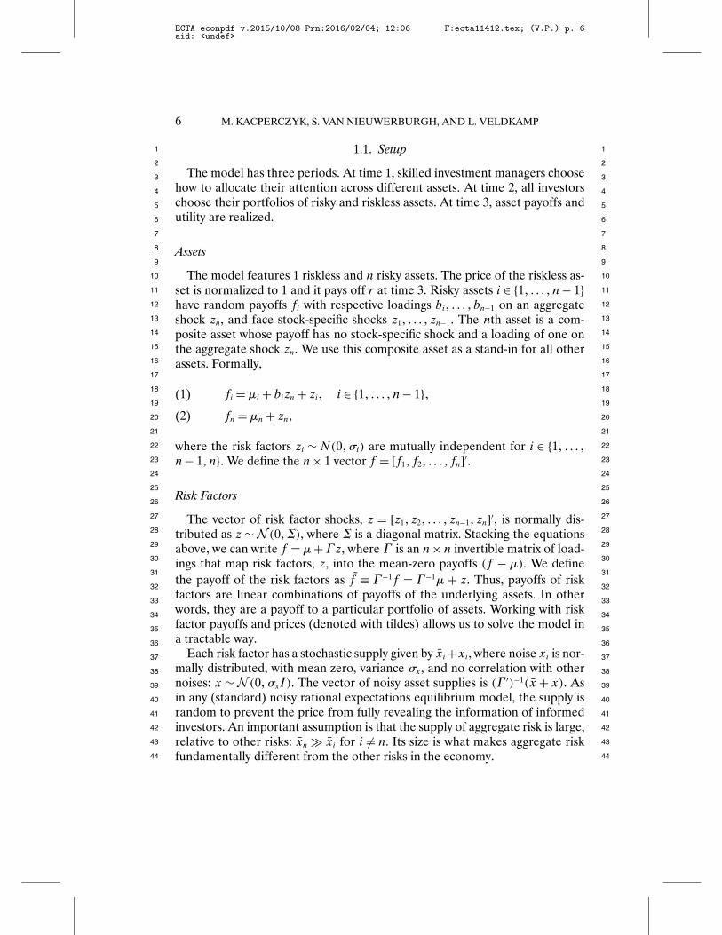
1.1. Setup
The model has three periods. At time 1, skilled investment managers choosehow to allocate their attention across different assets. At time 2, all investorschoose their portfolios of risky and riskless assets. At time 3, asset payoffs andutility are realized.
Assets
The model features 1 riskless and n risky assets. The price of the riskless as-set is normalized to 1 and it pays off r at time 3. Risky assets i ∈ {1� � � � � n− 1}have random payoffs fi with respective loadings bi� � � � � bn−1 on an aggregateshock zn, and face stock-specific shocks z1� � � � � zn−1. The nth asset is a com-posite asset whose payoff has no stock-specific shock and a loading of one onthe aggregate shock zn. We use this composite asset as a stand-in for all otherassets. Formally,
fi = μi + bizn + zi� i ∈ {1� � � � � n− 1}�(1)
fn = μn + zn�(2)
where the risk factors zi ∼ N(0�σi) are mutually independent for i ∈ {1� � � � �n− 1� n}. We define the n× 1 vector f = [f1� f2� � � � � fn]′.
Risk Factors
The vector of risk factor shocks, z = [z1� z2� � � � � zn−1� zn]′, is normally dis-tributed as z ∼ N (0�Σ), where Σ is a diagonal matrix. Stacking the equationsabove, we can write f = μ+ Γ z, where Γ is an n× n invertible matrix of load-ings that map risk factors, z, into the mean-zero payoffs (f − μ). We definethe payoff of the risk factors as f ≡ Γ −1f = Γ −1μ + z. Thus, payoffs of riskfactors are linear combinations of payoffs of the underlying assets. In otherwords, they are a payoff to a particular portfolio of assets. Working with riskfactor payoffs and prices (denoted with tildes) allows us to solve the model ina tractable way.
Each risk factor has a stochastic supply given by xi+xi, where noise xi is nor-mally distributed, with mean zero, variance σx, and no correlation with othernoises: x∼ N (0�σxI). The vector of noisy asset supplies is (Γ ′)−1(x+ x). Asin any (standard) noisy rational expectations equilibrium model, the supply israndom to prevent the price from fully revealing the information of informedinvestors. An important assumption is that the supply of aggregate risk is large,relative to other risks: xn � xi for i �= n. Its size is what makes aggregate riskfundamentally different from the other risks in the economy.
ECTA econpdf v.2015/10/08 Prn:2016/02/04; 12:06 F:ecta11412.tex; (V.P.) p. 6aid: <undef>
MUTUAL FUNDS’ ATTENTION ALLOCATION 7
1 1
2 2
3 3
4 4
5 5
6 6
7 7
8 8
9 9
10 10
11 11
12 12
13 13
14 14
15 15
16 16
17 17
18 18
19 19
20 20
21 21
22 22
23 23
24 24
25 25
26 26
27 27
28 28
29 29
30 30
31 31
32 32
33 33
34 34
35 35
36 36
37 37
38 38
39 39
40 40
41 41
42 42
43 43
44 44
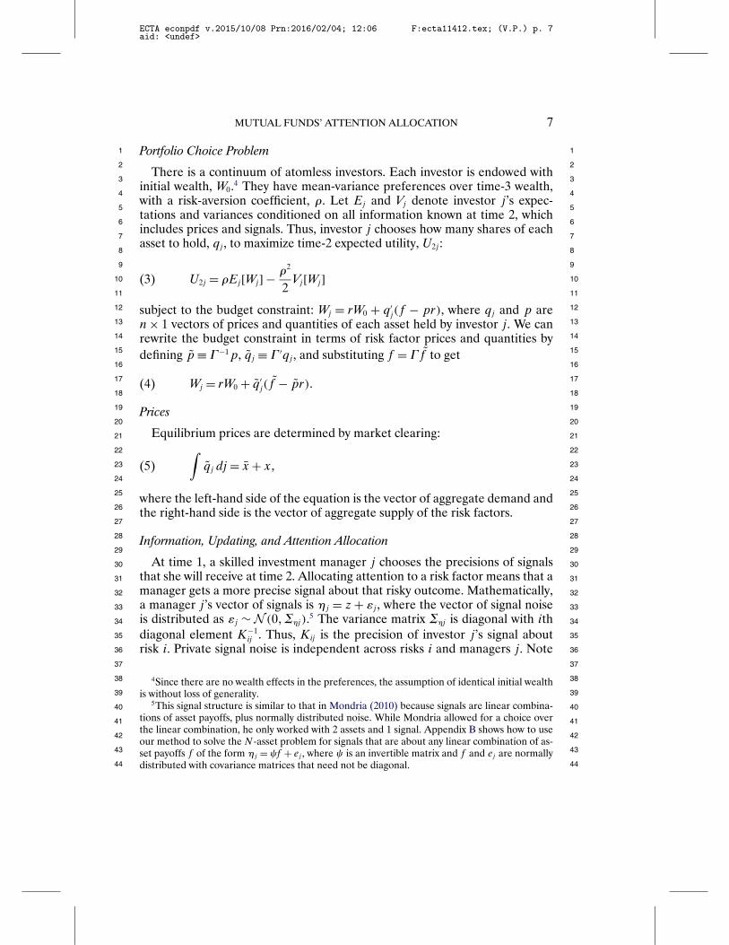
Portfolio Choice Problem
There is a continuum of atomless investors. Each investor is endowed withinitial wealth, W0.4 They have mean-variance preferences over time-3 wealth,with a risk-aversion coefficient, ρ. Let Ej and Vj denote investor j’s expec-tations and variances conditioned on all information known at time 2, whichincludes prices and signals. Thus, investor j chooses how many shares of eachasset to hold, qj , to maximize time-2 expected utility, U2j :
U2j = ρEj[Wj] − ρ2
2Vj[Wj](3)
subject to the budget constraint: Wj = rW0 + q′j(f − pr), where qj and p are
n× 1 vectors of prices and quantities of each asset held by investor j. We canrewrite the budget constraint in terms of risk factor prices and quantities bydefining p≡ Γ −1p, qj ≡ Γ ′qj , and substituting f = Γ f to get
Wj = rW0 + q′j(f − pr)�(4)
Prices
Equilibrium prices are determined by market clearing:∫qj dj = x+ x�(5)
where the left-hand side of the equation is the vector of aggregate demand andthe right-hand side is the vector of aggregate supply of the risk factors.
Information, Updating, and Attention Allocation
At time 1, a skilled investment manager j chooses the precisions of signalsthat she will receive at time 2. Allocating attention to a risk factor means that amanager gets a more precise signal about that risky outcome. Mathematically,a manager j’s vector of signals is ηj = z + εj , where the vector of signal noiseis distributed as εj ∼ N (0�Σηj).5 The variance matrix Σηj is diagonal with ithdiagonal element K−1
ij . Thus, Kij is the precision of investor j’s signal aboutrisk i. Private signal noise is independent across risks i and managers j. Note
4Since there are no wealth effects in the preferences, the assumption of identical initial wealthis without loss of generality.
5This signal structure is similar to that in Mondria (2010) because signals are linear combina-tions of asset payoffs, plus normally distributed noise. While Mondria allowed for a choice overthe linear combination, he only worked with 2 assets and 1 signal. Appendix B shows how to useour method to solve the N-asset problem for signals that are about any linear combination of as-set payoffs f of the form ηj =ψf + ej , where ψ is an invertible matrix and f and ej are normallydistributed with covariance matrices that need not be diagonal.
ECTA econpdf v.2015/10/08 Prn:2016/02/04; 12:06 F:ecta11412.tex; (V.P.) p. 7aid: <undef>

8 M. KACPERCZYK, S. VAN NIEUWERBURGH, AND L. VELDKAMP
1 1
2 2
3 3
4 4
5 5
6 6
7 7
8 8
9 9
10 10
11 11
12 12
13 13
14 14
15 15
16 16
17 17
18 18
19 19
20 20
21 21
22 22
23 23
24 24
25 25
26 26
27 27
28 28
29 29
30 30
31 31
32 32
33 33
34 34
35 35
36 36
37 37
38 38
39 39
40 40
41 41
42 42
43 43
44 44
that these signals are about asset payoffs and contain no direct informationabout asset supply x. Managers combine signal realizations with priors andinformation extracted from asset prices to update their beliefs, using Bayes’slaw.
Signal precision choices {Kij} maximize time-1 expected utility, U1j , of thefund’s terminal wealth Wj . The objective is −E[lnEj[exp(−ρWj)]], which isequivalent to maximizing
U1j =E[ρEj[Wj] − ρ2
2Vj[Wj]
]�(6)
subject to three constraints.6The first constraint is the budget constraint (4) that determinesWj as a func-
tion of investment decisions. The second constraint is information capacity con-straint. It states that the sum of the signal precisions must not exceed the infor-mation capacity:
n∑i=1
Kij ≤K�(7)
In Bayesian updating with normal variables, observing one signal with preci-sion Ki or two signals, each with precision Ki/2, is equivalent. Therefore, oneinterpretation of the capacity constraint is that it allows the manager to ob-serve N signal draws, each with precision Ki/N , for large N . The investmentmanager then chooses how many of those N signals will be about each shock.7Note that our model holds each manager’s total attention fixed and studies itsallocation in recessions and expansions. Section 1.8 relaxes this assumption.
The third constraint is the no-forgetting constraint, which ensures that thechosen precisions are nonnegative:
Kij ≥ 0� i ∈ {1� � � � � n− 1� n}�(8)
It prevents the manager from erasing any prior information, to make room togather new information about another shock.
6See Veldkamp (2011) for a discussion of the use of expected mean-variance utility in infor-mation choice problems. The Supplemental Material (Section S.2) proves versions of the mainpropositions for the expected exponential utility model.
7The results are not sensitive to the exact nature of the information capacity constraint. TheSupplemental Material (Section S.4) re-proves each one of our propositions for a model with anentropy constraint. The linear constraint (7) makes sense in our setting because additional fundanalysts can be hired to process information. Twice as many analysts could produce twice theprecision at twice the cost. To make information precision a continuous choice variable, let kδbe the precision of each analyst and let cδ be the cost of each analyst. Then take limδ→ 0. Thatproblem with a continuous, linear cost function is a dual problem to our constrained maximizationproblem.
ECTA econpdf v.2015/10/08 Prn:2016/02/04; 12:06 F:ecta11412.tex; (V.P.) p. 8aid: <undef>

MUTUAL FUNDS’ ATTENTION ALLOCATION 9
1 1
2 2
3 3
4 4
5 5
6 6
7 7
8 8
9 9
10 10
11 11
12 12
13 13
14 14
15 15
16 16
17 17
18 18
19 19
20 20
21 21
22 22
23 23
24 24
25 25
26 26
27 27
28 28
29 29
30 30
31 31
32 32
33 33
34 34
35 35
36 36
37 37
38 38
39 39
40 40
41 41
42 42
43 43
44 44
Skilled and Unskilled Investors
The only ex ante difference between investors is that a fraction χ of themhave skill, meaning that they can choose to observe a set of informative privatesignals about the risk factor shocks zi. Unskilled investors are ones with zerosignal precision: Σ−1
ηj = 0, or equivalently,Kij = 0, ∀i. Both unskilled and skilledinvestors observe the information in prices, which are public signals, costlessly.8
When we bring the model to the data, we will call all skilled investors mu-tual funds. Furthermore, we will distinguish between two types of unskilled in-vestors: unskilled mutual funds and non-fund investors.9 In the model, the lat-ter two types are identical. The reason for modeling non-fund investors is thatwithout them, we cannot talk about average fund performance. The sum of allfunds’ holdings would have to equal the market by market clearing, and there-fore, the average fund return would have to equal the market return. Withoutuninformed non-fund investors, the average fund could never systematicallyout-perform the market return, in recessions or expansions.
Modeling Recessions
Since this is a static model, the investment world is either in the recessionstate (R) or in the expansion state (E). The asset pricing literature identifiesthree principal effects of recessions: (1) returns are more volatile, (2) the priceof risk is high, and (3) returns are unexpectedly low. Section 3 discusses the em-pirical evidence supporting the first two effects. The third effect of recessions,unexpectedly low returns, cannot affect attention allocation because attentionmust be allocated before returns are observed. Therefore, we abstract fromit and consider only effects (1) and (2). To capture the return volatility effect(1) in the model, we assume that the prior variance of the aggregate shock inrecessions (R) is higher than the one in expansions (E): σn(R) > σn(E). Tocapture the varying price of risk (2), we vary the parameter that governs theprice of risk, which is risk aversion. We assume ρ(R) > ρ(E). We continueto use σn and ρ to denote aggregate shock variance and risk aversion in thecurrent business cycle state.
1.2. Equilibrium
This paper’s methodological innovation is that its model relaxes an impor-tant assumption. Previous work assumed that assets and signals have the sameprincipal components. Observing signals about aggregate and idiosyncraticshocks violates that assumption. Updating with such signals changes the con-ditional correlations of assets. So to solve the model, we perform a change
8If investors must expend capacity to learn from prices, the model predictions are unchanged.See Supplemental Material Section S.5.
9For our results to hold, it is sufficient to assume that the fraction of non-fund investors thatare unskilled is higher than that for the mutual funds.
ECTA econpdf v.2015/10/08 Prn:2016/02/04; 12:06 F:ecta11412.tex; (V.P.) p. 9aid: <undef>

10 M. KACPERCZYK, S. VAN NIEUWERBURGH, AND L. VELDKAMP
1 1
2 2
3 3
4 4
5 5
6 6
7 7
8 8
9 9
10 10
11 11
12 12
13 13
14 14
15 15
16 16
17 17
18 18
19 19
20 20
21 21
22 22
23 23
24 24
25 25
26 26
27 27
28 28
29 29
30 30
31 31
32 32
33 33
34 34
35 35
36 36
37 37
38 38
39 39
40 40
41 41
42 42
43 43
44 44
of variables. We create linear combinations of assets (synthetic assets) suchthat the payoff of each synthetic asset is determined only by one shock (eitheraggregate or idiosyncratic). Then, we can choose information about, choosequantities of, and price these synthetic assets easily because each asset’s pay-off is independent of all the others and each signal is informative about oneand only one asset. After we have a solution to the synthetic asset problem,we can invert the linear transformation to back out portfolios and prices of theoriginal assets.
We begin by working through the mechanics of Bayesian updating. Thereare three types of information that are aggregated in time-2 posteriors beliefs:prior beliefs, price information, and (private) signals. We conjecture and laterverify that a transformation of prices p generates an unbiased signal aboutthe risk factor payoffs, ηp = z + εp, where εp ∼ N(0�Σp), for some diagonalvariance matrix Σp. Then, by Bayes’s law, the posterior beliefs about z are nor-mally distributed with mean zj = Σj(Σ
−1ηj ηj + Σ−1
p ηp) and posterior precision
Σ−1j = Σ−1 +Σ−1
p +Σ−1ηj . Using the definition f = Γ −1μ+ z, we find that poste-
rior beliefs about risk factor payoffs are f ∼N(Ej[f ]� Σ−1j ), where
Ej[f ] = Γ −1μ+ Σj(Σ−1ηj ηj +Σ−1
p ηp)�(9)
Next, we solve the model in four steps.Step 1: Solve for the optimal portfolios, given information sets.Substituting the budget constraint (4) into the objective function (3) and
taking the first-order condition with respect to qj reveals that optimal holdingsare increasing in the investor’s risk tolerance, precision of beliefs, and expectedreturn:
qj = 1ρΣ−1j
(Ej[f ] − pr)�(10)
Step 2: Clear the asset market.Substitute each agent j’s optimal portfolio (10) into the market-clearing
condition (5). Collecting terms and simplifying reveals that equilibrium assetprices are linear in payoff risk shocks and in supply shocks:
LEMMA 1: p= 1r(A+Bz+Cx).
A detailed derivation of coefficients A, B, and C, expected utility, and theproofs of this lemma and all further propositions are in the Appendix.
In this model, agents learn from prices because prices are informative aboutthe payoff shocks z. Next, we deduce what information is implied by Lemma 1.Price information is the signal about z contained in prices. The transformationof the price vector p that yields an unbiased signal about z isηp ≡ B−1(pr−A).
ECTA econpdf v.2015/10/08 Prn:2016/02/04; 12:06 F:ecta11412.tex; (V.P.) p. 10aid: <undef>

MUTUAL FUNDS’ ATTENTION ALLOCATION 11
1 1
2 2
3 3
4 4
5 5
6 6
7 7
8 8
9 9
10 10
11 11
12 12
13 13
14 14
15 15
16 16
17 17
18 18
19 19
20 20
21 21
22 22
23 23
24 24
25 25
26 26
27 27
28 28
29 29
30 30
31 31
32 32
33 33
34 34
35 35
36 36
37 37
38 38
39 39
40 40
41 41
42 42
43 43
44 44
Note that applying the formula for ηp to Lemma 1 reveals that ηp = z + εp,where the signal noise in prices is εp = B−1Cx. Since we assume x∼N(0�σxI),the price noise is distributed εp ∼N(0�Σp), where Σp ≡ σxB−1CC ′B−1′. Substi-tuting in the coefficients B and C from the proof of Lemma 1 shows that public
signal precision Σ−1p is a diagonal matrix with ith diagonal element σ−1
pi = K2i
ρ2σx,
where Ki ≡∫Kij dj is the average capacity allocated to risk factor i.
Step 3: Compute ex ante expected utility.Substitute optimal risky asset holdings from equation (10) into the first-
period objective function (6) to get U1j = rW0 + 12E1[(Ej[f ] − pr)Σ−1
j (Ej[f ] −pr)]. Note that the expected excess return (Ej[f ]− pr) depends on signals andprices, both of which are unknown at time 1. Because asset prices are linearfunctions of normally distributed shocks, Ej[f ] − pr is normally distributed aswell. Thus, (Ej[f ] − pr)Σ−1
j (Ej[f ] − pr) is a non-central χ2-distributed vari-able. Computing its mean yields
U1j = rW0 + 12
trace(Σ−1j V1
[Ej[f ] − pr])(11)
+ 12E1
[Ej[f ] − pr]′
Σ−1j E1
[Ej[f ] − pr]�
Step 4: Solve for information choices.Note that in expected utility (11), the choice variablesKij enter only through
the posterior variance Σj and through V1[Ej[f ] − pr] = V1[f − pr] − Σj . Sincethere is a continuum of investors, and since V1[f − pr] and E1[Ej[f ] − pr] de-pend only on parameters and on aggregate information choices, each investortakes them as given.
Since Σ−1j and V1[Ej[f ] − pr] are both diagonal matrices and E1[Ej[f ] − pr]
is a vector, the last two terms of (11) are weighted sums of the diagonal ele-ments of Σ−1
j . Thus, (11) can be rewritten as U1j = rW0 + ∑i λiΣ
−1j (i� i)− n/2,
for positive coefficients λi. Since rW0 is a constant and Σ−1j (i� i) = Σ−1(i� i)+
Σ−1p (i� i)+Kij , the information choice problem is
maxK1j �����Knj
n∑i=1
λiKij + constant(12)
s.t.n∑i=1
Kij ≤K�(13)
where λi = σi[1 + (
ρ2σx + Ki
)σi
] + ρ2x2i σ
2i �(14)
ECTA econpdf v.2015/10/08 Prn:2016/02/04; 12:06 F:ecta11412.tex; (V.P.) p. 11aid: <undef>
12 M. KACPERCZYK, S. VAN NIEUWERBURGH, AND L. VELDKAMP
1 1
2 2
3 3
4 4
5 5
6 6
7 7
8 8
9 9
10 10
11 11
12 12
13 13
14 14
15 15
16 16
17 17
18 18
19 19
20 20
21 21
22 22
23 23
24 24
25 25
26 26
27 27
28 28
29 29
30 30
31 31
32 32
33 33
34 34
35 35
36 36
37 37
38 38
39 39
40 40
41 41
42 42
43 43
44 44
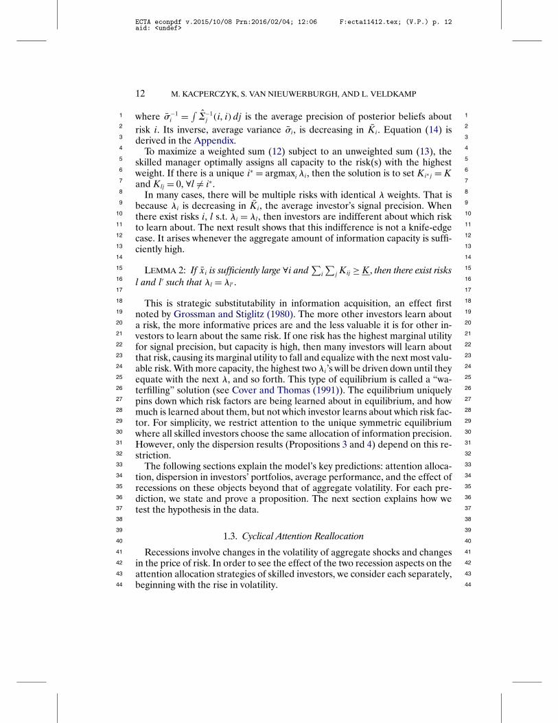
where σ−1i = ∫
Σ−1j (i� i)dj is the average precision of posterior beliefs about
risk i. Its inverse, average variance σi, is decreasing in Ki. Equation (14) isderived in the Appendix.
To maximize a weighted sum (12) subject to an unweighted sum (13), theskilled manager optimally assigns all capacity to the risk(s) with the highestweight. If there is a unique i∗ = argmaxi λi, then the solution is to set Ki∗j =Kand Klj = 0, ∀l �= i∗.
In many cases, there will be multiple risks with identical λ weights. That isbecause λi is decreasing in Ki, the average investor’s signal precision. Whenthere exist risks i, l s.t. λi = λl, then investors are indifferent about which riskto learn about. The next result shows that this indifference is not a knife-edgecase. It arises whenever the aggregate amount of information capacity is suffi-ciently high.
LEMMA 2: If xi is sufficiently large ∀i and∑
i
∑j Kij ≥K, then there exist risks
l and l′ such that λl = λl′ .This is strategic substitutability in information acquisition, an effect first
noted by Grossman and Stiglitz (1980). The more other investors learn abouta risk, the more informative prices are and the less valuable it is for other in-vestors to learn about the same risk. If one risk has the highest marginal utilityfor signal precision, but capacity is high, then many investors will learn aboutthat risk, causing its marginal utility to fall and equalize with the next most valu-able risk. With more capacity, the highest two λi’s will be driven down until theyequate with the next λ, and so forth. This type of equilibrium is called a “wa-terfilling” solution (see Cover and Thomas (1991)). The equilibrium uniquelypins down which risk factors are being learned about in equilibrium, and howmuch is learned about them, but not which investor learns about which risk fac-tor. For simplicity, we restrict attention to the unique symmetric equilibriumwhere all skilled investors choose the same allocation of information precision.However, only the dispersion results (Propositions 3 and 4) depend on this re-striction.
The following sections explain the model’s key predictions: attention alloca-tion, dispersion in investors’ portfolios, average performance, and the effect ofrecessions on these objects beyond that of aggregate volatility. For each pre-diction, we state and prove a proposition. The next section explains how wetest the hypothesis in the data.
1.3. Cyclical Attention Reallocation
Recessions involve changes in the volatility of aggregate shocks and changesin the price of risk. In order to see the effect of the two recession aspects on theattention allocation strategies of skilled investors, we consider each separately,beginning with the rise in volatility.
ECTA econpdf v.2015/10/08 Prn:2016/02/04; 12:06 F:ecta11412.tex; (V.P.) p. 12aid: <undef>

MUTUAL FUNDS’ ATTENTION ALLOCATION 13
1 1
2 2
3 3
4 4
5 5
6 6
7 7
8 8
9 9
10 10
11 11
12 12
13 13
14 14
15 15
16 16
17 17
18 18
19 19
20 20
21 21
22 22
23 23
24 24
25 25
26 26
27 27
28 28
29 29
30 30
31 31
32 32
33 33
34 34
35 35
36 36
37 37
38 38
39 39
40 40
41 41
42 42
43 43
44 44
PROPOSITION 1: For each skilled investor j, the optimal attention allocationfor risk i (Kij) is weakly increasing in its variance σi.
The proof of this and subsequent propositions are in the Appendix.The result tells us that investors prefer to learn more about any shock that
has a high prior payoff variance. Information is most valuable about the mostuncertain outcomes. The shift of attention to aggregate risk in recessions isjust one application of this proposition, but it is the empirically relevant case.Since recessions are times when aggregate volatility increases (while idiosyn-cratic volatilities do not), it is a time when aggregate shocks are relatively morevaluable to learn about. The converse is true in expansions.
The proposition takes into account not only the effect of a marginal increaseof variance on the marginal value of learning about a risk, and hence on thecapacity allocated to that risk, but also the offsetting equilibrium effect. In anyinterior equilibrium, attention is reallocated until the marginal values of learn-ing about any risks that are learned about are equalized. Thus, when σn rises inrecessions, the marginal value of learning more about the aggregate risk rises,more attention is allocated to the aggregate risk, which offsets the increase inmarginal value until indifference in the marginal values across risk factors is re-stored. The net result is always a weakly increasing capacity devoted to the riskwhose variance increases. As the proof shows, the “weakly” increasing refersto the cases where either all capacity is already allocated to the risk whose vari-ance increases or no capacity is allocated to that risk and the marginal increasein variance does not change that. In all other cases, when risk i is one of therisks being learned about prior to the increase in σi, the increase in capacitydevoted to i is strict.
Next, we consider the effect of an increase in the price of risk. An increase inthe price of risk induces managers to allocate even more attention to the shockthat is in the most abundant supply. We have assumed that the aggregate riskis the most abundant. The additional price of risk effect should show up asan effect of recessions on attention allocation, over and above what aggregatevolatility alone can explain. The parameter that governs the price of risk inour model is risk aversion. The following result implies that an increase inrisk aversion in recessions is an independent force driving the reallocation ofattention from stock-specific to aggregate shocks.
PROPOSITION 2: If xi is sufficiently large, then, for each skilled investor j, theoptimal attention allocation for risk i (Kij) is weakly increasing in risk aversion ρ.
The intuition for this result rests on the fact that a shock in abundant sup-ply affects a large fraction of the value of an investor’s portfolio. Therefore,a marginal reduction in the uncertainty about this shock reduces total portfo-lio risk by more than the same-sized reduction in the uncertainty about a lessabundant shock. In other words, learning about the abundant shock, which
ECTA econpdf v.2015/10/08 Prn:2016/02/04; 12:06 F:ecta11412.tex; (V.P.) p. 13aid: <undef>

14 M. KACPERCZYK, S. VAN NIEUWERBURGH, AND L. VELDKAMP
1 1
2 2
3 3
4 4
5 5
6 6
7 7
8 8
9 9
10 10
11 11
12 12
13 13
14 14
15 15
16 16
17 17
18 18
19 19
20 20
21 21
22 22
23 23
24 24
25 25
26 26
27 27
28 28
29 29
30 30
31 31
32 32
33 33
34 34
35 35
36 36
37 37
38 38
39 39
40 40
41 41
42 42
43 43
44 44
is the aggregate shock, is the most efficient way to reduce portfolio risk. Themore risk averse an agent is, the more attractive allocating attention to aggre-gate shocks becomes. Like the previous one, this result takes into account theequilibrium reallocation of capacity after the increase in risk aversion.
These results are robust to many model changes. In the Supplemental Mate-rial, we examine versions of the model in which agents learn about the payoffsof assets, rather than about risks directly (Section S.3) and in which informa-tion choices are governed by an entropy constraint rather than a linear capacityconstraint (Section S.4). Both of our attention allocation results hold in thesesettings. When the aggregate shock variance rises or risk aversion increases,agents pay more attention to assets whose returns are most sensitive to aggre-gate shocks.
Investors’ optimal attention allocation decisions are reflected in their port-folio holdings. In recessions, skilled investors predominantly allocate attentionto the aggregate payoff shock, zn. They use the information they observe toform a portfolio that covaries with zn. In times when they learn that zn willbe high, they hold more risky assets whose returns are increasing in zn. Thispositive covariance can be seen from equation (10) in which q is increasing inEj[f ] and from equation (9) in which Ej[f ] is increasing in ηj , which is furtherincreasing in zn. The positive covariances between the aggregate shock andfunds’ portfolio holdings in recessions, on the one hand, and between stock-specific shocks and the portfolio holdings in expansions, on the other hand,directly follow from optimal attention allocation decisions switching over thebusiness cycle. As such, these covariances are the key moments that enable usto test the attention allocation predictions of the model. We define the empir-ical counterparts to these covariances in Section 2.
1.4. Portfolio Dispersion
Since many empirical studies on investment managers detect no outper-formance, perhaps the most controversial implication of the attention real-location result is that investment managers are processing information at all.The next four results speak directly to that implication. They do not identifychanges in attention allocation, but they help to distinguish our theory fromnon-information-based alternative explanations for mutual fund performancepatterns.
In recessions, as aggregate shocks become more volatile, the firm-specificshocks to assets’ payoffs account for less of the variation, and the comovementin stock payoffs rises. Since asset payoffs comove more, the payoffs to all pas-sive investment strategies that put fixed weights on assets also comove more.Dispersion across investor portfolios and portfolio returns would fall if invest-ment strategies were passive. But when investment managers are processinginformation and actively investing based on that information, this prediction
ECTA econpdf v.2015/10/08 Prn:2016/02/04; 12:06 F:ecta11412.tex; (V.P.) p. 14aid: <undef>

MUTUAL FUNDS’ ATTENTION ALLOCATION 15
1 1
2 2
3 3
4 4
5 5
6 6
7 7
8 8
9 9
10 10
11 11
12 12
13 13
14 14
15 15
16 16
17 17
18 18
19 19
20 20
21 21
22 22
23 23
24 24
25 25
26 26
27 27
28 28
29 29
30 30
31 31
32 32
33 33
34 34
35 35
36 36
37 37
38 38
39 39
40 40
41 41
42 42
43 43
44 44
is reversed. To see why, consider a simple example in which there is no learn-ing from prices. A skilled agent is updating beliefs about a random variablef ∼N(μ�Σ), using a signal ηj|f ∼N(f �Ση). Bayes’s law says that the poste-rior mean is a weighted average of the prior mean μ and the signal, where eachis weighted by their relative precision:
E[f |ηj] = (Σ−1 +Σ−1
η
)−1(Σ−1μ+Σ−1
η ηj)�(15)
If, in recessions, aggregate shock variance σn rises, then the prior beliefs aboutasset payoffs become more uncertain: Σ rises and Σ−1 falls. This makes theweight on prior beliefs μ decrease and the weight on the signal ηj increase.The prior μ is common across agents, while the signal realization ηj is hetero-geneous. When informed managers weigh their heterogeneous signals more,their resulting posterior beliefs become more different from each other andmore different from the beliefs of uninformed managers or investors. Moredisagreement about asset payoffs results in more heterogeneous portfolios andportfolio returns. Since price signals are also common, the same result holdsonce they are incorporated. The feature of the model that underpins this resultis the idiosyncratic component of signal noise. We could allow signal noise tobe correlated across agents, as long as signals are not identical. Such idiosyn-cratic signal noise is inherent in the idea of rational inattention.
Thus, the model’s second set of predictions are that in recessions, the cross-sectional dispersion in funds’ investment strategies and returns should rise.
PROPOSITION 3: If xi is sufficiently large, then an increase in variance σiweakly increases (a) the dispersion of fund portfolios,
∫E[(qj − ¯q)′(qj − ¯q)]dj,
and (b) the dispersion of portfolio excess returns,∫E[((qj − ¯q)′(f − pr))2]dj.
This result takes into account that when variance of a shock changes, theequilibrium allocation of attention and equilibrium asset returns change aswell. While this is a generic result for any risk i, the effect is particularly largefor the aggregate risk because it affects every asset and therefore it is in abun-dant supply. This shows up in the proof as a high xn, which amplifies the effectof σn on portfolio and return dispersion.
Next, we consider the second effect of recessions: an increase in the priceof risk. The following result shows that, when prices are sufficiently noisy, anincrease in the price of risk increases the dispersion of portfolio returns.
PROPOSITION 4: If σx and xn are sufficiently large, then an increase in riskaversion ρ increases the dispersion of portfolio excess returns,
∫E[((qj − ¯q)′(f −
pr))2]dj.When risk aversion rises, skilled investors make smaller bets on their infor-
mation. These smaller deviations from the market portfolio affect prices less
ECTA econpdf v.2015/10/08 Prn:2016/02/04; 12:06 F:ecta11412.tex; (V.P.) p. 15aid: <undef>

16 M. KACPERCZYK, S. VAN NIEUWERBURGH, AND L. VELDKAMP
1 1
2 2
3 3
4 4
5 5
6 6
7 7
8 8
9 9
10 10
11 11
12 12
13 13
14 14
15 15
16 16
17 17
18 18
19 19
20 20
21 21
22 22
23 23
24 24
25 25
26 26
27 27
28 28
29 29
30 30
31 31
32 32
33 33
34 34
35 35
36 36
37 37
38 38
39 39
40 40
41 41
42 42
43 43
44 44
and make prices less informative. The reduced precision of price informationimplies that agents weigh prices less and private signals more in their poste-rior beliefs. Just like priors, information in prices is common. Thus, weighingcommon signals less and heterogeneous private signals more leads to higherdispersion in beliefs and therefore in portfolio returns as well.
This effect has to offset a counteracting force. Recall that the optimal portfo-lio for investor j takes the form q= (1/ρ)Σ−1
j (f −pr). If ρ increases, investorsscale down their risky asset positions and q falls. The increase in returns needsto increase dispersion enough to offset the decrease in dispersion coming fromthe effect of 1/ρ reducing q. The proof of the proposition in the Appendixshows that a sufficient condition for the first effect to dominate is that theelasticity of V1[f − pr] with respect to ρ be greater than 1, which requires alarge enough asset supply variance. The high average supply of aggregate riskis what makes the nth risk aggregate. In addition to this result, we can sign theeffect of a change in risk aversion on the dispersion of risk-adjusted returns aswell, with looser conditions on parameters that produce stronger equilibriumeffects through aggregate attention reallocation. See Supplemental MaterialSection S.6 for a proof. In addition, our numerical example below confirmsthat portfolio dispersion increases in risk aversion, even in cases where ourparameter restrictions are not satisfied.
1.5. Fund Performance
To measure performance, we want to measure the portfolio return, adjustedfor risk. One risk adjustment that is both analytically tractable in our modeland often used in empirical work is the certainty equivalent return, which isalso an investor’s objective (6). The following proposition shows that abnormalportfolio returns, defined as the fund’s portfolio return, q′
j(f − pr), minus the
market return, ¯q′(f − pr), for skilled funds exceeds that for unskilled funds
and non-fund investors by more when volatility is higher.
PROPOSITION 5: If xi is sufficiently large, then, for each skilled investor j, anincrease in the variance σi weakly increases the portfolio excess return, E[(qj −¯q)′(f − pr)].
Because aggregate risk factor payoffs are more uncertain in recessions (σnis higher), recessions are times when information is more valuable. The returneffect is larger for the aggregate shock because it depends on how abundantthe risk is (xn) and the aggregate shock is naturally the most abundant one.
Next, we consider the effect of an increase in the price of risk on perfor-mance.
ECTA econpdf v.2015/10/08 Prn:2016/02/04; 12:06 F:ecta11412.tex; (V.P.) p. 16aid: <undef>

MUTUAL FUNDS’ ATTENTION ALLOCATION 17
1 1
2 2
3 3
4 4
5 5
6 6
7 7
8 8
9 9
10 10
11 11
12 12
13 13
14 14
15 15
16 16
17 17
18 18
19 19
20 20
21 21
22 22
23 23
24 24
25 25
26 26
27 27
28 28
29 29
30 30
31 31
32 32
33 33
34 34
35 35
36 36
37 37
38 38
39 39
40 40
41 41
42 42
43 43
44 44
PROPOSITION 6: If σx and xn are sufficiently large, then, for each skilled in-vestor j, an increase in risk aversion ρ increases excess return, E[(qj − ¯q)′(f −pr)].
The reason why a higher price of risk leads to higher performance is thatinformation can resolve risk. Therefore, informed managers are compensatedfor risk that they do not bear because the information has resolved some oftheir uncertainty about random asset payoffs. When the price of risk rises, thevalue of being able to resolve this risk rises as well. Put differently, informedfunds take larger positions in risky assets because they are less uncertain abouttheir returns. These larger positions pay off more on average when the price ofrisk is high.
The role of the high σx and xn is the same as in Proposition 4. And just likefor Proposition 4, we can prove that risk-adjusted returns rise with looser pa-rameter conditions. See Supplemental Material Section S.6. In addition, ournumerical example confirms that when the price of risk increases, average per-formance of informed funds rises, for a wide range of parameter values.
Taken together, these results provide two reasons why skilled investors’ ad-vantage over unskilled investors increases in recessions. Of course, the modelpredicts that skilled investors should always outperform unskilled. In practice,this outperformance is difficult to detect. The model helps to guide the searchfor skill by explaining why one ought to focus on recessions as times when skillshould be particularly salient.
Measuring Performance: Mapping Skill Into Alpha
The previous outperformance results were for abnormal fund returns, mea-sured as the fund’s return minus the market return. One other way to risk-adjust fund returns, which is common in the empirical literature, is to estimatea Capital Asset Pricing Model (CAPM) using each fund’s returns and look atthe fund’s α, the intercept of the Security Market Line. This CAPM is esti-mated using only information that is in every investor’s information set, whichis the unconditional moments of asset returns. The following result shows thatif one constructs such an unconditional CAPM from the fund returns in ourmodel, the fund α captures information capacity K (skill) and rises in reces-sions.
PROPOSITION 7: If the net supply of idiosyncratic risk is small, then expectedexcess portfolio return of fund j is E[Rj] − r = αj + βj(E[rm] − r), where αj =∑
i 1/ρ(var[fi](σ−1i +Kij)− 1)− ρij .
The model tells us that the CAPM alpha of a fund’s return is increasing inits ability to process information about each type of risk. But the alpha alsovaries over the cycle as aggregate risk changes. In recessions, aggregate risk
ECTA econpdf v.2015/10/08 Prn:2016/02/04; 12:06 F:ecta11412.tex; (V.P.) p. 17aid: <undef>

18 M. KACPERCZYK, S. VAN NIEUWERBURGH, AND L. VELDKAMP
1 1
2 2
3 3
4 4
5 5
6 6
7 7
8 8
9 9
10 10
11 11
12 12
13 13
14 14
15 15
16 16
17 17
18 18
19 19
20 20
21 21
22 22
23 23
24 24
25 25
26 26
27 27
28 28
29 29
30 30
31 31
32 32
33 33
34 34
35 35
36 36
37 37
38 38
39 39
40 40
41 41
42 42
43 43
44 44
(σn) increases, which increases αj . As in Hansen and Richard (1987), the un-conditional CAPM correctly prices all portfolios constructed using only thecommon information set and assigns them zero alpha. But when skilled in-vestors, who have a richer information set, construct portfolios, the portfolioswill lie on a different mean-variance frontier and thus achieve a higher alpha.
1.6. Who Underperforms?
The requirement that markets clear implies that not all investors can besuccessful at investing in the right stock at the right time (stock-picking) orat timing the aggregate market fluctuations. In each period, someone mustmake poor stock-picking or market-timing decisions if someone else makesprofitable decisions. We explain now why rational, unskilled investors under-perform in equilibrium.
In recessions, unskilled investors have negative timing ability. When the ag-gregate state zn is low, most skilled investors sell, pushing down asset prices,p, and making prior expected returns high. The high expected return (high(μ − pr)) causes uninformed investors to demand more of the asset (equa-tion (10)). The unskilled demand more because they cannot distinguish lowprices that arise because of information from those that arise from positiveasset supply shocks. Thus, unskilled investors’ holdings covary negatively withaggregate payoffs, making their market-timing measure negative. Since no in-vestors learn about the aggregate shock in expansions, prices do not fall whenunexpected aggregate shocks are negative and market timing is close to zerofor both skilled and unskilled.
Likewise, unskilled investors exhibit negative stock-picking ability in expan-sions. When the stock-specific shock zi is low, and some investors know this,they sell and depress the price of asset i. A low price raises the expected re-turn (μi − pir). The high expected return induces unskilled investors to buymore of the asset. Since they buy more of assets that subsequently have neg-ative asset-specific payoff shocks, these uninformed investors display negativestock-picking ability.
Note that when there is a positive aggregate supply shock, prices will belower (Lemma 1), and assets will look more attractive to both uninformed andinformed agents, all else equal. In that case, both informed and uninformedcan trade in the same direction because of the additional asset supply.
1.7. Interaction Effects
The previous results describe the effects of aggregate risk and risk aversionseparately. But there is also a subtle interaction between the two. Higher riskaversion amplifies the effect of aggregate risk on attention allocation, disper-sion, and performance. The resulting testable prediction is that the effect of
ECTA econpdf v.2015/10/08 Prn:2016/02/04; 12:06 F:ecta11412.tex; (V.P.) p. 18aid: <undef>

MUTUAL FUNDS’ ATTENTION ALLOCATION 19
1 1
2 2
3 3
4 4
5 5
6 6
7 7
8 8
9 9
10 10
11 11
12 12
13 13
14 14
15 15
16 16
17 17
18 18
19 19
20 20
21 21
22 22
23 23
24 24
25 25
26 26
27 27
28 28
29 29
30 30
31 31
32 32
33 33
34 34
35 35
36 36
37 37
38 38
39 39
40 40
41 41
42 42
43 43
44 44
aggregate volatility on all three outcome variables should be greater in reces-sions, when the market price of risk is high. We derive these results in theSupplemental Material (Section S.7).
1.8. Endogenous Capacity Choice
So far, we have assumed that skilled investment managers choose how toallocate a fixed information-processing capacity, K. We now extend the modelto allow for skilled managers to add capacity at a cost C(K). We model thiscost as a utility penalty, akin to the disutility from labor in business cycle mod-els. Since there are no wealth effects in our setting, it would be equivalentto modeling a cost of capacity through the budget constraint. We draw threemain conclusions. First, the proofs of Propositions 1 and 2 hold for any cho-sen level of capacity K, below an upper bound, no matter the functional formof C. The other propositions also continue to hold because they only dependon the attention reallocation effects proven in Propositions 1 and 2. Endoge-nous capacity only has quantitative, not qualitative, implications. Second, be-cause the marginal utility of learning about the aggregate shock is increasingin its prior variance (Proposition 1), skilled managers choose to acquire highercapacity in recessions. This extensive-margin effect amplifies our dispersionand performance results. Third, the degree of amplification depends on theconvexity of the cost function, C(K). The convexity determines how elasticequilibrium capacity choice is to the cyclical changes in the marginal benefitof learning. The Supplemental Material discusses numerical simulation resultsfrom an endogenous-K model; they are similar to our benchmark results.
2. BRINGING THE MODEL TO DATA
To test the model, we look at various measures of mutual fund investmentsin recessions and in non-recession periods. Of course, our model is not a dy-namic one. It could be. A simple dynamic model would amount to a successionof static models that are either in the expansion or in the recession state. Aswe stated in the model setup, a recession state would be one in which aggre-gate risk and the price of risk are both high. Aggregate risk is captured bythe variance parameter σa. We capture changes in the price of risk by vary-ing risk aversion ρ. A variety of economic mechanisms can generate this kindof time-varying price of risk: external habits, heterogeneous labor income riskand limited commitment, borrowing constraints, or a concern for model mis-specification (see Hansen (2013)). Since these mechanisms are too complex toembed in our model, we settle for varying a risk aversion parameter.
Propositions 1 and 2 teach us that both the increased aggregate shock vari-ances and the increased price of risk prompt attention reallocation toward ag-gregate risk. Thus, the prediction is that in recessions, the average amount ofattention devoted to aggregate shocks should increase and the average amount
ECTA econpdf v.2015/10/08 Prn:2016/02/04; 12:06 F:ecta11412.tex; (V.P.) p. 19aid: <undef>

20 M. KACPERCZYK, S. VAN NIEUWERBURGH, AND L. VELDKAMP
1 1
2 2
3 3
4 4
5 5
6 6
7 7
8 8
9 9
10 10
11 11
12 12
13 13
14 14
15 15
16 16
17 17
18 18
19 19
20 20
21 21
22 22
23 23
24 24
25 25
26 26
27 27
28 28
29 29
30 30
31 31
32 32
33 33
34 34
35 35
36 36
37 37
38 38
39 39
40 40
41 41
42 42
43 43
44 44
of attention devoted to stock-specific shocks should decrease. But of course,attention is not directly observable. Learning about a shock allows managersto choose portfolio holdings that covary more with that shock. We see this inthe portfolio first-order condition (10). A manager who knows nothing abouta shock cannot possibly hold a portfolio that covaries with the shock. It is not afeasible or measurable strategy. This covariance argument, combined with thereallocation results, leads us to make the first testable prediction:
PREDICTION 1: In recessions, portfolios should covary more with the ag-gregate component of payoffs. Conversely, in expansions, portfolio holdingsshould covary more with stock-specific payoff shocks.
Because recessions are times of high aggregate risk and high risk prices, andboth forces increase dispersion (Propositions 3 and 4), we make the next em-pirical prediction:
PREDICTION 2: In recessions, the dispersion of fund portfolios should rise.
Finally, both more aggregate risk and the higher price of risk cause skilledfunds Q2to generate higher returns (Propositions 5 and 6). The skill of these fundsshould be reflected in their portfolios’ α, which increases in σn (Proposition 7).Since fund managers are skilled or unskilled, while other investors are only un-skilled, an increase in the skill premium implies that the average mutual fund’sexcess return rises in recessions. Together, these findings lead us to make thefollowing empirical prediction:
PREDICTION 3: In recessions, the average fund should earn a higher excessreturn and have a higher alpha.
Next, we introduce the empirical measures that we use in Section 3 to testeach of these predictions.
2.1. Market-Timing and Stock-Picking Measures
We define a fund’s fundamentals-based timing ability, Ftiming, as the co-variance between its portfolio weights in deviation from the market portfolioweights, wj
i −wmi , and the aggregate payoff shock, zn, over a T -period horizon,
averaged across assets:
Ftimingjt =1TNj
Nj∑i=1
T−1∑τ=0
(wjit+τ −wm
it+τ)(bizn(t+τ+1))�(16)
where Nj is the number of individual assets held by fund j. The portfolioweights are dated t + τ because they are chosen and thus known at t + τ. The
ECTA econpdf v.2015/10/08 Prn:2016/02/04; 12:06 F:ecta11412.tex; (V.P.) p. 20aid: <undef>

MUTUAL FUNDS’ ATTENTION ALLOCATION 21
1 1
2 2
3 3
4 4
5 5
6 6
7 7
8 8
9 9
10 10
11 11
12 12
13 13
14 14
15 15
16 16
17 17
18 18
19 19
20 20
21 21
22 22
23 23
24 24
25 25
26 26
27 27
28 28
29 29
30 30
31 31
32 32
33 33
34 34
35 35
36 36
37 37
38 38
39 39
40 40
41 41
42 42
43 43
44 44
aggregate shock that affects the payoff of that portfolio is dated t + τ + 1 be-cause that shock is not fully observed until one period later. Relative to themarket, a fund with a high Ftiming overweights assets that have high (low) sen-sitivity to the aggregate shock in anticipation of a positive (negative) aggregateshock realization and underweights assets with a low (high) sensitivity.
When skilled investment managers allocate attention to stock-specific payoffshocks, zi, i ∈ {1� � � � � n− 1}, information about zi allows them to choose port-folios that covary with zi. Fundamentals-based stock-picking ability, Fpicking,measures the covariance of a fund’s portfolio weights of each stock, relative tothe market, with the stock-specific shock, zi:
Fpickingjt =1Nj
Nj∑i=1
(wjit −wm
it
)(zit+1)�(17)
How well can the manager choose portfolio weights in anticipation of futureasset-specific payoff shocks is closely linked to her stock-picking ability.
Ftiming and Fpicking are closely related to commonly used market-timingand stock-picking variables, which measure how a fund’s holdings of each as-set, relative to the market, covary with the systematic and idiosyncratic com-ponents of the stock return. The key difference is that we measure how aportfolio covaries with aggregate and firm-specific fundamentals. We use thefundamentals-based measures because they correspond more closely to theidea in the model that funds are learning about fundamentals and using signalsabout those fundamentals to time the market and pick stocks. The returns-based picking and timing facts might be explained by managers who forecastsentiment, momentum, liquidity, etc. Also, since funds affect asset values, butdo not directly affect earnings or production, the returns-based covariancecan come from some reverse causality. The fundamentals-based results makeit clear that the changing covariance between portfolios and returns comesfrom the covariance with one-quarter-ahead fundamentals. That offers a muchclearer view of what information fund managers are collecting and processing.It also significantly narrows down the set of possible explanations consistentwith the covariance facts.
2.2. Dispersion Measures
To connect the propositions to the data, we measure portfolio dispersion asthe sum of squared deviations of fund j’s portfolio weight in asset i at time t,wjit , from the average fund’s portfolio weight in asset i at time t, wm
it , summedover all assets held by fund j, Nj :
Portfolio Dispersionjt =Nj∑i=1
(wjit −wm
it
)2�(18)
ECTA econpdf v.2015/10/08 Prn:2016/02/04; 12:06 F:ecta11412.tex; (V.P.) p. 21aid: <undef>

22 M. KACPERCZYK, S. VAN NIEUWERBURGH, AND L. VELDKAMP
1 1
2 2
3 3
4 4
5 5
6 6
7 7
8 8
9 9
10 10
11 11
12 12
13 13
14 14
15 15
16 16
17 17
18 18
19 19
20 20
21 21
22 22
23 23
24 24
25 25
26 26
27 27
28 28
29 29
30 30
31 31
32 32
33 33
34 34
35 35
36 36
37 37
38 38
39 39
40 40
41 41
42 42
43 43
44 44
This measure is similar to the portfolio concentration measure in Kacperczyk,Sialm, and Zheng (2005) and the active share measure in Cremers and Peta-jisto (2009). The average dispersion
∫Portfolio Dispersionjt dj is the same quan-
tity as in Proposition 3, except that the number of shares q is replaced withportfolio weights w. In recessions, the portfolios of the informed managersdiffer more from each other and more from those of the uninformed investors.Part of this difference comes from a change in the composition of the riskyasset portfolio and part comes from differences in the fraction of assets heldin riskless securities. Fund j’s portfolio weight wj
it is a fraction of the fund’s as-sets, including both risky and riskless, held in asset i. Thus, when one informedfund gets a bearish signal about the market, its wj
it for all risky assets i falls.Dispersion can rise when funds take different positions in the risk-free asset,even if the fractional allocation among the risky assets remains identical.
The higher dispersion across funds’ portfolio strategies translates into ahigher cross-sectional dispersion in fund abnormal returns (Rj − Rm). To fa-cilitate comparison with the data, we define the dispersion of variable X as|Xj −X|, where X denotes the equally weighted cross-sectional average acrossall fund managers (excluding non-fund investors).
When funds get signals about the aggregate state zn that are heterogeneous,they take different directional bets on the market. Some funds tilt their portfo-lios to high-beta assets and other funds to low-beta assets, thus creating disper-sion in fund betas. To look for evidence of this mechanism, we form a CAPMregression for fund j and test for an increase in the beta dispersion in reces-sions as well.
We measure outperformance by looking at abnormal fund returns, measuredas the fund’s return minus the market return, and several risk-adjusted returns.One way to do that risk adjustment is to estimate a CAPM for each fund’s re-turn and look at the fund α. Proposition 7 shows that the alpha of a CAPMregression of fund returns on market returns should capture a fund’s total in-formation capacity, or skill. As a robustness check, we also compute the α frommodels with multiple risk factors that are common in the empirical literature,with the proviso that these additional risk factors are not present in our model.
3. EVIDENCE FROM EQUITY MUTUAL FUNDS
Our model studies attention allocation over the business cycle, and its con-sequences for investors’ strategies. We now turn to a specific set of investors,active U.S. equity mutual fund managers, to test the predictions of the model.The richness of the data makes the mutual fund industry a great laboratoryfor these tests. In principle, similar tests could be conducted for hedge funds,real estate investment trusts, other professional investment managers, or evenindividual investors.
ECTA econpdf v.2015/10/08 Prn:2016/02/04; 12:06 F:ecta11412.tex; (V.P.) p. 22aid: <undef>

MUTUAL FUNDS’ ATTENTION ALLOCATION 23
1 1
2 2
3 3
4 4
5 5
6 6
7 7
8 8
9 9
10 10
11 11
12 12
13 13
14 14
15 15
16 16
17 17
18 18
19 19
20 20
21 21
22 22
23 23
24 24
25 25
26 26
27 27
28 28
29 29
30 30
31 31
32 32
33 33
34 34
35 35
36 36
37 37
38 38
39 39
40 40
41 41
42 42
43 43
44 44
3.1. Data
Our sample builds upon several data sets. We begin with the Center for Re-search on Security Prices (CRSP) survivorship bias-free mutual fund database.The CRSP database provides comprehensive information about fund returnsand a host of other fund characteristics, such as size (total net assets), age,expense ratio, turnover, and load. Given the nature of our tests and data avail-ability, we focus on actively managed open-end U.S. equity mutual funds. Wefurther merge the CRSP data with fund holdings data from Thomson Finan-cial. The total number of funds in our merged sample is 3477.10 We also usethe CRSP/Compustat stock-level database, which is a source of informationon individual stocks’ returns, market capitalizations, book-to-market ratios,momentum, liquidity, and standardized unexpected earnings (SUE). The ag-gregate stock market return is the value-weighted average return of all stocksin the CRSP universe.
We use innovations in monthly seasonally adjusted industrial production,obtained from the Federal Reserve Statistical Release, as a proxy for aggregateshocks. We measure recessions using the definition of the National Bureauof Economic Research (NBER) business cycle dating committee. The start ofthe recession is the peak of economic activity and its end is the trough. Ouraggregate sample spans 312 months of data from January 1980 until December2005, among which 38 are NBER recession months (12%). We consider severalalternative recession indicators and find our results to be robust.11
3.2. Motivating Fact: Aggregate Risk and Prices of Risk Rise in Recessions
At the outset, we present empirical evidence for the main assumption in ourmodel: Recessions are periods in which individual stocks contain more aggre-gate risk and prices of risk are higher.
Table I shows that an average stock’s aggregate risk increases substantially inrecessions whereas the change in idiosyncratic risk is not statistically differentfrom zero. The table uses monthly returns for all stocks in the CRSP universe.For each stock and each month, we estimate a CAPM equation based on atwelve-month rolling-window regression, delivering the stock’s beta, βit , andits residual standard deviation, σiεt . We define the aggregate risk of stock i inmonth t as |βitσmt | and its idiosyncratic risk as σiεt , where σmt is formed monthlyas the realized volatility from daily return observations. Panel A reports the re-sults from a time-series regression of the aggregate risk (columns 1 and 2), theidiosyncratic risk (columns 3 and 4), and the ratio of aggregate to idiosyncraticrisk (columns 5 and 6), all averaged across stocks, on the NBER recession in-
10The unit of observation is a fund. In Supplemental Material Section S.10, we verify that ourresults are robust to using the manager as a unit of observation.
11Results are omitted for brevity but are available from the authors upon request.
ECTA econpdf v.2015/10/08 Prn:2016/02/04; 12:06 F:ecta11412.tex; (V.P.) p. 23aid: <undef>

24 M. KACPERCZYK, S. VAN NIEUWERBURGH, AND L. VELDKAMP
1 1
2 2
3 3
4 4
5 5
6 6
7 7
8 8
9 9
10 10
11 11
12 12
13 13
14 14
15 15
16 16
17 17
18 18
19 19
20 20
21 21
22 22
23 23
24 24
25 25
26 26
27 27
28 28
29 29
30 30
31 31
32 32
33 33
34 34
35 35
36 36
37 37
38 38
39 39
40 40
41 41
42 42
43 43
44 44
TABLE I
INDIVIDUAL STOCKS HAVE MORE AGGREGATE RISK IN RECESSIONSa
Aggregate Risk Idiosyncratic Risk Aggregate/Idiosyncratic Risk
(1) (2) (3) (4) (5) (6)
Panel A: Time-Series RegressionRecession 1.348 1.308 0.058 0.016 0.098 0.097
(0.693) (0.678) (1.018) (1.016) (0.027) (0.027)MKTPREM −4.034 −1.865 −0.215
(3.055) (3.043) (0.226)SMB 8.110 12.045 0.167
(3.780) (4.923) (0.199)HML 0.292 9.664 −0.308
(5.458) (8.150) (0.302)UMD −4.279 −1.112 −0.270
(2.349) (3.888) (0.178)Constant 6.694 6.748 13.229 13.196 0.508 0.513
(0.204) (0.212) (0.286) (0.276) (0.013) (0.014)
Observations 309 309 309 309 309 309R-squared 6.85 9.70 0.10 3.33 8.58 10.52
(Continues)
dicator variable. The aggregate risk is twenty percent higher in recessions thanit is in expansions (8.04% versus 6.69% per month), an economically and sta-tistically significant difference. In contrast, the stock’s idiosyncratic risk is notstatistically different in expansions and in recessions. As a result, the ratio ofaggregate to idiosyncratic risk increases from 0.508 in expansions to 0.606 inrecessions, and this cyclicality is driven exclusively by the numerator. The re-sults are similar whether one controls for other aggregate risk factors (columns2, 4, and 6) or not (columns 1, 3, and 5).
Panel B reports estimates from pooled (panel) regressions of each stock’saggregate risk (columns 1 and 2), idiosyncratic risk (columns 3 and 4), or theratio of aggregate to idiosyncratic risk (columns 5 and 6) on the recession in-dicator variable, Recession, and additional stock-specific control variables in-cluding size, book-to-market ratio, and leverage. The panel results confirm thetime-series findings.
A large literature in economics and finance presents evidence supporting theresults in Table I. First, Ang and Chen (2002), Ribeiro and Veronesi (2002),and Forbes and Rigobon (2002) documented that stocks exhibit more co-movement in recessions, consistent with stocks carrying higher systematic riskin recessions. In addition, Schwert (1989, 2011), Hamilton and Lin (1996),Campbell, Lettau, Malkiel, and Xu (2001), and Engle and Rangel (2008)showed that aggregate stock market return volatility is much higher during pe-riods of low economic activity. The evidence on the cyclicality of idiosyncratic
ECTA econpdf v.2015/10/08 Prn:2016/02/04; 12:06 F:ecta11412.tex; (V.P.) p. 24aid: <undef>
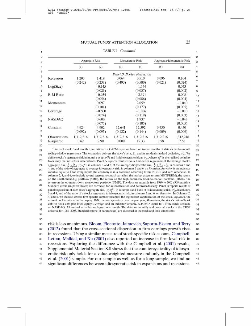
MUTUAL FUNDS’ ATTENTION ALLOCATION 25
1 1
2 2
3 3
4 4
5 5
6 6
7 7
8 8
9 9
10 10
11 11
12 12
13 13
14 14
15 15
16 16
17 17
18 18
19 19
20 20
21 21
22 22
23 23
24 24
25 25
26 26
27 27
28 28
29 29
30 30
31 31
32 32
33 33
34 34
35 35
36 36
37 37
38 38
39 39
40 40
41 41
42 42
43 43
44 44
TABLE I—Continued
Aggregate Risk Idiosyncratic Risk Aggregate/Idiosyncratic Risk
(1) (2) (3) (4) (5) (6)
Panel B: Pooled RegressionRecession 1.203 1.419 0.064 0.510 0.096 0.104
(0.242) (0.238) (0.493) (0.580) (0.021) (0.024)Log(Size) −0.145 −1.544 0.043
(0.021) (0.037) (0.002)B-M Ratio −0.934 −2.691 0.008
(0.056) (0.086) (0.004)Momentum 0.097 2.059 −0.040
(0.101) (0.177) (0.005)Leverage −0.600 −1.006 −0.010
(0.074) (0.119) (0.003)NASDAQ 0.600 1.937 −0.043
(0.075) (0.105) (0.005)Constant 4.924 4.902 12.641 12.592 0.450 0.450
(0.092) (0.095) (0.122) (0.144) (0.009) (0.009)
Observations 1,312,216 1,312,216 1,312,216 1,312,216 1,312,216 1,312,216R-squared 0.62 2.90 0.000 19.33 0.58 7.56
aFor each stock i and month t , we estimate a CAPM equation based on twelve months of data (a twelve-monthrolling-window regression). This estimation delivers the stock’s beta, βit , and its residual standard deviation, σiεt . Wedefine stock i’s aggregate risk in month t as |βitσmt | and its idiosyncratic risk as σiεt , where σmt is the realized volatilityfrom daily market return observations. Panel A reports results from a time-series regression of the average stock’saggregate risk, 1
N
∑Ni=1 |βitσmt |, in columns 1 and 2, of the average idiosyncratic risk, 1
N
∑Ni=1 σ
iεt , in columns 3 and
4, and of the ratio of aggregate to average idiosyncratic risk, in columns 5 and 6, on Recession. Recession is an indicatorvariable equal to 1 for every month the economy is in a recession according to the NBER, and zero otherwise. Incolumns 2, 4, and 6, we include several aggregate control variables: the market excess return (MKTPREM), the returnon the small-minus-big portfolio (SMB), the return on the high-minus-low book-to-market portfolio (HML), thereturn on the up-minus-down momentum portfolio (UMD). The data are monthly from 1980 to 2005 (309 months).Standard errors (in parentheses) are corrected for autocorrelation and heteroscedasticity. Panel B reports results ofpanel regressions of each stock’s aggregate risk, |βitσmt |, in columns 1 and 2 and of its idiosyncratic risk, σiεt , in columns3 and 4, and of the ratio of a stock’s aggregate to idiosyncratic risk, in columns 5 and 6, on Recession. In Columns 2,4, and 6, we include several firm-specific control variables: the log market capitalization of the stock, log(Size), theratio of book equity to market equity, B-M, the average return over the past year, Momentum, the stock’s ratio of bookdebt to book debt plus book equity, Leverage, and an indicator variable, NASDAQ, equal to 1 if the stock is tradedon NASDAQ. All control variables are lagged one month. The data are monthly and cover all stocks in the CRSPuniverse for 1980–2005. Standard errors (in parentheses) are clustered at the stock and time dimensions.
risk is less unanimous. Bloom, Floetotto, Jaimovich, Saporta-Eksten, and Terry(2012) found that the cross-sectional dispersion in firm earnings growth risesin recessions. Using a similar measure of stock-specific risk as ours, Campbell,Lettau, Malkiel, and Xu (2001) also reported an increase in firm-level risk inrecessions. Exploring the difference with the Campbell et al. (2001) results,Supplemental Material Section S.8 shows that the countercyclicality of idiosyn-cratic risk only holds for a value-weighted measure and only in the Campbellet al. (2001) sample. For our sample as well as for a long sample, we find nosignificant differences between idiosyncratic risk in expansions and recessions.
ECTA econpdf v.2015/10/08 Prn:2016/02/04; 12:06 F:ecta11412.tex; (V.P.) p. 25aid: <undef>

26 M. KACPERCZYK, S. VAN NIEUWERBURGH, AND L. VELDKAMP
1 1
2 2
3 3
4 4
5 5
6 6
7 7
8 8
9 9
10 10
11 11
12 12
13 13
14 14
15 15
16 16
17 17
18 18
19 19
20 20
21 21
22 22
23 23
24 24
25 25
26 26
27 27
28 28
29 29
30 30
31 31
32 32
33 33
34 34
35 35
36 36
37 37
38 38
39 39
40 40
41 41
42 42
43 43
44 44
Finally, we reiterate that what matters for our theoretical results is that ag-gregate risk rises by more than idiosyncratic risk in recessions, a conclusionsupported by the last two columns of Table I.
Our second assumption, that the price of risk rises in recessions, is supportedin four ways. First is an empirical literature that documents the countercyclicalnature of risk premia and Sharpe ratios on equity, bonds, options, and curren-cies.12 Second, a large theoretical literature has developed models that gen-erate such countercyclical market prices of risk (see Section 2). Third, Dew-Becker (2012) used the structure of his model to construct an empirical proxyfor risk aversion and showed it rises in recessions. Fourth, several papers showthat aggregate risk aversion rises in recessions because of properties of aggre-gation.13
3.3. Testing Predictions 1 and 2: Time-Varying Skill
Turning to our main model predictions, we first test whether skilled invest-ment managers reallocate their attention over the business cycle in a way thatis consistent with measures of time-varying skill. To estimate time-varying skill,we need measures of Ftiming and Fpicking for each fund j in each month t.We proxy for the aggregate payoff shock with the innovation in log industrialproduction growth, estimated from an AR(1).14 A time series of Ftimingjt isobtained by computing the covariance of the innovations and each fund j’sportfolio weights (as in equation (16)), using twelve-month rolling windows.Following equation (17), Fpicking is computed in each month t as a cross-sectional covariance across the assets between the fund’s portfolio weights andfirm-specific earnings shocks (SUE). We then estimate the following two equa-tions using pooled (panel) regression model and calculating standard errors byclustering at the fund and time dimensions:
Fpickingjt = a0 + a1Recessiont + a2Xjt + εjt �(19)
Ftimingjt = a3 + a4Recessiont + a5Xjt + εjt �(20)
12For example, Fama and French (1989), Cochrane (2006), Ludvigson and Ng (2009), Lettauand Ludvigson (2010), Lustig, Roussanov, and Verdelhan (2014), and the references therein.A related fact consistent with countercyclical market prices of risk is high corporate bond yieldsin recessions despite only modestly higher default rates; see Chen (2010).
13See Dumas (1989), Chan and Kogan (2002), and Garleanu and Panageas (2015), among oth-ers. In these models, heterogeneous agents with the same preferences but different risk aversionparameters aggregate into a representative agent who has wealth-weighted functions of the indi-vidual agent’s parameters. Because more risk-averse agents are more conservative, their relativewealth rises in recessions, making aggregate risk aversion countercyclical.
14Our results are robust to using industrial productions growth itself. Our results are also ro-bust to measuring aggregate shocks to fundamentals as innovations in non-farm employmentgrowth.
ECTA econpdf v.2015/10/08 Prn:2016/02/04; 12:06 F:ecta11412.tex; (V.P.) p. 26aid: <undef>

MUTUAL FUNDS’ ATTENTION ALLOCATION 27
1 1
2 2
3 3
4 4
5 5
6 6
7 7
8 8
9 9
10 10
11 11
12 12
13 13
14 14
15 15
16 16
17 17
18 18
19 19
20 20
21 21
22 22
23 23
24 24
25 25
26 26
27 27
28 28
29 29
30 30
31 31
32 32
33 33
34 34
35 35
36 36
37 37
38 38
39 39
40 40
41 41
42 42
43 43
44 44
Recessiont is an indicator variable equal to 1 if the economy in month t is inrecession, as defined by the NBER, and zero otherwise. X is a vector of fund-specific control variables, including the fund age, the fund size, the averagefund expense ratio, the turnover rate, the percentage flow of new funds, thefund load, the volatility of fund flows, and the fund style characteristics alongthe size, value, and momentum dimensions.
Our model predicts that Ftiming should be higher in recessions, which meansthat the coefficient of Recession, a4, should be positive. Conversely, the fund’sportfolio holdings and its returns covary more with subsequent firm-specificshocks in expansions. Therefore, our hypothesis is that Fpicking should fall inrecessions, or that a1 should be negative.
The parameter estimates appear in columns 1, 2, 4, and 5 of Table II. Col-umn 1 shows the results for a univariate regression model. In expansions,Ftiming is not different from zero, implying that funds’ portfolios do not co-move with future macroeconomic information in those periods. In recessions,Ftiming increases. The increase amounts to ten percent of a standard devia-tion of Ftiming. It is measured precisely, with a t-statistic of 3. To remedy thepossibility of a bias in the coefficient due to omitted fund characteristics corre-lated with recession times, we turn to a multivariate regression. Our findings, incolumn 2, remain largely unaffected by the inclusion of the control variables.Columns 4 and 5 of Table II show that the average Fpicking across funds ispositive in expansions and substantially lower in recessions. The effect is sta-tistically significant at the 1% level. It is also economically significant: Fpickingdecreases by approximately ten percent of one standard deviation. In sum, thedata support both main predictions of the theory: Portfolio holdings are moresensitive to aggregate shocks in recessions and more sensitive to firm-specificshocks in expansions.
These results differ from Kacperczyk, Van Nieuwerburgh, and Veldkamp(2014), who measured timing and picking as covariances with returns, ratherthan covariances with fundamental payoffs. The return-based results inKacperczyk, Van Nieuwerburgh, and Veldkamp (2014) could, in principle, beexplained by funds who forecast non-fundamental return drivers such as sen-timent, momentum, liquidity, etc. That would be harder to reconcile with aninformation-processing theory like ours. In unreported results, we constructa measure of covariation of portfolio weights with innovations to the Bakerand Wurgler (2006) sentiment index. We subsequently correlate this measurewith the (return-based) timing measure, but find no relationship between thetwo quantities. In contrast, Ftiming shows a strong positive correlation withthe return-based timing measure, highlighting that managers seem to adjustportfolio weights in anticipation of fundamental news.
Testing for Separate Effects of Volatility and Price of Risk
To identify a more nuanced prediction of the model, we can split the re-cession effect into that which comes from aggregate volatility and that which
ECTA econpdf v.2015/10/08 Prn:2016/02/04; 12:06 F:ecta11412.tex; (V.P.) p. 27aid: <undef>

28 M. KACPERCZYK, S. VAN NIEUWERBURGH, AND L. VELDKAMP
1 1
2 2
3 3
4 4
5 5
6 6
7 7
8 8
9 9
10 10
11 11
12 12
13 13
14 14
15 15
16 16
17 17
18 18
19 19
20 20
21 21
22 22
23 23
24 24
25 25
26 26
27 27
28 28
29 29
30 30
31 31
32 32
33 33
34 34
35 35
36 36
37 37
38 38
39 39
40 40
41 41
42 42
43 43
44 44
TABLE II
ATTENTION ALLOCATION IS CYCLICALa
Ftiming Fpicking
(1) (2) (3) (4) (5) (6)
Recession 0.011 0.012 −0.742 −0.680(0.003) (0.003) (0.138) (0.126)
Price of Risk 0.019 −2.780(0.012) (0.514)
Volatility 0.003 −0.440(0.003) (0.123)
log(Age) −0.001 −0.001 0.447 0.040(0.001) (0.001) (0.061) (0.144)
log(TNA) −0.001 −0.001 −0.130 −0.225(0.000) (0.000) (0.029) (0.052)
Expenses −0.208 −0.208 96.748 −90.819(0.219) (0.219) (11.200) (21.241)
Turnover −0.004 −0.004 −0.260 0.182(0.001) (0.001) (0.063) (0.087)
Flow −0.010 −0.010 0.637 1.305(0.011) (0.011) (0.652) (0.526)
Load 0.006 0.006 −9.851 −9.876(0.022) (0.023) (1.951) (5.322)
Flow Vol. −0.006 −0.004 6.684 3.931(0.017) (0.017) (1.042) (1.164)
Constant −0.001 0.000 −0.001 3.082 3.238 3.119(0.001) (0.002) (0.001) (0.069) (0.107) (0.072)
Observations 221,488 221,488 221,488 165,029 165,029 165,029R-squared 0.03 0.09 0.08 0.03 0.25 0.21
aDependent variables: Fund j’s Ftimingjt is defined in equation (16), where the rolling window T is 12 monthsand the aggregate shock at+1 is the change in industrial production growth between t and t + 1. A fund j’s Fpickingjtis defined as in equation (17), where sit+1 is the change in asset i’s earnings growth between t and t + 1. All aremultiplied by 10,000 for readability. Independent variables: Recession is an indicator variable equal to 1 for everymonth the economy is in a recession according to the NBER, and zero otherwise. log(Age) is the natural logarithmof fund age in years. log(TNA) is the natural logarithm of a fund total net assets. Expenses is the fund expense ratio.Turnover is the fund turnover ratio. Flow is the percentage growth in a fund’s new money. Load is the total fund load.Flow Vol� is the volatility of fund flows, measured from the last twelve months of fund flows. The last three controlvariables measure the style of a fund along the size, value, and momentum dimensions, calculated from the scoresof the stocks in their portfolio in that month. They are omitted for brevity. All control variables are demeaned. Flowand Turnover are winsorized at the 1% level. Price of Risk is an indicator variable for periods with high default spread.Default spread is defined as a difference in yields of Baa and Aaa-rated U.S. corporate bonds. Price of risk equals 1if default spread is in the highest 10% of months in the sample. Volatility is an indicator variable for periods of highvolatile earnings. We calculate the twelve-month rolling-window standard deviation of the year-to-year log changein the earnings of S&P 500 Index constituents; the earnings data are from Robert Shiller for 1926–2008. Volatilityequals 1 if this standard deviation is in the highest 10% of months in the 1926–2008 sample. During 1985–2005, 12%of months are such high volatility months. The data are monthly and cover the period 1980 to 2005. Standard errors(in parentheses) are clustered by fund and time.
comes from an increased price of risk. Proposition 1 predicts that an increasein aggregate volatility alone should cause managers to reallocate attention toaggregate shocks. Furthermore, there should be an additional effect of reces-
ECTA econpdf v.2015/10/08 Prn:2016/02/04; 12:06 F:ecta11412.tex; (V.P.) p. 28aid: <undef>

MUTUAL FUNDS’ ATTENTION ALLOCATION 29
1 1
2 2
3 3
4 4
5 5
6 6
7 7
8 8
9 9
10 10
11 11
12 12
13 13
14 14
15 15
16 16
17 17
18 18
19 19
20 20
21 21
22 22
23 23
24 24
25 25
26 26
27 27
28 28
29 29
30 30
31 31
32 32
33 33
34 34
35 35
36 36
37 37
38 38
39 39
40 40
41 41
42 42
43 43
44 44
sions, after controlling for aggregate volatility, that comes from the increasein the price of risk (Proposition 2). To test for these two separate effects, were-estimate the previous results with both an indicator for price of risk andan indicator for high aggregate payoff volatility. The price of risk indicatorvariable equals 1 in months with the highest level of default spread, wheredefault spread is defined as a difference in yields between BBB- and AAA-rated bonds. The high-volatility indicator variable equals 1 in months with thehighest volatility of aggregate earnings growth, where aggregate volatility is es-timated from Shiller’s S&P 500 earnings growth data.15 We include both highprice of risk and high aggregate payoff volatility indicators as explanatory vari-ables in an empirical horse race.
Columns 3 and 6 of Table II show that both price of risk and volatility con-tribute to a lower Fpicking in expansions. For the Ftiming result, the price ofrisk effect is much stronger and drives out some of the volatility effect, whilefor the Fpicking result both price of risk and volatility contribute to a large de-gree. Clearly, there is an effect of recessions beyond the one coming throughvolatility. This is consistent with the predictions of our model, where reces-sions are characterized by both an increase in aggregate payoff volatility andan increase in the price of risk. In the Supplemental Material (Section S.9), wealso explore a nonlinear volatility specification and find the same pattern butsomewhat stronger effects for the highest-volatility periods. Finally, when weinteract volatility with a recession indicator and with an expansion indicator,we find the strongest effects of volatility in recessions. This is consistent withthe model’s prediction that the effect of aggregate risk (volatility) should bestrong in recessions, when the price of risk is high (Section 1.7).
3.4. Testing Predictions 3 and 4: Dispersion
The second main prediction of the model states that heterogeneity infund investment strategies and portfolio returns rises in recessions. To testthis hypothesis, we estimate the following regression specification, using var-ious return and investment heterogeneity measures, generically denoted asDispersionjt , the dispersion of fund j at month t:
Dispersionjt = g0 + g1Recessiont + g2Xjt + εjt �(21)
The definitions of Recession and other controls mirror those in regression (19).Our coefficient of interest is g1.
15We calculate the twelve-month rolling-window standard deviation of aggregate earningsgrowth. The volatility cutoff selects 6% of months. Of the high-volatility periods, 28% are re-cessions. Of all other periods (when high-volatility indicator is 0), 10.6% are recessions. Con-versely, 14% of recessions are also high-volatility periods whereas only 4.8% of expansions arehigh-volatility periods.
ECTA econpdf v.2015/10/08 Prn:2016/02/04; 12:06 F:ecta11412.tex; (V.P.) p. 29aid: <undef>

30 M. KACPERCZYK, S. VAN NIEUWERBURGH, AND L. VELDKAMP
1 1
2 2
3 3
4 4
5 5
6 6
7 7
8 8
9 9
10 10
11 11
12 12
13 13
14 14
15 15
16 16
17 17
18 18
19 19
20 20
21 21
22 22
23 23
24 24
25 25
26 26
27 27
28 28
29 29
30 30
31 31
32 32
33 33
34 34
35 35
36 36
37 37
38 38
39 39
40 40
41 41
42 42
43 43
44 44
TABLE III
PORTFOLIO AND RETURN DISPERSION RISE IN RECESSIONSa
Portfolio Dispersion Beta Dispersion Return Dispersion
(1) (2) (3) (4) (5) (6) (7)
Recession 0.204 0.118 0.083 0.088 0.316 0.380(0.027) (0.025) (0.015) (0.014) (0.147) (0.146)
Price of Risk 0.188(0.088)
Volatility 0.637(0.201)
log(Age) 0.210 −0.005 −0.121 −0.108(0.028) (0.002) (0.017) (0.018)
log(TNA) −0.165 0.004 0.043 0.035(0.014) (0.001) (0.009) (0.010)
Expenses 31.986 4.162 28.330 25.526(4.867) (0.212) (2.621) (2.519)
Turnover −0.113 0.013 0.090 0.076(0.026) (0.001) (0.013) (0.015)
Flow −0.230 −0.004 −0.230 −0.280(0.108) (0.018) (0.223) (0.218)
Load −1.658 −0.318 −4.071 −3.519(0.900) (0.041) (0.509) (0.517)
Flow Vol. 2.379 0.075 1.570 1.905(0.304) (0.027) (0.240) (0.242)
Constant 1.525 1.524 0.228 0.228 1.904 1.899 1.843(0.024) (0.022) (0.006) (0.006) (0.084) (0.077) (0.078)
Observations 227,141 227,141 224,130 224,130 227,141 227,141 227,141R-squared 0.10 4.80 1.35 8.10 0.19 7.00 7.83
aDependent variables: Portfolio dispersion is the Herfindahl index of portfolio weights in stocks i ∈ {1� � � � �N} indeviation from the market portfolio weights
∑Ni=1(w
jit −wmit )
2 × 100. Return dispersion is |returnjt − returnt |, wherereturn denotes the (equally weighted) cross-sectional average. The CAPM beta comes from twelve-month rolling-window regressions of fund-level excess returns on excess market returns (and returns on SMB, HML, and MOM).Beta dispersion is constructed analogously to return dispersion. The right-hand-side variables, the sample period, andthe standard error calculation are the same as in Table II.
The first dispersion measure we examine is Portfolio Dispersion, defined inequation (18). It measures a deviation of a fund’s investment strategy from apassive market strategy, and hence, in equilibrium, from the strategies of otherinvestors. The results in columns 1 and 2 of Table III indicate an increase inaverage Portfolio Dispersion across funds in recessions. The increase is statisti-cally significant at the 1% level. It is also economically significant: The valueof portfolio dispersion in recessions goes up by about 15% of a standard devi-ation.
Since dispersion in fund strategies should generate dispersion in fund re-turns, we next look for evidence of higher return dispersion in recessions. Tomeasure dispersion, we use the absolute deviation between fund j’s return and
ECTA econpdf v.2015/10/08 Prn:2016/02/04; 12:06 F:ecta11412.tex; (V.P.) p. 30aid: <undef>

MUTUAL FUNDS’ ATTENTION ALLOCATION 31
1 1
2 2
3 3
4 4
5 5
6 6
7 7
8 8
9 9
10 10
11 11
12 12
13 13
14 14
15 15
16 16
17 17
18 18
19 19
20 20
21 21
22 22
23 23
24 24
25 25
26 26
27 27
28 28
29 29
30 30
31 31
32 32
33 33
34 34
35 35
36 36
37 37
38 38
39 39
40 40
41 41
42 42
43 43
44 44
the equally weighted cross-sectional average, |returnjt − returnt |, as the depen-dent variable in (21). Columns 5 and 6 of Table III show that return disper-sion increases by 17% in recessions. Finally, portfolio and return dispersionin recessions should come from different directional bets on the market. Thisshould show up as an increase in the dispersion of portfolio betas. Columns 3and 4 show that the CAPM-beta dispersion increases by 36% in recessions, allconsistent with the predictions of our model.
These findings are robust. Countercyclical dispersion in funds’ portfoliostrategies is also found in measures of fund style shifting and sectoral assetallocation. The dispersion in returns is also found for abnormal returns andfund alphas. Results are available on request.
Testing for Separate Effects of Volatility and Price of Risk
Propositions 3 and 4 tell us that return dispersion increases in recessionsfor two reasons. One is that the volatility of aggregate shocks increases andthe other reason is that the price of risk increases. We can disentangle thesetwo effects by regressing return dispersion on volatility and price of risk si-multaneously. The model would predict that volatility should be a significantdeterminant of dispersion and that after controlling for volatility, there shouldbe some additional explanatory power of recessions that comes from the priceof risk effect.
Column 7 of Table III shows that both the price of risk and the volatilityeffects are present in the data. Both are associated with a significant increasein the dispersion of returns. The volatility and price of risk fluctuations bothhave significant effects on portfolio dispersion, with the effect of volatility be-ing somewhat larger. Similar results are found for the other dispersion mea-sures. A nonlinear volatility specification in the Supplemental Material showsthat the effect of volatility on return dispersion is strongest in high-volatilityperiods. Both recession and high-volatility indicators are significant when a re-cession indicator is used instead of the price of risk as explanatory variable.Finally, the volatility effect on dispersion is significant in both recessions andexpansions. But the fact that it is twice as strong in recessions supports theinteraction effect predicted by the theory (Section 1.7).
3.5. Testing Predictions 5 and 6: Performance
The third prediction of our model is that recessions are times when informa-tion allows funds to earn higher average risk-adjusted returns. Empirical workby Moskowitz (2000), Kosowski (2011), Glode (2011), and de Souza and Lynch(2012) also documented such evidence. Their results are based on time-seriesanalysis, while we account for differences in fund size, age, turnover, flows,loads, style, and flow volatility, using the following regression specification:
Performancejt = c0 + c1Recessiont + c2Xjt + εjt �(22)
ECTA econpdf v.2015/10/08 Prn:2016/02/04; 12:06 F:ecta11412.tex; (V.P.) p. 31aid: <undef>

32 M. KACPERCZYK, S. VAN NIEUWERBURGH, AND L. VELDKAMP
1 1
2 2
3 3
4 4
5 5
6 6
7 7
8 8
9 9
10 10
11 11
12 12
13 13
14 14
15 15
16 16
17 17
18 18
19 19
20 20
21 21
22 22
23 23
24 24
25 25
26 26
27 27
28 28
29 29
30 30
31 31
32 32
33 33
34 34
35 35
36 36
37 37
38 38
39 39
40 40
41 41
42 42
43 43
44 44
where Performancejt denotes fund j’s performance in month t, measured asfund abnormal returns, or CAPM, three-factor, or four-factor alphas. All re-turns are net of management fees. The coefficient of interest is c1.
Column 1 of Table IV shows that the average fund’s net return is statisticallyindistinguishable from zero in expansions. But the coefficient of Recession is38bp per month, implying that the average mutual fund’s abnormal return is4.6% per year higher in recessions. This difference is highly statistically signifi-cant and increases further after we control for fund characteristics (column 2).Similar results (columns 3 and 4) obtain when we use the CAPM alpha as ameasure of fund performance, except that the net alpha is now significantlynegative in expansions. In recessions, the 34bp per month higher net alphacorresponds to 4% per year. When we use alphas from the three- and four-factor models, the recession return premium diminishes (columns 5–8). Butin recessions, the four-factor alpha still represents a nontrivial 1% per yearrisk-adjusted excess return, 1.6% higher (significant at the 1% level) than the−0�6% recorded in expansions.
The advantage of this cross-sectional regression model is that it allows us toinclude fund-specific control variables. The disadvantage is that performanceis measured using past twelve-month rolling-window regressions. Thus, a givenobservation can be classified as a recession when some or even all of the re-maining eleven months of the window are expansions. To verify the robustnessof our cross-sectional results, we also employ a time-series approach.16 We ex-plore alternative performance measures, such as gross fund returns, gross al-phas, or the information ratio (the ratio of the CAPM alpha to the CAPMresidual volatility). Finally, we find similar results when we lead alpha on theleft-hand side by one month instead of using a contemporaneous alpha. Allresults point in the same direction: Outperformance increases in recessions.
Testing for Separate Effects of Volatility and Price of Risk
As before, two forces increase the performance of funds relative to non-funds in recessions: the increase in volatility and the increase in the price ofrisk (Propositions 5 and 6). Column 9 of Table IV shows that the data are con-sistent with each force having a distinct effect on fund outperformance. We usethe 4-factor alpha as the dependent variable for this exercise because we wantto avoid conflating more risk taking in recessions with greater fund outperfor-mance in recessions. When we regress each fund’s 4-factor alpha on a priceof risk indicator and a volatility measure, both have positive, significant coeffi-cients. We also estimated the effect of price of risk and volatility on the otherthree measures of performance. The results are qualitatively similar but quan-titatively stronger. A nonlinear volatility specification shows that the effect of
16In each month, we form the equally weighted portfolio of funds and calculate its net return, inexcess of the risk-free rate. We then regress this time series of fund portfolio returns on Recessionand common risk factors, adjusting standard errors for heteroscedasticity and autocorrelation.
ECTA econpdf v.2015/10/08 Prn:2016/02/04; 12:06 F:ecta11412.tex; (V.P.) p. 32aid: <undef>

MU
TU
AL
FU
ND
S’AT
TE
NT
ION
AL
LO
CA
TIO
N33
11
22
33
44
55
66
77
88
99
1010
1111
1212
1313
1414
1515
1616
1717
1818
1919
2020
2121
2222
2323
2424
2525
2626
2727
2828
2929
3030
3131
3232
3333
3434
3535
3636
3737
3838
3939
4040
4141
4242
4343
4444
TABLE IV
FUND PERFORMANCE IMPROVES IN RECESSIONSa
Abnormal Return CAPM Alpha 3-Factor Alpha 4-Factor Alpha
(1) (2) (3) (4) (5) (6) (7) (8) (9)
Recession 0.384 0.433 0.339 0.399 0.043 0.062 0.108 0.131(0.056) (0.059) (0.048) (0.050) (0.034) (0.026) (0.041) (0.033)
Price of Risk 0.052(0.031)
Volatility 0.149(0.061)
log(Age) −0.015 −0.032 −0.023 −0.035 −0.036(0.021) (0.008) (0.006) (0.006) (0.006)
log(TNA) 0.023 0.040 0.018 0.019 0.010(0.013) (0.004) (0.003) (0.003) (0.003)
Expenses −5.120 −0.929 −5.793 −5.970 −8.277(2.817) (0.892) (0.720) (0.677) (1.248)
Turnover 0.021 −0.054 −0.087 −0.076 −0.068(0.039) (0.010) (0.010) (0.008) (0.009)
Flow 2.127 2.308 1.510 1.386 1.544(0.672) (0.172) (0.096) (0.096) (0.056)
Load −0.698 −0.810 −0.143 −0.371 −0.205(0.457) (0.174) (0.129) (0.139) (0.200)
Flow Vol. −0.106 1.025 1.461 1.210 1.311(0.588) (0.137) (0.109) (0.104) (0.109)
Constant −0.032 −0.036 −0.060 −0.065 −0.059 −0.061 −0.051 −0.053 −0.066(0.064) (0.063) (0.025) (0.024) (0.020) (0.018) (0.023) (0.021) (0.021)
Observations 224,130 224,130 224,130 224,130 224,130 224,130 224,130 224,130 224,130R-squared 0.01 0.57 1.15 10.70 0.03 6.20 0.16 5.50 5.16
aDependent variables: Abnormal Return is the fund return minus the market return. The alphas come from twelve-month rolling-window regressions of fund-level excessreturns on excess market returns for the CAPM alpha, additionally on the size (SMB) and the book-to-market (HML) factors for the three-factor alpha, and additionally on themomentum (UMD) factor for the four-factor alpha. The independent variables, the sample period, and the standard error calculations are the same as in Table II.
ECTA
econpdf
v.2015/10/08
Prn:2016/02/04;
12:06
F:ecta11412.tex;
(V.P.)
p.
33
aid:
<undef>

34 M. KACPERCZYK, S. VAN NIEUWERBURGH, AND L. VELDKAMP
1 1
2 2
3 3
4 4
5 5
6 6
7 7
8 8
9 9
10 10
11 11
12 12
13 13
14 14
15 15
16 16
17 17
18 18
19 19
20 20
21 21
22 22
23 23
24 24
25 25
26 26
27 27
28 28
29 29
30 30
31 31
32 32
33 33
34 34
35 35
36 36
37 37
38 38
39 39
40 40
41 41
42 42
43 43
44 44
volatility on performance is strongest in high-volatility periods (SupplementalMaterial Section S.9). In a specification that adds the recession indicator, bothrecession and high-volatility indicators retain significance. The volatility effectis only significant in recessions. These results suggest that fund outperformancein recessions is due mostly to the higher volatility of aggregate shocks and isdue to a lesser extent to the increased price of risk. But the fact that both vari-ables have a significant relationship with fund outperformance, dispersion, andattention, in the direction predicted by the theory, offers solid support for themodel. Furthermore, the fact that the volatility effect is four times as strongin recessions as in expansions is empirical support for the interaction effectbetween volatility and price of risk predicted by the model.
4. CONCLUSION
Do investment managers add value for their clients? The answer to thisquestion matters for issues ranging from the discussion of market efficiencyto practical portfolio advice for households. The large amount of randomnessin financial asset returns makes it a difficult question to answer. The multi-billion investment management industry is first and foremost an information-processing business. We model investment managers not only as agents mak-ing optimal portfolio decisions, but also as human beings with finite mentalcapacity (attention), who optimally allocate that scarce capacity to process in-formation at each point in time. Since the optimal attention allocation varieswith the state of the economy, so do investment strategies and fund returns.As long as a subset of skilled investment managers can process informationabout future asset payoffs, the model predicts a higher covariance of portfolioholdings with aggregate asset payoff shocks, more cross-sectional dispersion inportfolio investment strategies and returns across funds, and a higher averageoutperformance in recessions. We observe these patterns in investments andreturns of actively managed U.S. mutual funds. Hence, the data are consistentwith a world in which some investment managers have skill.
On the technical side, our paper contributes a novel change-of variabletechnique to solve models with normal signals, but arbitrary signal structures.These tools can be used to generalize the information assumptions in relatedmodels of rational inattention, a generalization advocated by Sims (2006).
Beyond the mutual fund industry, a sizeable fraction of GDP currentlycomes from industries that produce and process information (consulting, busi-ness management, product design, marketing analysis, accounting, rating agen-cies, equity analysts, etc.). Ever increasing access to information has made theproblem of how to best allocate a limited amount of information-processingcapacity ever more relevant. While information choices have consequences forreal outcomes, they are often poorly understood because they are difficult tomeasure. By predicting how information choices are linked to observable vari-ables (such as the state of the economy) and by tying information choices to
ECTA econpdf v.2015/10/08 Prn:2016/02/04; 12:06 F:ecta11412.tex; (V.P.) p. 34aid: <undef>

MUTUAL FUNDS’ ATTENTION ALLOCATION 35
1 1
2 2
3 3
4 4
5 5
6 6
7 7
8 8
9 9
10 10
11 11
12 12
13 13
14 14
15 15
16 16
17 17
18 18
19 19
20 20
21 21
22 22
23 23
24 24
25 25
26 26
27 27
28 28
29 29
30 30
31 31
32 32
33 33
34 34
35 35
36 36
37 37
38 38
39 39
40 40
41 41
42 42
43 43
44 44
real outcomes (such as portfolio investment), we show how models of infor-mation choices can be brought to the data. This information-choice-based ap-proach could be useful in examining other information-processing sectors ofthe economy.
APPENDIX A: PROOFS
A.1. Useful Notation, Matrices, and Derivatives
All the following matrices are diagonal with ii entry given by:1. Precision of the information prices convey about shock i: (Σ−1
p )ii =1
ρ2σx(Σ−1
η )2ii = K2
i
ρ2σx= σ−1
ip .2. Precision of posterior belief about shock i for an investor j is σ−1
ij , whichis equivalent to
(Σ−1j
)ii= (Σ−1 +Σ−1
ηj +Σ−1p
)ii= σ−1
i +Kij + K2i
ρ2σx= σ−1
ij �(23)
3. Average signal precision: (Σ−1η )ii = Ki, where Ki ≡
∫Kij dj. Since we focus
on symmetric equilibria and the fraction of skilled investors is χ, Ki = χKij forany skilled investor j.
4. Average posterior precision of shock i: σ−1i ≡ σ−1
i +Ki+ K2i
ρ2σx. The average
variance is therefore Σii = [(σ−1i + Ki + K2
i
ρ2σx)]−1 = σi, with derivatives
∂σi
∂σi=
(σi
σi
)2
> 0�(24)
∂σi
∂ρ= 2ρ
σ2i
σip> 0�(25)
5. Difference from average posterior beliefs: Recall that Σ−1η ≡ ∫
Σ−1ηj dj is
the average private signal precision and that Σ−1 ≡ ∫Σ−1j dj = Σ−1 + Σ−1
p +Σ−1η is the average posterior precision. Define Δ as the difference between the
precision of an informed investor’s posterior beliefs and the average posteriorprecision. Since the Σ−1 + Σ−1
p terms are equal for all investors, this quantityis also equal to the difference between the precision of an informed investor’sprivate signals and the average private signal precision:
Δ≡ Σ−1j − Σ−1 = Σ−1
ηj − Σ−1η �(26)
In symmetric information choice equilibria, Δ= (1 − χ)Σ−1ηj for any skilled in-
vestor j.
ECTA econpdf v.2015/10/08 Prn:2016/02/04; 12:06 F:ecta11412.tex; (V.P.) p. 35aid: <undef>

36 M. KACPERCZYK, S. VAN NIEUWERBURGH, AND L. VELDKAMP
1 1
2 2
3 3
4 4
5 5
6 6
7 7
8 8
9 9
10 10
11 11
12 12
13 13
14 14
15 15
16 16
17 17
18 18
19 19
20 20
21 21
22 22
23 23
24 24
25 25
26 26
27 27
28 28
29 29
30 30
31 31
32 32
33 33
34 34
35 35
36 36
37 37
38 38
39 39
40 40
41 41
42 42
43 43
44 44
6. Ex ante mean and variance of returns: Using Lemma 1 and the coeffi-cients given by (42), we can write the risk factor return as
f − pr = (I −B)z−Cx−A
= Σ
[Σ−1z+ ρ
(I + 1
ρ2σxΣ−1′η
)x
]+ ρΣx�
This expression is a constant plus a linear combination of two normal variables,which is also a normal variable. Therefore, we can write
f − pr = V 1/2u+w�(27)
where u is a standard normally distributed random variable u ∼N(0� I), andw is a non-random vector measuring the ex ante mean of excess returns
w≡ ρΣx�(28)
and V is the ex ante variance matrix of excess returns:
V ≡ Σ
[Σ−1 + ρ2σx
(I + 1
ρ2σxΣ−1′η
)(I + 1
ρ2σxΣ−1′η
)′]Σ
= Σ
[Σ−1 + ρ2σx
(I + 1
ρ2σx
(Σ−1′η + Σ−1
η
) + 1ρ4σ2
x
Σ−1′η Σ
−1η
)]Σ
= Σ
[Σ−1 + ρ2σxI + (
Σ−1′η + Σ−1
η
) + 1ρ2σx
Σ−1′η Σ
−1η
]Σ
= Σ[ρ2σxI + Σ−1′
η +Σ−1 + Σ−1η +Σ−1
p
]Σ
= Σ[ρ2σxI + Σ−1′
η + Σ−1]Σ�
The first line uses E[xx′] = σxI and E[zz′] = Σ, the fourth line uses (43), andthe fifth line uses Σ−1 = Σ−1 +Σ−1
p + Σ−1η .
This variance matrix V is a diagonal matrix. Its diagonal elements are
Vii =(Σ
[ρ2σxI + Σ−1
η + Σ−1]Σ
)ii
(29)
= σi[1 + (
ρ2σx + Ki
)σi
]�
Diagonals of V have the following derivatives (using (24) and (25)):
∂Vii
∂σi=
(σi
σi
)2(1 + 2
(ρ2σx + Ki
)σi
)> 0�(30)
∂Vii
∂ρ= 2ρσxσ2
i
[1 + 1
ρ2σxσip
(1 + 2
(ρ2σx + Ki
)σi
)]> 0�(31)
ECTA econpdf v.2015/10/08 Prn:2016/02/04; 12:06 F:ecta11412.tex; (V.P.) p. 36aid: <undef>

MUTUAL FUNDS’ ATTENTION ALLOCATION 37
1 1
2 2
3 3
4 4
5 5
6 6
7 7
8 8
9 9
10 10
11 11
12 12
13 13
14 14
15 15
16 16
17 17
18 18
19 19
20 20
21 21
22 22
23 23
24 24
25 25
26 26
27 27
28 28
29 29
30 30
31 31
32 32
33 33
34 34
35 35
36 36
37 37
38 38
39 39
40 40
41 41
42 42
43 43
44 44
7. The elasticity of Vii with respect to ρ is
∂Vii
∂ρ
ρ
Vii= 2ρσxσ2
i
[1 + 1
ρ2σxσip
(1 + 2
(ρ2σx + Ki
)σi
)]
× ρ
σi[1 + (
ρ2σx + Ki
)σi
]= 2ρ2σxσi[
1 + (ρ2σx + Ki
)σi
][1 + 1
ρ2σxσip
(1 + 2
(ρ2σx + Ki
)σi
)]�
The second term is always larger than 1. We look for a sufficient condition thatalso makes the first term larger than 1:
2ρ2σxσi > 1 + (ρ2σx + Ki
)σi�(32)
ρ2σx > σ−1i + Ki�
ρ2σx > σ−1i + 2Ki + K2
i
ρ2σx�
Since the LHS is increasing in σx and the RHS is decreasing in σx, if σx issufficiently high, the elasticity of Vii with respect to ρ becomes larger than 1.
A.2. Solving the Model
Step 1: Portfolio Choices
From the FOC, the optimal portfolio of risk factors chosen by investor j is
qj = 1ρΣ−1j
(Ej[f ] − pr)�(33)
where Ej[f ] and Σj depend on the skill of the investor.Next, we compute the risk factor portfolio of the average investor:
¯q ≡∫qj dj = 1
ρ
∫Σ−1j
(Ej[f ] − pr)dj(34)
= 1ρ
(∫Σ−1j
(Γ −1μ+Ej[z]
)dj − Σ−1pr
)
= 1ρ
(∫Σ−1ηj ηj dj +Σ−1
p ηp + Σ−1(Γ −1μ− pr))
= 1ρ
(Σ−1η z+Σ−1
p ηp + Σ−1(Γ −1μ− pr))�
ECTA econpdf v.2015/10/08 Prn:2016/02/04; 12:06 F:ecta11412.tex; (V.P.) p. 37aid: <undef>

38 M. KACPERCZYK, S. VAN NIEUWERBURGH, AND L. VELDKAMP
1 1
2 2
3 3
4 4
5 5
6 6
7 7
8 8
9 9
10 10
11 11
12 12
13 13
14 14
15 15
16 16
17 17
18 18
19 19
20 20
21 21
22 22
23 23
24 24
25 25
26 26
27 27
28 28
29 29
30 30
31 31
32 32
33 33
34 34
35 35
36 36
37 37
38 38
39 39
40 40
41 41
42 42
43 43
44 44
where the fourth equality uses the fact that average noise of private signals iszero. Using the portfolio expressions (33) and (34), we compute the differencebetween the portfolio of investor j and the average investor portfolio:
qj − ¯q = 1ρ
(Σ−1j
(Ej[f ] − pr) − (
Σ−1η +Σ−1
p
)z
−Σ−1p εp − Σ−1
(Γ −1μ− pr))
= 1ρ
((Σ−1ηj ηj +Σ−1
p ηp) − Σ−1
η z−Σ−1p ηp
+ (Σ−1j − Σ−1
)(Γ −1μ− pr))
= 1ρ
((Σ−1ηj − Σ−1
η
)z+Σ−1
ηj εj +(Σ−1j − Σ−1
)(Γ −1μ− pr))
= 1ρ
(Δ(f − pr)+Σ−1
ηj εj)
(35)
= 1ρ
[Σ−1ηj εj +Δ
(V 1/2u+w)]
�(36)
where the third equality uses ηj = z+ εj , the fourth equality uses (26) and thedefinition f = Γ −1μ+ z, and the last line uses (27).
Step 2: Clearing the Asset Market and Computing Expected Excess Return
Lemma 1 describes the solution to the market-clearing problem and derivesthe coefficients A, B, and C in the pricing equation. The equilibrium price,along with the random signal realizations, determines the time-2 expected re-turn (Ej[f ] − pr). But at time 1, the equilibrium price and one’s realized sig-nals are not known. To compute period-1 utility, we need to know the time-1expectation and variance of this time-2 expected return.
The time-2 expected excess return can be written as Ej[f ] − pr = Ej[f ] −f + f − pr, and therefore its variance is
V1
[Ej[f ] − pr] = V1
[Ej[f ] − f ] + V1[f − pr](37)
+ 2 Cov1
[Ej[f ] − f � f − pr]�
Combining (9) with the definitions ηj = z+εj andηp = z+εp, we can computeexpectation errors:
Ej[f ] − f = Σj[(Σ−1ηj +Σ−1
p − Σ−1j
)z+Σ−1
ηj εj +Σ−1p εp
]= Σj
[−Σ−1z+Σ−1ηj εj +Σ−1
p εp]�
ECTA econpdf v.2015/10/08 Prn:2016/02/04; 12:06 F:ecta11412.tex; (V.P.) p. 38aid: <undef>

MUTUAL FUNDS’ ATTENTION ALLOCATION 39
1 1
2 2
3 3
4 4
5 5
6 6
7 7
8 8
9 9
10 10
11 11
12 12
13 13
14 14
15 15
16 16
17 17
18 18
19 19
20 20
21 21
22 22
23 23
24 24
25 25
26 26
27 27
28 28
29 29
30 30
31 31
32 32
33 33
34 34
35 35
36 36
37 37
38 38
39 39
40 40
41 41
42 42
43 43
44 44
Since this is a sum of mean-zero variables, its expectation is E1[Ej[f ] − f ] = 0and its variance is V1[Ej[f ] − f ] = Σj[Σ−1 +Σ−1
ηj +Σ−1p ]Σ′
j = Σj .From (27), we know that V1[f − pr] = V . To compute the covariance term,
we can use the definition f = Γ −1μ+ z and rearrange the definition of ηp toget pr = Bηp +A and ηp = z+ εp to write
f − pr = Γ −1μ+ (I −B)z−A−Bεp(38)
= ρΣx+ ΣΣ−1z− (I − ΣΣ−1
)εp�(39)
where the second line comes from substituting the coefficients A and B fromLemma 1. Since the constant ρΣx does not affect the covariance, we can write
Cov1
[Ej[f ] − f � f − pr]
= Cov[−ΣjΣ−1z+ ΣjΣ−1
p εp� ΣΣ−1z− (
I − ΣΣ−1)εp
]= −ΣjΣ−1ΣΣΣ−1 − ΣjΣ−1
p Σp(I − ΣΣ−1
)= −ΣjΣΣ−1 − Σj
(I − ΣΣ−1
) = −Σj�Substituting the three variance and covariance terms into (37), we find thatthe variance of excess return is V1[Ej[f ] − pr] = Σj + V − 2Σj = V − Σj . Notethat this is a diagonal matrix. Substituting the expressions (29) and (23) for thediagonal elements of V and Σj , we have
V1
[Ej[f ] − pr] = (V − Σj)ii = (σi − σi)+ (
ρ2σx + Ki
)σ2i �
In summary, the excess return is normally distributed as Ej[f ] − pr ∼ N (w�V − Σj).
Step 3: Compute ex ante Expected Utility
Ex ante expected utility for investor j is U1j = E1[ρEj[Wj] − ρ2
2 Vj[Wj]]. Inperiod 2, the investor has chosen his portfolio and the price is in his infor-mation set, therefore the only random variable is z. We substitute the budgetconstraint in the optimal portfolio choice from (33) and take expectation andvariance conditioning on Ej[f ] and Σj to obtain U1j = ρrW0 + 1
2E1[(Ej[f ] −pr)′Σj(Ej[f ] − pr)].
Define m ≡ Σ−1/2j (Ej[f ] − pr) and note that m ∼ N (Σ−1/2
j w� Σ−1j V − I).
The second term in the Uij is equal to E[m′m], which is the mean of a
ECTA econpdf v.2015/10/08 Prn:2016/02/04; 12:06 F:ecta11412.tex; (V.P.) p. 39aid: <undef>

40 M. KACPERCZYK, S. VAN NIEUWERBURGH, AND L. VELDKAMP
1 1
2 2
3 3
4 4
5 5
6 6
7 7
8 8
9 9
10 10
11 11
12 12
13 13
14 14
15 15
16 16
17 17
18 18
19 19
20 20
21 21
22 22
23 23
24 24
25 25
26 26
27 27
28 28
29 29
30 30
31 31
32 32
33 33
34 34
35 35
36 36
37 37
38 38
39 39
40 40
41 41
42 42
43 43
44 44
non-central chi-square. Using the formula, if m ∼ N (E[m]�Var[m]), thenE[m′m] = tr(Var[m])+E[m]′E[m], we get
U1j = ρrW0 + 12
tr(Σ−1j V − I) + 1
2w′Σ−1
j w�
Finally, we substitute the expressions for Σ−1j and w from (23) and (28):
U1j = ρrW0 − N
2+ 1
2
N∑i=1
(σ−1i +Kij + K2
i
ρ2σx
)Vii
+ ρ2
2
N∑i=1
x2i σ
2i
(σ−1i +Kij + K2
i
ρ2σx
)
= 12
N∑i=1
Kij
[Vii + ρ2x2
i σ2i
] + ρrW0 − N
2
+ 12
N∑i=1
(σ−1i + K2
i
ρ2σx
)[Vii + ρ2x2
i σ2i
]
= 12
N∑i=1
Kijλi + constant�(40)
λi = σi[1 + (
ρ2σx + Ki
)σi
] + ρ2x2i σ
2i �(41)
where the weights λi are given by the variance of expected excess return Viifrom (29) plus a term that depends on the supply of the risk.
Step 4: Information Choices
The attention allocation problem maximizes ex ante utility in (40) subject tothe information capacity and no-forgetting constraints:
max{Kij }Ni=1
12
N∑i=1
Kijλi + constant
subject toN∑i=1
Kij ≤K and Kij ≥ 0 ∀i�
Observe that λi depends only on parameters and on aggregate average preci-sions. Since each investor has zero mass within a continuum of investors, hetakes λi as given. Since the constant is irrelevant, the optimal choice maxi-mizes a weighted sum of attention allocations, where the weights are given by
ECTA econpdf v.2015/10/08 Prn:2016/02/04; 12:06 F:ecta11412.tex; (V.P.) p. 40aid: <undef>

MUTUAL FUNDS’ ATTENTION ALLOCATION 41
1 1
2 2
3 3
4 4
5 5
6 6
7 7
8 8
9 9
10 10
11 11
12 12
13 13
14 14
15 15
16 16
17 17
18 18
19 19
20 20
21 21
22 22
23 23
24 24
25 25
26 26
27 27
28 28
29 29
30 30
31 31
32 32
33 33
34 34
35 35
36 36
37 37
38 38
39 39
40 40
41 41
42 42
43 43
44 44
λi (equation (14)), subject to a constraint on an unweighted sum. This is not aconcave objective, so a first-order approach will not deliver a solution. A sim-ple variational argument reveals that allocating all capacity to the risk(s) withthe highest λi achieves the maximum utility. For a formal proof of this result,see Van Nieuwerburgh and Veldkamp (2010). Thus, the solution is given byKij = K if λi = maxk λk, and Kij = 0, otherwise. There may be multiple risksi that achieve the same maximum value of λi. In that case, the manager isindifferent about how to allocate attention between those risks. We focus onsymmetric equilibria.
A.3. Proofs
Proof of Lemma 1
PROOF: Following Admati (?Adm85), we know that the equilibrium price <ref:Adm85?>takes the form pr =A+Bz+Cx, where
A= Γ −1μ− ρΣx�(42)
B= I − ΣΣ−1�
C = −ρΣ(I + 1
ρ2σxΣ−1′η
)�
and therefore the price is given by pr = Γ −1μ+ Σ[(Σ−1 −Σ−1)z− ρ(x+ x)−1ρσxΣ−1′η x]. Furthermore, the precision of the public signal is
Σ−1p ≡ (
σxB−1CC ′B−1′)−1 = 1
ρ2σxΣ−1′η Σ
−1η �(43)
Q.E.D.
Proof of Lemma 2
To show: If xi is sufficiently large ∀i and∑
i
∑j Kij ≥K, then there exist risks l
and l′ such that λl = λl′ .
PROOF: Suppose not. Then, there would be a unique maximum λi in theset of {λl}Nl=1, no matter how large K is. Since there is a unique maximum, thesolution above dictates that all information capacity is used to study this risk:Kij =K for all skilled investors j. Thus, Ki becomes arbitrarily large.
However, the value of learning about risk i falls as the aggregate capacitydevoted to studying it increases: ∂λi/∂Ki < 0. We show this next. The solutionfor λi is given by (41). It is clearly increasing in Ki directly. But there is alsoan indirect negative effect through σi. Recall that by Bayes’s Law, the average
ECTA econpdf v.2015/10/08 Prn:2016/02/04; 12:06 F:ecta11412.tex; (V.P.) p. 41aid: <undef>

42 M. KACPERCZYK, S. VAN NIEUWERBURGH, AND L. VELDKAMP
1 1
2 2
3 3
4 4
5 5
6 6
7 7
8 8
9 9
10 10
11 11
12 12
13 13
14 14
15 15
16 16
17 17
18 18
19 19
20 20
21 21
22 22
23 23
24 24
25 25
26 26
27 27
28 28
29 29
30 30
31 31
32 32
33 33
34 34
35 35
36 36
37 37
38 38
39 39
40 40
41 41
42 42
43 43
44 44
posterior precision σ−1i = σ−1
i +σ−1pi + Ki. Thus, ∂σi
∂Ki< 0. To sign the net effect,
it is helpful to rewrite λi as
λi = σ2i
[σ−1i + ρ2
(σx + x2
i
) + Ki
]�
Substituting in σ−1i = σ−1
i + σ−1pi + Ki, we get
λi =σ−1i + σ−1
pi + ρ2(σx + 2x2
i
) + Ki(σ−1i + σ−1
pi + Ki
)2 �
Finally, the partial derivative with respect to Ki is
∂λi
∂Ki
= 2(σ−1i + σ−1
pi + Ki
) − 2(σ−1i + σ−1
pi + ρ2(σx + 2x2
i
) + Ki
)(σ−1i + σ−1
pi + Ki
)3
= −2ρ2(σx + 2x2
i
) − 2Ki(σ−1i + σ−1
pi + Ki
)3 < 0�
Since the numerator is all terms that can only be negative and the denominatoris a sum of precisions, that can only be positive, the sign is negative. This provesthat λi is decreasing in Ki.
Furthermore, as the supply of the risk factor xi becomes large, ∂λi/∂Ki be-comes an arbitrarily large negative number. Thus, for a sufficiently large xi,there exists a K such that if Ki = K, then λi < λi′ for some other risk i′. Butthen, λi is not a unique maximum in the set of {λl}Nl=1, which is a contradic-tion. Q.E.D.
Proof of Proposition 1
For each skilled investor j, the optimal attention allocation for risk i (Kij) isweakly increasing in its variance σi.
PROOF: The information choice problem is not a concave optimizationproblem. Therefore, a first-order approach is not valid. Instead, we need toconsider each of the various possible corner solutions, one by one. Let j de-note an informed investor. From step 4 of the model solution, we know thatwhen there is a unique maximum λi the optimal information choice is Klj =Kif λl = maxi λi, and Klj = 0, otherwise. If multiple risks achieve the same max-imum λl, then all attention will be allocated amongst those risks. Therefore,there are three cases to consider.
Case 1: λl is the unique maximum λi. Holding attention allocations constant,a marginal increase in σl will cause λl to increase:
∂λl
∂σl= [
1 + 2σi(ρ2
(σx + x2
l
) + Kl
)]( σlσl
)2
> 0�
ECTA econpdf v.2015/10/08 Prn:2016/02/04; 12:06 F:ecta11412.tex; (V.P.) p. 42aid: <undef>

MUTUAL FUNDS’ ATTENTION ALLOCATION 43
1 1
2 2
3 3
4 4
5 5
6 6
7 7
8 8
9 9
10 10
11 11
12 12
13 13
14 14
15 15
16 16
17 17
18 18
19 19
20 20
21 21
22 22
23 23
24 24
25 25
26 26
27 27
28 28
29 29
30 30
31 31
32 32
33 33
34 34
35 35
36 36
37 37
38 38
39 39
40 40
41 41
42 42
43 43
44 44
The marginal increase in σl will not affect λl′ for l′ �= l (see equations (14) and(23)). It follows that after the increase in σl, λl will still be the unique maximumλi. Therefore, in the new equilibrium, attention allocation is unchanged.
Case 2: Prior to the increase in σl, multiple risks—including risk l—attainthe maximum λi. Let IM be the set of such risks. If σl marginally increases andwe held attention allocations fixed, then λl would be the unique maximum λi.If λl is the unique maximum, then Klj should increase and Kl′j for l′ ∈ IM \ lshould decrease. However, using equations (14) and (23), we can show that anincrease in Klj would decrease λl:
∂λl
∂Kl
= −2σ2l
{Kl
ρ2σx+ σl
[ρ2
(σx + x2
l
) + Kl
](1 + 2Kl
ρ2σx
)}< 0�(44)
and since Kl = χKlj , ∂λl/∂Klj < 0. This effect works to partially offset the ini-tial increase in λl. In the rest of the proof that follows, we construct the newequilibrium attention allocation, following an initial increase in λl, and showthat even though the attention reallocation works to reduce λl, the net effectis a larger Kl.
This solution to this type of convex problem is referred to as a “waterfill-ing” solution in the information theory literature. (See textbook by Cover andThomas (1991).) To construct a new equilibrium, we reallocate attention fromrisk l′ ∈ IM \ l to risk l (increasing Kl, decreasing Kl′). This decreases λl andincreases λl′ . We continue to reallocate attention from all risks l′ ∈ IM \ l torisk l in such a way that λl′ = λl′′ for all l′� l′′ ∈ IM \ l is maintained. We do thisuntil either (i) all attention has been allocated to risk l or (ii) λl = λl′ for alll′ ∈ IM \ l. Note that in the new equilibrium, λl will be larger than before andthe new equilibrium Ki will be larger than before.
Case 3: Prior to the increase in σl, λl < λl′ for some l′ �= l. Because λl is a con-tinuous function of σl, a marginal increase in σl will only change λl marginally.Because λl is discretely less than λ′
l, the ranking of the λi’s will not change andthe new equilibrium will maintain the same attention allocation.
In cases 1 and 3, Klj does not change in response to a marginal increase inσl. In case 2, Klj is strictly increasing in σl. Therefore, Klj is weakly increasingin σl. Q.E.D.
Proof of Proposition 2
If xi is sufficiently large, then, for each skilled investor j, the optimal atten-tion allocation for risk i (Kij) is weakly increasing in risk aversion ρ.
PROOF: Let j denote an informed investor. Differentiating (41), we see thatthe partial derivative of λi with respect to ρ is
∂λi
∂ρ= 2σ2
i
[ρ(σx + x2
i
) + K2i
ρ3σx
(1 + 2σi
[ρ2
(σx + x2
i
) + Ki
])]> 0�(45)
ECTA econpdf v.2015/10/08 Prn:2016/02/04; 12:06 F:ecta11412.tex; (V.P.) p. 43aid: <undef>

44 M. KACPERCZYK, S. VAN NIEUWERBURGH, AND L. VELDKAMP
1 1
2 2
3 3
4 4
5 5
6 6
7 7
8 8
9 9
10 10
11 11
12 12
13 13
14 14
15 15
16 16
17 17
18 18
19 19
20 20
21 21
22 22
23 23
24 24
25 25
26 26
27 27
28 28
29 29
30 30
31 31
32 32
33 33
34 34
35 35
36 36
37 37
38 38
39 39
40 40
41 41
42 42
43 43
44 44
The remaining task is to determine how the change in the marginal value of allsignals λi, ∀i affects the attention allocation Ki, ∀i. There are again three casesto consider.
Case 1: Prior to the increase in ρ, there is a unique maximum λi. HoldingKi fixed, λi is continuous in ρ, so a marginal change in ρ cannot change therankings of the λi’s. Therefore, it is an equilibrium to maintain the same Kij
for all i.Case 2: Let IM be the set of risks which attain the maximum λl. In the previ-
ous proof, we showed that an increase in λl increases Kl if λl ∈ IM . The sameequilibrium assignment argument demonstrates that Kl will increase after thechange in ρ if ∂λl/∂ρ≥ ∂λl′/∂ρ for all l′ ∈ IM \ l.
From equation (45), we see that ∂λi/∂ρ is strictly increasing in xi, finite-valued, and not bounded above. Therefore, there exists x∗ such that ∂λi/∂ρ >∂λi′/∂ρ, ∀i′ if xi > x∗. It follows that Ki, and therefore Kij , is weakly increasingin ρ if xi > x∗.
Case 3: Prior to the increase in ρ, λi < maxj λj . Since λi is not part of themaximal set, Ki = 0 before the increase in ρ. But λi is continuous in ρ, so amarginal change in ρ cannot cause λi ≥ maxj λj to hold. Since λi is not part ofthe maximal set, Ki = 0 after the increase in ρ. Thus, Ki does not change.
In all three cases, Kij , is weakly increasing in ρ if xi > x∗. Q.E.D.
Derivation of Excess Returns and Their Dispersion
We begin by calculating the portfolio excess return. Note that the return ofthe portfolio expressed in terms of assets is equal to the return expressed inrisk factors:
(qj − q)′(f −pr)= (qj − q)′Γ −1(Γf − Γpr)= (qj − ¯q)′(f − pr)�(46)
Substitute (27) and (36) into (46) to get
E[(qj − ¯q)′(f − pr)] = 1
ρE
[(Σ−1ηj εj +Δ
(V 1/2u+w))′(
V 1/2u+w)](47)
= 1ρE
[ε′jΣ
−1ηj w+ ε′
jΣ−1ηj V
1/2u+ 2w′ΔV 1/2u
+w′Δw+ u′V 1/2ΔV 1/2u]
= 1ρE
[w′Δw+ u′V 1/2ΔV 1/2u
]
= 1ρ
[ρ2x′ΣΔΣx+ Tr
(V 1/2ΔV 1/2E
(uu′))]
= ρTr(x′ΣΔΣx
) + 1ρ
Tr(ΔV )�
ECTA econpdf v.2015/10/08 Prn:2016/02/04; 12:06 F:ecta11412.tex; (V.P.) p. 44aid: <undef>

MUTUAL FUNDS’ ATTENTION ALLOCATION 45
1 1
2 2
3 3
4 4
5 5
6 6
7 7
8 8
9 9
10 10
11 11
12 12
13 13
14 14
15 15
16 16
17 17
18 18
19 19
20 20
21 21
22 22
23 23
24 24
25 25
26 26
27 27
28 28
29 29
30 30
31 31
32 32
33 33
34 34
35 35
36 36
37 37
38 38
39 39
40 40
41 41
42 42
43 43
44 44
where the third equality comes from the fact that w is a constant and εj and uare mean zero and uncorrelated.
To get return dispersion, we substitute (27) and (36) into (46), then squarethe excess return and take the expectation:
E[((qj − ¯q)′(f − pr))2]
=E[(
1ρ
[Σ−1η εj +ΔV 1/2u+Δw]′(
w+ V 1/2u))2]
�
Using the fact that for any random variable x, V (x)= E(x2)−E2(x), the dis-persion of funds’ portfolio returns is equal to
E[((qj − ¯q)′(f − pr))2]
= 1ρ2V
([Σ−1ηj εj +ΔV 1/2u+Δw]′(
V 1/2u+w))
+ 1ρ2
(E
[Σ−1ηj εj +ΔV 1/2u+Δw]′(
V 1/2u+w))2�
We compute each term separately:
V (·)= V [ε′jΣ
−1ηj w+ ε′
jΣ−1ηj V
1/2u+ 2w′ΔV 1/2u
+w′Δw+ u′V 1/2ΔV 1/2u]
=w′Σ−1ηj w+ 0 + 4w′ΔV Δw+ 0 + 2 Tr(ΔV ΔV )
= ρ2 Tr(x′ΣΣ−1
ηj Σx) + 4ρ2 Tr
(x′ΣΔV ΔΣx
) + 2 Tr(ΔV ΔV )�
E(·)2 = (w′Δw+ Tr(ΔV )
)2 = (ρ2x′ΣΔΣx+ Tr(ΔV )
)2�
where the last line uses the definition of w from (28). Next, we use the def-inition of Δ and the focus on symmetric information acquisition equilibria toget Δ = (1 − χ)Kj for any informed investor j. For an uninformed investor,the expression is the same, except that the (1 − χ) terms are replaced with−χ. Substituting in the squared expectation and variance, we have that, forany informed investor j,
E[((qj − qz)′(f − pr))2]
(48)
= Tr(x′ΣΣ−1
ηj Σx) + 4(1 −χ)Tr
(x′ΣKjV ΔΣx
)+ 2ρ2 (1 −χ)2 Tr(ΔKjV KjV )
ECTA econpdf v.2015/10/08 Prn:2016/02/04; 12:06 F:ecta11412.tex; (V.P.) p. 45aid: <undef>

46 M. KACPERCZYK, S. VAN NIEUWERBURGH, AND L. VELDKAMP
1 1
2 2
3 3
4 4
5 5
6 6
7 7
8 8
9 9
10 10
11 11
12 12
13 13
14 14
15 15
16 16
17 17
18 18
19 19
20 20
21 21
22 22
23 23
24 24
25 25
26 26
27 27
28 28
29 29
30 30
31 31
32 32
33 33
34 34
35 35
36 36
37 37
38 38
39 39
40 40
41 41
42 42
43 43
44 44
+ (1 −χ)2
ρ2
(ρ2x′ΣKjΣx+ Tr(KjV )
)2
=n∑i=1
x2i σ
2i Kij
(1 + 4(1 −χ)2KijVii
) + 2ρ2 (1 −χ)2K2
ijV2ii
+ (1 −χ)2
(n∑i=1
ρx2i σ
2i Kij + 1
ρKijVii
)2
�
The last line uses the fact that all square matrices are diagonal and that thetrace is the sum of the diagonal elements.
Proof of Proposition 3
We prove part (a) and then part (b).Proposition 3(a). If xi is sufficiently large, then an increase in variance σi
weakly increases the dispersion of fund portfolios,∫E[(qj − ¯q)′(qj − ¯q)]dj.
PROOF: We prove the proposition by proving that for any given investor j,E[(qj − ¯q)′(qj − ¯q)] increases. Thus, the integral over j increases as well.
From (35), we know that qj − ¯qj = 1ρ(Δ(f − pr)+ Σ−1
ηj εj)), where Δ and Σηare diagonal matrices with diagonal elements Δii =Kij − Ki and (Σ−1
ηj )ii =Kij .Using these elements, we can write
E[(qj − ¯q)′(qj − ¯q)] = 1
ρ2E
[n∑l=1
((Klj − Kl)(fl − plr)+Kljεlj
)2
]�
Recall that the expected return is f − pr = V 1/2u + w, with u ∼ N(0�1) andw ≡ ρΣx. Since E[ε2
ij] =K−1ij , εlj is uncorrelated with (fl − plr), ul ∼N(0�1),
and in equilibrium∑
l Klj =K, we get
E[(qj − ¯q)′(qj − ¯q)] = 1
ρ2E
[∑l
(Klj − Kl)2(V 1/2ll ul +wl
)2]
+ 1ρ2K(49)
= 1ρ2
∑l
(Klj − Kl)2(Vll + ρ2σ2
l x2l
) + 1ρ2K�
To assess the effect of an increase in σi, we consider two cases. The first caseis when there is no change in attention allocation after a marginal increase inσi and the second case is when there is a change in attention allocation. Thefirst case occurs if all attention or no attention is allocated to risk i before thechange in σi; otherwise the second case occurs (this is explained in the proofof Proposition 1).
ECTA econpdf v.2015/10/08 Prn:2016/02/04; 12:06 F:ecta11412.tex; (V.P.) p. 46aid: <undef>

MUTUAL FUNDS’ ATTENTION ALLOCATION 47
1 1
2 2
3 3
4 4
5 5
6 6
7 7
8 8
9 9
10 10
11 11
12 12
13 13
14 14
15 15
16 16
17 17
18 18
19 19
20 20
21 21
22 22
23 23
24 24
25 25
26 26
27 27
28 28
29 29
30 30
31 31
32 32
33 33
34 34
35 35
36 36
37 37
38 38
39 39
40 40
41 41
42 42
43 43
44 44
Case 1 (includes also what was previously called case 3): A marginal increasein σi will only change two variables on the right-hand side of equation (49), Viiand σi. In equations (24) and (30), we showed that both σi and Vii are strictlyincreasing in σi. If all attention or no attention is allocated to risk i before theincrease in σi, then Kij − Ki > 0 or Kij − Ki = 0, respectively. Therefore, whenall attention is allocated to risk i before the change in σi, E[(qj − ¯q)′(qj − ¯q)]strictly increases in σi. When no attention is allocated to risk i, E[(qj − ¯q)′(qj −¯q)] is constant in σi.
Case 2: From Proposition 1, we know that a marginal increase in σi will causeKij − Ki to increase and Klj − Kl to decrease for all risks l ∈ IM \ i. The othervariables that will change in equation (49) are Vll and σl for all risks l ∈ IM . Ifxi is sufficiently large, then the sign of the effect of σi on E[(qj − ¯q)′(qj − ¯q)]will be determined by its effect on σi. We will now show that, when xi is suf-ficiently large, σi is increasing in σi, even after accounting for the reallocationof attention, so E[(qj − ¯q)′(qj − ¯q)] is increasing in σi. We will prove this bycontradiction.
Suppose that σi decreases when σi increases. Recall that
λi = σi[1 + (
ρ2σx + Ki
)σi
] + ρ2x2i σ
2i �
Therefore, if xi is sufficiently large and σi decreases, λi decreases. But, weknow from Proposition 1 that if Kij > 0 and σi increases, then λi increases.Therefore, σi must increase in σi.
Combining cases, if xi is sufficiently large, dispersion weakly increasesin σi. Q.E.D.
Proposition 3(b). Prove: If xi is sufficiently large, then an increase in vari-ance σi weakly increases the dispersion of portfolio excess returns,
∫E[((qj −
¯q)′(f − pr))2]dj.PROOF: As before, we prove that the integral increases by proving that the
expectation increases for every investor j, and we consider three cases. Thefirst case is when all attention is allocated to risk i before the change in σi. Thesecond case is where some, but not all, attention is allocated to risk i. In thethird case, no attention is allocated to risk i
Case 1: All attention is allocated to risk i. Since λi > λl, ∀l �= i, a marginalchange in σi will change λ’s continuously and will not reverse the inequality.Thus λi will still be the unique maximum and attention will not change. Theonly variables on the right-hand side of equation (48) that will change when σiincreases are Vii and σi. Both will increase strictly. Both are multiplied by quan-tities and parameters that are always nonnegative. Thus, dispersion increasesstrictly.
Case 2: For an informed investor, some, but not all, attention is allocated torisk i before the change in σi. To prove that expression (48) increases in σi we
ECTA econpdf v.2015/10/08 Prn:2016/02/04; 12:06 F:ecta11412.tex; (V.P.) p. 47aid: <undef>

48 M. KACPERCZYK, S. VAN NIEUWERBURGH, AND L. VELDKAMP
1 1
2 2
3 3
4 4
5 5
6 6
7 7
8 8
9 9
10 10
11 11
12 12
13 13
14 14
15 15
16 16
17 17
18 18
19 19
20 20
21 21
22 22
23 23
24 24
25 25
26 26
27 27
28 28
29 29
30 30
31 31
32 32
33 33
34 34
35 35
36 36
37 37
38 38
39 39
40 40
41 41
42 42
43 43
44 44
use the same method that we used for this case in the proof of Proposition 3(a).If xi is sufficiently large, then the positive effect of the increase in Kij andσi will outweigh any negative effect of the decrease in Klj and σl for l �= i.We established in the proof of Proposition 3(a) that an increase in σi causesσi to increase. Therefore, if xi is sufficiently large, E[((qj − ¯q)′(f − pr))2] isincreasing in σi.
Case 3: When no attention is allocated to risk i (Kij = 0), dispersion is con-stant in σi because all the σi and Vii terms are multiplied by Kij .
For an uninformed investor, dispersion is the same, except that the (1 −χ)2
terms are replaced with (−χ)2 terms. Since both are nonnegative, the samearguments hold for any uninformed investor j. Since E[((qj − ¯q)′(f − pr))2]weakly increases in σi for every investor j, the integral
∫E[((qj − ¯q)′(f −
pr))2]dj weakly increases as well. Q.E.D.
Proof of Proposition 4
If σx and xn are sufficiently large, then an increase in risk aversion ρ increasesthe dispersion of portfolio excess returns,
∫E[((qj − ¯q)′(f − pr))2]dj.
PROOF: Dispersion of excess returns is given in (48). We first work throughthe direct effect of ρ on σl and Vll and then turn to the indirect effect thatworks through attention allocation K. Both σl and Vll are increasing in ρ, asshown in (25) and (31). Both are multiplied by parameters and variables thatare always non-negative. Therefore, the only terms of (48) whose derivative weneed to work out to sign are the ones with Vii/ρ or V 2
ii /ρ2:
∂
∂ρ
Vll
ρ= 1ρ
[∂Vll
∂ρ− Vll
ρ
]�
This expression is positive if the elasticity of Vll with respect to ρ is larger than1 for all l, which is ensured if σx is sufficiently large, that is, it satisfies (32).Thus, the direct effect of risk aversion is to increase E[((qj − ¯q)′(f − pr))2] foreach investor j and therefore increase
∫E[((qj − ¯q)′(f − pr))2]dj as well.
The total derivative is the sum of the partial derivative and the indirect effectthat comes from reallocation of attention: d/dρ = ∂/∂ρ + (∂/∂Kj)(∂Kj/∂ρ).The previous part of the proof signed the first term. This second part signs thesecond term.
From (41), note that ∂λi/∂xi = 2ρ2σ2i xi. This is positive and increasing in xi.
For any values of ρ2σ2i , there is an xi sufficiently large that λi > λj , ∀j �= i.
Specifically for the supply of aggregate risk, if xn is sufficiently large, thenλn > λj , ∀j �= n and thus Knj = K, for all informed investors j. At this cor-ner solution, where λn > λj , with strict inequality ∀j �= n, a marginal changein ρ will not change the inequality because λi is continuous in ρ. Thus, after amarginal change in ρ, it is still true that Knj =K, for all informed investors j.
ECTA econpdf v.2015/10/08 Prn:2016/02/04; 12:06 F:ecta11412.tex; (V.P.) p. 48aid: <undef>

MUTUAL FUNDS’ ATTENTION ALLOCATION 49
1 1
2 2
3 3
4 4
5 5
6 6
7 7
8 8
9 9
10 10
11 11
12 12
13 13
14 14
15 15
16 16
17 17
18 18
19 19
20 20
21 21
22 22
23 23
24 24
25 25
26 26
27 27
28 28
29 29
30 30
31 31
32 32
33 33
34 34
35 35
36 36
37 37
38 38
39 39
40 40
41 41
42 42
43 43
44 44
Because attention allocation is unchanged by a marginal change in ρ, the directeffect and the total effect are identical. Next, consider lower levels of xn wherea marginal increase in ρ does change the attention allocation. Since dispersionis continuously differentiable in Kj , and is strictly increasing in ρ for a givencapacity allocation, there exists a ball of parameters such that ∂Kij/∂ρ > 0 forsome risk i �= n and d/dρE[((qj − ¯q)′(f − pr))2]> 0. Q.E.D.
Proof of Proposition 5
If xi is sufficiently large, then an increase in the variance σi weakly increases theportfolio excess return of an informed fund, E[(qj − ¯q)′(f − pr)].
PROOF: Writing the trace terms in equation (47) as sums and using the def-inition of Δ yields
E[(qj − ¯q)′(f − pr)] = 1
ρ
[∑l
(Klj − Kl)(Vll + (ρσlxl)2
)]�(50)
To determine the effect of an increase in σi on this expression, we considertwo cases. The first case is when there is no change in attention allocation afterthe increase in σi and the second one is when there is a change in attentionallocation. Recall (from the proof of Proposition 1) that the first case occursif all attention or no attention is allocated to risk i before the change in σi;otherwise the second case occurs.
Case 1: As discussed in the proof of Proposition 3(a), the only variables thatwill change on the right-hand side of equation (50) when σi increases are Viiand σi. Both will increase. If no attention is allocated to risk i before the changein σi, then Kij − Ki = 0, and the change in σi has no effect on E[(qj − ¯q)′(f −pr)]. If all attention is allocated to risk i, then Kij − Ki > 0. Thus, the increasein σi causes E[(qj − ¯q)′(f − pr)] to increase strictly.
Case 2: As argued in the proof of Proposition 3(a), if xi is sufficiently large,then we can assess the effect of an increase in σi on E[(qj− ¯q)′(f − pr)] by onlyconsidering the effect on Kij − Ki, Vii, and σi. As proved in Proposition 3(a),Kij − Ki is increasing in σi and, if xi is large enough, σi is increasing in σi.Therefore, it follows from equation (50) that if xi is sufficiently large, thenE[(qj − ¯q)′(f − pr)] is increasing in σi. Q.E.D.
Proof of Proposition 6
If σx and xn are sufficiently large, then an increase in risk aversion ρ increasesexpected excess return, E[(qj − ¯q)′(f − pr)].
ECTA econpdf v.2015/10/08 Prn:2016/02/04; 12:06 F:ecta11412.tex; (V.P.) p. 49aid: <undef>

50 M. KACPERCZYK, S. VAN NIEUWERBURGH, AND L. VELDKAMP
1 1
2 2
3 3
4 4
5 5
6 6
7 7
8 8
9 9
10 10
11 11
12 12
13 13
14 14
15 15
16 16
17 17
18 18
19 19
20 20
21 21
22 22
23 23
24 24
25 25
26 26
27 27
28 28
29 29
30 30
31 31
32 32
33 33
34 34
35 35
36 36
37 37
38 38
39 39
40 40
41 41
42 42
43 43
44 44
PROOF: Taking a partial derivative of (47) with respect to ρ, we get
∂E[(qj − ¯q)′(f − pr)]
∂ρ= Tr
(x′ΣΔΣx
) + 2ρTr(x′Δ
[∂Σ
∂ρ
]Σx
)
− 1ρ2 Tr(ΔV )+ 1
ρTr
(Δ
[∂V
∂ρ
])
= Tr(x′ΣΔΣx
) + 2ρTr(x′Δ
[∂Σ
∂ρ
]Σx
)
+ 1ρ
[Tr
(Δ
[∂V
∂ρ− V
ρ
])]�
Since (25) tells us that ∂Σii/∂ρ≥ 0, ∀i, a sufficient condition for this expressionto be positive is ∂V
∂ρ− V
ρ> 0, which is equivalent to the elasticity of Vii with
respect to ρ larger than 1 for each i. This holds if σx is sufficiently large, thatis, it satisfies (32).
The total derivative is the sum of the partial derivative and the indirect effectthat comes from reallocation of attention: d/dρ = ∂/∂ρ + (∂/∂Kj)(∂Kj/∂ρ).The previous part of the proof signed the first term. This second part signs thesecond term. Note that capacity allocation Kj enters through Δ.
From (41), note that ∂λi/∂xi = 2ρ2σ2i xi. This is positive increasing in xi. For
any values of ρ2σ2i , there is an xi sufficiently large that λi > λj , ∀j �= i. Specif-
ically for the supply of aggregate risk, if xn is sufficiently large, then λn > λj ,∀j �= n and thus Knj =K, for all informed investors j. At this corner solution,where λn > λj , with strict inequality ∀j �= n, a marginal change in ρ will notchange the inequality because λi is continuous in ρ. Thus, after a marginalchange in ρ, it is still true that Knj = K, for all informed investors j. BecauseK is unchanged by a marginal change in ρ, the direct effect and the total effectare identical. Next, consider lower levels of xn where a marginal increase in ρdoes change K. Since expected return is continuously differentiable in Kj , andis strictly increasing in ρ for a given capacity allocation, there exists a ball ofparameters such that ∂Kij/∂ρ > 0 for some risk i and E[(qj − ¯q)′(f − pr)] isstill increasing in risk aversion. Q.E.D.
Proof of Proposition 7
If the net supply of idiosyncratic risk is small, then expected excess portfolio re-turn of fund j is E[Rj]−r = αj+βj(E[rm]−r), where αj = ∑
i 1/ρ(var[fi](σ−1i +
Kij)− 1)− ρij .
ECTA econpdf v.2015/10/08 Prn:2016/02/04; 12:06 F:ecta11412.tex; (V.P.) p. 50aid: <undef>

MUTUAL FUNDS’ ATTENTION ALLOCATION 51
1 1
2 2
3 3
4 4
5 5
6 6
7 7
8 8
9 9
10 10
11 11
12 12
13 13
14 14
15 15
16 16
17 17
18 18
19 19
20 20
21 21
22 22
23 23
24 24
25 25
26 26
27 27
28 28
29 29
30 30
31 31
32 32
33 33
34 34
35 35
36 36
37 37
38 38
39 39
40 40
41 41
42 42
43 43
44 44
PROOF: Define the weight that fund j puts on asset i as
ωij ≡ qijpi∑k
qkjpk= qijpi
W0�
let ωj ≡ [ω1j� � � � �ωnj]′, and define Rj ≡ω′jR, where R is the vector of all risky
asset returns, [r1� r2� � � � � rn]′. The unconditional expected value of fund j’s ex-cess return Rj is
E[ω′j(R− r)] =
∑i
E[ωij(ri − r)
]�
Next, we substitute in the following definitions. Let R be a vector of returnswith ith entry Ri ≡ fi/pi and ωij = piqij/W0 be portfolio weight of investor jon asset i, whereW0 is initial wealth and by the budget constraintW0 = ∑
i piqij :
E[ω′j(R− r)] =
∑i
E
[1W0piqij
(fi
pi− r
)]
= 1W0
∑i
E[qij(fi −pir)
]
= 1W0
∑i
E[qij]E[(fi −pir)
] + cov[qij� (fi −pir)
]�
where the last line follows from the definition of a covariance.First, we work out the sum of the covariances. In matrix notation, this sum
is∑
i cov[qij� (fi − pir)] = Tr(Cov(qj� (f − pr))). This covariance is slightlydifferent from the unconditional covariance we worked out to solve themodel, because this is a covariance conditional on the signals and pricein fund j’s interim information set. This is the term that will distinguishskilled funds, whose portfolios covary with payoffs, from unskilled ones. Sincef = Γ f , qj = (Γ ′)−1qj , and (Γ ′)−1 = (Γ −1)′, we can express this covariancein terms of risk quantities and payoffs as Tr(Cov((Γ −1)′qj� Γ (f − pr))) =Γ −1Γ Tr(Cov(qj� f − pr)). Canceling the Γ terms and rewriting this as a sum,we obtain
∑i cov[qij� (fi− pir)]. Recall from the portfolio first-order condition
that qij = 1ρσ−1ij (Ej[fi] − pir). Thus,
cov[qij� (fi − pir)
] = 1/(ρσi) var[Ej[fi]
]�
By the law of total variance, the unconditional variance of a posterior beliefvar[Ej[fi]] is the variance of the prior σi minus the posterior variance σi:
cov[qij� (fi − pir)
] = 1/(ρσij)(σi − σij)�
ECTA econpdf v.2015/10/08 Prn:2016/02/04; 12:06 F:ecta11412.tex; (V.P.) p. 51aid: <undef>

52 M. KACPERCZYK, S. VAN NIEUWERBURGH, AND L. VELDKAMP
1 1
2 2
3 3
4 4
5 5
6 6
7 7
8 8
9 9
10 10
11 11
12 12
13 13
14 14
15 15
16 16
17 17
18 18
19 19
20 20
21 21
22 22
23 23
24 24
25 25
26 26
27 27
28 28
29 29
30 30
31 31
32 32
33 33
34 34
35 35
36 36
37 37
38 38
39 39
40 40
41 41
42 42
43 43
44 44
By Bayes’s law, this posterior variance is σij = 1/(σ−1i +Kij). Substituting this
in, we get
cov[qij� (fi − pir)
] = 1ρ
(σi
(σ−1i +Ki
) − 1)�
Since ρ > 0 and the variance term is positive, this covariance is increasing insignal precision Ki.
Next, we work out the product of the expectations E[qij]E[(fi − pir)] andrewrite it in a CAPM representation:
E[qij]E[(fi −pir)
] = E[qij]E[pi(Ri − r)
]= E[qij]
(E[pi]E[Ri − r] + cov(pi�Ri)
)= E[qij]E[pi]βi
(E[rm] − r) +E[qij] cov(pi�Ri)�
where the last line holds approximately if the relative supply of aggregate riskis large, and thus Ri = βirm. Using the definitions ωij ≡ E[qij]E[pi]/W0 andρij ≡ −E[qij] cov(pi�Ri)/W0, we can write
1W0E[qij]E
[(fi −pir)
] = ωjβi(E[rm] − r) − ρij�
Note that sinceRi = fi/pi, cov(fi�Ri) < 0, the ρij terms are positive for positiveexpected portfolio holdings.
Putting the two pieces together,
Rj =∑i
ωijβi(E[rm] − r) − ρij + 1
ρ
(var[fi]
(σ−1i +Ki
) − 1)�
Rj = αj +βj(E[rm] − r)�
where αj = ∑i 1/ρ(var[fi](σ−1
i +Ki)− 1)− ρij and βj = ∑i ωijβi. Q.E.D.
APPENDIX B: MODEL WITH A GENERAL SIGNAL COVARIANCESTRUCTURE
For the purposes of this mutual fund theory, we assumed a particular riskfactor structure and assumed the signals are the payoffs of these risk factors,plus independent noise. However, our methodology can solve a much moregeneral class of models. We show here how to transform any problem with anarbitrary asset and signal covariance structure into an equivalent problem ofindependent signals about independent risk factors.
ECTA econpdf v.2015/10/08 Prn:2016/02/04; 12:06 F:ecta11412.tex; (V.P.) p. 52aid: <undef>

MUTUAL FUNDS’ ATTENTION ALLOCATION 53
1 1
2 2
3 3
4 4
5 5
6 6
7 7
8 8
9 9
10 10
11 11
12 12
13 13
14 14
15 15
16 16
17 17
18 18
19 19
20 20
21 21
22 22
23 23
24 24
25 25
26 26
27 27
28 28
29 29
30 30
31 31
32 32
33 33
34 34
35 35
36 36
37 37
38 38
39 39
40 40
41 41
42 42
43 43
44 44
Model: Suppose there areN assets with a randomN×1 vector of payoffs f ∼N(μ�Σ). Each agent j receives a signal vector ηj about linear combinations ofthese asset payoffs plus noise:
ηj =ψf + ej�(51)
where ψ is invertible and theN×1 vector of signal noise ej ∼N(0�Σe). Σe andΣ need not be diagonal, but must be positive-definite and invertible. As before,portfolio choices q maximize (3) subject to (4) and information choices maxi-mize (6) subject to (7) and (8).
Solution: Begin by using a Cholesky decomposition to transform signals sothat each signal is about an independent payoff event. Consider the trans-formed signal
Σ−1/2ψ−1ηj = Σ−1/2f +Σ−1/2ψ−1ej�(52)
Note that var(Σ−1/2f )= I. Thus, each signal in the signal vector Σ−1/2ψ−1ηj isabout an independent random event—an entry ofΣ−1/2f , albeit with correlatedsignal error.
Next, use an eigendecomposition to make the signal noise independent.The variance–covariance matrix of the transformed signal above isΣ−1/2ψ−1Σeψ
−1′Σ−1/2′ = GLG′, where G is the eigenvector matrix and L isthe diagonal matrix of eigenvalues of the variance-covariance matrix. Next,let ηj ≡G′Σ−1/2ψ−1ηj , let f ≡G′Σ−1/2f , and let ej ≡G′Σ−1/2ψ−1ej . Then, pre-multiplying each term in (52) by G′ yields
ηj = f + ej s.t. var(f )= I and var(ej)=L (diagonal)�(53)
The new signal ηj is simply a linear combination of observed signals ηj .Each new signal (element of ηj) is about an independent event—an ele-ment of the vector f—and each has independent signal noise. To see that,note that var(f ) = G′Σ−1/2ΣΣ−1/2G. Canceling inverse matrices yields G′G.Since eigenvector matrices are idempotent, G′G = I. Thus, var(f ) = I. Fur-thermore, var(ej)=G′Σ−1/2ψ−1Σeψ
−1′Σ−1/2′G. Substituting in the definition ofthe eigendecomposition GLG′, we get var(ej) = G′GLG′G. Since G′G = I,var(ej)=L. Since L is an eigenvalue matrix, it is diagonal.
Given this set of independent signals about independent risk factors (com-binations of assets with payoffs f ), we can follow the steps above to solve ourportfolio choice problem: Choose quantities q of each risk to hold. Computeexpected utility from that portfolio problem for a given signal precision matrixΣ−1e . Then choose precisions, diagonal entries of the L−1 matrix, to maximize
the expected continuation utility, as outlined in the steps below. Finally, mapthe solutions of the risk-factor problem q∗, L∗ back to quantities and precisionin the underlying problem: q= Σ−1/2Gq∗ and Σe =ψΣ1/2GL∗G′Σ1/2ψ′.
ECTA econpdf v.2015/10/08 Prn:2016/02/04; 12:06 F:ecta11412.tex; (V.P.) p. 53aid: <undef>

54 M. KACPERCZYK, S. VAN NIEUWERBURGH, AND L. VELDKAMP
1 1
2 2
3 3
4 4
5 5
6 6
7 7
8 8
9 9
10 10
11 11
12 12
13 13
14 14
15 15
16 16
17 17
18 18
19 19
20 20
21 21
22 22
23 23
24 24
25 25
26 26
27 27
28 28
29 29
30 30
31 31
32 32
33 33
34 34
35 35
36 36
37 37
38 38
39 39
40 40
41 41
42 42
43 43
44 44
REFERENCES
ANG, A., AND J. CHEN (2002): “Asymmetric Correlations of Equity Portfolios,” Journal of Finan-cial Economics, 63 (3), 443–494. [24] <LS_link>
BAKER, M., AND J. WURGLER (2006): “Investor Sentiment and the Cross-Section of Stock Re-turns,” Journal of Finance, 61 (4), 1645–1680. [27] <LS_link>
BAKER, M., L. LITOV, J. WACHTER, AND J. WURGLER (2010): “Can Mutual Fund Managers PickStocks? Evidence From Their Trades Prior to Earnings Announcements,” Journal of Financialand Quantitative Analysis, 45 (5), 1111–1131. [2] <LS_link>
BERK, J., AND R. C. GREEN (2004): “Mutual Fund Flows and Performance in Rational Markets,”Journal of Political Economy, 112, 1269–1295. [2,4] <LS_link>
BERK, J., AND J. H. VAN BINSBERGEN (2015): “Measuring Managerial Skill in the Mutual FundIndustry,” Journal of Financial Economics, 118 (1), 1–20. [4] <LS_link>
BLOOM, N., M. FLOETOTTO, N. JAIMOVICH, I. SAPORTA-EKSTEN, AND S. J. TERRY (2012): “Re-ally Uncertain Business Cycles,” NBER Working Paper 18245. [25]
CAMPBELL, J., M. LETTAU, B. MALKIEL, AND Y. XU (2001): “Have Individual Stocks BecomeMore Volatile? An Empirical Exploration of Idiosyncratic Risk,” Journal of Finance, 56 (1), <LS_link>1–44. [24,25]
CHAN, Y. L., AND L. KOGAN (2002): “Catching up With the Joneses: Heterogeneous Preferencesand the Dynamics of Asset Prices,” Journal of Political Economy, 110 (6), 1255–1285. [26] <LS_link>
CHAPMAN, D., R. EVANS, AND Z. XU (2010): “The Portfolio Choices of Young and Old ActiveMutual Fund Managers,” Working Paper, Boston College. [2]
CHEN, H. (2010): “Macroeconomic Conditions and the Puzzles of Credit Spreads and CapitalStructure,” Journal of Finance, 65 (6), 2171–2212. [26] <LS_link>
CHEVALIER, J., AND G. ELLISON (1999): “Career Concerns of Mutual Fund Managers,” QuarterlyJournal of Economics, 104, 389–432. [5] <LS_link>
CHIEN, Y., H. COLE, AND H. LUSTIG (2011): “A Multiplier Approach to Understanding theMacro Implications of Household Finance,” Review of Economic Studies, 78 (1), 199–234. <LS_link>MR2807725[2]
COCHRANE, J. H. (2006): “Financial Markets and the Real Economy,” in International Library ofCritical Writings in Financial Economics, Vol. 18. London: Edward Elgar. [26]
COVER, T., AND J. THOMAS (1991): Elements of Information Theory (First Ed.). New York: JohnWiley and Sons. MR1122806[12,43]
CREMERS, M., AND A. PETAJISTO (2009): “How Active Is Your Fund Manager? A New MeasureThat Predicts Performance,” Review of Financial Studies, 22, 3329–3365. [2,22] <LS_link>
CUOCO, D., AND R. KANIEL (2011): “Equilibrium Prices in the Presence of Delegated PortfolioManagement,” Journal of Financial Economics, 101 (2), 264–296. [2] <LS_link>
DE SOUZA, A., AND A. W. LYNCH (2012): “Does Mutual Fund Performance Vary Over the Busi-ness Cycle?” Working Paper, Fordham University and New York University. [31]
DEW-BECKER, I. (2012): “A Model of Time-Varying Risk Premia With Habits and Production,”Working Paper, Harvard. [26]
DUMAS, B. (1989): “Two-Person Dynamic Equilibrium in the Capital Market,” Review of Finan-cial Studies, 2 (2), 157–188. [26] <LS_link>
ENGLE, R., AND J. RANGEL (2008): “The Spline-GARCH Model for low-Frequency Volatilityand Its Global Macroeconomic Causes,” Review of Financial Studies, 21 (3), 1187–1222. [24] <LS_link>
FAMA, E. F., AND K. R. FRENCH (1989): “Business Conditions and Expected Returns on Stocksand Bonds,” Journal of Financial Economics, 25 (1), 23–49. [26] <LS_link>
FORBES, K., AND R. RIGOBON (2002): “No Contagion, Only Interdependence: Measuring StockCo-Movements,” Journal of Finance, 57, 2223–2261. [24] <LS_link>
GARLEANU, N., AND S. PANAGEAS (2015): “Young, Old, Conservative and Bold: The Implicationsof Heterogeneity and Finite Lives for Asset Pricing,” Journal of Political Economy, 123 (3), <LS_link>670–685. [26]
GLODE, V. (2011): “Why Mutual Funds Underperform?” Journal of Financial Economics, 99 (3), <LS_link>546–559. [1,5,31]
ECTA econpdf v.2015/10/08 Prn:2016/02/04; 12:06 F:ecta11412.tex; (V.P.) p. 54aid: <undef>

MUTUAL FUNDS’ ATTENTION ALLOCATION 55
1 1
2 2
3 3
4 4
5 5
6 6
7 7
8 8
9 9
10 10
11 11
12 12
13 13
14 14
15 15
16 16
17 17
18 18
19 19
20 20
21 21
22 22
23 23
24 24
25 25
26 26
27 27
28 28
29 29
30 30
31 31
32 32
33 33
34 34
35 35
36 36
37 37
38 38
39 39
40 40
41 41
42 42
43 43
44 44
GROSSMAN, S., AND J. STIGLITZ (1980): “On the Impossibility of Informationally Efficient Mar-kets,” American Economic Review, 70 (3), 393–408. [12] <LS_link>
HAMILTON, J. D., AND G. LIN (1996): “Stock Market Volatility and the Business Cycle,” Journalof Applied Econometrics, 11 (5), 573–593. [24] <LS_link>
HANSEN, L., AND S. RICHARD (1987): “The Role of Conditional Information in DeducingTestable Restrictions Implied by Dynamic Asset Pricing Models,” Econometrica, 55 (3), <LS_link>587–613. MR0890855[18]
HANSEN, L. P. (2013): “Risk Pricing Over Alternative Investment Horizons,” in Handbook of theEconomics of Finance. Amsterdam: Elsevier, 1571–1611. [19]
HUANG, J., C. SIALM, AND H. ZHANG (2011): “Risk Shifting and Mutual Fund Performance,”Review of Financial Studies, 24 (8), 2575–2616. [2] <LS_link>
KACPERCZYK, M., AND A. SERU (2007): “Fund Manager Use of Public Information: New Evi-dence on Managerial Skills,” Journal of Finance, 62, 485–528. [2] <LS_link>
KACPERCZYK, M., C. SIALM, AND L. ZHENG (2005): “On the Industry Concentration of ActivelyManaged Equity Mutual Funds,” Journal of Finance, 60, 1983–2012. [2,22] <LS_link>
(2008): “Unobserved Actions of Mutual Funds,” Review of Financial Studies, 21, <LS_link>2379–2416. [2]
KACPERCZYK, M., S. VAN NIEUWERBURGH, AND L. VELDKAMP (2014): “Time-Varying FundManager Skill,” Journal of Finance, 69, 1455–1484. [1,5,27] <LS_link>
(2016): “Supplement to ‘A Rational Theory of Mutual Funds’ Attention Allocation’,”Econometrica Supplemental Material, 84, http://dx.doi.org/10.3982/ECTA11412. [5]
KANIEL, R., AND P. KONDOR (2013): “The Delegated Lucas Tree,” Review of Financial Studies, <LS_link>26 (4), 929–984. [2,5]
KOIJEN, R. (2014): “The Cross-Section of Managerial Ability, Incentives, and Risk Preferences,”Journal of Finance, 69 (3), 1051–1098. [2] <LS_link>
KOSOWSKI, R. (2011): “Do Mutual Funds Perform When It Matters Most to Investors? US Mu-tual Fund Performance and Risk in Recessions and Expansions,” Quarterly Journal of Finance, <LS_link>1 (3), 607–664. [1,31]
LETTAU, M., AND S. LUDVIGSON (2010): “Measuring and Modeling Variation in the Risk-ReturnTradeoff,” in Handbook of Financial Econometrics, Vol. 1, ed. by Y. Ait-Sahalia and L. P.Hansen. Amsterdam: Elsevier Science B.V., North Holland. [26]
LUDVIGSON, S., AND S. NG (2009): “Macro Factors in Bond Risk Premia,” Review of FinancialStudies, 22, 5027–5067. [26] <LS_link>
LUSTIG, H., N. ROUSSANOV, AND A. VERDELHAN (2014): “Countercyclical Currency Risk Pre-mia,” Journal of Financial Economics, 111 (3), 527–553. [26] <LS_link>
MACKOWIAK, B., AND M. WIEDERHOLT (2009): “Optimal Sticky Prices Under Rational Inatten-tion,” American Economic Review, 99 (3), 769–803. [4] <LS_link>
(2015): “Business Cycle Dynamics Under Rational Inattention,” Review of EconomicStudies, 82 (4), 1502–1532. MR3404071[4] <LS_link>
MACKOWIAK, B., E. MOENCH, AND M. WIEDERHOLT (2009): “Sectoral Price Data and Modelsof Price Setting,” Journal of Monetary Economics, 56S, 78–99. [4] <LS_link>
MAMAYSKY, H., AND M. SPIEGEL (2002): “A Theory of Mutual Funds: Optimal Fund Objectivesand Industry Organization,” Working Paper, Yale School of Management. [2]
MONDRIA, J. (2010): “Portfolio Choice, Attention Allocation, and Price Comovement,” Journalof Economic Theory, 145, 1837–1864. MR2888891[2,7] <LS_link>
MOSKOWITZ, T. J. (2000): “Discussion of Mutual Fund Performance: An Empirical Decompo-sition Into Stock-Picking Talent, Style, Transactions Costs, and Expenses,” Journal of Finance, <LS_link>55, 1695–1704. [31]
PÁSTOR, L., AND R. F. STAMBAUGH (2012): “On the Size of the Active Management Industry,”Journal of Political Economy, 120, 740–781. [2] <LS_link>
RIBEIRO, R., AND P. VERONESI (2002): “Excess Co-Movement of International Stock Marketsin Bad Times: A Rational Expectations Equilibrium Model,” Working Paper, University ofChicago. [24]
ECTA econpdf v.2015/10/08 Prn:2016/02/04; 12:06 F:ecta11412.tex; (V.P.) p. 55aid: <undef>

56 M. KACPERCZYK, S. VAN NIEUWERBURGH, AND L. VELDKAMP
1 1
2 2
3 3
4 4
5 5
6 6
7 7
8 8
9 9
10 10
11 11
12 12
13 13
14 14
15 15
16 16
17 17
18 18
19 19
20 20
21 21
22 22
23 23
24 24
25 25
26 26
27 27
28 28
29 29
30 30
31 31
32 32
33 33
34 34
35 35
36 36
37 37
38 38
39 39
40 40
41 41
42 42
43 43
44 44
SCHWERT, G. W. (1989): “Why Does Stock Market Volatility Change Over Time?” Journal ofFinance, 44 (5), 1115–1153. [24] <LS_link>
(2011): “Stock Volatility During the Recent Financial Crisis,” European FinancialManagement, 17 (5), 789–805. [24] <LS_link>
SIMON, H. (1971): “Designing Organizations for an Information-Rich World,” in Computers,Communications, and the Public Interest, ed. by M. Greenberger. Baltimore: The Johns Hop-kins Press. [1]
SIMS, C. (2003): “Implications of Rational Inattention,” Journal of Monetary Economics, 50 (3), <LS_link>665–690. [4]
(2006): “Rational Inattention: Beyond the Linear-Quadratic Case,” American EconomicReview, Papers and Proceedings, 96, 158–163. [5,34] <LS_link>
VAN NIEUWERBURGH, S., AND L. VELDKAMP (2010): “Information Acquisition and Under-Diversification,” Review of Economic Studies, 77 (2), 779–805. MR2654724[2,5,41] <LS_link>
VELDKAMP, L. (2011): Information Choice in Macroeconomics and Finance. Princeton: PrincetonUniversity Press. [8]
Imperial College London, South Kensington Campus, London, SW7 2AZ, U.K.and NBER; [email protected]; http://www3.imperial.ac.uk/people/m.kacperczyk,
Dept. of Finance, Stern School of Business, New York University, 44 W.4th Street, New York, NY 10012, U.S.A., NBER, and CEPR; [email protected]; http://www.stern.nyu.edu/~svnieuwe,
andDept. of Economics, Stern School of Business, New York University, 44 W.
4th Street, New York, NY 10012, U.S.A., NBER, and CEPR; [email protected]; http://www.stern.nyu.edu/~lveldkam.
Manuscript received February, 2013; final revision received October, 2015.
ECTA econpdf v.2015/10/08 Prn:2016/02/04; 12:06 F:ecta11412.tex; (V.P.) p. 56aid: <undef>

1 1
2 2
3 3
4 4
5 5
6 6
7 7
8 8
9 9
10 10
11 11
12 12
13 13
14 14
15 15
16 16
17 17
18 18
19 19
20 20
21 21
22 22
23 23
24 24
25 25
26 26
27 27
28 28
29 29
30 30
31 31
32 32
33 33
34 34
35 35
36 36
37 37
38 38
39 39
40 40
41 41
42 42
43 43
44 44
THE LIST OF SOURCE ENTRIES RETRIEVED FROM MATHSCINET
The list of entries below corresponds to the Reference section of your article and was retrievedfrom MathSciNet applying an automated procedure. Please check the list and cross out thoseentries which lead to mistaken sources. Please update your references entries with the data fromthe corresponding sources, when applicable. More information can be found in the support page.
Not Found!Not Found!Not Found!Not Found!Not Found!Not Found!Not Found!Not Found!Not Found!Not Found!Not Found!CHIEN, Y., COLE, H., AND LUSTIG, H. (2011). A multiplier approach to understanding the macro
implications of household finance. Rev. Econ. Stud. 78 199–234. MR2807725Not Found!COVER, T. M. AND THOMAS, J. A. (1991). Elements of information theory. Wiley Series in
Telecommunications. John Wiley & Sons, Inc., New York. A Wiley-Interscience Publication.MR1122806
Not Found!Not Found!Not Found!Not Found!Not Found!Not Found!Not Found!Not Found!Not Found!Not Found!Not Found!Not Found!HANSEN, L. P. AND RICHARD, S. F. (1987). The role of conditioning information in deduc-
ing testable restrictions implied by dynamic asset pricing models. Econometrica 55 587–613.MR0890855
Not Found!Not Found!Not Found!Not Found!Not Found!Not Found!Not Found!Not Found!Not Found!Not Found!Not Found!Not Found!Not Found!
ECTA econpdf v.2015/10/08 Prn:2016/02/04; 12:06 F:ecta11412.tex; (V.P.) p. 57aid: <undef>

1 1
2 2
3 3
4 4
5 5
6 6
7 7
8 8
9 9
10 10
11 11
12 12
13 13
14 14
15 15
16 16
17 17
18 18
19 19
20 20
21 21
22 22
23 23
24 24
25 25
26 26
27 27
28 28
29 29
30 30
31 31
32 32
33 33
34 34
35 35
36 36
37 37
38 38
39 39
40 40
41 41
42 42
43 43
44 44
MACKOWIAK, B. AND WIEDERHOLT, M. (2015). Business cycle dynamics under rational inatten-tion. Rev. Econ. Stud. 82 1502–1532. MR3404071
Not Found!Not Found!MONDRIA, J. (2010). Portfolio choice, attention allocation, and price comovement. J. Econom.
Theory 145 1837–1864. MR2888891Not Found!Not Found!Not Found!Not Found!Not Found!Not Found!Not Found!Not Found!VAN NIEUWERBURGH, S. AND VELDKAMP, L. (2010). Information acquisition and under-
diversification. Rev. Econom. Stud. 77 779–805. MR2654724Not Found!
ECTA econpdf v.2015/10/08 Prn:2016/02/04; 12:06 F:ecta11412.tex; (V.P.) p. 58aid: <undef>

1 1
2 2
3 3
4 4
5 5
6 6
7 7
8 8
9 9
10 10
11 11
12 12
13 13
14 14
15 15
16 16
17 17
18 18
19 19
20 20
21 21
22 22
23 23
24 24
25 25
26 26
27 27
28 28
29 29
30 30
31 31
32 32
33 33
34 34
35 35
36 36
37 37
38 38
39 39
40 40
41 41
42 42
43 43
44 44
META DATA IN THE PDF FILE
Following information will be included as pdf file Document Properties:
Title : A Rational Theory of Mutual Funds’ Attention AllocationAuthor : Marcin Kacperczyk, Stijn Van Nieuwerburgh, Laura VeldkampSubject : Econometrica, Vol. 0, No. 00, ????, 0, 1-56Keywords: ???
THE LIST OF URI ADDRESSES
Listed below are all uri addresses found in your paper. The non-active uri addresses, if any, areindicated as ERROR. Please check and update the list where necessary. The e-mail addressesare not checked – they are listed just for your information. More information can be found in thesupport page.
200 http://www.econometricsociety.org/ [6:pp.0,0,1,1,1,1] OK404 http://dx.doi.org/10.3982/ECTA11412 [2:pp.54,54] Not Found--- mailto:[email protected] [2:pp.54,54] Check skip302 http://www3.imperial.ac.uk/people/m.kacperczyk [2:pp.54,54] Found--- mailto:[email protected] [2:pp.55,55] Check skip302 http://www.stern.nyu.edu/~svnieuwe [2:pp.55,55] Found--- mailto:[email protected] [2:pp.55,55] Check skip302 http://www.stern.nyu.edu/~lveldkam [2:pp.55,55] Found
ECTA econpdf v.2015/10/08 Prn:2016/02/04; 12:06 F:ecta11412.tex; (V.P.) p. 59aid: <undef>

1 1
2 2
3 3
4 4
5 5
6 6
7 7
8 8
9 9
10 10
11 11
12 12
13 13
14 14
15 15
16 16
17 17
18 18
19 19
20 20
21 21
22 22
23 23
24 24
25 25
26 26
27 27
28 28
29 29
30 30
31 31
32 32
33 33
34 34
35 35
36 36
37 37
38 38
39 39
40 40
41 41
42 42
43 43
44 44
Copyeditor’s queries:
Q1: Author: please provide at least three Key Words that describe the arti-cle. (1)
Q2: Author: please verify word choice: ‘skilled funds’ okay? (20)
ECTA econpdf v.2015/10/08 Prn:2016/02/04; 12:06 F:ecta11412.tex; (V.P.) p. 60aid: <undef>
Related Documents