Temporal reasoning for a collaborative planning agent in a dynamic environment

Temporal Reasoning for a Collaborative Planning Agentin a Dynamic Environment�Meirav HadadDepartment of Mathematics and Computer ScienceBar-Ilan UniversityRamat-Gan 52900, IsraelSarit KrausDepartment of Mathematics and Computer ScienceBar-Ilan UniversityRamat-Gan 52900, IsraelInstitute for Advanced Computer Studies, University of MarylandCollege Park, MD 20742ph.: 972-3-5318863Yakov GalDivision of Engineering and Applied SciencesHarvard UniversityCambridge, MA 02138 USARaz LinDepartment of Mathematics and Computer ScienceBar-Ilan UniversityRamat-Gan 52900, IsraelMarch 18, 2002AbstractWe present a temporal reasoning mechanism for an individual agent situated in adynamic environment such as the web and collaborating with other agents while inter-leaving planning and acting. Building a collaborative agent that can exibly achieve itsgoals in changing environments requires a blending of real-time computing and AI tech-nologies. Therefore, our mechanism consists of an Arti�cial Intelligence (AI) planning�This material is based upon work supported in part by the NSF, under Grant No. IIS-9907482.1

subsystem and a Real-Time (RT) scheduling subsystem. The AI planning subsystemis based on a model for collaborative planning. The AI planning subsystem generatesa partial order plan dynamically. During the planning it sends the RT-Schedulingsubsystem basic actions and time constraints. The RT scheduling subsystem receivesthe dynamic basic actions set with associated temporal constraints and inserts theseactions into the agent's schedule of activities in such a way that the resulting scheduleis feasible and satis�es the temporal constraints. Our mechanism allows the agent toconstruct its individual schedule independently. The mechanism handles various typesof temporal constraints arising from individual activities and its collaborators. In con-trast to other works on scheduling in planning systems which are either not appropriatefor uncertain and dynamic environments or cannot be expanded for use in multi-agentsystems, our mechanism enables the individual agent to determine the time of its ac-tivities in uncertain situations and to easily integrate its activities with the activitiesof other agents. We have proved that under certain conditions temporal reasoningmechanism of the AI planning subsystem is sound and complete. We show the resultsof several experiments on the system. The results demonstrate that interleave planningand acting in our environment is crucial.1 IntroductionCooperative intelligent agents acting in uncertain dynamic environments should be able toschedule their activities under various temporal constraints. Temporal constraints may arisewhen an agent plans its own activities, or when an agent coordinates its activities with othercollaborating agents.Our work is based on the SharedPlan model of collaboration [23] that supports the designand construction of collaborative systems. It includes planning processes that are responsiblefor completing partial plans, for identifying recipes, for reconciling intentions, and for groupdecision making. Determining the execution times of the single-agent and multi-agent actionsin SharedPlans is di�cult because actions of di�erent agents must be coordinated, plans areoften partial, knowledge of other agents' activities and of the environment is often partial,and temporal and resource constraints must be accommodated.In this paper, we present a mechanism that enables cooperative agents to interleaveplanning for a complex activity with the execution of the constituents of that activity. Eachagent reasons individually while interacting with other agents. Each agent dynamicallydetermines the durations and time windows for all the actions it has to perform in such away that all of the appropriate temporal constraints of the joint activity will be satisfy. Theexecution times and the durations of the constituent activities need not be known in advance.That is, an agent may change its timetable easily if it identi�es new constraints arising fromchanges in the environment or communication with other agents. Furthermore, if the agentdetermines that the course of action it has adopted is unsuccessful, then it can easily reviseits timetable of future actions. The mechanism in this paper focuses on temporal scheduling.Thus, to simplify, the planner does not take into consideration preconditions and e�ects.Our mechanism's ability to schedule an agent's actions under uncertainty contrasts withother planners, who rely on perfect domain knowledge throughout plan development andexecution [34, 16, 11, 4]. Others, who can plan under uncertainty, are complex and cannot2

AI subsystem RT subsystem

mechanisim

Partial planning Execution

Scheduling decision

Dynamic Environment

AGENT :

feedback

basic-actions

feedback

dispatch

Temporal reasonningFigure 1: The structure of individual agent in the system.be easily extended for use in cooperative multi-agent environments [70, 19]. Our mechanismis simple and appropriate for uncertain, dynamic, multi-agent environments, and enablesagents to reason about their timetables during their planning process and thus to interleaveplanning and acting.Though our mechanism is appropriate for collaborative multi-agent environments, it en-ables each agent to determine its own timetable independently. Thus, unlike other collabora-tive multi-agent systems, which either suggest broadcasting messages among team membersto maintain the full synchronization [59, 65] or suggest that a team leader be responsible fordetermining the timing of the individual actions [27], our mechanism does not restrict theactivity of the individual agents.As will be described in section 2.1, building a collaborative agent that can exibly achieveits goals in changing environments requires a blend of real-time computing and AI technolo-gies [44]. Thus, our system consists of an AI planning subsystem and a Real-Time (RT)scheduling subsystem. Figure 1 illustrates the structure of an individual agent in our sys-tem. Given an agent's individual and shared goals, the AI planning subsystem plans theagent's activities. It computes incremently a set of basic actions1 and temporal constraintson them. Before sending the basic actions to the RT scheduling subsystem, the AI planningsubsystem determines consistency of the various types of the temporal constraints. The RTscheduling subsystem determines the exact time in which the basic actions will be performedin such a way that the constraints are satis�ed.In the next section we survey the related research �elds on temporal reasoning andscheduling, and we compare these �elds with our work. The SharedPlan model that isthe basis of the AI planning subsystem is brie y described in section 3. The temporalreasoning algorithm of the AI planning subsystem for the individual case is presented in1We de�ne a basic action as an action which must ful�ll three conditions: (a) it does not involve morethan one agent; (b) it must be performed in one sequence without preemption; and (c) there is only one wayto perform the action. 3

section 4. In section 5 we display the theorem of the correctness of this reasoning algorithmand discuss its complexity. Then, in section 6, we present a heuristic algorithm for schedulingby the RT scheduling subsystem. This heuristic tries to �nd a feasible schedule in whichall tasks meet their appropriate deadlines. In section 7 we present the results of severalexperiments performed on our system. We conducted these experiments in order to evaluatethe performance of the system and to study the in uence of several parameters on thesystem's performance. Finally, in section 8, we show how to expand the individual case intothe multi-agent case.2 Background2.1 AI vs RT SystemsMuch traditional and current AI research revolves around building powerful search-basedplanning mechanisms that can �nd useful plans of action in complex domains that includegoal interactions, uncertainty and temporal information [65, 23, 36, 30, 43]. Unfortunately,the traditional AI systems have been developed without much attention to critical temporallimitations that motivate RT systems research. However, as these AI systems move to real-world applications, they also become subject to the temporal constraints of the environmentsin which they operate. Thus, the needs of real applications are generating the integrationof the RT and AI system design technologies. This section discusses the issues arising fromattempting to combine RT methods and AI methods.A real-time AI problem solver must operate under certain temporal constraints imposedby the environment. The control system of a real-time AI problem solver must perform itssearch process in such a way that the temporal constraints of the problem are satis�ed. Real-time AI problem solvers di�er from conventional RT systems. For example, in conventionalreal-time domains, the system must know all the tasks that need to be executed, as wellas their worst-case resource requirements before they can be completed. In addition, thesystem must be able to �nish building the schedule of the tasks before any of the tasksbegin to be executed. Real-time AI problem solvers aim at dealing with other constraintsof the environment, such as uncertainty and incomplete knowledge about the environment,dynamics in the world, bounded validity time of information, and other resource constraints[25].Musliner et al. [44] compare the features of RT and AI systems and present a table whichsummarizes these features (see columns 2 and 3 in Table 1). As we can see in this table, theircomparison reveals a con ict between the constraints involved in making RT guarantees andthe characteristics of traditional AI methods.The characteristics of RT systems (e.g., [32, 71, 9, 56, 62, 72, 39]) are summarized inthe second column of Table 1: an RT system assumes an environment that may be dynamic(in the sense that the tasks required may vary at run time), but at least has knowledge ofthe worst-case task requirements (e.g., the deadline, release time, and duration of the task).Most RT systems run numeric control algorithms with well-understood resource requirementsand performance. Using these worst-case measures, it is possible to build task schedules thatallocate a system's limited execution resources and provide guaranteed response times. Thus,4

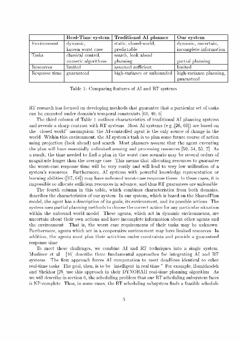
Real-Time system Traditional AI planner Our systemEnvironment dynamic, static, closed-world, dynamic, uncertain,known worst-case predictable incomplete informationTasks classical control, search, look aheadnumeric algorithms planning partial planningResources limited assumed su�cient limitedResponse time guaranteed high-variance or unbounded high-variance planning,guaranteedTable 1: Comparing features of AI and RT systems.RT research has focused on developing methods that guarantee that a particular set of taskscan be executed under domain's temporal constraints [63, 40, 6].The third column of Table 1 outlines characteristics of traditional AI planning systemsand reveals a sharp contrast with RT systems. Most AI systems (e.g.,[26, 69]) are based onthe \closed world" assumption: the AI-controlled agent is the only source of change in theworld. Within this environment, the AI system's task is to plan some future course of actionusing projection (look ahead) and search. Most planners assume that the agent executingthe plan will have essentially unlimited sensing and processing resources [50, 54, 55, 7]. Asa result, the time needed to �nd a plan in the worst case scenario may be several orders ofmagnitude longer than the average case. This means that allocating resources to guaranteethe worst-case response time will be very costly and will lead to very low utilization of asystem's resources. Furthermore, AI systems with powerful knowledge representation orlearning abilities ([17, 64]) may have unbound worst-case response times. In these cases, it isimpossible to allocate su�cient resources in advance, and thus RT guarantees are unfeasible.The fourth column in this table, which combines characteristics from both domains,describes the characteristics of our system. In our system, which is based on the SharedPlanmodel, the agent has a description of its goals, its environment, and its possible actions. Thesystem uses partial planning methods to choose the correct action for any particular situationwithin the unbound world model. These agents, which act in dynamic environments, areuncertain about their own actions and have incomplete information about other agents andthe environment. That is, the worst case requirements of their tasks may be unknown.Furthermore, agents which act in a cooperative environment may have limited resources. Inaddition, the agents must plan their activities under constraints and provide a guaranteedresponse time.To meet these challenges, we combine AI and RT techniques into a single system.Musliner et al. [46] describe three fundamental approaches for integrating AI and RTsystems. The �rst approach forces AI computation to meet deadlines identical to otherreal-time tasks. The goal, then, is to be \intelligent in real time." For example, Hamidzadehand Shekhar [25] use this approach in their DYNORAII real-time planning algorithm. Aswe will describe in section 6, the scheduling problem that our RT scheduling subsystem facesis NP-complete. Thus, in some cases, the RT scheduling subsystem �nds a feasible schedule5

by using the simulated annealing algorithm [55], which is a well known search method fromthe AI �eld.The second approach essentially assumes that the overall system employs typical AIsearch-based deliberation techniques, but under certain circumstances these techniques willbe short-circuited in favor of real-time re exive action. This type of system is suitable fordomains where deliberative action is the norm and mission-critical, real-time reactions arerare. The Soar system [33] is one example of these types of systems.The third approach, which has motivated the design of our system, tries to retain eachsystem's strength by allowing separate RT and AI subsystems to cooperate in achievingoverall desirable behaviors. The subsystems must be isolated so that the AI mechanisms donot interfere with the guaranteed operations of the RT subsystem, but the subsystems mustalso communicate and judiciously in uence each other. Thus, cooperative systems can beseen as being \intelligent about real time," rather than \intelligent in real time." Examplesof such architectures include Arkin's Autonomous Robot Architecture (AuRA) [3], Simmons'Task Control Architecture (TCA) [57], Miller and Gat's three-layer ATLANTIS system [41],and the CIRCA system [45].However, in all of these systems, the RT subsystem is a reactive system that is embeddedin the dynamic environment and responds by taking actions that a�ect that environmentwithout using any planning on reasoning methods. However, when it facing a problem(for example, a mobile robot facing an obstacle), the job of the AI subsystem is to resolvethe problem by building a plan and sending the constituent primitive actions to the RTsubsystem. That is, the AI subsystem in these works does not include any ability to reasonabout the temporal constraints of the high-level actions and the primitive actions in theproblem. As a result, although these systems work in uncertain and dynamic environments,the AI subsystem works as a traditional AI problem solver which is appropriate only for\closed world" environments. In our work, the AI-P subsystem is embedded in the dynamicenvironment and interacts with it. Our AI-P subsystem enables the agent to commit togoals as well as to actions that will enable it to achieve those goals under several kinds oftemporal constraints. It then builds a partial plan to achieve those goals. Each primitiveaction in the plan is sent to the RT scheduling subsystem for execution under appropriatetemporal constrains.An additional example of a system that belongs to the third approach is the RealPlansystem [60]. This system consists of a planner and a scheduler. The planner uses traditionalAI methods for reasoning about the way to allocate resources. After the planning is complete,the scheduler decides which resources to actually allocate based on resource allocation policiesproposed by the planner. The resource allocation polices proposed by the planner are givenin terms of constraints on values of scheduling variables. The RealPlan system does notproduce an exact timetable, but, rather, merely determines the order of the execution of theplanned actions in such a way that 2 actions will not use the same resource during the sameinterval. Thus, they do not consider critical temporal limitations as we do.6

2.2 Temporal Reasoning and Scheduling in AI SystemsAs mentioned above, contrary to our dynamic AI environment, the RT subsystem assumesthat the worst-case task requirements are known. Namely, the task data in an RT systemconsists of its performance requirements, including speci�c deadlines, precedence constraints,and duration time. However, in our uncertain dynamic environment, these performance re-quirements are typically unknown. Thus, we suggest that the AI planning subsystem mustbe able to reason about incomplete knowledge. That is, the AI planning subsystem mustbe able to reason about the temporal requirements of basic actions. When the AI plan-ning subsystem sends a basic action to the RT scheduling subsystem, it provides temporalrequirements as well.Representing and reasoning about incomplete and inde�nite qualitative temporal infor-mation is an essential part of many AI systems for individual agents. Several formalismsfor expressing and reasoning about temporal knowledge have been proposed, most notably,Allen's interval algebra [2], Vilain and Kautz's point algebra [68], and Dean and McDermott'stime map [13]. Each of these representation schemes is supported by a specialized constraint-directed reasoning algorithm. At the same time, extensive research has been carried out onproblems involving general constraints as in [42]. Some of these have been extended to prob-lems involving temporal constraints [14, 5]. Since all of these algorithms require their inputto include all the constraints on the events, and since these constraints cannot be changedduring the run of the algorithms, these works can be applied only in \static" environmentsin which the occurrence times of events and their durations are known beforehand.Recently, several works have developed techniques for \real world" environments, takinginto account changes in the environment while executing a plan. Although they suggestan intelligent control system that can dynamically plan its own behavior, they do not taketemporal constraints into consideration. Examples of such works include M-SHOP [49]which is focused on domain-independent planning formalization and planning algorithms;the Zeno system [29], which suggests a method for building a decision-making mechanismfor a planner in an uncertain environment; and the SGP contingent planning algorithm [12],which handles planning problems with uncertainty in initial conditions and with actions thatcombine causal and sensory e�ects. It also includes the planning model of the constraint-based Excalibure planning system [47, 48] and so on. The main goal of this paper is tohandle temporal constraints of the activity.Other recent planners such as O-plan [11], zeno [51], ParcPlan [16, 34] and Cypress [70]are able to handle temporal constraints. However, they do not produce an exact timetable,but rather only determine the order of the execution of the planned actions. Thus, most ofthem (e.g., [11, 51, 16, 34]) do not interleave planning and execution. Therefore they cannot,for example, backtrack in case of failure during execution. Even though Cypress [70] is builtfrom a planning subsystem (i.e., Sipe-2) and an execution subsystem (i.e., Prs-cl) andtherefore interleaves planning and execution, its execution subsystem is unable to handletemporal constraints. As a result, this system cannot perform planning and scheduling,as does our system. In addition, since these works do not determine explicit times for theplanned actions, using such systems in a cooperative multi-agent environment is problematic.Vidal and Ghallab [67] extend classical temporal constraint networks to handle all the7

types of temporal constraints presented by Allen [1] in uncertain environments. While theyhandle a wider range of constraints than we do, they do not study how their mechanism canbe used by a planner.In other works that combine planning and scheduling methods [8, 66, inter alia], theplanner builds a complete plan of the actions that it intends to perform before it beginsexecuting any of them. Also, in most cases, both the duration and the time window of eachaction that the planner needs to schedule are known in advance. These restrictions andrequirements are not needed in our mechanism's applications.In our work, we use networks of binary constraints [42], which are special cases of a gen-eral class of problems known as constraint satisfaction problems. Our development extendsthe previous works on temporal reasoning, as in [14]. However, in contrast to these previousworks, our algorithm is also appropriated for distributed, dynamic, and uncertain environ-ments. The AI planning subsystem in our work consists of a component for determiningconsistency of temporal data and procedures for discovering or inferring new facts aboutthis data. Our planning system is based on the SharedPlan model for collaborative agents.Using this model enables us to build reasoning mechanisms for collaborative multi-agentenvironments. The building of the temporal reasoning component is di�cult because theSharedPlan model deals with agents that may have only partial knowledge of the way inwhich to perform an action.2.3 Scheduling in RT systemsAs we mentioned in section 2.1, several works [44, inter alia] propose a blending of real-timecomputing and AI technologies in which a RT system is responsible for the execution of theactions generated by a planner. However, the RT systems in these works are based on existingreal-time developments. As a result, they do not pay attention to the unique properties of thetasks which are generated by the agent and are associated with uncertainty. In the literatureon real-time, computing a schedule at run time is often called \dynamic scheduling," incontrast to pre-run or \static scheduling," which assumes complete knowledge of all tasksbefore run time. Because our system must meet hard timing and precedence constraints, thepredictability of the system becomes an important concern.Most existing RT scheduling systems rely on pre-run static scheduling to achieve this,because computing the schedule at run time cannot, in general, guarantee that a feasibleschedule is found [73]. For example, Xu and Parnas [72] present a static scheduling algorithmthat �nds an optimal schedule on a single processor for a given set of processes with arbitraryrelease times, deadlines, precedence and exclusion relations, through a branch and boundalgorithm. The computation time to produce the schedule they present grows exponentiallyas the problem size increases. Most research dealing with dynamic scheduling of tasks hasfocused on preemptive scheduling or periodic task sets ([58] inter alia), or distributed systems[53, inter alia], both of which do not match the requirements of task sets generated by ourcooperative intelligent agents, which are non-preemptive and a-periodic. Other works [21]do not consider precedence relations between the tasks, which is considered to be a veryimportant requirement in the AI environment of a planner, in which several actions arepreconditions of other actions. Feasible dynamic scheduling in such an environment has8

been classi�ed as an NP-Hard problem [18]. A practical scheduling algorithm must be basedon heuristics that are practical and adaptive.Stankovic and Ramamritham [61] have developed the Spring Algorithm, which schedulesnon preemptive tasks at run-time. The Spring system treats the scheduling problem asa search tree, and directs each scheduling move to a plausible path by choosing the taskwith the smallest possible value of a heuristic function. Whenever a task is added to thepartial schedule and deemed infeasible, backtracking must be performed in order to �nda di�erent task to append to the partial schedule which might lead to a feasible schedule.This algorithm leads to good results for domains such as operating systems, in which severalprocesses compete for a set of resources. We tried this algorithm in our domain; however, inour domain this algorithm provided poor results.As will be described in the following section, the tasks in the set which are sent to theRT scheduling subsystem are the constitutes of a complex action that was separated intoits basic components. Thus, the constraints to which the high-level action was subjectedwill also in uence the constraints of its constitutes. As a result, all of the basic actionswhich are constitutes of a speci�c complex action must be scheduled in the time interval ofthis complex action. Thus, it is probable that if we build an initial schedule by using the\Earliest Deadline First" (EDF) algorithm, we will attain an initial schedule which will beclose to the desirable schedule. This factor led to the development of our own schedulingalgorithm, which consists of two major parts. The �rst is a primary EDF scheduler. Thesecond is a simulated annealing heuristic which which has been proved to be e�cient forother scheduling problems [15, inter alia]. The algorithm is described in section 6.3 The SharedPlan ModelWhen agents form teams, new problems emerge regarding the representation and executionof joint actions. A team must be aware of and concerned with the status of the group e�ortas a whole. To rectify this problem, it was proposed that agents have a well-grounded andexplicit model of cooperative problem solving on which their behavior can be based. Severalsuch models have been proposed [35, 30, 27], including the SharedPlan model [23], which isthe basis of our work.The SharedPlan formalization [23, 22] provides mental-state speci�cations of both sharedplans and individual plans. SharedPlans are constructed by groups of collaborating agentsand include subsidiary SharedPlans [36] formed by subgroups as well as subsidiary individualplans formed by individual participants in the group activity. The full group of agents mustmutually believe that the subgroup or the agent of each subact has a plan for the subact.However, only the performing agent(s) itself needs to hold speci�c beliefs about the detailsof that plan.Actions in the model are abstract complex entities that have been associated with variousproperties such as action type, agent, time of performance, and other objects involved inperforming the action. Following Pollack [52], the model uses the terms \recipe" and \plan"to distinguish between knowing how to perform an action and having a plan to performthe action. When agents have a SharedPlan to carry out a group action, they have certain9

individual and mutual beliefs about how the action and its constituent subactions are to beimplemented.The term recipe [52, 37] is used to refer to a speci�cation of a set of actions, which isdenoted by �i (1 � i � n), the performance of which under appropriate recipe-constraints,denoted by �j (1 � j � m), constitutes performance of �.2 The meta-language symbol R� isused in the model to denote a particular recipe for �.The subsidiary actions �i in the recipefor action �, which are also referred to as a subact or subactions of �, may be either basicactions or complex actions.Basic actions are executable at will if appropriate situational conditions hold. A complexaction can be either a single-agent action or a multi-agent action. In order to perform somecomplex action, �i, the agents have to identify a recipe R�i for it. There may be severalrecipes, R�i, for �i. The recipe R�i might include constituent subactions �iv. The �iv maysimilarly be either basic or complex. Thus, the general situation considering the actionswithout the associated constraints �j , is illustrated in Figure 2, in which the leaves of thetree are basic actions. We refer to this tree as \a complete recipe tree for �." The SharedPlanformalism uses Select Rec and Select Rec GR to refer respectively to the planning actionsthat agents perform individually or collectively to identify ways to perform (domain) actionsby extending the partial recipe Rp� for �. This hierarchical task decomposition method of thepartial order planning is known in the literature of AI planning systems as (HTN)-style [28]. . . . .

kn1 kn2

α

γ γ

η η

β

η

111 112

. . . . γ

η 11pη . . . .

β β4

γγ 3112 γ

1 3

32 3m

β

51

5

5m

β2

γ11Figure 2: Recipe tree. The leaf nodes are basic actions.Figure 3 presents an example of a possible recipe for some complex level action �. Asshown in this �gure, the recipe structure consists of subactions, temporal constraints, andmay also include other entities. Each subaction may be either an individual action or amulti-agent action and is associated with temporal intervals; each interval represents thetime period during which the corresponding subaction is performed. The recipe includes twotypes of temporal constraints, precedence constraints andmetric constraints. The parametersof an action may be partially speci�ed in a recipe and in a partial plan. For the agents tohave achieved a complete plan, the values of the temporal parameters of the actions that2The indices i and j are distinct; for simplicity of exposition, we omit the range speci�cations in theremainder of this document. 10

(make-recipe :action-type '�:name 'R1�:time-period 'unknown:subactions (1) (�1 Agent1 T1 � � �)(2) (�2 Agent1 T2 � � �)(3) (�3 (Agent1 Agent2) T3 � � �)(4) (�4 Agent1 T4 � � �)(5) (�5 (Agent1 Agent2) T5 � � �):precedence-constraints �1 before �2 �1 before �3�2 before �4 �2 before �5�3 before �5:metric-constraints (�nish-time T2� start-time T1 � 20minutes),(start-time T4� �nish-time T2 � 40minutes),(�nish-time T5� start-time T3 � 60minutes),(start-time T3 after 5:00): : : Figure 3: Recipe of the Complex Action �.constitute their joint activity must be identi�ed in such a way that all of the appropriateconstraints are satis�ed.The problem with reasoning about the temporal parameters of the actions that theagent is committed to perform results from the dynamic decomposition of the actions in theSharedPlan model. When a high-level action is broken up into sequences of subactions and�nally into basic actions, the time available to achieve the high-level action must also be splitinto intervals for each subaction. Doing this correctly would require the SharedPlan systemto have a predictable mechanism of how long it takes to solve the subactions. Unfortunately,building such a predictable model is di�cult because the SharedPlan model deals withagents that may only have partial knowledge on the way in which to perform an action.That is, as a result of the dynamic nature of plans, any of the components of its plan maybe incomplete and the agent does not know the duration of the complex actions before it�nishes constructing its plan. In this paper we describe the technique of temporal reasoningmechanisms which we propose to use in our system in order to build this type of predictablemechanism which may reason in a dynamic fashion.In the following section we present a temporal reasoning algorithm that enables theidenti�cation of the values of the temporal parameters. First the mechanism for an individualagent is presented; then we describe how it can be expanded into a collaborative environment.4 The Algorithm for Temporal ReasoningTo execute an action �, an agent has to execute all of the basic actions in a complete recipetree for � under the appropriate constraints. The goal of the temporal reasoning algorithmof the AI planning subsystem is to develop a complete recipe tree and to �nd the temporalrequirements associated with the basic actions. However, initially an agent may not be ableto develop the entire recipe tree and to identify its constraints: it may only have partialknowledge about how to perform an action; it may have incomplete information about the11

environment and other agents; and it may have to wait to receive temporal constraints ofother agents. For example, the agents may only have a partial recipe for the action; or theymay not yet have decided who will perform certain constituent subactions and thereforethey may have no individual or collaborative plans for those acts; or, an agent may not havedetermined whether potential new intentions are compatible with its current commitmentsand if they can be adopted. As the agents reason individually, communicate with oneanother, and obtain information from the environment, portions of their plans become morecomplete. Furthermore, it may need to start executing some of the basic actions before ithas been able to construct the entire tree. In addition, if an agent determines that the courseof action it has adopted is not working or receives a new temporal constraint from anotheragent, then the recipe tree may revert to a more partial state. The AI planning subsystemenables the agent to construct the recipe tree incremently and to backtrack when needed.As soon as it is identi�ed, each basic action � is sent to the RT scheduling subsystem3along with its temporal requirements hD�; d� ; r�; p�i, where D� is the Duration time, i.e., thetime necessary for the agent to execute the basic action � without interruption; d� denotesthe deadline, i.e., the time before the performance of the basic action should be completed;r� refers to the release time, i.e., the time at which the basic action becomes ready forexecution; p� is the predecessor actions, i.e., the set f�jj(1 � j � n)g of basic actions whoseexecution must end before the beginning of the execution of �. Note that a basic action maybe performed before the agent completes its plan to perform �.Let A = f�ij(1 � i � m)g be the set of all the basic actions which were sent dynamicallyto the RT scheduling subsystem as part of the performance of action �. It is important tonote that the AI planning subsystem's algorithm does not check if there is a schedule forA that satis�es the temporal constraints and meets all the deadlines, since this problem isNP-complete [18]. However, the algorithm ensures that performing �is under the associatedconstraints will constitute performing � without a con ict. Thus, a feasible schedule existsif actions can be performed in parallel. The task of �nding a feasible schedule (if such aschedule exists) is left for the RT scheduling subsystem. If the RT scheduling subsystemfails to schedule certain basic actions, it informs the AI planning subsystem of its failure.However, because the AI planning subsystem ensures that the temporal requirements of allthe basic actions do not con ict, the agent may ask another agent to execute the problematicbasic action in parallel with other actions.The temporal reasoning mechanism is based on previous work on the temporal constraintsatisfaction problem (TCSP) [14, inter alia]. Formally, TCSP involves a set of variables,X1; : : : ; Xn, having continuous domains4; each variable represents a time point. Each con-straint is represented by a set of intervals: fI1; : : : ; Img = f[a1; b1]; : : : ; [am; bm]g. A unaryconstraint, Ti, restricts the domain of variable Xi to the given set of intervals; namely, itrepresents the disjunction (a1 � Xi � b1) _ � � � _ (am � Xi � bm). A binary constraint,Tij , constrains the permissible values for the distance Xj �Xi; it represents the disjunction(a1 � Xj �Xi � b1) _ � � � _ (am � Xj �Xi � bm).A network of binary constraints (a binary TCSP) consists of a set of variables, X1; : : : ; Xn,and a set of unary and binary constraints. Such a network can be represented by a directed3Our RT scheduling subsystem can handle only basic actions.4In our mechanism we do not force the assumption that the domain is continuous.12

constraint graph, where nodes represent variables and an edge (i; j) indicates that a constraintTij is speci�ed; it is labeled by the interval set. Each input constraint, Tij, implies anequivalent constraint Tji; however, only one of them will usually be shown in the constraintgraph. A special time point, X0, is introduced to represent the \beginning of the world." Alltimes are relative to X0. Thus we may treat each unary constraint Ti as a binary constraintT0i (having the same interval representation). A tuple X = (x1; : : : ; xn) is called a solutionif the assignment fX1 = x1; : : : ; Xn = xng satis�es all the constraints. The problem isconsistent if at least one solution exists.The general TCSP problem is intractable, but there is a simpli�ed version, simple tempo-ral problem (STP), in which each constraint consists of a single interval. This version can besolved by using the e�cient techniques available for �nding the shortest paths in a directedgraph with weighed edges such as Floyd-Warshall's all-pairs-shortest-paths algorithm5 [10].In our work we also use a temporal constraints graph, which consists of the temporal con-straints associated with action � (including precedence constraints and metric constraints).However, because of the uncertainty and dynamic environment of the agents, in contrast toprevious works, the constraints graph which is built by our agents may include only partialknowledge; i.e., our algorithm enables the agents to build this graph incremently and tobacktrack when needed. In addition, the agents are able to determine the action for whichthe temporal parameters are known and to execute them.4.1 De�nitions and Notations for the Temporal Reasoning Mech-anismIn order to present our technique for temporal reasoning, we will �rst de�ne some basicconcepts that will be used throughout our reasoning mechanism.De�nition 4.1 (Time interval of an action) Let � be an action. We denote the timeinterval of � by [s�; f�], where s� is the time point at which the execution of action � startsand f� is the time point at which the execution of action � ends.There are two types of temporal constraints in the system. The �rst type is metric,where we treat the duration of an event in a numeric fashion. The temporal range of thestarting point and �nishing point, the length of time between disjoint events, and so forth,are numbers which may satisfy speci�c inequalities or various measurable constraints. Forexample, \�2 has to start at least 20 minutes after �1 would terminate." The second type isrelative, in which events are represented by abstract time points and time intervals; i.e., thetemporal constraints make no mention of numbers, clock times, dates, duration, etc. Rather,only qualitative relations such as before, after, or not after are given between pairs of events;e.g., \the subaction �1 has to occur before �2." The techniques which are used to reasonabout these two types of constraints are di�erent [20]. In the following we give more detailsabout the usage of these types of constraints in our system and describe them formally.As illustrated in �gure 3, in certain cases the subactions, �1; : : : ; �n, of a recipe R� haveto satisfy certain precedence relations which are relative constraints. The precedence rela-tionships between the subactions is speci�ed in our system using events. An event represents5Floyd-Warshall's algorithm e�ciently �nds the shortest paths between all pairs of vertices in a graph.13

a point in time that signi�es the completion of some actions or the beginning of new ones.The time points at which execution of action � starts and �nishes are thus described bytwo events. In the system, events are represented by nodes, and the activity of action �iis represented by a directed edge between the time points at which the execution of action�i starts and �nishes. A directed edge between the �nishing time point of an action �i andthe starting time point of another action �j , denotes that the execution of �j cannot startuntil the execution of �i has been completed. The label of the edge needs to be proportionalto the duration either of the activity of some action �i; or the delay between two di�erentactions �i and �j , and is referred to as the temporal distance between them [38]. As we willsee in the remainder of this section, this graphical representation will enable us to build thetemporal network (TCSP) which is mentioned in the earlier section. We have termed thisgraphical form of the precedence relations the precedence graph. The formal de�nition ofthe precedence graph which we use in our SharedPlan system is presented in the followingde�nition:De�nition 4.2 (Precedence graph of �, GrpR�) Let � be a complex action, and let R�be a recipe which is selected for executing �. Let �1; : : : ; �n be the subactions of the recipeR� and �pR� = f(i; j)j�i < �j ; i 6= jg are the precedence constraints associated with R�. Theprecedence graph of �, GrpR�= (V pR�,EpR�) with reference to R� and its precedence constraints�pR� satis�es the following:1. There is a set of vertices V pR� = fs�1; : : : ; s�n ; f�1; : : : ; f�ng where the vertices s�i andf�i represent the start time and the �nish time points of �i 1 � i � n, respectively6.2. There is a set of edges EpR� = f(u1; v1); : : : ; (um; vm)g, where each edge (uk; vk) 2 EpR�1 � k � m is either:(a) the edge (s�i ; f�i) that represents the precedence relations between the start timepoint s�i and the �nish time point f�i of each subaction �i. The edge is labeled bythe time period for the execution of the subaction �i; or(b) the edge (f�i; s�j) which represents the precedence relation �i < �j 2 �pR�, whichspeci�es that the execution of the subaction �j starts after the execution of thesubaction �j ended. This edge is labeled by the delay period between �i and �j.All of the edges of the precedence graph are initially labeled by [0;1].An example of precedence graph is given in the following:Example 1 :Figure 4 illustrates a precedence graph GrpR�=(V pR�,EpR�). In this Figure the subactions of theselected recipe R� are �i (1 � i � 5), and the precedence relations are �pR� = f�1 < �2; �1 <�3; �2 < �4; �2 < �5; �3 < �5g. These precedence relations are appropriated to the precedenceconstraints in the recipe of �, which is shown in �gure 3.14

time(β1 )

time( )time( )2

time( )β5time( )β4

β

delay

12

2425

delaydelay35

delay delay13

3β

s

s

β1

β1

β2

β2 β3

β3

f

f f

β4

β4f fβ5

β5

s

ssFigure 4: A precedence graph GrpR�.As depicted in Figure 4, the precedence relations do not induce a total order on allthe subactions. For example, the agent can begin the execution of action �3 before thecompletion of action �2 and vice versa. In such cases these actions can be executed also inparallel: e.g., agent G1 can begin to perform action �2 and another agent, G2, can begin toperform action �3 in the same time interval.De�nition 4.3 (parallel actions) Let GrpR�=(V pR� ,EpR�) be the precedence graph of an ac-tion �. Let �i and �j, i 6= j, be two subactions in R�. The subactions �i and �j are calledparallel actions if GrpR� does not include a path either from s�i to s�j or from s�j to s�i , i.e.there is no precedence constraints between �i and �j .In Figure 4, actions �3 and �2 are parallel actions, as are actions �4 and �5.De�nition 4.4 (beginning points, beginning actions, ending points, ending actions)Let GrpR�, be the precedence graph of the complex action � and let R� be the selected recipefor executing �. Let �1; : : : ; �n be the subactions of recipe R�.1. The set of vertices fs�b1 ; : : : ; s�bmg � V pR� with in-degree 0 of the graph GrpR� are calledbeginning points. The actions �b1 ; : : : ; �bm are called beginning actions.2. The set of vertices f�e1 ; : : : ; f�em � V pR� with out-degree 0 of the graph GrpR� are calledending points. The actions �e1 ; : : : ; �em are called ending actions.6We will use the notation and will refer to a node which is labeled by s as node s.15

This de�nition is illustrated in the following example:Example 2 :In the precedence graph of � GrpR� in Figure 4, the vertex s�1 is the only vertex with an in-degree of 0. Thus, only action �1 is a beginning action and the time point s�1 is a beginningpoint. Since vertex s�1 has no predecessors the agent can start executing action � by executingsubaction �1. The vertices f�4 and f�5, which have no successors, are called ending points.Thus, actions �4 and �5 are ending actions and the agent �nishes executing action � whenit �nishes the execution of subactions �4 and �5.As a result of the dynamic nature of the planning process, the agent may have onlypartial knowledge of how to perform a complex level action. Thus, the agent may not knowthe duration of the execution time which is required for performing a complex level actionuntil its plan for this action becomes complete. However, we assume that the time periodduring which a basic action is executed is always known. Thus, in our reasoning mechanism,we distinguish between complex and basic actions in the graph, as described in the followingde�nition.De�nition 4.5 (basic edge, basic vertex, complex edge, complex vertex) :Let GrpR�=(V pR� ,EpR�) be the precedence graph of an action �. Let (s�i ; f�i) be some edge inEpR� which denotes relations between the start time point, s�i , and the �nish time point, f�i,of subaction �i.1. If subaction �i is a basic action, the edge (s�i; f�i) is called a basic edge and the verticess�i and f�i, are called basic vertices.2. If subaction �i is a complex action, the edge (s�i; f�i) is called a complex edge and thevertices s�i and f�i, are called complex vertices.Examples of such actions and edges are as follows:Example 3 :Suppose that subactions �2 and �5 of R1� in Figure 3 are basic level actions and that the othersubactions; i.e., �1, �3 and �4, are complex actions. Thus, the edges (s�2; f�2) and (s�5; f�5)in Figure 4 are called basic edges. The time points s�2, f�2, s�5, f�5 are called basic vertices.The other edges are called complex edges, and the other vertices are called complex vertices.One of the requirements of our system is the ability to deal with metric information. Weconsider time points as the variables we wish to constrain. A time point may be a start or a�nish point of some action �, as well as a neutral point of time such as 4:00p.m. Malik andBinford [38] have suggested constraining the temporal distance between time points. Namely,if Xi and Xj are two time points, a constraint on their temporal distance would be of theform Xj�Xi � c, which gives rise to a set of linear inequalities on the Xi's. In the followingwe give the formal de�nition of the metric constraints in our system.16

De�nition 4.6 (Metric constraints) Let f�; �1; � � � ; �ng be the actions that agent G hasto perform, where � is the highest level action in the recipe tree which consists of theseactions. Let V = fs�; s�1 ; � � � ; s�n ; f�; f�1; � � � ; f�ng [ fs�plang be a set of variables wheresy and fy represent the start and �nish time points of some action y 2 f�; �1; � � � ; �ngrespectively, and the variable s�plan represents the time point when an agent G starts to planaction �. Let vi; vj 2 V be two di�erent variables. The metric constraints between thesevariables consists of a set of inequalities on their di�erences, namely �m� = fvi; vj(1 � i; j �jV j)jai;j � (vi � vj) � bi;jg.An example of metric constraints is described in Example 4.Example 4 :The recipe in Figure 3 consists of the following metric constraints:(�nish-time T2� start-time T1 � 20minutes),(start-time T4� �nish-time T2 � 40minutes),(�nish-time T5� start-time T3 � 60minutes),(start-time T3 after 5:00),where T� represents the time interval of the execution of action �. If we assume that theagent starts to plan � at 4:00 o'clock, then the agent may transfer these temporal constraintsto the following metric constraints7: �m� = f0 � f�2 � s�1 � 20; 0 � s�4 � f�2 � 40; 0 �f�5 � s�3 � 60; 60 � s�3 � 1g.As mentioned in section 4, we shall use constraints networks in our system. Thesenetworks are frequently used in AI to represent sets of values which may be assigned tovariables. In order to build a temporal constraints network, we have to build the temporalconstraints graph which will consist of all the temporal constraints that are associated withan action � (including precedence constraints and metric constraints). However, becausethe environment of the agents is uncertain and dynamic (i.e., the agent may have onlypartial knowledge of how it will perform action �), the temporal network which we buildwill consist of only partial knowledge. When this knowledge becomes more complete, theagent will update the temporal network accordingly. That is, the agent builds the temporalnetwork dynamically. At the beginning, when the agent adopts the intention of performing ahigh level action, �, it builds an initial temporal network with the initial information whichit has on �, and it expands this initial network dynamically. The graph which consists ofthe initial constraints associated with action � is called, in our terminology, the initial graphof �, InitGr�, as described in the following de�nition.De�nition 4.7 (Initial graph of �, InitGr�) Suppose that agent G has the intention todo an action �. Let � be the highest level action in the recipe tree and �m� = fvi; vj jai;j �(vi� vj) � bi;jg be the temporal metric constraints associated with �. The initial graph of �,InitGr� = (Vinit; Einit), satis�es the following.7The method of transferring metric information, which is given as natural points for a set of inequalities,can be found in several references, including Dechter et al. [14].17

s

f

α

α

sα 4:00plan

[0,210][0,150]

8[0, )

Figure 5: Example InitGr�.1. Vinit = fs�plan; s�; f�g is a set of vertices. The vertex s�plan 2 Vinit denotes the timepoint at which the agent starts to plan action �. This point is a �xed point in timewhich is called the origin. The vertex s� is the time point at which the agent startsexecuting �, and f� is the time point at which the agent �nishes executing �.2. Einit = f(s�plan; s�); (s�; f�); (s�plan; f�)g is a set of edges, where each edge(vi; vj) 2 Einit is labeled by the following weight:weight(vi; vj) = 8<: [ai;j ; bi;j ] if vi; vj 2 �m�[0;1) if vi; vj =2 �m�.An example of InitGr� for some action � is given next.Example 5 :Suppose that � is associated with the following temporal constraints: (a) the performanceof � has to be terminated in 150 minutes; (b) the performance of � has to start after 4:00o'clock; (c) the performance of � has to end before 7:30 o'clock. We also assume, as inexample 4, that the agent starts to plan � at 4:00 o'clock. Thus, the agent may transfer thesetemporal constraints to the following metric constraints, �m� = f(0 � s� � f� � 150); (0 �(f� � s�paln � 210)g, and to build the initial graph of action �, which is given in Figure 5.When working on action �, the agent maintains a temporal constraint graph of �. Thisgraph may be changed during the agent's planning. The following de�nition presents aformal description of this temporal constraint graph.De�nition 4.8 (Temporal constrains graph of �, Gr�) Let f�; �1; � � � ; �ng be a set ofbasic and complex level actions that agent G intends to perform, where � is the highest levelaction in the recipe tree which consists of these actions. Let V = fs�; s�1 ; � � � ; s�n ; f�; f�1; � � � ; f�ng[18

fs�plang be a set of variables, where sy and fy represent the start and �nish time points ofsome action y 2 f�; �1; � � � ; �ng, respectively, and the variable s�plan represents the time pointthat an agent G starts to plan action �. Let �pR� = f(�i; �j)j�i < �j ; i 6= jg be the set of all theprecedence constraints which are associated with all the recipes of the actions f�; �1; � � � ; �ng.Let �m� = fvi; vj jai;j � (vi � vj) � bi;jg be all of the temporal metric constraints that areassociated with f�; �1; � � � ; �ng and their recipes.1. If � is a basic level action, then the temporal constraints graph of �, Gr� = (V�; E�),is the initial graph InitGr� = (Vinit; Einit).2. If � is a complex level action, then the temporal constrains graph of �, Gr� = (V�; E�),satis�es the following:(a) There is a vertex which represents the origin time point s�plan 2 V�.(b) There is a set of basic vertices Vbasic = fs�b1 � � � s�bk ; f�b1 ; : : : ; f�bkg � V� and aset of basic edges Ebasic = f(s�b1; f�b1); : : : ; (s�bk ; f�bk)g � E�, where �bi (1 � i �k) is some basic level action in the recipe tree of �, and each edge (s�bi ; f�bi)g 2 E�is labeled by the time period of �bi .(c) There is a set of complex vertices Vcomlex = fs�c1; : : : ; s�cl ; f�c1; : : : ; f�clg � V�and a set of complex edges Ecomplex = f(s�c1; f�c1); : : : ; (s�cl ; f�cl)g � E� whereeach edge (s�cj ; f�cj ) 2 Ecomplex, 1 � j � l is labeled by the following weight:weight(s�cj ; f�cj) = 8>>>>>>>>>>>>>>><>>>>>>>>>>>>>>>:

[ai;j ; bi;j ] if (s�cj ; f�cj 2 �m� )and thetime period of �cj is unknownthe time period of �cj if (s�cj ; f�cj =2 �m� )and thetime period of �cj is known[ai;j ; bi;j ] \ (the time period of �cj) if (s�cj ; f�cj 2 �m� )and thetime period of �cj is known[0;1) if (s�cj ; f�cj =2 �m� )and thetime period of �cj is unknown(d) There is a set of delay edges Edelay = f(u1; v1); : : : ; (un; vn)g � E�, where ui; vi 2V�, (1 � i � n). The vertices ui; vi may be of the following forms:i. ui is the start time point of some action �u, and vi is some beginning pointin the precedence graph Grtimep�u of action �u.ii. ui is some ending point in the precedence graph Grtimep�v of some action �v,and vi is the �nish time point of action �v.iii. ui is the �nish time point of some action �u, and vi is a start time point ofanother action �v, where �u; �v 2 �timepR� .Each edge (vi; vj) 2 Edelay is labeled by the following weight:19

weight(vi; vj) = 8<: [ai;j ; bi;j ] if vi; vj 2 �m�[0;1) if vi; vj =2 �m�(e) There is a set of directed edges Emetric = f(u1; v1); : : : ; (un; vn)g � E� labeled byits metric constraints, where ui; vi 2 V�, (1 � i � n), but (ui; vi) =2 Ebasic [Ecomplex [ Edelay.Example 6 :Figure 6 illustrates an example of a temporal constraints graph of �. Action � is a complexlevel action, and thus the vertices s� and f� are complex vertices. The edge (s�; f�) isa complex edge. The vertex s�plan is the origin time point which represents the time 4:00o'clock, at which time the agent has begun its plan for �. The actions �1, �2, �3, �4, and�5 are the subactions in the recipe which is selected for performing �. As a result, all ofthe vertices which represent the start and �nish time points of these subactions appear inthe path between s� and f�. Some of these subactions may be multi-agent actions, and theothers are single agent actions. In this example we assume that �1 is a single agent actionand that the recipe which is selected for performing this action consists of subactions 11 and 12, which are basic level actions. Thus, the vertices fs 11; f 11; s 12; f 12g are called in ourterminology basic vertices, and the edges (s 11; f 11), (s 12; f 12) are called basic edges. Notethat the time period during which a basic action is executed is always known. As a result,the weights of these basic edges are �xed (exactly 5 minutes). However, since the durationof complex level actions is not known in advance and may change over time, the weights ofthe complex edges in the graph are not �xed. The next section describes the building of thisgraph.As mentioned above, some of the vertices in the temporal constraints graph may be�xed; i.e., these vertices denote a known time which cannot be modi�ed. The vertex s�planrepresents the time point at which an agent G starts to plan action �; it is a �xed vertex.The value of this vertex in Figure 6 is 4:00 o'clock. Other �xed vertices may be initiated,for example, by a request from a collaborator. The vertex s�5 is also a �xed vertex, whichrepresents the time 5:00 o'clock. We de�ne �xed time points as follows:De�nition 4.9 (�xed time point) A �xed time point is a known time which cannot bemodi�ed.In section 3 we illustrated the recipe tree for action �. This recipe tree may be derivedfrom the temporal constraints graph of � and in our terminology is called the implicit recipetree. This tree is described in the following de�nition.De�nition 4.10 (Implicit recipe tree, Tree�:) Let Gr� be a constraints graph. Let A= f�; �1; : : : ; �ng be the set of the actions whose start and �nish time points are represented bythe vertices in Gr�. The implicit recipe tree, Tree�, in Gr� satis�es the following: each nodein the recipe tree represents an action from the set A, where the root of this tree is action �.20

time( )time( )2

time( )β5time( )β4

β

delay

12

delay35

delay delay13

3β

s

β1

β2

β2 β3

β3

f

f f

β4

fβ5

β5

s

ss

β4f

f

delay

[0,40]

25

α5

[10,10]

[10,10]

[125,210]

[0,55]

[0,55]

[0,85]

[5,60]

α4delay

)β1

α

αs plan4:00

delayαplan

α1

sβ1

sγγ

fγ f11

12

γ12 [65,120]

[120,120]

[5,60]

[0,105]

[0,5][0,5]

[0,5][0,5]

delay[0,105]

[25,150]

[15,20]

[5,10]

[0,5]

[0,105]

[0,125]

[0,115]

s11

time( [5,5][5,5]γ γ11 12

time( ) time( )

delaydelay

delaydelays11 s12

f11f12

s

α

basic vertexFigure 6: An example of a temporal constraints graph Gr�.There is an edge between a node x 2 A to another node y 2 A (i.e., y is a child of x in the tree)if Gr� consists of the following vertices path (sx; : : : sy; fy; : : : fx) and there is no other actionz 2 A that exists, such that Gr� consists of the path (sx; : : : ; sz : : : ; sy; fy; : : : ; fz; : : : ; fx).21

Example 7 :Figure 7 presents the implicit recipe tree of the graph Gr� which is shown in Figure 6. It isobvious that A = f�; �1; � � � ; �5; 11; 12g. In this tree, for example, 11 is the son of �1 sinceGr� consists of the path (s�1; s 11; f 11; f�1).α

β β β4

γ12

1 3β 5β2

γ11Figure 7: Implicit recipe tree example.4.2 The AlgorithmFigure 8 presents the major constituents of the temporal reasoning algorithm which isused by the AI planning subsystem. The algorithm obtains as an input an action � and aninitial graph InitGr�, that is de�ned in de�nition 5. As shown in Figure 8, the algorithmconsists of two major constituents. In the �rst constituent, the agent initializes the relevantparameters. In particular, it forms the graph Gr�. Then, in the second constitute it runsa loop until all the subactions of a tree for � are performed. Figure 9 describes theseconstituents in more detail. The initialization constituent includes an initialization of thetemporal constraints graph Gr� by the initial graph InitGr�. It also includes initializationof the status of the vertices in this graph. In addition, it initializes two ags, where the(I) Initialization and formation of the temporal graph of � (Gr�);(II) Planning and executing Loop:(II.1) Planning for a chosen subaction � from Gr�:(II.1.a) � is a basic level action;(II.1.b) � is a complex level action;(II.2) Obtaining messages on execution from the RT scheduling subsystem;(II.3) Backtracking, if needed;Figure 8: The major constituents of the temporal reasoning mechanism for performing acomplex action �. 22

(I) Initialization : Initialize the values of the relevant parameters, including the set of Indepen-dent Unexplored vertices and the value of the temporal constraints graph of �, Gr�;(II) Planning and execution Loop: Run the following loop until all the basic actions have beenexecuted:(II.1) Planning for a chosen action � : If the plan for � has not been �nished, choosesome vertex, s�, from the IU set which is associated with an action �.(II.1a) If � is a basic action : identify its parameters, send them to the RT schedul-ing subsystem and start again from (II.1).(II.1b) If � is a complex action :(II.1b1) Select a recipe R� for �;(II.1b2) Construct the precedence graph GrpR� for � and add it to Gr�.(II.1b3) Add the metrics constraints of the recipe of � to Gr�.(II.1b4) Check consistency of the updated graph using Floyd-Warshall's all-pairs-shortest-paths algorithm.(II.1b5) If not consistent then remove GrpR� and all the metric edges added in(II.1b3) from Gr� and proceed to (II.1b1) to select a new recipe. If such a newrecipe for � does not exist, then return failure in the current plan.(II.2) Obtaining messages from the RT scheduling on execution: Listen to the RTscheduling subsystem as long as the agent did not execute all the actions and updatethe graph according to the messages of the RT scheduling subsystem.(II.3) Backtracking, if need: If there is a failure in the current plan or a failure messagefrom the RT scheduling subsystem, then perform backtracking.Figure 9: The description of the major constituents of the temporal reasoning algorithm.�rst indicates whether or not the planning of � has terminated, and the second indicateswhether or not all the subactions of � have already been executed. It also initializes the setof Independent Unexplored vertices that we discuss below.The second constituent is a loop which runs until the agent has �nished the executionof all the basic level actions in the complete recipe tree for �. This loop consists of aninternal loop (II.1) which is run until the agent has �nished the planning of action �. Thetwo nested loops are needed since in several cases the agent fails in the execution of somebasic level actions after the planning of � has been completed (i.e., after it �nished buildingthe complete recipe tree of �). As a result, the agent has to backtrack, and it tries to �nd anew plan for � by running the planning loop again.In the planning loop an action � is chosen (the method of choosing this action will bediscussed below). The agent distinguishes between a basic level action � (II.1.a) and acomplex level action (II.1.b). If the action is a basic level action, it sends this action and its23

associated time constraints to the RT scheduling subsystem, which schedules and executesthis action. If the action is a complex level action, the agent does not know the durationof �. Thus, the agent continues to plan the performance of this action by selecting a recipefor this action. It also expands the temporal constraints graph Gr� according to the newinformation. In the case of a failure in �nding a recipe in the planning loop for a chosen �or in the case of receipt of a failure message from the RT scheduling subsystem, the agentperforms backtracking, as described in section 4.3.The pseudo code of the reasoning algorithm's main procedure is given in Figure 10. Ineach line of the pseudo code we indicated the beginning of the appropriate constituent fromFigure 9. We demonstrate the algorithm using an example because it is complex.To keep track of the progress of the expansion of Gr�, all the vertices start out asunexplored (UE). When they are explored during the algorithm, the vertices of basic actionsbecome explored basic (EB), and the vertices of complex actions become explored complex(EC). The algorithm also takes into consideration that if the performance of some action �depends upon other actions f 1; : : : ; ng, then the agent cannot determine the time neededto perform � unless the �nish time of f 1; : : : ; ng is known. A vertex whose time can bedetermined and which does not depend on other actions is called an Independent Vertex(IndV), and it belongs to one of two disjoint sets. The �rst set, IU, contains the IndependentUnexplored vertices, i.e., the vertices whose values can be identi�ed, but have not yet beenhandled by the algorithm. The second set, IE, contains the Independent Explored vertices,i.e., the vertices whose values have been identi�ed. Table 2 provides a summary of thenotation used in the temporal reasoning of this paper.To exemplify the running of the algorithm in Figure 10, we suppose that the agenthas adopted an intention of performing an action � which is associated with the met-ric time constraints given in example 5: i.e., �m� = f(0 � s� � f� � 150); (0 � (f� �s�paln � 210)g. We also assume that, initially, the length of the interval of the exe-cution of action � is unknown. In order to start the temporal reasoning process, be-fore applying the algorithm identify times param, the agent �rst builds an initial tem-poral graph (see de�nition 4.7) denoted by InitGr� = (Vinit; Einit), which includes theinitial information of the time constraints of the highest level action �. In the exam-ple, if we assume that the agent starts its plan at 4pm, then Vinit = fs�plan; s�; f�g andEinit = f(s�plan; s�; [0;1]); (s�; f�; [0; 150]); (s�plan ; f�; [0; 210])g (see Figure 5). The initialgraph, InitGr� = (Vinit; Einit), is built according to de�nition 4.7 and is given as an inputto the procedure identify times param.In the initialization constituent (clause (I)) of the algorithm, the agent �rst checks ifthe initial graph is consistent (line 1 of the main procedure of Figure 10). For simplicity,we assume that each edge in the graph is labeled by a single interval. As a result, we canapply Floyd-Warshall's all-pairs-shortest-paths algorithm [10] in the check consistencyprocedure8. After applying the Floyd-Warshall's algorithm, the new intervals of the edgesin the example will be Einit = f(s�plan; s�; [0; 210]); (s�; f�; [0; 150]); (s�plan ; f�; [0; 210])g (seethe dashed edges in Figure 12).If the initial graph is consistent, as in our example, InitGr� is assigned to Gr� (line8The general problem of edges being labeled by several intervals can be solved using heuristic algorithms,as suggested in [14]. 24

identify times param(�; InitGr�)(I) 1 if check consistency(InitGr�) is false then FAIL;2 Gr�times InitGr�; IE ;;3 IU (the �xed vertices in Gr�) ;4 for each vertex u 2 V� do status[u] UE;5 status[s�plan ] EC;6 �nish execute all false; complete plan false;7 update IndV sets(s�plan);(II) 8 while(not �nish execute all)(II.1) 9 if (not complete plan) then10 select some vertex u from IU ;11 � action[u];(II.1a) 12 if � is a basic action then:13 status[s� ] EB; status[f�] EB;14 update IndV sets(s� ; f�)15 D� time period(�);16 r� time(s�plan ) +M(s�plan ; s�);17 d� time(s�plan ) +M(s�plan ; f�);18 p� find precedence actions(�;Gr�);19 transfer h�;D�; r� ; d� ; p�i to RT scheduling subsystemwhich tries schedule � and informs \succeed" or \fail"(II.1b) 20 if � is a complex action then:21 found false; <�tried ;;22 while (not found)^(<� �<�tried 6= ;)(II.1b1) 23 Select Rec R� for � not in R�tried ;24 add R� to <�tried ;(II.1b2) 25 GrpR� construct precedence graph(R�);26 add precedence graph((s� ; f�);GrpR�);(II.1b3) 27 add metric constraints(R�);(II.1b4) 28 if check consistency(Gr�) then:29 status[s� ] EC; status[f� ] EC;30 found true;(II.1b5) 31 update IndV sets(s�);32 else, Gr� is not consistent, remove(R�);33 end while;34 if all the vertices in the graph are explored then:35 complete plan true;36 end if (not complete plan);(II.2) 37 message listen to the real-time subsystem;38 if the message is \succeed to execute an action �" then39 status[s ] EXECUTED; status[f ] EXECUTED;40 if the status of all the vertices in the graph are EC or EXECUTED41 then �nish execute all true;(II.3) 42 if (not found) or (RT scheduling subsystem sent \fail")then: if possible, BACKTRACK; otherwise FAIL;43 end while;Figure 10: The main procedure for identifying the time parameters of � where � is a singleagent action.2), and the expansion of the graph continues. At the beginning, the �rst vertex s�planis denoted as EC (line 7). Then, the IU and IE sets are updated by the procedure Up-25

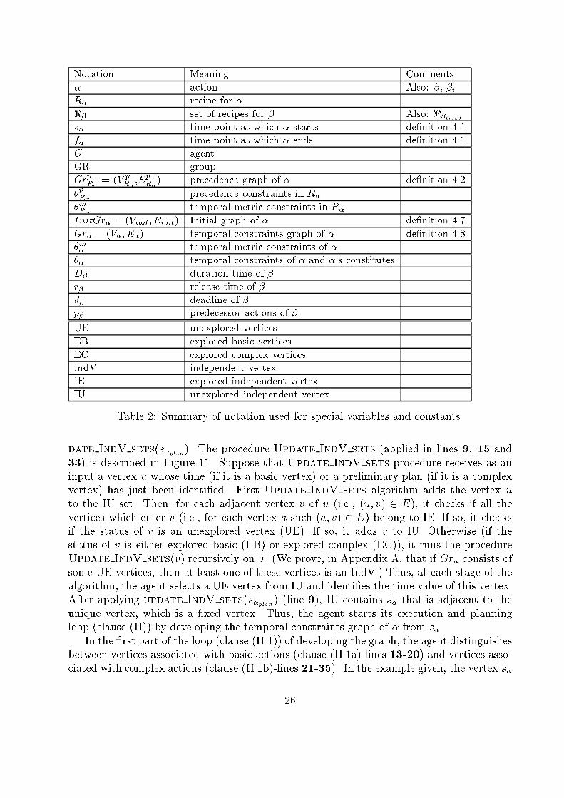
Notation Meaning Comments� action Also: �, �iR� recipe for �<� set of recipes for � Also: <�trieds� time point at which � starts de�nition 4.1f� time point at which � ends de�nition 4.1G agentGR groupGrpR� = (V pR� ,EpR�) precedence graph of � de�nition 4.2�pR� precedence constraints in R��mR� temporal metric constraints in R�InitGr� = (Vinit; Einit) Initial graph of � de�nition 4.7Gr� = (V�; E�) temporal constraints graph of � de�nition 4.8�m� temporal metric constraints of ��� temporal constraints of � and �'s constitutesD� duration time of �r� release time of �d� deadline of �p� predecessor actions of �UE unexplored verticesEB explored basic verticesEC explored complex verticesIndV independent vertexIE explored independent vertexIU unexplored independent vertexTable 2: Summary of notation used for special variables and constants.date IndV sets(s�plan). The procedure Update IndV sets (applied in lines 9, 15 and33) is described in Figure 11. Suppose that Update IndV sets procedure receives as aninput a vertex u whose time (if it is a basic vertex) or a preliminary plan (if it is a complexvertex) has just been identi�ed. First Update IndV sets algorithm adds the vertex uto the IU set. Then, for each adjacent vertex v of u (i.e., (u; v) 2 E), it checks if all thevertices which enter v (i.e., for each vertex a such (a; v) 2 E) belong to IE. If so, it checksif the status of v is an unexplored vertex (UE). If so, it adds v to IU. Otherwise (if thestatus of v is either explored basic (EB) or explored complex (EC)), it runs the procedureUpdate IndV sets(v) recursively on v. (We prove, in Appendix A, that if Gr� consists ofsome UE vertices, then at least one of these vertices is an IndV.) Thus, at each stage of thealgorithm, the agent selects a UE vertex from IU and identi�es the time value of this vertex.After applying update IndV sets(s�plan) (line 9), IU contains s� that is adjacent to theunique vertex, which is a �xed vertex. Thus, the agent starts its execution and planningloop (clause (II)) by developing the temporal constraints graph of � from s�.In the �rst part of the loop (clause (II.1)) of developing the graph, the agent distinguishesbetween vertices associated with basic actions (clause (II.1a)-lines 13-20) and vertices asso-ciated with complex actions (clause (II.1b)-lines 21-35). In the example given, the vertex s�26

update IndV sets(u)1 IE IE [ u; IU IU � u;2 for each vertex (u; v) 2 E� do3 BecomesIV True;4 for each vertex (a; v) 2 E� do5 if a =2 IE then BecomesIV False;6 if BecomesIV = True then7 if status[v] = UE then IU IU [ v;8 otherwise: update IV sets(v);Figure 11: The procedure update IV sets updates the sets of the Independent Vertices.denotes a time point of a complex action. Thus, the agent selects some applicable recipe R�for this action (clause (II.1b1)-line 25). Then, the agent builds the precedence graph of R�,GrpR� , by running the construct precedence graph procedure (clause (II.1b2)-line 27).GrpR� is built according to de�nition 4.2. In our example, we assume that the agent selects arecipe R1� which is associated with the subactions f�1; �2; �3g and with precedence constraintsf�1 < �2, �1 < �3g in which �1 is a basic level action. Thus, V p = fs�1; : : : ; s�3 ; f�1; : : : ; f�3gEp = f(s�1; f�1); : : : ; (s�3; f�3); (f�1; s�2); (f�1; s�3)g.After building GrpR� , it is incorporated into Gr� by adding directed edges from s� to thebeginning points of GrpR� and adding edges from the ending points of GrpR� to f�. Thatis, it adds directed edges from s� to each vertex vb1 ; : : : ; vbm � V p with an indegree of 0and adds edges from each vertex ve1; : : : vek � V p with an outdegree of 0 to f� (line 28).A pictorial illustration of running the procedure add recipe subactions on the exampleis given in Figure 12. The precedence graph is incorporated into Gr�times by adding theedges (s�; s�1); (f�2; f�); (f�3; f�). After this, the agent also updates the metric constraintswhich are associated with the appropriate recipe (Figure 13(A)). In the example, the metricconstraints given in R1� are: f(s�3 � f�1 � 60), (s�3 after 5:00) g.When the agent continues with its planning for �, it has to ensure that all the timeconstraints are satis�ed (clause (II.1b4) - line 28). Thus, if the graph is inconsistent, itreturns to the previous graph which was consistent by removing the new edges and verticesthat have been added to the graph when the last R� was chosen (clause (II.1b5) - line 34).Then, it tries to select another recipe for � (line 25), until it �nds a consistent recipe orfails.If there is a failure at any stage of the planning, it is very easy to remove the edges andthe vertices of a speci�c recipe of a certain action � since, according to the constructionof the graph, all of them are between s� and f�. It is also easy to add new constraintsrequired by changes in the environment by adding appropriate edges. In both cases, theFloyd-Warshall's algorithm is used to update the weights. Thus, in the case of failure to�nd a consistent recipe in the planning loop for a chosen � (i.e., in clause (II)), the agentremoves the appropriate edges and vertices from G� and changes the status of s� and f�back to UE. The agent's backtracking mechanism is discussed in section 4.3.In the example given, the graph is consistent; thus the agent continues to develop thegraph Gr� by selecting another unexplored (UE) independent vertex from the IU set. Sup-pose that the vertex s�2 is the �xed time point 6pm, the performance time of the basic action27

8[0, ] 8[0, ]

8[0, ]

8[0, ]

8[0, ]

8[0, ]

8[0, ]

8[0, ]

time(β1 )

time( )time( )2β

12delay delay13

3β

s

s

β1

β1

β2

β2 β3

β3

f

f f

s

s α

splanα

4:00

f α

[0,210]

[0,150] [0,210]

vertices types:

UE

EC

Figure 12: Example of running the procedure add recipe subactions on InitGr�.�1 is exactly 10 minutes, and �2 may take between 5 to 235 minutes. After applying theprocedure update IndV sets(s�), the IU set contains s�1 and s�2.If the procedure selects a basic action from IU (clause (II.1a) line 13), it should identifyhD�; r�; d� ; p�i. D� is derived from the entities of the basic action (we assume that theperformance time of each basic action is known). d� and r� are derived from the distancegraph, which is returned by the Floyd-Warshall algorithm and is maintained in a matrixM . p� is identi�ed by the find precedence action procedure, which �nds all the EBvertices that are ancestors of � and adds their associated actions to p�. � and these valuesare sent to the RT scheduling subsystem, and the decision regarding the exact time � willbe executed is left to the RT scheduling subsystem. In the example, if the basic action �1is selected, then the status of s�1 and f�1 becomes EB (Figure 13), D�1 = 10, r�1 = 4pm,d�1 = 6pm, p�1 = ;.4.3 The Backtracking MethodAs we have mentioned, our algorithm enables the agents to backtrack and to change theirtimetables easily. In the current system, the agent backtracks in two cases. The �rst caseis when the agent is unable to continue its plan for performing � under the appropriatetime constraints of �. As a result, the agent has to backtrack in order to �nd anotherplan for performing �. The second case is when the RT scheduling subsystem is unable toschedule various basics actions under their identi�ed constraints. As a result, these actionsare sent back to the AI planning subsystem, which tries to �nd a new way for planning andperforming �. In both cases, the agent runs the backtracking mechanism which is describedin Figure 14. In this mechanism we assume that the agent maintains the implicit recipe tree,Tree�, which is de�ned in De�nition 4.10. 28

[0, ]8

[0, ]8

[0, ]8[0, ]8

[0, ]8

α

αs plan4:00

s

s β1

sβ2

fβ2

fβ1

fα

β3s

fβ3

UE

EC

EB α

αs plan4:00

s

β1

sβ2

fβ2

vertices types:

fβ1

fα

β3s

fβ3

(A) (B)

[10,10]

[0,150]

[5,235]

[0,60]

[120,120]

[0,210]

[0,210]

8[60, ]s[10,10]

[15,150]

[0,85]

[120,120]

[0,110]

[0,110]

[60,180] [125,210]

[0,140]

[0,140][5,90]

[0,110] [0,60]

Figure 13: Examples of Gr�: (A) after applying the add metric constraints procedurewith the metric constrains f(s�3�f�1 � 60), (s�3 after 5:00) g on the graph in Figure 12; (B)after applying the check consistency procedure and updating status[s�] and status[f�].Suppose that the backtrack procedure (in Figure 14) receives action , a problematicaction, as input. Also, we suppose that � is the father of in the implicit recipe treeof �, Tree�, which is developed until then. The agent selects a random node ncurr fromTree�. Then it compares the number of its descendants which are not leaves in Tree� tothe number of descendants which are not leaves of �. It removes all of the descendants ofthe node with the lower number of descendants. This method is based on the random hillclimbing algorithm, which is proved as a good heuristic in our environment.After removing the descendants of the selected action (selected action) from Tree�, itremoves all of the relevant information from Gr� by running the remove procedure whichis described in Figure 24 in Appendix B. As shown in this �gure, it is very easy to removethe relevant information from the graph. The procedure just has to delete the vertices whichindicate the start and �nish time points of the descendants of the selected action. It alsoremoves these vertices from the IE and IU sets. Finally, it removes all the edges whichare connected to these vertices. Then it updates the independent vertices sets by using theprocedure update IV sets (see Figure 11). After the changing of Tree� and Gr� it tries29

backtrack ( ; T ree�)1 � the father of in Tree�;2 ComplexSubact� the number of the nodes which are descendantsof � in Tree� and are not leaves;3 complex nodesset all the actions in Tree� which are not leaves;4 ncurr select randomize node from complex nodesset;5 complex subactncurr the number of the nodes which are descendantsof ncurr in Tree� and are not leaves;6 If complex subactncurr � complex subact�7 then selected action �;8 else, selected action the action which is represented by the node ncurr;9 descendset all the descendants of selected action;10 Tree�new cut all the descendants of selected action from Tree�;11 remove(selected action; descendset);12 If selected action has additional recipe Rnew which is consistent withperforming � under the time constraints �� then13 continue the planning for � by selecting Rnew;14 else,15 If the selected action represents action � (the root of Tree�) then:;16 return FAILURE;17 else, 0 the action which is represented by the father of selected action;18 backtrack ( 0 ; T ree�new);Figure 14: Backtracking Mechanism.to �nd a new plan by selecting a new consistent recipe for the selected action. If such arecipe does not exist, it continues to backtrack by selecting additional new nodes. If theagent backtracks until the root of Tree� without �nding any consistent graph, it fails to �nda plan for �.5 The Correctness and the Complexity of the Algo-rithmIn this section we present the theorem which states the conditions for the correctness andcompleteness of the time reasoning algorithm in the AI planning subsystemwhich is describedin the former section. The proof of this theorem is based on the lemmas and the propositionswhich are given in Appendix A.Theorem 1 Suppose that the agent needs a plan for some action � with a given set ofconstraints ��. (1) If the identify times param terminates, such that the agent hasidenti�ed a set of basic actions, f�1; : : : ; �kg, and corresponding time requirements (i.e.,hD�i; r�i ; d�i ; p�ii, 1 � i � k), then, the performance of f�1; : : : ; �kg (possibly in parallel),under all the identi�ed constraints, constitutes performing � under ��. (2) Suppose that acomplete recipe tree for � exists which satis�es the appropriate time constraints and for whichthe RT scheduling subsystem can �nd a feasible schedule consisting of the given basic actions30

and their time constraints. Then, the identify times param algorithm can identify thebasic actions of such a tree and their constraints. If there is no complete recipe tree for �that satis�es the appropriate time constraints, or if the RT scheduling subsystem cannot �nda feasible schedule, then the algorithm fails.Proof: (1) According to corollary 1 (in Appendix A), the algorithm terminates when theagent has identi�ed a set of basic level actions, f�1; : : : ; �kg, and according to proposi-tion 2 (in Appendix A), the agent can identify all the time parameters of these actions(i.e. hC�i ; r�i ; d�i ; p�ii, 1 � i � k). Now we have to prove that performing f�1; : : : ; �kgunder the identi�ed constraints constitutes performing � under constraints ��. But,according to corollary 1, when the agent �nishes developing its plan for �, all the leavesin Tree� are basic level actions. Thus, according to lemma 2 in Appendix A, perform-ing the basic level actions, f�1; : : : ; �kg, under the identi�ed constraints, constitutesperforming � under constraints ��.(2) Suppose that the agent did not �nd a recipe which constitutes performing � underconstraints �� for some complex level action, while developing the implicit recipe treefor �. The agent can then use some known backtrack method, on the implicit recipetree for �, which enables him to check all of the options of all the other appropriateavailable recipes. As a result, if such a recipe does not exist, the agent will fail in itsplan. 2For the complexity analysis of the AI planning subsystem's algorithm, the number ofnodes of the largest partial recipe tree that has been developed by the agent during the per-formance of the algorithm is denoted by m. k denotes the number of times the Select Recprocess was initiated by the algorithm. Since the complexity of the Floyd-Warshall algo-rithm is O(n3), the complexity of the algorithm is O(km3). If no backtracking is needed(e.g., there is one possible recipe for each action), then k is the number of complex actionsin the complete recipe tree for �, and the algorithm is polynomial in the number of nodes ofthis tree. However, if backtracking is needed, k may be exponential in the size of the tree,and several heuristics can be used to limit the search.6 The RT scheduling SubsystemThe RT scheduling subsystem is responsible for the scheduling and execution of the ba-sic actions. The RT scheduling subsystem must schedule sets of actions generated by theAI planning subsystem. Therefore, the RT scheduling subsystem does not have completeknowledge about the action set and its constraints before starting the scheduling process.Consequently, the scheduler does not assume any knowledge of the characteristics of actionsthat have not yet been sent to the RT scheduling system; the schedule is computed on-lineas actions arrive (during run time). The RT scheduling subsystem also includes a dispatcherresponsible for executing the basic actions at the time determined by the scheduling process,even before the scheduling and the planning process have ended. This technique enables theagents to manage the times of critical tasks that have strict deadlines during the planningprocess. In addition, due to changes that occur in the dynamic environment, a feasible31

build feasible schedule()1 while(1)2 Anew get basic action set from AI planning subsystem;3 if Anew then:4 tc read current time();5 update the set A according to Anew ;6 Sbest build initial schedule(tc);7 Lmax(Sbest) maximum lateness of Sbest;8 if Lmax(Sbest) > 0 then:9 res improve schedule(Sbest);10 if res=FAILURE then �nd the actions whose deadlinewere missed and send them back to the AI planning subsystem;Figure 15: The pseudo code of the process in the RT scheduling subsystem which determinesthe schedule Sbest. The variables A and Sbest are global. For simplicity, we refer to thesevariables as sets. In addition, there is a dispatcher which executes the actions in Sbest whentheir start time arrives. Then these actions are deleted from A and Sbest by the dispatcherafter it completes their execution.schedule must sometimes be altered after having been previously determined. For example,agents may determine that the course of action they have committed to is not working.Therefore, a new course of action must be generated by the AI planning subsystem and anew scheduling process must be engaged by the RT scheduling subsystem. The RT schedul-ing subsystem must be able to �nd a new feasible schedule in response to the new changes.However, because our system interleaves planning and execution, some actions belonging tothe former schedule may have already been executed by the RT scheduling subsystem. Thus,the former schedule may in uence the agents' new planning. As a result, the RT schedulingsubsystem must send update messages to the AI planning subsystem and vice versa. In thissection we describe the scheduling algorithm which is used by the RT scheduling subsystem.The goal of the scheduling algorithm is to �nd a feasible schedule for the basic ac-tions set f�ij(1 � i � n)g, where each �i is associated with the appropriate constraintshD�i; d�i ; r�i ; p�ii. A feasible schedule of a set of tasks A at time tc represents a scheduleS, such that its maximum lateness is less than or equal to zero. The maximum lateness ofS, Lmax(S), is the maxiff�i � d�ig, where f�i represents the time in which the execution ofaction �i 2 S will be completed. The algorithm consists of two major steps. In the �rst step,it generates an initial schedule by using a predictable Earliest Deadline First (EDF) algo-rithm (Figure 16). In the second step, it tries to improve the schedule by using a simulatedannealing technique (Figure 17). If the improving process also fails to �nd a feasible sched-ule, the RT scheduling subsystem sends the actions which caused the maximum lateness tobe greater than zero back to the AI planning subsystem. Then the AI planning subsystemdecides what to do with these actions. For example, it may decide to ask for help from otheragents, or it may decide to change these actions' time requirements.The algorithm is described in Figure 15. In the algorithm we assume thatA=f�1; : : : ; �ngis the set of all the actions that should be scheduled which are known to the RT schedulingsubsystem at a given time. This set is updated when new messages arrive from the AIplanning subsystem. That is, the AI planning subsystem may send new actions, ask to delete32

build initial schedule(tsched)11 S ;;12 while (A� S 6= ;)13 A0 all the ELIGIBLE actions at tsched ;14 Select action �i from A0 which has earliest deadline;15 Check if there is any task �j 2 A such that �jis PREFERRED over �i at tsched;16 if an action �j is found then:17 �sched �j;18 else �sched �i;19 if the time slot chosen for �schedis occupied by a \constant action" �const then:20 �sched �const ;21 schedule action �sched into S;22 tsched f�sched ;23 RETURN S;Figure 16: The pseudo code of the EDF algorithm for building the initial schedule.improve schedule(Sbest)24 Scurr Sbest;25 B random value between 0 to 1;26 for k 1 to K do27 if message arrived from AI planning subsystem then RETURN;28 if Lmax(Sbest) � 0 then RETURN;29 S0 a randomly selected candidate successor of Scurr;30 if Lmax(Sbest) < Lmax(S0) < Lmax(Scurr) then:31 Scurr S0;32 if Lmax(Sbest) > Lmax(S0) then:33 Sbest S0; Scurr S0;34 if Lmax(Scurr) < Lmax(S0) then:35 U random value between 0 to 1;36 4E Lmax(Scurr)� Lmax(Sbest);37 if (U � exp4E=B) then:38 Scurr S0;39 Bnew random value less or equal than Bbut greater than 0;40 B Bnew ;41 RETURN FAILURE;Figure 17: The pseudo code of the simulated annealing algorithm, which is used in oursystem in order to improve the initial schedule.some actions as a result of backtracking, ask to change some of the time requirements, andmay also declare some actions to be \constant actions," i.e., actions that must be scheduledin a speci�c time slot (such \constant actions" may arise, for example, from a commitmentto other agents to perform this action in a speci�c time).In de�nition 4.2, we de�ned the relation \�j < �i" to be true if action �j must bescheduled before action �i, i.e., if a precedence relation between them exists. The adjustedrelease time, radj�i , of each action �i is de�ned as follows:33

radj�i = � r�i; if @�jsuch\�j < � 00imax(fr�ig [ fradj�j +D�j j8j; \�j < � 00i g); otherwise;That is, the adjusted release time is the actual time of which the execution of an action �imay begin as a result of the precedence constraints. In its �rst step, the algorithm calls theprocedure build initial schedule(A) (Figure 16) to build an initial schedule S by usingthe predictable EDF algorithm. With this algorithm it �rst tries to build S from the actionswith release times that have already been reached (i.e., greater than the current time tc),but all of their preceding actions have been scheduled. These actions are called ELIGIBLEactions. Formally, we say that \action �i is ELIGIBLE at a time point t" i�:(t � radj�i ) ^ :(f�i � t) ^ (@�j such\�j < � 00i ) ^ (f�j > t).In several cases, the arrival time of some action �j may be earlier than its release time,since the RT scheduling subsystem receives its knowledge from the AI planning subsystem,.However, the algorithm will prefer to schedule action �j before some other action �i, althoughthe release time of �i has already been reached, since executing action �i will cause �j tomiss its deadline. Formally, we say that \action �j is PREFERRED over the ELIGIBLEaction �i at a time point t" i�: (radj�j > radj�i ) ^ (t+D�i > d�j �D�j)^(@�k such(\�k < � 00j )) ^ (f�k > t). The procedure build initial schedule(A) also takes into consideration that some ba-sic actions may be \constant actions." However, the procedure build initial schedule(A)does not guarantee that a feasible schedule will be found. Thus, if S, which was found, isunfeasible, the improve schedule(S) procedure is initiated in the second step (line 9) totry to improve the initial schedule. The best schedule found at any time is kept in Sbest. Inaddition, another component of the RT scheduling subsystem is a dispatcher that executesthe actions of Sbest according to their appropriate start time. When an action is executedby the dispatcher, it is deleted from the schedule Sbest and from A.The improve schedule procedure runs, at most, K iterations9 and tries to improve theinitial schedule using a simulated annealing search algorithm [55]. It builds the \candidatesuccessor" schedule S 0 of Scurr, by selecting 2 random actions (which are not constant) fromScurr and by interchanging them. Then the maximum lateness, Lmax(S 0), of the \candidateschedule" is calculated, and if it is lower than the maximum lateness, Lmax(Sbest), of thebest possible schedule found so far, it will become the new best possible schedule. In somecases, we will choose to adopt a \candidate schedule" whose lateness is larger than our bestknown schedule. This is because we wish to avoid local minima. The chances of reverting toa bad schedule are determined by a probability function that takes into account the numberof iterations, as well as our best known lateness. Therefore, the chances of reverting to avery bad candidate schedule are slim, and will decrease even more as the iterations of thefunction progress. This is achieved through the parameter B, which receives an initial value9In our simulations, the value of K was 400 when a backtracking was allowed in the system, but whenthe backtracking was not allowed, K was 10000. 34

and decreases as the iterations progress, thus limiting the possibility of reverting to a badschedule.The improve schedule procedure stops before it performs K iterations if it managesto �nd a schedule in which the lateness is less than or equal to zero (line 28), or if a messageis received from the AI planning subsystem (line 27). In the �rst case, Sbest will be used bythe dispatcher (which is not described in the �gure.) In the case of a message from the AIplanning subsystem, the RT scheduling subsystem will update the set A (line 5), and theprocedure build initial schedule(T) will construct a new initial schedule for the newset of actions, taking into account constant actions. The improve schedule noti�es offailure after K iterations because no feasible schedule was found. In this case, the algorithmidenti�es the actions that miss their deadline and reports them to the AI planning subsystem(line 10). The AI planning subsystem either backtracks and searches for a di�erent plan orrequests help from other agents.It is easy to show that the order of the actions in Sbest satis�es the release time and theprecedence constraints, since the algorithm schedules the actions according to their partialorder. That is, it �rst schedules the �rst action in the partial order, and so on. It alsoschedules the actions in such a way that their start time in the schedule is greater thantheir release time. As a result, if Lmax(Sbest) � 0, then build feasible schedule buildsa schedule which satis�es all of the temporal requirements of the actions in A.7 Experimental ResultsIn this section we present the results of the experiments conducted using our system in asimulation environment. In our simulations, we ran the algorithm on several di�erent recipelibraries which were created randomly. Each recipe library strati�es the following: (1) theagent is able to build at least one \complete recipe tree" for action �, which constitutesperforming � under its associated time constraints ��, and (2) there is at least one feasibleschedule which may consist of the all basic actions in the \complete recipe tree" of � andtheir associated time constraints.We assert that the agent succeeded in performing the highest level action � if: (1) the AIplanning subsystem �nished the planning for � and built the complete recipe tree for � whichsatis�es the appropriate time constraints ��; and if (2) the RT scheduling subsystem founda feasible schedule, which consists of all the basic level actions in the complete recipe tree of�. A failure is de�ned as either a failure in the planning by the AI planning subsystem, oras a failure in �nding a feasible schedule by the RT scheduling subsystem. In the followingexperiments, we make the simplifying assumption that all of the time constraints of theagent's action are associated either with the action-type or with its appropriate recipe.In our simulation environments we built the recipe library according to the followingparameter settings: (1) the average number of the precedence constraints between subactionsin each recipe in the recipe library; (2) the average number of the metric constraints of allthe actions in the recipe tree; (3) the depth of the recipe tree; (4) the number of the totalbasic actions in the recipe tree, where the duration of each basic action may be between 1to 10 minutes; and (5) the idle time, which indicates the average time (in seconds) betweentwo basic actions that may be \empty" in the scheduler.35

In order to study the implications of the above parameters, we ran 4 sets of experiments.The goal of the �rst set of experiments was to identify environments in which our systemalways succeeds. In the second set of experiments we study how di�erent parameters in uencethe performance of our algorithm. After verifying in the second set of experiments that thenumber of the basic level actions in the full plan and the average idle time are the mostin uential parameters, we ran a third set of experiments. In this set of experiments westudied the average idle time that is necessary for a given number of basic actions to achievea high percentage of success. In the �rst, second, and third sets of our experiments, wechecked the algorithm in a simple environment of a single agent without the possibility ofbacktracking. In the fourth set, we enabled the agent to backtrack, while the goal of theexperiments, was to test the performance of the system when the agent is able to backtrack.The results of all the experiments are described below.7.1 Experiments with Single Agent without BacktrackingIn the �rst set of experiments, we ran 100 examples. The examples are created as describedabove. Our experiments proved that if the execution of all the basic actions begins 60seconds or more after the planning process has started, and if the total number of the basicactions is less than 70, then the system almost always succeeded (close to 100%), given thatthe idle time is at least 120 seconds. In addition, if the ideal time is very high (more than500 seconds), the system always succeeds, regardless of the values of the other parameters,given that the system does not need to start the planning and the execution simultaneously.Similarly, we attained a 100 percent rate of success when the average number of metricconstraints was high (an average of at least 1.4 constraints per action), regardless of thevalues of the other parameters, given that the system does not need to start the planningand the execution simultaneously.The major goal of the second set of the experiments was to check how the value ofeach parameter in uences the success rate of our system. Thus, in this set, we did notconsider environments that were identi�ed in the �rst set of experiments as environmentsin which the system almost always succeed. We ran 246 experiments. In each run, theabove parameters were drawn from the following given range: (1) the average number ofthe precedence constraints was between 0 and 12; (2) the average number of the metricconstraints was between 0 and 18; (3) the depth of the recipe tree was between 0 and 9; (4)the number of the total basic actions in the recipe tree was between 60 and 120; and (5) theidle time was between 50 and 500 seconds. In addition, in all the runs there was no delaybetween the start time of the planning and the beginning of the execution time. That is, therelease time of some of the basic level actions was concurrent with the time of the beginningof the planning.The graph in Figure 18 presents the success rate we attained for each given range ofbasic tasks in the \complete recipe tree." As shown in the graph, the success of the systemdepends on the number of the basic actions in the \complete recipe tree." When the numberof the basic actions was low (70-80 actions), the success rate was about 76 percent. Foran intermediate number of basic actions of 80-90, the success rate was about 58 percent,and for 90-100 basic actions, the success rate decreased to 53 percent. For a high number36

Figure 18: The graph \RealTime and AI with interleaving" describes the success rate ofour system, which interleaves planning and execution. The \RealTime and AI without in-terleaving" graph describes the performance of the system when the AI planning subsystem�rst �nishes the entire planning process for the action. Then, the scheduling and execu-tion process is run on the basic actions. The \RealTime stand-alone" graph describes theperformance of the RT scheduling stand alone system when no planning is necessary.of basic actions, the success rate was 43 percent. The reason why we attained a lower rate(62 percent) of success in the �rst range of basic actions (60-70) is that the planner couldsend the �rst tasks to the RT scheduling subsystem very quickly (in a matter of seconds).As a result, the RT scheduling subsystem started the execution of these actions. However,since our system performs non-preemptive basic-actions, we encountered situations in whichwe started to execute basic actions that could have potentially been scheduled much later.However, since they were the only available tasks at the moment, and since their release timeallowed us to begin their schedule, it caused other tasks, that were received several secondslater, to be scheduled later. In turn, this caused a failure in those runs. But, if we providethe schedule with a waiting time at the beginning of the schedule process (i.e., all the basicactions which arrive at the RT scheduling subsystem have to begin 60 seconds (or more)after the schedule process has been started), then the success rate of (60-70) basic actionsis 100 percent. However, if the AI planning subsystem would have always advised the RTscheduling subsystem to delay the execution of the �rst basic level actions in 60 seconds,the performance of the system when there are more than 70 basic actions will decreasesigni�cantly.To compare our method to other approaches that do not interleave planning and exe-cution, the agent was not allowed to start the execution before a full plan was available.Thus, in this experiment, we �rst ran the AI planning subsystem. Then, immediately afterthe AI planning subsystem �nished planning all the action, the scheduling algorithm (of theRT scheduling subsystem) was operated on the basic level actions and their associated timeconstraints (as in static environments). The outcome is given in the graph of Figure 18. Asindicated in the graph, the success rate of the case when the system has started the executiononly after a full plan had been identi�ed is very low (less than 50 percent). The reason for thelow success rate is result from the fact that a high number of basic tasks (about 100 actions)37

Figure 19: Success rate - average number of precedent constraints.cause the planning time to be high. Since the AI planning subsystem �rst completed theplanning and only then sent the basic actions to the RT scheduling subsystem, some basicactions missed their deadline and the RT scheduling subsystem was unable to schedule themunder their temporal constraints. Thus, it is clear that interleaving planning and executionis crucial in such environments.In order to evaluate the performance of our RT scheduling subsystem, which is based ona heuristic algorithm, we tested the success rate of the RT scheduling stand-alone systemon the same data, assuming that no planning is necessary. In this experiment, we ran thescheduling algorithm (of the RT scheduling subsystem) without the planning process. Thatis, all the basic actions were sent to the RT scheduling subsystem as an input at the beginningof its scheduling process. To our surprise, as indicated from the graph, up until a level of 80actions, the combined system that consists of both planning and execution is better than theRT scheduling stand-alone system. We believe that this is because the AI planning subsystemsends the basic actions to the RT scheduling subsystem according to their execution order.This helps the RT scheduling subsystem identify a feasible schedule. We conclude thatwhen the number of basic actions is low, the planning time is small and does not delay theoverall execution. This conclusion extends the results of Knblock's work [31] which builta system integrating planning and access to external information source (called \sensing").His experiments show that in his domain of information gathering, the planning time is onlya small fraction of the overall execution time. But his work considers only scenarios with10 actions maximum, while our results are correct for to up to 110 actions. However, whenthe number of the basic actions increases to more than 110, the RT scheduling stand-alonesystem outperforms our system. In such environments, the high planning time that leads toa delay in sending the basic actions to the RT scheduling is more in uential on the successrate than is the implicit information provided to the RT scheduling subsystem by receivingthe actions in correct order.Figure 19 shows the success rate we had in a given range of precedence constraints. The\Precedent Constraints Rate" axis represents the average number of precedence constraintsper action in the complete recipe tree. We can see that the trend of the line is a straightline, with a success rate that reaches almost 60 percent. We assume that the reason why the38

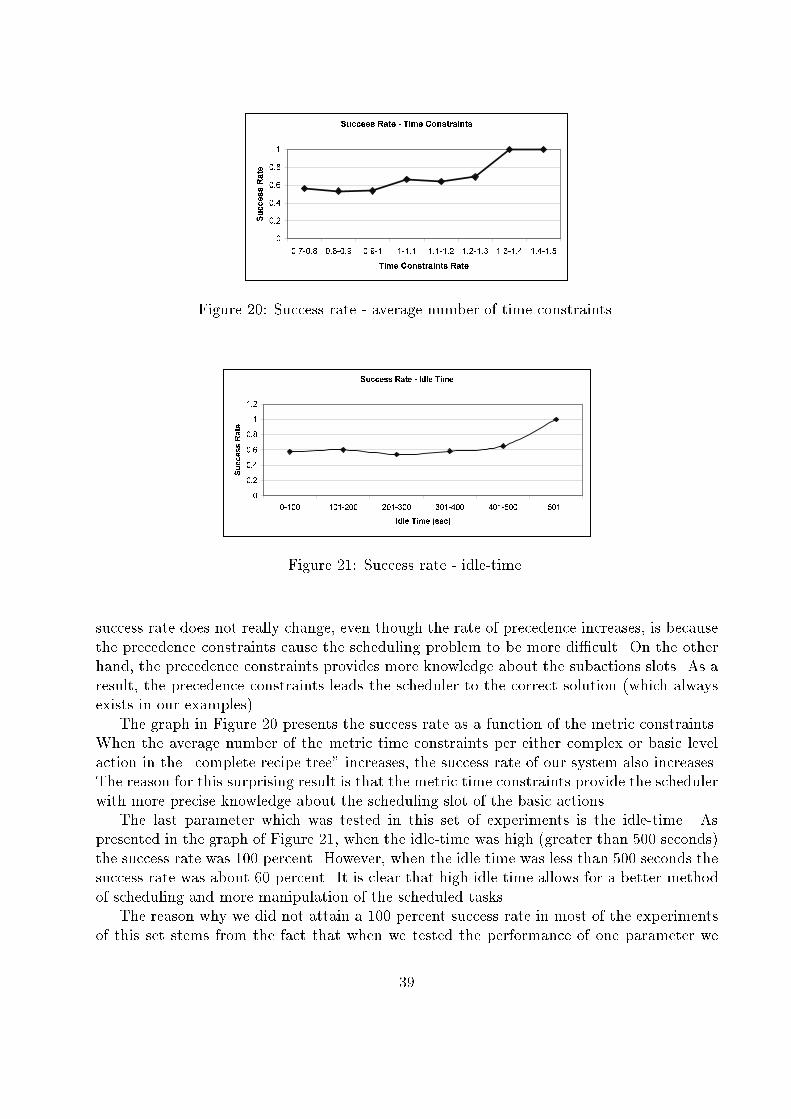
Figure 20: Success rate - average number of time constraints.Figure 21: Success rate - idle-time.success rate does not really change, even though the rate of precedence increases, is becausethe precedence constraints cause the scheduling problem to be more di�cult. On the otherhand, the precedence constraints provides more knowledge about the subactions slots. As aresult, the precedence constraints leads the scheduler to the correct solution (which alwaysexists in our examples).The graph in Figure 20 presents the success rate as a function of the metric constraints.When the average number of the metric time constraints per either complex or basic levelaction in the \complete recipe tree" increases, the success rate of our system also increases.The reason for this surprising result is that the metric time constraints provide the schedulerwith more precise knowledge about the scheduling slot of the basic actions.The last parameter which was tested in this set of experiments is the idle-time. Aspresented in the graph of Figure 21, when the idle-time was high (greater than 500 seconds)the success rate was 100 percent. However, when the idle time was less than 500 seconds thesuccess rate was about 60 percent. It is clear that high idle time allows for a better methodof scheduling and more manipulation of the scheduled tasks.The reason why we did not attain a 100 percent success rate in most of the experimentsof this set stems from the fact that when we tested the performance of one parameter we39

Figure 22: The average idle time that is necessary for a given number of basic actions for ahigh percentage of success rate.allowed the other parameters to have di�erent values. However, the above results provethat the major parameters which in uence the success of the system are the number ofbasic actions and the idle time. Thus, we ran a third set of experiments to check whichcon�guration set of these parameters attained about a 100 percent success rate. For thispurpose, we ran 120 examples (20 examples for each con�guration). Figure 22 presents theminimal idle time that is needed to attain about 100 percent success rate as a function ofthe number of basic actions in the recipe tree. The values of the other parameters in thisset were drawn from the same range as the second set of experiments described above. Asillustrated in the results' graph in Figure 22, when the number of basic level actions is small,the idle time may be low. However, when the number of basic actions is large, the planningprocess becomes slower. As a result, the idle time should be higher in order to guaranteeabout a 100 success percent rate.7.2 Single Agent BacktrackingIn this set of experiments, we tested the e�ects of backtracking by allowing more than onerecipe for each complex level action in the recipe tree of �. We ran 43 di�erent randomexamples of recipe libraries for action �. We changed each example of a recipe library 9times, as follows. At the beginning, the recipe library included only one recipe for eachcomplex level action (as in the case that backtracking was not allowed). Then, one complexaction had two recipes, two actions had two recipes, and so on (we increased the number ofrecipes by one 9 times). The examples were drawn from environments with a high successrate the value of the number of basic actions was between 50 and 70, and the value of the idealtime was between 80 and 150 (the con�gurations set of these values were selected accordingto the graph in Figure 22). The values of the other parameters were randomly selectedfrom the same range as the two former sets of experiments. The results of this experimentare presented in Figure 23. It is clear that the backtracking causes the planning time tobe higher, thus the performance of the system decreases. On the other hand, when thenumber of the additional recipes is high, in several cases, the agent has additional options40

Figure 23: Success Rate - in backtracking environment.in the performance its plan, which may cause the system's performance to improve. Sinceour system interleaves planning and execution, in the backtracking, the agent may removea recipe which consists of subactions that already have been executed. In our experiments,we analyzed the number of the basic actions that had been executed and then were removedfrom the agent plan. We found that in most cases (94 percent), the agent removed actionsthat had not been performed yet. However, we did not consider the e�ects of the executedactions which were removed.8 Expanding the Algorithm for the Multi-Agent Ac-tivityAlthough several collaborative multi-agent systems have been developed, they pay little at-tention to time coordination problems. There are mainly two approaches. The �rst approachsuggests a synchronization method; i.e., the team members broadcast messages that ensurethat the execution of an action will not be attempted until all the team members are ready[59, 65]. In the second approach [27], a team leader is responsible for the timing of theindividual actions. Both approaches restrict the activity of the individual agents, and thesecond approach is not appropriate for uncertain dynamic environments.The temporal reasoning mechanism for the multi-agent environment is very similar tothat of the individual case. Each individual agent G maintains a temporal constraints graphand develops its graph during its planning. However, in this case, the leaves of the fullrecipe tree may be complex actions to be performed by other agents. In particular, somevertices in the incremently constructed graph may represent joint actions. As a result, eachagent maintains a di�erent graph which consists of its constraints. Thus, Gr�, where � maybe either a joint action or an individual one of some agent G, could include �ve types ofvertices: (1) vertices which denote complex actions that G needs to perform individually;(2) vertices which denote basic actions that G needs to execute; (3) vertices which denotecomplex actions, where G belongs to the groups which have to perform the actions; (4)vertices that denote multi (or single) agent actions and where G does not belong to the41

groups (or is not the agent) that have (has) to perform these actions, but where the valueof these vertices are already known; and (5) vertices that denote multi (or single) actions,where G does not belong to the groups (or is not the agent) which have (has) to perform theactions and where the value of these vertices is unknown. When a vertex status is changedfrom unexplored to explored, the algorithm also determines to which of the cases describedabove it belongs.The concept IndV is also di�erent from the individual case, because each vertex maydepend on either other actions or other agents. In the multi-agent version of the algorithm,the �rst and the second types of vertices will be developed as in the individual case. Inthe development of the third type, the agents have to exchange their time constraints onthe joint action, and all agents need to agree to the set of constraints. Then the agentsuse the planning process Select Rec GR to jointly select the recipe for the joint actionand to assign subactions to individuals and subgroups. Based on these decisions, each agentconstructs the GrpR� graph of the joint action, incorporates it in Gr�, and continues itsplanning process. We refer to the fourth type of vertex as �xed (with the assumption thatthe agent may be asked to change the value). These values have been sent to the agent beforeit reaches this state of its planning. The last type in uences which vertices are independent;i.e., if some of the ancestors of a certain vertex is of this type, then the agent can not continuethe development of this vertex until it receives the value of the vertex from the appropriateagents.To con�rm the correctness of the multi-agent version of the algorithm, we have provedthat no deadlocks occur, since at each stage of the planning process at least one of the agentsin the group has a non-empty IU [24].9 ConclusionsIn this paper we have presented a mechanism for time planning in uncertain and dynamicmulti-agent systems, where the agents interleave planning and acting. This mechanism allowseach agent to develop its timetable individually and to take into consideration all types oftime constraints on its activities and on these of its collaborators. Thus, in contrast to otherworks on multi-agent systems, which suggest that either the team members maintain fullsynchronization by broadcasting messages or that a team leader determines the times ofactions, our mechanism enables the individual agent to determine its time individually, butalso to be easily integrated in the activities of other agents. We have proved that undercertain conditions the mechanism is sound and complete.We have also presented the results of several experiments on the system. The resultsproved that interleaving planning and acting in our environment is crucial. In our experi-ments, we tested the in uence of several parameters on the system's performance. We showedthe con�guration set of the parameters for the system provides an almost 100% success rate.We found out that as the number of the basic actions increases, the performance of thesystem decreases. However, this performance may be improved by improving the e�ciencyof the algorithm in the AI planning subsystem. We have left the task of improving thealgorithm for future work. 42

The development of this mechanism has uncovered several interesting problems in design-ing agents for collaborative activity. First, the planner does not consider the preconditionsof the actions while developing its plan. Second, the planner does not reason about resourceand resource con icts in the context of time coordination. We also did not consider the sidee�ects which arise from executing the actions that were canceled as a result of the agentbacktracking. We have left each of these research problems for future work. The next majorsteps that we envision includes developing strategies and protocols for elaborating partialplans, including mechanisms for combining time information possessed by di�erent agents, aswell as strategies for negotiating in the event of resource con icts, and reaching a consensuson how to allocate portions of the activity among di�erent participants.References[1] James Allen. Towards a general theory of action and time. Arti�cial Intelligence,23(2):123{144, 1984.[2] James F. Allen. Maintaining knowledge about temporal intervals. Communications ofthe ACM, 26:832{843, 1983.[3] R. C. Arkin. Integrating behavioal, perceptual, and world knowledge in reactive navi-gation. Robotics and Autonomous Syst., 6:105{222, 1990.[4] R. Arthur and J. Stillman. Tachyon: A model and environment for temporal reasoning.M.S. Thesis, Rensselaer Polytechnic Institute, Troy, NY, 1992.[5] Peter Van Beek. Reasoning about qualitative temporal information. Arti�cial Intelli-gence, 58:297{326, 1992.[6] Giorgio C. Buttazzo. Hard Real-Time Computing Systems. Kluwer Academic Publishers,1997.[7] Alison Cawsey. Arti�cial Intelligence. Prentice Hall Europe, London, 1998.[8] S. Chien, G. Rabideau, J. Willis, and T. Mann. Automating planning and schedulingof shuttle payload operations. Arti�cial Intelligence Journal, 114:239{255, 1999.[9] Wesley W. Chu and Kin K. Leung. Task response time for real-time distributed systemswith resource contentions. IEEE Transactions on software engineering, 17(10):1076{1092, 1991.[10] Thomas H. Cormen, Charles E. Leiserson, and Ronland L. Rivest. Introduction toAlgorithms. MIT Press, London, England, 1990.[11] Ken Currie and Austin Tate. O-plan: the open planning architecture. Arti�cial Intel-ligence, 52:49{86, 1991. 43

[12] C. Anderson D. Weld and D. Smith. Extending graphplan to handle uncertainty andsensing actions. In Proceedings of the Annual Conference of the American Associationfor Arti�cial Intelligence (AAAI-98), pages 897{904, 1998.[13] T. L. Dean and D. V. McDermott. Temporal data base management. Arti�cial Intelli-gence, 32:1{55, 1987.[14] Rina Dechter, Itay Meiri, and Judea Pearl. Temporal constraint networks. Arti�cialIntelligence, 49:61{95, 1991.[15] J. Dorn, M. Girsch, G. Skele, and W. Slany. Comparison of iterative improvementtechniques for schedule optimization. European Journal on Operations Research, pages349{361, 1996.[16] A. El-Kholy and B. Richards. Temporal and resource reasoning in planning: the parc-Plan approach. In 12th European Conference on Arti�cal Intelligence (ECAI '96), pages614{618, 1996.[17] R. E. Fikes, P.E. Hart, and N. J. Nilsson. Learning and executing generalized robotplans. Arti�cial Intelligence, 3(4):251{288, 1972.[18] Michael R. Garey and David S. Johnson. Computers and Intractability: A Guide to theTheory of NP-Completeness. W. H. Freeman, San Francisco, California, 1979.[19] Keith Golden, Oren Etzioni, and Daniel Weld. Planning with execution and incompleteinformation. Technical report, University of Washington, 1996.[20] Martin Charles Golumbic. Reasoning about time. Mathematical Aspects of Arti�cialIntelligance, 55:19{53, 1998. Proceedings of Symposia in Applied Mathematics.[21] M. Graham and M. Florian. On scheduling with ready times and due dates to minimizemaximum lateness. Operations Research, 23(3), 1975.[22] Barbara Grosz and Sarit Kraus. Collaborative plans for group activities. In Ruzena Ba-jcsy, editor, Proceedings of the 1993 International Joint Conference on Arti�cial Intelli-gence (IJCAI-93), pages 367{373, San Mateo, CA, 1993. Morgan Kaufmann Publishers,Inc.[23] Barbara J. Grosz and Sarit Kraus. Collaborative plans for complex group action. Ar-ti�cial Intelligence, 86(2):269{357, 1996.[24] Meirav Hadad and Sarit Kraus. Intelligent information agents. In Matthias Klusch,editor, Intelligent Information Agents, chapter SharedPlans in Electronic Commerce,pages 204{231. Springer Publishers, Berlin, 1999.[25] Babak Hamidzadeh and Shashi Shekhar. Speci�cation and analysis of real-time problemsolvers. IEEE Trans. on Computer, 19(8):788{803, August 1993.44

[26] Kristian J. Hammond. Chef: A model case-based planning. In Proceedings of theAnnual Conference of the American Association for Arti�cial Intelligence (AAAI-86),pages 267{271, 1986.[27] Nick R. Jennings. Controlling cooperative problem solving in industrial multi-agentsystems using joint intentions. Arti�cial Intelligence, 75(2):1{46, 1995.[28] J. Hendler K. Erol, D. Nau. HTN planning: Complexity and expressivity. In Proceedingsof the Annual Conference of the American Association for Arti�cial Intelligence (AAAI-94), pages 1123{1128, 1994.[29] Nikos I. Karacapilidis. Planning under uncertainty: A qualitative approach. LectureNotes in Computer Science, 990:285{296, 1995.[30] D. Kinny, M. Ljungberg, A. S. Rao, E. Sonenberg, G. Tidhar, and E. Werner. Plannedteam activity. In C. Castelfranchi and E. Werner, editors, Arti�cial Social Systems,Lecture Notes in Arti�cial Intelligence (LNAI-830), Amsterdam, The Netherlands, 1994.Springer Verlag.[31] Craig A. Knoblock. Building a planner for information gathering: A report from thetrenches. In Third International Conference on Arti�cial Intelligence Planning Systems,1996.[32] Carsten Hojmose Kristensen and Niels Drejer. Evaluating distributed timing constraintsimplementing run-time mechnisms. In 2ND IEEE workshop on Real-Time Applications,pages 157{162, Washington,DC., 1994.[33] John E. Laird, Allen Newell, and Paul S. Rosenbloom. Soar: An architecture for generalintelligence. Arti�cial Intelligence, 33:1{64, 1987.[34] J. Lever and B. Richards. parcPlan: a planning architecture with parallel actions,resources and constraints. Lecture Notes in Computer Science, 896:213{222, 1994.[35] H. Levesque, P. Cohen, and J. Nunes. On acting together. In Proceedings of the AnnualConference of the American Association for Arti�cial Intelligence (AAAI-90), pages94{99, 1990.[36] Karen Lochbaum. Using Collaborative Plans to Model the Intentional Structure of Dis-course. PhD thesis, Harvard University, 1994. Available as Tech Report TR-25-94.[37] Karen Lochbaum, Barbara Grosz, and Candace Sidner. Models of plans to supportcommunication: An initial report. In Proceedings of AAAI-90, pages 485{490, Boston,MA, 1990.[38] J. Malik and T.O. Biford. Reasonning in time and space. In Proceedings of the Inter-national Joint Conference on Arti�cial Intelligence (IJCAI-83), pages 343{345, 1983.[39] Graham Mcmahon and Michael Florian. On scheduling with ready times and due datesto minimize maximum lateness. Operations Research, 23(3):475{482, 1975.45

[40] Pinedo Michael. Scheduling. Prentice Hall, 1995.[41] D. P. Miller and E. Gat. Exploiting known topologies to navigate with low-computationsensing. In SPIE Sensor Fusion Conference, November 1990.[42] U. Montanari. Networks of constraints: fundamental properties and applications topicture processing. Information Sciences, 7:95{132, 1974.[43] L. Morgenstern. Knowledge preconditions for actions and plans. In Proceedings ofIJACAI-87, pages 867{874, Los Altos, CA, 1987. Morgan Kaufman Publishers Inc.[44] D. J. Musliner, E. H. Dufree, and K. G. Shin. World modeling for dynamic constructionof real-time control plans. AI, 74(1):83{127, 1995.[45] David J. Musliner, Edmund H. Dufree, and Kang G. Shin. Circa: A cooperative in-telligent real-time control architecture. IEEE trans. on computer, 23(6):1561{1574,November 1993.[46] David J. Musliner, James A. Hendler, Ashok K. Agrawala, Edmund H. Dufree, Jay K.Strosnider, and C. J. Paul. The challenges of real-time AI. IEEE trans. on computer,28(1):58{66, January 1995.[47] Alexander Nareyek. A planning model for agents in dynamic and uncertain real-timeenvironments. In AIPS Workshop on Integrating Planning, pages 7{14, 1998.[48] Alexander Nareyek. Open world planning as scsp. Technical Report WS-00-02, AAAIPress, Menlo Park, California, 2000.[49] Dana Nau, Yue Cao, Amnon Lotem, and Hector Munoz-Avila. Shop and m-shop plan-ning with ordered task decomposition. Technical report, University of Maryland, 2000.[50] Nils J. Nilsson. Principles of Arti�cial Intelligence, chapter 7 and 8. Tioga PublishingCompany, 1980.[51] J.S. Penberthy and D. Weld. Temporal planning with continuous change. In Proceedingsof the Annual Conference of the American Association for Arti�cial Intelligence (AAAI-94), pages 1010{1015, 1994.[52] Martha E. Pollack. Plans as complex mental attitudes. In P.N. Cohen, J.L. Morgan,and M.E. Pollack, editors, Intentions in Communication. Bradford Books, MIT Press,1990.[53] Krithivasan Ramamritham and John A. Stankovicand. Dynamic task scheduling in hardreal-time distributed systems. IEEE Software, 1(3):65{75, 1984.[54] Elaine Rich and Kevin Knight. Arti�cial Intelligence. McGraw-Hill, Inc., second edition,1991.[55] Stuart Russell and Peter Norvig. Arti�cial Intelligence: A Modern Approach. PrenticeHall, Englewood Cli�s, NJ, 1995. 46

[56] Terry Shepard and J. A. Martin Gagne. A pre-run-time scheduling algorithm for hardreal-time systems. IEEE Transactions on software engineering, 17(7):669{677, 1991.[57] R. Simmons. An architecture for coordinating planning, sensing and action. In Proceed-ings of the Workshop on Innovative Approaches to Planning, Scheduling, Contr., pages292{297, November 1990.[58] Hardeep Singh and Texas Instrument. Scheduling techniques for real-time applicationsconsisting of periodic task sets. In 2ND IEEE Workshop on real-time applications, pages12{15, Washington,DC, 1994.[59] E. Sonenberg, G. Tidhar, E. Werner, D. Kinny, M. Ljungberg, and A. Rao. Plannedteam activity. Technical Report 26, Australian Arti�cial Intelligence Institute, Australia,1992.[60] Biplav Srivastava. RealPlan: Decoupling causal and resource reasoning in planning.In Proceedings of the Annual Conference of the American Association for Arti�cialIntelligence (AAAI-00), pages 812{818, 2000.[61] J. A. Stankovic and K. Ramamritham. The spring kernal: a new paradigm for real-timesystems. IEEE Software, pages 62{72, May 1991.[62] John A. Stankovic, Krithivasan Ramamritham, and Shengchang Cheng. Evaluationof a exible task scheduling algorithm for distributed hard real-time systems. IEEETransactions on computers, 34(12):1130{1143, 1985.[63] John A. Stankovic, Marco Spuri, Macro Di Natale, and Giorgio Buttazzo. Implicationsof classical scheduling results for real-time syatems. IEEE computer, 28(6):16{25, 1995.[64] Richard S. Sutton. Integrated architectures for learning, planning, and reacting basedon approximating dynamic programming. In Proceedings of the Seventh InternationalConference on Machine Learning, 1990.[65] M. Tambe. Toward exible teamwork. Journal of AI Research, 7:83{124, 1997.[66] Steven A. Vere. Planning in time: Windows and durations for activities and goals. InJames Allen et al., editor, Readings in Planning, pages 297{318. Springer Publishers,Berlin, 1990.[67] T. Vidal and M. Ghallab. Dealing with uncertain durations in temporal constraintnetworks dedicated to planning. In 12th European Conference on Arti�cal Intelligence(ECAI '96), pages 54{48, 1996.[68] M. Vilain and H. A. Kautz. Constraint propagation algorithms for temporal reasoning.In Proceedings of the Annual Conference of the American Association for Arti�cialIntelligence (AAAI-86), pages 132{144, 1986.[69] D. Wilkins. Using pattern and plans in chess. Arti�cial Intelligence, 14(2):165{203,1983. 47

[70] D. E. Wilkins, K. L. Myers, J. D. Lowrance, and L. P. Wesley. Planning and reactingin uncertain and dynamic environments. Journal of Experimental and Theoretical AI,7(1):197{227, 1995.[71] Jia Xu. Multiprocessor scheduling of process with release times, deadlines, precedence,and exclusion relations. IEEE Transactions on software engineering, 19(2):139{154,1993.[72] Jia Xu and David Lorge Parnas. Scheduling processes with release times, dead-lines, precedence and exclusion relations. IEEE Transactions on software engineering,16(3):360{369, 1990.[73] Jia Xu and David Lorge Parnas. On satisfying timing constraints in hard-real-timesystems. IEEE Transactions on software engineering, 19(1):70{84, 1993.

48

A Lemmas and Propositions for the Correctness of theAlgorithmIn order to prove the correctness of the algorithm, we will �rst de�ne the following newconcepts. All of the concepts refer to the algorithm and the de�nitions in section 4.2.De�nition A.1 (CloserFixVertex(v), CloserFixSet(v)) Let PathSet(v) be the setfp1; : : : ; pmg which consists of all the paths from s�plan to the vertex v 2 V�. For eachpi 2 PathSet(v) (1 � i � m), the �xed vertices in pi which is closer to v, is calledthe CloserF ixV ertex(v) in pi. That is, if pi is the sequence (u0; u1; u2; : : : ; un) such thats�plan = u0 and v = un, then, uj 0 � j � n is the CloserF ixV ertex(v) in pi if for all other�xed vertex us in pi s < j. The CloserF ixSet(v) is a set of all the vertices fv1; v2; : : : ; vlgsuch that each vj 1 � j � l � m is a CloserF ixV ertex(v) in some pi.In each stage of the algorithm, the agent selects a vertex v which is an IndV in order toidentify the value of this vertex. In the following claims we will show that, according to thealgorithm, this vertex indeed can be identi�ed (because all the vertices in the path from thevertices in the CloserF ixSet(v) to v have been identi�ed). Then, we will show (in lemma 1)that the algorithm always terminates, and �nally we will prove that the algorithm is correctand complete.Proposition 1 Suppose that identify id times params builds a temporal constraints graphof �, Gr� = (V�; E�), from a given initial graph InitGr�. Let u be some vertex in V�. Then,during the execution of identify id times params, if each vertex in the path from all thevertices in the CloserF ixSet(u) to u are explored (i.e., either EB or EC), then u is IndV.Proof: The proof is by induction on the length of the longest path from CloserF ixSet(u)to u. Initially, when the vertex u is a �xed time point, the proposition certainly holds. Letu be some vertex such that the path from all the vertices in the CloserF ixSet(u) to u areexplored. If u is not a �xed vertex, then for each (v; u) 2 E� the CloserF ixSet(u) is longerthan the CloserF ixSet(v). Thus the path from all the vertices in the CloserF ixSet(v) tov is explored. Thus, according to the inductive hypothesis, each such v is IndV; that is,v 2 IE. Now, it remains to show that the weight of each edge (v; u) 2 E� is known. Since,according to the algorithm, this edge cannot be a complex edge,10 then the weight of thisedge is known. As a result, the weight of the edge from the CloserF ixSet(v) to v is knownand the value of v may be de�ned (i.e., v is IndV). 2In the following proposition we prove that all the values of the parameters associatedwith the basic actions which are sent to the RT scheduling subsystem will not be changedlater by the planning process (with the exception of the case of backtracking). Thus, theseactions can already be scheduled and executed before the agent �nishes its planning. Thisfact enables the agent to interleave planning and acting.10That is, in the building of the graph, it �rst adds the new vertices which are appropriated for theselected recipe of the complex edge (v; u) between u and v. Then, it changes the statues of v and u toexplored vertices. As a result, there is path of unexplored vertices between u and v.49

Proposition 2 Suppose that identify id times params runs and builds a temporal con-straints graph of �, Gr� = (V�; E�). Let v 2 V be an IndV which represents a start timepoint of some basic level action �. Then, the �nal values of < C�; d� ; r�; p� > can be iden-ti�ed, i.e.; these values will not be changed (unless the agent will backtrack and choose adi�erent recipe).Proof: Because � is a basic level action it is obvious that the computation time, C� , is�nal.11 Now, we have to show that if v represents a start time point of �, and v is an IndV,then r� can be identi�ed. Since v is IndV all the paths between the CloserF ixSet(v) to vare �nal, the weights of all the edges in these paths are �nal, thus the �nal value of r� canbe identi�ed. Similarly, the �nal value of d� can be identi�ed. Also, all the basic edges inthe paths between the CloserF ixSet(v) to v are �nal. Thus all the basics actions which areprecedent to v are �nal.2In the following lemma we prove that the algorithm always terminates.Lemma 1 Let Gr� = (V�; E�) be the temporal constraints graph of �, and suppose thatidentify id times params runs and builds Gr� from a given initial graph InitGr�. Then,during its execution:1. If Gr� consists of some unexplored vertices, then at least one of these vertices is anIndV start time point.2. If all the vertices in the graph are explored, then the agent �nished identifying all ofthe time parameters in its individual plan for �.Proof:1. Because Gr� is a \directed acyclic graph (dag)," we can perform a topological sort ofthe graph. Let vi be the �rst unexplored vertices in the order of the topological sort.Then, it is clear that all the vertices in the paths from s�plan to vi are explored. Thus,according to proposition 1, vi is an IndV. According to the algorithm, the start timepoint and the �nish time point of each action in the graph become unexplored in thesame step. The start time of the action always precedes the �nish point. Thus, vi is astart time point (since the start time point is also prior to the �nish time point in thetopological order).2. Suppose by contradiction that the agent did not �nish identifying all of the temporalparameters in its individual plan for �, but all the vertices in the graph were explored.Thus, the graph consists of at most one action � for which the agent did not identifyits time parameters. But, according to the algorithm, for each basic level action �, thevertices which represent action � become explored when the temporal parameters of� are identi�ed. For each complex level action �, when the vertices which representthis action become explored, new unexplored vertices are added to the graph (i.e., thevertices which represent the subactions of �). Thus, we obtain a contradiction to theassumption that all the vertices in the graph are explored.211We use the term \�nal" to refer to the values of the parameters that will not be changed during theplanning process (unless the agent backtracks). 50

Corollary 1 The algorithm terminates when all the leaves in the implicit recipe tree of Gr�are basic level actions.Proof: Otherwise, if the leaf of the recipe tree was a complex level action, then, accordingto the algorithm, the graph includes some unexplored vertex and the algorithm hasnot terminated.In the following lemma we prove that in each stage of the algorithm the leaves in theimplicit recipe tree constitute performing � under the associated time constraints �.Lemma 2 Suppose that the agent plans for some action �. Then, during the developmentof the graph Gr�, performing all the actions (possibly complex) in the leaves of the implicitrecipe tree, Tree�, constitutes performing � under constraints �� (possibly in parallel).Proof: The proof is by induction of the number of the vertices in the implicit recipe tree.Initially, when the recipe-tree consists of one vertex (i.e., only action �), the propositioncertainly holds. Suppose that the recipe tree consists of n vertices. As an inductivehypothesis we assume that all the actions in the leaves of the recipe tree with mvertices, where m < n constitute performing � under constraints ��. Let Tree� besome incomplete recipe tree of � withm vertices. According to the algorithm the agentexpands the recipe tree by selecting some leaf which represents a complex level action�. Suppose that the agent selected the recipe R� in order to expand the recipe treefor � which consists of b subactions. According to the inductive hypothesis, all of theactions in the leaves of the recipe tree with the m vertices constitute performing �under constraints ��. However, according to the algorithm, when the agent selects therecipe for � and adds it to the constraints graph, it also checks that all the constraintsof � constitute performing � under constraints ��. If these constraints constituteperforming �, it continues with its plan for � and the subactions of � become theleaves of the recipe tree of �. Thus, all the actions in the leaves of the tree whichconsists of n = m+ b vertices constitute performing � under constraints ��. 2

51

B The remove Procedureremove(�; descendset)1 status[s�] UE; status[f�] UE;2 remove s� and f� from IE and IU sets;3 for each node 2 descendset do;4 remove s and f from V�;5 if (s�plan; s ); (s�plan; f ) 2 E� remove it from E�;6 remove all the edges (s ; a) 2 E� from E�;7 remove s and f from IE and IU sets;8 update IV sets(s�);Figure 24: The procedure for removing recipes from Gr�.

52