Reasoning about Temporal Properties of Rational Play Nils Bulling, Wojciech Jamroga, and Jürgen Dix IfI Technical Report Series IfI-08-03

Welcome message from author
This document is posted to help you gain knowledge. Please leave a comment to let me know what you think about it! Share it to your friends and learn new things together.
Transcript
Reasoning about Temporal Propertiesof Rational PlayNils Bulling, Wojciech Jamroga, and Jürgen Dix
IfI Technical Report Series IfI-08-03
brought to you by COREView metadata, citation and similar papers at core.ac.uk
provided by Publikationsserver der Technischen Universität Clausthal
Impressum
Publisher: Institut für Informatik, Technische Universität ClausthalJulius-Albert Str. 4, 38678 Clausthal-Zellerfeld, Germany
Editor of the series: Jürgen DixTechnical editor: Wojciech JamrogaContact: [email protected]
URL: http://www.in.tu-clausthal.de/forschung/technical-reports/
ISSN: 1860-8477
The IfI ReviewBoard
Prof. Dr. Jürgen Dix (Theoretical Computer Science/Computational Intelli-gence)Prof. Dr. Klaus Ecker (Applied Computer Science)Prof. Dr. Barbara Hammer (Theoretical Foundations of Computer Science)Prof. Dr. Sven Hartmann (Databases and Information Systems)Prof. Dr. Kai Hormann (Computer Graphics)Prof. Dr. Gerhard R. Joubert (Practical Computer Science)apl. Prof. Dr. Günter Kemnitz (Hardware and Robotics)Prof. Dr. Ingbert Kupka (Theoretical Computer Science)Prof. Dr. Wilfried Lex (Mathematical Foundations of Computer Science)Prof. Dr. Jörg Müller (Business Information Technology)Prof. Dr. Niels Pinkwart (Business Information Technology)Prof. Dr. Andreas Rausch (Software Systems Engineering)apl. Prof. Dr. Matthias Reuter (Modeling and Simulation)Prof. Dr. Harald Richter (Technical Computer Science)Prof. Dr. Gabriel Zachmann (Computer Graphics)
Reasoning about Temporal Properties of RationalPlay
Nils Bulling, Wojciech Jamroga, and Jürgen Dix
Department of Informatics, Clausthal University of Technology, Germanywjamroga,bulling,[email protected]
Abstract
This article is about defining a suitable logic for expressing classical gametheoretical notions. We define an extension of alternating-time tempo-ral logic (ATL) that enables us to express various rationality assumptionsof intelligent agents. Our proposal, the logic ATLP (ATL with plausibil-ity) allows us to specify sets of rational strategy profiles in the object lan-guage, and reason about agents’ play if only these strategy profiles wereallowed. For example, wemay assume the agents to play only Nash equi-libria, Pareto-optimal profiles or undominated strategies, and ask aboutthe resulting behaviour (and outcomes) under such an assumption. Thelogic also gives rise to generalized versions of classical solution conceptsthrough characterizing patterns of payoffs by suitably parameterized for-mulae ofATLP.We investigate the complexity ofmodel checkingATLPfor several classes of formulae: It ranges from ∆P
3 to PSPACE in thegeneral case and from∆P
3 to∆P4 for themost interesting subclasses, and
roughly corresponds to solving extensive games with imperfect informa-tion.
Keywords: game theory,modal and temporal logic, reasoning about agents,rationality.
1 Introduction
Alternating-time temporal logic (ATL) [2, 3] is a temporal logic that incorpo-rates some basic game theoretical notions. In ATL we can express that agroup of agents is able to bring aboutψ, i.e., they are able to ensure a situationwhere ψ holds whatever the other agents might do. However, such a state-ment is weaker than it seems. Often, we know that agents behave accordingto some rationality assumptions, they are not completely dumb. Thereforewe do not have to check all possible plays – only those that are plausible in
1
Introduction
some reasonable sense. This has striking similarities to nonmonotonic rea-soning, where one considers default rules that describe themost plausible be-haviour and allow to draw conclusions when knowledge is incomplete.In general, plausibility can be seen as a broader notion than rationality:
One may obtain plausibility specifications e.g. from learning or folk knowl-edge. In this article, however, we mostly focus on plausibility as rationalityin a game-theoretical sense.Our idea has been inspired by the way in which games are analyzed in
game theory. Firstly, game theory identifies a number of solution concepts(e.g., Nash equilibrium, undominated strategies, Pareto optimality) that canbe used to define rational behaviour of players. Secondly, we usually assumethat players play rationally in the sense of one of the above concepts, and weask about the outcome of the game under this assumption.Solution concepts do not only help to determine the right decision for an
agent. Perhaps more importantly, they constrain the possible (predicted) re-sponses of the opponents to a proper subset of all the possibilities. For manygames the number of all possible outcomes is infinite, althoughonly someofthem, often finitely many, make sense. We need a notion of rationality (likesubgame-perfect Nash equilibrium) to discard the less sensible ones, and todetermine what should happen had the game been played by ideal players.
1.1 Idea andMain Results
While ATL is already a logic that incorporates some game theoretical con-cepts, we claim that extendingATLbyother useful constructs not onlyhelpsus to better understand the classical solution concepts in game theory, butit also paves the way for defining new solution concepts (which we call gen-eral). We extendATL by the notion of plausibility, and call the resulting logicATLP. We claim that this logic is suitable to model and to reason about therational behaviour of agents.In this article we discuss the following:
1. We recall from [5, 30] that models ofATL, called concurrent game struc-tures (CGS), embed extensive form games with perfect information in a nat-ural way. This can be done, e.g., by adding auxiliary propositions to theCGS, that describe the payoffs of agents. With this perspective, concur-rent game structures can be seen as a strict generalisation of extensivegames.
2. We discuss informally how these more general games can be “solved”,given an appropriate solution concept that defines which plays can beplausibly expected.
3. We extendATL to a new logicATLP that allows to reason about whatagents can achieve under an arbitrary plausibility assumption. Analy-
DEPARTMENTOF INFORMATICS 2
REASONING ABOUT TEMPORAL PROPERTIES OF RATIONAL PLAY
sis of this kind typically starts with assuming that agents are rational inthe sense that they only play strategies consistent with a selected solu-tion concept (e.g., they can only play Nash equilibria, or undominatedstrategies etc.). Then, we can ask which outcomes can be obtained bywhom under this assumption.
4. We extend the results from [45, 30], and show that the classical solu-tion concepts (Nash equilibrium, subgame perfect Nash equilibrium, Paretooptimality, and others) can be also characterized in the object languageof ATLP. That is, we propose expressions of ATLP that, given an ex-tensive game, denote exactly the set of Nash equilibria (subgame per-fect NE’s, Pareto optimal profiles, etc.) in that game. In consequence,ATLP can serve both as a language for reasoning about rational play,and for specifying what rational play is. We point out that these char-acterizations extend traditional solution concepts to the more generalclass ofmulti-stagemulti-player games definedby concurrent game struc-tures.
5. We also propose an alternative approach to defining solution conceptsfor games that involve infinite flow of time. In the new approach, pathformulae of ATL are used to specify the “winning conditions” of eachplayer. This implicitly leads to a normal form game with binary pay-offs, where the traditional solution concepts are well defined. We alsodemonstrate how these “qualitative” solution concepts (parametrizedbyATL path formulae) can be characterized inATLP.
6. We constructively show that several logics canbe embedded intoATLP.That is, we demonstrate how models and formulae of those logics canbe (independently) transformed to their ATLP counterparts in a waythat preserves their truth values.
7. Last but not least, we investigate themodel checkingproblem inATLP.We show that, for different subclasses of the new logic, the complexityofmodel checking ranges from∆P
3 -completeness toPSPACE-completeness.We also argue that, when the number of plausible strategy profiles isreasonably small, themodel checking can be done in polynomial time.
1.2 RelatedWork
In our approach, some strategies (or rather strategy profiles) can be assumedplausible, andone can reasonwhat can be plausibly achieved by agents undersuch an assumption. There are two possible points of focus in this context.Researchwithin game theory understandably favorswork on characterizationof various types of rationality (and defining most appropriate solution con-cepts). Applications of game theory, also understandably, tend toward using
3 Technical Report IfI-08-03
Introduction
the solution concepts in order to predict the outcome in a given game (inother words, to “solve” the game).The first issue has been studied in the framework of logic, for example
in [4, 6, 41, 42];more recently, game-theoretical solution concepts have beencharacterized in dynamic logic [21, 20], dynamic epistemic logic [5, 44], andATL [45, 30].The second thread seems to have been neglected in logic-based research:
papers by VanOtterloo and his colleagues [50, 51, 49, 48] are the only excep-tions we know of. Moreover, every proposal from [50, 51, 49, 48] commitsto a particular view of rationality (Nash equilibria, undominated strategiesetc.). In this paper, we try to generalize this kind of reasoning in a way thatallows to “plug in” any solution concept of choice. We also try to fill in thegap between the two threads by showinghow sets of rational strategy profilescan be specified in the object language, and building upon the existing workonmodal logic characterizations of solution concepts [21, 20, 5, 44, 45, 30].
1.3 Structure of the Article
Webeginby introducing somebasic notions fromgame theory and the alternating-time temporal logic (Section 2). In Section 3, we pave the way for Sections 4and 5: We relate ATL and its semantical models to extensive games. Thenwe do the same for an extension ofATL, calledATLI, which has been intro-duced in [30] to characterize solution concepts in extensive games.Section 4 introduces our logic ATLP: We extend ATL with a plausibility
operator. This constitutes the base language LbaseATLP. The main syntactic nov-elty are plausibility terms that refer to rational strategies. Then, we extend thebase language by allowing to specify sets of rational strategy profiles in the ob-ject language. To do this, we need to define a language with a much richerstructure of terms as in LbaseATLP. We achieve this by describing strategy profileswithATLI formulae, and extending LbaseATLP so that the concepts presented inSection 3.4 can be reused. Finally, we propose the full language LATLP whereATLP characterizations of solution concepts are “plugged” into ATLP for-mulae that describe the consequences of adopting this or that notion of ra-tionality. Thus, we create a single language for both characterizing rationalbehaviour and reasoning about its outcome. We define LATLP through a hi-erarchy of sublanguages LkATLP, each allowing for more levels of plausibilityupdates than the previous one.Section 5 lists ourmain conceptual results. We showhow to embed several
logics in ATLP and how to express several classical solution concepts (suchas Nash equilibria and others) already in L1
ATLP. Our third result is the gen-eralization of Nash equilibria, Pareto optimality, undominatedness and sub-game perfect Nash equilibria as certain parameterized formulae in the lan-guage ofATLP.
DEPARTMENTOF INFORMATICS 4
REASONING ABOUT TEMPORAL PROPERTIES OF RATIONAL PLAY
Section 6 contains the results of our study on the complexity of modelchecking in variants ofATLP. Finally, we conclude with Section 7.Some results reported in this article have been already presented in a pre-
liminary form in several conference and workshop papers. A rough idea of“ATL with plausibility” was proposed in [8, 25]. In [26], we studied a morecomplex language of terms that would allow to specify sets of rational strat-egy profiles in the object language; still, the language was not expressiveenough for our purposes. Some initial complexity results were also reportedin that paper. Finally, [11] put forward the idea that rationality specificationscan be written in ATLP itself, and nested in ATLP formulae. The idea of“qualitative” solution concept was also introduced in [11].
2 Preliminaries
In this section, we introduce some concepts that are important for the rest ofthis article. After recapitulating some machinery of game theory, togetherwith two running examples, we introduce ATL, which is the basis for ournew logicATLP.
2.1 Concepts FromGameTheory
We start with the definition of a normal form game, also called strategic game,and use the terminology of [35].
Definition 1 (Normal Form (NF) Game) A (perfect information) normalform game Γ, is a tuple of the form Γ = 〈P,A1, . . . ,Ak, µ〉, where
• P is a finite set of players (or agents), with |P| = k,
• Ai are nonempty sets of actions (or strategies) for player i,
• µ : P → (∏ki=1Ai → R) is the payoff function (which we also write
〈µ1, . . . , µk〉).
A combinations of actions (resp. strategies, payoffs), one per player, will be calledan action profile (resp. strategy profile, payoff profile) throughout the paper.
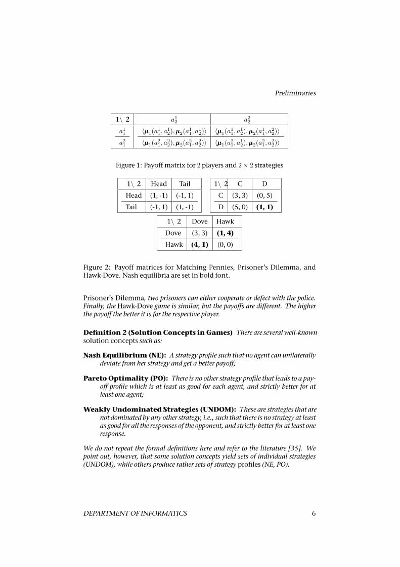
Such games are usually depictedwith a payoffmatrix. For example, a gamewith 2 players having 2 strategies each is represented by the matrix in Fig-ure 1.
Example 1 (Classical NF Games) Some classical NF games with 2 playersand 2 strategies are shown in Figure 2. In the Matching Pennies game, player1 wins when both pennies show the same side. Otherwise player 2 wins. In the
5 Technical Report IfI-08-03
Preliminaries
1\ 2 a12 a2
2
a11
a21
〈µµµ1(a11, a
12),µµµ2(a1
1, a12)〉
〈µµµ1(a21, a
22),µµµ2(a2
1, a22)〉
〈µµµ1(a11, a
12),µµµ2(a1
1, a22)〉
〈µµµ1(a21, a
12),µµµ2(a2
1, a22)〉
Figure 1: Payoff matrix for 2 players and 2× 2 strategies
1\ 2 Head Tail
Head
Tail
(1, -1)
(-1, 1)
(-1, 1)
(1, -1)
1\ 2 C D
C
D
(3, 3)
(5, 0)
(0, 5)
(1, 1)
1\ 2 Dove Hawk
Dove
Hawk
(3, 3)
(4, 1)
(1, 4)
(0, 0)
Figure 2: Payoff matrices for Matching Pennies, Prisoner’s Dilemma, andHawk-Dove. Nash equilibria are set in bold font.
Prisoner’s Dilemma, two prisoners can either cooperate or defect with the police.Finally, the Hawk-Dove game is similar, but the payoffs are different. The higherthe payoff the better it is for the respective player.
Definition 2 (Solution Concepts in Games) There are severalwell-knownsolution concepts such as:
Nash Equilibrium (NE): A strategy profile such that no agent can unilaterallydeviate from her strategy and get a better payoff;
Pareto Optimality (PO): There is no other strategy profile that leads to a pay-off profile which is at least as good for each agent, and strictly better for atleast one agent;
Weakly Undominated Strategies (UNDOM): These are strategies that arenot dominated by any other strategy, i.e., such that there is no strategy at leastas good for all the responses of the opponent, and strictly better for at least oneresponse.
We do not repeat the formal definitions here and refer to the literature [35]. Wepoint out, however, that some solution concepts yield sets of individual strategies(UNDOM), while others produce rather sets of strategy profiles (NE, PO).
DEPARTMENTOF INFORMATICS 6
REASONING ABOUT TEMPORAL PROPERTIES OF RATIONAL PLAY
In the examples fromFigure 2, there is noNash equilibrium for theMatch-ing Pennies game, exactly one Nash equilibrium for the Prisoner’s Dilemma(namely, the strategy profile 〈D,D〉), and two Nash equilibria for the Hawk-Dove game (〈Hawk,Dove〉 and 〈Dove,Hawk〉).In NF games, agents do their moves simultaneously: They do not see the
move of the opponent and therefore cannot act accordingly. On the otherhand, there are many games where the move of one player should dependon the preceding move of the opponent, or even on the whole history. Thisidea is captured in games of extensive form.
Definition 3 (Extensive Form (EF) Game) A (perfect information) exten-sive form game Γ is a tuple of the form Γ = 〈P,A,H, ow, u〉, where:
• P is a finite set of players,
• A a finite set of actions (moves),
• H is a set of finite action sequences (game histories), such that (1) ∅ ∈ H, (2)if h ∈ H, then every initial segment of h is also in H. We use the notationA(h) = m | h m ∈ H to denote themoves available at h, and Term =h | A(h) = ∅, the set of terminal positions,
• ow : H → P defines which player “owns” history h, i.e., has the next movegiven h,
• u : P × Term → U assigns agents’ utilities to every terminal position of thegame.
We will usually assume that the set of utilities U is finite.
Such games can be easily represented as trees of all possible plays.
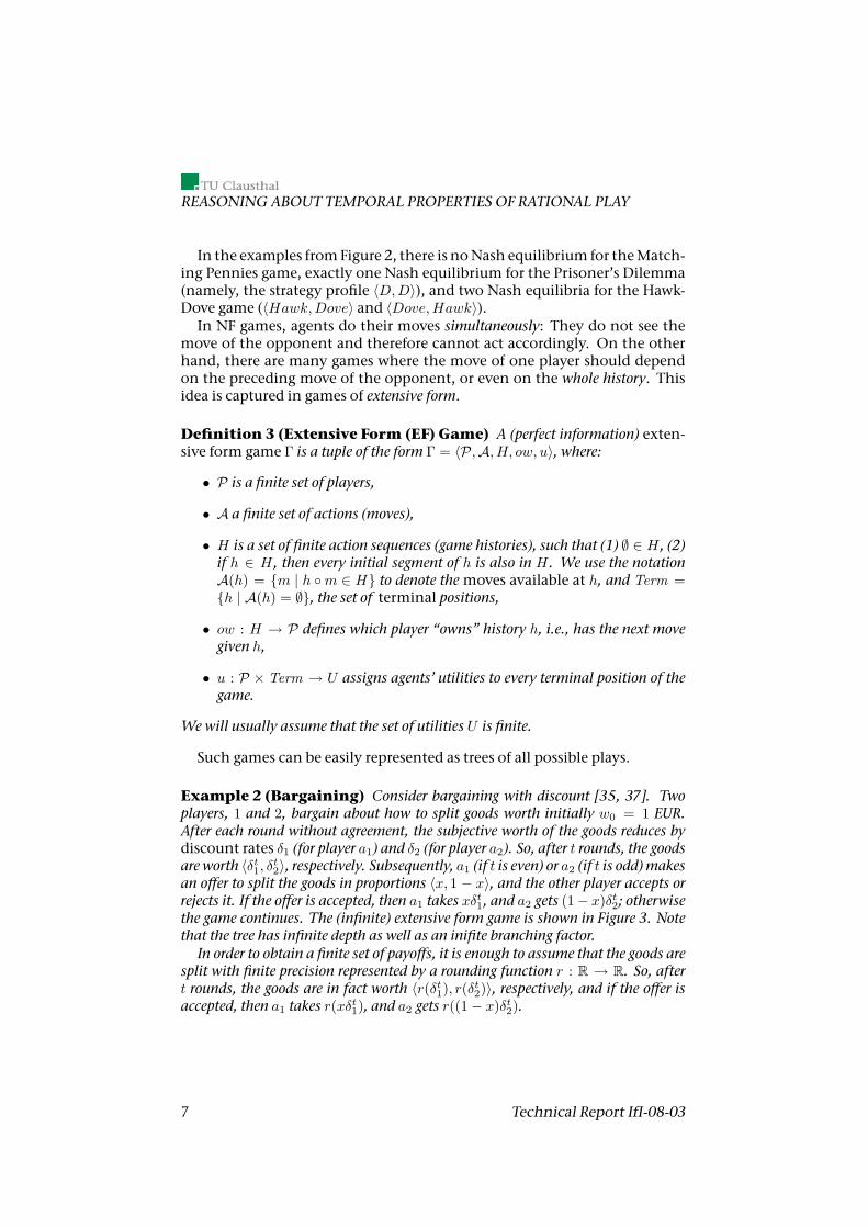
Example 2 (Bargaining) Consider bargaining with discount [35, 37]. Twoplayers, 1 and 2, bargain about how to split goods worth initially w0 = 1 EUR.After each round without agreement, the subjective worth of the goods reduces bydiscount rates δ1 (for player a1) and δ2 (for player a2). So, after t rounds, the goodsare worth 〈δt1, δt2〉, respectively. Subsequently, a1 (if t is even) or a2 (if t is odd)makesan offer to split the goods in proportions 〈x, 1 − x〉, and the other player accepts orrejects it. If the offer is accepted, then a1 takes xδt1, and a2 gets (1− x)δt2; otherwisethe game continues. The (infinite) extensive form game is shown in Figure 3. Notethat the tree has infinite depth as well as an inifite branching factor.In order to obtain a finite set of payoffs, it is enough to assume that the goods are
split with finite precision represented by a rounding function r : R → R. So, aftert rounds, the goods are in fact worth 〈r(δt1), r(δt2)〉, respectively, and if the offer isaccepted, then a1 takes r(xδt1), and a2 gets r((1− x)δt2).
7 Technical Report IfI-08-03
Preliminaries
1
2
(1, 0)1
(δ1, 0)2
...2
...1
...2
(0, 1)1
(0, δ2)2
...2
...1
......
......
......
(1,0)1(0,1)1
acc2
(1,0
) 2
(0,1)2acc2
(1,0
) 2
(0,1)2
acc1
(1,0
) 1
(0,1)1 acc1
(1,0
) 1
(0,1)1
Figure 3: The bargaining game.
A strategy for player i ∈ P in extensive game Γ is a function that assigns alegal move to each history owned by i. Note that a strategy profile (i.e., a com-bination of strategies, one per player) determines a unique path from thegame root (∅) to one of the terminal nodes (and hence also a single profile ofpayoffs). In consequence, one can construct the corresponding normal fromgame NF (Γ) by enumerating strategy profiles and filling the payoff matrixwith resulting payoffs.
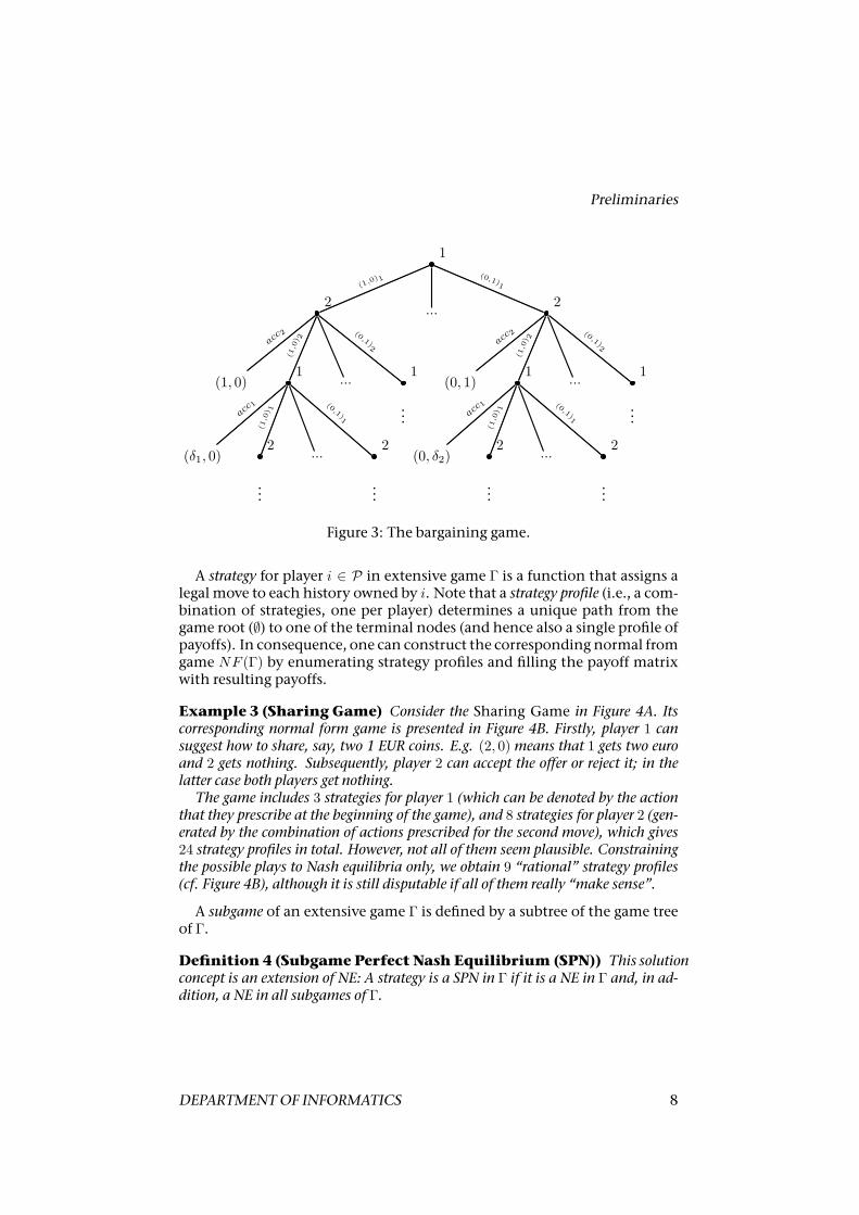
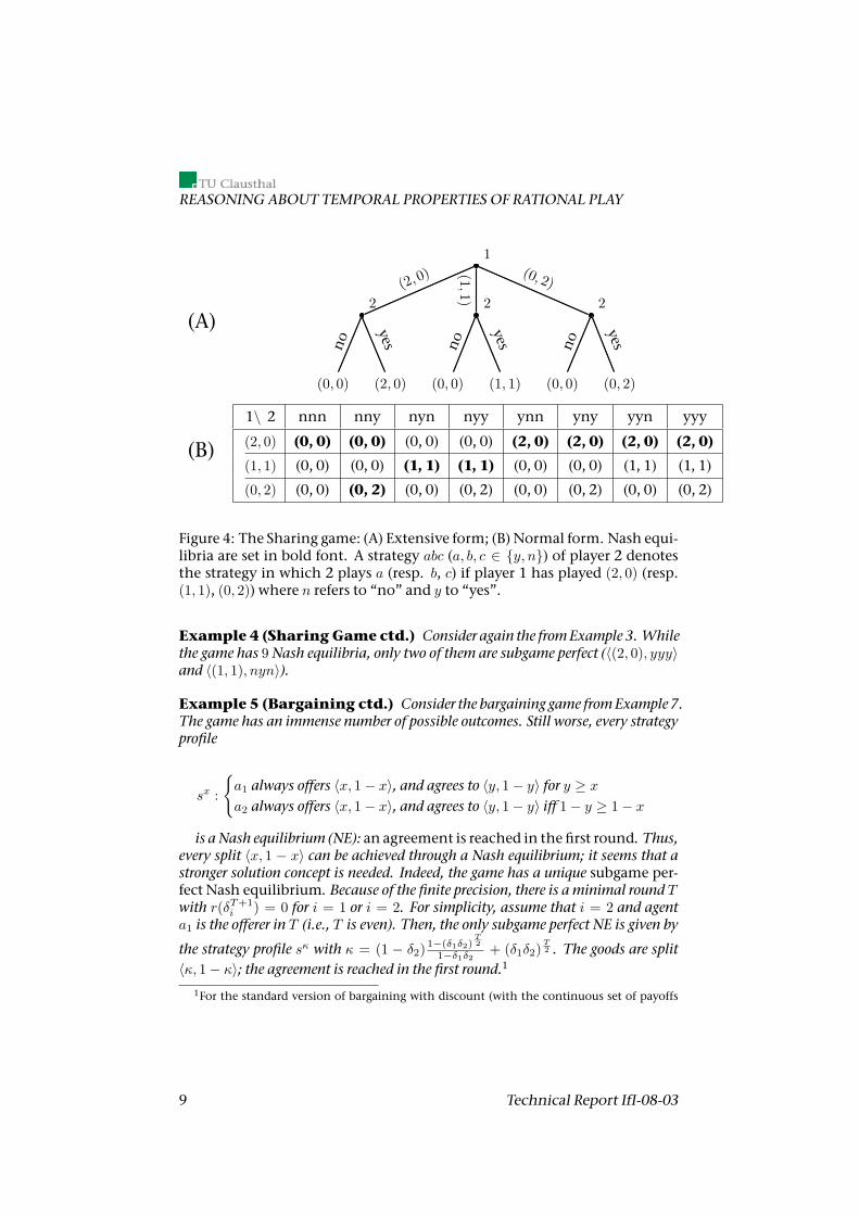
Example 3 (Sharing Game) Consider the Sharing Game in Figure 4A. Itscorresponding normal form game is presented in Figure 4B. Firstly, player 1 cansuggest how to share, say, two 1 EUR coins. E.g. (2, 0) means that 1 gets two euroand 2 gets nothing. Subsequently, player 2 can accept the offer or reject it; in thelatter case both players get nothing.The game includes 3 strategies for player 1 (which can be denoted by the action
that they prescribe at the beginning of the game), and 8 strategies for player 2 (gen-erated by the combination of actions prescribed for the second move), which gives24 strategy profiles in total. However, not all of them seem plausible. Constrainingthe possible plays to Nash equilibria only, we obtain 9 “rational” strategy profiles(cf. Figure 4B), although it is still disputable if all of them really “make sense”.
A subgame of an extensive game Γ is defined by a subtree of the game treeof Γ.
Definition 4 (Subgame Perfect Nash Equilibrium (SPN)) This solutionconcept is an extension of NE: A strategy is a SPN in Γ if it is a NE in Γ and, in ad-dition, a NE in all subgames of Γ.
DEPARTMENTOF INFORMATICS 8
REASONING ABOUT TEMPORAL PROPERTIES OF RATIONAL PLAY
(A)
1
2
(0, 0) (2, 0)
2
(0, 0) (1, 1)
2
(0, 0) (0, 2)
(2, 0) (1,1)
(0, 2)
no
yes no
yes no
yes
(B)
1\ 2 nnn nny nyn nyy ynn yny yyn yyy
(2, 0) (0, 0) (0, 0) (0, 0) (0, 0) (2, 0) (2, 0) (2, 0) (2, 0)
(1, 1) (0, 0) (0, 0) (1, 1) (1, 1) (0, 0) (0, 0) (1, 1) (1, 1)
(0, 2) (0, 0) (0, 2) (0, 0) (0, 2) (0, 0) (0, 2) (0, 0) (0, 2)
Figure 4: The Sharing game: (A) Extensive form; (B) Normal form. Nash equi-libria are set in bold font. A strategy abc (a, b, c ∈ y, n) of player 2 denotesthe strategy in which 2 plays a (resp. b, c) if player 1 has played (2, 0) (resp.(1, 1), (0, 2)) where n refers to “no” and y to “yes”.
Example 4 (Sharing Game ctd.) Consider again the fromExample 3. Whilethe game has 9Nash equilibria, only two of them are subgame perfect (〈(2, 0), yyy〉and 〈(1, 1), nyn〉).
Example 5 (Bargaining ctd.) Consider the bargaining game fromExample 7.The game has an immense number of possible outcomes. Still worse, every strategyprofile
sx :
a1 always offers 〈x, 1− x〉, and agrees to 〈y, 1− y〉 for y ≥ x
a2 always offers 〈x, 1− x〉, and agrees to 〈y, 1− y〉 iff 1− y ≥ 1− x
is a Nash equilibrium (NE): an agreement is reached in the first round. Thus,every split 〈x, 1 − x〉 can be achieved through a Nash equilibrium; it seems that astronger solution concept is needed. Indeed, the game has a unique subgame per-fect Nash equilibrium. Because of the finite precision, there is a minimal round Twith r(δT+1
i ) = 0 for i = 1 or i = 2. For simplicity, assume that i = 2 and agenta1 is the offerer in T (i.e., T is even). Then, the only subgame perfect NE is given by
the strategy profile sκ with κ = (1 − δ2)1−(δ1δ2)
T2
1−δ1δ2 + (δ1δ2)T2 . The goods are split
〈κ, 1− κ〉; the agreement is reached in the first round.1
1For the standard version of bargaining with discount (with the continuous set of payoffs
9 Technical Report IfI-08-03
Preliminaries
2.2 ATL
Alternating-time temporal logic (ATL) [2, 3] enables reasoning about temporalproperties and strategic abilities of agents. Formally, the language of ATL isgiven as follows.
Definition 5 (LATL) LetAgt = a1, . . . , ak be a nonempty finite set of all agents,and Π be a set of propositions (with typical element p). We use the symbol a to de-note a typical agent, and A to denote a typical group of agents from Agt. The logicLATL(Agt,Π) is defined by the following grammar:
ϕ ::= p | ¬ϕ | ϕ ∧ ϕ | 〈〈A〉〉 hϕ | 〈〈A〉〉2ϕ | 〈〈A〉〉ϕUϕ.Informally, 〈〈A〉〉ϕ says that agents A have a collective strategy to enforce
ϕ. ATL formulae include the usual temporal operators: h(in the next state),2 (always from now on) and U (strict until). Additionally, 3 (now or sometimein the future) can be defined as3ϕ ≡ >Uϕ. Like inCTL [13], every occurrenceof a temporal operator is immediately preceded by exactly one cooperationmodality (this variant of the language is sometimes called “vanilla” ATL).The broader language of ATL∗, where no such restriction is imposed, is notdiscussed in this article. It should be noted that the CTL path quantifiersA,E can be expressed inATLwith 〈〈∅〉〉, 〈〈Agt〉〉 respectively. The semantics ofATL is defined over concurrent game structures.
Definition 6 (CGS) A concurrent game structure (CGS) is a tuple: M =〈Agt,Q ,Π, π, Act, d, o〉, consisting of: a set Agt = a1, . . . , ak of agents; aset Q of states; a set Π of atomic propositions; a valuation of propositionsπ : Q → P(Π); a set Act of actions. Function d : Agt × Q → P(Act) indicatesthe actions available to agent a ∈ Agt in state q ∈ Q . We will often write da(q)instead of d(a, q), and use d(q) to denote the set d1(q)× · · · × dk(q) of action pro-files available in state q. Finally, o is a transition functionwhichmaps each stateq ∈ Q and action profile−→α = 〈α1, . . . , αk〉 ∈ d(q) to another state q′ = o(q,−→α ).
Remark 1 In the literature on ATL, the same symbols for agents (and groups ofagents) are used in the semantics and in the object language; we follow this tradi-tion here.
A computation or path λ = q0q1 · · · ∈ Qω is an infinite sequence of statessuch that there is a transition between each qi, qi+1.We define λ[i] = qi todenote the i-th state of λ. ΛM denotes all paths in M . The set of all pathsstarting in q is given by ΛM (q).
Definition 7 (Strategy, outcome) A (memoryless) strategy of agent a is afunction sa : Q → Act such that sa(q) ∈ da(q). We denote the set of such functions
[0, 1]), cf. [35, 37]. Restricting the payoffs to a finite set requires to alter the solution slightly [40,33], see also Appendix A.
DEPARTMENTOF INFORMATICS 10
REASONING ABOUT TEMPORAL PROPERTIES OF RATIONAL PLAY
by Σa. A collective strategy sA for team A ⊆ Agt specifies an individual strategyfor each agent a ∈ A; the set of A’s collective strategies is given by ΣA =
∏a∈A Σa.
The set of all strategy profiles is given by Σ = ΣAgt.The outcome of strategy sA in state q is defined as the set of all paths that may
result from executing sA from state q on: out(q, sA) = λ ∈ ΛM (q) | ∀i ∈ N0 ∃−→α =〈α1, . . . , αk〉 ∈ d(λ[i]) ∀a ∈ A (αa = saA(λ[i]) ∧ o(λ[i],−→α ) = λ[i + 1]), where saAdenotes agent a’s part of the collective strategy sA.
The semantics ofATL can be given by the following clauses:
M, q |= p iff p ∈ π(q)
M, q |= ¬ϕ iffM, q 6|= ϕ
M, q |= ϕ ∧ ψ iffM, q |= ϕ andM, q |= ψ
M, q |= 〈〈A〉〉 hϕ iff there is sA ∈ ΣA such thatM,λ[1] |= ϕ for allλ ∈ out(q, sA)
M, q |= 〈〈A〉〉2ϕ iff there is sA ∈ ΣA such thatM,λ[i] |= ϕ for all λ ∈ out(q, sA)and i ∈ N0
M, q |= 〈〈A〉〉ϕUψ iff there is sA ∈ ΣA such that, for all λ ∈ out(q, sA), there isi ∈ N0 withM,λ[i] |= ψ, andM,λ[j] |= ϕ for all 0 ≤ j < i.
Remark 2 Wesomewhat deviate from the original semantics ofATL [2, 3], wherestrategies assign agents’ choices to sequences of states (which suggests that agentscan recall the whole history of each game). While the choice between the two typesof strategies affects the semantics of most ATL extensions, both yield equivalentsemantics for pureATL [38].
3 Relating Games andATL-Like Logics
In this section we present some important ideas that form the starting pointfor later sections. (1) We discuss informally how the notion of strategic abil-ity in ATL can be refined so that it takes into account only “sensible” be-haviour of agents. (2) We look back on the logic of GLP [51] which imple-ments the idea formally, albeit in a very limitedway. (3)We summarize a cor-respondence between extensive games and the models ofATL. (4) We recallan extension ofATL, calledATLI (“ATLwith Intentions”), which will laterserve as an intermediate logical framework and as a motivation for our logicATLP.We also demonstrate how several game-theoretical solution conceptscan be expressed in ATLI. (5) Finally we present our idea of qualitative so-lution concepts, where ATL path formulae are used to define the winningconditions.We illustrate the ideaswith two examples from theprevious section:Match-
ing Pennies and Bargaining with Discounts.
11 Technical Report IfI-08-03
Relating Games andATL-Like Logics
(A)q0
start
q1 money1money2
q2 q3money2
head,head h
ead,tail
tail,head
tail, tail
nop,nopnop, nop
nop, n
op
(B)1\2 sh st
sh 1, 1 0, 0st 0, 0 0, 1
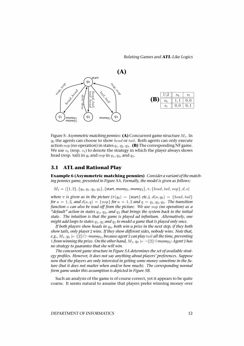
Figure 5: Asymmetricmatching pennies: (A)Concurrent game structureM1. Inq0 the agents can choose to show head or tail. Both agents can only executeactionnop (no operation) in states q1, q2, q3. (B)The correspondingNF game.We use sh (resp. st ) to denote the strategy in which the player always showshead (resp. tail) in q0 and nop in q1, q2, and q3.
3.1 ATL andRational Play
Example 6 (Asymmetricmatching pennies) Consider a variant of thematch-ing pennies game, presented in Figure 5A. Formally, the model is given as follows:
M1 = 〈1, 2, q0, q1, q2, q3, start,money1,money2, π, head , tail ,nop, d, o〉
where π is given as in the picture (π(q0) = start etc.), d(a, q0) = head , tailfor a = 1, 2, and d(a, q) = nop for a = 1, 2 and q = q1, q2, q3. The transitionfunction o can also be read off from the picture. We use nop (no operation) as a“default” action in states q1, q2, and q3 that brings the system back to the initialstate. The intuition is that the game is played ad infinitum. Alternatively, onemight add loops to states q1, q2 and q3 to model a game that is played only once.If both players show heads in q0, both win a prize in the next step; if they both
show tails, only player 2wins. If they show different sides, nobody wins. Note that,e.g.,M1, q0 |= 〈〈2〉〉2¬money1, because agent 2 can play tail all the time, preventing1 fromwinning the prize. On the other hand,M1, q0 |= ¬〈〈2〉〉3money2: Agent 2 hasno strategy to guarantee that she will win.The concurrent game structure in Figure 5A determines the set of available strat-
egy profiles. However, it does not say anything about players’ preferences. Supposenow that the players are only interested in getting some money sometime in the fu-ture (but it does not matter when and/or how much). The corresponding normalform game under this assumption is depicted in Figure 5B.
Such an analysis of the game is of course correct, yet it appears to be quitecoarse. It seems natural to assume that players prefer winning money over
DEPARTMENTOF INFORMATICS 12
REASONING ABOUT TEMPORAL PROPERTIES OF RATIONAL PLAY
losing it. If we additionally assume that the players are rational thinkers, itseems plausible that player 1 should always play head, as it keeps the possi-bility of getting money open (while playing tail guarantees loss). Under thisassumption, player 2 has complete control over the outcome of the game:She can play head too, granting herself and the other agent with the prize,or respond with tail, in which case both players lose. Note that this kindof analysis corresponds to the game-theoretical notion of weakly dominantstrategy: For agent 1, playing head is dominant in the corresponding normalform game in Figure 5B, while both strategies of player 2 are undominated,so they can be in principle considered for playing.It is still possible to refine our analysis of the game. Note that 2, knowing
that 1 ought to play head and preferring to win money too, should decideto play head herself. This kind of reasoning corresponds to the notion ofiterated undominated strategies. If we assume that both players do reason thisway, then 〈sh, sh〉 is the only rational strategy profile, and the game shouldend with both agents winning the prize.
3.2 Game Logicwith Preferences
Game Logic with Preferences [51] is, to our knowledge, the only logic de-signed to address the outcome of rational play in games with perfect infor-mation. Here, we summarize the idea very briefly.The central idea of GLP is facilitated by the preference operator [a : ϕ]. In-
terpretation of [a : ϕ]ψ in modelM proceeds as follows: if the truth of ϕ canbe enforced by a, then we remove from the model all the actions of a thatdo not lead to enforcing it, and evaluate ψ in the resulting model. Thus, theevaluation ofGLP formulae is underpinned by the assumption that rationalagents satisfy their preferences whenever they can. The requirement applies toall the subtrees of the game tree, and it is called “subgame perfectness” bythe authors.The scope ofGLP, however, is limited in several respects. Firstly, themod-
els of GLP are restricted to finite game trees. Secondly, agents’ preferencesmust be specified with propositional (non-modal) formulae, and they areevaluated only at the terminal states of the game. The temporal part of thelanguage is limited, too. Lastly, and perhaps most importantly, the seman-tics ofGLP is based on a very specific notion of rationality (see above). Onecan easily imagine variants of the semantics, in which other rationality cri-teria are used (NE, PO, UNDOM) to eliminate “irrational” strategies. Indeed,a preliminary version of GLP was based on the notion of Nash equilibriumrather than “subgame perfectness” [50]. In this article, we want to allow asmuch flexibility as possible with respect to the choice of a suitable solutionconcept.
13 Technical Report IfI-08-03
Relating Games andATL-Like Logics
3.3 Models of ATL vs. Extensive Games
In this section, we recall the correspondence between extensive form gamesand the semantical models ofATL, proposed in [30] and inspired by [5, 45].We only consider game trees in which the set of payoffs is finite. Let U de-
note the set of all possible utility values in a game; U will be finite and fixedfor any given game. For each value v ∈ U and agent a ∈ Agt, we introducea proposition pva into our set Π, and fix pva ∈ π(q) iff a gets payoff of at least vin q.2 States in the model represent finite histories in the game. In particu-lar, we us ∅ to denote the root of the game. The correspondence between anextensive game Γ and a CGSM can be captured as follows.
Definition 8 (FromExtensive Games to CGS) ACGSM = Agt,Q ,Π, π,Act, d, o corresponds to an extensive game Γ = 〈P,A,H, ow, u〉 if, and only if,the following holds:
• Agt = P,
• Q = H,
• Π and π include propositions pva to emulate utilities for terminal states in theway described above,
• Act = A ∪ nop,
• da(q) = A(q) if a = ow(q) and da(q) = nop otherwise,
• o(q, nop, . . . ,m, . . . , nop) = q ·m, and
• o(q, nop, nop, . . . , nop) = q for q ∈ Term.
We useM(Γ) to refer to theCGSwhich corresponds to Γ.
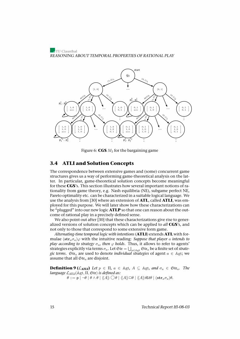
Example 7 (Bargaining in a CGS) We consider the bargaining game fromExample 2, but this time as a model of ATL. The CGS corresponding to the gameshown in Figure 6. Nodes represent various states of the negotiation process, andarcs show how agents’ moves change the state of the game. A node label refers tothe history of the game for better readability. For instance,
0, 11, 0acc
has the meaningthat in the first round 1 offered 〈0, 1〉 which was rejected by 2. In the next round 2’soffer 〈1, 0〉 has been accepted by 1 and the game has ended.
Note that, for every extensive game Γ, there is a corresponding CGS, butthe reverse is not true: Concurrent game structures can include cycles andsimultaneous moves of players, which are absent in game trees. Note alsothat, for those CGS’s that correspond to some EF game, we get an implicitcorrespondence to a normal form game. We will extend this notion of cor-respondence to all CGS’s in Section 3.5.2 Note that a state labeled by pv
a is also labeled by pv′a for all v′ ∈ U where v′ < v.
DEPARTMENTOF INFORMATICS 14
REASONING ABOUT TEMPORAL PROPERTIES OF RATIONAL PLAY
q0
[1, 0]
[1, 0acc
] [1, 01, 0
]
1, 01, 0acc
1, 01, 01, 0
... 1, 0
1, 00, 1
...[
1, 00, 1
]
... [0, 1]
[0, 1acc
] [0, 11, 0
]
0, 11, 0acc
0, 11, 01, 0
... 0, 1
1, 00, 1
...[
0, 10, 1
]
......
......
......
(1,0)1(0,1)1
acc2
(1,0
) 2
(0,1)2 acc2
(1,0
) 2
(0,1)2
acc1
(1,0
) 1
(0,1)1 acc1
(1,0
) 1
(0,1)1
start
p11, p0
2
p01, p1
2
pδ11 , p0
2 p01, p
δ22
Figure 6: CGSM2 for the bargaining game
3.4 ATLI and Solution Concepts
The correspondence between extensive games and (some) concurrent gamestructures gives us a way of performing game-theoretical analysis on the lat-ter. In particular, game-theoretical solution concepts become meaningfulfor these CGS’s. This section illustrates how several important notions of ra-tionality from game theory, e.g. Nash equilibria (NE), subgame perfect NE,Pareto optimality etc. can be characterized in a suitable logical language. Weuse the analysis from [30] where an extension ofATL, calledATLI, was em-ployed for this purpose. We will later show how these characterizations canbe “plugged” into our new logicATLP so that one can reason about the out-come of rational play in a precisely defined sense.We also point out after [30] that these characterizations give rise to gener-
alized versions of solution concepts which can be applied to all CGS’s, andnot only to those that correspond to some extensive form game.Alternating-time temporal logic with intentions (ATLI) extendsATLwith for-
mulae (straσa)ϕ with the intuitive reading: Suppose that player a intends toplay according to strategy σa, then ϕ holds. Thus, it allows to refer to agents’strategies explicitly via terms σa. LetStr =
⋃a∈Agt Stra be a finite set of strate-
gic terms. Stra are used to denote individual strategies of agent a ∈ Agt; weassume that allStra are disjoint.
Definition 9 (LATLI) Let p ∈ Π, a ∈ Agt, A ⊆ Agt, and σa ∈ Stra. Thelanguage LATLI(Agt,Π,Str) is defined as:
θ ::= p | ¬θ | θ ∧ θ | 〈〈A〉〉 hθ | 〈〈A〉〉2θ | 〈〈A〉〉θUθ | (straσa)θ.
15 Technical Report IfI-08-03
Relating Games andATL-Like Logics
ATLIModelsM = 〈Agt,Q ,Π, π, Act, d, o, I,Str, [·]〉 extend concurrent gamestructures with intention relations I ⊆ Q×Agt×Act (where qIaαmeans that apossibly intends to do action α when in q). Moreover, strategic terms are in-terpreted as strategies according to function [·] : Str →
⋃a∈Agt Σa such that
[σa] ∈ Σa for σa ∈ Stra (remember that Σa denotes the set of a’s strategies).The set of paths consistent with all agents’ intentions is defined as
ΛI = λ ∈ ΛM | ∀i ∃α ∈ d(λ[i]) (o(λ[i], α) = λ[i+ 1] ∧ ∀a ∈ Agt λ[i]Iaαa)
We impose on I the natural requirement that qIaα implies that α ∈ da(q) fora ∈ Agt; that is, agents only intend to do actions if they are actually able toperform them.We say that strategy sA is consistent with A’s intentions if qIasaA(q) for all
q ∈ Q , a ∈ A. The intention-consistent outcome set is defined as: outI(q, sA) =out(q, sA) ∩ ΛI . The semantics of strategic operators in ATLI extends andreplaces the semantic rules ofATL as follows:
M, q |= 〈〈A〉〉 hθ iff there is a collective strategy sA consistent with A’s in-tentions, such that for every λ ∈ outI(q, sA), we have thatM,λ[1] |= θ;
M, q |= 〈〈A〉〉2θ andM, q |= 〈〈A〉〉θUθ′: analogous;
M, q |= (straσ)θ iff revise(M,a, [σ]), q |= θ.
The function revise(M,a, sa) updates modelM by setting a’s intention rela-tion to
I ′a = 〈q, sa(q)〉 | q ∈ Q,
so that sa and Ia represent the same mapping in the resulting model. Notethat a pure CGSM can be seen as a CGSwith the full intention relation
I0 = 〈q, a, α〉 | q ∈ Q , a ∈ Agt, α ∈ da(q).
Additionally, forA = ai1 , . . . , air andσA = 〈σai1, . . . , σair
〉, wedefine: (strAσA)ϕ ≡(strai1
σai1) . . . (strair
σair)ϕ. Furthermore, for B = b1, . . . , bl ⊆ A we use
σA[B] to refer toB’s substrategy, i.e. to 〈σb1 , . . . , σbl〉
Example 8 (Asymmetricmatching pennies ctd.) Coming back to ourmatch-ing pennies example fromFigure 5, we have for instance thatM1, q0 |= (str1σ)〈〈2〉〉3money2
if the denotation of σ is set to sh .
With temporal logic, it is natural to define outcomes of strategies via prop-erties of resulting paths rather than single states. The notion of temporal T -Nash equilibrium, parameterizedwith aunary operatorT = h,2,3, _Uψ,ψU_,was proposed in [30]. Let σ = 〈σ1, . . . , σk〉 be a profile of strategic terms, and
DEPARTMENTOF INFORMATICS 16
REASONING ABOUT TEMPORAL PROPERTIES OF RATIONAL PLAY
let T stand for any of the following operators: h,2,3, _Uψ,ψU_ and let a bean agent. Then we consider the following LATLI formulae:
BRTa (σ) ≡ (strAgt\aσ[Agt \ a])∧v∈U
((〈〈a〉〉Tpva) → ((straσ[a])〈〈∅〉〉Tpva)
)NET (σ) ≡
∧a∈Agt
BRTa (σ)
SPNT (σ) ≡ 〈〈∅〉〉2NET (σ).
BRTa (σ) refers toσ[a]being aT -best strategy for a againstσ[Agt\a];NET (σ)expresses that strategy profile σ is a T-Nash equilibrium; finally, SPNT (σ)defines σ as subgame perfect T-NE. Thus, we have a family of equilibria: h-Nash equilibrium,2-Nash equilibrium etc., each corresponding to a differenttemporal pattern of utilities. For example, we may assume that agent a gets v ifa utility of at least v is guaranteed for every timemoment (2pva), is eventuallyachieved (3pva), and so on.The correspondence between solution concepts and their temporal coun-
terparts for extensive games is captured by the following proposition.
Proposition 3 Let Γ be an extensive game. Then the following holds:
1. M(Γ), ∅ |= NE3(σ) iff [σ]M(Γ) is a NE in Γ [30].3
2. M(Γ), ∅ |= SPN3(σ) iff [σ]M(Γ) is a SPN in Γ.
Proof sketch
1. Since M(Γ) corresponds to an EF game, the “payoff” propositions pvacan only become true at the end of each path inM(Γ). Thus,BR3
a (σ) inM(Γ), ∅ holds iff, whenever a can achieve the payoff of at least v againstσ[Agt\a] (by any strategy), it can also achieve that by using σ[a]. Thatis, a cannot obtain a better payoff by unilaterally changing her strategy.
2. M(Γ), ∅ |= SPN3(σ) iffM(Γ), q |= NE3(σ) for every q reachable fromthe root ∅ (*). However, Γ is a tree, so every node is reachable from ∅ inM(Γ). So, by the first part, (*) iff σ denotes a Nash equilibrium in everysubtree of Γ.
We can use the above ATLI formulae to express game-theoretical proper-ties of strategies in a straightforward way.
Example 9 (Bargaining ctd.) We extend theCGS in Figure 6 to aCGSwithintentions; then, we haveM2, q0 |= NE3(σ), with σ interpreted inM2 as sx (forany x ∈ [0, 1]). Still,M2, q0 |= SPN3(σ) if, and only if, [σ]M2 = sκ.
3 The empty history ∅ denotes the root of the game tree.
17 Technical Report IfI-08-03
Relating Games andATL-Like Logics
Wealsopropose a tentativeATLI characterizationofPareto optimality (basedon the characterization from [45] for normal form games):
POT (σ) ≡∧v1
· · ·∧vk
((〈〈Agt〉〉T
∧i
pvii ) → (strAgtσ)
((〈〈∅〉〉T
∧i
pvii ) ∨ (
∨i
∨v′ s.t.
v′ > vi
〈〈∅〉〉Tpv′i )
)).
That is, the strategy profile denoted by σ is Pareto optimal iff, for everyachievable pattern of payoff profiles, either it can be achieved by σ, or σ ob-tains a strictly better payoff pattern for at least one player. Note that theabove formula has exponential length with respect to the number of pay-offs in U . Moreover, it is not obvious that this characterization is the rightone, as it refers in fact to the evolution of payoff profiles (i.e., combinations ofpayoffs achieved by agents at the same time), and not temporal patterns ofpayoff evolution for each agent separately. So, for example,PO3(σ)mayholdeven if there is a strategy profile σ′ that makes each agent achieve eventuallya better payoff, as long as not all of them will achieve these better payoffs atthe samemoment. Still, the following holds.
Proposition 4 Let Γ be an extensive game. Then:
M(Γ), ∅ |= PO3(σ) iff [σ]M(Γ) is Pareto optimal in Γ.
Proof LetM(Γ), ∅ |= PO3(σ). Then, for every payoff profile 〈v1, . . . , vk〉 reach-able in Γ, we have that either [σ] obtains at least as good a profile,4 or it ob-tains an incomparable payoff profile. Thus, [σ] is Pareto optimal. The prooffor the other direction is analogous.
Example 10 (Asymmetricmatching pennies ctd.) LetM ′1 be ourmatch-
ing pennies modelM1 with additional propositions p1i ≡ moneyi (so, we assign to
moneyi a utility of 1 for i). Then, we have M ′1, q0 |= PO3(σ) iff σ denotes the
strategy profile 〈sh , sh〉.
3.5 General Solution Concepts
In this part we present an abstract formulation of our notion of general so-lution concept. We will elaborate on it later in Section 5.3, using our logicATLP.We have seen in Section 3.3 that some (but not all!) concurrent game
structures can be seen as extensive form games, which in turn defines theircorrespondence to NF games. These CGS’s must be turn-based (i.e., play-ers play by taking turns) and have a tree-like structure; moreover, they must
4We recall that∧
i pvii means that each player i gets at least vi.
DEPARTMENTOF INFORMATICS 18

REASONING ABOUT TEMPORAL PROPERTIES OF RATIONAL PLAY
include special propositions that emulate payoffs and can be used to defineagents’ preferences. Now,wewant to extend the correspondence to arbitraryCGS’s. Our idea is to determine the outcome of a game by the truth of certain pathformulae (e.g., in the case of binary payoffs, we can see the formulae as win-ning conditions). So, we give up the idea of assigning payoffs to leaves in a tree.Instead, we see a concurrent game structure as a game, paths in the structureas plays in the game, and satisfaction of some pre-specified formulae as themechanism that defines agents’ outcome for a given play.Which formulae can be used in this respect?
Definition 10 (ATL Path Formulae) ByATLpath formulae, we denote ar-bitraryATL formulae that are preceded by a temporal operator h,2,U .Given a CGSM and a path λ inM , satisfaction of path formulae is defined as
follows:
M,λ |= hϕ iffM,λ[1] |= ϕ
M,λ |= 2ϕ iffM,λ[i] |= ϕ for all i ∈ N0
M,λ |= ϕUψ iff there is i ∈ N0withM,λ[i] |= ψ, andM,λ[j] |= ϕ for all 0 ≤ j < i.
We propose that player i’s preferences can be specified by a finite list ofpath formulae ηi = 〈η1
i , . . . , ηnii 〉 (where ni ∈ N) with the underlying assump-
tion that agent i prefers η1i most, η
2i comes second best etc., and the worst
outcome occurs when no η1i , . . . , η
nii holds for the actual play. Thus, ηi im-
poses a total order on paths in a CGS.For k players, we need a k-vector of such preference lists −→η = 〈η1, . . . , ηk〉.
Then, every concurrent game structure gives rise to the strategic game de-fined as below.
Definition 11 (FromCGS ToNFGame) LetM be a CGS, q ∈ QM a state,and−→η = 〈η1, . . . , ηk〉 a vector of lists ofATL path formulae, where k = |Agt|.Then we define S(M,−→η , q), theNF game associated withM ,−→η , and q, as the
strategic game 〈Agt,A1, . . . ,Ak, µ〉, where the setAi of i’s strategies is given by Σifor each i ∈ Agt, and the payoff function is defined as follows:
µi(a1, . . . , ak) =
ni − j + 1 if ηji is the first formula from ηi such thatM,λ |= ηji
for all λ ∈ out(q, 〈a1, . . . , ak〉),0 no ηji is satisfied
where ηi = 〈η1i , . . . , η
nii 〉, 1 ≤ j ≤ ni and we write µi for µ(i).
19 Technical Report IfI-08-03
The LogicATLP
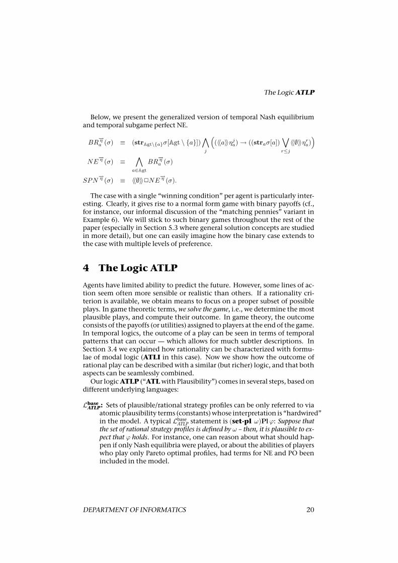
Below, we present the generalized version of temporal Nash equilibriumand temporal subgame perfect NE.
BR−→ηa (σ) ≡ (strAgt\aσ[Agt \ a])
∧j
((〈〈a〉〉ηja) → ((straσ[a])
∨r≤j
〈〈∅〉〉ηra))
NE−→η (σ) ≡
∧a∈Agt
BR−→ηa (σ)
SPN−→η (σ) ≡ 〈〈∅〉〉2NE
−→η (σ).
The case with a single “winning condition” per agent is particularly inter-esting. Clearly, it gives rise to a normal form game with binary payoffs (cf.,for instance, our informal discussion of the “matching pennies” variant inExample 6). We will stick to such binary games throughout the rest of thepaper (especially in Section 5.3 where general solution concepts are studiedin more detail), but one can easily imagine how the binary case extends tothe case withmultiple levels of preference.
4 The Logic ATLP
Agents have limited ability to predict the future. However, some lines of ac-tion seem often more sensible or realistic than others. If a rationality cri-terion is available, we obtain means to focus on a proper subset of possibleplays. In game theoretic terms,we solve the game, i.e., we determine themostplausible plays, and compute their outcome. In game theory, the outcomeconsists of the payoffs (or utilities) assigned to players at the end of the game.In temporal logics, the outcome of a play can be seen in terms of temporalpatterns that can occur — which allows for much subtler descriptions. InSection 3.4 we explained how rationality can be characterized with formu-lae of modal logic (ATLI in this case). Now we show how the outcome ofrational play can be described with a similar (but richer) logic, and that bothaspects can be seamlessly combined.Our logicATLP (“ATLwith Plausibility”) comes in several steps, based on
different underlying languages:
LbaseATLP: Sets of plausible/rational strategy profiles can be only referred to viaatomic plausibility terms (constants)whose interpretation is “hardwired”in the model. A typical LbaseATLP statement is (set-pl ω)Plϕ: Suppose thatthe set of rational strategy profiles is defined by ω – then, it is plausible to ex-pect that ϕ holds. For instance, one can reason about what should hap-pen if only Nash equilibria were played, or about the abilities of playerswho play only Pareto optimal profiles, had terms for NE and PO beenincluded in themodel.
DEPARTMENTOF INFORMATICS 20
REASONING ABOUT TEMPORAL PROPERTIES OF RATIONAL PLAY
L0ATLP: Amild extension of LbaseATLP. We allow some combinations of the con-stants of LbaseATLP to formmore complex terms.
LATLPATLI : An intermediate language,where rational strategyprofiles are char-acterized byATLI formulae.
LkATLP: Here we have nestings of plausibility updates up to level k. It turnsout that LATLPATLI is already embedded in L1
ATLP.
LATLP: Unbounded nestings of formulae are allowed.
The language LbaseATLP is presented in Sections 4.1 and 4.2. Then, in Sec-tion 4.3, we consider an intermediate step, namely plausibility terms writ-ten in ATLI. They serve as a motivation to extend LbaseATLP to L1
ATLP, and, moregenerally, to a hierarchy LATLP = limk→∞ LkATLP which we investigate in Sec-tion 4.4.
4.1 The Language LbaseATLP
Weextend the language ofATLwithoperatorsPlA , (set-pl ω), and (refn-pl ω).The first assumes plausible behaviour of agents inA; the latter are used to fixthe actual meaning of plausibility by plausibility terms ω. As yet, the termsare simply constants with no internal structure. Their meaning will be givenlater by a denotation function linking plausibility terms to sets of strategyprofiles.
Definition 12 (LbaseATLP) The base languageLbaseATLP(Agt,Π,Ω) is defined over nonemptysets: Π of propositions ,Agt of agents, andΩ of plausibility terms. We use p, a, ω torefer to typical elements ofΠ,Agt,Ω respectively, andA to refer to a group of agents.LATLP(Agt,Π,Ω) consists of all formulae defined by the following grammar:
ϕ ::= p | ¬ϕ | ϕ ∧ ϕ | 〈〈A〉〉 hϕ | 〈〈A〉〉2ϕ | 〈〈A〉〉ϕUϕ |PlA ϕ | (set-pl ω)ϕ | (refn-pl ω)ϕ,
Additionally, we define 3ϕ as >Uϕ, Pl as PlAgt , and Ph as Pl∅ . We will oftenuse LbaseATLP to refer to the language if the sets are clear from the context.
PlA assumes that agents in A play rationally; this means that the agentscan only use strategy profiles that are plausible in the given model. In par-ticular, Pl (≡ PlAgt ) imposes rational behaviour on all agents in the system.Similarly, Ph disregards plausibility assumptions, and refers to all physicallyavailable scenarios. The model update operator (set-pl ω) allows to define(or redefine) the set of plausible strategy profiles (referred to by Υ in themodel) to the ones described by plausibility term ω (in this sense, it imple-ments revision of plausibility). Operator (refn-pl σ) enables refining the set
21 Technical Report IfI-08-03
The LogicATLP
of plausible strategy profiles, i.e. selecting a subset of the previously plausibleprofiles.WithATLP, we can for example say thatPl 〈〈∅〉〉2(closed∧Ph 〈〈guard〉〉 h¬closed):
It is plausible to expect that the emergency door will always remain closed, but theguard retains the physical ability to open it; or (set-pl ωNE)Pl 〈〈2〉〉3money2: Sup-pose that only playing Nash equilibria is rational; then, agent a can plausibly reacha state where she gets some money.We note that, in contrast to [16, 43, 9], the concept of plausibility pre-
sented in this article is objective, i.e. it does not vary from agent to agent.This is very much in the spirit of game theory, where rationality criteria areused in an analogous way. Moreover, it is global, because plausibility sets donot depend on the state of the system. Note, however, that the denotationof plausibility terms depends on the actual state.
4.2 Semantics of LbaseATLP
To define the semantics of ATLP, we extend CGS’s to concurrent game struc-tures with plausibility. Apart from an actual set of plausible strategiesΥ, a con-current game structure with plausibility (CGSP) must specify the denotation ofplausibility terms ω ∈ Ω. It is defined via a plausibility mapping
[[·]] : Q → (Ω → P(Σ))
Instead of [[q]](ω)we will often write [[ω]]q to turn the focus to the plausibilityterms. Each term is mapped to a set of strategy profiles. Note also, that thedenotation of a term depends on the state. In a way, the current state of thesystem defines the “initial position in the game”, and this heavily influencesthe set of rational strategy profiles for most rationality criteria. For example,a strategy profile can be a Nash equilibrium (NE) in q0, and yet it may not bea NE in some of its successors.We will propose a more concrete (and more practical) implementation of
plausibility terms in Section 4.4.
Definition 13 (CGSP) A concurrent game structurewithplausibility (CGSP)is given by a tuple
M = 〈Agt,Q ,Π, π, Act, d, o,Υ,Ω, [[·]]〉
where 〈Agt,Q ,Π, π, Act, d, o〉 is aCGS,Υ ⊆ Σ is a set of plausible strategy profiles(called plausibility set); Ω is a set of of plausibility terms, and [[·]] is a plausibilitymapping overQ and Ω.By CGSP (Agt,Π,Ω) we denote the set of all CGSP’s over Agt, Π and Ω. Fur-
thermore, for a given CGSPM we useXM to refer to elementX ofM , e.g., QM torefer to the setQ of states ofM .
DEPARTMENTOF INFORMATICS 22
REASONING ABOUT TEMPORAL PROPERTIES OF RATIONAL PLAY
Definition 14 (Compatiblemodel) Given a formula ϕ ∈ LATLP(Agt,Π,Ω)a CGSPM is called compatible with ϕ if, and only if,M ∈ CGSP (Agt,Π,Ω).That is, the model interprets all symbols occurring in ϕ. A modelM is called com-patible with a set L of ATLP formulae if, and only if,M is compatible with eachformula in L.We will assume by default that, given a formula or a set of formulae, the model
we consider is compatible with it.
The formula Pl 〈〈A〉〉γ implies that A can only play plausible strategies.Thus,A’s part of the strategy profiles inΥ is of particular interest whichmo-tivates the following definition.
Definition 15 (Substrategy) Let A,B ⊆ Agt be groups of agents such thatA ⊆ B and let sB ∈ ΣB be a collective strategy for agentsB. We use sB |A to denoteA’s substrategy tA contained in sB , i.e., strategy tA ∈ ΣA such that taA = saB forevery a ∈ A.5 For a singleton coalition a, we also write sB |a instead of sB |a.For a given set PB ⊆ ΣB of collective strategies of agentsB, PB |A denotes the set
ofA’s substrategies in PB, i.e.:
PB |A = sA ∈ ΣA | ∃s′B ∈ PB (s′B |A = sA).
Often, we impose restrictions only on a subset B ⊆ Agt of agents, with-out assuming rational play of all agents. This can be desirable due to severalreasons. It might, for example, be the case that only information about theproponents’ play is available; hence, assuming plausible behavior of the op-ponents is neither sensible nor justified. Or, even simpler, a group of (simpleminded) agents might be known to not behave rationally.Consider formula PlB 〈〈A〉〉γ: The team A looks for a strategy that brings
about γ, but the members of the team who are also in B can only chooseplausible strategies. The same applies toA’s opponents that are contained inB. Strategies which comply with B’s part of some plausible strategy profileare calledB-plausible.
Definition 16 (B-plausibility of strategies) Let A,B ⊆ Agt and sA ∈ΣA. We say that sA is B-plausible in M if, and only if, B’s substrategy in sAis part of some plausible strategy profile inM , i.e., if sA|A∩B ∈ ΥM |A∩B.By ΥM (B) we denote the set of all B-plausible strategy profiles inM . That is,
ΥM (B) = s ∈ Σ | s|B ∈ ΥM |B. Note that sA isB-plausible iff sA ∈ ΥM (B)|A.
We observe that sA is triviallyB-plausible wheneverA andB are disjoint.As mentioned above, if some opponents belong to the set of agents who
are assumed to play plausibly then they must also comply with the actualplausibility specifications when choosing their actions; this is taken into ac-count by the following notion of plausible outcome.5We recall that sa
B (resp. taA) denotes a’s part of sB (resp. tA).
23 Technical Report IfI-08-03
The LogicATLP
Definition 17 (B-plausible outcome) TheB-plausible outcome, outM (q, sA, B),with respect to strategy sA and state q is defined as the set of paths which can occurwhen onlyB-plausible strategy profiles can be played and agents inA follow sA:
outM (q, sA, B) = λ ∈ ΛM (q) | there exists aB-plausible t ∈ Σ such thatt|A = sA and outM (q, t) = λ.
Note that the outcome outM (q, sA, B) is emptywhenever the (A∩B)’s partof sA is not part of any plausible strategy profile inΥM . For example, assumethat all agents in B play only parts of Nash equilibria. Then for a given sAthere are two possibilities for the B-consistent outcome. Either it is emptybecause (A ∩ B)’s part of sA does not belong to any Nash equilibrium, or itconsists of all paths which can occur when (1)A stick to sA, (2)B (includingA ∩ B) play according to some Nash equilibrium, and (3) the other agentsbehave arbitrarily.The truth ofATLP formulae is given with respect to a model, a state, and
a set B of agents. The intuitive reading ofM, q |=B ϕ is: “ϕ is true in modelM and state q if it is assumed that players in B play rationally”, i.e., by us-ing only plausible combinations of strategies. No constraints are imposedon the behaviour of agents outside B, but the plausibility operator PlA canbe used to change the set of agents (viz A) whose play is restricted. The up-date/refinement modalities (set-pl ω)/(refn-pl ω) are used to change theplausibility setΥM in the model.
Definition 18 (Semantics of LbaseATLP) LetM ∈ CGSP (Agt,Π,Ω) andA,B ⊆Agt. The semantics ofATLP formulae is given as follows:
M, q |=B p iff p ∈ π(q) and p ∈ Π
M, q |=B ¬ϕ iffM, q 6|=B ϕ
M, q |=B ϕ ∧ ψ iffM, q |=B ϕ andM, q |=B ψ
M, q |=B 〈〈A〉〉 hϕ iff there is a B-plausible sA s.t. M,λ[1] |=B ϕ for all λ ∈outM (q, sA, B)
M, q |=B 〈〈A〉〉2ϕ iff there is a B-plausible sA s.t. M,λ[i] |=B ϕ for all λ ∈outM (q, sA, B) and all i ∈ N0
M, q |=B 〈〈A〉〉ϕUψ iff there is aB-plausible sA such that, for allλ ∈ outM (q, sA, B),there is i ∈ N0 withM,λ[i] |=B ψ, andM,λ[j] |=B ϕ for all 0 ≤ j < i
M, q |=B PlA ϕ iffM, q |=A ϕ
M, q |=B (set-pl ω)ϕ iffM ′, q |=B ϕ where the new modelM ′ is equal toM butthe new setΥM ′ of plausible strategy profiles ofM ′ is set to [[ω]]qM .
DEPARTMENTOF INFORMATICS 24
REASONING ABOUT TEMPORAL PROPERTIES OF RATIONAL PLAY
M, q |=B (refn-pl ω)ϕ iff M ′, q |=B ϕ where M ′ is equal to M but ΥM ′ set toΥM ∩ [[ω]]qM .
The “absolute” satisfaction relation |= is given by |=∅.
Definition 19 (Validity) Letϕ ∈ LATLP(Agt,Π,Ω) andM ⊆ CGSP (Agt,Π,Ω).Formula ϕ is valid with respect toM if, and only if,M, q |= ϕ for everyM ∈ Mand state q ∈ QM .
Note that an ordinary concurrent game structure (without plausibility)can be interpreted as a CGSP with all strategy profiles assumed plausible,i.e., withΥ = Σ, and empty set of plausibility terms Ω.Let us clarify the semantics behindPlB〈〈A〉〉γ oncemore. The proponents
(A) look for a strategy that enforces γ; some of them (A ∩ B) are assumed toplay a part of a plausible strategy profile while the others (A \ B) can choosean arbitrary collective strategy. Analogously, some opponents (B\A) are sup-posed to play plausibly (that complies to set ΥM together with the strategyalready chosen by A ∩ B), while the rest (Agt \ (A ∪ B)) have unrestrictedchoice. In particular, when B = A, only the choices of the proponents arerestricted; for B = Agt \ A plausibility restrictions apply to the opponentsonly.
Remark 5 Weobserve that our framework is semantically similar to the approachof social laws [39, 34, 46]. However, we refer to strategy profiles as rational ornot, while social laws define constraints on agents’ individual actions. Also, ourmotivation is different: In our framework, agents are expected to behave in a speci-fied way because it is rational in some sense; social laws prescribe behaviour sanc-tioned by social norms and legal regulations.
Example 11 (Asymmetricmatching pennies ctd.) Suppose that it is plau-sible to expect that both agents are rational in the sense that they only play un-dominated strategies.6 Then, Υ = (sh , sh), (sh , st). Under this assumption,agent 2 is free to grant itself with the prize or to refuse it: Pl (〈〈2〉〉3 money2 ∧〈〈2〉〉2¬money2). Still, it cannot choose to win without making the other player wintoo: Pl¬〈〈2〉〉3(money2 ∧ ¬money1). Likewise, if rationality is defined via iteratedundominated strategies, then we have Υ = (sh , sh), and therefore the outcomeof the game is completely determined: Pl 〈〈∅〉〉2(¬start → money1 ∧money2).Note that, in order to include both notions of rationality in the model, we can
encode them as denotations of two different plausibility terms – say, ωundom andωiter, with [[ωundom]]q0 = (sh , sh), (sh , st), and [[ωiter]]q0 = (sh , sh). LetM ′
1 bemodel M1 with plausibility terms and their denotation defined as above. Then,
6 We recall from Section 2.1 that a strategy sa ∈ Σa is called undominated if, and only if,there is no strategy s′a ∈ Σa such that the achieved utility of s′a is at least as good as for sa forall counterstrategies s−a ∈ ΣAgt\a and strictly better for at least one counterstrategy s−a ∈ΣAgt\a.
25 Technical Report IfI-08-03
The LogicATLP
we have that M ′1, q0 |= (set-pl ωundom)Pl (〈〈2〉〉3money2 ∧ 〈〈2〉〉2¬money2) ∧
(set-pl ωiter)Pl 〈〈∅〉〉2(¬start → money1 ∧money2).
Out of many solution concepts, Nash equilibrium is the most widely ac-cepted, especially for non-cooperative games. We briefly extend ourworkingexample with game analysis based on Nash equilibrium. Note that, in thiscase, it is not possible to define rationality with independent constraints onagents’ individual strategies (like in normative systems). These are full strat-egy profiles being rational or not, since rationality of a strategy depends onthe actual response of the other players.
Example 12 (Asymmetricmatching pennies ctd.) Suppose that rational-ity is defined through Nash equilibria. Then, Υ = (sh , sh), (st , st). Under thisassumption, agent 2 is sure to get the prize: Pl 〈〈∅〉〉2(¬start → money2).Moreover, by choosing the right strategy, 2 can control the outcome of the other
agent: Pl (〈〈2〉〉2(¬start → money1) ∧ 〈〈2〉〉2¬money1). Note that agent 1 can con-trol her own outcome too, if we assume that the players are obliged to play ratio-nally: Pl (〈〈1〉〉2(¬start → money1) ∧ 〈〈1〉〉2¬money1). This may seem strange,but a Nash equilibrium assumes implicitly that the agents coordinate their actionssomehow. Then, assuming a particular choice of one agent in advance constrainsthe other agent responses considerably, which puts the first agent at advantage.
Example 13 (Bargaining ctd.) LetωNE denote the set ofNash equilibria (ev-ery payoff can be reached by a Nash equilibrium), and ωSPN the set of subgameperfect Nash equilibria in the game. Then, the following holds for every x ∈ [0, 1]:
M ′2, q0 |=
(set-pl ωNE)〈〈1, 2〉〉3(px1 ∧ p1−x
2 ) ∧ (set-pl ωSPN )〈〈∅〉〉3(p1−δ2
1−δ1δ21 ∧ p
δ2(1−δ1)1−δ1δ2
2 ).
where M ′2 is given by M2 extended by plausibility terms and their denotation as
introduced above.
Finally, we observe that the “plausibility refinement” operator (refn-pl ·)can be used to combine several solution concepts, e.g.,(set-pl ωNE)(refn-pl ωPO) restricts plausible play to Pareto optimal Nashequilibria. We can also use (refn-pl ·) to compare different notions of ratio-nality. For example, (set-pl ωNE)(refn-pl ωPO)〈〈Agt〉〉 h> can be used tocheck if Pareto optimal NE’s exist in themodel at all.
The base language LbaseATLP allows to restrict the analysis to a subset of avail-able strategy profiles. One drawback of LbaseATLP is that we cannot specify sets ofplausible/rational strategy profiles in the object language, simply because ourterms do not have any internal structure — they are just constants. Ideally,one would like to have a flexible language of terms that allows to specify anysensible rationality assumption, and then impose it on the system.
DEPARTMENTOF INFORMATICS 26
REASONING ABOUT TEMPORAL PROPERTIES OF RATIONAL PLAY
Our first step is to employ formulae ofATLI andmake use of the results inSection 3.4. The second step is to define a proper extension of LbaseATLP wherethese concepts can be expressed, thus enabling both specification of plau-sibility and reasoning about plausible behaviour to be conducted in ATLP.The idea is to use ATLP formulae θ to specify sets of plausible strategy pro-files, with the intendedmeaning thatΥ collects exactly theprofiles forwhichθ holds. Then, we can embed such anATLP-based plausibility specificationin another formula ofATLP.
4.3 Plausibility Terms based onATLI
Definition 20 (LATLPATLI) LetΩ∗ = (σ.θ) | θ ∈ LATLI(Agt,Π, σ[1], . . . , σ[k]).That is, Ω∗ collects terms of the form (σ.θ), where θ is an ATLI formula includingonly references to individual agents’ parts of the strategy profile σ.7 The languageofATLPATLI is defined as LbaseATLP(Agt,Π,Ω∗).
The idea behind terms of this form is simple. We have an ATLI formulaθ, parameterized with a variable σ that ranges over the set of strategy profilesΣ. Now, we want (σ.θ) to denote exactly the set of profiles from Σ, for whichformula θ holds. However – as σ denotes a strategy profile, and ATLI allowsonly to refer to strategies of individual agents – we need a way of addressingsubstrategies of σ in θ. This can be done by usingATLI terms σ[i], which areinterpreted as i’s substrategy in σ.For example, wemay assume that a rational agent does not grant the other
agentswith toomuch control over its life: (σ .∧a∈Agt((straσ[a])¬〈〈Agt \ a〉〉3deada)).
Note that games defined by CGS’s are, in general, not determined, so theabove specificationdoesnot guarantee that each rational agent can efficientlyprotect her life. It only requires that she should behave cautiously so that heropponents do not have complete power to kill her.
Definition 21 (Denotation of ATLI-based plausibility terms) LetMbe a CGS of the formM = 〈Agt,Q ,Π, π, Act, d, o〉 and Ω∗ be as in Definition 20.For each s ∈ Σwe defineMs to be the followingCGSwith intentions:
Ms = 〈Agt,Q ,Π, π, Act, d, o, I0,Str, [·]〉
withStra = σ[a], and [σ[a]] = s[a]. We recall from Section 3.4 that I0 representsthe full intention relation.The plausibility mapping for terms from Ω∗ is defined as:
[[σ.θ]]q = s ∈ Σ |Ms, q |= θ.
It is now possible to plug in arbitrary ATLI specifications of rationality,and reason about their consequences.7 σ is the only variable in θ and refers to a strategy profile.
27 Technical Report IfI-08-03
The LogicATLP
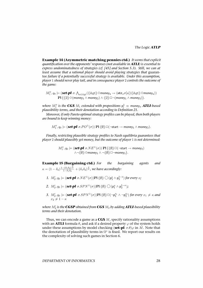
Example 14 (Asymmetricmatching pennies ctd.) It seems that explicitquantification over the opponents’ responses (not available inATLI) is essential toexpress undominatedness of strategies (cf. [45] and Section 5.3). Still, we can atleast assume that a rational player should avoid playing strategies that guaran-tee failure if a potentially successful strategy is available. Under this assumption,player 1 should never play tail, and in consequence player 2 controls the outcome ofthe game:
M ′′1 , q0 |= (set-pl σ.
∧a∈Agt(〈〈Agt〉〉3moneya → (straσ[a])〈〈Agt〉〉3moneya))
Pl(〈〈2〉〉3(money1 ∧money2) ∧ 〈〈2〉〉2¬(money1 ∧money2)
).
where M ′′1 is the CGS M1 extended with propositions p1
i ≡ moneyi, ATLI-basedplausibility terms, and their denotation according to Definition 21.Moreover, if only Pareto optimal strategy profiles can be played, then both players
are bound to keep winning money:
M ′′1 , q0 |= (set-pl σ.PO3(σ)) Pl 〈〈∅〉〉2(¬start → money1 ∧money2).
Finally, restricting plausible strategy profiles to Nash equilibria guarantees thatplayer 2 should plausibly get money, but the outcome of player 1 is not determined:
M ′′1 , q0 |= (set-pl σ.NE3(σ)) Pl
(〈〈∅〉〉2(¬start → money2)
∧¬〈〈∅〉〉3money1 ∧ ¬〈〈∅〉〉2¬money1
).
Example 15 (Bargaining ctd.) For the bargaining agents and
κ = (1− δ2)1−(δ1δ2)
T2
1−δ1δ2 + (δ1δ2)T2 , we have accordingly:
1. M ′2, q0 |= (set-pl σ.NE3(σ))Pl 〈〈∅〉〉 h(px
1 ∧ p1−x2 ) for every x;
2. M ′2, q0 |= (set-pl σ.SPN3(σ))Pl 〈〈∅〉〉 h(pκ1 ∧ p1−κ
2 );
3. M ′2, q0 |= (set-pl σ.SPN3(σ))Pl 〈〈∅〉〉2(¬px1
1 ∧ ¬px22 ) for every x1 6= κ and
x2 6= 1− κ
whereM ′2 is theCGSP obtained fromCGSM2 by addingATLI-based plausibility
terms and their denotation.
Thus, we can encode a game as a CGSM , specify rationality assumptionswith an ATLI formula θ, and ask if a desired property ϕ of the system holdsunder these assumptions by model checking (set-pl σ.θ)ϕ inM . Note thatthe denotation of plausibility terms in Ω∗ is fixed. We report our results onthe complexity of solving such games in Section 6.
DEPARTMENTOF INFORMATICS 28
REASONING ABOUT TEMPORAL PROPERTIES OF RATIONAL PLAY
4.4 Language LkATLP and L∞ATLP
As we have already explained, our main idea is to useATLP for both specifi-cation of rationality assumptions and describtion of the outcome of rationalplay. Thus, we need a possibility to embed anATLP formula ϕ (that definesthe rationality condition) in a “higher-level” formula of ATLP, as a part ofplausibility term (set-pl σ.ϕ). The reading of (set-pl σ.ϕ)ψ is, again: “Letthe plausibility set consist of profiles σ that satisfy ϕ; then, ψ holds”. Apartfrom the possibility of nesting formulae via plausibility updates, we also pro-pose to add quantifier-like structures to the language of terms. Consider, forexample, the term σ1.(∃σ2)ϕ. We would like to collect all strategies s1 suchthat there is a strategy s2 for which ϕ holds (we use σi to refer to si). Thus,σ1.(∃σ2)ϕ is supposed to act in a similar way as the first order logic-based setspecification x | ∃y : ϕ(x, y). It is easy to see that e.g. the set of all undom-inated strategies can now be specified in a straightforward way.As before, the new version of ATLP is given over a set Agt = a1, . . . , ak
of agents, a set Π of propositions, and a set Ω of primitive plausibility terms(cf. Section 3.4). In addition to these sets, we also include a set Var of strate-gic variables. Variables in Var range over strategy profiles; we need them tocharacterize specific rationality criteria, in a way similar to first order logicspecifications.The definition of LATLP is given recursively. In each step the structure of
plausibility terms becomes more sophisticated. At first, we only considerterms out of Ω; their interpretation is given in the model. On the next level,we also allow plausibility terms to be quantifiedATLP formulae which con-tain strategic variables and elements fromΩ. Plausibility terms of subsequentlevels can again be based on terms from the previous levels, and so forth. Inconsequence, the core 0-level language of our new ATLP is almost the sameas the base language LbaseATLP defined in Section 4.1: It extends it with simplecombinations of terms.In general, all the levels of the language canbe seen as containingordinary
formulae of the original ATLP, the only thing that changes as we move tohigher levels is the complexity of plausibility terms. We begin with definingsimple combinations of plausibility terms, and then present the hierarchyof languages LkATLP, with the underlying idea that LkATLP allows for at most k(k ∈ N0) nested plausibility updates. The full language LATLP allows for anyarbitrary finite number of nestings.
Definition 22 (Strategic combination) LetAgt denote a set of agents andX be a non-empty set of symbols. We say that y is a strategic combination of x ifit is generated by the following grammar:
y ::= x | 〈y, . . . , y〉 | y[A]
where x ∈ X, 〈y, . . . , y〉 is a vector of length |Agt|, andA ⊆ Agt. The set of strate-
29 Technical Report IfI-08-03
The LogicATLP
gic combinations over X is defined by T(X). It is easy to see that operator T isidempotent (T(X) = T(T(X))).
The intuition is that elements of x ∈ X are symbols in the object languagethat refer to sets of strategy profiles, and the elements of T(X) allow to com-bine these sets to new sets.8 Let x refer to a set of strategy profiles χ ⊆ Σ.Then, x[A] refers to all the profiles in Σ in which A’s substrategy agrees withsome profile from χ. Similarly, if x1, . . . , xk denote sets of strategy profilesχ1, . . . , χk, then 〈x1, . . . , xk〉 refers to all the profiles that agree on ai’s strategywith at least one profile from χi for each i = 1, . . . , k.
Definition 23 (LkATLP) Let Agt be a set of agents, Π a set of propositions, Ω bea set of primitive plausibility terms, and Var a set of strategic variables (withtypical element σ). The logicsLkATLP(Agt,Π,Var,Ω), k = 0, 1, 2, . . . , are recursivelydefined as follows:
• L0ATLP(Agt,Π,Var,Ω) = LbaseATLP(Agt,Π,Ω0), where Ω0 = T(Ω);
• LkATLP(Agt,Π,Var,Ω) = LbaseATLP(Agt,Π,Ωk), where:
Ωk = T(Ωk−1 ∪ Ωk),Ωk = σ1.(Q2σ2) . . . (Qnσn)ϕ | n ∈ N,∀i (1 ≤ i ≤ n⇒
σi ∈ Var, Qi ∈ ∀,∃, ϕ ∈ LbaseATLP(Agt,Π, T(Ωk−1 ∪ σ1, . . . , σn))) .
Thus, plausibility terms on level k (i.e., Ωk) augment terms from the pre-vious level (Ωk−1) with new terms Ωk that combine quantification over strate-gic variables σ1, . . . σn with formulae possibly containing these strategic variables.Such terms are used to collect (or describe) specific strategy profiles (referredto by variable σ1 which plays a distinctive role in comparison with the othervariables).
Definition 24 (LATLP) The set of ATLP formulae with arbitrary finite nestingof plausibility terms is defined by
LATLP = L∞ATLP(Agt,Π,Var,Ω) = limk→∞
LkATLP(Agt,Π,Var,Ω).
Definition 25 (k-formula, k-term) Formula ϕ ∈ L∞ATLP(Agt,Π,Var,Ω) iscalled anATLPk-formula (or simply k-formula) if, and only if,ϕ ∈ LkATLP(Agt,Π,Var,Ω).Analogously, a plausibility term occurring in a k-formula is called a k-term.
Remark 6 We use the acronym ATLP to refer to both the full language L∞ATLPand the basic sublanguage LbaseATLP.8 This correspondence will be given formally in Definition 26 (Section 4.5).
DEPARTMENTOF INFORMATICS 30
REASONING ABOUT TEMPORAL PROPERTIES OF RATIONAL PLAY
Example 16 (Illustrating plausibility terms in LkATLP) Belowwe presentsome simple formulae illustrating the different levels of our logic.
LbaseATLP: (set-pl ωNE)Pl 〈〈A〉〉γ; group A can enforce γ if only Nash equilibria areplayed (we assume that ωNE denotes exactly the set of Nash equilibria in themodel).
L0ATLP: (set-pl 〈ωNE, . . . , ωNE〉)Pl 〈〈A〉〉γ; plausibility terms can be combined. Notethe difference to the previous formula, agents are assumed to play a strategywhich is part of someNE. The resulting strategy profile does not have to be aNash equilibrium, though.
L1ATLP: ϕ ≡ (set-pl σ.∃σ1ϕ
′(σ, σ1))Pl 〈〈A〉〉γ where ϕ′(σ, σ1) is a formula pos-sibly containing operators (set-pl ω) with ω ∈ T(Ω ∪ σ, σ1); e.g. ϕ′ ≡(set-pl 〈σ, . . . σ, σ1, ωNE〉)Pl 〈〈A〉〉γ′. We will have a closer look at the (set-pl ·) operator in ϕ. Theoperator collects all strategies σ such that there exists another strategy profileσ1 for which Pl 〈〈A〉〉γ′ holds if all but the last 2 agents play according to σ,the second to last agent plays according to σ1, and the last one according to afixed strategy out of ωNE.
L2ATLP: Consider the previous formula ϕ again, but this time ϕ
′(σ, σ1) can alsocontain quantification; e.g. ϕ′ ≡ ((set-pl 〈σ, . . . , σ, σ1, ωNE〉)Pl 〈〈B〉〉γ′) →((set-pl σ′.∃σ′1ϕ′′(σ′, σ′1))Pl 〈〈A〉〉γ) where ϕ′′(σ′, σ′1) is a base formula withplausibility terms taken from T(Ω ∪ σ′, σ′1).
In the next section we show how the denotation of complex terms is con-structed, and how it is plugged into the semantics ofATLP from Section 4.2.
4.5 Semantics of LkATLP and L∞ATLP
LkATLP does not change the very structure of ATLP formulae, it only extendsLbaseATLP by more ornate plausibility terms. Therefore, it seems natural that theplausibilitymapping for theses terms is of particular interest; the denotationreflects the construction of strategic combinations given in Definition 22.
Definition 26 (Extended plausibilitymapping [[·]]) LetM ∈ CGSP (Agt,Π,Ω).The extended plausibility mapping [[·]]M with respect to [[·]]M is defined as fol-lows:
1. If ω ∈ Ω then [[ω]]q
M = [[ω]]qM ;
2. If ω = ω′[A] then [[ω]]q
M = s ∈ Σ | ∃s′ ∈ [[ω′]]q
M s|A = s′|A;
31 Technical Report IfI-08-03

Properties ofATLP
3. If ω = 〈ω1, . . . ωk〉 then [[ω]]q
M = s ∈ Σ | ∃t1 ∈ [[ω1]]q
M , . . . ,∃tk ∈ [[ωk]]q
M∀i =1, ..., k s|ai
= ti|ai);
4. If ω = σ1.(Q2σ2) . . . (Qnσn)ϕ then
[[ω]]q
M = s1 ∈ Σ | Q2s2 ∈ Σ, . . . , Qnsn ∈ Σ (Ms1,...,sn , q |= ϕ),
whereMs1,...,sn is equal toM except that we fixΥMs1,...,sn = Σ,ΩMs1,...,sn =ΩM ∪ σ1, . . . , σn, [[σi]]qMs1,...,sn = si, and [[ω]]qMs1,...,sn = [[ω]]qM for allω 6= σi, 1 ≤ i ≤ n, and q ∈ QM . That is, the denotation of σi inMs1,...,sn isset to strategy profile si.9
Consider, for instance, plausibility term σ1.∀σ2ϕ. The extended plausibil-ity mapping [[σ1.∀σ2ϕ]]q collects all strategy profiles s1 ∈ Σ (referred to by σ1)such that for all strategy profiles s2 ∈ Σ (referred to by σ2) ϕ is true in modelMs1,s2 and state q ∈ Q , i.e.Ms1,s2 , q |= ϕ for all s2 ∈ Σ.
Remark 7 Note that if the language includes a term ω> that refers to all strategyprofiles, then x[A] can be expressed as 〈ω1, . . . , ωk〉, where ωa = xa for a ∈ A, andωa = ω> otherwise. We also observe that in LkATLP, k > 0, ω> can be expressed asσ.>.
In Definition 18 we defined the semantics of the base language of ATLP.Truth of LkATLP formulae is defined in the same way, we only need to replacethe previous (simple) plausibility mapping by the extended one in the se-mantics of plausibility updates.
Definition 27 (Semantics of LkATLP and L∞ATLP) The semantics forLATLP for-mulae is given as inDefinition 18with the extended plausibilitymapping [[·]]M usedinstead of [[·]]M . I.e., only the semantic clauses for (set-pl ω)ϕ and (refn-pl ω)ϕchange as follows:
M, q |=B (set-pl ω)ϕ iffM ′, q |=B ϕ where the new modelM ′ is equal toM but
the new setΥM ′ of plausible strategy profiles is set to [[ω]]q
M ;
M, q |=B (refn-pl ω)ϕ iff M ′, q |=B ϕ where the new model M ′ is equal to M
but the new setΥM ′ of plausible strategy profiles is set toΥM ∩ [[ω]]q
M .
Remark 8 By a slight abuse of notation, we will refer to the extended plausibilitymapping with the same symbol as to the simple plausibility mapping, i.e., with [[·]].
Wewill discuss some important examples ofLATLP formulae and terms (to-gether with their interpretation) in Sections 5.2 and 5.3 where ATLP char-acterizations of solution concepts are presented.9 It should be emphasized that modelMs1,...,sn in which plausibility of profile s1 is evalu-
ated does not presuppose any notion of plausibility, i.e.,ΥMs1,...,sn = Σ.
DEPARTMENTOF INFORMATICS 32
REASONING ABOUT TEMPORAL PROPERTIES OF RATIONAL PLAY
5 Properties of ATLP
This section contains our main conceptual results. We show:
1. That several logics can be embedded into ATLP by means of polyno-mial translation of models and/or formulae (Section 5.1),
2. That several classical solution concepts for extensive games (Nash equi-libria, subgameperfectNash equilibria, ParetoOptimality), canbe char-acterized inATLP already in the language L1
ATLP (Section 5.2),
3. That these solution concepts can be also re-formulated in a qualitativeway, through appropriate formulae of ATLP parameterized by ATLpath formulae (Section 5.3).
5.1 Embedding Existing Logics into ATLP
In this section, we compareATLPwith several related logics and show theirformal relationships. To this end, we first define notions that allow to com-pare expressivity of logical systems. Embedding takes place on the level ofsatisfaction relations (|=): Logic L1 embeds L2 if models and formulae of L2
can be simulated in L1 in a truth-preserving way. Subsumption refers to thelevel of valid sentences: L1 subsumesL2 if all the validities ofL2 are validitiesof L1 as well.
Definition 28 (Embedding) LogicL1 embeds logicL2 iff there is a transla-tion tr of L2 formulae into formulae of L1, and a transformation TR of L2 modelsinto models of L1, such thatM, q |=L2
ϕ iff TR(M), q |=L1tr(ϕ) for every pointed
modelM, q and formula ϕ of L2.
Note that the translation of formulae and transformation of models aresupposed to be independent. This prevents translation schemes that trans-form triples M, q |= ϕ in L2 to M ′, q |= >, and triples M, q 6|= ϕ in L2 toM ′, q 6|= ⊥ (with an arbitrary model M ′), that would yield embeddings be-tween any pair of logics.It is important to point out that all the transformation and translation
schemes proposed in this section can be computed in polynomial time andincur only polynomial increase in the size of models and the length of for-mulae. Thus, we are in fact interested in polynomial embeddings of logics inATLP.
Definition 29 (Subsumption) LogicL1 subsumes logicL2 iff the set of va-lidities of L1 subsumes validities of L2.
Proposition 9 ATLP embedsATL.
33 Technical Report IfI-08-03
Properties ofATLP
Proof We use the identity translation of formulae: tr(ϕ) ≡ ϕ. As for models,TR(M) = M ′ that extendsM with an arbitrary set of plausible strategy pro-filesΥ. It is easy to see that the plausibility assumptionsΥ will never be usedin the evaluation of ϕ since ϕ includes no Pl operators. Thus, the result ofthe evaluation will be the same as forM, q |= ϕ.
The above reasoning implies also that ATL validities hold for all ATLPmodels.
Corollary 10 ATLP subsumesATL.
The relationship of ATLP to most other logics can be studied only in thecontext of embedding, as they use different modal operators (and thus yieldincomparable sets of valid formulae). We begin with embedding “ATLwithIntentions” [30] inATLP. Then,we show that “CTLwithPlausibility” from [10]can be embedded inATLP for a limited (but very natural) class ofmodels. Fi-nally, we propose an embedding of the two existing versions of Game Logicwith Preferences [50, 51] which allow to reason about what can happen un-der particular game-theoretical rationality assumptions.
Proposition 11 ATLP embedsATLI.
Proof sketch For an ATLI model M = 〈Agt,Q ,Π, π, Act, d, o, I,Str, [·]〉, weconstruct the corresponding concurrent game structurewithplausibilityTR(M) =〈Agt,Q ,Π, π, Act, d, o,Υ,Ω, [[·]]〉with the set of plausible strategy profiles Υ =s ∈ Σ | s is consistent with I, plausibility terms Ω = ωσ | σ ∈ Str ∪ ω>,and their denotation [[ω>]]q = Σ and [[ωσ]]q = s ∈ Σ | s|a = [σ] for eachσ ∈ Stra.For an ATLI formula ϕ, we construct its ATLP translation by transform-
ing strategic assumptions (about agents’ intentions) imposed by (straσ) toplausibility assumptions (about strategyprofiles that canbeplausibly played)defined by (set-pl ωσ) and applying them to the appropriate set of agents(i.e., those for whom strategic assumptions have been defined). Formally,the translation is defined as tr(ϕ) = Pl tr〈ω>,...,ω>〉(ϕ), where tr〈ω1,...,ωk〉 is de-fined as follows:
tr〈ω1,...,ωk〉(p) = p,
tr〈ω1,...,ωk〉(¬ϕ) = ¬tr〈ω1,...,ωk〉(ϕ),tr〈ω1,...,ωk〉(ϕ1 ∧ ϕ2) = tr〈ω1,...,ωk〉(ϕ1) ∧ tr〈ω1,...,ωk〉(ϕ2),tr〈ω1,...,ωk〉(〈〈A〉〉 hϕ) = 〈〈A〉〉 htr〈ω1,...,ωk〉(ϕ),
(for 〈〈A〉〉2ϕ and 〈〈A〉〉ϕ1Uϕ2 analogously)tr〈ω1,...,ωk〉((straσ
′a)ϕ) = (set-pl −→ω )tr−→ω (ϕ),
where −→ω = 〈ω1, . . . , ωσ′a , . . . , ωk〉.
DEPARTMENTOF INFORMATICS 34
REASONING ABOUT TEMPORAL PROPERTIES OF RATIONAL PLAY
Note that, for “vanilla” ATLI, 〈〈A〉〉γ holds iff γ can be enforced againstevery response strategy from Agt \ A. Thus, e.g.,M, q |=ATLI (straσa)〈〈A〉〉2p iffTR(M), q |=ATLP Pl (set-pl 〈ω>, . . . , ωσa
, . . . , ω>〉)〈〈A〉〉2p, and analogously forthe other cases.
CTLP, i.e., “CTLwith Plausibility” [10], is an extension of the branching-time logic CTL with a similar notion of plausibility as the one we use here.The main difference lies in the fact that CTLP formulae refer to plausiblepaths rather than strategy profiles.
Proposition 12 ATLP embedsCTLP in the class of transition systems.
Proof sketch To transform models, we first observe that every transition sys-temM can be seen as a concurrent game structure that includes only a singleagent a1. Furthermore, we can transform M to a CGSP TR(M) by addingΥ = Σ and Ω = ∅ (cf. Section 4.1). To translate CTLP formulae, we use thescheme below:
tr(ϕ) = tr(set-pl σ.>)(ϕ)trω(p) = p, trω(¬ϕ) = ¬trω(ϕ), trω(ϕ1 ∧ ϕ2) = trω(ϕ1) ∧ trω(ϕ2),
trω(Eγ) = 〈〈Agt〉〉trω(γ),trω( hϕ) = htrω(ϕ) (for2ϕ and ϕ1Uϕ2 analogously);trω(Plϕ) = (set-pl ω)Pl trω(ϕ),trω(Phϕ) = Ph trω(ϕ),
trω((set-pl γ)ϕ) = trω′(ϕ),where ω′ = σ.(set-pl σ)Pl 〈〈∅〉〉γ.
Now,M, q |=CTLP ϕ iffM, q |=ATLP tr(ϕ).Note that we cannot use the above construction for arbitrary models of
CTLP, as not every set of (plausible) paths can be obtained by memorylessstrategy profiles.
Proposition 13 ATLP cannot be polynomially embedded in neither ATL, norATLI, norCTLP.
Proof Suppose that any of these logics polynomially embeds ATLP. Then,the embedding provides a polynomial reduction of model checking fromATLP to that logic. Since model checking of ATL, ATLI, and CTLP canbe done in polynomial deterministic time [3, 30, 10], we get that the prob-lem forATLP is inP, too. But model checkingATLP is∆P
3 -hard already forLbaseATLP (see Section 6).
There is notmuchwork on logical descriptions of behaviour of agents un-der rationality assumptions based on game-theoretical solution concepts. In
35 Technical Report IfI-08-03
Properties ofATLP
fact, we know only of one such logic for agents with perfect information,which is GLP from [51]. There, agents can be assumed qualitative prefer-ences (i.e., a propositional formula ϕ0 that they supposedly want to makeeventually true). Moreover, they are assumed to play rationally in the sensethat if they have some strategies that guarantee3ϕ0, they can use only thosestrategies in their play. Interestingly enough, the preference criterion wasdifferent in a preliminary version ofGLP [50], where it was based on the no-tion of Nash equilibrium. Both versions ofGLP can be embedded inATLP.One may embed game logics with other preference criteria in an analogousway.
Proposition 14 GLP can be embedded inATLP.
Proof sketch For the translation of models, we transform game trees of GLPto concurrent game structures using the construction from Section 3.3, andtransform the CGS to CGSP by taking Υ = Σ and Ω = ∅. Then, we use thefollowing translation ofGLP formulae:
tr(ϕ) = Pl tr(set-pl σ.>)(ϕ),trω(p) = p, trω(¬ϕ) = ¬trω(ϕ), trω(ϕ ∨ ψ) = trω(ϕ) ∨ trω(ψ),
trω(2ϕ0) = 〈〈∅〉〉3ϕ0,
trω([a : ϕ0]ψ) = (set-pl ω′)trω′(ψ),where ω′ = σ.Pl (set-pl ω)〈〈∅〉〉2
(plausible(σ) ∧ prefers(a, σ, ϕ0)
)plausible(σ) ≡ (refn-pl σ)〈〈Agt〉〉 h>
prefers(a, σ, ϕ0) ≡ 〈〈a〉〉3ϕ0 → (refn-pl σ[a])〈〈∅〉〉3ϕ0.
That is, with each subsequent preference operator [a : ϕ0], only those fromthe (currently) plausible strategy profiles are selected that are preferred by a.The preference is based on the (subgame perfect) enforceability of the out-come ϕ0 at the end of the game: if ϕ0 can be enforced at all, then a prefersstrategies that do enforce it.Now, we have that Γ |=GLP ϕ iff TR(Γ), ∅ |=ATLP tr(ϕ).10
Proposition 15 PreliminaryGLP can be embedded inATLP.
Proof Analogous to Proposition 14. The translation only differs in the char-acterization of agents’ preferences. The agents are now assumed to stick totheir individual parts of Nash equilibria defined by a zero-sum gamewhere a
10 Again, ∅ denotes the position with empty history, i.e., the initial state of the game.
DEPARTMENTOF INFORMATICS 36
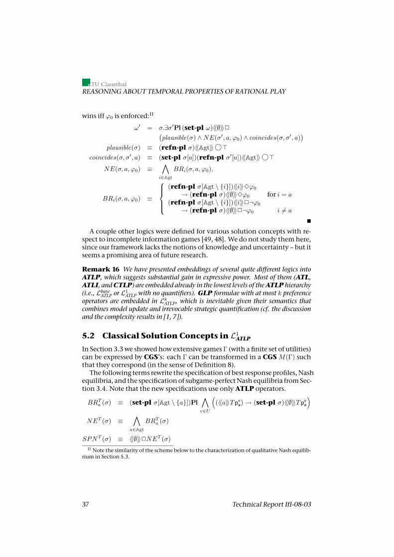
REASONING ABOUT TEMPORAL PROPERTIES OF RATIONAL PLAY
wins iff ϕ0 is enforced:11
ω′ = σ.∃σ′Pl (set-pl ω)〈〈∅〉〉2(plausible(σ) ∧NE(σ′, a, ϕ0) ∧ coincides(σ, σ′, a)
)plausible(σ) ≡ (refn-pl σ)〈〈Agt〉〉 h>
coincides(σ, σ′, a) ≡ (set-pl σ[a])(refn-pl σ′[a])〈〈Agt〉〉 h>NE(σ, a, ϕ0) ≡
∧i∈Agt
BRi(σ, a, ϕ0),
BRi(σ, a, ϕ0) ≡
(refn-pl σ[Agt \ i])〈〈i〉〉3ϕ0
→ (refn-pl σ)〈〈∅〉〉3ϕ0 for i = a(refn-pl σ[Agt \ i])〈〈i〉〉2¬ϕ0
→ (refn-pl σ)〈〈∅〉〉2¬ϕ0 i 6= a
A couple other logics were defined for various solution concepts with re-spect to incomplete information games [49, 48]. We do not study themhere,since our framework lacks the notions of knowledge and uncertainty – but itseems a promising area of future research.
Remark 16 We have presented embeddings of several quite different logics intoATLP, which suggests substantial gain in expressive power. Most of them (ATL,ATLI, andCTLP) are embedded already in the lowest levels of theATLP hierarchy(i.e., LbaseATLP or L1
ATLP with no quantifiers). GLP formulae with at most k preferenceoperators are embedded in LkATLP, which is inevitable given their semantics thatcombines model update and irrevocable strategic quantification (cf. the discussionand the complexity results in [1, 7]).
5.2 Classical Solution Concepts in L1ATLP
In Section 3.3we showed how extensive games Γ (with a finite set of utilities)can be expressed by CGS’s: each Γ can be transformed in a CGSM(Γ) suchthat they correspond (in the sense of Definition 8).The following terms rewrite the specificationof best response profiles, Nash
equilibria, and the specificationof subgame-perfectNash equilibria fromSec-tion 3.4. Note that the new specifications use onlyATLP operators.
BRTa (σ) ≡ (set-pl σ[Agt \ a])Pl∧v∈U
((〈〈a〉〉Tpv
a) → (set-pl σ)〈〈∅〉〉Tpva
)NET (σ) ≡
∧a∈Agt
BRTa (σ)
SPNT (σ) ≡ 〈〈∅〉〉2NET (σ)11 Note the similarity of the scheme below to the characterization of qualitative Nash equilib-rium in Section 5.3.
37 Technical Report IfI-08-03
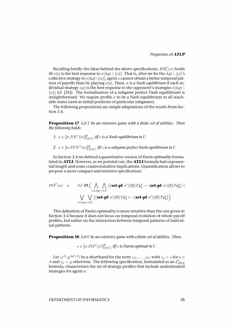
Properties ofATLP
Recalling briefly the ideas behind the above specifications, BRTa (σ) holdsiff σ[a] is the best response to σ[Agt \ a]. That is, after we fix the Agt \ a’scollective strategy to σ[Agt\a], agent a cannot obtain a better temporal pat-tern of payoffs than by playing σ[a]. Then, σ is a Nash equilibrium if each in-dividual strategy s[a] is the best response to the opponent’s strategies σ[Agt \a] (cf. [35]). The formalization of a subgame perfect Nash equilibrium isstraightforward: We require profile σ to be a Nash equilibrium in all reach-able states (seen as initial positions of particular subgames).The following propositions are simple adaptations of the results from Sec-
tion 3.4.
Proposition 17 Let Γ be an extensive game with a finite set of utilities. Thenthe following holds:
1. s ∈ [[σ.NE3(σ)]]∅M(Γ) iff s is a Nash equilibrium in Γ.
2. s ∈ [[σ.SPN3(σ)]]∅M(Γ) iff s is a subgame perfect Nash equilibrium in Γ.
In Section 3.4we defined a quantitative version of Pareto optimality formu-lated inATLI. However, as we pointed out, theATLI formula had exponen-tial length and some counterintuitive implications. Quantification allows topropose a more compact and intuitive specification:
POT (σ) ≡ ∀σ′ Pl( ∧a∈Agt
∧v∈U
((set-pl σ′)〈〈∅〉〉Tpv
a → (set-pl σ)〈〈∅〉〉Tpva
)∨
∨a∈Agt
∨v∈U
((set-pl σ)〈〈∅〉〉Tpv
a ∧ ¬(set-pl σ′)〈〈∅〉〉Tpva
)).
This definition of Pareto optimality ismore intuitive than the one given inSection 3.4 because it does not focus on temporal evolution of whole payoffprofiles, but rather on the interaction between temporal patterns of individ-ual patterns.
Proposition 18 Let Γ be an extensive game with a finite set of utilities. Then:
s ∈ [[σ.PO3(σ)]]∅M(Γ) iff s is Pareto optimal in Γ.
Let 〈xA, yAgt\A〉 be a shorthand for the term 〈z1, . . . , zk〉with za = x for a ∈A and za = y otherwise. The following specification, formulated as an L1
ATLPformula, characterizes the set of strategy profiles that include undominatedstrategies for agent a:
DEPARTMENTOF INFORMATICS 38

REASONING ABOUT TEMPORAL PROPERTIES OF RATIONAL PLAY
UNDOM T (σ) ≡ ∀σ1∀σ2∃σ3
Pl( ∧v∈U
((set-pl 〈σa1 , σ
Agt\a2 〉)〈〈∅〉〉Tpv
a → (set-pl 〈σa, σAgt\a2 〉)〈〈∅〉〉Tpv
a
)∨
∨v∈U
((set-pl 〈σa, σAgt\a
3 〉)〈〈∅〉〉Tpva ∧ ¬(set-pl 〈σa1 , σ
Agt\a3 〉)〈〈∅〉〉Tpv
a
)).
Proposition 19 Let Γ be an extensive game with a finite set of utilities. Then
s ∈ [[σ.UNDOM 3(σ)]]∅M(Γ) iff s|a is undominated in Γ.
5.3 General Solution Concepts in L1ATLP
In this section, we return to the idea of general solution concepts from Sec-tion 3.5 and show how qualitative versions of NE, SPN, PO andUNDOM canbe captured in ATLP. Like for temporalized solution concepts, it turns outthat their qualitative counterparts canbe already specified inL1
ATLP(Agt,Π, ∅).That is, we need only one level of nested plausibility updates (and no “hard-wired” plausibility terms) to effectively capture classical notions of rational-ity and extend them tomore general games that we study in this paper.We only consider one “winning condition” per agent to represent agents’
preferences, but this view can be naturally extended to full preference lists,as in Section 3.5. Inwhat follows, let−→η = 〈η1, . . . , ηk〉 be a vector ofLATL pathformulae.
Definition 30 (Transforming a CGSP into a NFGame) LetM ∈ CGSP(Agt,Π,Ω)and q ∈ QM . The associated NF game S(M,−→η , q)with respect to−→η is given as inDefinition 11 withM interpreted as a pureCGS by removingΥ and [[·]] from it.
Our aim is to define analogues of classical solution concepts (Nash equi-libria and such) that are based on explicit “winning conditions” ηi insteadof numerical payoffs. We can build on our results from the previous section;we only need to replace temporal patterns of payoffs with the formulae ηi:
BR−→ηa (σ) ≡ (set-pl σ[Agt\a])Pl
(〈〈a〉〉ηa → (set-pl σ)〈〈∅〉〉ηa
)NE
−→η (σ) ≡∧
a∈Agt
BR−→ηa (σ)
SPN−→η (σ) ≡ 〈〈∅〉〉2NE
−→η (σ)
PO−→η (σ) ≡ ∀σ′ Pl
( ∧a∈Agt
((set-pl σ′)〈〈∅〉〉ηa → (set-pl σ)〈〈∅〉〉ηa) ∨
∨a∈Agt
((set-pl σ)〈〈∅〉〉ηa ∧ ¬(set-pl σ′)〈〈∅〉〉ηa).
39 Technical Report IfI-08-03
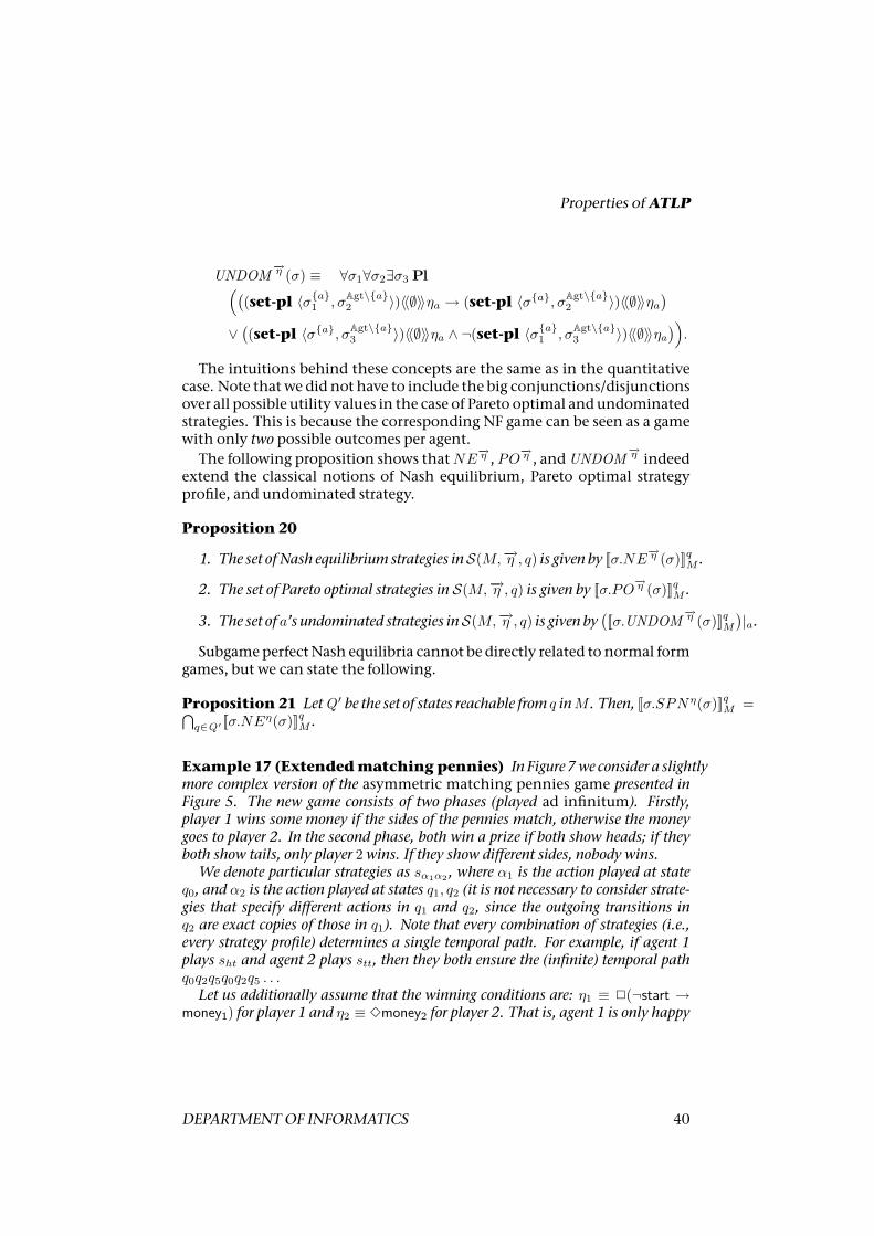
Properties ofATLP
UNDOM−→η (σ) ≡ ∀σ1∀σ2∃σ3 Pl((
(set-pl 〈σa1 , σAgt\a2 〉)〈〈∅〉〉ηa → (set-pl 〈σa, σAgt\a
2 〉)〈〈∅〉〉ηa)
∨((set-pl 〈σa, σAgt\a
3 〉)〈〈∅〉〉ηa ∧ ¬(set-pl 〈σa1 , σAgt\a3 〉)〈〈∅〉〉ηa
)).
The intuitions behind these concepts are the same as in the quantitativecase. Note that we did not have to include the big conjunctions/disjunctionsover all possible utility values in the case of Pareto optimal and undominatedstrategies. This is because the corresponding NF game can be seen as a gamewith only two possible outcomes per agent.The following proposition shows thatNE
−→η , PO−→η , andUNDOM
−→η indeedextend the classical notions of Nash equilibrium, Pareto optimal strategyprofile, and undominated strategy.
Proposition 20
1. The set ofNash equilibrium strategies inS(M,−→η , q) is given by [[σ.NE−→η (σ)]]qM .
2. The set of Pareto optimal strategies in S(M,−→η , q) is given by [[σ.PO−→η (σ)]]qM .
3. The set of a’s undominated strategies inS(M,−→η , q) is given by([[σ.UNDOM
−→η (σ)]]qM)|a.
SubgameperfectNash equilibria cannot be directly related to normal formgames, but we can state the following.
Proposition 21 LetQ ′ be the set of states reachable from q inM . Then, [[σ.SPNη(σ)]]qM =⋂q∈Q′ [[σ.NEη(σ)]]qM .
Example 17 (Extendedmatching pennies) In Figure 7we consider a slightlymore complex version of the asymmetric matching pennies game presented inFigure 5. The new game consists of two phases (played ad infinitum). Firstly,player 1 wins some money if the sides of the pennies match, otherwise the moneygoes to player 2. In the second phase, both win a prize if both show heads; if theyboth show tails, only player 2wins. If they show different sides, nobody wins.We denote particular strategies as sα1α2 , where α1 is the action played at state
q0, and α2 is the action played at states q1, q2 (it is not necessary to consider strate-gies that specify different actions in q1 and q2, since the outgoing transitions inq2 are exact copies of those in q1). Note that every combination of strategies (i.e.,every strategy profile) determines a single temporal path. For example, if agent 1plays sht and agent 2 plays stt, then they both ensure the (infinite) temporal pathq0q2q5q0q2q5 . . .Let us additionally assume that the winning conditions are: η1 ≡ 2(¬start →
money1) for player 1 and η2 ≡ 3money2 for player 2. That is, agent 1 is only happy
DEPARTMENTOF INFORMATICS 40
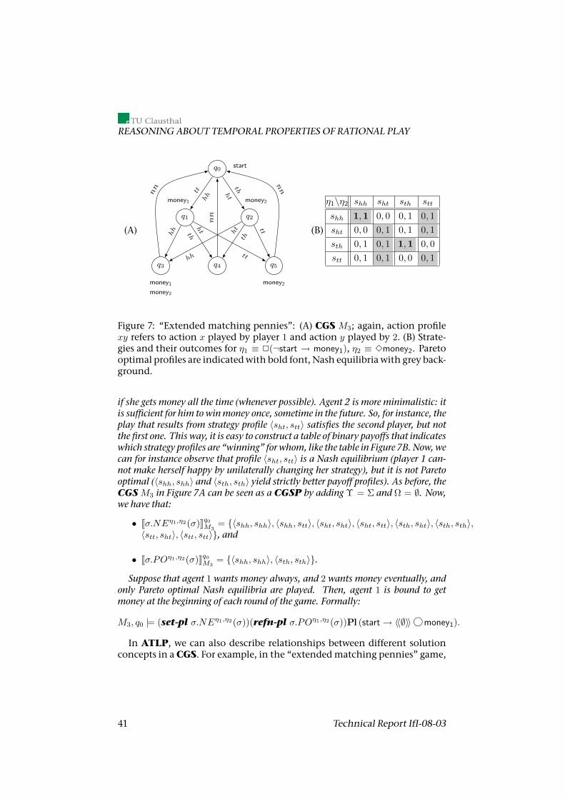
REASONING ABOUT TEMPORAL PROPERTIES OF RATIONAL PLAY
(A)
q0start
q1
money1
q2
money2
q3
money1
money2
q4 q5
money2
hh
tt ht
th
hh
htth
tthh
ht
th
tt
nn
nn
nn
(B)
η1\η2 shh sht sth stt
shh 1,1 0, 0 0, 1 0, 1sht 0, 0 0, 1 0, 1 0, 1sth 0, 1 0, 1 1,1 0, 0stt 0, 1 0, 1 0, 0 0, 1
Figure 7: “Extended matching pennies”: (A) CGS M3; again, action profilexy refers to action x played by player 1 and action y played by 2. (B) Strate-gies and their outcomes for η1 ≡ 2(¬start → money1), η2 ≡ 3money2. Paretooptimal profiles are indicatedwith bold font, Nash equilibria with grey back-ground.
if she gets money all the time (whenever possible). Agent 2 is more minimalistic: itis sufficient for him to winmoney once, sometime in the future. So, for instance, theplay that results from strategy profile 〈sht, stt〉 satisfies the second player, but notthe first one. This way, it is easy to construct a table of binary payoffs that indicateswhich strategy profiles are “winning” for whom, like the table in Figure 7B. Now, wecan for instance observe that profile 〈sht, stt〉 is a Nash equilibrium (player 1 can-not make herself happy by unilaterally changing her strategy), but it is not Paretooptimal (〈shh, shh〉 and 〈sth, sth〉 yield strictly better payoff profiles). As before, theCGSM3 in Figure 7A can be seen as a CGSP by adding Υ = Σ and Ω = ∅. Now,we have that:
• [[σ.NEη1,η2(σ)]]q0M3= 〈shh, shh〉, 〈shh, stt〉, 〈sht, sht〉, 〈sht, stt〉, 〈sth, sht〉, 〈sth, sth〉,
〈stt, sht〉, 〈stt, stt〉, and
• [[σ.POη1,η2(σ)]]q0M3= 〈shh, shh〉, 〈sth, sth〉.
Suppose that agent 1 wants money always, and 2 wants money eventually, andonly Pareto optimal Nash equilibria are played. Then, agent 1 is bound to getmoney at the beginning of each round of the game. Formally:
M3, q0 |= (set-pl σ.NEη1,η2(σ))(refn-pl σ.POη1,η2(σ))Pl (start → 〈〈∅〉〉 hmoney1).
In ATLP, we can also describe relationships between different solutionconcepts in a CGS. For example, in the “extendedmatching pennies” game,
41 Technical Report IfI-08-03
Model CheckingATLP
all Pareto optimal profiles happen to be in Nash equilibrium, which is equiv-alent to the following formula:
(set-pl σ.POη1,η2(σ))(refn-pl σ.¬NEη1,η2(σ))Pl¬〈〈Agt〉〉 h>,and the formula does indeed hold inM3, q0.
6 Model Checking ATLP
In this sectionwediscuss themodel checking complexity ofATLP. Themodelchecking problem refers to the question whether a given formula holds in agivenmodel and state. The size of the input is usually measured in the num-ber of transitions in the model (m) and the length of the formula (l). Notethat the problem of checking ATLP with respect to the size of the wholeCGSP (including the plausibility set Υ), is trivially linear in the size of themodel: The model size is exponential with respect to the number of states andtransitions. Hence, model checking CGSP’s does not make sense if the setof plausible strategies is stored explicitly. The set should be stored implicitly;for instance, bymeans of some decision procedure. Wewill assume through-out this section that the plausibility setΥ does not discriminate any strategyprofiles (i.e., all strategy profiles are initially plausible), and actual plausibil-ity assumptions must be specified in the object language through (simple orcomplex) plausibility terms.The same remark applies to the denotations of primitive (“hard-wired”)
plausibility terms. In this respect, we will consider two subclasses of CGSP’sin which the representation of plausibility assumptions of plausibility as-sumptions does not overwhelm the complexity of the rest of the input –namely, pure concurrent game structures and so called “well-behaved”CGSP’s.In pure CGS’s, plausibility terms and their denotations are simply absent.In well-behaved CGS’s, we put a limit on the complexity of the plausibil-ity check, i.e., the computational resources needed to determine whether agiven strategy is plausible according to a given plausibility term and plausi-bility mapping.
Definition 31 (CGS as CGSP) As before, we will take each CGS to be an im-plicit representation ofCGSPwhere all strategy profiles are initially plausible (Υ =Σ) and there are no “hardwired” plausibility terms (Ω = ∅).
Definition 32 (Well-Behaved CGSP) A CGSP M is called well-behavedif, and only if,
1. ΥM = Σ: all the strategy profiles are plausible inM ;
DEPARTMENTOF INFORMATICS 42

REASONING ABOUT TEMPORAL PROPERTIES OF RATIONAL PLAY
2. There is anNP-algorithm (with respect to l andm) which determineswhethers ∈ [[ω]]qM for every state q ∈ QM , strategy profile s ∈ Σ, and plausibility termω ∈ Ω.
Remark 22 We note that, if a list (or several alternative lists) of plausible strat-egy profiles is given explicitly in the model (via the plausibility set Υ and/or thedenotations of abstract plausibility terms ω from Section 4), then the problem ofguessing an appropriate strategy from such a list is in NP (memoryless strategieshave polynomial size with respect tom). Consequently, we assume that, if such alist is given explicitly, that it is stored outside the model.
We begin our study with the complexity of model checking the basic lan-guage LbaseATLP in Section 6.1. Then, we investigate the complexity for the in-termediate language LATLPATLI (Section 6.2). It turns out that the problem isin both cases∆P
3 -complete in general, which seems in line with existing re-sults on the complexity of solving games. In particular, it is known that ifboth players in a 2-player imperfect information game have imperfect recall,and chancemoves are allowed, then the problem of finding amax-min purestrategy is ΣP
2 -complete [31].12 That is, there are established results withingame theorywhich show that reasoning about the outcome of a gamewherethe strategies of both parties are restricted cannot be easier than ΣP
2 (resp.∆P
3 when nesting of game specifications is allowed). In the light of this, ourcomplexity results are not as pessimistic as they seem, especially asATLP al-lows specification of much more diverse restrictions than those imposed byimperfect information in 2-player turn-based games.13
Moreover, we show in Sections 6.1 and 6.2 that model checking LbaseATLP andLATLPATLI is∆P
2 -complete if only theproponents’ strategies are restricted. This,again, corresponds to some well-knownNP-hardness results for solving ex-tensive games with imperfect information and recall [12, 17, 31].Finally, in Section 6.3 we study the model checking complexity of LkATLP
and L∞ATLP. We summarize the results in Section 6.4.
6.1 Model Checking LbaseATLP
In this section we show that model checking LbaseATLP is ∆P3 -complete in gen-
eral, and∆P2 -complete when only the proponents’ strategies are restricted.
Moreover, model checking LbaseATLP over rectangular models and models withbounded plausibility sets can be done in polynomial time.
12Note that strategic operators can be nested in anATLP formula, thus specifying a sequenceof games, with the outcome of each game depending on the previous ones—and solving suchgames requires adaptive calls to aΣP
2 oracle.13 In particular, imperfect information strategies (sometimes called uniform strategies) can becharacterized inATLP for a relevant subclass of models, cf. Section 6.1.2.
43 Technical Report IfI-08-03
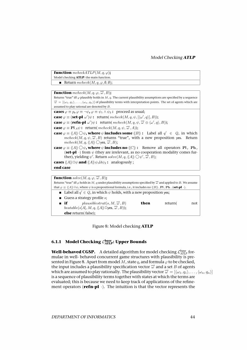
Model CheckingATLP
functionmcheckATLP(M, q, ϕ);Model checkingATLP: the main function.
Returnmcheck(M, q, ϕ, ∅, ∅);
functionmcheck(M, q, ϕ,−→ω ,B);Returns “true” iff ϕ plausibly holds inM, q. The current plausibility assumptions are specified by a sequence−→ω = [〈ω1, q1〉, . . . , 〈ωn, qn〉] of plausibility terms with interpretation points. The set of agents which areassumed to play rational are denoted byB.
cases ϕ ≡ p, ϕ ≡ ¬ψ, ϕ ≡ ψ1 ∧ ψ2 : proceed as usual;case ϕ ≡ (set-pl ω′)ψ : return(mcheck(M, q, ψ, [〈ω′, q〉], B));case ϕ ≡ (refn-pl ω′)ψ : return(mcheck(M, q, ψ,−→ω ⊕ 〈ω′, q〉, B));case ϕ ≡ Pl Aψ : return(mcheck(M, q, ψ,−→ω ,A));case ϕ ≡ 〈〈A〉〉 gψ, where ψ includes some 〈〈B〉〉 : Label all q′ ∈ Q , in which
mcheck(M, q, ψ,−→ω ,B) returns “true”, with a new proposition yes. Returnmcheck(M, q, 〈〈A〉〉 gyes,−→ω ,B);
case ϕ ≡ 〈〈A〉〉 gψ, where ψ includes no 〈〈C〉〉 : Remove all operators Pl , Ph ,(set-pl ·) from ψ (they are irrelevant, as no cooperation modality comes fur-ther), yielding ψ′. Return solve(M, q, 〈〈A〉〉 gψ′,−→ω ,B);
cases 〈〈A〉〉2ψ and 〈〈A〉〉ψ1Uψ2 : analogously ;end case
function solve(M, q, ϕ,−→ω ,B);Returns “true” iffϕholds inM, q under plausibility assumptions specified by−→ω and applied toB. We assumethatϕ ≡ 〈〈A〉〉2ψ, whereψ is a propositional formula, i.e., it includes no 〈〈B〉〉,Pl ,Ph , (set-pl ·).
Label all q′ ∈ Q , in which ψ holds, with a new proposition yes; Guess a strategy profile s; if plausiblestrat(s,M,−→ω ,B) then return( not
beatable(s[A],M, q, 〈〈A〉〉2yes,−→ω ,B));else return( false);
Figure 8: Model checkingATLP
6.1.1 Model Checking LbaseATLP: Upper Bounds
Well-behaved CGSP. A detailed algorithm for model checking LbaseATLP for-mulae in well- behaved concurrent game structures with plausibility is pre-sented in Figure 8. Apart frommodelM , state q, and formulaϕ to be checked,the input includes a plausibility specification vector −→ω and a set B of agentswhich are assumed toplay rationally. Theplausibility vector−→ω = [〈ω1, q1〉, . . . , 〈ωn, qn〉]is a sequence of plausibility terms together with states at which the terms areevaluated; this is because we need to keep track of applications of the refine-ment operators (refn-pl ·). The intuition is that the vector represents the
DEPARTMENTOF INFORMATICS 44
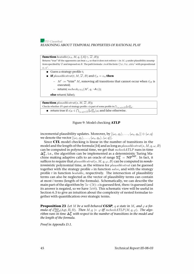
REASONING ABOUT TEMPORAL PROPERTIES OF RATIONAL PLAY
function beatable(sA,M, q, 〈〈A〉〉γ,−→ω ,B);Returns “true” iff the opponents can beat sA so that it does not enforce γ inM, q under plausibility assump-
tions specifiedby−→ω and imposedonB. Thepath formulaγ is of the form eψ,2ψ,ψUψ′ withpropositionalψ,ψ′.
Guess a strategy profile t; if plausiblestrat(t,M,−→ω ,B) and t|A = sA then
− M ′ := “trim”M , removing all transitions that cannot occur when t|B isexecuted;
− return(mcheckCTL(M ′, q,¬Aγ));
else return( false);
function plausiblestrat(s,M,−→ω ,B);Checks whetherB’s part of strategy profile s is part of some profile in
⋂〈ω,q〉∈−→ω [[ω]]qM .
return true if s|B ∈⋂〈ω,q〉∈−→ω [[ω]]qM |B ; and false otherwise.
Figure 9: Model checkingATLP
incremental plausibility updates. Moreover, by [〈ω1, q1〉, . . . , 〈ωn, qn〉] ⊕ 〈ω, q〉we denote the vector [〈ω1, q1〉, . . . , 〈ωn, qn〉, 〈ω, q〉].Since CTL model checking is linear in the number of transitions in the
model and the lengthof the formula [14] and as long as plausiblestrat(s,M, q, ω,B)can be computed in polynomial time, we get thatmcheckATLP runs in time∆P
3 , i.e., the algorithm can be implemented as a deterministic Turing Ma-chine making adaptive calls to an oracle of range ΣP
2 = NPNP. In fact, itsuffices to require that plausiblestrat(s,M, q, ω,B) can be computed in nonde-terministic polynomial time, as the witness for plausiblestrat can be guessedtogether with the strategy profile s in function solve, and with the strategyprofile t in function beatable, respectively. The intersection of plausibilityterms can also be neglected as the vector of plausibility terms can containat most l terms (length of the formula). Schematically, we can describe themainpart of the algorithmby ∃s¬(∃t): s is guessedfirst, then t is guessed (andits answer is negated, so we have ∃s∀t). This schematic view will be useful inSection 6.3 to give an intuition about the complexity of nested formulae to-gether with quantification over strategic terms.
Proposition 23 LetM be a well-behaved CGSP, q a state inM , and ϕ a for-mula of LbaseATLP(Agt,Π,Ω). Then M, q |= ϕ iff mcheckATLP(M, q, ϕ). The algo-rithm runs in time∆P
3 with respect to the number of transitions in the model andthe length of the formula.
Proof in Appendix D.1.
45 Technical Report IfI-08-03
Model CheckingATLP
Note that the requirement that the set of plausible strategies is given by Σis not a real restriction. Specific plausibility specification can always be setusing operator (set-pl ·), by adding a new plausibility term that denotes thedesired set of strategy profiles. The only restriction is that inclusion in theset must be verifiable in nondeterministic polynomial time.Finally, we observe that the complexity can be improved if only the strate-
gies of the proponents are restricted.
Proposition 24 Let γ be anLbaseATLP path formulawithout cooperationmodalities.Then the model checking problem for formulae of the form PlA〈〈A〉〉γ is in ∆P
2
(instead of∆P3 ).
Proof Sketch We consider the case ϕ ≡ 〈〈A〉〉 hψ, where ψ includes no 〈〈C〉〉.In solve a plausible strategy sA for A is guessed (NP-call). Then, in functionbeatable themodel is directly trimmed according to sA (without guessing an-other profile t) and the CTLmodel checking algorithm is executed. In thiscase, function beatable can be executed in polynomial time.
Corollary 25 Let ϕ ∈ LbaseATLP. If for each cooperation modality 〈〈A〉〉 occurringin ϕ it is specified that only agents A′ where A′ ⊆ A play plausibly then modelchecking is in∆P
2 .
Pure CGS. This is a somewhat degenerate case because inLbaseATLP only prim-itive plausibility terms can be used. With no such terms, (set-pl ·) and(refn-pl ·) operators cannot be used, so all strategy profiles will be consid-ered plausible in the evaluation of every subformula. In consequence,modelLbaseATLP(Agt,Π, ∅) can be done in the same way as forATL. Since model check-ingATL lies inP [3] we get the following result.
Proposition 26 Let M be a CGS, q a state in M , and ϕ ∈ LbaseATLP(Agt,Π, ∅).Model checking ϕ in M, q is in P with respect to the number of transitions in themodel and the length of the formula.
Proof Remove all PlA operators from ϕ and check whether M ′q, |=ATL ϕwhereM ′ is the CGS obtained fromM by leaving outΥ,Ω, and [[·]].
SpecialClassesofModels. Wewill nowconsider the special case inwhicheach plausibility term refers to at most polynomially many strategies.
Definition 33 (BoundedModelsMc) Given a fixed constant c ∈ N we con-sider the class Mc ⊆ CGSP (Agt,Π,Ω) of models such that for all M ∈ Mc,ω ∈ ΩM , and q ∈ QM it holds that |[[ω]]qM | ≤ lc · mc where l (resp. m) denotesthe length of the input formula (resp. number of transitions ofM ).
DEPARTMENTOF INFORMATICS 46
REASONING ABOUT TEMPORAL PROPERTIES OF RATIONAL PLAY
Proposition 27 Let c ∈ N be a constant. Model checking LbaseATLP formulae withrespect to the class of well-behaved bounded modelsMc can be done in polynomialtime with respect to the number of transitions in the model and the length of theformula.
Proof in Appendix D.1.
Even with arbitrarily many strategies the complexity can be improved ifthe set of plausible profiles has a specific structure, namely if the set can be(and is) represented in a rectangular way. Intuitively, such a set of profilescan be represented by behavioral constraints [46]. That is, we restrict theactions that can be performed independently for each state and agent, andthen consider all strategy profiles generated from the constrained repertoireof actions.
Definition 34 (Rectangularity,Mrect) Let Sa ⊆ Σa be a set of strategies ofagent a. We say that Sa is rectangular if it is represented by a function d′a : QM →P(Act) such that for all states q ∈ QM it holds that d′a(q) ⊆ da(q); then, Sa istaken to be the set sa ∈ Σa | ∀q ∈ QM (sa(q) ∈ d′a(q)).A set of collective strategies (resp. strategy profiles) SA ⊆ ΣA is rectangular if it
represented as a collection of rectangular sets of individual strategies. Then, SA isto the Cartesian product of the individual sets, i.e., SA =
∏a∈A Sa.
A set of plausibility terms Ω is rectangular in a modelM if all terms in ω ∈ Ωhave rectangular denotations [[ω]]qM . Finally, we say that aCGSPM is rectangularif the setΥM is rectangular and terms Ω are rectangular inM . We denote the classof such models byMrect.
Note, for example, that each ΣA is rectangular.
Proposition 28 Model checking LbaseATLP formulae in the classMrect can be donein P with respect to the number of transitions in the model and the length of theformula.
Proof The algorithm is very simple; we present the procedure forϕ ≡ 〈〈A〉〉2ψbeing in the scope of (set-pl ω) andPlB. Other cases are analogous.Firstly, we model-check (set-pl ω)PlBψ recursively and label the states
where the answer was “true” with a new proposition yes. Then, we take [[ω]]qM(recall that it is represented in a rectangular way, i.e., by function d′ : Agt ×Q → P(Act)), and replace function d inM by d′′ such that d′′(a, q) = d′(a, q)for a ∈ B and d′′(a, q) = d(a, q) for a /∈ B. Finally, we use any ATL modelchecker to model-check 〈〈A〉〉2yes in the resulting model, and return the an-swer.
We observe that strategic combinations of rectangular plausibility termsare also rectangular. In consequence, the results extends toL0
ATLP in a straight-
47 Technical Report IfI-08-03
Model CheckingATLP
forward way, which will prove useful in Section 6.3.14
Lemma 29 If S ⊆ Σa (resp. S ⊆ ΣA) contains only a single strategy (resp. strat-egy profile) then it is rectangular.
Lemma 30 Let Ω be a rectangular set of plausibility terms, then τ(Ω) is rectan-gular as well.
Corollary 31 Model checking L0ATLP formulae in the classM
rect can be done inPwith respect to the number of transitions in themodel and the length of the formula.
6.1.2 Model Checking LbaseATLP: Hardness and Completeness
Well-behavedCGSP. Weprove∆P3 -hardness through a reductionofSNSAT2,
a typical∆P3 -complete variant of the Boolean satisfiability problem. The re-
duction is done in two steps.
1. Firstly, we define a modification of ATLir [38], in which all agents arerequired to play only uniform strategies. We call it “uniform ATLir”(ATLuir in short), and show thatmodel checkingATLuir is∆P
3 -completebymeans of a polynomial reduction of SNSAT2 toATLuirmodel check-ing.
2. Then,wepoint out that each formula andmodel ofATLuir canbe equiv-alently translated (in polynomial time) to aCGSP and a formulaLbaseATLP,thus yielding a polynomial reduction of SNSAT2 to model checkingLbaseATLP.
Parts of our construction reuse techniques presented in [19, 27, 23, 28].In “uniform ATLir” (ATLuir), where we assume that all the players have
limited information about the current state, and each agent can only useuniform strategies (i.e., ones that assign same choices in indistinguishablestates). The syntax of ATLuir is the same as that of ATL, only cooperationmodalities are annotated with additional tags ir and u to indicate the imper-fect information and recall, and uniformity of all agents’ strategies. The se-mantics ofATLuir is defined over concurrent epistemic game structures (CEGS),i.e. CGS extended with epistemic relations that represent indistinguishabil-ity of states for agents. Details of the semantics and more thorough presen-tation can be found in Appendix B. The following proposition summarizesthe complexity results from Appendix B.2.
Proposition 32 Model checkingATLuir is∆P3 -complete with respect to the num-
ber of transitions in the model and the length of the formula.
14 Recall, thatL0ATLP consists of all base formulae in which plausibility terms form τ(Ω) can be
used (instead of plain terms fromΩ only).
DEPARTMENTOF INFORMATICS 48
REASONING ABOUT TEMPORAL PROPERTIES OF RATIONAL PLAY
Remark 33 We have thus proven that checking strategic abilities when all play-ers are required to play uniformly is∆P
3 -complete (that is, harder than ability com-pared with the worst line of events captured by ATLir formulae, which is “only”∆P
2 -complete). We believe it is an interesting result with respect to verification ofvarious kinds of agents’ abilities under incomplete information. We note that theresult from [31] for extensive games with incomplete information can be seen as aspecific case of our result, at least in the class of games with binary payoffs.
Nowwe showhowATLuirmodel checking can be reduced tomodel check-ing of LbaseATLP. We are given a CEGSM , a state q inM , and an ATL
uir formula
ϕ. Let Σu be the set of all uniform strategy profiles inM . We take CGSPM ′
asM (sans epistemic relations) extended with plausibility mapping [[·]] suchthat [[ω]]q = Σu. Then:
M, q |=ATLuir〈〈A〉〉uirϕ iff M ′, q |=ATLP (set-pl ω)Pl 〈〈A〉〉ϕ,
which completes the reduction.
Remark 34 We note in passing that, technically, the size of the resulting modelM ′ is not entirely polynomial. M ′ includes the plausibility set Υ, which is expo-nential in the number of states inM (since it is equal to the the set of all uniformstrategy profiles inM ). This is of course the case whenwewant to storeΥ explicitly.However, checking if a strategy profile is uniform can be done in time linear wrt thenumber of states inM , so an implicit representation ofΥ (e.g., the checking proce-dure itself) requires only linear space.
As a result of this and Proposition 23, we obtain the following theorem.
Theorem 35 Model checking LbaseATLP for well-behaved CGSP’s is ∆P3 -complete
with respect to the number of transitions in the model and the length of the for-mula.
For the special case when only the proponents have to follow plausiblestrategies, a reduction frommodel checkingATLir (instead ofATLuir) is suf-ficient. Since model checkingATLir is∆P
2 -complete [38, 28], we get the fol-lowing.
Theorem 36 LetL the subset ofLbaseATLP in which every cooperationmodality 〈〈A〉〉occurs in the scope of PlB with B ⊆ A. Then, model checking L in the class ofwell-behavedCGSP’s is∆P
2 -complete.
Proof sketch The inclusion in ∆P2 has been already shown in Section 6.1.1.
We prove the lower bound by a reduction of model checking Schobbens’ATLir [38] to model checking of our sublanguage L. Let M be a CEGS, qa state inM , and ϕ ≡ 〈〈A〉〉irγ a formula ofATLir. Moreover, let ΣuA be the set
49 Technical Report IfI-08-03
Model CheckingATLP
of all strategy profiles inM that are uniform for A. We take CGSPM ′ asM(sans epistemic relations) extended with plausibility mapping [[·]] such that[[ω]]q = ΣuA. Then:
M, q |=ATLir〈〈A〉〉irγ iff M ′, q |=ATLP (set-pl ω)Pl 〈〈A〉〉γ,
which completes the reduction.
PureCGSandSpecialClassesofModels. In order to show lower boundsfor model checking LbaseATLP for pure concurrent game structures, well-behavedboundedmodels, and rectangularmodels, we observe thatATL is a subset ofLbaseATLP even if the latter does not use plausibility terms – and model checkingATL isP-complete [3]. Thus, we conclude with the following.
Theorem 37 Let c ∈ N be a constant. Model checking LbaseATLP with respect towell-behaved bounded models Mc, rectangular models Mrect, and pure CGS’s isP-complete.
6.2 Model Checking LATLPATLIHere, we show that model checking ATLP with plausibility terms based onATLI is also∆P
3 -complete. Note that the only primitive terms occurring informulae of ATLPATLI are used to simulate strategic terms of ATLI (whichdenote individual strategies of particular agents. Thus, the results in this sec-tion refer to model checking with rectangular CGSP’s.
6.2.1 Model Checking LATLPATLI : Upper Bound
The algorithm in Figure 8 uses abstract plausibility terms but it can also beused for ATLI-based plausibility terms presented in Section 4.3. In [30] itwas shown that the model checking problem for ATLI is polynomial withrespect to the number of transitions and length of the formula. Thus, we getanother immediate corollary of Proposition 23.
Proposition 38 Model checking ATLP with ATLI-based plausibility terms inrectangular well-behaved CGSP’s is in ∆P
3 with respect to the number of transi-tions in the model and the length of the formula.
In Section 4.4 we have used L1ATLP formulae to characterize game theoretic
solution concepts. For this purpose it was not necessary to have hard-wiredplausibility terms in the language. Indeed, the absence of such terms posi-tively influences the model checking complexity of higher levels ofATLP.
DEPARTMENTOF INFORMATICS 50
REASONING ABOUT TEMPORAL PROPERTIES OF RATIONAL PLAY
6.2.2 Model Checking LATLPATLI : Hardness and Completeness
Like in Section 6.1.2, we show the lower bound by a reduction from modelcheckingATLuir. That is, we demonstrate how uniformity of strategy profilescan be characterized by formulae of ATLI for a relevant class of concurrentgame structures. The actual reduction is quite technical and can be foundin Appendix C. The following result is an immediate corollary of Proposi-tion 50, presented in Appendix C.
Theorem 39 Model checking LbaseATLP with ATLI-based plausibility terms is∆P3 -
complete with respect to the number of transitions in the model and the length ofthe formula.
Moreover, if plausibility restrictions apply only to proponents, then thecomplexity improves (the proof is analogous to Theorem 36).
Theorem 40 Let L the subset of LATLPATLI in which every cooperation modality〈〈A〉〉 occurs in the scope of PlB with B ⊆ A. Then, model checking L in the classof well-behaved rectangularCGSP’s is∆P
2 -complete.
Proof sketch Weprove the lower bound (again) by a reductionofmodel check-ing ATLir to model checking L. The reduction is very similar to the oneshown in Appendix C except that only the “verifier” decides upon the val-ues of the propositions (cf. [27]).
6.3 Model Checking LkATLP
In this sectionwepresent our results regarding themodel checking complex-ity of the full logic LATLP. The complexity depends on both the nesting levelof ATLP formulae and on the structure and alternations of strategic quan-tifiers. Before we state our results we introduce some additional definitionsneeded to classify such complex formulae.
6.3.1 Classifying LATLP Formulae: SomeDefinitions
The complexity of model checking formulae in LATLP does not only dependon the actual nesting depth of plausibility terms but also on the structure ofstrategic quantifiers used inside (set-pl ·) and (refn-pl ·) operators. The lat-ter structure is quite complex and cannot solely be described by the numberof quantifiers. Often, a specific position of quantifiers can be used to com-bine two “guessing” phases, improving complexity.Firstly, not the number of quantifiers is important but rather the num-
ber of alternations. We introduce function ALT : ∃,∀+ → ∃,∀+ whichmodifies a word over ∃,∀ such that each quantifier following a quantifier
51 Technical Report IfI-08-03
Model CheckingATLP
of the same type is removed; for example, ALT(∃∀∀∀∃∀) = ∃∀∃∀. Moreover,existential quantifiers at the beginning and end of a quantifier series can,under some conditions, be ignored without changing the model checkingcomplexity. For example, let us assume that the first quantifier is existen-tial. Then it follows a guess of the proponents (resp. opponents) strategyand both guesses can be combined. Analogously, an existential quantifier atthe end usually follows another existential guess. To take these issues intoaccount, we define function RALT : ∃,∀+ → Z that counts the number ofthe relevant alternations of quantifiers in a sequence:
RALT(−→Q) =
n if ALT(
−→Q) = Q1 . . . Qn andQ1 6= ∃ 6= Qn;
n− 1 if ALT(−→Q) = Q1 . . . Qn andQ1 = ∃ xorQn = ∃;
n− 2 if ALT(−→Q) = Q1 . . . Qn andQ1 = ∃ = Qn and n > 2;
−1 else.
Function RALT characterizes the “hardness” of the outermost level in agiven term. The next two functions take into account the recursive structureof terms, due to possibly nested (set-pl ·) or (refn-pl ·) operators. Firstly,UO(ϕ) returns the set of all the update operations (set-pl ω) and (refn-pl ω)within formula ϕ. Secondly, ql takes a set of update operations and returnsthe quantifier level in these operations as follows:
ql(S) =
maxs∈S ql(s) if |S| > 1ql(UO(ϕ′)) if S = (Op σ.ϕ′)RALT(Q1 . . . Qn) + ql(UO(ϕ′)) if S = (Op σ.Q1σ1 . . . Qnσnϕ
′) and(ϕ′ 6∈ L0
ATLP(Agt,Π,Var,Var) orQn = ∀)RALT(Q1 . . . Qn) + ql(UO(ϕ′)) + 1 if S = (Op σ.Q1σ1 . . . Qnσnϕ
′) andϕ′ ∈ L0
ATLP(Agt,Π,Var,Var) andQn = ∃0 if S = ∅ or (S = (Op ω) and ω ∈ Ω)
where (Op ·) is either (set-pl ·) or (refn-pl ·).The intuition behind ql is that it determines the maximal sum of relevant
alternations in each sequence of nestedupdate operators (set-pl ·), (refn-pl ·).Intuitively, the nested operators represent a tree. Given an LkATLP formulawe add arcs from the root of the tree to nodes representing update opera-tors operators in the kth level. Then, from such a new node representing(set-pl ω) or (refn-pl ω), we add arcs to nodes representing update opera-tors inside ω (i.e., on the k − 1th level) and so on. Leaves of the tree consistof nodes representing operators whose terms contain no further update op-erators. Now, each node represented by e.g. (set-pl σ.Q1σ1 . . . Qnσnϕ
′) islabeled by RALT(Q1 . . . Qn). Function ql returns the maximal sum of suchnumbers along all paths from the root to some leaf.
DEPARTMENTOF INFORMATICS 52
REASONING ABOUT TEMPORAL PROPERTIES OF RATIONAL PLAY
Given an operator (set-pl σ.Q1σ1 . . . Qnσnϕ′) on the second to last level
without hard-wired plausibility term (i.e., for ϕ′ ∈ L0ATLP(Agt,Π,Var,Var))
andwhich endswith an existential quantifier ∃, the very operatorQn cannotbe ignored in the calculation of the characteristic number, as it is usuallydone. The reason for that is that model chekcing ϕ′ can be done in P (cf.Corollary 31) and this does not allow to combine the existential quantifierof the last strategic term with another one. This is reflected in the third caseof the definition of ql.
Definition 35 (Level i Formula) We say that ϕ is a level i formula iffql(UO(ϕ)) = i.
Example 18 Formula:
ϕ ≡ (set-pl σ.∀σ1∃σ2∃σ3(set-pl σ.∀σ′1∃σ′2∃σ′3∀σ′4ϕ′′))Pl 〈〈A〉〉 hp
is 4-level since UO(ϕ) = (set-pl σ.∀σ1∃σ2∃σ3(set-pl σ.∀σ′1∃σ′2∃σ′3∀σ′4)ϕ′′)and ql(UO(ϕ)) = RALT(∀∃∃) + ql(UO(S)) = 1 + 3 = 4 where S =(set-pl σ.∀σ′1∃σ′2∃σ′3∀σ′4)ϕ′′ and ql(UO(S)) = RALT(∀∃∃∀) + ql(UO(ϕ′′)) =3 + 0where UO(ϕ′′) = ∅.
Moreover, (set-pl σ.∀σ1∃σ2∃σ3(set-pl σ.∀σ′1∃σ′2∀σ′3∃σ′4)ϕ′′)Pl 〈〈A〉〉 hp is a 4-level formula as well.
6.3.2 Model Checking LkATLP: Upper Bounds
Plausibility terms are quite important for the base languageLbaseATLP; it does notmake much sense to consider the logic without them. In fact, when LbaseATLPformulae are considered in the context of pureCGS’s, thewhole logic degen-erates to pureATL. This observation does not apply to higher levels ofATLPanymore. Indeed, all characterizations of game theoretic solutions conceptsthat we have presented are expressed as L1
ATLP formulae without hard-wiredterms. Moreover – as we will see – not using hard-wired terms yields an im-provedmodel checking complexity.Belowwe state themain results of this section. The intuition is the follow-
ing. For each level i formula we have i quantifier alternations; in addition tothat, in each level there can be two more implicit quantifiers due to the co-operationmodalities (there is a plausible strategy of the proponents such thatfor all plausible strategies of the opponents . . . ). It must also be ensured thatthe quantifiers of two nested levels are separated from each other, otherwisethey can be combined; the termmax0, k − i− 1 accounts for that.
Theorem 41 (Model Checking LkATLP in Pure CGS) For k ≥ 1, i ≥ 0 let ϕbe a level-i formula ofLkATLP(Agt,Π, ∅). Moreover, letM be aCGS, and q a state inM . Then, model checkingM, q |= ϕ can be done in time∆P
i+2k+1−max0,k−i−1.
53 Technical Report IfI-08-03
Model CheckingATLP
Proof in Appendix D.2.1.
Note, that the restriction to pureCGS is essential because defining a givenset of strategies Υ might require checking whether a strategy is plausible inthe final nesting stage. And that case the advantage of not havinghard-wiredplausibility terms would vanish and the complexity would increase. So, ifplausibility terms are available the last level of an ATLP formula cannot beverified in polynomial time anymore (according to Corollary 31). The com-plexity can increase as shown in the following result.
Theorem 42 (Model Checking LkATLP inWell-Behaved CGSP) Let ϕ bea level-i formula of LkATLP(Agt,Π,Ω), M a well-behaved CGSP, and q a state inM . Model checkingM, q |= ϕ can be done in∆P
i+2(k+1)+1−max0,k−i.
Proof in Appendix D.2.1.
6.3.3 Model Checking LkATLP: Hardness and Completeness
As it turns out,model checkingLATLP, and even eachLkATLP for k ≥ 1 is in gen-eral PSPACE-complete. To show the lower bounds for LkATLP (with arbitraryk ≥ 1) we show thatL1
ATLP isPSPACE-hard, implying that all logicsLkATLP (fork ≥ 1) are PSPACE-hard too. That the general model checking problem forLATLP formulae is in PSPACE follows directly from the algorithm shown inFigure 8.The hardness proof, similar to the one for LATLPATLI is rather technical and
can be found in Appendix D.2.2. As a corollary of Proposition 52, we get thefollowing.
Theorem 43 (LkATLP is PSPACE-complete) Themodel checking problems forLATLP and for LkATLP (for each k ≥ 1) arePSPACE-complete.
Proof Easiness is immediate since the model checking algorithm presentedin Figure 8 can be executed in polynomial space with respect to the input(cf. Theorem 41 and Proposition 26). Hardness is shown by the polynomialspace reduction fromQSAT (Proposition 52).
Finally, we turn to classes inwhich the number of alternations is restrictedby a fixed upper bound, andwe conjecture that themodel checking problemfor i-level formulae of LkATLP is in fact complete in its complexity classes de-termined in Theorems 41 and 42.
Conjecture 44 Let ϕ be a level-i formula of LkATLP(Agt,Π, ∅), k ≥ 1, i ≥ 0.Moreover, letM be a CGS, and q a state inM . Then, model checkingM, q |= ϕ is∆P
i+2k+1−max0,k−i−1-complete.
DEPARTMENTOF INFORMATICS 54
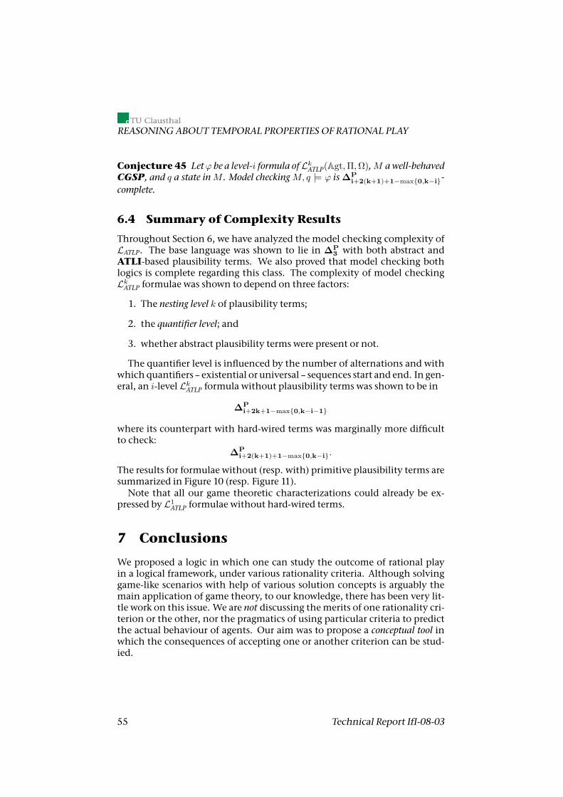
REASONING ABOUT TEMPORAL PROPERTIES OF RATIONAL PLAY
Conjecture 45 Letϕ be a level-i formula ofLkATLP(Agt,Π,Ω),M awell-behavedCGSP, and q a state inM . Model checkingM, q |= ϕ is∆P
i+2(k+1)+1−max0,k−i-complete.
6.4 Summary of Complexity Results
Throughout Section 6, we have analyzed the model checking complexity ofLATLP. The base language was shown to lie in ∆P
3 with both abstract andATLI-based plausibility terms. We also proved that model checking bothlogics is complete regarding this class. The complexity of model checkingLkATLP formulae was shown to depend on three factors:
1. The nesting level k of plausibility terms;
2. the quantifier level; and
3. whether abstract plausibility terms were present or not.
The quantifier level is influenced by the number of alternations and withwhich quantifiers – existential or universal – sequences start and end. In gen-eral, an i-level LkATLP formula without plausibility terms was shown to be in
∆Pi+2k+1−max0,k−i−1
where its counterpart with hard-wired terms was marginally more difficultto check:
∆Pi+2(k+1)+1−max0,k−i.
The results for formulae without (resp. with) primitive plausibility terms aresummarized in Figure 10 (resp. Figure 11).Note that all our game theoretic characterizations could already be ex-
pressed by L1ATLP formulae without hard-wired terms.
7 Conclusions
We proposed a logic in which one can study the outcome of rational playin a logical framework, under various rationality criteria. Although solvinggame-like scenarios with help of various solution concepts is arguably themain application of game theory, to our knowledge, there has been very lit-tle work on this issue. We are not discussing themerits of one rationality cri-terion or the other, nor the pragmatics of using particular criteria to predictthe actual behaviour of agents. Our aim was to propose a conceptual tool inwhich the consequences of accepting one or another criterion can be stud-ied.
55 Technical Report IfI-08-03
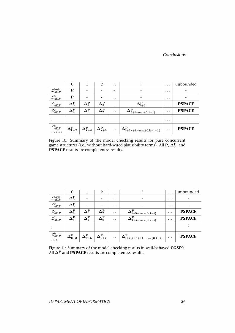
Conclusions
0 1 2 . . . i . . . unbounded
LbasicATLP P - - - - . . . -
L0ATLP P - - . . . - . . . -
L1ATLP ∆P
3 ∆P4 ∆P
5 . . . ∆Pi+3 . . . PSPACE
L2ATLP ∆P
4 ∆P6 ∆P
7 . . . ∆P5+i−max0,1−i . . . PSPACE
... . . ....
LkATLPi > k + 1
∆Pk+2 ∆P
k+4 ∆Pk+6 . . . ∆P
i+2k+1−max0,k−i−1 . . . PSPACE
Figure 10: Summary of the model checking results for pure concurrentgame structures (i.e., without hard-wired plausibility terms). AllP,∆P
3 , andPSPACE results are completeness results.
0 1 2 . . . i . . . unbounded
LbasicATLP ∆P3 - - . . . - . . . -
L0ATLP ∆P
3 - - . . . - . . . -
L1ATLP ∆P
4 ∆P6 ∆P
7 . . . ∆Pi+5−max0,1−i . . . PSPACE
L2ATLP ∆P
5 ∆P7 ∆P
9 . . . ∆P7+i−max0,2−i . . . PSPACE
......
LkATLPi > k
∆Pk+3 ∆P
k+5 ∆Pk+7 . . . ∆P
i+2(k+1)+1−max0,k−i . . . PSPACE
Figure 11: Summary of the model checking results in well-behaved CGSP’s.All∆P
3 and PSPACE results are completeness results.
DEPARTMENTOF INFORMATICS 56
REASONING ABOUT TEMPORAL PROPERTIES OF RATIONAL PLAY
We believe that the logic we propose provides much flexibility and mod-eling power. The results presented in Sections 5 and 6 also suggest that theexpressive power of the language is quite high. Our main technical resultsare as follows:
ATLP: The very definition of the logic ATLP in Section 4 and the study ofits expressive power in Section 5.1.
Classical Solution Concepts: There are several classical solution conceptsfor extensive games: Nash equilibrium, subgame perfect Nash equi-librium, undominated strategies, and Pareto optimality. We show, byrelating models of our logic (CGSP’s) to extensive form games, that thesesolution concepts can be formulated as formulae in ATLP (in fact, al-ready in L1
ATLP). This is shown in Section 5.2
General Solution Concepts: While the classical solution concepts for gamesare formulated using payoffs (which was the reason to extend modelsby additional propositions), we propose to formulate generalized solu-tion concepts as formulae in our logicATLP. More precisely, we proposeto use LATL-path formulae ηi as winning conditions for agent i. Thus,instead of computing payoffs in an extensive form game, we considerCGSPmodels plus a vector of LATL-path formulae ηi (representing thepayoff for agent i). We demonstrate L1
ATLP formulae that correctly ex-press in ATLP our generalized solution concepts. This is elaborated inSection 3.5.
Model Checking in ATLP: Anextensive studyof themodel checking com-plexity in several classes of models and variants of the language is pre-sented in Section 6. On theway,we also define another interesting vari-ant ofATL (where both proponents and opponents are required to useonly uniform strategies) and we establish its model checking complex-ity.
Our ultimate goal is to come up with a logic that would allow us to studystrategies, time, knowledge, andplausible/rational behaviour under bothper-fect and imperfect information. However, putting so many dimensions inone framework at once is usually not a good idea – even more so in thiscase because the interaction between abilities and knowledge is non-trivial(cf. [29, 24, 22]). In [10], we have investigated time, knowledge and plausibility.In this article, we studied strategies, time and rationality. We hope to integrateboth views into a single powerful framework in the future.We would like to thank two anonymous referees for pointing out several
issues that helped us to improve (and shorten) this article.
57 Technical Report IfI-08-03
References
References
[1] T. Ågotnes, V. Goranko, and W. Jamroga. Alternating-time temporallogics with irrevocable strategies. In D. Samet, editor, Proceedings ofTARK XI, pages 15–24, 2007.
[2] R. Alur, T. A. Henzinger, and O. Kupferman. Alternating-time Tempo-ral Logic. In Proceedings of the 38th Annual Symposium on Foundations ofComputer Science (FOCS), pages 100–109. IEEE Computer Society Press,1997.
[3] R. Alur, T. A. Henzinger, andO. Kupferman. Alternating-time TemporalLogic. Journal of the ACM, 49:672–713, 2002.
[4] M. Bacharach. A theory of rational decision in games. Erkenntnis, 27:17–55, 1987.
[5] A. Baltag. A logic for suspicious players. Bulletin of Economic Research,54(1):1–46, 2002.
[6] G. Bonanno. The logic of rational play in games of perfect information.Economics and Philosophy, 7:37–65, 1991.
[7] T. Brihaye, A. Da Costa, F. Laroussinie, and N. Markey. ATL with strat-egy contexts and bounded memory. Technical Report LSV-08-14, ENSCachan, 2008.
[8] N. Bulling. Modal logics for games, time, and beliefs. Master thesis,Clausthal University of Technology, 2006.
[9] N. Bulling and W. Jamroga. Agents, beliefs and plausible behaviour ina temporal setting. Technical Report IfI-06-05, Clausthal University ofTechnology, 2006.
[10] N. Bulling andW. Jamroga. Agents, beliefs and plausible behaviour in atemporal setting. In Proceedings of AAMAS’07, pages 570–577, 2007.
[11] N. Bulling andW.Jamroga. A logic for reasoning about rational agents:Yet another attempt. In L. Czaja, editor, Proceedings of CS&P, pages 87–99, 2007.
[12] F. Chu and J. Halpern. On the NP-completeness of finding an optimalstrategy in games with common payoffs. International Journal of GameTheory, 2001.
[13] E.M.Clarke andE.A. Emerson. Design and synthesis of synchronizationskeletons using branching time temporal logic. In Proceedings of Logicsof Programs Workshop, volume 131 of Lecture Notes in Computer Science,pages 52–71, 1981.
DEPARTMENTOF INFORMATICS 58
REASONING ABOUT TEMPORAL PROPERTIES OF RATIONAL PLAY
[14] E.M. Clarke, E.A. Emerson, and A.P. Sistla. Automatic verificationof finite-state concurrent systems using temporal logic specifications.ACM Transactions on Programming Languages and Systems, 8(2):244–263,1986.
[15] V. Conitzer and T. Sandholm. Complexity results about Nash equilib-ria. Technical Report CMU-CS-02-135, School of Computer Science,Carnegie-Mellon University, 2002.
[16] N. Friedman and J.Y. Halpern. A knowledge-based framework for beliefchange, Part I: Foundations. In Proceedings of TARK, pages 44–64, 1994.
[17] M. R. Garey and D. S. Johnson. Computers and Intractability: A Guide tothe Theory of NP-completeness. W. H. Freeman: San Francisco, 1979.
[18] I. Gilboa and E. Zemel. Nash and correlated equilibria: Some complex-ity considerations. Games and Economic Behavior, 1989.
[19] V. Goranko and W. Jamroga. Comparing semantics of logics for multi-agent systems. Synthese, 139(2):241–280, 2004.
[20] B.P. Harrenstein, W. van der Hoek, J.-J. Meyer, and C. Witteveen. Amodal characterization of Nash equilibrium. Fundamenta Informaticae,57(2–4):281–321, 2003.
[21] P. Harrenstein, W. van der Hoek, J-J. Meijer, and C. Witteveen.Subgame-perfect Nash equilibria in dynamic logic. In M. Pauly andA. Baltag, editors, Proceedings of the ILLC Workshop on Logic and Games,pages 29–30. University of Amsterdam, 2002. Tech. Report PP-1999-25.
[22] A. Herzig and N. Troquard. Knowing how to play: Uniform choices inlogics of agency. In Proceedings of AAMAS’06, pages 209–216, 2006.
[23] W. Jamroga. Reducing knowledge operators in the context of modelchecking. Technical Report IfI-07-09, Clausthal University of Technol-ogy, 2007.
[24] W. Jamroga and T. Ågotnes. What agents can achieve under incompleteinformation. In Proceedings of AAMAS’06, pages 232–234. ACM Press,2006.
[25] W. Jamroga and N. Bulling. A framework for reasoning about rationalagents. In Proceedings of AAMAS’07, pages 592–594, 2007.
[26] W. Jamroga and N. Bulling. A logic for reasoning about rational agents.In F. Sadri and K. Satoh, editors, Proceedings of CLIMA ’07, LNCS, 2008.To appear.
59 Technical Report IfI-08-03
References
[27] W. Jamroga and J. Dix. Model checking ATLir is indeed ∆P2 -complete.
In Proceedings of EUMAS’06, 2006.
[28] W. Jamroga and J. Dix. Model checking abilities of agents: A closer look.Theory of Computing Systems, 42(3):366–410, 2008.
[29] W. Jamroga andW. van der Hoek. Agents that know how to play. Fun-damenta Informaticae, 63(2–3):185–219, 2004.
[30] W. Jamroga, W. van der Hoek, and M. Wooldridge. Intentions andstrategies in game-like scenarios. InCarlos Bento, Amílcar Cardoso, andGaël Dias, editors, Progress in Artificial Intelligence: Proceedings of EPIA2005, volume 3808 of Lecture Notes in Artificial Intelligence, pages 512–523. Springer Verlag, 2005.
[31] D. Koller and N. Megiddo. The complexity of twoperson zero-sumgames in extensive form. Games and Economic Behavior, 4:528–552,1992.
[32] F. Laroussinie, N. Markey, and Ph. Schnoebelen. Model checking CTL+and FCTL is hard. In Proceedings of FoSSaCS’01, volume 2030 of LectureNotes in Computer Science, pages 318–331. Springer, 2001.
[33] Andreu Mas-Colell, Michael D. Whinston, and Jerry R. Green. Microe-conomic Theory. Oxford, 1995.
[34] Y. Moses and M. Tennenholz. Artificial social systems. Computers andAI, 14(6):533–562, 1995.
[35] M. Osborne and A. Rubinstein. A Course in Game Theory. MIT Press,1994.
[36] C.H. Papadimitriou. Computational Complexity. AddisonWesley : Read-ing, 1994.
[37] Tuomas W. Sandholm. Distributed rational decision making. In Ger-hard Weiss, editor,Multiagent Systems: A Modern Approach to DistributedArtificial Intelligence, pages 201–258. The MIT Press, Cambridge, MA,USA, 1999.
[38] P. Y. Schobbens. Alternating-time logic with imperfect recall. ElectronicNotes in Theoretical Computer Science, 85(2), 2004.
[39] Y. Shoham and M. Tennenholz. On the synthesis of useful social lawsfor artificial agent societies. In Proceedings of AAAI-92, 1992.
[40] I. Ståhl. Bargaining Theory. Stockholm School of Economics, Stock-holm, 1972.
DEPARTMENTOF INFORMATICS 60
REASONING ABOUT TEMPORAL PROPERTIES OF RATIONAL PLAY
[41] R. Stalnaker. On the evaluation of solution concepts. Theory and Deci-sion, 37(1):49–73, 1994.
[42] R. Stalnaker. Knowledge, belief and counterfactual reasoning in games.Economics and Philosophy, 12:133–163, 1996.
[43] K. Su, A. Sattar, G. Governatori, and Q. Chen. A computationallygrounded logic of knowledge, belief and certainty. In Proceedings of AA-MAS’05, pages 149–156. ACM Press, 2005.
[44] J. van Benthem. Rational dynamics and epistemic logic in games. InS. Vannucci, editor, Logic, Game Theory and Social Choice III, pages 19–23, 2003.
[45] W. van der Hoek, W. Jamroga, and M.Wooldridge. A logic for strategicreasoning. In Proceedings of AAMAS’05, pages 157–164, 2005.
[46] W. van der Hoek, M. Roberts, and M. Wooldridge. Social laws in alter-nating time: Effectiveness, feasibility and synthesis. Synthese, 156(1):1–19, 2005.
[47] W. van der Hoek and M. Wooldridge. Tractable multiagent planningfor epistemic goals. In C. Castelfranchi andW.L. Johnson, editors, Pro-ceedings of the First International Joint Conference on Autonomous Agentsand Multi-Agent Systems (AAMAS-02), pages 1167–1174. ACM Press, NewYork, 2002.
[48] S. van Otterloo and G. Jonker. On Epistemic Temporal Strategic Logic.Electronic Notes in Theoretical Computer Science, XX:35–45, 2004. Pro-ceedings of LCMAS’04.
[49] S. van Otterloo and O. Roy. Verification of voting protocols. Workingpaper, University of Amsterdam, 2005.
[50] S. van Otterloo, W. van der Hoek, and M. Wooldridge. Preferences ingame logics. Preliminary version, unpublishedmanuscript, 2004.
[51] S. van Otterloo, W. van der Hoek, and M. Wooldridge. Preferences ingame logics. In Proceedings of AAMAS-04, pages 152–159, 2004.
61 Technical Report IfI-08-03
UniformATLir
Appendix
A BargainingwithDiscount
In Example 7 we presented bargaining with discount. After each round theworth of the goods is reduced by δi. In round t the goods have a value ofr(δti). Because we use a rounding function r, there is aminimal round T suchthat r(δT+1
i ) = 0 for i = 1 or i = 2. We can treat this case as finite horizonbargaining game [40, 33].Now, consider the case that ai’s opponent, denoted by a−i, is the offerer
in T . It can offer 0 and ai should accept, because in the next round the goodsare worthless for ai.On the other hand, if ai is offerer in T we have to distinguish two cases. If
r(δT+1−i ) = 0 then following the same reasoning as before ai can offer 0 to a−i.
In the other case, namely r(δT+1−i ) 6= 0, we consider the subsequent round
T + 1 in which a−i takes the role as offerer and can successfully offer 0 to i.Now, it is possible to solve the game starting from the end. Solutions for
δ1 = δ2 can be found in the literature [33]. Here, we recall the idea for differ-ent discount rates.At first, let a1 be the last offerer and r(δT+1
2 ) = 0. This implies, that Tis even (the initial round is 0). In T , a1 offers 〈1, 0〉 and a2 accepts. Knowingthis, in T−1 agent a2 can offer 〈δ1, 1−δ1〉, since in the next round the value ofthe good for a1 would become reduced by δ1. Following the same reasoning,in T −2 a1 could successfully offer 〈1− δ2(1− δ1), δ2(1− δ1)〉. Finally, in roundt = 0 a1 can offer 〈ζ, 1− ζ〉where
ζ := (1− δ2)
T2 −1∑i=0
(δ1δ2)i + (δ1δ2)T2 = (1− δ2)
1− (δ1δ2)T2
1− δ1δ2+ (δ1δ2)
T2
Secondly, consider the case inwhich a2 is the last offerer inT and r(δT+11 ) =
0. This time T is odd but the reasoning stays the same. In round 0 a1 can offer〈ζ ′, 1− ζ ′〉where
ζ ′ := (1− δ2)1− (δ1δ2)
T+12
1− δ1δ2
B UniformATLirIn this section, we introduce and investigate the logic of “uniform ATLir”(ATLuir). We use the logic only for technical reasons, namely it provides theintermediate step in the completeness proof for the complexity of modelchecking ATLP. Still, we believe that the logic can be interesting in itself.
DEPARTMENTOF INFORMATICS 62
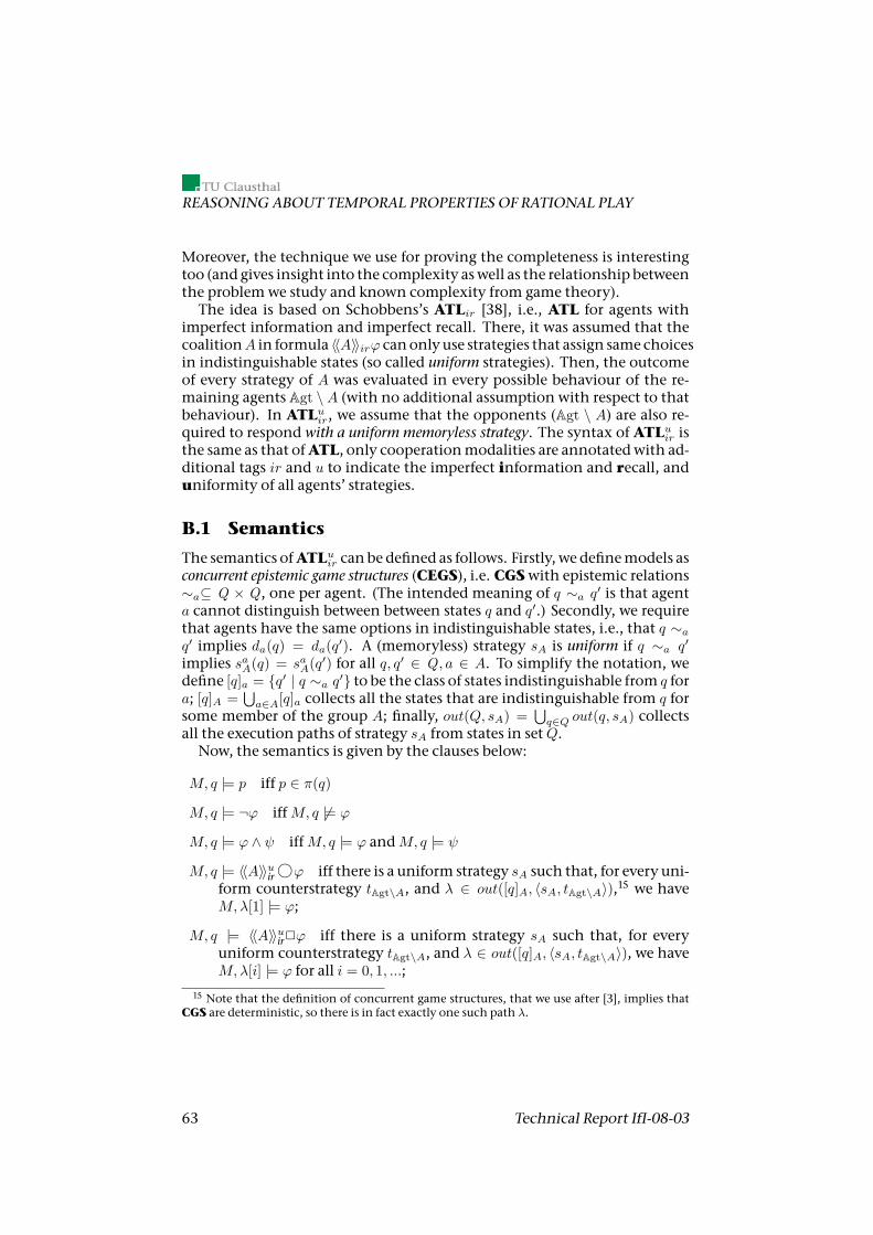
REASONING ABOUT TEMPORAL PROPERTIES OF RATIONAL PLAY
Moreover, the technique we use for proving the completeness is interestingtoo (and gives insight into the complexity aswell as the relationship betweenthe problemwe study and known complexity from game theory).The idea is based on Schobbens’s ATLir [38], i.e., ATL for agents with
imperfect information and imperfect recall. There, it was assumed that thecoalitionA in formula 〈〈A〉〉irϕ canonlyuse strategies that assign same choicesin indistinguishable states (so called uniform strategies). Then, the outcomeof every strategy of A was evaluated in every possible behaviour of the re-maining agents Agt \ A (with no additional assumption with respect to thatbehaviour). In ATLuir, we assume that the opponents (Agt \ A) are also re-quired to respond with a uniform memoryless strategy. The syntax of ATLuir isthe same as that ofATL, only cooperationmodalities are annotatedwith ad-ditional tags ir and u to indicate the imperfect information and recall, anduniformity of all agents’ strategies.
B.1 Semantics
The semantics ofATLuir can be defined as follows. Firstly, we definemodels asconcurrent epistemic game structures (CEGS), i.e. CGSwith epistemic relations∼a⊆ Q × Q , one per agent. (The intended meaning of q ∼a q′ is that agenta cannot distinguish between between states q and q′.) Secondly, we requirethat agents have the same options in indistinguishable states, i.e., that q ∼aq′ implies da(q) = da(q′). A (memoryless) strategy sA is uniform if q ∼a q′
implies saA(q) = saA(q′) for all q, q′ ∈ Q , a ∈ A. To simplify the notation, wedefine [q]a = q′ | q ∼a q′ to be the class of states indistinguishable from q fora; [q]A =
⋃a∈A[q]a collects all the states that are indistinguishable from q for
some member of the group A; finally, out(Q, sA) =⋃q∈Q out(q, sA) collects
all the execution paths of strategy sA from states in setQ.Now, the semantics is given by the clauses below:
M, q |= p iff p ∈ π(q)
M, q |= ¬ϕ iffM, q 6|= ϕ
M, q |= ϕ ∧ ψ iffM, q |= ϕ andM, q |= ψ
M, q |= 〈〈A〉〉uir hϕ iff there is a uniform strategy sA such that, for every uni-form counterstrategy tAgt\A, and λ ∈ out([q]A, 〈sA, tAgt\A〉),15 we haveM,λ[1] |= ϕ;
M, q |= 〈〈A〉〉uir2ϕ iff there is a uniform strategy sA such that, for everyuniform counterstrategy tAgt\A, and λ ∈ out([q]A, 〈sA, tAgt\A〉), we haveM,λ[i] |= ϕ for all i = 0, 1, ...;
15 Note that the definition of concurrent game structures, that we use after [3], implies thatCGS are deterministic, so there is in fact exactly one such path λ.
63 Technical Report IfI-08-03
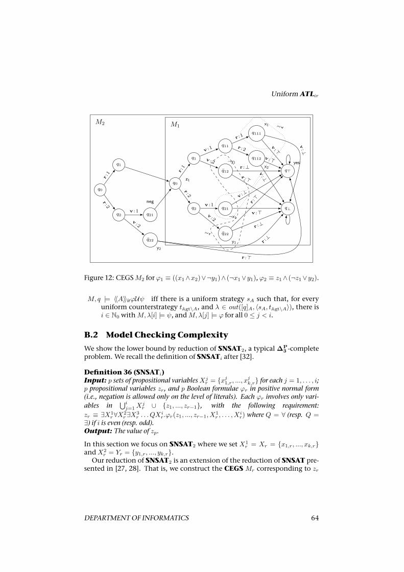
UniformATLir
M2 M1
q0
q1
q2 q21
neg
q22
y2
q0z1
q1
q2
q11
q12
¬y1
q21
¬x1
q22
y1
q111
x1
q112
x2q>
yes
q⊥
r:1
r:2
v :1
v:2
r:1
r:2
v :1
v :2
v :1
v:2
r :1
r :2
v:>
v :>
v :⊥
r :>
r :>
r :⊥
v:⊥
v:⊥
v :>
r :⊥
r :⊥
r :>
∼r
∼v
Figure 12: CEGSM2 for ϕ1 ≡ ((x1∧x2)∨¬y1)∧ (¬x1∨y1), ϕ2 ≡ z1∧ (¬z1∨y2).
M, q |= 〈〈A〉〉irϕUψ iff there is a uniform strategy sA such that, for everyuniform counterstrategy tAgt\A, and λ ∈ out([q]A, 〈sA, tAgt\A〉), there isi ∈ N0 withM,λ[i] |= ψ, andM,λ[j] |= ϕ for all 0 ≤ j < i.
B.2 Model Checking Complexity
We show the lower bound by reduction of SNSAT2, a typical∆P3 -complete
problem. We recall the definition of SNSATi after [32].
Definition 36 (SNSATi)Input: p sets of propositional variablesXj
r = xj1,r, ..., xjk,r for each j = 1, . . . , i;
p propositional variables zr, and p Boolean formulae ϕr in positive normal form(i.e., negation is allowed only on the level of literals). Each ϕr involves only vari-ables in
⋃ij=1X
jr ∪ z1, ..., zr−1, with the following requirement:
zr ≡ ∃X1r∀X2
r∃X3r . . . QX
ir.ϕr(z1, ..., zr−1, X
1r , . . . , X
ir) where Q = ∀ (resp. Q =
∃) if i is even (resp. odd).Output: The value of zp.
In this section we focus on SNSAT2 where we set X1r = Xr = x1,r, ..., xk,r
andX2r = Yr = y1,r, ..., yk,r.
Our reduction of SNSAT2 is an extension of the reduction of SNSAT pre-sented in [27, 28]. That is, we construct the CEGS Mr corresponding to zr
DEPARTMENTOF INFORMATICS 64
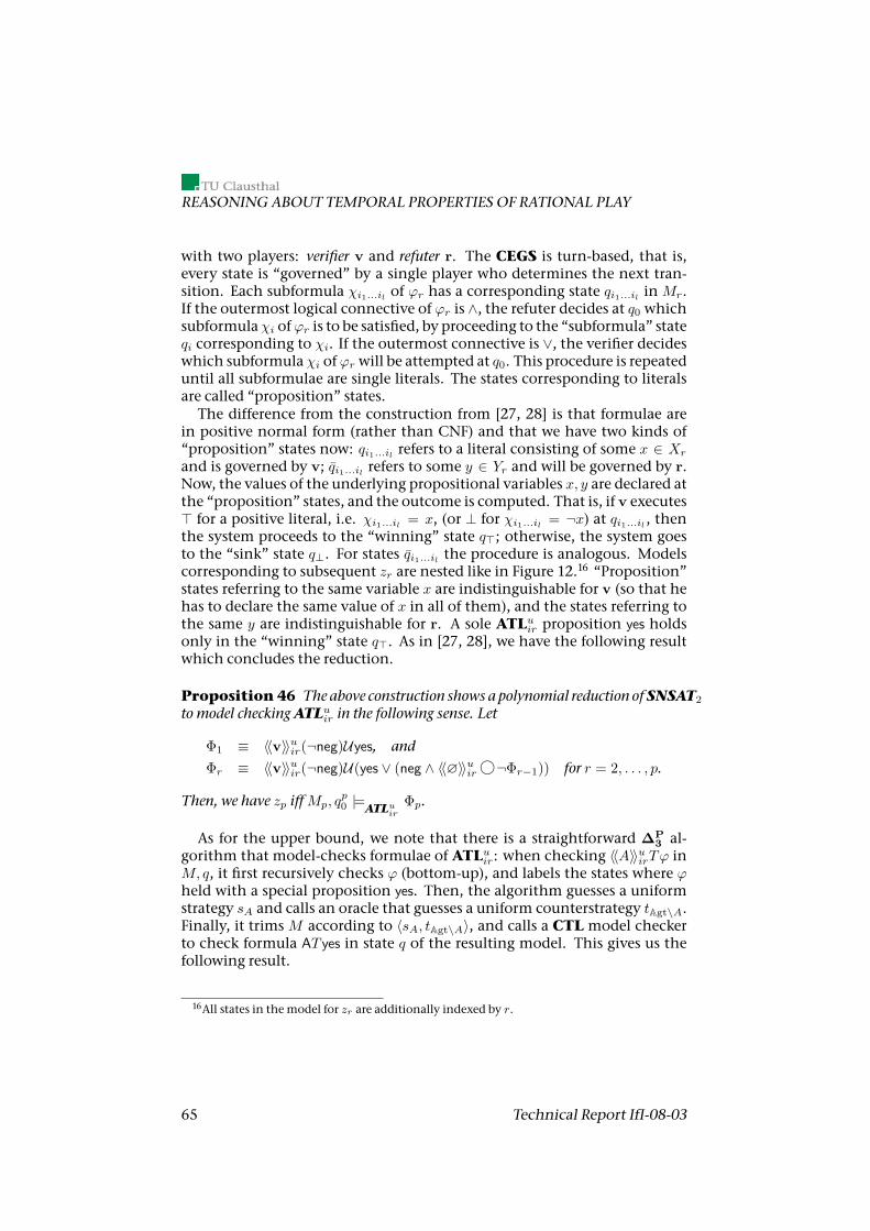
REASONING ABOUT TEMPORAL PROPERTIES OF RATIONAL PLAY
with two players: verifier v and refuter r. The CEGS is turn-based, that is,every state is “governed” by a single player who determines the next tran-sition. Each subformula χi1...il of ϕr has a corresponding state qi1...il inMr.If the outermost logical connective of ϕr is ∧, the refuter decides at q0 whichsubformulaχi ofϕr is to be satisfied, by proceeding to the “subformula” stateqi corresponding to χi. If the outermost connective is ∨, the verifier decideswhich subformula χi ofϕr will be attempted at q0. This procedure is repeateduntil all subformulae are single literals. The states corresponding to literalsare called “proposition” states.The difference from the construction from [27, 28] is that formulae are
in positive normal form (rather than CNF) and that we have two kinds of“proposition” states now: qi1...il refers to a literal consisting of some x ∈ Xr
and is governed by v; qi1...il refers to some y ∈ Yr and will be governed by r.Now, the values of the underlying propositional variables x, y are declared atthe “proposition” states, and the outcome is computed. That is, if v executes> for a positive literal, i.e. χi1...il = x, (or ⊥ for χi1...il = ¬x) at qi1...il , thenthe system proceeds to the “winning” state q>; otherwise, the system goesto the “sink” state q⊥. For states qi1...il the procedure is analogous. Modelscorresponding to subsequent zr are nested like in Figure 12.16 “Proposition”states referring to the same variable x are indistinguishable for v (so that hehas to declare the same value of x in all of them), and the states referring tothe same y are indistinguishable for r. A sole ATLuir proposition yes holdsonly in the “winning” state q>. As in [27, 28], we have the following resultwhich concludes the reduction.
Proposition 46 The above construction shows a polynomial reduction ofSNSAT2
to model checkingATLuir in the following sense. Let
Φ1 ≡ 〈〈v〉〉uir(¬neg)Uyes, andΦr ≡ 〈〈v〉〉uir(¬neg)U(yes ∨ (neg ∧ 〈〈∅〉〉uir h¬Φr−1)) for r = 2, . . . , p.
Then, we have zp iffMp, qp0 |=ATLu
irΦp.
As for the upper bound, we note that there is a straightforward ∆P3 al-
gorithm that model-checks formulae of ATLuir: when checking 〈〈A〉〉uirTϕ inM, q, it first recursively checks ϕ (bottom-up), and labels the states where ϕheld with a special proposition yes. Then, the algorithm guesses a uniformstrategy sA and calls an oracle that guesses a uniform counterstrategy tAgt\A.Finally, it trimsM according to 〈sA, tAgt\A〉, and calls a CTLmodel checkerto check formula AT yes in state q of the resulting model. This gives us thefollowing result.
16All states in themodel for zr are additionally indexed by r.
65 Technical Report IfI-08-03

FromATLuir toATLPwithATLI-Based Plausibility Terms
Theorem 47 Model checking ATLuir is∆P3 -complete with respect to the number
of transitions in the model and the length of the formula. It is∆P3 -complete even
for turn-basedCEGSwith at most two agents.
C FromATLuir to ATLPwith ATLI-Based Plau-sibility Terms
The reduction of ATLuir model checking to model checking of ATLPATLI in
“pure” CGS is rather sophisticated. We do not present a reduction for fullmodel checking ofATLuir; it is enough to show the reduction for the kind ofmodels that we get in Appendix B.2 (i.e., turn-basedmodels with two agents,two “final” states q>, q⊥, no cycles except for the loops at the final states, anduncertainty appearing only in states one step before the end of the game, cf.Figure 12).Firstly, we reconstruct the concurrent epistemic game structureMp from
Section B.2 so that the last action profile is always “remembered” in the fi-nal states. Then, we show how uniformity of strategies can be characterizedwith a formula ofATLI extendedwith epistemic operators. Thirdly, we showhow the model and the formula can be transformed to get rid of epistemiclinks and operators (yielding a “pure” CGS and a formula of “pure” ATLI).Finally, we show how the resulting characterization of uniformity can be“plugged” into an ATLP formula to require that only uniform strategy pro-files are taken into account.
Adding More Final States to the Model. To recall, the input of ATLuirmodel checking consists in our case of a concurrent epistemic game structureMp (like the one in Figure 12) and anATLuir formula Φp (cf. Proposition 46).We begin the reduction by reconstructingMp toM ′
p in which the last actionprofile is “remembered” in the final states. The idea is based on the construc-tion from [19, Proposition 16] where it is applied to all states of the system,cf. Figure 13.In our case, we first create copies of states q>, q⊥, one per incoming transi-
tion. That is, the construction yields states of the form 〈q, α1, . . . , αk〉, whereq ∈ q>, q⊥ is a final state of the originalmodelMp, and 〈α1, . . . , αk〉 is the ac-tionprofile executed just before the systemproceeded to q. Each copyhas thesamevaluationof propositions as the original state q, i.e., π′(〈q, α1, . . . , αk〉) =π(q). Then, for each action α ∈ Act and agent i ∈ Agt, we add a new proposi-tion i : α. Moreover, we fix the valuation of i : α inM ′
p so that it holds exactlyin the final states that can be achieved by an action profile in which i exe-cutes α (i.e., states 〈q, α1, ..., αi, ..., αk〉). Note that the number of both statesand transitions inM ′
p is linear in the transitions ofMp. The transformationproduces modelM ′
p which is equivalent toMp in the following sense. Let ϕ
DEPARTMENTOF INFORMATICS 66
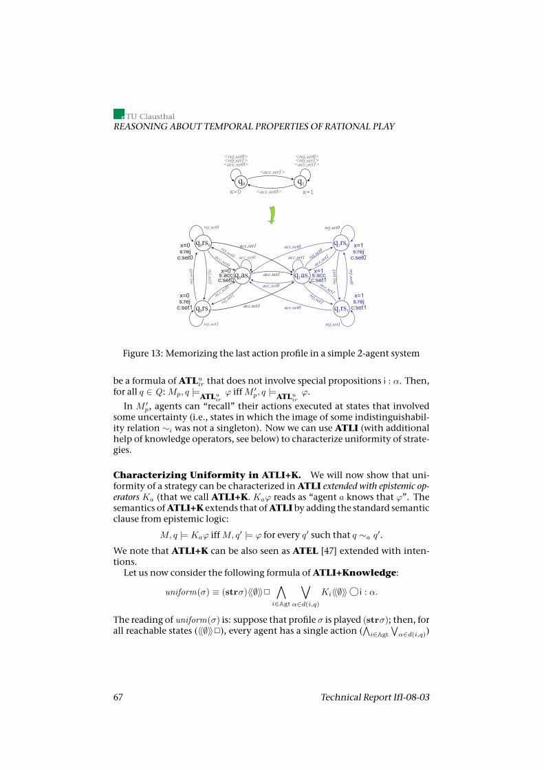
REASONING ABOUT TEMPORAL PROPERTIES OF RATIONAL PLAY
q0 q1
x=0 x=1
<acc,set0>
<acc,set0>
<rej,set1><rej,set0>
<acc,set1>
<acc,set1>
<rej,set1><rej,set0>
q0rs0x=0
x=0
x=0
q0rs1
q0as0
q rs1 0 x=1
x=1
q rs1 1
q as1 1
rej,set0
rej,set1
acc,set0
rej,set0
rej,
set0
rej,
set1
acc,set0
acc,set0
acc,se
t0
acc,set0
acc,set0rej
,set1
acc,set1
acc,set1
acc,set1
rej,set0
rej,set0
rej,set1
rej,set1
rej,se
t0
acc,se
t1
acc,set1rej,set1
acc,set1s:rej
s:acc
s:rej
s:rej
s:rej
c:set0
c:set0
c:set1
c:set0
c:set1
x=1s:accc:set1
Figure 13: Memorizing the last action profile in a simple 2-agent system
be a formula ofATLuir that does not involve special propositions i : α. Then,for all q ∈ Q :Mp, q |=ATLu
irϕ iffM ′
p, q |=ATLuirϕ.
In M ′p, agents can “recall” their actions executed at states that involved
some uncertainty (i.e., states in which the image of some indistinguishabil-ity relation ∼i was not a singleton). Now we can use ATLI (with additionalhelp of knowledge operators, see below) to characterize uniformity of strate-gies.
Characterizing Uniformity in ATLI+K. We will now show that uni-formity of a strategy can be characterized inATLI extended with epistemic op-erators Ka (that we call ATLI+K. Kaϕ reads as “agent a knows that ϕ”. Thesemantics ofATLI+K extends that ofATLI by adding the standard semanticclause from epistemic logic:
M, q |= Kaϕ iffM, q′ |= ϕ for every q′ such that q ∼a q′.
We note that ATLI+K can be also seen as ATEL [47] extended with inten-tions.Let us now consider the following formula ofATLI+Knowledge:
uniform(σ) ≡ (strσ)〈〈∅〉〉2∧i∈Agt
∨α∈d(i,q)
Ki〈〈∅〉〉 hi : α.
The reading of uniform(σ) is: suppose that profile σ is played (strσ); then, forall reachable states (〈〈∅〉〉2), every agent has a single action (
∧i∈Agt
∨α∈d(i,q))
67 Technical Report IfI-08-03
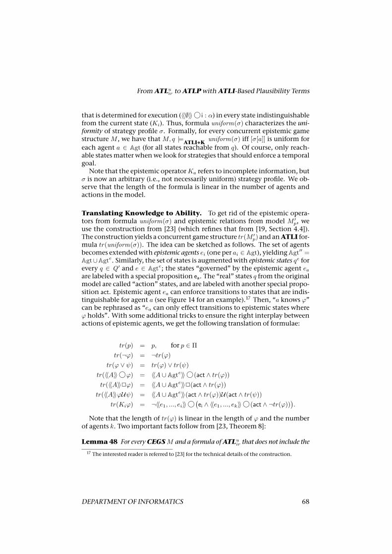
FromATLuir toATLPwithATLI-Based Plausibility Terms
that is determined for execution (〈〈∅〉〉 hi : α) in every state indistinguishablefrom the current state (Ki). Thus, formula uniform(σ) characterizes the uni-formity of strategy profile σ. Formally, for every concurrent epistemic gamestructureM , we have thatM, q |=ATLI+K uniform(σ) iff [σ[a]] is uniform foreach agent a ∈ Agt (for all states reachable from q). Of course, only reach-able statesmatter whenwe look for strategies that should enforce a temporalgoal.Note that the epistemic operatorKa refers to incomplete information, but
σ is now an arbitrary (i.e., not necessarily uniform) strategy profile. We ob-serve that the length of the formula is linear in the number of agents andactions in themodel.
Translating Knowledge to Ability. To get rid of the epistemic opera-tors from formula uniform(σ) and epistemic relations from model M ′
p, weuse the construction from [23] (which refines that from [19, Section 4.4]).The construction yields a concurrent game structure tr(M ′
p) and anATLI for-mula tr(uniform(σ)). The idea can be sketched as follows. The set of agentsbecomes extendedwith epistemic agents ei (one per ai ∈ Agt), yieldingAgt′′ =Agt∪Agte. Similarly, the set of states is augmentedwith epistemic states qe forevery q ∈ Q ′ and e ∈ Agte; the states “governed” by the epistemic agent eaare labeled with a special proposition ea. The “real” states q from the originalmodel are called “action” states, and are labeled with another special propo-sition act. Epistemic agent ea can enforce transitions to states that are indis-tinguishable for agent a (see Figure 14 for an example).17 Then, “a knows ϕ”can be rephrased as “ea can only effect transitions to epistemic states whereϕ holds”. With some additional tricks to ensure the right interplay betweenactions of epistemic agents, we get the following translation of formulae:
tr(p) = p, for p ∈ Πtr(¬ϕ) = ¬tr(ϕ)
tr(ϕ ∨ ψ) = tr(ϕ) ∨ tr(ψ)tr(〈〈A〉〉 hϕ) = 〈〈A ∪ Agte〉〉 h(act ∧ tr(ϕ))tr(〈〈A〉〉2ϕ) = 〈〈A ∪ Agte〉〉2(act ∧ tr(ϕ))
tr(〈〈A〉〉ϕUψ) = 〈〈A ∪ Agte〉〉(act ∧ tr(ϕ))U(act ∧ tr(ψ))tr(Kiϕ) = ¬〈〈e1, ..., ei〉〉 h(
ei ∧ 〈〈e1, ..., ek〉〉 h(act ∧ ¬tr(ϕ))).
Note that the length of tr(ϕ) is linear in the length of ϕ and the numberof agents k. Two important facts follow from [23, Theorem 8]:
Lemma 48 For everyCEGSM and a formula ofATLuir that does not include the17 The interested reader is referred to [23] for the technical details of the construction.
DEPARTMENTOF INFORMATICS 68
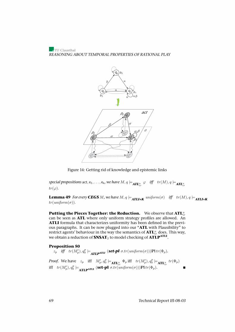
REASONING ABOUT TEMPORAL PROPERTIES OF RATIONAL PLAY
q0
q2 q1
p0
p1
p2
e
actq0
q1q2
eq2 q1e
q0e
p1
p2
p0
Figure 14: Getting rid of knowledge and epistemic links
special propositions act, e1, . . . , ek, we haveM, q |=ATLuirϕ iff tr(M), q |=ATLu
ir
tr(ϕ).
Lemma 49 For everyCEGSM , we haveM, q |=ATLI+K uniform(σ) iff tr(M), q |=ATLI+Ktr(uniform(σ)).
Putting the Pieces Together: the Reduction. We observe thatATLuircan be seen as ATL where only uniform strategy profiles are allowed. AnATLI formula that characterizes uniformity has been defined in the previ-ous paragraphs. It can be now plugged into our “ATL with Plausibility” torestrict agents’ behaviour in the way the semantics ofATLuir does. This way,we obtain a reduction of SNSAT2 to model checking ofATLPATLI.
Proposition 50zp iff tr(M ′
p), qp0 |=ATLPATLI (set-pl σ.tr(uniform(σ)))Pl tr(Φp).
Proof. We have zp iff M ′p, q
p0 |=ATLu
irΦp iff tr(M ′
p), qp0 |=ATLu
irtr(Φp)
iff tr(M ′p), q
p0 |=ATLPATLI (set-pl σ.tr(uniform(σ)))Pl tr(Φp).
69 Technical Report IfI-08-03
SomeModel Checking Complexity Proofs
D SomeModel Checking Complexity Proofs
D.1 Results in Section 6.1
Proposition 23: Let M be a well-behaved CGSP, q a state in M , and ϕ aformula of LbaseATLP(Agt,Π,Ω). Then M, q |= ϕ iff mcheckATLP(M, q, ϕ). Thealgorithm runs in time∆P
3 with respect to the number of transitions in themodel and the length of the formula.
Proof Function mcheck is called recursively, at most l times. All cases apartfrom ϕ ≡ 〈〈A〉〉 hψ where ψ includes no 〈〈C〉〉 (analogously for the othertemporal operators) can be performed in polynomial time. Now, there is anondeterministic Turing machine AB which implements function beatable:Firstly, it guesses a strategy t possibly together with another witness neces-sary for plausiblestrat (by assumption the latter is in NP) and verifies if t isplausible, the verification can be done in polynomial time (by the same as-sumption). Finally, if t is plausible AB has to perform CTLmodel checkingwhich lies inP.It remains to show that there is a nondeterministic oracle Turingmachine
AS with oracleAB implementing solve. (Formally, themachine requires twooracles, one answering the question whether s is plausible, and the other isgivenbyAB. However, the former is computationally less expensive then thelatter and can be ignored since we are interested in the oracle with the high-est complexity.) AS works as follows: Firstly, it guesses a profile s (again possi-bly together with a witness for plausiblestrat); secondly, it verifies whether sis plausible and then calls oracleAB and inverts its answer. Altogether, thereare polynomial many calls to machine AAB
S ∈ NPNP. This renders the algo-rithm to be in∆P
3 .
Proposition 27: Let c ∈ N be a constant. Model checking LbaseATLP formulaewith respect to the class of well-behaved boundedmodelsMc can be done inpolynomial time with respect to the number of transitions in themodel andthe length of the formula.
Proof sketch We modify the original ATLmodel checking procedure as fol-lows. Consider the formula ϕ ≡ 〈〈A〉〉γ where γ is a pure ATL path formula.Let B be the set of agents assumed to play plausibly and let Υ 6= Σ be thecurrent set of plausible strategies described by some term and state. For eachsB ∈ Υ|B we remove fromM all transitions which cannot occur according tosB, yieldingmodelMsB , and checkwhetherMsB , q |=ATL 〈〈A〉〉γ. We proceedlike this for all s ∈ Υ|B (there are only polynomiallymany). This procedure isincorporated into ourATLPmodel checking algorithm and applied bottomup.
DEPARTMENTOF INFORMATICS 70
REASONING ABOUT TEMPORAL PROPERTIES OF RATIONAL PLAY
D.2 Results in Section 6.3
D.2.1 Upper Bounds
First, we recall a basic complexity result that will be used in the rest of thissection. Then, we present proofs of upper bounds for model checking LkATLPfor pure CGS’s and well-behaved CGSP’s.
Remark 51 A relation R ⊆ ×k+1i=1 Σ∗ (k ≥ 1) is called polynomial decidable
whenever there is a deterministic Turingmachine (DTM)which decides (x, y1 . . . , yk) :(x, y1 . . . , yk) ∈ R in polynomial time; furthermore, R is called polynomial bal-anced if there is a k ∈ N such that for all (x, y1 . . . , yk) ∈ R: |yi| ≤ |x|k for alli = 1, . . . k.For a language L and k ≥ 1 the following holds: L ∈ ΣPk if, and only if, there
is a polynomial decidable and balanced (k + 1)-ary relation R such that L = x |∃y1∀y2∃y3 . . . Qyk ((x, y1 . . . , yk) ∈ R) where Q = ∀ (resp. Q = ∃) if k is odd(resp. k even) [36, Corollary 2 of Theorem 17.8].
Theorem 41: Let ϕ be a level-i formula of LkATLP(Agt,Π, ∅), k ≥ 1, i ≥ 0.Moreover, letM be aCGS, and q a state inM . Then,model checkingM, q |= ϕcan be done in time∆P
i+2k+1−max0,k−i−1.
Proof By induction over k. In the following we restrict ourselves to (set-pl ·)without loss of generality.
Case k = 1. Let ϕ be a level-i L1ATLP formula, (set-pl ω) an operator occur-
ring in ϕ such that l((set-pl ω)) = i and ω = σ.Q1σ1Q2σ2 . . . Qnσnϕ′
whereϕ′ ∈ LbaseATLP(Agt,Π, σ, σ1, . . . , σn).
Note thatMs,s1,...,sn , q |= ϕ′ canbe checked inpolynomial time since allconstructible plausibility terms are rectangular and the representationis directly given (see Corollary 31). Moreover, let q′ denote the state inwhich ω is evaluated. W.l.o.g. we can assume that ϕ has the followingstructure:
ϕ ≡ (set-pl ω)Pl 〈〈A〉〉2yes
Now, ϕ is true in M and q if and only if there is a plausible strategysA for A and no plausible strategy t with t|A = s such thatM ′, q |=CTL¬A2yeswhereM ′ is the trimmedmodel ofM wrt t. In the following weneglect the complexity needed to verify whether sA is plausible sincethe method beatable also verifies this property and its complexity is asleast as high (cf. proof of Proposition 23). Thus, ϕ is true if, and only if
∃sA¬(∃t (t ∈ [[ω]]
q′
andR|=(M, q, sA, t,2yes)))
iff ∃sA¬(∃tQ1s1Q2s2 . . . Qnsn (M t,s1,...,sn , q′ |= ϕ′ andR|=(M, q, sA, t,2yes))
)iff ∃sA∀tQ1s1Q2s2 . . . Qnsn (M t,s1,...,sn , q′ 6|= ϕ′ or ¬R|=(M, q, sA, t,2yes))
71 Technical Report IfI-08-03
SomeModel Checking Complexity Proofs
where R|=(M, q, sA, t,2yes) = true iff t|A = sA andM ′, q |=CTL ¬A2yeswhereM ′ is the “trimmed”model ofM wrt t, and Q is the dual operatortoQ.
Now, the latter conditions can be verified in polynomial time. We con-sider thenumber of quantifier alternations. Subsequent strategieswhichare quantified by quantifiers of the same type can be guessed together.The sameholds if the sequence startswith existential quantifiers. Thesestrategies can be guessed together with strategy t. A quantifier level ofl((set-pl ω)) = i denotes that it is sufficient to alternatingly guess iwitnesses. We obtain the following structure:
∃sA∀xt∃x1∀x2 . . . Qxi
where Q = ∃ (resp. Q = ∀) if i is even (resp. odd). Where xi denotes awitness for a strategy or several strategies if guessing can be combined.
Thus, according to Remark 51 checking whether ϕ is satisfied can bedetermined in time Σi+2 and the complete model checking algorithmfor level-i L1
ATLP formula can be performed in time ∆Pi+3 (there can be
polynomial many such constructs).
Induction step: k 7→ k + 1 (k > 1). Letϕbe a level-iLk+1ATLP formula and letω
be a term inϕof the formω = σ1.Q1σ1Q2σ2 . . . Qnσnϕ′ such that l((set-pl ω)) =
i. Furthermore, let RALT(Q1 . . . Qn) = j; then, lϕ′ := ql(UO(ϕ′)) = i− jand ϕ′ is anLkATLP formula. Thus, by induction hypothesis we have thatϕ′ can bemodel checked in time
∆Pr+1 where r := lϕ′ + 2k −max0, k − lϕ′ − 1.
Again, w.l.o.g. we can assume that ϕ has the following structure:
ϕ ≡ (set-pl ω)Pl 〈〈A〉〉2yes.
We proceed as in case k = 1. Firstly, a profile s is guessed, then a profilet and it is checked whether t is plausible and coincides with s wrt Aand whether the trimmed model (wrt t) satisfies ¬A2yes. We obtainthe following structure:
∃sA¬(∃t (t ∈ [[ω]]
q′
andR|=(M, q, sA, t,2yes)))
iff ∃sA¬
∃tQ1s1Q2s2 . . . Qnsn (M t,s1,...,sn , q′ |= ϕ′︸ ︷︷ ︸∈∆P
r+1
and R|=(M, q, sA, t,2yes)︸ ︷︷ ︸∈P
)
SinceM t,s1,...,sn , q′ |= ϕ′ is invoked by a nondeterministic polynomialTuring machine we can assume that its model checking problem can
DEPARTMENTOF INFORMATICS 72
REASONING ABOUT TEMPORAL PROPERTIES OF RATIONAL PLAY
be solved in ΣPr instead of ∆P
r+1; the polynomial effort of the deter-ministic machine can also be done by the invoking nondeterministicmachine. Hence to verifyM t,s1,...,sn , q′ |= ϕ′ witnesses according to
∃x1∀x2∃x3 . . . Qrxr
have to be guessed; then, the question whether ϕ is satisfied with re-spect to the witnesses x1, . . . , xr can be solved in polynomial time.
Because RALT(Q1Q2 . . . Qn) = j it suffices to guess witnesses accordingto the following structure:
∀x′1∃x′2∀x′3 . . .∀x′j .
If Q1Q2 . . . Qn would start (resp. end) with existential quantifiers thecorresponding witnesses could be guessed together with the one forprofile t (resp. witness x1). Putting things together the following wit-nesses have to be guessed:
(?) ∃sA∀xt ∃x′1∀x′2∃x′3 . . .∃x′j ∀x1∃x2∀x3 . . . Qrxr
It remains to show that the number of alternations in (?) does neverexceed i+ 2(k + 1)−max0, (k + 1)− i− 1We distinguish two cases (k + 1)− i− 1 ≤ 0 and (k + 1)− i− 1 > 0.
Case: k + 1− i− 1 ≤ 0. That is, k ≤ i. We are going to determine themaximal possible number of alternations in (?).Firstly, assume that j ≥ 1. That is the number of alternation isgiven by 2 + j + r = i + 2(k + 1) − max0, k − i + j − 1. Thisexpression is maximal whenever k− i+ j − 1 ≤ 0. Because of k ≤ ithis is always the case for j = 1. In this case the formula has atmost
i+ 2(k + 1)−maxk + 1− i− 1 alternations.
For j = 0 there is at least one alternation less, since the witness xtcan be guessed together with x1.
Case: k + 1− i− 1 > 0. That is, k > i. Firstly, we consider the casej ≥ 1. There are atmost i+2(k+1)−max0, k−i+j−1 alternations,where thenumber becomesmaximal for j = 1; i.e. wehave atmost
i+ 2(k + 1)−maxk + 1− i− 1 alternations.
Now, we consider the case j = 0. In this case there are at mosti+2(k+1)−1−max0, k− i−1 alternations. Because of k > i, wehave that k− i−1 ≥ 0 and, hence i+2(k+1)−1−max0, k− i−1is equivalent to i+ 2(k + 1)−max0, (k + 1)− i− 1.
73 Technical Report IfI-08-03
SomeModel Checking Complexity Proofs
Thus, i+ 2(k + 1)−maxk + 1− i− 1 alternations denotes themax-imal possible number of alternationswhichproofs our claim themodelchecking algorithm for level-i Lk+1
ATLP can be performed in timePΣP
i+2(k+1)−maxk+1−i−1 = ∆Pi+2(k+1)+1−maxk+1−i−1.
Theorem42: Letϕbe a level-i formula ofLkATLP(Agt,Π,Ω),M awell-behavedCGSP, and q a state inM . Model checkingM, q |= ϕ is in∆P
i+2(k+1)+1−max0,k−i.
Proof The proof is similar to the one of Theorem 41. In comparison to theclaim of Theorem 41, 2k has changed to 2(k + 1) and max0, k − i − 1 tomax0, k − i. The reason for this is that the final nesting (i.e. formulae inLbaseATLP) might contain hard-wired terms and it can not be verified in polyno-mial time anymore. This causes the change from k to k+1 (it requires to guesssA and verify it against all responses t). However, now the complexity mightbe increased too much since the final strategy sA of A could be guessed to-gether with the next to last strategy t′ of the opponents (∃s′A¬(∃t′∃sA¬(∃t)))if there is no further alternation between t′ and sA, caused by a plausibilityterm. Such an “interfering” alternation is only possible if the given formulais at least an level-k formula; this is reflected bymax0, k − i.
D.2.2 PSPACE-completeness of LkATLPModel Checking
Weuse quantified satisfiability (QSAT) to showPSPACE-completeness ofmodelchecking LkATLP and LATLP.
Definition 37 (QSAT [36])Input: A boolean formula ϕ in conjunctive normal with i variables x1, . . . , xi.Output: True if ∃x1∀x2 . . . Qixi ϕ is satisfiable, false otherwise (whereQ = ∀ if iis even, andQ = ∃ if i is odd).
Given an instanceϕofQSATweconstruct anL1ATLP formula θϕ and aCGSP
Mϕ (both are constructible in polynomial space regarding the length of ϕ)such that ϕ is satisfiable if, and only if, Mϕ, q0 |= θϕ. In the following wesketch the constructions which are based on the reduction of SNSAT2 tomodel checking ATLuir proposed in Appendix B.2, and the translation ofATLuir to LATLPATLI proposed in Appendix C.Let ϕ ≡ ∃x1∀x2 . . . Qnxn ψ be an instance of QSAT. Firstly, we sketch the
construction of the CEGSM ′ϕ which will then be transformed into a CGSP
Mϕ. In comparison to the construction inAppendixB.2,we considern agentsone for each quantifier (in fact, we consider max2, n agents; however, forthe rest of this section we assume that n ≥ 2). The agent belonging to quan-tifier i is named ai. Except for the proposition states the procedure is com-pletely analogous to the construction given in Appendix B.2 where agent a2
DEPARTMENTOF INFORMATICS 74
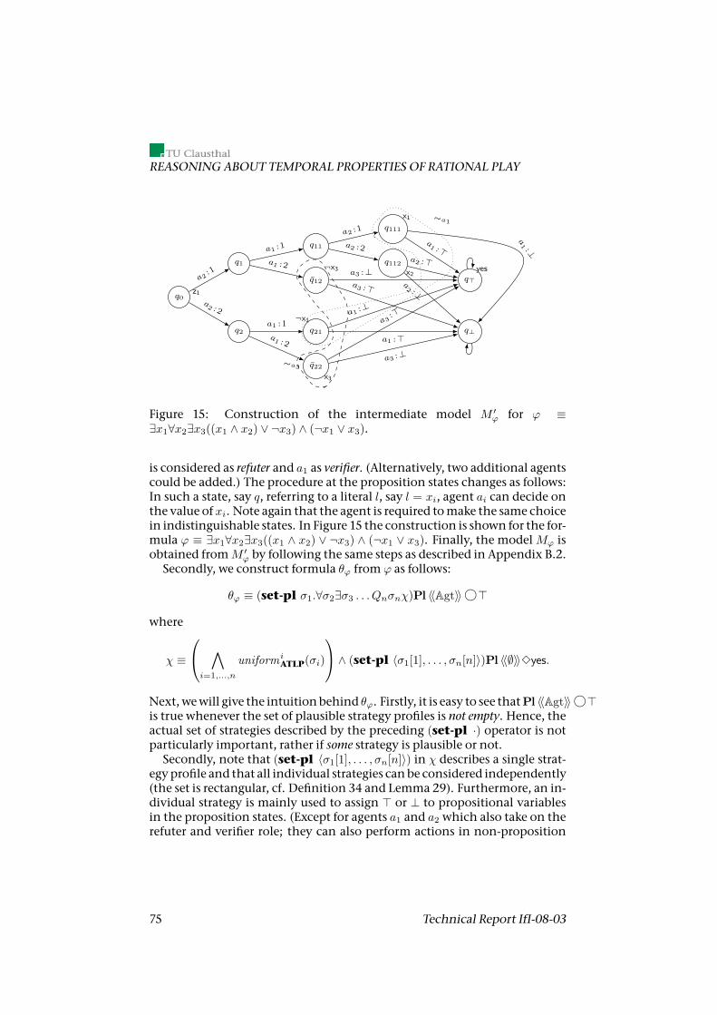
REASONING ABOUT TEMPORAL PROPERTIES OF RATIONAL PLAY
q0z1
q1
q2
q11
q12
¬x3
q21
¬x1
q22x3
q111
x1
q112x2
q>
yes
q⊥
a2:1
a2 :2
a1 :1
a1 :2
a1 :1
a1 :2
a2 :1
a2 :2a1 :>
a2 :>
a1 :⊥a3
:>
a3 :⊥
a1 :⊥
a2 :⊥
a1 :>
a3 :⊥
a3 :>
∼a3
∼a1
Figure 15: Construction of the intermediate model M ′ϕ for ϕ ≡
∃x1∀x2∃x3((x1 ∧ x2) ∨ ¬x3) ∧ (¬x1 ∨ x3).
is considered as refuter and a1 as verifier. (Alternatively, two additional agentscould be added.) The procedure at the proposition states changes as follows:In such a state, say q, referring to a literal l, say l = xi, agent ai can decide onthe value of xi. Note again that the agent is required tomake the same choicein indistinguishable states. In Figure 15 the construction is shown for the for-mula ϕ ≡ ∃x1∀x2∃x3((x1 ∧ x2) ∨ ¬x3) ∧ (¬x1 ∨ x3). Finally, the modelMϕ isobtained fromM ′
ϕ by following the same steps as described in Appendix B.2.Secondly, we construct formula θϕ from ϕ as follows:
θϕ ≡ (set-pl σ1.∀σ2∃σ3 . . . Qnσnχ)Pl 〈〈Agt〉〉 h>where
χ ≡
∧i=1,...,n
uniformiATLP(σi)
∧ (set-pl 〈σ1[1], . . . , σn[n]〉)Pl 〈〈∅〉〉3yes.
Next, wewill give the intuitionbehind θϕ. Firstly, it is easy to see thatPl 〈〈Agt〉〉 h>is true whenever the set of plausible strategy profiles is not empty. Hence, theactual set of strategies described by the preceding (set-pl ·) operator is notparticularly important, rather if some strategy is plausible or not.Secondly, note that (set-pl 〈σ1[1], . . . , σn[n]〉) in χ describes a single strat-
egyprofile and that all individual strategies canbe considered independently(the set is rectangular, cf. Definition 34 and Lemma 29). Furthermore, an in-dividual strategy is mainly used to assign > or ⊥ to propositional variablesin the proposition states. (Except for agents a1 and a2 which also take on therefuter and verifier role; they can also perform actions in non-proposition
75 Technical Report IfI-08-03
SomeModel Checking Complexity Proofs
states.) Hence, a given strategyprofile canbe seen as a valuationof thepropo-sitional variables.Thirdly, we analyze χ with respect to a given profile σ := 〈σ1[1], . . . , σn[n]〉
taking into account the previous points. By formula uniformiATLP(σi) it is
ensured that agent i assigns the same valuation to propositions in indistin-guishable states. Now, χ is true if the “winning state” q> is reached by fol-lowing the strategy described by σ (it describes a unique path in the model).In other words, χ is true if, and only if, the valuation described by σ satisfiesϕ.Finally, due to the previous observations, if [[σ1.∀σ2∃σ3 . . . Qnσnχ]] is non-
empty it can be interpreted as follows: There is a valuation of x1 such thatfor all valuations of x2 there is a valuation of x3, and so forth such that ϕ issatisfied.The following proposition states that the construction is correct.
Proposition 52 Let ϕ be aQSAT instance. Then it holds that ϕ is satisfiable if,and only if,Mϕ, q0 |= θϕ whereMϕ and θϕ are effectively constructible from ϕ inpolynomial space with respect to the length of the formula ϕ.
Proof sketch Let ϕ be aQSAT instance. We use the construction above to ob-tainM ′
ϕ and θϕ where uniformiATLP(σ) is obtained as follows: Firstly, we take
the ATLI +K formula uniform(σ|i) (where σ|i refers to agent i’s startegy inσ) as described in Appendix C; then, we use the polynomial translation tochange knowledge to ability, yielding a pure ATLI formula. Finally, we usethe polynomial translation from ATLI to ATLP given in Section 5.1 (Proofof Proposition 11) to obtain a pure ATLP formula uniformi
ATLP(σ). Hence,the latter formula is true if agent i’s strategy contained in the complete pro-file σ is a uniform strategy. This shows that θϕ can be constructed in polyno-mial space.ModelMϕ is obtained fromM ′
ϕ by the same scheme. Firstly, the construc-tion from [23] referred to in Appendix C is applied. Secondly, the resultingCGS with intentions is transformed to a CGSP using the construction fromSection 5.1 (Proposition 11) again. The constructed modelMϕ is also poly-nomial with respect to ϕ.We get that ϕ is satisfiable if, and only if,Mϕ, q0 |= θϕ.
DEPARTMENTOF INFORMATICS 76
Related Documents