TELE4653 Digital Modulation & Coding Synchronization Wei Zhang [email protected] School of Electrical Engineering and Telecommunications The University of New South Wales

Welcome message from author
This document is posted to help you gain knowledge. Please leave a comment to let me know what you think about it! Share it to your friends and learn new things together.
Transcript
TELE4653 Digital Modulation &Coding
Synchronization
Wei Zhang
School of Electrical Engineering and Telecommunications
The University of New South Wales
Outline
Carrier Phase Estimation
Decision-Directed Loops
Timing Estimation
TELE4653 - Digital Modulation & Coding - Lecture 5. March 29, 2010. – p.1/21
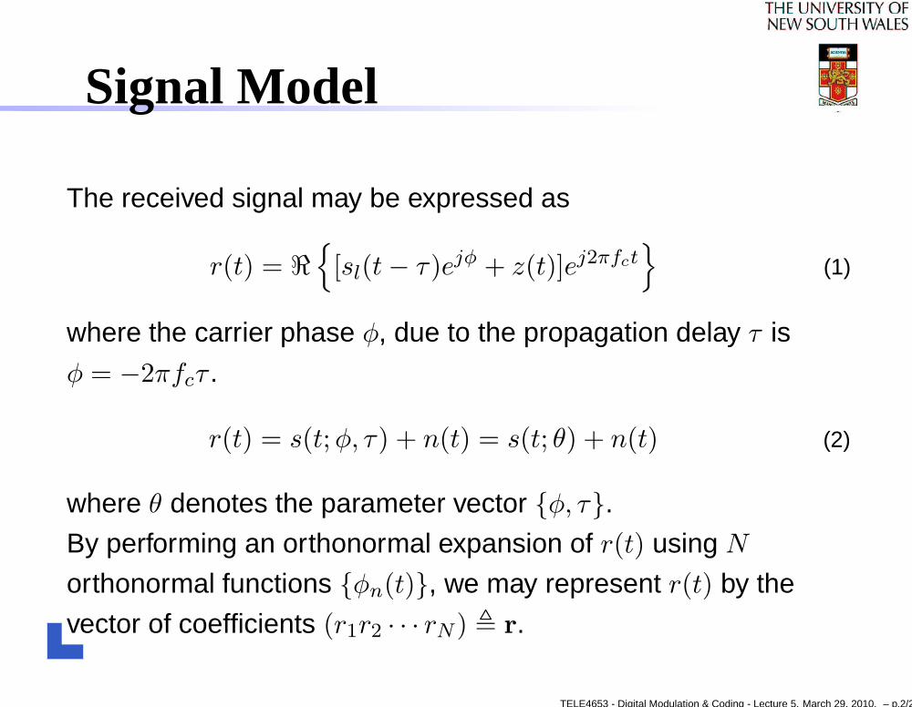
Signal Model
The received signal may be expressed as
r(t) = <{
[sl(t − τ)ejφ + z(t)]ej2πfct}
(1)
where the carrier phase φ, due to the propagation delay τ is
φ = −2πfcτ .
r(t) = s(t;φ, τ) + n(t) = s(t; θ) + n(t) (2)
where θ denotes the parameter vector {φ, τ}.
By performing an orthonormal expansion of r(t) using N
orthonormal functions {φn(t)}, we may represent r(t) by the
vector of coefficients (r1r2 · · · rN ) , r.
TELE4653 - Digital Modulation & Coding - Lecture 5. March 29, 2010. – p.2/21
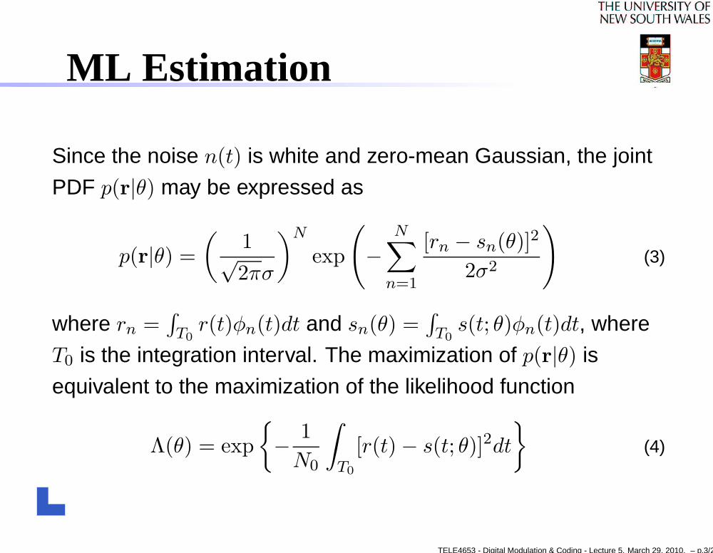
ML Estimation
Since the noise n(t) is white and zero-mean Gaussian, the joint
PDF p(r|θ) may be expressed as
p(r|θ) =
(
1√2πσ
)N
exp
(
−N∑
n=1
[rn − sn(θ)]2
2σ2
)
(3)
where rn =∫
T0r(t)φn(t)dt and sn(θ) =
∫
T0s(t; θ)φn(t)dt, where
T0 is the integration interval. The maximization of p(r|θ) is
equivalent to the maximization of the likelihood function
Λ(θ) = exp
{
− 1
N0
∫
T0
[r(t) − s(t; θ)]2dt
}
(4)
TELE4653 - Digital Modulation & Coding - Lecture 5. March 29, 2010. – p.3/21
Receiver Structure
Figure 5.1-1 shows a block diagram of a binary PSK receiver.
Figure 5.1-2 shows a block diagram of an M -ary PSK receiver.
Figure 5.1-3 shows a block diagram of an M -ary PAM receiver.
Figure 5.1-4 shows a block diagram of a QAM receiver.
TELE4653 - Digital Modulation & Coding - Lecture 5. March 29, 2010. – p.4/21
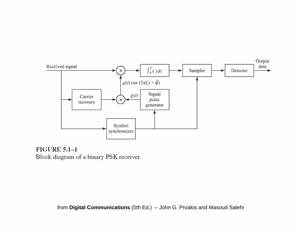
from Digital Communications (5th Ed.) – John G. Proakis and Masoud Salehi
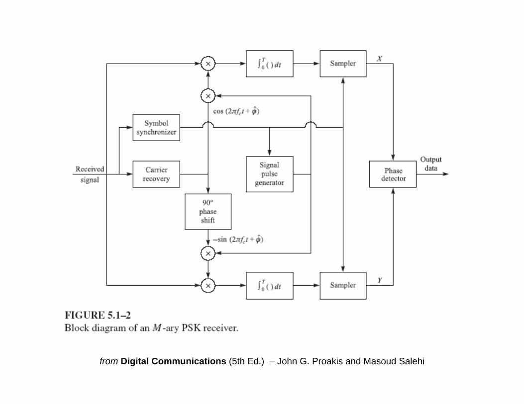
from Digital Communications (5th Ed.) – John G. Proakis and Masoud Salehi
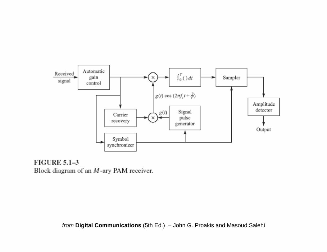
from Digital Communications (5th Ed.) – John G. Proakis and Masoud Salehi
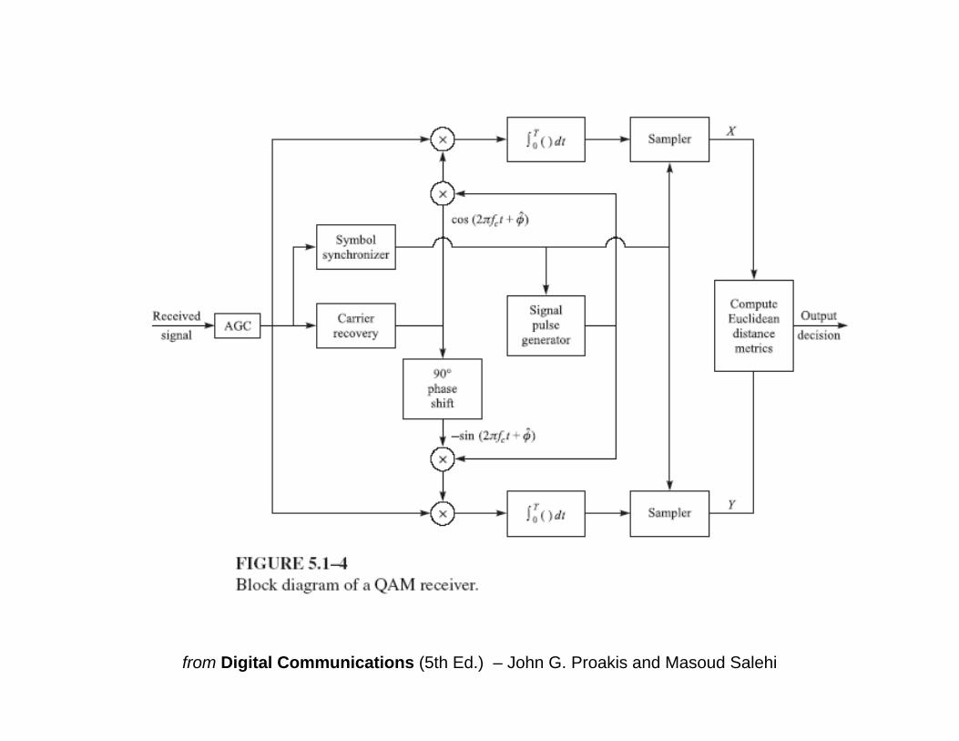
from Digital Communications (5th Ed.) – John G. Proakis and Masoud Salehi
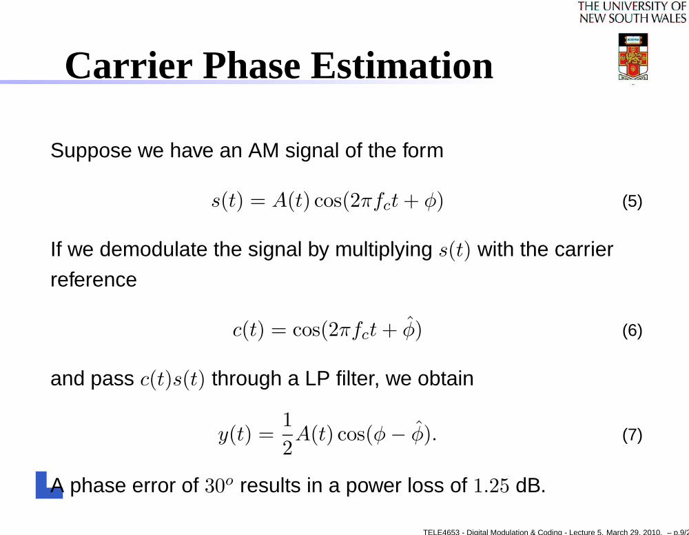
Carrier Phase Estimation
Suppose we have an AM signal of the form
s(t) = A(t) cos(2πfct + φ) (5)
If we demodulate the signal by multiplying s(t) with the carrier
reference
c(t) = cos(2πfct + φ̂) (6)
and pass c(t)s(t) through a LP filter, we obtain
y(t) =1
2A(t) cos(φ − φ̂). (7)
A phase error of 30o results in a power loss of 1.25 dB.
TELE4653 - Digital Modulation & Coding - Lecture 5. March 29, 2010. – p.9/21
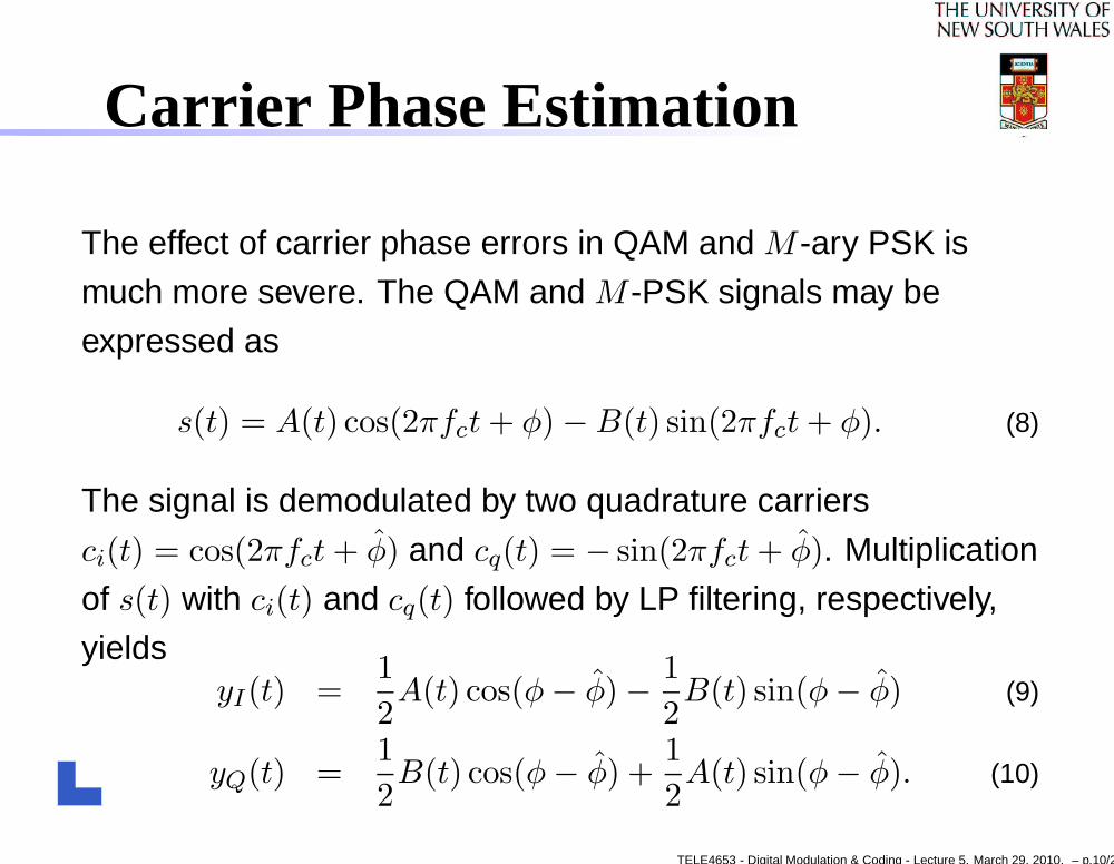
Carrier Phase Estimation
The effect of carrier phase errors in QAM and M -ary PSK is
much more severe. The QAM and M -PSK signals may be
expressed as
s(t) = A(t) cos(2πfct + φ) − B(t) sin(2πfct + φ). (8)
The signal is demodulated by two quadrature carriers
ci(t) = cos(2πfct + φ̂) and cq(t) = − sin(2πfct + φ̂). Multiplication
of s(t) with ci(t) and cq(t) followed by LP filtering, respectively,
yieldsyI(t) =
1
2A(t) cos(φ − φ̂) − 1
2B(t) sin(φ − φ̂) (9)
yQ(t) =1
2B(t) cos(φ − φ̂) +
1
2A(t) sin(φ − φ̂). (10)
TELE4653 - Digital Modulation & Coding - Lecture 5. March 29, 2010. – p.10/21

ML Phase Estimation
Assume τ = 0. The likelihood function Eq. (4) becomes
Λ(φ) = exp
{
− 1
N0
∫
T0
[r(t) − s(t;φ)]2dt
}
(11)
= exp
{
− 1
N0
∫
T0
r2(t)dt +2
N0
∫
T0
r(t)s(t;φ)dt
− 1
N0
∫
T0
s2(t;φ)dt
}
(12)
The log-likelihood function is
ΛL(φ) =2
N0
∫
T0
r(t)s(t;φ)dt (13)
TELE4653 - Digital Modulation & Coding - Lecture 5. March 29, 2010. – p.11/21
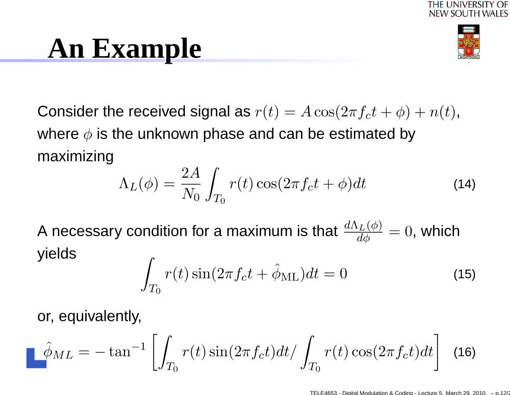
An Example
Consider the received signal as r(t) = A cos(2πfct + φ) + n(t),
where φ is the unknown phase and can be estimated by
maximizing
ΛL(φ) =2A
N0
∫
T0
r(t) cos(2πfct + φ)dt (14)
A necessary condition for a maximum is that dΛL(φ)dφ
= 0, which
yields ∫
T0
r(t) sin(2πfct + φ̂ML)dt = 0 (15)
or, equivalently,
φ̂ML = − tan−1
[∫
T0
r(t) sin(2πfct)dt/
∫
T0
r(t) cos(2πfct)dt
]
(16)
TELE4653 - Digital Modulation & Coding - Lecture 5. March 29, 2010. – p.12/21
PLL
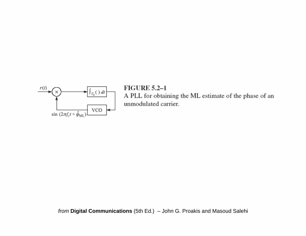
Eq. (15) implies the use of a loop (PLL) to extract the estimate
as illustrated in Fig. 5.2-1.
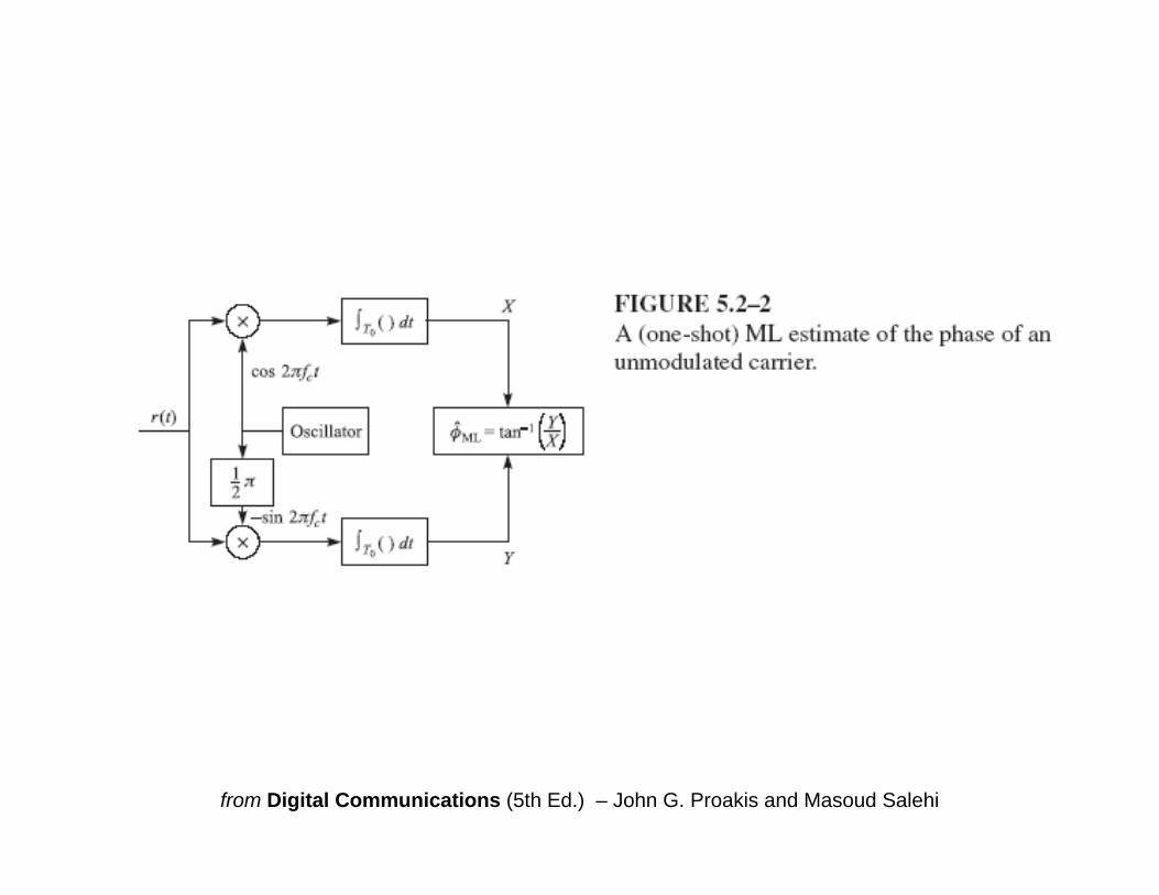
Eq. (16) implies an implementation that uses quadrature carriers
to cross-correlated with r(t), as shown in Fig. 5.2-2.
Please refer to TELE3113 lecture notes for details of PLL.
TELE4653 - Digital Modulation & Coding - Lecture 5. March 29, 2010. – p.13/21
from Digital Communications (5th Ed.) – John G. Proakis and Masoud Salehi
from Digital Communications (5th Ed.) – John G. Proakis and Masoud Salehi
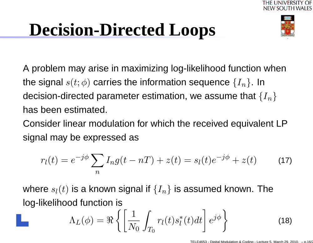
Decision-Directed Loops
A problem may arise in maximizing log-likelihood function when
the signal s(t;φ) carries the information sequence {In}. In
decision-directed parameter estimation, we assume that {In}has been estimated.
Consider linear modulation for which the received equivalent LP
signal may be expressed as
rl(t) = e−jφ∑
n
Ing(t − nT ) + z(t) = sl(t)e−jφ + z(t) (17)
where sl(t) is a known signal if {In} is assumed known. The
log-likelihood function is
ΛL(φ) = <{[
1
N0
∫
T0
rl(t)s∗
l (t)dt
]
ejφ
}
(18)
TELE4653 - Digital Modulation & Coding - Lecture 5. March 29, 2010. – p.16/21
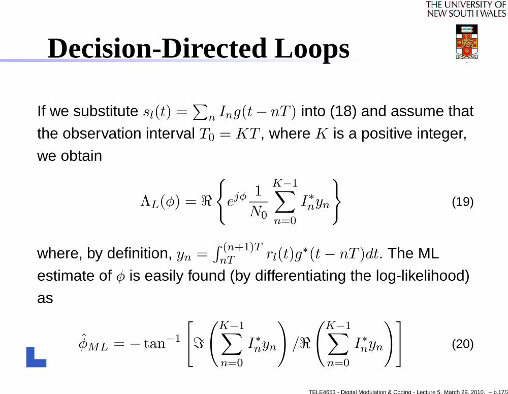
Decision-Directed Loops
If we substitute sl(t) =∑
n Ing(t− nT ) into (18) and assume that
the observation interval T0 = KT , where K is a positive integer,
we obtain
ΛL(φ) = <{
ejφ 1
N0
K−1∑
n=0
I∗nyn
}
(19)
where, by definition, yn =∫ (n+1)TnT
rl(t)g∗(t − nT )dt. The ML
estimate of φ is easily found (by differentiating the log-likelihood)
as
φ̂ML = − tan−1
[
=(
K−1∑
n=0
I∗nyn
)
/<(
K−1∑
n=0
I∗nyn
)]
(20)
TELE4653 - Digital Modulation & Coding - Lecture 5. March 29, 2010. – p.17/21
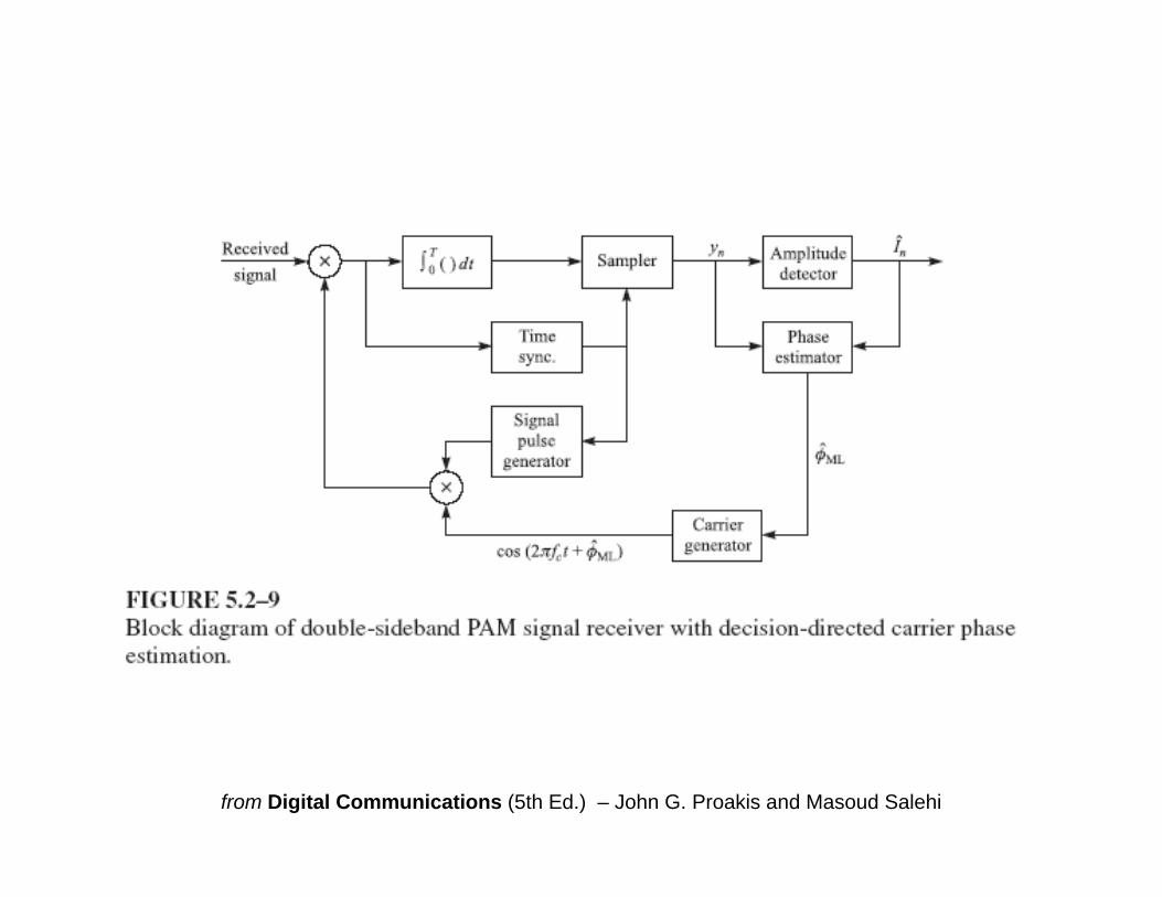
from Digital Communications (5th Ed.) – John G. Proakis and Masoud Salehi
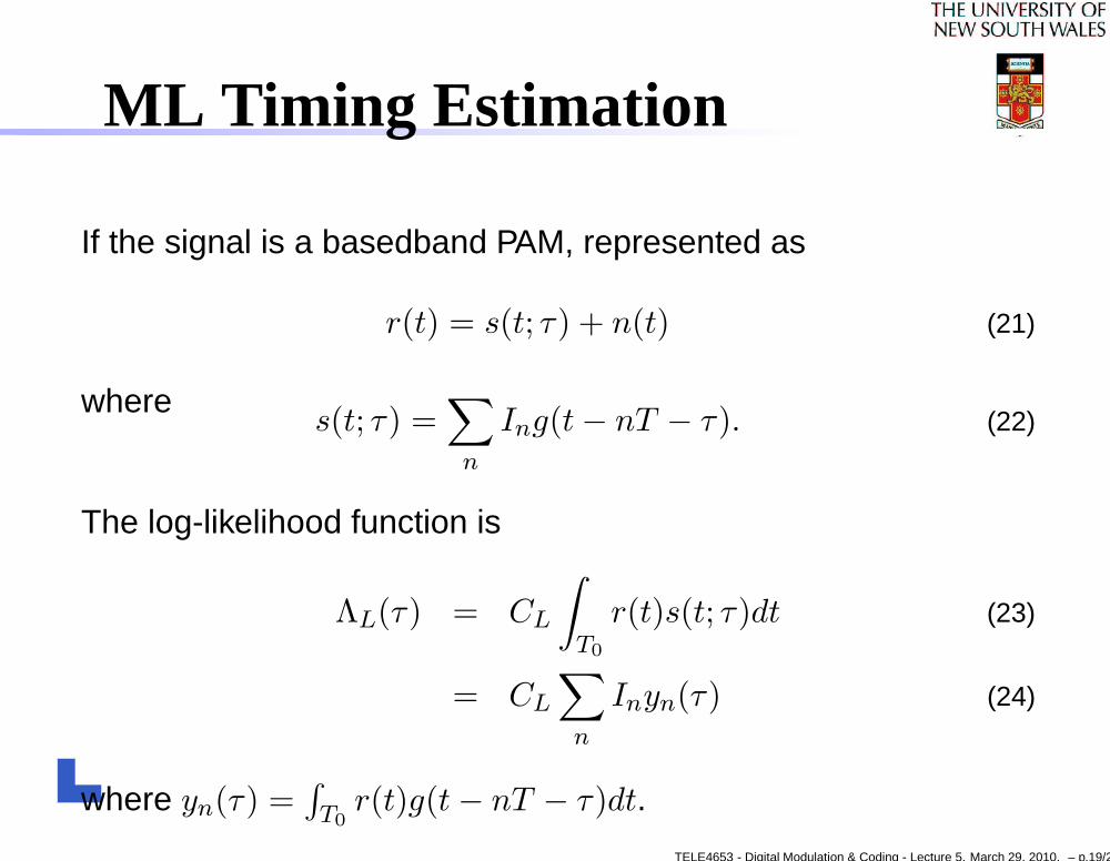
ML Timing Estimation
If the signal is a basedband PAM, represented as
r(t) = s(t; τ) + n(t) (21)
wheres(t; τ) =
∑
n
Ing(t − nT − τ). (22)
The log-likelihood function is
ΛL(τ) = CL
∫
T0
r(t)s(t; τ)dt (23)
= CL
∑
n
Inyn(τ) (24)
where yn(τ) =∫
T0r(t)g(t − nT − τ)dt.
TELE4653 - Digital Modulation & Coding - Lecture 5. March 29, 2010. – p.19/21
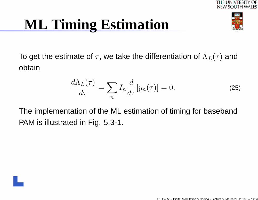
ML Timing Estimation
To get the estimate of τ , we take the differentiation of ΛL(τ) and
obtain
dΛL(τ)
dτ=∑
n
Ind
dτ[yn(τ)] = 0. (25)
The implementation of the ML estimation of timing for baseband
PAM is illustrated in Fig. 5.3-1.
TELE4653 - Digital Modulation & Coding - Lecture 5. March 29, 2010. – p.20/21
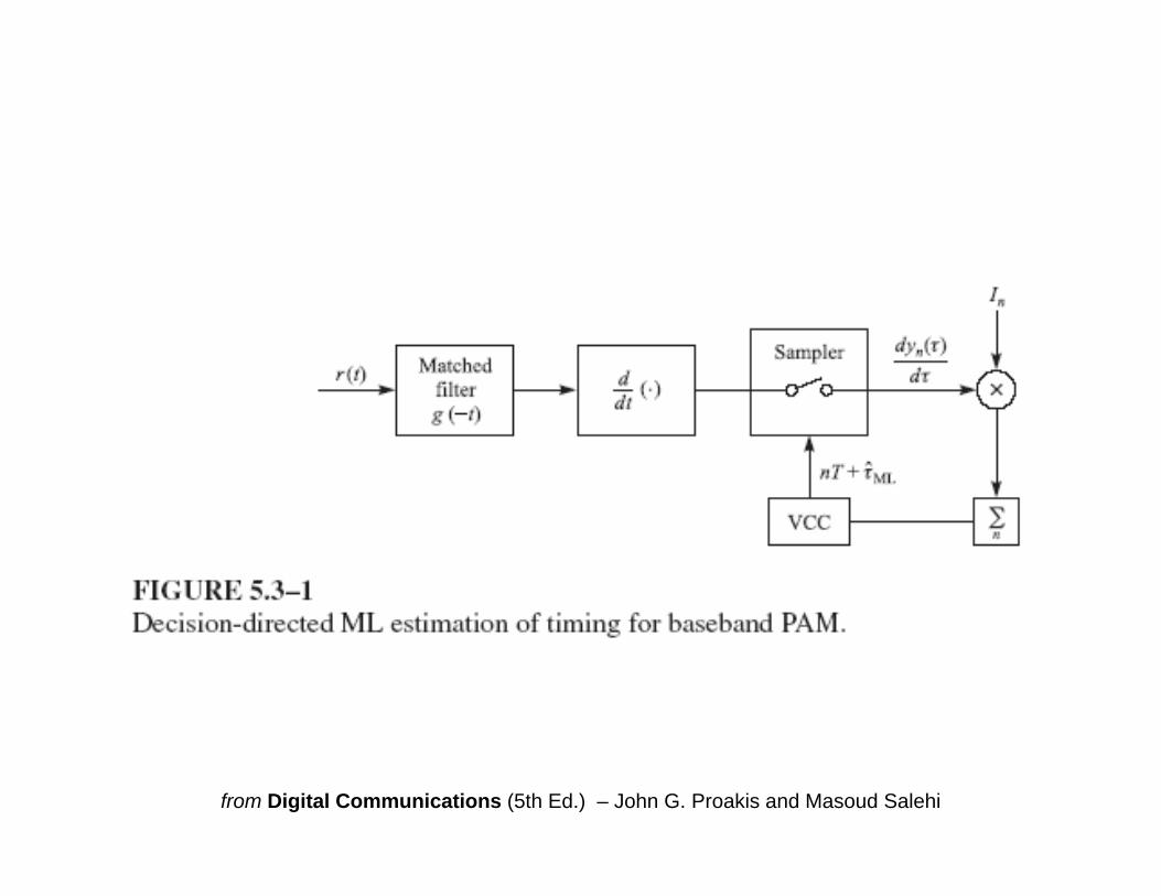
from Digital Communications (5th Ed.) – John G. Proakis and Masoud Salehi
Related Documents