University of Central Florida University of Central Florida STARS STARS Electronic Theses and Dissertations, 2004-2019 2005 Super High-speed Miniaturized Permanent Magnet Synchronous Super High-speed Miniaturized Permanent Magnet Synchronous Motor Motor Liping Zheng University of Central Florida Part of the Electrical and Electronics Commons Find similar works at: https://stars.library.ucf.edu/etd University of Central Florida Libraries http://library.ucf.edu This Doctoral Dissertation (Open Access) is brought to you for free and open access by STARS. It has been accepted for inclusion in Electronic Theses and Dissertations, 2004-2019 by an authorized administrator of STARS. For more information, please contact [email protected]. STARS Citation STARS Citation Zheng, Liping, "Super High-speed Miniaturized Permanent Magnet Synchronous Motor" (2005). Electronic Theses and Dissertations, 2004-2019. 640. https://stars.library.ucf.edu/etd/640

Welcome message from author
This document is posted to help you gain knowledge. Please leave a comment to let me know what you think about it! Share it to your friends and learn new things together.
Transcript
University of Central Florida University of Central Florida
STARS STARS
Electronic Theses and Dissertations, 2004-2019
2005
Super High-speed Miniaturized Permanent Magnet Synchronous Super High-speed Miniaturized Permanent Magnet Synchronous
Motor Motor
Liping Zheng University of Central Florida
Part of the Electrical and Electronics Commons
Find similar works at: https://stars.library.ucf.edu/etd
University of Central Florida Libraries http://library.ucf.edu
This Doctoral Dissertation (Open Access) is brought to you for free and open access by STARS. It has been accepted
for inclusion in Electronic Theses and Dissertations, 2004-2019 by an authorized administrator of STARS. For more
information, please contact [email protected].
STARS Citation STARS Citation Zheng, Liping, "Super High-speed Miniaturized Permanent Magnet Synchronous Motor" (2005). Electronic Theses and Dissertations, 2004-2019. 640. https://stars.library.ucf.edu/etd/640
SUPER HIGH-SPEED MINIATURIZED PERMANENT MAGNET SYNCHRONOUS MOTOR
by
LIPING ZHENG B.S. Shanghai Jiaotong University, P. R. China, 1990 M.S. Hangzhou Dianzi University, P. R. China, 1995
M.S. University of Central Florida, 2003
A dissertation submitted in partial fulfillment of the requirements for the degree of Doctor of Philosophy
in the Department of Electrical and Computer Engineering in the College of Engineering and Computer Science
at the University of Central Florida Orlando, Florida
Fall Term 2005
Major Professors: Dr. Kalpathy B. Sundaram Dr. Thomas X. Wu
ABSTRACT
This dissertation is concerned with the design of permanent magnet synchronous motors
(PMSM) to operate at super-high speed with high efficiency. The designed and fabricated
PMSM was successfully tested to run upto 210,000 rpm The designed PMSM has 2000 W shaft
output power at 200,000 rpm and at the cryogenic temperature of 77 K. The test results showed
the motor to have an efficiency reaching above 92%. This achieved efficiency indicated a
significant improvement compared to commercial motors with similar ratings.
This dissertation first discusses the basic concept of electrical machines. After that, the
modeling of PMSM for dynamic simulation is provided. Particular design strategies have to be
adopted for super-high speed applications since motor losses assume a key role in the motor
drive performance limit. The considerations of the PMSM structure for cryogenic applications
are also discussed. It is shown that slotless structure with multi-strand Litz-wire is favorable for
super-high speeds and cryogenic applications.
The design, simulation, and test of a single-sided axial flux pancake PMSM is presented.
The advantages and disadvantages of this kind of structure are discussed, and further
improvements are suggested and some have been verified by experiments.
The methodologies of designing super high-speed motors are provided in details. Based
on these methodologies, a super high-speed radial-flux PMSM was designed and fabricated. The
designed PMSM meets our expectation and the tested results agree with the design
specifications.
ii

2-D and 3-D modeling of the complicated PMSM structure for the electromagnetic
numerical simulations of motor performance and parameters such as phase inductors, core losses,
rotor eddy current loss, torque, and induced electromotive force (back-EMF) are also presented
in detail in this dissertation. Some mechanical issues such as thermal analysis, bearing pre-load,
rotor stress analysis, and rotor dynamics analysis are also discussed.
Different control schemes are presented and suitable control schemes for super high-
speed PMSM are also discussed in detail.
iii

ACKNOWLEDGMENTS
I would like to thank my academic advisors, Dr. Kalpathy B. Sundaram and Dr. Thomas
X. Wu, for their guidance and encouragement throughout my study. I would like to express my
deep and sincere gratitude to Dr. Louis C. Chow and Dr. Jay Kapat, without their support and
direction, this work would not have been possible. I would also like to thank Dr. Chan H. Ham
for his help and suggestions in machine design and control.
I would like to express my sincere appreciation to Mr. Jay Vaidya from Electrodynamic
Associates Inc. for his technical guidance through my research. I have learned a lot in machine
design and control through his selfless guide and help. I would also like to thank Dr. Nagaraj
Arakere from University of Florida for his help in mechanical design and rotordynamic analysis.
I would like to take this opportunity to thank Dipjyoti Acharya, Krishna Murty, Lei Zhou,
Limei Zhao, and all other members of the Electric Machine Research Group and Miniature
Engineering Systems Group for their help and support. I would like to thank my friend Ottman
Elkhomri from Electrodynamic Associates Inc. for the technical discussions in motor control. I
would also like to thank all members of our Applied Electromagnetics & High Speed Electronics
Group for their help and discussions in electromagnetic simulations and circuit design.
I also wish to sincerely thank Dr. David Block and Dr. Ali Raissi of Florida Solar Energy
Center; Mr. David Chato and Mr. James Burkhart of NASA Glenn Research Center; Dr. David
Bartine and Dr. H. T. Everett of NASA Kennedy Space Center for their unstinted and continued
support throughout the project.
iv

Finally, I would like to thank my wife Haiying Wang and our lovely daughter Yunjing
Zheng for their support and understanding. I am indebt to my grandmother who passed away
when I was an undergraduate, my parents, and my two brothers. Without their support and
encouragement, I could not have got my BS degree and would not have a chance to come to
University of Central Florida for my Ph. D degree.
v

TABLE OF CONTENTS
LIST OF FIGURES ....................................................................................................................... xi
LIST OF TABLES....................................................................................................................... xvi
CHAPTER ONE: INTRODUCTION..............................................................................................1
1.1 Motivation............................................................................................................................. 1
1.2 Dissertation Organization ..................................................................................................... 3
CHAPTER TWO: PMSM MODELING AND DESIGN................................................................4
2.1 Classification of Electric Motors .......................................................................................... 4
2.2 Modeling of PMSM .............................................................................................................. 7
2.2.1 Clarke’s Transformation ................................................................................................ 7
2.2.2 Park’s Transformation ................................................................................................... 8
2.2.3 Circuit Representation of PMSM................................................................................. 10
2.2.4 Mathematical Modeling ............................................................................................... 11
2.2.5 Phasor Diagram............................................................................................................ 15
2.3 PMSM Design Procedure ................................................................................................... 16
2.4 Motor Type and Structure Consideration ........................................................................... 20
2.5 Losses in PMSM................................................................................................................. 23
2.5.1 Iron Loss ...................................................................................................................... 23
2.5.1.1 Hysteresis Loss ..................................................................................................... 24
2.5.1.2 Eddy Current Loss ................................................................................................ 24
vi
2.5.2 Copper Loss ................................................................................................................. 27
2.5.3 Windage Loss............................................................................................................... 28
2.6 Analysis and Sizing............................................................................................................. 30
2.7 FEM Simulation of PMSM................................................................................................. 34
2.7.1 Calculation of Inductance ............................................................................................ 34
2.7.2 Back-EMF Analysis and Simulation ........................................................................... 37
2.7.3 Torque Simulation ....................................................................................................... 38
2.7.4 Transient Simulation.................................................................................................... 39
2.8 Optimization and Tradeoffs ................................................................................................ 40
2.9 PMSM Test ......................................................................................................................... 40
2.9.1 Spin-Down Test ........................................................................................................... 40
2.9.2 Free Spin Test .............................................................................................................. 42
2.9.3 Load Test ..................................................................................................................... 42
CHAPTER THREE: DESIGN AND MODIFICATION OF AN AXIAL-FLUX PMSM............45
3.1 Introduction......................................................................................................................... 45
3.2 Structure and Design Considerations.................................................................................. 46
3.3 Analytical Analyses ............................................................................................................ 48
3.4 FEM Simulation of the Axial-Flux PMSM ........................................................................ 52
3.4.1 Simulation and Optimization of Magnetic Flux Distributions .................................... 53
3.4.2 Simulation of Electromagnetic Torque........................................................................ 57
3.4.3 Simulation of Back-EMF............................................................................................. 59
vii

3.4.4 Inductances Analysis ................................................................................................... 60
3.4.5 Simulation of Rotor Stress ........................................................................................... 62
3.5 Axial-Flux Slotless PMSM Drive and Test ........................................................................ 64
3.5.1 Slotless PMSM Drive .................................................................................................. 64
3.5.2 Spin-Down Test ........................................................................................................... 65
3.5.3 Load Test ..................................................................................................................... 66
3.5.4 Separation of Losses .................................................................................................... 67
3.6 Improvement of the Axial-Flux PMSM.............................................................................. 72
3.7 Summary of Axial-Flux PMSM Design ............................................................................. 73
CHAPTER FOUR: DESIGN AND CONTROL OF A SUPER HIGH-SPEED CRYOGENIC
PMSM......................................................................................................................................74
4.1 Introduction......................................................................................................................... 74
4.2 Design Considerations ........................................................................................................ 74
4.2.1 Selection of Motor Type .............................................................................................. 74
4.2.2 Axial-Flux PMSM or Radial-Flux PMSM .................................................................. 75
4.2.3 Slotless Stator or Slotted Stator ................................................................................... 76
4.2.4 Rotor Structure............................................................................................................. 77
4.2.5 Designed Motor Structure............................................................................................ 77
4.3 Material Selection ............................................................................................................... 79
4.3.1 Permanent Magnet ....................................................................................................... 80
4.3.2 Winding........................................................................................................................ 80
viii

4.3.3 Stator ............................................................................................................................ 81
4.3.4 Bearing......................................................................................................................... 81
4.3.5 Shaft ............................................................................................................................. 82
4.4 FEM Simulation and Optimization..................................................................................... 82
4.4.1 Simulation of Magnetic Flux ....................................................................................... 82
4.4.2 Simulation of Back-EMF............................................................................................. 84
4.4.3 Calculation of Inductances........................................................................................... 85
4.4.4 Transient Simulation.................................................................................................... 85
4.4.4.1 Simulation in Motoring Mode .............................................................................. 86
4.4.4.2 Simulation in Generating Mode............................................................................ 87
4.5 Structural Design ................................................................................................................ 90
4.5 Loss Analysis ...................................................................................................................... 99
4.5.1 Copper Loss ................................................................................................................. 99
4.5.2 Stator Core Loss......................................................................................................... 102
4.5.3 Rotor Loss.................................................................................................................. 103
4.5.4 Windage Loss............................................................................................................. 104
4.5.5 Super High-Speed PMSM Efficiency........................................................................ 104
4.6 Prototype Design and Fabrication..................................................................................... 105
4.6.1 Bearing Design and Lubrication ................................................................................ 106
4.6.2 Rotor Assembly ......................................................................................................... 110
4.6.3 Housing and Pre-Load ............................................................................................... 111
ix

4.7 Motor Control and Test..................................................................................................... 114
4.7.1 Motor Control ............................................................................................................ 114
4.7.2 Free-Spin Test............................................................................................................ 118
4.7.3 Spin-Down Test ......................................................................................................... 120
4.7.4 Load Test ................................................................................................................... 121
CHAPTER FIVE: CONCLUSION..............................................................................................125
APPENDIX A: AXIAL FLUX PMSM DESIGN (USING MATHCAD)...................................129
APPENDIX B: RADIAL FLUX PMSM DESIGN (USING MATHCAD) ................................135
APPENDIX C: ROTOR DRAWINGS OF MOTOR AND MOTOR/GENERATOR................141
APPENDIX D: ANALYTICAL ANALYSIS OF ROTORDYNAMICS ...................................144
APPENDIX E: SCHEMETIC AND PCB LAYOUT OF THE PMSM CONTROLLER...........147
LIST OF REFERENCES.............................................................................................................151
x

LIST OF FIGURES
Figure 1 A classification of electric motors.................................................................................... 5
Figure 2 Relationship between the αβ and abc quantities.............................................................. 8
Figure 3 Relationship between αβ axis and dq axis........................................................................ 9
Figure 4 Relation between dq-axis and rδ-axis ............................................................................ 10
Figure 5 Circuit representation of an ideal machine..................................................................... 11
Figure 6 Equivalent qd0 circuits of a permanent magnet synchronous motor. ............................ 14
Figure 7 Phasor diagram of the motor with (a) a leading power factor, and (b) a lagging power
factor. .................................................................................................................................... 18
Figure 8 A flowchart of PMSM design......................................................................................... 19
Figure 9 Family of hysteresis loops. ............................................................................................. 25
Figure 10 Cross section of a radial flux slotless two-pole motor with round permanent magnet 32
Figure 11 A double excited magnetic structure. ........................................................................... 35
Figure 12 Motor load test circuitry with rectifiers........................................................................ 44
Figure 13 Motor load test circuitry without rectifiers................................................................... 44
Figure 14 Axial view of the axial-flux PMSM structure with single rotor and single stator. ...... 47
Figure 15 Photos of the rotor and its components. ....................................................................... 47
Figure 16 Winding structure: (a) winding of one group with 7 turns in the group, and (b) actual
winding with a total of 84 turns. ........................................................................................... 48
Figure 17 Parallel winding connections........................................................................................ 49
xi

Figure 18 Magnetic flux orientations in the motor ....................................................................... 50
Figure 19 The corresponding magnetic circuit model. ................................................................. 50
Figure 20 Simplified magnetic circuit model. .............................................................................. 51
Figure 21 FEM simulation model to calculate flux density.......................................................... 53
Figure 22 (a) airgap flux densities vs. angle for different magnetic gap Lg, where the thickness of
the permanent magnets is adjusted to keep the same peak flux density, and (b) the
corresponding normalized harmonics. .................................................................................. 55
Figure 23 (a) airgap flux densities for different pole pitch when magnetic gap Lg is 1.4 mm, and
(b) the corresponding normalized harmonics. ...................................................................... 56
Figure 24 FEM simulation model with fractional winding. ......................................................... 57
Figure 25 A model of the winding................................................................................................ 58
Figure 26 Simulated and measured back EMF at 50,000 rpm...................................................... 60
Figure 27. Simulated stress in the rotor steel when rotating at 100,000 rpm. .............................. 63
Figure 28 Simulated stress in the carbon ring when rotating at 100,000 rpm. ............................. 63
Figure 29 Schematic of space vector PWM drive and low-pass filters. ....................................... 64
Figure 30 Current and voltage waveforms when the speed is 50,000 rpm................................... 65
Figure 31 Tested spin down time vs. motor speed........................................................................ 66
Figure 32 Calculated damping power vs. motor speed................................................................. 67
Figure 33 Tested spin down time vs. the rotor speed of three motors. ......................................... 70
Figure 34 (a) tested damping power of the designed PMSM, damping motor and the PMSM
with larger airgap, and (b) separated bearing loss of the designed PMSM, damping motor
xii

and the PMSM with larger airgap......................................................................................... 71
Figure 35 The new winding of using multi-strand Litz-wire........................................................ 73
Figure 36 Cross section of the designed PMSM........................................................................... 78
Figure 37 Rotor structure of the radial-flux PMSM prototype. ................................................... 79
Figure 38 Flux lines caused by the permanent magnet at room temperature. .............................. 83
Figure 39 Simulated airgap flux densities in normal direction and tangential direction. ............. 83
Figure 40 Simulated back-EMF of the designed PMSM when the speed is 200,000 rpm. .......... 84
Figure 41 Calculated flux linkage................................................................................................. 86
Figure 42 Simulated torque when applying 61.4 A phase current together with harmonics........ 87
Figure 43 Simulated rotor eddy current loss and stator core loss when rotating at 200,000 rpm
and at 77 K. ........................................................................................................................... 88
Figure 44 Phase current. ............................................................................................................... 88
Figure 45 Rectified output voltage and current. ........................................................................... 89
Figure 46 Simulated torque in generating mode with rectifier circuit.......................................... 89
Figure 47 Simulated stator core loss and rotor eddy current loss at 200,000 rpm and the
cryogenic temperature of 77 K. ............................................................................................ 90
Figure 48 Simulated eddy currents in the shaft and permanent magnet in generating mode with
rectified output DC power of 2000 W. ................................................................................. 91
Figure 49 Stress in the shaft and magnet assembly. ..................................................................... 92
Figure 50 A shaft with two supporting bearings........................................................................... 94
Figure 51 FEM rotordynamics model of the radial-flux PMSM. ................................................. 96
xiii
Figure 52 Simulated critical speeds of the radial-flux PMSM. .................................................... 96
Figure 53 FEM rotordynamic model of the motor/generator. ...................................................... 97
Figure 54 Simulated (a) first bending mode, and (b) second bending mode of the
motor/generator..................................................................................................................... 97
Figure 55 Simulated critical speeds of the motor/generator. ........................................................ 98
Figure 56 Model of the stator and the attached winding. ............................................................. 99
Figure 57 Electrical resistivity of copper vs. temperature. ......................................................... 101
Figure 58 Simulated eddy current of the round solid wire when the rotor is rotating at 200,000
rpm and the operating temperature is 77 K......................................................................... 102
Figure 59 Simulated eddy current of the Litz-wire (75 strands at AWG 36) when the motor is
rotating at 200,000 rpm....................................................................................................... 103
Figure 60 Bearing inner ring fit. ................................................................................................. 107
Figure 61 Bearing outer ring fit. ................................................................................................. 108
Figure 62 Integrated shaft after balancing. ................................................................................. 110
Figure 63 Fixture to insert a permanent magnet into the hollow shaft. ...................................... 111
Figure 64 The designed housing, two caps, and the integrated rotor. ........................................ 111
Figure 65 Stator with winding. ................................................................................................... 112
Figure 66 Designed bearing support with spring preload........................................................... 113
Figure 67 The assembled motor prototype with cooling for lab test. ......................................... 114
Figure 68 Two parallel conductors of each phase are connected in parallel before they are
connected to an external inductor. ...................................................................................... 116
xiv

Figure 69 Each parallel conductor is connected to an external inductance and then connected
together. .............................................................................................................................. 116
Figure 70 Photo of the controller prototype................................................................................ 118
Figure 71 Phase current before and after the stability control switch is on................................ 119
Figure 72 Tested input power to controller versus motor free-spin speed. ................................ 119
Figure 73 Measured spin-down time versus rotor speed. ........................................................... 120
Figure 74 Damping power vs. motor speed. ............................................................................... 121
Figure 75 Parts of the integrated motor/generator shaft. ............................................................ 122
Figure 76 Photo of the fabricated motor/generator prototype. ................................................... 122
Figure 77 Tested motor efficiency vs. motor speed.................................................................... 123
xv

LIST OF TABLES
Table 1 Specifications of the axial-flux PMSM. .......................................................................... 46
Table 2 Three-phase and four-pole windings arrangement. ......................................................... 59
Table 3 Calculated inductances .................................................................................................... 62
Table 4 Requirements of the super high-speed motor .................................................................. 75
Table 5 Key dimensions of the designed cryogenic PMSM......................................................... 79
Table 6 Simulated and measured phase inductances. ................................................................... 85
Table 7 Summary of the rotordynamic analyses........................................................................... 98
Table 8 Simulated and /or analyzed losses of the super high-speed PMSM .............................. 105
Table 9 Bearing fit calculation.................................................................................................... 108
Table 10 Load test results ........................................................................................................... 124
xvi

CHAPTER ONE: INTRODUCTION
1.1 Motivation
An electric machine is electrically, mechanically and thermally a complex structure.
Although these machines were introduced more than one hundred years ago, the research and
development in this area appear to be never-ending.
Recently, more and more researchers are focusing on the design of high-speed, super
high-speed, or even ultra high-speed machines for the applications such as centrifugal
compressors, vacuum pumps, flywheel energy storage systems, friction welding units, and
machine tools that require higher speed drives [1]-[3]. Such high-speed machinery would include
small gas turbine engines as examples of fluid flow machines, and high-speed motors and
alternators as examples of electric machines. The increasing interest in these types of machines is
partially due to the very small size and weight achievable in comparison to machines using
conventional design strategies. The small size for a given power results from the requirement of
only low torque since the speed is high. The higher the motor speed, the smaller the electric
motor volume for the same power output. The volume (V) of the machine is proportional to the
output power (Pout), and inversely proportional to phase current density (J), airgap flux density
(Bg), and the rotor angular velocity (ωr) as shown in (1.1) [4]
rg
out
BJPV
ω∝ (1.1)
1

Increasing current density, flux density and rotor velocity can increase the power density.
However, increasing current density and flux density is limited due to the magnetic flux
saturation and copper loss. Although current density can be increased considerably by using
super conducting materials, it is still very expensive and not suitable for low-power machines.
Large volume of additional components required to provide cryogenic temperature for super
conducting will reduce the power density greatly for low-power machines. Therefore, increasing
rotor speed is desirable to increase power density of the machine.
The focus of this research is to design, simulate, fabricate and test of a super-high speed
permanent magnet synchronous motor (PMSM) for a compressor driving application.
The work proposes the design of a super-high speed PMSM with the output power of
2000 W at 200,000 rpm at a cryogenic temperature of 77 K. It is also required to operate at room
temperature at 200,000 rpm with reduced power output. As I know, little work has been done on
the study of super high-speed machines. When operating speed is high, the PMSM becomes
small for the same power, so the motor loss will become the key role to limit the motor drive
performance. It is very important to keep the loss as low as possible for the motor to operate at
super high-speed. Unique design strategies have to be adopted to achieve this. The friction loss,
that includes bearing loss and windage loss, will also be very significant when the speed is very
high. Therefore, proper rotor and bearing designs are needed. At super high-speeds, thermal,
rotordynamic, and rotor stress analyses will also become important. Proper design of the PMSM
structure and optimization of the dimensions to minimize losses become important for the
PMSM to operate at super high-speeds. At cryogenic temperatures, the design will be even more
2

challenging as the material properties change dramatically at cryogenic temperatures, which will
vary the design parameters significantly. Some materials, such as carbon steel, plastic, and
rubber, may become very brittle and are not suitable for cryogenic applications.
1.2 Dissertation Organization
Chapter 2 discusses briefly the basic motor concepts, the modeling of PMSM for analyses
and simulations, and design methodologies. The motor design procedures and the analysis
methods are also presented. In Chapter 3, the design, simulation, analysis, and test of a high-
speed axial-flux PMSM are introduced. Detailed analysis of the prototype is also presented and
some improvements are suggested and verified with experiments. Chapter 4 introduces the
design, simulation, analysis and testing of a super high-speed cryogenic PMSM. The structural
considerations and material selection are also addressed in detail. The analysis and simulation of
the prototype characteristics such as distribution of flux densities, induced electromagnetic force
(back-EMF), phase inductances, torque, and losses are also presented. Chapter 5 highlights the
contributions of this dissertation and provides direction for further research.
3
CHAPTER TWO: PMSM MODELING AND DESIGN
Electric machines provide the driving power for a large and still increasing part of our
modern industrial economy. The range of sizes and types of electrical machines are large and the
number and diversity of applications continue to expand.
In this section, the fundamentals of the electric machine concept are reviewed. After that,
the modeling of PMSM and PMSM design procedures are presented.
2.1 Classification of Electric Motors
The electric machines include electric motors and generators. The electric machine is a
simple device in principle. Electric motor converts electrical energy into mechanical energy,
while electric generator converts mechanical energy into electrical energy. Over the years,
electric motors have changed substantially in design. However, the basic principles have
remained the same.
There are many kinds of electric motors available. The electric motors are broadly
classified into two categories: AC and DC motors. Within these categories, there are many
subdivisions as shown in Figure 1.
DC motors operate with terminal voltage and current that is substantially constant. DC
motors are categorized into two classes: homopolar DC motors and commutator DC motors. The
homopolar motor was the first rotating electric motor developed and demonstrated by Michael
Faraday in 1831. Homopolar DC motors need very low voltage but huge current to drive. Thus,
4
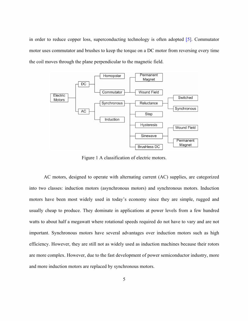
in order to reduce copper loss, superconducting technology is often adopted [5]. Commutator
motor uses commutator and brushes to keep the torque on a DC motor from reversing every time
the coil moves through the plane perpendicular to the magnetic field.
Figure 1 A classification of electric motors.
AC motors, designed to operate with alternating current (AC) supplies, are categorized
into two classes: induction motors (asynchronous motors) and synchronous motors. Induction
motors have been most widely used in today’s economy since they are simple, rugged and
usually cheap to produce. They dominate in applications at power levels from a few hundred
watts to about half a megawatt where rotational speeds required do not have to vary and are not
important. Synchronous motors have several advantages over induction motors such as high
efficiency. However, they are still not as widely used as induction machines because their rotors
are more complex. However, due to the fast development of power semiconductor industry, more
and more induction motors are replaced by synchronous motors.
5

Synchronous motors can further be classified into several types: brushless DC motors,
sine wave motors including PMSMs and wound field synchronous motors, hysteresis motors,
step motors, and reluctance motors.
Brushless DC motors, which have trapezoidally back-EMF, evolved from brush DC
motors as power electronic devices became available to provide electronic commutation in place
of the mechanical commutation provided by brushes. Brushless DC motors tend to be more
popular than AC synchronous motors in low cost and low power applications due to its
simplicity, though the efficiency is lower than that of PMSMs.
Sine wave synchronous motors have sinusoidal back-EMF, so are commonly referred as
AC synchronous motors. AC synchronous motors have sinusoidally distributed windings and the
generated back-EMF in each armature winding has a sinusoidal shape. These motors are driven
by sinusoidal currents and produce constant torque. A wound field synchronous motor has the
winding in the rotor that is supplied with DC current to generate constant magnetic flux. When
the winding in the rotor is replaced with permanent magnet, it is called PMSM. A PMSM has
higher efficiency than a wound field synchronous motor because the absence of active windings
in the rotor leads to no conduction loss in the rotor.
There are also other types of motors such as hybrid motors and double salient motors. A
hybrid motor is a motor that combines two or more types of motor structures together [6], [7]. A
double salient motor is a motor that has both permanent magnets and windings in the stator. It
incorporates the merits of both BLDC and SRM: a) single configuration and robust rotor, and b)
high efficiency because of the permanent magnets [8]-[10].
6

2.2 Modeling of PMSM
2.2.1 Clarke’s Transformation
Clarke’s transformation is a method of transferring three-phase to two-phase in stationary
coordinate system. In Figure 2, the three-phase variables are denoted as a, b and c. The two-
phase variables are denoted as α and β. A third variable known as the zero-sequence component
is added to make the transformation to be bi-directional:
]][[][ 00 abcfTf αβαβ = (2.1)
where variable f can be currents, voltages, or fluxes, and the transformation matrix is given by
⎥⎥⎥
⎦
⎤
⎢⎢⎢
⎣
⎡−−−
=
21
21
21
23
23
21
21
0 01
32
αβT (2.2)
And the inverse transform is
[ ]⎥⎥⎥
⎦
⎤
⎢⎢⎢
⎣
⎡
−−−=−
11101
23
21
23
211
0αβT (2.3)
Some literatures may express them as
⎥⎥⎥
⎦
⎤
⎢⎢⎢
⎣
⎡−−−
=
21
21
21
23
23
21
21
0 01
32
αβT (2.4)
7
[ ]⎥⎥⎥
⎦
⎤
⎢⎢⎢
⎣
⎡
−−−=−
11101
32
23
21
23
211
0αβT (2.5)
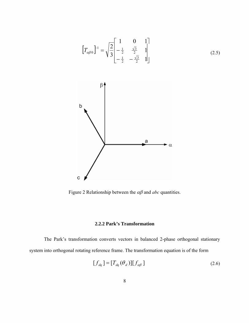
Figure 2 Relationship between the αβ and abc quantities.
2.2.2 Park’s Transformation
The Park’s transformation converts vectors in balanced 2-phase orthogonal stationary
system into orthogonal rotating reference frame. The transformation equation is of the form
])][([][ αβθ fTf ddqdq = (2.6)
8

where θd is the angle between α-axis and d-axis as shown in Figure 3, and the dq transformation
matrix is defined as
[ ] ⎥⎦
⎤⎢⎣
⎡−
=θθθθ
θcossinsincos
)(dqT (2.7)
And its inverse is given by
[ ] ⎥⎦
⎤⎢⎣
⎡ −=−
θθθθ
θcossinsincos
)( 1dqT (2.8)
Figure 3 Relationship between αβ axis and dq axis.
Park’s transformation is used to transform the stator quantities of a synchronous machine
onto a dq reference that is fixed to the rotor. The positive d-axis is aligned with the magnetic axis
of the field winding. When the rotating reference frame is based on the inverter output voltage
vector, this coordinate system is called r-δ coordinate system. d-q and r-δ coordinate systems
rotate at the same speed in the steady state but their speeds differ during the transient state. The
9

relationship between dq-axis and rδ-axis is shown in Figure 4 where angle δ is called the load
angle.
Figure 4 Relation between dq-axis and rδ-axis
2.2.3 Circuit Representation of PMSM
There is a wealth of literature on the synchronous machine modeling and the
determination of parameters [11]-[16]. Of these, the most popular and widely adopted is the
coupled-circuit approach that is also easy to understand [16]. Figure 5 shows a circuit
representation of an idealized three-phase synchronous motor.
Three phases connected in Y connection represents stator part. In rotor part, although the
rotor may have only one physically identifiable field winding (f) (for permanent magnet motor,
there is no field winding, but field winding can be used to represent permanent magnet field),
10

additional windings, such as winding g, are often used to represent the damper windings and the
effects of current flow in the rotor iron due to iron loss. For the salient-pole rotor machine,
usually two such additional windings are used, one on the d-axis (kd) and the other on the q-axis
(kq). Most synchronous generators can be adequately represented by a model that is based on an
equivalent idealized machine with one or two sets of damper windings, besides the field winding.
Damper windings in the equivalent machine can be used to represent the damping effects of eddy
currents in the solid iron portion of the rotor poles.
Figure 5 Circuit representation of an ideal machine.
2.2.4 Mathematical Modeling
Mathematical models of PMSM are often used in simulations. After transformations and
derivations, a PMSM can be represented using the following equations [16]
11

dtd
ir
dtdir
dtdirv
dtd
dtd
irv
dtd
dtdirv
kqkqkq
kdkdkd
s
rd
qqsq
rq
ddsd
λ
λ
λ
θλλ
θλλ
′+′′=
′+′′=
+=
++=
−+=
0
0
000 (2.9)
where the flux linkages are
mmdm
kqkqkqqmqkq
mkdkdkddmdkd
ls
kqmqqqq
mmdkdmdddd
iL
iLiLiLiL
iL
iLiLiLiLiL
′=
′+=′+′′+=′
=
′+=
′+′+=
λ
λλλ
λ
λλ
00
(2.10)
where
Vq, Vd, V0 qd0 voltages
iq, id, i0 qd0 currents
λq , λd , λ0 qd0 flux linkages
rs armature or stator winding resistance
θr rotor angle
Lmq, Lmd, mutual inductance in q-axis and d-axis
Lls armature or stator winding leakage inductance
12

Lq q-axis synchronous inductance, and Lq= Lmq + Lls
Ld d-axis synchronous inductance, and Ld= Lmd + Lls
, equivalent q-axis and d-axis damper winding resistance kqr′ kdr′
,kqλ′ kdλ′ equivalent q-axis and d-axis damper flux linkage
equivalent d-axis damper inductance kdkdL′
, equivalent q-axis and d-axis damper current kqi′ kdi′
equivalent magnetizing current of the permanent magnets mi′
λm flux linkage of permanent magnet
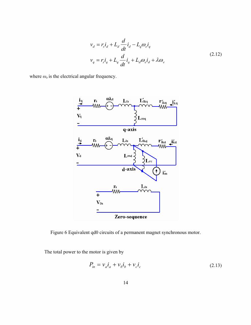
So the equivalent qd0 circuit is given in Figure 6 where Lrc is the equivalent permanent magnet
inductance that is associated with its recoil slope. It is lumped with the common d-axis mutual
inductance of the stator and damper windings, and the combined d-axis mutual inductance
denoted still by Lmd. A lot of literatures described the measurement and calculation of the above
parameters for simulations [17]-[21].
Most of PMSMs are designed without damping windings, so in reality, the damping
windings represent the associated loss in the rotor. If the loss associating with the rotor can also
be ignored, then and both become zero, so kqi′ kdi′
qqq
mddd
iLiL
=+=
λλλ
(2.11)
Therefore, (2.9) can be simplified as
13
ededqqqsq
qeqdddsd
iLidtdLirv
iLidtdLirv
λωω
ω
+++=
−+=
(2.12)
where ωe is the electrical angular frequency.
Figure 6 Equivalent qd0 circuits of a permanent magnet synchronous motor.
The total power to the motor is given by
ccbbaain ivivivP ++= (2.13)
14
Or it is
( )( ) )(23
23
23
)(23
22dqqde
dd
qqdqs
ddqqin
iidt
didt
diiir
ivivP
λλωλλ−+⎟⎟
⎠
⎞⎜⎜⎝
⎛+++=
+=
(2.14)
where the first term is the ohmic loss, the second term is the rate of change in magnetic energy,
and the last term is the electromagnetic power that converts to mechanical power
)(23
dqqdeem iiP λλω −= (2.15)
So the developed torque is
[ ]qdqdqm
dqqdr
emem
iiLLip
iipPT
)(23
)(23
−+=
−==
λ
λλω
(2.16)
where p is the number of pole pairs.
2.2.5 Phasor Diagram
When in steady-state, (2.12) will reduce to
fdedqsq
qeqdsd
EiLirv
iLirv
++=
−=
ω
ω (2.17)
where Ef, refered to as the steady-state field excitation voltage on the state side, is given by
efE λω= (2.18)
15

If written in space vector format, (2.17) becomes
fdqq
qd
EIIV
IIV
++=
−=
des
qesd
Lr
Lr
ω
ω (2.19)
And its scale format is
fddeqsq
qqedsd
EILjωIrV
ILjωIrV
+−=
+= (2.20)
Figure 7 shows the phasor diagrams of the motor with (a) a leading power factor, and (b)
a lagging power factor. Here, θ is the power factor angle, and δ is the load angle. As shown in
Figure 7 (a), for motoring with a leading terminal power factor, the armature magnetomotive
force (MMF), Fa, has a d-axis component that bucks the field MMF, Ef. When the terminal
voltage is increased, the power factor will change from leading to lagging, and Fa will reinforce
Ef as shown in Figure 7 (b).
2.3 PMSM Design Procedure
The design of electrical machine is interdisciplinary. Complicated mechanical,
electromagnetic, and thermal analysis must be considered. Figure 8 shows the general design
flow chart. The design work begins with the required specifications such as the rated speed, rated
voltage, output power, efficiency, total weight, and overall dimensions. According to the
experience, previous knowledge, and sizing equations, the basic design parameters of the motor
such as machine structure, type of the permanent magnet, number of poles and the winding
16
structure, can be selected first. Then the motor dimensions such as rotor, stator, and airgap are
roughly determined based on sizing equations and some tradeoffs. After that, electromagnetic
analysis and simulation are performed. At the same time, rotordynamic analysis, rotor stress
analysis, and thermal analysis are also considered to make sure that they meet the requirements.
The operation point of the permanent magnets has to be taken into account to avoid the
demagnetization of the magnets in all loading situation. An external magnetic field at a high
temperature can also cause demagnetization. The magnetic state of permanent magnets must be
checked in maximum operation conditions as well as in possible fault situations considering also
the temperature of the permanent magnets during these situations [22]. The design process of
electric machines involves continuous iterations of electromagnetic, thermal, structural, and
rotordynamic design and analysis. An optimum design requires the considerations of all these
design criteria. Both analytical analysis and FEM are used in electromagnetic design. Analytical
analysis method is based on permanent magnet synchronous machine theory. It provides fast
initial study of the machine parameters. FEM provides very accurate simulation results of the
machine performances such as airgap flux density, back-EMF, and losses. So it is especially
useful in the optimization.
The rotor aspect ratio, which is defined as length over diameter, is an important
parameter that is considered in the design process and optimization. A low rotor aspect ratio has
high rotor stiffness, so it has high critical speed. However, large rotor diameter of the low aspect
ratio machine may have large windage loss and large sleeve thickness which is not desirable.
17

(a)
(b)
Figure 7 Phasor diagram of the motor with (a) a leading power factor, and (b) a lagging power factor.
18

The thermal design goal is to insure acceptable operating temperatures of components
under all system operating conditions for optimum performance and high reliability. For low
power motor, the temperature of the rotor is very critical since no additional cooling is provided
for the rotor, mainly due to the small size of the rotor. Optimization is an important step to
obtain best motor performance based on the desired criteria. If the simulation results meet the
requirements, the prototype can be built and then tested. Otherwise, the above procedures need to
be repeated until the simulation results are satisfied.
Figure 8 A flowchart of PMSM design.
19

2.4 Motor Type and Structure Consideration
Selection of motor type and its structure is based on the applications and requirements.
Based on cost, robust and efficiency, each type of motor has its own advantages and
disadvantages. For high-speed and super high-speed applications, many types of motors can be
considered. (a) Induction motor (IM) is a low cost option. It is relatively easy to manufacture.
However, the efficiency of conventional induction motor is relatively low at high-speed due to
high iron loss in the rotor [2]. When it is scaled down in size and power, the efficiency will also
reduce considerably [23]. (b) Switched reluctance motor (SRM) has high reliability due to its
simple and robust rotor structure [2]. However, the core loss in the solid rotor is very large at
super high-speed. Lamination of the rotor can reduce the core loss in the rotor. However, it is not
recommended at super high-speeds since it will reduce critical speeds. (c) Wound-field
synchronous motor (WFSM) is widely used in high power applications. It is not practical for
high-speed applications since the mechanical contact of the slip rings and brushes are not reliable
at high-speeds. (d) BLDC also has high power density, but since large harmonics of the back-
EMF introduces large iron loss at high-speeds, the efficiency will reduce at super high-speeds.
(e) PMSM offers the advantage of high efficiency compared to other types of motors since there
is no excitation power loss in the rotor, and low eddy current loss in the stator and rotor.
Therefore, there is an increasing interest to consider PMSM for super high-speed applications.
Synchronous motors are used predominantly where a constant speed is required that is
independent of load torque and supply voltage. Mechanical position and speed are the respective
position and speed of the rotor output shaft. Electrical position is defined such that the movement
20
of the rotor by 360 electrical degrees puts the rotor back in an identical magnetic orientation. The
relationship between mechanical and electrical position and speed can be stated as
me pθθ = (2.21)
me pωω = (2.22)
where eθ and mθ are electrical and mechanical positions, respectively, eω and mω are electrical
and mechanical frequencies, in rad/s, respectively, and p is the number of magnetic pole pairs.
The mechanical speed N in terms of revolutions per minute (rpm) can be stated as
mN ωπ30
= (2.23)
The stator core can be slotted or slotless according to requirements. Increasing the slot
area means increasing the conduct area, and copper loss, also called ohmic loss, will reduce for
the same applied current. However, if the motor size is fixed, increasing the slot area means
reducing the teeth area, so the magnetic permeance will reduce due to saturation. The alternation
of slots and teeth along the airgap of electric machines is a compromise solution to the conflict
between magnetic permeance and electric conductance. The slotted machines have higher torque
density than the slotless machines, but slotless machines have higher efficiency in the higher
speed range. Slotting also has some other disadvantages [24]: (a) The iron surface along the
airgap is no longer smooth, but interrupted by zones of high reluctance; (b) The MMF across the
airgap is not changing smoothly in the peripheral direction, but instead of in steps; (c) It will
cause saturation phenomena in the leakage fields near the airgap; (d) Slots introduce a low limit
to the pole pitch length of heteropolar machines, due to the necessity of a minimum tooth width
21

for magnetic, mechanical, and manufacturing reasons.
There is an abundance of literature reported on undesirable harmonics in voltage and
current, on additional losses affecting the conversion efficiency and the machine temperature, on
parasitic torques causing cogging at standstill and crawling at low speed of cage induction
motors, on bearing currents, on radial and torsional vibrations, and on noise problems. For many
of these phenomena, a common cause is the slotting of the core.
The skewing of slots, or of salient poles, has been used against harmful slot effects.
However, it can only reduce effect, but does not take away the cause. Skew makes the machine
asymmetric in the axial direction, and that it is possibly the cause of more other losses, parasitic
forces, and noise.
For high power density motor, the use of high BH-product magnets is necessary, so the
magnetic saturation in the slot teeth becomes serious. Therefore, improvement of power density
of the motor is limited. Though these problems can be solved through designing wide-slot teeth,
it leads to decreased power density of the motor because the MMF of the windings decreases.
Thus, for high efficiency, the slotless permanent magnet (PM) motor is one of viable solution to
overcome these problems. The slotless PM motor construction eliminates the magnetic saturation
and iron loss in the stator teeth and therefore, high efficiency can be expected [25]. The major
disadvantages of the slotless motor are that the power density is low, and the thermal
conductivity between the winding and stator is low. Slotless design is not practical for high
power machine design.
The motor can also be in axial-flux structure or radial-flux structure. Axial-flux
22

permanent magnet (PM) motor has simple structure. It has relatively high efficiency and low
cost, so the machine can be used in the applications that require high power and torque density,
high efficiency and low noise with the use of high BH-product rare-earth magnetic materials
[26]. Axial flux PM motor can provide higher electromagnetic torque than radial-flux motor
when the structure is flat and with high number of poles [27]. Axial flux motors with multi-poles
and multi-stages are superior in terms of the torque density to the equivalent standard radial-flux
PM motors [28]. Axial-flux PM motor has high power density than traditional induction motor
by using high BH-production rare-earth magnetic materials and the degree of improvement could
reach a factor of three. Even using the low cost ferrite magnets, the power density can still be
increased by a factor of two [29]. However, the major disadvantage of axial-flux motor is that it
requires larger diameter than radial-flux motor for the same output power, which makes it
unsuitable for super high-speed applications due to critical speeds.
2.5 Losses in PMSM
Materials used in an electric machine may be grouped into [30]: (a) soft magnetic
materials, (b) electrical conducting materials, (c) insulating materials, and (d) permanent
magnets. The loss varies significantly for different materials in different conditions.
2.5.1 Iron Loss
Soft magnetic materials form the magnetic circuit in an electric machine. An ideal
23

material for this purpose is one exhibiting the highest possible permeability and saturation flux
density, and the lowest possible core loss or iron loss.
The core loss or iron loss produced in a magnetic material operating in an alternating
magnetizing field is generally separated into two components: hysteresis loss, and eddy current
loss.
2.5.1.1 Hysteresis Loss
Hysteresis loss is due to a form of intermolecular friction when a variable magnetic field
is applied to the magnetic material. The loss per cycle is proportional to the area enclosed by the
hysteresis loop on the B-H characteristics of the material. The hysteresis loss increases with the
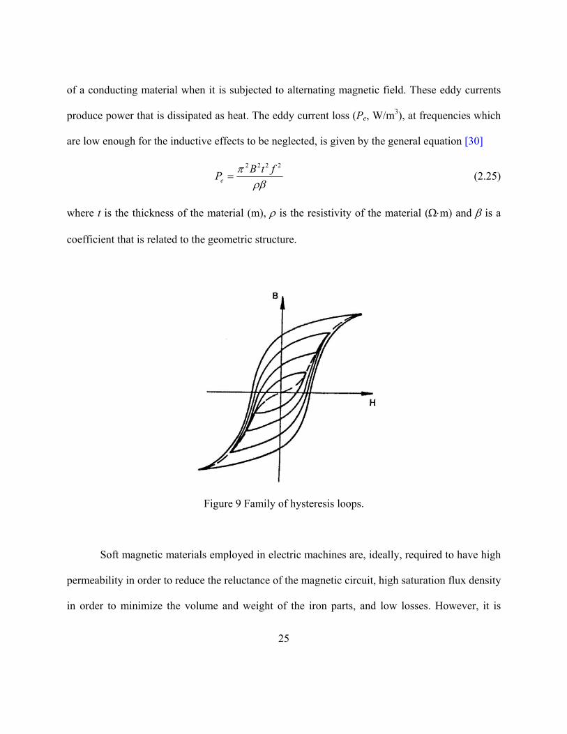
maximum magnetic field as is illustrated in Figure 9.
The empirical formula expressing the hysteresis loss (Ph, W/m3) in terms of the
maximum flux density (B, T) and frequency (f, Hz) was developed by Steinmetz [30] as follows
fBP nh η= (2.24)
where η is a material constant and n is an exponent which has a value between 1.6 and 2.0. The
loss is closely related to the coercivity, and processing of materials to reduce coercivity also
reduces hysteresis loss.
2.5.1.2 Eddy Current Loss
The term “eddy current” refers to circulating electric currents that are induced in a sheet
24
of a conducting material when it is subjected to alternating magnetic field. These eddy currents
produce power that is dissipated as heat. The eddy current loss (Pe, W/m3), at frequencies which
are low enough for the inductive effects to be neglected, is given by the general equation [30]
ρβπ 2222 ftBPe = (2.25)
where t is the thickness of the material (m), ρ is the resistivity of the material (Ω⋅m) and β is a
coefficient that is related to the geometric structure.
Figure 9 Family of hysteresis loops.
Soft magnetic materials employed in electric machines are, ideally, required to have high
permeability in order to reduce the reluctance of the magnetic circuit, high saturation flux density
in order to minimize the volume and weight of the iron parts, and low losses. However, it is
25

impossible to optimize all of these properties in a single material. This is because there are a
large number of factors that affect magnetic properties (chemical composition, mechanical
treatment and thermal treatment are the most important), and a conflict exists between obtaining
low losses and high permeability. To reduce core loss, that is to suppress the unwanted electrical
conductivity, the core section is subdivided. The subdivision in machines and transformers is
mostly realized by a laminated core, which is built up from thin sheets.
Besides the laminated core, there are also two alternative materials [31]: (a) amorphous
materials, instead of the poly-crystalline structure, have very low hysteresis and eddy-current
losses. Amorphous metals are produced by rapid cooling of alloys consisting of iron, nickel and
/or cobalt together with one or more of the following metalloids which is an element or
compound exhibiting both metallic and non-metallic properties: boron, silicon and carbon; and
(b) powder materials (such as grain-oriented electrical steels), which, in spite of a rather low
resulting core permeance, may be attractive for high-frequency applications, and also on account
of effective damping of vibrations.
Hysteresis loss and eddy current loss are both related to the frequency. If the current
distortion is so significant that results in very high frequency harmonics, the skin effect should
also be considered [32].
Eddy current loss can also be divided into classical eddy current loss and excess eddy
current loss. Therefore, at a given frequency, the core loss for electrical steel can be calculated
from [33], [34]:
2/322 )()( fBKfBKfBkP pepcphC ++= (2.26)
26
where Kh, Kc and Ke are the coefficients of hysteresis loss, classical eddy current loss, and excess
eddy current loss, respectively; Bp is the peak flux density. The coefficients can be found by
measuring the loss of the sample or using curve fitting by a least square method [35].
When the core is magnetized by nonsinusoidal magnetic field, the distorted excitation,
which can be represented by higher order harmonics, has to be considered [36], [37]. When
under rotational magnetic field condition, the calculation methods are discussed in [38], [39].
The finite element method is also widely used to directly simulate the core loss [40], [41].
2.5.2 Copper Loss
Copper loss is the loss due to the current going through the conductors. The copper loss
consists of I2R loss and eddy current loss. The I2R loss is given by
RImPc2
1= (2.27)
where m1 is the number of phases, I is the armature current, and R is the armature resistance.
The I2R loss can be very large when large current flows through the conductor with large
ohmic resistance. Recently, high temperature super conducting materials are frequently used in
some high current and high power machines to reduce the I2R loss [5].
The eddy current loss comes from: (a) skin effect resulting from the same source
conductors, and (b) proximity effect resulting from the motion of the DC magnetic flux, such as
permanent magnet.
An electromagnetic wave entering a conducting surface is damped and reduces in
27

amplitude by a factor 1/e, where e is equal to 2.71828…, in a distance δ given by
σωµδ
0
2= (2.28)
where ω is the angular frequency of the radiation and σ is the electrical conductivity of the
conducting material. This distance is referred to as the skin depth of the conductor. The skin
effect is caused by electromagnetic induction in the conducting material which opposes the
currents set up by the wave E-field.
When the electrical frequency is very low, and skin depth is much larger than the radius
of the copper wire, the skin effect can be ignored. For high-speed slotless motor, the main source
of eddy current loss comes from proximity effect caused by the rotation of permanent magnet.
The eddy current loss per volume for round wire can be calculated based on the following
equation [42]
(2.29) ρω 32/222 dBP PE =
where Bp is the peak flux density, ω is the electrical angular frequency, d is the wire diameter,
and ρ is the wire resistivity.
2.5.3 Windage Loss
Windage is the term generally used to denote the loss due to fluid drag on a rotating
body. For the motor at low-speed and without the cooling fan, windage losses are not significant.
However, when the rotor rotates at high-speed, windage in air is significant and hence the
28

accurate prediction and reduction of windage loss are becoming more and more important with
the growing development of high-speed machinery. Prediction of windage losses is now an
essential part of the design process for high-speed machinery. Not only is the loss itself
important in terms of maximizing efficiency, but also the heat generated by the loss can cause
overheating problems. Some studies have been made to calculate the windage loss [43]-[46].
The windage loss of axial-flux motor is given by [45]
g
iorWA L
RRP2
)( 442 −=
πµω (2.30)
where µ is the viscosity of the air which is equal to 2.08 × 10⁻⁵ kg/m.s at room temperature, ωr is
the rotor angle speed, Lg is the physical airgap length, Ro is the shaft outer radius, and Ri is the
shaft inner radius.
The windage loss of radial flux motor is given by [46]
LrCP airdWR43ωπρ= (2.31)
where Cd is the drag coefficient, ρair is the air density,ω is the rotor angular velocity, r is the
rotor radius, and L is the length of the rotor. The Reynolds number is defined as
µρω /airge rlR ×= (2.32)
where lg is the air gap length, and µ is the air viscosity. The Taylor Number is defined as
( ) 5.0/ rlRT gea = (2.33)
When Ta >> 400, it will have turbulence behavior, and the drag coefficient is given by
( ) 2.00095.0 −= ad TC (2.34)
29

2.6 Analysis and Sizing
The magnetic flux can be analyzed using lumped element model. The instantaneous
magnetic flux for some specific motors can also be calculated analytically [47]-[50].
Sizing equations are often used to assist in the design of electric machinery. V. B.
Honsinger developed four sizing equations for the radial-flux motor with slotted structure [51].
These are:
es LDnP 300/ ξ= (2.35)
errs LDnP 2/ ξ= (2.36)
es LDnP 5.200/ ξ ′= (2.37)
errs LDnP 5.2/ ξ ′= (2.38)
where P is the output power, ns is the machine mechanical angular speed, D0 is the stator outer
diameter, Le is the core length, Dr is the rotor diameter, and 0ξ , rξ , 0ξ ′ , rξ ′ are coefficients that
contain the useful information regarding the machine structure. The purpose of sizing is to
maximum these coefficients to get maximum power to speed ratio. The equation has been
used for decades to size electric machinery. However, it does not consider several key factors
such as slot and tooth dimensions, flux densities in the iron parts. The approach provides
many relations between physical dimensions and density-like quantities and is well adapted to
produce a design that is geometrically compatible from the start. and equations,
derived from (2.35) and (2.36), are preferred because they give more information than do the
er LD2
eo LD3
er LD 5.2eo LD 5.2
30
other two.
General purpose sizing equations for both axial-flux and radial-flux PM machines were
also developed in [52], [53]. These sizing equations can provide very basic sizing for the
machine design. These equations, which are adjustable for different topologies and different
machines, can take into account different waveforms and machine characteristics. To determine
the motor dimensions in more details, a set of sizing equations considering our specific motor
structure have been developed in the dissertation.
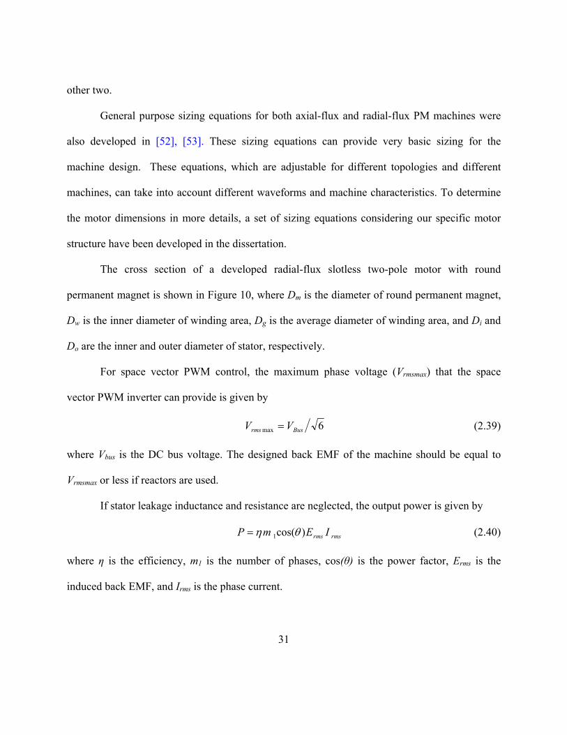
The cross section of a developed radial-flux slotless two-pole motor with round
permanent magnet is shown in Figure 10, where Dm is the diameter of round permanent magnet,
Dw is the inner diameter of winding area, Dg is the average diameter of winding area, and Di and
Do are the inner and outer diameter of stator, respectively.
For space vector PWM control, the maximum phase voltage (Vrmsmax) that the space
vector PWM inverter can provide is given by
6max Busrms VV = (2.39)
where Vbus is the DC bus voltage. The designed back EMF of the machine should be equal to
Vrmsmax or less if reactors are used.
If stator leakage inductance and resistance are neglected, the output power is given by
rmsrms IEmP )cos(1 θη= (2.40)
where η is the efficiency, m1 is the number of phases, cos(θ) is the power factor, Erms is the
induced back EMF, and Irms is the phase current.
31

Figure 10 Cross section of a radial flux slotless two-pole motor with round permanent
magnet
In order to calculate peak airgap flux density, a narrow bar of magnetic path with the
angle of θ is considered. Based on the definition, the reluctance of the airgap and permanent
magnet can be expressed as
LDD
R iog
)/ln(1θ
= (2.41)
LR
rmm θµ
2= (2.42)
where L is the length of stator and µrm is the relative permeability of the permanent magnet. If the
reluctance of the stator iron can be ignored, the airgap peak flux and flux density can be
32

represented as
gm
mmr
gm
mru RR
RLDBRR
R222 +
=+
=θ
φφ (2.43)
))/ln(1/
2/ rmmi
gmr
g
ugpk DD
DDBLD
Bµθ
φ+
== (2.44)
where Br is the residue flux density of the permanent magnet. The flux density in the stator is
given by
io
gpkgspk DD
BDB
−= (2.45)
The flux linkage each pole is written as
gpkgpole BLD=φ (2.46)
So the induced back EMF can be stated as
LDBkfNkfNE ggpkwphpolewphrms πφπ 22 == (2.47)
The phase current can be represented as
1
22
1 8)(
2 mNDDJk
mNNJkAN
Iph
wicucu
php
cucucuprms
−==
π (2.48)
where Np is the number of parallel coils, kcu is the copper filling factor, Jcu is the current density,
Nph is the number of turns for each coil, and m1 is the number of phases.
The inner diameter of the winding area can be expressed as
shaftmw TgDD 22 ++= (2.49)
Inserting (2.47), (2.48), (2.49) into (2.40) gives
33

( )( )rmmi
shaftmimrcuw DD
LTgDDDBfkkP
µθηπ
)/ln(122
)cos(82
222
+
++−= (2.50)
2.7 FEM Simulation of PMSM
Sizing equations can be used to determine the dimensions of the motor. They can also be
used on the size optimization to provide best power density. However, since these equations
cannot project the motor performance, especially at super high-speeds, for best performance,
more accurate FEM should be used to calculate motor performance and optimize dimensions.
2.7.1 Calculation of Inductance
An inductor is an energy storage device whose presence is manifested by the magnetic
flux produced by current flow. The inductance is defined as
0IL Λ
= (2.51)
where Λ is themagnetic flux linkage, and I0 is the current that produces the magnetic flux.
Inductance can be sorted as self-inductance and mutual-inductance. For self- inductance,
the magnetic flux linkage is produced by itself. While for mutual-inductance, the magnetic flux
linkage under consideration is produced by the other.
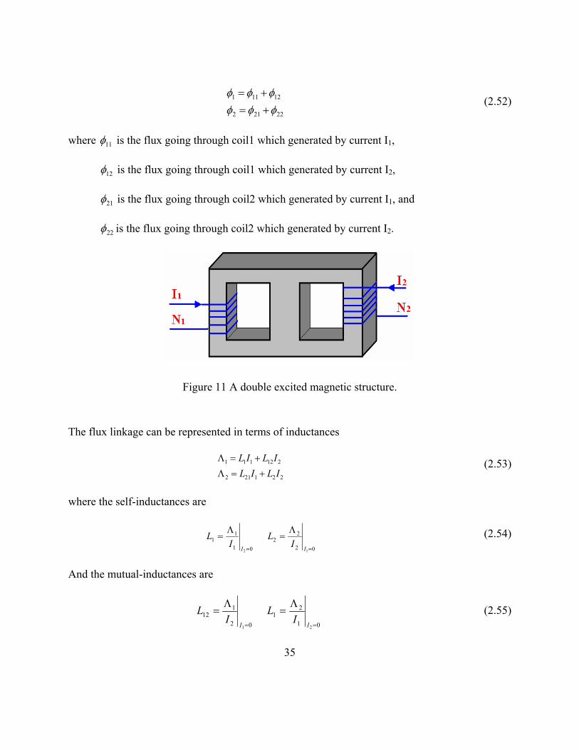
Figure 11 shows a double excited magnetic structure as an example. The magnetic flux
going through coil 1 and coil 2 can be stated as
34
22212
12111
φφφφφφ
+=+=
(2.52)
where 11φ is the flux going through coil1 which generated by current I1,
12φ is the flux going through coil1 which generated by current I2,
21φ is the flux going through coil2 which generated by current I1, and
22φ is the flux going through coil2 which generated by current I2.
Figure 11 A double excited magnetic structure.
The flux linkage can be represented in terms of inductances
221212
212111
ILILILIL
+=Λ+=Λ (2.53)
where the self-inductances are
01
11
2 =
Λ=
IIL
02
22
1=
Λ=
IIL (2.54)
And the mutual-inductances are
02
112
1=
Λ=
II
L 01
21
2 =
Λ=
II
L (2.55)
35

Some simplified analytical methods to calculate inductances for some kind of motors can be
found in [54]-[58].
Magnetic flux and energy approaches can be used to calculate the motor phase self-
inductances (including airgap inductance and leakage inductance), and mutual inductances. For
PMSM, to simplify the calculation, the stator is assumed to be without high saturation. So the
permanent magnets are replaced by dummy materials having same permeability. Magnetic flux
approach is an inductance calculation method that directly applies the inductance definition
(2.51). The flux linkage can be calculated as
∫ ⋅==Λs
dNN aBφ (2.56)
where N is the number of turns per coil, s is the considered area, and B is the flux density. Flux
linkage can also be calculated by a line integral of vector potential A along the boundary of the
area. For 2-D FEM, the flux is calculated by
)( 21 AAl −=φ (2.57)
Where l is the core length or machine depth, and A1 and A2 are the magnetic potentials at the two
points where the boundary intersects the 2-D finite-element plane. For windings with a non-
negligible cross-sectional area, the flux can be calculated as,
⎥⎥⎥
⎦
⎤
⎢⎢⎢
⎣
⎡
−=∫∫∫∫
S2
dsA
S1
dsAl SS 2
21
1
φ (2.58)
where S1 and S2 represent the area of the winding carrying the positive and the negative
36

currents, respectively.
To derive energy approach, assuming the inductance will not change with the applied
current within the considered range, that is, there is no saturation and the energy and co-energy
are the same, the instantaneous power delivered to the magnet can be stated as
dtdiiL
dtdiiL
dtdiiL
dtdiiL
dtdi
dtdieieiP
222
1221
2112
111
22
112211
+++=
Λ+
Λ=+=
(2.59)
By integrating the above equation, we can get the instantaneous energy stored in the inductors as
2112222
211 2
121 iiLiLiLW ++= (2.60)
The energy W can be simulated using FEM. Therefore, self- and mutual inductances can be
calculated by running the FEM for several times with different currents.
2.7.2 Back-EMF Analysis and Simulation
The conductors under the rotating magnetic field generate induced voltage, which is
called back-EMF. Many methods can be used to calculate the back-EMF of a motor [59]. The
following equation is a widely used method to calculate back-EMF
uwrms nkfE φπ2
2= (2.61)
where f is the electrical frequency, kw is the winding factor, n is the number of serial coils per
phase, and uφ is the useful flux per pole. The instantaneous back EMF can be calculated as
37

dtd
dd
dtdeb
θθ
⋅Λ
−=Λ
−= (2.62)
where
πθ 260
×=N
dtd (2.63)
and N is the mechanical speed in rpm.
2.7.3 Torque Simulation
The torque on an object can be calculated using virtual work principles. The torque on
the rotor about the axis of the rotation is given by the following relationship
Constant
),(=
=id
idWTθθ (2.64)
where ),( iW θ is the magnetic co-energy of the system and the current i is held constant. Field-
oriented currents are applied to the phase winding to simulate torque. For fractural winding, to
accurately simulate torque, it is necessary to model the fractional winding as accurate as
possible.
The operation of electric motors depends on the forces or torques that act upon either
current carrying conductors or permanent magnet parts. It is essential in electric machine design
to calculate the force or torque as accurately as possible. To calculate the force or torque in an
electromagnetic device by FEM, the virtual work and the Maxwell stress tensor are two basic
methods that are commonly used. The virtual work method calculates the force or torque by
38

taking the partial derivative of the total energy or co-energy against the virtual displacement. The
Coulomb virtual work method computes the force or torque on a moving structure by direct,
closed form differentiation of the magnetic energy or co-energy of the field in the air gap
between the movable and the fixed parts of the system under consideration. The Maxwell stress
tensor method calculates the force or torque from the magnetic field distribution by adding up
the force or torque over a surface or path in the air enclosing the part of interest. The
improvement of these methods can also be found in the literature [60].
Ansoft Maxwell 2D/3D is one of popular tools to simulate electromagnetic torque and
other performances. Since the torque calculation is very time consuming, a suitable model that is
accurate enough and not so time consuming needs to be developed.
2.7.4 Transient Simulation
To accurately simulate the dynamic behavior of the motor, including copper loss and core
loss, transient time-stepping solver with motion can be used. The equation dealing with coupled
time varying electric and magnetic fields is [61], [62]
AvHVtAJA cs ×∇×+×∇+∇−∂∂−=×∇×∇ σσσν )/( (2.65)
where v is the velocity of the moving parts, A is the magnetic vector potential, t is the time, V is
the electric scalar potential, Js is the current source density, Hc is the coercivity of the permanent
magnets, and σ is the conductivity of the material.
39

2.8 Optimization and Tradeoffs
Optimization is important in motor design to get better performance such as optimal
efficiency, minimizing volume, or minimizing pulsating torque for slotted motor. Many methods
have been used for optimization. The boundary search along active constraints method and the
Han-Powell method are compared and studied [63]. Chaotic theory is used for the motor design
optimization in [64]. Fuzzy optimization technique is used to optimize the motor drive in [65].
Recently, genetic algorithm has been widely used for electromagnetic topology optimization
[66]. Optimization of one parameter may worse other parameters. Some tradeoffs need to be
considered in optimization.
2.9 PMSM Test
The motor test is very important for the optimization of the design. Many literatures give
the procedures for the test of motor performances and parameters [67]-[70]. Spin down, steady
state, and load tests are widely used to measure efficiency and predict losses.
2.9.1 Spin-Down Test
There is a relationship between the electromagnetic torque and the inertia torque as [11]:
mechdampr
em TTdt
dJT −+=ω (2.66)
where Tem is the electromagnetic torque, Tdamp is the damping torque in the direction opposite to
40

rotation because of the friction and windage, Tmech is the externally applied mechanical torque in
the direction of the rotor speed, and J is the rotor inertia.
Spin-down test is a method to test the damping torque. When the motor is free spinning
without externally applied mechanical torque and electromagnetic torque, (2.66) becomes
dt
dJT r
rdamp
ωω1
−= (2.67)
By measuring the initial speed versus time duration of the rotor from the initial speed to fully
stop, the damping torque can be calculated. When performing spin-down test, any armature
electrical loops should be disconnected to ensure that the motor is spinning down freely without
any braking effect.
The moment of inertia, which is also called rotational inertia, is the resistance to any
change in rotation of a body. It is defined as
(2.68) ∫ ∫==M
dmrdJJ0
2
where r is the distance of the mass element dm from the axis of rotation. For a system of point
masses, this becomes
∑=i ii rmJ 2 (2.69)
where ri is the distance of the ith mass from the axis of rotation. Hence, to evaluate the moment of
inertia for an object, one would either do a calculation of the integral over the shape of the
object, or somehow subdivide the object into small mass elements mi to do the summation.
41

2.9.2 Free Spin Test
In steady state, we have
0=dt
d rω (2.70)
If no load is applied, Tmech is equal to zero. Thus, we have
dampem TT = (2.71)
Based on (2.66), the electromagnetic torque can be obtained from
r
ironcuinem
PPPT
ω+−
= (2.72)
where Pin is the input power, Pcu is the copper loss of the winding, Piron is the iron losses in the
stator and rotor, and ωr is the mechanical angular frequency of the rotor.
2.9.3 Load Test
The motor efficiency can be tested by coupling two identical motors, where one machine
is used as a motor and the other as a generator. Figure 12 shows the load test circuitry with
rectifiers, where the resistor is used as electrical DC power load. Due to rectifier circuits, the
phase currents of the generator are not sinusoidal. The load test circuitry without rectifiers is
shown in Figure 13, where three identical power resistors are used as AC loads. In that case, the
currents of the generator are sinusoidal.
The input phase voltages and currents to the motor are represented as
42

)3/2cos()3/2cos(
)cos(
πωπω
ω
−=+=
=
tVVtVVtVV
ma
ma
ma
(2.73)
)3/2cos()3/2cos(
)cos(
θπωθπω
θω
+−=++=
+=
tIItIItII
ma
ma
ma
(2.74)
where Vm is the phase voltage amplitude, Im is the phase current amplitude, and )cos(θ is the
power factor. Because the terminal neutral may not accessible in most 3-phase motors, input
power to the motor can be derived based on phase to phase voltage as
)sin()(3 θacbin IVVP −= (2.75)
Given high efficiencies of the motor and generator, they will have nearly the same efficiencies
which are expressed as
inout PP /=η (2.76)
where Pout is the output power of the generator that can be easily calculated from resistor loads.
43

Figure 12 Motor load test circuitry with rectifiers.
Figure 13 Motor load test circuitry without rectifiers
44
CHAPTER THREE: DESIGN AND MODIFICATION OF AN AXIAL-FLUX PMSM
3.1 Introduction
In this chapter, the design, simulation, test, and modification of an axial-flux surface
mounted PMSM are presented. The designed motor will be used to drive a cryocooler. Axial-flux
motors have been widely used for high torque and low speed applications. For high-speed
applications, there are also some reports [71]-[73]. Axial-flux PMSM is attractive because it can
be easily integrated to the compressor impellers. This was the main reason for the research work
that was focused on this type of motor. Our preliminary research on it can be found in [74].
The basic specifications of the designed axial-flux PMSM are shown in Table 1. The
structure of the axial-flux PMSM and the optimization of the rotor structure are presented. The
optimization is based on minimizing the harmonics of the airgap flux density. Modeling of the
complicated fractional winding is also provided. 3-D FEM simulations of the back-EMF, torque
and torque ripple are performed. The experimental results of the back-EMF are verified with
simulation results. The axial-flux PMSM was built based on the design. It was tested using an
open loop driving circuit with low-pass filters. The waveforms of the phase current and voltage
after low-pass filters are also presented. The bearing loss is calculated separating from the total
loss. Finally, the advantages and disadvantages of this type of motor are discussed, and further
improvements are proposed and verified by experiments.
45

46
Table 1 Specifications of the axial-flux PMSM.
Maximum speed (rpm) 100,000
Rated speed (rpm) 50,000
Rated output power (W) 100
Supplied DC voltage (V) 28
Rotor diameter (mm) 54.6
3.2 Structure and Design Considerations
Figure 14 shows the structure of the designed axial-flux PMSM. The motor configuration
was realized through a single rotor and a single stator. The stator core was slotless, and epoxy
bonding was used to securely attach the winding on the surface of the stator back iron that was
made from sintered metal powder. Four axially magnetized permanent magnets were mounted on
the back of the rotor as shown in Figure 15. The permanent magnets were made of Neodymium-
Iron-Boron (Nd-Fe-B) to provide high energy density. A carbon ring was used to hold the
permanent magnets against the centrifugal force when the rotor operates at high speeds. Steel
ball bearings were used and lubricated with grease.
Although the axial-flux PMSM with sandwich structure, that is one with two external
stators and one internal rotor, or with two external rotors and one internal toroidal stator, is
commonly used, the axial-flux structure with single stator and single rotor can be easily
integrated directly with the compressor impellers since the rotor back iron is a flat disc. This
results in reduced components and therefore the entire system is much small and light for the
same power level.

Figure 14 Axial view of the axial-flux PMSM structure with single rotor and single stator.
Figure 15 Photos of the rotor and its components.
47

The stator core is slotless and the windings were attached to the surface of the stator core
as shown in Figure 16 (a) and (b). Two-layer simplex lap winding was used [78]. Due to low
voltage and high current requirements, the windings were connected in parallel as shown in
Figure 17. Each phase has 4 groups of windings in parallel. Each group has 7 coils and each coil
has one turn.
(a) (b)
Figure 16 Winding structure: (a) winding of one group with 7 turns in the group, and (b) actual winding with a total of 84 turns.
3.3 Analytical Analyses
Magnetic flux densities in the airgap, stator iron and rotor back iron can be estimated by
using one-dimensional lumped magnetic circuits. It is a simple and fast way although not as
accurate as FEM. Lumped magnetic circuit method is very difficult for precise analysis of
magnetic circuits with arbitrary configuration since the analytical solution can hardly be
48

obtained. However, the permeance estimation of some typical configurations is available in the
literature [79]. Some analytical calculations for specific motors, which are based on FEM to
develop the analytical equations, are also available [80].
Figure 17 Parallel winding connections.
Figure 18 shows the magnetic flux orientation of the axial flux PMSM. The
corresponding lumped magnetic circuit can be developed as shown in Figure 19, where the
symbols are as follow
Rs and Rr are relative reluctances of stator iron and rotor iron,
)/( rmaxmm ALR µ⋅= is the relative reluctance of permanent magnet,
ggg ALR /= is the relative reluctance of airgap,
gml RELF
R 411⋅⎟
⎠⎞
⎜⎝⎛ −= is the relative reluctance of leakage path,
49
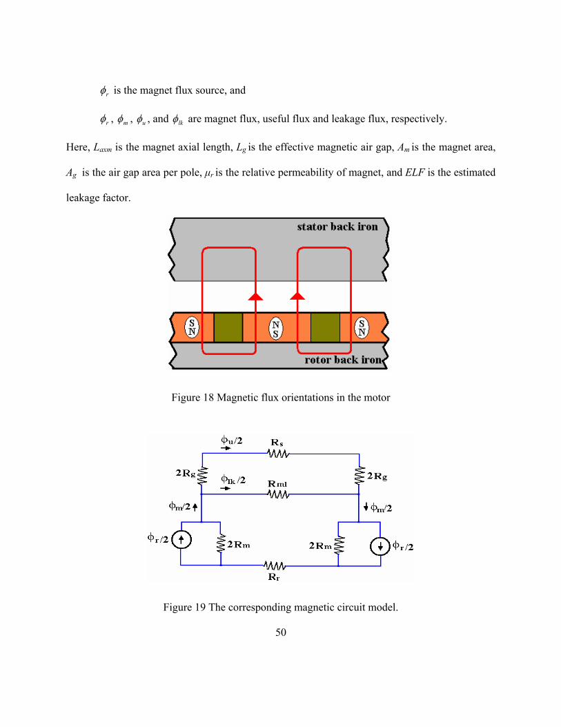
rφ is the magnet flux source, and
rφ , mφ , uφ , and lkφ are magnet flux, useful flux and leakage flux, respectively.
Here, Laxm is the magnet axial length, Lg is the effective magnetic air gap, Am is the magnet area,
Ag is the air gap area per pole, µr is the relative permeability of magnet, and ELF is the estimated
leakage factor.
Figure 18 Magnetic flux orientations in the motor
Figure 19 The corresponding magnetic circuit model.
50

51
Compared to airgap reluctance (Rg), the reluctance of stator iron (Rs) and rotor iron (Rr)
are much smaller, so they can be eliminated. By combining the two series magnet models, the
circuit model can be simplified and leads to Figure 20.
Figure 20 Simplified magnetic circuit model.
The magnetic fluxes are calculated as
mlmg
mlgrm PPP
PP4
4++
+= φφ (3.1)
mlmg
gru PPP
P4++
= φφ (3.2)
and the flux densities in the airgap (Bg), stator back iron (Bsi), and rotor back iron (Bri) are
calculated as
g
ug A
B φ= (3.3)
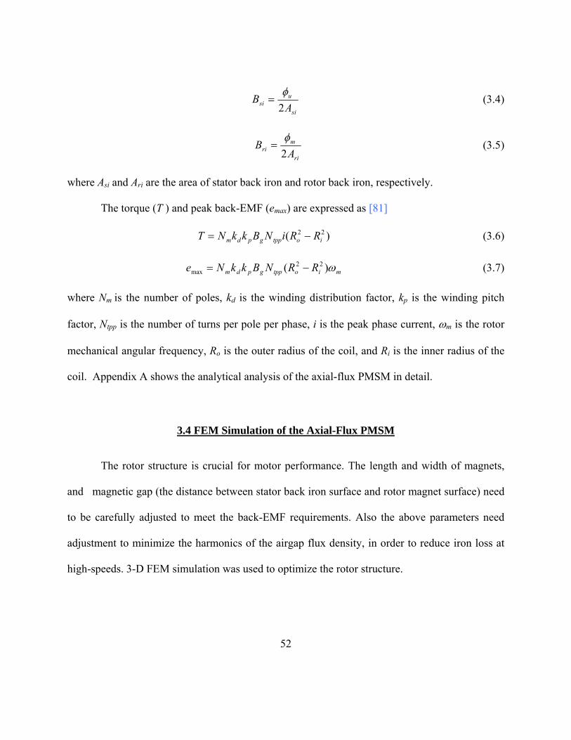
si
usi A
B2φ
= (3.4)
ri
mri A
B2φ
= (3.5)
where Asi and Ari are the area of stator back iron and rotor back iron, respectively.
The torque (T ) and peak back-EMF (emax) are expressed as [81]
)( 22iotppgpdm RRiNBkkNT −= (3.6)
miotppgpdm RRNBkkNe ω)( 22max −= (3.7)
where Nm is the number of poles, kd is the winding distribution factor, kp is the winding pitch
factor, Ntpp is the number of turns per pole per phase, i is the peak phase current, ωm is the rotor
mechanical angular frequency, Ro is the outer radius of the coil, and Ri is the inner radius of the
coil. Appendix A shows the analytical analysis of the axial-flux PMSM in detail.
3.4 FEM Simulation of the Axial-Flux PMSM
The rotor structure is crucial for motor performance. The length and width of magnets,
and magnetic gap (the distance between stator back iron surface and rotor magnet surface) need
to be carefully adjusted to meet the back-EMF requirements. Also the above parameters need
adjustment to minimize the harmonics of the airgap flux density, in order to reduce iron loss at
high-speeds. 3-D FEM simulation was used to optimize the rotor structure.
52

3.4.1 Simulation and Optimization of Magnetic Flux Distributions
To accurately get the flux density distributions, it is necessary to use some numerical
methods. FEM is one of very powerful numerical methods to do electromagnetic analysis. For
FEM simulation, to make the simulation accurate and fast, it is very important to construct an
effective simulation model. Figure 21 shows the FEM simulation model that has been developed
for the simulation of flux density using magnetostatic solver. Because of the symmetrical
structure, only quarter of the structure is required. The shaft, casing and magnet keeper are not
included in this model since their permeability is close to one, and no loss is considered for
magnetostatic solver.
Figure 21 FEM simulation model to calculate flux density.
Figure 22 (a) shows the flux density distribution in the airgap for different magnetic gaps
where the pole pitch (the ratio of magnet width to full width) is 0.7 and the thickness of the
53

permanent magnet is adjusted to keep the same peak flux density. Figure 22 (b) shows the
corresponding normalized harmonics. From Figure 22 (b), it can be seen that increasing the
magnetic gap reduces the harmonics so that the eddy current loss decreases in the stator.
However, the large magnetic gap will reduce the magnetic coupling. Therefore, magnet length
needs to be increased to keep the same peak flux density for the same output power. This will
cause a reduced power to volume ratio. Large airgap also increases the flux leakage. Hence, there
is a tradeoff between the power to volume ratio and harmonics reduction. The magnetic gap of
1.4 mm was used in the prototype design.
Figure 23 (a) shows the airgap flux density for pole pitch from 0.5 to 0.9 with the
magnetic gap Lg of 1.4 mm, and Figure 23 (b) shows the corresponding normalized harmonics. It
can be seen that the pole pitch affects the airgap flux density distribution significantly. Increase
in pole pitch will increase the flux density of the back iron. The peak flux density of the one with
larger pole pitch will be lower due to high saturation in the rotor back iron. It is found that the
lowest value of overall harmonics is realized when pole pitch is equal to 0.7.
Beveling of permanent magnets edges reduces the slope of the airgap flux density,
causing reduced harmonics. For small motor, the screw holes in the rotor iron as shown in Figure
15, also affects airgap flux density significantly since the flux will be easily saturated around the
holes. Simulation results show that the beveling reduces harmonics of the airgap flux density
while screw holes increase harmonics.
54
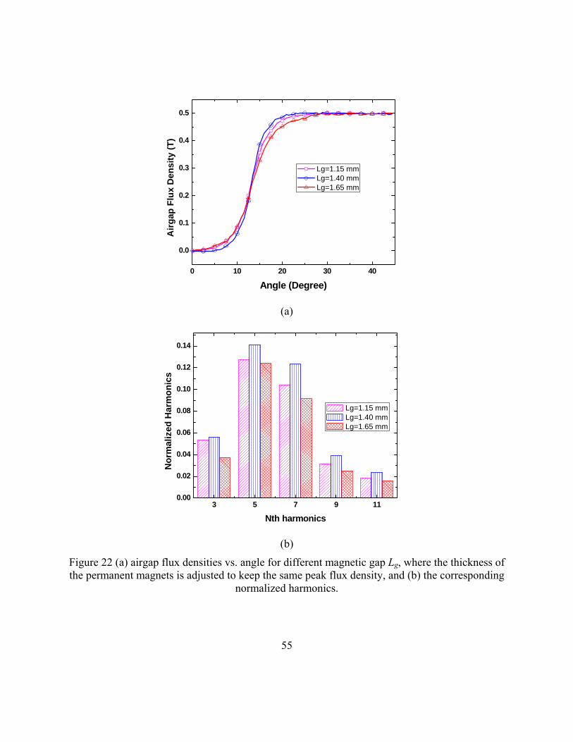
0 10 20 30 40
0.0
0.1
0.2
0.3
0.4
0.5
Airg
ap F
lux
Den
sity
(T)
Angle (Degree)
Lg=1.15 mm Lg=1.40 mm Lg=1.65 mm
(a)
3 5 7 9 110.00
0.02
0.04
0.06
0.08
0.10
0.12
0.14
Nor
mal
ized
Har
mon
ics
Nth harmonics
Lg=1.15 mm Lg=1.40 mm Lg=1.65 mm
(b)
Figure 22 (a) airgap flux densities vs. angle for different magnetic gap Lg, where the thickness of the permanent magnets is adjusted to keep the same peak flux density, and (b) the corresponding
normalized harmonics.
55
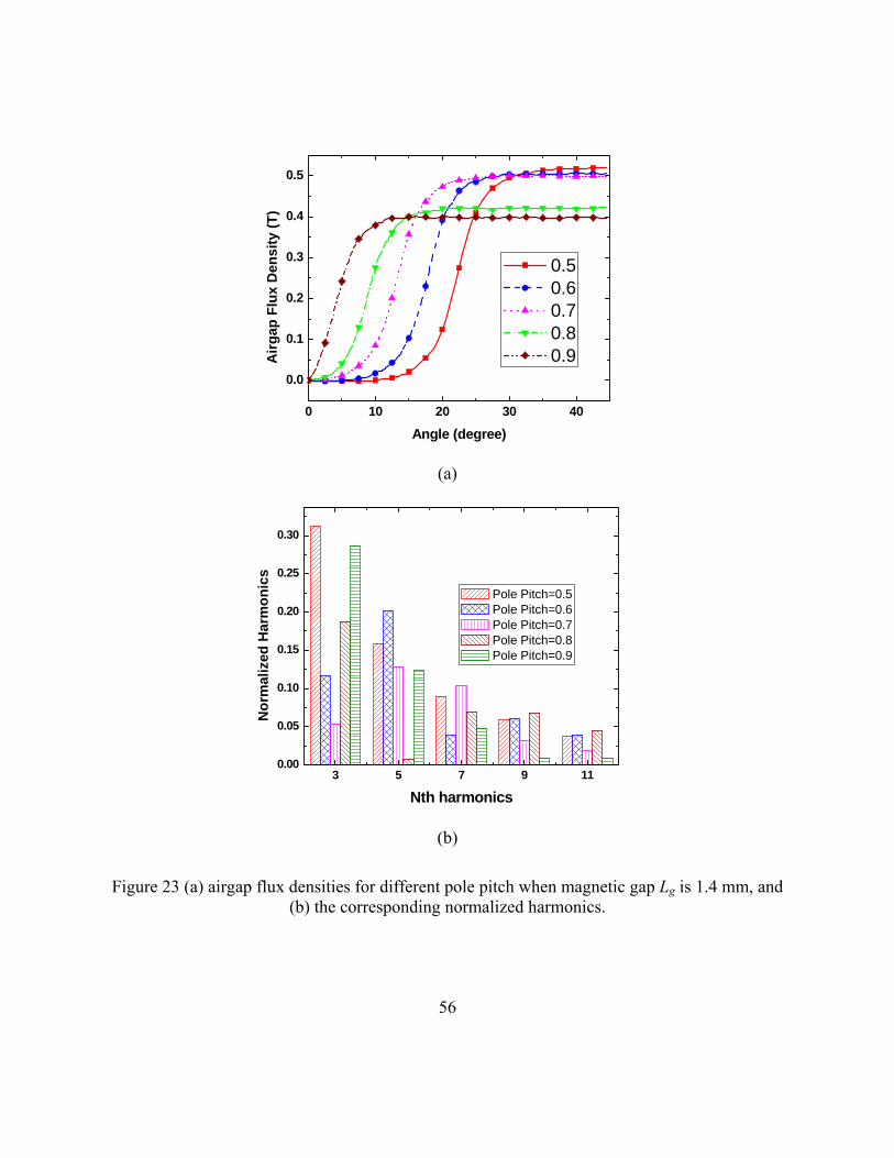
0 10 20 30 40
0.0
0.1
0.2
0.3
0.4
0.5
Airg
ap F
lux
Den
sity
(T)
Angle (degree)
0.5 0.6 0.7 0.8 0.9
(a)
3 5 7 9 110.00
0.05
0.10
0.15
0.20
0.25
0.30
Nor
mal
ized
Har
mon
ics
Nth harmonics
Pole Pitch=0.5 Pole Pitch=0.6 Pole Pitch=0.7 Pole Pitch=0.8 Pole Pitch=0.9
(b)
Figure 23 (a) airgap flux densities for different pole pitch when magnetic gap Lg is 1.4 mm, and (b) the corresponding normalized harmonics.
56

3.4.2 Simulation of Electromagnetic Torque
The electromagnetic torque was simulated based on (2.64). To simulate torque, currents
are applied in the windings, so it is necessary to model the fractional windings accurately. Figure
24 shows the FEM model to simulate torque.
Figure 24 FEM simulation model with fractional winding.
In FEM simulation of the slotless PMSM, distributed windings are difficult to model.
However, it is very critical for accurate simulation. Conventional current sheet method is not
accurate enough for high performance simulation. In this simulation, multi-terminal coil is used
to model fractional windings. The motor has three-phase and four-pole. The four coils of each
phase are connected in parallel in order to reduce DC bus voltage for low voltage applications.
Each coil has 7 turns, so there are total 84 turns. Figure 25 shows the model of the winding using
57

multi-terminal coil, where two-layer winding is modeled in one-layer and the current in each
branch is equal to that of two coils. The branch currents are determined according to the
arrangement of the winding described in Table 2.
According to Table 2, the current in each branch I(1), I(2), ..., I(84) can be represented
using phase currents Ia, Ib, and Ic as
( )( ) ( )
( ) ( ) 04)1(4...
4)1(040042
+−+=
−++=++=
ba
ca
a
III(84)
III(2)II(1)
(3.8)
Figure 25 A model of the winding.
58

where the phase currents can be written as
)3/2cos()3/2cos(
)cos(
πωπω
ω
+=−=
=
tIItIItII
mc
mb
ma
(3.9)
The torque constant was simulated to be 0.004 N.m/A. Toque ripple is very low and can
be ignored because of the slotless design.
Table 2 Three-phase and four-pole windings arrangement.
Coil number Phase Branches of 7 turns
1 a 1-16, 2-17, …, 7-22
2 -c 8-23, 9-24, …, 14-29
3 b 15-30, 16-31, …, 21-36
4 -a 22-37, 23-38, …, 28-43
5 c 29-44, 30-45, …, 35-50
6 -b 36-51, 37-52, …, 42-57
7 a 43-58, 44-59, …, 49-64
8 -c 50-65, 51-66, …, 56-71
9 b 57-72, 58-73, …, 63-78
10 -a 64-79, 65-80, …, 70- 1
11 c 71- 2, 72- 3, …, 77- 8
12 -b 78- 9, 79-10, …, 84-15
3.4.3 Simulation of Back-EMF
When the motor is rotating, the back-EMF will be induced in the conductors facing the
59

rotating magnetic field due to the variation of the flux linked with the winding. The following
equation was used to calculate the back-EMF:
ωθλθ
θλλ
dd
dtd
dd
dtdeb −=−=−= (3.10)
where ω is the frequency of rotation, λ is the flux linkage of the winding, and θ is the rotor angle.
Figure 26 shows the simulated and measured back-EMF voltage waveforms at 50,000 rpm. The
simulated and measured results agree very well.
Figure 26 Simulated and measured back EMF at 50,000 rpm.
3.4.4 Inductances Analysis
To simplify the inductance calculation, the stator is assumed to be without high
60

saturation. Therefore, the permanent magnets are replaced by dummy materials that have the
same permeability. Flux and energy approaches were used to calculate the motor phase self-
inductances (including airgap inductance and leakage inductance), and mutual inductances.
Flux approach is an inductance calculation method that directly applies the inductance
definition, that is, by calculating the flux linkage to get the inductance. Figure 5.15 shows flux
density distribution caused by the phase current (20 A sheet current is equal to 2.86 A phase
current).
Figure 5.15 Flux density distribution: (a) apply 20 A sheet current in each group of phase a, and (b) apply 20 A sheet current in each group of phase a & b.
To derive energy approach, it is assumed that the inductance will not change with the
applied current within the considered range, that is, the energy and coenergy are the same. The
energy can be simulated using FEM. So according to (2.60), inductances can be calculated based
on the following steps: a) Let i2=0, so and phase inductance is calculated as 2111 5.0 iLW =
61

21121 /2 iWLL == ; b) Applying arbitrary phase current i1 and i2 to get the corresponding energy
W12, mutual-inductances are calculated as )/()2( 21121221 iiWWLL −== . Table 3 shows the
calculated self- and mutual-inductances, and the measured results. From the table, it can be seen
that the energy approach is more accurate than flux approach.
Table 3 Calculated inductances
Flux Approach
Energy Approach
Measured @ 100Hz
Measured @1KHz
Self-Inductance (uH) 1.37 1.64 1.8 1.6
Mutual-Inductance (uH) -0.662 -0.647 N/A N/A
3.4.5 Simulation of Rotor Stress
The mechanical stresses are also important issues that need to be considered in the rotor
design. The carbon fiber ring with the thickness of 3.8 mm was used to radially hold the magnets
against the centrifugal force. Figure 27 shows the simulated stress distribution in the Titanium
rotor when rotating at 100,000 rpm. Maximum tensile stress is about 105 ksi when ignoring the
stress concentrations. It is still less than 140 ksi, the Youth Module of the Titanium grade. Figure
28 shows the simulated stress in the carbon ring when rotating at 100,000 rpm. It can be seen that
the maximum tensile stress is about 195 ksi, which is much lower that 400 ksi, the Youth
Module of carbon filter ring. Therefore, simulation results show that the carbon fiber ring and
Titanium shaft can work above 100,000 rpm.
62

Figure 27. Simulated stress in the rotor steel when rotating at 100,000 rpm.
Figure 28 Simulated stress in the carbon ring when rotating at 100,000 rpm.
63

3.5 Axial-Flux Slotless PMSM Drive and Test
3.5.1 Slotless PMSM Drive
The motor control was realized by using TI DSP 2407A. Since the phase inductance is
very low for slotless PMSM as shown in Table 3, low-pass filters were connected to remove the
harmonics of switching frequency of space vector PWM. The schematic of the space vector
PWM drive with low-pass filter is shown in Figure 29. The values of the inductors were
carefully adjusted through experiments to get better performance. Too large inductance values
make the control unstable and also reduce power factor while too small values introduce more
losses due to the harmonics.
Figure 29 Schematic of space vector PWM drive and low-pass filters.
64

Figure 30 shows the measured drive voltage and current waveforms when the speed is
50,000 rpm. Phase a and phase c voltages were measured between low-pass filter output and
ground. They are slightly different from the space vector PWM output due to low-pass filters.
However, since the phase winding are Y connected and the neutral terminal of the motor is
floating, the phase-to-phase voltage and phase current have very low harmonics.
Figure 30 Current and voltage waveforms when the speed is 50,000 rpm.
3.5.2 Spin-Down Test
Spin-down test was performed to measure the fixed loss vs. motor speed. Based on
(2.67), the damping power can be found to be
dtdJTP r
rrdampdampωωω −== (3.11)
65

Figure 31shows the tested spin down time vs. speed. Based on these data, the motor
damping power vs. speed is calculated as shown in Figure 32. It can be seen that the damping
power at 50,000 rpm is 48 W. So with 100 W shaft output power, the motor efficiency at 50,000
rpm will be less than 67% even ignoring all other losses.
Figure 31 Tested spin down time vs. motor speed.
3.5.3 Load Test
The load test was performed by coupling motor and generator as discussed in Chapter 2.
The test results show that the total loss is 65 W at 50,000 rpm with 100 W output. So the
efficiency at 50,000 rpm is about 60 % when output shaft power is 100 W. The efficiency is
lower than what was expected, so it is important to figure out losses.
66

Figure 32 Calculated damping power vs. motor speed.
3.5.4 Separation of Losses
The main sources of the losses are copper loss in the winding, iron loss in the stator,
windage loss, and bearing loss. The eddy current loss in the permanent magnets and rotor back
iron can be ignored in this slotless structure. At 50,000 rpm with 100 W output, the copper loss
including eddy current loss, which was calculated based on (2.29), was about 8 W. Based on the
manufacturer’s data sheet, the iron loss is calculated to be 9.8 W. The estimated windage loss
(PW), which is calculated from (2.30), is only 1.6 W. Therefore, the bearing loss, which is the
total loss minus copper loss, iron loss and windage loss, is found to be 45.6 W.
In order to separate and verify the bearing loss, and also to increase the efficiency, we
have to know which kind of loss is significant, so the separation of losses is needed. A damping
67

motor, which has the same structure but the permanent magnets are replaced with dummy
materials having the same density, was used and the following two steps were performed:
(a) Testing with coupled two identical motors
When two motors are coupled together (one as motor and the other as generator), the
input electromagnetic power will be
)()( 1111 mgemmegmine PPPPPPP +++=+= (3.12)
where Pine1 is the input electromagnetic power, Pm1 is the power consumed in the motor, Pg1 is
the power consumed in the generator, Pme1 is the electromagnetic loss in the motor, Pm is the
mechanical loss, and Pge is the electromagnetic loss in the generator.
(b) Replacing the rotor in generator with damper rotor and testing again
The mechanical loss of the damping motor is the same as the generator in first step but
there is no iron loss. So the input electromagnetic power is
mmmegmine PPPPPP ++=+= )( 2222 (3.13)
where Pine2 is the input electromagnetic power, Pm2 is the power consumed in the motor, Pg2 is
the power consumed by the damper motor, and Pme2 is the electromagnetic loss in the motor.
Supposing Pme1 is equal to Pme2, the electromagnetic loss Pge due to the rotor permanent magnets
is calculated to be
21 ineinege PPP −= (3.14)
If the electrical driving currents have low harmonics, the mechanical loss Pm can also be
calculated as
68

2/)(2/)( 222 geinemeinem PPPPP −≈−= (3.15)
The mechanical loss Pm includes bearing loss and windage loss. To accurately separate the
windage loss, the motor has to be kept under vacuum environment.
The bearing loss can be separated from damping power by subtracting windage loss, iron
loss, and eddy current loss in the winding. The following spin-down tests were performed in this
research: a) spin down test of the designed axial flux PMSM, b) spin down test of the designed
axial-flux PMSM coupled with the damping motor, and c) spin down test of another PMSM with
larger magnetic airgap (Lg=3.3 mm).
Figure 33 shows the tested spin down time vs. speed. Applying (3.11), the damping
powers of the PMSM, the PMSM coupled with the damping motor, and the large gap PMSM are
obtained as shown in Figure 34 (a). Ignoring the coupling loss, the damping power of the
damping motor, which is also shown in Figure 34 (a), is obtained by subtracting the damping
power of the PMSM from the damping power of PMSM coupled with the damping motor. By
subtracting the corresponding iron loss, eddy current loss in the winding and windage loss from
the damping power, the bearing loss of the designed PMSM and that of the PMSM with larger
airgap can be separated. The bearing loss of the damping motor is obtained by subtracting the
windage loss from the damping power. The results are shown in Figure 34 (b). For these three
cases, the damping motor has the lowest bearing loss since there is no axial force for the
damping motor [82]. From 3-D FEM simulations, the axial force applied on each bearing of the
designed PMSM and the PMSM with larger airgap were simulated and found to be 69.5 N and
25.5 N, respectively. This also explains why the PMSM with larger airgap has lower bearing loss
69

than the designed PMSM. When the speed is above 50,000 rpm, the coupler is not so effective,
and coupling loss increases dramatically. Since the coupling loss was ignored when separating
the damping power of the damping motor from that of the PMSM coupled with the damping
motor, the separated bearing loss of the damping motor is the combination of the bearing loss
and coupling loss. So it increases rapidly when speed is above 50,000 rpm.
Figure 33 Tested spin down time vs. the rotor speed of three motors.
The bearing loss is the dominant loss for low-cost, low-power and high-speed motor. The
friction torque caused by the thrust load is linearly dependent on the thrust loss [82]. Increase in
airgap length reduces the axial force, causing a reduction in the bearing loss. Large airgap also
reduces the airgap flux density, causing an increase in copper loss and decrease in power density.
There is a tradeoff between the bearing loss and the power density for the axial flux PMSM with
single stator and single rotor.
70

(a)
(b)
Figure 34 (a) tested damping power of the designed PMSM, damping motor and the PMSM with larger airgap, and (b) separated bearing loss of the designed PMSM, damping motor and the
PMSM with larger airgap.
71

3.6 Improvement of the Axial-Flux PMSM
Because the efficiency of the designed axial-flux prototype is low, to improve efficiency,
the following issues were considered:
a) Reducing bearing loss
Because thrust load increases bearing loss, sandwich structure can be considered to
balance the thrust force. The sandwich structure motor is the one with two external stators and
one internal rotor, or with two external rotors and one internal toroidal stator. Ceramic ball
bearings can be considered to further reduce bearing losses. If extremely low bearing loss is
required, non-contact bearings such as gas bearings, and magnetic bearings should be
considered.
b) Reducing copper loss
The copper wire diameter is too smaller to bear high current. Multi-strand litz-wire can
be considered to reduce winding resistance and eddy current loss in the winding.
c) Reducing saturation in the rotor back iron
The magnet keeper in the rotor can be replaced with a magnetic material to reduce
saturation in the back iron. And the airgap can be increased to reduce airgap flux density to
reduce iron loss and leave more space for the winding.
Figure 35 shows the picture of the new winding of using multi-strand Litz-wire. The new
test results of the axial flux PMSM with multi-strand Litz-wire winding, increased airgap length,
and steel magnet keeper shows that the efficiency can be increased to about 68%.
72

Figure 35 The new winding of using multi-strand Litz-wire.
3.7 Summary of Axial-Flux PMSM Design
Axial force of the single-sided motor affects the bearing loss extensively. It is important
to consider the effect of axial force to the loss of ball bearings when performing optimization.
Axial-flux PMSM can be used for high-speed applications. Rotordynamic problem is
much less for axial-flux motors than for radial-flux motors due to shorter length for same output
power. Axial force can be reduced greatly with sandwich structures such as two-stator /one rotor,
or two-rotor/ one stator. However, large diameter prevents it from super-high speed due to high
rotor stress. And also, permanent magnets are very brittle, and it is not safety to put them on the
surface of the rotor that rotates at high-speeds. Therefore, radial-flux PMSM was considered for
our super high-speed cryogenic drive that is described in Chapter 4.
73

CHAPTER FOUR: DESIGN AND CONTROL OF A SUPER HIGH-SPEED CRYOGENIC PMSM
4.1 Introduction
In this chapter, the design, fabrication, control, and test of an electric motor with 2000 W
output shaft power at 200,000 rpm is provided. The requirements of the super high-speed motor
are shown in Table 4. The designed motor is used in a two-stage cryocooler for application in
zero boil-off and long duration storage of liquid hydrogen systems. Although the operating
temperature of the motor is 77 K, it is also be able to run at room temperature with reduced
output power.
4.2 Design Considerations
4.2.1 Selection of Motor Type
Many types of motors can be considered for super high-speed applications as discussed in
Chapter 3. Selection of motor type is based on applications and specifications. PMSM offers the
advantage of higher efficiency compared to other types of motors since there is no excitation
power loss in the rotor, and lower eddy current loss in the stator and rotor. Therefore, there is an
increasing interest to consider PMSM for super high-speed applications. And PMSM is ideal in
74

meeting our required specifications.
Table 4 Requirements of the super high-speed motor
Output shaft power 2000 W
Shaft speed 200,000 rpm
Shaft diameter 16 mm
Maximum length 100 mm
Maximum outer diameter 44 mm
Efficiency > 90%
Operating temperature 77 K
4.2.2 Axial-Flux PMSM or Radial-Flux PMSM
Both axial-flux PMSM and radial-flux PMSM have been successfully used for high-
speed drives. However, there are some disadvantages by using axial-flux structure. Single-sided
axial-flux structure has large axial force applied to the bearings due to large magnetic force
between the rotor and the stator. This axial force will increase the bearing loss greatly as was
demonstrated in Chapter 3. Sandwich structure can solve this problem, but will make the
structure complicated.
Axial-flux PMSM has large diameter and short length, so the surface speed is much
larger than radial-flux PMSM that has the same mechanical rotor speed. Large diameter of the
rotor increases stress in the rotor, making the rotor less robust at super high-speed. Therefore, it
is not ideal for super high-speed applications. Large rotor diameter also has large windage loss
that may become significant at super high-speed. Because the permanent magnet is very brittle,
75
it has to be held by some high yield stress materials such as carbon fiber ring or inconel. It is
very critical for axial-flux PMSM due to large surface speed.
A radial-flux PMSM has smaller diameter and longer length compared to the axial-flux
PMSM, so it has smaller surface speed and lower rotor stress. Although long shaft will reduce
critical speed, it can still be above the operating speed by design. So a radial-flux PMSM is ideal
for this design.
4.2.3 Slotless Stator or Slotted Stator
The slotted structure of the motor increases the cogging torque, causing undesirable
vibrations. It also increases eddy current loss in the rotor, core loss in the stator teeth, and
windage loss. Various approaches have been considered to reduce the cogging torque and losses
associated with slotted structure [75]. Slotless structure is one of the effective methods especially
for super high-speed motors. By using slotless structure, the cogging torque due to the slots is
eliminated, and eddy current loss in the rotor due to the harmonics of air gap flux density is also
greatly reduced. Therefore, it is very desirable to have slotless structure for low power motor
running at super high-speed, especially when the rotor is very small and only air cooling is
provided. Slotless structure can also reduce the stator core loss.
For low-power motor, although the magnetic gap increases due to slotless structure,
causing the reduction of the air gap flux density and thus power density. Reduction of power
density does not increase the overall volume greatly since the motor size is already very small at
76

super high-speed, and the cooling system may be larger than motor itself.
One major disadvantage of slotless structure is that the eddy current loss in the winding
increases rapidly at higher speeds and lower temperatures. This eddy current loss is mainly due
to the proximity effect caused by the rotating permanent magnet, which will become very
significant at super high-speeds and cryogenic environment. Multi-strand twisted Litz-wire was
used to effectively reduce the eddy current loss.
4.2.4 Rotor Structure
For a permanent magnet motor, a major challenge is to retain the magnets against the
centrifugal force at super high-speed. The conventional method is to use a carbon fiber ring to
hold the permanent magnets against the shaft. However, at super high-speed, the required thick
carbon ring increases the magnetic gap, causing reduced airgap flux density and power density.
Because the required shaft diameter is small in this design, the permanent magnet was
considered to be centrally located inside the shaft.
4.2.5 Designed Motor Structure
The cross section of the preliminary design is shown in Figure 36. The key dimensions of
are shown in Table 5. The permanent magnet is centrally located inside the hollow shaft. The
rotor was assembled by heating the shaft and cooling the permanent magnet. For super high-
speeds, 2-pole configuration is preferred since the required electrical frequency is the lowest for
77

the same speed. Low electrical frequency reduces switching loss of the controller. The number of
turns per phase and the pitch factor were considered based on the requirements such as DC
supply voltage, shaft speed and desired back-EMF. Shaft diameter is fixed to be 16 mm due to
the requirements of gas foil bearing that are currently under development. To build a prototype
for lab test purpose, small diameter ceramic ball bearings were used and the step rotor with ball
bearings is shown in Figure 37. Appendix B provides the analytical design in detail. In order to
test load performance, a motor/generator was also designed and fabricated. The rotor structure of
motor/generator is very similar to that of the designed radial-flux PMSM except that there are
two permanent magnets inside the hollow shaft and the shaft is much longer. The detailed rotor
drawings of the motor and motor/generator can be found in Appendix C.
Figure 36 Cross section of the designed PMSM.
78

Table 5 Key dimensions of the designed cryogenic PMSM
Physical gap length 0.8 mm
Stator inner diameter 23.6mm
Stator outer diameter 35 mm
Motor active length 21 mm
Litz-wire configuration 100 strands @AWG 36
Turns/phase/pole 6
Winding pitch 15/18
Shaft diameter 16 mm
PM length 13 mm
PM width 10 mm
Figure 37 Rotor structure of the radial-flux PMSM prototype.
4.3 Material Selection
Cryogenics is generally defined as the science that deals with temperature below 120 K.
Properties of most materials change significantly with temperature and thus many materials are
unsuitable for cryogenic applications. For example, some materials, such as carbon steel, plastic,
and rubber, become very brittle at such low temperatures. For the PMSM operating at 77 K,
materials have been carefully selected.
79

4.3.1 Permanent Magnet
Neodymium-iron-boron (Nd-Fe-B), which has the highest energy product compared to
other types of permanent magnets, is widely used in electric machines and other applications.
However, when the temperature is below 140 K, Nd-Fe-B will change from a uniaxial material
to an easy-cone anisotropy material, which makes the magnet easily demagnetized [83].
Therefore, Nd-Fe-B is generally not considered for applications below 140 K, although an
application at 60~64 K has been reported in [84].
Samarium Cobalt (SmCo) also has very high energy product. It is very stable at low
temperature and has very low temperature coefficients of coercivity and remanence. SmCo also
has high Curie and operating temperatures. Thus, when inserting the permanent magnet into the
shaft, the shaft can be heated to very high temperature without affecting the performance.
Therefore, for 77 K application, SmCo was chosen as the permanent magnet material.
4.3.2 Winding
Copper was considered for the winding. The copper DC loss is greatly reduced at low
temperature due to increased conductivity. However, the eddy current loss of the winding due to
proximity effect increases because it is inversely proportional to the conductivity. Thus, multi-
strand Litz-wire was used to reduce the eddy current loss. The Litz-wire was constructed using
100 strands of AWG 36 (0.125 mm diameter), coated with heavy 200°C polyesterimide and
overcoated with polyamide-imide to meet IEC MW 35. After that, it was further wrapped with
80

sofimide to withstand temperature down to 77 K. The constructed Litz-wire was tested at 77 K,
and the results show that it can survive at 77 K without any insulation degeneration problems.
4.3.3 Stator
The motor stator is made of laminated silicon steel. The magnetic properties of the
silicon steel are relatively insensitive to the temperature change [85]. However, because the
conductivity of silicon steel increases with the decrease of temperature, the eddy current loss will
increase when temperature decreases [85], [86]. To reduce eddy current loss, thin laminations are
required. 0.127 mm (0.005 in) non-oriented silicon steel that is available in the market was used.
The conventional epoxy adhesive (Magna-Tac E645) was used to bond the laminations.
Additional contain ring can be used to hold the laminations together in case the adhesive is not
effective at 77 K.
4.3.4 Bearing
Selection of bearings is also an important issue. Conventional ball bearings, lubricated
with oil or grease, are unable to work at such low temperatures because of the solidification of
lubricants. And also at super high-speed, the loss of ball bearings will be very large. So it is
recommended to have non-contact bearings such as gas bearings or magnetic bearings. For the
prototype which is only tested at room temperature, low loss ceramic bearings lubricated with
high speed and low viscosity grease was considered.
81

4.3.5 Shaft
The shaft material was chosen to be high-stress Titanium, which has yield strength of
about 1400 MPa and low coefficient of thermal expansion. Low density of Titanium is also an
advantage to increase critical speed of the shaft. It is also known to be good for cryogenic
applications. The shaft was machined using electro-discharge machining (EDM).
4.4 FEM Simulation and Optimization
4.4.1 Simulation of Magnetic Flux
Magnetic flux density distribution is an important issue in the motor design. Low
harmonics of the magnetic flux density distribution can reduce loss. It can be simulated using
magnetostatic FEM. Figure 38 shows the flux lines generated by the permanent magnet in the
rotor. The MMF in the winding, even at the rated current, is weaker compared to that of
permanent magnet.
Figure 39 shows the airgap flux density distributions in the normal and tangential
directions, respectively. The corresponding harmonics analysis of the flux density in normal
direction shows that the dominated harmonics is the 3rd harmonics, which is very lower
compared to that of slotted structure. The flux in tangent direction cannot contribute to any
torque but increases eddy current loss.
82

Figure 38 Flux lines caused by the permanent magnet at room temperature.
-20 0 20 40 60 80 100 120 140 160 180 200-0.1
0.0
0.1
0.2
0.3
0.4
0.5
Flux
Den
sity
(T)
Angle (Deg.)
Normal Tangent
Figure 39 Simulated airgap flux densities in normal direction and tangential direction.
83

4.4.2 Simulation of Back-EMF
The back-EMF is caused by the variation of the flux linked with the winding. It can be
expressed as (2.62). For 2-D problem, the in (2.62) can be calculated as Λ
∫
∫∫ ∫∫−=⋅=
⋅×∇=⋅=
lsji
S S
LAAd
ddΛ
)(lA
SASB (4.1)
where B is the flux density, A is the vector magnetic potential and Ls is the length of the stator.
By running the magnetostatic problems for different rotor angles and using (2.62) and (4.1), no-
load back-EMF was calculated as shown in Figure 40. The FFT analysis shows that the
normalized third harmonics of back EMF is less than half that of the normalized third harmonics
of airgap flux density in normal direction. This improvement is due to the short-pitch winding.
0.0 0.2 0.4 0.6 0.8 1.0 1.2 1.4-20
-15
-10
-5
0
5
10
15
20
Bac
k EM
F (V
)
Time (ms)
Figure 40 Simulated back-EMF of the designed PMSM when the speed is 200,000 rpm.
84
4.4.3 Calculation of Inductances
The phase inductances were calculated by using energy method as discussed in Chapter
2. The simulated energy is 0.00186 J when applying 64 A phase a current and no currents in
phase b and c. It is 0.00215 J when apply 64 A phase a current, 64 A phase b current, and no
current in phase c. Based on these data, the phase magnetizing inductance was calculated as
shown in Table 6, where the measured result is also provided.
Table 6 Simulated and measured phase inductances.
Inductance Magnetizing Inductance (uH)
Leakage Inductance (uH)
Total self-inductance (uH)
Simulated 0.91 0.66 1.57
Measured N/A N/A 1.63
4.4.4 Transient Simulation
To accurately simulate the dynamic behavior of the motor, 2-D transient time-stepping
solver with motion was also used. The equation dealing with coupled time varying electrical and
magnetic field for transient simulation is [61], [62]
AvHVtAJA cs ×∇×+×∇+∇−∂∂−=×∇×∇ σσσν )/( (4.2)
where v is the velocity of the moving parts, A is the magnetic vector potential, t is the time, V is
the electrical scalar potential, Js is the current source density, Hc is the coercivity of the
permanent magnets, and σ is the conductivity of the material.
85

4.4.4.1 Simulation in Motoring Mode
In motoring mode simulation, A rms value of 61.4 A field oriented phase current was
applied to each phase, together with 10% of fifth harmonics, 8% of seventh harmonics, 1.2% of
eleventh harmonics and 1% of thirteenth harmonics. These harmonics were intently added to
simulate the motor performance in non-ideal case. Figure 41 shows the calculated phase flux
linkage when rotating at 200,000 rpm and at 77 K. Back-EMF can be calculated directly from
flux linkage by using (2.62).
0.0002 0.0004 0.0006 0.0008 0.0010
-8.0x10⁻⁴
-6.0x10⁻⁴
-4.0x10⁻⁴
-2.0x10⁻⁴
0.0
2.0x10⁻⁴
4.0x10⁻⁴
6.0x10⁻⁴
8.0x10⁻⁴
Phas
e lin
kage
(Wb)
Time (s)
Phase a Phase c Phase b
Figure 41 Calculated flux linkage.
Figure 42 shows the simulated torque. The large variation of torque is due to large
harmonics of the driving signal. The simulation also shows that there is no ripple in the toque
86

when there is no harmonics in the phase currents. Figure 43 shows the simulated eddy current
loss in the rotor (shaft and permanent magnet), and the stator core loss. The simulated average
core loss is 9.1 W at 77 K, and the rotor eddy current loss is less than 1 W even there are a lot of
time harmonics in the phase currents.
0.0 0.2 0.4 0.6 0.8 1.00.00
0.01
0.02
0.03
0.04
0.05
0.06
0.07
0.08
0.09
0.10
0.11
Torq
ue (N
/m)
Time (ms)
W ithout harmonics W ith harmonics
Figure 42 Simulated torque when applying 61.4 A phase current together with harmonics.
4.4.4.2 Simulation in Generating Mode
The PMSM was also simulated in generating mode with rectifier circuit similar to Figure
12 except that there is no capacitor. In that case, the phase current has a lot of harmonics as
shown in Figure 44. Figure 45 shows the output DC current and voltage waveforms, and the
average output power is 1950 W. The simulated torque is shown in Figure 46, where the average
is about 0.95 N.m.
87

0.70 0.75 0.80 0.85 0.90 0.95 1.000.0
0.5
1.0
1.5
2.0
2.5
3.0
3.5
0.0
2.5
5.0
7.5
10.0
Rot
or e
ddy
curr
ent l
oss
(W)
Time (ms)
Cor
e lo
ss (W
)
Core loss
Rotor eddy current loss
Figure 43 Simulated rotor eddy current loss and stator core loss when rotating at 200,000 rpm and at 77 K.
0.25 0.50 0.75 1.00 1.25 1.50 1.75 2.00
-100
-50
0
50
100
Cur
rent
(A)
Time (ms)
Figure 44 Phase current.
88

0
20
40
60
80
100
0.5 1.0 1.5 2.00
5
10
15
20
25
30
35
40
Cur
rent
(A)
Time (ms)
Vol
tage
(V)
Output current
Output voltage
Figure 45 Rectified output voltage and current.
0.8 1.0 1.2 1.4 1.6 1.8 2.0-0.12
-0.10
-0.08
-0.06
-0.04
-0.02
0.00
Torq
ue (N
.m)
Time (ms)
Figure 46 Simulated torque in generating mode with rectifier circuit.
89

Figure 47 shows the simulated stator core loss and rotor eddy current loss. The average
stator core loss is about 9.85 W, and the average rotor eddy current loss is 13 W. The eddy
current distributions in the shaft and permanent magnet are shown in Figure 48. Due to skin
effect, the eddy current loss in the hollow shaft is dominant. The large eddy current loss is due to
large harmonics in the phase current shown in Figure 44.
0.8 1.0 1.2 1.4 1.6 1.8 2.00
10
20
30
40
50
Loss
(W)
Time (ms)
Rotor eddy current loss Stator core loss
Figure 47 Simulated stator core loss and rotor eddy current loss at 200,000 rpm and the cryogenic temperature of 77 K.
4.5 Structural Design
The structural design involves both the rotor structural integrity as well as the
rotordynamic performance. For rotor structural integrity, the main focus is on the magnet
retention and the bearing design. The permanent magnet was designed to be inside the hollow
shaft. The thickness of the shaft was considered based on both stress requirements to hold the
90

permanent magnet and rotordynamic performance.
Figure 48 Simulated eddy currents in the shaft and permanent magnet in generating mode with rectified output DC power of 2000 W.
The rotor structure is subjected to various stresses under operation. The simulation shows
that the bending stress developed is much less than ultimate tensile strength of shaft and magnet.
The rotating shaft is also subjected to stress due to centrifugal force while operating at
200,000 rpm. Centrifugal stress analysis was done using FEM software at the operating speed.
The simulation shows that the shaft expands more than the magnet and will result in a clearance
fit. A high risk of crumbling of the magnet while shuddering inside the shaft prevails. Thus,
91

interference fit is required. It was calculated that heating the shaft to 400 0C and cooling the
magnet to liquid nitrogen temperature will produce the necessary clearance to insert the magnet
in the shaft. Residual stresses arising due to this process of assembling were also calculated. The
simulation also shows that the compressive stress due to interference fit between the shaft and
magnet will not damage the permanent magnet. The centrifugal stress and residual compressive
stress contributes to the total stress developed while the shaft is in operation. The maximum total
stress simulated is 852 MPa as shown in Figure 49. This value is much less than the yield
strength of Titanium grade that was used to build the shaft.
Figure 49 Stress in the shaft and magnet assembly.
For estimating the fundamental lateral critical speed of the motor shaft, classical
approximate methods can be used such as Rayleigh’s method or Dunkerley’s formula. Although
these methods were originally proposed for the calculation of fundamental natural frequency of
non-rotating systems such as beams, they can be applied for rotor systems with a small
92
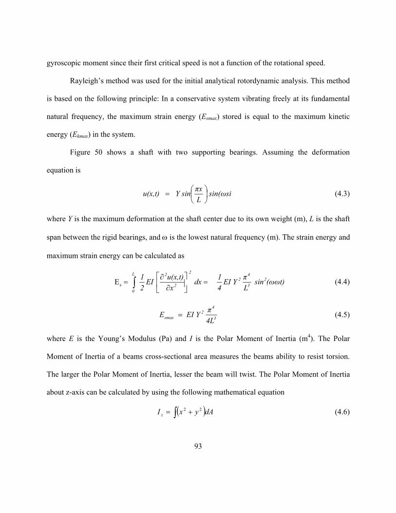
gyroscopic moment since their first critical speed is not a function of the rotational speed.
Rayleigh’s method was used for the initial analytical rotordynamic analysis. This method
is based on the following principle: In a conservative system vibrating freely at its fundamental
natural frequency, the maximum strain energy (Esmax) stored is equal to the maximum kinetic
energy (Ekmax) in the system.
Figure 50 shows a shaft with two supporting bearings. Assuming the deformation
equation is
sin(ωsiLπx Y sinu(x,t) ⎟
⎠⎞
⎜⎝⎛= (4.3)
where Y is the maximum deformation at the shaft center due to its own weight (m), L is the shaft
span between the rigid bearings, and ω is the lowest natural frequency (m). The strain energy and
maximum strain energy can be calculated as
Es (ωωt) sinLπEI Y
41 dx
xu(x,t) EI
21 2
3
42
2
2
2L
0
=⎥⎦
⎤⎢⎣
⎡∂
∂= ∫ (4.4)
4Lπ EI Y E 3
42
smax = (4.5)
where E is the Young’s Modulus (Pa) and I is the Polar Moment of Inertia (m4). The Polar
Moment of Inertia of a beams cross-sectional area measures the beams ability to resist torsion.
The larger the Polar Moment of Inertia, lesser the beam will twist. The Polar Moment of Inertia
about z-axis can be calculated by using the following mathematical equation
( )∫ += dAyxI z22 (4.6)
93
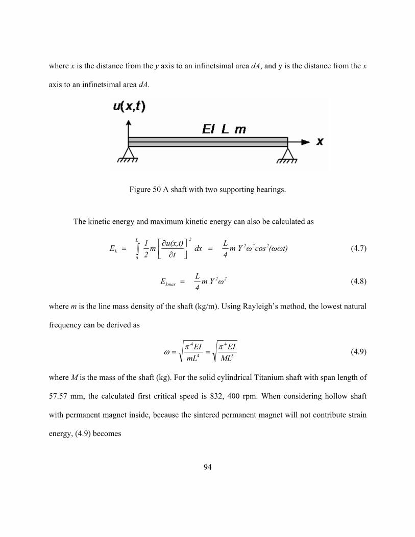
where x is the distance from the y axis to an infinetsimal area dA, and y is the distance from the x
axis to an infinetsimal area dA.
Figure 50 A shaft with two supporting bearings.
The kinetic energy and maximum kinetic energy can also be calculated as
(ωωt) (4.7) cosωm Y4L dx
tu(x,t) m
21 E 222
2L
0k =⎥⎦
⎤⎢⎣⎡
∂∂
= ∫
ωm Y4L E 22
kmax = (4.8)
where m is the line mass density of the shaft (kg/m). Using Rayleigh’s method, the lowest natural
frequency can be derived as
3
4
4
4
MLEI
mLEI ππω == (4.9)
where M is the mass of the shaft (kg). For the solid cylindrical Titanium shaft with span length of
57.57 mm, the calculated first critical speed is 832, 400 rpm. When considering hollow shaft
with permanent magnet inside, because the sintered permanent magnet will not contribute strain
energy, (4.9) becomes
94

( )( )( )2224
444
3
4
)2()2(8)2(
)(
tdtddLtddE
LMMIE
PMshaft
shaft
PMshaft
shaftshaft
−+−−
−−=
+=
ρρπ
πω
(4.10)
where d is the shaft outer diameter, t is the thickness of the hollow shaft, and ρshaft and ρPM are
the mass densities of the shaft and permanent magnet, respectively. Based on the above equation,
the first critical speed of the 57.57 mm span length, 1.5 mm thickness Titanium hollow shaft
with permanent magnet inside was calculated to be 515,800 rpm. Appendix D shows the
analytical calculation of critical speeds.
An FEA model was also built to perform rotordynamic simulation accurately. The
rotordynamic equation of motion for a coupled, flexible rotor/casing system with conventional
bearings is
[ ] [ ] [ ] fqqq =++ KCM &&& (4.11)
where q represents the physical coordinate degrees of freedom, f represents external forces, M
represents mass matrix, K represents the bearing stiffness matrix, and C represents damping
matrix. Figure 51 shows the FEM rotordynamic model of the radial-flux PMSM. The model
consists of three-pieces, shaft middle part, and two plugs. The three-piece rotor is modeled as a
3-shaft model with a coupling with translational and rotational stiffness at the joints. Figure 52
shows the simulated critical speeds assuming the translating stiffness is 107 N-mm, and rotational
stiffness is 5 x10⁷ N-mm.
The rotordynamic of the motor/generator rotor was also simulated. Figure 53 shows the
95

FEM simulation model. The simulated results are shown in Figure 54, and Figure 55. The
simulation results show that our operating speed of 200,000 rpm is between the first critical
speed and second critical speed. Therefore, it is necessary to quickly pass the first critical speed
during the load test.
Figure 51 FEM rotordynamics model of the radial-flux PMSM.
Figure 52 Simulated critical speeds of the radial-flux PMSM.
96

Figure 53 FEM rotordynamic model of the motor/generator.
(a)
(b)
Figure 54 Simulated (a) first bending mode, and (b) second bending mode of the motor/generator.
97

Figure 55 Simulated critical speeds of the motor/generator.
The rotordynamic analysis results are summarized in Table 7. The analytical analysis
results are larger than FEM simulation. It is because: (a) the analytical analysis is based on
simple model assuming infinite large stiffness of the bearings, and (b) the analytical analysis
assumes that the shaft has constant diameter and does not consider the steps near the bearings.
Table 7 Summary of the rotordynamic analyses.
FEM rotordynamic simulation Analytical analysis
1st bending (krpm)
2nd bending (krpm)
3rd bending (krpm)
Lowest natural frequency (rpm)
Motor 247 411 416 516
Motor/Generator 91.2 349 640 163
98

4.5 Loss Analysis
Accurate estimation of losses is a very important issue in the design of super high-speed
and high efficiency motors. The losses were estimated based on the analytical analyses and/or
numerical simulations.
4.5.1 Copper Loss
The stator and the attached winding are shown in Figure 56. The part of the winding that
is outside of the stator is called end winding. The copper loss consists of I2R loss and eddy
current loss. Short-pitch winding was considered to reduce the length of the end winding
resulting in reduced I2R loss.
Figure 56 Model of the stator and the attached winding.
99

The eddy current loss comes from: (a) skin effect resulting from the same source
conductors, and (b) proximity effect resulting from the motion of the permanent magnet.
Because the electrical frequency is very low, and skin depth is larger than the radius of the
copper wire, the skin effect can be ignored. Therefore, the main source of eddy current loss
comes from proximity effect.
The eddy current loss per volume for the round wire was calculated based on the
following equation [42]
(4.12) ρω 32/222 dBP PE =
where Bp is the peak flux density, ω is the electrical angular frequency, d is the diameter, and ρ
is the resistivity.
Figure 57 shows the electrical resistivity of copper vs. temperature. Residue resistivity
ratio (RRR), which shows the purity of a sample, is defined as the ratio of resistivity at 300 K to
resistivity at 4.2 K. Higher purity in copper will lower the electrical resistivity at low
temperatures. The RRR is 50 for the copper used in this design.
The electrical resistivity of the copper wire is greatly reduced at the cryogenic
temperature due to reduced phonon electron scattering. At 77 K, the resistance of the copper
winding is about one-ninth of that at room temperature, so the I2R loss can be greatly reduced.
However, the eddy current loss increases.
Eddy current losses of the winding are simulated for both solid wire and multi-strand
Litz-wire cases, assuming the temperature of the winding is kept at 77 K. If solid wire is used
instead of multi-strand Litz-wire, the peak eddy current density can be larger than 1,800 A/mm2
100

as shown in Figure 58, where the wire diameter is 1.5 mm. The simulated peak eddy current is
above 580 A when the rotor is rotating at 200,000 rpm and the operating temperature is 77 K.
Such a large eddy current is mainly due to the super high-speed and extremely low copper
resistivity at 77 K. So it is not practical for solid wire to be used in a cryogenic motor with
slotless structure and rotating at super-high speed.
1 10 100
1E-10
1E-9
1E-8
Elec
tric
al re
sist
ivity
(ohm
. m)
Temperature (K)
RRR=30
RRR=100
RRR=300
Figure 57 Electrical resistivity of copper vs. temperature.
The eddy current is greatly reduced after using 75 strands at AWG 36 (0.125 mm in
diameter) multi-strand Litz-wire as shown in Figure 59. From (4.12), it can be seen that the eddy
current loss is proportional to the square of the wire diameter. So it is very effective to reduce
eddy current loss by reducing wire size. Reducing peak flux density of the airgap can also reduce
101

eddy current loss per volume. However, the back-EMF will also reduce, resulting in the
increased total copper volume.
Figure 58 Simulated eddy current of the round solid wire when the rotor is rotating at 200,000
rpm and the operating temperature is 77 K.
4.5.2 Stator Core Loss
Time-step transient FEM with motion was used to calculate stator core loss. At 77 K, the
coefficients of eddy current losses can be adjusted since it is proportional to the conductivity
when the frequency is low [87]. The conductivity of silicon steel at the temperature t was
corrected since
( ))(1/ TtTt −+= ασσ (4.13)
where T is the reference temperature (normally 20 °C), σT is the conductivity at the reference
temperature and α is the temperature coefficient of the resistance.
102

Figure 59 Simulated eddy current of the Litz-wire (75 strands at AWG 36) when the motor is rotating at 200,000 rpm.
4.5.3 Rotor Loss
For super-high speed PMSM, rotor loss generated by induced eddy currents in the metal
shaft and permanent magnets may amount to a considerable part of the total loss. The major
causes of the rotor eddy currents can be categorized into the following three groups [72]: (a) no-
load rotor eddy current loss caused by the existence of slots, (b) on-load rotor eddy current loss
induced by the harmonics of windings’ MMF, and (c) on-load rotor eddy current loss induced by
the time harmonics of the phase currents due to PWM.
If the eddy current distribution in the rotor is known, the instant rotor power loss can be
expressed as
103

dVdVPV V∫ ∫== σσ /22 JE (4.14)
where σ is the material conductivity, E is the electric field, J is the eddy current density, and V is
the volume of the material. The analytical model for predicting eddy current loss in the rotor can
be found in [88].
For slotted structure, eddy current loss may be significant at super high-speeds. However,
slotless structure can eliminate no-load rotor eddy current loss. Harmonics of the winding’s
MMF can also be reduced using fractional windings. Low-pass filters were used to reduce the
time harmonics of phase currents due to PWM. The simulation results show that rotor loss can be
ignored after the above improvements.
4.5.4 Windage Loss
For the motor at super high-speeds, windage loss may become considerable. Accurate
prediction and reduction of windage loss becomes important. Based on (2.31), the windage loss
was calculated to be 6.3 W.
4.5.5 Super High-Speed PMSM Efficiency
Table 8 shows the simulated and/or analyzed losses of the designed super high-speed
PMSM with gas bearings that is intended to work at both the cryogenic temperature of 77 K and
room temperature. The stray load loss can also be ignored due to slotless design. The stray load
loss is mainly caused by the high frequency flux pulsations due to non-uniform current
104

105
distribution and distortion of the magnetic flux by the currents. The bearing loss is the estimated
air bearing loss. The designed radial-flux PMSM was well optimized based on efficiency and
also the bearings have very low loss, so the efficiency is much higher than the axial-flux PMSM
that is described in Chapter 3.
4.6 Prototype Design and Fabrication
The rotor of the motor was fabricated out of Titanium 6Al-4V. The shaft was machined
by EDM process. Two caps are used to house the bearings which support the integrated rotor.
These parts were machined partly by EDM and regular machining process.
Table 8 Simulated and /or analyzed losses of the super high-speed PMSM
At room temperature At 77 K
Copper DC loss (W) 71.3 7.5
Copper AC loss (W) 1.4 12.8
Stator iron loss (W) 4.2 9.85
Bearing loss (W) 30
Windage loss (W) 6.3
Low pass filters loss (W) 11
Controller loss (W) 100
Total loss (W) 224.2 177.5
Efficiency 89.9% 91.8%

4.6.1 Bearing Design and Lubrication
Internal clearance of a ball bearing affects life, noise, vibration and temperature
generation, so it is extremely important to select the optimum radial clearance for each
application. When a ball bearing is used, it is not used alone. It is likely to be used on a shaft or
in a housing bore by interference fit which is described as a value of tightness between the shaft
and bearing bore or the housing bore and the bearing outside diameter.
The purpose of interference fit is to prevent slipping. Once slipping occurs, the
temperature will be abnormally generated by the slipping abrasion. Creeping is associated with
the slipping between fitted surfaces. It will be a cause of premature life failure or that the
abrasion particles will enter the bearing and causes it to become noisy and eventually burn up.
Typically a large interference fit prevents creeping, but it is necessary to select the interference
fit by giving attention to the reduction of radial clearance, and the effect of the temperature
change to the interference fit and raceways during the bearing operation.
Figure 60 shows the structure of bearing inner ring fit. The reduction of bearing internal
clearance due to interference between the shaft and inner ring can be calculated as
⎪⎪⎭
⎪⎪⎬
⎫
⎪⎪⎩
⎪⎪⎨
⎧
⎥⎥⎥⎥
⎦
⎤
⎢⎢⎢⎢
⎣
⎡
−
−⎟⎠⎞
⎜⎝⎛
+⎟⎠⎞
⎜⎝⎛
+
⎥⎥⎥⎥
⎦
⎤
⎢⎢⎢⎢
⎣
⎡
+
−⎟⎠⎞
⎜⎝⎛
+⎟⎠⎞
⎜⎝⎛
⎥⎥⎦
⎤
⎢⎢⎣
⎡−⎟
⎠⎞
⎜⎝⎛
⎟⎠⎞
⎜⎝⎛
=
ss
b
b mdddd
EE
mdddd
dd
ddi
1
1
11
1
11
2
22
22
22
22
22
2
δ (4.15)
106

where d is the inner ring bore diameter, d1 is the shaft bore diameter, d2 is the inner ring raceway
diameter, i is the interference fit, Eb is the Young's modulus of bearing, Es is the Young's
modulus of shaft, mb is the Poisson's ratio of bearing, and ms is the Poisson's ratio of shaft.
Figure 61 shows the structure of bearing outer ring fit. The reduction of bearing internal
clearance due to interference between the outer ring and the housing is
⎪⎪⎭
⎪⎪⎬
⎫
⎪⎪⎩
⎪⎪⎨
⎧
⎥⎥⎥⎥
⎦
⎤
⎢⎢⎢⎢
⎣
⎡
+
−⎟⎠⎞
⎜⎝⎛
+⎟⎠⎞
⎜⎝⎛
+
⎥⎥⎥⎥
⎦
⎤
⎢⎢⎢⎢
⎣
⎡
−
−⎟⎠⎞
⎜⎝⎛
+⎟⎠⎞
⎜⎝⎛
⎥⎥⎦
⎤
⎢⎢⎣
⎡−⎟
⎠⎞
⎜⎝⎛
⎟⎠⎞
⎜⎝⎛
=∆
bh
b
b mDDDD
EE
mDDDD
DD
DDI
1
11
111
11
111
1
12
2
2
2
2
2
(4.16)
Figure 60 Bearing inner ring fit.
107

Figure 61 Bearing outer ring fit.
Table 9 Bearing fit calculation.
Symbol Value Unit
Young's modulus of shaft Es 2 × 10¹¹ Pa
Young's modulus of bearing Eb 1.15 × 10¹¹ Pa
Young's modulus of housing Eh 1.15 × 10¹¹ Pa
Shaft diameter d 6.35 mm
Innter ring outer diameter d2 8.35 mm
Interference fit between shaft and bearing i 0.00254 mm
Housing bearing support diameter D 12.7 mm
Housing outer diameter D2 50 mm
Interference between outer ring and housing I 0 mm
Internal clearance reduction due to inner ring fit 0.5δ 0.0012 mm
Internal clearance reduction due to outer ring fit 0.5∆ 0 mm
Total internal clearance reduced 0.5(δ+∆) 0.0012 mm
108

The initial clearance of the bearing is between 0.0051 mm and 0.0130 mm. Therefore,
after assembly, the internal clearance is between 0.0039 mm and 0.0118 mm. Sufficient internal
clearance was kept considering the reduction due to the shaft rotation and heat.
Lubricant selection is also importance for the performance of a ball bearing. It affects
life, torque, speed, noise, temperature and rust prevention. The two basic types of lubricants
available are oil and grease. Applications that require extremely low bearing loss are suited to
use oil as a lubricant. However, the volume of the oil circulating system is large.
Greases are comprised of oil base and thickener. The life obtained from greases is
considerably greater than that of oil. This is because of a continuous mechanism of lubrication by
base oil separation coming from the construction of the thickener.
To simplify housing design for the prototype, grease lubrication was considered. The
bearing has approximately 9 mm mean diameter. It is about 1,800,000 nDm when rotates at
200,000 rpm. Two greases were considered. Kluberspeed BF 72-22 is designed for high-speed
bearings. It has a low viscosity of 22 cSt at 40 oC and is shear stable even at super high-speeds.
This grease can provide optimum protection and friction loss is minimal once the bearing/grease
has been run-in. The disadvantage of this grease is that the maximum operating temperature is
only 80 °C (180 °F). Another type of grease that is also widely used for high-speed application is
Chevron SRI-2. The operating temperature of this grease can be as high as 150 °C (300 °F).
Although large viscosity increases bearing loss, the viscosity will reduce when temperature
increases.
109

4.6.2 Rotor Assembly
The rotor consists of hollow shaft, permanent magnet, and two plugs. Figure 62 shows
the integrated shaft after balancing. Permanent magnet was inserted into hollow shaft by first
cooling the permanent magnet down to 77 K and heating the hollow shaft to 570 K. The
temperature of the permanent magnet will increase and that of the hollow shaft will decrease
during assembling, so the clearance will decrease gradually. It is desirable to have a fixture, as
shown in Figure 63, to increase assembling speed. The plugs were welded to the shaft using
electron beam welding. After assembly, the rotor was balanced. The total material removed is
0.0049 gram on left side and 0.0037 gram on right side, so total unbalance is 0.034 gram-mm.
The test results show that the total power losses have been reduced greatly after balancing
although the total unbalance is still far beyond the requirement of 0.0075 gram-mm for the
medium quality grade of G2.5 [89].
Figure 62 Integrated shaft after balancing.
110

Figure 63 Fixture to insert a permanent magnet into the hollow shaft.
4.6.3 Housing and Pre-Load
The designed housing and the corresponding two caps are shown in Figure 64. There is
light interference fit between the housing and the stator that is shown in Figure 65.
Figure 64 The designed housing, two caps, and the integrated rotor.
111

Figure 65 Stator with winding.
Preload reduces the operating internal clearance. When a ball bearing is used in a motor,
it has "zero" radial clearance when an axial load is applied. This axial force is called preload. If
there is any radial clearance, vibration and noise of the balls will occur, and the stiffness of the
ball bearing will be very low. An optimum preload should be individually specified for each ball
bearing size. If the preload is applied excessively, Bearing fatigue life will be short and will
increase raceway noise as well. Bearing loss will also be large. If the applied preload is
insufficient, fretting corrosion can occur. This happens as a result of vibration causing the balls
to resonate and abrade on the raceways. Therefore, obtaining the correct preload is important.
There are two basic methods of preload: solid pre-load and spring preload. Solid pre-load
112

can be obtained by mechanically locking all the rings in position while under an axial load. The
advantages of this type of design are that the components remain simple and the stiffness is high.
The disadvantage is high variation in preload under temperature variation, and that the pre-load
can reduce with wear. Spring pre-load can be applied using a coil spring or a spring wave
washer, etc. An advantage of spring pre-load is that it maintains consistent pre-load with
temperature variation. The disadvantages are that the designs are more complex and normally
have lower stiffness. Since the exact pre-load value is not difficult to predict, an adjustable
spring pre-load cap was designed which is shown in Figure 66. The pre-load of this structure can
be adjusted by selecting the spring stiffness and modifying the thickness of shim that is located
between the cap and the housing.
Figure 66 Designed bearing support with spring preload.
113

Another design is to apply the preload directly to outer ring of the bearing by a large
diameter spring, which was used in the prototype of motor/generator system.
Water cooling was considered for the motor to be tested at room temperature, Figure 67
shows the assembled motor prototype with cooling for lab test.
Figure 67 The assembled motor prototype with cooling for lab test.
4.7 Motor Control and Test
4.7.1 Motor Control
The space vector PWM was used to control the inverter to drive the PMSM. It refers to a
114

special switching sequence of the upper three power devices of a three-phase voltage source
inverters (VSI) used in motor drives. This special switching scheme for the power devices results
in 3 pseudo-sinusoidal currents in the stator phases. It has been shown that space vector PWM
generates less harmonics distortion in the output voltage or currents in the windings of the motor
load and provides more efficient use of DC supply voltage, in the comparison to direct sinusoidal
modulation technique. To increase the efficiency of the inverter, soft switching technology can
be used [90]. However, three-phase soft switching is complicated and actually it will also reduce
maximum switching frequency. Therefore, at super high-speeds, soft switching is not widely
used.
The output of inverter driven by PWM is a serial of pulses, so it is necessary to remove
switching harmonics from the drive current. However, the phase inductance of a slotless PMSM
is low, so low-pass filters or reactors were used to remove harmonics as shown in Figure 68.
There are two parallel conductors. It was observed that there are very large circulating
currents within these parallel conductors due to unbalanced back EMF voltages. These
circulating currents increase winding resistance, causing increased winding losses. By
connecting one external inductor to each conductor, the circulating currents can almost be
eliminated. The modified connection is shown in Figure 69. Two inductors of each phase were
wounded in one Ferroxcube E core E42/21/15-3C90. The gap in the middle is 1.14 mm. The
self-inductance is 129 uH, and mutual-inductance is -120 uH. Therefore, for phase current, they
are connected in parallel, and the resulting inductance is 5.13 uH, and for unbalanced current,
they are connected in serial, and the resulting inductance becomes 496 uH.
115

Figure 68 Two parallel conductors of each phase are connected in parallel before they are connected to an external inductor.
Figure 69 Each parallel conductor is connected to an external inductance and then connected together.
116
Close-loop sensorless control is generally considered for high performance PMSM
control [91]-[99]. However, when the speed is very high, powerful DSPs are needed to realize
sensorless control. In high-speed range, some close-loop sensorless controllers based on
hardware or FPGA have been developed and are commercially available [100]-[102]. However,
no software based close-loop control for the speed above 100,000 rpm has been reported in the
literature. Sensorless six-step BLDC controllers can also be realized by using commercially
available controller chips such as Fairchild ML 4425 [103]-[105], ON Semiconductor
MC33033/33035 [106], [107] , Texas Instrument UC3625 [108], and Allegro A3932 [109]. The
performances of these popular BLDC control ICs were compared in [110].
Two control methods have been designed and implemented in one PCB. One method is
based on TI DSP 2407A to generator PWM, and the inverter was realized using high power
MOSFETs. The other method is based on six-step BLDC controller ML 4425. Figure 70 shows
the photo of the controller prototype that was used to drive the designed super high-speed
PMSM. The schematic and PCB layout can be found in Appendix E.
For constant speed drive at laboratory, conventional V/f control can be considered.
However, simple open-loop controller is not stable, especially when the phase resistance is very
small [111]. In order to reduce copper loss, the phase resistance needs to be as low as possible. If
the motor is unstable, the motor will stop abnormally at high speeds. It is necessary to consider
the stability control and high efficiency control in the controller [112], [113]. It is also shown
that the efficiency of the V/f with high efficiency control can be close to that of sensorless
control. The simple control scheme that comes from TI digital library was modified to
117

implement the stability control. The following figure shows the phase current of the PMSM
using modified control scheme when it is unstable (first part) in certain condition and stable
(second part) after stability control is on.
Figure 70 Photo of the controller prototype.
4.7.2 Free-Spin Test
The free spin test was performed based on the method discussed in Chapter 3. Figure 72
shows the tested input power versus free-spin motor speed. It shows that total input power to the
controller is less then 190 W when the motor spins at 200,000 rpm without load. The input
118

power is the summation of controller loss, bearing loss, windage loss, copper loss, and the iron
loss in the rotor and stator.
Figure 71 Phase current before and after the stability control switch is on.
20 40 60 80 100 120 140 160 180 2000
50
100
150
200
Inpu
t pow
er to
con
trol
ler (
W)
Motor speed (krpm)
Input power to controller
Figure 72 Tested input power to controller versus motor free-spin speed.
119

4.7.3 Spin-Down Test
Spin-down was also tested. Figure 73 shows the tested spin-down time versus the motor
speed. The inertia of the rotor was calculated to be 1.405 × 10⁻⁶ kg-m2. Based on (2.67), the
damping power of the motor was calculated as shown in Figure 74. It shows that the damping
power of the motor is about 94 W when rotating at 200,000 rpm. It consists of bearing loss,
windage loss, and no-load iron loss. No-load iron loss can be simulated using FEM and curve
fitting.
Figure 73 Measured spin-down time versus rotor speed.
120
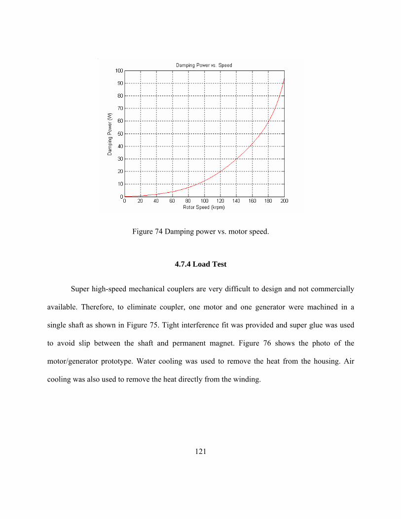
Figure 74 Damping power vs. motor speed.
4.7.4 Load Test
Super high-speed mechanical couplers are very difficult to design and not commercially
available. Therefore, to eliminate coupler, one motor and one generator were machined in a
single shaft as shown in Figure 75. Tight interference fit was provided and super glue was used
to avoid slip between the shaft and permanent magnet. Figure 76 shows the photo of the
motor/generator prototype. Water cooling was used to remove the heat from the housing. Air
cooling was also used to remove the heat directly from the winding.
121

Figure 75 Parts of the integrated motor/generator shaft.
Figure 76 Photo of the fabricated motor/generator prototype.
The load test method is described in Chapter 2. The circuitry shown in Figure 13 was
used in performing load test. The output power was calculated based on the measured AC
voltages acrossing the power resistors, and the AC currents flowing into the power resistors. The
input power was calculated based on the measured motor phase current and the motor back EMF
plus 5 % of estimated harmonics. Table 10 shows the load test results for the speed up to 109,800
rpm (The load test was not performed for higher speeds since the controller failed). The
122

efficiency of the PMSM was calculated based on the results of Motor/Generator efficiency
considering additional bearing loss. It can be seen that the efficiency of the designed PMSM is
above 92% at high-speeds. Due to high switching loss, the controller is not so efficient. Figure
77 shows the efficiency vs. motor speed for the torque shown on Table 10. We can see that when
the torque is low, the efficiency is also low. However, when the torque is too large, the winding
becomes too hot, so the efficiency will also become low. The optimized torque is 0.95 N-m
when the motor operates at 77 K. At the room temperature, the torque corresponding to highest
efficiency depends on cooling condition. Based on the current cooling condition, the ideal torque
is about 0.06 N-m. Therefore, at the room temperature, the PMSM can output about 63% of the
designed power at 77 K.
0 10 20 30 40 50 60 70 80 90 100 1100
20
40
60
80
100
20
30
40
50
60
70
0.00
0.01
0.02
0.03
0.04
0.05
0.06
0.07
0.08
0.09
0.10
Effic
ienc
y (%
)
Motor Speed (krpm)
MotorEfficiency WindingTemp Torque
Win
ding
Tem
pera
ture
(o C)
Tor
que
(N.m
)
Figure 77 Tested motor efficiency vs. motor speed.
123

Table 10 Load test results
Input to Motor Generator Output Efficiency Speed (krpm)
Input to Controller (W) Back
EMF (V)
Current (A)
Power (W)
Voltage (V)
Current (A)
Power (W)
M/G (%)
Motor (%)
Control (%)
Total (%)
Torque (N-m)
6.1 30.0 0.35 6.0 6.8 0.5 2.8 4.3 63.9 78.9 22.5 14.4 0.008
10 50.0 0.57 8.9 16.5 0.8 4.6 11.8 71.5 83.8 33.0 23.6 0.013
20.1 125.0 1.15 16.7 61.6 1.7 9.3 47.1 76.4 86.9 49.3 37.7 0.026
30.5 202.6 1.74 24.5 137.2 2.5 14.2 107.6 78.5 88.2 67.7 53.1 0.038
36.6 325.0 2.09 28.7 192.7 3.0 16.8 152.7 79.2 88.6 59.3 47.0 0.045
42.7 385.0 2.43 32.0 250.8 3.5 19.2 202.0 80.5 89.4 65.2 52.5 0.050
48.8 518.0 2.78 34.8 310.8 4.0 22.0 261.1 84.0 91.3 60.0 50.4 0.056
54.9 600.0 3.13 37.6 376.7 4.4 24.5 322.4 85.6 92.1 62.8 53.7 0.061
61 466.7 3.48 30.5 333.1 5.4 18.0 289.4 86.9 92.6 71.4 62.0 0.049
73.2 615.7 4.17 35.5 465.8 6.4 21.1 404.9 86.9 92.6 75.7 65.8 0.057
97.6 1060 5.56 46.2 809.5 8.4 27.7 695.2 85.9 92.0 76.3 65.6 0.073
109.8 897.1 6.26 37.0 717.5 10 21.2 637.2 88.8 93.2 80.0 71.0 0.059
124

CHAPTER FIVE: CONCLUSION
This work focused on the design of PMSM which is capable of operating at super high-
speed with high efficiency. The designed PMSM has 2000 W shaft output power at 200,000 rpm
and at the cryogenic temperature of 77 K. The fabricated PMSM has been successfully tested to
run upto 210,000 rpm. To test the load performance, a motor/generator prototype was also
fabricated and tested at room temperature with reduced power. The test results show that the
expected efficiency can be 92%, showing a significant improvement in efficiency compared to
the commercial motors with similar rating.
There are no commercially available motors that run at such high speed and output power
range. The state of the art technologies was used and the motor dimensions were optimized
based on analytical calculations and FEM simulations to increase performance. a) Multi-strand
twisted Litz-wire was used to dramatically reduce eddy current loss in the winding. b) Slotless
laminated stator was used to reduce torque pulsation and eddy current loss in the rotor. c) The
high energy product permanent magnet Samarium Cobalt (SmCo), which has a low temperature
coefficient and high Curie and operating temperatures, was used to avoid overheat of the magnet
during assembly and to reduce the complexity of the cooling design for the rotor.
This dissertation first talks about the basics of electric machines. After that, the modeling
of PMSM for dynamic simulation is provided. Particular design strategies have been adopted for
super high-speed applications since the motor losses assume a key role to limit the motor drive
performance. The considerations of PMSM structure for cryogenic application are also
125

discussed. It is shown that slotless structure with multi-strand Litz-wire is favorable for super-
high speed and cryogenic applications.
The design and analysis of an axial flux PMSM are presented. Based on FEM simulation,
the influence of the permanent magnet shape and the screw holes for small size motor were
analyzed and the rotor structure was optimized. From the simulation, it is shown that for small
motor, more attention should be paid to the mounting screw holes since they will affect the
performance especially when there is saturation in the rotor back iron. The simulated back-EMF
agrees very well with the experimental results. The torque and torque ripple were also simulated.
The bearing loss was separated after spin-down test. The tested efficiency at 50,000 rpm is about
60%. The motor is capable of running at 87,000 rpm with open loop control. To our knowledge,
it is the first time that a compact axial flux, low power motor was demonstrated that can run at
such high speed.
Based on experiments, bearings loss is the dominant loss for this kind of low power axial
flux single-sided motor. Changing airgap length will change the axial force which will also
change the bearing loss substantially. It is necessary to consider the change of bearing loss
during optimization.
Axial flux PMSM is suitable for the applications requiring short length but large
diameter. It also has a compact structure and can easily be integrated to the impellor of the
compressor. However, it has a lot of disadvantages. Large bearing loss due to axial force is one
of the major disadvantages. This will prevent it from further increase the speed. This positive
feedback axial force will make the use of contactless bearings difficult. Another major
126

disadvantage is that large rotor diameter will have high surface speed that will increase the stress
of rotor and also prevent the motor from going to super high-speed.
The methodologies of designing super-high speed motors are provided in details. Based
on these methodologies, a radial flux PMSM was designed and fabricated. The designed PMSM
meets our expectation and the tested results agree very well with our design specifications.
2-D and 3-D modeling of the complicated PMSM structure with respect to the
electromagnetic numerical simulations of motor performance and parameters such as phase
inductors, core losses, torque, back-EMF are also presented in details. Some mechanical issues
such as thermal analysis, bearing pre-load, rotor stress analysis and rotor dynamics analysis are
also elaborated. The different control schemes are presented and the suitable control scheme for
super high-speed PMSM is also discussed in details.
The main contributions of this research work are: (a) Developed the design
methodologies of super high-speed PMSM. (b) Designed and tested a super-high speed PMSM
with high efficiency. (c) Developed the simulation methods for both axial and radial flux
PMSMs with complicated structures.
This work has shown that a properly designed and optimized radial-flux PMSM can spin
at super high-speed with efficiency as high as 92%. However, considerable work may be
required further to improve the performance of the motor and make it commercially practical.
First integration of this motor with contactless bearing (such as gas bearing or magnetic bearing)
need to be considered in order to make it work at cryogenic temperatures, thus reducing bearing
loss. Further to increase output power, more complicated thermal design and analysis need to be
127

performed to keep the temperatures of the components below the limit. Finally, reliable and
efficient controller needs to be developed.
128

APPENDIX A: AXIAL FLUX PMSM DESIGN (USING MATHCAD)
129

Peak Phase Current: Ipsc Ieph 2⋅:= Ipsc 10.782 A= peak( )
Motor Outside Demensions:Doutside 3.6in:= Doutside 91.44 mm=
Loutside 1.18in:= Loutside 29.972 mm=
Rotor Dimensions:Diameter Over Magnet Dor 2.15in:= , Dor 54.61 mm=
Diameter Under Magnet Dir 0.8 in⋅:=
tri 2.54 mm=tri 0.1 in⋅:=Rotor Backiron Axial Thickness
ima 63 deg=ima360 deg⋅
Prpa⋅:=Magnet Arc Inside
rpa 0.7:=Rotor Pole Arc
Laxm 1.905 mm=,Laxm 0.075 in⋅:=Magnet Axial Length
Lrad 17.145 mm=,Lrad 0.5 Dor Dir−( ):=Radial Length of Magnet
Dir 20.32 mm=
Max Phase Voltage
ph 3:=No. of Stator Phase
f 1.667 103× Hz=f
Nrpm
60P2⋅ Hz⋅:=Electrical Frequency
Nrpm 50000:=Rated Shaft Speed
Nrpmmax 100000:=Max Shaft Speed
P 4:=Number of Poles
VDC 28V:=DC Bus Voltage
Pout 100W:=Output Mechanical Power Specifications:
rms( )Ieph 7.624 A=IephPin
3 Vphase⋅ PFe⋅:=Estimated Phase Current:
Pin 117.647 W=PinPout
η:=
Input Power:
PFe 0.9:=Estimated Power Factor:
η 85.00%:=Estimated Efficiency:
Estimation:
Vphase 5.715 V=Vphase 0.5Vphasemax:=Rated Phase Voltage
Vphasemax 11.431 V=VphasemaxVDC
6:=
130
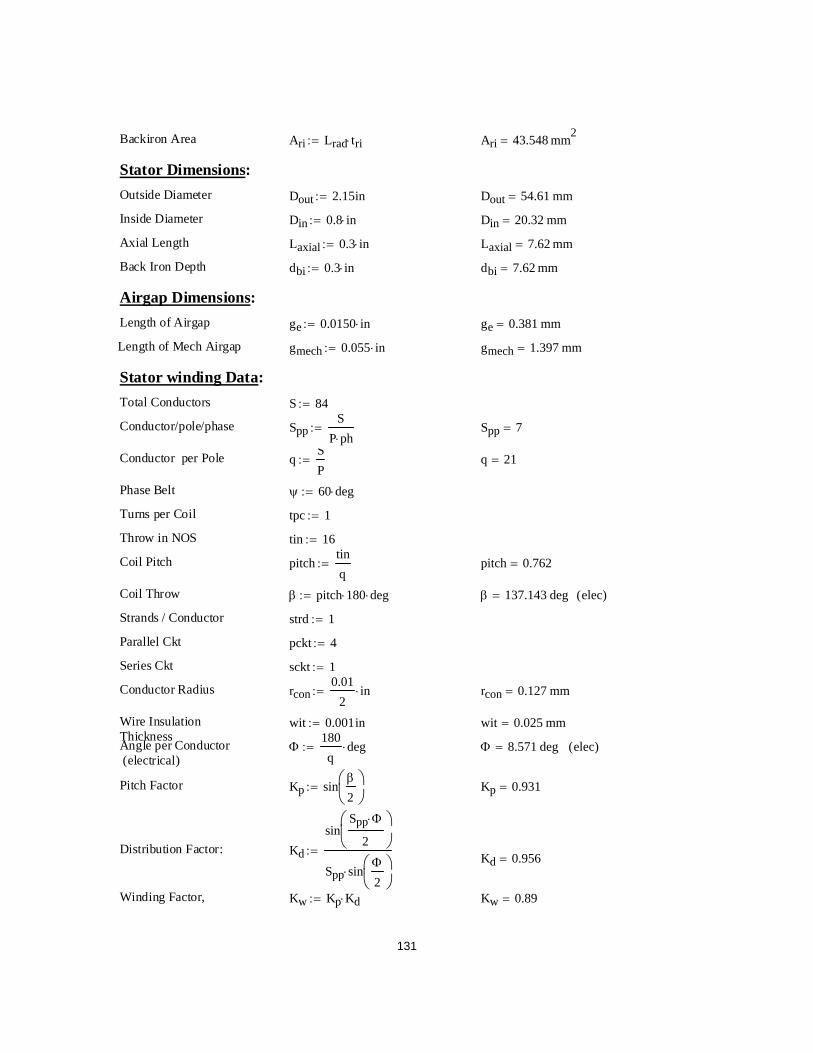
Conductor Radius
sckt 1:=Series Ckt
pckt 4:=Parallel Ckt
strd 1:=Strands / Conductor
elec( )β 137.143 deg=β pitch 180⋅ deg⋅:=Coil Throw
pitch 0.762=pitchtinq
:=Coil Pitch
tin 16:=Throw in NOS
tpc 1:=
Kw 0.89=Kw Kp Kd⋅:=Winding Factor,
Kd 0.956=Kd
sinSpp Φ⋅
2⎛⎜⎝
⎞⎠
Spp sinΦ
2⎛⎜⎝
⎞⎠
⋅
:=Distribution Factor:
Kp 0.931=Kp sinβ
2⎛⎜⎝
⎞⎠
:=Pitch Factor
elec( )Φ 8.571 deg=Φ180q
deg⋅:=Angle per Conductor (electrical)
wit 0.025 mm=wit 0.001in:=Wire Insulation Thickness
rcon 0.127 mm=rcon0.01
2in⋅:=
Airgap Dimensions:
dbi 7.62 mm=dbi 0.3 in⋅:=Back Iron Depth
Laxial 7.62 mm=Laxial 0.3 in⋅:=Axial Length
Din 20.32 mm=Din 0.8 in⋅:=Inside Diameter
Dout 54.61 mm=Dout 2.15in:=Outside Diameter
Stator Dimensions:
Ari 43.548 mm2=Ari Lrad tri⋅:=Backiron Area
Turns per Coil
ψ 60 deg⋅:=Phase Belt
q 21=qSP
:=Conductor per Pole
Spp 7=SppS
P ph⋅:=Conductor/pole/phase
S 84:=Total Conductors
Stator winding Data:
gmech 1.397 mm=gmech 0.055 in⋅:= Length of Mech Airgap
ge 0.381 mm=ge 0.0150 in⋅:=Length of Airgap
131

Lie 12.159 mm=Lieβ
360degπ⋅
Din
2⋅:=Inner end turn length
Loe 32.679 mm=Loeβ
360degπ⋅
Dout
2⋅:=Outer end turn length
Ls 17.145 mm=LsDout Din−
2:=Radial length
Phase Resistance:
dent 0.165 lb in 3−⋅=dent 4570 kg⋅ m 3−
⋅:=Density of Titanium
denb 7.474 103× kg m-3
=denb 0.27 lb⋅ in 3−⋅:=Density of rotor back iron
denm 7.474 103× kg m-3
=
Rph 0.06Ω=Rph Lcppsckt
pckt2⋅ Llead+⎛
⎜⎝
⎞
⎠
ρwire
Acon⋅:=Resistance /Phase@20oC
Llead 30mm:=Lead length
J 37.614 A mm 2−⋅=J
Ieph
pckt Acon⋅:=Current Density
Acon 0.051 mm2=Acon π rcon
2⋅:=
Conductor Area. Lcpp 2.216 103
× mm=Lcpp Lmt
S3⋅ tpc⋅ sckt⋅:=Length of conductor/ phase
Lmt 79.128 mm=Lmt Loe Lie+ 2 Ls⋅+:=Length of mean turn
Hc 1000kAm
⋅:=Hc coercive Field Intensity( )
Br 1.25 T⋅:=Br Restoring Flux Density( )
NdFeB35( )Magnet
ρwire 1.79 10 6−⋅( ) Ω⋅ cm⋅:=Wire Resistivity @ 20oC
sst 0.003in:=Slot Seperator Thickness
sit 0.003in:=Slot Insulation Thickness
wit 0.0018in:=Wire Insulation Thickness
Material Properties:
denm 0.27 lb⋅ in 3−⋅:=Density of magnet
denc 7.474 103× kg m-3
=denc 0.27 lb⋅ in 3−⋅:=Density of iron core
denw 9.134 103× kg m-3
=;denw 0.33 lb⋅ in 3−⋅:=Density of winding
Coeffhc 0.03−%C
:=HcTemp Coeff for
Coefbr 0.03−%C
:=BrTemp Coeff for
perm 1.11:=Magnet rela. Permiability
Hc 1.257 104× oersted=
132
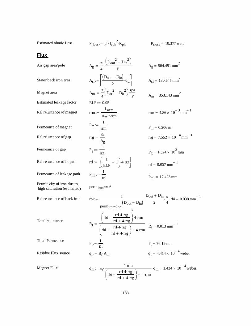
Pg1
rrg:= Pg 1.324 103
× mm=
Rel reluctance of lk path rrl1
ELF1−⎛⎜
⎝⎞⎠
4⋅ rrg⋅⎡⎢⎣
⎤⎥⎦
:= rrl 0.057 mm 1−=
Permeance of leakage path Pml1rrl
:= Pml 17.423 mm=
Permitivity of iron due to high saturation (estimated) permiron 6:=
Rel reluctance of back iron rbi1
permiron dbi⋅Dout Din−( )
2⋅
Dout Din+
2π
4⋅:= rbi 0.038 mm 1−
=
Total reluctance Rt
rbirrl 4⋅ rrg⋅
rrl 4 rrg⋅++⎛⎜
⎝⎞⎠
4⋅ rrm⋅
rbirrl 4⋅ rrg⋅
rrl 4 rrg⋅++⎛⎜
⎝⎞⎠
4 rrm⋅+
:= Rt 0.013 mm 1−=
Total PermeancePt
1Rt
:= Pt 76.19 mm=
Residue Flux source φr Br Am⋅:= φr 4.414 10 4−× weber=
Magnet Flux: φm φr4 rrm⋅
rbirrl 4⋅ rrg⋅
rrl 4 rrg⋅++⎛⎜
⎝⎞⎠
4 rrm⋅+
⋅:= φm 1.434 10 4−× weber=
Estimated ohmic Loss Prloss ph Ieph2
⋅ Rph⋅:= Prloss 10.377 watt=
Flux
Air gap area/pole Agπ
4
Dout2 Din
2−⎛
⎝⎞⎠
P⋅:= Ag 504.491 mm2
=
Stator back iron area AsiDout Din−( )
2dbi⋅
⎡⎢⎣
⎤⎥⎦
:= Asi 130.645 mm2=
Magnet area Amπ
4Dor
2 Dir2
−⎛⎝
⎞⎠
rpaP
⋅:= Am 353.143 mm2=
Estimated leakage factor ELF 0.05:=
Rel reluctance of magnet rrmLaxm
Am perm⋅:= rrm 4.86 10 3−
× mm 1−=
Pm1
rrm:=Permeance of magnet Pm 0.206 m=
Rel reluctance of gap rrgge
Ag:= rrg 7.552 10 4−
× mm 1−=
Permeance of gap
133

Pbearing 30W:=
Stator iron and Stray Loss Pisl 10 W⋅:=
Winding AC loss Pcuac 3W:=
Estimated Windage Loss Pwindage 5W:=
Electrical Efficiency ηePout
Pout Prloss+ Pcuac+ Pisl+ Pwindage+ Pbearing+:=
ηe 63.14 %=
Power Density:
Total Volume: VTπ
4Doutside
2⋅ Loutside⋅:= VT 1.968 105
× mm3=
POWER DENSITY: PdPout
VT:= Pd 5.081 10 4−
× W mm 3−⋅=
Userful Flux:φu φm
rrlrrl 4 rrg⋅+⋅:= φu 1.362 10 4−
× weber=
Airgap Flux Density, Bgφu
Ag:= Bg 0.27 tesla=
Stator Back iron Flux Density, Bsi
φu
2 Asi⋅:= Bsi 0.521 tesla=
Rotor Back iron Flux Density,
Briφm
2 Ari⋅:= Bri 1.646 tesla=
Back EMF:
Induced Back EMF Ebackrms2π f⋅
2φu⋅ Spp⋅ Kw⋅:= Ebackrms 6.282 volt=
Motor Efficiency:
Bearing loss
134

APPENDIX B: RADIAL FLUX PMSM DESIGN (USING MATHCAD)
135
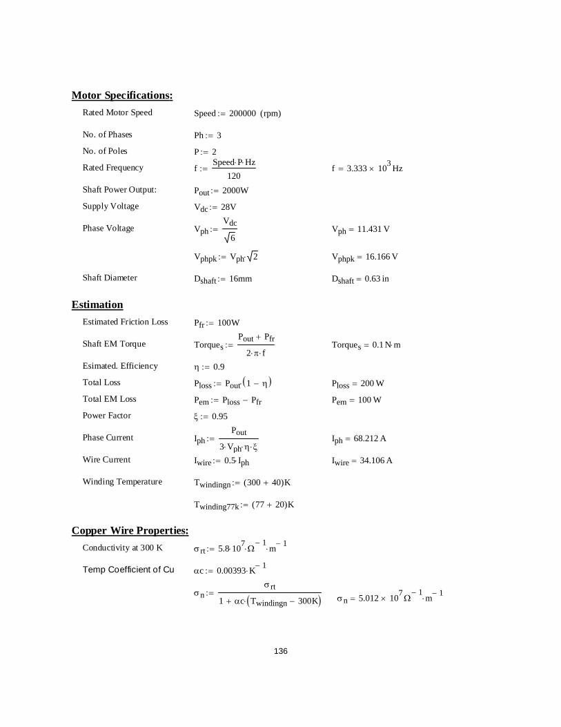
Torques 0.1 N m⋅=
Esimated. Efficiency η 0.9:=
Total Loss Ploss Pout 1 η−( )⋅:= Ploss 200 W=
Total EM Loss Pem Ploss Pfr−:= Pem 100 W=
Power Factor ξ 0.95:=
Phase Current IphPout
3 Vph⋅ η⋅ ξ⋅:= Iph 68.212 A=
Wire Current Iwire 0.5 Iph⋅:= Iwire 34.106 A=
Winding Temperature Twindingn 300 40+( )K:=
Twinding77k 77 20+( )K:=
Copper Wire Properties:Conductivity at 300 K σ rt 5.8 107
⋅ Ω1−
⋅ m 1−⋅:=
Temp Coefficient of Cu αc 0.00393 K 1−⋅:=
σnσ rt
1 αc Twindingn 300K−( )⋅+:=
σn 5.012 107× Ω
1−m 1−⋅=
Motor Specifications:Rated Motor Speed Speed 200000:= rpm( )
No. of Phases Ph 3:=
No. of Poles P 2:=
Rated Frequency fSpeed P⋅ Hz⋅
120:= f 3.333 103
× Hz=
Shaft Power Output: Pout 2000W:=
Supply Voltage Vdc 28V:=
Phase Voltage VphVdc
6:= Vph 11.431 V=
Vphpk Vph 2⋅:= Vphpk 16.166 V=
Shaft Diameter Dshaft 16mm:= Dshaft 0.63 in=
EstimationEstimated Friction Loss Pfr 100W:=
Shaft EM Torque TorquesPout Pfr+
2 π⋅ f⋅:=
136
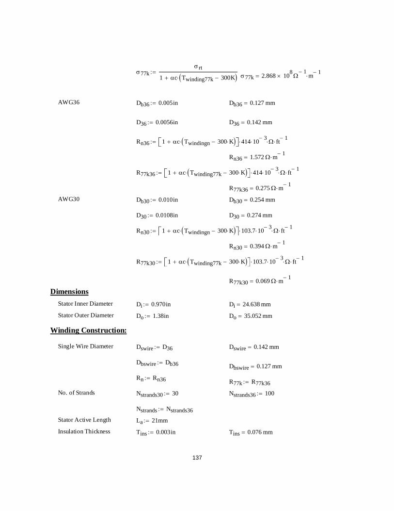
Di 0.970in:= Di 24.638 mm=
Stator Outer Diameter Do 1.38in:= Do 35.052 mm=
Winding Construction:
Single Wire Diameter Dswire D36:= Dswire 0.142 mm=
Dbswire Db36:= Dbswire 0.127 mm=
Rn Rn36:= R77k R77k36:=
No. of Strands Nstrands30 30:= Nstrands36 100:=
Nstrands Nstrands36:=
Stator Active Length La 21mm:=
Insulation Thickness Tins 0.003in:= Tins 0.076 mm=
σ77kσ rt
1 αc Twinding77k 300K−( )⋅+:=
σ77k 2.868 108× Ω
1−m 1−⋅=
AWG36 Db36 0.005in:= Db36 0.127 mm=
D36 0.0056in:= D36 0.142 mm=
Rn36 1 αc Twindingn 300 K⋅−( )⋅+⎡⎣ ⎤⎦ 414⋅ 10 3−⋅ Ω⋅ ft 1−
⋅:=
Rn36 1.572 Ω m 1−⋅=
R77k36 1 αc Twinding77k 300 K⋅−( )⋅+⎡⎣ ⎤⎦ 414⋅ 10 3−⋅ Ω⋅ ft 1−
⋅:=
R77k36 0.275 Ω m 1−⋅=
AWG30 Db30 0.010in:= Db30 0.254 mm=
D30 0.0108in:= D30 0.274 mm=
Rn30 1 αc Twindingn 300 K⋅−( )⋅+⎡⎣ ⎤⎦ 103.7⋅ 10 3−⋅ Ω⋅ ft 1−
⋅:=
Rn30 0.394 Ω m 1−⋅=
R77k30 1 αc Twinding77k 300 K⋅−( )⋅+⎡⎣ ⎤⎦ 103.7⋅ 10 3−⋅ Ω⋅ ft 1−
⋅:=
R77k30 0.069 Ω m 1−⋅=
DimensionsStator Inner Diameter
137
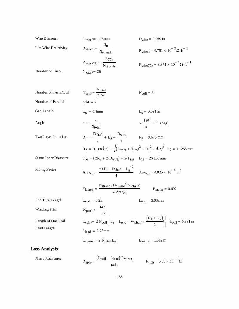
R2 11.258 mm=
Stator Inner Diameter Die 2R2 2 Dwire⋅+( ) 2 Tins⋅+:= Die 26.168 mm=
Filling FactorAreacu
π Di Dshaft− Lg−( )2
4:= Areacu 4.825 10 5−
× m2=
FfactorNstrands Dbswire
2⋅ Ntotal⋅ 2⋅
4 Areacu⋅:= Ffactor 0.602=
End Turn Length Lend 0.2in:= Lend 5.08 mm=
Winding Pitch Wpitch14.518
:=
Length of One Coil Lcoil 2 Ncoil⋅ La Lend+ Wpitch π⋅R1 R2+( )
2⋅+
⎡⎢⎣
⎤⎥⎦
⋅:= Lcoil 0.631 m=
Lead LengthLlead 2 25⋅ mm:=
Lawire 2 Ntotal⋅ La⋅:= Lawire 1.512 m=
Loss Analysis
Phase ResistanceRnph
Lcoil Llead+( ) Rwiren⋅
pckt:= Rnph 5.35 10 3−
× Ω=
Wire Diameter Dwire 1.75mm:= Dwire 0.069 in=
Litz Wire Resistivity RwirenRn
Nstrands:= Rwiren 4.791 10 3−
× Ω ft 1−⋅=
Rwire77kR77k
Nstrands:= Rwire77k 8.371 10 4−
× Ω ft 1−⋅=
Number of Turns Ntotal 36:=
Number of Turns/Coil NcoilNtotal
P Ph⋅:= Ncoil 6=
Number of Parallel pckt 2:=
Gap Length Lg 0.8mm:= Lg 0.031 in=
Angle απ
Ntotal:= α
180π
⋅ 5= deg( )
Two Layer Locations R1Dshaft
2Lg+
Dwire
2+:= R1 9.675 mm=
R2 R1 cos α( )⋅ Dwire Tins+( )2 R12 sin α( )2⋅−+:=
138

ACCuLoss77k 16.818 W=
Density of Stator Core denc 0.27lb in 3−⋅:=
Volume of Stator Core Vstator π La⋅Do
2 Di2
−⎛⎝
⎞⎠
4⋅:= Vstator 10.252 cm3
=
Weight of Stator Core Wstator Vstator denc⋅:= Wstator 0.077 kg=
Loss Parameters of Stator Core( from curvefitting)
Kh 0.0069W
Hz T2⋅ lb⋅
:= Kh 0.015W
Hz T2⋅ kg⋅
=
Ken 2.92 10 6−⋅
W
Hz2 T2⋅ lb⋅
:= Ken 6.437 10 6−×
W
Hz2 T2⋅ kg⋅
=
Kexen 0.00015W
Hz T⋅( )1.5 lb⋅:= Kexen 3.307 10 4−
×W
Hz T⋅( )1.5 kg⋅=
Ke77k 1.792 Ken⋅:= Ke77k 1.154 10 5−×
W
Hz2 T2⋅ kg⋅
=
R77kphLcoil Llead+( ) Rwire77k⋅
pckt:= R77kph 9.349 10 4−
× Ω=
Copper DC Loss Lossncu 3Iph2 Rnph⋅:= Lossncu 74.685 W=
Loss77kcu 3Iph2 R77kph⋅:= Loss77kcu 13.051 W=
Peak Flux Density Bp 0.3721T:=
Copper AC LossPE Bp
2 2 π⋅ f⋅( )2 Dbswire2σn
32⋅:= PE 1.534 106
×1
m3W=
Vola Lawire Nstrands⋅πDbswire
2
4⋅:= Vola 1.915 103
× mm3=
ACCuLossn PE Vola⋅:= ACCuLossn 2.939 W=
ACCuLoss77k ACCuLossnσ77k
σn⋅:=
139

ηmn 91.623 %=ηmn
Pout
Pout Lossn+:=
ηm77k 93.536 %=ηm77k
Pout
Pout Loss77k+:=
Motor Efficiency
Lossn 182.847 W=
Lossn Lossncu ACCuLossn+ Losssn+ Pfr+:=
Loss77k 138.21 W=
Loss77k Loss77kcu ACCuLoss77k+ Losss77k+ Pfr+:=Total loss
Losss77k 8.342 W=
Losss77k Wstator Kh f⋅ Bm2⋅ Ke77k f Bm⋅( )2
⋅+ Kexe77k f Bm⋅( )1.5⋅+⎡⎣ ⎤⎦⋅:=
Losssn 5.223 W=
Losssn Wstator Kh f⋅ Bm2⋅ Ken f Bm⋅( )2
⋅+ Kexen f Bm⋅( )1.5⋅+⎡⎣ ⎤⎦⋅:=
Lexe77k 3.81 W=Lexe77k Kexe77k f Bm⋅( )1.5⋅ Wstator⋅:=
Ledd77k 3.247 W=Ledd77k Ke77k f Bm⋅( )2⋅ Wstator⋅:=
Lexen 2.126 W=Lexen Kexen f Bm⋅( )1.5⋅ Wstator⋅:=
Leddn 1.812 W=Leddn Ken f Bm⋅( )2⋅ Wstator⋅:=
Lhys 1.285 W=Lhys Kh f⋅ Bm2⋅ Wstator⋅:=
Bm0.68 0.47+
2T:=Stator Flux Density
Kexe77k 5.926 10 4−×
W
Hz T⋅( )1.5 kg⋅=Kexe77k 1.792 Kexen⋅:=
140

APPENDIX C: ROTOR DRAWINGS OF MOTOR AND MOTOR/GENERATOR
141

142
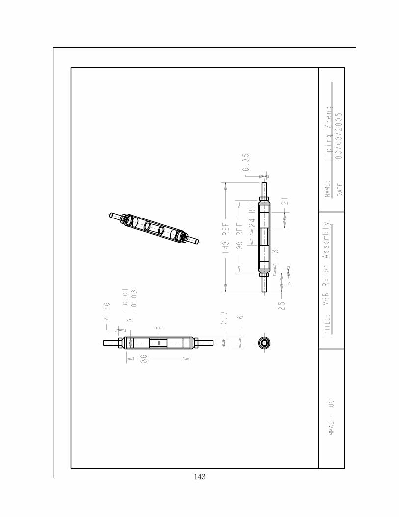
143

APPENDIX D: ANALYTICAL ANALYSIS OF ROTORDYNAMICS
144

Speedsolid 8.324 105× rpm=Speedsolid
ωsolid
2 π⋅:=
ωsolidπ
4EiTi⋅ d4 d 2 t⋅−( )4
−⎡⎣ ⎤⎦⋅
8Length4ρTi d2 d 2 t⋅−( )2
−⎡⎣ ⎤⎦⋅ ρPM d 2 t⋅−( )2⋅+⎡
⎣⎤⎦⋅
:=
td2
:=If Solid Shaft
Speed 5.158 105× rpm=
Speedω
2 π⋅:=Critical Speed
ωπ
4EiTi⋅ d4 d 2 t⋅−( )4
−⎡⎣ ⎤⎦⋅
8Length4ρTi d2 d 2 t⋅−( )2
−⎡⎣ ⎤⎦⋅ ρPM d 2 t⋅−( )2⋅+⎡
⎣⎤⎦⋅
:=Natural Frequency
Length 57.75mm:=Shaft Length
t 1.5mm:=Shaft Thickness
d 16mm:=Shaft Diameter
Calculation of Motor Rotor Dynamics:
rpm1
60s:=
ρPM 7700kg m 3−⋅:=Density of PM
ρTi 4500kg m 3−⋅:=Density of Ti
EiTi 1.22 1011⋅ Pa⋅:=Youth Module of Ti
145

Speedsolid 2.629 105× rpm=
Speedsolidωsolid
2 π⋅:=
ωsolidπ
4EiTi⋅ d4 d 2 t⋅−( )4
−⎡⎣ ⎤⎦⋅
8Length4ρTi d2 d 2 t⋅−( )2
−⎡⎣ ⎤⎦⋅ ρPM d 2 t⋅−( )2⋅+⎡
⎣⎤⎦⋅
:=
td2
:=If Solid Shaft
Speed 1.629 105× rpm=
Speedω
2 π⋅:=Critical Speed
ωπ
4EiTi⋅ d4 d 2 t⋅−( )4
−⎡⎣ ⎤⎦⋅
8Length4ρTi d2 d 2 t⋅−( )2
−⎡⎣ ⎤⎦⋅ ρPM d 2 t⋅−( )2⋅+⎡
⎣⎤⎦⋅
:=Natural Frequency
Length 102.75mm:=Shaft Length
t 1.5mm:=Shaft Thickness
d 16mm:=Shaft Diameter
Calculation of Motor/Generator Rotor Dynamics:
146

APPENDIX E: SCHEMETIC AND PCB LAYOUT OF THE PMSM CONTROLLER
147

12
34
56
ABCD
65
43
21
D C B A
Title
Num
ber
Revi
sion
Size B Dat
e:20
-Oct
-200
5Sh
eet
of
File
:D
:\PM
SMCn
tl1.d
dbD
raw
n By
:
VF1
+1
VF1
-2
VF2
-3
VF2
+4
Gnd
5
VD
26
VD
17
Vcc
8U
2
2631
12
U1A
7406
89
U1D
7406
34
U1B
7406
56
U1C
7406
1011
U1E
7406
1213
U1F
7406
Q1
IR16
07
Q2
IR16
07
R13
15 R14
15
VCC
LO1
COM
2V
CC34
VS
5V
B6
HO
78
VD
D9
HIN
10
SD11
LIN
12
VSS
13 14
U5
IR21
10
+12V
C4 2.2u
+28V
+5V
R7 470
R8 470
C2 0.1
C3 10u
VF1
+1
VF1
-2
VF2
-3
VF2
+4
Gnd
5
VD
26
VD
17
Vcc
8U
3
2631
Q5
IR16
07
Q6
IR16
07
R15
15 R16
15LO
1CO
M2
VCC
34V
S5
VB
6H
O7
8
VD
D9
HIN
10
SD11
LIN
12
VSS
13 14
U6
IR21
10
+12V
C8 2.2uD2
RS2A
+28V
+5V
R9 470
R10
470
C6 0.1
C7 10u
VF1
+1
VF1
-2
VF2
-3
VF2
+4
Gnd
5
VD
26
VD
17
Vcc
8U
4
2631
Q9
IR16
07
Q10
IR16
07
R17
15 R18
15LO
1CO
M2
VCC
34V
S5
VB
6H
O7
8
VD
D9
HIN
10
SD11
LIN
12
VSS
13 14
U7
IR21
10
+12V
C12
2.2uD3
RS2A
+28V
+5V
R11
470
R12
470
C10
0.1
C11
10u
R2 150
R1 150
VCC
R4 150
R3 150
VCC
R6 150
R5 150
VCC
VCC
A
C9 0.1
C13
0.1
C29
10u
VCC
A
VCC
A
1
J8 Phas
e C
AD
CIN
0
1
J7 28V
1
J2 GN
D
C20
1u/2
00V
C19
1u/2
00V
C18
470u
/200
V
Vin
1
GND 2
+5V
3
U13
MC7
805T
C31
47u
C30
220u
D4
RS2A
1
J9 +12V
IN
1
J3 GN
D
+5V
+12V
In4
Out
5
+5 1
Gnd 2
Sout 3
U8
ACS
754
In4
Out
5
+5 1
Gnd 2
Sout 3
U9
ACS
754
R20
10K
R21
10K
R19
10K
R24
10K 3 2
1
4 11
U11
A
LM32
4
1098
U11
C
LM32
4
1
J4Ph
ase
A
C21
1600
p
C22
1600
p
Vre
f1
AD
CIN
1R2
310
K
R25
10K
R26
10K
567
U11
B
LM32
4
1
J6Ph
ase
B
C25
1600
p
C23
1600
p
R22
10K
Vre
f1
R35
5KV
ar
C1 0.1
C17
100u
C5 0.1
VCC
A
C14
0.1
Vre
f1
AD
CIN
2R3
210
K
R38
820
R37
820
567
U12
B
LM32
4
C27
1600
p
C28
1600
p
R31
10K
+28V
1 2 3 4 5 6 7 8 9 10 11 12 13 14 15 16 17 18 19 20 21 22 23 24 25 26 27 28 29 30 31 32 33 34
J1 Dig
ital
VCC
1 2 3 4 5 6 7 8 9 10 11 12 13 14 15 16 17 18 19 20 21 22 23 24 25 26 27 28 29 30 31 32 33 34
J5 Ana
log
AD
CIN
0A
DCI
N1
AD
CIN
2A
DCI
N3
AD
COU
T0A
DCO
UT1
AD
COU
T2A
DCO
UT3
D1
RS2A
Q3
IR16
07
Q4
IR16
07
Q7
IR16
07
Q8
IR16
07
Q11
IR16
07
Q12
IR16
07
R33
2k
HA
LA HB
LB HC
LC
PA PB PC
C15
0.1
In4
Out
5
+5 1
Gnd 2
Sout 3
U10
ACS
754
AD
CIN
3R2
810
K
R30
10K
R29
10K109
8
U12
C
LM32
4
C26
1600
p
C24
1600
p
R27
10K
Vre
f2
+28V
3 21
4 11
U12
A
LM32
4R3
6
5KV
ar
VCC
A
C16
0.1
Vre
f2
R34
2k
IDC
Lipi
ng Z
heng
21
V1.
0
PMSM
Con
trolle
r
148
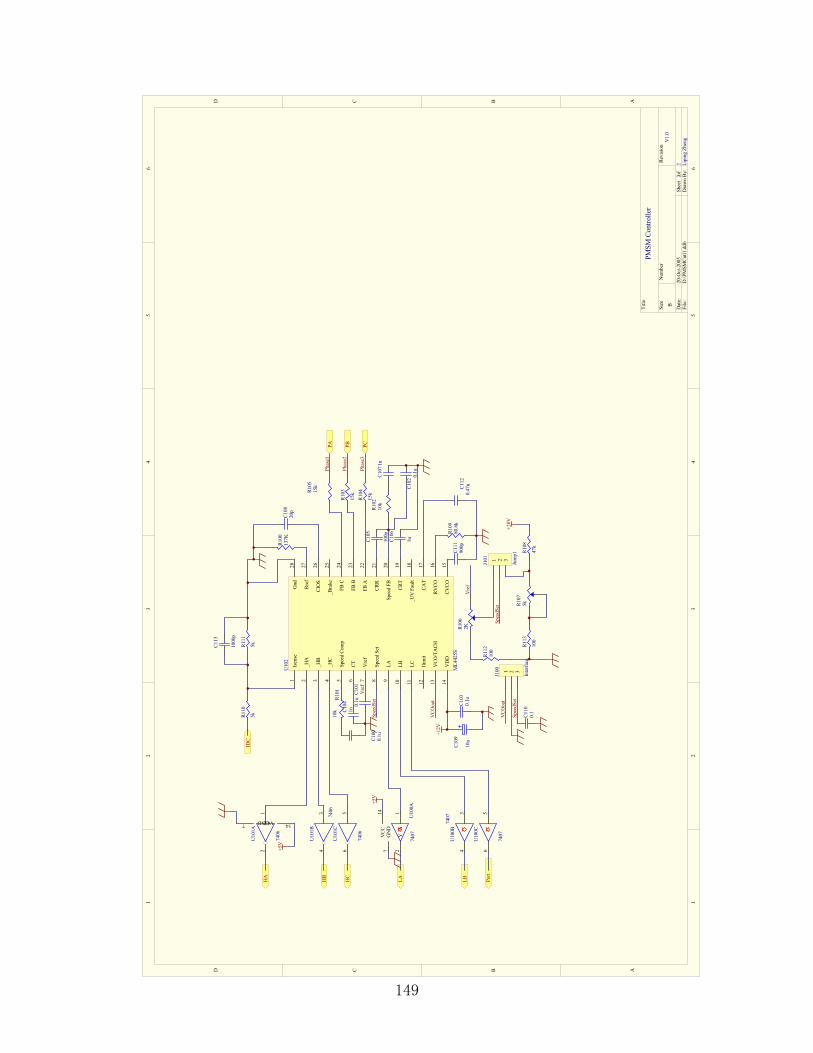
12
34
56
ABCD
65
43
21
D C B A
Title
Num
ber
Revi
sion
Size B Dat
e:20
-Oct
-200
5Sh
eet
of
File
:D
:\PM
SMCn
tl1.d
dbD
raw
n By
:
Isen
se1
_HA
2
_HB
3
_HC
4
Spee
d Co
mp
5
CT6
Vre
f7
Spee
d Se
t8
LA9
LB10
LC11
Ilim
it12
VCO
/TA
CH13
VD
D14
CVCO
15
RVCO
16
CAT
17
_UV
Fau
lt18
CRT
19
Spee
d FB
20
CRR
21
FB A
22
FB B
23
FB C
24
_Bra
ke25
CIO
S26
Rref
27
Gnd
28U
102
ML4
425S
R101
10k
C100
0.1u
C104
1nC1
010.
1u
Spee
dSet
+12V
C109
10u
C103
0.1u
C111
900p
R109
80.6
kC1
120.
47u
C105
100p
C106
1u
C107
1u
C102
0.1u
R102
10k
R100
137K
C108
20p
R105
15k
R103
15k
R104
15k
Phas
e1
Phas
e2
Phas
e3
1 2 3
J101
Jum
p1
Spee
dSet
Vre
f
R106
2K
R107
5kR1
08
47k
+28V
Vre
f
1 2 3
J100
Inte
rface
VCO
out
Spee
dSet
C110
0.1
VCO
out
IDC
PA PB PC
VCC
14
GN
D7
A1
Y2
U10
0A74
07
34
U10
0B74
07
56
U10
0C
7407
56
U10
1C
7406
34
U10
1B
74061
2
GND7 VCC 14
U10
1A
7406
HA
HB
HC
LA LB Port
+5V
+5V
R110
5k
R111
5kC113
1000
p
R112
100
R113
100
PMSM
Con
trolle
r
22 Li
ping
Zhe
ngV1.
0
149


LIST OF REFERENCES
[1] B. H. Bae, S. K. Sul, J. H. Kwon, and J. S. Byeon, “Implementation of sensorless vector control for super-high-speed PMSM of turbo-compressor,” IEEE Trans. Ind. Applic., vol. 39, pp. 811-818, 2003.
[2] L. Soong, G. B. Kliman, R. N. Johnson, R. A. White, and J. E. Miller, “Novel high-speed induction motor for a commercial centrifugal compressor,” IEEE Trans. Ind. Applic., vol. 36, pp.706-713, 2000.
[3] A. Boglietti, P. Ferraris, M. Lazzari, and F. Profumo, “About the design of very high frequency induction motors for spindle applications,” IEEE Trans. Ind. Applic. Society Annual Meeting, vol. 1, pp. 25-32, 1992.
[4] J. F. Gieras, “Comparison of high-power high-speed machines: cage induction versus switched reluctance motors,” IEEE AFRICON, vol. 2, pp.675-678, 1999.
[5] M. J. Superczynski and D. J. Waltman, “Homopolar motor with high temperature superconductor field windings,” IEEE Trans. Applied Superconductivity, vol.7, no. 2, part 1, pp. 513-518, June 1997.
[6] W. J. Jeon, S. Katoh, T. Iwamoto, Y. Kamiya, and T. Onuki, “Propulsive characteristics of a novel linear hybrid motor with both induction and synchronous operations,” IEEE Transactions on Magnetics, vol. 35, no. 5, part 2, pp.4025-4027, Sept. 1999.
[7] R. Qin, and M.A. Rahman, “Magnetic equivalent circuit of PM hysteresis synchronous motor,” IEEE Transactions on Magnetics, vol. 39, no.5, part 2, pp. 2998-3000, Sept. 2003.
[8] M. Cheng, et al, “Static characteristics of a new doubly salient permanent magnet motor Ming Cheng,” IEEE Trans. Energy Conversion, vol. 16, no. 1, pp.20-25, 2001.
[9] M. Cheng, et al, “Design and analysis of a new salient permanent magnet motor,” IEEE Trans. Magnetics, vol. 37, no, 4, pp. 3012-3020, 2001.
[10] Y. Liao, F. Liang and T. A. Lipo, “A novel permanent magnet motor with doubly salient structure,” IEEE Trans. Ind. Applic., vol. 31, no. 5, pp. 1069-1078, 1995.
[11] E. C. Lovelace, T. M. Jahns, and J. H. Lang, “A saturating lumped-parameter model for an interior PM synchronous machine,” IEEE Trans. Ind. Applic., vol. 38, no. 3, pp. 645-650, May-June, 2002.
[12] N. Urasaki, T. Senjyu, and K. Uezato, “Relationship of parallel model and series model for
151

PMSM,” IEEE Power Electronics Specialists Conference, vol. 2, pp. 788-793, 2001.
[13] G. Stumberger, B. Stumberger, and D. Dolinar, “Identification of linear synchronous reluctance motor parameters,” IEEE Trans. Ind. Applic., vol.40, no.5, pp. 1317-1324, Sept.-Oct., 2004.
[14] N. A. Demerdash, and T. W. Nehl, “Electric machinery parameters and torques by current and energy perturbations from field computations. I. Theory and formulation,” IEEE Trans. Energy Conversion, vol. 14, no. 4, pp. 1507-1513, Dec. 1999.
[15] U. Schaible, and B. Szabados, “Dynamic motor parameter identification for high speed flux weakening operation of brushless permanent magnet synchronous machines,” IEEE Trans. Energy Conversion, vol. 14, no. 3, pp. 486-492, Sept. 1999.
[16] Chee-Mun Ong, Dynamic Simulation of Electric Machinery, Prentice-Hall, 1998.
[17] Tomonobu, et.al, “Accurate parameter measurement for high speed permanent magnet synchronous motors,” IEEE Power Electronics Specialists Conf., vol. 2, pp.772-777, 2001.
[18] K. Atallah, et.al, “Armature reaction field and winding inductances of slotless permanent-magnet brushless machines,” IEEE Trans. on Magnetics, no.5, part 2, vol.34, pp.3737-3744, Sept. 1998.
[19] H. P. Nee, et.al, “Determination of d and q reactances of permanent-magnet synchronous motors without measurements of the rotor position,” IEEE Trans. Ind. Applic., vol. 36 , no. 5, pp. 1330-1335, Sept.-Oct. 2000.
[20] B. Stumberger, B. Kreca, B. Hribernik, “Determination of parameters of synchronous motor with permanent magnets from measurement of load conditions,” IEEE Transactions on Energy Conversion, vol.14, no. 4, pp. 1413-1416, Dec. 1999.
[21] S. F. Gorman, C. Chen, J. J. Cathey, “Determination of permanent magnet synchronous motor parameters for use in brushless DC motor drive analysis,” IEEE Trans. Energy Conversion, vol. 3, no. 3, pp. 674-681, Sept. 1988.
[22] M. Rosu, A. Arkkio, T. Jokinen, J. Mantere, J. Westerlund, “Demagnetization state of permanent magnets in large output power permanent magnet synchronous motor,” IEEE IEMDC’99, pp. 776-778, 9-12 May 1999.
[23] J. A. McCormick, G. F. Nellis, W. L. Swift and H. Sixsmith, “Design and test of low capacity reverse Brayton cryocooler for refrigeration at 35K and 60K,” Cryocoolers 10, Kluwer Academic/Plenum Publishers, pp. 420-429, 1999.
[24] H.C.J.de Jong, AC Motor Design: Rotating Magnetic Fields in a Changing Environment,
152
Hemisphere Publishing Corporation, 1989.
[25] T. Kosaka, et.al, “Drive characteristics of slotless PM motors,” IEEE Ind. Applic. Conference, Thirty-Fourth IAS Annual Meeting, vol. 2, pp. 894-899, 1999.
[26] M. Aydin, S. Huang and T. A. Lipo, “Optimum design and 3D finite element analysis of non-slotted and slotted internal rotor type axial flux PM disc machines,” Power Engineering Society Summer Meeting, vol. 3, pp. 1409-1416, 2001.
[27] A. Cavagnino, et.al, “A comparison between the axial flux and the radial flux structures for PM synchronous motors,” IEEE Ind. Applic. Conference, thirty-Sixth IAS Annual Meeting, vol. 3, pp. 1611-1618, 2001.
[28] F. Profumo, et. al, “Novel axial flux interior PM synchronous motor realized with powdered soft magnetic materials ,” IEEE Ind. Applic. Conference, vol. 1, pp. 152-158, 1998.
[29] S. Huang, et. al, “A comparison of power density for axial flux machines based on general purpose sizing equations,” IEEE Transaction on Energy conversion, Vol. 14, Issue 2 , pp. 185-192, June 1999.
[30] E. S. Hamdi, Design of small Electrical Machines. John Wiley & Sons Ltd. 1994.
[31] H. C. J. de Jong, AC Motor Design: Rotating Magnetic Fields in a Changing Environment, Hemisphere Publishing Corporation, 1989.
[32] T. Kosaka, et. al, “Experimental investigations into skin effect influences on current distortion and increase in loss for 20 kHz PWM-VSI-fed slotless PMSM drives,” IEEE Industry Applications Conference, Vol.4 , pp. 2374-2379, 2001.
[33] D. Binesti and J. P. Ducreux, “Core losses and efficiency of electrical motors using new magnetic materials,” IEEE Trans. on Magnetics, vol. 32, no.5, pp. 4887 - 4889, Sept. 1996.
[34] A.C. Smith, K. Edey, “Influence of manufacturing processes on iron losses,” IEE Electrical Machines and Drives Conference, pp.77-81, Sept. 1995.
[35] R. Aouli, et al, “Iron loss measurement device under rotating magnetic field ,” IEEE Proceedings on Science, Measurement and Technology, vol.146 ,no.1 , pp. 35-39, Jan. 1999 .
[36] G. R. Siemon, and X. Liu, “Core losses in permanent magnet motors,” IEEE Trans. Magnetics, vol. 26, no. 5, Sept. 1990.
[37] A. E. Emanuel, “The effect of nonsinusoidal excitation on eddy current losses in saturated
153

iron,” IEEE Trans. Power Delivery, vol. 3, no. 2, pp.662-671, April 1988.
[38] M. Enokizono, T. Suzuki, J. Sievert, and J. Xu, “Rotational power loss of silicon steel sheet,” IEEE Trans. Magnetics, vol. 26, no. 5, pp. 2562-2564, Sept. 1990.
[39] L. R. Dupre, R. V. Keer, and J. A. A. Melkebeek, “An iron loss model for electrical machines using the Preisach theory,” IEEE Trans. Magnetics, vol. 33, no. 5, pp. 4158-4160, Sept. 1997.
[40] M. V. K. Chari, “Finite element analysis of electrical machinery and devices,” IEEE Trans. Magnetics, vol. 16, no. 5, Sept. 1980.
[41] H. Shimoji, “Iron loss and magnetic fields analysis of permanent magnet motors by improved finite element method with E&S; model,” IEEE Transactions on Magnetics, vol.37, no.5, part 1, pp. 3526-3529, Sept. 2001
[42] Spooner, E., and Chalmers, B. J.: ‘`TORUS': a slotless, toroidal-stator, permanent-magnet generator’, IEE Proc. B Electric Power Appl., vol. 139, no.6 , pp.497-506, 1992.
[43] K. Dabala, “Analysis of mechanical losses in three-phase squirrel-cage induction motors,” ICEMS 2001, vol.1, pp. 39-42, Aug. 2000.
[44] I. Sato, K. Otani, S. Oguchi, and K. Hoshiya, “Characteristics of Heat Transfer in a Helium-Filled Disk Enclosure,” IEEE Trans. on Components, Hybrids, and Manufacturing Technology, vol. 11, no. 4, pp. 571-575 Dec 1988.
[45] L. A. Dorfman, Hydrodynamic resistance and the heat loss of rotating solids, Oliver and Boyd Ltd., 1963, Ch. 6.
[46] M. N. Awad and W. J. Martin, “Windage loss reduction study for TFTR pulse generator,” 17th IEEE/NPSS Symposium on Fusion Engineering, vol. 2, pp. 1125-1128, Oct. 1997.
[47] Z. Q. Zhu, et al, “Instantaneous magnetic field distribution in brushless permanent magnet DC motors. I. Open-circuit field,” IEEE Transactions on Magnetics, vol. 29, no.1, pp. 124-135, Jan. 1993.
[48] Z. Q. Zhu, et al, “Instantaneous magnetic field distribution in brushless permanent magnet DC motors. II. Armature-reaction field,” IEEE Transactions on Magnetics, vol. 29, no.1, pp. 136-142, Jan. 1993.
[49] Z. Q. Zhu, et al, “Instantaneous magnetic field distribution in brushless permanent magnet DC motors. III. Effect of stator slotting,” IEEE Transactions on Magnetics, vol. 29, no.1, pp. 143-151, Jan. 1993.
154

[50] Z. Q. Zhu, et al, “Instantaneous magnetic field distribution in brushless permanent magnet DC motors. IV. magnetic field on load,” IEEE Transactions on Magnetics, vol. 29, no.1, pp. 152-158, Jan. 1993.
[51] Honsinger, V. B., Sizing equations for electrical machinery. IEEE Trans. on Energy Conversion, no. 2, pp. 116-121, 1987.
[52] S. Huang, J. Luo; F. Leonardi, and T.A Lipo, “A general approach to sizing and power density equations for comparison of electrical machines,” IEEE Transactions on Industry Applications, vol. 34, no. 1, pp. 92-97, Jan.-Feb. 1998.
[53] S. Huang, M. Aydin, T.A. Lipo, “Torque quality assessment and sizing optimization for surface mounted permanent magnet machines,” IEEE Industry Applications Conference, vol. 3, pp. 1603-1610, 30 Sept.-4 Oct. 2001.
[54] Z. Q. Zhu, D. Howe, and J. K. Mitchell, “Magnetic field analysis and inductances of brushless DC machines with surface-mounted magnets and non-overlapping stator windings,” IEEE Trans. Magnetics, vol. 31, no. 3, pp. 2115-2118, May 1995.
[55] Liuchen Chang, “An improved FE inductance calculation for electrical machines,” IEEE Trans. Magnetics, vol. 32, no. 4, July 1996, pp.3237 - 3245.
[56] D. Ban, D. Zarko, and I. Mandic, “Turbogenerator end-winding leakage inductance calculation using a 3-D analytical approach based on the solution of Neumann Integrals,” IEEE Transactions on Energy Conversion, vol. 20, no.1, pp.98 - 105, March 2005,.
[57] T. J. E. Miller, M. I. McGilp, D. A. Staton, and J. J. Bremner, “Calculation of inductance in permanent-magnet DC motors,” IEE Proceedings Electric Power Applications, vol. 146, no. 2, pp. 129-137, March 1999.
[58] K. Shima, K. Ide, M. Takahashi, Y. Yoshinari, and M. Nitobe, “Calculation of leakage inductances of a salient-pole synchronous machine using finite elements,” IEEE Transactions on Energy Conversion, vol.14, no. 4, pp.1156 - 1161, Dec. 1999.
[59] P. Thelin, J. Soulard, H.P. Nee, and C. Sadarangani, “Comparison between different ways to calculate the induced no-load voltage of PM synchronous motors using finite element methods,” IEEE Proceedings on Power Electronics and Drive Systems, vol.2, pp. 468-747, 2001.
[60] Y. G. Guo, “Improved methods for force and torque calculation in electrical machines by 3D finite element analysis,” IEEE Proceedings of the Fifth International Conference on Electrical Machines and Systems, ICEMS 2001, vol. 2, pp. 1191-1194, 2001.
[61] P. Zhou, S. Stanton and Z. J. Cendes, “Dynamic modeling of electric machines,” Ansoft 155

application briefs.
[62] N. M. Abe, J. R. Cardoso and A. Foggia, “Coupling electric circuit and 2D-FEM model with Dommel’s approach for transient analysis,” IEEE Trans. Magnetics, vol.34 no.5, pp. 3487 -3490, Sept. 1998.
[63] R. Fei, E. F. Fuchs, and H. Huang, “Comparison of two optimization techniques as applied to three-phase induction motor design,” IEEE Trans. on Energy Conversion, vol. 4, no. 4, pp. 651-660, Dec. 1989.
[64] Z. Chen, H. Shi, Y. An, and C. Sun, “Globally convergent approach based on chaotic theory for underwater robot motor optimization,” IEEE International Conference on Robotics, Intelligent Systems and Signal Processing, vol. 2, pp. 996-1001, Oct. 2003.
[65] K. Cheng, and Y. Tzou, “Fuzzy optimization techniques applied to the design of a digital PMSM servo drive,” IEEE Transactions on Power Electronics, vol.19, no. 4, pp. 1085-1099, July 2004.
[66] C. Im, H. Jung, and Y. Kim, “Hybrid genetic algorithm for electromagnetic topology optimization,” IEEE Transactions on Magnetics, vol. 39, No.5, pp. 2163-2169, Sept. 2003
[67] IEEE Guide: Test Procedures for Synchronous Machines, IEEE Std115-1983.
[68] IEEE Standard Procedures for Obtaining Synchronous Machine Parameters by Standstill Frequency Response Testing (Supplement to ANSI/IEEE Std 115-1983), IEEE Std 115A-1987.
[69] IEEE Guide: Test Procedures for Synchronous Machines (Revision of IEEE Std115-1983 and IEEE Std 115A-1987), IEEE Std 115-1995.
[70] IEEE Guide for Evaluation of Torque Pulsations During Starting of Synchronous Motors, IEEE Std 1255-2000.
[71] T. S. El-Hasan, P. C. K. Luk, F. S. Bhinder, and M. S. Ebaid, “Modular design of high-speed permanent-magnet axial-flux generators,” IEEE Trans. Magnetics, vol. 36, no. 5, pp. 3558-3561, 2000.
[72] F. Sahin, A. M. Tuckey, and A. J. A. Vandenput, “Design, development and testing of a high-speed axial-flux permanent-magnet machine,” IEEE Ind. Appl. Conf., vol. 3, pp.1640-1647, 2001.
[73] K.R. Pullen, M. R. Etemad, and A. Fenocchi, “The high speed axial flux disc generator-unlocking the potential of the automotive gas turbine,” IEE Colloquium on Machines and Drives for Electric and Hybrid Vehicles, vol. 152, pp.8/1 - 8/4, 1996.
156

[74] M. G. Sarwar, Design, Simulation and Fabrication of a Pancake Shaped High Speed Motor, Master thesis, UCF 2001.
[75] B. N., and Bolognani, S.: ‘Design techniques for reducing the cogging torque in surface-mounted PM motors’, IEEE Trans. on Ind. Appl., vol. 38, no.5, pp. 1259-1263, 2002.
[76] I. Takahashi, T. Koganezawa, G. Su, and K. Ohyama, “A super-high speed PM motor drive system by a quasi-current source inverter,” IEEE Trans. on Ind. Applic., vol. 30, no. 3, pp. 683-690, 1994.
[77] C. P. Cho, B. K. Fussell, and J. Y. Hung, “ Detent torque and axial force effects in a dual air-gap axial-field brushless motor,” IEEE Trans. Magnetics, vol. 29, no. 6, pp.2416-2418, 1993.
[78] M. S., Sarma, Electric Machines: Steady-state Theory and Dynamic Performance, West Publishing Company, USA, 1994, Ch. 6.
[79] H.A. Leupold, “Approaches to permanent magnet circuit design,” IEEE Trans. Magnetics, vol. 29, no. 6, part 2, pp.2341-2346, Nov. 1993.
[80] P. Thelin, H. P. Nee, “Analytical calculation of the airgap flux density of PM synchronous motors with buried magnets including axial leakage, tooth and yoke saturations,” IEEE Conference on Power Electronics and Variable Speed Drives, no.475, pp. 281-223, 2000.
[81] D. C. Hanselman, Brushless Permanent-magnet Motor Design, McGraw-Hill, New York, 1994. Ch. 6.
[82] T. A. Harris, Rolling Bearing Analysis, John Wiley & Sons, Inc., 1991, 3rd edition, Ch.13.
[83] G.C. Hadjipanayis, “Temperature dependence of magnetic hysteresis in melt-spun and sintered Nd-Fe-B magnets,” IEEE Trans. Magnetics, vol. 23, no. 5, pp.2533-2535, 1987.
[84] T. Hoshino, I. Muta, and T. Nakamura, “Applied High-Tc Superconducting Electrical Machines,” Proceedings of 2000 KIASC Conference, pp. 73-76, 2000.
[85] M. Chen, Y.J. Yu, L. Y. Xiao, Q.L. Wang, W. Chung, K. Kim and S. Baang, “The magnetic properties of the ferromagnetic materials used for HTS transformers at 77 K,” IEEE Trans. App. Superconductivity, vol. 13, no.2, pp. 2313 - 2316, June 2003.
[86] P. Tixador, G. Donnier-Valentin, and E. Maher, “Design and construction of a 41 kVA Bi/Y transformer,” IEEE Trans. Appl. Superconductivity, vol. 13, no. 2, pp. 2331- 2336, June 2003.
[87] J. R. Brauer, Z. J. Cendes, B.C. Beihoff, and K. P. Phillips, “Laminated steel eddy-current
157
loss versus frequency computed using finite elements,” IEEE Trans. Ind. Appl., vol. 36, no. 4, pp. 1132-1137, 2000.
[88] D. Ishak, Z. Q. Zhu, and D. Howe, “Eddy-current loss in the rotor magnets of permanent-magnet brushless machines having a fractional number of slots per pole,” IEEE Transactions on Magnetics, vol. 41, no. 9, pp. 2462-2469, Sept. 2005.
[89] ISO 1940-1: Mechanical Vibration – Balance Quality Requirements of Rigid Rotors- Determination of Permissible Residual Unbalance.
[90] C. Y. Inaba, Y. Hirota, Y. Konishi, E. Hiraki, and M. Nakaoka, “Practical design procedure of resonant snubber with current transformer and performance evaluations of a digitally controlled three phase soft switching inverter,” IEEE Industry Applications Conference 2001, Thirty-Sixth IAS Annual Meeting, vol.4, pp. 2448 – 2454, 30 Sept.-4 Oct. 2001.
[91] B. Bae, S. Sul, J. Kwon, and J. Shin, “Implementation of sensorless vector control for super-high speed PMSM of turbo-compressor,” IEEE Trans. Ind. Applic., vol. 39, no.3, pp.811-818, May-June 2003.
[92] L. Xu, C. Wang, “Implementation and experimental investigation of sensorless control schemes for PMSM in super-high variable speed operation,” IEEE Ind. Applic. Conference, Thirty-Third IAS Annual Meeting, vol.1, pp.483-489, 12-15 Oct. 1998
[93] R. Masaki, S. Kaneko, M. Hombu, T. Sawada, and S. Yoshihara, “Development of a position sensorless control system on an electric vehicle driven by a permanent magnet synchronous motor,” IEEE Proceedings of the Power Conversion Conference, 2002, PCC Osaka 2002, vol.2, pp.571-576, 2-5 April, 2002.
[94] M. Leksell, L. Harnefors, M. Jansson, “Direct sensorless speed control of PM-motors – a simple and effective sensorless method,” IEEE 32nd Annual Power Electronics Specialists Conference, PESC 2001, vol.2, pp.805-810, 17-21 June, 2001.
[95] B. N. Mobarakeh, F. M. Tabar, and F. M. Sargos, “Robustness study of a model-based technique for mechanical sensorless PMSM,” IEEE 32nd Annual Power Electronics Specialists Conference, PESC. 2001, vol. 2, pp. 811-816, 17-21 June 2001.
[96] G. Zhu, A. Kaddouri, L. A. Dessaint, and O. Akhrif, “A nonlinear state observer for the sensorless control of a permanent-magnet AC machine,” IEEE Trans. Ind. Electronics, vol. 48, no. 6, Dec. 2001.
[97] E. Chiricozzi, F. Parasiliti, R. Petrella, M. Tursini, “Sensorless permanent magnet synchronous motor drive solution for compressor application,”
[98] A. Consoli, G. Scarcella, and A. Testa, “Industry application of zero-speed sensorless 158

control techniques for PM synchronous motors,” IEEE Trans. Ind. Applications, vol. 37, no. 2, March/April 2001.
[99] J. Jang, S. Sul, J. Ha, and M. Sawamura, “Sensorless drive of SMPM motor by high frequency signal injection,” Seventeenth Annual IEEE Applied Power Electronics Conference and Exposition, APEC 2002, vol. 1, pp. 279-285, 10-14 March 2002.
[100] International Rectifier datasheet, “IRMCK203, High performance sensorless motion control IC,” PD60225, rev. B.
[101] International Rectifier reference design, “IRMCS2033, Low voltage sensorless drive design platform for permanent magnet motors,” April, 2004.
[102] XILINX Spartan and Virtex FPGA families’ application note, “FPGA motor control reference design,” XAPP808, v1.0, Sept. 16, 2005.
[103] Fairchild semiconductor datasheet, “ML4425 Sensorless BLDC motor controller.”
[104] B. Wang, F. Wang, and C. Lin, “A hybrid speed and current controller based on ML4425 for brushless DC motor without position sensor,” The Third International Power Electronics and Motion Control Conference, PIEMC 2000, vol. 2, pp. 612-615, 15-18 Aug. 2000.
[105] J. X. Shen, and S. Iwasaki, “Improvement of ASIC-based sensorless control for ultrahigh-speed brushless DC motor drive,” IEEE Electric Machines and Drives Conference, IEMDC’03, vol. 2, pp. 1049-1054, 1-4 June 2003.
[106] ON Semiconductor data sheet, “MC33033, NCV33033 Brushless DC motor controller,” MC33033/D, rev. 7, April, 2004.
[107] ON Semiconductor data sheet, “MC33035, NCV33035 Brushless DC motor controller,” MC33035/D, rev. 7, April, 2004.
[108] Texas Instrument datasheet, “UC3625 Brushless DC motor controller,” Nov. 1999.
[109] Allegro datasheet, “3932 Three-phase power MOSFET controller,” 26301.101c.
[110] D. Y. Ohm, and R. J. Oleksuk, “Influence of PWM schemes and commutation methods for DC and brushless motors and drives,” PE Technology Conference 2002, Stephens convention center, Rosemont, IL, Oct. 27-31, 2002.
[111] G. C. Verghese, J. H. Lang, and L. F. Casey, “Analysis of Instability in Electrical Machines,” IEEE Tran. Ind. Appl., vol. 22, no. 5, Sept./Oct. 1986.
159
[112] P. D. C. Perera, F. Blaabjerg, J. K. Pedersen, and P. Thogersen, “A sensorless, stable V/f control method for permanent-magnet synchronous motor drives,” IEEE Transactions on Industry Applications, vol.39, no. 3, pp.783-791, May-June 2003.
[113] J. Itoh, N. Nomura, H. Ohsawa, “A comparison between V/f control and position-sensorless vector control for the permanent magnet synchronous motor,” Proceedings of IEEE Power Conversion Conference, 2002. PCC, vol. 3, pp. 1310-1315, 2-5 April 2002.
160
Related Documents