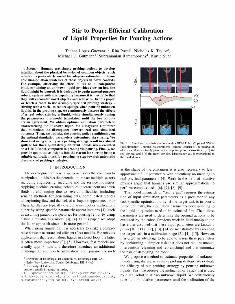
Stir to Pour: Efficient Calibration of Liquid Properties ...

Stir to Pour: Efficient Calibrationof Liquid Properties for Pouring Actions

Tatiana Lopez-Guevara1,2, Rita Pucci3, Nicholas K. Taylor2,Michael U. Gutmann1, Subramanian Ramamoorthy1, Kartic Subr1

Abstract— Humans use simple probing actions to developintuition about the physical behavior of common objects. Suchintuition is particularly useful for adaptive estimation of favor-able manipulation strategies of those objects in novel contexts.For example, observing the effect of tilt on a transparentbottle containing an unknown liquid provides clues on how theliquid might be poured. It is desirable to equip general-purposerobotic systems with this capability because it is inevitable thatthey will encounter novel objects and scenarios. In this paper,we teach a robot to use a simple, specified probing strategy –stirring with a stick– to reduce spillage when pouring unknownliquids. In the probing step, we continuously observe the effectsof a real robot stirring a liquid, while simultaneously tuningthe parameters to a model (simulator) until the two outputsare in agreement. We obtain optimal simulation parameters,characterizing the unknown liquid, via a Bayesian Optimizerthat minimizes the discrepancy between real and simulatedoutcomes. Then, we optimize the pouring policy conditioning onthe optimal simulation parameters determined via stirring. Weshow that using stirring as a probing strategy result in reducedspillage for three qualitatively different liquids when executedon a UR10 Robot, compared to probing via pouring. Finally, weprovide quantitative insights into the reason for stirring being asuitable calibration task for pouring –a step towards automaticdiscovery of probing strategies.

I. INTRODUCTION

The development of general-purpose robots that can learn tomanipulate liquids has the potential to impact multiple sectorsincluding engineering, medicine and the service industries.Applying machine learning techniques to learn about unknownfluids is challenging due to several difficulties includingsensing methods for generating data, complicated modelsunderpinning flow and the lack of a shape or appearance prior.These hurdles are typically overcome in robotics applicationseither by using specific parametric approximations [1], suchas assuming parabolic trajectories for pouring [2], or by usinga fluid simulator as a model [3], [4]. In this paper, we adoptthe latter approach since it is more general.

When using simulation, it is necessary to strike a compro-mise between accurate and efficient (fast) models. For roboticsapplications that reason about liquids in closed-loop, the latteris often more important [3], [5]. However, fast models areusually approximate and therefore introduce an additionalchallenge. In addition to simulation input parameters such

1University of Edinburgh, 10 Crichton St, Edinburgh EH8 9AB.2Heriot-Watt University, Currie, Edinburgh, EH14 4AS.3University of Udine.Authors emails in appearing order:[email protected], [email protected],

[email protected], [email protected],[email protected], [email protected]

Sim

Rea

l

θθ

Fig. 1. Synchronized stirring actions with a UR10 Robot (Top) and NVidiaFlex simulator (Bottom). Measurements (Middle) consist of the inclinationof a stick, that can freely pivot at the gripping point, across time: y(t) (inred) for real and y(t) (in green) for sim. Discrepancy ∆θ is proportional tothe shaded area.

as the shape of the containers it is also necessary to learnapproximate fluid parameters with potentially no mapping toreal physical parameters [4]. Work in the field of intuitivephysics argue that humans use similar approximations toperform complex tasks [6], [7], [8], [9].

The model mismatch or “reality gap” requires the estima-tion of input simulation parameters as a precursor to anytask-specific optimisation, i.e. if the target task is to pour aliquid optimally, the simulation parameters corresponding tothe liquid in question need to be estimated first. Then, theseparameters are used to determine the optimal actions to beexecuted by the robot. Previous work in fluid manipulationhas either assumed that these input parameters are known apriori [10], [11], [12], [13], [14] or are estimated by executingthe target task in a calibration stage [5], [4], [15]. However,it is often an advantage to be able to assess these parametersby performing a simpler task that does not require manualintervention (cleaning and replenishing) and that minimizethe risk of damaging the robot.

We propose a method to estimate properties of unknownliquids using stirring as a simple probing strategy. We evaluatethe efficacy of our probing strategy by pouring unknownliquids. First, we observe the inclination of a stick that is usedby a real robot to stir an unknown liquid. We continuouslytune fluid simulation parameters until the inclination of the

Simulation

Real

motionLEARNING FROM STIRRING (THIS PAPER)

discrepancy

BAYESIANOPTIMIZATION

MLEiterate N

POURING (USED TO EVALUATE LEARNING)

spillageas loss function

iterate N

transfer pouringpolicy

one-shot pour

measured spillage (%)

θ

as

inferred fluidparametersθf BAYESIAN

OPTIMIZATIONθ

real vs sim

ap

θ

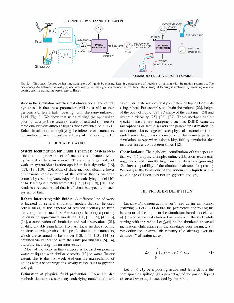
Fig. 2. This paper focuses on learning parameters of liquids by stirring. Learning parameters of liquids θ by stirring with the motion pattern as. Thediscrepancy ∆θ between the real y(t) and simulated y(t) time signals is obtained in real time. The efficacy of learning is evaluated by executing one-shotpouring and measuring the percentage spillage z.

stick in the simulation matches real observations. The centralhypothesis is that these parameters will be useful to thenperform a different task –pouring– with the same unknownfluid (Fig. 2). We show that using stirring (as opposed topouring) as a probing strategy results in reduced spillage forthree qualitatively different liquids when executed on a UR10Robot. In addition to simplifying the inference of parameters,our method also improves the efficacy of the pouring task.

II. RELATED WORK

System Identification for Fluids Dynamics: System iden-tification comprises a set of methods to characterize adynamical system for control. There is a large body ofwork on system identification applied to fluid dynamics [16],[17], [18], [19], [20]. Most of these methods obtain a lowerdimensional representation of the system that is easier tocontrol, by assuming knowledge of the underlying model [16]or by learning it directly from data [17], [18], [19], [20]. Theresult is a reduced model that is efficient, but specific to eachsystem or task.

Robots interacting with fluids: A different line of workis focused on general simulation models that can be usedacross tasks, at the expense of reduced accuracy to keepthe computation tractable. For example learning a pouringpolicy using approximate simulation [10], [11], [5], [4], [13],[14], a combination of simulation and real observations [21],or differentiable simulation [15]. All these methods requireprevious knowledge about the specific simulation parameters,which are assumed to be known [10], [11], [13], [14] orobtained via calibration with the same pouring task [5], [4],therefore involving human intervention.

Most of the work in this category is focused on pouringwater or liquids with similar viscosity [13] to water. To ourextent, this is the first work studying the manipulation ofliquids with a wider range of viscosity values, such as glycerinand gel.

Estimation of physical fluid properties: There are alsomethods that don’t assume any underlying model at all, and

directly estimate real-physical parameters of liquids from datausing robots. For example, to obtain the volume [22], heightof the body of liquid [23], 3D shape of the container [24] anddynamic viscosity [25], [26], [27]. These methods exploitspecial measurement equipment such as RGBD cameras,microphones or tactile sensors for parameter estimation. Inour context, knowledge of exact physical parameters is notuseful since they do not correspond to their counterparts insimulation, except when using a high-fidelity simulation thatinvolves higher computation times [12].

Contributions: The high-level contributions of this paper arethat we: (1) propose a simple, online calibration action (stir-ring) decoupled from the target manipulation task (pouring),(2) show adaptability of the obtained estimates for pouring.We analyze the behaviour of the system in 3 liquids with awide range of viscosities (water, glycerin and gel).

III. PROBLEM DEFINITION

Let as ∈ As denote actions performed during calibration(“stirring”). Let θ ∈ Θ define the parameters controlling thebehaviour of the liquid in the simulation-based model. Lety(t) describe the real observed inclination of the stick whilestirring with the robot. Let yθ(t) be the simulated observedinclination while stirring in the simulator with parameters θ.We define the observed discrepancy (for stirring) over theduration T of action as as

∆θ =

∫T

(y(t)− yθ(t))2dt. (1)

Let ap ∈ Ap be a pouring action and let z denote thecorresponding spillage (as a percentage of the poured liquid)observed when ap is executed by the robot.

∆θ z

as θ ap

Fig. 3. Graphical model showing relationships between variables: as and apare stirring and pouring actions; ∆θ is the discrepancy in real and simulatedinclinations; z is the measured relative spillage; and θ is the parameter thatcharacterizes the shared property of the simulated liquid. By stirring, wewish to obtain a maximum likelihood estimator for θ∗. During pouring, weuse θ∗ to determine an optimum a∗p which reduces z.

Here, we analyze the problem of inferring parametersθ∗ ∈ Θ of the liquid, given a space of calibration (stirring)actions As that are different from the space of goal(pouring) actions Ap. We quantify the suitability of Asby measuring the percentage of liquid spilled z whileperforming optimized one-shot pouring using a∗p ∈ Apobtained from θ∗ (See Fig 3).

Assumptions: We assume that the configuration of thescene including the geometry of the containers and the initialpositions are available, or can be estimated using sensors.Also, we rely on the robot’s estimation of its end effectorpose, to synchronise simulation with reality.

Inference: Given a specific As, say stirring using a givenmotion pattern, the goal of the inference step is to estimatethe best θ∗ in simulation such that the discrepancy ∆θ∗ isminimal. The optimization consists of k = 1 : N iterations.At each iteration k, an action as is executed by the robot(real) and in simulation (sim) using a hypothesized parameterθ. The resulting discrepancy ∆k

θ , calculated using Eq. 1,together with the parameter θ are provided to a BayesianOptimizer that learns a regression of ∆θ over θ using aGaussian Process [28]:

∆kθ ∼ GP(µk(θ), κk(θ, θ

′)), (2)

An approximation of the likelihood [29], [30] can becomputed using the cumulative density function (CDF) Φ ofthe standard Normal distribution and a threshold ε as:

LN (θ) ∝ Φ

(ε− µN (θ)

σN (θ)

). (3)

The goal is to determine the maximum likelihood estimatorMLE as:

θ∗ = argmaxθ∈Θ

LN (θ) (4)

In addition to the MLE, the likelihood function (Fig. 8-Left)can also be used to compute samples from the posterior via aHamiltonian Monte Carlo technique [31], by first generatingsamples from the prior distribution θ ∼ U(θmin, θmax) andevaluating their likelihood according to Eq. 3.

Evaluation: We quantitatively evaluate the suitability ofAs for the problem by measuring percentage spillage using

Algorithm 1: Inference Model (kth iter).Input: Stirring action asOutput: Discrepancy ∆θ

1 Sample from prior θk ∼ U(θmin, θmax)2 Get sim obs. yt(t) = NvFlex(as, θ

k)3 Get real obs. y(t) = Robot(as)4 Compute discrepancy: ∆θ using (Eq. 1)5 Return ∆θ

an optimized action a∗p ∈ Ap. This is due to the lack ofan existing ground truth of the parameters in the simulatorgiven its approximate nature. Since our contribution concernsthe calibration task, we use a pouring strategy exactly asprescribed by previous work [4]. They use a simulator toidentify a∗p, by defining the loss function to be the ratio ofthe spilled particles to the total number of particles simulated.The jth iteration of their method therefore involves executingthe simulator with action ajp ∈ As and θ∗. The minimizationresults in a∗p after a finite number of iterations (15 in ourcase). Finally, we execute a∗p using the robot and measurethe percentage of liquid spilled.

IV. EXPERIMENTAL SETUP

For all our experimets, we used a UR10 robot equippedwith a gripper in combination with MoveIt [32]. Simulationswere executed using NVIDIA Flex [33], running on DellAlienware Laptop with a NVIDIA GeForce GTX 1070Graphics card and 8GB of RAM. We used a Kern 2.5kweighting scale to measure the spillage when pouring. Weused two Logitech HD Pro C920 webcams to captureorthogonal views from the stick when the robot stirs theliquid. Each stirring iteration takes around 30 seconds and itdoes not involve human intervention. Each pouring iterationtakes between 2 and 4 minutes depending on the liquid, outof which the majority involves manual operation and cleaning.The experiments performed in this paper (including evaluationand comparison with prior work) consumed a total of about40 robot hours and 30 person hours for supervision. We usedthe Engine for Likelihood-Free Inference (ELFI) [34] for thecalibration process with Algorithm 1. as the model.

A. Robot Setup

Stirring: The robot’s gripper is used to hold a stick so thatit is free to pivot at the gripping point (see Fig. 1). Beforestirring begins, the stick is vertical and partly submerged inthe liquid. The motion of the end effector is limited to aplane P parallel to the ground plane. Due to this motion, andthe the resistance encountered by the stick due to the liquid,at any instant t, the stick might deviate from its verticalposition to y(t). The inclination is intricately dependent onthe velocity of the end effector and the physical propertiesof the liquid and the stick. y(t) is estimated using a HoughLine detector with OpenCV [35] on the video feed from 2webcams with image planes orthogonal to P . We average thediscrepancy across views to obtain ∆θ. The stick is wrapped

θad θbu θco θst θvi θvo0.0

2.5

5.0

S(θ

)star circ rand

θad θbu θco θst θvi θvo0.0

0.3

pouring

θad

θbu

θvo

θad

θbu

θvo

By Stirring By PouringShared NvFlex Parameters

θco

θst

θvi

Stirring is a suitable task for calibration towards pouring

S(θ)

Fig. 4. Model sensitivity analysis for six NvFlex parameters affecting liquid behaviour in simulation for (Left) Stirring using different patterns (star,circular, and random) and (Right) Pouring. We are interested in the shared parameter between tasks (Middle). Parameter names are abbreviated as (ad:Adhesion, bu: Buoyancy, co: Cohesion, st: Surface Tension, vi: Viscosity, vo: Vorticity).

in bright green paper to reduce the error of the estimates ofy(t). The light levels were kept similar across experimentsto avoid issues with the detection. The position of the endeffector of the robot is queried at 30Hz and supplied to thesimulator which replicates the executed action. The inclinationproduced in simulation at instant t is recorded as yθ(t). Thespace of stirring actions As is discrete and determined by thestirring pattern. In this work we used a continuous sequence,As = {ais}, i = 1, · · · ,m that visually follows one ofthree: 9−point star, circular or random patterns. Each actionais corresponds to the desired position of the robot’s endeffector.

Pouring: We replicate the one-shot pouring solution from [4].For completeness, we review their method here using ournotation. The space of pouring actions Ap is two dimensionaland continuous. The 2D space is parameterized by a constantangular velocity and the relative distance between source andtarget containers aip =

(ωi, pi

). After 15 iterations of the

optimizer over ap given θ∗, the robot obtains an estimate forthe optimal pouring action a∗p, which it then executes. Wemeasure the percentage of liquid spilled by the robot over 5repetitions of the above experiment.

B. Model Sensitivity

We started with the span of six input variables to thesimulator as the whole parameter space Θ ∈ R6 of liquidsthat can be handled by our system. We denote each parameteras θ ≡ (θad, θbu, θco, θst, θvi, θvo) where the six variablesare called (in NVIDIA Flex) adhesion, buoyancy, cohesion,surface tension, viscosity and vorticity confinement (SeeTable I for more detail). Despite their nomenclature, weobserved that these parameters do not behave as their physical(real) namesakes. We believe this is caused by the approximatenature of the simulator.

Stirring: We obtained j = 10 jittered samples within therange of each parameter θjp ∼ U(θp,min, θp,max) uniformlyfrom the lower and upper bounds of the parameter values (SeeTable I). Keeping all other parameters at their default values,we recorded the inclinations yjp,θ(t) observed in simulationwith the parameter set to each of the jth jittered values. Wecomputed the sensitivity of the experiment with respect to

each parameter as the average variance of the observationswith respect to the parameter as

S(θp) ≡1

T

∑t

Varθp [|yp,θ(t)|] . (5)

Pouring: We performed exactly the same experiment asabove, for stirring, except that we execute the simulator withpouring actions instead of stirring. Instead of defining thevariation with respect to the observed inclinations, in thiscase, we measure the variation in the ratio of spilled particlesacross multiple repetitions of pouring.

V. RESULTS AND DISCUSSION

Model Sensitivity: We first analyzed the impact of theparameters θ on the stirring experiment (Fig. 4-Left). Then,we analyzed their impact on pouring (Fig. 4-Right). Mostparameters show little or no variation, suggesting that theirvalues do not significantly impact the stirring experiment.The three parameters that do exhibit consistent variationacross the patterns are: cohesion, surface tension and viscosity(Fig. 4-Middle). We further found that, the sensitivity tothe surface tension parameter was caused by instabilities(particles behaving chaotically), rather than because of theaction performed. So, we set this parameter to its defaultvalue and only consider viscosity and cohesion Θ ∈ R2,which significantly lowers the calibration time.

Confidence of parameter estimates from stirring: Wecomputed a measure of confidence of the parameter estimatesusing the interquartile range (IQR) on samples from theposterior along the dimensions of each θ. We used theNo-U-Turn Sampler algorithm [31] with 4 chains with 1ksamples each. The samples were rescaled between 0 and 1before computing the statistics. Fig. 5 show the IQR for theparameters (cohesion and viscosity), motion patterns (star,circular, random) and liquids (water, glycerin, gel). Of thethree motion patterns generated, we found the star pattern toachieve the most confidence in the inferred parameters andtherefore is the one we chose to evaluate on the pouring task.We also report the obtained MLE estimates θ∗ across r = 5repetitions in Table. II computed using (Eq. 4). These values

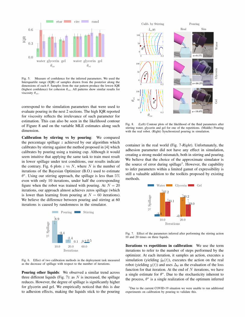
water glycerin gel0.0

0.3

0.6

IQR

water glycerin gel

star circ rand

θco θvi

Fig. 5. Measure of confidence for the inferred parameters. We used theInterquartile range (IQR) of samples drawn from the posterior along thedimensions of each θ. Samples from the star pattern produce the lowest IQR(highest confidence) for cohesion θco. All patterns show similar results forviscosity θvi.

correspond to the simulation parameters that were used toevaluate pouring in the next 2 sections. The high IQR reportedfor viscosity reflects the irrelevance of such parameter forestimation. This can also be seen in the likelihood contourof Figure 8 and on the variable MLE estimates along suchdimension.

Calibration by stirring vs by pouring: We comparedthe percentage spillage z achieved by our algorithm whichcalibrates by stirring against the method proposed in [4] whichcalibrates by pouring using a training cup. Although it wouldseem intuitive that applying the same task to train must resultin lower spillage under test conditions, our results indicatethe contrary. Fig. 6 plots z vs N , where N is the number ofiterations of the Bayesian Optimizer (B.O.) used to estimateθ∗. Using our stirring approach, the spillage is less than 5%even with only 10 iterations, under half the correspondingfigure when the robot was trained with pouring. At N = 20iterations, our approach almost achieves zeros spillage (whichis lower than learning from pouring at N = 60 iterations).We believe the difference between pouring and stirring at 60iterations is caused by randomness in the simulator.

10.0 20.0 60.0

Iterations

%S

pil

lage

8.9

1.40.2

3.4

0.1 0.5

Pouring Stirring

Fig. 6. Effect of two calibration methods in the deployment task measuredas the decrease of spillage with respect to the number of iterations.

Pouring other liquids: We observed a similar trend acrossthree different liquids (Fig. 7): as N is increased, the spillagereduces. However, the degree of spillage is significantly higherfor glycerin and gel. We empirically noticed that this is dueto adhesion effects, making the liquids stick to the pouring

0 0.2

100

50

0

•

0 0.2

100

50

0•

0 0.2

100

50

0

•

Wat

erG

lyce

rin

Gel

θn

θ

θ

θ

Real Sim

Calib. by Stirring Pouring

z=0.1%

z=30.2%

z=19.0%

θco

θ vi

Fig. 8. (Left) Contour plots of the likelihood of the fluid parameters afterstirring water, glycerin and gel for one of the repetitions. (Middle) Pouringwith the real robot. (Right) Synchronized pouring in simulation.

container in the real world (Fig. 7-Right). Unfortunately, theadhesion parameter did not have any effect in simulation,creating a strong model mismatch, both in stirring and pouring.We believe that the choice of the approximate simulator isthe source of error during spillage1. However, the capabilityto infer parameters within a limited gamut of expressibility isstill a valuable addition to the toolkits proposed by existingmethods.

10.0 20.0

Iterations

%S

pil

lage

3.40.1

37.2

30.2

23.119.0

Water Glycerin Gel

Fig. 7. Effect of the parameters inferred after performing the stirring action10 and 20 times on three liquids.

Iterations vs repetitions in calibration: We use the termiterations to refer to the number of steps performed by theoptimizer. At each iteration, it samples an action, executes asimulation (yielding yθ(t)), executes the action on the realrobot (yielding y(t)) and uses ∆θ as the evaluation of the lossfunction for that iteration. At the end of N iterations, we havea single estimate for θ∗. Due to the stochasticity inherent tothe process, θ∗ is a single realization of the optimum inferred

1Due to the current COVID-19 situation we were unable to run additionalexperiments on calibration by pouring to validate this.

0 200 400

Training Time (min)

0

4

8

%S

pilla

ge

min/pour4.0

8.0

min/stir0.5

1.0

7.0

Fig. 9. We compared percentage spillage achieved by our method(calibration by stirring) against calibration by pouring as a function ofthe time spent in calibration. Stirring is both quicker (solid light-blue curve,0.5 min per stir) as well as more efficient compared to learning by pouring(solid dark-blue curve, 4min per pour). The dashed and dotted curves arehypothetical calibration times. Another advantage of learning by stirring isthat it is completely autonomous, since no cleanup is required.

parameters. To robustify this estimate, we repeat the wholeexperiment by performing N iterations again to yield anotherestimate of θ∗. We then average these estimates, acrossrepetitions, obtain the final θ∗. So performing r repetitionswith N iterations each requires rN steps of the BayesianOptimizer (B.O.), and therefore rN executions of actions bythe robot. We recommend r = 5 and N = 20. Optimizingthis combination, so that more robust estimates are obtainedfor equal calibration effort, is an interesting avenue for futurework.

Calibration times: Each of the rN iterations of the optimizerin calibration requires one execution of the calibration task.The stirring method takes about 0.5 minutes. On the otherhand, calibrating by pouring [4] takes around 4 minutes perdata sample. Even if stirring was only as efficient as pouringin terms of the number of optimization iterations, this alreadyoffers an eightfold saving (8×) in time during estimation.In addition, since stirring is more efficient when smallernumber of iterations are used, the savings in calibration timeby switching from pouring to stirring is significant. Thisgap is evident in the plot shown in Fig. 9 which comparesthe spillage during testing resulting from the two differentcalibration approaches. The solid curves represent real timestaken per calibration task for the two approaches. The dashedcurves correspond different hypothesis of doubling the timeper iteration for each stir/pour. Even if stirring took 7 mins perstirring (which is heavily exaggerated), the spillage (dashedred curve) is comparable to that achieved by “learning bypouring” (solid blue curve). The plot also shows that the totalcalibration time can be hundreds of minutes as opposed tocalibrating by pouring.

Simultaneously sampling As and Ap: We proposed analgorithm that executes rN actions from As, infers θ∗ andfinally performs pouring. For one-shot pouring, the optimizersamples M actions, executes them in simulation and uses theratio of spillage in simulation as the loss function to generatean optimized action a∗p which when executed on the real

robot results in a spillage of z%. Again, since we use B.O.,just as for calibrating, z is a single realization of a randomvariable. We obtain a more robust estimate by performings repetitions (hence the error bars in all plots with spillageon the Y-axis). Thus, for each pouring task on a differentliquid, the total number of actions sampled is rNsM . Onepossibility would be to reallocate effort by increasing Mwhile setting r = 1. That is, for each repetition of pouringwe only use a single repetition of inference. This strategyperforms better overall due to the joint sampling of AsandAp. If calibration is being performed solely with the goalof pouring, we recommend that an a∗p be estimated for eachrepetition of inference (θ∗).

VI. CONCLUSIONS AND FUTURE WORK

We have proposed and evaluated a new calibration exper-iment that decouples the calibration action (stirring) fromthe final task (pouring) while adapting to liquids with widelydifferent properties. We demonstrated that stirring leads toreduced spillage for water compared to other methods. Wepresented results for calibrating and adapting the pouringto other liquids. Calibration by stirring is preferable tocalibration by pouring because it is easy to automate, itis time efficient and avoids the mess involved due to spillage.To our knowledge, this is the first work studying liquidsthat range from low to high viscosity. We also discussedthe several design decisions involved, along with quantitativejustification and recommendations for prospective use-cases.

Our work is limited to studying the effect of a fixed setof stirring actions that were selected after careful analysisin simulation. We believe an interesting avenue for futurework lies in studying how such actions can be generatedautomatically using information-based metrics [36], [37], suchas maximizing the information gain after each stir. Anotherinteresting direction is to relax the current assumption ofknowledge about the shapes and containers and includinguncertainty in the estimation of the stick configuration.

APPENDIX

TABLE IRANGE OF PARAMETERS ON NVFLEX USED IN EXPERIMENTS.

Parameter θ Abbrev. θmin θmaxAdhesion ad 0.0 0.1Buoyancy bu 0.3 2.0Cohesion co 0.0 0.2

Surface Tension st 0.0 50.0Viscosity vi 0.0 120.0

Vorticity Confinement vo 0.0 120.0

ACKNOWLEDGMENTS

This work is supported by the Engineering and PhysicalSciences Research Council (EPSRC), as part of the CDT inRobotics and Autonomous Systems at Heriot-Watt Universityand The University of Edinburgh. The authors would alsolike to thank the reviewers for their helpful comments.

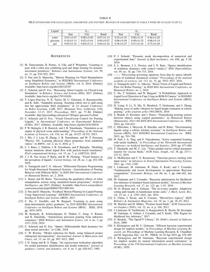
TABLE IIMLE ESTIMATORS FOR EACH LIQUID, PARAMETER AND PATTERN. RANGES OF PARAMETERS IN TABLE I WERE RE-SCALED TO [0-1].

Liquid θco θviStar Circ Rand Star Circ Rand

water 0.03±0.07 0.00±0.00 0.07±0.14 0.54±0.35 0.80±0.41 0.46±0.29glycerin 0.16±0.14 0.02±0.04 0.04±0.07 0.06±0.09 0.40±0.52 0.88±0.18

gel 0.65±0.16 0.84±0.15 0.64±0.34 0.36±0.27 0.51±0.48 0.75±0.28

REFERENCES

[1] M. Tamosiunaite, B. Nemec, A. Ude, and F. Worgotter, “Learning topour with a robot arm combining goal and shape learning for dynamicmovement primitives,” Robotics and Autonomous Systems, vol. 59,no. 11, pp. 910–922, 2011.

[2] Z. Pan and D. Manocha, “Motion Planning for Fluid Manipulationusing Simplified Dynamics,” in IEEE/RSJ International Conferenceon Intelligent Robots and Systems (IROS), vol. 0, 2016. [Online].Available: http://arxiv.org/abs/1603.02347

[3] C. Schenck and D. Fox, “Reasoning About Liquids via Closed-LoopSimulation,” in Robotics: Science and Systems (RSS), 2017. [Online].Available: http://arxiv.org/abs/1703.01656

[4] T. Lopez-Guevara, N. K. Taylor, M. U. Gutmann, S. Ramamoorthy,and K. Subr, “Adaptable pouring: Teaching robots not to spill usingfast but approximate fluid simulation,” in 1st Annual Conferenceon Robot Learning, CoRL 2017, Mountain View, California, USA,November 13-15, 2017, Proceedings, 2017, pp. 77–86. [Online].Available: http://proceedings.mlr.press/v78/lopez-guevara17a.html

[5] C. Schenck and D. Fox, “Visual Closed-Loop Control for PouringLiquids,” in International Conference on Experimental Robotics(ICRA), 2017. [Online]. Available: http://arxiv.org/abs/1610.02610

[6] P. W. Battaglia, J. B. Hamrick, and J. B. Tenenbaum, “Simulation as anengine of physical scene understanding,” Proceedings of the NationalAcademy of Sciences, vol. 110, no. 45, pp. 18 327–18 332, 2013.

[7] J. Wu, J. J. Lim, H. Zhang, J. B. Tenenbaum, and W. T. Freeman,“Physics 101: Learning physical object properties from unlabeledvideos.” in BMVC, vol. 2, no. 6, 2016, p. 7.

[8] C. J. Bates, I. Yildirim, J. B. Tenenbaum, and P. Battaglia, “Modelinghuman intuitions about liquid flow with particle-based simulation,”PLoS computational biology, vol. 15, no. 7, p. e1007210, 2019.

[9] J. J. R. Van Assen, P. Barla, and R. W. Fleming, “Visual features inthe perception of liquids,” Current biology, vol. 28, no. 3, pp. 452–458,2018.

[10] A. Yamaguchi and C. G. Atkeson, “Differential Dynamic Programmingfor Graph-Structured Dynamical Systems : Generalization of PouringBehavior with Different Skills,” in IEEE-RAS International Conferenceon Humanoid Robots, no. 2, 2016.

[11] L. Kunze and M. Beetz, “Envisioning the qualitative effects of robotmanipulation actions using simulation-based projections,” ArtificialIntelligence, jan 2015. [Online]. Available: http://www.sciencedirect.com/science/article/pii/S0004370214001544

[12] Z. Pan and D. Manocha, “Feedback Motion Planning for Liquid PouringUsing Supervised Learning,” IEEE/RSJ International Conference onIntelligent Robots and Systems (IROS), 2017.

[13] C. Do, C. Gordillo, and W. Burgard, “Learning to pour usingdeep deterministic policy gradients,” in 2018 IEEE/RSJ InternationalConference on Intelligent Robots and Systems (IROS). IEEE, 2018,pp. 3074–3079.

[14] M. Kennedy, K. Schmeckpeper, D. Thakur, C. Jiang, V. Kumar,and K. Daniilidis, “Autonomous precision pouring from unknowncontainers,” IEEE Robotics and Automation Letters, vol. 4, no. 3, pp.2317–2324, 2019.

[15] C. Schenck and D. Fox, “Spnets: Differentiable fluid dynamics fordeep neural networks,” in CoRL, 2018.

[16] C. W. Rowley, “Model reduction for fluids, using balanced properorthogonal decomposition,” International Journal of Bifurcation andChaos, vol. 15, no. 03, pp. 997–1013, 2005.

[17] J.-N. Juang and R. S. Pappa, “An eigensystem realization algorithmfor modal parameter identification and model reduction,” Journal ofguidance, control, and dynamics, vol. 8, no. 5, pp. 620–627, 1985.

[18] P. J. Schmid, “Dynamic mode decomposition of numerical andexperimental data,” Journal of fluid mechanics, vol. 656, pp. 5–28,2010.

[19] S. L. Brunton, J. L. Proctor, and J. N. Kutz, “Sparse identificationof nonlinear dynamics with control (sindyc),” IFAC-PapersOnLine,vol. 49, no. 18, pp. 710–715, 2016.

[20] ——, “Discovering governing equations from data by sparse identifi-cation of nonlinear dynamical systems,” Proceedings of the nationalacademy of sciences, vol. 113, no. 15, pp. 3932–3937, 2016.

[21] A. Yamaguchi and C. G. Atkeson, “Stereo Vision of Liquid and ParticleFlow for Robot Pouring,” in IEEE-RAS International Conference onHumanoid Robots, no. c, 2016.

[22] C. Do, T. Schubert, and W. Burgard, “A Probabilistic Approach toLiquid Level Detection in Cups Using an RGB-D Camera,” in IEEE/RSJInternational Conference on Intelligent Robots and Systems (IROS),2016.

[23] H. Liang, S. Li, X. Ma, N. Hendrich, T. Gerkmann, and J. Zhang,“Making sense of audio vibration for liquid height estimation in roboticpouring,” arXiv preprint arXiv:1903.00650, 2019.

[24] S. Brandi, O. Kroemer, and J. Peters, “Generalizing pouring actionsbetween objects using warped parameters,” in Humanoid Robots(Humanoids), 2014 14th IEEE-RAS International Conference on. IEEE,2014, pp. 616–621.

[25] C. Elbrechter, J. Maycock, R. Haschke, and H. Ritter, “Discriminatingliquids using a robotic kitchen assistant,” in Intelligent Robots andSystems (IROS), 2015 IEEE/RSJ International Conference on. IEEE,2015, pp. 703–708.

[26] H. Saal, J.-A. Ting, and S. Vijayakumar, “Active sequential learningwith tactile feedback,” in Proceedings of the Thirteenth InternationalConference on Artificial Intelligence and Statistics, 2010, pp. 677–684.

[27] T. Takahashi and M. C. Lin, “Video-guided real-to-virtual parametertransfer for viscous fluids,” ACM Trans. Graph., vol. 38, pp. 237:1–237:12, 2019.

[28] A. McHutchon and C. E. Rasmussen, “Gaussian process training withinput noise,” in Advances in Neural Information Processing Systems,2011, pp. 1341–1349.

[29] J. Lintusaari, M. Gutmann, R. Dutta, S. Kaski, and J. Corander,“Fundamentals and recent developments in approximate Bayesiancomputation,” Systematic Biology, vol. 66, no. 1, pp. e66–e82, Jan.2017.

[30] M. Gutmann and J. Corander, “Bayesian optimization for likelihood-free inference of simulator-based statistical models,” Journal of MachineLearning Research, vol. 17, no. 125, pp. 1–47, 2016.

[31] M. D. Homan and A. Gelman, “The no-u-turn sampler: Adaptivelysetting path lengths in hamiltonian monte carlo,” J. Mach. Learn. Res.,vol. 15, no. 1, p. 1593–1623, Jan. 2014.

[32] S. Chitta, I. Sucan, and S. Cousins, “Moveit![ros topics],” IEEERobotics & Automation Magazine, vol. 19, no. 1, pp. 18–19, 2012.

[33] M. Macklin and M. Muller, “Position based fluids,” ACM Transactionson Graphics (TOG), vol. 32, no. 4, p. 104, 2013.

[34] J. Lintusaari, H. Vuollekoski, A. Kangasraasio, K. Skyten, M. Jarvenpaa,M. Gutmann, A. Vehtari, J. Corander, and S. Kaski, “Elfi: Engine forlikelihood free inference,” 2017.

[35] G. Bradski, “The OpenCV Library,” Dr. Dobb’s Journal of SoftwareTools, 2000.

[36] S. Kleinegesse and M. U. Gutmann, “Efficient bayesian experimentaldesign for implicit models,” in Proceedings of Machine Learning Re-search, ser. Proceedings of Machine Learning Research, K. Chaudhuriand M. Sugiyama, Eds., vol. 89. PMLR, 16–18 Apr 2019, pp. 476–485.

[37] S. Kleinegesse and M. Gutmann, “Bayesian experimental designfor implicit models by mutual information neural estimation,” inProceedings of the 37th International Conference on Machine Learning(ICML), 2020.