N A T U R A L R E S O U R C E S Status and Trends Monitoring of Riparian and Aquatic Habitat in the Olympic Experimental State Forest Monitoring Protocols March 2017

Welcome message from author
This document is posted to help you gain knowledge. Please leave a comment to let me know what you think about it! Share it to your friends and learn new things together.
Transcript

N
A
T
U
R
A
L
R
E
S
O
U
R
C
E
S
Status and Trends Monitoring
of Riparian and Aquatic Habitat
in the Olympic Experimental
State Forest
Monitoring Protocols
March 2017

This page intentionally left blank.

Introduction
Status and Trends Monitoring of Riparian and Aquatic Habitat in the OESF Page i-1
Acknowledgements Editors Teodora Minkova, Research and Monitoring Manager for the Olympic Experimental State Forest, Washington State Department of Natural Resources (WADNR) Alex Foster, Ecologist, USDA Forest Service Pacific Northwest Research Station (PNW RS) Principal Contributors Warren Devine, Data Management Specialist, WADNR Mitchell Vorwerk, Scientific Technician, WADNR Ellis Cropper, Scientific Technician, WADNR Jeffrey Ricklefs, GIS Analyst, WADNR Rachel LovellFord, Hydrologist, Oregon Water Resources Department Richard Bigley, Silviculturist, WADNR Scott Horton, Wildlife Biologist, Olympic Region, WADNR Paul Dunnette, Scientific Technician, WADNR Kyle Martens, Fish Biologist, WADNR Reviewers Ashley Steel, Statistician, PNW RS Rebecca Flitcroft, Fish Biologist, PNW RS Technical Editor Paul Dunnette, Scientific Technician, WADNR Document formatting and illustrations by Cathy Chauvin, Communication Consultant, WADNR. Photo Credits Cover photo and photos within the document: Alex Foster, Ellis Cropper, Jessica Hanawalt, Mitchell Vorwerk, and Teodora Minkova. Suggested Citation Minkova, T. and A. Foster (Eds.). 2017. Status and Trends Monitoring of Riparian and Aquatic Habitat in the Olympic Experimental State Forest: Monitoring Protocols. Washington State Department of Natural Resources, Forest Resources Division, Olympia, WA. Washington State Department of Natural Resources Forest Resources Division 1111 Washington St. SE PO Box 47014 Olympia, WA 98504 www.dnr.wa.gov The document is available on WADNR website, copies may be obtained from Teodora Minkova: [email protected] or (360) 902-1175.

Introduction
Page i-2 Washington State Department of Natural Resources
Acronyms and Abbreviations 7-DADmax: 7Day Average Daily Maximum Temperature
BFD: Bankfull Depth
BFW: Bankfull Width
DEM: Digital Elevation Model
EPA: Environmental Protection Agency
ESA: Endangered Species Act
HCP: Habitat Conservation Plan
GIS: Geographic Information Systems
GPS: Global Positioning System
LED: Light-Emitting Diode
LEW: Left Edge of Water
LiDAR: Light Detection and Ranging
LWD: Large Woody Debris
OESF: Olympic Experimental State Forest
ONP: Olympic National Park
PNW: USDA Forest Service Pacific Northwest Research Station
PVC: Polyvinyl Chloride
REW: Right Edge of Water
RP: Reference Point
TFW: Timber, Fish, and Wildlife Agreement for Washington State Forest Practices
USGS: United States Geological Survey
WADNR: Washington Department of Natural Resources
WADOE: Washington Department of Ecology

Introduction
Status and Trends Monitoring of Riparian and Aquatic Habitat in the OESF Page i-3
Executive Summary Presented here are the monitoring protocols for the project Status and Trends Monitoring of Riparian and Aquatic Habitat in the Olympic Experimental State Forest (OESF). This long-term study documents changes in riparian and stream conditions within the OESF – 270,000 acres (110,000 ha) of state trust lands managed by the Washington State Department of Natural Resources (WADNR). The procedures and analyses described in this document will yield the empirical data needed to address key uncertainties regarding the integration of timber production and habitat conservation across landscapes and assess progress toward achieving the conservation objectives stated in the State Trust Lands Habitat Conservation Plan (HCP). The HCP calls for the provision of habitat for viable salmonid populations and riparian-obligate species. The OESF watersheds are managed under an experimental “integrated management” approach which includes riparian buffers with varied-width and blending forest management and habitat conservation at stand and landscape level. In a broader framework, the OESF as part of the USDA Forest Service Experimental Forest and Range Network, provides opportunities for research and education to improve our understanding of Pacific Northwest ecosystems and natural resource management. Riparian status and trends monitoring provides a basis for ancillary research and collaboration with universities, regulatory agencies, various stakeholder groups including tribes, conservation groups, and the timber industry. The working hypothesis for riparian management within the OESF is that current stream and riparian protections allow natural disturbance and ecological succession to improve aquatic and riparian habitat over time. The expected improvement trend is from the degraded habitat conditions prior to adoption of the 1997 HCP towards a range of habitat conditions reflective of the region’s natural variability. Key indicators of stream and riparian habitat are monitored at 50 watersheds representative of the OESF and four reference watersheds in Olympic National Park. The monitored watersheds are those of small, fish-bearing streams and range in size from 0.04 to 3 square miles (0.2-7.9 km2). Detailed monitoring protocols are developed for nine habitat attributes: stream temperature, channel morphology, stream shade, channel substrate, in-stream-large wood, habitat units and channel classification, stream discharge, riparian microclimate, and riparian vegetation. They describe field and data management procedures for all habitat measurements required by the project. The standardized protocols and robust quality assurance and quality control procedures in this document are essential to ensure the accuracy and repeatability of measurements needed to characterize site conditions and temporal trends over the duration of the project. Detection of trends in the monitored indicators will require several years of observation due to many factors, including high inter-annual variability and the rate of response to site and watershed-scale changes. Monitoring is expected to continue for at least 10 years, at which time the project’s value to WADNR will be assessed.

Introduction
Page i-4 Washington State Department of Natural Resources
Project results will be used to evaluate the effectiveness of HCP conservation strategies, test the habitat projections in the Environmental Impact Statement for the OESF Forest Land Plan, and assess fish response to forest management – contributing to the validation monitoring required by the HCP. In concert with information on OESF land management activities, the results will also facilitate inferences about management impacts on habitat, thus contributing to the adaptive management required by the HCP. More information about this monitoring project, including study plan, progress reports and first habitat status report are available on WADNR website at http://www.dnr.wa.gov/programs-and-services/forest-resources/olympic-experimental-forest/ongoing-research-and-monitoring
Introduction
Status and Trends Monitoring of Riparian and Aquatic Habitat in the OESF Page i-5
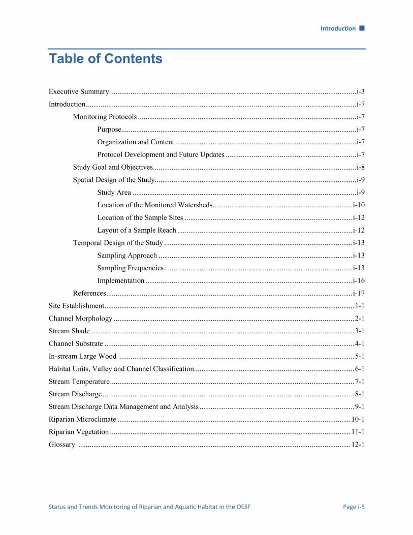
Table of Contents
Executive Summary .................................................................................................................................... i-3
Introduction ................................................................................................................................................. i-7
Monitoring Protocols ..................................................................................................................... i-7
Purpose.............................................................................................................................. i-7
Organization and Content ................................................................................................. i-7
Protocol Development and Future Updates ...................................................................... i-7
Study Goal and Objectives ............................................................................................................. i-8
Spatial Design of the Study ............................................................................................................ i-9
Study Area ........................................................................................................................ i-9
Location of the Monitored Watersheds ........................................................................... i-10
Location of the Sample Sites .......................................................................................... i-12
Layout of a Sample Reach .............................................................................................. i-12
Temporal Design of the Study ..................................................................................................... i-13
Sampling Approach ........................................................................................................ i-13
Sampling Frequencies ..................................................................................................... i-13
Implementation ............................................................................................................... i-16
References .................................................................................................................................... i-17
Site Establishment ...................................................................................................................................... 1-1
Channel Morphology ................................................................................................................................. 2-1
Stream Shade ............................................................................................................................................. 3-1
Channel Substrate ...................................................................................................................................... 4-1
In-stream Large Wood .............................................................................................................................. 5-1
Habitat Units, Valley and Channel Classification...................................................................................... 6-1
Stream Temperature ................................................................................................................................... 7-1
Stream Discharge ....................................................................................................................................... 8-1
Stream Discharge Data Management and Analysis ................................................................................... 9-1
Riparian Microclimate ............................................................................................................................. 10-1
Riparian Vegetation ................................................................................................................................. 11-1
Glossary .................................................................................................................................................. 12-1

Introduction
Page i-6 Washington State Department of Natural Resources
This page intentionally left blank.

Introduction
Status and Trends Monitoring of Riparian and Aquatic Habitat in the OESF Page i-7
Introduction This document includes monitoring protocols for the project Status and Trends Monitoring of Aquatic and Riparian Habitat in the Olympic Experimental State Forest (OESF). It describes detailed field and data management procedures for all habitat measurements required by the study. Standardized environmental monitoring protocols are necessary to characterize the conditions of multiple study sites, describe temporal trends, compare information among different projects, and ensure repeatability of measurements amid changing project staff (Bain and Stevenson 1999, McMahon et al. 1996).
Monitoring Protocols
PURPOSE The purpose of the monitoring protocols is to describe: (1) field and office procedures for sampling aquatic and riparian habitat indicators identified in the project study plan (Minkova et. al 2012); (2) quality assurance and quality control steps; and (3) data management procedures necessary to document and report the status and trends of habitat indicators in the monitored watersheds. ORGANIZATION AND CONTENT This document includes 11 monitoring protocols, organized as stand-alone chapters with their own tables of contents, appendices, and lists of references. One protocol describes field procedures for site establishment. Nine protocols focus on the monitored habitat attributes: stream temperature, channel morphology, stream shade, channel substrate, in-stream large wood, habitat units and valley and channel classification, stream discharge, riparian microclimate, and riparian vegetation. Because of the multiple steps and complexity of stream discharge data management and analyses, the office procedures for this indicator are described in a separate protocol. Each protocol includes a title page describing the revision history and the literature sources it is based on. This is followed by a description of the protocol’s monitoring design, a list of the equipment and supplies needed for sampling, detailed field procedures, procedures for calculating metrics, and a section on data management. Given the longevity of the project (at least 10 years), turnover among seasonal field technicians, and the participation of multiple researchers from different organizations, it is critical to develop robust quality assurance (QA) and quality control (QC) procedures. QA/QC procedures for field data collection and data management are described separately in each protocol.
PROTOCOL DEVELOPMENT AND FUTURE UPDATES The monitoring protocols were written by the project’s research team and six protocols were peer-reviewed by two external specialists from the USDA Forest Service Pacific Northwest Research Station (PNW RS) as early drafts: Stream Temperature, Channel Morphology, Stream Shade, Channel Coarse Substrate, In-stream Large Wood, and Habitat Units, Valley and Channel Classification.

Introduction
Page i-8 Washington State Department of Natural Resources
The field and data management protocols published in this document are expected to be updated as technology advances, new knowledge is gained, and field procedures are refined. To ensure high-quality and consistent data collection over time, all changes to the published protocols will be approved by the project manager or the researcher overseeing protocol implementation. Updated protocols will be assigned new version numbers and publication dates. Owing to sampling dependencies among protocols (e.g. channel substrate and morphology sampling are conducted together), field procedure updates may necessitate changes in other, dependent protocols. Specific dependencies are described in the protocols.
Study Goal and Objectives The project is organized as an extensive, long-term monitoring study of habitat attributes in watersheds representative of the OESF. These watersheds are managed by the Washington State Department of Natural Resources (WADNR) with the dual objectives of producing revenue (primarily through timber harvest) and ecological values (such as biological diversity and long-term site productivity). The riparian conservation strategy described in the State Trust Lands Habitat Conservation Plan (HCP) aims to provide habitat for viable salmonid populations and other riparian-obligate species (WADNR 1997). The study will test the hypothesis that current stream protection such as riparian buffers, protection of unstable slopes, and road improvements allows the natural processes of disturbance and succession to improve riparian and aquatic habitat over time. The improvement is relative to the habitat conditions before the adoption of the 1997 state lands HCP (WADNR 1997). This monitoring project tracks habitat conditions across the OESF as WADNR implements the OESF Forest Land Plan (WADNR 2016b). Specific monitoring objectives include assessing the habitat projections in the Environmental Impact Statement for the OESF Forest Land Plan (WADNR 2016a) and testing assumptions about ecological relationships among in-stream, riparian, and upland conditions, thus providing information that will help improve WADNR’s forest management planning. When integrated with information on management activities in the OESF, the monitoring data will help researchers make inferences about management effects on habitat, contributing to the effectiveness monitoring and adaptive management required by the HCP (WADNR 1997). Additionally, monitoring data will be used to characterize habitat conditions to study fish response to managed landscapes, contributing to the OESF riparian validation monitoring (Martens 2016). The project’s findings are expected to provide valuable information relevant to tribal, private, and federal land managers in the Pacific Northwest who face the challenge of managing forests for multiple uses. The monitoring project started in 2012 and is planned to continue for at least 10 years. A study plan (Minkova et al. 2012), annual progress reports (Minkova and Vorwerk 2013, Minkova and Vorwerk 2014, Minkova and Devine 2015), a quality control report (Devine and Minkova 2016) and the first habitat status report (Minkova and Devine 2016) are available on the WADNR website at http://www.dnr.wa.gov/programs-and-services/forest-resources/olympic-experimental-forest/ongoing-research-and-monitoring.
Introduction
Status and Trends Monitoring of Riparian and Aquatic Habitat in the OESF Page i-9
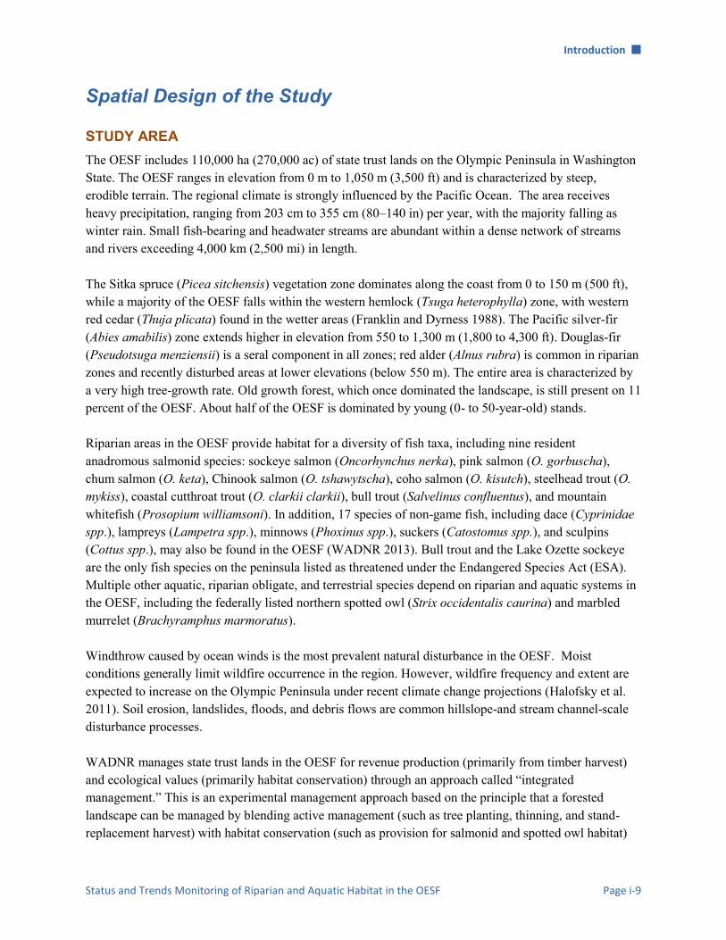
Spatial Design of the Study
STUDY AREA The OESF includes 110,000 ha (270,000 ac) of state trust lands on the Olympic Peninsula in Washington State. The OESF ranges in elevation from 0 m to 1,050 m (3,500 ft) and is characterized by steep, erodible terrain. The regional climate is strongly influenced by the Pacific Ocean. The area receives heavy precipitation, ranging from 203 cm to 355 cm (80–140 in) per year, with the majority falling as winter rain. Small fish-bearing and headwater streams are abundant within a dense network of streams and rivers exceeding 4,000 km (2,500 mi) in length. The Sitka spruce (Picea sitchensis) vegetation zone dominates along the coast from 0 to 150 m (500 ft), while a majority of the OESF falls within the western hemlock (Tsuga heterophylla) zone, with western red cedar (Thuja plicata) found in the wetter areas (Franklin and Dyrness 1988). The Pacific silver-fir (Abies amabilis) zone extends higher in elevation from 550 to 1,300 m (1,800 to 4,300 ft). Douglas-fir (Pseudotsuga menziensii) is a seral component in all zones; red alder (Alnus rubra) is common in riparian zones and recently disturbed areas at lower elevations (below 550 m). The entire area is characterized by a very high tree-growth rate. Old growth forest, which once dominated the landscape, is still present on 11 percent of the OESF. About half of the OESF is dominated by young (0- to 50-year-old) stands. Riparian areas in the OESF provide habitat for a diversity of fish taxa, including nine resident anadromous salmonid species: sockeye salmon (Oncorhynchus nerka), pink salmon (O. gorbuscha), chum salmon (O. keta), Chinook salmon (O. tshawytscha), coho salmon (O. kisutch), steelhead trout (O. mykiss), coastal cutthroat trout (O. clarkii clarkii), bull trout (Salvelinus confluentus), and mountain whitefish (Prosopium williamsoni). In addition, 17 species of non-game fish, including dace (Cyprinidae spp.), lampreys (Lampetra spp.), minnows (Phoxinus spp.), suckers (Catostomus spp.), and sculpins (Cottus spp.), may also be found in the OESF (WADNR 2013). Bull trout and the Lake Ozette sockeye are the only fish species on the peninsula listed as threatened under the Endangered Species Act (ESA). Multiple other aquatic, riparian obligate, and terrestrial species depend on riparian and aquatic systems in the OESF, including the federally listed northern spotted owl (Strix occidentalis caurina) and marbled murrelet (Brachyramphus marmoratus). Windthrow caused by ocean winds is the most prevalent natural disturbance in the OESF. Moist conditions generally limit wildfire occurrence in the region. However, wildfire frequency and extent are expected to increase on the Olympic Peninsula under recent climate change projections (Halofsky et al. 2011). Soil erosion, landslides, floods, and debris flows are common hillslope-and stream channel-scale disturbance processes. WADNR manages state trust lands in the OESF for revenue production (primarily from timber harvest) and ecological values (primarily habitat conservation) through an approach called “integrated management.” This is an experimental management approach based on the principle that a forested landscape can be managed by blending active management (such as tree planting, thinning, and stand-replacement harvest) with habitat conservation (such as provision for salmonid and spotted owl habitat)

Introduction
Page i-10 Washington State Department of Natural Resources
across the landscape. Integrated management is rooted in the concept of disturbance ecology, which recognizes a natural mosaic of successional stages that shift in time through disturbances. This approach differs from the more common conservation-biology approach that divides forested areas into large blocks, each managed for a single purpose such as late-successional habitat in late-successional reserves or timber production in the forest matrix. A notable element of the integrated management approach in the OESF is the ability to vary the width of the riparian buffers based on the overall health of a watershed. Implementation of this approach is described in detail in the OESF Forest Land Plan (WADNR 2016b). The current sustainable harvest level for the OESF is 576 million board feet per decade (WADNR 2007). An average of 1,475 ac (596 ha) of state trusts lands in the OESF (0.55% of the land base) have been harvested annually since the adoption of the HCP in 1997 (WADNR 1997). The main harvest methods on state lands in the OESF are variable retention harvest, commercial thinning, and variable density thinning. OESF conservation goals, described in the HCP, focus on restoring levels of habitat capable of supporting viable salmonid populations, spotted owls, and marbled murrelets with the expectation that this will also provide habitat for other native fish and wildlife species (WADNR 1997).
LOCATION OF THE MONITORED WATERSHEDS The Type 3 watershed1 (watersheds around the smallest fish-bearing streams) was selected as the sampling unit for the study because it is the smallest hydrologically complete unit, Type 3 watersheds are relevant to both the riparian ecological processes that provide salmonid habitat (such as sediment production and transport, wood production and transport to streams, and the hydrologic cycle) and to WADNR management activities in the OESF (primarily timber harvest and road management). The Type 3 watershed is also the spatial unit used for the environmental impact analyses of the OESF Forest Land Plan (WADNR 2013). A sample size of 50 OESF Type 3 watersheds was selected based on previous studies that determined n=50 to be sufficient to provide enough statistical power to detect relatively small trends (1–2% per year) in habitat indicators within a decade (Larsen et al. 2004; Reeves et al. 2004). The 50 sample watersheds were selected to represent the entire population of Type 3 watersheds in the OESF in terms of ecological conditions and management history of the forest (Figure i-1). Refer to the study plan (Minkova et al. 2012) for a description of the watershed selection process and to Minkova and Vorwerk (2014) for a description of modifications of the process following a statistical review of the spatial design. In addition to the 50 watersheds on the OESF, four reference watersheds are monitored in the adjacent Olympic National Park (ONP). They are Type 3 watersheds that drain into Queets, Bogachiel, Hoh and South Fork Hoh rivers (Figure i-1). The reference watersheds were selected to be ecologically similar to the OESF watersheds and readily accessible by established hiking trails. The purpose of the reference
1 The smallest fish-bearing stream as identified through biological criteria (fish presence) or physical criteria (a stream ≥ 0.7 m [2 ft] wide with a ≤16% gradient for watersheds up to 20 ha [ 50 ac ] or with a gradient between 16% and 20% for watersheds larger than 20 ha [50 ac]). Type 3 streams can be considered loosely equivalent to Strahler’s 3rd order streams.

Introduction
Status and Trends Monitoring of Riparian and Aquatic Habitat in the OESF Page i-11
Figure i-1. Map of the study area. Fifty monitored watersheds are located in the Olympic Experimental
State Forest (OESF); four reference watersheds are located in Olympic National Park.
Introduction
Page i-12 Washington State Department of Natural Resources
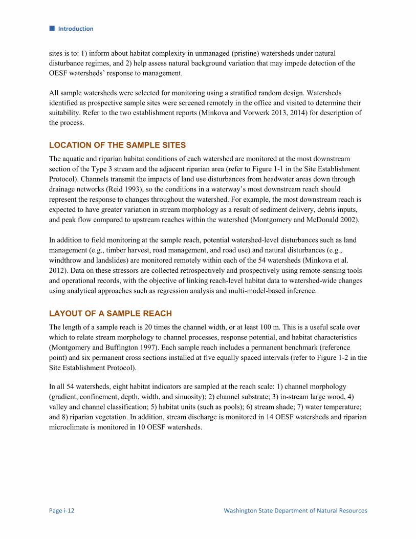
sites is to: 1) inform about habitat complexity in unmanaged (pristine) watersheds under natural disturbance regimes, and 2) help assess natural background variation that may impede detection of the OESF watersheds’ response to management. All sample watersheds were selected for monitoring using a stratified random design. Watersheds identified as prospective sample sites were screened remotely in the office and visited to determine their suitability. Refer to the two establishment reports (Minkova and Vorwerk 2013, 2014) for description of the process.
LOCATION OF THE SAMPLE SITES The aquatic and riparian habitat conditions of each watershed are monitored at the most downstream section of the Type 3 stream and the adjacent riparian area (refer to Figure 1-1 in the Site Establishment Protocol). Channels transmit the impacts of land use disturbances from headwater areas down through drainage networks (Reid 1993), so the conditions in a waterway’s most downstream reach should represent the response to changes throughout the watershed. For example, the most downstream reach is expected to have greater variation in stream morphology as a result of sediment delivery, debris inputs, and peak flow compared to upstream reaches within the watershed (Montgomery and McDonald 2002). In addition to field monitoring at the sample reach, potential watershed-level disturbances such as land management (e.g., timber harvest, road management, and road use) and natural disturbances (e.g., windthrow and landslides) are monitored remotely within each of the 54 watersheds (Minkova et al. 2012). Data on these stressors are collected retrospectively and prospectively using remote-sensing tools and operational records, with the objective of linking reach-level habitat data to watershed-wide changes using analytical approaches such as regression analysis and multi-model-based inference.
LAYOUT OF A SAMPLE REACH The length of a sample reach is 20 times the channel width, or at least 100 m. This is a useful scale over which to relate stream morphology to channel processes, response potential, and habitat characteristics (Montgomery and Buffington 1997). Each sample reach includes a permanent benchmark (reference point) and six permanent cross sections installed at five equally spaced intervals (refer to Figure 1-2 in the Site Establishment Protocol). In all 54 watersheds, eight habitat indicators are sampled at the reach scale: 1) channel morphology (gradient, confinement, depth, width, and sinuosity); 2) channel substrate; 3) in-stream large wood, 4) valley and channel classification; 5) habitat units (such as pools); 6) stream shade; 7) water temperature; and 8) riparian vegetation. In addition, stream discharge is monitored in 14 OESF watersheds and riparian microclimate is monitored in 10 OESF watersheds.

Introduction
Status and Trends Monitoring of Riparian and Aquatic Habitat in the OESF Page i-13
Temporal Design of the Study
SAMPLING APPROACH The temporal component of the sampling design influences the study’s capacity to detect long-term trends across a variety of habitat attributes. The sampling frequency of each habitat attribute was chosen to balance the need for enough sites to characterize habitat status across the OESF with the need for enough visits per site to characterize habitat trends over time. This balance between the spatial and temporal sampling effort is a result of finite resources available for sampling in each field season. The temporal sampling strategy for each habitat attribute is also a function of the temporal variability of the attribute. Whereas some habitat attributes have low inter-annual variability and measurement variability (i.e., measurement error) and do not require frequent sampling to detect trends, other attributes have high inter-annual or measurement variability and therefore require more frequent sampling to detect underlying trends. Therefore, in developing the temporal sampling design, we relied heavily on an analysis of temporal and measurement variability of 33 of the metrics monitored under this project (Devine and Minkova 2016).
SAMPLING FREQUENCIES Based on our understanding of the range in temporal variability among habitat attributes, and given our current level of resources for field work, we selected three levels of sampling intensity for this study:
High-frequency field sampling. This approach is for attributes that must be measured manually by a field crew and that have a relatively high level of temporal or measurement variability.
Low-frequency field sampling. This approach is for attributes that must be measured manually by a field crew and that have a relatively low level of both temporal and measurement variability.
Continuous sampling. This sampling is limited to habitat attributes that meet two criteria: (1) the attribute changes at a frequency of minutes or hours and thus necessitates continuous sampling, and (2) it is possible to sample the attribute by using automated sensors.
High-frequency field sampling
Some manually sampled habitat attributes, such as channel width and depth, habitat units, substrate, and in-stream large wood, are expected to change relatively rapidly as a result of natural stream flows and sediment delivery (Montgomery and Buffington 1997) or potentially anthropogenic disturbances such as road management and timber harvest. Additionally, attributes such as substrate and erosion have an inherently high level of measurement variability (Devine and Minkova 2016). For these reasons, this group of attributes is sampled relatively frequently. There are several potential sampling strategies for monitoring regional ecological trends with finite sampling resources, each strategy balancing spatial and temporal sampling intensities in different ways (Urquhart et al. 1998). In our case, we have the resources to measure the high-frequency habitat attributes in approximately 28 to 30 of the 54 sample reaches each year. We selected a temporal sampling design

Introduction
Page i-14 Washington State Department of Natural Resources
for these attributes that uses a combination of annually sampled “sentinel” reaches and a 3-year rotating panel of the remaining reaches for a total of 28 to 29 reaches sampled per year (Table i-1). The 16 sentinel reaches include the 4 reference reaches plus 12 OESF reaches selected to represent all of the strata that were originally used in the study plan during selection of the 50 OESF sample reaches. The remaining 38 OESF reaches are sampled on a 3-year panel rotation, with 13, 13, and 12 sites sampled in each of the three years. This combined sampling strategy is designed to capture the attributes’ inter-annual variability using the sentinel sites, while sampling the rotating panel sites at an interval that is still frequent enough—at 3 years—to identify long-term trends. This sampling design will be implemented starting in 2017, as all of these attributes had been measured at least once in every reach by 2016.
Table i-1. Temporal sampling design for status and trends monitoring of riparian and aquatic habitat attributes in the OESF. Values in the table represent the number of watersheds/reaches in which a habitat attribute is monitored in the specified year.
Attribute 20
13
-20
14
20
15
20
16
20
17
20
18
20
19
20
20
20
21
20
22
20
23
20
24
20
25
High-frequency field sampling (16 annual sentinel reaches plus a 3-year rotating panel of 13/13/12 reaches)
Channel width, depth, floodplain width
42 12 45 29 29 28 29 29 28 29 29 28
Channel substrate 42 12 45 29 29 28 29 29 28 29 29 28
Channel erosion 41 13 47 29 29 28 29 29 28 29 29 28
In-stream large wood 41 13 45 29 29 28 29 29 28 29 29 28
Habitat unit survey 40 14 40 29 29 28 29 29 28 29 29 28
Low-frequency field sampling (5-year sample rotation, divided among 2 or 5 years)
Channel gradient, azimuth
42 12 0 0 0 27 27 0 0 0 27 27
Channel sinuosity 39 12 0 0 0 27 27 0 0 0 27 27
Stream shade 35 8 13 7 10 11 11 11 11 10 11 11
Riparian vegetation 10 31 6 7 10 11 11 11 11 10 11 11
Continuous sampling (using electronic data loggers)
Stream temperature 54 54 54 54 54 54 54 54 54 54 54 54
Riparian microclimate 10 10 10 * * * * * * * * *
Stream discharge 14 14 10 10 10 10 10 10 10 10 10 10
* Sampling of microclimate beyond 2016 will be based on results of 2014-2016 sampling.
Introduction
Status and Trends Monitoring of Riparian and Aquatic Habitat in the OESF Page i-15
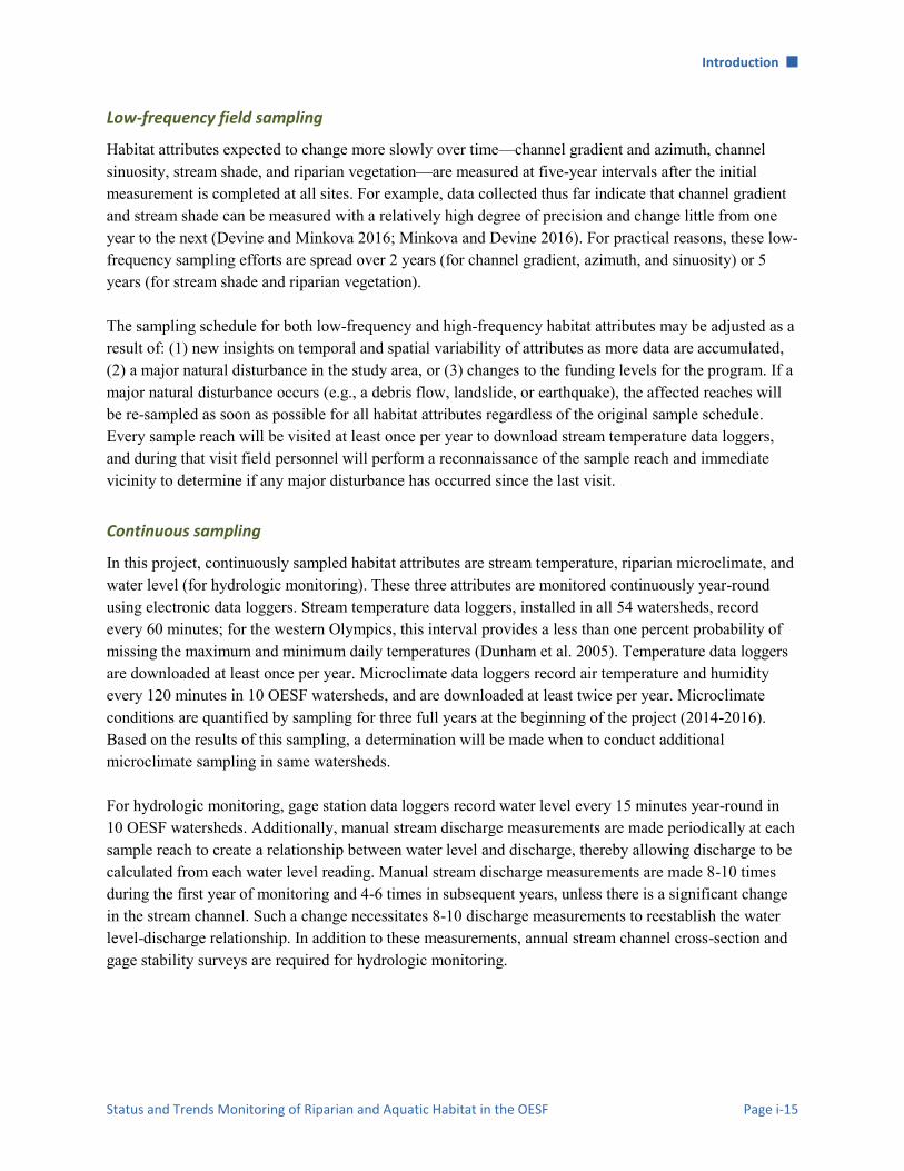
Low-frequency field sampling
Habitat attributes expected to change more slowly over time—channel gradient and azimuth, channel sinuosity, stream shade, and riparian vegetation—are measured at five-year intervals after the initial measurement is completed at all sites. For example, data collected thus far indicate that channel gradient and stream shade can be measured with a relatively high degree of precision and change little from one year to the next (Devine and Minkova 2016; Minkova and Devine 2016). For practical reasons, these low-frequency sampling efforts are spread over 2 years (for channel gradient, azimuth, and sinuosity) or 5 years (for stream shade and riparian vegetation). The sampling schedule for both low-frequency and high-frequency habitat attributes may be adjusted as a result of: (1) new insights on temporal and spatial variability of attributes as more data are accumulated, (2) a major natural disturbance in the study area, or (3) changes to the funding levels for the program. If a major natural disturbance occurs (e.g., a debris flow, landslide, or earthquake), the affected reaches will be re-sampled as soon as possible for all habitat attributes regardless of the original sample schedule. Every sample reach will be visited at least once per year to download stream temperature data loggers, and during that visit field personnel will perform a reconnaissance of the sample reach and immediate vicinity to determine if any major disturbance has occurred since the last visit.
Continuous sampling
In this project, continuously sampled habitat attributes are stream temperature, riparian microclimate, and water level (for hydrologic monitoring). These three attributes are monitored continuously year-round using electronic data loggers. Stream temperature data loggers, installed in all 54 watersheds, record every 60 minutes; for the western Olympics, this interval provides a less than one percent probability of missing the maximum and minimum daily temperatures (Dunham et al. 2005). Temperature data loggers are downloaded at least once per year. Microclimate data loggers record air temperature and humidity every 120 minutes in 10 OESF watersheds, and are downloaded at least twice per year. Microclimate conditions are quantified by sampling for three full years at the beginning of the project (2014-2016). Based on the results of this sampling, a determination will be made when to conduct additional microclimate sampling in same watersheds. For hydrologic monitoring, gage station data loggers record water level every 15 minutes year-round in 10 OESF watersheds. Additionally, manual stream discharge measurements are made periodically at each sample reach to create a relationship between water level and discharge, thereby allowing discharge to be calculated from each water level reading. Manual stream discharge measurements are made 8-10 times during the first year of monitoring and 4-6 times in subsequent years, unless there is a significant change in the stream channel. Such a change necessitates 8-10 discharge measurements to reestablish the water level-discharge relationship. In addition to these measurements, annual stream channel cross-section and gage stability surveys are required for hydrologic monitoring.
Introduction
Page i-16 Washington State Department of Natural Resources
IMPLEMENTATION All monitoring sites in OESF and reference watersheds were established from 2012 to 2014. The first round of field sampling was completed for most attributes from 2013 to 2015 (Minkova and Devine 2016). Installation of the continuously recording electronic data loggers measuring stream temperature, riparian microclimate, and water level (used to calculate stream discharge) was completed in 2012 and 2013. This long-term monitoring project will continue for at least 10 years, when the first robust habitat trend results are expected and at which point the project’s value for WADNR will be reassessed. Many years of monitoring will be required to detect any trends in habitat attributes because: (1) some metrics respond slowly to watershed-scale environmental change; (2) some metrics have high inter-annual variability; and (3) some metrics have high measurement variability. Similar monitoring projects (e.g. Watershed Condition Status and Trends Monitoring for the Northwest Forest Plan [Lanigan et al. 2012]) report habitat trends every five years. Trends in OESF watersheds also will be reported every five years.

Introduction
Status and Trends Monitoring of Riparian and Aquatic Habitat in the OESF Page i-17
References Bain, M. and Stevenson, N. editors. 1999. Aquatic habitat assessments: common methods. American
Fisheries Society. Bethesda, Maryland.
Devine W. and Minkova, T. 2016. 2015 Quality Control Report for Status and Trends Monitoring of Riparian and Aquatic Habitat in the Olympic Experimental State Forest. 2014 Progress Report. Washington State Department of Natural Resources, Forest Resources Division, Olympia, WA, 52 p.
Dunham, J., G. Chandler, B. Rieman, D. Martin. 2005. Measuring stream temperature with digital data loggers: a user’s guide. Gen. Tech. Rep. RMRS-GTR-150WWW. Fort Collins, CO: U.S. Department of Agriculture, Forest Service, Rocky Mountain Research Station. 15 p.
Franklin, J.F., and Dyrness, C.T. 1988. Natural vegetation of Oregon and Washington. Corvallis, OR: Oregon State University Press. 452 p.
Halofsky, J.; D. Peterson, K. O’Halloran, C. Hawkins. T. Hoffman. eds. 2011. Adapting to climate change at Olympic National Forest and Olympic National Park. USDA Forest Service, Pacific Northwest Research Station. Gen. Tech. Rep. PNW-GTR-844. 130 p.
Lanigan, S.H.; Gordon, S. N.; Eldred, P.; Isley, M.; Wilcox, S.; Moyer, C.; Andersen, H. 2012. Northwest Forest Plan—the first 15 years (1994–2008): watershed condition status and trend. Gen. Tech. Rep. PNW-GTR-856. Portland, OR: U.S. Department of Agriculture, Forest Service, Pacific Northwest Research Station. 155 p.
Larsen, D., P. Kaufmann, T. Kincaid, and N. Urquhart. 2004. Detecting persistent change in the habitat of salmon-bearing streams in the Pacific Northwest. Canadian Journal of Fisheries and Aquatic Science, 61:283-291.
Martens, K.D. 2016. Washington State Department of Natural Resources’ Riparian Validation Monitoring Program for salmonids on the Olympic Experimental State Forest – Study Plan. Washington State Department of Natural Resources. Forest Resources Division, Olympia, WA.
McMahon, T., A. Zale, and D. Orth. 1996. Aquatic habitat measurements. Pages 83-120 in B. Murphy and D. Willis, editors. Fisheries techniques, 2nd edition. American Fisheries Society. Bethesda, Maryland.
Minkova T., J. Ricklefs, S. Horton, and R. Bigley. 2012. Riparian Status and Trends Monitoring for the Olympic Experimental State Forest. Draft Study Plan. WADNR Forest Resources Division, Olympia, WA. 61 p.
Minkova, T. and M. Vorwerk. 2013. Riparian Status and Trends Monitoring for the Olympic Experimental State Forest. 2012 Establishment report: field reconnaissance and delineation of sample sites. WADNR Forest Resources Division, Olympia, WA, 48 p.
Minkova, T. and M. Vorwerk. 2014. Status and Trends Monitoring of Riparian and Aquatic Habitat in the Olympic Experimental State Forest. 2013 Establishment Report: Field Installations and Development of Monitoring Protocols. Washington State Department of Natural Resources, Forest Resources Division, Olympia, WA, 47 p.

Introduction
Page i-18 Washington State Department of Natural Resources
Minkova, T. and W. Devine. 2015. Status and Trends Monitoring of Riparian and Aquatic Habitat in the Olympic Experimental State Forest. 2014 Progress Report. Washington State Department of Natural Resources, Forest Resources Division, Olympia, WA, 47 p.
Minkova, T. and W. Devine. 2016. Status and Trends Monitoring of Riparian and Aquatic Habitat in the Olympic Experimental State Forest. Habitat Status Report and 2015 Project Progress Report. Washington State Department of Natural Resources, Forest Resources Division, Olympia, WA.
Montgomery, D. and L. MacDonald. 2002. Diagnostic approach to stream channel assessment and monitoring. Journal of the American Water Resources Association, 38:1-16.
Montgomery, D. and J. Buffington. 1997. Channel reach morphology in mountain drainage basins. Geological Society of America Bulletin, 109: 596–611.
Reeves, G., D. Hohler, D. Larsen, D. Busch, K. Kratz, K. Reynolds, K. Stein, T. Atzet, P. Hays, and M. Tehan. 2004. Effectiveness monitoring for the aquatic and riparian component of the Northwest Forest Plan: conceptual framework and options. Gen. Tech. Rep. PNW-GTR-577, Portland, OR.
Reid, L.M. 1993. Research and cumulative watershed effects, Berkeley, California, Pacific Southwest Research Station: U.S. Department of Agriculture. Forest Service General Technical Report. PSW-GTR-141, 118 p.
Urquhart, N.S., S.G. Paulsen, and D.P. Larsen. 1998. Monitoring for policy-relevant regional trends over time. Ecological Applications, 8(2): 246-257.
Washington State Department of Natural Resources. 1997. Final Habitat Conservation Plan: Washington State Department of Natural Resources, Olympia, Washington. 223 p.
Washington State Department of Natural Resources. 2007. Board of Natural Resources Resolution No. 1239. Sustainable Harvest Adjustment.
Washington State Department of Natural Resources. 2013. Olympic Experimental State Forest HCP Planning Unit Forest Land Plan Revised Draft Environmental Impact Statement. Washington State Department of Natural Resources, Olympia, Washington.
Washington State Department of Natural Resources. 2016a. Olympic Experimental State Forest HCP Planning Unit Forest Land Plan Final Environmental Impact Statement. Washington State Department of Natural Resources, Olympia, WA. http://file.dnr.wa.gov/publications/amp_sepa_nonpro_oesf_feis.pdf
Washington State Department of Natural Resources. 2016b. Olympic Experimental State Forest HCP Planning Unit Forest Land Plan. Washington State Department of Natural Resources, Olympia, WA. http://file.dnr.wa.gov/publications/lm_oesf_flplan_final.pdf

Site Establishment
Status and Trends Monitoring of Riparian and Aquatic Habitat in the OESF Page 1-1
Site Establishment
Authors: Teodora Minkova, Mitchell Vorwerk, Ellis Cropper Version: 1.2 Revision History:
Based on the Following Protocols:
This protocol is based on two protocols prepared for the Washington Department of Natural Resources under the Timber, Fish, and Wildlife Agreement (TFW): TFW Monitoring Program methods manual for stream segment identification (Pleus and Schuett-Hames 1998a) and TFW Monitoring Program methods manual for reference point survey (Pleus and Schuett-Hames 1998b). Reasons to Adopt the Above Protocols:
TFW protocols were created for long term-monitoring projects that are implemented over several years by seasonal field crews with various levels of experience. Consequently, the protocols are detailed, well-illustrated, and thorough in addressing unusual circumstances encountered in the field. The field procedures have been tested in western Washington watersheds and are similar to protocols from other regional aquatic monitoring efforts in the Pacific Northwest. Purpose and Content:
The purpose of this monitoring protocol is to describe the site establishment procedures and data management necessary to repeatedly locate the sampling points used in this long-term monitoring project. The protocol details the field procedures for identifying the start of a sample reach and establishing permanent cross sections, a reference point (benchmark), and a photo point.
Protocol Version Purpose / Changes Author(s) Reviewer(s) Date
1.0 Initial draft Teodora Minkova, Mitchell Vorwerk, Ellis Cropper
10/23/2014
1.1 Final draft with field and data management procedures updated from 2014 and 2015 field seasons
Teodora Minkova, Mitchell Vorwerk, Ellis Cropper
Alex Foster 06/10/2016
1.2 Final technical review and edit Teodora Minkova Mitchell Vorwerk, Ellis Cropper
Paul Dunnette, Warren Devine, Alex Foster
12/18/2016

Site Establishment
Page 1-2 Washington State Department of Natural Resources
Table of Contents Monitoring Design .......................................................................................................................................... 1-3
Equipment and Supplies .................................................................................................................................. 1-3
Pre-field Setup ............................................................................................................................................. 1-4
Field Procedures .............................................................................................................................................. 1-4
Identifying the Start of the Sample Reach .................................................................................................. 1-4
Determining Sample Reach Length and Establishing Permanent Cross Sections ...................................... 1-5
Establishing a Reference Point .................................................................................................................... 1-8
Measuring the reference point elevation ..................................................................................................... 1-9
Establishing a Permanent Photo Point ...................................................................................................... 1-10
Taking a Picture at the Photo point ........................................................................................................... 1-11
Time and Cost Estimates for Implementing the Field Procedures ................................................................ 1-11
Quality Assurance and Quality Control ........................................................................................................ 1-12
Training ..................................................................................................................................................... 1-12
Standard Protocols .................................................................................................................................... 1-12
Data Management ......................................................................................................................................... 1-13
Data Flow .................................................................................................................................................. 1-13
Data Storage .............................................................................................................................................. 1-15
Tablet Databases ................................................................................................................................... 1-15
Long-Term Data Storage ....................................................................................................................... 1-15
Data Quality Control ................................................................................................................................. 1-17
References ..................................................................................................................................................... 1-19
Appendix 1A. Directions for recording reference point elevation with Trimble Recon GPS unit .............. 1A-1
Site Establishment
Status and Trends Monitoring of Riparian and Aquatic Habitat in the OESF Page 1-3
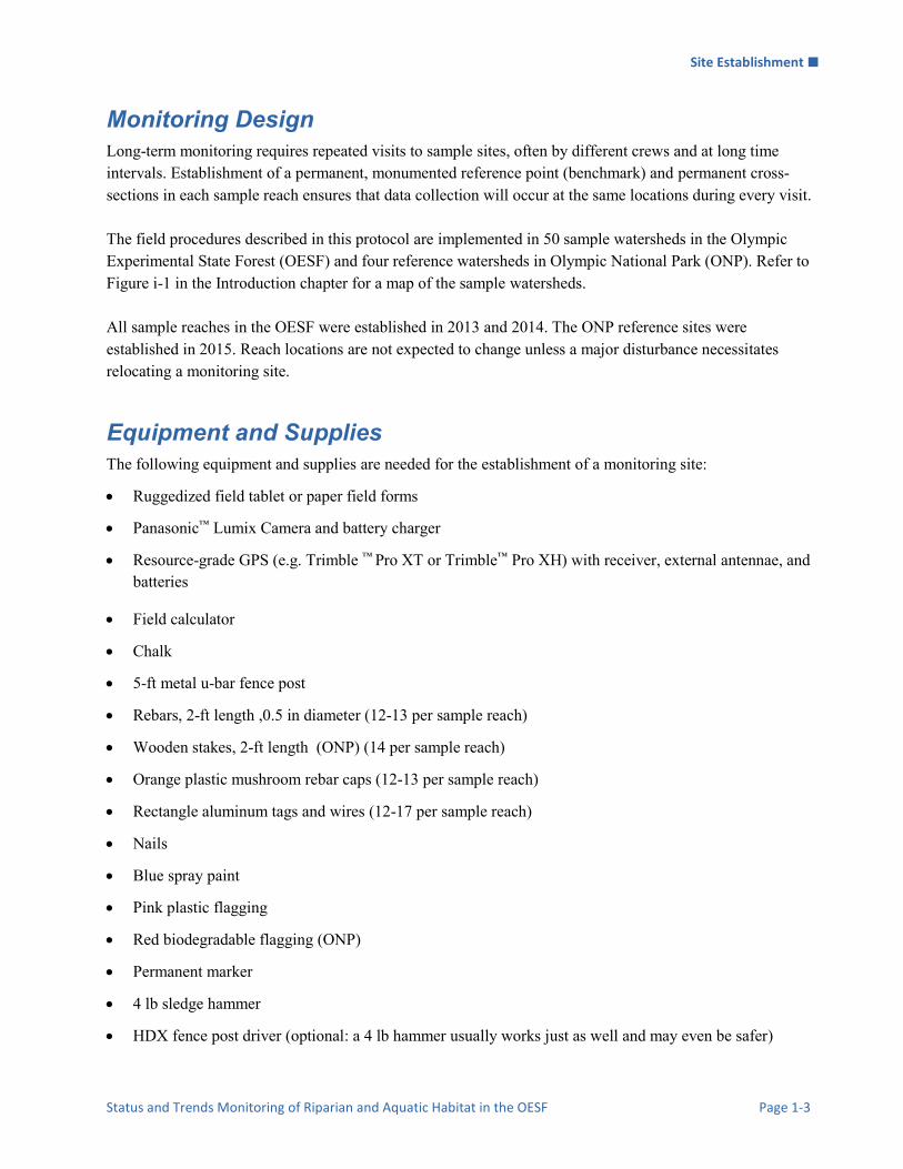
Monitoring Design Long-term monitoring requires repeated visits to sample sites, often by different crews and at long time intervals. Establishment of a permanent, monumented reference point (benchmark) and permanent cross-sections in each sample reach ensures that data collection will occur at the same locations during every visit. The field procedures described in this protocol are implemented in 50 sample watersheds in the Olympic Experimental State Forest (OESF) and four reference watersheds in Olympic National Park (ONP). Refer to Figure i-1 in the Introduction chapter for a map of the sample watersheds. All sample reaches in the OESF were established in 2013 and 2014. The ONP reference sites were established in 2015. Reach locations are not expected to change unless a major disturbance necessitates relocating a monitoring site.
Equipment and Supplies The following equipment and supplies are needed for the establishment of a monitoring site:
Ruggedized field tablet or paper field forms
Panasonic™ Lumix Camera and battery charger
Resource-grade GPS (e.g. Trimble ™ Pro XT or Trimble™ Pro XH) with receiver, external antennae, and batteries
Field calculator
Chalk
5-ft metal u-bar fence post
Rebars, 2-ft length ,0.5 in diameter (12-13 per sample reach)
Wooden stakes, 2-ft length (ONP) (14 per sample reach)
Orange plastic mushroom rebar caps (12-13 per sample reach)
Rectangle aluminum tags and wires (12-17 per sample reach)
Nails
Blue spray paint
Pink plastic flagging
Red biodegradable flagging (ONP)
Permanent marker
4 lb sledge hammer
HDX fence post driver (optional: a 4 lb hammer usually works just as well and may even be safer)

Site Establishment
Page 1-4 Washington State Department of Natural Resources
Sighting compass (e.g. Silva Ranger©)
50-meter tapes (2)
Chaining pins (2)
Spring clips (4)
Stadia rod
Installation field form
PRE-FIELD SETUP Check the batteries for the ruggedized field tablet and Panasonic™ Lumix camera. Paint the rebars blue with spray paint (optional). Adjust current declination on compass.
Field Procedures
IDENTIFYING THE START OF THE SAMPLE REACH First, measure the 100-year floodplain of the mainstem (i.e. larger stream) receiving flow from the Type 3 stream selected for the sample reach Sample reaches must start beyond the floodplain of the mainstem to avoid water mixing and other disturbances caused by high flows (Figure 1-1). Establish the bankfull stage of the mainstem at its confluence with the Type 3 stream. Bankfull stage represents the dominant discharge associated with channel-forming events (refer to the Channel Morphology protocol for a description of bankfull stage indicators). Stand at the deepest point of the mainstem at the confluence holding a stadia rod vertically with the rod bottom end placed on the stream bed. Find the bankfull stage on the stadia rod, double the measurement, and mark this value with flagging on the stadia rod. Use a 50-meter tape or clinometer to project a straight, horizontal line from the mark on the stadia rod toward the Type 3 stream and perpendicular to the mainstem channel. The point where the imaginary line touches the water surface of the Type 3 stream is the extent of the 100-year floodplain of the mainstem. The start of the sample reach can be moved upstream to avoid side channels, undercut banks, channel bends, log jams that could be dangerous to field crews or monitoring equipment, or other irregularities. Refer to the Special Circumstances section below. If no surface water is present, establish the reach start where steady flow begins (not just standing water).

Site Establishment
Status and Trends Monitoring of Riparian and Aquatic Habitat in the OESF Page 1-5
Figure 1-1. Schematic of a sample reach in a monitored watershed.
DETERMINING SAMPLE REACH LENGTH AND ESTABLISHING PERMANENT CROSS SECTIONS The length of a sample reach is determined as 20 times the bankfull width at the start point (cross section A). If the width is less than 5 m, the reach length is 100 m. Each sample reach includes six permanent cross sections installed at five equally spaced intervals (Figure 1-2). The cross sections are delineated by permanent rebar monuments placed on each stream bank. First, establish cross section A, which serves as a permanent marker for the reach start. Find stable locations on each bank, well outside the bankfull stage, that create a cross section perpendicular to the stream. Use the 4 lb sledge hammer to pound the rebar into the ground, a log, a root, or a rock until only 6-8 inches of rebar is visible. Make sure the rebar is secure; if it is loose, find a different position on the same perpendicular line. Once the rebar is installed, spray it with blue paint (or use a pre-painted rebar) and place

Site Establishment
Page 1-6 Washington State Department of Natural Resources
an orange plastic mushroom cap on top. Mark the rebar with pink flagging and an aluminum tag affixed with stainless wire. Label the top of the orange cap, both sides of the flagging, and both sides of the aluminum tag with the corresponding letter for the cross section (i.e. A, B, C, D, E, or F). Use a 50-meter tape to measure the distance to the nearest 0.01 m (1 cm) between the left and right monuments (rebars) at each cross-section and the azimuth from the left monument to the right monument. Record the measurements in the installation field form. This information can be used to locate/re-install a lost monument in the future. Next, measure the bankfull width at cross section A, following the procedures detailed in the Channel Morphology protocol. To mitigate for potential irregular bankfull width, also measure the bankfull width at 2 m and 4 m upstream of the cross section. Measure to the nearest 0.01 m (1 cm), and record the measurements in the field form. To calculate the sample reach length, average the three measurements and multiply the result by 20. Round to the nearest 5 m to allow easy calculation of the cross-section intervals, then divide that number by five to attain the cross-section interval for the sample reach. For a 100 m sample reach, the cross-section interval is 20 m. To find the location of the next cross-section (B), one technician holds the zero end of the 50-meter tape at the thalweg (deepest path of flowing water in the main channel) of cross section A. The other technician carries the reel end of the tape upstream, following the thalweg. Keep the tape at the water surface along the thalweg while measuring. If a sharp bend in the channel is encountered, hook the tape on a rock or stick in the bend to ensure that the tape follows the thalweg and accurately measures the interval distance. After reaching the predetermined interval distance, establish cross section B as described above. Repeat for all cross sections. Sample reach layout is illustrated in Figure 1-2. Collect the GPS coordinates of the sample reach start and end (cross sections A and F) and record multiple GPS waypoints throughout the reach along the thalweg. The spatial data will permit GIS mapping of the reach.
Special Circumstances
Reference Sites in Olympic National Park For sites in Olympic National Park (ONP), sample reach cross sections are monumented by wooden stakes instead of rebars. The corresponding letter for each cross section (i.e. A, B, C, D, E, or F) is written on the appropriate stake with a permanent marker. Each monument is also marked with red biodegradable flagging and labeled with the study permit number, ONP coordinator, and expected year of removal (e.g. “OLYM-361, Pat Crain, Down in 2022”). Stakes should be labeled before installation, when they are dry and clean. Plastic flagging, rebars, and orange plastic mushroom caps are not allowed in the park.

Site Establishment
Status and Trends Monitoring of Riparian and Aquatic Habitat in the OESF Page 1-7
Undercut Banks and Obstructions When establishing a cross section, try to avoid severe undercut banks, channel bends, large logjams that could be dangerous, or other obstructions that may occur at the intended cross section location. These obstacles can make it difficult to establish and measure the cross section accurately. If one of these obstructions is encountered, move the cross section to the nearest suitable location (upstream or downstream); measure and note the offset in the field form (e.g. “cross section B was moved 2.1 m upstream to avoid a severe undercut”).
Figure 1-2. Layout of a sample reach.

Site Establishment
Page 1-8 Washington State Department of Natural Resources
Avoid offsetting by more than 2 m. The sample reach should never be shortened from its calculated length. If it is not possible to install cross section F at its intended location, move the cross section upstream. Record any offsets in the field form. Side Channels (dry or wetted) Avoid side channels by moving the cross-section upstream or downstream. If this is not possible, install the cross section monuments beyond the side channel. When measuring a cross section that intersects a side channel, determine the bankfull stage of the side channel along the cross section line, measure the channel’s bankfull width, and add this value to the main channel bankfull width.
ESTABLISHING A REFERENCE POINT A reference point (RP) is established near each sample reach to assist in locating sampling points along the reach (e.g. reach start and data loggers). The RP will be used as a permanent benchmark that serves as a vertical and horizontal control point used for all monitoring conducted at a sample site. The RP is typically placed between the start of the sample reach and the temperature data loggers, in a location that provides a clear view of both (Figure 1-3). The location should be near the channel but on stable substrate (non-erodible slope) outside of the 100-year floodplain of the sample reach (refer to the Channel Morphology protocol for the procedure to identify the 100-year floodplain).
Figure 1-3. Typical layout of the sample reach start, RP, reference trees, and temperature loggers.

Site Establishment
Status and Trends Monitoring of Riparian and Aquatic Habitat in the OESF Page 1-9
Monument the RP with rebar pounded into the root of a live tree, a solid piece of LWD, or directly into the ground until only 6-8 inches of rebar is visible. Once installed, spray it with blue paint (or use a pre-painted rebar) and place an orange plastic mushroom cap on top. Mark the rebar with pink flagging and an aluminum tag affixed with stainless or copper wire. Write “RP” on the top of the orange cap, and label the flagging and both sides of the aluminum tag with the watershed number. Measure the distance (within 0.01 m [1 cm]) and azimuth from the RP to the start of the sample reach at the left edge of water (LEW) (Figure 1-3) and enter the data in the field form together with a short description of the RP location. Identify two live, vigorous trees near the RP that can be used to find the RP location via triangulation if the RP is lost. Mark these “reference trees” with pink flagging and blue spray paint. Nail an aluminum tag to the trunk of each tree at breast height (1.4 m) on the side facing the RP. Label each tag with the distance and azimuth to the RP (for example: Ref. Tree #1 RP at 7.8 m @ 320°). Record the distance, azimuth, species, and DBH of each reference tree in the field form. Take a photo of the RP from about 2 m to the north, including the reference trees in the image, if possible (Figure 1-4). Record the photo number in the field form. Collect the GPS coordinates of the RP and record them in the field form. The procedure for establishing an RP and reference trees at the ONP reference sites is the same as described above except that blue paint and pink plastic flagging are not used. Instead, use red biodegradable flagging as a marker. . Label all aluminum tags and flagging for the RP and reference trees with the study permit number, the name of the ONP coordinator, and the expected year of removal (e.g. “OLYM-361, Pat Crain, Down in 2022”).
MEASURING THE REFERENCE POINT ELEVATION The elevation of each RP is measured once during the study. These known elevations will be used as benchmarks for determining the absolute elevation of cross sections or other elements of sample reaches. However, for most analyses, a relative RP elevation of “0” will be used. Measure the RP elevation with survey-grade GPS or derive it from LiDAR (light detection and ranging) data. LiDAR may be a better option in some areas, such as incised valleys with dense canopy where it is difficult to obtain a satellite signal. Refer to Appendix 1A for step-by-step directions for recording elevation with a GPS unit.
Figure 1-4. Typical reference point and two marked reference trees.

Site Establishment
Page 1-10 Washington State Department of Natural Resources
ESTABLISHING A PERMANENT PHOTO POINT A permanent photo point establishes location for collecting repeated photographs of the same stretch of the sample reach over time. The photos will be used to illustrate stream dynamics over time, to clarify questionable data points, and to track vegetation succession. Each photo point includes a metal T or U fence post used to position the camera and a target placed across the stream from the post. As the situation warrants, a photo point target can be one of the following:
A plastic mushroom cap on a cross section monument (already installed). A plastic mushroom cap on a specially installed photo point target rebar. Four aluminum tags in an X-shape nailed to a live tree or piece of LWD. A bullseye drawn on a recording gage with a permanent marker. A recording gage cap. A bullseye drawn on a wooden stake with a permanent marker (ONP).
Find a stable location close to the RP, with a good view of the stream, preferably oriented upstream. If the watershed contains a gage station, it should be visible in the photo point photo. If there is an interesting feature (e.g. large erosion patch, log jam, large precarious tree) nearby, try to select a position for the fence post that will include the feature in the photo. Pound in the fence post using the 4 lb. hammer until only ~1.25 m of post is visible. If it is too difficult to pound in the post with the hammer, use the fence post driver. Mark the fence post with pink flagging labeled “Photo Point [Watershed ID]”. Install the target on the opposite bank near the stream. Mark the target with pink flagging labeled “Photo Point Target [Watershed ID]”. Measure the distance (within 0.01m [1 cm]) and bearing from the RP to top of u-bar fence post. Measure the distance (0.01m) and bearing from the top of the fence post to the photo point target. Measure the distance (0.01m) and bearing from the RP to the left edge of water (LEW) at the cross section. Label the fence post flagging with the distance and bearing from the photo point to the photo point target (e.g. “Photo Point Target is cross section B monument cap 2.53m @ 156˚). Record the photo point location and all measurements in the field form. For ONP sites, use wooden stakes marked with red biodegrdable flagging for both the photo point and the photo point target. Using a permanent marker, write the study permit number, the name of the ONP coordinator, and the expected year of removal (e.g. “OLYM-361, Pat Crain, Down in 2022”) on the stake and bioflagging marking the photo point. Draw a bullseye on the stake serving as the photo point target, and write the permit number, coordinator name, and removal year on the bioflagging marking the target.

Site Establishment
Status and Trends Monitoring of Riparian and Aquatic Habitat in the OESF Page 1-11
TAKING A PICTURE AT THE PHOTO POINT Set the camera’s display to “grid view.” Rest the camera on top of the fence post, zoom in all the way, and center the image on the photo point target. Holding the camera steady zoom out to the full extent and take the photo (Figure 1-5). Record the photo number in the field form. At the ONP reference sites, take the photo at 1.5 m above the base of the wooden stake marking the photo point. Conveniently, when a stadia rod is set at its lowest height, the top of the rod is at 1.5 m.
Time and Cost Estimates for Implementing the Field Procedures The estimated time for site establishment is about two to three hours per sample reach for an experienced two-member field crew. This estimate does not include travel time to sites. Table 1-1 shows the cost estimates for the equipment unique to site establishment protocol implementation. Many of the items listed in the Equipment and Supplies section above are shared with the Channel Morphology protocol (e.g., ruggedized field tablet and the camera). Their costs are detailed in that protocol and not included here. The survey-grade GPS unit for measuring the elevation at the RP and collecting the stream sinuosity points is borrowed from the WADNR Engineering Division.
Figure 1-5. Taking a photo from a permanent photo point. The photo target is drawn on the PVC of the gage station across the stream.

Site Establishment
Page 1-12 Washington State Department of Natural Resources
Table 1-1. Cost Estimates for the Equipment Used in the Site Establishment Field Protocol
Equipment/Supplies Amount per watershed Individual cost
Amount for the project (54 sites) Cost for the project*
2-ft rebar, 0.5 in diameter 13 $1.80 650 $1,170
Rebar caps, mushroom
orange
13 $10 (box of 25) 650 (26 boxes) $260
5-ft metal u-bar fence post 1 $3.50 50 $175
Nails, aluminum tags, wires $35 (box of 300) 2 $70
Plastic flagging $2 25 rolls $50
Biodegradable flagging $5 2 rolls $10
2-ft wooden stakes 14 $20 (pack of 12) 56 (5 packs) $100
Spray paint $7 10 cans $70
4-lb sledge hammer $20 1 $20
*Initial installation only, replacements are not included.
Quality Assurance and Quality Control The quality assurance for the site establishment field protocol includes staff training and the use of standardized protocols. The quality control for the field procedures includes field checks on 10% of the field measurements. The field checks are performed by the project researchers and/or assigned field crew. The QA/QC procedures for data management are described in the Data Management section below.
TRAINING All personnel conducting field protocols will be trained in a consistent manner to ensure that the surveys are conducted properly and in standardized fashion. The training is conducted or, for returning personnel, reviewed, annually before the start of the field season. At least one member of the field crew should be experienced with the field procedures.
STANDARD PROTOCOLS The standard procedures described in this protocol will be followed for the duration of the project. Any deviations from the procedures should be documented, and the reasons for deviation should be described and discussed with the project manager or the researcher overseeing the protocol implementation. Changes to the published protocols must be approved by the project manager or the researcher overseeing the protocol implementation. Revised protocols will be assigned new version numbers and publication dates.

Site Establishment
Status and Trends Monitoring of Riparian and Aquatic Habitat in the OESF Page 1-13
Data Management
DATA FLOW Site establishment data and metadata are recorded in the field using paper field forms (2013-2014 field seasons) or a ruggedized field tablet (2015 field season onward). In the office, data are then transferred to a database for long-term storage. The steps below detail the process.
Data flow for paper field forms
1. Fill out field forms. The Site Description section of the Stream Morphology, Substrate, Shade datasheet is used to record the data and metadata associated with site establishment at each sample reach.
2. Scan and store field forms. After returning from the field each week, the field forms are scanned and stored on the WADNR network drive; the original paper forms are archived by the OESF Data Management Specialist at the WADNR Forest Resources Division.
3. Enter data. All site establishment data collected on paper field forms are entered in the Stream Geomorphology Database by the OESF Data Management Specialist on a weekly basis. After data from a field form is entered, the Specialist writes “Entered” on the form followed by his or her initials and the date.
4. Quality control. Entered field form data are verified by comparing the data on the field form to the data in the database. This process is performed by someone other than the person who originally entered the data. After the data are verified, the person who verified it writes “Verified” on the field form followed by his or her initials and the date.
Data flow for electronically collected data
1. Fill out forms on electronic field data recorder. Field personnel collect all site establishment data using the Tablet Database, which is a customized database created in Microsoft Access and saved on the ruggedized field tablet.
2. Store field data. At the end of each day in the field, a copy of the Tablet Database, containing all data collected to date, is transferred to the OESF Data Management Specialist via cloud storage or email. If internet access is not available, the field crew makes a daily backup copy of the database on a laptop or other storage device and then transfers the data to the Data Management Specialist at the end of the work week. The Specialist stores these Tablet Database copies in a temporary location on the WADNR network drive (J:\hcp\monitoring_research\tminkova\01_OESF_R&M Program\01_Rip S&T Mon\07_Data management\_All new data and photos\) until they are processed and the data are transferred to a database for long-term storage.
3. Quality control. Because data are recorded electronically, and thus never transcribed, transcription errors do not exist. However, there is still a possibility of data entry errors in the field. In particular, if metadata (e.g., the date of a field visit or a watershed ID) are recorded incorrectly in the field, this could cause errors during the process of importing data from the Tablet Database to other databases for long-term storage (next step; see below). For this reason, metadata are examined for accuracy prior to importing data to the long-term storage databases.

Site Establishment
Page 1-14 Washington State Department of Natural Resources
4. Import data to database. On a weekly basis, the OESF Data Management Specialist imports all new data from the Tablet Database to databases for long-term storage, such as the Stream Geomorphology Database. This is accomplished using a set of queries stored in another database called “Distribute_Tablet_Data.accdb”.
5. Verify transfer of data. After data have been imported, the OESF Data Management Specialist verifies that no records have been missed, using the record count queries built into the Distribute_Tablet_Data database.
Photographs
1. Transfer photos to data manager for storage. All digital photographs taken in the field are transferred to the OESF Data Management Specialist at the end of each work week. The Specialist stores the uncatalogued photos on the DNR server at: J:\hcp\monitoring_research\tminkova\01_OESF_R&M Program\01_Rip S&T Mon\07_Data management\_All new data and photos\
2. Rename and archive photos. The OESF Data Management Specialist renames each photo point photo using the following naming convention: PT_<WatershedID>_<Date taken>_<Original photo name> (for example: PT_797_20140715_P1000851.JPG). The photos are then moved to long-term storage in the following directory: J:\hcp\monitoring_research\tminkova\01_OESF_R&M Program\01_Rip S&T Mon\03_Photos and videos\04_Stream_survey\Photo_Points\
GPS Data
1. Transfer data to data manager for storage. All GPS data recorded in the field are transferred to the OESF Data Management Specialist at the end of each work week. The Specialist stores the data on the WADNR server at: J:\hcp\monitoring_research\tminkova\01_OESF_R&M Program\01_Rip S&T Mon\07_Data management\_All new data and photos\
2. Differentially correct GPS data. All GPS data are differentially corrected using Pathfinder Office. Instructions are located here: J:\hcp\monitoring_research\tminkova\01_OESF_R&M Program\01_Rip S&T Mon\02_Spatial data\04_GIS Instructions\Differential Correction & Draw Linework in ArcMap-ArcView.docx After differential correction is completed, the original, uncorrected GPS files from the field are stored here: J:\hcp\monitoring_research\tminkova\01_OESF_R&M Program\01_Rip S&T Mon\02_Spatial data\01_GPS Field Data\
3. Transfer corrected data to long-term storage. Differentially corrected GPS data are added to the latest “SERP” feature class, which is located here: J:\hcp\monitoring_research\tminkova\01_OESF_R&M Program\01_Rip S&T Mon\02_Spatial data\07_Map_Data\OESF Map Data.gdb

Site Establishment
Status and Trends Monitoring of Riparian and Aquatic Habitat in the OESF Page 1-15
DATA STORAGE
Paper Field Forms
The paper field forms are archived at the WADNR Forest Resources Division. The designated data steward is Teodora Minkova, WADNR. Scanned copies of these forms are saved in the Adobe portable document format (.pdf) in the following directory:
J:\hcp\monitoring_research\tminkova\01_OESF_R&M Program\01_Rip S&T Mon\01_FIELD DATA\01_Stream survey\Data\Data archive\Field forms\
Tablet Databases
The original Tablet Databases, which are transferred to the OESF Data Management Specialist on a daily or weekly basis, are stored on the WADNR network drive after the field data they contain have been transferred to the Stream Geomorphology Database. The long-term storage location for the Tablet Databases is: J:\hcp\monitoring_research\tminkova\01_OESF_R&M Program\01_Rip S&T Mon\01_FIELD DATA\01_Stream survey\Data\Data archive\Processed tablet databases\
Long-Term Data Storage
The ultimate location of the site establishment data is the Stream Geomorphology Database, located on the WADNR network drive at: J:\hcp\monitoring_research\tminkova\01_OESF_R&M Program\01_Rip S&T Mon\01_FIELD DATA\01_Stream survey\Data\Stream_Geomorphology_Database.accdb Within the Stream Geomorphology Database, site establishment data are stored in three related tables: the Installation Table, the Site Visit Table, and the Visit Detail Table. The Installation Table contains data for which only one value exists, such as the location of the photo point or the sample reach length. The Site Visit Table contains data that change over time (e.g. hiking trail condition, photo point photo name), and therefore must be recorded each time the site is visited. The Visit Detail Table contains data that change every day (e.g. weather conditions, time of day that the visit began) and thus may differ on each day of a multi-day site visit. The Installation Table and the Site Visit Table are connected by a one-to-many relationship. One record exists in the Installation Table for each sample reach, but each record in that table is related to multiple records in the Site Visit Table because each sample reach has had multiple visits. Each record in the Visit Detail table represents one day of one site visit. Because a single visit can contain multiple days, the Site Visit Table is related to the Visit Detail Table through a one-to-many relationship. In the diagram below, the arrows point to the “many” side of each one-to-many relationship.
Installation Table → Site Visit Table → Visit Detail Table
Site Establishment
Page 1-16 Washington State Department of Natural Resources
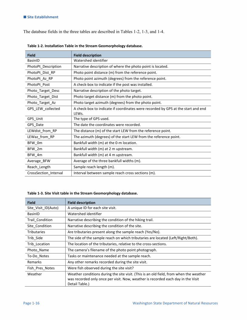
The database fields in the three tables are described in Tables 1-2, 1-3, and 1-4.
Table 1-2. Installation Table in the Stream Geomorphology database.
Field Field description
BasinID Watershed identifier
PhotoPt_Description Narrative description of where the photo point is located.
PhotoPt_Dist_RP Photo point distance (m) from the reference point.
PhotoPt_Az_RP Photo point azimuth (degrees) from the reference point.
PhotoPt_Post A check-box to indicate if the post was installed.
Photo_Target_Desc Narrative description of the photo target.
Photo_Target_Dist Photo target distance (m) from the photo point.
Photo_Target_Az Photo target azimuth (degrees) from the photo point.
GPS_LEW_collected A check-box to indicate if coordinates were recorded by GPS at the start and end LEWs.
GPS_Unit The type of GPS used.
GPS_Date The date the coordinates were recorded.
LEWdist_from_RP The distance (m) of the start LEW from the reference point.
LEWaz_from_RP The azimuth (degrees) of the start LEW from the reference point.
BFW_0m Bankfull width (m) at the 0-m location.
BFW_2m Bankfull width (m) at 2 m upstream.
BFW_4m Bankfull width (m) at 4 m upstream.
Average_BFW Average of the three bankfull widths (m).
Reach_Length Sample reach length (m).
CrossSection_Interval Interval between sample reach cross sections (m).
Table 1-3. Site Visit table in the Stream Geomorphology database.
Field Field description
Site_Visit_ID(Auto) A unique ID for each site visit.
BasinID Watershed identifier
Trail_Condition Narrative describing the condition of the hiking trail.
Site_Condition Narrative describing the condition of the site.
Tributaries Are tributaries present along the sample reach (Yes/No).
Trib_Side The side of the sample reach on which tributaries are located (Left/Right/Both).
Trib_Location The location of the tributaries, relative to the cross-sections.
Photo_Name The camera’s filename of the photo point photograph.
To-Do_Notes Tasks or maintenance needed at the sample reach.
Remarks Any other remarks recorded during the site visit.
Fish_Pres_Notes Were fish observed during the site visit?
Weather Weather conditions during the site visit. (This is an old field, from when the weather was recorded only once per visit. Now, weather is recorded each day in the Visit Detail Table.)

Site Establishment
Status and Trends Monitoring of Riparian and Aquatic Habitat in the OESF Page 1-17
Table 1-4. Visit Detail table in the Stream Geomorphology database.
Field Field description
Detail_ID(Auto) A unique ID for each day of each site visit.
Site_Visit_ID A unique ID for each site visit (because a visit may consist of multiple days). This ID is used to relate this table to the Site Visit Table.
Survey_Date The date.
Start_Time The time that work began on that date.
End_Time The time that work ended on that date.
Field_Crew The initials of the field crew members present on that date (this is an old field, from when datasheets recorded only the field crew once per site visit).
Field_Crew_tablet The initials of the field crew members present on that date (this is a field created when we began using the tablet to collect data; it accommodates difference crew members on each date).
Camera_Num The camera ID for the camera used on that date.
Weather The weather on that date.
DATA QUALITY CONTROL Prior to data analysis, all data in the data tables are assessed to identify potentially erroneous values. The first step is to examine individual fields, one at a time. For categorical data fields (e.g. GPS_Unit) and date or time fields, every field is assessed to identify any records exhibiting the following:
1. Missing values. 2. Illogical values. In some cases, where the data collector is free to enter values rather than selecting
values from a predefined list, illogical values may be recorded (e.g. a survey time of 3:00 AM).
For numerical fields, each is assessed for the following:
1. Missing values. 2. Outlier values (e.g. a bankfull width was recorded in cm instead of m).
The next step in quality control assessment is to examine values in the context of other fields. For example, if the three bankfull widths are 3.2, 3.5, and 26 meters, then there is most likely a decimal error in the third value. When missing values are discovered, it is generally not possible to “fill in the blank” from the office. The fact that data are missing should be recorded, in brackets, in the Remarks field, with the initials of the person who performed the quality control check (e.g., [Trail_Condition was not recorded. –WD]). Illogical or outlier values can sometimes be corrected in the office. For example, AM and PM might have been switched or a decimal place error can be corrected. When data are corrected, this must be noted in the

Site Establishment
Page 1-18 Washington State Department of Natural Resources
remarks field, in brackets, with the initials of the person who performed the quality control check. For example: [BFW_4m was recorded as 36 m. This was clearly incorrect and changed to 3.6 which is logical given the other two widths. –WD]. In many cases, clearly erroneous outlier values cannot be corrected in the office and should be edited so as not to affect the results of analysis. In such cases, the value should be removed from the field and transferred to the Remarks field with an explanation, in brackets, with the initials of the person who performed the quality control check. For example: [BFW_4m was recorded as 74.8 m. This was clearly incorrect and removed from the dataset. –WD]).

Site Establishment
Status and Trends Monitoring of Riparian and Aquatic Habitat in the OESF Page 1-19
References Pleus, A. E. and D. Schuett-Hames. 1998a. TFW Monitoring Program methods manual for stream segment
identification. Prepared for the Washington Department of Natural Resources under the Timber, Fish, and Wildlife Agreement. TFW-AM9-98-001. DNR #103. May.
Pleus, A. E. and D. Schuett-Hames. 1998b. TFW Monitoring Program methods manual for reference point survey. Prepared for the Washington Department of Natural Resources under the Timber, Fish, and Wildlife Agreement. TFW-AM9-98-002. DNR #104. May.

Site Establishment
Page 1-20 Washington State Department of Natural Resources
This page intentionally left blank.

Site Establishment
Status and Trends Monitoring of Riparian and Aquatic Habitat in the OESF Page 1A-1
Appendix 1A. Directions for recording reference point elevation with Trimble Recon survey-grade GPS unit
1. Power on the Trimble Recon and Trimble Receiver and attach all cables and antenna 2. Open ArcPad 3. File Folder-> open map -> map_settings.saved (to access all layers in a pre-saved map) 4. File Folder -> New -> Shapefile 5. Type: “Point Z”, CodePage: OEM- United States. Then click the “+”, click “ok”, click “ok” again 6. Name the file: [date]-b[watershed ID]-RP (e.g. 20150125-b433-RP) 7. Select folder: “none”, Type: “Shapefile”, Location: “Storage Card” 8. Click “Save”, Click “no” for creating a QuickForm. 9. Double check in the Layers whether the file was created and is editable. 10. GPS Preferences-> Protocol: Trimble GPScorrect ->Capture: check the box for “enable averaging”
with “30 points & 5 vertices”. ->GPS Height: Antenna Height: __m (while wearing the backpack have your partner measure the height from the ground to the bottom of the antenna mount). Check the box for “Use Height In Datum Transform”.
11. GPScorrect Settings->Logging settings->click the Antenna height wrench->Make sure the correct type of antenna is listed. Measure Height To: “Bottom of antenna mount”
12. GPScorrect Settings->Real-time Settings -> “Use uncorrected GPS” 13. Activate the GPS Receiver. See GPS cursor on the map, check the satellite reception. Once there are at
least 4 satellites with good geometry a point can be collected. 14. Stand at the base of the RP, with the antenna directly over it. 15. Click on the satellite icon to start averaging (percentages will show up on the top of the screen). 16. Name the field: “b[watershed ID]-RP (e.g. b433-RP) 17. When averaging reaches 100%, click “ok” and the collected point should now be visible on the map.
Watch the screen for a while and make sure that the Trimble still agrees with the location of the collected point. Also, make sure that the point looks reasonable in comparison to other points that have been collected in the stream.

Site Establishment
Page 1A-2 Washington State Department of Natural Resources
This page intentionally left blank.

Channel Morphology
Status and Trends Monitoring of Riparian and Aquatic Habitat in the OESF Page 2-1
Channel Morphology Authors: Teodora Minkova, Mitchell Vorwerk, Ellis Cropper Version: 1.4 Revision History:
Based on the Following Protocols: The general monitoring design follows the Field Protocol Manual for Aquatic and Riparian Effectiveness Monitoring Program (AREMP) for the Northwest Forest Plan (Lanigan et al. 2010). Details on some of the field procedures are adapted from the Illustrated Guide to Field Technique for Stream Channel Reference Sites (Harrelson et al. 1994) and the Timber, Fish, and Wildlife (TFW) Method Manual for the Reference Point Survey (Pleus and Schuett-Hames 1998).
Reasons to Adopt the Above Protocols: The AREMP protocols (Lanigan et al. 2010) have higher consistency scores and are better at describing environmental heterogeneity than other regional protocols (Roper et al. 2010). The AREMP conceptual framework (Reeves et al. 2004) has been adopted in the study plan for this monitoring project. The TFW protocols and Harrelson et al. (1994) are widely used in the Pacific Northwest because of their detailed and well-described field procedures.
Purpose and Content: The purpose of this monitoring protocol is to describe the sampling and data management necessary to document and report the shape, size, and slope of the stream channels and how they change over time. The protocol details the field procedures for sampling channel width, depth, gradient, sinuosity, confinement, and bank erosion; the quality assurance and quality control steps; and the data management procedures.) Classifications for valley and channel types and geomorphological units (e.g., pools, riffles) are described in the protocol Habitat Units and Valley and Channel Classification.
Protocol Version Purpose / Changes Author(s) Reviewer(s) Date
1.0 Initial draft presented to project staff Teodora Minkova Alex Foster 04/01/2013
1.1 Draft submitted to external review Teodora Minkova Rebecca Flitcroft, Ashley Steel
04/16/2013
1.2 Final draft incorporating external reviews, sampling procedures from 2013 field season, and data mgmt. procedures
Teodora Minkova, Mitchell Vorwerk, Ellis Cropper
04/20/2014
1.3 Final draft with field and data management procedures updated from 2014 and 2015 field seasons
Teodora Minkova, Mitchell Vorwerk, Ellis Cropper
Alex Foster 06/10/2016
1.4 Final technical review and edit Teodora Minkova, Mitchell Vorwerk, Ellis Cropper
Paul Dunnette, Warren Devine, Alex Foster
12/18/2016

Channel Morphology
Page 2-2 Washington State Department of Natural Resources
Table of Contents Introduction ..................................................................................................................................................... 2-3
Monitoring Design .......................................................................................................................................... 2-3
Spatial Sampling Design ............................................................................................................................. 2-3
Temporal Sampling Design ......................................................................................................................... 2-3
Equipment and Supplies .................................................................................................................................. 2-5
Pre-Field set up ........................................................................................................................................... 2-5
Field Procedures .............................................................................................................................................. 2-6
Measurement of bankfull width .................................................................................................................. 2-6
Measurement of bankfull depth................................................................................................................... 2-8
Measurement of bank erosion ................................................................................................................... 2-15
Measurement of channel confinement ...................................................................................................... 2-16
Measurement of water surface gradient .................................................................................................... 2-17
Azimuth survey ......................................................................................................................................... 2-20
Measurement of channel sinuosity ............................................................................................................ 2-21
Time and Cost Estimates for Implementing the Field Procedures ................................................................ 2-22
Procedures for Calculating Metrics ............................................................................................................... 2-22
Quality Assurance and Quality Control ........................................................................................................ 2-23
Calibration of the autolevel ....................................................................................................................... 2-24
Training ..................................................................................................................................................... 2-24
Standard Protocols .................................................................................................................................... 2-24
Field Checks .............................................................................................................................................. 2-24
Data Management ......................................................................................................................................... 2-24
Data Flow .................................................................................................................................................. 2-24
Data Storage .............................................................................................................................................. 2-26
Data Quality Control ................................................................................................................................. 2-29
References ..................................................................................................................................................... 2-31
Appendix 2A. Indicators of Bankfull Stage ................................................................................................. 2A-1
Appendix 2B. Directions for recording sinuosity points with Trimble™ Recon survey-grade GPS unit ..... 2B-1
Appendix 2C. Auto Level Checks/Calibration and Adjustments ................................................................. 2C-1

Channel Morphology
Status and Trends Monitoring of Riparian and Aquatic Habitat in the OESF Page 2-3
Introduction Channel morphology (i.e., shape, dimensions, and slope) reflects the stream-reach and watershed-level ecological process and provides a basis for interpreting the potential responses of the stream to perturbations such as sediment delivery and peak flows (Montgomery and Buffington 1993). Channel morphology influences the distribution and abundance of aquatic plants and animals by governing the characteristics of water flow and the capacity of streams to store sediment and transform organic matter (Bisson et al. 2006). Geomorphic characteristics such as channel width, confinement and gradient are used in models to identify fish habitat, which enable land managers to prioritize habitat conservation, maintenance, and restoration. Channel morphology changes as a result of water discharge, sediment deposition, and delivery of large wood (Montgomery and Buffington 1997). Forestry practices such as logging and road management can affect channel shape, size, and gradient directly through sediment and wood delivery to the streams or indirectly by modifying watershed vegetation and road density, which alter flow regimes (Grant et al. 2008). In the environmental impact analysis for the Olympic Experimental Forest (OESF) Forest Land Plan (WADNR 2016), stream gradient and confinement were used to identify stream reaches (the smallest analysis unit) and to assign reach-scale sensitivity ratings for in-stream large wood, fine sediment, coarse sediment, and peak flow. Channel width was used in the stream shade model (to locate the channel edge and define a non-forested area immediately above the stream) and in the microclimate model (to locate the channel edge and assign a starting point for the equations that represent the microclimate gradients). Finally, the models utilized in the environmental impact analysis for fish used channel width and gradient to identify fish habitat (chinook spawning, coho summer rearing, coho winter rearing, and steelhead rearing habitat).
Monitoring Design
SPATIAL SAMPLING DESIGN All channel morphology attributes described in this protocol are measured in each of the 50 sample watersheds in the OESF and in the four reference sample watersheds in Olympic National Park (ONP). Refer to the Introduction chapter for a map of the sample watersheds. Some channel morphology measurements are taken at the permanent cross-sections (e.g., channel depth, channel width, and valley width). Others are measured as a continuous survey over the entire sample reach (e.g. sinuosity, gradient, and bank erosion) (Figure 2-1).
TEMPORAL SAMPLING DESIGN Sampling should occur when flows are at relatively low levels, such as during summer and early fall. Sampling should not be performed when streams are near bankfull stage or higher because under such conditions it becomes difficult or impossible to accurately identified bankfull markers.

Channel Morphology
Page 2-4 Washington State Department of Natural Resources
Figure 2-1. Location of channel morphology attribute sampling within the sample reach
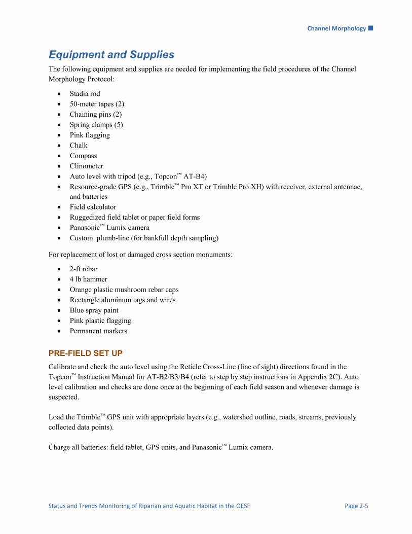
Channel Morphology
Status and Trends Monitoring of Riparian and Aquatic Habitat in the OESF Page 2-5
Equipment and Supplies The following equipment and supplies are needed for implementing the field procedures of the Channel Morphology Protocol:
Stadia rod 50-meter tapes (2) Chaining pins (2) Spring clamps (5) Pink flagging Chalk Compass Clinometer Auto level with tripod (e.g., Topcon™ AT-B4) Resource-grade GPS (e.g., Trimble™ Pro XT or Trimble Pro XH) with receiver, external antennae,
and batteries Field calculator Ruggedized field tablet or paper field forms Panasonic™ Lumix camera Custom plumb-line (for bankfull depth sampling)
For replacement of lost or damaged cross section monuments:
2-ft rebar 4 lb hammer Orange plastic mushroom rebar caps Rectangle aluminum tags and wires Blue spray paint Pink plastic flagging Permanent markers
PRE-FIELD SET UP Calibrate and check the auto level using the Reticle Cross-Line (line of sight) directions found in the Topcon™ Instruction Manual for AT-B2/B3/B4 (refer to step by step instructions in Appendix 2C). Auto level calibration and checks are done once at the beginning of each field season and whenever damage is suspected. Load the Trimble™ GPS unit with appropriate layers (e.g., watershed outline, roads, streams, previously collected data points). Charge all batteries: field tablet, GPS units, and Panasonic™ Lumix camera.

Channel Morphology
Page 2-6 Washington State Department of Natural Resources
Field Procedures
MEASUREMENT OF BANKFULL WIDTH
Bankfull width is the horizontal distance between the bankfull stage indicators on each side of a stream, measured directly across the channel. Bankfull stage represents the dominant discharge associated with channel-forming events. The recurrence interval of these events varies among channels and regions, but is generally between 0.5 and 2.0 years (Williams 1978). In this study, bankfull width (BFW) is measured at each permanent cross-section (Figure 2-1). First, extend a 50-meter tape between the rebars monumenting the cross sections (Figure 2-2). Attach the zero end of the tape to the left monument (rebar) with a spring clamp, extend the tape tautly across the channel, and attach the tape to the right monument with another clamp. Make sure the tape forms a straight line over the cross section, and clear any vegetation that may obstruct the tape. This is the “upper” tape. Next, determine the bankfull stage on both banks using the indicators described and illustrated in Appendix 2A. Insert chaining pins into the ground to mark the left and right bankfull stages (LBF and RBF, respectively) directly below the upper tape. Recommended tip: hang a plumb-line from the upper tape to correctly line up the chaining pins. This device can easily be fashioned with a spring clamp, ~3 m of cordage, and a small weight. A stadia rod may be used instead, but this can be inaccurate, especially if the monuments are placed very high above the stream.
Figure 2-2. Sample reach cross section.

Channel Morphology
Status and Trends Monitoring of Riparian and Aquatic Habitat in the OESF Page 2-7
Attach the zero end of a second 50-meter tape to the left chaining pin with a spring clamp, extend the tape tautly across the channel, and attach the tape to the right pin with another clamp. This is the “lower” tape. Make sure the upper and lower tapes are pulled tight and aligned; adjust the lower tape, if necessary. Aligning the lower tape with the permanent cross section line allows repeatable measurements over time. Ensure that the lower tape is unobstructed by vegetation, logs, or boulders. Prune vegetation if necessary or stretch the lower tape separately on both sides of the boulder or log. If a side channel is within the cross section, measure the side channel’s bankfull width using the upper tape and add the width to the main channel width (see Special Circumstances, below, for further instructions). A side channel exists when both of the following criteria are met:
1. There is an island or bar in the stream which is higher than bankfull stage and has bankfull indicators present (see Appendix 2A for indicators)
2. The portion of the island/bar that is above bankfull stage has a length at least twice that of the stream’s estimated BFW (average of BFW measurements already made, or, if none have been made yet, measure BFW above and below the island and average)
A side channel does not need to have water present in it, but it must have bankfull indicators. Measure the BFW on the lower tape and record the measurement in the appropriate field on the field tablet (nearest 1 cm). When measuring the BFW of the main channel or side channels, do not include the width of bars or islands that are above the bankfull stage, but do include the width of bars or islands that are below the bankfull stage (Figure 2-3).
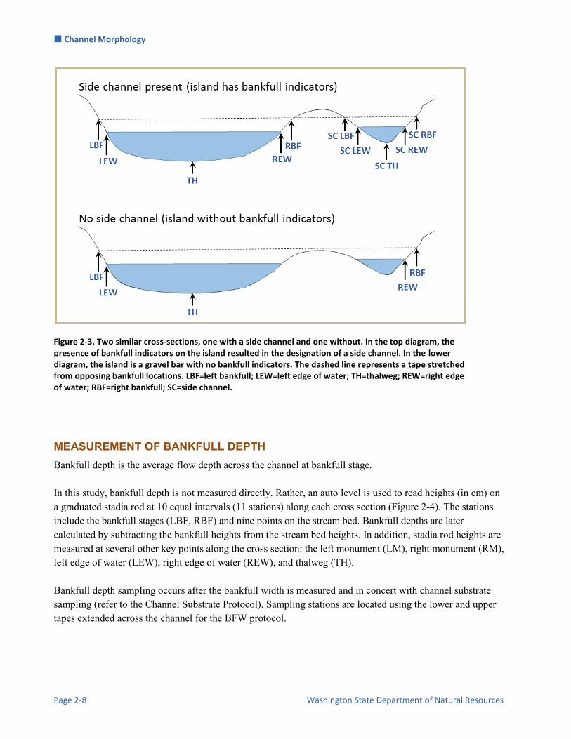
Channel Morphology
Page 2-8 Washington State Department of Natural Resources
Figure 2-3. Two similar cross-sections, one with a side channel and one without. In the top diagram, the presence of bankfull indicators on the island resulted in the designation of a side channel. In the lower diagram, the island is a gravel bar with no bankfull indicators. The dashed line represents a tape stretched from opposing bankfull locations. LBF=left bankfull; LEW=left edge of water; TH=thalweg; REW=right edge of water; RBF=right bankfull; SC=side channel.
MEASUREMENT OF BANKFULL DEPTH Bankfull depth is the average flow depth across the channel at bankfull stage. In this study, bankfull depth is not measured directly. Rather, an auto level is used to read heights (in cm) on a graduated stadia rod at 10 equal intervals (11 stations) along each cross section (Figure 2-4). The stations include the bankfull stages (LBF, RBF) and nine points on the stream bed. Bankfull depths are later calculated by subtracting the bankfull heights from the stream bed heights. In addition, stadia rod heights are measured at several other key points along the cross section: the left monument (LM), right monument (RM), left edge of water (LEW), right edge of water (REW), and thalweg (TH). Bankfull depth sampling occurs after the bankfull width is measured and in concert with channel substrate sampling (refer to the Channel Substrate Protocol). Sampling stations are located using the lower and upper tapes extended across the channel for the BFW protocol.

Channel Morphology
Status and Trends Monitoring of Riparian and Aquatic Habitat in the OESF Page 2-9
Figure 2-4. Bankfull depth sampling.
Auto Level Set-up and Operation
Set up the auto level and tripod in a stable location that is high enough to take stadia rod height measurements above both cross section monuments and provides a clear view of the entire cross section (Figure 2-5). Choose a location as close as possible to the cross section to facilitate clear communication between the auto level operator and the crew member holding the stadia rod. Before attaching the auto level to the tripod, secure the tripod feet in the ground or substrate and adjust the legs to make the tripod plate nearly level. Place the auto level on the tripod plate and tighten the centering screw. Next, level the auto level by adjusting the leveling foot screws to center the bubble in the center circle. Periodically check the bubble’s position throughout the survey; if the instrument goes out of level (i.e., the bubble leaves the circle), the survey may need to be restarted. To take measurements, aim the telescope at the stadia rod, focus using the focusing knob, identify the center reticle (line) in the sight, and note the height where the center line (reticle) intersects the rod (see Topcon instruction manual for further details). Heights should be measured to the nearest 0.5 cm. Record only the numbers viewed at the center line, not at the upper or lower lines.

Channel Morphology
Page 2-10 Washington State Department of Natural Resources
Figure 2-5. Sampling bankfull depth using a stadia rod and auto level.
Survey
Before starting the survey, enter the cross section BFW in the field tablet database, which will automatically calculate the sampling interval and produce a list of 21 sampling stations (distances in cm) along the lower tape. Stadia rod heights are measured at 11 of the stations (equally spaced, top row of the list), and channel substrate is sampled at every station (top and bottom rows). Be sure to measure heights before disturbing the substrate (see Channel Substrate Protocol). One crew member takes auto level measurements, enters data in the field tablet, and reads the distances to the other crew member, who positions the stadia rod at each sampling station. The rod should always be plumb, not leaning, when measurements are taken. If sampling occurs in the rain, use an umbrella to shield the field tablet touch screen. All sampling stations are based on the lower tape. Thus, stations for the LM, RM and other points outside the bankfull width are determined using their distances from the LBF or RBF, measured with the upper tape. Stations to the left of the LBF are negative values, and stations to the right of the RBF exceed the BFW. Begin measurements at the LM. Hold the stadia rod at the base (ground level) of the monument, record the height in the field tablet database “Fore.” (foresight) field, and select LM in the “Location” field.
Channel Morphology
Status and Trends Monitoring of Riparian and Aquatic Habitat in the OESF Page 2-11
Use the upper tape to determine the distance from the LBF to the LM and record this distance in the “Station” field as a negative number, because it extends past zero on the lower tape. An exception is when undercut banks at the bankfull stage extend beyond the monuments. Next, measure the LBF height. Hold the stadia rod at the correct bankfull height, even if an obstruction or undercut bank prevents attaching the lower tape and/or placing the stadia rod at the true bankfull stage (see Special Circumstances, below). The recorded distance for the LBF should always be zero. Move to the next predetermined station, place the stadia rod base on the stream bed, and take a height measurement. Record the distance and height in the appropriate field tablet fields. Continue on to collect and record stream bed heights and distances for each of the listed stations. Also identify, measure, and record distances and stadia rod heights for the LEW, TH, REW, RBF, and RM. Calculate the RM station distance by finding the distance from RBF to the RM (using the upper tape) and adding this value to the BFW. Record LM, LBF, LEW, TH, REW, RBF, or RM in the “Location” fields corresponding to the stations for these key points. A given cross section will only have one value for LM, LBF, LEW, TH, REW, RBF, or RM in the Location field. This remains true even if a side channel is present; in that case, follow the Location data entry protocol described below in the Side Channels subsection of the Special Circumstances section. The LEW and REW are the points where water meets the left and right banks. Measure LEW and REW heights with the stadia rod base held at the water surface. Unless there is a tributary or a qualifying side channel, it is not necessary to record more than one LEW and one REW per cross section, even in the Remarks section (see the lower diagram in Figure 2-3: there is a gravel bar present but there is no need to record a LEW2 or REW2). The TH is measured by probing with the stadia rod to find the deepest point along the cross section. Be careful not to move/remove rocks in deep sections of the channel during the substrate survey so an accurate TH measurement can be made and so that the 100 year floodplain can be correctly measured after the cross section survey. If channel gradient and azimuths are measured during the field visit, mark the LEW with chalk, to easily identify the location later. Before ending the survey, do two QC checks to ensure that the auto level has not moved. First, check that the leveling bubble is still centered in the circle. If the bubble has moved out of the circle, take an auto level reading back to the LM or another clearly defined QC point. If the two measurements differ by more than 1.0 cm, you will have to re-level the instrument and retake all the measurements.
Special Circumstances
Unable to pin the lower tape at the correct bankfull stage. Move up or down as necessary - it is ideal, but not imperative, that the lower tape be pinned exactly at both bankfull stages. It is most
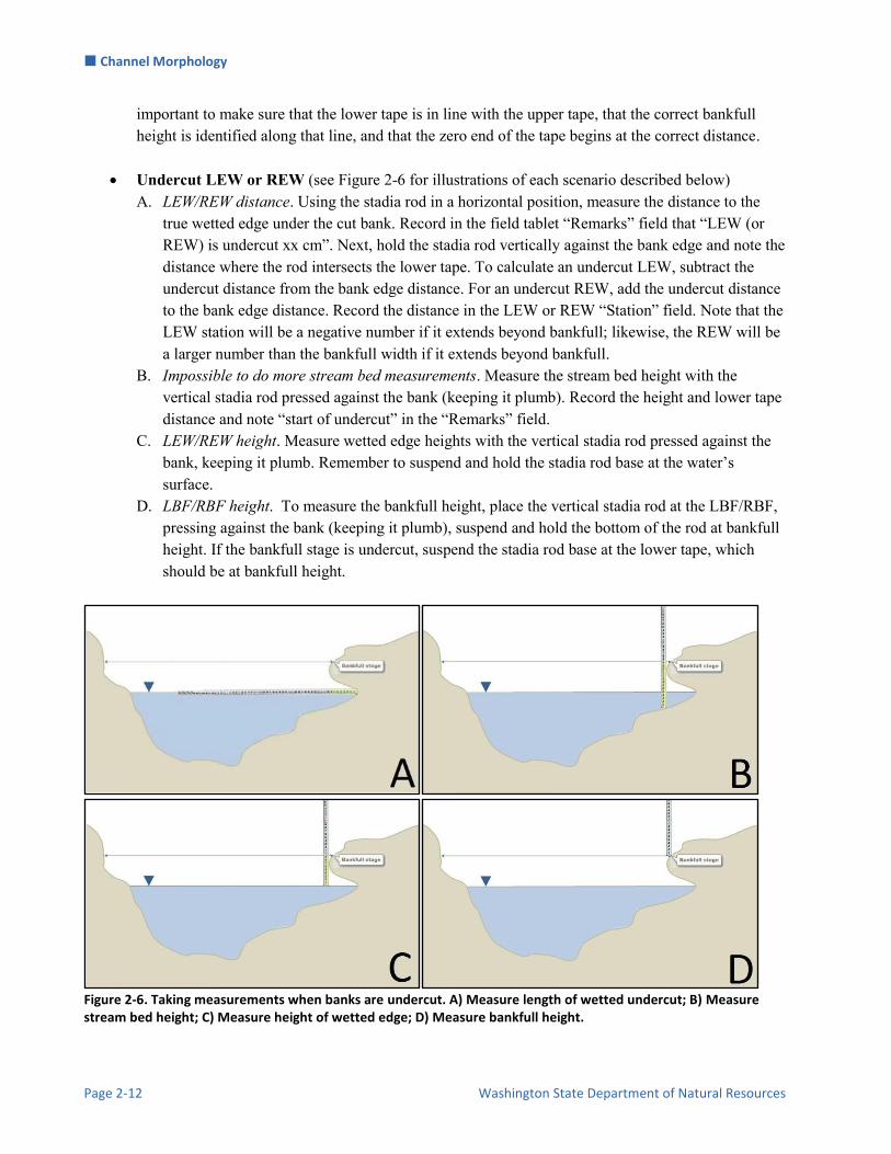
Channel Morphology
Page 2-12 Washington State Department of Natural Resources
important to make sure that the lower tape is in line with the upper tape, that the correct bankfull height is identified along that line, and that the zero end of the tape begins at the correct distance.
Undercut LEW or REW (see Figure 2-6 for illustrations of each scenario described below)
A. LEW/REW distance. Using the stadia rod in a horizontal position, measure the distance to the true wetted edge under the cut bank. Record in the field tablet “Remarks” field that “LEW (or REW) is undercut xx cm”. Next, hold the stadia rod vertically against the bank edge and note the distance where the rod intersects the lower tape. To calculate an undercut LEW, subtract the undercut distance from the bank edge distance. For an undercut REW, add the undercut distance to the bank edge distance. Record the distance in the LEW or REW “Station” field. Note that the LEW station will be a negative number if it extends beyond bankfull; likewise, the REW will be a larger number than the bankfull width if it extends beyond bankfull.
B. Impossible to do more stream bed measurements. Measure the stream bed height with the vertical stadia rod pressed against the bank (keeping it plumb). Record the height and lower tape distance and note “start of undercut” in the “Remarks” field.
C. LEW/REW height. Measure wetted edge heights with the vertical stadia rod pressed against the bank, keeping it plumb. Remember to suspend and hold the stadia rod base at the water’s surface.
D. LBF/RBF height. To measure the bankfull height, place the vertical stadia rod at the LBF/RBF, pressing against the bank (keeping it plumb), suspend and hold the bottom of the rod at bankfull height. If the bankfull stage is undercut, suspend the stadia rod base at the lower tape, which should be at bankfull height.
Figure 2-6. Taking measurements when banks are undercut. A) Measure length of wetted undercut; B) Measure stream bed height; C) Measure height of wetted edge; D) Measure bankfull height.

Channel Morphology
Status and Trends Monitoring of Riparian and Aquatic Habitat in the OESF Page 2-13
Undercut LBF or RBF. Follow the same procedure for measuring undercut LEW or REW distances and heights, substituting the undercut LBF/RBF. Note that the bankfull stage and wetted edge can both be undercut on one or both sides of the cross section.
Vertical bank. Measure and record heights for the LBF/RBF, LEW/REW, and stream bed. The tape
distances may be the same.
Large boulders/logs. If a large obstruction extends above the water surface and interferes with one or more height measurements, take measurements from the stream bed before the obstruction (stream left), from the top of the obstruction, and after the obstruction (stream right). Record the distances (stations) along the lower tape for each height measurement. Resume measuring at the regular intervals as soon as possible.
Side channels. Determining the side channel measurement stations If a side channel intersects the cross section, identify the side channel’s bankfull stage indicators and determine its BFW using the upper tape. Add the side channel BFW to the main channel BFW and record the sum on the tablet in the cross-section’s Bankfull Width field. The tablet will then display the stations; however, these stations will not be usable when a side channel exists because they do not account for the island’s width. So, instead of using the displayed measurement stations, manually calculate the sampling interval by dividing the entire BFW (i.e., sum of both channels) by 20. It may be helpful to write in a field notebook a list of sampling stations that includes both the distances along the lower tape (used in sampling) and the distances relative to the main channel LBF (recorded in the field tablet). Wetted width is calculated similarly to BFW: separately measure the wetted width of the main channel and the side channel, add the two, and enter the sum in the Wetted Width field for the cross section. Following the same process as described for cross-sections without a side channel, measure stadia rod heights at the calculated station interval across the main channel and side channel(s). This interval is designed to produce a total of 21 equally spaced stations across the combined main and side channels. For the main channel, also make stadia rod measurements as you normally would at LBF, LEW, TH, REW, and RBF. For the side channel, measure at these same five locations; if the side channel is dry, omit its LEW and REW locations. Because all station distances are based on the main channel’s LBF station distance of 0 cm, station distances left of the main channel LBF will be negative, and station distances right of the main channel RBF will exceed the RBF. The lower tape will need to be moved from the main channel to the side channel after the main channel is measured.
Recording data When recording data for a cross section with a side channel(s), record LBF, LEW, TH, REW, and RBF in the Location field only for the main channel. For each side channel, record SC in the Location field for all side channel stations beginning with the side channel’s LBF and ending with the side channel’s RBF (Table 2-1 and Figure 2-7). For the side channel’s LBF, LEW, TH, REW, and RBF, record these abbreviations in the Remarks field, prefaced by SC (e.g., SC LBF).

Channel Morphology
Page 2-14 Washington State Department of Natural Resources
Table 2-1. Example of how to record locations and remarks when a side channel is present (see Figure 2-7). Note that this example shows fewer stations than would be recorded in an actual measurement; also, foresight and particle fields are not shown.
Station (cm) Location Remarks
-55 LM
0 LBF
23 LEW
75
150
205 TH
225
300
368 REW
407 RBF
521 SC SC LBF
563 SC SC LEW
602 SC SC TH
651 SC SC REW
678 SC SC RBF
749 RM
Figure 2-7. Example of a cross-section with a side channel to the right of the main channel. Dashed lines represent the upper and lower tapes; vertical red lines represent measurement stations; blue text is entered in the Location field, red text is entered in the Remarks field, and numbers represent the station distance (cm) (see Table 2-1).

Channel Morphology
Status and Trends Monitoring of Riparian and Aquatic Habitat in the OESF Page 2-15
Tributaries. If a tributary intersects the cross section, three stadia rod measurement stations should be associated with the tributary: the left and right edges of water and the thalweg (i.e., the deepest point in the tributary). On the field tablet, record “TR” in the Location field for these three stations. Then, in the Remarks field, record like for side-channels, that is prefaced with a “TR” such as TR LEW, TR REW, and TR TH. The tape distances for the tributary’s stations are based on the lower tape, with 0 cm at the main channel’s LBF, as usual. Unlike side-channels, do not add the tributary width to the main channel bankfull width or take additional cross-section height measurements beyond the three mentioned here: TR LEW, TR REW, and TR TH.
MEASUREMENT OF BANK EROSION Streambank erosion is a natural process, however, the rate of erosion can change because of effects associated with forest management. Increased erosion and resulting sediment influx to streams can negatively affect habitat for fish and other aquatic organisms (Chamberlain et al. 1991). In this study, the metric “percent actively eroding bank” is used to quantify the amount of erosion within a sample reach. To qualify as “actively eroding,” an area of the bank (a “patch”) needs to meet all of the following criteria:
It is above but in contact with the bankfull stage. It is at least 2 m in length and 0.5 m in height above the bankfull stage. It has exposed soils with active sloughing or tension cracks (e.g., banks crumbling or falling into the
stream). It is not stabilized by rooted vegetation, although it may be covered with forest organic matter or
superficial non-rooted vegetation like moss and algae. Note that undercut banks that are stabilized by tree roots (soil near the roots is missing and/or not crumbling or falling into the stream) are not counted as active erosion even if their height is > 0.5 m above the bankfull stage. Undercut banks at or below the bankfull stage usually are well-supported by roots.
Measure the height above bankfull stage and the length of all qualifying erosion patches using the stadia rod and a 50-meter tape (nearest 0.1 m). (Figure 2-8). If the patch is long and varies in height, average several height measurements. Measure all qualifying erosion patches on both banks between cross sections A-B, B-C, C-D, D-E, and E-F. Split up an erosion patch into two measurements if it intersects a cross section.

Channel Morphology
Page 2-16 Washington State Department of Natural Resources
Figure 2-8. Field crew measuring active erosion height and length.
Note the cause of erosion ( e.g., road, uprooted tree, cut bank caused by stream, elk or human trail, logjam, etc.) if it is obvious. Enter any additional comments in the “Remarks” field. Photograph each patch of active erosion and include the stadia rod or 50-meter tape (for long sections) in the photos. Record the photo number in the appropriate field on the field tablet. “Percent actively eroding bank” is calculated at the office by dividing the total sample reach stream bank distance defined as “actively eroding” (both banks) by the total streambank distance (twice the reach length).
MEASUREMENT OF CHANNEL CONFINEMENT Channel confinement is defined as the ratio of flood plain width to channel bankfull width. Confinement values provide information on the ability of the channel to migrate within the floodplain under the present hydrologic regime (Dunne and Leopold 1978). The floodplain width, often called the channel migration zone, is the width of the stream at maximum flood flows that have a recurrence interval of 100 years (WADNR 2004). In this study, floodplain width is measured as channel width at an elevation of twice the maximum bankfull depth of the channel. Channel confinement is calculated from measurements of floodplain and bankfull width taken at the beginning, middle, and end of each sample reach (at cross sections A, C, and F) (Figure 2-1).

Channel Morphology
Status and Trends Monitoring of Riparian and Aquatic Habitat in the OESF Page 2-17
At cross section A, first measure the maximum bankfull depth standing at the thalweg (Figure 2-4). The field tablet database automatically calculates the floodplain height using the following equation:
[TH – ((LBF + RBF) / 2)] x 2 = FP height
where TH is the thalweg, LBF is the left bankfull stage, RBF is the right bankfull stage, and FP is the floodplain. Next, tie flagging to the stadia rod at the FP height. Hold the rod vertically at the thalweg. If a third crew member is not available to hold the stadia rod, prop up the rod with a camera tripod and spring clamps. At the flagged height, extend a 50-meter tape out level across the channel cross section and adjacent floodplains until you reach a terrace, hillside, or large barrier on each side of the channel. Measure up and over small gravel bars, logs or other nonpermanent barriers unlikely to impede floodwaters at FP height. The total distance across the channel and valley is the 100-year floodplain width. Record the width to the nearest 0.01 m. Repeat the measurement at the other two cross sections. The reach confinement ratio, commonly called the entrenchment ratio describes the degree to which the stream is vertically incised within its floodplain. This dimensionless rating describes the relationship of bankfull mean depth to stream discharge (Dunne and Leopold 1978). A widening and degrading stream over time (increase in confinement ratio) can result from several intertwined factors including higher or more frequent flood or peak discharges that exceed a stream’s floodplain capacity for conveyance. The confinement ratio is calculated:
FP width / mean BFW= reach confinement ratio Where FP is the floodplain and BFW is the bankfull width. The confinement ratios are then used to assign the sample reaches into three categories:
Unconfined: floodplain width ≥ 4 bankfull widths (ratio 2.2+) Moderately confined: floodplain width ≥2 and < 4 bankfull widths (ratio 1.4 - 2.2) Confined: floodplain width < 2 bankfull widths (ratio 1.0 - 1.4)
Further explanation of channel confinement can be found in WADNR (2004).
MEASUREMENT OF WATER SURFACE GRADIENT The elevation of the Reference Point (RP) is measured once during the study (refer to the Monitoring Site Establishment protocol). The measurement provides a known elevation in each watershed that will be used as a benchmark for determining the absolute elevation of cross section features or other elements of the sample reach. However, for most analyses, a relative RP elevation of “0” will be used.

Channel Morphology
Page 2-18 Washington State Department of Natural Resources
Stream gradient survey
Stream gradient, also called channel slope, is the elevational difference (rise) between two points in a stream divided by the distance between them (run), measured along the water surface (rise / run = % slope). In this study, we measure the water surface gradient using auto level and stadia rod (Figure 2-9). The difference in elevation is measured between the RP and the first cross section (A), then between consecutive cross sections heading upstream. It is most efficient to conduct the survey in concert with bankfull depth sampling, which establishes the elevation of the rebar monuments relative to the RP. Stream gradient surveys do not have to be done at the same frequency as bankfull depth surveys, because changes in stream gradients can be calculated from the data gathered during bankfull depth surveys, provided that monuments have not been lost or moved. As a rule of thumb, if any monuments have been found severely disturbed or are missing, then gradient cannot be calculated by bankfull depth surveys alone and must instead be determined via a full gradient survey of the sample reach.
Auto level set up
Set up the auto level on the tripod in a stable location that provides the height and visibility necessary to take a stadia rod height reading at the next cross section (or an intermediate point) and, if necessary, back to the previous cross section. The ideal auto level position allows readings at as many cross sections as possible to reduce the number of measurements and minimize cumulative error. If necessary, remove brush and branches to provide a clear view between cross sections. See Measurement of Bankfull Depth, above, for more detailed instructions on setting up, leveling, and operating the auto level. Stream gradient heights are recorded to the nearest 0.5 cm. Gradient Survey
In the gradient survey, a process called differential leveling is used to measure the elevational differences between stream reach cross sections (Figure 2-10). First, use the auto level and stadia rod to measure the difference in elevation between the RP (known elevation) and the beginning of the sample reach (cross section A). Hold the stadia rod at the base (ground level) of the RP and take a height reading with the auto level. Record the height in both the “Backsight (BS)” and “Height of Instrument (HI)” in the tablet field for cross section A. Also, note “BS to RP” in the “Remarks” section of the field form.
Figure 2-9. Using an auto level and stadia rod to measure stream gradient.

Channel Morphology
Status and Trends Monitoring of Riparian and Aquatic Habitat in the OESF Page 2-19
Figure 2-10. Example of a portion of a stream gradient survey, from the reference point (RP) to cross-section B, where an intermediate point was necessary. Calculations are performed sequentially, from left to right; all values are in centimeters. The elevation of the RP is zero for these calculations. BS—backsight; FS—foresight; HI—height of instrument; LEW—left edge of water.
Hold the stadia rod at the LEW of cross section A. The LEW should have already been marked with chalk during the bankfull depth survey. he bottom of the stadia rod must be held at the water surface, not the channel bottom. Measure the height with the auto level, and record the value in the “Foresight” in the field tablet database field for cross section A. Do not change the position of the auto level between the two measurements and make sure the leveling bubble is still centered when you turn the telescope toward the stadia rod at the LEW. Next, move the auto level upstream to a point with clear views of both the stadia rod at the LEW of cross section A and the LEW of cross section B. Do not move the stadia rod from its position at cross section A. Take a height reading at the LEW of cross section A from the new auto level position and record the value in the field form as backsight (“BS”). Leave the auto level in place, move the stadia rod to the LEW of cross section B (exact position marked with chalk), take a height reading at this location, and record the measurement as foresight (“FS”) in the field tablet. The HI in this case is the difference between FS and BS. Repeat this procedure for all of the intervals between cross sections (B-C, C-D, D-E, E-F). If possible, take readings of multiple cross section LEWs from the same auto level location; this will reduce the number of BS measurements and minimize error introduced by changes in auto level height. If a steep stream gradient or thick vegetation blocks the view to the next cross section, sight to an intermediate point (IP, also called a turning point [TP]). Select a stable point between the two cross sections (e.g., a large rock) and hold the stadia rod plumb at this IP. Measure the height of the IP and record it as an (A-B) Intermediate Foresight. Mark the exact location of the IP with chalk so it can be measured accurately

Channel Morphology
Page 2-20 Washington State Department of Natural Resources
for the next BS. Move the auto level to a stable point between the IP and the next cross section, then take a foresight height reading at the cross section LEW and a backsight height reading at the IP (Figure 2-10). Helpful tip: Although the field tablet has fields to record all gradient measurements, schematic field notes (Figure 2-11) should also be recorded to help technicians understand differential leveling, reduce errors in the field, and assist in future data verification.
Figure 2-11. Example of field notes illustrating differential leveling.
AZIMUTH SURVEY Azimuths are recorded between cross sections to assist in creating a map of the sample reach. The survey should begin at cross section A and proceed upstream. If the survey starts at cross section F, be sure to record back azimuth readings. One crew member holds the stadia rod, adorned with bright flagging, at the upstream cross section LEW and the other crew member uses a compass to measure the azimuth from the downstream cross section LEW to the rod. All LEWs should have been marked with chalk during the Bankfull Depth survey. Enter the azimuths in the field tablet database “Gradients and Azimuth” tab.

Channel Morphology
Status and Trends Monitoring of Riparian and Aquatic Habitat in the OESF Page 2-21
MEASUREMENT OF CHANNEL SINUOSITY
Channel sinuosity describes a stream or river channel’s tendency to meander across its floodplain. Changes in channel sinuosity may indicate a change in sediment supply or transport capacity (Grant et al 2008). Aerial photography, generally used to determine landscape-scale channel patterns, may record some finer-scale shifts in sinuosity over time. However, field measurements are needed for small streams in forested watersheds. Channel sinuosity is defined as the ratio of the sample reach length measured along the thalweg to the straight-line distance between the beginning and end of the sample reach (WADNR 2004) (Figure 2-12). Use a survey-grade GPS unit (Trimble™ Recon) to record the coordinates at the beginning and end of the sample reach. See step-by-step instructions in Appendix 2B. Sample reach length is measured to the nearest 0.1 m by extending a 50-meter tape along the thalweg at the water surface between consecutive cross sections (Figure 2-13). This is done during establishment of the permanent cross sections (refer to Site Establishment protocol). Sinuosity values are calculated in the office.
Figure 2-12. Channel sinuosity measured as a ratio of the sample reach thalweg length (blue line) to the straight line distance (dashed black line) between the reach ends. In this example, the ratio is 1.12.
Figure 2-13. Measuring sample reach length along the thalweg.

Channel Morphology
Page 2-22 Washington State Department of Natural Resources
Time and Cost Estimates for Implementing the Field Procedures The estimated time for sampling the channel morphology attributes is about five hours per sample reach for an experienced two-member field crew if all stream morphology protocols are implemented. Table 2-2 shows the cost estimates for all equipment needed to carry out the field procedures. Many of the listed items are used in other protocols, but their costs are not included in the other protocols’ estimates. The survey-grade GPS unit for measuring the elevation at the RP and collecting the stream sinuosity points is borrowed from the WADNR Engineering Division or can be rented. Table 2-2. Cost Estimates for the Equipment Used in the Channel Morphology Protocol
Equipment/Supplies Amount Individual cost Cost for the project
Ruggedized field tablet 1 $1,400 $1,400
Panasonic™ Lumix camera 1 $200 $200
Stadia rod 1 $220 $220
Topcon auto level with tripod 1 $650 $650
50-meter tapes 2 $35 $70
Clinometer 2 $180 $360
Compass 2 $50 $100
Orange flags with 18”wire Box of 100 $10 $10
Chaining pins Box of 11 $25 $25
Spring clamps 8 $5 $40
Miscellaneous hardware $100
Procedures for Calculating Metrics All metrics are calculated in the office following the procedures in Table 2-3
Channel Morphology
Status and Trends Monitoring of Riparian and Aquatic Habitat in the OESF Page 2-23
Table 2-3. Procedures for calculating metrics.
Metric Calculation Procedure
Mean bankfull width Mean of the bankfull widths at the six cross sections.
Mean bankfull depth
Mean of the mean bankfull depths at the six cross sections. At each cross section, mean bankfull depth is calculated as the mean of the bankfull depths at each of the 11 stations. At each station, bankfull depth is calculated as the difference between the distance-prorated mean of the two bankfull heights and the height of the streambed at that station.
Mean maximum bankfull depth (thalweg depth)
Mean of the six maximum bankfull depth measurements from the six cross sections. Maximum bankfull depth at each cross section is calculated as the difference between the distance-prorated mean of the two bankfull heights and the height of the thalweg at that cross section.
Bankfull width-to-depth ratio
Mean of the bankfull width-to-depth ratios from the six cross sections. For each cross section, the width-to-depth ratio is calculated as the bankfull width divided by the mean bankfull depth at that cross section.
Percent slope of the sample reach water surface
Cumulative difference in water surface heights (cross-sections A through F) divided by total reach length.
Sinuosity of the sample reach
Ratio of the sample reach length to the straight-line distance between the beginning and end of the sample reach.
Channel confinement category
Assigned based on the ratio of the mean 100-year floodplain width to the mean bankfull width. Mean of the 100-year floodplain widths at three cross sections (A, C, and F) The three categories are defined as: Unconfined: floodplain width ≥ 4 bankfull widths. Moderately confined: floodplain width ≥2 and < 4 bankfull widths. Confined: floodplain width < 2 bankfull widths
Percent of actively eroding stream bank
Sum of the streambank distance that is actively eroding along both sides of the sample reach, divided by twice the sample reach length, then multiplied by 100.
Quality Assurance and Quality Control The quality assurance for the channel morphology field protocol includes field instruments calibration, staff training and the use of standardized protocols. The quality control for the field procedures includes annual field checks. The QA/QC procedures for data management are described in the Data Management section below.

Channel Morphology
Page 2-24 Washington State Department of Natural Resources
CALIBRATION OF THE AUTOLEVEL The auto level is calibrated and checked at the beginning of each field season or whenever damage is suspected using the Reticle Cross-Line (line of sight) directions found in the Topcon Instruction Manual for AT-B2/B3/B4 (see Appendix 2C for step-by-step calibration procedure).
TRAINING All personnel conducting field protocols will be trained in a consistent manner to ensure that the surveys are conducted properly and in standardized fashion. The training is conducted or, for returning personnel, reviewed, annually before the start of the field season. At least one member of the field crew should be experienced with the field procedures.
STANDARD PROTOCOLS The standard procedures described in this protocol will be followed for the duration of the project. Any deviations from the procedures should be documented, and the reasons for deviation should be described and discussed with the project manager or the researcher overseeing the protocol implementation. Changes to the published protocols must be approved by the project manager or the researcher overseeing the protocol implementation. Revised protocols will be assigned new version numbers and publication dates.
FIELD CHECKS The researcher overseeing the protocol implementation or a different field crew will conduct spot checks on 10% of the field measurements every year.
Data Management
DATA FLOW All channel morphology data are recorded in the field using paper field forms (2013-2014 field seasons) or a field tablet (2015 season onward). In the office, data are then transferred to a database for long-term storage. The steps below detail the process.
Data flow for paper field forms
1. Fill out field forms. Channel Morphology field forms are used to record the data and metadata at each sample reach.
2. Scan and store field forms. After returning from the field each week, the field forms are scanned and stored on the WADNR network drive; the original paper forms are archived by the OESF Data Management Specialist at the WADNR Forest Resources Division (see Data Storage section below).
3. Enter data. All channel morphology data collected on paper field forms are entered in the Stream Geomorphology Database by the OESF Data Management Specialist on a weekly basis. After data

Channel Morphology
Status and Trends Monitoring of Riparian and Aquatic Habitat in the OESF Page 2-25
from a field form is entered, the Specialist writes “Entered” on the form followed by their initials and the date.
4. Quality control. Entered field form data are verified by comparing the data on the field form to the data in the database. This process is performed by someone other than the person who originally entered the data. After the data are verified, the person who verified it writes “Verified” on the form followed by his or her initials and the date.
Data flow for electronically collected data
1. Fill out forms on electronic field data recorder. Field personnel record all channel morphology data using the Tablet Database, a customized database created in Microsoft Access and saved on the field tablet.
2. Store field data. At the end of each day in the field, a copy of the Tablet Database, containing all data collected to date, is transferred to the OESF Data Management Specialist via cloud storage or email. If internet access is not available, the field crew makes a daily backup copy of the database on a laptop or other storage device and then transfers the data to the Specialist at the end of the work week. The Specialist stores these Tablet Database copies in a temporary location on the WADNR network drive (J:\hcp\monitoring_research\tminkova\01_OESF_R&M Program\01_Rip S&T Mon\07_Data management\_All new data and photos\) until they are processed and the data are transferred to a database for long-term storage:
3. Quality control. Because data are recorded electronically, and thus never transcribed, transcription errors do not exist. However, there is still a possibility of data entry errors in the field. In particular, if metadata (e.g., the date of a field visit or a watershed ID) are recorded incorrectly in the field, this could cause errors during the process of importing data from the Tablet Database to the Stream Geomorphology Database (next step; see below). For this reason, metadata are examined for accuracy prior to importing data to the Stream Geomorphology Database.
4. Import data to database. On a weekly basis, the OESF Data Management Specialist imports all new data from the Tablet Database to the Stream Geomorphology Database. This is accomplished using a set of queries stored in a third database: J:\hcp\monitoring_research\tminkova\01_OESF_R&M Program\01_Rip S&T Mon\07_Data management\Stream_Survey\Database\Distribute_Tablet_Data.accdb
5. Verify transfer of data. After data have been imported, the OESF Data Management Specialist verifies that no records have been missed, using the record count queries built into the Distribute_Tablet_Data database.
Photographs
1. Transfer photos to data manager for storage. All digital photographs taken in the field are transferred to the OESF Data Management Specialist at the end of each week. The Specialist stores the uncatalogued photos on the WADNR server at: J:\hcp\monitoring_research\tminkova\01_OESF_R&M Program\01_Rip S&T Mon\07_Data management\_All new data and photos\
2. Rename and archive photos. The OESF Data Management Specialist renames each photo using the following naming convention: <Photo type>_<BasinID>_<Date taken>_<Original photo name> (for

Channel Morphology
Page 2-26 Washington State Department of Natural Resources
example: ER_797_20140715_P1000851.JPG). The photos are then moved to long-term storage in the following directory: J:\hcp\monitoring_research\tminkova\01_OESF_R&M Program\01_Rip S&T Mon\03_Photos and videos\04_Stream_survey\
DATA STORAGE
Paper Field Forms
The paper field forms are archived at the WADNR Forest Resources Division. The designated data steward is Teodora Minkova, WADNR. Scanned copies of these forms are saved in the Adobe portable document format (.pdf) in the following directory: J:\hcp\monitoring_research\tminkova\01_OESF_R&M Program\01_Rip S&T Mon\01_FIELD DATA\01_Stream survey\Data\Data archive\Field forms\
Tablet Databases
The original Tablet Databases, which are transferred to the OESF Data Management Specialist on a daily or weekly basis, are stored on the WADNR network drive after the field data they contain have been transferred to the Stream Geomorphology Database. The storage location for these databases is: J:\hcp\monitoring_research\tminkova\01_OESF_R&M Program\01_Rip S&T Mon\01_FIELD DATA\01_Stream survey\Data\Data archive\Processed tablet databases\
Long-Term Data Storage
The ultimate location of the channel morphology data is the Stream Geomorphology Database, located on the WADNR network drive at: J:\hcp\monitoring_research\tminkova\01_OESF_R&M Program\01_Rip S&T Mon\01_FIELD DATA\01_Stream survey\Data\Stream_Geomorphology_Database.accdb Within the Stream Geomorphology Database, channel morphology data are stored in five related tables: the Cross Section Table, the Depth Table, the Substrate Table, the Erosion Table, and the Gradient Table (Figure 2-14). The Cross Section, Erosion, and Gradient tables are all related to metadata via one-to-many relationships with the Visit Detail Table. Based on these relationships, one visit date can be related to multiple records in each of the other three tables (the full structure of the metadata is described in detail in the Site Establishment protocol). The Cross Section Table is related to the Depth and Substrate tables via one-to-many relationships: each cross section is related to multiple depth and substrate records.

Channel Morphology
Status and Trends Monitoring of Riparian and Aquatic Habitat in the OESF Page 2-27
Figure 2-14. The structure of the Stream Geomorphology Database.
The database fields in the five tables containing channel morphology data are described in tables 2-4, 2-5, 2-6, 2-7, and 2-8.

Channel Morphology
Page 2-28 Washington State Department of Natural Resources
Table 2-4. The Cross Section table in the Stream Geomorphology Database.
Field Field description
CrossSectionID(Auto) A unique identifier for each cross section.
Detail_ID Relates the cross section to the appropriate metadata in the Visit Detail Table.
CrossSection Cross section letter (A-F).
Bankfull_Width Bankfull width (m).
Wetted_Width Wetted width (m).
100yrFloodplain_Width The width of the 100-year floodplain (m), measured for cross sections A, C, and F.
Remarks Remarks regarding the cross section.
Table 2-5. The Erosion table in the Stream Geomorphology Database.
Field Field description
ErosionID(Auto) A unique identifier for each erosion patch.
Detail_ID Relates the erosion patch to the appropriate metadata in the Visit Detail Table.
Cross_Section Cross sections directly above and below the erosion patch (e.g., A-B, B-C, C-D, etc.)
Location Left or right bank (LB, RB).
Length Length of erosion patch (m).
Height Height of erosion patch (m).
Photo_num Photo number/name for the photograph(s) of the erosion patch.
Cause Cause of erosion.
Remarks Remarks regarding the erosion patch.
Table 2-6. The Gradient table in the Stream Geomorphology Database.
Field Field description
GradientID(Auto) A unique identifier for each gradient measurement.
Detail_ID Relates the gradient measurement to the appropriate metadata in the Visit Detail Table.
Cross_Section Cross section name.
Backsight Backsight reading (+cm).
Height_Instrument Height of the instrument (cm), relative to the reference point.
Foresight Foresight reading (-cm).
Elevation Calculated elevation value (cm).
Azimuth Azimuth (degrees), taken from lower station.
Remarks Remarks regarding the gradient measurement.

Channel Morphology
Status and Trends Monitoring of Riparian and Aquatic Habitat in the OESF Page 2-29
Table 2-7. The Depth table in the Stream Geomorphology Database.
Field Field description
DepthID(Auto) A unique identifier for each depth measurement.
CrossSectionID Relates the depth measurement to the appropriate cross section in the Cross Section Table.
Station The measurement location along the cross section (cm).
Foresight The autolevel depth reading (-cm).
Location Indicates whether the station was located at a monument, bankfull stage, edge of water, or thalweg (LM/LBF/LEW/TH/REW/RBF/RM).
String_Depth Depth, measured by the string method (cm). This method was not used after 2013, and thus the field does not appear on the data entry forms after that year.
Remarks Remarks regarding the depth measurement.
Table 2-8. The Substrate table in the Stream Geomorphology Database.
Field Field description
SubstrateID(Auto) A unique identifier for each substrate measurement.
CrossSectionID Relates the substrate measurement to the appropriate cross section in the Cross Section Table.
Size Particle size (mm).
Embeddedness Particle embeddedness (%).
Remarks Remarks regarding the substrate measurement.
Category Particle size category (e.g., cobble, boulder).
D50_Category Particle size category (mm) used for calculating D50 and other metrics. This differs from the Size field in that the Size field may contain actual diameter measurements, especially for larger particles, rather than a size category.
DATA QUALITY CONTROL Prior to data analysis, all fields in the data tables are assessed to identify potentially erroneous values. The first step is to examine individual fields, one at a time. For categorical data fields (e.g., cross section) and date or time fields, every field is assessed to identify any records exhibiting the following:
Missing values. Illogical values. In some cases, where the data collector is free to enter values rather than selecting
values from a predefined list, illogical values may be recorded (e.g., a survey time of 3:00 AM). For numerical fields, each is assessed for the following:
Missing values. Outlier values (e.g., a stream width was recorded in cm instead of m).

Channel Morphology
Page 2-30 Washington State Department of Natural Resources
The next step in quality control assessment is to examine derived values and values in the context of other fields. An example of a derived value is the lengths of all erosion patches in a sample reach added together. If the sum of patch lengths is greater than twice the length of the sample reach, then the data should be examined to determine if one of the patch lengths was recorded incorrectly. An example of checking a value in the context of another field is the comparison of wetted width with bankfull width. If wetted width is greater than bankfull width, and there is no record of undercutting, then there may be an error in the data. When missing values are discovered, it is generally not possible to “fill in the blank” from the office. The fact that data are missing should be recorded, in brackets, in the Remarks field, with the initials of the person who performed the quality control check (e.g., [Location was not recorded. –WD]). Illogical or outlier values can sometimes be corrected in the office. For example, AM and PM might have been switched or a decimal place error can be corrected. When data are corrected, this must be noted in the remarks field, in brackets, with the initials of the person who performed the quality control check. For example: [Height was recorded as 250 m. This was clearly incorrect and changed to 2.5 m which is logical given nearby erosion heights. –WD]. In many cases, clearly erroneous outlier values cannot be corrected in the office and should be edited so as not to affect the results of analysis. In such cases, the value should be removed from the field and transferred to the Remarks field with an explanation, in brackets, with the initials of the person who performed the quality control check. For example: [Erosion height was recorded as 74.8 m. This value was clearly incorrect and removed from the dataset. –WD]).

Channel Morphology
Status and Trends Monitoring of Riparian and Aquatic Habitat in the OESF Page 2-31
References Bisson, P.A., D.R. Montgomery, J.M. Buffington. 2006. Valley segments, stream reaches, and channel units.
In: Methods in Stream Ecology. Second Edition, edited by F. R. Hauer, and G. A. Lamberti, Academic Press, pp. 23-49.
Chamberlain, T.W., R.D. Harr, F.H. Everest. 1991. Timber harvesting, silviculture, and watershed processes. In: W.R. Meehan (ed.), Influences of forest and rangeland management on salmonid fishes and their habitats. American Fisheries Society Special Publication 19. Bethesda, Maryland. pp. 181-204.
Dunne, T. and L.B. Leopold. 1978. Water in Environmental Planning. W.H. Freeman and Co., NY.
Grant, G.E., S.L. Lewis, F.J. Swanson, J.H. Cissel, J.J. McDonnell. 2008. Effects of forest practices on peak flows and consequent channel response: a state-of-science report for western Oregon and Washington. Gen. Tech. Rep. PNW-GTR-760. Portland, OR: U.S. Department of Agriculture, Forest Service, Pacific Northwest Research Station. 76 p.
Harrelson, C., C. Rawlins, J. Potyondy. 1994. Stream channel reference sites: an illustrated guide to field technique. Gen. Tech. Rep. RM-245. Fort Collins, CO: U.S. Department of Agriculture, Forest Service, Rocky Mountain Forest and Range Experiment Station. 61 p.
Lanigan, S., P. Eldred, C. Moyer, H. Andersen, M. Isley, S. Wilcox. 2010. Aquatic and Riparian Effectiveness Monitoring Program for the Northwest Forest Plan – 2010 Field Protocol Manual. http://www.reo.gov/monitoring/reports/watershed/2010.FieldProtocol.Final.pdf
Montgomery, D. R. and J. M. Buffington. 1993. Channel classification, prediction of channel response, and assessment of channel condition: Olympia, Washington State Department of Natural Resources Report TFW-SHIO-93-002, 84 p.
Montgomery, D. R. and J. M. Buffington. 1997. Channel reach morphology in mountain drainage basins. Geol. Soc. Am. Bull. 109: 596–611.
Pleus, A.E. and D. Schuett-Hames. 1998. TFW Monitoring Program methods manual for the reference point survey. Prepared for the Washington State Dept. of Natural Resources under the Timber, Fish, and Wildlife Agreement. TFW-AM9- 98-002. DNR #104.
Reeves, G, D. Hohler, D. Larsen, D. Busch, Kim Kratz, K. Reynolds, K. Stein, T. Atzet, P. Hays, M. Tehan. 2004. Effectiveness monitoring for the aquatic and riparian component of the Northwest Forest Plan: conceptual framework and options. Gen. Tech. Rep. PNW-GTR-577, Portland, OR.
Roper, B.B., J.M. Buffington, S. Bennett, S.H. Lanigan, E. Archer, S.T. Downie, J. Faustini, T.W. Hillman, S. Hubler, C. Jordan, P.R. Kaufman, G. Merritt, C. Moyer. 2010. A Comparison of the Performance and Compatibility of Protocols Used by Seven Monitoring Groups to Measure Stream Habitat in the Pacific Northwest. North American Journal of Fisheries Management 30:565–587.
Washington State Department of Natural Resources [WADNR]. 2004. Section 2, Standard Methods for Identifying Bankfull Channel Features and Channel Migration Zones. Forest Practices Board Manual. http://file.dnr.wa.gov/publications/fp_board_manual_section02.pdf (Accessed 6/2016)
Washington State Department of Natural Resources. 2016. Olympic Experimental State Forest HCP Planning Unit Forest Land Plan Final Environmental Impact Statement. Washington State Department of Natural Resources, Olympia, WA. http://file.dnr.wa.gov/publications/amp_sepa_nonpro_oesf_feis.pdf

Channel Morphology
Page 2-32 Washington State Department of Natural Resources
Williams, G.P. 1978. Bank-full discharge of rivers: Water Resources Research. 14(6): 1141-1154.

Channel Morphology
Status and Trends Monitoring of Riparian and Aquatic Habitat in the OESF Page 2A-1
Appendix 2A. Indicators of Bankfull Stage From Streamkeepers of Clallam County. 2012. Field procedures. 14th Edition. http://www.clallam.net/streamkeepers/assets/applets/Bankfull.pdf [accessed 12-14-2016]

Channel Morphology
Page 2A-2 Washington State Department of Natural Resources

Channel Morphology
Status and Trends Monitoring of Riparian and Aquatic Habitat in the OESF Page 2B-1
Appendix 2B. Directions for recording sinuosity points with Trimble™ Recon survey-grade GPS unit Record sinuosity points at the beginning and end of the sample reach: the left edge of water at cross sections A and F. 1. Power on the Trimble Recon and Trimble Receiver and attach all cables and antennas. 2. Open ArcPad. 3. File Folder-> open map -> map_settings.saved (to access all layers in a pre-saved map). 4. File Folder -> New -> Shapefile. 5. Type: “Point”, CodePage: OEM- United States. Then click the “+”, click “ok”, click “ok” again. 6. Name the file: [date]-b[basinID]-SIN (e.g. 20150125-b433-SIN). 7. Select folder: “none”, Type: “Shapefile”, Location: “Storage Card”. 8. Click “Save”, Click “no” for creating a QuickForm. 9. Double check in the Layers whether the file was created and is editable. 10. GPS Preferences-> Protocol: Trimble GPScorrect ->Capture: check the box for “enable averaging” with
“30 points & 5 vertices”. 11. GPScorrect Settings->Logging settings->click the Antenna height wrench->Make sure the correct type of
antenna is listed. 12. GPScorrect Settings->Real-time Settings -> “Use uncorrected GPS”. 13. Activate the GPS Receiver. See GPS cursor on the map, and check the satellite reception. Once there are
at least four satellites with good geometry, a point can be collected. 14. Stand at the LEW of cross section A, with the antenna directly over it. 15. Click on the satellite icon to start averaging (percentages will show up at the top of the screen). 16. Name the field: “b[basin ID]-Start-SIN (e.g. b433-Start-SIN). 17. When averaging reaches 100%, click “ok” and the collected point should now be visible on the map.
Watch the screen for a while and make sure that the Trimble still agrees with the location of the collected point. Make sure that the point looks reasonable in comparison to where other GPS points collected in the stream.
18. Stand at the LEW of cross section F, with the antenna directly over it. 19. Click on the satellite icon to start averaging (percentages will show up on the top of the screen). 20. Name the field: “b[basin ID]-End-SIN (e.g., b433-End-SIN). 21. When averaging reaches 100%, click “ok” and the collected point should now be visible on the map.
Watch the screen for a while and make sure that the Trimble still agrees with the location of the collected point. Make sure that the point looks reasonable in comparison to where other GPS points were collected in the stream.

Channel Morphology
Page 2B-2 Washington State Department of Natural Resources
This page intentionally left blank.

Channel Morphology
Status and Trends Monitoring of Riparian and Aquatic Habitat in the OESF Page 2C-1
Appendix 2C. Auto Level Checks/Calibration and Adjustments
Source: TOPCON Instruction Manual, Automatic Level, AT-B2/B3/B4. 2010.
http://geoshack.com/wp-content/uploads/2011/06/AT-B2_B3_B4_rm1.pdf
Auto level calibration and checks should be performed once at the start of each field season and whenever damage is observed or suspected.
See TOPCON Instruction Manual for part diagrams/descriptions.
1) Circular Level Check a. Adjust the leveling foot screws to center the bubble in the circular level. b. Turn the auto level 180 degrees. If the bubble remains within the circular level (the circle),
no adjustment is needed. If the bubble shifts out of the circle, adjust as follows: i. Compensate for one-half of the shift by adjusting the leveling foot screws.
ii. Compensate for the remaining half-shift using the circular level adjusting screws. Adjust the screws using the hexagonal wrench.
iii. After the adjustments, turn the auto level 180 degrees and check the circular level. If the bubble remains within the circle, the adjustment is complete.
2) Automatic Compensator Check a. Center the bubble in the circular level. b. Look through the eyepiece and identify the horizontal cross-line. While turning the leveling
screw nearest the sighting axis 1/8 of a turn to the right or left, check the movement of the cross-line. If the automatic compensator mechanism is working properly, the cross-line should bounce, then immediately return to its original position. Alternatively, the compensator can be checked by monitoring the cross-line’s behavior after tapping the tripod legs or the auto level’s main body while sighting on a clear target. The cross-line should quickly return to its original position after the disturbance.
3) Reticle Cross-Line (Line of Sight) Calibration a. Set up the auto level halfway between two points (A and B) that are 30 to 50 meters apart.
Take readings on the stadia rod while the rod is positioned at each point (a1 and b1). b. Set up the auto level at a point 2 meters from point A (still between A and B). Take a reading
on the stadia rod at Point A (a2), and then at Point B (b2). Leave the auto level telescope sighted on Point B after the second reading.
c. Calculate b2’ = a2 – (a1 – b1). If b2’ = b2, the horizontal cross-line is normal and no adjustment is necessary. If b2’ and b2 are different, adjust the cross line as follows:
i. Unscrew and remove the adjusting screw cover. ii. Use the adjusting pin (see “Standard Equipment” section of TOPCON manual) to
eliminate the difference between b2’ and b2. If the horizontal line needs to be lowered (when b2’ is higher), carefully loosen the adjusting screw slightly using the adjusting pin. To raise the horizontal line, tighten the adjusting screw.

Channel Morphology
Page 2C-2 Washington State Department of Natural Resources
i. Repeat the adjustment procedure described in (i) and (ii) until the difference between b2’ and b2 is “small.” (TOPCON does not define “small”.)

Stream Shade
Status and Trends Monitoring of Riparian and Aquatic Habitat in the OESF Page 3-1
Stream Shade Authors: Jeffrey Ricklefs, Teodora Minkova, Mitchell Vorwerk, Ellis Cropper Version: 1.4
Revision History:
Based on the Following Protocols: Solar input protocols from Bonneville Power Administration (BPA) Columbia Habitat Monitoring Program (CHaMP) (Bouwes et al. 2011). Reasons to Adopt the Above Protocols: The CHaMP sample framework is similar in scale to that of the Olympic Experimental State Forest (OESF) monitoring project. CHaMP provides an established protocol and detailed sampling procedures. Purpose and Content: The purpose of this monitoring protocol is to describe the sampling and data management necessary to document and report the status and multi-year trends of stream shade in the monitored watersheds. It details the field procedures for taking canopy photos, the field quality assurance and quality control steps, and the data management procedures.
Protocol
Version Purpose / Changes Author(s) Reviewer(s) Date
1.0 Initial draft presented to project staff Jeffrey Ricklefs Teodora Minkova
04/02/2013
1.1 Draft submitted to external review Jeffrey Ricklefs Rebecca Flitcroft 04/16/2013
1.2 Draft incorporating external reviews, sampling procedures from 2013 field season, and data mgmt. procedures
Jeff Ricklefs, Teodora Minkova
05/20/2014
1.3 Final draft with field and data management procedures updated from 2014 and 2015 field seasons
Jeff Ricklefs, Teodora Minkova, Mitchell Vorwerk, Ellis Cropper
Alex Foster 06/11/2016
1.4 Final technical review and edit Jeff Ricklefs, Teodora Minkova, Mitchell Vorwerk, Ellis Cropper
Paul Dunnette, Warren Devine, Alex Foster
12/18/2016

Stream Shade
Page 3-2 Washington State Department of Natural Resources
Table of Contents Introduction ..................................................................................................................................................... 3-3
Monitoring Design .......................................................................................................................................... 3-3
Spatial Sampling Design ............................................................................................................................. 3-3
Temporal Sampling Design ......................................................................................................................... 3-3
Equipment and Supplies .................................................................................................................................. 3-5
Field Procedures .............................................................................................................................................. 3-5
Pre-field Set-up ........................................................................................................................................... 3-5
Field Sampling ............................................................................................................................................ 3-7
Time and Cost Estimates for Implementing the Field Procedures ................................................................ 3-11
Procedures for Calculating Metrics ............................................................................................................... 3-11
Image processing ....................................................................................................................................... 3-11
Calculating Metrics ................................................................................................................................... 3-12
Quality Assurance and Quality Control ........................................................................................................ 3-12
Training ..................................................................................................................................................... 3-13
Standard Protocols .................................................................................................................................... 3-13
Field Quality Control ................................................................................................................................ 3-13
Data Management ......................................................................................................................................... 3-13
Data Flow .................................................................................................................................................. 3-13
Data Storage .............................................................................................................................................. 3-15
Data Quality Control ................................................................................................................................. 3-18
References ..................................................................................................................................................... 3-20
Appendix 3A. Image Processing Software Options ..................................................................................... 3A-1
Stream Shade
Status and Trends Monitoring of Riparian and Aquatic Habitat in the OESF Page 3-3
Introduction Stream shade, the extent to which a stream channel is shielded from incoming sunlight, is one of the primary factors influencing stream temperature (Brown 1969). Stream temperature, in turn, affects aquatic organisms directly, because all organisms have a temperature range outside of which they cannot exist, and indirectly, by regulating stream oxygen and nutrient levels. Shade can strongly influence stream structure (e.g. organic substrate, algal biomass) and function (e.g. primary production) (Gregory et al. 1991, Naiman and Decamps 1997). In the environmental impact analysis for the Olympic Experimental State Forest (OESF) Forest Land Plan, stream shade was recognized as an important indicator for fish habitat quality, riparian areas, and water quality (WADNR 2016). Because empirical stream shade data were not available at the time of the analysis, they were modeled using riparian vegetation inventory data and projected sun paths over streams.
Monitoring Design
SPATIAL SAMPLING DESIGN Stream shade is measured in all 50 OESF sample reaches and the four reference sample reaches in Olympic National Park (ONP). Refer to the Introduction chapter for a map of the sample watersheds. One stream shade measurement is taken at each of the permanent cross sections of the sample reach (Figure 3-1). The six measurements are then averaged to calculate the mean percent stream shade for the reach.
TEMPORAL SAMPLING DESIGN The sampling window is typically between June 1 and September 15, coincident with the leaf-out period of regional deciduous vegetation, but may vary from year to year as a result of climatic factors influencing vegetation. In case of major disturbance at the sample site (e.g., timber harvest, windthrow, or debris flow), photos are retaken during the next available sampling window. Repeated photos at each sample reach should be taken within two weeks of the date when the initial shade photos were taken at that reach. This minimizes the seasonal effects of phenology (specifically the emergence and falling of leaves) and the sun’s position over the horizon.
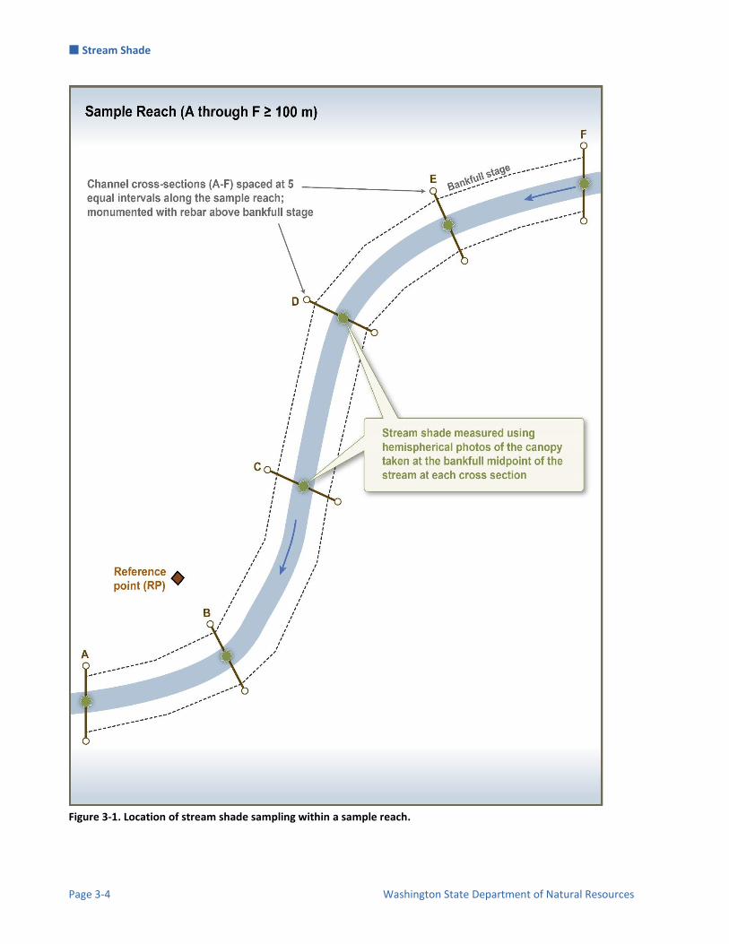
Stream Shade
Page 3-4 Washington State Department of Natural Resources
Figure 3-1. Location of stream shade sampling within a sample reach.

Stream Shade
Status and Trends Monitoring of Riparian and Aquatic Habitat in the OESF Page 3-5
Equipment and Supplies The following equipment and supplies are needed for implementing the stream shade protocol field procedures:
Nikon™ Coolpix 4500 digital camera Nikon™ FC-E8 fisheye converter (7.2 mm f/2.4, approximately 183º FOV) Pelican™ 1400 case, to transport and protect camera equipment in transit to sampling locations SimpleTech™ 512 MB CompactFlash Memory Card Nikon™ EN-EL1 camera battery or equivalent (two per camera. One in use, and another as backup) Nikon™ battery charger or equivalent Hemisfer software, version 2.16 or later Slik™ sprint 150 aluminum tripod w/ SBH-150DQ Ball Head Camera plate and Slik™ DQ-L Quick release adapter set StreamLight™ Stylus LED penlight (to indicate north on the photo) Compass Two 50-m measuring tapes Two chaining pins and four spring clamps Stadia rod Fixed-length plumb-line for setting camera tripod height (5 oz. plumb-line point, 24 gauge stainless
steel cable, and cable ferrules) Ruggedized field tablet or paper field forms Data on the location of the initial set of photos in each watershed. This information is on the field
tablet or it can be printed out. Camera operator’s manual (optional)
o The Nikon Guide to Digital Photography with the Coolpix 4500 Digital Camera o http://www.nikonusa.com/pdf/manuals/coolpix/CP4500man.pdf
Field Procedures In this study, stream shade is measured using hemispherical canopy photos taken with a digital camera with a fish-eye lens.
PRE-FIELD SET-UP Ensure that the camera batteries are fully charged, previous data has been downloaded from the compact flash card, and the 9v battery for the LED indicator is functioning. Ensure time and date are correctly set on camera. Camera settings should match the ones in Table 3-1.
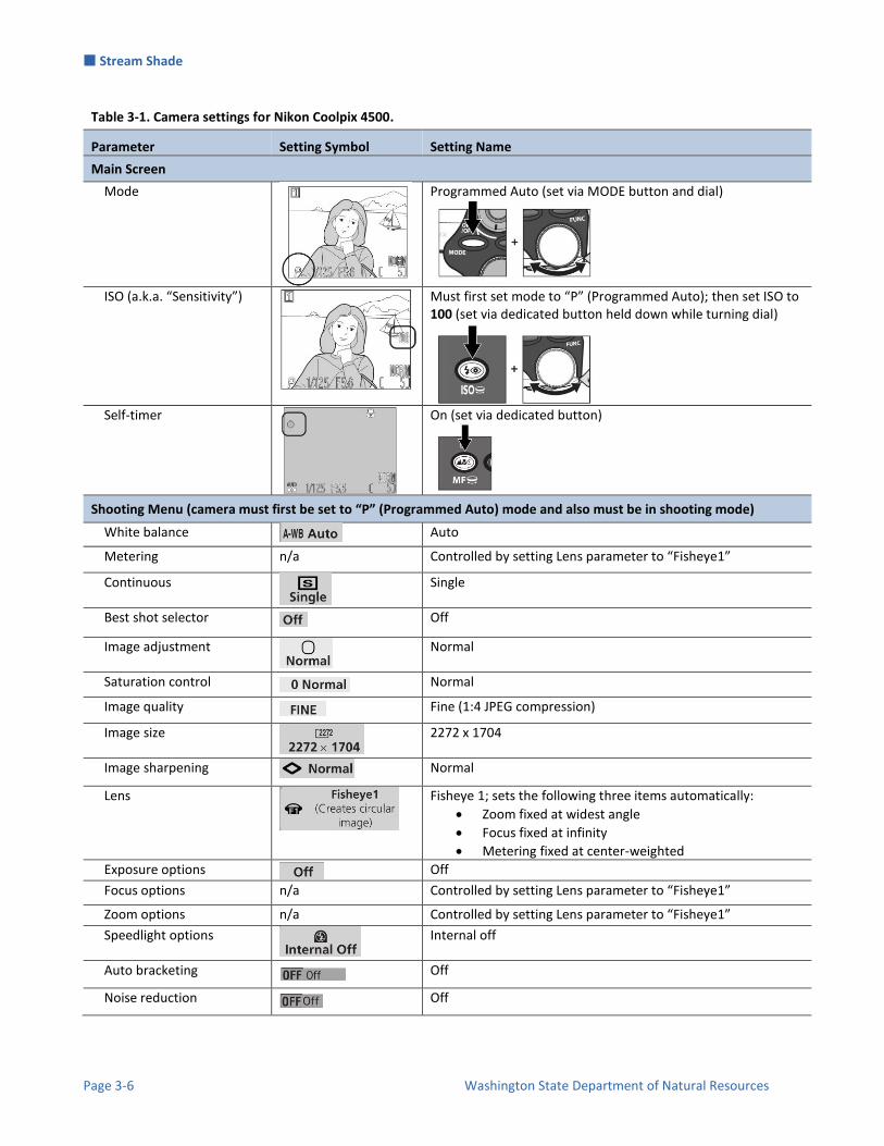
Stream Shade
Page 3-6 Washington State Department of Natural Resources
Table 3-1. Camera settings for Nikon Coolpix 4500.
Parameter Setting Symbol Setting Name
Main Screen
Mode
Programmed Auto (set via MODE button and dial)
ISO (a.k.a. “Sensitivity”)
Must first set mode to “P” (Programmed Auto); then set ISO to 100 (set via dedicated button held down while turning dial)
Self-timer
On (set via dedicated button)
Shooting Menu (camera must first be set to “P” (Programmed Auto) mode and also must be in shooting mode) White balance Auto
Metering n/a Controlled by setting Lens parameter to “Fisheye1”
Continuous
Single
Best shot selector Off
Image adjustment
Normal
Saturation control Normal
Image quality Fine (1:4 JPEG compression)
Image size
2272 x 1704
Image sharpening Normal
Lens
Fisheye 1; sets the following three items automatically:
Zoom fixed at widest angle
Focus fixed at infinity
Metering fixed at center-weighted
Exposure options Off
Focus options n/a Controlled by setting Lens parameter to “Fisheye1”
Zoom options n/a Controlled by setting Lens parameter to “Fisheye1”
Speedlight options
Internal off
Auto bracketing Off
Noise reduction Off

Stream Shade
Status and Trends Monitoring of Riparian and Aquatic Habitat in the OESF Page 3-7
FIELD SAMPLING Hemispherical canopy photos are taken at the midpoint between bankfull stages of the six permanently marked cross sections within each sample reach (Figure 3-1). Although stream shade photography can be done as an independent survey, it is best combined with channel morphology and/or channel substrate sampling because the measuring tapes extended across the channel for these protocols can be used to position the camera at the cross section midpoint. For optimal image quality, overcast flat lighting is preferred. Photos taken in direct sunlight or with a very bright sky can be washed out or include sun flares and glare. This can be partially corrected (see below). Photos are not to be taken in the rain.
Initial Photos
When assessing stream shade trends, it is important that repeated photos are taken at the exact same location (horizontally and vertically). Canopy closure can vary greatly over fine spatial scales; thus, even minor changes in the position of the camera can introduce large differences in shade values. Therefore, when the initial stream shade photo is taken at a cross section, multiple measurements are taken to quantify the camera’s location relative to the stream bed and monuments. This location is then replicated during the repeat photos. Sampling starts at cross section A. First, two 50-meter tapes are extended across the stream channel to measure bankfull width and the distance between the bankfull midpoint and the left monument. Attach the zero end of one tape (upper tape) to the left monument (rebar) with a spring clamp, extend the tape tautly across the channel, and attach the tape to the right monument with another clamp. Make sure that the tape is not obstructed by vegetation; prune if necessary. Identify bankfull stage at the cross section (using the indicators described in Appendix 3A of the Channel Morphology Protocol) and mark its position on both stream banks with chaining pins. Attach the zero end of the second tape (lower tape) to the chaining pin marking bankfull stage on the left side with a spring clamp, extend the tape tautly across the channel, and attach the tape to the chaining pin marking bankfull stage on the right side with another clamp. The lower tape should be aligned with the upper tape, and unobstructed by vegetation, logs, or boulders. Recommended tip: hang a plumb-line from the upper tape or use the stadia rod to correctly line up the chaining pins with the upper tape. Using the stadia rod or plumb-line, identify the distance along the upper tape that corresponds to the midpoint of the bankfull width (BFW/2) on the lower tape and record the bankfull midpoint’s distance from the left and right monuments. Use the compass to measure the azimuth from each cross section monument to the camera and record the measurements in the field tablet. Connect the plumb-line to the base of the camera tripod and set up the tripod with the plumb-line aligned with the bankfull midpoint. If debris, large boulders, or other obstacles prevent positioning the tripod at the

Stream Shade
Page 3-8 Washington State Department of Natural Resources
midpoint, reposition the tripod upstream or downstream, as necessary, while keeping it as close as possible to the bankfull midpoint along the cross section line. Record the offset on the field tablet shade data entry form as a distance and azimuth from the true bankfull midpoint. Mount the camera to the tripod (Figure 3-2). Switch on the LED penlight and insert it into the hole at the edge of the camera plate. Be sure that the front of the camera (not the screen-side) is facing the LED. Adjust the tripod height so the plumb-bob point is just touching the stream bed (not the water surface). At this height, the top of the fisheye lens is 1.4 m (4.5 ft) above the stream bed and the camera plate edge is 1.25 m above the stream bed. Line up the compass housing with a corner of the camera plate, such that the compass bottom is flush with the plate edge opposite the LED. Rotate the camera plate until the orienting arrow shows that the camera is facing true north. With this alignment, the LED will indicate true north in the photograph. Level the camera plate and camera using the two-axis bubble levels. Take down the upper tape and any equipment (e.g., auto level) above the height of the camera that could appear in the photo. Prune any vegetation within 1.0 m of the lens. Before taking the photo, check that the camera is still at the correct height, leveled, and aimed toward true north and make sure the fisheye lens is clean and free of fog/water droplets. To prevent glare, avoid taking the photograph with the lens positioned in direct sunlight. If possible, wait for the sun to be obscured by vegetation or clouds. If necessary, block the sunlight with a stick or the stadia rod, but try to affect the photo as little as possible. If a stick/stadia rod was used to shade the camera lens, note this in the field tablet “Remarks” field. Turn on the camera and enable the self-timer. Press the shutter release to start the timer (10 seconds), then duck below the camera plate to avoid appearing in the photo. Remain below the camera plate until the light on the camera bottom stops blinking, indicating that the photo was taken.
Figure 3-2. Camera positioned for a stream shade photo at the bankfull midpoint of a reach cross section.

Stream Shade
Status and Trends Monitoring of Riparian and Aquatic Habitat in the OESF Page 3-9
Review the photo on the camera screen to make sure that the image is in focus, with no major lens flare, equipment or people in the photo (Figure 3-3). To view the photo and the photo number, press the play button above the screen twice. The number will appear in the right upper corner of the screen (XXXX.JPG). If necessary, re-take the photo without deleting unsuccessful images. Return to the main screen by pressing the play button above the screen. Record the picture number and time of photo in the appropriate field tablet database field. Repeat the above steps at the remaining five cross-sections.
Repeat Photos
Photos that are taken subsequent to the initial set of photos in each basin (i.e., “repeat photos” taken in a subsequent year) should be taken in the same location and at the same height above the stream bed as the initial photos. For the repeat photos, the camera is positioned at the original bankfull midpoint, which can be found using the measurements recorded when the initial photo was taken. Extend a 50-meter tape from the left monument to the right monument and locate the original bankfull midpoint using its previously recorded distance from the left monument. This distance, along with other data from the previous photo visit (e.g. azimuth from each monument to the camera), is accessible on the field tablet database via the “Shade Photos” data entry option. Alternatively, it can be printed prior to going to the field. If a monument is missing or has been moved: first, find its original location and install a new monument (refer to the Monitoring Site Establishment protocol for field procedures); and then, use the original protocol for locating the bankfull midpoint at the cross section. If repeat stream shade sampling occurs in concert with channel morphology measurements, be sure to position the camera at the original bankfull midpoint (located using the upper tape), rather than at the new bankfull midpoint. Connect the plumb-line to the base of the camera tripod and set up the tripod with the plumb-line aligned with the original bankfull midpoint. If in-channel debris, large boulders, or other obstacles prevent positioning the tripod at the midpoint, position the tripod upstream or downstream, as necessary, while
Figure 3-3. Example of a hemispherical canopy photograph.
Stream Shade
Page 3-10 Washington State Department of Natural Resources
keeping it as close as possible to the midpoint at the cross section. Record any offset on the field tablet as the distance and azimuth from the original bankfull midpoint position. Mount the camera to the tripod camera plate (Figure 3-2). Switch on the LED penlight and insert into the hole at the edge of the plate. Be sure that the front of the camera (not the screen-side) is facing the LED. Adjust the tripod height so the plumb-bob point is just touching the stream bed (not the water surface). At this height, the top of fisheye lens is 1.4 m (4.5 ft) above the stream bed. Line up the compass housing with a corner of the camera plate, such that the compass bottom is flush with the plate edge opposite the LED. Rotate the camera plate until the orienting arrow shows that the camera is facing true north. With this alignment, the LED will indicate true north in the photograph. Level the camera plate and camera using the two-axis bubble levels. Take down the upper tape and any equipment (e.g., auto level) above the height of the camera that could appear in the photo. Prune any vegetation (salmonberry, devils club, vine maple, etc.) within 0.5 m of the lens. Before taking the photo, check that the camera is still at the correct height, leveled, and aimed toward true north and make sure the fisheye lens is clean and free of fog/water droplets. To prevent glare, avoid taking the photograph if the lens is positioned in direct sunlight. If possible, wait for the sun to be obscured by vegetation or clouds. If necessary, block the sunlight with a stick or the stadia rod, but try to affect the photo as little as possible. If a stick or the stadia rod was used to shade the camera lens, note this in the “Remarks” field. Turn on the camera and enable the self-timer. Press the shutter release to start the timer (10 seconds) then duck below the camera plate to avoid appearing in the photo. Remain below the camera plate until the light on the camera bottom stops blinking, indicating the photo has been taken. Review the photo on the camera screen to make sure the image – is in focus, with no major lens flare, equipment or people in the photo. (Figure 3-3). To view the photo and the picture number, press the play button above the screen twice and the picture number will appear in the right upper corner of the screen (XXXX.JPG). If necessary, re-take the photo without deleting unsuccessful images. Return to the main screen by pressing the play button above the screen. Record the picture number and time of photo in the field form. Repeat the above steps at the remaining five cross-sections.

Stream Shade
Status and Trends Monitoring of Riparian and Aquatic Habitat in the OESF Page 3-11
Time and Cost Estimates for Implementing the Field Procedures The estimated time for sampling stream shade in a sample reach is about two hours for an experienced two-member field crew (about 20 minutes per photo). This time estimate doesn’t include the travel to the site. Table 3-2 shows the cost estimates for the equipment unique to implementing the field procedures of the Stream Shade protocol. Many of the items listed in the Equipment and Supplies section above, such as the field tablet and stadia rod, are shared with other protocols. Their costs are detailed in the Channel Morphology protocol and not included here.
Table 3-2. Cost Estimates for the Equipment Used in the Stream Shade Field Protocol
Equipment/Supplies Quantity Individual cost
Nikon Coolpix 4500 (refurbished) 1 $150
Nikon FC E8 Fisheye lens 1 $100
Slik sprint 150 aluminum tripod w/ SBH-150DQ Ball Head
1 $60
Slik DQ-L Quick release adapter set 1 $50
Pelican 1150 Case 1 $30
SimpleTech 512MB CompactFlash
Memory Card
1 $90
Procedures for Calculating Metrics
IMAGE PROCESSING After photos have been renamed and moved to the archival folder, image processing is performed using Hemisfer software (Schleppi 2016). Hemisfer is capable of batch processing, although all settings must be carefully adjusted prior to running the batch. Settings chosen (April 2016) are shown in Table 3-3. If the decision is made in the future to process photos using any other software, then all photos must be re-analyzed using that software to ensure consistency in analysis.
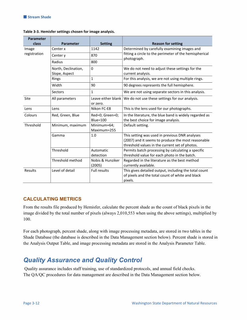
Stream Shade
Page 3-12 Washington State Department of Natural Resources
Table 3-3. Hemisfer settings chosen for image analysis.
Parameter class Parameter Setting Reason for setting
Image registration
Center x 1142 Determined by carefully examining images and fitting a circle to the perimeter of the hemispherical photograph.
Center y 870
Radius 800
North, Declination, Slope, Aspect
0 We do not need to adjust these settings for the current analysis.
Rings 1 For this analysis, we are not using multiple rings.
Width 90 90 degrees represents the full hemisphere.
Sectors 1 We are not using separate sectors in this analysis.
Site All parameters Leave either blank or zero.
We do not use these settings for our analysis.
Lens Lens Nikon FC-E8 This is the lens used for our photographs.
Colours Red, Green, Blue Red=0; Green=0; Blue=100
In the literature, the blue band is widely regarded as the best choice for image analysis.
Threshold Minimum, maximum Minimum=64; Maximum=255
Default setting.
Gamma 1.0 This setting was used in previous DNR analyses (2007) and it seems to produce the most reasonable threshold values in the current set of photos.
Threshold Automatic detection
Permits batch processing by calculating a specific threshold value for each photo in the batch.
Threshold method Nobis & Hunziker (2005)
Regarded in the literature as the best method currently available.
Results Level of detail Full results This gives detailed output, including the total count of pixels and the total count of white and black pixels.
CALCULATING METRICS From the results file produced by Hemisfer, calculate the percent shade as the count of black pixels in the image divided by the total number of pixels (always 2,010,553 when using the above settings), multiplied by 100. For each photograph, percent shade, along with image processing metadata, are stored in two tables in the Shade Database (the database is described in the Data Management section below). Percent shade is stored in the Analysis Output Table, and image processing metadata are stored in the Analysis Parameter Table.
Quality Assurance and Quality Control Quality assurance includes staff training, use of standardized protocols, and annual field checks. The QA/QC procedures for data management are described in the Data Management section below.

Stream Shade
Status and Trends Monitoring of Riparian and Aquatic Habitat in the OESF Page 3-13
TRAINING All personnel conducting field protocols will be trained in a consistent manner to ensure that the surveys are conducted properly and in standardized fashion. The training is conducted or, for returning personnel, reviewed, annually before the start of the field season. At least one member of the field crew should be experienced with the field procedures.
STANDARD PROTOCOLS The standard procedures described in this protocol are followed for the duration of the project. Any deviations from the procedures should be documented, and the reasons for deviation described and discussed with the project manager or the researcher overseeing the protocol implementation. Changes to the published protocols are approved by the project manager or by the researcher overseeing the protocol implementation. Revised protocols are assigned new version numbers and publication dates.
FIELD QUALITY CONTROL The researcher overseeing the protocol implementation or a different field crew will conduct spot checks on 10% of the field measurements every year.
Data Management
DATA FLOW The shade data collected in the field consist of digital photographs. Shade metadata are recorded in the field using paper field forms (2013-2014 field seasons) or a field tablet (2015 field season onward). In the office, digital photographs are stored on the network drive and metadata are transferred to a database for long-term storage. The steps below detail these processes.
Photographs
1. Transfer photos to data manager for storage All shade photos taken in the field are transferred to the OESF Data Management Specialist at the end of each field week. The Specialist temporarily stores the uncatalogued shade photos on the WADNR server at: J:\hcp\monitoring_research\tminkova\01_OESF_R&M Program\01_Rip S&T Mon\07_Data management\_All new data and photos\
2. Rename photos The OESF Data Management Specialist renames each photo using the following naming convention: SH_<WatershedID><cross section>_<Date taken>_<Original photo name> (for example: SH_797A_20140715_P1000851.JPG).
3. Archive photos The renamed photos are moved to long-term storage in the following directory: J:\hcp\monitoring_research\tminkova\01_OESF_R&M Program\01_Rip S&T Mon\03_Photos and videos\05_Shade\Photo archive\

Stream Shade
Page 3-14 Washington State Department of Natural Resources
Metadata recorded on paper field forms
1. Fill out field forms The Stream Morphology, Substrate, and Shade field forms are used to record the shade photo metadata at each sample reach.
2. Scan and store field forms After returning from the field each week, the field forms are scanned and stored on the WADNR network drive; the original paper forms are archived by the OESF Data Management Specialist at the WADNR Forest Resources Division.
3. Enter data All shade metadata collected on paper field forms is entered in the Shade Database by the OESF Data Management Specialist on a weekly basis. After each field form is entered, the person who entered it writes on it the word “Entered” followed by their initials and the date.
4. Quality control Entered field form data are verified by comparing the data on the field form to the data in the database. This process is performed by someone other than the person who originally entered the data. After the data are verified, the person who verified it writes on the field form the word “Verified” followed by their initials and the date.
Metadata collected electronically
1. Fill out forms on electronic field data recorder Field personnel record all shade metadata using the “Tablet Database”, which is a customized database created in Microsoft Access and saved on the field tablet.
2. Store field metadata At the end of each day in the field, a copy of the Tablet Database, containing all metadata and data collected to date, is transferred to the OESF Data Management Specialist via cloud storage or email. If internet access is not available, the field crew makes a daily backup copy of the database on a laptop or other storage device and then transfers the data to the Specialist at the end of the work week. The Specialist stores these Tablet Database copies in a temporary location on the WADNR network drive (J:\hcp\monitoring_research\tminkova\01_OESF_R&M Program\01_Rip S&T Mon\07_Data management\_All new data and photos\) until they are processed and the data are transferred to a database for long-term storage.
3. Quality control Because the metadata are recorded electronically, and thus never transcribed, transcription errors do not exist. However, there is still a possibility of data entry errors in the field. For this reason, metadata are examined for accuracy before they are imported to the Shade Database.
4. Import data to database On a weekly basis, the OESF Data Management Specialist imports all new metadata from the Tablet Database to the Shade Database. This is accomplished using a set of queries stored in a third database: J:\hcp\monitoring_research\tminkova\01_OESF_R&M Program\01_Rip S&T Mon\01_FIELD DATA\01_Stream survey\Data\ Distribute_Tablet_Data.accdb
5. Verify transfer of data After data have been imported, the OESF Data Management Specialist verifies that no records have been missed, using the record count queries built into the Distribute_Tablet_Data database.
Stream Shade
Status and Trends Monitoring of Riparian and Aquatic Habitat in the OESF Page 3-15
DATA STORAGE
Paper Field Forms
The paper field forms are archived at the Washington Department of Natural Resources (WADNR) Forest Resources Division. The designated data steward is Teodora Minkova, WADNR. Scanned copies of these forms are saved in the Adobe portable document format (.pdf) in the following directory: J:\hcp\monitoring_research\tminkova\01_OESF_R&M Program\01_Rip S&T Mon\01_FIELD DATA\01_Stream survey\Data\Data archive\Field forms\
Tablet Databases
The original Tablet Databases, which are transferred to the OESF Data Management Specialist on a daily or weekly basis, are stored on the WADNR network drive after the metadata they contain have been transferred to the Shade Database. The storage location for these databases is: J:\hcp\monitoring_research\tminkova\01_OESF_R&M Program\01_Rip S&T Mon\01_FIELD DATA\01_Stream survey\Data\Data archive\Processed tablet databases\
Long-term Data Storage
Shade photos are archived at: J:\hcp\monitoring_research\tminkova\01_OESF_R&M Program\01_Rip S&T Mon\03_Photos and videos\05_Shade\Photo archive\ Shade photo metadata, as well as all metadata and data produced during image analysis, are stored in the Shade Database, located on the WADNR network drive at: J:\hcp\monitoring_research\tminkova\01_OESF_R&M Program\01_Rip S&T Mon\01_FIELD DATA\01_Stream survey\Data\Shade_Database.accdb Within the Shade Database, data and metadata are stored in four related tables: the Form Header Table, the Field Data Table, the Analysis Output Table, and the Analysis Parameter Table (Figure 3-4). The Form Header Table is related to the Field Data Table through a one-to-many relationship: one record in the Form Header Table (i.e., a watershed visit) is related to multiple records in the Field Data Table (i.e., multiple photographs). Each record in the Field Data Table (i.e., each photograph) is related to a record in the Analysis Output Table (i.e., analysis results from that photograph). This relationship is facilitated by a query that constructs each photo name from metadata in the Field Data Table and then links that name to the actual photo name in the Analysis Output Table. This one-to-one relationship is possible because every photo has a unique name. Records in the Analysis Output Table are related to records in the Analysis Parameter Table, which contain all of the metadata associated with image analysis. The fields in the four tables of the Shade Database are listed below (Tables 3-4 through 3-7).

Stream Shade
Page 3-16 Washington State Department of Natural Resources
Figure 3-4. Structure of the Shade Database.
Table 3-4. Form Header Table from the Shade Database.
Field Field description
HeaderID(Auto) Unique ID for each record in this table.
BasinID Watershed identifier.
Photo_Date Date of the photo.
Field_Crew_tablet Initials of the field crew.
QC_Photos Indicates that the photos were taken for the purpose of quality control.

Stream Shade
Status and Trends Monitoring of Riparian and Aquatic Habitat in the OESF Page 3-17
Table 3-5. Field Data Table from the Shade Database.
Field Field description
DataTabID(Auto) Unique identifier for each record in the table.
HeaderID Links record to the appropriate record in the Form Header Table.
Cross_Section The cross section at which the photo was taken.
LM_Distance Camera distance from left monument (m).
LM_Azimuth Azimuth from the left monument to the camera (degrees).
RM_Distance Camera distance from right monument (m).
RM_Azimuth Azimuth from the right monument to the camera (degrees).
Offset_Distance Distance from middle (m).
Offset_Azimuth Azimuth from middle (degrees).
Plate_Ht_Autolevel Height of tripod plate, measured using auto level (cm).
Plate_Ht_String Height of tripod plate, measured using string method (cm).
Photo_Number The photo number assigned by the camera.
Time_of_Photo The time the photo was taken (PDT).
Remarks Remarks recorded in the field.
Plate_Backsight_Elev Elevation of plate (cm), measured to a monument of known elevation. (This variable was recorded for only 33 photos.)
Plate_Backsight_Loc The monument that the plate backsight elevation referenced. (This variable was recorded for only 32 photos.)
Plate_HI Plate height of instrument (cm). (This variable was recorded for only 13 photos.)
Sky_conditions_post_hoc The sky conditions (clear, partly cloudy, or overcast), as determined by examining the photo in the office.
Table 3-6. Analysis Output Table from the Shade Database.
Field Field description
AnalysisOutputID(Auto) A unique identifier for each record in the table.
PhotoName The name of the photo, taken from the file itself.
AnalysisParameterID ID linking each record to the software and settings that were used during image analysis.
Black_pixels_percent Percent of all pixels that are black; this value represents percent shade.

Stream Shade
Page 3-18 Washington State Department of Natural Resources
Table 3-7. Analysis Parameter Table from the Shade Database.
Field Field description
AnalysisParameterID(Auto) A unique identifier for each record in the table.
Analysis_software The software package or packages used in the image analysis, including version number.
Threshold_method The method used to calculate the threshold value.
Gamma_value The gamma value used during the threshold calculation.
Photo_center_x The x coordinate (measured in pixels), within the full rectangular photo, of the center of the round hemispherical image.
Photo_center_y The y coordinate (measured in pixels), within the full rectangular photo, of the center of the round hemispherical image.
Photo_radius The radius of the round hemispherical image (measured in pixels).
Lens_setting The lens type.
Color_balance The color balance (red, green, blue, each ranging from -100 to 100) used in the analysis (e.g., 0R 0G 100B).
Ring_count The number of rings used in the analysis.
Ring_width The width of the rings, measured in degrees.
DATA QUALITY CONTROL
Quality control for metadata
Prior to data analysis, all fields in the data tables are assessed to identify potentially erroneous values. The first step is to examine individual fields, one at a time. For categorical data fields (e.g., cross section) and date or time fields, every field is assessed to identify any records exhibiting the following:
1. Missing values. 2. Illogical values. In some cases, where the data collector is free to enter values rather than selecting
values from a predefined list, illogical values may be recorded (e.g., a survey time of 3:00 AM).
For numerical fields, each is assessed for the following: 1. Missing values. 2. Outlier values (e.g., an LM_Distance was recorded in cm instead of m).
When missing values are discovered, it is generally not possible to “fill in the blank” from the office. The fact that data are missing should be recorded, in brackets, in the “Remarks” field, with the initials of the person who performed the quality control check (e.g., [LM_Distance was not recorded. –WD]). Illogical or outlier values can sometimes be corrected in the office. For example, AM and PM might have been switched or a decimal place error can be corrected. When data are corrected, this must be noted in the

Stream Shade
Status and Trends Monitoring of Riparian and Aquatic Habitat in the OESF Page 3-19
remarks field, in brackets, with the initials of the person who performed the quality control check. For example: [LM_Distance was recorded as 550 m. This was clearly incorrect and changed to 5.5 m which is logical given RM_Distance. –WD]. In many cases, clearly erroneous outlier values cannot be corrected in the office and should be edited so as not to affect the results of analysis. In such cases, the value should be removed from the field and transferred to the Remarks field with an explanation, in brackets, with the initials of the person who performed the quality control check. For example: [Black_pixels_percent was recorded as 145.3; this value was clearly incorrect and removed from the dataset. –WD]).
Quality control for photographs
All photographs are reviewed to ensure there are no abnormalities that will affect the results of image analysis. Potential photo quality issues include:
1. Issues with camera settings such as focus or exposure. Blurry photos cannot be analyzed because the boundary between dark and light areas is unclear. Overexposed photos cannot be analyzed because shaded portions appear as light.
2. Obstructed photos. In some cases, understory plants, such as shrubs, obstruct significant portions of the image because they are close to the camera. If analyzed, these photos would produce a misleading result.
If a photo is unusable, then it is placed in a separate folder so that it will never be mistakenly analyzed: J:\hcp\monitoring_research\tminkova\01_OESF_R&M Program\01_Rip S&T Mon\03_Photos and videos\05_Shade\Unusable photos\ A minimum of four photos from each sample reach and date are required for analysis. If more than two of the six photos from a given sample reach and date are unusable, then the photos from that reach and date are not analyzed.

Stream Shade
Page 3-20 Washington State Department of Natural Resources
References Bouwes, N., J. Moberg, N. Weber, B. Bouwes, S. Bennett, C. Beasley, C.E. Jordan, P. Nelle, M. Polino, S.
Rentmeester, B. Semmens, C. Volk, M.B. Ward, and J. White. 2011. Scientific protocol for salmonid habitat surveys within the Columbia Habitat Monitoring Program. Prepared by the Integrated Status and Effectiveness Monitoring Program and published by Terraqua, Inc., Wauconda, WA. 118 p.
Brown, G.W. 1969. Predicting temperatures of small streams. Water Resources Research 5(1): 68-75.
Gregory, S.V., F.J. Swanson, W.A. McKee, and K.W. Cummins. 1991. An ecosystem perspective of riparian zones. BioScience 41:540-551.
Frazer, G.W., C.D. Canham, and K.P. Lertzman.1999. Gap light analyzer (GLA): imaging software to extract canopy structure and gap light transmission indices from true colour fisheye photographs. User’s Manual and Program Documentation, Version 2.0, Simon Fraser University, Burnaby, British Columbia, and the Institute of Ecosystem Studies, Millbrook, New York, p. 36.
Frazer, G. W., R.A. Fournier, J.A. Trofymow, and R.J. Hall. 2001. A comparison of digital and film fisheye photography for analysis of forest canopy structure and gap light transmission. Agricultural and Forest Meterology. 109: 249-263.
Lee, Y.J., R.I. Alfaro, and G.A.Van Sickle. 1983. Tree-crown defoliation measurement from digitized photographs. Canadian Journal of Forest Research 13: 956–961.
Naiman, R.J. and H. Decamps. 1997. The ecology of interfaces: riparian zones. Annual Review of Ecology and Systematics 28:621-658.
Nobis, M. and U. Hunziker. 2005. Automatic thresholding for hemispherical canopy-photographs based on edge detection. Agricultural and Forest Meteorology 128 (2005): 243-250.
Schleppi, P. 2016. Hemispher Version 2.16. WLS Swiss Federal Institute for Forest, Snow, and Landscape Research, Birmensdorf, Switzerland. (http://www.wsl.ch/dienstleistungen/produkte/software/hemisfer/index_EN)
Washington State Department of Natural Resources. 2016. Olympic Experimental State Forest HCP Planning Unit Forest Land Plan Final Environmental Impact Statement. Washington State Department of Natural Resources, Olympia, WA. http://file.dnr.wa.gov/publications/amp_sepa_nonpro_oesf_feis.pdf

Stream Shade
Status and Trends Monitoring of Riparian and Aquatic Habitat in the OESF Page 3A-1
Appendix 3A. Image Processing Software Options Prior to processing any of the images in this study, several potential options for image processing software were considered. The choice of image processing software was independent of the process of locating and taking the photographs. Although Hemisfer was been selected for image analysis (as of April 2016), the information in this Appendix may be of future use as a reference. Option 1: SideLook and Gap Light Analyzer This option requires two software packages to perform two separate steps of the analysis. First, SideLook 1.1.01 (http://www.appleco.ch) is used to establish an image threshold to distinguish sky from non-sky. Second, Gap Light Analyzer 2.0 (http://www.caryinstitute.org/science-program/our-scientists/dr-charles-d-canham/gap-light-analyzer-gla) is used to measure canopy openness. Option 1 is not currently feasible because the software packages are not maintained or updated and they will not run on the operating systems that WADNR uses. More on SideLook: SideLook is imaging software for the analysis of vegetation structure with true-color photographs. Sidelook is available for a nominal cost, and WADNR has a license. Sidelook implements an automatic threshold algorithm for edge detection (Nobis and Hunziker 2005) to distinguish sky from non-sky, and allows for processing of individual color channels (red, green, or blue). Processing of only the blue channel is recommended by several authors (Lee and others 1983; Frazer and others 1999, 2001). SideLook does not permit batch analysis and must run images individually. Note: Sidelook has not been updated since 2005 and is not likely to run on WADNR computers again, unless the authors of the software update it. More on Gap Light Analyzer (GLA): GLA is Imaging software used to extract forest canopy structure and gap light transmission indices from true-color hemispherical photographs. GLA is free and offers a variety of customizations. GLA allows the user to specify topographic masks to compensate for topographic vs. vegetative shading, compensates for lens distortion using standard or customized equations, enables processing of images by color channel (red, green, or blue), and generates 22 canopy structure and light transmission metrics in 3 general categories: openness, effective LAI (leaf area index), and irradiance. Note: GLA has not been updated since 1999 and will not run on the current operating systems that WADNR uses. Option 2: Hemisfer 2.16 Hemisfer 2.16 (http://www.wsl.ch/dienstleistungen/produkte/software/hemisfer/index_EN) is a canopy image analysis program designed by the Swiss Federal Institute for Forest, Snow and Landscape Research. The software is available for a nominal cost, and WADNR has a license. Hemisfer offers many of the same capabilities as GLA, such as automated image thesholding using the same algorithm as SideLook. Hemisfer offers the advantage of batch processing. Batch processing, however, assumes all images are oriented and registered in an identical manner. Hemisfer is maintained and updated; the author of the software, Patrick Schleppi, is responsive to comments and questions. Option 3: HemiView HemiView (http://dynamax.com/products/leaf-canopy-and-image-analysis/hemiview-hemispheric-image-analysis-system) is a commercially available canopy image analysis program developed by Delta T-Devices and sold

Stream Shade
Page 3A-2 Washington State Department of Natural Resources
by Dynamax. The software is sold as part of an integrated package that includes the camera, lens, tripod, mount, and software. The items are stocked as a kit and are not sold separately.

Channel Substrate
Status and Trends Monitoring of Riparian and Aquatic Habitat in the OESF Page 4-1
Channel Substrate Authors: Scott Horton, Mitchell Vorwerk, Teodora Minkova
Version: 1.4
Revision History:
Based on the Following Protocols: The general monitoring design follows the Field Protocol Manual for Aquatic and Riparian Effectiveness Monitoring Program (AREMP) for the Northwest Forest Plan (Lanigan et al. 2010). Details on some field procedures and adaptations are taken from Peck et al. (2006), which describes the U.S. Environmental Protection Agency’s wadeable stream monitoring program (EMAP), and from Archer et al. (2012), with the multi-federal agency PACFISH/INFISH Biological Opinion Monitoring Program (PIBO).
Reasons to Adopt the Above Protocols: The EMAP protocol (Peck et al. 2006) employs the methods of Wolman (1954), as adapted by Kaufman and Robison (1998). These methods have been widely used because they are easy to learn and apply to obtain objective, repeatable measures (Peck et al. 2006) and provide unbiased estimates of surface substrate composition (Kaufman et al. 1999). The EMAP and PIBO protocols use sampling methods that are applicable to this study’s site and cross-sectional transect layout and have the best-performing measures of substrate characteristics (Roper et al. 2010).
Purpose and Content: The purpose of this monitoring protocol is to describe the sampling and data management necessary to document and report the status and multi-year trends of channel substrate in the monitored watersheds. It details the field procedures for sampling substrate composition and embeddedness, the field quality assurance and quality control steps, and the data management procedures.
Protocol
Version Purpose / Changes Author(s) Reviewer(s) Date
1.0 Initial draft presented to project staff Scott Horton Teodora Minkova 03/28/2013
1.1 Draft submitted to external review Scott Horton Rebecca Flitcroft 04/16/2013
1.2 Final draft incorporating external
reviews, sampling procedures from
2013 field season, and data mgmt.
procedures
Scott Horton,
Teodora Minkova
Mitchell Vorwerk 05/20/2014
1.3 Final draft with field and data
management procedures updated
from 2014 and 2015 field seasons
Scott Horton,
Mitchell Vorwerk,
Teodora Minkova
Ellis Cropper
Alex Foster
06/10/2016
1.4 Final technical review and edit Scott Horton,
Mitchell Vorwerk,
Teodora Minkova
Paul Dunnette,
Warren Devine, Alex
Foster
12/18/2016

Channel Substrate
Page 4-2 Washington State Department of Natural Resources
Table of Contents Table of Contents ............................................................................................................................................ 4-2
Introduction ..................................................................................................................................................... 4-3
Monitoring Design .......................................................................................................................................... 4-3
Equipment and Supplies .................................................................................................................................. 4-3
Field Procedures .............................................................................................................................................. 4-5
Procedures for Calculating Metrics ................................................................................................................. 4-8
Time and Cost Estimates for Implementing Field Procedures ........................................................................ 4-9
Quality Assurance and Quality Control .......................................................................................................... 4-9
Training ....................................................................................................................................................... 4-9
Standard Protocols .................................................................................................................................... 4-10
Field Checks .............................................................................................................................................. 4-10
Data Management ......................................................................................................................................... 4-10
Data Flow .................................................................................................................................................. 4-10
Data Storage .............................................................................................................................................. 4-11
Data Quality Control ................................................................................................................................. 4-13
References ..................................................................................................................................................... 4-15

Channel Substrate
Status and Trends Monitoring of Riparian and Aquatic Habitat in the OESF Page 4-3
Introduction Channel substrate refers to the mineral and organic materials that form the bottom or bed of a stream. Substrate composition determines the roughness of stream channels, which influences channel hydraulics (water depth, width, velocity) and consequently stream habitat. Substrate provides micro-conditions needed by many aquatic species (Bain 1999). For example, specific substrates are needed for spawning because eggs adhere to some surfaces; interstitial water flow through substrate maintains high oxygen levels around buried eggs. Certain-size substrate provides living space and cover for macroinvertebrates, amphibians, and fish (Hicks et al. 1991, Mellina and Hinch 2009, Roni et al. 2006). Substrate composition, stability, and embeddedness (i.e., the degree to which gravel and larger materials are surrounded or covered by fine sediments) can be used as indicators of forest management impacts on sediment and hydrologic regimes. In the environmental impact analysis for the Olympic Experimental State Forest (OESF) Forest Land Plan, fine sediment delivery (small soil particles such as sand, silt, and clay) was recognized as an important indicator of management effects on fish habitat and riparian areas (WADNR 2013). Because empirical sediment delivery data were not available at the time of the analysis, they were modeled using road inventory data and traffic impact scores based on road surface type, road proximity to streams, and projected traffic levels.
Monitoring Design
SPATIAL SAMPLING DESIGN Channel substrate sampling is conducted in each of the 50 sample watersheds in Olympic Experimental State Forest (OESF) and the four reference watersheds in Olympic National Park (ONP). Refer to the Introduction chapter for a map of the sample watersheds. Channel substrate particle size and embeddedness are sampled at each of the six permanent cross sections established under the Monitoring Site Establishment Protocol (Figure 4-1). Substrate particles are sampled at 21 stations spaced at equal intervals at each cross section (minimum of 126 particles per sample reach).
TEMPORAL SAMPLING DESIGN Channel substrate is sampled during low flow conditions in the late spring or summer. Accuracy of substrate sampling is compromised if it is performed during high flows.
Equipment and Supplies Gravelometer Stadia rod Two 50-meter tapes Two chaining pins and four spring clamps Ruggedized field tablet or paper field forms

Channel Substrate
Page 4-4 Washington State Department of Natural Resources
Figure 4-1. Locations of channel substrate sampling within a sample reach.
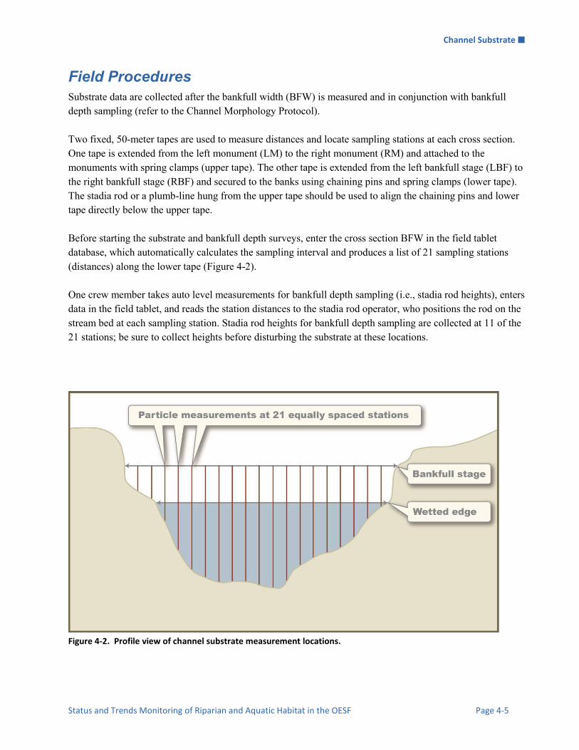
Channel Substrate
Status and Trends Monitoring of Riparian and Aquatic Habitat in the OESF Page 4-5
Field Procedures Substrate data are collected after the bankfull width (BFW) is measured and in conjunction with bankfull depth sampling (refer to the Channel Morphology Protocol). Two fixed, 50-meter tapes are used to measure distances and locate sampling stations at each cross section. One tape is extended from the left monument (LM) to the right monument (RM) and attached to the monuments with spring clamps (upper tape). The other tape is extended from the left bankfull stage (LBF) to the right bankfull stage (RBF) and secured to the banks using chaining pins and spring clamps (lower tape). The stadia rod or a plumb-line hung from the upper tape should be used to align the chaining pins and lower tape directly below the upper tape. Before starting the substrate and bankfull depth surveys, enter the cross section BFW in the field tablet database, which automatically calculates the sampling interval and produces a list of 21 sampling stations (distances) along the lower tape (Figure 4-2). One crew member takes auto level measurements for bankfull depth sampling (i.e., stadia rod heights), enters data in the field tablet, and reads the station distances to the stadia rod operator, who positions the rod on the stream bed at each sampling station. Stadia rod heights for bankfull depth sampling are collected at 11 of the 21 stations; be sure to collect heights before disturbing the substrate at these locations.
Figure 4-2. Profile view of channel substrate measurement locations.
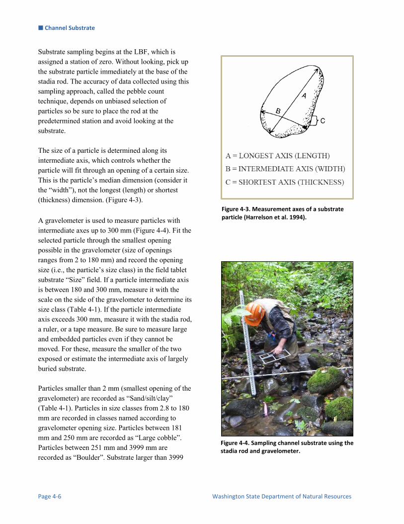
Channel Substrate
Page 4-6 Washington State Department of Natural Resources
Substrate sampling begins at the LBF, which is assigned a station of zero. Without looking, pick up the substrate particle immediately at the base of the stadia rod. The accuracy of data collected using this sampling approach, called the pebble count technique, depends on unbiased selection of particles so be sure to place the rod at the predetermined station and avoid looking at the substrate. The size of a particle is determined along its intermediate axis, which controls whether the particle will fit through an opening of a certain size. This is the particle’s median dimension (consider it the “width”), not the longest (length) or shortest (thickness) dimension. (Figure 4-3). A gravelometer is used to measure particles with intermediate axes up to 300 mm (Figure 4-4). Fit the selected particle through the smallest opening possible in the gravelometer (size of openings ranges from 2 to 180 mm) and record the opening size (i.e., the particle’s size class) in the field tablet substrate “Size” field. If a particle intermediate axis is between 180 and 300 mm, measure it with the scale on the side of the gravelometer to determine its size class (Table 4-1). If the particle intermediate axis exceeds 300 mm, measure it with the stadia rod, a ruler, or a tape measure. Be sure to measure large and embedded particles even if they cannot be moved. For these, measure the smaller of the two exposed or estimate the intermediate axis of largely buried substrate. Particles smaller than 2 mm (smallest opening of the gravelometer) are recorded as “Sand/silt/clay” (Table 4-1). Particles in size classes from 2.8 to 180 mm are recorded in classes named according to gravelometer opening size. Particles between 181 mm and 250 mm are recorded as “Large cobble”. Particles between 251 mm and 3999 mm are recorded as “Boulder”. Substrate larger than 3999
Figure 4-4. Sampling channel substrate using the stadia rod and gravelometer.
Figure 4-3. Measurement axes of a substrate particle (Harrelson et al. 1994).

Channel Substrate
Status and Trends Monitoring of Riparian and Aquatic Habitat in the OESF Page 4-7
mm is classified and recorded as “Bedrock”. Exposed bedrock also is recorded as “Bedrock” and no measurements are taken. Woody debris, such as logs, bark and twigs, are recorded as “wood” only if it is not possible to get a substrate particle under the wood (Lanigan et al. 2010). Moss, live plants, or thick layers of organic debris are recorded as “organic” only if a substrate particle cannot be dug out from under the organic matter. Do not measure wood or organic particles. Table 4-1. Values measured and recorded for various particle size classes.
Measurement method
Observed value (mm) based on gravelometer opening or manual measurement
Particle size class (mm) or descriptor recorded
Gravelometer opening ≤ 2 “Sand/silt/clay”
2.8 2.8
4 4
5.6 5.6
8 8
11 11
16 16
22.6 22.6
32 32
45 45
64 64
90 90
128 128
180 180
Side of gravelometer (measured manually)
181 to 250 “Large cobble”
Side of gravelometer, stadia rod, ruler, or tape measure (measured manually)
251 to 3999 “Boulder”
4000 and larger “Bedrock”
None Woody debris such as logs, bark, and twigs (if not possible to get a substrate particle from beneath)
“Wood”
Moss, live plants, thick layers of organic debris (if not possible to get a substrate particle from beneath)
“Organic”

Channel Substrate
Page 4-8 Washington State Department of Natural Resources
Embeddedness is estimated for particles measuring 45 mm or more. Embeddedness is the fraction of particle surface area surrounded or covered by fine sediment (≤ 2 mm). Embeddedness is estimated in increments of 10%. The following factors are considered:
The proportion of a particle’s surface area, including the underside, which is obviously covered with sand, silt, or clay.
The difficulty associated with removing a particle from the streambed and the size of the particles around it. Particles >2 mm do not contribute to embeddedness.
Staining or “biofouling” is usually caused by the accumulation of periphyton on the exposed wetted surface. The biofouled area thus has a different coloration. The surface area without biofouling is generally not exposed to flowing water and is the portion used to estimate embeddedness. However, use this last factor with caution as particles >2 mm that touch the selected particle can also prevent biofouling.
For particles classified as “sand/silt/clay”, embeddedness is recorded as 100%. For bedrock, embeddedness is recorded as 0%. No embeddedness is recorded for wood or organic material. Record the percentage embeddedness of each particle in the field tablet database “Embed.” field.
Procedures for Calculating Metrics Substrate data collected at each sample reach are condensed to site-level summaries that describe particular aspects of physical habitat (Kaufman et al. 1999). An initial list of metrics for substrate composition and embeddedness indicators is presented in Table 4-2. Data are often summarized by condensing the particle size classes from Table 4-1 into substrate type classes, as shown in Table 4-3. Numerous other metrics can be calculated from the substrate data (see Kaufman et al. [1999] for discussion of the conceptual basis and operational details for calculating summary metrics). Table 4-2. Indicators, metrics, and measurements for channel substrate analysis (modified from Kaufman et al. 1999).
Indicator Metric (reach-level averages) Measurement
Substrate composition
D50 (median particle size) Derived by ordering the particle size classes (Table 4-1), calculating the cumulative percentage of particles in each class, and identifying the class containing the median value. Wood, organics, and bedrock are not included in the D50 calculation.
Substrate percentage by size class
Percentage of particles in each substrate type class (Table 4-3).
Percent fines Percentage of particles in the ≤ 2 mm size class.
Percent boulders Percentage of particles in the 251–3999 mm size class.
Embeddedness Substrate mean percent embeddedness
Mean embeddedness of particles in each substrate type class (Table 4-3) assessed for embeddedness (boulder, cobble, and coarse gravel > 45 mm).

Channel Substrate
Status and Trends Monitoring of Riparian and Aquatic Habitat in the OESF Page 4-9
Table 4-3. Classification of substrate types by size
Substrate type Particle size (mm)
Fines (sand, silt, clay) ≤ 2
Fine gravel >2 – 16
Coarse gravel >16 – 64
Cobbles >64 - 250
Boulders > 250 - 3999
Bedrock ≥4000
Time and Cost Estimates for Implementing Field Procedures The estimated time needed to sample channel substrate is 15 minutes per cross section or 90 minutes per sample reach for an experienced two-member crew. If the measuring tapes have to be set at each cross section, the additional field time is 60 min per sample reach. These two estimates do not include time spent traveling to the site, setting up the tapes at a cross section, or measuring channel morphology attributes. Table 4-4 shows the cost estimates for specialty equipment unique to implementing the field procedures of the channel substrate protocol. Many of the items listed in the Equipment and Supplies section above are shared with other protocols, such as the field tablet, measuring tapes, and stadia rod. Their costs are detailed in the Channel Morphology protocol and not included here. Table 4-4. Cost estimates for the equipment used in the channel substrate protocol
Equipment/Supplies Amount Individual cost
Gravelometer 1 $75
Quality Assurance and Quality Control The quality assurance for the channel substrate field protocol includes staff training and the use of standardized protocols. The quality control for the field procedures includes annual field checks. The QA/QC procedures for data management are described in the Data Management section below.
TRAINING All personnel conducting field protocols will be trained in a consistent manner to ensure that the surveys are conducted properly and in standardized fashion. The training is conducted or, for returning personnel, reviewed, annually before the start of the field season. At least one member of the field crew should be experienced with the field procedures.

Channel Substrate
Page 4-10 Washington State Department of Natural Resources
STANDARD PROTOCOLS The standard procedures described in this protocol will be followed for the duration of the project. Any deviations from the procedures should be documented, and the reasons for deviation should be described and discussed with the project manager or the researcher overseeing the protocol implementation. Changes to the published protocols must be approved by the project manager or the researcher overseeing the protocol implementation. Revised protocols will be assigned new version numbers and publication dates.
FIELD CHECKS The researcher overseeing the protocol implementation or a different field crew will conduct spot checks on 10% of the field measurements every year.
Data Management The management procedures for channel substrate data are integrated within the overall channel morphology data management procedures. Therefore, this section summarizes procedures used for both channel substrate data and channel morphology data.
DATA FLOW All channel morphology data (including substrate data) are recorded in the field using paper field forms (2013-2014 field seasons) or a ruggedized field tablet (2015 field season onward). In the office, data are then transferred to a database for long-term storage. The steps below detail the process.
Data flow for paper field forms
1. Fill out field forms Channel Morphology field forms are used to record the substrate data and metadata at each sample reach.
2. Scan and store field forms After returning from the field each week, the field forms are scanned and stored on the WADNR network drive; the original paper forms are archived by the OESF Data Management Specialist at the WADNR Forest Resources Division.
3. Enter data All channel morphology data (including substrate data) collected on paper field forms is entered in the Stream Geomorphology Database by the OESF Data Management Specialist on a weekly basis. After data from a field form is entered, the Specialist writes “Entered” on the form followed by his or her initials and the date.
4. Quality control Entered field form data are verified by comparing the data on the field form to the data in the database. This process is performed by someone other than the person who originally entered the data. After the data are verified, the Specialist writes “Verified” on the form followed by his or her initials and the date.

Channel Substrate
Status and Trends Monitoring of Riparian and Aquatic Habitat in the OESF Page 4-11
Data flow for electronically collected data
1. Fill out forms on electronic field data recorder Field personnel record all channel morphology data (including substrate data) using the “Tablet Database,” a customized database created in Microsoft Access and saved on the field tablet.
2. Store field data At the end of each day in the field, a copy of the Tablet Database, containing all data collected to date, is transferred to the OESF Data Management Specialist via cloud storage or email. If internet access is not available, the field crew makes a daily backup copy of the database on a laptop or other storage device and then transfers the data to the Specialist at the end of the work week. The Specialist stores these Tablet Database copies in a temporary location on the WADNR network drive (J:\hcp\monitoring_research\tminkova\01_OESF_R&M Program\01_Rip S&T Mon\07_Data management\_All new data and photos )until they are processed and the data are transferred to a database for long-term storage.
3. Quality control Because data are recorded electronically, and thus never transcribed, transcription errors do not exist. However, there is still a possibility of data entry errors in the field. In particular, if metadata (e.g., the date of a field visit or a basin ID) are recorded incorrectly in the field, this could cause errors during the process of importing data from the Tablet Database to the Stream Geomorphology Database (next step; see below). For this reason, metadata are examined for accuracy prior to importing data to the Stream Geomorphology Database.
4. Import data to database On a weekly basis, the OESF Data Management Specialist imports all new data from the Tablet Database to the Stream Geomorphology Database. This is accomplished using a set of queries stored in a third database: J:\hcp\monitoring_research\tminkova\01_OESF_R&M Program\01_Rip S&T Mon\01_FIELD DATA\01_Stream survey\Data\ Distribute_Tablet_Data.accdb
5. Verify transfer of data After data have been imported, the OESF Data Management Specialist verifies that no records have been missed, using the record count queries built into the Distribute_Tablet_Data database.
DATA STORAGE
Paper Field Forms
The paper field forms are archived at the Forest Resources Division of Washington Department of Natural Resources. The designated data steward is Teodora Minkova, WADNR. Scanned copies of these forms are saved in the Adobe portable document format (.pdf) in the following directory: J:\hcp\monitoring_research\tminkova\01_OESF_R&M Program\01_Rip S&T Mon\01_FIELD DATA\01_Stream survey\Data\Data archive\Field forms\
Tablet Databases
The original Tablet Databases, which are transferred to the OESF Data Management Specialist on a daily or weekly basis, are stored on the WADNR network drive after the field data they contain have been transferred to the Stream Geomorphology Database. The storage location for these databases is: J:\hcp\monitoring_research\tminkova\01_OESF_R&M Program\01_Rip S&T Mon\01_FIELD DATA\01_Stream survey\Data\Data archive\Processed tablet databases\

Channel Substrate
Page 4-12 Washington State Department of Natural Resources
Long-term Data Storage
The ultimate location of the channel morphology and substrate data is the Stream Geomorphology Database, located on the WADNR network drive at: J:\hcp\monitoring_research\tminkova\01_OESF_R&M Program\01_Rip S&T Mon\01_FIELD DATA\01_Stream survey\Data\ Stream_Geomorphology_Database.accdb Within the Stream Geomorphology Database, data are stored in a series of related tables (Figure 4-5). The Cross Section Table is related to metadata via a one-to-many relationship with the Visit Detail Table: multiple cross-sections (e.g., from the same survey date and sample reach) are typically related to a single metadata record in the Visit Detail Table. The Cross Section Table is also related to the Substrate Table via a one-to-many relationship: each cross section is related to multiple substrate records. The database fields relevant to substrate data are described in Tables 4-5 and 4-6.
Figure 4-5. The structure of the Stream Geomorphology Database.
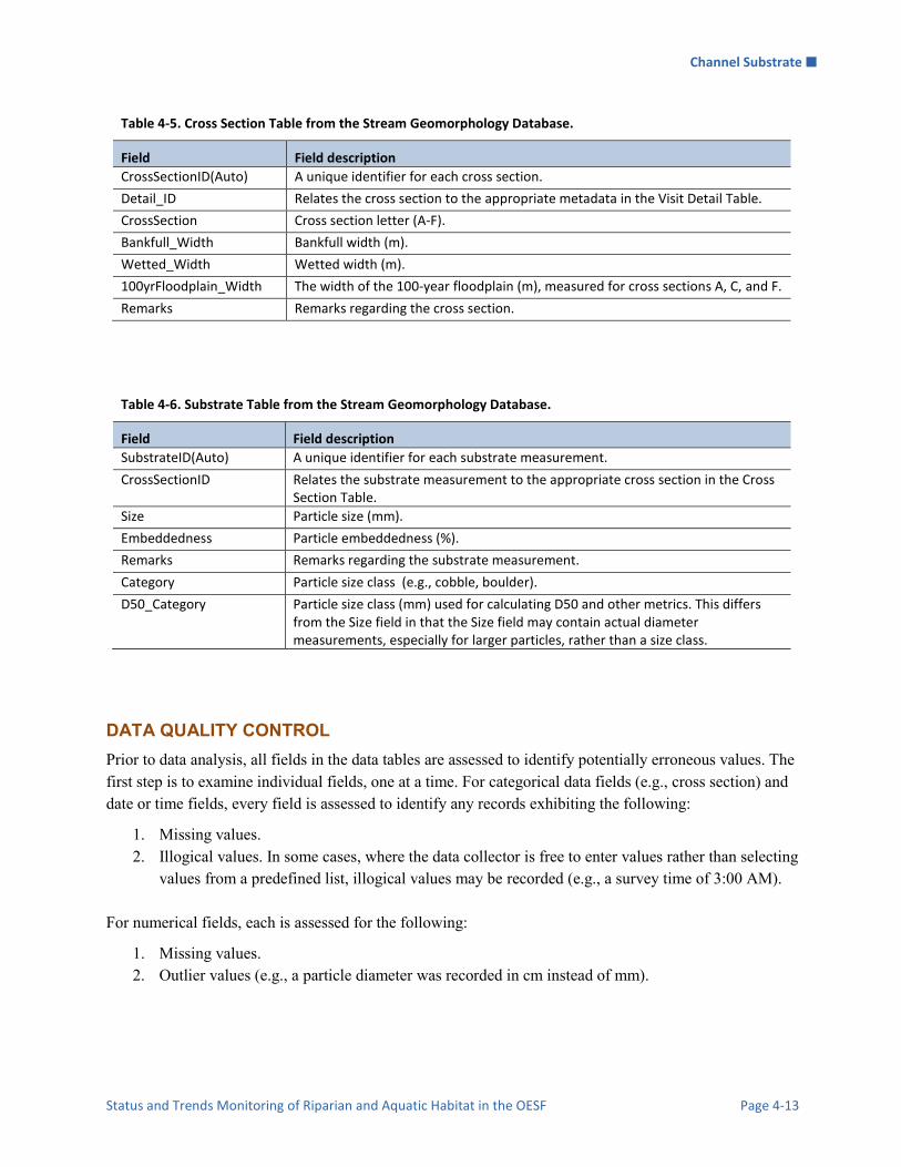
Channel Substrate
Status and Trends Monitoring of Riparian and Aquatic Habitat in the OESF Page 4-13
Table 4-5. Cross Section Table from the Stream Geomorphology Database.
Field Field description
CrossSectionID(Auto) A unique identifier for each cross section.
Detail_ID Relates the cross section to the appropriate metadata in the Visit Detail Table.
CrossSection Cross section letter (A-F).
Bankfull_Width Bankfull width (m).
Wetted_Width Wetted width (m).
100yrFloodplain_Width The width of the 100-year floodplain (m), measured for cross sections A, C, and F.
Remarks Remarks regarding the cross section.
Table 4-6. Substrate Table from the Stream Geomorphology Database.
Field Field description
SubstrateID(Auto) A unique identifier for each substrate measurement.
CrossSectionID Relates the substrate measurement to the appropriate cross section in the Cross Section Table.
Size Particle size (mm).
Embeddedness Particle embeddedness (%).
Remarks Remarks regarding the substrate measurement.
Category Particle size class (e.g., cobble, boulder).
D50_Category Particle size class (mm) used for calculating D50 and other metrics. This differs from the Size field in that the Size field may contain actual diameter measurements, especially for larger particles, rather than a size class.
DATA QUALITY CONTROL Prior to data analysis, all fields in the data tables are assessed to identify potentially erroneous values. The first step is to examine individual fields, one at a time. For categorical data fields (e.g., cross section) and date or time fields, every field is assessed to identify any records exhibiting the following:
1. Missing values. 2. Illogical values. In some cases, where the data collector is free to enter values rather than selecting
values from a predefined list, illogical values may be recorded (e.g., a survey time of 3:00 AM). For numerical fields, each is assessed for the following:
1. Missing values. 2. Outlier values (e.g., a particle diameter was recorded in cm instead of mm).

Channel Substrate
Page 4-14 Washington State Department of Natural Resources
The next step in quality control assessment is to examine whether all aspects of the data are within a reasonable range. For example, if one cross section has 40 substrate measurements, it is likely that an error has occurred somewhere. When missing values are discovered, it is generally not possible to “fill in the blank” from the office. The fact that data are missing should be recorded, in brackets, in the “Remarks” field, with the initials of the person who performed the quality control check (e.g., [Embeddedness was not recorded. –WD]). Illogical or outlier values can sometimes be corrected in the office. For example, AM and PM might have been switched or a decimal place error can be corrected. When data are corrected, this must be noted in the remarks field, in brackets, with the initials of the person who performed the quality control check. In many cases, clearly erroneous outlier values cannot be corrected in the office and should be edited so as not to affect the results of analysis. In such cases, the value should be removed and transferred to the “Remarks” field with an explanation, in brackets, with the initials of the person who performed the quality control check. For example: [Erosion height was recorded as 74.8 m. This value was clearly incorrect and removed from the dataset. –WD]).
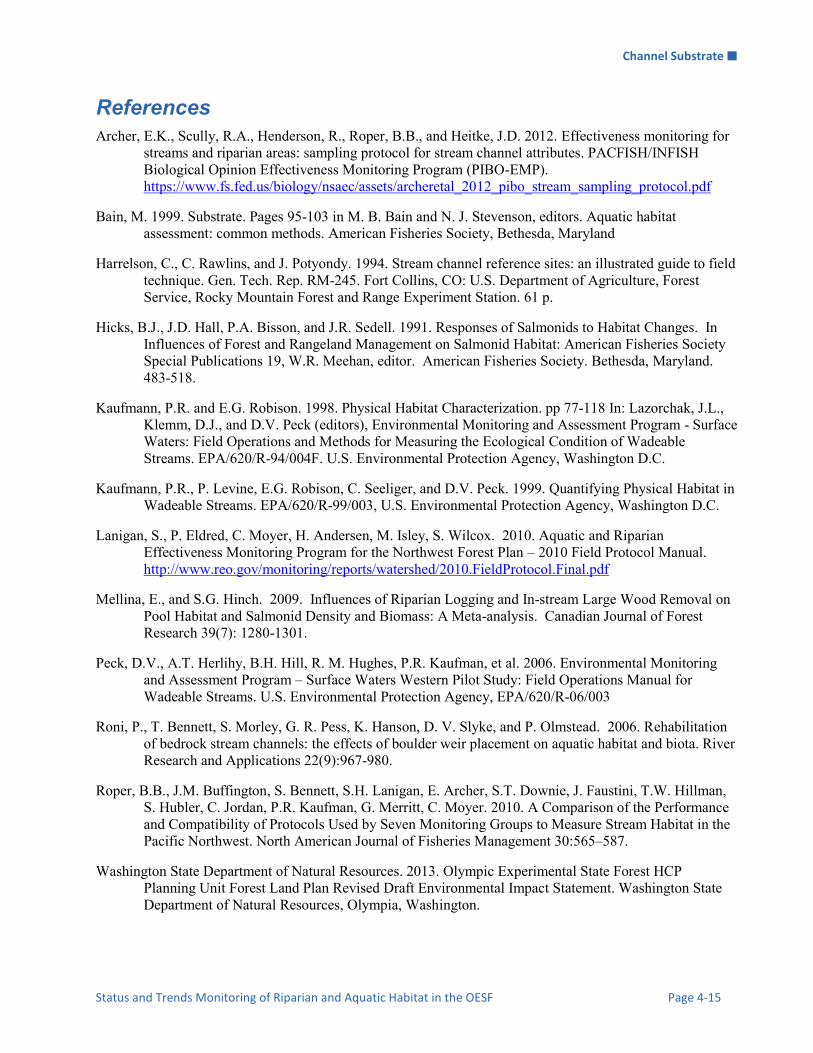
Channel Substrate
Status and Trends Monitoring of Riparian and Aquatic Habitat in the OESF Page 4-15
References Archer, E.K., Scully, R.A., Henderson, R., Roper, B.B., and Heitke, J.D. 2012. Effectiveness monitoring for
streams and riparian areas: sampling protocol for stream channel attributes. PACFISH/INFISH Biological Opinion Effectiveness Monitoring Program (PIBO-EMP). https://www.fs.fed.us/biology/nsaec/assets/archeretal_2012_pibo_stream_sampling_protocol.pdf
Bain, M. 1999. Substrate. Pages 95-103 in M. B. Bain and N. J. Stevenson, editors. Aquatic habitat assessment: common methods. American Fisheries Society, Bethesda, Maryland
Harrelson, C., C. Rawlins, and J. Potyondy. 1994. Stream channel reference sites: an illustrated guide to field technique. Gen. Tech. Rep. RM-245. Fort Collins, CO: U.S. Department of Agriculture, Forest Service, Rocky Mountain Forest and Range Experiment Station. 61 p.
Hicks, B.J., J.D. Hall, P.A. Bisson, and J.R. Sedell. 1991. Responses of Salmonids to Habitat Changes. In Influences of Forest and Rangeland Management on Salmonid Habitat: American Fisheries Society Special Publications 19, W.R. Meehan, editor. American Fisheries Society. Bethesda, Maryland. 483-518.
Kaufmann, P.R. and E.G. Robison. 1998. Physical Habitat Characterization. pp 77-118 In: Lazorchak, J.L., Klemm, D.J., and D.V. Peck (editors), Environmental Monitoring and Assessment Program - Surface Waters: Field Operations and Methods for Measuring the Ecological Condition of Wadeable Streams. EPA/620/R-94/004F. U.S. Environmental Protection Agency, Washington D.C.
Kaufmann, P.R., P. Levine, E.G. Robison, C. Seeliger, and D.V. Peck. 1999. Quantifying Physical Habitat in Wadeable Streams. EPA/620/R-99/003, U.S. Environmental Protection Agency, Washington D.C.
Lanigan, S., P. Eldred, C. Moyer, H. Andersen, M. Isley, S. Wilcox. 2010. Aquatic and Riparian Effectiveness Monitoring Program for the Northwest Forest Plan – 2010 Field Protocol Manual. http://www.reo.gov/monitoring/reports/watershed/2010.FieldProtocol.Final.pdf
Mellina, E., and S.G. Hinch. 2009. Influences of Riparian Logging and In-stream Large Wood Removal on Pool Habitat and Salmonid Density and Biomass: A Meta-analysis. Canadian Journal of Forest Research 39(7): 1280-1301.
Peck, D.V., A.T. Herlihy, B.H. Hill, R. M. Hughes, P.R. Kaufman, et al. 2006. Environmental Monitoring and Assessment Program – Surface Waters Western Pilot Study: Field Operations Manual for Wadeable Streams. U.S. Environmental Protection Agency, EPA/620/R-06/003
Roni, P., T. Bennett, S. Morley, G. R. Pess, K. Hanson, D. V. Slyke, and P. Olmstead. 2006. Rehabilitation of bedrock stream channels: the effects of boulder weir placement on aquatic habitat and biota. River Research and Applications 22(9):967-980.
Roper, B.B., J.M. Buffington, S. Bennett, S.H. Lanigan, E. Archer, S.T. Downie, J. Faustini, T.W. Hillman, S. Hubler, C. Jordan, P.R. Kaufman, G. Merritt, C. Moyer. 2010. A Comparison of the Performance and Compatibility of Protocols Used by Seven Monitoring Groups to Measure Stream Habitat in the Pacific Northwest. North American Journal of Fisheries Management 30:565–587.
Washington State Department of Natural Resources. 2013. Olympic Experimental State Forest HCP Planning Unit Forest Land Plan Revised Draft Environmental Impact Statement. Washington State Department of Natural Resources, Olympia, Washington.

Channel Substrate
Page 4-16 Washington State Department of Natural Resources
Wolman, M.G. 1954. A method of sampling coarse river-bed material. Trans. Am. Geophys. Union 35(6):951-956.

In-Stream Large Wood
Status and Trends Monitoring of Riparian and Aquatic Habitat in the OESF Page 5-1
In-stream Large Wood Authors: Alex Foster, Mitchell Vorwerk, Teodora Minkova Version: 1.4 Revision History:
Based on the Following Protocols: This protocol is adapted from the Level 2 large woody debris (LWD) survey, of the TFW Monitoring Program Method Manual for the LWD Survey by Schuett-Hames et al. (1999). Refer to the original document if clarification is needed. Reasons to Adopt the Above Protocols: Due to its rigorous wood classification, measurement, and counting methodologies, Schuett-Hames et al. (1999) had the lowest repeat survey variation in a comparison of several stream survey methods being implemented in the Pacific Northwest (Roper et al. 2010). Purpose and Content: This protocol details the field procedures for classifying and measuring pieces of large wood in the sample reaches, the field quality assurance and quality control steps, and the data management and analysis procedures necessary to document and report the status and trends of in-stream large wood across the Olympic Experimental State Forest.
Version number Purpose / Changes Author(s) Reviewer(s) Date
1.0 Initial draft presented to project staff Alex Foster Peter Bisson, Teodora Minkova
03/19/2013
1.1 Draft submitted to external review Alex Foster Rebecca Flitcroft 04/16/2013
1.2 Draft incorporating external reviews, sampling procedures from 2013 field season
Alex Foster, Teodora Minkova
Mitchell Vorwerk 05/20/2014
1.3 Final draft incorporating sampling procedures from 2014-2015 field season, and data mgmt. procedures
Alex Foster, Mitchell Vorwerk, Teodora Minkova
Ellis Cropper, Kyle Martens
05/10/2016
1.4 Final technical review and edit Alex Foster,
Mitchell Vorwerk,
Teodora Minkova
Paul Dunnette,
Warren Devine, Alex
Foster
12/18/2016

In-Stream Large Wood
Page 5-2 Washington State Department of Natural Resources
Table of Contents Introduction ..................................................................................................................................................... 5-3
Monitoring Design .......................................................................................................................................... 5-3
Spatial Sampling Design ............................................................................................................................. 5-3
Temporal Sampling Design ......................................................................................................................... 5-3
Equipment and Supplies .................................................................................................................................. 5-3
Field Procedures .............................................................................................................................................. 5-4
Large Woody Debris Identification Criteria ............................................................................................... 5-4
Sampling of Individual Logs and Rootwads ............................................................................................... 5-7
Sampling of Log Jams ............................................................................................................................... 5-12
Procedures for Calculating Metrics ............................................................................................................... 5-13
Time and Cost Estimates for Implementing Field Procedures ...................................................................... 5-13
Quality Assurance and Quality Control ........................................................................................................ 5-14
Training ..................................................................................................................................................... 5-14
Standard Protocols .................................................................................................................................... 5-14
Field Checks .............................................................................................................................................. 5-14
Data Management ......................................................................................................................................... 5-15
Data Flow .................................................................................................................................................. 5-15
Data Storage .............................................................................................................................................. 5-16
Data Quality Control ................................................................................................................................. 5-19
References ..................................................................................................................................................... 5-20
Appendix 5A. Indicators of Bankfull Stage ................................................................................................. 5A-1
Appendix 5B. Field Procedures Dropped from Original Monitoring Protocol Implemented in 2013-2015 ................................................................................................................................................ 5B-1

In-Stream Large Wood
Status and Trends Monitoring of Riparian and Aquatic Habitat in the OESF Page 5-3
Introduction In-stream large wood (or large woody debris (LWD) refers to logs, pieces of logs, root wads, or large chunks of wood that have fallen into stream channels. In-stream large wood has many roles in aquatic systems: it traps and retains sediment, changes water velocity and diverts stream flows, changes channel shape and gradient, releases nutrients as it decomposes, and provides habitat and cover for aquatic organisms (Bisson et al. 1987, Cummins 1974). The type and level of ecological function provided by LWD depends on the size, species, location, and distribution of the wood pieces. LWD functionality also depends on stream characteristics such as size and gradient. For example, logs of the same size may not provide the same level of ecological function in a large stream as they do in a small one. The condition and location of LWD vary considerably in time and space and reflect past and present recruitment rates and the rates of LWD transport through the channel (Schuett-Hames et al. 1999). Owing to all these factors, comprehensive and repeated LWD surveys are required to assess the status of and changes in riparian and aquatic habitat over time. In the environmental impact analysis for the Olympic Experimental Forest (OESF) Forest Land Plan, LWD recruitment was recognized as an important indicator for fish habitat and riparian areas (WADNR 2013).
Monitoring Design
SPATIAL SAMPLING DESIGN The LWD survey is conducted at each of the 50 sample watersheds in the OESF and in the four reference watersheds in Olympic National Park (ONP). Refer to the Project Background chapter for a map of the sample watersheds. LWD pieces are classified and measured during a continuous survey of the sample reach.
TEMPORAL SAMPLING DESIGN The ideal time to sample LWD in the OESF is in summer or early fall, when stream flow is typically low-to-moderate and discharge is most stable. To prevent unnecessary disturbance and mortality to salmon, avoid working in the channel during spawning or when there are eggs in the gravel.
Equipment and Supplies The following field equipment and supplies are needed for LWD surveys:
Stadia rod Log calipers (in metric units) Ruggedized field tablet with electronic data entry form and paper field forms (as backup to tablet) Railroad chalk

In-Stream Large Wood
Page 5-4 Washington State Department of Natural Resources
Field Procedures The field procedures below are simplified from the original procedures implemented from 2013 to 2015. Procedures dropped from the original field protocol include:
Identifying channel zones. Classifying LWD pieces by zone. Counting log jam LWD pieces by lowest zone. Estimating individual LWD piece orientation within the channel.
The dropped field procedures are included in Appendix 5B for historical reference or in case they are used again in the future. Procedures modified from the original field protocol include:
Reporting individual LWD piece location in three categories (within wetted portion of the channel, within bankfull stage, or suspended above the bankfull stage).
Estimating the stability of individual LWD piece in two categories (unstable or stable) instead of the previous five categories (rooted, buried, pinned, unstable, and stable).
The first round of LWD sampling in all watersheds was conducted using the original, more detailed procedures. The original field procedures were changed as a result of a field quality control analysis (Devine and Minkova 2016) and consultation with other researchers. The quality control report showed low precision of piece length measurements and piece count calculated by zone vs. the same metrics calculated for the total number of pieces. This difference was due to the smaller sample size in each zone. Review of available literature and consultation with researchers led to the conclusion that data on LWD pieces classified by zone and piece orientation in the channel are rarely used in analyses.
LARGE WOODY DEBRIS IDENTIFICATION CRITERIA Data are collected for all qualifying LWD pieces within the sample reach.
Logs and Rootwads
Qualifying LWD pieces are classified as either logs or rootwads. Logs must have a minimum diameter of 10 cm for at least 2 m of length. Rootwads must have an identifiable root system and bole (i.e., stem or tree trunk), a total length that is less than 2 m (i.e., less than the minimum log length), and a minimum diameter of 20 cm above the root swell (see Diameter and Length, below, for measurement details). Examples are illustrated in Figures 5-1 and 5-2.
In addition, an LWD piece (log or rootwad) must meet the following criteria to qualify:
1. It is completely dead. No live (green) needles or leaves or other signs of life are evident at the time of the survey.
2. At least 10 cm of its qualifying dimensions is within or directly above the bankfull stage of the channel (Figure 5-3; refer to Appendix 5A for indicators of bankfull stage).

In-Stream Large Wood
Status and Trends Monitoring of Riparian and Aquatic Habitat in the OESF Page 5-5
3. Its root system is detached from its original position (i.e., it is not rooted and has the ability to move along the length of the channel and become “debris” (Figures 5-1 and 5-2)).
LWD pieces are to be sampled separately if they are broken on the long axis; each broken piece should be sampled only if it qualifies. Branches still attached to the bole are not included in the survey (even if they are of qualifying diameter and length). See Diameter and Length, below, for instructions on measuring logs or rootwads with multiple boles.
If a portion of a LWD piece is buried and its full length and midpoint diameter (see Diameter and Length, below) cannot be determined, measure only the exposed section(s). Some probing/surface debris removal is acceptable, if necessary, to obtain a better length or diameter measurement.
Figure 5-1. Criteria for determining whether individual pieces of wood qualify for measurement (modified from Schuett-Hames et al. 1999).

In-Stream Large Wood
Page 5-6 Washington State Department of Natural Resources
Figure 5-3. Sample reach cross section, showing bankfull stage and the area above bankfull stage.
Figure 5-2. Criteria for determining whether a rootwad qualifies for measurement (modified from Schuett-Hames et al. 1999).

In-Stream Large Wood
Status and Trends Monitoring of Riparian and Aquatic Habitat in the OESF Page 5-7
Log Jams
An accumulation of LWD pieces (logs and rootwads) qualifies as a log jam if it meets the following criteria:
1. It has a minimum of 10 qualifying pieces of LWD that are touching at least one other piece in the accumulation.
2. At least one LWD piece associated with the accumulation must extend a minimum of 10 cm into or directly above the bankfull stage of the channel.
Pieces in an accumulation that are entirely outside the bankfull stage should not be included in the count unless they have a reasonable chance of being moved into the channel if the jam “blows out” during high flows.
SAMPLING OF INDIVIDUAL LOGS AND ROOTWADS Moving upstream from cross section A, one crew member records the data, while the other crew member identifies and examines LWD pieces and measures them with the calipers and stadia rod. Qualifying LWD pieces extending below or above the sample reach (i.e., below cross-section A or above cross-section F) are sampled if at least 10 cm of the qualifying dimensions enters the reach. If an LWD piece extends beyond the reach, note this in the field tablet database “Remarks” field. Record the cross section (A-E) that is immediately downstream of each LWD piece. If a piece intersects a cross section, determine the downstream cross section based on where the majority of the LWD mass is located (e.g., if a piece intersects cross-section C and most of the piece is upstream of the cross section, then C should be recorded). Pieces in side channels are included in the survey, but note in the “Remarks” field when a piece is located in a side channel.
Location
Identify the location of each LWD piece (Figure 5-3) using one of the following categories:
W (Wetted): At least 10 cm of its length is within the wetted portion of the channel.
B (Bankfull): At least 10 cm of its length is within the bankfull stage of the channel (refer to Appendix 5A for indicators of bankfull stage).
S (Suspended): At least 10 cm of its length is directly above the bankfull stage of the channel.
Assess location categories in the sequence listed above (W, B, S) and record the first category for which the piece qualifies.
Diameter and Length
Measure a log’s diameter at the midpoint of its length using calipers (preferred) or a diameter tape (nearest 0.01 m) (Figure 5-4). Measure rootwad diameter just above the tapered portion at the base of the tree (Figure 5-2). When measuring diameter, the beam of the caliper should always be horizontal (Figure 5-4a) unless obstacles make that impossible. The jaws of the caliper should always be perpendicular to the long axis of
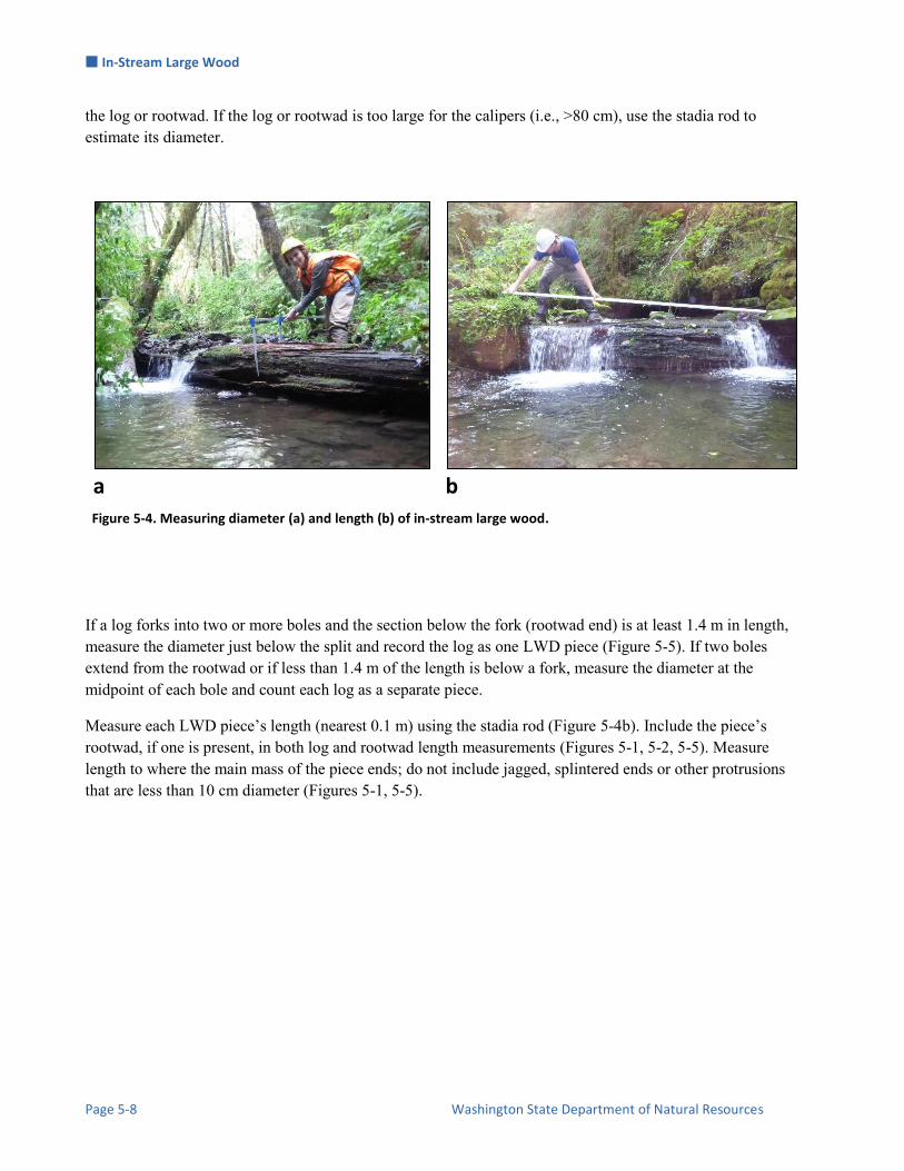
In-Stream Large Wood
Page 5-8 Washington State Department of Natural Resources
the log or rootwad. If the log or rootwad is too large for the calipers (i.e., >80 cm), use the stadia rod to estimate its diameter.
a b
Figure 5-4. Measuring diameter (a) and length (b) of in-stream large wood.
If a log forks into two or more boles and the section below the fork (rootwad end) is at least 1.4 m in length, measure the diameter just below the split and record the log as one LWD piece (Figure 5-5). If two boles extend from the rootwad or if less than 1.4 m of the length is below a fork, measure the diameter at the midpoint of each bole and count each log as a separate piece.
Measure each LWD piece’s length (nearest 0.1 m) using the stadia rod (Figure 5-4b). Include the piece’s rootwad, if one is present, in both log and rootwad length measurements (Figures 5-1, 5-2, 5-5). Measure length to where the main mass of the piece ends; do not include jagged, splintered ends or other protrusions that are less than 10 cm diameter (Figures 5-1, 5-5).

In-Stream Large Wood
Status and Trends Monitoring of Riparian and Aquatic Habitat in the OESF Page 5-9
Figure 5-5. Examples of diameter measurement locations, indicated by vertical arrows, for LWD pieces with single or multiple boles. “M” indicates the midpoint of the each piece.

In-Stream Large Wood
Page 5-10 Washington State Department of Natural Resources
Tree Species Category
Categorize each LWD piece as one of the following:
C (Coniferous species)
D (Deciduous species)
U (Unknown species)
Characteristics used to categorize LWD species include bark color and texture, wood color and firmness, branching pattern, and diameter. Local riparian tree species composition and tree size also may serve as guides.
Stability
Describe the stability of each LWD piece using one of the following categories:
U (Unstable): The piece could become mobile at high flows. If you are not certain, kick or push the piece to see if it wiggles, rocks, or feels unstable.
S (Stable): The piece does not move or seem unstable when it is kicked or pushed. An example of this is a very large log with a mass that makes it stable.
Pool-Forming Function
In forested stream channels, pool formation is often closely linked to flow alteration around woody debris. LWD may create dammed pools by blocking flow or enhance the scour of pools by changing channel hydraulics. Water may spill over a wood step, creating a plunge pool downstream, or be redirected down under woody debris, leading to stream bed scour.
Assess whether each recorded LWD piece contributed directly to pool formation. Pools considered under this section must meet minimum surface area requirements based on the average bankfull width of the sample reach (Table 5-1), which is automatically calculated by the field tablet database. Record Y for yes or N for no.
Table 5-1. LWD pool-forming function minimum pool surface area (modified from Schuett-Hames et al. 1999).
Bankfull width (m) Minimum pool surface area (m2)
0 to 2.4 0.5
2.5 to 4.9 1.0
5.0 to 9.9 2.0
10.0 to 14.9 3.0

In-Stream Large Wood
Status and Trends Monitoring of Riparian and Aquatic Habitat in the OESF Page 5-11
Decay Class
Classify the decay class of each LWD piece on a scale of 1 to 5, where 1 is not decayed (died very recently) and 5 is very decayed (advanced stages of rotting). Refer to Table 5-2 as a guide. Also, a “poke test” may be used to help determine decay class. Poke the LWD piece with the calipers or stadia rod to gauge how soft it is. The poke test is used in combination with the other factors to determine the decay class.
Table 5-2. A five-class system for evaluating wood decay (from USDA Forest Service 2005 and WADNR 2002)
Decay class Bark
Twigs (diam. <3 cm) Structural integrity
Texture of rotten portions Shape Wood color
1 Intact
Present Sound, freshly fallen, intact logs
Intact/firm; no rot Round Original
2 Intact
Absent Sound Mostly intact; sapwood partially soft, but can’t be pulled apart by hand
Round Original
3 Trace Absent Heartwood sound; piece supports its own weight
Hard, large pieces; sapwood can be pulled apart by hand
Round Original to faded
4 Absent Absent Heartwood rotten; piece does not support its own weight, but maintains its shape
Soft, small, blocky pieces
Round to oval
Light brown to reddish brown
5 Absent Absent None, piece no longer maintains its shape
Soft; powdery when dry
Oval/ Irregular
Light brown to dark brown
Sediment-Storing Function
Assess whether each LWD piece contributes directly to storage of coarse or fine sediment (Figure 5-6). If a sediment deposit would not exist without the presence of the LWD piece, and would likely mobilize if the piece were removed, the piece qualifies as “sediment storing.” Record Y for yes or N for no.

In-Stream Large Wood
Page 5-12 Washington State Department of Natural Resources
Figure 5-6. Examples of sediment-storing wood pieces.
SAMPLING OF LOG JAMS Owing to the difficulty and potential danger involved with maneuvering around a log jam, detailed data are not collected on LWD pieces associated with a jam. The pieces are categorized only by diameter size class.
Location
As with individual LWD pieces, log jam location is identified by the nearest downstream cross section. If the jam crosses multiple cross sections, it should be noted in the field tablet database “Remarks” field.
Counts by LWD Piece Type and Size
Identify each LWD piece associated with a jam as either a rootwad or a log. The same minimum midpoint diameter and length requirements used for LWD pieces sampled individually apply to pieces included in jams (i.e., rootwads must have a diameter > 20 cm and a length < 2 m, and logs must have a diameter > 10 cm and a length >2 m). It may be helpful to mark LWD pieces with chalk to help keep track of which pieces have been measured and counted, especially on large, complex, or mossy jams. If some pieces in a jam are unstable or high above the channel and cannot be measured safely, diameters may be visually estimated. After measuring or estimating the diameter of a qualified LWD piece, categorize the piece as: Small (10-19 cm), Medium (20-49 cm), or Large (>50 cm).
Pool-Forming Function
Log accumulations may increase pool frequency and depth via local scour of the stream bed and impoundment. Assess whether one or more LWD pieces associated with each log jam contributed directly to the formation of a pool by blocking or redirecting flow. Again, pools considered under this section must meet minimum surface area requirements based on the average bankfull width of the sample reach (Table 5-1). Record Y for yes or N for no.
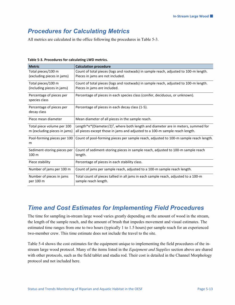
In-Stream Large Wood
Status and Trends Monitoring of Riparian and Aquatic Habitat in the OESF Page 5-13
Procedures for Calculating Metrics All metrics are calculated in the office following the procedures in Table 5-3.
Table 5-3. Procedures for calculating LWD metrics.
Metric Calculation procedure
Total pieces/100 m (excluding pieces in jams)
Count of total pieces (logs and rootwads) in sample reach, adjusted to 100-m length. Pieces in jams are not included.
Total pieces/100 m (including pieces in jams)
Count of total pieces (logs and rootwads) in sample reach, adjusted to 100-m length. Pieces in jams are included.
Percentage of pieces per species class
Percentage of pieces in each species class (conifer, deciduous, or unknown).
Percentage of pieces per decay class
Percentage of pieces in each decay class (1-5).
Piece mean diameter Mean diameter of all pieces in the sample reach.
Total piece volume per 100 m (excluding pieces in jams)
Length*π*(Diameter/2)2, where both length and diameter are in meters, summed for all pieces except those in jams and adjusted to a 100-m sample reach length.
Pool-forming pieces per 100 m
Count of pool-forming pieces per sample reach, adjusted to 100-m sample reach length.
Sediment-storing pieces per 100 m
Count of sediment-storing pieces in sample reach, adjusted to 100-m sample reach length.
Piece stability Percentage of pieces in each stability class.
Number of jams per 100 m Count of jams per sample reach, adjusted to a 100-m sample reach length.
Number of pieces in jams per 100 m
Total count of pieces tallied in all jams in each sample reach, adjusted to a 100-m sample reach length.
Time and Cost Estimates for Implementing Field Procedures The time for sampling in-stream large wood varies greatly depending on the amount of wood in the stream, the length of the sample reach, and the amount of brush that impedes movement and visual estimates. The estimated time ranges from one to two hours (typically 1 to 1.5 hours) per sample reach for an experienced two-member crew. This time estimate does not include the travel to the site. Table 5-4 shows the cost estimates for the equipment unique to implementing the field procedures of the in-stream large wood protocol. Many of the items listed in the Equipment and Supplies section above are shared with other protocols, such as the field tablet and stadia rod. Their cost is detailed in the Channel Morphology protocol and not included here.

In-Stream Large Wood
Page 5-14 Washington State Department of Natural Resources
Table 5-4. Cost estimates for the equipment used in the In-stream Large Wood Field Protocol.
Equipment/Supplies Amount Cost
Metric log calipers 1 $150
Railroad chalk 1 box (144 pieces) $30
Quality Assurance and Quality Control The quality assurance for the in-stream large wood field protocol includes staff training and use of standardized protocols. The quality control for the field procedures includes annual field checks. The QA/QC procedures for data management are described in the Data Management section below.
TRAINING All personnel conducting field protocols will be trained in a consistent manner to ensure that the surveys are conducted properly and in standardized fashion. The training is conducted (or reviewed for returning personnel) annually before the start of the field season. At least one member of the field crew should be experienced with the field procedures.
STANDARD PROTOCOLS The standard procedures described in this protocol are followed for the duration of the project. Any deviations from the procedures should be documented, and the reasons for deviation described and discussed with the project manager or the researcher overseeing the protocol implementation. Changes to the published protocols must be approved by the project manager or by the researcher overseeing the protocol implementation. Revised protocols are assigned new version numbers and publication dates.
FIELD CHECKS The field crew checks the data entry form for missing records or unusual numbers on site at the end the field survey. The researcher overseeing the protocol implementation or a different field crew will conduct spot checks on 10% of the field measurements every year.
In-Stream Large Wood
Status and Trends Monitoring of Riparian and Aquatic Habitat in the OESF Page 5-15
Data Management
DATA FLOW All LWD data are recorded in the field using paper field forms (2013-2014 field seasons or in case of tablet PC malfunction) or the ruggedized field tablet (2015 field season onward). In the office, data are then transferred to a database for long-term storage. The steps below detail the process.
Data flow for paper field forms
1. Fill out field forms Two types of field forms, an individual-piece form and a log jam form, are used to record data and metadata at each sample reach.
2. Scan and store field forms After returning from the field each week, the field forms are scanned and stored on the WADNR network drive; the original paper forms are archived by the OESF Data Management Specialist at the WADNR Forest Resources Division.
3. Enter data All LWD data collected on paper field forms are entered in the Habitat_LWD_Database by the OESF Data Management Specialist on a weekly basis. After data from a field form is entered, the Specialist writes “Entered” followed by his or her initials and the date.
4. Quality control Entered field form data are verified by comparing the data on the field form to the data in the database. This process is performed by someone other than the person who originally entered the data. After the data are verified, the person who verified it writes “Verified” on the form followed by his or her initials and the date.
Data flow for electronically collected data
1. Fill out forms on electronic field data recorder Field personnel record all LWD data using the Tablet Database, which is a customized database created in Microsoft Access and saved on the field tablet.
2. Store field data At the end of each day in the field, a copy of the Tablet Database, containing all data collected to date, is transferred to the OESF Data Management Specialist via cloud storage or email. If internet access is not available, the field crew makes a daily backup copy of the database on a laptop or other storage device and then transfers the data to the Specialist at the end of the work week. The Specialist stores these Tablet Database copies in a temporary location on the WADNR network drive (J:\hcp\monitoring_research\tminkova\01_OESF_R&M Program\01_Rip S&T Mon\07_Data management\_All new data and photos) until they are processed and the data are transferred to a database for long-term storage.
3. Quality control Because data are recorded electronically, and thus never transcribed, transcription errors do not exist. However, there is still a possibility of data entry errors in the field. In particular, if metadata (e.g., the date of a field visit or a watershed ID) are recorded incorrectly in the field, this could cause errors during the process of importing data from the Tablet Database to the Habitat_LWD_Database (next step; see below). For this reason, metadata are examined for accuracy prior to importing data to the Habitat_LWD_Database.
4. Import data to database On a weekly basis, the OESF Data Management Specialist imports all new data from the Tablet Database to the Habitat_LWD_Database. This is accomplished using a set of queries stored in a third database: J:\hcp\monitoring_research\tminkova\01_OESF_R&M

In-Stream Large Wood
Page 5-16 Washington State Department of Natural Resources
Program\01_Rip S&T Mon\01_FIELD DATA\01_Stream survey\Data\ Distribute_Tablet_Data.accdb
5. Verify transfer of data After data have been imported, the OESF Data Management Specialist verifies that no records have been missed, using the record count queries built into the Distribute_Tablet_Data database.
Photographs
1. Transfer photos to data manager for storage All digital photographs taken in the field are transferred to the OESF Data Management Specialist at the end of each week. The Specialist temporarily stores the uncatalogued photos on the WADNR server at: J:\hcp\monitoring_research\tminkova\01_OESF_R&M Program\01_Rip S&T Mon\07_Data management\_All new data and photos\
2. Rename and archive photos The OESF Data Management Specialist renames each photo using the following naming convention: <Photo type>_<BasinID>_<Date taken>_<Original photo name> (for example: ER_797_20140715_P1000851.JPG). The photos are then moved to long-term storage in the following directory: J:\hcp\monitoring_research\tminkova\01_OESF_R&M Program\01_Rip S&T Mon\03_Photos and videos\04_Stream_survey\LWD\
DATA STORAGE
Paper Field Forms
The paper field forms are archived at the WADNR Forest Resources Division. The designated data steward is Teodora Minkova, WADNR. Scanned copies of these forms are saved in the Adobe portable document format (.pdf) in the following directory: J:\hcp\monitoring_research\tminkova\01_OESF_R&M Program\01_Rip S&T Mon\01_FIELD DATA\01_Stream survey\Data\Data archive\Field forms\
Tablet Databases
The original Tablet Databases, which are transferred to the OESF Data Management Specialist on a daily or weekly basis, are stored on the WADNR network drive after the field data they contain have been transferred to the Habitat_LWD_Database. The storage location for these databases is: J:\hcp\monitoring_research\tminkova\01_OESF_R&M Program\01_Rip S&T Mon\01_FIELD DATA\01_Stream survey\Data\Data archive\Processed tablet databases\
Long-term Data Storage
The ultimate location of the LWD data is the Habitat_LWD_Database, located on the WADNR network drive at: J:\hcp\monitoring_research\tminkova\01_OESF_R&M Program\01_Rip S&T Mon\01_FIELD DATA\01_Stream survey\Data\Habitat_LWD_Database.accdb
Within the Habitat_LWD_Database, the LWD data are stored in three related tables: the LWD Survey Table, the LWD Data Table, and the LWD Jams Data Table (Figure 5-7). The LWD Survey Table contains the metadata from each survey. The LWD Data Table contains records on individual LWD pieces, and the LWD

In-Stream Large Wood
Status and Trends Monitoring of Riparian and Aquatic Habitat in the OESF Page 5-17
Jams Data Table contains data on log jams. The fields in the three database tables are described in Tables 5-5, 5-6, and 5-7. The LWD_Survey_Table is related to the other two tables through one-to-many relationships: a single record in the LWD Survey Table may be related to any number of records in the other tables.
Figure 5-7. The structure of the LWD portion of the Habitat_LWD_Database
Table 5-5. Fields in the LWD Survey Table.
Field Field description
LWD_ID(Auto) Unique identifier for each record in the table.
Date_Surveyed The date of the LWD survey.
Time_Started The time of day that the survey began.
Time_Ended The time of day that the survey ended.
Minimum_Pool_Area The minimum pool area for classifying pool-forming LWD pieces.
Remarks Remarks.
BasinID The watershed identifier.
Crew_tablet The initials of the crew members.

In-Stream Large Wood
Page 5-18 Washington State Department of Natural Resources
Table 5-6. Fields in the LWD Data Table.
Field Field description
LWDPieceID(Auto) Unique identifier for each record in the table.
LWD_ID A value that links the record to the appropriate metadata in the LWD Survey Table.
X-Section The downstream cross section, relative to the LWD piece’s location.
Category Left or right bank.
Diameter Piece midpoint diameter (cm).
Location Location of the piece (wetted, bankfull, suspended).
TotalLength Total length of the piece (m).
Zone1_Length [Field used through 2015 only] Length of the piece in zone 1 (m).
Zone2_Length [Field used through 2015 only] Length of the piece in zone 2 (m).
Zone3_Length [Field used through 2015 only] Length of the piece in zone 3 (m).
Zone4_Length [Field used through 2015 only] Length of the piece in zone 4 (m).
Sp_Category Species category (deciduous, conifer, or unknown).
Piece_Stability Piece stability (stable, unstable) [Through 2015, five fields were used (stable, unstable, buried, pinned, rooted)].
Pool_Forming Is the piece pool-forming? (Yes/No).
Chan_Orientation [Field used through 2015 only] Orientation of the piece, relative to the channel (A, B, C, or D).
Decay_Class Decay class (1, 2, 3, 4, or 5).
Sed_Storage Is the piece sediment-storing? (Yes/No).
Remarks Remarks.
Table 5-7. Fields in the LWD Jams Data Table.
Field Field description
LWDJamID(Auto) Unique identifier for each record in the table.
LWD_ID A value that links the record to the appropriate metadata in the LWD Survey Table.
Cross_Section The downstream cross section, relative to the LWD piece’s location.
Lowest_Zone [Field used through 2015 only] Lowest zone of the jam (1, 2, or 3).
Pool_Forming Is the jam pool forming? (Yes/No)
Rootwad_Count Count of rootwads in jam.
Small_Log_Count Count of small logs in jam.
Medium_Log_Count Count of medium logs in jam.
Large_Log_Count Count of large logs in jam.
Log_Count_Zone1 [Field used through 2015 only] Count of logs in zone 1.
Log_Count_Zone2 [Field used through 2015 only] Count of logs in zone 2.
Log_Count_Zone3 [Field used through 2015 only] Count of logs in zone 3.
Log_Count_Zone4 [Field used through 2015 only] Count of logs in zone 4.
Remarks Remarks.

In-Stream Large Wood
Status and Trends Monitoring of Riparian and Aquatic Habitat in the OESF Page 5-19
DATA QUALITY CONTROL Prior to data analysis, all fields in the data tables are assessed to identify potentially erroneous values. The first step is to examine individual fields, one at a time. For categorical data fields (e.g., cross section) and date or time fields, every field is assessed to identify any records exhibiting the following:
1. Missing values. 2. Illogical values. In some cases, where the data collector is free to enter values rather than selecting
values from a predefined list, illogical values may be recorded (e.g., a survey time of 3:00 AM).
For numerical fields, each is assessed for the following:
1. Missing values. 2. Outlier values (e.g., a log diameter was recorded in m instead of cm).
The next step in quality control assessment is to examine derived values and values in the context of other fields. An example of a derived value is the sum of log counts for a particular log jam. If the sum of log counts is less than 10, then the data should be examined more closely because this value does not meet the minimum requirement for a log jam. An example of checking a value in the context of another field is comparing the sum of the log counts with the sum of log counts by size (plus rootwads). These two sums should be equal; if they are not, then there may be an error in the data. When missing values are discovered, it is generally not possible to “fill in the blank” from the office. The fact that data are missing should be recorded, in brackets, in the “Remarks” field, with the initials of the person who performed the quality control check (e.g., [Lowest_Zone was not recorded. –WD]). Illogical or outlier values can sometimes be corrected in the office. For example, AM and PM might have been switched or a decimal place error can be corrected. When data are corrected, this must be noted in the “Remarks” field, in brackets, with the initials of the person who performed the quality control check. For example: [Diameter was recorded as .55. This was clearly incorrect and changed to 55. –WD].
In many cases, clearly erroneous outlier values cannot be corrected in the office and should be edited so as not to affect the results of analysis. In such cases, the value should be removed from the field and transferred to the “Remarks” field with an explanation, in brackets, with the initials of the person who performed the quality control check. For example: [Log_Count_Zone2 was recorded as 455. This was clearly incorrect and removed from the dataset. –WD]).
In-Stream Large Wood
Page 5-20 Washington State Department of Natural Resources
References Bisson, P.A., R.E. Bilby, M.D. Bryant, C.A. Dolloff, G.B. Grette, R.A. House, M.L. Murphy, K.V. Koski,
and J.R. Sedell. 1987. Large woody debris in forested streams in the Pacific Northwest: Past, present, and future, in Streamside Management: Forestry and Fisheries Interactions, edited by E.O. Salo, and T. W. Cundy, University of Washington Press, Seattle, WA, pp. 143–190.
Cummins, K.W. 1974. Structure and function of stream ecosystems. Bioscience 24:631-641.
Devine W. and T. Minkova. 2016. 2015 Quality Control Report for Status and Trends Monitoring of Riparian and Aquatic Habitat in the Olympic Experimental State Forest. 2014 Progress Report. Washington State Department of Natural Resources, Forest Resources Division, Olympia, WA, 52 p.
Roper, B.B., J.M. Buffington, S. Bennett, S.H. Lanigan, E. Archer, S.T. Downie, J. Faustini, T.W. Hillman, S. Hubler, C. Jordan, P.R. Kaufman, G. Merritt, and C. Moyer. 2010. A Comparison of the Performance and Compatibility of Protocols Used by Seven Monitoring Groups to Measure Stream Habitat in the Pacific Northwest. North American Journal of Fisheries Management 30:565–587.
Schuett-Hames, D., A.E. Pleus, J. Ward, M. Fox, and J. Light. 1999. TFW Monitoring Program method manual for the large woody debris survey. Prepared for the Washington State Department of Natural Resources under the Timber, Fish, and Wildlife Agreement. TFW-AM9-99-004. DNR #106. March. 66 p.
USDA Forest Service. 2005. 3.0 Phase 3 Field Guide – Down Woody Materials October, 2005. USDA Forest Service Forest Inventory and Analysis Program. http://www.fia.fs.fed.us/library/field-guides-methods-proc/docs/2006/p3_3-0_sec14_10_2005.pdf
Washington State Department of Natural Resources. 2002. Forest Resource Inventory System – Field Procedures Manual with Addendum .02 from 04/02/2003. Washington State Department of Natural Resources, Olympia, Washington, 51 p.
Washington State Department of Natural Resources. 2013. Olympic Experimental State Forest HCP Planning Unit Forest Land Plan Revised Draft Environmental Impact Statement. Washington State Department of Natural Resources, Olympia, Washington.
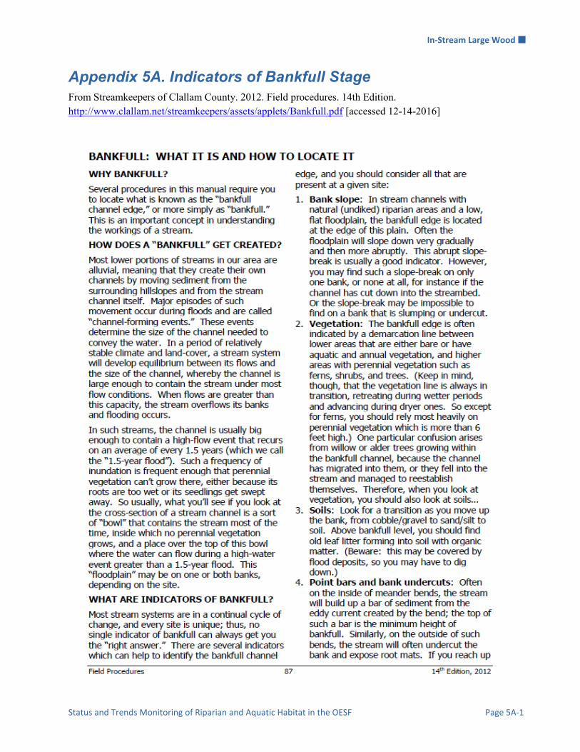
In-Stream Large Wood
Status and Trends Monitoring of Riparian and Aquatic Habitat in the OESF Page 5A-1
Appendix 5A. Indicators of Bankfull Stage From Streamkeepers of Clallam County. 2012. Field procedures. 14th Edition. http://www.clallam.net/streamkeepers/assets/applets/Bankfull.pdf [accessed 12-14-2016]

In-Stream Large Wood
Page 5A-2 Washington State Department of Natural Resources
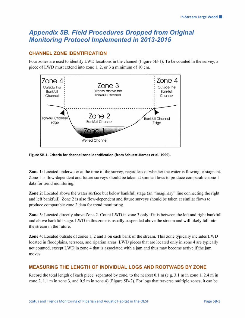
In-Stream Large Wood
Status and Trends Monitoring of Riparian and Aquatic Habitat in the OESF Page 5B-1
Appendix 5B. Field Procedures Dropped from Original Monitoring Protocol Implemented in 2013-2015
CHANNEL ZONE IDENTIFICATION
Four zones are used to identify LWD locations in the channel (Figure 5B-1). To be counted in the survey, a piece of LWD must extend into zone 1, 2, or 3 a minimum of 10 cm.
Figure 5B-1. Criteria for channel zone identification (from Schuett-Hames et al. 1999).
Zone 1: Located underwater at the time of the survey, regardless of whether the water is flowing or stagnant. Zone 1 is flow-dependent and future surveys should be taken at similar flows to produce comparable zone 1 data for trend monitoring.
Zone 2: Located above the water surface but below bankfull stage (an “imaginary” line connecting the right and left bankfull). Zone 2 is also flow-dependent and future surveys should be taken at similar flows to produce comparable zone 2 data for trend monitoring.
Zone 3: Located directly above Zone 2. Count LWD in zone 3 only if it is between the left and right bankfull and above bankfull stage. LWD in this zone is usually suspended above the stream and will likely fall into the stream in the future.
Zone 4: Located outside of zones 1, 2 and 3 on each bank of the stream. This zone typically includes LWD located in floodplains, terraces, and riparian areas. LWD pieces that are located only in zone 4 are typically not counted, except LWD in zone 4 that is associated with a jam and thus may become active if the jam moves.
MEASURING THE LENGTH OF INDIVIDUAL LOGS AND ROOTWADS BY ZONE Record the total length of each piece, separated by zone, to the nearest 0.1 m (e.g. 3.1 m in zone 1, 2.4 m in zone 2, 1.1 m in zone 3, and 0.5 m in zone 4) (Figure 5B-2). For logs that traverse multiple zones, it can be

In-Stream Large Wood
Page 5B-2 Washington State Department of Natural Resources
helpful to first mark each zone transition with chalk, then come back to measure the length of each marked zone.
Figure 5B-2. Recording piece length by channel zones (from Schuett-Hames et al. 1999).
ESTIMATING THE ORIENTATION OF INDIVIDUAL LOGS AND ROOTWADS Identify the piece orientation (horizontal direction within the channel) in one of four categories (Figure 5B-3). These categories are estimated and assume that directly upstream is 0 degrees and directly downstream is 180 degrees.
A for parallel to flow: A piece with its length axis either 337.5-22.5 degrees or 157.5-202.5 degrees. The direction of the root system or small-diameter end does not matter.
B for perpendicular to flow: a piece with its length axis between 67.5 and 112.5 degrees or 247.5 and 292.5 degrees. The direction of the root system or small-diameter end does not matter.
C for downstream: A piece with its length axis at any other angle (than Parallel (A) and Perpendicular (B)) and its small-diameter end downstream from its large-diameter or rootwad end.
D for upstream: A piece with its length axis at any other angle (than Parallel (A) and Perpendicular (B)) and its small-diameter end upstream from its large diameter or rootwad end.
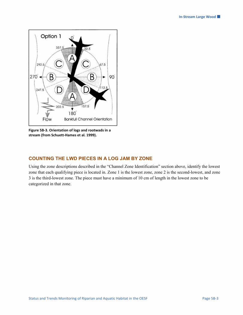
In-Stream Large Wood
Status and Trends Monitoring of Riparian and Aquatic Habitat in the OESF Page 5B-3
Figure 5B-3. Orientation of logs and rootwads in a stream (from Schuett-Hames et al. 1999).
COUNTING THE LWD PIECES IN A LOG JAM BY ZONE Using the zone descriptions described in the “Channel Zone Identification” section above, identify the lowest zone that each qualifying piece is located in. Zone 1 is the lowest zone, zone 2 is the second-lowest, and zone 3 is the third-lowest zone. The piece must have a minimum of 10 cm of length in the lowest zone to be categorized in that zone.

In-Stream Large Wood
Page 5B-4 Washington State Department of Natural Resources
This page intentionally left blank.

Habitat Units and Valley and Channel Classification
Status and Trends Monitoring of Riparian and Aquatic Habitat in the OESF Page 6-1
Habitat Units and Valley and Channel Classification Authors: Teodora Minkova, Mitchell Vorwerk Version: 1.4 Revision History:
Based on the Following Protocols: Habitat unit classification is adapted from Bisson et al. (2006) and Pleus et al. (1999). Stream valley and channel classification follows Bisson et al. (2006) and Montgomery and Buffington (1993 and 1997). Reasons to Adopt the Above Protocols: The selected classification methods are widely used in broad-scale monitoring programs in the Pacific Northwest, including the Northwest Forest Plan Aquatic and Riparian Effectiveness Monitoring Program (Lanigan et al. 2010), the Washington Department of Natural Resources Timber, Fish, and Wildlife Monitoring Program (Pleus et al. 1999), and the Columbia Habitat Monitoring Program(CHaMP) (Bouwes et al. 2011).
The reach-level assessments following these classifications are rapid, repeatable, and ecologically relevant. They rely on aspects of channel form that reflect channel processes such as sediment delivery. Purpose and Content: The purpose of this monitoring protocol is to describe the sampling and data management necessary to document and report stream channel and valley segment types and the status and multi-year trends of habitat units in the monitored watersheds. It details the field procedures for sampling habitat units and classifying channel reaches and valley segments, the field quality assurance and quality control steps, and the data management procedures.
ProtocolVersion Purpose / Changes Author(s) Reviewer(s) Date
1.0 Initial draft presented to project staff Teodora Minkova Peter Bisson, Alex Foster
04/02/2013
1.1 Draft submitted to external review Teodora Minkova Rebecca Flitcroft 04/16/2013
1.2 Final draft incorporating external reviews, sampling procedures from 2013 field season, and data mgmt. procedures
Teodora Minkova, Mitchell Vorwerk
05/20/2014
1.3 Final draft with field and data management procedures updated from 2014 and 2015 field seasons
Teodora Minkova, Mitchell Vorwerk
Ellis Cropper, Alex Foster
06/10/2016
1.4 Final technical review and edit Teodora Minkova,
Mitchell Vorwerk
Paul Dunnette,
Warren Devine,
Alex Foster
12/18/2016

Habitat Units and Valley and Channel Classification
Page 6-2 Washington State Department of Natural Resources
Table of Contents Introduction ................................................................................................................................................ 6-3
Monitoring Design ..................................................................................................................................... 6-3
Spatial Sampling Design ........................................................................................................................ 6-3
Temporal Sampling Design ................................................................................................................... 6-3
Equipment and Supplies ............................................................................................................................ 6-4
Field Procedures......................................................................................................................................... 6-4
Classification of Valley Segments ......................................................................................................... 6-4
Classification of Channel Reaches ......................................................................................................... 6-5
Habitat Unit Surveys ............................................................................................................................ 6-10
Time and Cost Estimates for Implementing the Field Procedures ........................................................... 6-15
Procedures for Calculating Metrics.......................................................................................................... 6-15
Quality Assurance and Quality Control ................................................................................................... 6-16
Training ................................................................................................................................................ 6-16
Standard Protocols ............................................................................................................................... 6-16
Field Checks......................................................................................................................................... 6-17
Data Management .................................................................................................................................... 6-17
Data Flow ............................................................................................................................................. 6-17
Data Storage ......................................................................................................................................... 6-18
Data Quality Control ............................................................................................................................ 6-21
References ................................................................................................................................................ 6-22
Appendix 6A. Habitat Units Identification at High Flows ..................................................................... 6A-1

Habitat Units and Valley and Channel Classification
Status and Trends Monitoring of Riparian and Aquatic Habitat in the OESF Page 6-3
Introduction Classification of stream valleys, channels, and habitat units provides a foundation for interpreting channel morphology, assessing channel conditions, describing microhabitat of fish and other aquatic organisms, and understanding stream response to natural and anthropogenic influences (Montgomery and Buffington 1993; Bisson et al. 2006). Understanding stream response to disturbance depends on established systems and procedures for stream classification and assessment that facilitate accurate, repeatable reach descriptions and provide information on the processes that govern channel structure (Bisson et al. 2006). Valley, channel, and habitat unit classification also allows for comparisons among drainages and/or extrapolation of results to other areas with similar features.
Monitoring Design
SPATIAL SAMPLING DESIGN Valley, channel, and habitat unit classification is conducted in each of the 50 sample watersheds in the Olympic Experimental State Forest (OESF) and in the four reference watersheds in Olympic National Park (ONP). Refer to the Introduction chapter for a map of the watersheds. Sample reaches in the watersheds are a minimum of 20 channel widths in length, a ratio that provides the scale necessary to relate stream morphology to channel processes, habitat characteristics, and potential response to disturbance (Montgomery and Buffington 1997). The entire length of the sample reach is considered for classifying the channel type and valley segment. Habitat units are delineated, classified, and measured from reach start (cross section A) to end (cross section F).
TEMPORAL SAMPLING DESIGN Valley and channel classification and habitat unit surveys should be conducted during low flow periods in late summer or early fall when discharge conditions are stable and habitat units are most defined. At higher flows, habitat units tend to “run together,” making delineation and repeat surveys difficult or impossible. Refer to Appendix 6-A for guidance when to discontinue the habitat unit surveys due to high stream flow. At the other end of the spectrum, do not survey during very low flow when the surface flow is not continuous throughout the reach length. Pre-survey reconnaissance should be done to determine flow conditions. To prevent unnecessary disturbance and mortality to salmon, avoid working in the channel during spawning or when there are eggs in the gravel.

Habitat Units and Valley and Channel Classification
Page 6-4 Washington State Department of Natural Resources
Equipment and Supplies The following equipment and supplies are needed for classifying the stream valley, channel, and habitat units and for measuring each habitat unit:
Stadia rod 50-meter tape Clinometer Ruggedized field tablet PC (and paper field forms as backup to the tablet). Field Guide for Identifying Stream Channel Types and Habitat Units (Minkova and Vorwerk
2015)
Field Procedures
CLASSIFICATION OF VALLEY SEGMENTS Valleys are areas of the landscape between higher terrain features, where runoff and sediment transport occur through downslope convergence (Armantrout 1998). Valley segments, hierarchically nested subdivisions of the drainage network, are classified as alluvial, bedrock, or colluvial based on valley fill, channel transport capacity, and sediment transport processes and supply (Bisson et al. 2006, Frissel et al. 1986). Their position within the hierarchy of watershed spatial scales is shown in Figure 6-1.
Figure 6-1. Hierarchical subdivision of watersheds into valley segments and stream reaches (adapted from Montgomery and Buffington 1993).
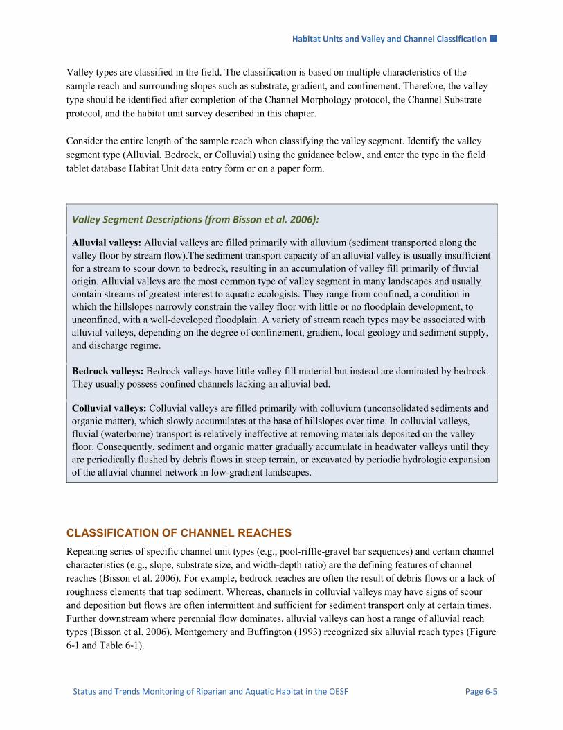
Habitat Units and Valley and Channel Classification
Status and Trends Monitoring of Riparian and Aquatic Habitat in the OESF Page 6-5
Valley types are classified in the field. The classification is based on multiple characteristics of the sample reach and surrounding slopes such as substrate, gradient, and confinement. Therefore, the valley type should be identified after completion of the Channel Morphology protocol, the Channel Substrate protocol, and the habitat unit survey described in this chapter. Consider the entire length of the sample reach when classifying the valley segment. Identify the valley segment type (Alluvial, Bedrock, or Colluvial) using the guidance below, and enter the type in the field tablet database Habitat Unit data entry form or on a paper form.
Valley Segment Descriptions (from Bisson et al. 2006):
Alluvial valleys: Alluvial valleys are filled primarily with alluvium (sediment transported along the valley floor by stream flow).The sediment transport capacity of an alluvial valley is usually insufficient for a stream to scour down to bedrock, resulting in an accumulation of valley fill primarily of fluvial origin. Alluvial valleys are the most common type of valley segment in many landscapes and usually contain streams of greatest interest to aquatic ecologists. They range from confined, a condition in which the hillslopes narrowly constrain the valley floor with little or no floodplain development, to unconfined, with a well-developed floodplain. A variety of stream reach types may be associated with alluvial valleys, depending on the degree of confinement, gradient, local geology and sediment supply, and discharge regime.
Bedrock valleys: Bedrock valleys have little valley fill material but instead are dominated by bedrock. They usually possess confined channels lacking an alluvial bed.
Colluvial valleys: Colluvial valleys are filled primarily with colluvium (unconsolidated sediments and organic matter), which slowly accumulates at the base of hillslopes over time. In colluvial valleys, fluvial (waterborne) transport is relatively ineffective at removing materials deposited on the valley floor. Consequently, sediment and organic matter gradually accumulate in headwater valleys until they are periodically flushed by debris flows in steep terrain, or excavated by periodic hydrologic expansion of the alluvial channel network in low-gradient landscapes.
CLASSIFICATION OF CHANNEL REACHES Repeating series of specific channel unit types (e.g., pool-riffle-gravel bar sequences) and certain channel characteristics (e.g., slope, substrate size, and width-depth ratio) are the defining features of channel reaches (Bisson et al. 2006). For example, bedrock reaches are often the result of debris flows or a lack of roughness elements that trap sediment. Whereas, channels in colluvial valleys may have signs of scour and deposition but flows are often intermittent and sufficient for sediment transport only at certain times. Further downstream where perennial flow dominates, alluvial valleys can host a range of alluvial reach types (Bisson et al. 2006). Montgomery and Buffington (1993) recognized six alluvial reach types (Figure 6-1 and Table 6-1).

Habitat Units and Valley and Channel Classification
Page 6-6 Washington State Department of Natural Resources
Table 6-1. Characteristics of different channel types (Bisson et al. 2006; modified from Montgomery and Buffington 1997). Continuous slope ranges from Buffington et al. (2003) but may vary regionally.

Habitat Units and Valley and Channel Classification
Status and Trends Monitoring of Riparian and Aquatic Habitat in the OESF Page 6-7
Channel types are classified in the field. The classification is based on multiple characteristics of the sample reach and surrounding slopes such as substrate, gradient, confinement, and habitat units. Therefore, the channel type should be identified after completion of the Channel Morphology and Channel Substrate protocols and the habitat unit survey described in this chapter. Consider the entire length of the sample reach when classifying the channel type. Identify the channel type using the diagnostic characteristics in Figure 6-2 and Table 6-1, the schematic and photo references in the protocol field guide (Minkova and Vorwerk 2015), and the descriptions below. Record the channel type (Cascade, Step-pool, Plane-bed, Pool-riffle, Braided, or Regime) in the field tablet database Habitat Unit data entry form.
Figure 6-2. Idealized longitudinal profile from hillslope down through the channel network, showing the general distribution of channel types and controls on channel processes (from Montgomery and Buffington 1997).

Habitat Units and Valley and Channel Classification
Page 6-8 Washington State Department of Natural Resources
Channel Reach Descriptions (from Bisson et al. 2006):
Cascade reaches: This reach type is characteristic of the steepest alluvial channels, with gradient typically ranging from 4 to 25% [defined as >7.5% in this study]. A few small, turbulent pools may be present in cascade reaches, but the majority of flowing water tumbles over and around boulders and large wood. The boulders are supplied from adjacent hillslopes or from periodic debris-flow deposition. Waterfalls (“hydraulic jumps”) of various sizes are abundant in cascade reaches. The large size of particles relative to water depth effectively prevents substrata mobilization during typical flows. Although cascade reaches may experience debris flows, sediment movement is predominantly fluvial. The cascading nature of water movement in this reach type is usually sufficient to remove all but the largest particles of sediment (cobbles and boulders) and organic matter. What little fine sediment and organic matter occurs in cascade reaches remains trapped behind boulders and logs, or it is stored in a few pockets where reduced velocity and turbulence permit deposition. The rapid flushing of fine sediment from cascade reaches during moderate to high flows suggests that transport from this reach type is limited by the supply of sediment recruited from upstream sources.
Step-pool reaches: Step-pool reaches, with typical gradients of 2-8% [defined as 3-7.5% in this study], possess discrete channel-spanning accumulations of boulders and logs that form a series of steps alternating with pools containing finer substrata. Step-pool reaches tend to be straight and have high gradients, coarse substrata (cobbles and boulders), and small width to depth ratios. Pools and alternating bands of channel-spanning flow obstructions typically occur at a spacing of every 1–4 channel widths in step-pool reaches, although step spacing increases with decreasing channel slope (Grant et al. 1990). A low supply of sediment, steep gradient, infrequent flows capable of mobilizing coarse streambed material, and heterogeneous sediment composition appear to favor the development of this reach type. The capacity of step-pool reaches to temporarily store fine sediment and organic matter generally exceeds the sediment storage capacity of cascade reaches. Flow thresholds necessary to transport sediment and mobilize channel substrata are complex in step-pool reaches. Large bed-forming structures (boulders and large wood) are relatively stable and move only during extreme flows. During high flows, fine sediment and organic matter in pools is transported over the large, stable bed-forming steps.
Plane-bed reaches: Plane-bed stream reaches, with gradients typically 1-4% [defined as 1.5-3% in this study] lack a stepped longitudinal profile and instead are characterized by long, relatively straight channels of uniform depth. They are usually intermediate in gradient and relative submergence (the ratio of bankfull flow [see note below on bankfull flow] depth to median particle size) between steep, boulder-dominated cascade and step-pool reaches, and the more shallow gradient pool-riffle reaches. At low to moderate flows, plane-bed stream reaches may possess large boulders extending above the water surface, forming mid-channel eddies. However, the absence of channel-spanning structures or significant constrictions by stream banks inhibits pool development. Particles in the surface layer of plane-bed reaches typically are larger than those in subsurface layers and form an armor layer over underlying finer materials (Montgomery and Buffington 1997). This armor layer prevents transport of fine sediments except during periods when flow is sufficient to mobilize armoring particles.
Pool-riffle reaches: This reach type is most commonly associated with small to midsized streams and is a very prevalent type of reach in alluvial valleys of low to moderate gradient (1-2%) [defined as <1.5% in this study]. Pool-riffle reaches tend to possess lower gradients than the three previous reach types and

Habitat Units and Valley and Channel Classification
Status and Trends Monitoring of Riparian and Aquatic Habitat in the OESF Page 6-9
are characterized by an undulating streambed that forms riffles and pools associated with gravel bars. Also, unlike most cascade, step-pool, and plane-bed reaches, the channel shape of pool-riffle reaches are often sinuous and contain a predictable and often regular sequence of pools, riffles, and bars in the channel. Pools are topographic depressions in the stream bottom and bars form the high points of the channel. Riffles are located at crossover areas from pools to bars. At low streamflow, the water meanders around bars and through pools and riffles that alternate from one side of the stream to the other. Pool-riffle reaches form naturally in alluvial channels of fine to moderate substrata coarseness (Leopold et al. 1964, Yang 1971) with single pool-riffle-bar sequences found every 5–7 channel widths (Keller and Melhorn 1978). Large wood, if present, anchors the location of pools and creates upstream sediment terraces that form riffles and bars (Bisson et al. 1987; Lisle 1986). Streams rich in large wood tend to have erratic and complex channel morphologies (Bryant 1980). Channel substrata in pool-riffle reaches are mobilized annually during freshets. At bankfull flows, pools and riffles are inundated to such an extent that the channel appears to have a uniform gradient, but local pool-riffle-bar features emerge as flows recede. Movement of bed materials at bankfull flow is sporadic and discontinuous (Montgomery and Buffington 1997). As portions of the surface armor layer are mobilized, finer sediment underneath is flushed, creating pulses of scour and deposition. This process contributes to the patchy nature of pool-riffle reaches, whose streambeds are among the most spatially heterogeneous of all reach types (Buffington and Montgomery 1999).
Regime (dune-ripple) reaches: Regime stream reaches consist of low gradient (<1%) [defined as <0.1% in this study], meandering channels with predominantly sand substrata. This reach type generally occurs in higher order channels within unconstrained valley segments and exhibits less turbulence than reach types with high gradients. Shallow and deep water areas are present and point bars may be present at meander bends. As current velocity increases over the fine-grained substrata of regime reaches, the stream bed is molded into a predictable succession of bedforms, from small ripples to a series of large dune-like elevations and depressions. Sediment movement occurs at all flows and is strongly correlated with discharge. A well-developed floodplain typically is present. The low gradient, continuous transport of sediment, and presence of ripples and dunes distinguish this reach type from pool-riffle reaches.
Braided reaches: Braided reaches possess multithread channels with low to moderate gradients (<3%) [defined as <2.5% in this study] and are characterized by large width–depth ratios and numerous bars scattered throughout the channel. Individual braid threads typically have pool-riffle morphology, with pools commonly formed at the confluence of two braids. Bed material varies from sand to cobble and boulder, depending on channel gradient and local sediment supply. Braiding results from high sediment loads or channel widening caused by destabilized banks. Braided channels commonly occur in glacial outwash zones and other locations overwhelmed by high sediment supply (e.g., downstream of massive landslides or volcanic eruptions) or in places with weak, erodible banks (e.g., river corridors that have lost vegetative root strength because of riparian cattle grazing or riparian clear cutting or in semiarid regions where riparian vegetation is naturally sparse) (Buffington et al. 2003). In braided reaches, the location of bars changes frequently and the channel containing the main flow can often move laterally over short periods of time. [Bankfull flow: refer to Chapter 5, In-Stream Large Wood, Appendix 5A, Indicators of Bankfull Stage for a more in-depth discussion of bankfull flow.]
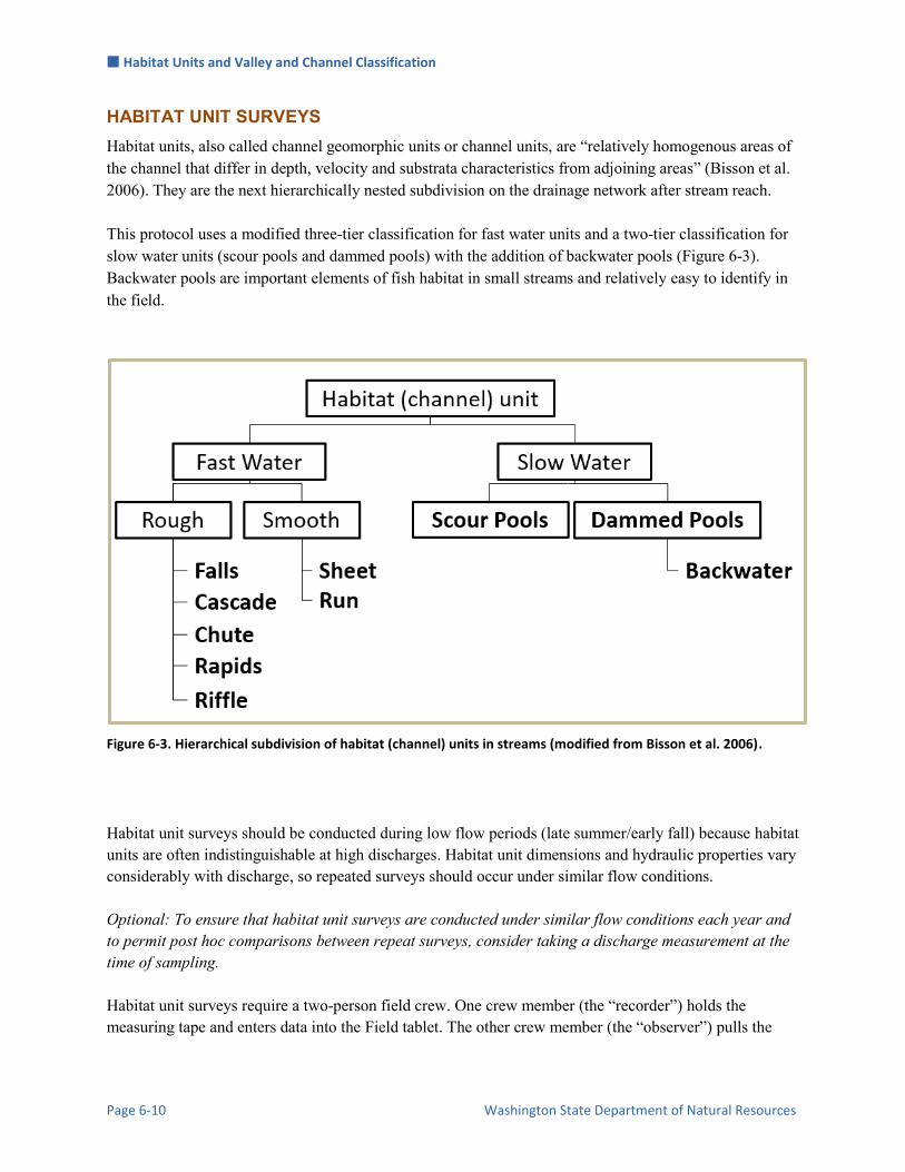
Habitat Units and Valley and Channel Classification
Page 6-10 Washington State Department of Natural Resources
HABITAT UNIT SURVEYS Habitat units, also called channel geomorphic units or channel units, are “relatively homogenous areas of the channel that differ in depth, velocity and substrata characteristics from adjoining areas” (Bisson et al. 2006). They are the next hierarchically nested subdivision on the drainage network after stream reach. This protocol uses a modified three-tier classification for fast water units and a two-tier classification for slow water units (scour pools and dammed pools) with the addition of backwater pools (Figure 6-3). Backwater pools are important elements of fish habitat in small streams and relatively easy to identify in the field.
Figure 6-3. Hierarchical subdivision of habitat (channel) units in streams (modified from Bisson et al. 2006).
Habitat unit surveys should be conducted during low flow periods (late summer/early fall) because habitat units are often indistinguishable at high discharges. Habitat unit dimensions and hydraulic properties vary considerably with discharge, so repeated surveys should occur under similar flow conditions. Optional: To ensure that habitat unit surveys are conducted under similar flow conditions each year and to permit post hoc comparisons between repeat surveys, consider taking a discharge measurement at the time of sampling. Habitat unit surveys require a two-person field crew. One crew member (the “recorder”) holds the measuring tape and enters data into the Field tablet. The other crew member (the “observer”) pulls the

Habitat Units and Valley and Channel Classification
Status and Trends Monitoring of Riparian and Aquatic Habitat in the OESF Page 6-11
zero end of the meter tape to the end of the habitat unit; identifies the unit type and boundary; and measures wetted widths, pool depths, and fall/step heights. Starting from the beginning of the sample reach (cross section A), the crew walks the reach and classifies and measures all habitat units. Include the units that are intersected by the first and last cross-sections (i.e., start below the beginning of the sample reach and/or end beyond the end of the sample reach.
Habitat unit identification is a two-step process. The first step is to identify the unit type. For this study, please refer to the photo and schematic references in the Field Guide for Identifying Stream Channel Types and Habitat Units (Minkova and Vorwerk 2015), which includes hydraulic and geomorphic indicators such as water velocity, water depth, gradient, and bed roughness. Unit types are listed in Figure 6-3. The second step is to identify the boundary where one unit ends and another begins. At first, the location of habitat unit boundaries can seem unclear, but as survey crews become familiar with what to look for, as identified in Minkova and Vorwerk (2015), consistency will develop.
An area of the stream should be counted as a habitat unit if:
1) The overall physical characteristics are clearly different from those of adjacent units, and 2) The length is equal to or greater than the average wetted width of the sample reach (Bisson et al.
2006). Exceptions to this rule are steps and falls, which have no minimum length. Backwater pool length must be at least half the average wetted width of the sample reach.
Stream areas that do not meet the minimum length requirements are lumped with the most similar adjacent unit.
Lumping multiple habitat units into one broader unit (e.g., a string of run-pool-riffle-run might be lumped into one run unit) is allowed if both crew members agree that this is the best way to capture the character of the stream. This can be the case where habitat units are not distinct enough to count using criteria 1 or 2 above. In practice, it is often helpful to use the stream’s average wetted width as a guide to help determine whether to lump or split. Calibration during training is essential to achieve sampling consistency across space and time (see the section on QA/QC below).
It can often be difficult to distinguish between cascades and rapids or between rapids and riffles. When identifying unit types, consider substrate, longitudinal profile, and gradient (i.e., % slope). Use the criteria below as an addendum to the habitat unit guide to help make the tough calls.
Cascades: ≥6% slope, stepped longitudinal profile, large substrate (boulders and large cobble). Rapids: 3-5% slope, somewhat planar longitudinal profile, coarse substrate (cobble, small boulders often submerged – causing eddies). Riffles: <3% slope, fine to moderate substrate (gravel, cobble).
A unit is identified as “subsurface flow” where the main channel becomes dry across its entire width. On small streams, short sections of subsurface flow (intermittency) are common during base flow sample
Habitat Units and Valley and Channel Classification
Page 6-12 Washington State Department of Natural Resources
periods, however if a sample reach is subsurface for more than 10% of its longitudinal profile, the habitat unit survey should not be done.
Measuring Gradient To take a gradient measurement with a clinometer, crew members should first determine where their eye levels correspond to their partner. One crew member stands at the upstream end of the habitat unit and the other stands at the downstream end – both with their feet at the water surface level. One crew member looks through the clinometer, aligns the horizontal crosshair with the predetermined height on his or her partner, and reads the % slope scale (right side) corresponding to that height. Include all gradients taken with a clinometer in the field tablet database “Remarks” field. Gradients can be measured only when a habitat unit is fairly straight. If the unit is on a stream bend, the gradient will be inaccurate.
Habitat unit measurement
Starting at cross section A, measure the length of each habitat unit along the thalweg at water surface level (nearest 0.1 m). If the first habitat unit is intersected by cross section A, measure that habitat unit’s entire length and enter that value into the field tablet database. Note the distance where the unit crosses the reach start, and record the measurement in the “Remarks” field (e.g., “this unit extends 0.5 m below the sample reach”). The survey will progress upstream until the last habitat unit at cross section F. If the last habitat unit extends beyond the reach, record the entire unit length and then note the unit distance outside the sample reach in the “Remarks” field (e.g., “this unit extends 0.5 m above the sample reach”). Use the stadia rod (or meter tape) to collect a minimum of three representative wetted widths per habitat unit (Figure 6-4a). Additional width measurements are recommended for long or complex units. Record each habitat unit’s type, length (nearest 0.1 m), and wetted widths (nearest 0.01 m) in the field tablet database. A subsurface section has a “0” wetted width. Record any notes or photo numbers in the “Remarks” field. If habitat units in the main channel are not arranged linearly and thus overlap, visualize a diagonal dividing line between the units and measure the lengths from the mid-point of that line. Where habitat types occur side-by-side (e.g., a qualifying scour pool next to a riffle), measure and record the length of the dominant unit type and note the type and width of the adjacent unit in the “Remarks” field. Be sure to record the entire wetted width in sections where habitat types occur side-by-side.
If the stream splits into two channels, identify the main channel and side channel based on flow (main channel has higher flow). Identify and measure habitat units within the main channel. For instructions on determining whether a side channel exists and measuring habitat units in the side channel, see the Side Channels section, below.

Habitat Units and Valley and Channel Classification
Status and Trends Monitoring of Riparian and Aquatic Habitat in the OESF Page 6-13
a b
Figure 6-4. Measuring habitat unit wetted width (a) and maximum pool depth (b).
Measuring Falls A water fall (i.e., falls) is a vertical or nearly vertical habitat unit ≥ 0.5 m in height. Measure the height of the falls from the water surface of the lower unit (usually a pool) up to the crest (where the water begins to fall). Record the length (nearest 0.1 m) and a minimum of one width. Falls should also be labeled as either classic or complex in the field tablet “Remarks” field. A classic falls is a well-defined falls over a sheer drop. A complex falls has a series of drops, breaks, or channels (Armantrout 1998). Measuring Steps Steps are abrupt, discrete breaks in channel gradient resulting from elevation changes <0.5 m. Steps are not habitat units per se; they are usually much shorter than the channel width and can separate sequential units of the same type. Measure the height of the step from the water surface of the lower unit up to the crest of the upper unit (where the water begins to fall). Record the length (nearest 0.1 m) and a minimum of one width. Measuring Pools Maximum depth: Probe the pool with the stadia rod to find the maximum pool depth (i.e., largest vertical measurement from stream bed to water surface). Record the depth in the field tablet database (nearest 0.01 m).

Habitat Units and Valley and Channel Classification
Page 6-14 Washington State Department of Natural Resources
Pool tail crest: Use the stadia rod to find and measure the maximum depth along the pool tail crest (the tail crest is the peak instream bed elevation on the downstream end of the pool) (Figure 6-5). For dammed pools, measure the tail crest depth along the top of the obstruction if all flow is going over the obstruction. If no water is flowing over, the tail crest for the dammed pool will be 0 cm (Pleus et al 1999). Record the pool tail crest depth (nearest 0.01 m) in the field tablet database.
Subtract the pool tail crest depth from the maximum pool depth to determine the residual depth. To qualify as a pool, a unit must meet a minimum residual depth, based on the mean reach bankfull width (see Table 6-2). For example, for sample reaches with bankfull widths < 2.5 m, the residual pool depth of a unit must be at least 10 cm.
Table 6-2. Minimum residual pool depth criteria by reach mean bankfull width (from Pleus et al. 1999)
Mean reach Bankfull Width (m) Minimum Residual Pool Depth (m)
0 to < 2.5 0.10
≥ 2.5 to <5.0 0.20
≥ 5.0 to < 10 0.25
≥ 10.0 to < 15 0.30
≥ 15.0 to < 20 0.35
residual pool
pool tail crest
water surface
stream bed
maximum pool depth maximum pool tail crest depth
Figure 6-5. Side profile illustration of a pool and the points of measurements.

Habitat Units and Valley and Channel Classification
Status and Trends Monitoring of Riparian and Aquatic Habitat in the OESF Page 6-15
Side channels
A side channel exists when both of the following criteria are met:
1. There is a stable island or bar in the stream that is higher than bankfull stage and has bankfull indicators present (see Appendix 3A for indicators).
2. The portion of the island/bar that is above bankfull stage has a length at least twice that of the stream’s estimated bankfull width (BFW). Use the average BFW calculated during Channel Morphology sampling. If no measurements have been taken, use the average BFW upstream and downstream of the island/bar.
If any there is a continuous surface flow in the side channel, the channel should be typed for habitat units. Label each side channel habitat unit as “SideChannel” in the field tablet database “Habitat Unit” field. Measure the unit’s length and wetted widths as usual and enter them in the database. Note in the “Remarks” section the type for each habitat unit, the stream side of the side channel, and the approximate distance from the nearest cross-section to the points of divergence and convergence. For example: [habitat unit type]-side channel on stream [left or right]. Side channel diverges 6 m [upstream or downstream] of cross section [A, B, C, D, E, or F] and converges 4 m [upstream or downstream] of cross section [A, B, C, D, E, or F]”.
Time and Cost Estimates for Implementing the Field Procedures The estimated time for classifying valley segment, channel reach, and habitat units and for measuring the habitat units along a 100-m reach is approximately one hour for an experienced two-member crew. Habitat unit classifications should be made by the same “observer” throughout the survey. However, consultation and discussion with the other crew member is highly encouraged. This estimate does not include travel time. All items listed in the Equipment and Supplies section are shared with other protocols, and their costs are detailed in the Channel Morphology protocol.
Procedures for Calculating Metrics All metrics are calculated in the office following the procedures in Table 6-3.

Habitat Units and Valley and Channel Classification
Page 6-16 Washington State Department of Natural Resources
Table 6-3. Procedures for Calculating Metrics
Metric Calculation Procedure
Units/100 m Total number of habitat units per sample reach, adjusted to a 100-m length.
Pools/100 m Total number of pools (scour pool, dammed pool, backwater pool) per sample reach, adjusted to a 100-m length.
Number of habitat units/100 m, by type
For each habitat unit type, the number of units per sample reach is calculated and adjusted to a 100-m length.
Percentage of sample reach allocated to each habitat unit type
Summed length of sample reach allocated to a given habitat type, divided by total reach length, multiplied by 100.
Mean residual pool depth For each pool, residual pool depth is calculated as the maximum depth minus the tail-crest depth. Residual pool depth is then averaged across all pools.
Quality Assurance and Quality Control The quality assurance for the Habitat Units and Valley and Channel Classification protocol includes staff training and the use of standardized protocols. The quality control for the field procedures includes annual field checks. The QA/QC procedures for data management are described in the Data Management section below.
TRAINING All personnel conducting field protocols will be trained in a consistent manner to ensure that the surveys are conducted properly and in standardized fashion. The training is conducted or, in case of returning personnel, reviewed, annually before the start of the field season. At least one member of the field crew should be experienced with the field procedures. One of the most important tasks for the classification procedures is to calibrate the observers so they are consistently identifying the features. One member of the crew, the observer, is assigned to make the final call if there is disagreement on the classification result.
STANDARD PROTOCOLS The standard procedures described in this protocol are followed for the duration of the project. Any deviations from the procedures should be documented, and the reasons for deviation described and discussed with the project manager or the researcher overseeing the protocol implementation. Changes to the published protocols are approved by the project manager or by the researcher overseeing the protocol implementation. Revised protocols are assigned new version numbers and publication dates.

Habitat Units and Valley and Channel Classification
Status and Trends Monitoring of Riparian and Aquatic Habitat in the OESF Page 6-17
FIELD CHECKS The researcher overseeing the protocol implementation or a different field crew will conduct spot checks on 10% of the field measurements every year.
Data Management
DATA FLOW All habitat unit data are recorded in the field using paper field forms (2013-2014 field seasons) or a ruggedized field tablet (2015 field season onward). In the office, data are then transferred to a database for long-term storage. The steps below detail the process.
Data flow for paper field forms
1. Fill out field forms Paper field forms are used to record data and metadata at each sample reach. 2. Scan and store field forms After returning from the field each week, the field forms are scanned
and stored on the WADNR network drive; the original paper forms are archived by the OESF Data Management Specialist at the Washington Department of Natural Resources Forest Resources Division.
3. Enter data All habitat unit data collected on paper field forms are entered in the “Habitat_LWD_Database” by the OESF Data Management Specialist on a weekly basis. After each field form is entered, the Specialist writes “Entered” on the form, followed by his or her initials and the date.
4. Quality control Entered field form data are verified by comparing the data on the field form to the data in the database. This process is performed by someone other than the person who originally entered the data. After the data are verified, the person who verified it writes “Verified” on the field form, followed by his or her initials and the date.
Data flow for electronically collected data
1. Fill out forms on electronic field data recorder Field personnel record all habitat unit data using the “Tablet Database”, which is a customized database created in Microsoft Access and saved on the field tablet.
2. Store field data At the end of each day in the field, a copy of the Tablet Database, containing all data collected to date, is transferred to the OESF Data Management Specialist via cloud storage or email. If internet access is not available, the field crew makes a daily backup copy of the database on a laptop or other storage device and then transfers the data to the Data Management Specialist after returning to the Natural Resources Building at the end of the week. The OESF Data Management Specialist stores these Tablet Database copies in a temporary location on the WADNR network drive (J:\hcp\monitoring_research\tminkova\01_OESF_R&M Program\01_Rip S&T Mon\07_Data management\_All new data and photos\) until they are processed and the data are transferred to a database for long-term storage.
3. Quality control Because data are recorded electronically, and thus never transcribed, transcription errors do not exist. However, there is still a possibility of data entry errors in the
Habitat Units and Valley and Channel Classification
Page 6-18 Washington State Department of Natural Resources
field. In particular, if metadata (e.g., the date of a field visit or a watershed ID) are recorded incorrectly in the field, this could cause errors during the process of importing data from the Tablet Database to the Habitat_LWD_Database (next step; see below). For this reason, metadata are examined for accuracy prior to importing data to the Habitat_LWD_Database.
4. Import data to database On a weekly basis, the OESF Data Management Specialist imports all new data from the Tablet Database to the Habitat_LWD_Database. This is accomplished using a set of queries stored in a third database: J:\hcp\monitoring_research\tminkova\01_OESF_R&M Program\01_Rip S&T Mon\01_FIELD DATA\01_Stream survey\Data\ Distribute_Tablet_Data.accdb
5. Verify transfer of data After data have been imported, the OESF Data Management Specialist verifies that no records have been missed, using the record count queries built into the Distribute_Tablet_Data database.
Photographs
1. Transfer photos to data manager for storage All digital photographs taken in the field are transferred to the OESF Data Management Specialist at the end of each week. The Specialist temporarily stores the uncatalogued photos on the WADNR server at: J:\hcp\monitoring_research\tminkova\01_OESF_R&M Program\01_Rip S&T Mon\07_Data management\_All new data and photos\
2. Rename and archive photos The OESF Data Management Specialist renames each photo using the following naming convention: <Photo type>_<WatershedID>_<Date taken>_<Original photo name> (for example: ER_797_20140715_P1000851.JPG). The photos are then moved to long-term storage in the following directory: J:\hcp\monitoring_research\tminkova\01_OESF_R&M Program\01_Rip S&T Mon\03_Photos and videos\04_Stream_survey\
DATA STORAGE
Paper field forms
The paper field forms are archived at the Washington Department of Natural Resources Forest Resources Division. The designated data steward is Teodora Minkova, WADNR. Scanned copies of these forms are saved in the Adobe portable document format (.pdf) in the following directory: J:\hcp\monitoring_research\tminkova\01_OESF_R&M Program\01_Rip S&T Mon\01_FIELD DATA\01_Stream survey\Data\Data archive\Field forms\
Tablet databases
The original Tablet Databases, which are transferred to the OESF Data Management Specialist on a daily or weekly basis, are stored on the WADNR network drive after the field data they contain have been transferred to the Habitat_LWD_Database. The storage location for these databases is: J:\hcp\monitoring_research\tminkova\01_OESF_R&M Program\01_Rip S&T Mon\01_FIELD DATA\01_Stream survey\Data\Data archive\Processed tablet databases\

Habitat Units and Valley and Channel Classification
Status and Trends Monitoring of Riparian and Aquatic Habitat in the OESF Page 6-19
Long-term data storage
The ultimate location of the habitat unit data is the Habitat_LWD_Database, located on the WADNR network drive at: J:\hcp\monitoring_research\tminkova\01_OESF_R&M Program\01_Rip S&T Mon\01_FIELD DATA\01_Stream survey\Data\Habitat_LWD_Database.accdb Within the Habitat_LWD_Database, the habitat data are stored in two related tables: the Habitat Survey Table and the Habitat Data Table (Figure 6-6). The Habitat Survey Table contains the metadata from each survey, and the Habitat Data Table contains the habitat unit data. The Habitat Survey Table is related to the Habitat Data Table through a one-to-many relationships: a single record in the Survey Table is related to multiple records in the Data Table. The fields in the two habitat unit database tables are described in Tables 6-3 and 6-4.
Figure 6-6. The structure of the habitat portion of the Habitat_LWD Database.

Habitat Units and Valley and Channel Classification
Page 6-20 Washington State Department of Natural Resources
Table 6-3. Fields in the Habitat Survey table in the Habitat_LWD database.
Field Field description
SurveyID(Auto) A unique identifier for each record in the table.
BasinID Watershed identifier.
Date_Surveyed The date of the habitat unit survey.
Time_Started The time of day that the survey began.
Time_Ended The time of day that the survey ended.
Camera The ID of the camera that was used.
Remarks Remarks.
Valley_Segment_Type The valley segment type.
Channel_Type The channel type.
Crew_tablet The initials of the crew members.
Table 6-4. Fields in the Habitat Data table in the Habitat_LWD database.
Field Field description
HabitatUnitID(Auto) Unique identifier for each record in the table.
SurveyID A value that links the record to the appropriate metadata in the LWD Survey Table.
Length Length of the habitat unit (m).
Side_Channel If the unit occurs on a side channel, then a “Y” is recorded in this field.
Habitat_Unit Habitat unit type.
Width1 Width of unit (m).
Width2 Width of unit (m).
Width3 Width of unit (m).
Width4 Width of unit (m).
Width5 Width of unit (m).
Width6 Width of unit (m). (More than five widths are measured only on rare occasions.)
Width7 Width of unit (m). (More than five widths are measured only on rare occasions.)
Width8 Width of unit (m). (More than five widths are measured only on rare occasions.)
Width9 Width of unit (m). (More than five widths are measured only on rare occasions.)
Mean_Width Mean width of the habitat unit (m). (This field is automatically calculated.)
Pool_Depth_Max Maximum pool depth (cm).
Pool_Depth_Tail_Crest Pool depth at tail crest (cm).
Falls_Height Falls height (m).
Remarks Remarks.
Habitat Units and Valley and Channel Classification
Status and Trends Monitoring of Riparian and Aquatic Habitat in the OESF Page 6-21
DATA QUALITY CONTROL Prior to data analysis, all fields in the data tables are assessed to identify potentially erroneous values. The first step is to examine individual fields, one at a time. For categorical data fields (e.g., habitat unit type) and date or time fields, every field is assessed to identify any records exhibiting the following:
1. Missing values. 2. Illogical values.
In some cases, where the data collector is free to enter values rather than selecting values from a predefined list, illogical values may be recorded (e.g., a survey time of 3:00 AM). For numerical fields, each is assessed for the following:
1. Missing values. 2. Outlier values (e.g., a stream width was recorded in cm instead of m).
The next step in quality control assessment is to examine derived values and values in the context of other fields. An example of a derived value is the lengths of all habitat units in a sample reach added together. If the sum of habitat unit lengths is significantly less than the length of the sample reach, then the data should be examined to determine if one of the habitat unit lengths was recorded incorrectly. An example of checking a value in the context of another field is the comparison of a maximum pool depth with the tail crest of the same pool. If the tail crest is significantly greater than the maximum pool depth, there may be an error in the data. When missing values are discovered, it is generally not possible to “fill in the blank” from the office. The fact that data are missing should be recorded, in brackets, in the “Remarks” field, with the initials of the person who performed the quality control check (e.g., [Pool_Depth_Max was not recorded. –WD]). Illogical or outlier values can sometimes be corrected in the office. For example, AM and PM might have been switched or a decimal place error can be corrected. When data are corrected, this must be noted in the remarks field, in brackets, with the initials of the person who performed the quality control check. For example: [Width2 was recorded as 50 m. This was clearly incorrect and changed to 5.0 which is logical given the other widths for that unit. –WD]. In many cases, clearly erroneous outlier values cannot be corrected in the office and should be edited so as not to affect the results of analysis. In such cases, the value should be removed from the field and transferred to the “Remarks” field with an explanation, in brackets, with the initials of the person who performed the quality control check. For example: [Width2 was recorded as 74.8 m. This was clearly incorrect and removed from the dataset. –WD]).

Habitat Units and Valley and Channel Classification
Page 6-22 Washington State Department of Natural Resources
References Armantrout, N.B., compiler. 1998. Glossary of aquatic habitat inventory terminology. American Fisheries
Society. Bethesda, Maryland.
Bisson, P.A., R.E. Bilby, M.D. Bryant, C.A. Dolloff, G.B. Grette, R.A. House, M.L. Murphy, K.V. Koski, and J.R. Sedell. 1987. Large woody debris in forested streams in the Pacific Northwest: Past, present, and future. Pages 143–190 in E.O. Salo, and T.W. Cundy (Eds.) Streamside Management: Forestry and Fishery Interactions. Contribution Number 57, Institute of Forest Resources, University of Washington, Seattle, WA.
Bisson, P.A., D.R. Montgomery, and J.M. Buffington. 2006. Valley segments, stream reaches, and channel units. In: Methods in Stream Ecology. Second Edition, edited by F.R. Hauer and G.A. Lamberti, Academic Press, pp. 23-49.
Bouwes, N., J. Moberg, N. Weber, B. Bouwes, S. Bennett, C. Beasley, C.E. Jordan, P. Nelle, M. Polino, S. Rentmeester, B. Semmens, C. Volk, M.B. Ward, and J. White. 2011. Scientific protocol for salmonid habitat surveys within the Columbia Habitat Monitoring Program. Prepared by the Integrated Status and Effectiveness Monitoring Program and published by Terraqua, Inc., Wauconda, WA. 118 pages.
Bryant, M. D. 1980. Evolution of Large, Organic Debris After Timber Harvest: Maybeso Creek, 1949 to 1978. United States Forest Service, General Technical Report PNW-101, Pacific Northwest Forest and Range Experiment Station, Portland, OR.
Buffington, J.M., R.D. Woodsmith, D.B. Booth, and D R. Montgomery. 2003. Fluvial processes in Puget Sound Rivers and the Pacific Northwest. Pages 46–78 in D.R. Montgomery, S. Bolton, D.B. Booth, and L.Wall (Eds.) Restoration of Puget Sound Rivers. University of Washington Press, Seattle, WA.
Buffington, J.M., and D.R. Montgomery. 1999. Effects of hydraulic roughness on surface textures of gravel-bed rivers. Water Resources Research 35: 3507–3522.
Frissell, C.A., W.J. Liss, C.E. Warren, and M.D. Hurley. 1986. A hierarchical framework for stream habitat classification: viewing streams in a watershed context. Environmental Management 10: 199-214.
Grant, G.E., F.J. Swanson, and M.G. Wolman. 1990. Pattern and origin of stepped-bed morphology in high-gradient streams, Western Cascades, Oregon. Geological Society of America Bulletin 102: 340–352.
Keller, E.A., and W.N. Melhorn. 1978. Rhythmic spacing and origin of pools and riffles. Geological Society of America Bulletin 89:723–730.
Lanigan, S., P. Eldred, C. Moyer, H. Andersen, M. Isley, and S. Wilcox. 2010. Aquatic and Riparian Effectiveness Monitoring Program for the Northwest Forest Plan – 2010 Field Protocol Manual. http://www.reo.gov/monitoring/reports/watershed/2010.FieldProtocol.Final.pdf
Leopold, L.B., M.G. Wolman, and J.P. Miller. 1964. Fluvial Processes in Geomorphology. W. H. Freeman, San Francisco, CA.
Lisle, T.E. 1986. Effects of woody debris on anadromous salmonid habitat, Prince of Wales Island, southeast Alaska. North American Journal of Fisheries Management 6:538–550.

Habitat Units and Valley and Channel Classification
Status and Trends Monitoring of Riparian and Aquatic Habitat in the OESF Page 6-23
Minkova, T. and M. Vorwerk. 2015. Field guide for identifying stream channel types and habitat units in Western Washington. Washington State Department of Natural Resources, Forest Resources Division, Olympia, WA. 54 p.
Montgomery, D. R, and J.M. Buffington. 1993. Channel classification, prediction of channel response, and assessment of channel condition. Report TFW-SH-93-002 prepared for the SHAMW committee of the Washington State Timber/Fish/Wildlife Agreement.
Montgomery, D. R, and J.M. Buffington. 1997. Channel-reach morphology in mountain drainage basins. Geological Society of America Bulletin 109: 596–611.
Pleus A.E., D. Schuett-Hames, and L. Bullchild. 1999. Timber, Fish, and Wildlife Monitoring Program - Method Manual for the Habitat Unit Survey. Washington Department of Natural Resources, Olympia, WA.
Yang, C.T. 1971. Formation of riffles and pools. Water Resources Research 7:1567–1574.

Habitat Units and Valley and Channel Classification
Page 6-24 Washington State Department of Natural Resources
This page intentionally left blank.
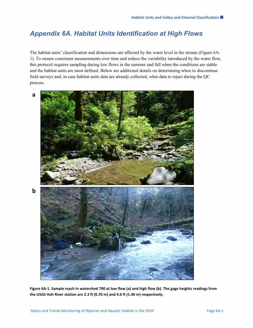
Habitat Units and Valley and Channel Classification
Status and Trends Monitoring of Riparian and Aquatic Habitat in the OESF Page 6A-1
Appendix 6A. Habitat Units Identification at High Flows
The habitat units’ classification and dimensions are affected by the water level in the stream (Figure 6A-1). To ensure consistent measurements over time and reduce the variability introduced by the water flow, this protocol requires sampling during low flows in the summer and fall when the conditions are stable and the habitat units are most defined. Below are additional details on determining when to discontinue field surveys and, in case habitat units data are already collected, what data to reject during the QC process.
a
b
Figure 6A-1. Sample reach in watershed 790 at low flow (a) and high flow (b). The gage heights readings from
the USGS Hoh River station are 2.3 ft (0.70 m) and 4.6 ft (1.40 m) respectively.

Habitat Units and Valley and Channel Classification
Page 6A-2 Washington State Department of Natural Resources
The determination is a two-step process: 1) screening of online data prior to the field and 2) if necessary, field assessment of site conditions.
Step 1. Check online data
Check the latest data from USGS Hoh River flow monitoring station. Visit http://waterdata.usgs.gov/wa/nwis/uv?site_no=12041200 and look at the parameter Gage height in tabular format.
If the last gage height reading is above 4.27 ft (1.30 m) and the water level is not declining, do not survey habitat units. If data have been collected during this flow it should be rejected.
If the last gage height reading is between 3.3 ft (1 m) and 4.27 ft (1.30 m) or the reading is closely above 4.27 ft (1.30 m) and the water level is declining, visit the site and do field assessment described in Step 2.
Our analyses showed similar flow patterns between the four USGS monitoring stations on the western Olympic Peninsula, therefore it is sufficient to use only one for online screening. If the precipitation event differs considerably between southern and northern part of the study area, check the gage height of the USGS Hoko River monitoring station (http://waterdata.usgs.gov/wa/nwis/uv?site_no=12043300) prior to visiting the sample reaches in the Clallam landscape.
Our analyses showed less than 12-hour delay between high peak flows in the sample reaches and the Hoh River station, therefore the latest gage height reading form that station is appropriate screening tool.
Step 2. Field assessment of the sample reach
Walk portion of the sample reach and observe the flow and safety conditions. Do not survey for habitat units if any of the following conditions are met:
The conditions are not safe (e.g. high water velocity, mobilized wood pieces) The demarcation lines between fast and slow water habitat units are not clearly visible (e.g.
between pool-riffle and pool) The water flow conditions look very different from the previous habitat unit survey Compare with the habitat unit data and pictures from previous surveys. When in doubt, ask a project researcher for advice.
Record the Hoh River gage height reading and your field observations in the Notes section on the field tablet.

Stream Temperature
Status and Trends Monitoring of Riparian and Aquatic Habitat in the OESF Page 7-1
Stream Temperature
Authors: Alex Foster, Warren Devine, Mitchell Vorwerk
Version: 1.4
Revision History:
Based on the Following Protocols: This protocol is based on two published protocols: Washington State Department of Ecology’s (WADOE) Standard Operating Procedures for Continuous Temperature Monitoring of Fresh Water Rivers and Streams Conducted in a Total Maximum Daily Load (TMDL) Project for Stream Temperature, version 3.0 (Bilhimer et al. 2013) and USDA Forest Service’s Measuring Stream Temperature with Digital Data Loggers: A User’s Guide (Dunham et al. 2005).
Reasons to Adopt the Above Protocols: WADOE already has three active, long-term monitoring sites established in the Olympic Experimental State Forest (OESF) and once had seven additional sites in the area. Thus, data-sharing between agencies would be mutually beneficial. The active WADOE sites in the OESF are included in a national network for stream temperature monitoring maintained by the U.S. Forest Service Rocky Mountain Research Station (http://www.fs.fed.us/rm/boise/AWAE/projects/stream_temperature.shtml). WADOE metrics are the same as those used by most other regional water monitoring efforts, and the field procedures have been proven in western Washington streams. Dunham et al. (2005) provides further information about sampling interval specifications, logger accuracy testing, and data analysis. WADOE uses Dunham et al. (2005) as a reference for its protocols.
Purpose and Content: The purpose of this monitoring protocol is to describe the sampling and data management necessary to document and report the status and multi-year trends of stream temperature in the monitored watersheds. It details the field procedures for deployment, maintenance, and downloading of temperature data loggers (thermistors), the field quality assurance and quality control steps, and the data management procedures.
Protocol
Version Purpose / Changes Author(s) Reviewer(s)
Publication
Date
1.0 Initial draft presented to project staff
Alex Foster Peter Bisson, Teodora Minkova
04/02/2013
1.1 Draft submitted to external review
Alex Foster Rebecca Flitcroft, Ashley Steel
04/16/2013
1.2 Draft incorporating external reviews, sampling procedures from 2013 field season, and data mgmt. procedures
Alex Foster, Warren Devine, Mitchell Vorwerk
Teodora Minkova, Ellis Cropper
12/03/2015
1.3 Final draft with field and data management procedures updated from 2014 and 2015 field seasons
Alex Foster, Warren Devine, Mitchell Vorwerk
Teodora Minkova 05/11/2016
1.4 Final technical review and edit Alex Foster, Warren Devine, Mitchell Vorwerk
Paul Dunnette, Warren Devine, Alex Foster
12/18/2016
Stream Temperature
Page 7-2 Washington State Department of Natural Resources
Table of Contents Introduction ..................................................................................................................................................... 7-3
Monitoring Design .......................................................................................................................................... 7-3
Spatial Sampling design .............................................................................................................................. 7-3
Temporal Sampling design ......................................................................................................................... 7-3
Equipment and Supplies .................................................................................................................................. 7-5
Testing Temperature Logger Accuracy ....................................................................................................... 7-6
Launching the Temperature Loggers .......................................................................................................... 7-6
Field Procedures .............................................................................................................................................. 7-6
Sampling Site Selection .............................................................................................................................. 7-6
Deployment Options ................................................................................................................................... 7-7
Downloading Procedures .......................................................................................................................... 7-11
Time and Cost Estimates for Implementing the Field Procedures ................................................................ 7-12
Procedures for Calculating Metrics ............................................................................................................... 7-12
Quality Assurance and Quality Control ........................................................................................................ 7-13
Training ..................................................................................................................................................... 7-14
Standard Protocols .................................................................................................................................... 7-14
Testing Data Loggers ................................................................................................................................ 7-14
Data Management ......................................................................................................................................... 7-14
Data Flow .................................................................................................................................................. 7-14
Data Storage .............................................................................................................................................. 7-21
Data Products ............................................................................................................................................ 7-24
References ..................................................................................................................................................... 7-26
Appendix 7A. Stream Temperature Monitoring Field Form ....................................................................... 7A-1
Appendix 7B. Stream Temperature Monitoring Installation Field Form ..................................................... 7B-1
Appendix 7C. Tables in the Stream Temperature Database ........................................................................ 7C-1
Stream Temperature
Status and Trends Monitoring of Riparian and Aquatic Habitat in the OESF Page 7-3
Introduction All aquatic life forms have a temperature range within which they can survive. Temperature changes can affect stress, mortality, and life histories of all aquatic species (i.e., invertebrates, fish, and amphibians) (Hauer and Hill 2006). Federal endangered species listings of trout and salmon cite increasing stream temperatures as a limiting factor for population recovery. As such, increases in stream temperature can affect embryonic development; juvenile growth; adult migration; competition with non-native species; and the relative risk and severity of disease (Sullivan et al. 2000). Stream temperature is a function of multiple energy transfer processes, including solar and long-wave input, air convection, stream bed conduction, groundwater flux, hyporheic flux, evaporation, and condensation. Solar radiation, as a function of the amount of surface area of unshaded water, is a primary contributor to daily maximum summer stream temperature. This process responds directly to riparian tree canopy removal resulting from logging, windthrow, wildfires, or mass wasting (Poole and Berman 2001, Moore et al. 2005). In the environmental impact analysis for the Olympic Experimental State Forest (OESF) Forest Land Plan, stream temperature was recognized as an important indicator for fish habitat quality, riparian area function, and water quality (WADNR 2013). Because comprehensive stream temperature data was not available at the time of the analysis, stream shade was used as a surrogate.
Monitoring Design
SPATIAL SAMPLING DESIGN Stream temperature is measured in each of the 50 sample reaches in the OESF and the four reference sample reaches in Olympic National Park (ONP). Refer to the Project Background chapter for a map of the sample watersheds. One water temperature data logger and one air temperature data logger are installed at each sample site (Figure 7-1). The water and air data loggers are always paired and installed in close proximity to each other. The air and water temperature digital records are compared to determine whether the water temperature data logger was de-watered (i.e., exposed to air) at any point during its deployment.
TEMPORAL SAMPLING DESIGN
Sampling Interval
Both air and water temperature data loggers are deployed year-round and set to record temperature every 60 minutes. For the western Olympics, this interval provides a less than one percent probability of missing the maximum and minimum daily temperatures (Dunham et al. 2005). At this interval, the data loggers’ memory limits and battery life will allow continuous recording for up to 5 years.

Stream Temperature
Page 7-4 Washington State Department of Natural Resources
Figure 7-1. Typical location of water and air temperature data loggers within a sample reach. Water and air loggers are always installed close together, though not necessarily between cross-sections B and C.

Stream Temperature
Status and Trends Monitoring of Riparian and Aquatic Habitat in the OESF Page 7-5
Download Schedule
Data will be downloaded and the loggers inspected at least once a year and preferably twice annually: in spring to check for dewatering, winter damage, and loss of loggers due to high flows; and in the fall to collect summer temperatures and check the status of installations to reduce the risk of damage or loss during upcoming winter high flows. It is most efficient to download data and inspect loggers when the sample sites are visited for other monitoring purposes.
Equipment and Supplies The following equipment and supplies are needed for initial data logger installation, replacement of lost or damaged loggers, and data download:
Onset© HOBO TidbiT v2 thermistors
Onset© HOBOware Pro software
Onset© HOBO Waterproof Shuttle (optical data shuttle for data download)
Ruggedized field tablet with data logger location photos and descriptions of observations from previous visits (optional) or Rite in the Rain™ field forms
Pre-drilled 1.5 inch diameter (43 mm) #80 PVC pipe cut to 6 cm long housings
Size No. 72 tar-coated nylon braided cordage
8 in (20 cm) nylon cable (zip) ties
10 gauge copper wire
Pre-drilled 8 oz (240 ml) #5 white plastic cup shade devices
Wire cutter/pliers
Pre-assembled anchor brick with soldered copper wire loop for cord tether installations
Pre-assembled PVC capped enclosures and tools for epoxy mount installations
Adjustable, prefabricated, or 1-inch open end wrench (for installing/removing caps on epoxy mount installations)
No. 10 hot dipped galvanized nails (can also be used for epoxy mount cap removal)
4 lb hammer
Blue spray paint and blue flagging for marking logger locations
Leatherman pliers or knife (needed to cut/remove the cable ties)
Lighter (used to melt the tips of the cordage to prevent fraying)
Stream Temperature
Page 7-6 Washington State Department of Natural Resources
TESTING TEMPERATURE LOGGER ACCURACY While the data loggers (Onset© HOBO TidbiT v2 thermistors) cannot be adjusted following factory calibration, they should be tested in a controlled environment to determine whether they are recording within their specifications before deployment. The testing process is described on the Onset© website (http://www.onsetcomp.com/support/tech-notes/quick-temp-accuracy-check-ice-bath) and is summarized here. Testing multiple data loggers at once saves time and can reveal loggers that may be unsuitable for deployment. The data loggers should be launched prior to testing and set to record at a 1-to-5-minute interval. To test the loggers, place crushed ice in an ice chest large enough to hold the loggers being tested. Crushing the ice will help maintain a consistent, uniform temperature. Fill the ice chest with water to just below the level of the ice and stir. String the loggers together and submerge them in the ice water. Place a certified thermometer in the ice water to monitor temperature. To minimize temperature gradients, place the ice chest in a refrigerator. The ice will melt slowly, so the actual temperature should settle around 0 °C if the ice bath was prepared correctly. Leave the loggers in the ice bath for a minimum of one hour, though immersion in the bath for several hours is preferable because it allows the loggers to fully acclimate. The test should provide enough data to allow for comparisons to temperatures recorded by the thermometer and to the manufacturer’s specifications on temperature drift and accuracy (the accuracy standard is +/- 0.2 °C). Check and record the water temperature when the data loggers are removed from the ice bath. Record the date, time, and results in a spreadsheet for each data logger. If data recorded by a logger do not fall within the temperature accuracy standard or have high variability (drift) compared to other loggers, the logger should not be deployed but should be retested.
LAUNCHING THE TEMPERATURE LOGGERS Set the clock on the computer used to launch the loggers to Pacific Standard Time (PST) through the use of the atomic clock (e.g., http://www.time.gov/timezone.cgi?Pacific/d/-8/java). This ensures that all loggers will record data at exactly the same times. Program all the loggers for a common delayed launch time that starts after the planned field deployment time and date (usually 12:00 a.m. PST if deployed the day before).
Field Procedures
SAMPLING SITE SELECTION Stream temperature loggers should be deployed in the lower half of the sample reach, within the active channel and close to the permanently marked reference point. Look for a suitable anchor location to securely attach the data logger (see details below). The location should be shielded from direct sunlight and provide protection from high flows. Avoid locations just downstream of tributaries, backwater areas, riparian

Stream Temperature
Status and Trends Monitoring of Riparian and Aquatic Habitat in the OESF Page 7-7
wetlands, and potential hillslope groundwater seeps because these features may seasonally bias the recorded temperatures. Consider locations upstream of these features. Loggers should be deployed deep enough to prevent exposure to air (dewatering) during low-flow periods but far enough above the stream bed to avoid recording temperatures affected by groundwater inflow. In small streams, deployment ~10 cm (4 in) above the stream bed is ideal. In reaches where loggers are deployed using cord tether installations (see below), this is facilitated by attaching the logger to an anchor weight (brick). In small streams, placing the data logger in a pool will often ensure it does not dewater during base flow. However, pools are turbulent during high flows, so care should be taken concerning the anchoring location (see below). In larger streams, a deep riffle or glide may be the preferred location. If necessary, place cobbles or boulders around and on top of the data logger to protect it from high flows.
DEPLOYMENT OPTIONS
Housing and Assemblies for Water Temperature Data Loggers
In small and/or low-gradient streams, loggers are deployed inside a PVC housing attached to a brick and tied to an anchor point in or along the stream with a nylon cord (cord tether installations; Figures 7-2B, 7-3C). The camouflaged (i.e., painted green) housing protects and hides the logger and minimizes indirect solar radiation. In streams where high gradient and/or stronger currents increase the probability of logger loss or damage, loggers are often encased in a different PVC housing that is affixed to a boulder below the water surface using epoxy (epoxy mount installations; Figures 7-2C, 7-3D). For cord tether installations, affix the logger within the PVC housing by threading a nylon cable (zip) tie through the hole in the logger casing (Figure 7-2A) and two holes drilled on opposite sides of the PVC (Figure 7-2B). Use another cable tie to attach the housing to a soldered copper wire wrapped around a brick, which will keep the assembly submerged and minimize movement. Due to corrosion and possible logger loss, do not use steel or aluminum cable, wire, or fasteners. A tar-coated, nylon braided cord is used to attach the assembly to the selected anchor (see below).
A B C
Figure 7-2. Assemble a temperature logger (A) in a PVC cover using nylon cable ties (for cord tether installations) (B) or a PVC cover (for epoxy mount installations) (C).

Stream Temperature
Page 7-8 Washington State Department of Natural Resources
A B
C D
Figure 7-3. Examples of anchor points for water temperature data loggers: (A) Live tree root; (B) tree trunk; (C) copper wire wrapped around the connection point of two boulders; (D) PVC enclosure mounted under water on the downstream side of a boulder.
Anchors for Water Temperature Data Loggers
Water temperature loggers are anchored to streamside or in-stream structures such as live tree roots, boulders, and woody debris (Figure 7-3). In order of preference these are: 1) Large boulders for epoxy mount installations (Figure 7-3D); 2) Live tree root at least 7 cm (2.5 in) in diameter (cord tether; Figure 7-3A); 3) Tree trunk close to the water’s surface (cord tether; Figure 7-3B); 4) Copper wire wrapped around the connection point of two boulders (“wedged rock”) that is close to the water’s surface (cord tether; Figure 7-3C); 5) Rebar driven into large, non-mobile, and solid woody debris (cord tether); and 6) Rebar driven into stream bed or stream bank (cord tether). Please note that for options 2-6, the anchor point should be as close to the water’s surface as possible during low flow installation.
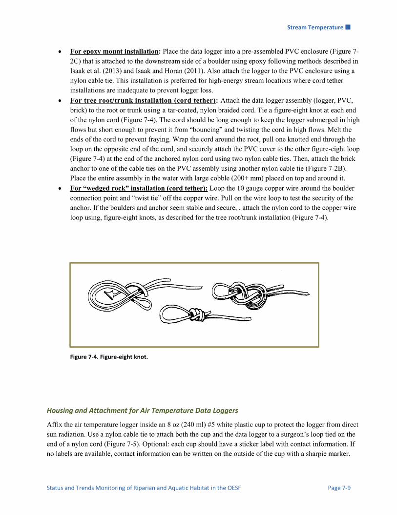
Stream Temperature
Status and Trends Monitoring of Riparian and Aquatic Habitat in the OESF Page 7-9
For epoxy mount installation: Place the data logger into a pre-assembled PVC enclosure (Figure 7-2C) that is attached to the downstream side of a boulder using epoxy following methods described in Isaak et al. (2013) and Isaak and Horan (2011). Also attach the logger to the PVC enclosure using a nylon cable tie. This installation is preferred for high-energy stream locations where cord tether installations are inadequate to prevent logger loss.
For tree root/trunk installation (cord tether): Attach the data logger assembly (logger, PVC, brick) to the root or trunk using a tar-coated, nylon braided cord. Tie a figure-eight knot at each end of the nylon cord (Figure 7-4). The cord should be long enough to keep the logger submerged in high flows but short enough to prevent it from “bouncing” and twisting the cord in high flows. Melt the ends of the cord to prevent fraying. Wrap the cord around the root, pull one knotted end through the loop on the opposite end of the cord, and securely attach the PVC cover to the other figure-eight loop (Figure 7-4) at the end of the anchored nylon cord using two nylon cable ties. Then, attach the brick anchor to one of the cable ties on the PVC assembly using another nylon cable tie (Figure 7-2B). Place the entire assembly in the water with large cobble (200+ mm) placed on top and around it.
For “wedged rock” installation (cord tether): Loop the 10 gauge copper wire around the boulder connection point and “twist tie” off the copper wire. Pull on the wire loop to test the security of the anchor. If the boulders and anchor seem stable and secure, , attach the nylon cord to the copper wire loop using, figure-eight knots, as described for the tree root/trunk installation (Figure 7-4).
Figure 7-4. Figure-eight knot.
Housing and Attachment for Air Temperature Data Loggers
Affix the air temperature logger inside an 8 oz (240 ml) #5 white plastic cup to protect the logger from direct sun radiation. Use a nylon cable tie to attach both the cup and the data logger to a surgeon’s loop tied on the end of a nylon cord (Figure 7-5). Optional: each cup should have a sticker label with contact information. If no labels are available, contact information can be written on the outside of the cup with a sharpie marker.

Stream Temperature
Page 7-10 Washington State Department of Natural Resources
Air temperature loggers should be located close to water temperature data loggers. Attach the air temperature assembly to a branch or nail on the north side of a live conifer tree with full canopy (Lundquist and Huggett 2008). Place the assembly not more than 2.5 m above the stream channel but at least one meter above the ground and within 5 m of the water logger. Branches lower on the bole of the tree will provide better shading year-round.
A B
Figure 7-5. Housing (A) and attachment (B) of air temperature logger.
Marking and Referencing the Location of Temperature Data Loggers
Mark all temperature sampling locations with blue flagging and blue paint. Measure and record the slope distance and azimuth from the top of the RP rebar to the water data logger anchor point (Figure 7-6). Measure and record the slope distance and azimuth from the water temperature data logger anchor point to the air temperature data logger. Take photos of the locations of both loggers. Record the locations and photo numbers on the installation field form (Appendix 7B). If a logger needs to be moved or is missing and needs to be replaced, take the appropriate action and enter new remarks and notes on the field form (Appendix 7A). Installation in a new location should be recorded in the installation field form (Appendix 7B). Reflag and paint the new location and take a picture of the station.
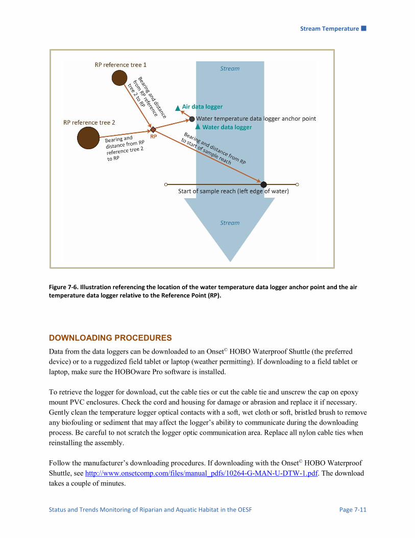
Stream Temperature
Status and Trends Monitoring of Riparian and Aquatic Habitat in the OESF Page 7-11
Figure 7-6. Illustration referencing the location of the water temperature data logger anchor point and the air temperature data logger relative to the Reference Point (RP).
DOWNLOADING PROCEDURES Data from the data loggers can be downloaded to an Onset© HOBO Waterproof Shuttle (the preferred device) or to a ruggedized field tablet or laptop (weather permitting). If downloading to a field tablet or laptop, make sure the HOBOware Pro software is installed. To retrieve the logger for download, cut the cable ties or cut the cable tie and unscrew the cap on epoxy mount PVC enclosures. Check the cord and housing for damage or abrasion and replace it if necessary. Gently clean the temperature logger optical contacts with a soft, wet cloth or soft, bristled brush to remove any biofouling or sediment that may affect the logger’s ability to communicate during the downloading process. Be careful to not scratch the logger optic communication area. Replace all nylon cable ties when reinstalling the assembly. Follow the manufacturer’s downloading procedures. If downloading with the Onset© HOBO Waterproof Shuttle, see http://www.onsetcomp.com/files/manual_pdfs/10264-G-MAN-U-DTW-1.pdf. The download takes a couple of minutes.

Stream Temperature
Page 7-12 Washington State Department of Natural Resources
Always record the loggers’ serial numbers and the watershed number on the field forms (Appendices 7A or 7B).
Time and Cost Estimates for Implementing the Field Procedures Tables 7-2 and 7-3 show the time and cost estimates for implementing the field procedures of the stream temperature protocol. Table 7-2. Time Estimates for Implementing the Stream Temperature Field Protocol*
Procedure Estimated time per thermistor Estimated time for all sites
Calibration 10 min 17 h
Installation 20 min 36 h
Download 10 min 18 h
*Does not include travel time to sites
Table 7-3. Cost Estimates for the Equipment Used in the Stream Temperature Field Protocol
Equipment/Supplies Cost per thermistor Cost for the project
Onset TidbiT v2 thermistor $120 $12960
Onset data shuttle _ $185
Onset HOBOware Pro software _ $80
Miscellaneous hardware _ $500
Procedures for Calculating Metrics All metrics are calculated in the office following the procedures in Table 7-4.

Stream Temperature
Status and Trends Monitoring of Riparian and Aquatic Habitat in the OESF Page 7-13
Table 7-4. Procedures for calculating metrics
Metric Calculation Procedure
Daily maximum and minimum temperatures. Maximum and minimum temperatures during each 24-hour period beginning at midnight.
Daily temperature range.
Maximum minus minimum temperature for each 24-hour period beginning at midnight.
Mean daily temperature and standard deviation.
Mean of all temperature readings during each 24-hour period beginning at midnight. Standard deviation for temperature readings during each 24-hour period beginning at midnight.
Residuals of measurements for the date. Sum of the differences between each measurement and the mean for that date, for a selected 24-hour period beginning at midnight.
7-day moving mean of daily maximum measurements and standard deviation.
Sum of daily maximum temperatures for seven consecutive days, divided by seven. Standard deviation of daily maximum for seven consecutive days.
7-day moving mean of daily range and standard deviation.
Sum of daily temperature range for seven consecutive days, divided by seven. Standard deviation of daily temperature range for seven consecutive days.
7-day moving mean of daily 7-day minimum measurements and standard deviation.
Sum of daily minimum temperatures for seven consecutive days, divided by seven. Standard deviation of daily minimum for seven consecutive days.
Minimum and maximum water temperature values and date for the year during the recorded period.
Minimum and maximum values for the year and the date of their occurrence.
Mean water temperature for the year during the recorded period and standard deviation.
Mean of all values for a selected year; standard deviation of all values for a selected year.
Correlation coefficient between water and air temperature.
Pearson's r, calculated using paired air and water temperature readings (i.e., recorded at the same time in the same watershed) within the time period of interest (e.g., season or year).
Quality Assurance and Quality Control The field quality assurance (QA) for the stream temperature protocol includes staff training and use of standardized protocols. The field quality control (QC) for the field procedures includes checks to evaluate performance and tests of data logger accuracy. The QA/QC procedures for data management are described in the Data Management section below.

Stream Temperature
Page 7-14 Washington State Department of Natural Resources
TRAINING All personnel conducting field protocols will be trained in a consistent manner to ensure that the surveys are conducted properly and in standardized fashion. The training is conducted or, in case of returning personnel, reviewed, annually before the start of the field season. At least one member of the field crew should be experienced with the field procedures.
STANDARD PROTOCOLS The standard procedures described in this protocol are followed for the duration of the project. Any deviations from the procedures should be documented, and the reasons for deviation described and discussed with the project manager or the researcher overseeing the protocol implementation. Changes to the published protocols are approved by the project manager or by the researcher overseeing the protocol implementation. Revised protocols will be assigned new version numbers and publication dates.
TESTING DATA LOGGERS The accuracy of each data logger should be tested prior to deployment and again after it has been retrieved from the field. Calibration procedures are described in the Equipment and Supplies section above, under the heading Testing Temperature Logger Accuracy. The manufacturer-reported accuracy level for the Onset© HOBO TidbiT v2 data logger thermistor is ±0.2⁰C.
Data Management
DATA FLOW Field data are collected in two formats: (1) field notes on paper data forms or tablet PC, and (2) electronic downloads of Onset© HOBO TidbiT data loggers. Additionally, photographs taken in the field are archived to document data logger locations, conditions, and data collection methods. This section contains a description of the steps used to process these data from their raw field formats through the quality control stage; the flowcharts in Figures 7-7 and 7-8 provide an overview of the process. Details on long-term data storage and archiving appear in the following section, titled Data Storage.
Data flow for paper field forms
1. Fill out field forms The Stream Temperature Monitoring Field Form (Appendix 7A) is used to record all activities related to data loggers: installations, retrievals, downloads, changes in location, reports of missing loggers, or observations such as dewatering events. If a data logger is moved to a new location, a separate installation form is filled out (Appendix 7B).
2. Scan and store field forms After returning from the field each week, the field forms are scanned and stored on the WADNR network drive (see Data Storage section below); the original paper forms are archived at the Forest WADNR Resources Division.
3. Enter data All of the information collected on paper field forms is entered in the stream temperature database by the OESF Data Management Specialist on a weekly basis. The Specialist initials and

Stream Temperature
Status and Trends Monitoring of Riparian and Aquatic Habitat in the OESF Page 7-15
dates the bottom of every field sheet entered. The database is then used to facilitate field work planning by producing updated lists of which watersheds need to be visited and of any data logger maintenance needs.
4. Quality control Entered field form data are verified by comparing them with the original field forms. The person who verifies the data initials and dates the bottom of each field sheet and writes the word “verified”.
Data flow for data logger downloads
1. Download data loggers Temperature data are downloaded from the Onset© HOBO TidbiT data loggers in the form of “.hobo” files, a proprietary file format that can be opened only using HOBOware® Pro software (Onset Computer Corp.). TidbiT data loggers are downloaded at least once per year using an optical shuttle (the files on the shuttle are later transferred to a computer), or can be downloaded directly to a tablet field computer or laptop. Each downloaded file is automatically named with the data logger’s serial number (e.g., “10186954.hobo”) unless it has been manually renamed at some point by DNR personnel. At each download, the field crew fills out the Stream Temperature Monitoring Field Form (Appendix 7A) to record each download’s metadata.
2. Store raw data files After returning to the office, a member of the field crew transfers all downloaded .hobo files to a temporary location on the WADNR network drive:
J:\hcp\monitoring_research\tminkova\01_OESF_R&M Program\01_Rip S&T Mon\07_Data management\_All new data and photos\
3. Export files Using HOBOware® Pro software, the data from all of the .hobo files are batch exported to comma-separated-variable (.csv) format files. (Note: steps 3 through 5 of this procedure are also described in detail within the Stream Temperature database. From the main menu, click the button titled “Data Import Form”)
4. Combine files To facilitate the process of importing the data to the database, all .csv files are merged into a single .csv file using the R script “Temp_Combine_Files.R”.
5. Import data to database Using the buttons on the Data Import Form in the Stream Temperature Database, the data in the merged .csv file are imported to the database.
6. Quality control A series of quality control inspections are performed (Figure 7-8). The results of the quality control inspections are recorded in the database, and the data are assigned a data quality level based on the completion of various quality control steps (Table 7-5). After an initial series of automated data quality checks, data are assigned the “Level 1: Provisional” quality level. After completion of all quality control steps, data are assigned the highest quality level, “Level 2: Published”. At this level, every record in the dataset is flagged as one of the following: accepted, rejected, estimated, or missing. Data are now ready for analysis and sharing.

Stream Temperature
Page 7-16 Washington State Department of Natural Resources
Figure 7-7. Data flow for field forms and data logger downloads.
Transfer a copy of the .hobo files to the WADNR network drive data archive folder
Use HOBOware to batch export the .hobo files to .csv format
Data importation complete; the next step is quality control
Data are now at Level 0 (Raw Data)
Start: Paper Field Forms
Archive scanned forms on WADNR network drive
Fill out field forms in the field
Scan and then archive the paper field forms at WADNR
Process complete
Enter (and verify) data from field forms in the stream temperature database
Start: Data Logger Downloads
Download the stream temperature data loggers in the field
Combine the .csv files into one .csv file using R
Import the combined .csv file to the Access database

Stream Temperature
Status and Trends Monitoring of Riparian and Aquatic Habitat in the OESF Page 7-17
Figure 7-8. Quality control process for stream temperature data.
Start: quality control process
Review field notes from each visit. Flag datafiles for any observed issues relevant to data quality (dewatering, burial, or low battery).
Flag datafiles with extreme values (automated; uses specified limits).
Data are now at Level 1 (Provisional
Data)
Internal flags (Table 7-6)
Change datafile status to “Level 1 (Provisional Data)”.
Using R, plot (1) maximum daily air and water temperatures, and (2) the daily range of air and water temperatures.
Review all data plots for data quality issues not previously detected. Specifically, look for (1) periods of abnormally large daily ranges or (2) abrupt changes in daily high temperature that may indicate dewatering. During this process, also consider: (1) the list of internal flags, (2) field notes from site visits, (3) data plots which are zoomed-in to show problematic sections of data, (4) precipitation data from public sources available online, (5) stream temperature data from previous years, (6) USGS flow data from gages in reasonable proximity, and (7) hydrographs from the 14 hydrology watersheds (to assist in identifying dewatering of loggers).
(continues)
Flag datafiles that contain any missing records.
Examine data for gaps between datafiles. Record all gaps in the Missing Data Table.
Remove all records that were recorded during non-deployed periods. This requires comparison of metadata with data plots.

Stream Temperature
Page 7-18 Washington State Department of Natural Resources
Figure 7-8. continued.
Examine metadata for completeness and accuracy. Correct any problems and note correction.
Change datafile status to “Level 2 (Published Data)”.
Data are now at Level 2
(Published Data)
(continued)
End of Quality Control Process
For all records not flagged “R”, flag as “A” (accepted).
Apply external flag “R” to reject individual temperature records representing dewatered loggers or otherwise erroneous data (Table 7-7). Apply appropriate explanation codes (Table 7-8).
Look for large day-to-day changes in mean daily water temperature (>3° C). If these are not natural (“real”) changes, reject data as necessary.

Stream Temperature
Status and Trends Monitoring of Riparian and Aquatic Habitat in the OESF Page 7-19
Table 7-5. Data quality levels for monitoring data collected using electronic data loggers on the OESF.
Data Quality Level Description
0: Raw Unprocessed data. No QC checks have been applied, and no flagging has been added. These data are archived as raw files produced by data loggers.
1: Provisional Data have been imported to a database. Checks for completeness (e.g., data gaps within or between datafiles) as well as automated QC checks have been performed, and datafiles have been flagged at the file level if any quality checks are not passed successfully.
2: Published All QC checks, both automated and manual, have been completed, and any potential problems in the data have been evaluated and resolved. Flags for any problematic data points are applied at the individual-record level. All metadata is verified as complete and accurate. Data at this level are unlikely to change in the future.
Table 7-6. Internal data quality flags. These are used for quality control and data management purposes only; they
are not released with published data.
Internal Flag Description
Extreme File contains extreme value(s) above or below a specified threshold.
Dewatered File contains data from a dewatered logger.
Buried File contains data from a logger buried in sediment.
Missing_data File contains missing data anywhere between its first and last records. This flag is not used for gaps that occur between datafiles.
Battery Battery low (for TidbiT loggers, the minimum acceptable value is 2.7 V).
Table 7-7. External data quality flags. These flags are associated with individual data records rather than datafiles.
They reflect the final conclusions after all of our quality control checks are completed.
External Flag Description
A Accepted. Data record passed all QC checks necessary to attain “Level 2: Published” status.
R Rejected. Data record failed Quality Control and should not be used in analysis.

Stream Temperature
Page 7-20 Washington State Department of Natural Resources
Table 7-8. Explanation codes to identify reasons for data rejection. If an individual data record is flagged as R, it
must also be coded with one of these explanation codes in the Level 2 (Published) data.
Explanation Code Description
D Dewatered. Stream temperature logger was determined to have been dewatered at the time data were recorded.
B Buried. Stream temperature logger was determined to have been buried in sediment at the time the data were recorded.
X Extreme value. An extreme value, not associated with a dewatering or burial event, was determined to be an erroneous measurement.
Photographs
All digital photographs taken to document stream temperature monitoring will be stored on the WADNR server at: J:\hcp\monitoring_research\tminkova\01_OESF_R&M Program\01_Rip S&T Mon\03_Photos and videos\03_Temperature\ Typically each watershed will have two photograph files: one each for air and water data loggers. Each photograph file will be labeled with the watershed number and the type of logger that the photo is documenting (AT for air temperature and WT for water temperature) using the following format: <Type>_<WatershedID>_<Date taken>_<Original photo number> (for example: WT_584_20130623_P1010238.jpg).

Stream Temperature
Status and Trends Monitoring of Riparian and Aquatic Habitat in the OESF Page 7-21
DATA STORAGE
Raw Data Archives
The raw data consist of paper field forms and electronic data files. The paper field forms are archived at the Washington Department of Natural Resources Forest Resources Division. The designated data steward is Teodora Minkova, WADNR. Scanned copies of these forms are saved in the Adobe portable document format (.pdf) in the following directory:
J:\hcp\monitoring_research\tminkova\01_OESF_R&M Program\01_Rip S&T Mon\01_FIELD DATA\03_Temperature\Data\Archived data\Field_Forms\
After the data have been batch exported to .csv format using HOBOware Pro, the electronic .hobo datafiles are saved on the WADNR network drive at:
J:\hcp\monitoring_research\tminkova\01_OESF_R&M Program\01_Rip S&T Mon\01_FIELD DATA\03_Temperature\Data\Archived data\Downloads_Hobo\
At the end of each field season, all of the archived data files from that season should be checked for completeness as well as accuracy of file names. These files will be archived together with a report containing all metadata. The metadata report will be produced by Microsoft Access, and will include the following information for each data file:
Watershed number Narrative description of logger location Distance and azimuth of water temperature data logger from the site reference point Distance and azimuth of air temperature logger from water temperature data logger Latitude and Longitude (with datum) Data logger type (Manufacturer and model; e.g., Onset© HOBO TidbiT v2) Data logger serial number Download date Date range (record begin and end date and time) Person who downloaded the data
Stream Temperature Database
All of the temperature monitoring data, including data collected on field forms and by data loggers, is stored in a Microsoft Access database (.accdb) on the WADNR network drive (Olympia, WA) at:
J:\hcp\monitoring_research\tminkova\01_OESF_R&M Program\01_Rip S&T Mon\01_FIELD DATA\03_Temperature\Data\Temperature_Database.accdb

Stream Temperature
Page 7-22 Washington State Department of Natural Resources
In addition to providing long-term storage of data, this database is used to produce reports and lists needed to facilitate field work, to create data summaries, and to prepare and export datasets for analysis by statistical software. Within the stream temperature database, data are organized into a series of tables (illustrated in Figure 7-9 and detailed in Appendix 7C), based on the type of data, its structure, and its intended use. The primary tables in the database are:
1. Logger Location Table: This table contains information about each monitoring location, including the date it was initially established as well as details on the logger’s current location, such as distance and azimuth from a reference point and type of anchor. Data come from entries recorded on field forms when loggers are installed, and from field forms that are filled out when loggers are moved to a new location within a watershed (Appendix 7A and Appendix 7B).
2. Logger Download Table: This table is used to document each data logger download; it includes the downloaded file name, date and time of download, field crew, and logger type and serial number. The source of the data in this table is the Stream Temperature Monitoring Field Form.
3. Logger Maintenance Table: This table is used to document data logger maintenance activities other than downloads. These activities are installation, retrieval, movement of a logger to a new location within a watershed, observation of a logger’s condition, or the discovery of a missing logger. Fields in this table include date and time of visit, field crew, logger type and serial number, and photo information. The source of the data in this table is the Stream Temperature Monitoring Field Form.
4. Data Quality Table: This table contains information describing the quality of each downloaded data file. It documents any potential problems with the logged temperature data (e.g., dewatering or data gaps) and also is used to record the data quality level. The table is filled out during the quality control process.
5. Temperature Data Table: This is the table in which all of the downloaded water and air temperature data are stored. The table also contains external flags indicating the status of every record (accepted or rejected). Before data are added to this table, the source datafile is already documented in the Logger Download Table.
6. Thermometer Temperature Table: This table stores all of the thermometer readings that were taken manually in the field as part of an earlier, discontinued quality control process. This table includes the location, date, and time of each thermometer record. Data are entered from the temperature records on the field forms. The source of the data in this table is the Stream Temperature Monitoring Field Form.
7. Missing Data Table: This table is used to record gaps in the data stream that occur between datafiles. Unlike gaps within datafiles, which are associated with specific files, gaps between datafiles are not associated with the files but rather with a logger location (e.g., watershed 584 water logger). Entries in this table are recorded manually during the quality control process.

Stream Temperature
Status and Trends Monitoring of Riparian and Aquatic Habitat in the OESF Page 7-23
Figure 7-9. Primary tables and relationships in the Stream Temperature Database.
These tables are linked to one another through a series of relationships. The core of the database consists of three related tables:
Logger Location Table → Logger Download Table → Temperature Data Table The first two tables are connected through a one-to-many relationship, with the arrow above pointing toward the “many” side. Each of the 108 logger locations is related to multiple download records in the Logger Download table. The Logger Download Table is related to the Temperature Data Table through a query that builds the datafile name from various fields within the Logger Download Table. Each logger download record is then related to many records in the Temperature Data Table that bear the same filename. This structure associates every temperature record with all of the metadata from the download, such as logger type

Stream Temperature
Page 7-24 Washington State Department of Natural Resources
and serial number, crew, and date of site visit. Every hourly temperature record is also associated with the logger location information in the Logger Location Table. In addition to these three core tables, there are four other related tables in the database, shown here in bold type: Thermometer Temperature Table Data Quality Table Logger Location Table → Logger Download Table → Temperature Data Table Logger Maintenance Table Missing Data Table The Data Quality Table is related to the Logger Download Table in a one-to-one relationship (via a query): each download record in the Logger Download Table is associated with a record in the Data Quality Table that contains the quality control information associated with all of the data within that datafile. The Logger Location Table is related to the Logger Maintenance Table in a one-to-many relationship. Each logger location is associated with multiple maintenance visits, each of which is documented by a record in the Logger Maintenance Table. The Thermometer Temperature Table is related to the Logger Location Table (in a one-to-many relationship) because it contains manual temperature measurements taken at the air and water logger locations. (Because the manual temperature measurements were typically made at a point in time between two datafiles, the manual temperature measurements are not directly associated with individual datafiles or loggers.) The Missing Data Table is related to the Logger Location Table through a one-to-many relationship because it documents all occurrences of missing data at a given logger location (i.e., gaps in the data stream between datafiles).
DATA PRODUCTS The stream temperature database contains various queries designed to facilitate field work planning, to perform data quality control checks, to create data summaries, and to export data for statistical analysis by other software. Often, these queries are used to create reports. Examples of database products include:
Field Work Planning:
A report containing a list of watersheds that have not yet been visited during the current field season, showing the last time each of the data loggers was downloaded.
A report containing a “to do” list based on the “to do” items that were noted on field forms during the field season.
A report of all water data loggers that became dewatered during the past season, and the date range of when they were dewatered.

Stream Temperature
Status and Trends Monitoring of Riparian and Aquatic Habitat in the OESF Page 7-25
Data Management:
A query that lists any missing metadata for each of the datafiles. A query to produce the metadata report that is required for annual archiving of logger data files.
Data Summaries:
Summaries of basic water temperature metrics listed in Table 7-1 of this protocol, such as mean daily stream temperature, daily temperature range, and daily maximum and minimum temperatures, by watershed.
A list of all occurrences when stream temperature exceeded a threshold value during the past summer (excluding dewatering events). The database can also create a temperature versus time plot of all such events.
Stream Temperature
Page 7-26 Washington State Department of Natural Resources
References Bilhimer, D., A. Stohr, W. Ward (ed.) 2013. Standard Operating Procedures for continuous temperature
monitoring of fresh water rivers and streams conducted in a Total Maximum Daily Load (TMDL) project for stream temperature, version 3.0. Washington Department of Ecology, Environmental Assessment Program. Olympia, WA.
Dunham, J., G. Chandler, B. Rieman, D. Martin. 2005. Measuring stream temperature with digital data loggers: a user’s guide. Gen. Tech. Rep. RMRS-GTR-150WWW. Fort Collins, CO: U.S. Department of Agriculture, Forest Service, Rocky Mountain Research Station. 15 p.
Hauer, F.R. and W.R. Hill. 2006. Temperature, Oxygen and Light, Chapter 5. In F. R. Hauer and G. A. Lamberti (editors). Methods in Stream Ecology, Second Edition. Elsevier Press.
Isaak, D.J., D.L. Horan, S. Wolrab. 2013. A Simple Method Using Underwater Epoxy to Permanently Install Temperature Sensors in Mountain Streams, ver. 4.1. USFS Rocky Mtn. Research Station, Boise, ID. https://www.fs.fed.us/rm/pubs/rmrs_gtr314.pdf
Isaak, D.J. and D.L. Horan. 2011. An Evaluation of Underwater Epoxies to Permanently Install Temperature Sensors in Mountain Streams. North American Journal of Fisheries Management 31:134-137.
Lundquist, J. and B. Huggett. 2008. Evergreen trees as inexpensive radiation shields for temperature sensors. Water Res. Research 44:, W00D04. http://onlinelibrary.wiley.com/doi/10.1029/2008WR006979/full
Moore, R.D., Spittlehouse, D.L., Story, A. 2005. Riparian microclimate and stream temperature response to forest harvesting: a review. Journal of the American Water Resource Association 41: 813–834.
Poole, G.C. and C.H. Berman. 2001. An ecological perspective on in-stream temperature: natural heat dynamics and mechanisms of human-caused thermal degradation. Environmental Management 27: 787–802.
Sullivan, K., D.J. Martin, R.D. Cardwell, J.E. Toll, S. Duke. 2000. An analysis of the effects of temperature on salmonids of the Pacific Northwest with implications for selecting temperature criteria. Sustainable Ecosystems Institute. Portland, OR.
Washington State Department of Natural Resources. 2013. Olympic Experimental State Forest HCP Planning Unit Forest Land Plan Revised Draft Environmental Impact Statement. Washington State Department of Natural Resources, Olympia, Washington.

Stream Temperature
Status and Trends Monitoring of Riparian and Aquatic Habitat in the OESF Page 7A-1
Appendix 7A. Stream Temperature Monitoring Field Form Use a separate line for each action (e.g., Downloaded, Not found, Installed) Version 2.1 (6/30/2016)
Basin ID
Date (mm/dd/ yyyy)
Time (PST)
(A)ir or (W)ater
Data logger's Serial #
(R)etrieved, (I)nstalled, (D)ownloaded, (M)aintenance, (L)ocation moved, (N)ot found
Sampler’s Name (s)
Describe changes in location and conditions, repairs, repositioning, etc. (PHOTOGRAPH LOGGER IF DEWATERED, BURIED, ETC.)
Stream Temperature
Page 7A-2 Washington State Department of Natural Resources
This page intentionally left blank.

Stream Temperature
Status and Trends Monitoring of Riparian and Aquatic Habitat in the OESF Page 7B-1
Appendix 7B. Stream Temperature Monitoring Installation Field Form

Stream Temperature
Page 7B-2 Washington State Department of Natural Resources
This page intentionally left blank.

Stream Temperature
Status and Trends Monitoring of Riparian and Aquatic Habitat in the OESF Page 7C-1
Appendix 7C. Tables in the Stream Temperature Database
Logger Location Table
Field Field description Selectable choices
BasinID Watershed number, or name (in the case of the reference watersheds).
Select watershed ID from a list of watersheds.
Air_Water Logger function: either 'Air' or 'Water'. Air / Water
Establish_DateTime Date and time on which logging initially began in this watershed.
Crew Crew who established the current logger location.
Select one or more from personnel list
Logger_Ref_Point Reference point: usually watershed reference point (RP) is ref. for Water, and Water is ref for Air.
Watershed RP / Water Logger Location / <enter other value>
Distance_From_Ref Current logger location's distance from reference point (meters).
Az_From_Ref Current logger location's azimuth from reference point (degrees).
Logger_Location_Desc Description of the current logger location.
Installation_Type For water loggers: record current type of installation.
Epoxy mount / cord tether
Anchor_Point Type of anchor point currently used.
Loc_Cam_Num ID number of camera used to photograph current logger location.
Loc_Photo_Num Photo number for the photo of the current logger location (hyperlinked to the photo file in .jpg format).
Loc_Remarks Notes on the logger location.

Stream Temperature
Page 7C-2 Washington State Department of Natural Resources
Logger Download Table
Field Field description Selectable choices
DownloadID Auto numbered record ID
BasinID Watershed number, or name (in the case of the reference watersheds).
Select watershed ID from a list of watersheds.
Air_Water Logger function: either 'Air' or 'Water'. Air / Water
Visit_Date_Time Date and time of visit (PST).
Crew Field crew members. Select one or more from personnel list.
Logger_Type Default logger type is set to "Tidbit (UTBI-001; Onset)".
Currently Tidbit is only option.
Logger_Serial_Num Serial number of data logger.
Remarks Comments that do not require any further action (e.g., “Installed epoxy mount on underside of boulder in same pool as it was previously located”).
To-Do_Remarks Issues that need to be addressed either in the office or field; used to create "to do" list.
Datafile_name Datefile name, updated from the query that constructs the name. It is included here because it simplifies some of the quality control forms.

Stream Temperature
Status and Trends Monitoring of Riparian and Aquatic Habitat in the OESF Page 7C-3
Logger Maintenance Table
Field Field description Selectable choices
MaintenanceID(Auto) Auto numbered to provide every record with a unique ID.
BasinID Watershed number, or name (in the case of the reference watersheds).
Select watershed ID from list of watersheds
Air_Water Logger function: either 'Air' or 'Water'. Air / Water
Visit_Date_Time Date and time of visit (Pacific Standard Time).
Action Type of action taken. Install / Retrieve / Report Missing / Move / Observe Condition
Crew Field crew members. Select one or more from personnel list.
Logger_Type Default logger type is set to "Tidbit (UTBI-001; Onset)".
Currently Tidbit is the only option.
Logger_Serial_Num Serial number of data logger.
Sample_Interval Sample interval length in minutes. 60 / 80 / <enter other value>
Start_Logging_Date Date on which logger is set to start recording (if using delayed start).
Start_Logging_Time Time at which logger is set to start recording (if using delayed start) (Pacific Standard Time).
Cam_Number ID number of camera used.
Photo_Number Photo number of photo taken to document action (hyperlinked to the photo file in .jpg format).
Remarks Comments that do not require any further action (e.g., “Installed epoxy mount on underside of boulder in same pool as it was previously located”).
To-Do_Remarks Issues that need to be addressed either in the office or field; used to create "to do" list.

Stream Temperature
Page 7C-4 Washington State Department of Natural Resources
Data Quality Table
Field Field description Selectable choices
Datafile_name Name of download file. A list of datafile names is automatically created from the names in the Logger Download Table.
Data_Quality_Level Data Quality Level. Level 0 (Raw Data) / Level 1 (Provisional) / Level 2 (Published)
Data_Management_Software Program(s) used to inspect, clean, and prepare the data prior to importing it into the stream temperature database.
HOBOware Pro / Excel / R / <enter other program>
Non-deployed_removed Data recorded during non-deployed status have been removed.
No / Yes
Gaps_checked Gaps between datafiles checked and recorded in Missing Data Table.
No / Yes
IntFlag_Missing_Data Records missing within the datafile. No / Yes
IntFlag_Extreme Extreme values present in the datafile. Extreme values are defined for water loggers as <-1 degree C or >20 degrees C.
No / Yes
IntFlag_Dewatered Remarks indicate logger was dewatered.
No / Yes
IntFlag_Buried Remarks indicate logger was buried. No / Yes
IntFlag_Battery Flag is battery went below 2.7 V for any period of time during data collection.
No / Yes
Ref_Thermometer_Checked Have all reference thermometer readings been checked against the logger data?
No / Yes
Metadata_Checked Were metadata checked for completeness and accuracy?
No / Yes
External_Flags_Applied Were all records flagged with an external flag?
No / Yes
Visual_Data_Check Was a plot of the data (daily max. temperature vs. time and daily range vs. time) visually inspected for potential data problems?
No / Yes

Stream Temperature
Status and Trends Monitoring of Riparian and Aquatic Habitat in the OESF Page 7C-5
Temperature Data Table
Field Field description Selectable choices
TempRecordID(Auto) Auto numbered to provide every temperature record with a unique ID.
Datafile_Name Name of datafile.
Date_Temperature Date of temperature record.
Time_Temperature Time of day of temperature record (Pacific Standard Time).
Temperature Recorded temperature (⁰C).
Flag External flag applied to every record (accepted, missing, rejected, or estimated).
A / R
Flag_Explanation Explanation of why record was rejected, applied to R records (dewatered, buried, extreme value).
D / B / X
Thermometer Temperature Table
Field Field description Selectable choices
ThermTempID(Auto) Auto numbered to provide each temperature record with a unique ID.
BasinID Watershed number, or name (in the case of the reference watersheds).
Air_Water Logger function: either 'Air' or 'Water'. Air / Water
Therm_Temp_Date Date of reading.
Therm_Temp_Time Time of reading (Pacific Standard Time).
Therm_Temperature Water or air temperature, measured by thermometer (degrees ⁰C).
Remarks Remarks.

Stream Temperature
Page 7C-6 Washington State Department of Natural Resources
Missing Data Table
Field Field description Selectable choices
RecordID Auto numbered to provide each record with a unique ID.
BasinID Watershed number, or name (in the case of the reference watersheds).
Air_Water Logger function: either 'Air' or 'Water'. Air / Water
Gap_Start Date/time of the first missing record in the data gap.
Gap_End Date/time of the last missing record in the data gap.
Remarks Remarks.
Status and Trends Monitoring of Riparian and Aquatic Habitat in the OESF Page 8-1
Stream Discharge Field Protocol Authors: Rachel LovellFord, Ellis Cropper, and Jeff Ricklefs
Version: 1.4
Revision History:
Based on the Following Protocols (in order of importance): Turnipseed, D., Sauer, V. 2010. Discharge measurements at gaging stations: U.S. Geological Survey
Techniques and Methods book 3, chap. A8, 87 p. Dalrymple, T., Benson, M.A. 1967. Measurement of peak discharge by the slope-area method: U.S.
Geological Survey Techniques of Water-Resources Investigations, book 3, chap. A2, 12 p. Kenney, T.A. 2010. Levels at gaging stations: U.S. Geological Survey Techniques and Methods 3-A19, 60 p. Butkus, S. 2007. Quality Assurance Monitoring Plan Streamflow Gaging Network. Environmental
Assessment Program, Washington State Department of Ecology, Olympia, WA. Pub. No. 05-03-204. www.ecy.wa.gov/biblio/0503204.html
Bouwes, N., J. Moberg, N. Weber, B. Bouwes, S. Bennett, C. Beasley, C.E. Jordan, P. Nelle, M. Polino, S. Rentmeester, B. Semmens, C. Volk, M.B. Ward, and J. White. 2011. Scientific protocol for salmonid habitat surveys within the Columbia Habitat Monitoring Program. Prepared by the Integrated Status and Effectiveness Monitoring Program and published by Terraqua, Inc., Wauconda, WA. 118 p.
Pleus. A. 1999. Method Manual for Wadeable Stream Discharge Measurement. NW Indian Fisheries Commission; Timber, Fish, & Wildlife Monitoring Program. TFW-AM9-99-009.
Adams, K. 2010. Quality Assurance Monitoring Plan; Ambient Biological Monitoring in Rivers and Streams: Benthic Macroinvertebrates and Periphyton. Washington State Department of Ecology. Publication No. 10-03-109
Reasons to Adopt the Above Protocols: Kenney (2010) and Dalrymple and Benson (1967) are the definitive water measurement resources. USGS protocols (Turnipseed and Sauer 2010, Kenney 2010, Dalrymple and Benson 1967) have been adhered to within this protocol where feasible given the remote nature of the project sites and limited budget. Bouwes et al. (2011) provides additional insight and specifications from a long running monitoring program with
Version
number Purpose / Changes Author(s) Reviewer(s)
Publication
Date
1.0 Initial draft presented to project staff
Jeff Ricklefs Teodora Minkova, Alex Foster
04/02/2013
1.1 Draft submitted to external review
Jeff Ricklefs Rebecca Flitcroft, Ashley Steel
04/16/2013
1.2 Initial draft including detailed field procedures
Rachel LovellFord, Jeff Ricklefs, Ellis Cropper
Teodora Minkova, Jeff Ricklefs
10/10/2013
1.3 Final draft including detailed field procedures
Rachel LovellFord, Ellis Cropper, Jeff Ricklefs
Teodora Minkova 05/16/2016
1.4 Final technical review and edit Rachel LovellFord, Ellis Cropper, Jeff Ricklefs
Paul Dunnette, Warren Devine, Alex Foster
12/18/2016

Page 8-2 Washington State Department of Natural Resources
similar budget and monitoring goals. Butkus (2007) also offers guidance on measurements and management of gaging stations. Purpose and Content: This protocol details the field procedures and field quality assurance steps necessary to document and report the status and trends of stream discharge across the Olympic Experimental State Forest. Described herein are methods for measuring discharge, installation and configuration of water level sensors to record stage height at set intervals, installation of staff gages, the general maintenance and tracking of the accuracy of the gaging stations (water level sensors plus staff gage), and general guidance on field data management. An additional protocol titled Stream Discharge Data Management and Analysis has been developed to describe data management, rating curve development, hydrograph creation, and quality control procedures.

Status and Trends Monitoring of Riparian and Aquatic Habitat in the OESF Page 8-3
Table of Contents Introduction ..................................................................................................................................................... 8-4
Monitoring Design .......................................................................................................................................... 8-4
Monitoring Approach .................................................................................................................................. 8-4
Temporal Sampling Design ........................................................................................................................ 8-5
Equipment and Supplies ................................................................................................................................. 8-7
Field Procedures.............................................................................................................................................. 8-9
Regular Site Visits ...................................................................................................................................... 8-9
Installation and Configuration of Water Level Sensors ............................................................................ 8-10
Installation and Configuration of Staff Gage and Cross Section .............................................................. 8-17
Discharge Measurements .......................................................................................................................... 8-19
Elevation Survey Data Collection for Cross-section and Gage Stability .................................................. 8-29
Procedures for Calculating Metrics............................................................................................................... 8-33
Time and Cost Estimates for Implementing the Field Procedures ................................................................ 8-33
Quality Assurance and Quality Control ........................................................................................................ 8-34
Training ..................................................................................................................................................... 8-34
Standard Protocols .................................................................................................................................... 8-35
Calibration and testing of the instruments ................................................................................................ 8-35
Field Checks .............................................................................................................................................. 8-35
Field Safety ............................................................................................................................................... 8-35
References ..................................................................................................................................................... 8-36
Appendix 8A. Site Visit Tracking Field Form ............................................................................................. 8A-1
Appendix 8B. Stream Gage Download Field Form ..................................................................................... 8B-1
Appendix 8C. Stream Gage Installation Field Form .................................................................................... 8C-1
Appendix 8D (a). Stream Discharge Field Forms: Velocity Area Method Using Flow Meter Hach FH 950 ................................................................................................................................................ 8D-1
Appendix 8D (b). Stream Discharge Field Forms: Velocity Area Method Using Marsh-McBirney Flow Meter ................................................................................................................................................... 8D-2
Appendix 8D (c). Stream Discharge Field Forms: Naturally Buoyant Method........................................... 8D-3
Appendix 8D (d). Stream Discharge Field Forms: Slope Area Method ...................................................... 8D-4
Appendix 8D (e). Stream Discharge Field Forms: Slope Area Method Using Manning’s Equation .......... 8D-6
Appendix 8E. Elevation Survey for Cross-Section Stability Field Form .................................................... 8E-1
Appendix 8F. Directions for Using Flow Meter Hach FH950 ...................................................................... 8F-1
Appendix 8G. Slope-Area Method Guidance .............................................................................................. 8G-1
Appendix 8H. Solinst® Leveloader, Levelogger, and Barologger Setup and Retrieval of data from Levelogger Water Level Sensor ................................................................................................................... 8H-1
Appendix 8I. List of Instrument Manuals ..................................................................................................... 8I-1

Page 8-4 Washington State Department of Natural Resources
Introduction Stream discharge, or stream flow, is the volume of water that moves over a designated point in a fixed period of time. Stream flow quantity and timing are critical components of water supply, water quality and the ecological integrity of river systems (Poff et al. 1997). Stream discharge is an important determinant of aquatic habitat conditions because it affects channel morphology, concentrations of chemical elements such as dissolved oxygen, and distribution of habitat elements such as in-stream large wood. The life histories of many aquatic species are dependent on stream flow regimes. For example, adult salmon distribution (Mitchell and Cunjak 2007) and juvenile coho survival and growth (Hartman and Scrivener 1990; Holtby and Hartman 1982) are strongly influenced by stream flow. Timber harvesting generally increases the fraction of precipitation that is available to become stream flow, increases rates of snowmelt, and modifies the runoff pathways by which water flows to the stream channel (Moore and Wondzell 2005). In small, headwater catchments, forest harvesting generally increases annual runoff and peak flows (Moore and Wondzel 2005). For example, ground-based harvesting equipment can cause soil compaction that decreases hydraulic conductivity and soil infiltration capacity (Startsev and McNabb 2000). Logging roads intercept overland and surface runoff thus effectually increasing the drainage network, leading to increased peak flows (Negishi et al. 2008; Wemple et al. 1996; Wemple and Jones 2003). Furthermore, there is a well-established link between the amount of basin timber harvest and peak flows. For example, timber harvesting has increased peak discharges by as much as 50% in small basins and 100% in large basins over the past 50 years in the western Oregon Cascades (Jones and Grant 1996). In the environmental impact analysis for the Olympic Experimental State Forest (OESF) Forest Land Plan, peak flow (periods of maximum discharge usually associated with storm events) was recognized as important indicator for fish habitat and riparian areas (WADNR 2016). Because empirical data on peak flows was not available at the time of the analyses, this indicator was assessed via analysis of the proportion of hydrologically immature forests in a watershed.
Monitoring Design
MONITORING APPROACH For this project, stream flow is measured through permanent gage stations installed in 10 OESF sample reaches; each station consists of a sensor that continuously records water level, and a staff gage. The water level sensor is composed of paired pressure transducers, one measuring the depth of the water in which it is submerged and the other measuring atmospheric pressure (atmospheric pressure must be compensated for when calculating water level from water pressure recorded by the submerged transducer). In addition to the permanent gage installations, stream discharge is manually measured in the field repeatedly throughout the year in the same sample reaches. The manually recorded discharge measurements are combined with simultaneous water level readings from the paired pressure transducers to build a rating curve (a relationship between water level and streamflow that is specific to each sample reach). Continuous discharge over time (i.e., a hydrograph) is then calculated using the rating curve in conjunction with the continuous water level

Status and Trends Monitoring of Riparian and Aquatic Habitat in the OESF Page 8-5
data. The hydrograph, in turn, will be used to characterize the rate and level of recovery of aquatic and riparian conditions within the OESF.
Spatial Sampling Design
Stream gaging stations were originally established in 14 of the 50 watersheds sampled in the OESF as part of the Status and Trends Monitoring of Riparian and Aquatic Habitat (Figure 8-1). Monitoring at four of these gaging stations was discontinued in 2016 because constant migration of the stream channels in those sample reaches made it unfeasible to monitor flow with a gage station of the type used in this project. The alternative—construction of weir-based gage stations—is beyond the scope of the project. Refer to the Introduction chapter for a map of all sample watersheds (Figure i-1). The study design, and specifically the selection of gaged streams, is described in the 2013 establishment report (Minkova and Vorwerk 2014). In each watershed, the gaging station is located within the sample reach, at the outlet of the watershed (refer to Figures 1-1 and 1-2 in the Site Establishment protocol for location and layout of the sample reaches).
TEMPORAL SAMPLING DESIGN During the first water year (the 12-month period from October 1 to September 30) that the gaging station is in operation, a minimum of 8 to 10 discharge measurements will be collected at various flow stages (Table 8-1). The more measurements that are taken at different flows, the more accurate the rating curve will be (refer to the Stream Discharge Data Management and Analysis Protocol for details on rating curves). The rating curve will be able to accurately predict discharge only for values within the range of measured events. Extrapolation of discharge beyond the highest measured flow should be done with great caution. If the cross sectional area of the gage site changes significantly (details below), another 8 to 10 measurements must be taken to create a new rating curve. After a reliable rating curve has been established, it must be regularly updated and verified with additional flow measurements. In general, the physical structure of a stream’s channel changes over time. The channel hydraulics can be altered by sediment deposition, erosion, or changes to the channel’s slope due to sediment supply. These changes in channel geometry and structure alter the stage/flow relationship and therefore the rating itself. As a result, discharge measurements should be made throughout the water year. In particular, measurements should be taken immediately following large flow events to verify the validity of the rating. If there is evidence that the rating has shifted, follow-up measurements should be done as soon as possible to modify the rating.
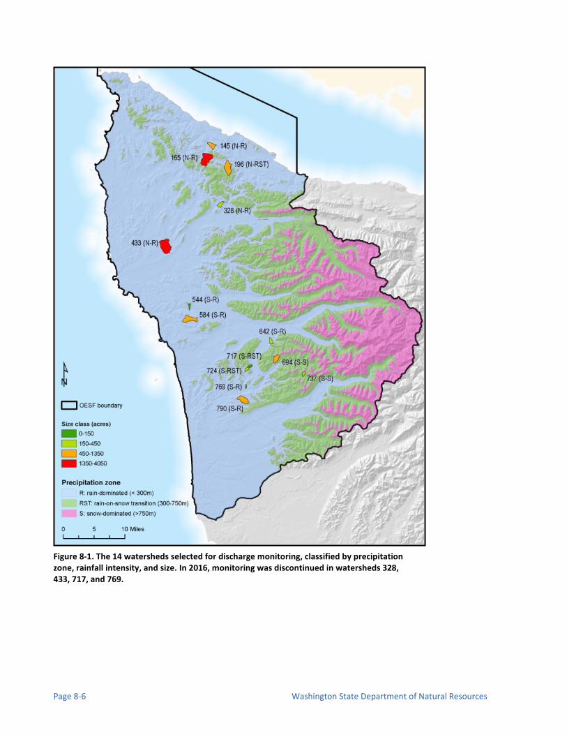
Page 8-6 Washington State Department of Natural Resources
Figure 8-1. The 14 watersheds selected for discharge monitoring, classified by precipitation zone, rainfall intensity, and size. In 2016, monitoring was discontinued in watersheds 328, 433, 717, and 769.

Status and Trends Monitoring of Riparian and Aquatic Habitat in the OESF Page 8-7
Table 8-1. Calendar of Field Activities to Maintain Gage Sites and Collect Pertinent Data
Time of activity Discharge Measurements
Gage/Equipment Calibration, Cleaning, and Maintenance
Cross-section and Gage Stability Survey
At Installation 8-10 measurements at various flows within the first water year, 4-6 in following years to maintain curve. Repeat 8-10 measurements if a new rating curve must be constructed. NOTE: These visits are also used to check on the condition of gaging stations. Sites should be visited after large storm events and a minimum of 4 times a year.
Perform initial survey
January
February
March
April
May
June
July Clean housing and repair/repaint staff and recording gage housing.
Additional surveys should be completed annually and following major storm events.
August
September
October
November
December
Equipment and Supplies
For measurement of instantaneous discharge
Field notebook, blank field forms printed on Rite-in-the-Rain paper, and pencils Distance measuring device, preferably 50m fiberglass tape (sufficient to span channel cross section);
multiple tapes (or other measuring devises) are needed for the Neutrally Buoyant Object discharge method
Spring clips and surveyor chaining pins, or other tape anchors Flow meter (Hach FH 950® or Marsh McBirney FloMate®) Metric top setting wading rod Calculator - It is recommended that calculations be completed in the field so measurements can be
retaken if an error is detected Neutrally buoyant object and stop watch Stadia rod and level (for non-fixed staff gage sites) Digital camera Small bucket for instrument calibration
For retrieval of data from water level sensor
Field notebook and blank field forms Solinst Leveloader® and/or field laptop with Solinst software installed Replacement Solinst Levelogger® Edge, M5/F15(water level pressure transducer)
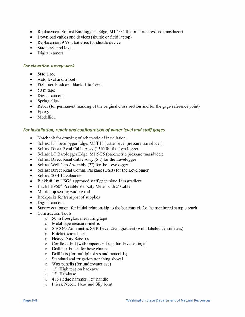
Page 8-8 Washington State Department of Natural Resources
Replacement Solinst Barologger® Edge, M1.5/F5 (barometric pressure transducer) Download cables and devices (shuttle or field laptop) Replacement 9 Volt batteries for shuttle device Stadia rod and level Digital camera
For elevation survey work
Stadia rod Auto level and tripod Field notebook and blank data forms 50 m tape Digital camera Spring clips Rebar (for permanent marking of the original cross section and for the gage reference point) Epoxy Medallion
For installation, repair and configuration of water level and staff gages
Notebook for drawing of schematic of installation Solinst LT Levelogger Edge, M5/F15 (water level pressure transducer) Solinst Direct Read Cable Assy (15ft) for the Levelogger Solinst LT Barologger Edge, M1.5/F5 (barometric pressure transducer) Solinst Direct Read Cable Assy (5ft) for the Levelogger Solinst Well Cap Assembly (2") for the Levelogger Solinst Direct Read Comm. Package (USB) for the Levelogger Solinst 3001 Leveloader Rickly® 1m USGS approved staff gage plate 1cm gradient Hach FH950® Portable Velocity Meter with 5' Cable Metric top setting wading rod Backpacks for transport of supplies Digital camera Survey equipment for initial relationship to the benchmark for the monitored sample reach Construction Tools:
o 50 m fiberglass measuring tape o Metal tape measure–metric o SECO® 7.6m metric SVR Level .5cm gradient (with labeled centimeters) o Ratchet wrench set o Heavy Duty Scissors o Cordless drill (with impact and regular drive settings) o Drill hex bit set for hose clamps o Drill bits (for multiple sizes and materials) o Standard and irrigation trenching shovel o Wax pencils (for underwater use) o 12” High tension hacksaw o 15” Handsaw o 4 lb sledge hammer, 15” handle o Pliers, Needle Nose and Slip Joint

Status and Trends Monitoring of Riparian and Aquatic Habitat in the OESF Page 8-9
o 2 ft standard box level
Construction Supplies: o 2” diameter PVC: straight sections, sweeping and regular elbows (45° and 90°), straight
couplers, and end caps o 2” X 4” pressure treated wood; length determined for each site o Washers; ¼” x 2” stainless steel fender washers and ¼” regular washers o ¼”x 4’ All-Thread rod (Cut to needed lengths) o PC Concrete Epoxy o ¼” x 3”, 1½”, 1” stainless steel hex bolts o ¼’ Stainless steel locking nuts o 2" hose clamp o Cement-60 lb bag; 1 bag per in-bank installation o PVC glue-all purpose o 2" two-hole straps o String to use for threading instruments-150 m o Rebar (1/2” and 3/4” in 2’ and 3’ lengths) o Screws Stainless Steel Square drive; (1½”-3”)size dependent on site and materials o Rock anchor screws hex head; ¼”, length dependent on site and materials o Rebar wire o Zip ties; approximately 6 per station o Electrical tape o Fiberglass screen ; standard window screening approximately 3 ft x 1 ft section o U-Post 13 gage 5’
Field Forms (see the appendices at the end of this chapter)
8A: Site Visit Tracking Field Form 8B: Stream Gage Download Field Form 8C: Stream Gage Installation Field Form 8D (a)-(e): Stream Discharge Field Forms (by method: Hach FH950, MMB, NBO, and Slope-Area) 8E: Elevation Survey for Cross-section Stability Field Form
Field Procedures Where feasible, the U.S. Geological Survey (USGS) gaging protocol (Turnipseed and Sauer 2010) has been followed and should be referred to for more detailed information and guidance.
REGULAR SITE VISITS Procedures are adapted from Butkus (2007)
Use the field forms Site Visit Tracking (Appendix 8A) and Stream Gage Download (Appendix 8B). Step-by-step instructions for operating the flow meter and downloading data from the gages are provided in Appendices 8F and 8H, respectively. At each site visit, at the minimum, a staff gage reading should be noted along with the date and time. During the site visits, the latest data set is downloaded from the recording gage (i.e., the paired pressure transducers)

Page 8-10 Washington State Department of Natural Resources
water level sensor to the Leveloader data transfer unit, a laptop, or a hand-held computer. If a stream discharge measurement is conducted during the visit, the water level sensor data is downloaded at the conclusion of the discharge measurement. After data is downloaded, loggers are restarted and recording intervals are double-checked. The field crew also takes a photo of the channel from the permanently established photo point, as well as upstream and downstream photos of the discharge measurement cross section. The crew should also provide a qualitative description of the status of the channel controls (i.e., natural or artificial channel feature(s) downstream of a gage station that influence the stage-discharge relationship at the gage station) and gage cross section. During each visit, clean any debris from gages and inspect them for damage. Inspection of channel controls, the gage cross section, and the gage (for any damage) are especially important after high flow events.
INSTALLATION AND CONFIGURATION OF WATER LEVEL SENSORS Use the Stream Gage Installation Field Form (Appendix 8C). This section describes the process of sighting, constructing, and installing the water level sensors. Although many water level sensor models are available commercially, this project is using the Solinst Levelogger and Solinst Barologger pressure transducers to measure and record relative water level. For specific information on these instruments, refer to Appendices 8H and 8I.
Step 1: Select site for gaging station
Gaging stations must be installed in stream channel locations that are suitable for accurate recording gage and staff gage measurements and also for nearby discharge measurements. Although it is rare to find all of these site conditions together, it is important to spend as much time as possible scouting for the best gage sites. Rantz (1982) identifies the following characteristics for an ideal gaging station installation:
1) The general course of the stream is straight for about 100 m (approx. 300 ft) upstream and downstream from the gage site.
2) The total flow is confined to one channel at low stages, and minimal flow bypasses the site as subsurface flow.
3) The streambed is not subject to scour and fill and is free of aquatic growth. 4) Banks are permanent, high enough to contain floods, and are free of brush. 5) Unchanging natural channel controls are present in the form of a bedrock outcrop or other stable
riffle for low flow and a channel constriction for high flow or a falls or cascade that is unsubmerged at all stages.
6) A pool is present upstream from the channel control at extremely low stages to ensure a recording of stage at extremely low flow, and to avoid high velocities at the streamward end of gaging station intakes during periods of high flow.
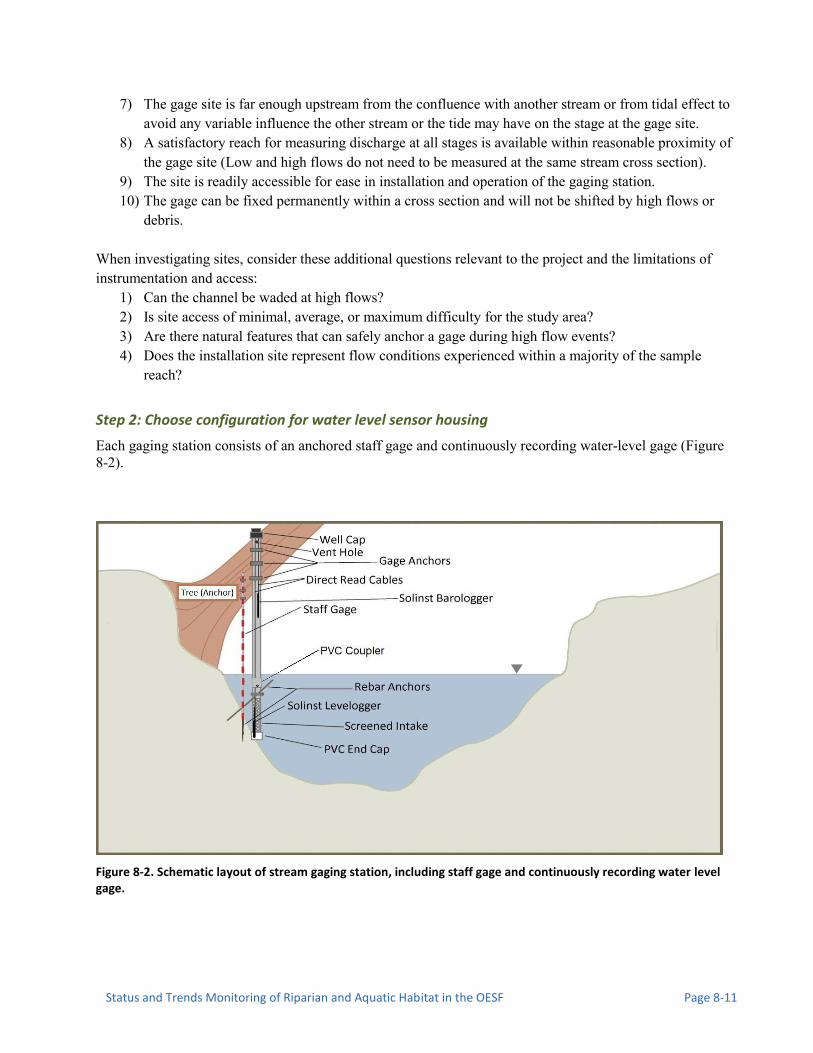
Status and Trends Monitoring of Riparian and Aquatic Habitat in the OESF Page 8-11
7) The gage site is far enough upstream from the confluence with another stream or from tidal effect to avoid any variable influence the other stream or the tide may have on the stage at the gage site.
8) A satisfactory reach for measuring discharge at all stages is available within reasonable proximity of the gage site (Low and high flows do not need to be measured at the same stream cross section).
9) The site is readily accessible for ease in installation and operation of the gaging station. 10) The gage can be fixed permanently within a cross section and will not be shifted by high flows or
debris.
When investigating sites, consider these additional questions relevant to the project and the limitations of instrumentation and access:
1) Can the channel be waded at high flows? 2) Is site access of minimal, average, or maximum difficulty for the study area? 3) Are there natural features that can safely anchor a gage during high flow events? 4) Does the installation site represent flow conditions experienced within a majority of the sample
reach?
Step 2: Choose configuration for water level sensor housing
Each gaging station consists of an anchored staff gage and continuously recording water-level gage (Figure 8-2).
Figure 8-2. Schematic layout of stream gaging station, including staff gage and continuously recording water level gage.

Page 8-12 Washington State Department of Natural Resources
All water level sensors are protected in a housing made of schedule 40 conduit (grey) PVC. These installations are attached to bankside trees, rocks, or other semi-permanent structures and, as a last resort, bankside sediment. Note that available anchors may limit the ability to gage a site. It is crucial that 1) the gage does not move during any flow event in order to maintain the gage’s datum and 2) the housing does not restrict the sensor’s access to the water surface in the housing. Although this can be difficult to achieve, especially for long-term installations, time spent on identifying a proper cross section and on securing the gages will pay off later in data quality. There are three general designs for the gage housing configuration; the simplest possible design appropriate for the site is the preferred option. Often this will be a vertical installation, though site characteristics may require a more stable installation configuration. The three installation configurations to be used are (Figure 8-3):
a) Vertical Installation: This is the simplest installation. Vertical installations require a tree or other anchor near the bank. Consider the project duration (10+ years) and likely stability of the anchor during high flow events when choosing an installation site.
b) In-bank Installation: As opposed to the vertical installation, the in-bank option requires excavating a
trench that is as deep as the channel thalweg and located far enough from the channel to reach a stable anchor. When choosing a site for this installation, consider future erosion or deposition that would influence the intake for the water level sensor housing. Also consider that this installation relies on sediment as its main anchor; this may make it very prone to failure/movement.
c) Over-bank Installation: This is the most complicated installation method because this setup requires more engineering and planning than the other two installation methods. Used primarily on bedrock, the anchors used in this setup may provide the most stable installation. Depending on the angles used, this option may require feeding instrument cables through the installation before it is glued together. If this is done, consider how the instrument will be replaced if it or the cable needs to be removed for maintenance. A string tied to the end of the cable before the cable is pulled up through the housing will allow the cable and instrument to be easily returned to the original configuration.
Once an installation configuration is selected, make sketches and notes on the Stream Gage Installation Field Form (Appendix 8C) to plan the project. Estimate the necessary length of PVC pipe, making sure to consider length added by the angle and coupler components. Make note of the anchor types and hardware you plan to use for the installation. Because of the wet, warm environment these gages will endure, be cautious when using wood for the installation.

Status and Trends Monitoring of Riparian and Aquatic Habitat in the OESF Page 8-13
a
b
Figure 8-3. Schematics and pictures of the three types of water level sensor installations: (a) vertical, (b) in-bank, and (c) over-bank.
c

Page 8-14 Washington State Department of Natural Resources
Step 3: Design and prepare water level sensor housing
Design and construction of the water level sensor housing will likely be an iterative process. Assume there will be difficulties with the installation and try to plan accordingly so you have extra materials and any tools needed to work around these problems. Key considerations when constructing the gage housing are:
Well cap: The locking cap, which is part of the Solinst® water level sensor system, consists of three parts (Figure 8-4): one which attaches to the PVC stilling well, a separate hanger for the Direct Read Cables, and a locking lid. The cables must be threaded through the hanger before the extra cable is contained. Casing: The main casing of the well is constructed of 2-in diameter PVC pipe. The pipe must be arranged in a way that will allow the free surface of the water to fluctuate inside the well. Additionally, the casing must protect the instruments, not be able to move or shift, and be arranged so as to reduce clogging of the intake screen. Screen: The bottom part of the gage housing provides the main intake for the gage when the housing works as a stilling well. It is
constructed out of a removable section of PVC pipe, drilled with many holes, and covered with a screen secured by three or four hose clamps (Figure 8-5). The end is sealed with a 2-inch diameter PVC cap, which is glued on. This screen section is attached to the main casing using a 3-inch stainless steel bolt and a PVC coupler. The bolt passes through the coupler and the screen section when assembled.
Figure 8-5. Schematic of the gage intake section.
Vent hole: The gage housing will ultimately be composed of one to several sections of PVC pipe that will be glued together. Each section of the casing should contain multiple drilled holes above the 100 year flood mark to allow equilibrium of the free water surface.
Figure 8-4. Solinst® locking well cap.

Status and Trends Monitoring of Riparian and Aquatic Habitat in the OESF Page 8-15
Anchors: Potential anchors include two-hole straps and wood screws, rebar and rebar wire, concrete, epoxy and All-Thread fully threaded rod, rock anchors, hose clamps, and streamside materials (trees and rocks) that are estimated to be stable enough to withstand most flow levels for a minimum of 10 years. Access/re-installation: The gage housing will need to be cleaned and/or the water level sensor may need to be replaced. Often, the simplest way to facilitate this work will be to make the intake portion (Figure 8-5) of the gage housing (i.e., the section containing the water level pressure transducer) easily removable. Consider this when planning the installation. Note that you will need to be able to return the sensor to its original location and that measurements of relative instrument depth will need to be made before and after any intentional movement of the gage (see QA/QC section, below). Installation tip: Each gage should be fabricated off-site and brought to the gaging location in sections and reassembled on-site.
Once the housing configuration has been determined, gather necessary supplies and cut PVC pipe to size; avoid cutting PVC in the stream. If possible, test the housing in place to verify that it will fit before you glue it together. If you cannot lift the entire unit into place, test the housing in sections starting with the intake portion. If you have a particularly complicated housing arrangement, make sure to run a string through the housing as you put it together; you will use this to pull the sensor into position once the housing is constructed. Step 4: Configure Solinst® Direct Read cable and well
cap
When using the Solinst® water level sensor system, there are two sensors in the housing,1) a water level sensor (Solinst Levelogger) and 2) a barometric pressure sensor (Solinst Barologger) (Figure 8-6). Each of these sensors will be connected to an optical port located at the well cap. The elevation of these two sensors is dependent on the length of the cable, which connects the optical port to the sensor. Once the cables have been fed through the well cap, determine the cable length needed to locate the Levelogger approximately 1 cm above the bottom of the stilling well/gage housing. The Barologger needs to rest above the anticipated 100-year flood elevation. Control the height of the data loggers inside the housing by shortening the Direct Read cable. This can be done by wrapping the cable carefully around a small section of 1-in diameter PVC pipe, using nylon cable zip ties to zip-tie each end through a hole drilled in PVC, and then covering the entire wrap with electrical tape (Figure 8-7). It is helpful to wrap the cable to the approximate length before installation, and then make final adjustments to the length once the cable has been installed.
Figure 8-6. Arrangement of Solinst® Levelogger and Barologger in a simple vertical installation.
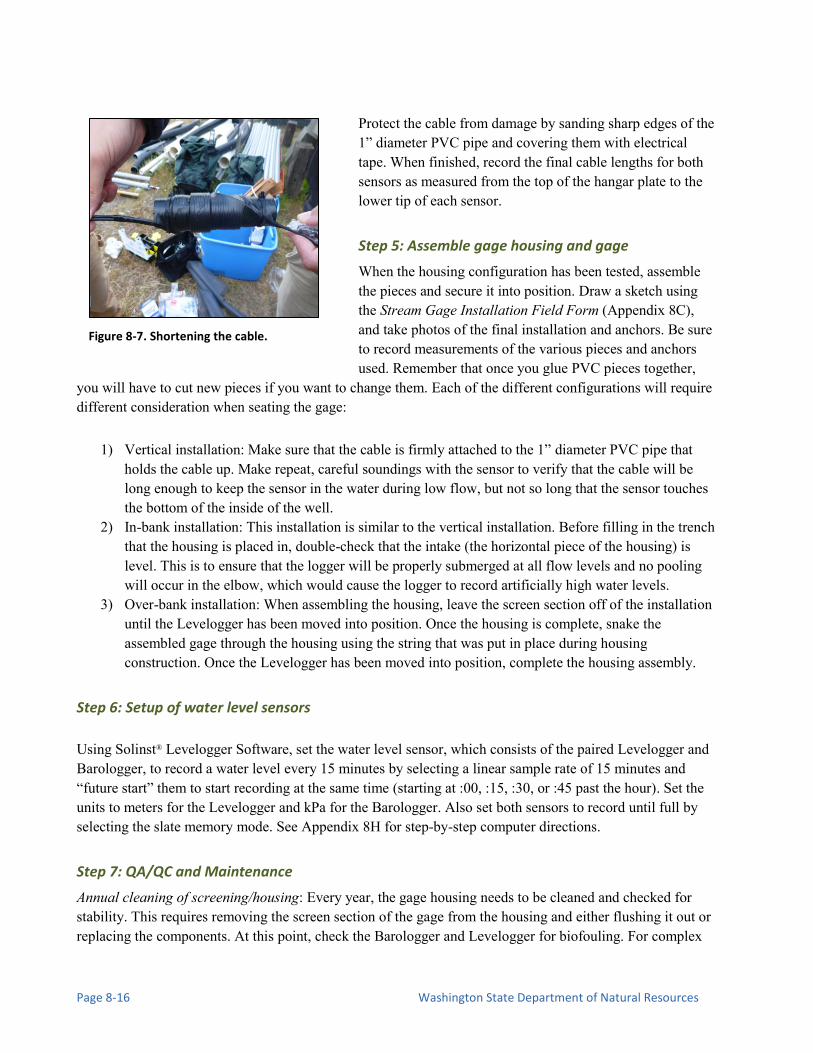
Page 8-16 Washington State Department of Natural Resources
Protect the cable from damage by sanding sharp edges of the 1” diameter PVC pipe and covering them with electrical tape. When finished, record the final cable lengths for both sensors as measured from the top of the hangar plate to the lower tip of each sensor.
Step 5: Assemble gage housing and gage
When the housing configuration has been tested, assemble the pieces and secure it into position. Draw a sketch using the Stream Gage Installation Field Form (Appendix 8C), and take photos of the final installation and anchors. Be sure to record measurements of the various pieces and anchors used. Remember that once you glue PVC pieces together,
you will have to cut new pieces if you want to change them. Each of the different configurations will require different consideration when seating the gage:
1) Vertical installation: Make sure that the cable is firmly attached to the 1” diameter PVC pipe that holds the cable up. Make repeat, careful soundings with the sensor to verify that the cable will be long enough to keep the sensor in the water during low flow, but not so long that the sensor touches the bottom of the inside of the well.
2) In-bank installation: This installation is similar to the vertical installation. Before filling in the trench that the housing is placed in, double-check that the intake (the horizontal piece of the housing) is level. This is to ensure that the logger will be properly submerged at all flow levels and no pooling will occur in the elbow, which would cause the logger to record artificially high water levels.
3) Over-bank installation: When assembling the housing, leave the screen section off of the installation until the Levelogger has been moved into position. Once the housing is complete, snake the assembled gage through the housing using the string that was put in place during housing construction. Once the Levelogger has been moved into position, complete the housing assembly.
Step 6: Setup of water level sensors
Using Solinst® Levelogger Software, set the water level sensor, which consists of the paired Levelogger and Barologger, to record a water level every 15 minutes by selecting a linear sample rate of 15 minutes and “future start” them to start recording at the same time (starting at :00, :15, :30, or :45 past the hour). Set the units to meters for the Levelogger and kPa for the Barologger. Also set both sensors to record until full by selecting the slate memory mode. See Appendix 8H for step-by-step computer directions.
Step 7: QA/QC and Maintenance
Annual cleaning of screening/housing: Every year, the gage housing needs to be cleaned and checked for stability. This requires removing the screen section of the gage from the housing and either flushing it out or replacing the components. At this point, check the Barologger and Levelogger for biofouling. For complex
Figure 8-7. Shortening the cable.

Status and Trends Monitoring of Riparian and Aquatic Habitat in the OESF Page 8-17
housing setups that require the Levelogger to be removed for inspection, tie a string around the end of the sensor before it is pulled up or removed. Re-snaking the sensor through the housing without the assistance of a string may prove difficult when the housing is fully assembled. Sensor accuracy check: Before the sensors are deployed, place them in a container of water, all at exactly the same depth, for at least one day, recording every hour. Check sensor data for any deviation from the measured water level (after barometric compensation). Any sensors reading outside the manufacturer’s acceptable error range (+/- 0.3 cm) should be returned to the manufacturer for re-calibration or replacement. For more details, see the list of manuals in Appendix 8I.
Step 8: Download and reading of water level sensor
The water level sensor (Solinst Levelogger and Barologger) should be downloaded whenever the gaging station is visited and recorded on the Stream Gage Download Field Form (Appendix 8B). Details on the operation of these sensors, as well as step-by-step directions for how to download the sensors, the barometric compensation process, where to store the data, and the file naming conventions can be found in Appendix 8H. Review and processing of the water level data is addressed in Stream Discharge Data Management and Analysis Protocol. The storage capacity of the sensors is 40,000 readings, which is more than 13 months at a 15-minute recording interval.
INSTALLATION AND CONFIGURATION OF STAFF GAGE AND CROSS SECTION Use the field forms Stream Gage Installation (Appendix 8C). The staff gage (Figure 8-8) is used as a calibration reference for the water level sensor as well as a real-world measurement of water depth. Essentially, this staff gage acts as a controlled check on the water level sensor’s calibration. The difference between the staff gage water height and the height reported by the water level sensor should remain constant in time and across all water levels. It is crucial to the stream gaging effort that the staff Figure 8-8. Staff gage installed alongside water level sensor housing.

Page 8-18 Washington State Department of Natural Resources
gage be stable and reliable. The staff gage stability is measured using surveying methods (see section Elevation Survey Data Collection for Cross-section and Gage Stability). A cross-section, separate from those used for measuring bankfull depth in the stream morphology protocol, is monumented at the gaging station to facilitate repeated surveys of the cross-section profile over time. These surveys will be used to identify any changes in stream channel morphology at the gage station. Such changes can significantly affect the stage-discharge relationship and thus necessitate modification of the rating curve or creation of a new rating curve.
Step 1: Locate a stable vertical surface or permanent measurement point
Ideal sites for the staff gage are the same as those for the vertical installations of water level sensor housing. Additionally, the staff gage should be within the same pool or behind the same channel control as the water level sensor. If no vertical installation is possible, a reliable measurement point should be located. This can be either a measurement from the stream bottom (e.g. a stake driven into the stream bed but be aware of potential scour and fill of the channel) or a measurement down to the stream surface from above (for example, a measurement from a bridge deck). A permanent staff gage installation is preferable however.
Step 2: Attach to anchor and establish location
Attach the staff gage to a stable anchor that will reliably hold the staff gage level. At least two attachment points must be used and the staff gage must be kept as level as possible. Ensure no vertical movement of the staff gage by securing multiple bolts through the staff gage plate into the anchor. Using the field form in Appendix 8C, record details of the gage installation; including a sketch of the staff gage with measurements and a photo of the installed gage. For an unfixed staff gage it is important to establish a location that will not change and is easy to locate for future visits. The top of the white endcap of the recording gage housing is a reliable, and easy to find location to measure from (Figure 8-9). Markings on the recording gage housing using permanent markers or paint pens have been found to wear away.
Step 3: Read the staff gage
Record stage height using the staff gage each time a discharge measurement is taken (at the start and the end of the discharge measurement) or the water level sensor is downloaded. If the water height is fluctuating as you attempt to read the staff gage or there is water pile up on the upstream side, estimate the average of the fluctuation or the mean of the pile up across the staff gage surface.
Step 4: Install gage station cross section
Establish cross section benchmarks at the gage station so repeated measurements can be taken at the same cross section. The cross sections of all gage stations in this project are marked with rebar topped by orange mushroom caps, installed above the stream bankfull stage.
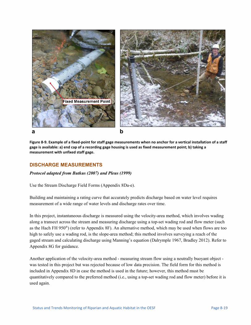
Status and Trends Monitoring of Riparian and Aquatic Habitat in the OESF Page 8-19
a b
Figure 8-9. Example of a fixed-point for staff gage measurements when no anchor for a vertical installation of a staff gage is available: a) end cap of a recording gage housing is used as fixed measurement point; b) taking a measurement with unfixed staff gage.
DISCHARGE MEASUREMENTS Protocol adapted from Butkus (2007) and Pleus (1999) Use the Stream Discharge Field Forms (Appendix 8Da-e). Building and maintaining a rating curve that accurately predicts discharge based on water level requires measurement of a wide range of water levels and discharge rates over time. In this project, instantaneous discharge is measured using the velocity-area method, which involves wading along a transect across the stream and measuring discharge using a top-set wading rod and flow meter (such as the Hach FH 950®) (refer to Appendix 8F). An alternative method, which may be used when flows are too high to safely use a wading rod, is the slope-area method; this method involves surveying a reach of the gaged stream and calculating discharge using Manning’s equation (Dalrymple 1967, Bradley 2012). Refer to Appendix 8G for guidance. Another application of the velocity-area method - measuring stream flow using a neutrally buoyant object - was tested in this project but was rejected because of low data precision. The field form for this method is included in Appendix 8D in case the method is used in the future; however, this method must be quantitatively compared to the preferred method (i.e., using a top-set wading rod and flow meter) before it is used again.

Page 8-20 Washington State Department of Natural Resources
All velocity-area discharge calculations will be done using the USGS mid-section method (Turnipseed and Sauer 2010). Explicit instructions for each discharge measurement method are included in this protocol and/or in its appendices. Because the velocity-area method (with a top-set wading rod and flow meter) is the standard method used for discharge measurements in this study, detailed notes on its application are outlined here:
Step 1: Select a discharge measurement site
For the discharge measurement, selection of a suitable site is very important and cannot be over-emphasized. Site selection is, in most cases, the most important factor in developing accurate flow information. The limitations of a poor measurement site cannot be overcome by the quality of equipment or the ability of the individual taking the measurement (Turnipseed and Sauer 2010). An ideal site for making a discharge measurement should have the following characteristics (the following list is a modified version of Butkus et al. 2007):
1) The discharge measurement site should be close enough to the gaging station to ensure that the gage station and discharge measurement site are receiving the same flow.
2) The stream course should be relatively straight and free-flowing both upstream and downstream of the discharge measurement site. The site should be free of excessive turbulence.
3) The stream channel should be free of vegetative growth and be relatively stable (free of major seasonal scouring or deposition of bed material).
4) Flow velocities exceed 0.15 m/s (0.5 ft/s) and depths are greater than 0.15 m (0.5 ft). 5) The stream bed should be relatively uniform with only minor irregularities (no large cobble or
boulders). When obstructions are present at an otherwise suitable site, it is acceptable to remove them. Place the obstructions downstream of the site so that they do not affect flow conditions at the measurement site. Examples of obstructions include small organic debris, such as leaves, twigs and branches, and larger sediment particles such as cobble and boulders with less than 50 percent of their mass embedded in the channel bed surface. Avoid channel bed disturbances that cause continuous movement of smaller sediment particles downstream while removing obstructions or taking measurements.
6) During low flow conditions (typically July-October) the stream channel should be confined to a single course. Temporary damming along shallow margins of the measurement site is acceptable to divert flow into deeper sections where the water level would not otherwise completely cover a velocity sensor.
7) The stream bank should be stable and able to contain the maximum measurable stream flow. Avoid areas with flow diversions, side channels, undercut banks, or other obstructions.
Note that it will be difficult to locate areas that include all of these features, but it is important to spend time finding a suitable location. It is recommended that you locate and mark typical high water and low water discharge measurement sites at each sample reach so they can be used for future discharge measurements if locations remain acceptable.

Status and Trends Monitoring of Riparian and Aquatic Habitat in the OESF Page 8-21
As described above, it may be necessary to slightly modify the streambed in order to obtain more accurate measurements. If such modifications are necessary, ensure that the modification will not affect stage height at the recording gage and that the discharge measurement site is not located near any permanent cross sections used in other project monitoring protocols. If the streambed at the discharge measurement site has been modified, the flow should be allowed to stabilize before starting discharge measurements. Do not alter the measurement site after measurements have begun because this will change the flow characteristics and affect data accuracy.
Step 2: Establish the measurement transect
Extend a measuring tape across the wetted portion of the stream channel (from left to right, determined facing downstream) perpendicular to the main direction of flow; this is typically perpendicular to the banks (Figure 8-10). Anchor the ends of the tape just past the wetted edges using spring clamps and surveyor chaining pins. Anchor the tape using rocks or roots, if the pins cannot be placed. Previously established discharge measurement sites can be used. Make sure the tape is taut, and above the water surface.
Figure 8-10. Discharge measurement transect with measuring tape anchored above wetted surface.
Step 3: Assemble and test the flow meter system
Assemble and test the flow meter system to ensure that it is working properly based on manufacturer specifications. This includes the flow sensor unit (probe/rotor assembly), the sensor cable, the data indicator/logger/meter, and the wading rod. If it is the first measurement of the day, be sure to calibrate the instrument in still water. See instrument manuals and directions in the appendices regarding the setup, calibration, and troubleshooting for specific flow meters (refer to Appendices 8F, 8H, and 8I).

Page 8-22 Washington State Department of Natural Resources
Step 4: Establishing measurement stations
For most wadeable streams, at least 15 measurement stations are required to ensure an accurate reading (Figure 8-11). To calculate the sampling interval, measure the wetted width at the transect and divide by the selected number of measurement stations. Intervals should be no smaller than 10 cm, even if this results in fewer than 15 stations (Peck et al. 1996). It is desirable to use more than the minimum number of stations where the stream channel morphology is variable or the water is turbulent.
Figure 8-11. A stream cross-section showing depth observation verticals (d), measurements of the distance from the initial vertical to the observed vertical (b) and boundaries of each station subsection (dashed lines). Total discharge is the sum of discharge within each rectangle (adapted from Turnipseed and Sauer 2010).
Locate the first measurement station one interval distance from the left wetted edge. If water depth at this distance is inadequate for measurement due to instrument limitations, move the station to the required depth. Note if the bank gradually slopes out to the first station or if the bank edge is vertical; record this on the field form. The second and subsequent measurement stations can be calculated by adding the interval distance to the previous measurement station. However, stations should be spaced equally throughout the transect only if discharge is evenly distributed across the stream. Measurement stations should be closer together in portions of the transect where flow is concentrated and/or where velocity or bottom irregularities are the greatest. In these sections, stations should represent average depth and velocity conditions within an area (observation station, referred hereafter as simply the “station”) defined as half the distance from the last station plus half the distance to the next station (Figure 8-11). Adjust station locations so that station boundaries fall wherever noticeable breaks or discontinuities in velocity and depth occur. Ideally, each cell should account for less than 10% of the total discharge. The discharge in some stations may be greater than 10% in small streams where the measurement stations are already at the minimum 10 cm interval, but this does affect the quality of the measurement.

Status and Trends Monitoring of Riparian and Aquatic Habitat in the OESF Page 8-23
The number of stations can be reduced depending upon the width, depth, and uniformity of the stream channel. Uniform flow has little vertical or horizontal variation in flow direction. These flow conditions are generally found in shallow stream reaches with a flat channel bed, small substrate, and little or no surface turbulence.
Step 5: Record wetted edge locations, station number, and tape distance
Station 1 is the start of the measurement transect at the left bank wetted channel edge. Note this as “LEW” in the Notes column and record the tape distance in the Distance Along Tape column of the “Station 1” row. Distance from Left Edge of Water is recorded as zero in the station 1 row. Next, record each station's location along the transect tape in the Distance Along Tape column and distance from the wetted edge in the Distance from Left Edge of Water column to the nearest 0.01 m. Record the ending wetted channel edge bank and location (“REW”) in the row following your final velocity station measurement (refer to Appendix 8Da).
Step 6: Record water level, as shown on the staff gage, before and after discharge measurement
In addition to the water level sensor, gaging stations are equipped with either a permanent staff gage (Figure 8-8) or a fixed point where water level can be measured using a stadia rod (Figure 8-9). To track any water level change during discharge measurement, read the water height on the gage or a stadia rod before and after measurement (i.e., prior to starting measurements, and after all cells have been measured) and record the heights in the header of the field form (nearest 0.001 m). If water height is difficult to determine due to fluctuation caused by turbulence, estimate the average across the staff gage or stadia rod surface.
Step 7: Measure and record water depth and velocity at each observation station.
Before taking flow velocity measurements, select: a) the number of measurements to be taken at the station, and b) the averaging time for each measurement. A velocity meter such as the Hach FH 950® flow meter (Figure 8-12) or Marsh McBirney® and a top-set wading rod (Figure 8-13) are used in each of these tasks, as described below. Measuring depth at a station: Station depth is the distance from the surface of the channel bed to the water surface, as measured with the wading rod held level. Measure the water depth at a given measurement station using the wading rod and record it in the Depth of Water column to the nearest centimeter. Figure 8-12. Hach FH 950® flow meter.

Page 8-24 Washington State Department of Natural Resources
When high velocities cause water to pile up on the upstream side of the wading rod, read the water depth on the rod as the average between the stacked water level on the upstream side and the depression level on the downstream side. Note that, for the first station, the distance from the edge of water is zero and in many cases the depth may also be zero. For the last station, the distance from the starting edge of water will equal the wetted width, and the depth may also be zero. If the bank at the edge of water is vertical, measure the depth of the water at the edge and enter it into to the field form and flow meter. When using the Hach FH950 flow meter you are prompted to select an edge factor on a vertical edge (Hach User’s Manual):
• Vertical edge: 0.8 to 0.9 • Brick sides with vegetation: 0.7 • Rough walls with heavy vegetation: 0.6 to 0.5
Note in the notes section of the field form the type of edge (vertical or sloped) and the edge factor (if it is a vertical edge).
Figure 8-13. Top setting wading rod set to measure velocity at six-tenths water depth (left) (Adams 2010). Top-set wading rod set to measure at a depth of 100 cm (right).

Status and Trends Monitoring of Riparian and Aquatic Habitat in the OESF Page 8-25
Considerations for the number of velocity readings taken in the water column at each station (from Butkus (2007): “In most natural stream conditions, a logarithmic relationship exists between velocities through the depth strata of the water column. Typically, velocity increases in the upper portion of the water column and decreases near the bottom.” In order to capture the average vertical velocity within a segment, use one of the following methods, depending on measurement conditions:
1) Six-tenths method: Use the six-tenths method in stream segments that are less than 0.76 m in depth. In this technique, a single station velocity is taken with the sensor unit positioned at 0.6 (i.e., 60%) of the total water depth from the water surface, which approximates the average velocity within that column of water. Velocity sampled at six-tenths of the depth represents the average velocity through the depth strata up to 0.76 m. In cases when stage is fluctuating rapidly and the measurement must be made quickly, it is acceptable to use only the six-tenths method at any depth.
2) Two-point method: Employ the two-point method in streams with depths greater than 0.76 m. This method can also be used when there are minor but noticeable flow field disruptors (for example, a single rock in an otherwise smooth streambed). Velocities are sampled at two-tenths and eight-tenths of the depth, and the results are averaged.”
Using a Top Setting Wading Rod: Top setting wading rods (Figure 8-13) are designed to automatically calculate 0.6 x the depth of the water, or 60% of the water’s depth. This value can be calculated by lining up markings on the suspension rod with those along the top of the depth rod (or Vernier) based on the station's total water depth (Figure 8-11). For example, for a station depth (or sounding) of 100 cm, the "10" on the suspension rod is lined up with the "0" on the depth rod handle, resulting in the sensor position at the 40 cm water depth mark on the guide rod shaft, or 0.6 x the water depth from the water surface. This position from the streambed can be calculated manually by multiplying the station depth by 0.6 (e.g., 100 x 0.6 = 60) and then subtracting that value from the water depth. The top setting wading rod can also be used to easily position the sensor for a 0.2 or 0.8 velocity reading. The 0.2 x depth is determined by multiplying the total depth by 2 and adjusting the rod to the calculated value. The 0.8 x depth is determined by dividing the total measured depth by 2. Selecting an Appropriate Velocity Averaging Time: Revised from Butkus (2007): Stream velocities in natural conditions tend to “pulse” or speed up and slow down over time at the same stage. These fluctuations compound the effects of horizontal and vertical velocity variability at fixed locations in the stream. Take 40-second velocity samples to address variations in velocity over time at each measurement point. In the case of mechanical instruments, take two 20-second samples. Measure 40-second velocity samples at each measurement point except in situations when stage is fluctuating significantly or when very low velocities are sampled with mechanical instruments. In circumstances when stage is fluctuating, take single 20-second velocity samples to complete the discharge measurement quickly and to obtain a stage that reasonably represents the measured discharge. When using mechanical equipment, increase the sample time to 60 seconds when velocity is less than 0.15 meters per second.

Page 8-26 Washington State Department of Natural Resources
Measuring Velocity: Before taking measurements, be sure that the operator is not interfering with the flow field and that the flow meter has adjusted to the speed of the current. To avoid affecting stream flow, the flow meter operator should stand 0.5 m (1.5 ft) downstream and to the side of the meter while facing the stream bank (stand perpendicular to the flow, on the downstream side of the tape extended across the transect) (Figure 8-14). In slower streams, the movement of the flow meter operator can greatly affect stream flow. Allow the stream to return to its normal flow pattern (~10-15 seconds) before a measurement is taken. To take a velocity measurement, hold the top setting wading rod in a vertical position and aim the velocity sensor upstream at a 90 degree angle, even if local flow eddies are hitting the sensor at oblique angles.
Measure the station's average velocity at an appropriate time interval and depth and record the measurement in the Velocity 1 column to the nearest 0.01 m/second. If additional measurements are taken at various depths, record them in the order they appear within the methods section. Make sure to circle the appropriate method(s) (0.2/0.6/0.8) in the Method column on the Stream Discharge Field Form (Appendix 8Da). Note that negative velocity readings are possible. For example, this can occur in local flow eddies near edges or behind boulders. When a negative value is recorded, make a clear note on the field form confirming the negative value. Discharge Measurement At High Flow: When a stream at high flow cannot be safely waded, an indirect discharge measurement method known as the slope-area method can be used (Appendix 8G). The measurement consists of surveying high water elevations, or markers of high water, at locations measured pre- or post-event. If the survey is taking place during a flood event, survey the water level at previously measured and marked locations. After the flood,
Figure 8-14 Proper positioning of the flow meter operator (Hach FH950 User Manual: Edition Three, 2013); performing a velocity-area measurements with the Hach FH950®.

Status and Trends Monitoring of Riparian and Aquatic Habitat in the OESF Page 8-27
these locations can be measured. It is suggested that the computer program SAC-GUI (USGS) be used to estimate these high flow levels. For more details on the implementation of this method, see the USGS documentation in Appendix 8G and the SAC-GUI manual (Dalrymple 1967; Bradley 2012). Use the field forms in Appendix 8Dd and 8De.
Step 8: Document discharge information on field form
When the measurement is complete, record the reported or calculated total discharge on the appropriate field form in Appendix 8D and determine the qualitative rating of the measurement (see below).
Qualitative Rating of the Discharge Measurement (from Turnipseed and Sauer (2010), page 79) Every discharge measurement should be evaluated for accuracy using the qualitative method. Historically, this has been the preferred method, and the hydrographer should make this evaluation immediately after making the measurement. The evaluation should be based on the hydrographer’s opinion of the accuracy of the measurement – not on how well, or how poorly, the measurement plots on the stage-discharge relation. It is difficult to provide written guidelines for making a qualitative evaluation of accuracy. A good qualitative evaluation depends mostly on the experience and training of the hydrographer. Several of the factors that should be considered by the hydrographer are as follows: Measuring section.—Consider factors such as the uniformity of depths, the smoothness of the streambed, the streambed material (that is, smooth sand; small, firm gravel; large rocks; soft muck; and so forth), the ability to accurately measure the depth, the approach conditions, presence of bridge piers, and other conditions that would affect measurement accuracy. Velocity conditions.—Consider smoothness of velocity, uniformity of velocity, very slow velocity, very high velocity, turbulence, obstructions that may affect the vertical velocity distribution, use of one-point or two-point method, length of averaging time (40 or more seconds versus half-counts), and other factors that affect accuracy of velocity measurements. Equipment.—Consider the type of current meter used, the type of depth-sounding equipment, and the condition of the equipment. Spacing of measurement stations.—Use about 25 to 30 verticals for a discharge measurement, spaced so that no more than 5 percent of the total discharge is contained in each subsection. Although this is frequently difficult to attain, except in unusual cases, no more than 10 percent of the total discharge should be in a subsection. Otherwise, the accuracy will be negatively affected. Rapidly changing stage.— Although discussed in previous sections of this chapter, this condition should also be considered when assessing the accuracy of the measurement. Using the shortcut methods previously described will result in less accurate measurements of discharge. Ice measurements.—Making discharge measurements under ice cover is usually more difficult, and sometimes less accurate, than making open-water discharge measurements. Presence of slush ice, layered ice, and anchor ice will have adverse effects on accurate measurement of depth and velocity. Velocity

Page 8-28 Washington State Department of Natural Resources
distribution will be affected if the water surface is in contact with the ice. Freezing of water in the meter cups and pivot chamber may affect performance of the equipment. Wind.—Wind can affect the accuracy of a discharge measurement by obscuring the angle of the current, or by creating waves that make it difficult to sense the water surface prior to making depth soundings. Wind can also affect the vertical-velocity distribution, particularly near the surface, and can cause vertical and (or) horizontal movement of the current meter while making a boat measurement, introducing possible error in velocity measurements. The qualitative method of assessing the accuracy of a discharge measurement requires that the hydrographer consider all of the above items and their cumulative effect on the measurement accuracy. The discharge measurement field form has space for describing (1) the streambed at the discharge measurement transect, (2) the flow, (3) the weather, and (4) any other flow conditions that relate to the accuracy. These descriptions, along with the type of equipment, number of verticals, velocity measurement method, and other measurement conditions, should provide the basis for rating the measurement (and associated estimated percent error) as excellent (2 percent), good (5 percent), fair (8 percent), or poor (more than 8 percent). For instance, a measurement might be rated as excellent (2 percent) if (1) the streambed at the measurement location is smooth, firm, and uniform; (2) the velocity is smooth and evenly distributed; (3) the equipment is in good condition; (4) the two-point velocity measurement method was used; and (5) weather conditions are good (no wind or ice). On the other hand, if several of these factors make it difficult to accurately measure depth and (or) velocity, the measurement might be rated fair (8 percent), or even poor (more than 8 percent). As stated previously, it is not possible to provide absolute guidelines for making the qualitative evaluation of accuracy. As a general rule, the accuracy of most discharge measurements will be about 5 percent, or qualitatively a “good” measurement. This is sometimes used as the base-line accuracy, with accuracy upgraded to “excellent” when measuring conditions are substantially better than average, and accuracy downgraded to “fair” or “poor” when conditions are substantially worse than average. The qualitative-accuracy evaluation is based on the hydrographer’s judgment.
Step 9: Quality assurance and quality control of discharge measurement
Perform instrument self-tests before each discharge measurement. Calibration tests of flow meters (0 m/s) should be performed daily before any measurements are taken. Record calibration checks and instrument self-tests on the field form. Make duplicate measurements during each field session (minimum of once per week). Randomly choose a single site and repeat the measurement. The repeat can be made in the same location and with the same tape, but locate the measurements at different increments along the transect. This duplicate measurement will be used to estimate measurement errors associated with discharge measurements at different flow levels. A discharge measurement should not be duplicated if the stage level is changing at the time of the field visit.

Status and Trends Monitoring of Riparian and Aquatic Habitat in the OESF Page 8-29
Butkus (2007) states: “The objective of duplicating measurements is to document the random variability inherent in the measurement procedure. The relative percent difference (RPD) is calculated and compared to the measurement quality objective of 5% (Equation 1). In addition, the cross-sectional areas and the average velocities of the two measurements should be within five percent. The following formula will be used to evaluate duplicate measurements:”
𝑅𝑃𝐷 = |𝑅1−𝑅2|
𝑅1+𝑅2𝑥200 (Equation 1; from Butkus (2007))
R1=Result for the first measurement R2=Result for the second measurement
ELEVATION SURVEY DATA COLLECTION FOR CROSS-SECTION AND GAGE STABILITY This section is adapted from Butkus (2007) and Kenney (2010). Use the Elevation Survey for Cross-Section Stability Field Form (Appendix 8E).
Survey of gage level and cross section
The stage/flow relationship is expressed through a rating curve or table constructed by plotting instantaneous flow measurements against corresponding stage heights (Figure 8-15). However, any time there is significant change in the cross section where the gage is installed, or in the elevation of a gage itself, the rating curve may become inaccurate. If these changes can be documented, particularly any changes in instrumentation elevation, the rating curve must be adjusted or a new rating curve must be established (similarly, it may be possible to use elevation survey data to adjust the “old” rating curve or already-collected data to improve its accuracy). In order to track the elevational stability of the gages and cross-sections over time, it is important to survey the water level sensor, staff gage, and cross section itself multiple times over the life of the gaging station. Perform surveys following the field techniques described in the Channel Morphology Protocol and Kenney (2010). A gage Reference Point (RP) should be installed in close proximity to the gage and the gage cross section. Close proximity of the RP is important for minimizing error when
Figure 8-15. Example rating curve taken from the USGS Hoh River gage station Water Watch Toolkit website (http://waterwatch.usgs.gov/)

Page 8-30 Washington State Department of Natural Resources
calculating the elevation of different points. The Gage RP should be installed so that it will not move in any direction and so there is only a single option of where to place the stadia rod when measuring the point. Therefore, a metal medallion epoxied to bedrock or a large boulder is recommended (Figure 8-16), if that is not available, the top of a very securely installed 2-ft rebar will suffice. Measure the elevation of specified points on the recording and staff gages, relative to the gage RP (i.e., RP = 0 cm elevation), using an auto level. The elevation of the top and bottom of each gage is measured, though is some cases the bottom of the gage is buried and unmeasurable. Assess the elevational stability of each gage (recording and staff gages) by plotting its elevation over time and examining the plot for any significant changes, either abrupt one-time changes or long-term drift. In situations where there is a removable staff gage, plot the gage reading against the surveyed water surface elevation (e.g., LEW) to verify consistency over time. Guidance on methods for comparing cross-sections is given in the Stream Discharge Data Management and Analysis Protocol. Although these surveys will be used to record and detect changes to the cross-sections, it is repeated discharge measurements that will allow for the simplest monitoring of the rating curve and gage stability over time. The water level sensors and staff gages installed as part of this monitoring project are located in small, natural stream channels; therefore a change in the bed form alters a larger percent of the cross sectional area than in a larger channel. As such, rating curves will likely have to be adjusted annually as rating shifts and additional curves may be necessary.
Repeating a gage elevation and cross-section stability survey
The gage elevation and cross-section stability survey is repeated at least once per year and after any exceptionally high flow events. It should also be repeated whenever differences in gage readings are unresolved or when stations have been damaged (refer to Figure 8-17 for guidance) (Kenney 2010).
In general, if a discharge measurement deviates from the value predicted by the rating curve greater than the estimated error of the discharge measurement or 5% of the discharge measurement, whichever is less, or if 2-3 discharge measurements plot on the same side of the curve and sources of measurement and equipment error have been eliminated, the rating curve is suspect and must be verified with a cross-sectional and gage elevation survey.
Staff with knowledge of hydraulics and hydrologic principles should use this information to adjust rating curves according to USGS documents (Rantz 1982).
Figure 8-16. Gage Reference Point installed on large stable boulder near recording gage.

Status and Trends Monitoring of Riparian and Aquatic Habitat in the OESF Page 8-31
Figure 8-17. Guidance on the frequency of gage stability elevation surveys (from Kenney 2010).

Page 8-32 Washington State Department of Natural Resources
It is possible that a cross-section will be too mobile to establish a reliable rating curve at all flow levels. If personnel notice that after collecting a season’s worth of data that there is no reliable relationship between discharge and water height or there are obvious major changes continuously made to the cross-section at the gage, then the current setup should be reassessed. Alternate gaging methods or gaging sites may be used, or the site will be abandoned.
Include the following points and notes for the survey of the gaging station cross section: a) Date and time of survey b) Floodplain elevation points; extended out to above the maximum stream stage height. c) Major points of inflection in the channel used to estimate channel area and hydraulic radius d) Changes in channel roughness (Manning’s n) e) RGT: The top of the recording gage sensor housing f) RGB: The bottom point of the recording gage sensor housing. If it is an in-bank installation measure
from the top of the white end cap(describe measurement point in notes and with a photo) g) SGT: One point on the top of the staff gage (if present) h) SGB: One point on the bottom of the staff gage or fixed point used for staff measurement (if present)
or at the marked non-fixed staff gage measurement point. i) Gage RP: Benchmark j) LEW and REW: Edge of water at the time of survey on both right and left bank k) Staff Gage Reading: Record the staff gage reading at the same time the survey is completed. l) Note that the survey should start on the left bank and move right.
Take a picture and note the location of your survey measurement in detail so that later surveys can be sure to survey the same point. Variables to check on the cross-section include: Changes in the elevation of the instrumentation: If it has been found that the recording gage or staff gage has changed in elevation, then the gage’s data must be adjusted accordingly. Adjustments to the recording gage or staff gage data should only be made if the gage’s elevation has changed by at least 0.5 cm. Refer to the Stream Discharge Data Management and Analysis Protocol for guidance on these adjustments.
Changes in the area or shape of the cross-section: Using Excel or other plotting software (e.g., R), plot the current cross-section against previous surveys and note if there have been any significant changes in its shape or in its cross-sectional area (+/- 10% as a general rule). Changes in the cross-section’s shape can be quantified by its hydraulic radius (cross-sectional area divided by the wetted perimeter at bankfull stage). Differences in the reported instrument water height: Compare the water surface elevation to the staff gage reading and the recording gage reading (after barometric compensation). This number should remain constant across time, though be careful of measuring this during storm events as there may be some lag between the channel and stilling well measurements.

Status and Trends Monitoring of Riparian and Aquatic Habitat in the OESF Page 8-33
Procedures for Calculating Metrics Discharge data calculated for each watershed are subsequently used to calculate metrics that can be compared across watersheds and over time. An initial list of metrics is shown in Table 8-2.
Table 8-2. Discharge metrics and calculation procedures.
Metric (calculated for each watershed) Calculation procedure
Q10 Discharge value that is exceeded 10% of the time.
Qmin: Minimum annual discharge
Minimum discharge recorded during each water year.
Qmin (7-day): Minimum 7-day mean discharge
Minimum 7-day mean discharge recorded during each water year.
Qmean: Mean annual discharge
Mean discharge, calculated by summing every discharge measurement taken within a water year and dividing by the total number of measurements.
VAR: Variation in discharge Coefficient of variation for all discharge measurements in a given water year.
Time and Cost Estimates for Implementing the Field Procedures Following are the time and cost estimates (Tables 8-3 and 8-4) for implementing the field procedures of the stream discharge protocol. These estimates do not include data management.
Table 8-3. Time Estimates for Implementing the Stream Discharge Field Protocol by a two-member field crew (not
including travel time to sites).
Procedure Estimated time
per gaging station
Estimated time per gaging station
per year (assuming 12 visits)
Estimated time for
10 sites per year
Discharge measurement and downloading water level sensors
3 h 36 h 360 h
Installation of gaging station (including planning, purchasing of assembly materials and fabricating sections of the gage station off site, and field installation)
24 h - 240 h (one-time activity unless a station is moved)
Testing of the water level sensors off site
- - 10 h

Page 8-34 Washington State Department of Natural Resources
Table 8-4. Cost Estimates for the Equipment Used in the Stream Discharge Field Protocol for 14 sites
Equipment/Supplies Cost per unit Number of units Cost for the project
Solinst Levelogger Edge 3001 LT M5 F15 $504 16* $8064
Solinst Barologger Edge 3001 LT M1.5 F5 $267 16 $4272
Solinst Direct Read Cable Assembly 15 ft $84 16 $1344
Solinst Direct Read Cable Assembly 5 ft $78 16 $1248
Well Cap 2” $26 16 $416
Direct Read Comm. USB Package $397 1 $397
3001 Leveloader Gold with cables $635 1 $635
FH950 HACH Velocity Meter with cable $4330 1 $4330
Top Setting Wading Rod (metric) $1004 1 $1004
Construction Tools (drills, pliers, shovel,
wrench set, etc.)
_ - $500
Construction Supplies (PVC, cement, wires,
epoxy, rebar, fiberglass screen, etc.)
_ - $1000
* Extras purchased in case of theft or damage.
Quality Assurance and Quality Control Upon completion of a Water Year, compile a “Final Record Packet,” for each stream gaging station. Each packet consists of a complete annual hydrograph, copies of discharge measurements with total discharge, notes on adjustments to the channel controls, copies of the rating curve(s), and any modeling notes used to estimate flow at stages above (or below) those actually measured. This packet, along with the database, is used in the review of the gaging station record. The researcher leading the hydrologic monitoring reviews each flow measurement to ensure that there is no evidence of errors made during data collection or discharge calculation. Directions on the process for acquiring this data and the QA/QC procedures for data management are described in the Stream Discharge Data Management and Analysis Protocol.
TRAINING Discharge measurements and gaging station installation and maintenance requires a dedicated hydrologic technician. All personnel conducting field protocols will be trained in a consistent manner to ensure that the surveys are conducted properly and in standardized fashion. The training is conducted or, for returning personnel, reviewed, annually before the start of the field season. At least one member of the field crew should be experienced with the field procedures.

Status and Trends Monitoring of Riparian and Aquatic Habitat in the OESF Page 8-35
STANDARD PROTOCOLS The standard procedures described in this protocol are followed for the duration of the project. Any deviations from the procedures should be documented, and the reasons for deviation described and discussed with the project manager or the researcher overseeing the protocol implementation. Changes to the published protocols are approved by the project manager or by the researcher overseeing the protocol implementation. Revised protocols are assigned new version numbers and publication dates. Pacific Standard Time (PST) should be used for all field procedures, year-round. During Pacific Daylight Time (PDT), March through November, one hour should be subtracted to arrive at standard time. The letters PST should be appended to all times in field notes to ensure consistency.
CALIBRATION AND TESTING OF THE INSTRUMENTS The calibration procedures for the flow meter are in Appendix 8F; a link to the manual is provided in Appendix 8I. Also see Step 9 (Quality assurance and quality control of discharge measurement) in the Discharge Measurements section, above. The water level sensors are factory calibrated, but this calibration is checked using the process described in Step 7 of the Installation and Configuration of Water Level Sensors section above.
FIELD CHECKS Field forms will be checked for errors immediately after data collection (i.e., in the field) so measurements can be repeated, if needed.
FIELD SAFETY Discharge monitoring will include field activities during all seasons, including periods of high discharge/flood conditions. It is recommended that field staff use personal floatation devices (PFD) when measuring discharge during moderate to high flow conditions. As a general rule of thumb, wear a PFD when entering water flowing faster than 1 m/s or above your mid-calf (~ 0.3 m deep). Do not enter water moving faster than 2.0 m/s or higher than your waist. Use your best judgment to determine if conditions are safe. When wearing chest waders in or near moving water, be sure to have your wading belt buckled and tight at all times.

Page 8-36 Washington State Department of Natural Resources
References Adams, K. 2010. Quality Assurance Monitoring Plan; Ambient Biological Monitoring in Rivers and
Streams: Benthic Macroinvertebrates and Periphyton. Washington State Department of Ecology. Publication No. 10-03-109
Bouwes, N., J. Moberg, N. Weber, B. Bouwes, S. Bennett, C. Beasley, C.E. Jordan, P. Nelle, M. Polino, S. Rentmeester, B. Semmens, C. Volk, M.B. Ward, and J. White. 2011. Scientific protocol for salmonid habitat surveys within the Columbia Habitat Monitoring Program. Prepared by the Integrated Status and Effectiveness Monitoring Program and published by Terraqua, Inc., Wauconda, WA. 118 p. (Also available at http://www.pnamp.org/sites/default/files/champhabitatprotocol_20110125.pdf)
Bradley, D.N. 2012. Slope-area computation program graphical user interface 1.0 - a preprocessing and postprocessing tool for estimating peak flood discharge using the slope-area method: U.S. Geological Survey Fact Sheet 2012-3112, 4 p. (Also available at http://water.usgs.gov/software/SAC/
Butkus, S. 2007. Quality Assurance Monitoring Plan Streamflow Gaging Network. Environmental Assessment Program , Washington State Department of Ecology, Olympia, WA. Pub. No. 05-03-204. (Also available at https://fortress.wa.gov/ecy/publications/publications/0503204.pdf)
Dalrymple, T., Benson, M.A. 1967. Measurement of peak discharge by the slope-area method: U.S. Geological Survey Techniques of Water-Resources Investigations, book 3, chap. A2, 12 p.
Hartman, G.F., J.C.E. Scrivener. 1990. Impacts of forestry practices on a coastal stream ecosystem, Carnation Creek, British Columbia. Dept. of Fisheries and Oceans.
Holtby, L.B., G.F. Hartman. 1982. The population dynamics of coho salmon (Oncorhynchus kisutch) in a west coast rain forest stream subjected to logging. In Proceedings of the Carnation Creek workshop, a (Vol. 10, pp. 24-26).
Jones, J.A., G.E. Grant. 1996. Peak flow responses to clear-cutting and roads in small and large basins, western Cascades, Oregon. Water Resources Research 32(4): 959-974.
Kenney, T.A., 2010, Levels at gaging stations: U.S. Geological Survey Techniques and Methods 3-A19, 60 p.
Minkova, T. and M. Vorwerk. 2014. Status and Trends Monitoring of Riparian and Aquatic Habitat in the Olympic Experimental State Forest. 2013 Establishment Report: Field Installations and Development of Monitoring Protocols. Washington State Department of Natural Resources, Forest Resources Division, Olympia, WA. (Also available at http://www.dnr.wa.gov/ResearchScience/Topics/TrustLandsHCP/Pages/lm_hcp_oesf_research_interest.aspx)
Mitchell, S.C., R.A. Cunjak. 2007. Stream flow, salmon and beaver dams: roles in the structuring of stream fish communities within an anadromous salmon dominated stream. Journal of Animal Ecology 76(6):1062-1074.
Moore, R. D., S.M. Wondzell, 2005. Physical Hydrology and the Effects of Forest Harvesting in the Pacific Northwest: A Review. Journal of the American Water Resources Association (JAWRA) 41(4):763-784.

Status and Trends Monitoring of Riparian and Aquatic Habitat in the OESF Page 8-37
Negishi, J.N., R. C. Sidle, A. D. Ziegler, S. Noguchi, and N. A. Rahim. 2008. Contribution of intercepted subsurface flow to road runoff and sediment transport in a logging‐disturbed tropical catchment. Earth Surface Processes and Landforms 33(8)1174-1191.
Peck, D.V., J.M. Lazorchak, and D.J. Klemm (editors).1996. Unpublished draft. Environmental Monitoring and Assessment Program -Surface Waters: Western Pilot Study Field Operations Manual for Wadeable Streams. EPA/XXX/X-XX/XXXX. U.S. Environmental Protection Agency, Washington, D.C.
Pleus. A. 1999. Method Manual for Wadeable Stream Discharge Measurement. NW Indian Fisheries Commission; Timber, Fish, & Wildlife Monitoring Program. TFW-AM9-99-009. (Also available at http://access.nwifc.org/tfw/documents/TFW_Wadable_Stream_Discharge_Measurement.pdf)
Poff, L.N., J.D. Allan, M.B. Bain, J.R. Karr, K.L. Prestegaard, B.D. Richter, R.E. Sparks, J.C. Stromberg. 1997. The Natural Flow Regime. Bioscience 47(11): 769-784.
Rantz, S.E. 1982. Measurement and computation of streamflow, Volume 1, Measurement of stage and discharge, U.S. Geol. Surv. Water Supply Pap. 2175.
Startsev, A.D. and D.H. McNabb, 2000. Effects of Skidding on Forest Soil Infiltration in West-Central Alberta. Canadian Journal of Soil Science 80:617-624.
Turnipseed, D., and V. Sauer. 2010. Discharge measurements at gaging stations: U.S. Geological Survey Techniques and Methods book 3, chap. A8, 87 p.
Washington State Department of Natural Resources. 2016. Olympic Experimental State Forest HCP Planning Unit Forest Land Plan Final Environmental Impact Statement. Washington State Department of Natural Resources, Olympia, WA. http://file.dnr.wa.gov/publications/amp_sepa_nonpro_oesf_feis.pdf
Wemple, B.C., Jones, J.A. and Grant, G.E., 1996. Channel network extension by logging roads in two basins, Western Cascades, Oregon. Water Resources Bulletin 32(6)1195-1207.
Wemple, B.C. and J. A. Jones. 2003. Runoff production on forest roads in a steep, mountain catchment. Water Resources Research 39(8) 1220.

Page 8-38 Washington State Department of Natural Resources
This page intentionally left blank.

Status and Trends Monitoring of Riparian and Aquatic Habitat in the OESF Page 8A-1
Appendix 8A. Site Visit Tracking Field Form
Start Date:
End Date:
Staff:
Site Discharge Measurement Staff Gage Recording Gage Download
145
165
196
328
433
544
584
642
694
717
724
737
769
790
Notes:
*Fill in the following sheet with the date and and any notes regarding maintenance.*
Discharge Task Tracking Checklist

Page 8A-2 Washington State Department of Natural Resources
This page intentionally left blank.
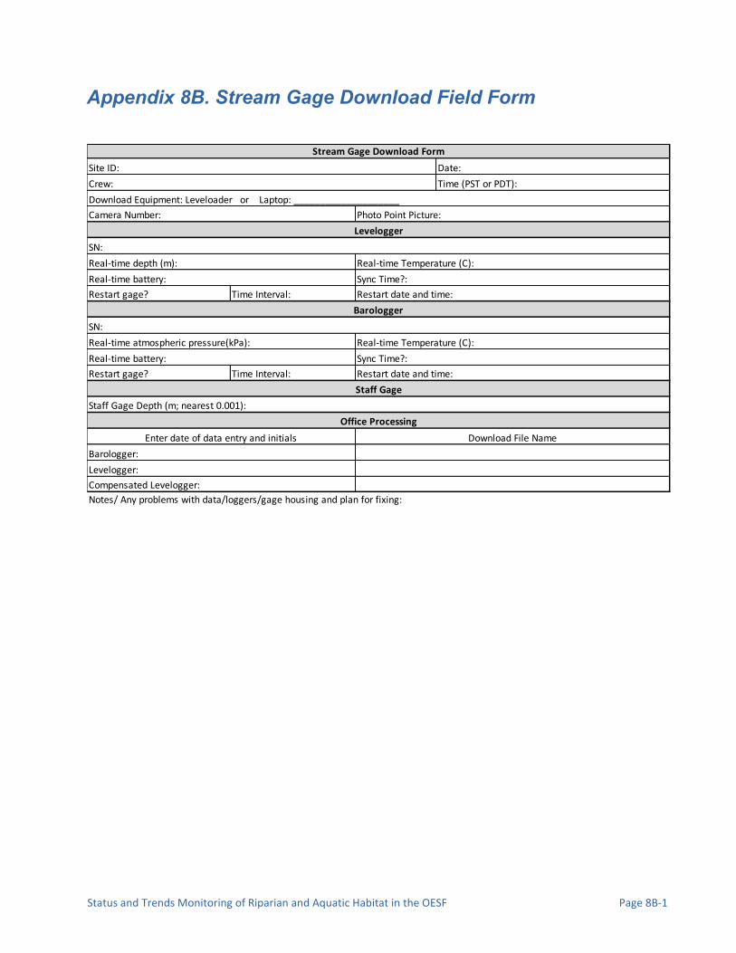
Status and Trends Monitoring of Riparian and Aquatic Habitat in the OESF Page 8B-1
Appendix 8B. Stream Gage Download Field Form
Restart gage?
Restart gage?
Notes/ Any problems with data/loggers/gage housing and plan for fixing:
Barologger:
Compensated Levelogger:
Levelogger:
Enter date of data entry and initials Download File Name
Time Interval: Restart date and time:
SN:
Real-time Temperature (C):Real-time depth (m):
Time Interval: Restart date and time:
SN:
Real-time atmospheric pressure(kPa): Real-time Temperature (C):
Staff Gage
Office Processing
Staff Gage Depth (m; nearest 0.001):
Stream Gage Download Form
Date:
Time (PST or PDT):
Site ID:
Levelogger
Crew:
Download Equipment: Leveloader or Laptop: ____________________
Camera Number: Photo Point Picture:
Barologger
Real-time battery: Sync Time?:
Real-time battery: Sync Time?:

Page 8B-2 Washington State Department of Natural Resources
This page intentionally left blank.

Status and Trends Monitoring of Riparian and Aquatic Habitat in the OESF Page 8C-1
Appendix 8C. Stream Gage Installation Field Form
GPS #
Installation: Plan *tie flagging at location of planned install*
Bankfull Width:
Manning's n at cross section: channel bed right bank left bank
* see roughness guide
Length of Straight: Gradient of Straight:
Notes:
Stream Gage Installation Field Sheet
Describe Stream Characteristics (Significant Structures, Strength of Flow, Section Controls, etc.):
Bank Compostion (Clay, Loose Gravel, Dirt, Bedrock, etc.):
Site Access different from main site accesss?
Install Type: vertical along bank in-bank other /combo:
Basin #: Crew:
Camera #:
Date/Time (PDT or PST):
Draw Gaging Equiptment Layout (w/ stream section control, significant structures, etc. Birdseye View ):
Draw Detailed Installation Plan( w/ estimated measurements, Elevation View ):
Installation: Site

Page 8C-2 Washington State Department of Natural Resources
Distance and Bearing from RP:
GPS of Stream Gage:
DBH:
DBH:
Is staff gage stable?: Yes No Yes No
Depth of water on Staff Gage:
Installation: Recording Gage Instrument Setup
Describe marking used to show if gage has shifted over time:
Averaging? Y or N; sec:
Barologger Sampling Interval:
Averaging? Y or N; sec:
Water Level (cm; Levelogger):
Levellogger:
Length of PVC (Used for Wrap):
Levellogger Serial number:
Start Date/ Time:
Barologger Serial number:
Start Date/ Time:
Atmospheric Pressure (kPa, Barologger):
Time of Atmospheric Reading:
Is staff gage level from all directions?:
*Label With Teodora Minkova's Contact Information: 360-902-1175, DNR Riparian Monitoring, and Site Number*
Detailed Schematic of Gage Housing (Exact Measurement of sections, Degrees of Angles, etc, Elevation View ):
Decribe Type of Anchor (Tree, Rebar, poured concrete, etc.):
Installation: Final Design and Location of Recording Gage
*DO NOT GLUE HOUSING UNTIL RECORDING GAGES HAVE BEEN INSTALLED*
Length from Tip of Sensor to
Well Cap Top:
N: W:
Describe Staff Gage Anchor (If different):
Describe Staff Gage Anchor Connection and Materials Used( Directly to tree, Bracket, plummers tape, etc):
Point #:
Date/Time (PDT or PST) (if different from Plan date and time):
Describe Anchor Connection and Materials Used( Directly to tree, Bracket, plummers tape, etc):
Levellogger Sampling Interval:
Barologger:
Time of Water Level Reading:
Time of Staff Gage Reading:
Tree Species:
Tree Species:
Installation: Anchoring for Recording and Staff Gages

Status and Trends Monitoring of Riparian and Aquatic Habitat in the OESF Page 8C-3
Installation: Photos
Bed Material
Sand 1 Benson and Dalrymple-No data.
2 For indicated material; Chow (1959)
Rock CutFirm Soil
Coarse Sand
Fine Gravel
Gravel
Coarse Gravel
Cobble
Boulder
Minimum Normal Maximum
0.025 0.03 0.033
0.03 0.035 0.04
0.033 0.04 0.045
0.035 0.045 0.05
0.04 0.048 0.055
0.045 0.05 0.06
0.05 0.07 0.08
0.075 0.1 0.15
0.03 0.04 0.050.04 0.05 0.07
0.025 0.03 0.035
0.03 0.035 0.05
0.02 0.03 0.04
0.025 0.035 0.045
0.03 0.04 0.05
0.035 0.05 0.07
0.035 0.05 0.06
0.04 0.06 0.08
0.045 0.07 0.11
0.07 0.1 0.16
0.11 0.15 0.2
0.03 0.04 0.05
0.05 0.06 0.08
0.08 0.1 0.12
0.1 0.12 0.16
General Notes:
--
--
--
5. same as 4. with flood stage reaching branches
0.0120.017
0.02
0.022
0.023
0.025
0.026
0.025 to 0.0320.026 to 0.035
0.028 to 0.035
0.030 to 0.050
0.040 to 0.070
0.20.3
0.4
c. Brush
3. mature field crops
e. same as above, lower stages, more ineffective slopes and sections
f. same as "d" with more stones
h. very weedy reaches, deep pools, or floodways with heavy stand of timber and underbrush
0.5
0.6
0.8
1
1 to 2
2 to 64
64 to 256
>256
0.025
0.02
--
--
--
----
--
--
--
--
--
--
d. Trees
1. dense willows, summer, straight
2. cleared land with tree stumps, no sprouts
3. same as above, but with heavy growth of sprouts
4. heavy stand of timber, a few down trees, little undergrowth, flood stage below branches
1. scattered brush, heavy weeds
2. light brush and trees, in winter
3. light brush and trees, in summer
4. medium to dense brush, in winter
5. medium to dense brush, in summer
g. sluggish reaches, weedy, deep pools
1. no crop
2. mature row crops
Manning's n for Channels (Chow, 1959).
b. Cultivated areas
1. Main Channels a. clean, straight, full stage, no rifts or deep pools
b. same as above, but more stones and weeds
c. clean, winding, some pools and shoals
d. same as above, but some weeds and stones
2. high grass
1.short grass
Natural streams - minor streams (top width at floodstage < 100 ft)
a. bottom: gravels, cobbles, and few boulders b. bottom: cobbles with large boulders
3. Floodplains a. Pasture, no brush
2. Mountain streams, no vegetation in channel, banks usually steep, trees and brush along banks submerged at high stages
Type of Channel and Description
0.024
--
0.026
--
--
--
Median Size of Bed
Material (mm)Straight Uniform Channel1 Smooth Channel
(minimum value)2
Upstream Photo: Downstream Photo:
Final Recording Gage Photo(s): Final Staff Gage Photo(s):
Final Recording Gage Anchor Photo(s): Final Staff Gage Anchor Photo(s):
Construction Photo(s):
Base Values of Manning's n (modified from United States Geological Survey Water-supply Paper 2339)

Page 8C-4 Washington State Department of Natural Resources
This page intentionally left blank.
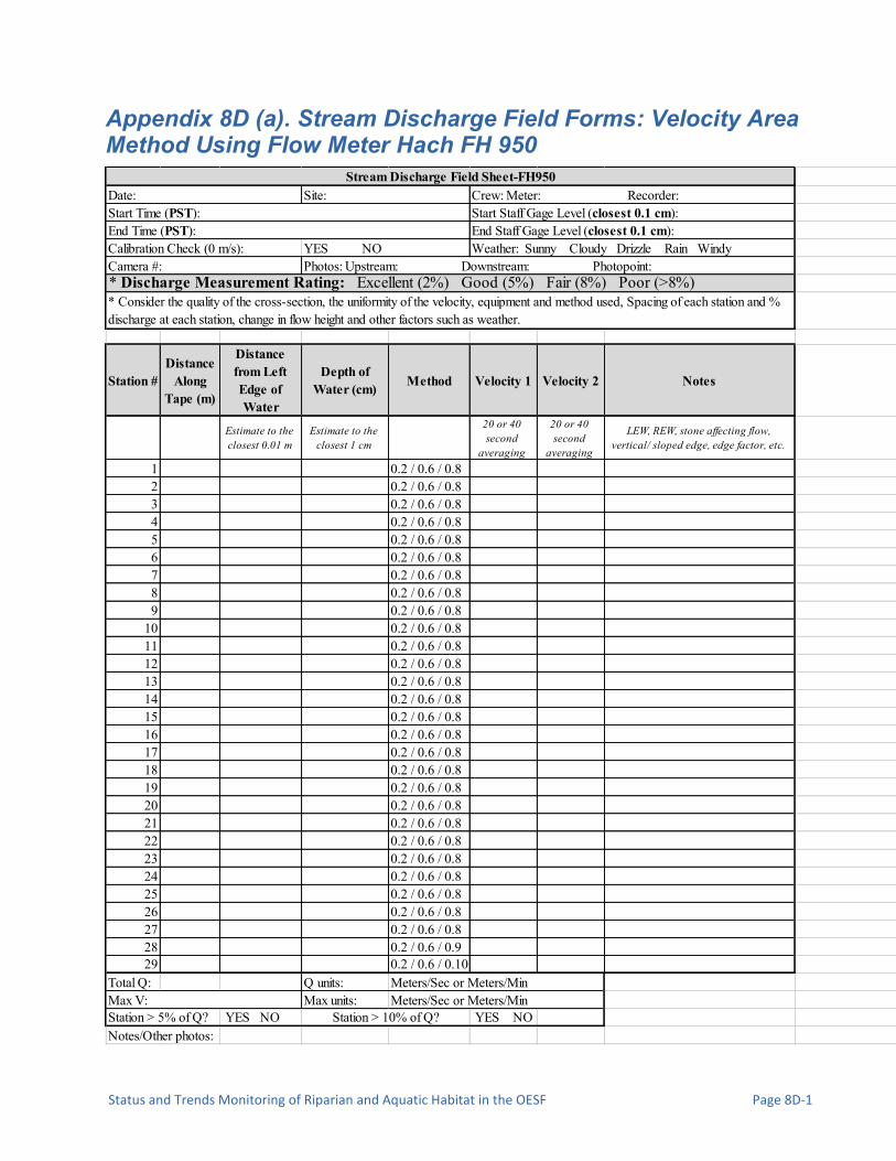
Status and Trends Monitoring of Riparian and Aquatic Habitat in the OESF Page 8D-1
Appendix 8D (a). Stream Discharge Field Forms: Velocity Area Method Using Flow Meter Hach FH 950
Calibration Check (0 m/s):
Station #Distance
Along Tape (m)
Distance from Left Edge of Water
Depth of Water (cm) Method Velocity 1 Velocity 2 Notes
Estimate to the closest 0.01 m
Estimate to the closest 1 cm
20 or 40 second
averaging
20 or 40 second
averaging
LEW, REW, stone affecting flow, vertical/ sloped edge, edge factor, etc.
1 0.2 / 0.6 / 0.82 0.2 / 0.6 / 0.83 0.2 / 0.6 / 0.84 0.2 / 0.6 / 0.85 0.2 / 0.6 / 0.86 0.2 / 0.6 / 0.87 0.2 / 0.6 / 0.88 0.2 / 0.6 / 0.89 0.2 / 0.6 / 0.8
10 0.2 / 0.6 / 0.811 0.2 / 0.6 / 0.812 0.2 / 0.6 / 0.813 0.2 / 0.6 / 0.814 0.2 / 0.6 / 0.815 0.2 / 0.6 / 0.816 0.2 / 0.6 / 0.817 0.2 / 0.6 / 0.818 0.2 / 0.6 / 0.819 0.2 / 0.6 / 0.820 0.2 / 0.6 / 0.821 0.2 / 0.6 / 0.822 0.2 / 0.6 / 0.823 0.2 / 0.6 / 0.824 0.2 / 0.6 / 0.825 0.2 / 0.6 / 0.826 0.2 / 0.6 / 0.827 0.2 / 0.6 / 0.828 0.2 / 0.6 / 0.929 0.2 / 0.6 / 0.10
Total Q: Q units:Max units:
Station > 5% of Q? YES NO YES NONotes/Other photos:
* Discharge Measurement Rating: Excellent (2%) Good (5%) Fair (8%) Poor (>8%)
End Staff Gage Level (closest 0.1 cm):
* Consider the quality of the cross-section, the uniformity of the velocity, equipment and method used, Spacing of each station and % discharge at each station, change in flow height and other factors such as weather.
Site: Date:
Station > 10% of Q?
Crew: Meter: Recorder:
Max V:Meters/Sec or Meters/MinMeters/Sec or Meters/Min
YES NO
Stream Discharge Field Sheet-FH950
Weather: Sunny Cloudy Drizzle Rain Windy
Start Time (PST):End Time (PST):
Start Staff Gage Level (closest 0.1 cm):
Photos: Upstream: Downstream: Photopoint:Camera #:

Page 8D-2 Washington State Department of Natural Resources
Appendix 8D (b). Stream Discharge Field Forms: Velocity Area Method Using Marsh-McBirney Flow Meter
Station
#
Distance
Along
Tape (m)
Distance from
Left Edge of
Water
Depth of
Water (cm)Method Velocity 1 Velocity 2 Notes
Estimate to the
closest 0.01 m
Estimate to the
closest 1 cm
20 or 40 second
averaging
20 or 40 second
averaging
Right bank, left bank, stone
affecting flow, roughness
0 0.2 / 0.6 / 0.8
1 0.2 / 0.6 / 0.8
2 0.2 / 0.6 / 0.8
3 0.2 / 0.6 / 0.8
4 0.2 / 0.6 / 0.8
5 0.2 / 0.6 / 0.8
6 0.2 / 0.6 / 0.8
7 0.2 / 0.6 / 0.8
8 0.2 / 0.6 / 0.8
9 0.2 / 0.6 / 0.8
10 0.2 / 0.6 / 0.8
11 0.2 / 0.6 / 0.8
12 0.2 / 0.6 / 0.8
13 0.2 / 0.6 / 0.8
14 0.2 / 0.6 / 0.8
15 0.2 / 0.6 / 0.8
16 0.2 / 0.6 / 0.8
17 0.2 / 0.6 / 0.8
18 0.2 / 0.6 / 0.8
19 0.2 / 0.6 / 0.8
20 0.2 / 0.6 / 0.8
21 0.2 / 0.6 / 0.8
22 0.2 / 0.6 / 0.8
23 0.2 / 0.6 / 0.8
24 0.2 / 0.6 / 0.8
25 0.2 / 0.6 / 0.8
26 0.2 / 0.6 / 0.8
27 0.2 / 0.6 / 0.8
28 0.2 / 0.6 / 0.8
29 0.2 / 0.6 / 0.8
30 0.2 / 0.6 / 0.8
Comments on Control/ General Notes:
Calibration Check (0 m/s)?
Camera #: Photos: Upstream Downstream Other
Discharge Measurement Rating: Excellent (2%) Good (5%) Fair (8%) Poor (>8%)
* Consider the quality o f the cross-section, the uniformity o f the velocity, equipment and method used, Spacing of each station
and % discharge at each station, change in flow height and other factors such as weather.
Stream Discharge Field Form: Velocity-Area Method Using Marsh McBirney
Date: Site: Crew:
Start Time (PST or PDT):
Weather: Sunny Cloudy Drizzle Rain Windy
End Time (PST or PDT):
Start Staff Gage Level (closest 0.001 m):
End Staff Gage Level (closest 0.001 m):
Instrument Serial Number:

Status and Trends Monitoring of Riparian and Aquatic Habitat in the OESF Page 8D-3
Appendix 8D (c). Stream Discharge Field Forms: Naturally Buoyant Method
Area Calculation
Cross-Section LB 2 3 4 RB
Upper Depth (cm)
Distance from LB (m)
Manning's #
Middle Depth (cm)
Distance from LB (m)
Manning's #
Lower Depth (cm)
Distance from LB (m)
Manning's #
Time (sec)
Right Bank
Center
Left Bank
Average Time (sec)
Notes:
Object used: whiffle ball stick other:
Length of Test Section (m)
End Time (PST or PDT):
Weather: Sunny Cloudy Drizzle Rain Windy Slope (%):
End Staff Gage Level (closest 0.001 m):
Discharge Measurement Rating: Excellent (2%) Good (5%) Fair (8%) Poor (>8%)
* Consider the quality o f the cross-section, the uniformity o f the velocity, equipment and method used, Spacing of each station and % discharge at each station,
change in flow height and other factors such as weather.
Stream Discharge Field Form: Neutrally-Buoyant Method
Date: Site: Crew:
Start Time (PST or PDT): Start Staff Gage Level (closest 0.001 m):
Camera #: Photos: Upstream Downstream Other

Page 8D-4 Washington State Department of Natural Resources
Appendix 8D (d). Stream Discharge Field Forms: Slope Area Method
page 1 of 2
Site: Crew:Weather: Sunny Cloudy Drizzle Rain Windy
Photo #
Tributaries in Reach?: Yes No Trib Notes:
Control Point: Tree Other?: Marked With?:
Seq. #DistanceBearing ElevationPoint ID Mannings Point Quality Backsite BS HeightNotes/photos:
1 X1-1 E | G | F | P
2 X1-2 E | G | F | P
3 X1-3 E | G | F | P
4 X1-4 E | G | F | P
5 X1-5 E | G | F | P
6 X1-6 E | G | F | P
7 X1-7 E | G | F | P
8 X1-8 E | G | F | P
9 X1-9 E | G | F | P
10 X1-10 E | G | F | P
Seq. #DistanceBearing ElevationPoint ID ManningsHWM Quality Backsite BS HeightNotes/Photos:
1R RH-1 E | G | F | P
1L LH-1 E | G | F | P
2R RH-2 E | G | F | P
2L LH-2 E | G | F | P
3R RH-3 E | G | F | P
3L LH-3 E | G | F | P
4R RH-4 E | G | F | P
4L LH-4 E | G | F | P
5R RH-5 E | G | F | P
5L LH-5 E | G | F | P
6R RH-6 E | G | F | P
6L RH-6 E | G | F | P
Notes:
X-Section #:
Stream Discharge Field Sheet- Slope Area Method
Date:GPS #:
Start Time (PST or PDT):End Time (PST or PDT):
Start Staff Gage Level (closest 0.001 m):End Staff Gage Level (closest 0.001 m):
Photopoint Photo: Camera #
Reach Length: Established Crossections Used:
Distance and Bearing Control Point to Basin RP:
GPS Coordinates of Control Point: N: W:
Highwater Marks
X-Section 1 (Furthest Downstream)
Previously Established X- Section?: Yes No

Status and Trends Monitoring of Riparian and Aquatic Habitat in the OESF Page 8D-5
page 2 of 2
Seq. #DistanceBearing ElevationPoint ID Mannings Point Quality Backsite BS HeightNotes/photos:
11 X2-1 E | G | F | P
12 X2-2 E | G | F | P
13 X2-3 E | G | F | P
14 X2-4 E | G | F | P
15 X2-5 E | G | F | P
16 X2-6 E | G | F | P
17 X2-7 E | G | F | P
18 X2-8 E | G | F | P
19 X2-9 E | G | F | P
20 X2-10 E | G | F | P
Seq. #DistanceBearing ElevationPoint ID ManningsHWM Quality Backsite BS HeightNotes/Photos:
7R RH-7 E | G | F | P
7L LH-7 E | G | F | P
8R RH-8 E | G | F | P
8L LH-8 E | G | F | P
9R RH-9 E | G | F | P
9L LH-9 E | G | F | P
10R RH-10 E | G | F | P
10L LH-10 E | G | F | P
11R RH-11 E | G | F | P
11L LH-11 E | G | F | P
12R RH-12 E | G | F | P
12L RH-12 E | G | F | P
Seq. #DistanceBearing ElevationPoint ID Mannings Point Quality Backsite BS HeightNotes/photos:
21 X3-1 E | G | F | P
22 X3-2 E | G | F | P
23 X3-3 E | G | F | P
24 X3-4 E | G | F | P
25 X3-5 E | G | F | P
26 X3-6 E | G | F | P
27 X3-7 E | G | F | P
28 X3-8 E | G | F | P
29 X3-9 E | G | F | P
30 X3-10 E | G | F | P
Notes:
X-Section 3 (Furthest Upstream)
Previously Established X- Section?: Yes No X-Section #:
Highwater Marks
Previously Established X- Section?: Yes No X-Section #:
X-Section 2 (Middle)
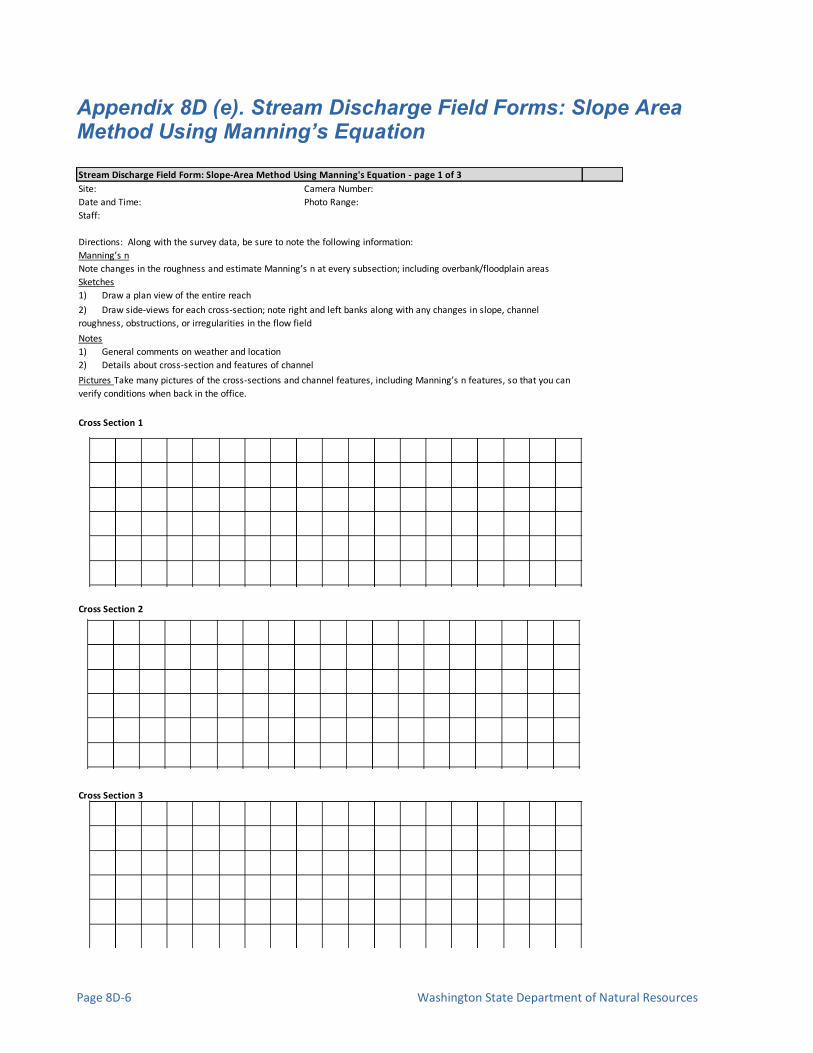
Page 8D-6 Washington State Department of Natural Resources
Appendix 8D (e). Stream Discharge Field Forms: Slope Area Method Using Manning’s Equation
Stream Discharge Field Form: Slope-Area Method Using Manning's Equation - page 1 of 3
Site: Camera Number:
Date and Time: Photo Range:
Staff:
Directions: Along with the survey data, be sure to note the following information:
Manning’s n
Sketches
Notes
Cross Section 1
Cross Section 2
Cross Section 3
1) Draw a plan view of the entire reach
Note changes in the roughness and estimate Manning’s n at every subsection; including overbank/floodplain areas
1) General comments on weather and location
2) Details about cross-section and features of channel
Pictures Take many pictures of the cross-sections and channel features, including Manning’s n features, so that you can
verify conditions when back in the office.
2) Draw side-views for each cross-section; note right and left banks along with any changes in slope, channel
roughness, obstructions, or irregularities in the flow field

Status and Trends Monitoring of Riparian and Aquatic Habitat in the OESF Page 8D-7
Stream Discharge Field Form: Slope-Area Method Using Manning's Equation - page 2 of 3
Plan View (number each point and label codes on additional sheet)

Page 8D-8 Washington State Department of Natural Resources
Stream Discharge Field Form: Slope-Area Method Using Manning's Equation - page 3 of 3
Point Codes Photo Number
Code Description
BM Benchmark/Reference Point
RM Other reference mark
HUB Surveying or turning point
LH Left-bank high-water mark
RH Right-bank high water mark
GH Stream gage
Code Description
E Excellent
G Good
F Fair
P Poor
NOTE: Point 1 should be furthest upstream
Point Codes Photo Number
Point Identifiers
High water mark quality codes
Cross-section point [1] indicates the
cross section number, "X1,""X2," etc.X[1]
SAC-GUI Codes: must use for easy calculation
in SAC-GUI program

Status and Trends Monitoring of Riparian and Aquatic Habitat in the OESF Page 8E-1
Appendix 8E. Elevation Survey for Cross-Section Stability Field Form
GAG
E ST
ATIO
N AN
D CR
OSS
SEC
TIO
N ST
ABIL
ITY
SURV
EYPa
ge 1
of 3
Basi
n #
Fiel
d cr
ew:
Dat
e:
Surv
ey s
tart
tim
e:Su
rvey
end
tim
e:W
eath
er: h
eavy
rain
, lig
ht ra
in, c
loud
y, s
unny
, fog
gy, w
indy
, sno
w, s
now
ing
Rem
arks
on
site
con
diti
on (e
.g. r
ecen
t dis
turb
ance
, los
t RP,
man
agem
ent a
ctiv
ity)
:
Phot
o po
int m
arke
d w
ith:
Mon
umen
t LB:
yes
no
Star
t of S
urve
y St
aff G
age
Read
ing
(m):
Phot
o ta
rget
:M
onum
ent R
B: y
es n
oEn
d of
Sur
vey
Staf
f Gag
e Re
adin
g (m
):
Pict
ure
#:
Cam
era
#:
Gag
e x-
sect
ion
loca
tion
(LB
mon
umen
t) fr
om 2
poi
nts:
1) N
eare
st x
-sec
tion
's L
B m
onum
ent:
X-se
ctio
n #:
Dis
tanc
e (m
):A
zim
uth:
2) B
acks
ite
Loca
tion
:
LBF
X-se
ctio
n #
or R
P:D
ista
nce
(m)
Azm
uth:
Not
es/s
ketc
hes:
Gage Station description
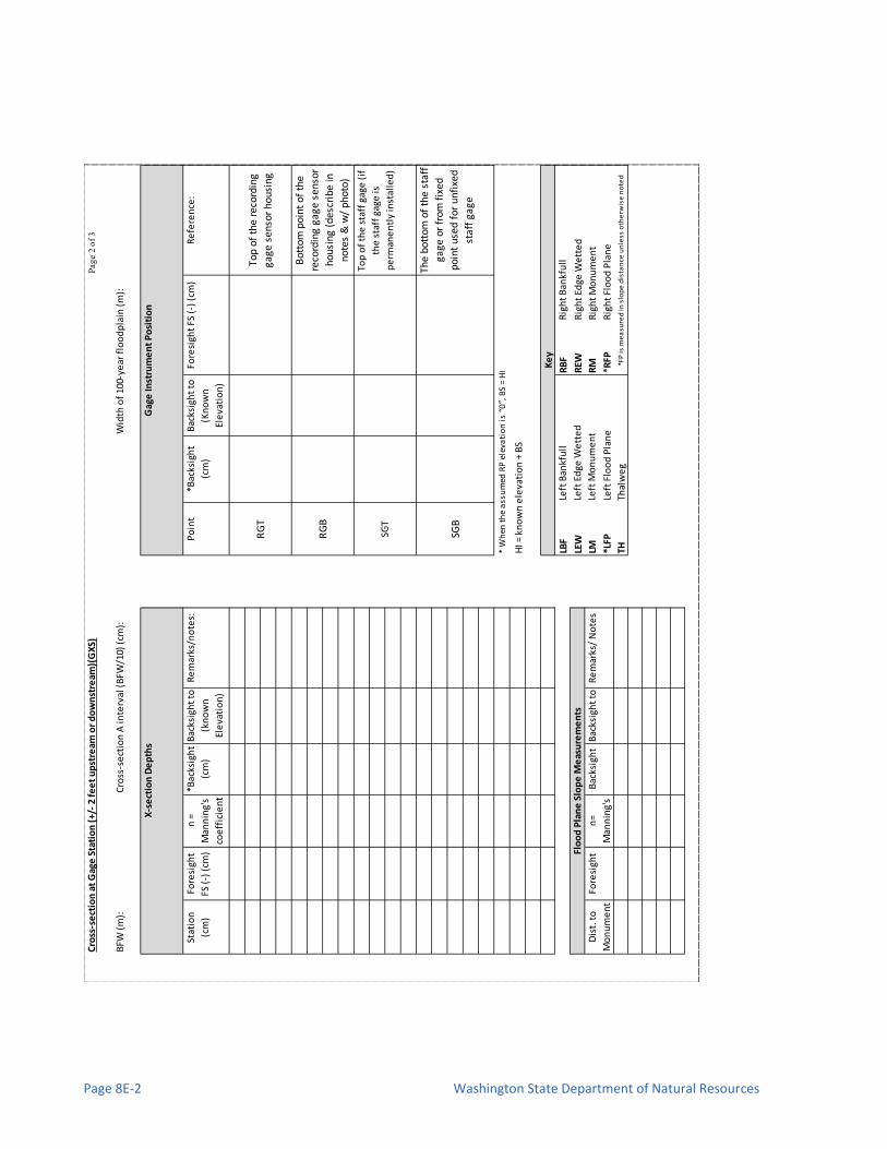
Page 8E-2 Washington State Department of Natural Resources
Cro
ss-s
ect
ion
at
Gag
e S
tati
on
(+/
- 2
fee
t u
pst
ream
or
do
wn
stre
am)(
GX
S)Pa
ge 2
of 3
BFW
(m
):C
ross
-se
ctio
n A
inte
rval
(B
FW/1
0) (
cm):
Wid
th o
f 10
0-ye
ar f
loo
dp
lain
(m
):
* W
hen
th
e a
ssu
med
RP
ele
vati
on
is
“0”,
BS
= H
I
HI =
kn
ow
n e
leva
tio
n +
BS
LBF
RB
F
LEW
REW
Rig
ht
Edge
We
tte
d
Fore
sigh
tLM
RM
*LFP
Left
Flo
od
Pla
ne
*RFP
TH
Stat
ion
(cm
)
Rig
ht
Flo
od
Pla
ne
Rig
ht
Ban
kfu
ll
Thal
we
g
Left
Ban
kfu
ll
RG
TTo
p of
the
rec
ordi
ng
gage
sen
sor
hous
ing
Bot
tom
poi
nt o
f th
e
reco
rdin
g ga
ge s
enso
r
hous
ing
(des
crib
e in
note
s &
w/
phot
o)
Top
of
the
sta
ff g
age
(if
the
sta
ff g
age
is
pe
rman
en
tly
inst
alle
d)
Fore
sigh
t
FS (
-) (
cm)
n =
Man
nin
g's
coe
ffic
ien
t
Fore
sigh
t FS
(-)
(cm
)*B
acks
igh
t
(cm
)
Po
int
*Bac
ksig
ht
(cm
)
X-s
ect
ion
De
pth
sG
age
Inst
rum
en
t P
osi
tio
n
The
bott
om o
f th
e st
aff
gage
or
from
fix
ed
poin
t us
ed f
or u
nfix
ed
staf
f ga
geSG
B
RG
B
SGT
Bac
ksig
ht
to
(kn
ow
n
Ele
vati
on
)
Re
mar
ks/n
ote
s:
*FP
is m
ea
sure
d in
slo
pe
dis
tan
ce u
nle
ss o
the
rwis
e n
ote
d
Left
Mo
nu
me
nt
Rig
ht
Mo
nu
me
nt
Re
fere
nce
:B
acks
igh
t to
(Kn
ow
n
Ele
vati
on
)
Left
Ed
ge W
ett
ed
Ke
y
Flo
od
Pla
ne
Slo
pe
Me
asu
rem
en
ts
n=
Man
nin
g's
Dis
t. t
o
Mo
nu
me
nt
Bac
ksig
ht
Bac
ksig
ht
toR
em
arks
/ N
ote
s

Status and Trends Monitoring of Riparian and Aquatic Habitat in the OESF Page 8E-3
Page
3 o
f 3
Cro
ss s
ect
ion
ske
tch
wit
h M
ann
ing'
s C
oe
ffic
ien
t; la
be
l sig
nif
ican
t p
oin
ts a
nd
ban
ks.

Page 8E-4 Washington State Department of Natural Resources
Site: Camera Number:
Date and Time: Photo Range:
Staff:
Directions: Along with the survey data, be sure to note the following information:
Manning’s n
Sketches
Notes
Points to gather:
Floodplain elevation points; extended out to next break in grade after main channel (100 yr FP)
Major points of inflection in the channel used to estimate channel area and hydraulic radius
Changes in channel roughness (Manning’s n)
RGT:The top of the recording gage sensor housing,
RGB: The bottom point of the recording gage sensor housing (describe in notes and with a photo)
SGT: One point on the top of the staff gage (if present) or on the staff gage data point
SGB: One point on the bottom of the staff gage or fixed point used for staff measurement (if present)
RP: Benchmark
WSE: Water surface at the time of survey on both right and left bank
Staff Gage Reading: Record the staff gage reading at the same time the survey is completed.
Note that the survey should start on the left bank and more right.
Enter the final, processed elevations into the Access database following field work.
Figure 1: Example of cross-section sketch with notation method for Manning's n
Notes:
Pictures Take many pictures of the cross-sections and channel features, including Manning’s n features, so that you can
verify conditions when back in the office.
2) Draw side-views for each cross-section; note right and left banks along with significant changes in slope, channel
roughness, obstructions, or irregularities in the flow field
Cross Section Stability Survey Ancillary Data Sheet - page 1
1) Draw a plan view of the entire reach
Note changes in the roughness and estimate Manning’s n at every subsection; including overbank/floodplain areas
1) General comments on weather and location
2) Details about cross-section and features of channel

Status and Trends Monitoring of Riparian and Aquatic Habitat in the OESF Page 8E-5
Side View of Cross Section and Plan View of Relationship between RP and Gages
Cross Section Stability Survey Ancillary Data Sheet - page 2

Page 8E-6 Washington State Department of Natural Resources
This page intentionally left blank.

Status and Trends Monitoring of Riparian and Aquatic Habitat in the OESF Page 8F-1
Appendix 8F. Directions for Using Flow Meter Hach FH950 Directions for setting up the instrument Step 1: Perform a velocity calibration once per day. Using a non-metallic bucket of still water at least 16 cm (6 in) deep, place the sensor in the center of the bucket so that it doesn’t touch the sidewall or bottom of bucket. After the water has stilled and the sensor is reading 0 m/s, go to “Setup->Velocity Calibration” and follow the directions on the screen. Step 2: After the velocity calibration, verify that the settings of the instrument are correct. On main screen, select “Setup->Flow Calculation>- Verify that “Mid-section” is selected. Step 3: Under “Setup->Filter Parameters-> FPA,” set the value to 40 seconds (see protocol above for discussion of this point). Step 4: Under “Setup->Units,” chose metric units for all variables. Depth (cm), width (m), velocity (m/s). Step 5: Under “Setup->Station Entry,” select “Non-fixed” so that you can easily change the distance between stations. Step 6: Upon startup of the instrument, the instrument will run a self-test. Note whether this test is passed or not. If not passed, do not use instrument to take measurements and return to the manufacturer for repairs. Directions for taking a discharge measurement Step 1: In main menu, select, “Profiler.” Step 2: Enter the operator name (initials of person using instrument). Step 3: Select the type of cross section you will be measuring, “Stream.” If you need to change the Fixed Point Averaging (FPA) time, you can also do that at this screen under “Setup.” Step 4: Enter a name for the stream (11 characters) in the following format, “site number (3)YYMMDD.” If an additional measurement is taken at this site on the same day, add “b, c, d…” to the end of the file name. Step 5: Leave the stage reference blank. Step 6: In the “Station” menu, select “Edge/Obstruction.” Choose the starting edge (try to start on the left edge when possible). Step 7: Enter the “Distance to Vertical,” or the distance from your first station to the starting edge. Step 8: Select “Set Depth” and enter the actual depth. If you are at an edge, the depth is automatically zero. If you have a sheer edge, you next station should be as close to the edge as possible. Step 9: Enter the “Edge Factor,” which is a roughness estimator/multiplier. The scale ranges from 0.50 (very rough) to 1.0 (totally smooth). The roughness factor is relevant only for right angled cross sections. It is used as a factor in the calculation of the discharge proportion of edge areas. For example:
Page 8F-2 Washington State Department of Natural Resources
• Smooth edge with no vegetation (e.g., concrete, steel, cement) - 0.8 to 0.9 • Brick sides with vegetation— 0.7 • Rough walls with heavy vegetation—0.6 to 0.5 Step 10: Select “Measure Velocity.” If you are at an edge, you will not have this option as the velocity is assumed to be zero. You will next be prompted to select the number of points at which you will measure velocity at this station. See the discharge guidelines above for a discussion of when to collect more than one point. Generally, you will collect a single point at 0.6 times the water depth. Step 11: Select the measurement point (ex. 0.6). Obey the instrument prompts and adjust the sensor to the correct depth. Step 12: Once the sensor is adjusted and it has had a few moments to adjust to the new station velocity, select, “Capture.” Once you push this button, the instrument will begin collecting data. Step 13: Once the instrument has finished reading, if you believe the value to be accurate, select “Verify.” Then return to the main menu and select “Next” to go to the next station. Step 14: Repeat steps until you reach the opposite edge where you will repeat the edge reading. Step 15: When all of the measurements have been completed, select “Channel Summary” to view the results. If any of the sections contain >5% of the total discharge, you will have the opportunity to add additional stations within these sections. NOTE: If the stations are already at the minimum distance apart (10 cm), do not take additional readings. Step 16: To insert a new station, navigate back to the station before the location you would like to add a measurement to. For example, if you want to add a measurement between stations 3 and 4, navigate to station 3 and push “OK” to display the station settings. Select “Ins” and push “OK.” Step 17: To delete a station, navigate to the desired station and select “Del” and “OK.” Directions for transferring data from the Hach FH950 to the field laptop: Step 1: Connect the Hach FH950 to the field laptop using the USB cable. The laptop will treat the instrument like a USB storage device, though it is read-only. Step 2: Files will be stored in folders designated for each gage station site. Copy the files over to “Hydrologic Databases/Discharge Data/Discharge_Download_Site_site number.” The file is limited to eight characters. File should be named, “MMDD_site number.TSV.” Open file in excel by right clicking on the file and then opening it with Excel. Separate the data into columns and then save the file as,”YYMMDD_sitenumber_FH950.xlsx.” Step 3: To delete files off of the meter (please do this once the files are backed up to the network), you must use the handheld device. Select “Main Menu->Diagnostics->Delete Files,” and follow the prompts.
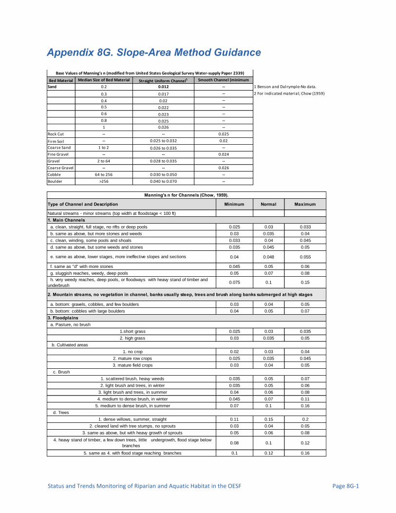
Status and Trends Monitoring of Riparian and Aquatic Habitat in the OESF Page 8G-1
Appendix 8G. Slope-Area Method Guidance
Bed Material
Sand 1 Benson and Dalrymple-No data.
2 For indicated material; Chow (1959)
Rock Cut
Firm Soil
Coarse Sand
Fine Gravel
Gravel
Coarse Gravel
Cobble
Boulder
Minimum Normal Maximum
0.025 0.03 0.033
0.03 0.035 0.04
0.033 0.04 0.045
0.035 0.045 0.05
0.04 0.048 0.055
0.045 0.05 0.06
0.05 0.07 0.08
0.075 0.1 0.15
0.03 0.04 0.05
0.04 0.05 0.07
0.025 0.03 0.035
0.03 0.035 0.05
0.02 0.03 0.04
0.025 0.035 0.045
0.03 0.04 0.05
0.035 0.05 0.07
0.035 0.05 0.06
0.04 0.06 0.08
0.045 0.07 0.11
0.07 0.1 0.16
0.11 0.15 0.2
0.03 0.04 0.05
0.05 0.06 0.08
0.08 0.1 0.12
0.1 0.12 0.16
Base Values of Manning's n (modified from United States Geological Survey Water-supply Paper 2339)
Median Size of Bed Material
(mm)Straight Uniform Channel1 Smooth Channel (minimum
value)20.2 0.012 --
0.3 0.017 --
0.4 0.02 --
0.5 0.022 --
0.6 0.023 --
0.8 0.025 --
1 0.026 --
-- -- 0.025
-- 0.025 to 0.032 0.02
1 to 2 0.026 to 0.035 --
-- -- 0.024
2 to 64 0.028 to 0.035 --
-- -- 0.026
b. same as above, but more stones and weeds
64 to 256 0.030 to 0.050 --
>256 0.040 to 0.070 --
Manning's n for Channels (Chow, 1959).
Type of Channel and Description
Natural streams - minor streams (top width at floodstage < 100 ft)
1. Main Channels a. clean, straight, full stage, no rifts or deep pools
1.short grass
c. clean, winding, some pools and shoals
d. same as above, but some weeds and stones
e. same as above, lower stages, more ineffective slopes and sections
f. same as "d" with more stones
g. sluggish reaches, weedy, deep pools
h. very weedy reaches, deep pools, or floodways with heavy stand of timber and
underbrush
2. Mountain streams, no vegetation in channel, banks usually steep, trees and brush along banks submerged at high stages
a. bottom: gravels, cobbles, and few boulders
b. bottom: cobbles with large boulders
3. Floodplains a. Pasture, no brush
d. Trees
2. high grass
b. Cultivated areas
1. no crop
2. mature row crops
3. mature field crops
c. Brush
1. scattered brush, heavy weeds
2. light brush and trees, in winter
3. light brush and trees, in summer
4. medium to dense brush, in winter
5. medium to dense brush, in summer
1. dense willows, summer, straight
2. cleared land with tree stumps, no sprouts
3. same as above, but with heavy growth of sprouts
4. heavy stand of timber, a few down trees, little undergrowth, flood stage below
branches
5. same as 4. with flood stage reaching branches

Page 8G-2 Washington State Department of Natural Resources
This page intentionally left blank.

Status and Trends Monitoring of Riparian and Aquatic Habitat in the OESF Page 8H-1
Appendix 8H. Solinst® Leveloader, Levelogger, and Barologger Setup and Retrieval of data from Levelogger Water Level Sensor This section includes specific computer commands for the setup and downloading of data using a laptop and the Solinst Leveloader data transfer device. The choice of how frequently to download data is not necessarily limited by the storage capacity of the water level sensor. Most units are capable of storing many months’ worth of data. Instead, a greater concern is equipment failure. Infrequent data retrieval could result in the loss of considerable amounts of data. If the equipment has failed, it would be better to know sooner than later. Directions for setting up the Levelogger and Barologger sensors using a computer Step 1: Connect logger to the computer using either the Direct Read cable or Base Station. Step 2: Select the “Datalogger Settings” tab, then select the “Retrieve Datalogger Settings” button in the upper, left-hand corner. Step 3: Under the “Datalogger Sampling Mode,” choose the “Linear” tab and then set the “Sampling Rate” to 15 minutes.
Step 4: Under “Datalogger Memory Mode,” select “Slate” Step 5: Under “Start/Stop Datalogger,” check the “Future Start,” box and set for the desired start time; then
select “Start Now.” Directions for setting up the Leveloader Step 1: Connect the Leveloader to the computer. Step 2: Open the Solinst program, select the “Leveloader” tab on the upper right hand side of the window.
Step 3: Select the “Retrieve Leveloader Settings” button . Step 4: Set the computer time to Pacific Standard time; then select “Synchronize” button on the bottom left side of the screen. Step 5: Under “Levelogger Default File Settings,” name the “Settings Title” with the type of logger and the interval (ex. Level_15min). Step 6: Under “Levelogger Type,” select the Sensor type (LT-Edge or LT-Edge-Baro). Step 7: Under “Logger Sampling Mode,” select the “Linear” tab and set the “Sampling Rate” to 15 minutes.

Page 8H-2 Washington State Department of Natural Resources
Step 8: Once settings are finalized, select “Apply Leveloader Settings,” to transfer the settings file to the
Leveloader. Step 9: Disconnect the Leveloader from the computer. Directions for setting up a levelogger or barologger sensor with the leveloader Step 1: Connect the leveloader to the logger using the “Direct Read” or “Direct Connect” cable. Step 2: Select “Connect to Logger” on the Leveloader Gold Menu Step 3: On the Levelogger Menu select “Load Settings File” Step 4: In the Load Settings Files Menu find the appropriate settings file (ex. If you are starting a Barologger and want 15min logging intervals select the “Baro_15min” settings file). Once a settings file is selected it will load onto the logger and a congfirmation message will appear. The Leveloader will then direct you back to the Levelogger Menu. Directions for double checking the settings file loaded on the logger Step 4a: Select “Edit Levelogger” from the Levelogger Menu.
Step 4b: From the Edit levelogger Menu select “Edit Sample Rate”. Observe the units and time duration to insure it is what you intended to be selected. Return to the “Edit Levelogger Menu” by selecting “Submit”.
Step 4c: From the Edit levelogger Menu select “Edit Unit”. Insure the unit of measurement selected for depth is meters, Pressure is kPa and temperature is degrees Celsius. When the desired units are shown select “OK” return to the Edit Levelogger menu.
Step 4d: Once logger setting are reviewed select “Menu” to return to the Levelogger menu.
Step 5: Select “Restart Levelogger” on the Levelogger Menu. Step 6: Select “Future Start Logging” on the Restart Levelogger menu. Step 7: If prompted to, stop the logger by pressing the up and down buttons on the instrument at the same time. Remember to save the data on the logger before restarting. Step 8: Input the preffered start time and select “Submit”. Once selected a confirmation message will appear informing you that the logger has been restarted.
* Save the data on the logger to the computer before restarting the water level sensor*

Status and Trends Monitoring of Riparian and Aquatic Habitat in the OESF Page 8H-3
Directions for downloading the Levelogger and Barologger sensors using a Leveloader Step 1: Open the locking well cap and remove direct read cable caps. Step 2: Before connecting the cable to the Leveloader first screw it onto the direct read cable, then connect it to the Leveloader. Step 3: Turn on the Leveloader and select “connect to Logger” Step 4: Select “Real Time-View Only” and enter the real time depth or barometric pressure and temperature in the field form. Then select “Menu” to return back to the main menu.
Note: You cannot tell if it is the Barologger or Levelogger until this point. Check the units used to identify which logger it is. If it is the Levelogger the units will be in meters and be generally around 10.00m. If it is the Barologger the units will be in Kilopascals and generally be around 100kPa.
Step 5: Select “Data from Levelogger”
Step 5a: Write down the serial number located at the top of the screen (ex. #202xxxx) in the “SN:” section of the field form. Step 5b: Check the download intervals under the “Time” header. There should be a download every 15 minutes. Enter the download interval into the “Time Interval” section of the field form Step 5c: Check the battery percentage in the upper right hand side of the screen and enter it into the “Real-Time battery” section of the field form. Step 5d: Finally, select “Save Log” to save all the data off the logger. Once the log has been saved it will automatically return you to the Levelogger menu.
Step 6: Select “Edit Levelogger” (note: it says “Edit Levelogger” whether you are connect to the Levelogger or the Barologger). Stop the Leveloader by pressing the Up and Down arrows at the same time. Next, sync the time by pressing “Edit” while the curser is on the “Time (sync to loader)” tab. Press the “Menu” button to return back to the main menu. Write “Yes” under in the “Sync Time?” section of the field form.
Step 7: At the very bottom of the main menu select “Restart Levelogger” (note: this is on the next page so if you don’t immediately see it just keep going down on the main menu)
Step 7a: select “Future Start Logging” and press “OK” at the scary warning screen (unless you haven’t downloaded the data off the logger) Step 7b: Enter the start time as the next even :15 minute interval (X:00:00, X:15:00, X:30:00, or X:45:00). Move the cursor to the number you want to edit by selecting the ”NXT” tab. Then using the up and down arrows select the number you want to enter. The date format is YY:MM:DD Step 7c: Select “Submit” when you have successfully entered the date and time you would like the logger to start on. Enter the date and time you selected into the field form under “Restart date and time”
Step 8: Disconnect the cable from the Leveloader, then the direct read cable and reconnect it on the logger you have not downloaded yet and repeat steps 2-7.

Page 8H-4 Washington State Department of Natural Resources
Directions for downloading the Levelogger and Barologger sensors using a computer Step 1: Connect the sensor to a computer using the base station. Step 2: Open The Solinst software and select the “Data Control” tab.
Step 3: Select the “Download Data” icon
Ste Step 4: Save the data into the appropriate folder. “Desktop\Hydrologic Databases\Recording Gage Data”, then select the “Recording_Gage_Site_Site_Number” folder for the desired watershed and put the files into the “SiteNumber_Levelogger_Barologger_files” folder. Save the file using the naming convention “YYMMDD_SiteNumber_LL or BL”. Step 5: Copy paste the Barologger or Levelogger data file from the desktop folder into the appropriate network folder: “\\snarf\div_lm\ecosystem\monitoring_research\tminkova\OESF_Projects\10_Rip S&T Mon\01_FIELD DATA\06_Hydrology\Hydrologic Databases\Recording Gage Data”, then select the “Recording_Gage_Site_Site_Number” folder for the desired watershed and paste the files into the “SiteNumber_Levelogger_Barologger_files” folder.
Directions for downloading the Leveloader data onto a computer Step 1: Connect Leveloader to laptop using the micro USB cable. Step 2: Select “Data to PC” on the Leveloader’s main menu. Step 3: On the laptop, open the Solinst software. When the application opens select the “Leveloader” tab on the top right side of the window. Step 4: On the laptop, select the “Retrieve Leveloader Settings” icon. Make sure you have selected the
correct Com Port. Step 5: Check the boxes of only the Barologger and Levelogger combination you wish to download. Then
click the “Download Data” icon.
Step 6: download the files onto the laptop into their appropriate folders. “Desktop\Hydrologic Databases\Recording Gage Data”, then select the “Recording_Gage_Site_Site_Number” folder for the desired watershed and put the files into the “SiteNumber_Levelogger_Barologger_files” folder. Save the file using the naming convention “YYMMDD_SiteNumber_LL or BL”
Step 7: When the files have downloaded select “Finish and Open all”. View the files and look for any irregularities.
Step 8: Repeat steps 5-7 for all loggers.
Status and Trends Monitoring of Riparian and Aquatic Habitat in the OESF Page 8H-5
Step 9: Once all the loggers have been downloaded copy paste each Barologger and Levelogger pair into the appropriate network folder: “\\snarf\div_lm\ecosystem\monitoring_research\tminkova\OESF_Projects\10_Rip S&T Mon\01_FIELD DATA\06_Hydrology\Hydrologic Databases\Recording Gage Data”, then select the “Recording_Gage_Site_Site_Number” folder for the desired watershed and paste the files into the “SiteNumber_Levelogger_Barologger_files” folder.
Directions for Levelogger barometric compensation
Step 1: On the laptop, open the Solinst software and select the Data Wizard tab.
Step 2: Select “Basic: Barometric Compensation (only)” and click next (at the bottom right of window)
Step 3: Click the Open File icon and navigate to the desired Levelogger and Barologger pair you wish to
compensate.
Step 4: Highlight the Barologger and Levelogger files you wish to compensate by clicking on them. Then click next.
Step 5: Once the files have been compensated click the Open button and look for any irregularities in the data.
Step 6: Export the data by clicking the Export Data icon and selecting Export Data.
Step 7: Navigate to the appropriate folder: “Desktop\Hydrologic Databases\Recording Gage Data” folder for the desired watershed and paste the files into the “Recording_Gage_Site_Site_Number” folder. Use the naming convention “YYMMDD_SiteNumber_LL_Comp_Exp”.
Step 8: Repeat steps 2-7 for all Barologger and Levelogger file combinations.
Step 9: Once all the loggers have been Compensated copy paste each compensated Levelogger file into the appropriate network folder: “\\snarf\div_lm\ecosystem\monitoring_research\tminkova\OESF_Projects\10_Rip S&T Mon\01_FIELD DATA\06_Hydrology\Hydrologic Databases\Recording Gage Data”, and paste the files into the appropriate “Recording_Gage_Site_Site_Number” folder.
Step 10: Open the data using Excel and Re-save the file as an .xlsx file.

Page 8H-6 Washington State Department of Natural Resources
This page intentionally left blank.

Status and Trends Monitoring of Riparian and Aquatic Habitat in the OESF Page 8I-1
Appendix 8I. List of Instrument Manuals Solinst Levelogger Series - Quick Start Guide http://www.solinst.com/products/dataloggers-and-telemetry/3001-levelogger-series/operating-instructions/quick-start-guide/3001-quick-start-guide.pdf Solinst Levelogger Series - Software Version 4, November 5, 2013 http://www.solinst.com/products/dataloggers-and-telemetry/3001-levelogger-series/operating-instructions/user-guide/3001-user-guide.pdf Solinst Levelogger Series – Technical Specifications and Setup http://www.solinst.com/products/data/3001.pdf Solinst Leveloader Gold – User Guide http://www.solinst.com/products/dataloggers-and-telemetry/3001-levelogger-series/leveloader/operating-instructions/user-guide/ HAC FH950 Flow Meter – Technical Specifications http://www.hachflow.com/pdf/FH950_ds.pdf HAC FH950 Flow Meter – User Manual http://www.hachflow.com/pdf/FH950_ds.pdf

8I-2 Washington State Department of Natural Resources
This page intentionally left blank.
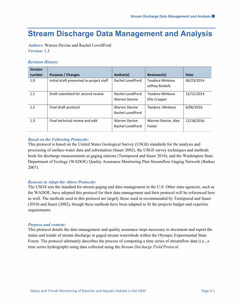
Stream Discharge Data Management and Analysis
Status and Trends Monitoring of Riparian and Aquatic Habitat in the OESF Page 9-1
Stream Discharge Data Management and Analysis Authors: Warren Devine and Rachel LovellFord Version: 1.3 Revision History:
Based on the Following Protocols: This protocol is based on the United States Geological Survey (USGS) standards for the analysis and processing of surface-water data and information (Sauer 2002), the USGS survey techniques and methods book for discharge measurements at gaging stations (Turnipseed and Sauer 2010), and the Washington State Department of Ecology (WADOE) Quality Assurance Monitoring Plan Streamflow Gaging Network (Butkus 2007).
Reasons to Adopt the Above Protocols: The USGS sets the standard for stream gaging and data management in the U.S. Other state agencies, such as the WADOE, have adopted this protocol for their data management and their protocol will be referenced here as well. The methods used in this protocol are largely those used in recommended by Turnipseed and Sauer (2010) and Sauer (2002), though these methods have been adapted to fit the projects budget and expertise requirements.
Purpose and content: This protocol details the data management and quality assurance steps necessary to document and report the status and trends of stream discharge at gaged stream watersheds within the Olympic Experimental State Forest. The protocol ultimately describes the process of computing a time series of streamflow data (i.e., a time series hydrograph) using data collected using the Stream Discharge Field Protocol.
Version
number Purpose / Changes Author(s) Reviewer(s) Date
1.0 Initial draft presented to project staff Rachel LovellFord Teodora Minkova
Jeffrey Ricklefs
06/23/2014
1.1 Draft submitted for second review Rachel LovellFord
Warren Devine
Teodora Minkova
Ellis Cropper
12/15/2014
1.2 Final draft protocol Warren Devine
Rachel LovellFord
Teodora Minkova 6/06/2016
1.3 Final technical review and edit Warren Devine
Rachel LovellFord
Warren Devine, Alex
Foster
12/18/2016

Stream Discharge Data Management and Analysis
Page 9-2 Washington State Department of Natural Resources
Table of Contents Introduction ........................................................................................................................................................ 5
Overview of Hydrology Data ......................................................................................................................... 5
Field Activity Tracking Data ............................................................................................................................. 8
Introduction .................................................................................................................................................... 8
Data Collection Tracking ............................................................................................................................... 8
Gaging Station Installation Metadata ............................................................................................................. 9
Field Maintenance Tracking ........................................................................................................................... 9
Data Flow ....................................................................................................................................................... 9
Recording Gage Data ....................................................................................................................................... 10
Introduction .................................................................................................................................................. 10
The Recording Gage Dataset ........................................................................................................................ 10
Data Products ............................................................................................................................................... 11
Data Flow ..................................................................................................................................................... 11
Discharge Data ................................................................................................................................................. 12
Introduction .................................................................................................................................................. 12
The Discharge Dataset ................................................................................................................................. 12
Data Products ............................................................................................................................................... 14
Data Flow ..................................................................................................................................................... 14
Gage Elevation and Stream Cross-Section Stability ........................................................................................ 15
Introduction .................................................................................................................................................. 15
The gage elevation and cross-section stability dataset ................................................................................. 16
Data products ............................................................................................................................................... 17
Data flow ...................................................................................................................................................... 17
Data Quality Control ........................................................................................................................................ 17
Introduction .................................................................................................................................................. 17
Data Verification .......................................................................................................................................... 18
Recording gage – Staff Gage consistency .................................................................................................... 20
Recording gage sensor calibration Check .................................................................................................... 23
Flow Meter Calibration ................................................................................................................................ 24
Data Archives ................................................................................................................................................... 24
Storage of Electronic Data and Paper Field Forms ...................................................................................... 24
Adjustment of Data .......................................................................................................................................... 25
Introduction .................................................................................................................................................. 25
Adjustment for staff gage replacement ........................................................................................................ 25
Adjustment of staff and recording gage data to watershed datum ............................................................... 26

Stream Discharge Data Management and Analysis
Status and Trends Monitoring of Riparian and Aquatic Habitat in the OESF Page 9-3
Adjustment of cross-section survey data to detect Cross-section changes .................................................. 27
Adjustment for a Shift in Staff or recording gage Elevation........................................................................ 27
Rating Curve Development .............................................................................................................................. 28
Introduction .................................................................................................................................................. 28
Construction of Rating Curves ..................................................................................................................... 29
Data for Rating Curve Development............................................................................................................ 30
Hydrograph Development ................................................................................................................................ 31
References ........................................................................................................................................................ 32
Appendix 9A: Hydrology Database Structure ................................................................................................... 1

Stream Discharge Data Management and Analysis
Page 9-4 Washington State Department of Natural Resources
This page intentionally left blank.

Stream Discharge Data Management and Analysis
Status and Trends Monitoring of Riparian and Aquatic Habitat in the OESF Page 9-5
Introduction This chapter describes all activities associated with management of the hydrology data, collected as described in Chapter 8 (Stream Discharge Field Protocol). After a brief overview of the database, the majority of the chapter is divided into sections that focus on managing each component of the data.
OVERVIEW OF HYDROLOGY DATA The hydrology database consists of multiple interrelated datasets. All of these datasets are stored within a single Microsoft Access database (hereafter called the “hydrology database”), and to the extent possible, all data management activities, including calculations, reports, and data manipulations, are performed within this database (Figure 9-1). The database is stored at: J:\hcp\monitoring_research\tminkova\01_OESF_R&M Program\01_Rip S&T Mon\01_FIELD DATA\02_Hydrology\Data\ Hydro_Database.accdb. All graphical representations of data are performed in R, which accesses the database directly via an Open Database Connectivity (ODBC) connection.
Figure 9-1. Main menu of the hydrology database.

Stream Discharge Data Management and Analysis
Page 9-6 Washington State Department of Natural Resources
Figure 9-2 shows a simplified representation of the datasets in the hydrology database and the relationships among them. The green and blue cells represent the primary datasets, the yellow cells represent quality control datasets, and the orange cells represent calculated data. The arrows represent data used directly in calculations. Among the datasets shown in Figure 9-2, there are three major datasets that are integral to all of the database’s functions and products: (1) the stream discharge dataset, (2) the staff gage dataset, and (3) the recording gage dataset. Discharge measurements are made multiple times per year in each watershed. A series of discharge measurements and simultaneous recording gage readings at various water levels is used to produce a rating curve for each watershed. The rating curve is the relation between stage (i.e., water level), as measured by the recording gage, and stream discharge (measured as cubic meters of water per second). The recording gage dataset consists of all the continuously logged water level data recorded by the submersible pressure transducers (Solinst Levelogger®, Solinst Canada Ltd.) installed in the 14 monitored watersheds. Each time these sensors are downloaded, a staff gage reading is recorded. The sensor data are subsequently adjusted to the staff gage datum. Because both the rating curve and the continuous water level data are now referenced the same datum within each watershed, these data be used to calculate continuous stream discharge, also known as a hydrograph, which is the ultimate product of the database.
Rating Curve
Hydrograph
Recording Gage Dataset
Recording Gage
Elevation Survey
Data
Continuous Water Level
Data, Adjusted to Staff
Gage Datum
Discharge Measurement
Dataset
Staff Gage Dataset
Recording Gage
Sensor
Calibration Data
Discharge
Measurements
Consistency Check
Staff Gage
Elevation
Survey Data
Cross-Section
Stability Data
Figure 9-2. Relationships among the datasets within the hydrology database. Manually collected data are shown in green cells; automatically collected data are blue; quality control data are yellow, and calculated data are shown in orange. Arrows represent data used to inform or calculate subsequent datasets.
Field Activity
Tracking Datasets
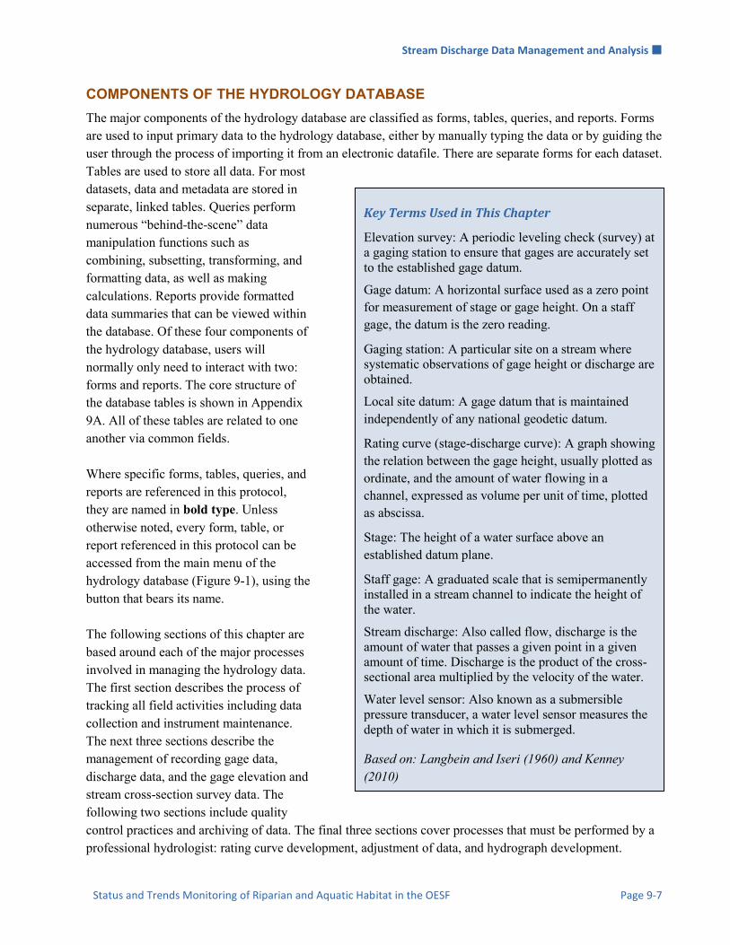
Stream Discharge Data Management and Analysis
Status and Trends Monitoring of Riparian and Aquatic Habitat in the OESF Page 9-7
COMPONENTS OF THE HYDROLOGY DATABASE The major components of the hydrology database are classified as forms, tables, queries, and reports. Forms are used to input primary data to the hydrology database, either by manually typing the data or by guiding the user through the process of importing it from an electronic datafile. There are separate forms for each dataset. Tables are used to store all data. For most datasets, data and metadata are stored in separate, linked tables. Queries perform numerous “behind-the-scene” data manipulation functions such as combining, subsetting, transforming, and formatting data, as well as making calculations. Reports provide formatted data summaries that can be viewed within the database. Of these four components of the hydrology database, users will normally only need to interact with two: forms and reports. The core structure of the database tables is shown in Appendix 9A. All of these tables are related to one another via common fields. Where specific forms, tables, queries, and reports are referenced in this protocol, they are named in bold type. Unless otherwise noted, every form, table, or report referenced in this protocol can be accessed from the main menu of the hydrology database (Figure 9-1), using the button that bears its name. The following sections of this chapter are based around each of the major processes involved in managing the hydrology data. The first section describes the process of tracking all field activities including data collection and instrument maintenance. The next three sections describe the management of recording gage data, discharge data, and the gage elevation and stream cross-section survey data. The following two sections include quality control practices and archiving of data. The final three sections cover processes that must be performed by a professional hydrologist: rating curve development, adjustment of data, and hydrograph development.
Key Terms Used in This Chapter
Elevation survey: A periodic leveling check (survey) at a gaging station to ensure that gages are accurately set to the established gage datum.
Gage datum: A horizontal surface used as a zero point for measurement of stage or gage height. On a staff gage, the datum is the zero reading.
Gaging station: A particular site on a stream where systematic observations of gage height or discharge are obtained.
Local site datum: A gage datum that is maintained independently of any national geodetic datum.
Rating curve (stage-discharge curve): A graph showing the relation between the gage height, usually plotted as ordinate, and the amount of water flowing in a channel, expressed as volume per unit of time, plotted as abscissa.
Stage: The height of a water surface above an established datum plane.
Staff gage: A graduated scale that is semipermanently installed in a stream channel to indicate the height of the water.
Stream discharge: Also called flow, discharge is the amount of water that passes a given point in a given amount of time. Discharge is the product of the cross-sectional area multiplied by the velocity of the water.
Water level sensor: Also known as a submersible pressure transducer, a water level sensor measures the depth of water in which it is submerged.
Based on: Langbein and Iseri (1960) and Kenney (2010)

Stream Discharge Data Management and Analysis
Page 9-8 Washington State Department of Natural Resources
Field Activity Tracking Data
INTRODUCTION To facilitate the scheduling of data collection and site maintenance, and to summarize past field activities, the hydrology database includes a system for tracking field work. Most field visits are performed during week-long trips, and the field tracking process is designed to record information on a weekly basis, which is a sufficient resolution for field work planning and summarization purposes. The process of entering the weekly field activity data is designed to be quick so that it can be performed by the field crew each week after they return to the office. This field activity tracking process produces a record independent of the metadata that are recorded in association with all data collection processes. The primary reason for this is that field data may not be entered in the database until weeks after they are collected. In the interim, there is no easily accessible record of what field work was performed or when it was performed. The field activity tracking process fills that need. In addition to the tracking of data collection, two other datasets used to document field activities are described in this section. One of these, gaging station installation metadata, is used to store all of the information associated with the installation of each gaging station. Data are added to this dataset when a new gaging station is installed or when all or a portion of a gaging station is replaced. The other dataset, field maintenance tracking, is used to document field maintenance activities performed on gaging stations or on individual instruments.
DATA COLLECTION TRACKING On a weekly basis, the field crew records, in the database, the types of data collected during that week and the watersheds at which it was collected (the field form is in Appendix 8A in the previous chapter). The Data Collection Tracking Form is used to enter these data. On the form, the field crew member enters:
1. The starting date and ending date of that week’s field visit. 2. Field crew members. 3. The watersheds at which discharge measurements were made. 4. The watersheds at which recording gages were downloaded. 5. The watersheds at which elevation stability and cross-section surveys were made. 6. Notes from the week’s work.
Data entered via this form are stored in the Field Visit Table. There are two reports that summarize the contents of this table. The first is called Data Collection Summary by Water Year and Last Visit. It lists the total number of discharge measurements and recording gage downloads, per watershed, per water year. It also lists the date of the most recent discharge measurement and recording gage download in each watershed. A second report, List of Visit Dates for All Watersheds, lists the dates of all discharge measurements, recording gage downloads, and elevation stability and cross-section surveys by watershed.

Stream Discharge Data Management and Analysis
Status and Trends Monitoring of Riparian and Aquatic Habitat in the OESF Page 9-9
GAGING STATION INSTALLATION METADATA During the installation of a new gaging station, or during replacement of instruments at a gaging station, a series of field forms are filled out to document the details of the work (see Stream Discharge protocol). The data from these forms are entered in the hydrology database via the Gage Installation Form. This form contains 59 different fields to document information such as site characteristics, details of the staff gage and recording gage installations, photo numbers, and general site notes. The data entered using this form are stored in the Installation Table. There is a separate form, the Staff Gage Installation/Replacement Form, for installation and replacement of the staff gage only. This form contains only fields relevant to the staff gage, although data entered populate the same table as the Gage Installation Form (i.e., the Installation Table). The form is accessed via a button on the Gage Installation Form.
FIELD MAINTENANCE TRACKING Occasionally, maintenance on the various components of the gaging stations is necessary. Some maintenance activities are performed regularly, but others occur on an irregular basis, as problems are noted in the field. Field maintenance activities, as well as observations of maintenance needs (or observations that maintenance is not needed), are documented using the Gage Maintenance Field Sheet. The Field Maintenance Tracking Form is used to enter maintenance records in the database. This form has fields for:
1. The watershed number where the maintenance was performed. 2. The date and time of the maintenance work. 3. Field crew members. 4. Camera and photo ID information. 5. The name of the instrument that was maintained. 6. A staff gage reading, if taken. 7. A description of the reason for the maintenance. 8. Field notes. 9. Necessary maintenance that was not performed (i.e., “to do” items).
All of the data entered via this form are stored in the Maintenance Table. The Maintenance Activities report lists all of the entries from the Maintenance Table.
DATA FLOW 1. Fill out field forms For each of the three datasets used to document field activities, field forms
(listed in the sections below) are used to record the details of the activity as it is performed in the field.
2. Scan and store field forms After returning from the field each week, all of the field forms are scanned and stored on the DNR network drive; the original paper forms are archived at the Forest Resources Division of Washington Department of Natural Resources.
3. Enter data All of the information collected on paper field forms will be entered in the hydrology database by the OESF Data Management Specialist. The data entry forms for these three datasets are listed above.
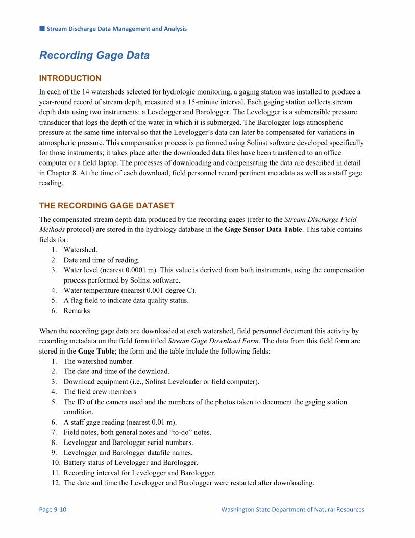
Stream Discharge Data Management and Analysis
Page 9-10 Washington State Department of Natural Resources
Recording Gage Data
INTRODUCTION In each of the 14 watersheds selected for hydrologic monitoring, a gaging station was installed to produce a year-round record of stream depth, measured at a 15-minute interval. Each gaging station collects stream depth data using two instruments: a Levelogger and Barologger. The Levelogger is a submersible pressure transducer that logs the depth of the water in which it is submerged. The Barologger logs atmospheric pressure at the same time interval so that the Levelogger’s data can later be compensated for variations in atmospheric pressure. This compensation process is performed using Solinst software developed specifically for those instruments; it takes place after the downloaded data files have been transferred to an office computer or a field laptop. The processes of downloading and compensating the data are described in detail in Chapter 8. At the time of each download, field personnel record pertinent metadata as well as a staff gage reading.
THE RECORDING GAGE DATASET The compensated stream depth data produced by the recording gages (refer to the Stream Discharge Field Methods protocol) are stored in the hydrology database in the Gage Sensor Data Table. This table contains fields for:
1. Watershed. 2. Date and time of reading. 3. Water level (nearest 0.0001 m). This value is derived from both instruments, using the compensation
process performed by Solinst software. 4. Water temperature (nearest 0.001 degree C). 5. A flag field to indicate data quality status. 6. Remarks
When the recording gage data are downloaded at each watershed, field personnel document this activity by recording metadata on the field form titled Stream Gage Download Form. The data from this field form are stored in the Gage Table; the form and the table include the following fields:
1. The watershed number. 2. The date and time of the download. 3. Download equipment (i.e., Solinst Leveloader or field computer). 4. The field crew members 5. The ID of the camera used and the numbers of the photos taken to document the gaging station
condition. 6. A staff gage reading (nearest 0.01 m). 7. Field notes, both general notes and “to-do” notes. 8. Levelogger and Barologger serial numbers. 9. Levelogger and Barologger datafile names. 10. Battery status of Levelogger and Barologger. 11. Recording interval for Levelogger and Barologger. 12. The date and time the Levelogger and Barologger were restarted after downloading.

Stream Discharge Data Management and Analysis
Status and Trends Monitoring of Riparian and Aquatic Habitat in the OESF Page 9-11
DATA PRODUCTS The recording gage dataset is ultimately used to produce a hydrograph for each watershed. However, the recorded water level data for each watershed first must be adjusted to the watershed’s datum (see Adjustment of Data section).
DATA FLOW
Field forms
1. Fill out field form The field form titled Stream Gage Download Form is used to record the metadata associated with each watershed visit during which recording gage data are downloaded.
2. Scan and store field forms After returning from the field each week, the field forms are scanned and stored on the DNR network drive; the original paper forms are archived at the Forest Resources Division of Washington Department of Natural Resources.
3. Enter data All of the metadata collected on paper field forms is entered in the hydrology database by the OESF Data Management Specialist, using the database form titled Recording Gage: Field Form Entry and Electronic Data Importation.
Electronic data
1. Download and process datafiles The Stream Discharge Field Methods protocol provides a detailed, step-by-step description of how the data are downloaded from the recording gage instruments (Levelogger and Barologger) and then processed in the office to compensate the water level readings for barometric pressure. The result is one comma-separated variable (.csv) file per watershed per download.
2. Store data files In the DNR office, the raw downloaded files and the processed (compensated) .csv files are stored on the DNR network drive. The raw datafiles are stored in the directory: J:\hcp\monitoring_research\tminkova\01_OESF_R&M Program\01_Rip S&T Mon\07_Data management\_All new data and photos\
The compensated datafiles are stored in the directory: J:\hcp\monitoring_research\tminkova\01_OESF_R&M Program\01_Rip S&T Mon\01_FIELD DATA\02_Hydrology\Data\Archived_data\Recording_gage_data\Compensated_data\
3. Import data to database The compensated data are imported to the hydrology database at the same time as the data from the field forms are entered, using the same database form (Recording Gage: Field Form Entry and Electronic Data Importation). The data importation process involves two simple steps described in detail on the form and summarized here:
a. The user copies the datasheet containing the compensated data and pastes it into the Gage_Import table in the hydrology database.
b. The user clicks a button to run a query which automatically formats the imported data and adds it to the Gage_Table.

Stream Discharge Data Management and Analysis
Page 9-12 Washington State Department of Natural Resources
Discharge Data
INTRODUCTION Stream discharge is measured 6 to 10 times per year in each of the 14 hydrology watersheds. The discharge data are used to produce and then update a rating curve for each watershed that is subsequently used to produce the watershed’s hydrograph. For each discharge measurement in a given watershed, the discharge dataset consists of a calculated stream discharge value, the raw data used to calculate the discharge value, and metadata.
Discharge data are usually collected using an electronic flow meter (currently the Hach FH 950® velocity meter is used), although two alternative measurement methods may be used under certain conditions, as described in detail in Chapter 8 (Stream Discharge). The first of these, the neutrally buoyant object (NBO) method (Peck et al. 1998), may be used when stream depth is too low (<6 cm) to use the Hach flow meter (Peck et al. 1998). Experience has suggested that the NBO method is far less accurate than the electronic flow meter and should only be used as a last resort. The second alternative measurement approach is the slope-area method (Dalrymple and Benson 1967; Bradley 2012), which can be used when the water level is too high to safely wade the stream (this method had not yet been used as of December 2016). In the event that the datafile produced by the Hach electronic flow meter is corrupted or lost, the raw discharge data, recorded on a field form, can be used to calculate discharge manually following the midsection method (Turnipseed and Sauer 2010). Within the OESF Riparian Status and Trends project, the midsection method is sometimes called the Marsh-McBirney (MMB) method, after the MMB flow meter which does not automatically compute discharge, necessitating a manual midsection discharge calculation. Regardless of the type of flow meter used, discharge data are added to the hydrology database via the form titled Discharge Field Form Entry and Electronic Data Import.
THE DISCHARGE DATASET Discharge data are stored in four tables in the hydrology database. The first of these is the Discharge Metadata Table, which stores all of the metadata recorded on the Stream Discharge Field Sheet, including a staff gage reading taken at the same time as each discharge measurement. This table contains one record per discharge measurement. The Discharge Metadata Table contains the following information:
1. Watershed number. 2. Date and time that the discharge measurement began and ended. 3. A Yes/No field indicating if it was a duplicate measurement (take for quality control purposes). 4. Measurement method (including instrument type). 5. Weather conditions during reading. 6. Crew members. 7. Instrument metadata including serial number, self-test, and calibration check. 8. Name of datafile. 9. Quality rating of the measurement. 10. The ID of the camera used and the numbers of the photos taken facing upstream and downstream. 11. Staff gage readings at the beginning and end of the discharge measurement.

Stream Discharge Data Management and Analysis
Status and Trends Monitoring of Riparian and Aquatic Habitat in the OESF Page 9-13
12. General notes about the measurement. 13. Notes about the control.
When discharge data are collected using the Hach electronic flow meter, two tables are used to store the data. The first of these, the Discharge Data Table, stores the summary data produced by the flow meter after a discharge measurement (e.g., calculated stream discharge, in m3/second). One record is stored per discharge measurement. The second table that stores flow meter data, the Discharge Detail Table, contains every data point recorded by the flow meter during each discharge measurement. Because 20 or more measurement stations are often used to produce a single discharge measurement, this table contains many records for each discharge measurement. The records in the Discharge Detail Table are stored primarily for archival and quality control purposes because the calculated discharge reading for each measurement is in the Discharge Data Table. The fields in the Discharge Data Table are:
1. Watershed number. 2. The date and time of the measurement. 3. The stream cross-sectional area, calculated by the flow meter. 4. Discharge value. 5. Units of the discharge value (may be either m3/second or m3/minute). 6. Stream width, calculated by the flow meter. 7. A Yes/No field indicating if it was a duplicate measurement (taken for quality control purposes). 8. A flag field to indicate data quality status.
The fields in the Discharge Detail Table are:
1. Watershed number. 2. The date and time that the measurement started. 3. ID number for each measurement station that composes the discharge measurement. 4. The location of the measurement station (identified by its distance from the starting point). 5. The method used for the reading (often the 1-point method, which is one reading per station). 6. Water depth at the station. 7. Edge factor, if one is used in the discharge calculation. 8. Velocity of the water. 9. The cross-sectional area represented by the reading. 10. Discharge rate represented by the station’s reading. 11. A Yes/No field indicating if it was a duplicate measurement (take for quality control purposes). 12. A flag field to indicate data quality status.
Beginning in 2015, all discharge data collected using an electronic flow meter are imported to the hydrology database through an automated process. Prior to 2015, all discharge data were entered manually. The pre-2015 data include fields that no longer need to be entered manually under the automated data import system. Therefore, pre-2015 data are stored in a separate table, Discharge Manual Data Table.

Stream Discharge Data Management and Analysis
Page 9-14 Washington State Department of Natural Resources
The only situation in which data from 2015 onward will be added to the Discharge Manual Data Table is if discharge measurements are collected using a method other than the electronic flow meter (i.e., NBO, slope-area, or a manual midsection-based calculation using data recorded on field sheets). For all data analysis, export, and summarization purposes, the data from the Discharge Manual Data Table are combined with the other discharge data using queries. The Discharge Manual Data Table contains these fields:
1. Edge slope (vertical or slanted) for each edge of the stream. 2. Edge factor for each edge of the stream. 3. Stream width. 4. Discharge. 5. Maximum water velocity measured at any station. 6. Cross-sectional area of the stream.
All three tables containing discharge data (Discharge Data Table, Discharge Detail Table, and Discharge Manual Data Table) are linked to the metadata in the Discharge Metadata Table.
DATA PRODUCTS The primary purpose of the discharge dataset is to create a rating curve for each watershed, based on the relation between the discharge measurements and the adjusted recording gage readings (recording gage readings are first adjusted to the watershed’s datum). The rating curves are then used with the adjusted recording gage data to produce each watershed’s hydrograph. The development of rating curves is a task that must be performed by a hydrologist. However, after the rating curves are developed, they should be added to the database so that the database can produce the data for the hydrographs. The database contains a query that creates a table of all the data needed to develop the rating curves. This table can then be exported in any standard data format (e.g, .xlsx, .csv, .txt) for use by a hydrologist. The query that creates the table is run by clicking the button on the main menu labeled Rating Curve Data (Queried).
DATA FLOW
Field forms
1. Fill out field form The field form titled Stream Discharge Field Sheet is used to record the metadata associated with each discharge measurement. There is a different version of this field sheet for each discharge measurement method, but all versions include the same metadata. This field form is also used, as a backup, to record the raw data that is stored electronically by the Hach flow meter. In the event that a duplicate discharge measurement is taken for quality control purposes, a second copy of the field form is filled out.
2. Scan and store field forms After returning from the field each week, the field forms are scanned and stored on the DNR network drive; the original paper forms are archived at the Forest Resources Division of Washington Department of Natural Resources.
3. Enter metadata All of the metadata collected on the paper field form are entered in the hydrology database by the OESF Data Management Specialist, using the database form titled Stream

Stream Discharge Data Management and Analysis
Status and Trends Monitoring of Riparian and Aquatic Habitat in the OESF Page 9-15
Discharge: Field Form Entry and Data Importation. When entering a duplicate measurement, the form instructs the user to indicate this by checking the appropriate check boxes.
4. Enter data When discharge data are collected using a method other than the electronic flow meter (i.e., the NBO, slope-area, or manual midsection calculation method), the discharge value must be entered manually on the Stream Discharge: Field Form Entry and Data Importation form.
Electronic data
These steps apply if discharge measurements were recorded using the Hach electronic flow meter. 1. Download and convert datafiles Chapter 8 provides detailed instructions on how to transfer the
datafiles, in “.TSV” format, from the Hach flow meter to a field laptop and save the file as a Microsoft Excel workbook (one workbook is created per discharge measurement).
2. Store data files In the DNR office, the Excel files containing the discharge measurements, and the original .TSV raw data files, are stored on the DNR network drive. The raw .TSV datafiles are stored in the directory: J:\hcp\monitoring_research\tminkova\01_OESF_R&M Program\01_Rip S&T Mon\01_FIELD DATA\02_Hydrology\Data\Archived_data\Discharge_data\Raw_data\
The datafiles converted to Excel format are stored in the directory: J:\hcp\monitoring_research\tminkova\01_OESF_R&M Program\01_Rip S&T Mon\01_FIELD DATA\02_Hydrology\Data\Archived_data\Discharge_data\Excel_format\
3. Import data to database The data are imported to the hydrology database at the same time as the discharge metadata from the field forms are entered, using the same database form (Stream Discharge: Field Form Entry and Data Importation)
Gage Elevation and Stream Cross-Section Stability
INTRODUCTION Gage elevation stability and stream cross-section stability are surveyed at least once per year and after any exceptionally high flow events. These data are used to quantify elevational movement in gages and changes in the stream cross-section. The gage elevation and cross-section stability data are summarized in reports available at the main menu of the database. If these reports show that the staff gage elevation has changed over time, then the staff gage data must be adjusted accordingly. If the reports show a change in the recording gage elevation, then the continuous stage data must be adjusted to reflect the change. Changes in the stream cross-sectional profile have the potential to impact the rating curve, and thus any such changes will influence the decision as to when a new rating curve is warranted.

Stream Discharge Data Management and Analysis
Page 9-16 Washington State Department of Natural Resources
THE GAGE ELEVATION AND CROSS-SECTION STABILITY DATASET The data produced by the gage elevation surveys and the cross-section stability survey are stored in the Elevation Stability Table and the Cross Section Table, respectively. Prior to 2015, the raw elevation and cross-section survey data recorded in the field were not entered in the database; instead, gage elevations and cross-section summary values (i.e., cross-sectional area and hydraulic radius) were calculated externally. The results of these calculations were recorded in the Elevation Stability Table. This approach was problematic for two reasons: 1) errors were common during these complex calculations, and the source of the errors can only be detected by manually reconstructing the calculations, and 2) the raw data were not saved in electronic format. Beginning in 2015, a new approach was adopted: the raw data recorded in the field are now entered directly into the database, without performing any manual calculations first. Using this approach, all calculations are performed automatically by the database (e.g., gage elevations, cross-sectional area). The Elevation Stability Table contains the following fields:
1. StabSurvID(Auto): an autonumbered ID for each record in the table. 2. Basin: watershed number. 3. Crew: field crew members. 4. Start_DateTime, End_DateTime: the dates and times when the survey started and ended. 5. Weather: weather conditions during survey. 6. Camera_num, Photo_name: camera ID and photo name/number. 7. StaffGage_Start: Staff gage reading at the time of the survey. 8. Instrument_ht: height of instrument, based on a known elevation, when cross-section and gage
elevations were measured. 9. RGT_foresight: foresight elevation reading for the top of the recording gage. 10. RGB_foresight: foresight elevation reading for the bottom of the recording gage. 11. SGT_foresight: foresight elevation reading for the top of the staff gage. 12. SGB_foresight: foresight elevation reading for the bottom of the staff gage. 13. Backsight: Backsight reading recorded when the instrument was set up to measure cross-section and
gage elevations. Backsight was not always explicitly recorded on the datasheets. 14. Backsight_Location: The location of known elevation to which backsight was shot. 15. Backsight_Dist: Distance to backsight location. 16. Backsight_Az: Azimuth to backsight location. 17. Near_Xsec: Nearest cross-section’s LB monument. 18. Near_LB_Mon_Dist: Distance to nearest cross-section’s LB monument. 19. Near_LB_Mon_Az: Azimuth to nearest cross-section’s LB monument. 20. Notes and “to-do” notes.
The Cross Section Table contains the raw cross-section profile data. These data enable the user to evaluate exactly how the cross-sectional profile changes over time (i.e., between surveys); it also can be used to calculate summary values such as cross-sectional area and hydraulic radius. The Cross Section Table contains the following fields:
1. RecordID(Auto): an autonumbered ID number for each record in the table. 2. StabSurvID: links each record to the appropriate metadata in the Elevation Stability Table.

Stream Discharge Data Management and Analysis
Status and Trends Monitoring of Riparian and Aquatic Habitat in the OESF Page 9-17
3. Station: distance along the cross-section transect (cm), beginning at the left monument. 4. SortforPlot: the sorting sequence for stations that is used to plot the cross-section profile, while
accounting for phenomena such as undercutting. (Simply sorting stations from least to greatest does not create the correct cross-section profile.)
5. Foresight: foresight measurement of channel depth at a given station. Units are negative cm (values below the height of the instrument are recorded as positive; values above the instrument are recorded as negative).
6. Manning: Manning’s n at a given station. 7. Location: identifier for that station (e.g., LBF, LEW, TH). 8. Duplicate: Indicates if a value was recorded twice for some reason, such as if a second, more
accurate measurement was taken. In that case, the first measurement would be marked “Y” to indicate that it is a duplicate.
9. Notes: remarks about a given station.
DATA PRODUCTS The gage elevation and cross-section stability data are accessed through three reports in the hydrology database. The first two of these are accessed by clicking on the “Elevation/Cross-Section Comparisons Menu” button. On that menu is a button to access a report called Gage Elevation and Cross-Section Survey: Earliest vs. Most Recent. This report summarizes changes in gage elevations and cross-section summary values for each watershed that occurred between the earliest and most recent surveys. The second report is called Gage Elevation and Cross-Section Survey: Comparison of Last Two Surveys. This report summarizes changes in summary values for each watershed that occurred between the two most recent surveys. On the main database menu is a link to a third report called Elevation Stability Survey: Calculated Gage Elevations and Stream Profile Parameters. This report contains all gage elevations plus cross-sectional area and hydraulic radius, which are calculated by the database.
DATA FLOW 1. Fill out field form The field form titled Gage Station and Cross Section Stability Survey is used to
record all data and metadata associated with each survey visit. 2. Scan and store field forms After returning from the field each week, the field forms are scanned
and stored on the DNR network drive; the original paper forms are archived at the Forest Resources Division of Washington Department of Natural Resources.
3. Enter data and metadata All of the data and metadata collected on the paper field form are entered in the hydrology database by the OESF Data Management Specialist, using the data entry form titled Elevation and Cross-Section Stability Survey Data Entry.
Data Quality Control
INTRODUCTION A variety of steps are taken for data quality control purposes. These are:
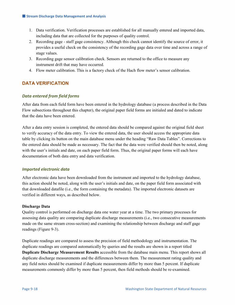
Stream Discharge Data Management and Analysis
Page 9-18 Washington State Department of Natural Resources
1. Data verification. Verification processes are established for all manually entered and imported data, including data that are collected for the purposes of quality control.
2. Recording gage - staff gage consistency. Although this check cannot identify the source of error, it provides a useful check on the consistency of the recording gage data over time and across a range of stage values.
3. Recording gage sensor calibration check. Sensors are returned to the office to measure any instrument drift that may have occurred.
4. Flow meter calibration. This is a factory check of the Hach flow meter’s sensor calibration.
DATA VERIFICATION
Data entered from field forms
After data from each field form have been entered in the hydrology database (a process described in the Data Flow subsections throughout this chapter), the original paper field forms are initialed and dated to indicate that the data have been entered. After a data entry session is completed, the entered data should be compared against the original field sheet to verify accuracy of the data entry. To view the entered data, the user should access the appropriate data table by clicking its button on the main database menu under the heading “Raw Data Tables”. Corrections to the entered data should be made as necessary. The fact that the data were verified should then be noted, along with the user’s initials and date, on each paper field form. Thus, the original paper forms will each have documentation of both data entry and data verification.
Imported electronic data
After electronic data have been downloaded from the instrument and imported to the hydrology database, this action should be noted, along with the user’s initials and date, on the paper field form associated with that downloaded datafile (i.e., the form containing the metadata). The imported electronic datasets are verified in different ways, as described below. Discharge Data Quality control is performed on discharge data one water year at a time. The two primary processes for assessing data quality are comparing duplicate discharge measurements (i.e., two consecutive measurements made on the same stream cross-section) and examining the relationship between discharge and staff gage readings (Figure 9-3). Duplicate readings are compared to assess the precision of field methodology and instrumentation. The duplicate readings are compared automatically by queries and the results are shown in a report titled Duplicate Discharge Measurement Results accessible from the database main menu. This report shows all duplicate discharge measurements and the differences between them. The measurement rating quality and any field notes should be examined if duplicate measurements differ by more than 5 percent. If duplicate measurements commonly differ by more than 5 percent, then field methods should be re-examined.
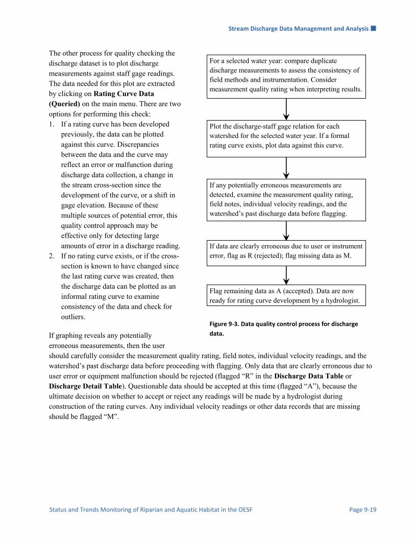
Stream Discharge Data Management and Analysis
Status and Trends Monitoring of Riparian and Aquatic Habitat in the OESF Page 9-19
The other process for quality checking the discharge dataset is to plot discharge measurements against staff gage readings. The data needed for this plot are extracted by clicking on Rating Curve Data (Queried) on the main menu. There are two options for performing this check: 1. If a rating curve has been developed
previously, the data can be plotted against this curve. Discrepancies between the data and the curve may reflect an error or malfunction during discharge data collection, a change in the stream cross-section since the development of the curve, or a shift in gage elevation. Because of these multiple sources of potential error, this quality control approach may be effective only for detecting large amounts of error in a discharge reading.
2. If no rating curve exists, or if the cross-section is known to have changed since the last rating curve was created, then the discharge data can be plotted as an informal rating curve to examine consistency of the data and check for outliers.
If graphing reveals any potentially erroneous measurements, then the user should carefully consider the measurement quality rating, field notes, individual velocity readings, and the watershed’s past discharge data before proceeding with flagging. Only data that are clearly erroneous due to user error or equipment malfunction should be rejected (flagged “R” in the Discharge Data Table or Discharge Detail Table). Questionable data should be accepted at this time (flagged “A”), because the ultimate decision on whether to accept or reject any readings will be made by a hydrologist during construction of the rating curves. Any individual velocity readings or other data records that are missing should be flagged “M”.
Plot the discharge-staff gage relation for each watershed for the selected water year. If a formal rating curve exists, plot data against this curve.
Flag remaining data as A (accepted). Data are now ready for rating curve development by a hydrologist.
For a selected water year: compare duplicate discharge measurements to assess the consistency of field methods and instrumentation. Consider measurement quality rating when interpreting results.
If any potentially erroneous measurements are detected, examine the measurement quality rating, field notes, individual velocity readings, and the watershed’s past discharge data before flagging.
If data are clearly erroneous due to user or instrument error, flag as R (rejected); flag missing data as M.
Figure 9-3. Data quality control process for discharge
data.

Stream Discharge Data Management and Analysis
Page 9-20 Washington State Department of Natural Resources
Recording Gage Data The quality control process for the recording gage data is described in this section and in the following section titled “Recording Gage – Staff Gage Consistency” (Figure 9-4). The first step in performing a quality control check of the recording gage data is to examine the gage download metadata, installation metadata, and maintenance activity records (via “Gage Download Metadata”, “Installation Metadata”, and “Maintenance Activities” buttons on the main menu) to identify any instrument problems or other issues that were recorded in the field. After reviewing the metadata, quality control is performed on the recording gage data by examining a time series plot of the data from each watershed. For this quality control process, data do not need to be adjusted to any specific datum. The data must be plotted in a program with graphical capabilities such as R or Excel (R Core Team 2013). To export the data, click on the main menu button labeled All Recording Gage Data (unadjusted datum) for Plots (Queried) and then export the resulting data table in the desired format. The table contains every data record from the Gage Sensor Data Table, but includes only the three fields needed for plotting:
1. Watershed number. 2. Date and time of reading. 3. Water level.
In examining the plotted recording gage data, look for any data continuity issues or unexpected values that do not appear to represent normal patterns in stream stage. These may appear as “stuck” values or as abrupt changes in stage. If it is unclear whether a pattern is natural or a result of an instrument malfunction, then the gage plot can be compared with data from another watershed’s recording gage or with the nearest USGS hydrograph for the same time period. Any recording gage records that are determined to be erroneous due to instrument malfunction or other reasons should be flagged “R” as rejected in the Gage Sensor Data Table. In cases where there is a single-record gap, the gap may be filled by averaging the values of the records immediately before and after it. These estimated values should be flagged “E” as estimated in the Gage Sensor Data Table. Records with missing data values should be flagged “M”. After the quality control process is completed; all unflagged records should be flagged “A” as accepted.
RECORDING GAGE – STAFF GAGE CONSISTENCY
Introduction
This assessment is a review of the relation between all of the staff gage readings and the corresponding recording gage readings (i.e., readings from the same watershed and time) collected during a specified time period. This assessment can be performed on raw, unadjusted data or it can be performed on adjusted datasets. However, for data quality control purposes, we assume that the user is working with raw, unadjusted data.
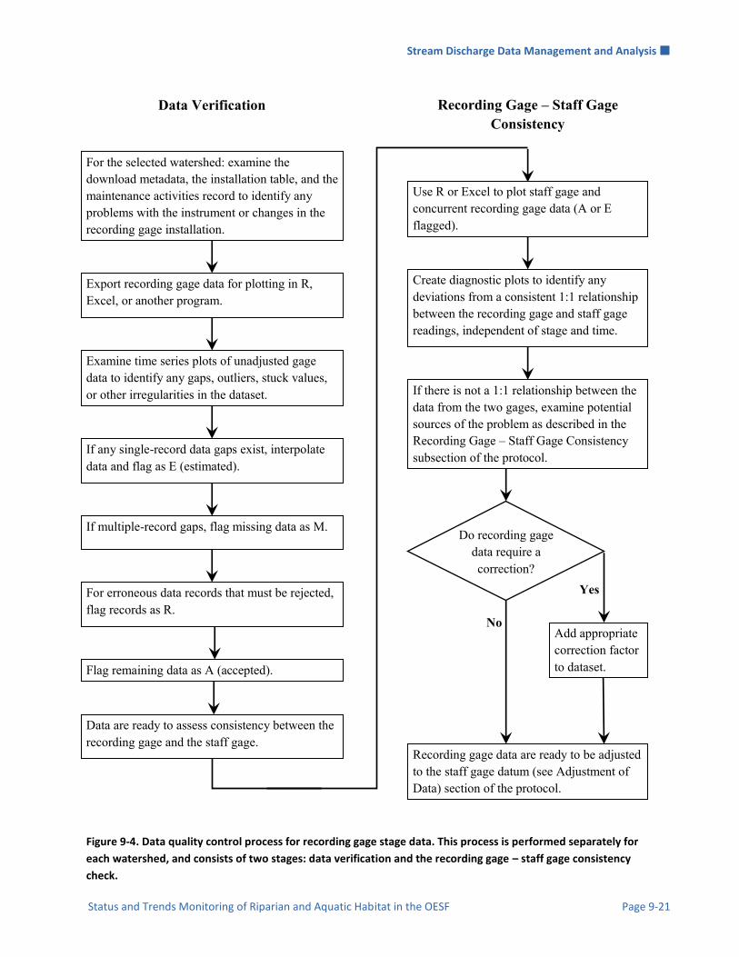
Stream Discharge Data Management and Analysis
Status and Trends Monitoring of Riparian and Aquatic Habitat in the OESF Page 9-21
Data Verification Recording Gage – Staff Gage Consistency
For the selected watershed: examine the download metadata, the installation table, and the maintenance activities record to identify any problems with the instrument or changes in the recording gage installation.
Examine time series plots of unadjusted gage data to identify any gaps, outliers, stuck values, or other irregularities in the dataset.
Export recording gage data for plotting in R, Excel, or another program.
For erroneous data records that must be rejected, flag records as R.
If any single-record data gaps exist, interpolate data and flag as E (estimated).
Flag remaining data as A (accepted).
If multiple-record gaps, flag missing data as M.
Data are ready to assess consistency between the recording gage and the staff gage.
No
Yes
If there is not a 1:1 relationship between the data from the two gages, examine potential sources of the problem as described in the Recording Gage – Staff Gage Consistency subsection of the protocol.
Use R or Excel to plot staff gage and concurrent recording gage data (A or E flagged).
Create diagnostic plots to identify any deviations from a consistent 1:1 relationship between the recording gage and staff gage readings, independent of stage and time.
Recording gage data are ready to be adjusted to the staff gage datum (see Adjustment of Data) section of the protocol.
Do recording gage data require a correction?
Add appropriate correction factor to dataset.
Figure 9-4. Data quality control process for recording gage stage data. This process is performed separately for
each watershed, and consists of two stages: data verification and the recording gage – staff gage consistency
check.

Stream Discharge Data Management and Analysis
Page 9-22 Washington State Department of Natural Resources
Ideally, changes in values on the recording gage and the staff gage should have a linear, 1:1 relationship: for any change in stage measured on the staff gage, there should be an identical change measured by the recording gage. This 1:1 relationship should not change over time, nor should it vary based on stage. This quality control assessment is designed to evaluate consistency between gage readings, but it cannot conclusively identify the cause of inconsistencies, which may arise from sensor drift, elevational movement of the gages, or other sources. It also is important to note that this assessment will not reveal all potential gage errors. For example, if both the staff gage and recording gage move in the same direction relative to the original gage datum (e.g., if they are mounted on the same tree and that tree moves), then this assessment will not reveal any problem in the data. Thus, the assessment is not a substitute for analysis of staff and recording gage elevation survey data and recording gage sensor calibration checks.
The dataset
The relation between the staff gage and recording gage readings can be assessed by exporting the data via a query. The query is run by clicking the button on the main menu titled All Staff Gage and Simultaneous Recording Gage Readings. This query extracts all staff gage readings from the Gage Table and the Discharge Metadata Table and then locates and extracts recording gage readings from the Gage Sensor Data Table that were made in the same watershed at approximately the same time. Because staff gage readings usually did not occur at precisely the same time as the recording gage readings, the query matches each staff gage reading with the recording gage reading nearest in time in the same watershed (the readings usually are within eight minutes of each other owing to the 15-minute recording gage interval). The query produces a table, titled SG-Sensor Diffs for R, with records equal in number to the number of staff gage readings. The data in this table can then be exported in the desired format for plotting. The SG-Sensor Diffs for R table includes five fields:
1. Watershed number. 2. Date and time of the staff gage reading. 3. Staff gage reading (m). 4. Sensor reading that was matched with the staff gage reading (m). 5. The difference between the readings (recording gage sensor reading minus the staff gage reading).
Products of the assessment
Three types of plots should be produced for each watershed using the data in the SG-Sensor Diffs for R table. The first is a time series plot showing staff gage readings, recording gage sensor readings, and the difference between the staff gage and recording gage readings. This plot will show whether the difference between the gages is consistent over time. Second, a plot should be produced showing the staff gage readings versus the recording gage readings for each watershed. This will indicate whether the gage readings have a 1:1 relation and whether the gages’ relation is linear. The third plot should show, for each watershed, the difference between the two gages versus the staff gage reading. This plot will help reveal any stage-dependent differences between the two gages. This quality control assessment is important for identifying at least two potential data quality issues:

Stream Discharge Data Management and Analysis
Status and Trends Monitoring of Riparian and Aquatic Habitat in the OESF Page 9-23
1. A non-linear relation between the staff and recording gages. For example, if the recording gage responds differently at high stage values than at low stage values.
2. Deviation from a 1:1 slope between the two gages. An increase of 1.0 cm in the staff gage reading should be accompanied by an increase of 1.0 cm in the recording gage reading.
Because the staff gage data are expected to be highly reliable, with error limited only to gage movement and user error, issues detected in the relation between the staff gage and recording gage readings are most likely a result of error associated with the recording gage. This error also may be the cumulative effect of multiple problems. Potential gage problems include:
1. Elevational movement of a gage. Examine the gage elevation survey results. This type of error is addressed in the Adjustment of Data section.
2. Recording gage sensor calibration. Examine the results of the periodic calibration check to determine if sensor drift is influencing the data. This type of error is addressed in the below subsection titled Recording Gage Sensor Calibration Check.
3. Problems within the recording gage housing. If the recording gage readings are lagging behind the staff gage readings, or if the sensitivity of the recording gage seems to be diminished, the recording gage housing may require maintenance. This issue can only be diagnosed by an evaluation in the field.
4. Recording gage clock error. If there a time series plot of recording gage and staff gage data show a temporal offset, then there may be an issue with clock settings (including daylight saving time). Address this by checking the sensor clock settings and by comparing data among multiple sensors.
RECORDING GAGE SENSOR CALIBRATION CHECK
Introduction
On a periodic basis, the recording gage sensors from every gaging station are transported to the office for a calibration check (refer to the Stream Discharge Field Methods protocol). Sensors are all submerged in water to a common depth, and then the reading from each sensor is compared to the measured depth of the water. This section describes the data involved in this process. The application of the sensor calibration is in the Recording Gage Data Adjustment section of this protocol.
The calibration dataset
After the calibration check in which all sensors are submerged to a common depth, data from the loggers are downloaded and the readings are compensated for atmospheric pressure using Solinst software. The resulting datafiles are in Microsoft Excel format. The data from these files are copied and pasted into the Solinst Sensor Calibration Data Table, which is accessed from the sensor calibration menu. Calibration metadata are entered directly in the Solinst Sensor Calibration Metadata Table, also accessed from the sensor calibration menu. The Solinst Sensor Calibration Data Table contains the following fields:
1. Sensor calibration ID number (used to relate data to metadata). 2. Sensor ID number (watershed number has been used thus far).

Stream Discharge Data Management and Analysis
Page 9-24 Washington State Department of Natural Resources
3. Date and time of measurement. 4. Water depth reading. 5. Temperature.
The Solinst Sensor Calibration Metadata Table contains the following fields:
1. Sensor calibration ID number (used to relate metadata to data). 2. Water year for which the calibration was performed. 3. Beginning and end date and time of the calibration. 4. Water depth at the beginning and end of the calibration.
Data products
The results of the annual calibration check appear in a report titled Summary of Solinst Sensor Calibration Check, accessed from the sensor calibration menu. This report contains, for each calibration of each sensor:
1. The mean water depth reading from the sensor during the calibration period. 2. The standard deviation of the water depth readings from the sensor during the calibration period. 3. The range in the water depth readings during the calibration period. 4. The actual, measured depth of the water during the calibration period. 5. The difference between the sensor reading and the actual depth of the water during the calibration
period.
FLOW METER CALIBRATION The flow meter sensor is shipped to the factory periodically for calibration. Data produced during this calibration are stored in the database in the Flow Meter Calibration Data table and in the Flow Meter Calibration Metadata table. Both of these tables are accessed from the sensor calibration menu.
Data Archives
STORAGE OF ELECTRONIC DATA AND PAPER FIELD FORMS Original completed field forms will be archived with the OESF Research and Monitoring Manager, at the Natural Resources Building in Olympia, WA. The original paper field forms will be placed in a binder organized either by site or by year and will be stored in the Forest Resources Division. It is crucial that the raw data, both field forms and electronic datafiles, retain their integrity and not be modified. Any new information added to field forms or datafiles after returning from the field must be clearly identified as not part of the original data. All electronic datafiles downloaded from field instruments will be stored on a server of Washington Department of Natural Resources in the appropriate subdirectories within: J:\hcp\monitoring_research\tminkova\01_OESF_R&M Program\01_Rip S&T Mon\01_FIELD DATA\02_Hydrology\Data\

Stream Discharge Data Management and Analysis
Status and Trends Monitoring of Riparian and Aquatic Habitat in the OESF Page 9-25
All scanned field forms will be stored in Adobe pdf format in the appropriate subdirectory within the same directory. The hydrology database itself is located at: J:\hcp\monitoring_research\tminkova\01_OESF_R&M Program\01_Rip S&T Mon\01_FIELD DATA\02_Hydrology\Data\Hydro_Database.accdb
Adjustment of Data
INTRODUCTION There are four types of data adjustments necessary prior to data analysis. These adjustments are:
1. Adjustment for staff gage replacement (required for all watersheds where a staff gage has been replaced). Ten staff gages were replaced between December 2014 and January 2015. Because the replacement staff gages could not be installed at exactly the same elevation as the original staff gages, the pre-replacement staff gage data had to be adjusted to the post-replacement staff gage datum.
2. Adjustment of staff and recording gage data to watershed datum (required for all watersheds). For analysis, all staff gage and recording gage data from a given watershed must be adjusted to the same watershed-specific datum.
3. Adjustment of cross-section survey data to detect cross section changes (required for all watersheds). To evaluate changes in the cross-section profile over time, multiple cross-section surveys are plotted together on the same graph. Before the cross-sections can be plotted, the data must be adjusted so that they are all in the same datum.
4. Adjustment for a shift in staff or recording gage elevation (required for watersheds in which gage elevation changed). If the staff gage elevation changes over time as a result of any type of disturbance, then the data must be adjusted to account for the change.
The procedures described here assume that the applicable quality control processes described in the Data Quality Control section have already been performed on the data.
ADJUSTMENT FOR STAFF GAGE REPLACEMENT Over time, staff gages may need to be replaced owing to normal wear-and-tear or damage during a flood. When a staff gage is replaced, it is rarely possible to install the new gage at exactly the same elevation as the old gage. For this reason, the all staff gage readings taken prior to the replacement must be adjusted so that the readings are comparable to the readings taken on the new staff gage. To adjust the staff gage readings, the adjustment factors must be determined using information recorded in the field at the time of gage replacement. This is done by taking a reading on the old gage, replacing it, and then taking a reading on the new gage. Assuming no change in stage during the replacement process, the difference between these two readings is the adjustment factor that should be applied to all readings prior to the gage replacement. These adjustment factors, and the dates of gage replacements, are stored in a table called SG_Adjustment_Values_Table.

Stream Discharge Data Management and Analysis
Page 9-26 Washington State Department of Natural Resources
ADJUSTMENT OF STAFF AND RECORDING GAGE DATA TO WATERSHED DATUM Prior to any analysis, each watershed must have a defined datum to which all staff and recording gage data are adjusted. There are various options for establishing this watershed-specific datum. For example, a watershed’s datum could be the watershed’s reference point, or it could be the “zero” reading on the staff gage at the time of initial gage installation. For the analysis conducted by Rebekah Korenowsky in 2015 (Korenowsky and Devine 2015), each watershed’s datum was defined as the lowest point of the gage cross-section (i.e., the thalweg) recorded in any of the gage cross-section surveys. (The 2015 survey not used considered because at the time of that analysis some of the 2015 survey data were deemed unreliable.) This datum is hereafter called the “deepest thalweg datum”. The process for converting the staff gage data to the watershed-specific datum (in this example using the deepest thalweg datum method selected by Rebekah Korenowsky in 2015) is as follows:
1. For each watershed, find the elevation of zero on the staff gage: a. Use the LEW and REW values from the gage cross-section survey (the 2014 survey was
determined to be most reliable) to calculate mean water surface elevation. b. Subtract the staff gage reading at the time of the survey from the water surface elevation.
The result is the staff gage zero datum. 2. Convert all of the staff gage readings at each watershed to elevations, by adding the staff gage
readings to the staff gage zero datum. 3. Apply the adjustment for staff gage replacement in watersheds where there was a staff gage
replacement (see previous subsection “Adjustment for Staff Gage Replacement”). 4. Adjust the staff gage reading elevations to that watershed’s deepest thalweg datum by subtracting
the thalweg elevation from that watershed’s staff gage reading elevations. The resulting values should be positive numbers.
The process for converting the recording gage data to the watershed-specific datum (again using the 2014 thalweg datum used by Rebekah Korenowsky in 2015) is as follows:
1. Calculate water surface elevation by averaging the LEW and REW values from the 2014 cross-section and gage elevation stability survey (the most reliable survey at the time of analysis).
2. For each watershed, find the elevation of zero on the recording gage, based on the 2014 elevation stability survey:
a. Establish a 1-hour window of time centered around each watershed’s 2014 stability survey, and then select and average the recording gage readings within that window of time. (We use an hour’s worth of readings rather than a single reading because there are small fluctuations in stage between readings, and we can achieve a more reliable value by averaging several readings.)
b. Subtract the recording gage reading average from the water surface elevation to calculate the elevation of the recording gage zero reading in each watershed.
Stream Discharge Data Management and Analysis
Status and Trends Monitoring of Riparian and Aquatic Habitat in the OESF Page 9-27
3. Subtract the deepest thalweg datum from the recording gage zero reading elevation (from the previous step). This is the adjustment factor that will be used to convert the recording gage data to the deepest thalweg datum.
4. Adjust the recording gage readings to the deepest thalweg datum by adding the adjustment factor from the previous step to the recording gage readings.
ADJUSTMENT OF CROSS-SECTION SURVEY DATA TO DETECT CROSS-SECTION CHANGES To evaluate changes in the cross-section profile over time in a given watershed, profiles from multiple cross-section surveys are plotted together on the same graph. However, simply plotting the unadjusted survey data together on the same graph is not effective due to frequent measurement errors between the reference point and the gage station cross-section. For example, the left and right monuments in a given watershed should have elevations that don’t change over time. This is not the case; the same monument often has different elevations in different surveys, presumably due to measurement error between the reference point and the cross-section. Thus, if the monument elevations indicate error, we would also expect measurement error in the entire profile. To plot the profiles without the measurement error that occurred between the reference point and the cross-section, we chose to adjust the survey data using the elevations of the left monument. For example, if our most reliable survey (the one with the fewest obvious errors) reported a left monument elevation of -200 cm and the next survey reported an elevation of -190 cm, then we would adjust all of the cross-section profile data from the second survey by -10 cm.
ADJUSTMENT FOR A SHIFT IN STAFF OR RECORDING GAGE ELEVATION The gage elevation survey is performed periodically to determine the elevation of the gages relative to the watershed’s gage reference point. If a staff or recording gage is found to have changed elevation over time, then a portion of the readings must be adjusted to compensate for that movement, therefore making all data points, before and after the movement, comparable. The adjustment is made to the data collected prior to the elevation change, and, if the change is determined to have occurred gradually over time, the data collected during the gradual change are adjusted as well, on a prorated basis. The procedure for identifying the need for data adjustment and for adjusting data is given below. This procedure is the same for either type of gage but must be applied separately to each gage if both gages in the same watershed are found to have changed elevation.
1. Use the Gage Elevation and Cross-Section Survey reports to determine whether the staff or recording gage elevation changed over time. In the reports, gage elevation change is calculated between the earliest and most recent elevation surveys and between the two most recent elevation surveys. A threshold of 1 cm is used as the minimum amount of movement that can be used to make an adjustment, though each situation should be examined on an individual basis to determine whether gage elevation changed enough to warrant adjustment.
2. If, for a given watershed, the reports show no change in gage elevation, then no data adjustment is necessary. If the reports show that a gage’s elevation changed, then that gage’s data must be adjusted. In that case, proceed to the next step.

Stream Discharge Data Management and Analysis
Page 9-28 Washington State Department of Natural Resources
3. Determine whether the specific date of the gage’s elevation change is known. For example, the gage might have moved during a specific flood event or as a result of instrument maintenance (see the Maintenance Activities report). There are two possible outcomes: a. The date of the staff gage movement is known. This scenario is based on the assumption that the
gage only moved on a specific date and not before or after that date. In this case, calculate the change in elevation as the difference between the gage’s elevation according to the surveys prior to and after the gage elevation change. Adjust all data prior to the change by the amount of change. For example, if the gage moved 5 cm lower in elevation, then add 5 cm to every reading prior to the change.
b. There is no known date of staff gage movement. In this case, make the assumption that the staff gage moved at a constant rate between the two surveys that indicate the change in elevation. Prorate the adjustment throughout this time period (Sauer 2002, p. 22). Thus, the adjustment factor for each record between the two surveys is calculated by multiplying the total gage movement for that interval by the fraction of the interval that has elapsed (see example of this calculation below).
Rating Curve Development
INTRODUCTION A rating curve, or stage-discharge curve, is the relationship at a given stream cross-section between a stream’s stage and its discharge rate. The rating curve is generated using discharge measurements and concurrent recording gage readings. The process of developing a rating curve should follow the guidelines described in Rantz (1982) and Sauer (2002). An initial rating curve has been developed for each watershed (Korenowsky and Devine 2015), but these rating curves will need to be reviewed and updated over time, as stream channel and other hydrologic changes are inevitable.
Example: Staff Gage Data Adjustment When the Date of Gage Elevation Change is Unknown
Based on the results of two consecutive gage elevation surveys, a staff gage is determined to have shifted in elevation. The staff gage top was found to be at -371 cm, relative to the reference point, during the watershed’s initial gage elevation survey on 5 December 2013, and then it was found to be at -365 cm in the second survey on 5 August 2014. Thus, the staff gage movement between surveys was +6 cm. There was no known date on which the movement occurred, so we assume the staff gage moved gradually during the interval. Therefore, the adjustment factor is prorated uniformly through the time period. If, for example, we are adjusting a staff gage reading made on 10 April 2014, the 126th day of the 243-day time period between elevation surveys, then the adjustment factor is: 6 cm × (126 days / 243 days) = 3.1 cm. To adjust a staff gage reading from 10 April 2014 to the site’s original staff gage datum, add 3.1 cm to the 10 April 2014 reading.

Stream Discharge Data Management and Analysis
Status and Trends Monitoring of Riparian and Aquatic Habitat in the OESF Page 9-29
In addition to building and maintaining a rating curve for each watershed, an informal, preliminary rating curve (i.e., a simple plot of stage vs. discharge) may be constructed for each watershed during the data collection period. This will assist in data collection planning by allowing the user to determine whether the distribution and quality of discharge measurements collected to date are sufficient to begin construction of a formal rating curve. For example, if there are large gaps between data points on the preliminary curve, it may be desirable to attempt to collect discharge readings at flow levels that would fill these gaps.
CONSTRUCTION OF RATING CURVES Rating curve development requires data on a site’s hydraulic conditions as well as the professional judgment of a hydrologist. Curves can be created using Microsoft Excel, R, or specialized software such as Hydstra™. Rating curve construction is an iterative process and may include adjustments due to site-specific characteristics. Detailed technical guidance on the construction of rating curves is provided in USGS publications (Kennedy 1984; Rantz 1982; Sauer 2002).
Rating curves may be developed using either linear regression or logarithmic interpolation. Alternatively, a curve may consist of several (likely no more than three) separate straight lines fit to a log-log plot. It is important to consider all measurements, and various hydraulic conditions present during the measurement, when building the rating curve:
“No discharge measurement, made either by current meter or indirectly, should be disregarded (left with an unaccountably high percentage difference from the rating) without a good reason. Disagreement with other measurements is generally not reason enough. If an outlier measurement is truly in error, the reason for the disparity often can be discovered. The hydrographer should check the arithmetic of an outlier measurement, compare the mean gage height with recorded and outside gage heights [staff gage], compare the plotted cross sections and velocity distributions for several measurements made at the same site, consider the possibility of backwater, and check the equipment used. If these checks and others indicate that the outlier is a valid discharge measurement, it should be given appropriate weight in the analysis.” (Kennedy, 1984).
After a formal rating curve is developed for each watershed, new data collected should be plotted on the same graph to determine if the data have diverged since the curve was created. Plotting the new measurements against the existing rating curve is the most powerful method of determining the “health” of the rating curve. If new measurements continue to fall along the curve, then it is still accurate. If new measurements consistently occur off the established rating curve, then the following factors should be examined to determine if construction of a new rating curve is warranted:
1. Cross-section changes: During the elevation stability surveys, a semipermanently marked cross-section profile is re-surveyed in each watershed. Comparing the results of multiple surveys over time will reveal any changes in the cross-section that could be affecting the stage-discharge relationship.
2. Gage instability: Movement of the gages may be affecting the new measurements. Consult the gage elevation survey results.
3. Measurement quality: A review of the quality ratings of the discharge measurements used in the curve will shed light on the amount of uncertainty associated with each measurement.

Stream Discharge Data Management and Analysis
Page 9-30 Washington State Department of Natural Resources
DATA FOR RATING CURVE DEVELOPMENT Several datasets are needed to develop the rating curve. These include: (1) discharge measurements and associated metadata, (2) the cross-section survey dataset, and (3) the table of maintenance activities, some of which may affect gage readings. These datasets can be accessed at:
1. The rating curve data table (called Rating Curve Data TH datum) is refreshed and accessed by clicking the “Rating Curve Data (Queried)” button on the main menu. This table contains the following fields:
a. Watershed number. b. Date and time of discharge measurement. c. Discharge rate. d. Staff gage reading at the time of the discharge measurement (adjusted to the deepest thalweg
datum). e. Recording gage reading at the time of the discharge measurement (adjusted to the deepest
thalweg datum). f. Year and month of the next cross-section survey following the discharge measurement date. g. Quality rating of the discharge measurement.
2. The cross-section survey dataset (adjusted so that left monument elevations are equivalent and also
adjusted to the deepest thalweg datum) is located in a table called X-section_R_adjusted2015elevations. The table is refreshed and opened by clicking the main menu button called “Elevation Stability Survey: Cross-Section Data”. This dataset includes:
a. Watershed number. b. Date of survey. c. Station (distance from left monument, in centimeters) d. Elevation (adjusted so that left monument elevations are equivalent and also adjusted to the
deepest thalweg datum) e. Location (e.g., LEW, TH, REW, etc.) f. Sort sequence. This is necessary because of bank undercutting, in which case stations are not
necessarily in ascending order.
3. The field maintenance report is accessed by clicking on Field Maintenance Activities on the main menu. This table can be exported in any format, based on the user’s requirements. The dataset includes:
a. Watershed number. b. Date of maintenance activity. c. Subject of the maintenance. d. The reason for the maintenance. e. Notes.

Stream Discharge Data Management and Analysis
Status and Trends Monitoring of Riparian and Aquatic Habitat in the OESF Page 9-31
Hydrograph Development The hydrograph for each watershed is produced using the recording gage dataset and the stage-discharge relationship (i.e., rating curve). The equation describing the stage-discharge relationship is applied to the stage data from the recording gage dataset to produce a discharge value for each record in the recording gage dataset. The limitations of each stage-discharge relationship must be considered when creating a hydrograph. Each stage-discharge relationship is bounded by a high and low stage value. Therefore, the hydrograph is only accurate within the highest and lowest stage values in the stage-discharge relationship. Additionally, each stage-discharge relationship is typically limited to a certain period of time, often because changes in the stream channel at the gage station affect the relationship. Therefore, a particular stage-discharge relationship may only apply to a specific range of stage values or a specific date range; in some cases, it may be limited by both stage and date.
Stream Discharge Data Management and Analysis
Page 9-32 Washington State Department of Natural Resources
References Bradley, D.N. 2012. Slope-area computation program graphical user interface 1.0 - a preprocessing and
postprocessing tool for estimating peak flood discharge using the slope-area method: U.S. Geological Survey Fact Sheet 2012-3112, 4 p. (Also available at http://water.usgs.gov/software/SAC/)
Butkus, S. 2007. Quality Assurance Monitoring Plan Streamflow Gaging Network. Environmental Assessment Program , Washington State Department of Ecology, Olympia, WA. Pub. No. 05-03-204. (Also available at https://fortress.wa.gov/ecy/publications/publications/0503204.pdf)
Dalrymple, T., Benson, M.A. 1967, Measurement of peak discharge by the slope-area method: U.S. Geological Survey Techniques of Water-Resources Investigations, book 3, chap. A2, 12 p.
Kennedy, E.J. 1984. Discharge ratings at gaging stations: U.S. Geological Survey Techniques of Water-Resources Investigations, book 3, chap. A10, 59 p. (Also available at http://pubs.usgs.gov/twri/twri3-a10/.)
Kenney, T.A. 2010. Levels at gaging stations: U.S. Geological Survey Techniques and Methods 3-A19, 60 p.
Korenowsky, R., Devine, W. 2015. Status and Trends Monitoring of Riparian and Aquatic Habitat in the Olympic Experimental State Forest: 2015 hydrology status report. Washington State Department of Natural Resources, Forest Resources Division, Olympia, WA.
Langbein, W.B., Iseri., K.T. 1960. General introduction and hydrologic definitions manual of hydrology. Part 1. General surface water techniques. U.S. Geological Survey, Water Supply Paper 1541–A. 29 p. (http://water.usgs.gov/wsc/glossary.html)
Peck, D.V., Lazorchak, J.M., Klemm, D.J. (editors). 1998. Environmental Monitoring and Assessment Program. Field Operations and Methods for Measuring the Ecological Condition of Wadeable Streams. EPA/620/R-94/004F.. U.S. Environmental Protection Agency, Washington, D.C. (Also available at http://www.epa.gov/emap2/html/pubs/docs/groupdocs/surfwatr/field/ws_abs.html)
R Core Team. 2013. R: A language and environment for statistical computing. R Foundation for Statistical Computing, Vienna, Austria. ISBN 3-900051-07-0, URL http://www.R-project.org/
Rantz, S.E. 1982. Measurement and computation of streamflow: Volume 1. Measurement of stage and discharge. U.S. Geological Survey Water-Supply Paper 2175.
Sauer, V.B. 2002. Standards for the Analysis and Processing of Surface-Water Data and Information using Electronic Methods: U.S. Geological Survey Water-Resources Investigations Report 01–4044, 91 p.
Turnipseed, D.P., Sauer, V.B. 2010. Discharge measurements at gaging stations: U.S. Geological Survey Techniques and Methods book 3, chap. A8, 87 p. (Also available at http://pubs.usgs.gov/tm/tm3-a8/pdf/tm3-a8.pdf).

Stream Discharge Data Management and Analysis
Status and Trends Monitoring of Riparian and Aquatic Habitat in the OESF Page 9A-1
Appendix 9A: Hydrology Database Structure
Discharge Metadata Table
Discharge
Data Table
Discharge
Detail Table
Discharge
Manual
Data Table
Gage Sensor Data
Table
Gage Metadata
Table
Field Visit Table
Cross Section
Table
Elevation Stability
Table
Solinst Sensor
Calibration
Data Table
Flow Meter
Calibration
Table
Solinst Sensor
Calibration
Metadata
Table
Maintenance
Table
Installation Table

Stream Discharge Data Management and Analysis
Page 9A-2 Washington State Department of Natural Resources
This page intentionally left blank.

Riparian Microclimate
Status and Trends Monitoring of Riparian and Aquatic Habitat in the OESF Page 10-1
Riparian Microclimate Authors: Richard Bigley, Paul Dunnette, Ellis Cropper, Warren Devine Version: 1.3
Revision History:
Based on the Following Protocols: In this protocol, the spatial monitoring design along the riparian gradient is adapted from Brosofske et al. (1997) and Anderson et al. (2007). Sampling generally follows Moore et al. (2005). Reasons to Adopt the Above Protocols: Brosofske et al. (1997) and Anderson et al. (2007) provided a general sense of the contours of the microclimate gradient. Moore et al. (2005) and Anderson et al. (2007) provided insight as to sampling intensity required to detect differences. Purpose and Content:
This protocol details the field procedures for deployment, maintenance, and downloading of microclimate data loggers, the field quality assurance and quality control steps, and the data management and analysis procedures necessary to document and report the status and trends of riparian microclimate across the Olympic Experimental State Forest (OESF).
Version
number Purpose / Changes Author(s) Reviewer(s) Date
1.0 Initial draft Richard Bigley, Ellis
Cropper
03/03/2014
1.1 Draft presented to project staff
for review
Richard Bigley, Ellis
Cropper
Teodora Minkova 07/03/2014
1.2 Final draft incorporating internal
reviews, sampling procedures
from 2013-2015 field seasons,
and data mgmt. procedures
Richard Bigley, Ellis
Cropper, Warren
Devine
Teodora Minkova 11/22/2016
1.3 Final technical review and edit Richard Bigley, Paul Dunnette, Ellis Cropper, Warren Devine
Alex Foster 12/18/2016

Riparian Microclimate
Page 10-2 Washington State Department of Natural Resources
Table of Contents Introduction ................................................................................................................................................... 10-3
Monitoring Design ........................................................................................................................................ 10-3
Spatial Sampling Design ........................................................................................................................... 10-3
Temporal Sampling Design ....................................................................................................................... 10-5
Equipment and Supplies ................................................................................................................................ 10-6
Pre-field set up .......................................................................................................................................... 10-6
Field Procedures ............................................................................................................................................ 10-8
Microclimate transect establishment ......................................................................................................... 10-8
Downloading Procedures .......................................................................................................................... 10-9
Time and Cost Estimates for Implementing the Field Procedures .............................................................. 10-10
Procedures for Calculating Metrics ............................................................................................................. 10-10
Quality Control and Quality Assurance ...................................................................................................... 10-11
Training ................................................................................................................................................... 10-11
Standard Protocols .................................................................................................................................. 10-11
Testing Data Loggers .............................................................................................................................. 10-12
Data Quality Control ............................................................................................................................... 10-12
Data Storage ............................................................................................................................................ 10-13
References ................................................................................................................................................... 10-14
Appendix 10A. Riparian Microclimate Installation Field Form ................................................................ 10A-1
Appendix 10B. Riparian Microclimate Download Field Form .................................................................. 10B-1
Riparian Microclimate
Status and Trends Monitoring of Riparian and Aquatic Habitat in the OESF Page 10-3
Introduction The goal of the Olympic Experimental State Forest (OESF) riparian conservation strategy is to provide habitat for salmonids and other species dependent on in-stream and riparian environments. The strategy is implemented by establishing riparian management areas designed to maintain a stream’s key physical and biological functions. Maintenance of aquatic and riparian ecosystem function hinges in part on preservation of riparian microclimate – a suite of variables including moisture, temperature, light, and wind speed that affect species adapted to conditions found in or near streams. Riparian microclimate moderates environmental fluctuation to maintain in-stream temperatures and provides habitat for riparian-associated wildlife. The high productivity, complex habitat, and moist conditions of riparian areas support the highest biodiversity in forested landscapes (Olson et al. 2007). Numerous invertebrate taxa, many small mammals, and all western Washington amphibians depend on the cool, moist conditions in stream corridors. Research has demonstrated that stream microhabitats can be strongly influenced by adjacent land use. Nonetheless, it is assumed that riparian buffers ameliorate edge effects created by upslope forest harvest Brosofske et al. (1997). The effects of partial cuts or thinning treatments within riparian areas are poorly understood and believed to be short-lived, owing to vegetation response to increased light after disturbance (Guenther et al 2012). However, studies have shown strong near-stream gradients and increased diurnal variation in relative humidity in the riparian zones of forest stands that were selectively harvested with no buffer (Danehy and Kirpes 2000, Moore et al. 2005, Anderson et al. 2007, Guenther et al. 2012). The environmental impact analysis for the OESF Forest Land Plan found that planned increases in timber harvesting could negatively affect riparian microclimate in managed stands. Presently, management effects on riparian microclimate are characterized as “medium impact” in nearly half of the OESF watersheds analyzed (WADNR 2016).
Monitoring Design
SPATIAL SAMPLING DESIGN Riparian microclimate (i.e., air temperature and humidity) is monitored in 10 of the 50 OESF sample watersheds. At each sample site, five microclimate monitoring stations are installed systematically along each of two, 60-m transects, perpendicular to the stream (Figures 10-1 and 10-2). The transects bisect permanent 30 x 60-m vegetation plots established adjacent to two of the six channel cross sections installed at each sample reach (see Riparian Vegetation Monitoring Protocol). The two transects are located at separate, randomly selected cross sections, on opposite sides of the stream.
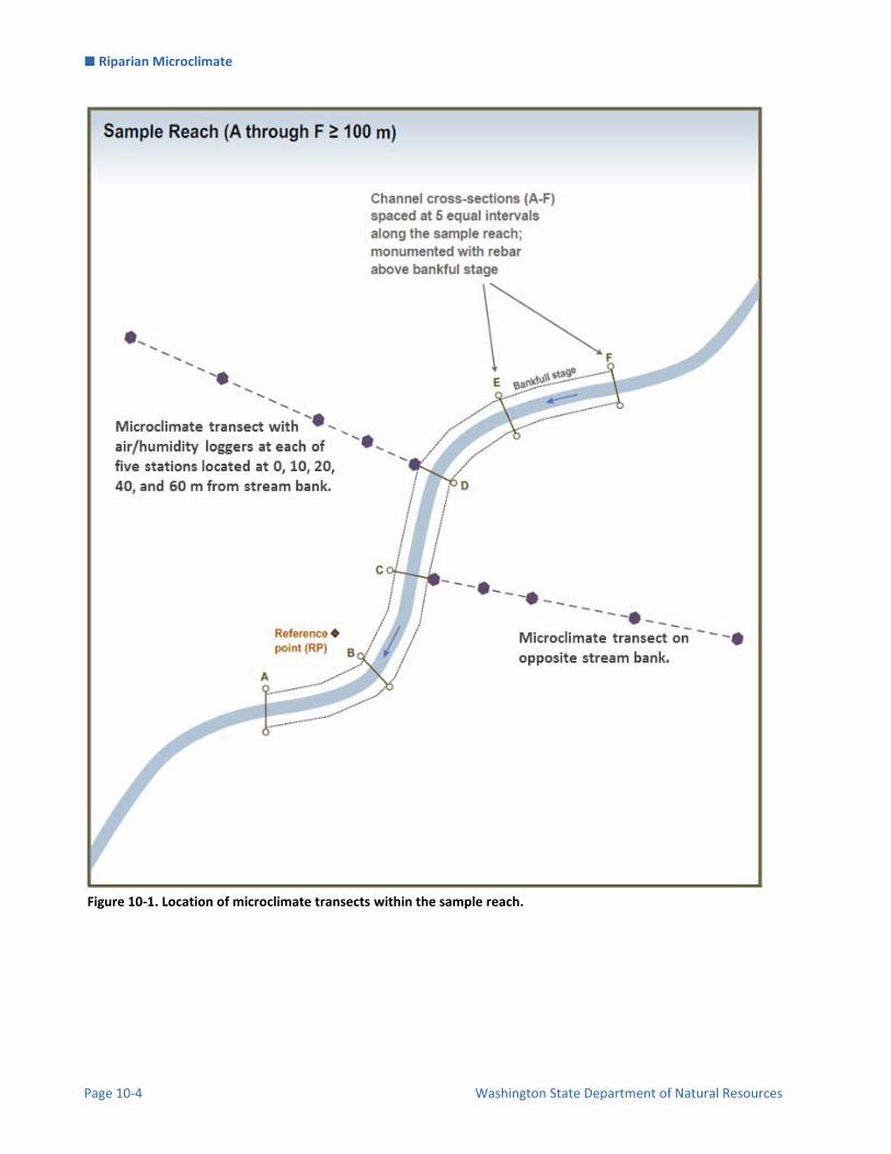
Riparian Microclimate
Page 10-4 Washington State Department of Natural Resources
Figure 10-1. Location of microclimate transects within the sample reach.

Riparian Microclimate
Status and Trends Monitoring of Riparian and Aquatic Habitat in the OESF Page 10-5
Figure 10-2. Location of microclimate monitoring stations in cross-section at a sample reach.
Site stratification followed the variables and methods used in selecting watersheds for hydrologic monitoring in this project (see Minkova and Vorwerk 2014). The stratification method aims to capture the full range of hydrologic conditions within the OESF by distinguishing different hydrologic regimes.
TEMPORAL SAMPLING DESIGN
Sampling Interval
Both air temperature and humidity data loggers are deployed year-round and set to record temperature every 120 minutes. At this interval, the data loggers’ memory limits and battery life will allow continuous recording for up to 4-5 years.
Download Schedule
Data will be downloaded and the loggers inspected twice annually: in spring (May-June) and fall (October-November). It is most efficient to download data and inspect loggers when the sample sites are visited for other monitoring activities.

Riparian Microclimate
Page 10-6 Washington State Department of Natural Resources
Equipment and Supplies The following equipment and supplies are needed for initial microclimate monitoring station installation, data logger download, and replacement of lost or damaged loggers:
Onset© HOBOware Pro software Onset© HOBO Pro v2 U23-001 Temp/RH Data Loggers Onset© HOBO Waterproof Shuttle (optical data shuttle for data download) 3-liter plastic paint-mixing buckets Onset© logger-specific mounting brackets 8 in nylon cable ties ¼ in foam boards Multitool/knife Hot glue gun and glue 5 ft U-post 4 lb hammer or post driver Laser range finder Compass set to current declination Brush-clearing tools (machete, brush ax, loppers, saw)
PRE-FIELD SET UP
Preparing the Microclimate Housing Assembly
Each microclimate station includes a 5-ft U-post, a housing, and a HOBO® Pro v2 logger, which measures air temperature and relative humidity. The housing protects the logger from direct sunlight and precipitation. The housing is composed of an upside-down 3-liter paint-mixing bucket equipped with a bracket to hold the logger (Figure 10-3). Two pieces of ¼ in foam board are attached between the bucket and the bracket. When the bracket is attached to the U-post, make sure the logger bottom is immediately above the bottom of the housing. The assembly is glued together and secured to the U-post with two nylon cable (zip) ties – one at the base and one near the top. Insert the logger into the bracket with the vented membrane (narrow end) pointed toward the ground (Figure 10-4). An instructional video showing the housing construction method is
Figure 10-3. Diagram of a microclimate monitoring station. View from below the microclimate housing (left), side view of microclimate housing (right).

Riparian Microclimate
Status and Trends Monitoring of Riparian and Aquatic Habitat in the OESF Page 10-7
available on the network drive at: J:\hcp\monitoring_research\tminkova\01_OESF_R&M Program\01_Rip S&T Mon\03_Photos and videos\01_Implementing Field Protocols\Microclimate\STRONG - A microclimate housing instructional video.MTS.
Launching and Testing the Loggers
First, make sure the HOBOware Pro software used to interact with HOBO data loggers has been downloaded on the computer. That software will be used to launch the logger and process data. Set the clock on the computer used to launch the loggers to Pacific Standard Time (PST) through the use of the atomic clock (e.g., http://www.time.gov/timezone.cgi?Pacific/d/-8/java). This ensures that all loggers will record data at exactly the same times. Before programming for field deployment, test all loggers to confirm that they are calibrated similarly. Do this by first programming them to record temperature and relative humidity at a short logging interval (e.g., five minutes) and launching them all at a common, delayed launch time. Follow the manufacturer’s programming and launching procedures described in the manual, which is available at: http://www.onsetcomp.com/files/manual_pdfs/10694-N%20MAN-U23.pdf. Put all loggers in a common indoor environment for at least 4 hours, then move them to a common outdoor environment for an additional 4 hours. Ensure that all loggers are exposed to exactly the same conditions, including shade/sunlight. After the outdoor period, download all loggers. Compare indoor data from all loggers to ensure that temperature among loggers is within a 0.21°C range and that relative humidity values are within 3.5 percentage points
Figure 10-4. Part of a microclimate transect (left) and microclimate data logger and housing (right).

Riparian Microclimate
Page 10-8 Washington State Department of Natural Resources
(these standards are from the manual). Repeat this comparison with the data recorded outdoors. The purpose of the test is to identify any loggers giving outlier values. Such loggers should be returned to the factory for re-calibration. After this test, loggers must then be re-programmed for field deployment. Program all the loggers for a common delayed launch time that starts after the planned field deployment time and date (usually 12:00 a.m. PST if deployed the day before. Program the loggers to measure and record temperature and relative humidity at 2-hour intervals. Field Procedures
MICROCLIMATE TRANSECT ESTABLISHMENT At each sample reach, two microclimate transects are established adjacent to separate, randomly selected channel cross section monuments, on opposite sides of the stream (Figure 10-1). The transects project 60 m into the forest along the center line of riparian vegetation plots (see Riparian Vegetation Monitoring Protocol for additional details). The six channel cross sections that define OESF sample reaches are marked by rebar topped with orange mushroom caps (i.e., monuments) labeled with the cross section identifier (A-F).
Transect Installation
Microclimate transects should start ~1-5 m upslope of the randomly selected cross-section monument (A-F, left or right bank, determined facing downstream) and extend upslope at an angle perpendicular to the stream. The reason for starting the microclimate transect slightly upslope from the monument is to avoid placing the first microclimate station in a location where it could be lost in a flood event. In some cases, the cross-section monument is high enough above the stream that the location is safe from floods, but in other cases the transect starting point may need to be located as much as 5 m upslope from the monument. If a vegetation plot has already been established at the cross section, use the previously recorded center line azimuth (also called the “plot azimuth”; see Riparian Vegetation Monitoring protocol) to locate microclimate monitoring station installation locations. If a vegetation plot has not been established at the cross section, use a compass to determine the stream azimuth. Then, calculate and record the azimuth perpendicular to the stream (add/subtract 90 degrees); this upslope azimuth will define the transect (as well as the vegetation plot center line). Microclimate monitoring stations are installed at 0, 10, 20, 40, and 60 m along this transect. Distances are horizontal distance, meaning measurements on sloping terrain must be taken using a range finder that can calculate horizontal distance. A measuring tape can be used on relatively flat terrain.

Riparian Microclimate
Status and Trends Monitoring of Riparian and Aquatic Habitat in the OESF Page 10-9
Installation of Microclimate Monitoring Stations
At each microclimate monitoring location, a metal post (U-post) and housing assembly (see Pre-field Set-up) are installed to hold and protect the data logger. To install the U-post, position the open side so it is facing north and use a hammer or post driver to pound the post into the ground until the wings are buried and the top of the post is 1.3 m above the forest floor. If needed, adjust the post location (move it parallel to the stream, so that it maintains the same distance from the stream) to ensure it is lodged in stable ground. Record the azimuth and distance of any offset from the original location. Attach the microclimate housing assembly (see Pre-field Set-up) to the open (north-facing) side of the U-post, using nylon cable (“zip”) ties. Insert the HOBO® Pro v2 logger into the bracket. The bracket should allow the logger to hang parallel to the side of the housing and the logger tip (the smaller end with a vented membrane) should be nearly flush with the bottom of the housing.
Topographic and forest structure characteristics will be documented as possible contributors to spatial variation in microclimate. The horizontal distance and azimuth from the cross-section monument to the 0-m station is measured. Additionally, the vertical distance from the base of the cross-section monument to the base of the 0-m station post is measured using the rangefinder and recorded (see Installation Field Form in Appendix A). For the 10-, 20-, 40-, and 60-m stations, measure the vertical distance between the base of that station’s post and the base of the preceding post (e.g., for the 10-m station, measure the vertical distance between its base and the base of the 0-m post). Vertical distances may be positive or negative, depending on topography.
DOWNLOADING PROCEDURES Microclimate data loggers (Onset HOBO Pro v2) should be downloaded and inspected twice annually: in the Spring (May-June) and Fall (October-November). Microclimate loggers can be downloaded directly to a laptop (weather permitting) or to an optical data shuttle (HOBO Waterproof Shuttle; preferred). Record metadata in the Microclimate Field Form (Appendix 10B). To retrieve the logger for download, reach inside the housing and slip the logger out of its bracket. Clean the logger communications window (clear face) with a cloth and connect the logger to the data shuttle or laptop. Follow the manufacturer’s download procedures (http://www.onsetcomp.com/files/manual_pdfs/10694-N%20MAN-U23.pdf). The download takes only a couple of minutes. Record the logger serial number and logger name (Watershed #_Stream Bank (Right/Left)_Station (0, 10, 20, 40, 60 m) on the Microclimate Field Form (Appendix 10B). Inspect the logger, housing, and U-post and note any damage on the form (e.g., bear bites can perforate the logger membrane that protects the sensors). If necessary, re-attach the housing to the U-post with nylon cable ties. If logger damage is severe (e.g., perforated membrane), the logger should be replaced. When installing a new logger, record the serial numbers of both loggers, the station (0-60 m), and the reason for replacement. Be sure to clearly communicate the change to the project Data Management Specialist.

Riparian Microclimate
Page 10-10 Washington State Department of Natural Resources
Time and Cost Estimates for Implementing the Field Procedures A skilled crew of two people can install a microclimate transect, including posts and housing installations, in two hours. Programming of loggers and manufacture of the housings is done in mass and takes about eight hours. This time estimate doesn’t include the travel to the site.
Table 10-1 shows the cost estimates for the equipment unique to implementing the field procedures of the microclimate protocol. Some of the items listed in the Equipment and Supplies section above, such as the laser rangefinder, are shared with the vegetation protocol. Their costs are detailed in that protocol and not included here.
Table 10-1. Cost Estimates for the equipment used in the riparian microclimate protocol.
Equipment/Supplies Amount per watershed Individual cost
Amount for the project (10 sites) Cost for the project*
Onset© HOBO Pro v2 U23-001
Temp/RH Data Loggers 10 $170 100 $17,000
Onset© HOBO waterproof shuttle
n/a $249 1 $249
Onset© HOBO Pro v2 clamp kit
10 $5 100 $500
HOBOware Pro software n/a $99 1 $99
5-ft metal u-bar fence post 10 $3.50 100 $350
Data Logger solar shield 10 $1 100 $100
Cable ties 50 $0.02 500 $10
Procedures for Calculating Metrics For air temperature, the daily minimum, maximum, mean, and range are calculated for each data
logger (Table 10-2). Values also will be summarized by month and season. For absolute humidity (g/m3), the daily minimum is derived for each data logger. Values will be
summarized by month and season. Vapor pressure deficit (kPa) may be calculated as well, if required by the objectives of the analysis.
Vapor pressure deficit is calculated, similarly to absolute humidity, from simultaneous temperature and relative humidity readings.
Temperature and humidity gradients will be calculated across each of the transects (i.e., 0- to 60-m horizontal distances from the stream).
Three forms of analyses will be conducted with respect to overstory density, canopy cover, and microclimate response variables:
o Influence of stand basal area on microclimate (temperature and humidity) will be assessed using overstory vegetation data collected in three zones (0-20, 20-40, 40-60 m from stream).

Riparian Microclimate
Status and Trends Monitoring of Riparian and Aquatic Habitat in the OESF Page 10-11
o Influence of canopy cover on microclimate (temperature and humidity) will be assessed using hemispherical canopy photos.
o Between-watershed differences will be evaluated statistically by evaluating data stratified into near-stream, mid-slope, and upslope zones.
Table 10-2. Microclimate metrics and calculations.
Metric Calculation procedure
Temperature: daily mean, min, max, and range.
Daily mean, minimum, maximum, and range (max minus min); calculated for each logger.
Absolute humidity (g/m3) Calculated from simultaneous relative humidity and temperature readings for each logger. Absolute humidity is calculated using the following equation where rh=relative humidity and T=temperature:
Absolute humidity: daily min.
Daily minimum of absolute humidity; calculated for each logger.
Quality Control and Quality Assurance Quality assurance includes staff training, use of standardized protocols, and periodic field checks. The QA/QC procedures for data management are described in the Data Management section, below.
TRAINING All personnel conducting field protocols will be trained in a consistent manner to ensure that the work is conducted properly and in standardized fashion. The training is conducted or, for returning personnel, reviewed, annually before the start of the field season.
STANDARD PROTOCOLS The standard procedures described in this protocol are followed for the duration of the project. Any deviations from the procedures should be documented, and the reasons for deviation described and discussed with the project manager or the researcher overseeing the protocol implementation. Changes to the published protocols are approved by the project manager or by the researcher overseeing the protocol implementation. Revised protocols are assigned new version numbers and publication dates. Pacific Standard Time (PST) should be used for all field procedures, year-round. Field personnel should be particularly aware of this during Pacific Daylight Time (PDT) from March through November. The letters PST should be appended to all times in field notes to ensure accuracy.

Riparian Microclimate
Page 10-12 Washington State Department of Natural Resources
TESTING DATA LOGGERS The accuracy of each data logger should be tested prior to deployment and again after it has been retrieved from the field. Calibration procedures are described in the Equipment and Supplies section above, under the heading Launching and Testing the Loggers. The manufacturer-reported accuracy level for the Onset© HOBO Pro v2 U23-001 Temp/RH Data Loggers is ±0.21°C from 0° to 50°C.
DATA QUALITY CONTROL All microclimate data (i.e., every data point recorded during this project) are plotted and evaluated graphically to identify any suspect data points that could indicate instrument malfunction or other errors. This is typically done using the software R. Temperature and humidity data are plotted separately. Typically, all temperature or humidity data points from each transect’s loggers (n=5) are plotted together on one graph, for one calendar month at a time. Each graph is then reviewed by two people (a scientist and the Data Management Specialist). Field notes are extremely valuable for detecting and diagnosing problems with data quality. All field notes should be examined during the quality control phase, and used in conjunction with the quality control plots.
Data Management
DATA FLOW Field data are collected in two formats: (1) paper field forms used to record metadata, and (2) electronic downloads of HOBO Pro v2 U23-001 data loggers. Additionally, photographs are taken in the field to document data logger damage or other irregularities. This section of the protocol describes the steps used to process these data from their raw field formats through the quality control stage. Details on long-term data storage and archiving appear in the following section on Data Storage.
Paper field forms
1. Fill out field forms The Microclimate Field Form (Appendix 10B) is used to record all activities related to data loggers, such as data downloads and logger replacements. Information recorded includes the logger location, date, time, crew, serial number, and notes.
2. Scan and store field forms After returning from the field each week, the field forms are scanned and stored on the WADNR network drive; the original paper forms are archived at the Washington Department of Natural Resources Forest Resources Division.
3. Enter data All of the information collected on microclimate field forms will be entered in the stream temperature database by the OESF Data Management Specialist on a weekly basis.
Data logger downloads
1. Download data loggers Temperature and relative humidity data are downloaded from the HOBO data loggers in the form of “.hobo” files, a proprietary file format that can only be opened using

Riparian Microclimate
Status and Trends Monitoring of Riparian and Aquatic Habitat in the OESF Page 10-13
HOBOware® software (Onset Computer Corp.). Data loggers are downloaded using an optical shuttle (the files on the shuttle are later transferred to a computer), or can be downloaded directly to a laptop. Each downloaded file contains the data logger’s serial number embedded within the file. This serial number is important for matching data files with monitoring locations.
2. Store raw data files In the WADNR office, a member of the field crew transfers all downloaded .hobo files to a temporary location on the WADNR network drive: J:\hcp\monitoring_research\tminkova\01_OESF_R&M Program\01_Rip S&T Mon\07_Data management\_All new data and photos\
3. Export files Using HOBOware® software, the data from all of the .hobo files are batch exported to comma separated variable format (.csv).
4. Import data to database Using R, the data from all .csv files are merged into a single file which is then imported into the Microsoft Access microclimate database.
5. Quality control Data are inspected as described in the Quality Control section above. The results of the quality control inspections are recorded in the database, and the data are assigned a data quality level based on the completion of various quality control steps. Data begin as “Level 0: Raw Data”. After an initial series of automated data quality checks, data are assigned the “Level 1: Provisional” quality level. After completion of all quality control steps, data are assigned the highest quality level, “Level 2: Published”. At this level, every record in the dataset is flagged as one of the following: accepted, rejected, estimated, or missing. Data are now ready for analysis and sharing.
DATA STORAGE
Paper Field Forms
The paper field forms are archived at the Washington Department of Natural Resources (WADNR) Forest Resources Division. Scanned copies of these forms are saved in the Adobe portable document format (.pdf) within the following directory: J:\hcp\monitoring_research\tminkova\01_OESF_R&M Program\01_Rip S&T Mon\01_FIELD DATA\
Long-term Data Storage
All microclimate data, as well as metadata, are stored in the Microclimate database, which is a Microsoft Access database designed specifically for this project. The database is located on the WADNR network drive at: J:\hcp\monitoring_research\tminkova\01_OESF_R&M Program\01_Rip S&T Mon\01_FIELD DATA\

Riparian Microclimate
Page 10-14 Washington State Department of Natural Resources
References Anderson, P.D., Larson, D.J. and Chan, S.S. 2007. Riparian buffer and density management influences on
microclimate of young headwater forests of western Oregon. Forest Science 53(2): 254-269.
Brosofske, K.D., Chen, J., Naiman, R.J., and Franklin, J.F. 1997. Harvesting effects on microclimatic gradients from small streams to uplands in western Washington. Ecological Applications 7(4): 1188-1200.
Danehy, R.J., Kirpes, B.J. 2000. Relative humidity gradients across riparian areas in eastern Oregon and Washington forests. Northwest Science 74(3): 224-233.
Guenther, S.M., Moore, R.D., Gomi, T., 2012. Riparian microclimate and evaporation from a coastal headwater stream, and their response to partial-retention forest harvesting. Agricultural and Forest Meteorology. 164:1-9.
Kluber, M.R., Olson, D.H. and Puettmann, K.J., 2009. Downed wood microclimates and their potential impact on plethodontid salamander habitat in the Oregon Coast Range. Northwest Science 83(1): 25-34.
Minkova, T., Vorwerk, M. 2014. Status and Trends Monitoring of Riparian and Aquatic Habitat in the Olympic Experimental State Forest. 2013 Establishment Report: Field Installations and Development of Monitoring Protocols. Washington State Department of Natural Resources, Forest Resources Division, Olympia, WA. (Also available at http://www.dnr.wa.gov/ResearchScience/Topics/TrustLandsHCP/Pages/lm_hcp_oesf_research_interest.aspx)
Moore, R.D., Spittlehouse, D.L., Story, A. 2005. Riparian microclimate and stream temperature response to forest harvesting: a review. Journal of the American Water Resources Association 41(4): 813.
Olson, D.H., Anderson, P.D., Frissell, C.A., Welsh, H.H., Bradford, D.F. 2007. Biodiversity management approaches for stream–riparian areas: perspectives for Pacific Northwest headwater forests, microclimates, and amphibians. Forest Ecology and Management 246(1): 81-107.
Washington State Department of Natural Resources. 2016. Olympic Experimental State Forest HCP Planning Unit Forest Land Plan Final Environmental Impact Statement. Washington State Department of Natural Resources, Olympia, WA. http://file.dnr.wa.gov/publications/amp_sepa_nonpro_oesf_feis.pdf

Riparian Microclimate
Status and Trends Monitoring of Riparian and Aquatic Habitat in the OESF Page 10A-1
Appendix 10A. Riparian Microclimate Installation Field Form
2hr
Distance(m): Serial #:
0 (monument to 0-m station)
10 (from 0-m to 10-m station)
20 (from 10-m to 20-m station)
40 (from 20-m to 40-m station)
60 (from 40-m to 60-m station)
Recording Interval: 2hr
Distance(m): Serial #:
0 (monument to 0-m station)
10 (from 0-m to 10-m station)
20 (from 10-m to 20-m station)
40 (from 20-m to 40-m station)
60 (from 40-m to 60-m station)
General Notes:
Transect #1
Transect #2 Transect azimuth (bet. 0- and 60-m stations) (deg.):
Azimuth from x-sec. monument to 0-m station:
Dist. from x-sec. monument to 0-m station:
Camera #: Photos #:
Date: Crew:
Bank:
Bank:
Crossection:
Crossection:
Elevation difference (+ or -) measured at
base of each post:
Elevation difference (+ or -) measured at
base of each post:
Azimuth from x-sec. monument to 0-m station:
Dist. from x-sec. monument to 0-m station:
Logger Name:
Recording Interval:
Logger Name:
Watershed:
Transect azimuth (bet. 0- and 60-m stations) (deg.):

Riparian Microclimate
Page 10A-2 Washington State Department of Natural Resources
This page intentionally left blank.

Riparian Microclimate
Status and Trends Monitoring of Riparian and Aquatic Habitat in the OESF Page 10B-1
Appendix 10B. Riparian Microclimate Download Field Form
Basin #:
Transect #1
Streamside:
Distance (m) Serial #
0
10
20
40
60
Transect #2
Streamside:
Distance (m) Serial #
0
10
20
40
60
X-section: Notes, picture #, etc:
Logger Name
X-section: Notes, picture #, etc:
Logger Name
Microclimate Download Form
Date: Crew: Recording
Interval: 2 hrStart time: End time: Camera #:

Riparian Microclimate
Page 10B-2 Washington State Department of Natural Resources
This page intentionally left blank.
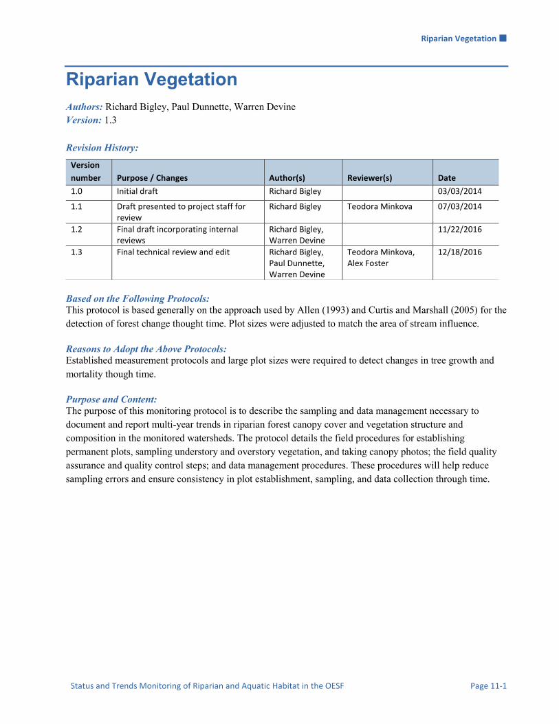
Riparian Vegetation
Status and Trends Monitoring of Riparian and Aquatic Habitat in the OESF Page 11-1
Riparian Vegetation Authors: Richard Bigley, Paul Dunnette, Warren Devine Version: 1.3
Revision History:
Based on the Following Protocols: This protocol is based generally on the approach used by Allen (1993) and Curtis and Marshall (2005) for the detection of forest change thought time. Plot sizes were adjusted to match the area of stream influence. Reasons to Adopt the Above Protocols: Established measurement protocols and large plot sizes were required to detect changes in tree growth and mortality though time. Purpose and Content: The purpose of this monitoring protocol is to describe the sampling and data management necessary to document and report multi-year trends in riparian forest canopy cover and vegetation structure and composition in the monitored watersheds. The protocol details the field procedures for establishing permanent plots, sampling understory and overstory vegetation, and taking canopy photos; the field quality assurance and quality control steps; and data management procedures. These procedures will help reduce sampling errors and ensure consistency in plot establishment, sampling, and data collection through time.
Version
number Purpose / Changes Author(s) Reviewer(s) Date
1.0 Initial draft Richard Bigley 03/03/2014
1.1 Draft presented to project staff for review
Richard Bigley Teodora Minkova 07/03/2014
1.2 Final draft incorporating internal reviews
Richard Bigley, Warren Devine
11/22/2016
1.3 Final technical review and edit Richard Bigley, Paul Dunnette, Warren Devine
Teodora Minkova, Alex Foster
12/18/2016

Riparian Vegetation
Page 11-2 Washington State Department of Natural Resources
Table of Contents Introduction ................................................................................................................................................... 11-3
Monitoring Design ........................................................................................................................................ 11-3
Spatial Sampling Design ........................................................................................................................... 11-3
Temporal Sampling Design ....................................................................................................................... 11-5
Equipment and Supplies ................................................................................................................................ 11-5
Field Procedures ............................................................................................................................................ 11-5
Pre-field set up .......................................................................................................................................... 11-5
Plot establishment ..................................................................................................................................... 11-6
Tree sampling and tagging ........................................................................................................................ 11-8
Understory vegetation and tree seedling sampling.................................................................................. 11-10
Hemispherical Canopy Photos ................................................................................................................ 11-12
Quality Assurance and Quality Control ...................................................................................................... 11-13
Training ................................................................................................................................................... 11-13
Standard Protocols .................................................................................................................................. 11-13
Field Quality Control .............................................................................................................................. 11-14
Time Estimates for Implementing the Field Procedures ............................................................................. 11-14
Procedures for Calculating Metrics ............................................................................................................. 11-14
Data Management ....................................................................................................................................... 11-15
Data Flow ................................................................................................................................................ 11-15
Data Storage ............................................................................................................................................ 11-17
Data Products .......................................................................................................................................... 11-19
References ................................................................................................................................................... 11-20
Appendix 11A. Riparian Vegetation Field Sheets ..................................................................................... 11A-1
Appendix 11B. Tables in the Riparian Vegetation Database ..................................................................... 11B-1

Riparian Vegetation
Status and Trends Monitoring of Riparian and Aquatic Habitat in the OESF Page 11-3
Introduction Understanding forest structure dynamics resulting from competition, forest decay, and disturbance is vital to assessing riparian forest influence on stream temperature (by influencing shade), near-stream microclimate, and litter, sediment and woody debris inputs to streams – all central indicators of stream habitat condition. When watersheds are disturbed, restoration of aquatic community-level resilience reflects a successional process driven by riparian vegetative recovery (Kauffman et al 1997). Modern riparian management practices designed to protect riparian areas from the effects of timber harvesting are known to differ in their effectiveness. Their capacity to maintain water quality, aquatic and riparian biodiversity, and ecosystem functions and services varies with the extent of near-stream vegetation removal (Cristan et al. 2016). In the Olympic Experimental State Forest (OESF), most riparian areas have been previously clear-cut to the stream edge. The resulting vegetation is a mixture of natural regeneration and plantation establishment. Changes in vegetation structure are key to interpretation of watershed recovery from past disturbance. The Washington Department of Natural Resources (WADNR) riparian conservation strategy assumes that as riparian forests recover from past disturbance, so too does riparian function. In the environmental impact analysis for the OESF Forest Land Plan, riparian vegetation height, composition, and mortality rate were key drivers in predicting stream habitat condition recovery (WADNR 2016). Streamside vegetation dictated stream temperature, inputs of litter and woody debris, and microclimate.
Monitoring Design
SPATIAL SAMPLING DESIGN Riparian vegetation is monitored in all 50 OESF sample watersheds and the four reference sample watersheds in Olympic National Park (ONP). Refer to the Introduction chapter for a map of the sample sites. The vegetation conditions sampled represent the common forest types on the OESF. The Sitka spruce (Picea sitchensis) vegetation zone dominates along the coast, while a majority of the OESF falls within the western hemlock (Tsuga heterophylla) vegetation zone. Vegetation monitoring occurs within two fixed-area plots established adjacent to two of the six systematically defined channel cross sections installed at each sample reach. The 0.18-ha plots are located at separate, randomly selected cross sections on opposite sides of the stream. Trees are tagged and measured throughout each plot, hemispherical canopy photos are taken at five photo points spaced systematically along the plot center line, and understory canopy cover and tree seedling recruitment are sampled within five circular 50-m2 subplots offset from the photo points (see Figure 11-1).

Riparian Vegetation
Page 11-4 Washington State Department of Natural Resources
Figure 11-1. Location of riparian vegetation sampling plots within the sample reach.

Riparian Vegetation
Status and Trends Monitoring of Riparian and Aquatic Habitat in the OESF Page 11-5
TEMPORAL SAMPLING DESIGN Riparian overstory and understory vegetation are sampled in the summer, every 3 to 5 years. Hemispherical canopy photos are taken annually, between June 1 and September 15, coincident with the leaf-out period of regional vegetation. Complementary remote sensing data are updated as they become available.
Equipment and Supplies
Red/white striped plastic flagging (for OESF sites) Blue or red biodegradable flagging (for ONP sites) Permanent markers (i.e., black sharpies) Hammers (to drive nails into trees and rebar/stakes into the ground) Sighting compass (e.g., Silva Ranger©) set to current declination Laser range finder or Haglöf Vertex Hypsometer Diameter (DBH) tapes 50-meter tape 30-meter logger’s tape Aluminum tree tags (numbered) Aluminum nails 2-ft rebar (for OESF sites) Orange plastic mushroom rebar caps (for OESF sites) Wood stakes (for ONP sites) Nikon™ Coolpix 4500 digital camera Nikon™ FC-E8 fisheye converter (7.2 mm f/2.4, approximately 183º FOV) Pelican™ 1400 case, to transport and protect camera equipment in transit to sampling locations SimpleTech™ 512 MB CompactFlash Memory Card Nikon™ EN-EL1 camera battery or equivalent (Two; one in use, another as backup) Nikon™ battery charger or equivalent Slik™ sprint 150 aluminum tripod w/ SBH-150DQ Ball Head Camera plate and Slik™ DQ-L Quick release adapter set StreamLight™ Stylus LED penlight (to indicate north in the photo) Plant field guide (e.g., Pojar and MacKinnon 1994)
Field Procedures
PRE-FIELD SET UP Crews should know the channel cross section (designated A-F) and stream bank (left or right) selected for vegetation plot establishment and sampling. If plots were previously established and/or sampled, obtain a list of the azimuths used to delineate the plot boundaries and center lines.

Riparian Vegetation
Page 11-6 Washington State Department of Natural Resources
If using Haglöf Vertex Hypsometer, calibrate daily and bring spare batteries.
Make sure that the canopy photo camera (Nikon™ Coolpix 4500) batteries are fully charged, previous data has been downloaded from the compact flash card, and the 9-volt battery for the LED penlight is functioning. Ensure that the time and date are correctly set on the camera. The camera settings should match the ones in Table 11-1.
PLOT ESTABLISHMENT
Sample Site Location and Assessment
In OESF sample reaches, six channel cross sections are delineated by rebar topped with orange mushroom caps (i.e., monuments) labeled with the cross section identifier (A-F). Flagged wood stakes mark ONP reach cross sections. The 60 m x 30 m overstory vegetation plots start ~1-5 m upslope from randomly selected cross-section monuments (A-F, left or right bank, determined facing downstream) and extend into the adjacent forest at an angle perpendicular to the stream. The reason that plots start upslope from the cross-section monument is that the 30-m wide base of the plot must not overlap the stream; due to a stream’s meandering, this may require starting the plot as much as 5 m upslope from monument. Rebar monuments (or wood stakes in ONP) are installed at 0, 10, 20, 40, and 60 m to delineate the plot center line and define locations for hemispherical canopy photos and understory vegetation sampling (see Figure 11-1). Plot dimensions are horizontal distance, meaning measurements on sloping terrain must be taken using a range finder. A measuring tape can be used on relatively flat terrain. After locating the channel cross section monument selected for plot establishment, use a compass to determine the azimuths that will be used to delineate the plot boundaries. Measure and record the azimuth of the stream at the cross section; this azimuth and its back-azimuth (“stream azimuths”) will define the upstream and downstream plot boundaries. Then, calculate and record the azimuth perpendicular to the stream (add/subtract 90 degrees); this azimuth (“plot azimuth”) will define the plot center line. Before starting plot establishment, use the azimuths to assess whether the selected location is suitable for plot establishment and sampling. A plot should be moved to an alternative, randomly chosen cross section if: 1) the slope cannot be traversed safely; 2) the plot would intersect a road, another perennial stream, or its riparian zone, or 3) there is a sharp stream bend in the sample reach. To verify suitability of the plot, measure 15 m along the stream azimuths (both upstream and downstream) from streamside plot center (just upslope from the monument at the plot azimuth); if this line intersects the stream channel, adjust the azimuths slightly and/or move the plot edge up the hillslope (but not more than 5 m). Next, from the streamside plot center, walk 60 m along the plot azimuth to verify that the entire plot can be traversed safely and that no roads or other perennial streams or their riparian zones are in the plot. Move the plot to a different cross section only if it cannot be situated to meet these criteria. In that scenario, randomly select another stream cross section for the vegetation plot.
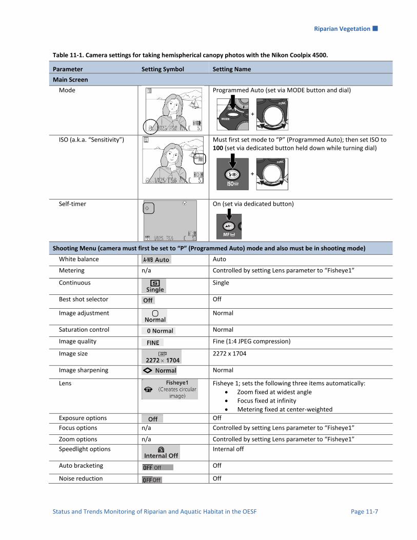
Riparian Vegetation
Status and Trends Monitoring of Riparian and Aquatic Habitat in the OESF Page 11-7
Table 11-1. Camera settings for taking hemispherical canopy photos with the Nikon Coolpix 4500.
Parameter Setting Symbol Setting Name
Main Screen
Mode
Programmed Auto (set via MODE button and dial)
ISO (a.k.a. “Sensitivity”)
Must first set mode to “P” (Programmed Auto); then set ISO to 100 (set via dedicated button held down while turning dial)
Self-timer
On (set via dedicated button)
Shooting Menu (camera must first be set to “P” (Programmed Auto) mode and also must be in shooting mode) White balance Auto
Metering n/a Controlled by setting Lens parameter to “Fisheye1”
Continuous
Single
Best shot selector Off
Image adjustment
Normal
Saturation control Normal
Image quality Fine (1:4 JPEG compression)
Image size
2272 x 1704
Image sharpening Normal
Lens
Fisheye 1; sets the following three items automatically:
Zoom fixed at widest angle
Focus fixed at infinity
Metering fixed at center-weighted
Exposure options Off
Focus options n/a Controlled by setting Lens parameter to “Fisheye1”
Zoom options n/a Controlled by setting Lens parameter to “Fisheye1”
Speedlight options
Internal off
Auto bracketing Off
Noise reduction Off
Riparian Vegetation
Page 11-8 Washington State Department of Natural Resources
Plot Installation
Once it is clear that a vegetation plot can be established, install a rebar monument at plot center, ~1-5 m upslope from the cross section monument along the plot azimuth. Use the hammer to pound the plot center monument into stable ground or a root. Leave ~15 cm (6 in) of rebar above ground, and place an orange mushroom cap on top. Make sure the rebar is secure; if it is loose, find a new location close to plot center. If the monument must be offset, record the azimuth and distance from true plot center on the data sheet and on the flagging tied to the rebar. Use a permanent marker to label the mushroom cap with “Veg” and the plot distance (0, 10, 20, 40, 60 m). Also attach red/white striped flagging labeled with the watershed number, “Vegetation”, the plot azimuth, and the corresponding letter for the cross section (A-F). At ONP reaches, plot center markers must be wood stakes with biodegradable flagging. After establishing the plot center monument near the cross section (i.e., at 0 m), use a compass and the range finder to locate plot center at 10, 20, 40, and 60 m upslope from the starting point (following the plot azimuth). Clear vegetation along the plot center line to facilitate travel and accurate horizontal distance measurements. Install flagged monuments and hang flagging at eye level at each designated distance along the center line, as described above. From the plot center monuments at 0, 20, 40, and 60 m, measure 15 m along the stream azimuths on the upstream and downstream sides and place flagging at or above eye level to mark the plot boundaries and delineate three zones (Zone 1: 0-20 m; Zone 2: 20-40 m; Zone 3: 40-60 m; Figure 11-1). Write the zone number on the flagging at plot center and at the plot edges.
TREE SAMPLING AND TAGGING Tag and measure all qualifying trees. A qualifying tree is a tree that meets one of the following criteria:
1. Live tree >12.5 cm diameter at breast height (DBH; 1.3 m above the forest floor). 2. Dead tree >12.5 cm DBH and ≥6.0 m in height. 3. Dead tree >12.5 cm DBH and < 6.0 m in height with an intact top.
Begin tagging and measuring trees on the upstream side of plot center (defined by the monuments), working your way away from the stream along plot center from Zone 1 to Zone 3 (see Figure 11-1). On the upstream side of the plot, tags should be placed on the stream-facing side of trees. Then, work your way back toward the stream from Zone 3 to Zone 1 on the downstream side of plot center, tagging trees on the side away from the stream. Keep careful track of plot and zone boundaries. A tree is considered within the plot only if its entire circumference at breast height is within the boundaries. Assign a tree to a zone if >50% of its circumference falls within the zone.

Riparian Vegetation
Status and Trends Monitoring of Riparian and Aquatic Habitat in the OESF Page 11-9
Nail a numbered tag to each qualifying tree at breast height. To determine breast height, carefully follow the examples in Figure 11-2. Be aware that, on steep slopes, tags facing the stream may be much higher than 1.3 m above the base of the tree’s downhill side (see “On slope” example in Figure 11-2). The nail should be hammered into the tree only so far that it cannot be pulled out with one’s fingers; it is important to leave
Figure 11-2. Location of tree diameter measurements. Adopted and redrawn from Curtis and Marshall 2005.

Riparian Vegetation
Page 11-10 Washington State Department of Natural Resources
much of the nail protruding from the tree to allow for growth. Angle nail ~5-10 degrees below horizontal to ensure that the tag rides the nail head and will not be consumed as the tree grows. When measuring DBH, wrap the diameter tape around the tree immediately above the nail. Make sure the tape is perpendicular to the main axis of the bole, even if the tree is leaning. Press the tape flat against the tree, and measure the diameter to the nearest 0.1 cm (Curtis and Marshall 2005). If the tree is covered by a thick layer of moss or lichens at breast height, peel these off before measuring diameter. Consistent, repeated measurement at the same point on the tree bole is vital for tracking growth over time (Curtis and Marshall 2005). Measure and tag trees only if it is safe to do so. Record tag number, tree species, DBH, whether the tree is alive or dead, and zone number for all qualifying trees (see Appendix 11A for field sheet). Species codes for common OESF taxa include: PISI (Sitka spruce); TSHE (Western hemlock); THPL (Western red cedar); ALRU (Red alder); PSME (Douglas-fir); ABAM (Pacific silver fir); and ACMA (Big leaf maple). More tree species codes can be found at: http://plants.usda.gov/dl_state.html.
Special Circumstances (see Figure 11-2)
Forked trees. Trees that fork above 1.3 m are considered single trees. Measure the diameter immediately below any swelling related to the fork but as close as possible to breast height (1.3 m). If the open crotch of the fork starts below 1.3 m, measure both boles 60 cm above the beginning of the fork (Curtis and Marshall 2005). If all forks are <12.5 cm in diameter, skip the entire tree. If all forks are >12.5 cm in diameter, measure each fork as a separate tree. If fork sizes are mixed, measure only forks >12.5 cm in diameter and do not measure the forks <12.5 cm in diameter. Identify forked trees on the data sheet as “fork stem.” If the forks appear to be trees that have grown together, follow the same guidelines but write “fused” on the data sheet.
Bole irregularities at DBH (limbs, scars, burls). If tree diameter cannot be measured at 1.3 m due to a limb, burl, scar, or other bole form irregularity, measure diameter immediately above the irregularity – where it ceases to affect the stem – and record the height at which diameter was measured on the field sheet. If the irregularity extends far up the bole, but stem form below 1.3 m is unaffected, measure diameter below the irregularity but as close as possible to 1.3 m. Do not measure tree diameter below 1 m on the stem. If bole irregularities (e.g., lightning scars) extend over most of the bole length, making adjustment impractical and/or misleading, measure the tree at normal DBH height.
UNDERSTORY VEGETATION AND TREE SEEDLING SAMPLING Understory vegetation percent cover is sampled within a 4-m-radius nested subplot offset from each plot center monument (at 0, 10, 20, 40, 60 m along the transect). From each monument, measure 6 m along the stream azimuth (i.e., perpendicular to the plot center line) on the upstream side and flag the location. This is the center of the circular understory vegetation subplot. To help define the subplot, place flagging at three or four locations 4 m from the subplot center. The understory field sheet appears in Appendix 11A.

Riparian Vegetation
Status and Trends Monitoring of Riparian and Aquatic Habitat in the OESF Page 11-11
Before sampling, scan the area within the subplot and make a list of the plant species present, identifying them by the USDA symbol (as identified in the latest version of the USDA Plants Database (http://plants.usda.gov/java). Shrubs (woody plants), forbs (herbaceous flowering plants), and graminoids (grasses and sedges) should all be sampled. If there is uncertainty regarding a species, place a sample in a plastic bag for later identification. Label the bag with the watershed number, cross section identifier (A-F), and nested subplot identifier (0, 10, 20, 40, 60 m). Estimate percent canopy cover for species within this circular subplot, one at a time (Figure 11-3). To estimate percent cover, mentally draw a convex, straight-line polygon around the outer portions of the crown of a plant, or around the crowns of closely spaced plants of the same species (Figure 11-3). Project this polygon to the ground; this is the canopy cover of the plant. Measure or estimate the diameter of the polygons and use these determinations and the count of individual plants to estimate cover of that species for the entire plot. If the entire plot cannot be viewed at once, determine cover by quarter wedges (i.e., 0 to 100% cover per wedge), sum the four wedges, and divide the sum by four to get the plot average. Do not subtract for small spaces between leaves or small gaps between branches. For each species, record cover as a percentage of the subplot in 1% increments. Estimate each species’ cover regardless of whether it is overlapped by other species. For each species, cover will range from 1 to 100%. Summing total percent cover of all species can exceed 100%, due to species overlap. Periodically cross-check individual species cover estimates (i.e., “calibrate”) to ensure consistency among technicians.
Figure 11-3. Polygon method to determine plant species cover. When multiple plants of the same species have overlapping polygons, construct polygons as shown in (A). For plants of different species, construct polygons separately for each species, even where those polygons overlap (B).

Riparian Vegetation
Page 11-12 Washington State Department of Natural Resources
Also determine the number of seedlings and saplings of each tree species within each subplot. Count trees <10 cm DBH and record by species and height class: 1) < 30 cm; 2) 30 cm-136 cm; 3) ≥137 cm. If the number exceeds 29 per species, simply record 30 to indicate that the number exceeded the counting threshold.
HEMISPHERICAL CANOPY PHOTOS
Timing of Canopy Photos
Hemispherical canopy photos are taken between June 1 and September 15, coincident with the leaf-out period of regional vegetation. Photos for each sample site should be taken within two weeks of the date when the previous canopy photos were taken at that site. This minimizes the seasonal effects of phenology (specifically the emergence and falling of leaves) and the sun’s position over the horizon. For optimal image quality, overcast flat lighting is preferred. Photos taken in direct sunlight or with a very bright sky can be washed out or include sun flares and glare. This can be partially corrected (see below). Photos are not to be taken in the rain.
Location of Canopy Photos
When assessing canopy cover trends, it is important that repeated photos are taken at the exact same location (horizontally and vertically). Canopy closure can vary greatly over fine spatial scales; thus, even minor changes in the position of the camera can introduce large differences in canopy cover values. Therefore, the camera should be positioned at the same location each time a hemispherical photo is taken. In this study, photos are taken at rebar/wood stake monuments placed at 0, 10, 20, 40, and 60 m along the center line of the vegetation plots established perpendicular to each study reach (see Plot Establishment, above, for details). Locate the vegetation plots, and walk upslope from the cross section monuments (perpendicular to the stream) to determine if plot center monuments have been installed. If monuments have not been installed, place them as you take canopy photos, following the instructions in the Plot Establishment section. Make sure to carefully follow the designated plot azimuths and distances.
Taking Canopy Photos
After locating or installing a plot center monument, position the camera tripod directly over the monument. If an obstacle makes it impossible to position the tripod above the monument, reposition the tripod as close as possible to plot center and record the distance (nearest 0.01 m) and azimuth from the monument. Mount the camera to the tripod, then switch on the LED penlight and insert it into the hole at the edge of the camera plate. Be sure that the front of the camera (not the screen-side) is facing the LED. Adjust the tripod height so the camera lens is 1.3 m above the forest floor next to the monument (measure with a stadia rod, transect tape, or diameter tape). Line up the compass housing with a corner of the camera plate, such that the compass bottom is flush with the plate edge opposite the LED. Rotate the camera plate until the orienting
Riparian Vegetation
Status and Trends Monitoring of Riparian and Aquatic Habitat in the OESF Page 11-13
arrow shows that the camera is facing true north. With this alignment, the LED will indicate true north in the photograph. Level the camera plate and camera using the two-axis bubble levels. Pull back any vegetation within 1.0 m of the lens. Before taking the photo, check that the camera is still at the correct height, leveled, and aimed toward true north and make sure the fisheye lens is clean and free of fog/water droplets. To prevent glare, avoid taking the photograph with the lens positioned in direct sunlight. If possible, wait for the sun to be obscured by vegetation or clouds. If necessary, block the sunlight with a stick, but try to affect the photo as little as possible. If a stick was used to shade the camera lens, note this on the data sheet. Turn on the camera and enable the self-timer. Press the shutter release to start the timer (10 seconds), then duck below the camera plate to avoid appearing in the photo. Remain below the camera plate until the light on the camera bottom stops blinking, indicating that the photo was taken. Review the photo on the camera screen to make sure that the image is in focus, with no major lens flare or field crew members in the photo. To view the photo and the photo number, press the play button above the screen twice. The number will appear in the right upper corner of the screen (XXXX.JPG). If necessary, re-take the photo without deleting unsuccessful images. Return to the main screen by pressing the play button above the screen. Record the photo number, stream cross section (A-F), stream bank (right or left), and plot distance (0, 10, 20, 40, 60 m) on the data sheet. Repeat the above steps at each sample site vegetation monument (total of10 photos per watershed).
Quality Assurance and Quality Control Quality assurance includes staff training, use of standardized protocols, and periodic field checks. The QA/QC procedures for data management are described in the Data Management section below.
TRAINING All personnel conducting field protocols will be trained in a consistent manner to ensure that the surveys are conducted properly and in standardized fashion. The training is conducted or, for returning personnel, reviewed, annually before the start of the field season. At least one member of the field crew should be experienced with the field procedures and have proven plant identification skills. Before field sampling begins, and at least once at each sample site, crew members will cross-check understory vegetation percent cover determinations (i.e., “calibrate”) to ensure consistency among technicians.
STANDARD PROTOCOLS The standard procedures described in this protocol are followed for the duration of the project. Any deviations from the procedures should be documented, and the reasons for deviation described and discussed with the project manager or the researcher overseeing the protocol implementation.

Riparian Vegetation
Page 11-14 Washington State Department of Natural Resources
Changes to the published protocols are approved by the project manager or by the researcher overseeing the protocol implementation. Revised protocols are assigned new version numbers and publication dates.
FIELD QUALITY CONTROL The researcher overseeing the protocol implementation or a different field crew will conduct spot checks on 10% of the field measurements every year.
Time Estimates for Implementing the Field Procedures Two skilled crew members can install one 30 x 60-m vegetation plot in 2 hours (4 hours per watershed). A two-member crew can tag and measure trees, sample the understory, and take canopy photos in one vegetation plot in 4 hours (8 hours per watershed). This is an average time estimate; actual time spent varies greatly by watershed, depending on riparian conditions. The time estimate doesn’t include the travel to the site.
Procedures for Calculating Metrics A variety of metrics will be reported for riparian vegetation. Examples of the metrics appear in Table 11-2. Table 11-2. Riparian vegetation metrics and calculation procedures.
Metric (calculated for each watershed) Calculation procedure
Overstory basal area per hectare
Use all measured living trees. Sum basal area by plot and convert to a per-hectare basis by dividing by 0.18 for each plot.
Overstory basal area per zone
Use all measured living trees. Sum basal area by zone within each plot and convert to a per-hectare basis by dividing by 0.06 for each zone.
Overstory trees per hectare Use all measured living trees. Count trees and convert to a per-hectare basis by dividing by 0.18 for each plot.
Overstory hardwood basal area per hectare
Use all measured living hardwood trees. Sum basal area by plot and convert to a per-hectare basis by dividing by 0.18 for each plot.
Overstory hardwood basal area per zone
Use all measured living hardwood trees. Sum basal area by zone within each plot and convert to a per-hectare basis by dividing by 0.06 for each zone.
Overstory conifer basal area per hectare
Use all measured living conifer trees. Sum basal area by plot and convert to a per-hectare basis by dividing by 0.18 for each plot.
Overstory hardwood basal area per zone
Use all measured living conifer trees. Sum basal area by zone within each plot and convert to a per-hectare basis by dividing by 0.06 for each zone.
Understory cover Sum cover and report for each growth form.
Riparian Vegetation
Status and Trends Monitoring of Riparian and Aquatic Habitat in the OESF Page 11-15
Data Management
DATA FLOW Data are collected in the field using paper field forms. Owing to the large number of different field personnel participating in riparian vegetation data collection, this is the most practical method of recording data at present. This section contains a description of the steps used to process this data from its field format through the quality control stage; flowcharts provide an overview of the process. Details on long-term data storage and archiving appear in the following section, titled Data Storage.
Data flow for paper field forms
1. Fill out field forms For overstory data, the field forms contain information at the plot level identifying the watershed ID, cross-section, and bank. At the individual tree level, the fields are: zone, tag number, dbh, species, live/dead status, and notes. For understory data, plot-level fields include watershed ID, cross-section, bank, and plot ID. For each plot, the following fields appear on the field sheet: species, percent cover, and notes.
2. Scan and store field forms After returning from the field each week, the field forms are scanned and stored on the WADNR network drive at: J:\hcp\monitoring_research\tminkova\01_OESF_R&M Program\01_Rip S&T Mon\07_Data management\_All new data and photos\ The original paper field forms are archived at the Washington Department of Natural Resources Forest Resources Division.
3. Enter data All of the information collected on paper field forms is entered into an Excel spreadsheet by personnel involved in its collection. This approach has been favored by personnel in the past (rather than entering data directly into the Access database) because they were familiar with Excel; this approach creates no additional work for the OESF Data Manager.
4. Data verification Entered field form data are verified by comparing it to the original field forms. 5. Import data to database The OESF Data Manager imports the data from Excel to the Access
database used for long-term storage of riparian vegetation data. 6. Quality control A series of quality control checks are performed by the OESF Data Manager
(Figure 11-4). After the quality control has been completed, data status is set to “Published”.

Riparian Vegetation
Page 11-16 Washington State Department of Natural Resources
Figure 11-4. Flow chart describing the riparian vegetation data quality control process.
Examine plot-level data to ensure that all values are valid
Data are ready for analysis
Begin quality control
Start: Overstory Data or Understory Data
Archive scanned forms on DNR network drive
Fill out field forms in the field
Scan and then archive the paper field forms at DNR
Enter field form data into Excel
Verify entered data
Ensure all dbh measurements are valid (i.e., greater than the minimum of 12. 7 cm and less than a reasonable maximum)
Import the Excel data to the Access database
Examine species field to ensure that each species code is valid
Ensure all cover estimates are valid numbers
Overstory or Understory? Overstory Understory
Change data status to “Published”
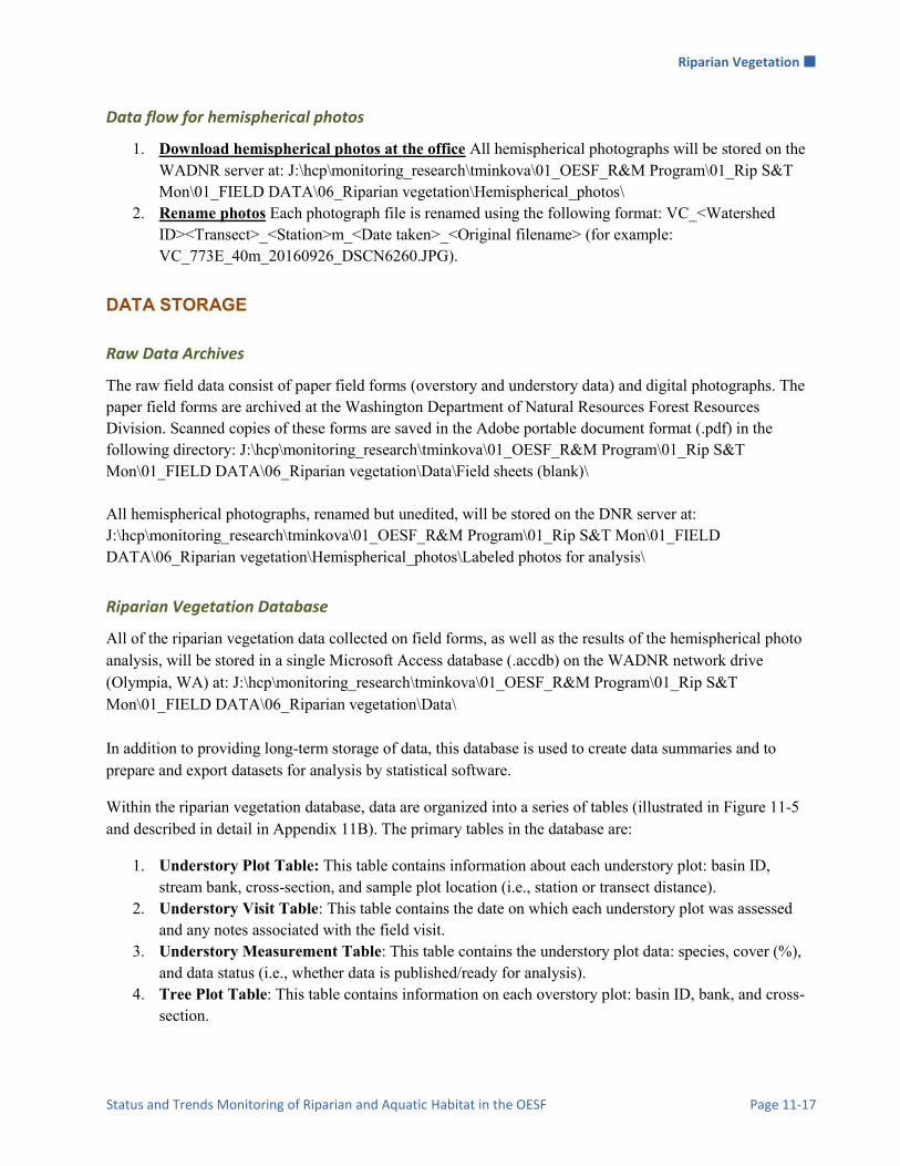
Riparian Vegetation
Status and Trends Monitoring of Riparian and Aquatic Habitat in the OESF Page 11-17
Data flow for hemispherical photos
1. Download hemispherical photos at the office All hemispherical photographs will be stored on the WADNR server at: J:\hcp\monitoring_research\tminkova\01_OESF_R&M Program\01_Rip S&T Mon\01_FIELD DATA\06_Riparian vegetation\Hemispherical_photos\
2. Rename photos Each photograph file is renamed using the following format: VC_<Watershed ID><Transect>_<Station>m_<Date taken>_<Original filename> (for example: VC_773E_40m_20160926_DSCN6260.JPG).
DATA STORAGE
Raw Data Archives
The raw field data consist of paper field forms (overstory and understory data) and digital photographs. The paper field forms are archived at the Washington Department of Natural Resources Forest Resources Division. Scanned copies of these forms are saved in the Adobe portable document format (.pdf) in the following directory: J:\hcp\monitoring_research\tminkova\01_OESF_R&M Program\01_Rip S&T Mon\01_FIELD DATA\06_Riparian vegetation\Data\Field sheets (blank)\ All hemispherical photographs, renamed but unedited, will be stored on the DNR server at: J:\hcp\monitoring_research\tminkova\01_OESF_R&M Program\01_Rip S&T Mon\01_FIELD DATA\06_Riparian vegetation\Hemispherical_photos\Labeled photos for analysis\
Riparian Vegetation Database
All of the riparian vegetation data collected on field forms, as well as the results of the hemispherical photo analysis, will be stored in a single Microsoft Access database (.accdb) on the WADNR network drive (Olympia, WA) at: J:\hcp\monitoring_research\tminkova\01_OESF_R&M Program\01_Rip S&T Mon\01_FIELD DATA\06_Riparian vegetation\Data\ In addition to providing long-term storage of data, this database is used to create data summaries and to prepare and export datasets for analysis by statistical software.
Within the riparian vegetation database, data are organized into a series of tables (illustrated in Figure 11-5 and described in detail in Appendix 11B). The primary tables in the database are:
1. Understory Plot Table: This table contains information about each understory plot: basin ID, stream bank, cross-section, and sample plot location (i.e., station or transect distance).
2. Understory Visit Table: This table contains the date on which each understory plot was assessed and any notes associated with the field visit.
3. Understory Measurement Table: This table contains the understory plot data: species, cover (%), and data status (i.e., whether data is published/ready for analysis).
4. Tree Plot Table: This table contains information on each overstory plot: basin ID, bank, and cross-section.
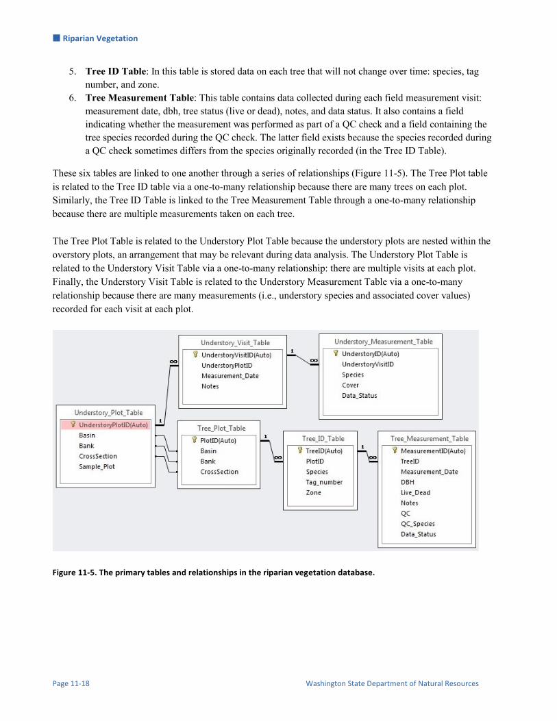
Riparian Vegetation
Page 11-18 Washington State Department of Natural Resources
5. Tree ID Table: In this table is stored data on each tree that will not change over time: species, tag number, and zone.
6. Tree Measurement Table: This table contains data collected during each field measurement visit: measurement date, dbh, tree status (live or dead), notes, and data status. It also contains a field indicating whether the measurement was performed as part of a QC check and a field containing the tree species recorded during the QC check. The latter field exists because the species recorded during a QC check sometimes differs from the species originally recorded (in the Tree ID Table).
These six tables are linked to one another through a series of relationships (Figure 11-5). The Tree Plot table is related to the Tree ID table via a one-to-many relationship because there are many trees on each plot. Similarly, the Tree ID Table is linked to the Tree Measurement Table through a one-to-many relationship because there are multiple measurements taken on each tree. The Tree Plot Table is related to the Understory Plot Table because the understory plots are nested within the overstory plots, an arrangement that may be relevant during data analysis. The Understory Plot Table is related to the Understory Visit Table via a one-to-many relationship: there are multiple visits at each plot. Finally, the Understory Visit Table is related to the Understory Measurement Table via a one-to-many relationship because there are many measurements (i.e., understory species and associated cover values) recorded for each visit at each plot.
Figure 11-5. The primary tables and relationships in the riparian vegetation database.

Riparian Vegetation
Status and Trends Monitoring of Riparian and Aquatic Habitat in the OESF Page 11-19
DATA PRODUCTS The stream temperature database contains various queries that create data summaries and prepare the data for statistical analysis by other software. These are accessed via the main database menu. Examples of data products include:
Data summaries:
A report containing a list of all tree species found on the overstory plots, as well as the frequency and average diameter of each species.
A report summarizing all understory species found on the understory plots. A report listing, for each overstory plot, trees per hectare and basal area per hectare.
Data for analysis:
A dataset containing all overstory data, except for that collected for QC purposes. A dataset containing all understory data.

Riparian Vegetation
Page 11-20 Washington State Department of Natural Resources
References Allen, R.B. 1993. A permanent plot method for monitoring changes in indigenous forests: a field manual.
Christchurch, New Zealand: Manaaki Whenua - Landcare Research. 24 p.
Cristan, R., Aust, W.M., Bolding, M.C., Barrett, S.M., Munsell, J.F., Schilling, E. 2016. Effectiveness of forestry best management practices in the United States: literature review. For. Ecol. Manage. 360: 133–151.
Curtis, Robert, O., and D.D. Marshall 2005. Permanent-plot procedures for silvicultural and yield research. Gen. Tech. Rep. PNW-GTR-634. Portland, OR: U.S. Department of Agriculture, Forest Service, Pacific Northwest Research Station. 86 p.
Kauffman J., Boone, R. L. Beschta , N. Otting and & D. Lytjen. 1997. An ecological perspective of riparian and stream restoration in the western United States. Fisheries. 22(5):12-24.
Pojar, J., MacKinnon, A. 1994. Plants of the Pacific Northwest coast. Vancouver, B.C.: Lone Pine. 528 p.
Washington State Department of Natural Resources. 2016. Olympic Experimental State Forest HCP Planning Unit Forest Land Plan Final Environmental Impact Statement. Washington State Department of Natural Resources, Olympia, WA. http://file.dnr.wa.gov/publications/amp_sepa_nonpro_oesf_feis.pdf

Riparian Vegetation
Status and Trends Monitoring of Riparian and Aquatic Habitat in the OESF Page 11-21
This page intentionally left blank.


Riparian Vegetation
Status and Trends Monitoring of Riparian and Aquatic Habitat in the OESF Page 11A-1
Appendix 11A. Riparian Vegetation Field Sheets
Plot Establishment and Canopy Photo Field Sheet
Plot (Horizontal) Azimuth:
Photo Photo number Time (PST)
0 m
10 m
20 m
40 m
60 m
Date:
Stream Azimuth:
Olympic Experimental State Forest (OESF) Stand Dynamics Vegetation Plot Data
Plot (Upslope) Azimuth:
Basin:
Date of photos:Photo location
(lens at 1.3 m above
stake or offset?) Photo notes (e.g., stick used to block sun)
Plot Establishment/Layout
Canopy Photos
Site and Plot Establishment notes:
Weather / Visit notes:
Azimuth to plot center
(at 0 m) from cross-sec
monument:
Distance to plot center
(at 0 m) from cross-sec
monument:
Crew:
Bank:
Cross-Sec:

Riparian Vegetation
11A-2 Washington State Department of Natural Resources
Understory Field Sheet
Species 0-m Plot 10-m Plot 20-m Plot 40-m Plot 60-m Plot
OESF Stand Dynamics Vegetation Plot: Understory
Basin: Date:
Cross Section:
Plot notes:
Crew:
Bank:
Understory Plant Data (% cover):

Riparian Vegetation
Status and Trends Monitoring of Riparian and Aquatic Habitat in the OESF Page 11A-3
Overstory Field Sheet
Zone Tag Species DBH (cm) L/D Notes Zone Tag Species DBH (cm) L/D Notes
Notes:
Date: Crew:
OESF Stand Dynamics Vegetation Plot: Overstory
Basin: Cross-Sec: Bank:
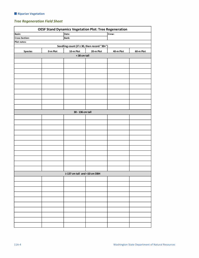
Riparian Vegetation
11A-4 Washington State Department of Natural Resources
Tree Regeneration Field Sheet
Species 0-m Plot 10-m Plot 20-m Plot 40-m Plot 60-m Plot
Seedling count (if ≥ 30, then record "30+")
< 30 cm tall
30 - 136 cm tall
≥ 137 cm tall and <10 cm DBH
OESF Stand Dynamics Vegetation Plot: Tree RegenerationBasin: Date: Crew:
Cross Section: Bank:
Plot notes:

Riparian Vegetation
Status and Trends Monitoring of Riparian and Aquatic Habitat in the OESF Page 11B-1
Appendix 11B. Tables in the Riparian Vegetation Database
Understory Plot Table
Field Field description
UnderstoryPlotID(Auto) Unique identifier for each record.
Basin Watershed identifier.
Bank The stream bank on which the plot is located.
CrossSection The cross section where the plot is located.
Sample_Plot The sample plot identifier, based on distance from beginning of transect.
Understory Visit Table
Field Field description
UnderstoryVisitID(Auto) Unique identifier for each record.
UnderstoryPlotID Relates records to a record in the Understory Plot Table.
Measurement_Date Date of measurement.
Notes Notes recorded in the field.
Understory Measurement Table
Field Field description
UnderstoryID(Auto) Unique identifier for each record.
UnderstoryVisitID Relates records to a record in the Understory Visit Table.
Species Plant species.
Cover Percentage of the plot covered by that species.
Data_Status Indicates whether data have passed the QC procedure (in which case status is changed to “Published”).
Tree Plot Table
Field Field description
PlotID(Auto) Unique identifier for each plot.
Basin Watershed identifier.
Bank The stream bank on which the plot is located.
CrossSection The cross section where the plot is located.

Riparian Vegetation
11B-2 Washington State Department of Natural Resources
Tree ID Table
Field Field description
TreeID(Auto) Unique identifier for each record.
PlotID Links records to the appropriate record in the Tree Plot Table.
Species Tree species.
Tag_number Tree tag number.
Zone The zone in which the tree is located.
Tree Measurement Table
Field Field description
MeasurementID(Auto) Unique identifier for each record.
TreeID Links records to the unique tree identifier in the Tree ID Table.
Measurement_Date Date of the measurement
DBH Diameter at breast height (cm).
Live_Dead Tree status at the time of measurement.
Notes Notes recorded during the measurement visit.
QC Is the measurement for the purpose of a quality control check? (Y/N)
QC_Species The species recorded during the QC measurement.
Data_Status Indicates whether data have passed the QC procedure (in which case status is changed to “Published”).

Glossary
Status and Trends Monitoring of Riparian and Aquatic Habitat in the OESF Page 12-1
Glossary Adapted from Armantrout 1998 unless otherwise indicated. Active channel – A streambank transition zone that marks a change from vegetative species able to survive extended periods of inundation like herbs and moss to permanent woody vegetation. Alluvial – Relating to the process of sediment transport and sorting, chiefly by water. Bankfull depth – Average flow depth across the channel at bankfull stage. Bankfull discharge - The dominant channel forming flow with a recurrence interval seldom outside the 1 to 2 year range.
Bankfull stage – Bankfull stage is delineated by the elevation point of incipient flooding, indicated by deposits of sand or silt at the active scour mark, a break in stream bank slope, perennial vegetation limit, rock discoloration, and root exposure. Bankfull width – Channel width between bankfull stage indicators, often congruent with the active channel. Canopy – The continuous cover of branches and foliage formed collectively by the crowns of adjacent trees and other woody growth. Channel confinement – The degree to which stream channel migration is limited in its lateral movement by valley walls or relic terraces. It is expressed as the ratio of the width of the floodplain to the channel’s bankfull width. Channel control – Natural or artificial channel feature(s) downstream of a gage station that influence the stage-discharge relationship at the gage station. Colluvial – Relating to the process through which sediment is transported chiefly by gravity and is unsorted. D50 – Median particle size of a distribution. Diameter at breast height (DBH) – The diameter of a tree, measured 1.37 m (4.5 ft) above the ground on the uphill side of the tree. Diel – Pertaining to a 24-hour period or a regular occurrence in every 24-hour period. Discharge – Rate at which a volume of water flows past a point per unit of time. Fines – Particulate material less than 2 mm in diameter, including sand, silt, clay, and fine organic material.

Glossary
Page 12-2 Washington State Department of Natural Resources
Floodplain width – The stream width at a discharge level defined as twice the maximum bankfull depth.
Floodplain, 100-year – Area adjoining a water body that becomes inundated during periods of overbank flooding that happens an average of once every 100 years. Gaging station – Particular location on a stream, canal, lake, or reservoir where systematic measurements of streamflow or quantity of water are made. Geographic information system (GIS) – A computer system that stores and manipulates spatial data, and can produce a variety of maps and analyses. Habitat attribute– Single element of the habitat or area (such as stream temperature or pools) where an organism lives or occurs (synonymous with habitat component). Habitat metric – Quantitative characteristics that describes the biological, chemical, and physical components of an ecosystem (for example mean daily stream temperature or residual pool depth) (synonymous with habitat parameter and habitat variable). A variety of metrics can be derived from original measurements. Hemispherical canopy photography – A method for indirectly characterizing the forest canopy using a camera equipped with a hemispherical (or “fish-eye”) lens which is aimed directly upward. Hydrograph – Graph that shows the rate of flow (discharge) versus time past a specific point in a channel. In-stream large wood (large woody debris) – Wood in the active channel with pieces larger than 10 cm in diameter and 2 m in length. Log jam or jam – Wholly or partially submerged accumulation of woody debris from winds, water currents, or logging activities that partially or completely blocks a stream channel and obstructs streamflow. Monitored Watersheds – For this project, the drainage around the smallest fish-bearing (Type 3) stream identified for sampling through GIS and subsequent field reconnaissance. Outlet – Terminus or mouth of a stream where if flows into a larger water body. Rating curve - A relationship between water level and streamflow (discharge) that is specific to each gaging station. Reach - A length of uniform channel with respect to discharge, depth, area, and slope. Riparian zone – A narrow band of moist soils and distinctive vegetation along the banks of lakes, rivers, and streams.
Glossary
Status and Trends Monitoring of Riparian and Aquatic Habitat in the OESF Page 12-3
Sample Reach – A portion of a stream where field sampling takes place. Signal-to-Noise Ratio – The ratio of the variation in a measured parameter (“signal”) to the variation in that parameter among repeated measurements (“noise”) (Kaufman et al. 1999). Sinuosity – An index (K) of a stream’s meander as a function of stream length. In this project, channel sinuosity is calculated as the ratio of sample reach length measured along the thalweg (using a reel tape) to the straight-line distance between the beginning and the end of the sample reach (measured with resource-grade GPS). Thalweg – Path of a stream that follows the deepest part of the channel. Type 3 Watershed – The drainage around the smallest fish-bearing (Type 3) stream (WADNR 1997). Type 3 Stream – smallest fish-bearing stream as identified through biological criterion (fish presence) or through physical criteria (a stream ≥ 2 ft (0.7 m) wide and ≤16% gradient for watersheds up to 50 ac (20 ha) or with a gradient between 16% and 20% for watersheds larger than 50 ac). Type 3 streams can be considered loosely equivalent to Strahler’s 3rd order streams (WADNR 1997). Wetted width – Width of a water surface at the time of a survey, measured perpendicular to the direction of flow. The average wetted width is often derived from multiple channel widths measured along a reach.

Glossary
Page 12-4 Washington State Department of Natural Resources
Literature Cited Armantrout, N.B., compiler. 1998. Glossary of aquatic habitat inventory terminology. American Fisheries
Society, Bethesda, Maryland.
Kaufmann, P.R., P. Levine, E.G. Robinson, C. Seeger, and D.V. Peck. 1999. Quantifying Physical Habitat in Wadeable Streams. EPA-620-R-99-003. US Environmental Protection Agency, Washington, DC.
Washington State Department of Natural Resources. 1997. Final Habitat Conservation Plan: Washington State Department of Natural Resources, Olympia, WA, 223p. http://www.dnr.wa.gov/programs-and-services/forest-resources/habitat-conservation-state-trust-lands

Glossary
Status and Trends Monitoring of Riparian and Aquatic Habitat in the OESF Page 12-5
This page intentionally left blank.
Related Documents


![Restoring Salmonid Aquatic/Riparian Habitat...aquatic/riparian habitat restoration activities. [5] [6] VISION AND OBJECTIVES The overreaching goal of this initiative is to improve](https://static.cupdf.com/doc/110x72/6104737c127ac45d1972c9a7/restoring-salmonid-aquaticriparian-habitat-aquaticriparian-habitat-restoration.jpg)