Stability of dynamical systems
Jun 14, 2015
Welcome message from author
This document is posted to help you gain knowledge. Please leave a comment to let me know what you think about it! Share it to your friends and learn new things together.
Transcript

Systems & Control: Foundations & Applications
Series EditorTamer Basar, University of Illinois at Urbana-Champaign
Editorial BoardKarl Johan Astrom, Lund University of Technology, Lund, SwedenHan-Fu Chen, Academia Sinica, BeijingWilliam Helton, University of California, San DiegoAlberto Isidori, University of Rome (Italy) and
Washington University, St. LouisPetar V. Kokotovic, University of California, Santa BarbaraAlexander Kurzhanski, Russian Academy of Sciences, Moscow
and University of California, BerkeleyH. Vincent Poor, Princeton UniversityMete Soner, Koc University, Istanbul
Anthony N. MichelLing Hou
Derong Liu
Stability ofDynamical Systems
Continuous, Discontinuous,and Discrete Systems
BirkhauserBoston • Basel • Berlin
Anthony N. MichelDepartment of Electrical EngineeringUniversity of Notre DameNotre Dame, IN 46556U.S.A.
Ling HouDepartment of Electrical and
Computer EngineeringSt. Cloud State UniversitySt. Cloud, MN 56301U.S.A.
Derong LiuDepartment of Electrical and
Computer EngineeringUniversity of Illinois at ChicagoChicago, IL 60607U.S.A.
Mathematics Subject Classification: 15-XX, 15A03, 15A04, 15A06, 15A09, 15A15, 15A18, 15A21,15A42, 15A60, 15A63, 26-XX, 26Axx, 26A06, 26A15, 26A16, 26A24, 26A42, 26A45, 26A46,26A48, 26Bxx, 26B05, 26B10, 26B12, 26B20, 26B30, 26E05, 26E10, 26E25, 34-XX, 34-01, 34Axx,34A12, 34A30, 34A34, 34A35, 34A36, 34A37, 34A40, 34A60, 34Cxx, 34C25, 34C60, 34Dxx, 34D05,34D10, 34D20, 34D23, 34D35, 34D40, 34Gxx, 34G10, 34G20, 34H05, 34Kxx, 34K05, 34K06, 34K20,34K30, 34K40, 35-XX, 35Axx, 35A05, 35Bxx, 35B35, 35Exx, 35E15, 35F10, 35F15, 35F25, 35F30,35Gxx, 35G10, 35G15, 35G25, 35G30, 35Kxx, 35K05, 35K25, 35K30, 35K35, 35Lxx, 35L05, 35L25,35L30, 35L35, 37-XX, 37-01, 37C75, 37Jxx, 37J25, 37N35, 39-XX, 39Axx, 39A11, 45-XX, 45A05,45D05, 45J05, 45Mxx, 45M10, 46-XX, 46Bxx, 46B25, 46Cxx, 46E35, 46N20, 47-XX, 47Axx, 47A10,47B44, 47Dxx, 47D03, 47D06, 47D60, 47E05, 47F05, 47Gxx, 47G20, 47H06, 47H10, 47H20,54-XX, 54E35, 54E45, 54E50, 70-XX, 70Exx, 70E50, 70Hxx, 70H14, 70Kxx, 70K05, 70K20,93-XX, 93B18, 93C10, 93C15, 93C20, 93C23, 93C62, 93C65, 93C73, 93Dxx, 93D05, 93D10, 93D20,93D30
Library of Congress Control Number: 2007933709
ISBN-13: 978-0-8176-4486-4 e-ISBN-13: 978-0-8176-4649-3
Printed on acid-free paper.
c©2008 Birkhauser BostonAll rights reserved. This work may not be translated or copied in whole or in part without the writ-ten permission of the publisher (Birkhauser Boston, c/o Springer Science+Business Media LLC, 233Spring Street, New York, NY 10013, USA), except for brief excerpts in connection with reviews orscholarly analysis. Use in connection with any form of information storage and retrieval, electronicadaptation, computer software, or by similar or dissimilar methodology now known or hereafter de-veloped is forbidden.The use in this publication of trade names, trademarks, service marks and similar terms, even if theyare not identified as such, is not to be taken as an expression of opinion as to whether or not they aresubject to proprietary rights.
9 8 7 6 5 4 3 2 1
www.birkhauser.com (Lap/MP)

To our families
Contents
Preface xi
1 Introduction 11.1 Dynamical Systems . . . . . . . . . . . . . . . . . . . . . . . . . . 11.2 A Brief Perspective on the Development of Stability Theory . . . . 41.3 Scope and Contents of the Book . . . . . . . . . . . . . . . . . . . 6Bibliography . . . . . . . . . . . . . . . . . . . . . . . . . . . . . . . . 12
2 Dynamical Systems 172.1 Notation . . . . . . . . . . . . . . . . . . . . . . . . . . . . . . . . 182.2 Dynamical Systems . . . . . . . . . . . . . . . . . . . . . . . . . . 192.3 Ordinary Differential Equations . . . . . . . . . . . . . . . . . . . 202.4 Ordinary Differential Inequalities . . . . . . . . . . . . . . . . . . . 262.5 Difference Equations and Inequalities . . . . . . . . . . . . . . . . 262.6 Differential Equations and Inclusions Defined on Banach Spaces . . 282.7 Functional Differential Equations . . . . . . . . . . . . . . . . . . . 312.8 Volterra Integrodifferential Equations . . . . . . . . . . . . . . . . 342.9 Semigroups . . . . . . . . . . . . . . . . . . . . . . . . . . . . . . 382.10 Partial Differential Equations . . . . . . . . . . . . . . . . . . . . . 462.11 Composite Dynamical Systems . . . . . . . . . . . . . . . . . . . . 512.12 Discontinuous Dynamical Systems . . . . . . . . . . . . . . . . . . 522.13 Notes and References . . . . . . . . . . . . . . . . . . . . . . . . . 592.14 Problems . . . . . . . . . . . . . . . . . . . . . . . . . . . . . . . 61Bibliography . . . . . . . . . . . . . . . . . . . . . . . . . . . . . . . . 67
3 Fundamental Theory: The Principal Stability and BoundednessResults on Metric Spaces 713.1 Some Qualitative Characterizations of Dynamical Systems . . . . . 733.2 The Principal Lyapunov and Lagrange Stability Results for
Discontinuous Dynamical Systems . . . . . . . . . . . . . . . . . . 82
vii
viii Contents
3.3 The Principal Lyapunov and Lagrange Stability Results forContinuous Dynamical Systems . . . . . . . . . . . . . . . . . . . 92
3.4 The Principal Lyapunov and Lagrange Stability Results forDiscrete-Time Dynamical Systems . . . . . . . . . . . . . . . . . . 103
3.5 Converse Theorems for Discontinuous Dynamical Systems . . . . . 1123.6 Converse Theorems for Continuous Dynamical Systems . . . . . . 1253.7 Converse Theorems for Discrete-Time Dynamical Systems . . . . . 1333.8 Appendix: Some Background Material on Differential Equations . . 1373.9 Notes and References . . . . . . . . . . . . . . . . . . . . . . . . . 1413.10 Problems . . . . . . . . . . . . . . . . . . . . . . . . . . . . . . . 142Bibliography . . . . . . . . . . . . . . . . . . . . . . . . . . . . . . . . 147
4 Fundamental Theory: Specialized Stability and BoundednessResults on Metric Spaces 1494.1 Autonomous Dynamical Systems . . . . . . . . . . . . . . . . . . . 1494.2 Invariance Theory . . . . . . . . . . . . . . . . . . . . . . . . . . . 1534.3 Comparison Theory . . . . . . . . . . . . . . . . . . . . . . . . . . 1584.4 Uniqueness of Motions . . . . . . . . . . . . . . . . . . . . . . . . 1654.5 Notes and References . . . . . . . . . . . . . . . . . . . . . . . . . 1674.6 Problems . . . . . . . . . . . . . . . . . . . . . . . . . . . . . . . 167Bibliography . . . . . . . . . . . . . . . . . . . . . . . . . . . . . . . . 172
5 Applications to a Class of Discrete-Event Systems 1735.1 A Class of Discrete-Event Systems . . . . . . . . . . . . . . . . . . 1735.2 Stability Analysis of Discrete-Event Systems . . . . . . . . . . . . 1755.3 Analysis of a Manufacturing System . . . . . . . . . . . . . . . . . 1765.4 Load Balancing in a Computer Network . . . . . . . . . . . . . . . 1795.5 Notes and References . . . . . . . . . . . . . . . . . . . . . . . . . 1815.6 Problems . . . . . . . . . . . . . . . . . . . . . . . . . . . . . . . 181Bibliography . . . . . . . . . . . . . . . . . . . . . . . . . . . . . . . . 182
6 Finite-Dimensional Dynamical Systems 1856.1 Preliminaries . . . . . . . . . . . . . . . . . . . . . . . . . . . . . 1856.2 The Principal Stability and Boundedness Results for Ordinary
Differential Equations . . . . . . . . . . . . . . . . . . . . . . . . . 1996.3 The Principal Stability and Boundedness Results for Ordinary
Difference Equations . . . . . . . . . . . . . . . . . . . . . . . . . 2116.4 The Principal Stability and Boundedness Results for Discontinuous
Dynamical Systems . . . . . . . . . . . . . . . . . . . . . . . . . . 2196.5 Converse Theorems for Ordinary Differential Equations . . . . . . . 2326.6 Converse Theorems for Ordinary Difference Equations . . . . . . . 241
Contents ix
6.7 Converse Theorems for Finite-Dimensional DDS . . . . . . . . . . 2436.8 Appendix: Some Background Material on Differential Equations . . 2456.9 Notes and References . . . . . . . . . . . . . . . . . . . . . . . . . 2496.10 Problems . . . . . . . . . . . . . . . . . . . . . . . . . . . . . . . 250Bibliography . . . . . . . . . . . . . . . . . . . . . . . . . . . . . . . . 253
7 Finite-Dimensional Dynamical Systems: Specialized Results 2557.1 Autonomous and Periodic Systems . . . . . . . . . . . . . . . . . . 2567.2 Invariance Theory . . . . . . . . . . . . . . . . . . . . . . . . . . . 2587.3 Domain of Attraction . . . . . . . . . . . . . . . . . . . . . . . . . 2637.4 Linear Continuous-Time Systems . . . . . . . . . . . . . . . . . . 2667.5 Linear Discrete-Time Systems . . . . . . . . . . . . . . . . . . . . 2857.6 Perturbed Linear Systems . . . . . . . . . . . . . . . . . . . . . . . 2957.7 Comparison Theory . . . . . . . . . . . . . . . . . . . . . . . . . . 3167.8 Appendix: Background Material on Differential Equations and
Difference Equations . . . . . . . . . . . . . . . . . . . . . . . . . 3207.9 Notes and References . . . . . . . . . . . . . . . . . . . . . . . . . 3287.10 Problems . . . . . . . . . . . . . . . . . . . . . . . . . . . . . . . 329Bibliography . . . . . . . . . . . . . . . . . . . . . . . . . . . . . . . . 335
8 Applications to Finite-Dimensional Dynamical Systems 3378.1 Absolute Stability of Regulator Systems . . . . . . . . . . . . . . . 3388.2 Hopfield Neural Networks . . . . . . . . . . . . . . . . . . . . . . 3448.3 Digital Control Systems . . . . . . . . . . . . . . . . . . . . . . . . 3538.4 Pulse-Width-Modulated Feedback Control Systems . . . . . . . . . 3648.5 Digital Filters . . . . . . . . . . . . . . . . . . . . . . . . . . . . . 3768.6 Notes and References . . . . . . . . . . . . . . . . . . . . . . . . . 387Bibliography . . . . . . . . . . . . . . . . . . . . . . . . . . . . . . . . 389
9 Infinite-Dimensional Dynamical Systems 3959.1 Preliminaries . . . . . . . . . . . . . . . . . . . . . . . . . . . . . 3969.2 The Principal Lyapunov Stability and Boundedness Results for
Differential Equations in Banach Spaces . . . . . . . . . . . . . . . 3989.3 Converse Theorems for Differential Equations in Banach Spaces . . 4089.4 Invariance Theory for Differential Equations in Banach Spaces . . . 4099.5 Comparison Theory for Differential Equations in Banach Spaces . . 4139.6 Composite Systems . . . . . . . . . . . . . . . . . . . . . . . . . . 4159.7 Analysis of a Point Kinetics Model of a Multicore Nuclear Reactor . 4209.8 Results for Retarded Functional Differential Equations . . . . . . . 4239.9 Applications to a Class of Artificial Neural Networks with Time
Delays . . . . . . . . . . . . . . . . . . . . . . . . . . . . . . . . . 438
x Contents
9.10 Discontinuous Dynamical Systems Determined by DifferentialEquations in Banach Spaces . . . . . . . . . . . . . . . . . . . . . 449
9.11 Discontinuous Dynamical Systems Determined by Semigroups . . . 4639.12 Notes and References . . . . . . . . . . . . . . . . . . . . . . . . . 4799.13 Problems . . . . . . . . . . . . . . . . . . . . . . . . . . . . . . . 480Bibliography . . . . . . . . . . . . . . . . . . . . . . . . . . . . . . . . 486
Index 489
Preface
In the analysis and synthesis of contemporary systems, engineers and scientists arefrequently confronted with increasingly complex models that may simultaneouslyinclude components whose states evolve along continuous time (continuous dynam-ics) and discrete instants (discrete dynamics); components whose descriptions mayexhibit hysteresis nonlinearities, time lags or transportation delays, lumped param-eters, spatially distributed parameters, uncertainties in the parameters, and the like;and components that cannot be described by the usual classical equations (ordinarydifferential equations, difference equations, functional differential equations, partialdifferential equations, and Volterra integrodifferential equations), as in the case ofdiscrete-event systems, logic commands, Petri nets, and the like. The qualitative anal-ysis of systems of this type may require results for finite-dimensional systems as wellas infinite-dimensional systems; continuous-time systems as well as discrete-time sys-tems; continuous continuous-time systems as well as discontinuous continuous-timesystems (DDS); and hybrid systems involving a mixture of continuous and discretedynamics.
Presently, there are no books on stability theory that are suitable to serve as a singlesource for the analysis of system models of the type described above. Most existingengineering texts on stability theory address finite-dimensional systems described byordinary differential equations, and discrete-time systems are frequently treated asanalogous afterthoughts, or are relegated to books on sampled-data control systems.On the other hand, books on the stability theory of infinite-dimensional dynamicalsystems usually focus on specific classes of systems (determined, e.g., by functionaldifferential equations, partial differential equations, and so forth). Finally, the liter-ature on the stability theory of discontinuous dynamical systems (DDS) is presentlyscattered throughout journals and conference proceedings. Consequently, to becomereasonably proficient in the stability analysis of contemporary dynamical systems ofthe type described above may require considerable investment of time. The presentbook aims to fill this void. To accomplish this, the book addresses four general ar-eas: the representation and modeling of a variety of dynamical systems of the typedescribed above; the presentation of the Lyapunov and Lagrange stability theory fordynamical systems defined on general metric spaces; the specialization of this sta-bility theory to finite-dimensional dynamical systems; and the specialization of thisstability theory to infinite-dimensional dynamical systems. Throughout the book, theapplicability of the developed theory is demonstrated by means of numerous specificexamples and applications to important classes of systems.
xi
xii Preface
We first develop the Lyapunov and Lagrange stability results for general dynam-ical systems defined on metric spaces. Next, we present corresponding results forfinite-dimensional dynamical systems and infinite-dimensional dynamical systems.Our presentation is very efficient, because in many cases the stability and bound-edness results of finite-dimensional and infinite-dimensional dynamical systems aredirect consequences of the corresponding stability and boundedness results of generaldynamical systems defined on metric spaces.
In developing the subject at hand, we first present stability and boundedness re-sults that are simultaneously applicable to discontinuous dynamical systems as wellas continuous dynamical systems. (We refer to these in the following simply as“DDS results.”) Because every discrete-time dynamical system can be associatedwith a DDS with identical stability and boundedness properties, the DDS results arealso applicable to discrete-time dynamical systems. Accordingly, the DDS resultsconstitute a unifying Lyapunov and Lagrange stability theory for continuous dynami-cal systems, discrete-time dynamical systems, and discontinuous dynamical systems.We further show that when the hypotheses of the classical Lyapunov stability andLagrange stability results are satisfied, then the hypotheses of the corresponding DDSstability and boundedness results are also satisfied. This approach enables us to estab-lish the classical Lyapunov and Lagrange stability results for continuous dynamicalsystems and discrete-time dynamical systems in an efficient manner. This also showsthat the DDS results are, in general, less conservative than the corresponding classi-cal Lyapunov and Lagrange stability results for continuous dynamical systems anddiscrete-time dynamical systems.
The book is suitable for a formal graduate course in stability theory of dynamicalsystems or for self-study by researchers and practitioners with an interest in systemstheory in the following areas: all engineering disciplines, computer science, physics,chemistry, life sciences, and economics. It is assumed that the reader of this book hassome background in linear algebra, analysis, and ordinary differential equations.
The authors are indebted to Tom Grasso, Birkhauser’s Computational Sciencesand Engineering Editor, for the consideration, support, and professionalism that herendered during the preparation and production of this book. The authors would alsolike to thank their families for their understanding during the writing of this book.
Summer 2007 Anthony N. MichelLing Hou
Derong Liu
Chapter 1
Introduction
In this book we present important results from the Lyapunov and Lagrange stabilitytheory of dynamical systems. Our approach is sufficiently general to be applicable tofinite- as well as infinite-dimensional dynamical systems whose motions may evolvealong a continuum (continuous-time dynamical systems), discrete-time (discrete-timedynamical systems), and in some cases, a mixture of these (hybrid dynamical sys-tems). In the case of continuous-time dynamical systems, we consider motions thatare continuous with respect to time (continuous dynamical systems) and motions thatallow discontinuities in time (discontinuous dynamical systems). The behavior of thedynamical systems that we consider may be described by various types of (differen-tial) equations encountered in the physical sciences and the engineering disciplines,or they may defy descriptions by equations of this type. In the present chapter, wesummarize the aims and scope of this book.
1.1 Dynamical Systems
A dynamical system is a four-tuple T, X, A, S where T denotes time set, X is thestate-space (a metric space with metric d), A is the set of initial states, and S denotes afamily of motions. When T =R
+ = [0,∞), we speak of a continuous-time dynamicalsystem; and when T = N = 0, 1, 2, 3, . . . , we speak of a discrete-time dynamicalsystem. For any motion x(·, x0, t0) ∈ S, we have x(t0, x0, t0) = x0 ∈ A ⊂ X andx(t, x0, t0) ∈ X for all t ∈ [t0, t1)∩T, t1 > t0, where t1 may be finite or infinite. Theset of motions S is obtained by varying (t0, x0) over (T ×A). A dynamical system issaid to be autonomous, if every x(·, x0, t0) ∈ S is defined on T∩[t0,∞) and if for eachx(·, x0, t0) ∈ S and for each τ such that t0+τ ∈ T , there exists a motion x(·, x0, t0+τ) ∈ S such that x(t+τ, x0, t0+τ) = x(t, x0, t0) for all t and τ satisfying t+τ ∈ T .
A set M ⊂ A is said to be invariant with respect to the set of motions S ifx0 ∈ M implies that x(t, x0, t0) ∈ M for all t ≥ t0, for all t0 ∈ T , and for
1
2 Chapter 1. Introduction
all x(·, x0, t0) ∈ S. A point p ∈ X is called an equilibrium for the dynamicalsystem T, X, A, S if the singleton p is an invariant set with respect to the mo-tions S. The term stability (more specifically, Lyapunov stability) usually refersto the qualitative behavior of motions relative to an invariant set (resp., an equilib-rium) whereas the term boundedness (more specifically, Lagrange stability) refers tothe (global) boundedness properties of the motions of a dynamical system. Of themany different types of Lyapunov stability that have been considered in the litera-ture, perhaps the most important ones include stability, uniform stability, asymptoticstability, uniform asymptotic stability, exponential stability, asymptotic stability inthe large, uniform asymptotic stability in the large, exponential stability in the large,instability, and complete instability. The most important Lagrange stability typesinclude boundedness, uniform boundedness, and uniform ultimate boundedness ofmotions.
Classification of dynamical systemsWhen the state-space X is a finite-dimensional normed linear space, we speak offinite-dimensional dynamical systems, and otherwise, of infinite-dimensional dynam-ical systems. Also, when all motions of a continuous-time dynamical system arecontinuous with respect to time t, we speak of a continuous dynamical system andwhen one or more of the motions are not continuous with respect to t, we speak of adiscontinuous dynamical system (DDS).
Continuous-time finite-dimensional dynamical systems may be determined, forexample, by the solutions of ordinary differential equations and ordinary differentialinequalities. These arise in a multitude of areas in science and engineering, includingmechanics, circuit theory, power and energy systems, chemical processes, feedbackcontrol systems, certain classes of artificial neural networks, socioeconomic systems,and so forth. Discrete-time finite-dimensional dynamical systems may be determined,for example, by the solutions of ordinary difference equations and inequalities. Thesearise primarily in cases when digital computers or specialized digital hardware arean integral part of the system or when the system model is defined only at discretepoints in time. Examples include digital control systems, digital filters, digital signalprocessing, digital integrated circuits, certain classes of artificial neural networks,and the like. In the case of both continuous-time and discrete-time finite-dimensionaldynamical systems one frequently speaks of lumped parameter systems.
Infinite-dimensional dynamical systems, frequently viewed as distributed para-meter systems, may be determined, for example, by the solutions of differential-difference equations (delay differential equations), functional differential equations(retarded and neutral types), Volterra integrodifferential equations, various classes ofpartial differential equations, and others. Also, continuous and discrete-time au-tonomous finite-dimensional and infinite-dimensional dynamical systems may begenerated by linear and nonlinear semigroups. Infinite-dimensional dynamical sys-tems are capable of incorporating effects that cannot be captured in finite-dimensionaldynamical systems, including time lags and transportation delays, hysteresis effects,spatial distributions of system parameters, and so forth. Some specific examples
Section 1.1 Dynamical Systems 3
of such systems include control systems with time delays, artificial neural networkmodels endowed with time delays, multicore nuclear reactor models (representedby a class of Volterra integrodifferential equations), systems represented by the heatequation, systems represented by the wave equation, and many others.
There are many classes of dynamical systems whose motions cannot be determinedby classical equations or inequalities of the type enumerated above. One of the mostimportant of these is discrete-event systems. Examples of such systems include loadbalancing in manufacturing systems and in computer networks.
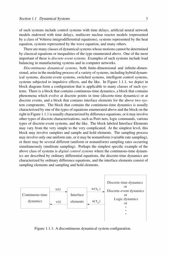
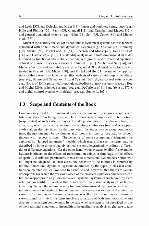
Discontinuous dynamical systems, both finite-dimensional and infinite-dimen-sional, arise in the modeling process of a variety of systems, including hybrid dynam-ical systems, discrete-event systems, switched systems, intelligent control systems,systems subjected to impulsive effects, and the like. In Figure 1.1.1, we depict inblock diagram form a configuration that is applicable to many classes of such sys-tems. There is a block that contains continuous-time dynamics, a block that containsphenomena which evolve at discrete points in time (discrete-time dynamics) or atdiscrete events, and a block that contains interface elements for the above two sys-tem components. The block that contains the continuous-time dynamics is usuallycharacterized by one of the types of equations enumerated above and the block on theright in Figure 1.1.1 is usually characterized by difference equations, or it may involveother types of discrete characterizations, such as Petri nets, logic commands, varioustypes of discrete-event systems, and the like. The block labeled Interface Elementsmay vary from the very simple to the very complicated. At the simplest level, thisblock may involve samplers and sample and hold elements. The sampling processmay involve only one uniform rate, or it may be nonuniform (variable rate sampling),or there may be several different (uniform or nonuniform) sampling rates occurringsimultaneously (multirate sampling). Perhaps the simplest specific example of theabove class of systems is digital control systems where the continuous-time dynam-ics are described by ordinary differential equations, the discrete-time dynamics arecharacterized by ordinary difference equations, and the interface elements consist ofsampling elements and sampling and hold elements.
Continuous-time
dynamics
Interface
elements
Discrete-event dynamics
Discrete-time dynamicsor
orLogic dynamics
or
. . .
v(t)
x(t) w( )τk
u( )τ k
Figure 1.1.1: A discontinuous dynamical system configuration.
4 Chapter 1. Introduction
1.2 A Brief Perspective on the Development ofStability Theory
In his famous doctoral dissertation, Aleksandr Mikhailovich Lyapunov [45] devel-oped the stability theory of dynamical systems determined by nonlinear time-varyingordinary differential equations. In doing so, he formulated his concepts of stabilityand instability and he developed two general methods for the stability analysis ofan equilibrium: Lyapunov’s Direct Method, also called The Second Method of Lya-punov, and The Indirect Method of Lyapunov, also called The First Method. Theformer involves the existence of scalar-valued auxiliary functions of the state space(called Lyapunov functions) to ascertain the stability properties of an equilibrium,whereas the latter seeks to deduce the stability properties of an equilibrium of a sys-tem described by a nonlinear differential equation from the stability properties of itslinearization. In the process of discovering The First Method, Lyapunov establishedsome important stability results for linear systems (involving the Lyapunov MatrixEquation). These results are equivalent to the independently discovered results byRouth (five years earlier) and Hurwitz (three years later).
Lyapunov did not use the concept of uniformity in his definitions of stabilityand asymptotic stability. Because his asymptotic stability theorem yields actuallymore than he was aware of (namely, uniform asymptotic stability) he was unable toestablish necessary conditions (called Converse Theorems in the literature) for theSecond Method. Once the issue of uniformity was settled by Malkin [46], progresson establishing Converse Theorems was made rapidly (Massera [47], [48]).
In the proofs of the various Converse Theorems, the Lyapunov functions are con-structed in terms of the system solutions, and as such, these results can in generalnot be used to generate Lyapunov functions; they are, however, indispensable in es-tablishing all kinds of general results. Thus, the principal disadvantage of the DirectMethod is that there are no general rules for determining Lyapunov functions. In anattempt to overcome these difficulties, results which now comprise the comparisontheory were discovered. In this approach, the stability properties of a given (com-plicated) system under study are deduced from the properties of a corresponding(simpler) system, called the comparison system. The system under study is relatedto the comparison system by means of a stability preserving mapping, which maybe viewed as a generalization of the concept of the Lyapunov function. Some of theearliest comparison results are due to Muller [60] and Kamke [33], followed by thesubsequent work reported in Wazewski [73], Matrosov [49], Bellman [8], Bailey [4],Lakshmikantham and Leela [37], Michel and Miller [53], Siljak [66], Grujic et al.[18], and others. In Michel et al. [57], a comparison theory for general dynamicalsystems is developed, using stability preserving mappings.
Of major importance in the further development of the Direct Method were resultsfor autonomous dynamical systems determined by ordinary differential equations, dueto Barbashin and Krasovskii [6] and LaSalle [38], [39], comprising the InvarianceTheory. Among other issues, these results provide an effective means of estimating thedomain of attraction of an asymptotically stable equilibrium, and more importantly,
Section 1.2 A Brief Perspective on the Development of Stability Theory 5
in the case of asymptotic stability, they require that the time derivative of a Lyapunovfunction along the motions of the system only be negative semidefinite, rather thannegative definite.
One of the first important applications of the Direct Method was in the stabilityanalysis of a class of nonlinear feedback control systems (regulator systems consistingof a linear part (described by linear, time-invariant ordinary differential equations) anda nonlinearity that is required to satisfy certain sector conditions). The formulation ofthis important class of systems constitutes the so called absolute stability problem. Itwas first posed and solved by Lure and Postnikov [44] who used a Lyapunov functionconsisting of a quadratic term in the states plus an integral term involving the systemnonlinearity. An entirely different approach to the problem of absolute stability wasdeveloped by Popov [64]. His results are in terms of the frequency response of thelinear part of the system and the sector conditions of the nonlinearity. Subsequently,Yacubovich [74] and Kalman [32] established a connection between the Lure typeof results and the Popov type of results. A fairly complete account of the resultsconcerning absolute stability is provided in the books by Aizerman and Gantmacher[1], Lefschetz [42], and Narendra and Taylor [61].
As mentioned earlier, there are many areas of applications of the Lyapunov stabilitytheory, and to touch upon even a small fraction of these would be futile. However,we would like to point to a few of them, including applications to large-scale systems(see, e.g., Matrosov [49], Bailey [4], Michel and Miller [53], Siljak [66], and Grujicet al. [18]), robustness issues in stabilization of control systems (see, e.g., Zames [79],Michel and Wang [56], Wang and Michel [70], [71], Wang et al. [72], and Ye et al.[77]), adaptive control (see, e.g., Ioannou and Sun [31] and Åstrom and Wittenmark[3]), power systems (see, e.g., Pai [62]), and artificial neural networks (see, e.g.,Michel and Liu [52]).
The results discussed thus far, pertaining to continuous finite-dimensional dynam-ical systems, are presented in numerous texts and monographs, including Hahn [20],LaSalle and Lefschetz [41], Krasovskii [35], Yoshizawa [78], Hale [23], Vidyasagar[68], Miller and Michel [59], and Khalil [34].
Lyapunov’s stability theory for continuous finite-dimensional dynamical systemshas been extended and generalized in every which way. Thus, the theory describedabove has been fully developed for discrete-time finite-dimensional dynamical sys-tems determined by ordinary difference equations as well (see, e.g., LaSalle [40],Franklin and Powell [15], and Antsaklis and Michel [2]). The stability of infinite-dimensional dynamical systems determined by differential-difference equations areaddressed, for example, in Bellman and Cooke [9], Halanay [22], and Hahn [21];for functional differential equations they are treated, for example, in Krasovskii [35],Yoshizawa [78], and Hale [24]; for Volterra integrodifferential equations they aredeveloped, for example, in Barbu and Grossman [7], Miller [58], Walter [69], Hale[25], and Lakshmikantham and Leela [37]; and for partial differential equations theyare considered, for example, in Friedman [16], Hormander [27], [28], and Garabedian[17]. In a more general approach, the stability analysis of infinite-dimensional dynam-ical systems is accomplished in the context of analyzing systems determined by differ-ential equations and inclusions on Banach space (e.g., Krein [36], Lakshmikantham
6 Chapter 1. Introduction
and Leela [37], and Daleckii and Krein [13]); linear and nonlinear semigroups (e.g.,Hille and Phillips [26], Pazy [63], Crandall [11], and Crandall and Liggett [12]);and general dynamical systems (e.g., Hahn [21], Sell [65], Zubov [80], and Michelet al. [57]).
Much of the stability analysis of discontinuous dynamical systems has thus far beenconcerned with finite-dimensional dynamical systems (e.g., Ye et al. [75], Branicky[10], Michel [50], Michel and Hu [51], Liberzon and Morse [43], DeCarlo et al.[14], and Haddad et al. [19]). The stability analysis of infinite-dimensional DDS de-termined by functional differential equations, semigroups, and differential equationsdefined on Banach spaces is addressed in Sun et al. [67], Michel and Sun [54], andMichel et al. [55] and the stability analysis of general DDS defined on metric space istreated in Ye et al. [75], Michel [50], and Michel and Hu [51]. Some of the applica-tions of these results include the stability analysis of systems with impulsive effects(see, e.g., Bainov and Simeonov [5], and Ye et al. [76]), digital control systems (see,e.g., Hou et al. [30]), pulse-width-modulated feedback control systems (see, e.g., Houand Michel [29]), switched systems (see, e.g., DeCarlo et al. [14] and Ye et al. [75]),and digital control systems with delays (see, e.g., Sun et al. [67]).
1.3 Scope and Contents of the Book
Contemporary models of dynamical systems encountered by engineers and scien-tists may vary from being very simple to being very complicated. The motions(resp., states) of such systems may evolve along continuous time, discrete time, ora mixture, where parts of the motion evolve along continuous time and other partsevolve along discrete time. In the case when the states evolve along continuoustime, the motions may be continuous at all points in time, or they may be discon-tinuous with respect to time. The behavior of some systems may adequately becaptured by “lumped parameter” models, which means that such systems may bedescribed by finite-dimensional dynamical systems determined by ordinary differen-tial or difference equations. On the other hand, when systems exhibit, for example,hysteresis effects, or the effects of transportation delays or time lags, or the effectsof spatially distributed parameters, then a finite-dimensional system description willno longer be adequate. In such cases, the behavior of the motions is captured byinfinite-dimensional dynamical systems determined by the types of classical equa-tions enumerated earlier. We need to hasten to add, however, that there are systemdescriptions for which the various classes of the classical equations enumerated ear-lier are inappropriate (e.g., discrete-event systems, systems characterized by Petrinets, and so forth). It is clear that a successful qualitative analysis of such sys-tems may frequently require results for finite-dimensional systems as well as forinfinite-dimensional systems; for continuous-time systems as well as for discrete-timesystems; for continuous dynamical systems as well as for discontinuous dynamicalsystems; and for (hybrid) systems involving a mixture of both continuous-time anddiscrete-time system components. In the case when a system is not described by oneof the traditional equations or inequalities, the qualitative analysis might have to take
Section 1.3 Scope and Contents of the Book 7
place, for example, in the setting of an abstract metric space, rather than a vectorspace.
Presently, there are no books on stability theory that are suitable to serve as a singlesource for the analysis of some of the system models enumerated above. Most of theengineering texts on stability theory are concerned with finite-dimensional continuousdynamical systems described by ordinary differential equations. The stability theoryof finite-dimensional discrete-time dynamical systems described by difference equa-tions is frequently addressed only briefly in books on sampled-data control systems, oras analogous afterthoughts in stability books dealing primarily with systems describedby ordinary differential equations. As we have seen earlier, texts and monographs onthe stability theory of infinite-dimensional dynamical systems usually focus on spe-cific classes of systems (determined, e.g., by functional differential equations, partialdifferential equations, etc.). Finally, as noted previously, the literature concerningthe stability of discontinuous dynamical systems is scattered throughout journal pub-lications and conference proceedings. As a consequence, to become proficient in thestability analysis of contemporary dynamical systems of the type described abovemay require considerable investment of time. Therefore, there seems to be need fora book on stability theory that addresses continuous-time as well as discrete-timesystems; continuous as well as discontinuous systems; finite-dimensional as well asinfinite-dimensional systems; and systems involving descriptions by classical equa-tions and inequalities as well as systems that cannot be described by such equationsand inequalities. We aim to fill this void in the present book.
Finally, in addition to the objectives and goals stated above, we believe that thepresent book will serve as a guide to enable the reader to pursue study of further topicsin greater depth, as needed.
Chapter ContentsThe remainder of this book is organized in eight chapters.
In Chapter 2 we introduce the concept of a dynamical system defined on a metricspace (more formally than was done earlier), we give a classification of dynamicalsystems, and we present several important specific classes of finite- and infinite-dimensional dynamical systems determined by the various classical differential equa-tions encountered in science and engineering. In a subsequent chapter (Chapter 5),we also present examples of dynamical systems that cannot be described by suchequations.
The classes of dynamical systems that we consider include continuous-time anddiscrete-time finite-dimensional dynamical systems determined by ordinary differ-ential equations and inequalities and ordinary difference equations and inequalities,respectively, and by infinite-dimensional dynamical systems described by differential-difference equations, functional differential equations, Volterra integrodifferentialequations, certain classes of partial differential equations, and more generally, differ-ential equations and inclusions defined on Banach spaces, and by linear and nonlinearsemigroups. For the cases of continuous-time systems, in addition to continuous sys-tems, we consider discontinuous dynamical systems as well.
8 Chapter 1. Introduction
In addition to the above, we also introduce the notion of a composite dynamicalsystem, consisting of a mixture of different equations (defined for the same time setT ). Also, in a subsequent chapter (Chapter 8) we consider a specific class of hybriddynamical systems consisting of a mixture of equations defined on different time sets.
In Chapter 3 we establish the Principal Lyapunov Stability and Boundedness Re-sults, including Converse Theorems, for dynamical systems defined on metric spaces.By considering the most general setting first (dynamical systems defined on metricspaces), we are able to utilize some of the results of the present chapter in establish-ing in an efficient manner corresponding results presented in subsequent chapters forimportant classes of finite- and infinite-dimensional dynamical systems.
We first introduce the notions of an invariant set (resp., equilibrium) with respect tothe motions of a dynamical system and we give the definitions of the various conceptsof Lyapunov and Lagrange stability (including stability, uniform stability, local andglobal asymptotic stability, local and global uniform asymptotic stability, local andglobal exponential stability, instability, complete instability, uniform boundedness,and uniform ultimate boundedness).
Next, we establish the Principal Lyapunov and Lagrange Stability Results (suf-ficient conditions for the above stability, instability, and boundedness concepts) fordiscontinuous dynamical systems, continuous dynamical systems, and discrete-timedynamical systems, respectively. Because continuous dynamical systems constitutespecial cases of DDS, the stability, instability, and boundedness results for DDS areapplicable to continuous dynamical systems as well. To prove the various PrincipalLyapunov and Lagrange stability results for continuous dynamical systems, we showthat when the hypotheses of any one of these results are satisfied, then the hypothesesof the corresponding DDS results are also satisfied; that is, the classical Lyapunovand Lagrange stability results for continuous dynamical systems reduce to the cor-responding Lyapunov and Lagrange stability results that we established for DDS.This shows that the DDS results are more general than the corresponding classicalLyapunov and Lagrange stability results for continuous dynamical systems. Indeed,a specific example is presented of a continuous dynamical system with an equilibriumthat can be shown to be uniformly asymptotically stable, using the uniform asymp-totic stability result for DDS, and we prove that for the same example, there does notexist a Lyapunov function that satisfies the classical Lyapunov theorem for uniformasymptotic stability for continuous dynamical systems.
Next, we show that for every discrete-time dynamical system there exists an asso-ciated DDS with identical Lyapunov and Lagrange stability properties. Making use ofsuch associated DDS, we prove, similarly as in the case of continuous dynamical sys-tems, that the Lyapunov and Lagrange stability results for DDS are more general thanthe corresponding results for the classical Lyapunov and Lagrange stability results fordiscrete-time dynamical systems. We give an example of a discrete-time dynamicalsystem with an equilibrium that can be shown to be uniformly asymptotically stable,by applying the uniform asymptotic stability result for DDS to the associated DDS,and we prove that for the same original discrete-time dynamical system there doesnot exist a Lyapunov function that satisfies the classical uniform asymptotic stabilitytheorem for discrete-time dynamical systems.
Section 1.3 Scope and Contents of the Book 9
In addition to proving that the classical Lyapunov and Lagrange stability resultsfor continuous dynamical systems and discrete-time dynamical systems reduce tothe corresponding DDS results, our approach described above establishes also a uni-fying theory for DDS, continuous dynamical systems, and discrete-time dynamicalsystems.
Next, under some additional mild conditions, we establish Converse Theorems(necessary conditions) for the above results for DDS, continuous dynamical systems,and discrete-time dynamical systems.
Finally, in an appendix section we present a comparison result involving maximaland minimal solutions of ordinary differential equations, which is required in someof the proofs of this chapter.
In Chapter 4 we present important specialized Lyapunov and Lagrange stabilityresults for dynamical systems defined on metric spaces. We first show that under somereasonable assumptions, in the case of autonomous dynamical systems, stability andasymptotic stability of an invariant set imply uniform stability and uniform asymp-totic stability of an invariant set, respectively. Furthermore, we establish necessaryand sufficient conditions for stability and asymptotic stability of an invariant set forautonomous dynamical systems. Next, for continuous and discrete-time autonomousdynamical systems, we present generalizations of LaSalle-type theorems that com-prise the invariance theory for dynamical systems defined by semigroups in metricspaces. Also, for both continuous and discrete-time dynamical systems we presentseveral results that make up a comparison theory for various Lyapunov and Lagrangestability types. In these results we deduce the qualitative properties of a complex dy-namical system (the object of inquiry) from corresponding qualitative properties of asimpler and well-understood dynamical system (the comparison system). Finally, wepresent Lyapunov-like results that ensure the uniqueness of motions for continuousand discrete-time dynamical systems defined on metric spaces.
In Chapter 5 we apply the results of Chapters 3 and 4 in the stability analysis ofan important class of discrete-event systems with applications to a computer load-balancing problem and a manufacturing system.
In the preceding three chapters, we concern ourselves with the qualitative anal-ysis of dynamical systems defined on metric spaces. In the next three chapters weaddress the Lyapunov and Lagrange stability of continuous-time and discrete-timefinite-dimensional dynamical systems determined by ordinary differential equationsand difference equations, respectively. For the case of continuous-time dynamicalsystems we consider continuous dynamical systems and discontinuous dynamicalsystems. In these three chapters our focus is on the qualitative analysis of equilibria(rather than general invariant sets). Throughout the next three chapters, we includenumerous specific examples to demonstrate the applicability of the various resultsthat are presented.
In Chapter 6 we first present some preliminary material that is required through-out the next three chapters, including material on ordinary differential equations andordinary difference equations; definition of the time-derivative of Lyapunov func-tions evaluated along the solutions of ordinary differential equations; evaluation ofthe first forward difference of Lyapunov functions along the solutions of difference
10 Chapter 1. Introduction
equations; characterizations of Lyapunov functions, including quadratic forms; anda motivation and geometric interpretation for Lyapunov stability results for two-dimensional systems. Next, we present the Principal Lyapunov and Lagrange Stabil-ity Results (sufficient conditions) for continuous dynamical systems determined byordinary differential equations; for discrete-time dynamical systems determined bydifference equations; and for DDS determined by ordinary differential equations. Inmost cases, the proofs of these results are direct consequences of corresponding resultsthat were presented in Chapter 3. Finally, we present converse theorems (necessaryconditions) for the above Lyapunov and Lagrange stability results. In an appendixsection we give some results concerning the continuous dependence of solutions ofordinary differential equations with respect to initial conditions.
In Chapter 7 we continue our study of finite-dimensional dynamical systems withthe presentation of some important specialized results for continuous and discrete-time systems. We first show that if for dynamical systems determined by autonomousand periodic ordinary differential equations, the equilibrium xe = 0 is stable orasymptotically stable, then the equilibrium xe = 0 is uniformly stable or uniformlyasymptotically stable, respectively. Also, for such kind of dynamical systems, wepresent converse theorems for asymptotically stable systems. Next, for continuousand discrete-time dynamical systems determined by autonomous ordinary differen-tial equations and ordinary difference equations, we establish LaSalle-type stabilityresults that comprise the invariance theory for such systems. These results are directconsequences of corresponding results that were established in Chapter 3 for au-tonomous dynamical systems defined on metric spaces. For autonomous dynamicalsystems determined by ordinary differential equations, we next present two meth-ods of determining estimates for the domain of attraction of an asymptotically stableequilibrium (including Zubov’s Theorem). Next, we present the main Lyapunovstability and boundedness results for dynamical systems determined by linear homo-geneous systems of ordinary differential equations (and difference equations), linearautonomous homogeneous ordinary differential equations (and difference equations),and linear periodic ordinary differential equations. Some of these results require ex-plicit knowledge of state transition matrices whereas other results involve Lyapunovmatrix equations. This is followed by a detailed study of the stability properties ofthe equilibrium xe = 0 of dynamical systems determined by linear, second-orderautonomous homogeneous systems of ordinary differential equations. Next, we in-vestigate the qualitative properties of perturbed linear systems. In doing so, wedevelop Lyapunov’s First Method (also called Lyapunov’s Indirect Method) for con-tinuous and discrete-time dynamical systems, and we study the existence of stableand unstable manifolds and the stability of periodic motions in continuous linearperturbed systems. Finally, similarly as in Chapter 4, we establish Lyapunov andLagrange stability results for continuous and discrete-time dynamical systems thatcomprise a comparison theory for finite-dimensional dynamical systems.
In Chapter 8 we apply the results presented in Chapters 6 and 7 in the analysisof several important classes of continuous, discontinuous, and discrete-time finite-dimensional dynamical systems. We first address the absolute stability problem ofnonlinear regulator systems, by presenting Lure’s result for direct control systems
Section 1.3 Scope and Contents of the Book 11
and Popov’s result for indirect control systems. Next, we establish global and localLyapunov stability results for Hopfield neural networks. This is followed by aninvestigation of an important class of hybrid systems, digital control systems. Weconsider system models with quantizers and without quantizers. Next, we presentstability results for an important class of pulse-width-modulated (PWM) feedbackcontrol systems. Finally, we study the stability properties of systems with saturationnonlinearities with applications to digital filters.
In Chapter 9 we address the Lyapunov and Lagrange stability of infinite-dimen-sional dynamical systems determined by differential equations defined on Banachspaces and semigroups. As in Chapters 6 through 8, we focus on the qualitative prop-erties of equilibria and we consider continuous as well as discontinuous dynamicalsystems. Throughout this chapter, we present several specific examples to demon-strate the applicability of the presented results. These include systems determinedby functional differential equations, Volterra integrodifferential equations, and par-tial differential equations. In addition, we apply the results of this chapter in theanalysis of two important classes of infinite-dimensional dynamical systems: a pointkinetics model of a multicore nuclear reactor (described by Volterra integrodifferen-tial equations) and Cohen–Grossberg neural networks with time delays (describedby differential-difference equations). As in Chapters 6 and 7, several of the resultspresented in this chapter are direct consequences of the results given in Chapters 3and 4 for dynamical systems defined on metric spaces.
We first present the Principal Lyapunov and Lagrange Stability Results (suffi-cient conditions) for dynamical systems determined by general differential equationsdefined on Banach spaces. Most of these results are direct consequences of the cor-responding results established in Chapter 3 for dynamical systems defined on metricspaces. We also present converse theorems (necessary conditions) for several of theabove results. Most of these are also direct consequences of corresponding resultsgiven in Chapter 3 for dynamical systems defined on metric spaces. Next, we presentLaSalle-type stability results that comprise the invariance theory for autonomousdifferential equations defined on Banach spaces. Essentially, these results are alsodirect consequences of corresponding results that are established in Chapter 4 fordynamical systems defined on metric spaces. This is followed by the presentationof several Lyapunov and Lagrange stability results that comprise a comparison the-ory for general differential equations defined on Banach spaces. Next, we presentstability results for composite dynamical systems defined on Banach spaces that aredescribed by a mixture of different types of differential equations. As mentionedearlier, we apply some of the results enumerated above in the analysis of a point ki-netics model of a multicore nuclear reactor (described by Volterra integrodifferentialequations). For the special case of functional differential equations, it is possible toimprove on the Lyapunov stability results for general differential equations definedon Banach spaces by taking into account some of the specific properties of functionaldifferential equations. We present improved Lyapunov stability results for dynami-cal systems determined by retarded functional differential equations. Some of theseresults include Razumikhin-type theorems. As pointed out earlier, we apply these re-sults in the qualitative analysis of a class of artificial neural networks with time delays
12 Chapter 1. Introduction
(described by differential-difference equations). Next, we establish Lyapunov andLagrange stability results for discontinuous dynamical systems defined on Banachand Hilbert spaces. We consider DDS determined by differential equations definedon Banach spaces, and by DDS determined by linear and nonlinear semigroups.
Bibliography
[1] M. A. Aizerman and F. R. Gantmacher, Absolute Stability of Regulator Systems,San Francisco: Holden-Day, 1964.
[2] P. J. Antsaklis and A. N. Michel, Linear Systems, Boston: Birkhauser, 2006.
[3] K. J. Astrom and B. Wittenmark, Adaptive Control, 2nd Edition, New York:Addison-Wesley, 1995.
[4] F. N. Bailey, “The application of Lyapunov’s Second Method to interconnectedsystems,” SIAM J. Control, vol. 3, pp. 443–462, 1966.
[5] D. D. Bainov and P. S. Simeonov, Systems with Impulse Effects: Stability Theoryand Applications, New York: Halsted, 1989.
[6] A. E. Barbashin and N. N. Krasovskii, “On the stability of motion in the large,”Dokl. Akad. Nauk., vol. 86, pp. 453-456, 1952.
[7] V. Barbu and S. I. Grossman, “Asymptotic behavior of linear integrodifferentialsystems,” Trans. Amer. Math. Soc., vol. 171, pp. 277–288, 1972.
[8] R. Bellman, “Vector Lyapunov functions,” SIAM J. Control, vol. 1, pp. 32–34,1962.
[9] R. Bellman and K. L. Cooke, Differential-Difference Equations, New York:Academic Press, 1963.
[10] M. S. Branicky, “Multiple Lyapunov functions and other analysis tools forswitched and hybrid systems,” IEEE Trans. Autom. Control, vol. 43, pp. 475–482, 1998.
[11] M. G. Crandall, “Semigroups of nonlinear transformations on general Banachspaces,” Contributions to Nonlinear Functional Analysis, E. H. Zarantonello,Ed., New York: Academic Press, 1971.
[12] M. G. Crandall and T. M. Liggett, “Generation of semigroups of nonlinear trans-formations on general Banach spaces,” Amer. J. Math., vol. 93, pp. 265–298,1971.
[13] J. L. Daleckii and S. G. Krein, Stability of Solutions of Differential Equations inBanach Spaces, Translations of Mathematical Monographs, vol. 43, Providence,RI: American Mathematical Society, 1974.
[14] R. DeCarlo, M. Branicky, S. Pettersson, and B. Lennartson, “Perspectives andresults on the stability and stabilizability of hybrid systems,” Proc. IEEE, vol.88, pp. 1069–1082, 2000.
Bibliography 13
[15] G. F. Franklin and J. D. Powell, Digital Control of Dynamical Systems, Reading,MA: Addison-Wesley, 1980.
[16] A. Friedman, Partial Differential Equations of Parabolic Type, EnglewoodCliffs, NJ: Prentice Hall, 1964.
[17] P. R. Garabedian, Partial Differential Equations, New York: Chelsea, 1986.
[18] L. T. Grujic, A. A. Martynyuk, and M. Ribbens-Pavella, Large Scale SystemsStability Under Structural and Singular Perturbations, Berlin: Springer-Verlag,1987.
[19] W. M. Haddad, V. S. Chellaboina, and S. G. Nersesov, Impulsive and Hybrid Dy-namical Systems: Stability, Dissipativity and Control, Princeton, NJ: PrincetonUniversity Press, 2006.
[20] W. Hahn, Theorie und Anwendung der direkten Methode von Ljapunov, Heidel-berg: Springer-Verlag, 1959.
[21] W. Hahn, Stability of Motion, Berlin: Springer-Verlag, 1967.
[22] A. Halanay, Differential Equations: Stability, Oscillations, Time Lags, NewYork: Academic Press, 1966.
[23] J. K. Hale, Ordinary Differential Equations, New York: Wiley-Interscience,1969.
[24] J. K. Hale, Functional Differential Equations, Berlin: Springer-Verlag, 1971.
[25] J. K. Hale, “Functional differential equations with infinite delays,” J. Math.Anal. Appl., vol. 48, pp. 276–283, 1974.
[26] E. Hille and R. S. Phillips, Functional Analysis and Semigroups, Amer. Math.Soc. Colloquium Publ. vol. 33, Providence, RI:American Mathematical Society,1957.
[27] L. Hormander, Linear Partial Differential Equations, Berlin: Springer-Verlag,1963
[28] L. Hormander, The Analysis of Linear Partial Differential Operators, vol. 1, 2,3, 4, Berlin: Springer-Verlag, 1983–1985.
[29] L. Hou andA. N. Michel, “Stability analysis of pulse-width-modulated feedbacksystems,” Automatica, vol. 37, pp. 1335–1349, 2001.
[30] L. Hou, A. N. Michel, and H. Ye, “Some qualitative properties of sampled-datacontrol systems,” IEEE Trans. Autom. Control, vol. 42, pp. 1721–1725, 1997.
[31] P. A. Ioannou and J. Sun, Robust Adaptive Control, Upper Saddle River, NJ:Prentice Hall, 1996.
[32] R. E. Kalman, “Lyapunov functions for the problem of Lure in automatic con-trol,” Proc. Nat. Acad. Sci. USA, vol. 49, pp. 201–205, 1963.
[33] E. Kamke, “Zur Theorie der Systeme gewohnlicher Differentialgleichungen,II,” Acta Math., vol. 58, pp. 57–85, 1932.
[34] H. K. Khalil, Nonlinear Systems, New York: Macmillan, 1992.
14 Chapter 1. Introduction
[35] N. N. Krasovskii, Stability of Motion, Stanford, CA: Stanford University Press,1963.
[36] S. G. Krein, Linear Differential Equations in Banach Spaces, Translation ofMathematical Monographs, vol. 29, Providence, RI: American MathematicalSociety, 1970.
[37] V. Lakshmikantham and S. Leela, Differential and Integral Inequalities, vol. 1and 2, New York: Academic Press, 1969.
[38] J. P. LaSalle, “The extent of asymptotic stability,” Proc. Nat. Acad. Sci., vol.48, pp. 363–365, 1960.
[39] J. P. LaSalle, “Some extensions of Liapunov’s Second Method,” IRE Trans.Circ. Theor., vol. 7, pp. 520–527, 1960.
[40] J. P. LaSalle, The Stability and Control of Discrete Processes, New York:Springer-Verlag, 1986.
[41] J. P. LaSalle and S. Lefschetz, Stability of Lyapunov’s Direct Method, New York:Academic Press, 1961.
[42] S. Lefschetz, Stability of Nonlinear Control Systems, New York: AcademicPress, 1965.
[43] D. Liberzon andA. S. Morse, “Basic problems in stability and design of switchedsystems,” IEEE Control Syst. Mag., vol. 19, pp. 59–70, 1999.
[44] A. I. Lure and V. N. Postnikov, “On the theory of stability of control systems,”Prikl. Mat. i. Mehk., vol. 8, pp. 3–13, 1944.
[45] A. M. Liapounoff, “Probleme generale de la stabilite de mouvement,” Annalesde la Faculte des Sciences de l’Universite de Toulouse, vol. 9, pp. 203–474,1907. (Translation of a paper published in Comm. Soc. Math., Kharkow, 1892,reprinted in Ann. Math. Studies, vol. 17, Princeton, NJ: Princeton, 1949. TheFrench version was translated into English by A. T. Fuller, and was publishedin the International Journal of Control, vol. 55, pp. 531–773, 1992.)
[46] I. G. Malkin, “On the question of reversibility of Lyapunov’s theorem on auto-matic stability,” Prikl. Mat. i Mehk., vol.18, pp. 129–138, 1954 (in Russian).
[47] J. L. Massera, “On Liapunoff’s conditions of stability,” Ann. Mat., vol. 50, pp.705–721, 1949.
[48] J. L. Massera, “Contributions to stability theory,” Ann. Mat., vol. 64, pp. 182–206, 1956.
[49] V. M. Matrosov, “The method of Lyapunov-vector functions in feedback sys-tems,” Automat. Remote Control, vol. 33, pp. 1458–1469, 1972.
[50] A. N. Michel, “Recent trends in the stability analysis of hybrid dynamical sys-tems,” IEEE Trans. Circ. and Syst.–I: Fund. Theor. Appl., vol. 46, pp. 120–134,1999.
[51] A. N. Michel and B. Hu, “Towards a stability theory of general hybrid dynamicalsystems,” Automatica, vol. 35, pp. 371–384, 1999.
Bibliography 15
[52] A. N. Michel and D. Liu, Qualitative Analysis and Synthesis of Recurrent NeuralNetworks, New York: Marcel Dekker, 2002.
[53] A. N. Michel and R. K. Miller, Qualitative Analysis of Large Scale DynamicalSystems, New York: Academic Press, 1977.
[54] A. N. Michel andY. Sun, “Stability of discontinuous Cauchy problems in Banachspace,” Nonlinear Anal., vol. 65, pp. 1805–1832, 2006.
[55] A. N. Michel, Y. Sun, and A. P. Molchanov, “Stability analysis of discontinuousdynamical systems determined by semigroups,” IEEE Trans. Autom. Control,vol. 50, pp. 1277–1290, 2005.
[56] A. N. Michel and K. Wang, “Robust stability: perturbed systems with perturbedequilibria,” Syst. and Control Lett., vol. 21, pp.155–162, 1993.
[57] A. N. Michel, K. Wang, and B. Hu, Qualitative Theory of Dynamical Systems:The Role of Stability Preserving Mappings, 2nd Edition, New York: MarcelDekker, 2001.
[58] R. K. Miller, Nonlinear Volterra Integral Equations, Menlo Park, CA: W. A.Benjamin, 1971.
[59] R. K. Miller and A. N. Michel, Ordinary Differential Equations, New York:Academic Press, 1982.
[60] M. Muller, “Uber das Fundamentaltheorem in der Theorie der gewohnlichenDifferentialgleichungen,” Mat. Zeit., vol. 26, pp. 615–645, 1926.
[61] K. S. Narendra and J. H. Taylor, Frequency Domain Stability for Absolute Sta-bility, New York: Academic Press, 1973.
[62] M. A. Pai, Power System Stability, New York: North-Holland, 1981.
[63] A. Pazy, Semigroups of Linear Operators and Applications to Partial Differen-tial Equations, New York: Springer-Verlag, 1983.
[64] V. M. Popov, “Absolute stability of nonlinear systems of automatic control,”Automation Remote Control, vol. 22, pp. 857–875, 1961.
[65] G. R. Sell, Lectures on Topological Dynamics and Differential Equations,Princeton, NJ: Van Nostrand, 1969.
[66] D. D. Siljak, Large-Scale Dynamical Systems: Stability and Structure, NewYork: North Holland, 1978.
[67] Y. Sun,A. N. Michel, and G. Zhai, “Stability of discontinuous retarded functionaldifferential equations with applications,” IEEE Trans. Autom. Control, vol. 50,pp. 1090–1105, 2005.
[68] M. Vidyasagar, Nonlinear Systems Analysis, 2nd Edition, Englewood Cliffs, NJ:Prentice Hall, 1993.
[69] W. Walter, Differential and Integral Inequalities, Berlin: Springer-Verlag, 1970.
[70] K. Wang and A. N. Michel, “On sufficient conditions for stability of intervalmatrices,” Syst. Control Lett., vol. 20, pp. 345–351, 1993.
16 Chapter 1. Introduction
[71] K. Wang and A. N. Michel, “Qualitative analysis of dynamical systems deter-mined by differential inequalities with applications to robust stability,” IEEETrans. Circ. Syst.–I: Fund. Theor. Appl., vol. 41, pp. 377–386, 1994.
[72] K. Wang, A. N. Michel, and D. Liu, “Necessary and sufficient conditions for theHurwitz and Schur stability of interval matrices,” IEEE Trans. Autom. Control,vol. 39, pp. 1251–1255, 1996.
[73] T. Wazewski, “Systemes des equations et des inegalites differentielles ordinairesaux deuxiemes membres monotones et leurs applications,” Ann. Soc. Poln. Mat.,vol. 23, pp. 112–166, 1950.
[74] V.A.Yacubovich, “Solution of certain matrix inequalities occurring in the theoryof automatic control,” Dokl. Acad. Nauk. SSSR, pp. 1304–1307, 1962.
[75] H. Ye, A. N. Michel, and L. Hou, “Stability theory for hybrid dynamical sys-tems,” IEEE Trans. Autom. Control, vol. 43, pp. 461–474, 1998.
[76] H. Ye, A. N. Michel, and L. Hou, “Stability analysis of systems with impulseeffects,” IEEE Trans. Autom. Control, vol. 43, pp. 1719–1923, 1998.
[77] H. Ye, A. N. Michel, and K. Wang, “Robust stability of nonlinear time-delaysystems with applications to neural networks,” IEEE Trans. Circ. Syst.–I: Fund.Theor. Appl., vol. 43, pp. 532–543, 1996.
[78] T. Yoshizawa, Stability Theory by Lyapunov’s Second Method, Tokyo: Math.Soc. Japan, 1966.
[79] G. Zames, “Input-output feedback stability and robustness, 1959–85,” IEEEControl Syst. Mag., vol. 16, pp. 61–66, 1996.
[80] V. I. Zubov, Methods of A. M. Lyapunov and Their Applications, Groningen,The Netherlands: P. Noordhoff, 1964.
Chapter 2
Dynamical Systems
Our main objective in the present chapter is to define a dynamical system and topresent several important classes of dynamical systems. The chapter is organizedinto twelve parts.
In the first section we establish some of the notation that we require in this chap-ter, as well as in the subsequent chapters. Next, in the second section we presentprecise definitions for dynamical system and related concepts. We introduce finite-dimensional dynamical systems determined by ordinary differential equations in thethird section, by differential inequalities in the fourth section, and by ordinary differ-ence equations and inequalities in the fifth section. In the sixth section, we addressinfinite-dimensional dynamical systems determined by differential equations and in-clusions defined on Banach spaces and in the seventh and eighth sections we considerspecial cases of infinite-dimensional dynamical systems determined by functionaldifferential equations and Volterra integrodifferential equations, respectively. In theninth section we discuss dynamical systems determined by semigroups defined onBanach and Hilbert spaces and in the tenth section we treat dynamical systems de-termined by specific classes of partial differential equations. Finally, we addresscomposite dynamical systems in the eleventh section and discontinuous dynamicalsystems in the twelfth section.
The specific classes of dynamical systems that we consider in this chapter are veryimportant. However, there are of course many more important classes of dynamicalsystems, not even alluded to in the present chapter. We address one such class ofsystems in Chapter 5, determined by discrete-event systems.
Much of the material presented in Sections 2.3–2.10 constitutes background ma-terial and concerns the well posedness (existence, uniqueness, continuation, and con-tinuity with respect to initial conditions of solutions) of a great variety of equations(resp., systems). Even if practical, it still would distract from our objectives on handif we were to present proofs for these results. Instead, we give detailed referenceswhere to find such proofs, and in some cases, we give hints (in the problem section)
17
18 Chapter 2. Dynamical Systems
on how to prove some of these results. The above is in contrast with our presentationsin the remainder of this book where we prove all results (except some, concerningadditional background material).
2.1 Notation
Let Y, Z be arbitrary sets. Then Y ∪ Z, Y ∩ Z, Y − Z, and Y × Z denote the union,intersection, difference, and Cartesian product of Y and Z, respectively. If Y is asubset of Z, we write Y ⊂ Z and if x is an element of Y , we write x ∈ Y . We denotea mapping f of Y into Z by f : Y → Z and we denote the set of all mappings fromY into Z by Y → Z. Let ∅ denote the empty set.
Let R denote the set of real numbers, let R+ = [0,∞), let N denote the set of
nonnegative integers (i.e., N = 0, 1, 2, . . . ), and let C denote the set of complexnumbers. Let J ⊂ R denote an interval (i.e., J = [a, b), (a, b], [a, b], or (a, b), b > a,with J = (−∞,∞) = R allowed). If Y1, . . . , Yn are n arbitrary sets, their Cartesianproduct is denoted by Y1 × · · · × Yn, and if in particular Y = Y1 = · · · = Yn wewrite Y n.
Let Rn denote real n-space. If x ∈ R
n, xT = (x1, . . . , xn) denotes the transposeof x. Also, if x, y ∈ R
n, then x ≤ y signifies xi ≤ yi, x < y signifies xi < yi, andx > 0 signifies xi > 0 for all i = 1, . . . , n. We let | · | denote the Euclidean norm;
that is, for x = (x1, . . . , xn)T ∈ Rn, |x| = (xT x)1/2 =
(∑ni=1 x2
i
)1/2.
Let A = [aij ]n×n denote a real n × n matrix (i.e., A ∈ Rn×n) and let AT denote
the transpose of A. The matrix norm | · |, induced by the Euclidean vector norm(defined on R
n), is defined by
|A| = infα ∈ R
+ : α|x| ≥ |Ax|, x ∈ Rn
=[λM (AT A)
]1/2
where λM (AT A) denotes the largest eigenvalue of AT A (recall that the eigenvaluesof symmetric matrices are real). In the interests of clarity, we also use the notation ‖·‖to distinguish the norm of a matrix (e.g., ‖A‖) from the norm of a vector (e.g., |x|).
We let Lp[G, U ], 1 ≤ p ≤ ∞, denote the usual Lebesgue space of all Lebesguemeasurable functions with domain G and range U . The norm in Lp[G, U ] is usuallydenoted ‖ · ‖p, or ‖ · ‖Lp if more explicit notation is required.
We let (X, d) be a metric space, where X denotes the underlying set and d denotesthe metric. When the choice of the particular metric used is clear from context, wespeak of a metric space X , rather than (X, d).
If Y and Z are metric spaces and if f : Y → Z, and if f is continuous, we writef ∈ C[Y, Z]; that is, C[Y, Z] denotes the set of all continuous mappings from Y toZ. We denote the inverse of a mapping f , if it exists, by f−1.
A function ψ ∈ C[[0, r1], R+] (resp., ψ ∈ C[R+, R+]) is said to belong to classK (i.e., ψ ∈ K) if ψ(0) = 0 and if ψ is strictly increasing on [0, r1] (resp., on R
+). Ifψ : R
+ → R+, if ψ ∈ K, and if limr→∞ ψ(r) = ∞, then ψ is said to belong to class
K∞ (i.e., ψ ∈ K∞).
Section 2.2 Dynamical Systems 19
For a function f : R → R, we denote the upper right-hand, upper left-hand, lowerright-hand, and lower left-hand Dini derivatives by D+f, D−f, D+f , and D−f ,respectively. When we have a fixed Dini derivative of f in mind, we simply writeDf , in place of the preceding notation.
2.2 Dynamical Systems
In characterizing the notion of dynamical system, we require the concepts of motionand family of motions.
Definition 2.2.1 Let (X, d) be a metric space, let A ⊂ X , and let T ⊂ R. Forany fixed a ∈ A, t0 ∈ T , a mapping p(·, a, t0) : Ta,t0 → X is called a motion ifp(t0, a, t0) = a where Ta,t0 = [t0, t1) ∩ T , t1 > t0, and t1 is finite or infinite.
Definition 2.2.2 A subset S of the set⋃(a,t0)∈A×T
Ta,t0 → X
is called a family of motions if for every p(·, a, t0) ∈ S, we have p(t0, a, t0) = a.
Definition 2.2.3 The four-tuple T, X, A, S is called a dynamical system.
In Definitions 2.2.1 and 2.2.2 we find it useful to think of X as state space, T astime set, t0 as initial time, a as the initial condition of the motion p(·, a, t0), and A asthe set of initial conditions. Note that in our definition of motion, we allow in generalmore than one motion to initiate from a given pair of initial data, (a, t0).
When in Definition 2.2.3, T = J ⊂ R+ (with J = R
+ allowed), we speak of acontinuous-time dynamical system and when T = J ∩ N (with J ∩ N = N allowed)we speak of a discrete-time dynamical system. Also, when in Definition 2.2.3, X is afinite-dimensional vector space, we speak of a finite-dimensional dynamical system,and otherwise, of an infinite-dimensional dynamical system. Furthermore, if in acontinuous-time dynamical system all motions (i.e., all elements of S) are continuouswith respect to time t, we speak of a continuous dynamical system. If at least onemotion of a continuous-time dynamical system is not continuous with respect to t,we speak of a discontinuous dynamical system.
When in Definition 2.2.3, T, X , and A are known from context, we frequentlyspeak of a dynamical system S, or even of a system S, rather than a dynamical systemT, X, A, S.
Definition 2.2.4 A dynamical system T, X1, A1, S1 is called a dynamical subsys-tem, or simply, a subsystem of a dynamical system T, X, A, S if X1 ⊂ X, A1 ⊂ A,and S1 ⊂ S.
Definition 2.2.5 A motion p = p(·, a, t0) in a dynamical system T, X, A, S is saidto be bounded if there exist an x0 ∈X and a β>0 such that d(p(t, a, t0), x0)<β forall t ∈ Ta,t0 .
20 Chapter 2. Dynamical Systems
Definition 2.2.6 A motion p∗ = p∗(·, a, t0) defined on [t0, c) ∩ T is called a con-tinuation of another motion p = p(·, a, t0) defined on [t0, b) ∩ T if p = p∗ on[t0, b) ∩ T, c > b, and [b, c) ∩ T = ∅. We say that p is noncontinuable if no continu-ation of p exists. Also, p = p(·, a, t0) is said to be continuable forward for all time ifthere exists a continuation p∗ = p∗(·, a, t0) of p that is defined on [t0,∞)∩T , whereit is assumed that for any α > 0, [α,∞) ∩ T = ∅.
In the remainder of this chapter, we present several important classes of dynamicalsystems. Most of this material serves as required background for the remainder ofthis book.
2.3 Ordinary Differential Equations
In this section we summarize some essential facts from the qualitative theory ofordinary differential equations that we require as background material and we showthat the solutions of differential equations determine continuous, finite-dimensionaldynamical systems.
A. Initial value problems
Let D ⊂ Rn+1 be a domain (an open connected set), let x = (x1, . . . , xn)T denote
elements of Rn, and let elements of D be denoted by (t, x). When x is a vector-valued
function of t, let
x =dx
dt=(
dx1
dt, . . . ,
dxn
dt
)T
= (x1, . . . , xn)T .
For a given function fi : D → R, i = 1, . . . , n, let f = (f1, . . . , fn)T . Considersystems of first-order ordinary differential equations given by
xi = fi(t, x1, . . . , xn), i = 1, . . . , n. (Ei)
Equation (Ei) can be written more compactly as
x = f(t, x). (E)
A solution of (E) is an n vector-valued differentiable function ϕ defined on a realinterval J = (a, b) (we express this by f ∈ C1[J, Rn]) such that (t, ϕ(t)) ∈ D forall t ∈ J and such that
ϕ(t) = f(t, ϕ(t))
for all t ∈ J . We also allow the cases when J = [a, b), J = (a, b], or J = [a, b].When J = [a, b], then ϕ(a) is interpreted as the right-side derivative and ϕ(b) isinterpreted as the left-side derivative.
For (t0, x0) ∈ D, the initial value problem associated with (E) is given by
x = f(t, x), x(t0) = x0. (IE)
Section 2.3 Ordinary Differential Equations 21
An n vector-valued function ϕ is a solution of (IE) if ϕ is a solution of (E) whichis defined on [t0, b) and if ϕ(t0) = x0. To denote the dependence of the solutions of(IE) on the initial data (t0, x0), we frequently write ϕ(t, t0, x0). However, when theinitial data are clear from context, we often write ϕ(t) in place of ϕ(t, t0, x0).
When f ∈ C[D, Rn], ϕ is a solution of (IE) if and only if ϕ satisfies the integralequation
ϕ(t) = x0 +∫ t
t0
f(s, ϕ(s))ds (E)
for t ∈ [t0, b). In (E), we have used the notation∫ t
t0
f(s, ϕ(s))ds =[∫ t
t0
f1(s, ϕ(s))ds, . . . ,
∫ t
t0
fn(s, ϕ(s))ds
]T
.
B. Existence, uniqueness, and continuation of solutions
The following examples demonstrate that we need to impose restrictions on the right-hand side of (E) to ensure the existence, uniqueness, and continuation of solutionsof the initial value problem (IE).
Example 2.3.1 For the scalar initial value problem
x = g(x), x(0) = 0 (2.3.1)
where x ∈ R and
g(x) =
1, x = 00, x = 0
there is no differentiable function ϕ that satisfies (2.3.1). Therefore, this initial valueproblem has no solution (in the sense defined above).
Example 2.3.2 The initial value problem
x = x1/3, x(t0) = 0
where x ∈ R, has at least two solutions given by
ϕ1(t) =[23(t − t0)
]3/2
and ϕ2(t) = 0 for t ≥ t0.
Example 2.3.3 The scalar initial value problem
x = ax, x(t0) = x0
where x ∈ R, has a unique solution given by ϕ(t) = ea(t−t0)x(t0) for t ≥ t0.
22 Chapter 2. Dynamical Systems
The following result, called the Peano–Cauchy Existence Theorem, provides a setof sufficient conditions for the existence of solutions of the initial value problem (IE).
Theorem 2.3.1 Let f ∈ C[D, Rn]. Then for any (t0, x0) ∈ D, the initial valueproblem (IE) has a solution defined on [t0, t0 + c) for some c > 0.
The next result provides a set of sufficient conditions for the uniqueness of solutionsof the initial value problem (IE).
Theorem 2.3.2 Let f ∈ C[D, Rn]. Assume that for every compact set K ⊂ D, fsatisfies the Lipschitz condition∣∣f(t, x) − f(t, y)
∣∣ ≤ LK |x − y| (2.3.2)
for all (t, x), (t, y) ∈ K where LK is a constant depending only on K. Then (IE)has at most one solution on any interval [t0, t0 + c), c > 0.
In the problem section we provide details for the proofs of Theorems 2.3.1 and2.3.2. Alternatively, the reader may wish to refer, for example, to Miller and Michel[37] for proofs of these results.
Next, let ϕ be a solution of (E) on an interval J . By a continuation or extension ofϕ we mean an extension ϕ0 of ϕ to a larger interval J0 in such a way that the extensionsolves (E) on J0. Then ϕ is said to be continued or extended to the larger intervalJ0. When no such continuation is possible, then ϕ is said to be noncontinuable.
Example 2.3.4 The differential equation
x = x2
has a solution ϕ(t) = 1/(1 − t) defined on J = (−1, 1). This solution is continuableto the left to −∞ and is not continuable to the right.
Example 2.3.5 The differential equation
x = x1/3 (2.3.3)
where x∈R, has a solution ψ(t)≡ 0 on J =(−∞, 0). This solution is continuable tothe right in more than one way. For example, both ψ1(t) ≡ 0 and ψ2(t) = (2t/3)3/2
are solutions of (2.3.3) for t ≥ 0.
Before stating the next result, we require the following concept.
Definition 2.3.1 A solution ϕ of (E) defined on the interval (a, b) is said to bebounded if there exists a β > 0 such that |ϕ(t)| < β for all t ∈ (a, b), where β maydepend on ϕ.
Section 2.3 Ordinary Differential Equations 23
In the next result we provide a set of sufficient conditions for the continuability ofsolutions of (E).
Theorem 2.3.3 Let f ∈ C[J × Rn, Rn] where J = (a, b) is a finite or an infinite
interval. Assume that every solution of (E) is bounded. Then every solution of (E)can be continued to the entire interval J = (a, b).
In the problem section we give details for the proof of the above result. Alterna-tively, the reader may want to refer, for example, to Miller and Michel [37] for theproof of this result.
In Chapter 6 we establish sufficient conditions that ensure the boundedness of thesolutions of (E), using the Lyapunov stability theory (refer to Example 6.2.9).
C. Dynamical systems determined by ordinary differentialequations
On Rn we define the metric d, using the Euclidean norm | · |, by
d(x, y) = |x − y| =
[n∑
i=1
(xi − yi)2]1/2
for all x, y ∈ Rn. Let A ⊂ R
n be an open set, let J ⊂ R be a finite or an infiniteopen interval, and let D = J × A. Assume that for (E) and (IE) f ∈ C[D, Rn]. Inview of Theorem 2.3.1, (IE) has at least one solution on [t0, t0 + c) for some c > 0.Let St0,x0 denote the set of all the solutions of (IE) and let SE = ∪(t0,x0)∈DSt0,x0 .Then SE constitutes the set of all the solutions of (E) that are defined on any halfclosed (resp., half open) interval [a, b) ⊂ J .
Let T = J and A ⊂ X = Rn. Then T, X, A, SE is a dynamical system in the
sense of Definition 2.2.3. When D = J × A is understood from context, we refer tothis dynamical system simply as SE and we call SE the dynamical system determinedby (E).
We note in particular if D = R+ × R
n and if for (E), f ∈ C[D, Rn], and ifevery motion in SE is bounded, then in view of Theorem 2.3.3, every motion of SE
is continuable forward for all time (see Definition 2.2.6).We conclude this subsection with the following important example.
Example 2.3.6 Let A ∈ C[R+, Rn×n] and consider the linear homogeneous ordi-nary differential equation
x = A(t)x. (LH)
The existence and uniqueness of solutions of the initial value problems determinedby (LH) are ensured by Theorems 2.3.1 and 2.3.2. In Chapter 6 (see Example 6.2.9)we show that all the motions of the dynamical systems SLH determined by (LH) arecontinuable forward for all time (resp., all the solutions of (LH) can be continuedto ∞).
24 Chapter 2. Dynamical Systems
D. Two specific examples
In the following we consider two important special cases which we revisit severaltimes.
Example 2.3.7 Conservative dynamical systems, encountered in classical mechanics,contain no energy-dissipating elements and are characterized by means of the Hamil-tonian function H(p, q), where qT = (q1, . . . , qn) denotes n generalized positioncoordinates and pT = (p1, . . . , pn) denotes n generalized momentum coordinates.We assume that H(p, q) is of the form
H(p, q) = T (q, q) + W (q) (2.3.4)
where T denotes the kinetic energy, W denotes the potential energy of the system,and q = dq/dt. These energy terms are determined from the path-independent lineintegrals
T (q, q) =∫ q
0p(q, ξ)T dξ =
∫ q
0
n∑i=1
pi(q, ξ)dξi (2.3.5)
W (q) =∫ q
0f(η)T dη =
∫ q
0
n∑i=1
fi(η)dηi (2.3.6)
where fi, i = 1, . . . , n, denote generalized potential forces.Necessary and sufficient conditions for the path independence of the integral (2.3.5)
are given by∂pi
∂qj(q, q) =
∂pj
∂qi(q, q), i, j = 1, . . . , n. (2.3.7)
A similar statement can be made for (2.3.6).Conservative dynamical systems are now given by the system of 2n differential
equations qi =
∂H
∂pi(p, q), i = 1, . . . , n
pi = −∂H
∂qi(p, q), i = 1, . . . , n.
(2.3.8)
If we compute the derivative of H(p, q) with respect to time t, evaluated along thesolutions of (2.3.8) (given by qi(t), pi(t), i = 1, . . . , n), we obtain
dH
dt(p(t), q(t)) =
n∑i=1
∂H
∂pi(p, q)pi +
n∑i=1
∂H
∂qi(p, q)qi
= −n∑
i=1
∂H
∂pi(p, q)
∂H
∂qi(p, q) +
n∑i=1
∂H
∂qi(p, q)
∂H
∂pi(p, q)
≡ 0.
Section 2.3 Ordinary Differential Equations 25
Thus, in a conservative dynamical system (2.3.8), the Hamiltonian (i.e., the totalenergy in the system) is constant along the solutions of (2.3.8).
Along with initial data qi(t0), pi(t0), i= 1, . . . , n, the equations (2.3.8) determinean initial value problem. If the right-hand side of (2.3.8) is Lipschitz continuous,then according to Theorems 2.3.1 and 2.3.2, this initial value problem has uniquesolutions for all initial data that can be continued forward for all time. The set ofthe solutions of (2.3.8) generated by varying the initial data (t0, q(t0), p(t0)) overR × R
2n determines a dynamical system in the sense of Definition 2.2.3.
Example 2.3.8 (Lagrange’s Equation) If the preceding dynamical system is mod-ified to contain elements that dissipate energy, such as viscous friction elements inmechanical systems and resistors in electric circuits, we employ Lagrange’s equationin describing such systems. For a system of n degrees of freedom, this equation isgiven by
d
dt
(∂L
∂qi(q, q)
)− ∂L
∂qi(q, q) +
∂D
∂qi(q) = Fi, i = 1, . . . , n (2.3.9)
where qT=(q1, . . . , qn) denotes the generalized position vector. The function L(q, q)is called the Lagrangian and is defined as
L(q, q) = T (q, q) − W (q);
that is, it is the difference between the kinetic energy T (see (2.3.5)) and the potentialenergy W (see (2.3.6)).
The function D(q) denotes Rayleigh’s dissipation function which is assumed to beof the form
D(q) =12
n∑i=1
n∑j=1
βij qiqj
where Q = [βij ] is a symmetric, positive semidefinite matrix. The dissipation func-tion D represents one-half the rate at which energy is dissipated as heat (produced byfriction in mechanical systems and resistance in electric circuits).
The term Fi, i = 1, . . . , n, in (2.3.9) denotes applied force and includes all externalforces associated with the ith coordinate. The force Fi is defined to be positive whenit acts to increase the value of qi.
System (2.3.9) consists of n second-order ordinary differential equations that canbe changed into a system of 2n first-order ordinary differential equations by lettingx1 = q1, x2 = q1, . . . , x2n−1 = qn, x2n = qn. This system of equations, alongwith given initial data xi(t0), i = 1, . . . , 2n, constitutes an initial value problem. Ifthe functions L and D are sufficiently smooth, as in the preceding example, then forevery set of initial data, the initial value problem has unique solutions that can becontinued forward for all time. Furthermore, similarly as in the preceding example,this initial value problem determines a dynamical system.
26 Chapter 2. Dynamical Systems
2.4 Ordinary Differential Inequalities
Let J ⊂ R be a finite or an infinite interval and let D denote a fixed Dini derivative.(E.g., if ϕ ∈ C[J, Rn], then Dϕ denotes one of the four different Dini derivativesD+ϕ, D+ϕ, D−ϕ, D−ϕ.) Let g ∈ C[J× (R+)n, Rn] where g(t, 0)≥0 for all t∈ J .We consider differential inequalities given by
Dx ≤ g(t, x). (EI)
We say that ϕ ∈ C[[t0, t1), (R+)n
]is a solution of (EI) if (Dϕ)(t) ≤ g(t, ϕ(t)) for
all t ∈ [t0, t1) ⊂ J . Associated with (EI) we consider the initial value problem
Dx ≤ g(t, x), x(t0) = x0 (IEI)
where t0 ∈ J and x0 ∈ Rn+ ∪ 0 and where R+ = (0,∞). ϕ ∈ C
[[t0, t1), (R+)n
]is said to be a solution of (IEI ) if ϕ is a solution of (EI) and if ϕ(t0) = x0 (recallthat R
+ = [0,∞)).For x0 ∈ R
n+, the existence of solutions of (IEI ) follows from the existence of the
initial value problemx = g(t, x), x(t0) = x0
where t0 ∈ J and x0 ∈ Rn+. Note that when x0 = 0, then ϕ(t) ≡ 0 is a solution of
(IEI ).Let T = J , A = R
n+ ∪ 0 ⊂ X = (R+)n, and let X be equipped with the
Euclidean metric. Let St0,x0 denote the set of all solutions of (IEI ), and let
SEI = ∪(t0,x0)∈J×ASt0,x0 .
Then SEI is the set of all the solutions of (EI) with their initial values belonging toA. It now follows that T, X, A, SEI is a dynamical system. We refer to this systemsimply as system SEI . We have occasion to use this system in subsequent chaptersas a comparison system.
2.5 Difference Equations and Inequalities
The present section consists of two parts.
A. Difference equations
We now consider systems of first-order difference equations of the form
x(k + 1) = f(k, x(k)) (D)
where k ∈ N, x(k) ∈ Rn, and f : N × R
n → Rn.
Associated with (D) we have the initial value problem
x(k + 1) = f(k, x(k)), x(k0) = x0 (ID)
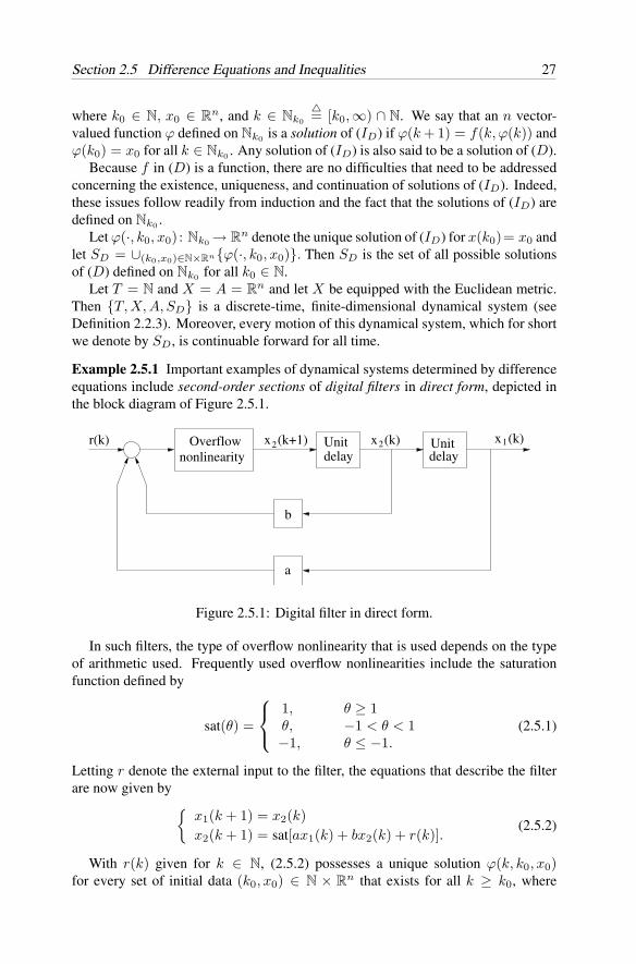
Section 2.5 Difference Equations and Inequalities 27
where k0 ∈ N, x0 ∈ Rn, and k ∈ Nk0
= [k0,∞) ∩ N. We say that an n vector-
valued function ϕ defined on Nk0 is a solution of (ID) if ϕ(k + 1) = f(k, ϕ(k)) andϕ(k0) = x0 for all k ∈ Nk0 . Any solution of (ID) is also said to be a solution of (D).
Because f in (D) is a function, there are no difficulties that need to be addressedconcerning the existence, uniqueness, and continuation of solutions of (ID). Indeed,these issues follow readily from induction and the fact that the solutions of (ID) aredefined on Nk0 .
Let ϕ(·, k0, x0) : Nk0 → Rn denote the unique solution of (ID) for x(k0)= x0 and
let SD = ∪(k0,x0)∈N×Rnϕ(·, k0, x0). Then SD is the set of all possible solutionsof (D) defined on Nk0 for all k0 ∈ N.
Let T = N and X = A = Rn and let X be equipped with the Euclidean metric.
Then T, X, A, SD is a discrete-time, finite-dimensional dynamical system (seeDefinition 2.2.3). Moreover, every motion of this dynamical system, which for shortwe denote by SD, is continuable forward for all time.
Example 2.5.1 Important examples of dynamical systems determined by differenceequations include second-order sections of digital filters in direct form, depicted inthe block diagram of Figure 2.5.1.
Unit r(k) Overflow x (k+1) x (k) Unit 22
b
a
nonlinearity delay delayx (k)1
Figure 2.5.1: Digital filter in direct form.
In such filters, the type of overflow nonlinearity that is used depends on the typeof arithmetic used. Frequently used overflow nonlinearities include the saturationfunction defined by
sat(θ) =
1, θ ≥ 1θ, −1 < θ < 1−1, θ ≤ −1.
(2.5.1)
Letting r denote the external input to the filter, the equations that describe the filterare now given by
x1(k + 1) = x2(k)x2(k + 1) = sat[ax1(k) + bx2(k) + r(k)].
(2.5.2)
With r(k) given for k ∈ N, (2.5.2) possesses a unique solution ϕ(k, k0, x0)for every set of initial data (k0, x0) ∈ N × R
n that exists for all k ≥ k0, where
28 Chapter 2. Dynamical Systems
x0 = [x1(k0), x2(k0)]T . The set of all solutions of (2.5.2) generated by varying(k0, x0) over N × R
n, determines a dynamical system.
B. Difference inequalitiesWe conclude the present section with a brief discussion of systems of differenceinequalities given by
x(k + 1) ≤ g(k, x(k)) (DI)
where k∈N and g : N × (R+)n → (R+)n with g(k, 0) ≥ 0 for all k ∈ N. A functionϕ : Nk0 → (R+)n is a solution of (DI) if
ϕ(k + 1) ≤ g(k, ϕ(k))
for all k∈Nk0 . In this case ϕ(k0) is an initial value. For any initial value x0 ∈(R+)n,solutions of (DI) exist. For example, the solution of the initial value problem
x(k + 1) = g(k, x(k)), x(k0) = x0
is such a solution of (DI) (refer to Part A above).Let T = N, A = X = (R+)n and let SDI denote the set of all solutions of
(DI) defined on Nk0 for any k0 ∈ N. Then T, X, A, SDI is a finite-dimensional,discrete-time dynamical system. We have occasion to make use of this system as acomparison system in subsequent chapters.
2.6 Differential Equations and Inclusions Defined onBanach Spaces
The present section consists of two parts.
A. Differential equations defined on Banach spaces
In order to put the presentations of the subsequent sections of this chapter into a clearercontext, we briefly consider differential equations in Banach spaces. A general formof a system of first-order differential equations in a Banach space X is given by
x(t) = F (t, x(t)) (GE)
where F : R+ × C → X, C ⊂ X . Associated with (GE) we have the initial value
problem given byx(t) = F (t, x(t)), x(t0) = x0 (IGE)
where t0 ∈ R+, t ≥ t0 ≥ 0, and x0 ∈ C ⊂ X . Under appropriate assumptions,
which ensure the existence of solutions of (GE), the initial value problem (IGE)determines a continuous-time, infinite-dimensional dynamical system, denoted bySGE , which consists of all the solutions x(t, t0, x0) of (IGE) with x(t0, x0, t0) = x0for all t0 ∈ R
+ and x0 ∈ C.
Section 2.6 Differential Equations and Inclusions Defined on Banach Spaces 29
For the conditions of existence, uniqueness, and continuation of solutions of theinitial value problem (IGE), the reader may want to refer, for example, to Lakshmikan-tham and Leela [26] and Lasota and Yorke [27]. For example, if F is continuouslydifferentiable, or at least locally Lipschitz continuous, then the theory of existence,uniqueness, and continuation of solutions of (IGE) is essentially the same as for thefinite-dimensional case we addressed in Section 2.3 when discussing ordinary differ-ential equations (see, e.g., Dieudonne [11, Chapter 10, Section 4]). This is furtherdemonstrated in Sections 2.7 and 2.8, where we concern ourselves with special classesof dynamical systems defined on Banach spaces, described by functional differentialequations and Volterra integrodifferential equations, respectively. In general, how-ever, issues concerning the well posedness of initial value problems (IGE) can bequite complicated. For example, as shown in Godunov [15], if F in (GE) is onlycontinuous, then (IGE) may not have a solution. Throughout this book, we assumethat (IGE) and the associated dynamical systems are well posed.
Important classes of infinite-dimensional continuous-time dynamical systems aredetermined by partial differential equations. Such systems are addressed in Sec-tion 2.10. In the analysis of initial and boundary value problems determined bypartial differential equations, semigroups play an important role. Semigroups, whichare important in their own right in determining a great variety of dynamical systems,are treated in Section 2.9. We show how such systems may frequently be viewed asspecial cases of (GE) and (IGE).
B. Differential inclusions defined on Banach spaces
In many applications (e.g., in certain classes of partial differential equations), thefunction F in (GE) may be discontinuous or even multivalued. This generalitygives rise to differential inclusions in Banach spaces. One such form of systems ofdifferential inclusions is briefly discussed in the following.
Let Ω be an open subset of a Banach space X , let 2X denote the set of all subsetsof X , let ∅ be the empty set, and let F : R
+ × Ω → 2X − ∅ be a set-valued mapping.We consider systems of differential inclusions given by ([1], [34])
x(t) ∈ F (t, x) (GI)
where t ∈ R+, x ∈ Ω, and x(t) = dx(t)/dt. Associated with (GI), we have the
initial value problemx(t) ∈ F (t, x), x(t0) = x0 (IGI)
where t0 ∈ R+ and x0 ∈ Ω.
Adifferentiable function ϕ defined on an interval [t0, t1) (t1 may be infinite) is saidto be a solution of (IGI ) if ϕ(t0) = x0 and if ϕ(t) ∈ F (t, ϕ(t)) for all t ∈ [t0, t1).We call any solution of (IGI ) a solution of (GI).
Now let
SGI =ϕ(·, t0, x0) : ϕ(·, t0, x0) is a solution of (IGI) defined on
[t0, t1), t1 > t0, t0 ∈ R+, x0 ∈ Ω
.
30 Chapter 2. Dynamical Systems
Then SGI is a dynamical system that we call the dynamical system determined by(GI).
In the following, we consider some specific cases.
Example 2.6.1 Let Ω be an open subset of Rn and let fm, fM ∈ C[R+ × Ω, Rn]
where fm(t, x) ≤ fM (t, x) for all (t, x) ∈ R+ × Ω where inequality of vectors is
to be interpreted componentwise. Now consider systems of differential inequalitiesgiven by
fm(t, x) ≤ x ≤ fM (t, x) (IE)
where x = dx/dt.A function ϕ ∈ C1
[[t0, t1), Ω
], where t0 ∈ R
+ and where t1 may be finite orinfinite, is said to be a solution of (IE) if for all t ∈ [t0, t1),
fm(t, ϕ(t)) ≤ ϕ(t) ≤ fM (t, ϕ(t)).
We refer to the set of all the solutions of (IE), denoted by SIE , as the dynamicalsystem determined by (IE).
The existence of the solutions of (IE) is guaranteed by the existence of the solutionsof systems of ordinary differential equations. Thus, for any f ∈ C[Ω × R
+, Rn]satisfying
fm(t, x) ≤ f(t, x) ≤ fM (t, x) (IE)
for all (t, x) ∈ R+ × Ω, any solution of the equation
x = f(t, x) (E)
must also be a solution of (IE).It is clear that SIE is a specific example of a dynamical system determined by
differential inclusions.
Example 2.6.2 Consider systems described by the set of equations
x = Ax + Bu (2.6.1a)
where x ∈ Rn, u ∈ R
m, A ∈ Rn×n, B ∈ R
n×m, x = dx/dt, and
u(t) =[g1(cT
1 x(t − τ)), . . . , gm(cTmx(t − τ))
]T (2.6.1b)
where τ > 0, C = [c1, . . . , cm] ∈ Rm×m, and gi ∈ C[R, R], i = 1, . . . , n, satisfy
the sector conditionsδiσ
2 ≤ gi(σ)σ ≤ ∆iσ2 (2.6.1c)
where ∆i ≥ δi ≥ 0, i = 1, . . . , m.System (2.6.1) defines a feedback control system consisting of a linear plant
and nonlinear controllers that take transportation delays into account. The sectorconditions (2.6.1c) allow for deterministic uncertainties associated with the controlactuators.
We refer to the set of all the solutions of system (2.6.1a)–(2.6.1c), denoted byS(2.6.1), as the dynamical system determined by (2.6.1). It is clear that S(2.6.1) is aspecific example of a dynamical system determined by differential inclusions.
Section 2.7 Functional Differential Equations 31
We conclude by noting that the system (2.6.1a)–(2.6.1c) is a differential-differenceequation. Such equations are special cases of functional differential equations, whichwe address next.
2.7 Functional Differential Equations
Let Cr denote the set C[[−r, 0], Rn
]with norm defined by
‖ϕ‖ = max|ϕ(t)| : − r ≤ t ≤ 0
. (2.7.1)
For a given function x(·) defined on [−r, c), c > 0, let xt be the function determinedby xt(s) = x(t+ s) for −r ≤ s ≤ 0 and t ∈ [0, c). A retarded functional differentialequation with delay r is defined as
x(t) = F (t, xt) (F )
where F : Ω → Rn and Ω is an open set in R × Cr. A differentiable function
p ∈ C[[t0 − r, t0 + c), Rn
], c > 0, is a solution of equation (F ) if (t, pt) ∈ Ω for
t ∈ [t0, t0 + c) and p = F (t, pt) for t ∈ [t0, t0 + c).At first glance it may appear that the functional differential equation (F ) is not
a special case of the general differential equation (GE) defined on a Banach spaceX (refer to Subsection 2.6A), because for the former, the range of the function F isin R
n (and not in Cr), and for the latter, the range of the function F is in C ⊂ X .However, it turns out that the functional differential equation (F ) can be transformedinto an equivalent equation which is a special case of (GE). To see this, we note that
xt(s) = x(t + s), −r ≤ s ≤ 0
= limh→0+
1h
[x(t + h + s) − x(t + s)], −r ≤ s ≤ 0
= limh→0+
1h
[xt+h(s) − xt(s)]
=
d
dtxt(s).
Defining Ft by
Ft(t, xt)(s) = F (t + s, xt+s), −r ≤ s ≤ 0,
it follows that the functional differential equation (F ) can equivalently be expressedby the equation
xt =d
dtxt = Ft(t, xt) (F )
which is a special case of equation (GE) because the range of Ft is in Cr.
32 Chapter 2. Dynamical Systems
Example 2.7.1 Linear retarded functional differential equations have the form
x = L(xt) (LF )
where L is a linear operator defined on Cr given by the Riemann–Stieltjes integral
L(ϕ) =∫ 0
−r
[dB(s)
]ϕ(s) (2.7.2)
where B(s) = [bij(s)] is an n × n matrix whose entries are functions of boundedvariation on [−r, 0] (see, e.g., Yoshizawa [47]).
A special case of (LF ) are linear differential-difference equations given by
x(t) = A1x(t) + B1x(t − r) (2.7.3)
where A1 and B1 are constant matrices (see, e.g., Bellman and Cooke [4]).
Example 2.7.2 As a special case of the above example, we consider the scalarequation
x(t) =∫ 0
−r
x(t + s)dη(s) (2.7.4)
where η is a function of bounded variation on [−r, 0] and the integral in (2.7.4) denotesa Riemann–Stieltjes integral. Defining L : Cr → R by
L(ϕ) =∫ 0
−r
ϕ(s)dη(s),
we can rewrite (2.7.4) asx(t) = L(xt).
If in particular, we consider the scalar differential-difference equation
x(t) = ax(t) + bx(t − r), (2.7.5)
where a, b are real constants and t ∈ [0, c), and if we let
η(s) =
0, s = −rb, −r < s < 0a + b, s = r
then we obtain in the present case
L(ϕ) =∫ 0
−r
ϕ(s)dη(s) = aϕ(0) + bϕ(−r).
We now associate with (F ) the initial value problem
x(t) = F (t, xt), xt0 = ψ (IF )
Section 2.7 Functional Differential Equations 33
where (t0, ψ) ∈ Ω ⊂ R × Cr. A function p ∈ C[[t0 − r, t0 + c), Rn
], c > 0, is a
solution of (IF ) if p is a solution of (F ) and if pt0 = ψ (i.e., pt0(s) = p(t0+s) = ψ(s)for −r ≤ s < 0).
If in (F ) the function F is continuous, then p ∈ C[[t0 − r, t0 + c), Rn
], c > 0, is
a solution of (IF ) if and only ifp(t) = ψ(t − t0), t0 − r ≤ t ≤ t0
p(t) = ψ(0) +∫ t
t0
F (s, ps)ds, t > t0.(2.7.6)
Alternatively, if we define an operatorT on the function spaceC[[t0−r, t0+c), Rn
]by
(T )(t) = ψ(t − t0), t0 − r ≤ t ≤ t0
(T )(t) = ψ(0) +∫ t
t0
F (x, ps)ds, t > t0(2.7.7)
then p is a solution of (IF ) if and only if p is a fixed point of the operator T , that is,if and only if Tp = p. Note that when p satisfies (2.7.6), then the continuity of pimplies the differentiability of p on [t0, c).
Similarly as in the case of ordinary differential equations (see Theorem 2.3.1), thefollowing result provides a set of sufficient conditions for the existence of solutionsof the initial value problem (IF ).
Theorem 2.7.1 Let Ω be an open set in R × Cr and let F ∈ C[Ω, Rn]. Then for any(t0, ψ) ∈ Ω, (IF ) has a solution defined on [t0 − r, t0 + c) for some c > 0.
In the problem section we provide details for the proof of Theorem 2.7.1.Similarly as in the case of ordinary differential equations (see Theorem 2.3.2), the
next result provides a set of sufficient conditions for the uniqueness of solutions ofthe initial value problem (IF ).
Theorem 2.7.2 Let Ω be an open set in R × Cr and assume that on every compactset K ⊂ Ω, F satisfies the Lipschitz condition∣∣F (t, x) − F (t, y)
∣∣ ≤ LK‖x − y‖ (2.7.8)
for all (t, x), (t, y) ∈ K, where LK is a constant that depends only on K, | · | is anorm on R
n, and ‖ · ‖ is the norm defined on Cr in (2.7.1). Then (IF ) has at mostone solution on the interval [t0 − r, t0 + c) for any c > 0.
In the problem section we provide details for the proof of Theorem 2.7.2. Also, inChapter 4, we prove a more general uniqueness result, applicable to differential equa-tions defined on Banach spaces, in the context of the Lyapunov theory. Theorem 2.7.2is a special case of that result (refer to Example 4.4.1).
Now let p ∈ C[[t0 − r, b), Rn
]be a solution of (F ) where b > t0. We say that p0
is a continuation of p if there exists a b0 > b such that p0 ∈ C[[t0 − r, b0), Rn
]is a
34 Chapter 2. Dynamical Systems
solution of (F ) with the property that p0(t) = p(t) for t ∈ [t0 − r, b). A solution p of(F ) is said to be noncontinuable if no such continuation exists.
Before giving a continuation result for (F ), we recall that a mapping F :X1 →X2,where X1 and X2 are metric spaces, is said to be completely continuous if F iscontinuous and if the closure of F (B) = F (x) : x ∈ B is compact for everybounded closed set B ⊂ X1.
Theorem 2.7.3 Let Ω = [t0 − r, a) × Cr where a > t0 is finite or infinite. Assumethat F : Ω → R
n is completely continuous and that every solution of (F ) is bounded.Then every solution of (F ) can be extended to the entire interval [t0 − r, a).
In the problem section we provide details for the proof of Theorem 2.7.3. InChapter 3 we present results that ensure the boundedness of the solutions of (F ),using Lyapunov stability theory.
Now let A ⊂ Cr be an open set, let J ⊂ R be a finite or an infinite interval, and letΩ = J × A. Assume that F ∈ C[Ω, Rn]. Then (IF ) has at least one solution definedon [t0 − r, t0 + c) (see Theorem 2.7.1). Let St0,ψ denote the set of all the solutionsof (IF ) and let SF = ∪(t0,ψ)∈ΩSt0,ψ . Then SF is the set of the solutions of (F ) thatare defined on any half closed (resp., half open) interval [a, b) ⊂ J .
Next, let T = J and let A ⊂ X = Cr with the metric determined by the norm‖ · ‖ given in (2.7.1). Then T, X, A, SF is a dynamical system in the sense of Def-inition 2.2.3. When T, X , and A are known from context, we refer to this dynamicalsystem simply as SF and we speak of the dynamical system determined by (F ).
Finally, we note that if in particular Ω = R+ × Cr and F : Ω → R
n is completelycontinuous and if every motion of SF is bounded, then in view of Theorem 2.7.3,every motion of SF is continuable forward for all time.
When F in equation (F ) is a function of t, xt, and xt (rather than t and xt),then the resulting equation is called a neutral functional differential equation. Asin the case of retarded functional differential equations, such equations determinedynamical systems. We do not pursue systems of this type in this book.
2.8 Volterra Integrodifferential Equations
Volterra integrodifferential equations may be viewed as retarded functional differen-tial equations with infinite delay; that is,
x(t) = F (t, xt) (V )
where the interval [−r, 0] is replaced by the interval (−∞, 0]. This necessitatesthe use of a fading memory space X which consists of all measurable functionsϕ : (−∞, 0] → R
n with the property that ϕ is continuous on −h ≤ t ≤ 0 and thatfor every ϕ ∈ X , the function ‖ · ‖ defined by
‖ϕ‖ = sup|ϕ(t)| : − h ≤ t ≤ 0
+∫ −h
−∞p(t)|ϕ(t)|dt (2.8.1)
Section 2.8 Volterra Integrodifferential Equations 35
is finite, where p : (−∞,−h) → R is a positive, continuously differentiable functionsuch that p(t) ≥ 0 on (−∞,−h). It can easily be verified that this function is anorm on X .
More generally other choices of norms for X include
‖ϕ‖ = sup|ϕ(t)| : − h ≤ t ≤ 0
+[ ∫ −h
−∞p(t)|ϕ(t)|qdt
]1/q
(2.8.2)
where q ∈ [1,∞). If in particular q = 2 and h = 0, then the norm (2.8.2) is inducedby the inner product
‖ϕ‖2 = 〈ϕ, ϕ〉 = 〈ϕ(0), ϕ(0)〉 +∫ 0
−∞p(t)〈ϕ(t), ϕ(t)〉dt. (2.8.3)
It can readily be shown that when X is equipped with (2.8.2), then (X, ‖ · ‖) is aBanach space and when X is equipped with the inner product (2.8.3), then (X, 〈·, ·〉)is a Hilbert space.
Associated with (V ) is the initial value problem
x(t) = F (t, xt), xt0 = ψ (IV )
where (t0, ψ) ∈ R+ × X . A function ϕ ∈ C[(−∞, t0 + c), Rn], c > 0, is a solution
of (IV ) if ϕ is a solution of (V ) (i.e., ϕ(t) = F (t, ϕt) for t ∈ [t0, t0 + c)), and ifϕt0 = ψ (i.e., ϕt0(s) = ϕ(t0 + s) = ψ(s) for −∞ < s ≤ 0).
We do not present results here concerning the existence, uniqueness, and con-tinuation of solutions of (IV ). Instead, we refer the reader to Hale [20] for suchresults.
Let T = R+ and A ⊂ X , let St0,ψ denote the set of all the solutions of (IV ) and
let SV = ∪(t0,ψ)St0,ψ . Then SV denotes the set of all the solutions of (V ) that aredefined on any interval [a, b) ⊂ R
+ and T, X, A, SV is a dynamical system. Whenthe context is clear, we simply speak of the dynamical system SV .
An important class of Volterra integrodifferential equations are linear Volterraintegrodifferential equations of the form
x(t) = Axt(0) +∫ 0
−∞K(s)xt(s)ds (LV )
which can equivalently be expressed as
x(t) = Ax(t) +∫ t
−∞K(s − t)x(s)ds (2.8.4)
for t ≥ 0, where A ∈ Rn×n and K = [kij ] is a matrix-valued function with elements
kij ∈ L1[(−∞, 0), R], 1 ≤ i, j ≤ n.Now let
Xp =ψ : (−∞, 0] → R
n and ψ : (−∞, 0) → Rn belong to Lp
[(−∞, 0), Rn
]
36 Chapter 2. Dynamical Systems
and let Xp be equipped with a norm given by
‖ψ‖ = |ψ(0)| +[∫ 0
−∞|ψ(t)|pdt
]1/p
(2.8.5)
where p ∈ [1,∞), and let
Yp =ψ ∈ Xp : ψ ∈ Lp
[(−∞, 0), Rn
]and
ψ(t) = ψ(0) +∫ t
0ψ(s)ds for all t ≥ 0
.
Associated with (LV ) we have the initial value problem x(t) = Axt(0) +∫ 0
−∞K(s)xt(s)ds, t ≥ 0
x(t) = ψ(t), t ≤ 0(ILV )
where ψ ∈ Yp.In Barbu and Grossman [3], the following result is established for (ILV ).
Theorem 2.8.1 For any ψ ∈ Yp, the initial value problem (ILV ) has a unique solutionx(t, ψ) that is defined on (−∞,∞).
For any t0 ∈ R, let y(t, ψ, t0) = x(t − t0, ψ) where x(t, ψ) denotes the uniquesolution of (ILV ). Let
SLV =y = y(t, ψ, t0) : t0 ∈ R, ψ ∈ Yp
,
let T = R, and let A = Yp ⊂ Xp = X . Then T, X, A, SLV is a dynamical system,which for short, we simply refer to as dynamical system SLV , or as the dynamicalsystem determined by (LV ).
In the following example we consider a simple model of the dynamics of a multi-core nuclear reactor. We revisit this model in Chapter 9.
Example 2.8.1 [31] (Point kinetics model of a multicore nuclear reactor) We con-sider the point kinetics model of a multicore nuclear reactor with l cores describedby the equations
Λipi(t) =[ρi(t) − εi − βi
]pi(t) + ρi(t) +
6∑k=1
βkicki(t)
+l∑
j=1
εji(Pj0/Pi0)∫ t
−∞hji(t − s)pj(s)ds
cki(t) = λki[pi(t) − cki(t)], i = 1, . . . , l, k = 1, . . . , 6
(2.8.6)
Section 2.8 Volterra Integrodifferential Equations 37
where pi : R → R and cki : R → R represent the power in the ith core and the concen-tration of the kth precursor in the ith core, respectively. The constants Λi, εi, βki, εji,Pi0, and λki are all positive and
βi =6∑
k=1
βki.
The functions hji ∈ L1(R+, R). They determine the coupling between cores dueto neutron migration from the jth to the ith core. The function ρi represents thereactivity of the ith core which we assume to have the form
ρi(t) =∫ t
−∞wi(t − s)pi(s)ds (2.8.7)
where wi ∈ L1[R+, R]. The functions pi(t) and cki(t) are assumed to be known,bounded, continuous functions defined on −∞ < t < 0.
In the present context, a physically realistic assumption is that cki(t)eλkit → 0 ast → −∞. Under this assumption, we can solve for cki in terms of pi to obtain
cki(t) =∫ t
−∞λkie
−λki(t−s)pi(s)ds. (2.8.8)
Using (2.8.7) and (2.8.8) to eliminate ρi and cki from (2.8.6), we obtain l Volterraintegrodifferential equations for pi(t), i = 1, . . . , l. To express these equations in amore compact form, we let
Fi(t) = Λ−1i
[wi(t) +
6∑k=1
βkiλkie−λkit + εiihii
],
Ki = Λ−1i [εi + βi],
ni(t) = Λ−1i wi(t), and
Gij =εijPj0hji(t)
ΛiPi0.
With pi(t) defined on −∞ < t < ∞, we have
pi(t) = −Kipi(t) +∫ t
−∞Fi(t − s)pi(s)ds + pi(t)
∫ t
−∞ni(t − s)pi(s)ds
+l∑
j=1,i =j
∫ t
−∞Gij(t − s)pj(s)ds, i = 1, . . . , l
for t ≥ 0 and pi(t) = ϕi(t) defined on −∞ < t ≤ 0 where ϕi ∈ Zi, the fadingmemory space of all absolutely continuous functions ψi defined on (−∞, 0] such that
‖ψi‖2 = |ψi(0)|2 +∫ 0
−∞|ψi(s)|2eLisds < ∞,
38 Chapter 2. Dynamical Systems
where Li > 0 is a constant. We address the choice of Li in Chapter 9, when studyingthe stability properties of (2.8.6). The set of all solutions of system (2.8.6), generatedby varying ϕi over Zi, i = 1, . . . , l, determines a dynamical system.
2.9 Semigroups
We now address linear and nonlinear semigroups that generate large classes of dy-namical systems. Before addressing the subject on hand we need to introduce someadditional notation.
A. Notation
Let X and Z denote Banach spaces and let ‖ · ‖ denote norms on such spaces. Also,Hilbert spaces are denoted X, Z, or H with inner product 〈·, ·〉. In this case, the normof x ∈ H is given by ‖x‖ = 〈x, x〉1/2.
Let A be a linear operator defined on a domain D(A) ⊂ X with range in Z. Wecall A closed if its graph, Gr(A) = (x, Ax) ∈ X × Z : x ∈ D(A) is a closedsubset of X × Z and we call A bounded if it maps bounded sets in X into boundedsets in Z, or equivalently, if it is continuous.
Subsequently, I : X → X denotes the identity transformation. Given a closedlinear operator A : D(A) → X, D(A) ⊂ X , we define the resolvent set of A, ρ(A),as the set of all points λ in the complex plane such that the linear transformation(A − λI) has a bounded inverse, (A − λI)−1 : X → X . The complement of ρ(A),denoted σ(A), is called the spectral set or the spectrum of A.
Finally, given a bounded linear operator A : D(A) → Z, D(A) ⊂ X , its norm isdefined by
‖A‖ = sup‖Ax‖ : ‖x‖ = 1
.
B. C0-semigroups
Consider a process whose evolution in time can be described by a linear differentialequation
x(t) = Ax(t), x(0) = x0 ∈ D(A) (IL)
for t ∈ R+. Here A : D(A) → X is assumed to be a linear operator with domain
D(A) dense in X . Moreover, A is always assumed to be closed or else to have anextension A that is closed. By a strong solution x(t) of (IL) we mean a functionx : R
+ → D(A) such that x(t) exists and is continuous on R+ → X and such that
(IL) is true. The abstract initial value problem (IL) is said to be well posed if foreach x0 ∈ D(A), there is one and only one strong solution x(t, x0) of (IL) definedon 0 ≤ t < ∞ and if in addition x(t, x0) depends continuously on (t, x0) in the sensethat given any N > 0 there is an M > 0 such that ‖x(t, x0)‖ ≤ M when 0 ≤ t ≤ Nand ‖x0‖ ≤ N .
Section 2.9 Semigroups 39
If (IL) is well posed, then there is an operator T defined by T (t)x0 = x(t, x0)which is (for each fixed t) a bounded linear mapping from D(A) to X . We callT (t)x0 = x(t, x0), t ≥ 0, a trajectory of (IL) for x0. Because T (t) is bounded,it has a continuous extension from D(A) to the larger domain X . The trajectoriesx(t, x0) = T (t)x0 for x0 ∈ X but x0 /∈ D(A) are called generalized solutions of(IL). The resulting family of operators T (t) : t ∈ R
+ is called a C0-semigroup ora linear semigroup.
Independent of the above discussion, we now define C0-semigroup.
Definition 2.9.1 [21], [23], [39] Aone-parameter family of bounded linear operatorsT (t) : X → X, t ∈ R
+, is said to be a C0-semigroup, or a linear semigroup, if
(i) T (0) = I (I is the identity operator on X);
(ii) T (t + s) = T (t)T (s) for any t, s ∈ R+; and
(iii) limt→0+ T (t)x = x for all x ∈ X .
Evidently, every C0-semigroup is generated by some abstract differential equationof the form (IL).
Definition 2.9.2 Given any C0-semigroup T (t), its infinitesimal generator is theoperator defined by
Ax = limt→0+
T (t)x − x
t
where D(A) consists of all x ∈ X for which this limit exists.
Theorem 2.9.1 [39] For a C0-semigroup T (t), there exist an ω ≥ 0 and an M ≥ 1such that
‖T (t)‖ ≤ Meωt.
The next result provides necessary and sufficient conditions for a given linearoperator A to be the infinitesimal generator of some C0-semigroup.
Theorem 2.9.2 [21], [39] (Hille–Yoshida–Phillips Theorem) A linear operator A isthe infinitesimal generator of a C0-semigroup T (t) satisfying ‖T (t)‖ ≤ Meωt, if andonly if
(i) A is closed and D(A) is dense in X;
(ii) the resolvent set ρ(A) of A contains (ω, ∞); and
∥∥(A − λI)−n∥∥ ≤ M
(λ − ω)nfor all λ > ω,
n = 1, 2, . . . , where I denotes the identity operator on X .
A C0-semigroup of contractions is a C0-semigroup T (t) satisfying ‖T (t)‖ ≤ 1(i.e., in Theorem 2.9.1, M = 1 and ω = 0). Such semigroups are of particular interestin Hilbert spaces.
40 Chapter 2. Dynamical Systems
Definition 2.9.3 A linear operator A : D(A) → H , D(A) ⊂ H , on a Hilbert spaceH is said to be dissipative if Re〈Ax, x〉 ≤ 0 for all x ∈ D(A).
For C0-semigroups of contractions we have the following result.
Theorem 2.9.3 If A is the infinitesimal generator of a C0-semigroup of contractionson a Hilbert space H , then A is dissipative and the range of (A − λI) is all of H forany λ > 0. Conversely, if A is dissipative and if the range of (A − λI) is H for atleast one constant λ0 > 0, then A is closed and A is the infinitesimal generator of aC0-semigroup of contractions.
The above result is useful in the study of parabolic partial differential equations(Section 2.10).
For linear semigroups with generator A one can deduce many important qualitativeproperties by determining the spectrum of A. Some of these are summarized in thefollowing results (refer to Slemrod [42]).
Theorem 2.9.4 Given any two real numbers α and β with α < β there exists a C0-semigroup T (t) on a Hilbert space H such that Reλ ≤ α for all λ ∈ σ(A) and inaddition ‖T (t)‖ = eβt for all t ≥ 0.
The next result applies to the following class of semigroups.
Definition 2.9.4 A C0-semigroup T (t) is called differentiable for t > r if for eachx ∈ X , T (t)x is continuously differentiable on r < t < ∞.
For example, a system of linear time-invariant functional differential equationswith delay [−r, 0] (as discussed in the last subsection of this section) determinesa semigroup that is differentiable for t > r. Also, systems of parabolic partialdifferential equations (as discussed in the next section) normally generate semigroupsthat are differentiable for t > 0. In the finite-dimensional case (when X = R
n), forlinear semigroups the generator A must be an n×n matrix whose spectrum is the setof eigenvalues λ of A. Such semigroups are differentiable as well for t > 0.
Following Slemrod [42] we have the following result.
Theorem 2.9.5 If T (t) is a C0-semigroup that is differentiable for t > r, if A is itsgenerator, and if Reλ ≤ −α0 for all λ ∈ σ(A), then given any positive α < α0, thereis a constant K(α) > 0 such that ‖T (t)‖ ≤ K(α)e−αt for all t > r.
We conclude by defining the dynamical system determined by a C0-semigroupT (t) as
SC0 =p = p(·, x0, t0) : p(t, x, t0)
= T (t − t0)x, t0 ∈ R
+, t ≥ t0, x ∈ X.
We consider some specific examples of dynamical systems determined by C0-semigroups in the last subsection of this section.
Section 2.9 Semigroups 41
C. Nonlinear semigroups
A nonlinear semigroup is a generalization of the notion of C0-semigroup. In arrivingat this generalization, the linear initial value problem (IL) is replaced by the nonlinearinitial value problem
x(t) = A(x(t)), x(0) = x0 (IN )
where A : D(A) → X is a nonlinear mapping. As mentioned already in Section 2.6(in connection with initial value problem (IGE)) if A is continuously differentiable(or at least locally Lipschitz continuous), then the theory of existence, uniqueness,and continuation of solutions of (IN ) is the same as in the finite-dimensional case(see Dieudonne [11, Chapter 10, Section 4]). If A is only continuous, then (IN ) needsnot to have any solution at all (see Dieudonne [11, p. 287, Problem 5]). In general,one wishes to have a theory that includes nonlinear partial differential equations.This mandates that A be allowed to be only defined on a dense set D(A) and to bediscontinuous. For such functions A, the accretive property (defined later) generalizesthe Lipschitz property.
Definition 2.9.5 [5], [8], [9], [15], [25], [27] Assume that C is a subset of a Banachspace X . A family of one-parameter (nonlinear) operators T (t) : C → C, t ∈ R
+, issaid to be a nonlinear semigroup defined on C if
(i) T (0)x = x for x ∈ C;
(ii) T (t + s)x = T (t)T (s)x for t, s ∈ R+, x ∈ C; and
(iii) T (t)x is continuous in (t, x) on R+ × C.
A nonlinear semigroup T (t) is called a quasi-contractive semigroup if there is anumber w ∈ R such that ∥∥T (t)x − T (t)y
∥∥ ≤ ewt‖x − y‖ (2.9.1)
for all t ∈ R+ and for all x, y ∈ C. If in (2.9.1) w ≤ 0, then T (t) is called a
contraction semigroup. Note that C = X is allowed as a special case.
The mapping A in (IN ) is sometimes multivalued (i.e., a relation) and in generalmust be extended to be multivalued if it is to generate a quasi-contractive semigroup.Thus, we assume that A(x), x∈X, is a subset of X and we identify A with its graph,
Gr(A) =(x, y) : x ∈ X and y ∈ A(x)
⊂ X × Y.
In this case the domain of A, written as D(A), is the set of all x ∈ X for whichA(x) = ∅, the range of A is the set
Ra(A) = ∪A(x) : x ∈ D(A)
,
and the inverse of A at any point y is defined as the set
A−1(y) =x ∈ X : y ∈ A(x)
.
42 Chapter 2. Dynamical Systems
Let λ be a real or complex scalar. Then λA is defined by
(λA)(x) =λy : y ∈ A(x)
and A + B is defined by
(A + B)(x) = A(x) + B(x) =y + z : y ∈ A(x), z ∈ B(x)
.
Definition 2.9.6 A multivalued operator A is said to generate a nonlinear semigroupT (t) on C if
T (t)x = limn→∞
(I − t
nA
)−n
(x)
for all x ∈ C.The infinitesimal generator As of a nonlinear semigroup T (t) is defined by
As(x) = limt→0+
T (t)x − x
t, x ∈ D(As)
for all x such that this limit exists. The operator A and the infinitesimal generator As
are generally different operators.
Definition 2.9.7 A multivalued operator A on X is said to be w-accretive if∥∥(x1 − λy1) − (x2 − λy2)∥∥ ≥ (1 − λw)‖x1 − x2‖ (2.9.2)
for all λ ≥ 0 and for all xi ∈ D(A) and yi ∈ A(xi), i = 1, 2.
If, in particular, X is a Hilbert space, then (2.9.2) reduces to⟨(wx1 − y1) − (wx2 − y2), x1 − x2
⟩≥ 0. (2.9.3)
The above property for the nonlinear case is analogous to (A−wI) being dissipativein the linear symmetric case.
Theorem 2.9.6 Assume that A is w-accretive and that for each λ ∈ (0, λ0),
Ra(I − λA) ⊃ C = D(A)
where D(A) denotes the closure of D(A) and λ0 > 0 is a constant. Then A generatesa quasi-contractive semigroup T (t) on C with∥∥T (t)x − T (t)y
∥∥ ≤ ewt‖x − y‖
for all t ∈ R+ and for all x, y ∈ C.
In general, the trajectories T (t)x determined by the semigroup in Theorem 2.9.6are generalized solutions of (IN ) that need not be differentiable. Indeed, an exampleis discussed in Crandall and Liggett [9, Section 4], where w = 0, D(A) = X , Agenerates a quasi-contraction T (t) but the infinitesimal generator As has an empty
Section 2.9 Semigroups 43
domain. This means that not even one trajectory T (t)x is differentiable at even onetime t. If the graph of A is closed, then A is always an extension of the infinitesimalgenerator As. So whenever x(t) = T (t)x has a derivative, then x(t) must be inA(x(t)).
The situation is more reasonable in the setting of a Hilbert space H . If A is w-accretive and closed (i.e., its graph is a closed subset of H×H), then for any x∈D(A)the set A(x) is closed and convex. Thus, there is an element A0(x)∈A(x) such thatA0(x) is the element of A(x) closest to the origin. Given a trajectory x(t) = T (t)x,the right derivative
D+x(t) = limh→0+
x(t + h) − x(t)h
must exist at all points t ∈ R+ and be continuous except possibly at a countably
infinite set of points. The derivative x(t) exists and is equal to D+x(t) at all pointswhere D+x(t) is continuous. Furthermore,
D+x(t) = A0(x(t))
for all t ≥ 0. These results can be generalized to any space X that is uniformlyconvex. (Refer to Dunford and Schwarz [12, p. 74], for the definition of a uniformlyconvex space. In particular, any Lp space, 1 < p < ∞, is a uniformly convex space.)
Definition 2.9.8 A trajectory x(t) = T (t)x0 is called a strong solution of (IN ) ifx(t) is absolutely continuous on any bounded subset of R
+ (so that x(t) exists almosteverywhere) if x(t) ∈ D(A) and if x(t) ∈ A(x(t)) almost everywhere on R
+.
We also have
Definition 2.9.9 The initial value problem (IN ) is called well posed on C if there isa semigroup T (t) such that for any x0 ∈ D(A), T (t)x0 is a strong solution of (IN ),and if D(A) = C.
We summarize the above discussion in the following theorem.
Theorem 2.9.7 If X is a Hilbert space or a uniformly convex Banach space and ifA is w-accretive and closed, then the initial value problem (IN ) is well posed onC = D(A) and x(t) = A0(x(t)) almost everywhere on R
+.
We conclude by defining the dynamical system determined by a nonlinear semi-group T (t) as
SN =p = p(·, x, t0) : p(t, x, t0)
= T (t − t0)x, t0 ∈ R
+, t ≥ t0, x ∈ C.
We consider in the next subsection several specific examples of semigroups.
D. Examples of semigroups
We now consider several classes of important semigroups that arise in applicationsand we provide some related background material which we find useful in subsequentchapters.
44 Chapter 2. Dynamical Systems
Example 2.9.1 (Ordinary differential equations) Consider initial value problems de-scribed by a system of autonomous first-order ordinary differential equations given by
x = g(x), x(0) = x0 (2.9.4)
where g : Rn → R
n and where it is assumed that g satisfies the Lipschitz condition∣∣g(x) − g(y)∣∣ ≤ L|x − y| (2.9.5)
for all x, y ∈ Rn. In this case g is w-accretive with w = L and (2.9.5) implies that
g is continuous on Rn. This continuity implies that the graph of g is closed. By
Theorem 2.9.7 there exist a semigroup T (t) and a subset D ⊂ Rn such that D is
dense in Rn and for any x0 ∈ D, any solution x(t) = T (t)x0 of (2.9.4) is absolutely
continuous on any finite interval in R+. In the present case D = R
n and T (t) is aquasi-contractive semigroup with∣∣T (t)x − T (t)y
∣∣ ≤ eLt|x − y| (2.9.6)
for all x, y ∈ Rn and t ∈ R
+.Now assume that in (2.9.4) g(x) = Ax where A ∈ R
n×n; that is,
x = Ax, x(0) = x0. (2.9.7)
In the present case (2.9.7) determines a differentiable C0-semigroup with generatorA. The spectrum of A, σ(A), coincides with the set of all eigenvalues of A, λ.Now according to Theorem 2.9.5, if Reλ ≤ −α0 for all λ ∈ σ(A), where α0 > 0 isa constant, then given any positive α < α0, there is a constant K(α) > 0 such that∥∥T (t)
∥∥ ≤ K(α)e−αt, t ∈ R+. (2.9.8)
Example 2.9.2 (Functional differential equations) Consider initial value problemsdescribed by a system of autonomous first-order functional differential equations
x(t) = F (xt), t > 0x(t) = ψ(t), −r ≤ t ≤ 0
(2.9.9)
where F : Cr → Rn. (For the notation used in this example, refer to Section 2.7.)
Assume that F satisfies the Lipschitz condition∣∣F (ξ) − F (η)∣∣ ≤ K‖ξ − η‖ (2.9.10)
for all ξ, η ∈ Cr. Under these conditions, the initial value problem (2.9.9) has aunique solution for every initial condition ψ, denoted by p(t, ψ) which is defined forall t ∈ R
+ (refer to Section 2.7). In this case T (t)ψ = pt(·, ψ), or equivalently,(T (t)ψ)(s) = p(t + s, ψ) defines a quasi-contractive semigroup on Cr. DefineA : D(A) → Cr by
Aψ = ψ, D(A) =ψ ∈ Cr : ψ ∈ Cr and ψ(0) = F (ψ)
. (2.9.11)
Section 2.9 Semigroups 45
Then D(A) is dense in Cr, A is the generator and also the infinitesimal generator ofT (t), and T (t) is differentiable for t > r.
If in (2.9.9) F = L is the linear mapping from Cr to Rn defined in (2.7.2), we have
x = L(xt) (2.9.12)
where
L(ϕ) =∫ 0
−r
[dB(s)
]ϕ(s). (2.9.13)
In this case the semigroup T (t) is a C0-semigroup. The spectrum of its generatorconsists of all solutions of the equation
det(∫ 0
−r
eλsB(s) − λI
)= 0. (2.9.14)
If all solutions of (2.9.14) satisfy the relation Reλ ≤ −γ0 for some γ0 > 0, thengiven any positive γ < γ0, there is a constant K(γ) > 0 such that∥∥T (t)
∥∥ ≤ K(γ)e−γt, t ∈ R+ (2.9.15)
(refer to Theorem 2.9.5).
Example 2.9.3 (Volterra integrodifferential equations) We discuss the class ofVolterra integrodifferential equations given in Section 2.8, x(t) = Ax(t) +
∫ t
−∞K(s − t)x(s)ds, t ≥ 0
x(t) = ϕ(t), −∞ < t ≤ 0(2.9.16)
where A ∈ Rn×n and K ∈ L1
[(−∞, 0), Rn×n
]; that is, K is an n×n matrix-valued
function whose entries kij ∈ L1[(−∞, 0), R
]. Let Xp, 1 ≤ p < ∞, be defined as in
Section 2.8. ThenXp Lp
[(−∞, 0), Rn
]× R
n (2.9.17)
where denotes an isomorphic relation. To see this, note that for any ϕ ∈ Xp,ϕ|(−∞,0) ∈Lp[(−∞, 0), Rn], ϕ(0) ∈ R
n. Conversely, for any ψ ∈ Lp[(−∞, 0), Rn]and Z ∈ R
n, there is a unique ϕ ∈ Xp such that ϕ|(−∞,0) = ψ, and ϕ(0) = Z. Inthis case, if we denote ϕ = (Z, ψ), the norm defined by (2.8.5) can now be written as
‖ϕ‖ = ‖(Z, ψ)‖ = |Z| +[∫ 0
−∞|ψ(s)|pds
]1/p
, 1 ≤ p < ∞. (2.9.18)
We now define an operator A by
A(Z, ψ) =(
AZ +∫ 0
−∞K(s)ψ(s)ds, ψ
)(2.9.19)
46 Chapter 2. Dynamical Systems
on the domain
D(A) =(Z, ψ) : ψ ∈ Lp
[(−∞, 0), Rn
]and ψ(t) = Z+
∫ t
0ψ(s)ds for all t ≤ 0
.
(2.9.20)Then A is an infinitesimal generator of a C0-semigroup T (t) on Xp. Furthermore,when (Z, ψ) ∈ D(A), the equation(
x(t), xt
)= T (t)(Z, ψ) (2.9.21)
determines a function x(t) which is the unique solution of (2.9.16) (refer to Barbuand Grossman [3]).
If Reλ > 0, then λ ∈ σ(A) if and only if
det(
A +∫ 0
−∞eλsK(s)ds − λI
)= 0. (2.9.22)
On the other hand, if Reλ ≤ 0, then λ is always in σ(A).
There are many other important classes of semigroups, including those that aredetermined by partial differential equations. We address some of these in the nextsection.
2.10 Partial Differential Equations
In our discussion of partial differential equations we require additional nomenclature.
A. Notation
A vector index or exponent is a vector αT = (α1, . . . , αn) whose components arenonnegative integers, |α| =
∑nj=1 αj , and for any x ∈ R
n,
xα = (x1, x2, . . . , xn)α = xα11 · · ·xαn
n .
Let Dk = i(∂/∂xk) for k = 1, . . . , n, where i = (−1)1/2 and let D = (D1, D2, . . . ,Dn) so that
Dα = Dα11 · · ·Dαn
n . (2.10.1)
In the sequel we let Ω be a domain in Rn (i.e., Ω is a connected set) with boundary
∂Ω and closure Ω. We assume that ∂Ω is of class Ck for suitable k ≥ 1. By this wemean that for each x ∈ ∂Ω, there is a ball B with center at x such that ∂Ω ∩ B canbe represented in the form
xi = ϕ(x1, . . . , xi−1, xi+1, . . . , xn)
for some i, i = 1, . . . , n, with ϕ continuously differentiable up to order k. Thissmoothness is easily seen to be true for the type of regions that normally occur inapplications.
Section 2.10 Partial Differential Equations 47
Also, let Cl[Ω, C] denote the set of all complex-valued functions defined on Ωwhose derivatives up to order l are continuous. For u ∈ Cl[Ω, C], l ∈ N, we definethe norm
‖u‖l =
∫Ω
∑|α|≤l
|Dαu|21/2
. (2.10.2)
LetCl[Ω, C] =
u ∈ Cl[Ω, C] : ‖u‖l < ∞
and let
Cl0[Ω, C] =
u ∈ Cl[Ω, C] : u = 0 in a neighborhood of ∂Ω
.
We define H l[Ω, C] and H l0[Ω, C] to be the completions in the norm ‖·‖l of the spaces
Cl[Ω, C] and Cl0[Ω, C], respectively. In a similar manner, we can define the spaces
H l[Ω, R] and H l0[Ω, R]. The spaces defined above are sometimes called Sobolev
spaces. Their construction builds “zero boundary conditions” into, for example,H l
0[Ω, R].Finally, we define C∞[Ω, C] = ∩l∈NCl[Ω, C] and we say that u ∈ C∞[Ω, C]
if Dαu can be extended to be a continuous function on Ω for any α ∈ Nn. We
define C∞[Ω, R] and C∞[Ω, R] in a similar manner. Occasionally, we say that uis a real-valued smooth function on Ω (on Ω) if u ∈ C∞[Ω, R] (if u ∈ C∞[Ω, R]).Complex-valued smooth functions on Ω (on Ω) are defined similarly.
B. Linear equations with constant coefficients
Given r × r complex constant square matrices Aα, α ∈ Nn, let
A(D) =∑
|α|≤m
AαDα,
and consider the initial value problem
∂u
∂t(t, x) = A(D)u(t, x), u(0, x) = ψ(x) (IP )
where t ∈ R+, x ∈ R
n, ψ ∈ L2[Rn, C] are given, and u : R+ × R
n → Cr is to be
determined.Proceeding intuitively for the moment, we apply L2-Fourier transforms to (IP ) to
obtain∂u(t, ω)
∂t= A(ω)u(t, ω), u(0, ω) = ψ(ω)
where A(ω) =∑
|α|≤m Aαωα for all ω ∈ Rn. In order to have a solution such that
u(t, x) and (∂u/∂t)(t, x) are in L2 over x ∈ Rn, it is necessary that A(ω)u(t, ω) be
in L2 over ω ∈ Rn. This places some restrictions on A(ω). For the proof of the next
result, refer to Krein [23, p. 163].
48 Chapter 2. Dynamical Systems
Theorem 2.10.1 The mapping T (t)ψ = u(t, ·) defined by the solutions u(t, x) of(IP ) determines a C0-semigroup on X = L2[Rn, C] if and only if there exists anonsingular matrix S(ω) and a constant K > 0 such that for all ω ∈ R
n, the followingconditions are satisfied.
(i) |S(ω)| ≤ K and |S(ω)−1| ≤ K.
(ii) S(ω)A(ω)S(ω)−1 = [Cij(ω)] is upper triangular.
(iii) ReCrr(ω) ≤ · · · ≤ ReC11(ω) ≤ K.
(iv) |Cik(ω)| ≤ K(1 + |ReCii(ω)|) for k = i + 1, . . . , r.
Parabolic equations (i.e., equations for which A(D) is strongly elliptic, definedlater) satisfy these conditions whereas hyperbolic equations do not. We demonstratethis in the next examples.
Example 2.10.1 Consider a special case of (IP ) with r = 1, m = n = 2, given by∂u
∂t=
∂2u
∂x2 +∂2u
∂y2 + a∂u
∂x+ b
∂u
∂y+ cu
u(0, x) = ψ(x).(2.10.3)
For ω = (ω1, ω2)T ∈ R2 we have
A(ω) = −ω21 − ω2
2 + iaω1 + ibω2 + c = C11(ω).
Clearly, ReA(ω) = −ω21 − ω2
2 + c ≤ c for all ω ∈ R2. Therefore, all the hypotheses
of Theorem 2.10.1 are satisfied and thus, (2.10.3) determines a C0-semigroup onX = L2[R2, C].
Example 2.10.2 Consider the initial value problem determined by the wave equation∂2u
∂t2=
∂2u
∂x2
u(0, x) = ψ(x).(2.10.4)
The above equation can equivalently be expressed by
∂u1
∂t= u2,
∂u2
∂t=
∂2u1
∂x2
with u1 = u and u2 = ∂u/∂t. Equation (2.10.4) is a specific case of (IP ) withr = 2, m = 2, n = 1, and
A(ω) =[
0 1−ω2 0
].
The eigenvalues of A(ω) are given by C11(ω) = iω and C22(ω) = −iω. In orderthat the hypotheses of Theorem 2.10.1 be satisfied, there must exist an S(ω) such that
Section 2.10 Partial Differential Equations 49
S(ω)A(ω)S(ω)−1 = C(ω) where C(ω) is upper triangular with diagonal elementsC11(ω) and C22(ω). Then
A(ω)S(ω)−1 = S(ω)−1[iω C12(ω)0 −iω
].
Let
S(ω)−1 =[x1(ω) y1(ω)x2(ω) y2(ω)
].
A straightforward calculation yields
S(ω)−1 =[
x1(ω) y1(ω)iωx1(ω) C12(ω)x1(ω) − iωy1(ω)
]and
S(ω) =1
[C12(ω)x1(ω)2 − 2iωx1(ω)y1(ω)]
[C12(ω)x1(ω) − iωy1(ω) −y1(ω)
−iωx1(ω) x1(ω)
].
Because ReC11(ω) = 0, condition (iv) in Theorem 2.10.1 implies that |C12(ω)| ≤ Kand condition (i) of this theorem implies that all elements of S(ω) and S(ω)−1 arebounded by K. Thus,
|C12(ω)x1(ω) − iωy1(ω)| ≤ K
and|ω||C12(ω)x1(ω) − 2iωy1(ω)|−1 ≤ K
can be combined to yield
|ω|/K ≤ |C12(ω)x1(ω) − iωy1(ω)| + |iωy1(ω)|≤ K + |iωy1(ω)|≤ 2K + |C12(ω)x1(ω)|.
Using |C12(ω)| ≤ K and |x1(ω)| ≤ K for all ω ∈ R, we obtain
|ω|/K ≤ 2K + K2
for all ω ∈ R. But this is impossible. Thus, no matrix S(ω) as asserted above exists.Therefore, the solutions of (2.10.4) do not generate a C0-semigroup.
C. Linear parabolic equations with smooth coefficients
In the following Ω ⊂ Rn is assumed to be a bounded domain with smooth boundary
∂Ω. We consider the differential operator of order 2m given by
A(t, x, D) =∑
|α|≤2m
aα(t, x)Dα (2.10.5)
50 Chapter 2. Dynamical Systems
where α ∈ Nn, Dα is defined in (2.10.1) and the coefficients aα(t, x) are complex-
valued functions defined on [0, T0) × Ω where T0 > 0 is allowed to be infinite. Theprincipal part of A(t, x, D) is the operator given by
A′(t, x, D) =∑
|α|=2m
aα(t, x)Dα (2.10.6)
and A(t, x, D) is said to be strongly elliptic if there exists a constant c > 0 such that
ReA′(t, x, ξ) ≥ c|ξ|2m
for all t ∈ [0, T0), x ∈ Ω, and ξ ∈ Rn.
In the following, we consider linear, parabolic partial differential equations withinitial conditions and boundary conditions given by
∂u
∂t(t, x) + A(t, x, D)u(t, x) = f(t, x) on (0, T0) × Ω
Dαu(t, x) = 0, |α| < m on (0, T0) × ∂Ωu(0, x) = u0(x) on Ω
(IPP )
where f and u0 are complex-valued functions defined on (0, T0) × Ω and Ω,respectively.
Using the theory of Sobolev spaces, generalized functions (distributions), and dif-ferentiation in the distribution sense, the following result concerning the well posed-ness of (IPP ) (involving generalized solutions for (IPP )) has been established (see,e.g., Pazy [39] and Friedman [14]).
Theorem 2.10.2 For (IPP ), assume the following.
(i) A(t, x, D) is strongly elliptic.
(ii) f, aα ∈ C∞[[0, T0] × Ω, C]
for all |α| ≤ 2m.
(iii) u0 ∈ C∞[Ω, C].(iv) limx→∂Ω Dαu0(x) = 0 for all |α| < m.
Then there exists a unique solution u ∈ C∞[[0, T0] × Ω, C].
If the operator A(t, x, D) and the functions f and u0 are real-valued, then Theo-rem 2.10.2 is still true with the solution u of (IPP ) being real-valued.
Now let T = [0, T0] and X = A = C∞[Ω, C] and let St0,u0 denote the set of the(unique) solutions of (IPP ), where in (IPP ), u(0, x) = u0(x) on Ω is replaced byu(t0, x) = u0(x) on Ω with t0 ∈ [0, T0). Let SPP = ∪(t0,u0)∈[0,T0)×ASt0,u0 . ThenT, X, A, SPP is a dynamical system. When T, X , and A are known from context,we refer to this system simply as dynamical system SPP .
Because A(t, x, D) is in general time-varying, (IPP ) will in general not generate asemigroup. However, in the special case when A(t, x, D) ≡ A(x, D), the followingresult has been established (refer, e.g., to Pazy [39]).
Section 2.11 Composite Dynamical Systems 51
Theorem 2.10.3 In (IPP ), let
A(x, D) =∑
|α|≤2m
aα(x)Dα
be strongly elliptic on Ω and let Au= A(x, D)u be defined on
D(A) = H2m[Ω, C] ∩ Hm0 [Ω, C].
Then A is the infinitesimal generator of a C0-semigroup on L2[Ω, C].
We conclude by pointing out that dynamical systems (as well as nonlinear semi-groups) are determined by nonlinear partial differential equations as well. We do notpursue this topic in this book.
2.11 Composite Dynamical Systems
Problems that arise in science and technology are frequently described by a mixtureof equations. For example, in control theory, feedback systems usually consist of aninterconnection of several blocks, such as the plant, the sensors, the actuators, andthe controller. Depending on the application, these components are characterizedby different types of equations. For example, in the case of distributed parametersystems, the plant may be described by a partial differential equation, a functionaldifferential equation, or by a Volterra integrodifferential equation, and the remainingblocks may be characterized by ordinary differential equations or ordinary differ-ence equations. In particular, the description of digital controllers involves ordinarydifference equations.
The above is an example of a large class of composite systems. Depending on thecontext, such systems are also referred to in the literature as interconnected systemsand decentralized systems (e.g., [31]). When the motions of some of the systemcomponents evolve along different notions of time (continuous time R
+ and discretetime N) such systems are usually referred to as hybrid systems (e.g., [45], [46]).
In the present section, we confine our attention to interconnected (resp., composite)dynamical systems whose motion components all evolve along the same notion oftime. In the next section, where we address discontinuous dynamical systems, andspecific examples of hybrid dynamical systems, we relax this requirement. A metricspace (X, d) is said to be nontrivial if X is neither empty nor a singleton, it is saidto be decomposable if there are nontrivial metric spaces (X1, d1) and (X2, d2) suchthat X = X1 × X2, and it is said to be undecomposable if it is not decomposable.
Now let (X, d), (Xi, di), i = 1, . . . , l, be metric spaces. We assume that X =X1 × · · · × Xl and that there are constants c1 > 0 and c2 > 0 such that
c1d(x, y) ≤l∑
i=1
di(xi, yi) ≤ c2d(x, y)
52 Chapter 2. Dynamical Systems
for all x, y ∈ X , where x = [x1, . . . , xl]T , y = [y1, . . . , yl]T , xi ∈ Xi, and yi ∈ Xi,i = 1, . . . , l. We can define the metric d on X in a variety of ways, including, forexample,
d(x, y) =l∑
i=1
di(xi, yi).
Definition 2.11.1 [34] A dynamical system T, X, A, S is called a composite dy-namical system if the metric space (X, d) can be decomposed as X = X1 ×· · ·×Xl,l ≥ 2, where X1, . . . , Xl are nontrivial and undecomposable metric spaces withmetrics d1, . . . , dl, respectively, and if there exist two metric spaces Xi and Xj ,i, j = 1, . . . , l, i = j, that are not isometric.
The following example may be viewed as a distributed control (in contrast to aboundary control) of a plant that is governed by the heat equation and a controller thatis governed by a system of first-order ordinary differential equations. The variablesfor the controller and the plant are represented by z1 = z1(t) and z2 = z2(t, x),respectively.
Example 2.11.1 [31], [40] We consider the composite system described by theequations
z1(t) = Az1(t) +∫Ω f(x)z2(t, x)dx, t ∈ R
+
∂z2
∂t(t, x) = α∆z2(t, x) + g(x)cT z1(t), (t, x) ∈ R
+ × Ω
z2(t, x) = 0 (t, x) ∈ R+ × ∂Ω
(2.11.1)
where z1 ∈ Rm, z2 ∈ R, A ∈ R
m×m, c ∈ Rm, f and g ∈ L2[Ω, R], α > 0, Ω is
a bounded domain in Rn with a smooth boundary ∂Ω, and ∆ denotes the Laplacian
(i.e., ∆ =∑n
i=1 ∂2/∂x2i ). The system of equations (2.11.1) may be viewed as a
differential equation in the Banach space X= R
m × H0[Ω, R] where H0[Ω, R] isthe completion of C0[Ω, R] with respect to the L2-norm and H0[Ω, R] ⊂ L2[Ω, R](refer to Section 2.10). For every initial condition z0 = [z10, z20] ∈ R
m ×H0[Ω, R],there exists a unique solution z(t, z0) which depends continuously on z0. For a proofof the well posedness of system (2.11.1), refer to [31].
The set of all solutions of (2.11.1) clearly determines a composite dynamicalsystem.
2.12 Discontinuous Dynamical Systems
All of the various types of dynamical systems that we have considered thus far includeeither discrete-time dynamical systems or continuous continuous-time dynamical sys-tems (which we simply call continuous dynamical systems). In the present sectionwe address discontinuous dynamical systems (continuous-time dynamical systemswith motions that need not be continuous), which we abbreviate as DDS. Although
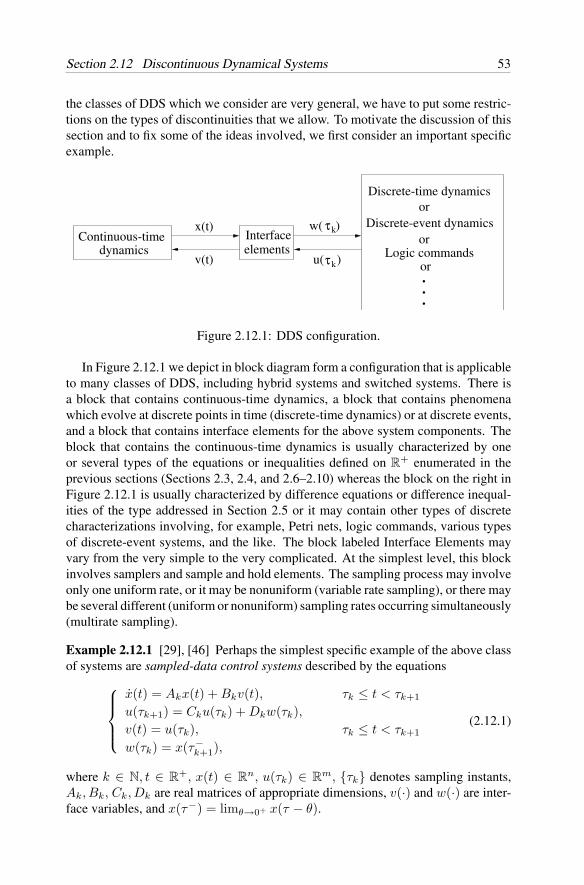
Section 2.12 Discontinuous Dynamical Systems 53
the classes of DDS which we consider are very general, we have to put some restric-tions on the types of discontinuities that we allow. To motivate the discussion of thissection and to fix some of the ideas involved, we first consider an important specificexample.
Discrete-time dynamics
x(t)Interfaceelements
orDiscrete-event dynamics
orLogic commands
or. . .
v(t) u( )
w( )
τk
Continuous-timedynamics
τk
Figure 2.12.1: DDS configuration.
In Figure 2.12.1 we depict in block diagram form a configuration that is applicableto many classes of DDS, including hybrid systems and switched systems. There isa block that contains continuous-time dynamics, a block that contains phenomenawhich evolve at discrete points in time (discrete-time dynamics) or at discrete events,and a block that contains interface elements for the above system components. Theblock that contains the continuous-time dynamics is usually characterized by oneor several types of the equations or inequalities defined on R
+ enumerated in theprevious sections (Sections 2.3, 2.4, and 2.6–2.10) whereas the block on the right inFigure 2.12.1 is usually characterized by difference equations or difference inequal-ities of the type addressed in Section 2.5 or it may contain other types of discretecharacterizations involving, for example, Petri nets, logic commands, various typesof discrete-event systems, and the like. The block labeled Interface Elements mayvary from the very simple to the very complicated. At the simplest level, this blockinvolves samplers and sample and hold elements. The sampling process may involveonly one uniform rate, or it may be nonuniform (variable rate sampling), or there maybe several different (uniform or nonuniform) sampling rates occurring simultaneously(multirate sampling).
Example 2.12.1 [29], [46] Perhaps the simplest specific example of the above classof systems are sampled-data control systems described by the equations
x(t) = Akx(t) + Bkv(t), τk ≤ t < τk+1
u(τk+1) = Cku(τk) + Dkw(τk),v(t) = u(τk), τk ≤ t < τk+1
w(τk) = x(τ−k+1),
(2.12.1)
where k ∈ N, t ∈ R+, x(t) ∈ R
n, u(τk) ∈ Rm, τk denotes sampling instants,
Ak, Bk, Ck, Dk are real matrices of appropriate dimensions, v(·) and w(·) are inter-face variables, and x(τ−) = limθ→0+ x(τ − θ).
54 Chapter 2. Dynamical Systems
Now define x(t) = x(t), t ≥ τ0 and u(t) = v(t) = u(τk), τk ≤ t < τk+1, k ∈ N.Then x(t) = x(t−) at t = τk and u(t−) = u(τk) at t = τk+1 for all k ∈ N. Lety(t)T = [x(t)T , u(t)T ]. Letting
Fk =[Ak Bk
0 0
], Hk =
[I 0
Dk Ck
]where I denotes the n × n identity matrix, the system (2.12.1) can be described bythe discontinuous ordinary differential equation
y(t) = Fky(t), τk ≤ t < τk+1
y(t) = Hky(t−), t = τk+1, k ∈ N.(2.12.2)
Next, for k ∈ N, let yk(t, yk, τk), t ≥ τk, denote the unique solution of the initialvalue problem
y(t) = Fky(t),y(τk) = yk.
(2.12.3)
Then clearly, for every y0 ∈ Rn+m, the unique solution of the DDS (2.12.2) is
given byy(t, y0, τ0) = yk(t, yk, τk), τk ≤ t < τk+1, k ∈ N.
Thus, the solutions of (2.12.2) are made up of an infinite sequence of solution seg-ments determined by the solutions of (2.12.3), k ∈ N, and these solutions may bediscontinuous at the points of discontinuity given by τk, k = 1, 2, . . . . Finally, itis clear that the solutions of (2.12.2) determine a DDS.
In Chapter 3 we develop a stability theory for general DDS, R+, X, A, S, defined
on metric spaces, and in subsequent chapters, we specialize this theory for specificclasses of finite-dimensional and infinite-dimensional dynamical systems determinedby various equations and semigroups of the type described in the present chapter. Inorder to establish meaningful and reasonable results, it is necessary to impose somerestrictions on the discontinuities of the motions p ∈ S, which of course shouldconform to assumptions that one needs to make in the modeling process of the DDS.Unless explicitly stated otherwise, we assume throughout this book that for a givendiscontinuous motion p ∈ S, the set of discontinuities is unbounded and discrete andis of the form
E1p =τp1 , τp
2 , . . . : τp1 < τp
2 < · · ·.
In the above expression, E1p signifies the fact that in general, different motions maypossess different sets of times at which discontinuities may occur. Because in mostcases, the particular set E1p in question is clear from context, we usually suppressthe p-notation and simply write
E1 =τ1, τ2, . . . : τ1 < τ2 < · · ·
.
In the remainder of this section we consider several important specific classes of DDS.
Section 2.12 Discontinuous Dynamical Systems 55
A. Ordinary differential equations
The sampled-data control system (2.12.1) which equivalently is represented by thediscontinuous differential equation (2.12.2) is a special case of discontinuous ordinarydifferential equations of the form
x(t) = fk(t, x(t)), τk ≤ t < τk+1,
x(t) = gk(x(t−)), t = τk+1, k ∈ N(SE)
where for each k ∈ N, fk ∈ C[R+ × Rn, Rn], gk : R
n → Rn, and x(τ−) is given in
Example 2.12.1.Associated with (SE), we consider the family of initial value problems given by
x(t) = fk(t, x(t))x(τk) = xk,
(SEk)
k∈N. We assume that for (τk, xk), (SEk) possesses a unique solution x(k)(t, xk, τk)which exists for all t ∈ [τk,∞) (refer to Section 2.3 for conditions that ensure this).Then for every (t0, x0) ∈ R
+ × Rn, t0 = τ0, (SE) has a unique solution x(t, x0, t0)
that exists for all t ∈ [t0,∞). This solution is made up of a sequence of continuoussolution segments x(k)(t, xk, τk), defined over the intervals [τk, τk+1) with initialconditions (τk, xk), k ∈ N, where xk+1 = x(τk+1) = gk(x(τ−
k+1)), k ∈ N and theinitial conditions (τ0 = t0, x0) are given. At the points τk+1, k ∈ N, the solutionsof (SE) have possible jumps (determined by gk(·)).
The set of all the solutions of (SE), SSE , determines a DDS, R+, X, A, SSE,
where X = A = Rn.
B. Functional differential equations ([43])
For the notation that we use in the present subsection, the reader should refer toSection 2.7.
We first consider a family of initial value problems described by continuous re-tarded functional differential equations (RFDEs) of the form
x(t) = Fk(t, xt),xτk
= ϕk,(SFk)
k ∈ N. For each k ∈ N we assume that Fk ∈ C[R+ ×Cr, Rn] and that (SFk) is well
posed so that for every (τk, ϕk) ∈ R+ × Cr, (SFk) possesses a unique continuous
solution x(k)(t, ϕk, τk) that exists for all t ∈ [τk,∞). (For conditions that ensurethis, refer to Section 2.7.)
We now consider discontinuous RFDEs of the formx(t) = Fk(t, xt), τk ≤ t < τk+1
xτk+1 = Gk
(xτ−
k+1
), k ∈ N
(SF )

56 Chapter 2. Dynamical Systems
where for each k ∈ N, Fk is assumed to possess the identical properties given in(SFk) and Gk : Cr → Cr. Thus, at t = τk+1, the mapping Gk(·) assigns to everystate xτ−
k+1(xτ−
k+1(θ) = x(τ−
k+1 + θ), −r ≤ θ ≤ 0) unambiguously a state xτk+1
(xτk+1(θ) = x(τk+1 + θ),−r ≤ θ ≤ 0).Under the above assumptions for (SF ) and (SFk), it is now clear that for every
(t0, ϕ0) ∈ R+×Cr, t0 = τ0, (SF ) has a unique solution x(t, ϕ0, t0) that exists for all
t ∈ [t0,∞). This solution is made up of a sequence of continuous solution segmentsx(k)(t, ϕk, τk) defined over the intervals [τk, τk+1), k ∈ N, with initial conditions(τk, ϕk), where ϕk = xτk
, k = 1, 2, . . . and where (τ0 = t0, ϕ0) are given. At thepoints τk+1, k ∈ N, the solutions of (SF ) have possible jumps (determined byGk(·)).
It is clear that (SF ) determines an infinite-dimensional DDS, T, X, A, S, whereT = R
+, X = A = Cr, the metric on X is determined by the norm ‖ · ‖ definedon Cr (i.e., d(ϕ, η) =‖ ϕ − η ‖ for all ϕ, η ∈ Cr), and S denotes the set of all thesolutions of (SF ) corresponding to all possible initial conditions (t0, ϕ0) ∈ R
+×Cr.In the interests of brevity, we refer to this DDS as “system (SF )” or as “(SF )”.
C. Differential equations in Banach spaces ([32])
We first consider a family of initial value Cauchy problems in Banach space X ofthe form
x(t) = Fk(t, x(t)), t ≥ τk,
x(τk) = xk(SGk)
for k ∈ N. For each k ∈ N, we assume that Fk : R+ × X → X and that x = dx/dt.
We assume that for every (τk, xk) ∈ R+ × X , (SGk) possesses a unique solution
x(k)(t, xk, τk) that exists for all t ∈ [τk,∞). We express this by saying that (SGk)is well posed.
We now consider discontinuous initial value problems in Banach space X given byx(t) = Fk(t, x(t)), τk ≤ t < τk+1
x(τk+1) = gk(x(τ−k+1)), k ∈ N
(SG)
where for each k ∈ N, Fk is assumed to possess the identical properties given in(SGk) and where gk : X → X . Under these assumptions, it is clear that for every(t0, x0) ∈ R
+ × X, t0 = τ0, (SG) has a unique solution x(t, x0, t0) that existsfor all t ∈ [t0,∞). This solution is made up of a sequence of solution segmentsx(k)(t, xk, τk), defined over the intervals [τk, τk+1), k ∈ N, with initial conditions(τk, xk), where xk = x(τk), k = 1, 2, . . . , and where (τ0 = t0, x0) are given. Atthe points τk+1, k ∈ N, the solutions of (SG) have possible jumps (determinedby gk(·)).
Consistent with the characterization of a discontinuous dynamical system given inSection 2.2, it is clear from the above that system (SG) determines a DDS, T, X,A, S, where T = R
+, A = X , the metric on X is determined by the norm ‖ · ‖defined on X (i.e., d(x, y) =‖ x−y ‖ for all x, y ∈ X), and S denotes the set of all thesolutions of (SG) corresponding to all possible initial conditions (t0, x0) ∈ R
+ ×X .
Section 2.12 Discontinuous Dynamical Systems 57
In the interests of brevity, we refer to this DDS simply as “system (SG)”, or simplyas “(SG)”.
D. Semigroups ([33])
We require a given collection of linear or nonlinear semigroups T = Ti(t) definedon a Banach space X , or on a set C ⊂ X , respectively; and a given collectionof linear and continuous operators H = Hj(Hj : X → X), or of nonlinear andcontinuous operators (Hj : C → C); and a given discrete and unbounded set E =t0 = τ0, τ1, τ2, . . . : τ0 < τ1 < τ2 · · · ⊂ R
+. The number of elements in T andH may be finite or infinite.
We now consider dynamical systems whose motions y(·, y0, t0) with initial timet0 = τ0 ∈ R
+ and initial state y(t0) = y0 ∈ X (resp., y0 ∈ C ⊂ X) are given byy(t, y0, t0) = Tk(t − τk)(y(τk)), τk ≤ t < τk+1,
y(t) = Hk(y(t−)), t = τk+1, k ∈ N.(SH)
We define the DDS determined by semigroups as
S =y = y(·, x, t0) : y(t, x, t0) = Tk(t − τk)(y(τk)), τk ≤ t < τk+1,
y(t) = Hk(y(t−)), t = τk+1, k ∈ N, t0 = τ0 ∈ R+,
y(τ0) = x ∈ X, resp., x ∈ C ⊂ X. (2.12.4)
Note that every motion y(·, x, t0) is unique, with y(t0, x, t0) = x, exists for all t≥ t0,and is continuous with respect to t on [t0,∞) − τ1, τ2, . . . , and that at t = τk,k = 1, 2, . . . , y(·, x, t0) may be discontinuous. We call the set E1 = τ1, τ2, . . . the set of discontinuities for the motion y(·, x, t0).
When in (2.12.4), T consists of C0-semigroups, we speak of a DDS determined bylinear semigroups and we denote this system by SDC0 . Similarly, when in (2.12.4),T consists of nonlinear semigroups, we speak of a DDS determined by nonlinearsemigroups and we denote this system by SDN . When the types of the elements inT are not specified, we simply speak of a DDS determined by semigroups and wedenote this system, as in (2.12.4), by S.
Finally, if in the case of SDC0 , the elements in H are linear, we use in (SH) thenotation Tk(t − τk)(y(τk)) = Tk(t − τk)y(τk) and Hk(y(t−)) = Hky(t−).
Next, a few observations may be in order:(a) For different initial conditions (x, t0), resulting in different motions y(·, x, t0),
we allow the set of discontinuities E1 = τ1, τ2, . . . , the set of semigroups Tk ⊂T , and the set of functions Hk ⊂ H to differ, and accordingly, the notationEx,t0
1 = τx,t01 , τx,t0
2 , . . . , T x,t0k and Hx,t0
k might be more appropriate. How-ever, because in all cases, all meaning is clear from context, we do not use suchsuperscripts.
(b) SDC0 and SDN are very general classes of DDS and include large classes offinite-dimensional dynamical systems determined by ordinary differential equationsand inequalities and large classes of infinite-dimensional dynamical systems deter-mined by differential-difference equations, functional differential equations, Volterra
58 Chapter 2. Dynamical Systems
integrodifferential equations, certain classes of partial differential equations, and thelike.
(c) The dynamical system models SDC0 and SDN are very flexible and include asspecial cases, many of the DDS considered in the literature (e.g., [2], [10], [28], [29],[30], [46]), as well as general autonomous continuous dynamical systems: (i) IfTk(t) = T (t) for all k (T has only one element) and if Hk = I for all k, whereI denotes the identity transformation, then SDC0 reduces to an autonomous, linear,continuous dynamical system and SDN reduces to an autonomous, nonlinear, con-tinuous dynamical system. (ii) In the case of dynamical systems subjected to impulseeffects (see, e.g., [2]), one would choose Tk(t) = T (t) for all k whereas the impulseeffects are captured by an infinite family of functions H = Hk. (iii) In the case ofswitched systems, frequently only a finite number of systems that are being switchedare required and so in this case one would choose a finite family of semigroups,T = Ti(t) (see, e.g., [10], [46]); and so forth. (iv) Perhaps it needs pointing outthat even though systems SDN and SDC0 are determined by families of semigroups(and nonlinearities), by themselves they are not semigroups, inasmuch as in general,they are time-varying and do not satisfy the hypotheses (i)–(iii) in Definitions 2.9.1and 2.9.5.
We conclude with a specific example involving partial differential equations.
Example 2.12.2 [33] (DDS determined by the heat equation) We let Ω ⊂ Rn be a
bounded domain with smooth boundary ∂Ω and we let ∆ =∑n
i=1 ∂2/∂x2i denote the
Laplacian. Also, we let X = H2[Ω, R] ∩ H10 [Ω, R] where H1
0 [Ω, R] and H2[Ω, R]are Sobolev spaces (refer to Section 2.10). For any ϕ ∈ X , we define the H1-norm by
‖ ϕ ‖2H1=
∫Ω(| ϕ|2 + |ϕ|2)dx (2.12.5)
where ϕT = (∂ϕ/∂x1, . . . , ∂ϕ/∂xn).We now consider DDS determined by the equations
∂u
∂t= ak∆u, (t, x) ∈ [τk, τk+1) × Ω
u(t, ·) = gk(u(t−, ·)) = ϕk+1(·), t = τk+1
u(t0, x) = ϕ0(x), x ∈ Ωu(t, x) = 0, (t, x) ∈ [t0,∞) × ∂Ω, k ∈ N
(2.12.6)
where ϕ0 ∈ X, ak > 0, k ∈ N, are constants, gk is a given family of mappingswith gk ∈ C[X, X], k ∈ N, and E = t0 = τ0, τ1, . . . : τ0 < τ1 < τ2 < · · · isa given unbounded and discrete set. We assume that gk(0) = 0 and there exists aconstant dk > 0 such that
‖ gk(ϕ) ‖H1≤ dk ‖ ϕ ‖H1 (2.12.7)
for all ϕ ∈ X, k ∈ N.
Section 2.13 Notes and References 59
Associated with (2.12.6) we have a family of initial and boundary value problemsdetermined by
∂u
∂t= ak∆u, (t, x) ∈ [τk,∞) × Ω
u(τk, x) = ϕk(x), x ∈ Ωu(t, x) = 0, (t, x) ∈ [τk,∞) × ∂Ω,
(2.12.8)
k ∈ N. It has been shown (e.g., [39]) that for each (τk, ϕk) ∈ R+ ×X , the initial and
boundary value problem (2.12.8) has a unique solution uk = uk(t, x), t ≥ τk, x ∈ Ω,such that uk(t, ·) ∈ X for each fixed t ≥ τk and uk(t, ·) ∈ X is a continuouslydifferentiable function from [τk,∞) to X with respect to the H1-norm given in(2.12.5).
It now follows that for every ϕ0 ∈ X , (2.12.6) possesses a unique solution u(t, ·)that exists for all t ≥ τ0 ≥ 0, given by
u(t, ·) =
uk(t, ·), τk ≤ t < τk+1
gk(uk(t−, ·)) = ϕk+1(·), t = τk+1, k ∈ N
(2.12.9)
with u(t0, x) = ϕ0(x). Notice that u(t, ·) is continuous with respect to t on the set[t0,∞)−τ1, τ2, . . . , and that at t = τk, k = 1, 2, . . . , u(t, ·) may be discontinuous(depending on the properties of gk(·)).
For each k ∈ N, (2.12.8) can be cast as an initial value problem in the space Xwith respect to the H1-norm, letting uk(t, ·) = Uk(t),
Uk(t) = AkUk(t), t ≥ τk
Uk(τk) = ϕk ∈ X(2.12.10)
where Ak = ak
∑ni=1 ∂2/∂x2
i and Uk(t, ϕk), t≥ τk, denotes the solution of (2.12.10)with U(τk, ϕk)=ϕk. It has been shown (see, e.g., [39]) that (2.12.10) determines aC0-semigroup Tk(t−τk) : X → X, where for any ϕk ∈ X, Uk(t, ϕk) = T (t−τk)ϕk.
Letting uk(t, ·) = Tk(t − τk)uk(τk) in (2.12.9), system (2.12.6) can now becharacterized as
u(t, ·) = Tk(t − τk)uk(τk, ·), τ ≤ t < τk+1
u(t, ·) = gk(uk(t−, ·)), t = τk+1, k ∈ N.(2.12.11)
Finally, it is clear that (2.12.6) (resp., (2.12.11)) determines a DDS which is a specialcase of the DDS (SH).
2.13 Notes and References
Depending on the applications, different variants of dynamical systems have beenemployed (e.g., Hahn [18], Willems [44], and Zubov [48]). Our concept of dynamicalsystem (Definition 2.2.3) was first used in [35], [36] and extensively further refinedin [34] in the study of the role of stability-preserving mappings in stability analysis
60 Chapter 2. Dynamical Systems
of dynamical systems. In the special case when X is a normed linear space andeach motion p(t, a, t0) is assumed to be continuous with respect to a, t, and t0, thedefinition of a dynamical system given in Definition 2.2.3 reduces to the definitionof a dynamical system used in Hahn [18, pp. 166–167] (called a family of motions in[18]). When the motions satisfy additional requirements that we do not enumerate,Definition 2.2.3 reduces to the definition of a dynamical system, defined on metricspace, used by Zubov [48, p. 199] (called a general system in [48]). The notion of adynamical system employed in [44] is defined on normed linear space and involvesvariations to Definition 2.2.3 which we do not specify here.
In the problem section we provide hints on how to prove the results given inSection 2.3. For the complete proofs of these results (except Theorem 2.3.3) and foradditional material on ordinary differential equations, refer to Miller and Michel [37].Our treatment of the continuation of solutions (Theorem 2.3.3) is not conventional,but very efficient, inasmuch as it involves Lyapunov results developed in subsequentchapters.
Ordinary differential inequalities (and ordinary difference inequalities) play animportant role in the qualitative analysis of dynamical systems (see, e.g., [26]) andare employed throughout this book.
Good sources on ordinary difference equations, with applications to control sys-tems and signal processing include Franklin and Powell [13] and Oppenheim andSchafer [38], respectively.
For the complete proofs of Theorems 2.7.1–2.7.3, and additional material on func-tional differential equations, refer to Hale [19]. Hale is perhaps the first to treatVolterra integrodifferential equations as functional differential equations with infinitedelay [20]. For a proof of Theorem 2.8.1, refer to Barbu and Grossman [3].
For the proofs of Theorems 2.9.1–2.9.4 and for additional material concerning Co-semigroups, refer to Hille and Phillips [21], Krein [23] (Chapter 1), and Pazy [39].For the proof of Theorem 2.9.5, refer to Slemrod [42]. For the proofs of Theorems2.9.6 and 2.9.7 and for additional material concerning nonlinear semigroups anddifferential inclusions defined on Banach spaces, refer to Crandall [8], Crandall andLiggett [9], Brezis [5], Kurtz [25], Godunov [15], Lasota and Yorke [27], and Aubinand Cellina [1]. Our presentation in Section 2.9 on semigroups and differentialinclusions defined on Banach spaces (see also Section 2.6) is in the spirit of thepresentation given in Michel and Miller [31] (Chapter 5), and Michel et al. [34].
For the proofs of Theorems 2.10.1–2.10.3, and additional material concerningpartial differential equations, refer to Krein [23], Friedman [14], and Pazy [39]. Ad-ditional sources on partial differential equations include Hormander [22] and Krylov[24]. Our presentation on partial differential equations in Section 2.10 is in the spiritof Michel and Miller [31, Chapter 5] and Michel et al. [34, Chapter 2].
Our presentation on composite dynamical systems in Section 2.11 is primarilybased on material from Michel and Miller [31], Michel et al. [34, Chapter 6], andRasmussen and Michel [40], and Section 2.12 on discontinuous dynamical systems re-lies primarily on material from Michel [29], Michel and Hu [30], Michel and Sun [32],Michel et al. [33], Sun et al. [43], and Ye et al. [46]. Finally, for a general formulationof a hybrid dynamical system defined on a metric space (involving a notion of
Section 2.14 Problems 61
generalized time), refer to Ye et al. [45] with subsequent developments given inYe et al. [46], Sun et al. [43], Michel et al. [33], Michel and Sun [32], Michel andHu [30], and Michel [29].
2.14 Problems
Problem 2.14.1 Consider a class of scalar nth-order ordinary differential equationsgiven by
y(n) = g(t, y, . . . , y(n−1)) (En)
where t ∈ J ⊂ R, J is a finite or an infinite interval, y ∈ R, y = y(1) = dy/dt, . . . ,y(n) = dny/dtn, and g ∈ C[J ×R
n, R]. Initial value problems associated with (En)are given by
y(n) = g(t, y, . . . , y(n−1))y(t0) = y0, y(t0) = y1, . . . , y(n−1)(t0) = yn−1
(IEn)
where t0 ∈ J and y0, y1, . . . , yn−1 ∈ R.Show that (En) determines a dynamical system (in the sense of Definition 2.2.3)
that we denote by SEn.
Hint: Show that (En) (and (IEn)) can equivalently be represented by a system of
n first-order ordinary differential equations.
Problem 2.14.2 Consider a class of nth-order ordinary scalar difference equationsgiven by
y(k) = g(k, y(k − 1), . . . , y(k − n)) (Dn)
where k ∈ Nn= [n, ∞) ∩ N, n ∈ N, y : N → R, and g : Nn × R
n → R. Associatedwith (Dn), consider initial value problems given by
y(k) = g(k, y(k − 1), . . . , y(k − n))y(0) = y0, y(1) = y1, . . . , y(n − 1) = yn−1
(IDn)
where y0, y1, . . . , yn−1 ∈ R.Show that (Dn) determines a dynamical system (in the sense of Definition 2.2.3)
which we denote by SDN.
Hint: Show that (Dn) (and (IDn)) can equivalently be represented by a system of
n first-order ordinary difference equations.
Problem 2.14.3 Let D denote a fixed Dini derivative and let g ∈ C[J × (R+)n, Rn]where g(t, 0) ≥ 0 for all t ∈ J . Consider differential inequalities given by
Dx ≥ g(t, x) (2.14.1)
and define a solution of (2.14.1) as a function ϕ ∈ C[[t0, t1), (R+)n
]that satisfies
(Dϕ)(t) ≥ g(t, ϕ(t)) for all t ∈ [t0, t1) ⊂ J . Associated with (2.14.1), we considerinitial value problems given by
Dx ≥ g(t, x), x(t0) = x0 (2.14.2)
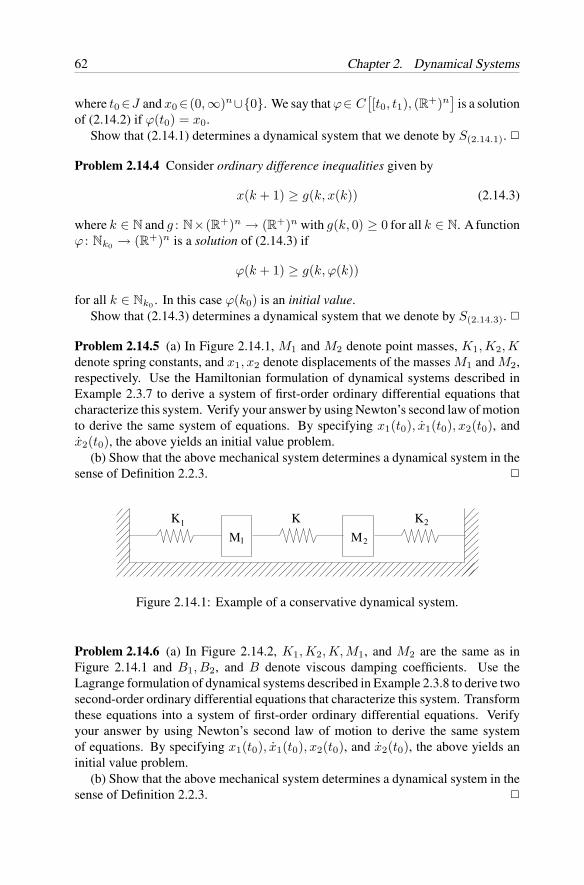
62 Chapter 2. Dynamical Systems
where t0 ∈J and x0 ∈(0,∞)n∪0. We say that ϕ∈ C[[t0, t1), (R+)n
]is a solution
of (2.14.2) if ϕ(t0) = x0.Show that (2.14.1) determines a dynamical system that we denote by S(2.14.1).
Problem 2.14.4 Consider ordinary difference inequalities given by
x(k + 1) ≥ g(k, x(k)) (2.14.3)
where k ∈ N and g : N×(R+)n → (R+)n with g(k, 0) ≥ 0 for all k ∈ N. A functionϕ : Nk0 → (R+)n is a solution of (2.14.3) if
ϕ(k + 1) ≥ g(k, ϕ(k))
for all k ∈ Nk0 . In this case ϕ(k0) is an initial value.Show that (2.14.3) determines a dynamical system that we denote by S(2.14.3).
Problem 2.14.5 (a) In Figure 2.14.1, M1 and M2 denote point masses, K1, K2, Kdenote spring constants, and x1, x2 denote displacements of the masses M1 and M2,respectively. Use the Hamiltonian formulation of dynamical systems described inExample 2.3.7 to derive a system of first-order ordinary differential equations thatcharacterize this system. Verify your answer by using Newton’s second law of motionto derive the same system of equations. By specifying x1(t0), x1(t0), x2(t0), andx2(t0), the above yields an initial value problem.
(b) Show that the above mechanical system determines a dynamical system in thesense of Definition 2.2.3.
K K K
M M1
1
2
2
Figure 2.14.1: Example of a conservative dynamical system.
Problem 2.14.6 (a) In Figure 2.14.2, K1, K2, K, M1, and M2 are the same as inFigure 2.14.1 and B1, B2, and B denote viscous damping coefficients. Use theLagrange formulation of dynamical systems described in Example 2.3.8 to derive twosecond-order ordinary differential equations that characterize this system. Transformthese equations into a system of first-order ordinary differential equations. Verifyyour answer by using Newton’s second law of motion to derive the same systemof equations. By specifying x1(t0), x1(t0), x2(t0), and x2(t0), the above yields aninitial value problem.
(b) Show that the above mechanical system determines a dynamical system in thesense of Definition 2.2.3.
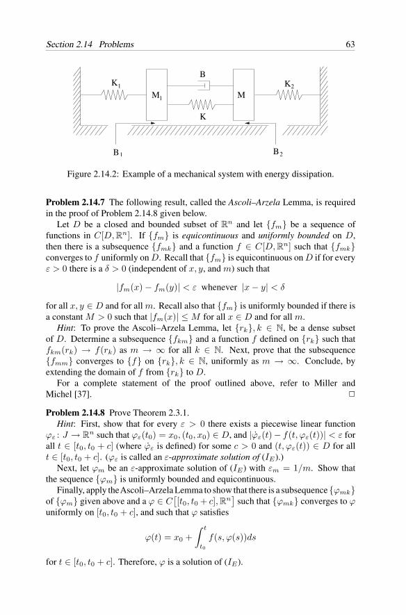
Section 2.14 Problems 63
K
K
KM M
B
B B
1
1
2
2
1
Figure 2.14.2: Example of a mechanical system with energy dissipation.
Problem 2.14.7 The following result, called the Ascoli–Arzela Lemma, is requiredin the proof of Problem 2.14.8 given below.
Let D be a closed and bounded subset of Rn and let fm be a sequence of
functions in C[D, Rn]. If fm is equicontinuous and uniformly bounded on D,then there is a subsequence fmk and a function f ∈ C[D, Rn] such that fmkconverges to f uniformly on D. Recall that fm is equicontinuous on D if for everyε > 0 there is a δ > 0 (independent of x, y, and m) such that
|fm(x) − fm(y)| < ε whenever |x − y| < δ
for all x, y ∈ D and for all m. Recall also that fm is uniformly bounded if there isa constant M > 0 such that |fm(x)| ≤ M for all x ∈ D and for all m.
Hint: To prove the Ascoli–Arzela Lemma, let rk, k ∈ N, be a dense subsetof D. Determine a subsequence fkm and a function f defined on rk such thatfkm(rk) → f(rk) as m → ∞ for all k ∈ N. Next, prove that the subsequencefmm converges to f on rk, k ∈ N, uniformly as m → ∞. Conclude, byextending the domain of f from rk to D.
For a complete statement of the proof outlined above, refer to Miller andMichel [37].
Problem 2.14.8 Prove Theorem 2.3.1.Hint: First, show that for every ε > 0 there exists a piecewise linear function
ϕε : J → Rn such that ϕε(t0) = x0, (t0, x0) ∈ D, and |ϕε(t) − f(t, ϕε(t))| < ε for
all t ∈ [t0, t0 + c] (where ϕε is defined) for some c > 0 and (t, ϕε(t)) ∈ D for allt ∈ [t0, t0 + c]. (ϕε is called an ε-approximate solution of (IE).)
Next, let ϕm be an ε-approximate solution of (IE) with εm = 1/m. Show thatthe sequence ϕm is uniformly bounded and equicontinuous.
Finally, apply theAscoli–Arzela Lemma to show that there is a subsequenceϕmkof ϕm given above and a ϕ ∈ C
[[t0, t0 + c], Rn
]such that ϕmk converges to ϕ
uniformly on [t0, t0 + c], and such that ϕ satisfies
ϕ(t) = x0 +∫ t
t0
f(s, ϕ(s))ds
for t ∈ [t0, t0 + c]. Therefore, ϕ is a solution of (IE).
64 Chapter 2. Dynamical Systems
For a complete statement of the proof outlined above, refer to Miller andMichel [37].
Problem 2.14.9 The following result, called the Gronwall Inequality is required inthe proof of Problem 2.14.10 given below.
Let r, k ∈ C[[a, b], R+
]and let δ ≥ 0 such that
r(t) ≤ δ +∫ t
a
k(s)r(s)ds, a ≤ t ≤ b. (2.14.4)
Then
r(t) ≤ δ exp[∫ t
a
k(s)ds
], a ≤ t ≤ b. (2.14.5)
Hint: For δ > 0, integrate both sides of
k(s)r(s)δ +
∫ s
ak(η)r(η)dη
≤ k(s)
from a to t. Use inequality (2.14.4) to conclude the result when δ = 0. When δ = 0,consider a positive sequence δn such that δn → 0 as n → ∞ and apply it to(2.14.5).
For a complete statement of the proof outlined above, refer to Miller andMichel [37].
Problem 2.14.10 Prove Theorem 2.3.2Hint: Apply the Gronwall inequality given above in Problem 2.14.9.For a complete statement of the proof, refer to Miller and Michel [37].
Problem 2.14.11 The following result is required in the proof of Problem 2.14.12given below.
Let D ⊂ R × Rn be a domain. Let f ∈ C[D, Rn] with f bounded on D and let
ϕ be a solution of (E) on the interval (a, b). Show that
(a) The two limits limt→a+ ϕ(t) = ϕ(a+) and limt→b− ϕ(t) = ϕ(b−) exist.
(b) If (a, ϕ(a+)) ∈ D (resp., (b, ϕ(b−)) ∈ D), then the solution ϕ can be continuedto the left past the point t = a (resp., to the right past the point t = b).
(A complete statement of the proof of the above result can be found in Miller andMichel [37].)
Problem 2.14.12 Prove Theorem 2.3.3.Hint: Use the result given in Problem 2.14.11.
Problem 2.14.13 Prove Theorem 2.7.1.Hint: To prove this result, use Schauder’s Fixed Point Theorem: A continuous
mapping of a compact convex set in a Banach space X into itself has at least onefixed point. Let T be the operator defined by (2.7.7). Find a compact convex set
Section 2.14 Problems 65
X ⊂ C[[t0 − r, t0 + c], Rn
]for some c > 0 such that T (X) ⊂ X . Now apply
Schauder’s Fixed Point Theorem. A possible choice of X is given by
X =x ∈ C
[[−r+t0, t0+c], Rn
]: xt0 = ψ, ‖ xt−ψ ‖≤ d for all t ∈ [t0, t0+c]
,
where 0 < c ≤ d/M, d > 0 sufficiently small, with M ≥ |f(t, ϕ)| for all (t, ϕ) in afixed neighborhood of (t0, ψ) in Ω.
For the complete proof of Theorem 2.7.1 outlined above, refer to Hale [19].
Problem 2.14.14 Prove Theorem 2.7.2.Hint: Let x(t) and y(t) be two solutions of (IF ). Then
x(t) − y(t) =∫ t
t0
[f(s, xs) − f(s, ys)] ds, t ≥ t0, xt0 − yt0 = 0.
Using the above, show that there exists a c0 > 0 such that x(t) = y(t) for allt ∈ [t0 − r, t0 + c0]. To complete the proof, repeat the above for successive intervalsof length c0.
For the complete proof of Theorem 2.7.2 outlined above, refer to Hale [19].
Problem 2.14.15 The following result is required in the proof of Problem 2.14.16given below.
Let Ω be an open set in R × Cr and let F : Ω → Rn be completely continuous.
Assume that p ∈ C[[t0 − r, b), Rn
]is a noncontinuable solution of (F ). Show that
for any bounded closed set U in R × Cr, U ⊂ Ω, there exists a tU ∈ (t0, b) such that(t, pt) /∈ U for every t ∈ [tU , b].
Hint: The case b = ∞ is clear. Suppose that b is finite. The case r = 0 reduces toan ordinary differential equation. So assume that r > 0. Now prove the assertion bycontradiction, assuming that b < ∞ and r > 0.
Problem 2.14.16 Prove Theorem 2.7.3.Hint: Apply the result given in Problem 2.14.15. For the complete proof, refer to
Hale [19].
Problem 2.14.17 Prove Theorem 2.8.1.Hint: Using the theory of C0-semigroups, refer to Example 2.9.3 for a choice of
the infinitesimal generator for the C0-semigroup (refer to [3]).
Problem 2.14.18 Consider the initial value problemx = A(t)xx(t0) = x0
(LH)
where A ∈ C[R+, Rn×n].(a) Show that the set of solutions obtained for (LH) by varying (t0, x0) over
(R+, Rn) determines a dynamical system in the sense of Definition 2.2.3.(b) Show that in general, (LH) does not determine a C0-semigroup.(c) Show that when A(t) ≡ A, (LH) determines a C0-semigroup.
66 Chapter 2. Dynamical Systems
Problem 2.14.19 Prove the assertion made in Example 2.9.1 that the initial valueproblem (2.9.4) determines a quasi-contractive semigroup.
Problem 2.14.20 Consider the initial value problem for the heat equation∂u
∂t= a2∆u, x ∈ R
n, t ∈ R+
u(0, x) = ϕ(x), x ∈ Rn
(2.14.6)
where a > 0, ∆ =∑n
i=1 ∂2/∂x2i , and ϕ ∈ C[Rn, R] is bounded.
(a) Verify that the unique solutions of (2.14.6) are given by Poisson’s formula,
u(t, x) =1
(2a√
πt)n
∫Rn
e−|x−y|2/(4a2t)ϕ(y)dy.
(b) Show that the operators T (t), t ∈ R+, determined by u(t, ·) = T (t)ϕ, deter-
mine a C0-semigroup.
Problem 2.14.21 Consider the initial value problem for the one-dimensional waveequation
∂2u
∂t2= c2 ∂2u
∂x2 , x ∈ R, t ∈ R+
u(0, x) = ϕ(x),∂u
∂t(0, x) = ψ(x), x ∈ R
(2.14.7)
where c > 0, ϕ ∈ C2[R, R], and ψ ∈ C1[R, R].
(a) Verify that the unique solution of (2.14.7) is given by d’Alembert’s formula
u(t, x) =12[ϕ(x − ct) + ϕ(x + ct)
]+
12c
∫ x+ct
x−ct
ψ(η)dη.
(b) Let ψ ≡ 0. For ϕ ∈ C2[R, R], define the operators T (t), t ∈ R+, by
T (t)ϕ = u(t, ·). Show that T (t), t ∈ R+, do not satisfy the semigroup property
(specifically, they do not satisfy the property T (t)T (s) = T (t + s), t, s ∈ R+).
(c) Now let u(t, ϕ, t0) denote the solutions of∂2u
∂t2= c2 ∂2u
∂x2 , x ∈ R, t ≥ t0
u(t0, x) = ϕ(x),∂u
∂t(t0, x) = 0, x ∈ R
(2.14.8)
where t0 ∈ R+ and ϕ ∈ C2[R, R]. Show that for all ϕ ∈ C2[R, R], the resulting
solutions u(t, ϕ, t0) form a dynamical system in the sense of Definition 2.2.3 withT = R
+, X = A = C2[R, R] where we assume that X is equipped with some norm(e.g., ‖ ϕ ‖= maxx∈R |ϕ(x)|).
Bibliography 67
Problem 2.14.22 We now consider a specific class of multirate digital feedback con-trol systems. The plant is described by
x(t) = Ax(t) + B1u1c(t) + B2u2c(t)
y(t) =[y1(t)y2(t)
]=[D1x(t)D2x(t)
](2.14.9)
where x∈Rn, A∈ R
n×n, B1 ∈ Rn×n1 , B2 ∈ R
n×n2 , D1 ∈ Rm1×n, D2 ∈ R
m2×n,u1c ∈ R
n1 , u2c ∈ Rn2 , and
u1c(t) = u1(k), kTb ≤ t < (k + 1)Tb, k ∈ N,u2c(t) = u2(2k), 2kTb ≤ t < 2(k + 1)Tb, k ∈ N.
(2.14.10)
In (2.14.10), Tb > 0 is the basic sampling period whereas u1(k) and u2(2k) arespecified by output feedback equations of the form
u1(k + 1) = F1u1(k) + K1y1(kTb)= F1u1(k) + K1D1x(kTb), k ∈ N (2.14.11)
u2(2(k + 1)) = F2u2(2k) + K2y2(2kTb)= F2u2(2k) + K2D2x(2kTb), k ∈ N
where K1, K2, F1, and F2 are matrices of appropriate dimensions. The system inputsu1c(t) and u2c(t) are realized by multirate zero-order hold elements.
Similarly as in Example 2.12.1, show that the above hybrid system can equiva-lently be represented by a system of discontinuous ordinary differential equations thatgenerate a discontinuous dynamical system.
Bibliography[1] J. P. Aubin and A. Cellina, Differential Inclusions, New York: Springer-Verlag,
1984.
[2] D. D. Bainov and P. S. Simeonov, Systems with Impulse Effects: Stability Theoryand Applications, New York: Halsted Press, 1989.
[3] V. Barbu and S. I. Grossman, “Asymptotic behavior of linear integrodifferentialsystems,” Trans. Amer. Math. Soc., vol. 171, pp. 277–288, 1972.
[4] R. Bellman and K. L. Cooke, Differential-Difference Equations, New York:Academic Press, 1963.
[5] H. Brezis, Operateurs Maximaux Monotones, Amsterdam: North-Holland,1973.
[6] R. W. Brockett, “Hybrid models for motion control systems,” Essays on ControlPerspectives in the Theory and Its Applications, H. L. Trentelman and J. C.Willems, Eds., Boston: Birkhauser, pp. 29–53, 1993.
68 Chapter 2. Dynamical Systems
[7] B. Brogliato, S. I. Niculescu, and P. Orhant, “On the control of finite-dimensionalsystems with unilateral constraints,” IEEE Trans. Autom. Control, vol. 42, pp.200–215, 1997.
[8] M. G. Crandall, “Semigroups of nonlinear transformations on general Banachspaces,” Contributions to Nonlinear Functional Analysis, E. H. Zarantonello,Ed., New York: Academic Press, 1971.
[9] M. G. Crandall and T. M. Liggett, “Generation of semigroups of nonlinear trans-formations on general Banach spaces,” Amer. J. Math., vol. 93, pp. 265–298,1971.
[10] R. DeCarlo, S. Branicky, S. Pettersson, and B. Lennartson, “Perspectives andresults on the stability and stabilizability of hybrid systems,” Proc. IEEE, vol.88, pp. 1069–1082, 2000.
[11] J. Dieudonne, Foundations of Modern Analysis, New York: Academic Press,1960.
[12] N. Dunford and J. T. Schwarz, Linear Operators, Part I, New York: Wiley,1958.
[13] G. F. Franklin and J. D. Powell, Digital Control of Dynamical Systems, Reading,MA: Addison-Wesley, 1980.
[14] A. Friedman, Partial Differential Equations of the Parabolic Type, EnglewoodCliffs, NJ: Prentice Hall, 1964.
[15] A. N. Godunov, “Peano’s theorem in Banach spaces,” Functional Anal. Appl.,vol. 9, pp. 53–56, 1975.
[16] A. Gollu and P. P. Varaiya, “Hybrid dynamical systems,” Proc. 28th IEEE Conf.on Decision and Control, Tampa, FL, Dec. 1989, pp. 2708–2712.
[17] R. Grossman, A. Nerode, A. Ravn, and H. Rischel, Eds., Hybrid Systems, NewYork: Springer-Verlag, 1993.
[18] W. Hahn, Stability of Motion, Berlin: Springer-Verlag, 1967.
[19] J. K. Hale, Functional Differential Equations, Berlin: Springer-Verlag, 1971.
[20] J. K. Hale, “Functional differential equations with infinite delays,” J. Math.Anal. Appl., vol. 48, pp. 276–283, 1974.
[21] E. Hille and R. S. Phillips, Functional Analysis and Semigroups, Amer. Math.Soc. Colloquium Publ., vol. 33, Providence, RI: American Mathematical Soci-ety, 1957.
[22] L. Hormander, Linear Partial Differential Equations, Berlin: Springer-Verlag,1963.
[23] S. G. Krein, Linear Differential Equations in Banach Spaces, Translation ofMathematical Monographs, vol. 29, Providence, RI: American MathematicalSociety, 1970.
[24] N. V. Krylov, Nonlinear Elliptic and Parabolic Equations of the Second Order,Boston: D. Reidel, 1987.
Bibliography 69
[25] T. Kurtz, “Convergence of sequences of semigroups of nonlinear equations withapplications to gas kinetics,” Trans. Amer. Math. Soc., vol. 186, pp. 259–272,1973.
[26] V. Lakshmikantham and S. Leela, Differential and Integral Inequalities, vol. I,II, New York: Academic Press, 1969.
[27] A. Lasota and J. A. Yorke, “The generic property of existence of solutions ofdifferential equations in Banach space,” J. Differential Equations, vol. 13, pp.1–12, 1973.
[28] D. Liberzon andA. S. Morse, “Basic problems in stability and design of switchedsystems,” IEEE Control Syst. Mag., vol. 19, pp. 59–70, 1999.
[29] A. N. Michel, “Recent trends in the stability analysis of hybrid dynamical sys-tems,” IEEE Trans. Circ. and Syst., vol. 46, pp. 120–134, 1999.
[30] A. N. Michel and B. Hu, “Towards a stability theory of general hybrid dynamicalsystems,” Automatica, vol. 35, pp. 371–384, 1999.
[31] A. N. Michel, and R. K. Miller, Qualitative Analysis of Large Scale DynamicalSystems, New York: Academic Press, 1977.
[32] A. N. Michel andY. Sun, “Stability of discontinuous Cauchy problems in Banachspace,” Nonlinear Anal., vol. 65, pp. 1805–1832, 2006.
[33] A. N. Michel, Y. Sun, and A. P. Molchanov, “Stability analysis of discontinuousdynamical systems determined by semigroups,” IEEE Trans. Autom. Control,vol. 50, pp. 1277–1290, 2005.
[34] A. N. Michel, K. Wang, and B. Hu, Qualitative Theory of Dynamical Systems –The Role of Stability Preserving Mappings, Second Edition, New York: MarcelDekker, 2001.
[35] A. N. Michel, K. Wang, and K. M. Passino, “Qualitative equivalence of dynam-ical systems with applications to discrete event systems,” Proc. of the 31st IEEEConf. on Decision and Control, Tucson, AZ, Dec. 1992, pp. 731–736.
[36] A. N. Michel, K. Wang and K. M. Passino, “Stability preserving mappingsand qualitative equivalence of dynamical systems, Part I,” Avtomatika i Tele-mekhanika, vol. 10, pp. 3–12, 1994.
[37] R. K. Miller and A. N. Michel, Ordinary Differential Equations, New York:Academic Press, 1982.
[38] A. V. Oppenheim and R. W. Schafer, Digital Signal Processing, EnglewoodCliffs, NJ: Prentice Hall, 1975.
[39] A. Pazy, Semigroups of Linear Operators and Applications to Partial Differen-tial Equations, New York: Springer-Verlag, 1963.
[40] R. D. Rasmussen and A. N. Michel, “Stability of interconnected dynamicalsystems described on Banach spaces,” IEEE Trans. Autom. Control, vol. 21, pp.464–471, 1976.
70 Chapter 2. Dynamical Systems
[41] C. Rui, I. Kolmanovsky, and N. H. McClamroch, “Hybrid control for stabiliza-tion of a class of cascade nonlinear systems,” Proc. American Control Conf.,Albuquerque, NM, June 1997, pp. 2800–2804.
[42] M. Slemrod, “Asymptotic behavior of C0-semigroup as determined by the spec-trum of the generator,” Indiana Univ. Math. J., vol. 25, pp. 783–791, 1976.
[43] Y. Sun,A. N. Michel, and G. Zhai, “ Stability of discontinuous retarded functionaldifferential equations with applications,” IEEE Trans. Autom. Control, vol. 50,pp. 1090–1105, 2005.
[44] J. C. Willems, “Paradigms and puzzles in the theory of dynamical systems,”IEEE Trans. Autom. Control, vol. 36, pp. 259–294, 1991.
[45] H. Ye, A. N. Michel, and P. J. Antsaklis “A general model for the qualitativeanalysis of hybrid dynamical systems,” Proc. of the 34th IEEE Conf. on Decisionand Control, New Orleans, LA, Dec. 1995, pp. 1473–1477.
[46] H. Ye, A. N. Michel, and L. Hou, “Stability theory for hybrid dynamical sys-tems,” IEEE Trans. Autom. Control, vol. 43, pp. 461–474, 1998.
[47] T. Yoshizawa, Stability Theory by Lyapunov’s Second Method, Math. Soc.,Japan, Tokyo, 1966.
[48] V. I. Zubov, Methods of A.M. Lyapunov and Their Applications, Groningen, TheNetherlands: P. Noordhoff, 1964.
Chapter 3
Fundamental Theory: ThePrincipal Stability andBoundedness Results onMetric Spaces
In this chapter we present the Principal Lyapunov and Lagrange Stability Results,including Converse Theorems for continuous dynamical systems, discrete-time dy-namical systems, and discontinuous dynamical systems (DDS) defined on metricspaces. The results of this chapter constitute the fundamental theory for the entirebook because most of the general results that we develop in the subsequent chap-ters concerning finite-dimensional systems (described on finite-dimensional linearspaces) and infinite-dimensional systems (defined on Banach and Hilbert spaces) canbe deduced as consequences of the results of the present chapter. Most of the spe-cific applications to the fundamental theory that we consider therefore are deferredto the later chapters where we address finite-dimensional and infinite-dimensionalsystems. However, after addressing in the next chapter additional (more specialized)stability and boundedness results for dynamical systems defined on metric spaces,we present applications to the results of this chapter in Chapter 5 in the analysis ofa class of discrete-event systems (with applications to a manufacturing system anda computer load-balancing problem) that determine dynamical systems defined onmetric spaces.
The conventional approach in proving the various Principal Lyapunov and La-grange Stability Results for continuous, discrete-time, and discontinuous dynamicalsystems is to show that when a dynamical system satisfies a certain set of hypotheses,then the system possesses a certain type of stability or boundedness property. For thereasons discussed below we do not pursue this approach (however, we ask the readerto do so in the exercise section).
71
72 Chapter 3. Principal Stability and Boundedness Results on Metric Spaces
In establishing the results presented in this chapter, we first prove the PrincipalLyapunov and Lagrange Stability Results for discontinuous dynamical systems, usingbasic principles and definitions. Next, to establish the Principal Lyapunov and La-grange Stability Results for continuous dynamical systems, we show that wheneverthe hypotheses of a given stability or boundedness result for continuous dynamicalsystems are satisfied, then the hypotheses of the corresponding stability or bound-edness result for DDS are also satisfied (using the fact that continuous dynamicalsystems may be viewed as special cases of DDS). This shows that the classical Lya-punov and Lagrange Stability Results for continuous dynamical systems reduce to thecorresponding results for DDS (i.e., the classical Principal Lyapunov and LagrangeStability Results for continuous dynamical systems are more conservative than thecorresponding Lyapunov and Lagrange Stability Results for DDS). Indeed, we presenta result for a continuous dynamical system whose equilibrium can be shown to beuniformly asymptotically stable, using the uniform asymptotic stability theorem forDDS, and we show that for the same example, no Lyapunov function exists that sat-isfies the classical uniform asymptotic stability theorem for continuous dynamicalsystems.
Next, we show that for every discrete-time dynamical system there exists an asso-ciated DDS with identical stability and boundedness properties. Making use of suchassociated DDSs, we show that when the hypotheses of a given classical Lyapunovor Lagrange stability result for discrete-time dynamical systems are satisfied, thenthe hypotheses of the corresponding Lyapunov and Lagrange stability result for DDSare satisfied. This shows that the classical Lyapunov and Lagrange stability resultsfor discrete-time dynamical systems reduce to the corresponding results for DDS(i.e., the classical Principal Lyapunov and Lagrange stability results for discrete-timedynamical systems are more conservative than the corresponding Lyapunov and La-grange stability results for DDS). We present a specific example of a discrete-timedynamical system whose equilibrium can be shown to be uniformly asymptoticallystable using the uniform asymptotic stability theorem for DDS, and we show that forthe same example, no Lyapunov function exists that satisfies the classical Lyapunovtheorem for uniform asymptotic stability for discrete-time dynamical systems.
In addition to giving us a great deal of insight, the approach that we employin proving the various stability and boundedness results culminates in a unifyingqualitative theory for the analysis of continuous, discrete-time, and discontinuousdynamical systems. Furthermore, our approach in proving the results presented hereinis more efficient than the conventional approach alluded to earlier.
This chapter is organized into eight sections. In the first section we addressthe qualitative characterization of invariant sets of dynamical systems. In the nextthree sections we present and prove the principal Lyapunov stability results and theLagrange stability results (boundedness of motions) for discontinuous dynamical sys-tems, continuous dynamical systems, and discrete-time dynamical systems, respec-tively. This is followed by three sections where we address converse theorems forDDS, continuous dynamical systems, and discrete-time dynamical systems. Finally,in Section 3.8 we present some required background material concerning ordinarydifferential equations.
Section 3.1 Some Qualitative Characterizations of Dynamical Systems 73
Before proceeding with our subject on hand, we would like to remind the reader thatour definition of dynamical system (Definition 2.2.3) does in general not require thattime be reversible in the motions (in contrast to many dynamical systems determined,e.g., by various types of differential equations), nor are the motions required to beunique with respect to initial conditions. For such general systems, when required,we make an assumption that is akin to the semigroup property, but is more general,which essentially requires that for a dynamical system S, any partial motion is alsoa motion of S, and any composition of two motions is also a motion of S (refer toAssumption 3.5.1). Of course when in a dynamical system the semigroup propertyholds, then Assumption 3.5.1 is automatically implied.
3.1 Some Qualitative Characterizations of DynamicalSystems
Most, but not all the qualitative aspects of dynamical systems that we address concernqualitative characterizations of invariant sets. In the present section, we first introducethe notion of an invariant set of a dynamical system. Next, we present various conceptsof stability of invariant sets, instability of sets, and boundedness of motions.
A. Invariant sets
In the following, we utilize the notation introduced in Chapter 2.
Definition 3.1.1 Let T, X, A, S be a dynamical system. A set M ⊂ A is said tobe invariant with respect to S, or for short, (S, M) is invariant, if a ∈ M impliesthat p(t, a, t0) ∈ M for all t ∈ Ta,t0 , all t0 ∈ T , and all p(·, a, t0) ∈ S.
Recall that Ta,t0 = [t0, t1)∩T , t1 > t0, which means that in the above definition,evolution in time is forward.
In a broader context, the evolution in time is allowed to be forward as well asbackward. In such cases, a distinction is made between positive invariant set (forwardin time) and negative invariant set (backward in time) (see, e.g., [11]).
We note that the union of invariant sets is also an invariant set.
Example 3.1.1 (Conservative dynamical systems) Recall the Hamiltonian systemgiven in Example 2.3.7, described by the equations
qi =∂H
∂pi(p, q), i = 1, . . . , n,
pi = −∂H
∂qi(p, q), i = 1, . . . , n.
(3.1.1)
The solutions of (3.1.1) determine a continuous dynamical system with T = R andX = A = R
2n. For any c ∈ R such that the set
Mc =(p, q)T ∈ R
2n : H(p, q) = c
74 Chapter 3. Principal Stability and Boundedness Results on Metric Spaces
is nonempty, Mc is an invariant set. This follows, because
dH
dt(p(t), q(t)) ≡ 0
for all solutions (p(t), q(t))T of (3.1.1), as shown in Example 2.3.7.
Example 3.1.2 (Heat equation) Let Ω ⊂ Rn be a domain with smooth boundary
∂Ω and consider the initial value and boundary value problem given by the equations(see also Chapter 2)
∂u
∂t= a2∆u, x ∈ Ω, t ≥ t0
u(t0, x) = ϕ(x), x ∈ Ωu(t, x) = 0, x ∈ ∂Ω, t > t0
(3.1.2)
where t0 ≥ 0, a > 0, ∆ =∑n
i=1∂2/∂x2
i , and ϕ ∈ C[Ω, R] with limx→∂Ω ϕ(x) = 0.Let T = R
+,X = A =
ϕ ∈ C[Ω, R] : lim
x→∂Ωϕ(x) = 0
and let X and A be equipped with the norm
‖ϕ‖ = maxx∈Ω
|ϕ(x)|.
It has been shown that for every ϕ ∈ A, (3.1.2) possesses a unique solution u(t, x)that exists for all t ≥ t0. It follows that T, X, A, S(3.1.2) is a dynamical systemwhere the set of motions is determined by the solutions of (3.1.2).
Let M ⊂ A = X denote the set given by
M =ϕ ∈ C2[Ω, R] ∩ X : ∆ϕ(x) = 0 for all x ∈ Ω
.
Then M is invariant with respect to S(3.1.2). Indeed, for any ϕ ∈ M , u(t, x) ≡ ϕ(x)is a solution of (3.1.2). By the uniqueness of each solution, it follows that M isinvariant with respect to S(3.1.2).
The most important special case of invariant sets is an equilibrium.
Definition 3.1.2 We call x0 ∈ A an equilibrium (or an equilibrium point) of a dy-namical system T, X, A, S if the set x0 ⊂ A is invariant with respect to S (i.e.,(S, x0) is invariant).
In the following, we enumerate several specific examples of equilibria.
Example 3.1.3 (Ordinary differential equations) Let f ∈ C[R+ × Ω, Rn] whereΩ ⊂ R
n is a domain, assume that xe ∈ Ω satisfies f(t, xe) = 0 for all t ∈ R+, and
that the system of first-order ordinary differential equations
x = f(t, x) (E)
has a unique solution for the initial condition x(t0) = xe. As pointed out in Chapter 2,this is true if, for example, f satisfies a Lipschitz condition. Then xe is an equilibriumof the dynamical system SE determined by the solutions of (E). In this case we alsosay that xe is an equilibrium of (E).
Section 3.1 Some Qualitative Characterizations of Dynamical Systems 75
Example 3.1.4 (Ordinary difference equations) Let f : N × Rn → R
n and assumethat there exists an xe ∈ R
n such that f(k, xe) = xe for all k ∈ N. Then xe is anequilibrium of the dynamical system SD determined by the solutions of the systemof ordinary difference equations given by
x(k + 1) = f(k, x(k)), (D)
k ∈ N.
Example 3.1.5 (Heat equation) In Example 3.1.2, each ϕ ∈ M is an equilibrium of(3.1.2).
Example 3.1.6 (Ordinary differential equations in a Banach space) Let X be aBanach space, let C ⊂ X , and let F : R
+ × C → X . Assume that F (t, xe) = 0 forall t ∈ R
+ and thatx(t) = F (t, x(t)), x(t0) = xe (3.1.3)
has a unique solution for any t0 ∈ R+. Then xe is an equilibrium of the dynamical
system determined by the solutions of
x(t) = F (t, x(t)). (3.1.4)
In this case we also say that xe is an equilibrium of (3.1.4).
Example 3.1.7 (Semigroups) Let T (t), t ∈ R+, be a linear or nonlinear semigroup
(see Chapter 2) defined on a subset C of a Banach space X . If there exists an xe ∈ Csuch that T (t)xe = xe for all t ∈ R
+, then xe is an equilibrium of the dynamicalsystem determined by the semigroup T (t). In this case we also say that xe is anequilibrium of the semigroup T (t).
We conclude this subsection by introducing several additional concepts that werequire.
Definition 3.1.3 A dynamical system T, X, A, S is said to satisfy the uniquenessproperty if for any (a, t0) ∈ A × T there exists a unique noncontinuable mo-tion p(·, a, t0) ∈ S (refer to Definition 2.2.6 for the definition of noncontinuablemotion).
When a dynamical system is determined by equations of the type considered inChapter 2, the uniqueness property of a dynamical system is equivalent to the unique-ness of solutions of initial value problems determined by such equations.
Definition 3.1.4 For each motion p(·, a, t0)∈S in a dynamical system T, X, A, S,the set
C(p) =x ∈ X : x = p(t, a, t0) for some t ≥ t0 and t ∈ T
is called a trajectory.
76 Chapter 3. Principal Stability and Boundedness Results on Metric Spaces
In the literature where evolution in time is allowed to be forward and backward, adistinction is made between positive semitrajectory (forward in time) and a negativesemitrajectory (backward in time) (refer, e.g., to [11]).
Definition 3.1.5 A motion p(·, a, t0) ∈ S in a dynamical system T, X, A, S is saidto be periodic if there exists a constant ω > 0 such that t + ω ∈ T for each t ∈ T ,and such that p(t + ω, a, t0) = p(t, a, t0) for all t ∈ T , t ≥ t0, and t ∈ T . We call ωa period of the periodic motion p(·, a, t0).
If a dynamical system S satisfies the uniqueness property, then clearly any trajec-tory of a motion in S is an invariant set. In particular, the trajectory of a periodicmotion, which is usually a closed curve in a metric space X , is an invariant set.Furthermore, the union of a family of trajectories is an invariant set of S.
B. Qualitative characterizations: Stability and boundedness
Let T, X, A, S be a dynamical system and assume that M ⊂ A is an invariant setof S, or for short, that (S, M) is invariant. In the definitions that follow, the phrase“(S, M) is said to be . . . ” is understood to mean “the set M that is invariant withrespect to system S is said to be . . . ”. Thus, in Definition 3.1.6 given below, “(S, M)is said to be stable . . . ” should be read as “the set M that is invariant with respect tosystem S is said to be stable . . . ”.
Let (X, d) be a metric space. We recall that the distance between a point a ∈ Xand a set M ⊂ X is defined as
d(a, M) = infx∈M
d(a, x).
Finally, the reader should make reference to Definition 2.2.1 for the meaning of theset Ta,t0 .
Definition 3.1.6 (S, M) is said to be stable if for every ε > 0 and every t0 ∈ T ,there exists a δ = δ(ε, t0) > 0 such that d(p(t, a, t0), M) < ε for all t ∈ Ta,t0 andfor all p(·, a, t0) ∈ S, whenever d(a, M) < δ. (S, M) is said to be uniformly stableif it is stable and if in the above, δ is independent of t0 (i.e., δ = δ(ε)).
In the following definitions, we address asymptotic properties of invariant setswith respect to dynamical systems. Throughout this book, whenever we deal withasymptotic properties, we assume that for any (a, t0) ∈ A × T , Ta,t0 = [t0,∞) ∩ Tand that T ∩ [α,∞) = ∅ for any α > 0.
Definition 3.1.7 (S, M) is attractive if there exists an η = η(t0) > 0 such thatlimt→∞ d(p(t, a, t0), M) = 0 for all p(·, a, t0) ∈ S whenever d(a, M) < η.
We call the set of all a ∈ A such that limt→∞ d(p(t, a, t0), M) = 0 for allp(·, a, t0) ∈ S the domain of attraction of (S, M) at time t0.
Definition 3.1.8 (S, M) is asymptotically stable if it is stable and attractive.
Section 3.1 Some Qualitative Characterizations of Dynamical Systems 77
Definition 3.1.9 (S, M) is uniformly asymptotically stable if
(i) it is uniformly stable; and(ii) for every ε > 0 and every t0 ∈ T , there exist a δ > 0, independent of t0 and
ε, and a τ = τ(ε) > 0, independent of t0, such that d(p(t, a, t0), M) < ε forall t ∈ Ta,t0+τ and for all p(·, a, t0) ∈ S whenever d(a, M) < δ.
When condition (ii) in the above definition is satisfied, we say that (S, M) isuniformly attractive.
Definition 3.1.10 (S, M) is exponentially stable if there exists an α > 0, and forevery ε > 0 and every t0 ∈ T , there exists a δ = δ(ε) > 0 such that
d(p(t, a, t0), M) < εe−α(t−t0)
for all t ∈ Ta,t0 and for all p(·, a, t0) ∈ S whenever d(a, M) < δ.
Note that the exponential stability of (S, M) implies the uniform asymptotic sta-bility of (S, M).
Definition 3.1.11 (S, M) is unstable if it is not stable.
The preceding definitions concern local characterizations. In the remaining defi-nitions we address global characterizations.
Definition 3.1.12 A motion p(·, a, t0) ∈ S is bounded if there exists a β > 0 suchthat d(p(t, a, t0), a) < β for all t ∈ Ta,t0 .
Definition 3.1.13 A dynamical system S is uniformly bounded if for every α > 0and for every t0 ∈ T there exists a β = β(α) > 0 (independent of t0) such that ifd(a, x0) < α, then for p(·, a, t0) ∈ S, d(p(t, a, t0), x0) < β for all t ∈ Ta,t0 , wherex0 is a fixed point in X .
Definition 3.1.14 A uniformly bounded dynamical system S is uniformly ultimatelybounded if there exists a B > 0 and if corresponding to any α > 0 and t0 ∈ T ,there exists a τ = τ(α) > 0 (independent of t0) such that for all p(·, a, t0) ∈ S,d(p(t, a, t0), x0) < B for all t ∈ Ta,t0+τ whenever d(a, x0) < α, where x0 is a fixedpoint in X .
In the above two definitions, the constants β and B may in general depend onthe choice of x0 ∈ X . However, the definitions themselves are independent of thechoice of x0. More generally, we may replace x0 ∈ X in these definitions by anyfixed bounded set in X .
Definition 3.1.15 (S, M) is asymptotically stable in the large if
(i) it is stable; and(ii) for every p(·, a, t0) ∈ S and for all (t0, a) ∈ T × A,
limt→∞ d(p(t, a, t0), M) = 0.
78 Chapter 3. Principal Stability and Boundedness Results on Metric Spaces
When Definition 3.1.15 is satisfied, the domain of attraction of (S, M) is the entireset A.
Definition 3.1.16 (S, M) is uniformly asymptotically stable in the large if
(i) it is uniformly stable;
(ii) S is uniformly bounded; and
(iii) for every α > 0, for every ε > 0, and for every t0 ∈ T , there exists aτ = τ(ε, α) > 0 (independent of t0), such that if d(a, M) < α, then for allp(·, a, t0) ∈ S, d(p(t, a, t0), M) < ε for all t ∈ Ta,t0+τ .
When condition (iii) in the above definition is satisfied, we say that (S, M) isglobally uniformly attractive.
Definition 3.1.17 (S, M) is exponentially stable in the large if there exist an α > 0,a γ > 0, and for every β > 0, there exists a k(β) > 0 such that
d(p(t, a, t0), M) ≤ k(β)[d(a, M)]γe−α(t−t0)
for all p(·, a, t0) ∈ S and for all t ∈ Ta,t0 whenever d(a, M) < β.
The preceding notions of stability, instability, asymptotic stability, and exponentialstability are referred to in the literature as stability concepts in the sense of Lyapunovwhereas the preceding concepts involving the boundedness of motions of dynamicalsystems, are referred to in the literature as Lagrange stability.
We now consider a few specific examples.
Example 3.1.8 (Linear ordinary differential equations with constant coefficients)For the system of linear ordinary differential equations
x = Ax, (3.1.5)
where x ∈ Rn and A ∈ R
n×n, the point xe = 0 is an equilibrium. For the initialconditions x(t0) = x0, the solution of (3.1.5) is given by
ϕ(t, x0, t0) = eA(t−t0)x0
where
eAt = I +∞∑
j=1
tj
j!Aj
(see, e.g., [1]). Letting P ∈ Rn×n denote a nonsingular matrix, we obtain
eAt = P−1e(PAP −1)tP.
Section 3.1 Some Qualitative Characterizations of Dynamical Systems 79
If we choose P so that PAP−1 is in Jordan canonical form, we can see readily thatthe following statements are true (see, e.g., [1]).
(a) The equilibrium xe = 0 of (3.1.5) is stable if and only if all eigenvalues ofA have nonpositive real parts, and every eigenvalue with zero real part has anassociated Jordan block of order one.
(b) When xe = 0 of (3.1.5) is stable, it is also uniformly stable.
(c) When xe = 0 is stable, the dynamical system determined by (3.1.5) is uniformlybounded.
(d) The equilibrium xe = 0 of (3.1.5) is attractive if and only if all eigenvalues ofA have negative real parts.
(e) When xe = 0 of (3.1.5) is attractive, it is also uniformly attractive.
(f) The equilibrium xe = 0 of (3.1.5) is uniformly asymptotically stable, in fact,uniformly asymptotically stable in the large if and only if all eigenvalues ofA have negative real parts. In this case, the dynamical system determined by(3.1.5) is uniformly ultimately bounded.
(g) The equilibrium xe = 0 of (3.1.5) is exponentially stable, in fact, exponentiallystable in the large if and only if all eigenvalues of A have negative real parts.
(h) When the conditions given in (a) are not satisfied, the equilibrium xe = 0 of(3.1.5) is unstable.
Example 3.1.9 (Linear ordinary difference equations with constant coefficients)For the system of linear ordinary difference equations
x(k + 1) = Ax(k), (3.1.6)
where k ∈ N, x(k) ∈ Rn and A ∈ R
n×n, the point xe = 0 is an equilibrium. Forthe initial conditions x(k0) = x0, the solutions of (3.1.6) are given by
ϕ(k, x0, k0) = A(k−k0)x0.
Similarly as in Example 3.1.8, we can transform the system (3.1.6) so that the matrixA is in Jordan canonical form to come to the following conclusions (see, e.g., [1]).
(a) The equilibrium xe = 0 of (3.1.6) is stable, in fact uniformly stable, if andonly if all eigenvalues of A have magnitude less than or equal to one and everyeigenvalue of A with magnitude equal to one has an associated Jordan block oforder one. In this case, the dynamical system determined by (3.1.6) is uniformlybounded.
(b) The equilibrium xe = 0 of (3.1.6) is uniformly asymptotically stable in thelarge (in fact, exponentially stable in the large) if and only if all eigenvalues ofA have magnitude less than one. In this case, the dynamical system determinedby (3.1.6) is uniformly ultimately bounded.
(c) When the conditions of (a) are not satisfied, the equilibrium xe = 0 of (3.1.6)is unstable.
80 Chapter 3. Principal Stability and Boundedness Results on Metric Spaces
Example 3.1.10 (Heat equation) Consider the initial-value problem given by∂u
∂t= a2∆u, x ∈ R
n, t ≥ t0 ≥ 0
u(t0, x) = ϕ(x), x ∈ Rn
(3.1.7)
where a > 0, t ∈ R+, ∆ =
∑ni=1 ∂2/∂x2
i , and ϕ ∈ C[Rn, R] is bounded. LetT = R
+ and let X = A be the set of real-valued and bounded functions defined onR
n with norm given by
‖ϕ‖ = max|ϕ(x)| : x ∈ R
n.
We let S(3.1.7) denote the dynamical system determined by (3.1.7). For any constantc, ϕe(x) = c (x ∈ R
n) is an equilibrium for S(3.1.7).For any initial condition ϕ, the solution of the heat equation (3.1.7) is given by
Poisson’s formula (see Chapter 2)
u(t, ϕ, t0) =1[
2a√
π(t − t0)]n ∫
Rn
e−|x−y|2/[4a2(t−t0)]ϕ(y)dy.
From this it is easily verified that
‖u(t, ϕ, t0) − c‖ ≤ ‖ϕ − c‖ (3.1.8)
for any ϕ ∈ X and for all t ≥ t0. Therefore, ϕe ≡ c is uniformly stable. However,the equilibrium ϕe ≡ c is not attractive, because for ϕ ≡ c + ε, u(t, ϕ, t0) = c + εfor any ε ∈ R. Therefore, the equilibrium ϕe ≡ c is not asymptotically stable andnot uniformly asymptotically stable.
Next, let M ⊂ X be the set of all constant functions. Then (S(3.1.7), M) isuniformly asymptotically stable in the large. To show this, note that for any ϕ∈X ,limt→∞ u(t, ϕ, t0) = u(x) exists and satisfies ∆u ≡ 0; that is, u is a harmonicfunction. Furthermore, u is bounded because ϕ is bounded, by (3.1.8). By Liouville’sTheorem, any bounded harmonic function on R
n must be constant. Therefore, u∈M.Hence, conditions (ii) and (iii) of Definition 3.1.16 are satisfied. The uniform stabilityof (S(3.1.7), M) follows from the uniform stability of (S(3.1.7), c) for each c ∈ R.Therefore, (S(3.1.7), M) is uniformly asymptotically stable in the large.
Finally, inequality (3.1.8) implies that S is uniformly bounded. However, S(3.1.7)is not uniformly ultimately bounded.
Example 3.1.11 Consider the scalar differential-difference equation
x(t) = x(t − 1), t ≥ t0 ≥ 1. (3.1.9)
Let T = [1,∞) and let X = A = C[[−1, 0], R
], with the norm given by
‖ϕ‖ = max|ϕ(t)| : − 1 ≤ t ≤ 0
.
Section 3.1 Some Qualitative Characterizations of Dynamical Systems 81
Associated with (3.1.9) we have the initial-value problemx(t) = x(t − 1), t ≥ t0x(t) = ϕ(t − t0), t ∈ [t0 − 1, t0]
(3.1.10)
which has a unique solution x(t, ϕ, t0) for each t0 ∈ T and each ϕ ∈ X = A.Let S(3.1.10) be the dynamical system determined by (3.1.10). Then ϕe = 0 is an
equilibrium of S(3.1.10). In the following, we show that ϕe = 0 is unstable.For ϕ(t) ≡ ε, t ∈ [−1, 0], we have that
x(t, ϕ, 1) = ε +N∑
j=1
(t − j)j
j!, N ≤ t ≤ (N + 1), (3.1.11)
N = 0, 1, 2, . . . . It follows from (3.1.11) that
x(N, ϕ, 1) ≥ ε(1 + N − 1) = Nε.
Therefore, for arbitrarily small ε > 0, when N ≥ 1/ε, we have x(N, ϕ, 1) ≥ 1 forϕ(t) ≡ ε, t ∈ [−1, 0]. Hence, ϕe = 0 is unstable.
Before proceeding any further, it should be pointed out that the notions of stability(Definition 3.1.6) and attractivity (Definition 3.1.7) are independent concepts. Thisis demonstrated by considering the specific example
x1 =x2
1(x2 − x1) + x52
(x21 + x2
2)[1 + (x21 + x2
2)2],
x2 =x2
2(x2 − 2x1)(x2
1 + x22)[1 + (x2
1 + x22)2]
.
(3.1.12)
The origin xe = 0 ∈ R2 is an equilibrium of (3.1.12). It is shown in [2, pp. 191–194],
that the equilibrium xe = 0 is attractive and unstable.In Definition 3.1.11, we defined instability of a set M that is invariant with respect
to a dynamical system S. It turns out that we require a more general concept, namely,instability of any set M ⊂ A with respect to a dynamical system S.
Definition 3.1.18 Let T, X, A, S be a dynamical system and let M ⊂ A. The setM is unstable with respect to S if for every δ>0, there exists a p(·, a, t0)∈ S with t0independent of δ, and a t1 ∈Ta,t0 such that d(a, M)< δ and d(p(t1, a, t0), M) ≥ ε0for some ε0 > 0 which is independent of the δ.
Note that when (S, M) is invariant, then Definitions 3.1.11 and 3.1.18 coincide.A severe case of instability is the concept of complete instability. To introduce this
concept, we require the following property of a set M.
Definition 3.1.19 Let T, X, A, S be a dynamical system and let M ⊂ A. The setM is said to be proper with respect to S if for every δ> 0, there exists a p(·, a, t0)∈ Swith Ta,t0 = ∅ and 0 < d(a, M) < δ.
82 Chapter 3. Principal Stability and Boundedness Results on Metric Spaces
Definition 3.1.20 Let T, X, A, S be a dynamical system and let M ⊂ A. The setM is said to be completely unstable with respect to S if for every subsystem S of Ssuch that M is proper with respect to S, M is unstable with respect to S.
We conclude the present section with an example.
Example 3.1.12 Consider the scalar differential inequality with initial conditionsgiven by
y(t) ≥ cy(t), t ≥ t0,
y(t0) = y0, t0 ∈ R+, y0 ∈ R
+.(3.1.13)
Let T = R, X = A = R+ and let S(3.1.13) denote the set of all solutions of (3.1.13).
Then T, X, A, S(3.1.13) is a dynamical system.We show that if c > 0, the set M = 0 is completely unstable with respect to
S(3.1.13).
First we note that (3.1.13) implies that y(t) ≥ y0ec(t−t0). For any subsystem
S ⊂ S(3.1.13) such that the set 0 is proper with respect to S, we can prove that 0 is
unstable with respect to S. To see this, let ε0 = 1. Because 0 is proper with respectto S, then for any δ > 0 there exists a y(·, y0, t0) ∈ S such that 0 < y0 < min1, δand such that y(t, y0, t0) ≥ y0e
c(t−t0). Let t1 ≥ t0 + (1/c)ln(1/y0) > t0. Theny(t1, t0, y0) ≥ y0e
c(t1−t0) ≥ 1 = c0. By Definition 3.1.18, 0 is unstable withrespect to S.
It now follows from Definition 3.1.20 that 0 is completely unstable with respectto S(3.1.13).
3.2 The Principal Lyapunov and Lagrange StabilityResults for Discontinuous Dynamical Systems
Before proceeding with our task on hand, we recall from the preceding chapter thatwe assume throughout, that for every motion p ∈ S in a DDS, R
+, X, A, S, theset of times at which discontinuities may occur is unbounded and discrete and is ofthe form
Ep = τp1 , τp
2 , . . . : τp1 < τp
2 < · · · .In the above expression, Ep signifies the fact that, in general, different motions maypossess different sets of times at which discontinuities may occur. Because in mostcases, the particular set Ep in question is clear from context, we usually suppress thep-notation and simply write
E = τ1, τ2, . . . : τ1 < τ2 < · · · .
A. Local stability results
In the results that follow, we require the notion of a neighborhood of a set.
Section 3.2 Stability Results for Discontinuous Dynamical Systems 83
Definition 3.2.1 U is called a neighborhood of a set M if U contains an open neigh-borhood of M , the closure of M .
Theorem 3.2.1 Let R+, X, A, S be a dynamical system and let M ⊂ A be closed.
Assume that there exist a function V : X ×R+ → R
+ and two functions ϕ1, ϕ2 ∈ Kdefined on R
+ such that
ϕ1(d(x, M)) ≤ V (x, t) ≤ ϕ2(d(x, M)) (3.2.1)
for all x ∈ X and t ∈ R+. (We recall that functions of class K are defined earlier in
Section 2.1.)Assume that for any motion p(·, a, t0) ∈ S, V (p(t, a, t0), t) is continuous every-
where on R+τ0
= t ∈ R+ : t ≥ τ0 except on an unbounded and discrete subset
E = τ1, τ2, . . . : τ1 < τ2 < · · · of R+τ0
. Also, assume that there exists a neighbor-hood U of M such that for all a ∈ U and for all p(·, a, τ0) ∈ S, V (p(τn, a, τ0), τn)is nonincreasing for n ∈ N = 0, 1, 2, . . . . Furthermore, assume that there exists afunction f ∈ C[R+, R+], independent of p ∈ S, such that f(0) = 0 and such that
V (p(t, a, τ0), t) ≤ f(V (p(τn, a, τ0), τn)) (3.2.2)
for all t ∈ (τn, τn+1), n ∈ N.Then, (S, M) is invariant and uniformly stable.
Proof . We first prove that (S, M) is invariant. If a∈M , then V (p(τ0, a, τ0), τ0)= 0because d(a, M) = 0 and V (p(τ0, a, τ0), τ0) = V (a, τ0) ≤ ϕ2(d(a, M)) = 0.Therefore, we know that V (p(τn, a, τ0), τn) = 0 for all n ∈ N because V (p(τn,a, τ0), τn) is nonincreasing. Furthermore V (p(t, a, τ0), t) = 0 for all t ∈ (τn, τn+1),n ∈ N, because V (p(t, a, τ0), t) ≤f(V (p(τn, a, τ0), τn))= 0. It is then implied thatp(t, a, τ0)∈ M for all t ≥ τ0. Therefore (S, M) is invariant by definition.
Because f is continuous and f(0) = 0, then for any ε > 0 there exists a δ =δ(ε) > 0 such that f(r) < ϕ1(ε) as long as 0 ≤ r < δ. We can assume thatδ < ϕ1(ε). Thus for any motion p(·, a, τ0) ∈ S, as long as the initial conditiond(a, M) < ϕ−1
2 (δ) is satisfied, then
V (p(τn, a, τ0), τn) ≤ V (p(τ0, a, τ0), τ0) ≤ ϕ2(d(a, M)) < δ < ϕ1(ε)
for n = 1, 2, . . . . Furthermore, for any t ∈ (τn, τn+1) we can conclude that
V (p(t, a, τ0), t) ≤ f(V (p(τn, a, τ0), τn)) < ϕ1(ε).
Thus, we have shown that V (p(t, a, τ0), t) < ϕ1(ε) is true for all t ∈ R+τ0
. In viewof (3.2.1), we have
d(p(t, a, τ0), M) ≤ ϕ−11 (V (p(t, a, τ0), t)) < ϕ−1
1 (ϕ1(ε)) = ε.
Therefore, by definition, (S, M) is uniformly stable.
84 Chapter 3. Principal Stability and Boundedness Results on Metric Spaces
Theorem 3.2.2 If in addition to the assumptions given in Theorem 3.2.1 there existsa function ϕ3 ∈ K defined on R
+ such that for all a ∈ U , for all p(·, a, τ0) ∈ S, andfor all n ∈ N,
DV (p(τn, a, τ0), τn) ≤ −ϕ3(d(p(τn, a, τ0), M)) (3.2.3)
where
DV (p(τn, a, τ0), τn)=
1τn+1 − τn
[V (p(τn+1, a, τ0), τn+1) − V (p(τn, a, τ0), τn)
](3.2.4)
then (S, M) is uniformly asymptotically stable.
Proof . For any a ∈ U and for any p(·, a, τ0) ∈ S, letting zn = V (p(τn, a, τ0), τn),n ∈ N, we obtain from the assumptions of the theorem that
zn+1 − zn ≤ −(τn+1 − τn)(ϕ3 ϕ−1
2
)(zn)
for all n ∈ N. If we denote ϕ = ϕ3 ϕ−12 , then ϕ ∈ K and the above inequality
becomeszn+1 − zn ≤ −(τn+1 − τn)ϕ(zn).
Inasmuch as zn is nonincreasing and ϕ ∈ K, it follows that
zk+1 − zk ≤ −ϕ(zk)(τk+1 − τk) ≤ −ϕ(zn)(τk+1 − τk)
for all k ≤ n. We thus obtain that
zn+1 − z0 ≤ −(τn+1 − τ0)ϕ(zn),
which in turn yields
ϕ(zn) ≤ z0 − zn+1
τn+1 − τ0≤ z0
τn+1 − τ0, (3.2.5)
for all n ∈ N.Now consider a fixed δ > 0. For any given ε > 0, we can choose a γ > 0 such
that
max
ϕ−11
(ϕ−1
(ϕ2(δ)γ
)), ϕ−1
1
(f(ϕ−1
(ϕ2(δ)γ
)))< ε (3.2.6)
because ϕ1, ϕ2, ϕ ∈ K and f(0) = 0. For any a ∈ A with d(a, M) < δ and anyτ0 ∈ R
+, we are now able to show that d(p(t, a, τ0), M) < ε whenever t ≥ τ0 + γ.This is because for any t ≥ τ0 + γ, t must belong to some interval [τn, τn+1) forsome n ∈ N, that is, t ∈ [τn, τn+1). Therefore we know that τn+1 − τ0 > γ. Itfollows from (3.2.5) that
ϕ(zn) ≤ z0
γ=
V (a, τ0)γ
≤ ϕ2(δ)γ
,
Section 3.2 Stability Results for Discontinuous Dynamical Systems 85
which implies that
V (p(τn, a, τ0), τn) = zn ≤ ϕ−1(
ϕ2(δ)γ
), (3.2.7)
and
V (p(t, a, τ0), t) ≤ f
(ϕ−1
(ϕ2(δ)
γ
))(3.2.8)
if t ∈ (τn, τn+1). In the case when t = τn, it follows from (3.2.7) that
d(p(τn, a, τ0), M) < ϕ−11 (V (p(τn, a, τ0), τn)) < ε,
noticing that (3.2.6) holds. In the case when t ∈ (τn, τn+1), we can conclude from(3.2.8) that
d(p(t, a, τ0), M) < ϕ−11 (V (p(t, a, τ0), t)) < ε.
This proves that (S, M) is uniformly asymptotically stable.
Theorem 3.2.3 Let R+, X, A, S be a dynamical system and let M ⊂ A be closed.
Assume that there exist a function V : X × R+ → R
+ and four positive constantsc1, c2, c3, and b such that
c1[d(x, M)]b ≤ V (x, t) ≤ c2[d(x, M)]b (3.2.9)
for all x ∈ X and t ∈ R+.
Assume that there exists a neighborhood U of M such that for all a ∈ U andfor all p(·, a, τ0) ∈ S, V (p(t, a, τ0), t) is continuous everywhere on R
+τ0
excepton an unbounded and discrete subset E = τ1, τ2, . . . : τ1 < τ2 < · · · of R
+τ0
.Furthermore, assume that there exists a function f ∈ C[R+, R+] such that
V (p(t, a, τ0), t) ≤ f(V (p(τn, a, τ0), τn)) (3.2.10)
for t ∈ (τn, τn+1), n ∈ N, and that for some positive constant q, f satisfies
f(r) = O(rq) as r → 0+ (3.2.11)
(i.e., limr→0+ f(r)/rq = 0). Assume that for all n ∈ N,
DV (p(τn, a, τ0), τn) ≤ −c3[d(p(τn, a, τ0), M)]b (3.2.12)
for all a ∈ U and all p(·, a, τ0) ∈ S, where DV (p(τn, a, τ0), τn) is given in (3.2.4).Then (S, M) is exponentially stable.
Proof . It follows from Theorem 3.2.1 that under the present hypotheses, M is aninvariant set of S. For any a ∈ U and p(·, a, τ0) ∈ S, let zn = V (p(τn, a, τ0), τn),n ∈ N, and z(t) = V (p(t, a, τ0), t). We obtain from (3.2.9) and (3.2.12) that
zn+1 − zn
τn+1 − τn≤ −c3
c2zn,
86 Chapter 3. Principal Stability and Boundedness Results on Metric Spaces
which yieldszn+1 ≤ [1 − η(τn+1 − τn)]zn,
where η = c3/c2. If 1 − η(τn+1 − τn) ≤ 0 is true for some n, then zk = 0 andz(t) ≤ f(zk) = 0 for all t ∈ (τk, τk+1) and all k > n. Thus, d(p(t, a, τ0), M) = 0for all t > τn+1. In the following we assume that 1−η(τn+1 −τn) > 0 for all n ≥ 0.
Because e−ηr ≥ 1 − ηr, it follows that
zn+1 ≤ e−η(τn+1−τn)zn.
Hence,zn+1 ≤ e−η(τn+1−τ0)z0
is true for all n ≥ 0. It now follows from (3.2.9) that
d(p(τn, a, τ0), M) ≤(
z0
c1
)1/b
e−(η/b)(τn−τ0) ≤(
c2
c1
)1/b
d(a, M)e−(η/b)(τn−τ0).
(3.2.13)In the last step, we have made use of the fact that
z0 = V (p(τ0, a, τ0), τ0) ≤ c2[d(a, M)]b.
Inasmuch as f(r) = O(rq) as r → 0+, it is easily seen that f(r)/rq ∈ C[R+,R
+]. Let
λd(a,M) = supr∈(0, c2(d(a,M))b]
f(r)rq
.
Then f(r) ≤ λd(a,M)rq for all r ∈ [0, c2(d(a, M))b]. It follows from (3.2.10) that
for all t ∈ (τn, τn+1), it is true that
z(t) ≤ f(zn)≤ λd(a,M)z
qn
≤ λd(a,M)e−ηq(τn−τ0)zq
0
= λd(a,M)eηq(t−τn)e−ηq(t−τ0)zq
0
≤ λd(a,M)eqe−ηq(t−τ0)zq
0 .
The last inequality follows because t − τn ≤ τn+1 − τn ≤ 1/η. Thus,
d(p(t, a, τ0), M) ≤(
z(t)c1
)1/b
≤[λd(a,M)e
qcq2
c1
]1/b
[d(a, M)]qe−(ηq/b)(t − τ0).
(3.2.14)For any ε > 0 there exists a δ > 0 such that
ε ≥ min
(c2
c1
)1/b
d(a, M),[λd(a,M)e
qcq2
c1
]1/b
[d(a, M)]q
Section 3.2 Stability Results for Discontinuous Dynamical Systems 87
for any a ∈ U whenever d(a, M) < δ. Letting
α = min
η
b,
ηq
b
,
we have, in view of (3.2.13 ) and (3.2.14), that
d(p(t, a, τ0), M) ≤ εe−α(t−τ0)
for all p(·, a, τ0) ∈ S and t ∈ R+τ0
, whenever d(a, M) < δ. Therefore (S, M) isexponentially stable. This concludes the proof of the theorem.
B. Global stability and boundedness results
Next, we address global results.
Theorem 3.2.4 Let R+, X, A, S be a dynamical system, let M ⊂ A, and assume
that M is bounded. Assume that there exist a function V : X × R+ → R
+ andtwo strictly increasing functions ϕ1, ϕ2 ∈ C[R+, R+] with limr→∞ ϕi(r) = ∞,i = 1, 2, such that
ϕ1(d(x, M)) ≤ V (x, t) ≤ ϕ2(d(x, M)) (3.2.15)
for all x ∈ X and for all t ∈ R+ whenever d(x, M) ≥ Ω, where Ω is a positive
constant.Assume that for every p(·, a, τ0)∈S, V(p(t, a, τ0), t) is continuous everywhere on
R+τ0
except on an unbounded and discrete subset E = τ1, τ2, . . . : τ1 < τ2 < · · · of R
+τ0
. Also, assume that for all p(·, a, τ0) ∈ S,
V (p(τn+1, a, τ0), τn+1) ≤ V (p(τn, a, τ0), τn) (3.2.16)
for all τn whenever d(p(τn, a, τ0), M) ≥ Ω.Furthermore, assume that there exists a function f ∈ C[R+, R+], independent of
p(·, a, t0) ∈ S, such that for all n ∈ N and all p(·, a, t0) ∈ S
V (p(t, a, τ0), t) ≤ f(V (p(τn, a, τ0), τn)) (3.2.17)
for all t ∈ (τn, τn+1) whenever d(p(t, a, τ0), M) ≥ Ω.Furthermore, assume that there exists a constant Γ > 0 such that
d(p(τn+1, a, τ0), M) ≤ Γ
whenever d(p(τn, a, τ0), M) ≤ Ω for all p(·, a, τ0) ∈ S.Then, S is uniformly bounded.
Proof . For any α > 0, τ0 ∈ R+, a ∈ A such that d(a, M) < α, and p(·, a, τ0) ∈ S,
let zn = V (p(τn, a, τ0), τn) and let z(t) = V (p(t, a, τ0), t). If d(a, M) ≥ Ω, itfollows from (3.2.15) and (3.2.16) that
ϕ1(d(p(τn, a, τ0), M)) ≤ zn ≤ z0 ≤ ϕ2(α).
88 Chapter 3. Principal Stability and Boundedness Results on Metric Spaces
Thus d(p(τn, a, τ0), M) ≤ (ϕ−11 ϕ2)(α) for as long as d(p(τk, a, τ0), M) ≥ Ω, for
all k < n.If d(p(τn, a, τ0), M) starts at a value less than Ω or if it reaches a value less than
Ω for some n0 (i.e., if d(p(τn0 , a, τ0), M) ≤ Ω), then d(p(τn0+1, a, τ0), M) ≤ Γ, byassumption. We can now replace α in the foregoing argument by Γ and obtain thatd(p(τn, a, τ0), M) ≤ (ϕ−1
1 ϕ2)(Γ) for as long as d(p(τk, a, τ0), M) ≤ Ω, for all ksuch that n0 < k < n.
By induction, we conclude that
d(p(τn, a, τ0), M) ≤ β1(α)= max
Γ, (ϕ−1
1 ϕ2)(Γ), (ϕ−11 ϕ2)(α)
for all n ∈ N.
Because f ∈ C[R+, R+], there exists a β2 = β2(α) such that f(r) ≤ β2 wheneverr ∈ [0, ϕ2(β1(α))]. For any t ∈ (τn, τn+1), we have that z(t) ≤ f(zn) ≤ β2.
If we letβ(α) = max
β1(α), ϕ−1
1 (β2(α)), (3.2.18)
then it is easily seen that d(p(t, a, τ0), M) ≤ β(α) for all t ∈ R+τ0
and a ∈ Awhenever d(a, M) < α. Because M is bounded, S is uniformly bounded. The proofis completed.
Theorem 3.2.5 If in addition to the assumptions in Theorem 3.2.4 there exists afunction ϕ3 ∈ K defined on R
+ such that for all p(·, a, τ0) ∈ S
DV (p(τn, a, τ0), τn) ≤ −ϕ3(d(p(τn, a, τ0), M)) (3.2.19)
for all τn whenever d(p(τn, a, τ0), M) ≥ Ω, where DV in (3.2.19) is defined in(3.2.4).
Then S is uniformly ultimately bounded.
Proof . LetB = β(Ω), whereβ(·) is given in (3.2.18). We show that corresponding toany α > 0 and τ0 ∈ R
+, there exists a τ = τ(α) > 0 such that d(p(t, a, τ0), M) ≤ Bfor all t > τ0 + τ and p(·, a, τ0) ∈ S whenever d(a, M) < α.
If d(p(τk, a, τ0), M) ≥ Ω for all k < n, we obtain, using the same argument asthat for (3.2.5), that
ϕ3(d(p(τn, a, τ0), M)) ≤ z0 − zn
τn+1 − τ0≤ z0
τn+1 − τ0≤ ϕ2(α)
τn+1 − τ0. (3.2.20)
Let τ = ϕ2(α)/ϕ3(Ω). For any t > τ0 + τ , there exists an n ∈ N such thatt ∈ [τn, τn+1). Thus τn+1 − τ0 > τ . There must exist a k0 ≤ n such thatd(p(τk0 , a, τ0), M) < Ω. Otherwise, in view of (3.2.19), d(p(τn, a, τ0), M) <ϕ−1
3 (ϕ2(α)/τ) < ϕ−13 (ϕ3(Ω)) = Ω. We have arrived at a contradiction. There-
fore, d(p(τk0 , a, τ0), M) < Ω for some k0 ≤ n. By the same argument as that inthe proof of Theorem 3.2.4, we know that d(p(t, a, τ0), M) ≤ B. Hence, we haveshown that S is uniformly ultimately bounded.
Section 3.2 Stability Results for Discontinuous Dynamical Systems 89
Theorem 3.2.6 Let R+, X, A, S be a dynamical system. Let M ⊂ A be bounded
and closed. Assume that there exist a function V : X ×R+ → R
+ and two functionsϕ1, ϕ2 ∈ K∞ such that
ϕ1(d(x, M)) ≤ V (x, t) ≤ ϕ2(d(x, M)) (3.2.21)
for all x ∈ X and t ∈ R+.
Assume that for any p(·, a, τ0) ∈ S, V (p(t, a, τ0), t) is continuous everywhere onR
+τ0
except on an unbounded and discrete subset E =τ1, τ2, . . . : τ1 < τ2 < · · · ofR
+τ0
. Furthermore, assume that there exists a function f ∈ C[R+, R+] with f(0) = 0such that for any p(·, a, τ0) ∈ S,
V (p(t, a, τ0), t) ≤ f(V (p(τn, a, τ0), τn)) (3.2.22)
for t ∈ (τn, τn+1), n ∈ N.Assume that there exists a function ϕ3 ∈ K defined on R
+ such that for anyp(·, a, τ0) ∈ S,
DV (p(τn, a, τ0), τn) ≤ −ϕ3(d(p(τn, a, τ0), M)) (3.2.23)
n ∈ N, where DV in (3.2.23) is defined in (3.2.4).Then, (S, M) is uniformly asymptotically stable in the large. (Recall that functions
of class K∞ are defined in Section 2.1.)
Proof . It follows from Theorem 3.2.1 that under the present hypotheses, M is aninvariant set of S and (S, M) is uniformly stable. We need to show that conditions(ii) and (iii) in Definition 3.1.16 are also satisfied.
Consider arbitrary α > 0, ε > 0, τ0 ∈ R+, and a ∈ A such that d(a, M) < α.
Letting zn = V (p(τn, a, τ0), τn) and z(t) = V (p(t, a, τ0), t), we obtain from theassumptions of the theorem that zn is nonincreasing and that
z(t) ≤ maxϕ2(α), max
r∈[0,ϕ2(α)]f(r)
whenever d(a, M) < α. Thus S is uniformly bounded.
Let ϕ = ϕ3 ϕ−12 . Using the same argument as that in the proof of Theorem 3.2.2,
we obtain thatϕ(zn) ≤ z0 − zn
τn+1 − τ0≤ z0
τn+1 − τ0.
Let γ1 = γ1(ε, α) = ϕ2(α)/ϕ(ϕ1(ε)) > 0 and choose a δ > 0 such thatmaxr∈[0,δ] f(r) < ϕ1(ε). Let γ2 = ϕ2(α)/ϕ(δ) and γ = maxγ1, γ2. Forany a ∈ A with d(a, M) < α and any τ0 ∈ R
+, we are now able to show thatd(p(t, a, τ0), M) < ε whenever t ≥ τ0 + γ. The above statement is true because forany t ≥ τ0 + γ, t must belong to some interval [τn, τn+1) for some n ∈ N; that is,t ∈ [τn, τn+1). Therefore we know that τn+1 − τ0 > γ and that
ϕ(zn) ≤ z0
γ<
ϕ2(α)γ
,
90 Chapter 3. Principal Stability and Boundedness Results on Metric Spaces
which implies that
V (p(τn, a, τ0), τn) = zn < ϕ−1(
ϕ2(α)γ
)≤ min
ϕ1(ε), δ
.
We thus have d(p(τn, a, τ0), M) < ε and V (p(t, a, τ0), t) ≤ f(zn) ≤ ϕ1(ε) forall t ∈ (τn, τn+1), and hence, d(p(t, a, τ0), M) < ε. This proves that (S, M) isuniformly asymptotically stable in the large.
Theorem 3.2.7 Let R+, X, A, S be a dynamical system. Let M ⊂ A be bounded
and closed. Assume that there exist a function V : X × R+ → R
+ and four positiveconstants c1, c2, c3, and b such that
c1[d(x, M)]b ≤ V (x, t) ≤ c2[d(x, M)]b (3.2.24)
for all x ∈ X and t ∈ R+.
Assume that for every p(·, a, τ0) ∈ S, V (p(t, a, τ0), t) is continuous everywhereon R
+τ0
except on an unbounded subset E = τ1, τ2, . . . : τ1 < τ2 < · · · of R+τ0
.Furthermore, assume that there exists a function f ∈ C[R+, R+] with f(0) = 0 suchthat
V (p(t, a, τ0), t) ≤ f(V (p(τn, a, τ0), τn)) (3.2.25)
for t ∈ (τn, τn+1), n ∈ N, and such that for some positive constant q, f satisfies
f(r) = O(rq) as r → 0+. (3.2.26)
Assume thatDV (p(τn, a, τ0), τn) ≤ −c3[d(p(τn, a, τ0), M)]b (3.2.27)
for all p(·, a, τ0) ∈ S and all a ∈ A where DV in (3.2.27) is defined in (3.2.4).Then (S, M) is exponentially stable in the large.
Proof . It follows from Theorem 3.2.1 that under the present hypotheses, M is aninvariant set of S.
For any β > 0 and any a such that d(a, M) < β, using the same argument as thatin the proof of Theorem 3.2.3, we obtain that
d(p(t, a, τ0), M) ≤(
z(t)c1
)1/b
≤[λd(a,M)e
qcq2
c1
]1/b
[d(a, M)]qe−ηq(t−τ0)/b
for all t ∈ R+τ0
, where η = c3/c2 and λd(a,M) is chosen such that f(r) ≤ λd(a,M)rq
for all r ∈ [0, c2(d(a, M))b]. Let
µ = minη
b,
ηq
b
,
λ = λβ ,
γ = min1, q,
Section 3.2 Stability Results for Discontinuous Dynamical Systems 91
and
k(β) = max
(c2
c1
)1/b
β1−γ ,
(λeqcq
2
c1
)1/b
βq−γ
.
Thend(p(t, a, τ0), M) ≤ k(β)[d(a, M)]γe−µ(t−τ0)
for all p(·, a, τ0) ∈ S and t ∈ R+τ0
. Therefore (S, M) is exponentially stable in thelarge. This concludes the proof of the theorem.
Remark 3.2.1 The hypotheses of Theorem 3.2.1 can be relaxed by requiring onlythat V (p(τ ′
n, a, τ0), τ ′n) is nonincreasing for n ∈ N and that
V (p(t, a, τ0), t) ≤ f(V (p(τ ′n, a, τ0), τ ′
n))
for all t ∈ (τ ′n, τ ′
n+1), n ∈ N, where E′ = τ ′1, τ
′2, . . . , is a strictly increasing
unbounded subsequence of the set E = τ1, τ2, . . . . In the same spirit, we canreplace in Theorem 3.2.2 inequality (3.2.3) by
DV (p(τ ′n, a, τ0), τ ′
n) ≤ ϕ3(d(p(τ ′n, a, τ0), M))
for all n ∈ N, where DV (p(τ ′n, a, τ0), τ ′
n) is defined as in (3.2.4) and τ ′n ∈ E′.
Furthermore, the hypotheses in Theorems 3.2.3–3.2.7 can be altered in a similarmanner. These assertions follow easily from the proofs of Theorems 3.2.1–3.2.7.
C. Instability results
Thus far, we have concerned ourselves with stability and boundedness results. Wenow address instability.
Theorem 3.2.8 Let R+, X, A, S be a dynamical system and let M ⊂ A be a closed
set. Assume that there exist a function V : X × R+ → R and a τ0 ∈ R
+ that satisfythe following conditions.
(i) There exists a function ϕ ∈ K defined on R+ such that
V (x, t) ≤ ϕ(d(x, M)) (3.2.28)
for all x ∈ X and t ∈ R+.
(ii) In every neighborhood of M there is a point x such that V (x, τ0) > 0 and thereexists a motion p(·, x, τ0) ∈ S.
(iii) For any a ∈ A such that V (a, τ0) > 0 and any p(·, a, τ0) ∈ S, V (p(t, a, τ0), t)is continuous everywhere on R
+τ0
except on an unbounded and discrete subsetE = τ1, τ2, . . . : τ1 < τ2 < · · · of R
+τ0
. Assume that there exists a functionψ ∈ K defined on R
+ such that
DV (p(τn, a, τ0), τn) ≥ ψ(|V (p(τn, a, τ0), τn)|
)(3.2.29)
for all n ∈ N, where DV (p(τn, a, τ0), τn) is given in (3.2.4).
92 Chapter 3. Principal Stability and Boundedness Results on Metric Spaces
Then M is unstable with respect to S.
Proof . By assumption, for every δ > 0 there exists an a ∈ A such that d(a, M) < δand V (a, τ0) > 0. Let zn = V (p(τn, a, τ0), τn). Then z0 = V (a, τ0) > 0. Fromassumption (iii) it follows that zn is increasing and
zn ≥ zn−1 + (τn − τn−1)ψ(zn−1)≥ z0 + (τn − τ0)ψ(z0)> (τn − τ0)ψ(V (a, τ0)).
Hence, as τn goes to ∞, d(p(τn, a, τ0), M) ≥ ϕ−1(V (p(τn, a, τ0), τn)) can becomearbitrarily large. Therefore, (S, M) is unstable.
Theorem 3.2.9 In addition to the assumptions given in Theorem 3.2.8, assume thatV (x, τ0) > 0 for all x ∈ M . Then M is completely unstable with respect to S.
Proof . Because V (a, τ0) is positive for every a /∈ M and every τ0 ∈ R+, the
argument in the proof of Theorem 3.2.8 applies for all a /∈ M ; that is, along everymotion p(·, a, τ0) ∈ S, d(p(τn, a, τ0), M) tends to ∞ as n goes to ∞. We concludethat (S, M) is completely unstable.
We conclude the present section with an important observation.
Remark 3.2.2 It is emphasized that because continuous dynamical systems consti-tute special cases of DDS, all the results of the present section are applicable tocontinuous dynamical systems as well.
3.3 The Principal Lyapunov and Lagrange StabilityResults for Continuous Dynamical Systems
In the present section we establish the Principal Lyapunov Stability and BoundednessResults for continuous dynamical systems. We show that these results are a directconsequence of the results of the preceding section (i.e., we show that when thehypotheses of the results of the present section for continuous dynamical systems aresatisfied, then the hypotheses of the corresponding results of the preceding section forDDS are also satisfied). In this way, we establish a unifying link between the stabilityresults of DDS and continuous dynamical systems. More important, we show that theresults of the present section, which constitute the Principal Lyapunov and LagrangeStability Results for continuous dynamical systems, are in general more conservativethan the corresponding results for DDS. We include in this section a specific examplethat reinforces these assertions.
A. Local stability results
We first consider local results.
Section 3.3 Stability Results for Continuous Dynamical Systems 93
Theorem 3.3.1 Let R+, X, A, S be a continuous dynamical system and let M ⊂A
be closed. Assume that there exist a function V : X × R+ → R
+ and two functionsϕ1, ϕ2 ∈ K defined on R
+ such that
ϕ1(d(x, M)) ≤ V (x, t) ≤ ϕ2(d(x, M)) (3.3.1)
for all x ∈ X and t ∈ R+. Assume that there exists a neighborhood U of M such
that for all a ∈ U and for all p(·, a, τ0) ∈ S, V (p(t, a, τ0), t) is continuous andnonincreasing for all t ∈ R
+τ0
. Then (S, M) is invariant and uniformly stable.
Proof . For any p(·, a, τ0) ∈ S, let E = τ1, τ2, . . . : τ1 < τ2 < · · · be an arbitraryunbounded subset of R
+τ0
. Let f ∈ C[R+, R+] be the identity function; that is,f(r) = r.
By assumption, for any a ∈ U and p(·, a, τ0) ∈ S, V (p(t, a, τ0), t) is continuouson R
+τ0
and V (p(τn, a, τ0), τn) is nonincreasing for n ∈ N. Furthermore,
V (p(t, a, τ0), t) ≤ V (p(τn, a, τ0), τn) = f(V (p(τn, a, τ0), τn))
for all t ∈ (τn, τn+1), n ∈ N. Hence, all the hypotheses of Theorem 3.2.1 are satisfiedand thus, (S, M) is invariant and uniformly stable.
Theorem 3.3.2 If in addition to the assumptions given in Theorem 3.3.1 there existsa function ϕ3 ∈ K defined on R
+ such that for all a ∈ U and for all p(·, a, τ0) ∈ Sthe upper right-hand Dini derivative D+V (p(t, a, τ0), t) satisfies
D+V (p(t, a, τ0), t) ≤ −ϕ3(d(p(t, a, τ0), M)) (3.3.2)
for all t ∈ R+τ0
, then (S, M) is uniformly asymptotically stable.
Proof . For any a ∈ U and any p(·, a, τ0) ∈ S, choose E = s1, s2, . . . recursivelyin the following manner. For n ∈ N, let s0 = τ0 and sn+1 = sn + min1, αn,where
αn = sup
τ : V (p(t, a, τ0), t) ≥ 12V (p(sn, a, τ0), sn) for all t ∈ (sn, sn + τ)
;
that is, V (p(t, a, τ0)) ≥ V (p(sn, a, τ0))/2 for all t ∈ (sn, sn+1).If E is unbounded then simply let τn = sn, n ∈ N. The set E = τ1, τ2, . . . is
clearly unbounded and discrete. It follows from the assumptions of the theorem andfrom the choice of τn that we have for any t ∈ (τn, τn+1),
d(p(t, a, τ0), M) ≥(ϕ−1
2 V)(p(t, a, τ0), t)
≥(ϕ−1
2 12V)(p(τn, a, τ0), τn)
≥(ϕ−1
2 12ϕ1
)(d(p(τn, a, τ0), M)).
Now refer to the Appendix, Section 3.8. Letting
g(t, V (p(t, a, τ0), t)) =−ϕ3(d(p(t, a, τ0), M)), t0 = τn, x0 = V (p(τn, a, τ0), τn),
94 Chapter 3. Principal Stability and Boundedness Results on Metric Spaces
the (maximal) solution of (IE) is given by
ϕM (τn+1) = V (p(τn, a, τ0), τn) −∫ τn+1
τn
ϕ3(d(p(t, a, τ0), M))dt.
It now follows from the Comparison Theorem (Theorem 3.8.1) that
V (p(τn+1, a, τ0), τn+1) − V (p(τn, a, τ0), τn)
≤ −∫ τn+1
τn
ϕ3(d(p(t, a, τ0), M))dt
≤ −∫ τn+1
τn
(ϕ3 ϕ−1
2 12ϕ1
)(d(p(τn, a, τ0), M))dt
= − (τn+1 − τn)(ϕ3 ϕ−1
2 12ϕ1
)(d(p(τn, a, τ0), M)).
It follows readily from the above inequality that for all n ∈ N
DV (p(τn, a, τ0), τn) ≤ −(ϕ3 ϕ−1
2 12ϕ1
)(d(p(τn, a, τ0), M)), (3.3.3)
where DV is defined in (3.2.4).Next, we consider the case when E is bounded; that is, supsn : n ∈ N = L < ∞.
Because sn is strictly increasing, it must be true that L = limn→∞ sn. Thereforethere exists an n0 ∈ N such that sn ∈ (L − 1, L) for all n ≥ n0. Furthermore, itfollows from the continuity of V (p(t, a, τ0), t) that
V (p(sn+1, a, τ0), sn+1) =12V (p(sn, a, τ0), sn),
which yields V (p(L, a, τ0), L) = limn→∞ V (p(sn, a, τ0), sn) = 0. Let τn = sn, ifn ≤ n0, and τn = sn0 + (n − n0) if n > n0. The set E = τ1, τ2, . . . is clearlyunbounded and discrete. Similarly as shown above, (3.3.3) holds for any n < n0.For all n > n0, we have
V (p(τn, a, τ0), τn) ≤ V (p(L, a, τ0), L) = 0.
Therefore (3.3.3) is also satisfied. When n = n0, we have τn0+1 = τn0 + 1 > L,V (p(τn0+1, a, τ0), τn0+1) ≤ V (p(L, a, τ0), L) = 0, and
DV (p(τn0 , a, τ0), τn0) = −V (p(τn0 , a, τ0), τn0) ≤ −ϕ1(d(p(τn0 , a, τ0), M)).(3.3.4)
If we let ϕ3 defined on R+ be given by
ϕ3(r) = minϕ1(r),
(ϕ3 ϕ−1
2 12ϕ1)(r),
then ϕ3 ∈ K. In view of (3.3.3) and (3.3.4), we have shown that
DV (p(τn, a, τ0), τn) ≤ −ϕ3(d(p(τn, a, τ0), M))
for all n ∈ N.Combining with Theorem 3.3.1, we have shown that the hypotheses of Theo-
rem 3.2.2 are satisfied. Therefore (S, M) is uniformly asymptotically stable.
Section 3.3 Stability Results for Continuous Dynamical Systems 95
Theorem 3.3.3 Let R+, X, A, S be a continuous dynamical system and let M ⊂A
be closed. Assume that there exist a function V : X × R+ → R
+ and four positiveconstants c1, c2, c3, and b such that
c1[d(x, M)]b ≤ V (x, t) ≤ c2[d(x, M)]b (3.3.5)
for all x ∈ X and t ∈ R+.
Assume that there exists a neighborhood U of M such that for all a ∈ U andfor all p(·, a, τ0) ∈ S, V (p(t, a, τ0), t) is continuous and the upper right-hand Diniderivative D+V (p(t, a, τ0), t) satisfies
D+V (p(t, a, τ0), t) ≤ −c3[d(p(t, a, τ0), M)]b (3.3.6)
for all t ∈ R+τ0
.Then (S, M) is exponentially stable.
Proof . Let c3 = minc1, c1c3/(2c2) and let ϕ1, ϕ2, ϕ3, and ϕ3 ∈ K defined onR
+ be given by ϕk(r) = ckrb, k = 1, 2, 3, and ϕ3(r) = c3rb. Let f ∈ C[R+, R+]
be the identity function. It follows from the proof of Theorem 3.3.2 that (3.2.9),(3.2.10), and (3.2.12), are all satisfied. In addition, (3.2.11) is clearly satisfied withany q ∈ (0, 1). Therefore, the hypotheses of Theorem 3.2.3 are satisfied and thus,(S, M) is exponentially stable.
B. Global stability and boundedness results
Next, we address global results.
Theorem 3.3.4 Let R+, X, A, S be a continuous dynamical system. Let M ⊂ A
be bounded. Assume that there exist a function V : X × R+ → R
+ and two strictlyincreasing functions ϕ1, ϕ2 ∈ C[R+, R+] with limr→∞ ϕi(r) = ∞, i = 1, 2, suchthat
ϕ1(d(x, M)) ≤ V (x, t) ≤ ϕ2(d(x, M)) (3.3.7)
for all x ∈ X and t ∈ R+ whenever d(x, M) ≥ Ω, where Ω is a positive constant.
Also, assume that V (p(t, a, τ0), t) is continuous and nonincreasing for all t ∈ R+
and p(·, a, τ0) ∈ S whenever d(p(t, a, τ0), M) ≥ Ω.Then S is uniformly bounded.
Proof . Let Ω = Ω+1. For any a ∈ A and p(·, a, τ0) ∈ S, choose E = τ1, τ2, . . . recursively in the following manner. For n ∈ N let τn+1 = τn + min1, αn, where
αn∆=
sup
τ : d(p(t, a, τ0), M) > Ω for all t ∈ (τn, τn + τ)
,
if d(p(τn, a, τ0), M) ≥ Ω;sup
τ : d(p(t, a, τ0), M) < Ω + 2 for all t ∈ (τn, τn + τ)
,
if d(p(τn, a, τ0), M) < Ω.
We first show that E is unbounded. Suppose that supn∈Nτn = L < ∞. Becauseτn is strictly increasing, it must be true that L = limn→∞ τn. Therefore there exists
96 Chapter 3. Principal Stability and Boundedness Results on Metric Spaces
an n0 ∈ N such that αn < 1 for all n ≥ n0. It follows from the definition of αn andthe continuity of V (p(t, a, τ0), t) that if d(p(τn, a, τ0), M) < Ω then
d(p(τn+1, a, τ0), M) = d(p(τn + αn, a, τ0), M) = Ω + 2 > Ω
and if d(p(τn, a, τ0), M) ≥ Ω then
d(p(τn+1, a, τ0), M) = d(p(τn + αn, a, τ0), M) = Ω < Ω.
Therefore, limn→∞ p(τn, a, τ0) does not exist. On the other hand, p(t, a, τ0) is con-tinuous and thus, limn→∞ p(τn, a, τ0) must exist. This is a contradiction. ThereforeE is unbounded. Clearly E is also discrete.
For any n ∈ N, if d(p(τn, a, τ0), M) ≥ Ω, it follows from the choice of τn+1that d(p(t, a, τ0), M) ≥ Ω for all t ∈ (τn, τn+1]. Thus, by the assumption thatV (p(t, a, τ0), t) is nonincreasing whenever d(p(t, a, τ0), M) ≥ Ω, we have
V (p(τn+1, a, τ0), τn+1) ≤ V (p(τn, a, τ0), τn)
andV (p(t, a, τ0), t) ≤ V (p(τn, a, τ0), τn)
for all t ∈ (τn, τn+1) whenever d(p(τn, a, τ0), M) ≥ Ω. Thus (3.2.16) and (3.2.17)are satisfied with f ∈C[R+, R+] being the identity function.
If d(p(τn, a, τ0), M) < Ω, then d(p(t, a, τ0), M) ≤ Ω + 2 ∆= Γ is true for allt ∈ (τn, τn+1) by the choice of τn+1.
Hence, all the hypotheses of Theorem 3.2.4 are satisfied and thus, S is uniformlybounded.
Theorem 3.3.5 If in addition to the assumptions given in Theorem 3.3.4 there existsa function ϕ3 ∈ K defined on R
+ such that for all p(·, a, τ0) ∈ S the upper right-handDini derivative D+V (p(t, a, τ0), t) satisfies
D+V (p(t, a, τ0), t) ≤ −ϕ3(d(p(t, a, τ0), M)) (3.3.8)
for all t ∈ R+τ0
whenever d(p(t, a, τ0), M) > Ω, then S is uniformly ultimatelybounded.
Proof . Let Ω = Ω+1. For any a ∈ A and p(·, a, τ0) ∈ S, choose E = τ1, τ2, . . . recursively in the following manner. For n ∈ N let τn+1 = τn + min1, αn, where
αn∆=
sup
τ : d(p(t, a, τ0), M) > Ω and
V (p(t, a, τ0), t) ≥ 12V (p(τn, a, τ0), τn)
for all t ∈ (τn, τn + τ), if d(p(τn, a, τ0), M) ≥ Ω;
supτ : d(p(t, a, τ0), M) < Ω + 2 for all t ∈ (τn, τn + τ)
,
if d(p(τn, a, τ0), M) < Ω.
We need to show that E is unbounded. Suppose that supn∈Nτn = L < ∞.Because τn is strictly increasing, it must be true that L = limn→∞ τn. Therefore there
Section 3.3 Stability Results for Continuous Dynamical Systems 97
exists an n0 ∈ N such that αn < 1 for all n ≥ n0. It follows from the choice of αn andthe continuity of p(t, a, τ0) and V (p(t, a, τ0), t) that if d(p(τn, a, τ0), M) < Ω then
d(p(τn+1, a, τ0), M) = d(p(τn + αn, a, τ0), M) = Ω + 2 > Ω,
and if d(p(τn, a, τ0), M) ≥ Ω then either
d(p(τn+1, a, τ0), M) = d(p(τn + αn, a, τ0), M) = Ω < Ω,
or
V (p(τn+1, a, τ0), τn+1) =12V (p(τn, a, τ0), τn).
Therefore, either limn→∞ p(τn, a, τ0) or limn→∞ V (p(τn, a, τ0), τn) does notexist. On the other hand, both p(t, a, τ0) and V (p(t, a, τ0), t) are continuous andtheir limit as τn approaches L must exist. This is a contradiction. Therefore E isunbounded. Clearly E is also discrete.
For any n ∈ N, if d(p(τn, a, τ0), M) ≥ Ω, it follows from the choice of τn+1that d(p(t, a, τ0), M) ≥ Ω and V (p(t, a, τ0), t) ≥ 0.5V (p(τn, a, τ0), τn) for allt ∈ (τn, τn+1]. In view of (3.3.7) we have that
d(p(t, a, τ0), M) ≥(ϕ−1
2 V)(p(t, a, τ0), t)
≥(ϕ−1
2 12V)(p(τn, a, τ0), τn)
≥(ϕ−1
2 12ϕ1
)(d(p(τn, a, τ0), M))
for all t ∈ (τn, τn+1]. As in the proof of Theorem 3.3.2, it follows from theComparison Theorem (see Theorem 3.8.1 in the Appendix of this chapter) and(3.3.8) that
V (p(τn+1, a, τ0), τn+1) − V (p(τn, a, τ0), τn)
≤ −∫ τn+1
τn
ϕ3(d(p(t, a, τ0), M))dt
≤ −∫ τn+1
τn
(ϕ3 ϕ−1
2 12ϕ1
)(d(p(τn, a, τ0), M))dt
= − (τn+1 − τn)(ϕ3 ϕ−1
2 12ϕ1
)(d(p(τn, a, τ0), M)).
Let ϕ3∆= ϕ3 ϕ−1
2 12ϕ1. It follows readily from the above inequality that for
all n ∈ N
DV (p(τn, a, τ0), τn) ≤ −ϕ3(d(p(τn, a, τ0), M))
whenever d(p(τn, a, τ0), M) ≥ Ω. Combining with Theorem 3.3.4, we have shownthat the hypotheses of Theorem 3.2.5 are satisfied. Therefore S is uniformly ultimatelybounded.
98 Chapter 3. Principal Stability and Boundedness Results on Metric Spaces
Theorem 3.3.6 Let R+, X, A, S be a continuous dynamical system. Let M ⊂ A
be bounded and closed. Assume that there exist a function V : X × R+ → R
+ andtwo functions ϕ1, ϕ2 ∈ K∞ such that
ϕ1(d(x, M)) ≤ V (x, t) ≤ ϕ2(d(x, M)) (3.3.9)
for all x ∈ X and t ∈ R+.
Assume that for all p(·, a, τ0) ∈ S and t ∈ R+τ0
, V (p(t, a, τ0), t) is continuous. Fur-thermore, assume that there exists a function ϕ3 ∈ K defined on R
+ such that for alla∈A and all p(·, a, τ0) ∈ S, the upper right-hand Dini derivative D+V (p(t, a, τ0), t)satisfies
D+V (p(t, a, τ0), t) ≤ −ϕ3(d(p(t, a, τ0), M)) (3.3.10)
for all t ∈ R+τ0
.Then (S, M) is uniformly asymptotically stable in the large.
Proof . For any a ∈ A and p(·, a, τ0) ∈ S, choose E = τ1, τ2, . . . : τ1 < τ2 < · · · in the same manner as in the proof of Theorem 3.3.2. Let f ∈ C[R+, R+] be theidentity function; that is, f(r) = r.
It follows from (3.3.10) and the Comparison Theorem (Theorem 3.8.1 in the Ap-pendix of this chapter) that
V (p(t, a, τ0), t) − V (p(τn, a, τ0), τn) ≤ −∫ t
τn
ϕ3(d(p(s, a, τ0), M))ds ≤ 0,
and thus,
V (p(t, a, τ0), t) ≤ V (p(τn, a, τ0), τn) = f(V (p(τn, a, τ0), τn))
for all t ∈ (τn, τn+1), n ∈ N.Similarly as in the proof of Theorem 3.3.2, we can show that
DV (p(τn, a, τ0), τn) ≤ −ϕ3(d(p(τn, a, τ0), M)),
for all n ∈ N, where ϕ3 ∈ K is given by ϕ3(r) = minϕ1(r),(ϕ3 ϕ−1
2 12ϕ1
)(r).
Hence, we have shown that the hypotheses of Theorem 3.2.6 are satisfied. There-fore (S, M) is uniformly asymptotically stable in the large.
Theorem 3.3.7 Let R+, X, A, S be a continuous dynamical system and let M ⊂A
be closed and bounded. Assume that there exist a function V : X × R+ → R
+ andfour positive constants c1, c2, c3, and b such that
c1[d(x, M)]b ≤ V (x, t) ≤ c2[d(x, M)]b (3.3.11)
for all x ∈ X and t ∈ R+.
Assume that for all p(·, a, τ0) ∈ S and t ∈ R+τ0
, V (p(t, a, τ0), t) is continuous.Furthermore, assume that for all a ∈ A and for all p(·, a, τ0) ∈ S, the upper right-handDini derivative D+V (p(t, a, τ0), t) satisfies
D+V (p(t, a, τ0), t) ≤ −c3[d(p(t, a, τ0), M)]b (3.3.12)
for all t ∈ R+τ0
.Then (S, M) is exponentially stable in the large.
Section 3.3 Stability Results for Continuous Dynamical Systems 99
Proof . Let c3 = minc1, c1c3/(2c2) and let ϕ1, ϕ2, ϕ3, and ϕ3 ∈ K defined onR
+ be given by ϕk(r) = ckrb, k = 1, 2, 3, and ϕ3(r) = c3rb. Let f ∈ C[R+, R+]
be the identity function. It follows from the proof of Theorem 3.3.3 that (3.2.24),(3.2.25), and (3.2.27) are all satisfied. In addition, (3.2.26) is clearly satisfied for anyq ∈ (0, 1). Therefore, the hypotheses of Theorem 3.2.7 are satisfied and thus, (S, M)is exponentially stable in the large.
C. Instability results
Next, we consider instability results of a set M with respect to S.
Theorem 3.3.8 (Lyapunov’s First Instability Theorem) Let R+, X, A, S be a
dynamical system and let M ⊂ A be closed, where A is assumed to be a neighborhoodof M . Assume that every motion p(·, a, τ0) ∈ S is a continuous function of t on R
+τ0
and assume that there exist a function V : X × R+ → R and a t0 ∈ R
+ that satisfythe following conditions.
(i) There exists a function ϕ ∈ K defined on R+ such that
V (x, t) ≤ ϕ(d(x, M)) (3.3.13)
for all x ∈ X and t ∈ R+.
(ii) In every neighborhood of M , there is a point x such that V (x, t0) > 0 andthere exists a motion p(·, x, τ0) ∈ S.
(iii) There exists a function ψ ∈ K defined on R+ such that
D+V (p(t, a, t0), t) ≥ ψ(|V (p(t, a, t0), t)|
)(3.3.14)
for all p(·, a, t0) ∈ S and for all t ∈ R+t0 , where D+ denotes the upper right-
hand Dini derivative with respect to t.Then M is unstable with respect to S.
Proof . Note that assumptions (i) and (ii) are identical to those of Theorem 3.2.8. Wenow show that assumption (iii) reduces to assumption (iii) of Theorem 3.2.8.
For any a ∈ A and p(·, a, t0) ∈ S, choose arbitrarily an unbounded and discretesubset E = t1, t2, . . . : t1 < t2 < · · · of R
+t0 .
It follows from assumption (iii) that V (p(t, a, t0), t) is nondecreasing. There-fore for any a ∈ A such that V (a, t0) > 0 and any p(·, a, t0) ∈ S, we haveV (p(t, a, t0), t) > 0 for all t > t0. By the Comparison Theorem (Theorem 3.8.1 inthe Appendix) we obtain
V (p(tn+1, a, t0), tn+1) − V (p(tn, a, t0), tn)
≥∫ tn+1
tn
ψ(|V (p(t, a, t0), t)|)dt
≥∫ tn+1
tn
ψ(|V (p(tn, a, t0), tn)|)dt
= (tn+1 − tn)ψ(V (p(tn, a, t0), tn)).
Hence, inequality (3.2.29) is satisfied.
100 Chapter 3. Principal Stability and Boundedness Results on Metric Spaces
Therefore, all the hypotheses of Theorem 3.2.8 are satisfied and thus, M is unstablewith respect to S.
Theorem 3.3.9 In addition to the assumptions given in Theorem 3.3.8, assume thatV (x, t0) > 0 for all x ∈ M . Then M is completely unstable with respect to S.
Proof . Note that combining with Theorem 3.3.8, the present assumptions reduce tothose of Theorem 3.2.9. Therefore we conclude that M is completely unstable withrespect to S.
In our next result we require the following notion.
Definition 3.3.1 Let T, X, A, S be a dynamical system and let Y ⊂ X . Wedenote by S|Y the family of motions of S restricted to Y . Thus, p(·, a, τ0) ∈ S|Ywith domain Ta,τ0 if and only if a ∈ A ∩ Y and there exists a p(·, a, τ0) ∈ S suchthat p(t, a, τ0) = p(t, a, τ0) whenever p(t, a, τ0) ∈ Y , and Ta,τ0 is the subset of Ta,τ0
which consists of all t such that p(t, a, τ0) ∈ Y . We call S|Y the restriction of systemS on Y .
Theorem 3.3.10 (Lyapunov’s Second Instability Theorem) Let R+, X, A, S be a
dynamical system and let M ⊂ A be closed, where A is assumed to be a neighborhoodof M . Assume that every motion p(·, a, τ0) ∈ S is a continuous function of t on R
+τ0
,and that there exist a τ0 ∈ T and a function V ∈ C[Mε × (τ0,∞), R], whereMε = x ∈ X : d(x, M) < ε, ε > 0, such that the following conditions aresatisfied.
(i) V is bounded on Mε × [τ0,∞).
(ii) For all p(·, a, τ0) ∈ S|Mε and t ∈ R+τ0
,
DV (p(t, a, τ0), t) ≥ λV (p(t, a, τ0), t) (3.3.15)
where λ > 0 is a constant and D denotes a fixed Dini derivative with respectto t.
(iii) In every neighborhood of M , there exists an x such that V (x, t1) > 0 for afixed t1 ≥ τ0.
Then M is unstable with respect to S.
Proof . By contradiction. If M is invariant and stable with respect to S, then for theε > 0 and t1 ∈ R
+, there exists a δ = δ(ε, t1) > 0 such that d(p(t, a, t1), M) < εfor all p(·, a, t1) ∈ S and for all t ∈ R
+t1 whenever d(a, M) < δ. Because A is a
neighborhood of M , there exists by condition (iii) an x1 ∈ a ∈ A : d(a, M) < δ
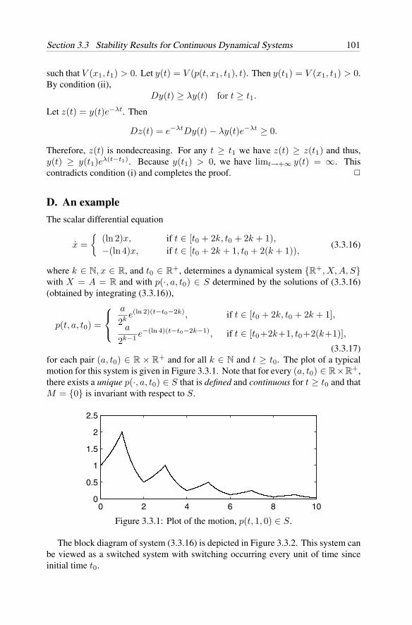
Section 3.3 Stability Results for Continuous Dynamical Systems 101
such that V (x1, t1) > 0. Let y(t) = V (p(t, x1, t1), t). Then y(t1) = V (x1, t1) > 0.By condition (ii),
Dy(t) ≥ λy(t) for t ≥ t1.
Let z(t) = y(t)e−λt. Then
Dz(t) = e−λtDy(t) − λy(t)e−λt ≥ 0.
Therefore, z(t) is nondecreasing. For any t ≥ t1 we have z(t) ≥ z(t1) and thus,y(t) ≥ y(t1)eλ(t−t1). Because y(t1) > 0, we have limt→+∞ y(t) = ∞. Thiscontradicts condition (i) and completes the proof.
D. An example
The scalar differential equation
x =
(ln 2)x, if t ∈ [t0 + 2k, t0 + 2k + 1),−(ln 4)x, if t ∈ [t0 + 2k + 1, t0 + 2(k + 1)),
(3.3.16)
where k ∈ N, x ∈ R, and t0 ∈ R+, determines a dynamical system R
+, X, A, Swith X = A = R and with p(·, a, t0) ∈ S determined by the solutions of (3.3.16)(obtained by integrating (3.3.16)),
p(t, a, t0) =
a
2ke(ln 2)(t−t0−2k), if t ∈ [t0 + 2k, t0 + 2k + 1],
a
2k−1 e−(ln 4)(t−t0−2k−1), if t ∈ [t0+2k+1, t0+2(k+1)],
(3.3.17)for each pair (a, t0) ∈ R × R
+ and for all k ∈ N and t ≥ t0. The plot of a typicalmotion for this system is given in Figure 3.3.1. Note that for every (a, t0) ∈ R×R
+,there exists a unique p(·, a, t0) ∈ S that is defined and continuous for t ≥ t0 and thatM = 0 is invariant with respect to S.
0 2 4 6 8 100
0.5
1
1.5
2
2.5
Figure 3.3.1: Plot of the motion, p(t, 1, 0) ∈ S.
The block diagram of system (3.3.16) is depicted in Figure 3.3.2. This system canbe viewed as a switched system with switching occurring every unit of time sinceinitial time t0.
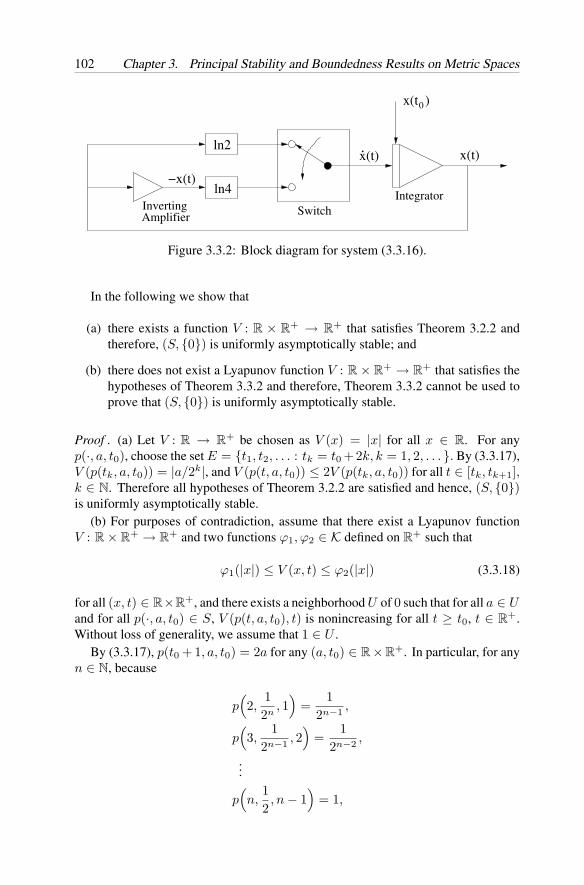
102 Chapter 3. Principal Stability and Boundedness Results on Metric Spaces
x(t )
x(t)ln2
ln4Inverting
Integrator
0
.
−x(t)
Amplifier Switch
x(t)
Figure 3.3.2: Block diagram for system (3.3.16).
In the following we show that
(a) there exists a function V : R × R+ → R
+ that satisfies Theorem 3.2.2 andtherefore, (S, 0) is uniformly asymptotically stable; and
(b) there does not exist a Lyapunov function V : R × R+ → R
+ that satisfies thehypotheses of Theorem 3.3.2 and therefore, Theorem 3.3.2 cannot be used toprove that (S, 0) is uniformly asymptotically stable.
Proof . (a) Let V : R → R+ be chosen as V (x) = |x| for all x ∈ R. For any
p(·, a, t0), choose the set E = t1, t2, . . . : tk = t0 +2k, k = 1, 2, . . . . By (3.3.17),V (p(tk, a, t0)) = |a/2k|, and V (p(t, a, t0)) ≤ 2V (p(tk, a, t0)) for all t ∈ [tk, tk+1],k ∈ N. Therefore all hypotheses of Theorem 3.2.2 are satisfied and hence, (S, 0)is uniformly asymptotically stable.
(b) For purposes of contradiction, assume that there exist a Lyapunov functionV : R × R
+ → R+ and two functions ϕ1, ϕ2 ∈ K defined on R
+ such that
ϕ1(|x|) ≤ V (x, t) ≤ ϕ2(|x|) (3.3.18)
for all (x, t) ∈ R×R+, and there exists a neighborhood U of 0 such that for all a ∈ U
and for all p(·, a, t0) ∈ S, V (p(t, a, t0), t) is nonincreasing for all t ≥ t0, t ∈ R+.
Without loss of generality, we assume that 1 ∈ U .By (3.3.17), p(t0 + 1, a, t0) = 2a for any (a, t0) ∈ R × R
+. In particular, for anyn ∈ N, because
p(2,
12n
, 1)
=1
2n−1 ,
p(3,
12n−1 , 2
)=
12n−2 ,
...
p(n,
12, n − 1
)= 1,
Section 3.4 Stability Results for Discrete-Time Dynamical Systems 103
and because V (p(t, a, t0), t) is nonincreasing for all p(·, a, t0) ∈ S, we have that
V( 1
2n, 1)
≥ V(p(2,
12n
, 1), 2)
= V( 1
2n−1 , 2)
(along the motion p(·, 1
2n, 1));
V( 1
2n−1 , 2)
≥ V(p(3,
12n−1 , 2
), 3)
= V( 1
2n−2 , 3)
(along the motion p(·, 1
2n−1 , 2));
...
V(1
2, n − 1
)≥ V
(p(n,
12, n − 1
), n)
= V (1, n)
(along the motion p(·, 1
2, n − 1
)).
Therefore,
V( 1
2n, 1)
≥ V (1, n).
On the other hand,
ϕ1
( 12n
)≤ V
( 12n
, 1)
≤ ϕ2
( 12n
)and ϕ1(1) ≤ V (1, n) ≤ ϕ2(1).
Thus,
ϕ2
( 12n
)≥ ϕ1(1)
is true for all n ∈ N, which implies that
ϕ2(0) = limn→∞ ϕ2
( 12n
)≥ ϕ1(1) > 0.
However, by the assumption ϕ2 ∈ K, we know that ϕ2(0) = 0. We have arrived at acontradiction. Therefore, there does not exist a Lyapunov function that satisfies thehypotheses of the classical Lyapunov Theorem for uniform asymptotic stability forcontinuous dynamical systems, Theorem 3.3.2.
3.4 The Principal Lyapunov and Lagrange StabilityResults for Discrete-Time Dynamical Systems
In this section we present the Principal Lyapunov Stability and Boundedness Resultsfor discrete-time dynamical systems. As in the case of continuous dynamical systems,we show that these results are a direct consequence of the corresponding stability andboundedness results for DDS given in Section 3.2. To accomplish this, we firstembed the class of discrete-time systems considered herein into a class of DDS with
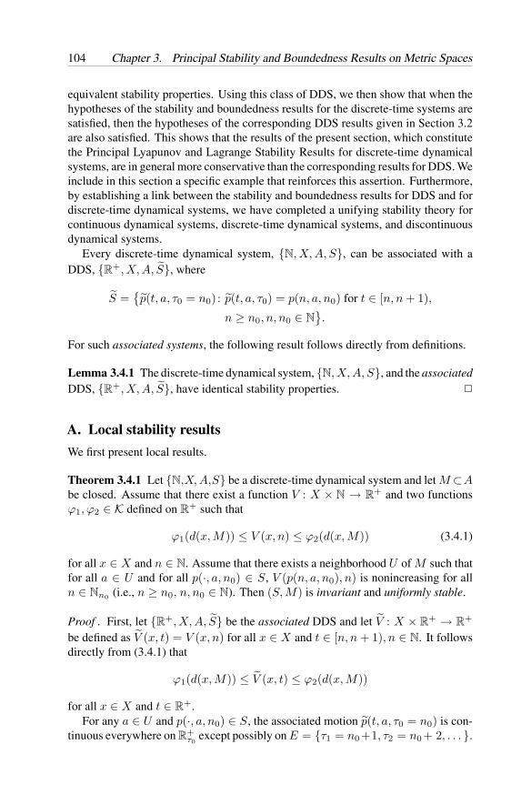
104 Chapter 3. Principal Stability and Boundedness Results on Metric Spaces
equivalent stability properties. Using this class of DDS, we then show that when thehypotheses of the stability and boundedness results for the discrete-time systems aresatisfied, then the hypotheses of the corresponding DDS results given in Section 3.2are also satisfied. This shows that the results of the present section, which constitutethe Principal Lyapunov and Lagrange Stability Results for discrete-time dynamicalsystems, are in general more conservative than the corresponding results for DDS. Weinclude in this section a specific example that reinforces this assertion. Furthermore,by establishing a link between the stability and boundedness results for DDS and fordiscrete-time dynamical systems, we have completed a unifying stability theory forcontinuous dynamical systems, discrete-time dynamical systems, and discontinuousdynamical systems.
Every discrete-time dynamical system, N, X, A, S, can be associated with aDDS, R
+, X, A, S, where
S =p(t, a, τ0 = n0) : p(t, a, τ0) = p(n, a, n0) for t ∈ [n, n + 1),
n ≥ n0, n, n0 ∈ N.
For such associated systems, the following result follows directly from definitions.
Lemma 3.4.1 The discrete-time dynamical system, N, X, A, S, and the associatedDDS, R
+, X, A, S, have identical stability properties.
A. Local stability results
We first present local results.
Theorem 3.4.1 Let N,X, A,S be a discrete-time dynamical system and let M ⊂Abe closed. Assume that there exist a function V : X × N → R
+ and two functionsϕ1, ϕ2 ∈ K defined on R
+ such that
ϕ1(d(x, M)) ≤ V (x, n) ≤ ϕ2(d(x, M)) (3.4.1)
for all x ∈ X and n ∈ N. Assume that there exists a neighborhood U of M such thatfor all a ∈ U and for all p(·, a, n0) ∈ S, V (p(n, a, n0), n) is nonincreasing for alln ∈ Nn0 (i.e., n ≥ n0, n, n0 ∈ N). Then (S, M) is invariant and uniformly stable.
Proof . First, let R+, X, A, S be the associated DDS and let V : X × R
+ → R+
be defined as V (x, t) = V (x, n) for all x ∈ X and t ∈ [n, n + 1), n ∈ N. It followsdirectly from (3.4.1) that
ϕ1(d(x, M)) ≤ V (x, t) ≤ ϕ2(d(x, M))
for all x ∈ X and t ∈ R+.
For any a ∈ U and p(·, a, n0) ∈ S, the associated motion p(t, a, τ0 = n0) is con-tinuous everywhere on R
+τ0
except possibly on E = τ1 = n0+1, τ2 = n0+ 2, . . . .
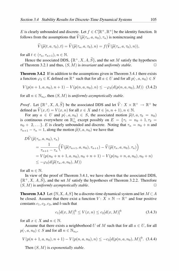
Section 3.4 Stability Results for Discrete-Time Dynamical Systems 105
E is clearly unbounded and discrete. Let f ∈ C[R+, R+] be the identity function. Itfollows from the assumptions that V (p(τn, a, n0), τn) is nonincreasing and
V (p(t, a, τ0), t) = V (p(τn, a, τ0), n) = f(V (p(τn, a, τ0), n)),
for all t ∈ (τn, τn+1), n ∈ N.Hence the associated DDS, R
+, X, A, S, and the set M satisfy the hypothesesof Theorem 3.2.1 and thus, (S, M) is invariant and uniformly stable.
Theorem 3.4.2 If in addition to the assumptions given in Theorem 3.4.1 there existsa function ϕ3 ∈ K defined on R
+ such that for all a ∈ U and for all p(·, a, n0) ∈ S
V (p(n + 1, a, n0), n + 1) − V (p(n, a, n0), n) ≤ −ϕ3(d(p(n, a, n0), M)) (3.4.2)
for all n ∈ Nn0 , then (S, M) is uniformly asymptotically stable.
Proof . Let R+, X, A, S be the associated DDS and let V : X × R
+ → R+ be
defined as V (x, t) = V (x, n) for all x ∈ X and t ∈ [n, n + 1), n ∈ N.For any a ∈ U and p(·, a, n0) ∈ S, the associated motion p(t, a, τ0 = n0)
is continuous everywhere on R+τ0
except possibly on E = τ1 = n0 + 1, τ2 =n0 + 2, . . . . E is clearly unbounded and discrete. Noting that τn = n0 + n andτn+1 − τn = 1, along the motion p(t, a, n0) we have that
DV (p(τn, a, n0), τn)
=1
τn+1 − τn
(V (p(τn+1, a, n0), τn+1) − V (p(τn, a, n0), τn)
)= V (p(n0 + n + 1, a, n0), n0 + n + 1) − V (p(n0 + n, a, n0), n0 + n)≤ −ϕ3(d(p(τn, a, n0), M))
for all n ∈ N.In view of the proof of Theorem 3.4.1, we have shown that the associated DDS,
R+, X, A, S, and the set M satisfy the hypotheses of Theorem 3.2.2. Therefore
(S, M) is uniformly asymptotically stable.
Theorem 3.4.3 Let N,X, A,S be a discrete-time dynamical system and let M ⊂Abe closed. Assume that there exist a function V : X × N → R
+ and four positiveconstants c1, c2, c3, and b such that
c1[d(x, M)]b ≤ V (x, n) ≤ c2[d(x, M)]b (3.4.3)
for all x ∈ X and n ∈ N.Assume that there exists a neighborhood U of M such that for all a ∈ U , for all
p(·, a, n0) ∈ S and for all n ∈ Nn0 ,
V (p(n + 1, a, n0), n + 1) − V (p(n, a, n0), n) ≤ −c3[d(p(n, a, n0), M)]b. (3.4.4)
Then (S, M) is exponentially stable.
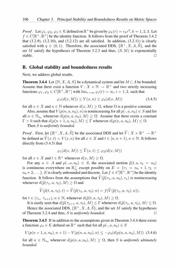
106 Chapter 3. Principal Stability and Boundedness Results on Metric Spaces
Proof . Let ϕ1, ϕ2, ϕ3 ∈ K defined on R+ be given by ϕk(r) = ckrb, k = 1, 2, 3. Let
f ∈ C[R+, R+] be the identity function. It follows from the proof of Theorem 3.4.2that (3.2.9), (3.2.10), and (3.2.12) are all satisfied. In addition, (3.2.11) is clearlysatisfied with q ∈ (0, 1). Therefore, the associated DDS, R
+, X, A, S, and theset M satisfy the hypotheses of Theorem 3.2.3 and thus, (S, M) is exponentiallystable.
B. Global stability and boundedness results
Next, we address global results.
Theorem 3.4.4 Let N, X, A, S be a dynamical system and let M ⊂A be bounded.Assume that there exist a function V : X × N → R
+ and two strictly increasingfunctions ϕ1, ϕ2 ∈ C[R+, R+] with limr→∞ ϕi(r) = ∞, i = 1, 2, such that
ϕ1(d(x, M)) ≤ V (x, n) ≤ ϕ2(d(x, M)) (3.4.5)
for all x ∈ X and n ∈ N whenever d(x, M) ≥ Ω, where Ω is a positive constant.Also, assume that V (p(n, a, n0), n) is nonincreasing for all p(·, a, n0) ∈ S and for
all n ∈ Nn0 whenever d(p(n, a, n0), M) ≥ Ω. Assume that there exists a constantΓ > 0 such that d(p(n + 1, a, n0), M) ≤ Γ whenever d(p(n, a, n0), M) ≤ Ω.
Then S is uniformly bounded.
Proof . First, let R+, X, A, S be the associated DDS and let V : X × R
+ → R+
be defined as V (x, t) = V (x, n) for all x ∈ X and t ∈ [n, n + 1), n ∈ N. It followsdirectly from (3.4.5) that
ϕ1(d(x, M)) ≤ V (x, t) ≤ ϕ2(d(x, M))
for all x ∈ X and t ∈ R+ whenever d(x, M) ≥ Ω.
For any a ∈ A and p(·, a, n0) ∈ S, the associated motion p(t, a, τ0 = n0)is continuous everywhere on R
+τ0
except possibly on E = τ1 = n0 + 1, τ2 =n0+ 2, . . . . E is clearly unbounded and discrete. Let f ∈ C[R+, R+] be the identityfunction. It follows from the assumptions that V (p(τn, a, n0), τn) is nonincreasingwhenever d(p(τn, a, τ0), M) ≥ Ω and
V (p(t, a, τ0), t) = V (p(τn, a, τ0), n) = f(V (p(τn, a, τ0), n)),
for t ∈ (τn, τn+1), n ∈ N, whenever d(p(t, a, τ0), M) ≥ Ω.It is easily seen that d(p(τn+1, a, τ0), M) ≤ Γ whenever d(p(τn, a, τ0), M) ≤ Ω.Hence the associated DDS, R
+, X, A, S, and the set M satisfy the hypothesesof Theorem 3.2.4 and thus, S is uniformly bounded.
Theorem 3.4.5 If in addition to the assumptions given in Theorem 3.4.4 there existsa function ϕ3 ∈ K defined on R
+ such that for all p(·, a, n0) ∈ S
V (p(n + 1, a, n0), n + 1) − V (p(n, a, n0), n) ≤ −ϕ3(d(p(n, a, n0), M)) (3.4.6)
for all n ∈ Nn0 whenever d(p(n, a, n0), M) ≥ Ω, then S is uniformly ultimatelybounded.
Section 3.4 Stability Results for Discrete-Time Dynamical Systems 107
Proof . Let R+, X, A, S be the associated DDS and let V : X × R
+ → R+ be
defined as V (x, t) = V (x, n) for all x ∈ X and t ∈ [n, n + 1), n ∈ N.For any a ∈ A and p(·, a, n0) ∈ S, the associated motion p(t, a, τ0 = n0)
is continuous everywhere on R+τ0
except possibly on E = τ1 = n0 + 1, τ2 =n0 + 2, . . . . E is clearly unbounded and discrete. Noting that τn = n0 + n andτn+1 − τn = 1, along the motion p(t, a, n0) we have that
DV (p(τn, a, n0), τn)
=1
τn+1 − τn
(V (p(τn+1, a, n0), τn+1) − V (p(τn, a, n0), τn)
)= V (p(n0 + n + 1, a, n0), n0 + n + 1) − V (p(n0 + n, a, n0), n0 + n)≤ −ϕ3(d(p(τn, a, n0), M))
for all n ∈ N whenever d(p(τn, a, n0), M) ≥ Ω.In view of the proof of Theorem 3.4.4, we have shown that the associated DDS,
R+, X, A, S, and the set M satisfy the hypotheses of Theorem 3.2.5. Therefore S
is uniformly ultimately bounded.
Theorem 3.4.6 Let N, X, A, S be a dynamical system and let M ⊂ A be closedand bounded. Assume that there exist a function V : X ×N → R
+ and two functionsϕ1, ϕ2 ∈ K∞ such that
ϕ1(d(x, M)) ≤ V (x, n) ≤ ϕ2(d(x, M)) (3.4.7)
for all x ∈ X and n ∈ N.Assume that there exists a function ϕ3 ∈ K defined on R
+ such that for all a ∈ Aand for all p(·, a, n0) ∈ S,
V (p(n + 1, a, n0), n + 1) − V (p(n, a, n0), n) ≤ −ϕ3(d(p(n, a, n0), M)) (3.4.8)
for all n ∈ Nn0 .Then (S, M) is uniformly asymptotically stable in the large.
Proof . Let R+, X, A, S be the associated DDS and let V : X × R
+ → R+ be
defined as V (x, t) = V (x, n) for all x ∈ X and t ∈ [n, n + 1), n ∈ N.For any a ∈ A and p(·, a, n0) ∈ S, the associated motion p(t, a, τ0 = n0)
is continuous everywhere on R+τ0
except possibly on E = τ1 = n0 + 1, τ2 =n0 + 2, . . . . E is clearly unbounded and discrete. Let f ∈ C[R+, R+] be theidentity function; that is, f(r) = r. Similarly as in the proof of Theorem 3.4.5, wecan show that the associated motions and the function V satisfy (3.2.21)–(3.2.23).
Thus, we have shown that the associated DDS R+, X, A, S and the set M satisfy
the hypotheses of Theorem 3.2.6. Therefore (S, M) is uniformly asymptotically stablein the large.
108 Chapter 3. Principal Stability and Boundedness Results on Metric Spaces
Theorem 3.4.7 Let N, X, A, S be a dynamical system and let M ⊂ A be closedand bounded. Assume that there exist a function V : X × N → R
+ and four positiveconstants c1, c2, c3, and b such that
c1[d(x, M)]b ≤ V (x, n) ≤ c2[d(x, M)]b (3.4.9)
for all x ∈ X and n ∈ N.Assume that for all a ∈ A and for all p(·, a, n0) ∈ S,
V (p(n + 1, a, n0), n + 1) − V (p(n, a, n0), n) ≤ −c3[d(p(n, a, n0), M)]b (3.4.10)
for all n ∈ Nn0 .Then (S, M) is exponentially stable in the large.
Proof . The proof proceeds similarly as that in the local exponential stability case.See the proof of Theorem 3.4.3.
C. Instability results
We now address instability results of a set M with respect to S.
Theorem 3.4.8 (Lyapunov’s First Instability Theorem) Let N, X, A, S be a dy-namical system and let M ⊂ A be closed, where A is assumed to be a neighborhoodof M . Assume that there exist a function V : X × N → R and a k0 ∈ N that satisfythe following conditions.
(i) There exists a function ψ ∈ K defined on R+ such that
V (x, k) ≤ ψ(d(x, M))
for all (x, k) ∈ X × N.
(ii) There exists a function ϕ ∈ K defined on R+ such that
V (p(k + 1, a, k0), k + 1) − V (p(k, a, k0), k) ≥ ϕ(|V (p(k, a, k0), k)|
)for all p(·, a, k0) ∈ S and all k ∈ Nk0 .
(iii) In every neighborhood of M there is a point x such that V (x, k0) > 0 andthere exists a motion p(·, x, k0) ∈ S.
Then M is unstable with respect to S.
Proof . Let R+, X, A, S be the associated DDS and let V : X × R
+ → R bedefined as V (x, t) = V (x, n) for all x ∈ X and t ∈ [n, n + 1), n ∈ N.
For any a ∈ A and p(·, a, n0) ∈ S, the associated motion p(t, a, τ0 = n0) is con-tinuous everywhere on R
+τ0
except possibly on E = τ1 = n0+1, τ2 = n0+ 2, . . . .E is clearly unbounded and discrete. Along the motion p(·, a, n0) we have
DV (p(τn, a, n0), τn) = V (p(τn+1, a, n0), τn+1) − V (p(τn, a, n0), τn).
Section 3.4 Stability Results for Discrete-Time Dynamical Systems 109
It is easily seen that the associated DDS, R+, X, A, S, and the set M satisfy the
hypotheses of Theorem 3.2.8 and thus, M is unstable with respect to S.
Theorem 3.4.9 In addition to the assumptions given in Theorem 3.4.8, assume thatV (x, k0) > 0 for all x ∈ M . Then M is completely unstable with respect to S.
Proof . Note that by combining with Theorem 3.4.8, the present assumptions reduceto those of Theorem 3.2.9. Therefore, we conclude that M is completely unstablewith respect to S.
Theorem 3.4.10 (Lyapunov’s Second Instability Theorem) Let N, X, A, S be adynamical system and let M ⊂ A be closed, where A is assumed to be a neighborhoodof M . Assume that for any (a, k0) ∈ A × N and every p(·, a, k0) ∈ S, there exist ak0 ∈ N and a function V : Mε × Nk0 → R, where Mε = x ∈ X : d(x, M) < ε,ε > 0, such that the following conditions are satisfied.
(i) V is bounded on Mε × Nk0 .
(ii) For all p(·, a, k0) ∈ S|Mεand k ∈ Nk0 ,
V (p(k + 1, a, k0), k + 1) ≥ λV (p(k, a, k0), k)
where λ > 1 is a constant.
(iii) In every neighborhood of M , there exists an x such that V (x, k1) > 0 andthere exists a motion p(·, x, k1) ∈ S for a fixed k1 ≥ k0.
Then M is unstable with respect to S.
Proof . By contradiction. If M is invariant and stable with respect to S, then for anyε > 0 and k1 ∈ R
+, there exists a δ = δ(ε, k1) > 0 such that d(p(k, a, k1), M) < εfor all p(·, a, k1) ∈ S and k ∈ Nk1 whenever d(a, M) < δ. Because A is aneighborhood of M , it follows from condition (iii) that there exists an x1 ∈ a ∈A : d(a, M) < δ such that V (x1, k1) > 0. By condition (ii),
V (p(k + 1, a, k1), k + 1) ≥ λV (p(k, a, k1), k)≥ . . .
≥ λ(k+1−k1)V (p(k1, a, k1), k1)
for all k ≥ k1. Because V (p(k1, a, k1), k1) = V (x1, k1) > 0 and λ > 1, wehave limk→+∞ V (p(k + 1, a, k1), k + 1) = ∞. This contradicts condition (i) andcompletes the proof.
D. An example
The scalar difference equation
x(n + 1) =
2x(n) if n = n0 + 2k,x(n)/4 if n = n0 + 2k + 1,
(3.4.11)
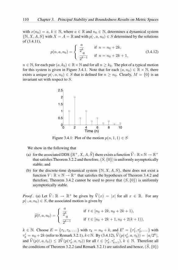
110 Chapter 3. Principal Stability and Boundedness Results on Metric Spaces
with x(n0) = a, k ∈ N, where a ∈ R and n0 ∈ N, determines a dynamical systemN, X, A, S with X = A = R and with p(·, a, n0) ∈ S determined by the solutionsof (3.4.11),
p(n, a, n0) =
a
2kif n = n0 + 2k,
a
2k−1 if n = n0 + 2k + 1,(3.4.12)
n ∈ N, for each pair (a, k0) ∈ R×N and for all n ≥ k0. The plot of a typical motionfor this system is given in Figure 3.4.1. Note that for each (a, n0) ∈ R × N, thereexists a unique p(·, a, n0) ∈ S that is defined for n ≥ n0. Clearly, M = 0 is aninvariant set with respect to S.
0 2 4 6 8 100
0.5
1
1.5
2
2.5
Time (n)
Figure 3.4.1: Plot of the motion p(n, 1, 1) ∈ S
We show in the following that
(a) for the associated DDS R+, X, A, S there exists a function V : R×N → R
+
that satisfies Theorem 3.2.2 and therefore, (S, 0) is uniformly asymptoticallystable; and
(b) for the discrete-time dynamical system N, X, A, S, there does not exist afunction V : R × N → R
+ that satisfies the hypotheses of Theorem 3.4.2 andtherefore, Theorem 3.4.2 cannot be used to prove that (S, 0) is uniformlyasymptotically stable.
Proof . (a) Let V : R → R+ be given by V (x) = |x| for all x ∈ R. For any
p(·, a, n0) ∈ S, the associated motion is given by
p(t, a, n0) =
a
2kif t ∈ [n0 + 2k, n0 + 2k + 1),
a
2k−1 if t ∈ [n0 + 2k + 1, n0 + 2(k + 1)),
k ∈ N. Choose E = τ1, τ2, . . . with τk = n0 + k, and E′ = τ ′1, τ
′2, . . . with
τ ′k = n0 +2k (refer to Remark 3.2.1), k∈N. By (3.4.12), V (p(τ ′
k, a, τ0)) = |a/2k|,and V (p(t, a, t0)) ≤ 2V (p(τ ′
k, a, τ0)) for all t ∈ [τ ′k, τ ′
k+1), k ∈ N. Therefore all
the conditions of Theorem 3.2.2 (and Remark 3.2.1) are satisfied and hence, (S, 0)
Section 3.4 Stability Results for Discrete-Time Dynamical Systems 111
is uniformly asymptotically stable. By Lemma 3.4.1 it now follows that (S, 0) isuniformly asymptotically stable.
(b) For purposes of contradiction, assume that there exist a Lyapunov functionV : R × N → R
+ and two functions ϕ1, ϕ2 ∈ K defined on R+ such that
ϕ1(|x|) ≤ V (x, n) ≤ ϕ2(|x|) (3.4.13)
for all (x, n) ∈ R×N, and there exists a neighborhood U of 0 such that for all a ∈ Uand for all p(·, a, n0) ∈ S, V (p(n, a, n0), n) is nonincreasing for all n ≥ n0, n ∈ N.Without loss of generality, we assume that 1 ∈ U .
By (3.4.12), p(n0 +1, a, n0) = 2a for any (a, n0) ∈ R × N. In particular, for anyn ∈ N, because
p(2,
12n
, 1)
=1
2n−1 , p(3,
12n−1 , 2
)=
12n−2 , . . . , p
(n,
12, n − 1
)= 1,
and because V (p(n, a, n0), n) is nonincreasing for all p(·, a, n0) ∈ S, we have that
V( 1
2n, 1)
≥ V(p(2,
12n
, 1), 2)
= V( 1
2n−1 , 2)
(along the motion p(·, 1
2n, 1));
V( 1
2n−1 , 2)
≥ V(p(3,
12n−1 , 2
), 3)
= V( 1
2n−2 , 3)
(along the motion p(·, 1
2n−1 , 2));
...
V(1
2, n − 1
)≥ V
(p(n,
12, n − 1
), n)
= V (1, n)
(along the motion p(·, 1
2, n − 1
)).
Therefore,
V( 1
2n, 1)
≥ V (1, n) .
On the other hand,
ϕ1
( 12n
)≤ V
( 12n
, 1)
≤ ϕ2
( 12n
)and ϕ1(1) ≤ V (1, n) ≤ ϕ2(1).
Thus,
ϕ2
( 12n
)≥ ϕ1(1)
is true for all n ∈ N, which implies that
ϕ2(0) = limn→∞ ϕ2
( 12n
)≥ ϕ1(1) > 0.
112 Chapter 3. Principal Stability and Boundedness Results on Metric Spaces
However, by the assumption ϕ2 ∈ K, we know that ϕ2(0) = 0. We have arrived at acontradiction. Therefore, there does not exist a Lyapunov function that satisfies thehypotheses of the classical Lyapunov Theorem for uniform asymptotic stability fordiscrete-time dynamical systems, Theorem 3.4.2.
3.5 Converse Theorems for Discontinuous DynamicalSystems
The results of the previous three sections constitute sufficient conditions for varioustypes of stability, instability, and boundedness for discontinuous dynamical systems,continuous dynamical systems, and discrete-time dynamical systems, respectively.It turns out that under some additional mild assumptions, these results constitutenecessary conditions as well. Such results are referred to as converse theorems in theliterature. The proofs of these results do not provide us with the means of constructingLyapunov functions V (p(·, a, τ0), ·) in a systematic manner in applications. Never-theless, converse theorems occupy an important place in the general developmentof the qualitative theory of dynamical systems. We address only converse theoremsconcerning local results.
A. Local results
In our first result, we require the following hypothesis.
Assumption 3.5.1 Let R+, X, A, S be a DDS and assume that
(i) for any p(·, a, t0) ∈ S, there exists a p(·, a1, t1) ∈ S with a1 = p(t1, a, t0) andt1 > t0 such that p(·, a1, t1) = p(·, a, t0) for all t ≥ t1; and
(ii) for any two motions pi(·, ai, ti) ∈ S, i = 1, 2, t2 > t1, if a2 = p1(t2, a1, t1),then there exists a p(·, a1, t1) ∈ S such that p(t, a1, t1) = p1(t, a1, t0) fort ∈ [t1, t2) and p(t, a1, t1) = p2(t, a2, t2) for t ≥ t2.
In part (i) of Assumption 3.5.1, p(·, a1, t1) may be viewed as a partial motion ofthe motion p(·, a, t0), and in part (ii), p(·, a, t1) may be viewed as a composition ofp1(·, a1, t1) and p2(·, a2, t2). With this convention, Assumption 3.5.1 states that
(a) any partial motion is a motion in S; and
(b) any composition of two motions is a motion in S.
We require the above assumption in all converse theorems for dynamical systemsdefined on metric spaces. The reason for this is that in Definitions 2.2.1 and 2.2.2,the motions are defined for initial conditions and forward in time, and in general,time is not required to be reversible. (This is in contrast to many dynamical systemsdetermined, e.g., by various types of differential equations, addressed in subsequentchapters.) We note, however, that when in a dynamical system the semigroup propertyholds, then Assumption 3.5.1 is automatically implied.
Section 3.5 Converse Theorems for Discontinuous Dynamical Systems 113
Theorem 3.5.1 Let R+, X, A, S be a DDS and let M ⊂ A be a closed invariant
set, where A is assumed to be a neighborhood of M . Suppose that S satisfies As-sumption 3.5.1 and that (S, M) is uniformly stable. Then there exist neighborhoodsA1 and X1 of M such that A1 ⊂ X1 ⊂ A and a mapping V : X1 × R
+ → R+ that
satisfies the following conditions.(i) There exist ψ1, ψ2 ∈ K such that
ψ1(d(x, M)) ≤ V (x, t) ≤ ψ2(d(x, M)) (3.5.1)
for all (x, t) ∈ X1 × R+.
(ii) For every p(·, a, τ0) ∈ S with a ∈ A1, V (p(t, a, τ0), t) is nonincreasing for allt ∈ R
+τ0
.
Proof . If (S, M) is uniformly stable, then in view of Lemma 3.10.3 (refer to Section3.10, Problem 3.10.15), there exists a function ϕ ∈ K defined on [0, h0] for someh0 > 0 such that
d(p(t, a, τ0), M) ≤ ϕ(d(a, M)) (3.5.2)
for all p(·, a, τ0) ∈ S, for all t ∈ R+τ0
and for all τ0 ∈ R+ whenever d(a, M) < h0.
A is a neighborhood of M , therefore it follows that X1 = x ∈ A : d(x, M) < h0is also a neighborhood of M . We now define V : X1 × R
+ → R+ by
V (x, t) = supd(p(t′, x, t), M) : p(·, x, t) ∈ S, t′ ∈ R
+t
.
Then for all x ∈ X, t ∈ R+, we have that
V (x, t) ≥ d(p(t, x, t), M) = d(x, M)
and in view of (3.5.2) we have that V (x, t) ≤ ϕ(d(x, M)). Therefore, V satisfiescondition (i) of this theorem.
Next, let A1 = a ∈ X1 : d(a, M) < ϕ−1(h0) if ϕ(h0) > h0 and A1 = X1otherwise. We now prove that for any p0(·, a, τ0) ∈ S with a ∈ X1, we have thatv(t) = V (p0(t, a, τ0), t) is nonincreasing for all t ∈ R
+τ0
.Let t1, t2 ∈ R
+τ0
and t1 < t2. Let ai = p0(ti, a, τ0), i = 1, 2. Then,
v(ti) = supd(p(t′, ai, ti), M) : p(·, ai, ti) ∈ S, t′ ∈ R
+ti
, i = 1, 2.
To prove that v(t2) ≤ v(t1), it suffices to show that for every p2(·, a2, t2) ∈ S and forevery t′ ∈ R
+t2 , there exists a p1(·, a1, t1) ∈ S such that p2(t′, a2, t2) = p1(t′, a1, t1).
By (i) in Assumption 3.5.1 there exists a p0(·, a1, t1) ∈ S such that
p0(t, a1, t1) = p0(t, a, t0)
for all t ∈ R+t1 . By (ii) in Assumption 3.5.1, for p0(·, a1, t1) and p2(·, a2, t2), where
a2 = p0(t2, a, t0) = p0(t2, a1, t1), there exists a p1(·, a1, t1) ∈ S such that
p2(t′, a2, t2)= p1(t′, a1, t1)
because t′ ∈ R+t2 . Therefore, v(t2) ≤ v(t1).
This concludes the proof of the theorem.
114 Chapter 3. Principal Stability and Boundedness Results on Metric Spaces
In the proofs of the remaining results of the present section, we require the fol-lowing additional assumption.
Assumption 3.5.2 Let R+, X, A, S be a DDS. We assume that every motion
p(·, a, τ0) ∈ S is continuous everywhere on R+τ0
, except possibly on an unboundedand discrete set E = τ1, τ2, . . . : τ1 < τ2 < · · · (recall that in general E de-
pends on p(·, a, τ0) ∈ S), and that lE= infk∈1,2,... ,p∈Sτk+1 − τk > 0, and that
LE= supk∈1,2,... ,p∈Sτk+1 − τk < ∞.
In the proof of the converse theorem for uniform asymptotic stability, we requirea preliminary result.
Definition 3.5.1 A continuous function σ : [s1,∞) → R+ is said to belong to class
L if σ is strictly decreasing on [s1,∞) and if lims→∞ σ(s) = 0 where s1 ∈ R+.
Lemma 3.5.1 Let β ∈ L be defined on R+. Then there exists a function α ∈ K
defined on R+ such that for any discrete subset τ0, τ1, . . . ⊂ R
+ satisfyinginfτk+1 − τk : k = 1, 2, . . . > 0, it is true that
∑∞i=0 α(β(τi − τ0)) < ∞.
Proof . We define η ∈ C[(0,∞), (0,∞)] as
η(t) =
β(t)/t, t ∈ (0, 1),β(t), t ∈ [1,∞).
Clearly, η(t) is strictly decreasing for all t>0, limt→0+η(t) =+∞, and η(t)≥β(t)for all t > 0. Furthermore, η is invertible, and η−1 ∈ C[(0,∞), (0,∞)] is strictlydecreasing, and η−1(β(τ)) ≥ η−1(η(τ)) = τ for all τ > 0.
We now define α(0) = 0 and
α(t) = e−η−1(t), t > 0.
Then α ∈ K, and
α(β(τ)) = e−η−1(β(τ)) ≤ e−τ .
If we denote lm = infτj+1 − τj : j = 1, 2 . . . , we know that τj − τ0 ≥ (j − 1)lm.Hence it is true that
∞∑j=0
α(β(τj − τ0)) ≤∞∑
j=0
e−(τj−τ0) ≤ 1 +∞∑
j=1
e−(j−1)lm
= 1 +1
1 − e−lm< +∞.
This completes the proof.
We are now in a position to prove the following result.
Section 3.5 Converse Theorems for Discontinuous Dynamical Systems 115
Theorem 3.5.2 Let R+, X, A, S be a DDS and let M ⊂ A be a closed invariant
set, where A is assumed to be a neighborhood of M . Assume that S satisfies As-sumptions 3.5.1 and 3.5.2, and furthermore, assume that for every (a, τ0) ∈ A×R
+,there exists a unique motion p(·, a, τ0) ∈ S. Let (S, M) be uniformly asymptoticallystable. Then there exist neighborhoods A1, X1 of M such that A1 ⊂ X1 ⊂ A, and amapping V : X1 × R
+ → R+ that satisfies the following conditions.
(i) There exist functions ψ1, ψ2 ∈ K (defined on R+) such that
ψ1(d(x, M)) ≤ V (x, t) ≤ ψ2(d(x, M)) (3.5.3)
for all (x, t) ∈ X1 × R+;
(ii) There exists a function ψ3 ∈ K, defined on R+, such that for all p(·, a, τ0) ∈ S,
we haveDV (p(τk, a, τ0), τk) ≤ −ψ3(d(p(τk, a, τ0), M)) (3.5.4)
where a ∈ A1, k ∈ N and where DV is defined in (3.2.4).(iii) There exists a function f ∈ C[R+, R+] such that f(0) = 0 and such that
V (p(t, a, τ0), t) ≤ f(V (p(τk, a, τ0), τk)) (3.5.5)
for every p(·, a, τ0) ∈ S and all t ∈ (τk, τk+1), a ∈ A1 and τ0 ∈ R+.
Proof . Inasmuch as (S, M) is uniformly asymptotically stable, we know by The-orem 3.5.1 that there exist some neighborhoods A1 and X1 of M such that A1 ⊂X1 ⊂ A, and a mapping V : X1 × R
+ → R+ that satisfies the following conditions.
(a) There exist two functions ϕ1, ϕ2 ∈ K such that
ϕ1(d(x, M)) ≤ V (x, t) ≤ ϕ2(d(x, M))
for all (x, t) ∈ X1 × R+.
(b) For every p(·, a, τ0) ∈ S with a ∈ A1, V (p(t, a, τ0), t) is nonincreasing for allt ≥ τ0.
From (a) and (b) above, we conclude that for any t ∈ [τk, τk+1), it is true that
ϕ1(d(p(t, a, τ0), M)) ≤ V (p(t, a, τ0), t) ≤ V (p(τk, a, τ0), τk)≤ ϕ2(d(p(τk, a, τ0), M))
which implies that
d(p(t, a, τ0), M) ≤(ϕ−1
1 ϕ2)(d(p(τk, a, τ0), M)) (3.5.6)
for all t ∈ [τk, τk+1) and k ∈ N.By Lemma 3.10.5 (see Problem 3.10.17 in Section 3.10), there exist a function
ϕ ∈ K defined on [0, h0] for some h0 > 0, and a function σ ∈ L, defined on R+,
such that for all t ≥ τ0
d(p(t, a, τ0), M) < ϕ(d(a, M))σ(t − τ0) (3.5.7)
116 Chapter 3. Principal Stability and Boundedness Results on Metric Spaces
for all p(·, a, τ0) ∈ S whenever d(a, M) < h0. Let X1 = x ∈ A1 : d(x, M) < h0and A1 = a ∈ X1 : d(a, M) < ϕ−1(h0) if ϕ−1(h0) ≤ h0 and A1 = X1 other-wise.
We now define the Lyapunov function V (x, τ0) for (x, τ0) ∈ X1 × R+. Because
for any (x, τ0) ∈ X1 ×R+, there exists a unique motion p(·, x, τ0) that is continuous
everywhere on R+τ0
except on E = τ1, τ2 . . . : τ1 < τ2 < · · · , we define
V (x, τ0) =∞∑
j=0
u(d(p(τj , x, τ0), M)
)(3.5.8)
where u ∈ K, defined on R+, is specified later in such a manner that the above
summation converges. Obviously,
V (x, τ0) ≥ u(d(p(τ0, x, τ0), M)
)= u
(d(x, M)
).
Hence, if we define ψ1 = u, then V (x, τ0) ≥ ψ1(d(x, M)) for all (x, τ0) ∈ X1×R+.
Consider p(·, x, τ0) ∈ S and the corresponding set E = τ1, τ2, . . . . If we denotex = p(τk, a, τ0), and τ0 = τk for some k ≥ 1, we know there exists a unique motionp(·, x, τ0) ∈ S that is continuous everywhere on t ≥ τ0 except on τ1, τ2, . . . . Bythe definition of V given in (3.5.8), we know that
V (x, τ0) =∞∑
j=0
u(d(p(τj , x, τ0), M)
).
By the uniqueness property and Assumption 3.5.1(i), we know that τj = τk+j , and
p(τj , x, τ0) = p(τk+j , p(τk, a, τ0), τk) = p(τk+j , a, τ0).
Therefore, it is clear that
V (p(τk, a, τ0), τk) =∞∑
j=k
u(d(p(τj , a, τ0), M)
). (3.5.9)
Similarly, for any t ∈ (τk, τk+1), k ∈ N, V (p(t, a, τ0), t) is defined as
V (p(t, a, τ0), t) = u(d(p(t, a, τ0), M)
)+
∞∑j=k+1
u(d(p(τj , a, τ0), M)
). (3.5.10)
It follows that
DV (p(τk, a, τ0), τk)
=1
τk+1 − τk
[V (p(τk+1, a, τ0), τk+1) − V (p(τk, a, τ0), τk)
]=
1τk+1 − τk
[ ∞∑j=k+1
u(d(p(τj , a, τ0), M)
)−
∞∑j=k
u(d(p(τj , a, τ0), M)
)]= − 1
τk+1 − τku(d(p(τk, a, τ0), M)
)
Section 3.5 Converse Theorems for Discontinuous Dynamical Systems 117
for k ∈ N. Because τk+1 − τk ≤ LE by Assumption 3.5.2, it follows that
DV (p(τk, a, τ0), τk) ≤ −u(d(p(τk, a, τ0), M)
)/LE = −ψ3(d(p(τk, a, τ0), M))
where we have defined ψ3 = u/LE .We now show how to choose u ∈ K so that the infinite summation in (3.5.8)
converges. It follows from (3.5.7) that for any (x, τ0) ∈ X1 × R+, we have
u(d(p(t, x, τ0), M)
)< u
(ϕ(d(x, M)
)σ(t − τ0))
≤[u(ϕ(d(x, M))σ(0)
)]1/2[u(ϕ(h0)σ(t − τ0)
)]1/2.
(3.5.11)
Let β(τ) = ϕ(h0)σ(τ). Then β ∈ L. Hence, by Lemma 3.5.1, there exists afunction α ∈ K defined on R
+ such that∑∞
i=0 α(β(τi − τ0)
)< ∞. If we define
u(r) = [α(r)]2, then it follows that[u(ϕ(h0)σ(t − τ0)
)]1/2 = α(ϕ(h0)σ(t − τ0)
)= α
(β(t − τ0)
). (3.5.12)
Hence, we conclude from (3.5.8)–(3.5.10) that
V (x, τ0) =∞∑
j=0
u(d(p(τj , x, τ0), M)
)<
∞∑j=0
[u(ϕ(d(x, M))σ(0)
)]1/2[u(ϕ(h0)σ(τj − τ0)
)]1/2
=[u(ϕ(d(x, M))σ(0)
)]1/2∞∑
j=0
α(β(τj − τ0)
)<[u(ϕ(d(x, M))σ(0)
)]1/2[1 + 1/(1 − e−lE )],
where lE is the lower bound given in Assumption 3.5.2. If we define ψ2 ∈ K by
ψ2(r) = [u(ϕ(σ(0)r))]1/2[1 + 1/(1 − e−lE )],
then it follows that V (x, τ0) ≤ ψ2(d(x, M)). Thus we have proved conditions (i)and (ii) of the theorem.
To prove condition (iii) of the theorem, let t ∈ (τk, τk+1). We have alreadyshown that
V (p(t, a, τ0), t) ≤ ψ2(d(p(t, a, τ0), M)).
Furthermore, because a ∈ A1 ⊂ A1, (3.5.6) is satisfied. Hence, we know that
V (p(t, a, τ0), t) ≤(ψ2 ϕ−1
1 ϕ2
)(d(p(τk, a, τ0), M)). (3.5.13)
On the other hand, we have also shown that
V (p(τk, a, τ0), τk) ≥ ψ1(d(p(τk, a, τ0), M)),
118 Chapter 3. Principal Stability and Boundedness Results on Metric Spaces
which implies that(ψ−1
1 V)(p(τk, a, τ0), τk) ≥ d(p(τk, a, τ0), M). (3.5.14)
Combining (3.5.13) and (3.5.14), we obtain that
V (p(t, a, τ0), t) ≤(ψ2 ϕ−1
1 ϕ2 ψ−11
)(V (p(τk, a, τ0), τk))
for all t ∈ (τk, τk+1), k ∈ N, and all (a, τ0) ∈ A1×R+. If we define f ∈ C[R+, R+]
as f = ψ2 ϕ−11 ϕ2 ψ−1
1 , then f(0) = 0 and
V (p(t, a, τ0), t) ≤ f(V (p(τk, a, τ0), τk)).
This concludes the proof of the theorem.
The hypotheses in the next result are not exactly symmetric with the correspondinghypotheses given in Theorem 3.2.3. Nevertheless, they do provide a set of necessaryconditions for exponential stability.
Theorem 3.5.3 Let R+, X, A, S be a DDS and let M ⊂ A be a closed invariant set,
where A is a neighborhood of M . Suppose that system S satisfies Assumptions 3.5.1and 3.5.2 and that for every (a, τ0) ∈ A×R
+, there exists a unique motionp(·, a, τ0) ∈S. Let (S, M) be exponentially stable. Then there exist neighborhoods A1 and X1of M such that A1 ⊂ X1 ⊂ A, and a mapping V : X1 × R
+ → R+ that satisfies the
following conditions.
(i) There exist functions ψ1, ψ2 ∈ K, defined on R+, such that
ψ1(d(x, M)) ≤ V (x, t) ≤ ψ2(d(x, M)) (3.5.15)
for all (x, t) ∈ X1 × R+.
(ii) There exists a constant c > 0 such that for every p(·, a, τ0) ∈ S,
DV (p(τk, a, τ0), τk) ≤ −cV (p(τk, a, τ0), τk) (3.5.16)
for k ∈ N, where a ∈ A1 and where DV is defined in (3.2.4).
(iii) There exists a function f ∈ C[R+, R+] with f(0) = 0 and
f(r) = O(rq) as r → 0+ (3.5.17)
for some constant q > 0 such that
V (p(t, a, τ0), t) ≤ f(V (p(τk, a, τ0), τk)) (3.5.18)
for every p(·, a, τ0) ∈ S, t ∈ (τk, τk+1), k ∈ N, a ∈ A1, and τ0 ∈ R+.
Section 3.5 Converse Theorems for Discontinuous Dynamical Systems 119
Proof . By Lemma 3.10.6 (see Problem 3.10.18, Section 3.10), there exist a functionϕ ∈ K defined on [0, h0] for some h0 > 0, and an α > 0 such that for all t ∈ R
+τ0
d(p(t, a, τ0), M) ≤ ϕ(d(a, M))e−α(t−τ0) (3.5.19)
for all p(·, a, τ0) ∈ S whenever d(a, M) < h0. Let X1 = x ∈ A : d(x, M) < h0and A1 = a ∈ X1 : d(a, M) < ϕ−1(h0) if ϕ−1(h0) ≤h0 and A1 = X1 otherwise.
For (x, τ0) ∈ X1 × R+, there exists a unique motion p(·, x, τ0) ∈ S. We define
V (x, τ0) = supt′≥τ0
d(p(t′, x, τ0), M)eα(t′−τ0)
. (3.5.20)
Now for (a, τ0) ∈ A1 × R+ and p(t, a, τ0), t ∈ R
+τ0
, it must be true by Assumption3.5.1 that the unique motion p(t′, p(t, a, τ0), t) = p(t′, a, τ0) for all t′ ∈ R
+t . Thus,
V (p(t, a, τ0), t) = supt′≥t
d(p(t′, p(t, a, τ0), t), M)eα(t′−t)
= supt′≥t
d(p(t′, a, τ0), M)eα(t′−t). (3.5.21)
For k ∈ N, we have
V (p(τk+1, a, τ0), τk+1) = supt′≥τk+1
d(p(t′, a, τ0), M)eα(t′−τk)e−α(τk+1−τk)
≤ supt′≥τk+1
d(p(t′, a, τ0), M)eα(t′−τk)e−αlE
≤ supt′≥τk
d(p(t′, a, τ0), M)eα(t′−τk)e−αlE
= e−αlE V (p(τk, a, τ0), τk),
where lE is the lower limit given in Assumption 3.5.2. Letting c = (1− e−αlE )/LE ,where LE is the upper limit given in Assumption 3.5.2, we obtain
DV (p(τk, a, τ0), τk) =1
τk+1 − τk
[V (p(τk+1, a, τ0), τk+1) − V (p(τk, a, τ0), τk)
]≤ − 1
LE
(1 − e−αLE
)V (p(τk, a, τ0), τk)
= − cV (p(τk, a, τ0), τk).
Also, (3.5.19)–(3.5.21) imply that d(x, M)≤ V (x, τ0) ≤ ϕ(d(x, M)) for all (x, t)∈X1 × R
+. By (3.5.21), for every t ∈ (τk, τk+1) we have that
V (p(t, a, τ0), t) = supt′≥t
d(p(t′, a, τ0), M)eα(t′−τk)e−α(t−τk)
≤ supt′≥t
d(p(t′, a, τ0), M)eα(t′−τk)
≤ supt′≥τk
d(p(t′, a, τ0), M)eα(t′−τk)
= V (p(τk, a, τ0), τk).
The proof is completed by letting f(r) = r and q = 1/2.
120 Chapter 3. Principal Stability and Boundedness Results on Metric Spaces
We conclude by noting that converse theorems for DDSs for uniform boundedness,uniform ultimate boundedness, uniform asymptotic stability in the large, exponentialstability in the large, and instability can also be established, using the methodologyemployed in the preceding results.
B. Refinements: Continuity of Lyapunov functions
The converse theorems presented in this section involve Lyapunov functions that neednot necessarily be continuous. In the present subsection, we show that under someadditional very mild assumptions, the Lyapunov functions for the converse theoremsare continuous with respect to initial conditions.
In the proof of Theorem 3.5.2, the Lyapunov function V is constructed based on theunique motion that starts at (x, τ0) ∈ A × R
+. In the following, we show that undersome additional very mild assumptions (Assumption 3.5.3) the function V given inthe converse Theorem 3.5.2 is continuous (i.e., V (x0m, τ0m) approaches V (x0, τ0)as m → ∞ if x0m → x0 and τ0m → τ0 as m → ∞). We then define continuousdependence on the initial conditions for motions of DDSs and show that Assumption3.5.3 is satisfied when the motions are continuous with respect to initial conditions.
Assumption 3.5.3 Let R+, X, A, S be a DDS and let x0m ⊂ A, τ0m ⊂ R
+,x0m → x0 ∈ A, and τ0m → τ0 as m → ∞. The motion starting at (x0m, τ0m) isdenoted by pm(t, x0m, τ0m) with the discontinuity set
E(x0m,τ0m) = τ1m, τ2m, . . . : τ0m < τ1m < τ2m < · · · ,
m ∈ N. Assume that
(a) τkm → τk as m → ∞, for all k ∈ N; and
(b) pm(τkm, x0m, τ0m) → xk = p(τk, x0, τ0) as m → ∞ for all k ∈ N.
We first strengthen Lemma 3.5.1 as follows.
Lemma 3.5.2 Let β ∈ L be defined on R+. Then there exists a function α ∈ K
defined on R+ such that for any discrete subset r0, r1, . . . ⊂ R
+ satisfying lE =infrn+1 − rn : n = 1, 2, . . . > 0, it is true that
∞∑i=0
α(β(ri − r0)) < +∞,
and∞∑
i=k
α(β(ri − r0)) <exp (−(k − 1)lE)
1 − exp(−lE),
for all k ≥ 1.
Section 3.5 Converse Theorems for Discontinuous Dynamical Systems 121
Proof . Let η and α ∈ C[(0,∞), (0,∞)] be the same as in the proof of Lemma 3.5.1.Then
∞∑j=k
α(β(τj − τ0)) ≤∞∑
j=k
exp(−(τj − τ0))
≤∞∑
j=k
exp(−(j − 1)lE)
=exp (−(k − 1)lE)
1 − exp(−lE),
and ∞∑j=0
α(β(τj − τ0)) < +∞,
as shown in Lemma 3.5.1. The proof is completed.
We are now in a position to present our first result.
Theorem 3.5.4 If in addition to the assumptions given in Theorem 3.5.2, the motionsin S also satisfy Assumption 3.5.3, then the Lyapunov function in the ConverseTheorem 3.5.2 is continuous with respect to initial conditions.
Proof . It follows from the proof of Theorem 3.5.2 that there exist a function ϕ ∈ Kdefined on [0, h0] for some h0 > 0, and a function σ ∈ L defined on R
+, such thatfor all t ≥ τ0
d(p(t, a, τ0), M) < ϕ(d(a, M))σ(t − τ0) (3.5.22)
for all p(·, a, τ0) ∈ S whenever d(a, M) < h0. Let X1 = x ∈ A : d(x, M) < h0,and A1 = a ∈ X1 : d(a, M) < ϕ−1(h0) if ϕ−1(h0) ≤ h0 and A1 = X1otherwise.
Let β(τ) = ϕ(h0)σ(τ), α ∈ K be defined on R+ such that Lemma 3.5.2 is true,
and u(r) = [α(r)]2. For any (x, τ0) ∈ X1 × R+, the Lyapunov function V (x, τ0) is
defined as
V (x, τ0) =∞∑
j=0
u(d(p(τj , x, τ0), M)
). (3.5.23)
It follows from (3.5.22) that for any (x, τ0) ∈ X1 × R+, we have
u(d(p(t, x, τ0), M)
)< u
(ϕ(d(x, M)
)σ(t − τ0))
≤[u(ϕ(d(x, M))σ(0)
)]1/2[u(ϕ(h0)σ(t − τ0)
)]1/2.
(3.5.24)
From the choice of u, we have[u(ϕ(h0)σ(t − τ0)
)]1/2 = α(ϕ(h0)σ(t − τ0)
)= α
(β(t − τ0)
). (3.5.25)
122 Chapter 3. Principal Stability and Boundedness Results on Metric Spaces
We now show that V is continuous with respect to initial conditions. Supposex0m → x0 and τ0m → τ0 as m→∞. We denote pm(τkm, x0m, τ0m) by xkm. Then
V (x0m, τ0m) =∞∑
i=0
u(d(pm(τim, x0m, τ0m), M))
=∞∑
i=0
u(d(xim, M)). (3.5.26)
We show that V (x0m, τ0m) approaches V (x0, τ0) =∑∞
i=0 u(d(xi, M)) as m → ∞.It follows from (3.5.24), (3.5.25), and Lemma 3.5.2 that
∞∑i=k
u(d(p(τi, x0, τ0), M)) <
∞∑i=k
[u(ϕ(d(x0, M))σ(0))]1/2[u(ϕ(h0)σ(τi − τ0))]1/2
≤ [u(ϕ(h0)σ(0))]1/2∞∑
i=k
α(β(τi − τ0))
< [u(ϕ(h0)σ(0))]1/2 exp(−(k − 1)lE)1 − exp(−lE)
.
For every ε > 0, in view of the above inequality, there exists an n0 > 0 such that
∞∑i=n0
u(d(xi, M)) < ε/4 (3.5.27)
for all x0 ∈ A1. Similarly,
∞∑i=n0
u(d(xim, M)) < ε/4 (3.5.28)
for all x0m ∈ A1.On the other hand, for every k ≤ n0, there exists a δk > 0 such that
|u(r) − u(d(xk, M))| <ε
2n0
whenever |r − d(xk, M)| < δk (because u(·) is continuous everywhere on R+).
Because xkm → xk as m → ∞, there exists for each k ≤ n0 an mk > 0 such thatd(xkm, xk) < δk is true for all m ≥ mk. Now let mε = maxk≤n0mk. For everym > mε we have |d(xk, M) − d(xkm, M)| ≤ d(xk, xkm) < δk and thus∣∣∣∣ n0−1∑
k=0
u(d(xk, M))−n0−1∑k=0
u(d(xkm, M))∣∣∣∣
≤n0−1∑k=0
|u(d(xk, M)) − u(d(xkm, M))|
<ε
2.
Section 3.5 Converse Theorems for Discontinuous Dynamical Systems 123
Therefore we have shown that
|V (x0, τ0) − V (x0m, τ0m)| =
∣∣∣∣∣∞∑
k=0
u(d(xk, M)) −∞∑
k=0
u(d(xkm, M))
∣∣∣∣∣≤∣∣∣∣∣n0−1∑k=0
u(d(xk, M)) −n0−1∑k=0
u(d(xkm, M))
∣∣∣∣∣+
∞∑k=n0
u(d(xk, M)) +∞∑
k=n0
u(d(xkm, M))
< ε. (3.5.29)
Therefore, we conclude that V is continuous with respect to initial conditions(x0, τ0).
The following concept of continuous dependence on initial conditions for DDS ismotivated by a corresponding term for ordinary differential equations (see, e.g., [11]),and is used as a sufficient condition for Assumption 3.5.3.
Definition 3.5.2 Suppose x0m ⊂ A ⊂ X, τ0m ⊂ R+, x0m → x0 ∈ A and
τ0m → τ0 as m → ∞. Assume that the motions are given by
p(t, x0, τ0) = p(k)(t, xk, τk), t ∈ [τk, τk+1),
andpm(t, x0m, τ0m) = p(k)
m (t, xkm, τkm), t ∈ [τkm, τ(k+1)m),
k ∈ N, where p(k)(t, xk, τk) and p(k)m (t, xkm, τkm) are continuous for all t ∈ R
+ with
p(k)(τk, xk, τk) = p(τk, x0, τ0) = xk
andp(k)
m (τkm, xkm, τkm) = pm(τkm, x0m, τ0m) = xkm.
The motions in S are said to be continuous with respect to the initial conditions(x0, τ0) if
(a) τkm → τk as m → ∞, for all k ∈ N; and(b) for every compact set K ⊂ R
+ and every ε > 0 there exists an L = L(K, ε) >0 such that for all t ∈ K and k ∈ N such that K ∩ [τk, τk+1) = ∅,
d(p(k)m (t, xkm, τkm), p(k)(t, xk, τk)) < ε
whenever m > L.
An example of the set of continuous functions p(k)(t, xk, τk) is
p(k)(t, xk, τk) =
xk, t < τk,
p(t, x0, τ0), t ∈ [τk, τk+1),p(τ−
k+1, x0, τ0), t ≥ τk+1.
124 Chapter 3. Principal Stability and Boundedness Results on Metric Spaces
Another example of p(k)(t, xk, τk) is given in Example 3.5.1, following the nextresult.
Theorem 3.5.5 If in addition to the assumptions given in Theorem 3.5.2, the motionsinS are continuous with respect to initial conditions, then the Lyapunov function givenin (3.5.23) is continuous with respect to initial conditions (x0, τ0).
Proof . We show that under the present hypotheses, Assumption 3.5.3 is satisfied andhence V is continuous with respect to initial conditions by Theorem 3.5.4.
Suppose x0m → x0 and τ0m → τ0 as m → ∞. Assumption 3.5.3(a) is the sameas Definition 3.5.2(a). We only need to show Assumption 3.5.3(b) is satisfied; that is,xkm → xk as m → ∞ for all k ∈ N.
For a fixed k > 0, k ∈ N, let K = [τk − lE/2, τk + lE/2]. For every ε > 0 thereexists an L = L(K, ε/2) > 0 such that for all t ∈ K
d(p(k)m (t, xkm, τkm), p(k)(t, xk, τk)) < ε/2 (3.5.30)
whenever m > L. Because p(k)(t, xk, τk) is continuous on R+, there exists a δ > 0
such that d(p(k)(t′, xk, τk), p(k)(τk, xk, τk)) < ε/2 whenever |t′ −τk| < δ. Becauseτkm → τk as m → ∞, there exists an L1 > 0 such that τkm ∈ K and |τkm −τk| < δfor all m > L1. Therefore, when m > maxL, L1, we have by (3.5.30)
d(p(k)m (τkm, xkm, τkm), p(k)(τkm, xk, τk)) < ε/2,
and by the continuity of p(k)(t, xk, τk)
d(p(k)(τkm, xk, τk), p(k)(τk, xk, τk)) < ε/2.
By the triangle inequality we have
d(p(k)m (τkm, xkm, τkm), p(k)(τk, xk, τk))
≤ d(p(k)m (τkm, xkm, τkm), p(k)(τkm, xk, τk))
+ d(p(k)(τkm, xk, τk), p(k)(τk, xk, τk))< ε.
This shows that xkm = p(k)m (τkm, xkm, τkm) → xk as m → ∞. This completes the
proof.
We conclude the present subsection by considering a specific example to demon-strate that the assumptions concerning the continuous dependence of the solutions(motions) on initial data, is a realistic assumption.
Example 3.5.1 Consider systems with impulse effects, which are described by equa-tions of the form dx
dt= f(x, t), t = tk,
x(tk) = g(x(t−k )),(3.5.31)
Section 3.6 Converse Theorems for Continuous Dynamical Systems 125
where x ∈ Rn denotes the state, g ∈ C[Rn, Rn], and f ∈ C[Rn × R
+, Rn]satisfies a Lipschitz condition with respect to x that guarantees the existence anduniqueness of solutions of system (3.5.31) for given initial conditions. The setE = t1, t2, . . . : t1 < t2 < · · · ⊂ R
+ denotes the set of times when jumpsoccur. Assume that E is fixed in the interest of simplicity.
A function ϕ : [t0,∞) → Rn is said to be a solution of the system with impulse
effects (3.5.31) if (i) ϕ(t) is left continuous on [t0,∞) for some t0 ≥ 0; (ii) ϕ(t)is differentiable and (dϕ/dt)(t) = f(ϕ(t), t) everywhere on (t0,∞) except on anunbounded subset E ∩ t : t > t0; and (iii) for any t = tk ∈ E ∩ t : t > t0,
ϕ(t+) = limt′→t,t′>t
ϕ(t′) = g(ϕ(t−)).
Suppose τ0 ∈ [tk0 , tk0+1) for some k0 ∈ N. The motion p(t, x0, τ0) is given by
p(t, x0, τ0) =
p(d)(t, xk, tk), t ∈ [tk, tk+1), k > k0
g(p(d)(t−k+1, xk, tk)), t = tk+1
and p(t, x0, τ0) = p(d)(t, x0, τ0), t ∈ [τ0, tk0+1), where xk = p(tk, x0, τ0), andwhere p(d)(t, xk, tk), t ∈ R
+ is the solution of the following ordinary differentialequation
dx
dt= f(x, t), x(tk) = xk. (3.5.32)
Suppose x0m → x0 and τ0m → τ0 as m → ∞. Without loss of generality, wemay assume that τ0 < t1 ∈ E. By the assumption that E is fixed it follows that forsufficiently large m, the discontinuity set is τkm = tk, for all k > 0. From thecontinuous dependence on initial conditions of ordinary differential equations, weknow that p(d)(t, x0m, τ0m) → p(d)(t, x0, τ0) for t in any compact set of R
+ asm → ∞.
Because g(·) is continuous, we have
x1m = g(p(d)(t−1 , x0m, τ0m)) → x1 = g(p(d)(t−1 , x0, τ0)) as m → ∞.
In turn, we have p(d)(t, x1m, t1) → p(d)(t, x1, t1) for t in any compact set of R+ as
m → ∞ and thus,
x2m = g(p(d)(t−2 , x1m, t1)) → x2 = g(p(d)(t−2 , x1, t1)) as m → ∞.
By induction, we can show that xkm → xk as m → ∞ for all k > 0. Thereforewe have shown that the motions of (3.5.31) are continuous with respect to initialconditions.
3.6 Converse Theorems for Continuous DynamicalSystems
We address only local converse theorems.
126 Chapter 3. Principal Stability and Boundedness Results on Metric Spaces
A. Local results
Our first result, concerning uniform stability, is identical to the converse theorem foruniform stability for DDS.
Theorem 3.6.1 Let R+, X, A, S be a continuous dynamical system and let M ⊂A
be a closed invariant set, where A is assumed to be a neighborhood of M . Supposethat S satisfies Assumption 3.5.1. Assume that (S, M) is uniformly stable. Thenthere exist neighborhoods A1 and X1 of M such that A1 ⊂ X1 ⊂ A and a mappingV : X1 × R
+ → R+ that satisfies the following conditions.
(i) There exist functions ψ1, ψ2 ∈ K such that
ψ1(d(x, M)) ≤ V (x, t) ≤ ψ2(d(x, M))
for all (x, t) ∈ X1 × R+.
(ii) For every p(·, a, τ0) ∈ S with a ∈ A1, V (p(t, a, τ0), t) is nonincreasing for allt ∈ R
+τ0
.
Proof . The proof is identical to the proof of Theorem 3.5.1 and is not repeatedhere.
Before proceeding further, it might be instructive to comment on the hypothesesof the next two results, the converse theorems for uniform asymptotic stability andexponential stability. In such results, for the case of continuous dynamical systems(see, e.g., Hahn [2], Miller and Michel [11], andYoshizawa [14]), it is usually assumedthat the motions are unique forward in time, unique backward in time, and that theysatisfy the semigroup property; that is, for any p(·, a, t0) ∈ S and t0 ≤ t1 ≤ t,p(t, p(t1, a, t0), t1) = p(t, a, t0). The latter property ensures that Assumption 3.5.1concerning partial motions is satisfied.
In contrast, as in the case of DDS, we require in the present section in the conversetheorems for uniform asymptotic stability and exponential stability for continuousdynamical systems the weaker assumptions that the motions of a dynamical systemare unique forward in time and that they satisfy Assumption 3.5.1 concerning partialmotions.
We note in passing that for discrete-time dynamical systems determined by differ-ence equations, the motions are in general not unique backward in time, unless theright-hand side of the difference equation is a bijective function which is only rarelythe case.
Examples of dynamical systems whose motions are not unique forward in time,nor backward in time, and that do not satisfy Assumption 3.5.1 concerning partialmotions include the examples given in Subsections 3.3D and 3.4D. To see this, weconsider in particular the example given in Subsection 3.3D. Examining Figure 3.6.1,where we depict two solutions with initial conditions (t0 = 0, x(0) = 1) and (t0 = 1,x(1) = 2), we see that the motions are unique with respect to initial conditions: foreach initial condition there exists one and only one motion that exists for all t ≥ t0.However, because these motions intersect at different time instants, the motions of
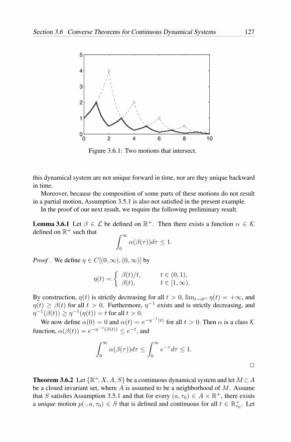
Section 3.6 Converse Theorems for Continuous Dynamical Systems 127
0 2 4 6 8 100
1
2
3
4
5
Figure 3.6.1: Two motions that intersect.
this dynamical system are not unique forward in time, nor are they unique backwardin time.
Moreover, because the composition of some parts of these motions do not resultin a partial motion, Assumption 3.5.1 is also not satisfied in the present example.
In the proof of our next result, we require the following preliminary result.
Lemma 3.6.1 Let β ∈ L be defined on R+. Then there exists a function α ∈ K
defined on R+ such that ∫ ∞
0α(β(τ))dτ ≤ 1.
Proof . We define η ∈ C[(0,∞), (0,∞)] by
η(t) =
β(t)/t, t ∈ (0, 1),β(t), t ∈ [1,∞).
By construction, η(t) is strictly decreasing for all t > 0, limt→0+ η(t) = +∞, andη(t) ≥ β(t) for all t > 0. Furthermore, η−1 exists and is strictly decreasing, andη−1(β(t)) ≥ η−1(η(t)) = t for all t > 0.
We now define α(0) = 0 and α(t) = e−η−1(t) for all t > 0. Then α is a class Kfunction, α(β(t)) = e−η−1(β(t)) ≤ e−t, and∫ ∞
0α(β(τ))dτ ≤
∫ ∞
0e−τdτ ≤ 1.
Theorem 3.6.2 Let R+, X, A, S be a continuous dynamical system and let M ⊂A
be a closed invariant set, where A is assumed to be a neighborhood of M . Assumethat S satisfies Assumption 3.5.1 and that for every (a, τ0) ∈ A × R
+, there existsa unique motion p(·, a, τ0) ∈ S that is defined and continuous for all t ∈ R
+τ0
. Let
128 Chapter 3. Principal Stability and Boundedness Results on Metric Spaces
(S, M) be uniformly asymptotically stable. Then there exist neighborhoods A1 andX1 of M such that A1 ⊂ X1 ⊂ A, and a mapping V : X1 × R
+ → R+ that satisfies
the following conditions.
(i) There exist two functions ψ1, ψ2 ∈ K such that
ψ1(d(x, M)) ≤ V (x, t) ≤ ψ2(d(x, M))
for all (x, t) ∈ X1 × R+.
(ii) There exists a function ψ3 ∈ K such that for all p(·, a, τ0) ∈ S and for allt ∈ [τ0,∞), we have
D+V (p(t, a, τ0), t) ≤ −ψ3(d(p(t, a, τ0), M))
whenever a ∈ A1.
Proof . By Lemma 3.10.5 (see Problem 3.10.17, Section 3.10), there exist a functionϕ ∈ K defined on [0, h0] for some h0 > 0, and a function σ ∈ L defined on R
+, suchthat for all t ≥ τ0
d(p(t, a, τ0), M) < ϕ(d(a, M))σ(t − τ0) (3.6.1)
for all p(·, a, τ0) ∈ S whenever d(a, M) < h0. Let X1 = x ∈ A : d(x, M) < h0and let
A1 =
a ∈ X1 : d(a, M) < ϕ−1(h0)
if ϕ(h0) > h0,
X1 otherwise.
We define
Z(x, t) =∫ ∞
t
u(d(p(τ, x, t), M)
)dτ (3.6.2)
where u ∈ K is to be determined later and is such that the integral converges forall (x, t) ∈ X1 × R
+. For p(·, a, τ0) ∈ S, p(τ, p(t, a, τ0), t) = p(τ, a, τ0) becauseof Assumption 3.5.1 and the uniqueness of the motion p(·, a, τ0). Therefore, theintegrand in the right-hand side of (3.6.2) is independent of t for x = p(t, a, τ0)where a ∈ A1. Because u(d(p(τ, a, τ0), M)) is a continuous function of τ , it followsthat Z(p(t, a, τ0), t) is differentiable with respect to t and that
d
dtZ(p(t, a, τ0), t) = −u
(d(p(t, x, τ0), M)
)(3.6.3)
for all (a, τ0) ∈ A1 × R+ and t ≥ τ0.
To determine how to choose u ∈ K so that the integral in (3.6.2) converges for all(x, t) ∈ X1 × R
+, we use (3.6.1). For x ∈ X1, t ∈ R+, and τ ≥ t, we have
d(p(τ, x, t), M) ≤ ϕ(d(x, M))σ(τ − t).
Because ϕ(d(x, M)) ≤ ϕ(h0) for x ∈ X1 and because σ(τ −t) ≤ σ(0), we have that
u(ϕ(d(x, M))σ(τ − t)
)≤[u(ϕ(d(x, M))σ(0)
)]1/2[u(ϕ(h0)σ(τ − t)
)]1/2
Section 3.6 Converse Theorems for Continuous Dynamical Systems 129
for x ∈ X1 and τ ≥ t ≥ 0. Therefore,
Z(x, t) ≤[u(ϕ(d(x, M))σ(0)
)]1/2∫ ∞
t
[u(ϕ(h0)σ(τ − t)
)]1/2dτ
=[u(ϕ(d(x, M))σ(0)
)]1/2∫ ∞
0
[u(ϕ(h0)σ(τ)
)]1/2dτ.
In applying Lemma 3.6.1, we choose β(τ) = ϕ(h0)σ(τ) and u(r) =[α(r)
]2. Then
Z(x, t) ≤[u(ϕ(d(x, M))σ(0)
)]1/2 = α(ϕ(d(x, M))σ(0)
). (3.6.4)
For (x, t) ∈ X1 × R+, we now define
W (x, t) = supt′≥t
d(p(t′, x, t), M)
.
Then
d(x, M) = d(p(t, x, t), M) ≤ W (x, t) ≤ ϕ(d(x, M))σ(0). (3.6.5)
Let V (x, t) = Z(x, t) + W (x, t). In the proof of Theorem 3.5.1 we have shownthat W (p(t, a, τ0), t) is nonincreasing for all t ≥ τ0 (i.e., D+W (p(t, a, τ0), t) ≤ 0).Therefore, (3.6.3) implies that
D+V (p(t, a, τ0), t) ≤ −u(d(p(t, a, τ0), M)
)for all a ∈ A1 and t ≥ τ0; that is, V satisfies condition (ii) of the theorem.
To show that V satisfies condition (i), we note that
d(x, M) ≤ V (x, t) ≤ α(ϕ(d(x, M))σ(0)
)+ ϕ(d(x, M))σ(0).
for all x ∈ X1 and t ∈ R+, where we have used (3.6.4) and (3.6.5). This concludes
the proof of the theorem.
The hypotheses in our next result are not precisely symmetric with the correspond-ing assumptions in Theorem 3.3.3 for exponential stability of (S, M). Nevertheless,they do constitute necessary conditions for exponential stability of (S, M).
Theorem 3.6.3 Let R+, X, A, S be a continuous dynamical system and let M ⊂A
be a closed invariant set, where A is assumed to be a neighborhood of M . Assumethat S satisfies Assumption 3.5.1, and furthermore, assume that for every (a, τ0) ∈A × R
+, there exists a unique continuous motion p(·, a, τ0) ∈ S that is defined andcontinuous for all t ∈ [τ0,∞). Let (S, M) be exponentially stable. Then thereexist neighborhoods A1 and X1 of M such that A1 ⊂ X1 ⊂ A, and a mappingV : X1 × R
+ → R+ that satisfies the following conditions.
(i) There exist two functions ψ1, ψ2 ∈ K such that
ψ1(d(x, M)) ≤ V (x, t) ≤ ψ2(d(x, M))
for all (x, t) ∈ X1 × R+.
130 Chapter 3. Principal Stability and Boundedness Results on Metric Spaces
(ii) There exists a constant c > 0 such that for every p(·, a, τ0) ∈ S and for allt ∈ [τ0,∞),
D+V (p(t, a, τ0), t) ≤ −cV (p(t, a, τ0), t)
where a ∈ A1.
Proof . By Lemma 3.10.6 (see Problem 3.10.18, Section 3.10), there exist a functionϕ ∈ K, defined on [0, h0] for some h0 > 0, and a constant α > 0 such that
d(p(t, a, τ0), M) < ϕ(d(a, M))e−α(t−τ0) (3.6.6)
for all p(·, a, τ0) ∈ S and all t ≥ τ0 whenever d(a, M) < h0.Let X1 = x ∈ A : d(x, M) < h0 and let
V (x, t) = supt′≥t
d(p(t′, x, t), M)eα(t′−t) (3.6.7)
for all (x, t) ∈ X1 × R+. Let A1 = a ∈ X1 : d(a, M) < ϕ−1(h0) if ϕ(h0) > h0
and A1 = X1 otherwise. Then for a ∈ A1 and τ0 ∈ R+, we have byAssumption 3.5.1
and the uniqueness of the motions that
V (p(t, a, τ0), t) = supt′≥t
d(p(t′, p(t, a, τ0), t), M)eα(t′−t)
= supt′≥t
d(p(t′, a, τ0), M)eα(t′−t).
Therefore, for ∆t > 0, we have
V (p(t + ∆t, a, τ0), t + ∆t) = supt′≥t+∆t
d(p(t′, p(t, a, τ0), t), M)eα(t′−t−∆t)
= supt′≥t+∆t
d(p(t′, a, τ0), M)eα(t′−t)e−α∆t
≤ V (p(t, a, τ0), t)e−α∆t.
The above inequality yields
D+V (p(t, a, τ0), t) ≤ lim∆t→0+
V (p(t, a, τ0), t)e−α∆t − 1
∆t= −αV (p(t, a, τ0), t).
Finally, (3.6.6) and (3.6.7) imply that
d(x, M) ≤ V (x, t) ≤ ϕ(d(x, M))
for all (x, t) ∈ X1 × R+. This concludes the proof of the theorem.
We conclude by noting that converse theorems for continuous dynamical systemsfor uniform boundedness, uniform ultimate boundedness, uniform asymptotic stabilityin the large, exponential stability in the large, and instability can also be established,using the methodology employed in the preceding results.
B. Refinements: Continuity of Lyapunov functions
In this subsection, we first define the notion of continuity with respect to initialconditions for continuous dynamical systems. We then show that the Lyapunovfunctions in the converse theorems (Theorems 3.6.2 and 3.6.3) are continuous.
Section 3.6 Converse Theorems for Continuous Dynamical Systems 131
Definition 3.6.1 Let R+, X, A, S be a dynamical system. Let am ⊂ A ⊂ X,
tm ⊂ R+, am → a ∈ A, and tm → t0 as m→∞, let pm = pm(·, am, tm)
be a sequence of noncontinuable motions defined on intervals Jm = [tm, cm), and letp = p(·, a, t0) be a noncontinuable motion defined on an interval [t0, c0). We say thatthe motion p is continuous with respect to initial conditions if there is a subsequencemj ⊂ m such that
(i) limj→∞ inf[0, cmj− tmj
) ⊃ J0 = [0, c0 − t0); and(ii) pmj
(t+ tmj, amj
, tmj) → p(t+ t0, a, t0) uniformly on compact subsets of J0
as j → ∞.If in particular, the motion p is unique, then it is required that the entire sequencepm(t + tm, am, tm) tends to p(t + t0, a, t0) uniformly in t on compact subsetsof J0.
For the motivation of Definition 3.6.1, the reader may want to refer to Theorem6.8.1 in the appendix section of Chapter 6 (Section 6.8), where conditions for thecontinuous dependence of the solutions of ordinary differential equations on initialconditions and parameters are presented (as required background material).
Theorem 3.6.4 Let R+, X, A, S be a continuous dynamical system and let M ⊂A
be a closed invariant set, where A is assumed to be a neighborhood of M . Assumethat S satisfies Assumption 3.5.1 and the motions in S are continuous with respectto initial conditions, and furthermore, assume that for every (a, τ0) ∈ A × R
+, thereexists a unique motion p(·, a, τ0) ∈ S that is defined and continuous for all t ∈ R
+τ0
.Let (S, M) be uniformly asymptotically stable. Then there exist neighborhoods A1and X1 of M such that A1 ⊂ X1 ⊂ A, and a function V ∈ C[X1 × R
+, R+] thatsatisfies the conditions of Theorem 3.6.2.
Proof . Let V (x, t) = W (x, t) + Z(x, t), where Z(x, t) and W (x, t) are the sameas in the proof of Theorem 3.6.2; that is,
W (x, t) = supt′≥t
d(p(t′, x, t), M)
,
Z(x, t) =∫ ∞
t
u(d(p(τ, x, t), M)
)dτ,
for all (x, t) ∈ X1 × R+, where X1 is given in the proof of Theorem 3.6.2. We show
in the following that both W (·, ·) and Z(·, ·) are continuous in (x, t), and hence,V (x, t) is continuous.
Let ε > 0 be arbitrary. Suppose that (xm, tm) ⊂ X1 × R+, m = 1, 2, . . . , and
(xm, tm) → (x0, t0) as m → ∞. There exists an L1 > 0 such that σ(s) < ε/ϕ(h0)for all s > L1, where σ(·) ∈ L is given in (3.6.1). Then d(p(τ + t, x, t), M) ≤ϕ(h0)σ(τ) < ε for all τ > L1. Thus,
|W (xm, tm) − W (x0, t0)|= sup
τ≥0
d(p(τ + tm, xm, tm), M)
− sup
τ≥0
d(p(τ + t0, x0, t0), M)
≤ sup
0≤τ≤L1
∣∣d(p(τ + tm, xm, tm), M) − d(p(τ + t0, x0, t0), M)∣∣+ 2ε.
132 Chapter 3. Principal Stability and Boundedness Results on Metric Spaces
Because the motions inS are continuous with respect to initial conditions, p(t, xm, tm)converges to p(t, x0, t0) uniformly on the compact set [0, L1]; that is, there exists anm0 ∈ N such that sup0≤τ≤L1
|d(p(τ, xm, tm), M) − d(p(τ, x0, t0), M)| < ε for allm > m0. The continuity of W (·, ·) now follows immediately.
Similarly, there exists an L2 > 0 such that∫ ∞
t+L2
u(d(p(τ, x, t), M))dτ ≤ α(ϕ(h0)σ(0))∫ ∞
L2
α(ϕ(h0))σ(τ)dτ < ε,
for all (x, t) ∈ X1 × R+, where u and α are given in the proof of Theorem 3.6.2.
Hence,
|Z(xm, tm) − Z(x0, t0)|
=∫ ∞
tm
u(d(p(τ, xm, tm), M))dτ −∫ ∞
t0
u(d(p(τ, x0, t0), M))dτ
≤∫ L2
0
∣∣∣u(d(p(τ + tm, xm, tm), M)) − u(d(p(τ + t0, x0, t0), M))∣∣∣dτ
+∫ ∞
tm+L2
u(d(p(τ, xm, tm), M))dτ +∫ ∞
t0+L2
u(d(p(τ, x0, t0), M))dτ
≤∫ L2
0
∣∣∣u(d(p(τ + tm, xm, tm), M)) − u(d(p(τ + t0, x0, t0), M))∣∣∣dτ + 2ε.
The term∫ L2
0
∣∣u(d(p(τ + tm, xm, tm), M)) − u(d(p(τ + t0, x0, t0), M))∣∣dτ
becomes arbitrarily small for sufficiently large m because p(t, xm, tm) convergesto p(t, x0, t0) uniformly on the compact set [0, L2]. Therefore we have shown thatZ(x, t) is continuous in (x, t).
In our next result, the Lyapunov function is constructed slightly differently fromthat in the proof of Theorem 3.6.3 to ensure the continuity of the Lyapunov function.
Theorem 3.6.5 Let R+, X, A, S be a continuous dynamical system and let M ⊂A
be a closed invariant set, where A is assumed to be a neighborhood of M . Assumethat S satisfies Assumption 3.5.1 and the motions in S are continuous with respectto initial conditions, and furthermore, assume that for every (a, τ0) ∈ A × R
+, thereexists a unique motion p(·, a, τ0) ∈ S that is defined and continuous for all t ∈ R
+τ0
.Let (S, M) be exponentially stable. Then there exist neighborhoods A1 and X1 ofM such that A1 ⊂ X1 ⊂ A, and a function V ∈ C[X1 × R
+, R+] that satisfies theconditions of Theorem 3.6.3.
Proof . By Lemma 3.10.6 (refer to Problem 3.10.18), there exist a function ϕ ∈ K,defined on [0, h0] for some h0 > 0, and a constant α > 0 such that
d(p(t, a, τ0), M) < ϕ(d(a, M))e−α(t−τ0) (3.6.8)
Section 3.7 Converse Theorems for Discrete-Time Dynamical Systems 133
for all p(·, a, τ0) ∈ S and all t ≥ τ0 whenever d(a, M) < h0.Let X1 = x ∈ A : d(x, M) < h0 and let
V (x, t) = supt′≥t
d(p(t′, x, t), M)eλα(t′−t) (3.6.9)
for all (x, t) ∈ X1 × R+, where 0 < λ < 1 is a constant. Let
A1 =
a ∈ X1 : d(a, M) < ϕ−1(h0) if ϕ(h0) > h0,
X1 otherwise.
It can be shown in the manner as in the proof of Theorem 3.6.3 that the V functionsatisfies the conditions in Theorem 3.6.3 with the constant c = λα.
To establish the continuity of V , we let ε> 0 be arbitrary, (xm, tm)⊂X1 ×R+,
m = 1, 2, . . . , and (xm, tm) → (x0, t0) as m → ∞. It follows from (3.6.8) that
d(p(τ + t, x, t), M)eλατ ≤ ϕ(h0)e−(1−λ)ατ < ε
for all τ > L= ln(ε/ϕ(h0))/[(1 − λ)α]. Thus,
|V (xm, tm) − V (x0, t0)|= sup
τ≥0
d(p(τ + tm, xm, tm), M)eλατ
− sup
τ≥0
d(p(τ + t0, x0, t0), M)eλατ
≤ sup
0≤τ≤L
∣∣d(p(τ + tm, xm, tm), M) − d(p(τ + t0, x0, t0), M)∣∣eλατ
+ 2ε.
Because the motions inS are continuous with respect to initial conditions, p(t, xm, tm)converges to p(t, x0, t0) uniformly on the compact set [0, L] as m → ∞; that is, thereexists an m0 ∈ N such that
sup0≤τ≤L
|d(p(τ + tm, xm, tm), M) − d(p(τ + t0, x0, t0), M)|eλατ < ε
for all m > m0. Therefore V is continuous in X1 × R+.
3.7 Converse Theorems for Discrete-Time DynamicalSystems
In the present section we address local converse theorems for discrete-time systems.Our first result, concerning uniform stability, is similar to the converse theorems
for uniform stability for DDS and continuous dynamical systems.
Theorem 3.7.1 Let N,X, A,S be a discrete-time dynamical system and let M ⊂Abe a closed invariant set, where A is assumed to be a neighborhood of M . Supposethat S satisfies Assumption 3.5.1 (modified in the obvious way for discrete-timesystems). Let (S, M) be uniformly stable. Then there exist neighborhoods A1 and
134 Chapter 3. Principal Stability and Boundedness Results on Metric Spaces
X1 of M such that A1 ⊂ X1 ⊂ A and a mapping V : X1 × N → R+ that satisfies
the following conditions.
(i) There exist functions ψ1, ψ2 ∈ K such that
ψ1(d(x, M)) ≤ V (x, n) ≤ ψ2(d(x, M)) (3.7.1)
for all (x, n) ∈ X1 × N.
(ii) For every p(·, a, n0) ∈ S with a ∈ A1, V (p(n, a, n0), n) is nonincreasing forall n ∈ Nn0 (i.e., n ≥ n0, n, n0 ∈ N).
Proof . The proof is similar to the proof of Theorem 3.5.1 and is not repeatedhere.
Theorem 3.7.2 Let N,X, A,S be a discrete-time dynamical system and let M ⊂Abe a closed invariant set, where A is assumed to be a neighborhood of M . Assume thatS satisfies Assumption 3.5.1 and that for every (a, n0) ∈ A× N there exists a uniquemotion p(·, a, n0) ∈ S that is defined for all n ∈ Nn0 (i.e., n ≥ n0, n, n0 ∈ N). Let(S, M) be uniformly asymptotically stable. Then there exist neighborhoods A1 andX1 of M such that A1 ⊂ X1 ⊂ A and a mapping V : X1 × N → R
+ that satisfiesthe following conditions.
(i) There exist functions ψ1, ψ2 ∈ K such that
ψ1(d(x, M)) ≤ V (x, n) ≤ ψ2(d(x, M)) (3.7.2)
for all (x, n) ∈ X1 × N.
(ii) There exists a function ψ3 ∈ K such that for all p(·, a, n0) ∈ S and for alln ∈ Nn0 , we have
DV (p(n, a, n0), n) ≤ −ψ3(d(p(n, a, n0), M)) (3.7.3)
where a ∈ A1, and
DV (p(n, a, n0), n) = V (p(n+1, a, n0), n+1)−V (p(n, a, n0), n). (3.7.4)
Proof . By Lemma 3.10.5 (refer to Problem 3.10.17, Section 3.10), there exist afunction ϕ ∈ K defined on [0, h0] for some h0 > 0, and a function σ ∈ L defined onR
+, such that for all n ∈ N+n0
,
d(p(n, a, n0), M) < ϕ(d(a, M))σ(n − n0) (3.7.5)
for all p(·, a, n0) ∈ S whenever d(a, M) < h0. Let X1 = x ∈ A : d(x, M) < h0and let
A1 =
a ∈ X1 : d(a, M) < ϕ−1(h0) if ϕ(h0) > h0,
X1 otherwise.
Section 3.7 Converse Theorems for Discrete-Time Dynamical Systems 135
We define
V (x, n0) =∞∑
j=n0
u(d(p(j, x, n0), M)) (3.7.6)
where u ∈ K is to be determined later and is such that the summation converges for all(x, n0) ∈ X1 × N. For p(·, a, n0) ∈ S, p(n, p(n1, a, n0), n1) = p(n, a, n0) becauseof Assumption 3.5.1 and the uniqueness of the motion p(·, a, n0). Therefore, thesummation in the right-hand side of (3.7.6) is independent of n0 for x = p(n, a, n0)where a ∈ A1.
To determine how to choose u ∈ K so that the summation in (3.7.6) converges forall (x, n0) ∈ X1 × N, we apply Lemma 3.5.1. It follows from (3.7.5) that for any(x, n0) ∈ X1 × N, we have
u(d(p(n, x, n0), M)) < u(ϕ(d(x, M))σ(n − n0))
≤ [u(ϕ(d(x, M))σ(0))]1/2[u(ϕ(h0)σ(n − n0))]1/2. (3.7.7)
Let β(τ) = ϕ(h0)σ(τ). Then β ∈ L. Hence, by Lemma 3.5.1, there exists a functionα ∈ K defined on R
+ such that∞∑
i=0
α(β((n0 + i) − n0)) =∞∑
j=n0
α(β(j − n0)) < ∞.
If we define u(r) = [α(r)]2, then it follows that
[u(ϕ(h0)σ(n − n0))]1/2 = [α(ϕ(h0)σ(n − n0))]1/2 = α(β(n − n0)).
Hence, we conclude that
V (x, n0) =∞∑
j=n0
u(d(p(j, x, n0), M))
<
∞∑j=n0
[u(ϕ(d(x, M))σ(0))]1/2[u(ϕ(h0)σ(j − n0))]1/2
= [u(ϕ(d(x, M))σ(0))]1/2∞∑
j=n0
α(β(j − n0))
< [u(ϕ(d(x, M))σ(0))]1/2[1 + 1/(1 − e−1)].
If we define ψ2 ∈ K by
ψ2(r) = [u(ϕ(r)σ(0))]1/2[1 + 1/(1 − e−1)],
then it follows that d(x, M) ≤ V (x, n0) ≤ ψ2(d(x, M)). Thus we have provedcondition (i) of the theorem.
For any p(·, a, n0) ∈ S and any n > n0, it follows from the uniqueness assump-tion that
V (p(n, a, n0), n) =∞∑
j=n
u(d(p(j, p(n, a, n0), n), M)) =∞∑
j=n
u(d(p(j, x, n0), M)).
136 Chapter 3. Principal Stability and Boundedness Results on Metric Spaces
Along each motion p(·, a, n0) ∈ S, we have that
DV (p(n, a, n0), n) =∞∑
j=n+1
u(d(p(j, a, n0), M)) −∞∑
j=n
u(d(p(j, a, n0), M))
= − u(d(p(n, x, n0), M))
for all (a, n0) ∈ A1 ×N and n ≥ n0; that is, V satisfies condition (ii) of the theorem.This concludes the proof of the theorem.
The hypotheses in our next result are not exactly symmetric with the correspondingassumptions in Theorem 3.4.3. However, they do provide a set of necessary conditionsfor exponential stability of (S, M).
Theorem 3.7.3 Let N,X, A,S be a discrete-time dynamical system and let M ⊂Abe a closed invariant set, where A is assumed to be a neighborhood of M . Assume thatS satisfies Assumption 3.5.1 and that for every (a, n0) ∈ A× N there exists a uniquemotion p(·, a, n0) ∈ S that is defined for all n ∈ Nn0 . Let (S, M) be exponentiallystable. Then there exist neighborhoods A1 and X1 of M such that A1 ⊂ X1 ⊂ Aand a mapping V : X1 × N → R
+ that satisfies the following conditions.(i) There exist functions ψ1, ψ2 ∈ K such that
ψ1(d(x, M)) ≤ V (x, n) ≤ ψ2(d(x, M)) (3.7.8)
for all (x, n) ∈ X1 × N.(ii) There exists a constant c > 0 such that for all p(·, a, n0) ∈ S and for all
n ∈ Nn0 , we have
DV (p(n, a, n0), n) ≤ −cV (p(n, a, n0), n) (3.7.9)
where a ∈ A1, c > 0 is a constant and DV (p(n, a, n0), n) is defined in (3.7.4).
Proof . By Lemma 3.10.6 (refer to Problem 3.10.18, Section 3.10), there exist afunction ϕ ∈ K, defined on [0, h0] for some h0 > 0, and a constant α > 0 such that
d(p(n, a, n0), M) < ϕ(d(a, M))e−α(n−n0) (3.7.10)
for all p(n, a, n0) ∈ S and n ≥ n0 whenever d(a, M) < h0.Let X1 = x ∈ A : d(x, M) < h0 and let
V (x, n0) = supn′≥n0
d(p(n′, x, n0), M)eα(n′−n0)
(3.7.11)
for all (x, n0) ∈ X1 × N. Let A1 = a ∈ X1 : d(a, M) < ϕ−1(h0) if ϕ(h0) > h0and A1 = X1 otherwise. Then for a ∈ A1 and n0 ∈ N, we have by Assumption 3.5.1and the uniqueness of the motions that
V (p(n, a, n0), n) = supn′≥n
d(p(n′, p(n, a, n0), n), M)eα(n′−n)
= supn′≥n
d(p(n′, a, n0), M)eα(n′−n).
Section 3.8 Appendix: Background Material on Differential Equations 137
Therefore, we have
V (p(n + 1, a, n0), n + 1) = supn′≥n+1
d(p(n′, a, n0), M)eα(n′−(n+1))
= supn′≥n+1
d(p(n′, a, n0), M)eα(n′−n)e−α
≤ supn′≥n
d(p(n′, a, n0), M)eα(n′−n)e−α
= V (p(n, a, n0), n)e−α. (3.7.12)
Equation (3.7.12) yields
DV (p(n, a, n0), n) ≤ −(1 − e−α)V (p(n, a, n0), n).
Finally, (3.7.10) and (3.7.11) imply that
d(x, M) ≤ V (x, n) ≤ ϕ(d(x, M))
for all (x, n) ∈ X1 × N. This concludes the proof of the theorem.
We conclude by noting that converse theorems for discrete-time dynamical systemsfor uniform boundedness, uniform ultimate boundedness, uniform asymptotic stabilityin the large, exponential stability in the large, and instability can also be established,using the methodology employed in the preceding results.
3.8 Appendix: Some Background Material onDifferential Equations
In this section we present a result that is required in the proof of some of the resultsof Section 3.3, relating the maximal solution of (IE),
x = g(t, x), x(t0) = x0 (IE)
to the solutions of (EI),Dx ≤ g(t, x) (EI)
where g ∈ C[R+ × Rl, Rl], D denotes a Dini derivative, and inequality of vectors is
to be interpreted componentwise. In the proof of the main result of this section, werequire several preliminary results that we state and prove first.
Definition 3.8.1 Let Ω be a connected set in Rl. A function g : R
+ ×Ω → Rl is said
to be quasi-monotone nondecreasing if for each component gj of g, j = 1, . . . , l, theinequality gj(t, y) ≤ gj(t, z) is true whenever y, z ∈ Ω and yi ≤ zi for all i = j,i, j = 1, . . . , l and yj = zj .
We note that when g is a scalar-valued function, it is automatically quasi-monotonenondecreasing.
138 Chapter 3. Principal Stability and Boundedness Results on Metric Spaces
Definition 3.8.2 A solution ϕM of the initial value problem (IE) is called a maximalsolution on [t0, t0 + c) if for any solution ϕ defined on [t0, t0 + c) it is true thatϕM (t) ≥ ϕ(t) for all t ∈ [t0, t0 + c), where c > 0 and the inequality (for vectors) isunderstood to be componentwise.
A minimal solution of (IE) on some interval is defined similarly. By definition, amaximal (resp., minimal) solution of (IE), if it exists, must be unique.
Lemma 3.8.1 Let g ∈ C[R+ × Ω, Rl], let v, w ∈ C[[t0, t0 + c), Rl
], t0 ∈ R
+, andc > 0, and assume that the following conditions are true.
(i) g is quasi-monotone nondecreasing.
(ii) v(t0) < w(t0).
(iii) D−v(t) ≤ g(t, v(t)) and D−w(t) > g(t, w(t)) for t ∈ (t0, t0 + c), whereD− denotes the lower-left Dini derivative.
Then it is true that
v(t) < w(t) (3.8.1)
for t ∈ [t0, t0 + c).
Proof . Let u(t) = w(t) − v(t). Then condition (ii) reads as u(t0) > 0. Supposethat the assertion (3.8.1) is not true. Then the set
F =l⋃
i=1
t ∈ [t0, t0 + c) : ui(t) ≤ 0
= ∅.
Let t1 = inf F . Because ui(t0) > 0, 1 ≤ i ≤ l, and u ∈ C[[t0, t0 + c), Rl
], it is
clear that t1 > t0. The set F is closed, and thus t1 ∈ F . We now show that thereexists a j ∈ 1, 2, . . . , l such that
uj(t1) = 0. (3.8.2)
If (3.8.2) is not true (i.e., if ui(t1) < 0 for all 1 ≤ i ≤ l), then ui(t) < 0 in asufficiently small neighborhood to the left of t1 by the continuity of u. This contradictsthe definition of t1, and therefore (3.8.2) holds. Moreover, t1 = inf F implies that
ui(t1) ≥ 0, i = j (3.8.3)
and
D−uj(t1) ≤ 0. (3.8.4)
Combining (3.8.4) and condition (iii), we obtain
gj(t1, w(t1)) < gj(t1, v(t1)). (3.8.5)
Section 3.8 Appendix: Background Material on Differential Equations 139
On the other hand, (3.8.2), (3.8.3), and the quasi-monotonicity condition imply that
gj(t1, w(t1)) > gj(t1, v(t1))
which contradicts (3.8.5). This concludes the proof.
The above result makes possible the proof of the next result.
Lemma 3.8.2 Let v, f ∈ C[[t0, t0 + c), Rl
]. If for a fixed Dini derivative D it is
true that Dv(t) ≤ f(t) for t ∈ [t0, t0 + c), c > 0, then
D−v(t) ≤ f(t) (3.8.6)
for t ∈ (t0, t0 + c).
Proof . Because D−v(t) ≤ D−v(t) and D+v(t) ≤ D+v(t), we only need to provethe lemma for D = D+. Let
u(t) = v(t) −∫ t
t0
f(s)ds.
Then D+u(t) = D+v(t) − f(t) ≤ 0 for t ∈ [t0, t0 + c). We want to prove that u(t)is nonincreasing on [t0, t0 + c), which is equivalent to proving that m(t) = −u(−t)is nonincreasing on (−t0 − c,−t0]. Note that D−m(t) = D+u(−t) ≤ 0. We applyLemma 3.8.1 to show that for any t1, t2 ∈ (−t0 − c,−t0], t1 < t2, m(t1) ≥ m(t2).Let w(t) = m(t1) + ε(t − t1 + ε) for t ∈ [t1,−t0] where ε > 0. Then D−w(t) =ε > 0, D−m(t) ≤ 0, and m(t1) < w(t1) + ε2. By Lemma 3.8.1, m(t) < w(t) forall t ∈ [t1,−t0]. In particular, m(t2) < w(t2) = m(t1) + ε(t2 − t1 + ε). Becauseε > 0 is arbitrary, we obtain m(t2) ≤ m(t1) by letting ε → 0.
We have proved that u(t) is nondecreasing on [t0, t0 +c). Therefore, D−u(t) ≤ 0and D−v(t) = D−u(t) + f(t) ≤ f(t) for t ∈ (t0, t0 + c).
We require one more preliminary result.
Lemma 3.8.3 Let g ∈ C[R+ × Ω, Rl] and assume that g is quasi-monotone non-decreasing. Then for each (t0, x0) ∈ R
+ × Rl, there exists a c > 0 such that the
maximal solution of (IE) exists on [t0, t0 + c].
Proof . Let
Da,b = Da,b(t0, x0) =(t, x) ∈ R
+ × Ω: t0 ≤ t ≤ t0 + a, |x − x0| ≤ b.
Inasmuch as g is continuous, we may assume that |g(t, x)| ≤ M for all (t, x) ∈ Da,b.According to Theorem 2.3.1 and Problem 2.14.8, we may choose c1 = mina, b/Msuch that (IE) has a solution defined on [t0, t0 + c1].
Now consider the differential equation with the initial condition given by
y = g(t, y) + ε, y(t0) = x0 + ε (3.8.7)
140 Chapter 3. Principal Stability and Boundedness Results on Metric Spaces
where 0 ≤ ε < b/2. We note that for
D′a,(b/2) = D′
a,(b/2)(t0, x0+ε) =
(t, y) ∈ R+× Ω: t0 ≤ t ≤ t0 + a, |x−x0| ≤ b
2
we have |g(t, y) + ε| ≤ M + b/2 for all (t, y) ∈ D′
a,(b/2). Therefore, (3.8.7) has asolution y(t, ε) defined on [t0, t0 + c], where
c = min
a,b/2
M + b/2
= min
a,
b
2M + b
.
For 0 < ε2 < ε1 ≤ ε, Lemma 3.8.1 implies that y(t, 0) < y(t, ε2) < y(t, ε1) fort ∈ [t0, t0 + c]. Therefore, limε→0+ y(t, ε) = y∗(t) exists and the convergence isuniform for t ∈ [t0, t0 + c]. Hence y∗(t) is a solution of (IE), because
y∗(t) = limε→0+
y(t, ε)
= limε→0+
(x0 + ε +
∫ t
t0
(g(s, y(s, ε)) + ε
)ds)
= x0 +∫ t
t0
g(s, y∗(s))ds.
Because y(t, ε) > y(t, 0) for t ∈ [t0, t0 + c] we obtain y∗(t) ≥ y(t, 0) for t ∈[t0, t0 + c]. Because y(t, 0) is any solution of (IE) defined on [t0, t0 + c], it followsthat y∗ is a maximal solution of (IE).
The above result concerns the local existence of a maximal solution for (IE). Theexistence of a noncontinuable maximal solution follows by invoking Zorn’s lemma(see, e.g., [11]).
We now state and prove the main result of this section.
Theorem 3.8.1 (Comparison Theorem) Assume that g ∈ C[R+ × Ω, Rl] is quasi-monotone nondecreasing. Let x(t) be a solution of (EI) defined on [t0, t0 + c],c > 0, and let r(t), defined on [t0, t0 + c], be the maximal solution of (IE), wherer(t0) = x(t0) = x0. Then
x(t) ≤ r(t)
for all t ∈ [t0, t0 + c).
Proof . Let
F =t′ ∈ [t0, t0 + c) : x(t) ≤ r(t) for all t ∈ [t0, t′]
.
Then t0 ∈ F , because x(t0) = r(t0). It suffices to show that supF = t0 + c. If thisis not true (i.e., if supF = t1 < t0 + c), then r(t1) ≥ x(t1). We consider
y = g(t, y) + ε, y(t1) = r(t1) + ε (3.8.8)
Section 3.9 Notes and References 141
where ε > 0 is sufficiently small. By the proof of Lemma 3.8.3, there exists a c1 > 0such that solutions y(t, ε) of (3.8.8) are defined on [t1, t1 + c1], and limε→0+ y(t, ε)exists as the maximal solution of
y = g(t, y), y(t1) = r(t1)
for t ∈ [t1, t1+c1]. By the uniqueness of the maximal solution, r(t)=limε→0+y(t, ε)for t ∈ [t1, t1 + c1]. We assume without loss of generality that t1 + c1 < t0 + c (forotherwise, we choose c1 smaller).
Now D−y(t, ε) = y(t, ε)> g(t, y(t, ε)) together with Lemma 3.8.2 implies thatD−x(t) ≤ g(t, x(t)) for all t ∈ (t1, t1 + c1). In addition, y(t1, ε) = r(t1) + ε >r(t1) ≥ x(t1). By Lemma 3.8.1, y(t, ε) > x(t) for all t ∈ [t1, t1 + c1). Lettingε → 0+, we see that r(t) ≥ x(t) for all t ∈ [t1, t1 + c1). Therefore, for anyt′ ∈ (t1, t1 + c1), we have that t′ ∈ F . But this contradicts the fact that t1 = supF .This concludes the proof of the theorem.
In the scalar case (l = 1), we can forgo the quasi-monotone condition.
3.9 Notes and References
The material given in Section 3.1 is standard fare in the qualitative analysis of dy-namical systems (see, e.g., Zubov [15], Hahn [2], and Michel et al. [10]).
The stability and boundedness results for discontinuous dynamical systems pre-sented in Section 3.2 were first reported in Ye [12] and Ye et al. [13], with subsequentdevelopments given in Hou [3], Hu [5], Michel [8], and Michel and Hu [9].
The Principal Lyapunov Stability Results given in Sections 3.3 and 3.4 are includedin several texts (see, e.g., Hahn [2], Zubov [15], and Michel et al. [10]). In [2] and[15], these results are proved using the basic stability and boundedness definitionsand fundamental methods of analysis, whereas in [10], these results are establishedby invoking a comparison theory, making use of stability preserving mappings. Ourapproach of proving these results by using the stability and boundedness results forDDS established in Section 3.2 (and thus, establishing a unifying stability theory fordiscontinuous, continuous, and discrete-time dynamical systems) is novel and new(refer to Hou and Michel [4]).
The converse theorems for DDS presented in Section 3.5 were originally estab-lished in [12] and [13] with subsequent refinements and developments given in Hou[3], Hu [5], Michel [8], and Michel and Hu [9].
The converse theorems for uniform stability, Theorem 3.6.1 and Theorem 3.7.1,are in the spirit of results given in Zubov [15]. The converse theorems for uniformasymptotic stability, Theorem 3.6.2 and Theorem 3.7.2 and their proofs, includingLemma 3.6.1, are adaptations of material given in Hahn [2] and the converse theoremsfor exponential stability, Theorem 3.6.3 and Theorem 3.7.3, are based on a result inMassera [7].
References for the background material on differential equations given in Section3.8 include Lakshmikantham and Leela [6], Miller and Michel [11], and Michelet al. [10].
142 Chapter 3. Principal Stability and Boundedness Results on Metric Spaces
3.10 Problems
Problem 3.10.1 Consider the autonomous system of first-order ordinary differentialequations
x = f(x) (3.10.1)
where f ∈ C[Rn, Rn]. Assume that there exists a function V ∈ C1[Rn, R] such that
V(3.10.1)(x)= [∇V (x)]T f(x) = 0
for all x ∈ Rn, where ∇V (x) =
[∂V /∂x1, . . . , ∂V /∂xn
]T. Let
Bλ = x ∈ Rn : V (x) = λ (3.10.2)
Cλ = x ∈ Rn : V (x) ≤ λ (3.10.3)
andDλ = x ∈ R
n : V (x) ≥ λ. (3.10.4)
It should be noted that each of these sets may consist of several disjoint componentsets. Prove that the sets Bλ, Cλ, and Dλ are invariant with respect to (3.10.1). Provethat each disjoint component set of Bλ, Cλ, and Dλ is invariant with respect to(3.10.1).
Problem 3.10.2 Consider the autonomous system of first-order difference equations
x(k + 1) = f(x(k)) (3.10.5)
where k ∈ N = 0, 1, 2, . . . and f : Rn → R
n. Assume that there exists a functionV : R
n → R such that
DV(3.10.5)(x)= V (f(x)) − V (x) = 0
for all x ∈ Rn. Let Bλ, Cλ, and Dλ be defined by (3.10.2), (3.10.3), and (3.10.4),
respectively. Prove that Bλ, Cλ, and Dλ are invariant with respect to (3.10.5). Provethat each disjoint component set of Bλ, Cλ, and Dλ is invariant with respect to(3.10.5).
Problem 3.10.3 For a dynamical system R+, X, A, S assume that there exists a
function V ∈ C[X, R] such that
D+V(S)(x)= lim
∆t→0+sup
p(·, x, t0) ∈ Sp(t0, x, t0) = x
1∆t
V (p(t+∆t, x, t0))−V (p(t, x, t0))
≤ 0
for all x ∈ X . Let Cλ be defined by (3.10.3). Prove that Cλ is an invariant set withrespect to S.
Section 3.10 Problems 143
In Sections 3.3 and 3.4 we proved the Principal Lyapunov and Lagrange stabilityresults for continuous dynamical systems and discrete-time dynamical systems usingin most cases the corresponding results for DDS. In the following, we ask the readerto prove these results, using definitions of stability and boundedness (as was done inproving the stability and boundedness results for DDS in Section 3.2).
Problem 3.10.4 Prove Theorems 3.3.1 and 3.4.1 by using the definition of uniformstability (given in Definition 3.1.6).
Problem 3.10.5 Prove Theorems 3.3.2 and 3.4.2 by using the definition of uniformasymptotic stability (given in Definition 3.1.9).
Problem 3.10.6 Prove Theorems 3.3.3 and 3.4.3 by using the definition of exponen-tial stability (given in Definition 3.1.10).
Problem 3.10.7 Prove Theorems 3.3.4 and 3.4.4 by using the definition of uniformboundedness (given in Definition 3.1.13).
Problem 3.10.8 Prove Theorems 3.3.5 and 3.4.5 by using the definition of uniformultimate boundedness (given in Definition 3.1.14).
Problem 3.10.9 Prove Theorems 3.3.6 and 3.4.6 by using the definition of uniformasymptotic stability in the large (given in Definition 3.1.16).
Problem 3.10.10 Prove Theorems 3.3.7 and 3.4.7 by using the definition of expo-nential stability in the large (given in Definition 3.1.17).
Problem 3.10.11 Prove Theorems 3.3.8 and 3.3.10 and Theorems 3.4.8 and 3.4.10by using the definition of instability (given in Definition 3.1.18).
Problem 3.10.12 Prove Theorems 3.3.9 and 3.4.9 by using the definition of completeinstability (given in Definition 3.1.20).
For most of the boundedness and stability concepts that we introduced in Section3.1 there are equivalent definitions which frequently make the proofs of the stabilityand boundedness results easier and more systematic. These definitions involve certaincomparison functions whose properties we ask the reader to explore in the next twoproblems.
Problem 3.10.13 Prove the following results.
Lemma 3.10.1 [2] A continuous function σ : [s1,∞) → R+ is said to belong to
class L if σ is strictly decreasing on [s1,∞) and if lims→∞ σ(s) = 0 where s1 ∈ R+
(refer to Definition 3.5.1). Show that the functions of class K, class K∞, and class Lpossess the following properties.
(i) If ϕ1, ϕ2 ∈ K, then ϕ1 ϕ2 ∈ K, where (ϕ1 ϕ2)(r) = ϕ1(ϕ2(r)).(ii) If ϕ ∈ K and σ ∈ L, then ϕ σ ∈ L.
(iii) If ϕ ∈ K, then ϕ−1 exists and ϕ−1 ∈ K; also, if ϕ ∈ K∞, then ϕ−1 ∈ K∞.
144 Chapter 3. Principal Stability and Boundedness Results on Metric Spaces
(iv) If ϕ ∈ K and if ϕ is defined on [0, k2], then there exist ϕ1, ϕ2 ∈ K, defined on[0, k], k > 0, such that
ϕ(r1r2) ≤ ϕ1(r1)ϕ2(r2)
for all r1, r2 ∈ [0, k].
Hint: In (iv), choose ϕ1(r) = ϕ2(r) =√
ϕ(kr).
Problem 3.10.14 Prove the following results.
Lemma 3.10.2 [2] A real-valued function l = l(r, s) is said to belong to the classKL if
(i) it is defined for 0 ≤ r ≤ r1 (resp., 0 ≤ r < ∞) and for 0 ≤ s0 ≤ s < ∞; and
(ii) for each fixed s it belongs to class K with respect to r and it is monotonedecreasing to zero as s increases (it need not be strictly monotone decreasing).
Let l ∈ KL. Show that there exist functions ϕ ∈ K and σ ∈ L such that
l(r, s) ≤ ϕ(r)σ(s)
for the following two cases.
(a) l(r, s) is bounded with respect to r (i.e., l(r, s) ≤ l0(s)).(b) 0 ≤ r < ∞ and l(r, s)/l(r0, s) is monotone decreasing for all r ≥ r0 as s
increases.
Hint: In (a), assume without loss of generality that l0 ∈ L and choose
ϕ(r) =√
l(r, s0), σ(s) =√
l0(s).
In (b) we havel(r, s) < l(r, s0)l0(r0, s)/l(r0, s0).
In the next four problems we ask the reader to establish several equivalent stabilitydefinitions phrased in terms of comparison functions discussed above.
Problem 3.10.15 Prove the following results.
Lemma 3.10.3 [2] Show that (S, M) is stable if and only if for each t0 ∈ T thereexists a function ϕ ∈ K defined on [0, r0], r0 > 0, such that
d(p(t, a, t0), M) ≤ ϕ(d, (a, M))
for all p(·, a, t0) ∈ S and for all t ∈ Ta,t0 whenever d(a, M) < r0, where ϕ maydepend on t0.
Prove that (S, M) is uniformly stable if and only if in the above, ϕ is independentof t0.
Problem 3.10.16 Prove the following results.
Section 3.10 Problems 145
Lemma 3.10.4 [2] Show that (S, M) is attractive if and only if for each t0 ∈ Tthere exists an η = η(t0) > 0 such that for each p(·, a, t0) ∈ S, there exists a functionσ ∈ L (where σ may depend on t0 and p(·, a, t0)) such that if d(a, M) < η, thend(p(t, a, t0), M) < σ(t − t0) for all t ∈ Ta,t0 . (The class of functions L is definedin Problem 3.10.13.)
Show that (S, M) is uniformly attractive if and only if the above is true for ηindependent of t0 and for σ independent of t0 and of p(·, a, t0).
Problem 3.10.17 Prove the following results.
Lemma 3.10.5 [2] Prove that (S, M) is asymptotically stable if and only if foreach t0 ∈ T there exists a function ϕ ∈ K on [0, r0], r0 > 0, such that for eachp(·, a, t0) ∈ S, there exists a function σ ∈ L such that if d(a, M) < r0, then
d(p(t, a, t0), M) ≤ ϕ(d(a, M))σ(t − t0)
for all t ∈ Ta,t0 .
Prove that (S, M) is uniformly asymptotically stable if and only if the above istrue for ϕ independent of t0 and for σ independent of t0 and of p(·, a, t0).
Prove that (S, M) is uniformly asymptotically stable in the large if and only if theabove is true for ϕ independent of t0 and for σ independent of t0 and of p(·, a, t0),and furthermore, ϕ ∈ K∞.Hint: Use the results of Problem 3.10.14
Problem 3.10.18 Prove the following results.
Lemma 3.10.6 [2] Show that (S, M) is exponentially stable (resp., exponentiallystable in the large) if and only if (S, M) is uniformly asymptotically stable (resp., uni-formly asymptotically stable in the large) and in the statement for uniform asymptoticstability in Problem 3.10.17 σ(s) = e−αs with α > 0.
In the next six problems we ask the reader to prove several of the stability resultsof Sections 3.3 and 3.4 by utilizing the equivalent definitions for stability establishedabove.
Problem 3.10.19 Prove Theorem 3.3.1 by utilizing the equivalent definition of uni-form stability given in Problem 3.10.15.
Problem 3.10.20 Prove Theorem 3.3.2 and Theorem 3.3.6 by utilizing the equivalentdefinitions of uniform asymptotic stability and uniform asymptotic stability in the largegiven in Problem 3.10.17.
Problem 3.10.21 Prove Theorem 3.3.3 and Theorem 3.3.7 by utilizing the equivalentdefinitions of exponential stability and exponential stability in the large given inProblem 3.10.18.
Problem 3.10.22 Prove Theorem 3.4.1 by utilizing the equivalent definition of uni-form stability given in Problem 3.10.15.
146 Chapter 3. Principal Stability and Boundedness Results on Metric Spaces
Problem 3.10.23 Prove Theorem 3.4.2 and Theorem 3.4.6 by utilizing the equivalentdefinitions of uniform asymptotic stability and uniform asymptotic stability in the largegiven in Problem 3.10.17.
Problem 3.10.24 Prove Theorem 3.4.3 and Theorem 3.4.7 by utilizing the equivalentdefinitions of exponential stability and exponential stability in the large given inProblem 3.10.18.
Problem 3.10.25 Let S be the dynamical system determined by the scalar differentialequation
y = −ψ(y), y ∈ R+
where ψ ∈ K. Prove that (S, 0) is uniformly asymptotically stable.Hint [2]: Let G denote a primitive function of −1/ψ. Then
y(t) = G−1(t − t0 + G(y0))
where G−1 denotes the inverse of G. If the function −1/ψ is integrable near 0, thenthere exists a finite number t1 such that y(t) = 0 for all t ≥ t1. If the function −1/ψis not integrable near 0, then G−1 ∈ L (see Problem 3.10.13 for the definition ofclass L). In a similar manner as in Problem 3.10.13(iv), conclude that for s1 ≥ c1,s2 ≥ c2 and σ ∈ L, there exist σ1, σ2 ∈ L such that
σ(s1 + s2) ≤ σ1(s1)σ2(s2).
Next, apply the above inequality to G−1 ∈ L with s1 = t − t0 and s2 = G(y0) toobtain
y(t) ≤ σ1(t − t0)σ2(G(y0)).
This inequality implies the uniform attractivity of (S, 0) (refer to Definition 3.1.7and Problem 3.10.16). The uniform stability of (S, 0) follows from the uniformstability of (S1, 0) where S ⊂ S1 and S1 is the dynamical system determined by
y ≤ 0, y ∈ R+.
Problem 3.10.26 Prove that if in Problem 3.10.25 ψ ∈ K∞, then (S, 0) is uni-formly asymptotically stable in the large.
Problem 3.10.27 Let y ∈ C[[t0,∞), R
]and assume that y(t0) > 0 and that
Dy(t) ≥ ψ(y(t))
for all t ≥ t0 where D is a fixed Dini derivative and ψ ∈ K is defined on R+. Show
that limt→∞ y(t) = ∞.Hint: Apply Theorem 3.8.1 to show that y(t) ≥ r(t) where r(t) is the minimalsolution of
y = ψ(y)
with the initial condition r(t0) = y(t0). Problem 3.10.27 can now be reduced toproving that limt→∞ r(t) = ∞.
Bibliography 147
Problem 3.10.28 Let S be the dynamical system determined by the scalar differenceequation
yk+1 ≤ yk − ψ(yk), yk ∈ R+, ψ ∈ K,
for all k ∈ Ta,k0 . Prove that (S, 0) is uniformly asymptotically stable.Hint: (S, 0) is uniformly stable because every motion of S is a decreasing non-negative sequence. To show that (S, 0) is uniformly attractive, first establish thatyk+1 − yk0 ≤ −(k − k0 + 1)ψ(yk) and conclude that
ψ(yk) ≤ yk0 − yk+1
k − k0 + 1≤ yk0
k − k0 + 1. (3.10.6)
Choose δ > 0 in such a manner that ψ−1 exists on [0, δ], and for every ε > 0, k0 ∈ N,choose τ = δ/ψ(ε). Then for k ≥ k0+τ , we have k−k0+1 ≥ τ +1 > τ = δ/ψ(ε).By (3.10.6), we have that
|yk| = yk = ψ−1( yk0
k − k0 + 1
)< ψ−1
( δ
k − k0 + 1
)< ε
for all k ≥ k0 + τ whenever |yk0 | = yk0 < δ. Therefore, (S, 0) is uniformlyattractive (see Definition 3.1.9).
Problem 3.10.29 Prove that if in Problem 3.10.28 ψ ∈ K∞, then (S, 0) is uni-formly asymptotically stable in the large.
Problem 3.10.30 Prove the assertions made in Examples 3.1.8 and 3.1.9.
Bibliography
[1] P. J. Antsaklis and A. N. Michel, Linear Systems, Boston: Birkhauser, 2006.
[2] W. Hahn, Stability of Motion, Berlin: Springer-Verlag, 1967.
[3] L. Hou, Qualitative Analysis of Discontinuous Deterministic and StochasticDynamical Systems, Ph.D. Dissertation, University of Notre Dame, Notre Dame,IN, 2000.
[4] L. Hou and A. N. Michel, “Unifying theory for stability of continuous, discon-tinuous and discrete-time dynamical systems,” Nonlinear Anal. Hybrid Syst.,vol. 1, no. 2, pp.154-172, 2007.
[5] B. Hu, Qualitative Analysis of Hybrid Dynamical Systems, Ph.D. Dissertation,University of Notre Dame, Notre Dame, IN, 1999.
[6] V. Lakshmikantham and S. Leela, Differential and Integral Inequalities, vol. Iand vol. II, New York: Academic Press, 1969.
[7] J. L. Massera, “Contributions to stability theory,” Ann. Math., vol. 64, pp. 182–206, 1956.
148 Chapter 3. Principal Stability and Boundedness Results on Metric Spaces
[8] A. N. Michel, “Recent trends in the stability analysis of hybrid dynamicalsystems,” IEEE Trans. Circ. Syst. I: Fund. Theor. Appl., vol. 46, pp. 120–134,1999.
[9] A. N. Michel and B. Hu, “Towards a stability theory of general hybrid dynamicalsystems,” Automatica, vol. 35, pp. 371–384, 1999.
[10] A. N. Michel, K. Wang, and B. Hu, Qualitative Theory of Dynamical Systems-The Role of Stability Preserving Mappings, 2nd Edition, New York: MarcelDekker, 2001.
[11] R. K. Miller and A. N. Michel, Ordinary Differential Equations, New York:Academic Press, 1982.
[12] H. Ye, Stability Analysis of Two Classes of Dynamical Systems: General Hy-brid Dynamical Systems and Neural Networks with Delays, Ph.D. Dissertation,University of Notre Dame, Notre Dame, IN, 1996.
[13] H. Ye, A. N. Michel, and L. Hou, “Stability theory for hybrid dynamical sys-tems,” IEEE Trans. Autom. Control, vol. 43, pp. 461–474, 1998.
[14] T. Yoshizawa, Stability Theory by Lyapunov’s Second Method, Tokyo: Math.Soc. of Japan, 1966.
[15] V. I. Zubov, Methods of A. M. Lyapunov and their Applications, Groningen, TheNetherlands: P. Noordhoff, 1964.
Chapter 4
Fundamental Theory:Specialized Stability andBoundedness Results onMetric Spaces
In this chapter we present a number of important specialized stability and boundednessresults for dynamical systems defined on metric spaces. These include results forautonomous dynamical systems (in Section 4.1), results that comprise the InvarianceTheory (in Section 4.2), some results that go under the heading of Comparison Theory(in Section 4.3), and a result that addresses the uniqueness of motions in dynamicalsystems (in Section 4.4).
Before proceeding with our subject on hand, we would like to remind the readeronce more that our definition of dynamical system (Definition 2.2.3) does in generalnot require that time be reversible in the motions (in contrast to many dynamicalsystems determined, e.g., by various types of differential equations), nor are themotions required to be unique with respect to initial conditions. For such generalsystems, when required, we make an assumption that is akin to the semigroup property,but is more general, which essentially requires that for a dynamical system S, anypartial motion is also a motion of S, and any composition of two motions is also amotion of S (refer to Assumption 3.5.1). Of course when in a dynamical system thesemigroup property holds, then Assumption 3.5.1 is automatically implied.
4.1 Autonomous Dynamical Systems
In the present section we show that under reasonable assumptions, in the case ofautonomous dynamical systems, the stability and asymptotic stability of an invariant
149
150 Chapter 4. Specialized Stability and Boundedness Results on Metric Spaces
set M ⊂ A, with respect to S, imply the uniform stability and uniform asymptoticstability of (S, M), respectively. We also establish necessary and sufficient condi-tions for stability and asymptotic stability of (S, M) for autonomous systems in thissection.
Definition 4.1.1 A dynamical system T, X, A, S is said to be an autonomous dy-namical system if
(i) every p(·, a, t0) ∈ S is defined on Ta,t0 = T ∩ [t0,∞); and
(ii) for each p(·, a, t0) ∈ S and for each τ such that t0 + τ ∈ T , there exists amotion p(·, a, t0 + τ) ∈ S such that p(t + τ, a, t0 + τ) = p(t, a, t0) for allt ∈ Ta,t0 and all τ satisfying t + τ ∈ T .
Examples of autonomous dynamical systems include linear and nonlinear semi-groups. These systems have motions that are unique and continuous with respect toinitial conditions.
In general we do not require that autonomous dynamical systems satisfy the unique-ness property. For example, autonomous dynamical systems determined by differ-ential inclusions defined on Banach spaces (refer to Chapter 2) do not satisfy theuniqueness property.
In the next two results we assume that the motions of the dynamical systems arecontinuous with respect to initial conditions in the sense of Definition 3.6.1.
Theorem 4.1.1 Let R+, X, A, S be an autonomous dynamical system that satisfies
Assumption 3.5.1 and for which the motions are continuous with respect to initialconditions. Let M ⊂ A be a closed and invariant set. If (S, M) is stable, then(S, M) is uniformly stable.
Proof . Because R+, X, A, S is autonomous, for each p(·, a, t0) ∈ S, there exists
a motion p(·, a, 0) ∈ S such that p(t, a, t0) = p(t − t0, a, 0) for all t ≥ t0.Because (S, M) is stable, for every ε > 0 there exists a δ = δ(ε, 0) > 0 such
that d(p(t, a, 0), M) < ε for all t ≥ 0 and all p(·, a, 0) ∈ S whenever d(a, M) < δ.Therefore, d(p(t, a, t0), M) = d(p(t − t0, a, 0), M) < ε for all t ≥ t0. Note that δis independent of t0. We have shown that (S, M) is uniformly stable.
An analogous result and proof of Theorem 4.1.1 for discrete-time dynamical sys-tems can be established by making obvious modifications.
Theorem 4.1.2 Let R+, X, A, S be an autonomous dynamical system for which
the motions are continuous with respect to initial conditions and that satisfies As-sumption 3.5.1. Let M ⊂ A be a closed and invariant set and assume that A iscompact. If (S, M) is asymptotically stable, then (S, M) is uniformly asymptoticallystable.
Proof . The uniform stability of (S, M) follows from Theorem 4.1.1. We onlyneed to show the uniform attractivity of (S, M); that is, we need to show thatthere exists a δ > 0, and for every ε > 0 and every t0 ∈ R
+, there exists a
Section 4.1 Autonomous Dynamical Systems 151
τ = τ(ε) > 0, independent of t0, such that d(p(t, a, t0), M) < ε for all t ≥ t0 + τand for all p(·, a, t0) ∈ S whenever d(a, M) < δ. Because R
+, X, A, S is au-tonomous, for each p(·, a, t0) ∈ S, there exists a motion p(·, a, 0) ∈ S such thatp(t, a, t0) = p(t − t0, a, 0) for all t ≥ t0. Therefore, it is equivalent to showthat there exists a δ > 0, and for every ε > 0, there exists a τ = τ(ε) > 0,such that d(p(t, a, 0), M) < ε for all t ≥ τ and for all p(·, a, 0) ∈ S wheneverd(a, M) < δ.
Assume that (S, M) is not uniformly attractive. In view of the above statement,for every δ > 0, there exists an ε > 0, two sequences am : m ∈ N ⊂ Xand tm : m ∈ N ⊂ R
+ with limm→∞ tm = ∞ such that d(am, M) < δ andd(p(tm, am, 0), M) > ε for all m ∈ N.
Because A is compact, am : m ∈ N has a convergent subsequence. Withoutloss of generality, we may assume that am → a∗ ∈ A.
The uniform stability of (S, M) implies that there exists a δ∗ > 0 such thatd(p(t, a, t0), M) < ε/2 whenever d(a, M) < δ∗. The attractivity of (S, M) impliesthat there exists a τ > 0 such that d(p(t, a∗, 0), M) < δ∗ for all t ≥ τ . In particular,d(p(τ, a∗, 0), M) < δ∗. Therefore,
d(p(t, a∗, 0), M) = d(p(t, p(τ, a∗, 0), τ), M) < ε/2
for all t ≥ τ . On the other hand, by continuity with respect to initial conditions,p(τ, am, 0) → p(τ, a∗, 0). Together with limm→∞ tm = ∞, there exists an m′ suchthat tm′ > τ and d(p(τ, am′ , 0), M) < δ∗. Thus,
d(p(tm′ , am′ , 0), M) = d(p(tm′ , p(τ, am′ , 0), τ), M) < ε/2.
We have arrived at a contradiction. Therefore, (S, M) is uniformly asymptoticallystable.
Similarly as in Theorem 4.1.2, we can also show that when R+, X, A, S is an
autonomous dynamical system with motions that are continuous with respect to initialconditions and that satisfies Assumption 3.5.1, and if M ⊂ A is invariant and A iscompact, then if (S, M) is asymptotically stable in the large, then (S, M) is uniformlyasymptotically stable in the large. Also, we can establish an analogous result of Theo-rem 4.1.2 for discrete-time dynamical systems by making appropriate modifications.In proving converse theorems for the uniform asymptotic stability of invariant setsM ⊂ A for dynamical systems T, X, A, S, we require in Theorem 3.6.2 (T = R
+)and Theorem 3.7.2 (T = N) that the systems satisfy the uniqueness property of themotions. In the next two results we remove this restriction for autonomous dynamicalsystems. In doing so, we are able to establish necessary and sufficient conditions forstability and asymptotic stability of invariant sets. In these results, the Lyapunovfunctions V are independent of t (i.e., V (x, t) ≡ V (x)).
Theorem 4.1.3 Let T, X, A, S be an autonomous dynamical system with T =R+
or T = N, and let M ⊂ A be a closed invariant set, where A is assumed to be aneighborhood of M . Assume that S satisfiesAssumption 3.5.1. Then (S, M) is stableif and only if there exist neighborhoods A1 and X1 of M such that A1 ⊂ X1 ⊂ A
152 Chapter 4. Specialized Stability and Boundedness Results on Metric Spaces
and a mapping V : X1 → R+ that satisfies the following conditions.
(i) There exist ψ1, ψ2 ∈ K such that
ψ1(d(x, M)) ≤ V (x) ≤ ψ2(d(x, M))
for all x ∈ X1.
(ii) For every p(·, a, t0) ∈ S with a ∈ A1, V (p(t, a, t0)) is nonincreasing for allt ∈ T ∩ [t0,∞).
Proof . (Sufficiency) We define SA1 by
SA1 =p(·, a, t0) ∈ S : a ∈ A1, t0 ∈ T
. (4.1.1)
Then T, X, A1, S1 is a dynamical system. It follows from Theorem 3.3.1 (T =R+)
or Theorem 3.4.1 (T = N) that (SA1 , M) is stable. Because A1 is a neighborhood ofM , it is straightforward to verify that the stability of (SA1 , M) implies the stabilityof (S, M).
(Necessity) We apply Theorem 3.5.1 (resp., Theorem 3.6.1). It suffices to showthat in the proof of that theorem, V (x, t) is independent of t when S is an autonomoussystem.
Recall that in the proof of Theorem 3.5.1,
V (x, t) = supd(p(t′, x, t), M) : p(·, x, t) ∈ S, t′ ∈ Tx,t
.
We prove that for any t1, t2 ∈ T , V (x, t1) = V (x, t2). Let t2 = t1 + τ . We note thatfor either T = R
+ or T = N, t′ ∈ T ∩ [t1,∞) implies that t′ + τ ∈ T ∩ [t2,∞).For every motion p(·, x, t1) ∈ S, there exists a motion p(·, x, t2) ∈ S such thatp(t′, x, t1) = p(t′ + τ, x, t2) for all t′ ∈ T ∩ [t1,∞). Therefore, by (4.1.1) itfollows that V (x, t1) ≤ V (x, t2). In a similar manner as above, it also follows thatV (x, t2) ≤ V (x, t1). Therefore, we have V (x, t1) = V (x, t2) for any t1, t2 ∈ T ,which means that V (x, t) is independent of t.
In the final result of this section, we establish necessary and sufficient conditionsfor the asymptotic stability of invariant sets for autonomous dynamical systems.
Theorem 4.1.4 Let T, X, A, S be an autonomous dynamical system with T =R+
or T = N, and let M ⊂ A be a closed invariant set, where A is assumed to be aneighborhood of M . Assume that S satisfies Assumption 3.5.1 and that all motionsin S are continuous with respect to initial conditions. Then (S, M) is asymptoticallystable if and only if there exist neighborhoods A1 and X1 of M such that A1 ⊂X1 ⊂ A and a mapping V : X1 → R
+ that satisfies the following conditions.
(i) There exist ψ1, ψ2 ∈ K such that
ψ1(d(x, M)) ≤ V (x) ≤ ψ2(d(x, M))
for all x ∈ X1.
Section 4.2 Invariance Theory 153
(ii) For every p(·, a, t0) ∈ S with a ∈ A1, V (p(t, a, t0)) is nonincreasing for allt ∈ T ∩ [t0,∞) and limt→∞ V (p(t, a, t0)) = 0.
Proof. The necessity and sufficiency of stability follow from Theorem 4.1.3. There-fore, we only need to address the attractivity of (S, M).
(Sufficiency) We choose η > 0 such that a ∈ A : d(a, M) < η ⊂ A1. Then,whenever d(a, M) < η, we have
limt→∞ ψ1(d(p(t, a, t0), M)) ≤ lim
t→∞ V (p(t, a, t0)) = 0
which implies that limt→∞ d(p(t, a, t0), M) = 0. This implies the attractivityof (S, M).
(Necessity) If (S, M) is attractive, then there exists an η > 0 such that
limt→∞ d(p(t, a, t0), M) = 0
for all p(·, a, t0) ∈ S whenever d(a, M) < η. Therefore, for every p(·, a, t0) ∈ Swith a ∈ x ∈ A : d(a, M) < η, we have that
limt→∞ V (p(t, a, t0)) ≤ lim
t→∞ ψ2(d(p(t, a, t0), M)) = 0.
4.2 Invariance Theory
In the present section we establish sufficient conditions for the asymptotic stabilityof invariant sets for dynamical systems determined by semigroups defined on metricspaces. These sufficient conditions may be easier to satisfy than the correspondingresults given in Sections 3.3 and 3.4. We first need to generalize the notion of a semi-group defined on Banach spaces, presented in Chapter 2. In the following definition,we allow T = R
+, for a continuous semigroup on metric space and T = N, for adiscrete-time semigroup on metric space.
Definition 4.2.1 Let X be a metric space. A family of mappings G(t) : X → X ,t ∈ T (T = R
+ or T = N), is said to be a semigroup defined on X if
(i) G(0)x = x for all x ∈ X;
(ii) G(t + s)x = G(t)G(s)x for all t, s ∈ T and x ∈ X; and
(iii) G(t)x is continuous in x ∈ X for each t ∈ T .
When T = R+ and the metric space is a subset of a Banach space, then the above
definition coincides with Definition 2.9.5.As was shown in Chapter 2, semigroups determine dynamical systems, in fact
autonomous dynamical systems. We denote a dynamical system determined by asemigroup (as defined above) by SG.
We require the following concept.
154 Chapter 4. Specialized Stability and Boundedness Results on Metric Spaces
Definition 4.2.2 Let T, X, A, S be a dynamical system where T = R+ or T = N.
For each motion p(·, a, t0) ∈ S which is defined on T ∩ [t0,∞), the set
ω(p) =x ∈ X : x = lim
n→∞ p(tn, a, t0)
where tn ⊂ Ta,t0 is any increasing sequence such that limn→∞ tn = ∞
is called the ω-limit set of the motion p(·, a, t0).
It can be shown that
ω(p) =⋂
t∈T∩[t0,∞)
p(t′, a, t0) : t′ ∈ T ∩ [t0,∞) (4.2.1)
where B denotes the closure in X of the set B.In the subsequent results of the present section, we require the following prelimi-
nary result concerning limit sets.
Lemma 4.2.1 Let T, X, A, SG be a dynamical system determined by semigroupG where T = R
+ or T = N and G is defined on the metric space X = A. For amotion p(·, a, t0) ∈ SG, assume that the trajectory
γ+(p) =p(t, a, t0) ∈ X : t ∈ T ∩ [t0,∞)
⊂ X0
where X0 is a compact subset of X . Then the ω-limit set ω(p) is nonempty, compact,and invariant with respect to SG. Furthermore, p(t, a, t0) → ω(p) as t → ∞.
Proof . By (4.2.1), ω(p) is closed and ω(p) ⊂ X0. Because any closed subsetof a compact set is compact (see [3]), it follows that ω(p) is compact. Furthermore,because γ+(p) ⊂ X0 and any compact set is sequentially compact (see [3]), it followsthat ω(p) is nonempty.
For any y ∈ ω(p), there exists by definition an increasing sequence tn >t0⊂Twith limn→∞ tn = ∞ and tn ∈ T ∩ [t0,∞) such that limn→∞ p(tn, a, t0) = y. Letun(t) = p(tn + t, a, t0) for all t ∈ T and a ∈ X . Then un(t) ∈ X0 for all t ∈ T .The compactness of X0 implies that the sequence of functions un is uniformlybounded on t ∈ T for n ∈ N.
When T = N, there exists for each k ∈ N a subsequence unj,k such that
unj,k(k) → u(k) as j → ∞. Therefore, for the (diagonalized) subsequence unj,j
,we have that unj,j
(k) → u(k) as j → ∞ for all k ∈ N.For the case T = R
+, we have
un(t) = p(tn + t, a, t0)= G(tn + t − t0)a
(4.2.2)= G(t)G(tn − t0)a= G(t)p(tn, a, t0).
Section 4.2 Invariance Theory 155
Because p(tn, a, t0) ∈ X0 and X0 is compact, and because G(t)x is uniformly con-tinuous for (t, x) ∈ [0, k]×X0, where k ∈ N, it follows that un(t) is equicontinuousfor t ∈ [0, k] (refer to Problem 2.14.7). By the Ascoli–Arzela Lemma, there exists foreach fixed k ∈ N a subsequence unj,k
that converges uniformly on [0, k] as j → ∞(refer to Problem 2.14.7). We have shown that unj,j converges to a continuousfunction, say u, on R
+.Summarizing, when T = N, there exists a subsequence unj that converges on
T to a function u : T → X , and when T = R+, there exists a subsequence unj
that converges to u ∈ C[T, X] on T .
Clearly, for each t ∈ T, u(t) ∈ ω(p) because p(tnj+ t, a, t0) = unj (t) → u(t)
as j → ∞.Now for each t ∈ T ,
G(t)y = limn→∞ G(t)p(tn, a, t0) = lim
n→∞ un(t) = u(t) (4.2.3)
where we have used (4.2.2). This implies that G(t)y = u(t) ∈ ω(p) for all t ∈ T .Because y ∈ ω(p) was arbitrarily chosen at the outset, we have proved that ω(p) isinvariant with respect to SG.
To complete the proof, we need to show that p(t, a, t0) → ω(p) as t → ∞. Ifthis is not the case, then there is an ε > 0 and an increasing sequence tm withlimm→∞ tm = ∞ such that d(p(tm, a, t0), ω(p)) ≥ ε for all m ∈ N. Becausep(tm, a, t0) ∈ X0 and because X0 is compact, there exists a subsequence tmj
suchthat limj→∞ tmj
= ∞ and such that p(tmj, a, t0) converges to a point, say y0, in
X0 (see [3]). By definition, y0 ∈ ω(p). On the other hand, d(p(tmj , a, t0), ω(p)) ≥ εimplies that d(y0, ω(p)) ≥ ε. We have thus arrived at a contradiction. This provesthat p(t, a, t0) → ω(p) as t → ∞. This completes the proof of the theorem.
For a continuous function V we now define the derivative of V with respect toSG when T = R
+ and the difference of V with respect to SG when T = N in thefollowing manner.
Definition 4.2.3 Let G be a continuous or discrete semigroup on a metric space Xand let SG denote the dynamical system determined by G. For each V ∈ C[X1, R],X1 ⊂ X , we define a function D(G)V : X1 → R in the following manner.
For T = R+,
D(G)V (x) = limt→0+
(1t
)[V (G(t)x) − V (x)] (4.2.4)
and for T = N,
D(G)V (x) = V (G(1)x) − V (x). (4.2.5)
We also require the next preliminary result.
156 Chapter 4. Specialized Stability and Boundedness Results on Metric Spaces
Lemma 4.2.2 Let G be a semigroup defined on a metric space X and let X1 be acompact subset of X . Let V ∈ C[X1, R] and assume that D(G)V (x) ≤ 0 for allx ∈ X1. Then for any p(·, a, t0) ∈ SG such that the trajectory for p(·, a, t0) is asubset of X1 (i.e., γ+(p) ⊂ X1), the following relation holds.
ω(p) ⊂ Z∆=
x ∈ X1 : D(G)V (x) = 0
. (4.2.6)
Proof . We first show that v(t)= V (p(t, a, t0)) is nonincreasing for t ∈ T . This fol-
lows immediately because for T = R+, we have D+v(t) = D(G)V (p(t, a, t0)) ≤ 0
and because for T = N, we have v(t + 1) − v(t) = D(G)V (p(t, a, t0)) ≤ 0.Because any continuous function on a compact set is bounded, V is bounded on
X1 and in particular, the nonincreasing function v(t) = V (p(t, a, t0)) is bounded.This implies that limt→∞ V (p(t, a, t0)) = v0 ∈ R exists.
To prove that for any y ∈ ω(p) it is true that y ∈ Z (i.e., D(G)V (y) = 0), it sufficesto show that V (G(t)y) is independent of t ∈ T . Indeed, there exists an increasingsequence tn ⊂ T ∩ [t0,∞) such that
V (G(t)y) = limn→∞ V (G(t)p(tn, a, t0)) = lim
n→∞ V (p(tn + t, a, t0)) = v0.
This completes the proof.
We are now in a position to state and prove the main invariance results for dy-namical systems determined by semigroups on metric spaces.
Theorem 4.2.1 Let G be a continuous semigroup (T = R+) or a discrete semigroup
(T = N) defined on a metric space X , let SG be a dynamical system determined byG, and let X1 be a compact subset of X . Assume that there exists a V ∈ C[X1, R]such that D(G)V (x) ≤ 0 for all x ∈ X1 (where D(G)V is defined by (4.2.4) whenT = R
+ and by (4.2.5) when T = N). Then for any p(·, a, t0) ∈ SG such that thetrajectory γ+(p) ⊂ X1, p(t, a, t0) → M as t → ∞, where M is the largest invariantset in Z with respect to SG and Z is defined in (4.2.6).
Proof . By Lemma 4.2.1, p(t, a, t0) → ω(p) as t → ∞ and ω(p) is invariant withrespect to SG. By Lemma 4.2.2, ω(p) ⊂ Z. Inasmuch as M is the largest invariantset in Z, we have ω(p) ⊂ M . Therefore, p(t, a, t0) → M as t → ∞.
Corollary 4.2.1 In addition to the assumptions in Theorem 4.2.1, suppose that thelargest invariant set M ⊂ Z is the minimal set determined by the function V on aneighborhood X0 of M , where X0 ⊂ X1, and M is given by
M =x ∈ X0 : V (x) ≤ V (y) for all y ∈ X0
. (4.2.7)
Then M is asymptotically stable with respect to SG.
Proof . It is clear that V (x) is a constant for all x ∈ M . We denote this constantby V (M). Now let V1(x) = V (x) − V (M). Then by the assumptions there existψ1, ψ2 ∈ K such that
ψ1(d(x, M)) ≤ V1(x) ≤ ψ2(d(x, M))
Section 4.2 Invariance Theory 157
for all x ∈ X0. In fact, we may choose ψ1 and ψ2 as
ψ1(r) = minV1(y) : r ≤ d(y, M), y ∈ X0
,
ψ2(r) = maxV1(y) : d(y, M) ≤ r
,
which are defined on [0, r0], r0 > 0, where we assume that y : d(y, M) ≤ r0⊂X0.It now follows from Theorem 3.3.1 (resp., Theorem 3.4.1) that (SG, M) is uni-
formly stable and from Theorem 4.2.1 that (SG, M) is attractive. Therefore, (SG,M)is asymptotically stable.
In the last result of the present section, we require the following concept.
Definition 4.2.4 Ametric space X is said to be locally compact if any bounded closedsubset of X is compact.
Corollary 4.2.2 Let G be a continuous semigroup (T = R+) or a discrete semigroup
(T = N) defined on a metric space X , and let SG be the dynamical system determinedby G. Assume that X is locally compact and that there exists a V ∈ C[X, R] thatsatisfies the following conditions.
(i) D(G)V (x) ≤ 0 for all x ∈ X , where D(G)V is defined in (4.2.4) when T =R+
and by (4.2.5) when T = N.
(ii) The largest invariant set M in the set Z = x ∈ X : D(G)V (x) = 0 isbounded and is the minimal set in X determined by V ; that is,
M = x ∈ X : V (x) ≤ V (y) for all y ∈ X.
(iii) V (x) → ∞ as d(x, M) → ∞.
Then M is uniformly asymptotically stable in the large with respect to SG; that is,(SG, M) is uniformly asymptotically stable in the large.
Proof . In a similar manner as in the proof of Corollary 4.2.1, for
V1(x) = V (x) − V (M)
there exist ψ1, ψ2 ∈ K∞ such that
ψ1(d(x, M)) ≤ V1(x) ≤ ψ2(d(x, M))
for all x ∈ X , where we need to use hypothesis (iii) to conclude that ψ1, ψ2 ∈ K∞.By Corollary 4.2.1, (SG, M) is uniformly stable. By Theorem 3.3.4, (SG, M) is
uniformly bounded. We now apply Theorem 4.2.1 to prove that (SG, M) is globallyattractive. For any α > 0, it follows from the uniform boundedness of (SG, M) thatthere exists a β = β(α) > 0 such that if d(a, M) ≤ α, then for all p(·, a, t0) ∈ SG,d(p(t, a, t0), M) ≤ β for all t ∈ T ∩ [t0,∞). Choose X1 = x ∈ X : d(x, M) ≥ βin applying Theorem 4.2.1. It now follows from Theorem 4.2.1 that p(t, a, t0) → Mas t → ∞ whenever d(a, M) < α.
We have proved that (SG, M) is uniformly asymptotically stable in the large.
158 Chapter 4. Specialized Stability and Boundedness Results on Metric Spaces
We note that in contrast to the results of Section 3.2, where we require thatalong the motions p(·, a, t0) of a dynamical system we have D+V (p(t, a, t0), t) ≤−ϕ3(d(p(t, a, t0), M), where ϕ3 ∈ K (see Theorem 3.3.2), we can relax thecorresponding condition in the results of the present section by requiring thatD(G)V (x) ≤ 0. The significance of this becomes more apparent in applicationsof these results, presented in subsequent chapters. Identical statements can be madefor discrete-time dynamical systems as well.
4.3 Comparison Theory
In this section we present results that make it possible to deduce the qualitativeproperties of a dynamical system, the object of inquiry, from the properties of anotherdynamical system, the comparison system. This type of analysis is generally referredto as comparison theory. It is usually used to simplify the analysis of complex systems,which otherwise might be intractable.
We address both continuous dynamical systems and discrete-time dynamicalsystems.
A. Continuous dynamical systems
We begin by considering a system of ordinary differential equations given by
x = g(t, x) (E)
where g ∈ C[R+ × (R+)l, Rl], and an associated system of ordinary differentialinequalities given by
Dx ≤ g(t, x) (EI)
where D denotes a Dini derivative. We assume that g(t, xe) ≡ 0 if xe = 0, so thatxe = 0 is an equilibrium for (E). We first identify under what conditions one candeduce the qualitative properties of the dynamical system SEI (determined by (EI))from the qualitative properties of the dynamical system SE (determined by (E)). Nextwe use these results in establishing a comparison theory that enables us to deduce thequalitative properties of an invariant set with respect to a dynamical system S (morespecifically, a dynamical system R
+, X, A, S) from the corresponding qualitativeproperties of the invariant set 0 ⊂ R
l with respect to the dynamical system SE
determined by the differential equation (E).
Theorem 4.3.1 Assume that g ∈ C[R+ ×(R+)l, Rl] is quasi-monotone nondecreas-ing and that g(t, 0) = 0 for all t ∈ R
+. Then the following statements are true.
(a) If xe = 0 is an equilibrium of SE , then xe = 0 is also an equilibrium of SEI .
(b) The stability, uniform stability, asymptotic stability, uniform asymptotic stabil-ity, exponential stability, uniform asymptotic stability in the large, and expo-nential stability in the large of (SE , 0) imply the same corresponding typesof stability of (SEI , 0).
Section 4.3 Comparison Theory 159
(c) The uniform boundedness and uniform ultimate boundedness of SE imply thesame corresponding types of boundedness of SEI .
Proof . It follows from Theorem 3.8.1 that for any motion x(·, x0, t0) ∈ SEI , where(t0, x0) ∈ R
+ × (R+)l we have that
x(t, x0, t0) ≤ r(t, x0, t0) (4.3.1)
for all t ≥ t0, where r(·, x0, t0) denotes the maximal solution of (E) (and therefore,r(·, x0, t0) ∈ SE), and inequality is to be interpreted componentwise. In addition,we also have that
x(t, x0, t0) ≥ 0 (4.3.2)
for all t ≥ t0 by the way SEI is defined (i.e., g ∈ C[R+ × (R+)l, Rl]).All conclusions of the theorem follow now from (4.3.1) and (4.3.2) and from
Definitions 3.1.2, and 3.1.6–3.1.17.
We now state and prove the main result of this subsection.
Theorem 4.3.2 Let R+, X, A, S be a dynamical system and let M ⊂ A. As-
sume that there exists a function V : X × R+ → (R+)l that satisfies the following
conditions.
(i) There exists a function g ∈ C[R+ × (R+)l, Rl] that is quasi-monotone nonde-creasing such that g(t, 0) = 0 for all t ∈ R
+ and such that
D[V (p(t, a, t0), t)] ≤ g(t, V (p(t, a, t0), t))
for all p(·, a, t0) ∈ S and t ∈ R+t0 , where D denotes a fixed Dini derivative
with respect to t.(ii) There exist ψ1, ψ2 ∈ K defined on R
+ such that
ψ1(d(x, M)) ≤ |V (x, t)| ≤ ψ2(d(x, M))
for all (x, t) ∈ X × R+, where d(·, ·) denotes the metric on X and | · | is the
Euclidean norm on Rl.
If M is closed, the following statements are true.
(a) The invariance of (SE , 0) implies the invariance of (S, M).(b) The stability, asymptotic stability, uniform stability, and uniform asymptotic
stability of (SE , 0) imply the same corresponding types of stability of (S, M).(c) If in hypothesis (ii), ψ1(r) = arb, a > 0, b > 0, then the exponential stability
of (SE , 0) implies the exponential stability of (S, M).(d) If M is bounded and if in hypothesis (ii), ψ1, ψ2 ∈ K∞, then the uniform
asymptotic stability in the large of (SE , 0) implies the uniform asymptoticstability in the large of (S, M).
(e) If in (c) and in hypothesis (ii), ψi(r) = airb, ai > 0, b > 0, i = 1, 2, then the
exponential stability in the large of (SE , 0) implies the exponential stabilityin the large of (S, M).
160 Chapter 4. Specialized Stability and Boundedness Results on Metric Spaces
If M is bounded, but not necessarily closed, the following statement is true.
(f) If in (ii), ψ1, ψ2 ∈ K∞, then the uniform boundedness and uniform ultimateboundedness of SE imply the same corresponding types of boundedness of S.
Proof . For any a ∈ A, t0 ∈ R+, p(·, a, t0) ∈ S, it follows from (i) that
V (p(t, a, t0), t) = p(t, V (a, t0), t0)
is a motion in SEI .(a) It follows from Theorem 4.3.1 that xe = 0 is an equilibrium of SEI . For any
a ∈ M , t0 ∈ R+, p(·, a, t0) ∈ S, it follows from (ii) that
|V (p(t0, a, t0), t0)| ≤ ψ2(d(a, M)) = 0.
It follows from the invariance of (SEI , 0) that V (p(t, a, t0), t)= 0 for all t∈ R+t0 .
Thus d(p(t, a, t0), M)≤ ψ−1(|V (p(t, a, t0), t)|) = 0 for all t ∈ R+t0 . Because M is
closed, p(t, a, t0) ∈ M , which implies the invariance of (S, M).(b) Assume that (SE , 0) is stable. Then (SEI , 0) is stable by Theorem 4.3.1.
For every ε > 0 and every t0 ∈ R+, there exists a δ = δ(ε, t0) > 0 such that
|p(t, a, t0)| < ε for all t ∈ R+t0 and for all p(·, a, t0) ∈ SEI , whenever |a| < δ.
It follows from (ii) that whenever d(a, M) < ψ−12 (δ), |V (a, t0)| < δ. Hence,
d(p(t, a, t0), M) ≤ ψ−11 (|V (p(t, a, t0), t)|) = ψ−1
1 (|p(t, V (a, t0), t0)|) < ψ−11 (ε)
for all t ∈ R+t0 and for all p(·, a, t0) ∈ S whenever d(a, M) < ψ−1
2 (δ). Therefore,(S, M) is stable. Similarly, we can show that the asymptotic stability, uniform sta-bility, and uniform asymptotic stability of (SE , 0) imply the same correspondingtypes of stability of (S, M).
(c) Assume that (SE , 0) is exponentially stable. Then (SEI , 0) is exponen-tially stable by Theorem 4.3.1. There exists α > 0, and for every ε > 0 and everyt0 ∈ R
+, there exists a δ = δ(ε) > 0 such that |p(t, a, t0)| < εe−α(t−t0) for allt ∈ R
+t0 and for all p(·, a, t0) ∈ SEI whenever |a| < δ. It follows from (ii) that
whenever d(a, M) < ψ−12 (δ), |V (a, t0)| < δ. Hence,
d(p(t, a, t0), M) ≤ ψ−11 (|V (p(t, a, t0), t)|)
= ψ−11 (|p(t, V (a, t0), t0)|)
< ψ−11
(εe−α(t−t0)
)= (ε/a)1/be−(α/b)(t−t0)
for all t ∈ R+t0 and for all p(·, a, t0) ∈ S whenever d(a, M) < ψ−1
2 (δ). Therefore,(S, M) is exponentially stable.
(d) We have already shown in part (b) that (S, M) is uniformly stable. Because SE
is uniformly bounded by assumption, SEI is uniformly bounded by Theorem 4.3.1.Then for every α > 0 and for every t0 ∈ R
+ there exists a β = β(α) > 0 such that
Section 4.3 Comparison Theory 161
|p(t, a, t0) − x0| < β for all t ∈ R+t0 and p(·, a, t0) ∈ SEI if |a| < α, where x0 is a
fixed point in (R+)l. Hence, for all t ∈ R+t0 and for all p(·, a, t0) ∈ S
d(p(t, a, t0), M) ≤ ψ−11 (|V (p(t, a, t0), t)|)
= ψ−11 (|p(·, V (a, t0), t0)|)
< ψ−11 (β + |x0|).
Inasmuch as M is bounded, we conclude that S is uniformly bounded. Lastly, weshow that (S, M) is globally uniformly attractive. Because (SEI , 0) is uniformlyasymptotically stable in the large by Theorem 4.3.1, for every α > 0, ε > 0, andfor every t0 ∈ R
+, there exists a τ = τ(ε, α) > 0 such that if |a| < ϕ2(α),then for all p(·, a, t0) ∈ SEI , |p(t, a, t0)| < ϕ1(ε) for all t ∈ R
+t0+τ . Hence, it
follows from (ii) that whenever d(a, M) < α, V (a, t) ≤ ϕ2(α) and hence it is truethat |V (p(t, a, t0), t)| = |p(t, V (a, t0), t0)| < ϕ1(ε) for all t ∈ R
+t0+τ . Therefore,
d(p(t, a, t0), M) ≤ ϕ−11 (|V (p(t, a, t0), t)|) < ε for all t ∈ R
+t0+τ . It now follows
that (S, M) is uniformly asymptotically stable in the large.(e) Under the assumption, (SEI , 0) is exponentially stable in the large by The-
orem 4.3.1. Then there exist an α > 0, a γ > 0, and for every β > 0, there existsa k(β) > 0 such that |p(t, a, t0)| < k(β)|a|γe−α(t−t0) for all p(·, a, t0) ∈ SEI
and t ∈ R+t0 whenever |a| < a2β
b. Hence, it follows from (ii) that wheneverd(a, M) < β, V (a, t) < a2β
b and hence,
|V (p(t, a, t0), t)| = |p(t, V (a, t0), t0)| < k(β)|V (a, t0)|γe−α(t−t0).
Then
d(p(t, a, t0), M) ≤[|V (p(t, a, t0), t)|/a1
]1/b
<[k(β)|V (a, t0)|γe−α(t−t0)
]1/b
< [k(β)aγ2 ]1/b[d(a, M)]γe−(α/b)(t−t0).
Let k1(β) = [k(β)aγ2 ]1/b, and α1 = α/b. Then
d(p(t, a, t0), M) < k1(β)[d(a, M)]γe−α1(t−t0)
for all p(·, a, t0) ∈ S and for all t ∈ R+t0 whenever d(a, M) < β.
(f) The uniform boundedness of S is shown in (d). Note that in this part of theproof, M is only required to be bounded. The uniform ultimate boundedness can beshown similarly.
For obvious reasons, we call the function V in Theorem 4.3.2 a vector Lyapunovfunction.
If in equation (E), g ∈ [R+× Rl, Rl] and if in inequality (EI) we restrict the do-
main of g to R+ × (R+)l, then the statements of Theorem 4.3.2 are still true. Specif-
ically, if SE denotes the dynamical system determined by (E) for g ∈ [R+ × Rl, Rl]
162 Chapter 4. Specialized Stability and Boundedness Results on Metric Spaces
and if SE denotes the dynamical system determined by (E) with the domain of g
restricted to R+ × (R+)l, then SE is a subsystem of SE . Therefore, if we replace
SE by SE in the statements of Theorem 4.3.2, the conclusions of this theorem arestill true.
We conclude the present subsection with a specific example.
Example 4.3.1 We choose in particular
g(t, x) = Bx
where B ∈ Rl×l. Then g is quasi-monotone nondecreasing if and only if all the
off-diagonal elements of B = [bij ] are nonnegative. In view of Theorem 4.3.2 andthe results given in Example 3.1.8, we have the following results:
Let R+, X, A, S be a dynamical system and let M ⊂ A be closed. Assume that
there exists a continuous function V : X × R+ → (R+)l that satisfies the following
conditions:
(i) For all p(·, a, t0) ∈ S and all t ∈ R+t0 ,
DV (p(t, a, t0), t) ≤ BV (p(t, a, t0), t)
where the off-diagonal elements of B ∈ Rl×l are nonnegative and D is a fixed
Dini derivative.
(ii) There exist ψ1, ψ2 ∈ K such that
ψ1(d(x, M)) ≤ |V (x, t)| ≤ ψ2(d(x, M))
for all x ∈ X and t ∈ R+, where d is the metric defined on X and | · | denotes
the Euclidean norm on Rl.
Then the following statements are true.
(a) If the eigenvalues of B have nonpositive real parts and every eigenvalue of Bwith zero real part has an associated Jordan block of order one, then (S, M) isinvariant and uniformly stable;
(b) If all eigenvalues of B have negative real parts, then (S, M) is uniformlyasymptotically stable. In addition, if in hypothesis (ii) above, ψ1, ψ2 ∈ K∞and M is bounded, then (S, M) is uniformly asymptotically stable in the large.
(c) If in part (b), ψi(r) = airb, ai > 0, b > 0, i = 1, 2, then (S, M) is exponen-
tially stable in the large.
Finally, recalling that a matrix H ∈ Rl×l is called an M -matrix if all the off-
diagonal elements of H are nonpositive and if all the eigenvalues of H have positivereal parts, we can rephrase condition (b) given above by stating that −B is an M -matrix, in place of “all eigenvalues of B have negative real parts.” For the propertiesof M -matrices, refer, for example, to [4] and to Definition 7.7.1.
Section 4.3 Comparison Theory 163
B. Discrete-time dynamical systems
Next, we consider a system of difference equations given by
x(k + 1) = h(k, x(k)), (D)
where h : N×(R+)l → Rl, and the associated system of difference inequalities given
byx(k + 1) ≤ h(k, x(k)), (DI)
where for all k ∈ N, x(k) ∈ (R+)l. We denote the dynamical systems determinedby (D) and (DI) by SD and SDI , respectively.
Definition 4.3.1 A function g : N × Ω → Rl is said to be monotone nondecreasing
if g(k, x) ≤ g(k, y) for all x ≤ y, x, y ∈ Ω and all k ∈ N, where Ω ⊂ Rl is a subset
of Rl and where inequality of vectors is to be interpreted componentwise.
Lemma 4.3.1 Assume that h : N× (R+)l → Rl is monotone nondecreasing and that
h(k, 0) = 0 for all k ∈ N. Then the following statements are true.(a) If xe = 0 is an equilibrium of SD, then xe = 0 is also an equilibrium of SDI .(b) The stability, uniform stability, asymptotic stability, uniform asymptotic stabil-
ity, exponential stability, uniform asymptotic stability in the large, and expo-nential stability in the large of (SD, 0) imply the same corresponding typesof stability of (SDI , 0).
(c) The uniform boundedness and uniform ultimate boundedness of SD imply thesame corresponding types of boundedness of SDI .
Proof . For any motion x(·, x0, n0) ∈ SDI and any motion r(·, x0, n0) ∈ SD, where(n0, x0) ∈ N × (R+)l we have that
x(n0 + 1, x0, n0) ≤ h(n0, x0)= r(n0 + 1, x0, n0)
x(n0 + 2, x0, n0) ≤ h(n0 + 1, x(n0 + 1, x0, n0))≤ h(n0 + 1, r(n0 + 1, x0, n0))= r(n0 + 2, x0, n0)
...
x(n + 1, x0, n0) ≤ h(n, x(n, x0, n0))≤ h(n, r(n, x0, n0)) (4.3.3)
= r(n + 1, x0, n0)
for all n ≥ n0, and inequality is to be interpreted componentwise. In addition, wealso have that
x(n, x0, n0) ≥ 0 (4.3.4)
for all n ≥ n0 by the way SDI is defined (i.e., h : N × (R+)l → Rl).
All conclusions of the theorem follow now from (4.3.3) and (4.3.4) and fromDefinitions 3.1.2, and 3.1.6–3.1.17.
164 Chapter 4. Specialized Stability and Boundedness Results on Metric Spaces
We now present the main result of this subsection.
Theorem 4.3.3 Let N, X, A, S be a dynamical system and let M ⊂ A. Assumethat there exists a function V : X×N → (R+)l that satisfies the following conditions.
(i) There exists a function h : N× (R+)l → Rl which is monotone nondecreasing
such that h(k, 0) = 0 for all k ∈ N, and
V (p(k + 1, a, k0), k + 1) ≤ h(k, V (p(k, a, k0), k))
for all p(·, a, k0) ∈ S and k ∈ Nk0 .
(ii) There exist ψ1, ψ2 ∈ K defined on R+ such that
ψ1(d(x, M)) ≤ |V (x, k)| ≤ ψ2(d(x, M))
for all (x, k) ∈ X × N, where d(·, ·) denotes the metric on X and | · | is theEuclidean norm on R
l.
If M is closed, then the following statements are true.
(a) The invariance of (SD, 0) implies the invariance of (S, M).(b) The stability, asymptotic stability, uniform stability, and uniform asymptotic
stability of (SD, 0) imply the same corresponding types of stability of (S, M).(c) If in hypothesis (ii), ψ1(r) = arb, a > 0, b > 0, then the exponential stability
of (SD, 0) implies the exponential stability of (S, M).(d) If M is bounded and if in hypothesis (ii), ψ1, ψ2 ∈ K∞, then the uniform
asymptotic stability in the large of (SD, 0) implies the uniform asymptoticstability in the large of (S, M).
(e) If in (c), ψi(r) = airb, ai > 0, b > 0, i = 1, 2, and M is bounded, then the
exponential stability in the large of (SD, 0) implies the exponential stabilityin the large of (S, M).
If M is bounded, but not necessarily closed, the following statement is true.
(f) If in (ii), ψ1, ψ2 ∈ K∞, then the uniform boundedness and uniform ultimateboundedness of SD imply the same corresponding types of boundedness of S.
Proof . For any a ∈ A, k0 ∈ N, p(·, a, k0) ∈ S, it follows from (i) that
V (p(k, a, k0), k) = p(k, V (a, k0), k0)
is a motion in SDI . The rest of the proof is similar to the proof of Theorem 4.3.2 andis not repeated here.
If in equation (D), h : N × Rl → R
l, and if in inequality (DI), we restrict thedomain of h to N × (R+)l, then the statements of Theorem 4.3.3 are still true, for thesame reasons as given immediately after Theorem 4.3.2.
We conclude the present subsection with a specific example.
Section 4.4 Uniqueness of Motions 165
Example 4.3.2 We choose in particular
h(k, x) = Bx
where B = [bij ] ∈ Rl×l. Then h is monotone nondecreasing if and only if bij ≥ 0 for
all i, j = 1, . . . , l. In view of Theorem 4.3.3 and the results given in Example 3.1.9,we have the following results.
Let N, X, A, S be a dynamical system and let M ⊂ A be closed. Assume thatthere exists a continuous function V : X × N → (R+)l that satisfies the followingconditions.
(i) For all p(·, a, k0) ∈ S and all k ∈ Nk0 ,
V (p(k + 1, a, k0), k + 1) ≤ BV (p(k, a, k0), k)
where B = [bij ] ∈ Rl×l with bij ≥ 0 for all i, j = 1, . . . , l.
(ii) There exist ψ1, ψ2 ∈ K defined on R+ such that
ψ1(d(x, M)) ≤ |V (x, k)| ≤ ψ2(d(x, M))
for all x ∈ X and k ∈ N, where d is the metric defined on X and | · | denotesthe Euclidean norm on R
l.
Then the following statements are true.
(a) If the eigenvalues of B have magnitude less than or equal to one and everyeigenvalue of B with magnitude equal to one has an associated Jordan blockof order one, then (S, M) is invariant and uniformly stable.
(b) If all eigenvalues of B have magnitude less than one, then (S, M) is uniformlyasymptotically stable. In addition, if in hypothesis (ii) above, ψ1, ψ2 ∈ K∞and M is bounded, then (S, M) is uniformly asymptotically stable in the large.
(c) If in part (b), ψi(r) = airb, ai > 0, b > 0, i = 1, 2, then (S, M) is exponen-
tially stable in the large.
4.4 Uniqueness of Motions
In several results that we have encountered thus far and which we will encounter, thedynamical systems are endowed with the uniqueness of motions property (refer toDefinition 3.1.3). This property is especially prevalent in applications. In the presentsection we establish a Lyapunov-type result which ensures that a dynamical systempossesses the uniqueness of motions property.
In the following, we let T = R+ or T = N.
Theorem 4.4.1 Let T, X, A, S be a dynamical system and assume that there existsa function V : X × X × T → R
+ that satisfies the following conditions.
(i) V (x, y, t) = 0 for all t ∈ T if x = y.
166 Chapter 4. Specialized Stability and Boundedness Results on Metric Spaces
(ii) V (x, y, t) > 0 for all t ∈ T if x = y.
(iii) For anypi(·, a, t0) ∈ S, i = 1, 2, V (p1(t, a, t0), p2(t, a, t0), t) is nonincreasingin t.
Then S satisfies the uniqueness of motions property.
Proof . Let pi(·, a, t0) ∈ S, i = 1, 2, and let q(t) = V (p1(t, a, t0), p2(t, a, t0), t),for all t ∈ Ta,t0 . Then q(t0) = 0 by (i). By (iii), q(t) is nonincreasing. Thereforeq(t) = 0 for all t ∈ Ta,t0 . Finally, by (ii), p1(t, a, t0) = p2(t, a, t0) for all t ∈ Ta,t0 .We have proved that S satisfies the uniqueness property.
We demonstrate the applicability of Theorem 4.4.1 by means of the followingexample.
Example 4.4.1 We consider dynamical systems determined by first-order differentialequations in a Banach space X with norm ‖ · ‖, given by
x(t) = F (t, x(t)) (F )
where t ∈ R+, F : R
+ × C → X , and x(t) ∈ C ⊂ X .Associated with (F ) is the initial value problem given by
x(t) = F (t, x(t)), x(t0) = x0 (IF )
where t0 ∈ R+, t ≥ t0, and x0 ∈ C ⊂ X . The following result yields sufficient
conditions for the uniqueness of the solutions of the initial value problem (IF ).
Theorem 4.4.2 For (F ), assume that on every compact set K ⊂ R+ × C, F (·, ·)
satisfies the Lipschitz condition
‖F (t, x) − F (t, y)‖ ≤ LK‖x − y‖
for all (t, x), (t, y) ∈ K, where LK is a constant that depends only on the choice ofK. Then for every (t0, x0) ∈ R
+ × C, (F ) has at most one solution x(t) defined on[t0, t0 + c) for some c > 0, that satisfies x(t0) = x0.
Proof . It suffices to show that (F ) has at most one solution on [t0, b] that satisfiesx(t0) = x0 where b is any finite number greater than t0.
Let x(t) and y(t) be two solutions of (F ) that are defined on [t0, b]. By thecontinuity of x(t) and y(t), the set
K =(t, ϕ) ∈ [t0, b] × C: ϕ = x(t) or ϕ = y(t) for some t ∈ [t0, b]
is compact. Let L = LK be the Lipschitz constant for F (·, ·) corresponding to K, andlet D+ denote the upper-right Dini derivative in t. Choose V (x, y, t) = ‖x−y‖e−Lt,
Section 4.6 Problems 167
t ≥ 0. Then for t ∈ [t0, b],
D+V (x(t), y(t), t)
= limh→0+
1h
[e−L(t+h)‖x(t + h) − y(t + h)‖ − e−Lt‖x(t) − y(t)‖
]= lim
h→0+
1h
[(e−L(t+h) − e−Lt
)‖x(t) − y(t)‖
+ e−L(t+h)(‖x(t + h) − y(t + h)‖ − ‖x(t) − y(t)‖)]
≤ −e−LtL‖x(t) − y(t)‖ + e−LtD+‖x(t) − y(t)‖≤ −e−LtL‖x(t) − y(t)‖ + e−Lt‖x(t) − y(t)‖= e−Lt
[− L‖x(t) − y(t)‖ + ‖F (t, x(t)) − F (t, y(t))‖
]≤ e−Lt
[− L‖x(t) − y(t)‖ + L‖x(t) − y(t)‖
]= 0.
Therefore, condition (iii) of Theorem 4.4.1 is satisfied. Conditions (i) and (ii) ofTheorem 4.4.1 are clearly also satisfied. Therefore, x(t) = y(t) for t ∈ [t0, t0 + c)for some c > 0.
4.5 Notes and References
The necessary and sufficient conditions for stability and asymptotic stability for au-tonomous dynamical systems given in Section 4.1, Theorems 4.1.3 and 4.1.4, arebased on results presented in Zubov [8].
The invariance theory for continuous-time dynamical systems determined by semi-groups defined on metric spaces, given in Section 4.2, is based on work reported inHale [1], and the results for the discrete-time case were first reported in Michelet al. [5].
The results for the Comparison Theory presented in Section 4.3 are based onmaterial presented in Lakshmikantham and Leela [2] and Miller and Michel [6] con-cerning Theorems 4.3.1 and 4.3.2, whereas Lemma 4.3.1 and Theorem 4.3.3 are basedon material presented in Michel et al. [5].
The uniqueness result given in Section 4.4, Theorem 4.4.1, is motivated by ex-isting results for dynamical systems determined by functional differential equations(Yoshizawa [7]) and differential equations in Banach space (Lakshmikantham andLeela [2]).
4.6 Problems
In Sections 3.3 and 3.4 we proved several stability and boundedness results for con-tinuous dynamical systems and discrete-time dynamical systems making use of corre-sponding results for DDS. In Problems 3.10.4–3.10.12, we asked the reader to provethe results of Sections 3.3 and 3.4 by invoking the basic definitions for the varioustypes of stability and boundedness. In Problems 3.10.19–3.10.24, we asked the reader
168 Chapter 4. Specialized Stability and Boundedness Results on Metric Spaces
to prove some of the results of Sections 3.3 and 3.4 by using the equivalent definitionsfor various stability and boundedness concepts (involving comparison functions), es-tablished in Problems 3.10.15–3.10.18. In the next four problems we ask the readerto prove some of the results of Sections 3.3 and 3.4 yet another way: by invoking thecomparison theory established in Section 4.3.
Problem 4.6.1 Prove Theorems 3.3.4 and 3.4.4 by using the comparison theorems,Theorems 4.3.2(f) and 4.3.3(f), respectively.Hint: Let l = 1. Let y(t) = V (p(t, a, t0), t) for the case when t ∈ T = R
+
and yk = V (p(k, a, k0), k) when k ∈ T = N. Choose g(t, y) ≡ 0 in applyingTheorem 4.3.2 for the case T = R
+ and h(k, y) ≡ 0 in applying Theorem 4.3.3.
Problem 4.6.2 Prove Theorems 3.3.6 and 3.4.6 by using the comparison theorems,Theorem 4.3.2(d) and 4.3.3(d), respectively.Hint: Let l = 1. For T = R
+, let y(t) = V (p(t, a, t0), t) and from (3.3.9) and(3.3.10), obtain for all t ∈ Ta,t0
Dy(t) ≤ −ψ(y(t)) (4.6.1)
where ψ = ϕ3 ϕ−12 ∈ K. In applying Theorem 4.3.2, let g(t, y) = −ψ(y). In
Problem 3.10.25 we ask the reader to prove that the equilibrium ye = 0 is a uniformlyasymptotically stable equilibrium of the dynamical system SE = S(4.6.2) determinedby the scalar differential equation
y = −ψ(y), y ∈ R+ (4.6.2)
where ψ ∈ K.Next, we note that ψ ∈ K∞ if ϕ2, ϕ3 ∈ K∞. In Problem 3.10.26 we ask the reader
to prove that the equilibrium ye = 0 of (4.6.2) is uniformly asymptotically stable inthe large when ψ ∈ K∞. It now follows from Theorem 4.3.2 that (S, M) is alsouniformly asymptotically stable in the large.
The reader can show that for T = N, the proof follows along similar lines, usingTheorem 4.3.3 and Problems 3.10.28 and 3.10.29.
Problem 4.6.3 Prove Theorems 3.3.7 and 3.4.7 by using the comparison theorems,Theorems 4.3.2(e) and 4.3.3(e), respectively.Hint: In the hint given for Problem 4.6.2 we let ϕi(r) = cir
b, ci > 0, b > 0,r ≥ 0, i = 1, 2, 3. For T = R
+, we have that ψ(r) = (ϕ3 ϕ−12 )(r) = ar, where
a = c3/c2 > 0. System SE = S(4.6.2) is now determined by
y = −ay, y ∈ R+,
so that y(t) = y0e−a(t−t0), t ≥ t0. It is clear that in this case (SE , 0) is ex-
ponentially stable in the large. It now follows from Theorem 4.3.2 that (S, M) isexponentially stable in the large.
The reader can show that for T = N, the proof follows along similar lines, usingTheorem 4.3.3.
Problem 4.6.4 Prove Theorems 3.3.5 and 3.4.5, using the comparison theorems,Theorem 4.3.2(f) and 4.3.3(f), respectively.
Section 4.6 Problems 169
Hint: For both T = R+ and T = N, if (S, M) is uniformly asymptotically stable in
the large and if M is bounded, then S is uniformly ultimately bounded. This can beverified from Definitions 3.1.14 and 3.1.16, replacing x0 ∈ X in Definition 3.1.14by a bounded set M .
Problem 4.6.5 Consider the initial and boundary value problem for a parabolic partialdifferential equation given by
∂u
∂t(t, x) =
∂2u
∂x2 (t, x) + F (t, x, u), x ∈ [λ1(t), λ2(t)], t ∈ [a, b]
u(a, x) = g(x), x ∈ [λ1(a), λ2(a)]u(t, λi(t)) = hi(t), t ∈ [a, b], i = 1, 2,
(4.6.3)
where λ01 ≤ λ1(t) ≤ λ2(t) ≤ λ0
2 for all t ∈ [a, b], F ∈ C[[a, b] × [λ0
1, λ02] × R, R
]λ1, λ2, h1, h2 ∈ C
[[a, b], R
], g ∈ C
[[λ0
1, λ02], R
]and g(λi(a)) = hi(a), i = 1, 2.
Assume that there exists a constant K > 0 such that
F (t, x, u1) − F (t, x, u2) ≤ K(u1 − u2)
for all u1 > u2 and for all (t, x) ∈ [a, b] × [λ01, λ
02].
By applying Theorem 4.4.1, show that there exists at most one solution of system(4.6.3).Hint: For any v1, v2 ∈ X = C[R, R] choose
V (t, v1, v2) = e−2Kt
∫ λ2(t)
λ1(t)|v1(x) − v2(x)|2dx.
For any two solutions of (4.6.3), ui = ui(t, x), i = 1, 2, using the fact that
u1(t, λ1(t)) = u2(t, λ2(t))
for all t ∈ [t0, b], show that
D+V (t, u1(t, x), u2(t, x)) ≤ −2e−2Kt
∫ λ2(t)
λ1(t)
[∂u1
∂x(t, x) − ∂u2
∂x(t, x)
]2dx ≤ 0.
To complete the proof, show that the hypotheses of Theorem 4.4.1 are satisfied.
Problem 4.6.6 Prove the following results.
Theorem 4.6.1 [5] (Comparison Theorem) Let T, X1, A1, S1 and T, X2, A2, S2be two dynamical systems and let M1 ⊂ A1 ⊂ X1 and M2 ⊂ A2 ⊂ X2. Assumethere exists a function V : X1 × T → X2 that satisfies the following hypotheses.
(i) V(S1) ⊂ S2, where V(S1) is defined as
V(S1)= q(·, b, t0) : q(t, b, t0) = V (p(t, a, t0), t), p(·, a, t0) ∈ S1, t ∈ T,
with b = V (a, t0) and Tb,t0 = Ta,t0 , a ∈ A1, t0 ∈ T.
170 Chapter 4. Specialized Stability and Boundedness Results on Metric Spaces
(ii) M1 and M2 satisfy the relation
M2 ⊃ x2 ∈ X2 : x2 = V (x1, t′) for some x1 ∈ M1 and t′ ∈ T,
and A1 and A2 satisfy the relation
A2 ⊃ x2 ∈ X2 : x2 = V (x1, t′) for some x1 ∈ A1 and t′ ∈ T.
(iii) There exist ψ1, ψ2 ∈ K defined on R+, such that
ψ1(d1(x, M1)) ≤ d2(V (x, t), M2) ≤ ψ2(d1(x, M1)) (4.6.4)
for all x ∈ X1 and t ∈ T , where d1 and d2 are the metrics on X1 and X2,respectively.
If M1 is closed, then the following statements are true.
(a) The invariance of (S2, M2) implies the invariance of (S1, M1).(b) The stability, uniform stability, asymptotic stability, and uniform asymptotic
stability of (S2, M2) imply the stability, uniform stability, asymptotic stability,and uniform asymptotic stability of (S1, M1), respectively.
(c) If in (4.6.4), ψ1(r) = µrν , µ > 0, ν > 0, then the exponential stability of(S2, M2) implies the exponential stability of (S1, M1).
(d) If in (4.6.4), ψ1, ψ2 ∈K∞, then the asymptotic stability in the large of (S2, M2)implies the asymptotic stability in the large of (S1, M1).
If M1 and M2 are bounded, but not necessarily closed, and if in (4.6.4), ψ1, ψ2 ∈K∞,then the following statement is true.
(e) The uniform boundedness and the uniform ultimate boundedness of S2 implythe uniform boundedness and the uniform ultimate boundedness of S1, respec-tively.
If M1 and M2 are bounded and closed, and if in (4.6.4), ψ1, ψ2 ∈ K∞, then thefollowing statement is true.
(f) The uniform asymptotic stability in the large of (S2, M2) implies the uniformasymptotic stability in the large of (S1, M1).
(g) If in addition, we have in (4.6.4) that ψi(r) = µirν , µi > 0, ν > 0, i = 1, 2,
then the exponential stability in the large of (S2, M2) implies the exponentialstability in the large of (S1, M1).
Hint: In each case, use the definitions of the various stability and boundedness con-cepts to establish the indicated relationships. (The complete proof of this theorem isgiven in [5, Section 3.3]).
In the next results we employ the continuous-time dynamical system SEI de-termined by the differential inequality (EI) and discrete-time dynamical systemSDI determined by the difference inequality (DI), as comparison systems (referto Subsections 4.3A and 4.3B).
Section 4.6 Problems 171
Problem 4.6.7 Prove the following results.
Proposition 4.6.1 Let T, X, A, S be a dynamical system and let M ⊂ A ⊂ X .Let T = R
+ or N. Assume that there exists a function V : X × T → (R+)l thatsatisfies the following conditions.
(i) When T = R+, there exists a function g ∈ C[R+ × (R+)l, Rl] such that
g(t, 0) = 0 for all t ∈ R+, and such that
D[V (p(t, a, t0), t)] ≤ g(t, V (p(t, a, t0), t)) (4.6.5)
for all p(·, a, t0) ∈ S, t ∈ Ta,t0 .
When T = N, there exists a function h : N×(R+)l → Rl such that h(k, 0) = 0
for all k ∈ N, and such that
V (p(k + 1, a, k0), k + 1) ≤ h(k, V (p(k, a, k0), k)) (4.6.6)
for all p(·, a, k0) ∈ S, k ∈ Ta,k0 .
(ii) There exist functions ψ1, ψ2 ∈ K defined on R+ such that when T = R
+,
ψ1(d(x, M)) ≤ |V (x, t)| ≤ ψ2(d(x, M)) (4.6.7)
and when T = N,
ψ1(d(x, M)) ≤ |V (x, k)| ≤ ψ2(d(x, M)) (4.6.8)
for all x ∈ X and t ∈ R+ (resp., k ∈ N), where d denotes the metric defined
on X and | · | denotes the Euclidean norm on Rl.
If M is closed, then the following statements are true.
(a) The invariance of (SEI , 0) (resp., (SDI , 0)), implies the invariance of(S, M).
(b) The stability, uniform stability, asymptotic stability, and uniform asymptoticstability of (SEI , 0) (resp., (SDI , 0)), imply the corresponding types ofstability of (S, M), respectively.
(c) If in (4.6.7) (resp., in (4.6.8)), ψ1(r) = µrν , µ > 0, ν > 0, then the exponentialstability of (SEI , 0) (resp., (SDI , 0)), implies the exponential stability of(S, M).
(d) If in (4.6.7) (resp., in (4.6.8)), ψ1, ψ2 ∈ K∞, then the asymptotic stability inthe large of (SEI , 0) (resp., (SDI , 0)), implies the asymptotic stability inthe large of (S, M).
If M is bounded (but not necessarily closed), and if in (4.6.7) (resp., in (4.6.8)),ψ1, ψ2 ∈ K∞, then the following statement is true.
(e) The uniform boundedness and the uniform ultimate boundedness of SEI (resp.,SDI ), imply the uniform boundedness and the uniform ultimate boundednessof S, respectively.
172 Chapter 4. Specialized Stability and Boundedness Results on Metric Spaces
If M is bounded and closed, and if in (4.6.7) (resp., in (4.6.8)), ψ1, ψ2 ∈ K∞, thenthe following statements are true.
(f) The uniform asymptotic stability in the large of (SEI , 0) (resp., (SDI , 0)),implies the uniform asymptotic stability in the large of (S, M).
(g) If in addition to the conditions of part (f), we have in (4.6.7) (resp., in (4.6.8)),that ψi(r) = µir
ν , µi > 0, ν > 0, i = 1, 2, then the exponential stability inthe large of (SEI , 0) (resp., (SDI , 0)), implies the exponential stability inthe large of (S, M).
Hint: In the notation of Theorem 4.6.1, let X = X1, A = A1, and S = S1. LetR
l = X2 = A2 and SEI = S2 (resp., SDI = S2). Let M = M1, 0 = M2, andnote that V(S1) ⊂ SEI (resp., V(S1) ⊂ SDI ). All statements of the proposition arenow a direct consequence of Theorem 4.6.1.
In proving Theorems 4.3.2 and 4.3.3, we invoked the basic stability and bound-edness definitions introduced in Section 3.1. In the next two problems we ask thereader to use Proposition 4.6.1 to prove these results.
Problem 4.6.8 Prove Theorem 4.3.2 using Proposition 4.6.1 and Theorem 4.3.1.
Problem 4.6.9 Prove Theorem 4.3.3 using Proposition 4.6.1 and Lemma 4.3.1.
Problem 4.6.10 Prove relation (4.2.1).
Bibliography
[1] J. K. Hale, “Dynamical systems and stability,” J. Math. Anal. Appl., vol. 26,pp. 39–59, 1969.
[2] V. Lakshmikantham and S. Leela, Differential and Integral Inequalities, vol. Iand vol. II, New York: Academic Press, 1969.
[3] A. N. Michel and C. J. Herget, Algebra and Analysis for Engineers and Scientists,Boston: Birkhauser, 2007.
[4] A. N. Michel and R. K. Miller, Qualitative Analysis of Large Scale DynamicalSystems, New York: Academic Press, 1977.
[5] A. N. Michel, K. Wang, and B. Hu, Qualitative Theory of Dynamical Systems—The Role of Stability Preserving Mappings, 2nd Edition, New York: MarcelDekker, 2001.
[6] R. K. Miller and A. N. Michel, Ordinary Differential Equations, New York:Academic Press, 1982.
[7] T.Yoshizawa, Stability Theory by Liapunov’s Second Method, Tokyo: The Math-ematical Society of Japan, 1966.
[8] V. I. Zubov, Methods of A. M. Lyapunov and Their Applications, Groningen,The Netherlands: P. Noordhoff, 1964.
Chapter 5
Applications to a Class ofDiscrete-Event Systems
In this chapter we apply the stability theory of dynamical systems defined on metricspaces in the analysis of an important class of discrete-event systems. We first givea description of the types of discrete-event systems that we consider and we thenshow that these discrete-event systems determine dynamical systems (Section 5.1).Next, we establish necessary conditions for the uniform stability, uniform asymp-totic stability, and exponential stability of invariant sets with respect to the class ofdiscrete-event systems considered herein (Section 5.2). We then apply these resultsin the analysis of two specific examples, a manufacturing system (Section 5.3) and acomputer network (Section 5.4).
5.1 A Class of Discrete-Event Systems
Discrete-event systems (DES) are systems whose evolution in time is characterizedby the occurrence of events at possibly irregular time intervals. For example, “log-ical” DES constitute a class of nonlinear discrete-time systems whose behavior cangenerally not be described by conventional nonlinear discrete-time systems definedon R
n. Examples of logical DES models include the standard automata-theoreticmodels (e.g., the Moore and Mealy machines). A large class of the logical DES inturn, can be represented by Petri Nets.
We consider DES described by
G = (X, E , fe, g, Ev) (5.1.1)
where (X, d) is a metric space which denotes the set of states (the metric d is specifiedas needed), E is the set of events,
fe : X → X (5.1.2)
173
174 Chapter 5. Applications to a Class of Discrete-Event Systems
for e ∈ E are operators,g : X → P (E) − ∅ (5.1.3)
is the enable function and Ev ⊂ EN is the set of valid event trajectories. Presently,for an arbitrary set Z, ZN denotes the set of all sequences zkk∈N, where zk ∈ Zfor k ∈ N and P (Z) denotes the power set of Z. We require that fe(x) be definedonly when e ∈ g(x). The inclusion of P (E) − ∅ in the co-domain of g ensuresthat there will always exist some event that can occur. If for some physical system,it is possible that at some state no events occur, we model this by appending a nullevent e0. When this occurs, the state remains the same while time advances. We callG defined in the above manner, a discrete-event system.
We associate “time” indices with states xk ∈ X and corresponding enabled eventsek ∈ E at time k ∈ N if ek ∈ g(xk). Thus, if at state xk ∈ X , event ek ∈ E occurs attime k∈ N, then the next state is given by xk+1 =fek
(xk). Any sequence xk∈XN
such that for all k, xk+1 = fek(xk), where ek ∈ g(xk), is a state trajectory. The set
of all event trajectories, Eg ⊂ EN, is composed of sequences ek ∈ EN having theproperty that there exists a state trajectory xk ∈ XN where for all k, ek ∈ g(xk).Hence, to each event trajectory, which specifies the order of the application of theoperators fe, there corresponds a unique state trajectory (but, in general, not viceversa). We define the set of valid event trajectories Ev ⊂ Eg ⊂ EN as those eventtrajectories that are physically possible in the DES G. We let Ev(x0) ⊂ Ev denotethe set of all event trajectories in Ev that initiate at x0 ∈ X . We also utilize a setof allowed event trajectories, Ea ⊂ Ev , and correspondingly, Ea(x0). All suchevent trajectories must be of infinite length. If one is concerned with the analysis ofsystems with finite length trajectories, this can be modeled by a null event as discussedabove.
Next, for fixed k ∈ N, let Ek denote an event sequence of k events that haveoccurred (E0 =∅ is the empty sequence). If Ek= e0, e1, . . . , ek−1, let EkE ∈Ev(x0)denote the concatenation of Ek and E = ekek+1, . . . , i.e.,
EkE = e0, e1, . . . , ek−1, ek, ek+1, . . . .
We let x(x0, Ek, k) denote the state reached at time k from x0 ∈ X by applicationof an event sequence Ek such that EkE ∈ Ev(x0). By definition, x(x0, ∅, 0) = x0
for all x0 ∈ X . We call x(x0, Ek, ·) a DES motion. Presently, we assume that for allx0 ∈ X , if EkE ∈ Ev(x0) and Ek′E′ ∈ Ev(x(x0, Ek, k)), then EkEk′E′ ∈ Ev(x0).Consequently, for all x0 ∈ X , we have
x(x(x0, Ek, k), Ek′ , k′) = x(x0, EkEk′ , k + k′) for all k, k′ ∈ N.
We now define SG,Ev by
SG,Ev = p(·, x0, k0) : p(k, x0, k0) = x(x0, Ek−k0 , k − k0), k ≥ k0,
k, k0 ∈ N, x0 ∈ X, Ek−k0E ∈ Ev(x0). (5.1.4)
Let T = N and A = X . Then T, X, A, SG,Ev is a dynamical system in thesense of Definition 2.2.3. Indeed, it is an autonomous dynamical system (refer to
Section 5.2 Stability Analysis of Discrete-Event Systems 175
Definition 4.1.1). We call T, X, A, SG,Ev the dynamical system determined bythe discrete-event system G. In the interests of brevity, we refer to this henceforthas a dynamical system X, SG,Ev
. We define SG,Ea⊂ SG,Ev
and X, SG,Ea
similarly. We note that (5.1.4) implies that SG,Evsatisfies Assumption 3.5.1. In
general, however, SG,Ea does not satisfy Assumption 3.5.1.
5.2 Stability Analysis of Discrete-Event Systems
Because discrete-event systems of the type discussed above determine dynamicalsystems, the concepts of invariant sets and various types of stability of invariant setsarise in a natural manner. When (SG,Ev
, M) is invariant, stable, or asymptoticallystable, we say that M is invariant, stable, or asymptotically stable with respect to Ev ,respectively. The invariance, stability, or asymptotic stability with respect to Ea aredefined similarly.
Theorem 5.2.1 Let X, SG,Ev be a discrete-event system and let M ⊂X be closed.Then M is invariant and stable with respect to Ev if and only if there exist neighbor-hoods of M , given by Bi = x ∈ X : d(x, M) < ri, i = 1, 2, where 0 < r2 ≤ r1,and a mapping V : B1 → R
+ that satisfies the following conditions.
(i) There exist ψ1, ψ2 ∈ K such that
ψ1(d(x, M)) ≤ V (x) ≤ ψ2(d(x, M))
for all x ∈ B1.
(ii) V (x(x0, Ek, k)) is a nonincreasing function for k ∈ N for all Ek such thatEkE ∈ Ev(x0) whenever x0 ∈ B2.
Proof . Because SG,Ev is an autonomous system that satisfies Assumption 3.5.1, thetheorem is an immediate consequence of Theorem 4.1.3. The choices of B1 and B2are given as X1 and A1 in Theorem 4.1.3.
Theorem 5.2.2 Let X, SG,Ev be a discrete-event system and let M ⊂X be closed.Then M is invariant and asymptotically stable with respect to Ev if and only if thereexist neighborhoods of M given by Bi = x ∈ M : d(x, M) < ri, i = 1, 2, where0 < r2 ≤ r1, and a mapping V : B1 → R
+ that satisfies conditions (i) and (ii) ofTheorem 5.2.1, and furthermore, limk→∞ V (x(x0, Ek, k)) = 0 for all Ek such thatEkE ∈ Ev(x0) whenever x0 ∈ B2.
Proof . The proof of this theorem is a direct consequence of Theorem 4.1.4.
When considering the stability or asymptotic stability of an invariant set M withrespect to Ea, if we replace Ev by Ea everywhere in the statements of Theorems 5.2.1and 5.2.2, then the “if” parts (i.e., the sufficient conditions) remain true; however, the“only if” parts of these results (i.e., the necessary conditions) in general do not holdbecause we do not require that SG,Ea
satisfy Assumption 3.5.1.
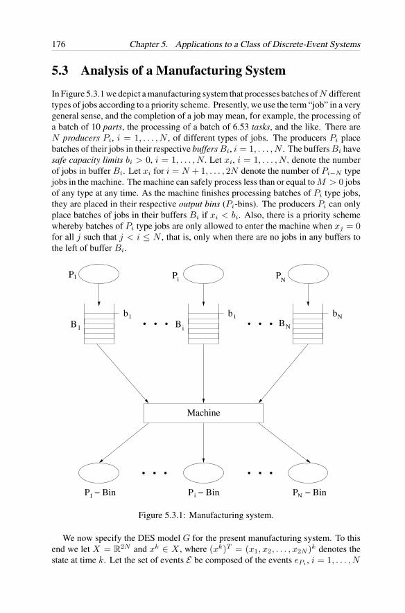
176 Chapter 5. Applications to a Class of Discrete-Event Systems
5.3 Analysis of a Manufacturing System
In Figure 5.3.1 we depict a manufacturing system that processes batches of N differenttypes of jobs according to a priority scheme. Presently, we use the term “job” in a verygeneral sense, and the completion of a job may mean, for example, the processing ofa batch of 10 parts, the processing of a batch of 6.53 tasks, and the like. There areN producers Pi, i = 1, . . . , N , of different types of jobs. The producers Pi placebatches of their jobs in their respective buffers Bi, i = 1, . . . , N . The buffers Bi havesafe capacity limits bi > 0, i = 1, . . . , N. Let xi, i = 1, . . . , N, denote the numberof jobs in buffer Bi. Let xi for i = N + 1, . . . , 2N denote the number of Pi−N typejobs in the machine. The machine can safely process less than or equal to M > 0 jobsof any type at any time. As the machine finishes processing batches of Pi type jobs,they are placed in their respective output bins (Pi-bins). The producers Pi can onlyplace batches of jobs in their buffers Bi if xi < bi. Also, there is a priority schemewhereby batches of Pi type jobs are only allowed to enter the machine when xj = 0for all j such that j < i ≤ N , that is, only when there are no jobs in any buffers tothe left of buffer Bi.
. . . . . .
. . .. . .
Machine
P
Bb
P − Bin P − Bin
P P
Bb b
1
1
1
1
i
i
i
i
N
N
BN
P − BinN
Figure 5.3.1: Manufacturing system.
We now specify the DES model G for the present manufacturing system. To thisend we let X = R
2N and xk ∈ X , where (xk)T = (x1, x2, . . . , x2N )k denotes thestate at time k. Let the set of events E be composed of the events ePi
, i = 1, . . . , N
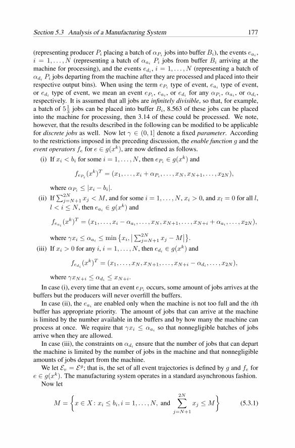
Section 5.3 Analysis of a Manufacturing System 177
(representing producer Pi placing a batch of αPi jobs into buffer Bi), the events eai ,i = 1, . . . , N (representing a batch of αai
Pi jobs from buffer Bi arriving at themachine for processing), and the events edi
, i = 1, . . . , N (representing a batch ofαdi
Pi jobs departing from the machine after they are processed and placed into theirrespective output bins). When using the term ePi type of event, eai type of event,or edi type of event, we mean an event ePi , eai , or edi for any αPi , αai , or αdi ,respectively. It is assumed that all jobs are infinitely divisible, so that, for example,a batch of 5 1
3 jobs can be placed into buffer Bi, 8.563 of these jobs can be placedinto the machine for processing, then 3.14 of these could be processed. We note,however, that the results described in the following can be modified to be applicablefor discrete jobs as well. Now let γ ∈ (0, 1] denote a fixed parameter. Accordingto the restrictions imposed in the preceding discussion, the enable function g and theevent operators fe for e ∈ g(xk), are now defined as follows.
(i) If xi < bi for some i = 1, . . . , N , then ePi ∈ g(xk) and
fePi(xk)T = (x1, . . . , xi + αPi , . . . , xN , xN+1, . . . , x2N ),
where αPi≤ |xi − bi|.
(ii) If∑2N
j=N+1 xj < M , and for some i = 1, . . . , N , xi > 0, and xl = 0 for all l,l < i ≤ N , then eai ∈ g(xk) and
feai(xk)T = (x1, . . . , xi − αai , . . . , xN , xN+1, . . . , xN+i + αai , . . . , x2N ),
where γxi ≤ αai≤ min
xi,∣∣∑2N
j=N+1 xj − M∣∣.
(iii) If xi > 0 for any i, i = 1, . . . , N , then edi∈ g(xk) and
fedi(xk)T = (x1, . . . , xN , xN+1, . . . , xN+i − αdi
, . . . , x2N ),
where γxN+i ≤ αdi ≤ xN+i.
In case (i), every time that an event ePioccurs, some amount of jobs arrives at the
buffers but the producers will never overfill the buffers.In case (ii), the eai are enabled only when the machine is not too full and the ith
buffer has appropriate priority. The amount of jobs that can arrive at the machineis limited by the number available in the buffers and by how many the machine canprocess at once. We require that γxi ≤ αai so that nonnegligible batches of jobsarrive when they are allowed.
In case (iii), the constraints on αdi ensure that the number of jobs that can departthe machine is limited by the number of jobs in the machine and that nonnegligibleamounts of jobs depart from the machine.
We let Ev = Eg; that is, the set of all event trajectories is defined by g and fe fore ∈ g(xk). The manufacturing system operates in a standard asynchronous fashion.
Now let
M =
x ∈ X : xi ≤ bi, i = 1, . . . , N, and2N∑
j=N+1
xj ≤ M
(5.3.1)
178 Chapter 5. Applications to a Class of Discrete-Event Systems
which represents all states for which the manufacturing system is in a safe operatingmode. It is easy to see that M is invariant by letting xk ∈ M and by showing that nomatter which event occurs, it will always be true that the next state xk+1 ∈ M .
In the following, we study the stability properties of the manufacturing systemformulated above. Our results show that under conditions when our manufacturingsystem starts in an unsafe mode (too many jobs in a buffer, or in the machine, or inboth), it will eventually return to a safe operating condition.
To simplify our notation, we let (xk)T=(x1, . . . , x2N ), (xk+1)T=(x′1, . . . , x
′2N ),
x = (x1, . . . , x2N )T , and x′ = (x′1, . . . , x
′2N )T , suppressing the “k” notation as
indicated. For this manufacturing system example we take
d(x, M) = inf 2N∑
j=1
|xj − xj | : x ∈ M
. (5.3.2)
Proposition 5.3.1 For the manufacturing system, the closed invariant set M definedin (5.3.1) is stable with respect to Ev .
Proof . We choose V (xk) = d(xk, M). We show that the function V (xk) satisfieshypotheses (i) and (ii) of Theorem 5.2.1 for all xk ∈ M .
Hypothesis (i) follows directly from the choice of V (xk). To verify that V (xk)satisfies hypothesis (ii) we show that V (xk) ≥ V (xk+1) for all xk ∈ M , no matterwhat event e ∈ g(xk) occurs, causing xk+1 = fe(xk), whenever it lies on an eventtrajectory in Ev .
(a) For xk ∈ M , if ePioccurs for some i, i = 1, . . . , N , we need to show that
inf 2N∑
j=1
|xj − xj | : x ∈ M
≥ inf
2N∑j=1,j =i
|xj − x′j |+ |xi +αPi − x′
i| : x′ ∈ M
.
(5.3.3)It suffices to show that for all x ∈ M at which the inf is achieved on the left of (5.3.3),there exists x′ ∈ M such that
2N∑j=1
|xj − xj | ≥2N∑
j=1,j =i
|xj − x′j | + |xi + αPi − x′
i|. (5.3.4)
If we choose x′l = xl for all l = i, then it suffices to show that for all xi, 0 ≤ xi ≤ bi,
at which the inf on the left side of (5.3.3) is achieved, there exists x′i, 0 ≤ x′
i ≤ bi,such that
|xi − xi| ≥ |xi + αPi − x′i| (5.3.5)
where αPi ≤ |xi − bi|. Choosing x′i = xi + αPi , so that 0 ≤ x′
i ≤ bi, results inx′ ∈ M , and relation (5.3.5) is satisfied.
(b) For xk ∈ M , if eai occurs for some i, i = 1, . . . , N , then following the aboveapproach, it suffices to show that for all x ∈ M at which the inf is achieved, thereexists x′ ∈ M such that
2N∑j=1
|xj−xj | ≥2N∑
j=1,j =i,N+i
|xj−x′j |+|xi−αai−x′
i|+|xN+i+αai−x′N+i|. (5.3.6)
Section 5.4 Load Balancing in a Computer Network 179
Choose x′l = xl for all l = i, N + i. It suffices to show that for all xi and xN+i, there
exist x′i, x
′N+i, such that
|xi − xi| ≥ |xi − αai − x′i| (5.3.7)
and|xN+i − xN+i| ≥ |xN+i + αai
− x′N+i|. (5.3.8)
For (5.3.7), if xi ≤ bi, then the inf is achieved so that |xi − xi| = |xi −αai− x′
i| = 0,whereas if xi > bi, the inf is achieved at xi = bi. Therefore, |xi−bi| ≥ |xi−αai −x′
i|,because either x′
i = bi or x′i = xi − αai
. The case for (5.3.8) is similar to case (a)above.
The proof for when edioccurs is similar to the case for (5.3.8).
We note that for the above manufacturing system, the closed set M specified in(5.3.1) is not asymptotically stable in the large with respect to Ev . (We ask the readerto prove this assertion in the problem section. Alternatively, the reader may wish torefer to [13, Proposition 2] for the proof.)
In the following, we identify a hypothesis that ensures asymptotic stability in thelarge for the above manufacturing system. To this end, we let Ea ⊂ Ev denote the setof event trajectories such that each type of event ePi , eai and edi , i = 1, . . . , N , occursinfinitely often on each event trajectory E ∈ Ea. If we assume for the manufacturingsystem that only events which lie on event trajectories in Ea occur, then it is alwaysthe case that eventually each type of event (ePi , eai and edi , i = 1, . . . , N ) will occur.
Proposition 5.3.2 For the manufacturing system, the closed invariant set M givenin (5.3.1) is asymptotically stable in the large with respect to Ea where Ea ⊂ Ev is asdefined above.
Proof . By Proposition 5.3.1, M is stable with respect to Ea. To establish asymptoticstability, we show that V (xk) → 0 for all Ek such that EkE ∈ Ea(x0) as k → ∞for all xk ∈ M .
Because αai ≥ γxi and αdi ≥ γxN+i, where γ ∈ (0, 1], if eai and edi , i =1, . . . , N , occur infinitely often (as the restrictions on Ea guarantee), xi and xN+i willconverge so that V (xk) → 0 as k → ∞ (of course it could happen that V (xk) = 0for some finite k). Therefore, if the manufacturing system starts out in an unsafeoperating mode, it will eventually enter a safe operating mode.
5.4 Load Balancing in a Computer Network
We consider a computer network specified by a digraph (C, A) where C=1, . . ., Nrepresents a set of computers labeled by i ∈ C and A ⊂ C × C specifies the set ofconnections; that is, if (i, j) ∈ A, then computer i is connected to computer j. Werequire that every computer is connected to the network so that if i ∈ C, then thereexists a pair (i, j) ∈ A or a pair (j, i) ∈ A for some j ∈ C. Also, we assume that if(i, j) ∈ A, then (j, i) ∈ A and furthermore, if (i, j) ∈ A, then i = j. We assume that
180 Chapter 5. Applications to a Class of Discrete-Event Systems
for each computer there is a buffer that holds tasks (the load), and we assume thateach task (load) can be executed by any of the computers in the network. We let theload of computer i ∈ C be denoted xi ≥ 0 and we assume that each connection inthe network, (i, j) ∈ A, allows computer i to pass a portion of its load to computer j.We also assume that in the case of every connection (i, j), computer i is able to sensethe size of the load of computer j, and furthermore, when (i, j) ∈ A, then computeri cannot pass a load directly to computer j, nor can computer i sense the load ofcomputer j.
We assume that the initial load distribution in the computer network is uneven andwe wish to establish rules (resp., an algorithm) under which a more even load distri-bution in the computer network is realized. We assume that no tasks are performedby any of the computers during the load-balancing process.
In the literature, distinctions are made between continuous loads (also called fluidloads) and discrete loads. In the former case, it is assumed that the computer load isinfinitely divisible whereas in the case of the latter, a load is a multiple of a uniformlysized block that is not divisible. In the following, we consider only continuous loads.
We next specify the discrete-event system model G for the computer balancingproblem described above. To this end, we let X = R
N denote the state space, and welet xk = (x1, . . . , xN )T and xk+1 = (x′
1, . . . , x′N )T denote the state at times k and
k +1, respectively. Let eijαk
denote the event that a load of amount αk is passed fromcomputer i to computer j at time k. If the state is xk, then for some (i, j) ∈ A, eij
αk
occurs to produce the next state xk+1. Let E = eijα : (i, j) ∈ A, α ∈ R+ denote
the infinite set of events. (Note that eij0 are valid events.) In the following, “an event
of type eijα ” means the passing of a load of the amount α > 0 from computer i to
computer j.We now specify the enable function g and the event operator fe for e ∈ g(xk).
We choose the parameter γ ∈ (0, 1/2].(i) If for any (i, j) ∈ A, xi > xj , then eij
α ∈ g(xk) and fe(xk) = xk+1 wheree = eij
α , x′i = xi − α, x′
j = xj + α, x′l = xl for all l = i, l = j, and
γ|xi − xj | ≤ α ≤ (1/2)|xi − xj |.(ii) If for any (i, j) ∈ A, xi = xj , then eij
0 ∈ g(xk) and fe(xk) = xk wheree = eij
0 .
Let Ev = Eg and let Ea ⊂ Ev denote the set of event trajectories such that events ofeach type eij
α occur infinitely often on each E ∈ Ea. This assumption ensures that eachpair of connected computers will continually try to balance the load between them.
In order to ensure load balancing, we make use of the set
M =x ∈ X : xi = xj for all (i, j) ∈ A
, (5.4.1)
which represents perfect load balancing. It is easy to show that M is invariant byletting xk ∈ M and then showing that no matter which event occurs, xk+1 ∈ M .
Proposition 5.4.1 For the computer network load-balancing problem, the followingis true.
(a) M is stable with respect to Ev .
Section 5.6 Problems 181
(b) M is not asymptotically stable with respect to Ev .
(c) M is asymptotically stable in the large with respect to Ea ⊂ Ev .
In proving Proposition 5.4.1, one proceeds similarly as was done in the proofof Propositions 5.3.1 and 5.3.2 for the manufacturing system. In the proof ofProposition 5.4.1, we find it convenient to choose as the distance function
d(x, M) = inf
max|x1 − x1|, . . . , |xN − xN | : x ∈ M
where x = (x1, . . . , xN )T and x = (x1, . . . , xN )T , and as the Lyapunov function
V (x) = d(x, M),
and applying the results of Section 5.2. We leave the details of these proofs as anexercise for the reader.
5.5 Notes and References
The applications to discrete-event systems presented in this chapter are based on [8],[9], and [13]. For additional background material on discrete-event systems, refer,for example, to [1], [3], and [15].
The manufacturing system considered in Section 5.3 is a generalization of systemsused in the study of a simple “mutual exclusion problem” in the computer scienceliterature (see, e.g., [7] and [10]) and is similar to several applications addressed inthe DES literature (e.g., [6] and [15]).
The results of Section 5.3 have been extended in [11] and [12] to be applicable to“discrete” jobs.
Usage of the set Ea in Proposition 5.3.2 imposes what is called in the computerscience literature a “fairness constraint” (see, e.g., [5]). One can guarantee that thisconstraint is met using a mechanism for sequencing access to the machine. Suchfairness constraints have also been used in the study of temporal logic (e.g., [3] and[7]) and the mutual exclusion problem in the computer science literature (e.g., [14]).
The load-balancing problem presented in Section 5.4 was motivated by a similarproblem studied in [1]. Various other forms of this problem have also been addressedin the DES literature (e.g., [2]) and in the computer science literature (e.g., [1], [2],and [4]), and in the numerous references cited in these sources.
5.6 Problems
Problem 5.6.1 For the manufacturing system discussed in Section 5.3, let M denotethe closed invariant set defined in (5.3.1). Prove that M is not asymptotically stablein the large with respect to Ev , where Ev is the same as in Proposition 5.3.1.
Hint: Let xi > bi for all i = 1, . . . , N , where the bi are as defined in (5.3.1). ChoosexN+i > 0 for some i so that edi
occurs, to process Pi type jobs and to put them into the
182 Chapter 5. Applications to a Class of Discrete-Event Systems
Pi-bin. For each successive time αdi = γxN+i, it can happen that E = ediediedi · · ·(a constant string) and E ∈ Ev . This shows that M is not asymptotically stable in thelarge with respect to Ev .
Problem 5.6.2 The matrix equations that describe the dynamical behavior of a Petrinet P are given by
Mk+1 = Mk + AT uk (5.6.1)
where k ∈ N, Mk ∈ Nm, A is an n×m matrix of integers (the incidence matrix), and
uk ∈ 0, 1n denotes a firing vector (refer, e.g., to [8], [9], and [10] for backgroundmaterial on Petri nets). A Petri net P is said to be uniformly bounded (resp., uniformlyultimately bounded) if the motions of the dynamical system determined by (5.6.1) areuniformly bounded (resp., uniformly ultimately bounded). Prove that the followingstatements are true.
(a) A Petri net P is uniformly bounded if there exists an m-vector ϕ > 0 such thatAϕ ≤ 0 (inequality of vectors is understood to be componentwise).
(b) A Petri net P is uniformly ultimately bounded if there exist an m-vector ϕ > 0and an n-vector b > 0 such that Aϕ ≤ −b.
Hint: Apply Theorems 3.4.4 and 3.4.5 with the choice of M = 0 and V (x) = xT ϕfor x = (n1, . . . , nm) ∈ N
m.
Problem 5.6.3 Prove Proposition 5.4.1, using the hints given in Section 5.4.
Bibliography
[1] D. P. Bertsekas and J. N. Tsitsiklis, Parallel and Distributed Computation:Numerical Methods, Englewood Cliffs, NJ: Prentice Hall, 1989.
[2] R. K. Boel and J. H. van Schuppen, “Distributed routing for load balancing,”Proc. IEEE, vol. 77, pp. 210–221, 1989.
[3] E. M. Clark, M. C. Browne, E. A. Emerson, and A. P. Sistla, “Using temporallogic for automatic verification of finite state systems,” in Logic and Mod-els of Concurrent Systems, K. R. Apt, ed., New York: Springer-Verlag, 1985,pp. 3–25.
[4] G. Cybenko, “Dynamic load balancing for distributed memory multi-processors,” Technical Report 87-1, Department of Computer Science, TuftsUniversity, Medford, MA, 1987.
[5] N. Francez, Fairness, New York: Springer-Verlag, 1986.
[6] J. F. Knight and K. M. Passino, “Decidability for a temporal logic used in discreteevent system analysis,” Int. J. Control, vol. 52, pp. 1489–1506, 1990.
[7] Z. Manna and A. Pnueli, “Verification of concurrent programs: A temporalproof system,” Report No. STAN-CS-83-967, Department of Computer Science,Stanford University, 1983.
Bibliography 183
[8] A. N. Michel, K. Wang, and K. M. Passino, “Qualitative equivalence of dynam-ical systems with applications to discrete event systems,” Proc. of the 31st IEEEConference on Decision and Control, Tuscon, AZ, Dec. 1992, pp. 731–736.
[9] A. N. Michel, K. Wang, and K. M. Passino, “Stability preserving mappingsand qualitative equivalence of dynamical systems-Part I,” Avtomatika i Tele-mekhanika, vol. 10, pp. 3–12, 1994.
[10] T. Murata, “Petri nets: Properties, analysis, and applications,” Proc. IEEE,vol. 77, pp. 541–580, 1989.
[11] K. M. Passino, A. N. Michel, and P. J. Antsaklis, “Stability analysis of discreteevent systems,” Proc. of the 28th Annual Allerton Conference on Communica-tion, Control, and Computing, University of Illinois at Urbana-Champaign, Oct.1990, pp. 487–496.
[12] K. M. Passino, A. N. Michel, and P. J. Antsaklis, “Lyapunov stability of discreteevent systems,” Proc. of the 1991 American Control Conference, Boston, MA,June 1991, pp. 2911–2916.
[13] K. M. Passino, A. N. Michel, and P. J. Antsaklis, “Lyapunov stability of a classof discrete event systems,” IEEE Trans. Autom. Control, vol. 39, pp. 269–279,1994.
[14] M. Raynal, Algorithms for Mutual Exclusion, Cambridge, MA: MIT Press,1986.
[15] J. G. Thistle and W. M. Wonham, “Control problems in a temporal logic frame-work,” Int. J. Control, vol. 44, pp. 943–976, 1986.
Chapter 6
Finite-DimensionalDynamical Systems
In the present chapter we apply the results of Chapter 3 (for the stability of invari-ant sets and the boundedness of motions of general dynamical systems defined onmetric spaces) in the analysis of continuous finite-dimensional dynamical systemsdetermined by differential equations (E), discrete-time finite-dimensional dynamicalsystems determined by difference equations (D), and finite-dimensional discontin-uous dynamical systems. When considering various stability types, our focus is oninvariant sets that are equilibria.
This chapter consists of eight parts. In the first section we introduce some im-portant preliminary results which we require throughout the chapter. In the second,third, and fourth sections we present the principal Lyapunov stability and bound-edness results for continuous dynamical systems, discrete-time dynamical systems,and discontinuous dynamical systems, respectively. Throughout these sections weconsider specific examples to demonstrate applications of the various results. In thefifth, sixth, and seventh sections we establish converse theorems for the results ofthe second, third, and fourth sections, respectively. In the eighth section we providesome background material concerning the continuous dependence of the solutions ofordinary differential equations on initial conditions.
The results of the present chapter are general and fundamental in nature. In the nextchapter, where we continue the qualitative analysis of finite-dimensional dynamicalsystems, we concentrate on important specialized results.
6.1 Preliminaries
In this section we present preliminary material which we require throughout thischapter. The present section is organized into seven parts. In the first three subsec-tions we recall facts concerning finite-dimensional dynamical systems determined
185
186 Chapter 6. Finite-Dimensional Dynamical Systems
by ordinary differential equations, ordinary difference equations, and discontinuousdynamical systems, respectively. In the fourth subsection we rephrase the variousdefinitions of stability and boundedness given in Chapter 3 for dynamical systems de-fined on metric spaces, for the case of finite-dimensional dynamical systems (definedon R
n). In the fifth subsection we introduce several characterizations of Lyapunovfunctions and in the sixth subsection we discuss an important special class of Lya-punov functions, quadratic forms. In the final subsection we present some geometricinterpretations and motivation for Lyapunov stability results (for two-dimensionalautonomous systems).
Before proceeding, a comment concerning the notation that we employ in theremainder of this book to designate Lyapunov functions is in order. When address-ing general dynamical systems, T, X, A, S, defined on metric spaces, we useduppercase letters in Chapters 3 and 4 to denote such functions (V -functions). Inkeeping with the notation most frequently used in texts on specific classes of finite-dimensional and infinite-dimensional dynamical systems, we use lowercase letters todenote Lyapunov functions when dealing with such systems.
A. Dynamical systems determined by ordinary differentialequations
We consider systems of first-order ordinary differential equations of the form
x = f(t, x) (E)
where t ∈ R+, x ∈ Ω ⊂ R
n, x = dx/dt, and f : R+ × Ω → R
n. We assumethat Ω is an open connected set and that 0 ∈ Ω. We always assume that for each(t0, x0) ∈ R
+ × Ω, (E) possesses at least one solution (refer to Theorem 2.3.1),we sometimes require that these solutions be unique (refer to Theorem 2.3.2) andwe usually (but not always) require that the solutions, denoted by ϕ(t, t0, x0), existfor all t ∈ [t0,∞). Recall that ϕ(t0, t0, x0) = x0. Under the assumption thatf ∈ C[R+ × Ω, Rn], the solutions ϕ(t, t0, x0) of (E) are continuous with respect toinitial conditions (t0, x0) (refer to the appendix section, Section 6.8). Recall that (E)determines a dynamical system T, X, A, SE where T = R
+, X = Rn, A ⊂ X ,
and SE denotes the set of motions determined by (E). We usually denote this systemsimply by SE (refer to Subsection 2.3C).
In the present chapter we study primarily the stability properties of invariant setsM ⊂ R
n for the special case when M = xe ⊂ Rn, and the boundedness of SE .
Recall that in this case we say that xe is an equilibrium (resp., equilibrium point)of (E).
In Example 3.1.3 we noted that if f(t, xe) = 0 for all t ∈ R+, then xe = M
is an invariant set with respect to SE (i.e., (SE , M) is invariant). Furthermore, it iseasily shown that when (E) possesses a unique solution for every (t0, x0) ∈ R
+ ×Ω,then (SE , xe) is invariant if and only if f(t, xe) = 0 for all t ∈ R
+.To simplify our language throughout this chapter, we say that “xe is an equilibrium
of (E)”, rather than “the set xe is invariant with respect to SE” (or, “(SE , xe)
Section 6.1 Preliminaries 187
is invariant”); “the equilibrium xe of (E) is asymptotically stable”, rather than “theinvariant set xe of (E) is asymptotically stable” (or, “(SE , xe) is asymptoticallystable”); and so forth.
Without loss of generality, we may assume that a given equilibrium xe of (E) islocated at the origin (i.e., xe = 0). To see this, suppose that xe = 0 is an equilibriumof (E). Let y = x − xe and f(t, y) = f(t, y + xe). Then (E) can be written as
y = f(t, y),
with f(t, 0) = 0 for all t ∈ R+.
As in Chapter 3, we employ Lyapunov functions v ∈ C[B(r) × R+, R] where
B(r) ⊂ Ω, B(r) = x ∈ Rn : |x| < r with r > 0. For such functions, we
define the upper-right derivative of v with respect to t along the solutions of (E)(ϕ(·, t, x)) by
v′(E)(x, t) = lim
∆t→0+sup
ϕ(t,t,x)=x
1∆t
[v(ϕ(t + ∆t, t, x), t + ∆t) − v(x, t)
](6.1.1)
which is defined on B(r) × R+. When for each (t0, x0) ∈ R
+ × B(r), (E) has aunique solution, (6.1.1) reduces to
v′(E)(x, t) = lim
∆t→0+
1∆t
[v(ϕ(t + ∆t, t, x), t + ∆t) − v(x, t)
]. (6.1.2)
If in addition, v satisfies a local Lipschitz condition in x, that is, for each T > 0 thereexists a constant L > 0 such that
|v(x, t) − v(y, t)| ≤ L|x − y|
for all x, y ∈ B(r) and all t ∈ [0, T ], then (6.1.2) can equivalently be expressed as
v′(E)(x, t) = lim
∆t→0+
1∆t
[v(x + (∆t)f(t, x), t + ∆t) − v(x, t)
]. (6.1.3)
(We ask the reader to verify (6.1.3).) Finally, if in addition to the above assumptions,we have v ∈ C1[B(r) × R
+, R], then (6.1.3) assumes the equivalent form
v′(E)(x, t) =
n∑i=1
∂v
∂xi(x, t)fi(t, x) +
∂v
∂t(x, t) (6.1.4)
where f(t, x) = [f1(t, x), . . . , fn(t, x)]T is given in (E).
B. Dynamical systems determined by ordinary differenceequations
We now consider systems of first-order ordinary difference equations of the form
x(k + 1) = f(k, x(k)) (D)
188 Chapter 6. Finite-Dimensional Dynamical Systems
where k ∈ N, x(k) ∈ Ω ⊂ Rn, and f : N × Ω → Ω. We assume that Ω is an
open connected set and that 0 ∈ Ω. For each (k0, x0) ∈ N × Ω there exists aunique solution ϕ(k, k0, x0) with ϕ(k0, k0, x0) = x(k0) = x0. We recall that (D)determines a dynamical system T, X, A, SD where T = N, X = R
n, A ⊂ X , andSD denotes the set of motions determined by (D). We usually denote this systemsimply by SD (refer to Section 2.5).
As in the case of dynamical systems determined by (E), we concentrate primarilyin studying the qualitative properties of an equilibrium xe of D (i.e., in studying thestability properties of an invariant set M = xe). It is easily shown that a pointxe ∈ Ω is an equilibrium of (D) if and only if
xe = f(k, xe)
for all k ∈ N. As in the case of ordinary differential equations, we may assumewithout loss of generality that the equilibrium xe of (D) is located at the origin(xe = 0).
Finally, we let ϕ(k, k0, x0) denote any solution of (D) with initial conditionsϕ(k0, k0, x0) = x(k0) = x0. For a function v ∈ C[Ω × N, R], we define the firstforward difference of v with respect to k along the solutions of (D) by
∆(D)v(x, k) = v(ϕ(k + 1, k, x), k + 1) − v(ϕ(k, k, x), k)= v(f(k, x), k + 1) − v(x, k). (6.1.5)
C. Discontinuous dynamical systems (DDS)
In the present chapter we address finite-dimensional discontinuous dynamical systems(finite-dimensional DDS), T, X, A, S, where T = R
+, Rn = X ⊃ A, and themotions of S are determined by the solutions ϕ(·, t0, x0) of discontinuous ordinarydifferential equations of the type specified later. As in Chapter 3 we assume that theset of times at which discontinuities may occur is unbounded and discrete and is ofthe form
Eϕ = τϕ1 , τϕ
2 , . . . : τϕ1 < τϕ
2 < · · · .In the above expression, Eϕ signifies that in general, different motions may possessdifferent sets of times at which discontinuities may occur. Usually, the particular setEϕ in question is clear from context and accordingly, we suppress the ϕ-notation andsimply write
E = τ1, τ2, . . . : τ1 < τ2 < · · · .We find it sometimes useful to express the motions (solutions) of finite-dimensionalDDS by
ϕ(t, t0, x0) = x(k)(t, τk, xk), τk ≤ t < τk+1, k ∈ N,
where t0 = τ0 and x0 are given initial conditions. Throughout, we assume that Scontains the trivial solution ϕ(t, t0, 0) = 0 for all t ≥ t0 so that (S, 0) is invariant;that is, xe = 0 is an equilibrium for the finite-dimensional DDS.
Section 6.1 Preliminaries 189
The most general specific class of finite-dimensional DDS that we consider isgenerated by differential equations of the form (refer to Subsection 2.12A).
x(t) = fk(t, x(t)), τk ≤ t < τk+1
x(t) = gk(x(t−)), t = τk+1, k ∈ N,(SE)
where for each k ∈ N, fk ∈ C[R+ × Rn, Rn], gk : R
n → Rn, and x(t−) =
limt′→t,t′<t x(t′) denotes the left limit of x(t′) at t′ = t.As in Subsection 2.12A, associated with (SE), we consider the family of initial
value problems given by x(t) = fk(t, x(t))x(τk) = xk,
(SEk)
k∈N. We assume that for (τk, xk), (SEk) possesses a unique solution x(k)(t, τk, xk)that exists for all t ∈ [τk,∞) (refer to Section 2.3 for conditions that ensure this).Then for every (t0, x0) ∈ R
+ × Rn, t0 = τ0, (SE) has a unique solution ϕ(t, t0, x0)
that exists for all t ∈ [t0,∞). This solution is made up of a sequence of continuoussolution segments x(k)(t, τk, xk) defined over the intervals [τk, τk+1), k ∈ N, withinitial conditions (τk, xk), where xk = x(τk) = gk−1(x(τ−
k )), k = 1, 2, . . . , and theinitial conditions (τ0 = t0, x0) are given. At the points τk+1, k ∈ N, the solutionsof (SE) may have possible jumps, or the four derivatives D+ϕ, D+ϕ, D−ϕ, andD−ϕ may not be equal, or ϕ may be continuous.
We assume that for each k ∈ N, fk(t, 0) = 0 for all t ≥ τk. Then xe = 0 will bean equilibrium for (SEk) and (SE).
D. Qualitative characterizations: Stability and boundednessAt this point it might be instructive to rephrase the various stability and bounded-ness concepts given in Definitions 3.1.6–3.1.20 for the case of finite-dimensionaldynamical systems. We consider here only systems determined by ordinary differ-ential equations. The various stability and boundedness definitions for discrete-timesystems determined by difference equations involve obvious modifications.
Let X = Rn, M = 0, T = R
+, and d(x, y) = |x − y| for all x, y ∈ Rn
where | · | denotes any one of the equivalent norms on Rn. Also, note that for any
x ∈ Rn, d(x, 0) = |x|. From Definitions 3.1.6–3.1.20 we now have the following
characterizations of the equilibrium xe = 0 of (E) and the solutions of (E).
Definition 6.1.1 (a) The equilibrium xe = 0 of (E) is stable if for every ε > 0 andany t0 ∈ R
+ there exists a δ(ε, t0) > 0 such that for all solutions of (E),
|ϕ(t, t0, x0)| < ε for all t ≥ t0 (6.1.6)
whenever
|x0| < δ(ε, t0). (6.1.7)
190 Chapter 6. Finite-Dimensional Dynamical Systems
If in (6.1.7) δ(ε, t0) is independent of t0 (i.e., δ(ε, t0) = δ(ε)), then the equilibriumxe = 0 of (E) is said to be uniformly stable. (Note that in this definition the solutionsϕ(t, t0, x0) exist over [t0, t1) where t1 may be finite or infinite.)
(b) The equilibrium xe = 0 of (E) is asymptotically stable if
(1) it is stable; and(2) for every t0 ≥ 0 there exists an η(t0)> 0 such that limt→∞ ϕ(t, t0, x0)=0
for all solutions of (E) whenever |x| < η(t0).When (2) is true, we say that the equilibrium xe = 0 of (E) is attractive. Also,
the set of all x0 ∈ Rn such that ϕ(t, t0, x0) → 0 as t → 0 for some t0 ≥ 0 is called
the domain of attraction of the equilibrium xe = 0 of (E) (at t0).
(c) The equilibrium xe = 0 of (E) is uniformly asymptotically stable if(1) it is uniformly stable; and(2) for every ε> 0 and every t0 ∈R
+, there exist a δ0 > 0, independent of t0and ε, and a T (ε)> 0, independent of t0, such that for all solutions of (E)
|ϕ(t, t0, x0)| < ε for all t ≥ t0 + T (ε)
whenever |x0| < δ0.
When (2) is true, we say that the equilibrium xe = 0 of (E) is uniformly attractive.Note that condition (2) is often paraphrased by saying that there exists a δ0 > 0such that
limt→∞ ϕ(t + t0, t0, x0) = 0
uniformly in (t0, x0) for t0 ≥ 0 and for |x0| ≤ δ0.
(d) The equilibrium xe = 0 of (E) is exponentially stable if there exists an α > 0and for every ε > 0 and every t0 ≥ 0, there exists a δ(ε) > 0 such that for allsolutions of (E)
|ϕ(t, t0, x0)| ≤ εe−α(t−t0) for all t ≥ t0
wherever |x0| < δ(ε).As in Chapter 3, we note that the exponential stability of the equilibrium xe = 0
of (E) implies its uniform asymptotic stability.
(e) A solution ϕ(t, t0, x0) of (E) is bounded if there exists a β > 0 such that|ϕ(t, t0, x0)| < β for all t ≥ t0, where β may depend on each solution. System (E)is said to possess Lagrange stability if for each t0 ≥ 0 and x0 ∈ R
n, the solutionϕ(t, t0, x0) is bounded.
(f) The solutions of (E) are uniformly bounded if for any α > 0 and every t0 ∈ R+,
there exists a β = β(α) > 0 (independent of t0) such that if |x0| < α, then|ϕ(t, t0, x0)| < β for all t ≥ t0. (To arrive at this definition, we choose in Defi-nition 3.1.13, without loss of generality, that x0 = 0.)
(g) The solutions of (E) are uniformly ultimately bounded (with bound B) if thereexists a B > 0 and if corresponding to any α > 0 and for every t0 ∈ R
+, there exists
Section 6.1 Preliminaries 191
a T =T (α) > 0 (independent of t0) such that |x0|< α implies that |ϕ(t, t0, x0)| <Bfor all t ≥ t0 + T (α).
(h) The equilibrium xe = 0 of (E) is asymptotically stable in the large if it isstable and if every solution of (E) tends to zero as t → ∞. In this case, the domainof attraction of the equilibrium xe = 0 of (E) is all of R
n and xe = 0 is the onlyequilibrium of (E).
(i) The equilibrium xe =0 of (E) is uniformly asymptotically stable in the large if
(1) it is uniformly stable;
(2) the solutions of (E) are uniformly bounded; and
(3) for any α > 0, any ε > 0 and every t0 ∈ R+, there exists a T (ε, α) > 0,
independent of t0, such that if |x0| < α, then for all solutions of (E), wehave |ϕ(t, t0, x0)| < ε for all t ≥ t0 + T (ε, α).
When (3) is true, we say that the equilibrium xe = 0 of (E) is globally uniformlyattractive (resp., uniformly attractive in the large).
(j) The equilibrium xe = 0 of (E) is exponentially stable in the large if there existan α > 0 and a γ > 0, and for any β > 0, there exists a k(β) > 0 such that for allsolutions of (E),
|ϕ(t, t0, x0)| ≤ k(β)|x0|γe−α(t−t0) for all t ≥ t0
whenever |x0| < β.
(k) The equilibrium xe = 0 of (E) is unstable if it is not stable. In this case, thereexist a t0 ≥ 0 and a sequence x0m → 0 of initial points and a sequence tm ≥ 0such that |ϕ(t0 + tm, t0, x0m)| ≥ ε for all m.
E. Some characterizations of Lyapunov functions
We now address several important properties that Lyapunov functions may possess.We first consider the case w : B(r) → R (resp., w : Ω → R) where B(r) ⊂ Ω ⊂ R
n,B(r) = x ∈ R
n : |x| < r for some r > 0, Ω is an open connected set, and0 ∈ Ω.
Definition 6.1.2 A function w ∈ C[B(r), R] (resp., w ∈ C[Ω, R]) is said to bepositive definite if
(i) w(0) = 0; and
(ii) w(x) > 0 for all x = 0.
Definition 6.1.3 A function w ∈ C[B(r), R] (resp., w ∈ C[Ω, R]) is said to benegative definite if −w is positive definite.
Definition 6.1.4 A function w ∈ C[Rn, R] is said to be radially unbounded if
(i) w(0) = 0;
192 Chapter 6. Finite-Dimensional Dynamical Systems
(ii) w(x) > 0 for all x ∈ (Rn − 0); and
(iii) w(x) → ∞ as |x| → ∞.
Definition 6.1.5 A function w ∈ C[B(r), R] (resp., w ∈ C[Ω, R]) is said to beindefinite if
(i) w(0) = 0; and
(ii) in every neighborhood of the origin x = 0, w assumes negative and positivevalues.
Definition 6.1.6 A function w ∈ C[B(r), R] (resp., w ∈ C[Ω, R]) is said to bepositive semidefinite if
(i) w(0) = 0; and
(ii) w(x) ≥ 0 for all x ∈ B(r) (resp., x ∈ Ω).
Definition 6.1.7 A function w ∈ C[B(r), R] (resp., w ∈ C[Ω, R]) is said to benegative semidefinite if −w is positive semidefinite.
Next, we consider the case v ∈ C[B(r) × R+, R] (resp., v ∈ C[Ω × R
+, R]).
Definition 6.1.8 A function v ∈ C[B(r)× R+, R] (resp., v ∈ C[Ω× R
+, R]) is saidto be positive definite if there exists a positive definite function w ∈ C[B(r), R](resp., w ∈ C[Ω, R]) such that
(i) v(0, t) = 0 for all t ≥ 0; and
(ii) v(x, t) ≥ w(x) for all t ≥ 0 and all x ∈ B(r) (resp., x ∈ Ω).
Definition 6.1.9 A function v ∈ C[B(r)× R+, R] (resp., v ∈ C[Ω× R
+, R]) is saidto be negative definite if −v is positive definite.
Definition 6.1.10 A function v ∈ C[Rn × R+, R] is said to be radially unbounded
if there exists a radially unbounded function w ∈ C[Rn, R] such that
(i) v(0, t) = 0 for all t ≥ 0; and
(ii) v(x, t) ≥ w(x) for all t ≥ 0 and all x ∈ Rn.
Definition 6.1.11 A function v ∈ C[B(r)×R+, R] (resp., v ∈ C[Ω×R
+, R]) is saidto be decrescent if there exists a positive definite function w ∈ C[B(r), R] (resp.,w ∈ C[Ω, R]) such that
|v(x, t)| ≤ w(x)
for all (x, t) ∈ B(r) × R+ (resp., (x, t) ∈ Ω × R
+).
Definition 6.1.12 A function v ∈ C[B(r) × R+, R] (resp., v ∈ C[Ω × R
+, R]) issaid to be positive semidefinite if
(i) v(0, t) = 0 for all t ∈ R+; and
(ii) v(x, t) ≥ 0 for all t ∈ R+ and all x ∈ B(r) (resp., x ∈ Ω).
Section 6.1 Preliminaries 193
Definition 6.1.13 A function v ∈ C[B(r) × R+, R] (resp., v ∈ C[Ω × R
+, R]) issaid to be negative semidefinite if −v is positive semidefinite.
Some of the preceding characterizations of v-functions (and w-functions) canbe rephrased in equivalent and very useful ways. In doing so, we use comparisonfunctions of class K and class K∞.
Theorem 6.1.1 A function v ∈ C[B(r) × R+, R] (resp., v ∈ C[Ω × R
+, R]) ispositive definite if and only if
(i) v(0, t) = 0 for all t ∈ R+; and
(ii) there exists a function ψ ∈ K defined on [0, r] (resp., on R+) such that
v(x, t) ≥ ψ(|x|)
for all t ∈ R+ and all x ∈ B(r) (resp., x ∈ Ω).
Proof . If v(x, t) is positive definite, then there exists a positive definite functionw(x) such that v(x, t) ≥ w(x) for t ∈ R
+ and |x| ≤ r. Define
ψ0(s) = infw(x) : s ≤ |x| ≤ r
for 0 < s ≤ r. Clearly ψ0 is a positive and nondecreasing function such thatψ0(|x|) ≤ w(x) on 0 < |x| ≤ r. Because ψ0 is continuous, it is Riemann integrable.Define the function ψ by ψ(0) = 0 and
ψ(u) = u−1∫ u
0(s/r)ψ0(s)ds, 0 < u ≤ r.
Clearly 0 < ψ(u) ≤ ψ0(u) ≤ w(x) ≤ v(x, t) if t ≥ 0 and |x| = u. Moreover, ψ iscontinuous and increasing (i.e., ψ ∈ K, by construction).
Conversely, assume that (i) and (ii) are true and define w(x) = ψ(|x|). It nowfollows readily from Definition 6.1.8 that v(x, t) is positive definite.
Theorem 6.1.2 A function v ∈ C[Rn × R+, R] is radially unbounded if and only if
(i) v(0, t) = 0 for all t ∈ R+; and
(ii) there exists a function ψ ∈ K∞ such that
v(x, t) ≥ ψ(|x|)
for all (x, t) ∈ Rn × R
+.
We ask the reader to prove Theorem 6.1.2 in the problem section.
Theorem 6.1.3 A function v ∈ C[B(r) × R+, R] (resp., v ∈ C[Ω × R
+, R]) isdecrescent if and only if there exists a function ψ ∈ K defined on [0, r] (resp., on R
+)such that
|v(x, t)| ≤ ψ(|x|)for all (x, t) ∈ B(r) × R
+ (resp., (x, t) ∈ Ω × R+).
194 Chapter 6. Finite-Dimensional Dynamical Systems
We ask the reader to prove Theorem 6.1.3 in the problem section.Note that when w∈C[B(r), R] (resp., w∈C[Ω, R]) is positive or negative definite,
then it is also decrescent for in this case we can always find ψ1, ψ2 ∈K such that
ψ1(|x|) ≤ |w(x)| ≤ ψ2(|x|)
for all x ∈ B(r) for some r > 0. On the other hand, when v ∈ C[B(r) × R+, R]
(resp., v ∈ C[Ω×R+, R]), care must be taken in establishing whether v is decrescent.
For the case of discrete-time dynamical systems determined by differenceequations (D), we employ functions v ∈C[B(r) × N, R] (resp., v ∈ C[Ω × N, R]).We define such functions as being positive definite, negative definite, positive semidef-inite, negative semidefinite, decrescent, and radially unbounded by modifying Defi-nitions 6.1.2–6.1.13 (and Theorems 6.1.1–6.1.3) in an obvious way.
Example 6.1.1 (a) For v ∈ C[R2 ×R+, R] given by v(x, t) = (1+cos2 t)x2
1 +2x22,
we haveψ1(|x|)
= xT x ≤ V (x, t) ≤ 2xT x= ψ2(|x|)
for all x ∈ R2 and t ∈ R
+, where ψ1, ψ2 ∈ K∞. Therefore, v is positive definite,decrescent, and radially unbounded.
(b) For v ∈ C[R2 × R+, R] given by v(x, t) = (x2
1 + x22) cos2 t, we have
0 ≤ v(x, t) ≤ xT x= ψ(|x|)
for all x ∈ R2 and t ∈ R
+, where ψ ∈ K. Thus, v is positive semidefinite anddecrescent.
(c) For v ∈ C[R2 × R+, R] given by v(x, t) = (1 + t)(x2
1 + x22), we have
ψ(|x|) = xT x ≤ v(x, t)
for all x ∈ R2 and t ∈ R
+, where ψ ∈ K∞. Thus, v is positive definite and radiallyunbounded. It is not decrescent.
(d) For v ∈ C[R2 × R+, R] given by v(x, t) = x2
1/(1 + t) + x22, we have
v(x, t) ≤ xT x= ψ(|x|)
for all x ∈ R2 and t ∈ R
+, where ψ ∈ K∞. Hence, v is decrescent and positivesemidefinite. It is not positive definite.
(e) The function v ∈ C[R2 × R+, R] given by v(x, t) = (x2 − x1)2(1 + t) is
positive semidefinite. It is not positive definite nor decrescent.
F. Quadratic forms
We now consider an important class of Lyapunov functions, quadratic forms, given by
v(x) = xT Bx =n∑
i,k=1
bikxixk (6.1.8)
Section 6.1 Preliminaries 195
where x ∈ Rn and B = [bij ] ∈ R
n×n is assumed to be symmetric (i.e., B = BT ).Recall that in this case B is diagonalizable and all of its eigenvalues are real. Fora proof of the next results, the reader should consult any text on linear algebra andmatrices (e.g., Michel and Herget [16]).
Theorem 6.1.4 Let v be the quadratic form defined in (6.1.8). Then
(i) v is positive definite (and radially unbounded) if and only if all principal minorsof B are positive, that is, if and only if
det
b11 · · · b1k
· ·· ·· ·
bk1 · · · bkk
> 0, k = 1, . . . , n.
These inequalities are called the Sylvester inequalities.
(ii) v is negative definite if and only if
(−1)k det
b11 · · · b1k
· ·· ·· ·
bk1 · · · bkk
> 0, k = 1, . . . , n.
(iii) v is definite (i.e., either positive definite or negative definite) if and only if alleigenvalues are nonzero and have the same sign.
(iv) v is semidefinite (i.e., either positive semidefinite or negative semidefinite) ifand only if the nonzero eigenvalues of B have the same sign.
(v) If λ1, . . . , λn denote all the eigenvalues of B (not necessarily distinct), if λm =min1≤i≤n λi, if λM = max1≤i≤n λi, and if | · | denotes the Euclidean norm(|x| = (xT x)1/2), then
λm|x|2 ≤ v(x) ≤ λM |x|2 for all x ∈ Rn.
(vi) v is indefinite if and only if B possesses both positive and negativeeigenvalues.
The purpose of the next example is to point out some of the geometric propertiesof quadratic forms.
Example 6.1.2 Let B be a real symmetric 2 × 2 matrix and let
v(x) = xT Bx.
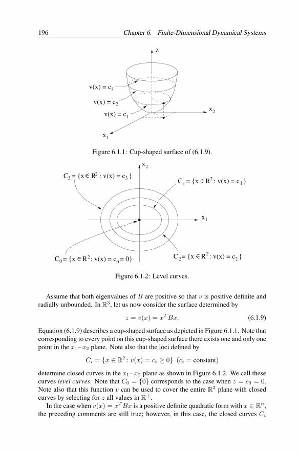
196 Chapter 6. Finite-Dimensional Dynamical Systems
v(x) = c
v(x) = c
v(x) = c
2
3
x
z
x
1
1
2
Figure 6.1.1: Cup-shaped surface of (6.1.9).
12C = x R : v(x) = c
C = x R : v(x) = c 3
C = x R : v(x) = c = 00C = x R : v(x) = c 2
x1
32
1
22
02
x2
Figure 6.1.2: Level curves.
Assume that both eigenvalues of B are positive so that v is positive definite andradially unbounded. In R
3, let us now consider the surface determined by
z = v(x) = xT Bx. (6.1.9)
Equation (6.1.9) describes a cup-shaped surface as depicted in Figure 6.1.1. Note thatcorresponding to every point on this cup-shaped surface there exists one and only onepoint in the x1– x2 plane. Note also that the loci defined by
Ci = x ∈ R2 : v(x) = ci ≥ 0 (ci = constant)
determine closed curves in the x1– x2 plane as shown in Figure 6.1.2. We call thesecurves level curves. Note that C0 = 0 corresponds to the case when z = c0 = 0.Note also that this function v can be used to cover the entire R
2 plane with closedcurves by selecting for z all values in R
+.In the case when v(x) = xT Bx is a positive definite quadratic form with x ∈ R
n,the preceding comments are still true; however, in this case, the closed curves Ci
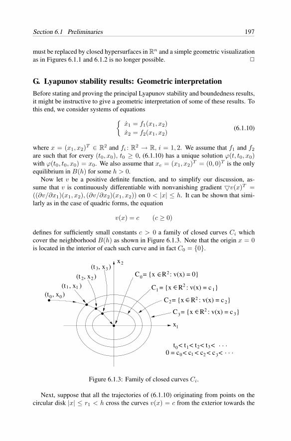
Section 6.1 Preliminaries 197
must be replaced by closed hypersurfaces in Rn and a simple geometric visualization
as in Figures 6.1.1 and 6.1.2 is no longer possible.
G. Lyapunov stability results: Geometric interpretation
Before stating and proving the principal Lyapunov stability and boundedness results,it might be instructive to give a geometric interpretation of some of these results. Tothis end, we consider systems of equations
x1 = f1(x1, x2)x2 = f2(x1, x2)
(6.1.10)
where x = (x1, x2)T ∈ R2 and fi : R
2 → R, i = 1, 2. We assume that f1 and f2are such that for every (t0, x0), t0 ≥ 0, (6.1.10) has a unique solution ϕ(t, t0, x0)with ϕ(t0, t0, x0) = x0. We also assume that xe = (x1, x2)T = (0, 0)T is the onlyequilibrium in B(h) for some h > 0.
Now let v be a positive definite function, and to simplify our discussion, as-sume that v is continuously differentiable with nonvanishing gradient v(x)T =((∂v/∂x1)(x1, x2), (∂v/∂x2)(x1, x2)) on 0 < |x| ≤ h. It can be shown that simi-larly as in the case of quadric forms, the equation
v(x) = c (c ≥ 0)
defines for sufficiently small constants c > 0 a family of closed curves Ci whichcover the neighborhood B(h) as shown in Figure 6.1.3. Note that the origin x = 0is located in the interior of each such curve and in fact C0 = 0.
(t , x )(t , x )
(t , x )
(t , x )
0
1
2
3
2
2
2
2
00
1 1
2 2
3 3
C = x R : v(x) = c
C = x R : v(x) = c
C = x R : v(x) = c
1
C = x R : v(x) = 0
2
3
t < t < t < t < 0 = c < c < c < c <
0
0 1
1
32. . .
. . .32
x
x
1
2
Figure 6.1.3: Family of closed curves Ci.
Next, suppose that all the trajectories of (6.1.10) originating from points on thecircular disk |x| ≤ r1 < h cross the curves v(x) = c from the exterior towards the
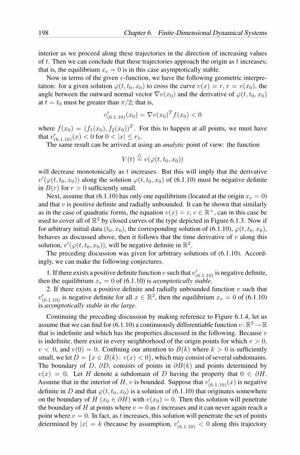
198 Chapter 6. Finite-Dimensional Dynamical Systems
interior as we proceed along these trajectories in the direction of increasing valuesof t. Then we can conclude that these trajectories approach the origin as t increases;that is, the equilibrium xe = 0 is in this case asymptotically stable.
Now in terms of the given v-function, we have the following geometric interpre-tation: for a given solution ϕ(t, t0, x0) to cross the curve v(x) = r, r = v(x0), theangle between the outward normal vector ∇v(x0) and the derivative of ϕ(t, t0, x0)at t = t0 must be greater than π/2; that is,
v′(6.1.10)(x0) = ∇v(x0)T f(x0) < 0
where f(x0) = (f1(x0), f2(x0))T . For this to happen at all points, we must havethat v′
(6.1.10)(x) < 0 for 0 < |x| ≤ r1.The same result can be arrived at using an analytic point of view: the function
V (t)= v(ϕ(t, t0, x0))
will decrease monotonically as t increases. But this will imply that the derivativev′(ϕ(t, t0, x0)) along the solution ϕ(t, t0, x0) of (6.1.10) must be negative definitein B(r) for r > 0 sufficiently small.
Next, assume that (6.1.10) has only one equilibrium (located at the origin xe = 0)and that v is positive definite and radially unbounded. It can be shown that similarlyas in the case of quadratic forms, the equation v(x) = c, c ∈ R
+, can in this case beused to cover all of R
2 by closed curves of the type depicted in Figure 6.1.3. Now iffor arbitrary initial data (t0, x0), the corresponding solution of (6.1.10), ϕ(t, t0, x0),behaves as discussed above, then it follows that the time derivative of v along thissolution, v′(ϕ(t, t0, x0)), will be negative definite in R
2.The preceding discussion was given for arbitrary solutions of (6.1.10). Accord-
ingly, we can make the following conjectures.
1. If there exists a positive definite function v such that v′(6.1.10) is negative definite,
then the equilibrium xe = 0 of (6.1.10) is asymptotically stable.2. If there exists a positive definite and radially unbounded function v such that
v′(6.1.10) is negative definite for all x ∈ R
2, then the equilibrium xe = 0 of (6.1.10)is asymptotically stable in the large.
Continuing the preceding discussion by making reference to Figure 6.1.4, let usassume that we can find for (6.1.10) a continuously differentiable function v : R2 →R
that is indefinite and which has the properties discussed in the following. Because vis indefinite, there exist in every neighborhood of the origin points for which v > 0,v < 0, and v(0) = 0. Confining our attention to B(k) where k > 0 is sufficientlysmall, we let D = x ∈ B(k) : v(x) < 0, which may consist of several subdomains.The boundary of D, ∂D, consists of points in ∂B(k) and points determined byv(x) = 0. Let H denote a subdomain of D having the property that 0 ∈ ∂H .Assume that in the interior of H, v is bounded. Suppose that v′
(6.1.10)(x) is negativedefinite in D and that ϕ(t, t0, x0) is a solution of (6.1.10) that originates somewhereon the boundary of H (x0 ∈ ∂H) with v(x0) = 0. Then this solution will penetratethe boundary of H at points where v = 0 as t increases and it can never again reach apoint where v = 0. In fact, as t increases, this solution will penetrate the set of pointsdetermined by |x| = k (because by assumption, v′
(6.1.10) < 0 along this trajectory
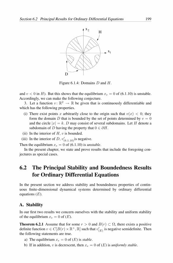
Section 6.2 Principal Results for Ordinary Differential Equations 199
x
x
1
2 H
D
Figure 6.1.4: Domains D and H .
and v < 0 in H). But this shows that the equilibrium xe = 0 of (6.1.10) is unstable.Accordingly, we can make the following conjecture.
3. Let a function v : R2 → R be given that is continuously differentiable and
which has the following properties.
(i) There exist points x arbitrarily close to the origin such that v(x) < 0; theyform the domain D that is bounded by the set of points determined by v = 0and the circle |x| = k. D may consist of several subdomains. Let H denote asubdomain of D having the property that 0 ∈ ∂H .
(ii) In the interior of H, v is bounded.(iii) In the interior of D, v′
(6.1.10)is negative.
Then the equilibrium xe = 0 of (6.1.10) is unstable.In the present chapter, we state and prove results that include the foregoing con-
jectures as special cases.
6.2 The Principal Stability and Boundedness Resultsfor Ordinary Differential Equations
In the present section we address stability and boundedness properties of contin-uous finite-dimensional dynamical systems determined by ordinary differentialequations (E).
A. Stability
In our first two results we concern ourselves with the stability and uniform stabilityof the equilibrium xe = 0 of (E).
Theorem 6.2.1 Assume that for some r > 0 and B(r) ⊂ Ω, there exists a positivedefinite function v ∈ C[B(r)× R
+, R] such that v′(E) is negative semidefinite. Then
the following statements are true.
a) The equilibrium xe = 0 of (E) is stable.b) If in addition, v is decrescent, then xe = 0 of (E) is uniformly stable.
200 Chapter 6. Finite-Dimensional Dynamical Systems
Proof . (a) According to Definition 6.1.1(a), we fix ε > 0 and t0 ≥ 0 and we seek aδ > 0 such that ∣∣ϕ(t, t0, x0)
∣∣ < ε for all t ≥ t0
whenever |x0| < δ. Without loss of generality, we can assume that ε < r. Becausev(x, t) is positive definite, then by Theorem 6.1.1 there is a function ψ ∈ K such thatv(x, t)≥ ψ(|x|) for all 0 ≤ |x| < r, t ≥ 0. Pick δ > 0 so small that v(x0, t0) < ψ(ε)if |x0| ≤ δ. Because v′
(E)(x, t) ≤ 0, then v(ϕ(t, t0, x0), t) is monotone nonincreasingand v(ϕ(t, t0, x0), t) < ψ(ε) for all t ≥ t0. Thus, |ϕ(t, t0, x0)| cannot reach the valueε, because this would imply that v(ϕ(t, t0, x0), t) ≥ ψ(|ϕ(t, t0, x0)|) = ψ(ε).
(b) Because v(x, t) is positive definite and decrescent, it follows from Theo-rems 6.1.1 and 6.1.3 that there exist two functions ψ1, ψ2 ∈ K such that
ψ1(|x|) ≤ v(x, t) ≤ ψ2(|x|)
for all (x, t) ∈ B(r) × R+.
Let ϕ(t, t0, x0) be a solution of (E) with initial condition ϕ(t0) = x0. Thenwe have
D+v(ϕ(t, t0, x0), t
)≤ v′
(E)
(ϕ(t, t0, x0), t
)for all (t0, x0) ∈ R
+ × B(r) and all t ∈ R+t0 such that ϕ(t, t0, x0) ∈ B(r), where
D+ denotes the upper-right Dini derivative with respect to t. Inasmuch as v′(E)
is negative semidefinite, we conclude that v(ϕ(t, t0, x0), t) is nonincreasing for allt ∈ R
+t0 . Statement (b) follows now directly from Theorem 3.3.1.
Example 6.2.1 (Simple pendulum) Consider the simple pendulum described by theequations
x1 = x2
x2 = −k sin x1(6.2.1)
where k > 0 is a constant. System (6.2.1) clearly has an equilibrium xe = 0 . Thetotal energy for (6.2.1) is the sum of the kinetic energy and potential energy, given by
v(x) =12x2
2 + k
∫ x1
0sin ηdη =
12x2
2 + k(1 − cos x1).
This function is continuously differentiable, v(0) = 0, and v is positive definite inΩ = (x1, x2)T ∈ R
2 : |x1| < c < 2π. Also, v is decrescent, because it does notdepend on t.
Along the solutions of (6.2.1) we have
v′(6.2.1)(x) = (k sin x1)x1 + x2x2 = (k sin x1)x2 + x2(−k sin x1) = 0.
In accordance with Theorem 6.2.1(b), the equilibrium xe = 0 of (6.2.1) is uniformlystable.
Note that because v′(6.2.1)(x) = 0, the total energy for system (6.2.1) is constant
for a given set of initial conditions for all t ≥ 0.
Section 6.2 Principal Results for Ordinary Differential Equations 201
The major shortcoming of the results that comprise the Principal Lyapunov Sta-bility Results (called the Direct Method of Lyapunov) is that there are no specificrules which tell us how to choose a v-function in a particular problem. The precedingexample suggests that a good choice for a v-function is the total energy of a sys-tem. Another widely used class of v-functions consists of quadratic forms (refer toSubsection 6.1F).
Example 6.2.2 Consider the second-order system
x + x + e−tx = 0. (6.2.2)
Letting x = x1, x = x2, we can express (6.2.2) equivalently byx1 = x2
x2 = −x2 − e−tx1.(6.2.3)
This system has an equilibrium at the origin xe = (x1, x2)T = (0, 0)T = 0. Let uschoose the positive definite function
v(x1, x2) = x21 + x2
2.
Along the solutions of (6.2.3), we have
v′(6.2.3)(x1, x2, t) = 2x1x2(1 − e−t) − 2x2
2.
The above choice of v-function does not satisfy the hypotheses of Theorem 6.2.1.Thus, we can reach no conclusion. Therefore, let us choose another v-function,
v(x1, x2, t) = x21 + etx2
2.
In this case we obtainv′(6.2.3)(x1, x2, t) = −etx2
2.
This v-function is positive definite and v′(6.2.3) is negative semidefinite. Therefore,
Theorem 6.2.1(a) is applicable and we can conclude that the equilibrium xe = 0 isstable. However, because v is not decrescent, Theorem 6.2.1(b) is not applicable andwe cannot conclude from this choice of v-function that the equilibrium xe = 0 isuniformly stable.
Example 6.2.3 (Hamiltonian system) Consider the conservative dynamical systemwith n degrees of freedom, which we discussed in Chapter 2 (Example 2.3.7) andwhich is given by
qi =∂H
∂pi(p, q), i = 1, . . . , n
pi = −∂H
∂qi(p, q), i = 1, . . . , n
(6.2.4)
202 Chapter 6. Finite-Dimensional Dynamical Systems
where qT = (q1, . . . , qn) denotes the generalized position vector, pT = (p1, . . . , pn)the generalized momentum vector, H(p, q) = T (p)+W (q) the Hamiltonian, T (p) thekinetic energy, and W (q) the potential energy. The positions of the equilibrium pointsof (6.2.4) correspond to the points in R
2n where the partial derivatives of H vanish.In the following, we assume that (pT , qT ) = (0T , 0T ) is an isolated equilibrium of(6.2.4), and without loss of generality we also assume that H(0, 0)= 0. Furthermore,we assume that H is smooth and that T (p) and W (q) are of the form
T (p) = T2(p) + T3(p) + · · ·
andW (q) = Wk(q) + Wk+1(q) + · · · , k ≥ 2.
Here Tj(p) denotes the terms in p of order j and Wj(q) denotes the terms in q of orderj. The kinetic energy T (p) is always assumed to be positive definite with respectto p. If the potential energy has an isolated minimum at q = 0, then W is positivedefinite with respect to q. We choose as a v-function
v(p, q) = H(p, q) = T (p) + W (q)
which is positive definite. Inasmuch as
v′(6.2.4)(p, q) =
dH
dt(p, q) = 0,
Theorem 6.2.1(a) is applicable and we conclude that the equilibrium at the origin isstable. Because v is independent of t, it is also decrescent, and so Theorem 6.2.1(b)is also applicable. Therefore, the equilibrium at the origin is also uniformly sta-ble. Note that Example 6.2.1 (the simple pendulum) is a special case of the presentexample.
B. Asymptotic stability
In the next two results we address the asymptotic stability of the equilibrium xe = 0of (E).
Theorem 6.2.2 For (E) we assume that there exists a positive definite and decres-cent function v ∈ C[B(r) × R
+, R] such that v′(E) is negative definite. Then the
equilibrium xe = 0 of (E) is uniformly asymptotically stable.
Proof . Because v′(E) is negative definite, there exists a function ψ3 ∈ K such that
v′(E)(x, t) ≤ −ψ3(|x|)
for all (x, t) ∈ B(r) × R+.
Let ϕ(t, t0, x0) be a solution of (E) with initial condition ϕ(t0) = x0. Thenwe have
D+v(ϕ(t, t0, x0), t
)≤ v′
(E)
(ϕ(t, t0, x0), t
)≤ −ψ3
(|ϕ(t, t0, x0)|
)
Section 6.2 Principal Results for Ordinary Differential Equations 203
for all (x0, t0) ∈ B(r) × R+ and all t ∈ R
+t0 such that ϕ(t, t0, x0) ∈ B(r), where
D+ denotes the upper-right Dini derivative with respect to t. The rest of the prooffollows directly from Theorem 3.3.2.
Theorem 6.2.3 With Ω = Rn, assume that there exists a positive definite, decrescent,
and radially unbounded functionv ∈ C[Rn×R+, R] such thatv′
(E) is negative definite(on R
n × R+) (i.e., there exist ψ1, ψ2 ∈ K∞ and ψ3 ∈ K such that
ψ1(|x|) ≤ v(x, t) ≤ ψ2(|x|)
andv′(E)(x, t) ≤ −ψ3(|x|)
for all (x, t) ∈ Rn × R
+). Then the equilibrium xe = 0 of (E) is uniformly asymp-totically stable in the large.
Proof . This result is a direct consequence of Theorem 3.3.6.
Example 6.2.4 Consider the systemx1 = (x1 − c2x2)(x2
1 + x22 − 1)
x2 = (c1x1 + x2)(x21 + x2
2 − 1)(6.2.5)
which has an equilibrium at the origin xe = (x1, x2)T = (0, 0)T = 0. We choose asa v-function
v(x) = c1x21 + c2x
22
and obtainv′(6.2.5)(x) = 2(c1x
21 + c2x
22)(x
21 + x2
2 − 1).
If c1 > 0 and c2 > 0, then v is positive definite and radially unbounded and v′(6.2.5) is
negative definite in the domain x21 + x2
2 < 1. Therefore, Theorem 6.2.2 is applicableand we conclude that the equilibrium xe = 0 is uniformly asymptotically stable.On the other hand, Theorem 6.2.3 is not applicable and we cannot conclude that theequilibrium xe = 0 is uniformly asymptotically stable in the large.
Example 6.2.5 Consider the systemx1 = x2 + cx1(x2
1 + x22)
x2 = −x1 + cx2(x21 + x2
2)(6.2.6)
where c is a real constant. For this system, xe = 0 is the only equilibrium. We chooseas a v-function
v(x) = x21 + x2
2
and we obtainv′(6.2.6)(x) = 2c(x2
1 + x22)
2.
If c = 0, Theorem 6.2.1(b) is applicable and we conclude that the equilibrium xe = 0of (6.2.6) is uniformly stable. If c < 0, then Theorem 6.2.3 is applicable and weconclude that the equilibrium xe = 0 of (6.2.6) is uniformly asymptotically stable inthe large.
204 Chapter 6. Finite-Dimensional Dynamical Systems
C. Exponential stability
In the next two results we address the exponential stability of the equilibrium xe = 0of (E).
Theorem 6.2.4 Assume that there exist a function v ∈ C[B(r) × R+, R] and four
positive constants c1, c2, c3, and b such that
c1|x|b ≤ v(x, t) ≤ c2|x|b
andv′(E)(x, t) ≤ −c3|x|b
for all (x, t) ∈ B(r) × R+. Then the equilibrium xe = 0 of (E) is exponentially
stable.
Proof . This result is a direct consequence of Theorem 3.3.3.
Theorem 6.2.5 With Ω = Rn, assume that there exist a function v ∈C[Rn ×R
+, R]and four positive constants c1, c2, c3, and b such that
c1|x|b ≤ v(x, t) ≤ c2|x|b
andv′(E)(x, t) ≤ −c3|x|b
for all (x, t) ∈ Rn × R
+. Then the equilibrium xe = 0 of (E) is exponentially stablein the large.
Proof . This result is a direct consequence of Theorem 3.3.7.
Example 6.2.6 Consider the systemx1 = −a(t)x1 − bx2
x2 = bx1 − c(t)x2(6.2.7)
where b is a real constant and a and c are real and continuous functions defined fort ≥ 0 satisfying a(t) ≥ δ > 0 and c(t) ≥ δ > 0 for all t ≥ 0. We assume that xe = 0is the only equilibrium for (6.2.7).
Choosing
v(x) =12(x2
1 + x22),
we obtainv′(6.2.7)(x, t) = −a(t)x2
1 − c(t)x21 ≤ −δ(x2
1 + x22)
for all t ≥ 0, x ∈ R2. All the hypotheses of Theorem 6.2.5 are satisfied and we
conclude that the equilibrium xe = 0 of (6.2.7) is exponentially stable in the large.
Section 6.2 Principal Results for Ordinary Differential Equations 205
Example 6.2.7 Consider the systemx1 = x2 − x1(x2
1 + x22)
x2 = −x1 − x2(x21 + x2
2).(6.2.8)
Clearly, xe = 0 is an equilibrium for (6.2.8). Now choose
v(x) = x21 + x2
2
which is positive definite, radially unbounded, and decrescent. Along the solutionsof (6.2.8), we have
v′(6.2.8)(x) = −2(x2
1 + x22)
2
which is negative definite on R2. By Theorem 6.2.3, the equilibrium xe = 0 of (6.2.8)
is uniformly asymptotically stable in the large. However, the hypotheses of Theorem6.2.5 are not satisfied and we cannot conclude that the equilibrium xe = 0 of (6.2.8)is exponentially stable in the large. In fact, in Problem 6.10.10 we ask the reader toshow that this equilibrium is not exponentially stable.
D. Boundedness of solutions
In the next two results we concern ourselves with the uniform boundedness and theuniform ultimate boundedness of the solutions of (E).
Theorem 6.2.6 With Ω = Rn, assume that there exists a function v ∈C[Rn×R
+, R]that satisfies the following conditions.
(i) There exist two functions ψ1, ψ2 ∈ C[R+, R+] that are strictly increasing withlimr→∞ ψi(r) = ∞, i = 1, 2, and a constant M > 0, such that
ψ1(|x|) ≤ v(x, t) ≤ ψ2(|x|)
for all |x| ≥ M and t ∈ R+.
(ii) For all |x| ≥ M and t ∈ R+,
v′(E)(x, t) ≤ 0.
Then the solutions of (E) are uniformly bounded.
Proof . This result is a direct consequence of Theorem 3.3.4.
Theorem 6.2.7 In addition to all hypotheses of Theorem 6.2.6, assume that thereexists a function ψ3 ∈ K such that
v′(E)(x, t) ≤ −ψ3(|x|)
for all |x| ≥ M and t ∈ R+. Then the solutions of (E) are uniformly ultimately
bounded.
206 Chapter 6. Finite-Dimensional Dynamical Systems
Proof . This result is a direct consequence of Theorem 3.3.5.
Example 6.2.8 Consider the systemx = −x − y
y = −y − f(y) + x(6.2.9)
where f(y) = y(y2−6). System (6.2.9) has equilibrium points located at x = y = 0,x = −y = 2, and x = −y = −2.
Choosing for a v-function
v(x, y) =12(x2 + y2)
we obtain
v′(6.2.9)(x, y) = −x2 − y2(y2 − 5) ≤ −x2 −
(y2 − 5
2
)2
+254
.
The v-function is positive definite and radially unbounded and v′(6.2.9) is negative for
all (x, y) such that x2 + y2 > R2, where, for example, R = 10 is acceptable. Allthe hypotheses of Theorem 6.2.6 are satisfied and we conclude that the solutions of(6.2.9) are uniformly bounded. Furthermore, all the hypotheses of Theorem 6.2.7 aresatisfied and we conclude that the solutions of (6.2.9) are in fact uniformly ultimatelybounded.
Returning now to Theorem 2.3.3, we recall the following result concerning thecontinuation of solutions of (E). Let f ∈ C[J × R
n, Rn] where J = (a, b) is afinite or infinite interval. Assume that every solution of (E) is bounded. Then everysolution of (E) can be continued to the entire interval J .
The above result is in a certain sense wanting, because it assumes that all thesolutions of (E) are bounded. In the next example, we provide reasonable conditionsunder which this assumption is satisfied.
Example 6.2.9 With Ω = Rn, assume for (E) that f ∈ C[R+ × R
n, Rn] and that|f(t, x)| ≤ λ(t)ψ(|x|) for all t ∈ R
+ and all |x| ≥ M > 0, where λ ∈ C[R+, R+]has the property that
∫∞0 λ(t)dt < ∞ and ψ ∈ [[M, ∞), (0,∞)] has the property
that∫∞
M(1/ψ(r)) dr = ∞. Then SE , the set of all the solutions of (E), is uniformly
bounded. To prove this, we choose the v-function
v(x, t) = −∫ t
0λ(s)ds +
∫ |x|
M
du
ψ(u)
and we apply Theorem 6.2.6. Condition (i) of the theorem is clearly satisfied. Toshow that condition (ii) is also satisfied, we note that
v′(E)(x, t) ≤ −λ(t) +
1ψ(|x|) · |x| |f(t, x)|
|x| ≤ 0
for all t ∈ R+ and |x| ≥ M .
Section 6.2 Principal Results for Ordinary Differential Equations 207
For the case when∫∞0 λ(t)dt = ∞ along with Example 6.2.9, we have the fol-
lowing result.
Corollary 6.2.1 With Ω = Rn, assume for (E) that f ∈ C[R+ × R
n, Rn] and that|f(t, x)| ≤ λ(t)ψ(|x|) for all t ∈ R
+ and all |x| ≥ M , where λ ∈ C[R+, R+],ψ ∈ C[[M, ∞), (0,∞)], and
∫∞M
(1/ψ(r))dr = ∞. Then every solution of (E) iscontinuable forward for all time.
Proof . It has been shown in Example 6.2.9 that the solutions of (E) are boundedwhen
∫∞0 λ(t)dt < ∞. Therefore, it follows from Theorem 2.3.3 that every solution
is continuable forward for all time. In the following we assume that∫∞0 λ(t)dt = ∞.
We first show that for any T > 0, every solution ϕ(·, t0, x0) of (E) is boundedon (t0, T ). For otherwise there exist a T > 0 and a solution ϕ(t, t0, x0) which isunbounded on (t0, T ). Let αT =
∫ T
0 λ(s)ds. Because∫∞
M(1/ψ(r))dr = ∞, there
exist b > a > M such that∫ b
a(1/ψ(r))dr > 2αT . Furthermore, there must exist t1
and t2, t0 ≤ t1 ≤ t2 ≤T , such that |ϕ(t1)| = a, |ϕ(t2)| = b, and |x(t)| ≥ M for allt ∈ [t1, t2].
Let
v(ϕ(t), t) = −∫ t
0λ(s)ds +
∫ |ϕ(t)|
M
du
ψ(u), t ∈ [t1, t2].
Then similarly as done in Example 6.2.9 we can show that v′(E)(ϕ(t), t) ≤ 0 for all
t ∈ [t1, t2]. Hence, v(ϕ(t2), t2) ≤ v(ϕ(t1), t1).On the other hand,
v(ϕ(t2), t2) = −∫ t2
0λ(s)ds +
∫ |ϕ(t2)|
M
du
ψ(u)
= −∫ t1
0λ(s)ds −
∫ t2
t1
λ(s)ds +∫ |ϕ(t1)|
M
du
ψ(u)+∫ |ϕ(t2)|
|ϕ(t1)|
du
ψ(u)
> −αT + 2αT + v(ϕ(t1), t1)= αT + v(ϕ(t1), t1).
We have arrived at a contradiction. Therefore, for any T > 0, every solutionϕ(·, t0, x0) of (E) is bounded on (t0, T ). It now follows from Theorem 2.3.3 that ev-ery solution is continuable to T . Because T is arbitrary, every solution is continuableforward for all time.
Corollary 6.2.1 is readily applied to linear homogeneous systems
x = A(t)x (LH)
where A ∈ C[R+, Rn×n]. In the present case we have |f(t, x)| = |A(t)x| ≤λ(t)ψ(|x|) where λ(t) = ‖A(t)‖ and ψ(|x|) = |x|. It is readily verified that allthe conditions of Corollary 6.2.1 are satisfied. Therefore, every solution of (LH) iscontinuable forward for all time.
208 Chapter 6. Finite-Dimensional Dynamical Systems
E. Instability
We now present three instability results for (E).
Theorem 6.2.8 (Lyapunov’s First Instability Theorem) The equilibrium xe = 0 of(E) is unstable if there exist a t0 ∈R
+ and a decrescent function v∈C[B(r)×R+, R]
for some r > 0 such that v′(E) is positive definite (negative definite) and if in every
neighborhood of the origin there are points x such that v(x, t0) > 0 (v(x, t0) < 0).Furthermore, if v is positive definite (negative definite), then the equilibrium xe = 0of (E) is completely unstable (refer to Definition 3.1.20).
Proof . This result is a direct consequence of Theorems 3.3.8 and 3.3.9.
Example 6.2.10 If in Example 6.2.5, we have c > 0, then v(x) = x21 + x2
2 andv′(6.2.6)(x) = 2c(x2
1+x22)
2. We can conclude from Theorem 6.2.8 that the equilibriumxe = 0 of (6.2.6) is unstable, in fact, completely unstable.
Example 6.2.11 We now considerx1 = c1x1 + x1x2
x2 = −c2x2 + x21
(6.2.10)
where c1 > 0 and c2 > 0 are constants. We choose as a v-function
v(x) = x21 − x2
2
to obtainv′(6.2.10)(x) = 2(c1x
21 + c2x
22).
Because v is indefinite and v′(6.2.10) is positive definite, Theorem 6.2.8 applies and
we conclude that the equilibrium xe = 0 of (6.2.10) is unstable.
Example 6.2.12 (Hamiltonian system) We now return to the conservative systemconsidered in Example 6.2.3. In the present case we assume that W (0) = 0 isan isolated maximum. This is ensured by assuming that Wk is a negative definitehomogeneous polynomial of degree k, where k is an even integer. Now recall that weassumed in Example 6.2.3 that T2 is positive definite. We now choose as a v-function
v(p, q) = pT q =n∑
i=1
piqi.
Along the solutions of (6.2.4) we now have
v′(6.2.4)(p, q) =
n∑i=1
pi∂T2
∂pi+
n∑i=1
pi∂T3
∂pi+ · · · −
n∑i=1
qi∂Wk
∂qi−
n∑i=1
qi∂Wk+1
∂qi− · · ·
= 2T2(p) + 3T3(p) + · · · − kWk(q) − (k + 1)Wk+1(q) − · · · .
In a sufficiently small neighborhood of the origin, the sign of v′(6.2.4) is determined
by the sign of the term 2T2(p) − kWk(q), and thus, v′(6.2.4) is positive definite.
Because v is indefinite, Theorem 6.2.8 applies. We conclude that the equilibrium(pT , qT ) = (0T , 0T ) = 0 is unstable.
Section 6.2 Principal Results for Ordinary Differential Equations 209
Theorem 6.2.9 (Lyapunov’s Second Instability Theorem) Assume that for system(E) there exists a bounded function v ∈ C[B(ε) × [t0,∞), R] where ε > 0 andB(ε) ⊂ Ω, having the following properties.
(i) For all (x, t) ∈ B(ε) × [t0,∞),
v′(E)(x, t) ≥ λv(x, t)
where λ > 0 is a constant.(ii) In every neighborhood of the origin, there exists an x such that v(x, t1) > 0
for a fixed t1 ≥ t0.Then the equilibrium xe = 0 of (E) is unstable.
Proof . This result is a direct consequence of Theorem 3.3.10.
Example 6.2.13 Consider the systemx1 = x1 + x2 + x1x
42
x2 = x1 + x2 − x21x2.
(6.2.11)
This system clearly has an equilibrium at the origin. We choose the v-functionv(x) = 1
2 (x21 − x2
2) and compute
v′(6.2.11)(x) = 2v(x) + x2
1x42 + x2
1x22 ≥ 2v(x).
All the hypotheses of Theorem 6.2.9 are satisfied. Therefore, the equilibrium xe = 0of (6.2.11) is unstable.
Theorem 6.2.10 (Chetaev’s Instability Theorem) Assume that for system (E) thereexist a function v ∈ C[B(r) × R
+, R] for some r > 0, where B(r) ⊂ Ω, a t0 ∈ R+,
and an h > 0, h < r, such that the following conditions are satisfied.
(i) There exists a component D of the set (x, t)∈B(r)×R+: v(x, t)<0, |x|< h
such that for every neighborhood of the origin there exists an x in this neigh-borhood such that (x, t0) ∈ D.
(ii) v is bounded from below on D.(iii) v′
(E)(x, t) ≤ −ψ(|v(x, t)|) for all (x, t) ∈ D, where ψ ∈ K.
Then the equilibrium xe = 0 of (E) is unstable.
Proof . Let M > 0 be a number such that −M ≤ v(x, t) on D. Given any r1 > 0choose (x0, t0) ∈ B(r1) × R
+ ∩ D. Then the solution ϕ0(t, t0, x0) must leaveB(h) in finite time. Indeed, |ϕ0(t)| must become equal to h in finite time. Tosee this, assume the contrary. Let v(t) = v(ϕ0(t), t). Because v(t0) < 0 andv′(E)(x, t) ≤ −ψ(|v(x, t)|), we have v(t) ≤ v(t0) < 0 for all t ≥ 0. Thus
v(t) ≤ v(t0) −∫ t
t0
ψ(|v(t0)|)ds → −∞
as t → ∞. This contradicts the bound v(t) ≥ −M . Hence there is a t∗ > t0 suchthat (ϕ0(t∗), t∗) ∈ ∂D. But v(t∗) < 0, so the only part of ∂D that (ϕ0(t∗), t∗) canpenetrate is that part where |ϕ0(t)| = h. Because this can happen for arbitrarily small|x0|, the instability of xe = 0 is proved.
210 Chapter 6. Finite-Dimensional Dynamical Systems
For the case of autonomous systems,
x = f(x) (A)
where x ∈ Ω, f ∈ C[Ω, Rn], Ω is an open connected subset of Rn that contains the
origin and f(0) = 0, we have the following simpler version of Theorem 6.2.10.
Corollary 6.2.2 Assume that for system (A) there exists a function v ∈ C[B(r), R],r > 0, B(r) ⊂ Ω, that satisfies the following conditions.
(i) The open set x ∈ B(h) : v(x) < 0 for some h > 0, h < r, contains acomponent D for which 0 ∈ ∂D.
(ii) v′(A)(x) < 0 for all x ∈ D, x = 0.
Then the equilibrium xe = 0 of (A) is unstable.
Example 6.2.14 Consider the systemx1 = x1 + x2
x2 = x1 − x2 + x1x2(6.2.12)
which clearly has an equilibrium at the origin xe = 0 . Choose
v(x) = −x1x2
to obtainv′(6.2.12)(x) = −x2
1 − x22 − x2
1x2.
LetD = x ∈ R
2 : x1 > 0, x2 > 0 and x21 + x2
2 < 1.
Then for all x ∈ D, v(x) < 0, and v′(6.2.12)(x) < 2v(x). All the hypotheses
of Theorem 6.2.10 (and Corollary 6.2.2) are satisfied. Therefore, the equilibriumxe = 0 of (6.2.12) is unstable.
Example 6.2.15 Once more, we return to the conservative system considered inExamples 6.2.3 and 6.2.12. To complete the stability analysis of this system, weassume that W (0) = 0 is not a local minimum of the potential energy. Then there arepoints q arbitrarily close to the origin such that W (q) < 0. Because H(0, q) = W (q),there are points (pT , qT )T arbitrarily close to the origin where H(p, q) < 0 for allp sufficiently near the origin. Therefore, there are points (pT , qT )T arbitrarily closeto the origin such that pT q > 0 and −H(p, q) > 0, simultaneously. Let U be someneighborhood of the origin and let
U1 =(pT , qT )T ∈ U : pT q > 0 and − H(p, q) > 0
.
Now choosev(p, q) = H(p, q)pT q.
Section 6.3 Principal Results for Ordinary Difference Equations 211
Using the fact that (dH/dt)[p(t), q(t)] = 0 along the solutions of (6.2.4) (refer toExample 6.2.3), we obtain
v′(6.2.4)(p, q) = −H(p, q)[−2T2(p) − 3T3(p) − · · · + kWk(q) + · · · ]. (6.2.13)
Now choose U = B(r) with r > 0 sufficiently small so that T (p) > 0 withinU − 0. Because in U1, H(p, q) = T (p) + W (q) < 0 and T (p) > 0, itmust be true that W (q) < 0 within U1. Therefore, for U sufficiently small, theterm in brackets in (6.2.13) is negative within U1 and v′
(6.2.4) is negative withinU1. The origin is a boundary point of U1, thus there exists a component D of U1such that the origin is on the boundary of D. Because any component of U1 is acomponent of the set (pT , qT )T ∈ U : v(p, q) < 0, because v′
(6.2.4) is negativeon D, and because v is bounded on any compact set containing D, it follows fromTheorem 6.2.10 (or Corollary 6.2.2) that the equilibrium (pT , qT )T = 0 of system(6.2.4) is unstable.
We conclude this section by observing that frequently the results of the presentsection yield more than just stability (resp., instability and boundedness) information.For example, suppose that for system (A) there exist a continuously differentiablefunction v : R
n → R and three positive constants c1, c2, c3 such that
c1|x|2 ≤ v(x) ≤ c2|x|2, v′(A)(x) ≤ −c3|x|2 (6.2.14)
for all x ∈ Rn. Then in accordance with Theorem 6.2.5, the equilibrium xe = 0 of
system (A) is exponentially stable in the large. However, we know more: evaluating(6.2.14) along the solution ϕ(t, t0, x0) we obtain
c1|ϕ(t, t0, x0)|2 ≤ v(ϕ(t, t0, x0)) ≤ c2|ϕ(t, t0, x0)|2
v′(A)(ϕ(t, t0, x0)) ≤ −c3|ϕ(t, t0, x0)|2
(6.2.15)
for all t ≥ t0, x0 ∈ Rn. It is now an easy matter to obtain from (6.2.15) the very
useful estimate
|ϕ(t, t0, x0)| ≤√
c2/c1 |x0|e−[c3/(2c2)](t−t0)
for all t ≥ t0 and x0 ∈ Rn.
We present applications of the results of this section to specific important classesof dynamical systems determined by ordinary differential equations in Chapter 8.
6.3 The Principal Stability and Boundedness Resultsfor Ordinary Difference Equations
In the present section we address stability and boundedness properties of discrete-time finite-dimensional dynamical systems determined by ordinary differenceequations (D). As indicated in Subsection 6.1B, we assume without loss of generality
212 Chapter 6. Finite-Dimensional Dynamical Systems
that xe = 0 is an equilibrium of (D). Also, ∆(D)v(x, k) denotes the first forwarddifference of v(x, k) along the solutions of (D) (refer to (6.1.5)).
A. Local stability results
In our first result we concern ourselves with the stability, uniform stability, uniformasymptotic stability, and exponential stability of the equilibrium xe = 0 of (D).
Theorem 6.3.1 In the following, assume that v ∈ C[Ω × N, R] and that v is positivedefinite.
(a) If ∆(D)v is negative semidefinite, then the equilibrium xe = 0 of (D) is stable.(b) If v is decrescent and ∆(D)v is negative semidefinite, then the equilibrium
xe = 0 of (D) is uniformly stable.(c) If v is decrescent and ∆(D)v is negative definite, then the equilibrium xe = 0
of (D) is uniformly asymptotically stable.(d) If there exist four positive constants c1, c2, c3, and b such that
c1|x|b ≤ v(x, k) ≤ c2|x|b
and∆(D)v(x, k) ≤ −c3|x|b
for all (x, k) ∈ Ω × N, then the equilibrium xe = 0 of (D) is exponentiallystable.
Proof . The proof of statement (a) follows along similar lines as the proof of state-ment (a) of Theorem 6.2.1.
Statements (b), (c), and (d) are direct consequences of Theorems 3.4.1, 3.4.2, and3.4.3, respectively.
Example 6.3.1 Consider the linear systemx1(k + 1) = x1(k) + 0.5x2(k)x2(k + 1) = 0.5x2(k).
(6.3.1)
The origin xe = 0 is clearly an equilibrium of (6.3.1). Choose the v-function
v(x) = |x1 + x2| + |x2|.
Along the solutions of (6.3.1) we have
∆(6.3.1)v(x(k)) = |x1(k + 1) + x2(k + 1)| + |x2(k + 1)|− |x1(k) + x2(k)| − |x2(k)|
= |x1(k) + 0.5x2(k) + 0.5x2(k)| + 0.5|x2(k)|− |x1(k) + x2(k)| − |x2(k)|
= − 0.5|x2(k)|,
which is negative semidefinite. The function v is positive definite and decrescent.All conditions of Theorem 6.3.1(b) are satisfied. Therefore, the equilibrium xe = 0of (6.3.1) is uniformly stable.
Section 6.3 Principal Results for Ordinary Difference Equations 213
Example 6.3.2 Consider the linear system given by
x(k + 1) =(
1 − 12k+1
)x(k). (6.3.2)
The equilibrium xe = 0 of (6.3.2) is uniformly stable. This can be shown by choosingv(x) = |x|. Then it is clear that ∆(6.3.2)v is negative semidefinite. Therefore thetrivial solution is uniformly stable. Furthermore, every motion tends to 0 as k → ∞(i.e., the trivial solution is attractive). Thus the trivial solution is asymptoticallystable.
On the other hand the equilibrium xe =0 of (6.3.2) is not uniformly asymptoticallystable. For any δ > 0 and any τ ∈N, there exists a k0 ∈ N such that x(k0+τ) > 0.5δ,when x(k0) = 0.8δ. Condition (2) of Definition 6.1.1(c) is not satisfied. This is theresult of the fact that the motions decrease very slowly as k → ∞.
Exponential stability implies uniform asymptotic stability; thus the equilibriumxe = 0 of (6.3.2) cannot be exponentially stable, either.
Example 6.3.3 Consider the nonlinear autonomous system given by
x(k + 1) = x(k) − x(k)3 = x(k)(1 − x(k)2
). (6.3.3)
This system clearly has an equilibrium xe = 0 . Let the v-function be given by
v(x) = |x|.
Along the solutions of (6.3.3) we have
∆(6.3.3)v(x(k)) = |x(k + 1)| − |x(k)| = −|x(k)|3.
All the conditions of Theorem 6.3.1(c) are satisfied. Therefore, the equilibrium xe = 0of (6.3.3) is uniformly asymptotically stable.
For the v-function chosen above, there do not exist positive constants c1, c2, c3, andb that satisfy the conditions of Theorem 6.3.1(d). As a matter of fact, because of theslow decreasing rate of |x(k)|, the equilibrium xe = 0 of (6.3.3) is not exponentiallystable. This can be shown by contradiction. Suppose that there exist an α > 0 and aδ > 0 (let ε in Definition 6.1.1(d) be 1) such that
|x(k)| < e−α(k−k0) (6.3.4)
for all k ∈ N whenever |x(0)| < δ. Let m be sufficiently large such that
1 − e−2mα ≥ e−α/2.
Let x(0) = e−mα. We then have 1 − x(0)2 ≥ e−α/2. Because x(k) is positive andx(k) is decreasing, it is true that 1 − x(k)2 ≥ e−α/2 for all k ∈ N. Thus,
x(k + 1) = x(k)(1 − x(k)2) ≥ x(k)e−α/2,
214 Chapter 6. Finite-Dimensional Dynamical Systems
which in turn yields
x(k) ≥ x(0)e−kα/2 = e−(m+k/2)α
for all k ∈ N. Let k = 4m. Then
x(4m) ≥ e−3mα.
On the other hand, it follows from (6.3.4) that
x(4m) < e−4mα,
which is a contradiction. Therefore, the equilibrium xe = 0 of (6.3.3) is not expo-nentially stable.
Example 6.3.4 Consider the systemx1(k + 1) = x1(k)2 + x2(k)2
x2(k + 1) = x1(k)x2(k).(6.3.5)
The origin xe = 0 is clearly an equilibrium of (6.3.5). Choose the v-function
v(x) = |x1| + |x2| = |x|1.
Along the solutions of (6.3.5) we have
∆(6.3.5)v(x(k)) = x1(k)2 + x2(k)2 + |x1(k)x2(k)| − |x1(k)| − |x2(k)|≤ x1(k)2 + 2|x1(k)| |x2(k)| + x2(k)2 − |x1(k)| − |x2(k)|= (|x1(k)| + |x2(k)|)2 − (|x1(k)| + |x2(k)|)= |x(k)|21 − |x(k)|1= (|x(k)|1 − 1)|x(k)|1.
For any |x|1 < c < 1, we have ∆(6.3.5)v(x(k)) ≤ (c−1)|x(k)|1. In accordance withTheorem 6.3.1(d), the equilibrium xe = 0 of system (6.3.5) is exponentially stable.The domain of attraction of the equilibrium xe = 0 is given by
x ∈ R2 : |x|1 = |x1| + |x2| < c, 0 < c < 1
.
B. Global stability results
In our second result we concern ourselves with the global uniform asymptotic stabilityand the global exponential stability of the equilibrium xe = 0 of (D).
Theorem 6.3.2 (a) With Ω = Rn, assume that there exists a positive definite, decres-
cent, and radially unbounded function v ∈ C[Rn ×N, R] such that ∆(D)v is negativedefinite; that is, there exist ψ1, ψ2 ∈ K∞ and ψ3 ∈ K, such that
ψ1(|x|) ≤ v(x, k) ≤ ψ2(|x|) (6.3.6)
Section 6.3 Principal Results for Ordinary Difference Equations 215
and
∆(D)v(x, k) ≤ −ψ3(|x|) (6.3.7)
for all (x, k) ∈ Rn × N. Then the equilibrium xe = 0 of (D) is uniformly asymptot-
ically stable in the large.(b) In part (a), assume that inequalities (6.3.6) and (6.3.7) are of the form
c1|x|b ≤ v(x, k) ≤ c2|x|b
and
∆(D)v(x, k) ≤ −c3|x|b
for all (x, k) ∈ Rn × N, where c1, c2, c3, and b are positive constants. Then the
equilibrium xe = 0 of (D) is exponentially stable in the large.
Proof . (a) This result is a direct consequence of Theorem 3.4.6.(b) This result is a direct consequence of Theorem 3.4.7.
Example 6.3.5 Consider the systemx1(k + 1) = x1(k) − cx1(k)sat
(x1(k)2 + x2(k)2
)x2(k + 1) = x2(k) − cx2(k)sat
(x1(k)2 + x2(k)2
) (6.3.8)
where sat(·) is the saturation function given by
sat(r) =
1, r > 1r, −1 ≤ r ≤ 1
−1, r < −1.(6.3.9)
The origin xe = 0 is clearly an equilibrium of (6.3.8). Choose the v-function as
v(x) = x21 + x2
2.
Along the solutions of (6.3.8) we have
∆(6.3.8)v(x(k)) = x1(k + 1)2 + x2(k + 1)2 − x1(k)2 − x2(k)2
=(x1(k)2 + x2(k)2
)(1 − c sat
(x1(k)2 + x2(k)2
))2− x1(k)2− x2(k)2
= −c(x1(k)2 + x2(k)2
)sat(x1(k)2 + x2(k)2
)×(2 − c sat
(x2
1(k) + x2(k)2))
.
If 0 < c < 2, Theorem 6.3.2 applies and we conclude that the equilibrium xe = 0of (6.3.8) is uniformly asymptotically stable in the large. Similarly as was done inExample 6.3.3, we can show that xe = 0 is not exponentially stable in the large.
216 Chapter 6. Finite-Dimensional Dynamical Systems
Example 6.3.6 Consider the systemx1(k + 1) = 0.5x2(k) + cx1(k)sat
(x1(k)2 + x2(k)2
)x2(k + 1) = −0.5x1(k) + cx2(k)sat
(x1(k)2 + x2(k)2
) (6.3.10)
where sat(·) is given by (6.3.9). The origin xe = 0 is clearly an equilibrium of(6.3.10). Choose the v-function as
v(x) = x21 + x2
2.
Along the solutions of (6.3.10) we have
∆(6.3.10)v(x(k)) = x1(k + 1)2 + x2(k + 1)2 − x1(k)2 − x2(k)2
= −(x1(k)2 + x2(k)2
)(0.75 − c2[sat
(x1(k)2 + x2(k)2
)]2).
If c <√
0.75, Theorem 6.3.2(a) applies and we conclude that the equilibrium xe = 0of (6.3.10) is uniformly asymptotically stable in the large. In fact, Theorem 6.3.2(b)also applies. Hence, the equilibrium xe = 0 is also exponentially stable in thelarge.
Example 6.3.7 Consider the linear time-varying system given byx1(k + 1) =
1(k + 2)
x1(k) − 2(k + 2)
x2(k)
x2(k + 1) =2
(k + 2)x1(k) +
1(k + 2)
x2(k)(6.3.11)
where k ≥ 1. This system clearly has an equilibrium at the origin xe =(x1, x2)T= 0.We choose as a v-function
v(x1, x2) = x21 + x2
2.
Along the solutions of (6.3.11) we have
∆(6.3.11)v(x1(k), x2(k)) =5
(k + 2)2(x1(k)2 + x2(k)2) − (x1(k)2 + x2(k)2)
=(
5(k + 2)2
− 1)
(x1(k)2 + x2(k)2)
≤ − 49(x1(k)2 + x2(k)2
), (x1, x2)T ∈ R
2.
All the conditions of Theorem 6.3.2(b) are satisfied. Accordingly, the equilibriumxe = 0 of system (6.3.11) is exponentially stable in the large.
In the next result we address the uniform boundedness and the uniform ultimateboundedness of solutions of (D).
Section 6.3 Principal Results for Ordinary Difference Equations 217
Theorem 6.3.3 With Ω = Rn, assume that there exists a function v ∈ C[Rn ×N, R]
that satisfies the following conditions.
(i) There exist two functions ψ1, ψ2 ∈ C[R+, R+] that are strictly increasing withlimr→∞ ψi(r) = ∞, i = 1, 2, and a constant M > 0, such that
ψ1(|x|) ≤ v(x, k) ≤ ψ2(|x|)
for all |x| ≥ M and k ∈ N.
(ii) For all |x| ≥ M and k ∈ N,
∆(D)v(x, k) ≤ 0.
Then the solutions of (D) are uniformly bounded.
If in addition to (i) and (ii), there exists a function ψ3 ∈ K∞ such that
∆(D)v(x, k) ≤ −ψ3(|x|)
for all |x| ≥ M and k ∈ N, then the solutions of (D) are uniformly ultimatelybounded.
Proof . This theorem is a direct consequence of Theorems 3.4.4 and 3.4.5.
Example 6.3.8 Consider the systemx1(k + 1) = ax1(k) + f(x2(k)) + 0.5M
x2(k + 1) = ax2(k) + g(x1(k)) + 0.5M(6.3.12)
where |a| < 1, |f(η)| ≤ c|η| and |g(η)| ≤ c|η| for all η ∈ R, and M ∈ R+.
Choosev(x) = |x1| + |x2| = |x|1.
Along the solutions of (6.3.12) we have for all (x1, x2) ∈ R2,
∆(6.3.12)v(x(k)) =∣∣∣ax1(k) + f(x2(k)) +
12M∣∣∣
+∣∣∣ax2(k) + g(x1(k)) +
12M∣∣∣− |x1(k)| − |x2(k)|
≤ |a| |x1(k)| + c|x2(k)| + |a| |x2(k)| + c|x1(k)| + M
− |x1(k)| − |x2(k)|= (|a| + c − 1)|x1(k)| + (|a| + c − 1)|x2(k)| + M
= (|a| + c − 1)|x(k)|1 + M.
Assume that a and c are such that |a| + c − 1 < 0. Then ∆(6.3.12)v(x(k)) < 0 for all|x|1 > M/(1 − |a| − c). All conditions of Theorem 6.3.3 are satisfied. Therefore,the solutions of (6.3.12) are uniformly bounded.

218 Chapter 6. Finite-Dimensional Dynamical Systems
C. Instability results
In the next results we concern ourselves with the instability of the equilibrium xe = 0of (D).
Theorem 6.3.4 (Lyapunov’s First Instability Theorem) The equilibrium xe = 0 of(D) is unstable if there exist a k0 ∈ N and a decrescent function v ∈ C[B(r)×N, R]where r > 0, B(r) ⊂ Ω, such that ∆(D)v is positive definite (negative definite)and if in every neighborhood of the origin there are points x such that v(x, k0) > 0(v(x, k0) < 0). If in addition to the above assumptions, v is positive definite (neg-ative definite), then the equilibrium xe = 0 of (D) is completely unstable (refer toDefinition 3.1.20).
Proof . By definition, the function v is decrescent implies there exists a functionψ ∈ K defined on [0, r] such that∣∣v(x, k)
∣∣ ≤ ψ(|x|)for all (x, k) ∈ B(r) × N.
Under the assumptions of the present theorem, v (or −v) satisfies the hypothesesof Theorem 3.4.8 for instability and the hypotheses of Theorem 3.4.9 for completeinstability. The proof is completed.
Theorem 6.3.5 (Lyapunov’s Second Instability Theorem) Assume that for system(D) there exists a bounded function v∈C[B(r)×[k0,∞), R], where r>0, B(r)⊂Ω,and k0 ∈ N, such that the following conditions are satisfied.
(i) For all (x, k) ∈ B(r) × [k0,∞),
∆(D)v(x, k) ≥ λv(x, k),
where λ > 0 is a constant.(ii) In every neighborhood of the origin, there exists an x such that v(x, k1) > 0
for a fixed k1 ≥ k0, k1 ∈ N.
Then the equilibrium xe = 0 of (D) is unstable.
Proof . This result is a direct consequence of Theorem 3.4.10.
Example 6.3.9 Consider the systemx1(k + 1) = a2|x1(k)| + x2(k)f(x2(k))x2(k + 1) = a2|x2(k)| + x1(k)g(x1(k))
(6.3.13)
where a2 > 1, f ∈ C[R, R], g ∈ C[R, R], and ηf(η) ≥ 0 and ηg(η) ≥ 0 for allη ∈ R. The origin (x1, x2)T = (0, 0)T = 0 is clearly an equilibrium of (6.3.13).
We choose as a v-function
v(x) = |x1| + |x2| = |x|1.Along the solutions of (6.3.13) we have for all x ∈ R
2,
∆(6.3.13)v(x(k)) =∣∣a2|x1(k)| + x2(k)f(x2(k))
∣∣+ ∣∣a2|x2(k)| + x1(k)g(x1(k))∣∣
− |x1(k)| − |x2(k)|
Section 6.4 Principal Results for Discontinuous Dynamical Systems 219
≥ a2|x1(k)| + a2|x2(k)| − |x1(k)| − |x2(k)|= a2|x(k)|1 − |x(k)|1= (a2 − 1)|x(k)|1.
Because by assumption a2 > 1, ∆(6.3.13)v is positive definite. All the hypotheses ofTheorem 6.3.4 are satisfied and we conclude that the equilibrium xe = 0 of (6.3.13)is unstable, in fact, completely unstable.
Example 6.3.10 Consider the systemx1(k + 1) = a2|x1(k)| + x2(k)f(x2(k))x2(k + 1) = a2x2(k)
(6.3.14)
where a2 > 1, f ∈ C[R, R], and ηf(η) ≥ 0 for all η ∈ R. Choose as a v-function
v(x1, x2) = |x1| − |x2|.
Along the solutions of (6.3.14) we have
∆(6.3.14)v(x1, x2) = |a2|x1(k)| + x2(k)f(x2(k))| − |a2x2(k)| − |x1(k)| + |x2(k)|≥ a2|x1(k)| − a2|x2(k)| − |x1(k)| + |x2(k)|= (a2 − 1)|x1(k)| − (a2 − 1)|x2(k)|= (a2 − 1)(|x1(k)| − |x2(k)|)= λv(x1, x2)
where λ = a2 − 1 > 0 because a2 > 1. In every neighborhood of the origin thereare points x in R
2 such that v(x) > 0. Thus, all the hypotheses of Theorem 6.3.5 aresatisfied. Therefore, the equilibrium xe = 0 of (6.3.14) is unstable.
We present applications to important specific classes of finite-dimensional dynam-ical systems determined by ordinary difference equations in Chapter 8.
6.4 The Principal Stability and Boundedness Resultsfor Discontinuous Dynamical Systems
In this section we fist present local stability results, global stability and boundednessresults, and instability results for finite-dimensional DDS (refer to Subsection 6.1C).We address applications of these results in the last subsection of this section andfurther, in Chapter 8. As noted in Subsection 6.1C, we assume that for the dynamicalsystems in question, the origin xe = 0 ∈ R
n is an equilibrium.
A. Local stability results
We first address local results.
220 Chapter 6. Finite-Dimensional Dynamical Systems
Theorem 6.4.1 Let R+, Rn, A, S be a finite-dimensional discontinuous dynamical
system (for short, a finite-dimensional DDS S) and assume that xe = 0 is an equi-librium. Assume that there exist a function v : R
n × R+ → R
+ and two functionsψ1, ψ2 ∈ K defined on R
+ such that
ψ1(|x|) ≤ v(x, t) ≤ ψ2(|x|) (6.4.1)
for all x ∈ Rn and t ∈ R
+.Assume that for any ϕ(·, t0, x0) ∈ S (t0 = τ0), v(ϕ(t, t0, x0), t) is continuous
everywhere on R+t0 = t ∈ R
+ : t ≥ t0 except on an unbounded subset E =τ1, τ2, . . . : τ1 < τ2 < · · · of R
+t0 . Also assume that there exists a neighborhood U
of the origin xe = 0 such that for all x0 ∈ U and ϕ(·, t0, x0) ∈ S, v(ϕ(τk, t0, x0), τk)is nonincreasing for k ∈ N. Furthermore, assume that there exists a function f ∈C[R+, R+], independent of ϕ ∈ S, such that f(0) = 0 and such that
v(ϕ(t, t0, x0), t) ≤ f(v(ϕ(τk, t0, x0), τk)) (6.4.2)
for all t ∈ (τk, τk+1), k ∈ N.Then the equilibrium xe = 0 of the DDS S is uniformly stable.
Proof . This result is a direct consequence of Theorem 3.2.1.
Theorem 6.4.2 If in addition to the assumptions given in Theorem 6.4.1, there existsa function ψ3 ∈ K defined on R
+ such that for all x0 ∈ U , ϕ(·, t0, x0) ∈ S, andk ∈ N,
Dv(ϕ(τk, t0, x0), τk) ≤ −ψ3(|ϕ(τk, t0, x0)|) (6.4.3)
where
Dv(ϕ(τk, t0, x0), τk)=
1τk+1−τk
[v(ϕ(τk+1, t0, x0), τk+1)−v(ϕ(τk, t0, x0), τk)
],
(6.4.4)then the equilibrium xe = 0 of the DDS S is uniformly asymptotically stable.
Proof . This result is a direct consequence of Theorem 3.2.2.
Theorem 6.4.3 Let R+, Rn, A, S be a finite-dimensional DDS and assume that
xe = 0 is an equilibrium. Assume that there exist a function v : Rn × R
+ → R+ and
four positive constants c1, c2, c3, and b such that
c1|x|b ≤ v(x, t) ≤ c2|x|b (6.4.5)
for all x ∈ Rn and t ∈ R
+.Assume that there exists a neighborhood U of the origin xe = 0 such that for all
x0 ∈ U and ϕ(·, t0, x0) ∈ S (t0 = τ0), v(ϕ(t, t0, x0), t) is continuous everywhereon R
+t0 except on an unbounded subset E = τ1, τ2, . . . : τ1 < τ2 < · · · of R
+t0 . Fur-
thermore, assume that there exists a function f ∈ C[R+, R+] such that f(0) = 0 and
v(ϕ(t, t0, x0), t) ≤ f(v(ϕ(τk, t0, x0), τk)) (6.4.6)
Section 6.4 Principal Results for Discontinuous Dynamical Systems 221
for all t ∈ (τk, τk+1), k ∈ N, and that for some positive constant q, f satisfies
f(r) = O(rq) as r → 0+ (6.4.7)
(i.e., limr→0+ (f(r)/rq) = 0). Assume that for all k ∈ N,
Dv(ϕ(τk, t0, x0), τk) ≤ −c3∣∣ϕ(τk, t0, x0)
∣∣b (6.4.8)
for all x0 ∈ U and ϕ(·, t0, x0) ∈ S, where Dv is given in (6.4.4).Then the equilibrium xe = 0 of the DDS S is exponentially stable.
Proof . This result is a direct consequence of Theorem 3.2.3.
B. Global stability and boundedness results
Next, we address global results.
Theorem 6.4.4 Let R+, Rn, A, S be a finite-dimensional DDS and assume that
xe = 0 is an equilibrium. Assume that there exist a function v : Rn × R
+ → R+
and two strictly increasing functions ψ1, ψ2 ∈ C[R+, R+] with limr→∞ ψi(r) = ∞,i = 1, 2, such that
ψ1(|x|) ≤ v(x, t) ≤ ψ2(|x|) (6.4.9)
for all x ∈ Rn and t ∈ R
+ whenever |x| ≥ Ω, where Ω is a positive constant.Assume that for every ϕ(·, t0, x0) ∈ S (t0 = τ0), v(ϕ(t, t0, x0), t) is continuous
everywhere on R+t0 except on an unbounded subset E =τ1, τ2, . . . : τ1 <τ2 < · · ·
of R+t0 . Also, assume that
v(ϕ(τk+1, t0, x0), τk+1) ≤ v(ϕ(τk, t0, x0), τk) (6.4.10)
for all τk whenever |ϕ(τk, t0, x0)| ≥ Ω.Furthermore, assume that there exists a function f ∈ C[R+, R+], independent of
ϕ ∈ S, such that for all k ∈ N and ϕ ∈ S,
v(ϕ(t, t0, x0), t) ≤ f(v(ϕ(τk, t0, x0), τk)) (6.4.11)
for all t ∈ (τk, τk+1) whenever |ϕ(t, t0, x0)| ≥ Ω.Assume that there exists a constant Γ > 0 such that |ϕ(τk+1, t0, x0)| ≤ Γ when-
ever |ϕ(τk, t0, x0)| ≤ Ω for all ϕ ∈ S.Then S is uniformly bounded.
Proof . This result is a direct consequence of Theorem 3.2.4.
Theorem 6.4.5 If in addition to the assumptions in Theorem 6.4.4 there exists afunction ψ3 ∈ K defined on R
+ such that for all ϕ ∈ S
Dv(ϕ(τk, t0, x0), τk) ≤ −ψ3(|ϕ(τk, t0, x0)|) (6.4.12)
for all τk whenever |ϕ(τk, t0, x0)| ≥ Ω, where Dv in (6.4.12) is defined in (6.4.4),then S is uniformly ultimately bounded.
222 Chapter 6. Finite-Dimensional Dynamical Systems
Proof . This result is a direct consequence of Theorem 3.2.5.
Theorem 6.4.6 Let R+, Rn, A, S be a finite-dimensional DDS and assume that
xe = 0 is an equilibrium. Assume that there exist a function v : Rn × R
+ → R+ and
functions ψ1, ψ2 ∈ K∞ defined on R+ such that
ψ1(|x|) ≤ v(x, t) ≤ ψ2(|x|) (6.4.13)
for all x ∈ Rn and t ∈ R
+.Assume that for any ϕ(·, t0, x0)∈S (t0 = τ0), v(ϕ(t, t0, x0), t) is continuous ev-
erywhere on R+t0 except on an unbounded subset E =τ1, τ2, . . . : τ1 <τ2 < · · · of
R+t0 . Furthermore, assume that there exists a function f ∈ C[R+, R+] with f(0) = 0
such that for any ϕ ∈ S,
v(ϕ(t, t0, x0), t) ≤ f(v(ϕ(τk, t0, x0), τk)) (6.4.14)
for all t ∈ (τk, τk+1), k ∈ N.Assume that there exists a function ψ3 ∈K defined on R
+ such that for any ϕ ∈ S,
Dv(ϕ(τk, t0, x0), τk) ≤ −ψ3(|ϕ(τk, t0, x0)|), (6.4.15)
k ∈ N, where Dv in (6.4.15) is defined in (6.4.4).Then the equilibrium xe = 0 of the DDS S is uniformly asymptotically stable in
the large.
Proof . This result is a direct consequence of Theorem 3.2.6.
Theorem 6.4.7 Let R+, Rn, A, S be a finite-dimensional DDS and assume that
xe = 0 is an equilibrium. Assume that there exist a function v : Rn × R
+ → R+ and
four positive constants c1, c2, c3, and b such that
c1|x|b ≤ v(x, t) ≤ c2|x|b (6.4.16)
for all x ∈ Rn and t ∈ R
+.Assume that for every ϕ(·, t0, x0) ∈ S (t0 = τ0), v(ϕ(t, t0, x0), t) is continuous
everywhere on R+t0 except on an unbounded subset E =τ1, τ2, . . . : τ1 <τ2 < · · ·
of R+t0 . Furthermore, assume that there exists a function f ∈C[R+, R+] with f(0)=0
such thatv(ϕ(t, t0, x0), t) ≤ f(v(ϕ(τk, t0, x0), τk)) (6.4.17)
for all t ∈ (τk, τk+1), k ∈ N, and such that for some positive constant q, f satisfies
f(r) = O(rq) as r → 0+. (6.4.18)
Assume that for all k ∈ N
Dv(ϕ(τk, t0, x0), τk) ≤ −c3∣∣ϕ(τk, t0, x0)
∣∣b (6.4.19)
for all x0 ∈ A and ϕ ∈ S, where Dv in (6.4.19) is defined in (6.4.4).Then the equilibrium xe = 0 of the DDS S is exponentially stable in the large.
Section 6.4 Principal Results for Discontinuous Dynamical Systems 223
Proof . This result is a direct consequence of Theorem 3.2.7.
C. Instability results
Next, we address instability results.
Theorem 6.4.8 Let R+, Rn, A, S be a finite-dimensional DDS and assume that
xe = 0 is an equilibrium. Assume that there exist a function v : Rn × R
+ → R+ and
a t0 = τ0 ∈ R+ that satisfy the following conditions.
(i) There exists a function ψ2 ∈ K defined on R+ such that
v(x, t) ≤ ψ2(|x|) (6.4.20)
for all x ∈ Rn and t ∈ R
+.
(ii) In every neighborhood of xe = 0 there are points x such that v(x, t0) > 0.
(iii) For any x0 ∈ A such that v(x0, t0) > 0 and any ϕ(·, t0, x0) ∈ S (t0 = τ0),v(ϕ(t, t0, x0), t) is continuous everywhere on R
+t0 except on an unbounded
subset E = τ1, τ2, . . . : τ1 < τ2 < · · · of R+t0 . Assume that there exists a
function ψ ∈ K defined on R+ such that
Dv(ϕ(τk, t0, x0), τk) ≥ ψ(|v(ϕ(τk, t0, x0), τk)|
), (6.4.21)
k ∈ N, where Dv is defined in (6.4.4).
Then the equilibrium xe = 0 of the DDS S is unstable.
Proof . This result is a direct consequence of Theorem 3.2.8.
Theorem 6.4.9 If in addition to the assumptions given in Theorem 6.4.8, v(x, t0)>0for all x = 0, then xe = 0 of the DDS S is completely unstable.
Proof . This result is a direct consequence of Theorem 3.2.9.
D. Examples
We now consider several specific examples to demonstrate the applicability of theresults of the present section. In all cases, we assume that the sets of discontinuities,τ1, τ2, . . . : τ1 < τ2 < · · · , are unbounded.
Example 6.4.1 We consider dynamical systems determined by equations of the formx(t) = Ax(t), τk ≤ t < τk+1
x(t) = Bx(t−), t = τk+1, k ∈ N(6.4.22)
where x(t) ∈ Rn for all t ∈ R
+, A, B ∈ Rn×n, and x(t−) = limt′→t,t′<t x(t′)
denotes the left limit of x(t′) at t′ = t. We assume that for (6.4.22) the followingconditions hold.
224 Chapter 6. Finite-Dimensional Dynamical Systems
(i) supk∈Nτk+1 − τk ≤ λ < ∞ where λ > 0 is a constant.
(ii) ‖B‖e‖A‖λ ≤ α < 1, where α > 0 is constant and ‖ · ‖ denotes the matrixnorm induced by the vector norm | · |.
We choose v(x) = |x|. Then clearly (6.4.13) (resp., (6.4.16)) is satisfied. Along
the solutions ϕ(t, t0, x0)= x(t) of (6.4.22) we have, for all k ∈ N,
Dv(x(τk)) =
∣∣x(τk+1)∣∣− ∣∣x(τk)
∣∣τk+1 − τk
≤∥∥BeA(τk+1−τk)
∥∥ ∣∣x(τk)∣∣− ∣∣x(τk)
∣∣τk+1 − τk
≤(∥∥B∥∥e‖A‖λ − 1
)∣∣x(τk)∣∣
τk+1 − τk
≤ α − 1λ
∣∣x(τk)∣∣.
Therefore, inequality (6.4.15) (resp., (6.4.19)) is satisfied. Also,
v(x(t)) ≤ f(v(x(τk)))
is true for all t ∈ (τk, τk+1), k ∈ N, where f(r) = e‖A‖λr, and (6.4.14) (resp.,(6.4.17)) is satisfied. Also, f(r) = O(rq) as r → 0+ for 0 < q < 1. It follows fromTheorem 6.4.6 (resp., Theorem 6.4.7) that the equilibrium xe = 0 of (6.4.22) is uni-formly asymptotically stable in the large, in fact, exponentially stable in the large.
We emphasize that in the above example, the matrix A may be unstable. In thecase when A has eigenvalues in the right half of the complex plane, the functionv(x(t)) may increase over the intervals (τk, τk+1), k ∈ N. However, the jumps ofv(x(t)) = |x(t)| at τk+1, k ∈ N, offset these increases, with the consequence thatv(x(τk+1)), and hence the norms of the solutions of (6.4.22) tend to zero as t → ∞.
Example 6.4.2 We consider dynamical systems determined by equations of the formx(t) = Ax(t), τk ≤ t < τk+1
x(t) = Bx(t−) + u(t), t = τk+1, k ∈ N(6.4.23)
where x(t) ∈ Rn for all t ∈ R
+, u(t) ∈ Rn, and |u(t)| < K for t = τk+1, k ∈ N,
where K > 0 is a constant, and A, B ∈ Rn×n. We assume that for (6.4.23) the
following conditions hold.
(i) supk∈Nτk+1 − τk ≤ λ < ∞ where λ > 0 is a constant.
(ii) ‖B‖e‖A‖λ ≤ α < 1, where α > 0 is a constant.
Section 6.4 Principal Results for Discontinuous Dynamical Systems 225
We choose v(x) = |x|. Along the solutions ϕ(t, t0, x0)= x(t) of (6.4.23) we have
Dv(x(τk)) =
∣∣x(τk+1)∣∣− ∣∣x(τk)
∣∣τk+1 − τk
≤∥∥BeA(τk+1−τk)
∥∥ ∣∣x(τk)∣∣− ∣∣x(τk)
∣∣+ ∣∣u(τk+1)∣∣
τk+1 − τk
≤(∥∥B∥∥e‖A‖λ − 1
)∣∣x(τn)∣∣+ ∣∣u(τk+1)
∣∣τk+1 − τk
≤(α − 1)
∣∣x(τk)∣∣+ K
λ.
In the last step we require that |x(τk)| > Ω = K/(1−α). Therefore Dv(x(τk)) isnegative when |x(τk)| > Ω and condition (6.4.12) in Theorem 6.4.5 is satisfied. Also,v(x(t)) ≤ f(v(x(τk))) is true for all t ∈ (τk, τk+1), k ∈ N, where f(r) = e‖A‖λr,and relation (6.4.11) is satisfied. Finally, it is easily verified that when |x(τk)| ≤ Ω,|x(τk+1)| ≤ K + αK. All conditions of Theorems 6.4.4 and 6.4.5 are satisfied.Therefore, the solutions of system (6.4.23) are uniformly bounded, in fact, uniformlyultimately bounded.
The results given in Examples 6.4.1 and 6.4.2 can be improved by making use ofthe matrix measure, µ(A), of a real matrix A ∈ R
n×n, defined by
µ(A) = limε→0+
∣∣I + εA∣∣− 1
ε, (6.4.24)
where I ∈ Rn×n denotes the identity matrix. For x ∈ R
n and
|x|p =( n∑
i=1
|xi|p)1/p
, 1 ≤ p < ∞
and|x|∞ = max
1≤j≤n|xj |,
the matrix measure of A = [aij ] is given, for p = 1, 2,∞, by
µ1(A) = max1≤j≤n
ajj +
∑i =j
|aij |
, (6.4.25)
µ2(A) =12λM
(AT + A
),
where λM (AT + A) denotes the largest eigenvalue of A + AT , and
µ∞(A) = max1≤i≤n
aii +
∑i =j
|aij |
. (6.4.26)
226 Chapter 6. Finite-Dimensional Dynamical Systems
Of particular interest to us is the relation∣∣eAtx∣∣ ≤ eµ(A)t
∣∣x∣∣, t ≥ 0. (6.4.27)
A moment’s reflection makes it now clear that the results of Examples 6.4.1 and6.4.2 can be improved substantially by replacing condition (ii) in these examples bythe condition
(ii′) ‖B‖eµ(A)λ ≤ α < 1. (6.4.28)
Example 6.4.3 For system (6.4.22) assume that the following conditions hold.
(i) supk∈Nτk+1 − τk ≤ λ < ∞, where λ > 0 is a constant; and
(ii) B is nonsingular and ‖B−1‖e‖A‖λ ≤ β < 1, where β > 0 is a constant.
We now apply Theorem 6.4.9 to show that under the above assumptions, theequilibrium xe = 0 of (6.4.22) is unstable, in fact, completely unstable.
Choose v(x) = |x|. Along any solution ϕ(t, t0, x0)= x(t) of system (6.4.22)
we have
Dv(x(τk)) =
∣∣x(τk+1)∣∣− ∣∣x(τk)
∣∣τk+1 − τk
=
∣∣BeA(τk+1−τk)x(τk)∣∣− ∣∣x(τk)
∣∣τk+1 − τk
≥(∥∥e−A(τk+1−τk)B−1
∥∥)−1 ∣∣x(τk)∣∣− ∣∣x(τk)
∣∣τk+1 − τk
≥(‖B−1‖e‖A‖(τk+1−τk)
)−1 − 1τk+1 − τk
∣∣x(τk)∣∣
≥ β−1 − 1λ
∣∣x(τk)∣∣.
Therefore, (6.4.21) is satisfied. In fact, all the hypotheses of Theorems 6.4.8 and6.4.9 are satisfied. Therefore, the equilibrium xe = 0 of system (6.4.22) is unstable,in fact, completely unstable.
Example 6.4.4 We consider dynamical systems determined by equations of the formx(t) = f(x(t)), τk ≤ t < τk+1
x(t) = g(x(t−)), t = τk+1, k ∈ N(6.4.29)
and associated with (6.4.29), the initial value problems given byx(t) = f(x(t)),x(τk) = xk,
(6.4.30)
k ∈ N. We assume that f : Rn → R
n, f(0) = 0, g : Rn → R
n, g(0) = 0, and that|g(η)| ≤ γ|η| for all η ∈ R
n for some constant γ > 0. We assume that for every(τk, xk) ∈ R
+ × Rn, (6.4.30) possesses a unique solution x(k)(t, τk, xk) that exists
Section 6.4 Principal Results for Discontinuous Dynamical Systems 227
for all t ≥ τk. Then (6.4.29) possesses for every (t0, x0)= (τ0, x0) ∈ R
+ × Rn a
unique solution ϕ(t, t0, x0) that exists for all t ≥ t0, where
ϕ(t, t0, x0) = x(k)(t, τk, xk), τk ≤ t < τk+1, k ∈ N. (6.4.31)
In particular, (6.4.30) possesses the trivial solution x(k)(t, τk, 0) = 0 for all t ≥ τk,k ∈ N, (6.4.29) possesses the trivial solution ϕ(t, t0, 0) = 0, t ≥ t0 = τ0 ≥ 0, and(6.4.30) and (6.4.29) have an equilibrium at the origin xe = 0 .
We now assume that for every initial value problem (6.4.30) there exist a functionv ∈ C1[Rn, R+] and four positive constants c1, c2, c3, and b > 0 such that
c1|x|2 ≤ v(x) ≤ c2|x|2v′(6.4.30)(x) ≤ −c3|x|2. (6.4.32)
Letting c = −c3/c2, we have
v′(6.4.30)(x) ≤ cv(x) (6.4.33)
which yields for (6.4.30) the estimate
v(x(k)(t, τk, xk)) ≤ ec(t−τk)v(xk), t ≥ τk, k ∈ N. (6.4.34)
For (6.4.29) we choose the v-function
v(ϕ(t, t0, x0)) = v(x(k)(t, τk, xk)), τk ≤ t < τk+1, k ∈ N. (6.4.35)
Then for (6.4.29) we still have
c1|x|2 ≤ v(x) ≤ c2|x|2 (6.4.36)
for all x ∈ Rn. Thus, (6.4.13) in Theorem 6.4.6 and (6.4.16) in Theorem 6.4.7 are
satisfied with ψi(s) = cis2, i = 1, 2, and s ≥ 0.
Next, using (6.4.34) and (6.4.35), we have for the DDS given in (6.4.29) that
v(x(k)(t, τk, xk)) ≤ ec(t−τk)v(xk), τk ≤ t < τk+1, k ∈ N. (6.4.37)
At t = τk+1 we have in view of (6.4.29) and (6.4.32) that
v(x(k+1)(τk+1, τk+1, xk+1)) = v(xk+1)
≤ c2∣∣xk+1
∣∣2= c2
∣∣x(k+1)(τk+1, τk+1, xk+1)∣∣2
≤ c2γ2∣∣x(k)(τ−
k+1, τk, xk)∣∣2
≤ (c2/c1)γ2v(x(k)(τ−k+1, τk, xk)). (6.4.38)
Letting δk = τk+1 − τk, k ∈ N, and using (6.4.37) and (6.4.38), we have that
v(xk+1) ≤ (c2/c1)γ2e−(c3/c2)δkv(x(k)(τk, τk, xk))
= (c2/c1)γ2e−(c3/c2)δkv(xk), k ∈ N. (6.4.39)
228 Chapter 6. Finite-Dimensional Dynamical Systems
If we require that(c2/c1)γ2e−(c3/c2)δk ≤ 1 (6.4.40)
then v(xk) is nonincreasing with increasing k, and if
(c2/c1)γ2e−(c3/c2)δk ≤ αk < 1 (6.4.41)
then v(xk) is strictly decreasing with k.Next, from (6.4.39) and the definition of Dv, we have
Dv(ϕ(τk, t0, x0)) ≤ αk − 1τk+1 − τk
c1∣∣ϕ(τk, t0, x0)
∣∣2, k ∈ N.
We assume that infk∈N [(1 − αk)/(τk+1 − τk)] c1 = c3 > 0. Then (6.4.15) inTheorem 6.4.6 and (6.4.19) in Theorem 6.4.7 are satisfied with ψ3(s) = c3|s|2,s ≥ 0.
Next, assume that infk∈N(c3/c2)δk = β > 0. Then in view of (6.4.37) wehave that
v(ϕ(t, t0, x0)) ≤ e−βv(xk) = f(v(xk)), τk ≤ t < τk+1, k ∈ N,
where f(s) = e−βs, s ≥ 0. Thus, (6.4.17) in Theorem 6.4.7 holds. Furthermore,it is clear that f(s) = O(sq) as s → 0+ for any q ∈ (0, 1). Therefore, condition(6.4.18) of Theorem 6.4.7 holds as well.
All the conditions of Theorems 6.4.1, 6.4.6, and 6.4.7 are satisfied and we havethe following result.
Proposition 6.4.1 Let c1, c2, c3, γ, and δk be the parameters for system (6.4.29), asdefined above.
(a) If for all k ∈ N, (c2/c1)γ2e−(c3/c2)δk ≤ 1, then the equilibrium xe = 0 ofsystem (6.4.29) is uniformly stable.
(b) If for all k ∈ N, (c2/c1)γ2e−(c3/c2)δk ≤ α < 1 (α > 0), then the equilibriumxe = 0 of system (6.4.29) is uniformly asymptotically stable in the large andexponentially stable in the large.
Example 6.4.5 We now consider a class of DDS determined by equations of the formx(t) = fk(t, x(t)), τk ≤ t < τk+1
x(t) = gk(x(t−)), t = τk+1, k ∈ N(6.4.42)
and the associated family of initial value problems given byx(t) = fk(t, x(t))x(τk) = xk,
(6.4.43)
k ∈ N, where x(t) ∈ Rn, fk ∈ C[R+ × R
n, Rn], fk(t, 0) = 0 for all t ≥ 0,gk : R
n → Rn, and g(0) = 0. We assume that there exists a constant γk > 0 such
that |gk(η)| ≤ γk|η| for all η ∈ Rn.
Section 6.4 Principal Results for Discontinuous Dynamical Systems 229
We assume that for every (τk, xk) ∈ R+ × R
n there exists a unique solutionx(k)(t, τk, xk) for (6.4.43) that exists for all t ≥ τk. We note that for (6.4.43) wehave x(k)(t, τk, 0) = 0 for all t ≥ τk and that xe = 0 is an equilibrium.
As a consequence of the above assumptions, we have that (6.4.42) possesses forevery (t0, x0) a unique solution
ϕ(t, t0, x0) = x(k)(t, τk, xk), τk ≤ t < τk+1, k ∈ N,
with t0 = τ0 and that xe = 0 is an equilibrium for (6.4.42).Consistent with the above assumptions, we also assume that fk in (6.4.43) satisfies
the Lipschitz condition ∣∣fk(t, x) − fk(t, y)∣∣ ≤ Kk
∣∣x − y∣∣ (6.4.44)
for all x, y ∈ Rn and t ∈ [τk, τk+1], k ∈ N, where Kk > 0 is a constant.
From (6.4.43) we have∣∣x(k)(t, τk, xk) − y(k)(t, τk, yk)∣∣
=∣∣∣xk − yk +
∫ t
τk
(fk(η, x(k)(η, τk, xk)) − fk(η, y(k)(η, τk, yk))
)dη∣∣∣.
Choosing yk = 0 and recalling that fk(t, 0) = 0, t ≥ τk, we have in view of (6.4.44)that ∣∣x(k)(t, τk, xk)
∣∣ ≤ ∣∣xk
∣∣+ ∫ t
τk
Kk
∣∣x(k)(η, τk, xk)∣∣dη (6.4.45)
for all t ∈ [τk, τk+1) and k ∈ N. Applying the Gronwall inequality (see Problem2.14.9) to (6.4.45), we obtain the estimate∣∣x(k)(t, τk, xk)
∣∣ ≤ ∣∣xk
∣∣eKk(t−τk), τk ≤ t < τk+1 (6.4.46)
for all xk ∈ Rn and k ∈ N.
In what follows, we further assume that supk∈N Kk= K < ∞, and letting
λk = τk+1 − τk, that supk∈N λk= Λ < ∞, and that supk∈N γk
= Γ < ∞.
Proposition 6.4.2 Let Kk, γk, λk, K, Γ, and Λ be the parameters for system (6.4.42),as defined above.
(a) If for every k ∈ N, γkeKkλk ≤ 1, then the equilibrium xe = 0 of system(6.4.42) is uniformly stable.
(b) If for every k ∈ N, γkeKkλk ≤ α < 1, where α > 0 is a constant, then theequilibrium xe = 0 of system (6.4.42) is uniformly asymptotically stable in thelarge and exponentially stable in the large.
Proof . We choose the Lyapunov function v(x) = |x|, x ∈ Rn. When evaluated
along the solutions of (6.4.42) we have
v(ϕ(t, t0, x0)
) = v(x(k)(t, t0, x0)
)=∣∣x(k)(t, τk, xk)
∣∣, τk ≤ t < τk+1, k ∈ N.
230 Chapter 6. Finite-Dimensional Dynamical Systems
Clearly,ψ1(|x|) ≤ v(x) ≤ ψ2(|x|) (6.4.47)
for all x ∈ Rn, where ψ1(s) = ψ2(s) = s ≥ 0 and ψ1, ψ2 ∈ K∞. Along the
solutions of (6.4.42) we have, in view of (6.4.46),∣∣x(k)(t, τk, xk)∣∣ ≤ eKk(t−τk)
∣∣xk
∣∣ = eKk(t−τk)∣∣x(k)(τk, τk, xk)
∣∣, (6.4.48)
for all t ∈ [τk, τk+1). At t = τk+1 we have∣∣x(k+1)(τk+1, τk+1, xk+1)∣∣ = ∣∣g(x(k)(τ−
k+1, τk, xk))∣∣ ≤ γk
∣∣x(k)(τ−k+1, τk, xk)
∣∣.(6.4.49)
Combining (6.4.48) and (6.4.49), we have∣∣x(k+1)(τk+1, τk+1, xk+1)∣∣ ≤ γkeKkλk
∣∣x(k)(τk, τk, xk)∣∣ (6.4.50)
and because by assumption, γkeKkλk ≤ 1, we have that
v(x(k+1)(τk+1, τk+1, xk+1)
)=∣∣x(k+1)(τk+1, τk+1, xk+1)
∣∣≤∣∣x(k)(τk, τk, xk)
∣∣ = v(x(k)(τk, τk, xk)
).
The above relation holds for all k ∈ N; thus it follows that v(ϕ(τk, t0, x0)
), k ∈ N,
is nonincreasing.Next, from (6.4.48) we have, recalling that supk∈N Kk = K and supk∈N λk =
Λ, that
v(x(k)(t, τk, xk)
)=∣∣x(k)(t, τk, xk)
∣∣≤ eKΛ
∣∣x(k)(τk, τk, xk)∣∣
= f
(v(x(k)(τk, τk, xk)
)), (6.4.51)
t ∈ [τk, τk+1), k ∈ N, where f(s) = eKΛs. Therefore, all the hypotheses of Theo-rem 6.4.1 are satisfied and we conclude that the equilibrium xe = 0 of system (6.4.42)is uniformly stable.
If in (6.4.50) we assume that γkeKkλk ≤ α < 1, α > 0, we have that
v(x(k+1)(τk+1, τk+1, xk+1)
)< αv
(x(k)(τk, τk, xk)
)and [
v(x(k+1)(τk+1, τk+1, xk+1)
)− v(x(k)(τk, τk, xk)
)]/(τk+1 − τk)
≤[(α − 1)/Λ
]v(x(k)(τk, τk, xk)
)= −ψ3
(|x(k)(τk, τk, xk)|
)= −ψ3
(|ϕ(τk, t0, x0)|
)(6.4.52)
Section 6.4 Principal Results for Discontinuous Dynamical Systems 231
for all x0 ∈ Rn, k ∈ N. In (6.4.52) we have ψ3(s) = [(1 − α)/Λ]s, s ≥ 0 (i.e.,
ψ3 ∈ K∞). Therefore, all the hypotheses of Theorem 6.4.2 are satisfied and weconclude that the equilibrium xe = 0 of system (6.4.42) is uniformly asymptoticallystable.
Because (6.4.47) holds for all x ∈ Rn and because actually ψ1, ψ2 ∈ K∞ and
because (6.4.52) is true for all ϕ(τk, t0, x0) ∈ Rn, it follows from Theorem 6.4.6 that
the equilibrium xe = 0 of system (6.4.42) is uniformly asymptotically stable in thelarge.
From (6.4.47) it is clear that in relation (6.4.16) of Theorem 6.4.7 we have thatc1 = c2 = b = 1 and from (6.4.52) it is clear that in relation (6.4.19) in Theorem 6.4.7,c3 = (1 − α)/Λ. We have already shown that relation (6.4.17) of Theorem 6.4.7is true, and clearly, for f(s) = eKΛs, we have that f(s) = O(sq) as s → 0+ forany q ∈ (0, 1). Therefore, all the hypotheses of Theorem 6.4.7 are satisfied and weconclude that the equilibrium xe = 0 of system (6.4.42) is exponentially stable in thelarge.
Example 6.4.6 We now consider the DDS determined by equations of the formx(t) = Akx(t), τk ≤ t < τk+1
x(t) = Bkx(t−), t = τk+1, k ∈ N(6.4.53)
and the associated family of initial value problems given byx(t) = Akx(t),x(τk) = xk,
(6.4.54)
k ∈ N, where t ∈ R+, x(t) ∈ R
n, and Ak, Bk ∈ Rn×n. We denote the solutions of
(6.4.54) by x(k)(t, τk, xk), t ≥ τk, k ∈ N, and the solutions of (6.4.53) by
ϕ(t, t0, x0) = x(k)(t, τk, xk), τk ≤ t < τk+1,
k ∈ N, where τ0 = t0. Note that xe = 0 is an equilibrium for (6.4.53) and (6.4.54).If all the eigenvalues λ of Ak satisfy the relation Reλ ≤ −α0, then for any positive
αk < α0, there is a constant Mk(αk) > 0 such that the solutions of (6.4.54) satisfythe estimate ∣∣x(k)(t, τk, xk)
∣∣ ≤ Mk(αk)e−αk(t−τk)∣∣xk
∣∣ (6.4.55)
for all t ≥ τk ≥ 0 and xk ∈ Rn (refer to Theorem 2.9.5). When the aforementioned
assumption is not true, then the solutions of (6.4.54) still allow the estimate∣∣x(k)(t, τk, xk)∣∣ ≤ e‖Ak‖(t−τk)
∣∣xk
∣∣ (6.4.56)
for all t ≥ τk ≥ 0 and xk ∈ Rn. Thus, in either case we have∣∣x(k)(t, τk, xk)
∣∣ ≤ Qkewk(t−τk)∣∣xk
∣∣ (6.4.57)
for all t ≥ τk and xk ∈ Rn, where Qk = 1 and wk = ‖Ak‖ when (6.4.56) applies
and Qk = Mk(αk) and wk = −αk, αk > 0, when (6.4.55) applies.
232 Chapter 6. Finite-Dimensional Dynamical Systems
We assume that supk∈N Mk(αk) = M < ∞ and supk∈N λk = Λ < ∞.
Proposition 6.4.3 Let wk, Mk(αk), Qk, λk, Λ, and M be the parameters for system(6.4.53), as defined above.
(a) If for all k ∈ N, ‖Bk‖Qkewkλk ≤ 1, then the equilibrium xe = 0 of system(6.4.53) is uniformly stable.
(b) If for all k ∈ N, ‖Bk‖Qkewkλk ≤ α < 1, where α > 0 is a constant, then theequilibrium xe = 0 of system (6.4.53) is uniformly asymptotically stable in thelarge and exponentially stable in the large.
The proof of Proposition 6.4.3 is similar to the proof of Proposition 6.4.2 and isleft as an exercise for the reader.
6.5 Converse Theorems for Ordinary DifferentialEquations
In the present section we establish sample converse results for the principal Lya-punov stability and boundedness results for ordinary differential equations presentedin Section 6.2. We recall the system of ordinary differential equations given by
x = f(t, x) (E)
where t ∈ R+, x ∈ Ω, 0 ∈ Ω, Ω is an open connected subset of R
n, and where it isnow assumed that f ∈ C[R+ × Ω, Rn]. In the appendix section (Section 6.8) it isshown that the continuity of f(t, x) ensures the continuity of the solutions ϕ(t, t0, x0)of (E) with respect to the initial conditions (t0, x0). We assume that xe = 0 is anequilibrium for (E).
A. Local results
In our first result we address uniform stability.
Theorem 6.5.1 Assume that the equilibrium xe = 0 for (E) is uniformly stable.
(a) Then there exist functions ψ1, ψ2 ∈ K and a function v : B(r) × R+ → R
+
for some r > 0, where B(r) ⊂ Ω, such that
ψ1(|x|) ≤ v(x, t) ≤ ψ2(|x|)
for all (x, t) ∈ B(r) × R+, and v′
(E) is nonpositive.
(b) If f is Lipschitz continuous, then there exists a positive definite and decrescentfunction v ∈ C[B(r) × R
+, R] for some r > 0, where B(r) ⊂ Ω, such thatv′(E) is negative semidefinite.
Section 6.5 Converse Theorems for Ordinary Differential Equations 233
Proof . (a) This result is a direct consequence of Theorem 3.6.1.(b) Let r0 > 0 such that B(r0) ⊂ Ω. Because xe = 0 is uniformly stable, there
exists a δ(ε) > 0 for any 0 < ε ≤ r0 such that |x(t, t0, x0)| < ε for all t ≥ t0whenever |x0| < δ. Let δ(0) = 0. Without loss of generality, we may assume thatδ ∈ K and δ(ε) < ε for all ε ≤ r0.
Let r1 < r0 and r= δ(δ(r1)). Define the Lyapunov function v(x, t) as
v(x, t) = min|x(τ, t, x)| : τ ∈ [t∗, t]
for all (x, t) ∈ B(r) × R
+, where t∗ ∈ [0, t] is the smallest value to the left of t thatx(τ, t, x) can be continued to such that |x(τ, t, x)| < r0 for all τ ∈ (t∗, t].
Fix (x0, t0)∈B(r)×R+. If |x(t∗0, t0, x0)|< r0, then t∗0 = 0 and |x(τ, t0, x0)|<r0
for all τ ∈ [0, t0]. By the continuity of solutions with respect to initial conditions, thereexists a neighborhood U of (x0, t0) such that for all (x, t) in this neighborhood, t∗ = 0.If |x(t∗0, t0, x0)|= r0, let t0 < t0 be the value of t for which |x(t, t0, x0)|= r1 for thefirst time to the left of t0. Because r < δ(r1) < r1, there exists a neighborhood U of(x0, t0) such that all the solutions of (E) starting within this neighborhood stay withinthe (r1 − δ(r1))-neighborhood of x(t0, t0, x0). Therefore, they are all continuable tot0. Furthermore, if (x1, t1) ∈ U , then |x(t0, t1, x1)| > δ(r1). By the choice of δ(r1),it must be true that |x(τ, t1, x1)| ≥ δ(δ(r1)) = r for all τ < t0. On the other hand|x(t1, t1, x1)| = |x1| < r. Hence, v(x, t) takes place at some τ such that t0 ≤ τ ≤ tfor all (x, t) ∈ U .
Because (x0, t0) ∈ B(r), x(t, t0, x0) is continuable to the right. Without loss ofgenerality, we assume that x(t, t0, x0) can be continued to [t0, t0 + c], c > 0 andU ⊂ x : |x − x0| < ε × [t∗0, t0 + c] for some ε > 0. By the Lipschitz continuityof f , there exist an L > 0 such that |f(t, x) − f(t, y)| ≤ L|x − y| for (x, t), (y, t) ∈B(r1) × [0, t0 + c] and a K = max|f(t, x)| : (t, x) ∈ [0, t0 + c] × B(r0)]. For any(x, t), (y, t) ∈ U , subtract the integral equations satisfied by x(s, t, x) and x(s, t, y)and estimate as follows,
|x(s, t, x) − x(s, t, y)| ≤ |x − y| +∣∣∣ ∫ s
t
f(τ, x(τ, t, x))dτ −∫ s
t
f(τ, x(τ, t, y)dτ∣∣∣
≤ |x − y| + L
∫ s
t
∣∣x(τ, t, x) − x(τ, t, y)∣∣dτ
for all s ≥ t for which the solutions exist. Apply the Gronwall inequality to obtain|x(s, t, x) − x(s, t, y)| < eL|t−s||x − y|.
For any (x, t), (y, t)∈U , suppose v(x, t)= |x(tx, t, x)| and v(y, t)= |x(ty, t, y)|.Then
v(x, t) − v(y, t) ≤ |x(ty, t, x)| − |x(ty, t, y)| ≤ eL(t0+c)|x − y|,
and
v(x, t) − v(y, t) ≥ |x(tx, t, x)| − |x(tx, t, y)| ≥ −eL(t0+c)|x − y|.
Thus, we have|v(x, t) − v(y, t)| ≤ eL(t0+c)|x − y|. (6.5.1)
234 Chapter 6. Finite-Dimensional Dynamical Systems
We now are ready to establish the continuity of v(x, t). Let (x1, t1) ∈ U bearbitrarily close to (x0, t0). We have
|v(x0, t0) − v(x1, t1)| ≤ |v(x0, t0) − v(x(t1, t0, x0), t1)|+ |v(x(t1, t0, x0), t1) − v(x0, t1)|+ |v(x0, t1) − v(x1, t1)|. (6.5.2)
It follows from|x(t1, t0, x0) − x0| ≤ K|t1 − t0|
that when |t1−t0| is sufficiently small, we have x(t1, t0, x0) ∈ U . Hence, the secondand third terms in (6.5.2) are small in view of (6.5.1). To obtain an estimate for thefirst term, we first let t0 > t1 and set v(x0, t0) = |x(tx0 , t0, x0)|. If tx0 ≤ t1 then itis true that
v(x0, t0) = min|x(τ, t0, x0)| : τ ≤ t0
= min
|x(τ, t0, x0)| : τ ≤ t1
= v(x(t1, t0, x0), t1).
If tx0 is between t1 and t0, we have that
|x(tx0 , t0, x0)| = v(x0, t0) ≤ v(x(t1, t0, x0), t1) ≤ |x(t1, t0, x0)|.
Thus,
|v(x0, t0) − v(x(t1, t0, x0), t1)| ≤ |x(tx0 , t0, x0) − x(t1, t0, x0)| ≤ K|t1 − t0|.(6.5.3)
When t0 < t1, it can be shown similarly as above that (6.5.3) holds. Thus, we haveshown that v(x, t) is continuous.
Clearly, δ(|x|) ≤ v(x, t) ≤ |x| and v′(E) is negative semidefinite due to the fact
that v(x(t, t0, x0), t) is nonincreasing.The proof is completed.
In the next result we address the uniform asymptotic stability of the equilibriumxe = 0 for (E).
Theorem 6.5.2 Assume that for every initial condition resulting in a solution of(E), the solution is unique. Assume that the equilibrium xe = 0 is uniformlyasymptotically stable. Then there exists a positive definite and decrescent functionv ∈ C[B(r) × R
+, R] for some r > 0, where B(r) ⊂ Ω, such that v′(E) is negative
definite.
Proof . This result is a consequence of Theorem 3.6.4 and the continuity of the solu-tions of (E) with respect to initial conditions.
Section 6.5 Converse Theorems for Ordinary Differential Equations 235
The next result, which addresses the exponential stability of the equilibrium xe =0for (E), is not symmetric to the exponential stability theorem given in Theorem 6.2.4.Nevertheless, this result does provide a set of necessary conditions for exponentialstability.
Theorem 6.5.3 Assume that for every initial condition resulting in a solution of (E),the solution is unique. Assume that the equilibrium xe = 0 is exponentially stable.Then there exists a positive definite and decrescent function v ∈ C[B(r) × R
+, R]for some r > 0, where B(r) ⊂ Ω, such that v′
(E)(x, t) ≤ −cv(x, t) for all (x, t) ∈B(r) × R
+, where c > 0 is a constant.
Proof . This result is a consequence of Theorem 3.6.5 and the continuity of the solu-tions of (E) with respect to initial conditions.
We emphasize that converse theorems for ordinary differential equations for uni-form boundedness, uniform ultimate boundedness, uniform asymptotic stability in thelarge, exponential stability in the large, and instability can also be established.
B. Some refinements
By imposing appropriate restrictions on the function f in (E), it is possible to re-fine the converse theorems. For example, when f(t, x) ≡ f(x) then it turns out(similarly as in the case of Theorems 4.1.3 and 4.1.4) that the Lyapunov func-tions for the preceding results are time invariant (i.e., v(x, t) ≡ v(x)). (We ad-dress this in Chapter 7.) Similarly, for the case of periodic systems (where in (E),f(t, x) = f(t + T, x) for all t ∈ R, x ∈ R
n for some T > 0), the Lyapunov func-tions in the preceding converse theorems are also periodic with the same period T(i.e., v(x, t) = v(x, t + T ) for the same T > 0, x ∈ R
n). (We address this also inChapter 7.)
In the present subsection we first identify conditions on f in (E) that yield contin-uously differentiable v-functions in the converse theorems. We present only a sampleresult. In the proof of this result we require the following two preliminary results.(In these results, we use the notation fx(t, x) = (∂f/∂x)(t, x).)
Lemma 6.5.1 Let f, ∂f/∂xi ∈ C[R+×B(r), Rn], i = 1, . . . , n. Then there exists afunction ψ ∈ C1[R+, R+] such that ψ(0) = 0, dψ(t)/dt > 0, and such that s = ψ(t)transforms the equation
dx
dt= f(t, x) (E)
intodx
ds= f∗(s, x) (E∗)
where |∇f∗(s, x)| ≤ 1 for all (s, x) ∈ R+ × B(r) with
∇f∗(s, x)=[∂f∗
∂x1(s, x), . . . ,
∂f∗
∂xn(s, x)
].
236 Chapter 6. Finite-Dimensional Dynamical Systems
Moreover, if v(x, s) is a C1-smooth function such that v′(E∗)(x, s) is negative definite,
then for v(x, t) = v(x, ψ(t)), v′(E)(x, t) is negative definite.
Proof . Pick a positive and continuous function F such that |(∂f/∂x)(t, x)| ≤ F (t)for all (t, x) ∈ R
+ × B(r). We can assume that F (t) ≥ 1 for all t ≥ 0. Define
ψ(t) =∫ t
0F (v)dv
and define Ψ as the inverse function Ψ = ψ−1. Define s = ψ(t) so that (E) becomes(E∗) with
f∗(s, x) =f(Ψ(s), x
)F(Ψ(s)
) .
Clearly, for all (t, x) ∈ R+ × B(r) we have∣∣∣∣∂f∗
∂x(s, x)
∣∣∣∣ = ∣∣∣∣∂f
∂x(Ψ(s), x)
∣∣∣∣/F (Ψ(s)) ≤ F (Ψ(s))F (Ψ(s))
= 1.
If v(x, s) has a negative definite derivative with respect to system (E∗), then definev(x, t) = v(x, ψ(t)). There is a function ψ1 ∈ K such that v′
(E∗)(x, t) ≤ −ψ1(|x|).Thus
v′(E)(x, t) = vs(x, ψ(t))ψ(t) + ∇v(x, ψ(t))f(t, x)
= vs(x, ψ(t))F (t) + ∇v(x, ψ(t))f(t, x)F (t)
F (t)
= F (t)v′(E∗)(x, ψ(t))
≤ v′(E∗)(x, ψ(t))
≤ −ψ1(|x|).
Thus v′(E)(t, x) is also negative definite.
Lemma 6.5.2 Let g(t) be a positive, continuous function defined for all t ≥ 0 andsatisfying g(t) → 0 as t → ∞. Let h(t) be a positive, continuous, monotonenondecreasing function defined for all t ≥ 0. Then there exists a function G(u)defined for u ≥ 0, positive for u > 0, continuous, increasing, having an increasing,continuous derivative G, and such that G(0) = G(0) = 0, and such that for any a > 0and any continuous function g∗(t) which satisfies 0 < g∗(t) ≤ ag(t) the integrals∫ ∞
0G(g∗(t))ds and
∫ ∞
0G(g∗(t))h(t)dt (6.5.4)
converge uniformly in g∗.
Proof . We first construct a function u(t) defined for t > 0 that is continuous anddecreasing and satisfies u(t) → 0 as t → ∞, and u(t) → ∞ as t → 0+ such that forany a > 0 there exists a T (a) with the property that if t ≥ T (a) then ag(t) ≤ u(t).
Section 6.5 Converse Theorems for Ordinary Differential Equations 237
Pick a sequence tm such that t1 ≥ 1, tm+1 ≥ tm + 1, and such that if t ≥ tmthen g(t) ≤ (m+1)−2. Define u(tm) = m−1, u(t) linear between the tms and suchthat u(t) = (t1/t)p on 0 < t < t1, where p is chosen so large that u(t−1 ) < u(t+1 ).For tm ≤ t ≤ tm+1 we have
ag(t) ≤ a(m + 1)−2 and u(t) ≥ (m + 1)−1
so thatag(t) ≤ u(t)a(m + 1)−1 ≤ u(t)
as soon as m is larger than [a], the integer part of a. Thus we can take T (a) = [a].Define F (u) to be the inverse function of u(t) and define
G(u) =∫ u
0
e−F (s)
h(F (s))ds. (6.5.5)
Because F is continuous and h is positive, the integrand in (6.5.5) is continuous on0 < u < ∞ and F (u) → ∞ as u → 0+. Hence the integral exists and defines afunction G ∈ C1[R+, R+].
Fix a > 0 and choose a continuous function g∗ such that 0 < g∗(t) < ag(t). Fort ≥ T (a) we have 0 < g∗(t) ≤ u(t) or F (g∗(u)) ≥ t. Thus
G(g∗)) =e−F (g∗(t))
h(F (g∗(t)))≤ e−t
h(t), t ≥ T (a).
Hence the uniform convergence of the second integral in (6.5.4) is clear.The tail of the first integral in (6.5.4) can be estimated by∫ ∞
T (a)
(∫ u(t)
0
e−F (s)
h(0)ds
)dt.
Because u(t) is piecewise C1 on 0 < t < ∞, we can change variables from u to s inthe inner integral to compute∫ ∞
T (a)
(∫ s
∞
u(s)e−s
h(s)ds
)dt ≤
∫ ∞
T (a)
(∫ t
∞
u(s)e−s
h(0)ds
)dt
≤ h(0)−1∫ ∞
T (a)
(∫ ∞
t
e−sds
)dt
< ∞
because 0 > u(t) > −1. Hence the uniform convergence of the first integral in(6.5.4) is also clear.
In our next result we make use of the fact that if f is continuously differentiable,then it is Lipschitz continuous and if |∂f/∂x| ≤ L for some L > 0, then L is aLipschitz constant for f .
238 Chapter 6. Finite-Dimensional Dynamical Systems
Theorem 6.5.4 Assume that f, ∂f/∂xi ∈ C[R+ × B(r), Rn], i = 1, . . . , n forsome r > 0. Assume that xe = 0 is an equilibrium of (E) which is uniformlyasymptotically stable. Then there exists a function v ∈ C1[B(r1) × R
+, R+] forsome r1 > 0 such that v is positive definite and decrescent and such that v′
(E) isnegative definite.
Proof . By Lemma 6.5.1 we can assume without loss of generality that |∂f/∂x| ≤ 1on R
+ ×B(r). For all x0, y0 ∈ B(r), t0 ≥ 0, subtract the integral equations satisfiedby ϕ(t, t0, x0) and ϕ(t, t0, y0) and estimate as follows,∣∣ϕ(t, t0, x0) − ϕ(t, t0, y0)
∣∣ ≤ ∣∣x0 − y0∣∣
+∫ t
t0
∣∣f(s, ϕ(t, t0, x0)) − f(s, ϕ(t, t0, y0))∣∣ds
≤∣∣x0 − y0
∣∣+ ∫ t
t0
L∣∣ϕ(t, t0, x0) − ϕ(t, t0, y0)
∣∣ds
for all t ≥ t0 for which the solutions exist. Apply the Gronwall inequality to obtain∣∣ϕ(t, t0, x0) − ϕ(t, t0, y0)∣∣ ≤ ∣∣x0 − y0
∣∣et−t0 .
Define h(t) = et.Pick r1 such that 0 < r1 ≤ r and such that if (t0, x0) ∈ R
+ × B(r1), thenϕ(t, t0, x0) ∈ B(r) for all t ≥ t0 and such that
limt→∞ ϕ(t + t0, t0, x0) = 0
uniformly for (t0, x0) ∈ R+ × B(r1). This is possible because xe = 0 is uniformly
asymptotically stable. Let g(s) be a positive continuous function such that g(s) → 0as s → ∞, and such that |ϕ(s + t, t, x)|2 ≤ g(s) on s ≥ 0, t ≥ 0, x ∈ B(r1).
Let G be the function given by Lemma 6.5.2 and define
v(x, t) =∫ ∞
0G(|ϕ(s + t, t, x)|2
)ds.
Clearly v is defined on B(r1) × R+. The integral converges uniformly in (x, t) ∈
B(r1) × R+, therefore v is also continuous. If D = ∂/∂x1, Dϕ(s + t, t, x) must
satisfy the linear equation
dy
ds= fx
(s, ϕ(s + t, t, x)
)y; y(t) = (1, 0, . . . , 0)T
(refer to Miller and Michel [19, p. 69, Theorem 2.7.1]). Thus |Dϕ(s+ t, t, x)| ≤ kes
for some constant k ≥ 1. Thus
∂v
∂x1(x, t) =
∫ ∞
0G(|ϕ(s + t, t, x)|2
)(2ϕ(s + t, t, x)
∂ϕ
∂x1(s + t, t, x)
)ds
Section 6.5 Converse Theorems for Ordinary Differential Equations 239
exists and is continuous and∣∣∣∣ ∂v
∂x1(x, t)
∣∣∣∣ ≤ ∫ ∞
0G(g(s))k1e
sds < ∞
for some constant k1 > 0. A similar argument can be used on the other partialderivatives. Hence v ∈ C1[B(r1) × R
+, R+].Because vx exists and is bounded by some number B whereas v(0, t) is zero, then
clearly0 ≤ v(x, t) = v(x, t) − v(0, t) ≤ B|x|.
Thus, v is decrescent. To see that v is positive definite, first find M1 > 0 such that|f(t, x)| ≤ M1|x| for all (t, x) ∈ R
+ × B(r1). For M = M1r1 we have
∣∣ϕ(t + s, t, x) − x∣∣ ≤ ∫ t+s
t
∣∣f(u, ϕ(u, t, x))∣∣du ≤ Ms.
Thus, for 0 ≤ s ≤ |x|/(2M) we have |ϕ(t + s, t, x)| ≥ |x|/2 and
v(x, t) ≥∫ |x|/(2M)
0G(|ϕ(t + s, t, x)|2
)ds ≥
(|x|/(2M)
)G(|x|2/4).
This proves that v is positive definite.To compute v′
(E) we replace x by a solution ϕ(t, t0, x0). Because by uniquenessϕ(t + s, t, ϕ(t, t0, x0)) = ϕ(t + s, t0, x0), then
v(ϕ(t, t0, x0), t) =∫ ∞
0G(|ϕ(t + s, t0, x0)|2
)ds =
∫ ∞
t
G(|ϕ(s, t0, x0)|2
)ds,
andv′(E)(ϕ(t, t0, x0), t) = −G
(|ϕ(t, t0, x0)|2
).
Thus, v′(E)(x0, t0) = −G(|x0|2).
Next, as we noted earlier in Subsection 6.5A, the converse theorem for exponentialstability presented in Theorem 6.5.3 is not symmetric to the exponential stabilitytheorem given in Theorem 6.2.4. However, by imposing additional restrictions, weare able to establish a converse result for exponential stability that is nearly symmetricto the stability result given in Theorem 6.2.4, as demonstrated in the last result of thissubsection.
Theorem 6.5.5 Assume that for the system
x = f(t, x) (E)
f ∈ C[R+ ×Ω, Rn], where Ω is a neighborhood of the origin in Rn, and assume that
f satisfies the Lipschitz condition∣∣f(t, x) − f(t, y)∣∣ ≤ L
∣∣x − y∣∣
240 Chapter 6. Finite-Dimensional Dynamical Systems
for all x, y ∈ B(r), r > 0, B(r) ⊂ Ω, and for all t ∈ R+. Assume that the
equilibrium xe = 0 of (E) is exponentially stable in the sense that
|ϕ(t, t0, x0)| ≤ B|x0|e−α(t−t0) (6.5.6)
for all t ≥ t0, whenever |x0| < r, where B and α are positive constants. Then thereexist a function v ∈ C[B(r) × R
+, R], and three positive constants c1, c2, and c3such that
c1|x|2 ≤ v(x,t) ≤ c2|x|2
v′(E)(x, t) ≤ −c3|x|2.
Proof . Let the function v(x, t) be given by
v(x0, t0) =∫ t0+T
t0
|ϕ(t, t0, x0)|2dt, (6.5.7)
for all (x0, t0) ∈ B(r) × R+, where T = ln(B
√2/α) is a constant.
First we need to obtain a lower bound for |ϕ(t, t0, x0)|. To this end, we lety(s) = x(−s), s ∈ (−∞,−t0]. Then
y(s) = x(−s) = −f(s, y(s)),
and for an arbitrary t ≥ t0,
y(s) = y(−t) +∫ s
−t
−f(τ, y(τ))dτ
for all s∈ [−t, −t0]. From the Lipschitz condition it is easily obtained that |f(t, x)|=|f(t, x) − f(t, 0)| ≤ L|x|. Thus,
|y(s)| ≤ |y(−t)| +∫ s
−t
L|y(τ)|dτ.
By the Gronwall inequality, we have
|y(s)| ≤ |y(−t)|eL(s+t).
In particular, at s = −t0, we have
|x(t0)| = |y(−t0)| ≤ |x(t)|eL(t−t0),
which in turn yields |x(t)| ≥ |x(t0)|e−L(t−t0) for all t ≥ t0.We now have the following estimates for the v-function,
v(x0, t0) ≤∫ t0+T
t0
|x0|2B2e−2α(t−t0)dt = |x0|2B2∫ T
0e−2αtdt = c2|x0|2,
Section 6.6 Converse Theorems for Ordinary Difference Equations 241
and
v(x0, t0) ≥∫ t0+T
t0
|x0|2e−2L(t−t0)dt = |x0|2∫ T
0e−2Ltdt = c1|x0|2.
Along the solution ϕ(t, t0, x0) of (E), we have
v′(E)(ϕ(t, t0, x0), t) = −|ϕ(t, t0, x0)|2 + |ϕ(t + T, t0, x0)|2
+∫ t+T
t
d
dt|ϕ(τ, t, ϕ(t, t0, x0))|2dt.
Because
ϕ(τ, t + ∆t, ϕ(t + ∆t, t0, x0)) = ϕ(τ, t0, x0) = ϕ(τ, t, ϕ(t, t0, x0)),
the last term in the above equation is zero. Additionally, it follows from (6.5.6) that
|ϕ(t + T, t0, x0)| = |ϕ(t + T, t, ϕ(t, t0, x0))| ≤ B|ϕ(t, t0, x0)|.
Hence,
v′(E)(ϕ(t, t0, x0), t) ≤ −|ϕ(t, t0, x0)|2 + Be−2Tα|ϕ(t + T, t0, x0)|2
= −12|ϕ(t, t0, x0)|2.
This completes the proof of the theorem.
6.6 Converse Theorems for Ordinary DifferenceEquations
In the present section we establish sample converse results for the principalLyapunov stability and boundedness results for ordinary difference equations pre-sented in Section 6.3. We recall the system of ordinary difference equations given by
x(k + 1) = f(k, x(k)) (D)
where k ∈ N, x(k) ∈ Ω ⊂ Rn, and f : N × Ω → Ω. We assume that Ω is an open
connected set and that 0 ∈ Ω. We assume that xe = 0 is an equilibrium for (D).In our first result we address uniform stability.
Theorem 6.6.1 Assume that the equilibrium xe = 0 for (D) is uniformly stable.Then there exists a function v : B(r) × N → R
+ for some r > 0, B(r) ⊂ Ω, whichsatisfies the following conditions.
(i) There exist functions ψ1, ψ2 ∈ K such that
ψ1(|x|) ≤ v(x, k) ≤ ψ2(|x|)
for all (x, k) ∈ B(r) × N.
242 Chapter 6. Finite-Dimensional Dynamical Systems
(ii) ∆(D)v(x, k) ≤ 0 for all (x, k) ∈ B(r) × N.
Proof . This result is a direct consequence of Theorem 3.7.1.
In the next result we address the uniform asymptotic stability of the equilibriumxe = 0 for (D). We recall that the motions determined by (D) are unique.
Theorem 6.6.2 Assume that the equilibrium xe = 0 of (D) is uniformly asymptot-ically stable. Then there exists a function v : B(r) × N → R
+ for some r > 0,B(r) ⊂ Ω, that satisfies the following conditions.
(i) There exist functions ψ1, ψ2 ∈ K such that
ψ1(|x|) ≤ v(x, k) ≤ ψ2(|x|)
for all (x, k) ∈ B(r) × N.
(ii) There exists a function ψ3 ∈ K such that
∆(D)v(x, k) ≤ −ψ3(|x|)
for all (x, k) ∈ B(r) × N.
Proof . This result is a direct consequence of Theorem 3.7.2.
The next result, which address the exponential stability of the equilibrium xe = 0for (E), is not symmetric to the exponential stability theorem given in Theorem6.3.1(d). Nevertheless, this result does provide a set of necessary conditions forexponential stability.
Theorem 6.6.3 Assume that the equilibrium xe = 0 of (D) is exponentially stable.Then there exists a function v : B(r) × N → R
+ for some r > 0, B(r) ⊂ Ω, thatsatisfies the following conditions.
(i) There exist functions ψ1, ψ2 ∈ K such that
ψ1(|x|) ≤ v(x, k) ≤ ψ2(|x|)
for all (x, k) ∈ B(r) × N.
(ii) There exists a positive constant c such that
∆(D)v(x, k) ≤ −cv(x, k)
for all (x, k) ∈ B(r) × N.
Proof . This result is a direct consequence of Theorem 3.7.3.
We emphasize that converse theorems for ordinary difference equations can also beestablished for uniform boundedness, uniform ultimate boundedness, uniform asymp-totic stability in the large, exponential stability in the large, and instability.
Section 6.7 Converse Theorems for Finite-Dimensional DDS 243
6.7 Converse Theorems for Finite-Dimensional DDS
In this section we present sample converse theorems for the stability and boundednessresults of Section 6.4 for finite-dimensional discontinuous dynamical systems. In thefirst subsection we present results involving Lyapunov functions that in general neednot be continuous. In the second subsection we show that under reasonable additionalassumptions, the Lyapunov functions for the converse theorems are continuous.
A. Local results
We first address the uniform stability of the equilibrium xe = 0 for finite-dimensional DDS.
Theorem 6.7.1 Let R+, Rn, A, S be a finite-dimensional discontinuous dynamical
system (for short, a finite-dimensional DDS S) for which Assumption 3.5.1 holds.Assume that the equilibrium xe = 0 is uniformly stable. Then there exists a functionv : B(r) × R
+ → R+, B(r) ⊂ Ω, for some r > 0, that satisfies the following
conditions.
(i) There exist two functions ψ1, ψ2 ∈ K such that
ψ1(|x|) ≤ v(x, t) ≤ ψ2(|x|)
for all (x, t) ∈ B(r) × R+.
(ii) For every ϕ(·, t0, x0) ∈ S with x0 ∈ B(r), v(ϕ(t, t0, x0), t) is nonincreasingfor all t ≥ t0.
Proof . This result is a direct consequence of Theorem 3.5.1.
In the next result we address the uniform asymptotic stability of the equilibriumxe = 0 of finite-dimensional DDS.
Theorem 6.7.2 Let R+, Rn, A, S be a finite-dimensional DDS for whichAssump-
tions 3.5.1 and 3.5.2 hold. Assume that for every (t0, x0) ∈ R+ × A there exists a
unique ϕ(·, t0, x0) ∈ S. Assume that the equilibrium xe = 0 is uniformly asymptoti-cally stable. Then there exists a function v : B(r)×R
+ → R+, B(r) ⊂ Ω, for some
r > 0, that satisfies the following conditions.
(i) There exist two functions ψ1, ψ2 ∈ K such that
ψ1(|x|) ≤ v(x, t) ≤ ψ2(|x|)
for all (x, t) ∈ B(r) × R+.
(ii) There exists a function ψ3 ∈ K such that for all ϕ(·, t0, x0) ∈ S (t0 = τ0), wehave
Dv(ϕ(τk, t0, x0), τk) ≤ −ψ3(|ϕ(τk, t0, x0)|),
k ∈ N, where x0 ∈ B(r) and Dv is defined in (6.4.4).
244 Chapter 6. Finite-Dimensional Dynamical Systems
(iii) There exists a function f ∈ C[R+, R+] such that f(0) = 0 and such that
v(ϕ(t, t0, x0), t) ≤ f(v(ϕ(τk, t0, x0), τk))
for every ϕ(·, t0, x0) ∈ S, t ∈ [τk, τk+1), k ∈ N with x0 ∈ B(r) and t0 ∈ R+.
Proof . This result is a direct consequence of Theorem 3.5.2.
Next, we consider the exponential stability of the equilibrium xe = 0 of the finite-dimensional DDS.
Theorem 6.7.3 Let R+, Rn, A, S be a finite-dimensional DDS for whichAssump-
tions 3.5.1 and 3.5.2 hold. Assume that for every (t0, x0) ∈ R+ × A there exists a
unique ϕ(·, t0, x0) ∈ S. Assume that the equilibrium xe = 0 for system S is expo-nentially stable. Then there exists a function v : B(r) × R
+ → R+, B(r) ⊂ Ω, for
some r > 0, that satisfies the following conditions.(i) There exist two functions ψ1, ψ2 ∈ K such that
ψ1(|x|) ≤ v(x, t) ≤ ψ2(|x|)
for all (x, t) ∈ B(r) × R+.
(ii) There exists a constant c > 0 such that for all ϕ(·, t0, x0) ∈ S (t0 = τ0),
Dv(ϕ(τk, t0, x0), τk) ≤ −cv(ϕ(τk, t0, x0), τk),
for all k ∈ N, t0 ∈ R+, x0 ∈ B(r), and Dv is defined in (6.4.4).
(iii) There exists a function f ∈ C[R+, R+] with f(0) = 0 and
f(r) = O(rq) as r → 0+
for some constant q > 0 such that
v(ϕ(t, t0, x0), t) ≤ f(v(ϕ(τk, t0, x0), τk))
for every ϕ(·, t0, x0) ∈ S, t ∈ [τk, τk+1), k ∈ N with x0 ∈ B(r) and t0 ∈ R+.
Proof . This result is a direct consequence of Theorem 3.5.3.
We emphasize that converse theorems for finite-dimensional DDS for uniformboundedness, uniform ultimate boundedness, uniform asymptotic stability in thelarge, exponential stability in the large, and instability can also be established.
B. Some refinements
The converse theorems presented in the preceding subsection involve Lyapunov func-tions that need not necessarily be continuous. In the present subsection, we show thatunder some additional mild assumptions, the Lyapunov functions for converse theo-rems are continuous.
The following concept of continuous dependence of solution on initial conditionsfor finite-dimensional DDS is used as a sufficient condition for the continuity of theLyapunov functions.
Section 6.8 Appendix: Some Background Material on Differential Equations 245
Definition 6.7.1 Suppose x0m ⊂ A ⊂ Rn, τ0m ⊂ R
+, and x0m → x0 ∈ Aand τ0m → τ0 as m → ∞. Assume that the motions of the dynamical systemR
+, Rn, A, S are given by
p(t, τ0, x0) = p(k)(t, τk, xk), t ∈ [τk, τk+1),
andpm(t, τ0m, x0m) = p(k)
m (t, τkm, xkm), t ∈ [τkm, τ(k+1)m),
k∈N, where p(k)(t, τk, xk) and p(k)m (t, τkm, xkm) are continuous for all t∈R
+ withp(k)(τk, τk, xk)=p(τk, τ0, x0) = xk and p
(k)m (τkm, τkm, xkm)=pm(τkm, τ0m, τ0m)
= xkm.The motions in S are said to be continuous with respect to initial conditions if
(1) τkm → τk as m → ∞, for all k ∈ N; and(2) for every compact set K ⊂R
+ and every ε>0 there exists an L=L(K, ε)>0such that for all t ∈ K and k ∈ N such that K ∩ [τk, τk+1) = ∅,∣∣p(k)
m (t, τkm, xkm) − p(k)(t, τk, xk)∣∣ < ε
whenever m > L.
Theorem 6.7.4 If in addition to the assumptions given in Theorem 6.7.2, the motionsin S are continuous with respect to initial conditions (in the sense of Definition 6.7.1),then there exists a continuous Lyapunov function that satisfies the conditions ofTheorem 6.7.2.
Proof . The proof of this result is a direct consequence of Theorem 3.5.5.
Converse theorems for DDS with continuous Lyapunov functions for other Lya-punov stability and boundedness types, which are in the spirit of Theorem 6.7.4, canalso be established.
6.8 Appendix: Some Background Material onDifferential Equations
In this section we present results concerning the continuity of solutions with respectto initial conditions for ordinary differential equations. We require these results inestablishing the continuity of v-functions in the converse theorems for continuousfinite-dimensional dynamical systems and finite-dimensional DDS.
We consider systems of differential equations given by
x = f(t, x) (E)
where (t, x) ∈ D, D is a domain in the (t, x)-space (t ∈ R+, x ∈ R
n), and f ∈C[D, Rn]. Associated with (E) we have the initial value problem
x = f(t, x), x(τ) = ξ, (IE)
246 Chapter 6. Finite-Dimensional Dynamical Systems
which can equivalently be expressed as
x(t) = ξ +∫ t
τ
f(s, x(s))ds, (I)
with noncontinuable solution ϕ(t) defined on interval J .In our subsequent discussion we require “perturbed systems” characterized by a
sequence of initial value problems
x(t) = ξm +∫ t
τ
fm(s, x(s))ds, (Im)
with noncontinuable solutions ϕm(t) defined on intervals Jm. We assume thatfm ∈ C[D, Rn], that ξm → ξ as m → ∞ and that fm → f uniformly on compactsubsets of D.
In the proof of the main result of the present section, we require the followingpreliminary result.
Lemma 6.8.1 Let D be bounded. Suppose a solution ϕ of (I) exists on an intervalJ = [τ, b), or on [τ, b], or on the “degenerate interval” [τ, τ ], and suppose that (t, ϕ(t))does not approach ∂D as t → b−; that is,
dist((t, ϕ(t)), ∂D)= inf
|t − s| + |ϕ(t) − x| : (s, x) /∈ D
≥ η > 0 (6.8.1)
for all t ∈ J . Suppose that bm ⊂ J is a sequence that tends to b and the solutionsϕm(t) of (Im) are defined on [τ, bm] ⊂ J and satisfy
Φm = sup|ϕm(t) − ϕ(t)| : τ ≤ t ≤ bm
→ 0
as m → ∞. Then there is a number b′ > b, where b′ depends only on η (in (6.8.1))and there is a subsequence ϕmj such that ϕmj
and ϕ are defined on [τ, b′] andϕmj
→ ϕ as j → ∞ uniformly on [τ, b′].
Proof . Define G = (t, ϕ(t)) : t ∈ J, the graph of ϕ over J . By hypothesis, thedistance from G to ∂D is at least η = 3A > 0. Define
D(b) =(t, x) ∈ D : dist((t, x), G) ≤ b
.
Then D(2A) is a compact subset of D and f is bounded there, say |f(t, x)| ≤ M(M > 1) on D(2A). Because fm → f uniformly on D(2A), it may be assumed (byincreasing the size of M ) that |fm(t, x)| ≤ M on D(2A) for all m ≥ 1. Choose m0such that for m ≥ m0, Φm < A. This means that (t, ϕm(t)) ∈ D(A) for all m ≥ m0and t ∈ [τ, bm]. Choose m1 ≥ m0 so that if m ≥ m1, then b − bm < A/(4M).Define b′ = b + A/(4M).
Fix m ≥ m1. Because (t, ϕm(t)) ∈ D(A) on [τ, bm], then |ϕm(t)| ≤ M on[τ, bm] and until such time as (t, ϕm(t)) leaves D(2A). Hence
|ϕm(t) − ϕm(bm)| ≤ M |t − bm| ≤ MA/(2M) = A/2
Section 6.8 Appendix: Some Background Material on Differential Equations 247
for as long as both (t, ϕm(t)) ∈ D(2A) and |t − bm| ≤ A/(2M). Thus (t, ϕm(t)) ∈D(2A) on τ ≤ t ≤ bm + A/(2M). Moreover, bm + A/(2M) > b′ when m is large.
Thus, it has been shown that ϕm : m ≥ m1 is a uniformly bounded family offunctions and each is Lipschitz continuous with Lipschitz constant M on [τ, b′]. ByAscoli’s Lemma (see Problem 2.14.7), a subsequence ϕmj will converge uniformlyto a limit ϕ. The arguments used at the end of the proof of Theorem 2.3.1 (refer tothe hint in Problem 2.14.8) show that
limj→∞
∫ t
τ
f(s, ϕmj(s))ds =
∫ t
τ
f(s, ϕ(s))ds.
Thus, the limit of
φmj (t) = ξmj +∫ t
τ
f(s, ϕmj (s))ds +∫ t
τ
[fmj (s, ϕmj (s)) − f(s, ϕmj (s))
]ds
as j → ∞, is
ϕ(t) = ξ +∫ t
τ
f(s, ϕ(s))ds.
We are now in a position to prove the following result.
Theorem 6.8.1 Let f, fm ∈ C[D, Rn], let ξm → ξ, and let fm → f uniformly oncompact subsets of D. If ϕm is a sequence of noncontinuable solutions of (Im)defined on intervals Jm, then there is a subsequence mj and a noncontinuablesolution ϕ of (I) defined on an interval J0 containing τ such that
(i) limj→∞ inf Jmj ⊃ J0; and
(ii) ϕmj→ ϕ uniformly on compact subsets of J0 as j → ∞.
If in addition, the solution of (I) is unique, then the entire sequence ϕm tendsto ϕ uniformly for t on compact subsets of J0.
Proof . With J = [τ, τ ] (a single point) and bm = τ for all m ≥ 1 apply Lemma6.8.1. (If D is not bounded, use a subdomain.) Thus, there is a subsequence of ϕmthat converges uniformly to a limit function ϕ on some interval [τ, b′], b′ > τ . LetB1 be the supremum of these numbers b′. If B1 = +∞, choose b1 to be any fixedb′. If B1 < ∞, let b1 be a number b1 ≥ τ such that B1 − b′ < 1. Let ϕ1m be asubsequence of ϕm that converges uniformly on [τ, b1].
Suppose for induction that we are given ϕkm, bk, Bk > bk with ϕkm → ϕuniformly on [τ, bk] as m → ∞. Define Bk+1 as the supremum of all numbersb′ > bk such that a subsequence of ϕkm will converge uniformly on [τ, b′]. Clearlybk < Bk+1 ≤ Bk. If Bk+1 = +∞, pick bk+1 > bk + 1 and if Bk+1 < ∞, pickbk+1 so that bk < bk+1 < Bk+1 and bk+1 > Bk+1 − 1/(k + 1). Let ϕk+1,m bea subsequence of ϕkm that converges uniformly on [τ, bk+1] to a limit ϕ. Clearly,by possibly deleting finitely many terms of the new subsequence, we can assume
248 Chapter 6. Finite-Dimensional Dynamical Systems
without loss of generality that |ϕk+1,m(t) − ϕ(t)| < 1/(k + 1) for t ∈ [τ, bk+1] andm ≥ k + 1.
Because bk is monotonically increasing, it has a limit b ≤ +∞. Define J0 =[τ, b). The diagonal sequence ϕmm will eventually become a subsequence of eachsequence ϕkm. Hence ϕmm → ϕ as m → ∞ with convergence uniform oncompact subsets of J0. By the argument used at the end of the proof of Lemma 6.8.1,the limit ϕ must be a solution of (IE).
If b = ∞, then ϕ is clearly noncontinuable. If b < ∞, then this means that Bk
tends to b from above. If ϕ could be continued to the right past b (i.e., if (t, ϕ(t))stays in a compact subset of D as t → b−), then by Lemma 6.8.1 there would be anumber b′ > b, a continuation of ϕ, and a subsequence of ϕmm that would convergeuniformly on [τ, b′] to ϕ. Because b′ > b and Bk → b+, then for sufficiently large k(i.e., when b′ > Bk), this would contradict the definition of Bk. Hence, ϕ must benoncontinuable. A similar argument works for t < τ , therefore parts (i) and (ii) areproved.
Now assume that the solution of (IE) is unique. If the entire sequence ϕm doesnot converge to ϕ uniformly on compact subsets of J0, then there is a compact setK ⊂ J0, an ε > 0, a sequence tk ⊂ K, and a subsequence ϕmk such that
|ϕmk(tk) − ϕ(tk)| ≥ ε. (6.8.2)
By the part of the present theorem that has already been proved, there is a subsequence,we still call it ϕmk in order to avoid a proliferation of subscripts, that convergesuniformly on compact subsets of an interval J ′ to a solution ψ of (IE). By uniquenessJ ′ = J0 and ψ = ϕ. Thus ϕmk → ϕ as k → ∞ uniformly on K ⊂ J0 whichcontradicts (6.8.2).
Using Theorem 6.8.1, we now can prove the following result.
Corollary 6.8.1 Consider the system
x = f(t, x) (E)
where t ∈ R+, x ∈ Ω, Ω is an open connected subset of R
n, and f ∈ C[R+ ×Ω, Rn].Assume that for each (t0, x0) ∈ R
+×Ω, there exists a unique noncontinuable solutionϕ(t, t0, x0) with initial condition ϕ(t0) = x0. Then ϕ is continuous for (t, t0, x0) ∈ Swhere
S=(t, t0, x0) ∈ R
+ × R+ × Ω: α(t0, x0) < t < β(t0, x0)
,
where ϕ(·, t0, x0) is defined on (α, β), α = α(t0, x0) is upper semicontinuous in(t0, x0) ∈ R
+ ×Ω and β = β(t0, x0) is lower semicontinuous in (t0, x0) ∈ R+ ×Ω.
Proof . Define ψ(t, t0, x0) = ϕ(t + t0, t0, x0) so that ψ solves
y = f(t + t0, y), y(0) = x0.
Section 6.9 Notes and References 249
Let (t1m, t0m, x0m) be a sequence in S that tends to a limit (t1, t0, x0) ∈ S. ByTheorem 6.8.1 it follows that
ψ(t, t0m, x0m) → ψ(t, t0, x0) as m → ∞
uniformly for t in compact subsets of α(t0, x0) − t0 < t < β(t0, x0) − t0 and inparticular uniformly in m for t = t1. Therefore, we see that∣∣ϕ(t1m, t0m, x0m) − ϕ(t1, t0, x0)
∣∣ ≤ ∣∣ϕ(t1m, t0m, x0m) − ϕ(t1m, t0, x0)∣∣
+∣∣ϕ(t1m, t0, x0) − ϕ(t1, t0, x0)
∣∣→ 0 as m → ∞.
This proves that ϕ is continuous on S.To prove the remainder of the conclusions, we note that by Theorem 6.8.1(i), if
Jm is the interval (α(t0m, x0m), β(t0m, x0m)), then
limm→∞ inf Jm ⊃ J0.
The remaining assertions follow immediately.
6.9 Notes and References
The various concepts of stability of an equilibrium for systems determined by ordinarydifferential equations, without reference to uniformity, were originally formulated byA. M. Lyapunov in 1892 [12]. The distinction between stability and uniform stability(resp., asymptotic stability and uniform asymptotic stability) was introduced in theprocess of establishing converse theorems (e.g., Malkin [13] and Massera [14]).
There are many interesting and excellent texts and monographs dealing with thestability theory of dynamical systems determined by ordinary differential equations(e.g., Hahn [4], Hale [5], Krasovskii [8], Lakshmikantham and Leela [9], Yoshizawa[22], and Zubov [23]). Excellent references that emphasize engineering applicationsinclude Khalil [7] and Vidyasagar [20]. Our presentation in Sections 6.2 and 6.5concerning the stability of an equilibrium and the boundedness of solutions wasgreatly influenced by the presentations in Hahn [4], Miller and Michel [19], andMichel et al. [18]. For more complete treatments of converse theorems for ordinarydifferential equations, refer to Hahn [4, Chapter 6] and Yoshizawa [22, Chapter 5].
Our treatment in Sections 6.3 and 6.6 of the stability of an equilibrium and theboundedness of solutions of discrete-time dynamical systems determined by ordinarydifference equations is more complete than what is usually found in texts. We notehere that in the converse theorems presented in Section 6.6 we do not have anyrestrictions on the function f in (D), whereas the results in the literature usuallyrequire f to be continuous (see, e.g., [6]), globally Lipschitz continuous (see, e.g., [1]and [10]), or bijective (see, e.g., [3]). A good source on the stability of discrete-timesystems determined by difference equations is the monograph by LaSalle [11]. Referalso to Antsaklis and Michel [2] and Michel et al. [18].
250 Chapter 6. Finite-Dimensional Dynamical Systems
The material given in Sections 6.4 and 6.7 is perhaps the first systematic presen-tation of the stability and boundedness results of finite-dimensional discontinuousdynamical systems in book form. The first results of the type presented in Sections6.4 and 6.7 were first addressed in Ye et al. [21]. For subsequent results on thissubject, refer to Michel [15], Michel and Hu [17], and Michel et al. [18].
The results presented in Section 6.8 concerning the continuity of solutions ofordinary differential equations with respect to initial conditions are based on similarresults given in Miller and Michel [19]. For additional results concerning this topic,refer to [19].
6.10 Problems
Problem 6.10.1 Show that if the equilibrium xe = 0 of (E) satisfies (6.1.6) for asingle initial time t0 ≥ 0 when (6.1.7) is true, then it also satisfies this condition atevery other initial time t′0 > t0.
Problem 6.10.2 Prove that if f(t, xe) = 0 for all t ∈ R+, then xe is an equilibrium
for (E).Prove that if (E) possesses a unique solution for every (t0, x0) ∈ R
+ × Ω, whereΩ is an open connected set and 0 ∈ Ω, then xe = 0 is an equilibrium for (E) if andonly if f(t, 0) = 0 for all t ∈ R
+.
Problem 6.10.3 Prove relation (6.1.3). Prove relation (6.1.4).
Problem 6.10.4 Prove that xe ∈ Ω is an equilibrium of (D) if and only if for allk ∈ N, xe = f(k, xe).
Similarly as in the case of ordinary differential equations, prove that if (D) has anequilibrium at xe, we may assume without loss of generality that the equilibrium isat the origin.
Problem 6.10.5 Prove Theorem 6.1.2.
Problem 6.10.6 Prove Theorem 6.1.3.
Problem 6.10.7 Determine all the equilibrium points of the following differentialequations (or systems of differential equations).
(a) y = sin y.
(b) y = y2(y2 − 3y + 2).(c) x + (x2 − 1)x + x = 0.
(d)
x1 = x2 + x1x2x2 = −x1 + 2x2.
(e) x + x + sinx = 0.
(f) x + x + x(x2 − 4) = 0.
(g) x = a(1 + t2)−1x, a > 0 is a constant or a < 0 is a constant.
Section 6.10 Problems 251
Problem 6.10.8 Determine the stability properties of the systems given in Problem6.10.7.
Problem 6.10.9 Consider the scalar equation
x = −x2n+1 (6.10.1)
where k ∈ N. Prove that for arbitrary n, the equilibrium xe = 0 of (6.10.1) isuniformly asymptotically stable in the large. Prove that when n = 0, the equilibriumxe = 0 is exponentially stable in the large. Prove that when n ≥ 1, the equilibriumxe = 0 of system (6.10.1) is not exponentially stable.
Problem 6.10.10 Consider the systemx1 = x2 − x1(x2
1 + x22)
x2 = −x1 − x2(x21 + x2
2).(6.10.2)
Prove that the equilibrium xe = 0 of (6.10.2) is not exponentially stable.
Problem 6.10.11 Let f ∈ C1[R+ × Rn, Rn] with f(t, 0) = 0 for all t ≥ 0, and
assume that the eigenvalues λi(t, x), i = 1, . . . , n, of the symmetric matrix
J(t, x) =12[fx(t, x) + fx(t, x)T ]
satisfy λi(t, x) ≤ −c, i = 1, . . . , n for all (t, x) ∈ R+ × R
n.
(i) If c = 0, show that the trivial solution of (E) is stable and that the solutions of(E) are uniformly bounded.
(ii) If c > 0, show that the equilibrium xe = 0 of (E) is exponentially stable in thelarge.
Problem 6.10.12 Investigate the boundedness, uniform boundedness, and uniformultimate boundedness of the solutions for each of the following systems.
(a) x + x + x(x2 − 4) = 0.
(b) x + x + x3 = sin t.
(c)
x1 = x2 + (x1x2)/(1 + x2
1 + x22)
x22 = −2x1 + 2x2 + arctanx1.
(d)
x1 = x3
2 + x1(x23 + 1)
x2 = −x31 + x2(x2
3 + 2)x3 = −(x3)2/3.
Problem 6.10.13 Analyze the stability of the equilibrium (x, x) = 0 of the system
x(n) + g(x) = 0
where n > 2 is odd and xg(x) > 0 when x = 0.
252 Chapter 6. Finite-Dimensional Dynamical Systems
Hint: For n = 2m + 1, use the Lyapunov function
v =m∑
k=1
(−1)kxkx2m+2−k + (−1)m+1x2m+1/2.
Problem 6.10.14 Prove Corollary 6.2.2
Problem 6.10.15 Determine all the equilibrium points of the following discrete-timesystems given by
(a)
x1(k + 1) = x2(k) + |x1(k)|x2(k + 1) = −x1(k) + |x2(k)|.
(b)
x1(k + 1) = x1(k)x2(k) − 1x2(k + 1) = 2x1(k)x2(k) + 1.
(c)
x1(k + 1) = sat(x1(k) + 2x2(k))x2(k + 1) = sat(−x1(k) + 2x2(k)).
Problem 6.10.16 Consider the system given byx1(k + 1) =
ax2(k)1 + x1(k)2
x2(k + 1) =bx1(k)
1 + x2(k)2,
where a and b are constants with a2 < 1 and b2 < 1. Show that the equilibriumxe = (x1, x2)T = 0 is uniformly asymptotically stable.
Problem 6.10.17 Prove that the equilibrium xe = 0 of (6.3.8) is not exponentiallystable.
Problem 6.10.18 Analyze the stability of the equilibrium xe = 0 of the system
x(k + 1) =[
cos θ sin θ− sin θ cos θ
]x(k)
where θ is fixed.
Problem 6.10.19 Investigate the boundedness, uniform boundedness, and uniformultimate boundedness of the solutions for the following system
x1(k + 1) = −0.5x1(k) + 0.5x2(k) + cos(kω0)x2(k + 1) = −0.5x1(k) − 0.5x2(k) + sin(kω0),
where ω0 is fixed.
Problem 6.10.20 Prove Proposition 6.4.3.
Bibliography 253
Problem 6.10.21 Consider the discontinuous dynamical system given byx(t) = Ak(t)x(t), τk ≤ t < τk+1
x(t) = Bk(t−)x(t−), t = τk+1(6.10.3)
where t ∈ R+, x(t) ∈ R
n, Ak ∈ C[R+, Rn×m], and Bk ∈ C[R+, Rn×n]. Assumethat ‖Ak(t)‖ ≤ Mk for all t ≥ 0, where Mk > 0 is a constant, k ∈ N, and‖Bk(t)‖ < Lk for all t ≥ 0, where Lk > 0 is a constant.
Prove that xe = 0 is an equilibrium of (6.10.3). Establish conditions for theuniform stability, uniform asymptotic stability in the large, and exponential stabilityin the large of the equilibrium xe = 0 of (6.10.3).
Problem 6.10.22 Without making reference to the results given in Chapter 3, proveTheorems 6.2.1–6.2.10 by invoking fundamental concepts.
Problem 6.10.23 Without making reference to the results given in Chapter 3, proveTheorems 6.3.1–6.3.5 by invoking fundamental concepts.
Bibliography[1] R. P. Agarwal, Difference Equations and Inequalities: Theory, Methods, and
Applications, New York: Marcel Dekker, 1992.
[2] P. J. Antsaklis and A. N. Michel, Linear Systems, Boston: Birkhauser, 2005.
[3] S. P. Gordon, “On converse to the stability theorems for difference equations,”SIAM J. Control Optim., vol. 10, pp. 76–81, 1972.
[4] W. Hahn, Stability of Motion, Berlin: Springer-Verlag, 1967.
[5] J. K. Hale, Ordinary Differential Equations, New York: Wiley-Interscience,1969.
[6] Z. P. Jiang and Y. Wang, “A converse Lyapunov theorem for discrete-time sys-tems with disturbances,” Syst. Control Lett., vol. 45, pp. 49–58, 2002.
[7] H. K. Khalil, Nonlinear Systems, New York: Macmillan, 1992.
[8] N. N. Krasovskii, Stability of Motion, Stanford, CA: Stanford University Press,1963.
[9] V. Lakshmikantham and S. Leela, Differential and Integral Inequalities, vol. Iand II, New York: Academic Press, 1969.
[10] V. Lakshmikantham and D. Trigiante, Theory of Difference Equations: Numer-ical Methods and Applications, New York: Marcel Dekker, 1988.
[11] J. P. LaSalle, The Stability and Control of Discrete Processes, New York:Springer-Verlag, 1986.
[12] A. M. Liapounoff, “Probleme generale de la stabilite de mouvement,” Annalesde la Faculte des Sciences de l’Universite de Toulouse, vol. 9, pp. 203–474,1907. (Translation of a paper published in Comm. Soc. Math., Kharkow, 1892,reprinted in Ann. Math. Studies, vol. 17, Princeton, NJ: Princeton, 1949.)
254 Chapter 6. Finite-Dimensional Dynamical Systems
[13] I. G. Malkin, “On the question of the reciprocal of Lyapunov’s theorem onasymptotic stability,” Prikl. Mat. Mekh., vol. 18, pp. 129–138, 1954.
[14] J. L. Massera, “Contributions to stability theory,” Ann. Math., vol. 64, pp. 182–206, 1956.
[15] A. N. Michel, “Recent trends in the stability analysis of hybrid dynamical sys-tems,” IEEE Trans. Circ. Syst. – Part I: Fund. Theor. Appl., vol. 46, pp. 120–134,1999.
[16] A. N. Michel and C. J. Herget, Algebra and Analysis for Engineers and Scientists,Boston: Birkhauser, 2007.
[17] A. N. Michel and B. Hu, “Towards a stability theory of general hybrid dynamicalsystems,” Automatica, vol. 35, pp. 371–384, 1999.
[18] A. N. Michel, K. Wang, and B. Hu, Qualitative Theory of Dynamical Systems –The Role of Stability Preserving Mappings, Second Edition, New York: MarcelDekker, 2001.
[19] R. K. Miller and A. N. Michel, Ordinary Differential Equations, New York:Academic Press, 1982.
[20] M. Vidyasagar, Nonlinear Systems Analysis, Second Edition, Englewood Cliffs,NJ: Prentice-Hall, 1993.
[21] H. Ye, A. N. Michel, and L. Hou, “Stability theory for hybrid dynamical sys-tems,” IEEE Trans. Autom. Control, vol. 43, pp. 461–474, 1998.
[22] T. Yoshizawa, Stability Theory by Liapinov’s Second Method, Tokyo: Math.Soc. of Japan, 1966.
[23] V. I. Zubov, Methods of A. M. Lyapunov and Their Applications, Amsterdam:Noordhoff, 1964.
Chapter 7
Finite-Dimensional DynamicalSystems: Specialized Results
In Chapter 6 we presented the principal stability and boundedness results for con-tinuous, discrete-time, and discontinuous finite-dimensional dynamical systems,including converse theorems. In the present chapter we continue our study of finite-dimensional dynamical systems with the presentation of some important specializedresults for continuous and discrete-time dynamical systems. This chapter consists ofeight sections.
In the first section we present some general stability results concerning autonomousand periodic systems for continuous systems and in the second section we presentsome of the results from the invariance theory for differential equations and differenceequations. In the third section we consider some results that make it possible to esti-mate the domain of attraction of an asymptotically stable equilibrium for systems de-scribed by differential equations. In the fourth and fifth sections we concern ourselveswith the stability of systems described by linear homogeneous differential equationsand difference equations, respectively. Some of these results require knowledge ofstate transition matrices, whereas other results involve Lyapunov matrix equations.Also, in the fourth section we present stability results for linear periodic systems andwe study in detail second-order systems described by differential equations. In thesixth section we investigate various aspects of the qualitative properties of perturbedlinear systems, including Lyapunov’s First Method (also called Lyapunov’s IndirectMethod) for continuous and discrete-time systems; existence of stable and unstablemanifolds in continuous linear perturbed systems; and stability properties of periodicsolutions in continuous perturbed linear systems. In the seventh section we presentstability results for the comparison theory for continuous and discrete-time finite-dimensional systems. Finally, in the eighth section, we provide some backgroundmaterial on differential and difference equations.
255
256 Chapter 7. Finite-Dimensional Dynamical Systems: Specialized Results
7.1 Autonomous and Periodic Systems
In the present section we first show that in the case of autonomous systems,
x = f(x) (A)
and in the case of periodic systems (with period T > 0),
x = f(t, x), f(t, x) = f(t + T, x) (P )
the stability of the equilibrium xe = 0 is equivalent to the uniform stability, and theasymptotic stability of the equilibrium xe = 0 is equivalent to the uniform asymptoticstability. In (A), we assume that f ∈ C[Ω, Rn] where Ω ⊂ R
n is an open connectedset, and we assume that 0 ∈ Ω and f(0) = 0. In (P ), Ω is defined as above and weassume that f(t, 0) = 0 for all t ≥ 0 and that f ∈ C[R+ × Ω, Rn].
Because an autonomous system may be viewed as a periodic system with arbitraryperiod, it suffices to prove our first two results for the case of periodic systems.
Theorem 7.1.1 Assume that for every initial condition resulting in a solution of (P )(or of (A)), the solution is unique. If the equilibrium xe = 0 of (P ) (or of (A)) isstable, then it is uniformly stable.
Proof . Denote the solutions of (P ) by ϕ(t, t0, ξ0) with ϕ(t0, t0, ξ0) = ξ0. Forpurposes of contradiction, assume that the equilibrium xe = 0 of (P ) is not uniformlystable. Then there is an ε > 0 and sequences t0m with t0m ≥ 0, ξm, and tmsuch that ξm → 0, tm ≥ t0m, and |ϕ(tm, t0m, ξm)| ≥ ε. Let t0m = kmT +τm, where km is a nonnegative integer and 0 ≤ τm < T , and define t∗m = tm −kmT ≥ τm. Then by the uniqueness of solutions and periodicity of (P ), we haveϕ(t + kmT, t0m, ξm)≡ ϕ(t, τm, ξm) because both of these solve (P ) and satisfy theinitial condition x(τm) = ξm. Thus,
|ϕ(t∗m, τm, ξm)| ≥ ε. (7.1.1)
We claim that the sequence t∗m → ∞. For if it did not, then by going to a convergentsubsequence and relabeling, we could assume that τm → τ∗ and t∗m → t∗. Thenby continuity with respect to initial conditions, ϕ(t∗m, τm, ξm) → ϕ(t∗, τ∗, 0) = 0.This contradicts (7.1.1).
Because xe = 0 is stable by assumption, then at t0 = T there is a δ > 0 such thatif |ξ| < δ then |ϕ(t, T, ξ)| < ε for t ≥ T . Because ξm → 0, then by continuity withrespect to initial conditions, |ϕ(T, τm, ξm)| < δ for all m ≥ m(δ). But then by thechoice of δ and by (7.1.1), we have
ε > |ϕ(t∗m, T, ϕ(T, τm, ξm))| = |ϕ(t∗m, τm, ξm)| ≥ ε.
This contradiction completes the proof.
Theorem 7.1.2 If the equilibrium xe = 0 of (P ) (or of (A)) is asymptotically stable,then it is uniformly asymptotically stable.
Section 7.1 Autonomous and Periodic Systems 257
Proof . The uniform stability is already proved in Theorem 7.1.1. We only need toprove uniform attractivity. Fix ε > 0. By hypothesis, there is an η(T ) > 0 anda t(ε, T ) > 0 such that if |ξ| ≤ η(T ), then |ϕ(t, T, ξ)| < ε for all t ≥ T +t(ε, T ). Uniform stability and attractivity imply t(ε, T ) is independent of |ξ| ≤ η. Bycontinuity with respect to initial conditions, there is a δ′ > 0 such that |ϕ(T, τ, ξ)| <η(T ) if |ξ| < δ′ and 0 ≤ τ ≤ T . So |ϕ(t + T, τ, ξ)| < ε if |ξ| < δ′, 0 ≤ τ ≤ T ,and t ≥ t(ε, T ). Thus for 0 ≤ τ ≤ T , |ξ| < δ′, and t ≥ (T − τ) + t(ε, T ), we have|ϕ(t + τ, τ, ξ)| < ε. Put δ(ε) = δ′ and t(ε) = t(ε, T ) + T . If kT ≤ τ < (k + 1)T ,then ϕ(t, τ, ξ) = ϕ(t − kT, τ − kT, ξ). Thus, if |ξ| < δ(ε) and t ≥ τ + t(ε), thent − kT ≥ τ − kT + t(ε) and |ϕ(t, τ, ξ)| = |ϕ(t − kT, τ − kT, ξ)| < ε.
Next we address sample converse theorems for systems (A) and (P ).
Theorem 7.1.3 Assume that for every initial condition resulting in a solution of (A),the solution is unique. Assume that the equilibrium xe = 0 of (A) is asymptoticallystable. Then there exists a positive definite function v ∈ C[B(r), R] for some r > 0where B(r) ⊂ Ω such that v′
(A) is negative definite.
Proof . It follows from Theorem 7.1.2 that the asymptotic stability of the equilibriumxe = 0 implies that it is also uniformly asymptotically stable. Furthermore, byLemma 3.10.5 (refer to Problem 3.10.17), there exist a function ψ ∈ K, defined on[0, r] for some r > 0, and a function σ ∈ L, defined on R
+, such that∣∣ϕ(t, t0, x0)∣∣ < ψ(|x0|)σ(t − t0) (7.1.2)
for all ϕ(·, t0, x0) and all t ≥ t0 whenever |x0| < r.Let
Z(x, t) =∫ ∞
t
u(|ϕ(τ, t, x)|
)dτ, (7.1.3)
where u(s)=α(s)2 and α(·) is chosen by applying Lemma 3.6.1 to β(τ)=ψ(r)σ(τ)so that
∫∞0 α(β(τ))dτ ≤ 1. Therefore,
Z(x, t) ≤ [u(ψ(|x|))]1/2∫ ∞
t
[u(ψ(r)σ(τ − t))]1/2dτ ≤[u(ψ(|x|))
]1/2, (7.1.4)
which implies that the integral in (7.1.3) converges uniformly with respect to |x|. ByCorollary 6.8.1, Z(x, t) is continuous with respect to x. Furthermore, because thesystem is assumed to be autonomous, it is easily seen that Z(x, t) is independent of t.We let the v-function be v(x) = Z(x, t). Then v(x) ∈ C[B(r), R] is positive definite.Inequality (7.1.4) shows that v(x) is decrescent. Also, v′
(A) is clearly negative definite.The proof is completed.
Theorem 7.1.4 Assume that for every initial condition resulting in a solution of (P ),the solution is unique and that the equilibrium xe = 0 of (P ) is asymptotically stable.Then there exists a positive definite and decrescent function v ∈ C[B(r) × R
+, R]for some r > 0, where B(r) ⊂ Ω, which is periodic in t with period T (i.e., v(x, t) =v(x, t+T ) for all (x, t), (x, t+T ) ∈ B(r)×R
+) such that v′(P ) is negative definite.
258 Chapter 7. Finite-Dimensional Dynamical Systems: Specialized Results
Proof . The proof proceeds similarly as in the proof of Theorem 7.1.3. Let thev-function be v(x, t) = Z(x, t) which is given by (7.1.3). It can readily be verifiedthat v(x, t + T ) = v(x, t) for all (x, t), (x, t + T ) ∈ B(r) × R
+. It has been provedthat v(x, t) is decrescent and v′
(A) is negative definite. We only need to show that vis positive definite.
Lety(t) = |ϕ(t, t0, x0)|. Then limt→∞ y(t) = 0becausexe = 0 is asymptoticallystable. Because
xT x = xT f(t, x),
we have the following estimate for |y(t)|,
|y(t)| ≤∣∣f(t, ϕ(t, t0, x0))
∣∣.By the assumption that f is continuous and f(t, x) = f(t + T, x) for all x ∈ Ω andt ∈ R
+, there exists a K > 0 such that∣∣f(t, x)
∣∣ < K for all (t, x) ∈ R+ × B(r).
To obtain an estimate for v(x, t) from below, we first assume that y(t) is monotonedecreasing. By change of variables, we have
v(x, t) =∫ 0
|x0|u(y)
(dy
dt
)−1
dy ≥ 1K
∫ |x0|
0u(y)dy,
from which we conclude that v is positive definite. If y(t) is increasing in certainintervals aj < t < bj , j = 1, 2, . . . , we omit them and restrict the integration to theremaining t-axis. Then the above estimate is still valid.
The proof is completed.
Results for autonomous and periodic discrete-time dynamical systems describedby ordinary difference equations that are in the spirit of Theorems 7.1.1 to 7.1.4 canalso be established. Also, converse theorems of the type given in Theorems 7.1.3 and7.1.4 for other types of stability and boundedness can be established as well.
7.2 Invariance Theory
In this section we first present some of the results that comprise the invariance the-ory for continuous dynamical systems described by autonomous ordinary differentialequations (Subsection A). Next, we present some of the results that make up theinvariance theory for discrete-time dynamical systems described by autonomous or-dinary difference equations (Subsection B). At the end of this section we consider acouple of examples to demonstrate the applicability of these results.
A. Continuous-time systems
We consider again autonomous systems given by
x = f(x) (A)
where f ∈ C[Ω, Rn], Ω ⊂ Rn is an open connected set, 0 ∈ Ω, and f(0) = 0.
Section 7.2 Invariance Theory 259
In the results that follow, we relax some of the conditions required in the stabilityand boundedness results given in Chapter 6 that broaden the applicability of the DirectMethod of Lyapunov (the Second Method of Lyapunov) appreciably.
Theorem 7.2.1 Assume that there exists a function v∈C[Ω, R] such that v′(A)(x)≤0
for all x ∈ Ω and such that for some constant c ∈ R, the set Hc is a closed and boundedcomponent of the set x ∈ Ω: v(x) ≤ c. Let M be the largest invariant set in the set
Z =x ∈ Ω: v′
(A)(x) = 0
with respect to (A). Then every solution ϕ(t) of (A) with ϕ(t0) ∈ Hc approachesthe set M as t → ∞.
Proof . The proof of this result is a direct consequence of Theorem 4.2.1 for thecase T = R
+.
Theorem 7.2.2 With Ω = Rn, assume that there exists a function v ∈ C[Rn, R]
such that v′(A)(x) ≤ 0 for all x ∈ R
n. Let M be the largest invariant set with respectto (A) in the set
Z =x ∈ Ω: v′
(A)(x) = 0.
Then every bounded solution ϕ(t) of (A) approaches the set M as t → ∞.
Proof . The proof of this theorem is a direct consequence of Theorem 4.2.1 for thecase T = R
+, where for every bounded solution ϕ(t) of (A) we choose X1 as acompact set that contains the trajectory of ϕ.
Corollary 7.2.1 With Ω = Rn, assume that there exists a positive definite and ra-
dially unbounded function v ∈ C[Rn, R] such that v′(A)(x) ≤ 0 for all x ∈ R
n.Suppose that the origin xe = 0 of R
n is the only invariant subset of the set
Z =x ∈ Ω: v′
(A)(x) = 0.
Then the equilibrium xe = 0 of (A) is uniformly asymptotically stable in the large.
Proof . The proof of this result is an immediate consequence of Theorems 7.2.2,6.2.1(b), and 6.2.6.
Note that in the above result for the uniform asymptotic stability in the large ofthe equilibrium xe = 0 of (A) we require only that v′
(A) be negative semidefinitewhereas in the corresponding results given in Chapter 6, we require that v′
(A) benegative definite.
B. Discrete-time systems
Next, we consider dynamical systems that are determined by systems of autonomousordinary difference equations of the form
x(k + 1) = f(x(k)) (DA)
where k ∈ N, x(k) ∈ Ω, f : Ω → Ω, and Ω is an open connected subset of Rn that
contains the origin x = 0.
260 Chapter 7. Finite-Dimensional Dynamical Systems: Specialized Results
Theorem 7.2.3 Assume for (DA) that there exists a function v ∈ C[Ω, R] such thatv(f(x)) ≤ v(x) for all x ∈ Ω. Assume that the set Sc = x ∈ Ω: v(x) ≤ c, forsome c ∈ R, is bounded. Let M be the largest invariant set with respect to (DA)contained in the set
Z =x ∈ Ω: v(f(x)) = v(x)
.
Then every solution ϕ(k) of (DA) with ϕ(k0) ∈ Sc approaches the set M as k → ∞.
Proof . The proof of this result is a direct consequence of Theorem 4.2.1 for thecase T = N.
Theorem 7.2.4 With Ω = Rn, assume that there exists a radially unbounded function
v ∈ C[Rn, R] such that v(f(x)) ≤ v(x) for all x ∈ Rn. Let M be the largest invariant
set with respect to (DA) in the set
Z =x ∈ Ω: v(f(x)) = v(x)
.
Then every bounded solution ϕ(k) of (DA) approaches the set M as k → ∞.
Proof . The proof of this theorem is a direct consequence of Theorem 4.2.1 for thecase T = N.
Corollary 7.2.2 With Ω = Rn, assume that there exists a positive definite and ra-
dially unbounded function v ∈ C[Rn, R] such that v(f(x)) ≤ v(x) for all x ∈ Rn.
Suppose that the origin xe = 0 of Rn is the only invariant subset of the set
Z =x ∈ Ω: v(f(x)) = v(x)
.
Then the equilibrium xe = 0 of (DA) is uniformly asymptotically stable in the large.
Proof . The proof of this result is an immediate consequence of Theorems 7.2.3,6.3.1(b), and 6.3.3.
C. Examples
To demonstrate the applicability of the above results, we now consider two specificexamples.
Example 7.2.1 (Lienard equation) Consider systems described by the equation
x + f(x)x + g(x) = 0 (7.2.1)
where f ∈ C1[R, R+], g ∈ C1[R, R], g(x) = 0 if and only if x = 0, xg(x) > 0 forx ∈ R − 0, and lim|x|→∞
∫ x
0 g(s)ds = ∞. Equation (7.2.1), called the Lienardequation, has been used in the modeling of a variety of physical systems.
Letting x1 = x and x2 = x, we obtain from (7.2.1) the equivalent systemx1 = x2x2 = −f(x1)x2 − g(x1).
(7.2.2)
Section 7.2 Invariance Theory 261
The origin (x1, x2)T = (0, 0)T ∈ R2 is clearly an equilibrium for (7.2.2). We show
that this equilibrium is uniformly asymptotically stable in the large.We choose as a v-function,
v(x1, x2) =12x2
2 +∫ x1
0g(s)ds (7.2.3)
which is positive definite and radially unbounded. Along the solutions of (7.2.2)we have
v′(7.2.2)(x1, x2) = −x2
2f(x1) ≤ 0
for all (x1, x2)T ∈ R2.
In the notation of Corollary 7.2.1, the set
Z =(x1, x2)T ∈ R
2 : v′(7.2.2)(x1, x2) = 0
(7.2.4)
is the x1-axis. Let M be the largest invariant set in Z. At any point (x1, 0)T ∈ Mwith x1 = 0, equation (7.2.2) implies that x2 = −g(x1) = 0. Therefore, the solutionemanating from (x1, 0)T must leave the x1-axis. This means that (x1, 0) /∈ M ifx1 = 0. However, the origin (0, 0)T is clearly in M . Hence, M = (0, 0)T .
It follows from Corollary 7.2.1 that the origin in R2, which is an equilibrium for
system (7.2.2), is uniformly asymptotically stable in the large.
Example 7.2.2 Let us consider the Lienard equation (7.2.2) given in Example 7.2.1.We assume again that f ∈ C1[R, R+], g ∈ C1[R, R], g(x) = 0 if and only if x = 0,and xg(x) > 0 for x ∈ R−0. We also assume that lim|x1|→∞ |
∫ x1
0 f(s)ds| = ∞.This is the case if, for example, f(s) = k > 0 for all s ∈ R. However, we no longerassume that lim|x1|→∞
∫ x1
0 g(s)ds = ∞.We choose again the v-function
v(x1, x2) =12x2
2 +∫ x1
0g(s)ds,
resulting again inv′(7.2.2)(x1, x2) = −x2
2f(x1) ≤ 0
for all (x1, x2)T ∈ R2.
As before, v is positive definite. However, it is not necessarily radially unboundedand therefore, we cannot apply Corollary 7.2.1 to conclude that the equilibrium(x1, x2)T = (0, 0)T of system (7.2.2) is asymptotically stable in the large.
Because v(x1, x2) is positive definite and because v′(7.2.2) is negative semidefinite,
we can conclude that the equilibrium (x1, x2)T = (0, 0)T of system (7.2.2) is stable.We use Theorem 7.2.2 to prove that the equilibrium (x1, x2)T = (0, 0)T is globallyattractive, and therefore, that the equilibrium (x1, x2)T = (0, 0)T of system (7.2.2)is asymptotically stable in the large.
From Example 7.2.1 we know that M = 0 is the largest invariant set in Z givenin (7.2.4). To apply Theorem 7.2.2, what remains to be shown is that all the solutionsϕ(t) of system (7.2.2) are bounded.
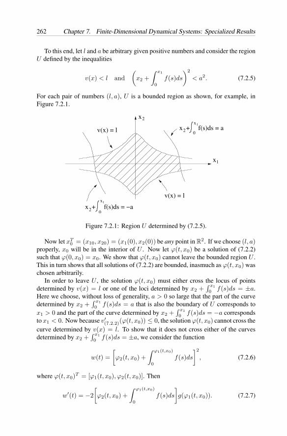
262 Chapter 7. Finite-Dimensional Dynamical Systems: Specialized Results
To this end, let l and a be arbitrary given positive numbers and consider the regionU defined by the inequalities
v(x) < l and(
x2 +∫ x1
0f(s)ds
)2
< a2. (7.2.5)
For each pair of numbers (l, a), U is a bounded region as shown, for example, inFigure 7.2.1.
x + f(s)ds = −a
x1
2
2x + f(s)ds = a
0
xv(x) = l
1
x2
v(x) = l 0
x 1
Figure 7.2.1: Region U determined by (7.2.5).
Now let xT0 = (x10, x20) = (x1(0), x2(0)) be any point in R
2. If we choose (l, a)properly, x0 will be in the interior of U . Now let ϕ(t, x0) be a solution of (7.2.2)such that ϕ(0, x0) = x0. We show that ϕ(t, x0) cannot leave the bounded region U .This in turn shows that all solutions of (7.2.2) are bounded, inasmuch as ϕ(t, x0) waschosen arbitrarily.
In order to leave U , the solution ϕ(t, x0) must either cross the locus of pointsdetermined by v(x) = l or one of the loci determined by x2 +
∫ x1
0 f(s)ds = ±a.Here we choose, without loss of generality, a > 0 so large that the part of the curvedetermined by x2 +
∫ x1
0 f(s)ds = a that is also the boundary of U corresponds tox1 > 0 and the part of the curve determined by x2 +
∫ x1
0 f(s)ds = −a correspondsto x1 < 0. Now because v′
(7.2.2)(ϕ(t, x0)) ≤ 0, the solution ϕ(t, x0) cannot cross thecurve determined by v(x) = l. To show that it does not cross either of the curvesdetermined by x2 +
∫ x1
0 f(s)ds = ±a, we consider the function
w(t) =[ϕ2(t, x0) +
∫ ϕ1(t,x0)
0f(s)ds
]2, (7.2.6)
where ϕ(t, x0)T = [ϕ1(t, x0), ϕ2(t, x0)]. Then
w′(t) = −2[ϕ2(t, x0) +
∫ ϕ1(t,x0)
0f(s)ds
]g(ϕ1(t, x0)). (7.2.7)
Section 7.3 Domain of Attraction 263
Now suppose that ϕ(t, x0) reaches that part of the boundary of U determined bythe equation x2 +
∫ x1
0 f(s)ds = a, x1 > 0. Then along this part of the boundaryw′(t) = −2ag(ϕ(t, x0)) < 0 because x1 > 0 and a > 0. Therefore, the solutionϕ(t, x0) cannot cross outside of the set U through that part of the boundary determinedby x2 +
∫ x1
0 f(s)ds = a. We apply the same argument to the part of the boundarydetermined by x2 +
∫ x1
0 f(s)ds = −a.Therefore, every solution of (7.2.2) is bounded and we can apply Theorem 7.2.2
to conclude that the equilibrium (x1, x2)T = (0, 0)T is globally attractive.
We apply some of the results of this section in Chapter 8 in the qualitative analysisof a large class of artificial neural networks.
7.3 Domain of Attraction
Many practical systems possess more than one equilibrium point. In such cases, theconcept of asymptotic stability in the large is no longer applicable and one is usuallyinterested in knowing the extent of the domain of attraction of an asymptoticallystable equilibrium. In the present section, we briefly address the problem of obtainingestimates of the domain of attraction of the equilibrium xe = 0 of the autonomoussystem
x = f(x) (A)
where f ∈ C[Ω, Rn], Ω ⊂ Rn is an open connected set, 0 ∈ Ω, and f(0) = 0.
We assume that there exists a positive definite and time-independent functionv ∈ C[Ω, R+] such that v′
(A) is negative definite on some subset Ω1 ⊂ Ω, 0 ∈ Ω1.Let Dc = x ∈ Ω: v(x) ≤ c for c > 0. If Dc ⊂ Ω1, then Dc is contained in thedomain of attraction of the equilibrium xe = 0 of (A). In fact, Dc is an invariantset for system (A): any trajectory of a solution of (A) starting within Dc will remainin Dc. As such it will remain in Ω1 where v′
(A) is negative definite. Therefore, itfollows from the proof of Theorem 6.2.2 that all trajectories for (A) that start in Dc
will approach the equilibrium xe = 0. If cM denotes the largest number for whichthe above discussion is true, then DcM
is the best estimate of the domain of attractionof xe = 0 for (A), using the particular v-function employed. Another choice ofLyapunov function will generally result in a different estimate for the domain ofattraction.
Example 7.3.1 Consider the systemx1 = −x1 + x1
(x2
1 + x22)
x2 = −x2 + x2(x2
1 + x22).
(7.3.1)
This system clearly has an equilibrium at the origin xe = (x1, x2)T = (0, 0)T .We choose the function
v(x1, x2) =12(x2
1 + x22)
(7.3.2)
264 Chapter 7. Finite-Dimensional Dynamical Systems: Specialized Results
and we compute
v′(7.3.1)(x1, x2) = −
(x2
1 + x22)
+(x2
1 + x22)2
. (7.3.3)
The function v is positive definite and radially unbounded whereas v′(7.3.1) is negative
definite on the set x ∈ R2 : (x2
1 + x22) < 2c, c < 1/2; that is, on the set
Dc =x ∈ R
2 : v(x) < c, c <
12. (7.3.4)
We conclude that the equilibrium xe = 0 of (7.3.1) is asymptotically stable and thatthe set x ∈ R
2 : (x21 + x2
2) < 1 is contained in the domain of attraction of xe = 0.Indeed, it is not hard to show that this set is the entire domain of attraction of theequilibrium xe = 0.
The procedure described above for determining estimates for the domain of at-traction of an asymptotically stable equilibrium xe = 0 applies, without substantialchanges, to autonomous discrete-time systems described by difference equations
x(k + 1) = f(x(k)) (DA)
where f : Ω → Ω, Ω ⊂ Rn is an open connected set, and 0 ∈ Ω. We omit the details
in the interests of brevity.There are results that determine the domain of attraction of an asymptotically stable
equilibrium xe = 0 of (A) precisely. In the following, we let G ⊂ Ω and we assumethat G is a simply connected domain containing a neighborhood of the origin.
Theorem 7.3.1 [21] (Zubov) Suppose there exist two functions v ∈ C1[G, R] andh ∈ C[Rn, R] satisfying the following hypotheses.
(i) v is positive definite in G and satisfies on G the inequality 0 < v(x) < 1 whenx = 0. For any b ∈ (0, 1), the set x ∈ G : v(x) ≤ b is bounded.
(ii) h(0) = 0, and h(x) > 0 for x = 0.(iii) For x ∈ G, we have
v′(A)(x) = −h(x)
[1 − v(x)
][1 + |f(x)|2
]1/2. (7.3.5)
(iv) As x ∈ G approaches a point on the boundary of G, or in case of an unboundedregion G, as |x| → ∞, lim v(x) = 1.
Then G is exactly the domain of attraction of the equilibrium xe = 0.
Proof . Under the given hypotheses, it follows from Theorem 6.2.2 that xe = 0 isuniformly asymptotically stable. Note also that if we introduce the change of variables
ds =[1 + |f(ϕ(t))|2
]1/2dt,
then (7.3.5) reduces todv
ds= −h(x)
[1 − v(x)
],
Section 7.3 Domain of Attraction 265
but the stability properties of (A) remain unchanged. Let V (s) = v(ϕ(s)) for a givenfunction ϕ(s) such that ϕ(0) = x0. Then
d
dslog[1 − V (s)
]= h(ϕ(s)),
or
1 − V (s) =[1 − V (0)
]exp(∫ s
0h(ϕ(u))du
). (7.3.6)
Let x0 ∈ G and assume that x0 is not in the domain of attraction of the trivialsolution. Then h(ϕ(s)) ≥ δ > 0 for some fixed δ and for all s ≥ 0. Hence, in (7.3.6)as s → ∞ the term on the left is at most one, whereas the term on the right tends toinfinity, which is impossible. Thus, x0 is in the domain of attraction of xe = 0.
Suppose x1 is in the domain of attraction but x1 /∈ G. Then ϕ(s, x1) → 0 ass → ∞, so there must exist s1 and s2 such that ϕ(s1, x1) ∈ ∂G and ϕ(s2, x1) ∈ G.Let x0 = ϕ(s2, x1) in (7.3.6). Take the limit in (7.3.6) as s → s+
1 . We see that
lims→s+
1
[1 − V (s)
]= 1 − 1 = 0,
and the limit on the right-hand side is
[1 − v(x0)
]exp(∫ s1
s2
h(ϕ(s, x1))ds
)> 0.
This is impossible. Hence x1 must be in G.
An immediate result of Theorem 7.3.1 is the following result.
Corollary 7.3.1 Assume that there exists a function h that satisfies the hypothesesof Theorem 7.3.1 and assume that there exists a continuously differentiable, positivedefinite function v : G → R that satisfies the inequality 0 ≤ v(x) ≤ 1 for all x ∈ Gas well as the differential equation
∇v(x)T f(x) = −h(x)[[1 − v(x)
][1 + |f(x)|2
]1/2. (7.3.7)
Then the boundary of the domain of attraction is defined by the equation
v(x) = 1. (7.3.8)
If the domain of attraction G is all of Rn, then the equilibrium xe = 0 of (A) is
asymptotically stable in the large. In this case, we have
v(x) → 1 as |x| → ∞. (7.3.9)
266 Chapter 7. Finite-Dimensional Dynamical Systems: Specialized Results
In the foregoing results, we can work with different v functions. For example, ifwe let
w(x) = − log[1 − v(x)
],
then (7.3.5) assumes the form
w′(A)(x) = −h(x)
[1 + |f(x)|2
]1/2
and condition (7.3.8) defining the boundary becomes w(x) → ∞.Note that in Theorem 7.3.1, the function h(x) is arbitrary. In specific applications
it is chosen in a fashion that makes the solution of the partial differential equation(7.3.7) easy.
Example 7.3.2 Consider the systemx1 = 2x1
1 − x21 + x2
2
(x1 + 1)2 + x22
+ x1x2= f1(x1, x2)
x2 =1 − x2
1 + x22
2− 4x2
1x2
(x1 + 1)2 + x22
= f2(x1, x2).
(7.3.10)
This system has an equilibrium at x1 = 1, x2 = 0. The partial differential equation(7.3.7) assumes the form
∂v
∂x1(x1, x2)f1(x1, x2)+
∂v
∂x2(x1, x2)f2(x1, x2)=−2
(x1 − 1)2+x22
(x1 + 1)2+x22
[1−v(x1, x2)
]where
h(x1, x2) = 2(x1 − 1)2 + x2
2
(x1 + 1)2 + x22
[1 + f1(x1, x2)2 + f2(x1, x2)2
]−(1/2).
It is readily verified that a solution of the above partial differential equation is
v(x1, x2) =(x1 − 1)2 + x2
2
(x1 + 1)2 + x22.
Because v(x1, x2) = 1 if and only if x1 = 0, the domain of attraction is the set(x1, x2) : 0 < x1 < ∞,−∞ < x2 < ∞.
7.4 Linear Continuous-Time Systems
In this section we study the stability properties of the equilibrium of linear homoge-neous systems
x = A(t)x, t ≥ t0, t0 ≥ 0 (LH)
and linear autonomous homogeneous systems
x = Ax, t ≥ 0. (L)
Section 7.4 Linear Continuous-Time Systems 267
In (LH), t ∈ R+, x ∈ R
n, and A ∈ C[R+, Rn×n]. In (L), t ∈ R+, x ∈ R
n, andA ∈ R
n×n. Recall that xe = 0 is always an equilibrium of (L) and (LH) and thatxe = 0 is the only equilibrium of (LH) if A(t) is nonsingular for t ≥ 0. Recall alsothat the solution of (LH) for x(t0) = x0 is of the form
ϕ(t, t0, x0) = Φ(t, t0)x0, t ≥ t0
where Φ denotes the state transition matrix of A(t). Recall further that the solutionof (L) for x(t0) = x0 is given by
ϕ(t, t0, x0) = Φ(t, t0)x0
= Φ(t − t0, 0)x0
= Φ(t − t0)x0
= eA(t−t0)x0
where in the preceding equation, a slight abuse in notation has been used.For some of the properties of the transition matrix Φ(t, t0) that are used in the proofs
of the result that follow, the reader should refer to the appendix (Subsection 7.8A).
A. Linear homogeneous systems
In the next four results, we explore some of the basic qualitative properties of (LH).
Theorem 7.4.1 The equilibrium xe = 0 of (LH) is stable if and only if the solutionsof (LH) are bounded, or equivalently, if and only if
supt≥t0
∥∥Φ(t, t0)∥∥
= c(t0) < ∞
where ‖Φ(t, t0)‖ denotes the matrix norm induced by the vector norm used on Rn
and c(t0) denotes a constant that may depend on the choice of t0.
Proof . Assume that the equilibrium xe = 0 of (LH) is stable. Then for any t0 ≥ 0and for ε = 1 there is a δ = δ(1, t0) > 0 such that |ϕ(t, t0, x0)| < 1 for all t ≥ t0and all x0 with |x0| ≤ δ. In this case
|ϕ(t, t0, x0)| = |Φ(t, t0)x0| =∣∣∣∣Φ(t, t0)(x0δ)
|x0|
∣∣∣∣ ( |x0|δ
)<
|x0|δ
for all x0 = 0 and all t ≥ t0. In the above inequality we have used the fact that∣∣∣∣ϕ(t, t0,x0δ
|x0|
)∣∣∣∣ = ∣∣∣∣Φ(t, t0)(x0δ)|x0|
∣∣∣∣ < 1.
Using the definition of matrix norm it follows that∥∥Φ(t, t0)∥∥ ≤ δ−1, t ≥ t0.
268 Chapter 7. Finite-Dimensional Dynamical Systems: Specialized Results
We have proved that if the equilibrium xe = 0 of system (LH) is stable, then thesolutions of (LH) are bounded.
Conversely, suppose that all solutions ϕ(t, t0, x0) = Φ(t, t0)x0 are bounded. Lete1, . . . , en denote the natural basis for n-space and let |ϕ(t, t0, ej)| < βj for allt ≥ t0, j = 1, . . . , n. Then for any vector x0 =
∑nj=1 αjej we have that
|ϕ(t, t0, x0)| =∣∣∣∣ n∑
j=1
αjϕ(t, t0, ej)∣∣∣∣
≤n∑
j=1
|αj |βj
≤(
max1≤j≤n
βj
) n∑j=1
|αj |
≤ K|x0|
for some constant K > 0 and for t ≥ t0. For given ε > 0, we choose δ = ε/K.Thus, if |x0| < δ, then |ϕ(t, t0, x0)| < K|x0| < ε for all t ≥ t0. We have provedthat if the solutions of (LH) are bounded, then the equilibrium xe = 0 of (LH) isstable.
Theorem 7.4.2 The equilibrium xe = 0 of (LH) is uniformly stable if and only if
supt0≥0
c(t0)= sup
t0≥0
(supt≥t0
∥∥Φ(t, t0)∥∥)
= c0 < ∞.
The proof of the above result is similar to the proof of Theorem 7.4.1 and is leftas an exercise.
Example 7.4.1 Consider the system[x1x2
]=[e−2t
(e−t − e−2t
)0 e−t
] [x1x2
](7.4.1)
where x(0) = x0. We transform (7.4.1) using the relation x = Py, where
P =[1 10 1
], P−1 =
[1 −10 1
]to obtain the equivalent system[
y1y2
]=[e−2t 0
0 e−t
] [y1y2
](7.4.2)
with y(0) = y0 = P−1x0. System (7.4.2) has the solution ψ(t, 0, y0) = Ψ(t, 0)y0,where
Ψ(t, 0) =
[e(1/2)(1−e−2t) 0
0 e(1−e−t)
].
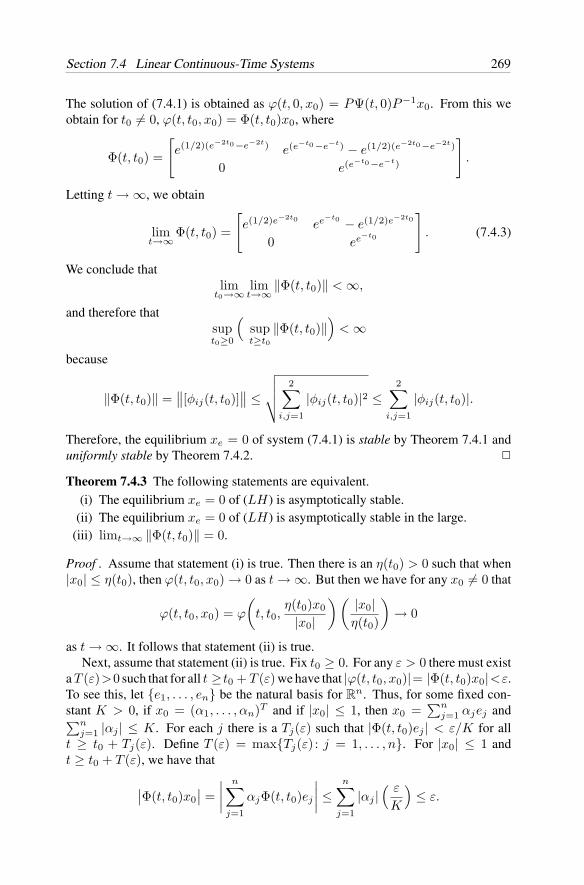
Section 7.4 Linear Continuous-Time Systems 269
The solution of (7.4.1) is obtained as ϕ(t, 0, x0) = PΨ(t, 0)P−1x0. From this weobtain for t0 = 0, ϕ(t, t0, x0) = Φ(t, t0)x0, where
Φ(t, t0) =
[e(1/2)(e−2t0−e−2t) e(e−t0−e−t) − e(1/2)(e−2t0−e−2t)
0 e(e−t0−e−t)
].
Letting t → ∞, we obtain
limt→∞ Φ(t, t0) =
[e(1/2)e−2t0
ee−t0 − e(1/2)e−2t0
0 ee−t0
]. (7.4.3)
We conclude thatlim
t0→∞ limt→∞ ‖Φ(t, t0)‖ < ∞,
and therefore thatsupt0≥0
(supt≥t0
‖Φ(t, t0)‖)
< ∞
because
‖Φ(t, t0)‖ =∥∥[φij(t, t0)]
∥∥ ≤
√√√√ 2∑i,j=1
|φij(t, t0)|2 ≤2∑
i,j=1
|φij(t, t0)|.
Therefore, the equilibrium xe = 0 of system (7.4.1) is stable by Theorem 7.4.1 anduniformly stable by Theorem 7.4.2.
Theorem 7.4.3 The following statements are equivalent.(i) The equilibrium xe = 0 of (LH) is asymptotically stable.
(ii) The equilibrium xe = 0 of (LH) is asymptotically stable in the large.(iii) limt→∞ ‖Φ(t, t0)‖ = 0.
Proof . Assume that statement (i) is true. Then there is an η(t0) > 0 such that when|x0| ≤ η(t0), then ϕ(t, t0, x0) → 0 as t → ∞. But then we have for any x0 = 0 that
ϕ(t, t0, x0) = ϕ
(t, t0,
η(t0)x0
|x0|
)(|x0|η(t0)
)→ 0
as t → ∞. It follows that statement (ii) is true.Next, assume that statement (ii) is true. Fix t0 ≥ 0. For any ε > 0 there must exist
a T (ε)>0 such that for all t ≥ t0 + T (ε) we have that |ϕ(t, t0, x0)|= |Φ(t, t0)x0|<ε.To see this, let e1, . . . , en be the natural basis for R
n. Thus, for some fixed con-stant K > 0, if x0 = (α1, . . . , αn)T and if |x0| ≤ 1, then x0 =
∑nj=1 αjej and∑n
j=1 |αj | ≤ K. For each j there is a Tj(ε) such that |Φ(t, t0)ej | < ε/K for allt ≥ t0 + Tj(ε). Define T (ε) = maxTj(ε) : j = 1, . . . , n. For |x0| ≤ 1 andt ≥ t0 + T (ε), we have that
∣∣Φ(t, t0)x0∣∣ = ∣∣∣∣ n∑
j=1
αjΦ(t, t0)ej
∣∣∣∣ ≤ n∑j=1
|αj |( ε
K
)≤ ε.
270 Chapter 7. Finite-Dimensional Dynamical Systems: Specialized Results
By the definition of matrix norm, this means that ‖Φ(t, t0)‖ ≤ ε for all t ≥ t0 +T (ε).Therefore, statement (iii) is true.
Finally, assume that statement (iii) is true. Then ‖Φ(t, t0)‖ is bounded in t for allt≥ t0. By Theorem 7.4.1, the equilibrium xe =0 is stable. To prove asymptotic sta-bility, fix t0 ≥0 and ε>0. If |x0|<η(t0)=1, then |ϕ(t, t0, x0)|≤‖Φ(t, t0)‖|x0|→ 0as t → ∞. Therefore, statement (i) is true. This completes the proof.
Example 7.4.2 The equilibrium xe = 0 of system (7.4.1) given in Example 7.4.1 isstable but not asymptotically stable because limt→∞ ‖Φ(t, t0)‖ = 0.
Example 7.4.3 The solution of the system
x = −e2tx, x(t0) = x0 (7.4.4)
is ϕ(t, t0, x0) = Φ(t, t0)x0, where
Φ(t, t0) = e(1/2)(e2t0−e2t).
Because limt→∞ Φ(t, t0) = 0, it follows that the equilibrium xe = 0 of system(7.4.4) is asymptotically stable in the large.
Theorem 7.4.4 The equilibrium xe = 0 of system (LH) is uniformly asymptoticallystable if and only if it is exponentially stable.
Proof . The exponential stability of the equilibrium xe = 0 implies the uniformasymptotic stability of the equilibrium xe = 0 of system (E) in general, and hence,for system (LH) in particular.
Conversely, assume that the equilibrium xe = 0 of system (LH) is uniformlyasymptotically stable. Then there are a δ > 0 and a T > 0 such that if |x0| ≤ δ, then∣∣Φ(t + t0 + T, t0)x0
∣∣ ≤ (δ/2) for all t, t0 ≥ 0. This implies that∥∥Φ(t + t0 + T, t0)∥∥ ≤ 1
2if t, t0 ≥ 0. (7.4.5)
From Theorem 7.8.6(iii) (Subsection 7.8A) we have that Φ(t, τ) = Φ(t, σ)Φ(σ, τ)for any t, σ, and τ . Therefore,∥∥Φ(t + t0 + 2T, t0)
∥∥ =∥∥Φ(t + t0 + 2T, t + t0 + T )Φ(t + t0 + T, t0)
∥∥ ≤ 14,
in view of (7.4.5). By induction, we obtain for t, t0 ≥ 0 that∥∥Φ(t + t0 + nT, t0)∥∥ ≤ 2−n. (7.4.6)
Now let α = (ln 2)/T . Then (7.4.6) implies that for 0 ≤ t < T we have that∣∣ϕ(t + t0 + nT, t0, x0)∣∣ ≤ 2|x0|2−(n+1)
= 2|x0|e−α(n+1)T
≤ 2|x0|e−α(t+nT ),
which proves the result.
Section 7.4 Linear Continuous-Time Systems 271
Example 7.4.4 For system (7.4.4) given in Example 7.4.3 we have∣∣ϕ(t, t0, x0)∣∣ = ∣∣∣x0e
(1/2)e2t0e−(1/2)e2t
∣∣∣ ≤ |x0|e(1/2)e2t0e−t, t ≥ t0 ≥ 0,
because e2t > 2t. Therefore, the equilibrium xe = 0 of system (7.4.4) is uniformlyasymptotically stable in the large, and exponentially stable in the large.
Even though the preceding results require knowledge of the state transition matrixΦ(t, t0) of (LH), they are quite useful in the qualitative analysis of linear systems.
B. Linear autonomous homogeneous systems
Revisiting Example 3.1.8, we now address the stability properties of system (L),
x = Ax, t ≥ 0. (L)
To this end we transform matrix A into the Jordan canonical form, J = P−1AP ,using the transformation x = Py to obtain from (L) the equivalent system
y = P−1APy = Jy. (7.4.7)
It is easily verified (the reader is asked to do this in the exercise section) that theequilibrium xe = 0 of (L) is stable (resp., asymptotically stable or unstable) if andonly if ye = 0 of system (7.4.7) is stable (resp., asymptotically stable or unstable).In view of this, we can assume without loss of generality that the matrix A in (L) isin Jordan canonical form given by
A = diag[J0, J1, . . . , Js
]where
J0 = diag[λ1, . . . , λk
]and Ji = λk+iIi + Ni
for the Jordan blocks J1, . . . , Js, where Ii denotes the ni ×ni identity matrix and Ni
denotes the ni × ni nilpotent matrix given by
Ni =
0 1 0 · · · 00 0 1 · · · 0...
.... . .
. . ....
0 0 0. . . 1
0 0 0 · · · 0
,
and λj , j = 1, . . . n, denote the eigenvalues of A. We have
eAt =
eJ0t 0
eJ1t
. . .0 eJst
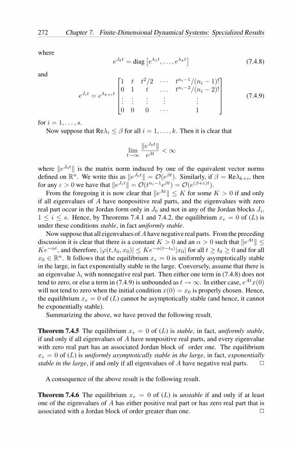
272 Chapter 7. Finite-Dimensional Dynamical Systems: Specialized Results
whereeJ0t = diag
[eλ1t, . . . , eλkt
](7.4.8)
and
eJit = eλk+it
1 t t2/2 · · · tni−1/(ni − 1)!0 1 t . . . tni−2/(ni − 2)!...
......
......
0 0 0 · · · 1
(7.4.9)
for i = 1, . . . , s.Now suppose that Reλi ≤ β for all i = 1, . . . , k. Then it is clear that
limt→∞
‖eJ0t‖eβt
< ∞
where ‖eJ0t‖ is the matrix norm induced by one of the equivalent vector normsdefined on R
n. We write this as ‖eJ0t‖ = O(eβt). Similarly, if β = Reλk+i, thenfor any ε > 0 we have that ‖eJit‖ = O(tni−1eβt) = O(e(β+ε)t).
From the foregoing it is now clear that ‖eAt‖ ≤ K for some K > 0 if and onlyif all eigenvalues of A have nonpositive real parts, and the eigenvalues with zeroreal part occur in the Jordan form only in J0 and not in any of the Jordan blocks Ji,1 ≤ i ≤ s. Hence, by Theorems 7.4.1 and 7.4.2, the equilibrium xe = 0 of (L) isunder these conditions stable, in fact uniformly stable.
Now suppose that all eigenvalues of A have negative real parts. From the precedingdiscussion it is clear that there is a constant K > 0 and an α > 0 such that ‖eAt‖ ≤Ke−αt, and therefore, |ϕ(t, t0, x0)| ≤ Ke−α(t−t0)|x0| for all t ≥ t0 ≥ 0 and for allx0 ∈ R
n. It follows that the equilibrium xe = 0 is uniformly asymptotically stablein the large, in fact exponentially stable in the large. Conversely, assume that there isan eigenvalue λi with nonnegative real part. Then either one term in (7.4.8) does nottend to zero, or else a term in (7.4.9) is unbounded as t → ∞. In either case, eAtx(0)will not tend to zero when the initial condition x(0) = x0 is properly chosen. Hence,the equilibrium xe = 0 of (L) cannot be asymptotically stable (and hence, it cannotbe exponentially stable).
Summarizing the above, we have proved the following result.
Theorem 7.4.5 The equilibrium xe = 0 of (L) is stable, in fact, uniformly stable,if and only if all eigenvalues of A have nonpositive real parts, and every eigenvaluewith zero real part has an associated Jordan block of order one. The equilibriumxe = 0 of (L) is uniformly asymptotically stable in the large, in fact, exponentiallystable in the large, if and only if all eigenvalues of A have negative real parts.
A consequence of the above result is the following result.
Theorem 7.4.6 The equilibrium xe = 0 of (L) is unstable if and only if at leastone of the eigenvalues of A has either positive real part or has zero real part that isassociated with a Jordan block of order greater than one.
Section 7.4 Linear Continuous-Time Systems 273
Before proceeding any further, it may be appropriate to take note of certain con-ventions concerning matrices that are used in the literature. Some of these are notconsistent with the terminology used in Theorem 7.4.5. Thus, a real n × n matrix Ais called stable or a Hurwitz matrix if all its eigenvalues have negative real parts. Ifat least one of the eigenvalues has a positive real part, then A is called unstable. Amatrix A, which is neither stable nor unstable, is called critical, and the eigenvalueswith zero real parts are called critical eigenvalues.
We conclude the present subsection with some examples.
Example 7.4.5 Consider system (L) with
A =[
0 1−1 0
].
The eigenvalues of A are λ1, λ2 = ±i (i =√
−1). According to Theorem 7.4.5, theequilibrium xe = 0 of this system is stable. This can also be verified by computingthe solutions of this system for the given set of initial data x(0) = (x1(0), x2(0))T ,
ϕ1(t, 0, x0) = x1(0)cos t + x2(0)sin t
ϕ2(t, 0, x0) = −x1(0)sin t + x2(0)cos t,
t ≥ 0, and then applying Definition 6.1.1(a).
Example 7.4.6 Consider system (L) with
A =[
2.8 9.69.6 −2.8
].
The eigenvalues of A are λ1, λ2 = ±10. According to Theorem 7.4.6, the equilibriumxe = 0 of this system is unstable.
Example 7.4.7 Consider system (L) with
A =[0 10 0
].
The eigenvalues of A are λ1 = 0 and λ2 = 0. According to Theorem 7.4.6, theequilibrium xe = 0 of this system is unstable. This can also be verified by computingthe solutions of this system for the given set of initial data x(0) = (x1(0), x2(0))T ,
ϕ1(t, 0, x0) = x1(0) + x2(0)t,ϕ2(t, 0, x0) = x2(0),
t ≥ 0, and then applying Definition 6.1.1(k).
Example 7.4.8 Consider system (L) with
A =[
−1 0−1 −2
].
The eigenvalues of A are λ1, λ2 = −1,−2. According to Theorem 7.4.5, the equi-librium xe = 0 of this system is exponentially stable.
274 Chapter 7. Finite-Dimensional Dynamical Systems: Specialized Results
C. The Lyapunov matrix equation
The stability results that we established thus far in this section require explicit knowl-edge of the solutions of (L) and (LH). In the present subsection we develop stabilitycriteria for system (L) with arbitrary matrix A. To accomplish this, we employ theLyapunov stability results established in Chapter 6. We recall that these involve theexistence of Lyapunov functions.
Lyapunov functions v for a system are sometimes viewed as “generalized distancefunctions” of the state x from the equilibrium xe (xe = 0) and the stability propertiesare then deduced directly from the properties of v and its time derivative v′, alongthe solutions of the system on hand.
A logical choice of Lyapunov function for system (L) is v(x) = xT x = |x|2which represents the square of the Euclidean distance of the state from the equilibriumxe = 0. The stability properties of this equilibrium are then determined by examiningthe properties of v′
(L)(x), the time derivative of v(x) along the solutions of (L),
x = Ax. (L)
This derivative can be determined without explicitly solving for the solutions ofsystem (L) as
v′(L)(x) = xT x + xT x
= (Ax)T x + xT (Ax)
= xT (AT + A)x.
If the matrix A is such that v′(L)(x) is negative for all x = 0, then it is reasonable to
expect that the distance of the state of (L) from the equilibrium xe = 0 will decreasewith increasing time, and that the state will therefore tend to the equilibrium of (L)with increasing time.
The above discussion is consistent with our earlier discussion of Subsection 6.1G.It turns out that the Lyapunov function used above is not sufficiently flexible. In thefollowing we employ as a “generalized distance function” the quadratic form
v(x) = xT Px, P = PT (7.4.10)
where P ∈ Rn×n. (Refer to Subsection 6.1F for a discussion of quadratic forms.)
The derivative of v(x) along the solutions of (L) is determined as
v′(L)(x) = xT Px + xT Px
= xT AT Px + xT PAx
= xT (AT P + PA)x;
that is,v′(L)(x) = xT Cx, (7.4.11)
whereC = AT P + PA. (7.4.12)
Section 7.4 Linear Continuous-Time Systems 275
Note that C is real and CT = C. The system of equations given in (7.4.12) is calledthe Lyapunov Matrix Equation.
Before proceeding further, we recall that because P is real and symmetric, all ofits eigenvalues are real. Also, we recall that P is said to be positive definite (resp.,positive semidefinite) if all its eigenvalues are positive (resp., nonnegative) and iscalled indefinite if P has eigenvalues of opposite sign. The notions of negativedefinite and negative semidefinite for matrix P are defined similarly (refer, e.g., toMichel and Herget [14]). Thus (see Subsection 6.1F), the function v(x) given in(7.4.10) is positive definite, positive semidefinite, and so forth, if the matrix P hasthe corresponding definiteness properties. Finally, we recall from Subsection 6.1Fthat instead of solving for the eigenvalues of a real symmetric matrix to determineits definiteness properties, there are more efficient and direct methods to accomplishthis (refer to Theorem 6.1.4).
In view of the above discussion, the results below now follow readily by invokingthe Lyapunov results established in Section 6.2.
Proposition 7.4.1 (a) The equilibrium xe = 0 of (L) is uniformly stable if thereexists a real, symmetric, and positive definite n × n matrix P such that the matrix Cgiven in (7.4.12) is negative semidefinite.
(b) The equilibrium xe = 0 of (L) is exponentially stable in the large if there existsa real, symmetric, and positive definite n × n matrix P such that the matrix C givenin (7.4.12) is negative definite.
(c) The equilibrium xe = 0 of (L) is unstable if there exists a real, symmetricn × n matrix P that is either negative definite or indefinite such that the matrix Cgiven in (7.4.12) is negative definite.
We leave the proofs of the above results as an exercise to the reader.
Example 7.4.9 For the system given in Example 7.4.5 we choose P = I , and wecompute
C = AT P + PA = AT + A = 0.
According to Proposition 7.4.1(a), the equilibrium xe = 0 of this system is stable (asexpected in Example 7.4.5).
Example 7.4.10 For the system given in Example 7.4.8 we choose
P =[1 00 0.5
]and we compute the matrix
C = AT P + PA =[
−2 −0.5−0.5 −2
].
According to Proposition 7.4.1(b), the equilibrium xe = 0 of this system is exponen-tially stable in the large (as expected in Example 7.4.8).
276 Chapter 7. Finite-Dimensional Dynamical Systems: Specialized Results
Example 7.4.11 For the system given in Example 7.4.7 we choose
P =[
−0.28 −0.96−0.96 0.28
]and we compute
C = AT P + PA =[−20 00 −20
].
The eigenvalues of P are ±1. According to Proposition 7.4.1(c), the equilibriumxe = 0 of this system is unstable (as expected from Example 7.4.7).
In applying the results given in Proposition 7.4.1, we start by guessing a matrix Pthat has certain desired properties. Next, we solve the Lyapunov matrix equationfor C, using (7.4.12). If C possesses certain desired properties (it is negative definite),we draw appropriate conclusions, using Proposition 7.4.1; if this is not possible(i.e., Proposition 7.4.1 does not apply), we need to choose another matrix P . Thispoints to the principal shortcomings of Lyapunov’s Direct Method, when applied togeneral systems. However, in the case of the special case of linear system (L), it ispossible to construct Lyapunov functions of the form v(x) = xT Px in a systematicmanner. In the process of doing so, one first chooses the matrix C in (7.4.12),having desired properties, and then one solves (7.4.12) for P . Conclusions are thendrawn by applying the appropriate results given in Proposition 7.4.1. In applyingthis construction procedure, we need to know the conditions under which (7.4.12)possesses a unique solution P for a given C. We address this topic next.
Once more, we consider the quadratic form
v(x) = xT Px, P = PT (7.4.13)
and the time derivative of v along the solutions of (L), given by
v′(L)(x) = xT Cx, C = CT (7.4.14)
whereC = AT P + PA, (7.4.15)
where all symbols are defined as before. Our objective is to determine the as yetunknown matrix P in such a way that v′
(L) becomes a preassigned negative definitequadratic form, that is, in such a way that C is a preassigned negative definite matrix.
We first note that (7.4.15) constitutes a system of n(n + 1)/2 linear equations,because P is symmetric. We need to determine under what conditions we can solvefor the n(n + 1)/2 elements, pik, given the matrices A and C. To make thingstractable, we choose a similarity transformation Q such that
QAQ−1 = A, (7.4.16)
or equivalently,A = Q−1AQ, (7.4.17)
Section 7.4 Linear Continuous-Time Systems 277
where A is similar to A and Q is a real n × n nonsingular matrix. From (7.4.17) and(7.4.15) we obtain
(A)T (Q−1)T PQ−1 + (Q−1)T PQ−1A = (Q−1)T CQ−1 (7.4.18)
or(A)T P + P A = C (7.4.19)
whereP = (Q−1)T PQ−1, C = (Q−1)T CQ−1. (7.4.20)
In (7.4.19) and (7.4.20), P and C are subjected to a congruence transformation andP and C have the same definiteness properties as P and C, respectively. Becauseevery real n × n matrix can be triangularized, we can choose Q in such a mannerthat A = [aij ] is triangular; that is, aij = 0 for i > j. Note that in this case theeigenvalues of A, λ1, . . . , λn, appear in the main diagonal of A. To simplify oursubsequent notation, we rewrite (7.4.19), (7.4.20) in the form of (7.4.15) by droppingthe bars, that is,
AT P + PA = C, C = CT (7.4.21)
and we assume without loss of generality that A = [aij ] has been triangularized;that is, aij = 0 for i > j. Because the eigenvalues λ1, . . . , λn appear in the diagonalof A, we can rewrite (7.4.21) as
2λ1p11 = c11
a12p11 + (λ1 + λ2)p12 = c12 (7.4.22)
...
.
Note that λ1 may be a complex number, in which case c11 will also be complex.Because this system of equations is triangular, and because its determinant is equal to
2nλ1 · · ·λn
∏i<j
(λi + λj), (7.4.23)
the matrix P can be determined uniquely if and only this determinant is not zero.This is true when all eigenvalues of A are nonzero and no two of them are such thatλi + λj = 0. This condition is not affected by a similarity transformation and istherefore also valid for the original system of equations (7.4.15).
We summarize the above discussion as follows.
Lemma 7.4.1 Let A ∈ Rn×n and let λ1, . . . , λn denote the (not necessarily distinct)
eigenvalues of A. Then (7.4.21) has a unique solution for P corresponding to eachC ∈ R
n×n if and only if
λi = 0 for all i = 1, . . . , n and λi+λj = 0 for all i, j = 1, . . . , n. (7.4.24)
278 Chapter 7. Finite-Dimensional Dynamical Systems: Specialized Results
In order to construct v(x), we must still check the definiteness of P . This canbe done in a purely algebraic way; however, it is much easier to invoke the stabilityresults of the present section and argue as follows.
(a) If all the eigenvalues λi of A have negative real parts, then the equilibriumxe = 0 of (L) is exponentially stable in the large and if C in (7.4.15) is negativedefinite, then P must be positive definite. To prove this, we note that if P is notpositive definite, then for δ > 0 and sufficiently small, (P − δI) has at least onenegative eigenvalue and the function v(x) = xT (P − δI)x has a negative definitederivative; that is,
v′(L)(x) = xT [C − δ(A + AT )]x < 0
for all x = 0. By Theorem 6.2.8 (resp., Proposition 7.4.1(c)), the equilibrium xe = 0of (L) is unstable. We have arrived at a contradiction. Therefore, P must be positivedefinite.
(b) If A has eigenvalues with positive real parts and no eigenvalues with zero realparts we can use a similarity transformation x = Qy in such a way that Q−1AQ is ablock diagonal matrix of the form diag[A1, A2], where all the eigenvalues of A1 havepositive real parts and all eigenvalues of A2 have negative real parts. (If A does nothave any eigenvalues with negative real parts, then we take A = A1). By the resultestablished in (a), noting that all eigenvalues of −A1 have negative real parts, givenany negative definite matrices C1 and C2, there exist positive definite matrices P1and P2 such that
(−AT1 )P1 + P1(−A1) = C1, AT
2 P2 + P2A2 = C2.
Then w(y) = yT Py, with P = diag[−P1, P2] is a Lyapunov function for the systemy = Q−1AQy (and hence, for the system x = Ax) that satisfies the hypotheses ofTheorem 6.2.8 (resp., Proposition 7.4.1(c)). Therefore, the equilibrium xe = 0 ofsystem (L) is unstable. If A does not have any eigenvalues with negative real parts,then the equilibrium xe = 0 of (L) is completely unstable.
In the above proof, we did not invoke Lemma 7.4.1. We note, however, that ifadditionally, (7.4.24) is true, then we can construct the Lyapunov function for (L) ina systematic manner.
Summarizing the above discussion, we now can state the main result of this sub-section.
Theorem 7.4.7 Assume that the matrix A (for system (L)) has no eigenvalues withreal part equal to zero. If all the eigenvalues of A have negative real parts, or if atleast one of the eigenvalues of A has a positive real part, then there exists a quadraticLyapunov function
v(x) = xT Px, P = PT
whose derivative along the solutions of (L) is definite (i.e., either negative definite orpositive definite).
This result shows that when A is a stable matrix (i.e., all the eigenvalues of Ahave negative real parts), then for system (L), the conditions of Theorem 6.2.3 are
Section 7.4 Linear Continuous-Time Systems 279
also necessary conditions for asymptotic stability. Moreover, in the case when thematrix A has at least one eigenvalue with positive real part and no eigenvalues on theimaginary axis, then the conditions of Theorem 6.2.8 are also necessary conditionsfor instability.
Example 7.4.12 We consider the system (L) with
A =[
0 1−1 0
].
The eigenvalues of A are λ1, λ2 = ±i (i =√
−1) and therefore, condition (7.4.24)is violated. According to Lemma 7.4.1, the Lyapunov matrix equation
AT P + PA = C
does not possess a unique solution for a given C. We demonstrate this for two specificcases:
(i) If C = 0, we obtain[0 −11 0
][p11 p12p12 p22
]+[p11 p12p12 p22
][0 1
−1 0
]=[
−2p12 p11 − p22p11 − p22 2p12
]=[0 00 0
],
or p12 = 0 and p11 = p22. Therefore, for any c ∈ R, the matrix P = cI is a solutionof the Lyapunov matrix equation. Thus, for C = 0, the Lyapunov matrix equationhas in this case denumerably many solutions.
(ii) If C = −2I , we have[−2p12 p11 − p22
p11 − p22 2p12
]=[−2 00 −2
],
or p11 = p22 and p12 = 1 and p12 = −1, which is impossible. Therefore, forC = −2I , the Lyapunov matrix equation has in this example no solution at all.
We conclude the present section with a result which shows that when all theeigenvalues of matrix A for system (L) have negative real parts, then the matrix P in(7.4.15) can be computed explicitly.
Theorem 7.4.8 If all the eigenvalues of a real n × n matrix A have negative realparts, then for each matrix C ∈ R
n×n, the unique solution of (7.4.15) is given by
P =∫ ∞
0eAT s(−C)eAsds. (7.4.25)
Proof . If all eigenvalues of A have negative real parts, then (7.4.24) is satisfied andtherefore (7.4.15) has a unique solution for every C ∈ R
n×n. To verify that (7.4.25)is indeed this solution, we first note that the right-hand side of (7.4.25) is well defined,
280 Chapter 7. Finite-Dimensional Dynamical Systems: Specialized Results
because all eigenvalues of A have negative real parts. Substituting the right-hand sideof (7.4.25) for P into (7.4.15), we obtain
AT P + PA =∫ ∞
0AT eAT t(−C)eAtdt +
∫ ∞
0eAT t(−C)eAtAdt
=∫ ∞
0
d
dt
(eAT t(−C)eAt
)dt
= eAT t(−C)eAt∣∣∣∞0
= C,
which proves the theorem.
D. Periodic systems
We now briefly consider linear periodic systems given by
x = A(t)x (LP )
where A ∈ C[R, Rn×n] and A(t) = A(t + T ) for all t ∈ R, where T > 0 denotesthe period for (LP ). Making reference to the appendix section (Subsection 7.8B),we recall that if Φ(t, t0) is the state transition matrix for (LP ), then there exists aconstant matrix R ∈ R
n×n and a nonsingular n × n matrix Ψ(t, t0) such that
Φ(t, t0) = Ψ(t, t0)eR(t−t0), (7.4.26)
whereΨ(t, t0) = Ψ(t + T, t0)
for all t ∈ R. In Section 7.8 it is shown that the change of variables given by
x = Ψ(t, t0)y
transforms system (LP ) into the system
y = Ry, (7.4.27)
whereR is given in (7.4.26). Moreover, becauseΨ(t, t0)−1 exists over t0 ≤ t ≤ t+T ,the equilibrium xe = 0 is uniformly stable (resp., uniformly asymptotically stable) ifand only if ye = 0 is also uniformly stable (resp., uniformly asymptotically stable).Applying Theorem 7.4.5 to system (7.4.27), we obtain the following results.
Theorem 7.4.9 The equilibrium xe = 0 of (LP ) is uniformly stable if and only ifall eigenvalues of the matrix R (given in (7.4.26)) have nonpositive real parts, andevery eigenvalue with a zero real part has an associated Jordan block of order one.The equilibrium xe = 0 of (LP ) is uniformly asymptotically stable in the large if andonly if all the eigenvalues of R have negative real parts.
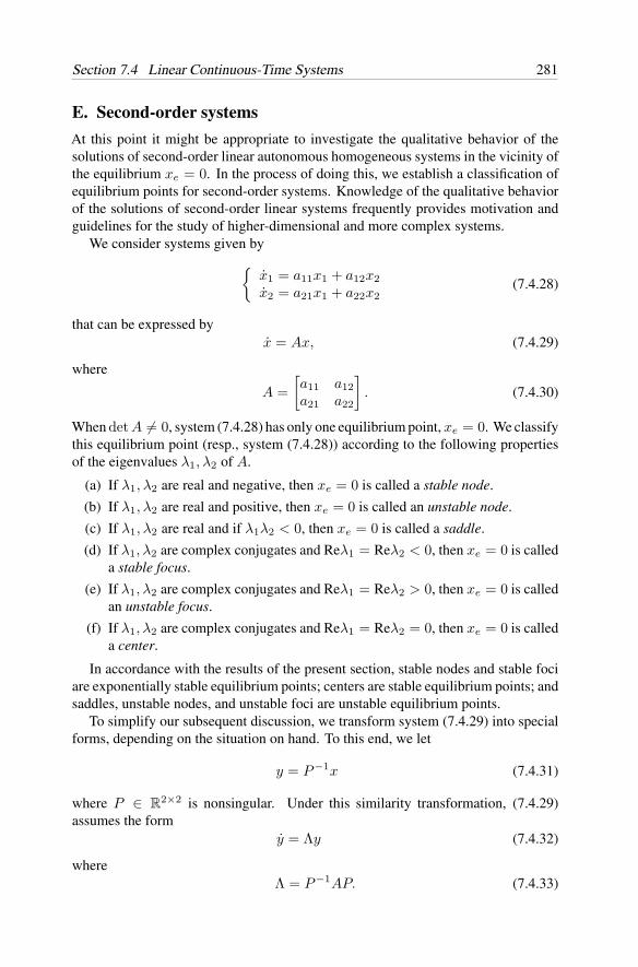
Section 7.4 Linear Continuous-Time Systems 281
E. Second-order systems
At this point it might be appropriate to investigate the qualitative behavior of thesolutions of second-order linear autonomous homogeneous systems in the vicinity ofthe equilibrium xe = 0. In the process of doing this, we establish a classification ofequilibrium points for second-order systems. Knowledge of the qualitative behaviorof the solutions of second-order linear systems frequently provides motivation andguidelines for the study of higher-dimensional and more complex systems.
We consider systems given byx1 = a11x1 + a12x2x2 = a21x1 + a22x2
(7.4.28)
that can be expressed byx = Ax, (7.4.29)
where
A =[a11 a12a21 a22
]. (7.4.30)
When det A = 0, system (7.4.28) has only one equilibrium point, xe = 0. We classifythis equilibrium point (resp., system (7.4.28)) according to the following propertiesof the eigenvalues λ1, λ2 of A.
(a) If λ1, λ2 are real and negative, then xe = 0 is called a stable node.
(b) If λ1, λ2 are real and positive, then xe = 0 is called an unstable node.
(c) If λ1, λ2 are real and if λ1λ2 < 0, then xe = 0 is called a saddle.
(d) If λ1, λ2 are complex conjugates and Reλ1 = Reλ2 < 0, then xe = 0 is calleda stable focus.
(e) If λ1, λ2 are complex conjugates and Reλ1 = Reλ2 > 0, then xe = 0 is calledan unstable focus.
(f) If λ1, λ2 are complex conjugates and Reλ1 = Reλ2 = 0, then xe = 0 is calleda center.
In accordance with the results of the present section, stable nodes and stable fociare exponentially stable equilibrium points; centers are stable equilibrium points; andsaddles, unstable nodes, and unstable foci are unstable equilibrium points.
To simplify our subsequent discussion, we transform system (7.4.29) into specialforms, depending on the situation on hand. To this end, we let
y = P−1x (7.4.31)
where P ∈ R2×2 is nonsingular. Under this similarity transformation, (7.4.29)
assumes the formy = Λy (7.4.32)
whereΛ = P−1AP. (7.4.33)
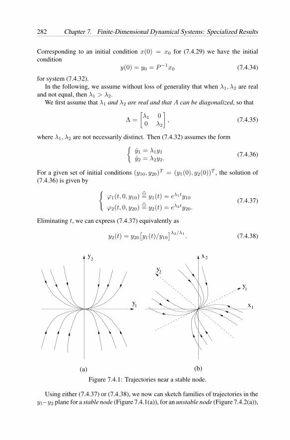
282 Chapter 7. Finite-Dimensional Dynamical Systems: Specialized Results
Corresponding to an initial condition x(0) = x0 for (7.4.29) we have the initialcondition
y(0) = y0 = P−1x0 (7.4.34)
for system (7.4.32).In the following, we assume without loss of generality that when λ1, λ2 are real
and not equal, then λ1 > λ2.We first assume that λ1 and λ2 are real and that A can be diagonalized, so that
Λ =[λ1 00 λ2
], (7.4.35)
where λ1, λ2 are not necessarily distinct. Then (7.4.32) assumes the formy1 = λ1y1y2 = λ2y2.
(7.4.36)
For a given set of initial conditions (y10, y20)T = (y1(0), y2(0))T , the solution of(7.4.36) is given by
ϕ1(t, 0, y10)= y1(t) = eλ1ty10
ϕ2(t, 0, y20)= y2(t) = eλ2ty20.
(7.4.37)
Eliminating t, we can express (7.4.37) equivalently as
y2(t) = y20[y1(t)/y10
]λ2/λ1. (7.4.38)
x
(a) (b)
y2
y1
2
x1
y2
y1
Figure 7.4.1: Trajectories near a stable node.
Using either (7.4.37) or (7.4.38), we now can sketch families of trajectories in they1– y2 plane for a stable node (Figure 7.4.1(a)), for an unstable node (Figure 7.4.2(a)),
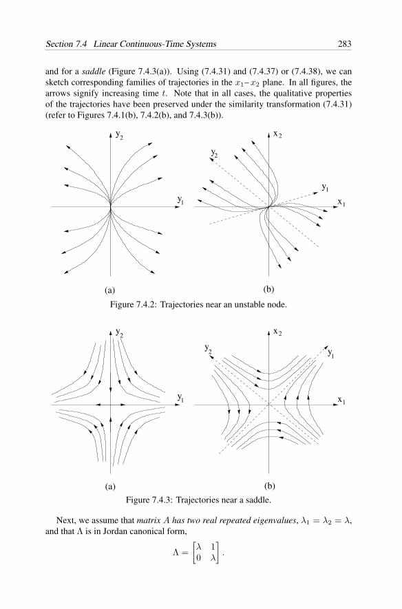
Section 7.4 Linear Continuous-Time Systems 283
and for a saddle (Figure 7.4.3(a)). Using (7.4.31) and (7.4.37) or (7.4.38), we cansketch corresponding families of trajectories in the x1– x2 plane. In all figures, thearrows signify increasing time t. Note that in all cases, the qualitative propertiesof the trajectories have been preserved under the similarity transformation (7.4.31)(refer to Figures 7.4.1(b), 7.4.2(b), and 7.4.3(b)).
x
y1
(a) (b)
y2
y1
2
x1
y2
Figure 7.4.2: Trajectories near an unstable node.
xy2
y1
2
x1
2y y
1
(a) (b)
Figure 7.4.3: Trajectories near a saddle.
Next, we assume that matrix A has two real repeated eigenvalues, λ1 = λ2 = λ,and that Λ is in Jordan canonical form,
Λ =[λ 10 λ
].
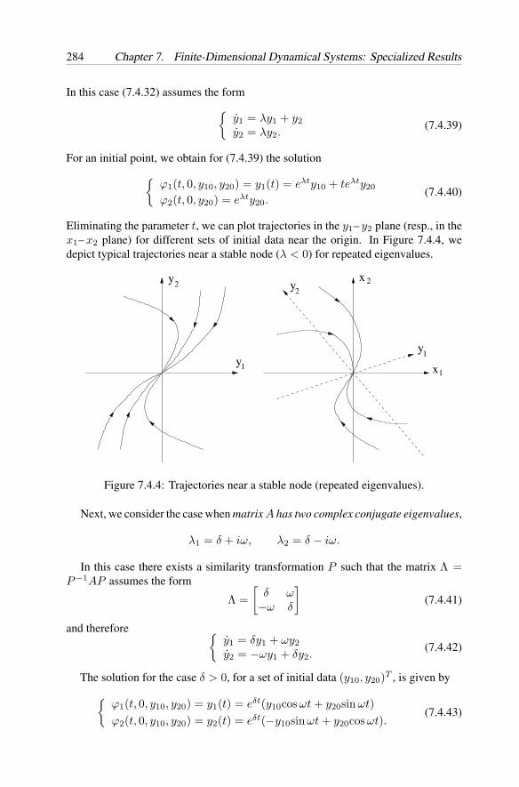
284 Chapter 7. Finite-Dimensional Dynamical Systems: Specialized Results
In this case (7.4.32) assumes the formy1 = λy1 + y2y2 = λy2.
(7.4.39)
For an initial point, we obtain for (7.4.39) the solutionϕ1(t, 0, y10, y20) = y1(t) = eλty10 + teλty20
ϕ2(t, 0, y20) = eλty20.(7.4.40)
Eliminating the parameter t, we can plot trajectories in the y1– y2 plane (resp., in thex1– x2 plane) for different sets of initial data near the origin. In Figure 7.4.4, wedepict typical trajectories near a stable node (λ < 0) for repeated eigenvalues.
xy
y
y2
1
22
y1
x1
Figure 7.4.4: Trajectories near a stable node (repeated eigenvalues).
Next, we consider the case when matrix A has two complex conjugate eigenvalues,
λ1 = δ + iω, λ2 = δ − iω.
In this case there exists a similarity transformation P such that the matrix Λ =P−1AP assumes the form
Λ =[
δ ω−ω δ
](7.4.41)
and therefore y1 = δy1 + ωy2y2 = −ωy1 + δy2.
(7.4.42)
The solution for the case δ > 0, for a set of initial data (y10, y20)T , is given byϕ1(t, 0, y10, y20) = y1(t) = eδt(y10cos ωt + y20sin ωt)ϕ2(t, 0, y10, y20) = y2(t) = eδt(−y10sin ωt + y20cos ωt).
(7.4.43)
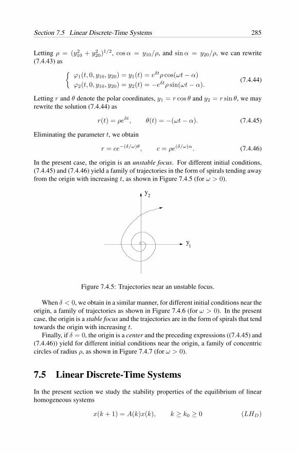
Section 7.5 Linear Discrete-Time Systems 285
Letting ρ = (y210 + y2
20)1/2, cos α = y10/ρ, and sin α = y20/ρ, we can rewrite
(7.4.43) as ϕ1(t, 0, y10, y20) = y1(t) = eδtρ cos(ωt − α)ϕ2(t, 0, y10, y20) = y2(t) = −eδtρ sin(ωt − α).
(7.4.44)
Letting r and θ denote the polar coordinates, y1 = r cos θ and y2 = r sin θ, we mayrewrite the solution (7.4.44) as
r(t) = ρeδt, θ(t) = −(ωt − α). (7.4.45)
Eliminating the parameter t, we obtain
r = ce−(δ/ω)θ, c = ρe(δ/ω)α. (7.4.46)
In the present case, the origin is an unstable focus. For different initial conditions,(7.4.45) and (7.4.46) yield a family of trajectories in the form of spirals tending awayfrom the origin with increasing t, as shown in Figure 7.4.5 (for ω > 0).
y
y
1
2
Figure 7.4.5: Trajectories near an unstable focus.
When δ < 0, we obtain in a similar manner, for different initial conditions near theorigin, a family of trajectories as shown in Figure 7.4.6 (for ω > 0). In the presentcase, the origin is a stable focus and the trajectories are in the form of spirals that tendtowards the origin with increasing t.
Finally, if δ = 0, the origin is a center and the preceding expressions ((7.4.45) and(7.4.46)) yield for different initial conditions near the origin, a family of concentriccircles of radius ρ, as shown in Figure 7.4.7 (for ω > 0).
7.5 Linear Discrete-Time Systems
In the present section we study the stability properties of the equilibrium of linearhomogeneous systems
x(k + 1) = A(k)x(k), k ≥ k0 ≥ 0 (LHD)
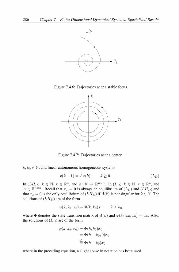
286 Chapter 7. Finite-Dimensional Dynamical Systems: Specialized Results
y
y
1
2
Figure 7.4.6: Trajectories near a stable focus.
2y
y1
Figure 7.4.7: Trajectories near a center.
k, k0 ∈ N, and linear autonomous homogeneous systems
x(k + 1) = Ax(k), k ≥ 0. (LD)
In (LHD), k ∈ N, x ∈ Rn, and A : N → R
n×n. In (LD), k ∈ N, x ∈ Rn, and
A ∈ Rn×n. Recall that xe = 0 is always an equilibrium of (LD) and (LHD) and
that xe = 0 is the only equilibrium of (LHD) if A(k) is nonsingular for k ∈ N. Thesolutions of (LHD) are of the form
ϕ(k, k0, x0) = Φ(k, k0)x0, k ≥ k0,
where Φ denotes the state transition matrix of A(k) and ϕ(k0, k0, x0) = x0. Also,the solutions of (LD) are of the form
ϕ(k, k0, x0) = Φ(k, k0)x0
= Φ(k − k0, 0)x0
= Φ(k − k0)x0
where in the preceding equation, a slight abuse in notation has been used.
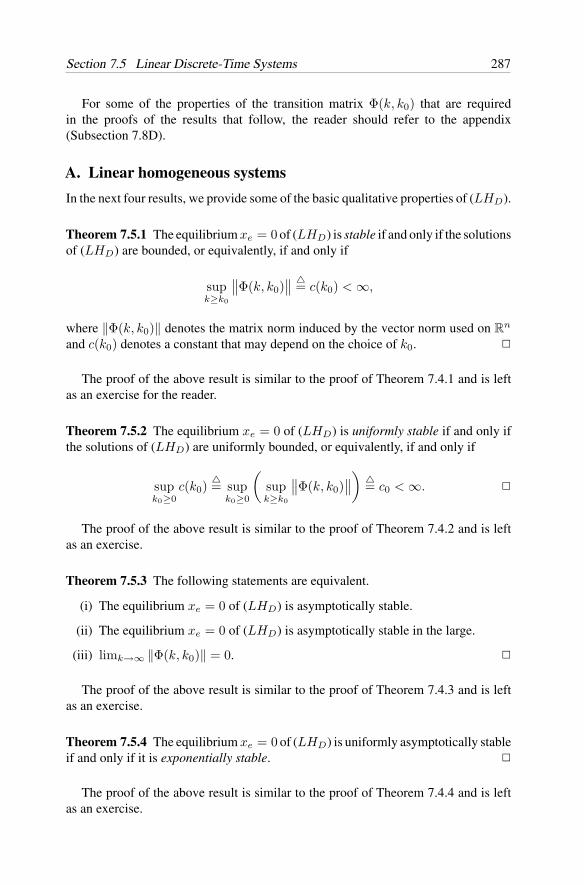
Section 7.5 Linear Discrete-Time Systems 287
For some of the properties of the transition matrix Φ(k, k0) that are requiredin the proofs of the results that follow, the reader should refer to the appendix(Subsection 7.8D).
A. Linear homogeneous systems
In the next four results, we provide some of the basic qualitative properties of (LHD).
Theorem 7.5.1 The equilibrium xe = 0 of (LHD) is stable if and only if the solutionsof (LHD) are bounded, or equivalently, if and only if
supk≥k0
∥∥Φ(k, k0)∥∥
= c(k0) < ∞,
where ‖Φ(k, k0)‖ denotes the matrix norm induced by the vector norm used on Rn
and c(k0) denotes a constant that may depend on the choice of k0.
The proof of the above result is similar to the proof of Theorem 7.4.1 and is leftas an exercise for the reader.
Theorem 7.5.2 The equilibrium xe = 0 of (LHD) is uniformly stable if and only ifthe solutions of (LHD) are uniformly bounded, or equivalently, if and only if
supk0≥0
c(k0)= sup
k0≥0
(supk≥k0
∥∥Φ(k, k0)∥∥)
= c0 < ∞.
The proof of the above result is similar to the proof of Theorem 7.4.2 and is leftas an exercise.
Theorem 7.5.3 The following statements are equivalent.
(i) The equilibrium xe = 0 of (LHD) is asymptotically stable.
(ii) The equilibrium xe = 0 of (LHD) is asymptotically stable in the large.
(iii) limk→∞ ‖Φ(k, k0)‖ = 0.
The proof of the above result is similar to the proof of Theorem 7.4.3 and is leftas an exercise.
Theorem 7.5.4 The equilibrium xe = 0 of (LHD) is uniformly asymptotically stableif and only if it is exponentially stable.
The proof of the above result is similar to the proof of Theorem 7.4.4 and is leftas an exercise.
288 Chapter 7. Finite-Dimensional Dynamical Systems: Specialized Results
B. Linear autonomous homogeneous systems
Revisiting Example 3.1.9, we now address the stability properties of system (LD),
x(k + 1) = Ax(k), k ≥ 0. (LD)
To this end we transform the matrix A into the Jordan canonical form, J = P−1AP ,using the transformation x = Py to obtain the equivalent system
y(k + 1) = P−1APy(k) = Jy(k). (7.5.1)
Because the equilibrium xe = 0 of (LD) possesses the same stability propertiesas the equilibrium ye = 0 of (7.5.1), we may assume without loss of generalitythat the matrix A in (LD) is in Jordan canonical form. We may now use the samereasoning as was done in Subsection 7.4B (for system (L)), to arrive at the followingresult.
Theorem 7.5.5 The equilibrium xe = 0 of system (LD) is stable, in fact, uniformlystable, if and only if all eigenvalues of A are within or on the unit circle of the complexplane, and every eigenvalue that is on the unit circle has an associated Jordan blockof order one. The equilibrium xe = 0 of (LD) is uniformly asymptotically stable inthe large, in fact, exponentially stable in the large, if and only if all eigenvalues of Aare within the unit circle of the complex plane.
The proof of this result proceeds along similar lines as the proof of Theorem 7.4.5and is left to the reader as an exercise. As a consequence of Theorem 7.5.5, we havethe following result.
Theorem 7.5.6 The equilibrium xe = 0 of (LD) is unstable if and only if at leastone of the eigenvalues of A is outside of the unit circle in the complex plane or atleast one of the eigenvalues of A is on the unit circle in the complex plane and isassociated with a Jordan block of order greater than one.
The proof of the above result is similar to the proof of Theorem 7.4.6 and is leftas an exercise.
As in the case of linear system (L), it may be appropriate to take note of certainconventions concerning matrices for system (LD) that are used in the literature. Again,these are not consistent with the terminology used in the preceding results. Thus, areal n × n matrix A is called Schur stable or just stable, if all of its eigenvalues arewithin the unit circle of the complex plane. If at least one of the eigenvalues of A isoutside the unit circle, then A is called unstable. A matrix A that is neither stable norunstable is called critical, and the eigenvalues on the unit circle in the complex planeare called critical eigenvalues.
Example 7.5.1 For system (LD), we let
A =[
0 1−1 0
].
Section 7.5 Linear Discrete-Time Systems 289
The eigenvalues of A are λ1, λ2 = ±√
−1. According to Theorem 7.5.5, the equi-librium xe = 0 of the system is stable, and according to Theorems 7.5.1 and 7.5.2,the matrix Ak is bounded (resp., uniformly bounded) for all k ≥ 0.
Example 7.5.2 For system (LD), we let
A =[
0 −1/2−1 0
].
The eigenvalues of A are λ1, λ2 = ±1/√
2. According to Theorem 7.5.5, the equilib-rium xe = 0 of the system is asymptotically stable and according to Theorem 7.5.3,limk→∞ Ak = 0.
Example 7.5.3 For system (LD), we let
A =[
0 −1/2−3 0
].
The eigenvalues of A are λ1, λ2 = ±√
3/2. According to Theorem 7.5.6, the equi-librium xe = 0 of system (LD) is unstable, and according to Theorems 7.5.1 and7.5.2, the matrix Ak is not bounded with increasing k.
Example 7.5.4 For system (LD), we let
A =[1 10 1
].
The matrix A is a Jordan block of order 2 for the eigenvalue λ = 1. According toTheorem 7.5.6, the equilibrium xe = 0 of the system is unstable.
C. The Lyapunov matrix equation
In the present section we employ quadratic forms
v(x) = xT Bx, B = BT (7.5.2)
to establish stability criteria for linear systems
x(k + 1) = Ax(k). (LD)
Evaluating v along the solutions of system (LD), we obtain the first forward differenceof v as
∆LDv(x(k)) = v(x(k + 1)) − v(x(k))
= x(k + 1)T Bx(k + 1) − x(k)T Bx(k)
= x(k)T AT BAx(k) − x(k)T Bx(k)
= x(k)T (AT BA − B)x(k),
290 Chapter 7. Finite-Dimensional Dynamical Systems: Specialized Results
and therefore∆LD
v(x) = xT (AT BA − B)x= xT Cx (7.5.3)
whereAT BA − B = C, CT = C. (7.5.4)
Equation (7.5.4) is called the Lyapunov Matrix Equation for system (LD).Invoking the Lyapunov stability results of Section 6.3, the following results follow
readily.
Proposition 7.5.1 (a) The equilibrium xe = 0 of system (LD) is stable if there existsa real, symmetric, and positive definite matrix B such that the matrix C given in(7.5.4) is negative semidefinite.
(b) The equilibrium xe = 0 of system (LD) is asymptotically stable in the large,in fact, exponentially stable in the large, if there exists a real, symmetric, and positivedefinite matrix B such that the matrix C given in (7.5.4) is negative definite.
(c) The equilibrium xe = 0 of system (LD) is unstable if there exists a real,symmetric matrix B that is either negative definite or indefinite such that the matrixC given in (7.5.4) is negative definite.
We leave the proofs of the above results as an exercise for the reader.In applying Proposition 7.5.1, we start by guessing a matrix B having certain
properties and we then solve for the matrix C in (7.5.4). If C possesses desiredproperties, we can apply Proposition 7.5.1 to draw appropriate conclusions; if not,we need to choose another matrix B. This is not a very satisfactory approach, and inthe following, we derive results that, similarly as in the case of linear continuous-timesystems (L), enable us to construct Lyapunov functions of the form v(x) = xT Bxin a systematic manner. In this approach we first choose a matrix C in (7.5.4) whichis either negative definite or positive definite, then we solve (7.5.4) for B, and thenwe draw appropriate conclusions by invoking existing Lyapunov results (e.g., Propo-sition 7.5.1). In applying this approach of constructing Lyapunov functions, we needto know under what conditions equation (7.5.4) possesses a unique solution B for anydefinite (i.e., positive definite or negative definite) matrix C. We address this issuenext.
We first show that if all the eigenvalues of A are within the unit circle of thecomplex plane (i.e., A is stable), then we can compute B in (7.5.4) explicitly. To seethis, assume that in (7.5.4) C is given and that A is stable. Then
(AT )k+1BAk+1 − (AT )kBAk = (AT )kCAk,
and summing from k = 0 to l yields
AT BA − B + (AT )2BA2 − AT BA + · · · + (AT )l+1BAl+1 − (AT )lBAl
=l∑
k=0
(AT )kCAk
Section 7.5 Linear Discrete-Time Systems 291
or
(AT )l+1BAl+1 − B =l∑
k=0
(AT )kCAk.
Letting l → ∞, we have
B = −∞∑
k=0
(AT )kCAk. (7.5.5)
It is easily verified that (7.5.5) is a solution of (7.5.4). Indeed, we have
−AT
[ ∞∑k=0
(AT )kCAk
]A +
∞∑k=0
(AT )kCAk = C
or
−AT CA + C − (AT )2CA2 + AT CA − (AT )3CA3 + (AT )2CA2 − · · · = C.
Furthermore, if C is negative definite, then B is positive definite.Combining the above discussion with Proposition 7.5.1(b), we have proved the
following result.
Theorem 7.5.7 If there is a positive definite and symmetric matrix B and a negativedefinite and symmetric matrix C satisfying the Lyapunov matrix equation (7.5.4),then the matrix A is stable. Conversely, if A is stable, then given any symmetricmatrix C, equation (7.5.4) has a unique solution B, and if C is negative definite, thenB is positive definite.
Next, we determine conditions under which the Lyapunov matrix equation (7.5.4)has a unique solution B = BT ∈ R
n×n for a given matrix C = CT ∈ Rn×n. In
doing so, we consider the more general system of equations
A1XA2 − X = C (7.5.6)
where A1 ∈ Rm×m, A2 ∈ R
n×n, X ∈ Rm×n, and C ∈ R
m×n.
Lemma 7.5.1 Let A1 ∈ Rm×m and A2 ∈ R
n×n. Then equation (7.5.6) has a uniquesolution X ∈ R
m×n for a given C ∈ Rm×n if and only if no eigenvalue of A1 is a
reciprocal of an eigenvalue of A2.
Proof . We need to show that the condition on A1 and A2 is equivalent to the conditionthat A1XA2 = X implies X = 0. Once we have proved that A1XA2 = X has theunique solution X = 0, then it can be shown that (7.5.6) has a unique solution forevery C, because (7.5.6) is a linear equation.
Assume first that the condition on A1 and A2 is satisfied. Now A1XA2 = Ximplies that Ak−j
1 XAk−j2 = X and
Aj1 = Ak
1XAk−j2 for k ≥ j ≥ 0.
292 Chapter 7. Finite-Dimensional Dynamical Systems: Specialized Results
Now for the polynomial of degree k,
p(λ) =k∑
j=0
ajλj ,
we define the polynomial of degree k,
p∗(λ) =k∑
j=0
ajλk−j = λkp
(1λ
),
from which it follows that
p(A1)X = Ak1Xp∗(A2). (7.5.7)
Now let ϕi(λ) be the characteristic polynomial of Ai, i = 1, 2. It follows from theassumption that ϕ1(λ) and ϕ∗
2(λ) do not have common roots. Thus, ϕ1(λ) and ϕ∗2(λ)
are relatively prime, which in turn yields that there are polynomials p(λ) and q(λ)such that
p(λ)ϕ1(λ) + q(λ)ϕ∗2(λ) = 1.
Now define ϕ(λ) = q(λ)ϕ∗2(λ) and note that ϕ∗(λ) = q∗(λ)ϕ2(λ). It follows that
ϕ∗(A2) = 0 and ϕ(A1) = I . Replacing p(λ) in (7.5.7) by ϕ(λ), we obtain
X = ϕ(A1)X = Ak1Xϕ∗(A2) = 0.
From this it follows that A1XA2 = X implies X = 0.To prove the converse, we assume that λ is an eigenvalue of A1 and λ−1 is an
eigenvalue of A2 (and hence, is also an eigenvalue of AT2 ). Let A1w = λw and
AT2 z = λ−1z, 0 = w ∈ R
n×1, and 0 = z ∈ Rm×1. Define X = wzT . Then X = 0
and A1XA2 = X .
To construct the Lyapunov function v(x), using Lemma 7.5.1, we must still checkthe definiteness of B, using the results of the present section (e.g., Proposition 7.5.1).
(a) If all the eigenvalues of A for system (LD) are within the unit circle of the com-plex plane, then no reciprocal of an eigenvalue of A is an eigenvalue, and Lemma 7.5.1gives another way of showing that equation (7.5.4) has a unique solution B for everyC if A is stable. If C is negative definite, then B is positive definite. This can beshown similarly as was done for the corresponding case of linear ordinary differentialequations (Subsection 7.4C).
(b) Suppose that at least one of the eigenvalues of A is outside the unit circle inthe complex plane and that A has no eigenvalues on the unit circle. As in the case oflinear differential equations (L) (Subsection 7.4C), we use a similarity transformationx = Qy in such a way that Q−1AQ = diag[A1, A2], where all eigenvalues of A1are outside the unit circle and all eigenvalues of A2 are within the unit circle. Wethen proceed identically as in the case of linear differential equations to show thatunder the present assumptions there exists for system (LD) a Lyapunov function that
Section 7.5 Linear Discrete-Time Systems 293
satisfies the hypotheses of Proposition 7.5.1(c). Therefore, the equilibrium xe = 0 ofsystem (LD) is unstable. If A does not have any eigenvalues within the unit circle,then the equilibrium xe = 0 of (L) is completely unstable. In this proof, Lemma 7.5.1has not been invoked. If additionally, the hypotheses of Lemma 7.5.1 are true (i.e.,no reciprocal of an eigenvalue of A is an eigenvalue of A), then we can construct theLyapunov function for (LD) in a systematic manner.
Summarizing the above discussion, we have arrived at the following result.
Theorem 7.5.8 Assume that the matrix A (for system (LD)) has no eigenvalues onthe unit circle. If all the eigenvalues of A are within the unit circle of the complexplane, or if at least one eigenvalue is outside the unit circle of the complex plane, thenthere exists a Lyapunov function of the form v(x) = xT Bx, B = BT , whose firstforward difference along the solutions of system (LD) is definite (i.e., ∆LD
v(x) iseither negative definite or positive definite).
Theorem 7.5.8 shows that when all the eigenvalues of A are within the unit circle,then for system (LD), the conditions of Theorem 6.3.2 are also necessary conditionsfor asymptotic stability. Furthermore, when at least one eigenvalue is outside the unitcircle and no eigenvalues are on the unit circle, then the conditions of Theorem 6.3.4are also necessary conditions for instability.
We conclude the present section by considering several specific examples.
Example 7.5.5 For system (LD), let
A =[
0 1−1 0
].
Choose B = I , which is positive definite. From (7.5.4) we have
C = AT A − I =[0 −11 0
] [0 1
−1 0
]−[1 00 1
]=[0 00 0
].
It follows from Proposition 7.5.1(a) that the equilibrium xe = 0 of (LD) is stable.This is the same conclusion as the one we arrived at in Example 7.5.1.
Example 7.5.6 For system (LD), let
A =[
0 −1/2−1 0
].
We choose
B =[8/3 00 5/3
],
which is positive definite. From (7.5.4) we obtain
C = AT BA − B
=[
0 −1−1/2 0
] [8/3 00 5/3
] [0 −1/2
−1 0
]−[8/3 00 5/3
]=[−1 00 −1
],
294 Chapter 7. Finite-Dimensional Dynamical Systems: Specialized Results
which is negative definite. It follows from Proposition 7.5.1(b) that the equilibriumxe = 0 of system (LD) is asymptotically stable in the large, in fact, exponentiallystable in the large. This is the same conclusion that was drawn in Example 7.5.2.
Example 7.5.7 For system (LD), let
A =[
0 −1/2−3 0
].
We choose
C =[−1 00 −1
]which is negative definite. From (7.5.4) we obtain
C = AT BA − B =[
0 −3−1/2 0
] [b11 b12b12 b22
] [0 −1/2
−3 0
]−[b11 b12b12 b22
]or [(
9b22 − b11)
b12/2b12/2
(b11/4 − b22
)] =[−1 00 −1
],
which yields
B =[−8 00 −1
],
which is also negative definite. It follows from Proposition 7.5.1(c) that the equi-librium xe = 0 of this system is unstable. This conclusion is consistent with theconclusion made in Example 7.5.3.
Example 7.5.8 For system (LD), let
A =[1/3 10 3
].
The eigenvalues of A are λ1 = 1/3 and λ2 = 3. According to Lemma 7.5.1, for agiven matrix C = CT , equation (7.5.4) does not have a unique solution, because inthis case λ1 = 1/λ2. For purposes of illustration, we choose C = −I . Then
−I = AT BA − B =[1/3 01 3
] [b11 b12b12 b22
] [1/3 10 3
]−[b11 b12b12 b22
]or [
−8/9 b11/3b11/3
(b11 + 6b12 + 8b22
)] =[−1 00 −1
],
which shows that for C = −I , equation (7.5.4) does not have any solution for Bat all.
Section 7.6 Perturbed Linear Systems 295
7.6 Perturbed Linear Systems
Perturbed linear systems come about because of uncertainties incurred during themodeling process; because of errors made in measurements; because of errors in-troduced when linearizing nonlinear systems; and the like. A natural question offundamental importance is to identify conditions under which linear systems andtheir perturbations have similar qualitative properties. We answer this question inpieces, by addressing different aspects of system behavior.
We first determine conditions under which the stability properties of the equilib-rium xe = 0 of a nonlinear system can be deduced from the stability properties ofthe equilibrium w = 0 of its linearization, for noncritical cases. This is known asLyapunov’s First Method or Lyapunov’s Indirect Method. Next, for noncritical cases,we determine the qualitative properties of the solutions of perturbed linear systems byproving the existence of stable and unstable manifolds near the equilibrium xe = 0of such systems. Finally, by introducing the notion of orbital stability, we study thestability and instability properties of periodic solutions of perturbed linear periodicsystems.
A. Preliminaries
The present subsection consists of several parts.
Some Notation
We recall that for a function g : Rl → R
k, the notation g(x) = O(|x|β) as |x| → αmeans that
lim|x|→α
sup|g(x)||x|β < ∞,
β ≥ 0, with the interesting cases including α = 0 and α = ∞. Above, |·| denotes anyone of the equivalent norms on R
l. Also, when g : R × Rl → R
k, g(t, x) = O(|x|β)as |x| → α uniformly for t in an interval I means that
lim|x|→α
sup
(supt∈I
|g(t, x)||x|β
)< ∞.
We also recall that g(x) = O(|x|β) as |x| → α means that
lim|x|→α
|g(x)||x|β = 0
and g(t, x) = O(|x|β) as |x| → α uniformly for t in an interval is defined in theobvious way.
The Implicit Function Theorem
In Subsection 7.6D we make use of the Implicit Function Theorem which we presentnext, without proof. To this end, we consider a system of functions
gi(x, y) = gi(x1, . . . , xn, y1, . . . , yr), i = 1, . . . , r.
296 Chapter 7. Finite-Dimensional Dynamical Systems: Specialized Results
We assume that these functions have continuous first derivatives in an open set con-taining a point (x0, y0). We define the Jacobian matrix of g(·) = (g1(·), . . . , gr(·))with respect to (y1, . . . , yr) by
gy(·) =∂g
∂y(·) =
∂g1/∂y1 · · · ∂g1/∂yr
∂g2/∂y1 · · · ∂g2/∂yr
.... . .
...∂gr/∂y1 · · · ∂gr/∂yr
.
The determinant of this matrix is called the Jacobian ofg(·)with respect to (y1, . . . , yr)and is denoted
J = det(∂g/∂y).
Theorem 7.6.1 (Implicit Function Theorem) Let g1(·), . . . , gr(·) have continuousfirst derivatives in a neighborhood of a point (x0, y0). Assume that gi(x0, y0) = 0, i =1, . . . , r and that J = 0 at (x0, y0). Then there is a δ-neighborhood U of x0 and a γ-neighborhood S of y0 such that for any x ∈ U there is a unique solution y of gi(x, y) =0, i = 1, . . . , r in S. The vector-valued function y(x) = (y1(x), . . . , yr(x))T definedin this way has continuous first derivatives. If the functions gi(·), i = 1, . . . , r, havea continuous kth derivative, or if they are analytic, then so are the functions yi(·),i = 1, . . . , r.
Hypersurfaces
We characterize stable and unstable manifolds by means of hypersurfaces in Rn.
Definition 7.6.1 A local hypersurface S of dimension k + 1 located along a curvev(t) is determined as follows. There is a neighborhood V of the origin x = 0 in R
n
and there are (n − k) functions Hi ∈ C1[R × V, R] such that
S =(t, x) : t ∈ R, x − v(t) ∈ V and Hi(t, x + v(t)) = 0, i = k + 1, . . . , n
.
(7.6.1)Here Hi(t, v(t)) = 0, i = k + 1, . . . , n, for all t ∈ R. Moreover, if ∇ denotes thegradient with respect to x, then for each t ∈ R, ∇Hi(t, v(t)) : i = k + 1, . . . , n isa set of (n − k) linearly independent vectors. A tangent hypersurface to S at a point(t, x) is determined by y ∈ R
n : 〈y, ∇Hi(t, v(t))〉 = 0, i = k + 1, . . . , n. We saythat S is Cm-smooth if v ∈ Cm[R, Rn] and Hi ∈ Cm[R × V, R] and we say that Sis analytic if v and Hi are holomorphic in t and (t, x), respectively.
In the present section, v(t) is usually a constant (usually, v(t) ≡ 0) or it is a periodicfunction. Moreover, there is typically a constant n × n matrix Q, a neighborhood Uof the origin in the y = (y1, . . . , yk)T -space, and a function G ∈ C1[R × U, Rn−k]such that G(t, 0) ≡ 0 and such that
S =(t, x) : y = Q(x − v) ∈ U and (yk+1, . . . , yn)T = G(t, y1, . . . , yk)
.
(7.6.2)
Section 7.6 Perturbed Linear Systems 297
The functions Hi(t, x) can be determined immediately from G(t, y) and Q.
Positively and Negatively Invariant Sets
In Subsection 7.6D where we study the qualitative properties of the solutions ofperturbed linear equations using stable and unstable manifolds, we need to allow thesolutions of the equations to evolve forward and backward in time. As a consequenceof this, as pointed out in Subsection 3.1A, we require not only positively invariantsets but negatively invariant sets as well. Thus, a set M ⊂ R
n is positively invariantwith respect to (E) if for every solution ϕ(·, t0, x0) of (E), x0 ∈ M implies thatϕ(t, t0, x0) ∈ M for all t ≥ t0 and negatively invariant with respect to (E) if forevery solution ϕ(·, t0, x0) of (E), x0 ∈ M implies that ϕ(t, t0, x0) ∈ M for allt ≤ t0.
B. Stability of an equilibrium (continuous-time systems)
To fix some of the ideas involved, we consider systems of equations
x = g(t, x) (G)
where g ∈ C1[R+ × Ω, Rn] and Ω is an open connected set. Let ϕ denote a givensolution of (G) that is defined for all t ≥ t0 ≥ 0. We can linearize (G) about ϕ in thefollowing manner. Define y = x − ϕ(t) so that
y = g(t, x) − g(t, ϕ(t))= g(t, y + ϕ(t)) − g(t, ϕ(t))
=∂g
∂x(t, ϕ(t))y + G(t, y)
where
G(t, y)= [g(t, y + ϕ(t)) − g(t, ϕ(t))] − ∂g
∂x(t, ϕ(t))y
which is O(|y|) as |y| → 0, uniformly in t on compact subsets of [t0,∞).Of special interest is the case when g(t, x) ≡ g(x) and ϕ(t) = x0 is a constant
(i.e., an equilibrium point). Under these conditions, we have
y = Ay + G(y)
where A = (∂g/∂x)(x0).Also, of special interest is the case in which g(t, x) is T periodic in t (or is inde-
pendent of t) and ϕ(t) is T periodic. We consider this case in Subsection E.We now consider systems of equations given by
x = Ax + F (t, x) (PE)
where F ∈ C[R+ × B(r), Rn], B(r) ⊂ Ω ⊂ Rn for some r > 0, where Ω is a
connected set containing the origin x = 0 and A ∈ Rn×n. We call Ax the linear part
of the right-hand side of (PE) and F (t, x) represents the remaining terms of order
298 Chapter 7. Finite-Dimensional Dynamical Systems: Specialized Results
higher than one in the various components of x. System (PE) constitutes a perturbedlinear system corresponding to the unperturbed linear system
w = Aw. (L)
Theorem 7.6.2 Let A ∈ Rn×n be stable, let F ∈ C[R+×B(r), Rn], and assume that
F (t, x) = O(|x|) as |x| → 0, (7.6.3)
uniformly in t ∈ R+. Then the equilibrium xe = 0 of (PE) is uniformly asymptoti-
cally stable, in fact, exponentially stable.
Proof . Because (L) is an autonomous linear system, Theorem 7.4.7 applies. In viewof that theorem, there exists a symmetric, real, positive definite n × n matrix P suchthat AT P +PA = −C, where C is positive definite. Consider the Lyapunov functionv(x) = xT Px. The derivative of v with respect to t along the solutions of (PE) isgiven by
v′(PE)(t, x) = −xT Cx + 2xT PF (t, x). (7.6.4)
Now pick γ > 0 such that xT Cx ≥ 3γ|x|2 for all x ∈ Rn. By (7.6.3) there is a δ
with 0 < δ < r such that if |x| ≤ δ, then |PF (t, x)| ≤ γ|x| for all (t, x) ∈R+×B(δ).
For all (t, x) ∈ R+ × B(δ) we obtain, in view of (7.6.4), the estimate
v′(PE)(t, x) ≤ −3γ|x|2 + 2γ|x|2 = −γ|x|2.
It follows that v′(PE)(t, x) is negative definite in a neighborhood of the origin. By
Theorem 6.2.2 the trivial solution of (PE) is uniformly asymptotically stable and byTheorem 6.2.4, it is exponentially stable, because c1|x|2 ≤ v(x) ≤ c2|x|2 for somec2 > c1 > 0 and for all x ∈ R
n.
Example 7.6.1 We consider the Lienard Equation
x + f(x)x + x = 0 (7.6.5)
where f ∈ C[R, R]. Assume that f(0) > 0. We can rewrite (7.6.5) (letting x = x1and x = x2) as
x1 = x2x2 = −x1 − f(0)x2 +
(f(0) − f(x1)
)x2
(7.6.6)
and we can apply Theorem 7.6.2 with xT = (x1, x2),
A =[
0 1−1 −f(0)
]and F (t, x) =
[0(
f(0) − f(x1))x2
].
Because A is a stable matrix and F (t, x) satisfies (7.6.3), we conclude that the equi-librium xe = 0 of (7.6.5) is uniformly asymptotically stable.
Section 7.6 Perturbed Linear Systems 299
We emphasize that the results one obtains by applying Theorem 7.6.2 are local,and no information concerning the extent of the uniform asymptotic stability of theequilibrium xe = 0 (domain of attraction) is provided.
Theorem 7.6.3 Assume that A ∈ Rn×n has at least one eigenvalue with positive
real part and no eigenvalues with real part equal to zero. If F ∈ C[R+ × B(r), Rn]and if F satisfies (7.6.3), then the equilibrium xe = 0 of (PE) is unstable.
Proof . We use Theorem 7.4.7 to choose a real, symmetric n × n matrix P such thatAT P + PA = −C is negative definite. The matrix P is not positive definite or
even positive semidefinite. Hence, the function v(x)= xT Px is negative at points
arbitrarily close to the origin. Evaluating the derivative of v with respect to t alongthe solutions of (PE), we obtain
v′(PE)(t, x) = −xT Cx + 2xT PF (t, x).
Pick γ > 0 such that xT Cx ≥ 3γ|x|2 for all x ∈ Rn. In view of (7.6.3) we can pick
δ such that 0 < δ < r and |PF (t, x)| ≤ γ|x| for all (t, x) ∈ R+ × B(δ). Thus, for
all (t, x) ∈ R+ × B(δ), we obtain
v′(PE)(t, x) ≤ −3γ|x|2 + 2γ|x|2 = −γ|x|2,
so that v′(PE)(t, x) is negative definite. By Theorem 6.2.8 the trivial solution of (PE)
is unstable.
Example 7.6.2 Consider the simple pendulum described by the equation
x + a sin x = 0 (7.6.7)
where a > 0 is a constant. Note that (xe, xe)T = (π, 0)T is an equilibrium for(7.6.7). Let y = x − xe. Then
y + a sin(y + π) = y − ay + a(sin(y + π) + y) = 0.
This equation can be put into the form of (PE) with
A =[
0 1a 0
]and F (t, x) =
[0
a(sin(y + π) + y)
].
The eigenvalues of A are λ1, λ2 = ±√
a and F satisfies condition (7.6.3). Thus,Theorem 7.6.3 is applicable and we can conclude that the equilibrium (xe, xe) =(π, 0) is unstable.
Next, we consider periodic systems given by
x = P (t)x + F (t, x) (7.6.8)
where P ∈ C[R, Rn×n] is periodic with period T > 0 and where F has the propertiesenumerated in Theorem 7.6.2. As in the case of system (PE), system (7.6.8) may
300 Chapter 7. Finite-Dimensional Dynamical Systems: Specialized Results
arise in the process of linearizing equations of the form (E) or they may arise in theprocess of modeling a physical system. Thus, system (7.6.8) constitutes a perturbedlinear periodic system corresponding to the unperturbed linear periodic system
w = P (t)w. (LP )
Corollary 7.6.1 Let P (t) be defined as above and let F satisfy the hypotheses ofTheorem 7.6.2.
(i) If all the characteristic exponents of the linear system (LP ) have negative realparts, then the equilibrium xe = 0 of system (7.6.8) is uniformly asymptoticallystable.
(ii) If at least one characteristic exponent of (LP ) has positive real part and nocharacteristic exponent has zero real part, then the equilibrium xe = 0 ofsystem (7.6.8) is unstable.
Proof . By Theorem 7.8.8 (in the appendix section, Section 7.8), the fundamentalmatrix Φ for (LP ) satisfying Φ(0) = I has the form Φ(t) = U(t)eRt, where U(t)is a continuous, periodic, and nonsingular matrix. Now define x = U(t)y, where xsolves (7.6.8), so that
U(t)y + U(t)y = P (t)U(t)y + F (t, U(t)y),
and U = PU − UR. Thus y solves the equation
y = Ry + U−1(t)F (t, U(t)y),
and U−1(t)F (t, U(t)y) satisfies (7.6.3). Now apply Theorem 7.6.2 or 7.6.3 todetermine the stability of the equilibrium ye = 0. Because U(t) and U−1(t) areboth bounded on R, the trivial solution ye = 0 and xe = 0 have the same stabilityproperties.
It is clear from the preceding results that the stability properties of the trivialsolution of many nonlinear systems can be deduced from their linearizations. Asmentioned earlier, these results comprise what is called Lyapunov’s First Method orLyapunov’s Indirect Method for systems described by ordinary differential equations.
C. Stability of an equilibrium (discrete-time systems)
We now establish conditions under which the stability properties of the equilibriumxe = 0 of the perturbed linear system
x(k + 1) = Ax(k) + F (k, x(k)) (7.6.9)
can be deduced from the stability properties of the equilibrium we = 0 of the linearsystem
w(k + 1) = Aw(k) (7.6.10)
under the assumption that F (k, x) = O(|x|) as |x| → 0, uniformly in k ∈ N1 ⊂ N.In (7.6.9), A ∈ R
n×n and F ∈ C[N × Ω, Ω] where Ω ⊂ Rn is a connected set
containing the origin x = 0.
Section 7.6 Perturbed Linear Systems 301
Theorem 7.6.4 Assume that F ∈ C[N × Ω, Ω] where Ω ⊂ Rn is an open connected
set containing the origin xe = 0 and assume that F (k, x) = O(|x|) as |x| → 0,uniformly in k ∈ N1 where N1 is a subset of N.
(i) If A is Schur stable (i.e., all eigenvalues of A are within the unit circle of thecomplex plane), then the equilibrium xe = 0 of system (7.6.9) is uniformlyasymptotically stable (in fact, exponentially stable).
(ii) If at least one eigenvalue of A is outside the unit circle of the complex planeand if A has no eigenvalues on the unit circle in the complex plane, then theequilibrium xe = 0 of system (7.6.9) is unstable.
The proofs of the results inTheorem 7.6.4 are similar to the proofs ofTheorems 7.6.2and 7.6.3 and are left as an exercise to the reader.
Example 7.6.3 Consider the systemx1(k + 1) = −0.5x2(k) + x1(k)2 + x2(k)2
x2(k + 1) = −x1(k) + x1(k)2 + x2(k)2.(7.6.11)
System (7.6.11) has an equilibrium at the origin, xe = (x1, x2)T = (0, 0)T . Usingthe notation of (7.6.9) we have
A =[
0 −1/2−1 0
]and F (k, x) ≡ F (x) =
[x2
1 + x22
x21 + x2
2
].
The eigenvalues of A are λ1, λ2 = ±√
1/2. Also, it is clear that F (x) = O(|x|)as |x| → 0. All the hypotheses of Theorem 7.6.4(i) are satisfied. Therefore, theequilibrium xe = 0 of system (7.6.11) is asymptotically stable.
Example 7.6.4 Consider the systemx1(k + 1) = −0.5x2(k) + x1(k)3 + x2(k)2
x2(k + 1) = −3x1(k) + x1(k)4 − x2(k)5.(7.6.12)
Using the notation of (7.6.9), we have
A =[
0 −1/2−3 0
]and F (k, x) ≡ F (x) =
[x3
1 + x22
x41 − x5
2
].
The eigenvalues of A are λ1, λ2 = ±√
3/2. Also, it is clear that F (x) = O(|x|)as |x| → 0. All the hypotheses of Theorem 7.6.4(ii) are satisfied. Therefore, theequilibrium xe = 0 of system (7.6.12) is unstable.
D. Stable and unstable manifolds
In the present subsection we consider systems described by equations of the form
x = Ax + F (t, x) (PE)
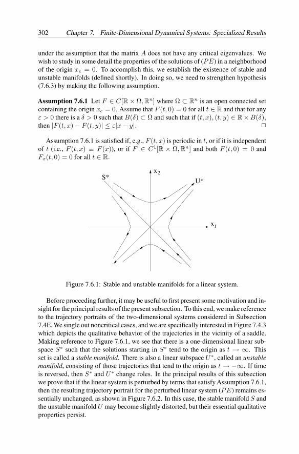
302 Chapter 7. Finite-Dimensional Dynamical Systems: Specialized Results
under the assumption that the matrix A does not have any critical eigenvalues. Wewish to study in some detail the properties of the solutions of (PE) in a neighborhoodof the origin xe = 0. To accomplish this, we establish the existence of stable andunstable manifolds (defined shortly). In doing so, we need to strengthen hypothesis(7.6.3) by making the following assumption.
Assumption 7.6.1 Let F ∈ C[R × Ω, Rn] where Ω ⊂ Rn is an open connected set
containing the origin xe = 0. Assume that F (t, 0) = 0 for all t ∈ R and that for anyε > 0 there is a δ > 0 such that B(δ) ⊂ Ω and such that if (t, x), (t, y) ∈ R × B(δ),then |F (t, x) − F (t, y)| ≤ ε|x − y|.
Assumption 7.6.1 is satisfied if, e.g., F (t, x) is periodic in t, or if it is independentof t (i.e., F (t, x) ≡ F (x)), or if F ∈ C1[R × Ω, Rn] and both F (t, 0) = 0 andFx(t, 0) = 0 for all t ∈ R.
x
x1
2S* U*
Figure 7.6.1: Stable and unstable manifolds for a linear system.
Before proceeding further, it may be useful to first present some motivation and in-sight for the principal results of the present subsection. To this end, we make referenceto the trajectory portraits of the two-dimensional systems considered in Subsection7.4E. We single out noncritical cases, and we are specifically interested in Figure 7.4.3which depicts the qualitative behavior of the trajectories in the vicinity of a saddle.Making reference to Figure 7.6.1, we see that there is a one-dimensional linear sub-space S∗ such that the solutions starting in S∗ tend to the origin as t → ∞. Thisset is called a stable manifold. There is also a linear subspace U∗, called an unstablemanifold, consisting of those trajectories that tend to the origin as t → −∞. If timeis reversed, then S∗ and U∗ change roles. In the principal results of this subsectionwe prove that if the linear system is perturbed by terms that satisfy Assumption 7.6.1,then the resulting trajectory portrait for the perturbed linear system (PE) remains es-sentially unchanged, as shown in Figure 7.6.2. In this case, the stable manifold S andthe unstable manifold U may become slightly distorted, but their essential qualitativeproperties persist.
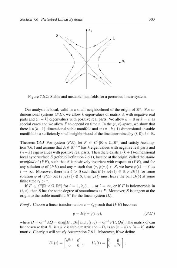
Section 7.6 Perturbed Linear Systems 303
x
x1
2
US
Figure 7.6.2: Stable and unstable manifolds for a perturbed linear system.
Our analysis is local, valid in a small neighborhood of the origin of Rn. For n-
dimensional systems (PE), we allow k eigenvalues of matrix A with negative realparts and (n − k) eigenvalues with positive real parts. We allow k = 0 or k = n asspecial cases and we allow F to depend on time t. In the (t, x)-space, we show thatthere is a (k+1)-dimensional stable manifold and an (n−k+1)-dimensional unstablemanifold in a sufficiently small neighborhood of the line determined by (t, 0), t ∈ R.
Theorem 7.6.5 For system (PE), let F ∈ C1[R × Ω, Rn] and satisfy Assump-tion 7.6.1 and assume that A ∈ R
n×n has k eigenvalues with negative real parts and(n− k) eigenvalues with positive real parts. Then there exists a (k +1)-dimensionallocal hypersurface S (refer to Definition 7.6.1), located at the origin, called the stablemanifold of (PE), such that S is positively invariant with respect to (PE), and forany solution ϕ of (PE) and any τ such that (τ, ϕ(τ)) ∈ S, we have ϕ(t) → 0 ast → ∞. Moreover, there is a δ > 0 such that if (τ, ϕ(τ)) ∈ R × B(δ) for somesolution ϕ of (PE) but (τ, ϕ(τ)) ∈ S, then ϕ(t) must leave the ball B(δ) at somefinite time t1 > τ .
If F ∈ Cl[R × Ω, Rn] for l = 1, 2, 3, . . . or l = ∞, or if F is holomorphic in(t, x), then S has the same degree of smoothness as F . Moreover, S is tangent at theorigin to the stable manifold S∗ for the linear system (L).
Proof . Choose a linear transformation x = Qy such that (PE) becomes
y = By + g(t, y), (PE′)
where B = Q−1AQ = diag[B1, B2] and g(t, y) = Q−1F (t, Qy). The matrix Q canbe chosen so that B1 is a k × k stable matrix and −B2 is an (n − k) × (n − k) stablematrix. Clearly g will satisfy Assumption 7.6.1. Moreover, if we define
U1(t) =[eB1t 00 0
], U2(t) =
[0 00 eB2t
],
304 Chapter 7. Finite-Dimensional Dynamical Systems: Specialized Results
then eBt = U1(t) + U2(t) and for some positive constants K and σ we have
|U1(t)| ≤ Ke−2σt, t ≥ 0, and |U2(t)| ≤ Keσt, t ≤ 0.
Let ϕ be a bounded solution of (PE′) with ϕ(τ) = ξ. Then by the variation ofconstants formula (see (7.8.10)), we have
ϕ(t) = eB(t−τ)ξ +∫ t
τ
eB(t−s)g(s, ϕ(s))ds
= U1(t − τ)ξ +∫ t
τ
U1(t − s)g(s, ϕ(s))ds + U2(t − τ)ξ
+∫ ∞
τ
U2(t − s)g(s, ϕ(s))ds −∫ ∞
t
U2(t − s)g(s, ϕ(s))ds.
Because U2(t − s) = U2(t)U2(−s), the bounded solution ϕ of (PE′) must satisfy
ϕ(t) = U1(t − τ)ξ +∫ t
τ
U1(t − s)g(s, ϕ(s))ds −∫ ∞
t
U2(t − s)g(s, ϕ(s))ds
+ U2(t)(
U2(−τ)ξ +∫ ∞
τ
U2(−s)g(s, ϕ(s))ds
). (7.6.13)
Conversely, any solution ϕ of (7.6.13) that is bounded and continuous on [τ, ∞) mustsolve (PE′).
In order to satisfy (7.6.13) it is sufficient to find bounded and continuous solutionsof the integral equation
ψ(t, τ, ξ) = U1(t − τ)ξ +∫ t
τ
U1(t − s)g(s, ψ(s, τ, ξ))ds
−∫ ∞
t
U2(t − s)g(s, ψ(s, τ, ξ))ds (7.6.14)
that also satisfy the condition
U2(−τ)ξ +∫ ∞
τ
U2(−s)g(s, ψ(s, τ, ξ))ds = 0. (7.6.15)
Successive approximation is used (refer, e.g., to Theorem 7.8.10) to solve (7.6.14)starting with ψ0(t, τ, ξ) ≡ 0. Choose ε > 0 such that 4εK < σ, pick δ = δ(ε) usingAssumption 7.6.1, and choose ξ with |ξ| < δ/(2K). Define
‖ψ‖ = sup
|ψ(t)| : t ≥ τ
.
If ‖ψj‖ ≤ δ, then ψj+1 must satisfy∣∣ψj+1(t, τ, ξ)∣∣ ≤ K|ξ| +
∫ t
τ
Ke−σ(t−s)ε‖ψj‖ds +∫ ∞
t
Keσ(t−s)ε‖ψj‖ds
≤ 12δ + (2εK/σ)‖ψj‖
≤ δ.
Section 7.6 Perturbed Linear Systems 305
Because ψ0 ≡ 0, then the ψj are well defined and satisfy ‖ψj‖ ≤ δ for all j. Thus
∣∣ψj+1(t, τ, ξ) − ψj(t, τ, ξ)∣∣ ≤∫ t
τ
Ke−σ(t−s)ε∥∥ψj − ψj−1
∥∥ds
+∫ ∞
t
Keσ(t−s)ε∥∥ψj − ψj−1
∥∥ds
≤ (2εK/σ)∥∥ψj − ψj−1
∥∥≤ 1
2
∥∥ψj − ψj−1∥∥.
By induction, we have ‖ψk+l+1 − ψk+l‖ ≤ 2−l‖ψk+1 − ψk‖ and∥∥ψk+j − ψk
∥∥ ≤∥∥ψk+j − ψk+j−1
∥∥+ · · · +∥∥ψk+1 − ψk
∥∥≤(2−j+1 + · · · + 2−1 + 1
) ∥∥ψk+1 − ψk
∥∥≤ 2∥∥ψk+1 − ψk
∥∥≤ 2−k+1
∥∥ψ1∥∥.
From this estimate, it follows that ψj is a Cauchy sequence uniformly in (t, τ, ξ)over τ ∈ R, t ∈ [τ, ∞), and ξ ∈ B(δ/(2K)). Thus ψj(t, τ, ξ) tends to a limitψ(t, τ, ξ) uniformly on (t, τ, ξ) on compact subsets of (τ, ξ) ∈ R × B(δ/(2K)),t ∈ [τ, ∞). The limit function ψ must be continuous in (t, τ, ξ) and it must satisfy‖ψ‖ ≤ δ.
The limit function ψ must satisfy (7.6.14). This is argued as follows. Note first that∣∣∣∣∫ ∞
t
U2(t − s)g(s, ψ(s, τ, ξ))ds −∫ ∞
t
U2(t − s)g(s, ψj(s, τ, ξ))ds
∣∣∣∣≤∫ ∞
t
Keσ(t−s)ε∣∣ψ(s, τ, ξ) − ψj(s, τ, ξ)
∣∣ds → 0, j → ∞.
A similar procedure applies to the other integral term in (7.6.14). Thus we can takethe limit as j → ∞ in the equation
ψj+1(t, τ, ξ) = U1(t − τ)ξ +∫ t
τ
U1(t − s)g(s, ψj(s, τξ))ds
−∫ ∞
t
U2(t − s)g(s, ψj(s, τ, ξ))ds
to obtain (7.6.14). Note that the solution of (7.6.14) is unique for given τ and ξ
inasmuch as a second solution ψ would have to satisfy ‖ψ − ψ‖ ≤ 0.5‖ψ − ψ‖.The stable manifold S is the set of all points (τ, ξ) such that equation (7.6.15) is
true. It will be clear that S is a local hypersurface of dimension (k+1). If ξ = 0, thenby uniqueness ψ(t, τ, 0) ≡ 0 for t ≥ τ and so g(t, ψ(t, τ, 0)) ≡ 0. Hence, (τ, 0) ∈ Sfor all τ ∈ R. To see that S is positively invariant, let (τ, ξ) ∈ S. Then ψ(t, τ, ξ) willsolve (7.6.13), and hence it will solve (PE′). For any τ1 > τ let ξ1 = ψ(τ1, τ, ξ)
306 Chapter 7. Finite-Dimensional Dynamical Systems: Specialized Results
and define ϕ(t, τ1, ξ1)= ψ(t, τ, ξ). Then ϕ(t, τ1, ξ1) solves (PE′) and hence it also
solves (7.6.13) with (τ, ξ) replaced by (τ1, ξ1). Hence∣∣∣∣U2(t)(
U2(−τ1)ξ1 +∫ ∞
τ1
U2(−s)g(s, ϕ(s, τ1, ξ1))ds
)∣∣∣∣=∣∣∣∣ϕ(t, τ1, ξ1) − U1(t − τ1)ξ1 −
∫ t
τ1
U1(t − s)g(s, ϕ(s, τ1, ξ1))ds
+∫ ∞
t
U2(t − s)g(s, ϕ(s, τ1, ξ1))ds
∣∣∣∣≤ δ + Ke−σ(t−τ1)|ξ1| +
∫ t
τ1
Ke−σ(t−s)εδds +∫ ∞
t
Keσ(t−s)εδds
≤ δ + δ + (2Kεδ/σ)≤ 3δ
< ∞. (7.6.16)
Because U2(t) = diag[0, eB2t] and −B2 is a stable matrix, this is only possible when(τ1, ξ1) ∈ S. Hence S is positively invariant.
To see that any solution starting on S tends to the origin as t → ∞, let (τ, ξ) ∈ Sand let ψj be the successive approximation defined above. Then clearly∣∣ψ1(t, τ, ξ)
∣∣ ≤ K|ξ|e−2σ(t−τ) ≤ 2K|ξ|e−σ(t−τ).
If |ψj(t, τ, ξ)| ≤ 2K|ξ|e−σ(t−τ), then
∣∣ψj+1(t, τ, ξ)∣∣ ≤ K|ξ|e−σ(t−τ) +
∫ t
τ
Ke−2σ(t−s)ε(2K|ξ|e−σ(s−τ)
)ds
+∫ ∞
t
Keσ(t−s)ε(2K|ξ|e−σ(s−τ)
)ds
≤ K|ξ|e−σ(t−τ)+ 2K|ξ|(εK/σ)e−σ(t−τ)+ 2K|ξ|(εK/2σ)e−σ(t−τ)
≤ 2K|ξ|e−σ(t−τ)
because (4εK/σ) < 1. Hence in the limit as j → ∞ we have
|ψ(t, τ, ξ)| ≤ 2K|ξ|e−σ(t−τ)
for all t ≥ τ and for all ξ ∈ B(δ/(2K)).Suppose that ϕ(t, τ, ξ) solves (PE′) but (τ, ξ) does not belong to S. If ϕ(t) stays
in the ball B(δ) (i.e., |ϕ(t, τ, ξ)| ≤ δ, for all t ≥ τ ), then (7.6.16) is true. Hence(τ, ξ) ∈ S, which is a contradiction.
Equation (7.6.15) can be rearranged as
(ξk+1, . . . , ξn
)T = P
(−∫ ∞
t
U(τ − s)g(s, ψ(s, τ, ξ))ds
), (7.6.17)
Section 7.6 Perturbed Linear Systems 307
where P denotes the projection on the last n − k components. Utilizing estimates ofthe type used above, we see that the function on the right side of (7.6.17) is Lipschitzcontinuous in ξ with Lipschitz constant L ≤ 1. Hence, successive approximationscan be used to solve (7.6.17), say(
ξk+1, . . . , ξn
)T = h(τ, ξ1, . . . , ξk) (7.6.18)
with h continuous. If F is of class C1 in (t, x), then the partial derivatives ofthe right-hand side of (7.6.17) with respect to ξ1, . . . , ξn all exist and are zero atξ1 = · · · = ξn = 0. The Jacobian with respect to (ξk+1, . . . , ξn) on the left side of(7.6.17) is one. By the implicit function theorem (see Theorem 7.6.1), the solutionof (7.6.18) is C1 smooth; indeed h is at least as smooth as F is. Inasmuch as
∂h
∂ξj= 0 for k < j ≤ n at ξ1 = · · · = ξn = 0,
then S is tangent to the hyperplane ξk+1 = · · · = ξn = 0 at ξ = 0; that is, S istangent to the stable manifold of the linear system (L) at ξ = 0.
If in (PE) we reverse time, we obtain the system
y = −Ay − F (−t, y). (7.6.19)
Applying Theorem 7.6.5 to system (7.6.19), we obtain the following result.
Theorem 7.6.6 If the hypotheses of Theorem 7.6.5 are satisfied, then there is an(n−k +1)-dimensional local hypersurface U based at the origin, called the unstablemanifold of (PE), such that U is negatively invariant with respect to (PE), and forany solution ϕ of (PE) and any τ ∈ R such that (τ, ϕ(τ)) ∈ U , we have ϕ(t) → 0as t → −∞. Moreover, there is a δ > 0 such that if (τ, ϕ(τ)) ∈ R × B(δ) but(τ, ϕ(τ)) ∈ U , then ϕ(t) must leave the ball B(δ) at some finite time t1 < τ .
The surface U has the same degree of smoothness as F and is tangent at the originto the unstable manifold U∗ of the linear system (L).
If F in (PE) is independent of time t, that is, if F (t, x) ≡ F (x), then it is notnecessary to keep track of initial time in Theorems 7.6.5 and 7.6.6. Thus, in this caseone dispenses with time and one defines S and U in the x-space, R
n. This was donein our discussion concerning Figures 7.6.1 and 7.6.2.
Example 7.6.5 Consider equations of the formx1 = ax1 − bx1x2x2 = cx2 − dx1x2
(7.6.20)
where a, b, c, d > 0 are constants, where x1 ≥ 0 and x2 ≥ 0, and where nonnegativeinitial data x1(0) = x10 and x2(0) = x20 must be specified.
Equation (7.6.20), which is an example of a Volterra competition equation, can beused to describe the growth of two competing species (e.g., of small fish) that prey on
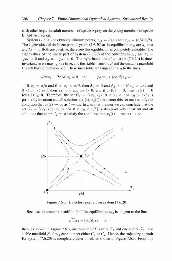
308 Chapter 7. Finite-Dimensional Dynamical Systems: Specialized Results
each other (e.g., the adult members of specie A prey on the young members of specieB, and vice versa).
System (7.6.20) has two equilibrium points, xe1 = (0, 0) and xe2 = (c/d, a/b).The eigenvalues of the linear part of system (7.6.20) at the equilibrium xe1 are λ1 = aand λ2 = c. Both are positive, therefore this equilibrium is completely unstable. Theeigenvalues of the linear part of system (7.6.20) at the equilibrium xe2 are λ1 =√
ac > 0 and λ2 = −√
ac < 0. The right-hand side of equation (7.6.20) is time-invariant, so we may ignore time, and the stable manifold S and the unstable manifoldU each have dimension one. These manifolds are tangent at xe2 to the lines
√acx1 + (bc/d)x2 = 0 and −
√acx1 + (bc/d)x2 = 0.
If x2 = a/b and 0 < x1 < c/d, then x1 = 0 and x2 > 0; if x2 > a/b and0 < x1 < c/d, then x1 < 0 and x2 > 0; and if x1(0) = 0, then x1(t) = 0for all t ≥ 0. Therefore, the set G1 = (x1, x2) : 0 < x1 < c/d, x2 > a/b ispositively invariant and all solutions (x1(t), x2(t)) that enter this set must satisfy thecondition that x2(t) → ∞ as t → ∞. In a similar manner we can conclude that theset G2 = (x1, x2) : x1 > c/d, 0 < x2 < a/b is also positively invariant and allsolutions that enter G2 must satisfy the condition that x1(t) → ∞ as t → ∞.
xx
x
1
e1
e2a/b
c/d
x2
S
S
U
U
Figure 7.6.3: Trajectory portrait for system (7.6.20).
Because the unstable manifold U of the equilibrium xe2 is tangent to the line
√acx1 + (bc/d)x2 = 0,
then, as shown in Figure 7.6.3, one branch of U enters G1 and one enters G2. Thestable manifold S of xe2 cannot meet either G1 or G2. Hence, the trajectory portraitfor system (7.6.20) is completely determined, as shown in Figure 7.6.3. From this
Section 7.6 Perturbed Linear Systems 309
portrait we can conclude that for almost all initial conditions one of the competingspecies will eventually die out and the second will grow. However, the outcome isunpredictable in the sense that near the manifold S, a slight change in initial conditionscan radically alter the outcome.
E. Stability of periodic solutions
We first consider T -periodic systems described by
x = f(t, x) (P )
where f ∈ C1[R × Ω, Rn], Ω ⊂ Rn is a domain and f(t, x) = f(t + T, x) for all
(t, x) ∈ R × Ω. Now let ϕ be a T -periodic solution of (P ) with the property thatϕ(t) ∈ Ω for all t ∈ R. Defining y = x − ϕ(t), we obtain from (P ) that
y = fx(t, ϕ(t))y + h(t, y) (7.6.21)
whereh(t, y) = f(t, y + ϕ(t)) − f(t, ϕ(t)) − fx(t, ϕ(t))y
satisfies Assumption 7.6.1. Corresponding to the perturbed linear system (7.6.21),we have the linear system
y = fx(t, ϕ(t))y. (7.6.22)
By the Floquet theory (refer to Subsection 7.8B), there is a periodic nonsingularmatrix V (t) that transforms (7.6.21), using y = V (t)z, into a system of the form
z = Az +[V (t)
]−1(h(t, V (t)z)
).
If A is noncritical, then this system satisfies all the hypotheses of Theorems 7.6.5 and7.6.6 to yield the following result.
Theorem 7.6.7 Assume that f ∈ C1[R × Ω, Rn] and let ϕ be a periodic solution of(P ) with period T . Suppose that the linear variational system (7.6.22) for ϕ(t) has kcharacteristic exponents with negative real parts and (n−k) characteristic exponentswith positive real parts. Then there exist two hypersurfaces S and U for (P ), eachcontaining (t, ϕ(t)) for all t ∈ R, where S is positively invariant and U is negativelyinvariant with respect to (P ), and where S has dimension (k+1) and U has dimension(n − k + 1) such that for any solution ψ of (P ) in a δ neighborhood of ϕ and anyτ ∈ R we have
(i) ψ(t) − ϕ(t) → 0 as t → ∞ if (τ, ψ(τ)) ∈ S;(ii) ψ(t) − ϕ(t) → 0 as t → −∞ if (τ, ψ(τ)) ∈ U ; and
(iii) ψ must leave the δ neighborhood of ϕ in finite time as t increases from τ andas t decreases from τ if (τ, ψ(τ)) is not in S and not in U .
The sets S and U are the stable and the unstable manifolds associated with ϕ. Whenk = n, then S is (n + 1)-dimensional, U consists only of the points (t, ϕ(t)) fort ∈ R, and ϕ is asymptotically stable. If k < n, then clearly ϕ is unstable.
310 Chapter 7. Finite-Dimensional Dynamical Systems: Specialized Results
Next, assume that ϕ is a T -periodic solution of an autonomous system described by
x = f(x) (A)
where f ∈ C1[Ω, Rn]. Using the transformation y = x−ϕ(t), we obtain in this casethe variational equation
y = fx(ϕ(t))y + h(t, y) (7.6.23)
where h(t, y)= f(y + ϕ(t)) − f(ϕ(t)) − fx(ϕ(t))y which satisfies Assumption
7.6.1. Corresponding to (7.6.23) we have the linear first approximation given by
y = fx(ϕ(t))y. (7.6.24)
Because ϕ(t) solves (A), ϕ(t) is a T -periodic solution of (7.6.24). Therefore equation(7.6.24) cannot possibly satisfy the hypothesis that no characteristic exponent has zeroreal part. Indeed, one Floquet multiplier is one. Thus, the hypotheses of Theorem7.6.7 can never be satisfied. Even if the remaining (n − 1) characteristic exponentsare all negative, ϕ cannot possibly be asymptotically stable. This can be seen bynoting that for small τ , ϕ(t + τ) is near ϕ(t) at t = 0, but |ϕ(t + τ) − ϕ(t)| does nottend to zero as t → ∞. However, ϕ will satisfy the following more general notionof stability.
Definition 7.6.2 A T -periodic solution ϕ of system (A) is called orbitally stable ifthere is a δ > 0 such that any solution ψ of (A) with |ψ(τ) − ϕ(τ)| < δ for some τtends to the orbit
C(ϕ(τ)) =ϕ(t) : 0 ≤ t ≤ T
as t → ∞. If in addition for each such ψ there is a constant α ∈ [0, T ) such thatψ(t) − ϕ(t + α) → 0 as t → ∞, then ψ is said to have asymptotic phase α.
We are now in a position to prove the following result.
Theorem 7.6.8 Let ϕ be a periodic solution of (A) with least period T > 0 and letf ∈ C1[Ω, Rn] where Ω ⊂ R
n is a domain. If the linear system (7.6.24) has (n − 1)characteristic exponents with negative real parts, then ϕ is orbitally stable and nearbysolutions of (A) possess an asymptotic phase.
Proof . By a change of variables of the form x = Qw + ϕ(0), where Q is assumedto be nonsingular, so that
w = Q−1f(Qw + ϕ(0)),
Q can be arranged so that w(0)=0 and w(0)=Q−1f(ϕ(0))= (1, 0, . . . , 0)T . Hence,without loss of generality, we may assume in the original problem (A) that ϕ(0) = 0
and ϕ(0) = e1= (1, 0, . . . , 0)T .
Let Φ0 be a real fundamental matrix solution of (7.6.24). There is a real nonsingularmatrix C such that Φ0(t+T ) = Φ0(t)C all t ∈ R (refer to Subsection 7.8B). Because
Section 7.6 Perturbed Linear Systems 311
ϕ(t) is a solution of (7.6.24), one eigenvalue of C is equal to one (refer to (7.8.8)).By hypothesis, all other eigenvalues of C have magnitude less than one; that is, allother characteristic exponents of (7.6.24) have negative real parts. Thus, there is areal n × n matrix R such that
R−1CR =[1 00 D0
],
where D0 is an (n − 1) × (n − 1) matrix and all eigenvalues of D0 have absolutevalue less than one.
Now define Φ1(t) = Φ0(t)R so that Φ1 is a fundamental matrix for (7.6.24) and
Φ1(t + T ) = Φ0(t + T )R = Φ0(t)CR = Φ0(t)R(R−1CR) = Φ1(t)[1 00 D0
].
The first column ϕ1(t) of Φ1(t) necessarily must satisfy the relation
ϕ1(t + T ) = ϕ1(t) for all t ∈ R;
that is, it must be T periodic. Because (n − 1) characteristic exponents of (7.6.24)have negative real parts, there cannot be two linearly independent T periodic solutionsof (7.6.24). Thus, there is a constant k = 0 such that ϕ1 = kϕ. If Φ1(t) is replaced by
Φ(t)= Φ1(t)diag
[k−1, 1, . . . , 1
],
then Φ satisfies the same conditions as Φ1 but now k = 1.There is a T periodic matrix P (t) and a constant matrix B such that
eTB =[1 00 D0
], Φ(t) = P (t)eBt.
(Both P (t) and B may be complex valued.) The matrix B can be taken in the blockdiagonal form
B =[0 00 B1
]where eB1T = D0 and B1 is a stable (n − 1) × (n − 1) matrix. Define
U1(t, s) = P (t)[1 00 0
]P−1(s)
and
U2(t, s) = P (t)[0 00 eB1(t−s)
]P−1(s)
so thatU1(t, s) + U2(t, s) = P (t)eB(t−s)P−1(s) = Φ(t)Φ−1(s).
312 Chapter 7. Finite-Dimensional Dynamical Systems: Specialized Results
Clearly U1 + U2 is real-valued. Because
P (t)[1 00 0
]= (ϕ1, 0, . . . , 0),
this matrix is real. Similarly, the first row of[1 00 0
]P−1(s)
is the first row of Φ−1(s) and the remaining rows are zero. Thus,
U1(t, s) = P (t)[1 00 0
] [1 00 0
]P−1(s)
is a real matrix. Hence,
U2(t, s) = Φ(t)Φ−1(s) − U1(t, s)
is also real.Choose constants K > 1 and σ > 0 such that |U1(t, s)| ≤ K and |U2(t, s)| ≤
Ke−2σ(t−s) for all t ≥ s ≥ 0. As in the proof of Theorem 7.6.5, we utilize an integralequation. In the present case, it assumes the form
ψ(t) = U2(t, τ)ξ+∫ t
τ
U2(t, s)h(s, ψ(s))ds−∫ ∞
t
U1(t, s)h(s, ψ(s))ds, (7.6.25)
where h is the function defined in (7.6.23). This integral equation is again solvedby successive approximations to obtain a unique, continuous solution ψ(t, τ, ξ) fort ≥ τ, τ ∈ R, and |ξ| ≤ δ and with∣∣ψ(t + τ, τ, ξ)
∣∣ ≤ 2K|ξ|e−σt.
Solutions of (7.6.25) will be solutions of (7.6.23) provided that the condition
U1(t, τ)ξ +∫ ∞
τ
U1(t, s)h(s, ψ(s, τ, ξ))ds = 0 (7.6.26)
is satisfied. Because
U1(t, s) = P (t)[1 00 0
]P−1(s),
one can write equivalently[1 00 0
](P−1(τ)ξ +
∫ ∞
τ
P−1(s)h(s, ψ(s, τ, ξ))ds
)= 0.
Because hx and ψξ exist and are continuous with hx(t, 0) = 0, then by the implicitfunction theorem (Theorem 7.6.1) one can solve for some ξj in terms of τ and the
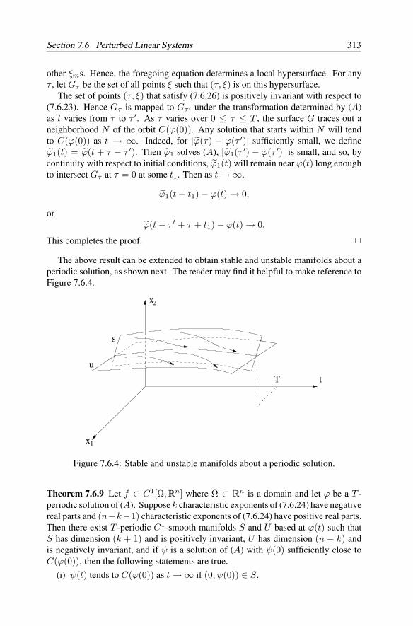
Section 7.6 Perturbed Linear Systems 313
other ξms. Hence, the foregoing equation determines a local hypersurface. For anyτ , let Gτ be the set of all points ξ such that (τ, ξ) is on this hypersurface.
The set of points (τ, ξ) that satisfy (7.6.26) is positively invariant with respect to(7.6.23). Hence Gτ is mapped to Gτ ′ under the transformation determined by (A)as t varies from τ to τ ′. As τ varies over 0 ≤ τ ≤ T , the surface G traces out aneighborhood N of the orbit C(ϕ(0)). Any solution that starts within N will tendto C(ϕ(0)) as t → ∞. Indeed, for |ϕ(τ) − ϕ(τ ′)| sufficiently small, we defineϕ1(t) = ϕ(t + τ − τ ′). Then ϕ1 solves (A), |ϕ1(τ ′) − ϕ(τ ′)| is small, and so, bycontinuity with respect to initial conditions, ϕ1(t) will remain near ϕ(t) long enoughto intersect Gτ at τ = 0 at some t1. Then as t → ∞,
ϕ1(t + t1) − ϕ(t) → 0,
orϕ(t − τ ′ + τ + t1) − ϕ(t) → 0.
This completes the proof.
The above result can be extended to obtain stable and unstable manifolds about aperiodic solution, as shown next. The reader may find it helpful to make reference toFigure 7.6.4.
t
s
u
T
x
1x
2
Figure 7.6.4: Stable and unstable manifolds about a periodic solution.
Theorem 7.6.9 Let f ∈ C1[Ω, Rn] where Ω ⊂ Rn is a domain and let ϕ be a T -
periodic solution of (A). Suppose k characteristic exponents of (7.6.24) have negativereal parts and (n−k−1) characteristic exponents of (7.6.24) have positive real parts.Then there exist T -periodic C1-smooth manifolds S and U based at ϕ(t) such thatS has dimension (k + 1) and is positively invariant, U has dimension (n − k) andis negatively invariant, and if ψ is a solution of (A) with ψ(0) sufficiently close toC(ϕ(0)), then the following statements are true.
(i) ψ(t) tends to C(ϕ(0)) as t → ∞ if (0, ψ(0)) ∈ S.
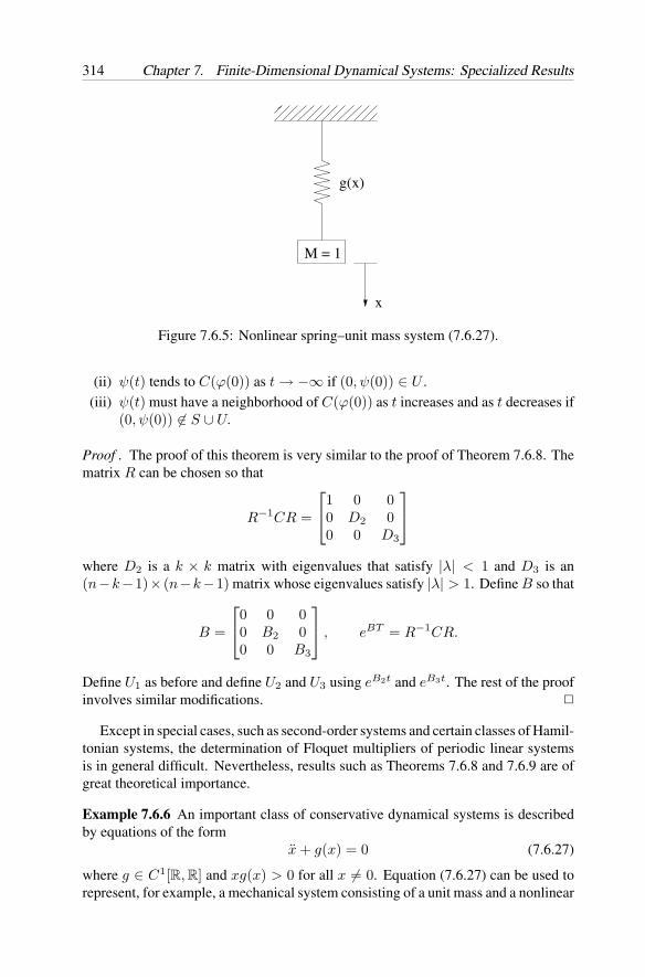
314 Chapter 7. Finite-Dimensional Dynamical Systems: Specialized Results
x
g(x)
M = 1
Figure 7.6.5: Nonlinear spring–unit mass system (7.6.27).
(ii) ψ(t) tends to C(ϕ(0)) as t → −∞ if (0, ψ(0)) ∈ U .
(iii) ψ(t) must have a neighborhood of C(ϕ(0)) as t increases and as t decreases if(0, ψ(0)) ∈ S ∪ U.
Proof . The proof of this theorem is very similar to the proof of Theorem 7.6.8. Thematrix R can be chosen so that
R−1CR =
1 0 00 D2 00 0 D3
where D2 is a k × k matrix with eigenvalues that satisfy |λ| < 1 and D3 is an(n−k−1)× (n−k−1) matrix whose eigenvalues satisfy |λ| > 1. Define B so that
B =
0 0 00 B2 00 0 B3
, eBT = R−1CR.
Define U1 as before and define U2 and U3 using eB2t and eB3t. The rest of the proofinvolves similar modifications.
Except in special cases, such as second-order systems and certain classes of Hamil-tonian systems, the determination of Floquet multipliers of periodic linear systemsis in general difficult. Nevertheless, results such as Theorems 7.6.8 and 7.6.9 are ofgreat theoretical importance.
Example 7.6.6 An important class of conservative dynamical systems is describedby equations of the form
x + g(x) = 0 (7.6.27)
where g ∈ C1[R, R] and xg(x) > 0 for all x = 0. Equation (7.6.27) can be used torepresent, for example, a mechanical system consisting of a unit mass and a nonlinear
Section 7.6 Perturbed Linear Systems 315
spring, as shown in Figure 7.6.5. Here, x denotes displacement and g(x) denotes therestoring force due to the spring.
Letting x1 = x and x2 = x, we can express (7.6.27) equivalently asx1 = x2x2 = −g(x1).
(7.6.28)
The total energy for this system is given by
v(x) =12x2
2 +∫ x1
0g(η)dη =
12x2
2 + G(x1) (7.6.29)
where G(x1) =∫ x1
0g(η)dη. Note that v is positive definite and
v′(7.6.28)(x) = 0. (7.6.30)
Therefore, (7.6.28) is a conservative dynamical system and (x1, x2)T = (0, 0)T is astable equilibrium. Note that because v′
(7.6.28) = 0, it follows that
12x2
2 + G(x1) = c (7.6.31)
where c is determined by the initial conditions (x10, x20). For different values of cwe obtain different trajectories, as shown in Figure 7.6.6. The exact shapes of thesetrajectories depend on the function G. Note, however, that the curves determinedby (7.6.31) will always be symmetric with respect to the x1-axis. Furthermore, ifG(x) → ∞ as |x| → ∞ then the entire x1– x2 plane can be covered by closedtrajectories, each of which is an invariant set with respect to (7.6.28).
x 1
x2
Figure 7.6.6: Trajectory portrait for system (7.6.27).
Now notice that no two periodic solutions of system (7.6.28) will approach eachother or recede from each other. From this we see that the Floquet multipliers of agiven periodic solution ϕ of system (7.6.28) must both be one.
316 Chapter 7. Finite-Dimensional Dynamical Systems: Specialized Results
7.7 Comparison Theory
In this section we establish stability and boundedness results for ordinary differen-tial equations (E) and ordinary difference equations (D) using comparison resultsdeveloped in Section 4.3.
A. Continuous-time systems
Our object of inquiry is systems described by differential equations
x = f(t, x) (E)
where x ∈ Rn, f ∈ C[R+ × Ω, Rn], Ω ⊂ R
n is an open connected set, 0 ∈ Ω, andf(t, 0) = 0 for all t ∈ R
+. For (E), we use comparison systems given by
y = g(t, y) (C)
where y ∈ Rl, g ∈ C[R+ × B(r1), Rl] for some r1 > 0, B(r1) ⊂ (R+)l, and
g(t, 0) = 0 for all t ∈ R+.
For a vector-valued function V : B(r) × R+ → R
l, where B(r) ⊂ Ω, r > 0, weuse the notation
V (x, t) = [v1(x, t), . . . , vl(x, t)]T
andV ′
(E)(x, t) = [v′1(E)(x, t), . . . , v′
l(E)(x, t)]T .
In the results that follow, | · | denotes the Euclidean norm in Rl.
Theorem 7.7.1 Assume that there exists a function V ∈ C[B(r) × R+, (R+)l],
where B(r) ⊂ Ω ⊂ Rn, r > 0, such that |V (x, t)| is positive definite and decrescent,
and that there exists a function g ∈ C[R+ × B(r1), Rl], where B(r1) ⊂ (R+)l,r1 > 0, which is quasi-monotone nondecreasing (refer to Definition 3.8.1) and hasthe property that g(t, 0) = 0 for all t ∈ R
+, and that
V ′(E)(x, t) ≤ g(t, V (x, t))
holds componentwise for all (x, t) ∈ B(r) × R+. Then the following statements are
true.
(a) The stability, asymptotic stability, uniform stability, and uniform asymptoticstability of the equilibrium ye = 0 of (C) imply the same corresponding typesof stability of the equilibrium xe = 0 of (E).
(b) If in addition to the above assumptions,
|V (x, t)| ≥ a|x|b for (x, t) ∈ B(r) × R+,
where a > 0 and b > 0 are constants, then the exponential stability of theequilibrium ye = 0 of (C) implies the exponential stability of the equilibriumxe = 0 of (E).
Section 7.7 Comparison Theory 317
Proof . This theorem is a direct consequence of Theorem 4.3.2(b) and (c).
Theorem 7.7.2 With Ω = Rn, assume that there exists a vector Lyapunov function
V ∈ C[Rn × R+, (R+)l] such that |V (x, t)| is positive definite, decrescent, and
radially unbounded, and that there exists a quasi-monotone nondecreasing functiong ∈ C[R+ × (R+)l, Rl] such that g(t, 0) = 0 for all t ∈ R
+ and such that theinequality
V ′(E)(x, t) ≤ g(t, V (x, t))
holds componentwise for all (x, t) ∈ Rn ×R
+. Then the uniform asymptotic stabilityin the large of the equilibrium ye = 0 of (C) implies the uniform asymptotic stabilityin the large of the equilibrium xe = 0 of (E). Also, the uniform boundedness andthe uniform ultimate boundedness of the set of solutions of (C), imply the samecorresponding types of boundedness of the set of solutions of (E).
Proof . The proof is a direct consequence of Theorem 4.3.2(d) and (f).
In the special case when l = 1, g is a scalar function that automatically satisfiesthe quasi-monotone nondecreasing property. Accordingly, Theorems 7.7.1 and 7.7.2are applicable to any scalar comparison system (with l = 1).
Next, we consider comparison systems given by
y = Py + m(y, t) (LC)
where P = [pij ] ∈ Rl×l and m : B(r1) × R
+ → Rl is assumed to satisfy the
condition
lim|y|→0
|m(y, t)||y| = 0, uniformly for t ∈ R
+.
Applying Lyapunov’s First Method (i.e., Theorem 7.6.2) to (LC), we obtain the fol-lowing comparison results.
Corollary 7.7.1 Assume that there exists a function V ∈ C[B(r) × R+, (R+)l],
where B(r) ⊂ Ω ⊂ Rn, r > 0, such that |V (x, t)| is positive definite and decrescent,
and that there exist a real l× l matrix P = [pij ] and a quasi-monotone nondecreasingfunction m ∈ C[B(r1) × R
+, Rl], where B(r1) ⊂ (R+)l, r1 > 0, such that theinequality
V ′(E)(x, t) ≤ PV (x, t) + m(V (x, t), t) (7.7.1)
holds componentwise for (x, t) ∈ B(r) × R+, and that
lim|y|→0
|m(y, t)||y| = 0, uniformly for t ∈ R
+
where pij ≥ 0 for 1 ≤ i = j ≤ l. Then the following statements are true:
(a) If all eigenvalues of P have negative real parts, then the equilibrium xe = 0 of(E) is uniformly asymptotically stable.
318 Chapter 7. Finite-Dimensional Dynamical Systems: Specialized Results
(b) If in addition to (a), |V (x, t)| ≥ a|x|b for (x, t) ∈ B(r) × R+, where a > 0
and b > 0 are constants, then the equilibrium xe = 0 of (E) is exponentiallystable.
Proof . The proofs of the above results are a direct consequence of Theorems 7.6.2and 7.7.1.
In connection with Corollary 7.7.1, we find the concept of the M -matrix veryuseful. Before proceeding any further, it might be useful to recall the definition ofthe M -matrix, along with some of the properties of such matrices (see, e.g., [3]).
Definition 7.7.1 A matrix B = [bij ] ∈ Rl×l is called an M -matrix if bij ≤ 0 for all
1 ≤ i = j ≤ l and the real parts of all eigenvalues of B are positive.
In the following we enumerate several useful equivalent characterizations ofM -matrices.
(i) B is an M -matrix.
(ii) The principal minors of B are all positive.
(iii) The successive principal minors of B are all positive.
(iv) There is a vector u ∈ (R+)l such that Bu ∈ (R+)l (recall that R+ = (0,∞)).(v) There is a vector v ∈ (R+)l such that BT v ∈ (R+)l.
(vi) B is nonsingular and all elements of B−1 are nonnegative (in fact, all diagonalelements of B−1 are positive).
Clearly, the condition in part (a) of Corollary 7.7.1 is equivalent to saying that −Pis an M -matrix, and thus, the equivalent conditions for M -matrix enumerated above,apply to Corollary 7.7.1(a) as well.
Example 7.7.1 Consider the system
x = B(x, t)x (7.7.2)
where x ∈ Rn, t ∈ R
+, and B(x, t) = [bij(x, t)] ∈ C[B(r) × R+, Rn×n], where
B(r) ⊂ Rn, r > 0. Assume that
bii(x, t) ≤ aii, i = 1, . . . , n
and|bij(x, t)| ≤ aij , 1 ≤ i = j ≤ n,
for all (x, t) ∈ B(r) × R+. Assume that −A = −[aij ] ∈ R
n×n is an M -matrix.Clearly, xe = 0 is an equilibrium of (7.7.2).
Choose the vector Lyapunov function V (x) = (|x1|, . . . , |xn|)T where x =(x1, . . . , xn)T . The upper-right Dini derivative of |xi| with respect to time is given by
D+|xi| =
xi if xi > 0|xi| if xi = 0−xi if xi < 0.
Section 7.7 Comparison Theory 319
In all three cases (xi > 0, xi < 0, xi = 0) we have along the solutions of (7.7.2),
D+|xi| ≤ bii(x, t)|xi| +∑i =j
|bij(x, t)||xj |
≤ aii|xi| +∑i =j
aij |xj |
=n∑
j=1
aij |xj |.
We haveV ′
(7.7.2)(x) ≤ AV (x)
for all x ∈ B(r). Because by assumption −A is an M -matrix, it follows that alleigenvalues of A have negative real parts. Hence, all conditions of Corollary 7.7.1(b)are satisfied. Therefore, the equilibrium xe = 0 of (7.7.2) is exponentially stable.
B. Discrete-time systems
The object of inquiry is systems described by difference equations
x(k + 1) = f(k, x(k)) (D)
where k ∈ N, f : N×Ω → Ω, and Ω is an open connected subset of Rn that contains
the origin. We assume that f(k, 0) = 0 for all k ∈ N. For (D) we use comparisonsystems given by
y(k + 1) = h(k, y(k)) (DC)
where y ∈ Rl and h : N × Ω1 → (R+)l, where Ω1 is an open neighborhood of the
origin in (R+)l. We assume that h(k, 0) = 0 for all k ∈ N.Similarly as in the case of continuous-time systems, we employ vector-valued
Lyapunov functions V : Ω × N → (R+)l.
Theorem 7.7.3 Assume that there exists a function V ∈ C[Ω × N, (R+)l] such that|V (x, k)| is positive definite and decrescent on Ω×N, and that there exists a functionh : N × Ω1 → (R+)l that is monotone nondecreasing (refer to Definition 4.3.1), that
V (f(k, x), k + 1) ≤ h(k, V (x, k))
holds componentwise for all (x, k) ∈ Ω × N, and that V (x, k) ∈ Ω1 for all (x, k) ∈Ω × N. Then the following statements are true.
(a) The stability, asymptotic stability, uniform stability, and uniform asymptoticstability of the equilibrium ye = 0 of system (DC) imply the same corre-sponding types of stability of the equilibrium xe = 0 of system (D).
(b) If in addition to the above assumptions, |V (x, k)| ≥ a|x|b for (x, k) ∈ Ω × N,where a > 0 and b > 0 are constants, then the exponential stability of theequilibrium ye = 0 of (DC) implies the exponential stability of the equilibriumxe = 0 of (D).
320 Chapter 7. Finite-Dimensional Dynamical Systems: Specialized Results
(c) Let Ω = Rn. If |V (x, k)| is radially unbounded and decresent, then the uni-
form asymptotic stability in the large of ye = 0 of (DC) implies the uniformasymptotic stability in the large of xe = 0 of (D). Furthermore, the uniformboundedness and the uniform ultimate boundedness of the set of solutions of(DC) imply the same corresponding types of boundedness of the set of solutionsof (D).
(d) In the case Ω = Rn, if a1|x|b ≤ |V (x, k)| ≤ a2|x|b for all (x, k) ∈ R
n × N,where a2 > a1 > 0 and b > 0 are constants, then the exponential stability inthe large of the equilibrium ye = 0 of (DC) implies the exponential stabilityin the large of the equilibrium xe = 0 of (D).
The proofs of the above results can be accomplished by following similar steps tothe corresponding proofs for continuous-time systems given in Theorems 7.7.1 and7.7.2, and are left to the reader as an exercise.
By applying the First Method of Lyapunov (Theorem 7.6.4) to Theorem 7.7.3, wecan readily establish the following results.
Corollary 7.7.2 Assume for (D) that there exists a function V ∈ C[Ω × N, (R+)l]such that |V (x, k)| is positive definite and decrescent on Ω × N, and that there exista real l × l matrix P = [pij ] ∈ (R+)l×l, and a monotone nondecreasing functionm ∈ C[B(r1)×N, (R+)l], where B(r1) ⊂ (R+)l, r1 > 0, such that V (x, k) ∈B(r1)for all (x, k) ∈ Ω × N and such that the inequality
V (f(k, x), k) ≤ PV (x, k) + m(V (x, k), k) (7.7.3)
holds componentwise for all (x, k) ∈ Ω × N, and that
lim|y|→0
|m(y, k)||y| = 0, uniformly for k ∈ N.
Under the above assumptions, the following statements are true.
(a) If all eigenvalues of P are within the unit circle of the complex plane, then theequilibrium xe = 0 of (D) is uniformly asymptotically stable.
(b) If in addition to (a), |V (x, k)| ≥ a|x|b for all (x, k) ∈ Ω × N, where a > 0and b > 0 are constants, then the equilibrium xe = 0 of (D) is exponentiallystable.
7.8 Appendix: Background Material on DifferentialEquations and Difference Equations
In this section we address some background material concerning linear homogeneoussystems of ordinary differential equations and ordinary difference equations, linearnonhomogeneous systems of ordinary differential equations, and successive approx-imations of the solutions of ordinary differential equations. Because this material is
Section 7.8 Appendix: Background Material 321
standard fare in ordinary differential equations and linear systems, we do not includeproofs for the presented results. However, we point to sources where these proofscan be found.
A. Linear homogeneous systems of differential equations
We consider linear homogeneous systems
x = A(t)x (LH)
where t ∈ J = (a, b), x ∈ Rn, and A ∈ C[J, Rn×n] (J = (−∞,∞) is allowed).
We letΩ =
(t, x) : t ∈ J and x ∈ R
n
and we recall (see Chapter 2) that for every (t0, x0) ∈ Ω, (LH) possesses a unique
solution ϕ(t, t0, x0)= ϕ(t) that exists over the entire interval J .
Theorem 7.8.1 The set of all solutions of (LH) on the interval J forms an n-dimensional vector space.
For a proof of Theorem 7.8.1, refer, for example, to [17, p. 89]. This result enablesus to introduce the concept of fundamental matrix.
Definition 7.8.1 A set of n linearly independent solutions of system (LH) on J ,ϕ1, . . . , ϕn is called a fundamental set of solutions of (LH) and the n × n matrixΦ = [ϕ1 · · · ϕn] is called a fundamental matrix of (LH).
Note that there are infinitely many different fundamental matrices for (LH). Inthe following result we let X = [xij ] denote an n × n matrix and we let X = [xij ].If A(t) is the matrix given in (LH), then we call the system of n2 equations,
X = A(t)X (7.8.1)
a matrix differential equation for (LH).
Theorem 7.8.2 A fundamental matrix Φ of (LH) satisfies the matrix equation (7.8.1)on the interval J .
The proof of Theorem 7.8.2 follows trivially from definitions. The next result,called Abel’s formula, is used in the proofs of several of the subsequent results of thissection.
Theorem 7.8.3 If Φ is a solution of the matrix equation (7.8.1) on an interval J andif τ is any point of J , then
det Φ(t) = det Φ(τ)exp
[∫ t
τ
trA(s)ds
]for every t.
322 Chapter 7. Finite-Dimensional Dynamical Systems: Specialized Results
For a proof of Theorem 7.8.3, refer to [17, pp. 91, 92]. It follows from Theorem7.8.3, because τ ∈ J is arbitrary, that either det Φ(t) = 0 for each t ∈ J or thatdet Φ(t) = 0 for every t ∈ J .
Theorem 7.8.4 A solution Φ of the matrix equation (7.8.1) is a fundamental matrixof (LH) if and only if its determinant is nonzero for all t ∈ J.
For a proof of Theorem 7.8.4, refer to [17, p. 93]. The next result is also requiredin the development of some of the subsequent results.
Theorem 7.8.5 If Φ is a fundamental matrix of (LH) and if C is any nonsingularconstant n × n matrix, then ΦC is also a fundamental matrix of (LH). Moreover,if Ψ is any other fundamental matrix of (LH), then there exists a constant n × nnonsingular matrix P such that Ψ = ΦP .
For a proof of Theorem 7.8.5, refer, for example, to [17, pp. 94, 95].In what follows, we make use of the natural basis for R
n, e1, . . . , en wheree1 = (1, 0, . . . , 0)T , e2 = (0, 1, 0, . . . , 0)T , . . . , en = (0, . . . , 0, 1)T .
Definition 7.8.2 A fundamental matrix Φ of (LH) whose columns are determinedby the linearly independent solutions ϕ1, . . . , ϕn with
ϕ1(τ) = e1, . . . , ϕn(τ) = en, τ ∈ J,
is called the state transition matrix Φ for (LH). Equivalently, if Ψ is any fundamentalmatrix of (LH), then the matrix Φ determined by
Φ(t, τ)= Ψ(t)Ψ(τ)−1 for all t, τ ∈ J
is said to be the state transition matrix of (LH).
Note that the state transition matrix of (LH) is uniquely determined by the matrixA(t) and is independent of the particular choice of the fundamental matrix. For exam-ple, let Ψ1 and Ψ2 be two different fundamental matrices for (LH). By Theorem 7.8.5,there exists a constant n × n nonsingular matrix P such that Ψ2 = Ψ1P . By thedefinition of the state transition matrix, we have
Φ(t, τ) = Ψ2(t)[Ψ2(τ)]−1 = Ψ1(t)PP−1[Ψ1(τ)]−1 = Ψ1(t)[Ψ1(τ)]−1.
This shows that Φ(t, τ) is independent of the fundamental matrix chosen.In the next result, we summarize the principal properties of the state transition
matrix for (LH).
Theorem 7.8.6 Let τ ∈ J , let ϕ(τ) = ξ, and let Φ(t, τ) denote the state transitionmatrix for (LH) for all t ∈ J . Then
(i) Φ(t, τ) is the unique solution of the matrix equation
∂
∂tΦ(t, τ)
= Φ(t, τ) = A(t)Φ(t, τ)
with Φ(τ, τ) = I , the n × n identity matrix;
Section 7.8 Appendix: Background Material 323
(ii) Φ(t, τ) is nonsingular for all t ∈ J ;
(iii) for any t, σ, τ ∈ J , we have Φ(t, τ) = Φ(t, σ)Φ(σ, τ);
(iv) [Φ(t, τ)]−1 = Φ−1(t, τ) = Φ(τ, t) for all t, τ ∈ J ; and
(v) the unique solution ϕ(t, τ, ξ) of (LH), with ϕ(τ, τ, ξ) = ξ specified, is given by
ϕ(t, τ, ξ) = Φ(t, τ)ξ for all t ∈ J. (7.8.2)
For a proof of Theorem 7.8.6, refer, for example, to [17, pp. 96 and 97].
B. Linear systems with periodic coefficients
In this subsection we consider linear homogeneous systems
x = A(t)x, −∞ < t < ∞, (LP )
where A ∈ C[R, Rn×n] and where
A(t) = A(t + T ) (7.8.3)
for some T > 0. System (LP ) is called a linear periodic system and T is called aperiod of A(t).
Theorem 7.8.7 Let B be a nonsingular n × n matrix. Then there exists an n × nmatrix C, called the logarithm of B, such that
eC = B. (7.8.4)
For a proof of Theorem 7.8.7, refer to [17, pp. 112 and 113]. The matrix C in theabove result is not unique, because, for example, eC+2πkiI = eCe2πki = eC for allintegers k.
Theorem 7.8.8 Let (7.8.3) be true and let A ∈ C[R, Rn×n]. If Φ(t) is a fundamentalmatrix for (LP ), then so is Φ(t + T ), t ∈ R. Moreover, corresponding to every Φ,there exist a nonsingular matrix P that is also periodic with period T and a constantmatrix R such that
Φ(t) = P (t)etR. (7.8.5)
For a proof of Theorem 7.8.8, refer to [17, pp. 113 and 114].Now let us suppose that Φ(t) is known only over the interval [t0, t0 +T ]. Because
Φ(t + T ) = Φ(t)C, we have by setting t = t0, C = Φ(t0)−1Φ(t0 + T ) andR is given by T−1logC. P (t) = Φ(t)e−tR is now determined over [t0, t0 + T ].However, P (t) is periodic over (−∞,∞). Therefore, Φ(t) is given over (−∞,∞)
324 Chapter 7. Finite-Dimensional Dynamical Systems: Specialized Results
by Φ(t) = P (t)etR. In other words, Theorem 7.8.8 allows us to conclude that thedetermination of a fundamental matrix Φ for (LP ) over any interval of length T ,leads at once to the determination of Φ over (−∞,∞).
Next, let Φ1 be any other fundamental matrix for (LP ) with A(t+T ) = A(t). ThenΦ = Φ1S for some constant nonsingular matrix S. Because Φ(t + T ) = Φ(t)eTR,we have Φ1(t + T )S = Φ1(t)SetR, or
Φ1(t + T ) = Φ1(t)(SeTRS−1) = Φ1(t)eT (SRS−1). (7.8.6)
Therefore, every fundamental matrix Φ1 determines a matrix SeTRS−1 which issimilar to the matrix eTR.
Conversely, let S be any constant nonsingular matrix. Then there exists a fun-damental matrix of (LP ) such that (7.8.6) holds. Thus, although Φ does not deter-mine R uniquely, the set of all fundamental matrices of (LP ), and hence of A(t),determines uniquely all quantities associated with eTR that are invariant under asimilarity transformation. Specifically, the set of all fundamental matrices of A(t)determines a unique set of eigenvalues of the matrix eTR, λ1, . . . , λn, which arecalled the Floquet multipliers associated with A(t). None of these vanishes becauseΠλi = det eTR = 0. Also, the eigenvalues of R are called the characteristic expo-nents.
Next, we let Q be a constant nonsingular matrix such that J = Q−1RQ where Jis the Jordan canonical form of R; that is,
J =
J0 0 · · · 00 J1 · · · 0...
.... . .
...0 0 · · · Js
.
Let Φ1 = ΦQ and P1 = PQ. From Theorem 7.8.8 we have
Φ1(t) = P1(t)etJ and P1(t + T ) = P1(t). (7.8.7)
Let the eigenvalues of R be ρ1, . . . , ρn. Then
etJ =
etJ0 0 · · · 00 etJ1 · · · 0...
.... . .
...0 0 · · · etJs
where
etJ0 =
etρ1 0 · · · 00 etρ2 · · · 0...
.... . .
...0 0 · · · etρq
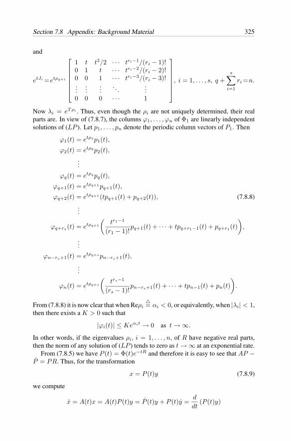
Section 7.8 Appendix: Background Material 325
and
etJi =etρq+i
1 t t2/2 · · · tri−1/(ri − 1)!0 1 t · · · tri−2/(ri − 2)!0 0 1 · · · tri−3/(ri − 3)!...
......
. . ....
0 0 0 · · · 1
, i = 1, . . . , s, q +s∑
i=1
ri =n.
Now λi = eTρi . Thus, even though the ρi are not uniquely determined, their realparts are. In view of (7.8.7), the columns ϕ1, . . . , ϕn of Φ1 are linearly independentsolutions of (LP ). Let p1, . . . , pn denote the periodic column vectors of P1. Then
ϕ1(t) = etρ1p1(t),
ϕ2(t) = etρ2p2(t),...
ϕq(t) = etρqpq(t),
ϕq+1(t) = etρq+1pq+1(t),
ϕq+2(t) = etρq+1(tpq+1(t) + pq+2(t)), (7.8.8)
...
ϕq+r1(t) = etρq+1
(tr1−1
(r1 − 1)!pq+1(t) + · · · + tpq+r1−1(t) + pq+r1(t)
),
...
ϕn−rs+1(t) = etρq+spn−rs+1(t),...
ϕn(t) = etρq+s
(trs−1
(rs − 1)!pn−rs+1(t) + · · · + tpn−1(t) + pn(t)
).
From (7.8.8) it is now clear that when Reρi= αi < 0, or equivalently, when |λi| < 1,
then there exists a K > 0 such that
|ϕi(t)| ≤ Keαit → 0 as t → ∞.
In other words, if the eigenvalues ρi, i = 1, . . . , n, of R have negative real parts,then the norm of any solution of (LP ) tends to zero as t → ∞ at an exponential rate.
From (7.8.5) we have P (t) = Φ(t)e−tR and therefore it is easy to see that AP −P = PR. Thus, for the transformation
x = P (t)y (7.8.9)
we compute
x = A(t)x = A(t)P (t)y = P (t)y + P (t)y =d
dt(P (t)y)
326 Chapter 7. Finite-Dimensional Dynamical Systems: Specialized Results
ory = P−1(t)(A(t)P (t) − P (t))y = P−1(t)(P (t)R)y = Ry.
This shows that the transformation (7.8.9) reduces the linear, homogeneous, periodicsystem (LP ) to
y = Ry,
a linear homogeneous system with constant coefficients.
C. Linear nonhomogeneous systems of differential equations
We consider linear nonhomogeneous systems of differential equations given by
x = A(t)x + g(t) (LN)
where g ∈ C[J, Rn] and all other symbols are as defined in (LH).
Theorem 7.8.9 Let τ ∈ J , let (τ, ξ) ∈ J × Rn, and let Φ(t, τ) denote the state
transition matrix for (LH) for all t ∈ J . Then the unique solution ϕ(t, τ, ξ) of (LN )satisfying ϕ(τ, τ, ξ) = ξ is given by the variation of constants formula
ϕ(t, τ, ξ) = Φ(t, τ)ξ +∫ t
τ
Φ(t, η)g(η)dη. (7.8.10)
For a proof of Theorem 7.8.9, refer, for example, to [17, p. 99].
D. Linear homogeneous systems of difference equations
We consider systems of linear homogeneous difference equations
x(k + 1) = A(k)x(k), x(k0) = x0, k ≥ k0 ≥ 0 (LHD)
where A : N → Rn×n, x(k) ∈ R
n, and k, k0 ∈ N. We denote the solutions of (LHD)by ϕ(k, k0, x0) with ϕ(k0, k0, x0) = x0.
For system (LHD), several results that are analogous to corresponding resultsgiven in Subsection 7.8A for system (LH), are still true. Thus, the set of the solutionsof system (LHD) over some subset J of N (say, J = k0, k0 + 1, . . . , k0 + nJ)forms an n-dimensional vector space. To prove this, we note that the linear combi-nation of solutions of system (LHD) is also a solution of system (LHD), and hence,this set of solutions forms a vector space. The dimension of this vector space is n.To show this, we choose a set of linearly independent vector x1
0, . . . , xn0 in the n-
dimensional x-space and we show that the set of solutions ϕ(k, k0, xi0), i = 1, . . . , n,
is linearly independent and spans the set of the solutions of (LHD) over the set J .If in particular, we choose ϕ(k, k0, e
i), i = 1, . . . , n, where ei, i = 1, . . . , ndenotes the natural basis for R
n, and if we let
Φ(k, k0) = [ϕ(k, k0, e1), . . . , ϕ(k, k0, e
n)],
Section 7.8 Appendix: Background Material 327
then it is easily verified that the n × n matrix Φ(k, k0) satisfies the matrix equation
Φ(k + 1, k0) = A(k)Φ(k, k0), Φ(k0, k0) = I,
where I denotes the n × n identity matrix. Furthermore,
Φ(k, k0) =k−1∏j=k0
A(j)
and
ϕ(k, k0, x0) = Φ(k, k0)x0, k > k0.
Other important properties that carry over from system (LH) include, for example,the semigroup property,
Φ(k, l) = Φ(k, m)Φ(m, l), k ≥ m ≥ l.
However, whereas in the case of system (LH) it is possible to reverse time, this isin general not valid for system (LHD). For example, in the case of system (LH),if ϕ(t) = Φ(t, τ)ϕ(τ), then we can compute ϕ(τ) = Φ−1(t, τ)ϕ(t) = Φ(τ, t)ϕ(t).For (LHD), this does not apply, unless A−1(k) exists for all k ∈ N.
E. Successive approximations of solutions of initial value problems
We consider initial value problems given by
x = f(t, x), x(τ) = ξ (I)
where f ∈ C[D, Rn], D = J × Ω (where J = (a, b) ⊂ R is an interval and Ω ⊂ Rn
is a domain), τ ∈ J , and x(τ) ∈ Ω. For (I) we define the successive approximationsϕ0(t) = ξ
ϕj+1 = ξ +∫ t
τ
f(s, ϕj(s))ds, j = 0, 1, 2, . . .(7.8.11)
for |t − τ | ≤ c for some c > 0.
Theorem 7.8.10 If f ∈ C[D, Rn], if f is Lipschitz continuous on a compact setS ⊂ D with Lipschitz constant L, and if S contains a neighborhood of (τ, ξ), thenthe successive approximations ϕj , j = 0, 1, 2, . . . given in (7.8.11) exist on |t−τ | ≤ cfor some c > 0, are continuous there, and converge uniformly to the unique solutionϕ(t, τ, ξ) of (I) as j → ∞.
For a proof of Theorem 7.8.10, refer, for example, to [17, pp. 56–58].
328 Chapter 7. Finite-Dimensional Dynamical Systems: Specialized Results
7.9 Notes and References
There are many excellent texts on the stability of finite dimensional dynamical systemsdetermined by ordinary differential equations that treat the topics addressed in thischapter, including Hahn [5], Hale [6], Krasovskii [8], LaSalle and Lefschetz [12],Yoshizawa [20], and Zubov [21]. Texts on these topics that emphasize engineeringapplications include Khalil [7] and Vidyasagar [19]. Our presentation in this chapterwas greatly influenced by Antsaklis and Michel [1], Hahn [5], Michel et al. [16], andMiller and Michel [17].
There are fewer sources dealing with the stability analysis of discrete-time systemsdescribed by difference equations. In our presentation in this chapter, we found thetexts by LaSalle [11], Antsaklis and Michel [1], Hahn [5], and Michel et al. [16]especially useful.
The results in Subsection 7.2A, along with other results that comprise the in-variance theory for systems described by ordinary differential equations are due toBarbashin and Krasovskii [2] and LaSalle [10]. Extensions of these results to othertypes of dynamical system (e.g., systems described by difference equations, as inSubsection 7.2B) have been reported, for example, in Michel et al. [16].
The necessary and sufficient conditions for the various Lyapunov stability typespresented in Subsection 7.4C involving the Lyapunov matrix equation were originallyestablished by Lyapunov [13] for ordinary differential equations. Our presentation inSubsection 7.5C of the analogous results for systems described by difference equationsare in the spirit of similar results given in LaSalle [11].
The results in Subsections 7.6B and 7.6C comprise the First Method of Lyapunov(also called the Indirect Method of Lyapunov). For the case of ordinary differentialequations (Subsection 7.6B) these results were originally established by Lyapunov [13].The results that we present in Subsection 7.6C for systems described by differenceequations are along similar lines as the results given in Antsaklis and Michel [1].
The stability results for autonomous systems (A), periodic systems (P ), linearhomogeneous systems (LH), linear autonomous systems (L), linear periodic sys-tems (LP ), and linear second-order differential equations with constant coefficients(Section 7.1, Subsections 7.4A, 7.4B, 7.4D, and 7.4E, resp.) are standard fare in textson stability of systems described by ordinary differential equations (e.g., [5]–[8], [12],[16], [17], [19]–[21]). Sources for the analogous results for linear systems describedby difference equations (LD) and (LHD) (Subsections 7.5A and 7.5B) include, forexample, [1] and [11]. Results to estimate the domain of attraction of an equilibrium(Subsection 7.3) are also included in most texts on stability theory of differential equa-tions ([5], [7], [8], [12], [17], [19]–[21]). The results concerning stable and unstablemanifolds and stability properties of periodic solutions in perturbed linear systems(Subsections 7.6D and 7.6E) are addressed in the usual texts on ordinary differentialequations (e.g., [6], [17]). A good source on the comparison theory for differentialequations (Subsection 7.7A) includes Lakshmikantham [9] and on difference equa-tions (Subsection 7.7B), Michel et al. [16]. For applications of the comparison theoryto large-scale dynamical systems, refer to Grujic et al. [4], Michel and Miller [15],and Siljak [18].
Section 7.10 Problems 329
7.10 Problems
Problem 7.10.1 Consider the systems
x = Ax (L)
andy = P−1APy (7.10.1)
where A, P ∈ Rn×n and where P is assumed to be nonsingular. Show that the
equilibrium xe = 0 of (L) is stable, exponentially stable, unstable, and completelyunstable if and only if the equilibrium ye = 0 of (7.10.1) has the same correspondingstability properties.
Problem 7.10.2 There are several variants to the results that make up the InvarianceTheory. Corollary 7.2.1 provides conditions for global asymptotic stability of theequilibrium xe = 0 of system (A). In the following we ask the reader to prove a localresult for asymptotic stability.
Corollary 7.10.1 Assume that for system (A) there exists a function v ∈ C[Ω, R]where Ω ⊂ R
n is an open connected set containing the origin. Assume that v ispositive definite. Assume that v′
(A)(x) ≤ 0 on Ω. Suppose that the origin is the onlyinvariant subset with respect to (A) of the set Z = x ∈ Ω: v′
(A)(x) = 0. Then theequilibrium xe = 0 of (A) is asymptotically stable.
Problem 7.10.3 Consider the systemx1 = x2 − ε(x1 − x3
1/3)x2 = −x1
(7.10.2)
where ε > 0. This system has an equilibrium at the origin xe = 0 ∈ R2.
First show that the equilibrium xe = 0 of system (7.10.2) is asymptotically stable,choosing
v(x1, x2) =12(x2
1 + x22)
and applying Corollary 7.10.1. Next, show that the region x ∈ R2 : x2
1 + x22 < 3
is contained in the domain of attraction of the equilibrium xe = 0 of (7.10.2).
Problem 7.10.4 Consider the linear system
x = Ax (L)
where x ∈ Rn and A ∈ R
n×n. Assume that there exists a positive definite matrix Gsuch that the matrix
B = AT G + GA
is negative semidefinite. Prove that the equilibrium xe = 0 of (L) is exponentiallystable if and only if
330 Chapter 7. Finite-Dimensional Dynamical Systems: Specialized Results
(a) the pair (B, A) is observable; that is, the n × n2 matrix
[B BA · · · BAn−1]
has full rank; or
(b) the pair (C, A − D) is observable, where C = P1B, D = P2B, P1 ∈ Rn×n
is nonsingular and P2 ∈ Rn×n is any matrix.
Hint: Apply Corollary 7.2.1, letting v(x) = xT Gx. Then v′(L)(x) = xT Bx.
Show that Z = x ∈ Rn : xT Bx = 0 = x ∈ R
n : Bx = 0, using the fact that Bis negative semidefinite. Next, show that 0 ⊂ R
n is the largest invariant set in Z.For further details, refer to Miller and Michel [16a].
Problem 7.10.5 Consider a mechanical system consisting of n rigid bodies withmasses mi, i = 1, . . . , n, that are interconnected by springs and are subjected toviscous damping, and are described by the equations
q = M−1pp = −Hq + KM−1p
(7.10.3)
where q ∈ Rn denotes the position vector, p ∈ R
n is the momentum vector, M =diag[m1, . . . , mn], K = KT ∈ R
n×n, and H = HT ∈ Rn×n. We assume that
M and H are positive definite and that K is negative semidefinite. Prove that theequilibrium (qT , pT ) = (0T , 0T ) of system (7.10.3) is exponentially stable if andonly if (K, M−1H) is observable.
Hint: Apply Problem 7.10.4(b) with
A =[
0 M−1
−H KM−1
], B =
[0 00 M−1KM−1
],
and
C = D =[
0 00 KM−1
].
For further details, consult Miller and Michel [16a].
Problem 7.10.6 In the mechanical system depicted in Figure 7.10.1, xi denotesdisplacement for mass mi, i = 1, 2, k1, k2, k denote linear spring constants, andB1, B2, B denote viscous damping coefficients. We assume that mi > 0, ki > 0,i = 1, 2, k > 0, B1 ≥ 0, B2 ≥ 0, B ≥ 0, and B1 + B2 + B > 0. This system isgoverned by the equations
m1x1 + k1x1 + k(x1 − x2) + B1x1 + B(x1 − x2) = 0m2x2 + k2x2 + k(x2 − x1) + B2x2 + B(x2 − x1) = 0.
(7.10.4)
System (7.10.4) is a special case of system (7.10.3) with
D =[
(−B1 − B) BB (−B2 − B)
], H =
[(k1 + k) −k
−k (k2 + k)
],
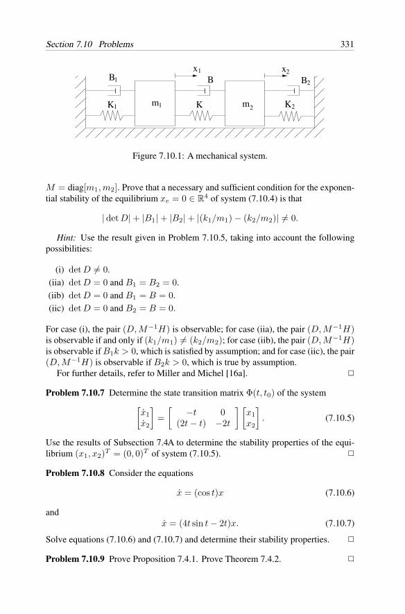
Section 7.10 Problems 331
B
K K K
x x1
1
1 m m2 2
B2
2
1
B
Figure 7.10.1: A mechanical system.
M = diag[m1, m2]. Prove that a necessary and sufficient condition for the exponen-tial stability of the equilibrium xe = 0 ∈ R
4 of system (7.10.4) is that
| det D| + |B1| + |B2| + |(k1/m1) − (k2/m2)| = 0.
Hint: Use the result given in Problem 7.10.5, taking into account the followingpossibilities:
(i) det D = 0.
(iia) det D = 0 and B1 = B2 = 0.
(iib) det D = 0 and B1 = B = 0.
(iic) det D = 0 and B2 = B = 0.
For case (i), the pair (D, M−1H) is observable; for case (iia), the pair (D, M−1H)is observable if and only if (k1/m1) = (k2/m2); for case (iib), the pair (D, M−1H)is observable if B1k > 0, which is satisfied by assumption; and for case (iic), the pair(D, M−1H) is observable if B2k > 0, which is true by assumption.
For further details, refer to Miller and Michel [16a].
Problem 7.10.7 Determine the state transition matrix Φ(t, t0) of the system[x1x2
]=[
−t 0(2t − t) −2t
] [x1x2
]. (7.10.5)
Use the results of Subsection 7.4A to determine the stability properties of the equi-librium (x1, x2)T = (0, 0)T of system (7.10.5).
Problem 7.10.8 Consider the equations
x = (cos t)x (7.10.6)
andx = (4t sin t − 2t)x. (7.10.7)
Solve equations (7.10.6) and (7.10.7) and determine their stability properties.
Problem 7.10.9 Prove Proposition 7.4.1. Prove Theorem 7.4.2.
332 Chapter 7. Finite-Dimensional Dynamical Systems: Specialized Results
Problem 7.10.10 Show that the trivial solution of an nth-order, linear autonomousdifferential equation
any(n) + an−1y(n−1) + · · · + a1y
1 + a0y = 0, an = 0 (7.10.8)
is stable if and only if all roots of
p(λ) = anλn + · · · + a1λ + a0 (7.10.9)
have nonpositive real parts and all roots with zero real parts are simple roots. (In(7.10.8), y(n) = d(n)y/dt(n).)
In the next few results, we use the following notation concerning quadratic forms.If S = ST ∈ R
n×n and R = RT ∈ Rn×n then we write R > S if xT Rx > xT Sx
for all x ∈ Rn − 0; R ≥ S if xT Rx ≥ xT Sx for all x ∈ R
n; R > 0 if xT Rx > 0for all x ∈ R
n − 0; R ≥ 0 if xT Rx ≥ 0 for all x ∈ Rn; and so forth.
Problem 7.10.11 Let A ∈ C[R+, Rn×n] and x ∈ Rn and consider the system
x = A(t)x. (LH)
Show that the equilibrium xe = 0 of (LH) is uniformly stable if there exists aQ ∈ C1[R+, Rn×n] such that Q(t) = [Q(t)]T for all t and if there exist constantsc2 ≥ c1 > 0 such that
c1I ≤ Q(t) ≤ c2I, t ∈ R (7.10.10)
and such that[A(t)]T Q(t) + Q(t)A(t) + Q ≤ 0, t ∈ R (7.10.11)
where I is the n × n identity matrix.
Problem 7.10.12 Show that the equilibrium xe = 0 of (LH) is exponentially stableif there exists a Q ∈ C1[R+, Rn×n] such that Q(t) = [Q(t)]T for all t and if thereexist constants c2 ≥ c1 > 0 and c3 > 0 such that (7.10.10) holds and such that
[A(t)]T Q(t) + Q(t)A(t) + Q(t) ≤ −c3I, t ∈ R. (7.10.12)
Problem 7.10.13 For (LH) let λm(t) and λM (t) denote the smallest and largesteigenvalues of A(t) + [A(t)]T at t ∈ R, respectively. Let ϕ(t, t0, x0) denote theunique solution of (LH) for the initial conditions x(t0) = x0 = ϕ(t0, t0, x0).
(a) Show that for any x0 ∈ Rn and any t0 ∈ R, the unique solution of (LH)
satisfies the estimate
|x0|e(1/2)∫ t
t0λm(s)ds ≤ |ϕ(t, t0, x0)| ≤ |x0|e(1/2)
∫ tt0
λM (s)ds, t ≥ t0.
(7.10.13)
Section 7.10 Problems 333
(b) Use the above result to show that the equilibrium xe = 0 of (LH) is uniformlystable if there exists a constant c such that∫ t
σ
λM (s)ds ≤ c (7.10.14)
for all t, σ such that t ≥ σ.
(c) Use the result in item (a) to show that the equilibrium xe = 0 of (LH) isexponentially stable if there exist constants ε > 0, α > 0 such that∫ t
σ
λM (s)ds ≤ −α(t − σ) + ε (7.10.15)
for all t, σ such that t ≥ σ.
Problem 7.10.14 Show that if the equilibrium xe = 0 of the system
x(k + 1) = eAx(k) (7.10.16)
is asymptotically stable, then the equilibrium xe = 0 of the system
x = Ax (L)
is also asymptotically stable. In systems (7.10.16) and (L), x ∈ Rn, A ∈ R
n×n, andk ∈ N.
Problem 7.10.15 Prove Theorem 7.5.1. Prove Theorem 7.5.2.
Problem 7.10.16 Prove Theorem 7.5.3. Prove Theorem 7.5.4.
Problem 7.10.17 Prove Theorem 7.5.5.
Problem 7.10.18 Prove Theorem 7.5.6.
Problem 7.10.19 Prove Proposition 7.5.1.
Problem 7.10.20 Prove Theorem 7.6.4.
Problem 7.10.21 Consider the system
x = f(x) (A)
where f ∈ C1[Ω, Rn] and assume that xe is an equilibrium of (A) (i.e., f(xe) = 0).Define A ∈ R
n×n by
A =∂f
∂x(xe).
Prove the following.
(a) If A is a stable matrix, then the equilibrium xe is exponentially stable.
334 Chapter 7. Finite-Dimensional Dynamical Systems: Specialized Results
(b) If A has an eigenvalue with a positive real part and no eigenvalue with zeroreal part, then the equilibrium xe is unstable.
(c) If A is critical, then xe can be either stable or unstable. (Show this by usingspecific examples.)
Problem 7.10.22 Using Problem 7.10.21, analyze the stability properties of eachequilibrium point of the following equations:
(a) x + ε(x2 − 1)x + x = 0, ε = 0.(b) x + x sin x = 0.(c) x + x + x(x2 − 4) = 0.(d) 3x(3) − 7x + 3x + ex − 1 = 0.(e) x + cx + sinx = x3, c = 0.(f) x + 2x + x = x3.
Problem 7.10.23 Ignoring the time dimension, for each equilibrium point in Prob-lems 7.10.22(a)–(d), determine the dimensions of the stable manifold and the unstablemanifold.
Problem 7.10.24 Analyze the stability properties of the trivial solution (origin) ofthe following equations
(a)
[x1x2
]=[
2 17 3
] [x1x2
]+[
(ex1 − 1) sin(x2t)e−tx1x2
].
(b)
[x1x2
]=[
arctanx1 + x2sin(x1 − x2)
].
(c)
x1x2x3
=
−3 −1 1−1 −4 01 0 −4
x1x2x3
+
x1x2x1x3
sin(x1x2x3)
.
(d)
x1 = −a0x2 − a1x3x2 = b0(ex1 − 1)x3 = −λx3 + b1(ex1 − 1)
where λ > 0, bi = 0, and ai/bi > 0, i = 0, 1.
Problem 7.10.25 In Problem 7.10.24, when possible, determine a set of basis vectorsfor the stable manifold for each associated linearized equation.
Problem 7.10.26 Let F satisfy Assumption 7.6.1, let T = 2π, and consider thesystem[
x1x2
]=[
−1 + 3(cos2 t)/2 1 − 3(sin t cos t)/2−1 − 3(sin t cos t)/2 −1 + 3(sin2 t)/2
] [x1x2
]+ F (t, x1, x2)
= P0(t)x + F (t, x). (7.10.17)
Bibliography 335
(a) Show that y(t) = (cos t, − sin t)T et/2 is a solution of
y = P0(t)y. (7.10.18)
(b) Compute the Floquet multipliers of (7.10.18).
(c) Determine the stability properties of the trivial solution of (7.10.17).
(d) Compute the eigenvalues of P0(t). Discuss the possibility of using the eigen-values of (7.10.18), rather than the Floquet multipliers, to determine the stabilityproperties of the trivial solution of (7.10.17).
Problem 7.10.27 The system described by the differential equationsx1 = x2 + x1(x2
1 + x22)
x2 = −x1 + x2(x21 + x2
2)(7.10.19)
has an equilibrium at the origin (x1, x2)T = (0, 0)T . Show that the trivial solutionof the linearization of system (7.10.19) is stable. Prove that the equilibrium xe = 0of system (7.10.19) is unstable. (This example shows that the assumptions on thematrix A in Theorems 7.6.2 and 7.6.3 are essential.)
Problem 7.10.28 Use the results of Section 7.7 (Comparison Theory) to show thatthe trivial solution of the system
x1 = −x1 − 2x22 + 2kx4
x2 = −x2 + 2x1x2x3 = −3x3 + x4 + kx1x4 = −2x4 − x3 − kx2
(7.10.20)
is uniformly asymptotically stable when |k| is small.Hint: Choose v1(x1, x2) = x2
1 + x22 and v2(x3, x4) = x2
3 + x24.
Problem 7.10.29 Prove Theorem 7.7.3.
Bibliography
[1] P. J. Antsaklis and A. N. Michel, Linear Systems, Boston: Birkhauser, 2006.
[2] E. A. Barbashin and N. N. Krasovskii, “On the stability of motion in the large,”Dokl. Akad. Nauk., vol. 86, pp. 453–456, 1952.
[3] M. Fiedler and V. Ptak, “On matrices with nonpositive off-diagonal elementsand positive principal minors,” Czechoslovak Math. J., vol. 12, pp. 382–400,1962.
[4] L. T. Grujic, A. A. Martynyuk, and M. Ribbens-Pavella, Large Scale SystemsUnder Structural and Singular Perturbations, Berlin: Springer-Verlag, 1987.
[5] W. Hahn, Stability of Motion, Berlin: Springer-Verlag, 1967.
336 Chapter 7. Finite-Dimensional Dynamical Systems: Specialized Results
[6] J. K. Hale, Ordinary Differential Equations, New York: Wiley, 1969.
[7] H. K. Khalil, Nonlinear Systems, New York: Macmillan, 1992.
[8] N. N. Krasovskii, Stability of Motion, Stanford, CA: Stanford University Press,1963.
[9] V. Lakshmikantham and S. Leela, Differential and Integral Inequalities, vol. Iand vol. II, New York: Academic Press, 1969.
[10] J. P. LaSalle, “The extent of asymptotic stability,” Proc. Nat. Acad. Sci., vol. 48,pp. 363–365, 1960.
[11] J. P. LaSalle, The Stability and Control of Discrete Processes, New York:Springer-Verlag, 1986.
[12] J. P. LaSalle and S. Lefschetz, Stability by Liapunov’s Direct Method, NewYork: Academic Press, 1961.
[13] A. M. Liapounoff, “Probleme generale de la stabilite de mouvement,” Annalesde la Faculte des Sciences de l’Universite de Toulouse, vol. 9, pp. 203–474,1907. (Translation of a paper published in Comm. Soc. Math., Kharkow, 1892,reprinted in Ann. Math. Studies, vol. 17, Princeton, NJ: Princeton, 1949.)
[14] A. N. Michel and C. J. Herget, Algebra and Analysis for Engineers and Scien-tists, Boston, Birkhauser, 2007.
[15] A. N. Michel and R. K. Miller, Qualitative Analysis of Large Scale DynamicalSystems, New York: Academic Press, 1977.
[16] A. N. Michel, K. Wang, and B. Hu, Qualitative Theory of Dynamical Systems-The Role of Stability Preserving Mappings, 2nd Edition, New York: MarcelDekker, 2001.
[16a] R. K. Miller and A. N. Michel, “Asymptotic stability of systems: Resultsinvolving the system topology,” SIAM J. Optim. Control, vol. 18, pp. 181–190, 1980.
[17] R. K. Miller and A. N. Michel, Ordinary Differential Equations, New York:Academic Press, 1982.
[18] D. D. Siljak, Large-Scale Dynamical Systems: Stability and Structure, NewYork: North Holland, 1978.
[19] M. Vidyasagar, Nonlinear Systems Analysis, Englewood Cliffs, NJ: PrenticeHall, 1993.
[20] T. Yoshizawa, Stability Theory by Liapunov’s Second Method, Tokyo: Math.Soc. of Japan, 1966.
[21] V. I. Zubov, Methods of A. M. Lyapunov and Their Applications, Amsterdam:Noordhoff, 1964.
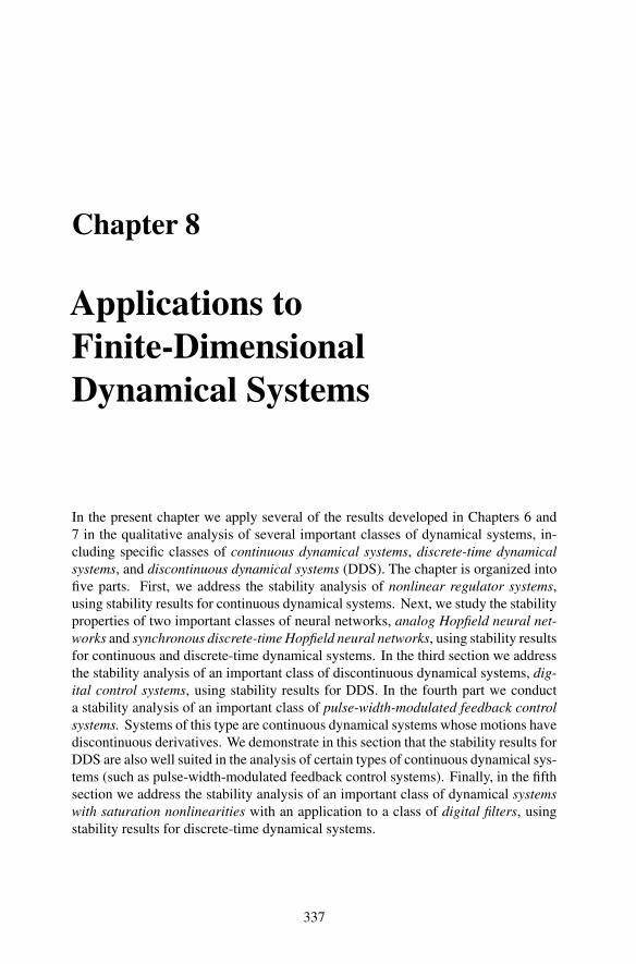
Chapter 8
Applications toFinite-DimensionalDynamical Systems
In the present chapter we apply several of the results developed in Chapters 6 and7 in the qualitative analysis of several important classes of dynamical systems, in-cluding specific classes of continuous dynamical systems, discrete-time dynamicalsystems, and discontinuous dynamical systems (DDS). The chapter is organized intofive parts. First, we address the stability analysis of nonlinear regulator systems,using stability results for continuous dynamical systems. Next, we study the stabilityproperties of two important classes of neural networks, analog Hopfield neural net-works and synchronous discrete-time Hopfield neural networks, using stability resultsfor continuous and discrete-time dynamical systems. In the third section we addressthe stability analysis of an important class of discontinuous dynamical systems, dig-ital control systems, using stability results for DDS. In the fourth part we conducta stability analysis of an important class of pulse-width-modulated feedback controlsystems. Systems of this type are continuous dynamical systems whose motions havediscontinuous derivatives. We demonstrate in this section that the stability results forDDS are also well suited in the analysis of certain types of continuous dynamical sys-tems (such as pulse-width-modulated feedback control systems). Finally, in the fifthsection we address the stability analysis of an important class of dynamical systemswith saturation nonlinearities with an application to a class of digital filters, usingstability results for discrete-time dynamical systems.
337
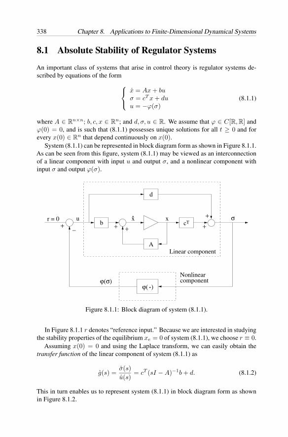
338 Chapter 8. Applications to Finite-Dimensional Dynamical Systems
8.1 Absolute Stability of Regulator Systems
An important class of systems that arise in control theory is regulator systems de-scribed by equations of the form
x = Ax + buσ = cT x + duu = −ϕ(σ)
(8.1.1)
where A ∈ Rn×n; b, c, x ∈ R
n; and d, σ, u ∈ R. We assume that ϕ ∈ C[R, R] andϕ(0) = 0, and is such that (8.1.1) possesses unique solutions for all t ≥ 0 and forevery x(0) ∈ R
n that depend continuously on x(0).System (8.1.1) can be represented in block diagram form as shown in Figure 8.1.1.
As can be seen from this figure, system (8.1.1) may be viewed as an interconnectionof a linear component with input u and output σ, and a nonlinear component withinput σ and output ϕ(σ).
Linear component
ϕ( )
r = 0
d
A
c+− + +
σb
.
Tu x x.
ϕ(σ)
+
+
componentNonlinear
Figure 8.1.1: Block diagram of system (8.1.1).
In Figure 8.1.1 r denotes “reference input.” Because we are interested in studyingthe stability properties of the equilibrium xe = 0 of system (8.1.1), we choose r ≡ 0.
Assuming x(0) = 0 and using the Laplace transform, we can easily obtain thetransfer function of the linear component of system (8.1.1) as
g(s) =σ(s)u(s)
= cT (sI − A)−1b + d. (8.1.2)
This in turn enables us to represent system (8.1.1) in block diagram form as shownin Figure 8.1.2.
Section 8.1 Absolute Stability of Regulator Systems 339
r = 0 + u
ϕ(σ)
σ
−g(s) = c (sI − A) b + d^ T
ϕ( ).
−1
Figure 8.1.2: Block diagram of system (8.1.1).
In addition to the preceding assumptions concerning the nonlinearity ϕ(·), weassume, for example, that
k1σ2 ≤ σϕ(σ) ≤ k2σ
2 (8.1.3)
where k1, k2 are real constants. In this case we say that ϕ belongs to the sector[k1, k2]. Similarly, if we require that k1σ
2 < σϕ(σ) < k2σ2, we say that ϕ belongs
to the sector (k1, k2). Other sectors, such as (k1, k2] and [k1, k2) are defined similarly.Also, when σϕ(σ) ≥ 0 for all σ ∈ R, we say that ϕ belongs to the sector [0,∞).
Now let d = 0 and replace ϕ(σ) by kσ, where k1 ≤ k ≤ k2. Then system (8.1.1)reduces to the linear system
x = (A − kbcT )x. (8.1.4)
In 1949, Aizerman conjectured that if d = 0, if ϕ belongs to the sector [k1, k2],and if for each k ∈ [k1, k2] the matrix (A − kbcT ) is a Hurwitz matrix, so thatsystem (8.1.4) is exponentially stable in the large, then the equilibrium xe = 0 ofthe nonlinear system (8.1.1) is uniformly asymptotically stable in the large. It turnsout that this conjecture, called Aizerman’s conjecture, is false. Nevertheless, it is stilluseful, because it serves as a benchmark in assessing how conservative some of thesubsequent results are in particular applications.
In the present section we address the following problem: find conditions onA, b, c, d that ensure the equilibrium xe = 0 of system (8.1.1) is uniformly asymp-totically stable in the large for any nonlinearity ϕ belonging to some specified sector.A system (8.1.1) satisfying this property is said to be absolutely stable.
In the present section we address the absolute stability problem of regulator systemsusing two different methods: Lure’s criterion and the Popov criterion.
A. Lure’s resultIn the following result, we assume that d = 0, that A is a Hurwitz matrix, and that ϕbelongs to the sector [0,∞). We use a Lyapunov function of the form
v(x) = xT Px + β
∫ σ
0ϕ(ξ)dξ, (8.1.5)
where P = PT ∈ Rn×n is positive definite and β ≥ 0. We require that P is a
solution of the Lyapunov matrix equation
AT P + PA = −C (8.1.6)
where C = CT is a positive definite matrix of our choice.
340 Chapter 8. Applications to Finite-Dimensional Dynamical Systems
Theorem 8.1.1 (Lure) For system (8.1.1) assume that d = 0, that all eigenvalues ofA have negative real parts (i.e., A is Hurwitz), and that there exist positive definitematrices P and C that satisfy (8.1.6). Also, assume that
βcT b − wT C−1w > 0 (8.1.7)
where
w = Pb − 12βAT c (8.1.8)
and β ≥ 0 is some constant (see (8.1.5)).Then the equilibrium xe = 0 of system (8.1.1) is asymptotically stable in the large
for any ϕ satisfying σφ(σ) ≥ 0 for all σ ∈ R.
Proof . We choose as a Lyapunov function (8.1.5) which is continuous, positive def-inite, and radially unbounded (because P is positive definite and because σϕ(σ) ≥ 0for all σ ∈ R implies that
∫ σ
0 ϕ(s)ds ≥ 0 for all σ ∈ R). Along the solutions of(8.1.1) we have
v′(8.1.1)(x) = xT P (Ax − bϕ(σ)) + (xT AT − bT ϕ(σ))Px + βϕ(σ)σ
= xT (PA + AT P )x − 2xT Pbϕ(σ) + βϕ(σ)cT (Ax − bϕ(σ))
= −xT Cx − 2xT Pbϕ(σ) + βxT AT cϕ(σ) − β(cT b)ϕ(σ)2
= −xT Cx − 2ϕ(σ)xT w − β(cT b)ϕ(σ)2
= −(x+C−1wϕ(σ))T C(x+C−1wϕ(σ))−(βcT b−wT C−1w)ϕ(σ)2.
Invoking (8.1.7) and the positive definiteness of C, it follows that v′(8.1.1)(x) is neg-
ative definite for all x ∈ Rn. Indeed, if v′
(8.1.1)(x) = 0, then ϕ(σ) = 0 and
x + C−1wϕ(σ) = x + C−1w · 0 = x = 0.
It now follows from Theorem 6.2.3 that the equilibrium xe = 0 of system (8.1.1) isasymptotically stable in the large for any ϕ satisfying σϕ(σ) ≥ 0 for all σ ∈ R.
B. The Popov criterion
System (8.1.1) which we considered in the preceding subsection is referred to inthe literature as a direct control system. We now consider indirect control systemsdescribed by equations of the form
x = Ax − bϕ(σ)σ = cT x + dξ
ξ = −ϕ(σ)(8.1.9)
where x, b, c ∈ Rn, σ, ξ, d ∈ R, and A ∈ R
n×n is assumed to be Hurwitz (i.e., allthe eigenvalues of A have negative real parts). We assume that d = 0, for otherwise,(8.1.9) reduces to (8.1.1).
Section 8.1 Absolute Stability of Regulator Systems 341
System (8.1.9) can be rewritten as
[x
ξ
]=[A 00 0
] [xξ
]+[b1
]η,
σ =[cT d
] [xξ
],
η = −ϕ(σ).
(8.1.10)
Equation (8.1.10) is clearly of the same form as equation (8.1.1). However, in thepresent case, the matrix of the linear system component is given by
A =[A 00 0
]and satisfies the assumption that one eigenvalue is equal to zero because all theeigenvalues of A have negative real parts. We note that Theorem 8.1.1 (for the directcontrol problem) is not applicable to the indirect control problem (8.1.9).
In the following, we present the Popov stability criterion for system (8.1.9),assuming that ϕ belongs to the sector (0, k], so that
0 < σϕ(σ) ≤ kσ2 (8.1.11)
for all σ ∈ R, σ = 0. In establishing his result, Popov relied heavily on results fromfunctional analysis. Presently, we make use of the Yacubovich–Kalman Lemma toestablish the absolute stability of system (8.1.9). In this lemma, which we statenext, without proof, we assume that the pair (A, b) is controllable, that is, the matrix[b Ab · · · An−1b] has full rank.
Lemma 8.1.1 (Yacubovich–Kalman) Assume that A ∈ Rn×n is a Hurwitz matrix
and that b ∈ Rn is such that the pair (A, b) is controllable. Assume that Q = QT is
a positive definite matrix. Let γ ≥ 0 and ε > 0. Then there exists an n × n positivedefinite matrix P = PT and a vector q ∈ R
n satisfying the equations
PA + AT P = −qqT − εQ (8.1.12)
andPb − w =
√γq (8.1.13)
if and only if ε is sufficiently small and
γ + 2Re[wT (iωI − A)−1b
]> 0 (8.1.14)
for all ω ∈ R, where i =√
−1 and I ∈ Rn×n denotes the identity matrix.
For a proof of the Yacubovich–Kalman Lemma, please refer, for example, toLefschetz [40, pp. 114–118].
342 Chapter 8. Applications to Finite-Dimensional Dynamical Systems
We can rewrite system (8.1.9) asx = Ax + bu
σ = cT x + d∫
uu = −ϕ(σ)
(8.1.15)
where∫
u denotes a primary function of u. Similarly as in system (8.1.1), we may view(8.1.15) as an interconnection of a linear system component with input u and output σ,and a nonlinear component (refer to Figures 8.1.1 and 8.1.2). Assuming x(0) = 0 andmaking use of the Laplace transform, we obtain in the present case the transfer function
σ(s)u(s)
= g(s) =d
s+ cT (sI − A)−1b. (8.1.16)
Theorem 8.1.2 (Popov) For system (8.1.9) assume that d > 0, that A is a Hurwitzmatrix, and that there exists a nonnegative constant δ such that
Re[(1 + iωδ)g(iω)
]+
1k
> 0 (8.1.17)
for all ω ∈ R, ω = 0, where i =√
−1 and g(·) is given in (8.1.16).Then the equilibrium (x, ξ) = (0, 0) of system (8.1.9) is asymptotically stable in
the large for any ϕ belonging to the sector (0, k].
Proof . In proving this result, we make use of Lemma 8.1.1. Choose α > 0 andβ ≥ 0 such that δ = β(2αd)−1. Also, choose γ = β(cT b + d) + (2αd)/k andw = αdc + βAT c/2. We must show that γ > 0 and that (8.1.14) is satisfied.
Using (8.1.17) and the identity
s(sI − A)−1 = I + A(sI − A)−1, (8.1.18)
we obtain
0 < Re[(1 + iωδ)g(iω)] + k−1
= k−1 + δd + RecT [iω(iωI − A)−1δ + (iωI − A)−1]b= k−1 + δd + RecT [δI + δA(iωI − A)−1 + (iωI − A)−1]b= k−1 + δ(d + cT b) + RecT [(δA + I)(iωI − A)−1]b
for all ω > 0. Let λ = 1/ω. Then
limω→∞RecT [(δA + I)(iωI − A)−1]b = lim
λ→0RecT [(δA + I)(iI − λA)−1]b = 0.
Therefore there exists an η > 0 such that
η ≤ k−1 + δ(d + cT b) + RecT [(δA + I)(iωI − A)−1]b.
Letting ω → ∞, we have
0 < η ≤ k−1 + δ(d + cT b) = k−1 +β
2αd(d + cT b)=
γ
2αd.
Therefore, γ > 0.
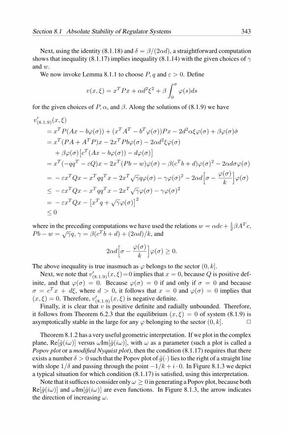
Section 8.1 Absolute Stability of Regulator Systems 343
Next, using the identity (8.1.18) and δ = β/(2αd), a straightforward computationshows that inequality (8.1.17) implies inequality (8.1.14) with the given choices of γand w.
We now invoke Lemma 8.1.1 to choose P, q and ε > 0. Define
v(x, ξ) = xT Px + αd2ξ2 + β
∫ σ
0ϕ(s)ds
for the given choices of P, α, and β. Along the solutions of (8.1.9) we have
v′(8.1.9)(x, ξ)
= xT P (Ax − bϕ(σ)) + (xT AT − bT ϕ(σ))Px − 2d2αξϕ(σ) + βϕ(σ)σ
= xT (PA + AT P )x − 2xT Pbϕ(σ) − 2αd2ξϕ(σ)
+ βϕ(σ)[cT (Ax − bϕ(σ)) − dϕ(σ)
]= xT (−qqT − εQ)x − 2xT (Pb − w)ϕ(σ) − β(cT b + d)ϕ(σ)2 − 2αdσϕ(σ)
= − εxT Qx − xT qqT x − 2xT √γqϕ(σ) − γϕ(σ)2 − 2αd
[σ − ϕ(σ)
k
]ϕ(σ)
≤ − εxT Qx − xT qqT x − 2xT √γϕ(σ) − γϕ(σ)2
= − εxT Qx −[xT q +
√γϕ(σ)
]2≤ 0
where in the preceding computations we have used the relations w = αdc+ 12βAT c,
Pb − w =√
γq, γ = β(cT b + d) + (2αd)/k, and
2αd[σ − ϕ(σ)
k
]ϕ(σ) ≥ 0.
The above inequality is true inasmuch as ϕ belongs to the sector (0, k].Next, we note that v′
(8.1.9)(x, ξ)=0 implies that x = 0, because Q is positive def-inite, and that ϕ(σ) = 0. Because ϕ(σ) = 0 if and only if σ = 0 and becauseσ = cT x + dξ, where d > 0, it follows that x = 0 and ϕ(σ) = 0 implies that(x, ξ) = 0. Therefore, v′
(8.1.9)(x, ξ) is negative definite.Finally, it is clear that v is positive definite and radially unbounded. Therefore,
it follows from Theorem 6.2.3 that the equilibrium (x, ξ) = 0 of system (8.1.9) isasymptotically stable in the large for any ϕ belonging to the sector (0, k].
Theorem 8.1.2 has a very useful geometric interpretation. If we plot in the complexplane, Re[g(iω)] versus ωIm[g(iω)], with ω as a parameter (such a plot is called aPopov plot or a modified Nyquist plot), then the condition (8.1.17) requires that thereexists a number δ > 0 such that the Popov plot of g(·) lies to the right of a straight linewith slope 1/δ and passing through the point −1/k + i · 0. In Figure 8.1.3 we depicta typical situation for which condition (8.1.17) is satisfied, using this interpretation.
Note that it suffices to consider only ω ≥ 0 in generating a Popov plot, because bothRe[g(iω)] and ωIm[g(iω)] are even functions. In Figure 8.1.3, the arrow indicatesthe direction of increasing ω.
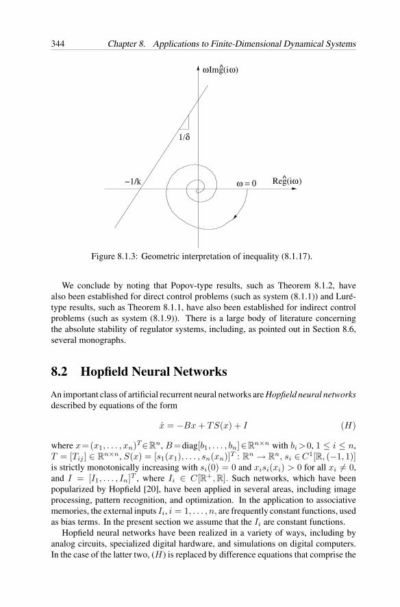
344 Chapter 8. Applications to Finite-Dimensional Dynamical Systems
−1/k
1/δ
ωω = 0 Reg(i )
Img(i )^
^
ωω
Figure 8.1.3: Geometric interpretation of inequality (8.1.17).
We conclude by noting that Popov-type results, such as Theorem 8.1.2, havealso been established for direct control problems (such as system (8.1.1)) and Lure-type results, such as Theorem 8.1.1, have also been established for indirect controlproblems (such as system (8.1.9)). There is a large body of literature concerningthe absolute stability of regulator systems, including, as pointed out in Section 8.6,several monographs.
8.2 Hopfield Neural Networks
An important class of artificial recurrent neural networks are Hopfield neural networksdescribed by equations of the form
x = −Bx + TS(x) + I (H)
where x=(x1, . . . , xn)T∈Rn, B =diag[b1, . . . , bn]∈R
n×n with bi >0, 1 ≤ i ≤ n,T = [Tij ] ∈ R
n×n, S(x) = [s1(x1), . . . , sn(xn)]T : Rn → R
n, si ∈ C1[R, (−1, 1)]is strictly monotonically increasing with si(0) = 0 and xisi(xi) > 0 for all xi = 0,and I = [I1, . . . , In]T , where Ii ∈ C[R+, R]. Such networks, which have beenpopularized by Hopfield [20], have been applied in several areas, including imageprocessing, pattern recognition, and optimization. In the application to associativememories, the external inputs Ii, i = 1, . . . , n, are frequently constant functions, usedas bias terms. In the present section we assume that the Ii are constant functions.
Hopfield neural networks have been realized in a variety of ways, including byanalog circuits, specialized digital hardware, and simulations on digital computers.In the case of the latter two, (H) is replaced by difference equations that comprise the
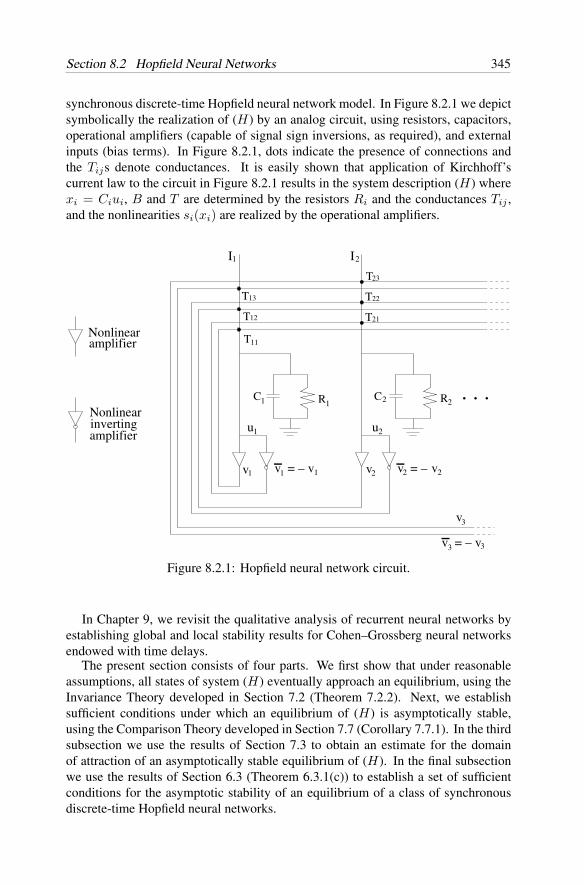
Section 8.2 Hopfield Neural Networks 345
synchronous discrete-time Hopfield neural network model. In Figure 8.2.1 we depictsymbolically the realization of (H) by an analog circuit, using resistors, capacitors,operational amplifiers (capable of signal sign inversions, as required), and externalinputs (bias terms). In Figure 8.2.1, dots indicate the presence of connections andthe Tijs denote conductances. It is easily shown that application of Kirchhoff’scurrent law to the circuit in Figure 8.2.1 results in the system description (H) wherexi = Ciui, B and T are determined by the resistors Ri and the conductances Tij ,and the nonlinearities si(xi) are realized by the operational amplifiers.
. . .invertingamplifier
Nonlinear
amplifierNonlinear
v = – v
u
1 v = – v2
T
T
T
T
C R C R
12
1 I
T13
1 2 2
2v2
I
11
22
T23
1
1
21
u
v
v = – v
3
3 3
1
v1
2
2
Figure 8.2.1: Hopfield neural network circuit.
In Chapter 9, we revisit the qualitative analysis of recurrent neural networks byestablishing global and local stability results for Cohen–Grossberg neural networksendowed with time delays.
The present section consists of four parts. We first show that under reasonableassumptions, all states of system (H) eventually approach an equilibrium, using theInvariance Theory developed in Section 7.2 (Theorem 7.2.2). Next, we establishsufficient conditions under which an equilibrium of (H) is asymptotically stable,using the Comparison Theory developed in Section 7.7 (Corollary 7.7.1). In the thirdsubsection we use the results of Section 7.3 to obtain an estimate for the domainof attraction of an asymptotically stable equilibrium of (H). In the final subsectionwe use the results of Section 6.3 (Theorem 6.3.1(c)) to establish a set of sufficientconditions for the asymptotic stability of an equilibrium of a class of synchronousdiscrete-time Hopfield neural networks.
346 Chapter 8. Applications to Finite-Dimensional Dynamical Systems
A. A global result
In this subsection we present a result that serves as the basis for the application ofHopfield neural networks in the areas enumerated earlier. We require the followinghypotheses.
(A–1) T is a symmetric matrix.
(A–2) si ∈ C1[R, (−1, 1)] anddsi
dη(η) > 0 for all η ∈ R.
(A–3) System (H) has a finite number of equilibrium points.
In [41], sufficient conditions are established which show that hypothesis (A–3) issatisfied under reasonable assumptions for (H).
Theorem 8.2.1 Assume that hypotheses (A–1), (A–2), and (A–3) are true. Thenfor every solution ϕ(t) of (H), there exists an equilibrium xe of (H) such thatlimt→∞ ϕ(t) = xe.
Proof . In view of the results given in Chapter 2 (refer to Subsection 2.3B) it is easilyestablished that for every x(0) ∈ R
n, (H) possesses a unique solution ϕ(t) withϕ(0) = x(0), which exists for all t ≥ 0.
To apply Theorem 7.2.2 in the present case, we first need to show that everysolution of (H) is bounded. To this end, let
ci =n∑
j=1
|Tij | + |Ii|,
i=1, . . . , n. Then in view of (A–2), every solution of (H), ϕ(t)=[ϕ1(t), . . . , ϕn(t)]T,satisfies the inequalities
ϕi(t) ≤ −biϕi(t) + ci,
i = 1, . . . , n.By the comparison theorem for ordinary differential equations, Theorem3.8.1 (for the case l = 1), we have that ϕi(t) ≤ yi(t) for all t ≥ 0, where yi(0) =xi(0) and where yi(t) is a solution of the differential equation
yi(t) = −biyi(t) + ci,
i = 1, . . . , n. Solving these equations, we have that
ϕi(t) ≤ ci
bi−(ci
bi− xi(0)
)e−bit ≤ ci
bi+∣∣∣ci
bi− xi(0)
∣∣∣,i = 1, . . . , n, for all t ∈ R
+. Therefore, all the solutions of (H) are bounded fromabove. In a similar manner, we can show that all the solutions ϕ(t) of (H) are boundedfrom below for all t ∈ R
+.
Section 8.2 Hopfield Neural Networks 347
Next, we choose as a Lyapunov function the “energy function” given by
v(x) = −12S(x)T TS(x) − S(x)T I +
n∑i=1
bi
∫ si(xi)
0s−1
i (η)dη.
Then v ∈ C1[Rn, R] and the gradient of v is given by
∇v(x) = ∇xS(x)[−TS(x) − I + Bx]
where
∇xS(x) = diag
[ds1
dx1(x1), . . . ,
dsn
dxn(xn)
]and hypothesis (A–1) has been used. Then
v′(H)(x) = −(−Bx + TS(x) + I)T ∇xS(x)(−Bx + TS(x) + I) ≤ 0
for all x ∈ Rn.
The set of all x ∈ Rn such that v′
(H)(x) = 0, given by
Z = x ∈ Rn : v′
(H)(x) = 0 = x ∈ Rn : − Bx + TS(x) + I = 0,
is an invariant set of (H) because it is precisely equal to the set of all equilibriumpoints of (H). By hypothesis (A–3), Z consists of a finite number of points. All thehypotheses of Theorem 7.2.2 are now satisfied and we conclude that every solutionϕ(t) of (H) approaches an equilibrium of (H) as t → ∞.
B. A local result
In applications (e.g., to associative memories), asymptotically stable equilibria (calledstable memories) are used to store information. It is important in such applicationsto establish conditions under which a given equilibrium xe of (H) is asymptoticallystable. We address this issue next.
Using the transformation w = x − xe, system (H) assumes the form
w = −Bw + T S(w) (8.2.1)
where S(w)=S(w+xe)−S(xe), S(0)=0, and we = 0 is an equilibrium of (8.2.1).We conclude that we may assume without loss of generality that xe = 0 is an equi-librium of the Hopfield neural network and that the network has the form
x = −Bx + TS(x), (H)
or equivalently,
xi = −bixi +n∑
j=1
Tijsj(xj), (Hi)
348 Chapter 8. Applications to Finite-Dimensional Dynamical Systems
i = 1, . . . , n, where B and T are the same as in (H), S(x) = [s1(x1), . . . , sn(xn)]T
for x = (x1, . . . , xn)T , si ∈ C1[R, (−2, 2)], si is strictly monotonically increasing,si(0) = 0, and xisi(xi) > 0 for all xi = 0. In what follows, we make the realisticassumption that for all i = 1, . . . , n,
0 <si(xi)
xi< δi, for 0 < |xi| < εi. (8.2.2)
System (Hi) (resp., (H)) can be rewritten as
x =
F (x)x, x = 0,0, x = 0 (8.2.3)
where F (x) = [fij(xj)] andfii(xi) = −bi + Tii
si(xi)xi
, xi = 0, i = 1, . . . , n,
fij(xj) = Tijsj(xj)
xj, xj = 0, 1 ≤ i = j ≤ n.
(8.2.4)
Now let A = [aij ], whereaii = −bi + Tiiδi, 1 ≤ i ≤ n,
aij = |Tij |δj , 1 ≤ i = j ≤ n(8.2.5)
where δi, i = 1, . . . , n, is defined in (8.2.2).
Choosing the vector Lyapunov function V (x) =[|x1|, . . . , |xn|
]T, where x =
(x1, . . . , xn)T , and proceeding identically as in Example 7.7.1, we obtain along thesolutions of (H) the vector inequality
V ′(H)
(x) ≤ AV (x) (8.2.6)
for all x ∈ B(ε), where ε = min1≤i≤nεi and εi > 0, i = 1, . . . , n, is given in(8.2.2). Identically as in Example 7.7.1, we now apply Corollary 7.7.1(b) to obtainthe following result.
Proposition 8.2.1 The equilibrium xe = 0 of (H) is exponentially stable if −A isan M -matrix (where A is defined in (8.2.5)).
Remark 8.2.1 In view of Definition 7.7.1, because the matrix D = −A given inProposition 8.2.1 is an M -matrix, the following equivalent statements are true.
(a) The principal minors of −A are all positive.(b) The successive principal minors of −A are all positive.(c) There is a vector u ∈(R+)n such that −Au ∈(R+)n (recall that R+ = (0,∞)).(d) There is a vector v ∈ (R+)n such that −AT v ∈ (R+)n.(e) −A is nonsingular and all elements of −A−1 are nonnegative (in fact, all
diagonal elements of −A−1 are positive).
Section 8.2 Hopfield Neural Networks 349
C. Domain of attraction
In applications (e.g., to associative memories), estimates for the domain of attractionof an asymptotically stable equilibrium are also of great interest. In the presentsubsection we apply the method developed in Section 7.3 to obtain estimates for thedomain of attraction of the equilibrium xe = 0 of system (H).
We assume that all the hypotheses of Proposition 8.2.1 are still in place. In par-ticular, we assume that −A is an M -matrix where A = [aij ] is given in (8.2.5). Inaccordance with the property of M -matrices given in Remark 8.2.1(c), there existλj > 0, j = 1, . . . , n, such that
n∑j=1
aij
λj< 0, i = 1, . . . , n. (8.2.7)
Proposition 8.2.2 Assume that all conditions of Proposition 8.2.1 are true. Let
S =
x ∈ Rn : max
1≤i≤nλi|xi| < min
1≤i≤nλiεi
where λi and εi, i = 1, . . . , n, are defined in (8.2.2) and (8.2.7), respectively. ThenS is a subset of the domain of attraction of the equilibrium xe = 0 of system (H).
Proof . We choose as a Lyapunov function for (H)
v(x) = max1≤i≤n
λi|xi|.
Along the solutions of (H), we have, in view of (8.2.7),
v′(H)
(x) ≤ max1≤i≤n
λiD+|xi|
≤ max1≤i≤n
λiaii|xi| +
∑i =j
λiaij |xj |
≤ aiiv(x) +∑i =j
λi
λjaijv(x)
= λi
( n∑j=1
aij
λj
)v(x)
≤ 0 (8.2.8)
for all |xi| < εi, i = 1, . . . , n. In the above inequalities we have evaluated the Diniderivative D+|xi| similarly as was done in Example 7.7.1.
For c = min1≤i≤n λiεi, any x ∈ Rn satisfying v(x) < c must satisfy |xi| < εi
and therefore, (8.2.8) must be satisfied. From the method developed in Section 7.3 itis now clear that the set
S = x ∈ Rn : v(x) < c =
x ∈ R
n : max1≤i≤n
λi|xi| < min1≤i≤n
λiεi
is contained in the domain of attraction of the equilibrium xe = 0 of system (H).
350 Chapter 8. Applications to Finite-Dimensional Dynamical Systems
D. Synchronous discrete-time Hopfield neural networks
In this subsection we establish local stability results for synchronous discrete-timeHopfield-type neural networks described by scalar-valued equations of the form
ui(k + 1) =n∑
j=1
Tijvj(uj(k)) + (1 − ∆t · bi)ui(k) + Ii
=n∑
j=1
Tijvj(uj(k)) − aiui(k) + Ii
vi(ui(k)) = gi(ui(k)),
(Wi)
i = 1, . . . , n, k ∈ N, where ai = 1 − ∆t · bi, ∆t denotes computation step size,gi ∈ C1[R, R], gi(0) = 0, uigi(ui) > 0 for all ui = 0,
dgi
dui(ui) > 0,
and gi(·) satisfies the sector condition
di1 ≤ gi(σ)σ
≤ di2 (8.2.9)
for all σ ∈ B(ri) − 0 for some ri > 0, i = 1, . . . , n, where di1, di2 > 0,i = 1, . . . , n, are constants.
Letting u = (u1, . . . , un)T ∈ Rn, v = (v1, . . . , vn)T ∈ R
n, T = [Tij ] ∈ Rn×n,
A = diag[a1, . . . , an], I = (I1, . . . , In)T , and g(·) = [g1(·), . . . , gn(·)]T : Rn → R
n,system (Wi) assumes the form
u(k + 1) = Tv(u(k)) + Au(k) + I,
v(u(k)) = g(u(k)),
k ∈ N. Any point ue ∈ Rn that satisfies the condition
ue = Tg(ue) + Aue + I
or0 = Tg(ue) + Bue + I (8.2.10)
where B = A − I , is an equilibrium for (W ). Lettingp(k) = u(k) − ue
G(p(k)) = g(u(k)) − g(ue)(8.2.11)
where ue satisfies (8.2.10) and G(·) = [G1(·), . . . , Gn(·)]T , system (W ) reduces tothe system
p(k + 1) = TG(p(k)) + Ap(k) (W )
which has an equilibrium at pe = 0.
Section 8.2 Hopfield Neural Networks 351
System (W ) can be rewritten in component form as
pi(k + 1) =n∑
j=1
TijGj(pj(k)) + aipi(k), (Wi)
i = 1, . . . , n. From the relationship (8.2.11) it follows that the functions Gi(·) havethe same qualitative properties as the functions gi(·), i = 1, . . . , n. In particular,Gi(0) = 0 and
ci1 ≤ Gi(σ)σ
≤ ci2 (8.2.12)
for all σ ∈ B(δi) − 0 for some δi > 0, i = 1, . . . , n, where ci1, ci2 > 0, i =1, . . . , n, are constants (in general not equal to di1, di2 given in (8.2.9)).
As in [19], [51], and [64], we can view (Wi) as an interconnection of n subsystemsdescribed by equations of the form
xi(k + 1) = TiiGi(xi(k)) + aixi(k), (Ωi)
i = 1, . . . , n, with the interconnecting structure specified by
hi(x1, . . . , xn)=
n∑j=1,i =j
TijGj(xj(k)), (8.2.13)
i = 1, . . . , n. Under this viewpoint, the stability properties of the equilibrium pe = 0of (W ) are established in terms of the qualitative properties of the subsystems (Ωi),i = 1, . . . , n, and the constraints imposed on the interconnecting structure of system(W ).
In the following, we assume that system (W ) satisfies the following hypotheses.
(B–1) For subsystem (Ωi),
0 < σi= (|ai| + |Tii|ci2) < 1
where ci2 is defined in (8.2.12).
(B–2) Given σi in (B–1), the successive principal minors of the matrix Q = [qij ]are all positive, where
qij =
−(σi − 1), 1 ≤ i = j ≤ n,−σij , 1 ≤ i = j ≤ n
where σij = |Tij |cj2 and cj2 is defined in (8.2.12).
We are now in a position to prove the last result of this section.
Theorem 8.2.2 If Assumptions (B–1) and (B–2) are true, then the equilibrium pe= 0of system (W ) (resp., (Wi)) is asymptotically stable.
352 Chapter 8. Applications to Finite-Dimensional Dynamical Systems
Proof . We choose as a Lyapunov function for (W ),
v(p(k)) =n∑
i=1
λi|pi(k)|,
for some constants λi > 0, i = 1, . . . , n. The first forward difference of v evaluatedalong the solutions of (Wi) is given by
D(Wi)v(p(k)) = v(p(k + 1)) − v(p(k))
=n∑
i=1
[|pi(k + 1)| − |pi(k)|]
=n∑
i=1
λi
[∣∣∣∣aipi(k) +n∑
j=1
TijGj(pj(k))∣∣∣∣− |pi(k)|
]
≤n∑
i=1
λi
[|ai| |pi(k)| +
n∑j=1
|Tij | |Gj(pj(k))| − |pi(k)|]
≤n∑
i=1
λi
[(|ai| − 1)|pi(k)| +
n∑j=1
|Tij | |Gj(pj(k))|]
≤n∑
i=1
λi
[(|ai| − 1)|pi(k)| +
n∑j=1
|Tij |cj2|pj(k)|]
=n∑
i=1
λi
[(|ai| − 1) + |Tii|ci2)|pi(k)| +
n∑j=1,i =j
|Tij |cj2|pj(k)|]
=n∑
i=1
λi(σi − 1)|pi(k)| +n∑
i=1
λi
n∑j=1,i =j
σij |pj(k)|
= −λT Qw
where λ = (λ1, . . . , λn)T and w = (|p1|, . . . , |pn|)T . Because by (B–2), qij ≤ 0when i = j, and because the successive principal minors of matrix Q are all positive,it follows that Q is an M -matrix (refer to Definition 7.7.1(iii)). Moreover, Q−1 existsand each element of Q−1 is nonnegative (refer to Definition 7.7.1(vi)). Hence, thereexists a vector y = (y1, . . . , yn)T with yi > 0, i = 1, . . . , n, such that
−yT w < 0 where yT = λT Q
andλ = (Q−1)T y > 0.
We have shown that D(Wi)v(p(k)) is negative for all p(k) ∈ B(δ) − 0 where
δ = min1≤i≤n δi with δi defined in (8.2.12). Because v is positive definite, it followsfrom Theorem 6.3.1(c) that the equilibrium point pe = 0 of (Wi) is asymptoticallystable.
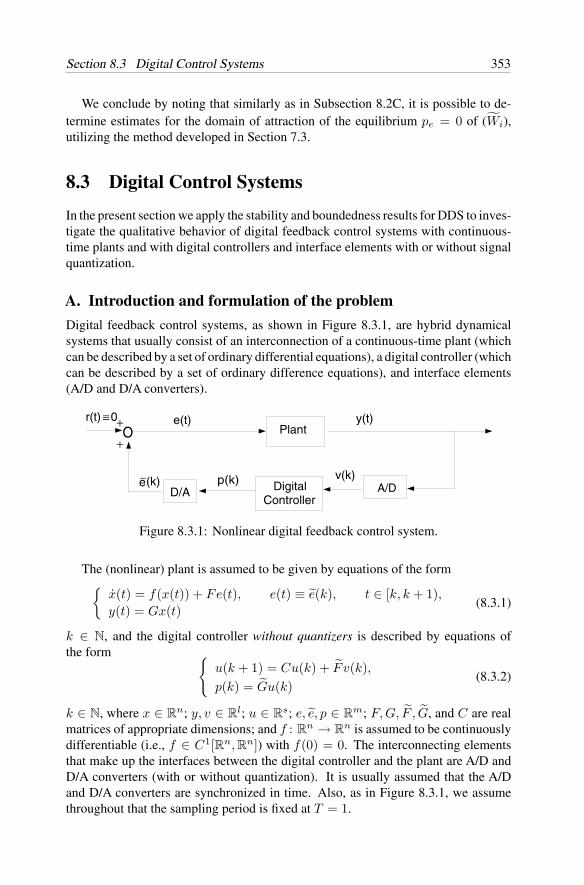
Section 8.3 Digital Control Systems 353
We conclude by noting that similarly as in Subsection 8.2C, it is possible to de-termine estimates for the domain of attraction of the equilibrium pe = 0 of (Wi),utilizing the method developed in Section 7.3.
8.3 Digital Control Systems
In the present section we apply the stability and boundedness results for DDS to inves-tigate the qualitative behavior of digital feedback control systems with continuous-time plants and with digital controllers and interface elements with or without signalquantization.
A. Introduction and formulation of the problem
Digital feedback control systems, as shown in Figure 8.3.1, are hybrid dynamicalsystems that usually consist of an interconnection of a continuous-time plant (whichcan be described by a set of ordinary differential equations), a digital controller (whichcan be described by a set of ordinary difference equations), and interface elements(A/D and D/A converters).
Plant
D/A A/D Digital Controller
Oe(t) y(t)
v(k)p(k)
r(t) ≡ 0+
+
e∼(k)
Figure 8.3.1: Nonlinear digital feedback control system.
The (nonlinear) plant is assumed to be given by equations of the formx(t) = f(x(t)) + Fe(t), e(t) ≡ e(k), t ∈ [k, k + 1),y(t) = Gx(t)
(8.3.1)
k ∈ N, and the digital controller without quantizers is described by equations ofthe form
u(k + 1) = Cu(k) + F v(k),p(k) = Gu(k)
(8.3.2)
k ∈ N, where x ∈ Rn; y, v ∈ R
l; u ∈ Rs; e, e, p ∈ R
m; F, G, F , G, and C are realmatrices of appropriate dimensions; and f : R
n → Rn is assumed to be continuously
differentiable (i.e., f ∈ C1[Rn, Rn]) with f(0) = 0. The interconnecting elementsthat make up the interfaces between the digital controller and the plant are A/D andD/A converters (with or without quantization). It is usually assumed that the A/Dand D/A converters are synchronized in time. Also, as in Figure 8.3.1, we assumethroughout that the sampling period is fixed at T = 1.
354 Chapter 8. Applications to Finite-Dimensional Dynamical Systems
B. Stability analysis of systems without quantizers
In the present subsection we assume ideal A/D and D/A converters (i.e., there are noquantizers in the converters) and we assume infinite wordlength digital controllers(i.e., there is no quantization in the digital controller). Then e(k) = p(k) = Gu(k),v(k) = y(k) = Gx(k), and the nonlinear digital feedback control system of Figure8.3.1 is described by equations of the form
x(t) = f(x(t)) + Bu(k), t ∈ [k, k + 1)u(k + 1) = Cu(k) + Dx(k),
(8.3.3)
k ∈N, where B =FG and D = FG. We note that because f(0)=0, (xT , uT )T= 0is an equilibrium of system (8.3.3). We show that the stability (resp., instability)properties of (8.3.3) can under reasonable conditions be deduced from the associatedlinear system given by
x(t) = Ax(t) + Bu(k), t ∈ [k, k + 1)u(k + 1) = Cu(k) + Dx(k), (8.3.4)
k ∈ N, where A ∈ Rn×n denotes the Jacobian of f evaluated at x = 0; that is,
A =[∂f
∂x(0)]
n×n
. (8.3.5)
For the linear digital control system (8.3.4), the following results are well known(refer, e.g., to [10], [14], [30]).
Lemma 8.3.1 The equilibrium (xT , uT )T = (0T , 0T )Tof the linear digital control
system (8.3.4) is uniformly asymptotically stable in the large if and only if the matrix
H=[H1 H2D C
](8.3.6)
is Schur stable, where H1 = eA and H2 =∫ 10 eA(1−τ)dτB.
Lemma 8.3.2 Assume that the matrix H given in (8.3.6) has at least one eigenvalueoutside the unit circle. Then the equilibrium (xT , uT )T = (0T , 0T )T
of the lineardigital control system (8.3.4) is unstable.
We now prove the first stability result for system (8.3.3).
Theorem 8.3.1 The equilibrium (xT, uT )T=(0T, 0T )Tof the nonlinear digital con-
trol system (8.3.3) is uniformly asymptotically stable if the equilibrium (xT , uT )T=(0T, 0T )T
of the linear digital control system (8.3.4) is uniformly asymptoticallystable, or equivalently, if the matrix H given in (8.3.6) is Schur stable.
Section 8.3 Digital Control Systems 355
Proof . To show that the trivial solution of system (8.3.3) is uniformly asymptoticallystable, we verify that the conditions of Theorem 6.4.2 are satisfied.
Because f ∈ C1[Rn, Rn] and because f(0) = 0, we can represent f as
f(x) = Ax + g(x), (8.3.7)
where A ∈ Rn×n is given in (8.3.5) and g ∈ C1[Rn, Rn] satisfies the condition
limx→0
|g(x)||x| = 0. (8.3.8)
The first equation in (8.3.3) now assumes the form
x(t) = Ax(t) + g(x(t)) + Bu(k) (8.3.9)
for t ∈ [k, k + 1). By the continuity of x(t), the solution of equation (8.3.9) isgiven by
x(t) = eA(t−k)x(k) +∫ t
k
eA(t−τ)Bu(k)dτ +∫ t
k
eA(t−τ)g(x(τ))dτ (8.3.10)
for all t ∈ [k, k + 1]. Specifically, at t = k + 1, we have
x(k + 1) = eAx(k) +∫ k+1
k
eA(k+1−τ)dτBu(k) +∫ k+1
k
eA(k+1−τ)g(x(τ))dτ.
(8.3.11)Combining (8.3.11) and the second equation in (8.3.3), we obtain[
x(k + 1)u(k + 1)
]= H
[x(k)u(k)
]+[∆(k)
0
](8.3.12)
where
∆(k)=∫ k+1
k
eA(k+1−τ)g(x(τ))dτ. (8.3.13)
By assumption H is Schur stable. Thus there exists a positive definite symmetricmatrix P such that HT PH − P = −I , where I ∈ R
(n+m)×(n+m) denotes theidentity matrix (refer to Theorem 7.5.8). Define a Lyapunov function as
v(w) = wT Pw (8.3.14)
where w ∈ Rn+m. Letting w(t) = (x(t)T , u(k)T )T
when t ∈ [k, k + 1), and
m(k)= (∆(k)T , 0T )T
, equation (8.3.12) can be written more concisely as
w(k + 1) = Hw(k) + m(k). (8.3.15)
356 Chapter 8. Applications to Finite-Dimensional Dynamical Systems
The first forward difference of v evaluated along the solutions of the discrete-timesystem (8.3.15) yields
Dv(w(k))= v(w(k + 1)) − v(w(k))
= w(k + 1)T Pw(k + 1) − w(k)T Pw(k)
= [Hw(k) + m(k)]T P [Hw(k) + m(k)] − w(k)T Pw(k)
= w(k)T [HT PH − P ]w(k) + 2m(k)T PHw(k) + m(k)T Pm(k)
= −|w(k)|2 + 2m(k)T PHw(k) + m(k)T Pm(k)
≤ −|w(k)|2 + 2|∆(k)|‖PH‖|w(k)| + |∆(k)|2‖P‖. (8.3.16)
Before proceeding further, we need the following result.
Proposition 8.3.1 For any given µ > 0, there exists a δ = δ(µ) > 0, such that
|∆(k)| ≤∫ k+1
k
e‖A‖|g(x(τ))|dτ < µ|w(k)| (8.3.17)
whenever |w(k)| < δ, for any k ∈ N.
The proof of this result is presented at the end of this subsection. If we nowchoose a µ0 > 0 such that c(µ0) = 1 − 2µ0‖PH‖ − µ2
0‖P‖ > 0, then there exists aδ(µ0) > 0 such that
Dv(w(k)) < −|w(k)|2 + 2µ0‖PH‖|w(k)|2 + µ20‖P‖|w(k)|2
= −c(µ0)|w(k)|2 (8.3.18)
whenever |w(k)| < δ(µ0). It follows from (8.3.14) and (8.3.18) that
λm(P )|w(k + 1)|2 ≤ v(w(k + 1)) < v(w(k)) ≤ λM (P )|w(k)|2 (8.3.19)
where λm(P ) and λM (P ) denote the smallest and largest eigenvalues of P , respec-
tively. Let d=√
λm(P )/λM (P )δ(µ0). If |w(k0)| < d for some k0, then (8.3.19)yields |w(k0 +1)| < δ(µ0). Thus, (8.3.18) is applicable for k = k0 +1, which yieldsv(w(k0 +2)) < v(w(k0 +1)) < v(w(k0)). Replacing (k +1) in (8.3.19) by (k +2)yields |w(k0 + 2)| < δ(µ0). By induction, it follows that |w(k)| < δ(µ0) for allk ≥ k0. Hence, (8.3.18) is satisfied for k ≥ k0 whenever |w(k0)| < d. Therefore,(6.4.3) of Theorem 6.4.2 is satisfied.
Next, we note that for t ∈ [k, k + 1), it follows from (8.3.10) and (8.3.17) that
|x(t)| ≤ e‖A‖|x(k)| + e‖A‖‖B‖|u(k)| +∫ k+1
k
e‖A‖ · |g(x(τ))|dτ
≤ e‖A‖√1 + ‖B‖2|w(k)| + µ0|w(k)|
=(e‖A‖√1 + ‖B‖2 + µ0
)|w(k)|. (8.3.20)
Section 8.3 Digital Control Systems 357
Hence for k ≤ t < k + 1, we obtain that
v(w(t)) ≤ λM (P )(|x(t)|2 + |u(k)|2
)≤ λM (P )
(e‖A‖√1 + ‖B‖2 + µ0 + 1
)|w(k)|2
≤ λM (P )λm(P )
(e‖A‖√1 + ‖B‖2 + µ0 + 1
)v(w(k)).
Let c1(µ0) = ((λM (P ))/(λm(P )))(e‖A‖√1 + ‖B‖2 + µ0 + 1
). Then, (6.4.2) of
Theorem 6.4.1 is satisfied with f(r) = c1(µ0)r. Noting that d is independent ofk0, we conclude from Theorem 6.4.2 that the trivial solution of system (8.3.3) isuniformly asymptotically stable if H is Schur stable.
Theorem 8.3.2 Assume that the matrix H given in (8.3.6) has no eigenvalues on theunit circle and has at least one eigenvalue outside the unit circle in the complex plane.Then the equilibrium we = (xT , uT )T = (0T , 0T )T
of the nonlinear digital feedbackcontrol system (8.3.3) is unstable.
Proof . The proof is similar to the proof of Theorem 8.3.1. By assumption, there existsa symmetric matrix P such that HT PH−P = I , where I ∈ R
(n+m)×(n+m) denotesthe identity matrix (refer to Theorem 7.5.8). As before, we consider a Lyapunovfunction of the form v(w) = wT Pw. Because in the present case P has at leastone positive eigenvalue, there must exist points in every neighborhood of the originwhere v is positive. Using a similar argument as in the proof of Theorem 8.3.1, wecan show that there exists a d > 0 such that v(w(k + 1)) − v(w(k)) > c|w(k)|2 fora certain positive constant c whenever |w(k)| < d. Therefore, all the hypotheses ofTheorem 6.4.8 are satisfied. Hence, the equilibrium we = 0 of (8.3.3) is unstable.
Proof of Proposition 8.3.1. From (8.3.8) it follows that there exists a δ1 > 0 suchthat |g(x)| ≤ |x| whenever |x| ≤ δ1. If we let
δ2 =e−(‖A‖+1)√1 + ‖B‖2
δ1,
then we can conclude that |x(t)| ≤ δ1 for all t ∈ [k, k + 1], whenever |w(k)| ≤ δ2.Otherwise, there must exist a t0 ∈ (k, k + 1) such that |x(t0)| = δ1 and |x(t)| ≤ δ1for all t ∈ [k, t0]. We show that this is impossible. For any t ∈ [k, k+1], we have that
x(t) = x(k) +∫ t
k
(Ax(τ) + g(x(τ)) + Bu(k)
)dτ, (8.3.21)
and therefore, when t ∈ [k, t0], it is true that
|x(t)| ≤(|x(k)| + (t − k)‖B‖|u(k)|
)+∫ t
k
(‖A‖|x(τ)| + |g(x(τ))|
)dτ
≤√
1 + ‖B‖2|w(k)| +∫ t
k
(‖A‖ + 1
)|x(τ)|dτ (8.3.22)
358 Chapter 8. Applications to Finite-Dimensional Dynamical Systems
where we have used in the last step of (8.3.22) the fact that |g(x(τ))| ≤ |x(τ)|,because |x(τ)| ≤ δ1 for all τ ∈ [k, t0], by assumption. By the Gronwall inequality(see, e.g., Problem 2.14.9), relation (8.3.22) implies that
|x(t)| ≤√
1 + ‖B‖2|w(k)|e(‖A‖+1)(t−k) (8.3.23)
for all t ∈ [k, t0]. Hence,
|x(t0)| ≤√
1 + ‖B‖2|w(k)|e(‖A‖+1)(t0−k) < δ1 (8.3.24)
because t0 < k +1. Inequality (8.3.24) contradicts the assumption that |x(t0)| = δ1.We have shown that for any k, |x(t)| ≤ δ1 for all t ∈ [k, k+1] whenever |w(k)| ≤ δ2.
For any given µ > 0, we choose µ1 > 0 such that µ = µ1 ·e(2‖A‖+1)√
1 + ‖B‖2.There exists a δ3 > 0 such that |g(x)| < µ1|x|, whenever |x| < δ3. Let
δ∆= min
δ2,
δ3√1 + ‖B‖2e(‖A‖+1)
.
It now follows from (8.3.23) that whenever |w(k)| ≤ δ, then
|x(t)| ≤ δ√
1 + ‖B‖2e(‖A‖+1) ≤ δ3
for all t ∈ [k, k + 1]. Hence, for ∆(k) given by (8.3.13), we obtain
|∆(k)| ≤∫ k+1
k
e‖A‖|g(x(τ))|dτ
≤ e‖A‖µ1√
1 + ‖B‖2|w(k)|e(‖A‖+1)
= µ · |w(k)|
whenever |w(k)| ≤ δ.
C. Analysis of systems with quantization nonlinearities
In the implementation of digital controllers, quantization is unavoidable. This is dueto the fact that computers store numbers with finite bits. In the present subsection,we investigate the nonlinear effects caused by quantization.
There are many types of quantization (see, e.g., [13], [55], and [56]). Presently, weconcern ourselves primarily with the most commonly used fixed-point quantizationwhich can be characterized by the relation
Q(θ) = θ + q(θ) (8.3.25)
where |q(θ)| < ε, for all θ ∈ R and ε depends on the desired precision.If we add fixed-point quantization to both the sampler (A/D converter) and to the
digital controller of the nonlinear digital feedback control system of Figure 8.3.1,assuming r ≡ 0, we obtain
v(k) = Q(y(k)) = y(k) + q1(y(k))
Section 8.3 Digital Control Systems 359
u(k + 1) = Q(Cu(k) + F v(k)) = Cu(k) + FGx(k) + q2(Cu(k) + F v(k))
p(k) = Q(Gu(k)) = Gu(k) + q3(Gu(k)),
k ∈ N, where q1, q2, and q3 should be interpreted as vectors whose componentscontain quantization terms. By a slight abuse of notation, we henceforth write q1(k)in place of q1(y(k)), q2(k) in place of q2(Cu(k) + F v(k)), and so forth. It is easilyverified that there exist positive constants Ji that are independent of ε such that|qi(k)| ≤ Jiε, i = 1, 2, 3, k ∈ N. (For further details concerning the inclusion ofquantizers into digital controllers, refer to [13], [55], [56], and [69].)
In the presence of the quantizer nonlinearities, we can no longer expect that thesystem of Figure 8.3.1 will have a uniformly asymptotically stable equilibrium at theorigin; in fact, there may not even be an equilibrium at the origin. In view of this, weinvestigate the (ultimate) boundedness of the solutions of the system of Figure 8.3.1,including the dependence of the bounds on the quantization size.
In the following, we represent the system of Figure 8.3.1 by the equationsx(t) = Ax(t) + g(x(t)) + FGu(k) + Fq3(k), t ∈ [k, k + 1)u(k + 1) = Cu(k) + FGx(k) + F q1(k) + q2(k),
(8.3.26)
k ∈ N. Lettingw(t) = (x(k)T , u(k)T )T when t ∈ [k, k+1), we obtain similarly as inSubsection B, the equivalent representation of (8.3.26), valid at sampling instants, as
w(k + 1) = Hw(k) + m(k) (8.3.27)
where H is defined as in (8.3.6) and where
m(k) =
∫ k+1
k
eA(k+1−τ)g(x(τ))dτ +∫ 1
0eAτdτFq3(k)
F q1(k) + q2(k)
. (8.3.28)
Now assume that H is Schur stable. Then there exists a symmetric positive definitematrix P such that HT PH −P = −I . As in Subsection B, we choose as a Lyapunovfunction v : R
n+m → R+,
v(w) = wT Pw. (8.3.29)
Lemma 8.3.3 For any d > 0 that satisfies the relation
1 − 2d‖PH‖ − d2‖P‖ > 0, (8.3.30)
there exists a δ = δ(d) > 0 such that the estimate
|m(k)| ≤ d|w(k)| + Jε, k ∈ N (8.3.31)
holds whenever√
1 + ‖B‖2|w(k)|+∥∥ ∫ 1
0 eAτdτ∥∥‖F‖J3ε < δ, where J is a positive
constant independent of ε. (Recall that ε denotes a bound for the quantization size(see (8.3.25)) and J3 is obtained from the estimate |q3(k)| ≤ J3ε.)
360 Chapter 8. Applications to Finite-Dimensional Dynamical Systems
Proof . The existence of d satisfying (8.3.30) is clear. By a similar argument as in theproof of Proposition 8.3.1, there exists a δ > 0 such that
∫ k+1k
e‖A‖|g(x(τ))|dτ <
d|w(k)|, whenever√
1 + ‖B‖2|w(k)| + ‖∫ 10 eAτdτ‖‖F‖J3ε < δ. Therefore,
|m(k)| ≤∣∣∣∣∫ k+1
k
eA(k+1−τ)g(x(τ))dτ +∫ 1
0eAτdτFq3(k)
∣∣∣∣+ ∣∣∣F q1(k) + q2(k)∣∣∣
≤ d|w(k)| + e‖A‖‖F‖J3ε + ‖F‖J1ε + J2ε
= d|w(k)| + Jε (8.3.32)
where J = e‖A‖‖F‖J3 + ‖F‖J1 + J2 whenever√1 + ‖B‖2|w(k)| +
∥∥∥∥∫ 1
0eAτdτ
∥∥∥∥ ‖F‖J3ε < δ.
Now let us consider the Lyapunov function v(w) given in (8.3.14). We compute thefirst forward difference of v along the solutions of the discrete-time system (8.3.26)to obtain
Dv(w(k))= v(w(k + 1)) − v(w(k))
= w(k + 1)T Pw(k + 1) − w(k)T Pw(k)
= [Hw(k) + m(k)]T P [Hw(k) + m(k)] − w(k)T Pw(k)
= w(k)T [HT PH − P ]w(k) + 2m(k)T PHw(k) + m(k)T Pm(k)
= −|w(k)|2 + 2m(k)T PHw(k) + m(k)T Pm(k)
≤ −a1|w(k)|2 + a2|w(k)|ε + a3ε2, (8.3.33)
where a1 = 1 − 2d‖PH‖ − d2‖P‖, a2 = 2(‖PH‖ + d‖P‖)J , and a3 = J2‖P‖.Let
R = a2 +
√a22 + 4a1a3
2a1.
We are now in a position to prove the following result.
Theorem 8.3.3 (i) If the matrix H defined in (8.3.6) is Schur stable, then the solutionsof system (8.3.26) are uniformly bounded, provided that√
1 + ‖B‖2|w(k0)| +∥∥∥∥∫ 1
0eAτdτ
∥∥∥∥‖F‖J3ε < δ,
for some δ > 0. (ii) Let L= max
(R√
1 + ‖B‖2 + J3‖F‖)e‖A‖+b, λM (P )R
,
where b is chosen such that |g(x)| < b|x| for all |x| ≤ Rε. Then for sufficiently largek, the estimates
|w(k)| ≤ Lε (8.3.34)
and|x(t)| ≤ ε
(L√
1 + ‖B‖2 + J3‖F‖)e‖A‖+b1 (8.3.35)
hold, where b1 is such that |g(x)| < b1|x| for all |x| ≤ L.
Section 8.3 Digital Control Systems 361
Proof . We apply Theorem 6.4.4 in the present proof.It is readily verified that under the present assumptions Dv(w(k)) is negative
whenever |w(k)| > Rε. Hence, (6.4.10) of Theorem 6.4.4 is satisfied with Ω = Rε.Furthermore, if |w(k)| > Rε, then v(w(k + 1)) < v(w(k)) and thus |w(k + 1)| ≤λM (P )Rε ≤ Lε.
If |w(k)| ≤ Rε, then by applying the Gronwall inequality to equation (8.3.26)when t = k + 1, we obtain that |w(k + 1)| ≤ Lε. Thus, the last hypothesis ofTheorem 6.4.4 is satisfied with Γ = Lε.
Solving the first equation in (8.3.26), we obtain
x(t) = eA(t−k)x(k) +∫ t
k
eA(t−τ)FGu(k)dτ +∫ t
k
eA(t−τ)g(x(τ))dτ
+∫ t
k
eA(t−τ)Fq3(k)dτ
for t ∈ (k, k + 1) and therefore, when |w(k)| ≤ Rε it is true that
|x(t)| ≤ e‖A‖|x(k)| + e‖A‖‖B‖|u(k)| +∫ k+1
k
e‖A‖|g(x(τ))|dτ + e‖A‖J3‖F‖ε
≤ e‖A‖√1 + ‖B‖2|w(k)| + d|w(k)| + e‖A‖J3‖F‖ε.
We have used the fact that∫ k+1
ke‖A‖|g(x(τ))|dτ < d|w(k)|, whenever (refer to the
proof of Lemma 8.3.3)√1 + ‖B‖2|w(k)| +
∥∥∥∥∫ 1
0eAτdτ
∥∥∥∥ ‖F‖J3ε < δ.
Therefore, (6.4.11) of Theorem 6.4.4 is satisfied with
f(r) =(e‖A‖√1 + ‖B‖2 + d
)r + e‖A‖J3‖F‖ε.
It now follows from Theorem 6.4.4 that the solutions of system (8.3.26) are uni-formly bounded.
We have also shown above that for sufficiently large k, |w(k)| ≤ Lε holds. Finally,for t ∈ (k, k + 1), we apply the same argument as in the proof of Theorem 8.3.1 toobtain the bound (8.3.35) for |x(t)|. This concludes the proof of the theorem.
In our final result we consider the difference in the response of the nonlinear digitalcontrol system with ideal samplers, given by equation (8.3.3), and the nonlinear digitalcontrol system with quantizers, given by (8.3.26). For our present purposes we rewrite(8.3.15) as
w(k + 1) = Hw(k) + m(k), (8.3.36)
where w(k) = (x(k)T , u(k)T )Tand
m(k) ∆=
∫ k+1
k
eA(k+1−τ)g(x(τ))dτ
0
. (8.3.37)
362 Chapter 8. Applications to Finite-Dimensional Dynamical Systems
Letting z(k) = w(k) − w(k), we obtain the relation
z(k + 1) = Hz(k)
+
∫ k+1
k
eA(k+1−τ)(g(x(τ)) − g(x(τ))
)dτ +
∫ 1
0eAτdτFq3(k)
F q1(k) + q2(k)
.
(8.3.38)
This equation is in the same form as equation (8.3.26), except that in (8.3.38) thenonlinearity includes the term
∫ k+1k
eA(k+1−τ)(g(x(τ)) − g(x(τ))
)dτ , rather than
the term∫ k+1
keA(k+1−τ)g(x(τ))dτ . Now suppose that g(·) has the property
limx→0,x→0
|g(x) − g(x)||x − x| = 0, (8.3.39)
which plays a similar role for system (8.3.38) as (8.3.8) does for system (8.3.26).Using similar arguments as in the proof of Theorem 8.3.3, we obtain the followingresult for the boundedness of z(k), k = 0, 1, . . . .
Theorem 8.3.4 Assume that H defined in (8.3.6) is Schur stable and g(·) satisfies(8.3.39). Then there exist a d > 0, a K > 0, and an ε0 > 0 such that
|z(k)| ≤ Kε when k is sufficiently large (8.3.40)
whenever ε < ε0, |w(k0)| < d, and |w(k0)| < d, for some k0, where ε is thequantization level.
D. Examples
The purpose of the following specific example is to show that all conditions ofTheorem 8.3.1 can be satisfied.
Example 8.3.1 In system (8.3.3) (resp., (8.3.4)) take
A =[−0.6 −10.8 0
], B =
[0
0.6
], D = [−0.8 − 0.3], C = [−1],
and in (8.3.7), take
g(x) =[
0.013 sin(x1)0.008x2 cos(x2)
].
Then |g(x)| ≤ α|x| for all x, where α = 0.0083. We also compute that
H =
0.2962 −0.6562 0.51740.5250 0.6899 0.0833
−0.8000 0.3000 −1.0000
, P =
3.2515 0.6514 1.89060.6514 2.4873 −0.07551.8906 −0.0755 2.9856
.
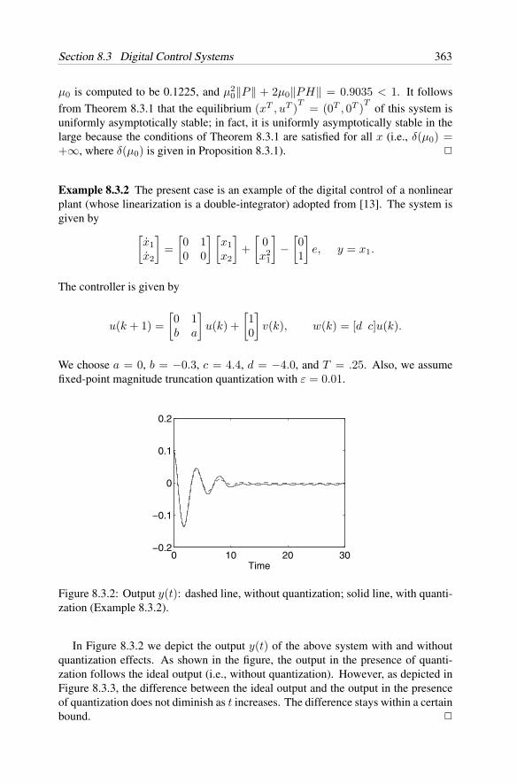
Section 8.3 Digital Control Systems 363
µ0 is computed to be 0.1225, and µ20‖P‖ + 2µ0‖PH‖ = 0.9035 < 1. It follows
from Theorem 8.3.1 that the equilibrium (xT , uT )T = (0T , 0T )Tof this system is
uniformly asymptotically stable; in fact, it is uniformly asymptotically stable in thelarge because the conditions of Theorem 8.3.1 are satisfied for all x (i.e., δ(µ0) =+∞, where δ(µ0) is given in Proposition 8.3.1).
Example 8.3.2 The present case is an example of the digital control of a nonlinearplant (whose linearization is a double-integrator) adopted from [13]. The system isgiven by [
x1x2
]=[0 10 0
] [x1x2
]+[
0x2
1
]−[01
]e, y = x1.
The controller is given by
u(k + 1) =[0 1b a
]u(k) +
[10
]v(k), w(k) = [d c]u(k).
We choose a = 0, b = −0.3, c = 4.4, d = −4.0, and T = .25. Also, we assumefixed-point magnitude truncation quantization with ε = 0.01.
0 10 20 30−0.2
−0.1
0
0.1
0.2
Time
Figure 8.3.2: Output y(t): dashed line, without quantization; solid line, with quanti-zation (Example 8.3.2).
In Figure 8.3.2 we depict the output y(t) of the above system with and withoutquantization effects. As shown in the figure, the output in the presence of quanti-zation follows the ideal output (i.e., without quantization). However, as depicted inFigure 8.3.3, the difference between the ideal output and the output in the presenceof quantization does not diminish as t increases. The difference stays within a certainbound.
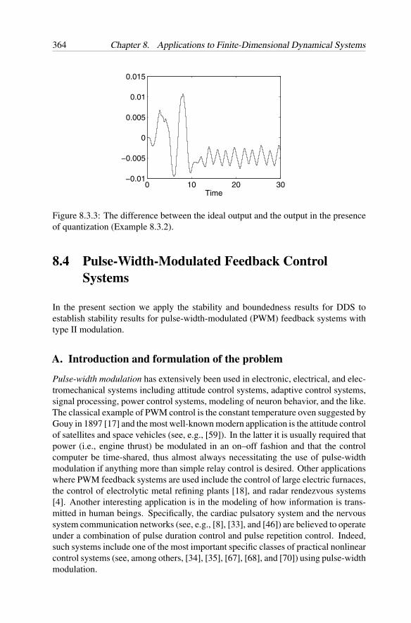
364 Chapter 8. Applications to Finite-Dimensional Dynamical Systems
0 10 20 30−0.01
−0.005
0
0.005
0.01
0.015
Time
Figure 8.3.3: The difference between the ideal output and the output in the presenceof quantization (Example 8.3.2).
8.4 Pulse-Width-Modulated Feedback ControlSystems
In the present section we apply the stability and boundedness results for DDS toestablish stability results for pulse-width-modulated (PWM) feedback systems withtype II modulation.
A. Introduction and formulation of the problem
Pulse-width modulation has extensively been used in electronic, electrical, and elec-tromechanical systems including attitude control systems, adaptive control systems,signal processing, power control systems, modeling of neuron behavior, and the like.The classical example of PWM control is the constant temperature oven suggested byGouy in 1897 [17] and the most well-known modern application is the attitude controlof satellites and space vehicles (see, e.g., [59]). In the latter it is usually required thatpower (i.e., engine thrust) be modulated in an on–off fashion and that the controlcomputer be time-shared, thus almost always necessitating the use of pulse-widthmodulation if anything more than simple relay control is desired. Other applicationswhere PWM feedback systems are used include the control of large electric furnaces,the control of electrolytic metal refining plants [18], and radar rendezvous systems[4]. Another interesting application is in the modeling of how information is trans-mitted in human beings. Specifically, the cardiac pulsatory system and the nervoussystem communication networks (see, e.g., [8], [33], and [46]) are believed to operateunder a combination of pulse duration control and pulse repetition control. Indeed,such systems include one of the most important specific classes of practical nonlinearcontrol systems (see, among others, [34], [35], [67], [68], and [70]) using pulse-widthmodulation.
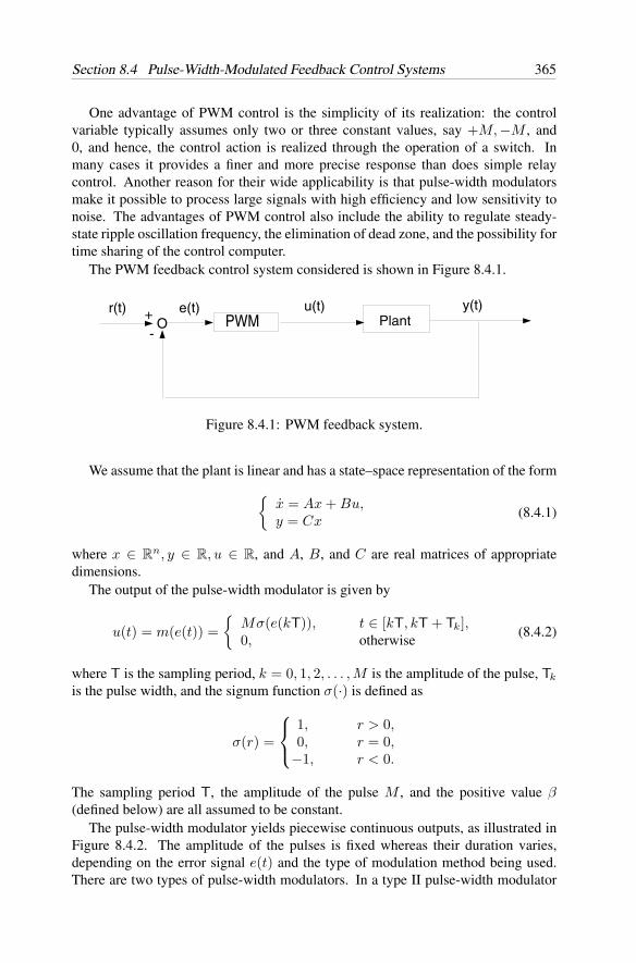
Section 8.4 Pulse-Width-Modulated Feedback Control Systems 365
One advantage of PWM control is the simplicity of its realization: the controlvariable typically assumes only two or three constant values, say +M, −M , and0, and hence, the control action is realized through the operation of a switch. Inmany cases it provides a finer and more precise response than does simple relaycontrol. Another reason for their wide applicability is that pulse-width modulatorsmake it possible to process large signals with high efficiency and low sensitivity tonoise. The advantages of PWM control also include the ability to regulate steady-state ripple oscillation frequency, the elimination of dead zone, and the possibility fortime sharing of the control computer.
The PWM feedback control system considered is shown in Figure 8.4.1.
PWM Plant +-O
r(t) e(t) u(t) y(t)
Figure 8.4.1: PWM feedback system.
We assume that the plant is linear and has a state–space representation of the formx = Ax + Bu,y = Cx
(8.4.1)
where x ∈ Rn, y ∈ R, u ∈ R, and A, B, and C are real matrices of appropriate
dimensions.The output of the pulse-width modulator is given by
u(t) = m(e(t)) =
Mσ(e(kT)), t ∈ [kT, kT + Tk],0, otherwise
(8.4.2)
where T is the sampling period, k = 0, 1, 2, . . . , M is the amplitude of the pulse, Tk
is the pulse width, and the signum function σ(·) is defined as
σ(r) =
1, r > 0,0, r = 0,
−1, r < 0.
The sampling period T, the amplitude of the pulse M , and the positive value β(defined below) are all assumed to be constant.
The pulse-width modulator yields piecewise continuous outputs, as illustrated inFigure 8.4.2. The amplitude of the pulses is fixed whereas their duration varies,depending on the error signal e(t) and the type of modulation method being used.There are two types of pulse-width modulators. In a type II pulse-width modulator
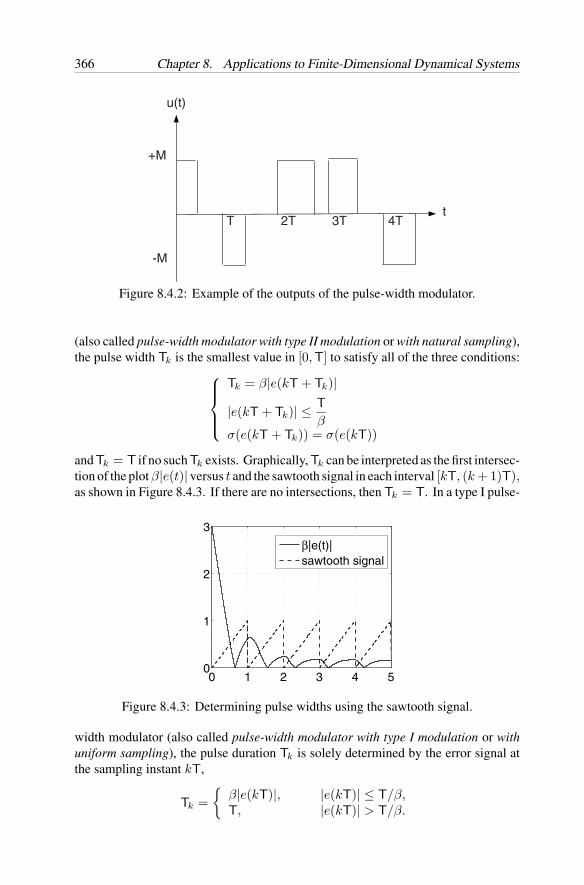
366 Chapter 8. Applications to Finite-Dimensional Dynamical Systems
-M
+M
t
u(t)
T 2T 3T 4T
Figure 8.4.2: Example of the outputs of the pulse-width modulator.
(also called pulse-width modulator with type II modulation or with natural sampling),the pulse width Tk is the smallest value in [0,T] to satisfy all of the three conditions:
Tk = β|e(kT + Tk)|
|e(kT + Tk)| ≤ Tβ
σ(e(kT + Tk)) = σ(e(kT))
and Tk = T if no such Tk exists. Graphically, Tk can be interpreted as the first intersec-tion of the plot β|e(t)| versus t and the sawtooth signal in each interval [kT, (k + 1)T),as shown in Figure 8.4.3. If there are no intersections, then Tk = T. In a type I pulse-
0 1 2 3 4 50
1
2
3
β|e(t)|sawtooth signal
Figure 8.4.3: Determining pulse widths using the sawtooth signal.
width modulator (also called pulse-width modulator with type I modulation or withuniform sampling), the pulse duration Tk is solely determined by the error signal atthe sampling instant kT,
Tk =
β|e(kT)|, |e(kT)| ≤ T/β,T, |e(kT)| > T/β.
Section 8.4 Pulse-Width-Modulated Feedback Control Systems 367
In this section, we investigate PWM feedback systems with type II modulation. Wepresent sufficient conditions for uniform asymptotic stability in the large of the trivialsolution and necessary and sufficient conditions for uniform ultimate boundednessof the solutions, respectively, for PWM feedback systems with Hurwitz stable linearplants. We also incorporate a procedure to compute and optimize the sufficientconditions for uniform asymptotic stability of the trivial solution presented herein.We demonstrate the applicability of our results by means of two specific examples.
B. Type II PWM feedback systems with Hurwitz stable plants
In the present subsection, we assume that A in (8.4.1) is Hurwitz stable.
Throughout this section, we let τ0 = 0 and τk+1= kT + Tk, k ∈ N. Combining
(8.4.1) and (8.4.2), the PWM feedback system of Figure 8.4.1 assumes the form (withr(t) ≡ 0 and e(t) ≡ −y(t))
x(t) =
Ax(t) − BMσ(Cx(kT)), t ∈ [kT, τk+1),Ax(t), t ∈ [τk+1, kT + T). (8.4.3)
Over the time intervals [kT, τk+1] and [τk+1, kT + T], k ∈ N, equation (8.4.3)can be solved to yield the exact solution
x(t) =
eA(t−kT)x(kT) −∫ t
kTeA(t−τ)dτBMσ(Cx(kT)), t ∈ [kT, τk+1],
eA(t−τk+1)x(τk+1), t ∈ [τk+1, kT + T].(8.4.4)
We note that the trivial solution xe = 0 is an equilibrium of system (8.4.3).The first result is concerned with the ultimate boundedness of the solutions of the
PWM feedback system (8.4.3).
Theorem 8.4.1 The solutions of system (8.4.3) are uniformly bounded and uniformlyultimately bounded for any choice of M and β.
Proof . To show that the solutions of system (8.4.3) are uniformly bounded anduniformly ultimately bounded, we verify that the hypotheses of Theorems 6.4.4and 6.4.5 are satisfied, respectively. In doing so, the set E is chosen to be E =k0T, k0T + T, . . . .
We recall that if A is Hurwitz stable, then eAT is Schur stable and there exists apositive definite matrix Q such that(
eAT)T Q(eAT)− Q = −I
where I is the identity matrix of appropriate dimensions. Choose v : Rn → R
+ as
v(x) = xT Qx.
The solutions of system (8.4.3) at t = kT + T are given by
x(kT + T) = eAT(x(kT) + ∆(kT))
(8.4.5)
368 Chapter 8. Applications to Finite-Dimensional Dynamical Systems
where
∆(kT)= −
∫ Tk
0e−AτdτBMσ(Cx(kT))
is bounded, because
|∆(kT)| =∣∣∣∣ ∫ Tk
0e−AτdτBM
∣∣∣∣ ≤ TMe‖A‖T‖B‖. (8.4.6)
Along the solutions of system (8.4.3) we have
∆v(x(kT))= v(x(kT + T)) − v(x(kT))
=(x(kT)T+ ∆(kT)T
)(Q − I)
(x(kT) + ∆(kT)
)− x(kT)T Qx(kT)
= −|x(kT)|2 + 2∆(kT)T (Q − I)x(kT) + ∆(kT)T (Q − I)∆(kT)
≤ −|x(kT)|2 + 2TMe‖A‖T‖B‖‖Q − I‖|x(kT)|
+(TMe‖A‖T‖B‖
)2‖Q − I‖.
It is readily verified that Dv(x(kT)) = ∆v(x(kT))/T < 0 whenever |x(kT)| >
Ω= TMe‖A‖T‖B‖‖Q − I‖(1 +
√1 + 1/‖Q − I‖).
If |x(kT)| < Ω, we have that∣∣x(kT + T)∣∣2 ≤ v(x(kT + T))
λm(Q)
≤ v(x(kT)) + ∆v(x(kT))λm(Q)
≤ 1λm(Q)
(‖Q − I‖Ω2 + 2TMe‖A‖T‖B‖‖Q − I‖Ω
+(TMe‖A‖T‖B‖
)2‖Q − I‖)
where λm(·) is the smallest eigenvalue of a matrix.Next, we obtain an estimate for x(t), t ∈ [kT, kT + T). It follows from (8.4.4)
that|x(t)| ≤ e‖A‖T|x(kT)| + Te‖A‖T‖B‖M,
and thus
v(x(t)) ≤ λM (Q)|x(t)|2
≤ λM (Q)(e‖A‖T|x(kT)| + Te‖A‖T‖B‖M
)2≤ λM (Q)
(e‖A‖T
√v(x(kT))/λm(Q) + Te‖A‖T‖B‖M
)2where λM (·) is the largest eigenvalue of a matrix.
Therefore, it follows from Theorems 6.4.4 and 6.4.5 that the solutions of system(8.4.3) are uniformly bounded and uniformly ultimately bounded, respectively.
Section 8.4 Pulse-Width-Modulated Feedback Control Systems 369
Remark 8.4.1 Note that the above proof does not rely on the modulation type. Thisresult is also true for PWM feedback systems with type I modulation (see [25]).
In the above proof, we utilized equation (8.4.5), which describes system (8.4.3) atdiscrete instants kT, k = 1, 2, 3, . . . . This representation, however, does not aid theanalysis of the Lyapunov stability properties of system (8.4.3) due to the fact that wecannot obtain an explicit estimate for ∆(kT) in terms of x(kT). We observe that themagnitude of ∆(kT) is determined by Tk, which is directly related to x(τk+1) ratherthan x(kT), and we easily can obtain an estimate of Tk in terms of x(τk+1). Theseobservations prompt us to consider system (8.4.3) at τk, k ∈ N.
Noting that σ(Cx(kT)) = σ(Cx(τk+1)), we have at t = τk+1,
x(τk+1) = eATkx(kT) −∫ Tk
0eA(Tk−τ)dτBMσ(Cx(τk+1)). (8.4.7)
To simplify equation (8.4.7), we let
x(τk+1)= −
∫ Tk
0eA(Tk−τ)dτBMσ(Cx(τk+1))
= −eATk(I − e−ATk)A−1BMσ(Cx(τk+1))
= −MβeATkW (δk)e−ATkx(τk+1)
where
δk= β
∣∣Cx(τk+1)∣∣ = Tk, Tk < T,
≥ T, Tk = T,
and W (·) is defined as
W (δ)=
0, δ = 0,I − e−Aδ
δA−1BCeAδ, 0 < δ < T,
Tδ
W (T), δ ≥ T.
(8.4.8)
Equation (8.4.7) is then reduced to
x(τk+1) = eATkx(kT) − MβeATkW (δk)e−ATkx(τk+1)
= eATk
(x(kT) − MβW (δk)e−ATkx(τk+1)
).
Substituting x(kT) = eA(T−Tk−1)x(τk) for k = 1, 2, . . . , we further can obtain(I + MβW (δk)
)e−ATkx(τk+1) = eATe−ATk−1x(τk), k = 1, 2, . . . . (8.4.9)
To simplify the analysis below, let z(τk+1)= e−ATkx(τk+1), k ∈ N and let
z(τ0) = e−ATx(0). At the discrete time instants in the set E = τ0, τ1, . . . , system(8.4.3) is governed by the following equation(
I + MβW (δk))z(τk+1) = eATz(τk), k = 1, 2, . . . . (8.4.10)
Note that the above equation is also true when k = 0.
370 Chapter 8. Applications to Finite-Dimensional Dynamical Systems
We use a quadratic Lyapunov function which is constructed using a positive definitematrix P such that (
eAT)T P(eAT)− P = −
(eAT)T eAT. (8.4.11)
P is chosen such that P + I = (e−AT)TP (e−AT).
We now are in a position to prove the following result.
Theorem 8.4.2 The trivial solution xe = 0 of the PWM feedback system (8.4.3) isuniformly asymptotically stable in the large whenever Mβ satisfies
ΘMβ= inf
δ∈(0,∞)λm
(Φ(δ, Mβ)
)> 0 (8.4.12)
where
Φ(δ, Mβ) = I + MβG1(δ) + M2β2G2(δ),
G1(δ) = W (δ)T (P + I) + (P + I)W (δ),
G2(δ) = W (δ)T (P + I)W (δ),
W (·) is given by (8.4.8), and P is given in (8.4.11).
Proof . Choosing the Lyapunov function v : Rn → R
+, v(z) = zT Pz, we obtain forthe first forward difference of v along the solutions of system (8.4.10), the expression
v(z(τk+1)) − v(z(τk))
= z(τk+1)T Pz(τk+1) − z(τk+1)T(I + MβW (δk)
)T (e−AT)TPe−AT
×(I + MβW (δk)
)z(τk+1)
= z(τk+1)T(P −
(I + MβW (δk)
)T (P + I)(I + MβW (δk)
))z(τk+1)
= −z(τk+1)T Φ(δk, Mβ)z(τk+1) (8.4.13)
for all k ∈ N. It follows from (8.4.13) that when Mβ satisfies (8.4.12) , it is true that
Dv(z(τk))=
v(z(τk+1)) − v(z(τk))τk+1 − τk
≤ −c1v(z(τk+1)). (8.4.14)
where
c1=
ΘMβ
2Tλm(P )> 0.
Next, we obtain an estimate for x(t) when t ∈ [kT, τk+1). It is easily seen fromthe definition of Tk that
Tk ≤ β|e(τk+1)| ≤ β‖C‖|x(τk+1)|.
Because∥∥eAτ
∥∥≤e‖A‖T for all τ ∈ [0,T], it follows from (8.4.4) that
|x(t)| ≤ e‖A‖T|x(τk+1)| (8.4.15)
Section 8.4 Pulse-Width-Modulated Feedback Control Systems 371
for t ∈ [τk+1, kT + T). When t ∈ [kT, τk+1), we solve the first equation in (8.4.3)to yield
x(t) = eA(t−τk+1)x(τk+1) −∫ t−τk+1
0eA(t−τk+1−τ)dτBMσ(Cx(τk)).
Thus, when t ∈ [kT, τk+1)
|x(t)| ≤ e‖A‖T|x(τk+1)| + Tke‖A‖T‖B‖M ≤ c2e‖A‖T|x(τk+1)| (8.4.16)
where c2= 1 + Mβ‖C‖‖B‖. In view of (8.4.15), (8.4.16) is true for all t ∈
[kT, kT + T).We now conclude from Theorem 6.4.1 that xe = 0 is uniformly stable. How-
ever, we cannot apply Theorem 6.4.6 directly to conclude that xe = 0 is uniformlyasymptotically stable in the large because relation (8.4.14) is slightly different from(6.4.15) in Theorem 6.4.6. Nevertheless, in the following we can prove along similarlines the global uniform attractivity of the equilibrium xe = 0 and hence the uniformasymptotic stability in the large of xe = 0.
It follows from (8.4.14) that v(z(τk)) is nonincreasing and that for all k∗ ≤ k,k∗ > 0,
v(z(τk∗)) − v(z(τk∗−1)) ≤ −c1v(z(τk∗))(τk∗ − τk∗−1)≤ −c1v(z(τk))(τk∗ − τk∗−1).
The above inequality yields
v(z(τk)) − v(z(τ0)) ≤ −c1v(z(τk))(τk − τ0) = −c1v(z(τk))τk.
Thus it is true for all k > 0 that
v(z(τk)) ≤ v(z(τ0)) − v(z(τk))c1τk
≤ v(z(0))c1τk
. (8.4.17)
For any ε > 0 and α > 0, let
Γ =c22λM (P )e2‖A‖Tα2
ε2c1λm(P ).
For any x(0) such that |x(0)| < α, and for all k ≥ Γ/T, we have τk ≥ Γ and
v(z(τk)) ≤ v(z(0))c1Γ
<λM (P )e2‖A‖Tα2
c1Γ.
Hence,
|x(τk)|2 ≤ e2‖A‖T
λm(P )v(z(τk)) <
ε2
c22e
2‖A‖T .
Now applying the estimates established in (8.4.16), we have for t ∈ [kT, kT+T)that
|x(t)| ≤ c2e‖A‖T|x(τk)| < ε.
Therefore, we have shown that the trivial solution of (8.4.3) is uniformly asymp-totically stable in the large.
372 Chapter 8. Applications to Finite-Dimensional Dynamical Systems
To obtain the least conservative stability results given by Theorem 8.4.2, we needto determine the largest upper bound of Mβ such that ΘMβ < 0 is satisfied for allstate representations of (8.4.3). We denote this value by (Mβ)opt. In Remark 8.4.2given below, we outline a procedure for computing an estimate of the optimal value ofMβ such that ΘMβ < 0 for a given state representation. We call this (Mβ)∗
opt. Thevalues of (Mβ)∗
opt for different but equivalent state representations will in generalvary. In Remark 8.4.3 given below, we outline a procedure for determining an estimateof (Mβ)opt using the different values of (Mβ)∗
opt obtained by employing different
state representations of (8.4.3). We denote the estimate of (Mβ)opt by (Mβ)opt.
Remark 8.4.2 To obtain (Mβ)∗opt for a given state representation, we proceed as
follows. Denote α= infδ∈[0,T] λm(G1(δ)). Because G1(δ) = G1(T)/δ for δ > T,
it is easily seen that
infδ∈[0,∞)
λm(G1(δ)) = α if α ≤ 0,
otherwiseinf
δ∈[0,T]λm(G1(δ)) = 0.
The matrix G2(δ) is positive semidefinite for all δ. Thus, ΘMβ > 0 wheneverMβ < −1/α if α < 0. When α ≥ 0, ΘMβ > 0 for any choice of Mβ.
We now assume that α < 0. Let m0 > 0 be such that ΘMβ > 0 is true for allMβ < m0 (m0 can be initialized by choosing, for example, −1/α). Notice thatwhen δ > T, it is true that
Φ(δ, Mβ) = I + MβG1(δ) + M2β2G2(δ)
= I + MβTδ
G1(T) +(
MβTδ
)2
G2(T)
= Φ(
T, MβTδ
). (8.4.18)
Therefore, if we can show that the matrix Φ(T, Mβ) is positive definite for all Mβless than a certain value, say m0 > 0, then in view of (8.4.18) the matrix Φ(δ, Mβ)is positive definite for all δ > T and all Mβ < m0.
Now let
G0(δ) = Φ(δ, m0), G1(δ) = G1(δ) + 2m0G2(δ). (8.4.19)
In order that ΘMβ given in (8.4.12) be positive, it is necessary that
Φ(δ, Mβ) = G0 + (Mβ − m0)G1(δ) + (Mβ − m0)2G2(δ)
be positive definite. For this to be true, we obtain, using the same arguments as above,that ΘMβ > 0 is true for all Mβ such that
Mβ < m0 + infδ∈(0,T]
− λm(G0(δ))
λm(G1(δ)). (8.4.20)
Section 8.4 Pulse-Width-Modulated Feedback Control Systems 373
We repeat the above computation, replacing in (8.4.19) m0 by the right-hand side of(8.4.20) until the increment of m0 is negligible. Set (Mβ)∗
opt equal to the final valueof m0.
Remark 8.4.3 To determine (Mβ)opt, we compute (Mβ)∗opt for different state rep-
resentations, A = SAS−1, B = SB, C = CS−1, where S is a nonsingular matrix.In doing so, we choose a set of nonsingular matrices S, say Ω, using a random genera-tor (e.g., the rand command in MATLAB). An estimate of (Mβ)opt, (Mβ)opt, can be
determined by setting (Mβ)opt = maxS∈Ω
(Mβ)∗opt. The above procedure is repeated,
increasing the size of Ω, until no further improvements are realized.
Remark 8.4.4 If M is allowed to assume negative values (corresponding to positivefeedback in Figure 8.4.1), then similarly as above, we can obtain a lower bound forMβ given by
Mβ >
sup
δ∈(0,T]− 1
λM (G1(δ)), if λM (G1(δ)) > 0
−∞, otherwise
where G1(δ) is given in Theorem 8.4.2.
Before giving two specific examples to demonstrate the applicability of the pre-ceding results, we point out that results for the boundedness of solutions and theasymptotic stability of the trivial solution for type II PWM systems with linear plantsthat have one pole at the origin have also been established [23].
C. Examples
To demonstrate the applicability of the results established in Subsection B, and toillustrate how to compute estimates of upper bounds (Mβ)opt, we consider in thepresent subsection two examples. In order to be able to make comparisons withexisting results, we choose one identical example that was considered by Balestrinoet al. [5], and Gelig and Churilov [16]. However, before doing so, we outline in thefollowing a procedure for computing an estimate for the optimal stability bound forMβ, based on Theorem 8.4.2 and Remarks 8.4.2 and 8.4.3.
Stability Bound Procedure: An upper bound of Mβ that satisfies (8.4.12) can becomputed and optimized in the following manner.
(1) Determine P from (eAT)TPeAT − P = −(eAT)T
eAT.
(2) Choose a precision level δ > 0 and a correspondingly dense partition of [0,T],say the set t0 = 0, t1, . . . , tN = T, where 0 < tj+1 − tj < δ, j =0, 1, . . . , N − 1.
(3) For each j, j = 0, 1, . . . , N , compute W (tj), G1(tj), and G2(tj).
(4) Initialize m0 by setting m0 = min0≤j≤N
− 1λm(G1(tj))
.
374 Chapter 8. Applications to Finite-Dimensional Dynamical Systems
(5) Let (see (8.4.19))
G0(tj) = I + m0G1(tj) − m20G2(tj), G1(tj) = G1(tj) − 2m0G2(tj),
m0 = m0. Then let m0 be (see (8.4.20))
m0 = m0 + min0≤j≤N
− λm(G0(tj))λm(G1(tj))
.
(6) Repeat Step (5) until the increment of m0 is negligible, say, m0 − m0 < ε,where ε > 0 is a chosen precision level. Set (Mβ)
∗opt = m0, where (Mβ)
∗opt
is an estimate of (Mβ)∗opt.
(7) Repeat Steps (1)–(6), using finer partitions of the interval [0,T] (i.e, smaller δ),until there is no further significant improvement for (Mβ)
∗opt.
(8) Repeat Steps (1)–(7) for different but equivalent matrices A, B, and C. This canbe done, for example, by generating a set Ω of random (nonsingular) matrices,and for each S ∈ Ω letting A = SAS−1, B = SB, and C = CS−1. Determinean optimal upper bound for Mβ by setting (Mβ)opt = max
S∈Ω(Mβ)
∗opt. In
general, the larger the size of Ω, the closer the computed value (Mβ)opt to theactual upper bound of Mβ.
We are now in a position to consider two examples.
Example 8.4.1 (First-order system) In the present case, the plant is characterizedby a transfer function of the form
G(s) =c
s + a, a > 0,
or by the state–space representation (8.4.3) with A = −a, B = 1, C = c. The upperbound of Mβ that satisfies (8.4.12) is inf
δk∈(0,T]
−G1 −√
G21 − 4G2
2G2=
1 − e−aT
|c| , if c < 0,
∞, if c ≥ 0.
The bound above is identical to the result reported in [5].Using a method that employs averaging of the pulse-width modulator output, and
assuming M = 1 and c > 0, the stability condition
1β
>2π
c +2
π√
3acT
is obtained in [16]. For this particular example, the present result is clearly lessconservative than that obtained in [16].
Note that the optimal bound obtained for Mβ above is the exact value, be-cause in the present case it was not necessary to invoke approximations to applyTheorem 8.4.2.
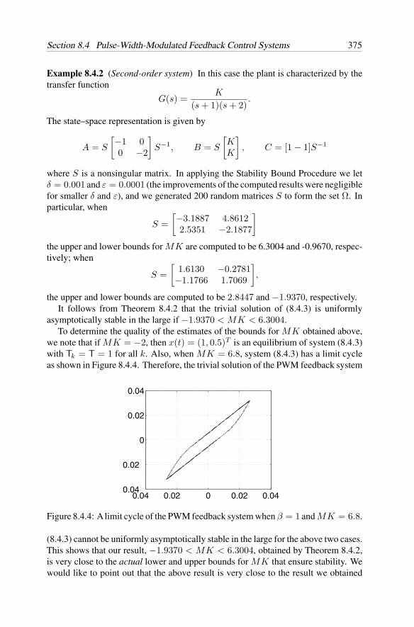
Section 8.4 Pulse-Width-Modulated Feedback Control Systems 375
Example 8.4.2 (Second-order system) In this case the plant is characterized by thetransfer function
G(s) =K
(s + 1)(s + 2).
The state–space representation is given by
A = S
[−1 00 −2
]S−1, B = S
[KK
], C = [1 − 1]S−1
where S is a nonsingular matrix. In applying the Stability Bound Procedure we letδ = 0.001 and ε = 0.0001 (the improvements of the computed results were negligiblefor smaller δ and ε), and we generated 200 random matrices S to form the set Ω. Inparticular, when
S =[−3.1887 4.86122.5351 −2.1877
]the upper and lower bounds for MK are computed to be 6.3004 and -0.9670, respec-tively; when
S =[
1.6130 −0.2781−1.1766 1.7069
],
the upper and lower bounds are computed to be 2.8447 and −1.9370, respectively.It follows from Theorem 8.4.2 that the trivial solution of (8.4.3) is uniformly
asymptotically stable in the large if −1.9370 < MK < 6.3004.To determine the quality of the estimates of the bounds for MK obtained above,
we note that if MK = −2, then x(t) = (1, 0.5)T is an equilibrium of system (8.4.3)with Tk = T = 1 for all k. Also, when MK = 6.8, system (8.4.3) has a limit cycleas shown in Figure 8.4.4. Therefore, the trivial solution of the PWM feedback system
0.04 0.02 0 0.02 0.040.04
0.02
0
0.02
0.04
Figure 8.4.4: Alimit cycle of the PWM feedback system when β = 1 and MK = 6.8.
(8.4.3) cannot be uniformly asymptotically stable in the large for the above two cases.This shows that our result, −1.9370 < MK < 6.3004, obtained by Theorem 8.4.2,is very close to the actual lower and upper bounds for MK that ensure stability. Wewould like to point out that the above result is very close to the result we obtained
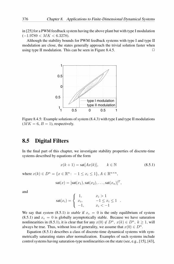
376 Chapter 8. Applications to Finite-Dimensional Dynamical Systems
in [25] for a PWM feedback system having the above plant but with type I modulation(−1.9789 < MK < 6.3278).
Although the stability bounds for PWM feedback systems with type I and type IImodulation are close, the states generally approach the trivial solution faster whenusing type II modulation. This can be seen in Figure 8.4.5.
1 0.5 0 0.5 11
0.5
0
0.5
1
type I modulationtype II modulation
Figure 8.4.5: Example solutions of system (8.4.3) with type I and type II modulations(MK = 6, B = 1), respectively.
8.5 Digital Filters
In the final part of this chapter, we investigate stability properties of discrete-timesystems described by equations of the form
x(k + 1) = sat[Ax(k)], k ∈ N (8.5.1)
where x(k) ∈ Dn = x ∈ Rn : − 1 ≤ xi ≤ 1, A ∈ R
n×n,
sat(x) = [sat(x1), sat(x2), . . . , sat(xn)]T ,
and
sat(xi) =
1, xi > 1xi, −1 ≤ xi ≤ 1−1, xi < −1
.
We say that system (8.5.1) is stable if xe = 0 is the only equilibrium of system(8.5.1) and xe = 0 is globally asymptotically stable. Because we have saturationnonlinearities in (8.5.1), it is clear that for any x(0) ∈ Dn, x(k) ∈ Dn, k ≥ 1, willalways be true. Thus, without loss of generality, we assume that x(0) ∈ Dn.
Equation (8.5.1) describes a class of discrete-time dynamical systems with sym-metrically saturating states after normalization. Examples of such systems includecontrol systems having saturation-type nonlinearities on the state (see, e.g., [15], [43],
Section 8.5 Digital Filters 377
and [56]), neural networks defined on hypercubes (see, e.g., [42] and [53]), and digitalfilters using saturation overflow arithmetic (see, e.g., [43], [57], and [63]).
System (8.5.1) may be used to represent control systems with saturating states withno external inputs. In the analysis and design of such systems, the first fundamentalquestion addresses stability: under what conditions is xe =0 an equilibrium and whenis this equilibrium globally asymptotically stable?
The condition that A is a stable matrix, that is, every eigenvalue λi of A satisfies|λi| < 1, is not sufficient for system (8.5.1) to be stable. (It is easy to give examplesfor which A is a stable matrix, but system (8.5.1) is not stable.)
In many important applications, equation (8.5.1) may be used to represent digitalprocessing systems, including digital filters and digital control systems (see, e.g., [15],[43], [56], [57], [63], and [72]) with finite wordlength arithmetic under zero externalinputs. In such systems, saturation arithmetic is used to cope with the overflow. Theabsence of limit cycles in such systems is of great interest and can be guaranteed bythe global asymptotic stability of the equilibrium xe = 0 for (8.5.1). The Lyapunovtheory has been found to be an appropriate method for solving such problems (see,e.g., [43], [57], and [72]).
A. A general result for discrete-time systems with state saturationnonlinearities
In establishing our results, we make use of Lyapunov functions for the linear systemscorresponding to system (8.5.1), given by
w(k + 1) = Aw(k), k ∈ N (8.5.2)
where A ∈ Rn×n is defined in (8.5.1).
We recall that for a general autonomous system
x(k + 1) = f(x(k)), k ∈ N, (8.5.3)
with x(k) ∈ Rn and f : R
n → Rn, xe is an equilibrium for (8.5.3) if and only if
xe = f(xe).
We assume, without loss of generality that xe =0 (refer to Subsection 6.1B). Recallalso that the equilibrium xe = 0 for system (8.5.3) is globally asymptotically stable,or asymptotically stable in the large, if there exists a continuous function v : R
n → R
which is positive definite, radially unbounded, and along solutions of (8.5.3) satisfiesthe condition that
Dv(8.5.3)(x(k))= v(x(k + 1)) − v(x(k)) = v(f(x(k))) − v(x(k)) (8.5.4)
is negative definite for all x(k) ∈ Rn (refer to Theorem 6.3.2(a)).
In the stability analysis of the equilibrium xe = 0 of system (8.5.1), we find ituseful to employ Lyapunov functions v whose value for a given state vector w ∈ Dn isgreater than the value for the corresponding saturated state vector sat(w). Specifically,we make the following assumption.
378 Chapter 8. Applications to Finite-Dimensional Dynamical Systems
Assumption 8.5.1 Assume that for system (8.5.2), there exists a continuous functionv : R
n → R with the following properties:
(i) v is positive definite, radially unbounded, and
Dv(8.5.2)(w(k))= v(w(k + 1)) − v(w(k)) = v(Aw(k)) − v(w(k))
is negative definite for all w(k) ∈ Rn (and thus, the eigenvalues of A are within the
unit circle).(ii) For all w ∈ R
n such that w ∈ Dn, it is true that
v(sat(w)) < v(w) (8.5.5)
where Dn and sat(·) are defined in (8.5.1).
An example of a function v1 : R2 → R that satisfies (8.5.5) is given by v1(w) =
d1w21 + d2w
22, d1, d2 > 0. On the other hand, the function v2 : R
2 → R given byv2(w) = w2
1 + (2w1 + w2)2 does not satisfy (8.5.5). To see this, consider the pointw = [−0.99, 1.05]T ∈ D2 and note that v2(sat(w)) = 1.9405 and v2(w) = 1.845.
We are now in a position to prove the following result.
Theorem 8.5.1 If Assumption 8.5.1 holds, then the equilibrium xe = 0 of system(8.5.1) is globally asymptotically stable.
Proof . Because Assumption 8.5.1 is true, there exists a positive definite and radiallyunbounded function v for system (8.5.2) such that (8.5.5) is true, which in turn impliesthat v(sat(Aw)) ≤ v(Aw) for all w ∈ R
n. Also, by Assumption 8.5.1, v(Aw(k)) −v(w(k)) < 0 for all w(k) = 0. Thus, along the solutions of system (8.5.1), we have
Dv(8.5.1)(x(k)) = v(x(k + 1)) − v(x(k))= v(sat[Ax(k)]) − v(x(k))≤ v(Ax(k)) − v(x(k))< 0
for all x(k) = 0 and Dv(8.5.1)(x(k)) = 0 if and only if x(k) = 0. Therefore, v(x) ispositive definite and radially unbounded, and Dv(8.5.1)(x) is negative definite for allx. Hence, in view of Theorem 6.3.2(a), the equilibrium xe = 0 of system (8.5.1) isglobally asymptotically stable.
Remark 8.5.1 In particular, for fixed p, 1 ≤ p ≤ ∞, let us choose
v(w) = |w|p =( n∑
i=1
|wi|p)1/p
for system (8.5.2) and assume that ‖A‖p < 1, where ‖A‖p denotes the matrix norminduced by the vector norm |w|p. Under these conditions, Assumption 8.5.1 is true.To see this, note that v is positive definite and radially unbounded, that
v(Aw) = |Aw|p ≤ ‖A‖p|w|p < |w|p = v(w),
and that |sat(w)|p < |w|p, for all w ∈ Rn such that w ∈ Dn.
Section 8.5 Digital Filters 379
Therefore, the equilibrium xe = 0 of system (8.5.1) is globally asymptoticallystable if
‖A‖p < 1 (8.5.6)
for some p, 1 ≤ p ≤ ∞.In the case of digital filters, the above argument holds for any type of overflow
nonlinearity ϕ : R → [−1, 1]. To see this, let f(w) = [ϕ(w1), . . . , ϕ(wn)]T and notethat in this case |f(w)|p < |w|p for all w ∈ R
n such that w ∈ Dn.
B. Results involving quadratic Lyapunov functions
In order to generate quadratic form Lyapunov functions that satisfy Assumption 8.5.1for systems described by equation (8.5.1), we find it convenient to utilize the nextassumption.
Assumption 8.5.2 Let
xs = sat(x) = [sat(x1), . . . , sat(xn)]T
for x ∈ Rn and let H ∈ R
n×n denote a positive definite matrix. Assume that
xTs Hxs < xT Hx, (8.5.7)
whenever x ∈ Dn, x ∈ Rn.
An example of a matrix that satisfies Assumption 8.5.2 is any diagonal matrixwith positive diagonal elements. On the other hand, the positive definite matrix Hgiven by
H =[
5 22 1
],
does not satisfy Assumption 8.5.2. (To see this, refer to the example followingAssumption 8.5.1 by noting that v2(x) = xT Hx.)
The next result gives a necessary and sufficient condition for matrices to satisfyAssumption 8.5.2. This result is very useful in applications.
Lemma 8.5.1 An n×n positive definite matrix H = [hij ] satisfies Assumption 8.5.2if and only if
hii ≥n∑
j=1,j =i
|hij |, i = 1, . . . , n. (8.5.8)
Proof . This lemma is a special case of Lemma 8.5.2 (when L = 1). For the statementand proof of Lemma 8.5.2, refer to Subsection C of the present section.
The following result is a direct consequence of Theorem 8.5.1.
380 Chapter 8. Applications to Finite-Dimensional Dynamical Systems
Corollary 8.5.1 The equilibrium xe = 0 of system (8.5.1) is globally asymptoticallystable if there exists a matrix H that satisfies Assumption 8.5.2 such that
Q= H − AT HA
is positive definite.
Proof . By choosing v(x) = xT Hx, the proof follows from Theorem 8.5.1.
In the next result, Theorem 8.5.2, we show that Corollary 8.5.1 is actually truewhen Q is only positive semidefinite, still assuming that A is stable.
Theorem 8.5.2 The equilibrium xe = 0 of system (8.5.1) is globally asymptoticallystable if A is stable and if there exists a matrix H that satisfies Assumption 8.5.2such that
Q= H − AT HA
is positive semidefinite.
Proof . Let us choose v(x(k)) = xT (k)Hx(k) for the system (8.5.1). The functionv is clearly positive definite and radially unbounded. Also, because
Dv(8.5.1)(x(k)) = v(x(k + 1)) − v(x(k))
= [sat(Ax(k))]T H[sat(Ax(k))] − xT (k)Hx(k)
≤ xT (k)(AT HA − H)x(k),
and because H−AT HA is positive semidefinite, Dv(8.5.1)(x(k)) is negative semidef-inite for all x(k). Therefore, the equilibrium xe = 0 is stable (refer to Theorem6.3.1(a)). To show that it is asymptotically stable, we must show that x(k) → 0 ask → ∞ (refer to Definition 6.1.1(h)).
Let us consider an n consecutive step iteration for system (8.5.1), from n0 ≥ 0 ton+n0. Without loss of generality, assume that system (8.5.1) saturates at k = l, l ∈[n0, n + n0). In view of Assumption 8.5.2, it follows that
v(x(l + 1)) = xT (l + 1)Hx(l + 1)
= [sat(Ax(l))]T H[sat(Ax(l))]
< [Ax(l)]T HAx(l)
≤ xT (l)Hx(l)
= v(x(l)).
On the other hand, if no saturation occurs during this period, then, using the factthat if H −AT HA is positive semidefinite, then H − (AT )nHAn is positive definite
Section 8.5 Digital Filters 381
for any n > 1 when A is stable (see, e.g., [72]), we have
v(x(n + n0)) = xT (n + n0)Hx(n + n0)
= [Anx(n0)]T HAnx(n0)
= xT (n0)(AT )nHAnx(n0)
< xT (n0)Hx(n0)
= v(x(n0)).
Therefore, we can conclude that for the sequence k : k = 1, 2, . . . , there alwaysexists an infinite subsequence kj : j = 1, 2, . . . , such that Dv(8.5.1)(x(kj)) isnegative for x(kj) = 0 and that v(x(k)) ≤ v(x(kj)) for all k ≥ kj . Because vis a positive definite quadratic form, it follows that v(x(kj)) → 0 as j → ∞, andtherefore v(x(k)) → 0 as k → ∞. This in turn implies that x(k) → 0 as k → ∞.Thus, the equilibrium xe = 0 of (8.5.1) is globally asymptotically stable.
C. Stability of digital filters with generalized overflownonlinearities
Because no limit cycles can exist in a digital filter if its trivial solution is globallyasymptotically stable, we can use the results of this section to establish the followingresults for n-th order digital filters with saturation arithmetic.
Corollary 8.5.2 (i) A digital filter described by (8.5.1) is free of limit cycles ifAssumption 8.5.1 is satisfied. (ii) A digital filter described by (8.5.1) is free of limitcycles if A is stable and if there exists a matrix H that satisfies Assumption 8.5.2,such that
Q= H − AT HA
is positive semidefinite.
We now consider nth-order digital filters described by equations of the form
x(k + 1) = f [Ax(k)], k ∈ N (8.5.9)
where x(k) ∈ Rn, A ∈ R
n×n,
f(x) = [ϕ(x1), ϕ(x2), . . . , ϕ(xn)]T , (8.5.10)
and ϕ : R → [−1, 1] is piecewise continuous. We call system (8.5.9) a fixed-pointdigital filter using overflow arithmetic. For such filters, we make the followingassumption.
Assumption 8.5.3 Let f be defined as in (8.5.10). Assume that H ∈ Rn×n is a
positive definite matrix and that
f(x)T Hf(x) < xT Hx, (8.5.11)
for all x ∈ Rn, x ∈ Dn.
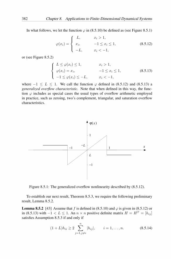
382 Chapter 8. Applications to Finite-Dimensional Dynamical Systems
In what follows, we let the function ϕ in (8.5.10) be defined as (see Figure 8.5.1)
ϕ(xi) =
L, xi > 1,
xi, −1 ≤ xi ≤ 1,
−L, xi < −1,
(8.5.12)
or (see Figure 8.5.2)L ≤ ϕ(xi) ≤ 1, xi > 1,
ϕ(xi) = xi, −1 ≤ xi ≤ 1,
−1 ≤ ϕ(xi) ≤ −L, xi < −1,
(8.5.13)
where −1 ≤ L ≤ 1. We call the function ϕ defined in (8.5.12) and (8.5.13) ageneralized overflow characteristic. Note that when defined in this way, the func-tion ϕ includes as special cases the usual types of overflow arithmetic employedin practice, such as zeroing, two’s complement, triangular, and saturation overflowcharacteristics.
ϕ( )
x
1
L
1
x
−1
−L−1
Figure 8.5.1: The generalized overflow nonlinearity described by (8.5.12).
To establish our next result, Theorem 8.5.3, we require the following preliminaryresult, Lemma 8.5.2.
Lemma 8.5.2 [43] Assume that f is defined in (8.5.10) and ϕ is given in (8.5.12) orin (8.5.13) with −1 < L ≤ 1. An n × n positive definite matrix H = HT = [hij ]satisfies Assumption 8.5.3 if and only if
(1 + L)hii ≥ 2n∑
j=1,j =i
|hij |, i = 1, . . . , n. (8.5.14)
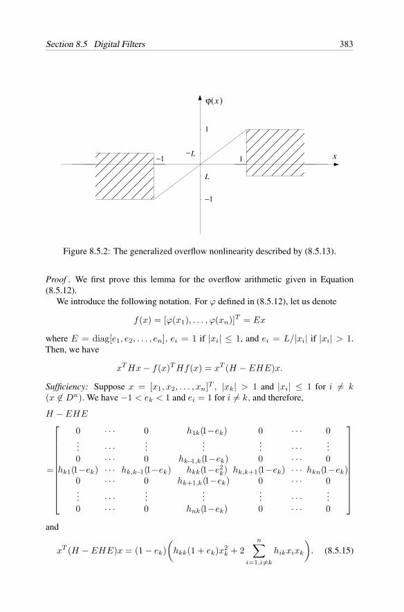
Section 8.5 Digital Filters 383
ϕ( )
x
1
L
1
x
−1
−L−1
Figure 8.5.2: The generalized overflow nonlinearity described by (8.5.13).
Proof . We first prove this lemma for the overflow arithmetic given in Equation(8.5.12).
We introduce the following notation. For ϕ defined in (8.5.12), let us denote
f(x) = [ϕ(x1), . . . , ϕ(xn)]T = Ex
where E = diag[e1, e2, . . . , en], ei = 1 if |xi| ≤ 1, and ei = L/|xi| if |xi| > 1.Then, we have
xT Hx − f(x)T Hf(x) = xT (H − EHE)x.
Sufficiency: Suppose x = [x1, x2, . . . , xn]T , |xk| > 1 and |xi| ≤ 1 for i = k(x ∈ Dn). We have −1 < ek < 1 and ei = 1 for i = k, and therefore,
H − EHE
=
0 · · · 0 h1k(1−ek) 0 · · · 0... · · ·
......
... · · ·...
0 · · · 0 hk−1,k(1−ek) 0 · · · 0hk1(1−ek) · · · hk,k−1(1−ek) hkk(1−e2
k) hk,k+1(1−ek) · · · hkn(1−ek)0 · · · 0 hk+1,k(1−ek) 0 · · · 0... · · ·
......
... · · ·...
0 · · · 0 hnk(1−ek) 0 · · · 0
and
xT (H − EHE)x = (1 − ek)(
hkk(1 + ek)x2k + 2
n∑i=1,i =k
hikxixk
). (8.5.15)
384 Chapter 8. Applications to Finite-Dimensional Dynamical Systems
Note that in the above equation we have used the fact that hij = hji.From |xi| ≤ 1 for i = k, |xk| > 1, ek|xk| = L and L > −1, we have
(1 + L)|xixk| ≤ (1 + L)|xk| < (|xk| + L)|xk| = (1 + ek)x2k.
Hence, from (8.5.15), we have
xT (H − EHE)x ≥ (1 − ek)(
hkk(1 + ek)x2k − 2
n∑i=1,i =k
|hikxixk|)
> (1 − e2k)x2
k
(hkk − 2
1 + L
n∑i=1,i =k
|hik|)
≥ 0;
that is, xT Hx > xT EHEx = f(x)T Hf(x).Denote M = 1, 2, . . . , m for any m, 0 < m ≤ n, and
N = ki : 0 < ki ≤ n, ki = kj , when i = j, i, j ∈ M.
Now suppose that x = [x1, x2, . . . , xn]T, |xk| > 1 for k∈N and |xi| ≤ 1 for i ∈ N(x ∈ Dn). Following the same procedure as above, we have
xT (H − EHE)x =∑k∈N
(1 − ek)(
hkk(1 + ek)x2k + 2
n∑i=1,i ∈N
hikxixk
)+∑k∈N
∑l∈N,l =k
hklxkxl(1 − ekel)
≥∑k∈N
(1 − ek)(
hkk(1 + ek)x2k − 2
n∑i=1,i ∈N
|hikxixk|)
+∑k∈N
∑l∈N,l =k
hklxkxl(1 − ekel)
>∑k∈N
(1 − e2k)x2
k
(hkk − 2
1 + L
n∑i=1,i ∈N
|hik|)
+∑k∈N
∑l∈N,l =k
hklxkxl(1 − ekel)
=∑k∈N
(1 − e2k)x2
k
(hkk − 2
1 + L
n∑i=1,i =k
|hik|)
+2
1 + L
∑k∈N
(1 − e2k)x2
k
∑i∈N,i =k
|hik|
+∑k∈N
∑l∈N,l =k
hklxkxl(1 − ekel). (8.5.16)
Section 8.5 Digital Filters 385
The first summation of the right-hand side in (8.5.16) is nonnegative, by assump-tion. Considering the last two terms in (8.5.16), by noting that −1 < ek < 1 andek|xk| = L for k ∈ N, and −1 < L ≤ 1, we have
21 + L
∑k∈N
(1 − e2k)x2
k
∑i∈N,i =k
|hik| +∑k∈N
∑l∈N,l =k
hklxkxl(1 − ekel)
≥∑k∈N
∑l∈N,l =k
(1 − e2k)x2
k|hkl| −∑k∈N
∑l∈N,l =k
|hklxkxl|(1 − ekel)
=∑k∈N
∑l∈N,l =k
|hklxk|(|xk| − ekL − |xl| + ekL
)=∑k∈N
∑l∈N,l =k
|hkl|x2k −
∑k∈N
∑l∈N,l =k
|hklxkxl|
=∑k∈N
∑l∈N,l>k
|hkl|(x2k + x2
l ) − 2∑k∈N
∑l∈N,l>k
|hklxkxl|
=∑k∈N
∑l∈N,l>k
|hkl|(|xk| − |xl|
)2 ≥ 0.
Therefore,xT Hx − f(x)T Hf(x) = xT (H − EHE)x > 0,
for any x ∈ Rn such that x ∈ Dn.This proves the sufficiency.
Necessity: It suffices to show that if (8.5.14) does not hold, there always exist somepoints x ∈ Dn, such that
xT Hx ≤ f(x)T Hf(x).
Suppose that (8.5.14) does not hold for i = k; that is,
δ= 2
n∑j=1,j =k
|hkj | − (1 + L)hkk > 0.
Let us choose |xk| = 1 + ξ, ξ > 0, and xi = −sign(hikxk), i = k, where
sign(y) =
1, y > 0,0, y = 0,
−1, y < 0.
Then, x = [x1, . . . , xn]T ∈ Dn and (8.5.15) becomes
xT (H − EHE)x = (1 − ek)(
hkk(1 + ek)x2k − 2
n∑i=1,i =k
|hikxk|)
= (1 − ek)|xk|(
hkkξ + (1 + L)hkk − 2n∑
i=1,i =k
|hki|)
= (1 − ek)|xk|(hkkξ − δ).
386 Chapter 8. Applications to Finite-Dimensional Dynamical Systems
Clearly, when we choose 0 < ξ ≤ δ/hkk, we have
xT Hx − f(x)T Hf(x) = xT (H − EHE)x ≤ 0.
Note here that hkk > 0 because H is positive definite.This proves the necessity.For the overflow nonlinearity given in (8.5.13), the proof of sufficiency is similar to
the proof given above. To prove necessity, we note that for a given L, when |xi| > 1,ϕ(xi) in (8.5.13) may assume any value in the crosshatched regions in 8.5.2 including±L (which is the case for the arithmetic given by (8.5.12)).
We note that condition (8.5.14) is usually called a diagonal dominance conditionin the literature [51].
We are now in a position to prove the following result.
Theorem 8.5.3 The nth-order digital filter described by (8.5.9), in which ϕ is givenin (8.5.12) or (8.5.13) with −1 < L ≤ 1, is free of limit cycles, if A is stable and ifthere exists a positive definite matrix H that satisfies (8.5.14), such that
Q= H − AT HA
is positive semidefinite.
Proof . We can follow the same procedure as in the proof of Theorem 8.5.2 to provethat under the present conditions, the equilibrium xe = 0 of system (8.5.9) is glob-ally asymptotically stable. Thus the digital filter described by (8.5.9) is free of limitcycles.
For the two’s complement and triangular overflow characteristics, we have thefollowing.
Lemma 8.5.3 An n×n positive definite matrix H = [hij ] satisfies Assumption 8.5.3when f represents the two’s complement or the triangular arithmetic, if and only ifH is a diagonal matrix with positive diagonal elements.
Proof . The proof is similar to the proof of Lemma 8.5.2.
D. Examples
To demonstrate the applicability of the results in the previous two subsections, wenow consider two specific examples.
Example 8.5.1 For system (8.5.1) with
A =[
1 2−3
−0.1 0.9
], (8.5.17)
we have ‖A‖p > 1, p = 1, 2, or ∞. Therefore, condition (8.5.6) fails as a globalasymptotic stability test for this example, as shown in the following.
Section 8.6 Notes and References 387
Assumption 8.5.2 is satisfied for this example by choosing
H =[
1 0.50.5 0.8
]. (8.5.18)
Inasmuch as
Q = H − AT HA =[
0.092 0.003250.00325 0.023875
]is positive definite, all conditions of Theorem 8.5.2 are satisfied and the equilibriumxe = 0 of system (8.5.1) with A specified by (8.5.17) is globally asymptoticallystable.
Example 8.5.2 For system (8.5.1) with A given by
A =
−1 0 0.1 00.2 −0.6 0 0.8
−0.1 0.1 0.8 00.1 0 0.1 −0.5
, (8.5.19)
it can easily be verified that ‖A‖p > 1, p = 1, 2, or ∞. Hence, condition (8.5.6) failsagain as a global asymptotic stability test for the present example.
Assumption 8.5.2 is satisfied for this example by choosing
H =
1.4 0 −0.2 0.40 1.6 0.2 −0.4
−0.2 0.2 3.4 0.50.4 −0.4 0.5 3
. (8.5.20)
Because
Q = H − AT HA =
0.026 0.161 −0.003 0.0770.161 1.014 −0.003 0.497
−0.003 −0.003 1.124 0.7740.077 0.497 0.774 0.906
is positive definite, all conditions of Theorem 8.5.2 are satisfied, and the equilibriumxe = 0 of system (8.5.1) with such a coefficient matrix is globally asymptoticallystable.
8.6 Notes and References
For further details concerning Lure-type of results (Theorem 8.1.1), refer to [45].The Yacubovich–Kalman Lemma (Lemma 8.1.1) was independently established byYacubovich [73] and Kalman [32]. The proof of Popov’s criterion (Theorem 8.1.2),using the Yacubovich–Kalman Lemma, follows along the proof given in Lefschetz[40]. In the original proof of results of this type, Popov relied on functional analysis
388 Chapter 8. Applications to Finite-Dimensional Dynamical Systems
techniques [62]. In addition to [40], there are several other monographs on theabsolute stability of regulator systems, including Aizerman and Gantmacher [2] andNarendra and Taylor [60]. Our treatment in Section 8.1 of the absolute stability ofregulator systems is in the spirit of the presentation on this subject given in [52]and [54].
For background material and further qualitative studies of the class of artificialneural networks considered in Section 8.2, refer, for example, to [9], [11], [20], [37],[41], and [47]–[50]. The particular method used in this section was popularized byHopfield [20]. The first rigorous proof of Theorem 8.2.1 (in a more general setting)was given in [11] by Cohen and Grossberg. For further results concerning associatememories realized by means of feedback artificial neural networks, refer to [47], [49],and [50]. The idea of viewing neural networks as interconnected systems is motivatedby the viewpoints adopted in [19], [51], and [64]. Our presentation in Section 8.2 isprimarily based on [48], [49], and [50].
The analysis and synthesis of linear digital feedback control systems with one uni-form sampling rate have been of interest for a long time ([1], [3], [14], [15], [30]) andin recent works, systems with nonuniform sampling rates have also been addressed(e.g., [28], and [29]). The implementation of the controllers of such systems by digitalcomputers, resulting in digital feedback control systems, has brought about severalinvestigations of the effects of the quantization nonlinearities (e.g., [7], [10], [13],[21], [26], [27], [55], [56], [65], and [69]). Additionally, analyses of digital controlsystems with nonlinear plants have also been conducted (e.g., [6], [21], and [26]).These works address the particular conditions under which a linearization of the plantis permissible (i.e., under which conditions the stability properties of the feedbackcontrol systems with nonlinear plants can be deduced from the corresponding feed-back control systems with the nonlinear plants replaced by their linearization). Wenote here that although similar in spirit, the results presented in [26] apply to a sub-stantially larger class of systems than those considered in [6]. Our presentation inSection 8.3 follows closely the development given in [21] and [26].
The results of Section 8.4 concerning pulse-width-modulated feedback controlsystems are based on [22]. There have only been a few results ([5], [16], [23], [36],[38]) concerning PWM feedback systems with type II modulation. (The majoritystability results reported in the literature are for PWM feedback systems with type Imodulation, e.g., [5], [25], [58], and [71].) The examples treated in this section arefrom [5] and [16]. Our comparisons, using these examples, indicate that the stabilityresults reported in Section 8.4 are less conservative than the results reported in theabove references. The reason for this appears twofold. First, the results in Section 8.4are based on the general stability results for DDS which require that the quadraticLyapunov functions employed in the analysis decrease along the solutions of thePWM systems only at instants when the PWM controller is turned off (and satisfycertain bounds at the remaining times) whereas the results reported in [5] requirethat the Lyapunov functions that are utilized (usually quadratic ones) decrease alongthe solutions of the PWM system at all times and results in [16] use an averagingmethod combined with the Popov criterion or the circle criterion. Additionally, thestability results for PWM feedback control systems reported in Section 8.4 incorporate
Bibliography 389
optimization procedures to decrease conservatism, which is not the case in the stabilityresults cited above.
For additional references on PWM feedback control systems (not necessarily deal-ing with stability), the reader may want to consult [4], [12], [17], [18], [31], [33]–[35],[39], [46], [61], [66]–[68], and [70], [71].
For a discussion of stability results of systems endowed with saturation nonlin-earities and their applications to digital filters, refer to the monograph [44] and thereferences cited therein. The material in Section 8.5 is based on results presented in[24] and [43].
Bibliography[1] J. Ackerman, Sampled-Data Control Systems: Analysis and Synthesis, Robust
Systems Design, New York: Springer-Verlag, 1985.
[2] M. A. Aizerman and F. R. Gantmacher, Absolute Stability of Regular Systems,San Francisco: Holden-Day, 1963.
[3] P. J. Antsaklis and A. N. Michel, Linear Systems, Boston: Birkhauser, 2006.
[4] G. S. Axelby, “Analysis of pulse-width modulation with a variable transport lagin a rendezvoue radar,” IEEE Trans. Autom. Control, vol. 9, pp. 514–525, 1964.
[5] A. Balestrino, A. Eisenberg, and L. Sciavicco, “A generalized approach to thestability analysis of PWM feedback control systems,” J. Franklin Institute,vol. 298, pp. 45–48, 1974.
[6] A. T. Barabanov and Ye. F. Starozhilov, “Investigation of the stability of con-tinuous discrete systems by Lyapunov’s second methods,” Soviet J. Autom. Inf.Sci., vol. 21, pp. 35–41, 1988.
[7] J. E. Bertram, “The effects of quantization in sampled feedback systems,” Trans.AIEE Appl. Ind., Part 2, vol. 77, pp. 177–181, 1958.
[8] E. Bolzer, “The limitation of impulses in cardiac muscle,” Amer. J. Physiol.,vol. 138, pp. 273–282, 1942.
[9] G. A. Carpenter, M. Cohen, and S. Grossberg, “Computing with neural net-works,” Science, vol. 235, pp. 1226–1227, 1987.
[10] J.-H. Chou, S.-H. Chen, and I.-R. Horng, “Robust stability bound on linear time-varying uncertainties for linear digital control systems under finite wordlengtheffects,” JSME Int. J., Series C, vol. 39, pp. 767–771, 1996.
[11] M. Cohen and S. Grossberg, “Absolute stability of global pattern formation andparallel memory storage by competitive networks,” IEEE Trans. Syst., Man,Cyberne., vol. 13, pp. 815–826, 1983.
[12] F. R. Delfelt and G. J. Murphy, “Analysis of pulse-width-modulated controlsystems,” IEEE Trans. Autom. Control, vol. 6, pp. 283–292, 1961.
[13] J. A. Farrell and A. N. Michel, “Estimates of asymptotic trajectory boundsin digital implementations of linear feedback control systems,” IEEE Trans.Autom. Control, vol. 34, pp. 1319–1324, 1989.
390 Chapter 8. Applications to Finite-Dimensional Dynamical Systems
[14] B. A. Francis and T. T. Georgiou, “Stability theory for linear time-invariantplants with periodic digital controllers,” IEEE Trans. Autom. Control, vol. 33,pp. 820–832, 1988.
[15] G. F. Franklin and J. D. Powell, Digital Control of Dynamic Systems, Reading,MA: Addison-Wesley, 1980.
[16] A. Kh. Gelig and A. N. Churilov, Stability and Oscillations of Nonlinear Pulse-Modulated Systems, Boston: Birkhauser, 1998.
[17] M. Gouy, “On a constant temperature oven,” J. Physique, vol. 6, pp. 479–483,1897.
[18] S. C. Gupta and E. I. Jury, “Statistical study of pulse-width-modulated controlsystems,” J. Franklin Institute, vol. 273, pp. 292–321, 1962.
[19] L. T. Grujic, A. A. Martynyuk, and M. Ribbens-Pavella, Large Scale SystemsUnder Structural and Singular Perturbation, Berlin: Springer-Verlag, 1987.
[20] J. J. Hopfield, “Neurons with graded response have collective computationalproperties like those of two-state neurons,” Proc. Nat. Acad. Sci. USA, vol. 81,pp. 3088–3092, 1984.
[21] L. Hou, Qualitative Analysis of Discontinuous Deterministic and StochasticDynamical Systems, Ph.D. Dissertation, University of Notre Dame, Notre Dame,IN, 2000.
[22] L. Hou, “Stability analysis of pulse-width-modulated feedback systems withtype 2 modulation,” Proc. 44th IEEE Conference on Decision and Control,Paradise Island, Bahamas, Dec. 2004, pp. 2972–2977.
[23] L. Hou, “Stability analysis of pulse-width-modulated feedback systems withtype 2 modulation: The critical case,” Proc. 2005 Int. Symposium on Circuitsand Systems, Tokyo, Japan, May 2005, pp. 3187–3190.
[24] L. Hou and A. N. Michel, “Asymptotic stability of systems with saturationconstraints,” IEEE Trans. Autom. Control, vol. 43, pp. 1148–1154, 1998.
[25] L. Hou andA. N. Michel, “Stability analysis of pulse-width-modulated feedbacksystems,” Automatica, vol. 37, pp. 1335–1349, 2001.
[26] L. Hou, A. N. Michel, and H. Ye, “Some qualitative properties of sampled-datacontrol systems,” Proc. 35th IEEE Conference on Decision and Control, Kobe,Japan, Dec. 1996, pp. 911–917.
[27] B. Hu, Z. Feng, and A. N. Michel, “Quantized sampled-data feedback stabiliza-tion for linear and nonlinear control systems,” Proc. 38th IEEE Conference onDecision and Control, Phoenix, AZ, Dec. 1999, pp. 4392–4397.
[28] B. Hu and A. N. Michel, “Robust analysis of digital control systems withtime-varying sampling periods,” Proc. 1999 American Control Conference, SanDiego, CA, June 1999, pp. 3484–3488.
[29] B. Hu and A. N. Michel, “Stability analysis of digital feedback control systemswith time-varying sampling periods,” Automatica, vol. 36, pp. 897–905, 2000.
Bibliography 391
[30] P. A. Iglesias, “On the stability of sampled-date linear time-varying feedbacksystems,” Proc. 33rd IEEE Conference on Decision and Control, Orlando, FL,Dec. 1994, pp. 219–224.
[31] T. T. Kadota and H. C. Bourne, “Stability conditions of pulse-width-modulatedsystems through the second method of Lyapunov,” IEEE Trans. Autom. Control,vol. 6, pp. 266–276, 1961.
[32] R. E. Kalman, “Lyapunov functions for the problem of Lure in automatic con-trol,” Proc. Nat. Acad. Sci. USA, vol. 49, pp. 201–205, 1963.
[33] B. Katz, “The nerve impulse,” Sci. Amer., vol. 187, pp. 55–64, 1962.
[34] A. Khayatian and D. G. Taylor, “Feedback control of linear systems by multi-ratepulse-width modulation,” IEEE Trans. Autom. Control, vol. 39, pp. 1292–1297,1994.
[35] A. Khayatian and D. G. Taylor, “Multi-rate modeling and control designfor switched-mode power converters,” IEEE Trans. Autom. Control, vol. 39,pp. 1848–1852, 1994.
[36] A. I. Korshunov, “Remarks on the article by V.M. Kuntsevich ‘Global asymp-totic stability of two classes of control systems with pulse-duration andpulse-frequency modulations’,” Autom. Remote Control, vol. 34, no. 8, pt. 2,pp. 1356–1357, Aug. 1973.
[37] B. Kosko, Neural Networks and Fuzzy Systems, Englewood Cliffs, NJ: PrenticeHall, 1992.
[38] V. M. Kuntsevich, “Global asymptotic stability of two classes of control systemswith pulse duration and pulse frequency modulations,” Autom. Remote Control,vol. 33, no. 7, pp. 1124–32, July 1972.
[39] V. M. Kuntsevich and Yu. N. Akekhovol, “Fundamentals of nonlinear controlsystems with pulse-frequency and pulse width modulation,” Automatica, vol. 7,pp. 83–81, 1971.
[40] S. Lefschetz, Stability of Nonlinear Control Systems, New York: AcademicPress, 1965.
[41] J.-H. Li, A. N. Michel, and W. Porod, “Qualitative analysis and synthesis of aclass of neural networks,” IEEE Trans. Circ. Syst., vol. 35, pp. 976–986, 1988.
[42] J.-H. Li, A. N. Michel, and W. Porod, “Analysis and synthesis of a class of neuralnetworks: Linear systems operating on a closed hypercube,” IEEE Trans. Circ.Syst., vol. 36, pp. 1405–1422, Nov. 1989.
[43] D. Liu and A. N. Michel, “Asymptotic stability of discrete-time systems withsaturation nonlinearities with applications to digital filters,” IEEE Trans. Circ.Syst. I: Fund. Theor. Appl.,vol. 39, pp. 798–807, Oct. 1992.
[44] D. Liu and A. N. Michel, Dynamical Systems with Saturation Nonlinearities:Analysis and Design, New York: Springer-Verlag, 1994.
[45] A. I. Lure, On Some Nonlinear Problems in the Theory of Automatic Control,London: H. M. Stationary Office, 1951.
392 Chapter 8. Applications to Finite-Dimensional Dynamical Systems
[46] B. H. C. Matthews, “The nervous system as an electrical instrument,” J. Inst.Elec. Eng., vol. 95, pp. 397–402, 1948.
[47] A. N. Michel and J. A. Farrell, “Associate memories via artificial neural net-works,” IEEE Control Sys. Mag., vol. 10, pp. 6–17, 1990.
[48] A. N. Michel, J. A. Farrell, and W. Porod, “Qualitative analysis of neural net-works,” IEEE Trans. Circ. Syst., vol. 36, pp. 229–243, 1989.
[49] A. N. Michel, J.A. Farrell, and H. F. Sun, “Analysis and synthesis techniques forHopfield type synchronous discrete time neural networks with applications tocontent addressable memory,” IEEE Trans. Circ. Syst., vol. 37, pp. 1356–1366,1990.
[50] A. N. Michel and D. Liu, Qualitative Analysis and Synthesis of Recurrent NeuralNetworks, New York: Marcel Dekker, 2002.
[51] A. N. Michel and R. K. Miller, Qualitative Analysis of Large Scale DynamicalSystems, New York: Academic Press, 1977.
[52] A. N. Michel, K. Wang, and B. Hu, Qualitative Theory of Dynamical Systems-The Role of Stability Preserving Mappings, 2nd Edition, New York: MarcelDekker, 2001.
[53] A. N. Michel, J. Si, and G. Yen, “Analysis and synthesis of a class of discrete-time neural networks described on hypercubes,” IEEE Trans. Neural Netw., vol.2, pp. 32–46, Jan. 1991.
[54] R. K. Miller and A. N. Michel, Ordinary Differential Equations, New York:Academic Press, 1982.
[55] R. K. Miller, A. N. Michel, and J. A. Farrell, “Quantizer effects on steady-stateerror specifications of digital feedback control systems,” IEEE Trans. Autom.Control, vol. 34, pp. 651–654, 1989.
[56] R. K. Miller, M. S. Mousa, andA. N. Michel, “Quantization and overflow effectsin digital implementations of linear dynamic controllers,” IEEE Trans. Autom.Control, vol. 33, pp. 698–704, July 1988.
[57] W. L. Mills, C. T. Mullis, and R. A. Roberts, “Digital filter realizations withoutoverflow oscillations,” IEEE Trans. Acoust., Speech, Signal Proc., vol. ASSP-26, pp. 334–338, Aug. 1978.
[58] B. J. Min, C. Slivinsky, and R. G. Hoft, “Absolute stability analysis of PWMsystems,” IEEE Trans. Autom. Control, vol. 22, pp. 447–452, 1977.
[59] G. J. Murphy and S. H. Wu, “A stability criterion for pulse-width-modulatedfeedback control systems,” IEEE Trans. Autom. Control, vol. 9, pp. 434–441,1964.
[60] K. S. Narendra and J. H. Taylor, Frequency Domain Stability for Absolute Sta-bility, New York: Academic Press, 1973.
[61] E. Polak, “Stability and graphical analysis of first-order pulse-width-modulatedsampled-data regulator systems,” IEEE Trans. Autom. Control, vol. 6, pp. 276–282, 1961.
Bibliography 393
[62] V. M. Popov, “Absolute stability of nonlinear systems of automatic control,”Autom. Remote Control, vol. 22, pp. 857–895, 1961.
[63] I. W. Sandberg, “A theorem concerning limit cycles in digital filters,” Proc.7th Annual Allerton Conference on Circuit and System Theory, University ofIllinois at Urbana-Champaign, Urbana, IL, pp. 63–68, Oct. 1969.
[64] D. D. Siljak, Large-Scale Dynamical Systems: Stability and Structure, NewYork: North Holland, 1978.
[65] V. Singh, “Elimination of overflow oscillations in fixed-point state-space digitalfilters using saturation arithmetic,” IEEE Trans. Circ. Syst., vol. 37, pp. 814–818,1990.
[66] H. Sira-Ramirez, “A geometric approach to pulse-width modulated control innonlinear dynamical systems,” IEEE Trans. Autom. Control, vol. 34, pp. 184–187, 1989.
[67] H. Sira-Ramirez and L. S. Orestes, “On the dynamical pulse-width-modulationcontrol of robotic manipulator systems,” Int. J. Robust Control, vol. 6, pp. 517–537, 1996.
[68] H. Sira-Ramirez and M. T. Prada-Rizzo, “Nonlinear feedback regulator designfor the Cuk converter,” IEEE Trans. Autom. Control, vol. 37, pp. 1173–1180,1992.
[69] J. E. Slaughter, “Quantization errors in digital control systems,” IEEE Trans.Autom. Control, vol. 9, pp. 70–74, 1964.
[70] D. G. Taylor, “Pulse-width modulated control of electromechanical systems,”IEEE Trans. Autom. Control, vol. 37, pp. 524–528, 1992. p. 70–74, 1964.
[71] S. G. Tsefastas, “Pulse width and pulse frequency modulated control systems,”in Simulation of Control Systems, I. Troch, Editor, New York: North-Holland,1978, pp. 41–48.
[72] P. P. Vaidyanathan and V. Liu, “An improved sufficient condition for absence oflimit cycles in digital filters,” IEEE Trans. Circ. Syst., vol. CAS-34, pp. 319–322,Mar. 1987
[73] V. A. Yacubovich, “Solution of certain matrix inequalities encountered in non-linear control theory,” Soviet Math. Doklady, vol. 5, pp. 652–666, 1964.

Chapter 9
Infinite-DimensionalDynamical Systems
In this chapter we address the Lyapunov stability and the boundedness of motions ofinfinite-dimensional dynamical systems determined by differential equations definedon Banach spaces and semigroups. As in Chapters 6, 7, and 8, we concentrateon the qualitative properties of equilibria and we consider continuous as well asdiscontinuous dynamical systems (DDS).
This chapter consists of eleven parts. In the first section we establish some of thenotation used throughout this chapter. In the second section we present the principalLyapunov stability and instability results of an equilibrium for dynamical systemsdetermined by general differential equations in Banach spaces, as well as results forthe boundedness of motions (Lagrange stability) for such systems. Most of theseresults are direct consequences of the corresponding results established in Chapter 3for dynamical systems defined on metric spaces. We demonstrate the applicabilityof these results in the analysis of several specific classes of differential equations de-fined on different Banach spaces. In the third section we present converse theorems(necessary conditions) for most of the results (sufficient conditions) established in thesecond section. Most of these results are also direct consequences of correspondingresults given in Chapter 3 for dynamical systems defined on metric spaces. In thefourth section we present the invariance theory for autonomous differential equationsdefined on Banach spaces and we apply these results in the analysis of specific classesof systems. In the fifth section we develop a comparison theory for general differen-tial equations defined on Banach spaces and we apply these results in a subsequentsection. In the sixth section we present stability results for composite systems de-fined on Banach spaces described by a mixture of different differential equations andwe apply these results in the analysis of a specific class of systems. In the seventhsection we apply the results developed in the fifth section in the stability analysis ofa point kinetics model of a multicore nuclear reactor (described by Volterra integrod-ifferential equations). In the eighth section we present general stability, instability,
395
396 Chapter 9. Infinite-Dimensional Dynamical Systems
and boundedness results for dynamical systems determined by retarded functionaldifferential equations (RFDEs) (a special important class of differential equations inBanach spaces). In addition to these general results, we present results concerningthe invariance theory for RFDEs and Razumikhin-type theorems for such systems.In the ninth section we apply the results of the eighth section in the analysis of aclass of artificial neural networks with time delays. In the tenth section we addressstability and boundedness results for discontinuous dynamical systems determined bydifferential equations in Banach spaces. We address local and global stability and in-stability results of an equilibrium and results for the boundedness of motions, as wellas converse theorems. We apply these results in the analysis of several specific classesof systems. Finally, in the eleventh section we present stability results for discontinu-ous dynamical systems determined by linear and nonlinear semigroups and we applythese results in the analysis of several specific classes of infinite-dimensional DDS.
9.1 Preliminaries
Let X be a Banach space with norm ‖ · ‖, let C be a subset of X , let 0 ∈ C and letF : R × C → X . Recall from Subsection 2.6A that the equation
x = F (t, x) (GE)
is called a differential equation in Banach space, where x = dx/dt. A functionϕ : [t0, t0 + c) → C, c > 0, is called a solution of (GE) if ϕ ∈ C [[t0, t0 + c), C], ifϕ is differentiable with respect to t for t ∈ [t0, t0 + c) and if ϕ satisfies the equation(dϕ/dt)(t) = F (t, ϕ(t)) for all t ∈ [t0, t0 + c). Associated with (GE) we have theinitial value problem given by
x = F (t, x), x(t0) = x0. (IGE)
Throughout this chapter we assume that for each (t0, x0) ∈ R+ × C there exists at
least one solution of (IGE), ϕ(t, t0, x0), that satisfies the initial condition x(t0) =x0 = ϕ(t0, t0, x0). The reader should refer to Subsection 2.6A for a discussionconcerning the existence and uniqueness of solutions of the initial value problem(IGE).
As discussed throughout Chapter 2, special classes of differential equations on Ba-nach spaces include ordinary differential equations, functional differential equations,Volterra integrodifferential equations and partial differential equations. All of thesedetermine dynamical systems. We denote a dynamical system determined by (GE)by SGE .
In a similar manner as in the case of finite-dimensional dynamical systems SE
determined by (E) (refer to Chapter 6), we use the phrase “M is an invariant set of(GE)” in place of the phrase “M is an invariant set with respect to SGE”, the phrase“the invariant set M of (GE) is stable” in place of “the invariant set M is stable withrespect to SGE”, and similar phrases for all other remaining stability, instability, andboundedness types that we encounter.
Section 9.1 Preliminaries 397
As in Chapters 6 through 8, we continue to focus on equilibria for (GE); that is,M = xe. We use the phrase “the equilibrium xe of (GE) is stable” in place of “theinvariant set xe of (GE) is stable”, “the equilibrium xe of (GE) is asymptoticallystable” in place of “the invariant set xe of (GE) is asymptotically stable”, and soforth.
We recall that in the case of finite-dimensional dynamical systems, all normsare topologically equivalent and therefore, when addressing convergence properties,(e.g., the stability of an equilibrium), the particular choice of norm plays no impor-tant role. This is in general not the case for dynamical systems defined on infinite-dimensional spaces. Specifically, for dynamical systems determined by (GE), thevarious stability and boundedness properties depend on the choice of the norm,because on infinite-dimensional normed linear spaces, different norms are in gen-eral not topologically equivalent. Accordingly, it is usually necessary to specifyexplicitly which norm is being used in a given result.
Similarly as in the case of finite-dimensional dynamical systems, we may assumewithout loss of generality that xe = 0 is an equilibrium for (GE).
As in Chapters 6 and 7, we employ lowercase letters to denote scalar-valuedLyapunov functions (e.g., v) and uppercase letters to denote vector-valued Lyapunovfunctions (e.g., V ). Also, we denote scalar Lyapunov functions that are the compo-nents of vector Lyapunov functions by lowercase letters (e.g., vi).
We can characterize a scalar Lyapunov function v ∈ C[B(r) × R+, R] (resp.,
v ∈ C[X × R+, R]) as being positive definite (negative definite), positive semidef-
inite (negative semidefinite), decrescent, or radially unbounded, by modifying Def-initions 6.1.8–6.1.13 (resp., Theorems 6.1.1–6.1.3) in an appropriate way, replacingR
n by X , Ω ⊂ Rn by C ⊂ X , and B(r) ⊂ Ω by B(r) ⊂ C. As in the case of
the various stability and boundedness concepts, the above characterizations are tiedto the choice of the particular Banach space being used. Thus, we may have to usephrases such as “v is positive definite with respect to the space X”, and similar otherphrases.
Let ϕ(·, t0, x0) denote a solution of (GE). For every function v∈C[B(r)×R+, R],
where B(r) = x ∈ X : ‖x‖ < r with r > 0 and B(r) ⊂ C, we define the upper-right derivative of v with respect to t along the solutions of (GE) by
v′(GE)(x, t) = lim
∆t→0+sup
ϕ(t,t,x)=x
1∆t
[v(ϕ(t + ∆t, t, x), t + ∆t) − v(x, t)
]. (9.1.1)
When (GE) has a unique solution for every x(t0) = x0 = ϕ(t0, t0, x0) with(t0, x0) ∈ R
+ × B(r), then (9.1.1) reduces to
v′(GE)(x, t) = lim
∆t→0+
1∆t
[v(ϕ(t + ∆t, t, x), t + ∆t) − v(x, t)
]. (9.1.2)
If in addition to the above assumptions, v satisfies a local Lipschitz condition in x,that is, if for every T > 0 there exists an L > 0 such that∣∣v(x, t) − v(y, t)
∣∣ ≤ L‖x − y‖ (9.1.3)
398 Chapter 9. Infinite-Dimensional Dynamical Systems
for all x, y ∈ B(r) and for all t ∈ [0, T ], then (9.1.2) can equivalently be expressed as
v′(GE)(x, t) = lim
∆t→0+
1∆t
[v(x + ∆tF (t, x), t + ∆t) − v(x, t)
]. (9.1.4)
We ask the reader to verify relation (9.1.4) in the problem section.
9.2 The Principal Lyapunov Stability andBoundedness Results for DifferentialEquations in Banach Spaces
In the present section we address stability and boundedness properties of infinite-dimensional dynamical systems determined by differential equations in Banach spaces(GE).
A. Local results
We assume that C ⊂ X, xe = 0 ∈ C, xe = 0 is an equilibrium for (GE) and we let‖ · ‖ denote the norm for the Banach space X .
Theorem 9.2.1 Assume that for system (GE) there exists a positive definite functionv ∈ C[B(r) × R
+, R] such that v′(GE) is negative semidefinite where B(r) ⊂ C for
some r > 0. Then the following are true.
(a) The equilibrium xe = 0 of (GE) is stable.
(b) If in addition to the above, v is decrescent, then xe = 0 of (GE) is uniformlystable.
(c) If in (b), v′(GE) is negative definite, then xe = 0 of (GE) is uniformly asymp-
totically stable.
(d) If in (c), v satisfiesc1‖x‖b ≤ v(x, t) ≤ c2‖x‖b
andv′(GE)(x, t) ≤ −c3‖x‖b
for all (x, t) ∈ B(r) × R+, where c1, c2, c3 and b are positive constants, then
xe = 0 of (GE) is exponentially stable.
Proof . The proof of this theorem follows from the proofs of Theorems 3.3.1–3.3.3and follows along the lines of the proof of Theorems 6.2.1, 6.2.2, and 6.2.4. We omitthe details in the interest of brevity.
In order to apply Theorem 9.2.1 (and the other Lyapunov theorems that we con-sider) in the stability analysis of initial value and boundary value problems determinedby partial differential equations, we need to show that such problems may be viewed
Section 9.2 Results for Differential Equations in Banach Spaces 399
as systems of differential equations (GE). To fix some of the ideas involved, weconsider in the following an important specific class of initial value and boundaryvalue problems determined by partial differential equations.
Let Ω be a bounded domain in Rn with smooth boundary ∂Ω (i.e., ∂Ω is of
class C∞ (refer to Section 2.10)), let ∂αx denote the operator ∂|α|/(∂α1
x1· · · ∂αn
xn) for
x = (x1, . . . , xn) and α = (α1, . . . , αn) with |α| = α1 + · · · + αn, and let f denotea real n vector-valued C∞ function of t, x, u, and ∂α
x u for all α such that |α| ≤ 2m,where u = (u1, . . . , ul)T : R
+ × Ω → Rl and ∂α
x u = (∂α1x1
u1 · · · ∂αlxl
ul)T . Wenow consider the class of partial differential equations with initial conditions andboundary conditions given by
∂u
∂t(t, x) = f(t, x, u, ∂xu, . . . , ∂α
x u, . . . ), (t, x) ∈ [t0,∞) × Ω
∂αx u(t, x) = 0, |α| < m, (t, x) ∈ [t0,∞) × ∂Ω
u(t0, x) = u0(x), x ∈ Ω(9.2.1)
where ∂u/∂t = (∂u1/∂t, . . . , ∂ul/∂t)T, t0 ∈ R
+, and u0 ∈ C∞[Ω, Rl] satisfieslimx→∂Ω ∂α
x u0(x) = 0 for all |α| < m.Assume that for every t0 ∈ R
+ and u0 ∈ C∞[Ω, Rl], there exists at least onesolution u ∈ C∞[[t0,∞) × Ω, Rl] that satisfies (9.2.1). Conditions that ensurethis for linear parabolic equations are given in Theorem 2.10.2. For results thatensure the existence of certain classes of nonlinear parabolic equations, refer to [17]and [19].
Now let C = C∞[Ω, Rl] ∩ Hm0 (Ω), let U(t) = u(t, ·) ∈ C∞[Ω, Rl], and define
F : R+ × C → C by
F (t, U(t))(x) = f(t, x, u, ∂xu, . . . , ∂αx u, . . . ).
(Refer to Section 2.10 for the definition of Hm0 (Ω).) We can now rewrite (9.2.1) as
dU
dt= F (t, U), U(t0) = u0 (9.2.2)
where t ∈ [t0,∞), (t0, u0) ∈ R+×C and F : R
+×C → C. Then (9.2.2) constitutesan initial value problem defined on the Banach space X = Hm
0 (Ω) for the differentialequation
dU
dt= F (t, U) (9.2.3)
which is a special case of the differential equation (GE).We conclude by noting that there are more general classes of initial value and
boundary value problems than (9.2.1) which can be cast as special cases of (GE).We now apply Theorem 9.2.1 in the stability analysis of a specific example of
(9.2.1).
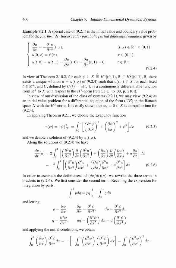
400 Chapter 9. Infinite-Dimensional Dynamical Systems
Example 9.2.1 A special case of (9.2.1) is the initial value and boundary value prob-lem for the fourth-order linear scalar parabolic partial differential equation given by
∂u
∂t= −∂4u
∂x4 (t, x), (t, x) ∈ R+ × (0, 1)
u(0, x) = ψ(x), x ∈ (0, 1)
u(t, 0) = u(t, 1) =∂u
∂x(t, 0) =
∂u
∂x(t, 1) = 0, t ∈ R
+.
(9.2.4)
In view of Theorem 2.10.2, for each ψ ∈ X= H4[(0, 1), R] ∩ H2
0 [(0, 1), R] thereexists a unique solution u = u(t, x) of (9.2.4) such that u(t, ·) ∈ X for each fixedt ∈ R
+, and U , defined by U(t) = u(t, ·), is a continuously differentiable functionfrom R
+ to X with respect to the H2-norm (refer, e.g., to [33, p. 210]).In view of our discussion of the class of systems (9.2.1), we may view (9.2.4) as
an initial value problem for a differential equation of the form (GE) in the Banachspace X with the H2-norm. It is easily shown that ϕe ≡ 0 ∈ X is an equilibrium for(9.2.4).
In applying Theorem 9.2.1, we choose the Lyapunov function
v(ψ) = ‖ψ‖2H2 =
∫ 1
0
[(∂2ψ
∂x2
)2
+(
∂ψ
∂x
)2
+ ψ2]dx (9.2.5)
and we denote a solution of (9.2.4) by u(t, x).Along the solutions of (9.2.4) we have
dv
dt(u) = 2
∫ 1
0
[(∂2u
∂x2
)∂
∂t
(∂2u
∂x2
)+(
∂u
∂x
)∂
∂t
(∂u
∂x
)+ u
∂u
∂t
]dx
= −2∫ 1
0
[(∂2u
∂x2
)∂6u
∂x6 +(
∂u
∂x
)∂5u
∂x5 + u∂4u
∂x4
]dx. (9.2.6)
In order to ascertain the definiteness of (dv/dt)(u), we rewrite the three terms inbrackets in (9.2.6). We first consider the second term. Recalling the expression forintegration by parts, ∫ 1
0pdq = pq
∣∣∣10
−∫ 1
0qdp
and letting
p =∂ψ
∂x,
∂p
∂x=
∂2ψ
∂x2 , dp =∂2ψ
∂x2 dx
q =∂4ψ
∂x4 , dq =(
∂5ψ
∂x5
)dx = d
(∂4ψ
∂x4
)and applying the initial conditions, we obtain∫ 1
0
(∂ψ
∂x
)∂5ψ
∂x5 dx = −[−∫ 1
0
(∂3ψ
∂x3
)(∂3ψ
∂x3
)dx
]=∫ 1
0
(∂3ψ
∂x3
)2
dx.
Section 9.2 Results for Differential Equations in Banach Spaces 401
In a similar manner, we obtain for the first term in brackets in (9.2.6)∫ 1
0
(∂2ψ
∂x2
)∂6ψ
∂x6 dx =∫ 1
0
(∂4ψ
∂x4
)2
dx
and for the third term, ∫ 1
0ψ
∂4ψ
∂x4 dx =∫ 1
0
(∂2ψ
∂x2
)2
dx.
Hence, we have
dv
dt(u) = −2
∫ 1
0
[(∂4u
∂x4
)2
+(
∂3u
∂x3
)2
+(
∂2u
∂x2
)2 ]= −2
∥∥∥∥∂2u
∂x2
∥∥∥∥2
H2
.
Therefore, along the solutions of (9.2.4) we have
dv
dt(u) = −2
∥∥∥∥∂2u
∂x2
∥∥∥∥2
H2
≤ 0 (9.2.7)
for all u ∈ X .It now follows from (9.2.5), (9.2.7) and Theorem 9.2.1 that the equilibrium ϕe = 0
of (9.2.4) is uniformly stable with respect to the H2-norm.In Section 9.4 (see Example 9.4.2) we show, utilizing a result from the invari-
ance theory for infinite-dimensional systems, that the equilibrium ϕe = 0 of system(9.2.4) is actually uniformly asymptotically stable in the large with respect to theH1-norm.
B. Global results
In the case of global results we let C = X .
Theorem 9.2.2 Assume that there exists a function v ∈ C[X×R+, R], two functions
ψ1, ψ2 ∈ K∞, and a function ψ3 ∈ K such that
ψ1(‖x‖) ≤ v(x, t) ≤ ψ2(‖x‖)
andv′(GE)(x, t) ≤ −ψ3(‖x‖)
for all (x, t) ∈ X ×R+. Then the equilibrium xe = 0 of (GE) is uniformly asymptot-
ically stable in the large. Furthermore, if there exist four positive constants c1, c2, c3,and b such that
c1‖x‖b ≤ v(x, t) ≤ c2‖x‖b
andv′(GE)(x, t) ≤ −c3‖x‖b
for all (x, t) ∈ X × R+, then the equilibrium xe = 0 of (GE) is exponentially stable
in the large.
402 Chapter 9. Infinite-Dimensional Dynamical Systems
Proof . The proof of this theorem is a direct consequence of Theorems 3.3.6 and3.3.7.
We apply the above results in the analysis of the heat equation.
Example 9.2.2 A class of initial and boundary value problems determined by theheat equation is given by
∂u
∂t= a2∆u, (t, x) ∈ R
+ × Ω
u(0, x) = ψ(x), x ∈ Ωu(t, x) = 0, (t, x) ∈ R
+ × ∂Ω
(9.2.8)
where Ω⊂Rn is a bounded domain with smooth boundary ∂Ω, a2 >0 is a constant,
and ∆=∑n
i=1 ∂2/∂x2i denotes the Laplacian. For eachψ∈X=H2[Ω, R] ∩ H1
0 [Ω, R]there exists a unique solution u = u(t, x) of (9.2.8) such that u(t, ·) ∈ X for eachfixed t ∈ R
+ and U , defined by U(t) = u(t, ·), is a continuously differentiablefunction from R
+ to X with respect to the H1-norm (refer, e.g., to [33, p. 210]).Then (9.2.8) can be written as an abstract Cauchy problem in the space X withrespect to the H1-norm (refer to the discussion of (9.2.2)),
U(t) = AU(t), t ≥ 0
with initial condition U(0) = ψ ∈ X , where the operator A is linear and is definedby A =
∑ni=1 a2d2/dx2
i .In Chapter 3 we showed that 0 ∈ X is an equilibrium for (9.2.8). We now show,
using Theorem 9.2.2, that the equilibrium xe = 0 is exponentially stable with respectto the H1-norm. In doing so, we make use of Gauss’Divergence Theorem [8], whichwe recall here in the context of the problem on hand: the volume integral of thedivergence of any continuously differentiable vector Q is equal to the closed surfaceintegral of the outward normal component of Q; that is,∫
Ω∇Q(x)dx =
∫∂Ω
Qndx
where Q = (Q1, . . . , Qn)T , ∇Q = (∂Q1/∂x1, . . . , ∂Qn/∂xn)T and Qn is thedirectional derivative of Q in the outward normal direction.
Now let Q = uT ∇u, where u is a solution of (9.2.8). Then for any u(t, ·) ∈H1
0 [Ω, R] we have∫Ω
[(∇u)T ∇u + u∆u
]dx =
∫∂Ω
u∂u
∂xdx = 0
which implies that ∫Ω
u∆udx = −∫
Ω
∣∣∇u∣∣2dx.
In applying Theorem 9.2.2, we choose as a Lyapunov function
v(ψ) = ‖ψ‖2H1 =
∫Ω
(|∇ψ|2 + |ψ|2
)dx. (9.2.9)
Section 9.2 Results for Differential Equations in Banach Spaces 403
Let u(t, x) denote a solution of (9.2.8). Then
dv
dt(u) =
∫Ω
∂
∂t
[ n∑i=1
(∂u
∂xi
)2+ u2
]dx
=∫
Ω
[ n∑i=1
2( ∂u
∂xi
) ∂2u
∂xi∂t+ 2u
∂u
∂t
]dx
= −n∑
i=1
2∫
Ω
∂2u
∂x2i
∂u
∂tdx + 2a2
∫Ω
u∆udx
= −2a2∫
Ω(∆u)2dx − 2a2
∫Ω
|∇u|2dx
≤ −2a2∫
Ω|∇u|2dx.
By Poincare’s inequality [34], we have that∫Ω
|u|2dx ≤ γ2∫
Ω|∇u|2dx
where γ can be chosen as δ/√
n and Ω can be put into a cube of length δ. Hence,we have
dv
dt(u) ≤ −a2
(∫Ω
|∇u|2dx +1γ2
∫Ω
|u|2dx
)≤ −c‖u‖2
H1
where c = a2 min1, 1/γ2. Therefore,
v′(9.2.8)(ψ) ≤ −c‖ψ‖2
H1 (9.2.10)
for all ψ ∈ X .It now follows from (9.2.9), (9.2.10), and Theorem 9.2.2 that the equilibrium 0 ∈X
of (9.2.8) is exponentially stable in the large with respect to the H1-norm.
Example 9.2.3 Scalar linear Volterra integrodifferential equations are of the form x(t) = −ax(t) +∫ t
−∞k(t − s)x(s)ds, t ≥ 0
x(t) = ϕ(t), t ≤ 0(9.2.11)
where a > 0 is a constant. As shown in Subsection 2.9D (refer to Example 2.9.3),such systems may be viewed as retarded functional differential equations, replacingthe delay [−r, 0] by (−∞, 0]. System (9.2.11) can be rewritten as x(t) = −axt(0) +
∫ 0
−∞k(−s)xt(s)ds, t ≥ 0
x(t) = ϕ(t), t ≤ 0.
(9.2.12)
For (9.2.12) we define the fading memory space X as consisting of all measurablefunctions ϕ : (−∞, 0) → R with norm
‖ϕ‖2m = |ϕ(0)|2 + K
∫ 0
−∞|ϕ(s)|2eLsds < ∞ (9.2.13)
404 Chapter 9. Infinite-Dimensional Dynamical Systems
with K > 0 to be determined as needed and L > 0 a fixed constant. We assume thatk(·) ∈ X and we define CL = (
∫∞0 |k(s)|2eLsds)1/2.
If we define F (t, ϕ) ≡ F (ϕ) = −ϕ(0) +∫ 0
−∞ k(−s)ϕ(s)ds for all ϕ ∈ X , then(9.2.12) is a special case of the differential equation in Banach space (GE) with theBanach space as specified above.
To obtain an estimate of solution bounds for (9.2.12) we choose for any ϕ ∈ X ,
v(ϕ) = ‖ϕ‖2m (9.2.14)
and we let y(t) = v(xt). Along the solutions of (9.2.12) we have
y(t) = (K − 2a)|x(t)|2 + 2CLx(t)z(t) − KL|z(t)|2 (9.2.15)
where z(t) = (∫ 0
−∞ |xt(s)|2eLsds)1/2. The right side of (9.2.15) is negative definiteif and only if the matrix
P =[2a − K −CL
−CL KL
](9.2.16)
is positive definite which is the case when (i) 0 ≤ K < 2a, (ii) KL > 0 (which isalways true), and (iii) CL/
√L ≤ a. Therefore, when CL/
√L ≤ a, there exists a
K > 0 such that the right-hand side of (9.2.15) is negative definite.We want to show that there exists an α < 0 such that
y(t) ≤ αy(t). (9.2.17)
Letting
Q =[1 00 K
], (9.2.18)
this is equivalent to finding an α such that P ≥ −αQ. It is easy to see that this is thecase when
α = − λm(P )max1, K < 0 (9.2.19)
where λm(P ) denotes the smallest eigenvalue of P .We conclude that if CL/
√L ≤ a and K is chosen appropriately, then there exists
an α < 0 such that y(t) ≤ αy(t). Therefore,
‖xt‖m ≤ e(α/2t)‖x0‖m, α < 0 (9.2.20)
and we conclude that the equilibrium ϕe = 0 of system (9.2.12) is exponentiallystable in the large with respect to the norm ‖ · ‖m.
Theorem 9.2.3 Assume that there exists a function v ∈ C[X × R+, R] that satisfies
the following conditions.
(i) There exist two continuous, real-valued and strictly increasing functions ψ1, ψ2that are defined on R
+ with limr→∞ ψi(r) = +∞, i = 1, 2, and a constantM > 0 such that
ψ1(‖x‖) ≤ v(x, t) ≤ ψ2(‖x‖)
for all ‖x‖ ≥ M and t ∈ R+.
Section 9.2 Results for Differential Equations in Banach Spaces 405
(ii) For all ‖x‖ ≥ M and t ∈ R+,
v′(GE)(x, t) ≤ 0.
Then the solutions of (GE) are uniformly bounded.If in addition to hypotheses (i) and (ii) there exists a function ψ3 ∈ K such that
v′(GE)(x, t) ≤ −ψ3(‖x‖)
for all ‖x‖ ≥ M and t ∈ R+, then the solutions of (GE) are uniformly ultimately
bounded.
Proof . The proof of this theorem is a direct consequence of Theorems 3.3.4 and3.3.5.
We conclude this subsection with two examples.
Example 9.2.4 We consider the dynamical system determined by (9.2.4) in Exam-ple 9.2.1. Because the function v defined in (9.2.5) is positive definite, decrescent,and radially unbounded with respect to the H2-norm, it follows from (9.2.7) andTheorem 9.2.3 that the solutions of (9.2.4) are uniformly bounded with respect to theH2-norm.
Example 9.2.5 We consider the dynamical system determined by (9.2.8) in Exam-ple 9.2.2. Because the function v defined in (9.2.9) is positive definite, decrescent,and radially unbounded with respect to the H1-norm, it follows from (9.2.10) andTheorem 9.2.3 that the solutions of (9.2.8) are uniformly ultimately bounded withrespect to the H1-norm.
C. Instability
As in Subsection A, we assume in the following that C ⊂ X , xe = 0 ∈ C, xe = 0 isan equilibrium for (GE) and we let ‖ · ‖ denote the norm for the Banach space X .
Theorem 9.2.4 (Lyapunov’s First Instability Theorem for differential equations inBanach spaces) The equilibrium xe = 0 of (GE) is unstable if there exist a t0 ∈ R
+
and a decrescent function v ∈ C[B(r)×R+, R] for some r > 0, B(r) ⊂ C, such that
v′(GE) is positive definite (negative definite) and if in every neighborhood of the origin
there is a point x such that v(x, t0) > 0 (v(x, t0) < 0). Moreover, if v is positivedefinite (negative definite), then the equilibrium xe = 0 is completely unstable.
Proof . The proof of this result is a direct consequence of Theorem 3.3.8.
We apply the above result in the stability analysis of the backward heat equation.
406 Chapter 9. Infinite-Dimensional Dynamical Systems
Example 9.2.6 Consider the initial and boundary value problem given by∂u
∂t= −a2∆u, (t, x) ∈ R
+ × Ω
u(0, x) = ψ(x), x ∈ Ωu(t, x) = 0, (t, x) ∈ R
+ × ∂Ω
(9.2.21)
where a2 > 0 is a constant, Ω ⊂ Rn is a bounded domain with smooth boundary ∂Ω,
∆ denotes the Laplacian, and ψ ∈ C0[Ω, R]. We may view (9.2.21) as a differentialequation in the Banach space X = H0[Ω, R]. (Refer to Section 2.10 for the definitionsof C0[Ω, R] and H0[Ω, R].) It is easy to show that 0 ∈ X is an equilibrium of (9.2.21).
In applying Theorem 9.2.4 in the stability analysis of (9.2.21), we choose as aLyapunov function
v(ϕ) =∫
Ω|ϕ(x)|2dx = ‖ϕ‖2
L2(9.2.22)
for all ϕ ∈ X . This function is clearly positive definite with respect to the L2-norm.Along the solutions of (9.2.21) we have
v′(9.2.21)(ϕ) = 2
∫Ω
ϕdϕ
dtdx = −2
∫Ω
ϕ(∆ϕ)dx.
By Gauss’ Divergence Theorem and Poincare’s Inequality (refer to Example 9.2.2)we have
−2∫
Ωϕ(∆ϕ)dx = 2
∫Ω
|∇ϕ|2dx ≥ 2γ2
∫Ω
|ϕ|2dx =2γ2 ‖ϕ‖L2
for all ϕ ∈ X , where γ is a positive constant that depends on Ω (refer to Example9.2.2). Therefore,
v′(9.2.21)(ϕ) ≥ 2
γ2 ‖ϕ‖L2 (9.2.23)
which shows that v′(9.2.21) is positive definite. It now follows from (9.2.22), (9.2.23),
and Theorem 9.2.4 that the equilibrium xe = 0 of (9.2.21) is completely unstablewith respect to the L2-norm.
Theorem 9.2.5 (Lyapunov’s Second Instability Theorem for differential equationsin Banach spaces) Assume that for system (GE) there exists a bounded functionv ∈ C[B(ε) × [t0,∞), R] where ε > 0 and B(ε) ⊂ C, having the followingproperties.
(i) For all (x, t) ∈ B(ε) × [t0,∞),
v′(GE)(x, t) ≥ λv(x, t)
where λ > 0 is a constant.(ii) In every neighborhood of xe = 0, there exists an x such that v(x, t1) > 0 for
a fixed t1 ≥ t0.
Then the equilibrium xe = 0 of (GE) is unstable.
Section 9.2 Results for Differential Equations in Banach Spaces 407
Proof . The proof of this result is a direct consequence of Theorem 3.3.10.
We demonstrate the applicability of Theorem 9.2.5 in the analysis of a specificexample.
Example 9.2.7 Consider the initial value and boundary value problem given by
∂u1
∂t= u1 + u2 +
n∑j=1
aj∂u1
∂xj(t, x) ∈ R
+× Ω
∂u2
∂t= u1 + u2 +
n∑j=1
bj∂u2
∂xj+ ∆u2, (t, x) ∈ R
+× Ω
ui(0, x) = ψi(x), x ∈ Ω, i = 1, 2ui(t, x) = 0, (t, x) ∈ R
+× ∂Ω, i = 1, 2(9.2.24)
where Ω ⊂ Rn is a bounded domain with smooth boundary, ∆ =
∑nj=1 ∂2/∂x2
j
denotes the Laplacian, aj , bj are real constants, j = 1, . . . , n, and ψi ∈ C0[Ω, R],i = 1, 2. (Refer to Section 2.10 for the definition of C0[Ω, R].)
Equations (9.2.24) may be viewed as differential equations in the Banach spaceX = H0[Ω, R]×H0[Ω, R]. It is easily verified that the origin of X is an equilibriumof (9.2.24).
In the following, we show that the equilibrium 0 ∈ X of system (9.2.24) is unstablewith respect to the L2-norm, using Theorem 9.2.5.
We choose as a Lyapunov function,
v(ϕ) =∫
Ω
(|ϕ1|2 − |ϕ2|2
)dx (9.2.25)
where ϕ = (ϕ1, ϕ2) ∈ X . Along the solutions of (9.2.24) we have
v′(9.2.24)(ϕ) = 2
∫Ω
ϕ1
[ϕ1 + ϕ2 +
n∑j=1
aj∂ϕ1
∂xj
]dx
− 2∫
Ωϕ2
[ϕ1 + ϕ2 +
n∑j=1
bj∂ϕ2
∂xj+ ∆ϕ2
]dx
= 2v(ϕ) − 2∫
Ωϕ2(∆ϕ2)dx
where in the last step we have used the fact that
2∫
Ωϕi
∂ϕi
∂xjdx =
∫Ω
∂[ϕ2i ]
∂xjdx = 0
j = 1, . . . , n, for ϕi ∈ C0[Ω, R], i = 1, 2.Invoking Gauss’ Divergence Theorem, we have
2v(ϕ) − 2∫
Ωϕ2(∆ϕ2)dx = 2v(ϕ) + 2
∫Ω
|∇ϕ2|2dx ≥ 2v(ϕ)
408 Chapter 9. Infinite-Dimensional Dynamical Systems
for all ϕ ∈ X . Therefore,v′(9.2.24)(ϕ) ≥ 2v(ϕ) (9.2.26)
for all ϕ ∈ X .Clearly, v(ϕ) is bounded on
B(1) =ϕ = (ϕ1, ϕ2) ∈ X : ‖ϕ‖2 = ‖ϕ1‖2
L2+ ‖ϕ1‖2
L2≤ 1
and v(ϕ) > 0 if ϕ = (ϕ1, 0) and ‖ϕ1‖L2 = 0. Therefore, condition (ii) inTheorem 9.2.5 is satisfied. It follows from (9.2.26) and Theorem 9.2.5 that theequilibrium ϕe = 0 ∈ X of (9.2.24) is unstable with respect to the L2-norm.
We now state the last result of the present section.
Theorem 9.2.6 (Chetaev’s Instability Theorem for differential equations in Banachspaces) Assume that for system (GE) there exist a function v ∈ C[B(r) × R
+, R]for some r > 0, where B(r) ⊂ C ⊂ X , and a t0 ∈ R
+ such that the followingconditions are satisfied.
(i) There exists a component D of the set (x, t) ∈ B(r)×R+ : v(x, t) < 0 such
that for every neighborhood of the origin there exists an x in this neighborhoodsuch that (x, t0) ∈ D.
(ii) v is bounded from below on D.(iii) v′
(GE)(x, t) ≤ −ψ(|v(x, t)|) for all (x, t) ∈ D where ψ ∈ K.
Then the equilibrium xe = 0 of (GE) is unstable.
We ask the reader to prove Theorem 9.2.6.
9.3 Converse Theorems for Differential Equations inBanach Spaces
In the present section we establish converse results for some of the principal Lyapunovstability and boundedness results for differential equations in Banach spaces presentedin Section 9.2. We recall the differential equation in Banach space given by
x = F (t, x) (GE)
where F : R × C → X . We assume that xe = 0 is an equilibrium for the dynamicalsystem determined by (GE) and that the set C contains a neighborhood of the originxe = 0. Also, we assume that for every (t0, x0) ∈ R
+ × C, there exists a uniquenoncontinuable solution of (GE) with initial condition x(t0) = x0 that dependscontinuously on (t0, x0).
We present only local results. Our first result concerns uniform stability.
Theorem 9.3.1 If the equilibrium xe = 0 of (GE) is uniformly stable, then thereexists a positive definite and decrescent function v ∈ C[B(r) × R
+, R+] for somer > 0, where B(r) ⊂ C, such that v′
(GE) is negative semidefinite.
Section 9.4 Invariance Theory for Differential Equations in Banach Spaces 409
Proof . The proof of this result is a direct consequence of Theorem 3.6.1 and followsalong the lines of the proof of Theorem 6.5.1. The continuity of v is a consequence ofthe assumed continuity of the solution ϕ(t, t0, x0) of (GE) with respect to the initialdata.
The next result concerns uniform asymptotic stability.
Theorem 9.3.2 If the equilibrium xe= 0 of (GE) is uniformly asymptotically stable,then there exists a positive definite and decrescent function v ∈ C[B(r) × R
+, R+]for some r > 0, where B(r) ⊂ C, such that v′
(GE) is negative definite.
Proof . The proof of this result is a consequence of Theorem 3.6.2, the continuityof the solutions of (GE) with respect to initial conditions and the continuity resultsgiven in Subsection 3.6B.
As in the case for finite-dimensional systems (see Theorem 6.5.3), the next result,which addresses the exponential stability of the equilibrium xe = 0 for (GE), is notsymmetric to the exponential stability result given in Theorem 9.2.1d. Nevertheless,this result does provide a set of necessary conditions for exponential stability.
Theorem 9.3.3 If the equilibrium xe = 0 of (GE) is exponentially stable, then thereexists a positive definite and decrescent function v ∈ C[B(r) × R
+, R+] for somer > 0, where B(r) ⊂ C, such that
v′(GE)(x, t) ≤ −cv(x, t)
for all (x, t) ∈ B(r) × R+, where c > 0 is a constant.
Proof . The proof of this result is a direct consequence of Theorem 3.6.3 and thecontinuity of the solutions of (GE).
We conclude by noting that converse theorems for system (GE) for uniform bound-edness, uniform ultimate boundedness, uniform asymptotic stability in the large,exponential stability in the large, and instability can also be established, using themethodology employed in the preceding results.
9.4 Invariance Theory for Differential Equations inBanach Spaces
In the present section we consider infinite-dimensional dynamical systems determinedby a class of autonomous differential equations in Banach space given by
x = F (x) (GA)
where F : C → X , C ⊂ X , and X is a Banach space. We assume that xe = 0 isan equilibrium for the dynamical system determined by (GA) and that C contains a
410 Chapter 9. Infinite-Dimensional Dynamical Systems
neighborhood of the origin xe = 0. Furthermore, we assume that for each x0 ∈ C,there exists one and only one solution of (GA) for the initial condition x(0) = x0.Under these conditions, the solutions of (GA) determine a semigroup and the invari-ance theory for dynamical systems developed in Section 4.2 is applicable to dynamicalsystems determined by (GA). Our aim in the present section is to improve some ofthe stability results presented in Section 9.2.
Theorem 9.4.1 Assume that for system (GA) there exists a function v ∈ C[C, R]such that v′
(GA)(x) ≤ 0 for all x ∈ C. Let M be the largest invariant set with respectto the dynamical system determined by (GA) in the set
Z =x ∈ C : v′
(GA)(x) = 0. (9.4.1)
Then for every solution ϕ of (GA) such that the closure of the trajectory of ϕ iscompact, ϕ(t) approaches M as t → ∞.
Proof . The proof of this theorem is a direct consequence of Theorem 4.2.1, whereX1 is generated by taking the closure of every solution ϕ of (GA) having the propertythat the closure of ϕ is compact.
We apply the above result in the analysis of a scalar Volterra integrodifferentialequation.
Example 9.4.1 Consider the equation (refer to [9])
x(t) = −∫ t
−∞a(t − u)g(x(u))du (9.4.2)
where t ∈ R+, a ∈ C2[R+, R], a(t) > 0, a(t) < 0, and a(t) ≥ 0 for all t ∈ R
+, andlimt→∞ t2a(t) = 0 and
∫∞0 t2a(t)dt < ∞. The fading memory space X for (9.4.2)
is the Banach space consisting of all functions ϕ : (−∞, 0] → R such that
‖ϕ‖2 = |ϕ(0)| +∫ 0
−∞k(θ)|ϕ(θ)|dθ
is finite, where k(θ) > 0 for −∞ < θ ≤ 0,∫ 0
−∞ k(θ)dθ < ∞, and k(θ) ≥ 0. Assume
that g(x) has a finite number of zeros and that g ∈ C1[R, R], and that∫ x
0 g(s)ds → ∞as |x| → ∞.
In the following, we apply Theorem 9.4.1 to prove that every solution of (9.4.2)with initial condition ϕ ∈ X satisfying sup−∞<θ≤0 |ϕ(θ)| < ∞ approaches anequilibrium of (9.4.2).
Choose
v(ϕ) =∫ ϕ(0)
0g(s)ds − 1
2
∫ 0
−∞a(−θ)
(∫ 0
θ
g(ϕ(s))ds
)2
dθ
Section 9.4 Invariance Theory for Differential Equations in Banach Spaces 411
for ϕ∈X . The second term in v is defined for all ϕ∈X satisfying sup−∞<θ≤0 |ϕ(θ)|= L < ∞ because
0 ≤ −12
∫ 0
−∞a(−θ)
(∫ 0
θ
g(ϕ(s))ds
)2
dθ
≤ −(
sup−L≤s≤L
|g(s)|)2 1
2
∫ 0
−∞a(−θ)θ2dθ
< ∞. (9.4.3)
Therefore v is defined for all ϕ ∈ X satisfying sup−∞<θ≤0 |ϕ(θ)| < ∞.Suppose that x(t, t0, ϕ0) is a solution of (9.4.2) with the initial condition ϕ0 ∈ X
satisfying sup−∞<θ≤t0 |ϕ0(θ)| < ∞. Then by the continuity of x(t, t0, ϕ0) withrespect to t, sup−∞<θ≤t |x(t, t0, ϕ0)| < ∞ and hence, v(xt) is defined for all t ≥ t0.
Along the solutions of (9.4.2), we have
v′(9.4.2)(xt) = −1
2
∫ 0
−∞a(−θ)
(∫ 0
θ
g(x(t + s))ds
)2
dθ ≤ 0,
which implies that v(xt) is nonincreasing and hence, v(xt) ≤ v(ϕ0) for all t > t0.
By hypothesis,∫ x(t)0 g(s)ds → ∞ if |x(t)| → ∞. Therefore there exists an L > 0
such that |x(t)| < L for all −∞ < t < ∞. We now have an estimate for the normof xt,
‖xt‖2 = |x(t)| +∫ 0
−∞k(θ)|x(t + θ)|dθ ≤ L
(1 +
∫ 0
−∞k(θ)dθ
),
which implies that the trajectory γ+(x)=xt(t0, ϕ0) : t≥ t0 is a bounded set in X .Next we show that the closure of the trajectory γ+(x) is compact. Because in
Banach spaces compactness is equivalent to sequential compactness and xt is con-tinuous with respect to t in X , we only need to show that there is a convergentsubsequence for any sequence xtk
k∈N with tk → ∞ monotonically as k → ∞.For any A > 0, xtk
with tk > A is equicontinuous on [−A, 0] and uniformlybounded on (−∞, 0] (|x(t)| < L was shown earlier). By the Ascoli–Arzela Lemma(refer to Problem 2.14.7), there exists a subsequence that converges uniformly to afunction ϕA ∈ C[[−A, 0], R]. Choosing A = 1, 2, . . . , there exist subsequencestAk such that tk ⊃ t1k ⊃ t2k ⊃ · · · and the subsequences xtAk
con-verge uniformly to a function ϕA ∈ C[[−A, 0], R] for all A = 1, 2, . . . . Then thesubsequence xtkk
: k = 1, 2, . . . converges uniformly on all compact subsets of(−∞, 0] to a function ϕ ∈ C[(−∞, 0], R]. ϕ is bounded by the same bound L andthus, ϕ ∈ X . What is left to be shown is that xtkk
→ ϕ as k → ∞ using the norm ‖·‖in X . Let ε > 0 be arbitrary. There exists an A > 0 such that
∫ −A
−∞ k(θ)dθ < ε/(2L).We have
‖xtkk− ϕ‖2 = |xtkk
(0) − ϕ(0)| +∫ 0
−∞k(θ)|x(tkk + θ) − ϕ(θ)|dθ
≤ |x(tkk) − ϕ(0)| + ε +∫ 0
−A
k(θ)|x(tkk + θ) − ϕ(θ)|dθ.
412 Chapter 9. Infinite-Dimensional Dynamical Systems
On the compact set [−A, 0], there exists an m > 0 such that the first and last term inthe above expression are less than ε for all k > m. Hence xtkk
→ ϕ as k → ∞.Finally, if ψ ∈ Z = x ∈ X : v′
(9.4.2)(x) = 0, then
v′(9.4.2)(ψt) =
∫ 0
−∞a(−θ)
(∫ 0
θ
g(ψ(t + s))ds
)2
dθ = 0.
Because a(t) ≥ 0, it must be true that∫ 0
θ
g(ψ(t + s))ds = 0 for all − ∞ < t < ∞ (9.4.4)
whenever a(−θ) > 0. From the assumptions that t2a(t) → 0 as t → ∞ anda(t) ≥ 0, there must exist a t0 and a δ with t0 > δ > 0 such that a(s) > 0 for alls ∈ [t0 − δ, t0 + δ]. In view of (9.4.4), we have∫ −s1
−s2
g(ψ(t + s))ds = 0 for all − ∞ < t < ∞,
for all s1, s2 ∈ [t0 − δ, t0 + δ]. This is true if and only if g(ψ(t)) ≡ 0 for all t. Underthe assumption that g(·) has a finite number of zeros, the set Z is comprised of thesezeros, which are also the equilibria of (9.4.2). It now follows from Theorem 9.4.1that xt approaches an equilibrium of (9.4.2).
In our next result we require the following concept.
Definition 9.4.1 Let X and X be two Banach spaces and assume that X ⊂ X . Theembedding X ⊂ X is said to be compact if every closed and bounded subset of X iscompact in X with respect to the norm ‖ · ‖X of X .
Now let Ω ⊂ Rn be a bounded domain with smooth boundary ∂Ω. One of
Sobolev’s Embedding Theorems (see, e.g., [6] and [33]) ensures that the embeddingHm[Ω, R] ⊂ H l[Ω, R] is compact and continuous for all m > l. Accordingly, theembedding Hm
0 [Ω, R] ⊂ H l0[Ω, R] is also compact and continuous for m > l.
The differential equation (GA) may be defined on different Banach spaces. Thiswill always be true for the Banach spaces X and X when X ⊂ X . Therefore,the Sobolev Embedding Theorem cited above suggests the next result, where ‖ · ‖X
denotes the norm for X and where we assume that C = X .
Theorem 9.4.2 Assume that for the dynamical system determined by (GA) thereexists a Banach space X ⊃ X such that the embedding X ⊂ X is compact. Assumethat there exists a function v : X → R that is continuous with respect to the norm‖ · ‖X that satisfies the following conditions.
(i) v′(GA)(x) ≤ 0 for all x ∈ X .
(ii) v(x) > v(0) = 0 for all x ∈ X − 0.
Section 9.5 Comparison Theory for Differential Equations in Banach Spaces 413
(iii) v(x) → ∞ as ‖x‖X → ∞.(iv) 0 is the only invariant subset in
Z =x ∈ X : v′
(GA)(x) = 0.
Then the equilibrium xe = 0 of (GA) is uniformly asymptotically stable in the largein X with respect to the norm ‖ · ‖X .
Proof . The proof of this theorem is a direct consequence of Corollary 4.2.2, wherewe let X be equipped with the norm ‖ · ‖X . We note that X is locally compactwith respect to the norm ‖ · ‖X and that in the proof of Corollary 4.2.2, the localcompactness of X is used, rather than the compactness of X .
Example 9.4.2 We now revisit system (9.2.4) given in Example 9.2.1 where X =H4[(0, 1), R] ∩ H2
0 [(0, 1), R] with the H2-norm. We choose X = H10 [(0, 1), R].
In view of Sobolev’s Embedding Theorem cited above, the embedding X ⊂ X iscompact. In applying Theorem 9.4.2, we choose as a Lyapunov function
v(ψ) = ‖ψ‖2H1 = ‖ψ‖2
X=∫ 1
0
[(∂ψ
∂x
)2
+ ψ2]dx.
The function v : X → R is clearly continuous with respect to the norm ‖ · ‖H1 . In asimilar manner as was done in Example 9.2.1, we compute
v′(9.2.4)(ψ) = −2
∫ 1
0
[(∂3ψ
∂x3
)2+(∂2ψ
∂x2
)2]dx = −2
∥∥∥∥d2ψ
dx2
∥∥∥∥H1
≤ 0
for all x ∈ X .We have v(0) = 0 and v(ψ) > 0 for all ψ ∈ X − 0, and in particular, for all
ψ ∈ X − 0. Moreover, v(ψ) → ∞ as ‖ψ‖H1 → ∞ also holds. Finally,
Z =ψ ∈ X : v′
(9.2.4)(ψ) = 0
= 0
because d2ψ/dx2 ≡ 0 and ψ(0) = ψ(1) = 0 imply that ψ ≡ 0 for ψ ∈ C2[(0, 1), R]and because C2[(0, 1), R] ∩ X is dense in X .
All hypotheses of Theorem 9.4.2 are satisfied and therefore, the equilibrium ϕe =0 ∈ X of system (9.2.4) is uniformly asymptotically stable in the large with respectto the H1-norm.
9.5 Comparison Theory for Differential Equations inBanach Spaces
In the present section we specialize the results of Section 4.3 to develop a comparisontheory in the stability analysis of infinite-dimensional dynamical systems determinedby differential equations in Banach spaces.
414 Chapter 9. Infinite-Dimensional Dynamical Systems
We consider once more a class of differential equations defined on a Banach spaceX of the form
x = F (t, x) (GE)
where F : R+ × C → X, C ⊂ X . We assume that xe = 0 ∈ C and that xe = 0 is
an equilibrium of (GE),For the l-dimensional Euclidean vector space, (Rl, | · |), we let in the following
Rl ⊃ BE(r)=x ∈ R
l : |x| < r, and as usual, we let B(r)=x ∈ X : ‖x‖ < r.Also, for a vector-valued function V : B(r) × R
+ → Rl, where B(r) ⊂ C ⊂ X for
some r > 0, we use the notation
V (x, t) = [v1(x, t), . . . , vl(x, t)]T
andV ′
(GE)(x, t) = [v′1(GE)(x, t), . . . , v′
l(GE)(x, t)]T .
For system (GE) we employ as a comparison system ordinary differential equa-tions of the form
y = g(t, y) (C)
where t ∈ R+, y ∈ R
l, g ∈ C[R+ ×BE(r1), Rl] for some r1 > 0, BE(r1) ⊂ (R+)l,and g(t, 0) = 0 for all t ∈ R
+. By making use of (C), we first establish local results.
Theorem 9.5.1 Assume that there exists a function V ∈C[B(r)×R+, (R+)l], where
B(r)⊂C ⊂X for some r>0, such that |V (x, t)| is positive definite and decrescent,and there exists a quasi-monotone nondecreasing function g∈C[R+× BE(r1), Rl],where BE(r1)⊂(R+)l for some r1 >0, which satisfies the conditions that g(t, 0)=0for all t ∈ R
+ andV ′
(GE)(x, t) ≤ g(t, V (x, t))
for all (x, t) ∈ B(r) × R+. In the above, inequality is to be interpreted component-
wise. Then the following statements are true.
(a) The stability, asymptotic stability, uniform stability and uniform asymptoticstability of the equilibrium ye = 0 of (C) implies the same correspondingtypes of stability of the equilibrium xe = 0 of (GE).
(b) If in addition to the above assumptions, |V (x, t)| ≥ a|x|b for all (x, t) ∈B(r) × R
+, where a > 0 and b > 0, then the exponential stability of theequilibrium ye = 0 of (C) implies the exponential stability of the equilibriumxe = 0 of (GE).
Proof . The proofs of these results follow directly from Theorem 4.3.2(b) and (c).
In the next theorem, where we address global results, we assume that C = X .
Theorem 9.5.2 Assume that for (GE) there exists a function V ∈C[X ×R+, (R+)l]
such that |V (x, t)| is positive definite, decrescent, and radially unbounded, and that
Section 9.6 Composite Systems 415
there exists a quasi-monotone nondecreasing function g ∈ C[R+ × (R+)l, Rl] suchthat g(t, 0) = 0 for all t ∈ R
+ and such that the inequality
V ′(GE)(x, t) ≤ g(t, V (x, t))
holds componentwise for all (x, t) ∈ X × R+. Then the following statements are
true.
(a) The uniform asymptotic stability in the large of the equilibrium ye = 0 of (C)implies the uniform asymptotic stability in the large of the equilibrium xe = 0of (GE).
(b) If in addition to the above assumptions, a1|x|b ≤ |V (x, t)| ≤ a2|x|b for all(x, t) ∈ X ×R
+, where a2 ≥ a1 > 0 and b > 0, then the exponential stabilityin the large of the equilibrium ye = 0 of (C) implies the exponential stabilityin the large of the equilibrium xe = 0 of (GE).
(c) The uniform boundedness and uniform ultimate boundedness of the solutionsof (C) imply the same corresponding types of boundedness properties of thesolutions of (GE).
We leave the proofs of the above results as an exercise.We note that when l = 1, the quasi-monotonicity condition in Theorems 9.5.1 and
9.5.2 are automatically satisfied because this is always true for scalar-valued functions(refer to Definition 3.8.1).
In applications, the comparison system given by
y = Py + m(t, y) (9.5.1)
is especially useful, where P = [pij ] ∈ Rl×l satisfies the condition that pij ≥ 0 for
i, j = 1, . . . , l and i = j, and where m : R+ × BE(r1) → R
l for some r1 > 0 andBE(r1) ⊂ (R+)l, is assumed to satisfy the condition
lim|y|→0
|m(t, y)||y| = 0 uniformly for t ∈ R
+.
Applying Lyapunov’s First Method (Theorem 7.6.2), it follows that the equilibriumye = 0 of (9.5.1) is uniformly asymptotically stable if −P is an M -matrix (refer toDefinition 7.7.1 for the definition of M -matrix and the discussion following thatdefinition for several equivalent characterizations of M -matrices).
We conclude by noting that in Section 9.7 we apply some of the results of thepresent section in the analysis of the model of a multicore nuclear reactor describedby a class of Volterra integrodifferential equations.
9.6 Composite Systems
In Section 2.11 we introduced composite dynamical systems on metric spaces. Wenow address the stability analysis of such systems in the context of composite dyna-mical systems defined on normed linear spaces.
416 Chapter 9. Infinite-Dimensional Dynamical Systems
We let (X, ‖ · ‖), (Xi, ‖ · ‖i), i = 1, . . . , l, be normed linear spaces; we assumethat X = X1 × · · ·Xl and that there are constants c1 > 0 and c2 > 0 such that
c1‖x‖ ≤l∑
i=1
‖xi‖i ≤ c2‖x‖
for all x ∈ X , where x = (x1, . . . , xl)T , xi ∈ Xi, i = 1, . . . , l. We can definethe norm ‖ · ‖ on X in a variety of ways, including ‖x‖ =
∑li=1 ‖xi‖i. We define
a composite dynamical system, R+, X, A, S, defined on a normed linear space
(X, ‖ · ‖) by modifying Definition 2.11.1 in the obvious way, choosing for metricspaces (X, d), (Xi, di), i = 1, . . . , l, normed linear spaces (X, ‖ · ‖), (Xi, ‖ · ‖i),i = 1, . . . , l, respectively.
In our first result, we define for Mi ⊂ Xi,
di(xi, Mi) = infx∈Mi
‖xi − x‖i.
Theorem 9.6.1 Let R+, X, A, S be a dynamical system where X =X1 ×· · ·×Xl
and Xi, i = 1, . . . , l, are normed linear spaces with norms ‖ · ‖i, i = 1, . . . , l, re-spectively. Assume that M = M1 × · · · × Ml is an invariant set (i.e., (S, M) isinvariant), where Mi ⊂ Xi, i = 1, . . . , l, and assume that the following hypothesesare satisfied.
(i) There exist vi ∈ C[Xi × R+, R] and ψi1, ψi2 ∈ K, i = 1, . . . , l, such that
ψi1(di(xi, Mi)) ≤ vi(xi, t) ≤ ψi2(di(xi, Mi))
for all xi ∈ Xi and t ∈ R+.
(ii) Given vi in hypothesis (i), there exist constants aij ∈ R and functions ψi4 ∈ K,i, j = 1, . . . , l, such that
Dvi(pi(t, a, t0), t) ≤ ψi4(di(pi, Mi))l∑
j=1
aijψj4(dj(pj , Mj))
for all p(·, a, t0)=[p1(·, a, t0), . . . , pl(·, a, t0)]T=[p1, . . . , pl]T∈S and t ≥ t0,where D denotes a fixed Dini derivative with respect to t ∈ R
+.
(iii) There exists an l-vector αT = (α1, . . . , αl), αi > 0, i = 1, . . . , l, such that thetest matrix B = [bij ] ∈ R
l×l specified by
bij =12(αiaij + αjaji
), i, j = 1, . . . , l,
is either negative semidefinite or negative definite.
Then the following statements are true.
(a) If B is negative semidefinite, then (S, M) is uniformly stable.
(b) If B is negative definite, then (S, M) is uniformly asymptotically stable.
Section 9.6 Composite Systems 417
(c) If B is negative semidefinite, if M is bounded, and if ψi1, ψi2 ∈ K∞ for alli = 1, . . . , l, then S is uniformly bounded.
(d) If in (c), B is negative definite, then S is uniformly ultimately bounded andfurthermore, (S, M) is uniformly asymptotically stable in the large.
(e) If B is negative definite and if there exist positive numbers a1, a2, b, and csuch that
a1rb ≤ ψi1(r) ≤ ψi2(r) ≤ a2r
b
andψ2
i4(r) ≥ crb
for all r ∈ R+, i = 1, . . . , l, then (S, M) is exponentially stable in the large.
Proof . The proof of this theorem is a consequence of Theorems 3.3.1–3.3.7. Wepresent here only the proofs of parts (a) and (b). The proofs of the remaining partsfollow along similar lines.
We choose
v(x, t) =l∑
i=1
αivi(xi, t)
where x = [x1, . . . , xl]T and α = [α1, . . . , αl]T is given in hypothesis (iii). Byhypothesis (i), we have
l∑i=1
αiψi1(di(xi, Mi)) ≤ v(x, t) ≤l∑
i=1
αiψi2(di(xi, Mi))
for all x=[x1, . . . , xl]T∈X1× · · · ×Xl = X . Let r=d(x, M) and ri =d(xi, Mi),1 ≤ i ≤ l. We may assume without loss of generality that r =
∑li=1 ri. We have
thatl∑
i=1
αiψi2(ri) ≤l∑
i=1
αiψi2(r)= ψ2(r).
Also, we let ψ1(r) = min1≤i≤lψi1(r) and a = min1≤i≤lαi. Then
l∑i=1
αiψi1(ri) ≥ max1≤i≤l
αiψi1(ri)
≥ max1≤i≤l
αiψ1(ri)
≥ a max1≤i≤l
ψ1(ri)
= aψ1(
max1≤i≤l
ri)
≥ aψ1(r/l)= ψ1(r).
418 Chapter 9. Infinite-Dimensional Dynamical Systems
Hence,ψ1(r) ≤ v(x, t) ≤ ψ2(r) (9.6.1)
for all x ∈ X and t ∈ T , where ψ1, ψ2 ∈ K. Let ri = di(pi, Mi), i = 1, . . . , l.Furthermore, in view of hypothesis (ii),
Dv(p(t, a, t0), t) ≤l∑
i=1
αi
(ψi4(ri)
l∑i=1
aijψj4(rj)
)= wT Rw
= wT
(R + RT
2
)w
= wT Bw
≤ λM (B)|w|2
for all t ≥ t0 and p(·, a, t0) ∈ S, where w = [ψ14(r1), . . . , ψl4(rl)]T , R = [αiaij ] ∈R
l×l, and λM (B) denotes the largest eigenvalue of B.Let ψ3(r) = min1≤i≤lψ2
i4(r) and d(p, M) = r =∑l
i=1 ri. Then
|w|2 ≥ max1≤i≤l
ψ2i4(ri) ≥ max
1≤i≤lψ3(ri) ≥ ψ3(r/l)
= ψ3(r).
Thus,Dv(p(t, a, t0), t) ≤ λM (B)ψ3(d(p, M)). (9.6.2)
In view of (9.6.1) and (9.6.2), it follows from Theorem 3.3.1 that (S, M) is uni-formly stable if B is negative semidefinite and from Theorem 3.3.2 that (S, M) isuniformly asymptotically stable if B is negative definite.
Our next result is easier to apply than Theorem 9.6.1; however, because it requiressome restrictions on the hypotheses of that theorem, it is more conservative thanTheorem 9.6.1.
Corollary 9.6.1 Assume that the hypotheses (i) and (ii) of Theorem 9.6.1 are true andthat −A = [−aij ] ∈ R
l×l is an M -matrix where the aij are given in Theorem 9.6.1.Then the following statements are true.
(a) (S, M) is uniformly asymptotically stable.
(b) If in hypothesis (i) of Theorem 9.6.1, ψi1, ψi2 ∈ K∞, i = 1, . . . , l, and ifM is bounded then S is uniformly bounded, and uniformly ultimately bounded.Furthermore, under these conditions, (S, M) is uniformly asymptotically stablein the large.
(c) If in hypotheses (i) and (ii) of Theorem 9.6.1, ψik =aikrbk with aik >0, bk >0and b1 = b2 = 2b4, i = 1, . . . , l, k = 1, 2, 4, and r ∈ R
+, then (S, M) isexponentially stable in the large.
Section 9.6 Composite Systems 419
Proof . The proofs of all parts are consequences of Theorem 9.6.1 by invoking thefollowing property of M -matrices [25]: if D ∈ R
l×l is an M -matrix, then thereexists a matrix Λ = diag[α1, . . . , αl], αi > 0, i = 1, . . . , l, such that the matrixΛD + DT Λ is positive definite. Choosing D = −A, we see that hypothesis (iii)of Theorem 9.6.1 is satisfied by choosing B = [bij ]l×l = (ΛA + AT Λ)/2 (i.e.,bij = (αiaij + αjaji)/2, 1 ≤ i, j ≤ j), where B is negative definite.
We now reconsider Example 2.11.1, which may be viewed as a control problemconsisting of an infinite-dimensional plant (the heat equation) and a finite-dimensionalcontroller (an ordinary differential equation), utilizing distributed control (in contrastto boundary control). As in Example 2.11.1, the state variables for the controller andthe plant are denoted by z1(t) and z2(t, x), respectively.
Example 9.6.1 [25], [36] We consider the composite system given byz1(t) = Az1(t) + b
∫Ω
f(x)z2(t, x)dx, t ∈ R+
∂z2
∂t(t, x) = α∆z2(t, x) + g(x)cT z1(t), (t, x) ∈ R
+ × Ω
z2(t, x) = 0 (t, x) ∈ R+ × ∂Ω
(9.6.3)
where z1 ∈ Rm, z2 ∈ R, A ∈ R
m×m, b, c ∈ Rm, f and g ∈ L2[Ω, R], α > 0,
Ω is a bounded domain in Rn with smooth boundary ∂Ω, and ∆ =
∑ni=1 ∂2/∂x2
i
denotes the Laplacian. System (9.6.3) may be viewed as a differential equation in theproduct Banach space X = R
m ×H0[Ω, R] where H0[Ω, R] denotes the completionof C0[Ω, R] with respect to the L2-norm and where H0[Ω, R] ⊂ L2[Ω, R] (refer toSection 2.10). In [26] it is shown that this initial value and boundary value problem iswell posed: for every initial condition z0 =(z10, z20)T∈R
m × H0[Ω, R] there existsa unique solution z(t, z0) that depends continuously on z0. It is easily shown thatthe set (z1, z2)T = (0, 0)T ⊂ X is an invariant set for the dynamical systemdetermined by (9.6.3).
Now assume that all the eigenvalues of A have negative real parts. Then thereexists a positive definite matrix P = PT such that
PA + AT P = C (9.6.4)
where C is negative definite (refer to Section 7.4).Next, we choose the Lyapunov functions
v1(z1) = zT1 Pz1 (9.6.5)
and
v2(z2) =12‖z2‖2
L2=
12
∫Ω
|z2(x)|2dx (9.6.6)
where P is given in (9.6.4). Then
λm(P )|z1|2 ≤ v1(z1) ≤ λM (P )|z1|2 (9.6.7)
420 Chapter 9. Infinite-Dimensional Dynamical Systems
for all z1 ∈ Rm, where λM (P ) > 0 and λm(P ) > 0 denote the largest and smallest
eigenvalues of P , respectively. In the notation of Theorem 9.6.1, we now have, inview of (9.6.4)–(9.6.7), that ψ11(r) = λm(P )r2, ψ12(r) = λM (P )r2, and ψ21(r) =ψ22(r) = r2 for all r ∈ R
+.Along the solutions of (9.6.3) we now have
v′1(9.6.3)(z1) = zT
1 Cz1 + 2zT1 Pb
∫Ω
f(x)z2(x)dx
≤ −γ|z1|2 + 2|b|‖P‖2‖f‖L2 |z1|‖z2‖L2
where −γ < 0 denotes the largest eigenvalue of C and ‖ ·‖2 denotes the matrix norminduced by the Euclidean vector norm | · | defined on R
m. Also, along the solutionsof (9.6.3) we have, invoking Gauss’ Divergence Theorem and Poincare’s Inequality(refer to Example 9.2.2),
v′2(9.6.3)(z2) = α
∫Ω
z2(∆z2)dx +∫
Ωz2gcT z1dx
= −α
∫Ω
|∇z2|2dx + cT z1
∫Ω
z2gdx
≤ −αΓ‖z2‖2L2
+ |c|‖g‖L2 |z1|‖z2‖L2 (9.6.8)
for all z=(z1, z2)T∈X , where Γ ≥n2/δ2 and where Ω can be put into a hypercubeof length δ.
It now follows that hypotheses (i) and (ii) of Theorem 9.6.1 are satisfied with
A= [aij ] given by
A =[
−γ 2|b| ‖P‖2‖f‖L2
|c| ‖g‖L2 −αΓ
].
If −A is an M -matrix, then the hypotheses of Corollary 9.6.1 are satisfied as well.It follows that the equilibrium ze = 0 of system (9.6.3) is exponentially stable in thelarge if
γαΓ > 2|b| |c| ‖P‖2‖f‖L2‖g‖L2 .
9.7 Analysis of a Point Kinetics Model of a MulticoreNuclear Reactor
We now return to the point kinetics model of a multicore nuclear reactor presented inExample 2.8.1 described by the Volterra integrodifferential equations [25], [35]
pi(t) = − Kipi(t) +∫ t
−∞Fi(t − s)pi(s)ds + pi(t)
∫ t
−∞ni(t − s)pi(s)ds
+l∑
j=1,i =j
∫ t
−∞Gij(t − s)pj(s)ds, i = 1, . . . , l, (9.7.1)
Section 9.7 Point Kinetics Model of a Multicore Nuclear Reactor 421
for t ≥ 0. For the meaning of all the symbols given in (9.7.1), as well as backgroundmaterial concerning the above model, the reader should refer to Example 2.8.1. Aspointed out in that example, the initial conditions for (9.7.1) given by pi(t) = ϕi(t)for t ∈ (−∞, 0] where ϕi ∈ Zi, the fading memory space of all absolutely continuousfunctions ψi defined on (−∞, 0] such that
‖ψi‖2 = |ψi(0)|2 +∫ 0
−∞|ψi(s)|2eLisds < ∞, (9.7.2)
where Li > 0, i = 1, . . . , l, are constants that are specified later. The set of allsolutions of system (9.7.1), generated by varying ϕi over Zi, i = 1, . . . , l, determinesa dynamical system in the Banach space X which is the completion of Z1 × · · · × Zl
with respect to the norm defined by (9.7.2).For ϕ = [ϕ1, . . . , ϕl]T ∈ X we now choose the vector Lyapunov function
V (ϕ) = [v1(ϕ1), . . . , vl(ϕl)]T ,
where
vi(ϕi) =(
ϕi(0)2 + Ki
∫ 0
−∞ϕi(u)2eLiudu
)1/2
.
Now define pit(θ) = pi(t + θ), θ ∈ (−∞, 0]. For pit ∈ Zi, we have along thesolutions of (9.7.1),
v′i(9.7.1)(pit) =
12vi(pit)
2pi(t)pi(t) + Ki
∫ 0
−∞
( d
du[pi(t + u)]2
)eLisdu
=
12vi(pit)
2pit(0)
[− Kipit(0) +
∫ 0
−∞Fi(−s)pit(s)ds
+ pit(0)∫ 0
−∞ni(−s)pit(s)ds +
l∑j=1,i =i
∫ 0
−∞Gij(−s)pit(s)ds
]
+ Ki
[[pit(0)]2 − Li
∫ 0
−∞[pit(s)]2eLisds
].
Now let
bi=(
Ki
∫ 0
−∞[pit(s)]2eLisds
)1/2
and assume that Li > 0, i = 1, . . . , l, are such that
ci=(∫ ∞
0[Fi(s)]2eLisds
)1/2
< ∞,
di=(∫ ∞
0[ni(s)]2eLisds
)1/2
< ∞,
422 Chapter 9. Infinite-Dimensional Dynamical Systems
and
cij=(∫ ∞
0[Gij(s)]2eLisds
)1/2
< ∞.
Then
v′i(9.7.1)(pit) ≤ 1
2vi(pit)
− Kipit(0)2 +
2pit(0)cibi√Ki
+ 2pit(0)2dibi√Ki
+ 2pit(0)l∑
j=1,i =j
cijbj√Kj
+ Kipit(0)2 − Lib2i
≤ 12vi(pit)
−Kipit(0)2 +
2ci√Ki
pit(0)bi − Lib2i
+2di√Ki
pit(0)2bi
+
l∑j=1,i =j
cij√Kj
vj(pjt). (9.7.3)
Now ifKi
√Li > ci, (9.7.4)
then the symmetric matrix given by
Di =[
Ki −ci/√
Ki
−ci/√
Ki Li
](9.7.5)
is positive definite. Let σi > 0 denote the smallest eigenvalue of Di, i = 1, . . . , l.Then for any ε > 0 with ε < σi, i = 1, . . . , l, there exists an r = r(ε) > 0 such thatif ‖ψ‖ < r, where ‖ · ‖ denotes the norm defined by (9.7.2), then
2di√Ki
ψi(0)2bi < ε(ψi(0)2 + b2
i
)where bi is defined as above. From (9.7.3) we now obtain
v′i(9.7.1)(ψi) ≤ − σi − ε
2vi(ψi)(ψi(0)2 + b2
i
)+
l∑j=1,i =j
cij√Kj
vj(ψj)
=σi − ε
2vi(ψi) +
l∑j=1,i =j
cij√Kj
vj(ψj), (9.7.6)
i = 1, . . . , l. Letting
A = [aij ], aii =σi
2, and aij =
cij√Kj
, i = j, (9.7.7)
for all i, j = 1, . . . , l, we can rewrite (9.7.6) more compactly in matrix form as
V ′(9.7.1)(ψ) ≤ −(A − εI)V (ψ) (9.7.8)
Section 9.8 Results for Retarded Functional Differential Equations 423
for all ‖ψ‖ < r. In (9.7.8), inequality is interpreted componentwise and I denotesthe l × l identity matrix.
Now assume that A in (9.7.8) is an M -matrix. Then there exists an ε > 0,sufficiently small, so that A− εI is also an M -matrix. It follows from Theorem 9.5.1(refer also to the discussion concerning equation (9.5.1)) that the exponential stabilityof the equilibrium ye = 0 of the comparison system
y = −(A − εI)y (9.7.9)
implies the exponential stability of the equilibrium ψe = 0 of the dynamical systemdetermined by (9.7.1).
We have proved (using the comparison theory of Section 9.5) that the equilibriumψe = 0 of (9.7.1) is exponentially stable if (9.7.4) is true for all i = 1, . . . , l and if thematrix A given in (9.7.7) is an M -matrix. (Refer to Definition 7.7.1 for the defini-tion of M -matrix and the discussion following that definition for several equivalentcharacterizations of M -matrices.)
9.8 Results for Retarded Functional DifferentialEquations
Referring to Section 2.7, we recall dynamical systems determined by retarded func-tional differential equations given by
x(t) = F (t, xt) (F )
where F ∈C[R+×C, Rn], C is an open connected subset of X=Cr =C[[−r, 0], Rn],and xt ∈ Cr is determined by xt(s) = x(t + s), s ∈ [−r, 0]. On Cr we define thenorm
‖ϕ‖ = max−r≤s≤0
|ϕ(s)| (9.8.1)
where | · | denotes a norm on Rn. Then (X, ‖ · ‖) is a Banach space.
From Section 2.7 we recall that a function p ∈ C[[t0 − r, r + c), Rn], c > 0, isa solution of (F ) if (t, xt) ∈ R × C for all t ∈ [t0 − r, r + c) and p = F (t, pt)for t ∈ [t0, t0 + c). The reader should refer to Section 2.7 for results that ensure theexistence, uniqueness, and continuation of solutions of (F ). We assume that 0 ∈ Cand that F (t, 0) = 0 for all t ∈ R
+, so that ϕe = 0 is an equilibrium for (F ).We employ functions v ∈ C[C × R
+, R] (resp., v ∈ C[Cr × R+, R]). Along the
solutions of (F ), the upper-right derivative of v with respect to t is given by
v′(F )(ϕ, t) = lim
h→0+
1h
[v(xt+h(t, ϕ), t + h) − v(ϕ, t)
](9.8.2)
where xt+h(t, ϕ) denotes the solution of (F ) through (t, ϕ).Finally, we let B(h) = ϕ ∈ Cr : ‖ϕ‖ < h for some h > 0. Throughout this
section, all results constitute statements relative to the norm ‖ · ‖ given in (9.8.1).
424 Chapter 9. Infinite-Dimensional Dynamical Systems
The stability and boundedness results that we presented in the preceding sectionsfor differential equations defined on Banach spaces are of course applicable in partic-ular to dynamical systems determined by retarded functional differential equations.(Recall from Section 2.7 that system (F ) can be transformed into an equivalent sys-tem (F ) which is a special case of the general differential equation (GE) defined onBanach spaces.) However, because a solution of (F ) is a function of t with range inR
n, it is reasonable to expect that one should be able to improve some of the resultspresented thus far for systems determined by (F ). This is indeed the case.
A. Stability and boundedness results
We first present local results.
Theorem 9.8.1 (i) Assume that for every bounded set G in Cr, the range of F on theset R+×G is bounded in R
n. Assume that there exist a function v ∈ C[B(h)×R+, R],
with h > 0 and B(h) ⊂ C, and two functions ψ1, ψ2 ∈ K, such that
ψ1(|ϕ(0)|) ≤ v(ϕ, t) ≤ ψ2(‖ϕ‖) (9.8.3)
where | · | denotes a norm on Rn, and
v′(F )(ϕ, t) ≤ 0 (9.8.4)
for all ϕ∈B(h) and t∈R+. Then the equilibrium ϕe = 0 of (F ) is uniformly stable.
(ii) If in addition to the above conditions there exists a function ψ3 ∈ K such that
v′(F )(ϕ, t) ≤ −ψ3(|ϕ(0)|) (9.8.5)
for all ϕ ∈ B(h) and t ∈ R+, then the equilibrium ϕe = 0 of (F ) is uniformly
asymptotically stable.
Proof . (i) For given ε > 0 and t0 > 0, we can assume without loss of generalitythat ε < h, and we choose δ = minε, ψ−1
2 ψ1(ε). Then ψ2(δ) ≤ ψ1(ε).Because (9.8.4) is true by assumption, we know that for ϕ ∈ B(h), v(xt(·, t0, ϕ), t)is nonincreasing for t ≥ t0, where xt(·, t0, ϕ) denotes a solution of (F ) with initialcondition xt0 = ϕ. Therefore,
ψ1(|xt(0, t0, ϕ)|) ≤ v(xt(·, t0, ϕ), t)≤ v(xt0(·, t0, ϕ), t0)= v(ϕ, t0)≤ ψ2(‖ϕ‖)< ψ2(δ)≤ ψ2(ε)
for all t ≥ t0 whenever ϕ ∈ B(δ). Thus, |xt(0, t0, ϕ)| ≤ ε for all t ≥ t0 wheneverϕ ∈ B(δ). Furthermore, because for all t ≥ t0,
‖xt(·, t0, ϕ)‖ = maxs∈[−r,0]
|xt−s(0, t0, ϕ)|
Section 9.8 Results for Retarded Functional Differential Equations 425
and for t0 > t − s ≥ t0 − r, |xt−s(0, t0, ϕ)| = |ϕ(t − s − t0)| ≤ ‖ϕ‖ < δ ≤ εif ϕ ∈ B(δ), then ‖xt(·, t0, ϕ)‖ < ε for all t ≥ t0 whenever ϕ ∈ B(δ). We haveproved that the equilibrium ϕe = 0 is uniformly stable.
(ii) Because the uniform stability of the equilibrium ϕe = 0 of (F ) has beenproved above, we only need to prove the uniform attractivity of ϕe = 0 of (F ).Specifically, we need to prove that there exists an η > 0 (independent of ε and t0),and for every ε > 0 and for every t0 ∈ R
+, there exists a T = T (ε) (independentof t0) such that ‖xt(·, t0, ϕ)‖ < ε for all t ≥ t0 + T whenever ‖ϕ‖ < η. By theuniform stability of ϕe = 0, there exists an η > 0 such that ‖xt(·, t0, ϕ)‖ < (r/2)for all t ≥ t0 whenever ϕ ∈ B(η). We now claim that the equilibrium ϕe = 0is uniformly attractive in B(η). For if this were not true, then there would exist anε0 > 0, a t0 ∈ R
+, and a ϕ0 ∈ B(η) such that ‖xtk(·, t0, ϕ0)‖ ≥ ε0 for a sequence of
tk ≥ t0 with limk→∞ tk = ∞. Now ‖xtk(·, t0, ϕ0)‖ ≥ ε0 implies that there exists
a sequence sk ∈ [−r, 0] such that |x(tk + sk, t0, ϕ0)| = |xtk(sk, t0, ϕ0)| ≥ ε0. Let
t′k = tk + sk and assume without loss of generality that t′k+1 ≥ t′k + 1 (if this is notthe case, then choose a subsequence of t′k). By our assumption on F for the boundedset B(r/2), there exists a constant L such that |x(t, t0, ϕ0)| = |F (t, xt)| ≤ L for allt ≥ t0, and such that L ≥ 2δ. We now have
|x(t, t0, ϕ0)| ≥ ε0
2for t ∈
[t′k − δ
2L, t′k +
δ
2L
].
Therefore, by (9.8.5), we have for t ∈ [t′k − (δ/2L), t′k + (δ/2L)] that
v′(F )(xt(·, t0, ϕ0), t) ≤ −ψ3(|x(t, t0, ϕ0)|) ≤ −ψ3
(ε0
2
)and if we let hk = t′k +δ/(2L) and lk = t′k −δ/(2L), then v(xhk
, hk)−v(xlk , lk) ≤−ψ3(ε0/2)δ/L, k = 1, 2, . . . . Because lk ≥ hk−1, it follows that v(xlk , lk) ≤v(xhk−1 , hk−1). Thus, v(xhk
, hk) − v(xl1 , l1) ≤ −ψ3(ε0/2)δk/L. For
k >v(xl1 , l1)Lψ3(ε0/2)δ
we now have v(xhk, hk) < 0, which is in contradiction with (9.8.3). We have proved
that the equilibrium ϕe = 0 of (F ) is uniformly asymptotically stable.
Next, we consider some global results.
Theorem 9.8.2 Assume that C = Cr and that for every bounded set G in Cr, therange of F on the set R
+ × G is a bounded set in Rn. Assume that there exist a
function v ∈ C[Cr × R+, R] and two functions ψ1, ψ2 ∈ K∞ such that
ψ1(|ϕ(0)|) ≤ v(ϕ, t) ≤ ψ2(‖ϕ‖) (9.8.6)
and such thatv′(F )(ϕ, t) ≤ 0 (9.8.7)
426 Chapter 9. Infinite-Dimensional Dynamical Systems
for all ‖ϕ‖ ≥ M for some M > 0 and for all t ∈ R+. Then SF , the set of all
solutions of (F ), is uniformly bounded.If in addition to the conditions given above, there exists a function ψ3 ∈ K such
thatv′(F )(ϕ, t) ≤ −ψ3(|ϕ(0)|) (9.8.8)
for all ‖ϕ‖ ≥ M and all t ∈ R+, then SF is uniformly ultimately bounded.
Proof . (i) For every α > 0, we choose β = max(ψ−11 ψ2)(α), α, 2M. If
ϕ ∈ B(α), then for all t ≥ t0 such that ‖xt(0, t0, ϕ)‖ ≥ M , we have
ψ1(|xt(0, t0, ϕ)|) ≤ v(xt(·, t0, ϕ), t)≤ v(xt0(·, t0, ϕ), t0)= v(ϕ, t0)≤ ψ2(‖ϕ‖)< ψ2(α)≤ ψ1(β),
and therefore, |xt(0, t0, ϕ)| < β. It follows that ‖xt(·, t0, ϕ)‖ < β for all t ≥ t0whenever ϕ ∈ B(α). We have proved that SF is uniformly bounded.
(ii) The proof of uniform ultimate boundedness can be accomplished in a similarmanner as the proof of part (ii) of Theorem 9.8.1 and is left as an exercise.
Theorem 9.8.3 Assume that C = Cr and that for every bounded set G in Cr, therange of F on the set R
+ × G is a bounded set in Rn. Assume that there exist a
function v ∈ C[Cr × R+, R], two functions ψ1, ψ2 ∈ K∞, and a function ψ3 ∈ K
such thatψ1(|ϕ(0)|) ≤ v(ϕ, t) ≤ ψ2(‖ϕ‖) (9.8.9)
andv′(F )(ϕ, t) ≤ −ψ3(|ϕ(0)|) (9.8.10)
for all ϕ ∈ Cr and t ∈ R+. Then the equilibrium ϕe = 0 of (F ) is uniformly
asymptotically stable in the large.
Proof . It follows from Theorems 9.8.1 and 9.8.2 that the equilibrium ϕe = 0 of(F ) is uniformly stable and that SF is uniformly bounded. To prove part (iii) ofDefinition 3.1.16, we repeat the proof given in part (ii) of Theorem 9.8.1 with ηreplaced by α and r/2 replaced by β, where α and β are the constants used above inthe proof of Theorem 9.8.2. We omit the details.
Before presenting instability results, we consider some specific examples.
Example 9.8.1 Let us consider the retarded functional differential equation
x(t) = Ax(t) + Bx(t − r), r > 0 (9.8.11)
Section 9.8 Results for Retarded Functional Differential Equations 427
where x ∈ Rn and A, B ∈ R
n×n. We assume that A is a stable matrix (i.e., all theeigenvalues of A have negative real parts).
If we let B = 0, then (9.8.11) reduces to the linear ordinary differential equation
x(t) = Ax(t). (9.8.12)
For (9.8.12) we can construct a Lyapunov function
w(x) = xT Px (9.8.13)
where P = PT ∈ Rn×n is a positive definite matrix (i.e., P > 0) such that
w′(9.8.12)(x) = −xT Cx (9.8.14)
where C = CT ∈ Rn×n is a positive definite matrix (i.e., C > 0). The validity of
(9.8.13) and (9.8.14) follows from the fact that for every positive definite matrix Cthere exists a unique positive definite matrix P such that
AT P + PA = −C. (9.8.15)
When B = 0, we cannot use (9.8.13) as a Lyapunov function for (9.8.11), because thisfunction would not capture the effects of the delayed term Bx(t− r). To accomplishthis, we append to (9.8.13) a term, resulting in the Lyapunov function
v(ϕ) = ϕT (0)Pϕ(0) +∫ 0
−r
ϕT (θ)Eϕ(θ)dθ (9.8.16)
where E = ET ∈ Rn×n is a positive definite matrix (i.e., E > 0).
Let δ1 and δ2 denote the smallest and largest eigenvalues of P , respectively, andlet µ1 and µ2 denote the smallest and largest eigenvalues of E, respectively. Then
v(ϕ) ≤ δ2|ϕ(0)|2 +∫ 0
−r
µ2|ϕ(θ)|2dθ
≤ δ2‖ϕ‖2 + µ2r‖ϕ‖2
= (δ2 + µ2r)‖ϕ‖2.
Also, v(ϕ) ≥ δ1|ϕ(0)|2. Thus, there are constants c2 > c1 > 0 such that
c1|ϕ(0)|2 ≤ v(ϕ) ≤ c2‖ϕ‖2 (9.8.17)
for all ϕ ∈ Cr.Along the solutions of (9.8.11) we have
v′(9.8.11)(ϕ) = −ϕT (0)Cϕ(0) + 2ϕT (0)PBϕ(−r)
+ ϕT (0)Eϕ(0) − ϕT (−r)Eϕ(−r)
= −[ϕT (0) ϕT (−r)
] [(C − E) −PB−(PB)T E
] [ϕ(0)
ϕ(−r)
]. (9.8.18)
428 Chapter 9. Infinite-Dimensional Dynamical Systems
If the matrix C −E is positive definite (i.e., C −E > 0 or C > E), and if λ1 denotesthe smallest eigenvalue of C − E, then
xT (C − E)x ≥ λ1|x|2 and xT Ex ≥ µ1|x|2 (9.8.19)
for all x ∈ Rn. Then
v′(9.8.11)(ϕ) ≤ −λ1|ϕ(0)|2 + 2‖PB‖ |ϕ(0)||ϕ(−r)| − µ1|ϕ(−r)|2
= −[|ϕ(0)| |ϕ(−r)|
] [ λ1 −‖PB‖−‖PB‖ µ1
] [|ϕ(0)|
|ϕ(−r)|
]. (9.8.20)
Thus, v′(9.8.11) is negative definite if λ1 > 0 (which is given) and λ1µ1−‖PB‖2 > 0.
In this case we obtain
v′(9.8.11)(ϕ) ≤ −c3
(|ϕ(0)|2 + |ϕ(−r)|2
)≤ −c3|ϕ(0)|2 (9.8.21)
for all ϕ ∈ Cr, where c3 > 0 denotes the smallest eigenvalue of the symmetric matrixgiven in (9.8.20).
It now follows from (9.8.17), (9.8.21), and Theorem 9.8.3 that under the aboveassumptions, the equilibrium ϕe = 0 of system (9.8.11) is uniformly asymptoticallystable in the large.
We have shown that if the matrix A in (9.8.11) is stable and if the matrix B issufficiently small in norm, then the equilibrium ϕe = 0 of system (9.8.11) is uniformlyasymptotically stable in the large for all r > 0.
Example 9.8.2 We now consider the system described by the scalar equation
x(t) = −a(t)x(t) − b(t)x(t − r) (9.8.22)
where t ∈ R+, r > 0, a(·) and b(·) are real-valued, bounded, and continuous func-
tions and a(t) > 0 for all t ∈ R+. We choose as a Lyapunov function
v(ϕ) =12ϕ(0)2 + µ
∫ 0
−r
ϕ(θ)2dθ (9.8.23)
where µ is a positive constant. Then
c1|ϕ(0)|2 =12|ϕ(0)|2 ≤ v(ϕ) ≤ 1
2‖ϕ‖2 + µr‖ϕ‖2 = c2‖ϕ‖2 (9.8.24)
for all ϕ ∈ Cr.Along the solutions of (9.8.22) we have
v′(9.8.22)(ϕ) = −
[ϕ(0) ϕ(−r)
] [a(t) − µ b(t)/2b(t)/2 µ
] [ϕ(0)
ϕ(−r)
](9.8.25)
for all ϕ ∈ Cr. Now assume that for some δ > 0, (a(t) − µ)µ − b(t)2/4 ≥ δ > 0for all t ∈ R
+, or equivalently, that
b(t)2 − 4(a(t) − µ)µ ≤ −δ < 0 (9.8.26)
Section 9.8 Results for Retarded Functional Differential Equations 429
for all t ∈ R+. Note that inequality (9.8.26) also implies that a(t) > µ > 0 (and
a(t) ≤ M for some M > 0, by assumption). Therefore, under these assumptions,the symmetric matrix in (9.8.25) is positive definite. From the characteristic equation
λ2 − a(t)λ + (a(t) − µ)µ − b(t)2/4 = 0,
the smallest eigenvalue of the above-mentioned matrix can be estimated as
λm =a(t) −
√a(t)2 −
(4(a(t) − µ)µ − b(t)2
)2
≥ a(t) −√
a(t)2 − δ2
2≥ δ
4M.
Therefore,v′(9.8.22)(ϕ) ≤ −c3
(ϕ(0)2 + ϕ(−r)2
)≤ −c3ϕ(0)2 (9.8.27)
for all ϕ ∈ Cr, where c3 = δ/4M . Inequality (9.8.24) and (9.8.27) along withTheorem 9.8.3 imply that the equilibrium ϕe = 0 of system (9.8.22) is uniformlyasymptotically stable in the large if there exist µ > 0 and δ > 0 such that inequality(9.8.26) is satisfied. In particular, these conditions are satisfied for b(t) ≡ b anda(t) ≡ a if |b| < a. In this case we choose µ = a/2 and δ = a2 − b2.
Example 9.8.3 In this example we demonstrate the advantage of the stability resultsof the present section over those of Section 9.2, when applied to functional differentialequations. To this end, we reconsider system (9.8.22), using the same Lyapunovfunction as before, restated here as
v(ϕ) =12ϕ(0)2 + µ
∫ 0
−r
ϕ(θ)2dθ.
We have in the present case
c1‖ϕ‖2 ≤ v(ϕ) ≤ c2‖ϕ‖2 (9.8.28)
where c1 = min1/2, µ and c2 = max1/2, µ and where the norm is given by(9.8.1).
As in Example 9.8.2, we have along the solutions of system (9.8.22) the estimate
v′(9.8.22)(ϕ) ≤ −c3
(ϕ(0)2 + ϕ(−r)2
)for all ϕ ∈ Cr. Therefore, v′
(9.8.22) is negative semidefinite with respect to the norm‖ · ‖ and we can conclude from Theorem 9.2.1(b) that the equilibrium ϕe = 0 ofsystem (9.8.22) is uniformly stable. However, because we cannot show in the presentcase that v′
(9.8.22) is negative definite with respect to the norm ‖ · ‖, we cannot applyTheorem 9.2.1(c) (resp., Theorem 9.2.2) to conclude that the equilibrium ϕe = 0 ofsystem (9.8.22) is uniformly asymptotically stable (in the large).
B. Instability results
We now present instability results for retarded functional differential equations (F )which in general will yield less conservative results than the corresponding instabilityresults given in Subsection 9.2C.

430 Chapter 9. Infinite-Dimensional Dynamical Systems
Theorem 9.8.4 (Lyapunov’s First Instability Theorem for retarded functional differ-ential equations) Assume that there exist a function v ∈ C[B(h) × R
+, R] for someh > 0, where B(h) ⊂ C, and a t0 ∈ R
+, such that the following conditions aresatisfied.
(i) There exists a function ψ1 ∈ K defined on [0, h] such that
v(ϕ, t) ≤ ψ1(|ϕ(0)|) (9.8.29)
for all ϕ ∈ B(h) and t ∈ R+.
(ii) There exists a function ψ2 ∈ K defined on [0, h] such that
v′(F )(ϕ, t) ≥ ψ2(|ϕ(0)|) (9.8.30)
for all ϕ ∈ B(h) and t ∈ R+.
(iii) In every neighborhood of the origin ϕe = 0 ∈ Cr, there are points ϕ such thatv(ϕ, t0) > 0.
Then the equilibrium ϕe = 0 of (F ) is unstable.
Proof . For a given ε ∈ (0, h), let ϕmm∈N be a sequence with ϕm ∈ B(ε), suchthat ‖ϕm‖ → 0 as m → ∞, and v(ϕm, t0) > 0, where we have used condition (iii).Let xt(·, t0, ϕm) be a solution of (F ) with the initial condition xt0 = ϕm, and let
vm(t)= v(xt(·, t0, ϕm), t). It suffices to prove that for every m ∈ N, xt(·, t0, ϕm)
must reach the boundary of B(ε) in finite time. For otherwise, we would have‖xt(·, t0, ϕm)‖ < ε for all t ≥ t0, and in particular, that |xt(0, t0, ϕm)| < ε for allt ≥ t0. It follows from hypothesis (ii) that vm(t) is nondecreasing for t ≥ t0, andfrom hypothesis (i) it follows that
ψ1(|xt(0, t0, ϕm)|) ≥ vm(t) ≥ vm(t0) = v(ϕm, t0) > 0
or
|xt(0, t0, ϕm)| ≥ ψ−11 (vm(t0))
= αm > 0
for all t ≥ t0. Using hypothesis (iii), we now have
ψ1(ε) > ψ1(|xt(0, t0, ϕm)|) ≥ vm(t)
≥ vm(t0) +∫ t
t0
ψ2(αm)ds
= vm(t0) + ψ2(αm)(t − t0)
for all t ≥ t0. But this is impossible. Therefore, the equilibrium ϕe = 0 of (F ) isunstable.
We demonstrate the applicability of Theorem 9.8.4 by means of a specific example.
Section 9.8 Results for Retarded Functional Differential Equations 431
Example 9.8.4 We consider the scalar retarded functional differential equation
x(t) = −ax(t) − bx(t − r) (9.8.31)
where t ∈ R+, r > 0 is a constant, and a, b ∈ R. We choose as a Lyapunov function
v(ϕ) =12ϕ(0)2 − µ
∫ 0
−r
ϕ(θ)2dθ (9.8.32)
for all ϕ ∈ Cr, where µ > 0 is a constant. Clearly,
v(ϕ) ≤ 12ϕ(0)2 (9.8.33)
for all ϕ ∈ Cr. Along the solutions of (9.8.31) we have
v′(9.8.31)(ϕ) =
[ϕ(0) ϕ(−r)
] [−(a + µ) −b/2−b/2 µ
] [ϕ(0)
ϕ(−r)
]≥ λ
(ϕ(0)2 + ϕ(−r)2
)≥ λϕ(0)2 (9.8.34)
where λ denotes the smallest eigenvalue of the symmetric matrix given in (9.8.34).Now λ > 0 if and only if
a + µ < 0 and − 4(a + µ)µ > b2. (9.8.35)
The second inequality in (9.8.35) is equivalent to the inequality
(a + 2µ)2 + (b2 − a2) < 0.
Thus, the conditions in (9.8.35) hold for some µ > 0 if and only if −a > |b|.Hypothesis (iii) in Theorem 9.8.4 is clearly satisfied for the choice of v(ϕ) given
in (9.8.32). It now follows from (9.8.33), (9.8.34), and Theorem 9.8.4 that the equi-librium ϕe = 0 of system (9.8.31) is unstable if −a > |b|.
Before addressing the next instability result, we note that Lyapunov’s Second In-stability Theorem for functional differential equations is identical in form to The-orem 9.2.5 (Lyapunov’s Second Instability Theorem for differential equations inBanach space) and is not restated here.
Theorem 9.8.5 (Chetaev’s Instability Theorem for retarded functional differentialequations) Assume that there exist a function v ∈ C[B(h)× R
+, R] for some h > 0,where B(h) ⊂ C, a t0 ∈ R
+ and an h0 > 0, such that the following conditions aresatisfied.
(i) There exists a component G of the set
D =(ϕ, t) ∈ B(h) × R
+ : v(ϕ, t) < 0 and ‖ϕ‖ < h0
such that in every neighborhood of the origin ϕe = 0 ∈ Cr, there exists a ϕwith (ϕ, t0) ∈ G.
(ii) v(ϕ, t) ≥ −ψ1(‖ϕ‖) for all (ϕ, t) ∈ G, where ψ1 ∈ K.
432 Chapter 9. Infinite-Dimensional Dynamical Systems
(iii) v′(F )(ϕ, t) ≤ −ψ2(|ϕ(0)|) for all (ϕ, t) ∈ G, where ψ2 ∈ K.
Then the equilibrium ϕe = 0 of (F ) is unstable.
Proof . Let ϕmm∈N be a sequence in Cr such that (ϕm, t0) ∈ D and such that‖ϕm‖ → 0 as m → ∞. The existence of such a sequence ϕm is guaranteed byhypothesis (i). Let xt(·, t0, ϕm) be a solution of (F ) with initial condition xt0 = ϕm.It suffices to prove that for every m ∈ N, xt(·, t0, ϕm) must reach the boundary ofB(h0) in finite time. For otherwise, we would have ‖xt(·, t0, ϕm)‖ < h0 for allt ≥ t0. Hypothesis (iii) implies now that v(xt(·, t0, ϕm), t) is nonincreasing for allt ≥ t0 and that
v(xt(·, t0, ϕm), t) ≤ v(ϕm, t0) −∫ t
t0
(ψ2 ψ−1
1
)(h0)ds
= v(ϕm, t0) −(ψ2 ψ−1
1
)(h0)(t − t0)
where we have assumed without loss of generality that h0 is in the range of ψ1.(Should this not be the case, then we can always replace h0 by a smaller number.)Therefore, v(xt(·, t0, ϕm), t) → −∞ as t → ∞. But this contradicts hypothesis (ii)which implies that v is bounded from below on D. This proves the theorem.
We apply Theorem 9.8.5 in the stability analysis of a specific example.
Example 9.8.5 We consider a scalar retarded functional differential equation given by
x(t) = −ax(t)3 − bx(t − r)3 (9.8.36)
where t ∈ R+, r > 0, and a, b ∈ R. We choose as a Lyapunov function
v(ϕ) = −ϕ(0)4
4+ µ
∫ 0
−r
ϕ(θ)6dθ (9.8.37)
for all ϕ ∈ Cr, where µ > 0 is a constant. Clearly,
v(ϕ) ≥ −‖ϕ‖4
4(9.8.38)
for all ϕ ∈ Cr. Along the solutions of (9.8.36) we have
v′(9.8.36)(ϕ) = −
[ϕ(0)3 ϕ(−r)3
] [−(a + µ) −b/2−b/2 µ
] [ϕ(0)3
ϕ(−r)3
]≤ −λ
(ϕ(0)6 + ϕ(−r)6
)≤ −λϕ(0)6 (9.8.39)
for all ϕ ∈ Cr. Now λ > 0 (where λ denotes the smallest eigenvalue of the symmetricmatrix given in (9.8.39) if and only if
a + µ < 0 and − 4(a + µ)µ > b2. (9.8.40)
In an identical manner as in Example 9.8.4, we can show that the conditions in (9.8.40)are satisfied if and only if −a > |b|.
Section 9.8 Results for Retarded Functional Differential Equations 433
For any h0 > 0, let G1 be any component of the set D=ϕ ∈ B(h0) : v(ϕ)< 0such that ϕe = 0 ∈ ∂G1, and let G = G1 × R
+. It now follows from Theorem 9.8.5that the equilibrium ϕe = 0 of system (9.8.36) is unstable if −a > |b|.
C. Invariance theory
We next address the stability analysis of dynamical systems determined by autonomousretarded functional differential equations given by
x(t) = F (xt) (FA)
where F ∈ C[C, Rn] and C is an open connected subset of Cr with norm ‖·‖ definedin (9.8.1). In the present subsection we assume that F is completely continuous; thatis, for any bounded closed set B ⊂ C, the closure of F (B) = F (x) : x ∈ B iscompact.
Theorem 9.8.6 Assume that F in (FA) is completely continuous and that there existsa function v ∈ C[C, R] such that v′
(FA)(ϕ) ≤ 0 for all ϕ ∈ C. Let M be the largestinvariant set with respect to (FA) in the set
Z =ϕ ∈ C : v′
(FA)(ϕ) = 0. (9.8.41)
Then every bounded solution of (FA) approaches M as t → ∞.
Proof . By Theorem 9.4.1 it suffices to prove that for every bounded solution ϕt(·)of (FA), the closure of the trajectory of ϕt(·) is compact in Cr. Given a boundedsolution ϕt(·) of (FA), because F is completely continuous, there exists a constantL > 0 such that |ϕ(t)| ≤ L for all t ∈ R
+, where ϕ(t) = ϕt(0). Therefore, byusing the Ascoli–Arzela lemma (refer to Problem 2.14.7), we can prove that for everysequence ϕtm(·), tm ∈ R
+, there exists a subsequence ϕtmk(·) that converges in
Cr. This proves that the closure of the trajectory of ϕt(·) is compact in Cr. Thiscompletes the proof of the theorem.
In the next result we assume that ϕe = 0 is an equilibrium of system (FA).
Theorem 9.8.7 Assume that C = Cr and that F in (FA) is completely continu-ous. Assume that there exists a function v ∈ C[Cr, R] that satisfies the followingconditions.
(i) v′(FA)(ϕ) ≤ 0 for all ϕ ∈ Cr.
(ii) There exists a function ψ ∈ K∞ such that
ψ(|ϕ(0)|) ≤ v(ϕ) (9.8.42)
for all ϕ ∈ Cr.(iii) 0 ⊂ Cr is the only invariant subset in
Z = ϕ ∈ Cr : v′(FA)(ϕ) = 0. (9.8.43)
Then the equilibrium ϕe = 0 of system (FA) is uniformly asymptotically stablein the large.
434 Chapter 9. Infinite-Dimensional Dynamical Systems
Proof . Let Uη = ϕ ∈ Cr : v(ϕ) < η. If ϕ ∈ Uη, because v′(FA)(ϕ) ≤ 0,
xt(ϕ, t0) ∈ Uη for all t ≥ t0. It follows from (9.8.43) that |xt(ϕ, t0)| ≤ ψ−11 (η) for
all t ≥ t0 if ϕ ∈ Uη, which implies that xt(ϕ, t0) is uniformly bounded.The uniform stability follows from Theorem 9.8.1. In applying Theorem 9.8.1 we
note that if v is independent of t, then the condition v(ϕ) ≤ ψ2(‖ϕ‖) can be deletedfor uniform stability, inasmuch as in this case the continuity of v can be utilizedinstead in the proof of Theorem 9.8.1.
It now follows from Theorem 9.8.6 that the equilibrium ϕe = 0 of system (FA)is uniformly asymptotically stable in the large.
In Example 9.8.2 we showed that for the system described by
x(t) = −ax(t) − bx(t − r), (9.8.44)
the equilibrium ϕe = 0 is uniformly asymptotically stable in the large if |b| < a andin Example 9.8.4 we showed that the equilibrium ϕe = 0 of this system is unstable if−a > |b|. In the next example we address some of the critical cases for this system,using the results of the present subsection. Specifically, we show that if a = b > 0,then the equilibrium ϕe = 0 of the above system is uniformly asymptotically stablein the large and if a = −b > 0, then the solutions ϕ of this system must approach aconstant as t → ∞.
Example 9.8.6 [29] For system (9.8.44) we assume that t∈R+, r>0, and a, b∈R.
We choose as a Lyapunov function
v(ϕ) =12ϕ(0)2 +
a
2
∫ 0
−r
ϕ(θ)2dθ. (9.8.45)
For a > 0, we havev(ϕ) ≥ 1
2ϕ(0)2 (9.8.46)
andv′(9.8.44)(ϕ) = −
[ϕ(0) ϕ(−r)
] [a bb a
] [ϕ(0)
ϕ(−r)
]. (9.8.47)
The symmetric matrix in (9.8.47) is positive semidefinite if and only if a2 − b2 ≥ 0and therefore, v′
(9.8.44)(ϕ) ≤ 0 for all ϕ ∈ Cr if and only if |b| ≤ a. In the followingwe address the critical case a = |b|. We accomplish this by considering the casesa = b > 0 and a = −b > 0.
(a) When a = b > 0, then
Z =ϕ ∈ Cr : v′
(9.8.44)(ϕ) = 0
=ϕ ∈ Cr : ϕ(0) = −ϕ(−r)
.
If M is the largest invariant subset in Z, then xt(·) ∈ M implies that x(t) = −x(t−r),and therefore, by invoking (9.8.44) it follows that x(t) = 0. Therefore, x(t) = c, aconstant, and in fact c = 0. It follows that M = 0. All conditions of Theorem 9.8.7
Section 9.8 Results for Retarded Functional Differential Equations 435
are satisfied and we conclude that the equilibrium ϕe = 0 of system (9.8.44) isuniformly asymptotically stable in the large.
(b) When a = −b > 0, then
Z =ϕ ∈ Cr : v′
(9.8.44)(ϕ) = 0
=ϕ ∈ Cr : ϕ(0) = ϕ(−r)
.
Similarly as in part (a), we can show that the largest invariant subset in Z is givenby M = ϕ ∈ Cr : ϕ ≡ k; that is, ϕ is a constant function. It follows fromTheorem 9.8.2 that the solutions of system (9.8.44) are uniformly bounded. Fromthe proof of Theorem 9.8.6 it follows that the trajectory of every solution of (9.8.44)must have a compact closure and from the proof of Lemma 4.2.2, that v(xt) → c,a constant, as t → ∞. Therefore, the ω-limit set of xt, ω(xt), must be a subset ofthe set v−1(c) ∩ M . Now in the case when ϕ is a constant function, we have thatv(ϕ) is a quadratic polynomial in ϕ and v−1(c)∩M consists of at most two constantfunctions. Therefore, xt approaches a constant as t → ∞.
In the next section, we apply Theorem 9.8.7 further in the analysis of a class ofartificial neural networks with time delays.
D. Razumikhin-type theorems
The stability analysis of dynamical systems determined by retarded functional differ-ential equations (F ) by the results presented thus far is in general more complicatedthan the analysis of dynamical systems determined by ordinary differential equationsbecause the former involve hypotheses in the setting of the space Cr whereas the hy-potheses of the latter involve assumptions defined on R
n (which is much simpler thanthe space Cr). Stability results of the Razumikhin-type circumvent such difficultiesby requiring hypotheses that are defined exclusively on R
n.In the present subsection we return to dynamical systems determined by retarded
functional differential equations (F ), as described at the beginning of the presentsection. In the following results, we let BE(h) = x ∈ R
n : |x| < h ⊂ Rn for
some h > 0, and as before B(h) = ϕ ∈ Cr : ‖ϕ‖ < h ⊂ C ⊂ Cr.
Theorem 9.8.8 Assume that for every bounded set G in Cr the range of F on theset R
+ × G is a bounded set in Rn. Assume that for (F ) there exist a function
v ∈ C[BE(h) × [−r, ∞), R] and two functions ψ1, ψ2 ∈ K and a nondecreasingfunction ψ3 ∈ C[R+, R+] such that
ψ1(|x|) ≤ v(x, t) ≤ ψ2(|x|) (9.8.48)
and for all t ≥ −r and all ϕ ∈ B(h), and
v′(F )(ϕ(0), t) ≤ −ψ3(|ϕ(0)|) if v(ϕ(θ), t + θ) ≤ v(ϕ(0), t) for all θ ∈ [−r, 0].
(9.8.49)Then the following statements are true.
(i) The equilibrium ϕe = 0 of (F ) is uniformly stable.
436 Chapter 9. Infinite-Dimensional Dynamical Systems
(ii) If ψ3 ∈ K and there exists a nondecreasing function f ∈ C[R+, R+] such thatf(s) > s for s ∈ (0, h] such that for all t ≥ −r and all ϕ ∈ B(h),
v′(F )(ϕ(0), t) ≤ −ψ3(|ϕ(0)|) if v(ϕ(θ), t + θ) ≤ f(v(ϕ(0), t))
for all θ ∈ [−r, 0], (9.8.50)
then the equilibrium ϕe = 0 of (F ) is uniformly asymptotically stable.
Proof . (a) Letv(ϕ, t)
= sup
θ∈[−r,0]v(ϕ(θ), t + θ)
for all (ϕ, t) ∈ B(h) × R+.
If v(xt(t0, ϕ0), t) = v(x(t, t0, ϕ0), t), that is,
v(x(t + θ, t0, ϕ0), t + θ) ≤ v(x(t, t0, ϕ0), t) < f(v(x(t, t0, ϕ0), t)),
then v′(F )(xt(t0, ϕ0), t)≤0 by hypothesis (ii). If v(xt(t0, ϕ0), t)<v(x(t, t0, ϕ0), t),
then for τ > 0 sufficiently small
v(xt+τ (t0, ϕ0), t + τ) = v(xt(t0, ϕ0), t).
Hence v′(F )(xt(t0, ϕ0), t) = 0. Therefore, v′(xt(t0, ϕ0), t) ≤ 0 under the present
assumptions.It follows from (9.8.48) that ψ1(|ϕ(0)|) ≤ v(ϕ, t) ≤ ψ2(‖ϕ‖). From Theo-
rem 9.8.1 we conclude that the equilibrium ϕe = 0 of (F ) is uniformly stable.(b) We first note that from part (a) and by (9.8.48) it follows that for a given ε0 > 0
there exists a δ0 > 0 such that supθ∈[−r,0] |x(t + θ)| < ε0 for all t ≥ t0 − r andfor any solution x(t) of (F ) whenever supθ∈[−r,0] |x(t0 + θ)| < δ0. To prove theuniform attractivity of the equilibrium ϕe = 0 of (F ) we need to show that for everyη > 0 there exists a T = T (η, δ0) > 0 such that |x(t)| ≤ η for all t ≥ t0 + Twhenever supθ∈[−r,0] |x(t0 + θ)| < δ0.
Without loss of generality, assume that η is sufficiently small so that ψ1(η) <ψ2(δ0). Then there exists an a > 0 such that f(s)−s > a for all s ∈ [ψ1(η), ψ2(δ0)].Also, there exists a positive integer N such that ψ1(η) + Na ≥ ψ2(δ0). For everyfixed η > 0 and every fixed solution x(t) of (F ), define
F1 =t ∈ [t0,∞) : v(x(t), t) > ψ1(η) + (N − 1)a
.
Then for every t ∈ F1, it follows that
f(v(x(t), t)) > v(x(t), t) + a
> ψ1(η) + Na
≥ ψ2(δ)≥ ψ2(|x(t + θ)|)≥ v(x(t + θ), t + θ).
Section 9.8 Results for Retarded Functional Differential Equations 437
It follows from (9.8.50) that
v′(F )(x(t), t) ≤ −ψ3(|x(t)|) < 0 (9.8.51)
for all t ∈ F1.We next show that F1 is bounded. Suppose that F1 = ∅. Let tm = inft ∈ F1.
It must be true that v(x(tm), tm) ≥ ψ1(η) + (N − 1)a. If tm > t0, then (9.8.51)holds for t = tm, which implies that v(x(tm − ∆t), tm − ∆t) > v(x(tm), tm) for∆t > 0 sufficiently small. Therefore, tm − ∆t ∈ F1. This contradicts the definitionof tm. Therefore, tm = t0 and furthermore, t0 < t1 ∈ F1 implies that [t0, t1] ⊂ F1.For any t ∈ F1, we have
|x(t)| ≥(ψ−1
2 v)(x(t), t) ≥ ψ−1
2
(ψ1(η) + (N − 1)a
).
Hence, for any t0 < t1 ∈ F1,
v(x(t1), t1) ≤ v(x(t0), t0) −(ψ3 ψ−1
2
)(ψ1(η) + (N − 1)a
)(t1 − t0).
From this we conclude that F1 is bounded, for otherwise for sufficiently large t1,v(x(t1), t1) will become negative, which contradicts the fact that v is positive definite.
For F1 bounded there exists a T1 ≥ t0 such that v(x(t), t) ≤ ψ1(η) + (N − 1)afor all t ≥ T1.
If N > 1, let
F2 = t ∈ [T1,∞) : v(x(t), t) > ψ1(η) + (N − 2)a.
In a similar manner as for F1, we can show that F2 is bounded. Inductively, define F3if N >2, . . . , FN . Then FN is bounded. Therefore, there exists a TN ≥ · · · ≥T1 ≥ t0such that ψ1(|x(t)|) ≤ v(x(t), t) ≤ ψ1(η) (i.e., |x(t)| ≤ η for all t ≥ TN ). Theproof is completed.
We conclude the present section with a specific example that demonstrates theapplicability of Theorem 9.8.8.
Example 9.8.7 We consider the scalar retarded functional differential equation
x(t) = −a(t)x(t) −n∑
j=1
bj(t)x(t − rj(t)) (9.8.52)
where a, bj , rj , j = 1, . . . , n, are continuous functions on R+ that satisfy a(t) ≥ δ
for some δ > 0 and∑n
j=1 |bj(t)| < kδ, 0 < k < 1, and 0 ≤ rj(t) ≤ r, j = 1, . . . , n,for all t ∈ R
+.We choose as a Lyapunov function
v(x) =12x2.
438 Chapter 9. Infinite-Dimensional Dynamical Systems
Along the solutions of (9.8.52) we have
v′(9.8.52)(x(t)) = −a(t)x(t)2 −
n∑j=1
bj(t)x(t)x(t − rj(t)).
Assume that x(θ)2 < qx(t)2, t − r ≤ θ ≤ t and choose f(s) = qs, q = 1/k > 1.Then
v′(9.8.52)(x(t)) ≤ −a(t)x(t)2 +
n∑j=1
|bj(t)|qx(t)2 ≤(
− δ + kδ)x(t)2.
Therefore, the equilibrium x(t) ≡ 0 of system (9.8.52) is uniformly asymptoticallystable in the large.
9.9 Applications to a Class of Artificial NeuralNetworks with Time Delays
An important class of artificial recurrent neural networks, Cohen–Grossberg neuralnetworks, is described by the set of ordinary differential equations,
xi(t) = −ai(xi(t))[bi(xi(t)) −
n∑j=1
tijsj(xj(t))], (9.9.1)
i = 1, . . . , n, where xi denotes the state variable associated with the ith neuron, thefunction ai(·) represents an amplification function, and bi(·) is an arbitrary function;however, we require that bi(·) be sufficiently well behaved to keep the solutions of(9.9.1) bounded. The matrix T = [tij ] ∈ R
n×n represents the neuron interconnec-tions and the real function si(·) is a sigmoidal nonlinearity (specified later), repre-senting the ith neuron. Letting xT = (x1, . . . , xn), A(x) = diag[a1(x), . . . , an(x)],B(x) = [b1(x1), . . . , bn(xn)]T , and S(x) = [s1(x1), . . . , sn(xn)]T , (9.9.1) can berewritten as
x(t) = −A(x(t))[B(x(t)) − TS(x(t))]. (9.9.2)
If T = TT , then (9.9.2) constitutes the Cohen–Grossberg neural network model.Frequently, multiple time delays are incurred in such networks, either intentionally
or unavoidably. Such networks are described by differential-difference equations ofthe form
xi(t) = −ai(xi(t))[bi(xi(t)) −
n∑j=1
t(0)ij sj(xj(t)) −
K∑k=1
n∑j=1
t(k)ij sj(xj(t − τk))
],
(9.9.3)i = 1, . . . , n, where t
(k)ij , i, j = 1, . . . , n, denote the interconnections that are associ-
ated with time delay τk, k = 0, 1, . . . , K. We assume without loss of generality that
Section 9.9 Applications to Neural Networks with Time Delays 439
0 = τ0 < τ1 < · · · < τK . The symbols xi, ai(·), bi(·), and si(·), are the same as in(9.9.1). System (9.9.3) can now be expressed as
x(t) = −A(x(t))[B(x(t)) − T0S(x(t)) −
K∑k=1
TkS(x(t − τk))]
(9.9.4)
where x, A(·), B(·), and S(·) are defined similarly as in (9.9.2) and where Tk makesup the interconnections associated with delay τk, k = 0, 1, . . . , K, so that T =T0 + T1 + · · · + TK .
Throughout this section we assume that the Cohen–Grossberg neural networkswithout delay, given by (9.9.1), and with delays, given by (9.9.3), satisfy the followingassumptions.
Assumption 9.9.1(i) The function ai(·) is continuous, positive, and bounded.
(ii) The function bi(·) is continuous.(iii) T = [tij ] is symmetric; that is, T = TT .(iv) sj ∈ C1[R, R] is a sigmoidal function; that is, sj(0) = 0,
s′j(xj)
=
dsj
dxj(xj) > 0,
limxj→∞ sj(xj) = 1, limxj→−∞ sj(xj) = −1, and lim|xj |→∞ s′j(xj) = 0.
(v) limxi→∞ bi(xi) = ∞ and limxi→−∞ bi(xi) = −∞.
Lemma 9.9.1 If Assumption 9.9.1 is satisfied, then the solutions of systems (9.9.1)and (9.9.3) are bounded.
Proof . Because system (9.9.1) may be viewed as a special case of system (9.9.3),we consider in our proof only system (9.9.3).
We know from Assumption 9.9.1 that the terms sj(xj(t)) and sj(xj(t − τk))are bounded for all j = 1, . . . , n. Furthermore, because limxi→∞ bi(xi) = ∞ andlimxi→−∞ bi(xi) = −∞, there must exist an M > 0 such that
bi(xi(t)) −n∑
j=1
t(0)ij sj(xj(t)) −
K∑k=1
n∑j=1
t(k)ij sj(xj(t − τk)) > 0
whenever xi(t) ≥ M and
bi(xi(t)) −n∑
j=1
t(0)ij sj(xj(t)) −
K∑k=1
n∑j=1
t(k)ij sj(xj(t − τk)) < 0
whenever xi(t) ≤ −M for all i = 1, . . . , n. Because ai(xi(t)) is positive byAssumption 9.9.1, we can conclude that for any solution x(t) of (9.9.3), xi(t) < 0whenever xi(t) ≥ M and xi(t) > 0 whenever xi(t) ≤ −M for all i = 1, . . . , n. Wemay assume that for the initial condition xt0 ∈ CτK
, ‖xt0‖ < M. If this is not thecase, we just pick a larger M . Therefore, we can conclude that |xi(t)| < M for allt ≥ 0 and all i = 1, . . . , n.
440 Chapter 9. Infinite-Dimensional Dynamical Systems
If every nonequilibrium solution of (9.9.1) (and of (9.9.3)) converges to an equi-librium, then system (9.9.1) (and system (9.9.3)) is said to be globally stable. In orderto ensure that the Cohen–Grossberg neural networks (9.9.1) and (9.9.3) are globallystable, we require that the sets of equilibria for these systems are discrete sets. It turnsout that the next assumption ensures this automatically.
Assumption 9.9.2 For any equilibrium xe of system (9.9.2), the matrix J(xe) isnonsingular, where
J(x) = −T + diag
[b′1(x1)
s′1(x1)
, . . . ,b′n(xn)
s′n(xn)
]and b′
i(xi) = (dbi/dxi)(xi), i = 1, . . . , n.
Using Sard’s Theorem [1], it can be shown that for almost all T ∈ Rn×n (except
a set with Lebesgue measure zero), system (9.9.2) satisfies Assumption 9.9.2. Fur-thermore, by making use of the implicit function theorem (refer to Subsection 7.6A),it can be shown that the set of all equilibria of system (9.9.2) is a discrete set. Be-cause the set of equilibria of system (9.9.2), xe(0) ⊂ R
n, and the set of vectorsϕe(0) ⊂ R
n, determined by the set of equilibria ϕk ⊂ CτKof system (9.9.4)
are identical, we have the following result.
Lemma 9.9.2 If system (9.9.4) satisfies Assumption 9.9.2, then the set of equilibriaof system (9.9.4) is a discrete set (i.e., with T = T0 +
∑Kk=1 Tk, the set of points xe
such that B(xe) − TS(xe) = 0 is discrete, where T = TT ). Furthermore, system(9.9.4) satisfiesAssumption 9.9.2 for all T = TT ∈ R
n×n except on a set of Lebesguemeasure zero.
For a proof of Lemma 9.9.2, the reader should refer to [21].
A. A global result
We are now in a position to prove the following result.
Theorem 9.9.1 [42] Suppose that for system (9.9.3) Assumptions 9.9.1 and 9.9.2are satisfied and that
K∑k=1
(τkβ‖Tk‖
)< 1 (9.9.5)
where β = maxx∈Rn ‖A(x)S′(x)‖ where S′(x) = diag[s′1(x1), . . . , s′
n(xn)]. Thensystem (9.9.3) is globally stable.
Proof . Because inequality (9.9.5) is satisfied, there must exist a sequence of positivenumbers (α1, . . . , αK), such that
K∑k=1
αk = 1, τkβ‖Tk‖ < αk for k = 1, . . . , K. (9.9.6)
Section 9.9 Applications to Neural Networks with Time Delays 441
To prove the present result, we define for any xt ∈ C[[−τK , 0], Rn] an “energyfunctional” E(xt) associated with (9.9.3) by
E(xt)= − ST (xt(0))TS(xt(0)) + 2n∑
i=1
∫ [xt(0)]i
0bi(σ)s′
i(σ)dσ
+K∑
k=1
1αk
∫ 0
−τk
[S(xt(θ))−S(xt(0))]T TTk fk(θ)Tk[S(xt(θ))−S(xt(0))]dθ
(9.9.7)
where (α1, . . . , αK) is a sequence of positive numbers such that condition (9.9.6)is satisfied and fk(θ) ∈ C1[[−τk, 0], Rn], k = 1, . . . , K, is specified later. Afterchanging integration variables, (9.9.7) can be written as
E(xt) = −ST (x(t))TS(x(t)) + 2n∑
i=1
∫ xi(t)
0bi(σ)s′
i(σ)dσ
+K∑
k=1
1αk
∫ t
t−τk
[S(x(w))−S(x(t))]TTTk fk(w − t)Tk[S(x(w))−S(x(t))]dw.
(9.9.8)
The derivative of E(xt) with respect to t along any solution of (9.9.3) is com-puted as
E′(9.9.3)(xt)
= −2ST (x(t))TS′(x(t))A(x(t))[−B(x(t))+T0S(x(t))+
K∑k=1
TkS(x(t − τk))]
+ 2xT(t)B(x(t))S′(x(t))A(x(t))[−B(x(t))+T0S(x(t))+
K∑k=1
TkS(x(t − τk))]
−K∑
k=1
1αk
[S(x(t − τk)) − S(x(t))]T TT
k fk(−τk)Tk[S(x(t − τk)) − S(x(t))]
+∫ t
t−τk
[S(x(w)) − S(x(t))]T TTk f ′
k(w − t)Tk[S(x(w)) − S(x(t))]dw
+∫ t
t−τk
[− B(x(t)) + T0S(x(t)) +
K∑k=1
TkS(x(t − τk))]T
× A(x(t))S′(x(t))TTk fk(w − t)Tk[S(x(w)) − S(x(t))]dw
+∫ t
t−τk
[S(x(w)) − S(x(t))]T TTk fk(w − t)TkS′(x(t))A(x(t))
×[
− B(x(t)) + T0S(x(t)) +K∑
k=1
TkS(x(t − τk))]dw
(9.9.9)
442 Chapter 9. Infinite-Dimensional Dynamical Systems
where f ′(θ) = (df/dθ)(θ). If we adopt the notation
H0 = −B(x(t)) + T0S(x(t)) +K∑
k=1
TkS(x(t − τk)), (9.9.10)
Hk = Tk[S(x(t − τk)) − S(x(t))], k = 1, . . . , K, (9.9.11)
Gk = Tk[S(x(w)) − S(x(t))], k = 1, . . . , K, (9.9.12)
Q = A(x(t))S′(x(t)) = S′(x(t))A(x(t)), (9.9.13)
(9.9.9) can be rewritten as
E′(9.9.3)(xt)
= −2ST (x(t))TQH0 + 2x(t)T B(x(t))QH0 −K∑
k=1
1αk
HT
k fk(−τk)Hk
+∫ t
t−τk
[GTk f ′
k(w − t)Gk+HT0 QTT
k fk(w − t)Gk + GTk fk(w − t)TkQH0]dw
= −2HT0 QH0 + 2
K∑k=1
HTk QH0 −
K∑k=1
1αk
HT
k fk(−τk)Hk
+∫ t
t−τk
[GTk f ′
k(w − t)Gk + HT0 QTT
k fk(w − t)Gk + GTk fk(w − t)TkQH0]dw
(9.9.14)
=K∑
k=1
[2HT
k QH0 − 1αk
2HT
0 QH0 + HTk fk(−τk)Hk
+∫ t
t−τk
[GTk f ′
k(w − t)Gk + HT0 QTT
k fk(w − t)Gk + GTk fk(w − t)TkQH0]dw
]
= −K∑
k=1
∫ 0
−τk
[ηk(xt, θ)]T Mk(xt, θ)ηk(xt, θ)dθ
where [ηk(xt, θ)]T = [HT0 , HT
k , GTk ]T with H0 and Hk given by (9.9.10) and
(9.9.11),
Gk = Tk[S(x(t + θ)) − S(x(t))], k = 1, . . . , K, (9.9.15)
Mk(xt, θ) =
2αkQ/τk −Q/τk QTTk fk(θ)/αk
−Q/τk fk(−τk)I/(τkαk) 0fk(θ)TkQ/αk 0 f ′
k(θ)I/αk
(9.9.16)
and I denotes the n × n identity matrix. To obtain the last expression of (9.9.14), wechanged the integration variables from w to θ.
Section 9.9 Applications to Neural Networks with Time Delays 443
We now show that if the hypotheses of Theorem 9.9.1 are satisfied, then Mk(xt, θ)is positive definite for all θ ∈ [−τk, 0] and all xt that satisfy (9.9.3), for k = 1, . . . , K.In doing so, we let U = U3U2U1, where
U1 =
I/√
αk 0 0I/(2
√αk)
√αkI 0
0 0√
αkI
U2 =
I 0 00 I 0
−τkfk(θ)Tk/(2αk) 0 I
and
U3 =
I 0 00 I 00 fk(θ)TkQU4/α4 I
where
U4 = −12
[fk(−τk)
τkI − Q
2τk
]−1
.
It is not difficult to verify that Mk = UMk(xt, θ)UT is a diagonal matrix. In fact
Mk = diag[Mk,1, Mk,2, Mk,3] (9.9.17)
where
Mk,1 =2Q
τk(9.9.18)
Mk,2 =fk(−τk)
τkI − Q
2τk(9.9.19)
and
Mk,3 = f ′k(θ)I − fk(θ)TkQ
2αk
[(fk(−τk)
τkI − Q
2τk
)−1
+ 2τkQ−1]QTT
k fk(θ)2αk
.
(9.9.20)
It follows that Mk(xt, θ) is positive definite if and only if Mk is positive definite andif and only if Mk,1, Mk,2, and Mk,3 are all positive definite.
We now show that if the condition τkβ‖Tk‖ < αk is satisfied, where
β = maxx∈R
‖A(x)S′(x)‖ = maxx∈R
‖Q‖
then we can always find a suitable fk(θ) ∈ C1[[−τk, 0], R+] such that Mk,1, Mk,2,and Mk,3 are positive definite for all xt that satisfy (9.9.3) and for all θ ∈ [−τk, 0].From this it follows that Mk(xt, θ) is positive definite for all k = 1, . . . , K andtherefore E′
(9.9.3)(xt) ≤ 0 along any solution xt of (9.9.3).
444 Chapter 9. Infinite-Dimensional Dynamical Systems
By the assumption that s′i(xi) > 0 and ai(xi) > 0 for all xi ∈ R, the matrix Mk,1
is automatically positive definite. The matrix Mk,2 is always positive definite if thecondition
2fk(−τk) − β > 0 (9.9.21)
is satisfied. For Mk,3, it is easily shown that if
f ′k(θ) >
14fk(θ)2
‖Tk‖2
α2k
∥∥∥∥∥Q[(
fk(−τk)τk
I − Q
2τk
)−1
+ 2τkQ−1
]Q
∥∥∥∥∥ (9.9.22)
is true, then Mk,3 is also positive definite. Notice that the matrix
D= Q
[(fk(−τk)
τkI − Q
2τk
)−1
+ 2τkQ−1
]Q
is a diagonal matrix; that is, D = diag[d1, . . . , dn]. If we denoteQ = diag[q1, . . . , qn],then it is easy to show that
di =4fk(−τk)qiτk
2fk(−τk) − qifor i = 1, . . . , n.
Because qi < β by the definitions of β and Q, we have, in view of (9.9.21), that
di <4fk(−τk)βτk
2fk(−τk) − β.
Therefore, we obtain
‖D‖ ≤ 4fk(−τk)βτk
2fk(−τk) − β
and, furthermore, condition (9.9.22) is satisfied if (9.9.21) is satisfied and
f ′k(θ) >
14fk(θ)2
‖Tk‖2
α2k
4fk(−τk)βτk
2fk(−τk) − β(9.9.23)
is satisfied.Next, we need to show that there is an fk ∈ C1[[−τk, 0], R] such that conditions
(9.9.21) and (9.9.23) are satisfied. We choose
fk(−τk) =[βτ2
k
‖Tk‖2
α2k
]−1
·(9.9.24)
Condition (9.9.21) is satisfied by the choice (9.9.24). Furthermore,[fk(−τk)
‖Tk‖αk
− αk
βτk‖Tk‖
]2+1− α2
k
β2τ2k‖Tk‖2 = 1− α2
k
β2τ2k‖Tk‖2 < 0 (9.9.25)
is true because βτk‖Tk‖ < αk. It follows from (9.9.25) that
δfk(−τk)τk < 1 (9.9.26)
Section 9.9 Applications to Neural Networks with Time Delays 445
where
δ =‖Tk‖2fk(−τk)βτk
α2k[2fk(−τk) − β]
. (9.9.27)
Because δfk(−τk)τk < 1, we can always find an l such that 0 < l < 1, andδfk(−τk)τk < l. Therefore, we always have γ > 0 where γ is given by
γ =l
δfk(−τk)− τk. (9.9.28)
We now choose fk(θ) on [−τk, 0] as
fk(θ) =l
δ(γ − θ). (9.9.29)
It is easily verified that this choice is consistent with condition (9.9.24). Clearly,fk ∈ C1[[−τk, 0], R+] because γ > 0. The derivative of fk(θ) is given by
f ′k(θ) =
l
δ(γ − θ)2=
δ
lfk(θ)2 > δfk(θ)2 (9.9.30)
because l < 1. Combining (9.9.27) and (9.9.30), we can verify that fk(θ) satisfiescondition (9.9.23).
Therefore, we have shown that if βτk‖Tk‖ < αk, then there exists an fk(θ) (givenby (9.9.29), where fk(−τk), δ, and γ are given by (9.9.24), (9.9.27), and (9.9.28),respectively) such that conditions (9.9.21) and (9.9.23) are satisfied. Thus Mk(xt, θ)is positive definite for all xt satisfying (9.9.3) and all θ ∈ [−τk, 0] for k = 1, . . . , K.We have shown that
E′(9.9.3)(xt) ≤ 0 (9.9.31)
along any solution xt of (9.9.3), where E(xt) is the “energy functional” given by(9.9.7).
We know from (9.9.14) that if E′(9.9.3)(xt) = 0, then H0 = 0, Hk = 0, and
Gk = 0 for k = 1, . . . , K, where H0, Hk, and Gk are given by (9.9.10), (9.9.11),and (9.9.15), respectively. For any ϕ ∈ C[[−τk, 0], Rn], we denote Eϕ = 0 if
−B(ϕ(0)) + T0S(ϕ(0)) +K∑
k=1
TkS(ϕ(−τk)) = 0 (9.9.32)
Tk[S(ϕ(−τk)) − S(ϕ(0))] = 0, k = 1, . . . , K (9.9.33)
Tk[S(ϕ(−θ)) − S(ϕ(0))] = 0 for all θ ∈ [−τK , 0], k = 1, . . . , K. (9.9.34)
It is obvious that for any solution xt of (9.9.3), E′(9.9.3)(xt)=0 if and only if Ext =0.
Because for any xt satisfying (9.9.3), xt is bounded (Lemma 9.9.1) and because
E′(9.9.3)(xt) ≤ 0,
it follows from the invariance theory (see Theorem 9.8.6) that the limit set of xt ast → ∞ is the invariant subset of the set Λ = ϕ ∈ C[[−τK , 0], Rn] : Eϕ = 0.
446 Chapter 9. Infinite-Dimensional Dynamical Systems
Therefore, we have |xt − ϕ| → 0 as t → ∞ for some ϕ ∈ Λ. In particular, we havext(0) → ϕ(0) and xt(−τk) → ϕ(−τk) as t → ∞, k = 1, . . . , K. Combining thiswith (9.9.32) and (9.9.33), we conclude that
−B(xt(0)) + T0S(xt(0)) +K∑
k=1
TkS(xt(−τk)) → 0
andTk[S(xt(ϕ(−τk))) − S(xt(0))] → 0, k = 1, . . . , K
as t → ∞. It follows that
−B(xt(0)) + TS(xt(0)) → 0,
or−B(x(t)) + TS(x(t) → 0,
as t approaches ∞. Now because xt is bounded (Lemma 9.9.1), we conclude thatany point in the limit set of x(t) as t → ∞ is an equilibrium of system (9.9.3) (or,equivalently, an equilibrium of system (9.9.1)). Furthermore, inasmuch as the setof equilibria of system (9.9.3) is a discrete set (Lemma 9.9.2), it follows that x(t)approaches some equilibrium of system (9.9.3) as t tends to ∞.
If τk = 0 for k = 1, . . . , K, then Theorem 9.9.1 reduces to a global stability resultfor Cohen–Grossberg neural networks without time delays: if for system (9.9.1)Assumptions 9.9.1 and 9.9.2 are satisfied, then system (9.9.1) is globally stable.
When the results given above apply, one can partition the state space, using thedomains of attraction of the asymptotically stable equilibria of system (9.9.2) or(9.9.4). These partitions in turn determine equivalence relations that can be used asthe basis for a variety of applications (e.g., in applications of associative memoriesto pattern recognition problems, classification of data, sorting problems, and thelike). Algorithms have been established that provide estimates for the total numberof equilibria and the total number of asymptotically stable equilibria (called stablememories). Also, algorithms have been developed that make it possible to placeequilibria at desired locations and to minimize the number of undesired asymptoticallystable equilibria (called spurious states). For additional material on these topics, thereader may wish to consult [24].
B. Local results
Good criteria that ensure the asymptotic stability of an equilibrium of system (9.9.3)are of great interest. We address this issue in the present subsection. By necessity,these results are local in nature.
We make use of the “energy functional” given in (9.9.7) which was used in theproof of Theorem 9.9.1. In the following, we require the following concept.
Definition 9.9.1 Let τ = τK . An element ϕ∈C [[−τ, 0], Rn] = Cτ is called a localminimum of the “energy functional” defined in (9.9.7) if there exists a δ > 0 suchthat for any ϕ ∈ Cτ , E(ϕ) ≤ E(ϕ) whenever ‖ϕ − ϕ‖ < δ.
Section 9.9 Applications to Neural Networks with Time Delays 447
Before stating and proving our next result, we recall that xe ∈ Rn is an equilibrium
of system (9.9.2) ifB(xe) − TS(xe) = 0.
Consistent with Lemma 9.9.2, ϕxe ∈ Cτ is an equilibrium of system (9.9.4) ifϕxe(θ) = xe, −τ ≤ θ ≤ 0, and
B(xe) − TS(xe) = 0,
where T = T0 +∑K
k=1 Tk.
Theorem 9.9.2 Suppose that the conditions of Theorem 9.9.1 are satisfied. If ϕxeis
an equilibrium of (9.9.4), then the following statements are equivalent.
(a) ϕxe is a stable equilibrium of (9.9.4).
(b) ϕxeis an asymptotically stable equilibrium of (9.9.4).
(c) ϕxeis a local minimum of the “energy functional” E given by (9.9.7), where,
as defined above, ϕxe∈ Cτ such that ϕxe
(θ) = xe, −τ ≤ θ ≤ 0.
(d) J(xe) is positive definite, where J(x) is defined in Assumption 9.9.2.
Proof . (a) =⇒ (b). Because Assumption 9.9.2 is satisfied, the set of equilibria ofsystem (9.9.4) is a discrete set by Lemma 9.9.2. Therefore, when ε > 0 is sufficientlysmall, there is no other equilibrium ϕx′
eof (9.9.4) such that
x′e ∈ U(xe, ε)
= x ∈ R
n : |x − xe| < ε. (9.9.35)
Because ϕxe is a stable equilibrium of (9.9.4), there exists an η > 0 such that forany ϕ ∈ Cτ satisfying ‖ϕ − ϕxe
‖ < η, ‖xt − ϕxe‖ < ε for all t > 0, where xt isthe solution of (9.9.4) with initial condition ϕ. Thus xt ∈ C[[−τ, 0], U(xe, ε)] for allt. In view of Theorem 9.9.1 xt will converge to some equilibrium of system (9.9.4).Because ϕxe
is the only equilibrium of (9.9.4) with xt ∈ C[[−τ, 0], U(xe, ε)], itfollows that xt converges to ϕxe . Thus we have shown that ϕxe is an attractiveequilibrium of system (9.9.4). Therefore the stable equilibrium ϕxe of (9.9.4) is anasymptotically stable equilibrium of system (9.9.4).
(b) =⇒ (c). Because ϕxeis an asymptotically stable equilibrium of system (9.9.4),
there exists an η > 0 such that for any ϕ ∈ Cτ satisfying ‖ϕ − ϕxe‖ < η, xt
converges to ϕxe , where xt is the solution of (9.9.4) with initial condition ϕ. ThereforeE(ϕxe) ≤ E(xt) ≤ E(ϕ) for any ϕ ∈ Cτ satisfying ‖ϕ − ϕxe
‖ < η. Therefore,ϕxe
is a local minimum of the energy functional E.(c) =⇒ (d). Let E be a function from R
n to R defined by
E(x)= −S(x)T TS(x) + 2
n∑i=1
∫ xi
0bi(σ)s′
i(σ)dσ. (9.9.36)
Comparing E with E, we note that E is a function defined on Rn, and E is a functional
defined on Cτ . Because ϕxe is a local minimum of E, xe must be a local minimum
448 Chapter 9. Infinite-Dimensional Dynamical Systems
of E. Otherwise there would exist a sequence xn ⊂ Rn such that xn → xe as
n → ∞ and E(xn) < E(xe). Let ϕxn denote the constant function ϕxn ≡ xn inCτ . Then |ϕxn
− ϕxe| → 0 as n → ∞ and
E(ϕxn) = E(xn) < E(xe) = E(ϕxe
).
This contradicts the fact that ϕxe is a local minimum of E. Therefore, xe is a localminimum of E. Hence J(xe) is positive semidefinite (see [21]), where J(x) is theHessian matrix of E given by
J(x) =
[∂2E
∂xi∂xj
]. (9.9.37)
It can be shown thatJ(x) = 2S′(x)J(x)S′(x) (9.9.38)
whereS′(x) = diag[s′
1(x1), . . . , s′n(xn)] (9.9.39)
and J(x) is given inAssumption 9.9.2. Therefore, J(xe) is also positive semidefinite.By Assumption 9.9.2, J(xe) is a nonsingular matrix. Thus we have shown that J(xe)is positive definite.
(d) =⇒ (a). We need to prove that ϕxeis a stable equilibrium of system (9.9.4);
that is, for any ε > 0, there exists a δ > 0 such that for any ϕ ∈ Cτ , if ‖ϕ−ϕxe‖ < δ,then ‖xt − ϕxe‖ < ε, where xt is the solution of (9.9.4) with initial condition ϕ.
Because J(xe) is positive definite, then J(xe) must also be positive definite whereJ(x) is the Hessian matrix of E given by (9.9.38). Furthermore,
∇xE(x) = 2[−TS(x) + B(x)]T S′(x)
where S′(x) is given in (9.9.39). Therefore, ∇xE(xe) = 0 because ϕxeis an
equilibrium of (9.9.4). It follows (see [21]) that xe is a local minimum of E; that is,there exists a δ1 > 0, δ1 < ε, such that whenever 0 < |x−xe| ≤ δ1, E(xe) < E(x).Let r = minE(x) : |x − xe| = δ1. Then it is true that r > E(xe). BecauseE(ϕxe) = E(xe), it follows that r > E(ϕxe). Note that E is a continuous functional.Therefore, there exists a δ ∈ (0, δ1) such that whenever ‖ϕ − ϕxe
‖ < δ, whereϕ ∈ Cτ , we have E(ϕ) < r. Suppose xt is any solution of (9.9.4) with the initialcondition ϕ such that ‖ϕ−ϕxe‖ < δ. We show that ‖xt −ϕxe‖ < δ1 < ε. Otherwisethere would exist a t0 > 0 such that |xt0(0) − xe| = δ1 (i.e., |x(t0) − xe| = δ1). Bythe definition of E and E, we have E(xt0) ≥ E(x(t0)) ≥ r. Therefore, we obtainE(xt0) > E(ϕ), which contradicts the fact that E is monotonically decreasing alongany solution of (9.9.4). Thus we have shown that ϕxe
is an asymptotically stableequilibrium of system (9.9.4).
We note that statement (d) in Theorem 9.9.2 is independent of the delays τk,k = 1, . . . , K. Therefore, if system (9.9.4) satisfies Assumptions 9.9.1 and 9.9.2 and
Section 9.10 Discontinuous Dynamical Systems in Banach Spaces 449
if the condition∑K
k=1 τkβ‖Tk‖ < 1 is satisfied, then the locations of the (asymp-totically) stable equilibria of system (9.9.4) will not depend on the delays τk fork = 1, . . . , K. This is true if, in particular, τk = 0, k = 1, . . . , K. Therefore, if∑K
k=1 τkβ‖Tk‖ < 1, then systems (9.9.4) and (9.9.2) (obtained by letting τk = 0 fork = 1, . . . , K in (9.9.4)) will have identical (asymptotically) stable equilibria. Westate this in the form of a corollary.
Corollary 9.9.1 Under the conditions of Theorem 9.9.1, ϕxeis an asymptotically
stable equilibrium of system (9.9.4) if and only if xe is an asymptotically stableequilibrium of system (9.9.2). This is true if and only if J(xe) is positive definite,where J(x) is given in Assumption 9.9.2.
Corollary 9.9.1 provides an effective criterion for testing the (asymptotic) stabil-ity of any equilibrium of Cohen–Grossberg neural networks with multiple delaysdescribed by (9.9.4). This criterion constitutes necessary and sufficient conditions,as long as
K∑k=1
τkβ‖Tk‖ < 1.
9.10 Discontinuous Dynamical Systems Determinedby Differential Equations in Banach Spaces
In the present section we address infinite-dimensional discontinuous dynamical sys-tems (infinite-dimensional DDS), T, X, A, S, where T = R
+, X is a Banach spacewith norm ‖·‖, X ⊃ A, and the motions S are determined by the solutions x(·, t0, x0)of discontinuous differential equations defined on Banach spaces, specified later. Asin Chapter 3, we assume that the set of times at which discontinuities may occur isunbounded and discrete and is of the form
Ex = τx1 , τx
2 , . . . : τx1 < τx
2 < · · · .
The notation Ex signifies that different motions may possess different sets of timesat which discontinuities may occur. Usually, the particular set Ex in question is clearfrom context and accordingly, we are able to suppress the x-notation and simply write
E = τ1, τ2, . . . : τ1 < τ2 < · · · .
As in Subsection 2.12C, we sometimes find it useful to express the motions (solu-tions) of infinite-dimensional DDS by
x(t, τ0, x0) = x(k)(t, τk, xk), τk ≤ t < τk+1, (9.10.1)
k ∈ N, where τ0 and x0 are given initial conditions.
450 Chapter 9. Infinite-Dimensional Dynamical Systems
The most general class of infinite-dimensional DDS that we consider in the presentsection is generated by differential equations of the form (refer to Subsection 2.12C),
x = Fk(t, x(t)), τk ≤ t < τk+1
x(τk+1) = gk(x(τ−k+1)), k ∈ N
(SG)
where for each k ∈ N, Fk : R+ × X → X, x = dx/dt, gk : X → X , and x(t−) =
limt′→t,t′<t x(t′). As in Subsection 2.12C, associated with (SG), we consider thefamily of initial value problems, given by
x(t) = Fk(t, x(t)), t ≥ τk
x(τk) = xk,(SGk)
k ∈ N. For each k ∈ N, we assume that for every (τk, xk) ∈ R+ × X, (SGk)
possesses a unique solution x(k)(t, τk, xk) that exists for all t ∈ [τk,∞). We expressthis by saying that (SGk) is well posed.
Under the above assumptions, it is clear that for every (τ0, x0) ∈ R+ × X , (SG)
has a unique solution x(t, τ0, x0) that exists for all t ∈ [τ0,∞). This solution ismade up of a sequence of solution segments x(k)(t, τk, xk) defined over the intervals[τk, τk+1), k ∈ N, where xk = x(τk), k = 1, 2, . . . and where (τ0, x0) are given. Atpoints τk+1, k ∈ N, the solutions of (SG) may have discontinuities (determinedby gk(·)).
In addition to the above, we assume that for every k∈N, Fk(t, 0)=0 for all t∈R+
and gk(0) = 0. This ensures the existence of the zero solution x(k)(t, τk, xk) = 0,t ≥ τk, with xk = 0, which means that xe = 0 is an equilibrium of (SGk), k ∈ N.Furthermore, xe = 0 is also an equilibrium for (SG).
A. Local stability results
We first address local results.
Theorem 9.10.1 Assume that there exist a function v : X ×R+ → R
+ and functionsψ1, ψ2 ∈ K defined on R
+ such that
ψ1(‖x‖) ≤ v(x, t) ≤ ψ2(‖x‖) (9.10.2)
for all x ∈ X and t ∈ R+.
(a) Assume that for every solution x(·, τ0, x0) of (SG), v(x(t, τ0, x0), t) is con-tinuous everywhere on R
+τ0
= t ∈ R+ : t ≥ τ0 except on an unbounded
and discrete subset E = τ1, τ2, . . . : τ1 < τ2 < · · · of R+τ0
. Also, as-sume that there exists a neighborhood U ⊂ X of the origin 0 ∈ X such thatv(x(τk, τ0, x0), τk) is nonincreasing for all x0 ∈ U and all k ∈ N, and assumethat there exists a function f ∈ C[R+, R+], independent of x(·, τ0, x0), suchthat f(0) = 0 and that
v(x(t, τ0, x0), t) ≤ f(v(x(τk, τ0, x0), τk)), t ∈ (τk, τk+1), (9.10.3)
k ∈ N.
Then the equilibrium xe = 0 of (SG) is uniformly stable.
Section 9.10 Discontinuous Dynamical Systems in Banach Spaces 451
(b) If in addition to the above assumptions, there exists a function ψ3 ∈ K definedon R
+ such that
Dv(x(τk, τ0, x0), τk) ≤ −ψ3(‖x(τk, τ0, x0)‖) (9.10.4)
for all x0 ∈ U , k ∈ N, where
Dv(x(τk, τ0, x0), τk) =1
τk+1 − τk
[v(x(τk+1, τ0, x0), τk+1)
− v(x(τk, τ0, x0), τk)], (9.10.5)
then the equilibrium xe = 0 of (SG) is uniformly asymptotically stable.
Proof . Parts (a) and (b) of this theorem are a direct consequence of Theorems 3.2.1and 3.2.2, respectively.
Theorem 9.10.2 Assume that there exist a function v : X × R+ → R
+ and fourpositive constants c1, c2, c3, and b such that
c1‖x‖b ≤ v(x, t) ≤ c2‖x‖b (9.10.6)
for all x ∈ X and t ∈ R+.
Assume that there exists a neighborhood U of the origin xe = 0 such that for allsolutionsx(·, τ0, x0)of (SG) withx0 ∈ U, v(x(t, τ0, x0), t) is continuous everywhereon R
+τ0
except on an unbounded and discrete subset E =τ1, τ2, . . . : τ1 < τ2 < · · · of R
+τ0
. Furthermore, assume that there exists a function f ∈ C[R+, R+], independentof x(·, τ0, x0), such that f(0) = 0 and that
v(x(t, τ0, x0), t) ≤ f(v(x(τk, τ0, x0), τk)), t ∈ (τk, τk+1), (9.10.7)
for all k ∈ N, and that for some positive q, f(·) satisfies
f(r) = O(rq) as r → 0+ (9.10.8)
(i.e., limr→0+ [f(r)/rq] = 0). Also, assume that for all k ∈ N,
Dv(x(τk, τ0, x0), τk) ≤ −c3‖x(τk, τ0, x0)‖b (9.10.9)
for all solutions x(·, τ0, x0) of (SG) with x0 ∈ U , where Dv is defined in (9.10.5).Then the equilibrium xe = 0 of (SG) is exponentially stable.
Proof . This result is a direct consequence of Theorem 3.2.3.
B. Global results
Next, we address global stability and boundedness results.
452 Chapter 9. Infinite-Dimensional Dynamical Systems
Theorem 9.10.3 (a) Assume that in Theorem 9.10.1, ψ1, ψ2 ∈ K∞ and that U = X .Then the equilibrium xe = 0 of (SG) is uniformly asymptotically stable in the large.
(b) Assume that in Theorem 9.10.2, U = X . Then the equilibrium xe = 0 of (SG)is exponentially stable in the large.
Proof . Parts (a) and (b) of this theorem are a direct consequence of Theorems 3.2.6and 3.2.7, respectively.
Theorem 9.10.4 Assume that there exist a function v : X × R+ → R
+ and twostrictly increasing functions ψ1, ψ2 ∈C[R+, R+] with limr→∞ ψi(r) = ∞, i=1, 2,such that
ψ1(‖x‖) ≤ v(x, t) ≤ ψ2(‖x‖) (9.10.10)
for all x ∈ X and all t ∈ R+ whenever ‖x‖ ≥ Ω, where Ω is a positive constant.
Assume that for all solutions x(·, τ0, x0) of (SG), v(x(t, τ0, x0), t) is continuouseverywhere on R
+τ0
except on an unbounded subset E =τ1, τ2, . . . : τ1 < τ2 < · · · of R
+τ0
. Also, assume that for every solution x(·, τ0, x0) of (SG),
v(x(τk+1, τ0, x0), τk+1) ≤ v(x(τk, τ0, x0), τk) (9.10.11)
for all τk, whenever ‖x(τk, τ0, x0)‖ ≥ Ω.Furthermore, assume that there exists a function f ∈ C[R+, R+], independent of
x(·, τ0, x0), such that for all k ∈ N and all x(·, τ0, x0)
v(x(t, τ0, x0), t) ≤ f(v(x(τk, τ0, x0), τk)), t ∈ (τk, τk+1), (9.10.12)
whenever ‖x(t, τ0, x0)‖ ≥ Ω.Moreover, assume that there exists a positive constant Γ such that
‖x(τk+1, τ0, x0)‖ ≤ Γ
whenever ‖x(τk, τ0, x0)‖ ≤ Ω for all solutions x(·, τ0, x0) of (SG).Then the solutions of (SG) are uniformly bounded.
Proof . This result is a direct consequence of Theorem 3.2.4.
Theorem 9.10.5 If in addition to the assumptions of Theorem 9.10.4 there exists afunction ψ3 ∈ K defined on R
+ such that for all solutions x(·, τ0, x0) of (SG),
Dv(x(τk, τ0, x0), τk) ≤ −ψ3(‖x(τk, τ0, x0)‖) (9.10.13)
for all τk, whenever ‖x(τk, τ0, x0)‖ ≥ Ω, where Dv is defined in (9.10.5), then thesolutions of (SG) are uniformly ultimately bounded.
Proof . This result is a direct consequence of Theorem 3.2.5.
C. Instability results
Next, we address instability results.
Section 9.10 Discontinuous Dynamical Systems in Banach Spaces 453
Theorem 9.10.6 Assume that for (SG) there exist a function v : X × R+ → R and
a τ0 ∈ R+ that satisfy the following conditions.
(i) There exists a function ψ2 ∈ K defined on R+ such that
v(x, t) ≤ ψ2(‖x‖) (9.10.14)
for all x ∈ X and t ∈ R+.
(ii) In every neighborhood of the origin xe = 0 there is a point x such thatv(x, τ0) > 0.
(iii) For any x0 ∈ X such that v(x0, τ0) > 0 and any solution x(·, τ0, x0) of (SG),v(x(t, τ0, x0), t) is continuous everywhere on R
+τ0
except on an unbounded anddiscrete subset E = τ1, τ2, . . . : τ1 < τ2 < · · · of R
+τ0
. Assume that thereexists a function ψ1 ∈ K defined on R
+ such that
Dv(x(τk, τ0, x0), τk) ≥ ψ1(|v(x(τk, τ0, x0), τk)|), (9.10.15)
for all k ∈ N, where Dv is defined in (9.10.5).
Then the equilibrium xe = 0 of (SG) is unstable.
Proof . This result is a direct consequence of Theorem 3.2.8.
Theorem 9.10.7 If in addition to the assumptions in Theorem 9.10.6, v(x, τ0) > 0for all x = 0, then the equilibrium xe = 0 of (SG) is completely unstable.
Proof . This result is a direct consequence of Theorem 3.2.9.
D. Converse theorems
We now establish necessary stability and boundedness results for infinite-dimensionaldynamical systems determined by differential equations in Banach spaces. Recall thatwe assume that (SG) possesses unique solutions x(·, τ0, x0) for the initial conditions(τ0, x0).
Theorem 9.10.8 Assume that the equilibrium xe = 0 of system (SG) is uniformlystable and that Assumption 3.5.1 holds. Then there exist neighborhoods A1 and X1of 0 ∈ X such that A1 ⊂ X1 and a mapping v : X1 × R
+ → R+ that satisfies the
following conditions.
(i) There exist ψ1, ψ2 ∈ K such that
ψ1(‖x‖) ≤ v(x, t) ≤ ψ2(‖x‖)
for all t ∈ R+ and x ∈ X1.
(ii) For every solution x(·, τ0, x0) of (SG) with x0 ∈ A1, v(x(t, τ0, x0), t) isnonincreasing for all t ≥ τ0.
454 Chapter 9. Infinite-Dimensional Dynamical Systems
The proof of Theorem 9.10.8 is identical to the proof of Theorem 9.3.1 for uniformstability of continuous dynamical systems determined by differential equations inBanach spaces. In the next result, we address uniform asymptotic stability.
Theorem 9.10.9 Assume that Assumptions 3.5.1 and 3.5.2 hold for system (SG).If the equilibrium xe = 0 of system (SG) is uniformly asymptotically stable, thenthere exist neighborhoods A1 and X1 of 0 ∈ X such that A1 ⊂ X1 and a mappingv : X1 × R
+ → R+ that satisfies the following conditions.
(i) There exist ψ1, ψ2 ∈ K such that
ψ1(‖x‖) ≤ v(x, t) ≤ ψ2(‖x‖)
for all t ∈ R+ and x ∈ X1.
(ii) There exists ψ3 ∈ K such that for all solutions x(·, τ0, x0) we have
Dv(x(τk, τ0, x0), τk) ≤ −ψ3(‖x(τk, τ0, x0)‖)
for all k ∈ N, where x0 ∈ A1, and Dv is defined in (9.10.5).
(iii) There exists a function f ∈ C[R+, R+] such that f(0) = 0 and
v(x(t, τ0, x0), t) ≤ f(v(x(τk, τ0, x0), τk))
for all x(·, τ0, x0), t ∈ (τk, τk+1), k ∈ N, x0 ∈ A1, and τ0 ∈ R+.
Proof . This result is a direct consequence of Theorem 3.5.2.
The next result, where we address a converse result for the exponential stabilityof the equilibrium xe = 0 of (SG), is not symmetric with the conditions given inTheorem 9.10.2 for exponential stability. Nevertheless, this result does provide uswith a set of necessary conditions for exponential stability.
Theorem 9.10.10 Assume that Assumptions 3.5.1 and 3.5.2 hold for system (SG).If the equilibrium xe = 0 of system (SG) is exponentially stable, then there existneighborhoods A1 and X1 of 0 ∈ X such that A1 ⊂ X1 and a mapping v : X1 ×R
+ → R+ that satisfies the following conditions.
(i) There exist ψ1, ψ2 ∈ K such that
ψ1(‖x‖) ≤ v(x, t) ≤ ψ2(‖x‖)
for all t ∈ R+ and x ∈ X1.
(ii) There exists a constant c > 0 such that for all solutions x(·, τ0, x0), we have
Dv(x(τk, τ0, x0), τk) ≤ −cv(x(τk, τ0, x0), τk)
for all k ∈ N, where x0 ∈ A1 and Dv is defined in (9.10.5).
Section 9.10 Discontinuous Dynamical Systems in Banach Spaces 455
(iii) There exists a function f ∈ C[R+, R+] such that
v(x(t, τ0, x0), t) ≤ f(v(x(τk, τ0, x0), τk))
for all x(·, τ0, x0), t ∈ (τk, τk+1), k ∈ N, x0 ∈ A1, and τ0 ∈ R+, and such
that for some positive q, f(·) satisfies
f(r) = O(rq) as r → 0+.
Proof . This result is a direct consequence of Theorem 3.5.3.
There are also converse results for uniform asymptotic stability in the large, expo-nential stability in the large, instability, and complete instability of the equilibriumxe = 0 of system (SG), as well as for the uniform boundedness and uniform ultimateboundedness of solutions of (SG). We do not address these.
The converse theorems presented above involve Lyapunov functions that need notnecessarily be continuous. In the next result, we show that under some additional verymild assumptions, the Lyapunov functions for the converse theorems are continuouswith respect to initial conditions. (We consider only the case for Theorem 9.10.9.)
Theorem 9.10.11 If in addition to the assumptions given in Theorem 9.10.9, themotions in S are continuous with respect to initial conditions (in the sense of Def-inition 3.5.2), then there exists a continuous Lyapunov function that satisfies theconditions of Theorem 9.10.9.
Proof . The proof of this theorem is a direct consequence of Theorem 3.5.5.
E. Examples
In the present subsection we apply the results of the preceding subsections in theanalysis of several specific classes of infinite-dimensional discontinuous dynamicalsystems described by differential equations in Banach spaces.
Example 9.10.1 (DDS system (SG)) For system (SGk) we assume that Fk satisfiesthe Lipschitz condition
‖Fk(t, x) − Fk(t, y)‖ ≤ Kk‖x − y‖ (9.10.16)
for all x, y ∈ X and t ∈ R+. Recalling our assumption that Fk(t, 0) = 0 for all
t ∈ R+, and making use of the Gronwall inequality in a similar manner as was done
in Example 6.4.5, we obtain the estimate
‖x(k)(t, τk, xk)‖ ≤ eKk(t−τk)‖xk‖ (9.10.17)
for all t ≥ τk and all xk ∈ X . We assume that
supk∈N
Kk = K < ∞. (9.10.18)
456 Chapter 9. Infinite-Dimensional Dynamical Systems
Recall that for system (SG) we assume that for all k ∈ N, gk(0) = 0. In addition,we assume that
‖gk(x)‖ ≤ γk‖x‖ (9.10.19)
for all x ∈ X , thatsupk∈N
γk = Γ < ∞, (9.10.20)
and letting τk+1 − τk = λk, that
supk∈N
λk = Λ < ∞. (9.10.21)
Proposition 9.10.1 Let Kk, γk, λk, K, Γ, and Λ be the parameters for system (SG)given in (9.10.16)–(9.10.21).
(a) If for all k ∈ N, γkeKkλk ≤ 1, then the equilibrium xe = 0 of (SG) is uniformlystable.
(b) If for all k ∈ N, γkeKkλk ≤ α < 1, where α > 0 is a constant, then theequilibrium xe = 0 of (SG) is uniformly asymptotically stable in the large, infact, exponentially stable in the large.
Proof . We choose for system (SG) the Lyapunov function v(x, t) ≡ v(x) = ‖x‖,x ∈ X , which when evaluated along the solutions of (SG) assumes the form
v(x(t, τ0, x0)) = v(x(k)(t, τk, xk)) = ‖x(k)(t, τk, xk)‖, τk ≤ t < τk+1,(9.10.22)
k ∈ N, where x(k)(·, τk, xk) denotes the solution segment of the solution x(·, τ0, x0)of (SG) over the interval [τk, τk+1). Clearly,
ψ1(‖x‖) ≤ v(x) ≤ ψ2(‖x‖) (9.10.23)
for all x ∈ X, where ψ1(s) = ψ2(s) = s ≥ 0; that is, ψ1, ψ2 ∈ K∞.Along the solutions of (SG) we have, in view of (9.10.17), that
‖x(k)(t, τk, xk)‖ ≤ eKk(t−τk)‖xk‖ = eKk(t−τk)‖x(k)(τk, τk, xk)‖ (9.10.24)
for t ∈ [τk, τk+1). At t = τk+1 we have, in view of (9.10.19), that
‖x(k+1)(τk+1, τk+1, xk+1)‖ = ‖g(x(k)(τ−k+1, τk, xk))‖ ≤ γk‖x(k)(τ−
k+1, τk, xk)‖.(9.10.25)
Combining (9.10.24) and (9.10.25), we have
‖x(k+1)(τk+1, τk+1, xk+1)‖ ≤ γkeKkλk‖x(k)(τk, τk, xk)‖, (9.10.26)
and because by assumption γkeKkλk ≤ 1, we have
v(x(k+1)(τk+1, τk+1, xk+1)) = ‖x(k+1)(τk+1, τk+1, xk+1)‖≤ ‖x(k)(τk, τk, xk)‖= v(x(k)(τk, τk, xk)). (9.10.27)
Section 9.10 Discontinuous Dynamical Systems in Banach Spaces 457
Because (9.10.27) holds for arbitrary k ∈ N, it follows that v(x(τk, τ0, x0)) isnonincreasing.
Next, from (9.10.24) we have, recalling that supk∈N Kk =K and supk∈N λk =Λ,that
v(x(k)(t, τk, xk)) = ‖x(k)(t, τk, xk)‖≤ eKΛv(x(k)(τk, τk, xk))
= f(v(x(k)(τk, τk, xk))), (9.10.28)
t ∈ [τk, τk+1), k ∈ N, where f(s) = eKΛs. Therefore, all conditions of Theorem9.10.1(a) are satisfied and we conclude that the equilibrium xe = 0 of system (SG)is uniformly stable.
If in (9.10.26) we assume that γkeKkλk ≤ α < 1, we have
v(x(k+1)(τk+1, τk+1, xk+1)) < αv(x(k)(τk, τk, xk)) (9.10.29)
and [v(x(k+1)(τk+1, τk+1, xk+1)) − v(x(k)(τk, τk, xk))
]/(τk+1 − τk)
≤ [(α − 1)/Λ]v(x(k)(τk, τk, xk))= −ψ3(‖x(k)(τk, τk, xk)‖)= −ψ3(‖x(τk, τ0, x0)‖) (9.10.30)
for all k ∈ N and (τ0, x0) ∈ R+ × X . In (9.10.30) we have ψ3(s) = [(1 −
α)/Λ]s, s ≥ 0 (i.e., ψ3 ∈ K∞). Therefore, all conditions of Theorem 9.10.1(b)and Theorem 9.10.3(a) are satisfied and we conclude that the equilibrium xe = 0 ofsystem (SG) is uniformly asymptotically stable in the large.
Finally, from (9.10.23), it is clear that in relation (9.10.6) in Theorem 9.10.2 wehave c1 = c2 = b = 1 and from (9.10.30), it is clear that in relation (9.10.9) inTheorem 9.10.2 we have c3 = (1 − α)/Λ. We have already shown that (9.10.7)of Theorem 9.10.2 is true, and clearly, for f(s) = eKΛs, we have f(s) = O(sq)as s → 0 for any q ∈ (0, 1). Therefore, all the conditions of Theorems 9.10.2 and9.10.3(b) are satisfied and we can conclude that the equilibrium xe = 0 of (SG) isexponentially stable in the large.
Example 9.10.2 (Time-invariant linear functional differential equations) If we letX = Cr and Fk(t, x) = Lkxt where Cr, xt, and Lk are defined as in Example 2.7.1,then (SGk) assumes the form
x(t) = Lkxt,xτk
= ϕk,(9.10.31)
k ∈ N, t ∈ [τk,∞). If in (SG) we let gk(η) = Gkη where Gk : Cr → Cr is a linearoperator, then (SG) assumes the form
x(t) = Lkxt, τk ≤ t < τk+1xτk+1 = Gkxτ−
k+1, k ∈ N. (9.10.32)
458 Chapter 9. Infinite-Dimensional Dynamical Systems
For each k ∈ N, Lk is defined, as in (2.7.2), by
Lk(ϕ) =∫ 0
−r
[dBk(s)
]ϕ(s), (9.10.33)
where B(s) = [bij(s)] is an n × n matrix whose entries are functions of boundedvariation on [−r, 0]. Then Lk is Lipschitz continuous on Cr with Lipschitz constantKk less than or equal to the variation of Bk, and as such, condition (9.10.17) stillholds for (9.10.31). As in (2.9.14), the spectrum of Lk consists of all solutions of theequation
det(∫ 0
−r
eλksdBk(s) − λkI
)= 0. (9.10.34)
In accordance with (2.9.15), when all the solutions of (9.10.34) satisfy the relationReλk ≤ −α0, then for any positive αk < α0, there is a constant Mk(αk) > 0 suchthat the solutions of (9.10.31) allow the estimate
‖x(k)t (τk, ϕk)‖ ≤ Mk(αk)e−αk(t−τk)‖ϕk‖ (9.10.35)
for all t ≥ τk ≥ 0 and ϕk ∈ Cr. When the above assumption is not true, then inaccordance with (9.10.17), the solutions of (9.10.31) still allow the estimate
‖x(k)t (τk, ϕk)‖ ≤ eKk(t−τk)‖ϕk‖ (9.10.36)
for all t ≥ τk and ϕk ∈ Cr. Thus, in all cases we have
‖x(k)t (τk, ϕk)‖ ≤ Qkewk(t−τk)‖ϕk‖ (9.10.37)
for all t ≥ τk ≥ 0 and ϕk ∈ Cr, where Qk = 1 and wk = Kk when (9.10.36) appliesand Qk = Mk(αk) and wk = −αk, αk > 0, when (9.10.35) applies.
Finally, for each k ∈ N, we have
‖Gkη‖ ≤ ‖Gk‖ ‖η‖ (9.10.38)
for all η ∈ Cr, where ‖Gk‖ is the norm of the linear operator Gk induced by thenorm ‖ · ‖ defined on Cr.
In the following, we still assume that (9.10.18) and (9.10.21) hold and we assumethat
supk∈N
Mk(αk) = M < ∞. (9.10.39)
Proposition 9.10.2 Let wk, ‖Gk‖,Qk, λk, Λ,M , and K be the parameters for system(9.10.32) defined above.
(a) If for all k ∈ N, ‖Gk‖Qkewkλk ≤ 1, then the equilibrium xe = 0 of system(9.10.32) is uniformly stable.
(b) If for all k ∈ N, ‖Gk‖Qkewkλk ≤ α < 1, where α > 0 is a constant, then theequilibrium xe = 0 of system (9.10.32) is uniformly asymptotically stable inthe large, and in fact, exponentially stable in the large.
Section 9.10 Discontinuous Dynamical Systems in Banach Spaces 459
Proof . Choosing v(ϕ, t) ≡ v(ϕ) = ‖ϕ‖, ϕ ∈ Cr, we obtain the relations
v(xt(τ0, x0)) = v(x(k)t (τk, ϕk)) = ‖x
(k)t (τk, ϕk)‖, τk ≤ t < τk+1 (9.10.40)
k ∈ N, andψ1(‖x‖) ≤ v(x) ≤ ψ2(‖x‖) (9.10.41)
for all x ∈ X , where ψ1(s) = ψ2(s) = s, s ≥ 0; that is, ψ1, ψ2 ∈ K∞.Along the solutions of (9.10.32) we have, in view of (9.10.37),
‖x(k)t (τk, ϕk)‖ ≤ Qkewk(t−τk)‖ϕk‖ = Qkewk(t−τk)‖x(k)
τk(τk, ϕk)‖ (9.10.42)
for t ∈ [τk, τk+1). At t = τk+1 we have, when (9.10.36) applies
‖x(k)τk+1
(τk+1, ϕk+1)‖ ≤ ‖Gk‖ ‖x(k)τ−
k+1(τk, ϕk)‖ ≤ ‖Gk‖eKkλk‖ϕk‖ (9.10.43)
and when (9.10.35) applies,
‖x(k+1)τk+1
(τk+1, ϕk+1)‖ ≤ ‖Gk‖Mk(αk)e−αkλk‖ϕk‖. (9.10.44)
Thus, in either case we have
‖x(k+1)τk+1
(τk+1, ϕk+1)‖ ≤ ‖Gk‖Qkewkλk‖x(k)τk
(τk, ϕk)‖. (9.10.45)
When ‖Gk‖Qkewkλk ≤ 1, we obtain
v(x(k+1)τk+1
(τk+1, ϕk+1)) = ‖x(k+1)τk+1
(τk+1, ϕk+1)‖≤ ‖x(k)
τk(τk, ϕk)‖
= v(x(k)τk
(τk, ϕk)), k ∈ N. (9.10.46)
Therefore, v(xτk(τ0, ϕ)), k ∈ N, is nonincreasing.
Next, from (9.10.42), we have
v(x(k)t (τk, ϕk)) ≤ Qkewk(t−τk)v(x(k)
τk(τk, ϕk)), (9.10.47)
t ∈ [τk, τk+1), k ∈ N. When (9.10.36) applies, Qk = 1 and wk = Kk and when(9.10.35) applies, Qk = Mk(αk) and wk = −αk < 0. Recall that supk∈N Kk = K,supk∈N λk = Λ, and supk∈N Mk(αk) = M . Let P = maxeΛK , M and choosef(s) = Ps, s ≥ 0. From (9.10.47) we now obtain
v(x(k)t (τk, ϕk)) ≤ f(v(x(k)
τk(τk, ϕk))), (9.10.48)
t ∈ [τk, τk+1).All conditions of Theorem 9.10.1(a) are satisfied and therefore the equilibrium
xe = 0 of system (9.10.32) is uniformly stable.When ‖Gk‖Qkewkλk ≤ α < 1, we have
v(x(k+1)
τk+1(τk+1, ϕk+1)
)< αv
(x(k)
τk(τk, ϕk)
)
460 Chapter 9. Infinite-Dimensional Dynamical Systems
and [v(x(k+1)
τk+1(τk+1, ϕk+1)) − v(x(k)
τk(τk, ϕk))
]/(τk+1 − τk)
≤ [(α − 1)/Λ]v(x(k)τk
(τk, ϕk))= −ψ3(‖x(k)
τk(τk, ϕk)‖)
= −ψ3(‖xτk(τ0, ϕ)‖) (9.10.49)
for all k ∈ N and ϕ ∈ Cr. In (9.10.49), we have ψ3(s) = [(1 − α)/Λ]s; that is,ψ3 ∈ K∞. Therefore, all conditions of Theorem 9.10.1(b) and Theorem 9.10.3(a) aresatisfied and the equilibrium xe = 0 of system (9.10.32) is uniformly asymptoticallystable in the large.
In the notation of Theorems 9.10.2 and 9.10.3(b), we have c1 = c2 = b = 1 andc3 = (1 − α)/Λ. Also, f(s) = Ps, so that f(s) = O(sq) as s → 0 where q ∈ (0, 1).Therefore, all the conditions of Theorems 9.10.2 and 9.10.3(b) are satisfied and weconclude that the equilibrium xe = 0 of system (9.10.32) is exponentially stable inthe large.
Example 9.10.3 (Heat equation) We consider a family of initial value and boundaryvalue problems determined by the heat equation
∂u
∂t= a2
k∆u, (t, x) ∈ [τk,∞) × Ω
u(τk, x) = ψk(x), x ∈ Ωu(t, x) = 0, (t, x) ∈ [τk,∞) × ∂Ω,
(9.10.50)
k ∈ N, where Ω ⊂ Rn is a bounded domain with smooth boundary ∂Ω, a2
k > 0are constants, and ∆ =
∑ni=1 ∂2/∂x2
i denotes the Laplacian. For a discussion andstability analysis of system (9.10.50), refer to Example 9.2.2.
Next, we consider a discontinuous dynamical system determined by∂u
∂t= a2
k∆u, (t, x) ∈ [τk, τk+1) × Ω
u(τk+1, ·) = gk(u(τ−k+1, ·))
u(t, x) = 0, (t, x) ∈ R+ × ∂Ω
(9.10.51)
where all terms are defined similarly as in (9.10.50), gk : X → X,
X = H2[Ω, R] ∩ H10 [Ω, R]
with the H1-norm (refer to Example 9.2.2), k ∈ N. We assume that gk(0) = 0 andthat for each k ∈ N, there exists a γk > 0 such that ‖gk(ψ)‖H1 ≤ γk‖ψ‖H1 for allψ ∈ X .
If, similarly as in Example 9.2.2, we define U (k)(t) = u(k)(t, ·) (u(k)(t, ψ) denotesthe unique solution of system (9.10.50); see Example 9.2.2), we obtain the estimate
‖U (k)(t)‖H1 ≤ e−ck(t−τk)/2‖U (k)(τk)‖H1 (9.10.52)
Section 9.10 Discontinuous Dynamical Systems in Banach Spaces 461
for t ≥ τk, where ck = mina2k, a2
k/γ, where γ can be chosen as δ/√
n and Ω canbe put into a cube of length δ (refer to Example 9.2.2, in particular, (9.2.10)).
Each solution u(t, x, ψ, τ0) of (9.10.51) is made up of a sequence of solutionsegments u(k)(t, x, ψ, τ0), defined on [τk, τk+1) for k ∈ N, that are determined by(9.10.50) with ϕk = u(τk, ·).
Proposition 9.10.3 For system (9.10.51), let wk = −ck/2 and λk = τk+1 − τk,k ∈ N. Assume that supk∈N λk = Λ < ∞ and supk∈N wk = w < ∞.
(a) If for all k ∈ N, γkewkλk ≤ 1, then the equilibrium ψe = 0 ∈ X for system(9.10.51) is uniformly stable (with respect to the H1-norm).
(b) If for all k ∈ N, γkewkλk ≤ α < 1, where α > 0 is a constant, then theequilibrium ψe = 0 for system (9.10.51) is uniformly asymptotically stable inthe large, in fact, exponentially stable in the large.
Proof . We choose the Lyapunov function v(ψ, t) ≡ v(ψ) = ‖ψ‖H1 , ψ ∈ X , whichwhen evaluated along the solutions u(t, x, ψ, τ0) of (9.10.51) assumes the form
v(U(t, τ0, ψ)) = v(U (k)(t, τk, ψk)) = ‖U (k)(t, τk, ψk)‖H1 , τk ≤ t < τk+1(9.10.53)
k ∈ N. Clearly,ψ1(‖ψ‖H1) ≤ v(ψ) ≤ ψ2(‖ψ‖H1) (9.10.54)
for all ψ ∈ X , where ψ1(s) = ψ2(s) = s, s ≥ 0; that is, ψ1, ψ2 ∈ K∞.Along the solutions of (9.10.51) we have, in view of (9.10.52), that
‖U (k)(t, τk, ψk)‖H1 ≤ e−ck(t−τk)/2‖ψk‖H1 = e−ck(t−τk)/2‖U (k)(τk, τk, ψk)‖H1
(9.10.55)for t ∈ [τk, τk+1). At t = τk+1, we have, in view of (9.10.51), that
‖U (k+1)(τk+1, τk+1, ψk+1)‖H1 = ‖g(U (k)(τ−k+1, τk, ψk))‖H1
≤ γk‖U (k)(τ−k+1, τk, ψk)‖H1 . (9.10.56)
Combining (9.10.55) and (9.10.56), we have
‖U (k+1)(τk+1, τk+1, ψk+1)‖H1 ≤ γke−ckλk/2‖U (k)(τk, τk, ψk)‖H1 (9.10.57)
where −ck/2 = wk and because by assumption γkewkλk ≤ 1, we have
v(U (k+1)(τk+1, τk+1, ψk+1)) = ‖U (k+1)(τk+1, τk+1, ψk+1)‖H1
≤ ‖U (k)(τk, τk, ψk)‖H1
= v(U (k)(τk, τk, ψk)).
Because this holds for arbitrary k ∈ N, it follows that v(U(τk, τ0, ψ)), k ∈ N, isnonincreasing.
462 Chapter 9. Infinite-Dimensional Dynamical Systems
Next, from (9.10.55) we have, recalling that supk∈N wk = w < ∞ and
supk∈N
λk = Λ < ∞,
that
v(U (k)(t, τk, ψk)) = ‖U (k)(t, τk, ψk)‖H1
≤ ewΛv(U (k)(τk, τk, ψk))= f(v(U (k)(τk, τk, ψk))),
t ∈ [τk, τk+1), k ∈ N, where f(s) = ewΛs. Therefore, all conditions of Theorem9.10.1(a) are satisfied and we conclude that the equilibrium ψe = 0 ∈ X of system(9.10.51) is uniformly stable.
If in (9.10.57) we assume that γkewkλk ≤ α < 1, we have
v(U (k+1)(τk+1, τk+1, ψk+1)) < αv(U (k)(τk, τk, ψk))
and [v(U (k+1)(τk+1, τk+1, ψk+1)) − v(U (k)(τk, τk, ψk))
]/(τk+1 − τk)
≤ [(α − 1)/Λ]v(U (k)(τk, τk, ψk))= −ψ3(‖U (k)(τk, τk, ψk)‖)= −ψ3(‖U(τk, τ0, ψ)‖) (9.10.58)
for all k ∈ N and (τ0, ψ) ∈ R+ × X . In (9.10.58) we have ψ3(s) = [(1 − α)/Λ]s,
s ≥ 0; that is, ψ3 ∈ K∞. Therefore, all conditions of Theorems 9.10.1(b) and9.10.3(a) are satisfied and the equilibrium ψe = 0 ∈ X of system (9.10.51) isuniformly asymptotically stable in the large.
In the notation of Theorems 9.10.2 and 9.10.3(b), we have c1 = c2 = b = 1 andc3 = (1−α)/Λ. We have already shown that f(s) = ewΛs and thus, f(s) = O(sq) ass → 0 for any q ∈ (0, 1). Therefore, all conditions of Theorems 9.10.2 and 9.10.3(b)are satisfied and we conclude that the equilibrium ψe = 0 of system (9.10.32) isexponentially stable in the large.
Example 9.10.4 (Linear scalar Volterra integrodifferential equation) We considera family of scalar linear Volterra integrodifferential equations given by x(t) = −anx(t) +
∫ t
−∞kn(t − s)x(s)ds, t ≥ τn
x(τn) = ϕn,
(9.10.59)
n ∈ N, which can equivalently be expressed as x(t) = −anxt(0) +∫ 0
−∞kn(−s)xt(s)ds, t ≥ τn
x(τn) = ϕn.
(9.10.60)
Section 9.11 Discontinuous Dynamical Systems Determined by Semigroups 463
In (9.10.60), all terms are defined similarly as in Example 9.2.3. In particular,the state space is the fading memory space X consisting of all measurable functionsϕ : (−∞, 0) → R with norm given by
‖ϕ‖2m = |ϕ(0)|2 + Kn
∫ 0
−∞|ϕ(s)|2eLsds < ∞, (9.10.61)
where Kn is determined later. Let CL,n =( ∫∞
0 |kn(s)|2eLsds)1/2
for some fixedL > 0. From Example 9.2.3, when CL,n/
√L ≤ an, with appropriate Kn (0 <
Kn < 2an), we can obtain αn < 0 such that
‖x(n)t ‖m ≤ ewn(t−τn)‖x(n)
τn‖m (9.10.62)
where wn = αn/2, αn = −λm(Pn)/ max1, Kn, where
Pn =[
2an − Kn −CL,n
−CL,n KnL
](9.10.63)
is positive definite.We now consider discontinuous dynamical systems described by x(t) = −anxt(0) +
∫ 0
−∞kn(−s)xt(s)ds, t ∈ [τn, τn+1)
xτn+1 = Gnx−τn+1
(9.10.64)
n ∈ N, where the Gn are bounded linear mappings. For (9.10.64), we assume thatinfn∈N an = a > 0, and we assume that CL,n/
√L ≤ an for all n ∈ N. Then we can
find an appropriate K (0 < K < 2a) such that (9.10.62) is true with Kn = K forany n ∈ N.
Proposition 9.10.4 For system (9.10.64), let wn = αn/2 and λn = τn+1 − τn,n ∈ N. Assume that supn∈N λn = Λ < ∞ and supn∈N wk = w < ∞.
(a) If for all n ∈ N, ‖Gn‖ewnλn ≤ 1, then the equilibrium 0 ∈ X of system(9.10.64) is uniformly stable.
(b) If for all n ∈ N, ‖Gn‖ewnλn ≤ δ < 1, where δ > 0 is a constant, then theequilibrium 0 ∈ X of system (9.10.64) is uniformly asymptotically stable inthe large, and in fact, exponentially stable in the large.
The proof is similar to the proof of Proposition 9.10.3 and is left as an exercise.
9.11 Discontinuous Dynamical Systems Determinedby Semigroups
In this section we establish stability results for discontinuous dynamical systemsdetermined by linear semigroups (C0-semigroups) and nonlinear semigroups (refer
464 Chapter 9. Infinite-Dimensional Dynamical Systems
to Section 2.9). In contrast to the preceding stability results for DDS, in the results ofthe present section we do not make use of Lyapunov functions, but instead, we bringto bear results known for linear and nonlinear semigroups.
A. DDS determined by semigroups
In the following, we require a given collection of C0-semigroups T = Ti(t)(each Ti(t) is defined on a Banach space X), a given collection of bounded lin-ear operators H = Hj (Hj : X → X), and a given unbounded and discrete setE = τ0, τ1, τ2, . . . : τ0 < τ1 < τ2 < · · · ⊂ R
+. The number of elements in Tand H may be finite or infinite.
We now consider dynamical systems whose motions y(·, y0, t0) with initial timet0 = τ0 ∈ R
+ and initial state y(t0) = y0 ∈ X are given by
y(t, y0, t0) = Tk(t − τk)y(τk), τk ≤ t < τk+1
y(t) = Hky(t−), t = τk+1, k ∈ N(9.11.1)
where for each k ∈ N, Tk(t) ∈ T , Hk ∈ H, and τk ∈ E. We define the discontinuousdynamical system determined by linear semigroups, SDC0 , as
SDC0 =y = y(·, x, t0) : y(t, x, t0) = Tk(t − τk)y(τk), τk ≤ t < τk+1,
y(t) = Hky(t−), t = τk+1, k ∈ N,
t0 = τ0 ∈ R+, y(τ0) = x ∈ X
.
Note that every motion y(·, x, t0) is unique, with y(t0, x, t0) = x, exists for all t≥ t0,and is continuous with respect to t on [t0,∞) − τ1, τ2, . . . , and that at t = τk,
k = 1, 2, . . . , y(·, x, t0) may be discontinuous. We call the set E1= τ1, τ2, . . .
the set of discontinuities for the motion y(·, x, t0). Because Hk and Tk(t), t ∈ R+,
are linear, it follows that in particular y(t, 0, t0) = 0 for all t ≥ t0. We call xe = 0the equilibrium for the dynamical system SDC0 and y(t, 0, t0) = 0, t ≥ t0, the trivialmotion.
In the following, we require a given collection of nonlinear semigroups T =Ti(t) (each Ti(t) is defined on C ⊂ X), a given collection of bounded continuousmappings H = Hj (Hj : C → C) and a given unbounded and discrete set E =t0 = τ0, τ1, τ2, . . . : τ0 < τ1 < τ2 < · · · . As before, the number of elements in Tand H may be finite or infinite.
We now consider dynamical systems whose motions y(·, y0, t0) with initial timet = τ0 ∈ R
+ and initial state y(t0) = y0 ∈ C ⊂ X are given by
y(t, y0, t0) = Tk(t − τk)(y(τk)), τk ≤ t < τk+1
y(t) = Hk(y(t−)), t = τk+1, k ∈ N(9.11.2)
Section 9.11 Discontinuous Dynamical Systems Determined by Semigroups 465
where for each k ∈ N, Tk(t) ∈ T , Hk ∈ H, and τk ∈ E. We define the discontinuousdynamical system determined by nonlinear semigroups, SDN , similarly, by
SDN =y = y(·, x, t0) : y(t, x, t0) = Tk(t − τk)(y(τk)), τk ≤ t < τk+1,
y(t) = Hk(y(t−)), t = τk+1, k ∈ N,
t0 = τ0 ∈ R+, y(τ0) = x ∈ C ⊂ X
. (9.11.3)
We assume that the origin y = 0 is in the interior of C. Note that every motiony(·, x, t0) is unique, with y(t0, x, t0) = x, exists for all t ≥ t0, is continuous withrespect to t on [t0,∞)−τ1, τ2, . . . , and that at t = τk, k = 1, 2, . . . , y(·, x, t0) maybe discontinuous. Throughout, we assume that Tk(t)(x) = 0 for all t ≥ 0 if x = 0and that Hk(x) = 0 if x = 0 for all k ∈ N. From this it follows that y(t, x, t0) = 0for all t ≥ t0 if x = 0 ∈ C. We call xe = 0 an equilibrium and y(t, 0, t0) = 0,t ≥ t0, a trivial motion for the dynamical system SDN .
Remark 9.11.1 For different initial conditions (x, t0), resulting in different motionsy(·, x, t0), we allow the set of discontinuities E1 = τ1, τ2, . . . , the set of semi-groups Tk ⊂ T , and the set of functions Hk ⊂ H to differ, and accordingly, thenotation Ex,t0
1 = τx,t01 , τx,t0
2 , . . . , T x,t0k , and Hx,t0
k might be more appropri-ate. However, because in all cases all meaning is clear from context, we do not usesuch superscripts.
Remark 9.11.2 The DDS models considered herein (SDC0 and SDN ) are very gen-eral and include large classes of finite-dimensional dynamical systems determined byordinary differential equations and by large classes of infinite-dimensional dynam-ical systems determined by differential-difference equations, functional differentialequations, Volterra integrodifferential equations, certain classes of partial differen-tial equations, and more generally, differential equations and inclusions defined onBanach spaces. This generality allows analysis of distributed parameter systems,systems with delays, systems endowed with hysteresis effects, and the like.
Remark 9.11.3 The dynamical system models SDC0 and SDN are very flexible, andinclude as special cases many of the DDS considered in the literature, as well asgeneral autonomous continuous dynamical systems: (a) if Tk(t) = T (t) for all k(T has only one element) and if Hk = I for all k, where I denotes the identitytransformation, then SDC0 reduces to an autonomous, linear, continuous dynamicalsystem and SDN to an autonomous nonlinear, continuous dynamical system; (b) in thecase of dynamical systems subjected to impulsive effects (considered in the literaturefor finite-dimensional systems; see, e.g., [2]), one would choose Tk(t) = T (t) for all kwhereas the impulse effects are captured by an infinite family of functions H = Hk;(c) in the case of switched systems, frequently only a finite number of systems thatare being switched are required, and so in this case one would choose a finite familyof semigroups T = Ti(t) (see, e.g., [5], [22], [23], and [40]); and so forth.
Remark 9.11.4 Perhaps it needs pointing out that even though systems SDN andSDC0 are determined by families of semigroups (and nonlinearities), by themselves
466 Chapter 9. Infinite-Dimensional Dynamical Systems
they are not semigroups, because in general, they are time-varying and do not satisfythe hypotheses (i)–(iii) given in Definitions 2.9.1 and 2.9.5. However, each individualsemigroup Tk(t), used in describing SDN or SDC0 , does possess the semigroupproperties, albeit, only over a finite interval (τk, τk+1), k ∈ N.
B. Qualitative characterizations of DDS
Recall that the DDS SDC0 determined by linear semigroups, is defined on a Banachspace X whereas the DDS given by SDN is defined on C ⊂ X . Recall also thatthe origin 0 is assumed to be in the interior of C and that ye = 0 is an equilibriumfor both SDC0 and SDN . Because the following definitions pertain to both SDN andSDC0 , we refer to either of them simply as S.
Definition 9.11.1 The equilibrium ye = 0 of S is stable if for every ε > 0 andevery t0 ≥ 0, there exists a δ = δ(ε, t0) > 0 such that for all y(·, y0, t0) ∈ S,‖y(t, y0, t0)‖ < ε for all t ≥ t0, whenever ‖y0‖ < δ (and y0 ∈ C). The equilibriumye = 0 is uniformly stable if δ is independent of t0; that is, δ = δ(ε). The equilibriumye = 0 of S is unstable if it is not stable.
Definition 9.11.2 The equilibrium ye = 0 of S is attractive if there exists an η =η(t0) > 0 such that
limt→∞ ‖y(t, y0, t0)‖ = 0 (9.11.4)
for all y(·, y, t0) ∈ S whenever ‖y0‖ < η (and y0 ∈ C).
We call the set of all y0 ∈ C such that (9.11.4) holds the domain of attraction ofye = 0.
Definition 9.11.3 The equilibrium ye = 0 of S is asymptotically stable if it is stableand attractive.
Definition 9.11.4 The equilibrium ye = 0 of S is uniformly attractive if for everyε > 0 and every t0 ≥ 0, there exist a δ > 0, independent of t0 and ε, and aµ = µ(ε) > 0, independent of t0, such that ‖y(t, y0, t0)‖ < ε for all t ≥ t0 + µ andfor all y(·, y0, t0) ∈ S, whenever ‖y0‖ < δ (and y0 ∈ C).
Definition 9.11.5 The equilibrium ye = 0 of S is uniformly asymptotically stable ifit is uniformly stable and uniformly attractive.
Definition 9.11.6 The equilibrium ye = 0 of S is exponentially stable if there existsan α > 0, and for every ε > 0 and every t0 ≥ 0, there exists a δ = δ(ε) > 0 suchthat ‖y(t, y0, t0)‖ < εe−α(t−t0) for all t ≥ t0 and for all y(·, y0, t0) ∈ S whenever‖y0‖ < δ (and y0 ∈ C).
The preceding definitions concern local characterizations of an equilibrium. Inthe following, we address global characterizations. In this case we find it convenientto let C = X .
Section 9.11 Discontinuous Dynamical Systems Determined by Semigroups 467
Definition 9.11.7 The equilibrium ye = 0 of S is asymptotically stable in the large if
(i) it is stable; and
(ii) for every y(·, y0, t0) ∈ S and for all (t0, y0) ∈ R+ × X , (9.11.4) holds.
In this case, the domain of attraction of ye = 0 is all of X .
Definition 9.11.8 The equilibrium ye = 0 of S is uniformly asymptotically stable inthe large if
(i) it is uniformly stable;
(ii) it is uniformly bounded; that is, for any α > 0 and every t0 ∈R+, there exists a
β=β(α) > 0 (independent of t0) such that if ‖y0‖<α, then ‖y(t, y0, t0)‖<βfor all t ≥ t0 for all y(·, y0, t0) ∈ S; and
(iii) it is uniformly attractive in the large; that is, for every α > 0 and every ε > 0,and for every t0 ≥ 0, there exists a µ = µ(ε, α) > 0 (independent of t0),such that if ‖y0‖ < α, then for all y(·, y0, t0) ∈ S, ‖y(t, y0, t0)‖ < ε for allt ≥ t0 + µ.
Definition 9.11.9 The equilibrium ye = 0 of S is exponentially stable in the large ifthere exist an α > 0 and a γ > 0, and for every β > 0, there exists a k(β) > 0 suchthat
‖y(t, y0, t0)‖ ≤ k(β)‖y0‖γe−α(t−t0) (9.11.5)
for all y(·, y0, t0) ∈ S, for all t ≥ t0, whenever ‖y0‖ < β.
C. The principal stability results for DDS determined bysemigroups
In our first result we establish sufficient conditions for various stability properties forsystem SDN . We assume in these results that for each nonlinear semigroup Tk(t)there exist constants Mk ≥ 1 and ωk ∈ R, k ∈ N, such that
‖Tk(t)(y)‖ ≤ Mkeωkt‖y‖ (9.11.6)
for all y ∈ C, t ≥ 0. We recall from Subsection 2.9C (see (2.9.1)) that in partic-ular, (9.11.6) is always satisfied for a quasi-contractive semigroup Tk(t) for somecomputable parameters (Mk, ωk), Mk ≥ 1 and ωk ∈ R, whereas for a contractivesemigroup Tk(t), inequality (9.11.6) is satisfied with Mk ≥ 1 and ωk ≤ 0.
Also, in our first results we let
λk = τk+1 − τk, k ∈ N (9.11.7)
and we assume that each mapping Hk : C → C satisfies the condition
‖Hk(y)‖ ≤ ck‖y‖ (9.11.8)
for all y ∈ C, k ∈ N, where ck > 0 is a constant.
468 Chapter 9. Infinite-Dimensional Dynamical Systems
We require some additional notation. For any given l0 ∈ N and lk ∈ N+l0+1
=
l0 + 1, l0 + 2, . . . , we let πl0,l0 = 1, and we let πlk,l0 and alk,l0 denote the finiteproducts
πlk,l0 =∏k−1
i=0 (cliMlieωli
λli )
alk,l0 = Mlke((ωlk+|ωlk
|)/2)λlk πlk,l0 , k ∈ N+1 = 1, 2, . . . .
(9.11.9)
Theorem 9.11.1 (a) For system SDN , under the conditions (9.11.6) and (9.11.8),assume that for any l0 ∈ N there exists a constant ν(l0) > 0 such that
alk,l0 ≤ ν(l0) (9.11.10)
for all k ∈ N, where alk,l0 is defined in (9.11.9). Then the equilibrium ye = 0 ofSDN is stable.
(b) If in part (a), ν(l0) = ν (i.e., ν(l0) in (9.11.10)) can be chosen independent ofl0 ∈ N, then the equilibrium ye = 0 of SDN is uniformly stable.
(c) If in part (a), (9.11.10) is replaced by
limk→∞
alk,l0 = 0 (9.11.11)
for all l0 ∈ N, then the equilibrium ye = 0 of SDN is asymptotically stable.
(d) If the conditions of part (b) are satisfied and if in part (c) relation (9.11.11) issatisfied uniformly with respect to l0 ∈ N (i.e., for every ε > 0 and every l0 ∈ N thereexists a K(ε) ∈ N, independent of l0 ∈ N, such that alk,l0 < ε for all k ≥ K(ε)),then the equilibrium ye = 0 of SDN is uniformly asymptotically stable.
(e) Assume that in part (a), (9.11.10) is replaced by
alk,l0 < aρlk−l0 , l0 ∈ N, k ∈ N (9.11.12)
where a > 0 and 0 < ρ < 1. Assume also that
λk = τk+1 − τk ≤ θ, k ∈ N (9.11.13)
where θ > 0 is a constant. Then the equilibrium ye = 0 of SDN is exponentiallystable.
(f) If in parts (c), (d), and (e), respectively, conditions (9.11.6) and (9.11.8) holdfor all y ∈ X , then the equilibrium ye = 0 of SDN is asymptotically stable in thelarge, uniformly asymptotically stable in the large, and exponentially stable in thelarge, respectively.
Proof. (a) For system SDN , with E = τ0, τ1, τ2, . . . , we associate each interval[τk, τk+1) with the index k ∈ N. We find it convenient to employ a relabeling ofindices. To this end, let l0 = [t0] = [τ0], where [x] denotes the integer part of x ∈ R,and let lk+1 = lk + 1, k ∈ N. Then we can relabel E as τl0 , τl1 , . . . and [τk, τk+1)as [τlk , τlk+1).
Section 9.11 Discontinuous Dynamical Systems Determined by Semigroups 469
If y(t0) = y(τl0) = y0 and y0 ∈ C, we have
y(t) ≤ Ml0eωl0 (t−τl0 )‖y(τl0)‖ ≤ Ml0e
((ωl0+|ωl0 |)/2)λl0 ‖y0‖
for t ∈ [τl0 , τl0+1). Therefore, in view of (9.11.9),
‖y(t)‖ ≤ al0,l0‖y0‖, t ∈ [τl0 , τl0+1) (9.11.14)
is true. It is clear that
‖y(τl0+1)‖ ≤ cl0Ml0eωl0λl0 ‖y0‖.
Similarly, for t ∈ [τlk , τlk+1), k ∈ N+1 = 1, 2, . . . , if y(τlk) ∈ C, then
‖y(t)‖ ≤ Mlkeωlk(t−τlk
)‖y(τlk)‖ ≤ Mlke((ωlk+|ωlk
|)/2)λlk ‖y(τlk)‖
is true for t ∈ [τlk , τlk+1), and
‖y(τlk+1)‖ ≤ clkMlkeωlkλlk ‖yk‖.
Therefore, by (9.11.9) and (9.11.14), we have
‖y(t)‖ ≤ alk,l0‖y0‖, t ∈ [τlk , τlk+1), k ∈ N. (9.11.15)
For any ε > 0 and l0 ∈ N, let δ′(ε, l0) = ε/ν(l0). From (9.11.10) and (9.11.15),it now follows that ‖y(t)‖ < ε, t ∈ [τlk , τlk+1), k ∈ N, whenever ‖y0‖ < δ andy0 ∈ C. Because l0 = [t0] and because for all l0 ∈ N and all k ∈ N we can equateδ(ε, t0) = δ′(ε, [t0]), t0 ≥ 0, it follows that the equilibrium ye = 0 of SDN is stable.
(b) In proving part (b), note that δ′(ε, l0) = δ′(ε) = ε/ν can be chosen independentof l0 ∈ N, and consequently, δ(ε, t0) = δ′(ε, [t0]) = δ′(ε) = δ(ε) can also be chosenindependent of t0 ∈ R
+. Therefore, the equilibrium ye = 0 of SDN is uniformlystable.
(c) From the assumptions on E = t0 = τ0, τ1, τ2, . . . it follows that limk→∞ τk
= ∞. Hence,∑k−1
i=0 λi = τk − τ0 → ∞ as k → ∞. Because for any t ∈ [τk, τk+1)we have t = t0 +
∑k−1i=0 λi + ξk = τk + ξk for some 0 ≤ ξk < τk+1 − τk = λk, then
t → ∞ when k → ∞. Hence, it follows from (9.11.11) and (9.11.15) that (9.11.4)holds for all y(·, y0, t0) ∈ SDN whenever y0 ∈ C. Therefore, the equilibrium ye = 0of SDN is attractive and its domain of attraction coincides with the entire set C ⊂ X .Because (9.11.10) follows from (9.11.11), then, as in part (a), ye = 0 of SDN isstable. Hence, the equilibrium ye = 0 of SDN is asymptotically stable.
(d) The conditions of part (b) are satisfied, and thus the equilibrium ye = 0 ofsystem SDN is uniformly stable. Therefore, we only need to prove that ye = 0 isuniformly attractive.
Choose δ > 0 in such a way that Bδ= y0 : ‖y0‖ < δ ⊂ C. Because (9.11.11)
is satisfied uniformly with respect to l0 ∈ N, then for every ε∗ > 0 and every l0 ∈ N
there exists a K∗(ε∗) ∈ N (independent of l0 ∈ N) such that alk,l0 < ε∗ for allk > K∗(ε∗). Hence, from (9.11.15), we have ‖y(t)‖ ≤ alk,l0‖y0‖ < ε∗δ for all
470 Chapter 9. Infinite-Dimensional Dynamical Systems
t ∈ [τlk , τlk+1) and for all k ≥ K∗(ε∗). Let ε∗ = ε/δ. Then K∗(ε∗) = K∗(ε/δ) =K(ε) and ‖y(t)‖ < ε for all t ≥ τl0+K(ε). If we let µ(ε) = τl0+K(ε) − τl0 , thenwe have that ‖y(t, y0, t0)‖ < ε for all t ≥ t0 + µ and for all y(·, y0, t0) ∈ SDN ,whenever ‖y0‖ < δ. Hence, the equilibrium ye = 0 of SDN is uniformly attractiveand uniformly asymptotically stable.
(e) To prove part (e), note that as was shown in the proofs of parts (a) and (c), for anyt0 ∈ R
+ and any t ≥ t0, there exist an l0 ∈ N and a k ∈ N such that t ∈ [τlk , τlk+1)and (9.11.15) holds. Because t−t0 < τlk+1−τl0 =
∑lki=l0
λi and in view of (9.11.13),∑lki=l0
λi ≤ (lk − l0 +1)θ, and therefore, we have lk − l0 > ((t− t0)/θ)−1. Hence,in view of (9.11.12), we have ‖y(t)‖ < aρ((t−t0)/θ)−1‖y0‖. For any ε > 0, letδ = (ερ)/a. Then for any y0 ∈ C with ‖y0‖ < δ, we have ‖y(t)‖ < εe−α(t−t0),t ≥ t0, where α = (− ln ρ)/θ > 0. Therefore, the equilibrium ye = 0 of SDN isexponentially stable.
(f) We note that if the estimates (9.11.6) and (9.11.8) hold for all y ∈ X , theninequality (9.11.15) is valid for all y0 ∈ X .
(i) Repeating the reasoning in the proof of part (c) for any y0 ∈X and any t0 ∈R+,
we can conclude that in this case (9.11.4) holds for all y(·, y0, t0) ∈ SDN
whenever y0 ∈ X and t0 ∈ R+. Therefore, the equilibrium ye = 0 of SDN is
asymptotically stable in the large.
(ii) The equilibrium ye = 0 is uniformly stable and (9.11.15) is valid for all y0 ∈ X .Therefore, whenever ‖y0‖ < δ, then ‖y(t, y0, t0)‖ < ε for all t ≥ t0, whereε = ε(δ). Therefore, for any α > 0 and every t0 ∈ R
+, there exists a β =β(α) > 0, independent of t0, such that when ‖y0‖ < δ, then ‖y(t, y0, t0)‖ < βfor all t ≥ t0 and all y(·, y0, t0) ∈ S. Therefore, the system SDN is uniformlybounded.Next, similarly as in the proof of part (d), for every α > 0 and for every ε > 0there exists a K(ε, α) ∈ N (independent of t0 ≥ 0), such that ‖y(t)‖ < ε forall t ≥ τl0 + K(ε, α). If we let µ(ε, α) = τl0+K(ε,α) − τlo , then we have that‖y(t, y0, t0)‖ < ε for all t ≥ t0 + µ and for all y(·, y0, t0) ∈ SDN , whenever‖y0‖ < δ. Hence, the equilibrium ye = 0 of SDN is uniformly asymptoticallystable in the large.
(iii) For every β > 0 and for every ‖y0‖ < β we have similarly as in the proof ofpart (e) above that
‖y(t)‖ < (α/ρ)ρ(t−t0)/θ‖y0‖ = (α/ρ)‖y0‖e−α(t−t0)
for all t ≥ t0 ≥ 0, where α = − ln ρ/θ > 0. Let k(β) = α/ρ. It now followsthat the equilibrium ye = 0 of SDN is exponentially stable in the large. Thiscompletes the proof.
Corollary 9.11.1 (a) For system SDN assume that the following statements aretrue.
(i) Condition (9.11.6) holds (with parameters Mk, ωk).
(ii) Condition (9.11.8) holds (with parameter ck).
Section 9.11 Discontinuous Dynamical Systems Determined by Semigroups 471
(iii) For all k ∈ N, λk = τk+1 − τk ≤ θ < ∞.
(iv) For all k ∈ N, Mk ≤ M < ∞ and ωk ≤ ω < ∞ where M ≥ 1 and ω ∈ R areconstants.
(v) For all k ∈ N,ckMkeωkλk ≤ 1. (9.11.16)
Then the equilibrium ye = 0 of SDN is stable and uniformly stable.(b) If in part (a), hypothesis (v) is replaced by
ckMkeωkλk ≤ δ < 1 (9.11.17)
for all k ∈ N, where δ > 0, then the equilibrium ye = 0 of SDN is asymptoticallystable, uniformly asymptotically stable, and exponentially stable.
(c) If in part (a) it is assumed that inequalities (9.11.6) and (9.11.8) hold for ally ∈ X and inequality (9.11.16) is replaced by (9.11.17), then the equilibrium ye = 0of SDN is asymptotically stable in the large, uniformly asymptotically stable in thelarge, and exponentially stable in the large.
Proof . (a) It is easily shown that in part (a) the estimate (9.11.10) is satisfied withν(l0) = ν = Me((ω+|ω|)/2)θ, independent of l0 ∈ N. Therefore, the conditions inparts (a) and (b) of Theorem 9.11.1 are satisfied. This proves part (a) of the corollary.
(b) In view of inequality (9.11.17) the estimate (9.11.12) is true with
a = (M + 1)e((ω+|ω|)/2)θ
and ρ = δ. Therefore the limit relation (9.11.11) is satisfied uniformly with respectto l0 ∈ N. This proves part (b) of the corollary.
(c) The conclusions of part (c) of this corollary follow directly from part (f) ofTheorem 9.11.1.
From Theorem 2.9.1, we recall that for any C0-semigroup Tk(t), there will existωk ≥ 0 and µk ≥ 1 such that
‖Tk(t)‖ ≤ µkeωkt, t ≥ 0. (9.11.18)
Furthermore, in accordance with Theorem 2.9.5, if Tk(t) is a C0-semigroup that isdifferentiable for t > r, if Ak is its infinitesimal generator, and if Reλk ≤ −αk0 forall λk ∈ σ(Ak), then given any positive αk < αk0 , there is a constant K(αk) > 0such that
‖Tk(t)‖ ≤ K(αk)e−αkt, t > r. (9.11.19)
These facts simplify considerably the estimates of the analogous parts of Theorem9.11.1 and Corollary 9.11.1, valid for C0-semigroups. We state these results in thefollowing. Their proofs are very similar to the corresponding proofs given in Theorem9.11.1 and Corollary 9.11.1 and are omitted.
Similarly as in Theorem 9.11.1, we utilize in our next result the relation
‖Tk(t)‖ ≤ Mkeωkt, t ≥ 0 (9.11.20)
472 Chapter 9. Infinite-Dimensional Dynamical Systems
where, depending on the situation on hand, the constants Mk ≥ 1 and ωk ∈ R areobtained from either (9.11.18) or (9.11.19).
Similarly as in (9.11.9), we define in the case of DDS SDC0 the finite productsπlk,l0 =
∏k−1i=0 (‖Hli‖Mlie
ωliλli )
alk,l0 = Mlke((ωlk+|ωlk
|)/2)λkπlk,l0 ,(9.11.21)
k ∈ N+1 = 1, 2, . . . , where ‖Hk‖, k ∈ N, denotes the norm of the bounded linear
operator Hk used in defining the DDS SDC0 in (9.11.1).
Theorem 9.11.2 (a) For system SDC0 assume that (9.11.20) is true and that for anyl0 ∈ N there exists a constant ν(l0) > 0 such that
alk,l0 ≤ ν(l0) (9.11.22)
holds for all k ∈ N, where alk,l0 is defined in (9.11.21). Then the equilibrium ye = 0of SDC0 is stable.
(b) If in part (a), ν(l0) = ν > 0 can be chosen independent of l0 ∈ N, then theequilibrium ye = 0 of SDC0 is uniformly stable.
(c) If in part (a), hypothesis (9.11.22) is replaced by
limk→∞
alk,l0 = 0 (9.11.23)
for all l0 ∈ N, then the equilibrium ye = 0 of SDC0 is asymptotically stable in thelarge.
(d) If the conditions of part (b) are satisfied and in part (c), the limit relation(9.11.23) is satisfied uniformly with respect to l0 ∈ N, then the equilibrium ye = 0of SDC0 is uniformly asymptotically stable in the large.
(e) If in part (d) relations (9.11.12) and (9.11.13) hold, then the equilibrium ye = 0of SDC0 is exponentially stable in the large.
Corollary 9.11.2 For system SDC0 assume that
(i) For all k ∈ N, λk = τk+1 − τk ≤ θ < ∞.
(ii) For all k ∈ N, Mk ≤ M < ∞ and ωk ≤ ω < ∞ where M ≥ 1 and ω ∈ R areconstants (Mk and ωk are given in (9.11.20)).
(a) Assume that‖Hk‖Mkeωkλk ≤ 1
for all k ∈ N. Then the equilibrium ye = 0 of SDC0 is stable and uniformly stable.(b) Assume that
‖Hk‖Mkeωkλk ≤ δ < 1
for all k ∈ N. Then the equilibrium ye = 0 of SDC0 is asymptotically stable,uniformly asymptotically stable, uniformly asymptotically stable in the large, expo-nentially stable, and exponentially stable in the large.
Section 9.11 Discontinuous Dynamical Systems Determined by Semigroups 473
Remark 9.11.5 Corollaries 9.11.1 and 9.11.2 are more conservative than Theorems9.11.1 and 9.11.2 because in the case of the latter we put restrictions on partial prod-ucts (see, e.g., (9.11.10)) whereas in the case of the former, we put correspondingrestrictions on the individual members of the partial products (see, e.g., (9.11.16)).However, the corollaries are easier to apply than the theorems.
Remark 9.11.6 In contrast to the stability results for DDS given in the precedingsection, the results of the present section do not require determination of appropriateLyapunov functions, which is not necessarily an easy task. Instead, in the applicationof Theorems 9.11.1 and 9.11.2 and Corollaries 9.11.1 and 9.11.2, we bring to bear thequalitative theory of semigroups in determining appropriate estimates of bounds of thenorms of semigroups. It must be pointed out, however, that the determination of suchestimates is not necessarily an easy task either. Moreover, the ambiguity involved inthe search of Lyapunov functions in the application of the results for DDS involvingsuch functions offers flexibility in efforts of reducing conservatism of results.
D. Applications
We now apply the results of the present section in the stability analysis of three classesof discontinuous dynamical systems.
Example 9.11.1 (Autonomous first-order retarded functional differential equations)
(1) Dynamical systems determined by nonlinear semigroups
Consider initial value problems described by a system of autonomous first-orderretarded functional differential equations (with delay r) given by
x(t) = f(xt), t > 0x(t) = ϕ(t), −r ≤ t ≤ 0 (9.11.24)
where f : C → R, C ⊂ Cr, Cr = C[[−r, 0], Rn] is a Banach space with normdefined by
‖ϕ‖ = max|ϕ(t)| : − r ≤ t ≤ 0
(9.11.25)
and xt ∈ C is the function determined by xt(s) = x(t + s) for −r ≤ s ≤ 0. Weassume that C is a neighborhood of the origin.
Assume that f satisfies a Lipschitz condition
|f(ξ) − f(η)| ≤ K‖ξ − η‖ (9.11.26)
for all ξ, η ∈ C. Under these conditions, the initial value problem (9.11.24) has aunique solution for every initial condition ϕ ∈ C, denoted by ψ(t, ϕ) that exists forall t ∈ R
+ (see Example 2.9.2). In this case, the mapping T (t) : C → C given byT (t)(ϕ) = ψt(·, ϕ), or equivalently, (T (t)ϕ)(s) = ψ(t + s, ϕ), defines a nonlinearsemigroup on C ⊂ Cr. In fact, T (t) is a quasi-contractive semigroup, and
‖T (t)(ξ) − T (t)(η)‖ ≤ eKt‖ξ − η‖ (9.11.27)
for all t ∈ R+ and ξ, η ∈ C (see Example 2.9.2).
474 Chapter 9. Infinite-Dimensional Dynamical Systems
If we define A : D(A)→C by Aϕ= ϕ, D(A)=ϕ∈C : ϕ∈C and ϕ(0)= f(ϕ),then D(A) is dense in C, A is the generator and also the infinitesimal generator ofT (t), and T (t) is differentiable for t > r (see Example 2.9.2).
(2) Discontinuous dynamical systems determined by nonlinear semigroups
Now consider the system of discontinuous retarded functional differential equa-tions given by
x(t) = Fk(xt), τk ≤ t < τk+1xt = Hk(xt−), t = τk+1, k ∈ N
(9.11.28)
where Fk and Hk are given collections of mappings Fk: C→Rn and Hk: C→C
and E = t0 = τ0, τ1, τ2, . . . : τ0 < τ1 < τ2 < · · · is a given unbounded set. Weassume that for all k ∈ N, Hk ∈ C[C, C], Hk(0) = 0, and
‖Hk(ξ)‖ ≤ Ck‖ξ‖ (9.11.29)
for all ξ ∈ C, where Ck > 0 is a finite constant. Also, we assume that Fk(0) = 0and that Fk satisfies the Lipschitz condition
|Fk(ξ) − Fk(η)| < Kk‖ξ − η‖ (9.11.30)
for all ξ, η ∈ C.For every k ∈ N, the initial value problem
x(t) = Fk(xt), t > τk
xt = ϕ(k), t = τk(9.11.31)
possesses a unique solution ψ(k)t (·, ϕ(k), τk) for every initial condition ϕ(k) ∈ C that
exists for all t ≥ τk with ψ(k)τk (·, ϕ(k), τk) = ϕ(k). Therefore, it follows that for
every ϕ(0), (9.11.28) possesses a unique solution that exists for all t ≥ t0 = τ0 ≥ 0,given by
ψt(·, ϕ(0), τ0) =
ψ
(k)t (·, ϕ(k), τk), τk ≤ t < τk+1
Hk(ψ(k)t− (·, ϕ(k), τk)) = ϕk+1, t = τk+1, k ∈ N.
(9.11.32)Note that ϕ(k) = Hk−1(ψ
(k−1)τ−
k
(·, ϕ(k−1), τk−1)), k = 1, 2, . . . . Also, note that
ψt(·, ϕ(0), t0) is continuous with respect to t on [t0,∞) − τ1, τ2, . . . and that att = τk, k = 1, 2, . . . , ψt(·, ϕ(0), t0) may be discontinuous. Furthermore, note thatξ = 0 is an equilibrium of (9.11.28) and that ψt(·, 0, t0) = 0 for all t ≥ t0.
Next, for the initial value problem (9.11.31) we define
ψ(k)t (·, ϕ(k), τk) = Tk(t − τk)(ϕ(k)),
Tk(t − τk) : C → C, t ≥ τk. It follows that Tk(s), s ∈ R+, is a quasi-contractive
semigroup. This allows us to characterize system (9.11.28) asy(t, ϕ(0), t0) = Tk(t − τk)ϕ(k)), τk ≤ t < τk+1yt = Hk(yt−), t = τk+1, k ∈ N.
(9.11.33)
Section 9.11 Discontinuous Dynamical Systems Determined by Semigroups 475
Finally, it is clear that (9.11.28) (resp., (9.11.33)) determines a discontinuous dynam-ical system that is a special case of the DDS SDN .
Proposition 9.11.1 (a) For system (9.11.28) (resp., (9.11.33)) assume the following.
(i) For each k ∈ N, the function Fk satisfies the Lipschitz condition (9.11.30) withLipschitz constant Kk for all ξ, η ∈ C ⊂ Cr, where C is a neighborhood ofthe origin.
(ii) For each k ∈ N, the function Hk satisfies condition (9.11.29) with constant Ck
for all ξ ∈ C.
(iii) For each k∈N, (τk+1−τk)=λk ≤ θ < ∞, Ck ≤ γ < ∞, and Kk ≤ K < ∞.
(iv) For all k ∈ N,CkeKkλk ≤ 1. (9.11.34)
Then the equilibrium ξ = 0 of system (9.11.28) (resp., (9.11.33)) is uniformly stable.(b) In part (a) above, replace (iv) by the following hypothesis.
(v) for all k ∈ N,CkeKkλk ≤ δ < 1. (9.11.35)
Then the equilibrium ξ = 0 of system (9.11.28) (resp., (9.11.33)) is uniformly asymp-totically stable and exponentially stable.
(c) In part (a) above, replace (iv) by hypothesis (v) and assume that conditions(9.11.29) and (9.11.30) hold for C = Cr. Then the equilibrium ξ = 0 of system(9.11.28) (resp., (9.11.33)) is uniformly asymptotically stable in the large and expo-nentially stable in the large.
Proof . In view of (9.11.27), we have, because Fk(0) = 0,
‖Tk(t)(ξ)‖ ≤ eKkt‖ξ‖ (9.11.36)
for all t ≥ 0, k ∈ N, and ξ ∈ C, resp., ξ ∈ Cr. Setting Mk = 1, ck = Ck, andωk = Kk, we can see that all hypotheses of Corollary 9.11.1 are satisfied. Thiscompletes the proof.
(3) Dynamical systems determined by linear semigroups
Now assume C = Cr. If in (9.11.24), f = L is a linear mapping from Cr to Rn
defined by the Stieltjes integral
L(ϕ) =∫ 0
−r
[dB(s)
]ϕ(s), (9.11.37)
we obtain the initial value problem (see Example 2.9.2)x(t) = L(xt), t > 0,x(t) = ϕ(t), −r ≤ t ≤ 0.
(9.11.38)
476 Chapter 9. Infinite-Dimensional Dynamical Systems
In (9.11.37), B(s) = [bij(s)] is an n × n matrix whose entries are assumed to befunctions of bounded variation on [−r, 0]. Then L is Lipschitz continuous on Cr withLipschitz constant K less than or equal to the variation of B in (9.11.37). In this case,the semigroup T (t) is a C0-semigroup. The spectrum of its generator consists of allsolutions of the equation
det(∫ 0
−r
eλsdB(s) − λI
)= 0. (9.11.39)
If in particular, all the solutions of (9.11.39) satisfy the relation Reλ < −α0 for someα0 > 0, then it follows from Theorem 2.9.5 that for any positive α < α0, there is aconstant P (α) > 0 such that
‖T (t)‖ ≤ P (α)e−αt, t ≥ 0. (9.11.40)
When the above assumptions do not hold, then in view of Theorem 2.9.1 we still havethe estimate
‖T (t)‖ ≤ Qeµt, t ≥ 0, (9.11.41)
for some µ ≥ 0 and Q ≥ 1.Next, let Fk(xt) = Lkxt where Lk : Cr → R
n is defined similarly as in (9.11.37)by Lk(ϕ) =
∫ 0−r
[dBk(s)]ϕ(s) and let Hk(xt) = Gkxt where Gk ∈ C[Cr, Cr] isassumed to be a bounded linear operator. Then system (9.11.28) assumes the form
x(t) = Lkxt, τk ≤ t < τk+1,xt = Gkxt− , t = τk+1, k ∈ N.
(9.11.42)
It is clear that (9.11.42) determines a DDS determined by linear semigroups that is aspecial case of SDC0 .
In the following, when all the solutions of the characteristic equation
det(∫ 0
−r
eλksd[Bk(s)] − λkI
)= 0
satisfy the condition Reλk ≤ −α0k, then given any 0 < αk < α0k, there is a constantPk(αk) > 0 such that
‖Tk(t)‖ ≤ Pk(αk)e−αkt, t ≥ 0 (9.11.43)
(see (9.11.40)). Otherwise, we still have the estimate
‖Tk(t)ϕ‖ ≤ Qkeµkt, t ≥ 0 (9.11.44)
for some Qk ≥ 1, µk ≥ 0 (see (9.11.41)).When (9.11.43) applies, we let in the following
Mk = Pk(αk), −αk = ωk (9.11.45)
Section 9.11 Discontinuous Dynamical Systems Determined by Semigroups 477
and when (9.11.44) applies, we let
Mk = Qk, µk = ωk. (9.11.46)
Thus, in all cases we have the estimate
‖Tk(t)‖ ≤ Mkeωkt, t ≥ 0. (9.11.47)
Proposition 9.11.2 (a) For system (9.11.42) assume the following.
(i) For each k∈N, (τk+1−τk)= λk ≤θ <∞, Mk ≤ M < ∞, and ωk ≤ ω < ∞.
(ii) For each k ∈ N,‖Gk‖Mkeωkλk ≤ 1 (9.11.48)
where Mk and ωk are given in (9.11.43)–(9.11.46).
Then the equilibrium ξ = 0 of system (9.11.42) is uniformly stable.(b) In part (a) above, replace (9.11.48) by
‖Gk‖Mkeωkλk ≤ δ < 1. (9.11.49)
Then the equilibrium ξ = 0 of system (9.11.42) is uniformly asymptotically stable inthe large and exponentially stable in the large.
Proof . The proof follows directly from Corollary 9.11.2.
Example 9.11.2 (Heat equation)
(1) Dynamical systems determined by the heat equation
We consider initial and boundary value problems described by equations of theform
∂u
∂t= a2∆u, (t, x) ∈ [t0,∞) × Ω
u(t0, x) = ϕ(x), x ∈ Ωu(t, x) = 0, (t, x) ∈ [t0,∞) × ∂Ω
(9.11.50)
where Ω ⊂ Rn is a bounded domain with smooth boundary ∂Ω, ∆ =
∑ni=1 ∂2/∂x2
i
denotes the Laplacian and a2 > 0 is a constant.We assume that in (9.11.50), ϕ ∈ X = H2[Ω, R]∩H1
0 [Ω, R] where H10 [Ω, R] and
H2[Ω, R] are Sobolev spaces (refer to Section 2.10). For any ϕ ∈ X , we define theH1-norm by
‖ϕ‖2H1 =
∫Ω(|∇ϕ|2 + |ϕ|2)dx (9.11.51)
where ∇ϕT = (∂ϕ/∂x1, . . . , ∂ϕ/∂xn).It has been shown (see, e.g., [33]) that for each ϕ ∈ X there exists a unique
solution u = u(t, x), t ≥ t0, x ∈ Ω for (9.11.50) such that u(t, ·) ∈ X for eachfixed t ≥ t0 and u(t, ·) ∈ X is a continuously differentiable functions from [t0,∞)to X with respect to the H1-norm (9.11.51). In the present case, (9.11.50) can be
478 Chapter 9. Infinite-Dimensional Dynamical Systems
cast as an initial value problem in the space X with respect to the H1-norm, lettingu(t, ·) = U(t) and assuming, without loss of generality, that t0 = 0,
U(t) = AU(t), t ≥ 0U(0) = ϕ ∈ X
(9.11.52)
where A is the linear operator determined by A =∑n
i=1 a2∂2/∂x2i with U(t, ϕ),
t ≥ 0, denoting the solution of (9.11.52) with U(0, ϕ) = ϕ. Furthermore, it has beenshown (e.g., [33]) that (9.11.52) determines a C0-semigroup T (t) : X → X , wherefor any ϕ ∈ X , U(t, ϕ) = T (t)ϕ. Because U(t, 0) = 0, t ≥ 0, then ϕ = 0 ∈ X isan equilibrium for (9.11.52) (resp., for (9.11.50)). Also (see (9.10.52) or [33]),
‖T (t)‖H1 ≤ e−(c/2)t, t ≥ 0 (9.11.53)
where c = mina2, a2/γ2, γ = δ/√
n and Ω can be put into a cube of length δ.
(2) Discontinuous dynamical systems determined by the heat equation
Now consider the DDS determined by the equations∂u
∂t= a2
k∆u, (t, x) ∈ [τk, τk+1) × Ω
u(t, ·) = gk(u(t−, ·)) = ϕk+1(·), t = τk+1
u(t0, x) = ϕ0(x), x ∈ Ωu(t, x) = 0, (t, x) ∈ [t0,∞) × ∂Ω,
(9.11.54)
k ∈ N, where all symbols are defined similarly as in (9.11.50), a2k > 0, k ∈ N, are
constants, gk is a given family of mappings gk ∈ C[X, X], k ∈ N, and
E = t0 = τ0, τ1, τ2, . . . : τ0 < τ1 < τ2 < · · ·
is a given unbounded set. We assume that gk(0) = 0 and that there exists a constantdk > 0 such that
‖gk(ϕ)‖H1 ≤ dk‖ϕ‖H1 (9.11.55)
for all ϕ ∈ X , k ∈ N.Associated with (9.11.54) we have a family of initial and boundary value problems
determined by∂u
∂t= a2
k∆u, (t, x) ∈ [τk,∞) × Ω
u(τk, x) = ϕk(x), x ∈ Ωu(t, x) = 0, (t, x) ∈ [τk,∞) × ∂Ω
(9.11.56)
k ∈ N. Because for every k ∈ N and every (τk, ϕk) ∈ R+ × X , the initial and
boundary value problem (9.11.56) possesses a unique solution uk(t, ·) that exists forall t ≥ τk with uk(τk, x) = ϕk(x), it follows that for every ϕ0 ∈ X , (9.11.54)possesses a unique solution u(t, ·) that exists for all t ≥ τ0 ≥ 0, given by
u(t, ·) =
uk(t, ·), τk ≤ t < τk+1
gk(uk(t−, ·)) = ϕk+1(·), t = τk+1, k ∈ N
(9.11.57)
Section 9.12 Notes and References 479
with u(t0, x) = ϕ0(x). Notice that every solution u(t, ·) is continuous with respect tot on [t0,∞)−τ1, τ2, . . . , and that at t = τk, k = 1, 2, . . . , u(t, ·) may be discontin-uous. Furthermore, ϕe = 0 ∈ X is an equilibrium for (9.11.54) and u(t, ·)|ϕ=0 = 0for all t ≥ t0 ≥ 0 is a trivial motion.
Next, as in the initial and boundary value problem (9.11.50), we can cast the initialand boundary value problems (9.11.56) as initial value problems (as in (9.11.52)) thatdetermine C0-semigroups Tk(t − τk), t ≥ τk, k ∈ N, that admit the estimates
‖Tk(t − τk)‖H1 ≤ e−(ck/2)(t−τk) (9.11.58)
where ck = mina2k, a2
k/γ2. Letting uk(t, ·) = Tk(t − τk)uk(τk, ·) in (9.11.57),system (9.11.54) can be characterized as
u(t, ·) = Tk(t − τk)uk(τk, ·), τk ≤ t < τk+1u(t, ·) = gk(uk(t−, ·)), t = τk+1, k ∈ N.
(9.11.59)
Finally, it is clear that (9.11.54) (resp., (9.11.59)) determines a discontinuous dynam-ical system that is a special case of the DDS SDN .
Proposition 9.11.3 For system (9.11.54) (resp., (9.11.59)) assume that
λk= τk+1 − τk ≤ θ < ∞, ωk
= −ck/2 ≤ ω < ∞,
and dk ≤ d < ∞, k ∈ N.
(a) If for each k ∈ N,dkeωkλk ≤ 1, (9.11.60)
then the equilibrium ϕe = 0 of system (9.11.54) is uniformly stable with respectto the H1-norm.
(b) If for all k ∈ N,dkeωkλk ≤ δ < 1, (9.11.61)
where δ > 0 is a constant, then the equilibrium ϕe = 0 of system (9.11.54)is uniformly asymptotically stable in the large and exponentially stable in thelarge.
Proof . The proof follows directly from Corollary 9.11.1.
9.12 Notes and References
The proofs of most of the results given in Sections 9.2–9.5, for dynamical systems de-termined by differential equations defined on Banach spaces, are direct consequencesof corresponding results presented in Chapter 3, for dynamical systems defined onmetric spaces. The results for composite systems presented in Section 9.6, whichconstitute generalizations of results established in [36], are motivated by resultsgiven in [29] for composite systems defined on metric spaces. The example given in
480 Chapter 9. Infinite-Dimensional Dynamical Systems
Section 9.6 is similar to an example considered in [36]. A good reference on pointkinetics models of multicore nuclear reactors is [35]. Our presentation of the stabilityanalysis of such models in Section 9.7 is based on the results established in [25].Good references on retarded functional differential equations include [10], [15], and[43]. Razumikhin-type theorems (originally presented in [37] and [38]) are presentedin [10] and [18]. The examples given in Section 9.8 are motivated by similar exam-ples addressed in [10], [18], and [29]. Our analysis of the Cohen–Grossberg neuralnetworks with delays in Section 9.9 is based on the results established in [42]. Foradditional results on this subject, the reader should consult [24] and [41]. Finally,Sections 9.10 and 9.11 are based on results established in [27] and [28], respectively.For related results concerning DDS determined by retarded functional differentialequations, refer to [39]. Throughout this chapter we considered specific examplesof infinite-dimensional dynamical systems determined by a variety of different typesof equations. Material concerning these equations, along with many other specificclasses of infinite-dimensional dynamical systems can be found in many references,including, for example, [3], [4], [6], [7], [9]–[18], [20], [25], [29], [33], and [43].
9.13 Problems
Problem 9.13.1 Similarly as in the case of finite-dimensional systems, show that if(GE) has an equilibrium, say xe ∈ X , then we may assume without loss of generalitythat xe = 0.
Problem 9.13.2 Prove relation (9.1.4).
Problem 9.13.3 Prove Theorem 9.2.6.
Problem 9.13.4 Prove Theorem 9.5.2.
Problem 9.13.5 Complete the proof of Theorem 9.6.1.
Problem 9.13.6 In Theorem 9.6.1 let Mi = 0 ⊂ Xi, i = 1, . . . , l, let M = 0 ⊂X , and replace hypothesis (i) by the following hypothesis.
(i′) Let L = 1, . . . , l, L = P ∪ Q, P ∩ Q = ∅, and Q = ∅.
(a) For i ∈ P , assume there exists vi ∈ C[Xi × R+, R+] and ψi1, ψi2 ∈ K such
thatψi1(‖xi‖i) ≤ vi(xi, t) ≤ ψi2(‖xi‖i)
for all xi ∈ Xi and t ∈ R+.
(b) For i ∈ Q, assume there exist vi ∈ C[Xi × R+, R] and ψi2 ∈ K such that
vi(0, t) = 0 for all t ∈ R+ and
ψi2(‖xi‖i) ≤ −vi(xi, t)
for all xi ∈ Xi and t ∈ R+.
Section 9.13 Problems 481
Assume that hypotheses (ii) and (iii) of Theorem 9.6.1 are true and that the matrixB is negative definite.
Prove that if the above assumptions are true, then the equilibrium xe = 0 of thecomposite system R
+, X, A, S is unstable (i.e., (S, 0) is unstable). If in addition,Q = L, then the equilibrium xe = 0 is completely unstable.
Problem 9.13.7 Assume that the hypotheses in Problem 9.13.6 are true and that−A = [aij ] ∈ R
l×l is an M -matrix, where the aij are given in Theorem 9.6.1 (andCorollary 9.6.1). Then the equilibrium xe =0 of the composite system R
+, X, A, Sis unstable.
Problem 9.13.8 Now let us reconsider the composite system (9.6.3) given in Exam-ple 9.6.1, except now assume that the matrix A ∈ R
m×m has at least one eigenvaluewith real part greater than zero and no eigenvalues with zero part. (We allow the possi-bility that A is completely unstable.) After an appropriate nonsingular transformationw = Bz, we obtain
BAB−1 =[
A1 00 A2
](9.13.1)
where −A1 is a stable k × k matrix and A2 is a stable j × j matrix with k + j = m.Then system (9.6.3) can be rewritten as
w1 = A1w1 + b1
∫Ωf(x)z2(t, x)dx, t ∈ R
+
w2 = A2w2 + b2
∫Ωf(x)z2(t, x)dx, t ∈ R
+
dz2
dt(t, x) = α∆z2(t, x)+ g(x)(cT
1 w1+ cT2 w2), (t, x) ∈ R
+× Ω
z2(t, x) = 0 (t, x) ∈ R+× ∂Ω
(9.13.2)where b1, b2, c1, and c2 are defined in the obvious way as consequences of the transfor-mation given in (9.13.1) and all other symbols in (9.13.2) are defined in Example 9.6.1.
Because A1 is completely unstable, there exists a matrix P1 = PT1 > 0 such that
the matrix(−A1)T P1 + P1(−A1) = Q1
is negative definite, and because A2 is stable, there exists a matrix P2 = PT2 > 0
such that the matrixAT
2 P2 + P2A2 = Q2
is negative definite.Let λM (Q1) and λM (Q2) denote the largest eigenvalues of Q1 and Q2, respec-
tively, and let Γ be as defined in (9.6.8). Let
S =
λM (Q1) 0 2‖P1‖2|b1| ‖f‖L2
0 λM (Q2) 2‖P2‖2|b2| ‖f‖L2
‖g‖L2 |c1| ‖g‖L2 |c2| −αΓ
.
482 Chapter 9. Infinite-Dimensional Dynamical Systems
Using the results given in Problems 9.13.6 and 9.13.7, prove that the equilibrium(wT
1 , wT2 , z2) = 0 of system (9.13.2) is unstable if the successive principal minors of
the matrix −S are positive.
Problem 9.13.9 Complete the proof of Theorem 9.8.2 for uniform ultimateboundedness.
Problem 9.13.10 Fill in the details for the proof of Theorem 9.8.3.
Problem 9.13.11 Consider the system
x(t) = Ax(t) + Bx(t − r) (9.13.3)
where A, B ∈ Rn×n. Assume that the matrix W = (A+B)+(A+B)T is negative
definite. Choose as a Lyapunov function v = xT x. Using Theorem 9.8.8, showthat the equilibrium ϕe = 0 ∈ Cτ of system (9.13.3) is uniformly asymptoticallystable if
2q‖B‖ + ‖B + BT ‖ < λ
where q > 1 is a constant and λM (W ) = −λ (λM (W ) denotes the largest eigenvalueof W ).
Problem 9.13.12 We recall from Chapter 8 the model for Hopfield neural networks,given by
x = −Bx + TS(x) + I (H)
where x = (x1, . . . , xn)T ∈ Rn, B = diag[b1, . . . , bn], bi > 0, i = 1, . . . , n, T =
[Tij ] ∈ Rn×n, TT = T , S(x) = [s1(x1), . . . , sn(xn)]T , and I = [I, . . . , In]T ∈ R
n.The xi, i = 1, . . . , n denotes the state variable associated with the ith neuron, the bi,i = 1, . . . , n represent self-feedback coefficients, the Tij represent interconnectionweights among the neurons, the Ii, i = 1, . . . , n denote external inputs and bias terms,and the si(·), i = 1, . . . , n are sigmoidal functions that represent the neurons. In thepresent case we have si ∈ C[R, (−1, 1)], si(·) is strictly increasing, xisi(xi) > 0 forall xi = 0, and si(0) = 0.
Frequently, time delays are introduced intentionally or unavoidably into the inter-connection structure of (H), resulting in neural networks described by equations ofthe form
x(t) = −Bx(t) + TS(x(t − τ)) + I, (HD)
where τ ≥ 0 denotes a time delay and all other symbols are as defined in (H).
Theorem 9.13.1 For system (HD) assume the following:
(i) T is symmetric.
(ii) For S(x) = [s1(x1), . . . , sn(xn)]T , si ∈ C1[R, (−1, 1)], and (dsi/dxi)(xi)=
s′i(xi) > 0 for all xi ∈ R, i = 1, . . . , n.
Section 9.13 Problems 483
(iii) τβ‖T‖2 < 1, where ‖ · ‖2 denotes the matrix norm induced by the Euclideannorm on R
n and β = supx∈Rn ‖S(x)‖2 where
S(x)= diag[s′
1(x1), . . . , s′n(xn)].
(iv) System (HD) has a finite number of equilibria.
Prove that for every solution ϕ of (HD), there exists an equilibrium xe such thatlimt→∞ ϕ(t) = xe.
Hint: Let y = S(x) and yt = S(xt) ∈ C [[−τ, 0], Rn] and choose as a Lyapunovfunction
v(xt) = − yTt (0)Tyt(0) + 2
n∑i=1
∫ (yt(0))i
0bis
−1i (σ)ds
− 2yTt (0)I +
∫ 0
−τ
[yt(θ) − yt(0)]T TT f(θ)TT [yt(θ) − yt(0)]dθ
where f ∈ C1 [[−τ, 0], R+] is to be determined in such a manner that v′(HD)(xt) ≤ 0
along any solution of (HD). Then apply Theorem 9.8.6.
Problem 9.13.13 Prove Theorem 9.10.8.
Problem 9.13.14 Prove Proposition 9.10.4.
Problem 9.13.15 Prove Theorem 9.11.2.
Problem 9.13.16 Prove Proposition 9.11.3.
Problem 9.13.17 [32] Consider dynamical systems determined by countably infinitesystems of ordinary differential equations given by
zn = hn(t, x), n = 1, 2, . . . . (9.13.4)
Here x is the infinite-dimensional vector x=(zT1 , zT
2 , . . . , zTn , . . . )T∈R
ω, zn ∈Rmn ,
and hn : R+× R
ω → Rmn . The infinite product R
ω = Rm1 × · · · × R
mn × · · ·is equipped with the usual product topology, which is equivalent to introducing themetric
d(x, x) =∞∑
i=1
(12n
)|zn − zn|
(1 + |zn − zn|) (9.13.5)
so that Rω is a metric space (a convex Frechet space).
A solution of (9.13.4) is a function x : [a, b] → D ⊂ Rω, b > a ≥ 0 such
that zn ∈ C1 [[a, b], Rmn ] and zn(t) = hn(t, x(t)) for all t ∈ [a, b] and for alln = 1, 2, 3, . . . .
Frequently we view system (9.13.4) as an interconnected system of the form (see,e.g., [25])
zn = fn(t, zn) + gn(t, x), n = 1, 2, . . . (Σ)
484 Chapter 9. Infinite-Dimensional Dynamical Systems
where in the notation of (9.13.4), hn(t, x)= fn(t, zn) + gn(t, x). We view (Σ) as
an interconnection of countably infinitely many isolated or free subsystems describedby equations of the form
wn = fn(t, wn), (Σn)
n = 1, 2, . . . , where wn ∈ Rmn . The terms gn(t, x), n = 1, 2, . . . comprise the
interconnecting structure of system (Σ).In the following, we let for some rn > 0,
Dk =x = (zT
1 , zT2 , . . . )T ∈ R
ω : |zn| ≤ krn, n = 1, 2, . . ., (9.13.6)
k > 0, and we assume that for every initial condition x(t0) = x0 with (t0, x0) ∈R
+ × D1, system (Σ) has at least one solution that exists over a finite or an infiniteinterval. For conditions that ensure this, refer to [32].
The system of equations (Σ) determines a dynamical system T, X, A, S whereT = R
+, X = Rω, A = D1, and S = SΣ, the set of motions determined by the
solutions of (Σ). We note that because Rω is a product of infinitely many Banach
spaces Rmn , n = 1, 2, . . . , the results for composite systems established in Section
9.6 are not applicable, because these systems are defined on a finite product of Banachspaces.
In the next result, we say that the trivial solution x ≡ 0 of system (Σ) is uniformlystable with respect to a set D (resp., (SΣ|D, 0) is uniformly stable) if for any ε > 0there is a δ(ε) > 0 such that when c ∈ D and d(c, 0) < δ, then d(x(t, c, t0), 0) < εfor all t ≥ t0 ≥ 0. The uniform asymptotic stability of the trivial solution x ≡ 0 ofsystem (Σ) with respect to set D is defined similarly.
Theorem 9.13.2 [32] Assume that for system (Σ), the following hypotheses aretrue.
(i) For each isolated subsystem (Σn), n = 1, 2, . . . , there exist a function vn ∈C1[Bmn
(rn) × R+, R], where Bmn
(rn) = zn ∈ Rmn : |zn| < rn for some
rn > 0, and three functions ψ1n, ψ2n, ψ3n ∈ K, and a constant σn ∈ R,such that
ψ1n(|zn|) ≤ vn(zn, t) ≤ ψ2n(|zn|)
andv′
n(Σn)(zn, t) ≤ σnψ3n(zn)
for all |zn| < rn and t ∈ R+.
(ii) Given ψ3n in hypothesis (i), there are constants anj ∈ R such that
∇vn(zn, t)Tgn(t, (z1, . . . , zN , 0, 0, . . . ))
≤ ψ3n(|zn|)1/2N∑
j=1
anjψ3j(|zn|)1/2
for all |zn| < rn and all t > 0, and all N = 1, 2, . . . .
Section 9.13 Problems 485
(iii) There exists a sequence of positive numbers λi, i = 1, 2, . . . , such that∑∞n=1 λnψ2n(rn) < ∞ and such that for each N = 1, 2, . . . , the N × N
matrix BN = [bij ] defined by
bij =
λi(σi + aii), i = j(λiaij + λjaji)/2, i = j
is negative semidefinite.
Prove that (SΣ|D1 , 0) is invariant and uniformly stable (D1 is defined in (9.13.6)for k = 1).
Hint: Note that because D1 is compact, then for every function w ∈ C[D1, R]such that w(x) > 0 for x ∈ D1 − 0, there must exist ψ1, ψ2 ∈ K such that
ψ2(d(x, 0)) ≥ w(x) ≥ ψ1(d(x, 0))
for all x ∈ D1. Now follow the proof of Theorem 9.6.1.
Problem 9.13.18 [32] Consider the countably infinite system of scalar differentialequations
z1 = −z1z2 = −zn + zn−1, n ≥ 2.
(9.13.7)
Prove that the trivial solution xe = 0 of (9.13.7) is stable with respect to Dk for anyk > 0.
Hint: Apply Theorem 9.13.2, choosing rn = r > 0, vn(zn) = z2n/2, and λn =
1/2n.
Problem 9.13.19 [32] (Invariance theorem for (Σ)) Assume that the functions fn
and gn in (Σ) are independent of t, n = 1, 2, . . . , and assume that any solutionx(t) ∈ Dk for some k > 1 and all t ≥ t0 whenever x(t0) ∈ D1, where Dk is definedin (9.13.6). Assume that there exists a function v ∈ C[Dk, R] such that v′
(Σ)(x) ≤ 0for all x ∈ R
ω. Let M be the largest invariant set with respect to (Σ) in the setZ = x ∈ Dk : v′
(Σ)(x) = 0. Prove that x(t) approaches M as t → ∞ wheneverx(t0) ∈ D1.
Hint: Noting that Dk is compact, apply Theorem 4.2.1.
Problem 9.13.20 [32] Consider the countably infinite system of scalar differentialequations
z1 = −2z1 + z2zn = zn−1 − 2zn + zn+1, n ≥ 2.
(9.13.8)
Prove that there exists a sequence of positive numbers rn, n = 1, 2, . . . such thatS(9.13.8)|Dk
, 0
is invariant and uniformly asymptotically stable.Hint: Let rn = 1/2n, choose v(x) =
∑∞i=1 |zn| for x = (z1, z2, . . . ) ∈ Dk,
and show that v′(9.13.8)(x) = −|z1| ≤ 0 for all x ∈ Dk. Next, show that the origin
0 ∈ Rω is the only invariant set in Z = x ∈ Dk : z1 = 0, and then, apply the result
given in Problem 9.13.19.
486 Chapter 9. Infinite-Dimensional Dynamical Systems
Bibliography
[1] A. Avez, Differential Calculus, New York: Wiley, 1986.
[2] D. D. Bainov and P. S. Simeonov, Systems with Impulse Effects: Stability Theoryand Applications, New York: Halsted Press, 1989.
[3] R. Bellman and K. L. Cooke, Differential-Difference Equations, New York:Academic Press, 1963.
[4] J. L. Daleckii and M. G. Krein, Stability of Solutions of Differential Equations inBanach Space, Translations of Mathematical Monographs, vol. 43, Providence,RI: American Mathematical Society, 1974.
[5] R. DeCarlo, M. Branicky, S. Pettersson, and B. Lennartson, “Perspectives onthe stability and stabilizability of hybrid systems,” Proc. IEEE, vol. 88, pp.1069–1082, 2000.
[6] A. Friedman, Partial Differential Equations of Parabolic Type, EnglewoodCliffs, NJ: Prentice Hall, 1964.
[7] P. R. Garabedian, Partial Differential Equations, New York: Chelsea, 1986.
[8] R. Haberman, Elementary Applied Differential Equations with Fourier Seriesand Boundary Value Problems, Englewood Cliffs, NJ: Prentice Hall, 1998.
[9] J. K. Hale, “Dynamical systems and stability,” J. Math. Anal. Appl., vol. 26,pp. 39–59, 1969.
[10] J. K. Hale, Functional Differential Equations, New York: Springer-Verlag,1971.
[11] J. K. Hale, “Functional differential equations with infinite delays,” J. Math.Anal. Appl., vol. 48, pp. 276–283, 1974.
[12] E. Hille and R. S. Phillips, Functional Analysis and Semigroups,American Math.Soc. Colloquium Publ. 33, Providence, RI: American Mathematical Society,1957.
[13] L. Hormander, Linear Partial Differential Equations, New York: Springer-Verlag, 1963.
[14] L. Hormander, The Analysis of Linear Partial Differential Operators, vol. I, II,III, IV, New York: Springer-Verlag, 1983–1985.
[15] N. N. Krasovskii, Stability of Motion, Stanford, CA: Stanford University Press,1963.
[16] S. G. Krein, Linear Differential Equations in Banach Spaces, Translation ofMathematical Monographs, vol. 29, Providence, RI: American MathematicalSociety, 1970.
[17] N. V. Krylov, Nonlinear Elliptic and Parabolic Equations of the Second Order,Boston: D. Reidel, 1987.
[18] Y. Kuang, Delay Differential Equations with Applications in Population Dy-namics, New York: Academic Press, 1993.
Bibliography 487
[19] T. Kurtz, “Convergence of sequences of semigroups of nonlinear equations withapplications to gas kinetics,” Trans. Amer. Math. Soc., vol. 186, pp. 259–272,1973.
[20] V. Lakshmikantham and S. Leela, Differential and Integral Inequalities, vol. I,II, New York: Academic Press, 1969.
[21] J.-H. Li, A. N. Michel, and W. Porod, “Qualitative analysis and synthesis of aclass of neural networks,” IEEE Trans. Circ. Syst., vol. 35, pp. 976–987, 1988.
[22] A. N. Michel, “Recent trends in the stability analysis of hybrid dynamical sys-tems,” IEEE Trans. Circ. Syst. I: Fund. Theor. Appl., vol. 46, pp. 120–134,1999.
[23] A. N. Michel and B. Hu, “Towards a stability theory of general hybrid dynamicalsystems,” Automatica, vol. 35, pp. 371–384, 1999.
[24] A. N. Michel and D. Liu, Qualitative Analysis and Synthesis of Recurrent NeuralNetworks, New York: Marcel Dekker, 2002.
[25] A. N. Michel and R. K. Miller, Qualitative Analysis of Large Scale DynamicalSystems, New York: Academic Press, 1977.
[26] A. N. Michel and R. K. Miller, “Qualitative analysis of interconnected sys-tems described on Banach spaces: Well posedness, instability, and Lagrangestability,” Zeitschrift fur angewandte Mathematik und Mechanik, vol. 58, pp.289–300, 1978.
[27] A. N. Michel andY. Sun, “Stability of discontinuous Cauchy problems in Banachspace,” Nonlinear Anal., vol. 65, pp. 1805–1832, 2006.
[28] A. N. Michel, Y. Sun, and A. P. Molchanov, “Stability analysis of discontinuousdynamical systems determined by semigroups,” IEEE Trans. Autom. Control,vol. 50, pp. 1277–1290, 2005.
[29] A. N. Michel, K. Wang, and B. Hu, Qualitative Theory of Dynamical Systems:The Role of Stability Preserving Mappings, Second Edition, New York: MarcelDekker, 2001.
[30] A. N. Michel, K. Wang, D. Liu, and H. Ye, “Qualitative limitations incurred inimplementations of recurrent neural networks,” IEEE Control Syst. Mag., vol.15, pp. 56–65, 1995.
[31] R. K. Miller, Nonlinear Volterra Integral Equations, New York: Benjamin,1971.
[32] R. K. Miller and A. N. Michel, “Stability theory for countably infinite systemsof differential equations,” Tohoku Math. J. vol. 32, pp. 155–168, 1980.
[33] A. Pazy, Semigroups of Linear Operators and Applications to Partial Differen-tial Equations, New York: Springer-Verlag, 1983.
[34] I. C. Petrovskij, Lectures on Partial Differential Equations, 3rd Ed., Moscow:Fizwatgiz, 1961.
[35] H. Plaza and W. H. Kohler, “Coupled-reactor kinetics equations,” Nuclear Sci.Eng., vol. 22, pp. 419–422, 1966.
488 Chapter 9. Infinite-Dimensional Dynamical Systems
[36] R. D. Rasmussen and A. N. Michel, “Stability of interconnected dynamicalsystems described on Banach spaces,” IEEE Trans. Autom. Control, vol. 21, pp.464–471, 1976.
[37] B. S. Razumikhin, “On the stability of systems with a delay,” Prikl. Mat. Mek.,vol. 20, pp. 500–512, 1956.
[38] B. S. Razumikhin, “Application of Liapunov’s method to problems in the sta-bility of systems with delay,” Avtomat. i Telemeh., vol. 21, pp. 740–774, 1960.
[39] Y. Sun,A. N. Michel, and G. Zhai, “Stability of discontinuous retarded functionaldifferential equations with applications,” IEEE Trans. Autom. Control, vol. 50,pp. 1090–1105, 2005.
[40] H. Ye, A. N. Michel, and L. Hou, “Stability theory for hybrid dynamical sys-tems,” IEEE Trans. Autom. Control, vol. 43, pp. 461–474, 1998.
[41] H. Ye, A. N. Michel, and K. Wang, “Global stability and local stability ofHopfield neural networks with delays,” Phys. Rev. E, vol. 50, pp. 4206–4213,1994.
[42] H. Ye, A. N. Michel, and K. Wang, “Qualitative analysis of Cohen-Grossbergneural networks with multiple delays,” Phys. Rev. E, vol. 51, pp. 2611–2618,1995.
[43] T. Yoshizawa, Stability Theory by Lyapunov’s Second Method, Tokyo: Math.Soc. Japan, 1966.
Index
(A), 210, 256, 258, 263, 310, 333Abel’s formula, 321absolute stability, absolutely stable, 5,
10, 338–340abstract Cauchy problem, 402abstract initial value problem, 38A/D converter, 353, 358Aizerman’s conjecture, 339allowed event trajectory, 174artificial neural network,
see neural networkAscoli–Arzela lemma, 63asymptotic phase, 310asymptotic stability,
see asymptotically stableasymptotically stable, 2, 8, 10, 76–78,
145, 175, 190, 191, 466continuous dynamical systems de-
fined on metric spaces, 93,98, 150, 152, 156–159, 170–172
continuous finite-dimensional dy-namical systems, 79, 198, 202,203, 256, 259, 269, 270, 272,279, 280, 298, 300, 316, 317,329, 340, 342, 370
continuous infinite-dimensional dy-namical systems, 398, 401,413–418, 424, 426, 433, 436,447, 449, 484
discontinuous dynamical systemsdefined on metric spaces, 84,89
discontinuous finite-dimensionaldynamical systems, 220, 222,354
discontinuous infinite-dimensionaldynamical systems, 451, 452,466–468, 471, 472
discrete-time dynamical systemsdefined on metric spaces, 105,107, 152, 156, 157, 163, 164,170–172
discrete-time finite-dimensional dy-namical systems, 79, 212, 215,260, 287, 288, 290, 293, 301,319, 320, 351, 378, 380
asymptotically stable in the large,see asymptotically stable
attractive, 76, 79, 145, 153, 190, 191,257, 466
attractivity,see attractive
autonomous dynamical system,see dynamical system
autonomous ordinary difference equa-tion,see difference equation
autonomous ordinary differential equa-tion,see differential equation
basic sampling period, 67boundary
class C∞, 47class Ck, 46
bounded,see also uniformly bounded,uniformly ultimately bounded
dynamical system, 19motion, 77solution, 22, 190
489
490 Index
boundedness, 2buffer, 176
C, 18(C), 316, 414center, 281, 285characteristic exponent, 309, 324Chetaev’s instability theorem
differential equation in Banach space,408
ordinary differential equation, 209retarded functional differential equa-
tion, 431class K, 18, 143, 193class K∞, 18, 143, 193class KL, 144class L, 114, 143Cl[Ω, C], Cl[Ω, C], Cl
0[Ω, C], C∞[Ω, C],C∞[Ω, C], C∞[Ω, R], C∞[Ω, R],47
Cohen–Grossberg neural network, 438with delays, 11, 438
compact embedding, 412comparison system, 26, 28, 316, 319,
414comparison theorem, comparison the-
ory, 4continuous dynamical systems on
metric spaces, 9, 158, 169–172
discrete-time dynamical systemson metric spaces, 9, 163, 169–172
ordinary difference equations, 10,319
ordinary differential equations, 10,94, 97–99, 140, 316
ordinary differential equations inBanach spaces, 11, 413
complete instability,see unstable
completely continuous, 34, 433completely unstable,
see unstable
composite dynamical system, 8, 11,52, 416
composition of motions, 112computer network load balancing, 9,
179concatenation of event sequences, 174conservative dynamical system, 24, 73,
201, 208, 210, 314continuable forward for all time, 20,
207continuation of motion, continuation
of solution, 20–22, 33continuous dynamical system, 1, 2, 19continuous embedding, 412continuous load, 180continuous semigroup on metric space,
153,see also semigroup
continuous-time dynamical system, 1,6, 19
contraction semigroup, 41contractive semigroup, 467controllable, 341converse theorems, 4, 8, 10, 11, 112,
125, 133, 232, 241, 243, 408,453
exponential stability, 118, 129, 132,136, 235, 239, 242, 244, 409,454
refinements, 120, 130, 235, 244,455
uniform asymptotic stability, 10,115, 127, 131, 134, 234, 238,242, 243, 245, 257, 293, 409,454
uniform stability, 113, 126, 133,232, 241, 243, 279, 408, 453
countably infinite system of ordinarydifferential equations, 483
C[[−r, 0], Rn
], 31
critical eigenvalue, 273, 288C0-semigroup, 38
contraction, 39differentiable, 40infinitesimal generator, 39, 40
Index 491
(D), 26, 75, 163, 188, 241, 319(DA), 259, 264D/A converter, 353d’Alembert’s formula, 66(DC), 319DDS,
see discontinuous dynami-cal system
decentralized system,see composite dynamical sys-tem, 51
decrescent, 192, 194decrescent function, 193, 194, 397delay differential equation, 2DES,
see discrete-event systemD+f, D−f, D+f, D−f , 19(DI), 28, 163difference equation, 5–7, 26
autonomous, 142, 259linear autonomous homogeneous,
286, 288linear homogeneous, 10, 285, 287,
326linear perturbed, 300
difference inequality, 7, 28, 62differentiable C0- semigroup,
see C0-semigroupdifferential equation, 4–7, 20
autonomous, 10, 210, 256linear autonomous, 266, 271linear homogeneous, 10, 23, 207,
266, 267, 321linear nonhomogeneous, 326linear periodic, 10, 280, 323linear periodic perturbed, 300linear perturbed, 298linear second-order, 10, 281successive approximation of so-
lutions, 327differential equation in Banach space,
5, 7, 11, 28, 396differential inclusion in Banach space,
5, 7, 29differential inequality, 7, 25, 61
differential-difference equation, 2, 31,32
digital control system, 3, 11, 337, 353digital controller, 353
with quantizer, 358, 363without quantizer, 353, 354, 363
digital filter, 11, 337, 376, 377fixed-point with overflow arith-
metic, 381second order section, 27with generalized overflow non-
linearity, 381, 382Dini derivative, 19direct control system, direct control
problem, 11, 340, 344Direct method of Lyapunov,
see the Second Method ofLyapunov
discontinuities, 53, 188, 449discontinuous dynamical system, 2, 3,
6, 7, 19, 53, 82, 112, 188,219, 243, 449
differential equations, 10, 55, 189differential equations in Banach
spaces, 12, 56, 449functional differential equations,
55, 474heat equation, 58, 478linear semigroup, 12, 57, 463, 476nonlinear semigroup, 12, 57, 463,
474semigroup, 57, 463
discrete-event motion, 174discrete-event system, 3, 9, 173, 174discrete load, 180discrete-time dynamical system, 1, 6,
19discrete-time semigroup on metric space,
153,see also semigroup
dissipative linear operator, 40distributed parameter system, 2(Dn), 61domain of attraction, 4, 10, 76, 190,
263–265, 349, 466
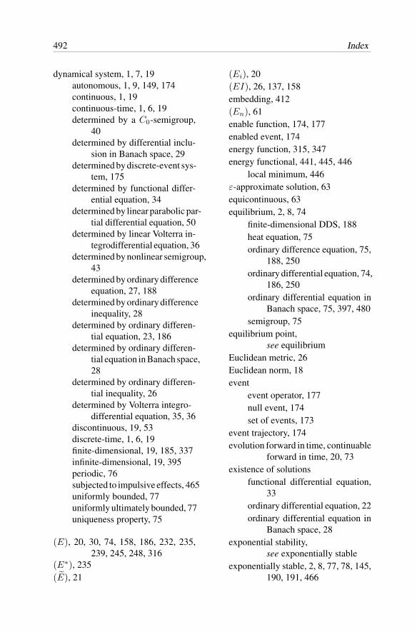
492 Index
dynamical system, 1, 7, 19autonomous, 1, 9, 149, 174continuous, 1, 19continuous-time, 1, 6, 19determined by a C0-semigroup,
40determined by differential inclu-
sion in Banach space, 29determined by discrete-event sys-
tem, 175determined by functional differ-
ential equation, 34determined by linear parabolic par-
tial differential equation, 50determined by linear Volterra in-
tegrodifferential equation, 36determined by nonlinear semigroup,
43determined by ordinary difference
equation, 27, 188determined by ordinary difference
inequality, 28determined by ordinary differen-
tial equation, 23, 186determined by ordinary differen-
tial equation in Banach space,28
determined by ordinary differen-tial inequality, 26
determined by Volterra integro-differential equation, 35, 36
discontinuous, 19, 53discrete-time, 1, 6, 19finite-dimensional, 19, 185, 337infinite-dimensional, 19, 395periodic, 76subjected to impulsive effects, 465uniformly bounded, 77uniformly ultimately bounded, 77uniqueness property, 75
(E), 20, 30, 74, 158, 186, 232, 235,239, 245, 248, 316
(E∗), 235(E), 21
(Ei), 20(EI), 26, 137, 158embedding, 412(En), 61enable function, 174, 177enabled event, 174energy function, 315, 347energy functional, 441, 445, 446
local minimum, 446ε-approximate solution, 63equicontinuous, 63equilibrium, 2, 8, 74
finite-dimensional DDS, 188heat equation, 75ordinary difference equation, 75,
188, 250ordinary differential equation, 74,
186, 250ordinary differential equation in
Banach space, 75, 397, 480semigroup, 75
equilibrium point,see equilibrium
Euclidean metric, 26Euclidean norm, 18event
event operator, 177null event, 174set of events, 173
event trajectory, 174evolution forward in time, continuable
forward in time, 20, 73existence of solutions
functional differential equation,33
ordinary differential equation, 22ordinary differential equation in
Banach space, 28exponential stability,
see exponentially stableexponentially stable, 2, 8, 77, 78, 145,
190, 191, 466
Index 493
continuous dynamical systems de-fined on metric spaces, 95,98, 158, 159, 170–172
continuous finite-dimensional dy-namical systems, 79, 204, 251,270, 272, 275, 298, 316, 318,333, 348
continuous infinite-dimensional dy-namical systems, 398, 401,414, 415, 418, 423
discontinuous dynamical systemsdefined on metric spaces, 85,90
discontinuous finite-dimensionaldynamical systems, 221, 222
discontinuous infinite-dimensionaldynamical systems, 451, 452,466–468, 471, 472
discrete-time dynamical systemsdefined on metric spaces, 105,108, 163, 164, 170–172
discrete-time finite-dimensional dy-namical systems, 79, 212, 215,287, 288, 290, 301, 319, 320
exponentially stable in the large,see exponentially stable
extended solution, 22, 34extension, 22
(F ), 31, 166, 423(F ), 31(FA), 433fading memory space, 34, 403, 410,
421, 463family of motions, 1, 19finite-dimensional dynamical system,
2, 5, 7, 19, 185, 255, 337continuous, 2, 5, 10, 186, 199,
232, 256, 258, 266, 316discontinuous, 6, 10, 188, 219,
243discrete-time, 2, 6, 10, 187, 211,
241, 259, 285, 319First Method of Lyapunov, 4, 10, 295,
300, 317, 320, 415
fixed-point digital filter, 381fixed-point quantization, 358Floquet multiplier, 310, 314, 315, 324function
decrescent, 192–194definite, 195indefinite, 192monotone nondecreasing, 163negative definite, 191, 192, 194negative semidefinite, 192–194positive definite, 191–194positive semidefinite, 192, 194quasi-monotone nondecreasing,
137, 138radially unbounded, 191–194semidefinite, 195
functional differential equation, 2, 5,7, 11, 28, 423, 473
linear retarded, 32, 457neutral, 2, 34retarded, 2, 11, 32, 423, 473
fundamental matrix, 321
(G), 297(GA), 409Gauss’ divergence theorem, 402, 406,
407, 420(GE), 28, 396, 408, 414generalized distance functions, 274generalized momentum coordinates,
24, 202generalized overflow characteristic, 382generalized position coordinates, 24,
25, 202generalized potential force, 24generalized solution, 39(GI), 29global exponential stability,
see exponentially stableglobal stability,
see globally stableglobal uniform asymptotic stability,
see asymptotically stableglobally asymptotically stable,
see asymptotically stable
494 Index
globally stable, 440, 446globally uniformly attractive,
see uniformly attractive inthe large
Gronwall inequality, 64
(H), 344, 482(H), 347Hamiltonian function, 24, 202Hamiltonian system, 73, 201, 208(HD), 482heat equation, 58, 66, 74, 75, 80, 402,
460, 477(Hi), 347Hille–Yoshida–Phillips theorem, 39H l[Ω, C], H l
0[Ω, C], H l[Ω, R], H l0[Ω, R],
47Hopfield neural network, 11, 337, 344,
482circuit, 345with time delay, 482
hybrid dynamical system, 1, 3, 6, 8,11, 51
hypersurface, 296local hypersurface, 296tangent hypersurface, 296
hysteresis effect, 2, 6
(I), 246, 327(ID), 26(IDn), 61(IE), 30(IE), 20, 137, 245(IEI), 26(IEn), 61(IF ), 32, 166(IGE), 28, 396(IGI), 29(IL), 38(ILV ), 36(Im), 246Implicit function theorem, 295, 296(IN ), 41incidence matrix, 182indefinite function, 192
indefinite matrix, 275indirect control system, 11, 340, 344Indirect Method of Lyapunov,
see the First Method of Lya-punov
infinite-dimensional dynamical system,2, 5–7, 19, 395
infinitesimal generatorC0-semigroup, 39nonlinear semigroup, 42
initial condition, 19initial data, 19initial state, 1initial time, 19initial value and boundary value prob-
lem, 74initial value problem, 20
differential inclusion in Banachspace, 29
functional differential equation,32
heat equation, 59, 80linear parabolic partial differen-
tial equation, 50linear partial differential equation
with constant coefficients, 47linear Volterra integrodifferential
equation, 36ordinary difference equation, 26ordinary differential equation, 20ordinary differential equation in
Banach space, 28, 396ordinary differential inequality, 26,
28Volterra integrodifferential equa-
tion, 35well posed, 43
instability,see unstable
integral equation, 21interconnected system, 51, 351, 483interconnecting structure, 351, 484interface element, 3, 53, 353
Index 495
invariance principle,see invariance theorem, in-variance theory
invariance theorem, invariance theory,4, 153, 258, 409, 433, 485
countably infinite system of ordi-nary differential equations,485
dynamical system defined on met-ric space, 9, 153
finite-dimensional dynamical sys-tem, 10, 258
infinite-dimensional dynamical sys-tem, 11, 409, 433
semigroup defined on metric space,9, 153
invariant, invariant set, 1, 8, 73, 83,93, 104, 159, 162, 175
(IP ), 47(IPP ), 50(IV ), 35
Jacobian, 296, 354Jacobian matrix, 296Jordan block
order greater than one, 272, 288order one, 79, 162, 165, 272, 280,
288Jordan canonical form, 271
kinetic energy, 200
(L), 266, 271, 274, 298Lagrange stability, 1, 2, 8, 11, 78, 190Lagrange’s equation, 25Lagrangian, 25Laplacian, 52, 58, 402, 477large-scale system, 5(LC), 317(LD), 286, 288, 289level curve, 196(LF ), 32(LH), 23, 65, 207, 266, 321(LHD), 285, 326Lienard equation, 298limit cycle, 375, 377, 381, 386
linear digital control system, 354linear homogeneous ordinary differ-
ential equation, 23, 207, 266,267
linear operatorbounded, 38closed, 38continuous, 38dissipative, 40graph, 38spectral set, spectrum, 38strongly elliptic, 50
linear ordinary difference equation withconstant coefficients, 79
linear ordinary differential equation withconstant coefficients, 78, 266,271
linear parabolic equation with smoothcoefficients, 49
linear partial differential equation withconstant coefficients, 47
linear periodic ordinary differential equa-tion, 280, 323
linear retarded functional differentialequation, 32, 457
linear sampled-data feedback controlsystem,see linear digital control sys-tem
linear semigroup, 2, 6, 7, 12, 38,see also C0-semigroup
linear system with state saturation, 377linearVolterra integrodifferential equa-
tion, 35, 403, 462linearization, 297Lipschitz condition, 22, 33, 44, 166,
187, 397, 455(LN), 326load balancing of a computer network,
179locally compact metric space, 157lower left-hand Dini derivative, 19lower right-hand Dini derivative, 19(LP ), 280, 300, 323Lp[G, U ], 18
496 Index
lumped parameter system, 2, 6Lure’s result, 5, 10, 339, 340, 344(LV ), 35Lyapunov function, 4
quadratic, 194, 276, 278vector, 161
Lyapunov matrix equation, 4, 274, 275,289, 290
unique solution, 277, 279, 291Lyapunov stability, 1, 2, 8, 11, 78Lyapunov stability results, geometric
interpretation, 10, 197Lyapunov’s first instability theorem
dynamical system defined on met-ric spaces, 99, 108
ordinary difference equation, 218ordinary differential equation, 208ordinary differential equation in
Banach spaces, 405retarded functional differential equa-
tion, 430Lyapunov’s First Method,
see the First Method of Lya-punov
Lyapunov’s Indirect Method,see the First Method of Lya-punov
Lyapunov’s second instability theoremdynamical system defined on met-
ric spaces, 100, 109ordinary difference equation, 218ordinary differential equation, 209ordinary differential equation in
Banach spaces, 406Lyapunov’s Second Method,
see the Second Method ofLyapunov
manufacturing system, 3, 9, 176matrix
critical, 273, 288Hurwitz, 273, 340Hurwitz stable, 273, 340indefinite, 275logarithm, 323
negative definite, 275negative semidefinite, 275positive definite, 275positive semidefinite, 275Schur, 288Schur stable, 288stable, 273, 278, 288triangular, 277triangularized, 277unstable, 273, 288
matrix differential equation, 321matrix measure, 225maximal solution, 138
noncontinuable, 140metric space, 1, 18minimal solution, 138M -matrix, 162, 318, 348modified Nyquist plot, 343monotone nondecreasing function, 163motion, 1, 19
bounded, 19, 77continuable, 20continuable forward for all time,
20continuation, 20continuity with respect to initial
conditions, 123, 131, 186,245, 247, 248
noncontinuable, 20periodic, 76unique forward in time, 75uniqueness, 165, 166
multirate digital feedback control sys-tem, 67
multicore nuclear reactor, 11, 36, 420multivalued operator, 42
N, 18natural basis, 322n degrees of freedom, 25negative definite function, 191, 192,
194, 195, 397negative definite matrix, 275negative invariant set, 73, 297
Index 497
negative semidefinite function, 192–195, 397
negative semidefinite matrix, 275negative semitrajectory, 76negatively invariant set,
see negative invariant setneighborhood of a set, 83neural network, 11, 337, 344, 438neutral functional differential equation,
see functional differential equa-tion of the neutral type
noncontinuable maximal solution, 140noncontinuable motion, noncontinuable
solution, 20, 34nonlinear semigroup, 2, 6, 7, 12, 41,
42contraction, 41infinitesimal generator, 42quasi-contractive, 41
nth-order ordinary difference equation,61
nth-order ordinary differential equa-tion, 61
null event, 174
O notation, 272, 295O notation, 295object of inquiry, 158, 316, 319observable, 330(Ωi), 351one-dimensional wave equation, 66operator
multivalued, 42principal part, 50strongly elliptic, 50w-accretive, 42
orbital stability,see orbitally stable
orbitally stable, 310ordinary difference equation,
see difference equationordinary difference inequality,
see difference inequalityordinary differential equation,
see differential equation
ordinary differential equation in Ba-nach spaces,see differential equation inBanach spaces
ordinary differential inequality,see differential inequality
output bin, 176
(P ), 256, 309partial differential equation, 2, 5, 7,
11, 46, 50hyperbolic equation, 48initial and boundary value prob-
lem, 74, 399, 402, 406, 477,478
initial value problem, 47, 50, 59,80
linear parabolic equation with smoothcoefficients, 49, 399
nonlinear parabolic equation, 399parabolic equation, 48, 399parabolic equation with smooth
coefficients, 399partial motion, 112(PE), 297, 301(PE′), 303Peano–Cauchy existence theorem, 22pendulum, 200, 299perfect load balancing, 180period, 76, 280, 323periodic differential equation, 10, 256,
280, 323linear, 280, 323
periodic dynamical system, 76, 256periodic motion, 76periodic system, 309perturbed linear periodic system, 300perturbed linear system, 10, 298, 300Petri net, 3, 6, 173, 182plant, 353, 365Poincare’s inequality, 403, 406, 420point kinetics model of a multicore nu-
clear reactor, 11, 36, 420Poisson’s formula, 66, 80Popov criterion, 5, 11, 339, 340, 342
498 Index
Popov plot, 343, 344positive definite function, 191–195, 275,
397positive definite matrix, 275positive invariant set, 73, 297positive semidefinite function, 192, 194,
195, 275, 397positive semidefinite matrix, 275positive semitrajectory, 76positively invariant set,
see positive invariant setpotential energy, 200principal boundedness results
dynamical system defined on met-ric spaces, 8, 82, 92, 103
finite-dimensional dynamical sys-tem, 10, 199, 211, 219
infinite-dimensional dynamical sys-tem, 11, 398, 404, 424
principal Lagrange stability results,see principal boundedness re-sults
principal Lyapunov stability resultsdynamical system defined on met-
ric spaces, 8, 82, 92, 103finite-dimensional dynamical sys-
tem, 10, 199, 211, 219infinite-dimensional dynamical sys-
tem, 11, 398, 424producer, 176proper set (with respect to motions),
81pulse-width modulation, 364
type I, 366type II, 366, 367
pulse-width-modulated feedback sys-tem, 11, 337, 364
with Hurwitz stable plant, 367
quadratic form, 10, 194, 274, 276, 289quadratic Lyapunov function, 194, 274,
276quantization level, quantization size,
359, 362quantization, quantizer, 11, 353, 358
fixed point, 358quasi-contractive semigroup, 41, 42,
44, 467, 473quasi-monotone nondecreasing func-
tion, 137, 138
R, 18R
+, 18R
n, 18radially unbounded function, 191–194,
397Rayleigh’s dissipation function, 25Razumikhin-type theorem, 11, 435regulator system, 337, 338resolvent set, 38restriction of a dynamical system, 100retarded functional differential equa-
tion,see functional differential equa-tion of the retarded type
saddle, 281, 283safe operating mode, 178sampled-data control system, 53saturation function, 215saturation nonlinearity, 376, 377scalar differential-difference equation,
32Schauder’s fixed point theorem, 64Schur stable matrix, 288(SE), 55, 189second method of Lyapunov, 4, 201second-order linear system, 281sector, sector condition, 5, 30, 339,
350(SEk), 55, 189semidefinite Lyapunov function, 195semigroup, 2, 11, 38,
see also C0-semigroup,see also nonlinear semigroup
contraction, contractive, 467defined on metric spaces, 153determined by functional differ-
ential equation, 44determined by ordinary differen-
tial equation, 44
Index 499
determined by Volterra integro-differential equation, 45
quasi-contractive, 41, 467, 473set of allowed event trajectories, 174set of discontinuities, 54, 82, 188, 464set of events, 173set of initial conditions, 19set of initial states, 1set of states, 173set of valid event trajectories, 174set-valued mapping, 29(SF ), 55(SFk), 55(SG), 56, 450(SGk), 56, 450(SH), 57(Σ), 483(Σn), 484sigmoidal function, 439, 482simple pendulum, 200, 299Sobolev space, 47, 477Sobolev’s embedding theorem, 412,
413solution, 20spatially distributed parameters, 6spectral set, 38spectrum of a linear semigroup, 38stability,
see stablein the sense of Lyapunov, 2, 78
stability of periodic motions, 10, 309stable, 2, 8, 76, 144, 189, 190, 466
continuous dynamical systems de-fined on metric spaces, 93,150, 151, 158, 159, 170, 171
continuous finite-dimensional dy-namical systems, 79, 200, 251,256, 267, 268, 272, 275, 280,316, 333
continuous infinite-dimensional dy-namical systems, 398, 414,416, 424, 435, 447, 484
discontinuous dynamical systemsdefined on metric spaces, 83
discontinuous finite-dimensionaldynamical systems, 220
discontinuous infinite-dimensionaldynamical systems, 450, 466,468, 471, 472
discrete-time dynamical systemsdefined on metric spaces, 104,150, 151, 163, 164, 170, 171
discrete-time finite-dimensional dy-namical systems, 79, 212, 287,290, 319
stable focus, 281, 285, 286stable manifold, 10, 296, 301–303, 309,
313stable node, 281, 282, 284state space, 1, 19state trajectory, 174state transition matrix, 322strong solution, 38, 43strongly elliptic operator, 50subsystem, 19
free, isolated, 484successive approximations of solutions,
see differential equationswitched system, 3, 465Sylvester inequalities, 195synchronous discrete-time Hopfield neu-
ral network, 337, 350system, 19system of differential inclusions, 29system of first-order ordinary differ-
ence equations, 26system of first-order ordinary differ-
ential equations, 20system subjected to impulsive effects,
3, 465system with saturation nonlinearities,
11, 337, 377
task, 176time lag, 2, 6time set, 1, 19trajectory, 39, 75,
see also negativesemitrajectory,
500 Index
see also positivesemitrajectory
transfer function, 338transportation delay, 2, 6trivial solution, 188
uniform asymptotic stability,see asymptotically stable
uniform asymptotic stability in the large,see asymptotically stable
uniform boundedness,see uniformly bounded
uniform global asymptotic stability,see asymptotically stable
uniform stability,see stable
uniform ultimate boundedness,see uniformly ultimately bounded
uniformly asymptotically stable,see asymptotically stable
uniformly asymptotically stable in thelarge,see asymptotically stable
uniformly attractive, 77, 79, 145, 190,466
in the large, 78, 191, 467uniformly bounded, 2, 77, 190
continuous dynamical systems de-fined on metric spaces, 95,159, 160, 170, 171
continuous finite-dimensional dy-namical systems, 79, 205, 251,267, 287, 317
continuous infinite-dimensional dy-namical systems, 405, 415,417, 418, 426
discontinuous dynamical systemsdefined on metric spaces, 87
discontinuous finite-dimensionaldynamical systems, 221
discontinuous infinite-dimensionaldynamical systems, 452, 467
discrete-time dynamical systemsdefined on metric spaces, 106,163, 164, 170, 171
discrete-time finite-dimensional dy-namical systems, 79, 217, 287,320
uniformly bounded sequence of func-tions, 63
uniformly stable,see stable
uniformly ultimately bounded, 2, 8,77, 190
continuous dynamical systems de-fined on metric spaces, 96,159, 160, 170, 171
continuous finite-dimensional dy-namical systems, 79, 205, 317
continuous infinite-dimensional dy-namical systems, 405, 415,417, 418, 426
discontinuous dynamical systemsdefined on metric spaces, 88
discontinuous finite-dimensionaldynamical systems, 221
discontinuous infinite-dimensionaldynamical systems, 452
discrete-time dynamical systemsdefined on metric spaces, 106,163, 164, 170, 171
discrete-time finite-dimensional dy-namical systems, 79, 217, 320
uniqueness of motion, 165uniqueness of solutions
ordinary differential equation, 22ordinary differential equation in
Banach spaces, 9, 29, 166retarded functional differential equa-
tion, 33uniqueness property, 75unstable, 2, 8, 77, 81, 82, 191, 466
continuous dynamical systems de-fined on metric spaces, 99,100
continuous finite-dimensional dy-namical systems, 79, 199, 208,209, 272, 275, 279, 299, 300,334
Index 501
continuous infinite-dimensional dy-namical systems, 405, 406,408, 430–432
discontinuous dynamical systemsdefined on metric spaces, 92
discontinuous finite-dimensionaldynamical systems, 223, 354,357
discontinuous infinite-dimensionaldynamical systems, 453, 466
discrete-time dynamical systemsdefined on metric spaces, 108,109
discrete-time finite-dimensional dy-namical systems, 79, 218, 288,290, 301
unstable focus, 281, 285unstable manifold, 10, 295, 296, 301–
303, 307–309, 313unstable node, 281–283upper left-hand Dini derivative, 19upper right-hand Dini derivative, 19
(V ), 34valid event trajectory, 174variation of constants formula, 326vector exponent, 46vector index, 46vector Lyapunov function, 161, 316,
348, 421Volterra competition equation, 307Volterra integrodifferential equation,
2, 5, 7, 11, 34, 403,410, 462
(W ), 350w-accretive, 42wave equation, 48, 66(Wi), 350(Wi), 351ω-limit set, 154
Yacubovich–Kalman lemma, 5, 341
Zubov’s theorem, 10, 264
Systems & Control: Foundations & Applications
Series EditorTamer BasarCoordinated Science LaboratoryUniversity of Illinois at Urbana-Champaign1308 W. Main St.Urbana, IL 61801-2307U.S.A.
Systems & Control: Foundations & Applications
Aims and Scope
The aim of this series is to publish top quality state-of-the art books and research mono-graphs at the graduate and post-graduate levels in systems, control, and related fields.Both foundations and applications will be covered, with the latter spanning the gamutof areas from information technology (particularly communication networks) to biotech-nology (particularly mathematical biology) and economics.
Readership
The books in this series are intended primarily for mathematically orientedengineers, scientists, and economists at the graduate and post-graduate levels.
Types of Books
Advanced books, graduate-level textbooks, and research monographs on current andemerging topics in systems, control and related fields.
Preparation of manuscripts is preferable in L T X. The publisher will supply a macropackage and examples of implementation for all types of manuscripts.
Proposals should be sent directly to the editor or to: Birkhäuser Boston,675 Massachusetts Avenue, Cambridge, MA 02139, U.S.A. or toBirkhäuser Publishers, 40-44 Viadukstrasse, CH-4051 Basel, Switzerland
A Partial Listing of Books Published in the Series
Identification and Stochastic Adaptive ControlHan-Fu Chen and Lei Guo
Viability TheoryJean-Pierre Aubin
¸
A E
Representation and Control of Infinite Dimensional Systems, Vol. IA. Bensoussan, G. Da Prato, M. C. Delfour, and S. K. Mitter
Representation and Control of Infinite Dimensional Systems, Vol. IIA. Bensoussan, G. Da Prato, M. C. Delfour, and S. K. Mitter
Mathematical Control Theory: An IntroductionJerzy Zabczyk
H -Control for Distributed Parameter Systems: A State-Space ApproachBert van Keulen
Disease DynamicsAlexander Asachenkov, Guri Marchuk, Ronald Mohler, and Serge Zuev
Theory of Chattering Control with Applications to Astronautics,Robotics, Economics, and Engineering
Michail I. Zelikin and Vladimir F. Borisov
Modeling, Analysis and Control of Dynamic ElasticMulti-Link StructuresJ. E. Lagnese, Günter Leugering, and E. J. P. G. Schmidt
First-Order Representations of Linear SystemsMargreet Kuijper
Hierarchical Decision Making in Stochastic Manufacturing SystemsSuresh P. Sethi and Qing Zhang
Optimal Control Theory for Infinite Dimensional SystemsXunjing Li and Jiongmin Yong
Generalized Solutions of First-Order PDEs: The DynamicalOptimization PerspectiveAndreı I. Subbotin
Finite Horizon H∞ and Related Control ProblemsM. B. Subrahmanyam
Control Under Lack of InformationA. N. Krasovskii and N. N. Krasovskii
H∞-Optimal Control and Related Minimax Design Problems:A Dynamic Game ApproachTamer Basar and Pierre Bernhard
∞
¸
˘
Control of Uncertain Sampled-Data SystemsGeir E. Dullerud
Robust Nonlinear Control Design: State-Space andLyapunov TechniquesRandy A. Freeman and Petar V. Kokotovic
Adaptive Systems: An IntroductionIven Mareels and Jan Willem Polderman
Sampling in Digital Signal Processing and ControlArie Feuer and Graham C. Goodwin
Ellipsoidal Calculus for Estimation and ControlAlexander Kurzhanski and István Vályi
Minimum Entropy Control for Time-Varying SystemsMarc A. Peters and Pablo A. Iglesias
Chain-Scattering Approach to H∞-ControlHidenori Kimura
Output Regulation of Uncertain Nonlinear SystemsChristopher I. Byrnes, Francesco Delli Priscoli,and Alberto Isidori
High Performance ControlTeng-Tiow Tay, Iven Mareels, and John B. Moore
Optimal Control and Viscosity Solutions ofHamilton–Jacobi–Bellman EquationsMartino Bardi and Italo Capuzzo-Dolcetta
Stochastic Analysis, Control, Optimization and Applications:A Volume in Honor of W.H. FlemingWilliam M. McEneaney, G. George Yin,and Qing Zhang, Editors
Mutational and Morphological Analysis: Tools for ShapeEvolution and MorphogenesisJean-Pierre Aubin
Stabilization of Linear SystemsVasile Dragan and Aristide Halanay
´
The Dynamics of ControlFritz Colonius and Wolfgang Kliemann
Optimal ControlRichard Vinter
Advances in Mathematical Systems Theory:A Volume in Honor of Diederich HinrichsenFritz Colonius, Uwe Helmke, Dieter Prätzel-Wolters,and Fabian Wirth, Editors
Nonlinear and Robust Control of PDE Systems:Methods and Applications to Transport-Reaction ProcessesPanagiotis D. Christofides
Foundations of Deterministic and Stochastic ControlJon H. Davis
Partially Observable Linear Systems Under Dependent NoisesAgamirza E. Bashirov
Switching in Systems and ControlDaniel Liberzon
Matrix Riccati Equations in Control and Systems TheoryHisham Abou-Kandil, Gerhard Freiling, Vlad Ionescu, and Gerhard Jank
The Mathematics of Internet Congestion ControlRayadurgam Srikant
H∞ Engineering and Amplifier OptimizationJeffery C. Allen
Advances in Control, Communication Networks, and Transportation Systems:In Honor of Pravin VaraiyaEyad H. Abed
Convex Functional AnalysisAndrew J. Kurdila and Michael Zabarankin
Max-Plus Methods for Nonlinear Control and EstimationWilliam M. McEneaney
Uniform Output Regulation of Nonlinear Systems:A Convergent Dynamics ApproachAlexey Pavlov, Nathan van de Wouw, and Henk Nijmeijer
Supervisory Control of Concurrent Systems: A Petri Net Structural ApproachMarian V. Iordache and Panos J. Antsaklis
Filtering Theory: With Applications to Fault Detection, Isolation, and EstimationAli Saberi, Anton A. Stoorvogel, and Peddapullaiah Sannuti
Representation and Control of Infinite-Dimensional Systems, Second EditionAlain Bensoussan, Giuseppe Da Prato, Michel C. Delfour, and Sanjoy K. Mitter
Set-Theoretic Methods in ControlFranco Blanchini and Stefano Miani
Stability of Dynamical Systems: Continuous, Discontinuous,and Discrete SystemsAnthony N. Michel, Ling Hou, and Derong Liu
Control of Turbulent and Magnetohydrodynamic Channel Flows:Boundary and Stabilization and State EstimationRafael Vazquez and Miroslav Krstic
Related Documents