Almost sure exponential stability of dynamical systems ...

September 13, 2019 International Journal of Control SDEs˙Levy˙Revise1

Almost sure exponential stability of dynamical systems driven by Levy

processes and its application to control design for magnetic bearings

K. D. Do

Department of Mechanical Engineering, Curtin University, Bentley, WA 6102, Australia

H. L. Nguyen

Department of Planning and Finance, Thai Nguyen University, Thai Nguyen City, Vietnam

A Lyapunov-type theorem is developed to study well-posedness and almost surely K∞-exponential sta-bility of dynamical systems driven by Levy processes. Sufficient conditions imposed by the theorem,which are relatively easy to be verified, make it applicable to control design and stability analysis. Thetheorem is then applied to design tracking controllers to achieve almost surely K-exponential stabilityfor magnetic bearings under diffuse-jump loads subject to an output tracking constraint.

Keywords: Lyapunov-type theorem; Well-posedness; Exponential Stability; Levy processes; Magneticbearings.

1. Introduction

Well-posedness (existence and uniqueness of the solution) and stability of stochastic differentialequations (SDEs), which model dynamical systems under stochastic loads, have been extensivelystudied (e.g., (H. Deng, Krstic, & Williams, 2001; Do, 2015, 2016; Khasminskii, 1980; Liu, 2006;X. Mao, 2007) on SDEs driven by diffuses (Brownian motions), (Applebaum, 2009; Applebaum& Siakalli, 2009; W. Mao, You, & Mao, 2016; X. Mao, 1999; X. Mao, Yin, & Yuan, 2007; Teel,Subbaramana, & Sferlazza, 2014; Zhu, 2014) on SDEs driven by diffuses and jumps, (Antunes,Hespanha, & Silvestre, 2010, 2012, 2013a, 2013b, 2014; F. Deng, Luo, & Mao, 2012; Hespanha &Teel, 2006; Teel et al., 2014) on impulsive SDEs driven by renewal processes, which can be viewedas SDEs driven by diffuses and jumps via the Levy-Ito decomposition (Applebaum, 2009, Theorem2.4.16)). To study local/global well-posedness of SDEs, different Lipschitz and growth conditions areimposed on the system functions. Because one type of stability does not usually imply the other(s)in a stochastic setting (X. Mao, 2007), different criteria are proposed to guarantee different typesof stability. Stability in moment and almost sure (a.s.) stability (sometime referred to as stabilityin probability) are often considered. Motivated by the fact that Lyapunov’s direct method has beenextensively used for deterministic dynamical system (Khalil, 2002), this method is also the mostpowerful tool to investigate stability in moment and a.s. stability of SDEs.There are excessive and excellent results on Lyapunov sufficient conditions to ensure exponen-

tial stability in moment and a.s asymptotic stability of both SDEs driven by diffuses and jumps(Applebaum, 2009; Applebaum & Siakalli, 2009; W. Mao et al., 2016; X. Mao, 1999; X. Mao et al.,2007; Teel et al., 2014; Zhu, 2014) and impulsive SDEs driven by renewal processes (Antunes etal., 2010, 2012, 2013a, 2013b, 2014; F. Deng et al., 2012; Hespanha & Teel, 2006; Nane & Ni, 2017;

Email: [email protected]

Email: [email protected]


Teel et al., 2014). These conditions are analogous to those developed for deterministic differentialequations, see (Khalil, 2002, Chapter 4), where an infinite generator should be used instead of thenormal time derivative of a Lyapunov function. On the other hand, there are several results on a.s.exponential stability of SDEs driven by diffuses and jumps. In (Applebaum, 2009; Applebaum &Siakalli, 2009), an important exponential martingale inequality is derived and the result on globala.s. exponential stability of SDES driven by diffuses in (X. Mao, 2007, Theorem 3.3) is generalizedto SDEs driven by diffuses and jumps, where a negative logarithm condition on the jump termin the infinite generator of a Lyapunov function plus usual Lyapunov sufficient conditions are im-posed, see (Applebaum & Siakalli, 2009, Theorem 3.1), whose proof is the most interesting due tothe use of the exponential martingale inequality that they derived. However, the negative logarithmcondition on the jump term in the infinite generator creates difficulty in applying (Applebaum &Siakalli, 2009, Theorem 3.1) to control design because the control is not able to change the abovejump term in the infinite generator. In (W. Mao et al., 2016), the result on a.s. exponential stabil-ity of SDEs driven by diffuses and jumps is derived under a growth condition on the jump term,see (W. Mao et al., 2016, Theorem 3.2). This condition also creates difficulty in its application tocontrol design. In (X. Mao et al., 2007), a linear growth condition is imposed on the jump term toprove a.s. exponential stability for SDEs with Markovian switching (or hybrid SDEs), see (X. Maoet al., 2007, Theorem 3.3). In (F. Deng et al., 2012), a different growth condition is imposed on theproduct of the Lyapunov function’s gradient and the jump function to prove a.s. exponential stabil-ity for SDEs with Markovian switching, see (F. Deng et al., 2012, Theorem 2.2). In (X. Mao, 1999),a linear growth condition is imposed on the system function to prove that the exponential stabilityin moment implies the almost sure exponential stability for SDEs with Markovian switching, see(X. Mao, 1999, Theorem 3.2). The common feature in the aforementioned works for the study ofa.s. exponential stability is the assumption made on the system jump function either independentlyor as a separate condition on the jump term of the Lyapunov function’s infinite generator. From acontrol design point of view, it is convenient to derive sufficient conditions impose on a Lyapunovfunction and its (whole) infinite generator. Conditions imposed on the whole infinite generator aremore relaxed than those on the individual jump term in the infinite generator in control designbecause the control can change the infinite generator on the whole but not its individual jumpterm. This is analogous to the results developed for deterministic systems, and has obtained forthe study of exponential stability in moment and a.s. asymptotic stability for SDEs as reviewedabove.The above discussion motivates the first contribution of this paper on developing a Lyapunov-

type theorem to study well-posedness and a.s. K∞-exponential stability of systems driven by Levyprocesses. We consider Levy processes as disturbances driving the system because a Levy process ispreferably used in systems with high uncertainties, and can be decomposed to three components byLevy-Ito decomposition (Applebaum, 2009): a drift, a Brownian motion, and a pure jump process,which can be used to correspondingly describe the deterministic, diffuse, and jump components.The Lyapunov conditions imposed by the theorem are similar to those required for exponentialstability in moment and a.s. asymptotic stability for SDEs in the literature.Based on well-posedness and stability results as discussed above, control of systems driven by

diffuses and/or jumps has also been considered. When using the powerful Lyapunov direct method,control of systems driven by diffuses and jumps (in comparison with deterministic systems) hastwo difficulties induced by the Hessian and jump terms in the infinite generator of a Lyapunovfunction. Despite the difficulty caused by the Hessian term, control of systems driven by diffuseswas considered by many authors (e.g., (H. Deng & Krstic, 1997; H. Deng et al., 2001; Do, 2015)).However, the jump term is more complicated to be dealt with than the Hessian term. Thus, controlof systems driven by both diffuses and jumps (Levy processes) is a new area. The only referenceis (Jagtap & Zamani, 2017) on backstepping control design for Hamiltonian systems driven bydiffuse-jumps to achieve stability in moment. As an application of the developed Lyapunov-typetheorem for study of well-posedness and stability of systems driven by diffuses and jumps to control

2


design, tracking controllers are designed for active magnetic bearings (AMBs) under stochastic(deterministic, diffusive, and jumped) loads. Control of AMBs under stochastic loads has notbeen addressed in the literature despite the fact that loads on the rotor of AMBs contain highuncertainties in a number of applications. Up to present, loads on the rotor of AMBs are onlyconsidered as (time-invariant or time-varying) deterministic disturbances. Related works include(Fujita, Hatake, & Matsumura, 1993; Matsumura & Yoshimoto, 1986; Mohamed & Emad, 1992;Smith & Weldon, 1995) on linear control, and (Charara, Miras, & Caron, 1996; de Queiroz &Dawson, 1996; de Queiroz, Dawson, & Suri, 1998; Do, 2010; Mittal & Menq, 1997; Smith & Weldon,1995; Torries, Sira-Ramirez, & Escobar, 1999) on nonlinear control.Motivated by the above review/discussion, the second contribution of this paper is the design of

tracking controllers for AMBs driven by Levy processes to achieve a.s. (practical) K-exponentialstability of the closed-loop system. The control design also imposes a hard constraint on the dis-placement tracking error.Notations. The symbols ∧ and ∨ denote the infimum and supremum operators, respectively.

The symbol E denotes the expected value while P denotes probability.

2. Well-posedness and Stability of SDEs

This section presents SDEs to be considered, definition of a.s. stability, and a Lyapunov-typetheorem on well-posedness and stability of SDEs. These results are to be used for control designand analysis of well-posedness and stability of magnetic bearings.

2.1 Nonlinear SDEs

LetW (t), t ≥ t0 ≥ 0 be anm1-dimensional standard Brownian motion vector defined on a completeprobability space (Ω,F ,P) equipped with a filtration Ft≥t0 such that it satisfies the usual hypothe-ses. Let N = col(N1, ..., Nℓ, ..., Nm2

) be an m2-dimensional Poisson random measure vector defined

on R+× (Rm2 −0) with an m2-dimensional compensator vector N and m2-dimensional intensitymeasure vector ν = col(ν1, ..., νℓ, ..., νm2

). We assume that all Nℓ are independent of each other, N

is independent of W , and ν is a Levy measure vector such that N(dt, dξ) := N(dt, dξ)− dtν(dξ)and

∫Rm2−0(∥ξ∥

2 ∧ 1)ν(dξ) <∞ with ξ = col(ξ1, · · · , ξℓ, · · · , ξm2).

Consider the nonlinear SDE driven by Levy processes:

dX(t) = F (X(t), t)dt+G(X(t), t)dW (t) +∫∥ξ∥<εΦ(X(t−), t, ξ)N(dt, dξ),

X(t0) = X0 ∈ Rn,(1)

where X(t−) = lims↑tX(s); F : Rn × [t0,∞) → Rn; G : Rn × [t0,∞) → Rn×m1 ; Φ : Rn × [t0,∞)×Rm2 → Rn×m2 , and

∫∥ξ∥<εΦ(X(t−), t, ξ)N(dt, dξ) :=

∑m2

ℓ=1

∫|ξℓ|<εℓ

Φ(ℓ)(X(t−), t, ξ)Nℓ(dt, dξℓ)

with Φ(ℓ) being the ℓth column of Φ for compact notation. The constants εℓ ∈ (0,∞] denotethe maximum allowable jump sizes.We assume that the system functions F (X(t), t), G(X(t), t), and Φ(X(t−), t, ξ) satisfy the

following local conditions to ensure local well-posedness of (1).

Assumption 2.1:C1. [Local Lipschitz] For any X,Y ∈ Rn with ∥X∥ ∨ ∥Y ∥ ≤ ϵ1, where ϵ1 is a positive constant,there exists a nonnegative constant L1 such that for all t ∈ [t0,∞):

∥F (X, t)−F (Y , t)∥2 + ∥G(X, t)−G(Y , t)∥2+∑m2

ℓ=1

∫|ξℓ|<εℓ

∥Φ(ℓ)(X, t, ξℓ)−Φ(ℓ)(Y , t, ξℓ)∥2νℓ(dξℓ) ≤ L1∥X − Y ∥2. (2)

3


C2. [Locally linear growth] For any X ∈ Rn with ∥X∥ ≤ ϵ2, where ϵ2 is a positive constant, thereexists a nonnegative constant L2 such that for all t ∈ [t0,∞):

∥F (X, t)∥2 + ∥G(X, t)∥2 +∑m2

ℓ=1

∫|ξℓ|<εℓ

∥Φ(ℓ)(X, t, ξℓ)∥2νℓ(dξℓ) ≤ L2(1 + ∥X∥2). (3)

2.2 Definition of a.s. stability

The following definition is based on (Applebaum, 2009) and (Khalil, 2002).

Definition 2.1: The trial solution of (1) is said to be

(1) almost surely globally practically stable if for ϵ ∈ (0, 1), there exists a class K∞-function αsuch that

P∥X(t)∥ < α(∥X0∥) + ϵ0 ≥ 1− ϵ (4)

for all t ∈ [t0,∞) and X0 ∈ Rn, where ϵ0 is a nonnegative constant.(2) almost surely globally practically K∞-exponentially stable if it is almost surely globally prac-

tically stable and

∥X(t)∥ ≤ α(∥X(t0)∥)e−ϵ(t−t0) + ϵ0, a.s. (5)

for all X0 ∈ Rn, where α is a class K∞-function, ϵ is a positive constant, and ϵ0 is anonnegative constant.

If ϵ0 = 0, “practically” is dropped from the above statements. Moreover, if α(∥X(t0)∥) ≡ c∥X(t0)∥with c being a positive constant, then “K∞” is dropped from the above statements.

2.3 A Lyapunov-type theorem

The following theorem gives sufficient conditions on global well-posedness and stability of nonlinearSDE (1).

Theorem 2.1: Under Assumption 2.1, assume further that there exists a function U ∈ C2(Rn ×[t0,∞)) called a Lyapunov function; class K∞-functions α1(.) and α2(.); and an integer p ≥ 2 suchthat ∀ (X, t) ∈ Rn × [t0,∞) :

α1(∥X∥p) ≤ U(X, t) ≤ α2(∥X∥p). (6)

1) [Well-posedness] Suppose that LU(X, t) satisfies

LU(X, t) ≤ c3(1 + U(X, t)), X ∈ V, t ∈ [t0,∞), (7)

where c3 is a nonnegative constant. Then the system (1) has a unique solution for each X0 ∈ Rn.2) [a.s. stability] Suppose that there exists a positive constant c4 such that ∀ (X, t) ∈ V × [t0,∞) :

LU(X, t) ≤ −c4U(X, t) + c0. (8)

If the constant c0 = 0, the equilibrium X ≡ 0 is a.s. globally stable. If c0 > 0, the equilibriumX ≡ 0 is a.s. globally practically stable.3) [a.s. exponential stability] Suppose further that α2(∥X + Φℓ∥p) ≤ α21(∥X∥p) + α22(∥Φℓ∥p),

where α21(∥X∥p) and α22(∥Φℓ∥p) are some class K∞-functions, and the function α22(∥Φℓ∥p) sat-isfies

supX∈E

∫|ξℓ|<εℓ

e∥Φℓ(X,t,ξℓ)∥νℓ(dξℓ) <∞ a.s. (9)

for all bounded sets E. If the constant c0 = 0, the equilibrium X ≡ 0 is a.s. globally K∞-exponentially stable. If c0 > 0, the equilibrium X ≡ 0 is a.s. globally practically K∞-exponentially

4


stable. Moreover,

∥X(t)∥p ≤ α−11

[α2(∥X0∥p)e−c4(t−t0) + c0

c4

]a.s. (10)

If α1(•) ≡ c1 • and α2(•) ≡ c2 • with c1 and c2 being positive constants, “K∞” is dropped in theabove statements.

Proof. See Appendix A.

Remark 2.1:

• Only local conditions (2) and (3) are needed. These conditions ensure existence and unique-ness of a local solution to (1). This local solution is then extended to a global solution by theconditions (6) and (7).

• The inequality (10) is equivalent to (5) by taking the power 1p both sides of (10) and applying

(|a|+ |b|)ℓ ≤ 2ℓ(|a|ℓ + |b|ℓ) for all (a, b) ∈ R2 and ℓ > 0.• Although conditions imposed in Theorem 2.1 are of the form similar to those for deterministic

systems, see e.g., (Khalil, 2002, Chapter 4), the infinite generator LU has to be used insteadof the normal time derivative of U . This makes Theorem 2.1 easily accessible to those whoare familiar to Lyapunov’s direct method for control design and stability analysis.

3. Stochastic control of magnetic bearings

3.1 Mathematical model and control objective

Since the dynamics of a magnetic bearing system in the y-direction is the same as that in thex-direction, we only consider its mathematical model in the x-direction as follows, see (Smith &Weldon, 1995):

mx =∑2

j=1 Fi(x, Ii) + F0x, (11)

where x(t), x(t) and x(t) represent the rotor disk position, velocity, and acceleration, respectively,along the x-direction; m represents the mass of the rotor; Fi(x, Ii), i = 1, 2 denote the forcesproduced by each stator electromagnetic circuit; Ii, i = 1, 2 represent the current in each statorcoil; F0x is the external disturbance force. The forces Fi(x, Ii) and F0x are detailed in what follows.Under a common assumption that the applied magnetic forces are only dependent on the direction

of major motion and the measured current in winding of the coil (for example F1(x, I1) only dependson x and I1), the flux linkage model is used to compute the model for the force produced by theelectrical phases as follows (Woodson & Melcher, 1968):

Fi(x, Ii) =∂∂x

∫ Ii0 λi(x, Ii)dIi, i = 1, 2 (12)

where λi(x, Ii) represents the flux linkage model. If fringing and leakage are neglected and themagnetic circuit is assumed to be linear, the following flux linkage model is often utilized tocomplete the electromechanical dynamic system description, see (Smith & Weldon, 1995):

λi(x, Ii) = Li(x)Ii, i = 1, 2, (13)

with

Li(x) =L0

2 (g0x + (−1)ix) + L1, i = 1, 2, (14)

where L0 and L1 are positive constant parameters which depend on the number of stator coilturns, permeability of the material, air, cross-sectional area of the electromagnet, etc., and g0x is aconstant kinematic quantity, i.e. the gap between the rotor and the stator when the rotor is in itsneutral position. The flux linkage model given by (13) can now be used to calculate Fi(x, Ii), i = 1, 2

5


in (12) explicitly as follows

Fi(x, Ii) =(−1)(i+1)L0I

2i

(2(g0x + (−1)ix) + L1)2, i = 1, 2. (15)

To cover various external disturbance forces in practice, we consider F0x of the following form:

F0x = a1f1(x) + a2, (16)

where the functions f1(x) is a continuous function of x, and is bounded if its argument x is bounded.We use a Levy process to describe each parameter ai, i = 1, 2 as discussed in Section 1 as follows:

ai = θi + δidwi(t)dt + γi

∫|ξi|<εi

Ni(dt,dξi)dt , (17)

where θi, δi, and γi with i = 1, 2 are unknown but bounded parameters and the constant εi ∈ (0,∞];

and wi(t) is a standard Wiener process. The compensated Poisson measure Ni(dt, dξi) is given by

Ni(dt, dξi) = Ni(dt, dξi)−dtνi(dξi), where Ni(dt, dξi) is a Poisson measure and νi(dξi) is a intensitymeasure, see also Section 2.1. Substituting (16), where ai are given in (17), into (11) results in thestochastic model of the magnetic bearing system:

dx1 = x2dt,

dx2 =1m

[( 2∑i=1

Fi(x1, Ii) +2∑

i=1θiΦi

)dt+

2∑i=1

δiΦidwi(t) +2∑

i=1γiΦi

∫|ξi|<εi

Ni(dt, dξi)],

(18)

where x1 = x, x2 = x, and

Φ1 = f1(x1), Φ2 = 1. (19)

Before stating the control objective, we make the following assumptions, which are reasonable inpractice.

Assumption 3.1: All the following conditions hold almost surely:

(1) From its neutral position, the rotor can displace in the interval [−g0x, g0x] along the x-axis.

The constants g0x, g0x are strictly positive such that g

0x∨ g0x ≤ g0x.

(2) The reference trajectory x1d(t) is feasible, i.e., there exist strictly positive constants CM1x < g

0x

and CM1x < g0x such that

−(g0x

− CM1x

)≤ x1d(t) ≤

(g0x − C

M1x

). (20)

Moreover, the time derivatives x1d(t) and x1d(t) are bounded.(3) The initial tracking error is feasible, i.e., there exist strictly positive constants C0x < CM

1x

and C0x < CM1x such that at the initial time t0 ≥ 0, the following conditions hold

−C0x ≤ x1(t0)− x1d(t0) ≤ C0x, (21)

where x1d(t0) is the initial value of x1d(t) at t = t0 ≥ 0.(4) All the parameters θi(t), δi(t), γi(t), and

∫|ξi|<ϵi

νi(dξi), i = 1, 2 are bounded, i.e., there exist

nonnegative constants θi, δi, γi, and ϖi such that

supt∈[t0,∞)

θ2ki (t) ≤ θi, supt∈[t0,∞)

δ2ki (t) ≤ δi,

supt∈[t0,∞)

γ2ki (t) ≤ γi, supt∈[t0,∞)

( ∫|ξi|<ϵi

νi(dξi))2k ≤ ϖ2k := ϖi,

(22)

where k is an integer larger than 1.

Control Objective 3.1: Under Assumption 3.1, design the control inputs Ii, i = 1, 2 that forcethe output x1(t), of the magnetic bearing system defined in (18) to track the reference trajectory

6


x1d(t), such that

(1) The output tracking error are within a pre-specified and feasible range almost surely, i.e.,

−C1x ≤ x1(t)− x1d(t) ≤ C1x, a.s. (23)

for all t ≥ t0 ≥ 0, where C1x and C1x are strictly positive constants that satisfy the followingfeasibility conditions

C0x < C1x ≤ CM1x, C0x < C1x ≤ C

M1x, a.s. (24)

(2) Almost surely exponential tracking is achieved, i.e.

|x1(t)− x1d(t)| ≤ φ1(x1(t0), x2(t0))e−c11(t−t0) + c10, a.s. (25)

where φ1 is a class K-function, c11 is a positive constant, and c10 is a nonnegative constantsuch that c10 ≤ C1x ∧ C1x.

(3) All signals of the closed loop system are bounded.

3.2 Preliminaries

As the control objective imposes on both symmetric and asymmetric constraints on the trackingerror x1(t)− x1d(t), see (23), we first need a suitable smooth unbounded and increasing function,which will be embedded in our Lyapunov function in the sequel.

Definition 3.1: Let a and b be constants such that a < 0 < b, a function Ψ(x, a, b) is said to be asmooth unbounded and increasing function on the interval [a, b] if

1) x = 0 ⇔ Ψ(x, a, b) = 0,2) limx→a+ Ψ(x, a, b) = −∞, limx→b− Ψ(x, a, b) = ∞,3) Ψ(x, a, b) is smooth for all x ∈ (a, b),4) Ψ′(x, a, b) > 0 for all x ∈ (a, b),

(26)

where Ψ′(x, a, b) = ∂Ψ(x,a,b)∂x .

If a = −b, it is then easy to find many smooth unbounded and increasing functions such astanh−1(− 1

ax). If a = −b, construction of smooth unbounded and increasing functions is given inthe following lemma:

Lemma 3.1: For given constants a and b such that a < 0 < b and a+bb−a = 2n + 1 for all n =

0,±1,±2, · · · , the scalar function Ψ(x, a, b) defined by

Ψ(x, a, b) = tan[

πb−a

(x− a+b

2

)]+ tan

[π

b−aa+b2

](27)

is a smooth unbounded and increasing function of x on the interval [a, b]. Moreover, Ψ′(x, a, b) ≥π

b−a , ∀ x ∈ R.

−2 0 2 4−15

−10

−5

0

5

10

15

x

Ψ(x,−2,4)

Figure 1.: A plot of Ψ(x,−2, 4).

Proof. The proof follows by a direct verification of all prop-erties of smooth unbounded and increasing functions listedin (26). Lemma 3.1 provides a much simpler construction ofsmooth unbounded and increasing functions than Lemma 2.2in (Do, 2010). A plot of smooth unbounded and increasingfunction with a = −2 and b = 4 is given in Fig. 1.

7


3.3 Coordinate transformation

To transform the tracking control objective with constraintsto a stabilization problem, we introduce the coordinate trans-formation

z1 = Ψ(x1e, a, b), (28)

where x1e = x1 − xd is the output tracking error. The function Ψ(x1e, a, b) is chosen according toLemma 3.1. The constants a and b, are chosen such that

−C1x ≤ a < −C0x, C0x < b ≤ C1x,a+bb−a = 2n+ 1, ∀ n = 0,±1,±2, · · · (29)

Applying the Ito formula, see (Applebaum, 2009), to (28) along the solutions of (18) gives

dz1 = Ψ′(x1e, a, b)(x2 − xd)dt,

dx2 =1m

[( 2∑i=1

Fi(x1, Ii) +2∑

i=1θiΦi

)dt+

2∑i=1

δiΦidwi(t) +2∑

i=1γiΦi

∫|ξi|<εi

Ni(dt, dξi)].

(30)

Thus, the control objective now is to design Ii, i = 1, 2 such that they stabilize (30) at the originalmost surely.

3.4 Control design

The control design consists of two steps by applying the ingredients developed in Section 2 andthe backstepping method (Krstic, Kanellakopoulos, & Kokotovic, 1995), which are detailed below.

3.4.1 Step 1

Define

z2 = x2 − α1, (31)

where α1 is a virtual control of x2. To design α1, we consider the following Lyapunov functioncandidate

U1 =1

2kz2k1 (32)

where k is a positive integer to be determined. The above choice of U1 is motivated by the workin (Do, 2015) to handle the Hessian term in the infinite generator LU2, which will appear in thesecond step. Applying the Ito formula to U1 along the solutions of the first equation of (30) and(31) yields

LU1 = z2k−11 Ψ′(z2 + α1 − xd), (33)

where we have dropped the arguments (x1e, a, b) of Ψ′ for clarity. From (33), we choose α1 as

α1 = −k11z1 − k12(Ψ′)2k−1z1 + xd, (34)

where k11 and k12 are positive constants to be chosen later. It is noted that α1 is a function of(x1, xd, xd). Substituting (34) into (33) gives

LU1 = −[k11Ψ′ + k12(Ψ

′)2k]z2k1 +Ψ′z2k−11 z2. (35)

8


3.4.2 Step 2

To design the controls I1 and I2, we consider the following Lyapunov function candidate

U2 = U1 +m2kz

2k2 . (36)

Applying the Ito formula to U2 along the solutions of the second equation of (30) and using (35)results in

LU2 = −[k11Ψ′ + k12(Ψ

′)2k]z2k1 +Ψ′z2k−11 z2

+z2k−12

( 2∑i=1

Fi(x1, Ii) +2∑

i=1θiΦi −m

(∂α1

∂x1x2 +

∂α1

∂xdxd +

∂α1

∂xdxd

))+ 2k−1

2 z2k−22

2∑i=1

δ2iΦ2i

+m2∑

i=1

∫|ξi|<εi

[12k (z2 + γiΦi)

2k − 12kz

2k2 − z2k−1

2 γiΦi

]νi(dξi).

(37)

We now need to find the upper-bound of the right hand-side of (37). Using the inequalities (a +b)2k ≤ 22k−1(a2k+b2k) and ab ≤ ϵp

p |a|p+ 1

qϵq |b|q with ϵ > 0, p > 1, q > 1, 1p+

1q = 1 for all (a, b) ∈ R2,

and the expression of Φi, i = 1, 2 in (19), we can calculate:

Ψ′z2k−11 z2 ≤ (Ψ′)2kϵ

2k

2k−1

10 z2k1 + 12kϵ2k10

z2k2 ,

z2k−12 θ1Φ1 ≤ 2k−1

2k ϵ2k

2k−1

11 z2k2 + 12kϵ2k11

θ1A,

z2k−12 θ2Φ2 ≤ 2k−1

2k ϵ2k

2k−1

12 z2k2 + 12kϵ2k12

θ2,

z2k−12 δ1Φ1 ≤ 2k−1

2k ϵ2k

2k−1

11 z2k2 + 12kϵ2k11

δ1A,

z2k−12 δ2 ≤ 2k−1

2k ϵ2k

2k−1

12 z2k2 + 12kϵ2k12

δ2,

m∫|ξ1|<ε1

12k (z2 + γ1Φ1)

2kν1(dξ1) ≤ m22k−1

2k ϖ1z2k2 + m22k−1

2k γ1Aϖ1,

m∫|ξ1|<ε1

z2k−12 γ1Φ1ν1(dξ1) ≤ m22k−1

2k ϵ2k

2k−1

15 z2k2 + m2kϵ2k15

γ1Aϖ1,

m∫|ξ2|<ε2

12k (z2 + γ2Φ2)

2kν2(dξ2) ≤ m22k−1

2k ϖ2z2k2 + m22k−1

2k γ2ϖ2,

m∫|ξ2|<ε2

z2k−12 γ2Φ2ν2(dξ2) ≤ m22k−1

2k ϵ2k

2k−1

16 z2k2 + m2kϵ2k16

γ2ϖ2,

(38)

where ϵ1i, i = 0, · · · , 6 are positive constants to be chosen later; δi, γi, ϖi, i = 1, 2 are defined in

(22); A =(supx∈[a−|xd|,b+|xd|] |f1(x)|

)2kwith a note that we have used (27) and (28) to obtain

x = arctan(z1 − tan

(π

b−aa+b2

))b−aπ + a+b

2 + xd. Substituting (38) into (37) results in

LU2 ≤ −[k11Ψ

′ +(k12 − ϵ

2k

2k−1

10

)(Ψ′)2k

]z2k1 + z2k−1

2

( 2∑i=1

Fi(x1, Ii)

−m(∂α1

∂x1x2 +

∂α1

∂xdxd +

∂α1

∂xdxd

)+ c1z2

)+ c0,

(39)

where

c1 =1

2kϵ2k10+ 2k−1

2k ϵ2k

2k−1

11 + 2k−12k ϵ

2k

2k−1

12 + 2k−12k ϵ

2k

2k−1

13 + 2k−12k ϵ

2k

2k−1

14 + m22k−1

2k ϖ1 +m22k−1

2k ϵ2k

2k−1

15 + m22k−1

2k ϖ2

+m22k−1

2k ϵ2k

2k−1

16 ,

c0 =1

2kϵ2k11θ1A+ 1

2kϵ2k12θ2 +

12kϵ2k13

δ1A+ 12kϵ2k14

δ2 +m22k−1

2k γ1Aϖ1 +m

2kϵ2k15γ1Aϖ1 +

m22k−1

2k γ2ϖ2

+ m2kϵ2k16

γ2ϖ2.

(40)From (39), we choose the controls I1 and I2 such that

2∑i=1

Fi(x1, Ii) = −k2z2 +m(∂α1

∂x1x2 +

∂α1

∂xdxd +

∂α1

∂xdxd

)− c1z2

:= ∆,(41)

9


where k2 is a positive constant to be chosen later. We now write (41) with (15) as follows

χ21(x1)I

21 − χ2

2(x1)I22 = ∆, (42)

where ∆ is defined in (41), and

χ1(x1) =√L0

2(g0x−x1)+L1,

χ2(x1) =√L0

2(g0x+x1)+L1.

(43)

To solve (42) for I1 and I2, we write (42) as follows(χ1(x1)I1 − χ2(x1)I2

)(χ1(x1)I1 + χ2(x1)I2

)=

∆

(∆ℓ + γℓ0)1

2ℓ

(∆ℓ + γℓ0)1

2ℓ , (44)

where γ0 is a small positive constant, and ℓ is a positive even number. Thus, we can simply choose

χ1(x1)I1 − χ2(x1)I2 = (∆ℓ + γℓ0)1

2ℓ ,

χ1(x1)I1 + χ2(x1)I2 =∆

(∆ℓ + γℓ0)1

2ℓ

,(45)

which gives

I1 =1

2χ1(x1)

( ∆

(∆ℓ + γℓ0)1

2ℓ

+ (∆ℓ + γℓ0)1

2ℓ

),

I2 =1

2χ2(x1)

( ∆

(∆ℓ + γℓ0)1

2ℓ

− (∆ℓ + γℓ0)1

2ℓ

),

(46)

Remark 3.1: The choice of the controls I1 and I2 as in (46) is not unique as we can specify

alternative terms for (∆ℓ + γℓ0)1

2ℓ in (44). Other choices like the ones in (de Queiroz & Dawson,1996; de Queiroz et al., 1998; Do, 2010) are possible. The controls I1 and I2 in (46) are smooth andtheir magnitude is proportional to

√|∆|, which makes the controls I1 and I2 behave very similar

to ideal switching controls such as if ≥ 0 then I1 = 1χ1(x1)

√ and I2 = 0, else if < 0 then

I1 = 0 and I2 = −1χ2(x1)

√− when || dominates γ0. Indeed, if γ0 is set to zero, the controls I1

and I2 in (46) become

I1 =1

2χ1(x1)

(∆√|∆|

+√|∆|

),

I2 =1

2χ2(x1)

(∆√|∆|

−√|∆|

),

(47)

which behave exactly the same as the aforementioned ideal switching controls. However, the controlsI1 and I2 in (47) are only continuous instead of being smooth as those in (46). The tradeoff is thatthe controls I1 and I2 in (46) require a small quantity of currents when ∆ = 0 due to nonzero γ0.

Substituting (41) into (39) gives

LU2 ≤ −[k11Ψ

′ +(k12 − ϵ

2k

2k−1

10

)(Ψ′)2k

]z2k1 − k2z

2k2 + c20. (48)

For a given ϵ10, we first choose k12 such that

k12 ≥ ϵ2k

2k−1

10 . (49)

Using (49) and Ψ′ ≥ πb−a , see Lemma 3.1, and definition of U2 given in (36), we can write (48) as

follows:

LU2 ≤ −cU2 + c0, (50)

10


where

c = 2k[(

k11πb−a +

(k12 − ϵ

2k

2k−1

30

)(π

b−a

)2k) ∧ k2]. (51)

The control design has been completed. We summarize the main results in the following theorem.

Theorem 3.1: Under Assumption 3.1, the controls I1 and I2 given in (46) ensure that the closed-loop system consisting of (41) and (30) or (18) is well-posed; x1e(t) ∈ (a, b) for all t ≥ t0 almostsurely; and |x1e(t)| almost surely exponentially converges to c⋆0 defined by

c⋆0 =[arctan

(2

1

2k

[22k−12k c0

c

] 1

2k − tan(

πb−a

a+b2

))b−aπ + a+b

2

]∨[∣∣∣− arctan

(2

1

2k

[22k−12k c0

c

] 1

2k + tan(

πb−a

a+b2

))b−aπ + a+b

2

∣∣∣], (52)

which can be made arbitrarily small choosing large control gains k11, k12, and k2 because c is givenby (51). Control Objective 3.1 is solved by the controls I1 and I2 given in (46) provided that controlgains k11, k12, and k2 are chosen such that c⋆0 ≤ c10, where c10 is defined in (25).

Proof. First, applying Theorem 2.1 to (50) with U2 given in (36) ensures that the closed-loopsystem consisting of (41) and (30) or the x-subsystem given in (18) is well-posed. Next, applyingTheorem 2.1 to (50) with U2 given in (36) yields

z2k1 (t) + z2k2 (t) ≤ 2k(

12k

(z2k1 (t0) + z2k2 (t0)

)e−c(t−t0) + c0

c

)a.s.

⇒ |z1(t)|+ |z2(t)| ≤[22k−12k

(12k

(z2k1 (t0) + z2k2 (t0)

)e−c(t−t0) + c0

c

)] 1

2k

≤ 21

2k

[22k−12k

(12k

(z2k1 (t0) + z2k2 (t0)

)e−c(t−t0)

] 1

2k

+ 21

2k

[22k−12k c0

c

] 1

2k

a.s.

(53)

where we have used (|z1| + |z2|)2k ≤ 22k−1(z2k1 + z2k2 ) for all (z1, z2) ∈ R2 and (|a| + |b|)1

2k ≤2

1

2k (|a|1

2k + |b|1

2k ) for all (a, b) ∈ R2. The inequality (53) ensures that z1(t) and z2(t) are boundedfor all bounded initial values z1(t0) and z2(t0), i.e., for all initial values of x1e(t0) ∈ (a, b) andbounded x2(t0) due to (28). Solving (28) gives

x1e = arctan(z1 − tan

(π

b−aa+b2

))b−aπ + a+b

2 . (54)

This together with boundedness of (z1(t), z2(t)) implies that x1e(t) ∈ (a, b) for all initial values ofx1e(t0) ∈ (a, b) and bounded x2(t0). Combining (53) and (54) yields

|x1e(t)| ≤[arctan

(|z1(t)| − tan

(π

b−aa+b2

))b−aπ + a+b

2

]∨[∣∣− arctan

(|z1(t)|+ tan

(π

b−aa+b2

))b−aπ + a+b

2

∣∣] a.s. (55)

Since arctan(·) is a class K-function, almost surely exponential convergence of |z1(t)| to

21

2k

[22k−12k c0

c

] 1

2k , which is implied from (53), implies that of x1e(t) to c⋆0 defined in (52). Fi-nally, it is noted from (43) that χ1(x1) and χ2(x1) are well-defined because g

0x∨ g0x ≤ g0x, see

Item 1 of Assumption 3.1.

3.5 Simulations

The system parameters are taken as m = 2.0[kg], g0 = 10−3[m], L0 = 3.0 × 10−4[Hm], L1 =1.25×10−5[m], R1 = R2 = 1.0[Ω]. We simulate a problem of forcing the rotor to track a sinusoidalsignal given by xd(t) =

g02 sin(0.5t). The initial conditions are

x1(0) = 0.6× 10−3[m], x2(0) = 5× 10−3[m/s]. (56)

Based on the conditions specified in Assumption 3.1 and Control Objective 3.1, we take CM1x =

CM1x = 0.9g0, C1x = C1x = 0.92g0, C0x = C0x = 0.93g0.

11


For the disturbance force F0x, the function f1(x1) is taken as f1(x1) = |x1|0.723 (usually usedin calculation of metal cutting force (Stachurski, Midera, & Kruszynski, 2012)); the deterministicparameters are taken as θ1 = 200 and θ2 = 19.6[N ]; the diffuse and jump coefficients δi and γiare taken to be 50% and 30% of their corresponding θi. The Poisson measures dtνi(dξi) are takenas dtνi(dξi) = λiψ(ξi)dξidt, where λ1 = 5 and λ2 = 7, ψ(ξi) = 1√

2πξie−ξ2i /2, which is the density

function of a lognormal random variable, and ε1 = ε2 = 103. Based on Theorem 3.1, the controldesign gains are chosen as

k11 = 1, k12 = 2, k2 = 8, γ0x = 0.15. (57)

The parameters a and b of the function Ψ(x1e, a, b) are chosen as a = −0.85g0 and b = 0.85g0.

Time [s]0 5 10 15

x,x1d[m

m]

-0.5

0

0.5

a

x

xd

Time [s]0 5 10 15

x2[m

m/s]

-2

0

2

4

b

Time [s]0 5 10 15

I1,I2[A

]

-100

-50

0

c

I1

I2

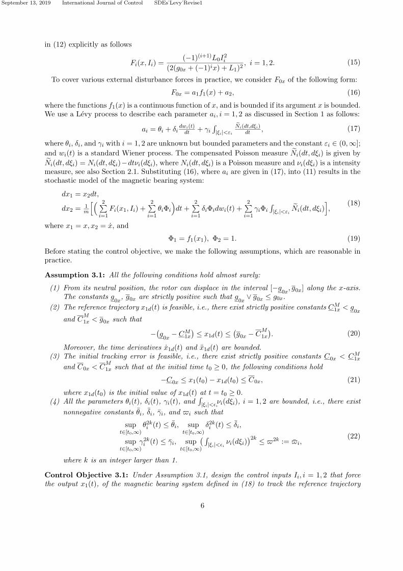
Figure 2.: Results by proposed control design

Time [s]0 5 10 15

x,x1d[m

m]

-1

0

1

a

x

xd

Time [s]0 5 10 15

x2[m

m/s]

-2

0

2

4

b

Time [s]0 5 10 15

I1,I2[A

]

-100

-50

0

50

c

I1

I2

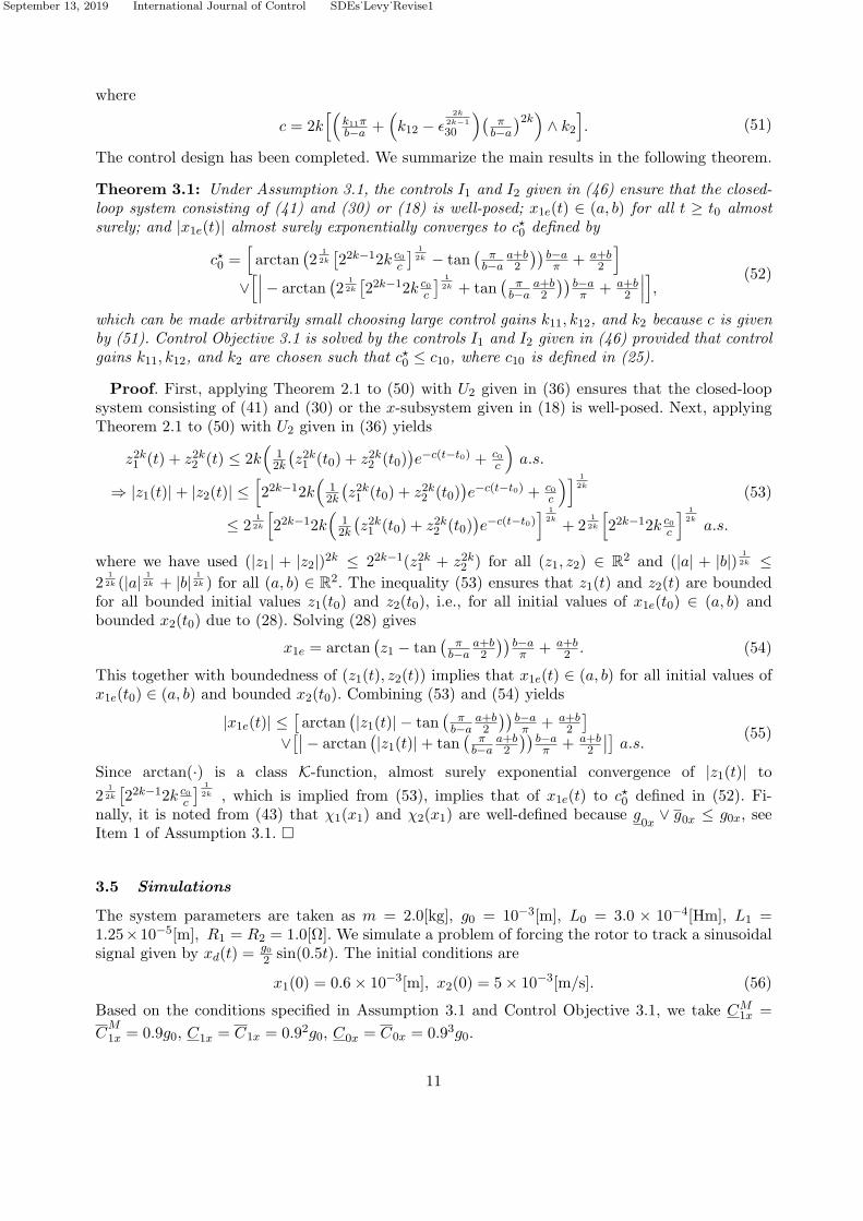
Figure 3.: Results by control design in (Do, 2010)

Simulation results are plotted in Figure 2, where the displacement x1 and its reference xd areplotted in Sub-figure 2.a, the velocity dx1

dt is plotted in Sub-figure 2.b, and the control currents I1and I2 are plotted in Sub-figure 2.c. It is seen from Sub-figure 2.a that the proposed controls forcethe rotor displacement to track its reference very well. From Sub-figure 2.c, we can see that the

12


control currents I1 and I2 are fairly large at the beginning. This is because of the fact that theinitial position x1(0) = 0.6× 10−3[m] is fairly close to its boundary value b, and the initial velocityx2(0) = 5×10−3[m/s] pushes the rotor toward the boundary value b. Therefore, the control currentsmust provide sufficiently large control efforts to push the rotor back to prevent it from contactingwith the stator. Then at the steady state, the currents I1 and I2 need to produce sufficient largeforce to handle the external disturbance force F0x, see (16) and (17) for the expression of this forcewith the above value of the parameters (θi, δi, γi).Since existing works on control of magnetic bearings only consider deterministic disturbances as

discussed in Section 1, it is not possible to run a simulation from these works on the stochasticmodel of magnetic bearings in this paper. This is because the diffuse and jump terms are simplyunbounded in the deterministic sense. Thus, the diffuse and jump terms are first saturated by themagnitude of δi and γi, i = 1, 2. Then the control design for magnetic bearings under deterministicloads in (Do, 2010) is implemented, where it is noted that the voltage-dynamics in (Do, 2010) isremoved as we are considering magnetic bearings with current driving mode. Simulation resultsof the control design in (Do, 2010) with diffuse and jump terms being saturated are shown inFigure 3. The information presented in each sub-figure has the same meaning as that in Figure 2.It is seen that deterministic design results in significantly poorer performance in comparison withthe stochastic design in this paper. This is due to the fact that the deterministic control designconsiders the time derivative of the Lyapunov function while the stochastic control design addressesthe infinite generator of the Lyapunov function, which has additional Hessian and jump terms (seethe last two terms in (37)) compared with its time derivative. Thus, the stochastic control designneeds to handle these terms while the deterministic control design does not. These terms actuallypresent in the system. The above analysis explains why the stochastic control design results inbetter performance than the deterministic one. Note that other controllers those papers such as(de Queiroz & Dawson, 1996) and (de Queiroz et al., 1998) would give worse results as the hardconstraint on the tracking error is not imposed, see (Do, 2010) for a discussion.

4. Conclusions

The paper developed a Lyapunov-type theorem to investigate well-posedness and (global practicalK∞) exponential stability of SDEs driven by Levy processes almost surely. Sufficient conditionsimposed by the theorem are relatively easy to be verified. The theorem was then applied to designcontrollers to achieve a.s. practical K-exponential stability of magnetic bearings driven by stochasticdiffuse-jumps. Future work is to apply Theorem 2.1 to financial and other engineering systemsdriven by diffuses and jumps.

Appendix A. Proof of Theorem 2.1

A.1 Proof of Item 1) of Theorem 2.1

We first need a lemma on global well-posedness of (1) if the conditions (2) and (3) hold globally.

Lemma A.1: Suppose that the conditions (2) and (3) hold for all X(t) ∈ Rn and Y (t) ∈ Rn.There exists a unique solution to (1) with the initial condition X0 ∈ Rn almost surely (a.s.) forwhich X0 is Ft0-measurable. This solution is adapted and cadlag.

Proof. See (Applebaum, 2009), Theorem 6.2.3.We now turn to proof of Item 1) of Theorem 2.1. Let k0 be the boundedness of the initial data,

13


i.e., ∥X0∥ ≤ k0. For any integer k > k0, let us define

Fk(X, t) = F(∥X∥∧k

∥X∥ X, t),

Gk(X, t) = G(∥X∥∧k

∥X∥ X, t),

Φk(X, t, ξ) = Φ(∥X∥∧k

∥X∥ X, t, ξ),

(A1)

where we let ∥X∥∧k∥X∥ X = 0 if X = 0. Then, it is clear that all the conditions of Lemma A.1 hold

for all X ∈ Rn. Thus, Lemma A.1 ensures well-posedness of the solution Xk(t) to the SDE:

dXk = Fk(Xk, t)dt+Gk(Xk, t)dW (t) +∫∥X∥<εΦ(Xk(t

−), t, ξ)N(dt, dξ) (A2)

for any Xk(t0) = X0 ∈ Rn. Define a stopping time

sk = inft ≥ t0 : ∥Xk(t)∥ > k, (A3)

where we let inf ∅ = ∞ as usual. Obviously for any σ < sk, we have ∥Xk(σ)∥ ≤ k. From definitionof Fk(X, t), Gk(X, t), and Φk(X, t−, ξ) in (A1), it is seen that

Fk+1(Xk(σ), t) = Fk(Xk(σ), t),

Gk+1(Xk(σ), t) = Gk(Xk(σ), t),

Φk+1(Xk(σ), t, ξ) = Φk(Xk(σ), t, ξ),

(A4)

for all t0 ≤ σ < sk. From (A2) and (A4), it holds that

Xk+1(t) = Xk(t), ∀ t0 ≤ t ≤ sk. (A5)

This further implies that sk is increasing in k. Thus, we can define s = limk→∞ sk. From (A5), wealso have

X(t) = Xk(t), ∀ t0 ≤ t < sk. (A6)

This together with (A4) means that X(t) is the unique solution of (1) for t ∈ [t0, sk). We need toshow that P(s = ∞) = 1. Applying the Ito formula to U(Xk, t) with Xk the solution of (A2) gives

U(Xk(t ∧ sk), t) = U(X0, t0) +∫ t∧skt0

LkU(Xk(σ), σ)dσ +∫ t∧skt0

UXk(Xk(σ), σ)Gk(Xk(σ), σ)dW (σ)

+∫ t∧skt0

m2∑ℓ=1

∫|ξℓ|<εℓ

[U(Xk(σ

−) +Φ(ℓ)(Xk(σ−), σ, ξℓ), σ

)− U(Xk(σ

−), σ)]Nℓ(dσ, dξℓ),

(A7)where

LkU(Xk, σ) = Uσ(Xk, σ) + Fk(Xk, σ)UXk(Xk, σ) +

12Tr

(GT

k (Xk, σ)UXkXk(X, σ)Gk(Xk, σ)

)+

m2∑ℓ=1

∫|ξℓ|<εℓ

[U(Xk(σ

−)+Φ(ℓ)(Xk(σ−), σ, ξℓ), σ

)− U(Xk(σ

−), σ)

−UXk(Xk(σ

−), σ)Φ(ℓ)(Xk(σ−), σ, ξℓ)

]νℓ(dξℓ).

(A8)By definition of Fk, Gk, and Φk in (A1), we have

LkU(Xk(σ), σ) = LU(Xk(σ), σ),∀ σ < t ∧ sk, (A9)

where LU(Xk(σ), σ) = LU(X(σ), σ)|X=Xk. Moreover, we have

E∫ t∧sk

t0UXk

(Xk(σ), σ)Gk(Xk(σ), σ)dW (σ)= 0, (A10)

which implies that

E∫ t∧sk

t0UXk

(Xk(σ), σ)G(Xk(σ), σ)dW (σ)= 0. (A11)

14


Thus, taking expectancy of (A7) and using (7) gives

EU(Xk(t ∧ sk), t)

≤ E

U(X0, t0)

+ c3E

∫ t∧skt0

(1 + U(Xk(σ), σ))dσ

≤ EU(X0, t0)

+ c3E

∫ tt0(1 + U(Xk(σ ∧ sk), σ))dσ

.

(A12)

Applying the Gronwall inequality to (A12) yields

EU(Xk(t ∧ sk), t)

≤(c3(t−t0)+E

U(X0, t0)

)ec3(t−t0), (A13)

which further gives

inf∥X∥≥k U(X, t)P(sk ≤ t) ≤ EU(Xk(sk), t)Isk≤t

≤

(c3(t− t0) + E

U(X0, t0)

)ec3(t−t0).

(A14)

Therefore

P(sk ≤ t) ≤(c3(t− t0) + E

U(X0, t0)

)ec3(t−t0)

inf∥X∥≥k U(X, t). (A15)

Letting k tend to infinity and using (6) result in P(sk ≤ t) = 0. Since t is arbitrary, P(sk = ∞) =1 ⇒ P(s = ∞) = 1 by definition s = limk→∞ sk.


Since all the conditions of Item 1) satisfy, there exists a global unique solution to (1). The techniquein (H. Deng et al., 2001) is used at places in our proof. Applying the Ito formula to U(X, t) andthe solution X(t) of (1) and using Condition (8) gives

U(X(t), t) = U(X(s), s) +∫ ts LU(X(r), r)dr +

∫ ts UX(X(r), r)G(X(r), r)dW (r)

+∫ ts

m2∑ℓ=1

∫|ξℓ|<εℓ

[U(X(r−) +Φ(ℓ)(X(r−), r, ξℓ), r

)− U(X(r−), r)

]Nℓ(dr, dξℓ)

≤ U(X(s), s) +∫ ts (−c4U(X(r), r) + c0)dr +

∫ ts UX(X(r), r)G(X(r), r)dW (r)

+∫ ts

m2∑ℓ=1

∫|ξℓ|<εℓ

[U(X(r−) +Φ(ℓ)(X(r−), r, ξ), r

)− U(X(r−), r)

]Nℓ(dr, dξℓ),

(A16)

To further consider (A16), let us define an increasing time sequence tk, k = 1, · · · ,∞ such thatt∞ = ∞. In each time interval [tk−1, tk], we show that the system (1) is stable in probability forany initial value Xtk−1

. For r ∈ [tk−1, tk], there are two cases:

Case I:∫ tktk−1

(−c4U(X(r), r) + c0)dr > 0,

Case II:∫ tktk−1

(−c4U(X(r), r) + c0)dr ≤ 0,a.s. (A17)

Case I already implies that the system (1) is stable in probability in the interval [tk−1, tk] due to(6). We now address Case II. For this case, we can write (A16) as

U(X(tk), tk) ≤ U(X(tk−1), tk−1) +∫ tktk−1

UX(X(r), r)G(X(r), r)dW (r)

+∫ tktk−1

m2∑ℓ=1

∫|ξℓ|<εℓ

[U(X(r−) +Φ(ℓ)(X(r−), r, ξ), r

)− U(X(r−), r)

]Nℓ(dr, dξℓ),

(A18)

which implies that U(X(tk), tk) is a supermartingale with respect to the filtration generated by

W (·) and Nℓ(·, ·), ℓ = 1, ...,m2. By the supermartingale inequality (X. Mao, 2007, Theorem 3.6),for any class K∞-function δ(·), we have

P

suptk−1≤s≤tk

U(X(s), s)≥δ(U(Xk−1, tk−1))≤ U(Xk−1,tk−1)

δ(U(Xk−1,tk−1)), (A19)

15


where Xk−1 := X(tk−1). Thus,

P

suptk−1≤s≤tk

U(X(s), s)<δ(U(Xk−1, tk−1))≥ 1− U(Xk−1,tk−1)

δ(U(Xk−1,tk−1)). (A20)

Using (6) shows that suptk−1≤s≤tk U(X(s), s) < δ(U(Xk−1, tk−1)) implies that

suptk−1≤s≤tk ∥X(s)∥ < ϱ(∥Xk−1∥), where ϱ = α−11 δ α2. For a given ε > 0, we choose a

class K∞-function δ(·) such that U(Xk−1,tk−1)δ(U(Xk−1,tk−1))

≤ ε. Thus, we can write (A20) as

P

suptk−1≤s≤tk

∥X(s)∥ < ϱ(∥Xk−1∥)≥ 1− ε. (A21)

This further implies that

P∥X(tk)∥ < ϱ(∥Xk−1∥)

≥ 1− ε. (A22)

For k = 1, ∥X0∥ is a.s. bounded. Combining Case I defined in (A17) and (A22) yields practicalstability of (1) in probability in the interval [t0, t1. Thus, X1 is a.s. bounded. The above procedureis repeated for each k = 2, · · · to yield global practical stability of (1) in probability.


Applying the Ito formula to ec4(t−t0)U(X, t) and the solution X(t) of (1), and using (8) gives

ec4(t−t0)U(X(t), t) = U(X(t0), t0) +∫ tt0ec4(r−t0)

(LU(X(r), r) + c4U(X(r), r)

)dr

+∫ tt0ec4(r−t0)

[UX(X(r), r)G(X(r), r)dW (r)

+m2∑ℓ=1

∫|ξℓ|<εℓ

(U(X(r−) +Φ(ℓ)(X(r−), r, ξℓ), r)− U(X(r−), r)

)Nℓ(dr, dξℓ)

]≤ U(X(t0), t0) + c0

∫ tt0ec4(r−t0)dr +

∫ tt0ec4(r−t0)


+m2∑ℓ=1

∫|ξℓ|<εℓ


)Nℓ(dr, dξℓ)

].

(A23)Multiplying both sides of (A23) with e−c4(t−t0) gives

U(X(t), t) ≤ U(X(t0), t0)e−c4(t−t0) + c0

c4+

∫ tt0e−c4(t−r)


+m2∑ℓ=1

∫|ξℓ|<εℓ


)Nℓ(dr, dξℓ)

],

(A24)

which can be written as

U(X(t), t) ≤ U(X(t0), t0)e−c4(t−t0) + c0

c4+

m∑ℓ=1

Mℓ(t), (A25)

where

Mℓ(t) :=∫ tt0gℓ(X(r), r)dWℓ(r) +

∫ tt0

∫|ξℓ|<εℓ

ϕℓ(X(r−), r, ξℓ)Nℓ(dr, dξℓ), (A26)

and

m = m1 ∨m2,

UX(X(r), r)G(X(r), r)=e−c4(t−r)row(g1(X(r), r)), · · · , gℓ(X(r), r), · · · , gm(X(r), r),

ϕℓ(X(r), r, ξℓ)=e−c4(t−r)

(U(X(r)+Φ(ℓ)(X(r), r, ξℓ), r)− U(X(r), r)

),

(A27)

and if m1 < m, we set gℓ = 0 and Wℓ = Wm1for ℓ = m1, · · · ,m; if m2 < m, we set

ϕℓ = 0 and Nℓ = Nm2for ℓ = m2, · · · ,m. Since we have already proved that the system

(1) is globally practically stable in probability, G(X, t) and Φ(X, t, ξ) satisfy Conditions C1and C2 of Assumption 2.1, U(X, t) ≤ α2(∥X∥p), see Condition (6), and α2(∥X + Φℓ∥p) ≤

16


α2(2p−1(∥X∥p + ∥Φℓ∥p)) ≤ α21(∥X∥p) + α22(∥Φℓ∥p) with α21 and α22 being some class K∞-

functions, we have∫ tt0|gℓ(X(r), r)|2dr <∞ and

∫ tt0

∫|ξℓ|<εℓ

|ϕℓ(X(r−), r, ξℓ)|2νℓ(dξℓ)dr <∞ a.s. for

all t ∈ [t0,∞). Thus, we can apply the exponential martingale inequality, see (Applebaum, 2009,Theorem 5.2.9), to Mℓ(t) with T = k, a = ϵ, b = ϵk, where ϵ ∈ (0, 12) and k ≥ t0 is an integer, asfollows:

Psupt0≤t≤k

[Mℓ(t)− ϵ

2

∫ tt0|gℓ(s)|2ds

−1ϵ

∫ tt0

∫|ξℓ|<εℓ

(eϵϕℓ(X(s−),s,ξℓ) − 1− ϵϕℓ(X(s−), s, ξℓ)

)νℓ(dξℓ)ds

]> ϵk

< e−ϵ2k.

(A28)

Since∑∞

k=1 e−ϵ2k <∞, applying the Borel-Cantelli lemma to (A28) gives

P

limk→∞

inf(

supt0≤t≤k

[Mℓ(t)− ϵ

2

∫ tt0|gℓ(s)|2ds− 1

ϵ

∫ tt0

∫|ξℓ|<εℓ

(eϵϕℓ(X(s−),s,ξℓ) − 1

−ϵϕℓ(X(s−), s, ξℓ))νℓ(dξℓ)ds

]≤ ϵk

)= 1.

(A29)

Therefore, for almost all ω ∈ Ω there exists a random integer k0 = k0(ω) such that for k ≥ k0 andt0 ≤ t ≤ n:

Mℓ(t) ≤ ϵ2

∫ tt0|gℓ(s)|2ds+ ϵk + 1

ϵ

∫ tt0

∫|ξℓ|<εℓ

(eϵϕℓ(X(s−),s,ξℓ) − 1− ϵϕℓ(X(s−), s, ξℓ)

)νℓ(dξℓ)ds.

(A30)To further consider (A30), we need the following inequality by using Taylor series expansion of ex

for all x ∈ R+:

ex = 1 + x+ x2

2!

[1 + 2!

3!x+ 2!2!4!

x2

2! +2!3!5!

x3

3! + · · ·]

≤ 1 + x+ x2

2! ex.

(A31)

Applying (A31) to (A30) yields

Mℓ(t) ≤ ϵ2

∫ tt0|gℓ(s)|2ds+ ϵk + ϵ

∫ tt0

∫|ξℓ|<εℓ

ϕ2ℓ(X(s−), s, ξℓ)eϵϕℓ(X(s−),s,ξℓ)νℓ(dξℓ)ds. (A32)

Since we have proved that the system (1) is globally stable in probability, under Conditions (9),C1 and C2 of Assumption 2.1, by letting ϵ→ 0 the dominated convergence theorem holds that forall t ≥ t0:

limϵ→0

[ϵ2

∫ tt0|gℓ(s)|2ds+ϵk+ϵ

∫ tt0

∫|ξℓ|<εℓ

ϕ2ℓ(X(s−), s, ξℓ)eϵϕℓ(X(s−),s,ξℓ)νℓ(dξℓ)ds

]= 0. (A33)

Substituting (A33) into (A32) then into (A25) and using (6) gives (10).

References

Antunes, D. J., Hespanha, J. P., & Silvestre, C. J. (2010). Impulsive systems triggered by superposedrenewal processes. Proceedings of the 49th IEEE conference on decision and control , 1779-1784.

Antunes, D. J., Hespanha, J. P., & Silvestre, C. J. (2012). Volterra integral approach to impulsive renewalsystems: application to networked control. IEEE Transactions on Automatic Control , 57 (3), 607-619.

Antunes, D. J., Hespanha, J. P., & Silvestre, C. J. (2013a). Stability of networked control systems withasynchronous renewal links: An impulsive systems approach. Automatica, 49 (2), 402-413.

Antunes, D. J., Hespanha, J. P., & Silvestre, C. J. (2013b). Stochastic hybrid systems with renewaltransitions: moment analysis with application to networked control systems with delays. SIAM Journalon Control and Optimization, 51 (2), 1481-1499.

Antunes, D. J., Hespanha, J. P., & Silvestre, C. J. (2014). Stochastic networked control systems withdynamic protocols. Asian Journal of Control , 16 (6), 1-12.

Applebaum, D. (2009). Levy processes and stochastic calculus (2nd ed.). Cambridge University Press.Applebaum, D., & Siakalli, M. (2009). Asymptotic stability of stochastic differential equations driven by

Levy noise. Journal of Applied Probability , 46 , 1116-1129.Charara, A., Miras, J. D., & Caron, B. (1996). Nonlinear control of a magnetic levitation system without

premagetization. IEEE Transactions on Control Systems Technology , 4 , 513-523.

17


Deng, F., Luo, Q., & Mao, X. (2012). Stochastic stabilization of hybrid differential equations. Automatica,48 (9), 2321-2328.

Deng, H., & Krstic, M. (1997). Stochastic nonlinear stabilization-Part I: A backstepping design. Systemsand Control Letters, 32 (3), 143-150.

Deng, H., Krstic, M., & Williams, R. (2001). Stabilization of stochastic nonlinear systems driven by noiseof unknown covariance. IEEE Transactions on Automatic Control , 46 (8), 1237-1253.

de Queiroz, M., & Dawson, D. (1996). Nonlinear control of active magnetic bearings: A backsteppingapproach. IEEE Transactions on Control Systems Technology , 14 (5), 545-552.

de Queiroz, M., Dawson, D., & Suri, A. (1998). Nonlinear control of a large-gap 2-dof magnetic bearingsystem based on a coupled force model. IEE Proceedings of Control Theory Applications, 145 (3),269-276.

Do, K. D. (2010). Control of nonlinear systems with output tracking error constraints and its applicationto magnetic bearings. International Journal of Control , 83 (6), 1199-1216.

Do, K. D. (2015). Global inverse optimal stabilization of stochastic nonholonomic systems. Systems &Control Letters, 41-55.

Do, K. D. (2016). Stability of nonlinear stochastic distributed parameter systems and its applications.Journal of Dynamic Systems, Measurement, and Control , 138 , 101010-1:101010-12.

Fujita, M., Hatake, K., & Matsumura, F. (1993). Loop shaping based robust control of a magnetic bearing.IEEE Control Systems Magazine, 13 (4), 47-85.

Hespanha, J. P., & Teel, A. R. (2006). Stochastic impulsive systems driven by renewal processes. 17thinternational symposium on mathematical theory of networks and systems.

Jagtap, P., & Zamani, M. (2017). Backstepping design for incremental stability of stochastic Hamiltoniansystems with jumps. IEEE Transactions on Automatic Control, In Press.

Khalil, H. (2002). Nonlinear systems. Prentice Hall.Khasminskii, R. (1980). Stochastic stability of differential equations. Rockville MD: S&N International.Krstic, M., Kanellakopoulos, I., & Kokotovic, P. (1995). Nonlinear and adaptive control design. New York:

Wiley.Liu, K. (2006). Stability of infinite dimensional stochastic differential equations with applications. Boca

Raton, FL: Chapman and Hall/CRC.Mao, W., You, S., & Mao, X. (2016). On the asymptotic stability and numerical analysis of solutions

to nonlinear stochastic differential equations with jumps. Journal of Computational and AppliedMathematics, 301 , 1-15.

Mao, X. (1999). Stability of stochastic differential equations with markovian switching. Stochastic Processesand their Applications, 79 (1), 45-67.

Mao, X. (2007). Stochastic differential equations and applications (2nd ed.). Cambridge: Woodhead pub-lishing.

Mao, X., Yin, G. G., & Yuan, C. (2007). Stabilization and destabilization of hybrid systems of stochasticdifferential equations. Automatica, 43 (2), 264-273.

Matsumura, F., & Yoshimoto, T. (1986). System modeling and control design of a horizontal-shaft magnetic-bearing system. IEEE Transactions on Magnetics, 22 (3), 196-203.

Mittal, S., & Menq, C. (1997). Precision motion control of a magnetic sspension actuator using a robustnonlinear compensation scheme. IEEE/ASME Transactions on Mechatronics, 2 , 268-280.

Mohamed, A. M., & Emad, F. P. (1992). Conical magnetic bearings with radial and thrust control. IEEETransactions on Automatic Control , 37 (3), 1859-1869.

Nane, E., & Ni, Y. (2017). Stability of the solution of stochastic differential equation driven by time-changedLevy noise. Proceedings of the American Mathematical Society , 145 , 3085-3104.

Smith, R. D., & Weldon, W. F. (1995). Nonlinear control of a rigid rotor magnetic bearing system: Modelingand simulation with full state feedback. IEEE Transactions on Magnetics, 31 (2), 973-980.

Stachurski, W., Midera, S., & Kruszynski, B. (2012). Determination of mathematical formulae for the cuttingforce fc during the turning of c45 steel. Mechanics and Mechanical Engineering , 16 (2), 73-79.

Teel, A. R., Subbaramana, A., & Sferlazza, A. (2014). Stability analysis for stochastic hybrid systems: Asurvey. Automatica, 50 , 2435-2456.

Torries, M., Sira-Ramirez, H., & Escobar, G. (1999). Sliding mode nonlinear control of magnetic bearings.Proceedings of the 1999 IEEE International Conference on Control Applications, 743-748.

Woodson, H. H., & Melcher, J. R. (1968). Electromechanical dynamics-part i: Discrete systems. New York:

18


Englewood Cliffs, NJ: Prentice-Hall.Zhu, Q. (2014). Asymptotic stability in the pth moment for stochastic differential equations with Levy

noise. Journal of Mathematical Analysis and Applications, 416 , 126-142.

19

Almost sure exponential stability of dynamical systems ...

Documents