Generalized matrix diagonal stability and linear dynamical systems

Linear Algebra and its Applications 419 (2006) 299–310www.elsevier.com/locate/laa

Generalized matrix diagonal stability and lineardynamical systems

Octavian Pastravanu∗, Mihail Voicu

Department of Automatic Control and Industrial Informatics, Technical University “Gh. Asachi” of Iasi,Blvd. Mangeron 53A, Iasi 700050, Romania

Received 21 December 2005; accepted 26 April 2006Available online 30 June 2006

Submitted by H. Schneider

Abstract

Let A = (aij ) be a real square matrix and 1 � p � ∞. We present two analogous developments. One forSchur stability and the discrete-time dynamical system x(t + 1) = Ax(t), and the other for Hurwitz stabilityand the continuous-time dynamical system x(t) = Ax(t). Here is a description of the latter development.

For A, we define and study “Hurwitz diagonal stability with respect to p-norms”, abbreviated as “HDSp”.HDS2 is the usual concept of diagonal stability. A is HDSp implies “Re λ < 0 for every eigenvalue λ ofA”, which means A is “Hurwitz stable”, abbreviated as “HS”. When the off-diagonal elements of A arenonnegative, A is HS iff A is HDSp for all p.

For the dynamical system x(t) = Ax(t), we define “diagonally invariant exponential stability relative tothe p-norm”, abbreviated as DIESp, meaning there exist time-dependent sets, which decrease exponentiallyand are invariant with respect to the system. We show that DIESp is a special type of exponential stabilityand the dynamical system has this property iff A is HDSp.© 2006 Elsevier Inc. All rights reserved.

AMS classification: 15A45; 15A60; 15A48; 15A18; 34A30; 34C14; 34D20; 93C05; 93D20

Keywords: Matrix diagonal stability; Stein/Lyapunov matrix inequality; (essentially) Nonnegative matrices; Gershgorin’sdisks; Linear dynamical systems; Invariant sets; (diagonally invariant) Exponential stability

∗ Corresponding author. Tel./fax: +40 232 230751.E-mail addresses: [email protected] (O. Pastravanu), [email protected] (M. Voicu).

0024-3795/$ - see front matter ( 2006 Elsevier Inc. All rights reserved.doi:10.1016/j.laa.2006.04.021

www.elsevier.com/locate/laa

mailto:[email protected]

mailto:[email protected]

300 O. Pastravanu, M. Voicu / Linear Algebra and its Applications 419 (2006) 299–310

1. Introduction

First, let us introduce the following notations:• For a vector x ∈ Rn:

‖x‖ is an arbitrary vector norm;‖x‖p is the Hölder vector p-norm and 1 � p � ∞;‖x‖D

p = ‖D−1x‖p, where D is a positive definite diagonal matrix;|x| denotes a nonnegative vector defined by taking the absolute values of the elements of x.

• For a matrix M ∈ Rn×n:‖M‖ is the matrix norm induced by the vector norm ‖•‖;‖M‖p is the matrix norm induced by the vector norm ‖•‖p;‖M‖D

p = ‖D−1MD‖p is the matrix norm induced by the vector norm ‖•‖Dp ;

mDp (M) = limh↓0(‖I + hM‖D

p − 1)/h is a matrix measure [1, p. 41], based on the matrixnorm ‖•‖D

p ;σ(M) = {z ∈ C| det(zI − M) = 0} is the spectrum of M, and λi(M) ∈ σ(M), i = 1, . . . , n,denotes its eigenvalues;|M| denotes a nonnegative matrix defined by taking the absolute values of the entries of M.

If x, y ∈ Rn, then “x � y” and “x < y” mean componentwise inequalities.If M, P ∈ Rn×n, then “M � P ”, “M < P ” mean componentwise inequalities.We shall write “X // Y” in place of “X [respectively Y]”.In the complex plane C, define the regions CS = {z ∈ C||z| < 1} // CH = {z ∈ C|Re z < 0}.

If σ(M) ⊂ CS // CH , then M ∈ Rn×n is said to be Schur stable (abbreviated as SS) // Hurwitzstable (abbreviated as HS).

If M ∈ Rn×n is symmetric, then “M � 0” // “M ≺ 0” means M is positive definite // negativedefinite.

Throughout the text, A = (aij ) denotes a real n by n matrix.

“Matrix diagonal stability” is defined in [2] as follows: A is Schur // Hurwitz diagonally stableif there exists a diagonal matrix P � 0, such that

ATPA − P ≺ 0 // ATP + PA ≺ 0. (1-S//H)

For these concepts, we propose the following generalizations:

Definition 1. A is called Schur // Hurwitz diagonally stable relative to the p-norm (abbreviatedSDSp // HDSp) if there exists a diagonal matrix D � 0, such that

‖A‖Dp < 1 // mD

p (A) < 0. (2-S//H)

In the remainder of the text we shall also use the abbreviation SDSp // HDSp to mean“Schur // Hurwitz diagonal stability relative to the p-norm”.

Remark 1. Set P = (D−1)2. When p = 2, inequality (2-S//H) is equivalent to theStein // Lyapunov matrix inequality (1-S//H).

Remark 2. If 1 � p � ∞ and A is SDSp // HDSp, then A is SS // HS. Indeed,σ(A) = σ(D−1AD)

and we can denote the eigenvalues of A and (D−1AD), such that λi(A) = λi(D−1AD), i =

1, . . . , n. Thus |λi(A)| = |λi(D−1AD)| � ‖A‖D

p < 1 and Re{λi(A)} = Re{λi(D−1AD)} �

mDp (A) < 0, i = 1, . . . , n [1, p. 41].

O. Pastravanu, M. Voicu / Linear Algebra and its Applications 419 (2006) 299–310 301

We first analyze SDSp // HDSp as a matrix property. Then we explore the connections betweenSDSp // HDSp and the behavior of a linear dynamical system with discrete-time // continuous-time (abbreviated as DT // CT) dynamics, defined by

x(t + 1) = Ax(t) // x(t) = Ax(t)

for t, t0 ∈ Z+ = {0, 1, 2, . . .} // R+ = {τ ∈ R|τ � 0}, and t � t0,

with the initial condition x(t0) = x0 ∈ Rn. (3-S//H)

The remainder of the paper is organized as follows:Section 2 provides some useful results about nonnegative // essentially nonnegative matrices.Section 3 presents SDSp // HDSp criteria that rely on

• a test matrix AS // AH built from A as

AS = |A| // AH = (aHij ), where aH

ij = aii if i = j and |aij | otherwise; (4-S//H)

• the generalized Gershgorin’s disks of A, defined with D = diag{d1, . . . , dn} � 0, for columnsby

Gcj (D

−1AD) =z ∈ C

∣∣∣∣∣|z − ajj | �n∑

i=1,i /=j

dj

di

|aij | , j = 1, . . . , n, (5)

or for rows by

Gri (D

−1AD) =z ∈ C

∣∣∣∣∣|z − aii | �n∑

j=1,j /=i

dj

di

|aij | , i = 1, . . . , n. (6)

Section 4 introduces a property called diagonally invariant exponential stability relative tothe p-norm (abbreviated as DIESp) of a linear dynamical system (3-S//H). DIESp ensures theexistence of time-dependent sets with DT // CT exponential decrease, which are invariant withrespect to (abbreviated w.r.t.) the state-space trajectories (solutions) of system (3-S//H). Thismeans once the initial condition x(t0) = x0 belongs to such a set, the corresponding solutionx(t; t0, x0) also belongs to the set, for any t � t0 (see [3, p. 100]). We show that DIESp is aspecial type of exponential stability (abbreviated as ES) (see [3, pp. 107–108]) of the dynamicalsystem (3-S//H), fully characterized by A’s being in SDSp // HDSp.

Section 5 illustrates the applicability of the main results by an example.

2. Preliminary results

2.1. Nonnegative // essentially nonnegative matrices

A real square matrix is called nonnegative // essentially nonnegative if its entries // off-diagonalentries are nonnegative. In the following lemmas, we use the notation “S // H” for presentingresults that refer to nonnegative // essentially nonnegative matrices, since these results supportthe approach to SDSp // HDSp to be developed in Section 3.

Lemma 1. (S) If A is nonnegative, its spectral radiusλmax(A) is an eigenvalue such that |λi(A)| �λmax(A), i = 1, . . . , n.


(H) If A is essentially nonnegative, then it has a real eigenvalue, denoted by λmax(A), suchthat Re{λi(A)} � λmax(A), i = 1, . . . , n.

Proof. (S) From Theorem 8.2.2 in [4].(H) Pick a real s such that sI + A is nonnegative. Denote the eigenvalues of A and sI + A

such that λi(sI + A) = s + λi(A), i = 1, . . . , n. Define λmax(A) so that s + λmax(A) =λmax(sI + A) � |λi(sI + A)| � s + Re{λi(A)}, i = 1, . . . , n. �

So whenever both definitions of λmax(A) make sense, they agree.

Lemma 2. Let 1 � p � ∞ and D � 0 diagonal. If A, B are nonnegative // essentially nonneg-ative and A � B, then (S) ‖A‖D

p � ‖B‖Dp // (H) mD

p (A) � mDp (B).

Proof. (S) If A, B are nonnegative, then, for any y ∈ Rn, we can write the componentwise inequal-ities |(D−1AD)y| � |(D−1AD)|y|| � |(D−1BD)|y||. From Theorem 5.5.10 in [4], the mono-tonicity of the p-vector-norms implies ‖(D−1AD)y‖p � ‖(D−1AD)|y|‖p � ‖(D−1BD)|y|‖p,yielding ‖(D−1AD)y‖p �‖D−1BD‖p‖|y|‖p =‖D−1BD‖p‖y‖p. Consequently, ‖D−1AD‖p =max‖y‖p=1 ‖(D−1AD)y‖p � ‖D−1BD‖p, which completes the proof of part (S).

(H) If A, B are essentially nonnegative, then, for small h > 0, we have the componentwiseinequality 0 � (I + hD−1AD) � (I + hD−1BD) that implies ‖I + hD−1AD‖p �‖I+hD−1BD‖p, according to part (S). Thus, (‖D−1(I+hA)D‖p−1)/h�(‖D−1(I+hB)D‖p −1)/h and taking h ↓ 0, we get mD

p (A) � mDp (B). �

Lemma 3. Let 1 � p � ∞ and r > λmax(A), where A is nonnegative // essentially nonnegative.Then there exists a diagonal matrix D � 0 such that (S) λmax(A) � ‖A‖D

p < r // (H) λmax(A) �mD

p (A) < r.

Proof. (S) Suppose A is nonnegative. If J is the n by n matrix with all its entries 1, thenλmax(A + εJ ) as a function of ε � 0 is continuous and increasing, according to Theorem 8.1.18in [4]. Hence, for any r > λmax(A), we can find an ε∗ > 0 such that λmax(A + ε∗J ) < r . On theother hand, the matrix A + ε∗J is positive and there exists its right and left Perron eigenvectors v =[v1 . . . vn]T > 0 and w = [w1 · · · wn]T > 0, respectively. If 1/p + 1/q = 1, then, from [5] wehave ‖D−1(A + ε∗J )D‖p = λmax(A + ε∗J ) with D = diag{v1/q

1 /w1/p

1 , . . . , v1/qn /w

1/pn },

where the particular cases of norms p = 1 and p = ∞ mean 1/p = 1, 1/q = 0, and 1/p = 0,

1/q = 1, respectively. Since 0 � A < A + ε∗J , by using Lemma 2 we can write ‖D−1AD‖p �‖D−1(A + ε∗J )D‖p and, finally, we get λmax(A) � ‖D−1AD‖p = ‖A‖D

p < r .(H) Suppose A is essentially nonnegative. Consider an arbitrary s > 0 such that sI + A is non-

negative. Choose r such that λmax(A) < r < r . By using part (H) with r instead of r and taking intoaccount that the eigenvectors of sI + A + ε∗J and A + ε∗J are identical, we find a matrix D � 0diagonal, such that s + λmax(A) = λmax(sI + A) � ‖sI + A‖D

p < s + r . For s = 1/h, we haveλmax(A) � (‖I + hA‖D

p − 1)/h < r that, when h ↓ 0, yields λmax(A) � mDp (A) � r < r . �

Remark 3. Let 1 � p � ∞. For A irreducible (i.e. the oriented graph associated with A is stronglyconnected; other equivalent characterizations are given by Theorem 6.2.24 in [4]), we have aparticular case of Lemma 3. If A is nonnegative // essentially nonnegative, then there exists adiagonal matrix D � 0 such that λmax(A) = ‖A‖D

p // λmax(A) = mDp (A). The matrix D is built


by the procedure presented in the proof of Lemma 3, applied to the right and left Perron–Frobeniuseigenvectors of A (which are positive, since A is irreducible – see Theorem 8.4.4 in [4]).

2.2. Matrices majorized by nonnegative // essentially nonnegative matrices

The matrix AS // AH defined by (4-S//H) is nonnegative // essentially nonnegative and major-izes A.

Lemma 4. If 1 � p � ∞ and D � 0 is diagonal, then (S) ‖A‖Dp � ‖AS‖D

p // (H) mDp (A) �

mDp (AH ).

Proof. (S) For any y ∈ Rn, we can write the componentwise inequality |(D−1AD)y| �|(D−1ASD)|y‖, and the monotonicity of the p-vector-norms (Theorem 5.5.10 in [4]) yields‖(D−1AD)y||p � ‖(D−1ASD)|y|‖p � ‖D−1ASD‖p‖|y|‖p = ‖D−1ASD‖p‖y‖p. Hence,

‖D−1AD‖p = max‖y‖p=1 ‖(D−1AD)y‖p � ‖D−1ASD‖p, which completes the proof of part(S).

(H) For small h > 0, we have |I + hD−1AD| = (I + hD−1AH D) and we can applypart (S), obtaining ‖I + hA‖D

p = ‖I + hD−1AD‖p � ‖I + hD−1AH D‖p = ‖I + hAH ‖Dp ⇒

(‖I + hA‖Dp − 1)/h � (‖I + hAH ‖D

p )/h. Taking h ↓ 0, we get mDp (A) � mD

p (AH ). �

Remark 4. If p = 1, ∞ and D � 0 is diagonal, we have a particular case of Lemma 4, namely, (S)‖A‖D

p = ‖AS‖Dp , (H) mD

p (A) = mDp (AH ). Indeed, for any matrix M ∈ Rn×n, ‖M‖p = ‖|M|‖p if

p = 1, ∞, and taking into account the equality (S) |D−1AD| = D−1ASD, (H) |I + hD−1AD| =I + hD−1AH D for small h > 0, we get (S) ‖D−1AD‖p = ‖D−1ASD‖p, (H) (‖I +hD−1AD‖p − 1)/h = (‖I + hD−1AH D‖p − 1)/h, respectively.

3. SDSp // HDSp criteria

Theorem 1. The following six statements are equivalent:

(i) AS // AH is SS // HS.

(ii) A is SDS1 // HDS1.

(iii) A is SDS∞ // HDS∞.

(iv) There exists a diagonal matrix D � 0, such that⋃n

j=1 Gcj (D

−1AD) ⊆ CS // CH .

(v) There exists a diagonal matrix D � 0, such that⋃n

i=1 Gri (D

−1AD) ⊆ CS // CH .

(vi) A is SDSp // HDSp for all 1 � p � ∞.

Proof. (S) (i) ⇒ (vi). Let 1 � p � ∞. If AS is SS, then λmax(AS) < 1 and, according to Lemma

3(S), one can find a diagonal matrix D � 0 such that λmax(AS) � ‖AS‖D

p < 1. Then apply Lemma4(S).

(S) (ii) ⇒ (i) and (iii) ⇒ (i). If A is SDSp, with p = 1 or ∞, then by (2-S) there exists a diagonalmatrix D � 0 such that ‖A‖D

p < 1 and the spectral radius of AS is λmax(AS) � ‖AS‖D

p = ‖A‖Dp

by Remark 4(S).(S) (ii) ⇔ (iv). It results from ‖A‖D

1 < 1 ⇔ −1 < ajj − ∑ni=1,i /=j

dj

di|aij | and ajj +∑n

i=1,i /=j

dj

di|aij | < 1, j = 1, . . . , n ⇔ Gc

j (D−1AD) ⊆ CS, j = 1, . . . , n.


(S) (iii) ⇔ (v). It is similar to the proof of (S) (ii) ⇔ (iv).(H) (i) ⇒ (vi). Let 1 � p � ∞. If AH is HS, then λmax(A

H ) < 0 and, according to Lemma3(H), one can find a diagonal matrix D � 0 such that λmax(A

H ) � mDp (AH ) < 0. Then apply

Lemma 4(H).(H) (ii) ⇒ (i) and (iii) ⇒ (i). If A is HDSp, with p = 1 or ∞, then by (2-H) there exists a

diagonal matrix D � 0 such that mDp (A) < 0 and λmax(A

H ) � mDp (AH ) = mD

p (A) by Remark4(H).

(H) (ii) ⇔ (iv). It results from mD1 (A) < 0 ⇔ 0 > mD

1 (A) = ajj + ∑ni=1,i /=j

dj

di|aij |, j =

1, . . . , n [1, p. 41] ⇔ Gcj (D

−1AD) ⊂ CH , j = 1, . . . , n.(H) (iii) ⇔ (v). It is similar to the proof of (H) (ii) ⇔ (iv).(S // H) (i) ⇒ (ii) and (i) ⇒ (iii). These are particular cases of the implication (S // H) (i) ⇒ (vi),

with p = 1 and p = ∞, respectively.(S // H) (vi) ⇒ (ii) and (vi) ⇒ (iii). These are obvious. �

Corollary 1. If A is nonnegative // essentially nonnegative, then the following five statements areequivalent:

(i) A is SS // HS.

(ii) There exists a p, 1 � p � ∞, such that A is SDSp // HDSp.

(iii) There exists a diagonal matrix D � 0, such that⋃n

j=1 Gcj (D

−1AD) ⊆ CS // CH .

(iv) There exists a diagonal matrix D � 0, such that⋃n

i=1 Gri (D

−1AD) ⊆ CS // CH .

(v) A is SDSp // HDSp for all 1 � p � ∞.

Proof. (S) (ii) ⇒ (i). If A is SDSp, then the spectral radius λmax(A) � ‖A‖Dp < 1.

(H) (ii) ⇒ (i). If A is HDSp, then λmax(A) � mDp (A) < 0.

(S // H) (i) ⇔ (iii) ⇔ (iv) and (i) ⇒ (v). These result from Theorem 1, since A = AS // AH .(S // H) (v) ⇒ (ii). It is obvious. �

Remark 5. Part of the results presented by Theorem 1 and Corollary 1 can also be found in [2].In terms of our notations, these results are as follows. A is SDS∞ ⇔ AS is SS (Corollary 2.7.29 in[2]). AS is SS ⇒ A is SDS2 (Corollary 2.7.27 in [2]). If A is nonnegative, then A is SDS∞ ⇔ A isSDS2 ⇔ A is SS (Lemma 2.7.25 in [2], but its proof does not cover the case of A reducible). If A isessentially nonnegative, then A is HDS2 ⇔ A is HS (Theorem 2.2.1 in [2]). However, [2] remainsfocused on diagonal stability as considered by that text (i.e. SDS2 // HDS2 in our formulation)and does not suggest a generalization of the “diagonal stability” concept to general p-norms.

4. Connections to the dynamics of linear systems

Let x(t; t0, x0) denote the solution of (3-S//H) satisfying the initial condition x(t0) = x0.

Definition 2. The system (3-S//H) is called diagonally invariant exponentially stable relativeto the p-norm (abbreviated as DIESp) if there exist a diagonal matrix D � 0 and a constant0 < r < 1 // r < 0, such that

∀ε > 0, ∀t, t0 ∈ Z+ // R+, t � t0, ∀x0 = x(t0) ∈ Rn,

‖x0‖Dp � ε ⇒ ‖x(t; t0, x0)‖D

p � εr(t−t0) // ‖x(t; t0, x0)‖Dp � εer(t−t0). (7-S//H)


In the remainder of the text we shall also use the abbreviation DIESp to mean “diagonallyinvariant exponential stability relative to the p-norm”.

Remark 6. In terms of invariant sets (see [3, p. 100]), Definition 2 is equivalent to the existenceof a diagonal matrix D � 0 and a constant 0 < r < 1 // r < 0 ensuring that the time-dependentsets

Xεp(t; t0) =

{x ∈ Rn‖|x‖D

p � εr(t−t0) // ‖x‖Dp � εer(t−t0)

},

t, t0 ∈ Z+ // R+, t � t0, ε > 0, (8-S//H)

are (positively) invariant w.r.t. the solutions (state-space trajectories) of system (3-S//H). For theusual values p = 1, 2, ∞, these sets have well-known geometric shapes (i.e. hyper-diamonds,ellipses and rectangles, respectively), scaled in accordance with the diagonal entries of the matrixD.

Theorem 2. Let 1 � p � ∞, D � 0 diagonal and 0 < r < 1 // r < 0. The following four state-ments are equivalent:

(i) System (3-S//H) is DIESp for D and r, i.e. (7-S//H) holds.(ii) V (x) = ‖x‖D

p is a strong Lyapunov function for system (3-S//H), with the decreasing rater, i.e.

∀t ∈ Z+ // R+, ∀ solution x(t) to (3�S//H),

V (x(t + 1)) � rV (x(t)) // D+V (x(t)) � rV (x(t)), (9-S//H)

where D+V (x(t)) = limh↓0(V (x(t + h)) − V (x(t)))/h.

(iii) ∀τ ∈ Z+ // R+, ‖Aτ‖Dp � rτ // ‖eAτ‖D

p � erτ . (10-S//H)

(iv) ‖A‖Dp � r // mD

p (A) � r. (11-S//H)

Proof. (S) (i) ⇒ (ii). Let x solve (3-S) and let t ∈ Z+. Set ε = ‖x(t)‖Dp = V (x(t)). If ε = 0,

then x(t), and hence x(t + 1), is 0. If ε > 0, then by (7-S) V (x(t + 1)) = ‖x(t + 1; t, x(t))‖Dp �

V (x(t))r .(S) (ii) ⇒ (i). Assume that system (3-S) is not DIESp for D and r. Let x(t) solve (3-S) and violate

the condition (7-S), i.e. there exist ε > 0, t∗, t0 ∈ Z+, t∗ � t0, with ‖x(t∗)‖Dp � εr(t∗−t0) and

‖x(t∗ + 1)‖Dp > εr(t∗+1−t0). This means r‖x(t∗)‖D

p < ‖x(t∗ + 1)‖Dp , which contradicts (9-S).

(S) (ii) ⇒ (iii). ∀t0, τ ∈ Z+, ‖Aτ‖Dp = supx(t0) /=0

‖Aτ x(t0)‖Dp

‖x(t0)‖Dp

= supx(t0) /=0‖x(t0+τ)‖D

p

‖x(t0)‖Dp

� rτ

according to (9-S).(S) (iii) ⇒ (iv). Set τ = 1 in (10-S).(S) (iv) ⇒ (ii). By (3-S).(H) First let us show that (9-H) can be written in the equivalent form

∀t � t0 � 0, ∀x0 ∈ Rn, ‖x(t; t0, x0)‖Dp � er(t−t0)‖x0‖D

p . (12)

Indeed, if (12) is true, then, for any solution x(s) of (3-H) with initial condition at s0 = t , wehaveD+V (x(s0)) = limh↓0(‖x(s0 + h; s0, x0)‖D

p − ‖x0‖Dp )/h � (limh↓0(erh − 1)/h)‖x0‖D

p =rV (x(s0)). Conversely, let t0 � 0 and x0 ∈ Rn. If (9-H) holds for x(t) = x(t; t0, x0), consider the


differential equation y(t) = ry(t) with the initial condition y(t0) = V (x(t0)) = V (x0). Then, forall t � t0, V (x(t)) � y(t) = er(t−t0)y(t0) = er(t−t0)V (x0), according to Theorem 4.2.11 in [3].Thus we may use (12) instead of (9-H) in the following proofs.

We also need to show that

limh↓0

(‖eAh‖Dp − 1)/h = mD

p (A). (13)

Indeed, eAh = I + hA + hO(h), limh↓0 O(h) = 0, together with ‖I + hA‖Dp − h‖O(h)‖D

p �‖I + hA + hO(h)‖D

p � ‖I + hA‖Dp + h‖O(h)‖D

p yield (‖I + hA‖Dp − 1)/h − ‖O(h)‖D

p �(‖eAh‖D

p − 1)/h � (‖I + hA‖Dp − 1)/h + ‖O(h)‖D

p .(H) (i) ⇒ (ii). By taking ε = ‖x0‖D

p in (7-H), we get (12) if ε > 0. If ε = 0, then x0 = 0 and

hence x(t) = eA(t−t0)x0 = 0, for t � t0.(H) (ii) ⇒ (i). Assume that system (3-H) is not DIESp for D and r. Let x(t) solve (3-H) and

violate the condition (7-H), i.e. there exist ε > 0, t∗, t∗∗ ∈ R+, t∗∗ > t∗ � t0, with ‖x(t∗)‖Dp �

εer(t∗−t0) and ‖x(t∗∗)‖Dp > εer(t∗∗−t0). This means er(t∗∗−t∗)‖x(t∗)‖D

p < ‖x(t∗∗)‖Dp , which con-

tradicts (12).

(H) (ii) ⇒ (iii). ∀t0, τ ∈ R+, ‖eAτ‖Dp = supx0 /=0

‖eAτ x0‖Dp

‖x0‖Dp

= supx0 /=0‖x(t0+τ ;t0,x0)‖D

p

‖x0‖Dp

� erτ

according to (12).(H) (iii) ⇒ (iv). It results from (10-H) and (13), since mD

p (A) = limh↓0(‖eAh‖Dp − 1)/h �

limh↓0(erh − 1)/h = r .(H) (iv) ⇒ (ii). ∀ solution x to (3-H), ∀t ∈ R+, we can write D+‖x(t)‖D

p =limh↓0(‖x(t + h)‖D

p − ‖x(t)‖Dp )/h = limh↓0(‖eAhx(t)‖D

p − ‖x(t)‖Dp )/h � [limh↓0(‖eAh‖D

p −1)/h]‖x(t)‖D

p = mDp (A)‖x(t)‖D

p � r‖x(t)‖Dp , according to (13). �

We are interested in exploring the relationship between the DIESp of the linear system (3-S//H)and the classical concept of ES.

Generally speaking, for a DT // CT dynamical system (nonlinear, time-variant), the ES isa property associated with a certain solution (trajectory) x(t). If x(t) ≡ 0 is a solution to theconsidered system, then {0} is called an equilibrium of the system, and its ES is defined by

Definition 3 (see Definition 3.2.6 in [3]). The equilibrium {0} is ES in the small if

∃r ∈ (0, 1) // r < 0 : ∀α > 0, ∀t, t0 ∈ Z+ // R+, t � t0, ∃δ(α) :‖x0‖ < δ(α) ⇒ ‖x(t; t0, x0)‖ � αr(t−t0) // ‖x(t; t0, x0)‖ � αer(t−t0). (14-S//H)

Definition 4 (see Definition 3.2.13 in [3]). The equilibrium {0} is ES in the large if

∃r ∈ (0, 1) // r < 0, ∃γ > 0 : ∀β > 0, ∀t, t0 ∈ Z+ // R+, t � t0, ∃M(β) > 0 :‖x0‖ < β ⇒ ‖x(t; t0, x0)‖ � M(β)r(t−t0)‖x0‖γ // ‖x(t; t0, x0)‖ � M(β)er(t−t0)‖x0‖γ .

(15-S//H)

In the particular case of the linear time-invariant system (3-S//H), the ES is considered asystem property, with a global meaning. Thus, “system (3-S//H) is ES” is equivalent to “theequilibrium {0} is ES in the large” (see Examples 3.2.14, 3.2.16 in [3]). The ES of system(3-S//H) is characterized by the following two well known results:


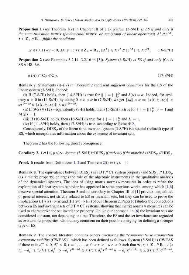
Proposition 1 (see Theorem 1(v) in Chapter III of [1]). System (3-S//H) is ES if and only ifthe state-transition matrix (fundamental matrix, or semigroup of linear operators) Aτ // eAτ ,

τ ∈ Z+ // R+, fulfils the condition:

∃r ∈ (0, 1) // r < 0, ∃K � 1 : ∀τ ∈ Z+ // R+, ‖Aτ‖ � Krτ // ‖eAτ‖ � Kerτ . (16-S//H)

Proposition 2 (see Examples 3.2.14, 3.2.16 in [3]). System (3-S//H) is ES if and only if A isSS // HS, i.e.

σ (A) ⊂ CS // CH . (17-S//H)

Remark 7. Statements (i)–(iv) in Theorem 2 represent sufficient conditions for the ES of thelinear system (3-S//H). Indeed:

(i) If (7-S//H) holds, then (14-S//H) is true for ‖ ‖ = ‖ ‖Dp and δ(α) = α. Indeed, for arbi-

trary α > 0 in (14-S//H), by taking 0 < ε < α in (7-S//H), we get ‖x0‖ < α ⇒ ‖x(t; t0, x0)‖ <

αr(t−t0) // ‖x(t; t0, x0)‖ < αer(t−t0).(ii) If (9-S) // (12) – equivalently (9-H) holds, then (15-S//H) is true for ‖ ‖ = ‖ ‖D

p , γ = 1 andM(β) = 1.

(iii) If (10-S//H) holds, then (16-S//H) is true for ‖ ‖ = ‖ ‖Dp and K = 1.

(iv) If (11-S//H) holds, then (17-S//H) is true, according to Remark 2.Consequently, DIESp of the linear time-invariant system (3-S//H) is a special (refined) type of

ES, which incorporates information about the existence of invariant sets.

Theorem 2 has the following direct consequence:

Corollary 2. Let 1�p�∞.System (3-S//H) is DIESp if and only if the matrix A is SDSp // HDSp.

Proof. It results from Definitions 1, 2 and Theorem 2(i) ⇔ (iv). �

Remark 8. The equivalence between DIESp (as a DT // CT system property) and SDSp // HDSp

(as a matrix property) enlarges the role of the algebraic instruments in the qualitative analysisof the dynamical systems. The idea of using matrix norms // measures in order to refine theexploration of linear system behavior has appeared in some previous works, among which [1,6]deserve special attention. Theorem 3 and its corollary in Chapter III of [1] provide inequalitiesof general interest, not strictly related to ES or invariant sets, but they can be used to prove theimplications (H) (iv) ⇒ (ii) and (H) (iv) ⇒ (iii) of our Theorem 2. Paper [6] studies the connectionsbetween ES and invariant sets of DT // CT systems, showing that matrix norms // measures can beused to characterize the set invariance property. Unlike our approach, in [6] the invariant sets areconsidered constant, not depending on time. Therefore, the ES and the set invariance are regardedas two distinct properties, without any comment on their possible merging for defining a strongertype of ES.

Remark 9. The control literature contains papers discussing the “componentwise exponentialasymptotic stability (CWEAS)”, which has been defined as follows. System (3-S//H) is CWEASif there exist d+

i > 0, d−i > 0, i = 1, . . . , n, 0 < r < 1 // r < 0 such that ∀t, t0 ∈ Z+ // R+, t �

t0, −d−i � xi(t0) � d+

i ⇒ −d−i r(t−t0) � xi(t) � d+

i r(t−t0) // − d−i er(t−t0) � xi(t) � d+

i er(t−t0),


i = 1, . . . , n, where xi(t0), xi(t) denote the components of the initial condition x(t0) of (3-S//H)and of the corresponding solution x(t), respectively. In terms of the notations introduced by thecurrent paper, the symmetrical CWEAS (meaning d−

i = d+i in the above definition) has been

characterized by “AH is HS” for CT linear systems [7–11], and by “AS is SS” for DT linearsystems [12]. In our recent work [11], for the symmetrical CWEAS of CT linear systems wehave given three equivalent characterizations, similar to the statements (i), (ii), (iv) of the aboveTheorem 2 (part H) in the particular case p = ∞. Thus, paper [11] has opened the perspectivesof a generalization for symmetrical CWEAS, developed by the current analysis of DIESp with1 � p � ∞.

Remark 10. A DT // CT system can be DIESp for different r’s and D’s. All these constantsr play the role of decreasing rates for the time-dependent invariant sets Xε

p(t; t0) defined by(8-S//H). Thus, according to Theorem 2(iv), we define the fastest decreasing rate as r∗

p(A) =infD�0 diagonal ‖A‖D

p // r∗p(A) = infD�0 diagonal m

Dp (A). Moreover, the positive value 1 − r∗

p(A)

(DT case) // |r∗p(A)| (CT case) can be regarded as the DIESp degree of system (3-S//H), by

using the analogy with the ES degree of system (3-H//S) defined as 1 − maxi=1,...,n |λi(A)| (DTcase) // | maxi=1,...,n Re{λi(A)}| (CT case) (e.g. [13]). For a DT // CT system, ∀p, 1 � p � ∞,the DIESp degree cannot exceed the ES degree, by Remark 2.

Corollary 3. The following three statements are equivalent:

(i) System (3-S//H) is DIES1.

(ii) System (3-S//H) is DIES∞.

(iii) System (3-S//H) is DIESp for all 1 � p � ∞.

Proof. It is a direct consequence of Theorem 1 and Corollary 2. �

Remark 11. For a DT // CT system which is DIESp for all 1 � p � ∞, the fastestdecreasing rate r∗

p(A) introduced in Remark 10 can have different values for different p.If A is irreducible, then (S) maxi=1,...,n |λi(A)| � r∗

p(A) � r∗1 (A) = r∗∞(A) = λmax(A

S);(H) maxi=1,...,n Re{λi(A)}� r∗

p(A)� r∗1 (A)= r∗∞(A)=λmax(A

H ). Indeed, maxi=1,...,n |λi(A)| �r∗p(A) // maxi=1,...,n Re{λi(A)} � r∗

p(A) (by Remark 2), r∗p(A) � r∗

p(AS) // r∗p(A) � r∗

p(AH ) (byLemma 4), r∗

p(AS) = λmax(AS) // r∗

p(AH ) = λmax(AH ) (by Remark 3), and, for p = 1, ∞,

r∗p(A) = r∗

p(AS) // r∗p(A) = r∗

p(AH ) (by Remark 4). Note that, when A is irreducible, Remarks3 and 4 provide a procedure for constructing the diagonal matrix D � 0 such that r∗

p(A) =λmax(A

S), p = 1, ∞.

Corollary 4. If A is nonnegative // essentially nonnegative, then the following three statementsare equivalent:

(i) System (3-S//H) is ES.

(ii) There exists a p, 1 � p � ∞, such that system (3-S//H) is DIESp.

(iii) System (3-S//H) is DIESp for all 1 � p � ∞.

Proof. This is a direct consequence of Corollaries 1, 2 and Proposition 2. �


Remark 12. If the matrix A of the system (3-S//H) is nonnegative // essentially nonnegative andSS // HS, then r∗

p(A) = λmax(A), ∀p, 1 � p � ∞, as resulting from the proof of Lemma 3. WhenA is irreducible, Remark 3 ensures a construction procedure for the diagonal matrix D � 0, ∀p,1 � p � ∞.

Remark 13. Corollary 3 and Remark 12 provide a generalization of Theorem 7.4(iv) in [14],which proves two properties of CT systems that can be related to our DIES1 and DIES∞. ForA essentially nonnegative and HS, work [14] uses the equivalent characterization “A is a −M

matrix”, λmax(A) is referred to as the “importance value of A”, and the invariant sets are called“exponentially contractive” with coefficient λmax(A). However, at the conceptual level, [14] doesnot merge the properties of ES and set invariance in the sense of our DIESp. For A both irreducibleand reducible, [14] constructs the invariant sets from the left and right eigenvectors of A associatedwith λmax(A), which may contain 0 elements, when A is reducible. Thus, the similarity betweenthe approach in [14] and our DIES1, DIES∞ appears only for A irreducible and it is limited to theinvariant sets with the fastest decreasing rate, i.e. in our notations, r∗

1 (A) = r∗∞(A) = λmax(A).

The use of AS // AH for testing the SDSp // HDSp of the matrix A suggests considering theDT // CT dynamical system defined by

y(t + 1) = ASy(t) // y(t) = AH y(t), t, t0 ∈ Z+ // R+, t � t0,

with y(t0) = y0 ∈ Rn initial condition, (18-S//H)

as a comparison system for studying the DIESp of system (3-S//H).

Corollary 5. Let 0 < r < 1 // r < 0 and D � 0 diagonal

(i) Let p = 1, ∞. The comparison system (18-S//H) is DIESp for r and D if and only if system(3-H//S) is DIESp for r and D.

(ii) Let 1 < p < ∞. If the comparison system (18-S//H) is DIESp for r and D, then system(3-S//H) is DIESp for r and D.

Proof. This follows from Theorem 2 together with Remark 4 for (i) and Lemma 4 for (ii). �

5. Example

Consider the matrix A defined by

A =[−a b

−b −a

], a > 0, b > 0, (19)

which is HS.The matrix A is HDSp, p = 1, ∞, if and only if a > b. Indeed, for D = diag{d1, d2}, d1, d2 >

0, we have mDp (A) = max{−a + bd2/d1, −a + bd1/d2},p = 1, ∞, and mD

p (A) < 0 if and onlyif b/a < d1/d2 < a/b. The same condition results from Theorem 1, since

AH =[−a b

b −a

], (20)

is HS if and only if a > b.


The condition a > b is sufficient for A to be HDSp, 1 � p � ∞ (according to Theorem 1),but it may not be necessary, as shown below for p = 2.

The matrix A is HDS2 for any a > 0, b > 0. Indeed, for D = diag{d1, d2}, d1, d2 > 0, we havemD

2 (A) = max{−a + b(d2/d1 − d1/d2)/2, −a − b(d2/d1 − d1/d2)/2} < 0, which is equivalent

to√

(a/b)2 + 1 − (a/b) < d1/d2 <√

(a/b)2 + 1 + (a/b).Consider the CT linear system (3-H) with A defined by (19). System (3-H) is ES for any a > 0,

b > 0, and the ES degree is a. If a > b, system (3-H) is DIESp, 1 � p � ∞, by Corollary 2. Thecondition a > b is also necessary for DIESp, p = 1, ∞. System (3-H) is DIES2 for any a > 0,b > 0.

If p = 1, ∞, then r∗p(A) = −a + b = λmax(A) corresponds to d1 = d2, which means the

invariant sets are squares, as a particular type of diamonds (p = 1) or rectangles (p = ∞). TheDIESp degree is a − b.

If p = 2, then r∗2 (A) = −a < λmax(A) corresponds to d1 = d2, which means the invariant sets

are circles, as a particular type of ellipses. The DIES2 degree is a.

Acknowledgments

The authors are grateful to the referees for their comments and suggestions.

References

[1] W.A. Coppel, Stability and Asymptotic Behavior of Differential Equations, D.C. Heath and Company, Boston, 1965.[2] E. Kaszkurewicz, A. Bhaya, Matrix Diagonal Stability in Systems and Computation, Birkhäuser, Boston, 2000.[3] A. Michel, K. Wang, Qualitative Theory of Dynamical Systems, Marcel Dekker, Inc., New York–Bassel–Hong

Kong, 1995.[4] R.A. Horn, C.R. Johnson, Matrix Analysis, Cambridge University Press, Cambridge, 1985.[5] J. Stoer, C. Witzgall, Transformations by diagonal matrices in a normed space, Numer. Math. 4 (1962) 158–171.[6] H. Kiendl, J. Adamy, P. Stelzner, Vector norms as Lyapunov functions for linear systems, IEEE Trans. Automat.

Control 37 (1992) 839–842.[7] M. Voicu, Componentwise asymptotic stability of linear constant dynamical systems, IEEE Trans. Automat. Control

29 (1984) 937–939.[8] M. Voicu, Free response characterization via flow-invariance, Preprints of the 9th World Congress of IFAC, Budapest,

vol. 5, 1984, pp. 12–17.[9] M. Voicu, On the application of the flow-invariance method in control theory and design, Preprints of the 10th World

Congress of IFAC, München, vol. 8, 1987, pp. 364–369.[10] A. Hmamed, A. Benzaouia, Componentwise stability of linear systems: a non-symmetrical case, Int. J. Robust

Nonlinear Control 7 (1997) 1023–1028.[11] O. Pastravanu, M. Voicu, On the componentwise stability of linear systems, Int. J. Robust Nonlinear Control 15

(2005) 15–23.[12] A. Hmamed, Componentwise stability of 1-D and 2-D linear discrete systems, Automatica 33 (1997) 1759–1762.[13] V. Balakrishnan, S. Boyd, S. Balemi, Computing the minimum stability degree of parameter-dependent linear

systems, in: S.P. Bhattacharyya, L.H. Keel (Eds.), Control of Uncertain Dynamic Systems, CRC Press, 1991,pp. 359–378.

[14] L. Gruyitch, J.-P. Richard, P. Borne, J.-C. Gentina, Stability Domains, Chapman & Hall/CRC, Boca Raton, 2004.

Generalized matrix diagonal stability and linear dynamical systems

Documents