Spike to Spike Model and Applications: A biological plausible approach for the motion processing

Spike to Spike Model and Applications: A biological

plausible approach for the motion processing

Maria-Jose Escobar, Guillaume Masson, Thierry Vieville, Pierre Kornprobst

To cite this version:

Maria-Jose Escobar, Guillaume Masson, Thierry Vieville, Pierre Kornprobst. Spike to SpikeModel and Applications: A biological plausible approach for the motion processing. [ResearchReport] RR-6280, INRIA. 2007, pp.37. <inria-00170153v3>

HAL Id: inria-00170153

https://hal.inria.fr/inria-00170153v3

Submitted on 29 Jan 2008

HAL is a multi-disciplinary open accessarchive for the deposit and dissemination of sci-entific research documents, whether they are pub-lished or not. The documents may come fromteaching and research institutions in France orabroad, or from public or private research centers.

L’archive ouverte pluridisciplinaire HAL, estdestinee au depot et a la diffusion de documentsscientifiques de niveau recherche, publies ou non,emanant des etablissements d’enseignement et derecherche francais ou etrangers, des laboratoirespublics ou prives.

https://hal.archives-ouvertes.fr

https://hal.inria.fr/inria-00170153v3

ap por t de r e c h e r c h e

ISS

N02

49-6

399

ISR

NIN

RIA

/RR

--62

80--

FR+E

NG

Thème BIO

INSTITUT NATIONAL DE RECHERCHE EN INFORMATIQUE ET EN AUTOMATIQUE

Spike to Spike Model and Applications: A biologicalplausible approach for the motion processing

Maria-Jose Escobar — Guillaume Masson — Thierry Vieville — Pierre Kornprobst

N° 6280

September 2007

Unité de recherche INRIA Sophia Antipolis2004, route des Lucioles, BP 93, 06902 Sophia Antipolis Cedex (France)

Téléphone : +33 4 92 38 77 77 — Télécopie : +33 4 92 38 77 65

Spike to Spike Model and Applications: A biologicalplausible approach for the motion processing

Maria-Jose Escobar∗ , Guillaume Masson† , Thierry Vieville‡ , PierreKornprobst§

Theme BIO — Systemes biologiquesProjet Odyssee

Rapport de recherche n° 6280 — September 2007 — 37 pages

Abstract: We propose V1 and MT functional models for biological motion recognition.Our V1 model transforms a video stream into spike trains through local motion detectors.The spike trains are the inputs of a spiking MT network. Each entity in the MT networkcorresponds to a simplified model of an MT cell. From the spike trains of MT cells a motionmap of velocity distribution is built representing a sequence. Biological plausibility of bothmodels is discused in detail in the paper. In order to show the efficiency of these models,the motion maps here obtained are used in the biological motion recognition task. We ranthe experiments using two databases Giese and Weizmann, containing two (march, walk)and ten (e.g. march, jump, run) different classes, respectively. The results revealed thatthe motion map here proposed can be used as a reliable motion representation.

Key-words: spiking networks, motion analysis, V1, MT, biological motion recognition

∗ [email protected]† [email protected]‡ [email protected]§ [email protected]

Spiking to Spike Model et Applications: Une modelebiologique pour le traitement du movement

Resume : Pas de resume

Mots-cles : reseau des neurones, traitement du movement, V1, MT, reconaissance dumovement biologique

Spike to Spike Model: motion processing 3

Contents

1 Introduction 4

2 A phenomenological V1 model 72.1 Some facts about V1 . . . . . . . . . . . . . . . . . . . . . . . . . . . . . . . . 72.2 V1 cells model . . . . . . . . . . . . . . . . . . . . . . . . . . . . . . . . . . . 7

2.2.1 Simple cell model . . . . . . . . . . . . . . . . . . . . . . . . . . . . . . 72.2.2 Spatio-temporal frequency analysis of simple cells . . . . . . . . . . . . 92.2.3 Complex cell model . . . . . . . . . . . . . . . . . . . . . . . . . . . . 11

2.3 Organization of V1 . . . . . . . . . . . . . . . . . . . . . . . . . . . . . . . . . 122.4 Layer of integrate and fire neurons . . . . . . . . . . . . . . . . . . . . . . . . 132.5 Surround suppression . . . . . . . . . . . . . . . . . . . . . . . . . . . . . . . . 14

3 Introducing a spiking MT model 143.1 Some facts about MT . . . . . . . . . . . . . . . . . . . . . . . . . . . . . . . 143.2 Spiking MT model . . . . . . . . . . . . . . . . . . . . . . . . . . . . . . . . . 16

3.2.1 Connections to V1 cells . . . . . . . . . . . . . . . . . . . . . . . . . . 163.2.2 Horizontal connectivity . . . . . . . . . . . . . . . . . . . . . . . . . . 193.2.3 Receptive fields: geometry and dynamics . . . . . . . . . . . . . . . . 19

4 Motion maps 21

5 Experiments 245.1 Ground Truth of the Model . . . . . . . . . . . . . . . . . . . . . . . . . . . . 25

6 Discussion and perspectives 28

A Spatio-temporal filters frequency analysis 31

RR n° 6280

4 M-J. Escobar, G. Masson, T. Vieville, P. Kornprobst

1 Introduction

Biological motion recognition is a task that our brain performs very efficiently, but it is stilla challenge in computer sciences to model it. Our ability to recognize human actions doesnot need necessarily a real moving scene as input. We are also able to recognize actions whenwe watch some point-light stimuli corresponding to joint positions for example. This kind ofsimplified stimuli was highly used in the phychophysics community in order to obtain a betterunderstanding in the underlying mechanism involved. The neural mechanisms processingform or motion taking part of biological motion recognition remains unclear. One the onehand, [4] suggests that biological motion can be derived from dynamic form information ofbody postures and without local image motion; On the other hand, [12] proposes a newtype of point-light stimulus which suggests that, in this case, only the motion information isenough and the detection of specific spatial arrangements of opponent-motion features canexplain our ability to recognize actions. In fact, in a recent work [13] showed that biologicalmotion recognition can be done with a coarse spatial location of the mid-level optic flowfeatures.

Studies with functional magnetic resonance (fMRI) confirm that biological motion pro-cessing does not consider the motion or form information separately. The motion path needssome form feedbacks to perform an accurate categorization. Experiments in [27] showedneural activity uniquely associated with the perception of complex motion as biologicallymotion. Michels et al. [36], also with fMRI, studied the brain activation related to bio-logical motion. They found that this kind of stimulus with a high form information causesa strong activation of form-processing areas. They measured that the activations in formareas such as FFA/OFA and EBA are dependent on the amount of form information in theinput stimuli. Neurophysiological studies also suggest that the biological motion analysis isa combined process between the related dorsal and ventral path in the brain, see [25] for areview.

Visual motion analysis has been studied during many years in several fields as physiology,psychology and computer vision. Many of those studies tried to relate our perception withthe activation of the primary visual cortex V1 and extrastiate visual areas as MT/MST. Itseems that the area most involved in motion processing is MT, who receives input motionafferents mainly from V1 [22]. Several works such as [16], [18] have established experimen-tally the spatial-temporal behavior of simple/complex V1 cells and MT cells, in the formof activation maps. With different methods, both have found directionally selective cellssensitive to motion for a certain speed and direction. More properties about MT can befound in the recent survey [8].

Our goal is to show how the information coming from V1-MT neurons (represented byspike trains) can be used in order to classify successfully real scenes. Our motivation comesfrom the idea proposed by several authors such as Thorpe et al [19], [57] who introduced thenotion of rank order coding to classify static images. The authors propose that the neuralinformation is coded by the relative order in which these neurons fire. This idea, which wasproposed originally for images, can be extended to video streams. The extension to videosequences is not so simple, using rank order coding for each frame is not sufficient. It is

INRIA


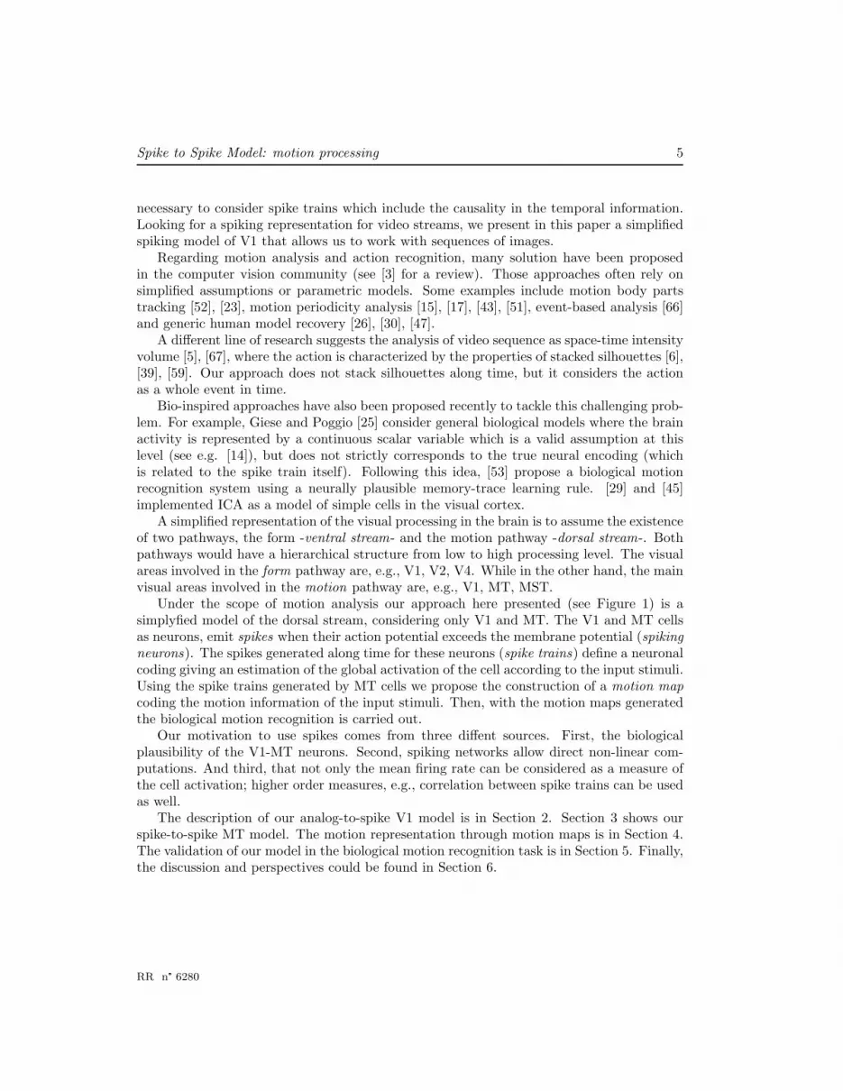
necessary to consider spike trains which include the causality in the temporal information.Looking for a spiking representation for video streams, we present in this paper a simplifiedspiking model of V1 that allows us to work with sequences of images.

Regarding motion analysis and action recognition, many solution have been proposedin the computer vision community (see [3] for a review). Those approaches often rely onsimplified assumptions or parametric models. Some examples include motion body partstracking [52], [23], motion periodicity analysis [15], [17], [43], [51], event-based analysis [66]and generic human model recovery [26], [30], [47].

A different line of research suggests the analysis of video sequence as space-time intensityvolume [5], [67], where the action is characterized by the properties of stacked silhouettes [6],[39], [59]. Our approach does not stack silhouettes along time, but it considers the actionas a whole event in time.

Bio-inspired approaches have also been proposed recently to tackle this challenging prob-lem. For example, Giese and Poggio [25] consider general biological models where the brainactivity is represented by a continuous scalar variable which is a valid assumption at thislevel (see e.g. [14]), but does not strictly corresponds to the true neural encoding (whichis related to the spike train itself). Following this idea, [53] propose a biological motionrecognition system using a neurally plausible memory-trace learning rule. [29] and [45]implemented ICA as a model of simple cells in the visual cortex.

A simplified representation of the visual processing in the brain is to assume the existenceof two pathways, the form -ventral stream- and the motion pathway -dorsal stream-. Bothpathways would have a hierarchical structure from low to high processing level. The visualareas involved in the form pathway are, e.g., V1, V2, V4. While in the other hand, the mainvisual areas involved in the motion pathway are, e.g., V1, MT, MST.

Under the scope of motion analysis our approach here presented (see Figure 1) is asimplyfied model of the dorsal stream, considering only V1 and MT. The V1 and MT cellsas neurons, emit spikes when their action potential exceeds the membrane potential (spikingneurons). The spikes generated along time for these neurons (spike trains) define a neuronalcoding giving an estimation of the global activation of the cell according to the input stimuli.Using the spike trains generated by MT cells we propose the construction of a motion mapcoding the motion information of the input stimuli. Then, with the motion maps generatedthe biological motion recognition is carried out.

Our motivation to use spikes comes from three diffent sources. First, the biologicalplausibility of the V1-MT neurons. Second, spiking networks allow direct non-linear com-putations. And third, that not only the mean firing rate can be considered as a measure ofthe cell activation; higher order measures, e.g., correlation between spike trains can be usedas well.

The description of our analog-to-spike V1 model is in Section 2. Section 3 shows ourspike-to-spike MT model. The motion representation through motion maps is in Section 4.The validation of our model in the biological motion recognition task is in Section 5. Finally,the discussion and perspectives could be found in Section 6.

RR n° 6280


Figure 1: Block diagram showing the different steps of our approach from the input image sequence asstimulus until the motion map encoding the pattern motion. (a) We use real video sequence as input, theinput sequences are preprocessed in order to have contrast normalization and centered moving stimuli. Tocompute the motion map representing the input image we consider a sliding temporal window of length ∆t.(b) Directional-selectivity filters are applied over each frame of the input sequence in a log-polar distributiongrid obtaining spike trains as V1 output. These spike trains feed the spiking MT which integrates theinformation in space and time. (c) The motion map is constructed calculating the mean firing rates of MTspike trains inside the sliding temporal window. The motion map has a length of NL ×Nc elements, whereNL is the number of MT layers of cells and Nc is the number of MT cells per layer.

INRIA


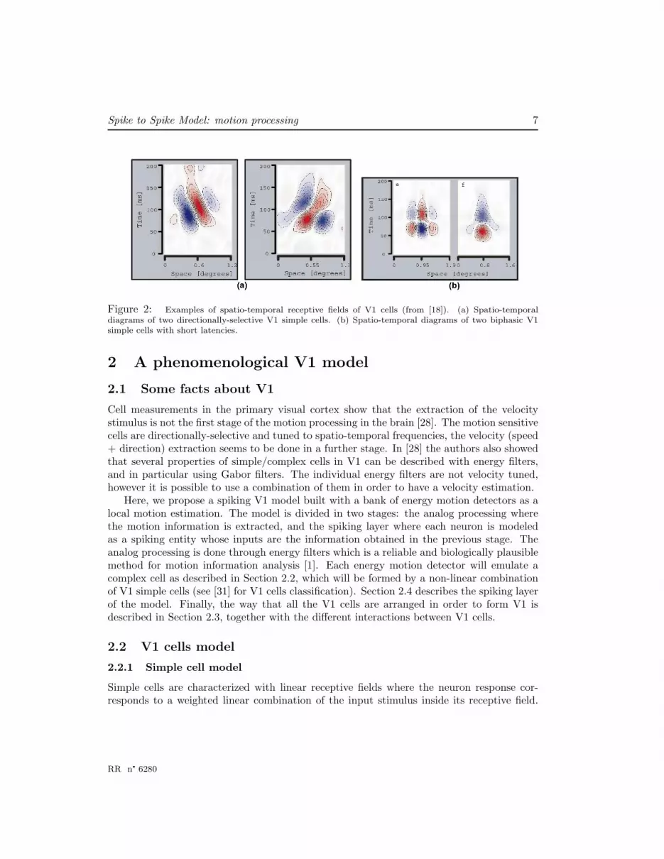
Figure 2: Examples of spatio-temporal receptive fields of V1 cells (from [18]). (a) Spatio-temporaldiagrams of two directionally-selective V1 simple cells. (b) Spatio-temporal diagrams of two biphasic V1simple cells with short latencies.

2 A phenomenological V1 model

2.1 Some facts about V1

Cell measurements in the primary visual cortex show that the extraction of the velocitystimulus is not the first stage of the motion processing in the brain [28]. The motion sensitivecells are directionally-selective and tuned to spatio-temporal frequencies, the velocity (speed+ direction) extraction seems to be done in a further stage. In [28] the authors also showedthat several properties of simple/complex cells in V1 can be described with energy filters,and in particular using Gabor filters. The individual energy filters are not velocity tuned,however it is possible to use a combination of them in order to have a velocity estimation.

Here, we propose a spiking V1 model built with a bank of energy motion detectors as alocal motion estimation. The model is divided in two stages: the analog processing wherethe motion information is extracted, and the spiking layer where each neuron is modeledas a spiking entity whose inputs are the information obtained in the previous stage. Theanalog processing is done through energy filters which is a reliable and biologically plausiblemethod for motion information analysis [1]. Each energy motion detector will emulate acomplex cell as described in Section 2.2, which will be formed by a non-linear combinationof V1 simple cells (see [31] for V1 cells classification). Section 2.4 describes the spiking layerof the model. Finally, the way that all the V1 cells are arranged in order to form V1 isdescribed in Section 2.3, together with the different interactions between V1 cells.

2.2 V1 cells model

2.2.1 Simple cell model

Simple cells are characterized with linear receptive fields where the neuron response cor-responds to a weighted linear combination of the input stimulus inside its receptive field.

RR n° 6280


Combining two simple cells in a linear manner it is possible to get direction-selective neurons,that is, simple cells selective for stimulus orientation and spatial frequency. Since simplecells combine input stimulus using positive a negative weights, the linear receptive fields canhave positive or negative responses.

The direction-selectivity (DS) refer to the property of a neuron to respond selectivelyto the direction of the motion of a stimulus. The way to model this selectivity is obtainreceptive fields oriented in space and time. Adding or subtracting neuron responses in spatio-temporal quadrature it is possible to obtain DS simple cells. Let us define the followingspatio-temporal oriented simple cells

F aθ,f (x, y, t) = F oddθ (x, y)Hfast(t)− F evenθ (x, y)Hslow(t),

F bθ,f (x, y, t) = F oddθ (x, y)Hslow(t) + F evenθ (x, y)Hfast(t), (1)

where simple cells defined in (1) are spatially oriented in an angle θ, and f = (ξ, ω) isthe spatio-temporal orientation in the frequency domain, where ξ and ω are the spatio andtemporal maximal responses, respectively (see Section 2.2.2). Each conforming simple cellis formed using the first and second derivative of a Gabor function for the spatial part anda Gamma function for the temporal part, respectively, as described below:

F oddθ (~x) =∂Gθ(~x)∂x

F evenθ (~x) =∂2Gθ(~x)∂x2

(2)

(3)

where ~x = (x, y), ~k =(

cos θsin θ

), ωf = 2πf , and Gθ(x, y) corresponds to the Gabor function

defined as

Gθ(x, y) = exp

(−~k2~x2

2σ2

)sin(ωf~k~x

)(4)

where f is the spatial frequency of the gabor function, and θ the spatial orientation.

The temporal contributions Hfast(t) and Hslow(t) come from the substraction of twoGamma functions with a difference of two in their respective orders.

Hfast(t) = T3,τ (t)− T5,τ (t),Hslow(t) = T5,τ (t)− T7,τ (t), (5)

and Tα,τ (t) is defined as

Tα,τ (t) =tα

τα+1α!exp

(− t

τ

), (6)

who models the series of synaptic and cellular delays in signal transmission, from retinalphotoreceptors to V1 afferents serving as a plausible approximation of biological findings [46].

INRIA


The biphasic shape of Hfast(t) and Hslow(t) could be a consequence of the combination ofcells of M and P pathways [18], [49] or due to the delayed inhibitions in the retina and LGN[16].

2.2.2 Spatio-temporal frequency analysis of simple cells

Here we analyze the spatio-temporal frequency content of our V1 simple cell model. Forsimplicity and without loss of generality, we will use just one spatial dimension x and focuson the function F a(x).

To get the impulse response, we calculate the Fourier transform of F a, denoted by F a,considering an input stimuli L(x, t) = δ(x, t)

F a(ξ, ω) = F odd(ξ)Hfast(ω)− F even(ξ)Hslow(ω) (7)

Expanding each term we obtain

F odd(ξ) =σ√

2π2

{exp

(−σ

2(ξ − ξ0)2

2

)+ exp

(−σ

2(ξ + ξ0)2

2

)}, (8)

F even(ξ) = −j σ√

2π2

{exp

(−σ

2(ξ − ξ0)2

2

)− exp

(−σ

2(ξ + ξ0)2

2

)},

Hfast(ω) =1

(1 + jω)4− 1

(1 + jω)6,

Hslow(ω) =1

(1 + jω)6− 1

(1 + jω)8,

To visualize the range of spatial and temporal frequencies of this filter it is necessary to getthe power spectrum, which is given by

|F a(ξ, ω)|2 =F a(ξ, ω)F a(ξ, ω)

2π

=12π

{|F odd(ξ)Hfast(ω)|2 + |F even(ξ)Hslow(ω)|2

}(9)

+j

2π

{R{F odd(ξ)}={F even(ξ)}

(Hfast(ω)Hslow(ω)− Hslow(ω)Hfast(ω)

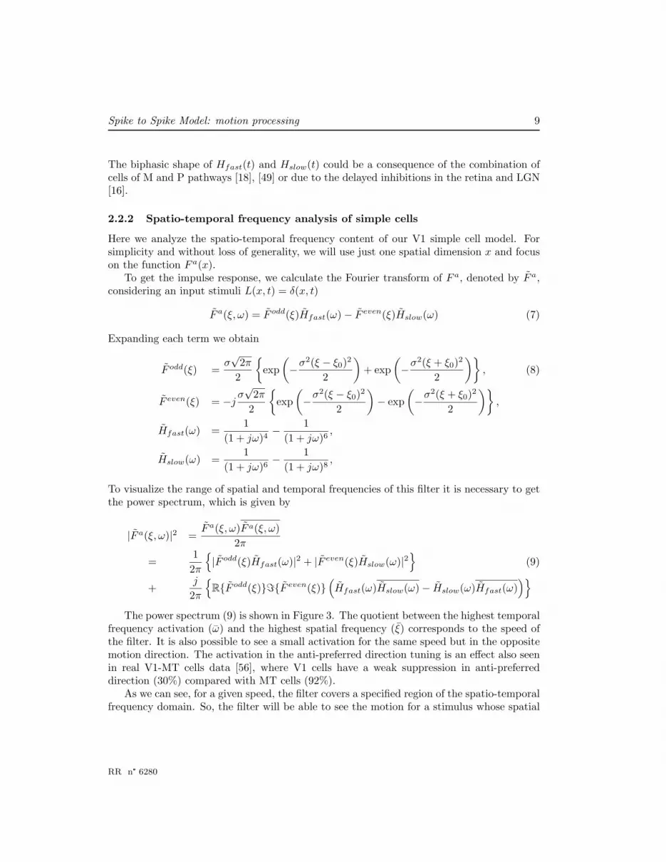
)}The power spectrum (9) is shown in Figure 3. The quotient between the highest temporal

frequency activation (ω) and the highest spatial frequency (ξ) corresponds to the speed ofthe filter. It is also possible to see a small activation for the same speed but in the oppositemotion direction. The activation in the anti-preferred direction tuning is an effect also seenin real V1-MT cells data [56], where V1 cells have a weak suppression in anti-preferreddirection (30%) compared with MT cells (92%).

As we can see, for a given speed, the filter covers a specified region of the spatio-temporalfrequency domain. So, the filter will be able to see the motion for a stimulus whose spatial

RR n° 6280


Figure 3: Space-time diagrams for F a(x, t) (left) and its power spectrum |F a(ξ, ω)|2 (right). Both graphswere constructed considering just one spatial dimension x. Left: It is possible to see directionality-selectiveobtained after the linear combination of cells. It is important also to remark the similarities with thebiological maps measured by [18] (Figure 2). Right: Spatio-temporal energy spectrum of the directional-selective filter F a(x, t). The slope formed by the peak of the two blobs corresponds to the speed tuning ofthe filter.

Figure 4: Different filters tuned at the same speed used to tile the spatial-temporal frequency space. Thisgraph was obtained considering just one spatial dimension x.

frequency is inside the energy spectrum of the filter. To pave all the space in a homogeneousway, it is necessary to take more than one filter for the same spatio-temporal frequencyorientation. Each filter, for a given orientation, must have different spatial frequencies andthereafter different temporal frequencies to keep the ratio peakω/peakξ constant. A diagramwith the filter bank tuned at the same speed can be seen in Figure 4.

INRIA


In our case, the causality of Hfast(t) and Hslow(t) generates a more realistic model thanthe one proposed by [54]. Using the temporal components defined in (5), the search of ananalytic expression for |F a(ξ, ω)|2, is not an easy task, specially due to the non-separabilityof F a(x, t).

2.2.3 Complex cell model

Complex cells are also direction-selectivity neurons, however they include other characteris-tics that cannot be explained by a linear combination of the input stimulus. Their responsesare relatively independent of the precise stimulus position inside the receptive field, whichsuggest a combination of a set of V1 simple cells responses. The complex cells are also in-variant to contrast polarity which indicates a kind of rectification of their ON-OFF receptivefield responses.

Based on [1], we define our complex cells combining V1 simple cells responses in anonlinear manner. The combination is done taking the squared sum of a pair of them withthe same amplitude response but in spatial quadrature, obtaining an estimation of the localenergy of the stimulus. The squared sum of the quadrature filters is independent of the signof the contrast, it is and constant in time for a drifting sinusoidal as stimulus. A diagramwith this procedure can be seen in Figure 5

Let us denote Cxi,θi,fi(t) the response of the ith complex cell located at position xi =(xi, yi), orientation tuning θi and spatio-temporal frequencies fi = (ξi, ωi). So, for an inputluminosity profile L(x, y, t) the response of the complex cell i, is given by

Cxi,θi,fi(t) =[(F aθi,fi ∗ L

)(xi, yi, t)

]2 +[(F bθi,fi ∗ L

)(xi, yi, t)

]2(10)

where the symbol ∗ represents the spatial-temporal convolution, and F aθi,fi and F bθi,fi arethe V1 simple cells defined in (1).

Remark Velocity Estimation: As we mentioned in this section, the individual energy filters are not velocitytuned. It is necessary to combine their responses in order to extract the velocity. The spatio-temporal filtersdefined in (1) can be tuned for a particular orientation in the spatio-temporal domain, but the energymeasured is a function of both the velocity and the contrast of the stimulus pattern. In order to do themotion detectors independent of the stimulus contrast, Adelson and Bergen [1] propose a velocity estimation,defined as

v =

P(Cθ(x, y, t))2 −

P(Cθ+π(x, y, t))2P

(Sθ(x, y, t))2(11)

where Sθ(x, y, t) is the response of a filter tuned for stationary stimulus, same spatial orientation and samespatio-temporal frequencies than Cθ(x, y, t).

In our model we will not consider the velocity magnitude estimation defined in (11). At V1 level we will

just put emphasis in the uniform tile of the frequency space. MT layer will be in charge of the extraction of

the velocity stimulus starting from V1 complex cell responses. �

RR n° 6280


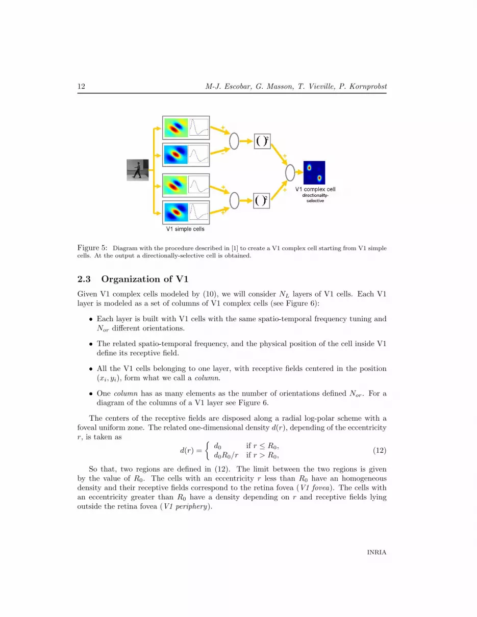
Figure 5: Diagram with the procedure described in [1] to create a V1 complex cell starting from V1 simplecells. At the output a directionally-selective cell is obtained.

2.3 Organization of V1

Given V1 complex cells modeled by (10), we will consider NL layers of V1 cells. Each V1layer is modeled as a set of columns of V1 complex cells (see Figure 6):

� Each layer is built with V1 cells with the same spatio-temporal frequency tuning andNor different orientations.

� The related spatio-temporal frequency, and the physical position of the cell inside V1define its receptive field.

� All the V1 cells belonging to one layer, with receptive fields centered in the position(xi, yi), form what we call a column.

� One column has as many elements as the number of orientations defined Nor. For adiagram of the columns of a V1 layer see Figure 6.

The centers of the receptive fields are disposed along a radial log-polar scheme with afoveal uniform zone. The related one-dimensional density d(r), depending of the eccentricityr, is taken as

d(r) ={d0 if r ≤ R0,d0R0/r if r > R0,

(12)

So that, two regions are defined in (12). The limit between the two regions is givenby the value of R0. The cells with an eccentricity r less than R0 have an homogeneousdensity and their receptive fields correspond to the retina fovea (V1 fovea). The cells withan eccentricity greater than R0 have a density depending on r and receptive fields lyingoutside the retina fovea (V1 periphery).

INRIA


Figure 6: Diagram with the architecture of one V1 layer. There are two different regions in V1, the foveaand periphery. Each element of the V1 layer is a column of Nor V1 cells, where Nor corresponds to thenumber of orientations.

2.4 Layer of integrate and fire neurons

The response of the V1 complex cell Cx,θ,f defined in (10), formed as a combination ofthe V1 simple cells defined in (1), is analogous. To transform the analogous response to aspiking response, the cell will be model as a conductance-driven integrate-and-fire neuron[61], [20].

Considering a spiking V1 complex cell i whose center is located in xi = (xi, yi) of thevisual space, the integrate-and-fire normalized equation is given by

dui(t)dt

= Gexci (t)(ui(t)− Eexc) +Ginhi (t)(ui(t)− Einh)− gL(ui(t)− EL) + Ii(t), (13)

The neuron i, with orientation tuning θi and spatio-temporal frequencies fi = (ξi, ωi), emitsa spike when the normalized membrane potential of the cell ui(t) is equal to 1, then ui(t)is reinitialized to 0. Ii(t) denotes the external current inputs to the neuron. Gexci (t) is thenormalized excitatory conductance directly associated with the presynaptic neurons con-nected to neuron i. The conductance gL is the passive leaks in the cell’s membrane. Finally,Ginhi (t) is an inhibitory normalized conductance dependent on, e.g., lateral connections orfeedbacks from upper cortical layers. The typical values for the reversal potentials Eexc,Einh and EL are 0mv, -80mv and -70mV, respectively [61].

So, in the particular case of V1, let us consider a spiking V1 complex cell i previously de-fined. For this neurons, Gexci (t) is the normalized excitatory conductance directly associatedwith the pre-synaptic neurons connected to V1 cells. The external input current Ii(t) is hereassociated with the analogous V1 complex cell response. Finally, Ginhi (t) is an inhibitorynormalized conductance dependent on the spikes of neighboring cells of the same V1 layer.

We model the external input current Ii(t) of the ith cell in 13 as the analog response

Ii(t) = kexcΛi(t)Cxi,θi,fi(t), (14)

where kexc is an amplification factor, Cxi,θi,fi refers to the complex cell response defined in(10) and Λi summarizes the modulating effect of the neighboring cell interactions provokedmainly by surround suppression interactions [32, 50].

RR n° 6280


2.5 Surround suppression

The majority of V1 cells present surround modulation, which is normally suppressive [32, 50].The effect of the surround on the total activation of the neuron can be either subtractive ordivisive.

Using the data of 138 cells, Sceniak et al. [50] found that the mean size of the suppressionarea is of 2.2◦. In order to explore the spatial organization of the surround suppressionJones et al. [32] studied the spatial location of suppressive zones in a population of V1neurons. The majority of the cells analyzed in this way (81%) exhibited spatial heterogenityof surround locations, although 19% showed spatially uniform surround suppression.

Cells exhibiting heterogeneous surrounds, were divided into spatially asymmetric cells(44%) where the surround suppression was biased toward one location and bilaterally sym-metric cells (37%) where the surround effect was localized to two opposing regions along asingle axis. For cell with heterogenous surrounds, suppressive effects were nearly equally dis-tributed in all directions round the CRF; there was no evidence to suggest that suppressiveeffects were concentrated in end-zones or side-band regions.

Considering the subtractive or divisive effect of the surround in the activation of a V1neuron, we will model the surround modulation Λi(t) of equation (14) as a division ofdifference of integrated Gaussians. So, considering divisive effect of the surround activationthe value of Λi(t) will be given by

Λi(t) =(

kc1 + ksLc(t)

)(15)

where Ls(t) is the surround activation defined as

Ls(t) =∫ Rs

−RsCxψ,θψ,fψ (t)e−ψ

2/2σ2sdψ (16)

and where Rs is the radius of the surround suppression area, and σs is the correspondingparameter of the Gaussian modeling the surround effect.

3 Introducing a spiking MT model

3.1 Some facts about MT

The middle temporal visual area (MT or V5) of the macaque monkey is an extrastiate visualarea in which most cells are selective for the direction of stimulus motion. MT receives inputfrom several areas in the brain [8] mainly from V1 layer, in particular from the layer 4Bwhich is highly directional-selective [37]. MT is retinotopically organized with an emphasisin the fovea, where the half of MT surface is destinated to the processing of the central 15◦ofthe visual field. At a given eccentricity, the MT receptive fields are about 10 times largerthan those in V1.

INRIA


Different kinds of surround geometry of MT receptive fields are observed in the computa-tion of structure of motion. Half of MT neurons have asymmetric receptive fields introducinganisotropies in the processing of the spatial information [33]. The second half of the popula-tion examined by [65] has two different symmetries: circular symmetry surround (20% of thepopulation) and bilaterally symmetric surrounds, which correspond to a pair of surroundingregions on opposite sides. The neurons with asymmetric receptive fields seem to be involvedin the encoding of important surfaces features, such as slant and tilt or curvature [10].

Regardless the shape of the MT receptive fields, it is possible to classify them accordingto the interactions between the center and surround [7]. The direction tuning of the surroundis broader than that of the center, and the preferred direction, with respect to that of thecenter, tended to be either in the same (Reinforcing surrounds) or opposite (Antagonisticsurrounds) direction and rarely in orthogonal directions. The antagonistic surrounds areinsensitive to wide-field motion but very sensitive to local motion contrast. Otherwise, thereinforcing surrounds have better response to wide-field motion.

MT cells are highly directionally-selective compared with V1. Both V1 and MT havedirection tuned neurons, but MT shows a strong inhibition in the anti-preferred direction.The proportion of directionally-selective responses is 30% in V1 and 92% in MT [56].

Compairing the direction selectivity of MT neurons for gratings and plaids, it is possibleto classify them as pattern direction selective (PDS) or component direction selective (CDS).The PDS neurons have a unimodal response for plaids, while the CDS neurons show a bi-modal response indicating that two directions of the gratings conforming the plaid stimulus.The fact that the time response of CDS neurons is faster (about 6ms) than PDS neurons(about 50-75ms), suggests a two-stage model for MT, where the outputs of the CDS neu-rons are used as input of the PDS [38]. The selectivity of a PDS cells evolve during thefirst 100-150 ms after the exposition of a complex stimulus as plaid [55], starting with abroader selectivity resembling CDS cells. After some tens of milliseconds, their responsesevolve to be more PDS-like. By the other hand, CDS cells give a stable response as soon asthe stimulus is set.

It is well known that MT cells are tuned to speed, but is this tuning invariant to thespatial frequency of the stimulus? In [44] the authors, over a population of 104 MT cells,found three types of cells: speed-tuned neurons, spatio-temporally independent neurons anda third group without classification. The speed-tuned neurons are motion-sensitive cellsinvariant to the spatial frequency of the stimulus. The spatio-temporally independent neuronsare also motion-sensitive cells but tuned for an specific spatial and temporal frequencies, sothe speed tuning changes together with the spatial frequency of the stimulus.

For the computation of speed in MT cells, there are two branches of study about howthis process is carried out. One group (e.g. [2], [54]) considers that the information comingfrom V1 cells is linear and MT is who adds the needed non-linearities for the velocitycomputation. The second group (e.g. [62]) points out that the 2D motion is extracted in V1through nonlinearities such as endstopping, and MT just polls this information. In addition,there is evidence that the overall level of speed is modulated by the surround motion [7].

RR n° 6280


The energy model used for V1 simple/complex cells representation does not allow them tobe sensitive to an specific speed. In space they are sensitive just to the orthogonal componentof their preferred spatial orientation. A velocity-selective neuron may be constructed pollingthe output of several V1 complex cells with the spatio-temporal orientation consistent withthe velocity desired.

3.2 Spiking MT model

3.2.1 Connections to V1 cells

Our model is a spiking neural network where each entity or node is a MT cell. Each MTcell i can be modeled as conductance-driven integrate-and-fire neuron similar to (13).

dui(t)dt

= Gexci (t) (ui(t)− Eexc) +Ginhi (t)(ui(t)− Einh

)+ gL

(ui(t)− EL(t)

)+ I(t) (17)

where ui(t) is the normalized membrane potential of the cell. Gexci refers to the normalizedexcitatory conductance associated to an excitatory reversal potential Eexc. Similarly, Ginhi isthe normalized inhibitory conductance associated to an inhibitory reversal potential Einh.gL denotes the passive leaks in the cell’s membrane associated to the reversal potentialEL(t). I(t) denotes the external current inputs to the neuron. Like in (13) there is alsoa reinitialization of the neuron membrane potential to zero as soon as its voltage reachesthe threshold, which in this case for normalizations effects the threshold is considered as1. Typical values for the conductances Eexc, Einh and EL are 0mv, -80mv and -70mV,respectively [61].

The neuron i is a part of a spiking neural network where the input conductances Gexci (t)and Ginhi (t) are obtained considering the activity of all the pre-synaptic neurons connectedto it. For example, if a pre-synaptic neuron j has fired a spike at time t(f)

j , this spike reflects

an input conductance to the post-synaptic neuron i with a time course α(t − t(f)j ). In our

case the pre-synaptic neurons corresponds to the V1 outputs (see Figure 8(a)). Accordingto this, the total input conductances Gexci (t) and Ginhi (t) of the post-synaptic neuron i areexpressed as

Gexci (t) =∑j

w+ij

∑f

α(t− t(f)j )

Ginhi (t) =∑j

w−ij∑f

α(t− t(f)j ) (18)

where the factor w+ij (w−ij) is the efficacy of the positive (negative) synapse from neuron j

to neuron i (See [24] for more details). The time course α(s) of the postsynaptic current in(18) can be modeled as an exponential decay with time constant τs as follows

α(s; τs) =(s

τs

)exp

(− s

τs

)(19)

INRIA


Figure 7: Sample of log-polar architecture used for a MT layer. The cell distribution law is divided intotwo zones, a homogeneous distribution in the center with a certain radius and then a periphery where thedensity of cells decays with the eccentricity.

Inserting (18) into (17) we finally obtain

dui(t)dt

=

∑j

w+ij

∑f

α(t− t(f)j )

(ui(t)− Eexc) +

∑j

w−ij∑f

α(t− t(f)j )

(ui(t)− Einh)

+ gL(ui(t)− EL(t)

)+ I(t) (20)

Each MT cell has a receptive field from where converge V1 complex cells afferents insideits receptive field, which correspond to the pre-synaptic neurons j in (20). Those inputs willbe excitatory (w+

ij > 0) or inhibitory (w−ij < 0) depending on the characteristic and shapeof the respective receptive fields [65, 63].

The receptive field associated with an MT cell corresponds to a certain area inside thevisual field. The half of MT surface is assigned to process the information coming from thecentral 15◦ of the visual field, which receptive field size of a MT cell inside this region isabout 4-6 times bigger than the V1 receptive field [35].

The MT cells are distributed in a log-polar architecture, with a homogeneous area of cellsin the center and a periphery where the density decreases with the distance to the centerof focus. While the density of cells decreases with the eccentricity, the size of the receptivefields increases preserving its original shape. Figure 7 shows an example of the log-polardistribution of MT cells.

Different layers of MT cells conform our model. Each layer is built with MT cells ofthe same characteristics, this is same speed and direction tuning. Depending on the tuningvalues, the MT cell decides which V1 cells contribute with relevant information and estab-lishes the proper connection between them. The criteria of selection is to consider all the V1cells inside the MT receptive field with an absolute difference of motion direction-selectivityrespect to MT cell no more than π/2 radians. The weight associated to the connectionbetween neuron j and i is proportional to the angle αij between the two preferred motiondirection-selectivity (see Figure 8(b)). The connection weight wij between the jth V1 cell

RR n° 6280


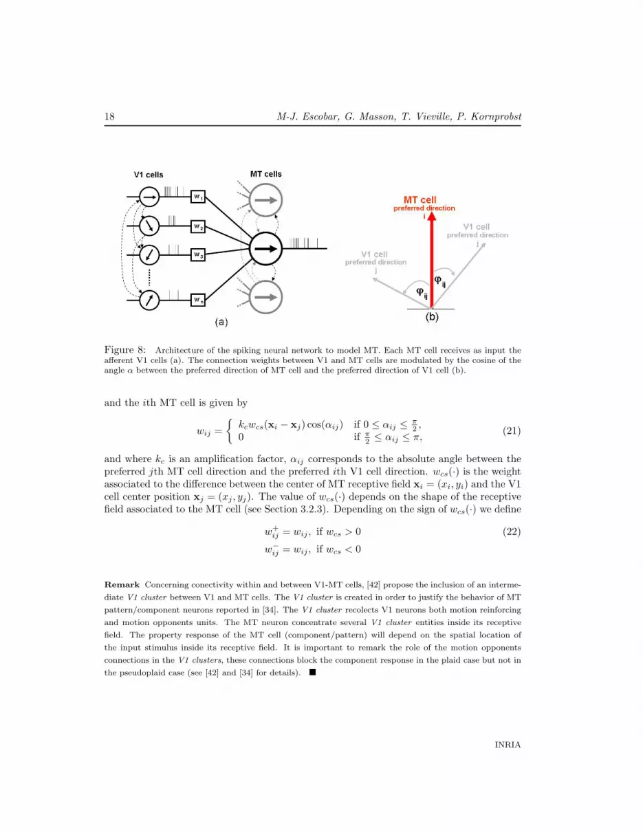
Figure 8: Architecture of the spiking neural network to model MT. Each MT cell receives as input theafferent V1 cells (a). The connection weights between V1 and MT cells are modulated by the cosine of theangle α between the preferred direction of MT cell and the preferred direction of V1 cell (b).

and the ith MT cell is given by

wij ={kcwcs(xi − xj) cos(αij) if 0 ≤ αij ≤ π

2 ,0 if π

2 ≤ αij ≤ π,(21)

and where kc is an amplification factor, αij corresponds to the absolute angle between thepreferred jth MT cell direction and the preferred ith V1 cell direction. wcs(·) is the weightassociated to the difference between the center of MT receptive field xi = (xi, yi) and the V1cell center position xj = (xj , yj). The value of wcs(·) depends on the shape of the receptivefield associated to the MT cell (see Section 3.2.3). Depending on the sign of wcs(·) we define

w+ij = wij , if wcs > 0 (22)

w−ij = wij , if wcs < 0

Remark Concerning conectivity within and between V1-MT cells, [42] propose the inclusion of an interme-

diate V1 cluster between V1 and MT cells. The V1 cluster is created in order to justify the behavior of MT

pattern/component neurons reported in [34]. The V1 cluster recolects V1 neurons both motion reinforcing

and motion opponents units. The MT neuron concentrate several V1 cluster entities inside its receptive

field. The property response of the MT cell (component/pattern) will depend on the spatial location of

the input stimulus inside its receptive field. It is important to remark the role of the motion opponents

connections in the V1 clusters, these connections block the component response in the plaid case but not in

the pseudoplaid case (see [42] and [34] for details). �

INRIA


3.2.2 Horizontal connectivity

Diffusion is a biological mechanisms through the cells transmit some distinctive and impor-tant information to the neighboring ones. Diffusion also occurs between neighboring cellswith different characteristics like different velocities, speed, receptive field. Diffusion of ac-tivity between neighboring cells is observed and it is due to a local horizontal connectivitypatter. The diffusion can be included in the dynamic of the neuron extending (20) as follows

dui(t)dt

= gL(ui(t)− EL(t)

)+ I(t) +

∑j∈V1

w+ij

∑f

α(t− t(f)j )

(ui(t)− Eexc) (23)

+

∑j∈V1

w−ij∑f

α(t− t(f)j )

(ui(t)− Einh)

+

∑k∈MT

ζ+ik

∑f

α(t− t(f)k )

(ui(t)− Eexc)

+

∑k∈MT

ζ−ik

∑f

α(t− t(f)k )

(ui(t)− Einh)

where the two last terms correspond to diffusion. ζ+ik (ζ−ik) corresponds to a weight matrix

with the positive (negative) diffusion shape modeled.For the implementation of diffusion it is necessary create connections between MT cells.

The connection radius and weights are given by the diffusion function, which is normallya Gaussian. As a first step inside our model the MT cells connected for diffusion are thecells with the same velocity direction. So, inside a neighborhood all the cells with the samevelocity direction share information trough diffusion without concerning the different speedsof the cells.

The information exchange between MT cells is done through spikes, where the first cellwho fires send the diffusion signal to the assigned neighbors.

3.2.3 Receptive fields: geometry and dynamics

The geometry and dynamics of the MT receptive fields is far from be completely understood.Their geometry is the main responsible of the direction tuning of the MT cell and it changesalong time, either switching from component to pattern behavior [55] or showing a directionreversal from preferred to antipreferred direction tuning [41].

The contrast of the input stimulus plays an important role in the MT velocity tuning.Experiments done by [40] showed that the velocity tuning of the MT cell is modulated bythe contrast of the input stimulus. They found two types of cells: The first group of cellshas to low input a broad tuning to low speed switching to high speed tuning when the inputcontrast is high. The second group has the opposite behavior, this means at low contrastthe cells are broadly tuned to high speeds while at high contrast they are highly tuned tolow speed.

RR n° 6280


A second level of complexity in the MT receptive fields is their spatial organization.Experiments in [65] revealed that only 20% of the MT cells tested have circularly symmetricsurrounds, 50% were asymmetric concentrating the suppression in only one location onone side of the preferred-null direction axis, and 25% have bilaterally symmetric zones ofsuppression lying along the same axis (see Figure 9). In our case we will just considercircularly symmetric surrounds. Altough this kind of surrounds are just the 20% of the MTcells tested by [65], it looks to be a good inital approximation for the motion recognitiontask (see Section 5).

Figure 9: Different geometries of asymmetric center-surround organization in MT cells [65, 64]. (a)Circularly symmetric surrounds. (b) Asymmetric configuration concentrating the suppression at one side ofthe motion preferred axis. (c) Bilaterally symmetric zones of suppression lying in the motion preferred axis.

Regarding organization and center-surround interactions, [7] shows two different typesof cells, the reinforcing surrounds and the antagonistic surround. The direction tuningof the surround is always broader than the center. The direction tuning of the surroundcompared with the center tends to be either the same or opposite, but rarely orthogonal.The antagonistic surrounds are insensitive to wide-field motion but sensitive to local motioncontrast. By the other hand, the cells with reinforcing surround are best sensitive to wide-field motion. The author in [7] also suggests a columnar organization in MT cells, groupingthe columns according to its center-surround properties.

Considering the results found by [7], we propose three types of MT center-surround inter-actions in our model. Our claim is that the antagonistic surrounds contain key informationabout the motion characterization, which could highly helps the motion recognition task.We propose one reinforcing center-surround interaction and two antagonistic as shown inFigure 10. It is important to mention that this approach corresponds to a coarse approxima-tion of the real receptive field shapes, but anyways this approach is capable to extract keyinformation from the motion stimulus. The receptive fields shown in Figure 10(a) and Figure10(b)-(c) were created using a Gaussian and a Difference of Gaussians (DoG), respectively.

We put at the entrance of our system a stimulus consisting of a circle of variable radiuswith a drifting grating inside. The motion direction of the drifting grating corresponds tomotion direction tuning of our MT cells. We varied the radius of the circle and we measured

INRIA


Figure 10: Center-surround interactions modeled in the MT cells. The reinforcing surround (a) is modeledthrough a gaussian. The two receptive fields with inhibitory surround (b), (c) are modeled with a Difference-of-Gaussians. The cells with inhibitory surround have either antagonistic direction tuning between the centerand surround or the same direction tuning.

the firing rate of the cell. The graphs with the firing rate measured according to the radiusof the stimulus can be seen in Figure 11. A more realistic receptive fields shapes can beobtained using also difference-of-gaussian and trying to fit them with the real data collectedby [9], [7], [65], or [64].

4 Motion maps

We proposed in previous sections a bio-inspired MT model where a video stream is convertedinto a set of spike trains. Our claim is that the information contained in those spike trainscorresponds to a discrete representation of the motion information contained in the inputsequence. The idea of coding through spike trains has been previously proposed by Thorpeet al ([57], [48], [?]), who introduced the notion of rank order coding to classify static images.The authors claim that the neural information is coded by the relative order in which theseneurons fire. The direct extension to video sequences is not so simple, since the use ofrank order coding cannot be easily applied to each frame due to time overlapping. It isnecessary to consider spike trains which include the causality in the temporal information.Here, we propose a novel representation which summarizes the motion characteristics of agiven sequence based in these spike trains.

A motion representation starting from spike trains is not an easy challenge: The differenceof phase between two spike trains, the time of the first spike emitted, the mean firingrate (spikes/time window) of a neuron or the synchrony between spike trains of neuronpopulations could be examples of different information coding in the brain. In our case, itis required to find which MT cells responses are the most representative of a certain motionsequence. Visualizing the video stream as a continuous in time, we could define for an input

RR n° 6280


Figure 11: Graph with the firing rates measured for the three different receptive fields modeled for MTcells (Figure 10). The stimulus consisted in a circle of variable radius with a drifting grating inside (ii). Theeffect of vary the radius of the stimulus in the firing rate of the cell is graphed in (i). Each curve correspondsto the receptive fields (a), (b) and (c) defined in Figure 10. The motion direction tuning of the center ofeach MT cell corresponds to the orthogonal direction of the drifting grating. Here it is possible to see theno-reaction for wide-field motion in the case of antagonistic surrounds cells.

INRIA


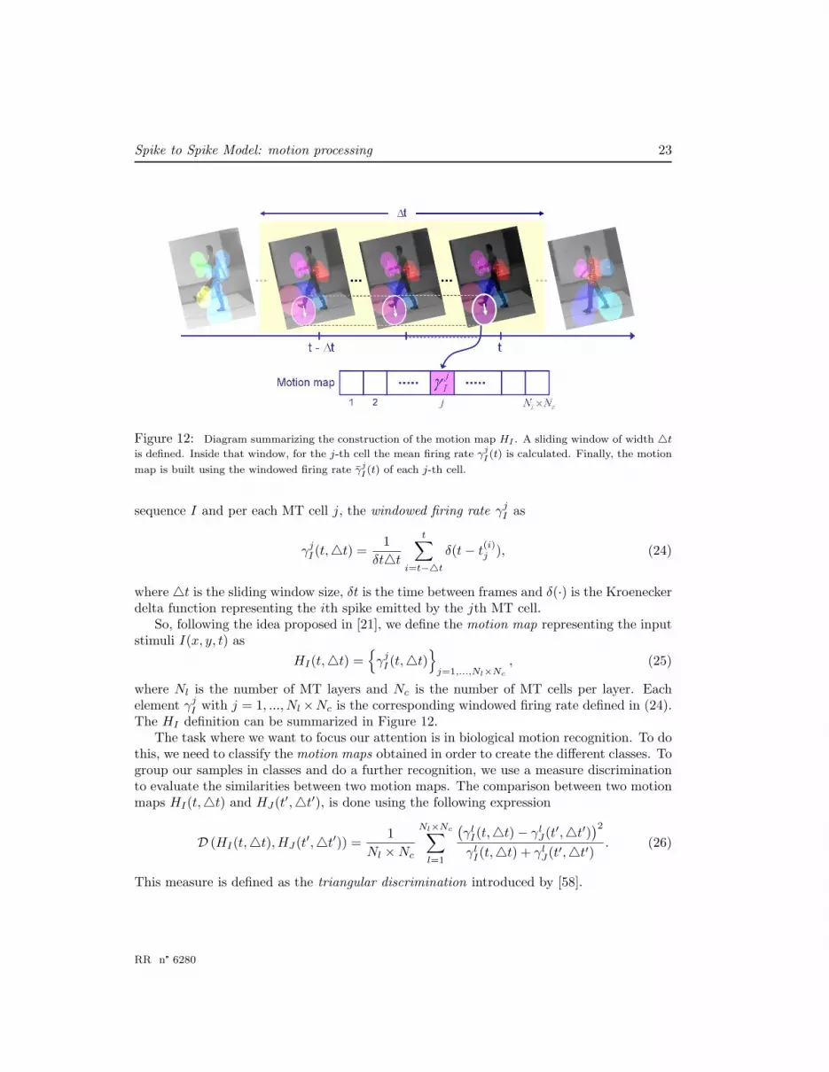
Figure 12: Diagram summarizing the construction of the motion map HI . A sliding window of width 4t

is defined. Inside that window, for the j-th cell the mean firing rate γjI (t) is calculated. Finally, the motion

map is built using the windowed firing rate γjI (t) of each j-th cell.

sequence I and per each MT cell j, the windowed firing rate γjI as

γjI (t,4t) =1

δt4t

t∑i=t−4t

δ(t− t(i)j ), (24)

where 4t is the sliding window size, δt is the time between frames and δ(·) is the Kroeneckerdelta function representing the ith spike emitted by the jth MT cell.

So, following the idea proposed in [21], we define the motion map representing the inputstimuli I(x, y, t) as

HI(t,4t) ={γjI (t,4t)

}j=1,...,Nl×Nc

, (25)

where Nl is the number of MT layers and Nc is the number of MT cells per layer. Eachelement γjI with j = 1, ..., Nl×Nc is the corresponding windowed firing rate defined in (24).The HI definition can be summarized in Figure 12.

The task where we want to focus our attention is in biological motion recognition. To dothis, we need to classify the motion maps obtained in order to create the different classes. Togroup our samples in classes and do a further recognition, we use a measure discriminationto evaluate the similarities between two motion maps. The comparison between two motionmaps HI(t,4t) and HJ(t′,4t′), is done using the following expression

D (HI(t,4t),HJ(t′,4t′)) =1

Nl ×Nc

Nl×Nc∑l=1

(γlI(t,4t)− γlJ(t′,4t′)

)2γlI(t,4t) + γlJ(t′,4t′)

. (26)

This measure is defined as the triangular discrimination introduced by [58].

RR n° 6280


Another measures derivated from statistics, such as Kullback and Leiber (KL) would alsobe used. The experiments done using the KL measure showed no significant improvements.

Remark The representation shown in (25) is invariant to the sequence length an its starting point. It

is also included information regarding the temporal evolution of the activation of MT cells, respecting the

causality in the order of events. The fact of use a sliding window allows us to include motion changes inside

the sequence. �

5 Experiments

The architecture proposed for the whole model, starting from the input sequence and endingwith the motion map representation HI , is represented in Figure 1. The system receivesas input a sequences of images where the biological motion is carried out. The directional-selective V1 filters are applied over each frame of the sequence in a log-polar distributiongrid, using one layer per each velocity. The spike trains generated feed the MT layers whereeach MT cell is activated according to the activation in V1 stage. The MT cells are arrangedin a log-polar grid as well, working joint with V1 cells as a spiking network. Per each inputframe the firing rate of all MT cells is calculated, then the mean firing rate along the wholesequence is obtained in order to construct the motion map described in (25). This motionmap characterizes and codes the biological motion stimulus.

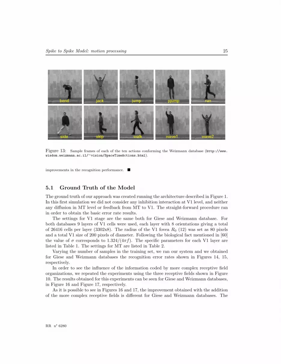
We ran the experiment using two databases: Giese and Weizmann. The V1 and MTparameters change depending on the database. For Giese database we consider 20 differentsamples of the same subject walking and another 20 samples of marching. Each sequencecontains 30 frames. The size of the images that form the sequence is 210x210 pixels. Weiz-mann database is formed by 9 different samples of different persons doing 10 different actionsas: bend, jack, jump, pjump, run, side, skip, walk, wave1 and wave2. A representative frameof each action can be seen in Figure 13. Each sequence contains at least 18 frames and theoriginal video streams were resized to have also images of 210x210 pixels.

The experiment protocol is equal to all the tests done. Each experiment consideredrandomly training sets with the same number of elements per class. The remaining sequenceswere used to construct the test set. For each number of elements in the training set, theexperiment was repeated 20 times obtaining the mean error recognition, the best recognitionrate and the standard deviation. All the motion maps of the training set were obtained andstored in a data container. When a new input sequence belonging to the test set is present tothe system, the motion map is calculated and it is compared using (26) with all the motionmaps stored in the training set. The input sequence class will be selected as the same classof the sequence with the smallest distance (see (26)). This selection mechanism correspondsto a RAW classifier.

Remark We repeated the experiments using a different classifier as SVM, but we did not get significant

INRIA


Figure 13: Sample frames of each of the ten actions conforming the Weizmann database (http://www.wisdom.weizmann.ac.il/∼vision/SpaceTimeActions.html).

improvements in the recognition performance. �

5.1 Ground Truth of the Model

The ground truth of our approach was created running the architecture described in Figure 1.In this first simulation we did not consider any inhibition interaction at V1 level, and neitherany diffusion in MT level or feedback from MT to V1. The straight-forward procedure ranin order to obtain the basic error rate results.

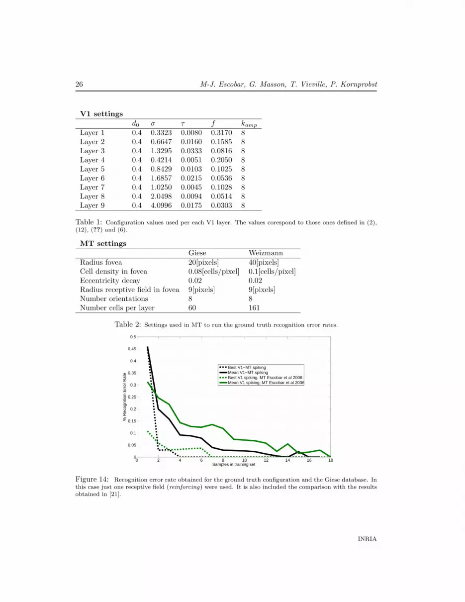
The settings for V1 stage are the same both for Giese and Weizmann database. Forboth databases 9 layers of V1 cells were used, each layer with 8 orientations giving a totalof 26416 cells per layer (3302x8). The radius of the V1 fovea R0 (12) was set as 80 pixelsand a total V1 size of 200 pixels of diameter. Following the biological fact mentioned in [60]the value of σ corresponds to 1.324/(4πf). The specific parameters for each V1 layer arelisted in Table 1. The settings for MT are listed in Table 2.

Varying the number of samples in the training set, we ran our system and we obtainedfor Giese and Weizmann databases the recognition error rates shown in Figures 14, 15,respectively.

In order to see the influence of the information coded by more complex receptive fieldorganizations, we repeated the experiments using the three receptive fields shown in Figure10. The results obtained for this experiments can be seen for Giese and Weizmann databases,in Figure 16 and Figure 17, respectively.

As it is possible to see in Figures 16 and 17, the improvement obtained with the additionof the more complex receptive fields is different for Giese and Weizmann databases. The

RR n° 6280

http://www.wisdom.weizmann.ac.il/~vision/SpaceTimeActions.html

http://www.wisdom.weizmann.ac.il/~vision/SpaceTimeActions.html


V1 settingsd0 σ τ f kamp

Layer 1 0.4 0.3323 0.0080 0.3170 8Layer 2 0.4 0.6647 0.0160 0.1585 8Layer 3 0.4 1.3295 0.0333 0.0816 8Layer 4 0.4 0.4214 0.0051 0.2050 8Layer 5 0.4 0.8429 0.0103 0.1025 8Layer 6 0.4 1.6857 0.0215 0.0536 8Layer 7 0.4 1.0250 0.0045 0.1028 8Layer 8 0.4 2.0498 0.0094 0.0514 8Layer 9 0.4 4.0996 0.0175 0.0303 8

Table 1: Configuration values used per each V1 layer. The values corespond to those ones defined in (2),(12), (??) and (6).

MT settingsGiese Weizmann

Radius fovea 20[pixels] 40[pixels]Cell density in fovea 0.08[cells/pixel] 0.1[cells/pixel]Eccentricity decay 0.02 0.02Radius receptive field in fovea 9[pixels] 9[pixels]Number orientations 8 8Number cells per layer 60 161

Table 2: Settings used in MT to run the ground truth recognition error rates.

0 2 4 6 8 10 12 14 16 180

0.05

0.1

0.15

0.2

0.25

0.3

0.35

0.4

0.45

0.5

Samples in training set

% R

ecog

nitio

n E

rror

Rat

e

Best V1−MT spikingMean V1−MT spikingBest V1 spiking, MT Escobar et al 2006Mean V1 spiking, MT Escobar et al 2006

Figure 14: Recognition error rate obtained for the ground truth configuration and the Giese database. Inthis case just one receptive field (reinforcing) were used. It is also included the comparison with the resultsobtained in [21].

INRIA


0 10 20 30 40 50 60 70 800

0.05

0.1

0.15

0.2

0.25


% R

ecog

nitio

n E

rror

Rat

e

Best Recognition Rate, 1 RFMean Recognition Rate, 1 RF

Figure 15: Recognition error rate obtained for the ground truth configuration and the Weizmann database.In this case just one receptive field (reinforcing) were used.

0 2 4 6 8 10 12 14 16 180

0.05

0.1

0.15

0.2

0.25

0.3

0.35

0.4

0.45

0.5


% R

ecog

nitio

n E

rror

Rat

e

Best Recognition Rate, 1 RFMean Recognition Rate, 1 RFBest Recognition Rate, 3 RFMean Recognition Rate, 3 RF

Figure 16: Recognition error rate obtained for Giese database using the three different receptive fieldsdescribed in Figure 10. It is possible to see an improvement in the recognition error rates in comparisonwith the case of just one receptive field (Figure 14).

RR n° 6280


0 10 20 30 40 50 60 70 800

0.05

0.1

0.15

0.2

0.25


% R

ecog

nitio

n E

rror

Rat

e

Best Recognition Rate, 1 RFMean Recognition Rate, 1 RFBest Recognition Rate, 3 RFMean Recognition Rate, 3 RF

Figure 17: Recognition error rate obtained for Weizmann database using the three different receptivefields described in Figure 10. The improvement obtained with the approach of the three receptive fieldsinstead only one is considerably.

fact that Giese database only contains two classes, gives a good recognition performancein the case of only one receptive field. The recognition performance is improved if we addthe more complex receptive fields, but the improvement is not very notoriously. In thecase of Weizmann database, which contains ten different classes, we obtained an evidentimprovement adding the new receptive fields.

6 Discussion and perspectives

We have proposed a spiking V1-MT model. The model receives as input a sequences ofimages. The V1 cells activated generate spike train feeding the next MT spiking layer.According to the activation of the MT cell, we proposed a motion representation (motionmap) encoding the information needed for a motion categorization task.

Our spiking V1 model is built with a bank of energy motion detectors as local motionestimators. The V1 model is divided in two stages: the analog processing where the motioninformation is extracted, and the spiking layer where each neuron is modeled as a spikingentity whose inputs are the information obtained in the previous stage.

The local motion estimation is done through the combination of different spatio-temporalfilters. The spatio-temporal filters are combined in order to obtain directional-selectivity(DS) properties. The DS refer to the property of a neuron to respond selectively to thedirection of the motion of a stimulus. This property can be obtained combining differentspatio-temporal filters. The construction of the spatio-temporal filters, and further DS ones,is inspired by [1]. The spatial parts of the filters are modeled by Gaussian derivatives. Thetemporal part is characterized by a biphasic shape, which it could be a consequence of the

INRIA


combination of cells of M and P pathways [18], [49] or due to the delayed inhibitions in theretina and LGN [16].

The V1 spiking layer receives as input the filter response of each V1 directional-selectivitycell. Each spiking cell is modeled as a leaky-integrate-and-fire neuron whose output feed theupper spiking MT layer. There are connections between the different V1 cells, specially tocreate inhibitory interactions as cross-orientation inhibition [11].

Different layers of V1 cells are used, each of them with a different spatio-temporal fre-quency tuning. The spatio-temporal frequency distribution of each layer is done in orderto tile the whole frequency space of interest. Cells with the same spatio-temporal badwithsand different spatial orientations are considered to be part of a column. The V1 columnsare arranged in a radial log-polar scheme paving the visual field.

Regarding MT, the model proposed is a spiking neural network where each node cor-responds to a MT neuron. The nature of the MT cell, its receptive field geometry and itscenter-surround interactions define the subset of V1 cells to be connected and their respectiveconnection weights.

In connectivity, each MT neuron is connected with a subset of V1 neurons inside itsreceptive field, whose spike trains outputs are the input of the MT cell. MT neurons are alsoconnected between them, allowing interactions such as spatial diffusion. The information ispropagated within a radius of action following a Gaussian law.

Each MT neuron has a receptive field geometry and a center-surround interaction codinga certain motion information. The shape and interaction of the MT receptive fields arechosen considering the results obtained by [7].

Considering the spike trains generated by the MT cells we propose a motion map as arepresentation of the motion information contained in the input stimulus. The motion mapssummarize along time the activation of the different MT cells. We claim that our motionmap represents the input stimuli and can be used in a motion categorization task. Thesemotion maps are invariant to the input sequence lengths and their starting point.

In order to validate our motion map as a valid motion representation, we applied themodel to biological motion recognition. We tested the model with two different databases(Giese and Weizmann), obtaining the results shown in Section 5. The good recognitionperformance obtained with our spike-to-spike model reinforces our hypothesis about therepresentability of our motion maps. It is also possible to see that the motion informationcoded by the different receptive field shapes and interactions of MT cells is a key issue inmotion categorization.

Giese database, with only two classes, has a good recognition performance neverthelessthe center-surround interactions of the MT cells. Of course, the inclusion of more complexinteractions improve the recognition performance, but the improvement is not significantcompared to the case of the reinforcing center-surround interaction only (see Figure 10).Weizmann database, formed by ten different classes (Figure 13), is a different scenario. Theinclusion of center-surround interactions coding more complex motion patterns is a key issuein the recognition performance. The complexity of the variety of classes suggests the use ofa more complex model to obtain motion maps more representatives of the input stimulus.

RR n° 6280


The results here described were obtained using no interactions within V1 or MT cells.These interactions will be tested in order to validate our model with real cell measurements.For this, we will use standard input stimuli such as drifting gratings, plaids or barber poles.Also the inclusion of more complex receptive field geometries in MT cells will be implementedand tested.

Some dynamics in the behavior of MT cells will be considered. Information contained inthe neurons described by [41] could code important events for the motion categorization andfurther recognition. The facts that pattern selectivity cells could come from the activationof the component selectivity cells, and that the pattern cells receive inputs from the ventralstream areas as V2 and V3 [55], give us an idea of the different connections and interactionsbetween different areas of the visual cortex. The changes in MT cell responses to differentinput contrast [40] could be an important issue for robustness.

Acknowledgments

The dataset has been kindly provided by Dr. Giese and the present work has been realizedthanks to this data set. This work was partially supported by the EC IP project FP6-015879, FACETS and CONICYT Chile. We also thank to Olivier Rochel for his Mvaspikesimulator, this tools allowed us to create and simulate spiking networks in an easy manner.

INRIA


Appendix

A Spatio-temporal filters frequency analysis

As we previously mentioned in Section 2.2.3, the directionally-selective complex cell comesfrom the relation (10)

Cθ(x, y, t) = [F aθ (x, y, t) ∗ I(x, y, t)]2 +[F bθ (x, y, t) ∗ I(x, y, t)

]2,

where the spatial and temporal bandwiths are given by the frequence response of F aθ (x, y, t)and F bθ (x, y, t), both not separable. An alternative analysis to the one in Section 2.2.2could be done through complex analysis. In order to look for separability, let us study thefrequence response of the following complex number

gθ(x, y, t) = F aθ (x, y, t) + jF bθ (x, y, t), (27)

which is separable in space and time, it means

gθ(x, y, t) = gxθ (x)gyθ (y)g

t(t) (28)

Considering θ = 0 we can write gxθ (x), gyθ (y) and gt(t) as follows

gx(x) = −exp

(− x2

2σ2

)σ4

sin(2πfx)[−x2 + σ2 + 4π2f2σ4 − jσ2x

]−

exp(− x2

2σ2

)σ4

2πfσ2 cos(2πfx)[2x+ jσ2

]gy(y) = exp

(− y2

2σ2

),

gt(t) =1

5040τ8

3

exp(− t

τ

)[840jτ4 + (−42− 42j)t2τ2 + t4

]Θ(t), (29)

The separability property of gθ(x, y, t) allows us to study its frequence response consid-ering the frequence response of each of its components gxθ , g

yθ and gt, separately. For an

easier analysis, and without loss of generality, we will consider just one spatial componentgx(x) with θ = 0. Applying the Fourier transform to g(x, t) we get g(ξ, ω) defined as

g(ξ, ω) = gx(ξ)gt(ω), (30)

where gx(ξ) and gt(ω) are the Fourier transforms of gx(x) and gt(ω), respectively. Thepower spectrum |g(ξ, ω)|2 of g(ξ, ω), is given by

|g(ξ, ω)|2 = |F a(ξ, ω)|2 + |F b(ξ, ω)|2 = |gx(ξ)|2 ∗ |gt(ω)|2 (31)

RR n° 6280


1.5

1

u

0.5

0.5

2

1-0.50

0-1

xi = 0.01

xi = 0.02

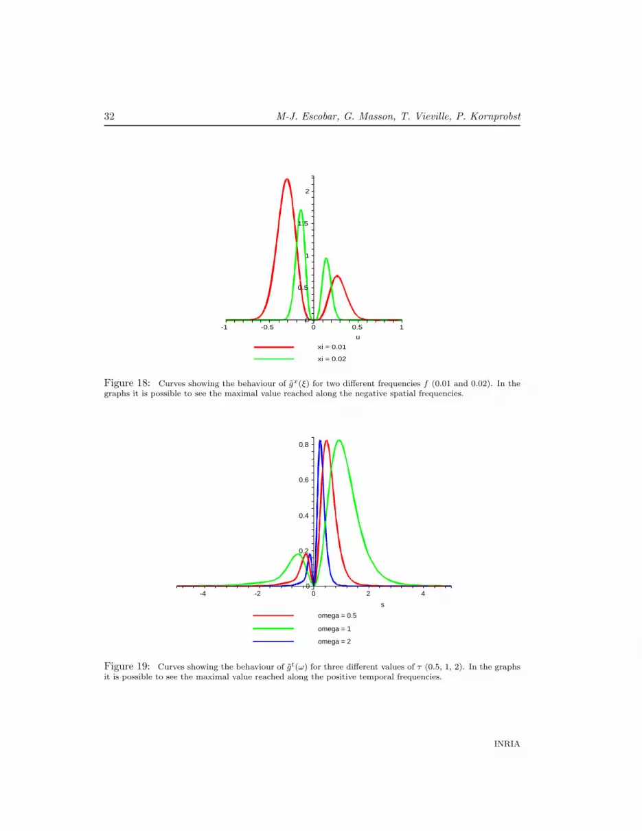
Figure 18: Curves showing the behaviour of gx(ξ) for two different frequencies f (0.01 and 0.02). In thegraphs it is possible to see the maximal value reached along the negative spatial frequencies.

0.6

0

0.4

0.2

-20

-4

0.8

s

42

omega = 0.5

omega = 1

omega = 2

Figure 19: Curves showing the behaviour of gt(ω) for three different values of τ (0.5, 1, 2). In the graphsit is possible to see the maximal value reached along the positive temporal frequencies.

INRIA


Some graphs obtained for gx(ξ) and gt(ω) can be seen in Figures 18 and 19, respectively.

Combining gt(ω) and gx(ξ) it is possible to find frequency activity maps as the the onesshown in Figure 3 (Right).

The goal of this analysis is the bank filter design. To do so, it is required to find expres-sions relating the values of f , τ of equations (2) and (5) with the filter frequence responsegiven by (31). These relationships were done using numerical analysis approximating thecurves by polynomials of second order.

References

[1] E.H. Adelson and J.R. Bergen. Spatiotemporal energy models for the perception ofmotion. Journal of the Optical Society of America A, 2:284–299, 1985.

[2] EH Adelson and JA Movshon. Phenomenal coherence of moving visual patterns. Nature,300(5892):523–525, 1982.

[3] J. Aggarwal and Q. Cai. Human motion analysis: a review. Computer Vision andImage Understanding, 73(3):428–440, 1999.

[4] J.A. Beintema and M. Lappe. Perception of biological motion without local imagemotion. Proceedings of the National Academy of Sciences of the USA, 99(8):5661–5663,2002.

[5] Moshe Blank, Lena Gorelick, Eli Shechtman, Michal Irani, and Ronen Basri. Actions asspace-time shapes. In Proceeding IEEE International Conference on Computer Vision,2005.

[6] A.F. Bobick and J.W. Davis. The recognition of human movement using temporaltemplates. 23(3):257–267, March 2001.

[7] R. T. Born. Center-surround interactions in the middle temporal visual area of the owlmonkey. Journal of Neurophysioly, 84:2658–2669, 2000.

[8] R.T. Born and D.C. Bradley. Structure and function of visual area MT. Annu. Rev.Neurosci, 28:157–189, 2005.

[9] David Bradley and Richard Andersen. Center-surround antagonism based on disparityin primate area mt. Journal of Neuroscience, 18(18):7552–7565, sep 1998.

[10] G. T. Buracas and T. D. Albright. Contribution of area mt to perception of three-dimensional shape: a computational study. Vision Res, 36(6):869–87, 1996.

[11] M Carandini, DJ Heeger, and JA Movshon. Linearity and normalization in simple cellsof the macaque primary visual cortex. Jounal of Neuroscience, 17(21):8621–8644, nov1997.

RR n° 6280


[12] A. Casile and M. Giese. Roles of motion and form in biological motion recognition. Ar-tifical Networks and Neural Information Processing, Lecture Notes in Computer Science2714, pages 854–862, 2003.

[13] A. Casile and M. Giese. Critical features for the recognition of biological motion.Journal of Vision, 5:348–360, 2005.

[14] J. Chey, S. Grossberg, and E. Mingolla. Neural dynamics of motion processing andspeed discrimination. Vision Res., 38:2769–2786, 1997.

[15] R. Collins, R. Gross, and J. Shi. Silhouette-based human identification from body shapeand gait. In 5th Intl. Conf. on Automatic Face and Gesture Recognition, 2002.

[16] B. Conway and M. Livingstone. Space-time maps and two-bar interactions of differentclasses of direction-selective cells in macaque v-1. Journal of Neurophysiology, 89:2726–2742, 2003.

[17] R. Cutler and L. Davis. Robust real-time periodic motion detection, analysis, andapplications. 22(8), August 2000.

[18] R De Valois, N. Cottaris, et al. Spatial and temporal receptive fields of geniculate andcortical cells and directional selectivity. Vision Research, 40:3685–3702, 2000.

[19] A. Delorme, L. Perrinet, and S. Thorpe. Network of integrate-and-fire neurons usingrank order coding b: spike timing dependant plasticity and emergence of orientationselectivity. Neurocomputing, 38:539–545, 2001.

[20] A. Destexhe, M. Rudolph, and D. Pare. The high-conductance state of neocorticalneurons in vivo. Nature Reviews Neuroscience, 4:739–751, 2003.

[21] M.-J. Escobar, A. Wohrer, P. Kornprobst, and T. Vieville. Biological motion recognitionusing an mt-like model. In Proceedings of 3rd Latin American Robotic Symposium, 2006.

[22] D.J. Felleman and D.C. Van Essen. Distributed hierarchical processing in the primatecerebral cortex. Cereb Cortex, 1:1–47, 1991.

[23] D.M. Gavrila. The visual analysis of human movement: A survey. 73(1):82–98, 1999.

[24] W. Gerstner and W. Kistler. Spiking Neuron Models. Cambridge University Press,2002.

[25] M.A. Giese and T. Poggio. Neural mechanisms for the recognition of biological move-ments and actions. Nature Reviews Neuroscience, 4:179–192, 2003.

[26] L. Goncalves, E. DiBernardo, E. Ursella, and P. Perona. Monocular tracking of thehuman arm in 3D. In 5, pages 764–770, Boston, MA, June 1995.

INRIA


[27] E. Grossman, M.Donnelly, R. Price, D. Pickens, V. Morgan, G. Neighbor, and R. Blake.Brain areas involved in perception of biological motion. Journal of Cognitive Neuro-science, 12(5):711–720, 2000.

[28] Norberto Grzywacz and A.L. Yuille. A model for the estimate of local image velocityby cells on the visual cortex. Proc R Soc Lond B Biol Sci., 239(1295):129–161, mar1990.

[29] J. Hateren and A. van der Schaff. Independent component filters of natural imagescompared with simple cells in primary visual cortex. Proceedings. Biological Science,Royal Society of London, 265:359–366, 1998.

[30] D. Hogg. Model-based vision: a paradigm to see a walking person. Image and VisionComputing, 1(1):5–20, 1983.

[31] D.H. Hubel and T.N. Wiesel. Receptive fields, binocular interaction and functionalarchitecture in the cat visual cortex. J Physiol, 160:106–154, 1962.

[32] H.E. Jones, K.L. Grieve, W. Wang, and A.M. Sillito. Surround suppression in primatev1. Journal of Neurophysiology, 86:2011–2028, 2001.

[33] L. L. Lui, J. A. Bourne, and M. G. P. Rosa. Spatial summation, end inhibition andside inhibition in the middle temporal visual area (mt). Journal of Neurophysiology,97(2):1135, 2007.

[34] N. Majaj, M. Carandini, and Movshon J.A. Motion integration by neurons in macaquemt is local, not global. The Journal of Neuroscience, 27(2):366–370, jan 2007.

[35] D. R. Mestre, G. S. Masson, and L. S. Stone. Spatial scale of motion segmentationfrom speed cues. Vision Research, 41(21):2697–2713, September 2001.

[36] L. Michels, M.Lappe, and L.M. Vaina. Visual areas involved in the perception of humanmovement from dynamic analysis. Brain Imaging, 16(10):1037–1041, July 2005.

[37] J. A. Movshon and W. T. Newsome. Visual response properties of striate cortical neu-rons projecting to area mt in macaque monkeys. Journal of Neuroscience, 16(23):7733–7741, 1996.

[38] JA Movshon, EH Adelson, MS Gizzi, and WT Newsome. The analysis of moving visualpatterns. Experimental Brain Research, 11:117–151, 1986.

[39] S. A. Niyogi and E. H. Adelson. Analyzing gait with spatiotemporal surfaces. Vismod,(290), 1994.

[40] C. C. Pack, J. N. Hunter, and R. T. Born. Contrast dependence of suppressive influencesin cortical area mt of alert macaque. Journal of Neurophysiology, 93(3):1809–1815, Mar2005.

RR n° 6280


[41] Janos Perge, Bart Borghuis, Roger Bours, Martin Lankheet, and Richard van Wezel.Temporal dynamics of direction tuning in motion-sensitive macaque area mt. Journalof Neurophysiology, 93:2194–2116, 2005.

[42] J. A. Perrone and R.J. Krauzlis. Motion integration by mt pattern neurons: An expla-nation for pattern-to-component effects. In Perception 36 ECVP Abstract Supplement,2007.

[43] R. Polana and R.C. Nelson. Detection and recognition of periodic, non-rigid motion.ijcv, 23(3):261–282, 1997.

[44] Nicholas Priebe, Carlos Cassanello, and Stephen Lisberger. The neural representationof speed in macaque area mt/v5. Journal of Neuroscience, 23(13):5650–5661, jul 2003.

[45] D. Putthividhya and T.W. Lee. Motion patterns: High-level representation of naturalvideo sequences. IEEE Computer Society Conference on Computer Vision and PatternRecognition, 2006.

[46] J.G. Robson. Spatial and temporal contrast-sensitivity functions of the visual system.J. Opt. Soc. Am., 69:1141–1142, 1966.

[47] K. Rohr. Toward model-based recognition of human movements in image sequences.CVGIP, Image Understanding, 1:94–115, 1994.

[48] R. Van Rullen and S. Thorpe. Rate coding versus temporal order coding: What theretina ganglion cells tell the visual cortex. Neural Computing, 13(6):1255–1283, 2001.

[49] Alan Saul, Peter Carras, and Allen Humphrey. Temporal properties of inputs todirection-selective neurons in monkey v1. Journal of Neurophysiology, 94:282–294, 2005.

[50] M.P. Sceniak, M.J. Hawken, and R. Shapley. Visual spatial characterization of macaquev1 neurons. Journal of Neurophysiology, 85:1873–1887, 2001.

[51] S.M. Seitz and C.R. Dyer. View-invariant analysis of cyclic motion. 25(3), 1997.

[52] M. Shah and R. Jain. Motion-based recognition. Computational Imaging and VisionSeries. Kluwer Academic Publisher, 1997.

[53] Rodrigo Sigala, Thomas Serre, Tomaso Poggio, and Martin Giese. Learning features ofintermediate complexity for the recognition of biological motion. ICANN 2005, LNCS3696, pages 241–246, 2005.

[54] E. P. Simoncelli and D.J. Heeger. A model of neuronal responses in visual area mt.Vision Research, 38:743–761, 1998.

[55] Matthew Smith, Najib Majaj, and Anthony Movshon. Dynamics of motion signalingby neurons in macaque area mt. Nature Neuroscience, 8(2):220–228, feb 2005.

INRIA


[56] R. J. Snowden, S. Treue, R. G. Erickson, and R. A. Andersen. The response of area mtand v1 neurons to transparent motion. The Journal of Neuroscience, 11(9):2768–2785,Sep 1991.

[57] S. Thorpe, A. Delorme, and R. VanRullen. Spike based strategies for rapid processing.Neural Networks, 14:715–726, 2001.

[58] Flemming Topsoe. Some inequalities for information divergence and related measuresof discrimination. IEEE Transactions on information theory, 46(4):1602–1609, 2000.

[59] Liang Wang and David Suter. Recognizing human activities from silhouettes: Motionsubspace and factorial discriminative graphical model. In Proceedings CVPR, 2007.

[60] A.B. Watson and A.J. Ahumada. A look at motion in the frequency domain. NASATech. Memo., 1983.

[61] D. J. Wielaard, M. Shelley, D. McLaughlin, and R. Shapley. How simple cells aremade in a nonlinear network model of the visual cortex. The Journal of Neuroscience,21(14):5203–5211, July 2001.

[62] HR Wilson, VP Ferrera, and C Yo. A psychophysically motivated model for two-dimensional motion perception. Visual Neuroscience, 9(1):79–97, jul 1992.

[63] D. Xiao, S. Raiguel, V. Marcar, J. Koenderink, and G. A. Orban. Spatial heterogeneityof inhibitory surrounds in the middle temporal visual area. Proceedings of the NationalAcademy of Sciences, 92(24):11303–11306, 1995.

[64] D.-K. Xiao, V.L. Marcar, S.E. Raiguel, and Orban G.A. Selectivity of macaque mt/v5neurons for surface orientation in depth specified by motion. European Journal ofNeuroscience, 9:956–964, 1997.

[65] D. K. Xiao, S. Raiguel, V. Marcar, and G. A. Orban. The spatial distribution of theantagonistic surround of mt/v5 neurons. Cereb Cortex, 7(7):662–77, 1997.

[66] L. Zelnik-Manor and M. Irani. Event-based analysis of video. In Proceedings ofCVPR’01, volume 2, pages 123–128, 2001.

[67] Lihi Zelnik-Manor and Michal Irani. Statistical analysis of dynamic actions. IEEETransactions on Pattern Analysis and Machine Intelligence, 28(9):1530–1535, sep 2006.

RR n° 6280

Unité de recherche INRIA Sophia Antipolis2004, route des Lucioles - BP 93 - 06902 Sophia Antipolis Cedex (France)

Unité de recherche INRIA Futurs : Parc Club Orsay Université - ZAC des Vignes4, rue Jacques Monod - 91893 ORSAY Cedex (France)

Unité de recherche INRIA Lorraine : LORIA, Technopôle de Nancy-Brabois - Campus scientifique615, rue du Jardin Botanique - BP 101 - 54602 Villers-lès-Nancy Cedex (France)

Unité de recherche INRIA Rennes : IRISA, Campus universitaire de Beaulieu - 35042 Rennes Cedex (France)Unité de recherche INRIA Rhône-Alpes : 655, avenue de l’Europe - 38334 Montbonnot Saint-Ismier (France)

Unité de recherche INRIA Rocquencourt : Domaine de Voluceau - Rocquencourt - BP 105 - 78153 Le Chesnay Cedex (France)

ÉditeurINRIA - Domaine de Voluceau - Rocquencourt, BP 105 - 78153 Le Chesnay Cedex (France)

http://www.inria.fr

ISSN 0249-6399

Spike to Spike Model and Applications: A biological plausible approach for the motion processing

Documents