Spectral estimation of human skin color using the Kubelka-Munk theory

��������� �� � �������� � ��

Pierre-Marc Jodoin and Victor Ostromoukhov

Universite de MontrealMontreal, Canada

ABSTRACT

In this contribution, we present an optimal halftoning algorithm that uniformly distributes pixels over a hexagonal grid.This method is based on a slightly modified error-diffusion approach presented at SIGGRAPH 2001.� Our algorithm’sparameters are optimized using a simplex downhill search method together with ablue noise based cost function. Wethus present a mathematical basis needed to perform spectral and spatial calculations on a hexagonal grid. The proposedalgorithm can be used in a wide variety of printing and visualization tasks. We introduce an application where our error-diffusion technique can be directly used to produce clustered screen cells.

Keywords: halftoning, error-diffusion, hexagonal grid, blue noise, Fourier transform.

1. INTRODUCTION

1.1. Motivations

Digital halftoning is a technique for rendering images with a wide dynamic range on devices having a limited numberof available intensity levels. Driving color and grayscale printers is a typical application of digital halftoning. Mostmodern laser and inkjet printers possess a limited number of available output intensity levels, whereas the input signalmay be considered as continuous-tone. In most applications, the input and output signals are sampled on a square orrectangular grid. It is for this reason that most research in digital halftoning has been focused on halftoning using square(or orthogonal) grids. Only a small amount of work has been done on hexagonal grids.���

Traditional digital halftoning using orthogonal grids has made tremendous progress during the last ten years. Anumber of algorithms have been proposed that considerably increase the visual quality of the produced images.�� ��� Atthe same time, none of the algorithms mentioned above can be easily reused with satisfactory results on hexagonal grids.

In the present contribution, we will try to fill this gap. We introduce an error-diffusion algorithm with optimizedcoefficients that produces decent output on a hexagonal grid. We base our algorithm essentially on the work made byOstromoukhov� and reusing ideas derived from other contributions.���� �

The motivations for our work were two-fold:

– first, from a theoretical point of view, generalization of existing halftoning algorithms to a hexagonal grid will leadto a better understanding of the fundamental digital halftoning algorithm – which is far from obvious;

– second, physical devices with a hexagonal organization of visualization elements do exist (e.g. displays with hexag-onal organization of RGB spots, inkjet printers with hexagonal organization of elementary ink drops). It may be moreappropriate to drive such entities directly, without passing through the intermediate orthogonal structure. An example ofsuch application will be presented in section 4.

Further author information:Pierre-Marc Jodoin’s e-mail: [email protected] Ostromoukhov’s e-mail: [email protected]

(a) Std. Floyd-Steinberg ED (without blue noise) (c) Halftoning with blue noise

(b) Fourier amplitude spectrum (d) Fourier amplitude spectrum

(e) RadialFourierTransform

fI frequency

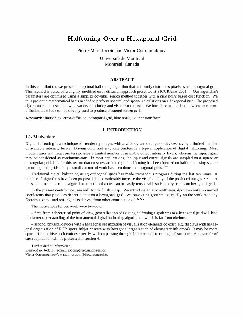
Figure 1. This figure illustrates the visual properties of blue noise: a light gray uniform patch halftoned with the scanline-path Floyd-Steinberg E-D algorithm (left) and with the algorithm proposed in�(right). The Radial Fourier Transform (blue noise profile) was takenfrom Ulichney’s book�� .

1.2. Error-Diffusion

Error-diffusion is a widespread binarization algorithm that is mostly used to render images on black-and-white devicesespecially in the case where the preservation of fine image detail is needed.�� This algorithm is a fairly good compromisebetween speed, simplicity and visual quality.

The way error-diffusion works is simple. First, every input pixel���� �� is selected one after the other. These pixelshave a value ranging between 0 and 1 and the order in which they are processed depends on the chosenpath (usuallyserpentine or scanline). When a pixel���� �� is selected, it is compared to a fixthreshold � that is generally set at 0.5.Whenever���� �� is larger than�, the value “1” is assigned to the output image���� ��, otherwise it is set to ”0”. Thisoutput value is then compared to the input intensity level and put their difference in the error image���� ��. The error isfinally “distributed” to the neighboring pixels according to a given coefficient set similar to the one presented in Figure3(a). The basic error-diffusion algorithm using ascanline path and the Floyd-Steinberg (FS) coefficient set is presentedin Table 1.

Table 1. Classical error-diffusion algorithm processing the pixels in a scanline order using Floyd-Steinberg (FS) coefficient set.

Function ERROR DIFFUSION(f[.],t): Function DISTRIBUTE ERR FS SCANLINE(�,f[.],P):. Create output image g[.] . f[pixel at the right of P] +=� � ���. Create error image e[.] . f[pixel at the bottom right of P] +=� � ���. For each pixel P of image f[.] on a scanline pathDo . f[pixel under P] +=� � ���. If f[P] ThresholdThen . f[pixel a the bottom left of P] +=� � ���. g[P]� white. Else. g[P]� black. e[P]� (f[P]-g[P]). DISTRIBUTE ERR FS SCANLINE(e[P],f[.],P). return output image g[.]

1.3. Blue Noise

Let us consider the problem of processing with a halftoning algorithm, an input image���� �� of size� ���� where eachpixel is assigned aconstant intensity level���� �� � � � ��. The goal of any halftoning algorithm is to generate abi-level output image���� �� thatapproximates best the input image. The output must consequently contain� � � �� �

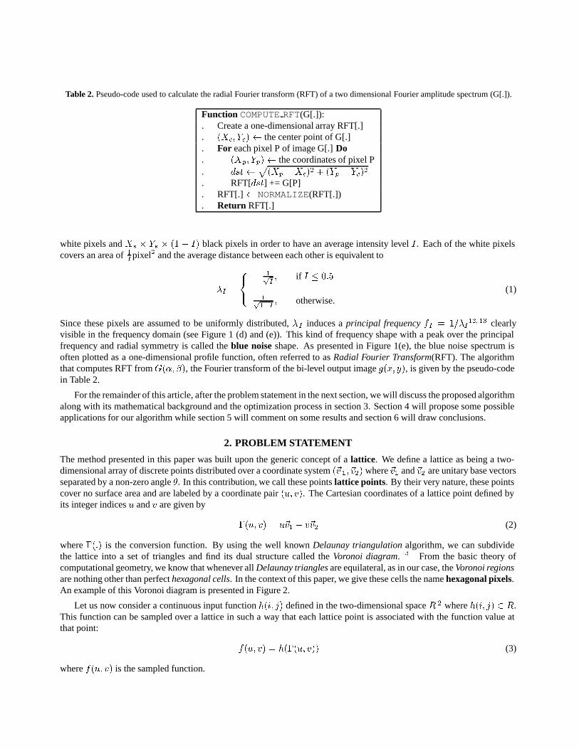
Table 2. Pseudo-code used to calculate the radial Fourier transform (RFT) of a two dimensional Fourier amplitude spectrum (G[.]).

Function COMPUTE RFT(G[.]):. Create a one-dimensional array RFT[.]. ���� ���� the center point of G[.]. For each pixel P of image G[.]Do. ���� ���� the coordinates of pixel P. �����

��� ����� � ��� � ����

. RFT[���] += G[P]

. RFT[.]� NORMALIZE(RFT[.])

. Return RFT[.]

white pixels and�� � �� � �� � � black pixels in order to have an average intensity level . Each of the white pixelscovers an area of�

�pixel� and the average distance between each other is equivalent to

�� �

���

���� if � ��

�����

� otherwise.(1)

Since these pixels are assumed to be uniformly distributed,� � induces aprincipal frequency �� � ������ �� clearly

visible in the frequency domain (see Figure 1 (d) and (e)). This kind of frequency shape with a peak over the principalfrequency and radial symmetry is called theblue noise shape. As presented in Figure 1(e), the blue noise spectrum isoften plotted as a one-dimensional profile function, often referred to asRadial Fourier Transform(RFT). The algorithmthat computes RFT from���� ��, the Fourier transform of the bi-level output image���� ��, is given by the pseudo-codein Table 2.

For the remainder of this article, after the problem statement in the next section, we will discuss the proposed algorithmalong with its mathematical background and the optimization process in section 3. Section 4 will propose some possibleapplications for our algorithm while section 5 will comment on some results and section 6 will draw conclusions.

2. PROBLEM STATEMENT

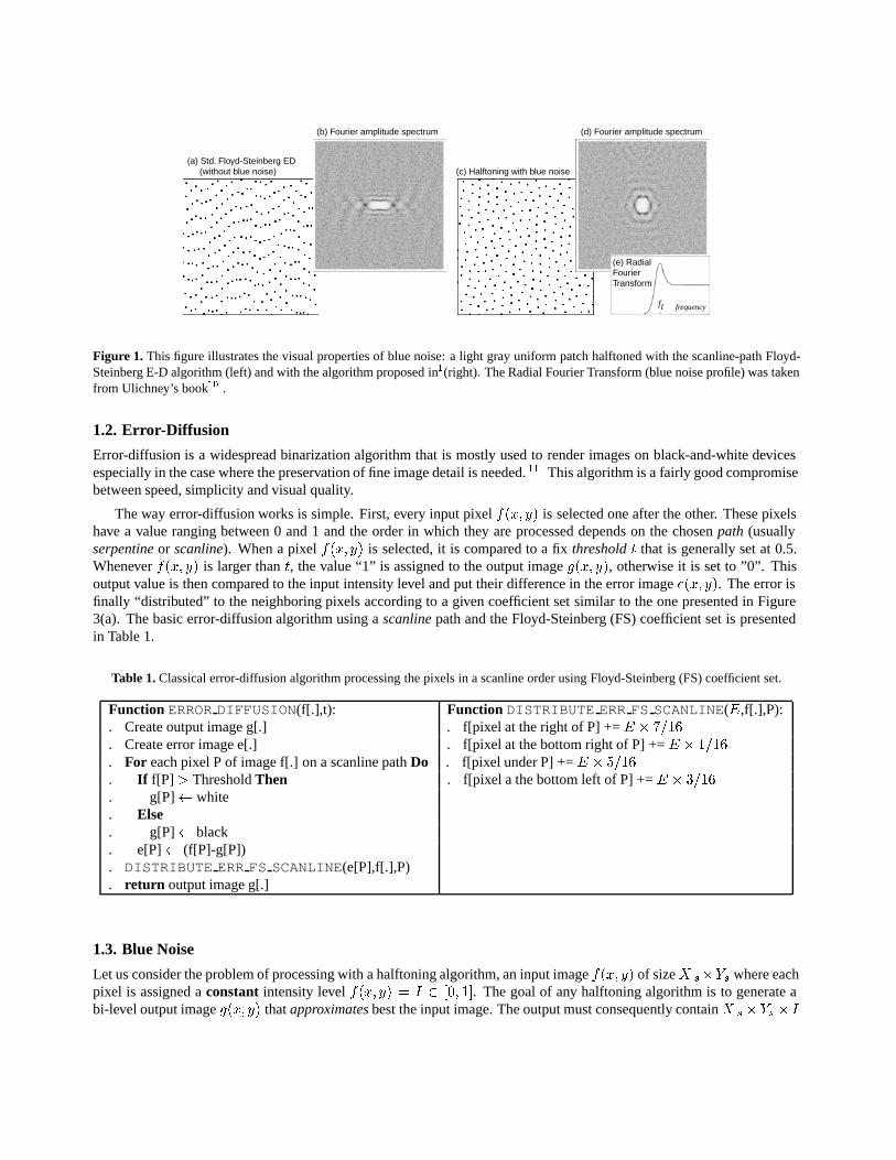
The method presented in this paper was built upon the generic concept of alattice. We define a lattice as being a two-dimensional array of discrete points distributed over a coordinate system��� �� ���� where��� and��� are unitary base vectorsseparated by a non-zero angle�. In this contribution, we call these pointslattice points. By their very nature, these pointscover no surface area and are labeled by a coordinate pair��� ��. The Cartesian coordinates of a lattice point defined byits integer indices� and� are given by

��� �� � ���� � ���� (2)

where ��� is the conversion function. By using the well knownDelaunay triangulation algorithm, we can subdividethe lattice into a set of triangles and find its dual structure called theVoronoi diagram. �� From the basic theory ofcomputational geometry, we know that whenever allDelaunay triangles are equilateral, as in our case, theVoronoi regionsare nothing other than perfecthexagonal cells. In the context of this paper, we give these cells the namehexagonal pixels.An example of this Voronoi diagram is presented in Figure 2.

Let us now consider a continuous input function���� �� defined in the two-dimensional space� � where���� �� � �.This function can be sampled over a lattice in such a way that each lattice point is associated with the function value atthat point:

���� �� � �� ��� ��� (3)

where���� �� is the sampled function.

Lattice points

Hexagonal pixelassociated to lattice

θ = 60

θ

1

2v

v

point

(u,v)

o

(u,v)

Grid of hexagonal pixels

Figure 2. View of a hexagonal grid. Such a structure is a particular Voronoi diagram since each Voronoi region is a perfect hexagonalpixel.

It is well known in the halftoning community that a sampled function such as���� �� can beapproximated by abi-level function����� ��. More precisely, a halftoning method refers to the process of representing a sampled functionsuch as���� �� over a limited number of values, typically set to 0 and 1. The problem we solve in this contribution cantherefore be formulated this way: from a two-dimensional function���� �� sampled over a hexagonal lattice, generate abi-level function����� �� that best approximates���� ��. We consider that����� �� approximates���� �� well, wheneverthe following two requirements are respected:

1. The local intensity of����� �� integrated over a small region equals���� ��. In other words,

���� �� �

� ���

���

� ���

�������� ������ (4)

where� is a constant as large as a few hexagonal pixels.

2. If ���� �� � � for all values of� and� where� is a constant, the binary pixels of� ���� �� must be homogeneouslydistributed in space. In other words,����� �� should have spectralblue noise characteristics as defined above.

To reach these requirements, we decided to use a modified version of the error-diffusion halftoning algorithm previouslyintroduced.

(b)(a)

2x

7/16

3/16 5/16 1/16

r1

x

(x,y)

processing direction

7/16

R

5/16 1/163/16

2

1

v

v

processing direction

(u,v)

Orthogonal Grid Hexagonal Grid

Figure 3. Example of the Floyd-Steinberg algorithm applied to an orthogonal grid (a) and to a hexagonal grid (b). The affine transfor-mation between the orthogonal grid and the hexagonal grid is made by the bijection operator� ���.

3. PROPOSED ALGORITHM

3.1. Model Description

As we stated previously, with the help of an error-diffusion algorithm, our goal is to compute a halftone image� ���� ��that approximates a function���� �� sampled over a hexagonal grid. Unfortunately, the basic error-diffusion algorithm

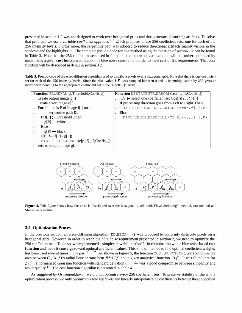
presented in section 1.2 was not designed to work over hexagonal grids and thus generates disturbing artifacts. To solvethat problem, we use avariable-coefficient approach�� which proposes to use 256 coefficient sets, one for each of the256 intensity levels. Furthermore, the serpentine path was adopted to reduce directional artifacts mainly visible in theshadows and the highlights.�� The complete pseudo-code for this method using the notation of section 1.2 can be foundin Table 3. Note that the 256 coefficient sets used in functionDISTRIBUTE ERROR(.) will be further optimized byminimizing a givencost function built upon the blue noise constraint in order to meet section 2’s requirements. That costfunction will be described in detail in section 3.2.

Table 3. Pseudo-code of the error-diffusion algorithm used to distribute pixels over a hexagonal grid. Note that there is one coefficientset for each of the 256 intensity levels. Since the pixel value� �� � was sampled between 0 and 1, its multiplication by 255 gives anindex corresponding to the appropriate coefficient set in the “Coeffs[.]” array.

Function ED HEXA(f[.],Threshold,Coeffs[.]): Function DISTRIBUTE ERROR(Error,f[.],P,Coeffs[.]):. Create output image g[.] . CS� select one coefficient set Coeffs[255*f[P]]. Create error image e[.] . If processing direction goes from Left to RightThen. For all pixels P of image f[.] on a . DISTRIBUTE ERROR L R(CS,Error,f[.],P). serpentine pathDo . Else. If f[P] ThresholdThen . DISTRIBUTE ERROR R L(CS,Error,f[.],P). g[P]� white. Else. g[P]� black. e[P]� (f[P] - g[P]). DISTRIBUTE ERROR(e[p],f[.],P,Coeffs[.]). return output image g[.]

7/16

5/163/16 1/16

Floyd-Steinberg

a)

d10

d01d-11

Our method

b)

8/16

4/162/161/161/16

Shiau-Fan

c)

processing direction processing direction processing direction

Figure 4. This figure shows how the error is distributed over the hexagonal pixels with Floyd-Steinberg’s method, our method andShiau-Fan’s method.

3.2. Optimization Process

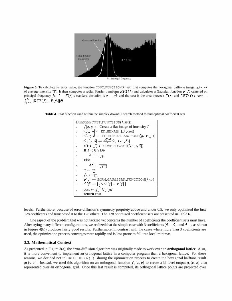
In the previous section, an error-diffusion algorithm (ED HEXA(.)) was proposed to uniformly distribute pixels on ahexagonal grid. However, in order to reach theblue noise requirement presented in section 2, we need to optimize the256 coefficient sets. To do so, we implemented a simplex downhill method�� in combination with a blue noise basedcostfunction and made it converge toward optimal coefficient values. This kind of method to find optimal coefficient weightshas been used several times in the past.�� �� �� As shown in Figure 5, the functionCOST FUNCTION( ,set) computes thearea between����� ��’s radial Fourier transform�� ��� and a given analytical function� ���. It was found that for� ���, a normalized Gaussian function with standard deviation! �

��

was a good compromise between simplicity andresult quality.�� The cost function algorithm is presented in Table 4.

As suggested by Ostromoukhov,� we did not optimise every 256 coefficient sets. To preserve stability of the wholeoptimization process, we only optimized a fewkey levels and linearly interpolated the coefficients between these specified

f

Gaussian Function

: Principal frequencyI

Radial FourierTransform

σ

= fI /10σ

Figure 5. To calculate its error value, the functionCOST FUNCTION(�, set) first computes the hexagonal halftone image����� �of average intensity “I”. It then computes a radial Fourier transform�� ��� and calculates a Gaussian function� ��� centered onprincipal frequency�� .�� �� � ���’s standard deviation is � ��

��and the cost is the area between� ��� and�� ��� : ���� �� ��

������� ���� � �������

Table 4. Cost function used within the simplex downhill search method to find optimal coefficient sets

Function COST FUNCTION( ,set):. � �� ��� Create a flat image of intensity . ��� ��� ED HEXA(f[.],��,set). �"� �� FOURIER TRANSFORM���� ���.

. ���� �������

�� �"� ��

. �� ���� COMPUTE RFT(���� ��)

. If # �� Do

. �� � ���

. Else

. �� � �����

. ! � ��

. �� � � �

. � � �� NORM GAUSSIAN FUNCTION(�� ,!)

. �� �� ���� � �� � � ���

. cost� � �

�� ���. return cost

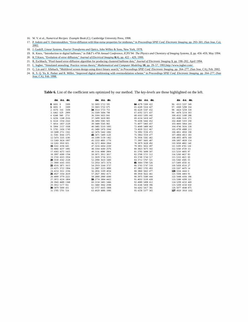
levels. Furthermore, because of error-diffusion’s symmetry propriety above and under 0.5, we only optimized the first128 coefficents and transposed it to the 128 others. The 128 optimized coefficient sets are presented in Table 6.

One aspect of the problem that was not tackled yet concerns the number of coefficients the coefficient sets must have.After trying many different configurations, we realized that the simple case with 3 coefficients (� � ,� � and���� as shownin Figure 4(b)) produces fairly good results. Furthermore, in contrast with the cases where more than 3 coefficients areused, the optimization process converges more rapidly and is less prone to fall into local minimas.

3.3. Mathematical Context

As presented in Figure 3(a), the error-diffusion algorithm was originally made to work over anorthogonal lattice. Also,it is more convenient to implement an orthogonal lattice in a computer program than a hexagonal lattice. For thesereasons, we decided not to useED HEXA(.) during the optimization process to create the hexagonal halftone result����� ��. Instead, we used this algorithm on an orthogonal function� ��� �� to create a bi-level output���� �� alsorepresented over an orthogonal grid. Once this last result is computed, its orthogonal lattice points are projected over

0 1286432 96

256 128192224 160

SF

Our

coefficients

SF

Our

coefficients

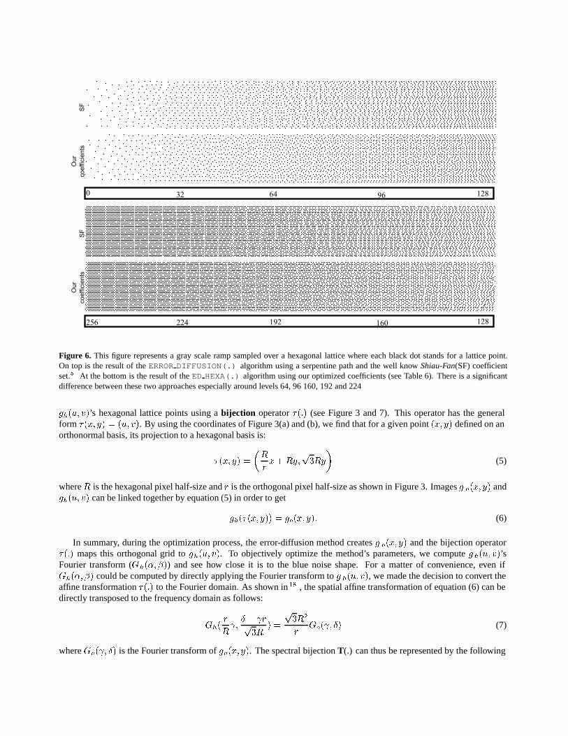
Figure 6. This figure represents a gray scale ramp sampled over a hexagonal lattice where each black dot stands for a lattice point.On top is the result of theERROR DIFFUSION(.) algorithm using a serpentine path and the well knowShiau-Fan(SF) coefficientset.� At the bottom is the result of theED HEXA(.) algorithm using our optimized coefficients (see Table 6). There is a significantdifference between these two approaches especially around levels 64, 96 160, 192 and 224

����� ��’s hexagonal lattice points using abijection operator$��� (see Figure 3 and 7). This operator has the generalform $��� �� � ��� ��. By using the coordinates of Figure 3(a) and (b), we find that for a given point��� �� defined on anorthonormal basis, its projection to a hexagonal basis is:

$��� �� �

��

%�����

����

�(5)

where� is the hexagonal pixel half-size and% is the orthogonal pixel half-size as shown in Figure 3. Images� ��� �� and����� �� can be linked together by equation (5) in order to get

���$��� ��� � ���� ��� (6)

In summary, during the optimization process, the error-diffusion method creates� ��� �� and the bijection operator$��� maps this orthogonal grid to����� ��. To objectively optimize the method’s parameters, we compute����� ��’sFourier transform (����� ��) and see how close it is to the blue noise shape. For a matter of convenience, even if����� �� could be computed by directly applying the Fourier transform to� ���� ��, we made the decision to convert theaffine transformation$��� to the Fourier domain. As shown in� , the spatial affine transformation of equation (6) can bedirectly transposed to the frequency domain as follows:

���%

�"�Æ � "%�

��� �

����

%��"� � (7)

where��"� � is the Fourier transform of���� ��. The spectral bijectionT(.) can thus be represented by the following

equation:

T�"� � � �%

�"�Æ � "%�

����

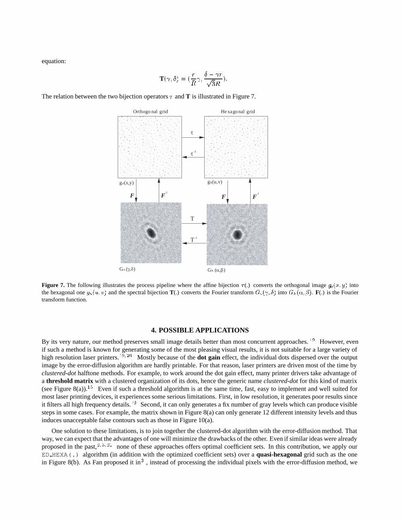
The relation between the two bijection operators$ andT is illustrated in Figure 7.

go(x,y)

Go (γ,δ) Gh (α,β)

gh(u,v)

Τ

Τ -1

τ

τ-1

-1

Orthogo nal grid Hexagonal grid

F F -1F F

Figure 7. The following illustrates the process pipeline where the affine bijection� (.) converts the orthogonal image����� �� intothe hexagonal one����� � and the spectral bijectionT(.) converts the Fourier transform����� � into ����� ��. F(.) is the Fouriertransform function.

4. POSSIBLE APPLICATIONS

By its very nature, our method preserves small image details better than most concurrent approaches.� However, evenif such a method is known for generating some of the most pleasing visual results, it is not suitable for a large variety ofhigh resolution laser printers.�� � Mostly because of thedot gain effect, the individual dots dispersed over the outputimage by the error-diffusion algorithm are hardly printable. For that reason, laser printers are driven most of the time byclustered-dot halftone methods. For example, to work around the dot gain effect, many printer drivers take advantage ofa threshold matrix with a clustered organization of its dots, hence the generic nameclustered-dot for this kind of matrix(see Figure 8(a)).�� Even if such a threshold algorithm is at the same time, fast, easy to implement and well suited formost laser printing devices, it experiences some serious limitations. First, in low resolution, it generates poor results sinceit filters all high frequency details.� Second, it can only generates a fix number of gray levels which can produce visiblesteps in some cases. For example, the matrix shown in Figure 8(a) can only generate 12 different intensity levels and thusinduces unacceptable false contours such as those in Figure 10(a).

One solution to these limitations, is to join together the clustered-dot algorithm with the error-diffusion method. Thatway, we can expect that the advantages of one will minimize the drawbacks of the other. Even if similar ideas were alreadyproposed in the past,�� �� �� none of these approaches offers optimal coefficient sets. In this contribution, we apply ourED HEXA(.) algorithm (in addition with the optimized coefficient sets) over aquasi-hexagonal grid such as the onein Figure 8(b). As Fan proposed it in� , instead of processing the individual pixels with the error-diffusion method, we

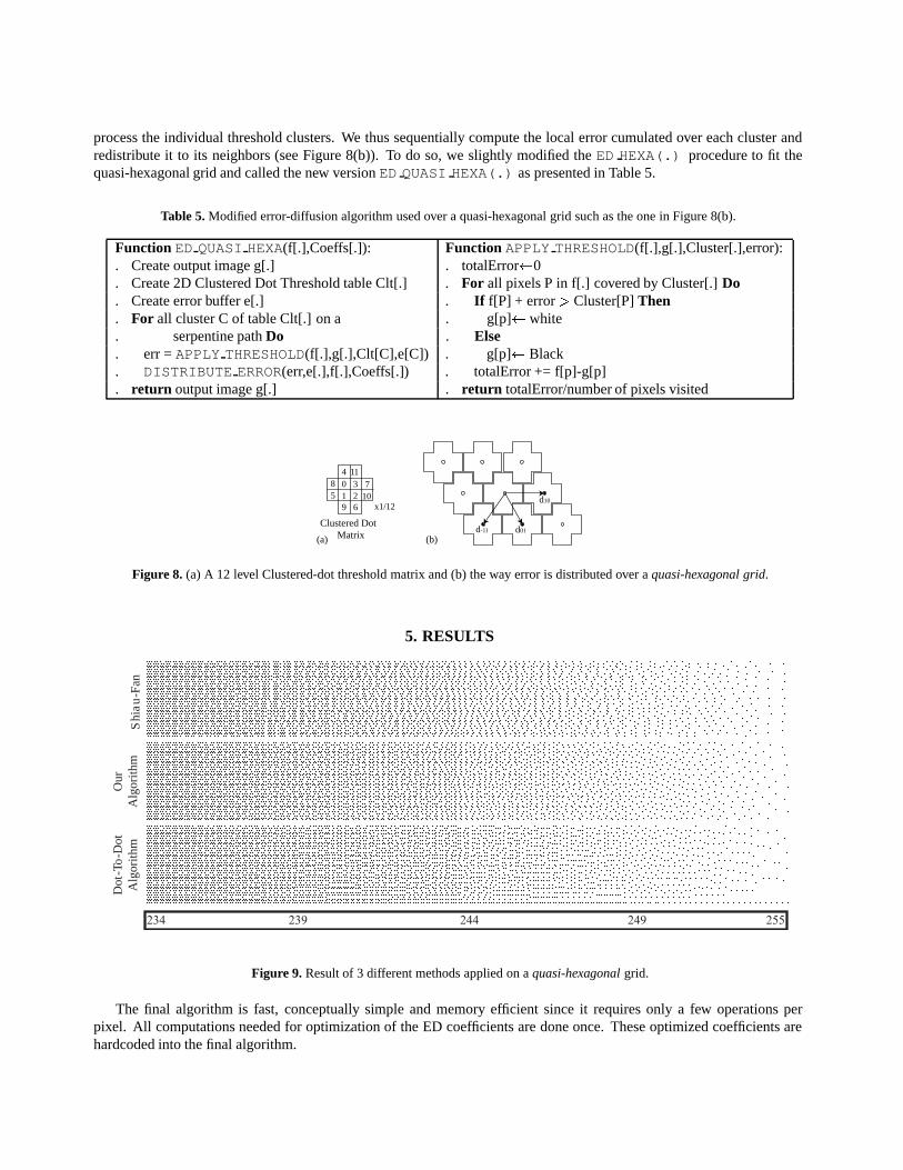
process the individual threshold clusters. We thus sequentially compute the local error cumulated over each cluster andredistribute it to its neighbors (see Figure 8(b)). To do so, we slightly modified theED HEXA(.) procedure to fit thequasi-hexagonal grid and called the new versionED QUASI HEXA(.) as presented in Table 5.

Table 5. Modified error-diffusion algorithm used over a quasi-hexagonal grid such as the one in Figure 8(b).

Function ED QUASI HEXA(f[.],Coeffs[.]): Function APPLY THRESHOLD(f[.],g[.],Cluster[.],error):. Create output image g[.] . totalError�0. Create 2D Clustered Dot Threshold table Clt[.] . For all pixels P in f[.] covered by Cluster[.]Do. Create error buffer e[.] . If f[P] + error Cluster[P]Then. For all cluster C of table Clt[.] on a . g[p]� white. serpentine pathDo . Else. err =APPLY THRESHOLD(f[.],g[.],Clt[C],e[C]) . g[p]� Black. DISTRIBUTE ERROR(err,e[.],f[.],Coeffs[.]) . totalError += f[p]-g[p]. return output image g[.] . return totalError/number of pixels visited

4019

11326

85

710

Clustered DotMatrix

d10

d01d-11

(a) (b)

x1/12

Figure 8. (a) A 12 level Clustered-dot threshold matrix and (b) the way error is distributed over aquasi-hexagonal grid.

5. RESULTS

234 255244239 249

Our

Alg

orith

mD

ot-T

o-D

otA

lgor

ithm

Shi

au

-Fan

Figure 9. Result of 3 different methods applied on aquasi-hexagonal grid.

The final algorithm is fast, conceptually simple and memory efficient since it requires only a few operations perpixel. All computations needed for optimization of the ED coefficients are done once. These optimized coefficients arehardcoded into the final algorithm.

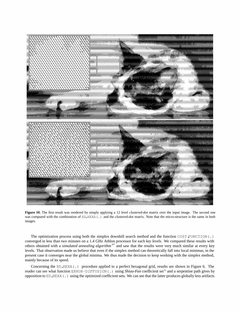
Figure 10. The first result was rendered by simply applying a 12 levelclustered-dot matrix over the input image. The second onewas computed with the combination ofED HEXA(.) and theclustered-dot matrix. Note that the micro-structure is the same in bothimages.

The optimization process using both the simplex downhill search method and the functionCOST FUNCTION(.)converged in less than two minutes on a 1.4 GHz Athlon processor for eachkey levels. We compared these results withothers obtained with asimulated annealing algorithm�� and saw that the results were very much similar at every keylevels. That observation made us believe that even if the simplex method can theoretically fall into local minimas, in thepresent case it converges near the global minima. We thus made the decision to keep working with the simplex method,mainly because of its speed.

Concerning theED HEXA(.) procedure applied to a perfect hexagonal grid, results are shown in Figure 6. Thereader can see what functionERROR-DIFFUSION(.) usingShiau-Fan coefficient set� and a serpentine path gives byopposition toED HEXA(.) using the optimized coefficient sets. We can see that the latter produces globally less artifacts

especially around levels 64, 96, 160, 192 and 224.

Finally, results ofED HEXA(.) applied over aquasi-hexagonal grid (such as the one in Figure 8) are presented inFigure 9 and 10. Figure 9 shows the difference betweenED HEXA(.) using Shiau-Fan’s coefficient set(SF), our approachand Fan’s dot-to-dot algorithm.� We decided to put a grayscale ramp going from���

���to ���

���because the clustered-dot

matrix with 12 thresholds divides the� � scale into 12 sections of equal length (�������

) all having a similar configuration.For this reason, the artifacts shown between���

���and ���

���are exactly the same between���

���and ���

���, � ���

and ������

, �����

and� ���

and so on down to zero.

Figure 10 shows the striking difference between our approach and a straight 12 levelsclustered-dot threshold. Amongother things, we can see that our approach minimizes the false contours while preserving the fundamental regular clusteredstructure of the matrix. The two images were printed in 300 dpi.

6. CONCLUSION

In this paper, an optimal error-diffusion technique was introduced. This simple and fast method uniformly distributespixels over a hexagonal grid. Instead of using the classical error-diffusion algorithm (ERROR-DIFFUSION(.)) we im-plemented a slightly modified version of that algorithm (ED HEXA(.)). This method takes advantage of 255 coefficientsets, each being optimized in order to minimize artifacts around their corresponding intensity level.

The optimization process used a simplex downhill search method together with the blue noise based cost functionCOST FUNCTION(.). During the optimization process, for a matter of simplicity, we made the decision not to use thehexagonal grid����� �� directly. Instead, an orthogonal grid���� �� was generated and converted to����� �� using abijection operator$ . By making use of the spectralbijection operatorT, the functionCOST FUNCTION(.) calculatesthe hexagonal grid Radial Fourier Transform (RFT) and measures how close it is to the blue noise profile. After manytests made over a large variety of images, it was found that a configuration with 3 coefficients was a good choice regardingsimplicity, speed and better optimization efficiency.

By its conceptual simplicity and speed, our algorithm can be used to work over a variety of printing and visualizationdevices as illustrated in figure 10. It is thus possible to drive physical hexagonal entities directly, without having topass through an intermediate orthogonal structure. We have shown that by mixing together clustered-dot matrices andED HEXA(.), the classical problems of dispersed dots can be considerably improved while reducing the false contours.

In the future, we expect to reduce the artifacts around level��

and ��

and address the question of the uniform areaslocated around the 12 intensity levels :����� ����� ����� ����,...,�����. We think that this last challenge could be addressedlike a multilevel contouring artifact.��� ��

ACKNOWLEDGMENTS

The authors would like to thank Pierre Poulin and Justin Bur for their very precious help.

REFERENCES1. V. Ostromoukhov, “A simple and efficient error-diffusion algorithm,” inSIGGRAPH 2001, Computer Graphics Proceedings, Annual Conference Series, pp. 567–572,

2001.2. G. Goertzel and G. Thompson, “Digital halftoning on the IBM 4250 printer,”IBM Journal of Research and Development 31, pp. 2–15, Jan. 1987.3. Z. Fan, “Dot-to-dot error diffusion,”Journal of Electronic lmaging , Jan.

4. R. Stevenson and G. Arce, “Binary display of hexagonally sampled continuous-tone images,”Journal of the Optical Society of America 2, pp. 1009–1013, July 1985.5. J. Shiau and Z. Fan, “A set of easily implementable coefficients in error diffusion with reduced worm artifacts,” inSPIE, 2658, pp. 222–225, 1996.6. P. Li and J. Allebach, “Tone dependent error diffusion,” inProceedings SPIE Conf. Electronic Imaging, pp. 293–301, (San Jose, Ca), 2002.

7. G. Marcu, “An error diffusion algorithm with output position constraints for homogeneous highlights and shadow dot distribution,”Journal of Electronic Imaging 9(1),pp. 46–51, 2000.

8. K. Knox, “Error image in error diffusion,” inProceedings SPIE Conf. Electronic Imaging, pp. 9–14, (San Jose, CA), Feb. 1992.

9. R. Eschbach, “Reduction of artifacts in error diffusion by means of input-dependent weights,”Journal of Electronic Imaging 2, pp. 352–358, October 1993.10. R. Ulichney,Digital Halftoning, MIT Press, Cambridge, MA, USA, 1987.11. R. Floyd and L. Steinberg, “An adaptive algorithm for spatial gray scale,” inSID 75, Int. Symp. Dig. Tech. Papers, p. 36, 1975.

12. R. Ulichney, “Dithering with blue noise,”Proceedings of the IEEE 76, pp. 56–79, 1988.13. K. Knox, “Evolution of error diffusion,”Electronic Imaging 8(4), pp. 422–429, 1999.14. F.P. Preparata and M.I. Shamos,Computational Geometry : An Introduction, Springer-Verlag, 1985.15. R. Ulichney, “A review of halftoning techniques,” inProceedings SPIE Conf., Proc. SPIE 3963, pp. 378–391, 2000.

16. W. V. et al.,Numerical Recipes: Example Book (C), Cambridge University Press, 1998.17. P. Jodoin and V. Ostromoukhov, “Error-diffusion with blue-noise properties for midtones,” inProceedings SPIE Conf. Electronic Imaging, pp. 293–301, (San Jose, Ca),

2002.18. J. Gaskill,Linear Systems, Fourier Transforms and Optics, John Willey & Sons, New York, 1978.19. K. Knox, “Introduction to digital halftones,” inIS&T’s 47th Annual Conference, ICPS’94: The Physics and Chemistry of Imaging Systems, 2, pp. 456–459, May 1994.

20. K.T.Knox, “Evolution of error diffusion,”Journal of Electrical Imaging 8(4), pp. 422 – 429, 1999.21. R. Eschbach, “Pixel-based error-diffusion algorithm for producing clustered halftone dots,”Journal of Electronic Imaging 3, pp. 198–202, April 1994.22. L. Ingber, “Simulated annealing: Practice versus theory,”Mathematical and Computer Modeling 18, pp. 29–57, 1993,http://www.ingber.com/.

23. G. Lin and J. Allebach, “Multilevel screen design using direct binary search,” inProceedings SPIE Conf. Electronic Imaging, pp. 264–277, (San Jose, CA), Feb. 2002.24. K. S. Q. Yu, K. Parker and R. Miller, “Improved digital multitoning with overmodulation scheme,” inProceedings SPIE Conf. Electronic Imaging, pp. 264–277, (San

Jose, CA), Feb. 1998.

Table 6. List of the coefficient sets optimized by our method. Thekey-levels are those highlighted on the left.

96: 4313 5337 34997: 4369 5298 33498: 4424 5258 31899: 4478 5219 303100: 4532 5180 288101: 4586 5141 273102: 4640 5103 258103: 4693 5064 243104: 4746 5026 228105: 4799 4988 213106: 4851 4950 198107: 4904 4913 183108: 4955 4876 169109: 5007 4839 154110: 5058 4802 140111: 5109 4765 126112: 5160 4729 111113: 5210 4693 97114: 5260 4657 83115: 5310 4621 69116: 5360 4585 55117: 5409 4550 41118: 5458 4514 27119: 5507 4479 14120: 5556 4444 0121: 5506 4403 91122: 5448 4356 196123: 5380 4299 321124: 5299 4232 469125: 5200 4150 650126: 5077 4048 875127: 4920 3918 1162

0: 6691 0 33091: 6691 0 33092: 6576 316 31083: 6462 629 29094 6348 940 27115: 6236 1248 25166: 6124 1554 23227: 6014 1857 21298: 5904 2157 19389: 5795 2456 174910: 5688 2751 156111: 5581 3044 137512: 5474 3335 119013: 5369 3624 100714: 5265 3910 82515: 5161 4194 64516: 4682 4237 108117: 4303 4272 142518: 3997 4300 170419: 3743 4323 193420: 3530 4342 212821: 3900 4165 193522: 4516 3871 161323: 4375 3722 190424: 4214 3551 223625: 4027 3354 261926: 4000 3779 222127: 3972 4224 180428: 3943 4689 136829: 3912 5177 91130: 3879 5690 43131: 3785 5701 514

32: 3693 5712 59533: 3603 5722 67534: 3514 5733 75335: 3509 5694 79836: 3504 5655 84137: 3499 5618 88338: 3494 5581 92539: 3489 5545 96540: 3485 5510 100541: 3480 5476 104442: 3476 5442 108243: 3471 5409 112044: 3399 5139 146245: 3333 4891 177646: 3272 4664 206447: 3216 4454 233048: 3164 4260 257649: 3116 4080 280450: 3071 3912 301751: 3029 3756 321552: 2990 3610 340053: 2954 3473 357454: 2919 3344 373755: 2887 3223 389056: 2856 3109 403457: 2827 3002 417158: 2800 2900 430059: 2774 2804 442260: 3134 3401 346661: 3460 3942 259862: 3757 4435 180863: 4029 4886 1086

64: 4278 5300 42265: 4249 5324 42766: 4220 5347 43267: 4192 5371 43768: 4163 5395 44269: 4134 5418 44770: 4106 5442 45271: 4077 5465 45772: 4049 5489 46273: 4020 5512 46774: 3992 5536 47275: 3964 5559 47776: 3936 5582 48277: 3907 5605 48778: 3879 5628 49279: 3851 5652 49780: 3823 5675 50281: 3795 5698 50782: 3768 5721 51283: 3740 5744 51784: 3712 5767 52185: 3684 5789 52686: 3743 5747 51087: 3802 5705 49388: 3860 5663 47789: 3918 5622 46190: 3975 5580 44491: 4032 5539 42892: 4089 5498 41293: 4146 5458 39694: 4202 5417 38195: 4258 5377 365

d10 d-11 d01 d10 d-11 d01 d10 d-11 d01 d10 d-11 d01