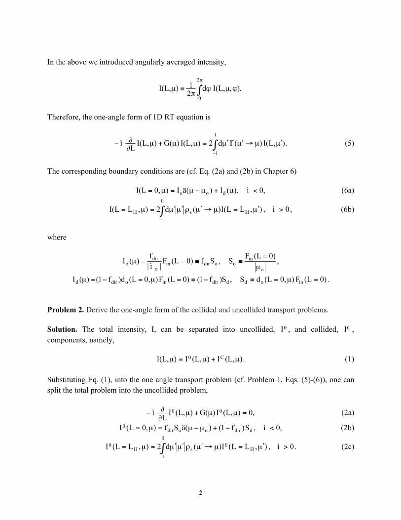
Solutions to Chapter 6 Problems - Boston Universitycliveg.bu.edu/courses/ge645spr09/chap-06-problems.pdf · 1 Solutions to Chapter 6 Problems Problem 1. Derive the one-angle form

1

Solutions to Chapter 6 Problems Problem 1. Derive the one-angle form of the vegetation transport problem. Solution. The 1D radiative transfer equation for vegetation canopies is (cf. Eq. (1) in Chapter 6)

.)I(z,)(z,d)z(u

)I(z,)G(z,(z)u)I(z,z

ì

4!

LL !"!#!"$!"

%=!!+!

&&' ( (1)

The vertical coordinate z can be changed to cumulative leaf area index L by dividing Eq. (1) with (z)uL , the leaf area density distribution ( z(z)uL L !" ),

.)I(L,)(L,d1)I(L,)G(L,)I(L,

Lì

4!

!"!#!"$!"%

=!!+!&&' ( (2)

In the following derivations we will assume that the geometry factor and the area scattering phase function are independent of the azimuth angle and cumulative leaf area index, namely, ,)(G)(L,G µ=! (3a)

.)(1)(L,1 µ!µ"#$

=%!%"#$

(3b)

In this case the 1D transport equation can be reduced to a one angle problem by averaging Eq. (2) over azimuth angle, ! . The derivations for the first and second items on the left hand side and the remaining item on the right-hand side of Eq. (2) are shown in Eq. (4a)-(4c) below:

),I(L,L

),I(L,d21

L)I(L,

Lìd

21

2

0

2

0

µ!!µ"=#µ#

$!!µ"=%&

'()* +

!!"#

$ ,,$$

(4a)

[ ] ),I(L,)(G),I(L,),(L,Gd21)I(L,)(L,Gd

21

2

0

2

0

µµ=!µµ!!"

=##!" $$

""

(4b)

! !"

" ##$

%

&&'

()*)+)*,)*-

"

2

0 4

)I(L,)(L,dd21

! !!" "

#

$%µ%$&$%µ&µ%'$%µ%$"

=

2

0

2

0

1

1

),I(L,),(L,ddd21

.)(L,I)(d2

1

1

µ!µ"µ!#µ!$= %&

(4c)

2

In the above we introduced angularly averaged intensity,

.),I(L,d21)I(L,

2

0

!"

#µ#"

$µ

Therefore, the one-angle form of 1D RT equation is

.)I(L,)(d2)I(L,)G()I(L,L

ì

1

1

µ!µ"µ!#µ!=µµ+µ$$% &

%

(5)

The corresponding boundary conditions are (cf. Eq. (2a) and (2b) in Chapter 6) ),(I)ä(I)0,I(L doo µ+µ!µ=µ= 0,ì < (6a)

! µ"=µ#µ"$µ"µ"=µ=

0

1-

HsH ),LL(I)(d2),LI(L , ,0ì > (6b)

where

,Sf0)(LF|ì|

f)(I odirin

o

diro !==µ ,

0)(LFS

o

ino

µ

=!

,S)f1(0)(LF)0,(L)df1()(I ddirinodird !"=µ=!=µ .0)(LF)0,(LdS inod =µ=! Problem 2. Derive the one-angle form of the collided and uncollided transport problems. Solution. The total intensity, I, can be separated into uncollided, 0I , and collided, CI , components, namely, .)(L,I)(L,I)I(L, C0 µ+µ=µ (1) Substituting Eq. (1), into the one angle transport problem (cf. Problem 1, Eqs. (5)-(6)), one can split the total problem into the uncollided problem, 0,)(L,I)G()(L,I

Lì 00 =µµ+µ!!" (2a)

,S)f1()ä(Sf)0,(LI ddiroodir0 !+µ!µ=µ= 0,ì < (2b)

! µ"=µ#µ"$µ"µ"=µ=

0

1-

H0

sH0 ),LL(I)(d2),L(LI , .0ì > (2c)

3

and the collided problem,

[ ].)(L,I)(L,I)(L,d2)(L,I)G()(L,IL

ì C0

1

1

CC µ!+µ!µ"µ!#µ!=µµ+µ$$% &

%

(3a)

,0)0,(LIC =µ= 0,ì < (3b)

! µ"=µ#µ"$µ"µ"=µ=

0

1-

HC

sHC ),LL(I)(d2),L(LI , .0ì > (3c)

Problem 3. Derive the analytical solution of the one-angle uncollided transport problem. Solution. The one-angle transport equation for the uncollided radiation is (cf. Problem 2, Eq. (2a))

)(L,I)G(

)(L,IL

00 µµ

µ=µ

!! (1)

The solution of this equations is

,L)G(

exp)(A)(L,I0 !"

#$%

&µ

µ'µ=µ

where coefficient )A(µ is determined from boundary conditions (cf. Problem 2, Eq. (2b) for

0,ì < and (2c) for 0ì > ). If 0ì < (downwelling radiation),

[ ] .L)G(

expS)f1()ä(Sf)(L,I ddiroodir0 !

"

#$%

&µ

µ'(+µ(µ=µ (2a)

If 0ì > (upwelling radiation),

[ ] !"

#$%

&'

µ(µ(

'+µ'µ(µ)µ(*µ(µ(=µ + )LL()G(

expS)f1()ä(Sf)(d2)(L,I H

0

1-

ddiroodirs0

!"

#$%

&'(

)µ

µ*+µ,µ-µ= H

o

oosoodir L

)G(exp)(2Sf

.)LL()G(

expL)G(

exp)(d2S)f1( HH

0

1-

sddir !"

#$%

&'

µ

µ())*

+!"

#$%

&µ,µ,

'µ-µ,.µ,µ,'+ / (2b)

Note, in the case of dense canopies

4

.0)(L,I

HL

0 !µ"!

Problem 4. Solve the two-stream differential equations for upward uF and downward dF fluxes in a vegetation canopy of horizontal leaves ,)L(F)1()L(F)L(F

Ld

L

u

L

d !"+#=$$

,)L(F)1()L(F)L(FL

u

L

d

L

u !"+#=$$!

with the boundary conditions ,F)0L(F d

0

d==

.)LL(Fr)LL(F H

d

SH

u===

Solution. The two-stream equations in this problem correspond to a homogeneous system of linear differential equations, which can be solved using matrix method. The original system can be rewritten in a matrix form as follows ,)L(yA)L(y =! (1a) where

,)L(F

)L(F)L(y

u

d

!"

#$%

&' ,

)L(FL

)L(FL)L(y

u

d

!!!

"

#

$$$

%

&

''''

() .)1(

)1(A

LL

LL

!"

#$%

&

'(')'

)'(* (1b)

If matrix A has n=2 independent eigenvectors

1v and

2v corresponding to eigenvalues

1! and

2! , then the general solution of Eqs. (1a)-(1b) is .)L(v)Lexp(C)L(v)Lexp(C)L(y 222111 !+!= (2) The eigenvalues of matrix A can be found as follows: 0)IAdet( =!" 0)1)(1( 2

LLL =!+"+#$"##$#%

.)1( 2

L

2

L2,1 !"#"±$%±=%& (3a) The corresponding eigenvectors are

5

./)1(

1)L(v

LL2,1 !

"

#$%

&

'(±)*

)+ (3b)

Substituting Eq. (3a)-3(b) into Eq. (2) and taking into account definition in given in Eq. (1b), we have

!"#

$%+$=

$%%$%=

),Lexp(BC)Lexp(AC)L(F

),Lexp(C)Lexp(C)L(F

21u

21d

(4a)

where

,1

AL

L

!

"##$= .

1B

L

L

!

"+#$= (4b)

Combining Eq. (4a)-(4b) with original boundary conditions, one solves for

1C and

2C .Therefore, the solution of the two-stream model is

,)L2exp()rB()rA(

])LL2[exp()rB()Lexp()rA(F)L(F

HSS

HSSd

0

d

!"+"+

"!"+"!"+=

,)L2exp()rB()rA(

])LL2[exp(A)rB()Lexp(B)rA(F)L(F

HSS

HSSd

0

u

!"+"+

"!"++!"+"=

where coefficients, ! , A, and B are given by Eq. (3a) and (4b). Problem 5. Show the limiting form of uF for the case of a very dense canopy. Solution. Recall (cf. Problem 4),

,)L2exp()rB()rA(

])LL2[exp(A)rB()Lexp(B)rA(F)L(F

Hss

HSSd0

u

!"+"+

"!"++!"+"=

where

,1

AL

L

!

"##$= ,

1B

L

L

!

"+#$= .)1( 2

L

2

L !"#"=$

Therefore, in the case of dense canopies

6

).)1(Lexp()1(1

F)L(F 2

L

2

LL

2

L

2

Ld

0L

u

H

!+"##!

!+"##"#$

%$