Problems and Procedures - computingbook.orgcomputingbook.org/spring2010/ch4-problems.pdf · Problems and Procedures ... solved and we can declare victory and move on to the next one.

4Problems and Procedures

A great discovery solves a great problem, but there is a grain of discovery in the solution ofany problem. Your problem may be modest, but if it challenges your curiosity and brings into

play your inventive faculties, and if you solve it by your own means, you may experience thetension and enjoy the triumph of discovery.

George Polya, How to Solve It

Computers are tools for performing computations to solve problems. In thischapter, we consider what it means to solve a problem and explore some strate-gies for constructing procedures that solve problems.

4.1 Solving ProblemsTraditionally, a problem is an obstacle to overcome or some question to answer.Once the question is answered or the obstacle circumvented, the problem issolved and we can declare victory and move on to the next one.

When we talk about writing programs to solve problems, though, we have alarger goal. We don’t just want to solve one instance of a problem, we want analgorithm that can solve all instances of a problem. A problem is defined by problem

its inputs and the desired property of the output. Recall from Chapter 1, that aprocedure is a precise description of a process and a procedure is guaranteedto always finish is called an algorithm. The name algorithm is a Latinizationof the name of the Persian mathematician and scientist, Muhammad ibn Musaal-Khwarizmı, who published a book in 825 on calculation with Hindu numer-als. Although the name algorithm was adopted after al-Khwarizmı’s book, algo-rithms go back much further than that. The ancient Babylonians had algorithmsfor finding square roots more than 3500 years ago (see Exploration 4.1).

For example, we don’t just want to find the best route between New York andWashington, we want an algorithm that takes as inputs the map, start location,and end location, and outputs the best route. There are infinitely many possibleinputs that each specify different instances of the problem; a general solution tothe problem is a procedure that finds the best route for all possible inputs.1

To define a procedure that can solve a problem, we need to define a procedurethat takes inputs describing the problem instance and produces a different in-formation process depending on the actual values of its inputs. A procedure

1Actually finding a general algorithm that does without needing to essentially try all possibleroutes is a challenging and interesting problem, for which no efficient solution is known. Find-ing one (or proving no fast algorithm exists) would resolve the most important open problem incomputer science!

54 4.2. Composing Procedures

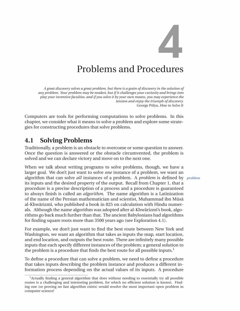
takes zero or more inputs, and produces one output or no outputs2, as shown inFigure 4.1.

Figure 4.1. A procedure maps inputs to an output.

Our goal in solving a problem is to devise a procedure that takes inputs thatdefine a problem instance, and produces as output the solution to that probleminstance. The procedure should be an algorithm — this means every applicationof the procedure must eventually finish evaluating and produce an output value.

There is no magic wand for solving problems. But, most problem solving in-volves breaking problems you do not yet know how to solve into simpler andsimpler problems until you find problems simple enough that you already knowhow to solve them. The creative challenge is to find the simpler subproblemsthat can be combined to solve the original problem. This approach of solvingproblems by breaking them into simpler parts is known as divide-and-conquer .

divide-and-conquerThe following sections describe a two key forms of divide-and-conquer problemsolving: composition and recursive problem solving. We will use these sameproblem-solving techniques in different forms throughout this book.

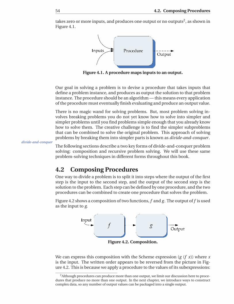
4.2 Composing ProceduresOne way to divide a problem is to split it into steps where the output of the firststep is the input to the second step, and the output of the second step is thesolution to the problem. Each step can be defined by one procedure, and the twoprocedures can be combined to create one procedure that solves the problem.

Figure 4.2 shows a composition of two functions, f and g . The output of f is usedas the input to g.

Figure 4.2. Composition.

We can express this composition with the Scheme expression (g (f x)) where xis the input. The written order appears to be reversed from the picture in Fig-ure 4.2. This is because we apply a procedure to the values of its subexpressions:

2Although procedures can produce more than one output, we limit our discussion here to proce-dures that produce no more than one output. In the next chapter, we introduce ways to constructcomplex data, so any number of output values can be packaged into a single output.

Chapter 4. Problems and Procedures 55

the values of the inner subexpressions must be computed first, and then used asthe inputs to the outer applications. So, the inner subexpression (f x) is evalu-ated first since the evaluation rule for the outer application expression is to firstevaluate all the subexpressions.

To define a procedure that implements the composed procedure we make x aparameter:

(define fog (lambda (x) (g (f x))))

This defines fog as a procedure that takes one input and produces as output thecomposition of f and g applied to the input parameter. This works for any twoprocedures that both take a single input parameter.

For example, we can compose the square and cube procedures from Chapter 3:

(define sixth-power (lambda (x) (cube (square x))))

Then, (sixth-power 2) evaluates to 64.

4.2.1 Procedures as Inputs and OutputsAll the procedure inputs and outputs we have seen so far have been numbers.The subexpressions of an application can be any expression including a proce-dure. A higher-order procedure is a procedure that takes other procedures as in- higher-order

procedureputs or that produces a procedure as its output. Higher-order procedures give usthe ability to write procedures that behave differently based on the proceduresthat are passed in as inputs.

For example, we can create a generic composition procedure by making f and gparameters:

(define fog (lambda (f g x) (g (f x))))

The fog procedure takes three parameters. The first two are both proceduresthat take one input. The third parameter is a value that can be the input to thefirst procedure.

For example, > (fog square cube 2) evaluates to 64, and > (fog (lambda (x) (+ x1)) square 2) evaluates to 9. In the second example the first parameter is the pro-cedure produced by the lambda expression (lambda (x) (+ x 1)). This proceduretakes a number as input and produces as output that number plus one. We usea definition to name this procedure inc (short for increment):

(define inc (lambda (x) (+ x 1)))

A more useful composition procedure would separate the input value, x, fromthe composition. The fcompose procedure takes two procedures as inputs andproduces as output a procedure that is their composition:3

(define fcompose(lambda (f g ) (lambda (x) (g (f x)))))

The body of the fcompose procedure is a lambda expression that makes a proce-dure. Hence, the result of applying fcompose to two procedures is not a simple

3We name our composition procedure fcompose to avoid collision with the built-in compose pro-cedure that behaves similarly.

56 4.3. Recursive Problem Solving

value, but a procedure. The resulting procedure can then be applied to a value.

Here are some examples using fcompose:

> (fcompose inc inc)#<procedure>

> ((fcompose inc inc) 1)3

> ((fcompose inc square) 2)9

> ((fcompose square inc) 2)5

Exercise 4.1. For each expression, give the value to which the expression evalu-ates. Assume fcompose and inc are defined as above.

a. (fcompose (lambda (x) (∗ x 2)) (lambda (x) (/ x 2)))

b. ((fcompose (lambda (x) (∗ x 2)) (lambda (x) (/ x 2))) 150)

c. ((fcompose (fcompose inc inc) inc) 2)

Exercise 4.2. Suppose we define self-compose as a procedure that composes aprocedure with itself:

(define (self-compose f ) (fcompose f f ))

Explain how (((fcompose self-compose self-compose) inc) 1) is evaluated.

Exercise 4.3. Define a procedure fcompose3 that takes three procedures as in-put, and produces as output a procedure that is the composition of the threeinput procedures. For example, ((fcompose3 abs inc square) −5) should evalu-ate to 36. Define fcompose3 two different ways: once without using fcompose,and once using fcompose.

Exercise 4.4. The fcompose procedure only works when both input procedurestake one input. Define a f2compose procedure that composes two procedureswhere the first procedure takes two inputs, and the second procedure takes oneinput. For example, ((f2compose add abs) 3 −5) should evaluate to 2.

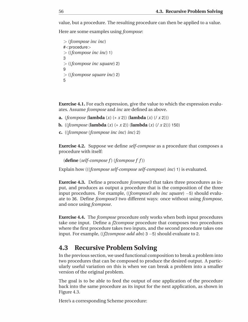
4.3 Recursive Problem SolvingIn the previous section, we used functional composition to break a problem intotwo procedures that can be composed to produce the desired output. A partic-ularly useful variation on this is when we can break a problem into a smallerversion of the original problem.

The goal is to be able to feed the output of one application of the procedureback into the same procedure as its input for the next application, as shown inFigure 4.3.

Here’s a corresponding Scheme procedure:


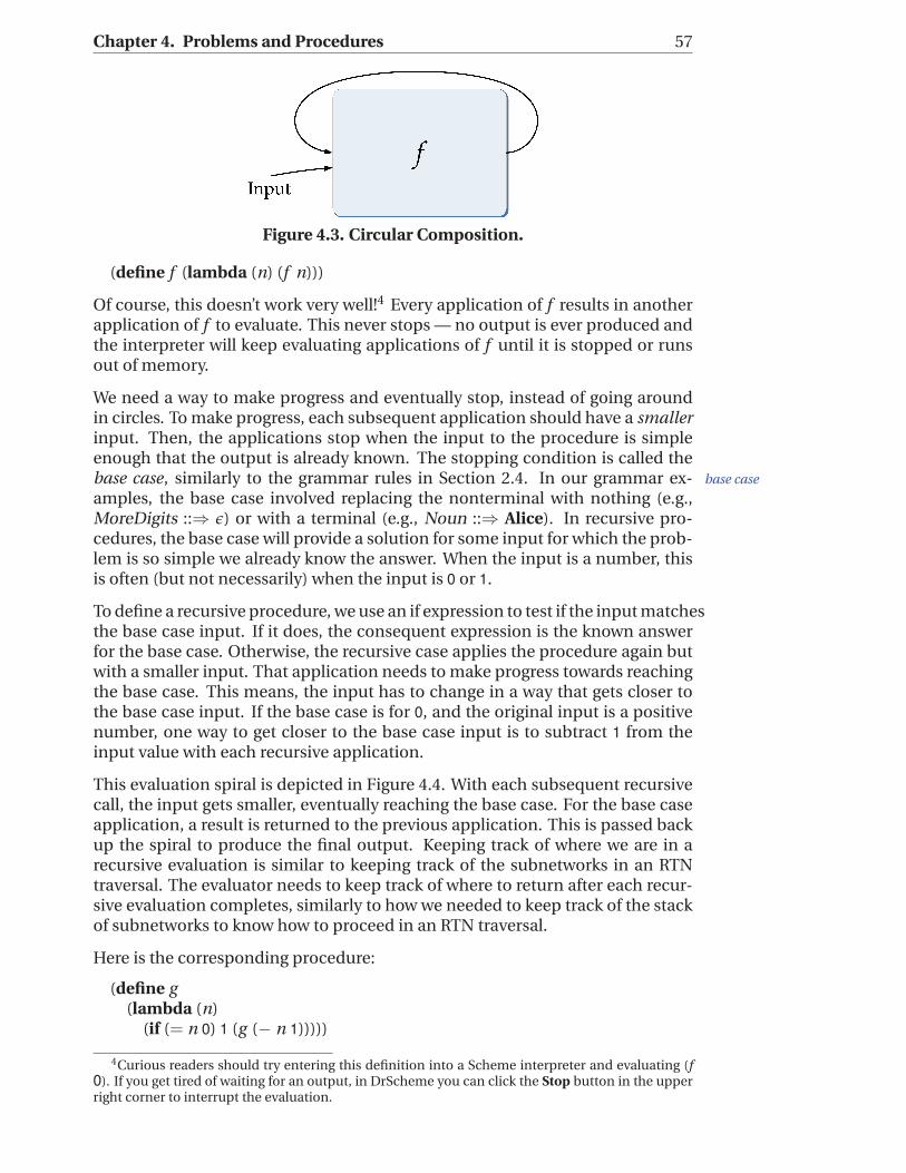
Figure 4.3. Circular Composition.

(define f (lambda (n) (f n)))

Of course, this doesn’t work very well!4 Every application of f results in anotherapplication of f to evaluate. This never stops — no output is ever produced andthe interpreter will keep evaluating applications of f until it is stopped or runsout of memory.

We need a way to make progress and eventually stop, instead of going aroundin circles. To make progress, each subsequent application should have a smallerinput. Then, the applications stop when the input to the procedure is simpleenough that the output is already known. The stopping condition is called thebase case, similarly to the grammar rules in Section 2.4. In our grammar ex- base case

amples, the base case involved replacing the nonterminal with nothing (e.g.,MoreDigits ::⇒ ε) or with a terminal (e.g., Noun ::⇒ Alice). In recursive pro-cedures, the base case will provide a solution for some input for which the prob-lem is so simple we already know the answer. When the input is a number, thisis often (but not necessarily) when the input is 0 or 1.

To define a recursive procedure, we use an if expression to test if the input matchesthe base case input. If it does, the consequent expression is the known answerfor the base case. Otherwise, the recursive case applies the procedure again butwith a smaller input. That application needs to make progress towards reachingthe base case. This means, the input has to change in a way that gets closer tothe base case input. If the base case is for 0, and the original input is a positivenumber, one way to get closer to the base case input is to subtract 1 from theinput value with each recursive application.

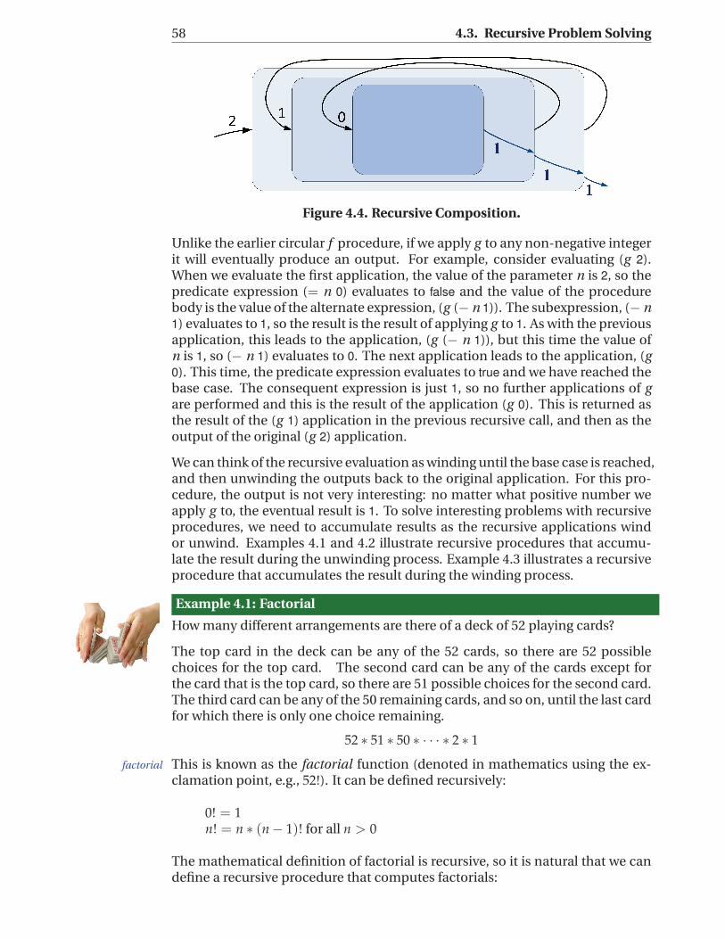
This evaluation spiral is depicted in Figure 4.4. With each subsequent recursivecall, the input gets smaller, eventually reaching the base case. For the base caseapplication, a result is returned to the previous application. This is passed backup the spiral to produce the final output. Keeping track of where we are in arecursive evaluation is similar to keeping track of the subnetworks in an RTNtraversal. The evaluator needs to keep track of where to return after each recur-sive evaluation completes, similarly to how we needed to keep track of the stackof subnetworks to know how to proceed in an RTN traversal.

Here is the corresponding procedure:

(define g(lambda (n)

(if (= n 0) 1 (g (− n 1)))))

4Curious readers should try entering this definition into a Scheme interpreter and evaluating (f0). If you get tired of waiting for an output, in DrScheme you can click the Stop button in the upperright corner to interrupt the evaluation.


Figure 4.4. Recursive Composition.

Unlike the earlier circular f procedure, if we apply g to any non-negative integerit will eventually produce an output. For example, consider evaluating (g 2).When we evaluate the first application, the value of the parameter n is 2, so thepredicate expression (= n 0) evaluates to false and the value of the procedurebody is the value of the alternate expression, (g (− n 1)). The subexpression, (− n1) evaluates to 1, so the result is the result of applying g to 1. As with the previousapplication, this leads to the application, (g (− n 1)), but this time the value ofn is 1, so (− n 1) evaluates to 0. The next application leads to the application, (g0). This time, the predicate expression evaluates to true and we have reached thebase case. The consequent expression is just 1, so no further applications of gare performed and this is the result of the application (g 0). This is returned asthe result of the (g 1) application in the previous recursive call, and then as theoutput of the original (g 2) application.

We can think of the recursive evaluation as winding until the base case is reached,and then unwinding the outputs back to the original application. For this pro-cedure, the output is not very interesting: no matter what positive number weapply g to, the eventual result is 1. To solve interesting problems with recursiveprocedures, we need to accumulate results as the recursive applications windor unwind. Examples 4.1 and 4.2 illustrate recursive procedures that accumu-late the result during the unwinding process. Example 4.3 illustrates a recursiveprocedure that accumulates the result during the winding process.

Example 4.1: Factorial

How many different arrangements are there of a deck of 52 playing cards?

The top card in the deck can be any of the 52 cards, so there are 52 possiblechoices for the top card. The second card can be any of the cards except forthe card that is the top card, so there are 51 possible choices for the second card.The third card can be any of the 50 remaining cards, and so on, until the last cardfor which there is only one choice remaining.

52 ∗ 51 ∗ 50 ∗ · · · ∗ 2 ∗ 1

This is known as the factorial function (denoted in mathematics using the ex-factorial

clamation point, e.g., 52!). It can be defined recursively:

0! = 1

n! = n ∗ (n− 1)! for all n > 0

The mathematical definition of factorial is recursive, so it is natural that we candefine a recursive procedure that computes factorials:


(define (factorial n)(if (= n 0)

1

(∗ n (factorial (− n 1)))))

Evaluating (factorial 52) produces the number of arrangements of a 52-card deck:a sixty-eight digit number starting with an 8.

The factorial procedure has structure very similar to our earlier definition of theuseless recursive g procedure. The only difference is the alternative expressionfor the if expression: in g we used (g (− n 1)); in factorial we added the outerapplication of ∗: (∗ n (factorial (− n 1))). Instead of just evaluating to the resultof the recursive application, we are now combining the output of the recursiveevaluation with the input n using a multiplication application.

Exercise 4.5. How many different ways are there of choosing an unordered 5-card hand from a 52-card deck?

This is an instance of the “n choose k” problem (also known as the binomialcoefficient): how many different ways are there to choose a set of k items fromn items. There are n ways to choose the first item, n − 1 ways to choose thesecond, . . ., and n− k + 1 ways to choose the kth item. But, since the order doesnot matter, some of these ways are equivalent. The number of possible ways toorder the k items is k!, so we can compute the number of ways to choose k itemsfrom a set of n items as:

n ∗ (n− 1) ∗ · · · ∗ (n− k + 1)

k!=

n!

(n− k)!k!

a. Define a procedure choose that takes two inputs, n (the size of the item set)and k (the number of items to choose), and outputs the number of possibleways to choose k items from n.

b. Compute the number of possible 5-card hands that can be dealt from a 52-card deck.

c. [?] Compute the likelihood of being dealt a flush (5 cards all of the same suit).In a standard 52-card deck, there are 13 cards of each of the four suits. Hint:divide the number of possible flush hands by the number of possible hands.

Exercise 4.6. Reputedly, when Karl Gauss was in elementary school his teacherassigned the class the task of summing the integers from 1 to 100 (e.g., 1 + 2 +3 + · · · + 100) to keep them busy. Being the (future) “Prince of Mathematics”,Gauss developed the formula for calculating this sum, that is now known as theGauss sum. Had he been a computer scientist, however, and had access to aScheme interpreter in the late 1700s, he might have instead defined a recursiveprocedure to solve the problem. Define a recursive procedure, gauss-sum, thattakes a number n as its input parameter, and evaluates to the sum of the integersfrom 1 to n as its output. For example, (gauss-sum 100) should evaluate to 5050.

Karl Gauss


Exercise 4.7. [?] Define a higher-order procedure, accumulate, that can be usedto make both gauss-sum (from Exercise 4.6) and factorial. The accumulate pro-cedure should take two inputs: the first is the function used for accumulation(e.g., ∗ for factorial, + for gauss-sum); the second is the base case value (that is,the value of the function when the input is 0). With your accumulate procedure,((accumulate + 0) 100) should evaluate to 5050 and ((accumulate ∗ 1) 3) shouldevaluate to 6.

Hint: since your procedure should produce a procedure as its output, it couldstart like this:

(define (accumulate f base)(lambda (n)

. . .

Example 4.2: Find Maximum

Consider the problem of defining a procedure that takes as its input a procedure,a low value, and a high value, and outputs the maximum value the input proce-dure produces when applied to an integer value between the low value and highvalue input. We name the inputs f , low, and high. To find the maximum, thefind-maximum procedure should evaluate the input procedure f at every inte-ger value between the low and high, and output the greatest value found.

Here are a few examples:

> (find-maximum (lambda (x) x) 1 20)20

> (find-maximum (lambda (x) (− 10 x)) 1 20)9

> (find-maximum (lambda (x) (∗ x (− 10 x))) 1 20)25

To define the procedure, think about how to combine results from simpler prob-lems to find the result. For the base case, we need a case so simple we alreadyknow the answer. Consider the case when low and high are equal. Then, thereis only one value to use, and we know the value of the maximum is (f low). So,the base case is (if (= low high) (f low) . . . ).

How do we make progress towards the base case? Suppose the value of high isequal to the value of low plus 1. Then, the maximum value is either the value of(f low) or the value of (f (+ low 1)). We could select it using the bigger procedure(from Example 3.3): (bigger (f low) (f (+ low 1))). We can extend this to the casewhere high is equal to low plus 2:

(bigger (f low) (bigger (f (+ low 1)) (f (+ low 2))))

The second operand for the outer bigger evaluation is the maximum value of theinput procedure between the low value plus one and the high value input. If wename the procedure we are defining find-maximum, then this second operandis the result of (find-maximum f (+ low 1) high). This works whether high isequal to (+ low 1), or (+ low 2), or any other value greater than high.

Putting things together, we have our recursive definition of find-maximum:


(define (find-maximum f low high)(if (= low high)

(f low)(bigger (f low) (find-maximum f (+ low 1) high)))))

Exercise 4.8. To find the maximum of a function that takes a real number asits input, we need to evaluate at all numbers in the range, not just the integers.There are infinitely many numbers between any two numbers, however, so thisis impossible. We can approximate this, however, by evaluating the function atmany numbers in the range.

Define a procedure find-maximum-epsilon that takes as input a function f , alow range value low, a high range value high, and an increment epsilon, andproduces as output the maximum value of f in the range between low and highat interval epsilon. As the value of epsilon decreases, find-maximum-epsilonshould evaluate to a value that approaches the actual maximum value.

For example,

(find-maximum-epsilon (lambda (x) (∗ x (− 5.5 x))) 1 10 1)

evaluates to 7.5. And,

(find-maximum-epsilon (lambda (x) (∗ x (− 5.5 x))) 1 10 0.0001)

evaluates to 7.5625.

Exercise 4.9. The find-maximum procedure we defined evaluates to the maxi-mum value of the input function in the range, but does not provide the inputvalue that produces that maximum output value. Define a procedure that findsthe input in the range that produces the maximum output value.

Exercise 4.10. [?] Define a find-area procedure that takes as input a functionf , a low range value low, a high range value high, and an increment inc, andproduces as output an estimate for the area under the curve produced by thefunction f between low and high using the inc value to determine how manypoints to evaluate.

Example 4.3: Euclid’s Algorithm

In Book 7 of the Elements, Euclid describes an algorithm for finding the greatestcommon divisor of two non-zero integers. The greatest common divisor is thegreatest integer that divides both of the input numbers without leaving any re-mainder. For example, the greatest common divisor of 150 and 200 is 50 since (/150 50) evaluates to 3 and (/ 200 50) evaluates to 4, and there is no number greaterthan 50 that can evenly divide both 150 and 200.

The modulo primitive procedure takes two integers as its inputs and evaluates tothe remainder when the first input is divided by the second input. For example,(modulo 6 3) evaluates to 0 and (modulo 7 3) evaluates to 1.

Euclid’s algorithm stems from two properties of integers:


1. If (modulo a b) evaluates to 0 then b is the greatest common divisor of aand b.

2. If (modulo a b) evaluates to a non-zero integer r, the greatest commondivisor of a and b is the greatest common divisor of b and r.

We can define a recursive procedure for finding the greatest common divisorclosely following Euclid’s algorithm:

(define (gcd a b)(if (= (modulo a b) 0)

b(gcd b (modulo a b))))

The structure of the definition is similar to the factorial definition: the proce-dure body is an if expression and the predicate tests for the base case. For thegcd procedure, the base case corresponds to the first property above. It occurswhen b divides a evenly, and the consequent expression is b. The alternate ex-pression, (gcd b (modulo a b)), is the recursive application.

The gcd procedure differs from the factorial definition in that there is no outerapplication expression in the recursive call. We do not need to combine theresult of the recursive application with some other value as was done in the fac-torial definition, the result of the recursive application is the final result. Unlikethe factorial and find-maximum examples, the gcd procedure produces the re-sult in the base case, and no further computation is necessary to produce thefinal result. When no further evaluation is necessary to get from the result of therecursive application to the final result, a recursive definition is said to be tail re-cursive. Tail recursive procedures have the advantage that they can be evaluatedtail recursive

without needing to keep track of the stack of previous recursive calls. Since thefinal call produces the final result, there is no need for the interpreter to unwindthe recursive calls to produce the answer.

Exercise 4.11. Show the structure of the gcd applications in evaluating (gcd 6 9).

Exercise 4.12. Provide a convincing argument why the evaluation of (gcd a b)will always finish when the inputs are both positive integers.

Exercise 4.13. Provide an alternate definition of factorial that is tail recursive.To be tail recursive, the expression containing the recursive application cannotbe part of another application expression. (Hint: define a factorial-helper proce-dure that takes an extra parameter, and then define factorial as (define (factorialn) (factorial-helper n 1)).)

Exercise 4.14. [?] Provide a tail recursive definition of find-maximum.

Exercise 4.15. [??] Provide a convincing argument why it is possible to trans-form any recursive procedure into an equivalent procedure that is tail recursive.


Exploration 4.1: Square Roots

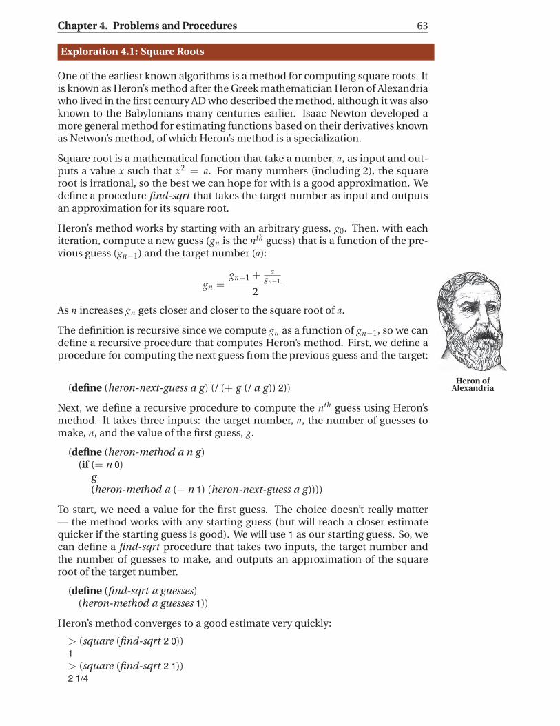
One of the earliest known algorithms is a method for computing square roots. Itis known as Heron’s method after the Greek mathematician Heron of Alexandriawho lived in the first century AD who described the method, although it was alsoknown to the Babylonians many centuries earlier. Isaac Newton developed amore general method for estimating functions based on their derivatives knownas Netwon’s method, of which Heron’s method is a specialization.

Square root is a mathematical function that take a number, a, as input and out-puts a value x such that x2 = a. For many numbers (including 2), the squareroot is irrational, so the best we can hope for with is a good approximation. Wedefine a procedure find-sqrt that takes the target number as input and outputsan approximation for its square root.

Heron’s method works by starting with an arbitrary guess, g0. Then, with eachiteration, compute a new guess (gn is the nth guess) that is a function of the pre-vious guess (gn−1) and the target number (a):

gn =gn−1 + a

gn−1

2

As n increases gn gets closer and closer to the square root of a.

The definition is recursive since we compute gn as a function of gn−1, so we candefine a recursive procedure that computes Heron’s method. First, we define aprocedure for computing the next guess from the previous guess and the target:

Heron ofAlexandria(define (heron-next-guess a g ) (/ (+ g (/ a g )) 2))

Next, we define a recursive procedure to compute the nth guess using Heron’smethod. It takes three inputs: the target number, a, the number of guesses tomake, n, and the value of the first guess, g.

(define (heron-method a n g )(if (= n 0)

g(heron-method a (− n 1) (heron-next-guess a g ))))

To start, we need a value for the first guess. The choice doesn’t really matter— the method works with any starting guess (but will reach a closer estimatequicker if the starting guess is good). We will use 1 as our starting guess. So, wecan define a find-sqrt procedure that takes two inputs, the target number andthe number of guesses to make, and outputs an approximation of the squareroot of the target number.

(define (find-sqrt a guesses)(heron-method a guesses 1))

Heron’s method converges to a good estimate very quickly:

> (square (find-sqrt 2 0))1

> (square (find-sqrt 2 1))2 1/4


> (square (find-sqrt 2 2))2 1/144

> (square (find-sqrt 2 3))2 1/166464

> (square (find-sqrt 2 4))2 1/221682772224

> (square (find-sqrt 2 5))2 1/393146012008229658338304

> (exact->inexact (find-sqrt 2 5))1.4142135623730951

The actual square root of 2 is 1.414213562373095048 . . ., so our estimate is correctto 16 digits after only five guesses.

Users of square roots don’t really care about the method used to find the squareroot (or how many guesses are used). Instead, what is important to a square rootuser is how close the estimate is to the actual value. Can we change our find-sqrtprocedure so that instead of taking the number of guesses to make as its secondinput it takes a minimum tolerance value?

Since we don’t know the actual square root value (otherwise, of course, we couldjust return that), we need to measure tolerance as how close the square of theapproximation is to the target number. Hence, we can stop when the square ofthe guess is close enough to the target value.

(define (close-enough? a tolerance g )(<= (abs (− a (square g ))) tolerance))

The stopping condition for the recursive definition is now when the guess isclose enough. Otherwise, our definitions are the same as before.

(define (heron-method-tolerance a tolerance g )(if (close-enough? a tolerance g )

g(heron-method-tolerance a tolerance (heron-next-guess a g ))))

(define (find-sqrt-approx a tolerance)(heron-method-tolerance a tolerance 1))

Note that the value passed in as tolerance does not change with each recursivecall. We are making the problem smaller by making each successive guess closerto the required answer.

Here are some example interactions with find-sqrt-approx:

> (exact->inexact (square (find-sqrt-approx 2 0.01)))2.0069444444444446

> (exact->inexact (square (find-sqrt-approx 2 0.0000001)))2.000000000004511

a. How accurate is the built-in sqrt procedure?

b. Can you produce more accurate square roots than the built-in sqrt proce-dure?

c. Why doesn’t the built-in procedure do better?


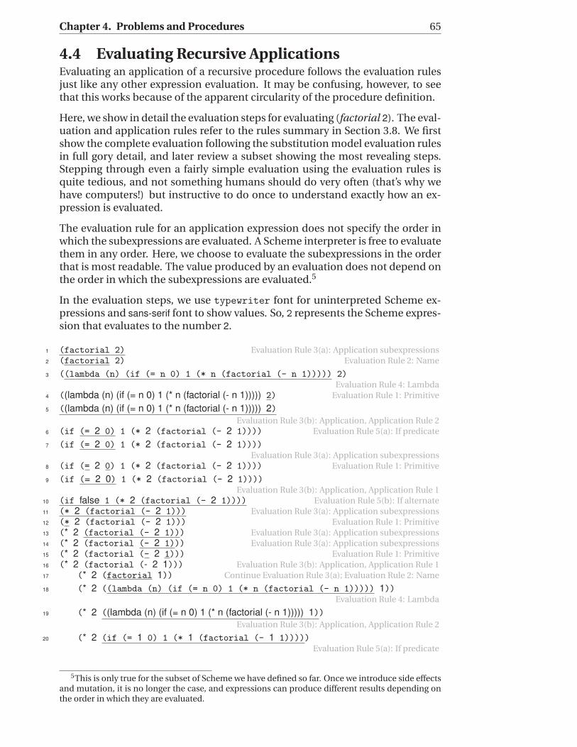
4.4 Evaluating Recursive ApplicationsEvaluating an application of a recursive procedure follows the evaluation rulesjust like any other expression evaluation. It may be confusing, however, to seethat this works because of the apparent circularity of the procedure definition.

Here, we show in detail the evaluation steps for evaluating (factorial 2). The eval-uation and application rules refer to the rules summary in Section 3.8. We firstshow the complete evaluation following the substitution model evaluation rulesin full gory detail, and later review a subset showing the most revealing steps.Stepping through even a fairly simple evaluation using the evaluation rules isquite tedious, and not something humans should do very often (that’s why wehave computers!) but instructive to do once to understand exactly how an ex-pression is evaluated.

The evaluation rule for an application expression does not specify the order inwhich the subexpressions are evaluated. A Scheme interpreter is free to evaluatethem in any order. Here, we choose to evaluate the subexpressions in the orderthat is most readable. The value produced by an evaluation does not depend onthe order in which the subexpressions are evaluated.5

In the evaluation steps, we use typewriter font for uninterpreted Scheme ex-pressions and sans-serif font to show values. So, 2 represents the Scheme expres-sion that evaluates to the number 2.

(factorial 2) Evaluation Rule 3(a): Application subexpressions1

(factorial 2) Evaluation Rule 2: Name2

((lambda (n) (if (= n 0) 1 (* n (factorial (- n 1))))) 2)3

Evaluation Rule 4: Lambda

((lambda (n) (if (= n 0) 1 (* n (factorial (- n 1))))) 2) Evaluation Rule 1: Primitive4

((lambda (n) (if (= n 0) 1 (* n (factorial (- n 1))))) 2)5

Evaluation Rule 3(b): Application, Application Rule 2

(if (= 2 0) 1 (* 2 (factorial (- 2 1)))) Evaluation Rule 5(a): If predicate6

(if (= 2 0) 1 (* 2 (factorial (- 2 1))))7

Evaluation Rule 3(a): Application subexpressions

(if (= 2 0) 1 (* 2 (factorial (- 2 1)))) Evaluation Rule 1: Primitive8

(if (= 2 0) 1 (* 2 (factorial (- 2 1))))9


(if false 1 (* 2 (factorial (- 2 1)))) Evaluation Rule 5(b): If alternate10

(* 2 (factorial (- 2 1))) Evaluation Rule 3(a): Application subexpressions11

(* 2 (factorial (- 2 1))) Evaluation Rule 1: Primitive12



(* 2 (factorial (- 2 1))) Evaluation Rule 1: Primitive15

(* 2 (factorial (- 2 1))) Evaluation Rule 3(b): Application, Application Rule 116

(* 2 (factorial 1)) Continue Evaluation Rule 3(a); Evaluation Rule 2: Name17

(* 2 ((lambda (n) (if (= n 0) 1 (* n (factorial (- n 1))))) 1))18

Evaluation Rule 4: Lambda

(* 2 ((lambda (n) (if (= n 0) 1 (* n (factorial (- n 1))))) 1))19


(* 2 (if (= 1 0) 1 (* 1 (factorial (- 1 1)))))20

Evaluation Rule 5(a): If predicate

5This is only true for the subset of Scheme we have defined so far. Once we introduce side effectsand mutation, it is no longer the case, and expressions can produce different results depending onthe order in which they are evaluated.

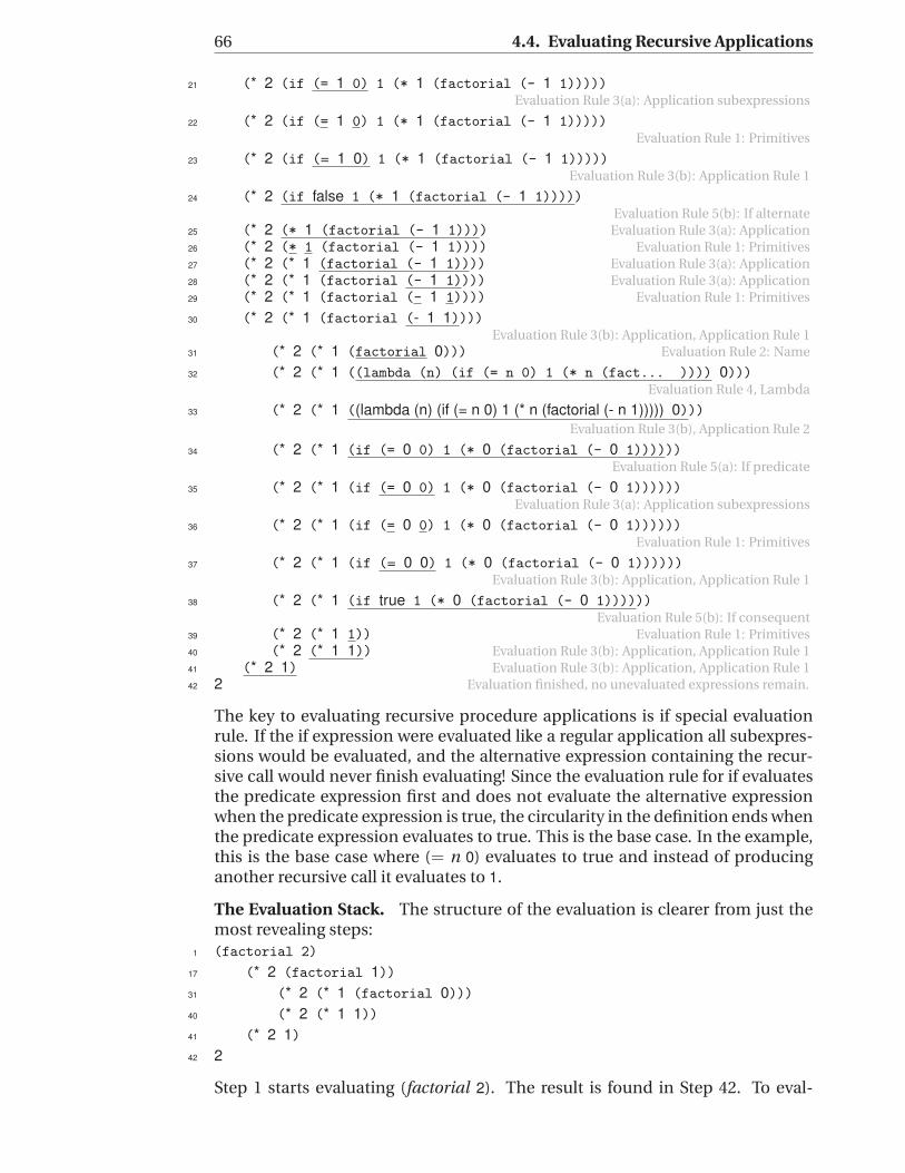
66 4.4. Evaluating Recursive Applications

(* 2 (if (= 1 0) 1 (* 1 (factorial (- 1 1)))))21


(* 2 (if (= 1 0) 1 (* 1 (factorial (- 1 1)))))22

Evaluation Rule 1: Primitives

(* 2 (if (= 1 0) 1 (* 1 (factorial (- 1 1)))))23

Evaluation Rule 3(b): Application Rule 1

(* 2 (if false 1 (* 1 (factorial (- 1 1)))))24

Evaluation Rule 5(b): If alternate

(* 2 (* 1 (factorial (- 1 1)))) Evaluation Rule 3(a): Application25

(* 2 (* 1 (factorial (- 1 1)))) Evaluation Rule 1: Primitives26



(* 2 (* 1 (factorial (- 1 1)))) Evaluation Rule 1: Primitives29

(* 2 (* 1 (factorial (- 1 1))))30


(* 2 (* 1 (factorial 0))) Evaluation Rule 2: Name31

(* 2 (* 1 ((lambda (n) (if (= n 0) 1 (* n (fact... )))) 0)))32

Evaluation Rule 4, Lambda

(* 2 (* 1 ((lambda (n) (if (= n 0) 1 (* n (factorial (- n 1))))) 0)))33

Evaluation Rule 3(b), Application Rule 2

(* 2 (* 1 (if (= 0 0) 1 (* 0 (factorial (- 0 1))))))34

Evaluation Rule 5(a): If predicate

(* 2 (* 1 (if (= 0 0) 1 (* 0 (factorial (- 0 1))))))35


(* 2 (* 1 (if (= 0 0) 1 (* 0 (factorial (- 0 1))))))36

Evaluation Rule 1: Primitives

(* 2 (* 1 (if (= 0 0) 1 (* 0 (factorial (- 0 1))))))37


(* 2 (* 1 (if true 1 (* 0 (factorial (- 0 1))))))38

Evaluation Rule 5(b): If consequent

(* 2 (* 1 1)) Evaluation Rule 1: Primitives39

(* 2 (* 1 1)) Evaluation Rule 3(b): Application, Application Rule 140

(* 2 1) Evaluation Rule 3(b): Application, Application Rule 141

2 Evaluation finished, no unevaluated expressions remain.42

The key to evaluating recursive procedure applications is if special evaluationrule. If the if expression were evaluated like a regular application all subexpres-sions would be evaluated, and the alternative expression containing the recur-sive call would never finish evaluating! Since the evaluation rule for if evaluatesthe predicate expression first and does not evaluate the alternative expressionwhen the predicate expression is true, the circularity in the definition ends whenthe predicate expression evaluates to true. This is the base case. In the example,this is the base case where (= n 0) evaluates to true and instead of producinganother recursive call it evaluates to 1.

The Evaluation Stack. The structure of the evaluation is clearer from just themost revealing steps:

(factorial 2)1

(* 2 (factorial 1))17

(* 2 (* 1 (factorial 0)))31

(* 2 (* 1 1))40

(* 2 1)41

242

Step 1 starts evaluating (factorial 2). The result is found in Step 42. To eval-


uate (factorial 2), we follow the evaluation rules, eventually reaching the bodyexpression of the if expression in the factorial definition in Step 17. Evaluatingthis expression requires evaluating the (factorial 1) subexpression. At Step 17,the first evaluation is in progress, but to complete it we need the value resultingfrom the second recursive application.

Evaluating the second application results in the body expression, (∗ 1 (factorial0)), shown for Step 31. At this point, the evaluation of (factorial 2) is stuck inEvaluation Rule 3, waiting for the value of (factorial 1) subexpression. The eval-uation of the (factorial 1) application leads to the (factorial 0) subexpression,which must be evaluated before the (factorial 1) evaluation can complete.

In Step 40, the (factorial 0) subexpression evaluation has completed and pro-duced the value 1. Now, the (factorial 1) evaluation can complete, producing 1

as shown in Step 41. Once the (factorial 1) evaluation completes, all the subex-pressions needed to evaluate the expression in Step 17 are now evaluated, andthe evaluation completes in Step 42.

Each recursive application can be tracked using a stack, similarly to process-ing RTN subnetworks (Section 2.3). A stack has the property that the first itempushed on the stack will be the last item removed—all the items pushed ontop of this one must be removed before this item can be removed. For appli-cation evaluations, the elements on the stack are expressions to evaluate. Tofinish evaluating the first expression, all of its component subexpressions mustbe evaluated. Hence, the first application evaluation started is the last one tofinish.

Exercise 4.16. This exercise tests your understanding of the (factorial 2) evalua-tion.

a. In step 5, the second part of the application evaluation rule, Rule 3(b), is used.In which step does this evaluation rule complete?

b. In step 11, the first part of the application evaluation rule, Rule 3(a), is used.In which step is the following use of Rule 3(b) started?

c. In step 25, the first part of the application evaluation rule, Rule 3(a), is used.In which step is the following use of Rule 3(b) started?

d. To evaluate (factorial 3), how many times would Evaluation Rule 2 be used toevaluate the name factorial?

e. [?] To evaluate (factorial n) for any positive integer n, how many times wouldEvaluation Rule 2 be used to evaluate the name factorial?

Exercise 4.17. For which input values n will an evaluation of (factorial n) even-tually reach a value? For values where the evaluation is guaranteed to finish,make a convincing argument why it must finish. For values where the evalua-tion would not finish, explain why.

4.5 Developing Complex ProgramsTo develop and use more complex procedures it will be useful to learn somehelpful techniques for understanding what is going on when procedures areevaluated. It is very rare for a first version of a program to be completely correct,

68 4.5. Developing Complex Programs

even for an expert programmer. Wise programmers build programs incremen-tally, by writing and testing small components one at a time.

The process of fixing broken programs is known as debugging . The key to debug-debugging

ging effectively is to be systematic and thoughtful. It is a good idea to take notesto keep track of what you have learned and what you have tried. Thoughtlessdebugging can be very frustrating, and is unlikely to lead to a correct program.

A good strategy for debugging is to:

1. Ensure you understand the intended behavior of your procedure. Think ofa few representative inputs, and what the expected output should be.

2. Do experiments to observe the actual behavior of your procedure. Try yourprogram on simple inputs first. What is the relationship between the ac-tual outputs and the desired outputs? Does it work correctly for some in-puts but not others?

3. Make changes to your procedure and retest it. If you are not sure what todo, make changes in small steps and carefully observe the impact of eachchange.

First actual bugFrom Grace Hopper’s notebook,

1947

For more complex programs, follow this strategy at the level of sub-components.For example, you can try debugging at the level of one expression before tryingthe whole procedure. Break your program into several procedures so you cantest and debug each procedure independently. The smaller the unit you test atone time, the easier it is to understand and fix problems.

DrScheme provides many useful and powerful features to aid debugging, but themost important tool for debugging is using your brain to think carefully aboutwhat your program should be doing and how its observed behavior differs fromthe desired behavior. Next, we describe two simple ways to observe programbehavior.

4.5.1 PrintingOne useful procedure built-in to DrScheme is the display procedure. It takesone input, and produces no output. Instead of producing an output, it printsout the value of the input (it will appear in purple in the Interactions window).We can use display to observe what a procedure is doing as it is evaluated.

For example, if we add a (display n) expression at the beginning of our factorialprocedure we can see all the intermediate calls. To make each printed valueappear on a separate line, we use the newline procedure. The newline procedureprints a new line; it takes no inputs and produces no output.

(define (factorial n)(display "Enter factorial: ") (display n) (newline)(if (= n 0) 1 (∗ n (factorial (− n 1)))))

Evaluating (factorial 2) produces:

Enter factorial: 2Enter factorial: 1Enter factorial: 02

The built-in printf procedure makes it easier to print out many values at once.It takes one or more inputs. The first input is a string (a sequence of characters


enclosed in double quotes). The string can include special ~a markers that printout values of objects inside the string. Each ~a marker is matched with a corre-sponding input, and the value of that input is printed in place of the ~a in thestring. Another special marker, ~n, prints out a new line inside the string.

Using printf , we can define our factorial procedure with printing as:

(define (factorial n)(printf "Enter factorial: ˜a˜n" n)(if (= n 0) 1 (∗ n (factorial (− n 1)))))

The display, printf , and newline procedures do not produce output values. In-stead, they are applied to produce side effects. A side effect is something that side effects

changes the state of a computation. In this case, the side effect is printing inthe Interactions window. Side effects make reasoning about what programs domuch more complicated since the order in which events happen now matters.We will mostly avoid using procedures with side effects until Chapter 9, butprinting procedures are so useful that we introduce them here.

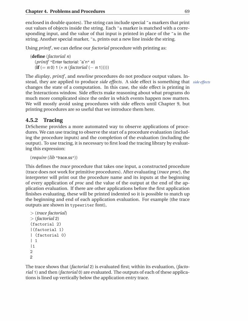
4.5.2 TracingDrScheme provides a more automated way to observe applications of proce-dures. We can use tracing to observe the start of a procedure evaluation (includ-ing the procedure inputs) and the completion of the evaluation (including theoutput). To use tracing, it is necessary to first load the tracing library by evaluat-ing this expression:

(require (lib "trace.ss"))

This defines the trace procedure that takes one input, a constructed procedure(trace does not work for primitive procedures). After evaluating (trace proc), theinterpreter will print out the procedure name and its inputs at the beginningof every application of proc and the value of the output at the end of the ap-plication evaluation. If there are other applications before the first applicationfinishes evaluating, these will be printed indented so it is possible to match upthe beginning and end of each application evaluation. For example (the traceoutputs are shown in typewriter font),

> (trace factorial)> (factorial 2)(factorial 2)

|(factorial 1)

| (factorial 0)

| 1

|1

2

2

The trace shows that (factorial 2) is evaluated first; within its evaluation, (facto-rial 1) and then (factorial 0) are evaluated. The outputs of each of these applica-tions is lined up vertically below the application entry trace.


Exploration 4.2: Recipes for π

The value π is the defined as the ratio between the circumference of a circle andits diameter. One way to calculate the approximate value of π is the Gregory-Leibniz series (which was actually discovered by the Indian mathematician Madhavain the 14

th century):

π =4

1−

4

3+

4

5−

4

7+

4

9− · · ·

This summation converges to π. The more terms that are included, the closerthe computed value will be to the actual value of π.

a. [?] Define a procedure compute-pi that takes as input n, the number of termsto include and outputs an approximation of π computed using the first nterms of the Gregory-Leibniz series. (compute-pi 1) should evaluate to 4 and(compute-pi 2) should evaluate to 2 2/3. For higher terms, use the built-inprocedure exact->inexact to see the decimal value. For example,

(exact->inexact (compute-pi 10000))

evaluates (after a long wait!) to 3.1414926535900434.

The Gregory-Leibniz series is fairly simple, but it takes an awful long time to con-verge to a good approximation for π — only one digit is correct after 10 terms,and after summing 10000 terms only the first four digits are correct.

Madhava discovered another series for computing the value of π that convergesmuch more quickly:

π =√

12 ∗ (1−1

3 ∗ 3+

1

5 ∗ 32−

1

7 ∗ 33+

1

9 ∗ 34− . . .)

Madhava computed the first 21 terms of this series, finding an approximation ofπ that is correct for the first 12 digits: 3.14159265359.

b. [??] Define a procedure cherry-pi that takes as input n, the number of termsto include and outputs an approximation of π computed using the first nterms of the Madhava series. (Continue reading for hints.)

To define faster-pi, first define two helper functions: faster-pi-helper , that takesone input, n, and computes the sum of the first n terms in the series without the√

12 factor, and faster-pi-term that takes one input n and computes the valueof the nth term in the series (without alternating the adding and subtracting).(faster-pi-term 1) should evaluate to 1 and (faster-pi-term 2) should evaluate to1/9. Then, define faster-pi as:

(define (faster-pi terms) (∗ (sqrt 12) (faster-pi-helper terms)))

This uses the built-in sqrt procedure that takes one input and produces as out-put an approximation of its square root. The accuracy of the sqrt procedure6

limits the number of digits of π that can be correctly computed using this method(see Exploration 4.1 for ways to compute a more accurate approximation for thesquare root of 12). You should be able to get a few more correct digits than

6To test its accuracy, try evaluating (square (sqrt 12)).


Madhava was able to get without a computer 600 years ago, but to get moredigits would need a more accurate sqrt procedure or another method for com-puting π.

The built-in expt procedure takes two inputs, a and b, and produces ab as itsoutput. You could also define your own procedure to compute ab for any integerinputs a and b.

c. [? ? ?] Find a procedure for computing enough digits of π to find the Feyn-man point where there are six consecutive 9 digits. This point is named forRichard Feynman, who quipped that he wanted to memorize π to that pointso he could recite it as “. . . nine, nine, nine, nine, nine, nine, and so on”.

Exploration 4.3: Recursive Definitions and Games

Many games can be analyzed by thinking recursively. For this exploration, weconsider how to develop a winning strategy for some two-player games. In allthe games, we assume player 1 moves first, and the two players take turns untilthe game ends. The game ends when the player who’s turn it is cannot move; theother player wins. A strategy is a winning strategy if it provides a way to alwaysselect a move that wins the game, regardless of what the other player does.

One approach for developing a winning strategy is to work backwards from thewinning position. This position corresponds to the base case in a recursive def-inition. If the game reaches a winning position for player 1, then player 1 wins.Moving back one move, if the game reaches a position where it is player 2’s move,but all possible moves lead to a winning position for player 1, then player 1 isguaranteed to win. Continuing backwards, if the game reaches a position whereit is player 1’s move, and there is a move that leads to a position where all pos-sible moves for player 2 lead to a winning position for player 1, then player 1 isguaranteed to win.

The first game we will consider is called Nim. Variants on Nim have been playedwidely over many centuries, but no one is quite sure where the name comesfrom. We’ll start with a simple variation on the game that was called Thai 21when it was used as an Immunity Challenge on Survivor.

In this version of Nim, the game starts with a pile of 21 stones. One each turn, aplayer removes one, two, or three stones. The player who removes the last stonewins, since the other player cannot make a valid move on the following turn.

a. What should the player who moves first do to ensure she can always win thegame? (Hint: start with the base case, and work backwards. Think about agame starting with 5 stones first, before trying 21.)


b. Suppose instead of being able to take 1 to 3 stones with each turn, you cantake 1 to n stones where n is some number greater than or equal to 1. Forwhat values of n should the first player always win (when the game starts with21 stones)?

A standard Nim game starts with three heaps. At each turn, a player removes anynumber of stones from any one heap (but may not remove stones from morethan one heap). We can describe the state of a 3-heap game of Nim using threenumbers, representing the number of stones in each heap. For example, theThai 21 game starts with the state (21 0 0) (one heap with 21 stones, and twoempty heaps).7

c. What should the first player do to win if the starting state is (2 1 0)?

d. Which player should win if the starting state is (2 2 2)?

e. [?] Which player should win if the starting state is (5 6 7)?

f. [??] Describe a strategy for always winning a winnable game of Nim startingfrom any position.8

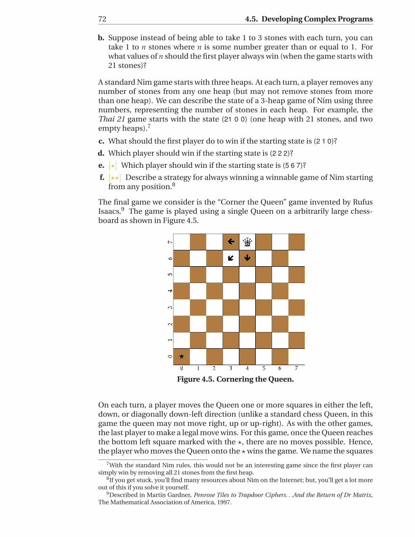
The final game we consider is the “Corner the Queen” game invented by RufusIsaacs.9 The game is played using a single Queen on a arbitrarily large chess-board as shown in Figure 4.5.

Figure 4.5. Cornering the Queen.

On each turn, a player moves the Queen one or more squares in either the left,down, or diagonally down-left direction (unlike a standard chess Queen, in thisgame the queen may not move right, up or up-right). As with the other games,the last player to make a legal move wins. For this game, once the Queen reachesthe bottom left square marked with the ?, there are no moves possible. Hence,the player who moves the Queen onto the ? wins the game. We name the squares

7With the standard Nim rules, this would not be an interesting game since the first player cansimply win by removing all 21 stones from the first heap.

8If you get stuck, you’ll find many resources about Nim on the Internet; but, you’ll get a lot moreout of this if you solve it yourself.

9Described in Martin Gardner, Penrose Tiles to Trapdoor Ciphers. . .And the Return of Dr Matrix,The Mathematical Association of America, 1997.


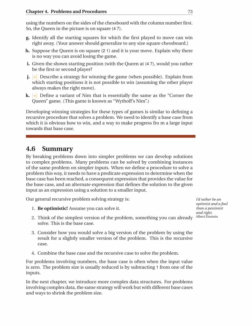
using the numbers on the sides of the chessboard with the column number first.So, the Queen in the picture is on square (4 7).

g. Identify all the starting squares for which the first played to move can winright away. (Your answer should generalize to any size square chessboard.)

h. Suppose the Queen is on square (2 1) and it is your move. Explain why thereis no way you can avoid losing the game.

i. Given the shown starting position (with the Queen at (4 7), would you ratherbe the first or second player?

j. [?] Describe a strategy for winning the game (when possible). Explain fromwhich starting positions it is not possible to win (assuming the other playeralways makes the right move).

k. [?] Define a variant of Nim that is essentially the same as the “Corner theQueen” game. (This game is known as “Wythoff’s Nim”.)

Developing winning strategies for these types of games is similar to defining arecursive procedure that solves a problem. We need to identify a base case fromwhich it is obvious how to win, and a way to make progress fro m a large inputtowards that base case.

4.6 SummaryBy breaking problems down into simpler problems we can develop solutionsto complex problems. Many problems can be solved by combining instancesof the same problem on simpler inputs. When we define a procedure to solve aproblem this way, it needs to have a predicate expression to determine when thebase case has been reached, a consequent expression that provides the value forthe base case, and an alternate expression that defines the solution to the giveninput as an expression using a solution to a smaller input.

Our general recursive problem solving strategy is:

1. Be optimistic! Assume you can solve it.

2. Think of the simplest version of the problem, something you can alreadysolve. This is the base case.

3. Consider how you would solve a big version of the problem by using theresult for a slightly smaller version of the problem. This is the recursivecase.

4. Combine the base case and the recursive case to solve the problem.

I’d rather be anoptimist and a foolthan a pessimistand right.Albert Einstein

For problems involving numbers, the base case is often when the input valueis zero. The problem size is usually reduced is by subtracting 1 from one of theinputs.

In the next chapter, we introduce more complex data structures. For problemsinvolving complex data, the same strategy will work but with different base casesand ways to shrink the problem size.

Problems and Procedures - computingbook.orgcomputingbook.org/spring2010/ch4-problems.pdf · Problems and Procedures ... solved and we can declare victory and move on to the next one.

Documents