Signature redacted - DSpace@MIT

The Mechanics of Tractor Performance and Their

Impact on Historical and Future Device Designs

by

Guillermo Fabidn Diaz Lankenau

B.S., Instituto Tecnologico y de Estudios Superiores de Monterrey(2012)

Submitted to the Department of Mechanical Engineeringin partial fulfillment of the requirements for the degree of

Master of Science in Mechanical Engineering

at the

MASSACHUSETTS INSTITUTE OF TECHNOLOGY

June 2017

@ Massachusetts Institute of Technology 2017. All rights reserved.

,4 0

Author

C ertified by ......................

MA-As-US-T0Tr7INSTITUTEOF TECHNOLOGY

JUN 21 2017

LIBRARIESARCHIVES

Signature redactedDepartment of Mechanical Engineering

May 12, 2017

Signature redactedmo G. Winter, V

Assistant Professor 6 ec anical EngineeringThesis Supervisor

Signature redactedAccepted by ................................

Rohan AbeyaratneChairman, Department Committee on Graduate Theses

The Mechanics of Tractor Performance and Their Impact on

Historical and Future Device Designs

by

Guillermo Fabian Diaz Lankenau

Submitted to the Department of Mechanical Engineeringon May 12, 2017, in partial fulfillment of the

requirements for the degree ofMaster of Science in Mechanical Engineering

Abstract

This thesis utilizes a terramechanics-based farm tractor model to predict machineperformance. This model is used to reflect on tractor evolution throughout the lastcentury and the physics-based principles that govern tractor performance. Insightsfrom this model and reflection can help designers create new farm tractor embodi-ments, especially for markets where farming practices and industrial context differsignificantly from those that shaped the conventional tractor's major evolutionarysteps.

It is shown how the small tractor evolved to its conventional modern form inin the early 1900s in USA pushed not only by suitability to domestic agricultureat the time but also efficiency in contemporary mass manufacturing and symbiosiswith the burgeoning automotive industry. The farm tractor model as suggested inthis thesis is proven to be in good agreement with published experimental data andhistorical standarized tractor testing. Inline drive wheels and mounting soil workingimplements between front and rear axles are identified as high potential design optionsfor adapting the small tractor to modern emerging markets where draft animals arethe dominant source of draft power.

Thesis Supervisor: Amos G. Winter, VTitle: Assistant Professor of Mechanical Engineering

3

4

Acknowledgments

I am deeply grateful to for everyone and everything that has allowed me to be here

now. I feel fortunate to have met amazing, supportive people throughout my life

and to have been at the right place, at the right time more than once. Thank you

Prof. Amos Winter for believing in me and helping me better realize my strengths

and improve my weaknesses in work and in life. Thank you Jaya, my wife, for your

patience, love, and advice. Your breathtaking awesomeness makes my life more splen-

did than it has ever been and I look forward to sharing a lifetime of happiness with

you. Thank you to Guillermo and Maga, my parents, for your unwavering support

of my education and your rock-solid confidence in my ability to be an outstanding

student even when results at times may have indicated otherwise. You have been the

concrete that has allowed me build the life and achievements I now enjoy. iMuchas

Gracias!

5

6

Contents

1 Introduction 15

1.1 Contributions . . . . . . . . . . . . . . . . . . . . . . . . . . . . . . . 15

1.2 Tractors are ubiquitous in high productivity farming . . . . . . . . . 15

1.3 Brief History of the Farm Tractor . . . . . . . . . . . . . . . . . . . . 16

1.4 Evolution of small tractor to consolidated design . . . . . . . . . . . . 20

1.5 There is an untapped market for which tractors could be designed . . 25

1.6 We want to know how tractors work parametrically, reflecting on the

strengths and drawbacks of previous designs . . . . . . . . . . . . . . 26

2 Tractor Theory 27

2.1 Qualitative description of importance of soil-tire interaction in tractor

design . . . . . . . . . . . . . . . . . . . . . . . . . . . . . . . . . . . 27

2.2 Analytical model for interaction of single drive tire with soil . . . . . 30

2.3 M ulti-pass effect for tires . . . . . . . . . . . . . . . . . . . . . . . . . 33

2.4 Conventional tractor dimensions and relevant forces . . . . . . . . . . 34

2.5 Proposed generalized vertical load per tire calculation . . . . . . . . . 36

2.6 Proposed generalized horizontal load per tire calculation . . . . . . . 40

2.7 Variable sensitivity of tractor-soil model as implemented . . . . . . . 41

2.8 Flowchart of tractor design exploration model . . . . . . . . . . . . . 42

3 Validation of Tractor Model with Published Data 45

3.1 Comparison to specific tractor tests . . . . . . . . . . . . . . . . . . . 45

3.2 Comparison to design trends . . . . . . . . . . . . . . . . . . . . . . . 46

7

4 Insights into small tractor design 51

4.1 Comments on past and current tractor designs . . . . . . . . . . . . . 51

4.1.1 "Fulcrum and Lever" towing adjusts drive tire vertical loading

in proportion to pulling force. . . . . . . . . . . . . . . . . . . 51

4.1.2 Central tool mounting increases safety but can be detrimental

to traction in conventional tractors. . . . . . . . . . . . . . . . 55

4.1.3 Inline and side-by-side drive wheels each have their advantages. 61

4.1.4 Hypothetical inline drive wheels with centrally mounted tool . 63

4.2 Recommendations for future designs . . . . . . . . . . . . . . . . . . 65

5 Conclusions 69

A 1910 to 1920 Production Vehicles Matched to Layouts in Ch. 1 71

B Evolution Steps, matched to vehicles in Ch. 1 75

8

List of Figures

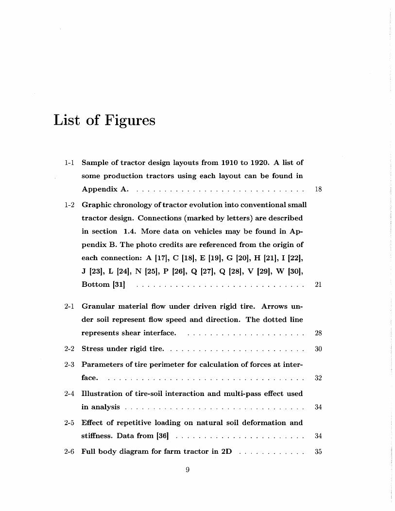
1-1 Sample of tractor design layouts from 1910 to 1920. A list of

some production tractors using each layout can be found in

A ppendix A . . . . . . . . . . . . . . . . . . . . . . . . . . . . . . . 18

1-2 Graphic chronology of tractor evolution into conventional small

tractor design. Connections (marked by letters) are described

in section 1.4. More data on vehicles may be found in Ap-

pendix B. The photo credits are referenced from the origin of

each connection: A [171, C [18], E [19], G [20], H [21], I [22],

J [23], L [24], N [25], P [26], Q [27], Q [28], V [29], W [30],

B ottom [31] . . . . . . . . . . . . . . . . . . . . . . . . . . . . . . 21

2-1 Granular material flow under driven rigid tire. Arrows un-

der soil represent flow speed and direction. The dotted line

represents shear interface. . . . . . . . . . . . . . . . . . . . . . 28

2-2 Stress under rigid tire. . . . . . . . . . . . . . . . . . . . . . . . . 30

2-3 Parameters of tire perimeter for calculation of forces at inter-

fa ce . . . . . . . . . . . . . . . . . . . . . . . . . . . . . . . . . . . . 32

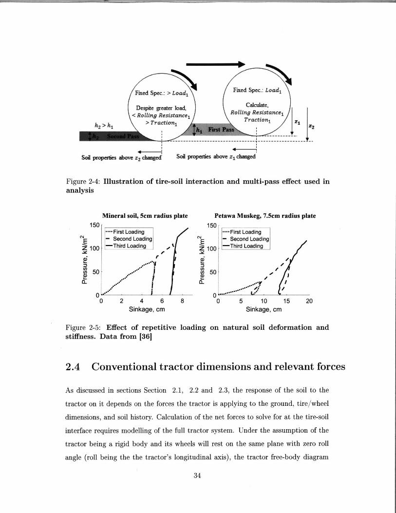
2-4 Illustration of tire-soil interaction and multi-pass effect used

in analysis . . . . . . . . . . . . . . . . . . . . . . . . . . . . . . . . 34

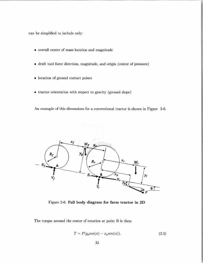
2-5 Effect of repetitive loading on natural soil deformation and

stiffness. Data from [36] . . . . . . . . . . . . . . . . . . . . . . . 34

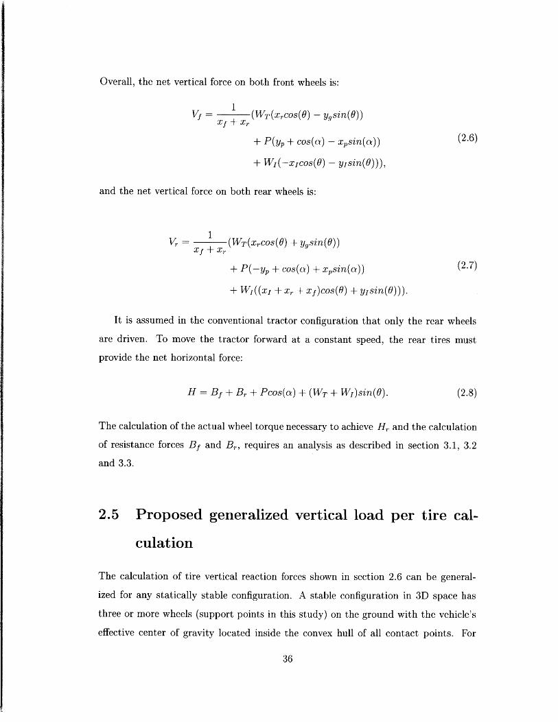
2-6 Full body diagram for farm tractor in 2D . . . . . . . . . . . . 35

9

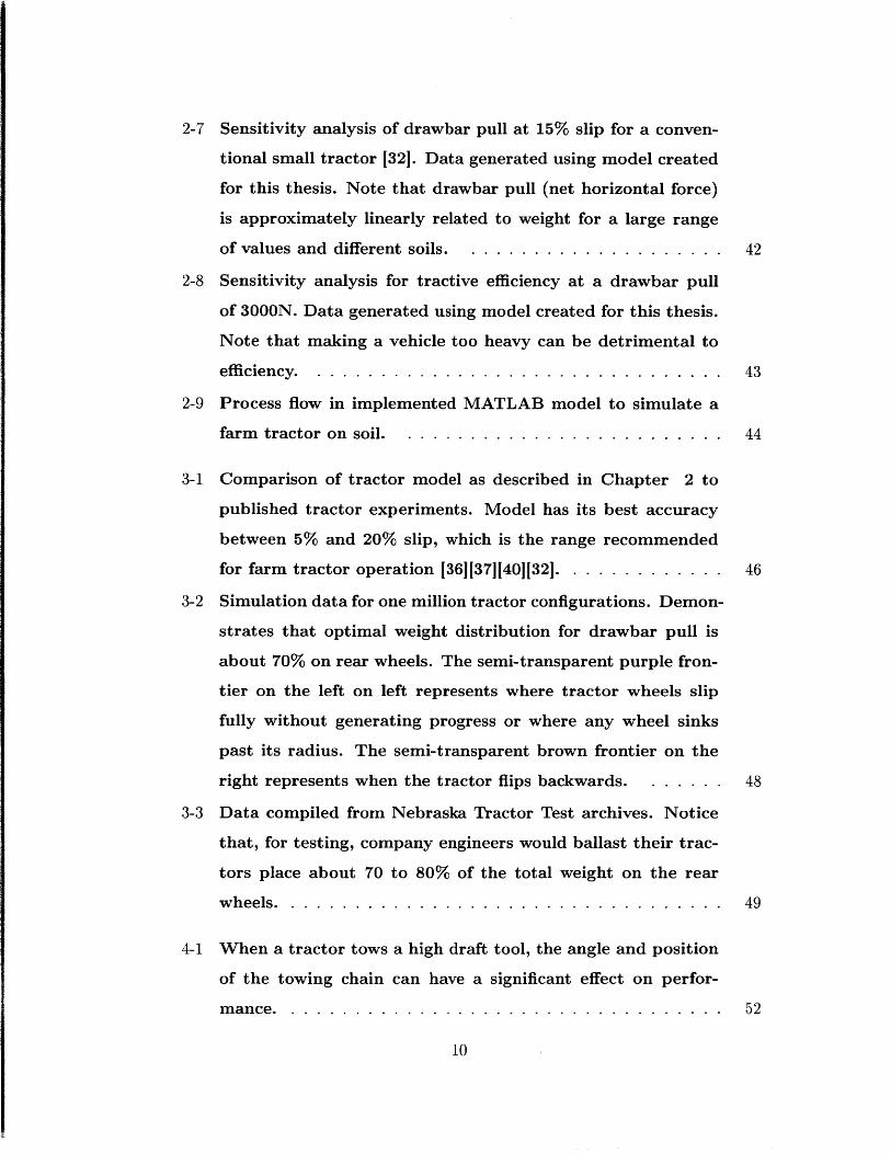
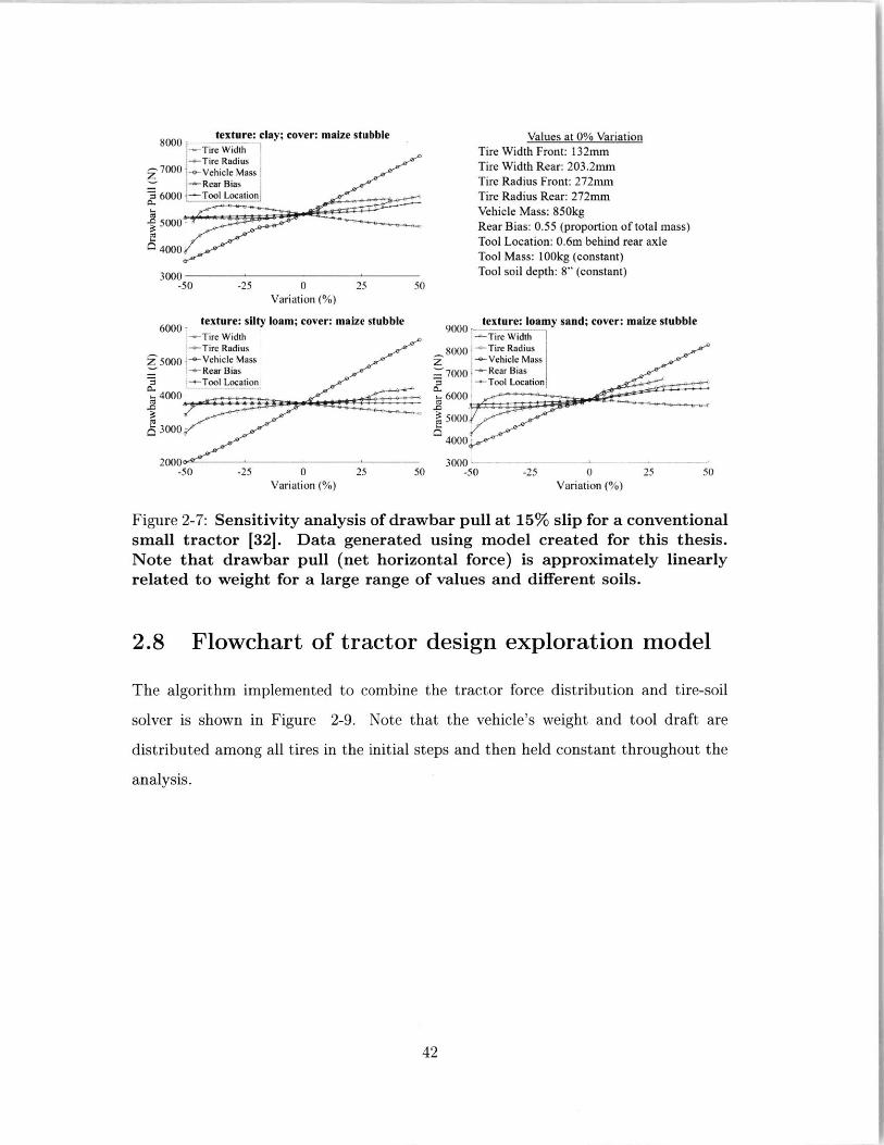
2-7 Sensitivity analysis of drawbar pull at 15% slip for a conven-

tional small tractor [32]. Data generated using model created

for this thesis. Note that drawbar pull (net horizontal force)

is approximately linearly related to weight for a large range

of values and different soils. . . . . . . . . . . . . . . . . . . . . 42

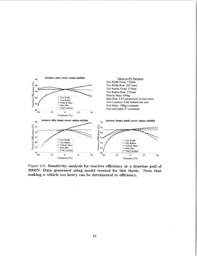
2-8 Sensitivity analysis for tractive efficiency at a drawbar pull

of 3000N. Data generated using model created for this thesis.

Note that making a vehicle too heavy can be detrimental to

efficiency. . . . . . . . . . . . . . . . . . . . . . . . . . . . . . . . . 43

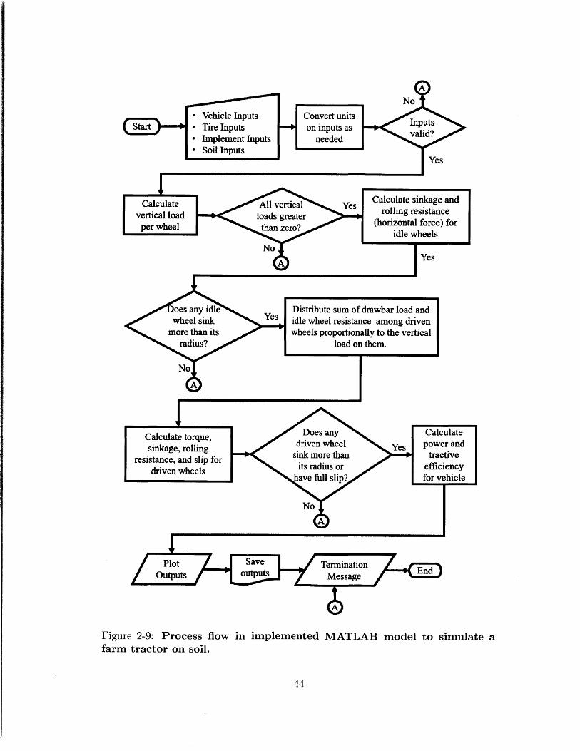
2-9 Process flow in implemented MATLAB model to simulate a

farm tractor on soil. . . . . . . . . . . . . . . . . . . . . . . . . . 44

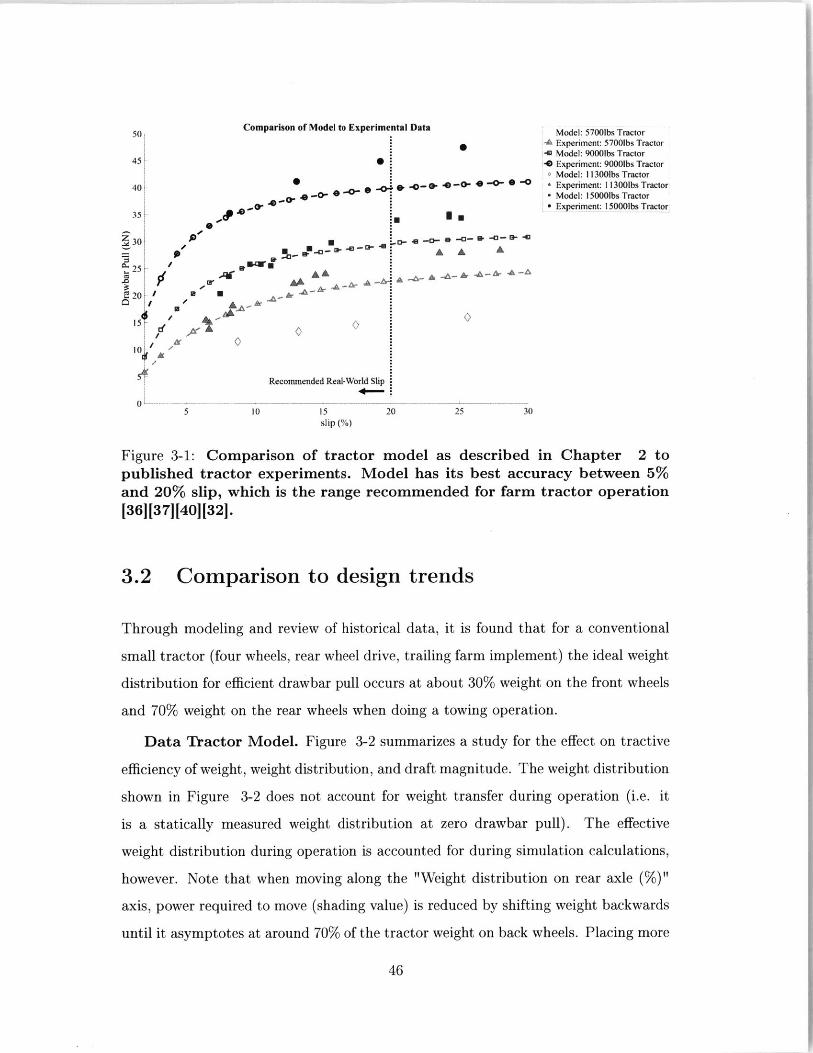
3-1 Comparison of tractor model as described in Chapter 2 to

published tractor experiments. Model has its best accuracy

between 5% and 20% slip, which is the range recommended

for farm tractor operation [36][371140][32]. . . . . . . . . . . . . 46

3-2 Simulation data for one million tractor configurations. Demon-

strates that optimal weight distribution for drawbar pull is

about 70% on rear wheels. The semi-transparent purple fron-

tier on the left on left represents where tractor wheels slip

fully without generating progress or where any wheel sinks

past its radius. The semi-transparent brown frontier on the

right represents when the tractor flips backwards. . . . . . . 48

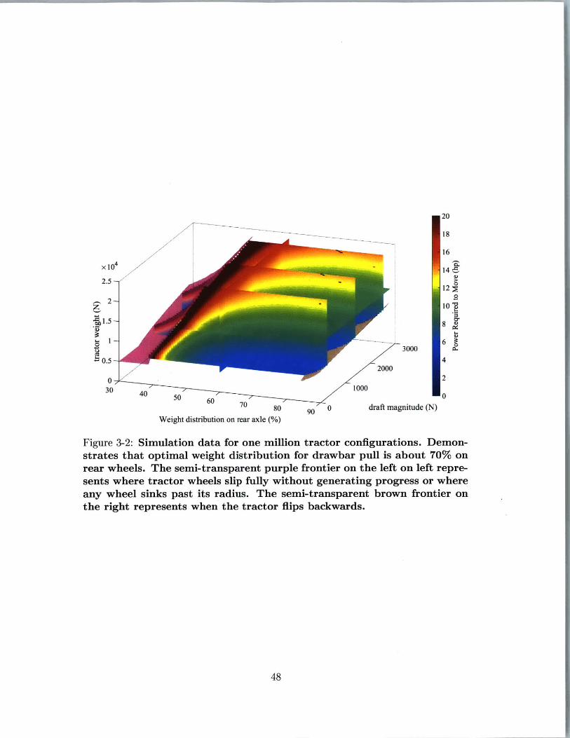
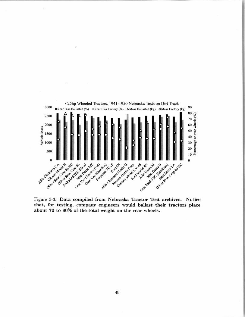
3-3 Data compiled from Nebraska Tractor Test archives. Notice

that, for testing, company engineers would ballast their trac-

tors place about 70 to 80% of the total weight on the rear

w h eels. . . . . . . . . . . . . . . . . . . . . . . . . . . . . . . . . . . 49

4-1 When a tractor tows a high draft tool, the angle and position

of the towing chain can have a significant effect on perfor-

m an ce. . . . . . . . . . . . . . . . . . . . . . . . . . . . . . . . . . . 52

10

4-2 Labeled standard conventional tractor like the Ford 8N (four

wheels, rear wheel drive, and rigidly attached trailing tool)

and conventional tractor with centrally mounted tool like the

Allis Chalmers G. . . . . . . . . . . . . . . . . . . . . . .. . . 56

4-3 Examples of tractor layouts with inline wheels. Layouts are

selection from those of Figure 1-1. . . . . . . . . . . . . . . . . 63

4-4 A comparison of the drawbar pull of inline wheels vs. side-by-

side wheels in a 500kg. In both cases, the horizontal drag from

rolling idle wheels through the soil has been ignored. The

model described in Chapter 2 was used. The drawbar pull

of a bullock team (two animals) has been added for reference. 64

11

12

List of Tables

1.1 Data from FAO for farm sizes worldwide [citation needed]. The sample

is from 460million farms in 111 countries. . . . . . . . . . . . . . . . . 25

1.2 Data from USDA agricultural census [citation needed] [citation needed]. 26

4.1 A comparison on some aspects of the 1948 to 1952 Ford 8N and the

1948 to 1955 Allis Chalmers G . . . . . . . . . . . . . . . . . . . . . . 56

4.2 Values for side-by-side wheels and inline wheels used in Figure 4-4.

Side-by-side wheels based on Mahindra Yuvraj and inline wheels based

on ROKON Scout. . . . . . . . . . . . . . . . . . . . . . . . . . . . . 65

13

14

Chapter 1

Introduction

1.1 Contributions

This thesis provides tools and background to facilitate the creation of a novel farm

tractor specialized to small farms (<2Ha), which represent 72% of the world's farms

(Table 1.1). Contributions include:

" Description of evolution process to arrive at current conventional tractor (Chap-

ter 1).

" Tractor mathematical model for exploring large design space with minimal ex-

periments (Chapter 2 and Chapter 3).

" Physics-based observations on past tractor designs (Chapter 4).

" Design suggestions for creation of tractors well suited to small farmers in devel-

oping countries (Chapter 4).

1.2 Tractors are ubiquitous in high productivity farm-

ing

Tractors are an icon of industrialized, modern farming and their presence has been

noted as a differentiator between farming in developed vs. developing countries 1]

15

[2]. In 1950, the USA Census Bureau stated the benefits of mechanizing American

agriculture [31:

" The increased use of mechanical power on farms has influenced agriculture more

than any other factor during the present century. The changes from horses and mules

to tractors for farm work has made available an acreage of cropland greater than

the total increase in cropland during the half century for the production, directly or

indirectly, of meat, milk, eggs, and other food. The use of the tractor and related

equipment for farm work, and the use of farm trucks for hauling and automobiles for

traveling have increased the rate at which farm work is done and has increased the

capacity of agricultural workers, enabling considerable numbers of farm workers to

leave the farms or to engage in non-farm work, notwithstanding considerable increases

in total farm production. Tractors and power-operated equipment have made an

increase in the size of farms possible. The substitution of tractors for animal power

has also made available additional power for farm use. With a tractor, the farmer of

1950 probably turned out twice the amount of farm products for market as his father

did with a team of horses 50 years earlier. Moreover, less of the farmer's time was

required to care for the tractor than to raise feed for and to produce and care for

horses that were replaced by the tractor."

There is high correlation worldwide between farm productivity and available trac-

tor power f4] [51 [61 [1].

1.3 Brief History of the Farm Tractor

The conventional small tractor produced today found its form mostly in the USA

between 1910 and 1940. This "conventional tractor" or "dominant tractor design" is a

four wheeled tractor, with front steering, rear wheel drive, and a trailing implement

behind the rear axle. The design has changed little in the following 80 years [71 [8]

[81 [9] [101.

In 1903 the term "tractor" was first coined by the Hart Parr Gasoline Engine

company of Charles City, Iowa. In the USA, the Homestead Act of 1862 was still

16

ongoing with minor revisions and motivated farmers to extend westward from the

northeastern cities, rapidly expanding the amount of available arable land [7]. At

the time, horses and mules were the primary source of draft power in the burgeoning

American farming industry. Tractors were more capable at opening new land for

farming but also unwieldy and expensive.

During the late 1910's the agricultural industry in the USA became highly prof-

itable as food exports increased dramatically to feed Europe and Russia during and

after WWI. Farming land prices were on a sharp rise as farmers had surplus money

and looked to increase production by expanding their properties. Farms grew in

number and size yet farm labor was more scarce as the rural youth went to fight in

WWI and later returned preferring an urban lifestyle [citation needed]. Farm tractors

became an attractive way to multiply the capacity of each laborer [3].

In the year 1920, 166 companies in the USA manufactured farm tractors and had

a combined year production of 203,207 tractors. These were dramatic increases from

1910, when only 15 farm tractor companies were in business and had a combined

production of 4,000 tractors [111. These 166 companies were fighting to define the

shape of the "farm tractor" and to distinguish themselves through innovative designs

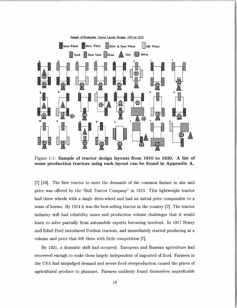
[121 1131. A sample of 24 production tractor layout designs from the 1910 to 1920

period with their respective manufacturers can be found in Figure 1-1. Layouts

varied widely in traction gear (tracks, wheels, or drums mostly), number of axles,

driver position, tool position, and overall dimensions.

In the 1910's the rapidly expanding tractor industry was learning from the more

readily availabe feedback from farmers and taking some engineering lessons from its

younger but more refined cousin, the automobile [12]. Important obstacles to more

tractor adoption were initial cost and need for more versatility in usage. The demand

for a less expensive, smaller, lighter tractor became apparent during this decade [141

[151. It was often the case that the farmer who owned a tractor still had to own

horses, which were more manageable and smaller, for cultivation operations [13][121.

Very large tractors that had been used to open large fields in the expanding West

would lay rusting with little or no use after that initial heavy ploughing operation

17

-J

Sample of Production Tractor Layout Designs 1910 to 1920

Steer Wheel Drive Wheel Drive & Steer Wheel L Idle Wheel

f-Track 11Steer Track lgDrum Tol Driver

a b f v t

g h W U

~FL7)

S n m pq r ~~ s

Figure 1-1: Sample of tractor design layouts from 1910 to 1920. A list ofsome production tractors using each layout can be found in Appendix A.

[7] [16]. The first tractor to meet the demands of the common farmer in size and

price was offered by the "Bull Tractor Company" in 1913. This lightweight tractor

had three wheels with a single drive-wheel and had an initial price comparable to a

team of horses. By 1914 it was the best-selling tractor in the country [71. The tractor

industry still had reliability issues and production volume challenges that it would

learn to solve partially from automobile experts becoming involved. In 1917 Henry

and Edsel Ford introduced Fordson tractors, and immediately started producing at a

volume and price that left them with little competition [7].

By 1921, a dramatic shift had occurred. European and Russian agriculture had

recovered enough to make them largely independent of imported of food. Farmers in

the USA had misjudged demand and severe food overproduction caused the prices of

agricultural produce to plummet. Farmers suddenly found themselves unprofitable

18

and with outstanding bank loans used to purchase farmland that had since collapsed

in value. Farm tractor production plunged from 203,277 in 1920 to 68,029 in 1921

[111.

The great depression and stock market crash would keep American farmers in a

difficult position through the 1920's and forced tractor manufacturers to adapt to a

low cash flow style of farming. In February 1922, the "Tractor Price Wars" started

when Ford (known then as Fordson Tractors) slashed the price of its Model F from

$625 to $395. Over the next 20 years a fiercely price-competitive tractor market

would see manufacturers converge on similar designs [7]. Many manufacturers would

disappear in this "war", from 166 manufacturers in 1920 to only 38 in 1930. However,

combined production had rebounded to 196,297 in 1930, very similar to the level

of 1920[111. Yearly total production of American tractors would keep rising until

reaching a peak in 1951, when 564,000 tractors were manufactured. By 1950 there

were over 3.6 million tractors operating in American farms (about 1 tractor for every 6

people living on a farm) and the internal combustion engine had become the primary

source of draft power for farmers [3].

Some major innovations between 1920 and 1940 that shaped the modern small

tractor are [10J:

1921 - First Nebraska Tractor Test is performed. These tests would go on to

become the national, and later international, standard for tractor testing. The test's

prominence would make it a major quantifiable target for tractor manufacturers.

1922 - International Harvester introduces the Power Take Off (PTO), allowing the

tractor's engine to power farming implements through a rigid shaft instead of using

a belt. Implement manufacturers rush to take advantage of this innovation.

1925 - International Harvester introduces its Farmall "General Purpose" (GP)

tractor. The Farmall series would become the best-selling tractor series ever in the

USA. Compared to most other tractors on the market it:

" Was Lighter

" Had higher ground clearance

19

. Utilized smaller front wheels (enabling tighter turns)

" Had adjustable track width

" Was advertised for cultivating, plowing, and cutting.

1927 - John Deere introduces "Power Lift", allowing the farmer to use the engine's

power to raise and lower farming implements. This reduced the drudgery of tractor

usage and increased tractors' field capacity.

1932 - Firestone and Allis Chalmers introduce the pneumatic rubber tire. This al-

lowed tractors on the growing network of paved roads (where steel, lugged wheel were

not permitted) and enabled farmers to operate at higher speeds more comfortably.

Circa 1935 - Diesel engines are advanced enough to become standard in farm

tractors, lowering fuel costs.

1937 - Henry Ford licenses the now standard "three point hitch" design from Harry

Ferguson. The "N series" tractors created after this agreement would culminate in

the 8N, which is the best-selling single tractor model ever in the USA.

After the 1940s, a small tractor design now common to major brands would rapidly

overtake the market and finish replacing animal power in farms. By 1945, more work

was being performed by tractors on farms than horses and mules combined. By

1955 the total number of tractors on farms was greater than the total number of

horses and mules combined. This common design was as mentioned at the beginning

of Section 1.3: four wheeled, with front steering, rear wheel drive, and a trailing

implement behind the rear axle. This tractor design from the 1940's still remains as

the standard layout for modern small tractors [71 [81 [81 [91 [10]

1.4 Evolution of small tractor to consolidated design

The modern, conventional small tractor is four wheeled, with front steering, rear

wheel drive, and a trailing implement but its predecessors came in larger variety of

configurations. A sample of these configurations is shown in Figure 1-1. This section

exemplifies some important milestones and configurations in the evolution towards

20

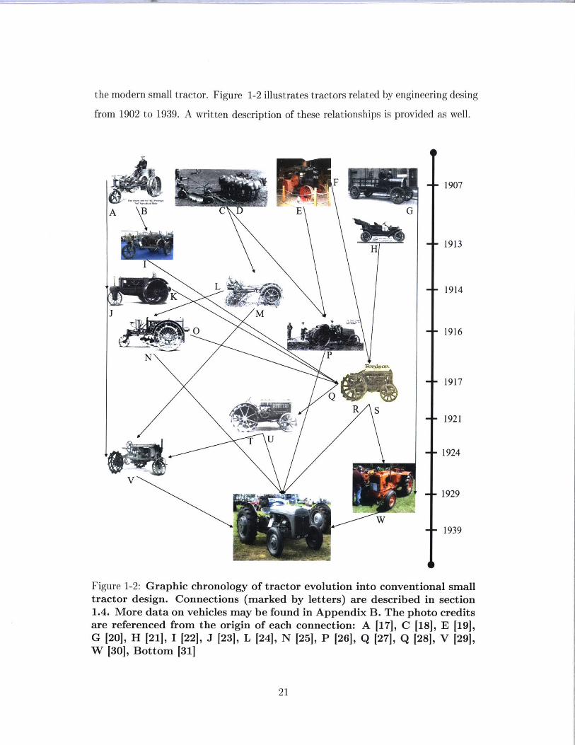
the modern small tractor. Figure 1-2 illustrates tractors related by engineering desing

from 1902 to 1939. A written description of these relationships is provided as well.

A BCD

J

IE

F

E

4

G

H

R S

W

Figure 1-2: Graphic chronology of tractor evolution into conventional smalltractor design. Connections (marked by letters) are described in section1.4. More data on vehicles may be found in Appendix B. The photo creditsare referenced from the origin of each connection: A [17], C [18], E [19],G [20], H [21], I [22], J [23], L [24], N [25], P [26], Q [27], Q [28], V [29],W [30], Bottom [31]

21

1907

1913

1914

- 1916

- 1917

- 1921

- 1924

- 1929

- 1939

KL

M

N

U

I

A) 1902 Ivel Tractor to 1914 Wallis Cub: Lightweight three-wheeled vehicles.

B) 1902 Ivel Tractor to 1913 Bull: Lightweight, mechanically simple, three-wheeled

vehicles. Exposed "I-beam" frame.

C) Horse Plow to 1914 Moline Universal: Driver is behind or above implements which

facilitates supervising field operation. Advertising boasted of user-friendly layout be-

ing similar to horses.

D) Horse Plow to 1916 Nilson: "Fulcrum and lever" attachment system increases

downward force on rear wheels as draft force increases. Compared to other tractors,

tool is attached higher above the rear axle but pulled same distance behind tractor.

This increases the downward vertical force generated by pulling the implement, it also

increases the lever-arm that the backward forces have to rotate the vehicle around the

rear wheels ground contact point. Nilson advertises that tool pulling angle is similar

to that of horses pulling a plow. More details on this design can be found in Chapter

4.

E) 1907 Hart-Parr 30-60 to Nilson 1916: Similar layout with two front steering wheels.

Nilson attempts to achieve high pulling force of heavier vehicles (like the Hart-Parr)

in lightweight vehicle by taking advantage of draft force and increasing wheel rear

area (the Nilson has three rear wheels, the central one being a drum). F) 1907 Hart-

Parr 30-60 to 1917 Fordson: The Fordson miniaturized the "Praire Style" four wheel

tractors like the Hart-Parr. This smaller tractor was more versatile and less expen-

sive.

G) 1909 Avery Farm & City to 1929 Allis-Chalmers U: When the Avery was made,

the farm "tractor" still did not have a definite shape or use on the farm. The Farm

& City placed high importance on road haulage as well as plowing and made a com-

promise between both. The tractor was supplied with wooden "plugs" that could be

placed on steel wheels to prevent them from damaging paved roads (which made the

wheels road-legal and more comfortable).

H) 1908 Ford Model T to 1917 Fordson: Ford's automobile engineering and assem-

bly line manufacturing expertise (along with the the brand's fame) made it a near-

immediate leader in the tractor industry.

22

I) 1913 Bull Tractor to 1917 Fordson: The Bull tractor was novel in its low cost and

light weight. It became the selling tractor in the country within a year of launch. Four

years later, the Fordson will repeat the same feat due to the similar characteristics

but in a more reliable package.

J) 1914 Wallis Cub to 1924 International Harvester (IHC) Farmall: Both vehicles

shared a tricycle layout. The Farmall utilized the U-frame design that had been

pioneered by Wallis. This design utilized the transmission and engine castings as

structural components, which yielded a lighter and less expensive tractor.

K) 1914 Wallis Cub to 1917 Fordson: The Fordson utilized the U-frame design that

had been pioneered by Wallis. This design utilized the transmission and engine cast-

ings as structural components, which yielded a lighter and less expensive tractor.

L) 1914 Moline Universal to 1916 Square Turn: Like the Moline, the Square-Turn

offers a similar driver experience to horses. The Square-Turn takes the experience

further by allowing each drive wheel to be controlled independently, this meant the

wheels could be driven in opposite directions for in-place turning. This tight turning

was important in the smaller 80-100 acre farms that were common in Nebraska, where

the Square-Turn was designed and made.

M) 1914 Moline Universal to 1924 International Harvester (IHC) Farmall: The Mo-

line was the first popular tractor that attempted to be useful for all farm operations.

This was a tractor that could not only do plowing but also cultivating once crops

were growing. The Farmall would later become the best-selling tractor series ever in

the USA due in good part to its "General Purpose" design. The Moline was also a

thoroughly modern tractor for its time, using unusually advanced electric features.

The Farmall would later also be a very modern tractor for its time.

N) 1916 Square Turn to 1939 Ford 9N: The Square Turn provided powered control

of the tillage tool's vertical position (mounted under the frame between both axles).

The use could control the tool even when the tractor was static, which was unusual

at the time. The Fordson was the first popular tractor with hydraulics, which allowed

the user a high level of control over the tillage tool's position.

0) 1916 Square Turn to 1917 Fordson: Both of these tractors were intended to be

23

useful to the small farmer as well as the large farmer. The Square Turn achieved

this through tight turning, the Fordson did it through a compact overall size, a large

dealer network, and a low selling price.

P) 1916 Nilson to 1939 Ford 9N: The Nilson's "Fulcrum and Lever" rear tool attach-

ment system utilized tillage draft forces to increase downward load on the tires and

therefore traction. The "Three-Point Hitch" in the Fordson would utilize the same

principle but include powered-tool control. More details on this evolution can be

found in Chapter 4.

Q) 1917 Fordson to 1921 International Harvester (IHC) 15-30: The success of the

Fordson tractor pushed other manufacturers to make smaller, less expensive, four-

wheel tractors. The 15-30 was IHC's first significant response to the Fordson.

R) 1917 Fordson to 1939 Ford 9N: Ford would stop American production of the Ford-

son in 1928 but would come back to take advantage of the lessons learned then and

novel technologies in 1939 with the Ford 9N.

S) 1917 Fordson to 1929 Allis-Chalmers U: When Ford stopped making the Fordson

in 1928, suddenly hundreds of dealers were left without a product to sell. These

dealers formed the "United Tractor and Equipment Corporation" and contracted

Allis-Chalmers to make a small, modern tractor similar to the Fordson they could

sell (the model name "U" stands for "United").

T) 1921 International Harvester (IHC) 15-30 to 1924 Farmall: The 15-30 was IHC's

quick response to the Fordson's market success but eventually they released the highly

novel Farmall which would go on to replace the Fordson as the best-selling tractor.

The Farmall included a Power Take Off (PTO) shaft, which had first been introduced

to the market by the 15-30.

U) 1921 International Harvester (IHC) 15-30 to 1939 Ford 9N: The IHC 15-30 was the

first tractor with a Power Take OFF (PTO) shaft. This was a very popular feature

that would become standard in the industry and was included in the Ford 9N.

V) 1924 International Harvester (IHC) Farmall to 1939 Ford 9N: The Ford 9N was a

"General Purpose" tractor, a category that the Farmall had made the biggest one in

the American tractor market.

24

W) 1929 Allis-Chalmers U to 1939 Ford 9N: The Allis-Chalmers U was the first farm

tractor with pneumatic rubber tires. A feature that would become a market standard

and that was present in the Ford 9N.

1.5 There is an untapped market for which tractors

could be designed

In developing countries, more acres of farmland are tended to with animals than

farm tractors. Adoption of conventional small tractors has been delayed by an initial

cost higher than animals but also by a functionality that differs starkly from that of

animals and that is not as well suited to remote, small farms [32]. This may not come

as a surprise when one considers the small tractor has remained largely unchanged

worldwide since its evolution mainly in the USA during the first half of the 20th

century (as described in Section 1.3). Farms in early 20th century USA were smaller

than those in the country today but were nonetheless significantly larger than those

found in most developing countries (Table 1.1 and Table 1.2). In addition to this

farm size discrepancy, driving the conventional tractor's form was not only farming

operations but also suitability in a different era for manufacturing and distribution at

low cost and high volume, success at standardized testing, and use on paved roads.

The conventional tractor shape is not necessarily well suited to the style and scale of

farming currently practiced in developing countries with farm animals.

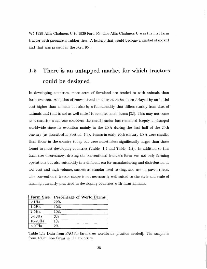
Farm Size Percentage of World Farms<IHa 72%1-2Ha 12%2-5Ha 10%5-1OHa 3%10-20Ha 1%>20Ha 2%

Table 1.1: Data from FAO for farm sizes worldwide [citation needed]. The sample isfrom 460million farms in 111 countries.

25

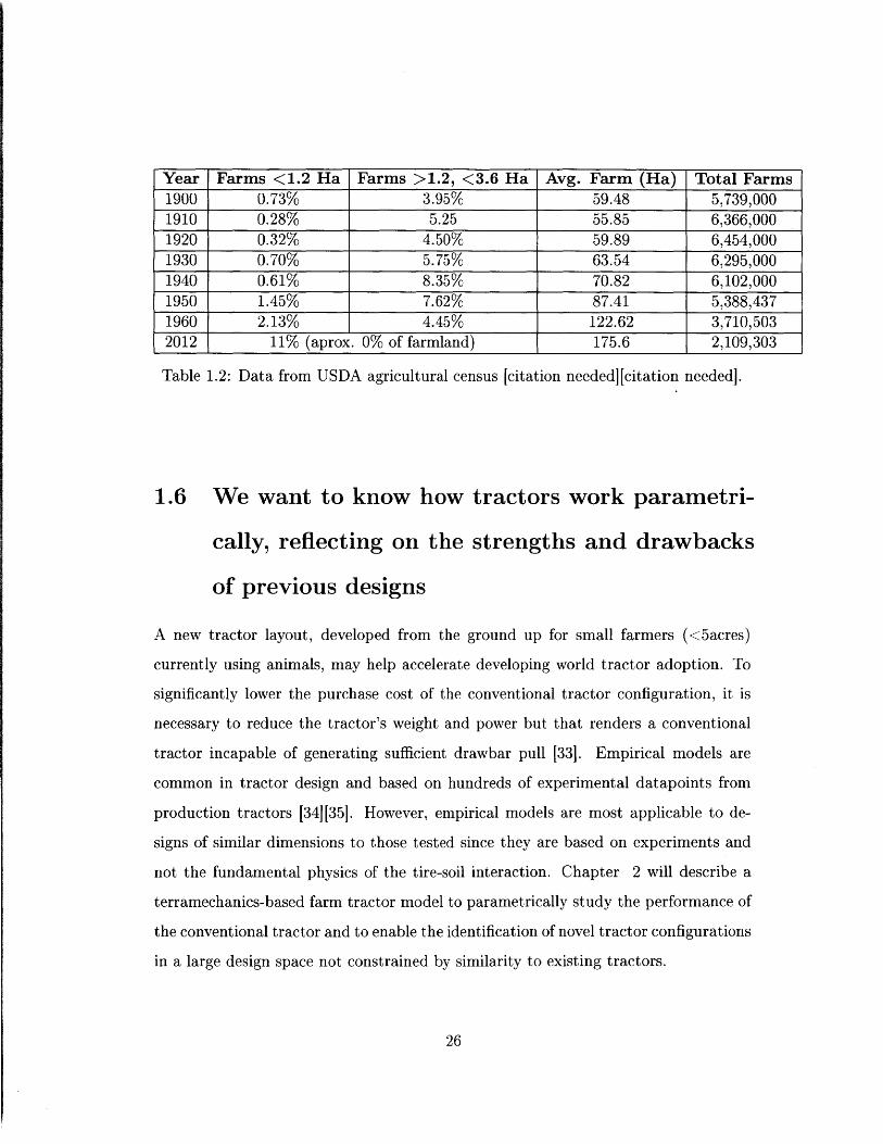
Year Farms <1.2 Ha Farms >1.2, <3.6 Ha Avg. Farm (Ha) Total Farms1900 0.73% 3.95% 59.48 5,739,0001910 0.28% 5.25 55.85 6,366,0001920 0.32% 4.50% 59.89 6,454,0001930 0.70% 5.75% 63.54 6,295,0001940 0.61% 8.35% 70.82 6,102,0001950 1.45% 7.62% 87.41 5,388,4371960 2.13% 4.45% 122.62 3,710,5032012 11% (aprox. 0% of farmland) 175.6 2,109,303

Table 1.2: Data from USDA agricultural census [citation needed][citation needed].

1.6 We want to know how tractors work parametri-

cally, reflecting on the strengths and drawbacks

of previous designs

A new tractor layout, developed from the ground up for small farmers (<5acres)

currently using animals, may help accelerate developing world tractor adoption. To

significantly lower the purchase cost of the conventional tractor configuration, it is

necessary to reduce the tractor's weight and power but that renders a conventional

tractor incapable of generating sufficient drawbar pull [331. Empirical models are

common in tractor design and based on hundreds of experimental datapoints from

production tractors [34][35]. However, empirical models are most applicable to de-

signs of similar dimensions to those tested since they are based on experiments and

not the fundamental physics of the tire-soil interaction. Chapter 2 will describe a

terramechanics-based farm tractor model to parametrically study the performance of

the conventional tractor and to enable the identification of novel tractor configurations

in a large design space not constrained by similarity to existing tractors.

26

Chapter 2

Tractor Theory

Important performance improvements can be attained in off-road vehicles by predict-

ing soil-tire interactions. In the case of farm tractors this usually means minimizing

power losses and damage to soil while maximizing tractive force. The modelling of a

tractor on soil can be separated into two related parts: calculating the distribution of

forces at all tires (which hold the tractor afloat and propel it forward) and calculating

the tire deformation, tire sinkage, and tire slippage at each individual tire. For force

distribution: This thesis contributes a strategy for distributing the forces among tires

without requiring iterative calculations in parallel with solving for individual tire-soil

performance. Reducing the number of calculations per iteration facilitates design ex-

ploration by allowing more configurations to be tested in the same amount of time.

For individual tire-soil interactions: This thesis uses a semi-empirical model proposed

by J.Y. Wong [36].

2.1 Qualitative description of importance of soil-tire

interaction in tractor design

Converting engine power to drawbar power (i.e. pulling force times forward speed)

results from converting engine power into traction force at the wheel-soil interface and

overcoming all internal mechanical losses plus motion resistance at the tire-soil inter-

27

face. While drivetrain mechanical losses in a small tractor can be under 5% , power

conversion at the tire-soil interface usually involves losses of 30 to 60% [371. A refined

terramechanic design can reduce the power lost at the soil-tire interfaces, something

especially critical for tractors that may initially appear to be underpowered. The two

major causes of power loss are soil deformation and slippage at the tire-soil interface

[361. The effects of soil deformation from wheeled vehicles are observed in the ruts

they leave behind. As the wheel rolls forward it deforms soil ahead of it (known as

"bulldozing"), this deformation requires energy but achieves no useful work. Slippage

occurs when the tangential speed of the tire contact points is faster than the forward

speed of the vehicle. Presence of at least minimal slippage is unavoidable because for

a thrust force to occur the tire must exert a shear force on the soil (therefore causing

soil deformation). When the shear strength of the soil is low relative to the trac-

tion being generated, the shear stress may result in large shear deformation and thus

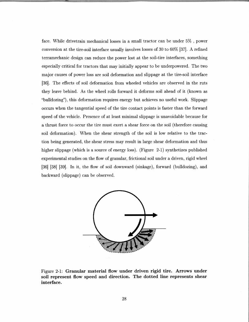
higher slippage (which is a source of energy loss). (Figure 2-1) synthetizes published

experimental studies on the flow of granular, frictional soil under a driven, rigid wheel

[36] [38] [39]. In it, the flow of soil downward (sinkage), forward (bulldozing), and

backward (slippage) can be observed.

Figure 2-1: Granular material flow under driven rigid tire. Arrows undersoil represent flow speed and direction. The dotted line represents shearinterface.

28

An efficient terramechanic design must strike a balance between sinkage and slip-

page The amount of power lost to slippage and lost to bulldozing are both correlated

to ground pressure but with opposite effects [40][36]. As ground pressure increases

the shear strength of soils with a frictional component (most natural soils) increases

and thus less shear deformation is provoked by a given shear stress. This reduces

energy lost to slippage. The counterpoint is that as ground pressure increases so

usually does the sinkage of the tire into the soil. This increases the energy lost to

bulldozing. Ground pressure is affected by tire vertical load but also by contact patch

dimensions. A larger contact patch will reduce contact pressure. This larger area can

be obtained by increasing tire diameter, and thus contact length for a given sinkage,

increasing tire width, and/or increasing tire compliance in the case of deformable

tires. Increasing tire width will increase the frontal area of the tire sinkage pattern,

this will be observed as wider tire rut which is a sign of more tire bulldozing occur-

ring for a given rut depth. Increasing tire diameter yields similar smaller contact

patch benefits than increasing width [36] but does not increase rut width, on the

other hand, larger diameter tires can come with packaging and inertial challenges.

Increasing tire compliance can increase both contact patch length and width for a

given tire load but usually comes at the cost of more mechanical losses within the

tire and higher slippage at the tire-soil interface due to tire deformation. A final note

on contact patch shape: if two tire-soil ruts have the same cross-sectional areas, the

deeper rut will experience higher bulldozing resistance (despite being less wide) all

else being equal because soil strength increases with depth. The ideal tire properties

(vertical load, width, diameter, compliance) minimize the sum of power consumed by

slippage, bulldozing and tire internal losses, while of course remaining mechanically

and economically practical with the tractor system.

29

2.2 Analytical model for interaction of single drive

tire with soil

The tire-soil model suggested here is as described by J.Y. Wong [36]. This model is

commonly accepted in terramechanics and has been improved for accuracy by several

groups, but often at the expense of requiring more experimental data [411.

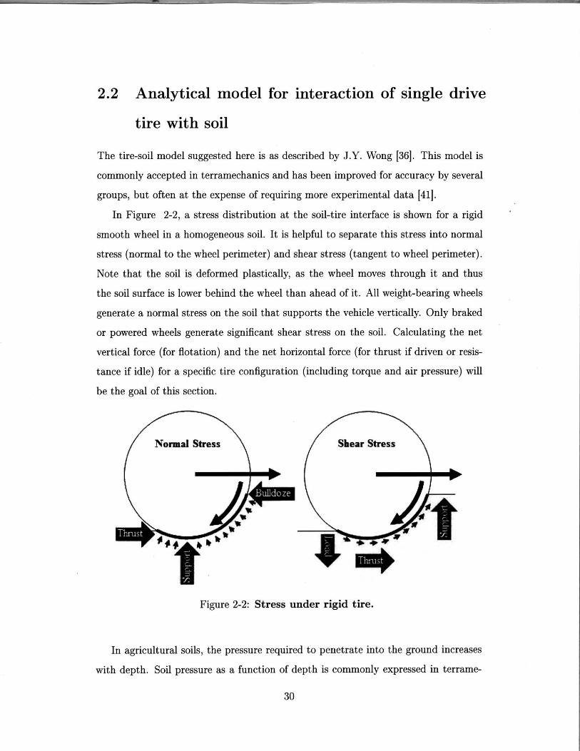
In Figure 2-2, a stress distribution at the soil-tire interface is shown for a rigid

smooth wheel in a homogeneous soil. It is helpful to separate this stress into normal

stress (normal to the wheel perimeter) and shear stress (tangent to wheel perimeter).

Note that the soil is deformed plastically, as the wheel moves through it and thus

the soil surface is lower behind the wheel than ahead of it. All weight-bearing wheels

generate a normal stress on the soil that supports the vehicle vertically. Only braked

or powered wheels generate significant shear stress on the soil. Calculating the net

vertical force (for flotation) and the net horizontal force (for thrust if driven or resis-

tance if idle) for a specific tire configuration (including torque and air pressure) will

be the goal of this section.

Shear Stress

Figure 2-2: Stress under rigid tire.

In agricultural soils, the pressure required to penetrate into the ground increases

with depth. Soil pressure as a function of depth is commonly expressed in terrame-

30

Normal Stress

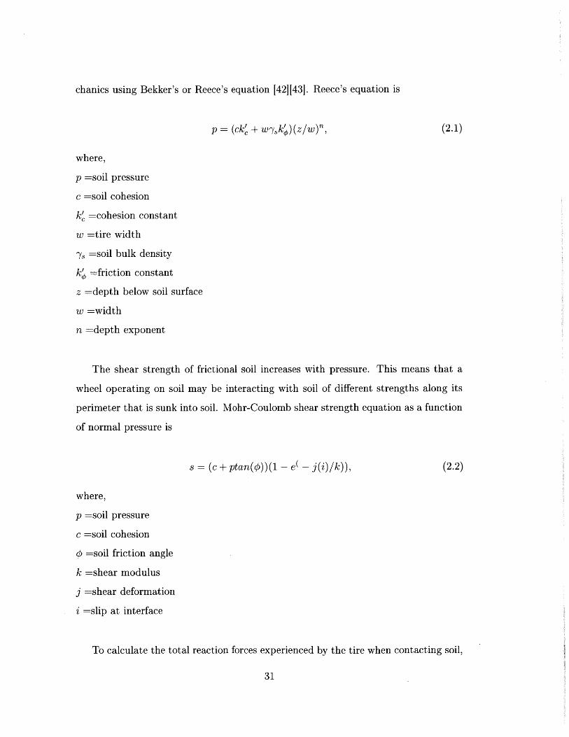
chanics using Bekker's or Reece's equation 142][431. Reece's equation is

p=(ck' + w-yk)(Z/W)", (2.1)

where,

p =soil pressure

c =soil cohesion

k' =cohesion constant

w =tire width

-y =soil bulk density

k =friction constant

z =depth below soil surface

w =width

n =depth exponent

The shear strength of frictional soil increases with pressure. This means that a

wheel operating on soil may be interacting with soil of different strengths along its

perimeter that is sunk into soil. Mohr-Coulomb shear strength equation as a function

of normal pressure is

s = (c + ptan(0))(1 - e( - j(i)/k)), (2.2)

where,

p =soil pressure

c =soil cohesion

# =soil friction angle

k =shear modulus

j =shear deformation

i =slip at interface

To calculate the total reaction forces experienced by the tire when contacting soil,

31

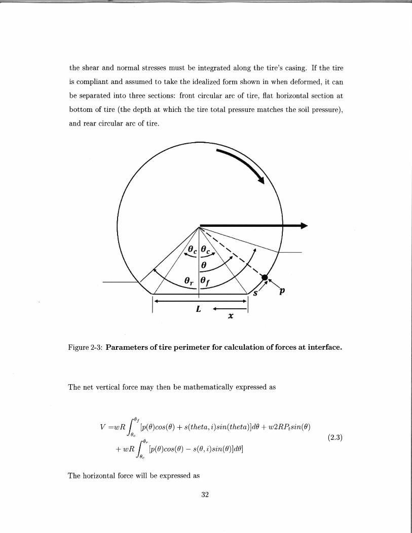
the shear and normal stresses must be integrated along the tire's casing. If the tire

is compliant and assumed to take the idealized form shown in when deformed, it can

be separated into three sections: front circular arc of tire, flat horizontal section at

bottom of tire (the depth at which the tire total pressure matches the soil pressure),

and rear circular arc of tire.

L -x

Figure 2-3: Parameters of tire perimeter for calculation of forces at interface.

The net vertical force may then be mathematically expressed as

OefV =wR [p(9)cos(9) + s(theta, i)sin(theta)]d9 + w2RPtsin(9)

oc (2.3)

+w Rj [p(O)cos(O) - s(O, i)sin(O)]dO]

The horizontal force will be expressed as

32

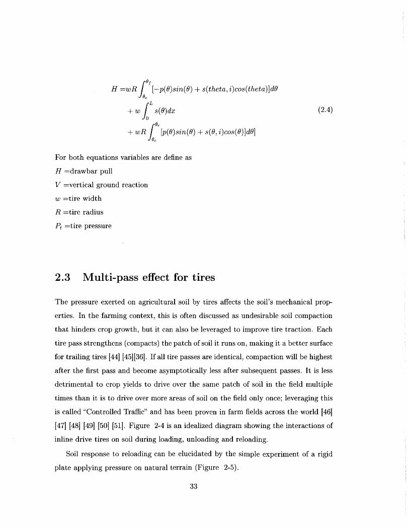
H =wR ] [-p(O)sin(O) + s(theta, i)cos(theta)]dOoc

+Wj s(O)dx (2.4)

+ wR [p(O)sin(O) + s(O, i)cos(O)]dO]0,

For both equations variables are define as

H =drawbar pull

V =vertical ground reaction

w =tire width

R =tire radius

Pt =tire pressure

2.3 Multi-pass effect for tires

The pressure exerted on agricultural soil by tires affects the soil's mechanical prop-

erties. In the farming context, this is often discussed as undesirable soil compaction

that hinders crop growth, but it can also be leveraged to improve tire traction. Each

tire pass strengthens (compacts) the patch of soil it runs on, making it a better surface

for trailing tires [441 [45][361. If all tire passes are identical, compaction will be highest

after the first pass and become asymptotically less after subsequent passes. It is less

detrimental to crop yields to drive over the same patch of soil in the field multiple

times than it is to drive over more areas of soil on the field only once; leveraging this

is called "Controlled Traffic" and has been proven in farm fields across the world [46]

[471 [48] [49] [50] [51]. Figure 2-4 is an idealized diagram showing the interactions of

inline drive tires on soil during loading, unloading and reloading.

Soil response to reloading can be elucidated by the simple experiment of a rigid

plate applying pressure on natural terrain (Figure 2-5).

33

Fixed Spec.: > Load1 Fixed Spec.: Load1

Despite greater W Calculate.

<Rolling Resistance, Rolling Resistance,

h2 > h, > Traction, Traction 1 z 2Se First a s

Sol properties above Z2 changed Soi properties above zjL changed

Illustration of tire-soil interaction and multi-pass effect used in

Mineral soil, 5cm radius plate

- First Loading- Second Loading-Third Loading -'

4e

.+0

2 4 6Sinkage, cm

Petawa Muskeg, 7.5cm

I-

U)(j)a.

1C

8

... First Loading- Second Loading

0 -Third Loading

0

00 5 10 15

Sinkage, cm

loading on natural soil deformation and

2.4 Conventional tractor dimensions and relevant forces

As discussed in sections Section 2.1, 2.2 and 2.3, the response of the soil to the

tractor on it depends on the forces the tractor is applying to the ground, tire/wheel

dimensions, and soil history. Calculation of the net forces to solve for at the tire-soil

interface requires modelling of the full tractor system. Under the assumption of the

tractor being a rigid body and its wheels will rest on the same plane with zero roll

angle (roll being the the tractor's longitudinal axis), the tractor free-body diagram

34

Figure 2-4:analysis

150

100

50

EZ

0)

radius plate

A0

Figure 2-5: Effect of repetitivestiffness. Data from [36]

5

20

can be simplified to include only:

" overall center of mass location and magnitude

" draft tool force direction, magnitude, and origin (center of pressure)

" location of ground contact points

" tractor orientation with respect to gravity (ground slope)

An example of this dimensions for a conventional tractor is shown in Figure 2-6.

Wr

R o XIWBf A

Br j XP y,

Vf HrI YpVT9 ypp

P

Figure 2-6: Full body diagram for farm tractor in 2D

The torque around the center of rotation at point B is then:

T = P(ypcos(a) - xpsin(a)). (2.5)

35

Overall, the net vertical force on both front wheels is:

1Vf = (WT(xcos(0) - ygsin(O))

+ P(yp + cos(t) - xpsin(a)) (2.6)

+ Wi(-x1 cos(O) - yisin(0))),

and the net vertical force on both rear wheels is:

V, = (WT(xrcos(O) + ygsin(9))If + Xr

+ P(-yp + cos(cv) + xpsin(a)) (2.7)

+ W((xi + x, + xf)cos() + yisin(0))).

It is assumed in the conventional tractor configuration that only the rear wheels

are driven. To move the tractor forward at a constant speed, the rear tires must

provide the net horizontal force:

H = Bf + B, + Pcos(a) + (WT + Wi)sin(0). (2.8)

The calculation of the actual wheel torque necessary to achieve H, and the calculation

of resistance forces Bf and B,, requires an analysis as described in section 3.1, 3.2

and 3.3.

2.5 Proposed generalized vertical load per tire cal-

culation

The calculation of tire vertical reaction forces shown in section 2.6 can be general-

ized for any statically stable configuration. A stable configuration in 3D space has

three or more wheels (support points in this study) on the ground with the vehicle's

effective center of gravity located inside the convex hull of all contact points. For

36

three support points, the problem is statically determinate and can be solved as a

simple rigid body problem where the net forces and moments over the vehicles are

zero. With four or more contact points (a fairly common occurrence) the problem

becomes statically indeterminate. An attempt to solve this as a rigid body will yield

four or more unknowns but only three equations. The conventional way of solving

this is to calculate the stiffness of the structure and contact points to find the con-

figuration of reaction forces that yields the least work (i.e. the least energy spent

deforming tractor and soil). In the case of a tractor on deformable soil (potentially

with pneumatic tires), a useful simplification for computer calculations is to assume

deformation will only occur at the wheels and soil, and that all support points have

equal stiffness properties. The problem is then simplified to finding all solutions that

generate zero net force and zero net moment around vehicle, and then identifying the

solution with the least energy spent deforming soil and tires. To efficiently estimate

the energy spent deforming tires and soil at each contact point, it is recommended to

select an exponent C. The energy spent deforming tires and soil is then:

E= ZVC, (2.9)i=1

where,

E =Energy spent deforming support points

V, =vertical ground reaction force at tire "n"

C =exponent to estimate energy deformation. Use 2 if idealizing support points as

springs.

If multiple solutions exist for the reaction forces at the tires (which will likely

be the case for four or more tires) then the solution recommended is the one that

minimizes the energy. The preferred solution V comes from Equation 2.10.

min E (2.10)V

where,

37

V =vector with vertical ground reaction forces for all tires

We can calculate the set of solutions for reaction forces at each tire for any vehicle

with three or more tires. This can be stated as a linear system:

pb + R = 0 (2.11)

where,

p =particular solution to problem. nxl vector.

b =Forces and torques not caused by support points. 3x1 vector

R =Forces and torques caused by support points. 3x1 vector

p will be solved for from R and b. The elements in R and b respectively are:

b, nxl vector of ones (2.12)

X1

b2 = . ,(2.13)

Tn

Y1

b3 Y2 (2.14)

bi

b = (-I) b2 ,(2.15)

b3

and

F g(m1 + mT + md) + Pz, (2.16)

38

My = x1 gm1 + xPPz - zpPx, (2.17)

Mx = x 1gm1 + xpPz + zpPy, (2.18)

F

R =My (2.19)

_MX

where,

n =number of tires (support points)

g =gravity acceleration

m, =mass of implement

mT =mass of tractor

md =mass of driver

Mx =moment around vehicle CG about x axis

MY =moment around vehicle CG about y axis

Px =longitudinal draft force from tillage tool

Py =lateral draft force from tillage tool

Pz =vertical draft force from tillage tool

xp =longitudinal distance from vehicle CG to tillage tool COP

zp =vertical distance from vehicle CG to tillage tool COP

xI =longitudinal distance from vehicle CG to tillage tool CG

xi =longitudinal distance from vehicle CG to tire "i" CG

yj =lateral distance from vehicle CG to tire "i" CG

Since the equation system may be indeterminate, the null space is then calculated.

This can be achieved through singular value decomposition or use of the "null()"

function in MATLAB,

Z = null(R). (2.20)

All mathematically valid solutions for the vertical reaction forces V at each tire

39

can then be obtained by inputting values of q in

V = p + Zq. (2.21)

The preferred solution V is that which minimizes deformation energy (Equation

2.10) as defined in Equation 2.9.

2.6 Proposed generalized horizontal load per tire cal-

culation

For soils with a frictional component (most natural soils), there is an approximately

linear relationship between a large range of values for normal pressure and for maxi-

mum traction generated (Figure 2-7). This can be leveraged to accelerate calculations

of tractor slip, sinkage, and power by distributing the drawbar pull amongst all tires

proportionally to the vertical reaction force on each tire.

The drawbar pull that each drive tire will be "assigned" to pull can then be cal-

culated as:

Hn = x Dn(2.22)k DiE D,

where,

Hn = Drawbar pull tire "n" must generate.

Dn = Vertical reaction force at tire "n"

k =number of drive tires in vehicle.

This idealizes the power distribution among the tires to get an estimate of the

maximum drawbar pull a tractor configuration could achieve. For example, if a tractor

has a simple differential between two drive tires, the drawbar pull distribution strategy

suggested here would not consider that both tires must receive the same torque.

40

2.7 Variable sensitivity of tractor-soil model as im-

plemented

The model presented in this section is highly non-linear and accepts many tractor

parameters as inputs. To give the reader a better feel for the influence of key design

parameters on a small tractor's performance, sensitivity studies for drawbar pull and

tractive efficiency are shown in Figure 2-7 and 2-8. Soil data used for this sensitivity

analysis was obtained from [521.

Tractive efficiency is the efficiency in converting power at the wheel axle into useful

work. It is defined as:

Fpulling * Vforwardrqtract. = els '(2.23)

Pw heel s

where,

etatract. =tractive efficiency

Fpulling =pulling force generated by tire

Vforward =actual forward speed of vehicle

Paheels =power delivered to the wheel

Some behaviors that are worth highlighting:

" Drawbar pull increases approximately linearly with vehicle mass. This behavior

becomes non-linear with mass is increased or decreased too much.

r Tractive efficiency is highest when mass is optimized to a happy medium.

" For a vehicle operating below its maximum drawbar pull,.tractive efficiency may

be improved by increasing tire width or radius.

" Drawbar pull increases with tire radius.

" Drawbar pull is maximized by an optimal tire width (not too much or too little).

41

8000 _- texture: clay; cover: maize stubble-Tire Width--Tire Radius

Z7000 Vehicle Mass

-Rear Biasa 6000 -Tool Location

5000 I

4000.

-50 -25 0Variation (%)

25 50

6000 texture: silty loam; cover: maize stubble-Tire Width+Tire Radius

5000 +Vehicle MassRear Bias

1 :-Tool Location%4000

S3000

2000a-50 -25 0 25 50

Variation ()

9000

8000

Z700o

6000

5000

4000(

3000--50

Values at 0% VariationTire Width Front: 132mmTire Width Rear: 203.2mmTire Radius Front: 272mmTire Radius Rear: 272mmVehicle Mass: 850kgRear Bias: 0.55 (proportion of total mass)Tool Location: 0.6m behind rear axleTool Mass: 100kg (constant)Tool soil depth: 8" (constant)

texture: loamy sand; cover: maize stubbleiTire Width

-Tire Radius-Vehicle Mass

Rear BiasTool Location

-25 0Variation (%)

Figure 2-7: Sensitivity analysis of drawbar pull at 15% slip for a conventionalsmall tractor [321. Data generated using model created for this thesis.Note that drawbar pull (net horizontal force) is approximately linearlyrelated to weight for a large range of values and different soils.

2.8 Flowchart of tractor design exploration model

The algorithm implemented to combine the tractor force distribution and tire-soil

solver is shown in Figure 2-9. Note that the vehicle's weight and tool draft are

distributed among all tires in the initial steps and then held constant throughout the

analysis.

42

25 50

texture: clay; cover: maize stubble

Rear Bmas-Tool Location(

-25 0 25 50

70

Variation (%)

texture: silty loam; cover: maize stubble

-Tool Location

-25 0 25 50Variation (%)

Values at 0% VariationTire Width Front: 132mmTire Width Rear: 203.2mmTire Radius Front: 272mmTire Radius Rear: 272mmVehicle Mass: 850kgRear Bias: 0.55 (proportion of total mass)Tool Location: 0.6m behind rear axleTool Mass: 100kg (constant)Tool soil depth: 8" (constant)

texture: loamy sand; cover: maize stubble

~65'

560-

55.-Tire Width

50 - -Tire Radius-e+Vehicle Mass

[ 45 IlRear Bias-*-Tool Location

40-50 -25 0 25 50

Variation (%)

Figure 2-8: Sensitivity analysis for tractive efficiency at a drawbar pull of3000N. Data generated using model created for this thesis. Note thatmaking a vehicle too heavy can be detrimental to efficiency.

43

90

80

.070

60

50,

40-50

40

~35230

25

.020

15

10-5 0

- ieWidths+Vehicle Mass

-Tire Width+Tire Radius+Vehicle Mass

+erBi

ANo

Vehicle Inputs Convert unitsStart Tire Inputs on inputs as valid?

Implement Inputs needed-Soil Inputs .

e

Caslculate All vertical Ye swertical load loads greatern

per wheel than zero?

No

A

oes any idle Distribute sum ofdwheel sink Yes idle wheel resistanc

more than its wheels proportionaradius? load on

No

A

Calculate sinkage androlling resistance

(horizontal force) foridle wheels

Yes

-~Ir

Calculate torque,sinkage, rolling

resistance, and slip fordriven wheels

Does any Calculatedriven wheel Yes power and

sink more than tractiveits radius or efficiency

have full slip? for vehicle

No

A

Figure 2-9: Process flow in implemented MATLAB model to simulate afarm tractor on soil.

44

rawbar load ande among drivenIly to the verticalthem.

IPlot Save Termination

Outputs outputs Message End

Chapter 3

Validation of Tractor Model with

Published Data

The model discussed in Chapter 2 may be used to evaluate and inform design of farm

tractors. To verify the model's accuracy, in this chapter its outputs are compared to

existing data on conventional tractors. By conventional we mean a four wheeled, rear

wheel drive tractor with a trailing implement.

3.1 Comparison to specific tractor tests

The model presented in Chapter 2 has been evaluated against published experiments.

The model magnitudes and trends show useful agreement to the experimental data

available for specific tractor configurations (Figure 3-1). In particular, the model

has its best accuracy between 5% and 20% slip, which is the range recommended for

farm tractor operation [36][37][40][321.

Experiment data was obtained from [53][54], where four different-sized produc-

tion tractors were tested in various soil conditions. To test a tractor's drawbar pull

performance, it would tow a "braking" tractor behind via an instrumented cable.

The braking tractor would be operated and adjusted to generate only the desired

horizontal drawbar pull force on the tractor being evaluated.

45

Comparison of Model to Experimental Data50

45

40 j

35

25

1 5

0 1 ---- -- -0 --slip (%)

20 25

Model: 57001bs TractorExperiment: 5700lbs Tractor

; Model: 9000Ibs Tractor4 Experiment: 9000lbs Tractoro Model: 113001bs Tractor& Experiment: 113001bs Tractor

Model: I 50001bs TractorExperiment: 15000lbs Tractor

30

Figure 3-1: Comparison of tractor model as described in Chapter 2 topublished tractor experiments. Model has its best accuracy between 5%and 20% slip, which is the range recommended for farm tractor operation[36][37][40][32].

3.2 Comparison to design trends

Through modeling and review of historical data, it is found that for a conventional

small tractor (four wheels, rear wheel drive, trailing farm implement) the ideal weight

distribution for efficient drawbar pull occurs at about 30% weight on the front wheels

and 70% weight on the rear wheels when doing a towing operation.

Data Tractor Model. Figure 3-2 summarizes a study for the effect on tractive

efficiency of weight, weight distribution, and draft magnitude. The weight distribution

shown in Figure 3-2 does not account for weight transfer during operation (i.e. it

is a statically measured weight distribution at zero drawbar pull). The effective

weight distribution during operation is accounted for during simulation calculations,

however. Note that when moving along the "Weight distribution on rear axle (%)"

axis, power required to move (shading value) is reduced by shifting weight backwards

until it asymptotes at around 70% of the tractor weight on back wheels. Placing more

46

,.o. O .0- 0. - 0 --04-00

t3 -43- W -,.. _M a 1:

0g

Air AA p A--t -&A- A-A- A -a -- "

a

R d - dAr>

44

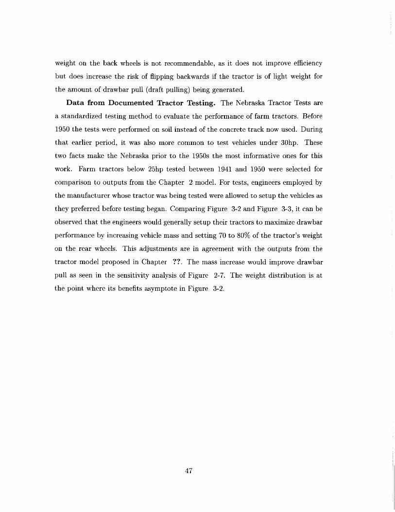
weight on the back wheels is not recommendable, as it does not improve efficiency

but does increase the risk of flipping backwards if the tractor is of light weight for

the amount of drawbar pull (draft pulling) being generated.

Data from Documented Tractor Testing. The Nebraska Tractor Tests are

a standardized testing method to evaluate the performance of farm tractors. Before

1950 the tests were performed on soil instead of the concrete track now used. During

that earlier period, it was also more common to test vehicles under 30hp. These

two facts make the Nebraska prior to the 1950s the most informative ones for this

work. Farm tractors below 25hp tested between 1941 and 1950 were selected for

comparison to outputs from the Chapter 2 model. For tests, engineers employed by

the manufacturer whose tractor was being tested were allowed to setup the vehicles as

they preferred before testing began. Comparing Figure 3-2 and Figure 3-3, it can be

observed that the engineers would generally setup their tractors to maximize drawbar

performance by increasing vehicle mass and setting 70 to 80% of the tractor's weight

on the rear wheels. This adjustments are in agreement with the outputs from the

tractor model proposed in Chapter ??. The mass increase would improve drawbar

pull as seen in the sensitivity analysis of Figure 2-7. The weight distribution is at

the point where its benefits asymptote in Figure 3-2.

47

20

18

16

44 -IS

2.5 -12

2-210

1.5 - 8

6.013000

4

20002

30 2

70 80 90 0 draft magnitude (N)Weight distribution on rear axle (%)

Figure 3-2: Simulation data for one million tractor configurations. Demon-strates that optimal weight distribution for drawbar pull is about 70% onrear wheels. The semi-transparent purple frontier on the left on left repre-sents where tractor wheels slip fully without generating progress or whereany wheel sinks past its radius. The semi-transparent brown frontier onthe right represents when the tractor flips backwards.

48

<25hp Wheeled Tractors, 1941-1950 Nebraska Tests on Dirt Track3000 Rear Bias Ballasted (%) a Rear Bias Factory (%) &Mass Ballasted (kg) O Mass Factory (kg) 90

802500 8

70

2000 60'U 50

1500 5-40

1000 30

20500

00 0

104~ i P '*

Figure 3-3: Data compiled from Nebraska Tractor Test archives. Noticethat, for testing, company engineers would ballast their tractors placeabout 70 to 80% of the total weight on the rear wheels.

49

50

Chapter 4

Insights into small tractor design

4.1 Comments on past and current tractor designs

This section will discuss some layout innovations and challenges that guided tractor

design between 1900 and 1940 to deliver the conventional small tractor we are familiar

with today.

4.1.1 "Fulcrum and Lever" towing adjusts drive tire vertical

loading in proportion to pulling force.

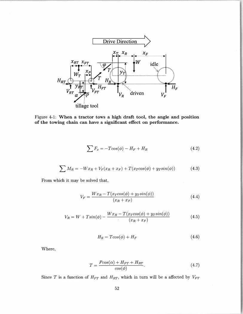
In 1916 Nilson Tractor Company introduced their "Fulcrum and Lever" hitch system.

The goal was to use the draft force from the implement being towed to increase the

downward force on the drive wheels. This would in turn increase the maximum pulling

force the drive wheels could generate (the relationship between normal pressure on soil

and shear strength at the tire-soil interface is better described in Chapter 2. Nilson's

system attached implement towing bar or chain (which was under pure tension), much

higher above the ground than other similar sized tractors had before. The effects of

doing so on the vertical load at the rear wheel can be quantified from the free body

diagram in Figure 4-1 (where variables are labeled) as

Z Fy = -W + -Tsin( ) + VF + VR, (4.1)

51

I Drive Direction

XT XR XF

XRT XFT 41W idle

HRT HR

VRT P FT

tillage tool

VR driven

Figure 4-1: When a tractor tows a high draft tool, the angle and positionof the towing chain can have a significant effect on performance.

SF = -Tcos(o) - HF + HR

5 MR = -WXR + VF(XR + XF) + T(xTcOS() + YT sin(O))

(4.2)

(4.3)

From which it may be solved that,

VF =WXR - T(xTcOS() + yTsin(O))

(XR - XF)(4.4)

VR= W + Tsin($) - WXR - T(xTcos($) + yTsin())

(XR+ XF)

Where,

(4-6)HR = Tcos() + HF

Pcos(a) + HFT + HRT

cos()(4.7)

Since T is a function of HFT and HRT, which in turn will be a affected by VFT

52

IHF

VF

(4.5)

and VRT, respectively, it is useful to calculate these values as well. When focused on

the towed cart:

S F= -Psin(a) - WT + VFT + VRT + Tsi(O), (4.8)

5 F. = -Pcos($) - HFT - HRT + Tcos(O), (4.9)

SMFT= Pxpsin($) - Pypsin() + WXFT - VRT (XRT + XFT), (4.10)

from which it may be solved that,

VRT= -Pxpsin($) + Pypsin($) - WXFT

XRT + XFT

VFT = P +W- -Pxpsin(O) + Pypsin($) - WXFT + VRT (4.12)FT=Psin(ci)+WT -T sin($3- XRT. 12F

XRT + XFT

The vertical reaction forces calculated at each tire, VFT/ 2 and VRT/2, are im-

portant because they will affect the motion resistance and thrust experienced by the

vehicle. Since drawbar pull increases approximately linearly with vertical tire loading

(as seen in Chapter ?? and Figure 2-7), it is proposed in this thesis that a first

approach for drawbar pull capacity of a tractor distributes total required drawbar

pull among all drive tires proportionally to their vertical vertical load

From the equations presented above, several important mechanical design obser-

vations may be made about raising the towing attachment point yT on the tractor:

. It will likely increase traction. Raising the attachment point will increase

the vertical reaction force on the rear tire VR, which in turn increases the max-

imum shear strength of the soil and usually increases the generated drawbar

pull (see Chapter 2). The 1916 Nilson tractor featured three rear wheels: a

53

wide drum-wheel with a less wide wheel on each side. This wide contact patch

helps reduce the risk of increasing the vertical load on the rear wheels to the

point that it is detrimental to maximum drawbar pull (due to excessive wheel

sinkage).

" It will worsen safety of operation. Raising the attachment point will de-

crease the vertical reaction force on the front tire VF. This reduces the steering

authority of the front wheels and increases the risk of the tractor flipping back-

wards during operation and crushing the driver.

" It will reduce the draft of the trailing tool. When a tillage tool is towed

by a tractor, the tractor must overcome the horizontal tillage force but also the

horizontal force generated by rolling the implement wheels in soil (see E F,.

Raising the tractor attachment point YT decreases VFT, which in turn reduces

wheel sinkage and therefore HFT (see Chapter 2).

It may be recalled from Chapter 2 that farm tractors usually have a tractive

efficiency of about 0.3 to 0.7 on agricultural soils. Where tractive efficiency is defined

as etarct. Pforce*peed (Equation 2.23 in Chapter 2.

Rearranging the terms and using the pulling force (PForce) generated by the

tractor in Figure 4-1 this becomes:

Tcos(O)VpeedPwheels = (4.13)

71 tract.

It may be observed that rigidly mounting the tillage tool behind the tractor would

eliminate the need for implement wheels and would place the implement's weight

and the vertical component of P directly on the tractor's wheels. This has several

important effects on the tractor's drawbar pull performance:

* Eliminating the implement wheels eliminates the terms HFT and HRT from the

calculation of T, thus reducing the required pulling force which is proportional

to the required pulling power.

54

" Placing the implement's weight WT directly on the vehicle would increase the

magnitude of W and reduce the distance XR. This can then increase the verti-

cal load on the rear drive wheels VR (increasing it is usually beneficial) without

increasing the vertical load front idle wheels VF (increasing it is usually detri-

mental).

" Likewise, the downward component of draft force P can increase VR without

increasing VF.

The case of the implement being rigidly attached to the tractor will be more

carefully studied in the next subsection.

4.1.2 Central tool mounting increases safety but can be detri-

mental to traction in conventional tractors.

In 1939 Ford released the 9N tractor which featured the "Three-Point Hitch" trailing

tool attachment system patented by Harry Ferguson. An updated version of this

tractor with the same attachment system, the Ford 8N released in 1948, would go on

to become the single best selling tractor model in the USA. The "three point hitch"

is the standard implement attachment system for tractors. In 1948, a much lighter

and differently designed tractor was also released: the Allis-Chalmers Model G. The

Model G featured a tubular frame, an engine mounted behind the rear wheels, and a

tool attachment point in front of the driver between the front and rear axles.

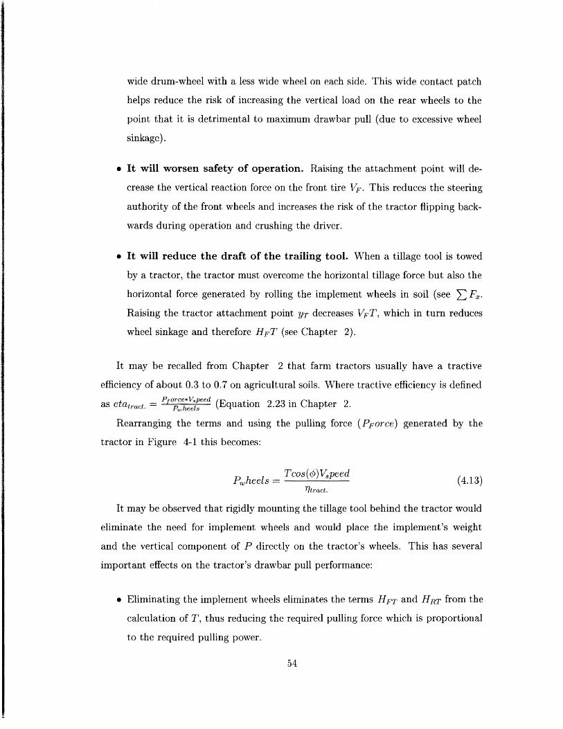
Table 4.1 shows a comparison on specifications for both these tractors.

55

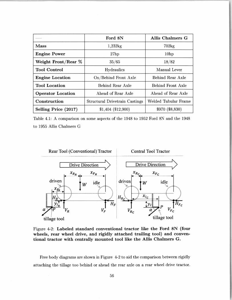
Table 4.1: A comparison on

to 1955 Allis Chalmers G

some aspects of the 1948 to 1952 Ford 8N and the 1948

Rear Tool (Conventional) Tractor Central Tool Tractor

Drive Direction Drive Direction

XRR XFRXRc XFC

driven driven idlex W

HR

HF . Fca VF

ill VF tiVg too

Figure 4-2: Labeledwheels, rear wheeltional tractor with

standard conventional tractor like the Ford 8N (fourdrive, and rigidly attached trailing tool) and conven-centrally mounted tool like the Allis Chalmers G.

Free body diagrams are shown in Figure 4-2 to aid the comparison between rigidly

attaching the tillage too behind or ahead the rear axle on a rear wheel drive tractor.

56

U

Ford 8N Allis Chalmers G

Mass 1,232kg 702kg

Engine Power 27hp 10hp

Weight Front/Rear % 35/65 18/82

Tool Control Hydraulics Manual Lever

Engine Location On/Behind Front Axle Behind Rear Axle

Tool Location Behind Rear Axle Behind Front Axle

Operator Location Ahead of Rear Axle Ahead of Rear Axle

Construction Structural Drivetrain Castings Welded Tubular Frame

Selling Price (2017) $1,404 ($12,900) $970 ($8,830)

L age Lo tillaore tool

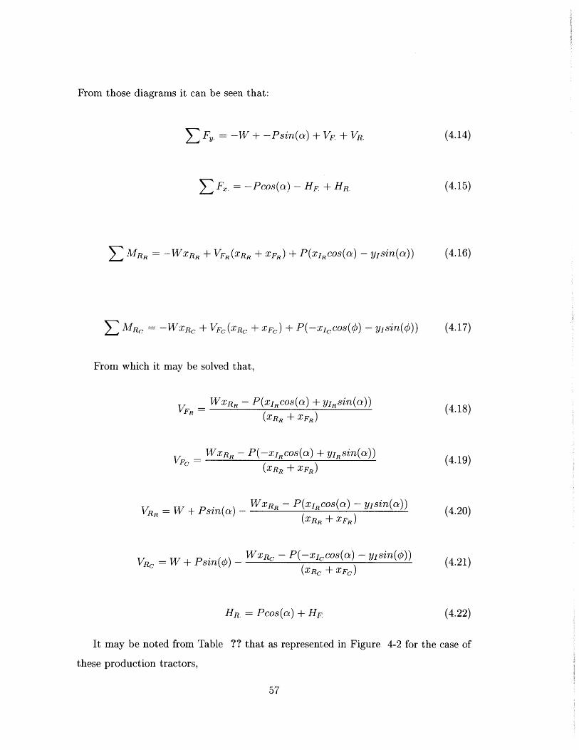
From those diagrams it can be seen that:

E Fy. = -W + -Psin(a) + VF + VR.

S F, = -Pcos(a) - HF + HR,

S MRR -WXRR + VFR (XRR + XFR) + P(XIRCOS(a) - y;sin(a))

5 MR =-WXRC + VFC(XRC + XFC) + P(-XIcCOS() - yjsin())

From which it may be solved that,

VFR

VFc

WX RR - P(XIRcos(a) YIR sin(a))

(XRR + XFR)

WXRR - P(-hxRcos(a) + ylRsin(a))

(XRR + XFR)

VRR = W + Psin(a) -

VRC W +

WXRR - P(XIRcos(a) - ysin(a))

(XRR XFR)

Psin(O) - WXRC - P(-xccos(a) - y 1sin(o))

(XRC + XFC)

HR. = Pcos (a) + HF. (4.22)

It may be noted from Table ?? that as represented in Figure 4-2 for the case of

these production tractors,

57

(4.14)

(4.15)

(4.16)

(4.17)

(4.18)

(4.19)

(4.20)

(4.21)

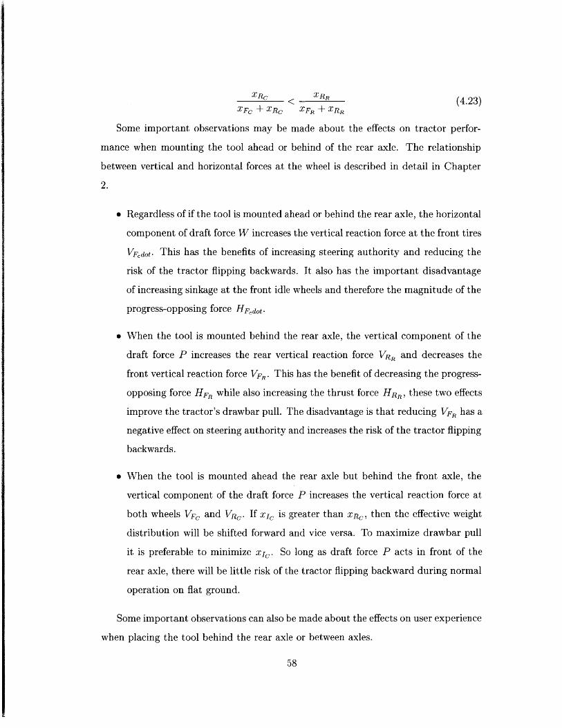
XRC RR(4.23)

XFC + XRC XFR + XRR

Some important observations may be made about the effects on tractor perfor-

mance when mounting the tool ahead or behind of the rear axle. The relationship

between vertical and horizontal forces at the wheel is described in detail in Chapter

2.

" Regardless of if the tool is mounted ahead or behind the rear axle, the horizontal

component of draft force W increases the vertical reaction force at the front tires

VFedOt. This has the benefits of increasing steering authority and reducing the

risk of the tractor flipping backwards. It also has the important disadvantage

of increasing sinkage at the front idle wheels and therefore the magnitude of the

progress-opposing force HFdOt-

* When the tool is mounted behind the rear axle, the vertical component of the

draft force P increases the rear vertical reaction force VR, and decreases the

front vertical reaction force VF,. This has the benefit of decreasing the progress-

opposing force HFR while also increasing the thrust force HR,, these two effects

improve the tractor's drawbar pull. The disadvantage is that reducing VFR has a

negative effect on steering authority and increases the risk of the tractor flipping

backwards.

* When the tool is mounted ahead the rear axle but behind the front axle, the

vertical component of the draft force P increases the vertical reaction force at

both wheels VFC and VR,. If xj, is greater than XRC, then the effective weight

distribution will be shifted forward and vice versa. To maximize drawbar pull

it is preferable to minimize xj,. So long as draft force P acts in front of the

rear axle, there will be little risk of the tractor flipping backward during normal

operation on flat ground.

Some important observations can also be made about the effects on user experience

when placing the tool behind the rear axle or between axles.

58

User experiences advantages of tool between axles

" Placing the implement (tillage tool) in between both axles, in front of the oper-

ator (especially in a tubular frame that allows good ground visibility) makes it

easier for the operator to keep a close eye on the quality of the operation with-

out needing to look over their shoulder. This visual advantage also facilitates

the operator having manual control over the tool's position since they can more

easily supervise it and make small adjustments.

" Placing the implement in between both axles, prevents the tractor from flipping

backwards, which is a major source of injuries and fatalities in farming [55J. This

is not only safer but also allows the operator to utilize the maximum drawbar

pull from their vehicle without this becoming a potential hazard.

" Placing the implement between both axles can reduce the total length of the

vehicle. This can be beneficial for operations in close quarters.

" Placing the implement between both axles enables mounting the engine behind

the rear axle while still maintaing good weight distribution (see Figure 3-2 in

Chapter 2). Putting the engine behind the operator (who usually sits ahead of

the rear axle in modern tractors) allows better forward visibility and prevents

engine heat, fumes, and noise from being blown into the operator's face while

driving.

User experiences advantages of tool behind rear axles

* Placing the implement (tillage tool) behind the rear axle, especially in combi-

nation with hydraulics, makes it easier to pick up and drop off many farming

implements. The driver need only reverse the implement-less tractor towards

and implement, lock the implement attachment points, and use the hydraulics

to lift the implement and drive away. When selling the 8N, Ford advertised an

implement could be mounted in less than one minute.

59

" Placing the implement behind the rear axle does not constrain the length of the

implement. This in an important advantage for more powerfull tractors that

can pull several ground engaging "bottoms" at once.

" Placing a ground-engaging implement behind the rear axle (and therefore be-

hind the driver) minimizes the amount of dirt that is kicked up into the driver

and into the tractor.

" Placing the implement behind the driver places the driver further away from the

moving parts of the implement. This can be especially important for implements

that have moving parts powered by the engine.

Finally, some comments on manufacturing when the farming implement is placed

behind the rear axle or between axles. For more information on preferred weight

distributions see (see Figure 3-2 in Chapter 2).

* Placing the implement (tillage tool) behind the rear axle makes it beneficial

for weight distribution to have the engine near the front axle. Since power is

delivered to the ground at the rear wheels this means the engine and trans-

mission castings together span the full length of the tractor. Using the engine

and transmission casting as the structural "frame" of the tractor minimizes the

amount of components, which facilitates fabrication and reduces mass, both of

which help lower production costs and the latter can improve performance [7].

* Placing the implement (tillage tool) between axle makes it beneficial for weight

distribution to have the engine near the rear axle. This can reduce the structural

demands on the tractor since torque is being generated (at the engine) where it

is needed (the rear axle). This then can lighten the tractor frame ahead of the

rear axle.

* Placing the implement (tillage tool) behind the rear axle can facilitate packag-

ing. The drive axle, hydraulics, and power take-off (PTO) shaft are all around

the same location where engine power is being delivered. Additionally, the space

60

behind the rear axle can be fully dedicated to the implement, its attachment

linkages, and its power sources (hydraulics and PTO). The space between both

axles must be share with other objects including the operator, the operator

controls (along with their transmission lines), and the tractor frame.

4.1.3 Inline and side-by-side drive wheels each have their ad-

vantages.

In this section the side-by-side drive wheels are qualitatively compared against inline

drive wheels. To facilitate clear discussion, three default configurations have been

selected:

" Side-by-side drive wheels are represented by the configuration of a conven-

tional tractor: four wheels, rear wheels are driven, trailing implement.

" Inline drive wheels (I) is an all-wheel-drive, four wheeled tractor with front

wheel steering and a trailing implement.

" Inline drive wheels (II) is a configuration akin to an all-wheel-drive, two-

wheeled motorcycle with outrigger support wheels, and a trailing implement.

This layout would be similar to "f" in Figure 4-3 but with only front wheel

steering.

Advantages of side-by-side drive wheels

* Tighter turning. This happens in a conventional layout for two reasons:

smaller front wheels (advantage vs. Inline A), and ability to steer with brake

pedals (advantage vs. Inline B). For a tractor to take best advantage of inline

drive wheels, all drive wheels must be of similar size. In a four wheeled tractor,

the front wheels are usually a small diameter to prevent them from hitting the

tractor frame during tight turning (during a steered turn, the rearmost part of

the inside front tire swings toward the tractor). Making the front wheels larger

to match the size of the rear wheels would increase the tractor's turning radius

61

if nothing else was changed. Most tractors are equipped with a rear differential

and the two rear drive wheels can be braked separately. Applying the brake on

just one wheel causes the tractor to make a tight turn around that wheel.

o Simpler construction. Side-by-side drive wheels allow easy use of a standard

differential and a drivetrain layout similar to automobiles. When front (steered)

wheels are driven, additional linkages must be added to the powerline to enable

steering. Since most implements are attached closely behind the rear axle,

having all torque delivered to that axle shortens the load path between the

implement and the traction force.

o Well suited to weight transfer from rear mounted tool. A tillage tool

attached behind the tractor will cause the effective weight distribution of the

tractor to shift rearward (as described in the previous subsection). This added

vertical load on the rear wheels can increase their maximum tractive force. The

opposite effect is occurring to the front wheels, which can reduce the benefits

of inline drive wheels.

Advantages of inline drive wheels

9 Higher tractive efficiency. The front drive wheel will compact the soil for

the trailing drive wheel. This allows the trailing drive wheel to generate higher

thrust while also sinking less into the soil 1441. This is described in more detail

in Chapter 2.

9 Smaller track width. A two-wheeled motorcycle-type layout (inline layout I)

minimizes the vehicles width while still having two full size drive wheels.

e Less damage to crops. Inline drive wheels will usually cause less damage to

crop soil than other comparable configurations. In the case of inline I: a lighter

vehicle can achieve the same drawbar pull due to all wheels being driven [441.

In the case of inline I: the amount of drive wheel "traffic" lanes can be reduced

since only one lane is created by each fresh tractor pass. Minimizing traffic

lanes is the essence traffic control strategies [461 [471.

62

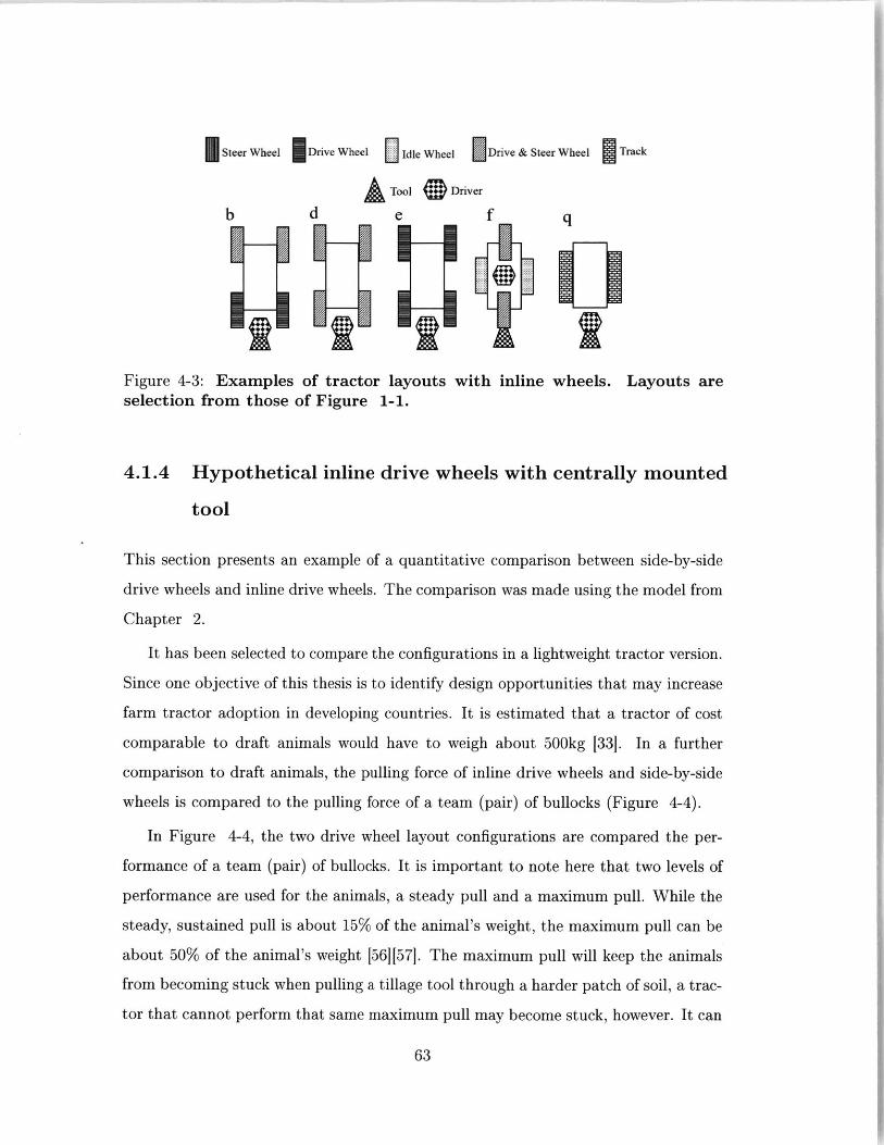
Steer Wheel Drive Wheel Id Wheel Drive & Steer Wheel Track

Tool Driver

b d e f q

Figure 4-3: Examples of tractor layouts with inline wheels. Layouts areselection from those of Figure 1-1.

4.1.4 Hypothetical inline drive wheels with centrally mounted

tool

This section presents an example of a quantitative comparison between side-by-side

drive wheels and inline drive wheels. The comparison was made using the model from

Chapter 2.

It has been selected to compare the configurations in a lightweight tractor version.

Since one objective of this thesis is to identify design opportunities that may increase

farm tractor adoption in developing countries. It is estimated that a tractor of cost

comparable to draft animals would have to weigh about 500kg [33]. In a further

comparison to draft animals, the pulling force of inline drive wheels and side-by-side

wheels is compared to the pulling force of a team (pair) of bullocks (Figure 4-4).

In Figure 4-4, the two drive wheel layout configurations are compared the per-

formance of a team (pair) of bullocks. It is important to note here that two levels of

performance are used for the animals, a steady pull and a maximum pull. While the

steady, sustained pull is about 15% of the animal's weight, the maximum pull can be

about 50% of the animal's weight [561[571. The maximum pull will keep the animals

from becoming stuck when pulling a tillage tool through a harder patch of soil, a trac-

tor that cannot perform that same maximum pull may become stuck, however. It can

63

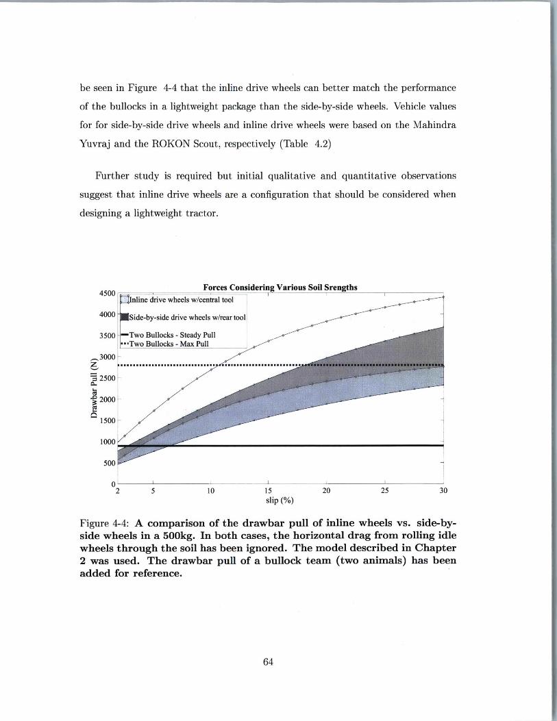
be seen in Figure 4-4 that the inline drive wheels can better match the performance

of the bullocks in a lightweight package than the side-by-side wheels. Vehicle values

for for side-by-side drive wheels and inline drive wheels were based on the Mahindra

Yuvraj and the ROKON Scout, respectively (Table 4.2)

Further study is required but initial qualitative and quantitative observations

suggest that inline drive wheels are a configuration that should be considered when

designing a lightweight tractor.

Forces Considering Various Soil Srengths4500

40 4Inine drive wheels w/central tool

4000 Side-by-side drive wheels w/rear tool

3500 -- Two Bullocks - Steady Pull-Two Bullocks - Max Pull

,3000

2500 -..........

2000-

1500 --

1000

500

02 5 10 15 20 25 30

slip (%)

Figure 4-4: A comparison of the drawbar pull of inline wheels vs. side-by-side wheels in a 500kg. In both cases, the horizontal drag from rolling idlewheels through the soil has been ignored. The model described in Chapter2 was used. The drawbar pull of a bullock team (two animals) has beenadded for reference.

64

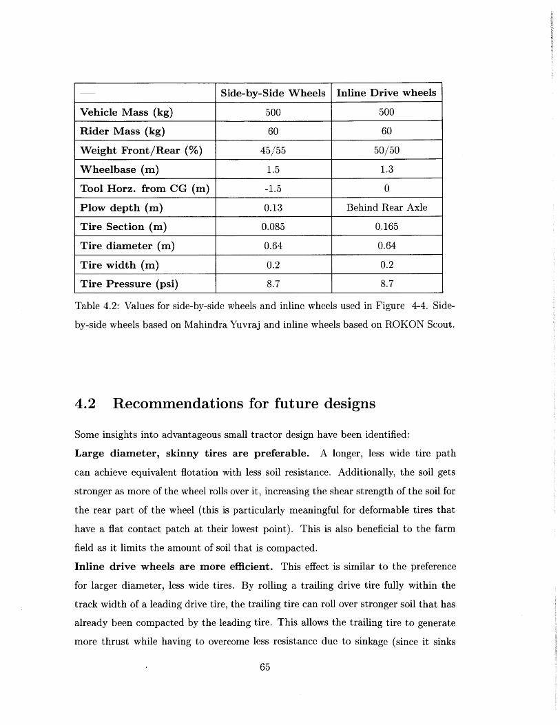
Side-by-Side Wheels Inline Drive wheels

Vehicle Mass (kg) 500 500

Rider Mass (kg) 60 60

Weight Front/Rear (%) 45/55 50/50

Wheelbase (m) 1.5 1.3

Tool Horz. from CG (m) -1.5 0

Plow depth (m) 0.13 Behind Rear Axle

Tire Section (m) 0.085 0.165

Tire diameter (M) 0.64 0.64

Tire width (m) 0.2 0.2

Tire Pressure (psi) 8.7 8.7

Table 4.2: Values for side-by-side wheels and inline wheels used in Figure 4-4. Side-

by-side wheels based on Mahindra Yuvraj and inline wheels based on ROKON Scout.

4.2 Recommendations for future designs

Some insights into advantageous small tractor design have been identified:

Large diameter, skinny tires are preferable. A longer, less wide tire path

can achieve equivalent flotation with less soil resistance. Additionally, the soil gets

stronger as more of the wheel rolls over it, increasing the shear strength of the soil for

the rear part of the wheel (this is particularly meaningful for deformable tires that

have a flat contact patch at their lowest point). This is also beneficial to the farm

field as it limits the amount of soil that is compacted.

Inline drive wheels are more efficient. This effect is similar to the preference

for larger diameter, less wide tires. By rolling a trailing drive tire fully within the

track width of a leading drive tire, the trailing tire can roll over stronger soil that has

already been compacted by the leading tire. This allows the trailing tire to generate

more thrust while having to overcome less resistance due to sinkage (since it sinks

65

less).

A longitudinally central tool is safer, easier to manually adjust, and is

efficient for inline drive wheels. In a conventional small tractor, a tillage tool is

mounted behind the rear wheels and its vertical position is controlled via the tractor's

hydraulic system. The downward reaction force felt by the tool underground at the

soil working center-of-pressure and the tool's weight combine to increase the normal

reaction force in the rear (drive) tires. This then usually increases the maximum

drawbar pull of the tractor.

This configuration can pose some challenges for smaller tractors, especially

those with no hydraulic system. In smaller tractors the front wheels may become

so unweighted that they offer no significant steering authority. In the more critical

cases, the tractor may even flip over backward around its rear wheels, crushing the

driver. Additionally, in the absence of a hydraulic with "Automatic Draft Control"

the operator must keep an eye on the tool and use manual power to lower or raise it

as needed. This operation forces the driver to look exactly opposite of the direction

they are driving in.

Mounting the tool longitudinally central (i.e. between the front and rear

axles, ahead of and beneath the driver) means that the tool's weight and

soil reaction forces increase the normal reaction force on both the front

and rear tires. This can be disadvantageous for traction generation if only the rear

wheels are driven, as is often the case, but when both front and rear wheels are driven

the extra load on the front tires can be beneficial. In all drivetrain configurations,

central tool mounting makes the tractor safer and easier to operate. The tool's loca-

tion makes it easier to observe by the operator and basically eliminates the possibility

of flipping the tractor backward during tillage operations.

Track width, turning radius, and off-roadability are primary concerns. The

dimensions of a conventional small tractor and its offroad-capabilities do not allow it

to operate in some spaces and/or terrains that are accessible to animals. An animal

moves via intermittent steps that allow it to step over natural obstacles or farm field

objects like furrow ridges, bunds, and vegetable crops. The tractor must drive over

66

any object that is directly in its tire's path. The animal's width allows it to walk

in between rows of growing crops to do intercultivating activities like mechanical de-

weeding. The animal's stepping motion, low width, and high maneuverability negate

the need for the significant headland that tractors require to make 180 urns at the

end of each row.

A small tractor that replaces animals must match their maximum pulling

force, not only their average force. The steady state pulling force of a bullock

working on a farm field is about 15% of its body weight. However, a bullock is capable

of pulling about 50% of its body weight for a few moments when conditions require

it [56][571. To smoothly work the same fields as a bullock team, an engine-powered,

wheeled off-road vehicle must match the team's maximum drawbar pull. Otherwise,

the tractor may become stuck upon hitting a stronger patch of soil or other sub-

merged obstacle with an underground tool in a situation where the animals would

have applied a brief increase in force.

Initial cost is a major obstacle to tractor adoption. Small tractors have lower

year round maintenance and operation costs than animals, and most farmers that we

have spoken to in India are aware of this. However, tractors usually have an initial

cost at least three times higher than animals [321. Many farmers cannot afford to

self-finance themselves for a few years until the total ownership of a tractor becomes

less than that of animals bought during the same period [321. To make the invest-

ment proposition riskier, some farmers will find that they must modify their farming

practices (including row spacing and use of arable land for headland) when replacing

their animals with a tractor.

67

68

Chapter 5

Conclusions

This thesis has described how the conventional small farm tractor evolved mostly in

the USA between 1910 and 1940. Emerging markets in the contemporary world are

not necessarily best served by a product configuration that evolved in different context

80 years ago. The tractor model proposed in this thesis and the observations made

on the physics of farm tractors allow engineers to parametrically explore novel tractor

designs that are created specifically to suit the needs of small farmers in developing

countries.

Results shown in this thesis include:

" The conventional small tractor evolved in a different context than what occurs

today in emerging markets. Farms were larger during the tractor's inception,

this means the conventional small tractor may be too expensive and unwieldy

for the majority of the world's farms (Chapter 1). Simply reducing the size of

the conventional tractor may render it uncapable of matching the maximum

drawbar pull performance of a draft animal team (Chapter 4).

" The mathematical tractor model proposed (Chapter 2) is shown to have good

accuracy (Chapter 3). The model can be used to guide design decisions and

create novel tractor designs. Design recommendations for a tractor better suited

to small farmers have been drawn from model (Chapter 4).

" A high potential configuration is a narrow tractor with inline drive wheels and a

69

tillage tool attached near the center of the vehicle (longitudinally between front

and rear axles). This is shown in Chapter 4 based on the theory of Chapter 2.

e Quantifiable advantages and disadvantages of the modern conventional tractor

layout are discussed in Chapter 4.

70

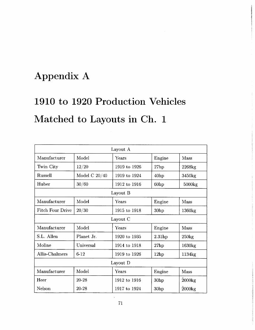
Appendix A

1910 to 1920 Production Vehicles

Matched to Layouts in Ch. 1

71

Layout A

Manufacturer Model Years Engine Mass

Twin City 12/20 1919 to 1926 27hp 2268kg

Russell Model C 20/40 1919 to 1924 40hp 3450kg

Huber 30/60 1912 to 1916 60hp 5000kg

Layout B

Manufacturer Model Years Engine Mass

Fitch Four Drive 20/30 1915 to 1918 30hp 1360kg

Layout C

Manufacturer Model Years Engine Mass

S.L. Allen Planet Jr. 1920 to 1935 2.31hp 250kg

Moline Universal 1914 to 1918 27hp 1630kg

Allis-Chalmers 6-12 1919 to 1926 12hp 1134kg

Layout D

Manufacturer Model Years Engine Mass

Heer 20-28 1912 to 1916 30hp 2000kg

Nelson 20-28 1917 to 1924 30hp 2000kg

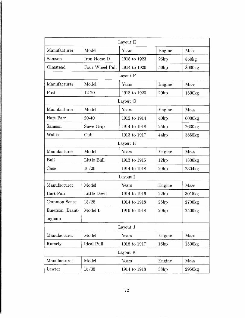
Layout E

Manufacturer Model Years Engine Mass

Samson Iron Horse D 1918 to 1923 26hp 850kg

Olmstead Four Wheel Pull 1914 to 1920 50hp 3000kg

Layout F

Manufacturer Model Years Engine Mass

Post 12-20 1918 to 1920 20hp 1500kg

Layout G

Manufacturer Model Years Engine Mass

Hart Parr 20-40 1912 to 1914 40hp 6000kg

Samson Sieve Grip 1914 to 1918 25hp 2630kg

Wallis Cub 1913 to 1917 44hp 3855kg

Layout H

Manufacturer Model Years Engine Mass

Bull Little Bull 1913 to 1915 12hp 1800kg

Case 10/20 1914 to 1918 20hp 2304kg

Layout I

Manufacturer Model Years Engine Mass

Hart-Parr Little Devil 1914 to 1916 22hp 3015kg

Common Sense 15/25 1914 to 1918 25hp 2700kg

Emerson Brant- Model L 1916 to 1918 20hp 2500kg

ingham I I I

Layout J

Manufacturer Model Years Engine Mass

Rumely Ideal Pull 1916 to 1917 16hp 1500kg

Layout K

Manufacturer Model Years Engine Mass

Lawter 18/38 1914 to 1918 38hp 2950kg

72

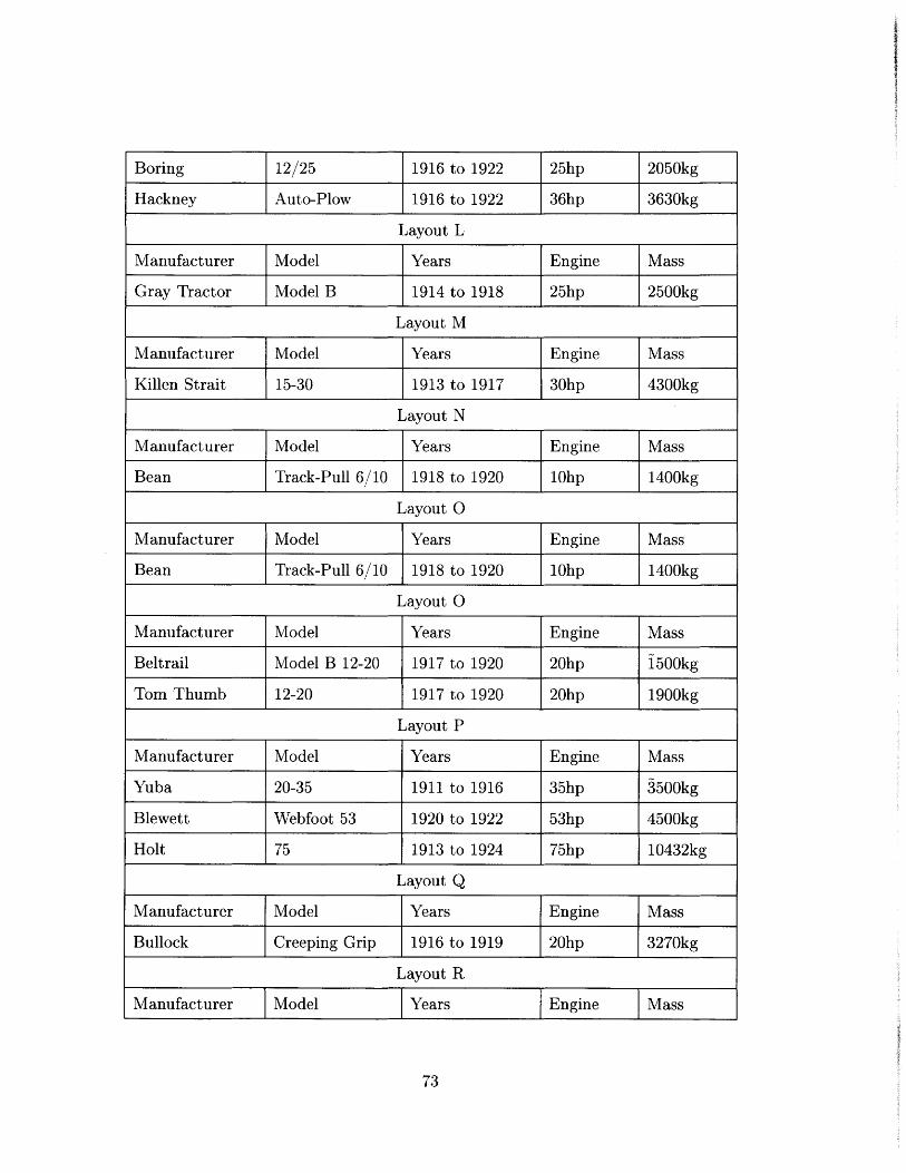
Boring 12/25 1916 to 1922 25hp 2050kg

Hackney Auto-Plow 1916 to 1922 36hp 3630kg

Layout L

Manufacturer Model Years Engine Mass

Gray Tractor Model B 1914 to 1918 25hp 2500kg

Layout M

Manufacturer Model Years Engine Mass

Killen Strait 15-30 1913 to 1917 30hp 4300kg

Layout N

Manufacturer Model Years Engine Mass

Bean Track-Pull 6/10 1918 to 1920 10hp 1400kg

Layout 0

Manufacturer Model Years Engine Mass

Bean Track-Pull 6/10 1918 to 1920 10hp 1400kg

Layout 0

Manufacturer Model Years Engine Mass

Beltrail Model B 12-20 1917 to 1920 20hp 1500kg

Tom Thumb 12-20 1917 to 1920 20hp 1900kg

Layout P

Manufacturer Model Years Engine Mass

Yuba 20-35 1911 to 1916 35hp 3500kg

Blewett Webfoot 53 1920 to 1922 53hp 4500kg

Holt 75 1913 to 1924 75hp 10432kg

Layout Q

Manufacturer Model Years Engine Mass

Bullock Creeping Grip 1916 to 1919 20hp 3270kg

Layout R

Manufacturer Model Years Engine Mass

73

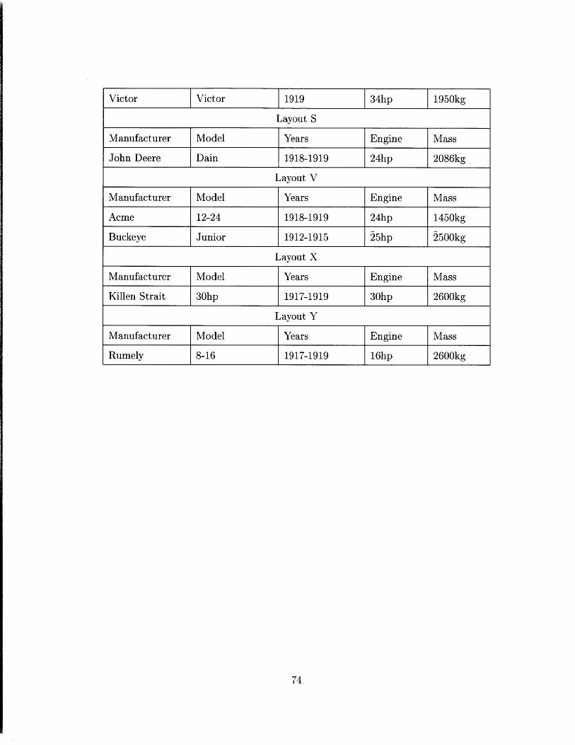
74

Victor Victor 1919 34hp 1950kg

Layout S

Manufacturer Model Years Engine Mass

John Deere Dain 1918-1919 24hp 2086kg

Layout V

Manufacturer Model Years Engine Mass

Acme 12-24 1918-1919 24hp 1450kg

Buckeye Junior 1912-1915 25hp 2500kg

Layout X

Manufacturer Model Years Engine Mass

Killen Strait 30hp 1917-1919 30hp 2600kg

Layout Y

Manufacturer Model Years Engine Mass

Rumely 8-16 1917-1919 16hp 2600kg

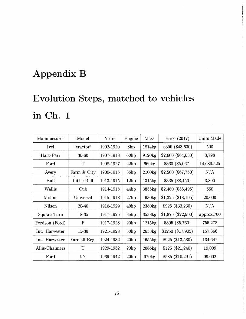
Appendix B

Evolution Steps, matched to vehicles

in Ch. 1

75

Manufacturer Model Years Engine Mass Price (2017) Units Made

Ivel "tractor" 1902-1920 8hp 1814kg 300 ($43,630) 500

Hart-Parr 30-60 1907-1918 60hp 9120kg $2,600 ($64,030) 3,798

Ford T 1908-1927 22hp 660kg $360 ($5,067) 14,689,525

Avery Farm & City 1909-1915 36hp 2100kg $2,500 ($67,750) N/A

Bull Little Bull 1913-1915 12hp 1315kg $335 ($8,450) 3,800

Wallis Cub 1914-1918 44hp 3855kg $2,480 ($55,495) 660

Moline Universal 1915-1918 27hp 1630kg $1,325 ($18,105) 20,000

Nilson 20-40 1916-1929 40hp 2380kg $925 ($33,230) N/A

Square Turn 18-35 1917-1925 35hp 3538kg $1,875 ($22,900) approx.700

Fordson (Ford) F 1917-1928 20hp 1215kg $395 ($5,760) 755,278

Int. Harvester 15-30 1921-1928 30hp 2653kg $1250 ($17,905) 157,366

Int. Harvester Farmall Reg. 1924-1932 20hp 1655kg $925 ($13,530) 134,647

Allis-Chalmers U 1929-1952 20hp 2086kg $125 ($21,240) 19,009

Ford 9N 1939-1942 20hp 970kg $585 ($10,291) 99,002

76

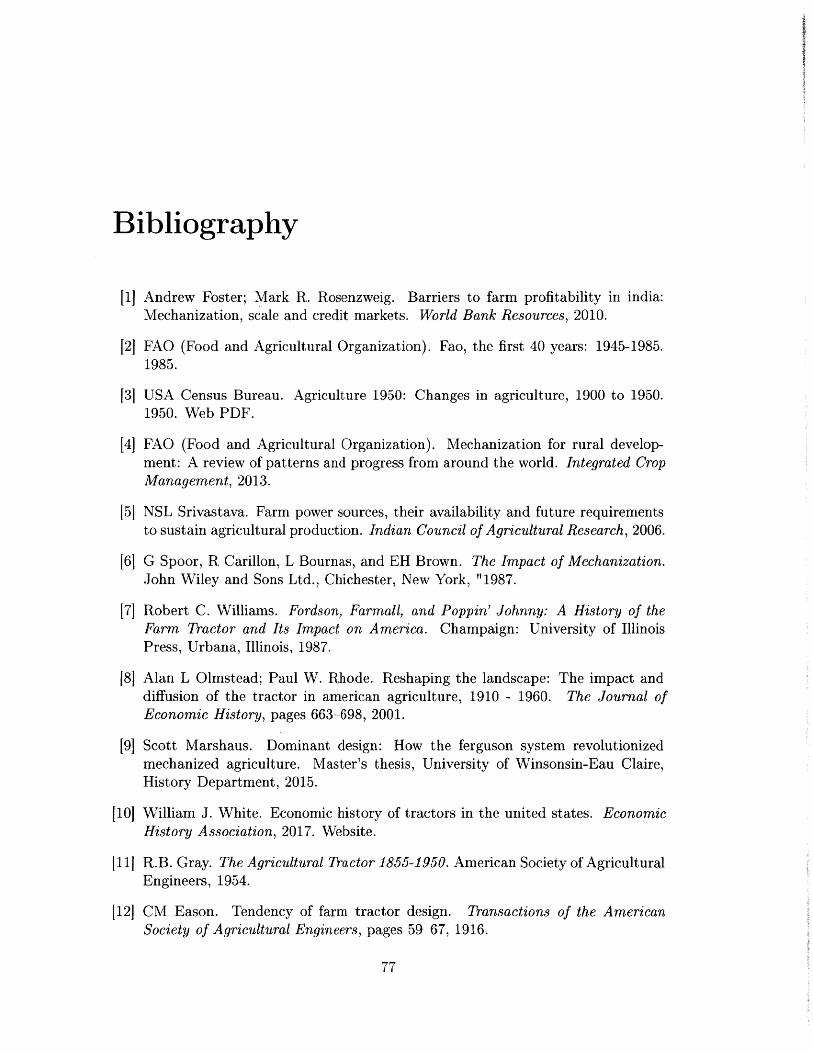
Bibliography

[1] Andrew Foster; Mark R. Rosenzweig. Barriers to farm profitability in india:Mechanization, scale and credit markets. World Bank Resources, 2010.

[21 FAQ (Food and Agricultural Organization). Fao, the first 40 years: 1945-1985.1985.

[31 USA Census Bureau. Agriculture 1950: Changes in agriculture, 1900 to 1950.1950. Web PDF.

[4] FAO (Food and Agricultural Organization). Mechanization for rural develop-ment: A review of patterns and progress from around the world. Integrated CropManagement, 2013.

[5J NSL Srivastava. Farm power sources, their availability and future requirementsto sustain agricultural production. Indian Council of Agricultural Research, 2006.

[61 G Spoor, R Carillon, L Bournas, and EH Brown. The Impact of Mechanization.John Wiley and Sons Ltd., Chichester, New York, "1987.

[71 Robert C. Williams. Fordson, Farmall, and Poppin' Johnny: A History of theFarm Tractor and Its Impact on America. Champaign: University of IllinoisPress, Urbana, Illinois, 1987.

[81 Alan L Olmstead; Paul W. Rhode. Reshaping the landscape: The impact anddiffusion of the tractor in american agriculture, 1910 - 1960. The Journal ofEconomic History, pages 663--698, 2001.

[9] Scott Marshaus. Dominant design: How the ferguson system revolutionizedmechanized agriculture. Master's thesis, University of Winsonsin-Eau Claire,History Department, 2015.

[101 William J. White. Economic history of tractors in the united states. EconomicHistory Association, 2017. Website.

[111 R.B. Gray. The Agricultural Tractor 1855-1950. American Society of AgriculturalEngineers, 1954.

[12] CM Eason. Tendency of farm tractor design. Transactions of the AmericanSociety of Agricultural Engineers, pages 59 67, 1916.

77

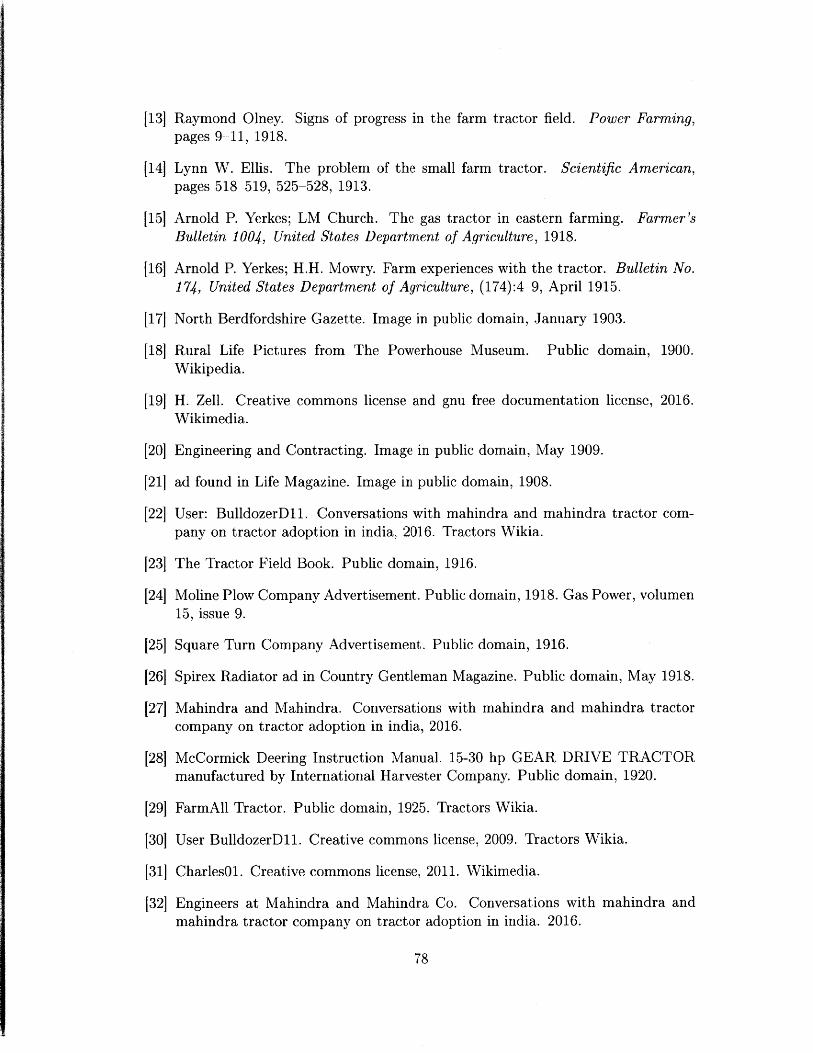
[13] Raymond Olney. Signs of progress in the farm tractor field. Power Farming,pages 9- 11, 1918.

[14] Lynn W. Ellis. The problem of the small farm tractor. Scientific American,pages 518-519, 525-528, 1913.

[15] Arnold P. Yerkes; LM Church. The gas tractor in eastern farming. Farmer'sBulletin 1004, United States Department of Agriculture, 1918.

[16] Arnold P. Yerkes; H.H. Mowry. Farm experiences with the tractor. Bulletin No.

174, United States Department of Agriculture, (174):4-9, April 1915.

[171 North Berdfordshire Gazette. Image in public domain, January 1903.

[181 Rural Life Pictures from The Powerhouse Museum. Public domain, 1900.

Wikipedia.

[19] H. Zell. Creative commons license and gnu free documentation license, 2016.Wikimedia.

[20] Engineering and Contracting. Image in public domain, May 1909.

[21] ad found in Life Magazine. Image in public domain, 1908.

[22] User: BulldozerD11. Conversations with mahindra and mahindra tractor com-pany on tractor adoption in india, 2016. Tractors Wikia.

[23] The Tractor Field Book. Public domain, 1916.

[24] Moline Plow Company Advertisement. Public domain, 1918. Gas Power, volumen

15, issue 9.

[25] Square Turn Company Advertisement. Public domain, 1916.

[26] Spirex Radiator ad in Country Gentleman Magazine. Public domain, May 1918.

[27] Mahindra and Mahindra. Conversations with mahindra and mahindra tractor

company on tractor adoption in india, 2016.

[28] McCormick Deering Instruction Manual. 15-30 hp GEAR DRIVE TRACTORmanufactured by International Harvester Company. Public domain, 1920.

[29] FarmAll Tractor. Public domain, 1925. Tractors Wikia.

[30] User BulldozerD11. Creative commons license, 2009. Tractors Wikia.

[31] Charles0l. Creative commons license, 2011. Wikimedia.

[32] Engineers at Mahindra and Mahindra Co. Conversations with mahindra and

mahindra tractor company on tractor adoption in india. 2016.

78

[331 V. N. Murthy Arelekatti; Douglas H. Bjdrkdal; Carmen W. Graves; AnthonyWong; Armen Mkrtchyan; Amos G. Winter V. Proof-of-concept evaluation of alow-cost and low-weight tractor for small-scale farms. In ASME IDETC 2014,Buffalo, New York, 2014.

[341 Frank M Zoz and Robert D Grisso. Traction and tractor performance. In Agri-cultural Equipment Technology Conference, pages 1-47, 2003.

[351 W.W. Brixius. Traction prediction equations for bias ply tires. ASAE Paper,1987.

[361 J.Y. Wong. Terramechanics and Off-Road Vehicle Engineering. Elsevier, Oxford,UK, 2010.

[371 William W. Cassidy. Tractor tire and ballast management. University Extension,University of Missouri Columbia, 2017.

[381 Scott J. Moreland; Krzysztof Skonieczny; David Wettergreen; Colin Creager; Vi-vake Asnani. Soil motion analysis system for examining wheel-soil shearing. In17th International Conference of the International Society of Terrain VehicleSystems, 2011.

[391 Carmine Senatore; Markus Wulfmeiera; Ivan Vlahini; Jose Andradeb; Karl Iag-nemma. Design and implementation of a particle image velocimetry methodfor analysis of running gear-soil interaction. Journal of Terramechanics, pages311-326, 2013.

[401 Smitth and Grisso. Using tillage horsepower more efficiently: Selecting speed,slip and ballast. In Conservation Tillage Proceeding 9:79-81, 1990.

[411 Carmine Senatore. Prediction of mobility, handling, and tractive efficiency ofwheeled off-road vehicles. PhD dissertation, Virginia Polytechnic Institute andState University, Department of Mechanical Engineering, 2010.

[421 Mieczyslaw Gregory Bekker. Theory of Land Locomotion. University of MichiganPress, 1956.

1431 J.Y. Wong and A. Reece. Prediction of rigid wheel performance based on theanalysis of soil-wheel stresses part i. performance of driven rigid wheels. Journalof Terramechanics, pages 81-98, 1967.

[44] I.C. Holm. Multi-pass behaviour of pneumatic tires. Journal of Terramechanics,pages 47 71, 1969.

[451 Bahareh Ghotbi; Francisco GonzAlez; J6zsef K5vecses; Jorge Angeles. Effect ofmulti-pass on the mobility of wheeled robots on soft terrain. In ECCOMASThematic Conference on Multibody Dynamics, Barcelona, 2015.

79

1461 Juan Agdera Diego L. Valera, JesAs Gil. Design of a new sensor for determinationof the effects of tractor field usage in southern spain: Soil sinkage and alterationsin the cone index and dry bulk density. Sensors, 2012.

1471 Troy A. Jensen Diogenes L. Antille, John McL. Bennett. Soil compaction andcontrolled traffic considerations in australian cotton-farming systems. Crop andPasture Science, 2016.

1481 Gustavo Soares de Souza; Zigomar Menezes de Souza; Reginaldo Barboza daSilva; Ronny Sobreira Barbosa; Fernando Silva Araujo. Effects of traffic controlon the soil physical quality and the cultivation of sugarcane. Revista Brasileirade Ciencia do Solo, 2014.

[491 Ismet Onal. Controlled traffic and widespan tractors. Tarim Makinalari BilimiDergisi (Journal of Agricultural Machinery Science), 2012. -

[501 Tim Chamen. Controlled traffic farming hA from worldwide research to adop-tion in europe and its future prospects. In International Conference of Agricul-tural Engineering, Zurich, 2014.

1511 Jodi Dejong-Hughes. Tires, traction and compaction. University of MinnesotaExtension, 2017. Extension UMN website.

[52] Andrea Battiato; Ettiene Diserens; L. Sartori. Tractor traction performancesimulation on differently textured soils and validation: a basic study to maketraction and energy requirements accessible to the practice. Soil and TillageResearch, 2017.

[531 Andrea Battiato and Ettiene Diserens. Influence of tyre inflation pressure andwheel load on the traction performance of a 65 kw mfwd tractor on a cohesivesoil. Journal of Agricultural Science, 2013.

[541 Andrea Battiato, Ettiene Diserens, and L. Sartori. Traction performance simu-lation for mechanical front wheel drive tractors: towards a practical computertool. Journal of Agricultural Engineering, 2013.

[551 Fatai Butola Akande Mohammed Shu'aibu Abubakar, Desa Ahmad. A review offarm tractor overturning accidents and safety. Petranika Journal of Science andTechnology, 2010.

[561 Michael R. Goe and Robert E. McDowell. Animal traction guidelines for utiliza-tion. Cornell International Agriculture Mimeograph, 1980.

[57] Peter R. Watson. Animal traction. Peace Corps. by TransCentury Corporation,1981.

80