Copyright © by SIAM. Unauthorized reproduction of this article is prohibited. SIAM J. OPTIM. c 2009 Society for Industrial and Applied Mathematics Vol. 20, No. 1, pp. 416–444 SHAPE OPTIMIZATION IN THREE-DIMENSIONAL CONTACT PROBLEMS WITH COULOMB FRICTION ∗ P. BEREMLIJSKI † , J. HASLINGER ‡ , M. KO ˇ CVARA § , R. KU ˇ CERA ¶ , AND J.V. OUTRATA Abstract. We study the discretized problem of the shape optimization of three-dimensional (3D) elastic bodies in unilateral contact. The aim is to extend existing results to the case of contact problems obeying the Coulomb friction law. Mathematical modeling of the Coulomb friction problem leads to an implicit variational inequality. It is shown that for small coefficients of friction the discretized problem with Coulomb friction has a unique solution and that this solution is Lipschitzian as a function of a control variable describing the shape of the elastic body. The 2D case of this problem was studied by the authors in [P. Beremlijski, J. Haslinger, M. Koˇ cvara, and J. V. Outrata, SIAM J. Optim., 13 (2002), pp. 561–587]; there we used the so-called implicit programming approach combined with the generalized differential calculus of Clarke. The extension of this technique to the 3D situation is by no means straightforward. The main source of difficulties is the nonpolyhedral character of the second-order (Lorentz) cone, arising in the 3D model. To facilitate the computation of the subgradient information, needed in the used numerical method, we exploit the substantially richer generalized differential calculus of Mordukhovich. Numerical examples illustrate the efficiency and reliability of the suggested approach. Key words. shape optimization, contact problems, Coulomb friction, mathematical programs with equilibrium constraints AMS subject classifications. 49Q10, 74M10, 74S05 DOI. 10.1137/080714427 1. Introduction and preliminaries. Contact shape optimization is a special branch of structural optimization whose goal is to find shapes of deformable bodies which are in mutual contact. A typical problem in many applications is to find shapes guaranteeing a priori given stress distributions on parts in contact [1]. A specific feature of contact shape optimization is its nonsmooth character due to the fact that the respective state mapping is given by various types of variational inequalities. For contact problems without friction or with the so-called given friction (see [9]), whose mathematical models lead to variational inequalities of the first and the second kind, sensitivity analysis was done in [26] for continuous models and in [10] for discretized models. Assuming a more realistic Coulomb law of friction, the situation becomes much more complicated in view of the fact that the state problem is now represented ∗ Received by the editors January 27, 2008; accepted for publication (in revised form) December 8, 2008; published electronically April 29, 2009. This work was supported by grants IAA1075402 and IAA100750802 of the Czech Academy of Sciences (JH, MK, JVO), grant 201/07/0294 of the Grant Agency of the Czech Republic (PB), research projects MSM6198910027 (PB, RK) and MSM0021620839 (JH) of the Czech Ministry of Education, and the EU Commission in the Sixth Framework Program, project 30717 PLATO-N (MK). http://www.siam.org/journals/siopt/20-1/71442.html † Faculty of Electrical Engineering, V ˇ SB-Technical University of Ostrava, 17. listopadu 15, 70833 Ostrava-Poruba, Czech Republic ([email protected]). ‡ Department of NumericalMathematics, Charles University, Sokolovsk´a 83, 18675 Praha 8, Czech Republic (Jaroslav.Haslinger@mff.cuni.cz). § School of Mathematics, University of Birmingham, Birmingham B15 2TT, UK and Institute of Information Theory and Automation, Academy of Sciences of the Czech Republic, Pod vod´arenskou vˇ eˇ z´ ı 4, 182 08 Praha 8, Czech Republic ([email protected]). ¶ Department of Mathematics and Descriptive Geometry, V ˇ SB-Technical University of Ostrava, 17. listopadu 15, 708 33 Ostrava-Poruba, Czech Republic ([email protected]). Institute of Information Theory and Automation, Academy of Sciences of the Czech Republic, Pod vod´arenskou vˇ eˇ z´ ı 4, 182 08 Praha 8, Czech Republic ([email protected]). 416

Welcome message from author
This document is posted to help you gain knowledge. Please leave a comment to let me know what you think about it! Share it to your friends and learn new things together.
Transcript
Copyright © by SIAM. Unauthorized reproduction of this article is prohibited.
SIAM J. OPTIM. c© 2009 Society for Industrial and Applied MathematicsVol. 20, No. 1, pp. 416–444
SHAPE OPTIMIZATION IN THREE-DIMENSIONAL CONTACTPROBLEMS WITH COULOMB FRICTION∗
P. BEREMLIJSKI† , J. HASLINGER‡ , M. KOCVARA§ , R. KUCERA¶, AND J.V. OUTRATA‖
Abstract. We study the discretized problem of the shape optimization of three-dimensional(3D) elastic bodies in unilateral contact. The aim is to extend existing results to the case of contactproblems obeying the Coulomb friction law. Mathematical modeling of the Coulomb friction problemleads to an implicit variational inequality. It is shown that for small coefficients of friction thediscretized problem with Coulomb friction has a unique solution and that this solution is Lipschitzianas a function of a control variable describing the shape of the elastic body. The 2D case of thisproblem was studied by the authors in [P. Beremlijski, J. Haslinger, M. Kocvara, and J. V. Outrata,SIAM J. Optim., 13 (2002), pp. 561–587]; there we used the so-called implicit programming approachcombined with the generalized differential calculus of Clarke. The extension of this technique to the3D situation is by no means straightforward. The main source of difficulties is the nonpolyhedralcharacter of the second-order (Lorentz) cone, arising in the 3D model. To facilitate the computationof the subgradient information, needed in the used numerical method, we exploit the substantiallyricher generalized differential calculus of Mordukhovich. Numerical examples illustrate the efficiencyand reliability of the suggested approach.
Key words. shape optimization, contact problems, Coulomb friction, mathematical programswith equilibrium constraints
AMS subject classifications. 49Q10, 74M10, 74S05
DOI. 10.1137/080714427
1. Introduction and preliminaries. Contact shape optimization is a specialbranch of structural optimization whose goal is to find shapes of deformable bodieswhich are in mutual contact. A typical problem in many applications is to find shapesguaranteeing a priori given stress distributions on parts in contact [1]. A specificfeature of contact shape optimization is its nonsmooth character due to the fact thatthe respective state mapping is given by various types of variational inequalities. Forcontact problems without friction or with the so-called given friction (see [9]), whosemathematical models lead to variational inequalities of the first and the second kind,sensitivity analysis was done in [26] for continuous models and in [10] for discretizedmodels. Assuming a more realistic Coulomb law of friction, the situation becomesmuch more complicated in view of the fact that the state problem is now represented
∗Received by the editors January 27, 2008; accepted for publication (in revised form) December8, 2008; published electronically April 29, 2009. This work was supported by grants IAA1075402and IAA100750802 of the Czech Academy of Sciences (JH, MK, JVO), grant 201/07/0294 ofthe Grant Agency of the Czech Republic (PB), research projects MSM6198910027 (PB, RK) andMSM0021620839 (JH) of the Czech Ministry of Education, and the EU Commission in the SixthFramework Program, project 30717 PLATO-N (MK).
http://www.siam.org/journals/siopt/20-1/71442.html†Faculty of Electrical Engineering, VSB-Technical University of Ostrava, 17. listopadu 15, 708 33
Ostrava-Poruba, Czech Republic ([email protected]).‡Department of Numerical Mathematics, Charles University, Sokolovska 83, 186 75 Praha 8, Czech
Republic ([email protected]).§School of Mathematics, University of Birmingham, Birmingham B15 2TT, UK and Institute of
Information Theory and Automation, Academy of Sciences of the Czech Republic, Pod vodarenskouvezı 4, 182 08 Praha 8, Czech Republic ([email protected]).
¶Department of Mathematics and Descriptive Geometry, VSB-Technical University of Ostrava,17. listopadu 15, 708 33 Ostrava-Poruba, Czech Republic ([email protected]).
‖Institute of Information Theory and Automation, Academy of Sciences of the Czech Republic,Pod vodarenskou vezı 4, 182 08 Praha 8, Czech Republic ([email protected]).
416

Copyright © by SIAM. Unauthorized reproduction of this article is prohibited.
SHAPE OPTIMIZATION IN 3D COULOMB CONTACT 417
by a nontrivial implicit variational inequality [6]. For the sake of simplicity we restrictourselves to structures consisting of one deformable body unilaterally supported bya rigid foundation (the so-called Signorini problem) considering Coulomb friction ona common part. The paper is solely devoted to a finite-dimensional case resultingfrom an appropriate finite element approximation of our problem and, in particular,to sensitivity analysis. The continuous setting, however, is also presented in order toclarify the form of the resulting discrete model. Since our discrete design variablesare given by control points of Bezier surfaces shaping contact zones, we deal with theclassic boundary variation approach in shape optimization; i.e., topological changesof the structure are not admitted.
The two-dimensional (2D) case of this problem was studied by the authors in [2];there we used the so-called implicit programming approach [16, 21] combined with thegeneralized differential calculus of Clarke [3]. One could definitely extend the approachfrom [2] to the 3D case by using a polyhedral approximation of the friction cone. It is,however, much more challenging to consider in the 3D model the right nonpolyhedralsecond-order (Lorentz) cone, but then the respective extension of the technique from[2] meets serious hurdles. This concerns both the numerical solution of the respectivestate problem as well as appropriate stability and sensitivity issues. To facilitate thecomputation of the subgradient information, needed in the used numerical method, wehave thus invoked the results of [13] and exploited the substantially richer generalizeddifferential calculus of Mordukhovich [17, 19]. This means that we compute now amatrix from the Clarke generalized Jacobian of the discretized state mapping via thelimiting (Mordukhovich) coderivative of this mapping. This has enabled us to havean efficient treatment of coupled multifunctions arising on the right-hand side of thegeneralized equation defining the state mapping.
The outline of the paper is as follows. Section 2 is devoted to a brief descriptionof the state problem, i.e., the contact problem with Coulomb friction in its original,infinite-dimensional formulation. In section 3 we describe its finite element discretiza-tion and introduce our shape optimization problem. Thereafter we present variousproperties of the discretized state mapping and end up with the proof of its strongregularity. Section 4 concerns the used implicit-programming method. In particular,it deals with the computation of Clarke’s subgradients of the respective composite costfunction which have to be supplied to the used algorithm of nonsmooth optimization.In this section we make use of several sophisticated rules of generalized differentiation.The first part of the last section 5 is devoted to the numerical solution of the stateproblem. In the second part we present the test examples.
Our notation is standard: A denotes the closure of a set A and, for a multifunctionΦ : X ⇒ Y, GrΦ = {(x, y) ∈ X × Y | y ∈ Φ(x)} is the graph of Φ. BR denotes aball in R
n of radius R centered at the origin. For a vector x ∈ Rn and an index set
N ⊂ {1, 2, . . . , n}, xN denotes the subvector of x composed from the components xi,i ∈ N . For a Lipschitz single-valued mapping F : R
n → Rm, ∂F (x) is the generalized
Jacobian of Clarke, defined by
∂F (x) = conv{
limi→∞
∇F (xi) | xiΩF→ x
},
where “conv” denotes the convex hull and ΩF is the set of points at which F isdifferentiable. If m = 1, we speak of the Clarke subdifferential.
In section 4 we extensively use the following notions of the generalized differentialcalculus of Mordukhovich [18, 19].

Copyright © by SIAM. Unauthorized reproduction of this article is prohibited.
418 BEREMLIJSKI, HASLINGER, KOCVARA, KUCERA, OUTRATA
Given a closed set A ⊂ Rn and a point x ∈ A, we denote by NA(x) the Frechet
(regular) normal cone to A at x, defined by
NA(x) =
{x∗ ∈ R
n | lim supx
A−→x
〈x∗, x − x〉‖x − x‖ ≤ 0
}.
The limiting (Mordukhovich) normal cone to A at x, denoted by NA(x), is defined by
NA(x) := Lim supx
A−→x
NA(x) ,
where “Lim sup” is the Kuratowski–Painleve outer limit of sets (see [24]). If A isconvex, then NA(x) = NA(x) amounts to the classic normal cone in the sense ofconvex analysis. We say that A is normally regular at x, provided NA(x) = NA(x).
On the basis of the above notions, we can also describe the local behavior ofmultifunctions. Let Φ : R
n ⇒ Rm be a multifunction with closed graph and (x, y) ∈
Gr Φ. The multifunction D∗Φ(x, y) : Rm ⇒ R
n, defined by
D∗Φ(x, y)(y∗) := {x∗ ∈ Rn | (x∗,−y∗) ∈ NGr Φ(x, y)},
is called the regular coderivative of Φ at (x, y). Analogously, the multifunctionD∗Φ(x, y) : R
m ⇒ Rn, defined by
D∗Φ(x, y)(y∗) := {x∗ ∈ Rn | (x∗,−y∗) ∈ NGr Φ(x, y)},
is called the limiting (Mordukhovich) coderivative of Φ at (x, y). These two coderiva-tives coincide whenever GrΦ is normally regular at (x, y). If Φ happens to be single-valued, we simply write D∗Φ(x)(D∗Φ(x)). If Φ is continuously differentiable, thenD∗Φ(x) = D∗Φ(x) amounts to the adjoint Jacobian.
In what follows the considered discretized mechanical equilibrium is modeled bya generalized equation (GE) of the form
(1.1) 0 ∈ G(x, y) + Q(y),
where G[Rn ×Rm → R
m] is continuously differentiable and Q[Rm ⇒ Rm] is a closed-
graph multifunction. Consider the reference pair (x, y) ∈ GrS, where S[Rn ⇒ Rm] is
defined by
S(x) = {y ∈ Rm|0 ∈ G(x, y) + Q(y)}.
In agreement with a slight generalization [4] of Robinson’s concept of strong regularityfrom [23] we say that the GE (1.1) satisfies the strong regularity condition (SRC) at(x, y) (is strongly regular at (x, y)), provided there exist neighborhoods U of 0 and Vof y such that the mapping
v → {y ∈ V|v ∈ G(x, y) + ∇yG(x, y)(y − y) + Q(y)}is single-valued and Lipschitz on U . It is well known ([4, Theorem 2.1]) that the strongregularity of (1.1) at (x, y) implies the existence of neighborhoods U of x and V of ysuch that the mapping
x → S(x) ∩ Vis single-valued and Lipschitz on U .
Copyright © by SIAM. Unauthorized reproduction of this article is prohibited.
SHAPE OPTIMIZATION IN 3D COULOMB CONTACT 419
2. Setting of the problem. We start with the definition of the state problem.Let Ω = R× (0, c), R = (0, a) × (0, b), be a block in R
3, a, b, c > 0 given. By Uad wedenote a family of admissible functions, where
(2.1) Uad ={
α ∈ C0,1(R) | 0 ≤ α ≤ C0 in R, ‖α′‖∞,R ≤ C1,
C2 ≤∫R
α dx1dx2 ≤ C3
};
i.e., the set Uad contains all nonnegative, bounded, Lipschitz equicontinuous functionsin R, satisfying an integral type constraint. Positive numbers C0, C1, C2, and C3 arechosen in such a way that Uad �= ∅. With any α ∈ Uad we associate a subdomainΩ(α) ⊂ Ω:
Ω(α) = {(x1, x2, x3) ∈ Ω | x3 ≥ α(x1, x2) ∀(x1, x2) ∈ R}.
Functions α ∈ Uad will play the role of control variables determining the shape ofΩ(α).
Let α ∈ Uad be fixed, and consider an elastic body represented by Ω(α). Itsboundary ∂Ω(α) is split into three nonempty, nonoverlapping parts Γu(α), Γp(α),and Γc(α): ∂Ω(α) = Γu(α) ∪ Γp(α) ∪ Γc(α), where different boundary conditionswill be prescribed. On Γu(α) the body is fixed, while surface tractions of densityP = (P1, P2, P3) act on Γp(α). The body is unilaterally supported along Γc(α) by arigid foundation represented by the half-space R
2 × R−, where
Γc(α) = {(x1, x2, x3) | x3 = α(x1, x2) ∀(x1, x2) ∈ R}
is the graph of α. Finally, Ω(α) is subject to body forces of density F = (F1, F2, F3).Our aim is to find an equilibrium state taking into account friction on Γc(α). Thisstate is characterized by a displacement field u = (u1, u2, u3) satisfying the followingsystem of differential equations and boundary conditions:
- equilibrium equations:
(2.2)∂σij
∂xj+ Fi = 0 in Ω(α), i = 1, 2, 3;1
- Hooke’s law :
(2.3) σij : = σij(u) = cijklεkl(u) in Ω(α), where εkl =12
(∂uk
∂xl+
∂ul
∂xk
),
i, j, k, l = 1, 2, 3;
- kinematical boundary conditions :
(2.4) ui = 0 on Γu(α), i = 1, 2, 3;
- prescribed tractions :
(2.5) Ti : = σijνj = Pi on Γp(α), i = 1, 2, 3;
1Here and in what follows the summation convention is adopted.
Copyright © by SIAM. Unauthorized reproduction of this article is prohibited.
420 BEREMLIJSKI, HASLINGER, KOCVARA, KUCERA, OUTRATA
- unilateral conditions :
(2.6)u3(x′, α(x′)) ≥ −α(x′) ∀x′ = (x1, x2) ∈ R;T3(x) : = σ33(x) ≥ 0, T3(x)(u3(x) + α(x′)) = 0 ∀x ∈ Γc(α);
}
- Coulomb law of friction:
(2.7)
if ut(x) : = (u1(x), u2(x), 0) = 0 ⇒ ‖Tt(x)‖ ≤ FT3(x),where Tt(x) : = (T1(x), T2(x), 0), x ∈ Γc(α);
if ut(x) �= 0 ⇒ Tt(x) = −FT3(x)ut(x)
‖ut(x)‖ , x ∈ Γc(α).
⎫⎪⎪⎪⎬⎪⎪⎪⎭Remark 2.1. The equations and boundary conditions (2.2)–(2.7) represent the
classical formulation of a contact problem with Coulomb friction. The meaning ofsymbols is the following: σ = (σij)3i,j=1 stands for a symmetric stress tensor which isrelated to a linearized strain tensor ε = (εij)3i,j=1 by means of a linear Hooke’s law(2.3), ν is the unit outward normal vector to ∂Ω(α), and T = (T1, T2, T3) denotes thestress vector on ∂Ω(α). Finally, ‖ ‖ is the Euclidean norm of a vector and F is acoefficient of Coulomb friction. In what follows we shall suppose that F is a positiveconstant.
To give a weak form of the state problem we introduce the following spaces andsets:
V (α) = {v = (v1, v2, v3) ∈ (H1(Ω(α)))3 | v = 0 on Γu(α)},K(α) = {v ∈ V (α) | v3(x′, α(x′)) ≥ −α(x′) a.e. in R},
X = {ϕ ∈ L2(R) | ∃v ∈ V (α) : ϕ(x′) = v3(x′, α(x′)), x′ ∈ R},X ′ is the dual of X, X ′
+ is the cone of positive elements of X ′.
The duality pairing between X ′ and X will be denoted by 〈·, ·〉.We start with a simpler model of friction in which the unknown component T3
in (2.7) is replaced by a given slip bound g ∈ X ′+ (model with given friction; see [9]).
Its mathematical formulation leads to a variational inequality of the 2nd kind:
(P(g))Find u : = u(g) ∈ K(α) such that
aα(u, v − u) + 〈Fg, ‖vt‖ − ‖ut‖〉 ≥ Lα(v − u) ∀v ∈ K(α),
}
where
(2.8) aα(u, v) : =∫
Ω(α)
cijklεij(u)εkl(v) dx,
(2.9) Lα(v) : =∫
Ω(α)
Fivi dx +∫
Γp(α)
Pivi ds
are the inner energy and the work of external forces, respectively. Further, ‖vt‖ de-notes the Euclidean norm of the vector vt : = vt ◦ α given by (v1(x′, α(x′)),v2(x′, α(x′)), 0), x′ ∈ R. Next we shall suppose that F ∈ (L2(Ω))3, P ∈ (L2(∂Ω))3,and the linear elasticity coefficients cijkl in (2.3) satisfy the usual symmetry and ellip-ticity conditions [20]. It is well-known that under these assumptions problem (P(g))
Copyright © by SIAM. Unauthorized reproduction of this article is prohibited.
SHAPE OPTIMIZATION IN 3D COULOMB CONTACT 421
has a unique solution u(g) for every g ∈ X ′+. To release the unilateral constraint
u(g) ∈ K(α) we use an alternative formulation of (P(g)) involving Lagrange multi-pliers:
(M(g))Find (u, λ) : = (u(g), λ(g)) ∈ V (α) × X ′
+ such thataα(u, v − u) + 〈Fg, ‖vt‖ − ‖ut‖〉 ≥ Lα(v − u) + 〈λ, v3 − u3〉 ∀v ∈ V (α)〈μ − λ, u3 + α〉 ≥ 0 ∀μ ∈ X ′
+,
⎫⎪⎬⎪⎭where v3(x′) : = v3(x′, α(x′)), x′ ∈ R. It is easy to show that problem (M(g)) hasa unique solution (u(g), λ(g)) for every g ∈ X ′
+. This makes it possible to define amapping Φ : X ′
+ −→ X ′+ by
(2.10) Φ(g) = λ(g) ∀g ∈ X ′+,
where λ(g) ∈ X ′+ is the second component of the solution to (M(g)).
Definition 2.2. By a weak solution of a contact problem with Coulomb frictionwe call any pair (u, λ) ∈ V (α) × X ′
+ satisfying
(Q(α))aα(u, v − u) + 〈Fλ, ‖vt‖ − ‖ut‖〉 ≥ Lα(v − u) + 〈λ, v3 − u3〉 ∀v ∈ V (α)〈μ − λ, u3 + α〉 ≥ 0 ∀μ ∈ X ′
+.
}From this definition it follows that λ is a fixed point of Φ. The existence of such
fixed points has been analyzed in [6].So far the function α ∈ Uad characterizing the shape of Ω(α) has been fixed. Now
we shall look at α ∈ Uad as a control variable governing state problem (Q(α)). Let Sbe the respective control-to-state mapping defined by
(2.11) S(α) = (u(α), λ(α)) ∀α ∈ Uad,
where (u(α), λ(α)) is a solution to (Q(α)), and denote by G the graph of S. Since(Q(α)) may have more than one solution, the mapping S is set-valued in general.
Finally, let J : G −→ R1 be a cost functional. Suppose that there exists a
minimizer (α∗, u(α∗), λ(α∗)) of J on G. Then Ω∗ : = Ω(α∗) will be called an op-timal domain. Since we are interested in numerical realization of this problem, itsdiscretization will be necessary.
To discretize the geometry we introduce a system Uhad containing functions which
are uniquely determined by a finite number of degrees of freedom (e.g., Bezier sur-faces). Admissible domains will be then given by Ω(αh), where αh ∈ Uh
ad. To dis-cretize the state problem we use a finite element method. The classical Galerkinmethod together with appropriate discretizations Vh(αh), Kh(αh), and Xh and X ′
h
of V (α), K(α), and X and X ′, respectively, represent an efficient tool of solvingfrictional contact problems. Analogously to the continuous setting we introduce adiscrete control-to-state mapping Sh defined on Uh
ad and its graph Gh. The discreteshape optimization is then given by the minimization of J on Gh. In the next sectionwe present an algebraic form of this problem arising from a typical finite elementapproximation. From this the structure of the problem to be solved will be seen.
3. Algebraic form of contact problems with Coulomb friction. The aimof this section is to present the algebraic form of the discretized state problem and toanalyze its basic properties. We will proceed analogously to the continuous setting.
Let the discretization parameter h > 0 be fixed. Next we shall use the followingnotation: ‖ · ‖s, 〈 ·, · 〉s stand for the Euclidean norm and the scalar product in R
s,
Copyright © by SIAM. Unauthorized reproduction of this article is prohibited.
422 BEREMLIJSKI, HASLINGER, KOCVARA, KUCERA, OUTRATA
respectively. In the frequent case s = 2 the subscript will be omitted. Every αh ∈ Uhad
will be uniquely characterized by a discrete design variable α ∈ Rd, and Uh
ad will beidentified with a set U ⊂ R
d. We shall suppose that U is a convex, compact subset ofR
d. Let {ϕi}ni=1 be a basis of a finite element space Vh(αh), αh ∈ Uh
ad, and supposethat its dimension n does not depend on αh. Then
aαh(vh, zh) = 〈A(α)v , z 〉n,
Lαh(vh) = 〈L(α), v〉n ∀vh, zh ∈ Vh(αh),
where v ∈ Rn is the vector of coordinates of vh with respect to {ϕi}n
i=1 and A(α) ∈R
n×n, L(α) ∈ Rn are a stiffness matrix and a load vector, respectively, both depending
on α ∈ U . The set of all A(α) ∈ Rn×n, α ∈ U , will be denoted by M . For the sake
of consistency we will denote in what follows all finite-dimensional vectors and allmatrices by bold letters. At mappings, however, this convention will not be appliedstrictly, and so most vector-valued and set-valued mappings are denoted by standard(nonbold) letters. We shall suppose that the following assumptions are satisfied:
All matrices A ∈ M are symmetric and uniformly positive definite, i.e.,there exists γ > 0 such that 〈Av , v〉n ≥ γ‖v‖2
n ∀v ∈ Rn ∀A ∈ M ;
}(3.1)
The mappings A : U −→ M,L : U −→ Rn are continuously
differentiable on an open set containing U .
}(3.2)
We start with the algebraic form of the contact problem with given friction forfixed α ∈ U . Let g ∈ R
p+ (p < n) be a given discrete slip bound (p is related to the
number of all contact nodes, i.e., the nodes of a used partition of Ω(αh) into finiteelements which are placed on Γc(αh)\ Γu(αh)). The discretized total potential energyhas the following form:
(3.3) J (v ) =12〈v ,Av〉n − 〈L, v〉n + F〈g , |Tv|〉p,
with A : = A(α), L : = L(α) for some α ∈ U (since α ∈ U is now fixed, it will beomitted in the argument of A and L). Further, T : R
n −→ R2p is a linear mapping
defined by Tv : = (T1v , T2v , . . . , Tpv), v ∈ Rn, where Tiv ∈ R
2 is the tangentialnodal displacement vector at the ith contact node. The symbol |Tv| ∈ R
p denotes avector defined by
|Tv | : = (‖T1v‖, . . . , ‖Tpv‖) .
Let K be a closed convex subset of Rn:
(3.4) K := {v ∈ Rn | Nv ≥ −α},
where N ∈ Rp×n is a matrix representation of the nonpenetration property. From
a displacement vector v ∈ Rn, N selects the normal components at the p contact
points. Clearly, N has the following properties:(a) It has full row rank.(b) Each column contains at most one nonzero element.(c) N (Rn) = N (kerT ).
From (a) it follows that
(3.5) ∃β = const. > 0 such that supv∈R
n
v �=0
〈μ,Nv〉p‖v‖n
≥ β‖μ‖p ∀μ ∈ Rp.
Copyright © by SIAM. Unauthorized reproduction of this article is prohibited.
SHAPE OPTIMIZATION IN 3D COULOMB CONTACT 423
Definition 3.1. By a solution of a discrete contact problem with given frictionwe mean a vector u ∈ K satisfying
(P (L, g)) 〈Au, v− u〉n + F〈g, |Tv| − |Tu|〉p ≥ 〈L, v− u〉n ∀v ∈ K.
Next we will analyze the dependence of u on L and g with α ∈ U being fixed.This is why we use notation (P (L, g)).
To conduct this analysis, we introduce an equivalent formulation of (P (L, g))which involves Lagrange multipliers releasing the constraint v ∈ K. It reads as follows:
(M (L, g))
Find (u , λ) ∈ Rn × R
p+ such that
〈Au , v − u〉n + F〈g , |Tv | − |Tu|〉p≥ 〈L, v − u〉n + 〈λ,Nv −Nu〉p ∀v ∈ R
n
〈μ− λ,Nu + α〉p ≥ 0 ∀μ ∈ Rp+.
⎫⎪⎪⎪⎬⎪⎪⎪⎭The first component u of the solution to (M (L, g)) solves (P (L, g)), and the secondcomponent λ represents the discrete normal contact stress. The following result iseasy to prove.
Proposition 3.2. Problems (P (L, g)), (M (L, g)) have unique solutions u,(u, λ), respectively, for every L ∈ R
n and g ∈ Rp+.
Proof. Both existence and uniqueness follow directly from (3.1) and (3.5).Next we will establish several useful properties of the solution to (M (L, g)).Proposition 3.3. Let (u, λ) be the solution to (M (L, g)). Then
(3.6) ‖u‖n ≤ 1γ‖L‖n,
(3.7) ‖λ‖m ≤ 1β
(‖A‖γ
+ 1)‖L‖n,
where γ, β > 0 are from (3.1) and (3.5).Proof. Inserting v = 0 ∈ K into (P (L, g)) we obtain
γ‖u‖2n ≤ 〈Au ,u〉n + F〈g , |Tu|〉p ≤ 〈L,u〉n
from which (3.6) follows. Further, substitutions v = 0 and v = 2u into the firstinequality in (M (L, g)) yield
〈Au ,u〉n + F〈g , |Tu|〉p = 〈L,u〉n + 〈λ,Nu〉p.Therefore,
(3.8) 〈Au , v 〉n + F〈g , |Tv |〉p ≥ 〈L, v〉n + 〈λ,Nv〉p ∀v ∈ Rn.
From (3.8) it follows that
(3.9) 〈Au , v〉n = 〈L, v〉n + 〈λ,Nv〉p ∀v ∈ kerT.
From this and (3.5) we obtain (3.7) using that N (Rn) = N (kerT ).Remark 3.4. It is worth noticing that the bounds (3.6) and (3.7) do not depend
on F > 0 and g ∈ Rp+.
Assume now that g is fixed, and let Ψ : Rn −→ K×R
p+ be a mapping defined by
Ψ(L) = (u , λ),
Copyright © by SIAM. Unauthorized reproduction of this article is prohibited.
424 BEREMLIJSKI, HASLINGER, KOCVARA, KUCERA, OUTRATA
where (u , λ) is a solution of (M (L, g)). It is very easy to show that Ψ is Lipschitzon R
n as follows from the next proposition.Proposition 3.5. Let (ui, λi) be the solution of (M (Li, g)), i = 1, 2. Then
(3.10) ‖u1 − u2‖n ≤ 1γ‖L1 − L2‖n,
(3.11) ‖λ1 − λ2‖p ≤ 1β
(‖A‖γ
+ 1)‖L1 − L2‖n.
Proof. The proof can be done in the same way as the proof of Proposi-tion 3.3.
Next, to define a solution of a discrete contact problem with Coulomb friction,we fix L and introduce the mapping Γ : R
p+ −→ R
p+:
(3.12) Γ(g ) = λ,
where λ is the second component of a solution to (M (L, g)).Definition 3.6. As a solution of a discrete contact problem with Coulomb fric-
tion we declare any couple (u, λ) ∈ Rn × R
p+ satisfying
(P)〈Au, v− u〉n + F〈λ, |Tv| − |Tu|〉p
≥ 〈L, v− u〉n + 〈λ,Nv−Nu〉p ∀v ∈ Rn
〈μ− λ,Nu + α〉p ≥ 0 ∀μ ∈ Rp+;
⎫⎪⎬⎪⎭i.e., λ is a fixed point of Γ and (u, λ) solves (M (L, λ)).
Proposition 3.7. For any L ∈ Rn and any F > 0 there exists at least one fixed
point λ of Γ. All fixed points λ belong to Rp+ ∩ BR, where R = 1
β (‖A‖γ + 1)‖L‖n.
Proof. It is easy to show that Γ is continuous in Rp+ and maps R
p+ ∩BR into itself
as follows from (3.7). The existence of a fixed point follows from Brower’s fixed pointtheorem.
Now we show that Γ is even contractive in Rp+ ∩ BR, provided that F is small
enough. Indeed, denote by u i ∈ K solutions to (P (L, g i)), i = 1, 2. Then one has
(3.13)i 〈Au i, v − u i〉n + F〈g i, |Tv | − |Tu i|〉p ≥ 〈L, v − u i〉n ∀v ∈ K.
Inserting v : = u2 into (3.13)1 and v : = u1 into (3.13)2 and summing up theseinequalities we obtain
(3.14) ‖u1 − u2‖n ≤ Fγ‖T ‖‖g1 − g2‖p.
From (3.9) we know that
〈Au i, v〉n = 〈L, v〉n + 〈λi,Nv〉p ∀v ∈ kerT.
Hence,
(3.15) ‖λ1 − λ2‖p ≤ 1β
Fγ‖A‖‖T ‖‖g1 − g2‖p.
In this way we obtain the following theorem.
Copyright © by SIAM. Unauthorized reproduction of this article is prohibited.
SHAPE OPTIMIZATION IN 3D COULOMB CONTACT 425
Theorem 3.8. Let
(3.16) 0 < F <βγ
‖A‖‖T ‖ .
Then Γ defined by (3.12) is contractive in Rp+∩BR so that the discrete contact problem
with Coulomb friction has a unique solution.Corollary 3.9. Let (3.16) be satisfied. Then the method of successive approxi-
mations
λ(0) ∈ Rp+ given;
for k = 0, 1, . . . , set λ(k+1) = Γ(λ(k)) until a stopping criterion is fulfilled
is convergent to the unique fixed point of Γ for any choice of λ(0) ∈ Rp+.
Indeed, it follows from Proposition 3.3 that λ(1) ∈ BR independent of the startingvalue λ(0).
Remark 3.10. Let us notice that the bound (3.16) does not depend on L ∈ Rn
and it can be also chosen to be independent of α ∈ U as follows from (3.1); i.e., thereexists an F0 > 0 such that for any (F ,L, α) ∈ (0,F0)×R
n ×U there is a unique fixedpoint λ of Γ.
Let α ∈ U be fixed, F ∈ (0,F0), and (u , λ) be the unique solution of the contactproblem with Coulomb friction in the sense of Definition 3.6. Now we shall considerthe couple (u , λ) : = (u(L), λ(L)) to be a function of the load vector L ∈ R
n. Wedefine the mapping SL : R
n −→ K × Rp+ by
SL(L) = (u(L), λ(L)) ∀L ∈ Rn.
An easy consequence of (3.11) and (3.14) is the fact that SL is Lipschitz on Rn
uniformly with respect to α ∈ U .Proposition 3.11. Let F ∈ (0,F0). Then there exists δ > 0 such that the
inequality
‖SL(L1) − SL(L2)‖n+p ≤ δ‖L1 − L2‖n
holds for all L1,L2 ∈ Rn and all α ∈ U .
So far, α ∈ U has been fixed. Next we will look at α as a control variableparameterizing our state problem. We denote by S the control-to-state mapping whichassigns α ∈ R
d the solutions (u , λ) of the contact problem with Coulomb friction inthe sense of Definition 3.6. We know that S(α) is nonempty for all α ∈ U and asingleton if F ∈ (0,F0). Let J : GrS −→ R be an objective function.
The discrete optimal shape design problem reads as follows:
(P)Find z ∗ := (α∗,u∗, λ∗) ∈ Gr S such that
J(z ∗) ≤ J(z ) ∀z ∈ GrS.
}
If F ∈ (0,F0), then S is single-valued and (P) takes the form
(P)find α∗ ∈ U such that
Θ(α∗) ≤ Θ(α) ∀α ∈ U ,
}
where Θ(α) : = J(α, S(α)). The following existence result is easy to prove.
Copyright © by SIAM. Unauthorized reproduction of this article is prohibited.
426 BEREMLIJSKI, HASLINGER, KOCVARA, KUCERA, OUTRATA
Theorem 3.12. Let J be lower semicontinuous on Gr S. Then (P) has a solu-tion.
Proof. It is readily seen that Gr S is a compact subset of Rd × R
n × Rm.
From now on we will suppose that F ∈ (0,F0). Our main aim is to show that thesingle-valued function S is Lipschitz on U . We start with a reduction of the problemby eliminating all components of u ∈ R
n associated with the noncontact nodes of thefinite element partition of Ω(αh). The resulting problem contains only the tangentialcomponents u t ∈ R
2p and the normal components uν ∈ Rp of u at p contact nodes.
In the next step we transform this reduced problem into the following GE for theunknowns ut, uν , and λ (for details see section 3 in [2]):
(3.17)
0 ∈ Att(α)u t + Atν(α)uν − Lt(α) + Qt(ut, λ)0 = Aνt(α)u t + Aνν(α)uν − Lν(α) − λ
0 ∈ uν + α + NRp+(λ),
⎫⎪⎬⎪⎭where Att(α) ∈ R
2p×2p, Aνν(α) ∈ Rp×p, Aνt(α) ∈ R
p×2p, Atν(α) = ATνt(α),
Lt(α) ∈ R2p, and Lν(α) ∈ R
p.In (3.17) NR
p+(·) is the normal cone mapping in the sense of convex analysis and
Qt : R2p × R
p −→ R2p is the set-valued mapping defined by
Qt(ut, λ) = ∂utj(u t, λ), j(ut, λ) = Fp∑
i=1
λi
∥∥u it
∥∥ ,
with u it ∈ R
2 being the tangential displacement at the ith contact node, ut =(u1
t , . . . ,upt
). Problem (3.17) can be written in a more compact form:
(3.18) 0 ∈ F (α)y − l(α) + Q(y),
where y = (u t,uν , λ) and
F (α) =
⎡⎣Att(α) Atν(α) 0Aνt(α) Aνν(α) −E
0 E 0
⎤⎦ ,
l(α) = (Lt(α),Lν(α),−α)T ,
Q(y) =(Qt(ut, λ),0, NR
p+(λ)
)T
,
with E being the identity matrix.In the rest of this section we prove that the GE (3.18) satisfies the SRC at
(α, y(α)) for any α ∈ U , where y(α) is the unique solution of (3.18). Let (α, y)be a reference point. We associate with (3.18) the following perturbed model at(α, y):
(3.19) ξ ∈ F (α)y − l(α) + Q(y),
where ξ = (ξt, ξν , ξλ) ∈ R2p ×R
p ×Rp is a canonical perturbation. This problem can
be again interpreted as a contact problem with Coulomb friction with a variable loadvector depending on ξ but formulated on a given shape specified by α ∈ U . Indeed,(3.19) is equivalent to
(3.20)
0 ∈ Att(α)u t + Atν(α)uν − Lt(α) − ξt + Qt(ut, λ)0 = Aνt(α)u t + Aνν(α)uν − Lν(α) − ξν − λ
0 ∈ uν + α + ξλ + NRp+(λ).
⎫⎪⎬⎪⎭
Copyright © by SIAM. Unauthorized reproduction of this article is prohibited.
SHAPE OPTIMIZATION IN 3D COULOMB CONTACT 427
The last inclusion in (3.20) corresponds to the nonpenetration condition uν ≥ −α−ξλ. Denote by ξλ = (0, ξλ) ∈ R
2p the extension of ξλ by the zero vector, and writeu = (u t,uν) in the form
(3.21) u = w − ξλ,
i.e., ut = w t and uν = wν − ξλ, where wν ≥ −α. Inserting (3.21) into (3.20) weobtain a new problem for the vector w : = w(ξ):
(3.22)
0 ∈ Att(α)w t + Atν(α)wν − F t(ξ) + Qt(w t, λ)0 = Aνt(α)w t + Aνν(α)w ν − F ν(ξ) − λ
0 ∈ wν + NRp+(λ),
⎫⎪⎬⎪⎭where
F t(ξ) :=Lt(α) + ξt + Atν(α)ξλ,
F ν(ξ) :=Lν(α) + ξν + Aνν(α)ξλ
represent a perturbation of the original load vector depending on ξ. From Remark 3.4we know that there exists a unique solution of (3.22) for any ξ, and Proposition 3.11says that this solution as a function of load vectors is Lipschitz on R
n. Hence, weobtain the following result.
Theorem 3.13. Let F ∈ (0,F0) with F0 > 0 sufficiently small. Then therespective GE (3.18) is strongly regular at each triple (α,u, λ) with α ∈ U and (u, λ) =S(α). Consequently, the control-to-state mapping S is Lipschitz on U .
Proof. The proof follows from Theorem 2.1 in [4].On the basis of the results of this section the Lipschitz continuity of S could be
proved in a direct way, without using the mentioned Robinson’s result. The strongregularity of (3.18) will play, however, an important role in the next section.
4. Implicit programming approach and sensitivity analysis. In this sec-tion the scalar product in R
n will be denoted by 〈·, ·〉 without any subscript relatedto the dimension, {0}k means the zero vector in R
k, and B stands for the unit ball.Consider the problem (P), and assume that the objective J is continuously differen-tiable. By virtue of the assumptions and Theorem 3.13, Θ is locally Lipschitz on anopen set containing U . It follows that (P) can be solved by a suitable bundle methodof nondifferentiable optimization, provided the structure of U is not too complicated.To this end we have to be able to compute for each admissible design variable α
(i) the solution y = S(α) of the respective contact problem and(ii) an arbitrary subgradient ξ from the Clarke subdifferential ∂Θ(α).
This section is devoted to task (ii). We start with the observation that
∂Θ(α) = ∇αJ(α, y) + {CT∇yJ(α, y) | C ∈ ∂S(α)}which follows directly from the chain rule in [3, Theorem 2.6.6]. Because of Lipschitzcontinuity of S one has from [17, Corollary 3.3.2] that D∗S(α)(y∗) �= ∅ for all y∗ andfrom [18, formula (2.23)] that
conv (D∗S(α))(y∗) = (∂S(α))∗y∗.
Thus, it suffices for our purposes to compute just one element from the set
D∗S(α)(∇yJ(α, y)),
Copyright © by SIAM. Unauthorized reproduction of this article is prohibited.
428 BEREMLIJSKI, HASLINGER, KOCVARA, KUCERA, OUTRATA
and we are done. To be able to express the coderivative D∗S(α) in terms of the dataof the GE (3.18), we reorder this GE in such a way that the multivalued part
Q(y) =
⎡⎢⎢⎢⎣Φ(y1)Φ(y2)
...Φ(yp)
⎤⎥⎥⎥⎦ ,
where the subvector yi = (u it, u
iν , λi) ∈ R
2 × R × R+ comprises all state variablesassociated with the ith contact node and
Φ(yi) =
⎡⎣Fλi∂‖u it‖
0NR+(λi)
⎤⎦ ,
i = 1, 2, . . . , p. Let d = (d1, d2, . . . , dp) ∈ (R4)p belong to the image set Q(y) so that
di ∈ Φ(yi); i = 1, 2, . . . , p.
Due to the above reordering, y∗ = (y∗1, y∗2, . . . , y∗p) ∈ (R4)p belongs to D∗Q(y, d)(d∗) with d∗ = (d∗1,d∗2, . . . ,d∗p) ∈ (R4)p whenever
y∗i ∈ D∗Φ(yi, di)(d∗i), i = 1, 2, . . . , p.
This facilitates the computation of the coderivative D∗Q conducted in the subsequentanalysis. Put m := 4p.
Theorem 4.1. Consider the reference pair (α, y) with α ∈ U , y = S(α). Thenfor each y∗ ∈ R
m
(4.1) (∇α(F (α)y− l(α)))T z ⊂ D∗S(α)(y∗) ⊂ (∇α(F (α)y− l(α)))TV ,
provided z is a solution of the regular adjoint GE (RAGE)
(4.2) 0 ∈ y∗ + (F (α))T z + D∗Q(y,−F (α)y + l(α))(z)
and V is the set of solutions v to the (limiting) adjoint GE (AGE)
(4.3) 0 ∈ y∗ + (F (α))T v + D∗Q(y,−F (α)y + l(α))(v).
Proof. By Theorem 3.13 the GE (3.18) satisfies SRC at (α, y). It follows from[22, Proposition 3.2] that the qualification condition
0 = (∇α(F (α)y − l(α)))T v
0 ∈ (F (α))T v + D∗Q(y,−F (α)y + l(α))(v )
}⇒ v = 0,
is fulfilled as well. Thus, the result holds true by virtue of [13, Theorem 2].Corollary 4.2. If GrQ is normally regular at (y,−F (α)y + l(α)), then the
second inclusion in (4.1) becomes equality.Let y∗ be an arbitrary vector from R
m. From the nonemptiness of conv D∗S(α)(y∗)we conclude that AGE possesses a solution v for each y∗ ∈ R
m. Further, again by theLipschitz continuity of S, AGE has among its solutions at least one which belongsto the image of y∗ by the linear mapping (limi→∞(∇S(α(i)))T (·) for some sequence
Copyright © by SIAM. Unauthorized reproduction of this article is prohibited.
SHAPE OPTIMIZATION IN 3D COULOMB CONTACT 429
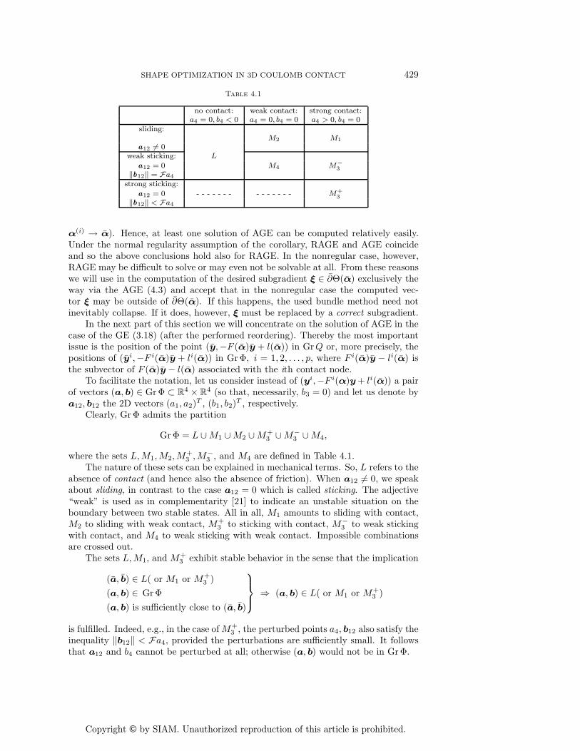
Table 4.1
no contact: weak contact: strong contact:a4 = 0, b4 < 0 a4 = 0, b4 = 0 a4 > 0, b4 = 0
sliding:M2 M1
a12 �= 0weak sticking: L
a12 = 0 M4 M−3
‖b12‖ = Fa4
strong sticking:
a12 = 0 - - - - - - - - - - - - - - M+3‖b12‖ < Fa4
α(i) → α). Hence, at least one solution of AGE can be computed relatively easily.Under the normal regularity assumption of the corollary, RAGE and AGE coincideand so the above conclusions hold also for RAGE. In the nonregular case, however,RAGE may be difficult to solve or may even not be solvable at all. From these reasonswe will use in the computation of the desired subgradient ξ ∈ ∂Θ(α) exclusively theway via the AGE (4.3) and accept that in the nonregular case the computed vec-tor ξ may be outside of ∂Θ(α). If this happens, the used bundle method need notinevitably collapse. If it does, however, ξ must be replaced by a correct subgradient.
In the next part of this section we will concentrate on the solution of AGE in thecase of the GE (3.18) (after the performed reordering). Thereby the most importantissue is the position of the point (y,−F (α)y + l(α)) in GrQ or, more precisely, thepositions of (yi,−F i(α)y + li(α)) in GrΦ, i = 1, 2, . . . , p, where F i(α)y − li(α) isthe subvector of F (α)y − l(α) associated with the ith contact node.
To facilitate the notation, let us consider instead of (yi,−F i(α)y + li(α)) a pairof vectors (a, b) ∈ GrΦ ⊂ R
4 × R4 (so that, necessarily, b3 = 0) and let us denote by
a12, b12 the 2D vectors (a1, a2)T , (b1, b2)T , respectively.Clearly, GrΦ admits the partition
Gr Φ = L ∪ M1 ∪ M2 ∪ M+3 ∪ M−
3 ∪ M4,
where the sets L, M1, M2, M+3 , M−
3 , and M4 are defined in Table 4.1.The nature of these sets can be explained in mechanical terms. So, L refers to the
absence of contact (and hence also the absence of friction). When a12 �= 0, we speakabout sliding, in contrast to the case a12 = 0 which is called sticking. The adjective“weak” is used as in complementarity [21] to indicate an unstable situation on theboundary between two stable states. All in all, M1 amounts to sliding with contact,M2 to sliding with weak contact, M+
3 to sticking with contact, M−3 to weak sticking
with contact, and M4 to weak sticking with weak contact. Impossible combinationsare crossed out.
The sets L, M1, and M+3 exhibit stable behavior in the sense that the implication
(a, b) ∈ L( or M1 or M+3 )
(a, b) ∈ GrΦ(a, b) is sufficiently close to (a, b)
⎫⎪⎬⎪⎭ ⇒ (a, b) ∈ L( or M1 or M+3 )
is fulfilled. Indeed, e.g., in the case of M+3 , the perturbed points a4, b12 also satisfy the
inequality ‖b12‖ < Fa4, provided the perturbations are sufficiently small. It followsthat a12 and b4 cannot be perturbed at all; otherwise (a, b) would not be in GrΦ.
Copyright © by SIAM. Unauthorized reproduction of this article is prohibited.
430 BEREMLIJSKI, HASLINGER, KOCVARA, KUCERA, OUTRATA
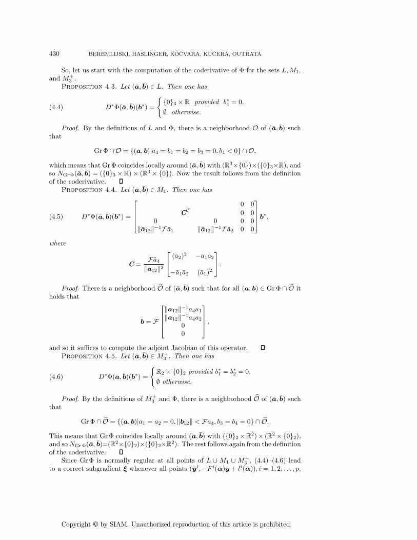
So, let us start with the computation of the coderivative of Φ for the sets L, M1,and M+
3 .Proposition 4.3. Let (a, b) ∈ L. Then one has
(4.4) D∗Φ(a, b)(b∗) =
{{0}3 × R provided b∗4 = 0,
∅ otherwise.
Proof. By the definitions of L and Φ, there is a neighborhood O of (a, b) suchthat
GrΦ ∩ O = {(a, b)|a4 = b1 = b2 = b3 = 0, b4 < 0} ∩ O,
which means that Gr Φ coincides locally around (a, b) with (R3×{0})×({0}3×R), andso NGrΦ(a, b) = ({0}3 × R) × (R3 × {0}). Now the result follows from the definitionof the coderivative.
Proposition 4.4. Let (a, b) ∈ M1. Then one has
(4.5) D∗Φ(a, b)(b∗) =
⎡⎢⎢⎣0 0
CT 0 00 0 0 0
‖a12‖−1F a1 ‖a12‖−1F a2 0 0
⎤⎥⎥⎦ b∗,
where
C =F a4
‖a12‖3
⎡⎣ (a2)2 −a1a2
−a1a2 (a1)2
⎤⎦ .
Proof. There is a neighborhood O of (a, b) such that for all (a, b) ∈ Gr Φ ∩ O itholds that
b = F
⎡⎢⎢⎣‖a12‖−1a4a1
‖a12‖−1a4a2
00
⎤⎥⎥⎦ ,
and so it suffices to compute the adjoint Jacobian of this operator.Proposition 4.5. Let (a, b) ∈ M+
3 . Then one has
(4.6) D∗Φ(a, b)(b∗) =
{R2 × {0}2 provided b∗1 = b∗2 = 0,
∅ otherwise.
Proof. By the definitions of M+3 and Φ, there is a neighborhood O of (a, b) such
that
Gr Φ ∩ O = {(a, b)|a1 = a2 = 0, ‖b12‖ < Fa4, b3 = b4 = 0} ∩ O.
This means that GrΦ coincides locally around (a, b) with ({0}2 ×R2)× (R2 ×{0}2),
and so NGrΦ(a, b)=(R2×{0}2)×({0}2×R2). The rest follows again from the definition
of the coderivative.Since GrΦ is normally regular at all points of L ∪ M1 ∪ M+
3 , (4.4)–(4.6) leadto a correct subgradient ξ whenever all points (yi,−F i(α)y + li(α)), i = 1, 2, . . . , p,
Copyright © by SIAM. Unauthorized reproduction of this article is prohibited.
SHAPE OPTIMIZATION IN 3D COULOMB CONTACT 431
belong to this union. The situation is not so satisfactory, provided we have to do withthe remaining sets M2, M
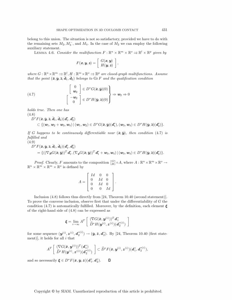
−3 , and M4. In the case of M2 we can employ the following
auxiliary statement.Lemma 4.6. Consider the multifunction F : R
n × Rm × R
o ⇒ Rl × R
p given by
F (x, y, z) =[
G(x, y)H(y, z)
],
where G : Rn×R
m ⇒ Rl, H : R
m×Ro ⇒ R
p are closed-graph multifunctions. Assumethat the point (x, y, z, d1, d2) belongs to GrF and the qualification condition
(4.7)
[0w2
]∈ D∗G(x, y)(0)[ −w2
0
]∈ D∗H(y, z)(0)
⎫⎪⎪⎬⎪⎪⎭ ⇒ w2 ⇒ 0
holds true. Then one has(4.8)
D∗F (x, y, z, d1, d2)(d∗1,d
∗2)
⊂ {(w1,w2 + w3,w4) | (w1,w2) ∈ D∗G(x, y)(d∗1), (w3,w4) ∈ D∗H(y, z)(d∗
2)}.
If G happens to be continuously differentiable near (x, y), then condition (4.7) isfulfilled and(4.9)
D∗F (x, y, z, d1, d2)(d∗1,d
∗2)
= {((∇xG(x, y))T d∗1, (∇yG(x, y))T d∗
1 + w3,w4) | (w3,w4) ∈ D∗H(y, z)(d∗2)}.
Proof. Clearly, F amounts to the composition[GH
]◦A, where A : Rn×R
m×Ro →
Rn × R
m × Rm × R
o is defined by
A =
⎡⎢⎢⎣Id 0 00 Id 00 Id 00 0 Id
⎤⎥⎥⎦ .
Inclusion (4.8) follows thus directly from [24, Theorem 10.40 (second statement)].To prove the converse inclusion, observe first that under the differentiability of G thecondition (4.7) is automatically fulfilled. Moreover, by the definition, each element ξ
of the right-hand side of (4.8) can be expressed as
ξ = limi→∞
AT
[(∇G(x , y(i)))Td∗
1
D∗H(y(i), z (i))(d∗(i)2 )
]for some sequence (y(i), z (i),d
∗(i)2 ) → (y, z ,d∗
2). By [24, Theorem 10.40 (first state-ment)], it holds for all i that
AT
[(∇G(x , y(i)))T (d∗
1)D∗H(y(i), z (i))(d∗(i)
2 )
]⊂ D∗F (x , y(i), z (i))(d∗
1,d∗(i)2 ),
and so necessarily ξ ∈ D∗F (x , y, z )(d∗1,d
∗2).
Copyright © by SIAM. Unauthorized reproduction of this article is prohibited.
432 BEREMLIJSKI, HASLINGER, KOCVARA, KUCERA, OUTRATA
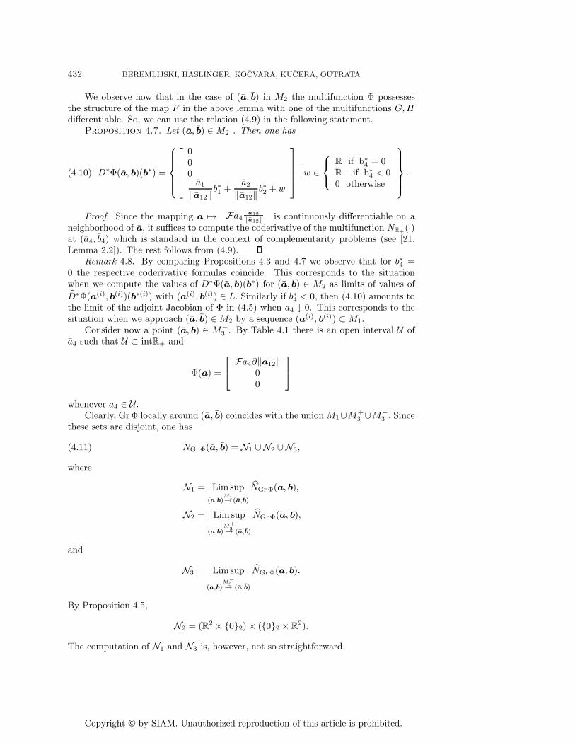
We observe now that in the case of (a, b) in M2 the multifunction Φ possessesthe structure of the map F in the above lemma with one of the multifunctions G, Hdifferentiable. So, we can use the relation (4.9) in the following statement.
Proposition 4.7. Let (a, b) ∈ M2 . Then one has
(4.10) D∗Φ(a, b)(b∗) =
⎧⎪⎪⎪⎨⎪⎪⎪⎩⎡⎢⎢⎢⎣
000
a1
‖a12‖b∗1 +a2
‖a12‖b∗2 + w
⎤⎥⎥⎥⎦ |w ∈⎧⎨⎩
R if b∗4 = 0
R− if b∗4 < 0
0 otherwise
⎫⎪⎪⎪⎬⎪⎪⎪⎭ .
Proof. Since the mapping a → Fa4a12
‖a12‖ is continuously differentiable on aneighborhood of a, it suffices to compute the coderivative of the multifunction NR+(·)at (a4, b4) which is standard in the context of complementarity problems (see [21,Lemma 2.2]). The rest follows from (4.9).
Remark 4.8. By comparing Propositions 4.3 and 4.7 we observe that for b∗4 =0 the respective coderivative formulas coincide. This corresponds to the situationwhen we compute the values of D∗Φ(a, b)(b∗) for (a, b) ∈ M2 as limits of values ofD∗Φ(a(i), b(i))(b∗(i)) with (a(i), b(i)) ∈ L. Similarly if b∗4 < 0, then (4.10) amounts tothe limit of the adjoint Jacobian of Φ in (4.5) when a4 ↓ 0. This corresponds to thesituation when we approach (a, b) ∈ M2 by a sequence (a(i), b(i)) ⊂ M1.
Consider now a point (a, b) ∈ M−3 . By Table 4.1 there is an open interval U of
a4 such that U ⊂ intR+ and
Φ(a) =
⎡⎣ Fa4∂‖a12‖00
⎤⎦whenever a4 ∈ U .
Clearly, Gr Φ locally around (a, b) coincides with the union M1∪M+3 ∪M−
3 . Sincethese sets are disjoint, one has
(4.11) NGr Φ(a, b) = N1 ∪ N2 ∪N3,
where
N1 = Lim sup(a,b)
M1→ (a,b)
NGr Φ(a, b),
N2 = Lim sup
(a,b)M
+3→ (a,b)
NGrΦ(a, b),
and
N3 = Limsup
(a,b)M
−3→ (a,b)
NGr Φ(a, b).
By Proposition 4.5,
N2 = (R2 × {0}2) × ({0}2 × R2).
The computation of N1 and N3 is, however, not so straightforward.

Copyright © by SIAM. Unauthorized reproduction of this article is prohibited.
SHAPE OPTIMIZATION IN 3D COULOMB CONTACT 433
Lemma 4.9. Put w = b12F a4
(so that ‖w‖ = 1). Then one has
(4.12)N1 = {(a∗, b∗) ∈ R
4 × R4|a∗
12 = 0, a∗3 = 0, (a∗
4, b∗12) ∈ R(−F , w)}
∪ {(a∗, b∗) ∈ R4 × R
4|a∗12 ∈ w⊥, a∗
3 = a∗4 = 0, b∗
12 = 0}.Proof. We have to compute all accumulation points of sequences (a∗(i), b∗(i))
satisfying the equations (see (4.5))
a∗(i)12 = − Fa
(i)4
‖a(i)12 ‖
⎡⎢⎢⎢⎢⎣(a(i)
2 )2
‖a(i)12 ‖2
−a(i)1 a
(i)2
‖a(i)12 ‖2
−a(i)1 a
(i)2
‖a(i)12 ‖2
(a(i)1 )2
‖a(i)12 ‖2
⎤⎥⎥⎥⎥⎦[
b∗(i)1
b∗(i)2
],
a∗(i)3 = 0,
a∗(i)4 = − F
‖a(i)12 ‖
(ai1b
∗(i)1 + ai
2b∗(i)2 )
when ‖a(i)12 ‖ ↓ 0 and a
(i)4 → a4 > 0. Put w (i) := a
(i)12
‖a(i)12 ‖ and
D(i) :=
⎡⎣ (w(i)2 )2 −w
(i)1 w
(i)2
−w(i)1 w
(i)2 (w(i)
1 )2
⎤⎦so that w (i) → w and
D(i) → D :=
[w2
2 −w1w2
−w1w2 w21
].
A sequence {(a∗(i)12 , a
∗(i)4 , b
∗(i)12 )} converges to an accumulation point (a∗
12, a∗4, b
∗12) if
and only if the sequence
ξ(i) := D(i)
⎡⎢⎢⎢⎢⎣b∗(i)1
‖a(i)12 ‖
b∗(i)2
‖a(i)12 ‖
⎤⎥⎥⎥⎥⎦converges. This happens if either b
∗(i)12 ∈ KerD(= Rw) for all i, or b∗
12 = 0. Theformer case generates the first cone on the right-hand side of (4.12). In the latter caselimi→∞ ξ(i) can be everywhere in the range space of D which amounts to w⊥. Thisgives rise to the second cone on the right-hand side of (4.12), and the statement hasbeen established.
Lemma 4.10. Consider a point (a, b) ∈ M−3 , and put w := b12
Fa4. Then one has
(4.13) NGr Φ(a, b) = {(a∗, b∗) | 〈a∗12,w〉 ≤ 0, a∗
3 = 0, (a∗4, b
∗12) ∈ R+(−F ,w)}.
Proof. We compute first the contingent cone TGrΦ(a, b). To this end we observethat GrΦ locally around (a, b) coincides with the union G1 ∪ G2, where
G1 ={
(a, b) |a12 �= 0, b12 = Fa4a12
‖a12‖ , b3 = b4 = 0}
Copyright © by SIAM. Unauthorized reproduction of this article is prohibited.
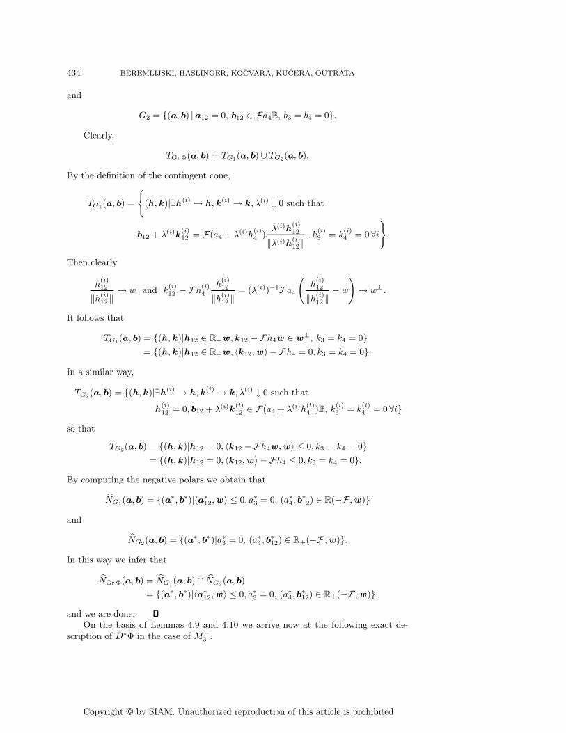
434 BEREMLIJSKI, HASLINGER, KOCVARA, KUCERA, OUTRATA
and
G2 = {(a, b) |a12 = 0, b12 ∈ Fa4B, b3 = b4 = 0}.Clearly,
TGr Φ(a, b) = TG1(a, b) ∪ TG2(a, b).
By the definition of the contingent cone,
TG1(a, b) =
{(h , k)|∃h (i) → h , k (i) → k , λ(i) ↓ 0 such that
b12 + λ(i)k(i)12 = F(a4 + λ(i)h
(i)4 )
λ(i)h(i)12
‖λ(i)h(i)12 ‖
, k(i)3 = k
(i)4 = 0 ∀i
}.
Then clearly
h(i)12
‖h(i)12 ‖
→ w and k(i)12 −Fh
(i)4
h(i)12
‖h(i)12 ‖
= (λ(i))−1Fa4
(h
(i)12
‖h(i)12 ‖
− w
)→ w⊥.
It follows that
TG1(a, b) = {(h , k )|h12 ∈ R+w , k12 −Fh4w ∈ w⊥, k3 = k4 = 0}= {(h , k )|h12 ∈ R+w , 〈k12,w〉 − Fh4 = 0, k3 = k4 = 0}.
In a similar way,
TG2(a, b) = {(h , k )|∃h (i) → h , k (i) → k , λ(i) ↓ 0 such that
h(i)12 = 0, b12 + λ(i)k
(i)12 ∈ F(a4 + λ(i)h
(i)4 )B, k
(i)3 = k
(i)4 = 0 ∀i}
so that
TG2(a, b) = {(h , k)|h12 = 0, 〈k12 −Fh4w ,w〉 ≤ 0, k3 = k4 = 0}= {(h , k)|h12 = 0, 〈k12,w〉 − Fh4 ≤ 0, k3 = k4 = 0}.
By computing the negative polars we obtain that
NG1(a, b) = {(a∗, b∗)|〈a∗12,w〉 ≤ 0, a∗
3 = 0, (a∗4, b
∗12) ∈ R(−F ,w)}
and
NG2(a, b) = {(a∗, b∗)|a∗3 = 0, (a∗
4, b∗12) ∈ R+(−F ,w)}.
In this way we infer that
NGrΦ(a, b) = NG1(a, b) ∩ NG2(a, b)= {(a∗, b∗)|〈a∗
12,w〉 ≤ 0, a∗3 = 0, (a∗
4, b∗12) ∈ R+(−F ,w)},
and we are done.On the basis of Lemmas 4.9 and 4.10 we arrive now at the following exact de-
scription of D∗Φ in the case of M−3 .
Copyright © by SIAM. Unauthorized reproduction of this article is prohibited.
SHAPE OPTIMIZATION IN 3D COULOMB CONTACT 435
Theorem 4.11. Let (a, b) ∈ M−3 and w = b12
F a4. Then one has
(4.14)
D∗Φ(a, b)(b∗) =
⎧⎪⎪⎪⎨⎪⎪⎪⎩{a∗ ∈ R
4|a∗12 = 0, a∗
3 = 0, a∗4 = Fα} if b∗
12 = αw, α ≥ 0,
{a∗ ∈ R4|〈a∗
12, w〉 ≤ 0, a∗3 = 0, a∗
4 = Fα} if b∗12 = αw, α ≤ 0,
R2 × {0}2 if b∗
12 = 0,
∅ otherwise.
Proof. On the basis of Lemma 4.10 we can compute the cone N3. To this end itsuffices to realize that a4 → a4(> 0) and b12 → b12 implies w = b12
Fa4→ w = b12
F a4.
Consequently, N3 = NGrΦ(a, b). The rest follows from (4.11) and the definition ofthe coderivative.
In the case of M4, however, this approach would be substantially more difficult.The respective limiting normal cone will again have the structure of a union, someparts of which can easily be computed. The set M4 consists, however, only of onepoint (when we ignore variable a3), and so the absence of an exact formula does nothave a negative impact on the proposed numerical method. From this reason we alsoomit a detailed analysis of this case here.
All derived formulas (4.4), (4.5), (4.6), (4.10), and (4.14) enable us to specify foreach node i a linear subspace
Li ∈ GrD∗Φ(yi,−F i(α)y + li(α))
such that the AGE (4.3) amounts to the linear system
0 = y∗ + (F (α))T v + w(4.15)
(wi, vi) ∈ Li, i = 1, 2, . . . p.
This of course facilitates its numerical solution.As already mentioned, if some nodes lie in M2 or M−
3 (or in M4), this techniqueneed not immediately lead to a correct subgradient due to the right inclusion in (4.1).Fortunately, as shown by the performed numerical tests, such nodes occur very rarelyduring the iteration process and typically cause some difficulties only close to optimalpoints. Formulas (4.10) and (4.14) offer then a possibility to restore the convergenceby a suitable change of the adjoint system (4.15).
5. Numerical results. The results of the previous sections will now be usedfor construction of a numerical method for the solution of (P). We assume that thefriction coefficient F is small enough in the sense of Theorem 3.8 so that the solutionof the contact problem with Coulomb friction is unique. Further, as in section 4, weassume that the cost functional J is continuously differentiable. For the minimizationof Θ we use the BT code [27] based on the bundle-truss algorithm of Schramm andZowe [25]. In every step of the iteration process, this code has to be supplied withthe function value Θ(α) and one (arbitrary) Clarke’s subgradient of Θ at α.
5.1. Solving the state problem. To compute a function value J(α, S(α)), wehave to evaluate S(α), i.e., to solve the fixed point problem (P). For that, we use themethod of successive approximations introduced in Corollary 3.9. Each iterative steprequires us to solve the contact problem with given friction (M (L, g)), in which theslip bound g is updated by the result of the previous iteration, i.e., g ≡ λ(k). Theproblem (M (L, g)) is solved using the so-called reciprocal variational formulation (see[8, 11, 12]). As in the previous sections, we denote by λ ∈ R
p the vector of normal
Copyright © by SIAM. Unauthorized reproduction of this article is prohibited.
436 BEREMLIJSKI, HASLINGER, KOCVARA, KUCERA, OUTRATA
contact stresses. Further, let τ ∈ R2p be the vector of tangential contact stresses.
Notice that with each contact node we associate one component λi of λ and twocomponents τ2i−1, τ2i of τ . After eliminating the first variable u from (M (L, g)),we arrive at the problem formulated in terms of contact stresses:
(5.1) minσ∈ S
f(σ) :=12σTQσ − σTh
with
S = {σ = (λ, τ) ∈ R3p | λi ≥ 0, τ2
2i−1 + τ22i ≤ g2
i , i = 1, 2, . . . , p},
where Q = BA−1BT , h = BA−1L + c, B = (N T ,TT )T , c = (αT , 0T )T , andT ∈ R
2p×n stands for a matrix representation of the linear mapping T used in (3.3).After computing λ, τ from (5.1), one obtains the eliminated variable u by
u = A−1(L−Nλ−Tτ).
As (5.1) is a strictly convex problem with quadratic objective and separable quadraticconstraints, it can be solved by the algorithm proposed by Kucera in [14] and analyzedin [15]. The algorithm generalizes ideas of Dostal and Schoberl [5] originally proposedfor convex quadratic problems with simple bounds. Because an efficient solutionprocedure for (5.1) is essential for the overall efficiency of our numerical approach, wegive a brief description of the algorithm.
Let N = {1, . . . , 3p} be the set of all indices. At a point σ ∈ S, we denote thegradient of f by r = r(σ) = Qσ − h and introduce an active set A ⊆ N by
A := A(σ) = {i | λi = 0} ∪ {j | j = 2i − 1 + p : τ22i−1 + τ2
2i = g2i }
∪ {j | j = 2i + p : τ22i−1 + τ2
2i = g2i }.
Using the orthogonal projection PS : R3p → S, we define the projected gradient for a
fixed α ≥ 0 as
r = r(σ) =1α
(σ − PS(σ − αr(σ))).
Notice that the projected gradient enables us to write down the optimality criterioncharacterizing the solution σ∗ of (5.1) in the form r(σ∗) = 0. Our algorithm is basedon the observation that nonzero components of r(σ) at σ �= σ∗ determine descent di-rections changing appropriately the active set. To this end, we introduce componentsof r(σ) and r(σ) called the projected free gradient ϕ = ϕ(σ), the projected boundarygradient β = β(σ), and the free gradient ϕ = ϕ(σ), respectively, defined by
ϕA = 0, ϕN\A = rN\A,
βA = rA, βN\A = 0,
ϕA = 0, ϕN\A = rN\A.
We combine three steps to generate a sequence of iterates {σ(l)} that approxi-mates the solution to (5.1):
• the expansion step: σ(l+1) = σ(l) − αϕ(σ(l)),• the proportioning step: σ(l+1) = σ(l) − αβ(σ(l)),
Copyright © by SIAM. Unauthorized reproduction of this article is prohibited.
SHAPE OPTIMIZATION IN 3D COULOMB CONTACT 437
• the conjugate gradient step: σ(l+1) = σ(l) − α(l)cg p(l), where the step size α
(l)cg
and the conjugate gradient directions p(l) are computed recurrently (see [7])so that the recurrence starts from σ(s) generated by the last expansion orproportioning step and A(σ(l+1)) = A(σ(s)).
The expansion step may add indices, while the proportioning step may release in-dices to/from the current active set. The conjugate gradient step is used to carryout efficiently minimization of the objective f on the interior of the set W (σ(s)) ={σ ∈ S | σA = σ
(s)A ,A = A(σ(s))}. Moreover, the algorithm exploits a given constant
Γ > 0 and the releasing criterion
(5.2) β(σ(l))T r(σ(l)) ≤ Γ ϕ(σ(l))T r(σ(l))
to decide which of the steps will be performed.Algorithm 1. Let σ(0) ∈ S, Γ > 0, α ∈ (0, ‖Q‖−1], and ε ≥ 0 be given. For σ(l),
σ(s) known, 0 ≤ s ≤ l, where σ(s) is computed by the last expansion or proportioningstep, choose σ(l+1) by the following rules:
(i) If ‖r(σ(l))‖ ≤ ε, return σ = σ(l).(ii) If σ(l) fulfills (5.2), try to generate σ(l+1) by the conjugate gradient step. If
σ(l+1) ∈ IntW (σ(s)), accept it, else generate σ(l+1) by the expansion step.(iii) If σ(l) does not fulfil (5.2), generate σ(l+1) by the proportioning step.Contrary to the simple bound problem analyzed in [5], the algorithm does not ex-
hibit the finite terminating property; the same convergence rate is, however, achieved.In [15] one can find the following statement.
Theorem 5.1. Let σ∗ ∈ S denote the solution to (5.1), αmin denote the smallesteigenvalue of Q, and Γ = max{Γ, Γ−1}. Let {σ(l)} be the sequence generated byAlgorithm 1 with ε = 0. Then
f(σ(l+1)) − f(σ∗) ≤ η(f(σ(l)) − f(σ∗)
),
where
η = 1 − ααmin
2 + 2Γ2< 1.
The error in the Q-energy norm is bounded by
‖σ(l) − σ∗‖2Q ≤ 2ηl
(f(σ(0)) − f(σ∗)
).
Theorem 5.1 yields the best value of the convergence rate factor η for the choiceΓ = Γ = 1 and α = ‖Q‖−1. Then
η = 1 − 14κ(Q),
where κ(Q) is the spectral condition number of Q .
5.2. Numerical examples. In order to work with a relatively small numberof control variables and, at the same time, to get a smooth shape of the optimalboundary, we will model the contact boundary Γc by a Bezier surface of order d. Thedesign variable α is thus the vector of its control points. The Bezier surface ϑα oforder (d1, d2) in R(= [0, a] × [0, b]) is generated by a d1 × d2 matrix α as
ϑα(x1, x2) =d1∑
i=0
d2∑j=0
α(i,j)βid1
(x1)βjd2
(x2), (x1, x2) ∈ R,

Copyright © by SIAM. Unauthorized reproduction of this article is prohibited.
438 BEREMLIJSKI, HASLINGER, KOCVARA, KUCERA, OUTRATA
where
β�d1
(x1) =1
ad1
(d1
�
)x�
1(a − x1)d1−�, β�d2
(x2) =1
bd2
(d2
�
)x�
2(b − x2)d2−�.
The corner points of ϑα are identical to the “corner elements” of the controlmatrix. The surface itself lies in the convex hull of the control points. This meansthat any upper and lower bounds on the control points hold for the whole surface inR, too.
The discrete shape optimization problem is now defined as follows:
(PB)minimize J(α, S(α))subject to α ∈ U ,
}
where U is given by
U =
{α ∈ R
d1×d2 | 0 ≤ α(i,j) ≤ C0, i = 0, 1, . . . , d1, j = 0, 1, . . . , d2;
|α(i+1,j) − α(i,j)| ≤ C1a
d1, i = 0, 1, . . . , d1 − 1, j = 0, 1, . . . , d2;
|α(i,j+1) − α(i,j)| ≤ C1b
d2, i = 0, 1, . . . , d1, j = 0, 1, . . . , d2 − 1;
d1∑i=0
d2∑j=0
α(i,j) = C2(d1 + 1)(d2 + 1)
⎫⎬⎭ ,
where C0, C1, and C2 are given positive constants. The first set of constraints guar-antees that |Fα(x)| ≤ C0 for all x ∈ R. The second and third constraint sets takecare of the slopes of ϑα in the direction of axes x1, x2. It is well known that if thecontrol points satisfy these conditions, then | ∂
∂xkϑα(x1, x2)| ≤ C1 for all (x1, x2) ∈ R,
k = 1, 2.The equality constraint is added to control the volume of the domain by the
control points of the Bezier surface. The number (c − C2)ab equals the volume ofΩ(α) defined by
(5.3) Ω(α) = {(x1, x2, x3) ∈ R3 | (x1, x2) ∈ (0, a) × (0, b), Fα(x1, x2) < x3 < c};
see Figure 5.1 which shows the body in 3D and 2D view. Thus, the equality constrainthas a physical meaning of preserving the weight of the structure.
All test examples solved below differ only in the cost function. The shape of theelastic body Ω(α), α ∈ U , is given by (5.3), with a = 2, b = 1, and c = 1. The set ofadmissible designs U is determined by the choice C0 = 0.75, C1 = 0.5, and C2 = 0.01.
The left-hand face Γu = {x ∈ Ω(α) | x1 = 0} is the part of the boundary with theprescribed Dirichlet condition where all displacements are fixed to zero. The nonzeroexternal loads are defined as follows. The top face ΓP1 = {x ∈ Ω(α) | x3 = 1}is subjected to constant pressure P1 = −8 · 10−2 N
m2 . The right-hand face ΓP2 ={x ∈ Ω(α) | x1 = 1} is subjected to constant traction P2 = 5 · 10−2 N
m2 . The bottomface Γc represented by the graph of ϑ(α) is supported by a rigid half-space R
2 ×R−.
Copyright © by SIAM. Unauthorized reproduction of this article is prohibited.
SHAPE OPTIMIZATION IN 3D COULOMB CONTACT 439
3x
x
x
1
2
c
P2
P1
uΓ
Γ
Γ
Γ
x 3
1x
Γu
Γ
Γ
c
P1Γ
P2
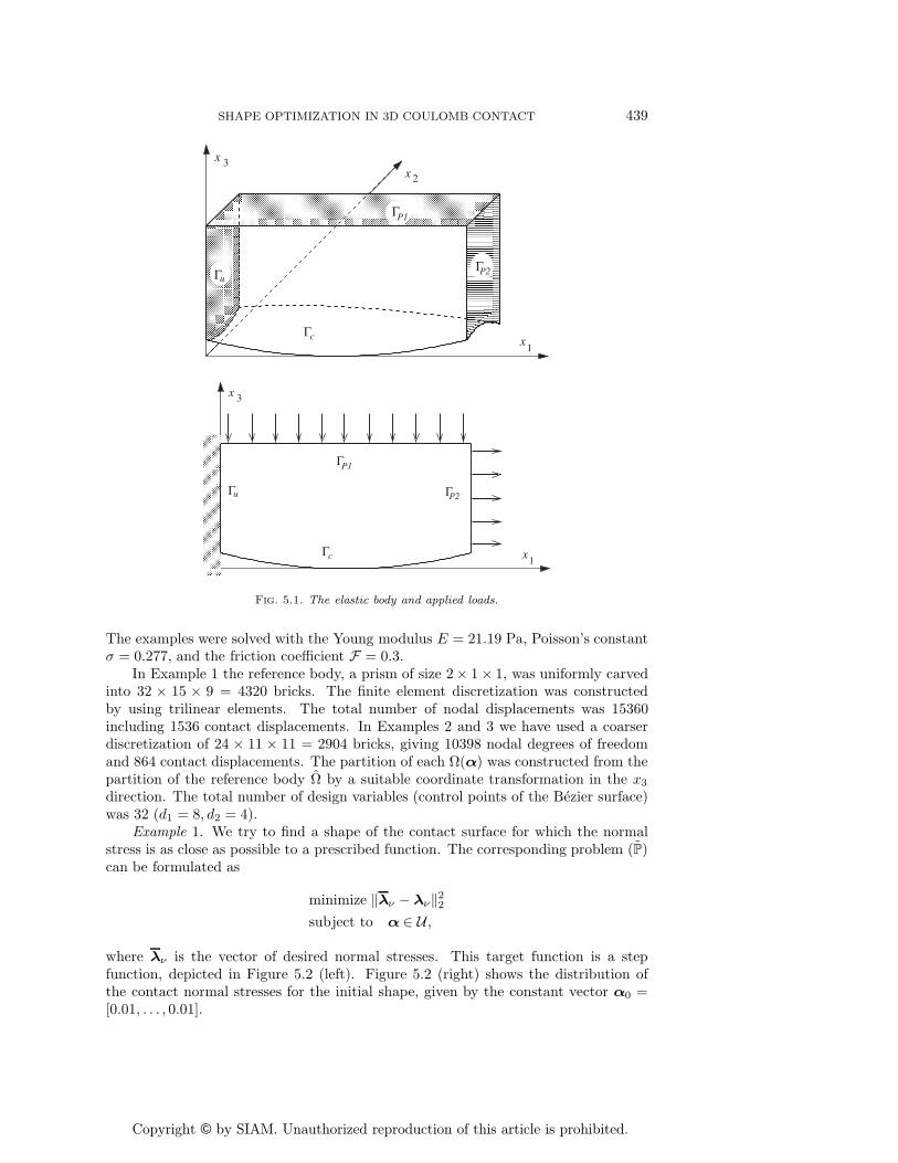
Fig. 5.1. The elastic body and applied loads.
The examples were solved with the Young modulus E = 21.19 Pa, Poisson’s constantσ = 0.277, and the friction coefficient F = 0.3.
In Example 1 the reference body, a prism of size 2× 1 × 1, was uniformly carvedinto 32 × 15 × 9 = 4320 bricks. The finite element discretization was constructedby using trilinear elements. The total number of nodal displacements was 15360including 1536 contact displacements. In Examples 2 and 3 we have used a coarserdiscretization of 24 × 11 × 11 = 2904 bricks, giving 10398 nodal degrees of freedomand 864 contact displacements. The partition of each Ω(α) was constructed from thepartition of the reference body Ω by a suitable coordinate transformation in the x3
direction. The total number of design variables (control points of the Bezier surface)was 32 (d1 = 8, d2 = 4).
Example 1. We try to find a shape of the contact surface for which the normalstress is as close as possible to a prescribed function. The corresponding problem (P)can be formulated as
minimize ‖λν − λν‖22
subject to α ∈ U ,
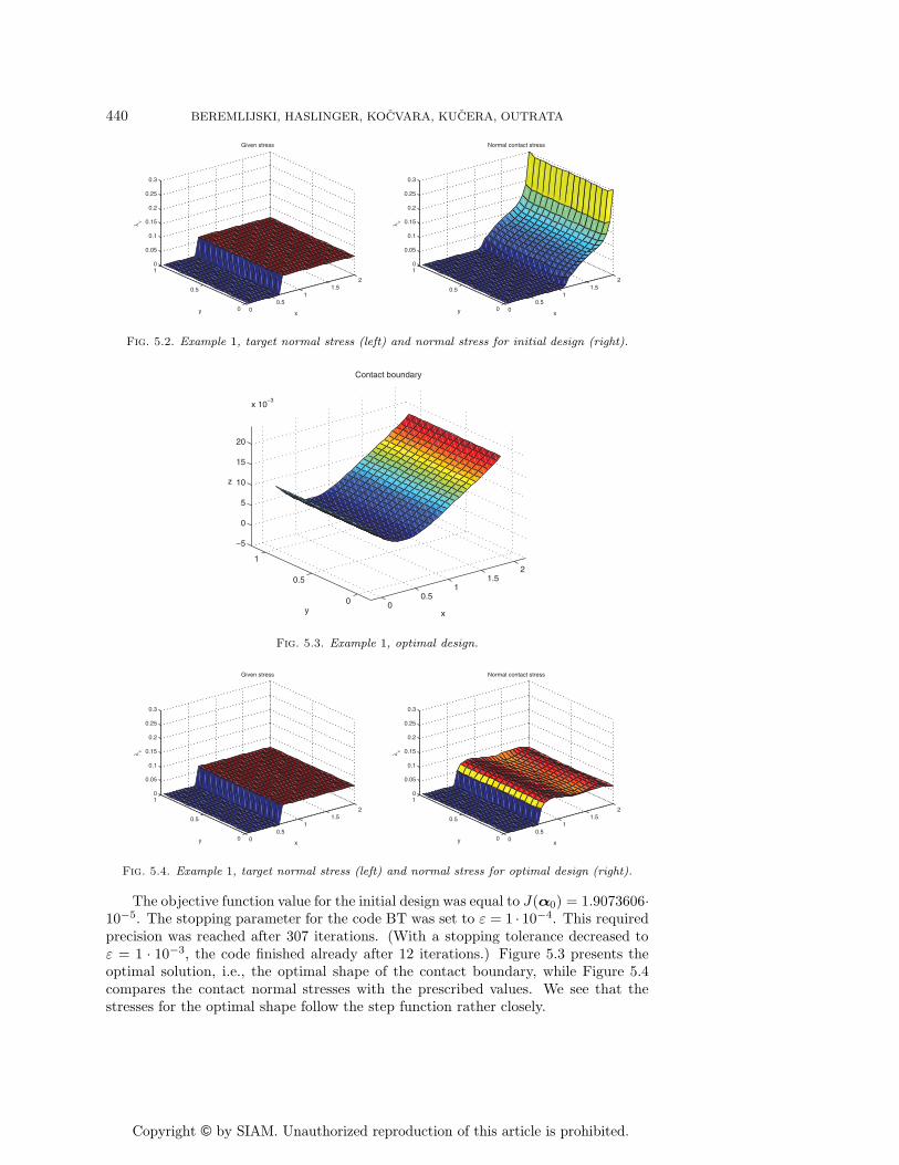
where λν is the vector of desired normal stresses. This target function is a stepfunction, depicted in Figure 5.2 (left). Figure 5.2 (right) shows the distribution ofthe contact normal stresses for the initial shape, given by the constant vector α0 =[0.01, . . . , 0.01].
Copyright © by SIAM. Unauthorized reproduction of this article is prohibited.
440 BEREMLIJSKI, HASLINGER, KOCVARA, KUCERA, OUTRATA
00.5
11.5
2
0
0.5
10
0.05
0.1
0.15
0.2
0.25
0.3
x
Given stress
y
λ ν
00.5
11.5
2
0
0.5
10
0.05
0.1
0.15
0.2
0.25
0.3
x
Normal contact stress
y
λ ν
Fig. 5.2. Example 1, target normal stress (left) and normal stress for initial design (right).
00.5
11.5
2
0
0.5
1
−5
0
5
10
15
20
x 10−3
x
Contact boundary
y
z
Fig. 5.3. Example 1, optimal design.
00.5
11.5
2
0
0.5
10
0.05
0.1
0.15
0.2
0.25
0.3
x
Given stress
y
λ ν
00.5
11.5
2
0
0.5
10
0.05
0.1
0.15
0.2
0.25
0.3
x
Normal contact stress
y
λ ν
Fig. 5.4. Example 1, target normal stress (left) and normal stress for optimal design (right).
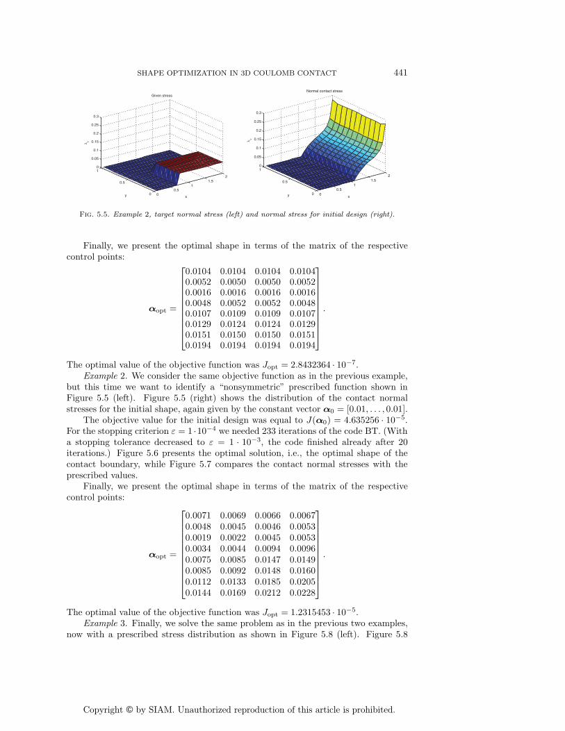
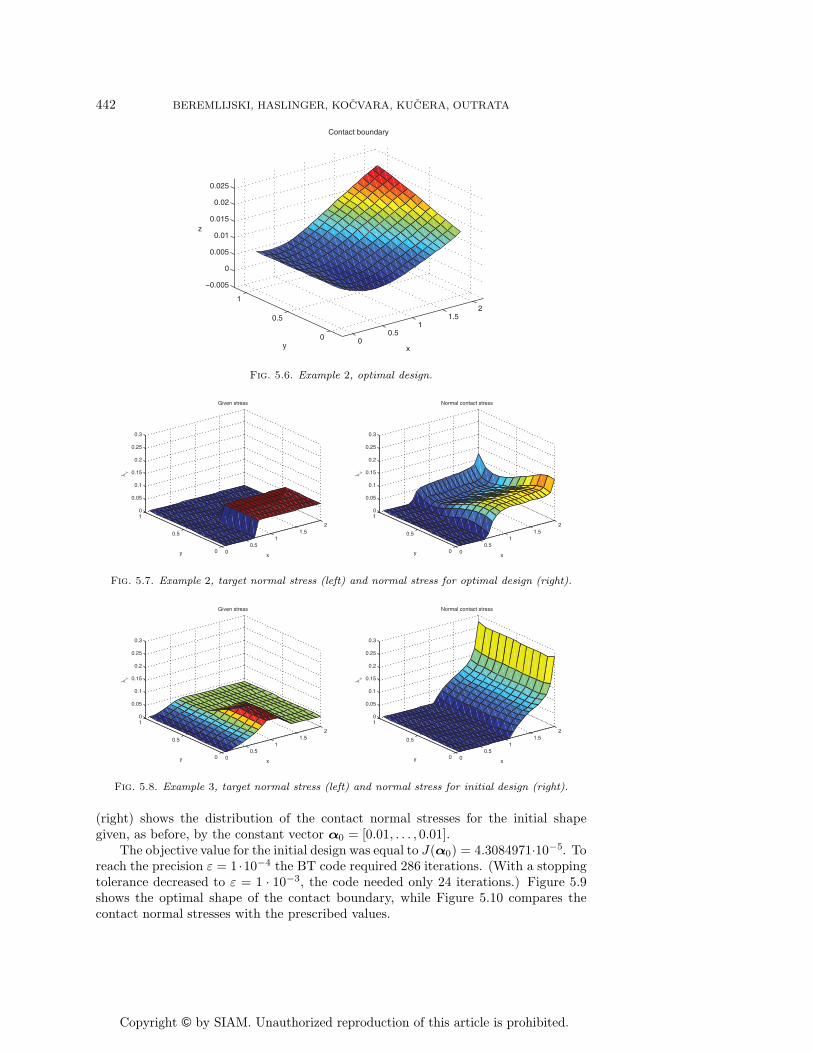
The objective function value for the initial design was equal to J(α0) = 1.9073606·10−5. The stopping parameter for the code BT was set to ε = 1 · 10−4. This requiredprecision was reached after 307 iterations. (With a stopping tolerance decreased toε = 1 · 10−3, the code finished already after 12 iterations.) Figure 5.3 presents theoptimal solution, i.e., the optimal shape of the contact boundary, while Figure 5.4compares the contact normal stresses with the prescribed values. We see that thestresses for the optimal shape follow the step function rather closely.
Copyright © by SIAM. Unauthorized reproduction of this article is prohibited.
SHAPE OPTIMIZATION IN 3D COULOMB CONTACT 441
00.5
11.5
2
0
0.5
10
0.05
0.1
0.15
0.2
0.25
0.3
x
Given stress
y
λ ν
00.5
11.5
2
0
0.5
10
0.05
0.1
0.15
0.2
0.25
0.3
x
Normal contact stress
y
λ ν
Fig. 5.5. Example 2, target normal stress (left) and normal stress for initial design (right).
Finally, we present the optimal shape in terms of the matrix of the respectivecontrol points:
αopt =
⎡⎢⎢⎢⎢⎢⎢⎢⎢⎢⎣
0.0104 0.0104 0.0104 0.01040.0052 0.0050 0.0050 0.00520.0016 0.0016 0.0016 0.00160.0048 0.0052 0.0052 0.00480.0107 0.0109 0.0109 0.01070.0129 0.0124 0.0124 0.01290.0151 0.0150 0.0150 0.01510.0194 0.0194 0.0194 0.0194
⎤⎥⎥⎥⎥⎥⎥⎥⎥⎥⎦.
The optimal value of the objective function was Jopt = 2.8432364 · 10−7.Example 2. We consider the same objective function as in the previous example,
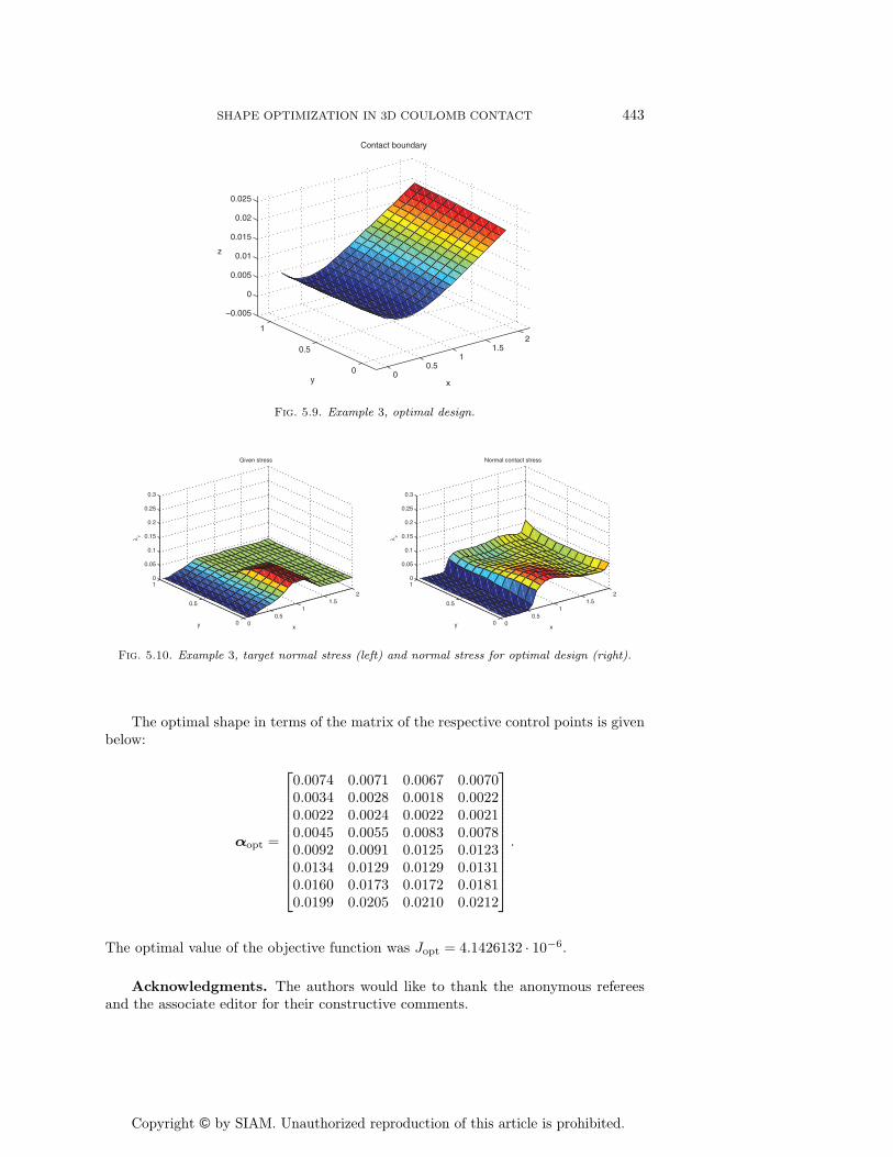
but this time we want to identify a “nonsymmetric” prescribed function shown inFigure 5.5 (left). Figure 5.5 (right) shows the distribution of the contact normalstresses for the initial shape, again given by the constant vector α0 = [0.01, . . . , 0.01].
The objective value for the initial design was equal to J(α0) = 4.635256 · 10−5.For the stopping criterion ε = 1 ·10−4 we needed 233 iterations of the code BT. (Witha stopping tolerance decreased to ε = 1 · 10−3, the code finished already after 20iterations.) Figure 5.6 presents the optimal solution, i.e., the optimal shape of thecontact boundary, while Figure 5.7 compares the contact normal stresses with theprescribed values.
Finally, we present the optimal shape in terms of the matrix of the respectivecontrol points:
αopt =
⎡⎢⎢⎢⎢⎢⎢⎢⎢⎢⎢⎣
0.0071 0.0069 0.0066 0.00670.0048 0.0045 0.0046 0.00530.0019 0.0022 0.0045 0.00530.0034 0.0044 0.0094 0.00960.0075 0.0085 0.0147 0.01490.0085 0.0092 0.0148 0.01600.0112 0.0133 0.0185 0.02050.0144 0.0169 0.0212 0.0228
⎤⎥⎥⎥⎥⎥⎥⎥⎥⎥⎥⎦.
The optimal value of the objective function was Jopt = 1.2315453 · 10−5.Example 3. Finally, we solve the same problem as in the previous two examples,
now with a prescribed stress distribution as shown in Figure 5.8 (left). Figure 5.8
Copyright © by SIAM. Unauthorized reproduction of this article is prohibited.
442 BEREMLIJSKI, HASLINGER, KOCVARA, KUCERA, OUTRATA
00.5
11.5
2
0
0.5
1
−0.005
0
0.005
0.01
0.015
0.02
0.025
x
Contact boundary
y
z
Fig. 5.6. Example 2, optimal design.
00.5
11.5
2
0
0.5
10
0.05
0.1
0.15
0.2
0.25
0.3
x
Given stress
y
λ ν
00.5
11.5
2
0
0.5
10
0.05
0.1
0.15
0.2
0.25
0.3
x
Normal contact stress
y
λ ν
Fig. 5.7. Example 2, target normal stress (left) and normal stress for optimal design (right).
00.5
11.5
2
0
0.5
10
0.05
0.1
0.15
0.2
0.25
0.3
x
Given stress
y
λ ν
00.5
11.5
2
0
0.5
10
0.05
0.1
0.15
0.2
0.25
0.3
x
Normal contact stress
y
λ ν
Fig. 5.8. Example 3, target normal stress (left) and normal stress for initial design (right).
(right) shows the distribution of the contact normal stresses for the initial shapegiven, as before, by the constant vector α0 = [0.01, . . . , 0.01].
The objective value for the initial design was equal to J(α0) = 4.3084971·10−5. Toreach the precision ε = 1 ·10−4 the BT code required 286 iterations. (With a stoppingtolerance decreased to ε = 1 · 10−3, the code needed only 24 iterations.) Figure 5.9shows the optimal shape of the contact boundary, while Figure 5.10 compares thecontact normal stresses with the prescribed values.
Copyright © by SIAM. Unauthorized reproduction of this article is prohibited.
SHAPE OPTIMIZATION IN 3D COULOMB CONTACT 443
00.5
11.5
2
0
0.5
1
−0.005
0
0.005
0.01
0.015
0.02
0.025
x
Contact boundary
y
z
Fig. 5.9. Example 3, optimal design.
00.5
11.5
2
0
0.5
10
0.05
0.1
0.15
0.2
0.25
0.3
x
Given stress
y
λ ν
00.5
11.5
2
0
0.5
10
0.05
0.1
0.15
0.2
0.25
0.3
x
Normal contact stress
y
λ ν
Fig. 5.10. Example 3, target normal stress (left) and normal stress for optimal design (right).
The optimal shape in terms of the matrix of the respective control points is givenbelow:
αopt =
⎡⎢⎢⎢⎢⎢⎢⎢⎢⎢⎢⎣
0.0074 0.0071 0.0067 0.00700.0034 0.0028 0.0018 0.00220.0022 0.0024 0.0022 0.00210.0045 0.0055 0.0083 0.00780.0092 0.0091 0.0125 0.01230.0134 0.0129 0.0129 0.01310.0160 0.0173 0.0172 0.01810.0199 0.0205 0.0210 0.0212
⎤⎥⎥⎥⎥⎥⎥⎥⎥⎥⎥⎦.
The optimal value of the objective function was Jopt = 4.1426132 · 10−6.
Acknowledgments. The authors would like to thank the anonymous refereesand the associate editor for their constructive comments.
Copyright © by SIAM. Unauthorized reproduction of this article is prohibited.
444 BEREMLIJSKI, HASLINGER, KOCVARA, KUCERA, OUTRATA
REFERENCES
[1] R. L. Benedict and J. E. Taylor, Optimal design for elastic bodies in contact, in Optimizationof Distributed Parameter Structures, Part II, E. J. Haug and J. Cea, eds., Sijthoff &Noorddhoff, Alphen aan den Rijn, The Netherlands, 1981, pp. 1553–1599.
[2] P. Beremlijski, J. Haslinger, M. Kocvara, and J. Outrata, Shape optimization in contactproblems with Coulomb friction, SIAM J. Optim., 13 (2002), pp. 561–587.
[3] F. F. Clarke, Optimization and Nonsmooth Analysis, John Wiley & Sons, New York, 1983.[4] A. L. Dontchev and W. W. Hager, Implicit functions, Lipschitz maps, and stability in
optimization, Math. Oper. Res., 19 (1994), pp. 753–768.[5] Z. Dostal and J. Schoberl, Minimizing quadratic functions over non-negative cone with the
rate of convergence and finite termination, Comput. Optim. Appl., 30 (2005), pp. 23–44.[6] C. Eck, J. Jarusek, and M. Krbec, Unilateral Contact Problems. Variational Methods and
Existence Theorems, Pure Appl. Math. (Boca Raton) 270, Chapman & Hall/CRC, BocaRaton, FL, 2005.
[7] G. H. Golub and C. F. V. Loan, Matrix Computation, The Johns Hopkins University Press,Baltimore, MD, 1996.
[8] J. Haslinger, Z. Dostal, and R. Kucera, Signorini problem with a given friction based onthe reciprocal variational formulation, in Nonsmooth/Nonconvex Mechanics: Modeling,Analysis and Numerical Methods, D. Y. Gao, R. W. Ogden, and G. E. Stavroulakis, eds.,Kluwer Academic Publishers, Dordrecht, 2001, pp. 141–172.
[9] J. Haslinger, I. Hlavacek, and J. Necas, Numerical methods for unilateral problems in solidmechanics, in Handbook of Numerical Analysis, Vol. IV, P. G. Ciarlet and J. L. Lions, eds.,North–Holland, 1996, Amsterdam, pp. 313–485.
[10] J. Haslinger and P. Neittaanmaki, Finite Element Approximation for Optimal Shape, Ma-terial and Topology Design, 2nd ed., John Wiley & Sons, Chichester, 1996.
[11] J. Haslinger and P. D. Panagiotopoulos, The reciprocal variational approach to the Sig-norini problem with friction. Approximation results, Proc. Roy. Soc. Edinburgh Sect. A,98 (1984), pp. 365–383.
[12] N. Kikuchi and J. T. Oden, Contact Problems in Elasticity: A Study of Variational Inequal-ities and Finite Element Methods, SIAM Stud. Appl. Math. 8, SIAM Press, Philadelphia,1988.
[13] M. Kocvara and J. V. Outrata, Optimization problems with equilibrium constraints andtheir numerical solution, Math. Program. B, 101 (2004), pp. 119–150.
[14] R. Kucera, Minimizing quadratic functions with separable quadratic constraints, Optim. Meth-ods Softw., 22 (2007), pp. 453–467.
[15] R. Kucera, Convergence rate of an optimal algorithm for minimizing quadratic functions withseparable convex constraints, SIAM J. Optim., 19 (2008), pp. 846–862.
[16] Z.-Q. Luo, J.-S. Pang, and D. Ralph, Mathematical Programs with Equilibrium Constraints,Cambridge University Press, Cambridge, 1996.
[17] B. S. Mordukhovich, Approximation Methods in Problems of Optimization and Control,Nauka, Moscow, 1988 (in Russian).
[18] B. S. Mordukhovich, Generalized differential calculus for nonsmooth and set-valued map-pings, J. Math. Anal. Appl. 183 (1994), pp. 250–288.
[19] B. S. Mordukhovich, Variational Analysis and Generalized Differentiation, Vols. I and II,Springer-Verlag, Berlin-Heidelberg, 2006.
[20] J. Necas and I. Hlavacek, Mathematical Theory of Elastic and Elasto-Plastic Bodies: AnIntroduction, Elsevier, Amsterdam, 1981.
[21] J. Outrata, M. Kocvara, and J. Zowe, Nonsmooth Approach to Optimization Problems withEquilibrium Constraints: Theory, Applications and Numerical Results, Kluwer AcademicPublishers, Dordrecht-Boston-London, 1998.
[22] J. V. Outrata, A generalized mathematical program with equilibrium constraints, SIAM J.Control Optim., 38 (2000), pp. 1623–1638.
[23] S. M. Robinson, Strongly regular generalized equations, Math. Oper. Res., 5 (1980), pp. 43–62.[24] R. T. Rockafellar and R. Wets, Variational Analysis, Springer-Verlag, Berlin, 1998.[25] H. Schramm and J. Zowe, A version of the bundle idea for minimizing a nonsmooth func-
tion: Conceptual idea, convergence analysis, numerical results, SIAM J. Optim., 2 (1992),pp. 121–152.
[26] J. Soko�lowski and J.-P. Zolesio, Introduction to Shape Optimization: Shape SensitivityAnalysis, Springer-Verlag, Berlin, 1992.
[27] J. Zowe and H. Schramm, Bundle Trust Methods: Fortran Codes for Nonsmooth Optimiza-tion. User’s Guide, Technical Report 259, Institute of Applied Mathematics, University ofErlangen, 2000.
Related Documents