Sufficient conditions of non-uniqueness for the Coulomb friction problem

MATHEMATICAL METHODS IN THE APPLIED SCIENCESMath. Meth. Appl. Sci. 2004; 27:47–67 (DOI: 10.1002/mma.438)MOS subject classi�cation: 74M10, 65N30

Su�cient conditions of non-uniqueness for the Coulombfriction problem

Riad Hassani1, Patrick Hild2 and Ioan Ionescu3;∗;†

1Laboratoire de G�eophysique Interne et Tectonophysique; Universit�e de Savoie=CNRS UMR 5559;73376 Le Bourget du Lac; France

2Laboratoire de Math�ematiques; Universit�e de Franche-Comt�e=CNRS UMR 6623; 16 route de Gray;25030 Besancon; France

3Laboratoire de Math�ematiques; Universit�e de Savoie=CNRS UMR 5127; 73376 Le Bourget du Lac; France

Communicated by D. Pearson

SUMMARY

We consider the Signorini problem with Coulomb friction in elasticity. Su�cient conditions of non-uniqueness are obtained for the continuous model. These conditions are linked to the existence of realeigenvalues of an operator in a Hilbert space. We prove that, under appropriate conditions, real eigenval-ues exist for a non-local Coulomb friction model. Finite element approximation of the eigenvalue prob-lem is considered and numerical experiments are performed. Copyright ? 2003 John Wiley & Sons, Ltd.

KEY WORDS: Coulomb friction; elastostatics; non-uniqueness; eigenvalue problem; �nite elementapproximation

1. INTRODUCTION

Many applications in solid mechanics involve contact problems between elastic structures.Very often, the Coulomb friction model is chosen in the modelling of the contact phenomena.From a mathematical point of view, the Coulomb frictional contact problem in (continuum)elastostatics causes considerable di�culties and is still open. From a mechanical point of view,there is special interest in the investigation of uniqueness of the solutions. The aim of thispaper is to shed some light on this question.The variational formulation of the continuous problem in elastostatics was given by Duvaut

and Lions [1]. The �rst existence results were obtained by Ne�cas et al. in Reference [2] foran in�nite elastic strip. Thereafter, existence results were obtained for an arbitrary domain[3–5]. In all these papers, the existence results hold for small friction coe�cients and theuniqueness is not discussed. The so-called non-local Coulomb frictional models mollifyingthe normal stresses were introduced by Duvaut [6] and developed in References [7–9]. The

∗Correspondence to: Ioan Ionescu, Laboratoire de Math�ematiques, Universit�e de Savoie, CNRS UMR 5127, 73376Le Bourget du Lac, France.

†E-mail: [email protected]

Published online 29 October 2003Copyright ? 2003 John Wiley & Sons, Ltd. Received 27 May 2002

48 R. HASSANI, P. HILD AND I. IONESCU

smoothing map used in the non-local friction model allows to obtain existence results forany friction coe�cient. Moreover, uniqueness results can also be established if the frictioncoe�cient is small enough [6–9]. The same type of result (existence for any friction coe�cientand uniqueness for small friction coe�cients) was obtained by Klarbring et al. [10,11] in thecase of the normal compliance model, introduced by Oden and Martins [12,13]. Finally, letus remark that the su�cient conditions for uniqueness (small friction) given in all the above-mentioned papers are not completed by neither su�cient conditions for non-uniqueness norby examples of non-uniqueness.The discrete (�nite element) problem, associated with the continuous static Coulomb friction

problem, always admits a solution [14–16] and it is unique if the friction coe�cient is smallenough. Moreover, a convergence result of the �nite element model towards the continuousmodel was established by Haslinger [14]. In the �nite dimensional context, numerous stud-ies using truss elements have led to examples of non-uniqueness. The early work concerningnon-uniqueness was done by Janovsk�y [17] and was followed by Klarbring who constructed aconcrete example of non-uniqueness involving a spring system in Reference [18]. Let us men-tion that Alart considered the general framework of �nite dimensional systems. He obtained inReference [19] abstract necessary and su�cient conditions for uniqueness. In elastostatics, allthe uniqueness results in the �nite dimensional context are valid for friction coe�cients lowerthan a critical value (in the quasi-static case, this does not hold according to the counter-example of Ballard [20]). This critical value always depends on the number of degrees offreedom (on the mesh size when �nite elements are used or on the dimension of the systemin the case of truss elements). Since this critical value vanishes as the number of degrees offreedom increases, we cannot deduce any result for the continuous problem. Furthermore,the examples of non-uniqueness are speci�c to the �nite dimensional system such that nocontinuous non-uniqueness example can be constructed from it.The aim of this paper is to give simple su�cient conditions for non-uniqueness of the

solution to the continuous Coulomb friction problem which are related to the analysis of aneigenvalue problem. The spectral approach developed here is di�erent from the widespread�xed-point technique used in the search of solutions to the Coulomb friction problem. To ourknowledge, this is the �rst preliminary result dealing with non-uniqueness conditions in thecontinuous context.After the statement of the problem, we give in Section 3 su�cient conditions for non-

uniqueness. They deal with a continuous branch of solutions and they do not cover the caseof isolated multiple solutions. Only multiple solutions with the same distribution of slip, freeand stick zones are considered. These conditions of non-uniqueness require that the frictioncoe�cient is a real eigenvalue of a spectral problem. That means that if this spectral problemhas a real eigenvalue then the Coulomb friction contact problem is open to non-uniqueness.In Section 5 we prove the existence of a countable set of complex eigenvalues for the

non-local friction model (recalled in Section 4). Moreover, we give there su�cient conditionsfor the existence of at least one real eigenvalue. The eigenvalue problem is approximated inSection 6, and convergence of the �nite element method is discussed.Finally in Section 7, we present some numerical results. First, we implement numerically the

eigenvalue problem and we illustrate the convergence of the real eigenvalues. Second we showthe non-uniqueness methodology using numerical computations, which unfortunately cannotprove an evidence of non-uniqueness since the convergence results of the �nite element modelare not established, but which explain quite well the spectral approach proposed in this paper.

Copyright ? 2003 John Wiley & Sons, Ltd. Math. Meth. Appl. Sci. 2004; 27:47–67

NON-UNIQUENESS FOR COULOMB FRICTION PROBLEM 49

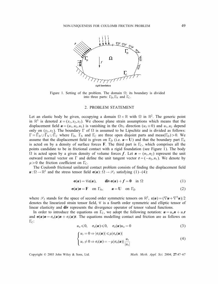
Figure 1. Setting of the problem. The domain �; its boundary is dividedinto three parts: �D;�N and �C.

2. PROBLEM STATEMENT

Let an elastic body be given, occupying a domain �×R with � in R2. The generic pointin R3 is denoted x=(x1; x2; x3). We choose plane strain assumptions which means that thedisplacement �eld u=(u1; u2; u3) is vanishing in the Ox3 direction (u3 ≡ 0) and u1; u2 dependonly on (x1; x2). The boundary � of � is assumed to be Lipschitz and is divided as follows:�= ��D ∪ ��N ∪ ��C where �D; �N and �C are three open disjoint parts and meas(�D)¿0. Weassume that the displacement �eld is given on �D (i.e. u=U) and that the boundary part �Nis acted on by a density of surface forces F. The third part is �C, which comprises all thepoints candidate to be in frictional contact with a rigid foundation (see Figure 1). The body� is acted upon by a given density of volume forces f . Let n = (n1; n2) represent the unitoutward normal vector on � and de�ne the unit tangent vector t=(−n2; n1). We denote by�¿0 the friction coe�cient on �C.The Coulomb frictional unilateral contact problem consists of �nding the displacement �eld

u : �→R2 and the stress tensor �eld �(u) :�→S2 satisfying (1)–(4):

�(u) =CU(u); div �(u) + f = 0 in � (1)

�(u)n= F on �N; u=U on �D (2)

where S2 stands for the space of second order symmetric tensors on R2; U(u)= (∇u+∇Tu)=2denotes the linearized strain tensor �eld, C is a fourth order symmetric and elliptic tensor oflinear elasticity and div represents the divergence operator of tensor valued functions.In order to introduce the equations on �C, we adopt the following notation: u= unn + utt

and �(u)n=�n(u)n+ �t(u)t. The equations modelling contact and friction are as follows on�C:

un60; �n(u)60; �n(u)un=0 (3)ut =0⇒ |�t(u)|6�|�n(u)|ut �=0⇒�t(u)=−�|�n(u)| ut|ut |

(4)

Copyright ? 2003 John Wiley & Sons, Ltd. Math. Meth. Appl. Sci. 2004; 27:47–67

50 R. HASSANI, P. HILD AND I. IONESCU

Remark 2.1Let us mention that the true Coulomb friction law involves the tangential contact velocitiesand not the tangential displacements. However, a problem analogous to the one discussed hereis obtained by time discretization of the quasistatic frictional contact evolution problem. In thiscase (see Reference [21]) u; f and F stand for u((i+1)t); f ((i+1)t) and F((i+1)t)respectively and ut has to be replaced by ut((i+1)t)− ut(it), where t denotes the timestep. For simplicity and without any loss of generality only the static case described abovewill be considered in the following.

The variational formulation of problem (1)–(4) has been obtained by Duvaut and Lions[1]. It consists of �nding u verifying:

u ∈ Kad ; a(u; C− u) + j(u; C)− j(u; u)¿L(C− u); ∀C∈Kad (5)

where

a(u; C)=∫�(CU(u)): U(C) d�; L(C)=

∫�f · C d� +

∫�NF · C d�

are de�ned for any u and C in the standard Sobolev space (H 1(�))2 (see Reference [22]) andthe notations · and : stand for the canonical inner products in R2 and S2, respectively.In (5), Kad denotes the closed convex set of admissible displacement �elds satisfying the

non-penetration conditions:

Kad = {C∈ (H 1(�))2: C=U on �D; vn60 on �C}

The functional j(·; ·) given by

j(u; C)=−∫�C��n(u)|vt | d� (6)

is de�ned for any C in (H 1(�))2 but more regularity is required for u. Two di�erent caseswhen j(u; ·) makes sense, are usually considered in the literature. The �rst one, which occursin the continuous problem, involves the space

V= {C∈ (H 1(�))2: div �(C)∈ (L2(�))2}

If u∈ V then �(u) belong to H (div;�) and �n(u) is an element of H−1=2(�) (i.e. the dual ofH 1=2(�)). Since H−1=2(�)|�C is di�erent from H−1=2(�C) we have to suppose in addition that�n(u)∈H−1=2(�C). With this assumption, (6) makes sense if we replace the integral term bythe duality product. For a more precise formulation involving the convenient Sobolev spacesand the set of nonnegative Radon measures, a detailed study can be found in Reference [23].In the second case, u belongs to a �nite element set Vh ⊂ (H 1(�))2, which implies that �(u)is at least piecewise continuous so that �(u)n admits a trace on the boundary. In the lattercase, the integral notation in (6) has to be understood in the classical sense.The �rst existence result of (1)–(4) has been proven in Reference [2] when � is an

in�nitely long strip and the friction coe�cient has compact support in �C and is su�ciently

Copyright ? 2003 John Wiley & Sons, Ltd. Math. Meth. Appl. Sci. 2004; 27:47–67

NON-UNIQUENESS FOR COULOMB FRICTION PROBLEM 51

small. The extension of these results to domains with smooth boundaries as well as improve-ments can be found in References [3] and [4]. More recently in Reference [5], existence isstated when the friction coe�cient � is smaller than

√3− 4�=(2−2�); � denoting Poisson’s ra-

tio in � (06�¡ 12 ). To our knowledge there exist neither uniqueness result nor non-uniqueness

example of (5) (unless the loads U; f and F are equal to zero).

3. SUFFICIENT CONDITIONS FOR NON-UNIQUENESS: A SPECTRAL APPROACH

Let us consider an equilibrium position u0 of the Coulomb frictional contact problem (i.e. asolution of (1)–(4)) supposed to be regular enough. The notation �0f stands for the pointsof �C which are currently free (separated from the rigid foundation). We denote by �0s thepoints of �C which are currently in contact but are stuck to the rigid foundation, and by �0Cthe points of �C which are currently in contact but are candidate to slip. That leads to thefollowing de�nitions:

�0f = {x∈�C: u0n(x)¡0} (7)

�0s = {x∈�C: u0n(x)=0; |�t(u0)(x)|¡− ��n(u0)(x)} (8)

�0C = {x∈�C: u0n(x)=0; |�t(u0)(x)|=−��n(u0)(x)} (9)

Let us adopt the following notation

�0D =�D ∪�0s and �0N =�N ∪�0fand consider now the following eigenvalue problem:Eigenvalue problem. Find �∈C and 0 �=�∈ (H 1(�))2 such that

�(�) =CU(�); div �(�)= 0 in � (10)

�= 0 on �0D; �(�)n=0 on �0N; �n=0 on �0C (11)

�t(�) = ��n(�) on �0C (12)

Remark 3.1If we choose the commonly used Hooke’s law, for homogeneous isotropic materials, givenby

�ij=E�

(1− 2�)(1 + �)�ij�kk(u) +E1 + �

�ij(u) in �

where E denotes Young’s modulus, � represents Poisson’s ratio and �ij is the Kroneckersymbol, then the only constitutive constant involved in the eigenvalue problem (10)–(12) isthe ratio �= �=(1 − 2�). Indeed, the eigenvalues and eigenfunctions are independent of theYoung modulus E.

Copyright ? 2003 John Wiley & Sons, Ltd. Math. Meth. Appl. Sci. 2004; 27:47–67

52 R. HASSANI, P. HILD AND I. IONESCU

The following theorem states su�cient conditions for the non-uniqueness of the equilibriumsolution u0.

Theorem 3.2Let u0 be a smooth solution of Coulomb’s frictional contact problem (1)–(4) with �¿0as friction coe�cient. Let u1 = u0 + �� for some �∈R and � a smooth eigenfunction of(10)–(12). Let us de�ne the two following cases (i) and (ii):

(i) �t(u0)(x)60 for all x∈�0C and � is the corresponding eigenvalue for �. Assume that:

u1n(x)¡0; for all x∈�0f (13)

�n(u1)(x)60; for all x∈�0C (14)

|�t(u1)(x)|¡− ��n(u1)(x); for all x∈�0s (15)

u1t (x)¿0; for all x∈�0C (16)

(ii) �t(u0)(x)¿0 for all x∈�0C and −� is the corresponding eigenvalue for �. Assumethat in addition to (13)–(15), one has:

u1t (x)60; for all x∈�0C (17)

If either (i) or (ii) holds then u1 is another (smooth) solution of (1)–(4).

ProofLet us �rstly remark that u1 = u0 + �� satis�es Equations (1)–(2) for any �∈R. Next, wehave to check that u1 veri�es the frictional contact conditions (3)–(4). We begin with theunilateral contact conditions (3).If x∈�0f then from (13) we have u1n(x)¡0. Since �

0f ⊂�C, from (7) we get �(u0)n(x)=0.

Having in mind that �0f ⊂�0N and according to (11), we deduce �n(u1)(x)=0. If x∈�0s ∪�0Cthen u0n(x)=0 and �n(x)=0, hence u1n(x)=0 and from (14) we deduce (3). Therefore u1

satis�es (3).If x∈�0s the condition (4) implies u0t (x)=0. From assumption (15) we get |�t(u1)(x)|

¡− ��n(u1)(x) and since �0s ⊂�0D we obtain u1t (x)=0. If x∈�0f , then owing to �0f ⊂�0N, wehave �n(u1)(x)=�t(u1)(x)=0 and (4) is satis�ed.Let x∈�0C. If case (i) holds, then, for all x∈�0C we have �t(u0)(x)60 and �t(u0)(x)=��n

(u0)(x). Using (12) with �=�, we obtain �t(u1)(x)=��n(u1)(x) and (4) follows from (14)and (16). If we consider case (ii) then �t(u0)(x)=−��n(u0)(x) and from (12) with �=−�we �nally get �t(u1)(x)=−��n(u1)(x). Consequently, u1 satis�es (4).In order to apply Theorem 3.2, one has to check the conditions (13)–(17) dealing with the

equilibrium u0, the eigenfunction � and an appropriately chosen value of �. The followingcorollary yields su�cient conditions concerning the solution u0 only. These conditions aremore restrictive than those of the previous theorem but easier to handle. Indeed, we shallsuppose that all the points of �C are in a slipping contact, i.e. �0s = ∅ and �0f = ∅.

Copyright ? 2003 John Wiley & Sons, Ltd. Math. Meth. Appl. Sci. 2004; 27:47–67

NON-UNIQUENESS FOR COULOMB FRICTION PROBLEM 53

Corollary 3.3Let u0 be a smooth solution of Coulomb’s frictional contact problem (1)–(4) with �¿0 asfriction coe�cient. Assume that �0C =�C and that there exist �; ¿0 such that

�n(u0)(x)6− for all x∈�0C (18)

Moreover, suppose that one of the following two conditions (i) or (ii) holds:(i) The pair (�;�) is a smooth solution of (10)–(12), and

u0t (x)¿�; for all x∈�0C (19)

(ii) The pair (−�;�) is a smooth solution of (10)–(12), and

u0t (x)6− �; for all x∈�0C (20)

Then Coulomb’s frictional contact problem (1)–(4) admits an in�nity of solutions. In par-ticular, there exists �0¿0 such that u1 = u0 + �� is solution for any � satisfying |�|6�0.ProofLet 0 = supx∈�C |�n(�)(x)| and �0 = supx∈�C |t(x)|. Keeping in mind that �n(u0 + ��)(x)6− + |�|0 we deduce that (14) holds when |�|6=0.If condition (i) holds, we can write u1t (x)= u

0t (x) + �t(x)¿� − |�|�0 so that the bound

|�|6�=�0 leads to (16). Moreover, condition (19) implies that �t(u0)(x)60 for all x∈�0C. Ifwe set �0 = min{=0; �=�0} then the �rst case in Theorem 3.2 proves the statement of thecorollary.If condition (ii) holds, then (17) is satis�ed if |�|6�=�0 and (20) implies that �t(u0)(x)¿0

for all x∈�0C. Employing the second case in Theorem 3.2 completes the proof of the corollary.

Remark 3.4The above results are only su�cient conditions for non-uniqueness. They take into considera-tion only the possibility of existence of multiple solutions having the same distribution of theslip, free and stick zones. Moreover, the above corollary does not cover the case of isolatedmultiple solutions.

Indeed, as it follows from Corollary 3.3, if the problem is open to non-uniqueness thenthere exists an in�nity of solutions located on a continuous branch.The non-uniqueness conditions considered here imply that the friction coe�cient � (or −�)

is an eigenvalue of (10)–(12). This eigenvalue problem depends exclusively on the geometry(the domain � and the distribution of the di�erent types of boundaries) and on the elasticproperties incorporated in the operator C (on the Poisson coe�cient � for an isotropic elasticmaterial).

Remark 3.5If (10)–(12) admits a real eigenvalue � then the pair geometry-material is open to the non-uniqueness of the Coulomb frictional contact problem.

Copyright ? 2003 John Wiley & Sons, Ltd. Math. Meth. Appl. Sci. 2004; 27:47–67

54 R. HASSANI, P. HILD AND I. IONESCU

As a matter of fact, one can think of a distribution of loads F; f and a displacement�eld U such that a solution u0 of (1)–(4) for this particular friction coe�cient � satis�es(18)–(19). We consider, for example, that �C is a straight line segment located on the Ox1-axis and that �N = ∅. We choose

U(x)=(�+ 2�

1− �1− 2� x2;−x2

)

for all x=(x1; x2)∈�D, with �¿0 and f = 0. One can easily check that u0(x)=U(x), for allx∈� is a solution of (1)–(4). Since �0C =�C; �n(u0)(x)=−E(1−�)=[(1−2�)(1+�)]¡0 andu0t (x)= �¿0, we deduce that the su�cient conditions of the corollary hold.

4. THE NON-LOCAL FRICTION MODEL

There exist several laws ‘mollifying’ Coulomb’s frictional contact model which lead generallyto more existence and uniqueness properties. Among these regularization techniques, a specialinterest is devoted to the non-local procedure introduced in Reference [6] and developed inReferences [7–9]. Moreover, from a physical point of view, this law takes into account someinteresting microscopic aspects: the normal pressure �n(u) is distributed over a contact areaof the deformed asperity (see Reference [7] for more arguments).Hence, we consider the non-local normal stress �∗

n (u) given by

�∗n (u)(x)=

∫�Cw(|x− y|)�n(u)(y) dy∫�Cw(|x− y|) dy (21)

where w; (¿0) stands for a non-negative function with its non-empty support in [−; ]such that x �→w(|x|) is an in�nitely di�erentiable function. As for the functional j, the aboveexpression of the non-local normal stress is meaningful in two di�erent cases. The �rst oneconcerns the continuous problem when �n(u)∈H−1=2(�C) and the above integral has to bereplaced by the duality product between H−1=2(�C) and H 1=2(�C). The second case happenswhen using a �nite element approximation when �(u) is at least piecewise continuous.Another type of smoothing procedure was introduced in Reference [24] for friction problems

in viscoplasticity. In this case the second order stress tensor �eld is averaged in the interiorof the domain and its normal trace on the contact boundary provides the non-local normalstress. The de�nition of the non-local normal stress �∗

n (u) becomes

�∗n (u)(x)=

∫� w(|x− y|)�(u)(y) dy∫

��w(|x− y|) dy n(x) · n(x) (22)

Unlike the �rst non-local approach in (21), this second procedure avoids the handling ofdual Sobolev spaces such as H−1=2(�). Indeed, the latter expression is well de�ned for anyu∈ (H 1(�))2.

Copyright ? 2003 John Wiley & Sons, Ltd. Math. Meth. Appl. Sci. 2004; 27:47–67

NON-UNIQUENESS FOR COULOMB FRICTION PROBLEM 55

If we replace the above formulas in (4) we get the following ‘regularized’, non-local frictionlaw on �C:

ut =0⇒ |�t(u)|6�|�∗

n (u)|ut �=0⇒ �t(u)=−�|�∗

n (u)|ut|ut |

(23)

The variational formulation of (1)–(3) and (23) is inequality (5), the same as in the localfriction case in which j is replaced by (see Reference [6]):

j(u; C)=−∫�C��∗

n (u)|vt |d� (24)

From a mathematical point of view, the smoothing map used in the non-local friction modelimplies compactness properties of the operators involved in the variational approach (5). Theseproperties permit using the Schauder and Tykhonov �xed point theorems in order to deducethe existence of at least one solution of the variational inequality [6–9]. In addition, someuniqueness results can also be obtained for the non-local friction model. As a matter of fact,it was proved in References [6–9] that there exists a critical friction coe�cient �c such thatif �¡�c (i.e. the friction is small) then the solution of (5) is unique. As for the local frictioncase there exist, to our knowledge, no non-uniqueness examples.The eigenvalue problem corresponding to the non-local friction case is (10)–(11) and

�t(�)= ��∗n (�) on �0C (25)

where �0s and �0C de�ned in (8) and (9) have to be replaced by

�0s = {x∈�C: u0n(x)=0; |�t(u0)(x)|¡− ��∗n (u

0)(x)}�0C = {x∈�C: u0n(x)=0; |�t(u0)(x)| = −��∗

n (u0)(x)}

If the normal stress �n is replaced by �∗n then all the su�cient conditions for non-uniqueness

given in Theorem 3.2 and Corollary 3.3 remain valid.

5. EXISTENCE OF EIGENVALUES AND EIGENFUNCTIONS

In order to derive the variational formulation of (10)–(11) and (25) we consider the subspacesV0 and V0 of (H 1(�))2 and V, respectively:

V0 = {C∈ (H 1(�))2: C= 0 on �0D; vn=0 on �0C}; and V0 =V0 ∩ V

Let us introduce the bilinear form b(:; :) given by:

b(u; C)=∫�C�∗n (u)vt d�

Copyright ? 2003 John Wiley & Sons, Ltd. Math. Meth. Appl. Sci. 2004; 27:47–67

56 R. HASSANI, P. HILD AND I. IONESCU

for any C in (H 1(�))2. Concerning the �rst variable, b(u; C) makes sense if the non-localnormal stress �∗

n (u) can be de�ned. Hence, b(u; C) is well de�ned for any u∈ V such that�n(u)∈H−1=2(�C) or for u∈Vh (the notation Vh represents a �nite element type space) if thenon-local normal stress (21) is considered. When adopting the non-local normal stress (22),this restriction disappears, so that b(u; C) is well de�ned for all u; C∈ (H 1(�))2.The variational formulation of problem (10)–(11) and (25) consists of �nding �∈C and

0 �=�∈ V0 such that:

a(�; C)= �b(�; C); ∀C∈V0 (26)

and it can be easily checked that if �∈C and a non-zero � satisfy (10)–(11) and (25) thenthere are a solution of (26). Conversely, if �∈C and a nonzero � satisfy (26), then the pair(�;�) is a weak solution of (10)–(11) and (25).

Theorem 5.1The eigenvalues of problem (26) consist of a countable set of complex numbers {�n}n∈I with�n �=0. Each eigenvalue �n is of �nite algebraic multiplicity. If I is in�nite then limn→∞ |�n|=+∞.ProofLet us �rst remark that �=0 is not an eigenvalue of (26). Otherwise, a(�;�)=0 where �is an eigenvector associated with �=0, which contradicts the V0-ellipticity of a(:; :). Let usdenote by

H =L2(�0C) and W0 = {C∈V0: div �(C)= 0 in �; �(C)n= 0 on �0N}

and de�ne P:H → V0 as follows: for any f∈H; P(f) is the unique solution of the variationalequality

a(P(f); C)=∫�0C

fvt d�; ∀C∈V0:

If we put C∈ (D(�))2 ⊂V0 in the previous equation (the notation D(�) stands for the space ofin�nitely di�erentiable functions with compact support in �), we deduce that div �(P(f))= 0in �. In the same way, it can be formally checked that �(P(f))n= 0 on �0N which impliesthat P(f)∈W0. Hence, P is a linear continuous operator from H into W0. Next, we provethe theorem separately for the two regularization techniques in (21) and (22).(i) Case (21). The function �∗

n (C)∈H is well de�ned for any C∈W0. Set Q:W0 →H sothat Q(C)=�∗

n (C), Since Q is a linear and completely continuous operator [9, Theorem 11.2,p. 338] we deduce that T =PQ :W0 → W0 is also completely continuous. In order to provethe statement of the theorem, we only have to mention that � is a solution in (26) if and onlyif 1=� is a non-zero eigenvalue for T which is true since �T (�)=� if and only if (�;�) isa solution for (26).(ii) Case (22). The operator Q :V0→H , given by Q(C)=�∗

n (C) is well de�ned. In addition,Q is a linear and completely continuous operator [24, Lemma 1.2, p. 181] and we deducethat T =PQ :V0 → V0 is also completely continuous. As a consequence, the proof follows asin case (i).

Copyright ? 2003 John Wiley & Sons, Ltd. Math. Meth. Appl. Sci. 2004; 27:47–67

NON-UNIQUENESS FOR COULOMB FRICTION PROBLEM 57

Remark 5.2The technique used in the proof above cannot be used if the non-local assumption is removed.The existence of a countable set of eigenvalues is linked to the compactness of operator Twhich is assured by the regularized trace operator Q.

The following result ensures, under speci�c conditions, the existence of at least one realpositive or negative eigenvalue for problem (26) which also minimizes the moduli among alleigenvalues satisfying (26). First, we need to de�ne the convex cone K0:

K0 = {C∈W0: �t(C)¿0 on �0C}

It is easy to see that each displacement �led C of W0 (and of K0) is determined uniquely bythe tangential component �t(C) of the stress vector on �0C.

Theorem 5.3Suppose that one of the two following conditions (i) or (ii) holds:

(i) any C in K0 satis�es �∗n (C)¿0 on �0C,

(ii) any C in K0 satis�es �∗n (C)60 on �0C.

Then the eigenvalue �0, minimizing the moduli of all eigenvalues in problem (26), is realand its associated eigenvector lies in K0. Moreover �0¿0 in the case (i) and �0¡0 in thecase (ii).

Let us �rst recall a weak form of the Krein–Rutman theorem [25–27] which we use in theproof of Theorem 5.3.

Theorem (Krein and Rutman [25])Let X be a Banach space and let K ⊂X be a convex cone containing 0 (i.e. �x+�y∈K; ∀�¿0;∀�¿0; x∈K; y∈K). Suppose that K is closed, X =K −K and K ∩ (−K)= {0}. Let T be alinear operator satisfying T (K)⊂K .If T is compact and its spectral radius r(T ) �=0 then there exists ’∈K − {0} such that

T (’)= r(T )’

ProofLet us consider operator T =PQ :W0 → W0 introduced in the proof of Theorem 5.1. Forboth non-local frictional approaches, the operator T is compact in the Hilbert space W0.Moreover, the closed convex cone K0 satis�es K0 ∩ (−K0)= 0 and K0 −K0 =W0 (it su�cesto write �t(C)= (�t(C))+ − (�t(C))− where the notations (:)+ and (:)− represent the positive andthe negative parts, respectively). We next show that T (K0)⊂K0.The assumptions of the theorem imply that the operator Q de�ned by Q(C)=�∗

n (C) mapsK0 into (L2(�0C))+. The operator P de�ned for all f∈L2(�0C) by

a(P(f); C)=∫�0C

fvt d�; ∀C∈W0

satis�es �t(P(f))=f. Hence C∈K0, which implies that Q(C)∈ (L2(�0C))+ and thus T (C)∈K0.

Copyright ? 2003 John Wiley & Sons, Ltd. Math. Meth. Appl. Sci. 2004; 27:47–67

58 R. HASSANI, P. HILD AND I. IONESCU

It follows then from Krein–Rutman’s theorem that if T admits a positive spectral radius,then there exists an eigenvalue which is equal to the spectral radius with an associated eigen-vector in K0.The case (ii) is handled similarly by using the operator −T .

6. FINITE ELEMENT APPROXIMATION OF THE EIGENVALUE PROBLEM

The problem we intend to approximate is as follows: �nd �∈C and 0 �=�∈V0 such that:

a(�; C)= �b(�; C); ∀C∈V0 (27)

which is exactly the eigenvalue problem corresponding to the non-local frictional approach(22). Notice that when the regularization procedure (21) is adopted, then the convergenceanalysis is more complicated. A remark at the end of this section explains and gives partialanswers to the convergence study in that case.We denote by ‖ · ‖1 the standard norm on (H 1(�))2. Our aim is to approximate the eigen-

values of problem (27). Let be given a family of �nite dimensional subspaces V0h ⊂V0 whereh denotes the discretization parameter [28]. The �nite dimensional problem consists then of�nding �h ∈C and 0 �=�h ∈V0h such that [29,30]:

a(�h; Ch)= �hb(�h; Ch); ∀Ch ∈V0h (28)

We assume that the following approximation property holds:

limh→0

infuh∈V0h

‖u − uh‖1 = 0; ∀u∈V0

Let �−1 be an eigenvalue of T de�ned in (ii) of the proof in Theorem 5.1. Denoting by I theidentity map, there exists a least integer � such that Ker((�−1I−T )�)=Ker((�−1I−T )�+1)=Ewith dim(E)=m¡∞. The algebraic multiplicity of �−1 is m and � stands for the ascent of�−1I −T . The set E contains the generalized eigenvectors of T corresponding to �−1. Let T ∗

be the adjoint operator of T de�ned on the dual space V0∗. Then ��−1 is an eigenvalueof T ∗ with algebraic multiplicity m and � is also the ascent of ��−1I − T ∗. The notationE∗=Ker(( ��−1I − T ∗)�) stands for the space of generalized eigenvectors of T ∗ associatedwith ��−1. Given two closed subspaces A and B of V0, de�ne the gap between A and B by

�(A; B)= max

(sup

u∈A;‖u‖1=1infC∈B

‖u − C‖1; supu∈B;‖u‖1=1

infC∈A

‖u − C‖1)

Let � be an eigenvalue of (27) and denote by m its algebraic multiplicity. When h tendsto zero, there exist exactly m eigenvalues of (28) denoted �1; h; �2; h; : : : ; �m; h converging to �.Let Eh be the direct sum of the generalized eigenspaces associated with �1; h; �2; h; : : : ; �m; h andde�ne

�h= supu∈E;‖u‖1=1

infCh∈V0h

‖u − Ch‖1 and �∗h = supu∈E∗ ;‖u‖1=1

infCh∈V0h

‖u − Ch‖1

Copyright ? 2003 John Wiley & Sons, Ltd. Math. Meth. Appl. Sci. 2004; 27:47–67

NON-UNIQUENESS FOR COULOMB FRICTION PROBLEM 59

The following theorem, taken from Kolata [31], describes the convergence of the �nite elementapproximation.

Theorem 6.1If h is small enough, the following estimates hold:

∣∣∣∣∣�− 1m

m∑i=1

�i; h

∣∣∣∣∣6C�h�∗h

|�− �i; h|6C(�h�∗h)1� ; 16i6m

�(E; Eh)6C�h

where the constant C does not depend on h.

If the �rst regularizing approach (21) is adopted then the eigenvalue problem becomes: �nd�∈C and 0 �=�∈W0 such that a(�; C)= �b(�; C), ∀C∈V0. In such a case there are at leasttwo alternatives for obtaining convergence results. The �rst one is to invoke again Kolata’sstudies in Reference [31] which are still valid. It su�ces then to show two families of �nitedimensional subspaces V0h and W

0h of V

0 and W0, respectively, where the dimensions of V0hand W0

h are equal. This necessitates to introduce more speci�c �nite element spaces which isout of the scope of this paper. The second possibility is to use a non-conforming �nite elementapproach and approximating V0 and W0 with the same �nite dimensional space V0h althoughV0h �⊂W0. In that case the convergence result requires strong supplementary hypotheses as inReference [32].

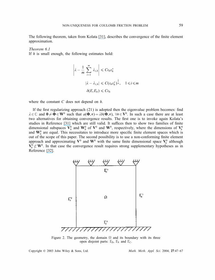
Figure 2. The geometry, the domain � and its boundary with its threeopen disjoint parts: �D, �N and �C.

Copyright ? 2003 John Wiley & Sons, Ltd. Math. Meth. Appl. Sci. 2004; 27:47–67

60 R. HASSANI, P. HILD AND I. IONESCU

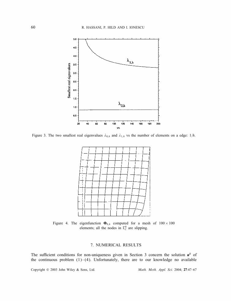
Figure 3. The two smallest real eigenvalues �0; h and �1; h vs the number of elements on a edge: 1=h.

Figure 4. The eigenfunction �0; h computed for a mesh of 100× 100elements; all the nodes in �0C are slipping.

7. NUMERICAL RESULTS

The su�cient conditions for non-uniqueness given in Section 3 concern the solution u0 ofthe continuous problem (1)–(4). Unfortunately, there are to our knowledge no available

Copyright ? 2003 John Wiley & Sons, Ltd. Math. Meth. Appl. Sci. 2004; 27:47–67

NON-UNIQUENESS FOR COULOMB FRICTION PROBLEM 61

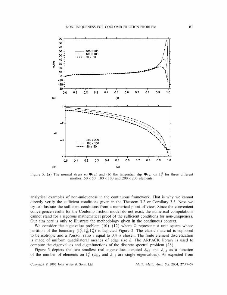
Figure 5. (a) The normal stress �n(�0; h) and (b) the tangential slip �0; ht on �0C for three di�erentmeshes: 50× 50, 100× 100 and 200× 200 elements.

analytical examples of non-uniqueness in the continuous framework. That is why we cannotdirectly verify the su�cient conditions given in the Theorem 3.2 or Corollary 3.3. Next wetry to illustrate the su�cient conditions from a numerical point of view. Since the convenientconvergence results for the Coulomb friction model do not exist, the numerical computationscannot stand for a rigorous mathematical proof of the su�cient conditions for non-uniqueness.Our aim here is only to illustrate the methodology given in the continuous context.We consider the eigenvalue problem (10)–(12) where � represents a unit square whose

partition of the boundary (�0C;�0D;�

0N) is depicted Figure 2. The elastic material is supposed

to be isotropic and a Poisson ratio � equal to 0.4 is chosen. The �nite element discretizationis made of uniform quadrilateral meshes of edge size h. The ARPACK library is used tocompute the eigenvalues and eigenfunctions of the discrete spectral problem (28).Figure 3 depicts the two smallest real eigenvalues denoted �0; h and �1; h as a function

of the number of elements on �0C (�0; h and �1; h are single eigenvalues). As expected from

Copyright ? 2003 John Wiley & Sons, Ltd. Math. Meth. Appl. Sci. 2004; 27:47–67

62 R. HASSANI, P. HILD AND I. IONESCU

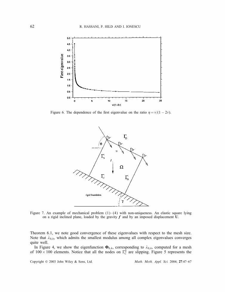
Figure 6. The dependence of the �rst eigenvalue on the ratio �= �=(1− 2�).

Figure 7. An example of mechanical problem (1)–(4) with non-uniqueness. An elastic square lyingon a rigid inclined plane, loaded by the gravity f and by an imposed displacement U.

Theorem 6.1, we note good convergence of these eigenvalues with respect to the mesh size.Note that �0; h, which admits the smallest modulus among all complex eigenvalues convergesquite well.In Figure 4, we show the eigenfunction �0; h, corresponding to �0; h, computed for a mesh

of 100× 100 elements. Notice that all the nodes on �0C are slipping. Figure 5 represents the

Copyright ? 2003 John Wiley & Sons, Ltd. Math. Meth. Appl. Sci. 2004; 27:47–67

NON-UNIQUENESS FOR COULOMB FRICTION PROBLEM 63

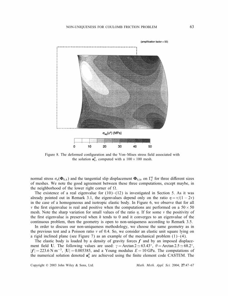
Figure 8. The deformed con�guration and the Von–Mises stress �eld associated withthe solution u0h , computed with a 100× 100 mesh.

normal stress �n(�0; h) and the tangential slip displacement �0; ht on �0C for three di�erent sizesof meshes. We note the good agreement between these three computations, except maybe, inthe neighborhood of the lower right corner of �.The existence of a real eigenvalue for (10)–(12) is investigated in Section 5. As it was

already pointed out in Remark 3.1, the eigenvalues depend only on the ratio �= �=(1 − 2�)in the case of a homogeneous and isotropic elastic body. In Figure 6, we observe that for all� the �rst eigenvalue is real and positive when the computations are performed on a 50× 50mesh. Note the sharp variation for small values of the ratio �. If for some � the positivity ofthe �rst eigenvalue is preserved when h tends to 0 and it converges to an eigenvalue of thecontinuous problem, then the geometry is open to non-uniqueness according to Remark 3.5.In order to discuss our non-uniqueness methodology, we choose the same geometry as in

the previous test and a Poisson ratio � of 0.4. So, we consider an elastic unit square lying ona rigid inclined plane (see Figure 7) as an example of the mechanical problem (1)–(4).The elastic body is loaded by a density of gravity forces f and by an imposed displace-

ment �eld U. The following values are used: �=Arctan 2� 63:43◦, �=Arctan 2:5� 68:2◦,|f |=223:6 N m−3, |U|=0:005385, and a Young modulus E=10 GPa. The computations ofthe numerical solution denoted u0h are achieved using the �nite element code CASTEM. The

Copyright ? 2003 John Wiley & Sons, Ltd. Math. Meth. Appl. Sci. 2004; 27:47–67

64 R. HASSANI, P. HILD AND I. IONESCU

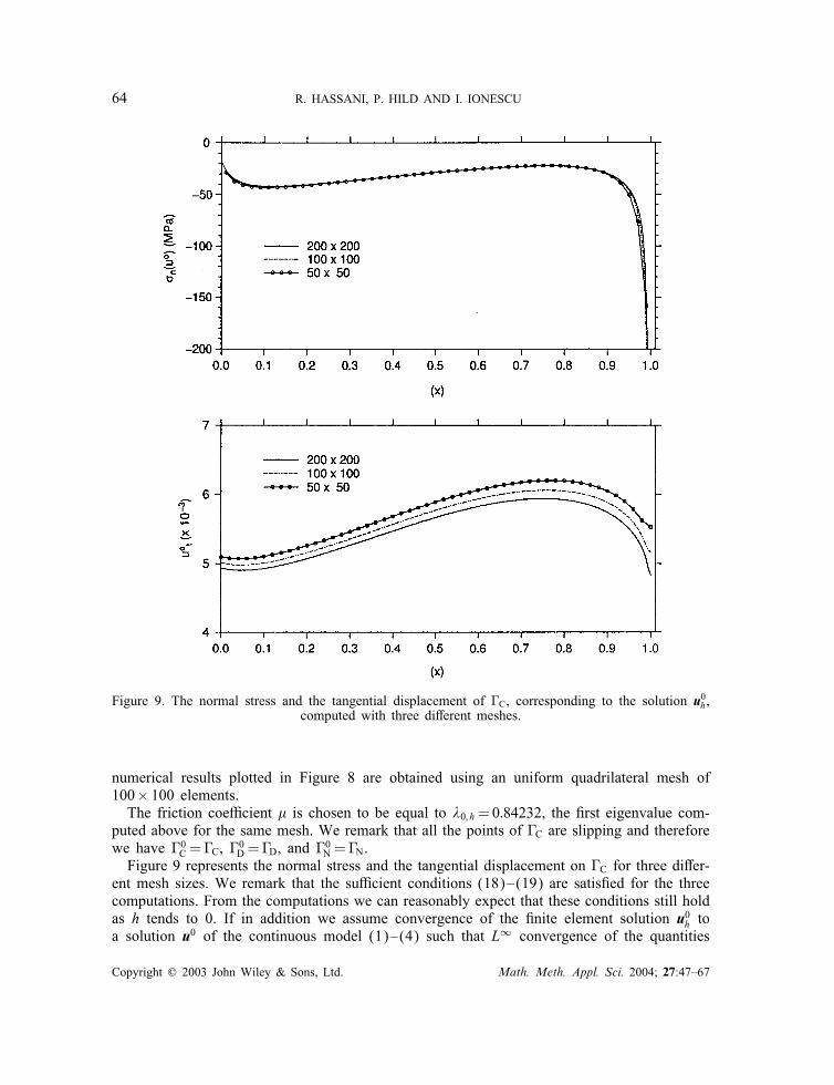
Figure 9. The normal stress and the tangential displacement of �C, corresponding to the solution u0h ,computed with three di�erent meshes.

numerical results plotted in Figure 8 are obtained using an uniform quadrilateral mesh of100× 100 elements.The friction coe�cient � is chosen to be equal to �0; h=0:84232, the �rst eigenvalue com-

puted above for the same mesh. We remark that all the points of �C are slipping and thereforewe have �0C =�C, �

0D =�D, and �

0N =�N.

Figure 9 represents the normal stress and the tangential displacement on �C for three di�er-ent mesh sizes. We remark that the su�cient conditions (18)–(19) are satis�ed for the threecomputations. From the computations we can reasonably expect that these conditions still holdas h tends to 0. If in addition we assume convergence of the �nite element solution u0h toa solution u0 of the continuous model (1)–(4) such that L∞ convergence of the quantities

Copyright ? 2003 John Wiley & Sons, Ltd. Math. Meth. Appl. Sci. 2004; 27:47–67

NON-UNIQUENESS FOR COULOMB FRICTION PROBLEM 65

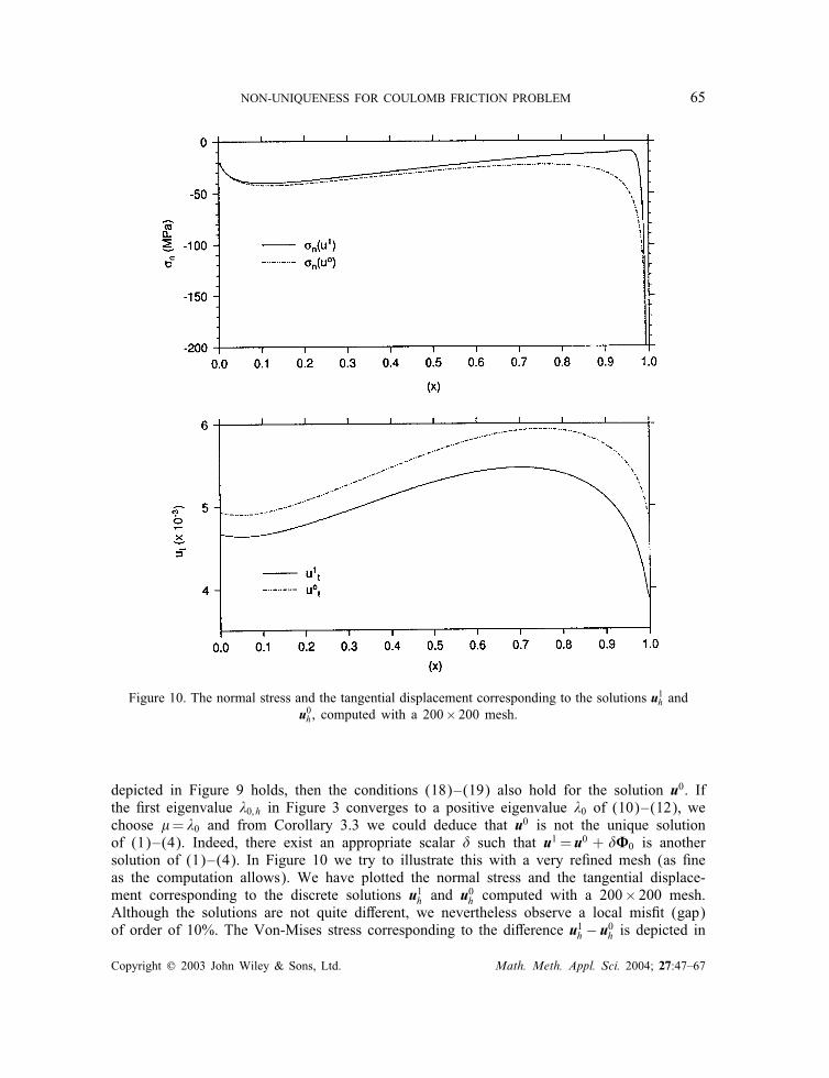
Figure 10. The normal stress and the tangential displacement corresponding to the solutions u1h andu0h , computed with a 200× 200 mesh.

depicted in Figure 9 holds, then the conditions (18)–(19) also hold for the solution u0. Ifthe �rst eigenvalue �0; h in Figure 3 converges to a positive eigenvalue �0 of (10)–(12), wechoose �= �0 and from Corollary 3.3 we could deduce that u0 is not the unique solutionof (1)–(4). Indeed, there exist an appropriate scalar � such that u1 = u0 + ��0 is anothersolution of (1)–(4). In Figure 10 we try to illustrate this with a very re�ned mesh (as �neas the computation allows). We have plotted the normal stress and the tangential displace-ment corresponding to the discrete solutions u1h and u

0h computed with a 200× 200 mesh.

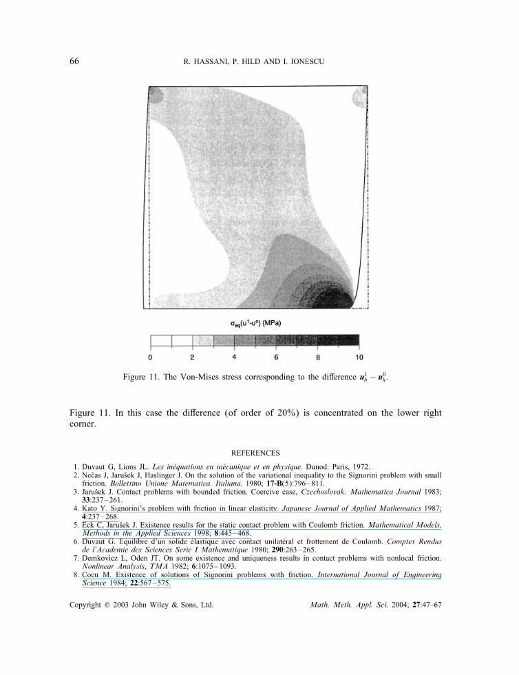
Although the solutions are not quite di�erent, we nevertheless observe a local mis�t (gap)of order of 10%. The Von-Mises stress corresponding to the di�erence u1h − u0h is depicted in

Copyright ? 2003 John Wiley & Sons, Ltd. Math. Meth. Appl. Sci. 2004; 27:47–67

66 R. HASSANI, P. HILD AND I. IONESCU

Figure 11. The Von-Mises stress corresponding to the di�erence u1h − u0h .

Figure 11. In this case the di�erence (of order of 20%) is concentrated on the lower rightcorner.

REFERENCES

1. Duvaut G, Lions JL. Les in�equations en m�ecanique et en physique. Dunod: Paris, 1972.2. Ne�cas J, Jaru�sek J, Haslinger J. On the solution of the variational inequality to the Signorini problem with smallfriction. Bollettino Unione Matematica. Italiana. 1980; 17-B(5):796–811.

3. Jaru�sek J. Contact problems with bounded friction. Coercive case, Czechoslovak. Mathematica Journal 1983;33:237–261.

4. Kato Y. Signorini’s problem with friction in linear elasticity. Japanese Journal of Applied Mathematics 1987;4:237–268.

5. Eck C, Jaru�sek J. Existence results for the static contact problem with Coulomb friction. Mathematical Models,Methods in the Applied Sciences 1998; 8:445–468.

6. Duvaut G. Equilibre d’un solide �elastique avec contact unilat�eral et frottement de Coulomb. Comptes Rendusde l’Academie des Sciences Serie I Mathematique 1980; 290:263–265.

7. Demkovicz L, Oden JT. On some existence and uniqueness results in contact problems with nonlocal friction.Nonlinear Analysis, TMA 1982; 6:1075–1093.

8. Cocu M. Existence of solutions of Signorini problems with friction. International Journal of EngineeringScience 1984; 22:567–575.

Copyright ? 2003 John Wiley & Sons, Ltd. Math. Meth. Appl. Sci. 2004; 27:47–67

NON-UNIQUENESS FOR COULOMB FRICTION PROBLEM 67

9. Kikuchi N, Oden JT. Contact Problems in Elasticity: A Study of Variational Inequalities and Finite ElementMethods. SIAM: Philadelphia, 1988.

10. Klarbring A, Mikel��c A, Shillor M. Frictional contact problems with normal compliance. International Journalof Engineering Science 1988; 26:811–832.

11. Klarbring A, Mikel��c A, Shillor M. On friction problems with normal compliance. Nonlinear Analysis TMA1989; 13:935–955.

12. Oden JT, Martins JAC. Models and computational methods for dynamic friction phenomena. Computer Methodsin Applied Mechanical Engineering 1985; 52:527–634.

13. Martins JAC, Oden JT. Existence and uniqueness results for dynamic contact problems with nonlinear normaland friction interface laws. Nonlinear Analysis TMA 1987; 11:407–428.

14. Haslinger J. Approximation of the Signorini problem with friction, obeying the Coulomb law. MathematicalMethods in the Applied Sciences 1983; 5:422–437.

15. Haslinger J. Least square method for solving contact problems with friction obeying Coulomb’s law. AplikaceMatematiky 1984; 29:212–224.

16. Haslinger J, Hlav�a�cek I, Ne�cas J. Numerical methods for unilateral problems in solid mechanics. In Handbookof Numerical Analysis, vol. IV, Part 2, Ciarlet PG, Lions JL (eds). North-Holland: Amsterdam, 1996;313–485.

17. Janovsk�y V. Catastrophic features of Coulomb friction model. In The Mathematics of Finite Elements andApplications, Whiteman JR (ed). Academic Press: London, 1981; 259–264.

18. Klarbring A. Examples of non-uniqueness and non-existence of solutions to quasistatic contact problems withfriction. Ingenieur- Archiv 1990; 60:529–541.

19. Alart P. Crit�eres d’injectivit�e et de surjectivit�e pour certaines applications de Rn dans lui meme: application �ala m�ecanique du contact. Mathematical Models in Numerical Analysis 1993; 27:203–222.

20. Ballard P. A counter-example to uniqueness in quasi-static elastic contact problems with small friction.International Journal of Engineering Science 1999; 37:163–178.

21. Cocu M. Pratt E, Raous M. Formulation and approximation of quasistatic frictional contact. International Journalof Engineering Science 1996; 22:783–798.

22. Adams RA. Sobolev Spaces. Academic Press: New York, 1975.23. Na�ejus C, Cimeti�ere A. Sur la formulation variationnelle du probl�eme de Signorini avec frottement de Coulomb.

Comptes Rendus de l’Academie des Sciences Serie I Mathematiques 1996; 323:307–312.24. Ionescu I, Sofonea M. Functional and Numerical Problems in Viscoplasticity. Oxford University Press: Oxford,

1993.25. Krein MG, Rutman MA. Linear operator leaving invariant a cone in a Banach space. Uspehi Mat. Nauk. III 3

(1948). American Mathematical Society Translation 1962; 10(1):199–325.26. Dautray R, Lions JL. Analyse math�ematique et calcul num�erique pour les sciences et techniques. Tome 2,

Chapitre VIII, Masson: Paris, 1985.27. Dautray R, Lions JL. Mathematical Analysis and Numerical Methods for Science and Technology, vol. 3,

Chapter VIII. Springer: Berlin, 2000.28. Ciarlet PG. The �nite element method for elliptic problems. In Handbook of Numerical Analysis, vol. II, Part

1, Ciarlet PG, Lions JL (eds). North-Holland: Amsterdam, 1991; 17–352.29. Fix G. Eigenvalue approximation by the �nite element method. Advances in Mathematics 1973; 10:300–316.30. Babu�ska I, Osborn J. Eigenvalue problems. In Handbook of Numerical Analysis, vol. II, Part 1, Ciarlet PG,

Lions JL (eds). North Holland: Amsterdam, 1991; 641–787.31. Kolata W. Approximation in variationally posed eigenvalue problems. Numerische Mathematik 1978; 29:

159–171.32. Mercier B, Osborn JE, Rappaz J, Raviart PA. Eigenvalue approximation by mixed and hybrid methods.

Mathematics of Computation 1981; 36:427–453.

Copyright ? 2003 John Wiley & Sons, Ltd. Math. Meth. Appl. Sci. 2004; 27:47–67